Untitled - Virtual Campus Sign In
409
-
Upload
khangminh22 -
Category
Documents
-
view
0 -
download
0
Transcript of Untitled - Virtual Campus Sign In


AGRICULTURALECONOMICS
THIRD EDITION
H. Evan DrummondUniversity of Florida
John W. GoodwinOklahoma Panhandle State University
Prentice Hall
Boston Columbus Indianapolis New York San Francisco Upper Saddle River
Amsterdam Cape Town Dubai London Madrid Milan Munich Paris Montreal Toronto
Delhi Mexico City São Paulo Sydney Hong Kong Seoul Singapore Taipei Tokyo

Editor in Chief: Vernon AnthonyAcquisitions Editor: Bill LawrensenEditorial Assistant: Lara DimmickDirector of Marketing: David GesellCampaign Marketing Manager: Leigh Ann SimsCurriculum Marketing Manager: Thomas HaywardSenior Marketing Coordinator: Alicia WozniakMarketing Assistant: Les RobertsProduction Editor: Holly ShufeldtCover Art Director: Jayne ConteCover Designer: Bruce KenselaarCover and chapter opener art: IstockLead Media Project Manager: Karen BretzFull-Service Project Management: Saraswathi Muralidhar, GGS Higher Education ResourcesComposition: GGS Higher Education Resources, A Division of PreMedia Global Inc.Printer/Binder: Edwards BrothersCover Printer: Lehigh-Phoenix Color Corp.
Credits and acknowledgments borrowed from other sources and reproduced, with permission, in this textbookappear on appropriate page within text.
Copyright © 2011, 2004 Pearson Education, Inc., publishing as Prentice Hall, One Lake Street, Upper SaddleRiver, NJ 07458. All rights reserved. Manufactured in the United States of America. This publication is protected byCopyright, and permission should be obtained from the publisher prior to any prohibited reproduction, storage in aretrieval system, or transmission in any form or by any means, electronic, mechanical, photocopying, recording, orlikewise. To obtain permission(s) to use material from this work, please submit a written request to PearsonEducation, Inc., Permissions Department, Prentice Hall, One Lake Street, Upper Saddle River, NJ 07458.
Many of the designations by manufacturers and seller to distinguish their products are claimed as trademarks.Where those designations appear in this book, and the publisher was aware of a trademark claim, the designationshave been printed in initial caps or all caps.
10 9 8 7 6 5 4 3 2 1
Library of Congress Cataloging-in-Publication DataDrummond, H. Evan (Harold Evan)
Agricultural economics / H. Evan Drummond, John W. Goodwin.—3rd ed.p. cm.
Includes bibliographical references and index.ISBN-13: 978-0-13-607192-1ISBN-10: 0-13-607192-9
1. Agriculture—Economic aspects. 2. Agriculture—Economic aspects—United States.I. Goodwin, John W. II. Title.
HD1433.D78 2011338.1—dc22
2009052979
Paper bound ISBN-13: 978-0-13-607192-1ISBN-10: 0-13-607192-9
Loose leaf ISBN-13: 978-0-13-506990-4ISBN-10: 0-13-506990-5

Preface ixNew to This Edition xiiAcknowledgments xiii
part oneFoundations
1The Food Industry 2Major Sectors—An Overview 2
Farm Service Sector 2Producers 3Processors 3Marketers 4
Contemporary Issues in the Food Industry 4Farm Structure 4Concentration 6Globalization 6Coordination 7Alternative Energy Sources 8
Summary 10
Key Terms 10
Problems and Discussion Questions 11
Sources 11
2Introduction to AgriculturalEconomics 13Agricultural Economics 13
Basis for Economics 14
Basic Economic Decisions 14
Economic Systems 14
Levels of Economic Activity 15Microeconomics 16Market Economics 16Macroeconomics 17
Basic Skills of the Agricultural Economist 18Economic Models 18Ceteris Paribus 19Opportunity Cost 19Diminishing Returns 20Marginality 21Logical Fallacies 22
Facts, Beliefs, and Values 24
Words 24
Summary 25
Key Terms 25
Problems and Discussion Questions 26
Sources 26
Appendix: Expressing Relationships 27
Relationships 27
Reading Graphs 29
Slope of a Line 31
Slope of a Curve 33
Special Cases 34
Key Terms 34
3Introduction to Market PriceDetermination 35Markets 35
Demand and Supply 36Demand 36Supply 38
Price Determination 39
Changes in Supply and Demand 41Demand Shifters 44Supply Shifters 45Supply or Demand 45
Summary 46
Key Terms 46
Problems and Discussion Questions 46
contents
iii

part twoMicroeconomics
4The Firm as a Production Unit 50Perfectly Competitive Markets 50
The Perfectly Competitive Firm 51Objective of the Perfectly Competitive Firm 51Conditions of Perfect Competition 52Behavior of the Perfectly Competitive Firm 53
Production 53Fixed and Variable Inputs 54Length of Run 54Returns to Scale 54
The Production Function 55The Total Product 56Diminishing Marginal Product 57
Summary 58
Key Terms 59
Problems and Discussion Questions 59
5Costs and Optimal Output Levels 60Environment of the Firm 60
Optimal Output Level 61Costs of the Firm 61Revenue of the Firm 66Profit Maximization 67Behavior of the Loss-Minimizing Firm 70
Summary 72
Key Terms 72
Problems and Discussion Questions 73
Appendix I: Factor-Factor Model 74
Local Cost Minimization 75
Constant Output 76
Local Profit Maximization 76
Graphical Solution 76
Expansion Path 78
Key Terms 79
Appendix II: Product-Product Model 80
Local Revenue Maximization 80
Graphical Solution 81
Generalization 83
Key Terms 83
iv contents
6Supply, Market Adjustments, and Input Demand 84Supply Curve of the Firm 84
Market Supply 85
Market Adjustments 86Dynamic Relationship Between the Firm
and the Market 86Cost Structure and Price Variability 88
Profit-Maximizing Input Use 89Value of the Marginal Product 90Profit Maximization 90Input Demand of the Firm 92Input Demand Shifters 92
Summary 92
Key Terms 93
Problems and Discussion Questions 93
7Imperfect Competition and GovernmentRegulation 94Market Structure 94
Perfect Competition 95Structure 95Conduct 95
Pure Monopoly 96Structure 96Barriers to Entry 97Conduct of the Monopoly Firm 98Unprofitable Monopolies 99Performance 100
Monopolistic Competition 101Structure 101Conduct of the Monopolistically
Competitive Firm 102Performance 104
Oligopoly 104Structure 104Conduct 105Game Theory 105
Government Regulation 106Railroads 106Standard Oil 107Antitrust 107Natural Monopolies 107Marketing Orders in Agriculture 108

contents v
Summary 108
Key Terms 109
Problems and Discussion Questions 110
8The Theory of Consumer Behavior 111The Law of Demand 111
Real Income and Substitution Effects 111Substitution Effect 112Real Income Effect 112
Market Demand and Individual Demand 112
Utility Analysis 113Assumptions about the Utility Model 113Deriving the Demand Curve 117
The Market Demand Function 118
Summary 118
Key Terms 119
Problems and Discussion Questions 119
Appendix: Indifference Curve Analysis 120
Utility Maximization 122
The Impact of Changes in Ceteris ParibusConditions 124
Substitutes and Complements 126
Derivation of the Individual Demand Curve 128
Summary 130
Key Terms 130
Problems and Discussion Questions 130
9The Concept of Elasticity 131Elasticity of Demand 132
Elasticity of Demand Related to Total Revenue 135
Factors Affecting Demand Elasticity 136
Cross-Price Elasticity 138
Income Elasticity 139
Elasticity of Supply 140
Price Discrimination 141
Summary 142
Key Terms 143
Problems and Discussion Questions 143
part threeMacroeconomics
10Money and Financial Intermediaries 146What Is Money? 146
Money as a Medium of Exchange 146Money as a Store of Wealth 148Money as a Basis for Keeping Records 148
What Backs Money? 148Legal Tender 149Money and Prices 149
The Money “Supply” 149M1 150Near-Monies 150Credit and Debit Cards 151
Financial Markets 151The Commercial Banking System 151Financial Failures 154Banks in the New Millennium 159
Summary 160
Key Terms 160
Problems and Discussion Questions 161
Sources 161
11The Circular Flow of Income 162Final Goods 163
Production 163Consumption 164
The Circular Flow 165The Physical Flow 165The Economic Flow 166The Basic Principle 167
Gross Domestic Product and National Income 169The Gross Domestic Product 169National Income 170Measurement Difficulties 170The Price Level and GDP 171
The Circular Flow by Economic Sector 175Households 175Business Firms 175Governments 176The Foreign Sector 176The Total System 177

vi contents
The Role of Financial Intermediaries 178
Summary 180
Key Terms 180
Problems and Discussion Questions 181
Sources 181
12Monetary Policy 182The Money Supply and Economic Activity 183
Objectives of Macroeconomic Policy 183How Monetary Policy May Affect These
Objectives 184
Implementing Monetary Policy 188Federal Reserve System 188Money Creation 189Instruments of Monetary Policy 190
Summary of Monetary Policy 194
Summary 194
Key Terms 195
Problems and Discussion Questions 195
Sources 195
13Fiscal Policy 196Debt and Deficits 197
The Classical School 198Say’s Law 198Classical Macroeconomic Policy 199
The Keynesian Revolution 200The Great Depression 200The Keynesian Contribution 201Fiscal Policy in the 1930s 204
Summary 206
Key Terms 206
Problems and Discussion Questions 207
Sources 207
14International Trade 208Changing U.S. Trade Patterns 208
Role of Trade in the U.S. Economy 208From Creditor to Debtor 209
The Importance of World Trade to U.S.Agriculture 210
Exports 210Imports 211
Why Do Nations Trade? 212The Basis for Trade 213Excess Supply/Demand 214A Simple Trade Model 215
Gains from Trade 216
Restraints to Trade 218Tariffs 218Quotas 220Restrict Domestic Demand 221
Foreign Exchange Markets 222
Trade Agreements 226General Agreement on Tariffs and Trade 226North American Free Trade Agreement 226
Summary 227
Key Terms 227
Problems and Discussion Questions 228
Sources 229
15Agricultural Policy 230The Perfect Food System 231
The Economic Environment of Agricultural PolicyIssues 231Agricultural Price Support Policies 232Agricultural Income Support Policies 236Current Price/Income Support Policies 236Average Crop Revenue Election—A New
Alternative 239
Conservation Reserve Program 240
U.S. Farm Policy in a Global Context 240
Summary 241
Key Terms 242
Problems and Discussion Questions 242
Sources 242
part fourAdvanced Topics
16Food Marketing: From Stable to Table 244Food Marketing Defined 245
Food Marketing Creates Utility 245The Four Utilities of Food Marketing 245

contents vii
Why Do Food Marketing Firms Produce Utility? 246Choices 246
The Food Bill 247Away from Home Share 247
The Food Marketing Bill 248Size and Composition 248
By Commodity 249Farm Service Marketing Bill 251
Food Market Levels 252Assemblers 252Commodity Processors 252Food Processors 253Distributors 253Retailers 253Vertical Integration 254Industrialization 254
Market Functions 255Primary Functions 255Facilitating Functions 255
Marketing Margins 256Derived Demand 256Derived Supply 257Market Equilibrium 258Dynamic Adjustment 258Gains from Marketing Efficiency 259Elasticity by Market Level 261
Food Market Regulations 262
Summary 263
Key Terms 264
Problems and Discussion Questions 264
Sources 264
17Futures Markets 266Risk Management 266
Futures Markets 267Exchanges 268Futures Contracts 269Futures Contract Prices 272Basis of Futures Contracts 273Speculators 274Hedgers 275
Options 280
A Final Word 283
Summary 284
Key Terms 285
Problems and Discussion Questions 285
Sources 287
18Financial Markets 288How Firms Obtain Funds 288
Stock 289Newly Issued Stock 289Previously Issued Stock 292Stock Price Determinants 293Reading Stock Reports 294Stock Splits 296Classes of Stock 297Types of Stocks 297Market Indicators 298Investors and Speculators 299Summary—What Makes Stock Prices Go Up
and Down? 300
Bonds 301Characteristics of Bonds 301Trading of Bonds 304Bond Prices 305Bond Price Quotations 306Other Bond Features 308
Mutual Funds 309How a Mutual Fund Works 310Managers and Advisors 311Types of Funds 312How to Read Mutual Fund Quotations 313Closed-End Funds 314
Summary 315
Key Terms 315
Problems and Discussion Questions 316
Sources 317
19Investment Analysis 318Typical Life of an Investment 319
Economic Profitability of an Investment 319Present Value 319Net Present Value 322Internal Rate of Return 323
Evaluating Alternatives 324
Summary 324
Key Terms 325

viii contents
Problems and Discussion Questions 325
Sources 325
20Farm Service Sector 326Purchased Inputs 326
Direct Sales 326Franchise Agents 326General Store 327Cooperatives 327
Insurance 331Crop Insurance 331Revenue Insurance 331
Credit 332Types of Credit 332Sources of Credit 332
Farm Labor 334Tenant Labor 334Labor Contractors 335Custom Hire 335Consultants 335
Summary 336
Key Terms 336
Problems and Discussion Questions 337
Sources 337
21The Economics of Market Failure 338Advantages of Markets 338
Coordination 338Prices Driven to Minimum Cost 339Disequilibria Are Self-Correcting 339No Coercion 339
Types of Market Failure 339Poorly Defined Property Rights 340Public Goods 342Common Property Goods 343
Externalities Cause Market Failure 345Externalities Defined 346Private and Social Costs/Benefits 346Pesticide Use—An Example of Externalities 346Higher Education—Another Example of
Externalities 347Optimal Level of Pollution 349Benefit-Cost Analyses 351Policy Alternatives 352
Information Asymmetries 355Used Cars 355Baseball’s Free Agents 356
Problems in Dealing with Market Failure 356Information Failure 357Economic Efficiency Considerations 357Equity Considerations 357
Summary 358
Key Terms 359
Problems and Discussion Questions 359
Sources 360
22The Malthusian Dilemma 361The Neo-Malthusians 362
The Non-Malthusians 363
The Demographic Transition 365Traditional 365Developing 366Developed 367
Land 368
Summary 369
Key Terms 369
Problems and Discussion Questions 369
Sources 369
23Economic Development and Food 370Quantity of Food 371
For Want of Food 371Who Is Hungry? 372Why Hunger? 374
Food Demand During Development 375Quantity 375Quality 375Processing and Marketing 376
Summary 376
Key Terms 376
Problems and Discussion Questions 377
Sources 377
Glossary 378
Index 390

ix
PrefaceThis text is designed for a one-semester (or two-quarter sequence) introductorycourse in agricultural and environmental economics. Many texts view agriculturaleconomics in a rather narrow context of the profit-maximizing farm business. We pre-fer a broad view of the food system that emphasizes linkages between and amongfinancial institutions, the macroeconomy, world markets, government programs,farms, agribusinesses, food marketing, and the environment. The objective of this textis to cover many topics lightly rather than any one or two topics in depth. The text isdesigned to allow for and encourage a maximum of “skipping around” rather thanrequiring a strict sequential ordering of the chapters.
Economics is about decision making. It deals with how decisions are madeunder varied conditions and situations. It also deals with the evaluation or implica-tions of alternative decisions for a given situation. Since decisions are a fact of every-day life, economics is with us in most of what we do. Even monastic monks who sellfruitcakes to support their spiritual endeavors make economic decisions when theydecide which ingredients to buy and what price to ask for their product.
You, the college student, are surrounded by economic decisions as you pursueacademic success at the institution of your choice. Several of the economic decisionsyou must make will be discussed to briefly introduce you to six economic conceptsthat will recur throughout this book. These concepts form the foundation of howeconomists approach decision making.
SUPPLY AND DEMANDThere is probably no better-known (and more poorly understood) concept in eco-nomics than supply and demand. Supply and demand are the central nervous systemof the economic system—they are the key to price determination. One decision thateach college or university student must make is “What am I going to major in?” Thespecific answer to that question depends upon the criterion used by the individualstudent to make a choice.
A student who bases his or her choice of a major on potential income is certainlyinto the use of supply and demand. In today’s market, we all know that computerengineers, on average, earn more than high school teachers. Why is that? It is a simplematter of supply and demand in the determination of the price (i.e., wage) for com-puter engineers and for high school teachers. In Chapter 3, the basic foundations ofsupply and demand will be examined in detail.
OPPORTUNITY COSTA second fundamental concept of economics is the concept of opportunity cost.Whenever a resource is employed in one activity, that means it can’t be used inanother. Something must be given up to do something else. That is, if you are attend-ing class, you can’t be earning money by flipping hamburgers at the same time. Thevalue of what is foregone is the opportunity cost of doing something else.
A relevant economic question that each college student should ask is “Whatdoes it cost for me to attend the university?” Most students will think of “costs” astuition, residence hall fees, meals, and so on. From the economist’s point of view,probably the single biggest cost (if you are in a public university) is the opportunity

x preface
cost of the student’s own time. By attending college, you are foregoing the incomeyou would earn by flipping burgers at the Burger Barn. Full-time pay at minimumwage (which is probably what you would make as a high school graduate) is about$14,500. Therefore, $14,500 is a minimum estimate of your annual opportunity costof attending the university.1
DIMINISHING RETURNSA basic concept in economics is that as you add more of something while holdingeverything else constant, the additional benefit from each additional unit eventuallybegins to decline. That is, the benefits increase at a decreasing rate. This we calldiminishing returns.
In the context of the university student, this is illustrated by asking a familiarquestion: “How much should I study for the next test?” Initially, you might think theanswer is “as much as possible,” but closer examination will show that, after somepoint, the additional benefit associated with each additional hour of study will beginto decline and eventually fall so low that you are probably better off to get some sleeprather than pulling an all-nighter.
Diminishing returns are something we find in all kinds of economic activity.Eating, sleeping, fertilizing house plants (ouch!), and exercising all exhibit diminish-ing returns—eventually.
As with most things in economics, you can look at one coin with two sides. Itmatters not which side you look at, the other is always the mirror image. In the caseof decreasing returns, the other side of the coin is increasing costs. That is, as returnsincrease at a constant rate, the cost of earning those returns will increase at an increas-ing rate. Same coin—two sides.
MARGINALITYThe discussion of diminishing returns unwittingly introduced you to the concept ofmarginality. The margin in economic terms refers to the “next additional” unit. So inthe previous example, when we spoke of “an additional hour of study,” we equallycould have said “a marginal hour of study.” In most economic analyses, it is what hap-pens on the margin that dictates decision making.
A question many postsecondary students ask is “Should I get a 2-year associate’sdegree or a 4-year bachelor’s degree?” The economist would evaluate this question byasking what the marginal costs and marginal returns are for the extra 2 years. That is,assume you have the 2-year associate’s, and then base your decision on the costs andreturns of the additional or marginal 2 years to earn the bachelor’s degree.
The economic theory of the firm is based on marginal revenues and marginalcosts. The economic theory of the consumer is based on marginal utility and mar-ginal cost. The investment decision of 2 more years of higher education is based onthe marginal returns and marginal costs (including opportunity costs) of that invest-ment. On a daily basis, the manager of a supermarket must decide whether to add anew product to the shelves that will force the elimination of some other productfrom the shelves. What are the marginal (additional) benefits of adding the new
1 One reason so few students pursue a Ph.D. is that the opportunity cost of doing so is very high. Ph.D. candidatesalready have a master’s degree and could easily be earning $40,000 to $60,000 (their opportunity cost) per year for the3 or 4 years spent studying for the Ph.D. So typically, the opportunity cost of seeking a Ph.D. easily exceeds$200,000. That’s quite an investment.

preface xi
product versus the marginal (additional) costs or removing the old product? In pol-lution control, the decision about more abatement depends on marginal benefits andmarginal costs. In other words, it is safe to say that in economics, all of the action ison the margin. So, economists are (to mix a metaphor) marginal characters.
COSTS AND RETURNSAs illustrated earlier, most of economics deals with the trade-off between costs andreturns. Measuring the costs and returns associated with some economic activities canbe a little tricky. Identifying the costs associated with most economic activities is usu-ally fairly straightforward once the concept of opportunity cost has been mastered.
The nature of economic returns to an economic activity is a little less cut anddried. We use different terms to refer to returns in different situations, but nonethe-less they are all returns. In the theory of the firm, we call returns revenue. In the the-ory of the consumer, we call returns utility. In investment analysis, we call returnsreturns. And, finally, in resource and environmental economics, we call returnsbenefits. Estimating returns often involves making a number of assumptions about thetiming of the returns, the duration of the returns, and the value of the returns.
For example, what is the return on a bachelor’s degree? The main return is thata B.S. graduate typically earns more than a high school graduate. The salary differencebetween the two at the present time is easy to measure. But will those salary differ-ences still be the same 5 or 10 years from now? If we assume that they will remain thesame, then we can easily calculate the lifetime earnings difference attributed to theB.S. degree. But there are probably other important returns to education that can’t bemeasured as easily, such as the pleasure one receives from being a college student andthe returns to networking initiated during the college experience.
What is critical is that we evaluate alternatives by comparing the costs andreturns of a marginal decision. That is what economics is all about. That is the scienceof decision making.
EXTERNALITIESFinally, economists talk about economic activities in terms of transactions. A typicaltransaction involves a seller and a buyer making a trade. A college student attendingthe university to increase his or her earning power is an economic transaction.
Frequently, the parties to a transaction do not bear all of the economic costs ofthat transaction and/or do not receive all of the economic returns of that transaction.When that happens, we call the costs not borne or the returns not captured externalitiesof the transaction. The economics of attending college is full of externalities. On thecost side, much of the cost of attending is not borne by the student but instead by stategovernment and/or the university foundation through gifts and grants. On the returnsside, society captures some returns because a college graduate will presumably be a bet-ter citizen and will be less likely to become a burden on society as a prison inmate (a very expensive proposition). These are benefits society receives from your educationthat you do not capture directly. Hence they are externalities.
A FINAL WORDEconomics is frequently called “the dismal science.” It is our fervent hope that yourstudy of economics and the reading of this book will not be a dismal experience. Infact, we hope it will be an enlightening and enjoyable one. In an effort to keep a

xii preface
potentially ponderous text somewhat light, we occasionally poke fun at one target oranother. Rest assured, our intention is to amuse and not to offend. If you feeloffended by anything in this text or have any other comments about the text, pleasedrop us an e-mail at [email protected] with your comments. Thanks.
H. Evan DrummondJohn W. Goodwin
NEW TO THIS EDITIONChanges made to this edition are in response to suggestions by several externalreviewers and observations of student response as the authors use the text in theirown teaching:
• Chapters have been substantially reorganized into four sections:Foundations, Microeconomics, Macroeconomics, and Advanced Topics.
• Micro now precedes macro—a change that many reviewers suggested.• Material has been added to several chapters dealing with the 2008/09 finan-
cial crises in the United States.• A section of futures options has been added, showing how options can be
used as a risk management tool.• The chapter on agricultural policy has been completely revamped to cover
the 2007 farm bill.• Numerous chapters have been shortened with the elimination of material
that students have found boring.• Economic data, most of which was for 2000 or 2001 in the second edition,
has been updated as much as possible to 2007 or 2008.• For many chapters, a new end-of-chapter feature called “Sources” has been
added with website addresses relevant to the material of the chapter.• The test bank in the Instructor’s Manual has been substantially edited to
remove redundant questions.

xiii
AcknowledgmentsThe authors and the publisher would like to thank the following reviewers for theirtime and valuable feedback:
Bert Greenwalt, ProfessorAgricultural EconomicsArkansas State UniversityJonesboro, AR
Laura Gow, Assistant ProfessorAgricultural and Resources EconomicsOSU Agricultural Program at EOULa Grande, OR
Barrett E. Kirwan, Assistant ProfessorAgricultural and Resource EconomicsUniversity of MarylandCollege Park, MD
Joey Mehlhorn, Associate ProfessorAgribusinessUniversity of Tennessee at MartinMartin, TN
Kerry W. Tudor, ProfessorAgricultural EconomicsIllinois State UniversityNormal, IL

This page intentionally left blank

part oneFoundations

1The Food IndustryIN AN EARLIER TIME, FARMER BROWN ENTERED HIS PIG PEN AND HOLLERED “SOO-E”to call his pigs to dinner. On college campuses today a similar call of “pizza” can usu-ally attract an immediate crowd of students. Food is one of the great universals inour lives and one of the things that brings us together. The industrial complex thatproduces, processes, and distributes that food is one of the largest industries in theworld. It is estimated that approximately one-fifth of all jobs in the United Statesare related to some aspect of the food industry, even though farmers representonly 1.6 percent of the population. In many developing countries, more than halfof the labor force is engaged in agriculture. There can be little doubt that on aglobal basis the food industry is the largest industry in terms of people employedand value of product. In a later chapter we will talk about that industry in the devel-oping world. For now, we will talk about the food industry in the United States andthe rest of the developed world.
MAJOR SECTORS—AN OVERVIEWThere is a universal myth that Mom (or Grandma) prepares the Thanksgivingfeast. And, like many myths, it is sure to endure even if it is at variance to reality.In this case, the reality is that someone other than Mom produced the feed thatwas fed to the turkey in Minnesota or North Carolina, and that someone else con-verted that turkey on the hoof to the Butterball® that Mom bought at the store,and that someone else delivered that turkey to Mom’s favorite supermarket in far-away Deming, New Mexico. Each “someone” is part of the food industry that pre-
pared the Thanksgiving feast—Mom (or Grandma)was little more than the final actor on the stage
when the curtain came down.The food industry (other than Mom
or Grandma) can be divided into fourmajor sectors: farm service, producers,
processors, and marketers. For every$100 spent at the supermarket, the farmservice sector accounts for about $12while the production sector (i.e., farm-ers) accounts for about $7. The remain-
ing $81 goes to processors of agriculturalcommodities and the marketing system
that brings food to your table.
Farm Service SectorAs shown in Figure 1-1, the farm servicesector provides the producer with theinputs he or she buys, such as feed, fertil-izer, fuel, equipment, and chemicals.Many of the firms in the farm service
Farm service sectorthose firms that produceand distribute the goodsand services that farmers(producers) buy as a part oftheir business activities.
Food industry all firms,large and small, engaged inthe production, processing,and/or distribution of food,fiber, and other agriculturalproducts.

the food industry chapter one 3
Farm service sector(implement dealers, chemical
sales, etc.)
Producers(Farmers,
ranchers, etc.)
Processors(Manufacturers,
bottlers, etc.)
Marketers(Distributors,retailers, etc.)
Figure 1-1The food industry.
sector are household names such as John Deere, DuPont, and Monsanto. These arelarge, multinational corporations with networks of local sales representatives. There isalso a variety of small, local service companies in any rural community that serves thediverse needs of local farmers for irrigation equipment, farm structures, and so on.
The farm service sector is not limited to the sellers of goods. There are alsonumerous firms that provide farmers with services such as banking, accounting,insurance, legal advice, and agronomic consulting. As farming becomes increasinglycomplex, farmers are pressed to rely heavily on providers of farm services. It is a fast-growing and highly localized sector of the food industry.
ProducersThe producers sector includes all of those firms engaged in the biological processesassociated with the production of food and fiber. Farmers, ranchers, grove owners,and nursery owners are examples of producers. As shown in Figure 1-1, producers buyfrom the farm service sector and sell to the processor sector. The unique thing aboutproducers is the link, often a nostalgic link, to the biological processes of producingraw food products. While the link to Mother Nature is appealing, we will see shortlythat most producers are rapidly becoming little more than food factories.
ProcessorsThe processors sector creates value by converting raw agricultural commodities intothose products that consumers want. Processors change the form of food and createvalue in the process. As shown in Figure 1-2, processors can be divided into twogroups: commodities processors (such as flour milling which turns wheat into flour)and food products processors (such as the bread baker who turns flour into bread).Frequently, one company will engage in both activities, such as Hershey, whichprocesses cocoa beans and manufactures chocolate bars, or ConAgra Foods, whichprocesses soybeans into soybean oil, which is used to produce margarine under theBlue Bonnet®, Fleischmann’s®, and Parkay® brands. Incidentally, ConAgra Foodsalso sells soybean oil directly under the Wesson® and Pam® brands.
Food product processors can be further divided into those that produce for theretail food consumer and those that produce for food service distributors. Todayroughly one-half of all spending on food is for food eaten away from home—it is thismarket that the food product processors serve.
Producers sector thosefirms engaged in theproduction of raw food,fiber, and other agriculturalproducts.
Processors sector thosefirms that convert rawagricultural products intofood products in the formthat the consumereventually buys.
Commodities processorsbuy raw agriculturalproducts that have not beenprocessed and convertthem into food ingredients.A flour miller who buyswheat and sells flour is anexample.
Food product processorsbuy food ingredients andprocess them into the formwhere they are ready forsale to the consumer. Forexample, Hunt’s buystomatoes and vinegar andmakes them into ketchup.
Food service distributorsthose firms that distributefood products from foodproduct processors to awayfrom home dining facilities.

4 part one foundations
Commodity processors
Food product processorsAt-home Food service
Wholesalers Distributors
RetailersRestaurants,
institutions, etc.
Final food consumer
Figure 1-2Detail of the processors andmarketers sectors.
A good example of a food product processor is the Coca-Cola Company. It buyshigh-fructose corn sweetener from a commodity processor such as ADM or Cargilland combines it with other ingredients using their secret formula to produce Coke®
in cans and bottles for the retail market and in bulk for the food service industry.Following the diagram in Figure 1-2, we can understand that Coca-Cola also playsthe role of wholesaler and distributor in the marketing sector. So, Coca-Cola spansboth the last half of the processing sector and the first half of the marketing sector.
MarketersThe marketers sector also creates value in the food industry by changing the timeand place of food. Wheat is harvested in Kansas in June. The consumer wants a ham-burger bun in Rhode Island in December. The distribution system that ties the pro-ducer and consumer together is the marketing system. It brings the consumer whatshe wants, where she wants it, and when she wants it. The absolutely incredible thingabout the marketing system is that you can almost always get what you want, whenand where you want it. The food marketing system is so effective and efficient thatmost of us take it for granted. Only when the system is disrupted by a hurricane or amassive snow storm do we recognize how flawlessly and easily the food distributionsystem usually operates.
CONTEMPORARY ISSUES IN THE FOOD INDUSTRYThe food industry, like any other major industry, is in a continuous dynamic ofchange and adjustment. In the remainder of this chapter we will highlight some of thetrends and issues in American agriculture. The issues discussed are by no meansexhaustive of the many issues facing American agriculture, but they should serve tosuggest some of the matters that agricultural economists deal with and some of thechallenges that face potential leaders in the food industry.
Farm StructureIn a Jeffersonian view of the nation, farmers were the bedrock of democracy. Many areconcerned today that this bedrock is crumbling and that the family farm is giving wayto large, impersonal, factory farms. Today farmers constitute about 1.6 percent of thepopulation of the United States. Characterizing the attributes of the American farmsand farmers is known as the study of farm structure. That is, what do farms andfarmers in the United States look like today? Is this an endangered species?
If there is one lesson to be learned from the study of farm structure in theUnited States, it is that there is no such thing as an “average” farm. As is the case inmany situations, averages cover up more than they reveal.
Marketers sector the setof firms that distributes foodproducts from processors tothe final consumer whenand where the consumerwants it. That consumer maybe a retail shopper orsomeone eating at an awayfrom home dining facility.
Farm structure the study and analysis of farmcharacteristics such as thephysical and economic sizeof farms, ownership offarms, and characteristics ofthe farm manager and his or her family.

the food industry chapter one 5
Number of Farms There are roughly 2 million farms in the United States today. In1915, there were 6.5 million farms, so in slightly less than a century, we have “lost”about 4.5 million farms. The United States Department of Agriculture (USDA)defines a farm as any establishment that produces (or should produce) at least $1,000of farm products each year.1 Thus, an individual who sells a couple of fattened cattleis considered to be a farmer.
Since there are roughly 305 million Americans, the average American farmerfeeds himself and 152 other Americans. Agricultural exports account for an additional50 or so mouths to feed, so the average American farmer actually feeds approximately200 people. Thus, our food chain, viewed as an inverted pyramid from producer toconsumer, has a very narrow base.
Ownership There is a myth, frequently propagated by the popular press, that farm-ing is being taken over by large, corporate farms. The other side of this coin is that thefamily farmer—owner and operator—is disappearing. To some extent, in limitedcases, the myth has some validity, but in the broad scheme of things it is little morethan a myth.
Of the 2 million farms in the United States, 98 percent are family farms that pro-duce about 85 percent of the total value of agricultural production.2 About 90 percentof these family farms are owned by sole proprietors, and the remainder is owned bypartnerships or multifamily corporations. Nonfamily farms, mostly owned by nonfam-ily corporations or cooperatives, currently are only 2.2 percent of all farm units, butthey produce 15.2 percent of total farm output. The bottom line is that at the currenttime, the self-employed family farmer is very much a part of our social fabric.
Farm Types Recently the USDA has started classifying farms into a typology basedon the characteristics of the farm operator and the value of farm sales. In creating thistypology, one of the critical questions asked of farm operators is “What is your pri-mary occupation?” About 14 percent, or nearly 300,000 farmers, responded “retired.”An astounding 40 percent of farm operators listed their primary occupation as a non-farm occupation. That is, they are just hobby farmers who primarily work off thefarm and maintain the farm as part of their lifestyle. As a group, these hobby farmsoperated at an economic loss. Retirement and hobby farms sure aren’t producing whatthe rest of us eat, but they represent a majority of total farm units.
Another 38 percent of farm operators listed their primary occupation as farmingbut had gross sales of less than $250,000. Assuming a profit rate of 3 percent of sales,a farm with sales of $250,000 would only generate $7,500 of profit—hardly enoughto support a farm family. In addition, most of these farms had sales of less than$100,000. These economically nonviable farmers aren’t the folks who are producingmuch of what the rest of us eat, either.
That leaves 8 percent, or about 160,000, of farms that are large, economicallyviable enterprises that produce most of the food and fiber in the food industry. In fact,these few farms produce about two-thirds of the sales of all farms.
So, what is the typical American farm like? In terms of numbers, most farms areeither retirement homes or hobby farms. The trend among these “farms” is increasingnumbers and smaller farm size—it is a way of life rather than an economic unit. Interms of food production, there are about 160,000 farms that produce most of what
Farm defined by the U.S.Department of Agricultureas any establishment thathas (or should have had) atleast $1,000 of sales ofagricultural products duringthe year.
Typology a systemdeveloped by the USDAthat classifies farms basedon economic size andcharacteristics of the farmoperator.
1 Farm products include food, fiber, turfgrass, ornamentals, flowers, and a variety of other specialty crops. Excludedare seafood and forestry.2 Data for this and the next section are drawn from Structure and Finances of U.S. Farms: Family Farm Report, 2007edition, Robert A. Hoppe, Penni Korb, Erik J. O’Donoghue, and David E. Banker, Economic Research Service,USDA, Economic Information Bulletin #24, June 2007.

6 part one foundations
we eat. Almost all of these farms are family farms, with only about 20,000 large, non-family farms. And the clear trend among these food producers is toward fewer, largerfarm units. Also, these large farms are becoming increasingly specialized in what theyproduce, legitimizing the term food factories.
ConcentrationA current concern, and one that has generated several legislative proposals at thenational level, is the degree of industrial concentration in some of the food process-ing sectors. Concentration is an economic concept that refers to the degree to which asmall number of firms control a large share of the market. The most common methodfor measuring concentration is the percentage of the total market accounted for bythe four (or any other number) largest producers. For instance, in the United States,87 percent of breakfast cereal is produced by the four largest producers, and virtuallyall baby food is produced by the three largest processors.
By far the greatest concern about concentration is in the meat packing business.About 85 percent of all beef is processed (i.e., slaughtered) by four companies thathave been rapidly buying out smaller competitors as the industry consolidates. Worseyet (in the eyes of many), one of these four firms is foreign owned. Moreover, a largepoultry producer, Tyson Foods, recently bought the second-largest beef processor. Inother words, concentration and consolidation are crossing species lines that had pre-viously separated processors. Some beef cattle producers have called for federal legisla-tion that would prevent any further consolidation.
Is concentration bad? Processors say that by consolidating into fewer, largerfirms they are able to cut costs, which benefits consumers. Opponents argue that con-centration provides the processors with unusual market power that allows them tobuy from farmers who have little market power at prices that border on exploitation.For example, it is becoming common for meat packers (i.e., processors) to force pro-ducers to sign secret contracts such that no one knows what price other beef cattleproducers are receiving or what price other packers are paying. This has been com-mon practice in the broiler (i.e., chicken) business for years. Another example of thealleged use of market power is the practice of offering a potential new farmer a veryattractive price. The farmer does the arithmetic and decides that this will be a profitablebusiness venture. The farmer makes the investment in new facilities and produces thefirst batch at the agreed-upon, attractive prices. When the processor comes back with acontract for a second batch, the farmer finds that the offered price is substantiallybelow the price in the first contract. What is the farmer to do? He has no marketpower, he has no alternatives to the one local processor, and he has a large investmentthat he has to pay off.
GlobalizationIn most instances, commodity processors tend to be on the forefront of globalizationbecause the demand for processing technologies is truly global. We all need food tosurvive. Among the commodity processors, most of the successful processors are veryinternationalized with processing facilities all over the globe. To fail to behave globallyin the commodity processing business is a recipe for corporate failure.
In food products processing, the drive to globalization has not been as strong, asconsumers in each country have different tastes and preferences. While a soybean is asoybean in every country, the final food product may be soy protein meal in one coun-try, tofu in another, and a nice steak in a third. There are three truly global food productprocessing companies: Coca-Cola, Unilever, and Nestlé, with Nestlé being the largestprocessor of food products in the world. While most Americans only associate Nestléwith chocolate bars and hot cocoa mix, Nestlé also appears in this country under brand
Concentration thedominance of an industry bya few firms, usuallymeasured by thepercentage of the totalmarket owned by thelargest four (or any othernumber) firms.
Market power the abilityof a firm or group of firms to control price and/orquantity traded in a marketbecause of the dominanceof the firm(s) in the market.
Globalization theexpansion of firms acrossnational boundaries.

the food industry chapter one 7
names such as Nescafé®, Taster’s Choice®, Perrier®, Friskies®, Alpo®, Mighty Dog®,Baby Ruth®, Butterfinger®, PowerBar®, and Carnation®. On a global basis, Nestlé’sstrong suit is in the infant formula market. Many food product processing companiesare making a big push to globalize, realizing that growth of the processed food market inthe United States is basically stagnant, while the growth of the processed food market inmany developing countries is exploding. This is an emerging challenge for domesticstand-outs like the Campbell Soup Company, H. J. Heinz, and Hershey Co.
Critics of globalization have three strong arguments. First is the issue of foodsecurity. Every country wants to be certain that its nutritional needs will be met. Asthe food industry is becoming globalized, individual countries are losing control tomultinational companies that may have objectives different from those of the individ-ual countries. Second is the issue of global concentration, which is similar to the issueof industrial concentration mentioned previously. An example is the acquisition of one ofthe largest beef processors in the United States by a Brazilian firm that has become theworld’s largest beef processor. Finally, many individuals are concerned about the loss ofnational identity associated with globalization. Skeptics see the future of a homogenizedworld in which French and Swiss cheeses all turn into cheddar.
CoordinationMarketers are the companies that tie the final food consumer to the processor. Theirjob is to make certain that whatever the consumer wants is there when and where theconsumer wants it. As shown in Figure 1-2, the traditional retail marketing system isquite distinct from the food service distribution system. The communication systemthat conveys consumer wants to the producer is called coordination. Traditionally,coordination has been accomplished by prices sending messages from one link in themarketing chain to the next. This system is rapidly changing with management andstrategic alliances replacing markets and the price system of allocation. Thanks totechnology, consumers can also send signals to producers using toll-free hotlines, web-sites, and product blogs.
As noted earlier, about one-half of expenditures on food is for food to be pre-pared at home. Notwithstanding the bucolic appeal of farmers’ markets and roadsidevendors, most food purchased for home consumption is purchased at a retail super-market. Traditionally, most retail stores purchased food from wholesalers, who pur-chased food in bulk from processors and sold it in smaller batches to retailers. Manyretailers, particularly the smaller ones, still use this system. However, many of thelarger chains combine the wholesale and retail functions into a single firm, therebyreducing transaction costs. Those reduced costs can be passed on to the consumer inthe form of lower prices or captured by the producer in the form of higher profits.
For many years, the largest food retailer in the United States in terms of salesvolume was Kroger.3 It sold about $66 billion of food and other items per yearthrough nearly 2,500 retail outlets, many of which carry the Kroger name.4 Wal-Martis at about one out of five retail food dollars. Kroger is not only into wholesaling butalso into food product processing, with 42 manufacturing plants producing some3,000 products that are sold through the Kroger chain.
This illustrates one of the dominant trends in the food system—verticalintegration. This refers to combining several steps in the food system chain into a single
Coordination thecommunication system thatconveys consumer wants toproducers. Traditionally,prices were the primarymeans of communication.More recently managementinformation systems havereplaced prices.
3 Today Wal-Mart is the largest food retailer. One of the causes of Wal-Mart’s rapid expansion in the food retailingbusiness has been their embrace of nonmarket coordination.4 Total food expenditures in the United States are about $1,000 billion. About half of that, or $500 billion, is throughretail outlets, so Kroger commands about one out of eight retail food dollars. Wal-Mart is at about one out of fiveretail food dollors.
Vertical integration thecombination of differentbusinesses at differentstages of theproduction/marketingsequence under a singlemanagement.

8 part one foundations
management system. Vertical integration allows the firm to coordinate different stagesin the food system through management, whereas without integration that coordina-tion is accomplished through the ebb and flow of markets and market prices. So, withvertical integration as a dominant trend, we are seeing a rise in the role of manage-ment and a decline in the role of markets in the coordination of the food system.
What are the pros and cons of nonmarket coordination? Markets and prices arehighly visible. Consequently, the consumer has many choices. On the other hand,nonmarket coordination can be more efficient (particularly in large volumes) thanmarket price coordination, resulting in lower prices to the consumer. What does theconsumer want? More choice or lower prices? The answer is clear when one comparesthe success of Sears (“Good, better, and best”) and Wal-Mart (“Always low prices”)over the past 20 years.
Alternative Energy SourcesHigh chicken prices cause consumers to think about the “other white meat.” Likewise,high gasoline prices cause consumers to consider alternatives to petroleum-basedenergy sources. The alternatives range from tar sands to hydrogen, but the alternativethat is of most interest is biofuels. In recent years, there has been a lot of renewedinterest in biofuels—particularly ethanol. But, this interest is not all that new. Thevery first diesel engines of the 19th century ran on soy oil. During World War II,Hitler used soy oil to propel the German war machine. So biofuels have been with usfor as long as the internal combustion engine has been around. The science of pro-ducing biofuels hasn’t changed much during the past century, but the politics andeconomics have changed substantially, leading to a renewed interest in biofuels.
Today, most of the interest is in ethanol as an alternative to gasoline, althoughsome truckers are using soy-based fuel as an alternative to diesel. Let’s begin with afew facts about ethanol. What is ethanol? It is a form of alcohol. Can it be burned?Sure—remember the alcohol lamp you had in your chemistry lab. How do you makeit? Here humankind has lots of experience. Humans have been making alcohol formillennia, but because our ancient ancestors lacked automobiles, they drank the stuffinstead. Whether it is in the tank or in the tummy, it is essentially the same stuff thatis made in the same way.
In the United States, at the present time, virtually all ethanol is produced fromcorn; however, other plant sources can be used to produce ethanol. For instance, inBrazil, ethanol is produced from sugar cane.5 Many have suggested that a better sourcematerial for ethanol in the United States would be switchgrass or even wood pulp as nei-ther of these competes with food for human consumption. Unfortunately, neither ofthese alternative energy sources has sufficient production to support a viable industry,nor do they have the technology to economically support industrial-scale production.
The ultimate objective of using corn-based ethanol is to reduce our consump-tion of imported petroleum. An unintended consequence is an added stimulus to themarket for corn. If you are a corn producer, this is good. If you are a corn consumer(such as a dairy farmer), then this is bad. While some people think we can grow ourway out of the energy crisis, there are a variety of issues associated with this alternativefuel that may mitigate this rosy projection:
• Because of its corrosive characteristics, ethanol is more difficult to transport thangasoline. Existing petroleum pipelines can’t handle ethanol. As a consequence,
Biofuels alternatives topetroleum-based fuelsproduced from biological orplant-based feedstocks.
Ethanol A biofuel form ofalcohol that can be mixedwith gasoline for use inautomobiles.
5 Other biofuel feedstocks used in other countries include palm oil, wheat, cassava, sorghum, and, even, wine (a sur-plus commodity in Europe). See Coyle, William, “The Future of Biofuels: A Global Perspective,” Amber Waves,Vol. 5, Issue 5, Economic Research Service, USDA, 2008.

the food industry chapter one 9
most ethanol is found in the midwestern part of the United States where mostof our corn and ethanol are produced.
• Ethanol does not have as many BTUs (British Thermal Units) per gallon asgasoline. Therefore, burning ethanol reduces the number of miles per gallon,meaning that you need more gallons to go a given distance.
• Using ethanol as a fuel reduces carbon emissions from automobiles.Nonetheless, most studies show that the carbon emissions generated by pro-ducing corn and then ethanol are greater than the carbon emissions saved.
• If every bushel of corn currently produced in the United States were con-verted into ethanol, we would still need imported oil to sustain our currentlevel of consumption. Corn ethanol alone is not going to solve our petroleumaddiction completely.
• The “fuel-versus-food” argument suggests that by converting corn to fuel, weare reducing the amount of food that is available, thus driving the price of foodupward. Most studies suggest that the impact of ethanol production on foodprices is very small. In 1992/93, the United States produced about 9.5 billionbushels of corn and no ethanol. In 2008/09, the United States produced 12.1 billion bushels and used 3.6 billion bushels for ethanol. As shown inFigure 1-3, what was available for nonfuel use in 2008/09 was just a little lessthan what had been available in past years.
• Most of the consumption of ethanol is not driven by market forces butinstead by government mandates and a $0.54 per gallon subsidy for produc-ing the stuff.
• Some observers point out that substituting ethanol for gasoline causes theprice of crude oil to fall. This is true, but note that the Chinese consumer bene-fits just as much as the U.S. consumer because we are all part of a global marketfor crude oil.
So, what is the bottom line on biofuels? So long as we continue to be lockedinto corn-based ethanol as the only viable alternative to gasoline, the economics andthe environmental impacts seem to be a wash—neither is a clear winner. In addition,it is safe to say that agriculture is not going to solve the “energy crisis” facing theUnited States.
0
2000
4000
6000
8000
10000
12000
14000
Mill
ions
of b
ushe
ls
2002
/3
2003
/4
2004
/5
2005
/6
2006
/7
2007
/8*
2008
/9**
Non-ethanol Ethanol
*estimate**projection
Figure 1-3Total corn production inthe United States, andproportion used toproduce ethanol.

10 part one foundations
Another alternative energy source that has become widely used in Spain andGermany is wind power. Both countries have massive “farms” of turbines that pro-duce electricity with virtually no adverse environmental impact (there is some noisepollution associated with wind power). The prospect for wind power in the UnitedStates is not bright. While the technology for wind power is well developed, peopleand wind are spatially separated in much of the United States. That is, we have lots ofwind in Kansas and lots of people in New York. But the transmission cost of electric-ity from Kansas to New York is prohibitive. So while some local wind farms maydevelop to serve the needs of the remaining folks in Kansas and Iowa, wind is notgoing to be a significant factor in the total energy market in the United States.
SUMMARY
The food industry consists of literally millions of firmsworking in one or more of four distinct sectors: thefarm service sector, the producers sector, the processorssector, and the marketers sector. While the activitiesperformed in each of the four sectors are distinct, manyfirms in the food industry have vertically integratedacross sector boundaries.
In the farm service sector, we find firms that pro-duce inputs and/or services that are purchased by pro-ducers. These include feed manufacturers, implementdealers, chemical companies, lawyers, bankers, andfarm consultants. The common thread of all firms inthe farm service sector is that their primary consumer isthe producer (farmer, rancher, and so on).
Producers refer to all who produce and harvest ourfood, fiber, and other agricultural commodities. Farmers,ranchers, nursery operators, vineyard and orchard oper-ators, grove owners, and others are included in the pro-ducers sector.
Processors buy raw agricultural commodities fromproducers and sell finished food products to the mar-keters sector. Some processors are commodity processors.These firms buy, store, and transport raw agriculturalcommodities and then convert those commodities intofood ingredients. Food product processors buy theseingredients and use them to produce the food products
we eat. Some firms are commodity processors only,others are food product processors only, and still othersdo both.
Marketer firms buy food products from processorsin bulk, store them, transport them, and distributethem to consumers in small, convenient lots. One mar-keter chain serves the needs of the retail food customerwhile another serves the needs of the food servicesector.
Five contemporary issues illustrate some of the eco-nomic currents in American agriculture:
1. Farm structure: Is the family farm being replacedby large corporate farms?
2. Concentration: Are processors becoming so largeand so few in number that they exert excessivemarket power over the producer?
3. Globalization: Does globalization serve the needsof consumers?
4. Coordination: What is the impact of nonmarketcoordination and vertical integration on consumerprices and consumer choices?
5. Alternative energy sources: What are the advan-tages and disadvantages of corn-based ethanol andother biofuels?
KEY TERMS
BiofuelsCommodities processorsConcentrationCoordinationEthanolFarm
Farm service sectorFarm structureFood industryFood product processorsFood service distributorsGlobalization
Market powerMarketers sectorProcessors sectorProducers sectorTypologyVertical integration

the food industry chapter one 11
PROBLEMS AND DISCUSSION QUESTIONS
1. Identify the four sectors in the food industry. Forfirms in each of the four sectors, identify what theybuy and what they sell. From what firms do theybuy inputs, and to what firms do they sell theiroutputs?
2. An important part of the farm service sector is theCooperative Extension Service, which has an office invirtually every county of the United States. Contactthe local office of your Cooperative Extension Serviceor visit the website of your state office of CooperativeExtension Service to determine what this publiclyfunded agency does. Who are the clientele, and whatare the services provided?
3. What proportion of all farm units in the UnitedStates is economically viable with sales of at least$250,000 per year?
4. Discuss the following proposition and its implica-tions: Most farm owners are more interested in arural way of life than in food production.
5. What is vertical integration? What are the advan-tages of vertical integration? What are the concernsabout vertical integration?
6. What is concentration in the processor sector andwhy is it considered to be a threat to producers?
7. Identify the major beef packers (i.e., commodityprocessors) in the United States and the share ofthe market held by each.
8. What is globalization?9. Marketers engaged in food retailing tend to be
regional phenomena. What are the leading food
retailers in your region? Are these retailers part of alarger chain such as Kroger or SUPERVALU?
10. During the 1990s Wal-Mart went from no foodretailing to being the largest food retailer in theUnited States. Has Wal-Mart, with its superstores,arrived in your community as a food retailer? Meetwith the store manager of a local supermarketand ask what the impact of Wal-Mart will be, orhas been, for traditional food retailing in yourcommunity.
11. Which food service distributor serves your studentunion? Get on the Internet or visit with a sales rep-resentative to learn more about this food servicedistributor. The director of your student union canhelp you with this task.
12. What portion of our total corn crop is currentlybeing used for biofuel? (Hint: See Sources #6)
13. What are the alternatives to petroleum beyondbiofuels?
14. What are the biofuel alternatives to corn ethanol?15. What are the pros and cons of using gasoline com-
bined with corn ethanol?16. What are the pros and cons of using pure ethanol
to completely replace petroleum-based fuels? For areal-world example of this, study the experience ofBrazil 20 or 30 years ago as they used their abun-dant sugarcane crop to produce cane ethanol,which replaced gasoline in many automobiles.
SOURCES
1. Archer Daniels Midland is not only the largestcommodity processor in the United States, but it isalso unique in that it has virtually no vertical inte-gration in either direction. Get a profile of thisinteresting company by visiting them at www.admworld.com.
2. ConAgra Foods is an example of a large commodityprocessor that has a high level of vertical integra-tion. It is a food processor as well as a commodityprocessor and produces for both the consumermarket and the food service market. Visit www.conagra.com to profile this major agriculturalprocessor.
3. Kraft Foods is the largest food processor in theUnited States. While the name Kraft is usually
associated with cheese, it produces a variety of foodproducts under a large number of well-knownbrand names. List the domestic brands used byKraft. You can prepare your list from their websiteat www.kraft.com.
4. Traditional food retailers in the United States tendto be both vertically and horizontally (manysimilar firms under a single management) inte-grated. Examples are Kroger (www.kroger.com)and SUPERVALU (www.supervalu.com). In bothwebsites, check out the “about the company” links.
5. At almost any highly visible international meeting,there are groups of protesters who are against glob-alization. One of the largest, most visible protestgroups is Greenpeace. Visit their U.S. website at

12 part one foundations
www.greenpeaceusa.org to learn why they opposeglobalization. What are their arguments againstglobalization?
6. For the best, most recent information about cropproduction and use in the United States and ona global basis, go to a monthly publication ofthe USDA called World Agricultural Supply andDemand Estimates (WASDE). This publicationprovides actual data for the past two crop years andestimates for the current or next crop year. The
monthly publication is available at www.usda.gov/oce/commodity/wasde.
7. The USDA is conducting a long-range researchproject dealing with the changing structure ofAmerican agriculture. The project is known asthe Agricultural Resources Management Survey(ARMS). An entry link to the publications result-ing from this project can be found at www.ers.usda.gov/Briefing/ARMS.

2Introduction to AgriculturalEconomicsAS THE NAME RIGHTLY IMPLIES, AGRICULTURAL ECONOMICS IS THAT PART OF
economics that surveys agriculture and the food industry in its many facets andforms. The agricultural economist is concerned with the entire food and fiber sys-tem, from the inputs used in production all the way through the production, pro-cessing, distribution, and consumption chain.
The food and fiber system is related to almost every facet of our economyand our environment. As a result, the study of agricultural economics necessarilyencompasses a great deal more than just the activities of the farmer or rancher.Since the food and fiber system is an important part of our natural environment,some agricultural economists deal with issues of resource conservation, pollutioncontrol, and water management. Others study the agribusiness sector as pur-chasers, processors, and distributors of food and fiber products.
As these examples illustrate, the scope of agricultural economics is verybroad and quite diverse. The common thread is that each deals with one of themany facets of the food system described in Chapter 1.
AGRICULTURAL ECONOMICSEconomics is a social science. The objective of any scientific inquiry is to observeand describe a particular range of phenomena, to organize those observationsinto recognizable patterns, and, where sufficient regularity warrants, to for-mulate “laws.” It is these laws that give the scientist a basis on which tomake predictions. The social scientist must deal with the laws of humannature, and since humans are not consistent in their behavior, the laws ofthe social scientist are necessarily less reliable and more open to excep-tion than those of the physical or biological scientist.Nevertheless, the economic behavior of most per-sons is generally consistent and, therefore, to somedegree predictable.
Economics is that particular social sciencethat deals with the allocation of scarce resourcesamong an unlimited number of competing alterna-tive uses. Economists use the word “resources” todescribe anything tangible: wheat, barbedwire, hamburgers, water, labor, clean air, andrecreation facilities. Every resource is rela-tively scarce, meaning that the availabilityof every resource is insufficient to satisfyall of its potential users. Scarcity createsthe need for a system to allocate theavailable resource among some of thosepotential users. Agricultural economics
Economics the socialscience that deals with theallocation of scarce resourcesamong an unlimited numberof competing alternativeuses.
Agricultural economicsthe social science that dealswith the allocation of scarceresources among thosecompeting alternative usesfound in the production,processing, distribution, and consumption of foodand fiber.

14 part one foundations
is the social science that deals with the allocation of scarce resources among thosecompeting alternative uses found in the production, processing, distribution, andconsumption of food and fiber.
BASIS FOR ECONOMICSThe study of economics rests on three foundations: self-interest, scarcity, and choice.Without scarcity, there would be no need for an allocation system. Before the indus-trial revolution there was no scarcity of clean air. It was consumed in unlimited quan-tities at a zero price with no choices to be made about who was to get it and howmuch of it they should get. Such is not the case today. Clean air is now quite costly.We pay for it with each dollar we spend on pollution control. We also pay an evendearer price—the damage to our health that pollution causes. Both of these costs areevidence of the scarcity of air, and both indicate the need for an allocation system.
Choice is important because without choices there is no decision to be made. Aspreviously stated, economics is about decision making and allocation. Without choicesthere would be no need for economics. A supermarket is the epitome of choice. Withapproximately 30,000 different bar codes in one store the consumer is given choicesof goods, brands, sizes, and flavors. Because of these choices our lives are enriched.
In addition to scarcity and choice, there is a third equally important driving forceof economics: self-interest. Self-interest is what drives the consumer to seek more “stuff”at a lower price. It is self-interest that drives the producer to produce as efficiently aspossible. It is what encourages the trucker to ship produce from one region to another.All economic activity is driven by self-interest. It is the fuel that drives the engine.
BASIC ECONOMIC DECISIONSEvery economic system must resolve five basic issues:
1. What to produce. Should we use our abundant corn crop to produce meator alcohol fuel?
2. How to produce it. Should tomatoes be grown in greenhouses inMinneapolis for the central Minnesota market, or should they be producedin the fields of south Florida and shipped to Minnesota? Should thosetomatoes be produced using chemical insecticides, or should they be grownwithout chemicals?
3. How much to produce. As contrary as it may sound, you will learn in alater chapter that one of the biggest problems in agriculture in the UnitedStates is a tendency to overproduce. How much is enough?
4. When to produce. Should a stand of timber be cut today and used forpulp, or should it be left growing for several more years until it reaches adiameter sufficient to serve as saw timber?
5. For whom to produce. Should this year’s production of sirloin steaks beequally distributed among everyone in the society, or should some potentialconsumers be excluded from the market because of financial limitations?
ECONOMIC SYSTEMSThe basic questions of what, how, how much, when, and for whom must be answeredin each society: they simply cannot be avoided. The institutional and political systemsof each society determine the manner in which these decisions will be made. At one

introduction to agricultural economics chapter two 15
extreme of possible allocation mechanisms lies the free market or price system. Inthis system, each individual producer and consumer, restricted only by financialresources, is free to choose what, how, how much, and when to produce or consume.The financial resources of each consumer resolves the “for whom” question. At theother extreme is the command system in which all decisions with respect to what,how, how much, when, and for whom are made by a central planning agency or otheradministrative individual such as an absolute dictator or tribal chief.
An advantage of the price system is that it provides the consumer with sovereigntyand freedom in making economic decisions. In addition, the price system is a veryefficient mechanism for making most of the “what,” “how,” “how much,” and “when”decisions. But, the price system has shortcomings even its most ardent supporters rec-ognize. First, when it comes to making the “for whom” decision, the price system isfar from egalitarian. In a price system, the old adage that the rich get richer and thepoor get poorer has some validity. Second, there are a number of resources that a pricesystem cannot efficiently allocate. These goods, frequently called public goods or non-market goods, include education, national defense, and fire protection.
The advantages of a command system are that it is very effective in allocatingpublic goods and it can be quite egalitarian in making the “for whom” decision. Thedisadvantages of a pure command allocation system are the loss of individual free-dom to make economic decisions and the inherent inefficiencies of central planningagencies.
The political institutions of the United States fully embrace a price system forallocating resources but with some adjustments to correct for the difficulties noted ear-lier. To address the “for whom” question for goods that are considered to be necessaryfor all citizens, we have a number of programs designed to transfer economic powerfrom the relatively rich to the relatively poor. Examples include the progressive incometax system, Medicare, public education, food stamps, and the Social Security system.The institutional fabric of the United States includes a pure command allocation systemfor some public goods such as national defense, and a mixed price/command system forother goods such as higher education.
LEVELS OF ECONOMIC ACTIVITYThere is a great deal of similarity between a wood screw and a common nail: bothmay be used to fasten two pieces of wood together, and both are longer than they arewide. While both a hammer and a screwdriver can be used to insert either into a pieceof wood, only one tool is best suited for each of the wood fastening devices.Economics is not unlike wood fastening devices: just as a hammer should be chosento drive a nail, the appropriate economic tool must be chosen to fit the particular eco-nomic problem being analyzed. Much of the economic misinformation that appearsdaily in the press, and with alarming frequency on the tongues of aspirants to publicoffice, is a consequence of using an inappropriate economic tool for the particulareconomic problem being discussed.
Economics can be divided into three parts: microeconomics, market economics,and macroeconomics. The important distinction among the three is the level of aggre-gation of the analysis. As will be demonstrated later, what is valid logic when dealingwith the economics of the individual may not necessarily be valid when dealing withthe economics of a group or an entire society. Thus, as the level of aggregationchanges, the economic tools must also be changed. An ordinary screwdriver may servethe needs of the home owner well, but it would be totally inappropriate for the pro-duction worker on an assembly line who is expected to drive thousands of screws aday. Again, the level of aggregation is critical.
Price system an allocativesystem in which economicchoices are based on prices.
Command system anallocative system in whicheconomic choices are madeby some centraladministrative unit.
Efficient a generaleconomic concept used in avariety of situationsmeasuring output per unitof input. The higher theratio, the more efficient theprocess.

16 part one foundations
MicroeconomicsMicroeconomics deals with the economics of individual producers and consumers.The microeconomics of production examines the economics of the individual pro-ducer or firm as that firm acquires resources and combines them in the productionprocess to earn as much profit as possible. The production management decisions thataffect the profit of the firm include which inputs to purchase, what production tech-nique to use, which product to produce, how much of each product to produce, andwhen to produce them. Obviously, the firm manager, whether farmer or rancher orowner of a donut shop, is deeply involved in the “what,” “how,” “how much,” and“when” allocation decisions. In the study of production microeconomics, we willdevelop a set of management rules detailing how the rational firm manager shouldresolve production management decisions to maximize the profit that the firm is ableto earn from a given set of productive resources.
The other branch of microeconomics deals with the behavior of the individualconsumer—hence, the microeconomics of consumption. The consumer is facedwith the economic problem of deciding what to purchase given the limited resources(i.e., money and time) available. The role of scarcity, choice, and self-interest in mak-ing consumption decisions is clearly and poignantly expressed by the face of a youngchild clutching a few precious coins in a store full of candy. The individual consumermust make a number of consumption decisions on a daily basis. Many of these deci-sions are not the products of conscious deliberation; instead, they tend to be habitualor impulsive. The consumer must decide what to buy and what not to buy. Should Ibuy pork or beef for supper tomorrow? Or should I buy neither so that I will haveenough money to buy a hot new CD? An examination of the economics of these deci-sions will enable us to develop some general rules of behavior suggesting how con-sumers will react to changes in relative prices or incomes. The consumer must alsodecide when to consume. Should I go into debt today to buy a new SUV, or shouldI continue to save so that I can buy the SUV later without going into debt? After all,the old Honda will do almost everything a new SUV will do.
Each consumer faces the inevitability of scarcity in the form of a limited budget.Given this scarcity, each consumer in a price allocation system uses his or her sover-eignty to resolve the “for whom” allocative decision. The “for whom” consumptiondecisions that a price system entails may be modified by subsidized school breakfastand lunch programs, food stamps, and other government programs.
Market EconomicsMarkets are the primary price determination mechanism found in the institutionalframework of most countries. To the economist, a market is established wheneverpotential buyers and potential sellers interact to establish prices and exchange goods.A market should be distinguished from a marketplace. The latter refers to a physicallocation, while the former refers to the interaction of buyers and sellers irrespective oftheir physical location. Auctions on the Internet provide a vivid example of the differ-ence between a market and a marketplace.
Market economics encompasses the study of the dealings in a particular commod-ity by all of its potential buyers and potential sellers taken as a group. In the neoclassicalmodel, each participant in a market is a price taker, yet the collective decisions of allparticipants in a market determine the price that all take. As a price taker, the onlydecision each producer or consumer can make is a choice of whether or not to buy orsell at the market price. As the number of yes votes changes, so too will the price. Inthis manner, each individual takes the market price, but all individuals together deter-mine or make the market price.
Microeconomics ofproduction the economicsof the individual produceror firm making managementdecisions.
Microeconomics ofconsumption theeconomics of the individualconsumer making decisionsabout the allocation of thefamily budget.
Market an interactionbetween potential buyersand potential sellers.
Price taker potentialbuyers and potential sellers in a perfectlycompetitive market whoface a “take-it-or-leave-it”decision at the prevailingmarket price.

introduction to agricultural economics chapter two 17
In the economics of markets, we study how value is created as a commoditymoves from producer to consumer. Four changes occur in the marketing of a good:time, place, form, and possession. It is a complex and interesting system that convertsthe Minnesota farmer’s August wheat harvest into a New York banker’s toast on acold, snowy January morning. The form of the wheat must be changed to that ofbread; the place of the wheat moves from Minnesota to New York; the time of thewheat shifts from the August harvest to the chills of January; and the possession of thewheat cum bread changes from the farmer to the banker. To follow the wheat throughits long and tortuous journey is to study the economics of agricultural marketing.
In traditional societies, most of the functional changes required in agriculturalmarketing are performed by middlemen. In the contemporary agricultural system ofthe United States, most of these functions are performed by extremely sophisticatedbusiness firms that specialize in performing certain functions or in marketing specificproducts. These specialized firms have become known collectively as agribusiness.The study of the management, financing, and marketing decisions of agribusinesses isa specialized branch of agricultural economics that deals with the economics of thecorporate sector.
MacroeconomicsMacroeconomics considers the entire economics system, usually at the national orinternational level. Its focus of concern is with how the total economic system operates,and how various policies and institutions affect the vitality of the economic system.Issues—such as the unemployment rate, the rate of inflation, the balance of pay-ments, and the federal deficit—form the material part of macroeconomics. The eco-nomic system’s performance at the macro level is crucially important to the agriculturalproducer or consumer because the “micro” management decisions each must makeare predicated on the existing “macro” economic situation. For example, if the rate ofinflation changes rapidly, firm managers must be able to perceive how that changemight affect their operations and then be prepared to make any and all appropriateadjustments.
Macroeconomics is that branch of economics that stares back at each of us as wewatch the television news or read the daily paper. It deals with the impact of publicpolicies such as food stamps, pesticide controls, or agricultural price supports on eachsector of the economy individually and on the entire economy collectively.
The macroeconomist also deals with international issues. For the agriculturalsector of the United States, an international perspective is becoming increasinglyimportant for at least three reasons:
1. The foreign buyer is one of the most important buyers of U.S. crop produc-tion. An estimated 40 percent of U.S. cropland is used to produce food andfiber that is eventually exported to another country.
2. Imports, particularly petroleum, are very important in the cost structure ofU.S. farmers, food processors, and distributors.
3. We share a humanitarian concern for that segment of the world’s popula-tion that lives in hunger. In addition, there is an element of self-interestinvolved, for we must realize that hunger, like ideas or beliefs, frequently liesat the heart of significant social revolutions and wars.
In an earlier era, international trade was hampered by transportation delays andcommunication difficulties. Today those hindrances have all but disappeared. Thishas led to the “globalization” of agricultural trade and agribusiness. As one author putit, we are all living in a highly interdependent fashion on “spaceship Earth.”
Marketing the study ofthe creation of value thatoccurs as a good movesfrom producer to consumer.
Agribusiness firmsengaged in farm servicemarketing, agriculturalproduction, foodprocessing, fooddistribution, andconsumption.
Macroeconomics thestudy of the entire economyincluding employment,inflation, international trade,and monetary issues.

18 part one foundations
BASIC SKILLS OF THE AGRICULTURAL ECONOMISTThe study of agricultural economics provides the student with an opportunity toexplore phenomena common to everyday life from the perspective of an analytical sci-entist. Just as artists or novelists try to explore human behavior through their chosenmedia, economists observe the behavior of man as an economic creature and try todevelop rules for behavior that will help every participant in economic society achievetheir goals. Thus, the role of the economist is to devise rules for making decisions inan ever-changing, uncertain economic environment. These rules can be used to makeproduction, consumption, marketing, and financial decisions. By studying the logicof these managerial rules, the student can learn how to adjust managerial decisions tothe changing environment in which our economic activity occurs. Since most readersof this book are neophytes to the study of economics, it is important that you be fore-warned about some of the pitfalls that have devoured many of those who precededyou through the logical maze called agricultural economics.
As with all sciences, economics is a way of thinking—a well-defined logical sys-tem designed to improve our understanding of the behavior observed in society.While it is the subject matter of economics that sets it apart from other social sciences,there are also several aspects of the economist’s way of thinking that are somewhatunique. Some of the more important of these deserve a bit of explanation.
Economic ModelsSince economics is a social science concerned with the behavior of individuals withintheir society, it is impossible for economists to explain, much less predict, all behavior.Different people act differently. But, as a general rule, most people will act in similarand, therefore, predictable ways. An expected pattern of economic behavior is calledan economic model. It is the basic building block in the logic of the economist.
A model usually will include some assumptions about human behavior as wellas a number of other assumptions about the institutional environment in which a par-ticular form of human behavior, economic activity, will take place. Once a model hasbeen developed, the economist uses the model in an attempt to describe the appropri-ate economic behavior that will lead to the eventual achievement of some goal. Thatis, an economic model is a set of logical premises from which can be deduced theappropriate behavior pattern that will lead to the attainment of an explicit goal.
A frequently used economic model is the “perfectly competitive firm.” Thismodel includes a number of assumptions about the firm and about the environmentin which it operates. For instance, the assumption is made that the firm is so small rel-ative to the market that its actions will not affect the market. There is also an assump-tion that the firm manager attempts to maximize profits given a particular resourceendowment. For the case of a typical farm firm, these assumptions seem to be realistic.Once the model of the perfectly competitive firm is developed, it is a straightforwardprocess to logically deduce the rules of managerial behavior that will achieve profitmaximization.
An obvious question that must be asked is whether the economist’s model isconsistent with reality. Are the assumptions valid? If the assumptions aren’t valid, thenthe results may not be appropriate. Frequently, the economist finds that the assump-tions of a particular model do not represent reality with a mirror-like accuracy, but doat least provide a close approximation of the situation being studied. In this case theeconomist takes the basic model as a starting point and asks what changes need to bemade to make the model better fit the situation. The deductive process is thenrepeated to arrive at an answer to the specific situation being studied.
Economic model aconceptualization, based onassumptions, of howeconomic activity occurs.

introduction to agricultural economics chapter two 19
At best, economic models approximate reality in a manner that enhances ourability to conceptualize and simplify the real world we are examining. Even thoughthe assumptions of a model are frequently violated, models do provide the economistwith an internally consistent mechanism for conceptualizing problems, and they forcethe economist to reason in a systematic, deductive manner.
Ceteris ParibusCeteris paribus is a Latin phrase that roughly translates to “everything else beingequal.” Since it is generally assumed that any economic principle is valid only whenall other external factors remain the same, the ceteris paribus assumption is frequentlyinvoked. As a kind of scientific shorthand, the economist will frequently end thestatement of a proposition with the phrase “ceteris paribus” rather than saying “thisproposition is predicated on the assumption that all other factors remain constant.”This allows the examination of a cause–effect relationship between two factors, know-ing that other factors are not involved in the relationship being examined. This use ofthe ceteris paribus assumption gives economics much of the logical rigor required in ascientific inquiry.
Opportunity CostOne of the more powerful concepts in economics is the concept of opportunity cost.All economic resources have value. Sometimes that value is determined in a market-place where the user of a resource pays the prevailing price for the use of the resource.On other occasions, resources are used that have economic value, but those resourcesare not purchased in the open market. In this latter case, economists use the principleof opportunity cost to determine the economic value of a resource even though thereis no manifest market price of that resource.
To see how this works, let’s look at an example of Terrell, who owns a smallfarming operation. Among other things, Terrell’s farm produces a corn crop. An econ-omist, Dr. Marge E. Nall from the state university, wants to determine the cost of pro-ducing corn. The costs associated with many of the resources used to produce corn arevery easy to identify and measure. “How much fertilizer did you buy, and what did itcost?” Dr. Nall wants to know. The costs associated with fuel, seeds, fertilizer, andmost other purchased inputs are easy to determine because the value or price of theseresources has been determined in the markets for fuel, seeds, and fertilizer.
Ceteris paribus ashorthand way of saying “letone economic variable (thecause) change and see howanother economic variable(the effect) changes,assuming that everythingelse remains unchanged.”
Opportunity cost ameasure of how much of an earning opportunity is foregone by using aresource in its currentemployment. Used byeconomists to establish aneconomic value for thoseresources that do not havean expressed market price.
CAUTION
A common mistake students of economics make is to confuse “price” and “cost.” Pricerefers to a per-unit concept. What is the price per gallon of gasoline, for example?Cost refers to a total concept of price times quantity purchased. What did it cost to fill upyour car?
But Dr. Nall realizes that there are other resources used in the production of corn thatare not purchased in the marketplace but nonetheless contribute economic value tothe enterprise. Two examples will suffice—Terrel’s own labor and Terrel’s land. Bothof these have economic value because if either were absent, there would be no corncrop. But how do we determine the economic value of each?
This is where opportunity cost comes into play. Opportunity cost is the economicvalue of a resource in its highest value alternative use. That is, if a resource (such as

20 part one foundations
Terrel’s labor) is being used in one economic activity, then that resource has given upthe opportunity of being used in another economic activity. What are the earningsforegone in that other activity? That is the opportunity cost of the resource. It isimportant to note that unlike the cost of fertilizer, opportunity costs cannot be meas-ured directly; they can only be estimated indirectly.
Let’s return to our example of Terrel’s labor. Certainly that labor has economicvalue that should be accounted for by Dr. Nall in estimating the costs of producingcorn. She recognizes that rather than measuring the cost of Terrel’s labor, she is goingto have to estimate the opportunity cost of his labor. Terrel provides both manage-ment and manual labor to the corn enterprise, but he does not pay himself for thatlabor.
But Terrel’s neighbor, Tanika Johnson, is an absentee landowner who hires afull-time farm manager to run her operation. If Terrel were not managing his ownfarm, he could be managing Tanika’s: that is his highest earning opportunity or alter-native use of his time. So, whatever Tanika pays her farm manager is Terrel’s opportu-nity cost.
Still there remains the question of the economic value of Terrel’s land. Certainlythe value of the land should be part of Dr. Nall’s estimation of the cost of producingcorn. If Terrel were not farming corn on that land, what would be the next highestvalue of the land? Well, if Terrel didn’t farm it, he could rent it out. What is the pre-vailing rental rate in the area for corn land? That is easy to determine, and that is theopportunity cost of Terrel’s land in his corn crop.
The study of economics is all about economic values—costs and returns. Whenavailable, we use market prices to determine economic value. When market prices arenot available, we use the concept of opportunity cost to estimate those values.
Diminishing ReturnsIn the economics of both production and consumption, the concept of diminishingreturns is central to the process of economizing. The basic idea of diminishing returnsis that as you increase the amount of something, ceteris paribus (that is, holding theamounts of everything else constant), the additional “bang for the buck” will eventu-ally increase at a decreasing rate—diminishing returns.
Two examples will suffice. In consumption the idea of diminishing returns isexpressed in the “law of diminishing marginal utility.” Marginal utility refers to theadditional utility or satisfaction associated with one additional unit of a good beingconsumed, ceteris paribus.
Operationally what this law says is that the amount of total utility gained fromconsuming a good eventually increases at a decreasing rate assuming the consumptionof everything else remains constant. That is, the additional or marginal utility associ-ated with a fourth slice of pizza is less than the additional utility associated with thethird. And the additional utility gained by the fifth slice will be less than that gainedfrom the fourth. This is an example of diminishing returns in consumption.
On the production side, the concept of diminishing returns is embodied in the“law of diminishing marginal product.” This law states that if you add additionalunits of an input to fixed amounts of other inputs, the additional production fromeach additional input will eventually decrease.
In practice, if you add additional units of fertilizer to a fixed amount of land, even-tually the response per unit of fertilizer will begin to increase at a decreasing rate. Thatis, if farmer Chin increases nitrogen per acre from 300 pounds per acre to 400 poundsper acre, he notes that output grows by 25 bushels per acre. If he increases from400 pounds per acre to 500 pounds per acre, the growth in output will be only 20 bushelsper acre. Output is increasing at a decreasing rate.
Diminishing returns asadditional units of aneconomic variable are used, the additional impact of that variable willeventually increase at adecreasing rate.

introduction to agricultural economics chapter two 21
The concept of diminishing returns applies to both production and consump-tion. This does not preclude the possibility of increasing returns over some range ofproduction or consumption. But eventually, diminishing returns will set in and ulti-mately become negative. In the case of consumption, the additional utility of that firstbeer may be quite high, but, eventually and inevitably, the additional returns fromeach additional beer will diminish and finally turn negative (with predictable conse-quences). Likewise, too much fertilizer can actually burn the crop, creating negativereturns.
MarginalityAs indicated earlier, economics is a science. This implies a certain element of rigor anda contribution to the orderly evaluation of our economic behavior. Perhaps one of thegreatest contributions of economics is the concept of marginality.
In economics, the term marginal refers to an additional or an incremental unitof something. Most economic analyses deal not with the total value of production orconsumption but instead with the marginal value of production or consumption, forit is on the margin where economic decisions are made.
As previously shown, as the consumer consumes additional units of a good,ceteris paribus, the additional satisfaction or utility obtained by each unit decreases. Atany given level of consumption the economist focuses on the economics of the mar-ginal or additional unit. The relevant economic question of the consumer should be,is the marginal utility associated with one additional unit greater than the marginalcost of acquiring that unit? Regardless of the current level of satisfaction or utility, ifthe marginal utility is greater than the marginal cost, then the consumer can increasetotal utility by consuming the marginal unit.
The same basic principle applies to production as well. We know that as addi-tional units of fertilizer are applied to a given amount of land, ceteris paribus, the incre-mental or marginal returns to that fertilizer decline. This is illustrated in Figure 2-1,showing declining marginal returns (MR) as the amount of fertilizer is increased,ceteris paribus.
The marginal cost (MC ) of obtaining additional units of fertilizer is a constantequal to the price per unit of fertilizer—$15 in this example. At any level of fertilizeruse, be it 5 units or 25, the additional cost of acquiring one more unit of fertilizer isalways $15.
Economizing occurs on the margin. Let us suppose that the farmer in Figure 2-1is currently using units of fertilizer. What are the economics of adding a very smallamount of incremental or additional fertilizer at this point? If additional fertilizer isused, it will add $20 to returns and only add $15 to costs. The farmer’s profits at thismarginal point will therefore increase by $5 per acre. What are the farmer’s total profits?
Q1
Marginal an additional oran incremental unit ofsomething.
Mar
gina
l cos
ts a
nd r
etur
ns
Quantity of fertilizer per acre
Q1 Q2 Q3
MC
MR
20
15
10
Figure 2-1Example of diminishingmarginal returns.

22 part one foundations
We don’t know. But we do know that given a choice between profits of x and the economically rational farmer will prefer
At output level the marginal return from a small addition of fertilizer is $10while the marginal cost is $15. Clearly, the farmer’s profit would decrease by $5 peracre if additional fertilizer were used. In fact, at this marginal point, removing oneunit of fertilizer from production would have the effect of decreasing marginal returnsby $10 and decreasing marginal costs by $15. Since costs fall more than returns, profitmust increase by $5 per acre.
At it is possible to increase profits by using more fertilizer; at it is possi-ble to increase profits by using less fertilizer. At , profits are maximized because amarginal shift in either direction would result in a decrease of profits. is the profitmaximizing amount of fertilizer to be used.
Using marginal analyses, we are able to determine economic optimizing behav-ior. By ignoring total costs or returns and concentrating only on marginal costs andreturns, we are able to focus on the economizing process. From the economist’s per-spective, everything happens on the margin.
Logical FallaciesSince almost everybody (with the possible exception of young children prior to thearrival of the tooth fairy) is a participant in economic society, we all become “experts”at economics. Economists probably suffer the criticisms of more “armchair quarter-backs” than any pro football coach. Unfortunately most amateur economists startwith good intentions but end with bad economics. One reason that many erstwhileeconomists go astray is that they fall into any one of four logical traps that have beenknown to snare large numbers of agricultural economics students and an occasionalprofessor as well.
The Correlation-Causation Fallacy Correlation refers to two events that sharesome sort of mutual relationship in a regular, predictable fashion. Causation refersto two events in which there is a cause-and-effect relationship between the two.Therefore, when two events have a causal relationship, they also have a correlation.For instance, the rotation of the moon about the earth causes tides. Consequently,there is a predictable correlation between tides and the moon. The fallacy is toassume that if two events are correlated, then they must be related in some sort ofcausative manner.
Frequently, events that are correlated behave in a mutual relationship becausethey are both related in a causative fashion to some third event. Some ancientsthought that thunder shook the rain out of the clouds. They reasoned that thundercaused rain. While thunder and rain are often associated with one another (that is,correlated), we now know that thunder does not cause rain. Instead, both rain andthunder are caused by the movement of air masses, and hence they frequently occurtogether.
Fallacy of Composition This fallacy asserts that what is true of a part is, therefore,true of the whole. For example, if Clarence likes meat, all consumers must like meat.Perhaps the most famous example of a fallacy of composition in economics was thestatement by Charles Wilson. A former General Motors executive who served asPresident Dwight Eisenhower’s Secretary of Defense, Wilson asserted that “what’sgood for General Motors is good for America.”
In many situations, it is perfectly valid to reason that what is true for the indi-vidual must also be true for the group. Adam Smith, the father of economics as a sci-ence, wrote that “what is prudence in the conduct of every private family, can scarcely
Q2
Q2
Q3Q1
Q3,x + 5.
x + 5,
Correlation changes intwo variables are related toone another in a predictablemanner but not necessarilyin a cause–effect manner.
Causation there is acause–effect relationbetween two variables. Achange in one variablecauses a change in thesecond variable.

introduction to agricultural economics chapter two 23
be folly in that of a great kingdom.” The main thesis of his seminal work titled AnInquiry into the Nature and Causes of the Wealth of Nations was that each individualacting in his or her own self-interest would also act in a manner that would benefitsociety as a whole. And, in general, this is still true today. As we will show later, thefarmer who attempts to maximize profits also provides food to the consumer at thelowest possible price. That is, if each farmer freely attempts to do what is in his or herbest interest, both farmers and consumers will benefit.
But there are instances where individual self-interest may not be in the bestinterest of the group. These are the cases where the fallacy of composition appears.A few quick examples will illustrate this point. A spectator at a basketball game canimprove his view of the game by standing. By so doing he is better off, but society asa whole is worse off because he destroys the view for many others. In making the fal-lacy of composition the spectator would declare: “If I stand up, I can see better. Thus,if everyone stood up, everyone could see better.”
Perhaps the most common fallacy of composition in economics concerns theoperation of the federal government. Many people reason that since it is prudent fora typical family to spend no more than it earns, the same must be true for the govern-ment. As will be shown in a later chapter, it is frequently in the best interests of soci-ety for the government to spend more than it takes in, running a budget deficit andenlarging the federal debt.
The Post Hoc Fallacy In Latin this fallacy is described as post hoc, ergo propter hoc. Asa service to those few who don’t read Latin, this translates to “after this, thereforebecause of this.” The basic fallacy here is the belief that because one event precedesanother, the first is the cause of the second. The proud rooster, convinced that hiscrowing causes the sun to rise, is guilty of this fallacy. In anatomy, it is relatively easyto distinguish between the tail and the dog, but in the logical framework of econom-ics it is much more difficult. This difficulty gives rise to the “post hoc” fallacy.
The Zero-Sum Game Fallacy This fallacy is common in economics and is easilystated: if someone gains, someone else must lose. This fallacy is at the heart of thenearly universal suspicion that both producers and consumers are repeatedly exploitedby “middlemen.” The fallacy is often expressed by the question, who got the betterpart of the deal? Let’s examine this fallacy more fully.
The basis of economics is exchange. Usually a good or service is exchanged formoney. The farmer sells his wheat to an elevator and buys his fertilizer from a supplystore. As with most of us, the farmer thinks the price he receives as a seller is “too low,”and the price he pays as a buyer is “too high.” If all buyers feel prices are too high andall sellers feel prices are too low, it is a wonder that economic transactions are everconsummated. The skeptic would claim that in a transaction the buyer and seller bothemerge equally worse off. To the contrary, both are better off, for each has acquiredsomething he wanted more than what he had. If they hadn’t, then they never wouldhave traded in the first place. A completed economic transaction, assuming there was nocoercion, is a win–win situation rather than a win–lose situation as this fallacy suggests.
When the farmer buys his fertilizer, he is implicitly saying that he places agreater value on the fertilizer than he does on the money he exchanges for it. Thus,when he has the fertilizer, he has increased the total amount of value he commands.The same is true of the seller, but to him the value of the money is greater than that ofthe fertilizer. As a result of the exchange, the perceived value controlled by each isincreased even though both will complain about the price of the transaction.
The zero-sum game fallacy maintains that value is available only in some finitequantity and that, like matter in physics, it can be neither created nor destroyed.Nothing could be further from the truth. Value can be created, and it can be

destroyed. As long as economic transactions are conducted with neither coercion norconstraint, an increase in the value held by one participant does not necessarily have to bethe result of a decrease in the value held by the other. Usually, both should be better off.
FACTS, BELIEFS, AND VALUESEconomics, particularly in its policy applications, inevitably must deal with the valuesystem of individuals and society. Therefore, it is important to distinguish amongfacts, beliefs, and values. Facts are what we know to be the case. There is usually agree-ment among people concerning the validity of facts, but where agreement does notexist, there does exist an accepted objective method designed to test, and thus settle,any disputes over validity. Beliefs are what we think to be the case. There is frequentlydisagreement about the validity of beliefs. One person may believe that today’s unem-ployment rate is higher than it was 10 years ago but doesn’t know for sure. Values arewhat we think should be the case. Values serve as the basis for making policy choices.Total agreement about values is never anticipated, so in every eco-political systemthere must be some procedure for determining which values shall dominate. In ourinstitutional system, the political process is the primary mechanism for converting asocially affirmed set of values into policies and programs. Quite frequently, well-intentioned people confuse their personal values with economic fact. The result ofthis is the reduction of economics from a social science to a useless polemic—an eventthat frequently occurs in any year that is exactly divisible by four.
WORDS
As a social scientist, the agricultural economist studies the behavior of man as bothproducer and consumer. For the most part, the words the economist uses to describethat behavior and environment are taken from everyday language. The failure of eco-nomics to develop its own unequivocal nomenclature leads to two serious difficulties,both of which make the study of economics more excruciatingly painful than itshould otherwise be:
1. There is frequent disagreement among economists on the exact meaning ofspecific words. And, to make matters worse, most economists frequentlyuse these words without providing the reader with a rigorous definition ofexactly what is perceived as the correct definition. Examples of words in thiscategory are “profit,” “capital,” and “resources.”
2. Many of the words whose definition is generally accepted by economists arealso used by noneconomists in a very different way. As a result, the studentbegins the study of economics thinking he or she already knows with certaintywhat words such as “demand,” “savings,” and “rent” mean, only to discoverthat to economists these words mean something entirely different.
CAUTION
The medical profession uses a language that few of us can understand. Veterinarians areno different. The language they use is powerful because it is unequivocal. There is com-plete, uniform agreement on the meaning of each phrase, such that communicationamong medical doctors can be precise, exact, and efficient. Unfortunately for the studentof economics, there is no similarity between medicine and economics. Beware of thisdifficulty!
24 part one foundations

The authors can offer the student no quick cures for these interpretive prob-lems, nor can they promise to be completely immune from this dreaded maladythemselves, for it seems to afflict all economists. The best we can do is to give you fairwarning and to encourage you to think in terms of the words that have special mean-ing for the economist when you seem to be falling into a logical contradiction, orwhen you encounter an idea that seems to make no sense at all. It may be that notbeing well versed in the terminology of economics is at the root of your difficulties.The successful student of economics will master and embrace the vocabulary of eco-nomics. To help you in this endeavor, definitions are provided in the marginsthroughout the text, and a glossary is provided at the back of the book.
SUMMARY
introduction to agricultural economics chapter two 25
Agricultural economics is a social science that dealswith the allocation of scarce resources among thosecompeting alternative uses found in the production,processing, distribution, and consumption of food andfiber. The three key foundations of economics are self-interest, scarcity, and choice. Every economic systemmust make five allocative decisions: what to produce,how to produce it, how much to produce, when to pro-duce, and for whom to produce. Economic decisionscan be made using the price system, the command sys-tem, or some combination of the two.
Microeconomics deals with the decision making ofthe individual producer or consumer. Market economicsdeals with the collective economic behaviors of all poten-tial producers and consumers of a single good.Macroeconomics deals with economic activity at theaggregate level and is concerned with such issues as infla-tion, unemployment, international trade, and the like.
Economists use several tools that are fairly unique.Economic models are a set of logical premises fromwhich can be deduced appropriate behavioral criteriathat will lead to the attainment of some explicit goal.Economists analyze the impact of changes in one eco-nomic variable on another economic variable, assumingthat everything else remains constant. This is called theceteris paribus assumption. When the economic value of
a resource is not revealed in the marketplace, we canestimate its value using the concept of opportunitycost—its value in its highest paying alternative use.Most economic activity exhibits diminishing returns,which means that increases in the activity eventuallyoccur at a decreasing rate. Economic decision makingoccurs at the level of the marginal, or additional, unit.If marginal benefits exceed marginal costs, then themarginal unit should be added to the total.
There are a number of logical fallacies that can dis-tort economic reasoning. Just because two economicvariables are correlated to one another does not implythat one causes the other. What is true for an individualmay not be true for the group. Just because one eventhappened after another event does not imply that thefirst caused the second. Most economic transactions arewin–win situations in which both parties are made bet-ter off. If one party is better off, that does not implythat the other party must be worse off.
Words are one of the greater impediments to a clearunderstanding of economics. Economists sometimesuse words that can take on different meanings in differ-ent situations. In addition, economists use commonwords to define specific economic concepts. Success ineconomics requires the student to adopt the vocabularyof economics.
KEY TERMS
AgribusinessAgricultural economicsCausationCeteris paribusCommand systemCorrelationDiminishing returns
Economic modelEconomicsEfficientMacroeconomicsMarginalMarketMarketing
Microeconomics of consumptionMicroeconomics of productionOpportunity costPrice systemPrice taker

26 part one foundations
PROBLEMS AND DISCUSSION QUESTIONS
1. What are the five allocative decisions that must bemade within each economic system?
2. Discuss the advantages and disadvantages of theprice system of allocation compared to a commandsystem.
3. Give an example drawn from the life of a collegestudent of each of the following types of logical fal-lacies: fallacy of composition, correlation–causationfallacy, post hoc fallacy, and the zero-sum gamefallacy.
4. Give an example of an economic question thatwould be answered by an analysis at the microeco-nomic level, at the market level, and at the macro-economic level.
5. Economic transactions that involve no coercionare win–win situations. Why?
6. Using the concept of ceteris paribus, describe anillustration of diminishing returns in the con-sumption of pizza.
7. Explain the concept of marginality.
SOURCES OF INFORMATION
1. Words are extremely important in the study of eco-nomics. Throughout this text, important eco-nomic words and concepts are highlighted withbold type. Each of these words is defined in a mar-gin box near the use of the word or phrase. All of
these words are collected in the Glossary at the endof the book. The Economist magazine, a Britishweekly news magazine, has an excellent economicsdictionary available. Go to www.economist.com/research/economics.

27
appendix Expressing Relationships
RELATIONSHIPSEconomics is the study of relationships—relationships between income and con-sumption, between advertising expenditures and consumer behavior, and betweencosts and returns. A relationship simply means that as one item changes some otheritem changes—either in association (correlation) or as a consequence (causation).Economics is the study of systematic relationships in our economic lives. As a result,how we describe these relationships is central to the study of economics.
Basically, there are four distinct methods used by economists to describerelationships:
• With the spoken or written word• With a chart, table, or schedule• With a graph• Mathematically
Each alternative has certain advantages and disadvantages. The four methodsare listed in order from the least specific to the most specific and from the easiest tounderstand to the most difficult to comprehend. Most introductory economics books(this one included) struggle to compromise these advantages and disadvantages byconcentrating on the middle ground of charts and graphs.
To illustrate these four approaches to describing relationships, let’s look at a wellknown relationship—that between the Fahrenheit and the Celsius temperature scales.
1. With Spoken or Written Words. The Fahrenheit scale and the Celsiusscale are both measures of temperature. In the Celsius scale water freezes at
and boils at The same values on the Fahrenheit scale are andA change on the Celsius scale is equivalent to a change on the
Fahrenheit scale.2. Charts, Tables, or Schedules. Figure 2-2 illustrates the relationship
between the Fahrenheit and Celsius temperature scales using a chart, table,or schedule. A chart is simply a listing of some possible equivalencies on thetwo scales. The critical points at which water changes from a solid state toliquid and from a liquid to a gas are highlighted.
1.8°1°212°.32°100°.0°
CAUTION
If you look closely at almost every standard economics textbook, you will find an appendixto a preliminary chapter that has a title similar to “Expressing Relationships.” Why? Do theauthors copy one another or is it all part of sinister plot? Neither!
Those of us who have taught a number of students over the years have learned thatoften those students who are not doing well on the tests are not having difficulty withthe economics, per se, but instead are having trouble understanding some of the com-mon tools of economists. At the introductory level, the tools most frequently used byeconomists are charts and graphs. The purpose of this section is to provide some assis-tance for those who might have difficulty using these common tools.

28 part one foundations
Celsius Fahrenheit
Absolute zero �273� �460�Crossover point �40� 40�Freezing point 0� 32�Body temperature 37� 98.6�Boiling point 100� 212�
�
Figure 2-2Chart of temperature scales.
The advantage of a chart is that a greater quantity of information canbe presented in a more abbreviated form than is possible with a verbaldescription. The disadvantage is that information is provided for only spe-cific portions of the relationship. For instance, what is normal room tem-perature? Imagine the shock of a Texan visiting relatives in Toronto whenthey tell her to turn the air conditioner thermostat down to !
3. Graphs. A graph of the relationship between Celsius and Fahrenheit isshown in Figure 2-3. The advantages of a graph are that it presents a quick,easily perceived expression of the fundamental relationship and it presentsinformation over the entire range of the relationship rather than just at afew points on the relationship.
When working with a chart, our eyes tend to read from top to bot-tom, so the first thing we read is the column headings. This tells us whatrelationship is contained in the chart—which variables are included. Toread a graph properly, the same basic information is needed. Usually therelationship being graphed is indicated by the labels on the two axes. Mostgraphs show the relationship between two variables—one on the horizontalaxis and the other on the vertical axis. The line drawn on the graph illus-trates the relationship between the two variables. In Figure 2-3, the graphshows two important aspects of the relationship between Celsius andFahrenheit. First, since the line is a straight line, the relationship betweenthe two scales is linear or constant. That means a given change in one vari-able will always produce the same change in the other whether the level ofthe temperature is high or low. Second, since the line is upward sloping, therelationship is a direct relationship, meaning that an increase in one variableis associated with an increase in the other. An upward-sloping graph alwaysdescribes a direct relationship.
A downward-sloping line indicates that there is an inverse relationshipbetween the two variables being graphed. In an inverse relationship, anincrease in the value of one variable is associated with a decrease in the valueof the other variable. A perfectly vertical or horizontal line indicates thatthere is no relationship between the two variables: a change in the value ofone generates no change in the value of the other.
22°
Deg
rees
of F
ahre
nhei
t
–100 0 100 200–200
–100
0
100
200
–200
–300
Degrees of Celsius
Figure 2-3Graph of the relationshipbetween Fahrenheit andCelsius temperature scales.

expressing relationships appendix 29
4. Math. Finally, the relationship between Celsius and Fahrenheit can bedescribed easily using the language of mathematics. The advantage of mathis that it is totally inclusive; that is, all possible values are expressed, and it isvery compact. The language of mathematics is quite precise so there is littlechance of misunderstanding. The difficulty with math is that you have toknow the rules of math to use the language, and it is difficult to describemany nonlinear relationships accurately. In the language of math the rela-tionship between Celsius (C) and Fahrenheit (F) is
Unfortunately, much of the mathematics that is appropriate to describeeconomic relationships requires the use of calculus, so most introductory eco-nomics texts don’t use math. Instead, charts and graphs get a good workout.
READING GRAPHSAs previously indicated, the first things to check out on a graph are the axis labels. Ifyou don’t know which variables you are dealing with, then any knowledge of the rela-tionship is meaningless. Failure to read the axes is probably the most common mistake inreading graphs. A picture may well be worth a thousand words, but if you don’t knowwhat’s in the picture, you’d better stick to the thousand words.
The second key to reading graphs effectively is to identify the nature of the rela-tionship between the two variables. The relationship between two variables can bedirect, inverse, or complex. The latter is a relationship that has both direct and inversesegments. Also, relationships can be linear or nonlinear. Figure 2-4 gives several exam-ples. The left panel is the direct linear relationship examined previously. In the centerpanel is a well-known economic relationship called an Engle’s Curve. This illustrates abit of common sense: the higher a person’s income, the lower the proportion of thatincome spent on food. After one’s income level is sufficient to acquire an adequatediet, the amount of food consumed will not change significantly with increases inincome, but the composition of the diet may change to higher-priced foods. This is anonlinear, inverse relationship.
The right panel of Figure 2-4 is an example of a complex relationship driven bythe laws of biology. The number of pregnancies (measured in pregnancies per 1,000women of the age group) increases from puberty to about the age of 25, and then itbegins to taper off. This complex relationship is, of course, nonlinear. During the pastfew decades, this particular curve has been getting flatter (i.e., fewer women pregnantper 1,000), and its peak has been moving to the right (i.e., women are waiting longerto enter the childbearing years). Both of these phenomena are partially driven by theeconomics of the contemporary American family, but that is another story for anotherday. What is important is that graphs can also be used to make before–after comparisons.
C = 15>92*1F - 322 or F = 19>52*C + 32
Directlinear
Fah
renh
eit
Celsius
Inversenonlinear
Foo
d/In
com
e
Income
Complexnonlinear
Pre
gnan
cies
Age
Figure 2-4Examples of relationshipsexpressed with graphs.

30 part one foundations
Economists call such comparisons comparative statics since two static situations arecompared. A hypothetical (and greatly exaggerated) comparative static illustration ofthe phenomenon discussed earlier is shown in Figure 2-5.
Another important aspect of a graph is the rate of change of one variable to aunit change in the other. The rate of change of the variable on the vertical axis ismeasured by the steepness of the curve. The steeper or more vertical the line, thegreater the rate of change of the variable on the vertical axis to a unit change of thevariable on the horizontal axis. For an upward-sloping curve the rate of change is pos-itive, and for an inverse or downward-sloping curve the rate of change is negative.
The apparent rate of change of a graph can be influenced by how the two axesare scaled. If they both have the same scale, then the steepness of the curve is an accu-rate measure of the rate of change of the variable; but if different scales are used forthe two axes, then distortion is possible. For instance, in Figure 2-6 the upper panel isa copy of the relationship shown earlier. The axes on this graph were scaled automati-cally by the chart-drawing software to fill up the available space with the available data.In the lower panel the same relationship is drawn on axes that are scaled differently.
Comparative statics abefore–after comparison todetermine the impact ofsome action.
Rate of change theamount of change in onevariable caused by orassociated with a unitchange in another variable.
2010
Pre
gnan
cies
Age
1950
Pre
gnan
cies
Age
Figure 2-5Comparative staticevaluation of changes inhypothetical childbearingpatterns.
Deg
rees
of F
ahre
nhei
t
Degrees of Celsius
–200 –100 0 100 200–300
–200
0
200
400
–400
–600
Deg
rees
of F
ahre
nhei
t
Degrees of Celsius
–500 –400 –300 –200 –100 0 100 200 300 400–600
–200
0
200
400
–400
–600
Figure 2-6Scaling of axes can affectgraph.

expressing relationships appendix 31
Slope at any point on acurve, slope is equal to theratio of rise (vertical change)to run (horizontal change);and it is equal to the rate ofchange of the relationshipat that point.
The change in the apparent relationship is obvious. This is a clear example of thepower of a clever graph maker to generate a graph that shows what the maker wantsto show rather than what the data actually show. Every U.S. president, politician,and minister building a new church keeps at least one such graph maker busy at alltimes.
SLOPE OF A LINEAn extremely important characteristic of a graph is the slope of the line or curve atany point on the graph. The slope of a line or curve is a measure of the rate of changeof the relationship. The rate of change of linear relationships (such as the temperaturescales) is constant. For nonlinear relationships, the slope changes as movement alongthe curve is made. Figure 2-7 shows a portion of the temperature scale graph that hasbeen greatly magnified so that you can see the change from one temperature level tothe next. The specific values of the two scales are shown to the left of the chart. As youcan see from the chart, if you want to turn the air conditioner down to room temper-ature of about you should crank it down to about C. As can be seen inFigure 2-7, a change in Celsius is associated with a change in Fahrenheit.Since this relationship is a direct relationship, increases in Celsius are always associ-ated with increases in Fahrenheit and decreases in Celsius are always associated withdecreases in Fahrenheit.
The slope of the line in Figure 2-7 measures the amount of change in Fahrenheitfor a 1-degree change in Celsius. The slope of a line is always its rise over run:
As you move between any two points on a line, the rise is the amount of verticalchange and the run is the amount of horizontal change. For example, in Figure 2-8movement from point A to point B involves an increase of (from to ) on theCelsius scale (horizontal movement or run) and an increase of (from to
) on the Fahrenheit scale (vertical movement or rise). Therefore, the slopebetween the points A and B is
Slope =
riserun =
+3.6
+2.0= +1.8
73.4°69.8°3.6°
23°21°2°
Slope =
riserun
1.8°1°22°72°F,
Degrees of Celsius
18 19 20 21 22 23 24 25
Deg
rees
of F
ahre
nhei
t
62
64
66
68
70
72
74
76
78
1819202122232425
64.4 66.2 68.0 69.8 71.6 73.4 75.2 77.0
°C °F Figure 2-7Close-up of the Celsius–Fahrenheit relationship.

32 part one foundations
Degrees of Celsius
18 19 20 21 22 23 24 25
Deg
rees
of F
ahre
nhei
t
64
66
68
70
72
74
76
78
A
B
Run(+)
Rise(+)
Figure 2-8Determining the slope of a line.
A movement on Figure 2-8 from point B to point A would result in a negativerise and a negative run. Consequently, the slope would again be a positive 1.8. Thegeneral rule is that slope between any two points on a curve is not dependent on thedirection of movement between the points.
Since the relationship between Celsius and Fahrenheit is linear, the slope is thesame between any two points on the curve. The ratio of rise to run always gives theamount of rise per unit of run, or the amount of change in the variable measured onthe vertical axis per unit change of the variable measured on the horizontal axis.
The relationship between Celsius and Fahrenheit is a direct relationship, mean-ing that an increase in one is associated with an increase in the other. Therefore, theslope of a direct relationship is always positive.
For an inverse relationship, an increase in one variable is associated with adecrease in the other. An inverse relationship is graphed as a downward-sloping line,and the slope is negative because the signs of the rise and run are opposite. This isillustrated in Figure 2-9, which shows the hypothetical relationship between the priceper unit of hamburgers and the quantity of hamburgers purchased per unit of time.As common sense would suggest, if the price of hamburgers increases from $1.00 perburger to $1.50, the quantity of burgers purchased per week will decrease—from sixto four in Figure 2-9. This is shown as a movement from point B in Figure 2-9 topoint A. Movement from B to A involves a positive rise and a negative run. Hence theslope between B and A (and all other points on the line) is negative. Likewise, move-ment from A to B would involve a negative rise and a positive run, also resulting in anegative slope. As in the case of positive slopes, the larger the absolute value of the
Hamburgers consumed per week
2 3 4 5 6 7 8
Pric
e pe
r ha
mbu
rger
$0.50
$0.75
$1.00
$1.25
$1.50
$1.75
$2.00
A
BRun(–)
Run(+)
Rise(+) Rise(–)
Figure 2-9Slope of a negatively slopedline.

expressing relationships appendix 33
Out
puts
Inputs
A
B
Run(+)
Rise(+)
Figure 2-10Measuring slope across anarc of a curve.
slope, the steeper the line. Very low slope values are associated with relatively flat ornearly horizontal lines.
SLOPE OF A CURVEThe slope of a curve can be measured over an arc of the curve or at a single point onthe curve. Figure 2-10 illustrates the arc method of determining the slope of a curve.Between points A and B a straight line can be drawn, and the slope of that line ismeasured the same as for any other line as the rise over the run. The slope of this lineis a measure of the “average” slope of the curve between points A and B. As you canimagine, as the distance between A and B grows smaller and smaller, the accuracy ofthe arc measurement increases.
In most cases, the measure of the slope of an arc of a curve is not an adequatemeasure of the slope of the line. A more accurate measurement is the slope of a curveat a point on that curve. The slope at a point is measured as the slope of a tangent lineat that point on the curve. In Figure 2-11 the measurement of the point slope atpoints A and B is illustrated. At both points a line has been drawn tangent to thecurve. The slope of this tangent line is the slope of the curve at that point. Clearly theslope at point A is much greater than at point B. Since the slope is the rate of change,the fact that the slope is greater at A indicates that output at A is increasing at a muchfaster rate than at B. That is, a unit increase in input at A will produce a larger increasein output than would occur for the same unit increase in input at B.
The curve in Figure 2-11 is drawn with fairly high or steep slopes at low levels ofinput and fairly low or flat slopes at higher input levels. Since slope measures the rateof change of output, we can say that output is increasing at a decreasing rate.
Out
puts
Inputs
A
B
Run(+)
Run(+)
Rise(+)
Rise(+)
Figure 2-11Measuring slope at a pointon a curve.

34 part one foundations
A B C
Figure 2-12Slopes of infinity and zero.
SPECIAL CASESTwo special cases of slope are illustrated in Figure 2-12. In panel A the slope of a tan-gent to the curve at the point drawn is infinite—all rise and no run. The slope of avertical line is infinity. Panels B and C illustrate curves that have a slope of zero at thepoint of tangency. In these two cases the rise is zero over an infinite run, hence theslope is zero. In both cases, as movement is made along the curve, the slope becomesless and less steep as the point of zero slope is approached. After that point, the previ-ous slope is reversed (from positive to negative or vice versa) and the slope begins toincrease. It is a fundamental concept of math that when the slope of a curve is equalto zero, that point on the curve is either a maximum point (Panel C) or a minimumpoint (Panel B). As a result, slopes equal to zero take on particular interest in manycases.
Recall that the slope of a curve is equal to the rate of change of the curve.Therefore, when the rate of change of a function is equal to zero, that function willusually either be at a maximum or minimum value. Since a lot of economics has to dowith maximizing and minimizing behavior, points at which slopes of curves are zerotake on added significance.
KEY TERMS
Comparative statics Rate of change Slope

3Introduction to Market PriceDeterminationTHERE IS PROBABLY NO BRANCH OF ECONOMICS THAT IS MORE WIDELY KNOWN YET
more widely misunderstood than the mystery of how prices are determinedthrough the interaction of demand and supply. That the economics of marketprice determination is a mystery to many politicians is repeatedly demonstrated tothe great embarrassment of the economists in their constituencies. That it remainsa mystery to many students of economics is a frequent cause of a declining gradepoint average. The process of establishing a market price was so mysterious toearly writers that Adam Smith observed that markets seem to be “led by an invis-ible hand.” Vladimir Lenin, certainly no fan of free markets (nor of spiritualbelief ), noted that markets were like a car that “is steered by something illegal,something unlawful, something that comes from God knows where.” As we shallsee, Adam Smith’s invisible hand and Lenin’s wayward car are really nothing morethan individual self-interests manifesting themselves in a free market.
MARKETSThe interaction of potential buyers and potential sellers establishes a market. It isimportant to distinguish between a marketplace and a market. The former is a phys-ical facility where buyers and sellers can come together. A market—the interactionbetween potential buyers and potential sellers of a good or service—can occur at anynumber of locations, or simply over the Internet. Frequently a regional or nationalmarket is composed of numerous smaller interrelated markets. For example, thenational corn market in the United States is composed of several markets trad-ing corn in a variety of forms; it is influenced by foreign markets for corn aswell as foreign and domestic markets for other grains. When we talk aboutany market, it is important to specify the temporal andspatial dimensions of that market. The market forcorn in October in Mason City, Iowa, is composed ofgrain elevators willing to buy corn and farmers will-ing to sell their recent harvest. The market for corn inChicago in April is composed of grain traders (suchas the elevator operators in Mason City) as sellersand industrial users or exporters as buyers. Thesetwo markets are distinct but highly interre-lated. The markets for shelled corn and corn-meal are also distinct yet interrelated. Whatis important to appreciate now is that theforces which determine market price areidentical in every market. It is thisprocess of price determination in a freemarket that will be the central theme ofthis chapter.
Market an interactionbetween potential buyersand potential sellers.

36 part one foundations
For the time being, we will examine the operation of markets in a perfect com-petition or free market model. In a later chapter, this assumption will be relaxedwhen we examine the effects of imperfect competition and monopolies. It is assumedin the perfectly competitive model that there are so many buyers and so many sellersthat each is insignificant relative to the market. As a consequence, no buyer or sellercan influence the price in the market by his or her actions. Both buyers and sellers areprice takers. The only decision the buyers and sellers make is whether or not to tradeat the price given to them by the market. The shopper at a typical supermarket is anexample of a price taker—a buyer so insignificant relative to the total size of the marketthat her buying decisions cannot influence price levels. The typical farmer selling steercalves at an auction is also a price taker because he is such a small seller relative to the sizeof the national market that any decision by him alone to withdraw from the auctionwould have no perceptible impact on the general price level for steers on that day.
DEMAND AND SUPPLYBefore getting further into the system of price determination, the concepts of demandand supply need to be examined. If these are fully mastered, the remainder of marketeconomics will be a relatively easy ride.
DemandThe concept of demand will be examined in depth in a later chapter. For the time being,let’s define demand as the quantities of a good that buyers are willing to purchase at aseries of alternative prices, in a given market, during a given period of time, ceterisparibus. The most important aspect of this definition is that demand is a relationshipbetween quantities and prices. At different prices, different quantities will be demanded.Demand is a series of these possible price-quantity combinations. Demand refers tothe desires or intentions of buyers rather than their actual purchases. Demand showshow much buyers are willing to purchase at various prices, ceteris paribus, whether ornot those prices are actually observed in the market.
The impact of the time and place dimensions in the definition of demand is ofobvious importance. The world is replete with examples of how the willingness ofconsumers to purchase certain commodities changes with time and place. Thedemand for turkeys is certainly much different around the end of November than it isthe rest of the year, and you find few stores with snow shovels on the shelf in Florida.
Perfect competition amarket in which there are somany buyers and so manysellers that no one of themcan influence the market byhis or her actions.
Price takers potentialbuyers and potential sellersin a perfectly competitivemarket who face a “take itor leave it” situation at theprevailing market price.
Demand the quantities ofa good that buyers arewilling to purchase at aseries of alternative prices,in a given market, during agiven period of time, ceterisparibus.
CAUTION
The economist’s concept of demand and of supply is probably different from your existingconcept. So read carefully and master these two fundamentals.
REVIEW
Demand:
• Is a relationship, not a quantity• Describes consumers’ desires, not their actions• Assumes that everything else besides the price and quantity of the good under con-
sideration remains the same (i.e., demand is defined ceteris paribus)• Is defined for a given place and a given time period

introduction to market price determination chapter three 37
Demand is a two-dimensional concept—the two dimensions being price andquantity. The relationship between these two dimensions is demand. The quantitydemanded is a one-dimensional concept that refers to how much of a good or servicea buyer is willing to purchase at a single, specified price, in a given market, at a giventime, ceteris paribus. It is very important to distinguish between the two related butdifferent concepts of demand and quantity demanded.
As suggested in Chapter 2, the demand relationship can be described in words,with a schedule, as a graph, or as an equation. The relationship is the same regardless ofthe method used to illustrate it. A hypothetical demand schedule is shown in Figure 3-1.This schedule shows the relationship between prices for ground beef and the quantitiesdemanded in the New York City metropolitan area during a typical week. As we mightexpect, when the price of ground beef increases, the quantity that consumers would bewilling to purchase is reduced. The reasons for this inverse relationship are several. Theywill be examined in detail at a later point in this book. Suffice it to say at this point thatas ground beef gets more expensive, ceteris paribus, consumers will react by eitherswitching from ground beef to some other meat or giving up meat altogether for one ortwo meals per week. Notice that for a change in price, the quantity demanded changes,but the demand relationship remains unchanged.
Because it is so frequently misunderstood, the last point merits restatement.Demand refers to the price-quantity relationship illustrated in the demand schedule.A change in price causes a jump to a different point on the schedule, but it does notchange the schedule itself. So, a change in price does not cause a change in demand,but it does cause a change in the quantity demanded. Demand is a relationship, butnot a point on that relationship. Quantity demanded is not a relationship, but a pointon that relationship.
As with all demand schedules, the one shown in Figure 3-1 is defined under theceteris paribus assumption that everything else (other than the price and the quantitydemanded of ground beef ) remains constant. From a practical point of view, thismeans that our demand relationship shows how consumers would react to differentprices for ground beef, assuming that the prices for chicken, pork, and other cuts ofbeef all remained the same. If the price of ground beef increases while that of chickenremains constant, then the relative price of ground beef to chicken has increased. Inthis case, it is only natural to expect the quantity demanded of beef to decrease.
The information contained in the demand schedule shown in Figure 3-1 can easilybe converted into a demand curve—a common two-dimensional graph such as thatshown in Figure 3-2. Remember that a graph can be used to show the relationshipbetween two variables. In this case the two variables are the price and the quantitydemanded of ground beef. The vertical axis measures different prices per pound ofground beef, while the horizontal axis shows different quantities demanded per week.Each price-quantity combination contained in the schedule of Figure 3-1 is transferred to
Quantity demanded howmuch of a good or service abuyer is willing to purchaseat a single, specified price,in a given market, at a giventime, ceteris paribus.
Demand schedule aschedule identifying specificprice-quantity combinationsthat exist in a demandrelationship.
Price per Pound Quantity Demanded($/lb) (million lb/week)
1.00 15.01.25 13.91.50 12.51.75 10.92.00 9.02.25 6.92.50 4.52.75 1.9
Figure 3-1Demand schedule forground beef at retail outletsin the New York Citymetropolitan area, typicalweek.
Demand curve a two-dimensional graphillustrating a demandrelationship.

38 part one foundations
the two-dimensional graph in Figure 3-2 and marked with a small dot at the appropriateset of coordinates. The first dot on the left is at a price of $2.75 per pound, and thequantity consumed at this price is 1.9 million pounds. Once a dot is entered for eachprice-quantity demanded combination shown on the demand schedule in Figure 3-1, thedots can be connected by a smooth line to produce a demand curve.
The advantage of a demand curve is that it provides a visual presentation of thedemand relationship and it allows for easy interpolation of prices between those listedin a demand schedule. For instance, using the demand curve in Figure 3-2, we can seethat at a price of $1.60, approximately 12 million pounds of ground beef would bethe quantity demanded.
SupplyThe concept of supply will be developed in depth in a later chapter. For the timebeing, however, we will define supply as the quantities of a good that sellers are will-ing to offer at a series of alternative prices, in a given market, during a given period oftime, ceteris paribus. Notice that this definition is identical with that of demand,except that supply is a relationship between prices and quantities that sellers are willingto offer. Supply describes a relationship, not a quantity.
As is the case with demand, it is important to distinguish between supply andthe quantity supplied. The quantity supplied is a one-dimensional concept thatrefers to how much of a good or service a seller is willing to offer at a single, specifiedprice, in a given market, at a given time, ceteris paribus. It is very important to distin-guish between the two related but different concepts of supply and quantity supplied.
Figures 3-3 and 3-4 show a supply schedule and a supply curve for ground beefin the New York City metropolitan area. As we would expect, when the price of groundbeef increases, sellers willingly offer greater quantities for sale. This direct relationship
Supply the quantities of agood that sellers are willingto offer at a series ofalternative prices, in a givenmarket, during a givenperiod of time, ceterisparibus.
Quantity supplied howmuch of a good or service aseller is willing to offer at asingle, specified price, in agiven market, at a giventime, ceteris paribus.
Pric
e pe
r po
und
Quantity of ground beef(million lb/week)
0 2 4 6 8 10 12 14 16$0.00
$0.50
$1.00
$1.50
$2.00
$2.50
$3.00Figure 3-2Demand curve for groundbeef at retail outlets in theNew York City metropolitanarea, typical week.
Price per Pound Quantity Supplied($/lb) (million lb/week)
$1.00 0.51.25 1.61.50 3.01.75 4.62.00 6.52.25 8.62.50 11.02.75 13.6
Figure 3-3Supply schedule for groundbeef at retail outlets in theNew York City metropolitanarea, typical week.
Supply schedule aschedule identifying specificprice-quantity combinationsthat exist in a supplyrelationship.
Supply curve a two-dimensional graphillustrating a supplyrelationship.

introduction to market price determination chapter three 39
between prices and quantities supplied is expected for several reasons. If prices are rela-tively low, some suppliers might be induced to sell their ground beef in another mar-ket, such as Boston or Pittsburgh. For this reason, as the price of ground beef in NewYork falls, ceteris paribus, the quantity of ground beef that will be offered in New Yorkwill also decline. A second reason why a direct relationship between prices and thequantities supplied can be expected is because suppliers will react to relatively lowprices by building up their inventories of ground beef, thus reducing the quantity sup-plied at the low prices. Conversely, if suppliers feel the price of ground beef is relativelyhigh, they will draw down inventories causing the quantity supplied to increase.
As in the case of demand, the time and space dimensions are an important partof the concept of supply. It takes a year to significantly increase the output of graincrops. Several years are required to expand beef production, and beef slaughter overthe intervening period must be reduced to accomplish the expansion.
The supply curve in Figure 3-4 was derived from the supply schedule in Figure 3-3in exactly the same manner as the demand curve was derived from a demand schedule.Note that the axes are labeled in exactly the same manner as for a demand curve sincethe two variables being graphed are exactly the same—price per unit and pounds ofground beef per week. The upward slope of the supply curve shows a positive relationshipbetween prices and the quantity supplied.
Pric
e pe
r po
und
Quantity of ground beef(million lb/week)
0 2 4 6 8 10 12 14 16$0.00
$0.50
$1.00
$1.50
$2.00
$2.50
$3.00 Figure 3-4Supply curve for groundbeef at retail outlets in theNew York City metropolitanarea, typical week.
CAUTION
Movement along a supply (demand) curve causes a change in the quantity supplied(quantity demanded), but it does not change the supply (demand) relationship.
PRICE DETERMINATIONThe interaction of demand and supply is fundamental to the process of price determi-nation and market clearing. So long as a perfectly competitive market is allowed tooperate with no external controls and no regulations on trading, the market price willadjust so as to clear the market of goods by equating the quantity demanded with thequantity supplied. This is illustrated in Figure 3-5, which shows the combined sched-ules of demand and supply of ground beef in New York City. Remember that bothsupply and demand refer to the willingness or intentions of sellers and buyers in themarket, not to actual transactions. At a price of $2.15, the intentions of buyers areconsistent with those of sellers. At this price, the quantity willingly demanded is equal

40 part one foundations
to the quantity willingly supplied and the market is cleared. In this market a price of$2.15 is the equilibrium price. In Figure 3-6, the same supply and demand relation-ships are shown as a graph with the equilibrium point being the point at which thetwo curves cross, identifying the one unique price at which the quantity willingly sup-plied is equal to the quantity willingly demanded. This is the market-clearing or equi-librium price.
For free and competitive markets, the market price will always move toward theequilibrium price until a stable equilibrium that just clears the market is attained. Atany price other than $2.15, either a surplus or a shortage will develop in the market,which, in turn, will put pressure on the price of the product to move back toward theequilibrium price. For instance, at a price of $2.75 per pound, retailers in New Yorkwould be willing to offer 13.6 million pounds of ground beef for sale during a typicalweek. However, consumers desire to purchase only 1.9 million pounds at that price.There is a difference of 11.7 million pounds of ground beef between what sellers arewilling to sell and what buyers are willing to buy at a price of $2.75 per pound. As theweek draws to a close, what would butchers do? Obviously, each butcher would wantto get rid of the excess ground beef that had not been sold during the week: he eithersells it or smells it. So, here sits a butcher in his shop with a lot of ground beef that isabout to rot. What would he do? He would lower his price to encourage consumers toeat more ground beef and to encourage consumers to buy from his shop rather thanfrom his competitors. Of course, all of his competitors would have the same idea atapproximately the same time, so the average or typical price in the market would movein a downward direction. This illustrates the basic principle that in a free market, the
Equilibrium price thesingle price at which thequantity supplied in amarket is equal to thequantity demanded.
Price per Pound Quantity Demanded Quantity Supplied Market Pressure($/lb) (million lb/week) (million lb/week) Condition on Price
1.00 15.0 0.5 Shortage Upward1.25 13.9 1.6 Shortage Upward1.50 12.5 3.0 Shortage Upward1.75 10.9 4.6 Shortage Upward2.00 9.0 6.5 Shortage Upward2.15 7.75 7.75 Equilibrium None2.25 6.9 8.6 Surplus Downward2.50 4.5 11.0 Surplus Downward2.75 1.9 13.6 Surplus Downward
Figure 3-5Market schedules for ground beef at retail outlets in the New York City metropolitan area, typical week.
Pric
e pe
r po
und
Quantity of ground beef(million lb/week)
D
D
S
S
0 2 4 6 8 10 12 14 16$0.00
$0.50
$1.00
$1.50
$2.00
$2.50
$3.00Figure 3-6Market curves for groundbeef at retail outlets in theNew York City metropolitanarea, typical week.

introduction to market price determination chapter three 41
existence of a surplus creates a downward pressure on market price. Therefore, if forsome reason the market price is above the equilibrium or market-clearing level, thereare automatic forces (an invisible hand perhaps) that will tend to push the market pricelower. Notice that the butcher lowers his price voluntarily in order to protect his ownself-interest. No central planning agency is needed here—just self-interest!
The same sort of automatic adjustment mechanism takes place if the marketprice should wander below the equilibrium price level. In this case, a shortage willdevelop, and consumers, acting in their own individual self-interest, will bid againstone another for the limited quantity available. Butchers will be encouraged to raiseprices as signs of shortages—such as declining inventories, customer lines, and panicbuying—appear. Thus, a market price that is below the equilibrium price will cause ashortage, inducing market prices to rise as long as the market is not constrained byany type of external regulation. This phenomenon is also shown in Figure 3-7, whereprices below the equilibrium level cause shortages to occur as the quantity consumerswant to consume is greater than the quantity retailers want to provide. When theseintentions or wants are inconsistent, there will automatically develop pressures to cor-rect the errant price. These pressures are created by the perceived self-interests of buy-ers and sellers as they interact in a market.
As shown in Figure 3-7, at a price of $1.75 per pound, the quantity being takenoff the market (quantity demanded) is greater than the quantity coming onto themarket (quantity supplied). So at that price inventories are being depleted. As sellerssee their inventories being drawn down, it is only natural that they would increase theprice because they perceive that the market could bear a higher price. A pressure forprice to move back toward equilibrium is, thus, ensured.
The important point here is that large numbers of buyers and sellers, acting outof self-interest, will automatically drive prices to their equilibrium levels. Price deter-mination in a price allocation system is an automatic, self-correcting process.
CHANGES IN SUPPLY AND DEMANDA market can be likened to a pond in which the water always returns to its own levelafter being disturbed. If a stone is thrown into a pond, the water will be disturbedtemporarily, but, with time, the water will return once again to a stable equilibriumwith a smooth surface. This equilibrium will remain stable until disturbed again bysome external force. In the same manner, if the price in a market changes because ofsome force that is external to the market, there will be some initial disruption, but theforces of the market will automatically correct for that disruption as rapidly as possi-ble. When the market price is pushed to the level of a new equilibrium price, a stable
Pric
e pe
r po
und
Quantity of ground beef(million lb/week)
D
D
S
S
Surplus
0 2 4 6 8 10 12 14 16$0.00
$0.50
$1.00
$1.50
$2.00
$2.50
$3.00
Equilibrium
Shortage
Figure 3-7Surplus and shortage in themarket for ground beef atretail outlets in the NewYork City metropolitan area,typical week.

42 part one foundations
equilibrium will again prevail until such time as some force external to the market againcauses a change in the equilibrium price. Some disturbances to a stable pond will causethe equilibrium level of the pond to change. For instance, if a large boulder is throwninto a small pond, it will disturb the equilibrium situation of the water and cause thenew equilibrium level to be higher than the previous level. A demand/supply shiftdue to an external disturbance (i.e., a change in a ceteris paribus condition) will causethe same thing to happen in a market. There will be an initial disequilibrium because thenew equilibrium price (like the level of the pond) will be either higher or lower thanthe previous market price. This initial disequilibrium will result in a surplus or shortagethat will generate pressures on the market price to move to a new level where a stableequilibrium can be attained again.
An example of a demand curve shift is shown in Figures 3-8 and 3-9. In thesefigures, the demand for ground beef in New York City used in previous examples isrepeated. Now assume that one of the ceteris paribus conditions for the demand rela-tionships shown in the previous figures was that the price of chicken was $0.80 perpound. That is, the demand schedules we have examined previously showed howmuch ground beef consumers were willing to buy at alternative prices for ground beef,assuming that the price of chicken remained constant at $0.80 per pound. The data inthe center column of Figure 3-8 show what would happen to the demand for groundbeef if the price of chicken were to fall to $0.60 per pound, ceteris paribus. It is easy toimagine how most consumers would react to the price change for chicken: instead ofeating chicken for one meal per week, the typical family might have two meals ofchicken. Consumers would substitute the now cheaper chicken for ground beef in thediet. Therefore, the quantity of ground beef demanded at each and every price forground beef would likely decline. The price decline for chicken encourages consumersto substitute chicken for ground beef, causing an inward shift of the ground beefdemand curve to D*D* in Figure 3-9. As a result of the inward shift of the ground beefdemand curve, consumers demand a lesser quantity of beef at every price for beef.
At the old equilibrium price of $2.15, there is now market disequilibrium.Suppliers are still willing to supply 7.75 million pounds per week at $2.15, but con-sumers are no longer willing to consume that much ground beef at that price. Sincemany consumers switched to the now cheaper chicken, they will purchase only 2 mil-lion pounds of ground beef at $2.15, so a surplus of ground beef on the New Yorkmarket will develop. The existence of the surplus will automatically force retail outletsto lower ground beef prices until a new equilibrium price is found. In this example,
Demand/supply shift achange in the demand/supply relationship causedby a change in one of theceteris paribus conditions.
Price per Pound Quantity Demanded Quantity Demanded Quantity Supplied($/lb) (million lb/week) (million lb/week) (million lb/week)
Chicken Chicken$0.80/lb $0.60/lb
1.00 15.0
13.611.0
8.67.756.55.74.63.01.60.5
1.25 13.91.50 12.5
4.56.9
9.09.8
10.91.751.902.002.15 7.752.252.502.75
13.912.110.07.45.74.52.01.2**
*The function used turned negative at these high prices. No market exists at these prices.
1.9
Figure 3-8Market schedules forground beef at retailoutlets in the New YorkCity metropolitan area,typical week.

introduction to market price determination chapter three 43
Pric
e pe
r po
und
Quantity of ground beef(million lb/week)
D
DD*
D*
S
S
0 2 4 6 8 10 12 14 16$0.00
$0.50
$1.00
$1.50
$2.00
$2.50
$3.00 Figure 3-9Market curves for groundbeef at retail outlets in theNew York City metropolitanarea, typical week.
the new equilibrium in the market for ground beef will be established at a price ofapproximately $1.90 with about 5.7 million pounds per week being the market-clear-ing quantity traded. So we see that the final effect of a decline in the price of chickenon the ground beef market is to cause the equilibrium price and the quantity traded ofground beef to decline as a result of a shift in the demand relationship for ground beef.
Let’s briefly review what occurred in the previous example. The ground beefmarket was in equilibrium at a price of $2.15. Then a change in one of the ceterisparibus conditions caused a shift of the entire ground beef demand curve. This, inturn, caused the equilibrium price of ground beef to decline to a new equilibriumlevel at $1.90. It is important to realize that the decline in the price of ground beef isthe result of a change in the ceteris paribus conditions. This is an illustration of a verysimple (but important) principle of economics that market prices are the result of theinteraction of supply and demand, rather than the cause of supply and demand. A fre-quent mistake of the beginning student of agricultural economics is to think that theprice of ground beef will determine the supply and demand of ground beef in a givenmarket. To the contrary, it is supply and demand that determine price. An equilib-rium price will not change unless there is a shift in either the supply or demand forthe product, and supply and demand shift only if there is a change in the ceterisparibus conditions. Thus, the direction of causality for price determination in a free,competitive market will always be as shown in Figure 3-10.
The direction of causality will never be reversed. As shown in Figure 3-11, mar-kets are the dog, and price is the tail. Just as the tail always follows the dog, pricesalways follow the market. And just as the tail never pushes the dog, product pricechanges never cause a change in the supply or demand of that product. Things can geta little tricky here, so make sure you have it clear in your mind that a change in theprice of chicken, ceteris paribus, will cause a shift in the demand for beef. A change in
Change inceteris paribus
conditions
Change insupply ordemand
Change inequilibrium
price
Change inequilibrium
quantitytraded
Figure 3-10Direction of causation inmarket adjustments.

44 part one foundations
CAUTION
While it is a basic premise of market economics that prices are determined by supply anddemand, the confused student will usually ask, “But if the price of ground beef falls,won’t the demand for ground beef rise?” The answer is an emphatic no! The student hasmade two serious mistakes. First, the student has confused “demand” and “quantitydemanded”; second, the student has confused correlation with causation. What has actu-ally happened is that as a result of the shift in the demand (a two-dimensional relationship)for ground beef, the equilibrium price and quantity traded in equilibrium decline. Noticethat both price and quantity traded decline simultaneously as a result of the demand curveshift. Thus, price and quantity demanded are not causally related but instead are linkedlike conjoined twins: when one moves, the other is certain to move as well. Since bothprice and quantity traded change simultaneously, it is relatively easy, but most incorrect, toinfer causality. To do so is to fall into the logical trap we discussed earlier—the correlation-causation fallacy. Beware of making this logical error!
the price of beef is the result of a shift in the demand or supply of beef; it is never thecause of it.
Demand ShiftersWe have seen that changes in ceteris paribus conditions can cause a demand shift. Siximportant demand shifters can be identified:
1. Prices of substitute goods. Substitute goods are alternative goods that can sat-isfy a want. For example, Chevy and Ford are substitutes. In the earlier exam-ple, a change in the price of chicken caused a shift in the demand for beef.
2. Prices of complementary goods. Complements are goods that are normallyconsumed together or jointly. Tires and gas are complements—if you con-sume gas, you also consume tires. An increase in the price of gasoline, ceterisparibus, will cause a shift in the demand for tires.
3. Consumers’ income. The demand for many big-ticket goods (known asdurable goods) is very sensitive to changes in consumers’ income. Also sen-sitive are nonessential goods. During recessions, when consumers’ incomesare declining, the demand for cruises, freezers, and new cars shifts inward.
4. Tastes and preferences. Over time, consumers’ tastes and preferences change,and this has implications for the demand for some goods. For instance, atypical college student a generation ago had a coffee pot and no refrigeratorin her room. Today a typical college student has a refrigerator and no coffeepot. Over the past 30 or 40 years, the demand for coffee has shifted signifi-cantly inward while the demand for bottled water has shifted outward.
Market supply and demand
Market p
rice
Figure 3-11Relationship betweenmarkets and prices.

introduction to market price determination chapter three 45
5. Expectations. On a normal day, the shelves of a normal supermarket inFlorida are filled with bottled water for sale. Two days before an expectedhurricane, there is not a single bottle to be found. Because of changedexpectations, the demand for bottled water shifted significantly outward.
6. Demographics. The fastest growing segment of our population today is theage group over 90 years. Astounding, isn’t it? Think about what this does forthe demand for prescription drugs. Certainly this demographic pushes thatdemand outward. A similar manifestation of demographics can be seen inthe market for beans. The demand for lima beans is virtually unchangedover the past 30 years, while the demand for black beans has shifted out-ward rapidly. Why? Among ethnic groups in the United States, Hispanicsare, by far, the fastest growing demographic group.
Supply ShiftersAs is the case with demand shifters, supply shifts occur when there is a change in anyone of the ceteris paribus conditions for which the supply relationship was drawn.Supply is a relationship between changes in prices and changes in quantities of a good,assuming that as these changes occur, everything else remains unchanged. But, ifsomething included in “everything else” changes, then the fundamental supply rela-tionship changes, and we have a supply shift. There are five major supply shifters thatcan be identified:
1. Prices of inputs. As input prices increase, the quantities of a good produc-ers are willing to produce at each price of the good is reduced. Farmers usea lot of energy either directly in the form of fuel for equipment or indirectlyin the form of fertilizers, chemicals, and so on, that are derived from petro-leum. If the price of energy goes up, ceteris paribus, the supply curve of foodwill shift inward.
2. Technology. The adoption of a new technology that improves productionefficiency will have the effect of shifting the supply curve outward. Forinstance, as most farmers adopted genetically modified seed corn, the sup-ply curve of corn shifted outward.
3. Taxes and subsidies. As taxes increase (or subsidies decrease), the cost ofproduction increases, and firms are willing to produce fewer units at eachalternative price of the product. Consequently, an increase in taxes, ceterisparibus, causes an inward shift of the supply curve.
4. Expectations. As is the case in demand, expectations about future eventscan affect current supply. When corn farmers expect corn prices to behigher in the future, they will hold their corn off the market, thereby shift-ing today’s supply curve for corn inward.
5. Number of firms. An increase in the number of firms in the industry willshift the supply curve outward. At a given price of the product, each firm willproduce that number of units that maximizes profit. If the product pricedoes not change and additional firms enter the industry, then the total quan-tity produced will increase causing an outward shift of the supply curve.
Supply or DemandOne final warning for the beginning student of market price determination: in 99.9 per-cent of the cases, a change in a given ceteris paribus condition will cause a shift ineither the supply curve or the demand curve, but not both. In our ground beef exam-ple, the supply relationship is not dependent on the price of chicken, but the demandrelationship is. Notice that even though the supply of ground beef does not change

46 part one foundations
when the price of chicken falls, the market-clearing (i.e., equilibrium) quantity sup-plied of ground beef will change because a change in the price of chicken causes theground beef demand curve to shift, which, in turn, will cause the market-clearingquantity traded to decline.
The basic principles of market economics will be used throughout the remainderof this book. In later chapters, a more thorough understanding of the fundamentals ofsupply and demand will be developed emphasizing the ceteris paribus conditions thatare important shifters of supply and demand. With these tools, it will be possible toanticipate how changes that are external to a given market will affect that market. Itis very important that the agricultural producer be able to evaluate how changes inthe economic environment will affect his or her operations. This is the essence ofmanagement—how to adjust to changing conditions. Economics allows the managerto systematically anticipate change. The use of simple, but powerful, market equilib-rium analysis is usually the starting point for these evaluations. Later chapters willexplain how the economist not only predicts the direction of change but also esti-mates how much a market price or quantity traded will change as a result of someexternal change.
SUMMARY
A market exists when potential buyers and potentialsellers of a commodity interact. The interaction may beface-to-face, on the phone, or on the Internet. Demand(supply) is a relationship between the quantities of agood buyers (sellers) are willing to buy (sell) at a seriesof alternative prices, in a given market, during a givenperiod of time, ceteris paribus. Quantity demanded(supplied) is the amount of a commodity a buyer(seller) is willing to buy (sell) at a specified price.Supply and demand relationships may be describedby either a schedule or a graph. Movements along ademand (supply) curve will change the quantitydemanded (supplied) but will not change demand(supply).
Equilibrium prices in a market are determined bythe interaction of supply and demand. An equilibriumprice is one at which the quantity supplied is equal tothe quantity demanded. At prices above (below) theequilibrium price, a surplus (shortage) will develop anddrive the price back to the equilibrium level.
A change in either the supply or demand relation-ship is called a shift. A shift will occur only when one ofthe ceteris paribus conditions external to the marketchanges. A shift of supply or demand usually will resultin a change in the equilibrium price and the equilibriumquantity traded. Changes in the price of a product are aresult of a shift in the supply or demand of the product:they are not a cause of a shift in supply or demand.
KEY TERMS
DemandDemand curveDemand scheduleDemand/supply shiftEquilibrium price
MarketPerfect competitionPrice takersQuantity demandedQuantity supplied
SupplySupply curveSupply schedule
PROBLEMS AND DISCUSSION QUESTIONS
1. Clearly distinguish between demand and quantitydemanded.
2. A demand schedule for rice is shown in the following.a. At a price of $4.00, what is the quantity
demanded?
b. If the price increases to $5.00, what happens tothe quantity demanded?
c. If the price again increases to $6.00, what hap-pens to demand? [Hint: the correct answer isnothing]

introduction to market price determination chapter three 47
1Æ 2 Æ 3 Æ 4 or
3Æ 2
4Æ
Æ1
3. The following four events are noted in amarketplace:a. The price of chicken goes up.b. The price of beef goes up.c. The demand for chicken shifts.d. The quantity consumed of chicken increases.
Diagram the order of causation of these four eventsusing arrows and numbers such asDemand for Rice
Price per Unit Quantity Purchased
$3.00 78 units4.00 565.00 436.00 307.00 15 4. A grocer notes that last week he sold 4,000 heads
of lettuce at $0.59 per head. This week he soldonly 3,500 at $0.49 per head. Was this changedue to a supply shift or a demand shift? Draw a supply–demand diagram to illustrate your answer.
5. Draw a supply–demand diagram illustrating theimpact of a drought in the corn belt on the marketfor corn. Be certain you clearly label the axes andidentify the change caused by the drought.

This page intentionally left blank

part twoMicroeconomics

4The Firm as a Production UnitMICROECONOMICS DEALS WITH THE BEHAVIOR OF THE INDIVIDUAL ECONOMIC
unit. Each of those units is engaged in either production or consumption. In thischapter, the behavior of the production unit is examined. The economic modeldeveloped invokes a number of rather critical assumptions, not the least of whichis that the producing unit—a firm—produces under conditions of perfect compe-tition. Once the model of the perfectly competitive firm is thoroughly under-stood, it will be possible to modify that assumption and examine the behavior ofa firm operating under conditions of imperfect competition in a later chapter.
PERFECTLY COMPETITIVE MARKETSA model of a perfectly competitive market is the easiest market model to under-stand, and it serves as a good beginning point to the understanding of other mar-kets that don’t have all of the attributes of perfect competition.
The essential key to perfectly competitive markets is that there are a largenumber of buyers (consumer demand) and a large number of sellers (producersupply), each of whom is so small relative to the total market that their individ-ual actions will not affect the market. When these conditions and a few otherconditions that will be mentioned later are met, we have perfect competition. Inperfect competition, both buyers and sellers recognize that price is somethingbeyond their individual control such that each potential participant in the
market can only make a “take-it-or-leave-it” decision atthe price dictated by the market.
Does perfect competition really exist inany market? Consider agriculture, one of themost frequently cited examples of perfectcompetition, and specifically the market foriceberg lettuce. There are a large number of
buyers and a large number of sellers, andprice adjusts over time to clear the market.Unlike some other agricultural markets,there is no government intervention inthe pricing of lettuce. Hence, the lettuce
market is a good example of perfect compe-tition. Examples of imperfect competition
abound. The market for military aircraft isone in which there are few buyers and few
sellers. The market for live cattle is one withmany sellers but only four major buyers.The automobile industry is one with a fewsellers and many buyers.
In this chapter and the next, we willexamine the behavior of the firm under
Microeconomics thebranch of economics thatdeals with the economicbehavior of individualunits—either producers orconsumers.

the firm as a production unit chapter four 51
the conditions of perfect competition. Later we will examine firm behavior underconditions of imperfect competition.
THE PERFECTLY COMPETITIVE FIRMThe basic theory of a perfectly competitive firm assumes that the firm is so small rela-tive to the market that actions by the firm do not affect the market. This model closelyapproximates the typical family farm, so it is quite useful for understanding manage-ment decisions faced by most farmers and other small businesses. There are ampleexamples of perfectly competitive firms in the nonfarm sector also. Most barber shops,beauty salons, not-so-beautiful saloons, Chinese restaurants, and shoe repair shops areexamples of firms that operate under the conditions of nearly perfect competition.
Objective of the Perfectly Competitive FirmIn basic microeconomics, it is always assumed that the perfectly competitive firmmakes management decisions with the sole objective of maximizing economic profit.While it seems intuitively comfortable to assume that a firm seeks to maximize profit,there are several nuances that deserve further attention.
The first of these is the concept of economic profit. For most of us, profit is sim-ply the difference between the receipts of a firm and its expenses. This is what econo-mists call accounting profit since this is the concept of profit that is typicallyreported by an accountant. This is a very limited concept of profit because the onlycosts that are considered are those for which payment is actually made. Accountingprofit can be misleading because it may omit some very important costs of produc-tion. This is illustrated in Figure 4-1. Here we have two farms that are similar in everyrespect except that Farm A makes cash payment for some items for which Farm Bmakes no cash payment. As a result, the accounting profits of Farm B greatly exceedthose of Farm A.
Notice that the accountant entered a zero for labor on Farm B’s account sinceno cash payment for labor was made. Does this imply that the value of the farmer’slabor is zero? Of course not! That labor is quite valuable, even if a cash payment for itsuse is not made. This is where the economist and the accountant part company. Theeconomist measures value, not payment, in the computation of economic profit. Forthose productive services for which a cash payment is not made, the economist esti-mates their value using the concept of opportunity cost. Remember that opportunity
Economic profit thedifference between allrevenues or receipts of thefirm and the value of allinputs used by the firm,whether paid or not.
Accounting profit thedifference between allrevenues or receipts of thefirm and all expenses paid.
Farm A Farm B
(Big city lawyer who rents (Family farmer who owns land,land, hires all machinery owns equipment, and uses
services, and hires all labor) only own labor)
Revenue (400 acres of wheat; 30 bu/acre @ $5/bu) $60,000 $60,000(�) Operating expenses 30,000 30,000(�) Land rent ($30/acre) 12,000 0(�) Machinery ($20/acre) 8,000 0(�) Hired labor ($5/acre) 2,000 0(�) Accounting profit 8,000 30,000
Figure 4-1Hypothetical accounting profits for two firms.

52 part two microeconomics
cost is an estimate of how much payment a resource would receive if that resourcewere employed in another activity for which payment would be made. That is, howmuch of an earning opportunity is given up by using the resource in its currentemployment. The economist uses this estimate of value in the computation of theeconomic profits of a firm.
To compute the economic profit of Farm B in Figure 4-1, it would be necessaryto include the opportunity cost of the farmer’s land, labor, and machinery. The oppor-tunity cost of the land would be equal to what the farmer would be paid for the landif he rented it out rather than farming it. The opportunity cost of the farmer’s labor isequal to what the farmer could earn if he were employed in the highest paying alter-native employment. The opportunity cost of the farmer’s machinery is what he wouldhave to pay to acquire the same services on a custom hire basis.1 Since each of thesethree opportunity costs would be roughly equal to the payments made for the factorservices by Farm A, the economic profits of the two farms would be similar eventhough their accounting profits are greatly different. The important point to remem-ber is that economic profit includes the value of all factors of production regardless ofwhether they are actually paid or not. Hereafter, the term profit will always refer toeconomic profit.
A second concern with the assumption that the perfectly competitive firm max-imizes profit is that other objectives of the firm are ignored. Other objectives of thefirm might include expansion of farm assets, risk minimization, maintaining a way oflife, size maximization, and avoidance of debt. Extensive research has been conductedby agricultural economists in an effort to determine to what extent farmers are profitmaximizers, and to identify other objectives of American farm managers. The evidenceindicates that most farmers behave as if they were attempting to maximize profits evenif the farmer states it is not his or her objective. Since the object of our economic studyis to understand behavior of the firm and since firms behave as if they were attemptingto maximize economic profit, the assumption that this is the objective of the firm is asound assumption.
Conditions of Perfect CompetitionThe most important characteristic of the perfectly competitive firm is that it isatomistic. That is, the perfectly competitive firm is so small relative to the marketthat any action by the firm will not have a noticeable effect on the market. By this def-inition, the typical family farm in the corn belt is certainly perfectly competitive, forif that farmer decided to halt production or destroy the crop, the impact on the mar-ket for corn would be imperceptible. However, Ocean Spray, the processor of about80 percent of the U.S. cranberry crop, is hardly a perfectly competitive firm. Thisdoes not mean that Ocean Spray is not a very competitive company, just that it is acompany that does not fit the perfectly competitive model of a firm.
Another condition of perfect competition is that each firm in the market producesa homogeneous product. That is, each producer’s output cannot be distinguished fromthat of another producer. This is certainly the case in production agriculture where thereis no perceptible difference between No. 2 corn produced by farmer X in Iowa andfarmer Y in Indiana.
A third strong assumption about the perfectly competitive firm is thatresources (i.e., factors of production such as labor, capital, and land) are free to move
Atomistic each economicunit is so small relative tothe total market that actionsby that unit will not affectthe market.
Homogeneous productsthat are alike such that theoutput of one competitorcannot be distinguishedfrom that of anothercompetitor.
1Custom hire refers to the common practice of one farmer (without machinery) hiring another farmer (with machinery)to perform plowing, planting, and harvesting work on a fixed-rate basis.

the firm as a production unit chapter four 53
in and out of production. That is, if a farmer decides she wants to be a computer tech-nician instead of a farmer, she could do it without any costs involved. Obviously thisis a limiting assumption for the farm firm where, in reality, a lot of resources are“locked in” to the farming operation and could not be easily transferred out of agriculture.This is known as the resource adjustment problem that is characteristic of agricul-ture. As you will see in Chapter 15, this is one of the fundamental problems ofAmerican agriculture that gives rise to the need for price and income supports for theagricultural sector.
A fourth assumption of perfect competition is that all market participants sharethe same knowledge about the market (buyers and sellers both know what is going onin related markets, and so on). In 2001, three American economists received theNobel Prize for Economic Science for their work on the behavior of markets wherethere is imperfect information. For example, one of them studied the market for usedcars and found that sellers had more information than buyers. This knowledge advan-tage gave the seller market power over the buyer. This issue will be addressed inChapter 21.
Behavior of the Perfectly Competitive FirmBecause of its inconsequential size and its inability to distinguish or differentiate itsproduct from that of its competitors, the perfectly competitive firm is a price taker,not a price maker. Again, a typical family farm is a good illustration of this point.The typical farmer is told what the prices are for the inputs he purchases and is toldwhat price he can receive at any given time for his product. The only decision thefarmer makes is whether to accept the given price or not. Glory be to the soybeanfarmer who proudly tells the operator of a grain elevator that he is going to demand$5.50 per bushel for his crop, when the market price is $5.25. The farmer will quicklydiscover that nobody will purchase his crop at $5.50. Moreover, until he accepts themarket price, the farmer will never be able to sell his crop. Truly, the farmer is a pricetaker. Then who makes prices? As you learned earlier, markets make prices and per-fectly competitive firms take prices.
Once again, the difference between the perfectly competitive firm and OceanSpray should be clear. Ocean Spray sets the price at which it sells frozen concentratedcranberry juice to food wholesalers rather than being dictated to by the market.Nonetheless, Ocean Spray is at the mercy of the market, for if it sets the price toohigh, consumers will not buy Ocean Spray, and if consumers don’t buy it, then whole-salers won’t buy it, and they will lose the market. So Ocean Spray sets the price for itsproducts within a competitive market system. As such, Ocean Spray is a price makerrather than a price taker. Wouldn’t it be a fine day for the American farmer if he or shehad that kind of market power?
PRODUCTIONEconomic activity involves a continuous interaction between producers and consumers.Producers, each of which is called a firm, are involved in production. Production is aprocess in which factors of production (also called inputs or resources) are combinedto produce an output (also called a product). Many of the inputs involved in a partic-ular production process will be intermediate goods that are a result of previous pro-duction processes.
On a typical farm in the United States, there are numerous production activitiestaking place simultaneously. A farmer may be involved in the simultaneous production
Price maker market inwhich the individualproducer or consumer isable to establish price.
Production process ofconverting inputs (factors,resources) into outputs(products); converting costsinto revenues.

54 part two microeconomics
of soybeans, corn, and fat cattle. Each of these production activities constitutes anenterprise of the firm. In our initial analysis of the firm, we will evaluate the simplecase of a one-enterprise firm. In an appendix to the next chapter, the question ofwhich enterprises a multiproduct firm should pursue will be addressed.
Fixed and Variable InputsInputs are very important in the production process. The manager must decide whichinputs to use, how much of each to use, and how to combine them in the most effi-cient manner to produce the output desired. To simplify our analysis, we will dealwith two kinds of inputs: fixed and variable. Fixed inputs are those for which the userate does not change as the level of output changes. In most instances, land is a fixedinput in agriculture. The farmer must determine how to combine fertilizer and othervariable inputs with a fixed or predetermined quantity of land. Variable inputs arethose inputs that affect the level of output and change with it. Since the manager of aperfectly competitive firm is a price taker, the amount of the variable input used perunit of the fixed factor is the only variable the manager can control. Hence, theessence of management is understanding the economics of determining the profit-maximizing quantity of the variable input to use.
Length of RunProduction processes are also classified according to the “length of run” or time periodbeing considered. The short run is a time period that is short enough such that somefactors of production are considered by the manager to be fixed. There is no predeter-mined amount of time that constitutes the short run since it depends greatly on theproduct being produced. For example, for a typical grain farmer, the short run wouldbe one crop year since the amount of land being farmed cannot be adjusted once theyear begins. For a radish producer in south Florida, the short run is 29 days becausethat is the length of time a crop will tie-up or “fix” the land resource. However, theshort run for a citrus producer would be at least 4 years since that is the amount oftime it takes to bring a newly established grove into production.
In the short run, the task of the manager is to determine which variableresources should be combined with the fixed resources in order to maximize the prof-its of the enterprise. In the long run when all resources are variable, managementmust evaluate investment alternatives such as whether the firm should purchase moreland or more equipment. For the time being, we will concentrate exclusively on pro-duction decisions in the short run because as John Maynard Keynes once said: “In thelong run, we’re all dead.” That is, if the manger can’t make good short-run decisions,there is little need to be concerned about managerial ability in the long run.2
Returns to ScaleIn the long run, all factors of production are variable. Suppose the manager of a par-ticular production process increased the quantity of each input used by 50 percent.What would happen to output? If output also increased by 50 percent, then we wouldsay that the firm exhibits constant returns to scale (or size). If output increased moreor less than 50 percent, we would say the firm has increasing returns to scale ordecreasing returns to scale, respectively.
If increasing returns to scale exist in a particular production process, then wewould logically expect to see larger firms driving the smaller ones out of business since
Fixed inputs inputs whoseuse rate does not change asthe output level changes.Property taxes are a fixedinput: they are the samewhether a restaurant serves1 customer or 100.
Variable inputs inputswhose use rate changes asthe output level changes.
Short run period of timeshort enough that someinputs are considered by themanager to be fixed inputs.
Long run period of time inwhich all inputs areconsidered variable inputsby the manager.
Constant returns toscale as all inputs areincreased by a givenproportion, output increasesby the same proportion.
2Long-run decision making is covered in Chapter 19, “Investment Analysis.”
Increasing returns toscale as all inputs areincreased by a givenproportion, output increasesby a greater proportion.
Decreasing returns toscale as all inputs areincreased by a givenproportion, output increasesby a lesser proportion.
Enterprise a singleproduction activity.

the firm as a production unit chapter four 55
the larger firms could produce more output per bundle of inputs than the smallerfirms. In economics, the ratio of output per unit of input is called efficiency, soindustries (collections of firms) that have production processes with increasing returnsto scale would likely have a few large, efficient firms rather than many smaller, lessefficient ones. If returns to scale are constant, then large firms and small firms areequally efficient and could be expected to happily coexist.
Economic studies have found that with the exception of very small farms, U.S.agriculture is characterized by constant returns to scale. This explains two phenomenathat can be observed:
• First, it explains the apparently peaceful coexistence of quite large andrelatively modest farms in the United States without any stampede to “corpo-rate farming” or “industrialization” as so many in the popular press havepredicted.
• Second, we can understand the demise of the small farm as a self-sustainingeconomic unit. Very small farms, as farm units, are simply not viable intoday’s economic climate because of the increasing returns to scale for largerunits.
THE PRODUCTION FUNCTIONReturns to scale measures the impact of a proportional change in all inputs. In theshort run, farm managers are not able to increase all inputs in like proportions becauseone or more of the inputs are fixed. A simple and straightforward question such as“How much fertilizer per acre should I apply?” deals with variable proportions. Inthis case, the proportions between fertilizer (a variable input) and land (a fixed input)change as additional fertilizer is applied to the fixed quantity of land. If land and fer-tilizer are being used to produce corn, then we would expect to see both the corn perland and corn per fertilizer proportions change as additional quantities of fertilizer perland are used. It is these proportions that constitute the heart of the short-run micro-economics of the firm, so we need to examine them closely.
A production function is a relationship between units of a variable input andunits of output associated with a given fixed input bundle. It is a technical, or physi-cal, relationship that is determined by the particular technology being used in theproduction process. It is important to emphasize that economics does not determinethe nature of the production function. To the contrary, the nature of the productionfunction determines economics.
To begin our analysis of the firm, we will use the simplest production functionpossible in which there is a single variable input used in combination with one ormore fixed inputs to produce a single product. This simple model is usually called the“factor-product” model because there is one variable factor producing one product. Inappendices to the next chapter you can explore more complicated models with multi-ple inputs and/or multiple outputs.
In the factor-product model, the production function describes the relation-ship between a single product and a single variable input that is used in combina-tion with any number of other inputs that are fixed or predetermined. To simplifymatters, assume that we have a production function in which fertilizer is the vari-able input, land represents all fixed inputs, and corn is the product. Then the pro-duction function would describe the relationship between the quantity of fertilizerper acre used and the amount of corn per acre produced. That is, the productionfunction describes the relationship between two proportions: fertilizer per acre andcorn per acre.
Variable proportions inthe short run, as additionalunits of the variable inputare used, the ratio orproportion of variable tofixed inputs changes.
Production function inthe short run, relationshipbetween units of thevariable input and units ofoutput, where units of thevariable input and outputare both measured per unitof the fixed input.

56 part two microeconomics
The Total ProductCommon sense tells us a good deal about the nature of this particular productionfunction. With low levels of fertilizer per acre, we would expect low levels of corn peracre. As the fertilizer-per-acre ratio is increased, we would expect the corn-per-acreratio to increase as well. The direct relationship between fertilizer per acre and cornper acre will continue until eventually a point is reached at which additional units offertilizer per acre will begin to burn the crop and corn per acre will decrease.
As with any relationship, the nature of the production relationship may beexpressed in a variety of manners. We have just expressed the fertilizer-corn rela-tionship verbally. It may also be expressed in the form of a schedule, graph, or for-mula. A hypothetical fertilizer-corn production function is shown in the form of aschedule in Figure 4-2. A graph of the same production function is shown in Figure 4-3.The curve shown in Figure 4-3 is labeled TP, which stands for total product—thename given to this input-output relationship. It is a “total” relationship because itdescribes the total amount of corn per acre produced from different combinations offertilizer per acre. Later we will convert this physical relationship into an economicrelationship.
Figures 4-2 and 4-3 illustrate identical relationships. As fertilizer per acreincreases, output per acre initially increases at an increasing rate, then it increases at a
Total product relationshipbetween variable input andoutput.
Figure 4-2A hypothetical productionfunction—schedule.
140
120
100
80
60
40
20
0
Cor
n/la
nd (
bu/a
cre)
Fertilizer/land (lb/acre)
6005004003002001000
TP
Figure 4-3A hypothetical productionfunction—graph.
Input OutputFertilizer/Land Corn/Land
(lb/acre) (bu/acre)
0 050 10
100 30150 60200 85250 100300 110350 117400 121450 123500 124550 122600 115

the firm as a production unit chapter four 57
decreasing rate, and, finally, it reaches a maximum value beyond which it decreases.This is the pattern followed by a normal, or typical, production function.
Diminishing Marginal ProductThe previous discussion touches on one of the most important concepts in economics—marginality. In the language of economics, marginal refers to additional. In the case ofa production function, when we speak about marginal products, we are talkingabout the additional production associated with a unit increase in the variable input.That is, marginal product answers the following question that a producer must ask:“If I add one more unit of the variable input to my bundle of fixed inputs, how muchmore output will I receive?” Or using our earlier example: “If I add one more poundof fertilizer per acre, by how much would my corn per acre increase?” That additionaloutput is known as the marginal product.
Marginal product measures the rate of change of the total product.3 As previ-ously mentioned, at low levels of the variable input use, output increases at an increas-ing rate. This is referred to as increasing marginal returns. Beyond some level ofvariable input use, output increases at a decreasing rate. This is called decreasingmarginal returns. Then, eventually, output reaches a maximum and begins todecrease. This is known as negative marginal returns. The relationship between totalproduct and marginal product is illustrated in Figure 4-4.
Remember that a production function is a technical, not an economic, relation-ship. That this technical relationship must have decreasing returns gives rise to animportant point. There are very few “laws” in economics, but one of the rare exceptionsis the law of diminishing marginal product, or the law of variable proportions as it issometimes called. This law may be stated in the following manner:
Assuming that technology and all inputs except one remain constant, as equal incre-ments of the variable input are added to the fixed inputs, there will inevitably occur adecrease in the rate of increase of the total product.
Marginal productadditional output (product)associated with a unitincrease of the variableinput.
Increasing marginalreturns as additional unitsof the variable input areused, output increases at anincreasing rate.
3 The concept of marginal product can be easily illustrated using the language of calculus. In calculus, the first deriva-tive of a function measures the rate of change of that function. Think of a production function as whereQ is output, V is a variable input, and F is a fixed input. The rate of change of Q at any level of V is measured by
(since F is a constant and the first derivative of a constant is zero, F falls out of the first derivative).0Q >0V
Q = f 1V ƒF2
Increasingmarginalreturns
Decreasingmarginalreturns
Negativemarginalreturns
Units of variable input
Uni
ts o
f out
put
TP
MP
Figure 4-4Relationship between totalproduct and marginalproduct.
Decreasing marginalreturns as additional unitsof the variable input areused, output increases at adecreasing rate.
Negative marginalreturns as additional unitsof the variable input areused, output decreases.
Law of diminishingmarginal product asequal increments of thevariable input are added tothe fixed inputs, there willinevitably occur a decreasein the rate of increase of thetotal product.

58 part two microeconomics
Stated differently, for every simple factor-product production function, theremust be a point of diminishing marginal product beyond which the rate of increase ofthe total product decreases.4
To illustrate this point, consider the case of a serving counter at a fast-foodemporium (we will not deign to call it a “restaurant”). The fixed resources are thephysical facilities, and the variable resource is the number of counter workersemployed. The product may be measured in the number of customers served perhour. There can be little doubt that if one worker can serve x customers, two workerscould serve more than 2x customers because each of the two workers would be able tospecialize, thereby performing each task more efficiently. This would be a case ofincreasing marginal returns. A third worker would most likely increase the total prod-uct even more dramatically. But, according to the law of diminishing marginalreturns, there will come a point beyond which additional workers will not cause thetotal product to increase at an increasing rate, but instead to increase at a decreasingrate. To rapidly conclude that there must, in fact, be a point of diminishing marginalproductivity, consider what a fast-food emporium would look like with 20 peoplebehind the counter! Moreover, at some point, the marginal product of an additionalworker would become negative as the workers bumped hopelessly into one anotherrather than serving the customers.
The production function is the foundation for the microeconomics of the per-fectly competitive firm in the short run. It is a technical relationship dictated by thetechnology that relates input use to output capacity. In the next chapter we will takethis technical relationship and convert it into an economic relationship between costs(inputs) and revenues (outputs) of the firm.
4 Mathematically, the point of diminishing marginal returns is the inflection point of the production function. At thispoint, the second derivative of the production function is equal to zero.
SUMMARY
Perfect competition is an economic model used todescribe the behavior of the firm as a production unit.The firm buys inputs (land, labor, and capital) and con-verts them into products (corn, wheat) that the firmsells. The difference between the costs of inputs and therevenue of products is the profit of the firm. In the per-fectly competitive model the objective of the firm isassumed to be that of profit maximization.
The perfectly competitive model is founded onfour essential assumptions. First, the firm is assumed tobe so small relative to the total market that the actionsof a single firm will not affect the market. That is, if onecorn farmer in Illinois decides to plant soybeans ratherthan corn, what is the impact of this decision on thenational markets for corn and soybeans? None! Becausesmall firms can’t affect markets, they are price takers:they are at the mercy of the market for price determina-tion. Second, perfectly competitive firms producehomogeneous products: each producer’s product is thesame as that of other producers. Third, resources are
free to move into or out of different productive uses insearch of the highest return possible. Fourth, all partici-pants in the market have access to the same informationwith no single participant able to take advantage of supe-rior information at the expense of other participants.
Inputs may be classified as either fixed or variable.Fixed inputs are those that are available to the firm man-ager in a given amount for the production period.Variable inputs are those inputs over which the managerhas control. It is the use rate of the variable factors thatthe manager can adjust in an effort to maximize profits.
The short run is a period of time in which the man-ager considers some factors of production to be fixed.In the long run, all inputs are variable and the managercan consider changing the size or scale of the operation.Critical profit-maximizing decisions are usually short-run decisions.
In the short run, a production function shows theamount of output the firm can produce at different userates of the variable input applied to a given quantity of

the firm as a production unit chapter four 59
KEY TERMS
Accounting profitAtomisticConstant returns to scaleDecreasing marginal returnsDecreasing returns to scaleEconomic profitEnterpriseFixed inputs
HomogeneousIncreasing marginal returnsIncreasing returns to scaleLaw of diminishing marginal
productLong runMarginal productMicroeconomics
Negative marginal returnsPrice makerProductionProduction functionShort runTotal productVariable inputsVariable proportions
the fixed input. A fertilizer response function is anexample of a production function. Varying quantities offertilizer per unit of land will produce varying quanti-ties of output per unit of land. A production function iscalled a total product curve because it shows the totalamount of product that can be obtained from the givenfixed input.
As the amount of the variable input is increased,ceteris paribus, the amount of output will increase at an
increasing rate, then increase at a decreasing rate, andfinally decrease. The rate of change of output per unitof the variable input is called the marginal product.A fundamental concept in economics is the “law” ofdiminishing marginal product. This law stipulates thatevery production function will eventually exhibit adiminishing marginal product; that is, output willincrease at a decreasing rate as units of the variableinput are added to the fixed inputs.
PROBLEMS AND DISCUSSION QUESTIONS
1. Clearly distinguish between economic profits andaccounting profits.
2. What are the four strong assumptions upon whichthe model of a perfectly competitive firm rests?
3. Give four examples of local businesses that operatein near-perfect competition.
4. The manager of a perfectly competitive firm is aprice taker for both the prices paid for inputs andprices received for products. He or she has no con-trol over prices. What does the firm manager con-trol and adjust in an effort to maximize profits?
5. Give examples of inputs of the typical farmer thatwould be considered fixed inputs for one produc-tion cycle. Also, give examples of variable inputs.
6. Using the following production function, what isthe variable input range for which there are:a. Increasing marginal returns?b. Decreasing marginal returns?c. Negative marginal returns?
7. Based on the same production function, what isthe marginal product of the sixth unit of the vari-able input?
Units of Variable Input Units of Output
0 01 102 253 504 655 756 807 828 809 75

5Costs and Optimal OutputLevelsWE NOW COME TO THE HEART OF THE MICROECONOMICS OF THE FIRM: PROFIT
maximization. In this chapter, we will examine the short-run, managerial rules formaximizing the profit of a perfectly competitive firm. As in Chapter 4, we willexamine the simple factor-product model in which it is assumed the firm has onlyone variable input that is used in combination with a bundle of other inputswhose quantity is fixed in the short run. These inputs, variable and fixed, are usedto produce a single output in a perfectly competitive market.
ENVIRONMENT OF THE FIRMBefore embarking on this journey, it will be useful to reflect on those items thatare exogenous to the firm and those that are endogenous. Exogenous factors arethose factors that are beyond the control of the manager. The manager must beknowledgeable about exogenous factors, but the manager cannot control thesefactors. In fact, to some extent these factors control the manager. Endogenous fac-tors are those things that the manager can control—decisions that the managermust make.
In the short run, the production function, reflecting the technology beingused in the production process, is given or fixed. In the short run, the productionfunction is exogenous. Assume the manager of the firm faces a typical production
function that has regions of increasing, decreasing, andnegative marginal returns. No manager would be
caught dead producing where the marginalreturns are negative because in this range itwould be possible to increase output (andhence revenues) by using fewer units of thevariable input (reducing costs). Likewise, the
manager would not produce where mar-ginal returns are increasing because themanager would clearly add inputs so longas output is expanding at an expandingrate. So, by process of elimination, we
know that the manager is going to be facingthat portion of the production function in
which output is increasing at a decreasing rate.Within this relevant segment of the
production function there is a one-to-onerelationship between input and output.That is, for each level of variable input usethere is one and only one level of output.So, by the manager’s choice of how manyunits of the variable input to use, the level
Endogenous internal tothe firm; may be controlledby the firm manager.
Exogenous external tothe firm; beyond the controlof the manager of the firm.

costs and optimal output levels chapter five 61
of output is uniquely determined. The choice of the input-output level is endogenousto the firm manager.
Finally, prices are exogenous to the firm. In perfect competition, prices aredetermined by the market and accepted by the manager. This is true for both the priceof the product and the price of the variable input. Fixed costs are predetermined andthus exogenous to the manager.
OPTIMAL OUTPUT LEVELIn order to analyze the economics of profit maximization, we are going to build a verysimple economic model known as a factor-product model. In a factor-productmodel, it is assumed that there is a single variable input and a single product. In theappendixes of this chapter, the model is expanded to allow for multiple variable inputsand multiple outputs. Since about the only thing the firm’s manager can control isoutput, the relevant question is, “What is the profit-maximizing level of output of thefirm?” As we examine the economics of profit maximization, there are several thingsthat should be kept in mind:
• Profit is the difference between the revenues from selling products and thecosts of buying inputs.
• The only way the firm can increase revenue is by increasing production.• The only way the firm can increase production is by increasing variable
input use.• Increased variable input use will cause an increase in costs.• So, the only way to increase revenue is to increase costs.• If revenue increases more than costs increase, then profit is increasing, and
vice versa.
Think of the firm as having two sides—a cost side and a revenue side. The interplaybetween the two determines profit. We are going to look at the cost side first and thenturn to the revenue side of the firm.
Costs of the FirmAs in the case of the production function, our cost curve analysis will be a short-runanalysis in which there is assumed to be one product (corn) and one variable factor ofproduction (fertilizer) that is used in combination with a bundle of fixed factors(land).
Total Cost The total cost (TC ) of producing a given level of output is equal to thesum of the total variable cost (TVC ) and the total fixed cost (TFC ). As the outputlevel changes, the total variable costs change, but, by definition, the total fixed costsdo not.
To derive these cost curves, let’s return to our original production function inwhich the quantity of corn produced was a function of the amount of fertilizerapplied, ceteris paribus. In that construct, units of the variable input were measured onthe horizontal axis and units of the product were listed on the vertical axis. Since wenow want to focus on the relationship between output levels and input costs, we sim-ply flip the production function over to transpose the axes. The result is shown inFigure 5-1.1
Factor-product model avery simple profitmaximizing model of thefirm with one variable inputand one output.
1For a quick demonstration of this transformation, draw a production function on a clean piece of paper. Make sureto label your axes. Then pick the paper up and look at the production function from the back of the paper with theaxes in the usual orientation. What you see should look like Figure 5-1.
Total cost all costs ofproducing a given level ofoutput. The sum of fixedand variable costs.
Total variable cost allcosts associated with thevariable input at a givenlevel of output.
Total fixed cost all costsassociated with the bundleof fixed factors. Fixed costsdo not change as the levelof output changes.

62 part two microeconomics
The units on the vertical axis are converted from physical units to economicunits by simply multiplying pounds of fertilizer times the price of fertilizer. SinceFigure 5-1 shows the relationship between levels of output (per acre of land) and thecosts associated with the variable factor of production, we call this the total variablecost (TVC ) curve.
A total fixed cost (TFC ) curve is about as exciting as watching a chess game onTV. By definition, fixed costs don’t change with changes in the output level. Therefore,the total fixed cost curve is simply a horizontal line as shown in Figure 5-2. Notethat the fixed costs are at the same level for all output levels including zero. In ourfertilizer-corn example, a farmer’s property tax is a good example of a fixed cost.The amount of property tax owed is the same whether the farmer produces 0 or 200bushels to the acre.
Since the total cost (TC ) of different levels of output is equal to the sum of thetotal fixed cost and the total variable cost, we can add them together graphically asshown in Figure 5-2. The total cost curve in Figure 5-2 illustrates clearly why produc-tion in the segment of negative marginal returns of the production function is irrational.Note that it is possible to produce many output levels at either of two cost levels.Obviously it would be irrational to produce at the higher cost in the portion of thetotal cost curve with negative marginal returns.
A similar kind of presentation in schedule form is given in Figure 5-3, which isbased on the fertilizer-corn production function introduced in the previous chapter,with the assumption of fixed costs per acre of $80 and a fertilizer price of $0.12/pound.Note that all the data in Figure 5-3 relate to the cost side of the firm. Later we will dealwith the revenue side.
Average or per Unit Cost The three total cost curves show costs per unit of the fixedinput—land in our example. That is, the total cost curve shows costs per acre. Theaverage cost curves show costs per unit of output—bushels of corn in our example.
Var
iabl
e in
put c
osts
/acr
e
Units of output/acre
Totalvariable
costs
Figure 5-1Total variable costs.
Var
iabl
e in
put c
osts
/acr
e
Units of output/acre
TVC
Total fixed costs
Total costs
Figure 5-2Total costs of production.

costs and optimal output levels chapter five 63
As in the case of the total costs, there are three varieties of average costs: variable,fixed, and total. In each case, the average cost is equal to the level of total cost dividedby units of output. The algebraic expression of the three average cost curves is
where total product or output. Notice that the terms output and total productare being used interchangeably. These three cost relationships are shown in a schedulein Figure 5-4 and as graphs in Figure 5-5.2
Several observations about the structure of the three average cost curves need tobe made. First, notice that the average fixed cost declines so long as output isexpanding. This phenomenon is commonly referred to as spreading the overhead. Boththe average variable cost and average total cost curves have a “U” shape. The twocurves are similarly shaped, with the vertical distance between them being the averagefixed cost. As output expands, the average fixed cost decreases so that the average vari-able cost and average total cost curves grow closer together as output increases.
Earlier efficiency was defined as the output/input ratio. Economic efficiency ismeasured in Figure 5-5 as costs per unit—the lower the cost per unit, the higher theeconomic efficiency. In fact, the fundamental economic problem that the managermust solve can be seen in Figure 5-5. The economic efficiency of the fixed factor atdifferent levels of output is shown by the average fixed cost curve. Efficiency of thefixed factor increases as output increases over the entire range of output choices.3
The economic efficiency of the variable factor is shown by the average variablecost curve. At low output levels, it increases as output increases, but, eventually, average
TP =
AVC =TVCTP AFC =
TFCTP ATC =
TCTP
Average fixed cost fixedcosts per unit of output.
Average variablecost variable costs perunit of output.
Average total cost totalcosts per unit of output.
Figure 5-3Total costs of production—schedule.
2 As shown earlier, total cost curves “double back” on themselves in the negative marginal returns segment. Otherstrange things with cost curves also happen in this irrational range of production. For clarity, this segment has beenomitted in all the cost curves drawn in the remainder of this chapter. This is really not important because the econom-ics of this range deals with the economics of irrational behavior, and most students find the economics of rationalbehavior to be challenging enough.3 Decreasing average fixed cost equals increasing economic efficiency of the fixed factor.
Total TotalUnits of Units of Variable Fixed Total
Input Output Costs Costs Costs(lb/acre) (bu/acre) ($/acre) ($/acre) ($/acre)
0 0 $0 $80 $8050 10 6 80 86
100 30 12 80 92150 60 18 80 98200 85 24 80 104250 100 30 80 110300 110 36 80 116350 117 42 80 122400 121 48 80 128450 123 54 80 134500 124 60 80 140550 122 66 80 146600 115 72 80 152
Note: Above schedule is based on the following prices:Land (fixed input) @ $80/acreFertilizer (variable input) @ $0.12/lb
Economic efficiencyoutput per dollar of inputcost. A decrease in costsper unit is an increase ineconomic efficiency.

64 part two microeconomics
Figure 5-4Average costs ofproduction—schedule.
variable cost reaches a minimum point, and then efficiency of the variable factorbegins decreasing; that is, variable cost per unit of output increases. When the eco-nomic efficiency of both the fixed and the variable input is increasing, there are nochoices to be made: expand production because the efficiency of both inputs isincreased. But once the average variable cost reaches its minimum value and startsincreasing, there is a trade-off to expanding production. If the manager expands pro-duction beyond the minimum average variable cost, the economic efficiency of thefixed factor increases while the efficiency of the variable factor decreases. As outputexpands, the manager must deal with the benefits of increased efficiency of the fixedinput versus the costs of decreased efficiency of the variable input.
The minimum point on the average variable cost curve is where the economictrade-off begins. Any output level lower than that at which the minimum average vari-able cost occurs would be irrational. Output levels greater than the one associated withthe minimum average variable cost are known as the rational range of production.
Marginal Cost The concept of marginality is central to all microeconomic theory.Earlier the concept of marginal product was introduced. There is an analogous con-cept in the cost realm—marginal cost. Marginal cost is the additional cost associ-ated with producing one additional unit of output. It is the rate of change of the
Cos
ts o
f pro
duct
ion
($/b
u)
Units of output (bu/acre)
ATC
AVC
AFC
Figure 5-5Average costs ofproduction—graph.
Rational range ofproduction the rationalfirm will always produce atoutput levels for which theaverage variable cost isincreasing and for which themarginal returns are notnegative.
Marginal cost theadditional cost of producingone additional unit ofoutput.
Units of Units of Average Average AverageVariable Output Variable Fixed Total
Input (TP) Costs Costs Costs(lb/acre) (bu/acre) ($/bu) ($/bu) ($/bu)
0 0 ——— ——— ———50 10 $0.60 $8.00 $8.60
100 30 0.40 2.67 3.07150 60 0.30 1.33 1.63200 85 0.28 0.94 1.22250 100 0.30 0.80 1.10300 110 0.33 0.73 1.05350 117 0.36 0.68 1.04400 121 0.40 0.66 1.06450 123 0.44 0.65 1.09500 124 0.48 0.65 1.13550 122 0.54 0.66 1.20600 115 0.63 0.70 1.32
Note: Above schedule is based on the following prices:Land (fixed input) @ $80/acreFertilizer (variable input) @ $0.12/lbAverage costs are not defined for TP � 0

costs and optimal output levels chapter five 65
total cost with respect to the output level. Over any output range, marginal cost iscalculated as
where is a change in output levels over which a change in costs is measured. A graphand a schedule with marginal cost are shown in Figures 5-6 and 5-7. In Figure 5-6, theaverage fixed cost curve has been omitted for clarity.
In Figure 5-7, the marginal cost is shown midway between any two productionlevels. This is done to indicate that this is the marginal cost between the two levels ofoutput. For instance, the marginal cost of the additional 20 bushels of corn betweenoutput levels of 10 and 30 is $0.30 per additional bushel 1$6.00>20 = $0.302.
¢TP
MC =¢TC¢TP
=¢TVC¢TP
Cos
ts o
f pro
duct
ion
($/b
u)Units of output (bu/acre)
ATC
AVC
MC
Figure 5-6Marginal costs ofproduction—graph.
Figure 5-7Marginal costs ofproduction—schedule.
TotalUnits of Units of Variable Marginal
Input Output Costs Costs(lb/acre) (bu/acre) ($) ($/bu)
0 0$0.60
50 100.30
100 300.20
150 600.24
200 850.40
250 1000.60
300 1100.86
350 1171.50
400 1213.00
450 1236.00
500 124�3.00
550 122�0.86
600 115
$0.00
6.00
12.00
18.00
24.00
30.00
36.00
42.00
48.00
54.00
60.00
66.00
72.00

66 part two microeconomics
Two aspects of the relationship between the average and marginal costs in Figure 5-6 need to be noted. First, note that the marginal cost is equal to the averagevariable cost and average total cost at their minimum points. Second, since rationalproduction occurs at some output level greater than the output level at the minimumaverage variable cost, we can say that in the rational range of production, marginalcost is always increasing as output increases. As we shall see in the next section, mar-ginal cost is the key to the profit-maximizing behavior of the firm manager.
Revenue of the FirmThe competitive firm should always be viewed as an interaction between inputs andoutputs in a physical sense or costs and revenues in an economic sense. Throughoutthe rational range of production, constant (per unit) increases in output or revenuesare matched by increasing marginal costs associated with the variable input.
Total Revenue The total revenue of a simple factor-product firm is simply the valueof sales, which is equal to the price per unit sold (a constant) times the number ofunits sold. As before, total revenue refers to revenue per unit of the fixed factor. In ourfertilizer/land example, total revenue would be revenue per unit of land or revenue peracre. Because the product price is constant, the total revenue curve in Figure 5-8 is astraight line, the slope of which is equal to the price per unit of the product.
Average and Marginal Revenue While total revenue refers to revenue per unit of thefixed factor, average revenue and marginal revenue refer to revenues per unit of output.Since the price of the product is a constant, both average revenue and marginal rev-enue are equal to the price of the product. This simple assertion deserves a bit ofreflection. First, with regards to the average revenue, we can define average revenue astotal revenue per unit of output:
Using “ ” for the per unit price of the product, then
or
In the case of marginal revenue, the equality between marginal revenue and priceof the product can be seen if we return to the fundamental concept of marginality.Marginal revenue is the additional revenue associated with one additional unit of output.Suppose rutabagas (because of their highly prized taste) are selling for $5 per pound. If
AR = Pp
AR =TP # Pp
TP
Pp
AR =TRTP
Average revenue revenueper unit of output; equal tothe price of the product inperfect competition.
Marginal revenueadditional revenueassociated with oneadditional unit of output;equal to the price of theproduct in perfectcompetition.
Rev
enue
/acr
e
Units of output/acre
Totalrevenue
Figure 5-8Total revenue.
Total revenue totalreceipts from the sale of theoutput or product. Totalrevenue is equal to price ofthe product times numberof units sold.

costs and optimal output levels chapter five 67
farmer Polopolus sells one more pound of rutabagas, by how much does his revenueincrease? Obviously, by $5. It doesn’t matter whether his sales went from 5 to 6 poundsor from 500 to 501 pounds; the additional revenue associated with each additionalunit sold is $5. So, marginal revenue is equal to the price of the product.
Since both marginal revenue and average revenue are equal to the price of theproduct at all output levels, they are also equal to one another. Average revenue andmarginal revenue are graphed in Figure 5-9.
Profit MaximizationAssuming that profit maximization is the sole objective of the firm, how must thefirm manager adjust the output level so as to maximize profit?4 For the perfectly com-petitive firm, the price per unit at which the firm can sell its output is determinedexogenously by the market. The manager has absolutely no control over the productprice. The market offers the manager a price on a take-it-or-leave-it basis (much thesame as a grocery store offers you a head of lettuce on a take-it-or-leave-it basis).
There are four equally valid approaches to finding the profit-maximizing outputlevel. Profits can be determined from either the total cost per total revenue informa-tion or the marginal cost per marginal revenue information. Both sets of informationcan be presented in a schedule or in a graph. In the following discussion, we will lookat each of the four possible alternatives.
Graphs Using TR and TC Profit is the difference between revenues and costs. Findingthe specific output level that will maximize the difference is the objective of the firmmanager. As shown in Figure 5-10, the vertical difference between the total revenue
Rev
enue
($/
bu)
Units of output (bu/acre)
AR = MR = Pp
Figure 5-9Average and marginalrevenue.
4In the simple factor-product model, the only way the manager can adjust output is by adjusting the use of the vari-able input. Therefore, the profit-maximizing output level is the same thing as the profit-maximizing input levelviewed from a different perspective
Rev
enue
and
cos
ts (
$/ac
re)
Units of output (bu/acre)
TC
TR
Profit-maximizingoutput level
Figure 5-10Profit maximization usingtotal revenue and totalcost—graph.

68 part two microeconomics
line and the total cost curve is the amount of profit. The point of profit maximization(the maximum vertical difference between the two curves) is located at the point oftangency between the TC curve and a line drawn parallel to the TR curve. This isshown in Figure 5-10 with a narrow line tangent to the TC curve. The output level atthe point of tangency is the profit-maximizing level of output. The amount of profitis the vertical distance shown by the blue arrow between the two curves.
Schedules Using TR and TC Profit-maximizing behavior is easy to identify whenworking with schedules such as in Figure 5-11. Clearly, the greatest profit of $174.50per acre is earned by using 400 pounds of fertilizer. To use either more or less than400 pounds per acre would be to forego some possible profits. The schedule can beused to illustrate two important points.
First, notice that between 0 and 500 pounds per acre of fertilizer there is a directrelationship between total costs and total revenues. As additional units of the inputare applied, output increases. As a result, both total costs and total revenues increase.Since both are increasing, it is not the increase that is critical; it is the rate of increasethat is important. The rate of increase is measured by marginal cost and marginal rev-enue. As those rates of increase change, the firm’s profits will change.
Second, look at the role of fixed costs in profit-maximizing behavior. Suppose thatthe fixed costs of the firm increased from $80 per acre to $85 per acre. What changeswould occur to the data in Figure 5-11? Each item in the total fixed cost column wouldincrease by $5. As a consequence, each item in the total cost column would increase by$5. There would be no changes in the total revenue column, and, as a consequence, eachentry in the profit column would fall by $5. Now the profit-maximizing firm wouldearn only $169.50 of profits, but it would earn those profits by continuing to use thesame amount of the variable input and producing the same level of output. So the bottomline is that an increase (decrease) in fixed costs:
• Does not affect the profit-maximizing output level• Will cause the level of profits to decrease (increase)
Figure 5-11Profit maximization using TR and TC—schedule.
Total TotalUnits of Variable Fixed Total Total
Input Costs Costs Costs Revenue Profit(lb/acre) ($/acre) ($/acre) ($/acre) ($/acre) ($/acre)
0 $0 $80 $80 $0 �$80.0050 6 80 86 25.00 �61.00
100 12 80 92 75.00 �17.00150 18 80 98 150.00 52.00200 24 80 104 212.50 108.50250 30 80 110 250.00 140.00300 36 80 116 275.00 159.00350 42 80 122 292.50 170.50400 48 80 128 302.50 174.50450 54 80 134 307.50 173.50500 60 80 140 310.00 170.00550 66 80 146 305.00 159.00600 72 80 152 287.50 135.50
Note: Above schedule is based on the following prices:Input (fertilizer) @ $0.12/lbOutput (corn) @ $2.50/bu
Units ofOutput
(bu/acre)
010306085
100110117121123124122115

costs and optimal output levels chapter five 69
Graphs Using MR and MC Marginal cost is the additional cost associated with oneadditional unit of output. Marginal revenue is the additional revenue associated withone additional unit of output. The profit-maximizing firm should continue to expandproduction within the rational range of production so long as additions to revenue(marginal revenue) are greater than additions to costs (marginal costs). Since marginalcosts increase and marginal revenue is constant, there will eventually be a point atwhich additions to cost become greater than additions to revenue. At that point, prof-its begin to fall. Therefore, the point at which marginal revenue is equal to marginalcosts is the point of maximum profits. Graphically it is shown as point a in Figure 5-12,which combines the cost side of the firm with the revenue side of the firm.
Schedules Using MR and MC While it is easy to visually identify the point of profitmaximization on a set of marginal cost and marginal revenue curves such as those inFigure 5-12, the economics of profit maximization is better illustrated with a set ofschedules such as in Figure 5-13. Let’s walk through the economics of profit maxi-mization in Figure 5-13 using a step-by-step approach. The first step is to begin exam-ining the economics of expanding output within the rational range of production bylooking at the relationship between additional costs and additional revenues for eachpossible output expansion. Suppose the firm is at an output level of 110 bushels peracre. Should it expand production to 117 bushels per acre? If it does, the marginal (oradditional) costs of each of the additional 7 units would be $0.86 per bushel. Theadditional revenue for each of the 7 units would be $2.50 per bushel. Therefore anexpansion of output to 117 bushels per acre would cause the firm’s profit to increaseby $1.64 for each of the 7 additional bushels produced. So, 117 bushels per acre ispreferred to 110 bushels per acre.
Next, examine the economics of moving from 117 bushels per acre to 121 bushelsper acre. The additional cost of each of those 4 bushels would be $1.50 per bushel, whilethe additional revenue would be $2.50 per bushel. By expanding output to 121 bushelsper acre, the firm is able to add $1.00 per bushel of profit on 4 bushels to the level ofprofit that would be earned at 117 bushels per acre. We don’t know what the amountof profits is at an output level of 117 bushels per acre, but we do know that the choicethe manager of the firm faces is either taking that amount by producing 117 bushels peracre or taking that amount plus $4.00 by producing 121 bushels per acre. Obviously,the profit-maximizing manager would prefer the latter alternative.
Continue the process of examining the economics of expanding production bylooking at the next possible expansion of output to 123 bushels per acre. The mar-ginal cost of each of the 2 additional bushels is $3.00/bushel, while the marginal rev-enue is only $2.50 per bushel. In this case, the firm would lose $0.50 per bushel oneach of the 2 additional bushels, bringing total profit down by $1.00 from where itwas at an output level of 121 bushels per acre.
Cos
ts o
f pro
duct
ion
($/b
u)
Units of output (bu/acre)
ATC
AVC
MC
aMR
Profit-maximizinglevel of output
Figure 5-12Profit maximization—marginal graph.

70 part two microeconomics
Figure 5-13Profit maximization—marginal schedule.
Profits of the firm are maximized at an output level of 121 bushels per acre.Imagine a producer who is at an output level of 121 bushels per acre. The managerreasons that he can change his cost-revenue relationship by either expanding orreducing the output level. If the output level is reduced to 117 bushels per acre,profit falls by $4.00. If output is expanded to 123 bushels per acre, profit falls by$1.00. Since profit falls from a movement in either direction from the output levelof 121 bushels per acre, that must be the profit-maximizing level of output. Infact, in this example 121 bushels per acre would be the profit-maximizing outputlevel for any product price in the range between $1.50 per bushel and $3.00 perbushel.
Behavior of the Loss-Minimizing FirmCost curves allow a thorough examination of the economics of the profit-maximizingfirm. In Figure 5-14, if the price of the product is then the profit-maximizing firmwould adjust output to The vertical distance measures the revenue per unitof output (average revenue). Vertical distance is the average total cost of produc-ing units. Vertical distance bc, being the difference between average total costsand average variable costs, is the average fixed cost of producing units. Since thedistance ab is the difference between per unit revenues and per unit costs, it measures
Q1
Q1
bQ1
aQ1Q1.P1,
Units of Units TotalVariable of Variable Marginal Marginal
Input Output Costs Costs Revenues(lb/acre) (bu/acre) ($/acre) ($/bu) ($/bu)
0 0 $0$0.60 $2.50
50 10 60.30 2.50
100 30 120.20 2.50
150 60 180.24 2.50
200 85 240.40 2.50
250 100 300.60 2.50
300 110 360.86 2.50
350 117 421.50 2.50
400 121 483.00 2.50
450 123 546.00 2.50
500 124 60�3.00 2.50
550 122 66�0.86 2.50
600 115 72
Note: Above schedule is based on the following prices:Corn (output) @ $2.50/buFertilizer (variable input) @ $0.12/lb

costs and optimal output levels chapter five 71
Break-even pointproduct price for which theeconomic profits of the firm are zero.
the average or per unit profit of producing units of output. The vertical distanceab multiplied by the horizontal distance is the total amount of profit earned bythe firm.
Break-Even Point Notice what would happen to average profits if the product priceincreased from to a higher price. Since the MC curve is rising more rapidly thanthe ATC curve, increases in the price of the product would lead to increases in theaverage profit per unit. Likewise, at prices below the average profit per unit pro-duced becomes smaller and smaller until, at a price of and a profit maximizing out-put level of the average profit per unit becomes zero. Point d at which economicprofits fall to zero is known as the break-even point. At any price greater than thefirm will earn economic profits. At any price less than economic profits will benegative (i.e., there will be economic losses).
Now let’s look at the economics of losing money and answer the question,“Why does the cattle rancher who claims to be losing $50 per head continue to pro-duce cattle?” Let’s suppose the price of the product (over which the producer has nocontrol) falls to At a market price of there is no way the firm can earn an eco-nomic profit, so the firm manager shifts from a short-run objective of profit maxi-mization to one of loss minimization. Our profit-maximizing criterion of marginalrevenue equals marginal costs suggests that the firm manager should adjust outputlevel to This criterion is also valid for loss minimization. What are the economicsof producing units? The revenue per unit is equal to the vertical distance (or
), while the total cost per unit is equal to vertical distance Thus, there is a lossper unit equal to the vertical distance ef. The average variable cost per unit is verticaldistance which is slightly less than the average revenue per unit. So, the firm isable to cover all variable costs ( ) and have a little left over (distance gf ) to con-tribute to fixed costs. At output level the firm can’t cover all fixed costs, but it canat least cover part of its fixed costs.
What is the alternative to producing at output level ? Since the firm can’tchange the price of the product, producing either more or less than units wouldcause the loss to be even greater than at output level . The only other alternativeis to produce nothing. If the firm produced nothing, it would still have to pay thefixed costs. So, the choice is between producing nothing and paying all fixed costs,or producing at units and covering a part of fixed costs. Given a choice betweenlosing a little or losing a lot, the decision to lose a little looks pretty good eventhough the manager would rather be given a chance to earn a profit rather than min-imizing a loss.
Q3
Q3
Q3
Q3
Q3
gQ3
gQ3,
eQ3.P3
f Q3Q3
Q3.
P3P3.
P2,P2,
Q2,P2
P1
P1
Q1
Q1
Cos
ts a
nd r
even
ues
($/b
u)
Units of output (bu/acre)
ATC
AVC
MC
a
Q4 Q3 Q2 Q1
P1
P2
P3
P4
0
e d b
cf
gh
Figure 5-14Profit maximization and lossminimization.

72 part two microeconomics
KEY TERMS
Average fixed costAverage revenueAverage total costAverage variable costBreak-even pointEconomic efficiency
EndogenousExogenousFactor-product modelMarginal costMarginal revenueRational range of production
Shutdown pointTotal costTotal fixed costTotal revenueTotal variable cost
SUMMARY
The firm is a production unit that converts inputs intooutputs. There are costs associated with the inputs andrevenues associated with the outputs. The objective ofthe firm is to maximize profits—the difference betweenthose revenues and costs. The costs of the firm aredivided into fixed costs, which do not change as thelevel of output changes, and variable costs, which dochange as output changes.
The simplest model of the firm is the factor-productmodel in which it is assumed that the firm uses onevariable input in combination with a bundle of fixedinputs to produce one product. This is a short-runmodel of a firm in a perfectly competitive market. Theonly thing the firm manager can control is the amountof the variable input used and hence the quantity ofproduct produced. All other factors, including the pricesof inputs and outputs, are exogenous or beyond thecontrol of the firm manager.
Within the rational range of production there is aone-to-one relationship between the amount of thevariable input used and the amount of product pro-duced. Within this range the economic efficiency of thefixed factors increases while the economic efficiency ofthe variable factor decreases.
The total costs of the firm may be divided into totalvariable costs and total fixed costs. Total costs are meas-ured per unit of the fixed factor. Average costs (total,variable, and fixed) are measured per unit of output.
Marginal cost is the additional cost associated with oneadditional unit of output.
The total revenue of the firm is equal to quantity ofthe product produced times the price per unit (which isa constant). Total revenue refers to revenue per unit ofthe fixed factor. Average revenue is the revenue per unitof output and is equal to the constant product price.Marginal revenue is the additional revenue associatedwith one additional unit of output and is also equal tothe price of the product.
In order to maximize profits, the manager of afactor-product firm should adjust the use of the variableinput to that level at which the marginal cost is equal tothe marginal revenue. The manager of the firm adjustsinput use (and hence output) whenever the price of theproduct (i.e., the marginal revenue) changes.
At product prices above the minimum average totalcost, the firm will earn economic profits. The minimumaverage total cost is called the break-even point, becauseat product prices below this point the firm will havenegative economic profits. At product prices betweenthe break-even point and the minimum average variablecost (or shutdown point), the firm manager will engagein loss minimization by continuing to adjust variableinput use to that point at which marginal revenue isequal to marginal cost. At product prices below theshutdown point, the firm will cease production andlimit losses to the amount of the fixed costs.
Shutdown Point The firm will minimize its losses by producing at output levelsbetween and at prices between and . Should the price of the product fallbelow the minimum average variable cost, then the firm is better off to produce noth-ing and the amount of the loss will be equal to the fixed costs. As a consequence,point h at output level is known as the shutdown point. At any price less than in Figure 5-14, the firm would not be able to cover all of its variable costs, and it alsocouldn’t cover any of the fixed costs. In such a situation, it is better to produce noth-ing at all in the short run, accept a loss equal to the fixed costs, and wait for marketprices to go back up. This is not an uncommon situation for the manager of a feedlotoperation.
P4Q4
P2P4Q2Q4
Shutdown point productprice for which the firmwould cease production;equal to the minimumaverage variable cost.

costs and optimal output levels chapter five 73
PROBLEMS AND DISCUSSION QUESTIONS
1. The following questions refer to the productionfunction in the following table. For all questions,the price of the input is $11 and the price of theproduct (or output) is $4. Fixed costs are $30.
a. What is the value of the following at 8 units ofthe variable input?TP AVC TVC
b. The profit-maximizing firm would useunits of the variable input.
c. The marginal cost of the fifth unit of the vari-able input is .
d. If the firm used 10 units of the variable input,profits would be $ .
Units of Input Units of Output
1 102 253 454 605 706 777 828 859 86
10 8411 80
Units of Variable Input
Units of
Output
Total Fixed Cost
Total Variable Cost
Total Cost
Marginal Cost
4 35 $40.005 42
e. If the variable input were free, the firm wouldproduce units.
2. Fill in the blanks in the following table. Carry allcalculations to two decimals. The price of the vari-able input is $3.00 per unit, and the price of theproduct is $6.00 per unit.
3. “Total” means amount per unit of , “aver-age” means amount per unit of , and“marginal” means amount per unit of .
4. What are the assumptions made in the simple factor-product model?
5. What is the objective of the firm manager, andwhat is the criterion for determining the outputlevel in each of the following cases:a. The price of the product is less than the shut-
down price?b. The price of the product is greater than the
shutdown price but less than the break-evenprice?
c. The price of the product is greater than thebreak-even price?

74
appendix IFactor-Factor Model
We have developed the factor-product model and used it to determine the profit-maximizing level of output. This is one of the decisions that the firm manager mustmake. But the world is usually more complex than the factor-product model wouldsuggest. In many cases managers face situations in which there are multiple factors ofproduction and/or multiple possible products to produce.
First, let’s take up the situation of multiple factors of production. We willassume there are two variable factors of production, labor and capital, that can beused in combination with a bundle of fixed factors to produce a given product. Thismodel is usually called the factor-factor model to emphasize the fact that the modelhas two variable factors rather than just one. Rather than asking what combination ofcapital and labor would maximize profit, we simplify the model by asking a simplerquestion: For a given level of output, what is the input combination that will mini-mize costs and hence maximize profits for that output level? Mathematically, this isknown as constrained optimization because you constrain one variable (output inthis case) and solve for the cost-minimizing combination of the other two. The solutionis a local optimization because it applies only to the one level of output specified.
Suppose the product is 3 miles of ditch to be dug. We do our research and findthere are at least three capital-labor combinations that can be used to dig this ditch. InFigure 5-15, point A illustrates a capital-intensive alternative: this would be a backhoewith one laborer to manipulate it. Point C is the labor-intensive alternative of perhaps30 laborers with capital limited to one shovel per man. Point B is some intermediatealternative.
Which is the best alternative? Well, it’s going to depend on the prices of laborand capital. In the United States, where capital is relatively inexpensive and labor isexpensive, alternative A is probably the least costly way to dig the ditch. But in India,where labor is very cheap, alternative C may well be the least costly way of digging theditch. So once again, economics is the study of trade-offs, and those trade-offs aredriven by relative prices.
Figure 5-16 shows a more generalized set of alternatives, where so many alterna-tive technologies have been evaluated that the curve linking them together hasbecome a smooth line. Each point on this curve shows a capital-labor combinationthat is capable of producing one given level of output or product. Therefore, this
Factor-factormodel model of a firmwith two variable factors of production used inproducing a single product.
Constrained optimizationsimplifying an optimizationproblem by holding one ormore variables constant(constrained) and findingthe optimal levels of theremaining variables.
Local optimization aconstrained optimal is valid only at the level atwhich the constrainedvariables are fixed. It is anoptimization for a subset ofthe entire problem.
Uni
ts o
f cap
ital
Units of labor
AKa
Kb
Kc
La Lb Lc
B
C
Figure 5-15Factor-factor combinationsto produce one level ofoutput.
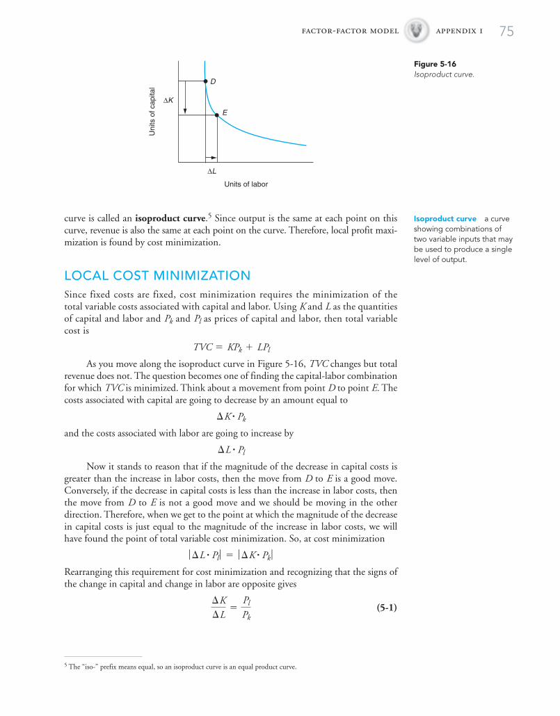
curve is called an isoproduct curve.5 Since output is the same at each point on thiscurve, revenue is also the same at each point on the curve. Therefore, local profit maxi-mization is found by cost minimization.
LOCAL COST MINIMIZATIONSince fixed costs are fixed, cost minimization requires the minimization of thetotal variable costs associated with capital and labor. Using K and L as the quantitiesof capital and labor and and as prices of capital and labor, then total variablecost is
As you move along the isoproduct curve in Figure 5-16, TVC changes but totalrevenue does not. The question becomes one of finding the capital-labor combinationfor which TVC is minimized. Think about a movement from point D to point E. Thecosts associated with capital are going to decrease by an amount equal to
and the costs associated with labor are going to increase by
Now it stands to reason that if the magnitude of the decrease in capital costs isgreater than the increase in labor costs, then the move from D to E is a good move.Conversely, if the decrease in capital costs is less than the increase in labor costs, thenthe move from D to E is not a good move and we should be moving in the otherdirection. Therefore, when we get to the point at which the magnitude of the decreasein capital costs is just equal to the magnitude of the increase in labor costs, we willhave found the point of total variable cost minimization. So, at cost minimization
Rearranging this requirement for cost minimization and recognizing that the signs ofthe change in capital and change in labor are opposite gives
(5-1)¢K¢L
=Pl
Pk
ƒ ¢L # Pl ƒ = ƒ ¢K # Pk ƒ
¢L # Pl
¢K # Pk
TVC = KPk + LPl
PlPk
factor-factor model appendix 1 75
Uni
ts o
f cap
ital
Units of labor
E
D
ΔL
ΔK
Figure 5-16Isoproduct curve.
5 The “iso-” prefix means equal, so an isoproduct curve is an equal product curve.
Isoproduct curve a curveshowing combinations oftwo variable inputs that maybe used to produce a singlelevel of output.

CONSTANT OUTPUTWe have stipulated that points D and E in Figure 5-16 both represent the same levelof output. Therefore, the contribution to output given up by the decrease in capitaluse must be compensated by the increase in output associated with the increased laboruse. In both cases, the contribution to output is equal to the number of units of capi-tal or labor times the respective marginal products. For a movement from D to E to beon an isoproduct curve requires that the magnitudes of the increase and the decreaseof output be the same:
where and refer to the marginal products of labor and capital, respectively.Rearranging the terms in this gives
(5-2)
LOCAL PROFIT MAXIMIZATIONThe right-hand sides of Equations 5-1 and 5-2 are both equal to and, there-fore, must be equal to one another:
(5-3)
Rearranging terms in this expression gives the constrained or local profit-maximizingcondition:
(5-4)
Here we have the economically meaningful condition for profit maximizationin the factor-factor model. The marginal contribution to output per dollar of inputcost must be the same for both labor and capital. That is, if the price of labor is $2 perunit and the price of capital is $4 per unit, then, in order to minimize costs, the mar-ginal product of capital should be twice that of labor such that the additional outputper dollar of each variable input is the same.
For the sake of argument, look at a situation where the conditions of Equation 5-4are not met. At the prices given previously, assume the marginal product of labor is5 units of output and the marginal product of capital is 15 units of output. In this case,the marginal product per dollar of labor is 2.5, and the marginal product per dollar ofcapital is 3.0. It is clear that the manager would increase capital use and reduce laboruse. Only when the marginal products per dollar of both capital and labor are equal isthere no further opportunity to decrease costs while keeping output constant.
GRAPHICAL SOLUTIONThe same solution to the factor-factor model can be shown graphically. In Figure 5-17,a single isoproduct curve is shown. Recall that each point on this line represents agiven level of total revenue and that the problem is to find the cost-minimizing com-bination of capital and labor. At any point on this curve, the slope of the curve is theratio of the rise over the run of a line drawn tangent to the isoproduct curve:
(5-5)¢K¢L
MPl
Pl=
MPk
Pk
Pl
Pk=
MPl
MPk
¢K/¢L
¢K¢L
=MPl
MPk
MPkMPl
ƒ ¢L # MPl ƒ = ƒ ¢K # MPk ƒ
76 part two microeconomics

factor-factor model appendix 1 77
This ratio is known as the marginal rate of factor substitution because it shows thatrate at which one factor must be substituted for the other in order to maintain a con-stant output level. Notice that as one moves along the isoproduct curve from upperleft to lower right, the marginal rate of factor substitution declines. This is known asdiminishing marginal rate of factor substitution. Because of the diminishing mar-ginal rate of factor substitution, the isoproduct curve in Figure 5-17 takes the shape ofbeing convex to the origin.
Now we need to introduce information about costs on our graph. Suppose thefirm spends on labor and capital. If all of that were spent on capital only, then
units of capital could be purchased. In this case, no labor would be pur-chased, so the input combination would lie on the capital axis as shown by the dot onFigure 5-17. If all input spending were for labor alone, then the input combinationwould lie on the labor axis. All other combinations of capital and labor that could beacquired with an outlay of lie on a straight line between these two points. Thisstraight line is known as the isocost line because each point on the line represents thesame amount of total variable cost to the firm.
As shown in Figure 5-17, no input combination that can be acquired with anoutlay equal to is capable of producing the level of output on the isoproductcurve. If the total amount of spending on variable inputs were increased, the isocostline would shift outward as it would be possible to buy either more capital or morelabor or both. The new isocost line will be parallel to because the pro-portions of increase for capital and labor are the same.
Since they are parallel to one another, the slopes of both and arethe same. As always, the slope of a line is equal to its rise over its run, so the slope ofeither isocost line is
(5-6)
So the slope of an isocost line is determined by the ratio of the prices of the two vari-able inputs.
Any number of isocost lines can be drawn on Figure 5-17 representing differentlevels of total variable cost. Since our objective is to minimize total variable costs
TVC>Pk
TVC>Pl= -
Pl
Pk
TVC2TVC1
TVC11TVC22
TVC1
TVC1
TVC1>Pk
TVC1
Uni
ts o
f cap
ital
Units of labor
Isoproductcurve
Isocostcurve
Lo
Ko
TVC1/Pk
TVC1/P1
TVC1 TVC
2
TVC3
TVC3
TVC4
TVC4
Figure 5-17Isoproduct and isocostcurves.
Marginal rate of factorsubstitution rate at whichone variable input must besubstituted for the othervariable input in order tokeep output constant.
Diminishing marginal rateof factor substitution asmore and more units of onevariable input are used, thequantity of the other inputthat would have to besubstituted for it to keepproduction constant falls.
Isocost line a graphicalline showing the variouscombinations of twovariable inputs that have thesame total variable cost.

needed to produce the amount of product specified by the isoproduct curve, we willselect because this is the least costly combination of capital and labor that iscapable of producing the level of output for the given isoproduct curve. We know thisis the least costly alternative because is the isocost line closest to the origin thatjust touches the isoproduct curve. It would be possible to produce the quantity ofoutput indicated by the isoproduct curve using but this would be more costlythan So the cost-minimizing firm would select that isocost line that is just tan-gent to the isoproduct curve. At this point of tangency, the firm would use units ofcapital and units of labor. At this point of tangency, the slope of the isoproduct curve(i.e., the marginal rate of factor substitution) is equal to the slope of the isocost line. Atthis point of tangency, the rate at which labor substitutes for capital in production (iso-product) is equal to the rate at which labor substitutes for capital in the market (isocost).Combining Equation 5-5 with Equation 5-6 and canceling out the minus signs gives
Substituting from Equation 5-2 gives
or, rearranging:
This is the same result we got in Equation 5-4 indicating that the marginal productper dollar of input should be the same for both of the inputs. If this were not the case,it would be possible to decrease total variable costs by rearranging inputs.
The factor-factor results presented here for a two-factor, one-product model canbe generalized to a multifactor situation:
(5-7)
for all i, j, and n.
EXPANSION PATHThe solution to the factor-factor model previously discussed is a local solution for agiven level of output. If the level of output were to change, the cost-minimizing inputcombination would also change. In Figure 5-18 we have drawn several isoproductcurves and the isocost curves that are tangent to them. Since the isocost lines are alldrawn for a given set of variable input prices, they are all parallel to one another.
The locus of all of the cost-minimizing points is called the expansion path,because as the firm expands production, it would move from one cost-minimizingpoint to another. Each point on the expansion path is a point of local cost minimiza-tion for the given level of output. At each point on the expansion path, the local cost-minimizing condition in Equation 5-7 is met.
The relevant question then becomes, “Which of the many points on the expan-sion path provides a global profit maximization?” We learned in the factor-productmodel that the profit-maximizing output level was at the point where the marginalcost of producing the last unit is equal to its marginal revenue, or price of the productin perfect competition.
MPi
Pi=
MPj
Pj=
MPn
Pn
MPl
Pl=
MPk
Pk
MPl
MPk=
Pl
Pk
¢Ko
¢Lo=
Pl
Pk
Lo
Ko
TVC3.TVC4,
TVC3
TVC3
78 part two microeconomics
Expansion path locus ofpoints of local optimalfactor-factor combinationsfor multiple isoproductcurves.

factor-factor model appendix 1 79
Profit maximization along the expansion path will occur at that output level ofproduct Q for which
Meeting the local cost-minimization criteria of Equation 5-7 ensures that the twomarginal costs are equal to one another at each point on the expansion path, so thetrick is to move along the expansion path until the point is reached where the mar-ginal costs of each variable input are equal to the marginal revenue. Expansion of thisresult to a multiple variable factor situation is straightforward:
for all n variable inputs.
MCi = MCj = Á = MCn = MRq
MCl = MCk = MRq
Uni
ts o
f cap
ital
Units of labor
Expansionpath
TVC1
TVC2
TVC3
TVC4
Figure 5-18Expansion path.
KEY TERMS
Constrained optimizationDiminishing marginal rate of factor
substitution
Expansion pathFactor-factor modelIsocost line
Isoproduct curveLocal optimizationMarginal rate of factor substitution

80
appendix IIProduct-Product Model
We now come to the final generalization of the factor-product model. In the simpleone-factor, one-product model, we found that the firm could maximize profit byadjusting output to that point at which the marginal cost of additional input is equalto the marginal revenue of additional output. Then we showed that in the case ofmultiple variable inputs, the firm should adjust the use of each input such that themarginal cost of each input is equal to the marginal revenue of the product. Now weturn to the case of a firm with multiple products.
The product-product model examines the case of a firm with two productsthat are produced using a given bundle of fixed and variable inputs. As before, this isa local or constrained optimization problem because the analysis assumes that the quan-tity of inputs is predetermined, and as a consequence, total costs are predetermined.Profit maximization therefore becomes a question of local revenue maximization.
LOCAL REVENUE MAXIMIZATIONAssume a firm with a set of resources that can be used to produce either of two products:canned peaches or fresh peaches. Since total costs are predetermined in this constrainedoptimization, the firm seeks to maximize total revenue, which is given by
where
Because of limited resources, any effort to increase canned production will comeat the expense of reducing fresh production. If this were not the case, the firm wouldobviously increase the production of both. That is, the only relevant economic ques-tion is how to adjust production of the two products when there is an economictrade-off. Assume the firm is currently producing half and half. The firm managerasks if the firm should produce more fresh peaches. To answer this question the man-ager calculates the additional revenue associated with more fresh production as
and the loss of revenue associated with less canned production is
where is negative, and, hence, is negative.If the magnitude of the additional fresh revenue is greater than the mag-
nitude of the loss of revenue from canned production then it makes economicsense to make the adjustment. However, if then the manager shouldbe considering an expansion of canned rather than fresh.
MRf 6 ƒMRc ƒ ,1MRc2,1MRf2
MRc¢C
-MRc = -¢C # Pc
MRf = ¢F # Pf
1MRf2
Pf = price per unit of fresh peaches
Pc = price per unit of canned peaches
F = units of fresh peaches produced
C = units of canned peaches produced
TR = total revenue
TR = C # Pc + F # Pf
Product-product modelmodel of the firm in whichthe firm produces twoproducts using a givenbundle of fixed and variableinputs.

As more and more fresh is substituted for canned, we would expect the marginalrevenue from fresh to decline because of the diminishing marginal productivity of theinputs used in the production of fresh, and we would expect the magnitude of the mar-ginal revenue of canned to increase for the same reason. As the magnitudes of the twomarginal revenues change, we should finally arrive at a point at which the two magni-tudes are equal. At this point there is no remaining reallocation of production thatcan increase revenue, so this point must be the point of revenue maximization. Thatis, in order to maximize revenue, the firm should adjust production of the two goodsto the point at which
To do otherwise would suggest that the firm is not reaching a constrained opti-mum, because a reallocation of the available inputs will increase revenue whenever thetwo marginal revenues are not equal.
GRAPHICAL SOLUTIONThis same principle of equi-marginal constrained revenue maximization can be illus-trated graphically. Figure 5-19 shows the different combinations of fresh and cannedpeaches that can be produced with a given resource allocation. The concave to the ori-gin shape of this curve suggests that as more and more canned peaches are produced,a greater and greater quantity of fresh must be given up to free up the resourcesneeded to produce one more unit of canned. This changing substitution rate is a con-sequence of the diminishing marginal productivity of available resources. As morecanned peaches are produced, the marginal productivity of resources used for cannedfalls, and as fewer fresh peaches are produced, the marginal productivity of resourcesused for fresh increases.
The curve in Figure 5-19 is called a production possibilities curve, and it isbased on the predetermined bundle of inputs. Changing the size of the input bundlewould produce a different production possibilities curve. Given the input constraint,the local optimization problem is to find the combination of the two products thatwill maximize revenue.
ƒMRf ƒ = ƒMRc ƒ
product-product model appendix 11 81
Fre
sh
Canned
Productionpossibilities curve
ΔC
ΔF
Figure 5-19Production possibilitiescurve.
Production possibilitiescurve a curve showingdifferent combinations oftwo products that can beproduced using a givenbundle of fixed and variableinputs.

82 part two microeconomics
The slope of the production possibilities curve at any point on the curve is equalto the slope of a tangent to the curve at that point. The slope of the tangent is equalto the rise over the run, which is (ignoring the signs)
This is called the marginal rate of product substitution. To find the point of localrevenue maximization, we need to have some information about revenues.
Figure 5-20 shows different combinations of the two goods that are capable ofgenerating a given amount of total revenue. For a given amount of total revenue
if only fresh were produced, it would take units of fresh output toproduce The output combination of all fresh and no canned is marked with adot on the vertical axis. Likewise if only canned were produced, it would take units of canned production to generate This output combination is marked witha dot on the horizontal axis. Output combinations on the straight line between thedots also generate This line is called an isorevenue line.
The slope of the isorevenue line is equal to its rise over the run, which,ignoring the signs, is given by
(5-8)
Numerous isorevenue lines can be drawn representing different levels of total rev-enue. Since the slope of these lines is equal to the ratio of product prices, they all will beparallel to one another for a given set of product prices. The greater the total revenue on anisorevenue line, the farther the line is from the origin. So revenue maximization seeks thatisorevenue line that is farthest from the origin within the limits of the resource constraint.
Revenue maximization will be found at the point of tangency between the produc-tion possibility curve and the highest isorevenue line drawn to that point of tangency. Atoutput combination and the firm will maximize revenue. At this point, theslope of the isorevenue curve is equal to the marginal rate of product substitution.That is, at this point, the rate of substitution in production is equal to the rate of sub-stitution in the market. Since the two slopes are equal at this point, we can combineEquations 5-8 and 5-9 to yield the revenue-maximizing condition:
¢Fo
¢Co=
Pc
Pf
Co,Fo
TR1>Pf
TR1>Pc=
Pc
Pf
TR1
TR1.
TR1.TR1>Pc
TR1.TR1>Pf1TR12,
¢F¢C
Marginal rate of productsubstitution rate at whichone product can besubstituted for another inthe production processusing a given bundle offixed and variable inputs.
Isorevenue line a lineshowing the differentcombinations of twoproducts that will produce agiven total revenue.
Fre
sh
Canned
TR2
Fo
Co
TR
1 TR1/Pf
TR1/Pc
Figure 5-20Isorevenue lines.

product-product model appendix 11 83
Cross multiplying gives
where a change in physical output times the price of the product is by definition themarginal revenue associated with the change in production so
This is the same result obtained previously.
GENERALIZATIONThe results of the product-product model can be generalized for a multiproduct firm.Local revenue maximization from a given bundle of resources will be found where
for all i, j, and n.Alternate sets of constrained input bundles would produce alternate production
possibilities curves, and a local optimum could be identified for each. A line throughthese local optimums would generate an expansion path in output space similar tothat in Figure 5-18 for input space.
A global or unconstrained optimum along this expansion path would occur atthat point at which the marginal revenues of each product are equal to the marginalcost of the production possibilities curve:
for all n products of the firm.The results of the factor-factor model can be combined with the previous result
to provide the profit-maximizing rule for a multifactor, multiproduct firm:
for all n products and r inputs.
MRi = MRj = Á = MRn = MCp = MCq = Á = MCr
MRi = MRj = Á = MRn = MC
MRi = MRj = Á = MRn
MRf = MRc = Á = MCn
¢Fo# Pf = ¢Co
# Pc
KEY TERMS
Isorevenue lineMarginal rate of product
substitution
Production possibilities curveProduct-product model

6Supply, Market Adjustments,and Input DemandTHE BASIC MICROECONOMIC THEORY OF THE PERFECTLY COMPETITIVE FIRM HAS
been developed in Chapters 4 and 5. In the short run, the profit-maximizing firmmanager adjusts input levels (and, hence, output) to that point at which additionsto cost are equal to additions to revenue; that is, marginal cost is equal to marginalrevenue. Changes in those factors exogenous to the firm (such as the price of theproduct) will cause the firm manager to react by changing the input-output level.Failure to adjust internally to changes caused externally results in suboptimal per-formance of the firm. Let’s face it, the college town restaurant manager who hasthe same crew on the Thursday of spring break as on the Saturday of a home foot-ball game is a manager who is throwing a lot of money into an empty hole. Thejob of the manager is to make endogenous adjustments to exogenous changes.
In our perfectly competitive model, one of the fundamental assumptions isthat the firm is so small relative to the market that no actions by the individualfirm can affect the market. However, if prices exogenous to the individual firmchange, then we would expect all firms within the market to adjust independentlyto the new situation. As all firms within an industry change, the market itself willchange. That is, individual firm managers, each acting in his or her own self-interest,will collectively bring about changes in the market. It is this relationship betweenthe individual firm and the industry to which this chapter is addressed.
SUPPLY CURVE OF THE FIRMThe cost curves of the individual firm can beused to derive the supply curve of the firm.Recall that supply is a relationship betweenprices of a product and the quantities the firmis willing to produce at alternative prices,
ceteris paribus.Figure 6-1 shows a typical set of cost
curves for a firm. These curves, as is thecase for all cost curves, are drawn assumingthat all other factors remain constant and
are drawn for a short-run time period inwhich some factors of production are fixed.
At alternative prices, the firm adjusts outputsuch that the marginal revenue (i.e., the price
of the product) is equal to the marginal costin order to maximize profit or minimizeloss. If the marginal revenue is less than theminimum average variable cost, the firmwill cease production. Several price-outputcombinations are listed on the schedule
Supply curve of thefirm quantities of a goodthe firm is willing toproduce at alternativeprices for the good, ceterisparibus. It is equal to themarginal cost curve of thefirm at prices above theshutdown point.
Industry a collection offirms producing the same orsimilar products.

supply, market adjustments, and input demand chapter six 85
below the chart. Each combination indicates how many units the firm is willing toproduce at each alternative price. Therefore, this schedule is a supply schedule of the firm.Now, if these points from the supply schedule were plotted on the axes above, they wouldgraph a supply curve. That curve would be superimposed on the marginal cost curve atany price greater than the shutdown price. So, the supply curve of the firm is themarginal cost curve of that firm above the shutdown price.
As we saw previously, for any price less than the minimum average variable cost,the quantity supplied would be zero. A typical firm supply curve is shown in Figure 6-2.Note that the supply function is discontinuous at the shutdown price.
MARKET SUPPLYA market supply curve is simply the horizontal summation of all the firm supplycurves in the industry. Therefore anything that affects the typical firm’s supply functionwould affect the market supply. Why changes in input prices and technology are marketsupply shifters should now be obvious. Anything that affects the marginal cost curve ofthe individual firm in the industry thus affects the market supply curve of the industry.
In addition, the market supply curve will shift as individual firms enter or leavethe industry. If additional firms enter the industry, the supply curve will shift outwardas there is more product produced at each alternative price. Conversely, as firms leave
Market supply curve thehorizontal summation ofthe firm supply curves forall the firms in the industry.
$5.00
$4.00
$3.00
$2.00
$1.00
60 70 80 90 100 110
Units of output (bu/acre)
$/bu
MC
AVC
Price per unitUnits produced
$1.000 83 94 103 109
$2.00 $3.00 $4.00 $5.00
Figure 6-1Derivation of the firm’ssupply curve.
Shu
tdow
n pr
ice
Units of output (bu/acre)
Supplycurve
of the firm($/b
u)
Figure 6-2Supply curve of the firm.

the industry, ceteris paribus, the market supply curve will shift inward. As we will seein a moment, the entry and exit of firms in a perfectly competitive industry is a driv-ing force behind Adam Smith’s “invisible hand.”
86 part two microeconomics
CAUTION
A change in the price of fertilizer (or any other input) will shift the firm’s supply curve ofcorn. Likewise, a change in the technology of producing corn, such as precision agricultureor genetically modified seeds, will shift the firm’s supply curve of corn. An increase ordecrease in the number of corn producers will shift the market supply of corn. However, achange in the price of corn will not shift either the firm or the market supply of corn.Finally, a change in the price of corn will be associated with a movement along the supplycurve but not a shift of the supply relationship itself. Likewise, a change in the demand forcorn will not cause a shift in the short-run supply of corn, but it may lead to an eventualmarket adjustment that does entail a long-run supply shift.
Static an economicanalysis at a point in time.
Dynamic an economicanalysis over a period oftime analyzing theadjustment process.
Stable equilibrium marketsituation in which thequantity demanded is equalto the quantity supplied atthe prevailing market priceand there are no incentivesfor additional firms to enteror leave the market.
It is appropriate at this time to briefly review the ground that has been covered.Our final destination was a short-run market supply curve. It is simply the summa-tion of individual firm supply curves. The firm supply curve is the marginal cost curveabove the shutdown price. The marginal cost curve is derived from the total costcurve. The total cost curve is derived from the production function. So, ultimately themarket supply curve is determined by the noneconomic, technical relationshipbetween inputs and outputs we know as the production function and the prices usedto transform that production function into a marginal cost curve.
MARKET ADJUSTMENTSThe analysis to this point has been static; that is, it has been assumed that there issome externally determined product price and that the firm must adjust to this price.In reality, we know that prices of agricultural commodities are continually changingover time. In examining the relationship between the individual firm and the marketfor an entire industry over time, we can begin to appreciate the dynamics of AdamSmith’s “invisible hand.”
Dynamic Relationship Between the Firm and the MarketFigure 6-3 illustrates a long-run, stable equilibrium relationship between a typicalfirm and the market (i.e., a collection of firms and consumers). A stable equilibriummeans there are no exogenous forces pushing for adjustments in the market. A shift ineither market demand or market supply caused by a change in some ceteris paribus
Qq* Q* Q
MC
ATC
Firm Market
AVC
DS
$ $
P*P*
Figure 6-3Long-run, stableequilibrium.

condition would lead to a short-run disequilibrium situation in which the quantitydemanded is not equal to the quantity supplied at the previous price. The disequilib-rium would encourage individual firms and the industry market to adjust to a newsituation in the search for a return to a long-run, stable equilibrium.
In Figure 6-3, the interaction of supply and demand in the market leads to amarket equilibrium price of P * and an equilibrium quantity traded of Q *. P * and Q *are stable equilibrium values because the quantity demanded is equal to the quantitysupplied; therefore, the market is cleared. The individual firm in this market, being aprice taker and a maximizer of economic profits, adjusts output to q * such that themarginal cost of producing q* is equal to the marginal revenue received, or P *. Forthe marginal firm (the highest cost producer in the industry), the market equilibriumprice, P *, is equal to the break-even point or the minimum average total cost. Since atthis point the average revenue (P *) is equal to the average total cost, the economicprofits of this marginal firm are zero. The relationship between the firm and the mar-ket shown in Figure 6-3 is a long-run, stable equilibrium situation because there areno pressures on the firm or on the market to change. Since the marginal firm is earn-ing zero economic profits, there are no incentives for other firms to enter the market,nor are there pressures for this marginal firm to leave the market. This equilibrium sit-uation will remain stable until such time as some exogenous change requires market,and hence firm level, adjustments. These exogenous forces could be a change in any ofthe market supply or demand shifters (i.e., the ceteris paribus conditions).
If, as a result of a change in one of the ceteris paribus conditions, the demand inthe market should shift upward to D' as shown in Figure 6-4, then there is a disequi-librium at P * as the quantity demanded far exceeds the quantity producers are willingto produce at P *. This results in a shortage at P *, which causes potential buyers to bidup the price of the product to P ** for a new market equilibrium with Q ** unitstraded.
In the short run, as the market price increases to P **, the firm reacts by increas-ing production to q ** such that the quantity traded on the market increases to q**. Atprice P**, the typical firm in the industry is earning pure economic profits at outputlevel q ** because the average revenue of the firm (P **) is greater than the average totalcost as shown by the double arrow in Figure 6-4. In the long run, the existence ofthese economic profits attracts additional firms to the industry. As more firms enterthe industry, the market supply curve (now being the summation of a larger numberof firm supply curves) shifts out to S� as shown in Figure 6-5.
Eventually the market supply curve shifts outward enough to bring the marketprice back to the long-run, stable equilibrium price of P *. At this new long-run equi-librium, the quantity produced by the typical firm falls back to q * and the marketclearing quantity expands to q *** because there are now more firms in the industry.The new equilibrium shown in Figure 6-5 is a stable equilibrium because at price P *there are neither incentives for additional firms to enter the market nor incentives for
supply, market adjustments, and input demand chapter six 87
Qq* q** Q**Q* Q
MC
ATC
Firm Market
AVC
D D'S
$ $
P*
P**
P*
P**Profits
Figure 6-4Demand shift causes short-run economic profits.

existing firms to leave the market. This illustrates the automatic, self-correcting natureof markets that Adam Smith attributed to the force of an invisible hand.
The dynamic adjustments illustrated in Figure 6-3 through 6-5 show the rela-tionship between the market and one firm in that market. Since the economic profitsof the firm shown are zero, this is what is known as the marginal firm or the highestcost firm remaining in this industry. There are many firms in a market, each with itsown unique production function and therefore unique cost structure. Some of theother firms in this industry may be more efficient than the firm shown. These moreefficient firms would have cost structures lower than for the firm shown and, there-fore, would earn economic profits at a market price of P*. So the marginal firm shownis the least efficient firm remaining in the industry that is just willing to produce atzero economic profits.
So, short-run market prices above the break-even price of the marginal firmattract firms into the industry and quickly drive the long-run market price back toequilibrium. A similar sequence of events will occur at market prices below the shut-down point of the marginal firm because firms would quickly leave the industry. Asfirms leave the industry, the market supply curve shifts inward, thus causing the priceto increase back up to the shutdown point of the remaining marginal firms.
At market prices between the break-even and shutdown points of the firm, theadjustment process is the same but much slower. As we have already seen, at marketprices between the break-even and shutdown prices of the firm, the loss-minimizingfirm will continue to operate in the short run although the firm has negative eco-nomic profits. In the long run, if market prices in this range persist, the firm will ceaseproduction and leave the industry. This will shift the industry supply curve inwardand drive the market equilibrium price up. This process will continue until the mar-ket price reaches the break-even point and another long-run, stable equilibrium isestablished.
Cost Structure and Price VariabilityDifferent firms in different industries have different cost structures. In some indus-tries, most costs are fixed costs, while in other industries the majority of total costs arevariable costs. The cost structure of the firm and the industry has a significant impacton the behavior of a typical profit-maximizing firm. Two different firms, one withhigh fixed costs and the other with low fixed costs, are illustrated in Figure 6-6.Airlines, auto manufacturers, and citrus groves are examples of firms with very highfixed costs relative to the variable costs. For these firms, the price range between thebreak-even point and the shutdown point is great. Therefore, a fall in the price caneasily push a firm with high fixed costs below the break-even point and into negativeprofits, but it takes a massive price reduction to push the firm into going out ofproduction at the shutdown point.
88 part two microeconomics
Marginal firm a firm in anindustry with the highestaverage costs and hencethe most likely firm to leavethe industry if prices fall.
Cost structure the relativeimportance of fixed andvariable costs in the totalcosts of the firm.
Qq* Q*** Q
MC
ATC
Firm Market
AVC
D D'S
S'
$ $
P*P*
Figure 6-5Economic profits attract newfirms into industry.

supply, market adjustments, and input demand chapter six 89
Most airlines today are examples of companies that have had negative profits fora number of years. Nonetheless, they continue to fly because the market price isbetween the break-even point and the shutdown point. For these airlines, to continueto fly is rational behavior in the short run. So, for the time being, they continue to flyin the hope that competitors will leave the market, thereby allowing prices to increase,or that variable costs (such as fuel) will fall.
Of course, an airline can’t survive as a company if it suffers losses forever.Eventually the company will run out of assets in the long run and be forced intobankruptcy. This is exactly what happened to Eastern Airlines and, more recently, theautomaker Chrysler.
By comparison, a cattle feedlot is an example of a firm with very few fixed costs(land) and very high variable costs (feed). As a consequence, very small movements ofcattle prices will result in either short-run economic profits or a shutdown (i.e., thefeedlot operator leaves the feedlot vacant) until prices recover.
Moving from the firm to the market, we expect to see market prices vary withinthe upper and lower limits imposed by the break-even and shutdown points as illus-trated in Figure 6-6. The implication of this is that for firms in high fixed-cost industries,tremendous market price variation is a fact of life, and firms are slow to enter or leavethe industry. For firms in low fixed-cost industries, relatively small market price vari-ation is expected over time, but a lot of firms enter and leave as the adjustmentprocess takes place.
Agriculture has abundant examples of firms with different cost structures—some with high fixed costs and some with very low fixed costs. Examples of firms withhigh fixed costs would be a cow-calf operator, orchards, and forestry. Low fixed costsare found in the broiler industry, high value vegetable production, and feedlots.
PROFIT-MAXIMIZING INPUT USEIn Chapter 4, the production function was developed, and in Chapter 5 it was usedto determine the profit-maximizing output level of a perfectly competitive firm. Itwas determined that profit maximization will always occur in the rational range ofproduction where output is increasing at a decreasing rate as additional units of thevariable input are employed. The law of diminishing marginal returns stipulates thatthis will be a characteristic of all production functions.
Figure 6-7 reproduces the marginal product curve that was introduced inChapter 4. Only that segment of the marginal product curve (MP) that is in the rel-evant range of production is shown. Throughout the relevant range of production,the marginal product decreases as variable input use increases. Within this range thereis a unique one-to-one relationship between input levels and output levels. That is,
Q Q
MCMC
ATC
ATC
High fixed costs Low fixed costs
AVC AVC
$ $
Figure 6-6Range of price variationbefore long-run adjustmentsoccur.

each output level is uniquely defined by one and only one input level. Therefore, wecan recast the profit-maximizing question that was asked in Chapter 5: what is theprofit-maximizing level of input use? This question is the mirror image of the profit-maximizing output level question posed in the previous chapter.
To solve the profit-maximizing output question, we compared marginal revenueof each additional unit of output to the marginal cost of producing that unit of out-put. So long as additions to revenue are greater than additions to cost, profit isincreasing. A similar approach is used to find the profit-maximizing level of input use.
Value of the Marginal ProductThe marginal product curve in Figure 6-7 shows the additional amount of outputthat each variable input will produce. For example, in this illustration, the 15th unitof the variable input produces 8 additional units of output. Since we don’t see thetotal product curve, we don’t know if output increased from 100 to 108 or 400 to408. All we know is that the 15th unit of variable input produced 8 additional unitsof output.
Now we need to convert this physical data into economic information that canbe used to describe profit-maximizing behavior. In this case, the relevant question is,how much additional revenue did those additional 8 units of output generate? This,of course, depends on the price of the product. Since we are dealing with a perfectlycompetitive situation, the price of the product is a constant. To find the value of themarginal product, simply multiply the amount of the marginal product timesthe constant price of the product. If the price of the product were $3.00 per unit, thenthe value of the marginal product in this example would be $24.00 (8 units * $3.00per unit). When this transformation from units of marginal product to value of mar-ginal product is completed for all variable input levels, a new curve is derived, whichis called the value of the marginal product (VMP) curve. This is shown in Figure 6-8,which is very similar to the marginal product curve in Figure 6-7 except that the ver-tical axis is now measured in dollars instead of units of output. The VMP curve showsus the additional amount of revenue associated with each additional unit of the vari-able input.
Profit MaximizationThe value marginal product curve in Figure 6-8 tells us about the revenue side of thefirm at different levels of variable input use. To complete the analysis of profit maxi-mization, we also need to know about the cost side of the firm. Since we are dealingwith perfectly competitive markets, the price of the variable input (and, hence, itscost) is a constant. The additional cost associated with one additional unit of the variable
90 part two microeconomics
MP
Units of the variable input
15
8
Add
ition
al u
nits
of o
utpu
t
Figure 6-7Marginal product curve.
Value of the marginalproduct the additionalrevenue associated with aunit increase of the variableinput, ceteris paribus.

supply, market adjustments, and input demand chapter six 91
input is called marginal factor cost (MFC ), which is a constant equal to the price ofthe variable input. In Figure 6-9 a MFC of $20.00 which is equal to the price of thevariable input is shown. Notice that on the vertical axis we are graphing both dollarsof marginal revenue and dollars of marginal factor costs associated with each addi-tional unit of the variable input.
Now let’s look at the economics of profit-maximizing variable input use. InFigure 6-9, if the manager of the firm employed the 15th unit of the variable input,the value of the marginal product (additional revenue) associated with that 15th unitis $24.00 while the marginal factor cost (additional cost) is only $20.00. So the man-ager, by adding the 15th unit of the variable input, can add $4.00 to the profits of thefirm. Clearly, given a profit-maximizing management objective, it is in the interest ofthe firm to hire that 15th unit of the variable input.
In a similar fashion, one can infer in Figure 6-9 that the 16th unit of the variableinput would also increase profits from the level obtained with 15 units because, onceagain, additions to revenue exceed additions to costs. The 17th unit of the variableinput would be the profit-maximizing level of variable input use because at this levelof input use, the additions to revenue (VMP) are just equal to the additions to cost(MFC). If the manager were to hire the 18th unit of input, the MFC would exceedthe VMP and profit would fall. So the basic profit-maximizing criterion for the firmis to use the variable input at that level for which the value of the marginal product isequal to the marginal factor cost.
This profit-maximizing criterion is the mirror image of the marginal revenueequals marginal cost criterion developed in Chapter 5 for the profit-maximizing levelof output. Since there is a one-to-one relationship between output and variable input
VMP
Units of the variable input
15
$24
$
Val
ue o
f add
ition
al u
nits
of o
utpu
t Figure 6-8Value of the marginalproduct curve.
VMP
MFC
Units of the variable input
15 17
$24
$20
$
Dol
lars
of a
dditi
onal
rev
enue
and
cos
t Figure 6-9Marginal factor cost.
Marginal factor cost Theadditional cost associatedwith a unit increase of thevariable input; equal to theprice of the variable input.

92 part two microeconomics
levels in the rational range of production, the solution of one problem is the same asthe solution for the other. It is just a matter of whether we approach the problem inoutput space or variable input space.
Input Demand of the FirmWe saw in Figure 6-9 that at a price of $20.00 per unit of the variable input (the mar-ginal factor cost), the profit-maximizing firm used 17 units of the variable input.Likewise, if the price of the variable input were $24.00, the firm would use 15 units.These two price-quantity combinations constitute two points on the firm’s demandcurve for the variable input. That is, at an input price of $20.00 per unit, the firm iswilling to purchase 17 units, ceteris paribus.
At all other possible variable input prices (marginal factor costs), the quantitydemanded would fall on the VMP curve, so the value of the marginal product curveis the demand curve of the variable input.
Input Demand ShiftersSince the demand curve for a variable input is the value of the marginal product ofthat input, anything that will change the VMP curve will change the demand curve.There are three main input demand shifters:
1. Price of the product. Since the VMP curve is equal to the marginal productcurve times the price of the product, any change in the product price willresult in a shift of the input demand curve.
2. Technology. A change in technology such as a change from hybrid seed togenetically modified seed will cause a shift in the production function,which will result in a shift in the marginal product curve and, ultimately, ashift in the value of the marginal product curve, that is, the demand curveof the variable input. The input demand shift can be either resource usingor resource saving depending on the nature of the technology change.
3. Supply shift of other factors. The production function developed inChapter 4 relates output to the quantity of a variable input used in conjunc-tion with other inputs that are assumed to be fixed. If there is a change inthe fixed factors, then the whole production function will shift, which willcause the marginal product curve to shift, and, ultimately, the value of themarginal product (demand curve for the variable input) will shift. Forinstance, if we are looking at a farmer’s demand curve for labor, thatdemand curve would shift inward if the farmer bought newer, bigger farmequipment because less labor would be needed at each price for labor.
Demand curve of thevariable input quantitiesof the variable input usedby the firm at alternativeinput prices, ceteris paribus;equal to the value of themarginal product curve inthe rational range ofproduction.
SUMMARY
The supply curve of an individual firm within an industryis equal to the marginal cost curve of the firm at pricesabove the shutdown point. At prices below the shutdownpoint, the quantity the firm will produce is zero.
The market supply curve is the horizontal summa-tion of all the firm supply curves in the industry.Therefore, any change in ceteris paribus conditions thatshifts firms’ supply curves will also shift the market sup-ply curve. Moreover, the market supply curve can beshifted if additional firms enter or leave the industry.
In a long-run, stable equilibrium situation, the eco-nomic profit of the marginal, high-cost firm is zero.There is neither incentive for existing firms in theindustry to exit, nor is there incentive for additionalfirms to enter. A short-run disequilibrium is createdwhenever a change in one of the ceteris paribus condi-tions causes a shift in market supply or demand.
The dynamic relationship between the firm and themarket may be illustrated with an outward shift of themarket demand curve. The market price will increase,

supply, market adjustments, and input demand chapter six 93
which will cause each firm to move along its firm sup-ply curve, producing more at the higher price. Now themarginal firm is earning economic profits, which sendsa signal to investors to enter this industry. As additionalfirms enter the industry, the market supply curve willshift outward, causing the market price to fall. Thisdynamic adjustment will continue until the marketprice falls to that point at which the marginal firm isearning economic profits of zero.
At prices above the break-even price or below theshutdown point, market adjustment occurs rapidly asfirms enter or leave the industry. However, at pricesbetween the shutdown price and the break-even price,the adjustment process is very slow because firms stayin the industry and continue to produce as they attemptto minimize losses.
For industries with high fixed costs, the price vari-ation from shutdown to break-even is large. As a con-sequence, prices can fluctuate over this wide rangewith no short-run adjustments by firms in the indus-try. In such industries, wide price swings are common.By comparison, industries with low fixed costs requireonly small price changes to bring about short-runadjustment.
The firm’s input demand curve is the value of themarginal product curve, which is derived from themarginal product curve. The firm maximizes profitby adjusting input use to that point at which thevalue of the marginal product is equal to the marginalfactor cost. Input demand shifters include the price ofthe product, technologies, and the supply of otherresources.
KEY TERMS
Cost structureDemand curve of the variable inputDynamicIndustry
Marginal factor costMarginal firmMarket supply curveStable equilibrium
StaticSupply curve of the firmValue of the marginal product
PROBLEMS AND DISCUSSION QUESTIONS
1. What changes would cause the market supplycurve to shift but not shift individual firm supplycurves?
2. Explain why a firm will not produce at pricesbelow the shutdown point.
3. At prices above the shutdown point, what criteriondoes the firm manager use to identify the outputlevel that will maximize profits or minimize losses?
4. Trace the lineage between the production functionand the market supply curve.
5. Assume the market for tomatoes is in a long-run,stable equilibrium. Trace the dynamic adjustmentsthat would occur in this market as a result of aninward shift of the market supply curve.
6. What distinguishes the “marginal” firm from allother firms in an industry?
7. Explain why adjustment is slow when the marketprice falls to a range below the break-even pointand above the shutdown point.
8. Discuss the implications of cost structure on mar-ket price variability.
9. Detail each of the steps needed to move from aproduction function to a demand curve for thevariable input.
10. Give an example of each of the three input demandshifters.

7Imperfect Competition and Government RegulationIN CHAPTERS 3 THROUGH 6, WE EXAMINED THE BEHAVIOR OF THE PROFIT-MAXIMIZING
firm in a perfectly competitive market. A skeptic might question the utility of theeconomic theory of the perfectly competitive firm because there are very fewinstances in which producers and consumers interact under the conditions of per-fect competition. Nonetheless, a vast number of industries behave as if they areperfectly competitive. However, many firms do not operate under conditions ofthe perfectly competitive model. In this chapter, we will examine the economicsof less than perfectly competitive firms—hence the term imperfect competition.
In reality, most markets are less than perfectly competitive. In fact, in mostmarkets for consumer goods, the assumption that the producer is so small relativeto the market that the producer has no control over prices is not a valid assump-tion. Certainly Campbell’s has some pricing power in the soup market, andKellogg’s has pricing power in the breakfast cereal market. Should that powerbecome excessive, government regulations might be necessary to protect the con-sumer from predatory business practices.
MARKET STRUCTUREEconomists use the term market structure to refer to the number of firms in anindustry and the relationship among them. Perfect competition is at one end of
the spectrum of market structures characterized by manyfirms such that no one firm can influence the mar-
ket by its actions. The opposite end of thespectrum from perfect competition is puremonopoly, in which there is only one firm inthe industry. In between these two extremeslie many firms in many markets. Two kinds
of structure in between the extremes will beexamined in this chapter: monopolisticcompetition and oligopoly. In studyingthese market structures, you will learnabout the markets you, the consumer,
frequently trade in.Market structure also refers to the rela-
tive ease with which additional firms mayenter the industry. In a monopoly structure,
there is one firm and entry of other firms isblocked completely. In an oligopoly struc-ture, there are a few firms and entry is dif-ficult. In a monopolistic competitionstructure, there are few or many firmswith virtually no barriers to entry.
Market structure thenumber of firms in anindustry and the relationshipamong them.

imperfect competition and government regulation chapter seven 95
One of the canons of economics is that the market structure in which a firmfinds itself determines the conduct and performance of the firm. That is, firms indifferent market structures behave differently as the managers of the firm seek tomaximize profit to the firm.
PERFECT COMPETITIONStructureBefore dealing with imperfect competition, it would be worthwhile to review the con-ditions necessary for the existence of perfect competition:
• There are so many producers and consumers that the individual producer orconsumer is insignificant in relation to the total market.
• The product is homogeneous; that is, the consumer does not distinguishbetween products of different producers.
• There are no artificial limitations on entry to or exit from the market.
In the economic sense, perfect competition simply refers to a market structure in whichthe individual unit provides such a minute portion of the total market supply (ordemand) that the actions of the individual cannot influence the market price of theproduct.
The second condition of homogeneity of the product is concerned with the uni-formity of the product bought and sold. One bushel of wheat, for example, is prettymuch like another bushel of wheat. One chicken is pretty much like another. Onechoice grade 1,000-pound slaughter steer is very much like another. In other words,when we are concerned with homogeneity, a product cannot be identified as to sourceor destination once it gets into the marketplace.
The third condition of no artificial limitations on entry to or exit from the mar-ket is concerned largely with the freedom of choice or sovereignty of both producersand consumers and with the mobility of resources and products. Prices are assumed tobe free to move in response to changes in market supply and market demand.Resources are free to move into those alternative employments that pay the highestreturns to the resources. Goods and services are free to move to those consumers andinto those areas that are willing to pay the highest prices.
ConductWhat kind of conduct by firm management can we expect in a perfectly competitivestructure? We’ve already seen that under conditions of perfect competition, the firm’smarginal cost curve defines the firm’s supply curve. We’ve seen how the demand curvefaced by the firm appears as a horizontal line at the market price level. This linedefines the marginal and average revenue curves as well as the demand function facedby the individual firm in Figure 7-1. Note that the quantity axis for the market ismeasured in much larger units than the quantity axis for the firm. Thus, the individ-ual firm provides only an infinitesimally small part of the market supply. Firm man-agers maximize profits by adjusting output such that marginal costs and marginalrevenue are equal.
In the world of perfect competition, we have said that resources are free to moveinto those industries in which returns are the greatest. What does this mean in thecase of economic profits? If average total costs (including the opportunity costs for allresources used) are less than average revenue per unit of a particular product, as atprice in Figure 7-1, in what direction would resources be expected to flow?Obviously, since the returns in this business are greater than “normal”—that is, since
P1
Conduct behavior of theprofit-maximizing firmmanager. Conduct isdetermined by structure.

96 part two microeconomics
$ $
Units
MC = s
P1
P2
q3 q2 q1
ATC
AVC
Individual firm
Millions of units
S
S'
P1
D1
P2
Q2Q1
MarketFigure 7-1Relationship between aperfectly competitive firmand the market.
resources are earning returns above their opportunity costs—resource owners couldbe expected to attempt to cut themselves in for a piece of the action. As a result,resources would be expected to flow into the industry where economic profits arebeing realized. As resources come into the production of the good in question, themarket supply curve for that product would shift to the right (S'), and the marketprice would fall to shifting the demand curve faced by each individual firm down-ward, causing the economic profits to ultimately disappear.
The existence of the perfectly competitive markets is rare in the real world out-side of basic commodity markets. However, the perfectly competitive market modelprovides us with a very convenient standard for comparing the impacts of varioustypes of market structures. Further, we do have certain important segments of oureconomy, notably farming, in which the real world situation approaches the perfectlycompetitive model.
PURE MONOPOLYStructureNow, using our perfectly competitive standard for comparison, let’s examine a marketstructure at the other extreme: pure monopoly. The conditions necessary for the exis-tence of pure monopoly include
• There is one and only one seller of a given product in a given market. Themarket demand function is the demand function faced by that individualfirm. The firm and the market are one and the same.
• There are no close substitute goods for the product. If there were, then thefirm would lose its monopoly power.
• Entry of other firms into the market for this product is blocked.
Like perfect competition, the incidence of pure monopoly is rare in the real world.One example of pure monopoly is the American postal system so far as first-class mailis concerned. However, the emergence of delivery services such as FedEx, UPS, and e-mail has created close substitutes that have reduced this monopoly power. Manypublic utility systems approach the purely monopolistic case, at least in a local sense.For example, most communities will grant a franchise to a single seller of electricityand another to a single seller of natural gas. Electricity and natural gas will substitute
P2,
Monopoly marketstructure in which there isonly one firm in the industry,there are no closesubstitutes, and entry intothe industry is blocked.

imperfect competition and government regulation chapter seven 97
for one another to some degree, so while the monopolistic character of these examplesis not “pure,” it unquestionably approaches purity at least in a locational sense.1
Other examples abound.
Barriers to EntryA necessary condition for a monopoly to exist is that barriers prevent other firms fromentering the industry. If other firms could enter, then obviously the monopolistwould be subjected to competition from the other firms, as the U.S. Postal Service isnow subjected to substantial competition in most fields. In fact, the only monopolypower the USPS retains is the right to use your physical mailbox, and the value of thatmonopoly power is diminishing as e-mail boxes and door-to-door deliveries replacethe quaint thing with a little flag on the side.
The most common barrier to entry is a patent. Patents are rights granted to inventors to the exclusive use of their invention for a period of time, currently20 years in the United States. The logic of patents is straightforward: an inventorof a product should have the exclusive right to earn the returns to the inventionwithout others stealing the idea and duplicating it. The economic consequence ofpatents is to create a 20-year monopoly. Patents are very common in high-techindustries. Many of the new genetically modified agricultural seeds are beingpatented.
Another effective barrier to entry is a company secret. The Coca-Cola Co. hasnever revealed its recipe—one of the most sacred of industrial secrets in the UnitedStates. Software and chip designers frequently keep their designs secret, realizing that20 years of patent protection is meaningless in the computer business.
A third barrier to entry may be the size of the market to be served. The mar-ket may be so small that the existence of another firm would drive prices so lowthat both firms would be forced into bankruptcy. This barrier to entry probablyhas more effect on agriculture than any other. In many farming communities, forexample, farmers are forced to patronize a particular feed or fertilizer dealerbecause the local market cannot support more than one such business. The nearestalternative source of these products is distant enough that the transportation costprohibits an effective transfer of this patronage. Another example may be found inthe case of a physician or a hospital in a sparsely populated area. By the time apatient could get to an alternative source of medical care, those services may nolonger be required.
Finally, in many cases governments sanction monopolies. These monopolies fallinto three categories.
• First, the government can grant trade associations the power to create monop-olies in their products. A most visible example of this is Major LeagueBaseball, where the owners’ association has been given the power to controlthe number and location of teams.
• Second, government can grant a franchise or concession to a firm and allow itto operate as a monopolist. For instance, all hotels, stores, and eating estab-lishments in Yellowstone Park are operated by a division of a company calledXanterra Parks and Resorts. This is an exclusive franchise granted by the
Patent rights granted toinventors to the exclusiveuse of their invention for aperiod of time, currently 20 years in the United States.
1But this too is about to change. Recent federal legislation has effectively forced a separation of electric power gen-eration from power distribution. In the future, a monopolist will continue to bring the power to your meter, but youwill be free to buy that power from any power generator. Large power users such as industrial plants are alreadybenefiting greatly as they are able to negotiate with alternative power providers to find the most attractive price. The monopoly of the local power generator has been broken.

98 part two microeconomics
National Park Service. In many cities, franchises create local monopolies ingarbage collection, school buses, and cable TV.
• Third, in many cases, particularly in the utilities, one firm can operate morecheaply than two or three could in competition. Imagine having three or fourwater companies competing to bring water to your house. There would be foursets of water mains, four companies digging up the street, and so forth. In thesekinds of cases, called natural monopolies, governments grant monopoly rightsto a single firm. Natural monopolies will be discussed later in this chapter.
Conduct of the Monopoly FirmLet’s compare the analytical concepts of pure monopoly with their counterparts underthe conditions of perfect competition. For purposes of simplicity, let’s assume that ourfriend, the monopolist, buys his resources in a purely competitive market. Since thebasic difference in monopoly and pure competition lies in the manner in which theproduct is sold, we can treat the monopolist’s cost curves as if they were derived inexactly the same manner as the cost curves for the purely competitive firm.
Since the monopolist is the only seller of the product, the demand curve facedby the firm is the market demand curve. Thus, the only way the monopolist canexpand sales during any given time interval is to lower the price at which the productis sold. The market demand curve is the firm’s average revenue curve. For any level ofoutput, it shows what price the firm can command, and that price is the average rev-enue per unit sold at that level of output. So unlike the perfectly competitive firm,which faces a perfectly horizontal average revenue curve, the monopolist faces adownward-sloping average revenue function.
The downward-sloping average revenue curve creates a marginal revenue curvethat is also downward sloping. The marginal revenue curve always lies below the aver-age revenue curve and is more steeply sloped than the average revenue curve. The der-ivation of two points on a marginal revenue curve is illustrated in Figure 7-2. Threepoints on the demand curve are identified, and the total revenue generated at each ofthe three output levels is noted. Then the marginal revenue between total revenuesmay be calculated. These points are plotted on the graph showing the expected result:the marginal revenue curve falls below the average revenue curve (i.e., the demandcurve) and is more steeply sloped.
The profit-maximizing behavior of the monopolist is identical to that of theprofit-maximizing manager of a perfectly competitive firm: expand production solong as additions to revenue are greater than additions to cost. When the point isreached at which additions to revenue are equal to additions to cost, the point ofprofit maximization has been reached. That is, the firm will maximize profit by
10
8
12
6
4
2
5 6 7 Q
$
MRD = AR
Q TR MR
5 60 6 66 7 70
64
Figure 7-2Monopoly: Average andmarginal revenue.

imperfect competition and government regulation chapter seven 99
adjusting output to that point at which marginal revenue equals marginal cost.Regardless of market structure, profit maximization always requires
Once the profit-maximizing level of output has been determined, the managerof the monopoly must determine a price. Unlike the competitive firm, the monopo-list is a price maker. However, he or she is a price maker within the constraintsimposed by the market. In fact, the monopolist makes the price according to what themarket will bear as dictated by market demand. In Figure 7-3, the profit-maximizingoutput is where The manager would set the price at because atthis price units will trade. If the manager had set a price lower than the firmwould forego some profit. At a price higher than consumers would not purchase
units. So is the profit-maximizing price to set.In Figure 7-3, the average revenue per unit of output is substantially
greater than the average total cost per unit of output the difference being pureeconomic profit. The total revenue is or all of the shaded areas on Figure 7-3.Total variable costs are shaded diagonally, and total fixed costs are shaded horizontally.The difference between total revenue and total cost is the profit of the monopolyfirm, shaded vertically.
We now come to the fundamental difference between the monopoly firm andthe perfectly competitive firm. In competition, if the typical firm is earning economicprofits, that will send out a signal to resource owners to shift their resources into thatindustry, and, eventually, the industry will return to a long-run stable equilibrium sit-uation with zero economic profits. The profits earned by the monopolist send out thesame signals, but resource owners find that entry into the industry is blocked by oneor more of the barriers to entry discussed earlier. As a consequence of the barriers toentry, the monopolist firm is able to earn economic profits in the long run as there isno chance for market adjustment.
It is the promise of those economic profits under the protection of the patentsystem that drives pharmaceutical companies to invest millions in research in an effortto develop new products. For the 20 years of patent protection, the firm is a monop-olist. At the end of the patent period, other companies introduce generic versions, andthe price of the drug falls dramatically as a new long-run equilibrium is established.The presence of those monopoly profits also sends out a signal to other firms todevelop products that have a similar use but are chemically different, which can alsobe patented. As a result, we have any number of distinct yet similar antibiotics on themarket today, many of which are still under patent.
Unprofitable MonopoliesMonopolistic firms are not necessarily always profitable. Examples of this may befound in abundance in the rural areas of the United States. In the case where a singlegrocery store remains in a community, if the building were to burn down, the business
Po * Q o
1Ct2,1Po2
PoQ o
Po,Po,Q o
Po,MR = MC.Q o
MR = MC.
$ per Unit
Units of Output
MC
Po
Ct
Qo
ATC
AVC
MR
AR
Figure 7-3Output and pricing for amonopoly firm.

100 part two microeconomics
would often cease to exist since the returns that can be generated are so limited that aninvestment in a new building would be unlikely to pay for itself.
This situation is illustrated in Figure 7-4. As before, the loss-minimizing firmadjusts output to that point at which marginal cost is equal to marginal revenue andthe price (P ) is the average revenue at that level of output. In this example, themonopolist is making some contribution to her fixed costs but is not completely cov-ering the expense necessary to provide for replacing all the capital equipment used inher business. If some contribution to overhead is possible, she will continue to dobusiness until she has depleted (or used up) the investment in fixed equipment. Onceit becomes necessary to replace the building (for example, in the case of a rural gro-cery store), the business will cease to operate.
Not all unprofitable monopolies are small rural monopolies. Amtrak has a vir-tual monopoly on passenger rail travel in the United States, but it has never had aprofitable year. The once powerful Penn Central Railroad went bankrupt in 1970because the opening of the Pennsylvania Turnpike provided an alternative transporta-tion route across Pennsylvania. For many years, Western Union had a monopoly inthe market for nearly instantaneous communication. The first nail in its coffin wasthe telephone, and the last was the advent of the fax machine and e-mail.
PerformanceWhat, then, are the effects of monopoly? Is monopoly necessarily bad? If the marketis of the nature where some competition could feasibly exist, consumers will pay ahigher price under monopoly conditions than they would pay under conditions ofcompetition. There are no economic profits under most competitive situations onceenough time has elapsed to permit economic adjustment to occur. But the economicprofits extracted by the monopolist will continue to be ripped out of the consumer’s
$
Units
Q
AVC
ATC
D = AR
P
MC
MR
Losses
Contributionto fixed costs
Figure 7-4Monopolies aren’t alwaysprofitable.

imperfect competition and government regulation chapter seven 101
hide in the long run—there being no opportunity for market adjustment. Thus, theeffects of monopoly in a market that is large enough to support competition are
• Higher prices• Reduced availability of product• A transfer of wealth from consumers to the monopolist through the economic
profits above and beyond the opportunity cost of all resources.
If, however, the monopoly is of the locational type as a result of a limited size market,consumers are very likely to be in a more favorable position under monopoly. In thecase of the rural feed store that has a local monopoly, local consumers will grudginglypay monopoly profits to the local store so long as its prices are less than the trans-portation cost of going to a distant, competitive market. “Natural” monopolies arealways preferred to any form of competition—more on that will be discussed later.
MONOPOLISTIC COMPETITIONWe’ve discussed the two extremes of market structure—perfect competition and puremonopoly—and some of the circumstances surrounding the existence of these twotypes of markets. We have recognized that these two types of market structures rarelyexist in the purest form in the real world, but certain industries, in fact, do approachperfect competition, and in a locational sense, we often encounter what amounts topure monopoly. Between these two extremes lies a broad area that includes manyindustries. The two main economic paradigms used to describe the structure and con-duct of these industries are monopolistic competition and oligopoly.
StructureMonopolistic competition is a form of imperfect competition that is very common ina number of markets for consumer goods from shampoo to bread. Monopolistic com-petition is characterized by many firms selling differentiated products. Entry byadditional firms is easy.
Product differentiation is the endless quest of the monopolistically competitivefirm. Differentiation is the effort to produce a unique product in what might other-wise be a homogeneous product market. If products evolve into a homogeneous mass,then monopolistic competition degenerates into perfect competition and low profits.In order to differentiate its product and earn some monopoly profits, the monopolis-tically competitive firm is striving continually for more and stronger differentiatedproducts by introducing “new and improved” versions of existing products or newproducts altogether.
There are several ways monopolistically competitive firms can differentiate theirproducts:
• Brand name. Put an exotic-sounding French name on a bottle of shampoo,and you can sell it for a dollar or two more than the wholesale club brand.
• Minor ingredients. Just plain shampoo is a competitive market for whatsome consumers see as a commodity. But put a nickel’s worth of egg or beer orspecial fragrance in the shampoo, and you have a differentiated product youcan sell for a dollar more.
• Product features. Many consumers are very environmentally conscious. Totap this segment of the total shampoo market, put “biodegradable” in big let-ters across the front of your shampoo bottle and sell it for a buck more thanthe same stuff without the label. If your stuff is biodegradable, the implication(whether true or false) must be that the other stuff isn’t.
Monopolisticcompetition marketstructure in which there aremany firms sellingdifferentiated products.
Differentiatedproducts products withunique characteristics thatseparate them from closesubstitutes.

102 part two microeconomics
• Packaging. Marketing experts know that beer drinkers are a diverse bunch.There’s “six-pack Joe” and the little old lady who likes to have a few sips beforeher afternoon nap. Nonetheless, almost all beer is marketed in the familiar 12-ounce bottle or can. Given the diversity of beer consumers, beer makershave tried (mostly unsuccessfully) to grab market share by selling beer in dif-ferent size packages. For many years, a small brewery in Golden, Colorado,has sold beer in 8-ounce cans at about the same price as the 12-ounce brew.Other brewers have tried 16-ounce and 1-liter cans with little success. Oneimported German brew comes in a 5-liter can! Look at the diversity ofpackaging in the soft-drink market compared with the beer market.
• Market Segments. Another strategy in product differentiation is to identifyunique segments of a market and produce slightly different products for eachsegment. For instance, breakfast cereal makers produce sugar-coated brandsfor kids, vitamin-enhanced brands for health-conscious consumers, and high-fiber products for the elderly. Why? Simple—if you can spray 2-cents worthof sugar on your cornflakes and sell them to kids for a quarter more, why not?
If the monopolistically competitive firm is successful in its efforts at product differen-tiation, then the firm holds a quasi-monopoly position in that differentiated productand it can earn monopoly profits so long as that quasi-monopoly position is held.Once competitors are able to match the differentiated product, the monopolydisappears and competition prevails—hence the term monopolistic competition.
Proctor & Gamble is one of the leading producers of consumer goods and one ofthe best in playing the monopolistic competition game. Among its well-known brandlines is Crest toothpaste. In the 1950s, it was common for most folks (and particularlykids) to visit the dentist regularly to have a coat of ill-tasting fluoride applied to theirteeth. Research had shown that such applications on a regular basis greatly reduced theincidence of cavities. P&G researchers (working with university researchers) came upwith a differentiated product plan. Instead of the dentist putting fluoride on your teethevery 6 months, why not put the fluoride in toothpaste so that you would fluorideyour teeth with each brushing? After several years of research, the company was ready,but before launching the new product, P&G asked for and received an endorsement ofthis new product from the American Dental Association (ADA).
In 1955, this new product with its one important differentiating characteristic waslaunched. A massive advertising campaign accompanied the new product with the crit-ical tag line: “The only toothpaste endorsed by the ADA.” The image that Crest, ratherthan fluoride (an ingredient in Crest), was endorsed by the ADA stuck for many years,and Crest was able to charge monopoly-level prices well above its competitors even afterthey added fluoride and received the blessing of the ADA for their fluoridated products.
Recently P&G introduced Crest Gum Care toothpaste. This product isdesigned for “reducing gingivitis and fighting cavities.” Initial prices are about twicethat of normal toothpaste. Right now P&G is a monopolist in this market (protectedby U.S. patent #5,004,597), and will behave like a monopolist—charging whateverprice the market will bear.
Conduct of the Monopolistically Competitive FirmThe economic dynamics of a firm in monopolistic competition are illustrated inFigures 7-5, 7-6, and 7-7. Initially when a firm introduces a differentiated product, itholds a short-run monopoly in that product. This is shown in Figure 7-5, which issimilar to Figure 7-3 for the monopoly firm. The firm faces a downward-slopingdemand curve, which is seen by the firm as the average revenue curve. Knowing thatthe firm will maximize its profits if the firm, a price maker, will adjustMC = MR,

imperfect competition and government regulation chapter seven 103
$ pe
r un
it
Units of output
MC
P2
P1
Q*
ATC
AVC
MR
AR
Figure 7-5Monopolistic competition inthe short run.
the market price to such that units are traded. At units traded so the firm is maximizing its profits. At units of output the average total costs ofproducing the product is and the monopoly profit per unit produced is
In the short run, the firm will retain this monopoly position and earn monop-oly profits. But unlike the monopolist, the monopolistically competitive firm hascompetitors, and the firm is unable to block entry of those competitors into the dif-ferentiated market. As competitors for the differentiated product enter the market inthe intermediate run, the share of the market for the initial firm shrinks. The firm seesthis as a downward rotation of the average revenue and marginal revenue curvesshown as dashed lines in Figure 7-6. The shifting revenue curves reduce the profit-maximizing quantity to produce, which, in turn, causes the firm to reduce its profit-maximizing product price. As a result of these adjustments, profit per unit falls to thedistance between the two heavy dashed lines in Figure 7-6.
P2–P1.P1
Q*MC = MR,Q*Q*P2
$ pe
r un
it
Units of output
MC
P2
P1
Q*
ATC
AVC
MRMR*
AR
AR*
Figure 7-6Monopolistic competition inthe intermediate run.
$ pe
r un
it
Units of output
MC
P3
Q**
ATC
AVC
MR AR
Figure 7-7Monopolistic competition inthe long run.

104 part two microeconomics
This process will continue over time until a long-run equilibrium such as that shownin Figure 7-7 is reached. The firm has lost its monopoly power and is sharing the marketwith competitors. Output of the firm has fallen to and the price the firm must chargeto maintain is which is also equal to the average total cost, so economicprofits are zero. The firm is a competitor in the market for its formally differentiated prod-uct, and the time for a “new and improved” version of the product has arrived.
PerformanceMonopolistic competition has its opponents and its proponents. The opponents pointout that in the long-run equilibrium situation, the profit-maximizing firm is not produc-ing at minimum average total costs, that expensive market promotion costs are inevitable,and that firms earn monopoly profits at the expense of consumers in the short run.Proponents argue that consumers benefit from monopolistic competition because firmsare driven to develop ever better products in an effort to gain market advantage. There isno such drive in the commodity businesses faced by perfectly competitive firms.
The drive to develop differentiated products and to introduce new productsinevitably leads the monopolistically competitive firm into product advertising andother forms of promotion. It is estimated that there are about 5,000 new food prod-ucts introduced each year. Trying to get the consumer’s attention is no small task.A quick look at any of the food-oriented magazines usually found at the checkoutcounter of supermarkets will vividly illustrate the dynamics of the process. The adsscream out that our “new” barbecue sauce has habañero peppers in it or our “new”diapers have improved elastic bands to prevent leaking. Never mind that they also cutoff all blood flow to the lower extremities.
Product advertising is sometimes designed to acquaint the consumer with anew, differentiated product. Other times it is designed to reinforce an existing brand.It is barren landscape indeed that doesn’t have a Coca-Cola logo on it somewhere. Orwhat is M�m! M�m! Good!? Or whose blimps are going to be at every major sportingevent? If you know, then this brand-reinforcing advertising is doing its job.
A final kind of advertising that is important in agriculture is what is known asgeneric advertising. Generic ads are for a commodity rather than a brand of that com-modity. These ads are usually financed by a tax on the producers of the food com-modity. The Florida Sunshine Tree reminds you to drink your orange juice and to becertain it is genuine Florida juice and not that of some other dubious origin. Noticethat it matters not what brand of juice you buy; just buy it. Other generic ad cam-paigns include the successful “other white meat” campaign and the much-malignedmilk mustache marketing promotion. Again, if you know what “the other whitemeat” is, then the generic advertising has been effective.
OLIGOPOLYStructureThe other form of imperfect competition that we as consumers confront is theoligopoly type of market structure. Examples of oligopolistic market structure includethe retail gasoline and airline industries. Under conditions of oligopoly, there are but afew sellers of a good. The conditions necessary for the presence of oligopoly include
• A market size that is saturated by existing firms in the market. Entry of a newfirm or expansion of an existing firm would imply loss of market share ofother existing firms. Thus, action taken by any individual market participantis likely to provoke retaliation on the part of the others.
• Every market participant recognizes that potential retaliation must be consid-ered in decisions regarding price, output, sales promotion, and so forth.
P3,MR = MCQ**,
Oligopoly market structurewith few firms that are highlyinterdependent.

imperfect competition and government regulation chapter seven 105
• A product that is basically homogeneous but is subject to minor product dif-ferentiation through techniques such as location, advertising, spice blends,additional services, or frequent flyer programs. (What real difference is therebetween Exxon and Shell or between Delta and United?)
ConductThe decisions as to pricing and output by each oligopolistic firm will have a definiteimpact on the volume of sales and profits realized by all other firms in the industry.Thus, any time one oligopolistic firm changes its pattern of operations, it is a prettygood bet that the competing oligopolists who share that market are going to retaliate.It is this interdependence of firms in the industry that is the distinguishing character-istic of the oligopoly market structure.
A classic example of oligopoly is provided by the retail gasoline industry. Almostevery community has at least two service stations that are affiliated with different oilcompanies. If one should attempt to increase its volume of sales by cutting the priceof gasoline by a few cents per gallon, what happens? We all know from experience(pleasant experience, unless you happen to own a filling station) that a full-scale price warmay well be in the making. Price wars, a form of competitive retaliation, are charac-teristic of oligopolistic industries.
In perfect competition, producers and consumers are passive price takers. Notso in the case of oligopoly. The chieftains of oligopolistic firms spend lots of timelooking over their shoulder to see what their competitor is doing and plotting how toreact to any changes that occur. Oligopolies live in a world of action and reaction—action and retaliation. It is a highly visceral form of competition.
Managers in an oligopolistic industry are apt to be very, very cautious aboutreducing prices. They must consider the impact that their actions will have on theirrivals and the retaliatory measures that those rivals may adopt. Rather than competingon the basis of price, firms operating under oligopolistic conditions are more likely torely on advertising and devices such as special services, frequent flyer programs, ortrading stamps, since the reaction to these techniques is generally less immediate andless disastrous than the reaction to a price reduction.
In a long-run equilibrium situation, each competing oligopolist will have a mar-ket share that all participants in the market perceive to be “normal.” Prices tend to beuniform among the firms in the market, and prices are very “sticky”—that is, notprone to change. At that “normal” volume of sales, if the oligopolist firm increases itsprice, its customers desert it—fleeing to its rivals who are charging lower prices. If itlowers its price, its rivals respond to this action with price reductions of their own,and all the competing oligopolists simply pick up their “normal” share of theincreased volume sold in the total market.
Game TheoryPerhaps the best way to understand the behavior of an oligopolistic firm manager isthrough the use of game theory. Game theory emphasizes firm behavior in an interde-pendent, noncooperative environment of action and reaction. Each action is viewedas having a payoff (profit) that depends not only on what action the firm takes butalso on the reaction of the competitors.
To keep things simple, let’s assume we have an industry with two firms sellinggrain on the world market—Cargill and Archer Daniels Midland (ADM). Each firmmust make a pricing decision—whether to price the grain it offers for sale at a highprice or at a low price. Based on experience, the managers know what happens toprofits in each of the four pricing possibilities shown in Figure 7-8.

106 part two microeconomics
If Cargill opts for a high price and ADM matches its high price, then they bothearn 14 and the total profit between them is 28—the highest total profit possible. Butif Cargill opts for the high price, ADM can improve its lot from 14 to 18 by selectinga low price and buying market share away from Cargill. In this case, Cargill’s reactionis clear: it can earn either 6 with high prices or 8 by matching the low price of ADM,so they both end up with low prices and total profits of 16.
Clearly, it is in their joint interest that both select high prices, and they bothknow that. But how far do you trust your competitor to work in your joint interestsrather than in his or her individual self-interest? If either foregoes high prices, theother will also and they are equally worse off. When one firm in the industry lowersits price, the others will retaliate by lowering theirs to protect their market share. Pricereductions are always matched; however, price increases may or may not be.
This illustrates another characteristic of oligopoly market structure—the exis-tence of price leaders. On any given day, American, United, and Continental airlinesall charge the same fare on the very competitive New York to Los Angeles route. Oneday the price leader, American, announces a 5 percent increase in its fares on thatroute. How do United and Continental react? They both realize that if they go alongwith American, they will be 5 percent better off with constant market shares. SupposeUnited goes along and increases its fares by 5 percent. Now Continental is in the cat-bird seat. It must weigh the advantage of a 5 percent fare increase against an expectedincrease in market share if it doesn’t go along. After much thought, Continentaldecides a 10 percent increase in market share at existing prices is better than a 5 per-cent fare increase at existing market shares. What must United and American do now?Each realizes that it stands to lose market share to Continental. Reacting toContinental’s move, they both will have to announce that they have rescinded the 5 percent fare increase immediately. This kind of interdependent action-reaction pric-ing goes on daily on hundreds of airline routes and at thousands of gas stations.
GOVERNMENT REGULATIONThe game theory illustration shows that competition among oligopolists inevitablyleads both companies to accept low prices and hence low profits. This less-than-desirable result (from the perspective of the oligopolists) became very obvious to therobber barons of the late 19th century. The industrial revolution led to the develop-ment of large corporations. The titans of these industries quickly learned that com-petition was not in their best interest and that profit could be increased if theycooperated with one another. There were basically two approaches to avoidingcompetition, illustrated by the railroads and Standard Oil.
RailroadsThe rail bosses learned early on that competition was not in the best interest of eitherparty, so they simply engaged in collusion to divide the market into geographicdistricts with the understanding that no one would invade another’s territory. That
Figure 7-8Payoff matrix for twointerdependent oligopolyfirms.
Cargill’s Price ADM’s Price ADM’s Profit
High High 146
188
Low HighHigh LowLow Low
141868
Cargill’s Profit

imperfect competition and government regulation chapter seven 107
made each rail tycoon a local monopolist in the designated area, able to earn monop-oly profits because entry was blocked by the secret agreement. These agreementsamong owners of independent railroads became known as trusts. They were veryeffective at creating a number of rail millionaires who depended on the power of thetrust to maintain their local monopolies.
Standard OilJohn D. Rockefeller was facing the same problem in the oligopolistic petroleumindustry about the same time. His approach was a little different. If another firmattempted to compete with Standard Oil, Rockefeller would simply merge the com-petitor into Standard Oil and, thus, regain control of pricing. Over time, Rockefellermerged with most of the competition, turning Standard Oil into a near monopoly inthe petroleum business. The basic philosophy here is that it is better to merge andcooperate than to compete.
AntitrustBy the late 1880s, it was clear that the public interest was not being served by the rail-road trusts and other monopolists. Particularly disadvantaged were the farmersstreaming into the Great Plains, who were totally dependent on the railroads to shiptheir crops to the markets in the East. Agrarian unrest finally led to the passage of theInterstate Commerce Act regulating railroads in 1887. This act required railroads topublish and post freight rates, and it created the Interstate Commerce Commission toregulate those rates to be certain they were “reasonable and just.” Three years later, theSherman Antitrust Act made mergers that create monopolies illegal and prohibitedpractices that result in a restraint of trade. These acts and subsequent legislation areknown collectively as antitrust legislation.
Today, these laws are still on the books. They prohibit price fixing, collusion,and other anticompetitive activity. Proposed mergers that might restrain competitionmust be approved by the Federal Trade Commission—a regulatory branch of the fed-eral government. So, while it would be in their collective best interest for Cargill andADM in Figure 7-8 to get together and agree on high prices, it would, under currentantitrust law, be illegal to do so.
Natural MonopoliesWe saw earlier that some monopolies are in the best interest of the public. We call thesenatural monopolies. They usually occur in industries with very high fixed costs suchthat if two or more firms divided the market among themselves, the cost to the consumerwould be higher than if a monopoly provided the service. From an economic perspective,a natural monopoly is a firm operating on the downward-sloping portion of the averagetotal cost curve. Examples of natural monopolies include the utilities (gas, water, sewer,electricity, garbage, cable, phone, and so on), mass transit, airports, and the like.
In the case of a natural monopoly, the best public policy is to grant a franchiseto the monopoly firm giving that firm exclusive rights to provide the service as amonopolist. In return, the franchisee is limited to charging consumers no more thanits average total costs of production (including normal profits). State and local gov-ernments usually have regulatory commissions that are responsible for making certainthe franchised monopoly provides the required service and that the prices charged arereasonable. In this way, consumers get the advantages of the natural monopoly with-out paying for monopoly profits.
Trusts noncompeteagreements amongoligopoly firms.
Antitrust laws prohibitingbusiness behavior thatthreatens competition, suchas price-fixing, collusion, andanticompetitive mergers.
Natural monopolieshigh fixed-cost industries in which the costs of amonopoly firm are lowerthan would be the costs ofseveral competitive firms.

Marketing Orders in AgricultureIn 1937, Congress passed legislation that allows the secretary of agriculture to createmarketing orders to regulate processors or handlers (e.g., packers) of highly perishableagricultural commodities. The marketing orders were created because farmers of per-ishable commodities (fruits, vegetables, and milk) felt that processors or handlers oftheir products were taking advantage of farmers who had little market power.
Marketing orders are requested by a vote of farmers and imposed on the proces-sors or handlers. The orders basically require the processors to collude on behalf of thefarmers and exempt them from antitrust when they do so. This, of course, is detri-mental to the consumer of products that are processed under marketing orders. Themost common elements of marketing orders are uniform grades and standards andflow control mechanisms.
Marketing orders in agriculture are very controversial. In any other industry, suchbehavior would fall under antitrust scrutiny. In the last couple of decades, the numberof marketing orders has been declining as secretaries of agriculture have canceled ordersconsidered to be no longer necessary for “orderly” marketing. Nonetheless, virtually allmilk processed in the United States is processed under the directives of a marketingorder assuring both farmer and consumer of high milk prices.
SUMMARY
Market structure refers to the number of firms in anindustry and relationship among them. The only mar-ket structure that has been examined to this point isperfect competition. In this chapter, some of the restric-tive assumptions of the perfectly competitive model arerelaxed in the examination of three additional marketstructures. In each case, we will find that the marketstructure determines the conduct of the typical firm inthe industry.
Monopoly is a market structure in which there isonly one firm in the industry. In order for a monopolyto exist there must be no close substitutes for the prod-uct and there must be barriers to the entry of additionalfirms to the industry. The most common form of bar-rier to entry is a patent on the product.
The cost structure of a monopoly is identical to thatof a perfectly competitive firm. The revenue side of thefirm is very different, however. Since the demand curveof the market is the demand curve of the firm, the firmfaces a downward-sloping demand curve such that if themonopoly firm changes its level of output, the price thatit can command in the market will change. The marketdemand curve is the firm’s average revenue curve. Themarginal revenue is also downward sloping and liesbelow and to the left of the average revenue curve.
As with any other profit-maximizing/loss-minimizingfirm, the monopolist adjusts output to that level atwhich marginal revenue is equal to marginal cost. Atthat level of output, the average revenue (demand)
108 part two microeconomics
curve shows the price that can be charged. In mostcases, the monopoly firm will earn economic profitsbeyond average total cost, but being a monopoly doesnot guarantee economic profits. The unique character-istic of a monopoly is that because of the barriers toentry, the firm can earn economic profits in the longrun as well as the short run.
In most cases, monopolies result in higher pricesand lower quantities traded than would be the case incompetition. However, there are two situations in whichmonopolies can be justified. Local monopolies are thosethat exist in markets so small that having more than onefirm is not economically viable. Many rural farm townscan support only one feed store, so that store becomes alocal monopoly. A second type of acceptable monopolyis called a natural monopoly. These exist in industrieswith high fixed costs such that the monopoly firm pro-duces in the downward-sloping portion of the averagetotal cost curve. In this case, if the market were split intwo, both firms would have higher costs than themonopolist. Natural monopolies are usually found inthe utilities such as electric, gas, and water. In the case ofa natural monopoly, the appropriate public policy is togrant the monopoly firm a franchise and then regulatethe price charged to the customers.
Monopolistic competition is a market structure thatis very common in many consumer goods. As its nameimplies, this is a structure with some characteristics ofmonopoly and some characteristics of competition. In

imperfect competition and government regulation chapter seven 109
the short run, the firm behaves as a monopolist, and inthe long run, the firm behaves as a competitor. There aretypically a few or many firms in the industry, and entryis easy. The key and distinguishing characteristic of thismarket structure is product differentiation. The firmseeks to differentiate its product by adding features thatcompetitors’ products do not have. At the time a newfeature differentiating the product is introduced, thefirm has a monopoly on that product feature. As com-petitors match the feature, the short-run monopolyposition is lost.
Features that are frequently used to differentiateinclude brand names, minor ingredients, packaging,and products designed for a segment of a market. Aproduct as mundane as laundry detergent is subject toproduct differentiation. Almost every year, the marketleader comes out with a “new and improved” product.Then it is up to competitors to match the improve-ments and recapture market share. If the differentiatingfeature can be patented, then the firm has the prospectof a longer-term monopoly position. Then competitorswill have to trump the patent with an even betterproduct—a practice that is common in the pharmaceu-tical business.
As with a monopolist, in the short run, the firm isthe market and the firm adjusts output to equate mar-ginal revenue and marginal cost. Price is the average rev-enue at this output level. As other firms enter the market,the monopolist loses market share, and the average rev-enue curve shifts downward, reducing the amount ofeconomic profits earned. This process continues untilthere are enough firms in the market to drive the pricedown to the average total cost of each firm such thatthere are zero economic profits. In the terminology ofmarketing, the product has matured.
In the short run, the firm is a monopolist and isable to charge monopoly prices that generate economicprofits to the firm. Long-run competition drives pricesdown to the average total cost, and economic profitsdisappear. While consumers pay more in the short run,they are continuously provided with more and moreproduct features. An inevitable consequence of thismarket structure is advertising.
A third form of imperfect competition is calledoligopoly. In an oligopolistic market structure, thereare few firms, but those firms are able to saturate themarket. The product is fairly homogeneous (in spite ofgreat efforts to differentiate it). The distinguishingcharacteristic of oligopoly market structure is that thefirms are interdependent. A classic example of anindustry characterized by oligopoly is the airline indus-try. If one airline lowers its price on a route, other air-lines will react by making similar price reductions. Ifone airline increases the price on a route, others mightmatch the increase or not. If they don’t match theincrease, then the airline initiating the increase willrescind it or face the prospect of losing market share.
One approach to evaluating the behavior of firmsin an oligopoly is game theory. This is a mathematicaltechnique that can be used to explain the rationalbehavior of interdependent firms. In most cases, theinterdependent behavior of oligopoly firms is not con-sistent with the collective best interest of all firms. As aresult, the potential returns to collusion, price fixing,and other noncompetitive behaviors among oligopolyfirms are substantial.
Since economic returns to noncompetitive behav-ior can be very substantial, a network of federal lawsknown as antitrust laws has evolved to protect the con-sumer from noncompetitive behaviors. Practices thatare prohibited include collusion, price fixing, loweringprices to run competitors out of business, and mergersto eliminate competition.
A form of government-sponsored imperfect com-petition that is unique to agriculture is called market-ing orders. Marketing orders are government directivesimposed on the processors of perishable commoditiesthat require the processor to behave in the best interestof the producer (the farmer) rather than the self-interest ofthe processor. The net effect of marketing orders is tocreate cartels, which ultimately result in higher pricesto consumers and higher returns for producers thanwould exist in a competitive realm. In recent years, severalmarketing orders have been eliminated.
KEY TERMS
AntitrustConductDifferentiated productsMarket structure
Monopolistic competitionMonopolyNatural monopoliesOligopoly
PatentTrusts
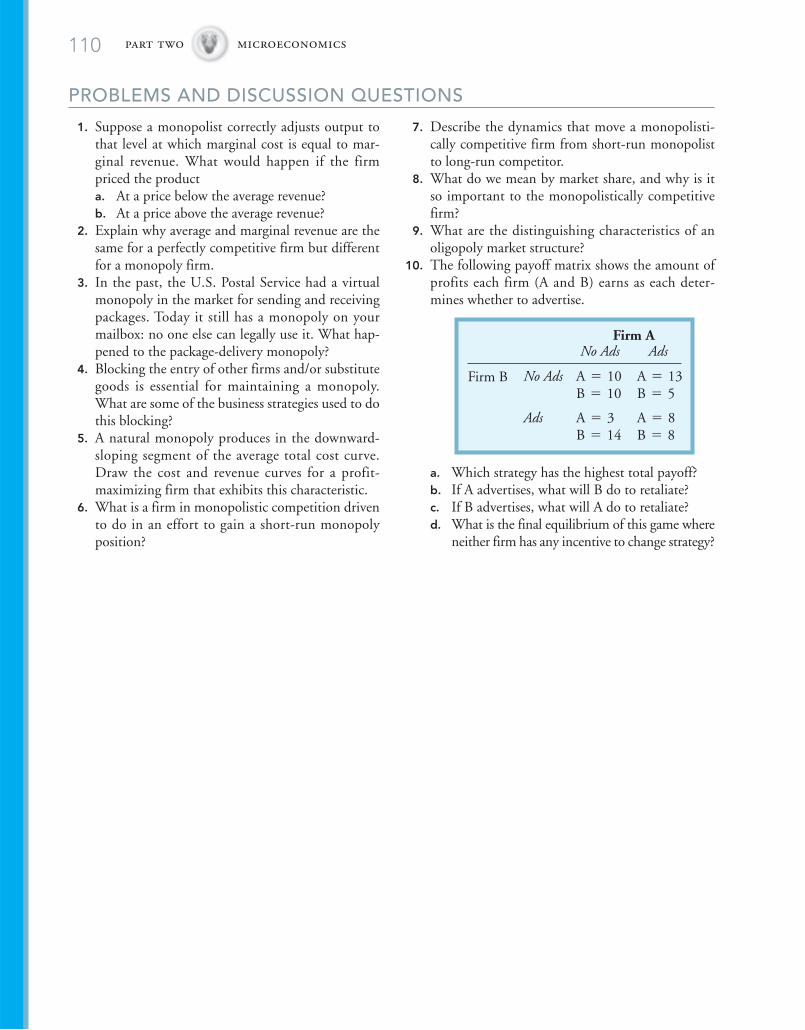
110 part two microeconomics
PROBLEMS AND DISCUSSION QUESTIONS
1. Suppose a monopolist correctly adjusts output tothat level at which marginal cost is equal to mar-ginal revenue. What would happen if the firmpriced the producta. At a price below the average revenue?b. At a price above the average revenue?
2. Explain why average and marginal revenue are thesame for a perfectly competitive firm but differentfor a monopoly firm.
3. In the past, the U.S. Postal Service had a virtualmonopoly in the market for sending and receivingpackages. Today it still has a monopoly on yourmailbox: no one else can legally use it. What hap-pened to the package-delivery monopoly?
4. Blocking the entry of other firms and/or substitutegoods is essential for maintaining a monopoly.What are some of the business strategies used to dothis blocking?
5. A natural monopoly produces in the downward-sloping segment of the average total cost curve.Draw the cost and revenue curves for a profit-maximizing firm that exhibits this characteristic.
6. What is a firm in monopolistic competition drivento do in an effort to gain a short-run monopolyposition?
7. Describe the dynamics that move a monopolisti-cally competitive firm from short-run monopolistto long-run competitor.
8. What do we mean by market share, and why is itso important to the monopolistically competitivefirm?
9. What are the distinguishing characteristics of anoligopoly market structure?
10. The following payoff matrix shows the amount ofprofits each firm (A and B) earns as each deter-mines whether to advertise.
a. Which strategy has the highest total payoff?b. If A advertises, what will B do to retaliate?c. If B advertises, what will A do to retaliate?d. What is the final equilibrium of this game where
neither firm has any incentive to change strategy?
Firm ANo Ads Ads
Firm B No AdsB = 10A = 10
B = 5A = 13
AdsB = 14A = 3
B = 8A = 8

8The Theory of ConsumerBehaviorTHE LAWS OF SUPPLY AND DEMAND ARE, TO A LARGE DEGREE, THE FORCES THAT
cause our economy to operate. We have discussed the concept of supply and thefactors underlying this concept in some detail. But production and supply of anygood are meaningless unless that good is ultimately to be utilized in the satisfac-tion of some of the needs and wants of humanity. So we move from productionand supply to consumption and demand—the theory of consumer behavior.
Production theory is based on the analysis of a production function—a real,tangible relationship between inputs and outputs. Using that production func-tion, we were able to derive optimizing behaviors for the firm manager.Consumption theory is based on the behavior of the individual consumer as thatconsumer seeks to optimize his or her self-interest. It deals with how the con-sumer behaves in an effort to maximize the benefits from consumption and howthe consumer evaluates those benefits. This is neither tangible nor real because wecan’t make interpersonal comparisons between consumers and we can’t quantita-tively measure satisfaction. So our treatment of the consumer as an optimizingunit will be more subjective and abstract than was the case for the producer.Nonetheless, the theory is quite robust in describing consumer behavior.
THE LAW OF DEMANDWe saw in an earlier chapter that demand refers to the quantities of a good con-sumers are willing to consume at alternative prices, ceteris paribus. Demand isdetermined for a given time and a given place. The law of demand simplystates that as the price of a good increases, ceteris paribus, the quantity ofthe good consumers are willing to consume will decrease.This doesn’t imply that every consumer in every mar-ket will react according to the law of demand, butthat in the aggregate of many consumers, there willbe an inverse relationship between quantities andprices. Rest assured that if the price of gas goes upby a dollar a gallon, a millionaire is not going to buyless gas, but there are enough of us who willchange our behavior to have a market impact.
REAL INCOME ANDSUBSTITUTION EFFECTSThe “law” of demand is, like much ofeconomics, common sense made difficult.It is easy to assert that as the price ofhamburger goes up, ceteris paribus

112 part two microeconomics
(i.e., the price of chicken, pork, and fish remaining constant), the quantity of hamburgerconsumers are willing to consume will go down. There are two reasons we expect the law ofdemand to be valid. They are known as the substitution effect and the real income effect.
To see how each of these two effects leads to a downward-sloping demand curve,let’s create a mythical consumer, a poorly nourished college student named Phelps,who has a budget of $150 per week. Suppose initially that Phelps buys 25 pounds ofhamburger a week at $2.00 per pound, or total spending on hamburger of $50. Theother $100 is spent on 100 units of stuff that costs $1.00 per unit.
Substitution EffectNow suppose the price of hamburger doubles to $4.00 per pound, ceteris paribus.While this initially looks like an increase in the price of hamburger, we can see that italso looks like the price of stuff, relative to hamburger, just got cheaper. So how doesPhelps react? He increases his purchases of the relatively cheap stuff (which includeschicken) and decreases his purchases of hamburger. He may reduce his consumptionof hamburger to 10 pounds, or $40, and increase his purchases of stuff to $110. Hehas substituted stuff for hamburger as the price of hamburger went up. Notice thetwo effects of the substitution effect: consumption of hamburger went down (law ofdemand) and the consumption of stuff went up (substitution effect).
Real Income EffectWhen the price of hamburger goes up to $4 per pound, ceteris paribus, Phelps finds(or phinds) that he can no longer buy 25 pounds of hamburger a week and 100 unitsof stuff a week on his budget of $150. The increase in the price of beef has reducedthe amount of goods that Phelps is able to buy with his $150. His purchasing poweror real income has fallen. To compensate for the loss of his purchasing power, he mustbuy less of both hamburger and stuff. If he reduces his consumption of both goodsproportionately, he would buy 18.75 pounds of hamburger per week and 75 units ofstuff. His hamburger budget would increase to $75 per week ($4.00 * 18.75), and hisstuff budget would fall from $100 to $75. Spending $75 on each commodity wouldkeep him within his total budget of $150. Notice the impact of the real income effect:as the price of hamburger goes up, ceteris paribus, the quantity of hamburger con-sumed goes down (law of demand) and the quantity of stuff consumed also goesdown (real income effect).
Taken together, the substitution and real income effects both suggest that asthe price of hamburger goes up, the quantity demanded of hamburger goes down.Both effects confirm the law of demand. The impact of an increase in the price ofhamburger on the consumption of stuff is indeterminate, depending on the relativestrengths of the two effects. If the substitution effect is stronger, then consumptionof stuff will increase; but, if the real income effect is stronger, then consumption ofstuff will fall.
MARKET DEMAND AND INDIVIDUAL DEMANDWe saw earlier that supply originates at the level of the firm. Market supply is theaggregation of all the supply curves of firms in the market. Adding more firms to theindustry has the effect of shifting the market supply curve outward. In a similar man-ner, demand originates with the behavior of the individual consumer. Those individualdemand curves are added up to generate market demand. The addition of more con-sumers to the market will have the effect of shifting the market demand curve outward.
Substitution effect as theprice of good A increases,ceteris paribus, the relativeprice of good B decreasesand the consumersubstitutes B for A inconsumption.
Real income effect as theprice of good A increases,ceteris paribus, the realincome, or purchasingpower, of the consumer fallsand as a result less of bothgood A and B areconsumed.

the theory of consumer behavior chapter eight 113
Therefore, in order to understand the forces that drive market demand, it isimportant that we understand how the typical consumer behaves—how the individ-ual demand curve is shaped. To do this we will introduce the utility theory of con-sumer behavior. Realizing that different consumers behave differently, we will analyzethe behavior of a typical consumer to develop an understanding of the economics ofconsumer behavior.
UTILITY ANALYSISConsumers buy stuff because they want to (hamburgers), have to (gasoline), ought to(cod liver oil), or out of habit (cigarettes). Regardless of the motivation, the consumerreceives satisfaction through consumption. Economists refer to the satisfaction gainedfrom consumption as utility. Utility is created by the consumption of goods and services.
Unfortunately, utility cannot be measured in an objective fashion. Despite yearsof dedicated research and development, our utilometer is still not functioning.Nonetheless, we can say a good deal about the utility associated with consumption.But first, let’s investigate a few assumptions about our utility model.
Assumptions about the Utility ModelAs with any economic model, the utility model of consumer behavior is founded onseveral important assumptions. Before getting into the model itself, it is best to makethose assumptions explicit.
Opportunity Costs and Price The consumer will purchase a product so long as theutility created by its consumption is greater than the opportunity cost of consumingit. Most of the opportunity cost of consuming a good is the price of the good itself.Price is a measure of the consumption foregone of other goods when the purchase ismade. But there are also other acquisition costs over and above price that may beincluded in the decision matrix. For instance, there may be transactions costs such aswaiting in line (time is money) or tax implications. There may be travel or locationalcosts involved. For instance, you wouldn’t drive 10 miles across town to get a gooddeal on a gallon of milk, but you might do so to get a good deal on a new car.
The key point is that the opportunity cost of consuming a good may well be morethan the price of the good. With that in mind, in the remainder of this chapter we aregoing to talk about the prices of goods as a shorthand for the opportunity cost of goods.
Rational Behavior We are going to assume that consumers behave in a rational fash-ion. There are really three fundamental assumptions concerning rationality.
• First, consumers will consume a good only if the utility of consuming it is greaterthan the disutility (price) of acquiring it. That is, consumers won’t buy thingsthat don’t provide them with a net utility gain. If the consumption of a good cre-ates a disutility, then the consumer would not buy it at any price. For vegetarianconsumers, the consumption of any meat would create a disutility, so no meat ispurchased at any price. For meat eaters, meat will be purchased so long as theutility of eating the meat is greater than the disutility of having to pay for it.
• Second, we assume that more is better than less. More stuff is a constant desireregardless of how much stuff we have.
• Third, our wants are unlimited. The hungry person wants food. The overfedperson wants a new car. The person with a new car wants an exotic vacation.Bill Gates wanted a new house that cost $35 million to build. Our wantsexceed our means, so we must choose among our wants. Choice is what eco-nomics is all about.
Utility the satisfactioncreated by the consumptionof goods and services.

114 part two microeconomics
Preferences It is assumed that the consumer is able to evaluate the utility gained fromthe consumption of alternative goods and is able to establish a system of preferencesbetween any two goods at any time. In practice this assumption means that a consumercan walk into the local Mickey-D, look at the menu board, and decide what he or shewants. We are basically assuming that the consumer is not clueless.
Budget Constraint It is assumed that our typical consumer is constrained in his orher purchasing decisions by a limited budget. For most of us, this is a far-too-realisticassumption.
Purchasing and Consuming The bumper sticker that proclaims “born to shop” sug-gests that some folks gain utility from the act of purchasing that is separate from thatof actually consuming what is purchased. For most, the act of shopping for food cre-ates a disutility—one that supermarkets work hard at minimizing. But for many,shopping for clothing is fun—a utility creator that is independent of the actual con-sumption of the final purchase. For our purposes, we consolidate these separate utili-ties into a single utility that we call consumption.
Objective of the Consumer We assume that the consumer is a utility maximizer,given the limited budget available. The set of consumption choices of the individualwill depend on the tastes and preferences of the individual. Each of us has our ownunique set of tastes and preferences and therefore will have our own unique pattern ofconsumption choices. While each of us will come to a different conclusion, each of usarrives there with the same objective—utility maximization.
Total and Marginal Utility As previously indicated, the objective of the consumer isto consume that combination of goods that will provide the consumer with the great-est amount of utility possible, given a budget constraint. Our task, then, is to developbehavior rules that will indicate how the consumer achieves this goal. To simplifymatters, we assume that utility can be measured in units called utils. And, while theconsumer may not know how many utils of satisfaction are obtained from a givengood, the consumer is able to identify which of two goods will provide the greaternumber of utils.
To begin, let’s look at the utility associated with the consumption of a singlegood—gatorburgers. This is a good that is highly prized by college students through-out the southeastern part of the United States and by others during spring break.Ignoring (for the moment) the disutility of obtaining gatorburgers, let’s look at theutility created by a typical consumer, Tivona, consuming this treat. As shown inFigure 8-1, as Tivona consumes more and more gatorburgers, the total amount ofutility she obtains from them increases at a decreasing rate, reaches a maximum, and
Preferences the ability ofthe consumer to identifywhich of two goods willproduce a greater amountof utility in consumption.
Util a hypothetical orimaginary unit of utility.
Gatorburgers/Day Total Utility/Day Marginal Utility/Day
0
1
2
3
4
10
7
4
2
�2
0
10
17
21
23
215
Figure 8-1Total utility and marginalutility from consuminggatorburgers—schedule.

then declines after four gatorburgers when she gets into the overdose range. To maxi-mize her utility, Tivona should consume four gatorburgers, but remember that wehave not yet considered the opportunity cost of buying the gatorburgers. The thirdcolumn of Figure 8-1 shows Tivona’s marginal (or additional) utility obtained by con-suming gatorburgers. As expected, the marginal utility associated with the consump-tion of the first gatorburger is greater than that of the second, which is greater thanthat of the third, and so on. This reflects the natural tendency towards satiation inconsumption.
This leads us to one of the fundamental tenets in the theory of consumerbehavior—the law of diminishing marginal utility: as additional units of one goodare consumed, ceteris paribus, the marginal or additional utility obtained from eachadditional unit of that good will decrease.
The left panel of Figure 8-2 graphs the total utility per day Tivona gains by con-suming gatorburgers. Total utility is maximized at four gatorburgers, and then itbegins to decrease, indicating that the marginal utility is negative as shown in theright panel of Figure 8-2. As expected, marginal utility falls steadily and, then, finallybecomes negative when the total utility is at its maximum level.
In a case where the consumer consumes only one good, utility-optimizingbehavior is rather simple. If the price of gatorburgers is $4 each and the budget is $30,then the consumer would consume four gatorburgers to maximize utility. But if thebudget were $15, the consumer would consume only three gatorburgers because con-sumption is limited by the budget constraint.
Now let’s move to a more relevant example in which the consumer consumestwo goods and must select between them in order to maximize utility. Figure 8-3shows the relevant information to solve this problem. The first three columns ofFigure 8-3 are a repeat of Figure 8-1. The fourth column is the amount of marginalutility per dollar that each additional unit of gatorburgers will generate based on aprice of $4 per gatorburger. With these numbers, we can analyze how much utility, or“bang for the buck,” Tivona gets from each dollar spent. Her objective is to get thegreatest amount of utility possible within her limited budget.
The right half of Figure 8-3 shows similar information for Gator Gulps, a highlyprized sports drink that Tivona likes to down while eating gatorburgers. If the pricesof gatorburgers and Gator Gulps are $4 and $5 each, respectively, and Tivona’s budgetis $27, how would she maximize the total utility she derives from her limited budget?
Assume she is consuming nothing. Then the choices before her are to buy eitherthe first gatorburger or the first Gator Gulp. Since the marginal utility per dollar of
Law of diminishingmarginal utility asadditional units of one goodare consumed, ceterisparibus, the marginal utility obtained from eachadditional unit of that goodwill decrease.
25
20
15
10
5
00
0
1
10
2
17
3
21
4
23
5
21Tota
l util
ity
Units consumed
12
10
8
6
4
2
0
–2
–41 2 3 4 5
Mar
gina
l util
ity
Units consumed
Figure 8-2Total utility and marginalutility from consuminggatorburgers—graph.
the theory of consumer behavior chapter eight 115
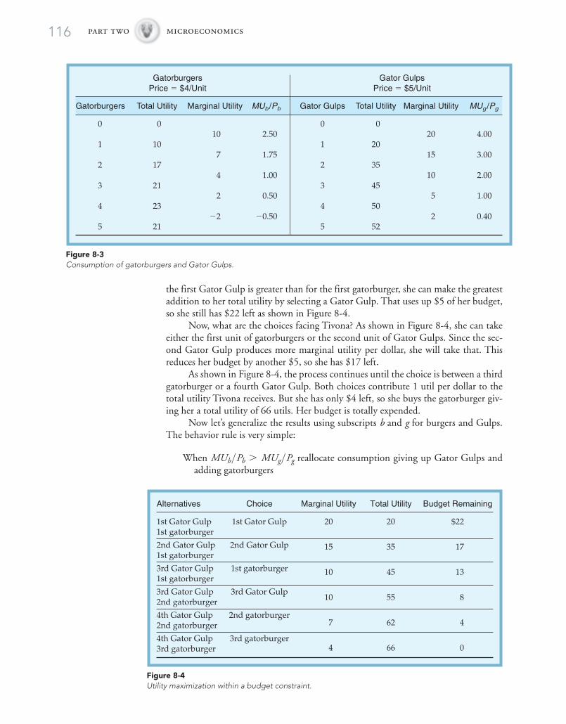
116 part two microeconomics
Alternatives Choice Marginal Utility Total Utility Budget Remaining
1st Gator Gulp 1st Gator Gulp 20
15
10
10
7
4
20
35
45
55
62
66
$22
17
13
8
4
0
1st gatorburger
2nd Gator Gulp 2nd Gator Gul1st gatorburger
3rd Gator Gulp 1st gatorburger1st gatorburger
3rd Gator Gulp 3rd Gator Gul2nd gatorburger
4th Gator Gulp 2nd gatorburger2nd gatorburger
4th Gator Gulp 3rd gatorburger
p
p
3rd gatorburger
Figure 8-4Utility maximization within a budget constraint.
Gatorburgers Gator GulpsPrice � $4/Unit Price � $5/Unit
Gatorburgers Total Utility Marginal Utility MUb /Pb Gator Gulps Total Utility Marginal Utility MUg /Pg
0 0 0 010 2.50 20 4.00
1 10 1 207 1.75 15 3.00
2 17 2 354 1.00 10 2.00
3 21 3 452 0.50 5 1.00
4 23 4 50�2 �0.50 2 0.40
5 21 5 52
Figure 8-3Consumption of gatorburgers and Gator Gulps.
the first Gator Gulp is greater than for the first gatorburger, she can make the greatestaddition to her total utility by selecting a Gator Gulp. That uses up $5 of her budget,so she still has $22 left as shown in Figure 8-4.
Now, what are the choices facing Tivona? As shown in Figure 8-4, she can takeeither the first unit of gatorburgers or the second unit of Gator Gulps. Since the sec-ond Gator Gulp produces more marginal utility per dollar, she will take that. Thisreduces her budget by another $5, so she has $17 left.
As shown in Figure 8-4, the process continues until the choice is between a thirdgatorburger or a fourth Gator Gulp. Both choices contribute 1 util per dollar to thetotal utility Tivona receives. But she has only $4 left, so she buys the gatorburger giv-ing her a total utility of 66 utils. Her budget is totally expended.
Now let’s generalize the results using subscripts b and g for burgers and Gulps.The behavior rule is very simple:
When reallocate consumption giving up Gator Gulps andadding gatorburgers
MUb>Pb 7 MUg>Pg

the theory of consumer behavior chapter eight 117
When reallocate consumption giving up gatorburgers andadding Gator Gulps
thusWhen no further reallocation can increase total utility.
Utility is maximized.
This result can be generalized to a multigood general rule for utility optimization:
for all i goods consumed. That is, the marginal contribution to total utility per dollarof expenditure must be the same for all goods. If it were not, then some sort of reallo-cation is possible that would result in an increase in total utility. This is known as theequi-marginal principle of optimization.
Deriving the Demand CurveThe law of demand posits that there is an inverse relationship between price of theproduct and the quantity demanded of that product, ceteris paribus. We can use theequi-marginal utility optimization principle to demonstrate the law of demand. Let’ssee what happens if the price of Gator Gulps changes, ceteris paribus. Suppose the priceof Gator Gulps falls from $5 per unit to $4 per unit. The impact of this price change isshown in Figure 8-5, which is identical to Figure 8-3 with the exception of the lastcolumn, which reflects the change in the price of Gator Gulps. As the price of GatorGulps falls, the marginal utility per dollar of expenditure on Gator Gulps increases.
Using the data in Figure 8-5, work through the process of utility maximizationas was done in Figure 8-4. You should find that Tivona will consume four units ofGator Gulps and three units of gatorburgers. So as the price of Gator Gulps fell,ceteris paribus, the quantity consumed increased as shown in Figure 8-6. In this exam-ple, we have found two points on the demand curve for Gator Gulps. Repeating theprocess would lead to additional points on the curve.
This example is a good illustration of the real income effect. The decline in theprice of Gator Gulp allowed Tivona to consume one more unit of Gator Gulps thanbefore and still have $3 left over. So a decrease in the price of Gator Gulps increased
MU1
P1=
MU2
P2= Á =
MUi
Pi
MUb >Pb = MUg>Pg
MUb>Pb 6 MUg>Pg
Equi-marginal principle ofoptimization in order tooptimize utility, given alimited budget, theconsumer will adjust theconsumption pattern suchthat the marginal utility perdollar of expenditure foreach good is the same.
Gatorburgers Gator GulpsPrice � $4/Unit Price � $4/Unit
Gatorburgers Total Utility Marginal Utility MUb /Pb Gator Gulps Total Utility Marginal Utility MUg /Pg
0 0 0 010 2.50 20 5.00
1 10 1 207 1.75 15 3.75
2 17 2 354 1.00 10 2.50
3 21 3 452 0.50 5 1.25
4 23 4 50�2 �0.50 2 0.50
5 21 5 52
Figure 8-5Consumption of gatorburgers and Gator Gulps after a price change.

118 part two microeconomics
$5
$4
$3
$2
$1
0
1 2 3 4 5
Units of Gator Gulps
Pric
e pe
r un
it of
Gat
or G
ulps D
D
Figure 8-6Tivona’s demand for GatorGulps.
the real income of Tivona, allowing her to consume more from her $27 budget. Notethat in this example there was no substitution effect.
THE MARKET DEMAND FUNCTIONWe’ve seen how consumers behave in their efforts to achieve the maximum level ofutility possible within the limits of their income constraint. In the process of maxi-mizing utility, individual demand curves can be specified. The market demand sched-ule can be derived by simply adding the quantities of product that each consumer iswilling to purchase at each specified level of price. Thus, as in the case of supply, themarket demand is simply the horizontal summation of all the demand curves for allthe individuals who are buying in a given market at a given time.
Several characteristics of the market demand schedule should be specified at thispoint. First of all, in the case of market demand there are more ceteris paribus condi-tions than for individuals. The factors of income, prices for alternative products, andtastes and preferences are defined to be constant within each of the individual demandcurves. But the market curve includes some additional factors that must be held con-stant. Other ceteris paribus conditions that are important in market demand include
• Size of the population• Demographic composition of the population• Distribution of income• The general price level• International trade patterns
Changes in any of these factors would change the market demand, resulting in a shiftof the market demand curve even though individual demands remain unchanged.
SUMMARY
The law of demand states that as the price of a goodincreases, ceteris paribus, the quantity demanded of thatgood will fall. The law of demand is justified by thesubstitution effect and the real income effect. The sub-stitution effect says that as the price of beef goes up,ceteris paribus, consumers will buy more chicken andsubstitute it for beef such that beef consumption falls.
The real income effect posits that as the price of beefgoes up, ceteris paribus, the quantity of beef that can bepurchased on a fixed budget will fall. Both effects vali-date the law of demand.
Consumption creates utility. We assume that theconsumer seeks to maximize total utility given a limitedbudget. The law of diminishing marginal utility states

the theory of consumer behavior chapter eight 119
that as additional units of a good are consumed, ceterisparibus, the marginal or additional utility associatedwith each additional unit will decrease. In order to max-imize utility from consumption, the consumer shouldconsume each good to that point at which the marginalutility per dollar of expenditure is the same for all goods.
By changing the price of one good, ceteris paribus,a schedule of individual demand can be developed,
showing the quantities of the good the consumer willconsume at alternative prices of the good. Individualdemand curves can be aggregated to produce marketdemand. Any changes in the ceteris paribus conditionswill result in a shift of individual and, hence, market,demand. Other factors that may shift market demandwere noted.
KEY TERMS
Equi-marginal principle of optimizationLaw of diminishing marginal utilityPreferences
Real income effectSubstitution effect
UtilUtility
PROBLEMS AND DISCUSSION QUESTIONS
1. The following table shows the total utility a con-sumer gets from consuming two goods—A and B.
Assume that the price of good A is $5 per unit andthe price of good B is $10 per unit.
a. For a budget of $55, how many units of eachgood would the consumer consume?
b. If the budget were to increase by $10, how manyunits of each good would the consumer consume?
2. Is the law of diminishing marginal utility valid fora true chocolate fanatic?
3. Suppose the price of tomatoes falls, ceteris paribus.Describe the impact the substitution effect and the
real income effect would have on the quantitydemanded of tomatoes.
4. Frequently the opportunity cost of acquiring agood is more than the price of the good. Why?
5. Weird Harold, being devoid of an economics edu-cation, declares that he is going to maximize hismarginal utility. What consumption pattern wouldachieve this objective?
6. Assume Samir is a rational consumer. Nonetheless,Samir’s entire food budget of $40 per week is usedonly for burgers and soda. Burgers cost $0.69 each,and soda is $0.75 per can. His marginal utilityfrom burgers is 234 utils, and his marginal utilityfrom soda is 175 utils. What should Samir do toincrease his total utility?
7. One day Suke ordered two hot dogs and threeorders of fries at the local diner (Suke is an unusu-ally hearty eater). The next day she ordered threehot dogs and two orders of fries. Assuming that herrather voracious tastes and preferences did notchange from day to day, what must have happened?
8. Prices at convenience stores are consistently higherthan at supermarkets. Why don’t they go out ofbusiness?
Total Utility
Units A B0 0 01 30 422 50 703 60 854 65 945 67 98

120
appendixIndifference Curve Analysis
An alternative approach to developing the theory of consumer behavior is known asindifference curve analysis. Through the use of indifference curves, we can developbehavioral rules for utility maximization given a budget restraint. In addition, withindifference curves we can examine in detail the impact of changing some of theceteris paribus conditions defining consumer demand.
We have defined utility to be the satisfaction that consumers derive from theconsumption or possession of goods. Utility can also be derived from services such asmedical care, dental care, or police protection since these services also fulfill humanwants and needs. The idea behind the entire concept of demand is that every rationalconsumer selects that combination of goods and services that will permit him or herto maximize utility within the limits imposed by his or her budget. This idea of max-imum consumer utility implies that consumers know the relative amounts of utilitythey can derive individually from the consumption of all the items available to them.
Let’s suppose that there are only two items available in our economy—food,representing the necessities of life, and clothing, representing the luxury items. Weknow that we can derive satisfaction from the consumption of each of these goods.
Imagine that satisfaction or utility gained from consuming these two goods is athree-dimensional hill as shown in Figure 8-7. Since this hill shows the level of utilityassociated with the consumption of the two goods, it is called a utility surface. As wemove up that hill, we achieve progressively higher and higher levels of utility as meas-ured on the vertical axis. If, however, we walk around the hill, we are merely stayingon the same level of satisfaction (in exactly the same sense that a terrace on a hillsidefield maintains a given level of elevation). Thus, each line or terrace going around thehill defines some constant level of utility. The various combinations of food andclothing that will give us that particular level of utility are defined by the line aroundthe utility surface. Therefore, we are indifferent as to where we are on that linebecause our level of utility is unchanged.
Utility surface a three-dimensional representationof the utility gained byconsuming two goodssimultaneously.
Food/unit time
Util
ity (
leve
l of s
atis
fact
ion)
a b
c
d
ef
g h
a
b
cde
f
g
hi
i
Clothing/unit time
Figure 8-7The utility surface.

indifference curve analysis appendix 121
Food/unit time
Clo
thin
g/un
it tim
e
a b c
d
e
f
ghi
Figure 8-8The utility map orindifference map of theutility surface.
Now let’s imagine that we are in an airplane looking straight down at the utilityhill. All we see are the lines or the terraces that define the various levels of satisfactionas shown in Figure 8-8. This type of illustration is the same as a military contour mapor a topographic map: the lines indicate the elevation or level of utility. This type ofdiagram is known as a utility map. As we move away from the origin toward thenortheast on the utility map, we are going up the hill to higher and higher terraces,thereby increasing the level of the consumer’s total utility.
The lines defining the levels of utility are known as indifference curves, sincewe are indifferent as to where we are along any single curve. There are several charac-teristics of indifference curves that should be specified. First of all, indifference curvesslope downward and to the right. Second, because of diminishing marginal utility1
they are convex to the origin with the “bow” of the curve pointing toward the originor corner of the diagram. Third, they cannot intersect.2
The curves slope downward and to the right because in order for a consumer togive up some of one commodity and still remain on the same level of satisfaction, theconsumer must be compensated with additional units of another product. Figure 8-9
Utility map contour linesof a utility surface.
Indifference curves lineson a utility map indicatingalternative combinationsof two goods that willgenerate a constant level ofutility in their consumption.
20
15
10
5
020 4 6 8 10 12
Units of food
Uni
ts o
f clo
thin
g
D
C
B A
Figure 8-9Indifference curves slopedown and to the right andare convex to the origin.
1 As additional units of one good are consumed, ceteris paribus, the marginal utility obtained from each additionalunit of that good will decrease.2 By this point, you should have identified indifference curves as being closely analogous to the isoproduct curves orisoquants in the appendix to Chapter 5. Indifference curves and isoproduct curves have exactly the same characteris-tics for exactly the same reasons.

122 part two microeconomics
illustrates the principle of diminishing marginal rates of substitution. As successiveunits of one product are lost, it will take progressively more and more of the substitutecommodity to adequately compensate for the loss of satisfaction. When the consumerhas lots of food and not much clothing, it doesn’t take much clothing to compensatefor the loss of one unit of food (as from point A to point B). Conversely, when theconsumer has lots of clothes and little food, he or she will gladly trade lots of clothesto get one more unit of food. The consumer at point D has only one unit of food anda strong hunger. In this case, the consumer is willing to give up 10 units or half of hisclothes to get the second unit of food.
We now have our two-product model, and we have identified the utility that theseproducts can yield from the indifference map of the utility surface. We also know therates at which those products will substitute for one another in maintaining any givenlevel of satisfaction. All we need to determine the quantities of food and clothing thatour sample consumer will buy is information concerning the prices of those commodi-ties and the consumer’s income or budget for those items. If the consumer should spendhis entire budget on food, there is some maximum amount of food that can be bought.To find that maximum, we divide his budget by the price for food. If he buys no cloth-ing and spends his entire budget on food, he can buy X units of food as in Figure 8-10.
Likewise, if the entire budget is spent on clothing, the consumer can buy Y unitsof clothing. A straight line connecting these two points shows all combinations of foodand clothing purchases that can be made with the consumer’s budget. The constraintimposed by the budget will permit the consumer to purchase any combination of foodand clothing that falls on or below this budget line. The consumer’s objective is to max-imize total utility within the limits imposed by this budget line. Therefore, he or she isgoing to attempt the highest possible level of satisfaction that this budget permits.
In a very real sense, a consumer’s budget line does the same thing to the utilitysurface that a fence does to livestock on a hillside pasture (Figure 8-11). No matterhow badly consumers might wish to graze the tender grasses available at higher eleva-tions, they are prevented from doing so by the unpleasant fact that there is a budgetfence between them and their unlimited wants.
Utility MaximizationNow, let’s combine the indifference map (wants and desires) with the budget line(ability), as shown in Figure 8-12. The objective of our analysis is to determine whatcombination of items the consumer is going to select for consumption, given income,the prices of the items, and a map of the consumer’s tastes and preferences.
Budget line combinationsof two goods the consumeris able to purchase given abudget constraint.
Units of food
Uni
ts o
f clo
thin
g
0X
Y
Budget line
Y =Budget
Clothing price
X =Budget
Food price
Figure 8-10Construction of the budgetline using the consumer’sbudget and the prices of thealternative commodities.

indifference curve analysis appendix 123
Food
Util
ity (
leve
l of s
atis
fact
ion)
Budget lineor "fence"
Clothing
Figure 8-11Budgetary limit on the utility surface.
First, let’s ask a question. Which level of satisfaction is our consumer, Marcella,going to select? Obviously, she is going to get the greatest amount of satisfaction herincome (i.e., budget) will permit. Any point on or below her budget line is attainable,but we have already said that we are going to assume that Marcella is rational.Therefore, she will not select a combination of goods such as A, which is below herbudgetary constraint, since she can increase satisfaction by moving out to the budgetlimit. She will not select combination E on since she will have a higher level of util-ity at any of the combinations B or D because they are on , with a higher total util-ity. Since combination C is on that just touches (or is tangent to) the budget line,this is the highest possible level of utility that Marcella can achieve, given her incomeconstraint and the product prices. Combination C is the point at which the rationalconsumer will choose to operate, consuming units of clothing and units of food.
At point C, the slope of the budget line is equal to the slope of the indifferencecurve. This means that the rate at which food and clothing substitute for one anotherin consumption (slope of the indifference curve) is the same as the rate at which theysubstitute for one another in the market (slope of the budget line).
F1C1
U3
U2
U1
Clo
thin
g
Food
U1
U2U3
U4
A
F1 B/Pf
B/Pc
C1
0
E
D
B
C
Figure 8-12Utility optimization for agiven budget.

124 part two microeconomics
Mathematical Illustration The slope of the indifference curve at any point on thatcurve is the marginal rate of substitution, which would be equal to the rise over therun or the rate of change of clothing per unit change in food. So
(8-1)
Every point on an indifference curve represents the same amount of total utility. Somovement along an indifference curve suggests that the additional utility of one goodwill be exactly equal to the decrease in the utility of the other. Ignoring signs, that is
(8-2)
Rearranging Equation 8-2 gives
(8-3)
Since the right-hand term of Equation 8-1 is equal to the left-hand term of Equation8-3, we find that
(8-4)
The slope of the budget line is the rise over the run, so if B is the amount of thebudget, then
(8-5)
Since at the optimizing point C in Figure 8-12 the slope of the indifferencecurve is equal to the slope of the budget at the point of tangency, we can combine theright-hand sides of Equations 8-4 and 8-5 to get the optimizing criterion:
(8-6)
Rearranging the terms of Equation 8-6 gives the utility-maximizing behaviorcriterion:
(8-7)
Here we again have the equi-marginal principle that utility optimization is achievedwhen the marginal utilities per dollar of the two goods are equal. If they were not, somerearranging of the consumption pattern would allow for additional utility to be obtained.
The Impact of Changes in Ceteris Paribus ConditionsDemand is a relationship between prices and quantities assuming everything elseremains constant. In reality, these conditions are in a continuous state of flux. Wemerely assume them to be constant (or we hold them constant) so that we can sort out
MUf
Pf=
MUc
Pc
MUf
MUc=
Pf
Pc
Slope of the budget line =B>Pc
B>Pf=
Pf
Pc
Slope of the indifference curve =MUf
MUc
¢C¢F
=MUf
MUc
¢C # MUc = ¢F # MUf
Slope of the indifference curve =¢C¢F

indifference curve analysis appendix 125
Clo
thin
g
Food
U1
U2U3
U4
F1 F2 B/Pf B*/Pf
B/Pc
B*/Pc
C1
C2
0
DC
Figure 8-13Impact of an increase in thebudget.
the effects of various types of changes. The ceteris paribus conditions do change overtime, and when they change, they cause changes in the demand schedule. In the caseof an individual consumer’s demand curve, the ceteris paribus conditions includeincome (budget), prices for substitute and complementary goods, and the preferencepattern of the individual consumer.
Change in the Budget The impact of a change in the budget, ceteris paribus, isillustrated in Figure 8-13. This figure shows the same consumer that we considered inFigure 8-12 who maximized utility given the budget constraint by adjusting the con-sumption of food and clothing to and . Now what would happen if the budgetof the consumer increased from B to B *, ceteris paribus?
Since the slope of the budget line is equal to a ratio of the prices for food andclothing and since these prices are held constant, the shift of the budget line will be aparallel shift. In the example in Figure 8-13, we are looking at an increase of thebudget, which means the amount of food and/or clothing that can be purchased hasincreased. As the budget grows from B to B *, the endpoints of the budget line moveout to and .
For this particular consumer, the higher budget line results in increased con-sumption of both food and clothing to and . And the consumer has increasedtotal utility from to .
While in the normal case one would expect an increase in the budget to result inincreased consumption of both goods, it does not necessarily have to be so. To seethis, in your mind’s eye drag the indifference curve downward such that point Dslides down the budget line. With just a little slide, would quickly be less than .An example of something like this would be a consumer who consumes beans andmeat. With an increase in the budget, the consumer is able to increase meat consump-tion, which allows a reduction in bean consumption.
Change in the Price of a Good A second ceteris paribus condition that mightchange is the price of either of the two goods. This is illustrated in Figure 8-14,where we have an increase in the price of clothing, ceteris paribus. The budget andthe price of food do not change, so the endpoint of the budget line on the foodaxis does not change.
An increase in the price of clothing to with the budget remaining constantwill cause the endpoint of the budget line on the clothing axis to be closer to the ori-gin. With the budget given, the maximum quantity of clothing that can be purchased
Pc2
C1C2
U4
U4U3
C2F2
B *>Pc B *>Pf
C1F1

126 part two microeconomics
is reduced by the price increase. This causes a downward rotation of the budget line(shown by the arrow) around a pivot point on the food axis.
In the case illustrated in Figure 8-14, the impact of the increased price of cloth-ing is to consume less clothing at (law of demand) and less food at (incomeeffect). In addition, the total utility of the consumer falls from to .
The impact of the clothing price change on food consumption is indeterminatebecause of the trade-off between the income effect and the substitution effect. Themagnitude of the two effects can be seen in the following manner. Draw a budget linetangent to that is parallel to the prior budget line. The change in food consump-tion from to the point of tangency is the total income effect. Then slide this imag-inary budget line along until you get to point D on the line. The change in foodconsumption as you slide along is a measure of the substitution effect.
Change in Consumer’s Tastes and Preferences A final ceteris paribus condition thatmight change would be the tastes and preferences of the consumer. Any suchchanges would result in a different set of indifference curves for the consumer. Suchchanges can occur rapidly or slowly over time. An impending hurricane in Floridacan produce a phenomenon many Americans have never experienced—bare shelvesat the supermarket. A slower, longer change is the move away from coffee consump-tion and the corresponding increase in soft-drink consumption. The averageAmerican now consumes more ounces of soft drinks per day than coffee and watercombined.
Such changes in tastes and preferences result in shifts of the indifference map withno change in the budget line. Figure 8-15 illustrates the coffee-soft drink example. Weknow that tastes and preferences have changed and that as a result consumption haschanged, but we are unable to determine if the utility level is greater than or lessthan .
Substitutes and ComplementsWe know that the tremendous range of commodities available in our society gives theconsumer a wide range of consumption alternatives. If beef becomes too expensive,the consumer has the option of shifting to pork. If both beef and pork are too expen-sive, the consumer can meet protein needs with poultry, fish, cheese, or vegetablesources such as dry beans. For any particular consumer, these products all possessvarying degrees of substitutability.
U2000
U1960
U2
U2
F1
U2
U2U3
F2C2
Clo
thin
g
Food
U1
U2U3
U4
F1F2 B/Pf
B/Pc2
B/Pc1
C1C2
0
D
C
Figure 8-14Impact of an increase in theprice of clothing.

indifference curve analysis appendix 127
SD2000
SD1960
0
C2000 C1960
Coffee
Sof
t drin
ks
U2000
U1960
Figure 8-15Impact of a change in tastesand preferences.
The relationships between commodities can be classified into two broad cate-gories. Products such as beef, pork, poultry, fish, cheese, and dry beans are generallyconsidered to be substitutes. Quantities of any of these products can, to a large degree,replace quantities of another. The rate of substitution may not be—and probably isnot—a one-to-one relationship. But if you eat pork chops for dinner, you aren’t likelyto be eating roast beef as well. Thus, an increase in the consumption of pork will likelybe associated with a decrease in the consumption of the substitute products, otherthings being equal.
The counterpart of substitute commodities is that group of items that arecomplementary in nature. Shoes and shoe laces, gasoline and tires, or ham andeggs are examples of commodities that tend to be complements. Complementarytypes of products tend to be consumed together. Thus, an increase in the use ofone complementary item would most likely be associated with an increase in theuse of the other.
The shape (or degree of convexity) exhibited by the indifference curves indicatesthe type of relationship that exists between products. As shown in Figure 8-16, prod-ucts that are almost perfectly substitutable—two brands of gasoline, for example—will be associated with an indifference map that shows the curves to be nearly straight.If the indifference curve had a 45-degree slope, then the loss of one unit of one brandof gasoline could be fully compensated by one unit of the other brand at any point onthe curve. Strong complements (two products that must be consumed in exact pro-portions) would be shown on an indifference map whose curves have an extremedegree of convexity. The amount of gasoline consumed largely determines the amountof tires consumed.
Substitute and complementary goods behave very differently in light of relativeprice changes. In Figure 8-17, we repeat the same indifference curves we had in
Substitutes goods thatmay be replaced, one forthe other, in consumption.An increase in theconsumption of onesubstitute good (Coke) willresult in a decrease of theother (Pepsi).
Complements goods thatare typically consumedtogether. An increase in theconsumption of onecomplementary good(gasoline) will result in anincrease of the other good(tires).
Substitutes
Exx
on
Shell
Complements
Gas
Tires
Figure 8-16Indifference curves forcomplementary andsubstitute goods.

128 part two microeconomics
Substitutes
Exx
on
Shell
Complements
Gas
Tires
Figure 8-17Impact of price changes oncomplementary andsubstitute goods.
Figure 8-16, but we have added two budget lines to each set of indifference curves.Both of the steeply sloped budget lines have the same slope and both of the flatterbudget lines have the same slope. Unlike previous examples of price changes, in thisillustration we have allowed the budget to adjust after the price change in order tomaintain the amount of total utility. That is, we have moved along a single indiffer-ence curve as prices changed.
In the case of close substitutes, a small change in relative prices pushed the con-sumer from a position of consuming only Shell to consuming only Exxon. So, smallchanges in prices bring about substantial substitution and significant consumptionadjustments. In the case of complements, the same change in relative prices bringsabout very little change in the consumption pattern. In the case of complements,there is little substitutability, so most of the impact of a price change in either com-modity would show up as an income effect rather than a substitution effect. If theprice of either good goes up, ceteris paribus, the consumption of both goes down.
Derivation of the Individual Demand CurveOur indifference curve analysis can be used to derive the demand curve of the indi-vidual consumer. The process of doing this is illustrated in Figure 8-18. Here we havea consumer, Samir, who is making consumption choices between pizza and Pepsi(both measured in servings). Three budget lines have been drawn for Samir. Eachbudget line shown reflects a budget of $5.00 and a price of Pepsi of $0.50 per serving.Therefore, each budget line crosses the Pepsi axis at 10 units.
Uni
ts o
f piz
za
Units of Pepsi
21 3 4 5 6 7 8 9 10
7
8
4
5
6
3
2
1
0
Figure 8-18Derivation of the individualdemand curve.

indifference curve analysis appendix 129
Budget Price of Pepsi Price of Pizza Pizza Consumed
$5.00 $0.50 $2.00 1.55.00 0.50 1.00 3.25.00 0.50 0.50 5.8
Figure 8-19Samir’s actual consumption pattern.
Each of the three budget lines are drawn for different prices of pizza. The lowestbudget line shows that Samir is able to buy 2.5 units of pizza if only pizza is purchasedwith a budget of $5.00 and a pizza price of $2.00 per serving. At this price for pizza,Samir will actually consume 1.5 servings of pizza to maximize his utility from pizzaand Pepsi.
The middle budget line intersects the pizza axis at 5 units, so for the $5.00budget this budget line must represent the case of pizza being $1.00 per serving.When pizza is $1.00 per unit, Samir consumes 3.2 units of pizza.
The topmost budget line intersects the pizza axis at 10 units (trust us), so for the$5.00 budget this must be the budget line for pizza at $0.50 per serving. So, at abudget of $5.00 and the price of pizza and Pepsi being $0.50 each, Samir will con-sume 5.8 units of pizza.
The information contained in each of the three budget lines on Figure 8-18 issummarized in Figure 8-19. The budget for each line was $5.00, and the price ofPepsi was $0.50 for each. The price of pizza was $2.00, $1.00, and $0.50 for the threebudget lines. The quantity of pizza that Samir is willing to consume varies inverselywith the price of pizza, confirming once again the law of demand.
The two right columns of Figure 8-19 show the quantity of pizza Samir is willingto consume at alternative prices for pizza. The two left columns show that other factorsremained constant, that is, ceteris paribus. Therefore, what we have in Figure 8-19 is thequantity of pizza Samir is willing to consume at alternative prices for pizza, ceterisparibus. We have Samir’s demand for pizza.
The information from the table in Figure 8-19 is plotted on Figure 8-20 for thethree budget lines in Figure 8-18. A curve drawn through these points is Samir’sdemand curve for pizza, ceteris paribus.
The indifference curve approach to deriving demand emphasizes the impor-tance of the ceteris paribus conditions. If either the budget or the price of Pepsi were to
2.00
1.50
1.00
0.50
01 2 3 4 5 6 7 8 9 10
Units of pizza
Pric
e pe
r un
it of
piz
za
D
D
Figure 8-20Samir’s demand for pizza.

130 part two microeconomics
SUMMARY
KEY TERMS
Budget lineComplements
Indifference curvesSubstitutes
Utility mapUtility surface
PROBLEMS AND DISCUSSION QUESTIONS
1. Draw a set of axes with the quantities of twogoods, A and B, measured on the axes. Draw a typ-ical budget line. Now show how this budget linewould change for each of the following changes inthe ceteris paribus conditions:• An increase in the price of A, ceteris paribus• A decrease in the price of A, ceteris paribus• An increase in the price of B, ceteris paribus
• A decrease in the price of B, ceteris paribus• An increase in income, ceteris paribus• A decrease in income, ceteris paribus• A 10 percent decrease in the price of both A and
B, ceteris paribus.2. Indifference curves never intersect. Why not?3. Use a set of indifference curves to derive the
demand for a good.
A utility surface is a three-dimensional representationshowing the total utility derived from consuming twogoods. Contour lines drawn on this surface anddropped onto a two-dimensional diagram with the twogoods on the axes are called a utility map. The individ-ual curves are called indifference curves because at everypoint along the curve, the amount of utility is the same.The further an indifference curve is from the origin, thehigher the level of utility. The slope of a tangent at anypoint along an indifference curve shows the marginalrate of substitution of one good for the other at thatpoint.
A budget line shows the combinations of the twogoods that the consumer is able to buy given a limitedbudget. The budget line is a constraint. To maximize
utility given this constraint the consumer seeks thathighest (furthest from the origin) indifference curvethat is just tangent to the budget line. This point oftangency defines the quantity of each good to beconsumed in order to maximize utility. At this point oftangency the rate of substitution in consumption isequal to the rate of substitution in the market.
Indifference curves can be used to illustrate theimpact on the consumer of a change in budget, achange in the price of either good, and a change intastes and preferences. The impact of price changes ofthe two goods depends on whether the goods are substi-tutes in consumption or complements. Indifferencecurves can also be used to derive the demand curve ofthe individual consumer.
change, the endpoints of the budget lines in Figure 8-18 would change and the quan-tity of pizza that Samir would consume at each price of pizza would also change. Achange in tastes and preferences would result in a change in the indifference curvesand a change in Samir’s consumption behavior. These three factors—income orbudget, prices of other goods, and tastes and preferences—are the three main shiftersof individual demand.

9The Concept of ElasticityWE KNOW THAT THE PRICE SYSTEM WILL MERELY WHISPER ABOUT A CHANGE IN THE
availability of one good while it will positively scream about a change in the avail-ability of another (like gasoline). On the other side of this coin, consumers willaccept an increase in the price of one product without too much reaction (likemedical care); but an increase in the price of another good will be met withstubborn resistance and a refusal to purchase.
We also know that a strong price increase for some commodities willinduce large numbers of producers to increase production and will furtherinterest other people in becoming producers of that commodity (think aboutcorn-based ethanol in this case). Yet there are other products that will absorb aprice increase with little reaction on the part of producers. A third situation isthat an increase in consumer income will be associated with a reduction in theuse of one commodity, an increase in the use of another, and no change in theuse of a third.
A measure of the sensitivity of consumers and producers to changes inprices and incomes is known as elasticity. Elasticity always deals with the sensi-tivity of the quantity demanded or quantity supplied to changes in some otherfactor. Thus, the elasticity of demand with respect to price would be concernedwith the change in the quantity demanded of a good in response to a change inthe price of that good.
An understanding of the elasticity concept indicates to managers how tomake adjustments in response to some of the changes that affect their busi-nesses. Through the use of elasticity estimates, managers can anticipate theprobable magnitude of the market impact of various sorts of changes. Forexample, if the borders of the United States were opened to unlimitedimports of beef, and if Australia and New Zealand could ship enoughproduct to increase the beef available in U.S. markets by 3 percent, theelasticity of demand for beef could be used to antici-pate by how much the beef price would be expectedto fall. As you can see in this example, the conceptof elasticity is a powerful tool that allows the econ-omist to predict the impact of possible changes inthe market relationships between different prod-ucts and their prices.
The number of elasticities is almostlimitless. We are going to focus on four fun-damental elasticity concepts—demand,supply, cross-price, and income. Each canbe used to characterize any given market.Let’s see how.
Elasticity a measure ofhow responsive the quantitydemanded by consumers orthe quantity supplied byproducers is to a change inthe equilibrium price orsome other economicfactor.

132 part two microeconomics
ELASTICITY OF DEMANDWe define the elasticity of demand as the responsiveness of the quantity demanded to achange in the price of the product. As one moves along a given demand curve, howquickly does quantity respond to changes in price? The degree of responsiveness is meas-ured by an elasticity coefficient. Elasticity coefficients are frequently called “elasticities.”At the most fundamental level, we can define the elasticity of demand coefficient, to be
If the rate of change of the quantity demanded is greater than the rate of changein price, then we say that the demand relationship is elastic. Conversely, if the rate ofchange of quantity is less than the rate of change of price, then the relationship is saidto be inelastic. That is, if the demand for a good is elastic, then we know that con-sumers are very responsive to price changes.
It should be clear by now that the concept of elasticity and elasticity coefficientshave a lot to do with rates of change. How that rate of change is measured, therefore,becomes a matter of central concern. As you move along a demand curve, both priceand quantity are changing simultaneously. We can measure the elasticity of demandcoefficient by dividing the rate of change in the quantity demanded by the rate ofchange in price for a small segment or arc along a given demand curve. Algebraically,the relationship may be expressed as1
(9-1)
where
is the demand elasticity coefficient
is the quantity purchased
is the price of the product
The mathematical symbol (delta) means “change in.” This algebraic formulation isshown geometrically in Figure 9-1. The change from point A to point B along thedemand curve is the arc over which we measure the elasticity coefficient. The changefrom to represents in our formula, and the change from to repre-sents Note that the signs of and are always going to be opposite, so theelasticity coefficient of demand will always be negative. This is a reflection of thedownward-sloping nature of the demand curve.
¢Q¢P¢P.P2P1¢QQ2Q1
¢
P
Q
e
e =¢Q>Q
¢P>P
e =rate of change of quantity demanded
rate of change of price
e,
Elasticity of demand ameasure of the sensitivity ofquantity demanded tochanges in the price of theproduct.
Elasticity coefficient aquantitative measure of thedegree of responsivenessfor a product in a market.Equal to the rate of changeof quantity demanded (orsupplied) divided by therate of change of the othervariable such as price of theproduct, and so forth.
Elastic a demandrelationship in which therate of change of quantitydemanded is greater thanthe rate of change of price.
Inelastic a demandrelationship in which therate of change of quantitydemanded is less than therate of change of price.
Pric
e
Quantity
A
�P
�Q
P1
P2
Q1 Q2
B
D
DFigure 9-1Elasticity of demand.
1 This chapter includes a number of algebraic equations. For ease of reference the equations are numbered consecu-tively in parentheses to the right of the equation.

the concept of elasticity chapter nine 133
Point A Point B
Q1 = 20 Q2 = 25
P1 = $8.00 P2 = $7.50
If our initial situation is at point A, and if the values of and are asshown in the following,
P2Q1, Q2, P1,
then the calculation of the elasticity of demand with respect to price for a move frompoint A to point B would be
(9-2)
If however, we were to calculate the elasticity of demand coefficient for a move frompoint B to point A, the estimate would be
(9-3)
Obviously, there is something amiss when we get two different estimates of the elas-ticity coefficient measured over the same arc. The key to our difficulty lies in the factthat our rates of change are different depending on the point we select as our initialsituation. This shows that our calculation of the elasticity coefficient for the arcbetween A and B is merely an approximation. The greater the size of the arc betweenA and B, the greater the difference between our two estimates and the less confidencethat may be attached to either. Therefore, it is imperative that the arc be small if theresulting estimate of the elasticity coefficient is to have any degree of reliability.
We can modify our basic elasticity formula to eliminate the discrepancy thatarises from selecting either of the two endpoints of the arc as the initial situation. Thismodification is accomplished by using the midpoints of and and of and in the calculation of the rates of change, such that
(9-4)
Thus, the calculation for our example would be
(9-5)=-77.50
22.50= -3.44
e =
20 - 2520 + 25
8.00 - 7.50
8.00 + 7.50
=
- 545
0.50
15.50
=-545
# 15.500.50
e =
Q1 - Q2
1Q1 + Q22>2
P1 - P2
1P1 + P22>2
=
Q1 - Q2
Q1 + Q2
P1 - P2
P1 + P2
P2,P1Q2,Q1
=5
25# 7.50
-0.5=
37.50
-12.5= -3.0
e =1Q2 - Q12>Q2
1P2 - P1>P2=
125 - 202>25
17.50 - 8.002>7.50=
5>25
-0.50>7.50
=-40
10= -4.0=
-5>20
0.50>8=
-520
# 80.5
e =1Q1 - Q22>Q1
1P1 - P2>P1=
120 - 252>20
18.00 - 7.502>8.00

134 part two microeconomics
The modified formula gives us an approximation of the elasticity coefficientwithin the arc between A and B in Figure 9-1. This represents a compromise betweenthe two estimates obtained in Equations 9-2 and 9-3. Further, using the midpointseliminates the problem of the discrepancy that arises from using either endpoint inEquation 9-1: no matter which end of the arc is selected as the initial situation, theresulting estimate of the elasticity coefficient is the same.
It should be pointed out that both the numerator and the denominator in theelasticity formula represent rates of change. Thus, the elasticity coefficient itself is apure number, with no dimensions. The algebraic sign of the elasticity coefficient tellsus nothing more than the direction of the relationship. In our example, the sign isnegative because the slope of the demand function in Figure 9-1 is negative. The mag-nitude of the estimated elasticity coefficient tells us about the degree of demandresponsiveness in this particular market. In our example, if price is increased by 1 per-cent, we would expect the quantity demanded to decline by approximately 3.44 per-cent. Since a 1 percent change in price is associated with more than 1 percent changein quantity taken, demand is relatively elastic with respect to price within that arc.
As shown in Figure 9-2, if the value of the demand elasticity coefficient is betweenzero and then demand is inelastic. If the value of the coefficient is less than (or,the absolute value is greater than 1), demand is elastic. If the elasticity coefficient shouldbe exactly equal to elasticity is said to be unitary. That is, a 1 percent change in pricewill be associated with a 1 percent change in the quantity consumed. The value of thedemand elasticity coefficient can range between zero and minus infinity on any givendemand curve, changing in magnitude as you move along a given demand curve.
Demand curves often will exhibit all three ranges of elasticity (elastic, inelastic,and unitary) within a single curve. This is always true in situations where the demandcurve is a straight line. Straight line demand curves are elastic with respect to price atrelatively high prices and inelastic at relatively low prices, as shown in Figure 9-3. Thissuggests that as the price of a product falls, sales will increase to some saturation pointat which consumers are virtually “filled up” on the product. When this is the case, fur-ther price cuts will not induce buyers to increase purchases at a rate as high as the rateat which the price has been cut (i.e., demand becomes inelastic). Conversely, whenprices are already high, further price increases will induce buyers to either seek outsubstitute goods or to do without the product, causing the reduction in sales to berelatively greater than the increase in price (in this case, demand is elastic).
Since both the elastic and inelastic ranges can occur within a single demandcurve, it is obvious that as consumers pass from the elastic into the inelastic range,they must pass through some point (or range) of unitary elasticity. For a straight linedemand curve like Figure 9-3, this will always occur at the midpoint on the quantityaxis between the origin and where the demand curve hits the horizontal axis.
Some Special Cases There are two extreme cases of the elasticity of demand thatshould be mentioned. The two extremes are shown in Figure 9-4. These are the casesin which the elasticity coefficient is equal to zero (or perfectly inelastic) at all pointson the function; and in which the elasticity coefficient is infinite (or perfectly elastic)at all points of the function. When demand is perfectly inelastic, the same quantitywill be demanded no matter what the price happens to be—that is, the demand
-1,
-1-1,
Perfectly inelastic ademand relationship inwhich any change of pricebrings about no quantitydemanded adjustment.
Elastic Inelastic
Unitary
Value of the coefficient
–1.0 0–�
Figure 9-2Demand elasticity ranges.
Perfectly elastic ademand relationship inwhich any change ofquantity demanded bringsabout no price adjustment.

Quantity
0 1 2 3 4 5 6 7 8 9 10
Pric
e pe
r un
it
0
2
4
6
8
10
12
= –3�
= –1�
= –.33�
Elastic
Inelastic
Figure 9-3Elasticity measurements atvarious points on a marketdemand curve.
the concept of elasticity chapter nine 135
function is perfectly vertical. This sort of demand function is largely theoretical, butthe demand for an item that normally represents a small part of the total budget andis an absolute necessity, such as table salt, will approach this situation. The demandfor insulin is also very inelastic.
The perfectly elastic demand function is one you have already seen. This is thesituation that is faced by the individual firm operating under the conditions of perfectcompetition in which the manager cannot affect the price received, no matter howmuch is sold. That is, the market will absorb any quantity offered by a perfectly com-petitive (i.e., atomistic) firm at the prevailing price. Since this situation approximatesthe conditions under which most farmers sell their products, the perfectly elasticdemand function is an important concept in agricultural microeconomics.
Elasticity of Demand Related to Total RevenueThe elasticity of demand for a good and the total revenues of a firm producing thatgood are very much interrelated. Think about a movement along a demand curve fromleft to right. That movement will result in an increase in quantity consumed and adecrease in the price per unit. Since the total revenue of the firm is equal to price timesquantity, what happens to total revenue depends on whether quantity increases at a
Perfectly inelasticdemand
Pric
e
Quantity
Perfectly elasticdemand
Pric
e
Quantity
D
D
Figure 9-4Demand functions—perfectlyelastic and perfectly inelastic.

136 part two microeconomics
faster rate than price decreases. Since the demand elasticity coefficient is a measure ofthe rate of change of quantity to the rate of change of price, the demand elasticity coef-ficient tells us what will happen to total revenue as price and quantity change together.
A linear demand schedule, along with the total revenue generated by the variouslevels of sales, is shown in Figure 9-5. Price reductions in the elastic range of thedemand curve are associated with increases in the total revenue. Price reductions in theinelastic range are associated with reductions in total revenue. When elasticity is uni-tary, total revenue is at its maximum. This may be shown graphically as in Figure 9-6.Remember that elasticity is unitary at the midpoint of the relevant range along thequantity axis. Thus, that portion of a straight line demand curve which lies to the leftof the midpoint is elastic with respect to price. The portion to the right of the mid-point is inelastic. At this midpoint, demand is unitarily elastic. Another way of statingthese relationships is that if the change in total revenue that is associated with a one-unit change in sales (that is, the marginal revenue) is positive, demand is elastic withregard to price. If marginal revenue is negative, demand is inelastic. If marginal revenueis zero, demand is unitary and total revenue is maximized.
Factors Affecting Demand ElasticityWe have seen that demand functions may include all three ranges of elasticity. While thatis a nice theoretical construct, in reality the relevant portion of the demand curve thatreflects current market conditions will usually be either elastic or inelastic depending onthe nature of the good in question. What are the characteristics of goods that determinewhether demand is elastic or inelastic? In general, the price elasticity of demand for anyproduct will be more elastic as the number of substitutes is greater. Demand elasticity willnormally be more elastic if expenditure on this product represents a large item in the con-sumer’s total budget. Finally, demand is likely to be more elastic for luxuries as opposedto necessities, since consumers can do very nicely without luxuries.
Price per Quantity Elasticity Total Change in Revenue Unit Sold Coefficient Classification Revenue Total Revenue Trend
$10.00 1 $10.00� �6.33 Elastic � �$8.00 Increasing
9.00 2 18.00� �3.56 Elastic � �$6.00 Increasing
8.00 3 24.00� �2.00 Elastic � �$4.00 Increasing
7.00 4 28.00� �1.44 Elastic � �$2.00 Increasing
6.00 5 30.00� �1.00 Unitary � $0.00 No Change
5.00 6 30.00� �0.69 Inelastic � �$2.00 Decreasing
4.00 7 28.00� �0.47 Inelastic � �$4.00 Decreasing
3.00 8 24.00� �0.29 Inelastic � �$6.00 Decreasing
2.00 9 18.00� �0.16 Inelastic � �$8.00 Decreasing
1.00 10 10.00
Figure 9-5Relationship between elasticity of demand and total revenue.

Quantity sold
Tota
l rev
enue
($)
0 2 4 6 8 10
D
D
5
10
15
20
25
30
Total revenueincreases asprice declines
Total revenuedeclines asprice declines
No change in total revenues
Quantity sold
Pric
e pe
r un
it ($
)
0 2 4 6 8 10
10
8
6
4
2
0
� � �–1�
� �–1�
� � �–1�
Figure 9-6Relationship among totalrevenue, demand, andelasticity of demand.
the concept of elasticity chapter nine 137
Let’s discuss these and other factors that influence the elasticity of demand forindividual goods.
1. Substitutes The demand for goods with lots of substitutes tends to be elas-tic. The logic is simple: as the price of one good goes up, ceteris paribus, theconsumer will easily shift to substitute goods, and the consumption of thegood with the price increase will fall substantially. The demand for goodswith few close substitutes tends to be inelastic. One good for which thereare no viable substitutes is insulin, and, as a result, the demand for insulin isvery inelastic. This example is a good way to remember what is elastic andinelastic—INsulin is INelastic.
2. Importance in Budget The elasticity of demand for those items that arevery important in the family budget (like a car or house) tends to be veryelastic indicating that consumers are very price sensitive. By comparison, thedemand for items that are a small part of the budget is frequently inelastic.Goods in the latter category are frequently called “impulse items” because webuy then on the basis of a sudden impulse rather than on the basis of price.You usually find these items (lip balm, comb, fingernail file, and replacementscrews for your glasses) located on displays by the checkout counter.
3. Luxury versus Necessity The elasticity of demand for luxury goods tendsto be very elastic while that of necessities tends to be inelastic. Think first ofa middle-class family shopping for a summer vacation. Will they shop dif-ferent transportation alternatives and hotel deals on the Internet? Sure,because they are price sensitive, which means demand is elastic. By compar-ison, the insulin consumer or the homeowner needing a drain unpluggedboth need something (as opposed to wanting something) and are quiteprice insensitive or inelastic in their demand.

138 part two microeconomics
There are numerous other factors that can affect demand elasticity. Consumersare creatures of habit. It is only over a period of time that they alter their customarypatterns of consumption in response to price changes. Demand, therefore, tends to bemore elastic as the length of time period in question is extended. Also, the durability ofsome products will affect the elasticity of demand for them. Repairing older durablegoods is frequently a good substitute for buying a new model. Durability/reparability,therefore, tends to make demand more elastic than might otherwise be the case.Finally, culture and tradition can affect demand elasticity. For example, in lateNovember, the demand for turkey by many Americans becomes highly inelastic due tothe Thanksgiving tradition. For the other 51 weeks of the year, the demand for turkeymay be quite elastic as there are numerous substitutes for the noble bird.
CROSS-PRICE ELASTICITYThe elasticity of demand with respect to price describes the price-quantity relationshipas one moves along a given demand curve. Another group of elasticity coefficients meas-ures changes in the demand curve itself when one of the ceteris paribus conditionschanges. One of these estimates is the cross-price elasticity coefficient, which measuresthe adjustment that consumers make in their consumption of one product in responseto a change in the price of another. Another way of saying this is that cross-price elastic-ity measures the extent to which the demands for various commodities are related.
A graphical example of a cross-price elasticity situation is shown in Figure 9-7.This shows the demand curve for breakfast sausage. As with any demand curve, thisexample shows the relationship between the quantities of sausage that consumers willconsume and alternative prices for sausage, ceteris paribus. One of the important ceterisparibus conditions for the sausage market is the price of bacon. The sausage demandcurve shown in black is drawn for a bacon price of $2.00 per pound and labeled as“ ” Now, what would happen in the market for sausage if the price of bacon roseto $3.00 per pound, ceteris paribus? Consumers would substitute sausage for bacon intheir morning diet, consuming a larger quantity of sausage at each and every sausageprice. This would result in a demand shift in the market for sausage caused by the pricechange in bacon. The new demand curve is shown in blue and is labeled “ ” Forany given price of sausage, such as the quantity demanded of sausage has increasedfrom to The amount of increased sausage consumptions associated with anincrease in the price of bacon is measured with a cross-price elasticity coefficient.
A cross-price elasticity coefficient is calculated in very much the same fashion asdemand elasticity. Only a slight alteration in the basic elasticity formula is required. Ifwe are interested in what happens to the consumption of beef as the price of pork ischanged, for example, we simply divide the rate of change in the quantity of beef
Q 3.Q 2
Ps,B = 3.
B = 2.
Cross-price elasticitya measure of the sensitivityof quantity demanded tochanges in the price ofanother product, usually asubstitute or complementarygood.
Pric
e of
sau
sage
Quantity of sausage
Ps
Q2 Q3
B=2 B=3Figure 9-7A cross-price elasticitycoefficient measures therate of change in sausageconsumption relative to therate of change of the priceof bacon.

the concept of elasticity chapter nine 139
purchased by the rate of change in the price of pork. In terms of our basic elasticityformula, this would be
(9-6)
where
is the cross-price elasticity coefficient
is the quantity of one good purchased (beef in this example)
is the price of another good (pork in this example)
which may be modified into an operational form by using midpoints (Equation 9-7).
(9-7)
When using cross-price elasticity coefficients, the economic relationship withwhich we are most concerned is the degree of substitutability or complementaritybetween the two commodities. When two commodities are substitutes for each other,the algebraic sign of the cross-price elasticity coefficient will be positive. That is, if theprice of one increases, the quantity of the other commodity purchased will alsoincrease. Beef and pork, for example, tend to be substitutes. As the price of pork rises,ceteris paribus, consumers respond by reducing consumption of pork and substitutingbeef in an effort to maximize their satisfaction within the limitations of their budgets.
Commodities that are complementary to each other have negative cross-priceelasticity coefficients. Dress shirts and neckties serve as an illustration. An increase in theprice of dress shirts, ceteris paribus, would cut dress-shirt consumption and, hopefully,the consumption of neckties (which are useless and archaic articles of apparel to beginwith). The direction of change in necktie consumption is opposite to the direction ofthe change in shirt price. Therefore, the cross-price elasticity coefficient will be negative.
The cross-price elasticity between the price of one product and the consumptionof another may be quite different when the direction is reversed. For example, Brandowfound the cross-price elasticity coefficient for lamb with respect to the price of beef to be0.62, but the cross-price elasticity coefficient for beef with respect to the price of lambwas only 0.04.2 This may be interpreted to mean that beef may be substituted for lambrather readily, but that lamb is in no way a satisfactory substitute for beef.
INCOME ELASTICITYA second ceteris paribus condition that, if allowed to change, will cause a shift in thedemand curve is that of consumer income. Here again, we have an elasticity measurethat will indicate the degree of sensitivity that consumers show in response to changesin income. An income elasticity coefficient shows the extent to which consumers altertheir purchases of any good as a result of changes in income. With slight alterations,our basic elasticity formula can be used to define an income elasticity coefficient:
(9-8)eI =¢Q>Q
¢I>I
ec =
Q1B - Q2B
Q1B + Q2B
P1P - P2P
P1P + P2P
Pp
QB
ec
ec =¢QB>QB
¢PP>PP
Income elasticity ameasure of the sensitivity ofquantity demanded tochanges in consumers’income.
2 G. E. Brandow, Interrelations Among Demand for Farm Products and Implications for Control of Market Supply,Pennsylvania Agricultural Experiment Station Bulletin 680, 1961.

140 part two microeconomics
where
is the income elasticity coefficient
Q is the quantity purchased
I is income
which may be modified into the standard midpoint formula:
(9-9)
This formula simply relates the rate of change in the quantity of some good that ispurchased to the rate of change in consumer income.
Normally, we expect the algebraic sign of the income elasticity coefficient to be pos-itive. That is, as a consumer has more income, his consumption of the good in questionwill increase. Such goods are called normal goods. However, there are a limited numberof goods—lard, for example—that will exhibit negative income elasticities.3 As con-sumers’ incomes rise, they will tend to reduce their consumption of these inferior goods;that is, if they can afford to substitute vegetable shortening for hog lard, they will do so.
If the income elasticity of demand for a particular good is 0.0, the demand forthat good is not affected by changes in income. This would normally be the case foritems such as salt and other condiments that are an insignificant part of the budget. Ifthe income elasticity of demand for a good is greater than 1.0, it means that anincreasing proportion of the consumer’s income is spent on the good as his or herincome increases. Examples of such goods are protein sources among the poor indeveloping countries. Numerous studies have found the income elasticity of demandfor milk among the poor to be well above 1.0. Most goods have an income elasticityof less than 1.0, meaning that the proportion of income spent on the good falls as theconsumer becomes richer. Most foods in developed countries fall into this category.
ELASTICITY OF SUPPLYThe idea of elasticity of supply is almost identical with the concept of elasticity ofdemand. The formula for measurement is identical, but whereas the algebraic sign ofthe elasticity of demand coefficient is normally negative, that of the elasticity of sup-ply coefficient is generally positive. Since the quantity supplied increases as priceincreases, the supply function slopes upward to the right with a positive slope—hencethe positive elasticity of supply coefficient with respect to price.
As with demand, supply is considered to be inelastic when the elasticity coeffi-cient is less than 1 and elastic when it is greater than 1. By far, the most important fac-tor in determining supply elasticity is time. The longer the time period consideredand the more time available for production adjustments, the more elastic the supply.
In the very short run (frequently called the market period), the quantity of thegood on the market is fixed and no amount of price change is going to bring moreproduct forward. Therefore, market period supply is very inelastic. In the short run,
eI =
Q1 - Q2
Q1 + Q2
I1 - I2
I1 + I2
eI
Normal goods goods withpositive income elasticity.
Inferior goods goods withnegative income elasticity.
Elasticity of supplya measure of the sensitivityof the quantity supplied tochanges in the price of theproduct.
3 Brandow found in 1961 that of 24 food products, only lard exhibited a negative income elasticity. George and Kinganalyzed the demand for 48 food products in 1971 and, again, found lard to be the only one exhibiting a negativeincome elasticity coefficient.

the concept of elasticity chapter nine 141
existing firms can adjust output as prices vary. So in the short run, there is some price-quantity reaction among existing firms, and, therefore, there is some elasticity(or price response) in supply. In the long-run, additional firms can enter or leave theindustry, bringing about substantial quantity adjustments for small price changes. Inthe long run, supply is quite elastic.
For annual crops such as corn, wheat, and soybeans, once the harvest is com-pleted, the relevant supply curve for the remainder of the marketing year is veryinelastic. As a consequence, prices of these goods are almost entirely demand deter-mined. Price variations from year to year are determined by both demand and supply,but within a single year most price changes are driven by demand shifts.
PRICE DISCRIMINATIONEarlier the relationship between demand elasticity and the total revenue of a firm pro-ducing a product was introduced. Later we examined the characteristics of goods thatmake the demand for them elastic or inelastic. We can bring these two threadstogether to explain a real-world phenomenon that we all observe but few understand.
When a firm produces a product that is sold in two different markets with dif-ferent demand elasticities, the firm can probably increase revenues by engaging inprice discrimination, that is, charging different prices in the two different markets.An example of price discrimination in the food industry is a vegetable packer that cansell vegetables in either the fresh market (inelastic demand) or the frozen market (elas-tic demand). Another example is the producer of tomato sauce that can sell it either asa branded product (inelastic demand) or as a generic (elastic demand).
The example we will use here to illustrate price discrimination is airline tickets.Airlines produce one product—flying seats—but they sell to two different markets.These two markets are the business traveler and the leisure traveler. These two marketshave vastly different demand elasticities. For the business traveler, a flight is a neces-sity rather than a luxury, there are no close substitutes, and the traveler usually isn’tpaying for it from personal funds so who cares what the ticket costs. All of these fac-tors make the demand of business travelers very inelastic.
By comparison, the demand of leisure travelers is very elastic. The leisure trav-eler is very price sensitive because this traveler is paying for the ticket with his or herown funds. Leisure travel is a luxury rather than a necessity, and there are substitutes.All of these factors give rise to a very elastic demand for airlines by leisure travelers.
So, airlines produce one product and sell it in two markets—one with an inelas-tic demand and the other with an elastic demand. Now think about the cost side ofthe airline: what is the marginal cost of serving one more customer? The costs of theplane, the crew, the ground infrastructure, and the fuel are the same whether there are130 or 131 customers on board. On most flights, the marginal cost of a customer isthe cost of a can of soda and a bag of peanuts. If an airline can sell an available seat atmore than the marginal cost, then the airline is adding to its profit.
The objective of the airline is to extract as much revenue from each flight as possi-ble since the costs of each flight are pretty much fixed costs. How to do this? For theinelastic part of the market, our theory tells us that the firm can increase revenues byincreasing prices. So airlines charge high prices to business travelers. For the elastic part ofthe market, the firm can increase revenue by reducing prices and, thereby, expanding vol-ume. If the airline charged all flyers the same fare, revenue would be less than what theycan earn by socking it to the business flyer and giving a price break to the leisure flyer.
The remaining issue, then, is how to segregate the two markets. That is, how doyou keep the guy in the three-piece suit from putting on a loud sport shirt and posing
Price discriminationrevenue-maximizingbehavior of a firm that facestwo different markets withtwo different elasticities forits single product. The pricediscriminator charges a highprice to the inelastic marketand a low price to the elasticmarket, thereby increasingrevenues in both marketsabove what would beearned with a single price.

142 part two microeconomics
SUMMARY
Elasticity is a measure of the responsiveness of changesin one economic variable to changes in another eco-nomic variable. An elasticity coefficient measures theratio of the rates of change of the two variables.
An elasticity of demand coefficient measures theratio of the rate of change of the quantity demandedrelative to the rate of change of the price of theproduct. Because the demand relationship is inverse,the demand elasticity coefficient is always a negativenumber. If the value of the coefficient is between 0.0and demand is said to be inelastic; that is, quan-tity demanded changes at a slower rate than price. Ifthe value of the coefficient is less than thendemand is said to be elastic; quantity is more respon-sive than price.
When demand is elastic, there is an inverse rela-tionship between changes in price and changes in totalrevenue of the firm. However, for inelastic demand, therelationship is direct: higher prices result in higher totalrevenue (or higher consumption expenses from thepoint of view of the consumer).
The degree of elasticity in demand depends onthree basic factors. Demand will tend to be more inelas-tic for goods that have few substitutes, for goods thatare necessities, and for goods that are relatively unim-portant in the family budget. Salt and insulin are exam-ples of goods with highly inelastic demand.
A cross-price elasticity coefficient measures the rateof change of the quantity demanded of one good withrespect to the rate of change of the price of another
-1.0,
-1.0,
good. If the sign of the cross-price coefficient is posi-tive, then the two goods are substitutes for one another.If the coefficient is negative, the two goods are comple-ments in consumption.
An income elasticity coefficient measures the rateof change of the quantity demanded with respect to therate of change of income. For most goods, the sign ofthe income elasticity coefficient is positive, indicatingthat as income increases, consumption increases. Theseare called normal goods. For some goods, known asinferior goods, the sign of the coefficient is negative.
The elasticity of supply is similar to the elasticity ofdemand except that the sign of the coefficient is alwayspositive. It measures the rate of change of the quantitysupplied with respect to the rate of change of the priceof the good. Elasticity of supply coefficients that are lessthan 1 are inelastic, while those greater than 1 are elas-tic. The elasticity of supply depends, more than any-thing else, on the time period being considered. Theshorter the time period being considered, the moreinelastic the supply, because there is not adequate timefor production adjustments.
A firm that faces two product markets that havedifferent demand elasticities can increase total revenuesby segregating the two markets and charging a highprice in the inelastic market segment and a low price inthe elastic market segment. This practice is known asprice discrimination. Examples of price discriminationinclude fresh/processed vegetables, business/leisure airtravel, and fluid/solid dairy products.
as a tourist sitting in the cheap seats? Two simple devices are used. To get the cheapseats you have to have a Saturday night stay-over. Most leisure travel naturallyincludes a Saturday stay-over but most business travelers loath a Saturday night on theroad. Second, require a 14-day advance purchase. The leisure traveler is usually plan-ning for travel 2 or 3 months in advance, whereas the business traveler sometimesdoesn’t know where he or she will be next week. So, by imposing these two restrictionson leisure fares, the airlines are able to effectively segment the ticket-buying publicinto the two market segments with different pricing systems.
To the typical traveler, the pricing of airline tickets appears to be chaotic. But tothe economist familiar with the price-discrimination model, it is a very rationalattempt by the airlines to maximize the total revenue earned on each flight. Again, thekey to price discrimination is that there must be two markets for one product withvastly different demand elasticities. In the inelastic market, push low volume and highprices, and in the elastic market, push high volume and low prices.

the concept of elasticity chapter nine 143
KEY TERMS
Cross-price elasticityElasticElasticityElasticity coefficientElasticity of demand
Elasticity of supplyIncome elasticityInelasticInferior goodsNormal goods
Perfectly elasticPerfectly inelasticPrice discrimination
PROBLEMS AND DISCUSSION QUESTIONS
1. It was pointed out that the income elasticity formilk among the poor in developing countries isgreater than 1.0. Interpret this by explaining whatwould happen if a poor person in such a countryreceived one more dollar of income.
2. What would you suppose is value of the cross-priceelasticity coefficient of the demand for ground beefwith respect to the price of latex wall paint? Why?
3. The demand for veterinary services in general isvery inelastic, but the demand for the services of aspecific vet is very elastic. Explain why.
4. Duck Airlines charges all passengers the same $400fare on one of its routes. The average flight carries 60people in a plane with a capacity of 100. One-thirdof the flyers are business travelers, and two-thirds areleisure travelers. A bright, young economist tells theairline that it should engage in price discrimination.She estimates that if it increases the business fares by10 percent, it will lose 5 percent of the business fly-ers, and if it reduces leisure fares by 10 percent, it willincrease leisure traffic by 20 percent. Calculate thetotal revenue of Duck under its current one-priceplan and under the price discrimination plan.
5. Calculate the elasticity of demand coefficientbetween point A and point B for the demand rela-tionship for Figure 9-8. Over this range, is demandelastic or inelastic?
6. The income elasticity of turnips is If con-sumers’ incomes were to increase by 10 percent,what would be the percentage increase in thequantity of turnips consumed?
7. Think about the markets for two goods. Both thesupply and demand of good A is very inelastic. Boththe supply and demand of good B is very elastic.a. Compare the potential for price variability in
the two markets.b. Which of these two is most likely to be the
market for food? Why?c. Which of these two is most likely to be the
market for ground beef? Why?8. The elasticity of demand coefficient for milk is
about while that of beef and chicken isabout What does this suggest about milkcompared with the meats?
9. The university drama department has deter-mined that the elasticity of demand for its pro-ductions is If the drama departmentwanted to increase its total revenue, what shouldit do?
10. As the price of maple syrup increased from $6 perpint to $7 per pint, production increased from 250pints to 300 pints. What is the elasticity of supplyover this range? Is supply elastic or inelastic overthis range?
-0.70.
-1.0.-0.25,
+0.7.
Pric
e ($
)
Quantity
A8
6
36 52
B
D
D
Figure 9-8

This page intentionally left blank

part threeMacroeconomics

Money anything that isgenerally accepted andcommonly used as a meansof payment.
1 Moscow, Russia, not Moscow, Idaho.
10Money and FinancialIntermediariesMOST THINGS HAVE VALUE. SCARCITY CREATES VALUE. FROM A RARE REMBRANDT
to the lowly pig, things have value. Our labor has value to our employer. A dia-mond has value to the soon-to-be-wed. Because things have value, man inventedmoney to measure and exchange those values. The existence of money naturallyled to money changers, and they eventually evolved into the financial institutionswe have today.
While each of us readily recognizes the importance of money in our personallives, we may not understand the importance of money to the welfare of the macro-economy. As we will see, too much money in the economy can lead to inflation andtoo little money can lead to recession. It is to these topics that we now turn.
WHAT IS MONEY?Our economy operates because of money. Money commands the resources thatare basic to economic growth. Money is anything that is generally accepted andcommonly used as a means of payment.
Many items have been used as money throughout history, and some of theseare still in use today. For example, some nomadic groups in Africa still use cattle asmoney. The forty-niners of the gold rush days used gold dust. The American
Indians used beadwork (wampum) and tobacco. Tobacco was again used asmoney in Europe during and immediately following
World War II. The price of the items thatAmerican occupation troops wished to buywas often denominated in cigarettes. Today, apack of Marlboro cigarettes can get a cab inMoscow1 faster than any ruble can. The
Chinese at one time used stone wheels; as aresult they needed a wheelbarrow ratherthan a pocketbook. Many metals havebeen used in various societies. Regardlessof the items used as money, they are all
regarded as a means of payment. Withinthe complex economies of the industrialized
countries, money plays three critical roles.
Money as a Medium of ExchangeIn societies without money, the exchange ofgoods must be accomplished throughbarter. Under a barter system, one good is

money and financial intermediaries chapter ten 147
2As a graduate student in a small Indiana town, one of the authors was told by a bank clerk that they did not acceptforeign currency for deposit. What strange thing was he trying to deposit? An income tax refund check issued by theState of New Mexico! Unbeknownst to this teller, most of what is New Mexico today was taken (purchased underduress) from Mexico in the 1840s. Apparently news of this had not yet reached Indiana.3Canada, learning from the errors committed by its neighbor to the south with the Susan B. Anthony dollar coin,introduced a dollar coin in the early 1990s with a loon on the obverse. Today dollar bills have been replaced by thevery popular “loonies.” In 1997 Canada introduced a two-dollar coin: these are known affectionately as “toonies.”
traded directly for another. A modern economy, based on specialization and the divi-sion of labor, could not operate under a system of barter. The use of money as amedium of exchange provides an alternative to barter. We sell our cattle for dollarsand cents and then pay dollars and cents to buy a tractor. Money allows us toexchange the value of the cattle for the value of the tractor. It is the oil that lubricatesthe economic machine.
In order for money to serve as a medium of exchange in an effective and effi-cient manner, it must have several qualities:
• It must be generally acceptable.• It must have a high value relative to its bulk and weight.• It must be easily divisible into small parts.• It must be difficult to counterfeit.
The absence of any one of these qualities would prevent any type of certificate or coinfrom functioning effectively as a medium of exchange. If it were not generally accept-able, no exchange could take place. Consider, for example, a trip that you may havemade to Mexico or Canada. American dollars are generally acceptable in both of thesenations and can be exchanged for goods with little difficulty. But any change receivedis typically in the local currency. If you should happen to bring back a pocket full ofMexican pesos, how satisfactory are they as a medium of exchange at the corner drug-store in Boise? Most of us have seen foreign coins and currency, but few of us arewilling to accept them in exchange for goods and services. Thus, any foreign currencyyou hold is an interesting curiosity, but because it lacks acceptability, it is considerablyless than satisfactory as a medium of exchange.2
If money did not have high value relative to its bulk and weight, carrying moneyfor purposes of buying one’s needs would be more trouble than it is worth. Theancient Chinese use of stone wheels discouraged exchange. The ancient Spartans’ useof iron was intended to focus the public attention on the importance of defense ratherthan on the accumulation of monetary wealth. During times of war, Spartan moneywas converted to armaments.
If money were not readily divisible, the only transactions that could be consum-mated would be those that were in exact multiples of the monetary unit. For example,if our smallest monetary unit were a thousand-dollar bill, we would be forced to usebarter for purchases of less than $1,000 and for those between $1,000 and $2,000.Conversely, if the economy is afflicted by inflation—that is, if the monetary unit buysless than it bought in some previous period—some monetary units may go out ofexistence and other new units may be created. In our own system, the less-than-totally-successful reintroduction of the two-dollar bill in the 1970s and the Susan B.Anthony dollar coin in the late 1970s was the result of inflation having drasticallyreduced the number of items that could be purchased for a dollar or less. In 2000, theU.S. Mint tried again with the introduction of the Sacagawea dollar coin. Again, theresults appear to be less than successful.3
If money were easy to counterfeit, no money would be generally acceptable.Improvements in scanners and color printers have endangered the integrity of ourpaper money in the United States. To avoid this situation, the U.S. Treasury has

148 part three macroeconomics
developed the new off-center, large picture bills with many features of microprintingand color that are difficult to duplicate.
Money as a Store of WealthA second function of money is to serve as a store of wealth. With barter, you musttrade one good for another at the same time. With money, however, you can sellgoods today and retain the money until you need some other good. Thus, you have aclaim to physical goods or wealth when you have money. Money itself has nointrinsic value,4 except for what it will buy. Without monetary status, dollar billswould probably be worth about as much as a mail-order catalog.
For money to serve as a satisfactory store of wealth, it must remain fairly con-stant in value. That is, a dollar must buy about the same amount and quality ofgoods today as it bought yesterday. In other words, there must be an absence of ram-pant inflation, or, at least, the rate of inflation must be fairly constant and lowenough to avoid significant losses of purchasing power during the time money isheld as a store of wealth. When inflation is a serious problem in an economy, peopleoften avoid using money as a store of wealth, trading it for precious metals, dia-monds, or other tangible goods that they hope will not lose intrinsic value or, atleast, will lose that value more slowly than the money whose value is being quicklyeroded by inflation.5
Money as a Basis for Keeping RecordsA third function of money is to provide a basis for accounting. When you write acheck, no coin or currency changes hands. Your check is simply an instruction to thebanking system to transfer a specified amount of money from your bank account tothat of someone else. The entire transaction has occurred in the records of the bank-ing system and has not involved actual coins or currency in any way. Still, your ordi-nary business has been conducted by way of the monetary unit of account.
In recent years, the monetary unit of account has become increasingly impor-tant in the American economy. The increased use of credit cards, debit cards, auto-matic payroll deposits, and e-banking means that more and more of our business isbeing done without actual money but, instead, with a monetary unit of account.
WHAT BACKS MONEY?Currency is the foundation of our money. Those familiar green sheets of paper pro-vide each of us with the power to acquire tangible goods and services to satisfy ourinsatiable desires. Yet as we mentioned earlier, currency today has no intrinsic value.Then what gives currency value?
Intrinsic value the marketvalue of the material fromwhich money is made. Gold coins have intrinsicvalue, while a commondime has little.
4 In our early history, coins were made of gold and silver, so the intrinsic value of the coin was its exchange value. Thefirst greenbacks were issued by the Lincoln administration to pay for the Union’s expenses in the Civil War (or the Warfor Southern Independence, since there was nothing “civil” about it). The status of these greenbacks as legal tenderbecame a significant political issue after the war with their value in gold falling as low as $0.73. Finally, in 1875,Congress passed the Resumption Act, which stipulated that greenbacks could be exchanged for gold dollars onrequest. Some diehards who felt all currency should be “hard” currency formed the Greenback Party, which ran pres-idential candidates in three elections on a platform of eliminating greenbacks. The strongest support for theGreenback Party came from agrarian interests in the newly opening west. The convertibility of greenbacks into goldwas ended by President Nixon in 1972, so today there is absolutely no intrinsic value in a greenback.5 In the early 1990s, inflation in Brazil was running in excess of 100 percent per month, meaning that what cost10 pesos at the beginning of the month would cost 20 at the end of the month and 40,960 at the end of a year. In suchconditions, workers would rush to the store to spend their entire paycheck on the day it was received, as stores weremarking up prices on a daily basis.

money and financial intermediaries chapter ten 149
Legal TenderU.S. currency is fiat money. On each piece of United States currency, you will findthe following statement to the left of the portrait: “This note is legal tender for alldebts, public and private.” This is the fiat, or statement, that greenbacks are herebydeclared by the government to be legal tender within the laws of the United States.Specifically, “legal tender” means that if an individual or firm refuses to accept green-backs as payment of money due, then that individual cannot charge interest on theoutstanding debt and cannot sue for nonpayment. So the first reason currency hasvalue is that the law says you must accept it.
Currency also has value because of its universal acceptance. It is basically a mat-ter of mutual trust that you accept greenbacks from your employer or parents with thecomplete expectation that any firm you choose to visit will gladly accept the green-backs as payment for goods or services. This universal acceptance—mandated as it isby fiat—creates value in exchange even though there is no intrinsic value.
Money and PricesCurrency is accepted as a store of value so long as there is reasonable expectation thatthe currency will be able to purchase about as much at a future point in time as it canpresently purchase. If the purchasing power of our currency is falling, then the cur-rency will not be a good store of value and individuals will seek to convert currencyinto tangible goods in the hope that those goods will retain their purchasing power.Of course what causes the purchasing power of currency to fall is inflation in theprice of goods. So long as the purchasing power of currency is fairly stable, consumerswill be willing to hold that currency from day to day until such time as the currencyis converted into a physical good or service.
Most of us have seen pictures of German peasants after World War I carryingmoney around in wheelbarrows. Prices were rising so fast during this period that thepurchasing power of the money was virtually wiped out. This is an example ofhyperinflation. During a period of hyperinflation, people lose all faith in the value ofthe currency, and its role as a store of value is diminished.
THE MONEY “SUPPLY”Daily newspapers frequently carry stories indicating that last month the money sup-ply grew rapidly or fell sharply. What happens to the money supply is importantnews because many economists believe that it is the primary throttle and brake of eco-nomic activity. If their belief is essentially accurate, then by regulating the money sup-ply it is possible to regulate the growth and health of the economy. The importance ofthe money supply in national economic policy will be examined in Chapter 12. Butfirst, we need to find out what the money supply is.
The money “supply” is a misnomer. Remember, supply is a two-dimensional rela-tionship between prices for a good or service and the quantities that will be offered byproducers at each price. However, what is popularly called the money supply is not aprice-quantity supply relationship; instead, it is a one-dimensional measure of the totalamount of money in circulation at any given moment. Although it would be more accu-rate to say “quantity of money supplied,” we will continue to use the commonlyaccepted phrase money supply to mean the quantity of money in an economy at anygiven point in time.
Fiat a legal decree bygovernment.
Legal tender a statementby the government that youmust accept dollar currencyto pay individual debts.Anyone not accepting dollarsas a means of payment hasno legal recourse to recoverthe unpaid debt.
Purchasing power valueof money expressed interms of units of goods thatmoney can command.
Inflation a decrease in thepurchasing power of acurrency.
Hyperinflation a viciousinflationary environment inwhich prices of goodsincrease daily and there ispanic buying of goods in aneffort to avoid holdingmoney.
Money supply quantity ofmoney in the economy at agiven point in time.

150 part three macroeconomics
M1You might think it would be a relatively easy matter to measure the size of the moneysupply. Certainly the U.S. Mint keeps records of how much money it has printed andminted. That much is easy. But remember that money is anything that is generallyaccepted and commonly used as a means of payment. Certainly coins and currencymeet these criteria and, therefore, constitute part of the money supply. For most of us,the word money is synonymous with coins and currency. But, according to our defini-tion, money is anything that is generally accepted and commonly used. Therefore, wemust also include checking account balances as a part of the money supply.
Since checks and debit cards are generally accepted (except in college towns at theend of the semester) and commonly used as a form of payment, they, too, are part of themoney supply. Technically, balances in checking accounts are called demand depositssince you are expected to make deposits with the bank prior to asking the bank to trans-fer funds to another account. The check you write represents nothing more than yourinstruction (i.e., demand) that your deposits be transferred. With debit cards, this trans-fer of existing deposits is done electronically. Technically, demand deposits refer only tocheckable deposits with commercial banks. Other checkable deposits refer to depositswith credit unions, savings and loan associations, and other thrift institutions.
Finally, what we know as traveler’s checks also fit our definition of money. So, forour purposes, the money supply is the sum of all coins, currency, demand deposits,other checkable deposits, and traveler’s checks in existence at any given time. This nar-row definition of the components of the money supply is known technically as M1.
Near-MoniesThere are many other forms of financial assets that are classified as near-money or“quasi-money.” Although not generally considered to be part of the money supply,they can be transformed into money quite readily. Time deposits (savings accounts),shares of money market mutual funds, and certificates of deposit are examples ofnear-money. Notice that few of these near-monies are commonly used as a means ofpayment. Instead, they must first be converted into money for eventual payment.
In 2008, the total money supply in the U.S. economy, as measured by M1,amounted to slightly more than $1,390 billion, and the quantity of near-monies wasfour and a half times greater. The sum of M1 plus near-monies is known as M2. Asshown in Figure 10-1, the M1 money supply is approximately one-half checkabledeposits and one-half coin and currency in circulation. The money supply of “only”$1,390 billion supports an economy many times greater in dollar volume since thequantity of money circulates not once but many times through the economy tofinance the total number of transactions in any year. The speed with which money isturned over is called the velocity of money. In recent years, the velocity of money hasbeen increasing as debit cards, e-banking, and other sophisticated technologies havebeen introduced into the banking system. With electronic transfer, funds moveinstantaneously; whereas, with the traditional method of physically transportingchecks, money was frequently tied up in transit, or “floating,” between the time eachcheck was written and when it cleared the deposit against which it was written.
Demand depositsbalances in checkingaccounts with commercialbanks.
M1 the narrowest measureof the money supply, includescurrency, demand deposits,and traveler’s checks.
Near-money financialassets not included in M1that can be easily andquickly converted into cash.
Time deposits accountbalances in savingsaccounts.
Velocity the number oftimes the average dollarturns over during a periodof time. The money supplytimes velocity is equal tothe gross domestic product(GDP).
CAUTION
The “money supply” is really the quantity supplied of money at any given point in time.The use of the term money supply is so pervasive that it is used here to mean the quantityof money in circulation at a point in time.

money and financial intermediaries chapter ten 151
($ billions)
Currency $776Demand deposits 300Traveler’s checks 6Other checkable deposits 309
Total (M1) $1,391 $1,391Time deposits 4,040Money market mutual funds 1,051Other quasi-money items 1,235
Total (M2) $7,717
Note: Data are seasonally adjusted for August 2008.Source: http://www.federalreserve.gov/releases/H6/Current
Figure 10-1Money and near-money in the United States economy, 2008.
Credit and Debit CardsAlthough credit cards are a commonly used form of payment, they are not part of themoney supply. A credit card is just what its name implies—a card that gives the holdercredit or a loan in the amount of the purchase. But the card itself is not evidence of moneyor any deposit anywhere. It is merely evidence that the issuer of the card thinks (anddevoutly hopes) the holder of the card has sufficient funds to cover the cost of whatever ischarged against the account. That credit is not money is a lesson too often learned thehard way by those consumers who find it convenient to charge what they cannot afford.
On the other hand, debit cards are nothing more than modern checks. Rather thanwriting a check, you simply swipe your card in the slot. Rather than signing your nameon the check, you simply enter your PIN. In either case, the result is the same: funds aretransferred from your deposits with the bank to someone else’s account. A debit card is aclaim against your demand deposits, and those deposits are a part of the money supply.
FINANCIAL MARKETSMoney, like any other commodity, is bought and sold on a daily basis. As with corn,pearls, or gold, the object is to buy cheap and sell dear. Sometimes buyers buy in onemarket and sell in another where the price is slightly higher. Or the buyer may repackagethe commodity and sell it at a higher price. The generic term for all firms engaged infinancial markets is financial intermediaries. These include insurance companies, pen-sion funds, credit unions, loan agencies, savings banks, commercial banks, and merchantbanks. All of these are financial intermediaries that in one form or another are buying andselling money. The markets created by financial intermediaries are tightly interconnectedsuch that changes in one usually result in changes or adjustments in all. As an example ofone of these financial markets, we will examine the commercial banking system.
The Commercial Banking SystemBanks6 and other financial intermediaries borrow money from depositors at one price(interest paid) and then turn around and lend it to borrowers at a higher price (interestcharged). The difference between the interest paid to the depositor and that charged
Financial intermediariesthose businesses that in oneform or another areinvolved in the buying andselling of money.
6Henceforth, the term “banks” will refer to commercial banks—those banks that provide check writing and otherservices to the general public.

152 part three macroeconomics
Assets LiabilitiesReserves Demand deposits $200
Required $40Excess $0
Loans $160Total $200 Total $200
Figure 10-2Balance sheet for a typical bank—Fully loaned out.
the borrower should be sufficient to cover the costs of the bank and to provide a rea-sonable profit, thereby encouraging the bank to stay around for another year.
Fractional Reserve System Today, banks in the United States are closely regulated bythe Federal Deposit Insurance Corporation, the Federal Reserve Board, and theComptroller of the Currency. One of the regulations with which all banks must live isthe requirement that they loan out only a fraction of each dollar deposited such that thebank has some reserves from which withdrawals can be made. These reserves are knownas required reserves. The portion of deposits that is not required reserves is known asloanable funds since these are funds that the bank can lend out.
The reserves that banks are required to hold (currently about 15 percent of depositsfor large banks) may be held in either of two forms. The first is good old-fashioned cashin the vault—the stuff you expect the bank to have when you show up requesting it. Thesecond form of required reserves is the commercial bank’s deposits with the FederalReserve System (these deposits will be explained further in Chapter 12). By law, eachbank must close the books at the end of the day with sufficient required reserves. Banksthat are short of reserves at the end of the day must borrow reserves from someone else,which can be quite costly. Since bankers have no way of accurately predicting how muchwill be deposited and withdrawn during each day, the task of managing required reservesis challenging.
Figures 10-2 and 10-3 show highly simplified balance sheets for two differentbanks. In both cases, a 20 percent required reserve ratio is assumed to keep the mathsimple. Both banks have deposits of $200 and must have reserves in vault cash or indeposits with the Federal Reserve of $40 at the end of the day. Therefore, both bankshave $160 of loanable funds. Figure 10-2 shows the ideal situation from the vantagepoint of the banker. This bank has loaned out all of the $160 the bank is authorizedto loan. Every penny is working. This banker would be anxiously looking for moredeposits so more loans could be made. While the situation in Figure 10-2 is idealfrom a profit perspective, it is also very precarious because if someone withdrew $10at the end of the day, the banker would have to come up with $2 more of requiredreserves. Unfortunately, you can’t call in loans at the end of the day.7
Figure 10-3 shows a bank that is not fully loaned out. This bank has loans of only$130, leaving it with $30 of excess reserves. Both banks have the same resources, butthis bank has not fully employed its resources. The earnings forgone on the $30 ofexcess reserves is substantial. This banker is anxiously seeking additional loan customers.And, of course, the way you can get more customers into your store is to lower yourprice (i.e., interest rate) just a little below that of your fully loaned-out competitor.
Therefore, the banker walks a very fine tightrope. If the banker falls off eitherside of the rope, the consequences are costly. If the banker ends the day with excess
Required reserves thatportion of commercial bankdeposits that the bank musthold in reserve (i.e., not loanout) against possiblewithdrawals.
Loanable funds thatportion of commercial bankdeposits that do not have tobe held as required reservesand can be lent out.
Excess reserves bankreserves in excess of theamount of requiredreserves.
7To add some relevance to this example, assume that Figure 10-2 is in millions of dollars. While the banker would betempted to lift $2.00 from the coffee fund to balance the books, that probably wouldn’t work for $2 million.

Assets LiabilitiesReserves Demand deposits $200
Required $40Excess $30
Loans $130Total $200 Total $200
Figure 10-3Balance sheet for a typical bank—Not fully loaned out.
money and financial intermediaries chapter ten 153
reserves, then earnings are forgone, which can be costly. However, if the banker endsthe day with insufficient required reserves, then additional reserves must be borrowed,which can also be quite costly. How well that tightrope is walked is a measure of theeffectiveness of the bank manager. Clearly, how the loanable funds held by a bank aremanaged is crucial to its financial success. It is to the market for these loanable fundsthat we now turn.
Supply of Loanable Funds Banks buy and sell money. The flow of loanable fundsinto the banking system is the result of three basic motives: safety, convenience, andavarice.
For reasons of safety, most people prefer to deposit money in the bank ratherthan leaving large collections of currency sitting around the house. Convenience is thesecond reason people have demand deposits. Being able to pay bills by writing checksis certainly more convenient than presenting yourself before the phone, cable, andwater companies every month.
For the most part, deposits made for reasons of safety and convenience are notvery sensitive to the price of money or, as it is more commonly called, the interestrate. The third reason people place deposits in banks is avarice—a perfectlyrespectable human emotion. Avarice results in deposits, typically in savings accountsor certificates of deposit, that are made in hope of earning an attractive return. Forthese deposits, the quantity offered for deposit will increase as the price (interest rate)increases. Rising interest rates will encourage potential savers to put more money intosavings accounts or to purchase certificates of deposit. Should interest rates decline,however, then savers will find it more profitable to withdraw funds in order to employthem in the stock market or in some other more attractive alternative. As a conse-quence of the positive correlation between interest rates and savings deposits, the sup-ply curve of loanable funds shown in Figure 10-4 slopes upward.
Inte
rest
rat
e
Quantity of loanable funds
0
i
q
S
SD
D
Figure 10-4Market for loanable funds.

154 part three macroeconomics
CAUTION
Investment is one of those very dangerous words in economics because it takes on dif-ferent meanings in different contexts and because it is a very common word that hascertain connotations to the noneconomist. For the economist, when dealing with themacroeconomy, investment has the specific meaning of new plant and equipmentpurchases by business firms.
Demand for Loanable Funds The demand for loanable funds includes the demand byconsumers for money to purchase goods and services and that of businesses to buildplant and equipment. The quantity of loanable funds demanded by consumers isinversely related to the interest rate. At relatively low interest rates, consumers (whoalways want more rather than less) are given an incentive to borrow money to buy thatnew beauty from Detroit or to move into the larger house necessitated by the mostrecent addition to the family. But when interest rates are relatively high, consumersfind that it may be in their best interest to squeeze one more year out of the old wreckor that Junior and Sis will just have to share the upstairs bedroom for a few more years.
Businesses may borrow money to purchase new plant and equipment. Thesepurchases are called investment. There are many alternative investments that businessfirms can make—some profitable, some not. The investment decisions a firm makeswill be affected by the rate of interest, or price, charged for the money it borrows tofinance its expenditures. If the rate of interest is quite low, the number of investmentsexpected to be profitable would be relatively large as low costs increase the likelihoodof a return that exceeds expenses. But if the interest rate is relatively high, the numberof investment alternatives expected to be profitable will decrease and the number ofloans made will also decrease. Therefore, the demand for loans is a downward-slopingdemand curve as shown in Figure 10-4.
Market Equilibrium The supply and demand of loanable funds interact to determinean equilibrium price for money. This is shown as interest rate i in Figure 10-4. At thisinterest rate, the quantity of deposits just equals the quantity of money that potentialborrowers wish to borrow. Through the normal course of competition, all banksshould arrive at approximately equal interest rates that would prevail until such time asa shift in either the demand or supply would cause a change in the interest rate.
The situation of a single interest rate for both savers and borrowers as shown inFigure 10-4 is a substantial oversimplification. In reality, banks “buy” money at oneinterest rate and “sell” it at a higher interest rate.8 The difference between the tworates should cover the banks’ expenses and compensate for the fact that part of whatthe bank borrows must remain idle as required reserves. Nonetheless, the concept ofinterest rate determination illustrated in Figure 10-4 is valid.
Financial FailuresBanks, like any other commercial venture, occasionally go bankrupt. This happenswhen the value of assets (loans and other investments) declines because of falling realestate values or other economic maladies. When the value of assets (loans) becomes
Investment the purchaseof plant and equipment bybusiness firms.
8An astute reader might suggest that banks don’t buy demand deposits, and, in fact, the customer frequently has to paythe bank for the right to have a checking account. This is true, but banks are still buying those deposits by providing aservice. Those customers who don’t deposit enough for the bank to earn the cost of that service are charged a fee for theservice. For larger depositors (minimum balance of $1,000, for instance), there is no charge for checking accounts. Foreven larger depositors (in excess of $10,000, for instance), banks will pay a low interest rate on the deposits.
money and financial intermediaries chapter ten 155
less than the value of liabilities (deposits), the bank is insolvent or bankrupt. In anygiven year, a score or two of commercial banks in the United States fail. While it is notuncommon for individual banks to fail, we have had three situations in the past cen-tury when a significant portion of the entire banking system failed. It is to these threeepisodes that we now turn.
Bank Failures in the 1930s In normal times, the intermediary role of banks is per-formed with the greatest of tranquillity. But in bad times, some depositors maybecome concerned that the loans made by the bank will not be repaid and demandthat their deposits be returned. This concern was not uncommon in the U.S. bankingsystem in the early 1930s. In the 4 years from 1930 through 1933, there were approx-imately 8,800 bank failures, with most of them occurring in rural areas. In each caseof failure, depositors lost all, or at least a part, of what had been deposited with thebank for “safe keeping.”
The reasons for the collapse of the rural banking system during this period arenot difficult to find. Depositors were given two basic assurances that they would beable to withdraw their deposits:
• The Federal Reserve System (the national central bank) required that bankshold a portion of all deposits in vault cash such that demand deposits couldalways be met.
• Most outstanding loans were secured by collateral pledged as a security thatthe loan would be repaid.
However, as it turned out in the early 1930s, neither of these safeguards providedsufficient security for depositors in rural banks. In the first place, the FederalReserve required minimum cash reserves of only 7 percent on demand deposits and3 percent on time deposits in rural banks. So, for the rural bank, at most only7 cents for every dollar deposited needed to remain available as vault cash to coverwithdrawals. The rest could be lent out. Since it is in a bank’s best interest to lendout as much of its deposits as possible, most rural banks didn’t have much cash onhand to pay off depositors should they want their deposits back. Second, most ofthe loans by rural banks were made to farmers, who used their equity in land as col-lateral. Unfortunately, in the late 1920s and the early 1930s, a combination of badweather and low prices caused many farmers to suffer significant losses. With noincome available to repay loans from the banks, many farmers were forced to sellthe farm to pay off the debt. With many farmers being forced to sell land at thesame time, the obvious occurred in the market for land: the bottom fell out. Themore banks foreclosed on loans collateralized by agricultural land, the less they gotfor the land.
Astute depositors could see what was happening to the value of the land thatwas supporting the assets of the banks, and they moved quickly to withdraw theirdeposits for cash. The more people withdrew their deposits from the rural banks, thefaster the remaining depositors rushed to the bank to make sure they would get theirdeposit out before the bank ran out of money. A run on a rural bank usually turnedinto panic as soon as the bank closed its doors, for closed doors signified that all avail-able cash had been withdrawn by a relatively small proportion of the depositors.
Bank panics led to the closing of more than 4,000 rural banks in 1933 alone. Bythen it had become painfully clear that insufficient reserve requirements and depositcollateral were the two main causes of the bank panics. To solve the first problem, in1933 Congress authorized the Federal Reserve Board to increase the reserve require-ments for rural banks from 7 to 14 percent on demand deposits, and from 3 to 6 per-cent on time deposits.

156 part three macroeconomics
The second problem of providing secure collateral for depositors was solvedwith the formation in 1933 of the Federal Deposit Insurance Corporation (FDIC), aninsurance company that insures, up to certain limits, all deposits in participatingbanks. The banks must pay annual premiums to the FDIC for the insurance protec-tion it affords. Originally established with U.S. Treasury funds that have been longsince repaid, the FDIC today operates much in the manner of a private insurancecompany. There is one big difference, however: if, at any time, the reserves of theFDIC are not sufficient to pay off all claims, it can borrow additional reserves fromthe U.S. Treasury. So, the ultimate collateral of FDIC-insured bank deposits is theU.S. Treasury. Therefore, the collateral the FDIC can provide is a good bit safer thanthe value of the agricultural land of neighboring farmers.
The combined effect of increased reserve requirements and the formation of theFDIC brought the banking system some desperately needed stability by the end of1933. Although the Depression continued for several more years, bank panics becamea thing of the past.
Savings and Loan Failures in the 1980s There is little doubt that in financial circlesthe decade of the 1980s will be remembered (none too fondly) as the decade of thedebacle of the savings and loan (S&L) industry. The final cost to the taxpayers of thiswild, financial frenzy was $550 billion, or approximately $2,200 for every man,woman, and child in the United States. Approximately 5 percent of our currentnational debt may be attributed to the S&L debacle of the 1980s. The magnitude ofthe losses staggers the imagination.9
After the crises in the financial markets of the 1930s, Congress passed a num-ber of banking laws subjecting financial intermediaries to stringent governmentregulations. Each type of financial intermediary was limited as to what kind ofloans it could make and what kind of deposits it could accept. S&Ls could acceptonly time deposits—almost exclusively from small individual savers. Maximuminterest rates that could be paid on deposits were set by the government—5 percentfor banks and 51⁄4 percent for S&Ls. The S&L industry was given an almost exclu-sive monopoly in the residential mortgage market and was forced to stick almostexclusively to that market. Within this cozy cocoon of regulations, the life of a savingsand loan manager was pretty easy. Buy money at 51⁄4 percent, sell it at 8 percent, andget home by 4 P.M.
From a technical point of view, what was important about the regulations onthe S&L industry was that they were forced to rely on savings accounts for theirsource of loanable funds and to use those funds almost exclusively for long-termhome mortgages. One of the fundamental rules of banking is that the sources anduses of funds should have similar terms or expected lives. Since mortgages are by def-inition a long-term commitment of funds, it was important that the source of fundsalso have an expected long term, and time deposits fit this need nicely. Under the reg-ulations, S&Ls were forced to have both long-term sources and long-term uses. Inessence, the regulations prevented S&L directors from engaging in what would beconsidered inappropriate or high-risk banking practices.
The early 1980s were the dawning of the age of Reaganomics. One tenet ofReaganomics was the need to deregulate American businesses so that they could com-pete and innovate. Among the industries that were deregulated in the early 1980swere trucking, airlines, railroads, and the financial markets. The rules and regulations
9The estimated losses are roughly equal to what was spent on defense in 2 years.

money and financial intermediaries chapter ten 157
that had made S&Ls cozy were suddenly removed, and chaos erupted on financialmarkets as banks and other kinds of financial intermediaries got into the residentialmortgage business and S&Ls got into checking accounts and certificates of deposit.10
The clear lines between different kinds of financial institutions became blurred, andeverybody was trying to get into everyone else’s business.
Suddenly, with deregulation, savers in S&Ls found that they could withdrawtheir money and place it in other recently deregulated financial intermediaries atmuch higher rates of interest. The typical S&L could either watch its deposit baseerode or match the competition. But in matching the competition, the S&Ls putthemselves in a situation where they were earning 8 percent on long-term mortgagesand paying savers 10 percent for deposits. You can’t expect to buy money for 10 per-cent, sell it for 8 percent, and stay in business very long.
In 1980 a grand total of three S&Ls failed. In the late 1980s and early 1990smore than 1,000 of the 3,000 S&Ls that had existed in 1987 failed. It is estimated bythe government agency that eventually straightened this mess out that approximately40 percent of those failures involved some sort of criminal activity.11
Banking Crisis of 2008 The deregulation of the banking industry led to some funda-mental changes in the market for residential mortgages. Prior to deregulation, mostresidential mortgages were originated by and owned by commercial banks or S&Ls.The money loaned to the home buyer came from the deposits of the bank’s cus-tomers. In this activity, banks were very conservative. They routinely would loan nomore than 80 percent of the value of the property and would not make loans thatexceeded 2 years of the borrower’s earnings.
In the 1970s, Congress created, with nothing but good intentions, twogovernment-sponsored enterprises designed to create a secondary market for homemortgages. The Federal National Mortgage Association (commonly known as FannieMae) and the Federal Home Loan Mortgage Corporation (commonly known asFreddie Mac) were created as private, shareholder-owned corporations subject toFederal supervision. Their primary role was to buy mortgages from banks and otheroriginators and then sell them to the public. Basically what they would do was buy amultitude of mortgages and put them into a package called a collateralized debtobligation (CDO) and sell the package to the general public. In this way they createda secondary market for mortgage debt.
As Freddie and Fannie grew, they dramatically changed the market for mortgagedebt in the United States. The CDOs (also known as mortgage-backed securities) cre-ated by them became very popular investments for several reasons:
• As issues of a government-sponsored enterprise, there was an implicit govern-ment guarantee of the CDOs;
• As a bundle of many mortgages, the risk associated with holding any singlemortgage was greatly reduced;
• The market for these CDOs was very liquid—that is, the market was largeenough that it was always easy to find a buyer or seller of these securities atany point in time.
Government-sponsoredenterprises private,shareholder-ownedcorporations for which thefederal governmentprovided the original capitaland that are subject tofederal oversight andregulation.
10Certificates of deposit as we know them today did not exist prior to deregulation.11The investigation that eventually led to the impeachment of President Bill Clinton initially began as an investiga-tion of possible fraud in the Whitewater land deal, which led to the collapse of an S&L owned by close friends of theClintons.
Collateralized debtobligation a bundle orpackage of real estatemortgages that are sold assomething similar to abond. Also known asmortgage-backed securities.

158 part three macroeconomics
As Freddie, Fannie, and the secondary market for mortgages grew in the 1980sand 1990s, two new players came into the market:
1. Following the 1999 Gramm-Leach-Bliley deregulation bill, largeinvestment banks12 got into the business of buying mortgages, creatingCDOs, and selling them. Over time, the increased competition amonginvestment banks, Freddie, and Fannie caused each of them to take increas-ing risks.
2. The traditional role of the commercial (and risk adverse) banker as loanoriginator was replaced with individuals and firms who did nothing butoriginate mortgages that were immediately sold to firms creating CDOs.These loan originators never took an equity (i.e., ownership) position in themortgages originated and, hence, were not concerned about the riskinvolved in the mortgage. All risk was shifted to the buyer of the CDO.Over time, competition among loan originators caused many of them tooriginate riskier and riskier mortgages, and some engaged in outright fraud.After all, they got paid according to the number of loans originated, notaccording to the soundness of those mortgages.
The entry of investment banks and loan originators into the secondary marketfor mortgage-backed securities expanded the availability of mortgages and the ease (orlack of scrutiny) of obtaining mortgages. The traditional, conservative, local commer-cial bank was replaced by a cabal of very aggressive players in the mortgage marketwho passed all the risk to buyers of the CDOs. The investment banks and the loanoriginators were essentially in a market in which there was no risk, and rewards werein proportion to the volume of loans made. Competition in the market for mort-gages, coupled with rapidly increasing real estate prices, led firms to accept high-riskmortgages. For instance, it was not unusual to see mortgages written for 100 percent(or more) of the value of the home. That is, the home buyer had no down paymentsuch that all of the risk of a possible decrease in value of the property and/or inabilityof the buyer to pay monthly installments on the mortgage was eventually passed for-ward to the buyer of the CDOs.
As long as real estate prices increased inexorably, most buyers and makers ofCDOs ignored the risks inherent in them. Then, in the latter part of 2007, the hous-ing market started to collapse as mortgage defaults and foreclosures increased rapidly.As real estate prices fell, the value of the collateral behind CDOs fell, and manyCDOs became worthless or close to worthless. Many financial institutions found thattheir assets diminished so much in value that they were insolvent. At the beginning of2008, there had been five major investment banks in New York City; by September2008 there were none—another casualty of the deregulation of financial markets.Freddie and Fannie were taken away from their directors and put into conservatorshipof the Federal Housing Finance Agency. Several of the wounded commercial banksagreed to be taken over by stronger banks. One of the largest investment banks,Lehman Brothers, could not find a partner and was forced into bankruptcy in 2008.Finally, Congress approved the expenditure of $800 billion to “bail out” commercialbanks holding “toxic” CDOs.
A large insurance company, American Insurance Group or AIG, following the1999 deregulation started selling a highly risky device known as credit default swaps.The “swaps” were essentially insurance policies that assured holders of CDOs that thevalue of CDOs would not decline. As these highly leveraged swaps turned sour, AIG
Investment banks banksthat do not accept deposits(such as demand deposits)and are, therefore, subjectto less supervision andregulation. In general, thesebanks borrow money fromvery large customers andinvest it on their behalf.
Loan originator theperson who creates amortgage loan contractbetween the lender and thereal estate buyer.
12 An investment bank differs from a more common commercial bank in that it does not accept deposits. Instead, aninvestment bank borrows money and then invests that borrowed money.

money and financial intermediaries chapter ten 159
became insolvent—they ran out of money to pay the claims of holders of the swaps.To avoid bankruptcy, AIG was given a $123 billion loan from the Federal Reservebecause AIG was “too big to fail.”
The meltdown of the CDOs and their makers caused a financial panic in theUnited States in 2008/09 that rapidly spread to the rest of the world. In numerous coun-tries, the government and/or the central bank intervened in an effort to stabilize financialmarkets. In the United States, the housing market collapsed, the stock market fell bynearly 40 percent, and credit markets were substantially frozen. As a consequence, thecountry fell into a recession that many compared to the Depression of the 1930s.
Banks in the New MillenniumBy the turn of the century, the S&L crisis was a thing of the past. There can be littledoubt that the “trigger” that set off the S&L crisis was the deregulation of the finan-cial industry in the early 1980s. Two new waves of deregulation are sweeping acrossthe landscape of the banking industry in the United States. Most observers attributemuch of the blame for the 2008/09 financial panic to these new deregulations.
The first deregulation concerns interstate banking. Nearly 70 years ago, federallegislation prohibited bank holding companies (the corporations that own banks)from owning banks with branches in more than one state.13 The Riegle-NealInterstate Banking and Branching Efficiency Act of 1994 eliminated that prohibition.This law allowed bank holding companies to acquire banks in any state, and it struckdown state laws that prohibit interstate banks. As of June 1, 1997, commercial bankswere able to open branches (as opposed to banks) across state lines. This allowedaggressive banks to spread out of their state of incorporation—usually by consolidat-ing with an existing state bank. In a short 2-week period, NationsBank of NorthCarolina acquired Barnett Banks of Florida and then was itself gobbled up byBankAmerica of California, which became the first coast-to-coast bank.
Most observers of the banking industry expect that the Riegle-Neal Act willresult in a significant consolidation in the banking business with several big interstatebanks dominating the industry within several years. The remaining banks may be solarge relative to the total economy that the failure of a single bank could seriously dis-rupt the entire economic system. During the bank panic of 2008/09, many arguedthat the bailout was necessary because some banks were “too big to fail.”
The second major deregulation facing the banking industry was the repeal in1999 of portions of the Glass-Steagall Act of 1933. The main thrust of Glass-Steagall(which also created the Federal Deposit Insurance Corporation) was to separate theinvestment business from the banking business. The intent was to get commercialbanks out of unregulated investment businesses that were inherently speculative sothere would be less chance of banks going under. Prior to Glass-Steagall, there was noclear line between banking and investing. Banks were free to accept deposits and usethose deposits to buy stocks or real estate.14 Glass-Steagall built a very high, substan-tial wall between commercial banks and any kind of investment activity. The invest-ment business went to firms like Merrill Lynch and E. F. Hutton. Investment firmswere prohibited from banking, and banks were prohibited from investment services.
13 Under previous laws, a bank could have branches in only one state. Many states had reciprocal laws with oneanother that allowed bank holding companies in one state to own banks in more than one state. But each of thosejointly owned banks could only branch in their state of incorporation.14Today in the United States there are a few specialized banks known as investment banks or merchant banks thataccept customers’ funds (they are not deposits in a legal sense) and invest the funds on behalf of the customer in a vari-ety of investment alternatives such as stocks, bonds, real estate, and the like. Most investment banks have minimumaccounts of $1 million. Investment banks are prohibited from engaging in the activities we normally associate withcommercial banks, such as checking accounts and so forth.

160 part three macroeconomics
That barrier has fallen. Now banks, insurance companies, and investment com-panies can enter one another’s markets. Consolidation of financial services isinevitable as companies seek to provide “one-stop” total financial services. During thepanic of 2008/09, Merrill Lynch (a major brokerage and investment bank) was swal-lowed up by Bank of America (a major commercial bank). Similar megamergers willcontinue as this industry consolidates and redefines itself.
Since the debacle of the Great Depression, we have learned that public faith inthe banking system is essential to the economic well-being of our commercial society.The generations that have grown up since the Depression accept the notion of a sol-vent banking system as a fact of life—something that “just is.” Both of the deregula-tions previously mentioned could potentially destabilize the commercial bankingindustry. As we learned in the panic of 2008/09, instability in the commercial bank-ing industry can have significant negative implications for our economy. This new eraof bank deregulation will require a high level of vigilance by bank regulators and morecareful shopping for banking services by the consumer. In this new environment,“rock solid” can turn into gravel very quickly.
SUMMARY
Money is anything that is generally accepted and com-monly used as a means of payment. Money has threeroles: as a medium of exchange, as a store of value, andas a unit of account. Currency in the United States islegal tender, which means the government says youmust accept it for payment.
The purchasing power of money is measured interms of how many physical goods can be acquired witha unit of money. A decrease in the purchasing power ofmoney is called inflation. When a currency collapses,hyperinflation will occur.
The money “supply” is the total quantity of moneyin circulation at any point in time. The narrowest meas-ure of the money supply, M1, includes currency,demand deposits (balances on checking accounts), and
traveler’s checks. Near-monies are financial balancesthat can readily and easily be converted into cash.
Banks are stores that buy and sell money. A portionof all deposits at banks must be held by the bank asrequired reserves. The rest can be lent out. The supplyof and demand for these loanable funds establish theprice of money or the interest rate.
The panics that struck the banking system in theearly 1930s resulted in significant New Deal legislationcreating the Federal Deposit Insurance Corporation andimplementing a variety of bank regulations. Deregulationof financial intermediaries in the early 1980s caused thecollapse of the savings and loan industry in the late 1980s.Further deregulation and the creation of the secondarymortgage market led to the bank panic of 2008/09.
KEY TERMS
Collateralized debt obligationDemand depositsExcess reservesFiatFinancial intermediariesGovernment-sponsored enterprisesHyperinflationInflation
Intrinsic valueInvestmentInvestment banksLegal tenderLoan originatorLoanable fundsM1Money
Money supplyNear-moneyPurchasing powerRequired reservesTime depositsVelocity

money and financial intermediaries chapter ten 161
PROBLEMS AND DISCUSSION QUESTIONS
1. What is money?2. What are the components of M1? M2?3. What three important roles does money play in
our economy?4. What is the relationship between the purchasing
power of money and inflation?5. What are the characteristics of money that are
essential for it to serve as a medium of exchange?6. Money has no intrinsic value. What does that
mean?
7. Money is legal tender. What does that mean?8. What is the definition of interest rate?9. What is the relationship between loanable funds
and required reserves?10. What were the causes and consequences of the
bank panics of the early 1930s?11. What are the two significant banking deregula-
tions that were passed in the 1990s?12. What are collateralized debt obligations (also
known as mortgage-backed securities)?
SOURCES
1. The most complete source of information aboutthe money supply and other macroeconomicfinancial information is from the Federal ReserveSystem at www.federalreserve.gov. In most cases,you will want to click on the link to “EconomicResearch and Data.”
2. For those who prefer hard copy, the FederalReserve publishes a monthly compilation of finan-cial information in the Federal Reserve Bulletin.This is a very common publication that can befound in most university libraries. In the daysbefore the Internet, this was the most importantsource of financial data.

11The Circular Flow of IncomeIN CHAPTER 10, THE CONCEPTS OF MONEY, THE MONEY “SUPPLY,” FINANCIAL
intermediaries (i.e., banks), and the fractional reserve system were explored. Theseare the basic elements of the macroeconomic financial system. In this chapter, we aregoing to develop a circular flow of income model of the macroeconomy. This modelwill emphasize the crucial role played by financial intermediaries as they convertsavings into investment. The model will also emphasize the role of governments inthe macroeconomy as they tax and spend. In Chapters 12 and 13, we will use thecircular flow of income to explore how these factors affect the macroeconomy.
Like it or not, governments constitute such a large portion of the total econ-omy that changes in government spending and/or taxing can have a powerfuleffect on the macroeconomy. In recent years, approximately one-fifth of all finalgoods and services were purchased by governments.1 Perhaps a better indicator ofthe importance of governments in our macroeconomy is the proportion of thetotal economy that is taken by taxes. In the United States, about 21 percent ofpersonal income is paid to governments in the form of one tax or another.2 Abouttwo-thirds of this is collected by the federal government alone.3 Hence, by pur-posefully changing its taxing and spending behavior, the federal government cansignificantly influence the aggregate level of macroeconomic activity.
Prior to the 1930s, the study of macroeconomic policy emphasized therevenue, or tax collection, side of government finance. For the most part, the tax sys-tem was viewed as a necessary evil existing for the purpose of collecting sufficientrevenue to keep the federal budget balanced. It was realized that different forms oftaxation could affect the economy in different ways, but the task of controlling or
1 Two things must be noted at this point. First, note the “s” atthe end of the word “governments.” We are talking here aboutall public bodies, from the mosquito control district to thefederal government. In terms of spending on final goods andservices, the aggregate of other governments exceeds the federal
government. Second, the federal government is a much largerpart of our economy than this figure would suggestbecause much of what the federal government does is toredistribute or transfer income from taxpayers to recipients.Programs such as Social Security, Medicare, and TemporaryAssistance for Needy Families are transfer programs that donot show up on the books as purchases of final goods and
services.2 This includes payments into social insurance programs such
as Social Security and Medicare, which, in recent decades, havebeen the fastest growing segment of personal taxes in the UnitedStates. Economic Report of the President: 2009. Japan’s tax burdenis slightly higher than that of the United States. In most other
industrialized countries, the percentage is much higher—reaching above 40 percent in Canada, Germany, France, andseveral other countries. (Source: Business Week, Jan. 23,1995, p. 30.)3 The impact of the federal government is greater on thetax side than on the expenditure side because a significantportion of the taxes collected by the federal government isgiven to state and local governments as federal grants.

the circular flow of income chapter eleven 163
regulating the business cycle was left entirely to the manipulation of financial markets.But times change and in the mid-1930s, government spending was recognized as animportant alternative to financial markets for regulating the business cycle in an effort tomaintain the macroeconomic health of the nation. There are two basic reasons thatgovernment spending rose to prominence at this time:
• The Great Depression of the 1930s created a need for some new policy per-spectives. While it is still hotly debated whether the financial policies of theearly 1930s were appropriate, there is no doubt that they were failing to haltthe vicious downward spiral in which the U.S. economy found itself.Something more was needed.
• In late 1935, John Maynard Keynes finished his seminal work, The GeneralTheory of Employment, Interest and Money, which developed the basic tenets ofcontemporary government spending policy—usually referred to as Keynesianpolicy. The power and force of the Keynesian “revolution” cut across the linesof economics, politics, and social philosophy. Keynes’s contributions tomacroeconomic policy were twofold: the federal government could influencethe level of economic activity through its spending and taxing policies; and thefederal government should intervene in the macroeconomy since, unlike the free market, it is not necessarily self-correcting. It is the second contentionthat has generated most of the debate over the past seven and a half decadesconcerning the relative merits of Keynesian macroeconomic policy.
In order to appreciate Keynesian policy, it is necessary to have a general idea of how thecontemporary macroeconomic system works. Because its operation is extremely complexand intricate, economists have been known to devote years to its study, only to realize thatthey only have scraped the surface. In this chapter, we will develop a very simple model ofthis complex system to explain both how it operates and how it can be used to managethe macroeconomy. We will use a very simple version of the circular flow of incomemodel, realizing that what we lose in specificity, we will gain in conceptual clarity.4
FINAL GOODSProductionWhen viewed from the broadest perspective, the economy may be seen conceptuallyas a continual process of two interdependent activities: production and consumption.Production is the process of combining factors of production (often called“resources” or “inputs”) into products. These factors of production may be brokeninto four broad categories:
• Land—the services of Mother Nature including air, water, soil, and the like.• Labor—services of a human nature.• Capital—the services rendered by physical entities such as tractors, fences,
computers, and telephones. Capital, best defined as “the produced means ofproduction,” is one of those dangerous words whose meaning may changedepending on context. Here we are talking about physical capital, which is usedduring the production process. This should not be confused with financialcapital, which is evidence of the ability to acquire factors of production.
• Management—the skill of combining land, labor, and capital in the mosteffective manner possible to produce the desired product.
Keynesian policy agovernment aa policy,suggested by John MaynardKeynes, of using federalbudget surpluses anddeficits to stabilize themacroeconomy duringperiods of disequilibrium.
Factors ofproduction goods,services, and resources usedin the production process toproduce goods andservices.
4 Many texts approach the basic macroeconomic model using systems of equations. That approach is avoided here inthe belief that mathematical equalities frequently mask conceptual understanding.

164 part three macroeconomics
Two or more factors of production are involved in the production of all goods andservices. For instance, the production of grain requires land (soil, water, sunshine),labor (the farmer’s time), and capital (seed, fertilizer, tractor, time, and so forth).The farm manager combines these factors of production as efficiently as possible inan effort to gain a profit. The provision of a simple service such as a man’s haircutalso involves the combination of land, labor, capital, and management. Land is nec-essary for the barber shop itself; labor is contributed by the barber; capital is presentin the form of the barber’s chair, clippers, and scissors; and management is neces-sary to determine work hours, hire assistants, procure supplies, and finally set aprice. All of these factors of production are brought together by the manager into asingle production process to generate the ultimate product—a haircut at a pricethat will attract customers and provide sufficient remuneration to keep the barberin business.
ConsumptionConsumption is the process of using up something that has been produced. Thereare two broad classes of goods: intermediate and final. Intermediate goods are prod-ucts that become inputs in the production of yet another product in a more advancedform. Examples of intermediate goods include wheat, flour, iron ore, and steel. Theseintermediate products are used to produce bread and automobiles, which are finalgoods because they will be consumed or used up to generate satisfaction or utility forthe final consumer.
Final goods and services are those goods and services that are ultimately consumedor used up. A loaf of bread, an apple, and a hamburger are examples of final goods. Finalgoods also include goods that become a part of the production stock of the country.Examples here include a tool die or a carpenter’s hammer. As shown in Figure 11-1, agreat deal of all production reenters the production process as intermediate goods, whileonly a small proportion of total production becomes final goods or services.
The dividing line between intermediate and final goods is not always distinct.In some instances, an automobile may be an intermediate good, not a final good. Forinstance, from the point of view of a traveling salesperson, a car is definitely a factorof production rather than a final consumption good. For a typical farmer, a pickuptruck is an intermediate good when it is being used to haul feed but a final good whenit hauls the weekly groceries. Likewise, a bicycle is a final good in most instances, butif an enterprising young newspaper delivery person uses a bicycle to distribute theDaily Blab, then the bicycle is definitely an intermediate good used in the productionof newspaper delivery services. It is not worthwhile to dwell on the gray areas betweenfinal and intermediate goods, for in most cases it will be quite clear which goods arewhich. And even when it is not so clear, it really isn’t very important to the basic prin-ciples of the circular flow of income.
Consumption using upsomething that has beenproduced.
Intermediategoods goods that will beused in some furtherproduction process ratherthan being consumed.
Final goods goods thatare consumed or thatbecome a part of the capitalstock.
InputsIntermediate
goods
Output
Final goodsFinal goods
Production
Figure 11-1Final and intermediategoods.

the circular flow of income chapter eleven 165
THE CIRCULAR FLOWThe Physical FlowWe are now ready to develop the basic circular flow model. Think of a simpleworld in which there are only producers and consumers. Many of the producersmanufacture intermediate goods that return to the production process. Final goodseventually emerge from the production process and flow to the final consumer asshown in the upper portion of Figure 11-2. The circular flow is completed when thefactors of production, which are owned by the final consumers, flow to producers.These factors of production are combined with previously produced intermediategoods in a continual process that eventually results in final goods and services.Without factors of production, it would be impossible to produce final goods andservices since they are really nothing more than transformed land, labor, capital,and management.
In Figure 11-2, we have a flow of goods and services in the upper portion and aflow of factors of production in the lower portion. Hours of labor and acres of landare converted into pounds of beef and quarts of orange juice during the productionprocess. The block labeled “producers” is merely a pictorial device that symbolizes thecontinual process in which land, labor, and capital are combined, recombined, andthen converted into final goods and services.
Both the producer and the final consumer play two roles within the economy(Figure 11-3). The producer is both (1) the purchaser of factor services and (2) theseller of final goods and services. The final consumer is both (1) the buyer of finalgoods and services and (2) the seller of factor services owned. For both the finalconsumer and the producer, if one side of the flow either prospers or declines, theother side likewise must prosper or decline. With this, we see a demonstration ofthe circularity of the system. The final consumer provides his services as a coalminer. That coal enters the production process to emerge later embodied in thesteel used in a new garden tractor that the miner buys. The circle is complete: theminer is the final purchaser of the goods produced with the factor services he pro-vided. The consumer provides factor services so that he or she will be able to acquirefinal goods and services. The producer acquires factor services so that final goodsand services can be produced.
Circular flow model amacroeconomic model thatemphasizes the continuousflow of goods and servicesthrough the production andconsumption processes.
Finalconsumers
Final goods and services
Producers
Factors of production
Intermediategoods
Figure 11-2The physical circular flow.

166 part three macroeconomics
Buyer of finalgoods and
services
Final goods and services
Producer of final goods and
services
Factors of production
Intermediategoods
Employer of factor services
Owner of factor services
Figure 11-3Roles of producers andconsumers in the physicalcircular flow.
The Economic FlowWe have seen how physical factors of production are converted into final goods andservices. We can view the same process from an economic perspective by observinghow money flows around the system. As the upper portion of Figure 11-4 shows, pay-ments by final consumers to producers for final goods and services are called expendi-tures. (Note: for purposes of clarity, the production of intermediate goods is notshown on this and subsequent illustrations.) In the lower portion, where we deal withfactors of production, there is a payment from producers to owners of factors of pro-duction called factor earnings. Expenditures and earnings are the monetary counter-parts of the physical flows shown in Figure 11-2. Note that it is the factor earnings ofthe coal miner that allow him to purchase a new garden tractor. In this case, the pay-ment made by the producer to the consumer for his labor services is used by the con-sumer to make expenditures for final goods and services.
Once again we see a circular flow. Either side of the economy (product side orfactor side) is dependent upon the other for its continued livelihood. The circularityof the economic system thus described emphasizes the important interdependencethat exists among producers and consumers. They are like the two faces of a coin:
Finalconsumers
Expenditures
Factor earnings
Producers
Figure 11-4The economic circular flow.

the circular flow of income chapter eleven 167
Finalconsumers
Expenditures
Producers
Factor earnings
Factors of production
Wag
es
Labo
r
$$$W
ages
Labor
$$$
Ora
nges
Final goods and services
Oranges
Figure 11-5The economic and physicalcircular flows combined.
each side is equal in value to the other. While the value of the coin may increase ordecrease, the values of the two faces will always remain equal.
The Basic PrincipleFigure 11-2 and Figure 11-4 may be combined to show the full economy in both itsphysical and economic dimensions. In Figure 11-5, the economic flows of earnings andexpenditures circle through the system in a clockwise direction. At the same time, thephysical flows of final goods and services and factors of production rotate in the oppo-site, or counterclockwise, direction. While at first the two flows may appear to be inde-pendent of one another, on closer scrutiny you will see that both the physical flow andthe economic flow describe the two sides of a single transaction. For instance, if anorange is the physical flow from the producers to the final consumers, there will be anopposite flow of expenditures made for the purchase of the orange from final con-sumers to producers. This leads us to the basic principle of the circular flow modelof income: for every physical flow there is an equal but opposite economic flow.
That the flows are opposite should be obvious. Final goods and services flow inone direction and expenditures for those goods and services flow in the other. Withone hand we gladly accept the goods and services that we, as final consumers, pur-chase, and with the other hand we push the payment for those goods and servicesacross the counter. The exchange of physical goods and services for economic expen-ditures is the essence of our typical daily transactions. On the other side of the system,factors of production are exchanged for earnings. Once again, the economic andphysical flows clearly are moving in opposite directions, reflecting the two sides of atransaction involving inputs. On either side of the system, the economic flows cannotoccur unless the physical flows surge through the system, and vice versa. This simpletenet is frequently expressed by labor union leaders as “no pay, no work.” The fact thatthe economic system is a closed circle (as shown in Figure 11-5) is illustrated by thepredictable response of management: “no work, no pay.”
Now we should ask what creates the equality between the physical and eco-nomic flows. Consider the example illustrated in Figure 11-6. Here we have a finalconsumer of oranges and an orange producer. They have agreed to exchange onedozen oranges for $1.25. The physical good (oranges) flows from the producer to theconsumer, while the economic value ($1.25) flows from the final consumer to theproducer. If the transaction is consummated, then both have agreed that the terms of
Basic principle of thecircular flow model forevery physical flow there isan equal but oppositeeconomic flow.

168 part three macroeconomics
trade as measured in dollars per dozen oranges are acceptable. This equivalencebetween physical value and economic value has been established through the freeinteraction between buyer and seller in a market. The market that brings buyer andseller together to determine mutually acceptable terms of trade is shown as a “blackbox” in Figure 11-6. If either participant in this market felt that the terms of trade didnot establish equivalence between physical and economic values, then the transactionwould not occur. Therefore, in the absence of any coercion, a free market always willestablish an equivalence of value between the physical and economic flows.
Since the only flows that do occur are those that are mutually agreeable, it mustfollow that all flows represent equivalence between physical and economic value fromthe point of view of those producers and consumers making transactions. The cattlerancher who sold his feeder cattle at $35 per hundredweight may not be pleased withthe price he received, but he freely accepted the dictates of the market for feeder cat-tle on that day. For that producer on that day, an equal but opposite flow occurred:feeder cattle flowed out and money flowed in. Remember that a market has twodimensions: prices and quantities. Within our current context, these two dimensionsare the economic flow (prices) and the physical flow (quantities). The role of the mar-ket is to create equivalence between prices and quantities that will be mutually agree-able to the two sides of the market.
The role of markets in the circular flow of income is displayed in Figure 11-7.Here we see markets on both sides of the economic system. Product markets deter-mine the price and quantity of final goods and services that will reach final customers,while the factor market determines the price and quantity of factors of productionthat are used in the production process. The arrows indicate what producers and finalconsumers offer to each market. For the product market, producers offer a physicalflow in the form of goods and services, while consumers offer an economic flow ofexpenditures. Once the product market finds a mutually agreeable price, the physicalgoods flow to the consumer while the economic flow reaches the producer. The mar-ket stands between these two flows operating like a control gate making sure that theopposite flows maintain a balance of equality.
The situation is reversed for factor markets. Here the physical flow originates withthe final consumer, who offers factor services for possible employment. The producers,however, offer an economic flow of factor earnings to the factor market to entice the
Product markets marketson which final goods andservices are traded.
Factor markets marketson which factors ofproduction are traded.
Producers
Consumers
One dozen oranges
One dozen oranges
$1.25
$1.25 Market for oranges
$
$1.25
S
D
0 12 Q
Figure 11-6For every physical flow thereis an equal but oppositeeconomic flow.

the circular flow of income chapter eleven 169
Product market
ExpendituresFinal goods and services
Finalconsumers
Producers
Factor market
Factor services
Factor earnings
Pric
e
Quantity
S
D
Pric
e
Quantity
S
D
Figure 11-7The role of markets in thecircular flow.
factors of production into employment. Once the factor market establishes a mutuallyagreeable price for factor services, the producer will receive the physical factor servicesdesired, and if the particular factor of production that is being traded in this market islabor, then this factor market will simultaneously determine the level of employmentand the wage rate. Shifts in either the supply side (final consumers) or the demand side(producers) will cause the equilibrium wage and/or employment level to change.
GROSS DOMESTIC PRODUCT AND NATIONAL INCOMEThe Gross Domestic ProductThe circular flow of income is a continuous, dynamic process in which factors of produc-tion are converted into final goods and services. The system illustrated in Figure 11-7 can bethought of as a giant hydraulic system in which the fluid circulates round-and-roundpropelled by consumers’ and producers’ pursuit of self-interest. As the flow of water ina home is measured with a water meter out in the front yard to determine how muchwater has passed through the system, the flow of economic activity through the sys-tem in Figure 11-7 may be measured to get an idea of the level of economic activity.The most common measure of the magnitude of the economic flow is the grossdomestic product (GDP). This is a measure of the total expenditures for final goodsand services within a given time period (usually a year). The concept of GDP isillustrated in Figure 11-8. We have placed a meter in the expenditure flow to measurethe rate of flow through the system during a period of time. The total amount of
Gross domestic product(GDP) total expenditureson final goods and servicesduring a period of time.

170 part three macroeconomics
expenditures measured during a year will be an accurate measure of the economicvalue of all final goods and services produced during the year.
The GDP is measured by economists in the U.S. Department of Commerceand reported in the press on a quarterly basis. The annualized rate of growth of thesequarterly estimates is watched closely as an indicator of the health of the economy. Ifthe rate of growth is negative, then the economy is said to be in a recession. A positivegrowth rate indicates that more jobs are being created and more “stuff ”5 is being pro-duced. Since more stuff is better than less stuff, a growing GDP is desired.
National IncomeA similar concept is used to measure the total value of all factor payments during aperiod of time. This is called national income, which is a measure of all paymentsduring a year for the services of land, labor, and capital. If the economy is functioningproperly, the total flow through the national income meter during a given period oftime should be equal conceptually to that measured by the GDP meter. In reality,there are many minor adjustments in the measurements that cause the two meters toregister slightly different results, but for our purposes we will assume that the twoflows are equal conceptually.
Measurement DifficultiesThere are a multitude of problems that exist in the measurement of GDP andnational income. Many economists have made a lifetime career of trying to improveour measurement techniques such that our accounts better reflect the true flow ofexpenditures and earnings through the economic system. In the United States, theBureau of Economic Analysis of the Department of Commerce works full time tryingto measure the circular flow of income in sufficient detail to provide an accurate viewof our macroeconomic performance over time. Unfortunately, the measurement ofGDP and national income is fraught with conceptual and empirical difficulties. Aftermentioning just two of these difficulties we will proceed to enhance our simple model
National income totalvalue of all factor paymentsduring a period of time.
5 Stuff is a highly technical term used by economists to refer to final goods and services.
Finalconsumers
Producers
$
$ $
$
Grossdomesticproduct
National income
Figure 11-8The measurement of grossdomestic product andnational income.

the circular flow of income chapter eleven 171
of the circular flow of income, recognizing that our conceptual model ignores somereal-world complications.6
The first problem is that both GDP and national income are measured at mar-ket-determined prices. To the extent that market prices are not a fair estimate of socialvalue, the GDP misrepresents the actual value of the expenditure flows. For instance,what is the appropriate value of cancer research or our national defense? Since bothconsume factors of production during the year and both produce a final service, wemust include these activities in our measurement of the GDP, but at what value? Inthe absence of any market to determine the value of such economic activities, they areusually included in the GDP at their cost of production as a best estimate of theirmarket value. A related problem is that the GDP may not be a valid measure of thewell-being of a given population. Consider the case of a poor country where much ofthe drinking water is drawn from contaminated pools. A project to develop simpletube wells for drinking water may increase greatly the well-being of the people of thecountry while changing the GDP by only a small amount. These problems occurwhen there is a divergence between “value” and “cost of production” and when thereis no market in which that value can be fairly determined.
A second difficulty in the measurement of GDP and national income is that someeconomic activity is not included because the good produced is not traded on any mar-ket. The most common example of this problem is the traditional stay-at-home parent.If a mother or father chooses not to work so she or he can care for children and clean thehouse, she or he produces absolutely nothing from the point of view of the GDP—anaccounting convenience that can unquestionably infuriate a lot of hardworking stay-at-home parents. However, should this parent decide to hire a child care provider and acleaning service, then the expenditures for both services would be part of the GDP sincethey are market transactions. In other words, if you do it yourself, the value of the workis not included in the GDP since no outright expenditure was made; but if you hiresomeone else to do it for you, it is included in the GDP.
The Price Level and GDPOne of the important roles of money is to serve as an accounting unit. By valuingeverything in the same monetary units, we are able to literally compare apples andoranges based on their relative prices. When viewed in cross section or at a point intime, prices tell us whether oranges are more highly valued than apples or vice versa.Across time, however, prices are not a good measure of relative value because the pur-chasing power of the dollar has changed over time. Since the measuring stick itself ischanging over time, the results from measurements taken at two points in time can-not be compared directly. For example, in 1977 the average price of apples was 10.6cents a pound. In 2007, the same pound of apples fetched 25.8 cents. These are whatare known as nominal prices that measure prices in terms of the dollar measuringstick in use at the time. A reasonable question is whether the price of apples in 2007was greater than in 1977. Certainly the nominal price was higher, but one might askif the inflation-adjusted price, or real price, was greater.
Inflation-adjusted, or real, prices account for the change in the purchasing powerof the dollar from one time period to the next. Purchasing power measures the value ofthe dollar in terms of what that dollar can acquire. For instance, as an undergraduate
6 The reader should carefully consider the difference between real-world complications and real-world contradictions.Our circular flow model is a conceptual abstraction of the complexity of the real world. An appropriate model shouldreduce this complexity to a level that can be easily comprehended by ignoring some of the relatively unimportantcomplications that exist in the real world. But in no case should the process of abstraction, which is necessary in thedevelopment of a workable conceptual model, introduce contradictions.
Nominal prices pricesobserved at any point intime measured in dollars ofthat time.
Real price price of a goodadjusted for inflation.

172 part three macroeconomics
student assistant many years ago, one coauthor earned $0.85/hour.7 Today studentassistants are paid about $10.00/hour. Are today’s students better paid? Let’s see usingthe idea of purchasing power.
Figure 11-9 shows the prices of three essential goods with approximate pricesboth then and now. For each good, the number of items that could be purchased with1 hour’s worth of pay is also shown. For instance, back then an hour’s worth of workwould buy 2.6 gallons of gas, while today’s student assistant is being paid the equiva-lent of 4.0 gallons per hour. Also for beer and hamburger, the real price today is lowerthan it was back then. The goods are cheaper now in the sense that it takes less workto purchase each of them. To determine whether the overall purchasing power of thestudent assistant is greater now than it was then, we need to construct a price index.
Price Indexes One of the realities that Figure 11-9 illustrates is that over time theprices of goods do not change proportionately. The price of gas has increased by a fac-tor of 7.5, while beer only increased by a factor of 5. This leads to the search for theaverage or typical good that can be used as the ultimate benchmark against which tomeasure price changes over time. Since no single average good exists, what is normallydone is to construct a market basket of goods that reflects the consumption patternsof the average consumer. Based on price changes of this market basket of goods, it ispossible to construct an index number corresponding to the nominal cost of the mar-ket basket at any point in time.
This process is illustrated in Figure 11-10. The Department of Commerce has deter-mined that the typical market basket of the typical consumer consists of 10 gallons of gas,2 six-packs of beer, and 5 pounds of hamburger. Using the prices from Figure 11-9, wecan calculate the cost of the market basket in both time periods. “Then” is chosen arbitrar-ily as the “base” year and is given an index number value of 100, meaning that the basketcost 100 percent of $7.60 back “then.” The “now” index number is 750.00, meaning thatthe cost of the basket now is 750 percent of the cost then. That is, prices are 7.5 timeshigher now than they were then based on this hypothetical market basket.
An index such as that in Figure 11-10 is known as a price index or an index ofprices. There are numerous price indexes that are used to measure different pricechanges over time, but the most common is the consumer price index (CPI) calcu-lated by the Department of Commerce. The CPI is based on a market basket ofapproximately 200 goods that are supposed to reflect the spending pattern of a typicalurban family. The CPI is calculated on a monthly basis using a procedure not unlikethat illustrated in Figure 11-10. The rate of change of the CPI over time is a common
Price index an indexnumber expressing thenominal cost of a marketbasket of goods at onepoint in time relative to thenominal cost of the samebasket of goods at anotherpoint in time.
7 This is what the junior half of the coauthors of this text earned in the early 1960s. The more senior coauthor earnedonly $0.45 when he was an undergraduate assistant.
Then Now
One gallon of gasPrice $0.33 $2.50Units/hour
1.7
0.9
2.6Six-pack of beer (cheap)
Price $0.90 $4.50Units/hour
One pound hamburgerPrice $0.50 $3.60
2.78
2.22
4.0
Units/hour
Figure 11-9Purchasing power of thedollar.

the circular flow of income chapter eleven 173
Units in theCost to Acquire
Market Basket Then Now
Gasoline 10 $3.30 $25.00Beer 2 $1.80 $9.00Hamburger 5 $2.50 $18.00
Total $7.60 $52.00Index 100.00 684.21
Figure 11-10Constructing a price index.
2006 201.62007 207.3
Inflation a decrease in thepurchasing power of acurrency.
measure of the rate of inflation, which is the most common measure of the change inthe purchasing power of the dollar. During periods of inflation the CPI index willincrease, meaning the purchasing power of the dollar has decreased.
The CPI for 2 recent years was
8 Rate of change is always measured as change over the base. Percentage rate of change is change over the base times100. In this case the change (207.3�201.6) is 5.7 and the base (or original value) is 201.6. Dividing 5.7/201.6 gives0.0283, which multiplied by 100 yields a percentage change of 2.83 percent.
Since the CPI increased by 2.83 percent from 2006 to 2007, we say that the rate ofinflation for 2006 was 2.83 percent.8
Every 15 years or so, the Department of Commerce modifies the “market basket”to reflect changes in consumer patterns. The last such revision was based on consump-tion patterns in the early 1980s and consequently excludes common items likesoftware, computer disks, air bags, CDs, and disposable diapers with elastic bands.
Real and Nominal GDP GDP is a measure of the total expenditures on all final goodsand services. Expenditure is equal to price times quantity. Over time, both price andquantity change. The use of a price index to calculate the real GDP eliminates theeffect of price changes and allows us to focus on the change in the physical quantity ofgoods and services produced.
Price indexes, as a measure of the purchasing power of the dollar over time, canbe used to adjust annual nominal measurements of the GDP to a constant dollar.Calculating the nominal or actual dollar value of GDP year after year is like measur-ing the height of a growing child with a measuring stick that is constantly changing.In order to accurately measure the child’s real growth, we have to use the samemeasuring stick year after year. By converting nominal estimates of GDP to real, orinflation-adjusted, estimates, we are able to measure true changes in the quantity ofeconomic activity independent of changes in the price level.
The process of converting nominal GDP (or anything else) to real GDP is quitesimple:
This procedure will convert the nominal GDP data to the purchasing power of thebase year used in the construction of the price index.
Real GDP =nominal GDP
price index# 100

174 part three macroeconomics
Figure 11-11Nominal and real GDP.
For example, in Figure 11-11, the real and nominal GDP are the same in 2000because that is the base year of the price index used.9 In years prior to 2000, the real GDP(measured in purchasing power of 2000) is greater than the nominal GDP. For thoseyears after 2000, the real GDP is less than the nominal GDP as the GDP figures are low-ered to account for the effects of inflation of prices rather than increases of output.
Figure 11-11 illustrates the danger of working with nominal data. At first blush,it would appear that during the Clinton era (1992–2000), the nominal GDPincreased by 55 percent (from $6,338 billion to $9,817 billion). However, the realGDP increased by only 34 percent during the 8-year period. Almost half of the appar-ent increase was accounted for not by increased production in the economy, butinstead by increased prices.
Real GDP per Capita as a Measure of Welfare Price indexes are used to convertnominal GDP into real or constant dollar values to remove the effects of price infla-tion. Another common adjustment is to divide the GDP by the size of the populationto obtain GDP per capita. This is a measure of how much “stuff ” is available to theaverage consumer (if such a critter exists). Real GDP per capita frequently is used tomake international comparisons of the well-being or welfare of the residents of differ-ent countries. Clearly the residents of a country such as the United States with a percapita GDP of approximately $46,000 are materially better off than the residents ofMalawi, where the per capita GDP is estimated at $800. That is, while the averageAmerican gets about $46,000 worth of stuff in a year, the average Malawi residentgets only $800 of stuff.
Limitations As indicated earlier, the use of GDP as an indicator of economic welfareis full of serious limitations, but it still is better than nothing. Without going into toomuch detail, two additional limitations need to be mentioned.
Nominal GDP Price Index Real GDPYear ($ billions) 2000 � 100 ($ billions)
1990 5,803.1 81.614 7,112.51991 5,995.9 84.457 7,100.51992 6,337.7 86.402 7,336.61993 6,657.4 88.390 7,532.71994 7,072.2 90.265 7,835.51995 7,397.7 92.115 8,031.71996 7,816.9 93.859 8,328.91997 8,304.3 95.415 8,703.51998 8,747.0 96.475 9,066.91999 9,268.4 97.868 9,470.32000 9,817.0 100.000 9,817.02001 10,128.0 102.402 9,890.72002 10,469.6 104.193 10,048.82003 10,960.8 106.409 10,301.02004 11,685.9 109.462 10,675.82005 12,433.9 113.005 11,003.42006 13,194.7 116.568 11,319.4
Source: Economic Report of the President, 2008, tables B1, B2, and B3.
9 The price index used in Figure 11-11 is not the consumer price index. It is a GDP deflator using a “chain” marketbasket that changes over time.

the circular flow of income chapter eleven 175
First, the use of GDP per capita does not reveal the nature of the income distri-bution. For instance, the per capita GDP of oil-rich Qatar is $87,600, which farexceeds all European countries. However, what you really have in Qatar is a handfulof multibillionaire sheiks—who profit from the oil exports—and a mass of very poorpeasants and nomads. Adding them together and taking an average does not presentan accurate picture of what life is like for the typical citizen in Qatar.
Second, a lot of economic activity in poorer countries never enters the cash econ-omy and, therefore, is never counted in the GDP. As indicated earlier, the valuable workof a stay-at-home parent is not counted in our GDP. Likewise, the economic value of asubsistence farmer in a poor country is not counted since the fruits of his labor are nevertraded in a market. As a consequence, much economic activity in poor countries nevergets measured, making the poor country appear to be poorer than it actually is.
THE CIRCULAR FLOW BY ECONOMIC SECTORThe model of the circular flow of income depicted in Figure 11-7 is too simple for thereader to be able to glean any information of real substance. To more accuratelyunderstand how the various components or sectors of the economy interact, we needto divide the circular flow into its component parts. As a general rule, economists dealwith four economic sectors: households, business firms, governments, and the foreignsector. Each of these four sectors receives earnings and makes expenditures.
HouseholdsThis sector includes all of us as individual consumers of final goods and services.Receipts or earnings by the household sector are called personal income. Disposablepersonal income is equal to gross income received by all persons minus personal contri-butions to social insurance programs (such as Social Security) and payment of personaltaxes. Basically, personal income includes wages and salaries received, proprietors’income from farm and nonfarm businesses, rental income of landlords, dividend andinterest income of individuals, and transfer payments received. Transfer payments arethose payments made to individuals for which no productive activity was rendered,such as Social Security payments, unemployment benefits, veterans’ benefits, andwelfare payments.
Expenditures by households are called personal consumption expenditures.These include payments made by individuals for all final goods, durable and non-durable, and for services. Examples of durables would be automobiles and washingmachines, nondurables would include food and clothing, and services would includehaircuts and restaurants.
Business FirmsThis sector comprises the economic activity of all firms other than those owned andoperated by a proprietor. To give an illustration, the typical family farm or ranch isconsidered a part of the household sector and that farm’s earnings are part of personalincome, while a corporate farm whose ownership and operation are not that of a soleproprietor is considered to be a business firm. The dividing line between the two inagriculture is somewhat indistinct but of little importance. The earnings of businessfirms in our circular flow of income model are called retained earnings. Retainedearnings are the firm’s final profit, or what remains after all dividends, interest, taxes,and other costs of operation have been paid. Basically, the retained earnings are whatthe firm has available for reinvestment in the growth of the businesses, depreciationallowances for capital consumption, and inventory adjustments.
Personal income earningsin the household sector.
Personal consumptionexpenditures expendituresby the household sector.
Retained earnings profitsof a business firm that areretained by the firm ratherthan paid out to the ownersof the firm. Retainedearnings can be used by thefirm to make additionalinvestments in new plantand equipment.

176 part three macroeconomics
Expenditures by business firms are called gross private domestic investment, orinvestment for short. Investment is the total gross purchase of final goods and servicesby business firms either to replace worn-out equipment or to add to the existing stock ofcapital as the firm grows. Both retained earnings and investment are defined in “gross”terms. Retained earnings include normal depreciation of capital; investment includesreplacement equipment. The amount of investment is a critical determinant of eco-nomic growth and vitality. The greater the level of investment, the larger the number ofworkers employed in the construction or manufacture of final physical capital. If invest-ment is greater than that needed solely to replace existing equipment, it means thatfirms will be expanding production, thus creating additional jobs and additional output.
GovernmentsWe now come to one of the most interesting sectors of the economy—governments.Notice the very important “s” at the end of this sector’s name. While most of us tendto think of government as the federal government, we will soon see that state and localgovernments actually play a larger collective role in the purchase of final goods andservices than the federal government. This sector includes all governments, from spe-cial districts for irrigation, schools, and fire protection right up through city, county,and state governments. Government earnings are taxes; expenditures are simply calledgovernment expenditures. In calculating both earnings and expenditures, all trans-fers between different governmental units must be excluded, so we measure only theactual purchase of final goods and services and actual net tax collections. As shown inFigure 11-12, total or gross expenditures by the federal government are nearly 40 per-cent greater than that of all state and local government units. But when we look at thepurchase of final goods and services by governments, the state and local governmentsare more important than the federal government. The explanation for this apparentparadox is that many of the expenditures by the federal government are transfer pay-ments to individuals or grants to other governmental units. Hence, in terms of grossexpenditures and receipts, the size of the federal government relative to all other stateand local governments is quite large. But from the point of view of the GDP, the fed-eral government turns out to be something of a mouse dressed in an elephant suit.
The Foreign SectorThe foreign sector includes all transactions that involve both an American householdor firm and a foreign household or firm. On the earnings side, we must adjust thenational income of the United States to include income received by Americans from
Taxes earnings in thegovernments sector.
Government expendituresexpenditures by thegovernments sector.
Figure 11-12Receipts and expendituresof governments, 2006.
Total($ billions) Federal State and Local
Total expenditures 4,488.8 2,715.8 1,773.0Transfer payments1-2 1,618.3 1,217.5 400.8Grants to S & L governments1-2 358.6 358.6Net interest paid1-2 372.9 277.5 95.4Subsidies1-2 49.8 49.4 0.4Purchases of final goods and services1=2 2,089.3 812.8 1,276.5
Total Receipts 4,293.5 2,495.8 1,797.7
Surplus or deficit 1-21+2 -195.4 -220.0 24.6
Note: Detail in this figure might not add to totals due to rounding.
Source: Economic Report of the President, 2008, tables B-84 and B-85.

the circular flow of income chapter eleven 177
foreign sources and to exclude income received by foreigners from American sources.For example, if an American owns shares of stock in Sony Corporation that pay her$10 in dividends during the year, that must be included in the national income orearnings of the United States. Conversely, if a Japanese investor owns shares of IBMstock, the dividends paid to the foreign investor are not part of the domestic earningsin the United States and should not be included in the U.S. circular flow of income.If we add to the circular flow of income from foreign sources and subtract paymentsto foreign sources, the net result is called net foreign earnings.
On the expenditure side, similar adjustments must be made for foreign purchasesof American goods and services and for American purchases of foreign goods and serv-ices. When a foreigner purchases a good or service from an American, that becomes afinal sale so far as the domestic economy is concerned. Such export sales are part of theGDP because domestic factors of production were used in the manufacture of the goodor service. Imports, however, represent the purchase of final goods and services from for-eigners and are not part of the domestic product. Therefore, we must add exports andsubtract imports from our domestic accounts to arrive at net foreign expenditures.
The Total SystemA detailed view of the circular flow of income is now emerging as shown in Figure 11-13.Producers have been divided into four sectors as have final consumers. The systemremains circular in the aggregate with total expenditures (GDP) equal to total earnings(national income). But individual sectors frequently earn more than is spent, or viceversa. As shown in Figure 11-14, in 2006 the firms and foreign sectors each spent sub-stantially more than they earned, resulting in dissavings in each sector. The householdand governments sectors earned more than they spent with savings of nearly $2.30trillion in 2006.10 Some of this household “savings” is not what we typically think of assavings (bank deposits, and so on). Savings (or the difference between earnings andexpenditures) also include payments on insurance premiums, pension funds, and otherforms of systematic savings that accumulate over our lifetime.
The important point illustrated in Figure 11-14 is that while the circular flow isa closed system in the aggregate, there is a good deal of intersector transfer going on
Households
Businesses
Governments
Foreign
Producers
Consumers
Foreign
Governments
Businesses
Households
Ear
nin
gs
Dis
posa
ble
pers
onal
inco
me
Ret
aine
d ea
rnin
gs
Taxe
s
Net
fore
ign
earn
ings
Personal consum
ption expenditures
Gross private dom
estic investment
Governm
ent expenditures
Net foreign expenditures
Sp
end
ing
Figure 11-13The circular flow of incomeby economic sector.
10 The difference between spending and earnings of the governments sector of the GDP accounts is not relateddirectly to the national debt, which is a financial accounting concept. In the GDP accounts, we consider the behaviorof governments only as a purchaser of final goods and services. As shown in Figure 11-12, a great deal of governmentspending is excluded from GDP.

178 part three macroeconomics
Figure 11-14GDP by sector, 2006.
from the saving sectors to the dissaving sectors. As we shall see, it is the smooth,frictionless flow among the sectors that is the key to economic prosperity.
THE ROLE OF FINANCIAL INTERMEDIARIESOur examination of the circular flow of income has now taken us back to where westarted—financial markets. Viewed from the perspective of the circular flow ofincome, the aggregate savings of the household and government sectors in 2006 wereequal to the dissavings of the other two sectors. That is, the market for loanable fundswas cleared in 2006 with the quantity of loans demanded by firms and foreigners of$2,288 billion and the quantity of loanable funds supplied by the household and gov-ernments sectors of $2,288 billion. The price of saving and borrowing (the interestrate) continually adjusted to market conditions in 2006, thus establishing equilib-rium between savers and dissavers (borrowers).
It should be clear that the intersectorial redistribution of earnings and expendituresin the circular flow of income is achieved through the use of financial intermediaries suchas banks, savings and loan associations, mortgage companies, pension funds, financecompanies, and other participants in the “money market.” Without these intermediaries,it would be difficult for the relatively large borrowing demands of a relatively small num-ber of business firms to be met by the relatively small savings of a large number of savers.
A typical example of a financial intermediary is an insurance company. Everymonth, insurance companies receive millions of dollars from households in the formof premium payments. These premiums are then invested by the insurance companyin the form of large loans to business firms to build a new plant or establish a newshopping center. An insurance company is nothing more than a conduit throughwhich savings flow from households to the other sectors. In fact, it is not uncommonto see an insurance company that has losses on its underwriting (insurance business)but a gain on its investments.
A simplified view of the redistributive role of financial intermediaries is shown inFigure 11-15. Several simplifying assumptions have been made in this figure. First, weassume that there is no foreign sector, since that sector is relatively small. Second, wemake the heroic assumption that government earnings (taxes) are equal to governmentexpenditures. With these simplifications, all savings occur in the household sector andall dissavings will be in the business firm sector. In Figure 11-15, the height of each col-umn represents either total earnings or total expenditures within the economy duringsome period of time. Figure 11-15 should be read from left to right, with movementfrom column to column representing rotation around the circular flow of income.
In column A, the total earnings flow of the economy is broken down into itsthree component parts: personal income, retained earnings, and taxes. Column B alsoshows earnings but emphasizes that a portion of the earnings of households will be
Expenditures Earnings ($ billions) Net Saving
Households 9,224 10,101 877Firms 2,209 1,554 -655Governments 2,523 3,934 1,411Net foreign -762 -2,394 -1,632Total 13,195 13,195 0
Note: Detail in this figure might not add to totals due to rounding.
Source: Economic Report of the President, 2008, tables B1 and B82.

the circular flow of income chapter eleven 179
Earnings ExpendituresEarnings Earnings Earnings
A CB D E
Gov
ernm
ents
Firm
sH
ouse
hold
s
Personalincome
Retainedearnings
Taxes Taxes Taxes TaxesGovernmentspending
Retainedearnings
Retainedearnings
Retainedearnings
Personalincomeminussaving
Personalconsumption
Wagesand
salaries
SavingsDividends
and interest
Financialintermediaries
Grossprivate
domesticinvestment
Personalincome
Figure 11-15Role of financial intermediaries.
saved through financial intermediaries rather than being used for the purchase of finalgoods and services. In column C, we have used the basic principle of the circular flowof money to turn earnings by sector into expenditures by sector. The financial inter-mediaries convert household savings into investment by business firms such thathouseholds spend less than they earn while businesses spend more than they earn.The expenditures in column C are converted back to earnings in column D. Here it isemphasized that since households helped finance the investments made by businessfirms, they should expect to receive a portion of the earnings generated by thoseinvestments. The payment by business firms for the use of household savings is madein the form of either interest payments or dividends. These payments by firms tohouseholds become part of the total earnings of households as shown in column E.Note that column E is identical to column A: the circular flow of income has made afull circle, and the distribution of earnings is unchanged.11
The situation illustrated in Figure 11-15 represents equilibrium in the circularflow of income in which earnings equal expenditures, which equals earnings. Thisillustrates the classical view of the macroeconomy as an economy in equilibrium.According to the classical view, equilibrium in the macroeconomy was the normal sit-uation just like equilibrium in markets was the normal situation. And as with markets,occasional external shocks to the macroeconomy would require adjustments to the new
11 The situation depicted in Figure 11-15 is that of a static economy. Note that the total earnings in column A areexactly equal to the total earnings in column E, even though we have gone through an economic cycle. In reality, thesize of the economy and the intersectorial distribution of earnings will change over time as the total earnings of house-holds, firms, and governments either increase or decrease.

180 part three macroeconomics
KEY TERMS
Basic principle of the circular flow modelCircular flow modelConsumptionFactor marketsFactors of productionFinal goods
Government expendituresGross domestic product (GDP)InflationIntermediate goodsKeynesian policyNational IncomeNominal prices
Personal consumption expendituresPersonal incomePrice indexProduct marketsReal priceRetained earningsTaxes
SUMMARY
The circular flow of income is an economic model ofthe macroeconomy. There are two sectors: firms as pro-ducers and households as consumers. In production,factors of production are combined to make final andintermediate goods and services. Intermediate productsare those that will be used as an input in some furtherproduction process. Final products are those that willbe consumed or become a part of the capital stock.
Households buy final goods and services fromfirms and sell factors of production to firms. This cre-ates a circular flow of physical items. Payment for thefinal goods and services is called expenditures, and theyflow from households to firms. Payment for factors ofproduction is called factor earnings, and they flow fromfirms to households. This creates an economic circularflow of money or payments.
The physical and economic flows are equal butopposite. The equality between the two flows is estab-lished in the product market in the case of final goods,and in the factor market in the case of factors of produc-tion. If the value of the physical and economic flowswere not equal, the transaction in the market would nottake place. The existence of markets ensures the equality.
The total value of all final goods and services that flowthrough the product market is called gross domestic prod-uct (GDP). The total value of all factors of production thatflow through the factor market is called national income.On a conceptual level, gross domestic product should beequal to national income in an equilibrium situation.
Economic growth is measured by a change in GDP.But GDP measured in nominal or current dollars meas-ures both the change in the quantity of goods producedand the change in the price of those goods. In order toeliminate the price-change effect, nominal measurementsmust be converted to real measures using a price index.
The circular flow model can be expanded by break-ing the economy into four sectors: households, firms,governments, and foreign. Each sector has earnings,and each sector buys final goods and services. Usuallythe household sector spends less than it earns, resultingin savings. At the same time firms usually spend morethan they earn, resulting in dissaving or investment. Itis the role of financial intermediaries to convert savingsinto investment. In equilibrium, earnings in timeperiod 1 equal expenditures in time period 1, whichequal earnings in time period 2, and so on.
situation. So, in the classical view, events like inflation, recession, and unemploymentwere seen as signs of an adjustment process to a new equilibrium in the economy.
Equilibrium in the macroeconomy is, of course, an ideal situation, but itdemonstrates the important role of financial intermediaries in our macroeconomy. InChapter 13, we will examine what happens when the financial intermediaries do notperform their essential role in the economy and explore some policy alternatives thatare available to remedy this situation.

the circular flow of income chapter eleven 181
Item Units Price per Price perConsumed Unit 2010 Unit 2011
Soda 10 $1.25 $1.50
Burgers 5 $2.25 $2.50
Pizza 4 $9.60 $9.90
PROBLEMS AND DISCUSSION QUESTIONS
1. Within the context of the circular flow of incomemodel, what is the role of financial intermediaries?
2. What is Keynesian policy?3. Give three examples each of final and intermediate
goods.4. The basic idea of the circular flow of income model
is that the economic and physical flows are oppositebut equal. What ensures the equality of flows?
5. What is the impact of home schooling on the esti-mation of GDP?
6. The following table shows the “market basket” of atypical student at Moo U. Use this information tocreate a price index in which 2010 is the indexyear. That is, if the index in 2010 is 100, what isvalue of the index in 2011?
SOURCES
1. Visit www.bea.gov to see the latest estimates of theGDP by the Bureau of Economic Analysis of theDepartment of Commerce. What are the estimatesfor the latest quarter in both nominal and realterms? What is the index year of the real estimates?What is the current value of the price index used incalculating the real estimates?
2. One of the best sources for economic data for coun-tries of the world is the Central Intelligence Agency.
They maintain an up-to-date factbook with infor-mation on all countries of the world. Visit them athttps://www.cia.gov/library/publications/the-world-factbook.
3. A second alternative for country data is the UnitedNations. Their data are not always reliable becausethey repeat whatever the individual countriesreport to them. You can start hunting at http://data.un.org.
7. Why does GDP per capita underestimate thewell-being of the poor in the poorest countries?
8. What are the earnings and expenditures of house-holds, firms, and governments called?

Federal ReserveSystem an independentfederal agency of 12regional Federal ReserveBanks that serve as banksfor commercial banks.
Monetary policy delib-erate changes in the rate ofgrowth of the quantity ofmoney in the economy in an effort to achieve macro-economic objectives.
1 Usually called “the Fed.”
12Monetary PolicyIN CHAPTER 10 WE EXAMINED THE MARKET FOR MONEY. WE FOUND THAT IN THIS
rather unusual market, the interaction of supply and demand of loanable fundsdetermines at what price (i.e., interest rate) and in what quantity financial inter-mediaries will make loans. As with any free market, the market price and thequantity actually traded are the consequences, not the causes, of demand andsupply. You might question whether interest rates are all that important foragriculture. The undeniable answer is an unequivocal and resounding yes! Asevidence for this claim, we should point out that in 2007 American farmers paid$15.1 billion in interest—a figure that exceeds what was paid for either fuels orproperty taxes. We rest our case.
The supply of loanable funds and the demand for them at an individualbank strongly influences the microeconomic management decisions of bothlenders and borrowers. These individual decisions are repeated millions of timesdaily throughout the macroeconomy. The aggregation of these millions of micro-economic decisions will, to some extent, determine the vigor and direction of themacroeconomy. When macroeconomic changes occur, microeconomic adjust-ments are frequently necessary. The essence of management is the adjustment ofthe microeconomic firm to macroeconomic changes. For instance, when macro-economic forces cause interest rates to rise, some farmers may decide to forgo buy-ing a new tractor this year. Instead, they will wait until next year in the hope thatthey will be able to borrow the money to buy the tractor at a lower interest rate,thus reducing the total cost of the purchase.
In this chapter, we will examine the macroeconomicforces that determine interest rates and the general
level of loan activity. They are jointly determinedin the market for loanable funds. Changes inthe quantity of loans made are caused by shiftsin the demand or supply of money. In thischapter, we will see how the Federal Reserve
System (an independent agency of the fed-eral government) can directly cause thesupply of money to shift. Frequently,changes in the money market are nothingmore than reflections of Federal Reserve
Board1 policy. A deliberate change in themoney supply in an effort to affect the
macroeconomy is called monetary policy.The “what,” “how,” and “why” of mon-
etary policy at the macroeconomic level willbe the focus of this chapter. But beforeproceeding with that discussion, one

monetary policy chapter twelve 183
Objectives ofmacroeconomic policy(1) stable prices, (2) full employment, and (3) economic growth.
2 Some secondary objectives, such as the international trade balance and a balanced budget, are not considered here.
caveat should be offered: economists hotly debate the extent to which changes in themoney supply determine the short-run rate of growth of economic activity. There is,however, general agreement among most economists that the long-run money supplyand major economic issues such as inflation, economic growth, and full employmentare all tied together in some fashion. In this chapter, we will try to develop a basic con-ceptual understanding of the relationship between monetary policy and macroeco-nomic activity. Once these relationships are understood, we can evaluate the policyinstruments available to control the money supply and hence economic activity.
THE MONEY SUPPLY AND ECONOMIC ACTIVITYAn economy perceived by the voters at election time as being healthy is a definitepolitical asset for the incumbent, while one that is perceived as being rather anemic isa political albatross that will frequently carry its bearer into the choppy, cold waters ofdefeat and subsequent early retirement. In our brief history, eight sitting presidentswho have sought reelection have been defeated. The last four (Hoover, Ford, Carter,and G. H. W. Bush) all lost because of voter dissatisfaction with the economy. DuringBill Clinton’s 1992 campaign against the first President George Bush, a sign in theClinton headquarters became quite famous. It read: “It’s the economy, stupid!” Withthe bank panic in the fall of 2008, no member of the Republican Party had a chanceto follow the second President George Bush into the White House.
Objectives of Macroeconomic PolicyGiven the political cost of an unhealthy economy, it would seem realistic to expectthat any president would conduct macroeconomic policy in a manner consideredacceptable to the voters. Certainly all presidents would like to do just that, not onlyfor the welfare of the people but also to ensure continued residence in the WhiteHouse. Unfortunately, it is much easier to espouse economic policy success than it isto actually achieve it. To understand why, we need to take a look at the three primaryobjectives of macroeconomic policy: stable prices, full employment, and economicgrowth.
Stable Prices Almost nobody benefits from inflation; hence, there is strong politicalsupport for economic policies that ensure relatively stable prices.2 Inflation is anath-ema to those who live on fixed incomes, for they see the cost of everything they pur-chase increase with no commensurate increase in their ability to acquire goods andservices. For these people, inflation is equivalent to a decline in their standard of liv-ing. Numerous studies have also shown that farmers are adversely affected by unstableprices because the efficiency of price as an allocative mechanism is compromisedwhen prices are unstable. The point is, in our system of price allocation, prices areused to send signals between producers and consumers. If those signals are subject tomisinterpretation because of inflation, then the efficiency of the system will becompromised.
Full Employment An economy that does not fully use the resources available to it isobviously underproducing. More goods and services could be produced if only the idleresources were brought into production. But since the decision to employ resources ismade by millions of producing units throughout the economy, it frequently turns outthat there are more people willing to work at prevailing wages than there are jobs to befilled. Unemployment also results from labor skill obsolescence. A TV repairman who

184 part three macroeconomics
was a whiz at fixing the old vacuum tube sets of the 1950s may very well be unem-ployed today if he did not follow the trend and learn how to repair integrated circuitsets. Whatever the cause, unemployment should be minimized since it wastesresources, it causes social and psychological problems, and it creates unhappy voters.
Economic Growth Economic growth is synonymous with prosperity, which is some-thing everyone wants. We all live in the hope that the goods and services available tothe next generation will be superior in both quantity and quality. To achieve the ever-elusive “American Dream” requires sustained growth of the American economy.Much of the history of our country has been a history of economic growth. Initially,that growth was fostered by the exploitation of seemingly endless expanses of highlyproductive land. The formula for achieving growth was simple during the 18th and19th centuries: expand the resource base and the economy will expand. Economicgrowth during the last half of the 19th century required additional personnel to runthe factories the industrial revolution was creating. Again resource base expansion wasthe key to economic growth. The massive European immigrations of the 1880s and1890s were essential to the industrial growth that followed. More recent economicgrowth in the United States has been technology based. In this era, we have relied onan expanding intellectual resource base as the source of our growth. We have learnedhow to use existing resources more efficiently through technological advances.Whatever the source of economic growth, it is certainly one of the three objectives ofa successful macroeconomic policy.
How Monetary Policy May Affect These ObjectivesThe rate of growth of the money supply is an important consideration in achievingeach of these three policy goals. Using the model introduced in Chapter 10, we seethat increases in the money supply (outward shifts of the supply curve of loanablefunds) will cause the level of loan activity to increase. As more loans are made to buildnew plant and equipment, construct new houses, or purchase new tractors, the levelof employment and rate of economic growth are stimulated. For example, assumethat through government policy the money supply is expanding rapidly. As the supplyof loanable funds shifts outward, interest rates will fall and the volume of loans willincrease. From the viewpoint of the corn farmer in Indiana, the lower interest ratesencourage him to purchase that new tractor he has been looking at but really didn’tthink he could afford. Since lower interest rates mean lower monthly payments, hebuys the tractor. Many of his neighbors do likewise. As a consequence, the John Deeretractor company must hire an entire new swing shift to produce all of the tractors thatfarmers want to buy. With lower interest rates and a strong market for tractors, JohnDeere will decide that it should expand its existing manufacturing plant or perhapsopen a new plant at another location. Construction workers will be needed to buildthe plant, and more steelworkers will be needed to produce the steel needed for theadditional tractors and new factory. The same sort of thing will happen in the hous-ing, automobile, and other sectors of the economy. In short, a rapid expansion of themoney supply results in lower interest rates and increased loan volume, which stimu-late the economy. This leads to rapid economic growth and additional employment.
This little scenario shows that merely expanding the money supply achieves themacroeconomic policy objectives of full employment and economic growth. But whatabout the third objective of stable prices? Here success may not come as easily. In fact,a rapid increase in the money supply may cause inflation. Let’s see why.
As previously shown, an increase in the money supply will cause an outward shiftin the demand for tractors, houses, automobiles, and just about everything else. If weadd up the demand for all of these items, we have what is called aggregate demand.
Aggregate demand thetotal quantity of goods andservices that will bepurchased at alternativeprice levels.

monetary policy chapter twelve 185
This is nothing more than the total quantity of goods and services that will be purchasedby society at each and every price level. Since an increase in the money supply will causethe quantity demanded of just about everything to increase at existing prices, we say thatthe aggregate demand has shifted outward. Remember that an outward shift of ademand curve means that a greater quantity will be purchased at each and every price. Asshown in Figure 12-1, the aggregate demand curve is the total quantity of goods andservices that will be demanded within the entire economy during a given period of timeat each and every price level. An aggregate supply curve is also shown. It indicates howmuch will be willingly produced within the economy at every price level.
As a result of an increase in the money supply, the aggregate demand curve shiftsoutward to , causing an increase from to in the equilibrium quantity ofgoods and services traded. The additional production to causes the employ-ment and growth effects of an increase in the money supply we traced earlier. But atthe same time the increased demand causes the general price level to increase from to An increase in the general price level for all goods and services is what is knownas inflation.
Since an increase in the money supply causes an outward shift of the aggregatedemand curve, it may cause inflation to worsen at the same time employment andgrowth improve. What’s the poor politician to do? To achieve the policy goal of lowerunemployment, the battle against inflation must be compromised. This is exactlywhat happened in the United States in the late 1960s when President LyndonJohnson decided to simultaneously pursue a war in Southeast Asia and his domesticGreat Society programs. Tax revenues of the federal government were not sufficient tofinance both guns and butter, so the Treasury did the obvious: it created more moneyto finance both. The additional money in the economy shifted the aggregate demandoutward causing production to increase and employment to rise. Unfortunately, infla-tion was an inevitable, but undesirable, consequence of the rapidly expanding econ-omy. Pity the poor president. Faced with an unpopular war and a rapidly inflatingeconomy, President Johnson decided it was better to not stand for reelection ratherthan face defeat (which many considered certain).3
In the early 1970s, it became obvious to the political leaders of the nation that amajority of the American people considered inflation to be the number one economicproblem confronting the nation. Hence, it became politically expedient to combatinflation. To do this, we just put the money machine into reverse: reduce the rate of
P2.P1
Q221Q1
Q2Q1D¿D¿
Aggregate supply thetotal quantity of goods andservices that will beproduced at alternativeprice levels.
Gen
eral
pric
e le
vel
Total goods and services produced
0
S
S
Q1
D'
D'
Q2
P2
P1
D
D
Figure 12-1Effect on themacroeconomy of anincrease in the moneysupply.
3 A decision that Presidents Ford, Carter, and the first Bush no doubt wish they had made.

186 part three macroeconomics
growth of the money supply and inflation should eventually be eliminated. When themoney supply is reduced, this causes an inward shift of the supply of loanable funds,resulting in rising interest rates and a reduced quantity of loans. Sales of homes andautomobiles will decline because of the higher interest rates, as will plant expansionsand general business investments. In other words, the aggregate demand within theeconomy will shift inward, causing the quantity of goods and services produced todecline and the price level to decline (illustrated as a move from to DD in Figure12-1). As the price level declines, inflation is reduced and the political objective isachieved. There is, unfortunately, a high political cost to fighting inflation by reduc-ing the rate of growth of the money supply: unemployment will increase, and the rateof economic growth will decline or even become negative. In the latter event, we havewhat is termed an economic recession. This is certainly a steep political price to payfor curing inflation.
As it turned out, none of the presidents of the 1970s had the political will todrive the economy into the necessary recession to exorcise inflation. As a result, thedecade of the 1970s was a period of increasing inflation, reaching a peak of 13.3 per-cent in 1979. In October 1979 (the last year of the Carter administration) theFederal Reserve, under the direction of a newly appointed chairman, Paul Volker,announced that it was going to adopt a tight monetary policy restraining thegrowth of the money supply until inflation was virtually eliminated. Since it takestime for changes in policy to affect the economy in the expected fashion, there wasstill raging inflation a year later when the presidential elections were held. Promisingto eliminate inflation, Ronald Reagan defeated a sitting President Jimmy Carter in asubstantial landslide.
With a clear mandate from the public and with the inflation-fighting monetarypolicies already implemented, President Reagan sat back and strapped himself in forthe wild ride that became known as “Reagan’s recession.” It turned out to be the worstrecession since the depression in the 1930s. The results of this premeditated, deliber-ate recession are illustrated in Figure 12-2. The medicine was harsh, but the resultswere favorable. The inflation rate fell from over 13 percent to about 4 percent, so theprimary policy objective was achieved. But the price was high: the economy wentfrom a 2.5 percent rate of economic growth to a negative 2.2 percent. With the falter-ing economy unemployment reached 9.5 percent—the highest it had been since1941. Over this period, the number of unemployed in the United States increased byapproximately 4.5 million people!
The Reagan recession was particularly hard on U.S. farmers. The 1970s hadbeen good for U.S. agriculture with high product prices and expanding foreign mar-kets driven by a relatively cheap dollar. As a result, many farmers expanded rapidly inthe 1970s, accumulating substantial debt. The recession turned all the factors aroundas product prices fell dramatically and interest rates soared. Between higher costs, highdebt, and lower product prices the American farmer got squeezed. Farm bankruptcieswere common features of the evening news on television. By 1982 there were 31,000fewer farms than had existed in 1979.
D¿D¿
Economic recessionperiod of time when the real(i.e., inflation-adjusted)economic growth isnegative.
Tight monetary policy apolicy of slow growth of themoney supply designed torestrain the economy andprevent or reduce inflation.
Year % Unemployed % Change Growth Inflation Rate
1979 5.8 2.5 13.31982 9.5 �2.2 3.8
Figure 12-2Macroeconomic Indicators, 1979 and 1982.

monetary policy chapter twelve 187
But, as shown in Figure 12-2, the bitter medicine performed its desired task.4
The fundamental policy change that the Federal Reserve Board adopted in October1979 was to focus on preventing inflation by restraining the growth of the money sup-ply and letting the rest of the economy adjust to that primary objective. That policyhas remained in place to this day with annual inflation rates in the 2 to 5 percent range.
The actual relationship between changes in the money supply and each of thethree macroeconomic policy objectives is illustrated with the historical data presentedin Figure 12-3. Since the effects of changes in the money supply are not transmittedinstantaneously through the economy, Figure 12-3 shows the unemployment ratesand economic growth 1 year after the change in the growth rate of the money supply.The change in price levels, the inflation rate, is shown 2 years after the rate of changeof the money supply. This reflects the fact that it frequently takes longer for the pricechange impacts of monetary policy to be felt than the initial employment effects. Infact, it is the change in the level of economic activity that causes the change in prices,so we would expect prices to lag behind employment and growth.
In considering the data in Figure 12-3, focus on the pattern of change, not onthe actual magnitude of any specific year’s data. If graphed, the growth rate of themoney supply (as measured by the percentage change in M1) would have a U-shaped pattern over this 6–year period: It starts high, then falls to a low, then risesagain. The rate of economic growth follows exactly the same pattern, decreasing asthe rate of growth of the money supply fell and increasing as it rose again. The slowrate of growth of the money supply in 1989/90 had the desired effect of getting theinflation rate down several years later, but at the expense of a mild recession in 1991(remember the growth data are lagged 1 year). In January 1991, with the first GulfWar success, it appeared to most observers that the first President George Bushwould be unbeatable in the 1992 elections. But the 1991 recession took its toll, andyet another sitting president discovered how fickle the American voter is when itcomes to the economy.
The bitter monetary pill of 1989/90 worked to perfection. In the followingdecade inflation was low, employment was high, and economic growth was robust—much to the delight of the Clinton administration. By the end of 2000, however, theparty was over and the economy started to slow down. In an effort to avoid or miti-gate a possible recession, the Fed poured money into the commercial banking system,dropping short-term interest rates from 6.5 percent to 1.75 percent.
Year % Change in M1 % Unemployed % Change Inflation Rate(t) (t � 1) Growth (t � 1) (t � 2)
1986 13.59 6.2 3.1 4.141987 11.61 5.5 3.9 4.821988 4.27 5.3 2.5 5.401989 0.99 5.5 1.2 4.211990 3.64 6.7 �0.7 3.011991 5.93 7.4 2.6 2.991992 12.33 6.8 2.9 2.56
Figure 12-3Recent monetary policy and its consequences.
4 And it did it early enough in President Ronald Reagan’s first term that most of the hurt was over by the time he hadto stand for reelection in 1984. Campaigning as the savior who slew a decade of inflation, he was easily reelected withDemocratic candidate Walter Mondale carrying only his home state of Minnesota and the District of Columbia.

188 part three macroeconomics
The foregoing discussion should lead to several conclusions:
• Changes in the rate of growth of the money supply affect unemployment,economic growth, and inflation in a predictable, but not always consistent,manner.
• While a causal relationship exists between monetary policy and the macroeco-nomic objectives, the magnitude of the changes is not precisely related in afunctional manner. In fact, as we will see later, there are other types of economicpolicies that also affect the three macroeconomic policy objectives. These poli-cies may either mitigate or accentuate the impact of monetary policy.
• There are some definite time lags between a change in monetary policy andthe consequent changes in unemployment, economic growth, and inflation.The lag appears to be about 2 years for inflation and 1 year for employmentand growth.
Monetary policy is certainly important to the agricultural sector. A tight monetarypolicy always hurts the farmer because high interest rates will increase costs whileunemployment and recession will reduce the demand for farm products. Now that wehave seen how monetary policy can affect the economy, let’s examine how monetarypolicy is implemented by the Federal Reserve Board.
IMPLEMENTING MONETARY POLICYFederal Reserve SystemEvery country has a central bank which serves as a bank for commercial banks and forthe national treasury. In the United States, the central bank is known as the FederalReserve Bank or the “Fed.”5 The Fed’s primary responsibility is to accept deposits from,and make loans to, commercial banks. Simply stated, it is a “bank for commercial banks.”
The most visible activity of the Fed is clearing checks drawn against one bankbut deposited in another. A system of nearly 40 Federal Reserve Banks and branchesthroughout the country handles this task on behalf of the commercial banking indus-try. To understand how the nationwide check clearing system works, let’s see whathappens when a farmer writes a check for $10 against his account in a rural Iowa bankto pay for a mail-order book from Dallas. The book dealer will deposit the check ather Dallas commercial bank. Upon deposit, the bank will (in most cases) credit theaccount of the book dealer for the amount on the check. From the point of view ofthe bookseller, her assets (command of funds) have increased by $10. From the pointof view of the bank, its liabilities (obligations to depositors) have increased by $10. Inorder to offset this liability, the Dallas commercial bank will deposit the check withthe Dallas branch of the Federal Reserve System and have its account with thatbranch of the Fed credited for the amount of the check. Now the Dallas commercialbank is in a neutral position: liabilities (to the book dealer) and assets (with the Fed)have both increased by $10. The Dallas Fed will then send the check to the Chicagobranch of the Federal Reserve System, which will credit the account of the Dallas Fedfor the amount of the check. Now the Dallas Fed is in a neutral position on its balancesheet: it has a $10 liability for the Dallas commercial bank’s deposit and a $10 asset inthe form of a credit from the Chicago Fed. Finally, the check will move from theChicago Fed to the Iowa commercial bank, which is located within the Chicago Fed’sdistrict. The Chicago Fed will debit the Iowa commercial bank for the amount of thecheck. This clears the balance sheet of the Chicago Fed by creating equal changes in
Central bank a specialbank created by thegovernment to serve as abank for commercial banksand for the nationaltreasury.
5 You can learn more about the Fed at its website: www.federalreserve.gov.

monetary policy chapter twelve 189
both assets and liabilities. Finally, the Iowa bank will debit the account of the farmerwho wrote the check in the first place. The Iowa bank sees two changes in itsaccounts: its deposits (assets) with the Chicago Fed have declined by $10, and its lia-bilities (obligations to the farmer) have decreased by $10. The Fed has served as thefinancial intermediary between the two commercial banks by crediting and debitingthe commercial banks’ accounts held with the Federal Reserve System. In the world ofcheck writing, this process takes 3 or 4 days. With debit cards, it takes a few seconds.
Although check clearing is an important responsibility of the Federal ReserveSystem, it is minor when compared with the Fed’s role in controlling the monetarypolicy of the country. The policies of the Fed determine whether the money supplyexpands at a rapid or a slow rate. As we have seen, the eventual impacts of these pol-icy decisions directly affect the achievement of the three macroeconomic policy objec-tives. In order to understand how the Fed implements monetary policies, we firstneed to examine how the commercial banking system can “create” money.
Money CreationAs we saw earlier, the commercial banking system in the United States is a fractionalreserve system. In this system, banks6 lend most of the money that is deposited,keeping only a small fraction in reserve either as vault cash or as deposits with FederalReserve Banks. These reserves are required to ensure that the bank has sufficient fundsavailable to honor a normal level of withdrawals. The reserve requirements for com-mercial banks are established by the Federal Reserve Board within broad limits set byCongress. In recent years, the reserve requirements for demand deposits have been 3 percent for the smaller banks and 10 to 15 percent for the larger banks.
Since having the ability to create money satisfies almost everyone’s childhood fan-tasies, let’s see how the commercial banking system does it. Suppose some “new” moneycame into the commercial banking system. By new money we mean money that has notbeen deposited anywhere else within the domestic commercial banking system.Examples of new money would include cash that someone had kept in the cookie jar fora number of years that is suddenly deposited in a bank, a foreigner holding dollars whodeposits them in an American account, or additional deposits by a Federal Reserve Bankin a commercial bank that does not replace existing deposits. As shown in Figure 12-4,let’s suppose that new money worth $1,000.00 is deposited in Bank A and that thereserve requirement for all banks is 121⁄2 percent. Since Bank A’s deposits have increasedby $1,000, the required reserves of the bank will increase by $125.00 (121⁄2 percent of$1,000). Hence, the free reserves (loanable funds) of Bank A will increase by $875.00($1,000 minus $125.00). Bank A will then make every effort to loan out the new freereserves so that the bank can earn some interest. Suppose the bank loans the $875.00 toMs. Black, who promptly uses the cash to buy a car from Mr. Green. Mr. Green will takethe cash received for his old wreck and deposit it in his checking account at his bank,which we will call Bank B.
As a result of Mr. Green’s deposit of $875.00, the required reserves of Bank Bincrease by $109.38 (121⁄2 percent of $875.00) and free reserves increase by $765.62($875.00 minus $109.38). Bank B turns around and lends the $765.62 to Ms. Fox,who uses the money to buy a garden tractor from Mr. Katz, who deposits the moneyin Bank C. The required and free reserves of Bank C will increase by $95.70 and$669.92, respectively. As shown in Figure 12-4, this process will continue throughoutthe banking system with each bank receiving a new deposit equal to the previous
Fractional reservesystem commercialbanking system in which thegovernment requires banksto hold a portion of alldeposits as reserves in theform of vault cash ordeposits in the central bank.
“New” money money thatcomes into the commercialbanking system fromoutside the system thatadds to the total amount ofdeposits in the system.
6 References to “banks” should always be interpreted as “commercial banks,” as distinct from Federal Reserve Banks,investment banks, or merchant banks.

190 part three macroeconomics
deposit minus the 121⁄2 percent required reserve. By the time this process reachesBank J (the 10th bank), the initial deposit of $1,000 of new money has generatedtotal deposits in the 10 banks of $5,895.50. How can this be? No single bank hasdone anything improper, but taken collectively all the banks have facilitated thecreation of $4,895.50 over and above the original deposit. Money, in the form ofdemand deposits, has been created.
If the creation process passes through 25 banks, the total deposits generated byand including the original $1,000 will be $7,715.97. Assuming that the process con-tinues ad infinitum, the total deposits created within the banking system will be$8,000.00. The total required reserves against all of these deposits will be $1,000.Therefore, the total loanable funds created by the initial deposits of $1,000 of newmoney is $7,000. The amount of total deposits that will be created by the injection ofsome new money into the commercial banking system is equal to the amount of thenew money deposited divided by the required reserve ratio. In our example, the totaldeposits created are equal to The amount of newrequired reserves created will always be equal to the amount of new money thatentered the commercial banking system in the initial deposit. Therefore, the amountof new loans generated is equal to the new deposits created ($8,000) minus theamount of new required reserves ($1,000), or $7,000 in the example in Figure 12-4.
The process of money creation through the commercial banking system is veryimportant because it means that the Federal Reserve Board can make rather substan-tial changes in the total money supply (which includes demand deposits) whenever itinjects some new money into the system.7 Let’s turn now to see how the Fed can usethe money creation (or money reduction) process to achieve its monetary policyobjectives.
Instruments of Monetary PolicyAs we have seen, the three broad objectives of macroeconomic policy of stable prices,low unemployment, and rapid economic growth are affected by the rate of growth inthe money supply. The Federal Reserve Board of Governors attempts to adjust the
$1,000 , 0.125 = $8,000.
Federal Reserve Board ofGovernors seven-membercommittee that determinespolicies and procedures tobe followed by the FederalReserve Banks.
7 The money process also works in reverse. If the Fed pulls money out of the system, the impact on the commercialbank system will also be amplified.
Initial Required LoanableDeposit Reserve Funds
Bank A $1,000.00 $125.00 $875.00Bank B 875.00 109.38 765.62Bank C 765.62 95.70 669.92Bank D 669.92 83.74 586.19Bank E 586.19 73.27 512.92Bank F 512.92 64.11 448.81Bank G 448.81 56.10 392.71Bank H 392.71 49.08 343.63Bank I 343.63 42.95 300.68Bank J 300.68 37.58 263.10After 10 loops 5,895.50 736.92 5,158.48After 25 loops 7,715.97 964.50 6,751.47After � loops 8,000.00 1,000.00 7,000.00
Figure 12-4Example of money creation assuming 12 1⁄2 percent required reserve ratio.

monetary policy chapter twelve 191
money supply growth rate through several different policy instruments in order toachieve these three goals or at least to balance the three in some acceptable manner.
The responsibility for the conduct of monetary policy is held exclusively by theFederal Reserve Board of Governors. The Board is composed of seven members, eachserving a 14-year term with one member’s term expiring every 2 years. Two additionalmembers serve 4-year terms as chairman and vice chairman. Members of the boardare nominated by the president and confirmed by the Senate. The current chairmanof the Board, Dr. Ben Bernanke, is an economic historian who specializes in the roleof monetary policy during the Great Depression.
Since the members of the Board are appointed for rather long terms, the Boardtends to be relatively independent of political forces. Neither Congress nor the presi-dent can direct the Board to pursue a particular monetary policy. Nor can the Boardbe held accountable to Congress or the president for its actions. Since the chairman ofthe Board is designated by the president, the chairman is usually rather partisan, butonce appointed to a 4-year term as chairman, he or she cannot be removed from thatposition at the will of the president. Consequently, the Board is usually sensitive tothe political implications of its monetary policy but is not driven by political expedi-ency to the same extent as members of Congress and the president.
The Federal Reserve Board implements monetary policy through three policyinstruments: the reserve requirement ratio, the discount rate, and open market opera-tions. By making adjustments in each of these, the Board is able to influence themoney creation process and thereby bring about shifts in the supply of loanable fundswithin the commercial banking system. As the supply of loanable funds changes, themacroeconomic performance of the economy will change. We have already seen howthis happens, so now let’s take a look at how the Fed implements monetary policy.
Reserve Requirement Ratio The reserve requirement ratio determines the magni-tude of new deposits that will be created by a given infusion of new money into thecommercial banking system. In the example we previously gave, an infusion of$1,000 of new money caused the total deposits to increase by $8,000 because thereserve requirement was assumed to be equal to 121⁄2 percent. If the Fed wished to pur-sue a loose monetary policy to stimulate the economy, it would reduce the reserverequirement ratio. With a lower reserve requirement, each bank in the system wouldbe able to expand its level of lending activity from its given deposit base. Also, with alower reserve requirement, any new money coming into the system would support thecreation of a larger total deposit base. For example, with a reserve requirement of 10 percent, $1,000 of new money would lead to the creation of additional depositsof $10,000 and additional loanable funds of $9,000.
Since the commercial banking system is very sensitive to the reserve requirementratio, it is not frequently used as a monetary policy instrument. When it is used, thechanges are of very slight magnitudes so as not to totally disrupt the banking system.Obviously, if the reserve requirement were to increase by several percentage pointsovernight, each commercial bank would have to call in some loans to generate theadditional reserves that would now be required. While such a change would certainlycause the money supply to fall, it would cause such a disruption in financial marketsthat it could be counterproductive.
Discount Rate Every bank is required by law to have vault cash and deposits withthe Federal Reserve Banks equal to the required reserve at the close of each bankingday. Since banks cannot accurately predict what the level of deposits and vault cashwill be at the end of each day, they frequently find themselves in technical violation ofthe reserve requirement regulation. If that is the case, the bank must borrow somemoney for overnight deposit with the Federal Reserve Bank. Frequently one bank
Loose monetarypolicy policy ofaccelerating the rate ofgrowth of the money supplyto stimulate the economy,causing faster economicgrowth and lowerunemployment.

192 part three macroeconomics
with excess reserves will lend money to another bank with deficient reserves. Theseovernight loans are arranged between bankers at a negotiated interest rate called thefederal funds rate. This interest rate is a closely watched indicator of the amount ofloanable funds in the banking system.
For most of us, the idea of lending money overnight sounds like a long run for ashort slide. But within the commercial banking system it can be rather significant.Recently commercial banks had deposits of about $985 billion against which therequired reserve was about $43 billion. Suppose that only 1 percent of the requiredreserve was deficient on a given day such that some banks (in aggregate) had to borrow$430 million at a 5 percent annual interest rate. The interest payment for one nightwould be about $60,000. On an annualized basis this amounts to interest paymentsamong banks of approximately $21 million—which is a lot of money, even to bankers.
Since it is in the best interest of each bank to keep free reserves down to a zerolevel (that is, to lend out all deposits that can be legally lent out), it is not uncommonto encounter a situation in which the entire banking community shows an aggregatenet deficit of required reserves. In this case, the delinquent banks can borrow therequired reserves from the Federal Reserve Banks at an interest rate that is called thediscount rate. This interest rate is fixed by the Federal Reserve Board as a part of itsmonetary policy. By adjusting the discount rate, the Fed can affect bankers’ behavior,and thus engage in monetary policy.
Suppose the Fed wished to pursue a tight monetary policy. It should increase thediscount rate to discourage commercial banks from borrowing from the Fed to covershortages in their required reserves. This would have the effect of increasing the requiredreserves that banks hold, ceteris paribus, thereby reducing the funds lent out. As the levelof loan activity decreased, the objectives of a tight monetary policy would be realized.
Conversely, if the Fed wished to pursue a stimulative or loose monetary policy, itwould reduce the discount rate. Suppose, for example, that banks are earning an averageof 4 percent on their outstanding loans and that the discount rate is 6 percent. This givesbanks a very clear signal that if they have to borrow from the Fed, it will cost more toborrow than the bank can earn on the loans. But if the discount rate were reduced to 3 percent, then the banks would do everything they could to make sure that every pos-sible dollar of deposits was lent out at 4 percent, because even if the bank inadvertentlyviolated the reserve requirement, it could always borrow the deficit from the Fed at 3 per-cent to cover the shortages. Since the discount rate at 3 percent is less than the 4 percentbanks can earn on loans, the bank will still earn a net interest of 1 percent even if it isforced to borrow from the Fed. Hence, a low discount rate relative to market interestrates encourages banks to expand loans, which, in turn, stimulates the economy.
The discount rate is used frequently by the Federal Reserve Board to fulfill mon-etary policy objectives. Usually changes in the discount rate are considered to be indi-cators of the general direction of the monetary policy of the Fed. When the discountrate is changed the Fed usually announces a new “target” for the federal funds rate aswell. While the federal funds rate is a market rate that fluctuates daily, the Fed, by itsactions, can influence the market to move toward the stipulated target rate. Typically,the discount rate will be changed no more than five or six times a year. It certainly isnot used to fine-tune monetary policy. That is the role of open market operations.
Open Market Operations We have seen that the Federal Reserve Banks are really just“commercial bankers’ banks.” Deposits made by commercial banks at Federal ReserveBanks can be used by the Fed to acquire interest-earning assets such as bonds. The inter-est income earned is used to pay the expenses of the Federal Reserve System. A substan-tial majority of the interest-earning assets of the Federal Reserve Banks are debt obligationsof the U.S. Treasury, which the Fed has purchased on the open market. The open marketis the public bond market centered on Wall Street where individuals, commercial banks,
Federal funds rateinterest rate charged on anovernight loan of reservesbetween commercial banks.
Discount rate interest ratecharged when commercialbanks borrow additionalreserves from the FederalReserve Bank.
Open market the public,or open, market on which allkinds of bonds are traded.

monetary policy chapter twelve 193
insurance companies, and others freely trade debt obligations of the U.S. Treasury and otherissuers of debt such as corporations and other governmental agencies. Transactions on theopen market are typically made through commercial brokers, just as corporate stocks aretraded on the New York Stock Exchange through a system of brokers. On any given day, theFederal Reserve Banks will simultaneously buy and sell millions of dollars worth of Treasuryobligations on the open market. Through these sales and purchases, the Federal ReserveBanks can directly influence the money supply.
Frequently the U.S. Treasury finds that Congress has authorized spending levelsthat are greater than taxes and other revenue sources. In these cases, the U.S. Treasurymust increase the national debt by selling additional debt instruments (i.e., bonds) to thehighest bidders (those willing to accept the lowest interest rates). When the Treasury sellsthis debt to the public, it issues bills, notes, and bonds as evidence of who should receivethe interest paid by the Treasury. Once issued, these Treasury debt obligations are freelytraded on the open market. While the Federal Reserve Banks rarely buy Treasury debtissues directly from the Treasury, they are one of the biggest traders on the open market.
Soon after its founding, the Fed began buying Treasury obligations as a means tofinance its operations, but over time, the Board began to realize that its purchases andsales of Treasury obligations in the open market had a very significant effect on themoney supply. The reason why should now be plain to see. First, remember that themoney supply refers to total currency and demand deposits held by the public or depositedin the commercial banking system. Money held by the Federal Reserve Banks is not partof the money supply because it cannot be used by the private sector for economic trans-actions. Given this bit of information, we can now see how the open market purchaseand sales of Treasury debt by Federal Reserve Banks can influence the money supply.
Suppose the Fed buys a Treasury bond in the open market. The seller of the bondmay be a private investor, a commercial bank, a pension fund, or an insurance com-pany. In any case, when the Fed buys the bond, it is taking a piece of paper (the bond)out of private hands and replacing it with money. Suppose the Fed buys a bond fromMr. Smith, where both the Fed and Mr. Smith are working through their respectivebrokers. When Mr. Smith’s broker says she has found a buyer for his bond, Mr. Smithgoes to his bank and removes a piece of paper (the bond) from his safety deposit box.This action certainly has no effect whatsoever on the deposits of the bank. On the fol-lowing day, Mr. Smith will return to his bank to deposit the proceeds from selling thebond. Bingo! Commercial bank deposits have increased as a result of Mr. Smith’sdeposit. So far as the commercial banking system is concerned, this is “new” moneybecause there were no offsetting withdrawals elsewhere in the commercial banking sys-tem. When this new money is injected into the commercial banking system, it will bemultiplied several times over by the process of money creation. So, by simply buyingbonds on the open market the Fed can cause the money supply to increase.
Similarly, if the Fed wished to pursue a tight monetary policy in order to reducethe growth of the money supply, it would sell Treasury obligations on the open mar-ket. By selling bonds the Fed is absorbing money from the public and replacing itwith paper bonds. As the money is absorbed, bank deposits decline, which creates areduction of total deposits throughout the system many times greater than the initialsale because the principle of money creation also works in reverse.
Open market operations are conducted by the Fed on a daily and even hourlybasis. The basic policy objectives of the open market operations are delineated by aFederal Open Market Committee (FOMC), which is composed of the seven membersof the Federal Reserve Board and five presidents of the regional Federal Reserve Banks.8
Federal Open MarketCommittee committeecomposed of all membersof the Federal ReserveBoard of Governors and fivepresidents of regionalFederal Reserve Banks whomeet periodically toestablish the open marketpolicy of the Fed.
8 The president of the New York Federal Reserve Bank (which conducts all international transactions for the entire system)is a permanent member of the FOMC. The other four seats rotate among the other 11 presidents on a regional basis.

194 part three macroeconomics
This committee periodically meets in secret to specify targets of the Fed’s open marketoperations. These objectives are usually stated in terms of a desired rate of growth of themoney supply or a target level of the federal funds rate. By being either a net buyer or anet seller of Treasury obligations on the open market, the Fed can cause the supply ofloanable funds in the commercial banking system to shift inward or outward.
If bond speculators knew if the FOMC was moving to be a net buyer or netseller of bonds, they could anticipate the Fed and claim substantial speculative profits.To avoid this, the FOMC operates under a strong cloak of secrecy. On a daily basisthe Fed trades with numerous bond brokers so that on any given day the Fed mayappear to be a buyer to one broker and a seller to another.9
SUMMARY OF MONETARY POLICYThe chain of events that are collectively known as monetary policy is now in place.Since the chain has many links, it is worth summarizing them again. It begins withthe selective wisdom of the 12 voting members of the Federal Open MarketCommittee. As they meet eight times a year, the FOMC may decide to tighten orloosen monetary policy or to leave well enough alone for the near future. If theFOMC should decide to tighten, that means they want to slow the economy down.They do this by selling bonds on the open market, which extracts money (in the formof bank reserves) from the commercial banking system. The money creation process(or reduction process, in this case) amplifies the action of the FOMC.
As money is extracted from the banking system, fewer loans will be made andinterest rates will go up. Fewer loans translate into fewer houses being built and fewercars being bought: the level of economic activity will be restrained. By reducing aggre-gate demand, pressures on inflation are relieved and price stability is maintained.
If the FOMC wanted to pursue a loose monetary policy to stimulate the econ-omy, they would become buyers of bonds, which would put more reserves into thebanks and create more economic activity. The Fed could also lower the discount rateand/or the required reserve ratio in an effort to stimulate the economy.
Monetary policy is one of two basic policies that can be pursued in an effort toachieve stated economic goals. The second alternative is called fiscal policy. Fiscal pol-icy deals with the impact on economic activity of the government as a collector of taxesand as a purchaser of goods and services. In order to understand how fiscal policy canaffect the economy it is important to develop a clear understanding of how the macro-economy of most industrialized countries operates. It is to that task that we now turn.
9 A few years ago, several of these bond brokers were found to be colluding (i.e., sharing information) with oneanother. Those firms are no longer doing business with the Fed.
SUMMARY
Macroeconomic policy seeks to achieve three often con-tradictory objectives: stable prices, full employment,and economic growth. Monetary policy seeks to achievethese objectives by regulating the rate of growth of themoney “supply.” An increase in the amount of moneyin the commercial banking system will encourage banksto make more loans, which will stimulate aggregatedemand in the economy.
The Federal Reserve System is composed of 12regional Federal Reserve Banks that serve as banks forcommercial banks. The Federal Reserve Board ofGovernors and the Federal Open Market Committeehave the power to regulate the money supply by adjust-ing the required reserve ratio, the discount rate, andopen market operations.

monetary policy chapter twelve 195
KEY TERMS
Aggregate demandAggregate supplyCentral bankDiscount rateEconomic recessionFederal funds rate
Federal Open Market CommitteeFederal Reserve Board of GovernorsFederal Reserve SystemFractional reserve systemLoose monetary policyMonetary policy
“New” moneyObjectives of macroeconomic policyOpen marketTight monetary policy
PROBLEMS AND DISCUSSION QUESTIONS
1. Assume the following:
If the Fed bought $10,000 of bonds on the openmarket, ceteris paribus, what is the theoretical max-imum impact of that purchase on:a. Deposits in the commercial banking system?b. New loans by the commercial banking system?
2. The Fed has three policy tools available to it.Identify these three tools, and indicate how the
Fed should change each in order to adopt a looser(more stimulative) monetary policy.
3. The three key indicators of the success of macroeco-nomic policy are the rate of economic growth(measured by the rate of change of the gross domes-tic product), the rate of inflation (measured by therate of change of the consumer price index), andemployment (measured by the unemploymentrate). Over the past 2 years, what is the trend of eachof the indicators? [Hint: see Sources #3 and #4 inthe following.]
4. What is the current policy of the Federal OpenMarket Committee?
5. Why do most economists feel that high rates ofinflation are not good for the economy?
Long-term interest rates 8%Discount rate 5%Marginal propensity to consume 60%Required reserve ratio 20%Short-term interest rates 6%
SOURCES
1. You can find information about current monetarypolicy at www.federalreserve.gov. Go to theFOMC calendar, and look at the end of the mostrecent minutes of the FOMC. (Note: FOMC min-utes are not released until several weeks after themeeting.)
2. If you want to learn more about the Fed and how itoperates, see the publication The Federal ReserveSystem: Purposes and Functions. It can be down-loaded from the “About the Fed” tab at the top ofthe Federal Reserve website given in Sources #1.
3. The three objectives of macroeconomic policy aremeasured with three economic data series: the rateof change of the Consumer Price Index; the rate of
change of GDP; and, the rate of unemployment.An excellent source that will lead you to each ofthese three indicators is a massive set of links calledFedStats. It can be found at www.fedstats.gov.Once there, click on the “Topic Links: A to Z.”For instance, to get the unemployment rate, sim-ply click on the “U” and then click on “unemploy-ment” and you will be on the website of the federalagency that collects data on unemployment.
4. If you want to take a direct route, data on inflationand unemployment are collected by the Bureau ofLabor Statistics and reported at www.bls.gov. Dataon GDP are collected by the Bureau of EconomicAnalysis and reported at www.bea.gov.

13Fiscal PolicyMONETARY POLICY IS ONE OF TWO BROAD POLICY OPTIONS AVAILABLE TO POLITICAL
leaders who would like to simultaneously achieve the major macroeconomic policyobjectives of high employment, rapid economic growth, and stable prices. Thesecond policy option is fiscal policy, which deals with the behavior of governmentsas purchasers of goods and services and as collectors of taxes. As the behavior ofgovernments changes, so will the economy.
Our view of the macroeconomic system now is nearly complete. We haveexplored the financial system and the circular flow of income. We have analyzedmonetary policy and learned that by adjusting the rate of monetary growth, theFederal Reserve Board can influence the three goals of macroeconomic policy: fullemployment, stable prices, and economic growth. As we shall see in this chapter,it is also possible to influence these policy objectives through fiscal policy. Brieflystated, fiscal policy deals with purposeful attempts by the federal government toinfluence the macroeconomy through changes in its taxing and spending patterns.Because of the importance of governments in the circular flow of income,changes in the earnings (taxes) or expenditures (spending) of this sector can sig-nificantly influence the performance of the entire macroeconomy. Seeminglysmall changes in fiscal policy can cause relatively large changes in the direction ofthe nation’s economy.
When it comes to fiscal policy, there is typically less than general agreementamong economists concerning appropriate macroeconomic policies for any givensituation. In fact, belligerent disagreement is not uncommon. The reason for the
disagreement is that different economists have differentperspectives about how the economy works and the
relative importance of different aspects of theeconomy. Most economists a generation or twoago would be classified as belonging to the“classical” school of macroeconomic thought.Today most economists are trained in the
Keynesian school based on the theoriesintroduced by John Maynard Keynes inthe post–World War I era. But not alleconomists today are Keynesians. A smallminority of “radical” and “institutional”
economists reject the Keynesian approachas being too far removed from the political
or institutional framework within which aneconomy operates. Yet others adhere to the
“rational expectations” school, which arguesthat the expected impact of fiscal policy isalready anticipated in sophisticated mar-kets, hence the impact of any change in fis-cal policy is negated. In spite of the manydifferent “flavors” of macroeconomics
Fiscal policy thepurposeful use ofgovernment taxing orspending authority in aneffort to influence economicactivity.

fiscal policy chapter thirteen 197
today, it is safe to say that for the past 50 years, the Keynesian approach has beenpreeminent in most academic programs and has been implicitly, and often unwittingly,the foundation for most political programs dealing with the macroeconomy.
DEBT AND DEFICITSGovernments, as a large part of our economy, are important economic agents whetherby purposeful policy or simply by their large size. It was pointed out earlier that interms of contributions to the gross domestic product (GDP), state and local govern-ments were larger than the federal government. This can be very deceptive becausemost federal spending is not for final goods and services but instead for transfer pay-ments and interest payments. Transfer payments refer to federal spending in whichfunds are transferred from the federal government to households, firms, or other gov-ernments. These funds are then spent by the recipients, thus adding to the GDP.A common example of a transfer payment is Social Security. In this case, funds aretransferred from the federal government to households. While the federal governmentactually does not spend the money in the GDP sense of spending on final goods andservices, it does create the ability of households to spend. When we look at the totalflow of dollars through governments rather than spending in the strict GDP sense, wefind that the federal government is about 50 percent larger than all state and localgovernments combined. Moreover, about one-fourth of all expenditures by state andlocal governments are funded by transfers from the federal government. Hence, interms of total economic impact, the actions of the federal government far outweighthose of state and local governments. For the remainder of this chapter, spending willrefer to total spending including transfers, and government will refer to the federalgovernment.
Over time, the government taxes and spends in accordance with needs and obli-gations as approved by Congress. During any given year,1 if the amount of revenue(taxes, and so on) exceeds the amount of spending, then the government is said tohave run a surplus. In fiscal 1998 the federal government (with much fanfare by thepresident) had a surplus of about $70 billion. This was the first surplus since 1969.Surpluses continued until the September 11, 2001, terrorist attacks generated addi-tional spending at the same time President Bush’s tax cuts kicked in, which reducedrevenue. As a result, the federal government was spending more than it earned,thereby running a deficit. Annual deficits have continued since 2002 and soared tohistoric levels in 2009 as President Obama’s $787 billion economic “stimulus pack-age” was not funded by any tax increases. The amount of the surplus or deficit in anygiven year is simply the difference between federal revenues and federal expenses.
In 2009, the year of the largest deficit ever (at the time this book went to press),the federal government collected “only” $2,651 billion while it spent $3,132 billion,creating a deficit of $481 billion, or more than $1,572 for every American citizen.How, you might ask, can the government spend more than it earns? The answer isthat the government does it exactly the same way consumers do—by borrowing thedifference. Consumers load up credit card balances or secure a mortgage to purchasea new home. In both of these cases, consumers borrow to finance current spendingbeyond current earnings. In the case of the federal government, this borrowing takesthe form of selling Treasury bonds. Each week the U.S. Treasury sells billions of dol-lars worth of bonds to finance the government’s voracious appetite for spending. Asthe Treasury sells these bonds to finance federal deficits, the amount of indebtedness
Surplus when governmentreceipts exceed governmentexpenditures during a fiscalyear.
Deficit when governmentreceipts are less thangovernment expendituresduring a fiscal year.
1 The fiscal or accounting year for the federal government is October 1 through September 30.

198 part three macroeconomics
of the federal government increases. The total amount of this indebtedness is knownas the federal debt. The federal debt is simply the outstanding balance on the biggestcredit card in the world.
As previously mentioned, in 2009 the federal government spent $481 billionmore than it collected in revenues. This “extra” spending was paid for by increasingthe debt by $481 billion during the 2009 fiscal year. So the debt at a point in time issimply the accumulation of previous deficits.
From time to time Congress, which must approve all federal spending, willimpose a limit on the amount of borrowing the Treasury can amass. These limits,known as debt ceilings, are usually increased shortly before the Treasury runs out ofborrowing authority. Changes in the debt ceiling are usually accompanied by substan-tial (if not substantive) oratory about the need for fiscal restraint and the like. In late1995, a defiant Congress refused to increase the debt ceiling, causing a partial shut-down of the federal government until the debt ceiling was increased once again.
The process of government spending and borrowing has serious implications forthe macroeconomy. As the largest borrower on bond markets, the government caninfluence interest rates, and we have already seen the powerful influence of interestrates on the macroeconomy. Government spending, a significant component in thecircular flow of income, can also significantly influence the macroeconomy by addingto or taking from the aggregate level of expenditures.
Our basic objective in this chapter is to provide the reader with an appreciation ofwhat fiscal policy is and how changes in fiscal policy can affect each of us in our dailyeconomic lives. Fiscal policy is interlaced with political dogma, and thus it is difficult toseparate politics from economics in matters of fiscal policy. In fact, throughout the 19thCentury this branch of economics was known as “political economy.” In this chapter, weseek to develop a conceptual (rather than theoretical) understanding of macroeconomicsfrom the point of view of both the classical and Keynesian schools of thought.
THE CLASSICAL SCHOOLSay’s LawThroughout the 19th Century and the first third of the 20th Century, macroeco-nomic fiscal policy was viewed as a relatively trivial matter. The classical economistsembraced a general principle known as Say’s law of markets. Simply stated, Say’s lawstipulates that “supply creates its own demand.” That is, the production process gen-erates factor payments, which constitute the means for payment for the goods andservices produced. Say’s law is an affirmation of the idea that the circular flow ofincome is a closed system that is usually in equilibrium.
Moreover, according to Say’s law of markets, the closed circular flow of incomecontained a self-correcting mechanism that would automatically stabilize the system,should it temporarily fall into disequilibrium. The entire economy was viewed asbeing analogous to a single market with production on the supply side and consump-tion on the demand side. If at any point in time there is excess production of aggre-gate goods relative to the quantity demanded at existing price levels, then prices mustfall in order to clear all markets. As prices fall, the ability to acquire goods with thegiven money supply increases until such time as the excess production is removedfrom the economy. As shown in Figure 13-1, aggregate supply and aggregate demandinteract to determine a price level for all goods.2 In Figure 13-1, price level is thePe
Federal debt totalamount of money borrowedby the federal governmentto finance deficits.
Debt ceilings legislativelimits on the amount of thefederal debt.
Say’s law of marketssupply creates its owndemand, or the circular flowcreates its own equilibrium.
Price level the generallevel of prices in aneconomy as measured by aprice index. An increase inthe price level is inflation; adecrease is deflation.
2 A price level in the macroeconomic system is analogous to a price in a market for a single good. An increase in pricelevels is called inflation, and a decrease is known as deflation.

fiscal policy chapter thirteen 199
Aggregatedemand
Aggregatesupply
Pric
e le
vel
Real national income
P1
Pe
Qd Qe Qs
Figure 13-1Classical view of themacroeconomy.
natural or equilibrium price level for the economy. Any other price level will result ineither excess production or deficient production relative to the purchasing power ordemand within the economy. For instance, at price level the quantity suppliedexceeds the quantity demanded such that a surplus of magnitude appears.This surplus production would encourage producers to reduce prices, which wouldcause some of the very marginal producers to cease production, resulting in a declinein output from to As prices decline, the quantity of goods that can be pur-chased with a given level of income increases. This is shown as an increase in the quan-tity demanded from to At price the combined effect of the increased quantitydemanded and the decreased quantity supplied is sufficient to eliminate the surplusthat had existed at and a stable equilibrium is established once again.
The reduction in the quantity supplied is accomplished by driving some mar-ginal producers out of business. Marginal businesses are those that were just barely ableto earn a profit at price level but find it impossible to do so at As these businessesfold, the demand for labor shifts inward, resulting in unemployment at existing wagerates. The classical view of the labor market was that of a relatively fixed supply of laborsuch that any demand shifts would cause changes in wages to maintain full employ-ment. Thus, any unemployment in the economy was viewed as a short-run disequilib-rium situation reflecting a natural adjustment back to a full-employment equilibrium.
Classical Macroeconomic PolicyThe bare bones of the classical view of the macroeconomy should now be clear. Pricelevel adjustments will automatically correct any disequilibrium between aggregate pro-duction and aggregate consumption. Given this classical perspective, what are theappropriate macroeconomic policies a government should pursue to achieve its ecopo-litical objectives? The classical writers argued that since the economy is self-correcting,the appropriate government policy is to leave the economy alone and let it take care ofitself. Should the economy fall into disequilibrium because of some shock to thesystem, the best thing to do is not to interfere with the price level adjustment mecha-nism that will bring the economy back to equilibrium. This policy of noninterventionof the government in the economy is known as laissez-faire policy.
Any unemployment, inflation, recession, or other unpleasant and politicallyunpopular consequences of the adjustment process were viewed as part of the essentialpurging of the forces that created the disequilibrium, and as such they could not be andshould not be ameliorated. To do so would only prolong the self-correcting process. Theclassical premise that government nonintervention is the best policy is particularly appar-ent in the monetary area. The classical writers felt that efforts to regulate the economythrough monetary policy would result in price level changes rather than changes in out-put levels. So, from the classical perspective, fiscal policy is considered to be unnecessary
Pe.P1
P1,
PeQ e .Q d
Q e .Q s
Q s–Q d
P1
Laissez-fairemacroeconomic policy thatthe government should donothing; nonintervention onthe part of government.

200 part three macroeconomics
and monetary policy is dangerous at best. The political admonitions of the classicalmacroeconomists are consistent with the Jeffersonian concept that the “governmentwhich governs least governs best”.
All of this was to change abruptly during the 1930s.
THE KEYNESIAN REVOLUTIONA revolution involves rapid and substantial changes. By these criteria, the change inmacroeconomic thought stimulated by the work of John Maynard Keynes betweenthe two world wars was most certainly a revolution. Within a decade the attitude ofmost economists toward macroeconomic policy changed from support of Say’s lawand all of its political implications to support of the views of Keynes and his support-ers. In retrospect, we can see that the force of this revolution was partly due to thepower of Keynes’ arguments and partly due to the failure of the economy to automat-ically correct itself during the Great Depression of the 1930s. In the next few pages,we will analyze the failure of the classical system during this turbulent period of ourhistory before turning to the contributions of Keynes.
The Great DepressionWhile the initial causes of the Great Depression were several, we will focus on the“savings gap” because of its role in sustaining the depression. To do this, we need toreturn to our model of the circular flow of income. As we saw at the end of Chapter 12,savings by households are converted into investments by business firms throughfinancial intermediaries. This process accomplishes two important goals. First, it sus-tains the circular flow of income at a given level, thereby maintaining full employment.Second, the additional investment financed by savings ensures future economic growththrough the construction of new plant and equipment. But what happens when thefinancial intermediaries are not able to play the important role of recycling savings intoinvestment? The economic machine is thrown into reverse, and we get the opposite ofeconomic growth—a downward spiral in the economy. This is exactly what happenedin the Great Depression and in the financial crisis of 2008/09.
Earlier we talked about the trauma caused by the financial failure of manybanks, particularly rural banks, during the early 1930s. As savers saw banks, insurancecompanies, and other financial institutions collapse around them, they did what wasprudent under the circumstances. They withdrew their deposits and began to save byhoarding. Since prices were falling during this period and financial intermediariescould not offer unquestioned security, there was a strong incentive to save by placingmoney in a cookie jar, stuffing it under the mattress, or burying it in the backyard.Today, these practices seem a bit ridiculous, but in the 1930s it was prudent (becauseof reduced risks) to “save” by hoarding cash.3
We have in this instance a classic example of the fallacy of composition. While itwas prudent for the individual to hoard, the collective impact on the economy ofeveryone hoarding is nothing short of an all-out disaster. The effect of hoarding onthe macroeconomy can be seen in Figure 13-2. As with previous illustrations, this fig-ure should be read from left to right with the height of each column measuring theGDP. Earnings received by households in 1931 are used for expenditures and some
Hoarding savings that arenot put into financialintermediaries but insteadare held by households ascash.
3 The demise of numerous commercial banks during the 2008/09 financial panic caused many people to revisit theirsavings strategies—particularly those whose savings were in uninsured accounts such as money market funds. To stemthe flow out of money market funds, the Federal Deposit Insurance Corporation (FDIC) quickly stepped in andstarted insuring these deposits.

fiscal policy chapter thirteen 201
Personalincome
Personalincome
Retainedearnings Retained
earnings
Taxes Taxes
Hou
seho
lds
Firm
sG
ov'ts
Earnings Earnings EarningsExpenditures Expenditures
Savings
Savings
Consumption
Investment
Gov'tspending
Gov'tspending
Personalincome
Retainedearnings
Taxes
Consumption
Investment
1931 1932 1933
TheSavings
Gap
Figure 13-2A savings gap leads toeconomic depression.
saving. If this saving is in the form of hoarding, it does not enter the earnings streamfor 1932, creating a savings gap. The money that is hoarded is not recycled intoinvestment by financial intermediaries but, instead, is lost from the economy.Consequently, earnings and expenditures of each sector in 1932 are less than in 1931.The same pattern is repeated in 1932: the “savings” hoarded by households is lostfrom the economy in 1933. So long as the hoarding continues, a vicious downwardspiral ensues in which each year’s GDP is less than in the previous year by the amountof the savings gap. This endless downward spiral will continue as the economydeclines without any solution in sight. And as the GDP declines, unemploymentincreases and the human cost of the savings gap becomes very real.
At this point, it is worthwhile to compare Figure 13-1 and Figure 13-2. In thefirst, which depicts Say’s law of markets, we see an economy that is automatically self-correcting. In the situation shown in Figure 13-2, where a savings gap is created byhoarding rather than by saving through financial intermediaries, there is not a self-correcting mechanism. Instead, the economy only worsens each year. Obviously, Say’slaw is not always true. The contribution of Keynes was to show why the economy in the1930s was not returning automatically to a healthier state and to suggest what should bedone to correct an economy caught in a seemingly endless, downward vortex.
The Keynesian ContributionJohn Maynard Keynes was an outstanding British economist who played a leading rolein European and world monetary affairs through both world wars. But his greatestcontribution was the publication in 1936 of The General Theory of Employment,Interest, and Money. In this work he argued that a modern industrial economy is notnecessarily self-correcting, and, therefore, Say’s law of markets is not a solid foundationon which to build the structure of macroeconomic policy. While his General Theory isquite complex, several of Keynes’ main arguments can be easily comprehended.
On the monetary side, Keynes argued that the classical theory of money was defi-cient because it considered only the supply of money without giving due consideration
Savings gap that portionof household earnings thatis neither spent nor savedthrough financialintermediaries.

202 part three macroeconomics
to the demand for money. In the classical theory of money it is implicitly assumed thatthe only use or demand for money is for transactions. But if there are other uses formoney beyond transactions, then the strong link between the money supply and theprice level will be broken. Keynes argued that there was also a speculative demand formoney that must be taken into consideration. If the general price level is declining(deflation), there will be a demand to hold money rather than spend it in the hope thatthe money will be able to purchase more next year than it could this year.4 This specu-lative demand would lead, of course, to hoarding by households and cause the savingsgap we saw in Figure 13-2. Because of the existence of a speculative demand for money,the mechanical link between the money supply and prices predicted by the classicalschool becomes less certain.
A second attack that Keynes made on the implicit assumptions of Say’s law con-cerned the flexibility of prices—particularly wage rates. Say’s law stipulates that theprice level will adjust to clear the aggregate market. This adjustment process impliesthat during periods of surplus production, product prices should decline. As productprices decline, factor prices should also decline. But with the advent of large corpora-tions and large labor unions in modern industrial economies, we find an institutionalframework in which prices are downward inflexible. Even in bad times, union work-ers will argue for higher wages, but they will never accept lower wages. If wages aredownward inflexible, then obviously the price of products that labor produces willalso be downward inflexible. In an institutional framework in which prices go up withrelative ease but down only with great difficulty, the self-correcting mechanism ofSay’s law is destroyed. Thus, Keynes argued that the unemployment problems in theU.S. economy would not correct themselves eventually and automatically.
The impact of downward inflexible prices on Say’s law of markets is illustratedin Figure 13-3. Here we see an initial equilibrium at price level and productionlevel For some reason, such as the stock market crash of 1929, the aggregatedemand curve shifts inward to Say’s law would hold that the price level should fallto But if the price level is downward inflexible, there will be a market surplus of
at price level The aggregate supply curve shows the quantity that producersP0.Q1Q0
P1.D1.
Q0.P0
Downward Inflexibleprices Keynes’ argumentthat because of institutionalconstraints, the classicalassumption of flexible pricesthat would either rise or fallto achieve equilibrium wasnot valid.
Pric
e le
vel
Real national income
P1
P0
Q1 Q0
D0
D1
SFigure 13-3Effect of downwardinflexible prices.
4 Since the last deflation in the United States was in 1955, it is sometimes difficult for students today to appreciate thespeculative demand for money. Suppose your grandfather had $1,000 to save in 1930. He had three alternatives: (1) put the money in a savings account in a rural bank, (2) buy prime farmland at $50 per acre, or (3) hoard the$1,000. The return on the first alternative was quite low in 1930—maybe 2 or 3 percent, and the risk of losing every-thing in a bank failure was great because deposits were not insured. The second alternative of buying 20 acres of landwith the money seems sound enough, unless land prices decline. And decline they did! By 1933 our hypothetical landhad declined to only $25 per acre. Therefore, if your grandfather was smart, he hoarded his savings in 1930 andbought 40 acres of land in 1933. Of the three alternatives, only hoarding has a high return with low risk. As a conse-quence, there was a demand for money to be held in speculative balances.
Speculative demand formoney Keynes’ argumentthat at times householdshold cash for speculativepurposes rather than fortransactions, creating adisequilibrium in the circularflow of income.

fiscal policy chapter thirteen 203
Pric
e le
vel
Real national income
P0
Q0
AS
AS
Figure 13-4Keynesian aggregate supplycurve.
are willing to produce at price level but if consumers are willing to purchase onlyunits, producers will be forced to cut production to which is less than the
quantity they are willing to produce This cut in production, an undesired cut,will cause unemployment in the labor market, which will cause yet another shift ofthe aggregate demand curve to the left. This will cause even more unemployment,and the vicious downward spiral continues.
From this argument it followed that the traditional aggregate supply functionthat is always upward sloping (as shown in Figure 13-3) is incorrect. Since downwardinflexible prices would drive the output level in Figure 13-3 to the actual supplyfunction would be a horizontal line at price Following this line of logic, Keynesargued that the correct form of the aggregate supply curve is similar to that shown inFigure 13-4. At some price level, the aggregate supply function becomes horizontal,meaning that shifts of aggregate demand to the left would result in decreasing output(and hence declining employment) without creating the disequilibrium present in theclassical model. In Figure 13-1, any decrease (an inward/downward shift) in aggregatedemand results in disequilibrium,5 which eventually brings about the self-correctingchanges in price levels. In the Keynesian model in Figure 13-4, it is possible to haveequilibrium between aggregate supply and aggregate demand at less than full employ-ment. And it is possible for output to decline (unemployment to increase) without cre-ating any disequilibria. For the classical economists, equilibrium and full employmentwere synonymous. For Keynes, equilibrium was possible at any employment level.
In Keynes’ view, what was happening in the 1930s was that the savings gap wascausing the aggregate demand curve to continually shift inward along the perfectly hor-izontal aggregate supply curve, resulting in a downward spiral of output with no self-correcting mechanism, because each demand shift resulted in a new equilibrium situa-tion with lower output, lower employment, and stable price levels. Given the aggregatesupply curve shown in Figure 13-4, the policy prescription is clear: stimulate aggregatedemand such that the aggregate demand curve shifts outward along the horizontal por-tion of the aggregate supply curve. One way to shift that aggregate demand curve out-ward is through an increase in government spending, ceteris paribus. So long as theaggregate supply curve remains horizontal, the economy can be stimulated (greater out-put, more employment) without causing the price level to increase (i.e., inflation).
Keynes argued that if there is a speculative demand for money, or if the prices ofsome important factors of production are downward inflexible, then the economy willnot automatically self-correct as the classical economists had always postulated. This
P0,
P0.Q1,
1Q02.Q1,Q1
P0,
5 Disequilibrium means that the aggregate quantity demanded is no longer equal to the aggregate quantity supplied atthe prevailing price level.

204 part three macroeconomics
evaluation of the economic situation then confronting most of the industrial economiesduring the 1930s won rapid endorsement from many economists. However, there wasless agreement concerning the economic policy recommendations and political implica-tions of Keynes’ analysis. An examination of these implications is now in order.
As we have seen, the first element of Keynes’ work was to show that the econ-omy was not necessarily self-correcting. The second was to demonstrate that the cen-tral government could use its taxing and spending powers to stimulate an economythat is caught in a vicious downward spiral. The third element of Keynes’ work bor-ders on social philosophy more than economics. He and his followers argued thatsince the central government could regulate the economy, it was the correct andproper role of the government to intervene directly in the economy in an effort tobring about the simultaneous achievement of full employment, stable prices, and eco-nomic growth. This last assertion was in complete and direct conflict with the laissez-faire policy approach taken by the classical economists preceding Keynes’ work. As aresult, it ignited a substantial debate concerning the proper role of government in reg-ulating the economy that continues to this day. The debate was rekindled in 2009when President Obama called for a $787 billion stimulus package to “restart the econ-omy.” Many Americans taking a laissez-faire approach argued that if banks made mis-takes we should simply let them fail—a financial version of the survival-of-the-fittestapproach. Rather than get involved in what is essentially a question of political philos-ophy, we will turn our direction to the second element of Keynes’ work and see howthe government can influence or regulate the economy through fiscal policy.
Fiscal Policy in the 1930sIn the Keynesian model, a depression is caused by insufficient aggregate expendituresor demand. This was shown in Figure 13-2, where the expenditures in each yeardecreased as a result of a savings gap. Keynes argued that when aggregate spendingwithin the private sectors of the economy is inadequate to sustain the circular flow ofincome, it is incumbent upon government to increase its own spending to make upfor it. That is, if aggregate private demand is not sufficient to absorb the aggregatefull-employment supply at the existing (and downward inflexible) price level, thengovernment spending should be increased in order to bring the aggregate quantitydemanded and full-employment quantity supplied into balance, thereby ensuringthat full employment is maintained.
The process of closing the savings gap with additional government spending isillustrated in Figure 13-5 (which is similar to Figure 13-2). In this example, a portionof the earnings in 1932 are “saved” by hoarding. Without financial intermediationthese earnings will leave the circular flow of the economy. To compensate for this lossof spending in the private sectors, government will increase its expenditures in 1932,running a budget deficit equal in size to the savings gap. The government, as a dis-saver, injects the deficit expenditures into the economy in order to offset the leakagefrom the economy caused by hoarding in the household sector. As a result of the gov-ernment deficit spending, the total earnings received in 1933 are the same as in1932: a depression has been avoided. The cost of avoiding this depression is anincrease in the deficit of the federal government, but given a political choice betweena depression or a deficit, there is usually no contest.
The savings gap in Figure 13-5 could also be closed through a tax cut, with gov-ernment spending remaining constant.6 A tax cut would increase the deficit of the
Deficit spending policy ofpurposeful governmentdeficits to compensate forinsufficient aggregatedemand in other sectors ofthe economy.
6 This proposition would be true only if households actually spent the proceeds from the tax cut. If they put thereduced taxes in the cookie jar, there would be no fiscal impact.

fiscal policy chapter thirteen 205
Earnings EarningsExpenditures
Savings
Gov'tspending
Personalincome
Retainedearnings
Taxes
Personalincome
Retainedearnings
Taxes
Consumption
Investment
1932 1933
Deficit
Hou
seho
lds
Firm
sG
ov'ts
Figure 13-5Use of deficit spending toclose savings gap.
government to the level necessary to offset the savings gap without causing the size ofgovernment spending to increase. In both cases, the argument is the same: govern-ment dissaving resulting in a government deficit is necessary to offset a savings gap ordeficient spending in the private sector.
In retrospect, the “make work” projects that President Franklin Rooseveltembraced as a last resort to support the unemployed workers of the era were goodmacroeconomic policies. The projects were financed with government deficits thatfilled the substantial savings gap that had developed. The banking reform measuresintroduced during the famous first 100 days of the Roosevelt administration also didmuch to reduce the disintermediation associated with the savings gap.7 HadRoosevelt continued with President Herbert Hoover’s policies of avoiding deficits atall costs, the depression certainly would have been longer and deeper than it was. Inthe 2008 presidential election, many candidates from the Democratic Party werequick to compare departing President Bush to President Hoover. Upon taking officein 2009, President Obama wasted little time demonstrating to the American peoplethat he was willing to spend his way out of a recession as President Roosevelt did inthe early 1930s.
The use of government deficits to ensure an adequate level of aggregate demandduring periods of economic stagnation was the basic prescription that evolved fromKeynes’ work. The other side of the coin was also of importance to Keynes but not ofimmediate relevance. During periods when the aggregate demands of the private sec-tor are greater than the quantity supplied at existing price levels, inflationary pressuresdevelop. The extreme version of this situation is illustrated in Figure 13-4 with thevertical portion of the Keynesian aggregate supply curve. In this case, the full employ-ment of all resources would be capable of producing at output level Any increases(i.e., upward shifts) of aggregate demand will not increase output but will result ininflation as the price level increases.
Q0.
7 Disintermediation refers to the failure to use financial intermediaries to convert savings into investment. Hoardingand the speculative demand for money are forms of disintermediation.

206 part three macroeconomics
In this case, the appropriate role of government fiscal policy is to cut spending(reducing aggregate demand), or increase taxes (take some of the spending power outof the private sector), or both. In each case, the government would run a surplus tooffset excessive spending in the private sector. It was argued that a Keynesian fiscalpolicy would have a sound financial basis over time since government surpluses cre-ated during periods of excess aggregate demand would balance any deficits that maybe incurred during periods of stagnation. Keynes never would have endorsed the con-tinuous federal deficits that we have seen during most of the post–World War II era.8
So while the classical authors argued that unemployment and inflation weremerely part of the adjustment process back to an equilibrium situation, Keynesargued that it was possible to have a macroeconomic equilibrium and at the sametime have either unemployment or inflation. That is, the automatic adjustmentprocess that is inherent to markets is not necessarily present in the macroeconomy asthe classical writers had maintained. The policy challenge, therefore, is to keep aggre-gate demand within that curved portion of the Keynesian aggregate supply curvewhere employment is high and inflation is low.
SUMMARY
Budget deficits are the amount by which the spendingof the federal government exceeds federal receipts dur-ing a fiscal year. Deficits add to the federal debt, whichis the total amount of federal borrowing outstanding ata point in time. Congress imposes debt ceilings in aneffort to control the total amount of federal debt.Budget surpluses are the opposite of deficits and theywill reduce the federal debt.
The classical view of the macroeconomy was that itwas very similar to a market and that adjustments of theprice level would eventually drive the economy to equi-librium. Say’s law of markets held that supply creates itsown demand—that the circular flow of income perpet-uates itself. The policy prescription of the classicalschool was laissez-faire, or do nothing.
The combined impact of the Great Depressionand the publication of Keynes’ General Theory
dramatically changed economists’ view of the macro-economy. Keynes argued that the classical theory wasinvalid because of the speculative demand for moneyand the institutionalized downward inflexibility ofprices. Unlike the classical theorists, he argued that itwas possible to have a less than full-employmentequilibrium.
Keynes argued that the federal government canand should use its economic power to regulate themacroeconomy. In the case of a depression, the federalgovernment should run a deficit of sufficient magni-tude to offset the savings gap created by speculativehoarding. According to Keynes, during a period ofinflation the appropriate government policy is to runa surplus to absorb some of the excess aggregatedemand.
KEY TERMS
Debt ceilingsDeficitDeficit spendingDownward inflexible pricesFederal debt
Fiscal policyHoardingLaissez-fairePrice levelSavings gap
Say’s law of marketsSpeculative demand for moneySurplus
8 To Keynes, the idea of occasional surpluses offsetting occasional deficits was all part of the natural order.Unfortunately, he did not anticipate the fact that deficits (stimulus) are politically attractive while surpluses (restraint)are political suicide. Politicians, who are usually interested in their own short term well-being, have a natural incentiveto embrace deficits and shun surpluses.

fiscal policy chapter thirteen 207
Economic Advisors to the president. The annualreport always has a very comprehensive collection ofstatistical information as an appendix to the Report.Many of the data series included in the appendixcover more than 40 years. The web address of theERP has changed several times in the past few yearsand is currently www.gpoaccess.gov/eop.
PROBLEMS AND DISCUSSION QUESTIONS
1. Draw an aggregate supply curve as viewed by theclassical school of economics, making sure to prop-erly label the axes. Clearly label this curve with a“C.” Now draw an aggregate supply curve asviewed by the Keynesian school. Clearly label itwith a “K.”
2. Assume that the federal debt on December 31,2009, was $490 billion. The 2010 (calendar year)budget deficit was $115 billion. What is the fed-eral debt on December 31, 2010?
3. Compare and contrast the macroeconomic policyrecommendations of the classical school and theKeynesian school.
4. During the Great Depression, what created the“savings gap”?
5. Keynes argued that the classical view of the macro-economy was not always valid. Why? (Give tworeasons.)
SOURCES
1. The primary sources of macroeconomic informa-tion were listed in Chapter 12. They are theBureau of Economic Analysis (www.bea.gov) andthe Bureau of Labor Statistics (www.bls.gov).
2. Another excellent, go-to reference source is theEconomic Report of the President. This is an annualpublication that is prepared by the Council of

14International TradeADAM SMITH, THE FIRST MODERN ECONOMIST, ARGUED THAT THE BASIS OF
economic activity was a “certain propensity in human nature . . . to truck, barter, andexchange one thing for another.”1 Throughout the history of the WesternHemisphere, trade has been important to the economic system. Remains of the pre-Columbian Indians in the American Southwest indicate that trade had been wellestablished with other Indian groups residing as far away as the Pacific coast ofMexico. Columbus was in search of an improved trade route to the riches of theIndies when he bumped into a stubborn land mass that he repeatedly attempted tocircumnavigate. The first colonists in Jamestown arrived with the hope they would beable to export precious metals and gems, but alas, the eastern seaboard offered noriches until the new settlers learned from the Indians how to smoke the leaves from acertain “noxious weed”—tobacco. This weed created the basis for trade between thecolonies and Europe. Today trade, including the trade of several different weeds, is ofvital importance to our economy and to our agriculture. In recent years, nearly one-half of U.S. cropland has been used to produce commodities for export. Certainlyour study of the macroeconomy and its relationship with the agricultural sectorwould not be complete without an understanding of the causes and consequences ofinternational trade.
CHANGING U.S. TRADE PATTERNSDuring the past generation, the pattern of U.S. trade with other countries has
changed in two significant ways. Americans have opened their economy to agreater amount of trade and at the same time they
have become a debtor nation. Both of thesechanges are illustrated in Figure 14-1.
Role of Trade in the U.S. EconomyThe period between the two world wars wasa time characterized by very intransigentisolationist sentiments by a majority of theU.S. population. These feelings—a conse-quence of the massive waves of immigra-
tion around the turn of the century and theultimate entanglement of the United States
in World War I—which many Americans con-sidered to be a “European war”—manifested
themselves politically in ever higher trade
1 Adam Smith was a Scottish philosopher who pub-lished The Wealth of Nations in 1776. This is generallyconsidered to be the first book published in the field ofeconomics.

international trade chapter fourteen 209
Trade as a Percentageof Gross Domestic Product
U.S.Exports
U.S.Imports
Trade Balance($ billions)Year
1950 4.5 3.9 1.41960 4.9 4.4 5.41970 5.6 5.5 2.81980 10.3 10.8 �23.41990 10.0 11.3 �115.8
2006 11.1 16.9 �838.32000 7.2 12.2 �493.1
Figure 14-1Importance of internationaltrade to the U.S. economy:historical perspective.
barriers in an effort to make each country self-sufficient and independent. Most econo-mists agree that one of the primary contributing causes of the Great Depression was thereduction in world trade associated with high tariffs (import taxes) and “beggar thyneighbor” economic policies.
While the general mood of the public after the second World War was moreinternationalist (rather than isolationist), the economy was still fundamentally iso-lated. This is illustrated in Figure 14-1 which shows the value of U.S. trade as a per-centage of gross domestic product (GDP). This is a measure of what proportion ofU.S. domestic resources were used to produce goods for sale to foreigners. The per-centage of GDP accounted for in imports is a measure of what proportion of our totaldomestic consumption was purchased from foreigners. As shown in Figure 14-1, in1950 imports and exports each accounted for about 4 percent of total economic activ-ity. This pattern was little changed until the decade of the 1970s, when our economyfinally opened up with the amount of trade relative to total economic activity almostdoubling in one short decade. While this has represented a vast opening for the U.S.economy, our international trade is still relatively small when compared with that ofmost other industrialized nations.
The reasons for this explosion in world trade are many. First, a number of inter-national treaties brought about fundamental changes in the trading relations amongnations, with trade barriers falling rapidly. The economic consequences of isolation-ism were replaced with the trade and prosperity of internationalism. Second, theglobe was rapidly shrinking. Jet travel and global telecommunications greatly facili-tated international trade and the means to finance it.2 Finally, both Japan and Europehad fully recovered from the effects of World War II and had become active traders inthe world economy. In the 1950s “Made in Japan” was synonymous with “junk.”Today U.S. consumers pay a premium for the opportunity to drive a Japanese car orlisten to a Japanese boombox.
From Creditor to DebtorThe numbers in the last column of Figure 14-1 reveal a rather dark side of the currentU.S. economy. If during a period of time Juan earns $20,000 and spends $18,000 withthe remainder going into a savings account, then Juan has become a creditor—one to
Tariff a tax on importsimposed by the importingcountry. Tariffs are usuallyapplied to discourage theimportation of a particularitem or imports in general.
Creditor one to whomothers owe money.
2 In 1969 one author was a graduate student at Purdue University in West Lafayette, Indiana. At that time, Lafayettebeing something of a backward place, it was not yet possible to telephone his parents in Albuquerque, New Mexico,using direct dial. Each call required the intervention of an operator and at least 25 tin cans strung together. Later thatyear he temporarily moved to Santiago, Chile, where it was possible to direct dial from his apartment to Albuquerque!The other author couldn’t call Durham, Oklahoma, using direct dial until 1975. In 1995 AT&T announced that withthe addition of North Korea it was now possible to direct dial to every country in the world—even “far away” Cuba.

210 part three macroeconomics
whom others (the bank in this case) owe money. If, by comparison, Samir earns$20,000 and spends $25,000 by borrowing from the bank to buy that set of wheels he“just had to have,” then he has become a debtor—one who owes money to others. Ingeneral it is “good” to be a creditor and “bad” to be a debtor—particularly a debtoryear after year with the accumulating effects of repeated indebtedness. The yin andyang of being a creditor or debtor boils down to a decision of whether you wouldrather drive a flashy new set of wheels that the bank owns or an old junker that youown. Debt allows us to consume beyond our means, and for many of us that is a temp-tation that is hard to refuse.
Countries also may be either creditors or debtors depending on the collectivebehavior of the citizens of the country. From World War I until 1985, the United Stateswas a creditor nation, but since 1985 the United States has become a debtor nation. Infact, the United States is currently the world’s largest debtor nation with a total debt toother countries in excess of $2.5 trillion. The cause of this phenomenon can be seen inFigure 14-1. In 1950, 1960, and 1970, the United States exported more than itimported; that is, it had a positive trade balance. How did other countries buy morefrom the United States than it bought from them? Simple, they borrowed from theUnited States to allow them to consume more than they earned. As other countries bor-rowed from the United States, it became a creditor country. During most of the 20thcentury the United States was a net creditor such that by 1983 the accumulated foreigncredits of the United States exceeded $160 billion—the largest of any nation. But by1986, the United States was $300 billion in debt to other nations. What happened?
As shown in Figure 14-1, in 1980 and beyond, the United States purchasedmore from foreigners than they bought from it. How did the United States financethose purchases? Simple, the United States borrowed from other countries so that itwas possible for it to spend more than it earned. Currently the United States is bor-rowing at a rate of more than $2 billion a day. And since the United States has beenrunning annual trade deficits since 1982, the cumulative effect has grown to a totalexternal deficit in excess of $2.5 trillion in 2007.
To be a debtor nation is not inherently “bad” or “good,” but several aspects ofthe recent movement of the United States from the world’s largest creditor nation tothe world’s largest debtor nation are worrisome. The United States became a debtornation for all the wrong reasons: it borrowed to consume rather than to invest. Andthe foreign investment that was attracted to the U.S. markets is the kind of invest-ment that increases financial volatility rather than adding to its productive capacity.One of the major economic challenges of the future is to extricate the United Statesfrom this situation without causing major, irreparable harm.
THE IMPORTANCE OF WORLD TRADE TO U.S. AGRICULTUREInternational markets are vital to American agricultural producers, and to Americanconsumers. If international trade were to cease, American producers would find thatapproximately 60 percent of the market for wheat, rice, and soybeans—and one quar-ter of the market for corn—had disappeared. Consumers would find the shelves barewhen they looked for coffee, chocolate, bananas, spices, or tea.
ExportsApproximately one-half of all cash receipts of grain farmers can be traced to theexport market. It is estimated that about 2 out of every 5 acres of cropland in theUnited States are used to produce crops for export. This is equal to all the cropland
Trade balance value of acountry’s exports minusimports.
External deficit amountborrowed from outside theUnited States to finance netimports.
Debtor one who owesmoney to others.

international trade chapter fourteen 211
east of the Mississippi River with Texas thrown in for good measure. About 9 percentof total agricultural export value comes from the two food grains—wheat and rice.For both of these commodities, exports account for about 60 percent of total farmlevel sales. The other two important agricultural exports in terms of sales value arefeed grains (primarily corn) and oilseeds (primarily soybeans). Together theyaccount for approximately one-fourth of agricultural exports today, but severaldecades ago they accounted for nearly one-half of export value. Clearly, foreign com-petition has severely cut into the export markets for corn and soybeans—our twomain midwestern crops.
The United States is easily the world’s largest grain-exporting nation. TheUnited States was the country of origin for 50 percent of all feed grains, 22 percent ofall wheat, and 10 percent of all rice that entered world markets in 2006/07. TheUnited States accounted for 33 percent of total world grain exports even though itaccounted for only 17 percent of world production.
The importance of continued U.S. agricultural exports to the world food situa-tion is awesome. For every 20 tons of grain consumed outside the United States,approximately 1 ton came from U.S. exports. That is, for the average non-U.S. resi-dent, imports from the United States provide grain for 17 days of consumption peryear. If rice is eliminated from the data, the dependence of the rest of the world onU.S. agricultural exports is even more striking.
ImportsFor the most part, imports of agricultural commodities into the United States are notas important to the agricultural sector as export markets. In a typical year, a little lessthan one-fourth of all U.S. agricultural imports are commodities that are not pro-duced in the United States, and, therefore, do not compete with domestic produc-tion. An interesting example of a noncompetitive import is coffee.3 In 1980 almostone-fourth of all agricultural imports in terms of value were coffee imports. Butbecause of changing consumer attitudes about caffeine, coffee accounted for onlyabout 4 percent of the $68 billion of agricultural imports in 2007. Other tropicalproducts such as cocoa, bananas, silk, rubber, tea, and spices make up most of the restof the noncompetitive imports.
Competitive imports account for most of our agricultural imports. The majorcategories of these imports include animal products,4 fruits, nuts, vegetables, wine,beer, and sugar. American producers of these products feel that imports displacedomestic production and cause domestic prices to decline. But in most cases, importsare very small relative to domestic production, and they frequently are not directlycompetitive. For example, many wine experts would argue that French wines do notcompete with California wines because they are not in the same class. Needless to say,such an assertion would bring a speedy rebuttal from California wine producers. Forsome other products, the imports are clearly competitive in one sense but not in a sea-sonal sense. For instance, Chilean table grapes have become a major agriculturalimport during the December–February Southern Hemisphere harvest season. Nottoo many U.S. table grape producers can legitimately complain about foreign compe-tition in these months.
Food grains those grainsthat are usually consumedby humans as food. Theprimary food grains arewheat and rice.
Oilseeds those crops thatare generally crushed underhigh pressure and heat toproduce vegetable oil andmeal. The meal is usuallyused for livestock feed, andthe oil is used in a variety of food products such asmargarine, mayonnaise, andcooking oil. The primaryoilseed is soybeans. Othersinclude sunflower, rapeseed,cottonseed, peanuts, olive,and flaxseed.
3 Technically, coffee should not be considered as noncompetitive because there is some minor coffee production in ourmost southern state—Hawaii.4 Much of the imported meat is not really competitive. Examples include mutton from New Zealand, corned beeffrom Brazil, and Danish hams. Also included are hides, tallow, and frog’s legs: where they came from and where theywent are anybody’s guess.
Noncompetitiveimport imports ofagricultural commoditiesthat are not produced in theUnited States, such asbananas.
Competitiveimports imports of itemsthat are commerciallyproduced in the UnitedStates, such as wine.
Feed grains those grainsthat are usually used aslivestock feed. All feedgrains are used for humanconsumption (oats foroatmeal, rye for rye flour,and barley for beer), butthey are generallyconsidered to be inferior to food grains for humanconsumption. The mostcommon feed grain is corn(field corn, not the sweetcorn that you find in thestore). Others include rye,oats, barley, millet, andsorghum (also called milo).

212 part three macroeconomics
Since competitive imports do displace some domestic production, it is commonfor domestic producers to seek a political remedy to what is essentially an economicproblem. The cattle industry has been successful in getting Congress to establish meatimport quotas to limit the amount of red meat that can be imported. The orange juiceindustry has been equally successful in creating tariff barriers to avoid massive importsfrom Brazil. Sugar, oilseeds, dairy, and all the other affected sectors have mobilizedpolitical support to reduce, limit, or prevent the importation of commodities that areperceived to destroy domestic markets. Whether imports of agricultural productsshould be limited, and how to implement any restrictions that may be approved, arebasically policy issues. Let’s turn now to see why trade in these commodities occursand then explore the world of trade policy.
WHY DO NATIONS TRADE?“Why do nations trade?” This question should really be rephrased as, “Why do peopletrade?” Simply stated, people trade because they feel they can gain as a consequence.We trade because by doing so we are able to obtain goods that have been producedwith greater efficiency by someone else. Most people take their car to a mechanicwhen repairs are needed. While we hate to pay for “old Betsy’s” repairs, we realize thatit is cheaper for the mechanic to do it than for each of us to learn to be a mechanic andto acquire the tools and equipment that are necessary to do the job properly. However,many drivers change the oil in their cars themselves since this is a task that requireslittle time to learn and few tools to perform.
When trade is possible and competition is present, every resource will beemployed in that pursuit for which it is relatively efficient. In most instances themechanic buys his tools from a factory that can produce tools more efficiently than hecould. The relationship is symbiotic. The mechanic buys tools from the factory, andthe factory worker gets his car fixed at the mechanic’s garage. Each realizes that theother is more capable of doing his own specialized job more efficiently, and hence,cheaper. By trading their services, they are both better off.
Nations don’t trade, but people in different nations do. When a student atMoo U. buys a new car, it makes little difference to her whether that car is a Toyotaor a Ford, as long as she gets the better car at the better price.5 The only essentialeconomic difference between a Ford and a Toyota is that the workers who assem-bled the Ford insist on being paid in dollars, while the workers who assembled theToyota expect to be paid in yen. In either case, the student feels she will benefit bytrading her dollars for a car. The transactions involved in the purchase of a Ford anda Toyota are illustrated in Figure 14-2. Since students at Moo U. and the Ford fac-tory both use the same currency, there are no complications if the student elects tobuy a Ford. But Moo U. and Toyota’s factory are in different countries with differ-ent currencies. So if the student should decide to purchase a Toyota, not only is acar exchanged but the currency paid by the student is also exchanged at a bank sothat Toyota can pay its workers in Japan with the yen they prefer. This currencyexchange is what makes international trade unique.
Thus, it is people who trade, not countries. When trade involves different cur-rencies, we frequently say that countries are trading since each currency is unique toits own country. Rather than saying dollars are being traded for yen, we say that theUnited States trades with Japan.
Efficiency a generaleconomic concept used in avariety of situationsmeasuring output per unitof input. The higher theratio, the more efficient theprocess.
5 In the discussion that follows it is assumed that Toyotas are made in Japan and that Fords are made in the UnitedStates. In reality, many Fords are made outside the United States (including Japan and Korea), and many Toyotas aremade in Kentucky or Texas. For this discussion, think of Toyota and Ford as foreign and domestic, respectively.

international trade chapter fourteen 213
CowtownFord
Factory inDetroit
Studentat
Moo U.
Worker atfactory
CowtownToyota
Factory inJapan
Studentat
Moo U.
Worker atfactory
Importerin San Diego
Bank
Car Car
Car
Car
LaborLabor
Car
$
$
$
$
$
$
¥
¥
Student buys a Ford Student buys a Toyota
Figure 14-2The difference betweendomestic and internationaltrade.
The Basis for TradeTrade occurs because of interregional or international differences in production effi-ciencies and therefore in the costs of production. These differences may be due tonatural resource endowments, technological advantages, or differences in resourceproductivities. It is important to realize that the same economic forces that causeMinnesota consumers to buy citrus from Florida producers also cause Manitoba con-sumers to buy citrus from Florida producers. Quite simply, Florida citrus producersare more efficient than potential citrus producers in either Minnesota or Manitoba.
At the same time, Florida consumers buy pancakes, bread, and sticky bunsmade with wheat from Minnesota. While some Florida farmers grow a little bit ofwheat, it is relatively cheaper to produce wheat during the one week of summer inMinnesota because the opportunity cost of doing so is lower than in Florida. The bot-tom line is that in general, a country (or a region of a country) imports those goodsthat it produces (or could produce) at relatively high opportunity costs and exportsthose goods it produces at relatively low opportunity costs.
Wheat and oranges are examples of commodities—undifferentiated6 productsthat are traded almost exclusively on the basis of price. Lower cost producers are ableto dominate the market. Think of how ludicrous it would be to drive into Minnesotaand see a billboard that says “Take pride in Minnesota: Eat only Minnesota oranges.”Which would the consumer prefer, Minnesota oranges at $10 per pound or Floridaoranges at $1 per pound? Since the consumer perceives no difference between theproducts of the two states, she is going to buy from the lower cost producer. So, thepattern of trade in commodities is based primarily on costs of production.7
Commodities undifferenti-ated goods in which oneproducer’s product isindistinguishable fromanother’s. Examples are ironore, field corn, and iceberglettuce.
6 Undifferentiated means that there is little or no difference between one unit and another. Wheat is wheat, flour isflour, and oranges are oranges. While there are different types or varieties (white versus rye flour, navel versus Valenciaoranges), there is little difference between one mill’s flour and another’s, or one grove’s navel oranges and another’s.7 Costs of transportation will also be important, but for the moment these costs will be ignored.

214 part three macroeconomics
Quantity
Pric
e pe
r un
it
0 10 20 30 40 50 60 70 80 90 100$0
$5
$10
$15
$20
$25
$30
$35
$40
Exportable surplus
Importdemand
Domestic supply
Domestic demand
Figure 14-3Trade opportunities in anopen economy.
Goods that are differentiated are called products. Most products are sold undera brand name to identify one producer’s product as being different from another’s.While the trade in products is also driven by relative costs of production, there areadditional forces that determine the flow of trade. Products are differentiated to caterto the unique tastes and preferences of individual consumers. When consumers buy aproduct, the purchase decision is usually made on the basis of value—a balancebetween the perceived satisfaction of using the product and the price of the product.And since different people have different perceptions, they behave differently. As aresult, you can buy French wines in California and Porsches in Detroit. One does notbuy French wine or Porsche cars because they are the least expensive product avail-able. Instead, the consumer perceives their value to be greater than some less costlyalternatives. Another important perception that drives consumption is whatThorstein Veblen called “conspicuous consumption.”8 That is, Americans consumecertain products in the hopes that others will observe their consumption and perceiveof them in a certain fashion. The host who serves guests only French wines seeks animage more than a bargain. Because perceptions and tastes vary widely across nationalboundaries, it is not uncommon to find a Frenchman driving a U.S.-made car and anAmerican driving a French-made car.
So, while the trade in commodities is usually unidirectional, flowing from thecountry with lower relative costs to the country with higher relative costs, the flow ofproducts is multidirectional, driven by the variety of tastes and preferences. In the caseof products it is value (a perception of the individual consumer) rather than costs thatdictate the flow of trade.
Excess Supply/DemandThe forces that determine the magnitude and direction of international trade can beexamined using the basic tools of supply and demand developed earlier. In our earlieranalyses we used supply and demand in a “closed” economy, that is, one in whichthere is neither international trade nor the possibility of trade. Now we will expand onthat model within the context of an “open” economy in which trade beyond thedomestic economy is possible.
The case of an open economy is illustrated in Figure 14-3. If no trade wereallowed, the interaction of supply and demand would result in a domestic price of$20 per unit with the quantity demanded equal to the quantity supplied which isequal to 50 units. At prices below the domestic equilibrium price of $20 a domestic
Products goods that aredifferentiated: oneproducer’s output isdistinguishable fromanother’s. Most productscarry a brand name—Heinzketchup, for instance.
8 Veblen, Thorstein, The Theory of the Leisure Class, Macmillan, 1899.

international trade chapter fourteen 215
Quantity
Pric
e pe
r un
it
0 10 20 30 40 50 60 70 80 90 100$0
$5
$10
$15
$20
$25
$30
$35
$40
Exportable surplus
Importdemand
Domestic supply
Domestic demand
Quantity
Pric
e pe
r un
it
0 10 20 30 40 50 60 70 80 90 100$0
$5
$10
$15
$20
$25
$30
$35
$40
Export supply
Import demand
Figure 14-4Derivation of importdemand and export supply.
shortage develops. If trade is allowed, this domestic “shortage” could be filled withimports from other countries. For example, at a price of $10 per unit the quantitydomestic consumers want to consume is 75 units, and the amount domestic produc-ers are willing to produce is 25 units. From a domestic point of view this wouldappear as a shortage of 50 units, but from an international trade perspective, thisappears as an import demand for 50 units at a price of $10 per unit.
Likewise, at prices above the domestic equilibrium price there is an exportablesurplus equal to the difference between the domestic quantity supplied (about 62units at $25) and the domestic quantity demanded (about 38 units at $25). At pricesgreater than $25 the exportable surplus is even greater.
So at a price other than the domestic equilibrium price there is either an importdemand or an export supply in an open economy. This is illustrated in Figure 14-4.
In this case, at the domestic equilibrium price of $20 the quantity demanded forimports is zero and the quantity supplied for export is zero. At a price of $25 per unitthe quantity supplied for exports is equal to 44, and at a price of $10 the quantitydemanded of imports is 50.
A Simple Trade ModelThe concepts of import demand and export supply can be used to illustrate howcost differentials between two countries explain the flow of trade. To keep matterssimple, assume a world of two countries, both of which produce and consume a sin-gle commodity—call it “stuff.” Further assume that there are no transportation
Import demand quantitiesof goods domesticconsumers are willing toimport at alternative prices,ceteris paribus.
Export supply quantitiesof goods domesticproducers are willing toexport at alternative prices,ceteris paribus.

216 part three macroeconomics
costs and no barriers to trade such as tariffs or taxes. Because of different resourceendowments and resource productivities, one country is a lower-cost producer ofstuff while the other is a higher-cost producer.
The domestic supply and demand diagrams for both countries are shown in theright and left panels of Figure 14-5. Country A (left panel) is a relatively high-costproducer of stuff, while Country B (right panel) is a relatively low-cost producer.Without trade between the two, a price of would prevail in Country A and a priceof would prevail in Country B. The price differential between the two countriessuggests that there is an incentive to trade. The center panel of Figure 14-5 shows theimport demand of Country A (the high-cost producer wants imports) and the exportsupply of Country B (which seeks markets for what it can produce at a low opportu-nity cost).
The import demand and export supply on the world market operate like anyother supply-demand situation. The interaction of potential buyers and sellersdetermines an equilibrium price at which the market is cleared. This is shown as At this price the quantity that Country B is willing to export is equal to the quan-tity that Country A is willing to import and the world market clears. At this oneunique price, the three line segments (quantity imported, quantity exported, andquantity traded) are of equal length showing that the international market clearswith global quantity demanded in A plus B equal to global quantity supplied fromA plus B.
Producers in Country B are happy because they are selling more stuff at higherprices than prevailed without trade. Likewise, consumers in Country A are delightedbecause they can now consume more stuff at a lower price. So, the impulse to tradeinternationally comes from differences in domestic prices that would prevail in theabsence of trade. These differences arise because of different resource endowmentsand different resource productivities.
GAINS FROM TRADETrade, whether among regions or among nations, encourages resources to seek thoseemployments where they are relatively efficient. From a global point of view, this real-location of resources has the effect of increasing global production and hence globalwell-being. This improvement in global well-being is possible only so long as freetrade is unobstructed by national or international intervention. Economists, usually arather contentious group of individuals, universally agree on two basic propositionsdealing with trade:
• Trade increases global well-being by causing resources to be used moreefficiently.
• Trade increases the overall well-being of the citizens of each trading partner.
Pw.
Pb
Pa
Q
P
S
P P
Q Q
Country A World market Country B
D S
D
ES
ID
D S
S DQuantityimported
Quantitytraded
Quantityexported
Pa
Pw
Pb
Figure 14-5A two-country, one-commodity trade model.

international trade chapter fourteen 217
Wheat Cloth
United States 10 bushels 6 yardsUnited Kingdom 5 bushels 10 yards
Figure 14-6Output per unit labor.
That is, while there are individual winners and losers from trade, the aggregate gainsof the winners will outweigh the losses of the losers.9
To illustrate the first point let’s use a simple two-country, two-good model.Assume that the United States and the United Kingdom both produce wheat and cloth.The productivity of labor in both countries for both goods is shown in Figure 14-6.Clearly the United States is able to produce wheat more efficiently than the UnitedKingdom, while the latter is more efficient in the production of cloth. Therefore, iftrade were allowed between the two countries, we would expect the United States toexport wheat and the United Kingdom to export cloth.
To illustrate that trade and the resulting reallocation of resources would improvethe global well-being, let’s conduct the following exercise. Assume that each countryhas a fixed number of laborers involved in the production of each commodity. Nowassume that each country reallocates just one unit of that labor into the production ofthe product that is produced more efficiently. What will happen to global production?The result is shown in Figure 14-7. In the United States when one unit of labor is with-drawn from the relatively inefficient cloth industry and reallocated to wheat produc-tion, we find that cloth production falls by 6 yards while wheat production increases by10 bushels. In the United Kingdom, a similar reallocation in the other direction causeswheat production to fall by 5 bushels while cloth production increases by 10 yards.
What happens within each country is relatively unimportant. What is impor-tant is what has happened to production at the world level. As is clear in Figure 14-7,global production of both commodities has increased as a result of the kind ofresource allocation that would occur as a result of trade. So unlike the situation in aclosed economy where something must be forgone in order to increase output ofsomething else, in an open economy the possibility of a “win-win” situation is a cer-tainty. This is the reason that virtually all economists embrace free trade.
By now the astute reader is probably asking, “If free trade is such a good deal, whydoesn’t everybody embrace it?” The easy answer is that while trade will always make soci-ety as a whole better off, there will be winners and losers within each trading partner. Tosee this dichotomy, return to the trade example in Figure 14-7. Look at the impacts ofthis reallocation on producers and consumers in the United States. If trade is opened withthe United Kingdom, then relatively cheap cloth will come into the U.S. cloth market.American consumers will be happy because they are getting more cloth at a lower price.But U.S. cloth producers will be unhappy because they will be producing less cloth andreceiving a lower price for what they do produce. Layoffs and idle resources in the U.S.cloth industry will be grave concerns for producers of cloth. If those resources can be
9 This is an appropriate time to revisit the zero-sum game fallacy discussed in Chapter 2.
Wheat Cloth
United States 10 bushels 6 yardsUnited Kingdom 5 bushels 10 yards
World 5 bushels 4 yards
Figure 14-7Impact of reallocating oneunit of labor in each country.

218 part three macroeconomics
Importedgood(cloth)
Exportedgood
(wheat)
Consumers ProducersFigure 14-8Winners and losers in theUnited States with openmarkets.
reallocated easily, then there won’t be too much grief over the reallocation, but in mostcases it is very difficult to convert capital and labor from one employment to another.
In the wheat market, U.S. wheat producers will be delighted to export to theUnited Kingdom because it means that they are producing more wheat at higherprices than in the no-trade situation. However, American wheat consumers areunhappy because prices are higher than they were in the no-trade situation and alesser quantity is available for domestic consumption.
So while trade is a win-win situation from the perspective of the society as awhole in both countries, it may be a win-lose situation from the point of view of pro-ducers and/or consumers within each country. The winners and losers in the UnitedStates from trade with the United Kingdom are summarized in Figure 14-8. The reac-tions to the prospect of trade are always the same: producers of goods being exportedare happy, producers of goods being imported are unhappy, consumers of goods beingimported are happy, and consumers of goods being exported are unhappy.
While the U.S. consumer of wheat is made worse off by free trade with theUnited Kingdom, the pain is so small and spreads across so many consumers that it isalmost imperceptible. And even if the consumer notes that the price of a loaf of breadhas gone up by a penny or two, the consumer is not driven to find a political remedyto this economic reality. However, the textile mill owners and workers who see theirfortunes and jobs disappearing as cheap cloth from the United Kingdom enters theUnited States, are going to be enraged. Usually this rage will manifest itself in a callfor a political remedy to what is perceived as unfair foreign competition. The mostcommon political solution to this problem is a restraint on trade. Free trade is great solong as you are not the one adversely affected by it.
RESTRAINTS TO TRADEAs shown in the previous section, free international (or interregional) trade will bebeneficial, in the aggregate, to citizens in both of the trading countries. By shifting theproduction of each good to the country that is more efficient, the total output of bothgoods increases and the total amount of consumption in both of the countriesincreases. In theory, more consumers are made better off by trade than are made worseoff. But in the real world, we often find that trade among nations is restricted by tar-iffs, quotas, or other barriers. A tariff is a tax imposed by the importing country thatis levied at the point of entry. A quota is a quantitative limitation of the quantity of agood that may be imported per unit of time. Such restraints to trade are usuallyimposed by the importing country in order to protect entrenched, inefficient domes-tic factors of production from more efficient foreign competition.
TariffsA tariff is a tax or surcharge levied on an imported good. The main justification forimposing tariffs today is to reduce foreign competition in order to protect domesticproducers. Tariffs are also a revenue source for the government imposing the tariff.

international trade chapter fourteen 219
Quantity
Pric
e pe
r un
it
0 10 20 30 40 50 60 70 80 90 100$0
$5
$10
$15
$20
$25
$30
$35
$40
Import demand
Export supply
Export supply + $10 tariff
Figure 14-9Impact of imposing aspecific tariff of $10/unit.
Today tariffs are important tax sources in many smaller developing countries, but theyare relatively insignificant as a revenue source in the United States10
The impact of a tariff can be illustrated using the two-country, one-goodmodel introduced earlier. The curves labeled export supply and import demand inFigure 14-9 illustrate the situation on the world market in the absence of a tariff. Inthis example, the world market clears at a price of $20 with 50 units being traded.11
The quantity exported is just equal to the quantity imported, and the world marketis cleared. The markets in each country also clear at the world price. In the exportingcountry, domestic production at a price of $20 is equal to the quantity consumeddomestically plus exports. In the importing country, domestic consumption at aprice of $20 is equal to the quantity produced domestically plus imports.
This trade will be viewed favorably by producers in the exporting country(higher prices, more output) and consumers in the importing country (lower prices,more consumption). Their gains will be offset by those groups that are affectedadversely by the trade: consumers in the exporting country (higher prices, lower con-sumption) and producers in the importing country (lower prices, less production). Itis this latter group that invariably argues most vociferously in favor of imposing tariffsto protect domestic jobs.
Assume that the importing country imposes a tariff of $10 per unit. Theeffect of the tariff is to shift upward the world market export supply curve asviewed by the importing country. This occurs because, from the viewpoint of con-sumers in the importing country, each unit offered for sale on the world markethas increased in price by $10. The world market export supply curve as viewed bythe exporting country is unaffected by the tariff since its producers are still willing toproduce the same quantity at each and every price offered. In this example, theexporting country is still willing to export 50 units at $20 per unit. But whenthose 50 units arrive at the port of entry of the importing country, a $10 per unittax will be added. Now the 50 units are valued at $30 per unit in the importingcountry. But at a price of $30 per unit, the quantity demanded by consumers inthe importing country is zero, so a market disequilibrium occurs at the pretariffequilibrium price/quantity combination.
10 In the early days of the U.S. government, its two main sources of revenue were tariffs and profits from the PostOffice.11 Transportation charges and other transaction costs continue to be ignored in this illustration.

220 part three macroeconomics
When the export supply curve (as perceived by the importing country) shiftsupward, the intersection of the import demand and the export supply plus tariffoccurs at a higher price and lower volume than for the equilibrium without the tariff.After the tariff, consumers in the importing country will pay $24 per unit, andimports have been reduced to only 30 units. Because of the $4 increase in the internalprice, domestic producers in the importing country increase production and con-sumers reduce the quantity demanded such that the internal market in the importingcountry is in equilibrium. The increase in domestic production and the reduction inthe quantity of imports are the desired internal effects of the tariff.
With the $10 tariff and a $24 imported price, the producers in the exportingcountry must be receiving only $14 per unit. This is the price that corresponds to anexport volume of 30 units on the world market export supply curve without the tar-iff, which is the relevant export supply curve for the exporting country. At a domesticprice of $14 in the exporting country its internal market also clears, resulting from acombination of an increase in domestic consumption (because of a decline in theinternal price) and a decrease in domestic production.
The net effect of the tariff is to cause a divergence between the market prices inthe importing and exporting countries. With completely free trade, the price in thetwo markets was exactly the same at $20. The tariff allows trade to occur, but main-tains the price differential between the two countries at a level equal to the amount ofthe tariff. If the tariff in this example had been $25 per unit or more, the effect of thetariff would be to completely discourage any trade because the tariff is greater than theprice differential without trade.12 At any tariff less than $25, there will be an incentivefor some trade between the two countries.
An appropriate question to raise at this point is, “Who pays the tariff?” Atfirst, it would seem reasonable to say consumers in the importing country pay thetariff since the $10 tariff is added to the world price by the importing country.This is an oversimplification, for trade restrictions affect both importers andexporters. Notice that the price the consumer in the importing country paid inFigure 14-9 was only $4 higher than the $20 price that would have prevailed withcompletely free trade. The other $6 of the tariff is “paid” by producers in theexporting country who, as a natural consequence of competition, lower theirprices as they each fight to maintain their share of a smaller export market. That is,a tariff causes a reduction in total volume traded on world markets, causing adomestic surplus in the exporting country. In time, this surplus will result in areduction of domestic production and a reduction in the export price as less effi-cient producers are driven out of business. Thus, the burden of a tariff is shared byconsumers in the importing country and producers in the exporting country. Theshare that each will bear is dependent on the elasticity of the domestic supply anddemand curves in each country.
QuotasA quota is a restriction on the quantity of a good that is allowed to be imported dur-ing a given period of time. Like other trade restrictions, the purpose of a quota is toprotect domestic resources from foreign competition. The most important quotafrom the point of view of American agriculture is a red meat import quota that is
Quota limitation on thequantity of a good that maybe imported per unit of time.
12 The no-trade domestic equilibrium price in the importing country is $30 per unit and is shown as the intersectionof the import demand curve and the vertical axis. That is, without trade the domestic market is clearing at $30, andtherefore the import demand is zero. At any price less than $30, there is a nonzero import demand. Likewise, in theexporting country the domestic equilibrium price is $5 per unit, and at any price above $5 there is an exportable sup-ply. The difference between these two nontrade equilibria is $25.

international trade chapter fourteen 221
Q
P
S
P P
Q Q
United States World market Australia
D S
D
G F
ES
ID
D S
S D
Quota
PU
PW
PA
Figure 14-10Impact of a quota.
designed to protect American producers of beef, mutton, and pork from importsoriginating in countries with lower costs of production—particularly Australia andNew Zealand.13 The United States also has a very strong quota on sugar.14
Figure 14-10 shows how a quota on U.S. meat imports affects both Australia(the exporter) and the United States. Without any trade restrictions, the world pricewould be and the quantity traded on world markets would be F. For political rea-sons, F units of imported meat are considered to be excessive, so Congress passes a lawestablishing a quota and gives the Secretary of Agriculture authority to administer theprogram. After much evaluation, the Secretary determines that imports should belimited to G units per year. With only G units being imported, the price that con-sumers are willing to pay for the imports in the United States will increase to andthe price that Australian producers will receive will fall to .
The similarity of the quota and tariff should be clear. Both create a two-pricemarket. Tariffs work through the price side of the world market, while quotas areimplemented on the quantity side. In the case of a tariff, the difference between theexport and import prices is the tariff itself. But in the case of a quota, who gets thatprice differential? In the absence of any other controls, the importer, who is fortunateenough to ship meat before the quota is filled, would receive a windfall profit equal tothe difference in prices ( ) times the quantity imported (G ). Since the wind-fall profit would be available to any importer that came in under the wire, therewould be a wild rush to import until the quota is filled.
To avoid this problem, a quota is usually implemented through a system ofimport permits that are sold by the government to the highest bidder at a free auction.The highest bidding importers will be willing to pay for the import permits.In this manner, the windfall is returned to the government in the form of permit fees.Thus, for a quota, as was the case for tariffs, the government creates and collects theprice differential associated with a trade restraint.
Restrict Domestic DemandA third trade restraint policy is to introduce programs to restrict domestic demand forthe imported product. Presumably, if domestic demand for the imported good can berestrained, then imports of the good will fall.
PU - PA
PU - PA
PA
PU
Pw
13 Meat imports are prohibited from those countries where hoof-and-mouth disease exists. This nontariff trade barrier(NTB in the State Department lingo) is for herd health maintenance, and it effectively prohibits imports from mostof Latin America.14 The sugar quota is designed to protect domestic sugar producers in the United States. Because of the quota, rawsugar prices in the United States are about three times the world price. Makers of hard candy have reacted to the U.S.sugar quota in a rational manner—they have moved their plants to Mexico where they can buy cheap Mexican sugarfor their candy. There are no trade restrictions on candy entering the United States so the sugar (in the form of candy)enters the United States freely.

222 part three macroeconomics
Q1 Q0 Q
ES
ID
ID'
P
P0
P1
Figure 14-11Restrict domestic demand.
An example of a demand restricting policy is the so-called gas guzzler taxCongress imposed some years ago on cars that get low gas mileage. The idea is that bytaxing low-mileage cars, the consumer will be enticed to buy high-mileage cars and,thereby, will consume less gasoline, and the United States will have to import lesscrude oil than would be the case without the tax. The economics of such a policy isillustrated in Figure 14-11, in which ID refers to the import demand before the tax isimposed. The United States is importing quantity of crude oil at a price of .Imposing the gas guzzler tax causes an inward shift of the import demand curve to
as consumers want less gas at every price for gas. As a result of the inward shift ofthe import demand curve, the policy objective of reducing imports is achieved as thequantity imported falls to .
In addition to achieving the desired policy objective, a demand restriction pol-icy also has the salubrious result that the price of imports falls from to . So,unlike tariffs and quotas that result in higher domestic prices, a demand restrictionresults in lower domestic prices. With both the quantity of imports and the price ofimports reduced, spending by domestic consumers on the imported good is greatlyreduced.
FOREIGN EXCHANGE MARKETSEvery physical trade generates an equal, but opposite, flow of money to pay for thegoods. When a Japanese car is imported into the United States, dollars flow from theUnited States to Japan. Or when wheat is exported to Japan, yen are received inthe United States as payment for the wheat. The American exporter really doesn’twant the yen, nor does the Japanese auto exporter want dollars. Therefore, each ofthese exporters will take the foreign exchange they received to their respective banksfor conversion into domestic currencies. The U.S. and the Japanese banks will thenget together and swap the foreign exchange such that dollars return to the UnitedStates and yen return to Japan. The determination of the terms of trade for this swapis established in what is known as the foreign exchange market. This market is nodifferent than the market for dog food in terms of how it operates. What is unique isthat the commodity being traded is the currency of a country rather than Fido’sreward for faithful guard duty and lots of naps.
An example of a foreign exchange market is shown in Figure 14-12. In this case,we are looking at the market for U.S. dollars in Japan. Dollars and dog food have a lotin common in Japan: both have recognized value, yet neither is readily accepted as a
P1P0
Q1
ID¿
P0Q0
Foreign exchangecurrency of another country.In Japan, dollars are foreignexchange.
Foreign exchange marketmarket on which foreigncurrencies are traded.

international trade chapter fourteen 223
Pric
e of
dol
lars
(ye
n pe
r $)
Quantity of dollars
Q*
Supply(export earnings)
Demand(to buy imports)
P*
Figure 14-12Market for U.S. dollars inJapan.
means of payment.15 The demand for dollars in Japan comes from Japanese wheatimporters who need dollars to purchase wheat from American exporters. Thisdemand curve is downward sloping because as the yen price of the dollar declines, theyen price of American wheat also declines and more wheat will be demanded. Forexample, if wheat imported to Japan costs $3 per bushel and each dollar costs150 yen, then the price of American wheat to the Japanese consumer is 450 yen. If theprice of the dollar should fall to 100 yen per dollar, ceteris paribus, then the price ofwheat to the consumer would decline to 300 yen and the quantity of wheatdemanded would increase. With more wheat demanded at a constant dollar price forthe wheat, more dollars will be demanded. Conversely, if the price of the dollar, meas-ured in yen per dollar, increases, then fewer dollars will be demanded in Japan.
The supply of dollars in Japan is created by Americans making dollar payments forJapanese exports to the United States. It is upward sloping because when the price of thedollar measured in yen is low, it takes a large number of dollars to buy Japanese products.From the point of view of American consumers, imports from Japan are expensive, sotrade volume is low and the inflow of dollars to Japan (the quantity supplied) is low. Asthe yen price of the dollar increases, Japanese goods become cheaper to American con-sumers and the quantity of dollars flowing into Japan will increase. For example, a pocketradio that costs 1,500 yen in Japan will sell for $15 in the United States (ignoring trans-portation costs) if the price of the dollar in Japan is 100 yen per dollar. If the price of thedollar in Japan were to increase to 150 yen per dollar, the same radio would now cost $10in the United States. Since more radios would be demanded by American consumers atthe lower dollar price, the quantity of dollars flowing to Japan would increase.16
As is the case in any market, the market for U.S. dollars in Japan will establish anequilibrium price (measured in yen per dollar) that will just balance the quantity ofdollars demanded with the quantity supplied per unit of time. An equilibrium price ina foreign exchange market is called an exchange rate. The exchange rate for dollars inTokyo (yen per dollar) depends on the quantity of dollars demanded and supplied at
Exchange rateequilibrium price on aforeign exchange market.
15 Take special note of how the axes are labeled in Figure 14-13. If we were to analyze the market for dog food inJapan, the vertical axis would measure the price as yen per pound of dog food, and the horizontal axis would measurequantity as pounds of dog food per unit of time. Instead of dog food, we are looking at the market for dollars in Japan.Hence, the vertical price axis measures yen per dollar—the price of a dollar in Japan.16 If American consumers were not very price responsive, it is possible that they would continue to purchase the samenumber of radios at the lower dollar price. If that were the case, then the total number of dollars supplied to Japanwould decrease when the yen price of the dollar increased. While it is not common to find instances in which the sup-ply of foreign exchange has a negatively sloped curve, the supply of U.S. dollars to petroleum exporting countries maywell be an exception.

224 part three macroeconomics
Pric
e of
dol
lars
(ye
n pe
r $)
S'
S'
S
SD
D
P0
P1
Q0 Q1 Qx0
Quantity of dollars
Figure 14-13Supply shift in foreignexchange market.
any given moment. There is also a market for yen in New York City that will determinethe exchange rate for yen measured in dollars per yen. If, at a given moment, the dollarper yen price in New York is not a perfect reciprocal of the yen per dollar price inTokyo, then dealers (called arbitragers) will simultaneously buy in the low-priced mar-ket and sell in the high-priced market. The buying activity in the low-priced marketwill drive the price up, and the selling activity in the high-priced market will drive theprice down until an equilibrium exchange rate between markets is achieved. Since trad-ing occurs continuously, foreign exchange markets are very dynamic with frequent, butusually small, changes in exchange rates from hour to hour as traders attempt to keepone step ahead of the developments affecting foreign exchange markets.
If Japan exports more to the United States than it imports from the UnitedStates, there will develop a surplus of dollars in Japan at the existing exchange rate. Asthis surplus of dollars grows, there will be pressure for the price of the dollar to fall.This is shown in Figure 14-13, which is similar to Figure 14-12 except there has beena change in some ceteris paribus condition that caused an outward shift in the supplyof dollars in Japan.17 Before the shift the equilibrium exchange rate was . If theexchange rate remains at after the supply shifts outward to , there will be a sur-plus of dollars in each time period equal to the distance of . If these surplusescontinue to mount in Japanese banks, the yen price for dollars will eventually declineuntil a new equilibrium is reached at a price of .
At the new equilibrium price of the quantity of dollars entering Japan in pay-ment for Japanese exports has increased from to . There are two forces at workhere. If American consumers continued to buy the same number of cars at as theydid at , then the quantity of dollars supplied would be , because more dollars arerequired to buy the same quantity of yen to buy the car. From the American perspec-tive the price of Japanese cars measured in dollars has gone up, so the number of carssold will go down with a final result of dollars entering the Japanese market at .
At the new equilibrium exchange rate of the quantity of dollars demanded inJapan has also increased from to . This occurs because from the point of viewof the Japanese consumer, American imports are cheaper, since at the Japanese con-sumer has to pay fewer yen to purchase each dollar. Hence, goods for which the dol-lar price is constant will have lower yen prices in Japan than before, and a greaterquantity of dollars will be demanded.
P1
Q1Q0
P1
P1Q1
QxP0
P1
Q1Q0
P1
P1
Q0Q x
S –P0
P0
17 This shift might have been caused by a change in consumers’ preferences in the luxury car market away fromMercedes and Porsche to Lexus and Infiniti models.

international trade chapter fourteen 225
In the previous example, the depreciation of the dollar from to has thedual effect of discouraging Japanese exports to the United States and encouragingJapanese imports from the United States. The interaction of these two pressures willestablish a new equilibrium between the quantity of dollars demanded and suppliedin the Japanese market at a lower exchange rate. Therefore, over time exchange rateadjustments will ensure that the value of exports and imports of any given country ismaintained in approximate balance. In other words, exchange rate adjustments willeventually correct a persistent trade imbalance.
Adjustments of exchange rates because of trade imbalances are not instanta-neous because it takes time for market pressures to build up to the point whereexchange rates change and because governments frequently intervene in foreignexchange markets in an effort to maintain exchange rates above equilibrium rates inorder to encourage exports and discourage imports. For example, in Figure 14-13,the internal politics of Japan would prefer to maintain after the shift to , sinceat this exchange rate exports (i.e., domestic employment) are higher than would bethe case at . And at imports (i.e., foreign competition) are lower than theywould be at . The only problem with maintaining the exchange rate at is thatthe government must intervene to absorb dollars per unit of time. A policy tomaintain exchange rates at artificially high levels is called overvaluation of the cur-rency. In Figure 14-13 the dollar is overvalued at price . That is, the number of yennecessary to purchase a dollar is greater than what the market would indicate itsprice should be. The dollar is overvalued or priced too high in light of the existingsupply and demand situation.
Overvaluation of the dollar was a very serious problem in the late 1960s andearly 1970s. For a number of reasons, the dollar was seriously overvalued relativeto the currencies of most of the United States’ major industrial trading partners.The overvaluation of the dollar discouraged exports from the United States andencouraged imports into the United States, causing a persistent trade imbalance.This trade imbalance led to the massive accumulation of dollars by our tradingpartners. Prior to 1971, a policy of relatively fixed exchange rates was in existence,so the exchange rates between the U.S. dollar and other currencies did not adjustto clear the foreign exchange markets that had become clogged with excessive dol-lars. Finally, in 1971 and again in 1973, President Richard Nixon moved todevalue the dollar relative to other currencies by allowing the price of the dollar tobe freely determined on world foreign exchange markets. The effect of the devalu-ations was to reduce the cost of the dollar to foreigners (a move from to inFigure 14-13 represents a devaluation of the dollar) and to increase the dollar costof imports into the United States. Within the United States, both of these changesare viewed positively since they both serve to stimulate the domestic economy.Both of these changes are viewed negatively by our trading partners for just theopposite reasons.
The impact of the 1971 and 1973 devaluations of the U.S. dollar on relativeprices in Japan and the United States is illustrated in Figure 14-14. Here we assumethat the domestic dollar price of wheat remains constant at $3.00 per bu. and that thedomestic price of a Toyota remains constant at ¥1.32 million . As the dollar depreci-ated against the yen, the price of a dollar in Japan fell from 358 yen per dollar in 1969to only 80 yen per dollar in 1994. As a result, the yen price of a bushel of U.S. wheatfell. Since 1994, the dollar has appreciated against the yen by more than 30 percent toa level around 105 yen per dollar. With the appreciation of the dollar the price ofwheat has increased to 315 yen and the quantity of wheat that would be exported toJapan has declined from its 1994 level.
P1P0
P0
Q0Qx
P0P1
P0P1
S –P0
P1P0 Depreciation a decline inthe value of a country’scurrency relative to thecurrency of another country.
Overvaluation effort tomaintain the exchange rateof a currency at a levelhigher than the free marketexchange rate.
Devalue a change in theofficial value of one currencyrelative to another orallowing market forces todecrease the exchange rate.
Appreciation an increasein the value of a country’scurrency relative to thecurrency of another country.If A appreciates relative toB, then B depreciatesrelative to A.

226 part three macroeconomics
Year
1969 1974 1979 1984 1994 2008
Exchange rates:$/yen $0.0028 $0.0034 $0.0045 $0.0042 $0.0124 $0.0095Yen/$ ¥358.38 ¥291.53 ¥221.24 ¥237.46 ¥80.63 ¥105.00
Price of U.S. wheat$/bushel $3.00 $3.00 $3.00 $3.00 $3.00 $3.00Yen/bushel ¥1,075 ¥875 ¥664 ¥712 ¥242 ¥315
Price of Japanese carYen/car ¥1.32m ¥1.32m ¥1.32m ¥1.32m ¥1.32m ¥1.32m$/car $3,683 $4,528 $5,966 $5,559 $16,371 $12,571
Figure 14-14Effect of dollar devaluations assuming constant internal prices.
TRADE AGREEMENTSThe trade history of the past century can be divided into two broad epochs, withWorld War II as a dividing line. The first half of the century saw increasing isolation-ism in the form of higher and higher trade barriers, and the second half saw trade lib-eralization with lower and lower trade barriers. The primary instrument of post-wartrade liberalization has been the General Agreement on Tariffs and Trade.
General Agreement on Tariffs and TradeIn 1947, representatives from many of the leading nations of the world completed amultilateral trade agreement known as the General Agreement on Tariffs and Trade(GATT). This agreement established rules for fair trade among the signatories andcalled for mutual reductions in tariffs. Since then additional “rounds” of discussionshave resulted in additional treaties liberalizing trade incrementally.
The most recent round, the Uruguay Round, was completed in 1994 and wasvery important for several reasons. First, trade in agriculture, services, and intellectualproperty was included in the agreement for the first time. Agricultural trade was, andcontinues to be, a very contentious issue. Second, the name of the organization waschanged from GATT to the World Trade Organization (WTO). The name changewas primarily cosmetic. Third, trade dispute resolution was turned over to a panel ofindependent judges, who have the final say in trade disputes.
With more than 140 members, the WTO has become a very powerful and con-tentious multilateral entity. Policy differences between rich nations (United States,Europe, Japan) and the poor nations (lead by Brazil, China, and India) concerningagriculture have dominated WTO discussions during the past decade (see Chapter 15).Because of these differences, negotiators who have been at it since 1998 have not beenable to reach an agreement. As of 2009, there is little prospect that agreement will bereached in the foreseeable future.
North American Free Trade AgreementIn 1993 Canada, the United States, and Mexico signed the trilateral North AmericanFree Trade Agreement (NAFTA). Under the terms of this treaty, trade barriersamong the three countries would be reduced over a period of 15 years until all barri-ers are eliminated. So, on January 1, 2008, the three countries became a free tradezone, and trade with Mexico or Canada is no different than trade between North and
General Agreement onTariffs and Trade (GATT)a multilateral tradeagreement among mostmajor countries thatestablishes the rules for fairtrade and calls for themutual reduction of tradebarriers such as tariffs.
World Trade Organization(WTO) current version ofGATT, which includes tradein agriculture, services, andintellectual property.
North American FreeTrade Agreement(NAFTA) agreementamong Canada, the UnitedStates, and Mexico that leadto a free market in NorthAmerica with no tradebarriers.

international trade chapter fourteen 227
South Dakota. The implementation of a free trade zone with open borders was dealta serious setback by the events of 9/11.
NAFTA was, and continues to be, hotly debated. As with any change in tradepatterns there are sure to be some individual winners and losers. Corn and livestockproducers in the United States view the Mexican market for their products as onewith great promise. Fruit and vegetable producers in the United States view Mexicanproducers as low-cost competitors who do not have to match the labor and environ-mental standards of the United States. As is always the case with free trade, consumersin each of the three countries stand to benefit.
SUMMARY
International trade is becoming increasingly importantfor the American economy in general and for agricul-ture in particular. Over the past few decades, theUnited States has faced chronic trade deficits that havemade us the largest debtor nation in the world.
The most important agricultural exports are wheat,corn, and soybeans. The United States is the world’slargest exporter for each of these crops. It is estimated thatabout two-fifths of all cropland in the United States isused to produce crops that are eventually exported. Aboutone-fourth of agricultural imports are noncompetitivecommodities like bananas, coffee, and spices. Many of thecompetitive imports are specialty products like cheesesand wines, where the commodity is competitive but thespecific brand or product imported may be unique.
Free trade allows each country to specialize in theproduction of what its resources can produce relativelyefficiently. This specialization allows more “stuff ” to beproduced globally than would be produced if therewere no trade. Hence, trade is always net beneficialfrom a global perspective. However, there are bothwinners and losers as a result of trade. The losers aredomestic producers who are not as efficient as foreignproducers and see low-cost imports hurting theirdomestic market. Such producers frequently seek pro-tection from foreign competition in the form of a tariff
(import tax) or a quota (quantitative limit on imports).Both a tariff and a quota have the effect of driving upthe price the importing consumer pays above what theexporting producer receives.
Markets for foreign exchange establish equilibriumprices for currency called exchange rates. Normal pres-sures of supply and demand cause exchange rates to vary.If the home currency commands fewer units of foreigncurrency, we say the home currency has depreciated.The depreciation of one currency can also be viewed asan appreciation of the other currency. Relative to thecurrencies of most of our major trading partners, thedollar has depreciated over the past 15 years.
The United States is part of two important tradeagreements: one old and one new. The World TradeOrganization (formerly the General Agreement onTariffs and Trade) was created after World War II toestablish fair trade rules and mutual agreements tolower tariffs. The 1994 WTO agreement includedagricultural products for the first time. Since then,agriculture has been a contentious policy issue amongthe member nations of the WTO. The NorthAmerican Free Trade Agreement (NAFTA) is a 1993trilateral agreement with Canada and Mexico thatcreated a free trade zone among the three countrieswithin 15 years.
AppreciationCommoditiesCompetitive importsCreditorDebtorDepreciationDevalueEfficiencyExchange rateExport supply
External deficitFeed grainsFood grainsForeign exchangeForeign exchange marketGeneral Agreement on Tariffs
and Trade (GATT)Import demandNoncompetitive import
North American Free Trade Agreement (NAFTA)
OilseedsOvervaluationProductsQuotaTariffTrade balanceWorld Trade Organization (WTO)
KEY TERMS

228 part three macroeconomics
P
P
S
D S
D
P
Q
D S
S D
Highland Lowland
Peso ExchangePrice of Wheat Rate of Mexican
in Mexico Peso ($/P)
2007 30.00 0.122008 39.00 0.10
PROBLEMS AND DISCUSSION QUESTIONS
1. The domestic supply and demand situations intwo countries, Highland and Lowland, are shown.Accurately draw the appropriate export supply and
import demand curves for the world market. Labelthe curves you have drawn, and identify the worldprice of the good if free trade is allowed.
ES
ID
P0
P
Q0 Q
2. Based on the information in the following table,what is the domestic (i.e., dollar) price of wheat inthe United States in 2007 and 2008? (Assume notransport costs, tariffs, and so on).
4. The pound (£) and the euro ( ) are the currenciesof England and Germany, respectively. On January 1,2009 a German investor withdrew 10,000 fromhis account and bought British pounds, which hethen deposited in a London account that earns 7percent per annum (simple interest, payable annu-ally). On January 1, 2010, he withdrew all thepounds that had accumulated and converted themback to euros. How many euros did he receive?The relevant exchange rates are
January 1, 2009 0.68/£
January 1, 2010 0.82/£
Answer:
5. Discuss the following proposition: Textile millsused to generate thousands of jobs in the south-eastern part of the United States, but import com-petition has caused most of the mills to shut down.Therefore, the U.S. government should imposehigh tariffs on textile imports.
6. NAFTA is a process of creating free trade amongthe United States, Canada, and Mexico. In yourstate or province, what economic groups are theexpected “winners” and “losers” from the prospectof this free trade?
:
:
:
:
3. The following diagram shows a free trade world mar-ket. On the diagram show the changes that wouldoccur if the importing country imposed a tariff. Onthe diagram clearly identify the posttariff price paidby consumers in the importing country as and theprice received by producers in the exporting countryas Show the posttariff quantity traded as Qt .Pp.
Pc

international trade chapter fourteen 229
4. A branch of the United States Department ofAgriculture (USDA) publishes a monthly estimateof production, trade, and consumption of majorcrops with data for the United States and theworld. The monthly publication is called WorldAgricultural Supply and Demand Estimates(WASDE). The latest edition is available in either.TXT or .PDF format at http://www.usda.gov/oce/commodity/wasde.
SOURCES
1. Information about current trade patterns can befound at Foreign Agricultural Trade of the UnitedStates (FATUS) at http://www.ers.usda.gov/Data/FATUS/.
2. The WTO is a very important and very controver-sial part of our global community. More informa-tion is available at http://www.wto.org/.
3. Information about NAFTA and its impact onAmerican agriculture can be found at http://www.fas.usda.gov/info/factsheets/NAFTA.asp.

15Agricultural PolicyAGRICULTURAL POLICY MAY BE VIEWED AS A TWO-STAGE PROCESS. THE FIRST STAGE IS
a discussion of what ought to be. This is the process of identifying the goals of thepolicy-making process. The second stage is an examination of how to use the pow-ers of governments and markets to achieve the objectives identified. Most discus-sions about what ought to be naturally occur within the political process and are areflection of the perceived problems of the time. The Boston Tea Party, the WhiskeyRebellion, and John Brown’s raid of the Harpers Ferry arsenal are examples of thesenational discussions moving beyond mere words. The transcontinental railroad andthe numerous homestead acts are examples of implemented agricultural policiesusing the power of government to achieve a national objective. The Civil War wasfought over an agricultural policy issue: should a system of agricultural productionbased on human slavery be allowed to continue?1
There are two reasons why agricultural policy issues are so potent. First, policyissues inherently deal with what ought to be rather than what is. The framers ofthe Constitution were divided between the interests of the merchants fromMassachusetts (John Adams) and the planters from Virginia (Thomas Jefferson).Their visions of the proper role of government in economic policy varied from thefederalists to the antifederalists. Those visions have not changed greatly over thecourse of more than two centuries.
In our more recent history, we have seen the policy pendulum swing in the fed-eralists’ direction starting with the New Deal in the 1930s and culminating with thedeclaration of a “war on poverty” during the first half of the 1960s. The different pro-
grams that were inaugurated in this era were variously hailedby some as the first really significant progress in mod-
ern social legislation, and by others as the firstsignificant American steps toward socialism.
In the 1980s, the policy pendulumstarted swinging in the antifederalists’ direc-tion as the “Reagan revolution” promised to
get big government off the backs of farmers.Calls for ending “welfare for farmers” andrestoring agriculture to a market economyhave heralded a decided shift of publicopinion about what ought to be. This
pendulum passed its nadir with the passage
1 The Civil War played a role in two of the most importantagricultural policies in our country’s history. The southernstates opposed a federal role in agriculture, and with one-halfof the Senate seats they blocked all such efforts for severaldecades. In 1862, with most of the southern states out of theUnion, an agrarian president from the western state of Illinoispushed through Congress a bill establishing the United StatesDepartment of Agriculture and the Morrill Act providing forthe establishment of land grant universities in each state toteach the “agricultural and mechanical arts.”

agricultural policy chapter fifteen 231
of the 1996 Farm Bill by the first Congress since 1927 in which the Republican Partycontrolled both houses.
The second reason that agricultural policy issues are so important is that agricul-ture and the food industry are important in our economy. Until very recently, foodexpenditures were the largest single item in the typical American family’s budget.2 Asa result, food issues are very much a “gut” issue.
THE PERFECT FOOD SYSTEMDiscussions of agricultural or food policy deal with what ought to be. One’s percep-tion of this depends greatly upon individual circumstances. The tomato farmer insouth Florida, the cattle rancher on the high plains of Texas, and the consumer inAlaska probably have very different perspectives about “what ought to be” in Americanagriculture. The point is that the perception of the food producer may not necessarilybe consistent with that of the food consumer. And among producers there is frequentlydisagreement about “what ought to be.” The Illinois corn farmer seeks high cornprices, while Tyson Foods and all other feeders of livestock seek low corn prices.
Nonetheless, some general outlines of “what ought to be” can be identified.While agreement on such issues is never unanimous, there is, nonetheless, a generalconsensus about what our food system should do for us. The ideal food system shouldprovide the following:
• Adequate food for all• Cheap food• Reliable food over time• Safe food• A reasonable way of life for the farmer
In this chapter, we are going to look at some of the unique problems of agriculture inthe United States that make it difficult to achieve the above objectives and then turnto some of the policies implemented by government in an effort to make the foodsystem behave the way we want it to.
THE ECONOMIC ENVIRONMENT OF AGRICULTURAL POLICY ISSUESA frequently asked question is why are there government programs to help farmersbut not other sectors of the economy? Why is there a Farm Bill in Congress every 5 years? These are good questions, and there is no simple answer to them. Instead, weneed to examine three interrelated characteristics of American agriculture:
1. Farm poverty In 1933 when the first Farm Bill was passed by Congress, thecountry was in the midst of the Great Depression and nobody was very well off.Nonetheless, the average farm family income at that time was one-sixth that ofthe average nonfarm family. In short, to be a farmer was to live in poverty. Mostwould agree that in 1933 the free market was not providing the farmer with areasonable way of life. President Roosevelt said that if the market would notprovide for the farmer, then the government would. This basic philosophy
Agricultural or foodpolicy purposefulgovernment action in theagricultural and foodsectors designed toproduce results consistentwith a societal belief aboutwhat “ought to be.”
2 In 1992, health care expenses as a percentage of total consumer spending finally exceeded the percent spent on food.The primary reason is that the real (i.e., inflation-adjusted) price of food continues to fall while the real price of healthcare continues to rise. Health care today is about 17 percent of personal consumption expenditures, while food isdown to about 14 percent.

232 part three macroeconomics
about the responsibility of the government to provide the farmer with a reason-able way of life was the basic moral argument for the first Farm Bill.
2. Low prices Why were farmers poor? Well, clearly their family incomes werelow because farm prices for the corn, barley, and wheat they produced werelow. And, prices were low because of a chronic tendency in agriculture tooverproduce. Given the very inelastic (not price-responsive) nature of demandfor food and the constant pressure on the individual farmer to expand produc-tion, prices at the farm level were in a chronic, downward spiral.
3. Resource adjustment One of the basic assumptions about a perfectlycompetitive market is that resources are mobile. That mobility allowsresources to move from employments with low returns to employmentswith high returns. If the market for typewriter repair disappears over time,those resources (particularly labor) involved in typewriter repair will rede-ploy (adjust) into computer repair or some other higher-paying job. Thetrouble with agriculture is that many resources, and particularly land, arenot mobile, and, as a consequence, resource adjustment that should bestimulated by low prices does not occur. And the situation with agriculturalland is even more perverse. Suppose VanShelton is an old-fashioned, ineffi-cient farmer. Eventually he is going to go into bankruptcy and sell his land.Who will buy it? In most cases, it will be a successful, modern farmer whois making enough money to afford more land. Using his modern tech-niques, he will vastly expand production beyond what VanShelton had pro-duced and the problem of overproduction will only get worse.
These three factors reinforce one another to drive agricultural prices and, hence,incomes down over time. While there have been times of strong prices such as duringWorld War II and the 1973 grain shortage, most of our recent history has been char-acterized by low farm level prices and government programs designed to provide somerelief to the farmers seeking a reasonable way of life.
In a nutshell, the purpose of many agricultural policies is to prevent the achieve-ment of the market equilibrium that would normally be expected to prevail. Thus,our “capitalistic” economic system is politically “corrupted” in the interests of com-passion for those farm units that could be disadvantaged by a completely free marketsystem. That is, the weakness of the free market system as an allocative mechanism hasbeen acknowledged and ameliorated through political action.
Agricultural Price Support PoliciesThe micro-macro “trap” illustrated in Figure 15-1 has nagged at American agriculturefor the past 150 years. At the micro level, it is in the farmer’s self-interest to adoptnew, cost-cutting technologies. This shifts the supply curve of the individual firm
Overproduction the mostfundamental problem facingUnited States agriculture.Our ability to produce andexpand production farexceeds our capacity toconsume and expandconsumption.
Resource adjustment thefree market flow ofproduction resources fromactivities with low economicreturns into those usesproviding the highest returnto each resource.
Food quantity
Foo
d pr
ice
0
D
D S
S*
S*
S
Q*Q
P
P*
Figure 15-1The micro-macro trap.

agricultural policy chapter fifteen 233
outward. As other firms adopt the new technologies at the macro level the conse-quence is overproduction and lower farm prices. Lower farm prices result in lowerfarm incomes, depriving the farmer of a reasonable way of life. Recall that a reason-able return to farming was one of the objectives identified in the ideal food system.One way to avoid the trap is for government to support farm prices and/or incomes ata socially acceptable level.
In 1933 Congress passed the Agricultural Adjustment Act (AAA). The ulti-mate objective of this legislation, and similar legislation that has followed eversince, was to increase farm income. This was to be accomplished by using the powerof government to push prices artificially higher than they would be in a free marketenvironment. Since 1933, price supports have been used through a complex andconfusing system of measures to assure farmers of specific crops an “adequate” pricefor their product.
There are three approaches to price supports that are designed to maintain farmprices at a level deemed to be sufficient to provide farmers with an adequate income.In all three cases, the basic premise is that free markets, if left to themselves, fail toprovide the farmer with prices high enough to provide the farmer with an adequateincome. Given this failure of markets, the government must intervene to increaseprices above the level that would otherwise prevail. This can be done by controllingprices, by controlling quantity produced, or by controlling input use.
Minimum Price Programs In a minimum price policy, the government simply estab-lishes a minimum price (often called a price floor or support price) and then does whatis necessary to make sure farmers receive no less than the minimum price. This can beaccomplished either through government purchases or deficiency payments.
Government Purchases The operation of a price floor program using governmentpurchases is illustrated in Figure 15-2. DD and SS are the market demand and supplycurves. In the absence of any governmental intervention, the price prevailing in themarket would be and the quantity traded in equilibrium is . But since price is below the price floor, , established in the Farm Bill, the government supports ahigher price at . Basically, if the market price falls to , the government says that itwill buy as much of the commodity as necessary to maintain the price at that level. Atprice the quantity demanded by consumers is and the quantity producers arewilling to produce is . Since consumers will take only off the market, thegovernment must buy the difference equal to the distance 3QDQS.
QDQS
QDPS
PSPS
PS
POQOPO
Minimum price policy agovernment policy to assurefarmers that the marketprice will not be allowed tofall below a specified pricefloor or support level.
Commodity quantity
Com
mod
ity p
rice
0
PO
QO
D
D S
S
QD QS
PS D*
Figure 15-2Effect of a governmentpurchase minimum pricepolicy.
3 Notice that in this alternative, all production is either purchased by domestic consumers or by the government.There are no exports.

234 part three macroeconomics
By setting the price floor at , the government has effectively changed thedemand curve from DD to DD* shown by the heavy line in Figure 15-2. The cost ofthe program is equal to the units purchased by the government times the price perunit, which is equal to the shaded area in Figure 15-2.
Notice the perverse effects of a price floor. Because of overproduction, marketprices are deemed by the government to be too low. As shown in Figure 15-2, a pricefloor to support prices actually encourages producers to expand production from to , which increases the overproduction and drives prices even lower. By imposinga price floor program, the government gets caught in a downward cycle from whichthere is no exit.
Another problem with government purchasing the surplus to support prices iswhat to do with the purchased surplus. The government can’t turn around and sell itbecause that would depress prices. When faced with the dilemma of disposing of thesurplus, many suggest that the government should give it away to the poor and starv-ing people in Country X. Trouble is, Country X doesn’t want our donations becausethat will only depress domestic prices for X’s farmers. So, in most cases, the govern-ment simply lets the surplus rot (at the taxpayers’ expense).
Deficiency Payments A second approach to establishing a minimum pricereceived by farmers is illustrated in Figure 15-3. The relevant demand curve isDD, which is made up of two segments. The first and more inelastic (moresteeply sloped) segment is the domestic demand curve. The second, more elastic,segment is the export demand. The combination of domestic demand and exportdemand give us a “kinked” demand curve DD. In a deficiency payment policyoption, the government sets the support price at which encourages producersto produce at and the market price will fall to which is the price that willclear the market such that quantity supplied at is equal to quantity demandedat . At price the quantity consumed in the domestic market is and theamount exported is . Since farmers did not receive the minimum supportprice in the market, the government makes a deficiency payment for each unitproduced in the amount of the difference between the minimum price ( ) andthe market price ( ). Total cost to the government is equal to the area of theshaded rectangle, which is equal to the per unit deficiency payment times thenumber of units produced.4
As was the case in the government purchasing minimum price policy, the deficiency-payment approach has the perverse effect of encouraging farmers
PM
PS
QDQS
0QDPM,PM
PS
PMQS
PS
QS
QO
PS
Commodity quantity
Com
mod
ity p
rice
D
DS
S
QO QSQD
PO
PM
PS
0
Figure 15-3Effect of a deficiencypayment minimum pricepolicy.
4 Note that in this case, the domestic consumer pays less for food than she would pay in a perfectly competitive situa-tion. In addition, U.S. exports are greater than they would be in a perfectly competitive environment.

agricultural policy chapter fifteen 235
to produce more than they would in a free market scenario. However in thedeficiency-payment approach, the government does not buy up the surplus but,instead, it is sold on world markets. As we dump our domestic surplus on worldmarkets, it depresses world prices. Then the United States is rightly accused ofshifting the burden of solving our overproduction problem onto the backs of foreign farmers.
Marketing Quota Programs Another way to raise farm prices above what they wouldbe in a free market is to restrict production. In setting a marketing quota or produc-tion limit, the government is able to drive prices up. This is illustrated in Figure 15-4,where by setting a quota at output level , the government is able to drive the marketprice up from to . For a quota, there is no cost to the government as it neitherbuys goods nor makes payments to farmers. In this case, the cost of the program isshifted to the consumers who receive less of the good at a higher price than would pre-vail in a free market. Moreover, a quota program, unlike minimum price programs,contributes to a reduction of the overproduction problem.
The downside of a quota system is that it requires a substantial bureaucracy todetermine how much each farmer is permitted to produce and then to enforce it.Another problem with a quota system is that the farmer loses sovereignty when thegovernment tells the farmer how much of a specific crop the farmer is allowed to grow.
Restrict Inputs Programs A third way to support prices is to restrict inputs that canbe used in production. Presumably, restricting inputs will cause production to fall,which will cause prices to increase. Until 1996, most Farm Bills included a provi-sion that forced farmers receiving subsidies to take a portion of their land out ofproduction. This was known as the “set-aside” program. Typically, farmers had tofallow (not plant) 10 to 15 percent of their total farm acreage in order to be eligiblefor the subsidies.
Most studies of this program found that farmers took the nonland resources(fertilizer, etc.) that would have been used on the set-aside acres and used them tofarm the remaining planted acres more intensively. In addition, the land that was usedfor set-aside was the least productive land in the farm. As a result, most studies foundthat the level of production was little affected by the set-aside program.
Farmers hated the set-aside provision because of the burdensome bureaucracynecessary to enforce the program. Aerial photos were taken annually to evaluate indi-vidual compliance. On-site inspections were performed by United States Departmentof Agriculture (USDA) officials to confirm compliance. Because of farmers’ incessantcomplaints about the set-aside program, it was dropped from the 1996 Farm Bill andhas not been heard from since.
PMPO
Marketing quota aquantitative limit on theamount of product that canbe sold by each farmer.
Commodity quantity
Com
mod
ity p
rice
D
D S
S
PM
PO
QOQQ0
Figure 15-4Effect of a marketing quotapolicy.

236 part three macroeconomics
Agricultural Income Support PoliciesIn the 1950s, income supports were added to the existing system of price supports formany commodities. While each subsequent Farm Bill has added its own unique fea-tures to the income support program, the basic essence of it has not changed. Incomesupport policies have appeared in two different forms.
1. Deficiency Payments We have already looked at deficiency payments as aform of price support; now let’s look at their use in income support. Prior tothe beginning of the crop year, the Farm Bill or the Secretary of Agriculturedetermines target prices for each covered commodity. The intent is thatthe target price will be high enough to cover the costs of production of anefficient farmer.
If the annual average price of a commodity is less than the target price, then thegovernment sends a check to each farmer in the amount of the difference betweenthe target price and the average market price multiplied by the number of bushels thefarmer produced. These direct cash payments to farmers are known as “deficiencypayments” because they compensate the farmer for the failure of the market to pro-vide farmers with adequate prices. Income support through deficiency payments is acountercyclical policy. That is, when market prices are low, deficiency payments arehigh, and vice versa.
2. Direct Cash Payments A final approach to getting more money into thepockets of farmers is to give it away. The government simply sends a checkto the farmer just because he or she is a farmer. It matters not whether it isa good year or a bad year, whether prices are high or low; the check will bein the mail. Direct cash payments are the ultimate entitlement program.
Current Price/Income Support PoliciesAll Farm Bills passed by Congress since the initial 1933 Agricultural Adjustment Acthave included one or more of the price and income support policies described previ-ously. Different policies have been used for different commodities in a bewilderingcombination of these basic elements. The 2007 Farm Bill is no exception.5
The “Farm Bill” is actually a collection of hundreds of legislative items. In termsof funding, the largest section of the bill is the nutrition section, which includes foodstamps and the school breakfast/lunch programs. Of greatest interest to farmers arethe sections that deal with price and income support programs. The primary priceand income support policies in the 2007 Farm Bill cover the following commodities:
• Food grains (wheat and rice)• Feed grains (corn, barley, etc.)• Oilseeds (soybeans, sunflower, etc.)• Cotton• Peanuts• Other minor crops such as mohair and pulses
For each of the covered commodities in the 2007 Farm Bill, there are three basicprograms that work together as a unit:
• A deficiency payment minimum price program• A direct cash payment program• A deficiency payment income support program
Deficiency payment ifaverage market prices areless than the target price, acash payment is made tofarmers to make up thedifference.
Farm Bill a legislativepackage typically passed byCongress every 5 years thatdeals with agriculturalsubsidies, nutritionprograms, conservationprograms, and othermatters related toagriculture.
5 The 2007 Farm Bill was finally passed by Congress in May 2008. A rare veto by President Bush was overridden byCongress in June 2008.

agricultural policy chapter fifteen 237
Let’s look at how each of these works without getting into too much detail.6
1. Minimum Price Program with Deficiency Payments Planting a crop is avery costly endeavor. A typical family farm with 1,000 acres of corn willneed about $200,000 of operating funds for spring planting. Since mostfarmers don’t have that kind of money, they borrow it from their local bankin what is known as a production loan. Production loans are made at thebeginning of the season and are payable at harvest. But if most farmers soldtheir crop at harvest, prices would plummet, and those being forced to sellwould sell at a large disadvantage.
To smooth things out over time and to give farmers marketing flexibility, theUSDA gives farmers the option of taking out a marketing loan from the USDA at har-vest time. The 2007 Farm Bill specifies a loan rate for each commodity. The loan rate isessentially the support price for that commodity. If the farmer opts for a marketing loan,the USDA loans the farmer an amount equal to the loan rate times the number of units(bushels, pounds, etc.) put into storage. The farmer typically uses the proceeds of themarketing loan to pay off the production loan from the commercial bank.
At any time during the marketing year (i.e., harvest to harvest), the farmer maytake the commodity out of storage and sell it. At the time of sale, either of two thingscan happen depending on the market price of the commodity at the time of the sale:
• If the market price of the commodity exceeds the loan rate, then the farmer sellsthe commodity at the market price and repays the loan plus interest. In this case,the farmer has sold the crop at a price above the support price (the loan rate).
• If the market price of the commodity is less than the loan rate, then the farmerrepays the loan at the market price rather than at the loan rate. Suppose theloan rate on corn is $2.00 per bushel and the current market price is $1.80 perbushel. The farmer would sell the corn for $1.80 per bushel and pay USDA$1.80 per bushel to pay off the $2.00 per bushel loan. The farmer would keepthe $0.20 per bushel difference between the amount of loan received (the loanrate) and the amount of the repayment (the market price). This $0.20 perbushel difference is called a marketing loan gain. That $0.20 plus the $1.80that he got from the market gives total receipts of $2.00, which is the loan rateor minimum price. The $0.20 that the farmer gets to keep from the marketingloan is, in effect, a price support deficiency payment. The cash flow of a farmerreceiving a marketing loan gain is illustrated in Figure 15-5.
Farmers who do not take out marketing loans are eligible to receive a “loan defi-ciency payment” equal to the difference between the market price and the loan rate.Note that for any given market price less than the loan rate, the amount of the market-ing loan gain (for farmers with marketing loans) is equal to the amount of the loandeficiency payment (for farmers without marketing loans). So everybody is assuredthat one way or another they are going to receive total payments (from the government
Production loan a short-term loan from acommercial bank to afarmer to finance a crop inthe ground. Typically theloan is made in the springto buy seeds, fertilizers, andchemicals and it is due tobe paid off at harvest timein the fall.
Marketing loan USDAprogram that provides afarmer with a loan againsthis or her crop at harvest. Ifthe farmer sells the crop ata market price below theloan rate, the farmerreceives a payment equal tothe difference between theloan rate and the marketprice.
Loan rate the amount thatis lent to the farmer underthe loan program for eachbushel put into storage.
6 Other legislation covers dairy and sugar, both of which have a complex form of a marketing quota system.
October Marketing loan receipts (loan rate) +$2.00March Repay marketing loan (market price)
Marketing loan gainSell crop at market price +$1.80
+$0.20-$1.80
Final net Total proceeds 1market sales + loan gain2 +$2.00
Figure 15-5Cash flow of a marketingloan (market price loanrate).
6

238 part three macroeconomics
and from the market) at least in the amount of the loan rate. So the loan rate functionsas a minimum price.
2. Direct Cash Payments The 2007 Farm Bill continued a policy that wasfirst introduced in the 1996 Farm Bill of making direct cash payments tofarmers regardless of production or prices. If a farmer has historically pro-duced a covered commodity, then that farmer receives an annual checkfrom the government. The amount of the check is based on the historicalacreage and historical yield of the covered commodity. The amount of thedirect cash payment is stipulated in the 2007 Farm Bill. The payment ismade on only 83.3 percent of the historical acres.
For example, the direct cash payment on corn for 2009 was $0.28 per bushel. Afarmer with a history of 600 acres of corn with a historic yield of 130 bushel per acrewould receive a direct cash payment of
The farmer is entitled to this payment regardless of what the farmer planted in 2009and regardless of what the market price of corn was for the year. The direct cash pay-ment program is the ultimate federal entitlement.
3. Income Support with Deficiency Payments The deficiency paymentincome support provision of the 2007 Farm Bill is known as thecountercyclical payments (CCP) program. The key provision in the legisla-tion creating the CCP program is the target price. The target price is supposedto be a price that will give the average farmer a fair return on the coveredcommodity. If the sum of
• annual average market price,• marketing loan gains ( or loan deficiency payments), and• direct cash payments
is less than the target price, then the USDA makes up the difference with acheck to the farmer in the amount of the difference using the same calcula-tion method described for direct cash payments.
It is important that the amount of the CCP be based on annual average marketprices. If farmer Brown sold his corn for $2.50 per bushel and farmer Green sold hercorn for $1.50 per bushel and the USDA determined that the average annual pricewas $2.00 per bushel, then they both would get the same CCP payment per bushel.That is, the operation of the CCP program neither rewards nor punishes farmerGreen for her poor marketing decisions.
2007 Farm Bill—Examples From the perspective of the farmer, the three componentparts of the 2007 Farm Bill discussed previously operate in a coordinated fashion. Thebottom line of what the farmer receives from the market and from the governmentdepends on the market price of the commodity at the time of sale and the annual aver-age market price that is used to calculate the CCP. To appreciate these relationships,let’s look at several scenarios for corn in 2009.
For crop year 2009, the critical parameters for corn were
• Loan rate $1.95 per bushel• Direct cash payment $0.28 per bushel• Target price $2.63 per bushel
Figure 15-6 shows what a corn farmer would receive under a variety of alternativemarket prices. For simplicity, the calculations in Figure 15-6 are done on a per-bushel
==
=
1600 * 0.8332 * 130 * 0.28 = $18,192.72
Direct cash payment anentitlement program thatpays farmers who havegrown or who are growingcertain crops regardless ofprice and/or production.
Countercyclical payments(CCP) made to farmerswhen average annual pricesare less than an establishedtarget price.
Target price a legislativelyestablished minimumaverage annual totalreceipts by farmers fromgovernment programs andthe market.

agricultural policy chapter fifteen 239
basis. In addition, it is assumed that the market price and the average annual price usedto calculate CCP are the same. The number of eligible bushels varies among programs.The marketing loan gain (or loan deficiency payment) is based on the current year’sactual production. The direct cash payment and the CCP are based on 83.3 percent ofthe historical acreage and the historical yield.
As shown in Figure 15-6, at market prices below the loan rate, the farmer wouldreceive a marketing loan gain (or loan deficiency payment). At a market price of$1.75 per bushel, the marketing loan gain is $0.20 per bushel, which is the differencebetween the loan rate and the market price. At all market prices, the farmer receives adirect cash payment of $0.28 per bushel. At market prices below $2.35 per bushel($2.63–$0.28), the farmer receives countercyclical payments to bring total receipts upto $2.63 per bushel At market prices above $2.35 per bushel, the farmer receivesneither a marketing loan gain nor a countercyclical payment.
Average Crop Revenue Election—A New AlternativeThe three-part price and income support package just described has been in placesince 2002 and has been extended to at least 2012 by the 2007 Farm Bill. Most ofthe framework for the current policy package has been in place for at least 50 years.Consequently, the program is well known and well understood by farmers. Policystability and predictability simplify long-run planning by the farm manager.Nonetheless, every time a new Farm Bill is considered, there are proposals frominterest groups, academics, and politicians for radical changes in the entire farmsupport program.
The 2007 Farm Bill included a radical alternative to the traditional three-partprogram. The new alternative is called the Average Crop Revenue Election whichhas the convenient acronym of ACRE. At the most fundamental level, ACRE replacesprice and income supports with revenue support. The idea of some form of revenueinsurance has been in place on an experimental basis for about 15 years (see Chapter 19).ACRE takes the idea of purchased revenue insurance and converts it into a govern-ment sponsored support program that is an alternative to the traditional three-partprice and income support programs.
Revenue support differs from traditional price support in that revenue is equalto price times quantity. With traditional price supports, if market prices are low, thengovernment payments kick in to increase the price received from the market plus thegovernment to some established minimum level. With ACRE, if revenue is lowbecause of either low prices or low quantity (or both), then government paymentskick in to increase total revenue. While the conceptual idea of ACRE is quite simple,the implementation of the program is quite complex. What follows is a vast oversim-plification of the ACRE program.
ACRE is a voluntary option to the traditional programs. Any farmer eligible forthe traditional programs can elect to switch to ACRE in the 2009 crop year or there-after. Once the ACRE option has been taken, the farmer may not revert back to thetraditional programs. A farmer that elects ACRE is no longer eligible for the counter-cyclical program and receives reduced loan rate and direct payment benefits.
Figure 15-62008 Corn receiptsdepending on market price.
------------- $ per bushel ------------
Market price 1.75 2.00 2.25 2.50 2.75Marketing loan gain 0.20 0 0 0 0Direct cash payment 0.28 0.28 0.28 0.28 0.28Countercyclical payment 0.40 0.35 0.10 0 0Total receipts from market and USDA 2.63 2.63 2.63 2.78 3.03
Average Crop RevenueElection (ACRE) analternative to the traditionalprice/income supportprograms. Rather thansupporting prices/incomes,ACRE supports totalrevenue (i.e., output * price).

240 part three macroeconomics
ACRE benefits are paid to the farmer when this year’s revenue is less than abenchmark revenue based on prices of the last 2 years and yields of the last 5 years.Benefits are paid to a farmer when both of two events occur: 7
1. The actual state revenue must be less than the benchmark state revenue; and2. The actual farm revenue must be less than the benchmark farm revenue.
When both conditions apply, the farmer will receive a payment equal to the differencebetween the state actual revenue and the state benchmark times planted acres timesyield. The calculation of the benefits is similar to that used to calculate direct pay-ments and countercyclical payments in the traditional programs.
CONSERVATION RESERVE PROGRAMTraditional price support program payments are based on the number of acres plantedand the amount produced. More acres and more bushels result in more subsidies. Toreceive subsidies, the farmer has to grow crops, and that implies plowing the land evenwhen it may be better from an agronomic point of view to leave the land in pasture orsome other unplowed use. There was a clear policy bias toward crop production andaway from conservation.
In 1985 Congress created the Conservation Reserve Program (CRP) in aneffort to counterbalance the cultivation-oriented subsidies. The CRP rewards farmerswho put some of their land into long-term conservation uses such as forests, grass-lands, or other natural cover.
A farmer who wishes to put some land into the CRP will submit a bid to theUSDA specifying what will be done with the land and how much payment the farmerseeks to receive. Usually land in the CRP calls for a 10-year contract between thefarmer and the USDA with the latter making annual payments of the amount bid bythe farmer. After the bid is received by the USDA, scientists examine the land and con-sider the proposed use to determine an environmental benefits index (EBI). At the endof the year, those bids with the highest EBI per dollar of the bid are put into the CRP.If a bid is accepted, then the farmer is responsible for putting the land into the usespecified in the bid and the government is responsible for making annual payments tothe farmer. In essence, the farmer receives a subsidy for beneficial conservation prac-tices. At present there are about 38 million acres in the CRP out of approximately400 million acres of total arable land; so approximately 10 percent of our arable land isin the CRP. To the extent that CRP land is taken out of production, it helps address theproblem of overproduction.
U.S. FARM POLICY IN A GLOBAL CONTEXTSince 1947, the United States and most of our trading partners have engaged in aseries of multilateral trade agreements that essentially define the rules of fair interna-tional trade. Since 1994, the trade of agricultural commodities has been included inthese agreements. These trade agreements are supervised by the World TradeOrganization (WTO), and if there is a trade dispute between two nations, the WTOadjudicates that dispute.
Conservation ReserveProgram (CRP) a set ofpolicies designed toencourage land owners toput their fragile lands intoconservation uses such asforests, wildlife habitat, andgrassland buffers.
7 The 5-year average yield is calculated as the average yield over a 5-year period after the lowest and the highest yearshave been eliminated. The average of the 3 remaining years is used. This is what is known among policy wonks as an“Olympic” average because of the five rings in the Olympic symbol.
World Trade Organization(WTO) a multinationalorganization that establishesand enforces internationalfair trade rules andregulations.

agricultural policy chapter fifteen 241
One provision of the 1994 treaty is that members of the WTO may not imple-ment domestic agricultural policies that cause production and/or trade distortions. Atthe time of treaty, the United States, the European Union (EU), Japan, Australia, andCanada all had subsidy policies that caused production distortions. As pointed outearlier, the marketing assistance loan program and the countercyclical payments pro-gram are production distorting because they encourage producers to produce morethan they would under a free market system. Eliminating production distorting sub-sidies has two problems: (1) no country with agricultural subsidies would unilaterallyeliminate those subsidies and (2) a sudden elimination of subsidies would inflict greathardship on farmers in the subsidy-paying countries. To solve these problems, it wasagreed to reduce the value of subsidies jointly and slowly over a period of time.
At the present time, the United States is limited to about $18 billion of production-distorting subsidies. Each year the amount allowed is reduced. So far, neither the U.S.Congress nor the European Parliament has lived up to its treaty obligations—both arein violation because they are spending more than the WTO limit. Domestic politicstrumps international agreements in every case. Many of the nonsubsidy-paying coun-tries are trying to force the elimination of the subsidies. Brazil, India, and China haveprovided leadership for what is known as the “Group of 20” trying to force the sub-sidy-paying countries into compliance. Further complicating the situation is the failureof the United States and the EU to agree on a common prosubsidy strategy.
SUMMARY
Agricultural policy deals with purposeful or deliberategovernment actions that are designed to bring aboutresults that are consistent with a societal concept ofwhat ought to be. Agricultural price and income sup-port policies seek to maintain prices and incomes athigher levels than a free market will provide.
With the exception of a few periods, the primaryproblem facing U.S. agriculture for the past 150 yearshas been the capacity to overproduce. During periods ofoverproduction, market prices of food fall dramaticallyas markets try to clear themselves. Low farm prices resultin low farm incomes that drive farmers into poverty andeventually force some out of agriculture. Unfortunately,when farmers are driven out of agriculture, someone elsepicks up the land and continues producing. The inabil-ity to push resources out of agriculture is a resourceadjustment problem that negates the automatic adjust-ments that occur in other industries when there is anoverproduction problem.
Because of agriculture’s overproduction problem andlack of resource adjustments during periods of low prices,various agricultural price and income policies have beenimplemented to support agricultural prices and incomesat higher levels than can be achieved by free markets.
The first agricultural price support policy was part ofPresident Franklin Roosevelt’s New Deal in 1933. Hisbasic philosophy was that if free markets would not pro-vide farmers with a decent living, then government
should. Price supports were implemented with a loanprogram in which the government bought surplus pro-duction from the farmers at a price known as the loanrate. Later an income support feature was added in whichthe government sent a check to the farmer at the end ofthe year if market prices for the product were less than atarget price. Today these payments are known as defi-ciency payments or countercyclical payments.
The 2007 Farm Bill continues a three-part pro-gram of price and income supports. The marketingloan program assures the farmer of a minimum price;the direct cash payment provides farmers with an enti-tlement payment regardless of prices or production;and the countercyclical payment assures that the aver-age total receipts from the market and the governmentwill meet a minimum target level. The 2007 Farm Billincludes a novel alternative to the traditional three-partprogram. The Average Crop Receipt Election (ACRE)provides a form of total receipts insurance with benefitspaid when both farm-level receipts and average statereceipts fall below established benchmarks.
The CRP is designed to encourage farmers toadopt appropriate conservation practices on fragilelands. Long-term contracts between the farmer and thegovernment assure an income stream to the farmer inexchange for conservation practices.
The inclusion of agricultural trade in the multi-national World Trade Organization agreement has

242 part three macroeconomics
studies. Your state university may well have such acenter. Two well-established centers are at theUniversity of Tennessee (http://agpolicy.org) andTexas A & M (http://www.afpc.tamu.edu).
3. The branch of the USDA that is responsible for theactual implementation and administration of ourfarm policies is the Farm Service Agency (FSA).There is an FSA office in almost every county of theUnited States. There you may pick up brochuresand other publications designed for farmers thatexplain the details of different programs. You canfind them on the web at www.fsa.usda.gov.
resulted in a process of eliminating production- and/ortrade-distorting agricultural subsidies. This has led to a
conflict between our domestic farm policies and ourinternational treaty obligations.
KEY TERMS
Agricultural or food policyAverage Crop Revenue Election
(ACRE)Conservation Reserve Program (CRP)Countercyclical payments (CCP)Deficiency payment
Direct cash paymentsFarm BillLoan rateMarketing loanMarketing quotaMinimum price policy
OverproductionProduction loanResource adjustmentTarget priceWorld Trade Organization (WTO)
PROBLEMS AND DISCUSSION QUESTIONS
1. Our federal government has substantial and expen-sive price and income support policies for agricul-ture but none for copper, cement, or attorneys.What are the unique characteristics of agriculturethat merit this special attention?
2. What are the objectives of the ConservationReserve Program?
3. The income deficiency payment program is acountercyclical program. Explain.
4. The problem of overproduction in U.S. agricul-ture has been described as a micro-macro trap andas an illustration of the fallacy of composition.Explain both.
5. What are the price and income support compo-nents of the 2007 Farm Bill?
6. Compare and contrast the traditional three-partprice and income supports with the new alterna-tive ACRE.
7. The United States has signed the treaty creatingthe WTO. What is the conflict between domesticfarm policy and our obligations under the WTOtreaty?
8. One way to support farm prices is to induce anartificial shortage with a marketing quota policy.Explain how a marketing quota policy operates.
SOURCES
1. One of the interesting aspects of studying agricul-tural policy is that there is always some new topicbeing considered. One branch of the USDA, theEconomic Research Service (ERS), is charged withevaluating alternative policies affecting agriculture,the environment, and food. On their website, theERS maintains Briefing Rooms with brief studieson the latest issues coming before them. See whatissues are current at htpp://www.ers.usda.gov/whatsnew/issues.
2. Many agricultural economics departments containpolicy centers that specialize in agricultural policy

part fourAdvanced Topics

16Food Marketing: From Stableto TableTHE FOOD MARKETING SYSTEM IN THE UNITED STATES IS SOMETHING TO BEHOLD.On a cold winter day in Minnesota, Ingmar punches through a snow drift on theway to the supermarket in search of a head of iceberg lettuce. And there in thewarm glow of the supermarket he finds a head of lettuce waiting for him. Howdid that lettuce know he was coming? On a hot, humid day in Miami, the radia-tor of Juan’s car boils over as he arrives at the supermarket in search of a head oficeberg lettuce. And there in the cool, air-conditioned comfort of the supermarkethe finds a head of iceberg lettuce waiting for him. How did that lettuce know hewas coming?
Just think about the millions of food items that are purchased every day atmore than 100,000 retail food stores and 377,000 eating and drinking establish-ments that dot the nation, and then think about how many times in your ownexperience you have walked into a supermarket or restaurant and have not beenable to find an item that you desire. You may not like the price, but almost alwaysthe item will be there when you want it, where you want it, and in the form youwant it. Milk in large containers, milk in small containers, milk with no fat, milkwith 2 percent fat, soy milk, milk with chocolate added, organic milk, cannedmilk, boxed milk, and powdered milk: they are all there awaiting your selection.How did they know you were coming?
A typical large, modern supermarket has about 40,000 UPCs (universalproduct codes, or bar codes) on its shelf. Spaghetti for dinner tonight? Do I want
a large package or a small package? Imported ordomestic? Green or white? Which of four dif-ferent brands? Think of the choices you haveand the richness this brings to our lives. Andeach of those choices is available to you everyday of the year absent a hurricane, massive
snowstorm, or other unusual event.This marvelous system that ties the
consumer and the farmer together usuallyis referred to as the food marketing system,and the study of that system is called
“food marketing.” The complexity of pro-ducing, distributing, and selling millions of
food products a day is mind-boggling. Theprocess of controlling, simplifying, and rou-
tinizing this system is what food marketingis all about.

food marketing: from stable to table chapter sixteen 245
FOOD MARKETING DEFINEDFood marketing obviously deals with food—what we eat. When we think of food,we naturally think of the farmer or rancher. But our vision should not be so narrow.We should also think about the oysterman, the fisherman, and the crabber. And don’tforget the importers who bring us coffee, tea, spices, bananas, and chocolate. Andfinally, some of what we eat comes from industrial plants such as salt, vitamin andmineral supplements, and yeast. All of these players are part of the food productionand distribution system.
The food marketing system refers to all the activities and services that occurbetween the producers of food and the consumers of food. Food marketing dealswith how the product of a wheat farmer in Kansas, an underground salt mine inNew York, and a manufacturer of fungi in St. Louis eventually ends up as yourhamburger bun at a fast-food outlet in California. A customer at the Burger Barnwould derive little or no utility from a serving of wheat, salt, and yeast, but the cus-tomer receives great utility from a hamburger bun and is gleefully willing to pay forthat utility.
There is another marketing system that is important for agriculture and that isthe input or farm service marketing system that sells purchased inputs such as fertil-izers and chemicals to farmers. While nowhere near as large in terms of dollar volumeas the food marketing system, the farm service marketing system is equally critical inachieving the ultimate goal of getting food to the consumer. This marketing sectorwill be discussed in Chapter 20.
Firms engaged in farm service marketing, agricultural production, and foodmarketing are collectively known as agribusiness. The study of the management,marketing, and finance of agribusiness firms has become a specialized field at manycolleges of agriculture. The agribusiness sector accounts for about one out of six jobsin the American economy.
FOOD MARKETING CREATES UTILITYFood marketing can be thought of as a production process just like the farmer orrancher is a production process. The farmer buys inputs and combines them insome unique fashion to produce an output. In a similar fashion, food marketingfirms buy inputs at one price, enhance those inputs in one manner or another,which adds utility to the inputs, and then sell the output at a higher price reflectingthe additional utility. So in a very real sense, food marketing is about creating orproducing utility.
The Four Utilities of Food MarketingFood marketing produces utility—utility for which the ultimate consumer is willingto pay. The four utilities that are produced are time, place, form, and possession. Let’slook at each through the eyes of a consumer at the Burger Barn in California.
Time The Kansas wheat farmer harvests all of his wheat in the month of June, butthe consumer at the Burger Barn wants a hamburger bun in April. Since buns havea shelf life of no more than a week or so, someone somewhere must have stored theflour the bun was made of or, more likely, stored the wheat the flour was made of.The agribusiness firm that stored the wheat or the flour created a time utility,allowing production and consumption to occur at different points of time. Sincestorage is not a free good, the consumer will ultimately pay for the time utility thatis created.
Food marketing all of theactivities and services thatoccur between theproducers of food andfoodstuffs and theconsumer. Food marketingcreates utility for theconsumer.
Farm service marketingall of the activities andservices that are brought tothe farmer, rancher, orproducer in the form ofpurchased inputs.
Time utility utility createdby storage activities.

246 part four advanced topics
Place The wheat is produced in Kansas and the Burger Barn is in California. Either thewheat has to go to California, or the customer has to go to Kansas. Given these choices,the California customer is more than willing to pay someone to create place utility forher. Moving the product to the consumer creates place utility and adds to the value of thegood as perceived by the consumer.
Form The Kansas farmer has wheat and the California consumer wants a bun to wraparound the burger. Before it reaches the consumer, the wheat must be converted intoflour by some agribusiness firm, and the flour must be converted into a bun by anotheragribusiness firm. These conversions or production processes create form utility: theychange the form of the product into something that the consumer wants. In doing so,they add utility to the product—additional utility that the consumer is willing to pay for.
Possession A bun sitting on the Burger Barn shelf provides the consumer with verylittle utility and may even create a little disutility associated with the yearning for aburger. Clearly, the possession of the bun on the shelf belongs to the Burger Barn, andthe consumer can’t (or at least shouldn’t) eat it. When the marketing system changesthe possession of that bun (along with its burger) to our consumer, her utility imme-diately increases. It is the expected increase of possession utility that encourages herto exchange some green slips of paper for the right to claim possession. Chomp.Yummm. Burp. Ahhhh. Utility has been created.
Why Do Food Marketing Firms Produce Utility?Why does the grain elevator operator store wheat from June until April? Why does thetruck driver carry wheat from Kansas to California? Simple: they both hope that theircustomers (other agribusiness or food marketing firms) will pay more for the utilityadded than it cost them to produce that utility. The difference is profit. So, it is theprofit motive that drives the marketing system.
The search for profits in the creation or production of time, place, form, andpossession utilities is a continuous, dynamic process that is part of what makes foodmarketing such an exciting area. How does the trucker loading up with wheat inKansas know whether to go to California, Oregon, or Rhode Island? Whichever regionis willing to pay the most for the utility he creates is the region that will get the wheat.If Oregon has abundant quantities of wheat and flour while California is scraping thebottom of the barrel, then the value of the utility created in California will be greaterand the willingness to pay the trucker to create that utility will be greater.
The dynamic price system and the profit motive are like a giant, integratedinformation system that continually sends out signals about what is needed whereand in what form by whom. That is, information about the demand for time,place, form, and possession utilities is conveyed by the dynamic price system. Andit is an information system with a good memory: it remembers to send fewer bunsto the Burger Barn during spring break and more on the weekends of home foot-ball games.
ChoicesThe food marketing system and the competition within that system create choices forthe consumer. Choice is one of the foundations of economics: without choice there isno need to allocate those scarce resources. Having choices allows consumers to expresstheir preferences in the marketplace—maximizing utility from a given budget or min-imizing the cost of obtaining a given level of utility.
A dynamic, vibrant food marketing system provides consumers with abun-dant choices. The food marketing firm that can give the potential customer what hewants (form), when he wants it (time), where he wants it (place), and at the lowest
Form utility utility createdby the processing function.
Possession utility utilitycreated through exchangein the marketing system.
Place utility utility createdby the transportationfunction.

food marketing: from stable to table chapter sixteen 247
Food bill value of totalexpenditures on food in anygiven year.
Away from homeexpenditures on food thatis not prepared at anindividual’s residence.
Food at home$583,654
Food away from home$555,735
Alcoholic beverages$162,539
Figure 16-1Total food expenditures,U.S., 2007 (millions ofdollars).
price (possession) is the firm that will make the sale and prosper. Reflect on this byasking—“Why have Wal-Mart and McDonald’s been two of the most successfulcompanies in the past 30 years?”
THE FOOD BILLAmerican consumers spent $1.3 trillion on food in 2007. This food bill works outto almost $4,340 per person in the United States. As shown in Figure 16-1, about 12 percent of total food expenditures are for alcoholic beverages. All would agree thatalcoholic beverages are agricultural products since these products are nothing morethan fermented grains, but most would also agree that alcoholic beverages are not“food” in the traditional sense. In all subsequent discussions alcoholic beverages areeliminated from consideration.1
With the elimination of alcoholic beverages, total 2007 food expenditures in theUnited States amounted to approximately $1.14 trillion, or about $3,800 per person.This represented only 9.8 percent of disposable (i.e., after tax) personal income. In1930 and 1980, this number stood at 24.2 and 13.2 percent, respectively, and foodwas the largest single expense item in the family budget. Over time as income rose,food’s share of the family’s budget has continued to fall. At the same time, the share ofhealth care has increased, and as of the mid-1990s it has surpassed the share for foodas the largest single item in the average family budget.
Away from Home ShareAs can be seen in Figure 16-2, about 49 percent of our total food expenditures are forfood consumed away from home. The U.S. Department of Agriculture (USDA) esti-mates that about one-third of all food quantity (as opposed to expenditures) is con-sumed away from home. Of all meals eaten away from home, approximately one insix is eaten in a car or other vehicle.
Figure 16-3 illustrates what has been one of the most persistent trends in foodexpenditures for the past 70 years: the steady increase in the percentage of food expen-ditures for food eaten away from home.2 Since 1960, the percentage away from homehas increased by about 7 to 8 percentage points each decade.
1 All data in this section were provided by the Economic Research Service of the U.S. Department of Agriculture. Thedata may be accessed at www.ers.usda.gov/Briefing/CPIFoodAndExpenditures/index.htm.2 The anomaly in Figure 16-3 for 1945 is due to the number of meals eaten away from home in fox holes or on mili-tary bases. By 1950 the men and women were home, and things had returned to normal.

248 part four advanced topics
Food at home51%
Food awayfrom home
49%
Figure 16-2Food away from home as apercentage of total.
0.00
10.00
20.00
30.00
Per
cent
age
of to
tal f
ood
cons
umed
(%
)
40.00
50.00
60.00
1940 1945 1950 1955 1960 1965 1970Year1975 1980 1985 1990 1995 2000 2005 2007
Figure 16-3Total food expenditures,U.S., 2007 (millions ofdollars).
THE FOOD MARKETING BILLAs we saw earlier, the food marketing system produces utility or value by changingsome characteristic of a product as it moves from the farm to the consumer. Each ofthese productive activities has a cost that must ultimately be paid for by the consumer.The sum of all of these costs is called the food marketing bill.
Size and CompositionIn 2006, U.S. consumers purchased $881 million of domestically produced farmfood. This compares with the total food expenditures shown in Figure 16-1.Domestically produced farm food is equal to total food expenditures minus
• Alcoholic beverages• Imported foods, and• Nonfarm food items such as salt and yeast.
As shown in Figure 16-4, of the $881 billion spent on domestically produced farmfood, only $163 billion makes its way to the farmer producing the food. The remain-ing $718 billion is the food marketing bill.
Food marketing bill thatportion of the food bill thatis created by the marketingsystem; the food bill minusfarm value.

food marketing: from stable to table chapter sixteen 249
Domesticfarm value$163.20
Marketing bill$717.50
Figure 16-4Farm value of domesticfood expenditures, 2006(billions of dollars).
Farm share value of farmproduction as a percentageof the retail price of food.
$341.00
$70.50
$35.20
$33.50
$39.70
$197.60 Labor
Packaging
Transportation
Energy
Profits before taxes
Other
Figure 16-5Components of the foodmarketing bill, 2006 (billionsof dollars).
When the consumer checks out at the supermarket and pays $100 for severalbags of food, what is that consumer buying? Basically, two things are being purchased:the farm value of the agricultural commodity and the food marketing services thathave been added to the value of the food as it moved through the marketing chain. Asshown in Figure 16-4, the vast majority of what the consumer purchases is marketingservices as opposed to farm value. In fact, the average consumer of domestically pro-duced farm foods spends four times as much on marketing services as on the farmvalue of the food. That’s what the consumer pays to have the utility of time, place,form, and possession added to the farm food.
The component parts of the food marketing bill for domestic farm food are bro-ken out in Figure 16-5. Of the total marketing bill of $718 billion, almost half is forlabor. This labor includes everything from the driver of the truck to the butcher to thecashier at the supermarket. Each of these people enhances the utility of what you buy;and you, the consumer, ultimately pay for that additional utility.
The other half of the food marketing bill is a collection of various expenses, thelargest of which is packaging—a necessary utility that is usually added by the proces-sor. The “other” category includes expenses such as advertising, depreciation, interest,rent, repairs, and taxes.
BY COMMODITYWe have seen that the marketing bill for domestic farm food is 81 percent of the totalretail price and that the farm share is 19 percent. Over time, as shown in Figure 16-6,the marketing bill has grown much faster than the farm share. This reflects an increas-ing demand for convenience foods, further processed foods, and food away from

250 part four advanced topics
100
0
200
300
400
500
600
700
800
900
1000
Bill
ions
of d
olla
rs
1980 1985 1990 1995
Year
2000 2005
Total food expenditures
Marketing bill
Farm value
Figure 16-6Food expenditures,1980–2006.
50
Per
cent
age
40
60
30
20
10
0Beef
49%
Eggs
47%
FrozenOJ
35%
Freshoranges
Food products
28%
Potatochips
14%
Cornflakes
Bread
5% 4%
Figure 16-7Farm value share of retailfood prices, 1999.
home. As is frequently the case, an average can hide the tremendous variation thatexists within the data for which the average is calculated.
Figure 16-7 shows the farm share for several different food products. The high-est farm share (i.e., lowest marketing bill) is for beef and eggs. That is, the amount ofutility added to the farm product is relatively low for beef and eggs. The reasons themarketing bill for eggs is low are rather obvious. The time utility added is minimal:layers (the hens that produce eggs) and people get along quite well with a typical layerproducing slightly less than one egg a day and the typical consumer eating about oneegg a day. There is virtually no seasonality with regard to either production or con-sumption (Easter being an exception) and, therefore, little need for storage.
There is also little place utility created in the egg business. Since layers producein hen houses that can be built in any climate, it is much easier to locate the layersclose to the customer than to ship the eggs to the customer. As a consequence, there istypically very little transportation cost for eggs.
The form utility is also minimal in the case of eggs. The eggs are washed,graded, and packed, but what the consumer gets is pretty much what the hen laid.Finally, the possession utility is also minimal. In most cases the supermarket buys eggs

food marketing: from stable to table chapter sixteen 251
directly from the farmer/packer and the consumer buys them from the supermarket,so there are only two changes of possession. By comparison, many products will gothrough five to seven changes of possession before the consumer owns the product.Each change of possession entails costs, and it is the consumer who ultimately paysthose costs.
The farm value share for beef is also quite high. There is little time utilitycreated as both production and consumption show no marked seasonality. Usually asubstantial amount of transportation is required, but most of it is done by low-costrail. While the form change is substantial from the animal on the hoof to the steak inthe display case, that form change is completed in highly efficient packing plants atrelatively low costs.
The difference between the farm share of frozen concentrated orange juice(FCOJ) and fresh oranges is quite interesting. The basic difference here is the cost ofmarketing a nonperishable commodity (FCOJ) versus a perishable one (freshoranges). Since fresh oranges cannot be stored for any appreciable length of time, theymust get to the market as quickly as possible. This means shipping by refrigeratedtruck, which is, next to air cargo, the most expensive mode of transportation. Sowhile there is little form utility in fresh oranges, substantial place utility is created.Since most fresh oranges come from California and since most consumers are in theeastern part of the country, the amount of shipping is substantial.3
By comparison, FCOJ goes through substantial changes in form, converting itinto a storable, nonperishable commodity that eliminates problems of seasonality andlowers the cost of transportation. As a result, the marketing bill for FCOJ is substan-tially below that of fresh oranges.
At the bottom of the list of farm share are bread and cornflakes. The 4 percentshown for bread is 3 percent for wheat and 1 percent for other agricultural productssuch as lard, salt, and sugar.
The case of cornflakes is an almost perfect counterpoint to the case of eggs.There is a tremendous seasonality to the production of corn and virtually none inconsumption. Therefore, storage becomes a very important cost element. Place utilityis also high because every Kellogg cornflake sold in the United States is produced inBattle Creek, Michigan. The form utility change is also substantial. The corn isground into a slush and then baked, which requires a high-energy cost. Finally thepossession utility is fairly substantial. At a minimum, there are six possession changesbetween the corn farmer and the cornflake consumer, and a few more are quite likelyin most cases. Since each change of possession has a cost associated with it, these costsget added on to the retail price of the cornflakes.
Farm Service Marketing BillUp to now we have looked at the food marketing bill, which covers the marketingcosts between the farmer and the consumer. But the farmer is also a buyer of inputsthat are marketed to the farmer. The farmer essentially passes these marketing costs onto the consumer as part of the 19 percent of farm value in the retail food cost. Ofthese costs, it is estimated that 12 percent is for inputs purchased by farmers and theother 7 percent is value added by the farmer.
If this is the case, then when you buy $100 of food at retail, you are actuallybuying $12 of farmer-bought marketing costs and $81 of postfarmer marketing costs
3 About 10 percent of Florida’s orange crop goes into the fresh market. The other 90 percent goes into FCOJ. By com-parison, only about 10 percent of the California crop goes into juice. At certain times of the year it is difficult to findfresh Florida oranges in Florida supermarkets, but there are always ample quantities of California fruit.

252 part four advanced topics
Assembly the collectionof small amounts of productfrom many producers tocreate a large enoughamount of product forefficient shipment.
Grain elevator a grainstorage facility that buysgrain from farmers by thetruckload and sells it toprocessors by the railcarload.
Commodity processorscompanies that buy rawagricultural commodities(such as soybeans) andprocess them into foodproduct ingredients.
for a total of $93 of marketing costs. So the value added by marketing in your foodbill is about 13 times as large as the value added by the farmer. If you want to find themoney in the food business, look to marketing, not farming.
FOOD MARKET LEVELSThe study of food market levels examines the different middlemen through which atypical product will move. Some foods will move through many different levels, whileothers will take a more direct approach. In some instances the roles of several differentmiddlemen may be combined into a single firm or activity.
AssemblersThe first postharvest activity is assembly, in which a small quantity of output from alarge number of producers is brought together in large enough volume to enter intothe processing chain. The cattle drive of times since gone is an example of the assem-bly process. Two contemporary examples of assembly will suffice.
The local grain elevator in grain-producing regions is a classic example of theassembly process.4 Most grain that leaves the farm leaves in a farm truck. The truckcarries the grain to the elevator where it is purchased by the elevator operator. Thefarmer’s truckload of grain is added to hundreds of other truckloads in the elevator’sstorage compartments. As small loads are assembled into larger loads, the productionof a number of farmers is commingled in the elevator’s storage compartments. Whenthe elevator’s storage is about full, the elevator operator will look for a buyer of thegrain. It will be sold by the railcar load—a fairly standard unit of commerce amongthe big grain handlers. So the grain elevator buys grain by the truckload and sells it bythe carload—assembly.
Another example is in the marketing of fresh vegetables. The first market level formost fresh vegetables is the local broker. Local brokers buy numerous small shipmentsfrom local farmers, combine them into truckload lots, and arrange for shipping. So thelocal broker buys by the box and sells by the truckload.
Commodity ProcessorsCommodity processors are firms that buy raw agricultural commodities such ascorn or wheat and process them into ingredients for retail food products. Mostconsumers have never heard of companies such as Archer Daniels Midland,Cargill, CPC International, or ConAgra, yet they eat food processed by thosemajor conglomerates every day. These are the companies that buy soybeans bytrainload (yes, trainload, not carload), crush the beans into soybean oil and soy-bean meal, and then ship the oil by the carload to manufacturers of margarine andmayonnaise. These are the companies that buy wheat by the trainload and produceflour for sale to the bakeries. These are the companies that buy corn by the train-load to make high fructose corn sweetener that is sold to soft-drink bottlers by thetanker carload.
4 For those not familiar with grain elevators, they are the tall, usually circular structures found adjacent to railroadtracks in grain-farming regions. Frequently several of these large silos will be joined together in a long bank ofadjoined cylinders. They are called grain elevators because when grain is put into them, it is carried to the top of thesilo by an elevator and put on the top of the rest of the grain in storage. When grain is taken out, it flows out of thebottom of the structure by gravity feed or by an auger.

food marketing: from stable to table chapter sixteen 253
Food processorscompanies that buyingredients and/or rawagricultural commoditiesand process them into retailproducts.
Distributors wholesalesand others who buy largelots of food from processorsand distribute it to manyretailers in smaller lots.
Retailers the supermarketand other vendors fromwhom the public buys food.
Food ProcessorsFood processors are manufacturers of final food products. They have names we allknow like Campbell’s, Heinz, Kellogg’s, and Quaker Oats. These firms buy both rawagricultural products from assemblers and processed ingredients from commodityprocessors and convert them into finished food products ready for the shelf.
DistributorsDistributors are the mirror image of assemblers (consequently, some experts call thislink in the marketing chain “disassembly”). They buy from the food processor by thecarload and sell to many retailers by the carton. Most distributors are traditionalwholesalers who earn their keep by buying large lots and selling small lots.
The importance of food wholesalers is diminishing. Today most wholesalersserve independent supermarkets and small chains of convenience stores. Most super-market chains do their own wholesaling, which is one reason the large chains can usu-ally underprice the independents, there being one fewer possession change.
In some cases of foods with short shelf lives, the processor is also the distributor.This is done so the processor can be certain that no product past its time will be onthe retail shelf. If you try brand X hamburger buns and find that 2 days later they looklike a science fair project on the properties of molds, you probably won’t buy thatbrand again. To avoid this, brand X sends its own distributor into the retail outlet topull the stale and stock the fresh. Hang around the back of a supermarket one day andyou will quickly learn which processors are also distributors: bread, potato chips, beer,soft drinks, and some cookies. In these cases the distribution system is the same forindependents, chain supermarkets, and convenience stores.
RetailersAt the last level in the food chain we find the retailers from whom the customerbuys the food product. This is the part of the marketing chain that is best known tomost of us. It is a fiercely competitive business in which stores attempt to attract cus-tomers on the basis of convenience and price. Here are a few trends in the food retailbusiness:
1. From having virtually no presence in the food retailing business in 1990,Wal-Mart has grown to be the largest food retailer in the United Statesthrough the expansion of its superstore concept. For those who have nothad the experience, a superstore is a full-sized Wal-Mart discount store plusa full-sized supermarket all under one roof. Its 2008 food sales of anestimated $100 billion was almost twice that of long-time leader Kroger.Wal-Mart sales now represent about 9 percent of all retail food sales.
2. There is rapid consolidation in the industry as big fish gobble up little fishto get even bigger. In the past decade, Kroger (the second largest foodretailer) bought up the Fred Meyer chain of supermarkets, and Albertson’s(then the third largest) bought American Stores (Jewel-Osco). In 2006,SUPERVALU (Save-A-Lot, Shop ‘N Save) bought Albertson’s, making itthe third largest food retailer in the United States.
3. The consolidation trend has involved international retailers too. Ahold, aDutch food retailer, and Delhaize, a Belgian retailer, were the fourth andsixth largest food retailers in the United States in 2005. Ahold owns GiantFood (dominant in the Washington, D.C. area), Stop and Shop, and TopsFriendly Markets. Delhaize, hardly a household name in the United States,retails under the Food Lion, Bloom, Bottom Dollar, Harveys, HannafordBros., Kash n’ Karry, and Sweetbay brands.

254 part four advanced topics
Industrialization the useof modern industrialconcepts of productionroutinization, procurementthrough strategic alliances,coordination, andcontracting in the foodmarketing system.
4. Larger stores with more nonfood boutiques are all the rage in supermarketland. Pharmacies, banks, flower shops, photo processing labs, and even restau-rants are appearing inside of supermarkets—anything to snag a customer.
5. Some supermarkets are putting in play areas and day care to entertain thekids while mom or dad shops. The logic of this development isinescapable—without the kids, mom will spend more time (and, hence,money) shopping.
6. Further prepared foods are available from the deli, including full meals thatyou can pop in the microwave when you get home.5
7. And finally, in a throwback to the old days, many supermarkets now offerhome delivery. The “shopper” can fax or e-mail an order, and the store willpull the items and deliver at the appointed time for a small service charge.For a two-worker family this can be very attractive. A few companies havetried the e-commerce route where a customer orders from a catalog on theInternet and in several days the order is delivered by a delivery service, or insome communities delivery is available the same day by the e-companyitself.6 During the recession of 2001, many of the food e-tailing venturesjoined the dot-com meltdown and went out of business.
Vertical IntegrationOne of the most notable trends in food marketing is vertical integration. This refers tothe combination of two or more marketing levels into a single firm. Then the coordi-nation between the levels is accomplished by management directive rather thanthrough markets sending price signals. An example of vertical coordination is a chainof popular drive-through convenience stores in the Miami area called The Milk Store.About all they sell are dairy products from their own processing plant that gets its rawmilk from its own dairy farm. So everything from the cow to the milk on the shelf isunder a single management structure.
In a more typical situation, the dairy farmer sells raw milk to a processor. Thenthe processor sells milk to the convenience store. By vertically integrating, The MilkStore is able to eliminate these two changes of possession and the costs associated withthose exchanges.
IndustrializationAnother trend in the food marketing business has been given the name ofindustrialization. Basically this refers to the use of modern industrial concepts ofproduction routinization, procurement through strategic alliances, coordination, andcontracting in the food marketing system.
For example, when McDonald’s decided to get into the salad business, it deter-mined the best thing to do was to outsource the job because it really didn’t know any-thing about salads and fresh vegetable markets. The company knew and understoodburgers, but not salads. So McDonald’s found one salad maker that agreed to produceall salads needed in the United States under a rigid contract specifying salad content,packaging, freshness, and the like. This is what is known as a strategic alliance inwhich the two companies rely heavily on each other and agree to share informationwith each other. Instead of competition, there is cooperation in recognition of their
5 A colleague never goes to restaurants when traveling by car: he buys all of his meals at supermarket delis and eatsthem in the comfort of his motel room.6 If you want to see the new world of a virtual supermarket, check out www.peapod.com.

interdependence. The salad maker, in turn, contracts with lettuce producers to pro-vide a steady flow of lettuce. With contracts, a prior agreement replaces the role of themarket as a controlling force. Management control replaces market control.
MARKET FUNCTIONSAnother way to analyze markets is to study how the various functional activities areperformed. What is the mode of transportation? Who stores the grain, the assembleror the processor? These are the kinds of questions that get asked in the functionalapproach.
Primary FunctionsWe have already introduced the four primary functions of creating time, place, form,and possession utility. These four utilities are created by the transportation system, thestorage system, the processing system, and the exchange system. But these are not theonly four functions in a marketing system. The other functions are called the facilitat-ing functions.
Facilitating FunctionsFirst, markets are more efficient if buyers and sellers can agree on a price without aphysical examination of the product. To facilitate this, there must be a system ofgrades and standards upon which both buyers and sellers agree. In some cases it isthe federal government that creates grades and standards, and in other cases the indus-try will impose grades and standards upon itself.
In the case of tomatoes, for instance, there are federal standards with regard toquality and size. Quality is listed as U.S. #1, #2, or #3. A combination grade is alsoused such as 85 percent U.S. #1 where 85 percent of the pack must meet U.S. #1standards. Size is referred to as extra large, large, and so forth. Thus, a broker inChicago can talk with a broker in Florida and get a price quote for Florida maturegreen, U.S. #1 large and know exactly what he will get without ever examining it.He can check with three or four Florida brokers to see who has the best price forU.S. #1 large, knowing that he is comparing tomatoes with tomatoes. For toma-toes, the size of the box is not part of the federal grades and standards, but it is partof the industry standards. The Chicago broker does not have to ask each Floridaseller the size of the box because Florida mature green tomatoes must be packed in25-pound containers.
A second facilitating function is financing. The creation of the time utilityimplies storage costs, but it also implies a financial cost for the time value of moneyfor whoever has ownership of the commodity while it is in storage. So financing theownership of a commodity during the marketing period of that commodity becomesa part of the marketing cost that the consumer must eventually pay.
A third facilitating function is risk bearing. During the marketing process there aretwo significant risks that the owner of the commodity/product faces. There is a physicalrisk that the commodity/product may be destroyed in a fire or accident. And there is theprice risk that between the time the good is bought and sold, its price may change.
Physical risk is pretty easy to deal with because of the well-established insur-ance system that is in place. Insurance is simply paying someone else to assume a riskyou are not willing to take. In the marketing system, insurance against physical loss isvery common.
Price risk is another matter. This is a risk that most insurance companies won’ttouch. Large, sophisticated firms in the food marketing system use a system called
food marketing: from stable to table chapter sixteen 255
Grades and standardsthe sorting of diverseproducts into uniformgroups based on attributessuch as quality and size.
Physical risk the risk thata product in the marketingsystem will be accidentallydestroyed.
Price risk the risk thatwhile a product is movingthrough the marketing chainits market value maychange.

256 part four advanced topics
hedging on futures markets to control price risk. Hedging does not eliminate pricerisk, nor does it fully insure against price losses, but hedging does allow the food mar-keting firm to shift most of this risk elsewhere. In Chapter 17, we will examine hedg-ing and futures markets more fully.
A final facilitating function is market information. For markets to work effi-ciently and effectively, both buyers and sellers need full information about prevailingprices and quantities of goods that are moving at those prices. The only thing worsethan no information is misinformation, so it is very important that market informa-tion be created by a disinterested party. Consequently, most market information inthe U.S. food marketing system is created by the federal government and reportedover information services of private providers. The creation and dissemination of thisinformation to anyone who wants it establishes the proverbial “level playing field”because everybody has similar information.7
MARKETING MARGINSWe have seen that marketing creates utility and that the consumer ultimately pays forthe utility created. The value of a good that the consumer purchases is equal to thevalue of that good when it leaves the farm plus the value that is added by the market-ing system. The difference between the value or price of a good at the retail level andat the farm level is known as the marketing margin. So the marketing margin is ameasure of the amount of value created by the marketing system.
Derived DemandAs we saw in Chapter 8, demand originates at the level of the final consumer. Theconsumer by his or her actions determines how many units of a good will bedemanded at alternative prices for the commodity. The law of demand stipulatesthat as the price of the good goes up, ceteris paribus, the quantity demanded will godown. The summation of individual demands at each price results in marketdemand.
Market demand is expressed at the retail level where consumers make their pur-chases. For this reason, retail-level market demand is called primary demand. Whatabout demand at the farm level? It is passed down to the farmer through the market-ing chain. For any given quantity demanded, such as Q* in Figure 16-8, the retailprice minus the marketing margin will give the farm level price, which is a point onthe derived farm-level demand curve.
If, as shown in Figure 16-8, we assume the marketing margin is constant forall output levels, then the farm-level demand is parallel to the retail-level demandbut shifted down by the amount of the marketing margin.8 The farm-level demand
Marketing margin thedifference between theprices of a product at anytwo points in the marketingchain. The marketingmargin is equal to themarketing costs betweenthose two points.
7 In 2001, three American economists, George A. Akerlof, A. Michael Spence, and Joseph E. Stiglitz, won the Nobelprize in economic sciences for the work they had done concerning the operation of markets in which there is “asym-metric information” (i.e., when buyer and seller do not have the same information). The example that was used in oneof the landmark studies in this field was the market for used cars where the dealer has more knowledge than the poten-tial buyer. This may be why used car dealers are so universally scorned.8 The parallel shift from retail to farm in Figure 16-8 suggests that the marketing margin is the same at all outputlevels. The assumption of a constant marketing margin, in most cases, is unrealistic. Marketing, like other productionprocesses, normally exhibits diminishing marginal productivity, which translates into increasing marginal costs. Theassumption of a constant marketing margin in no way detracts from the basic economic principles being discussed,and it makes the entire presentation much simpler.
Derived farm-leveldemand the primaryretail-level demand minusthe marketing margin.

food marketing: from stable to table chapter sixteen 257
Marketing margin
PR
P
PF
QQ*
Farm (derived)
Retail (primary)
Figure 16-8Derived farm-level demand.
is called a derived demand since it is based on, or derived from, the primarydemand at the retail level. Shifts in the primary demand, ceteris paribus, will resultin shifts in the derived farm-level demand. Changes in the marketing margin, ceterisparibus, will shift the derived farm-level demand but not change the primary retail-level demand.
Derived SupplyA similar derivation can be made on the supply side of the market. There is, however,one important difference: the primary supply originates at the level of the producer orfarmer based on the costs of production. From this primary supply, the marketingmargin is added on to obtain the derived retail-level supply.
As shown in Figure 16-9, for any given quantity supplied such as Q *, thefarm-level price is determined from the primary supply curve, and the retail-levelprice is equal to the farm-level price plus the marketing margin. Repeating thisprocess for all possible quantities supplied traces out the derived retail-level supplycurve. Again assuming a constant marketing margin at all output levels, thederived retail-level supply curve is parallel to and above the primary farm-levelsupply.
Derived retail-levelsupply the primary farmlevel supply plus themarketing margin.
Marketing margin
PR
P
PF
QQ*
Farm (primary)
Retail (derived)
Figure 16-9Derived retail-level supply.

258 part four advanced topics
Quantity
Pric
e ($
)0 10 20 30 40 50 60 70
1
2
3
4
5
6
Farm demand
Farm supply
Retail supply
Retail demand
–1
+1
Figure 16-10Multi-level equilibrium.
Market EquilibriumThe farm- and retail-level supply and demand can now be combined into a singleanalysis as in Figure 16-10. Here we have an example with a constant marketing mar-gin of $1. The primary retail-level demand is used to derive the farm-level demand bysubtracting $1 from the retail price at all output levels. The primary farm-level supplyis used to derive the retail-level supply by adding $1 to the farm-level price at eachoutput level.
There is a retail-level market equilibrium at 30 units with a retail-level price of$3 per unit. There is a farm-level market equilibrium also at 30 units but at a farm-level price of $2 per unit. The difference between the equilibrium retail price and theequilibrium farm price is $1, which is equal to the marketing margin. Since themarket clearing quantity at both levels is the same, this is an overall, stableequilibrium situation.
Dynamic AdjustmentThe situation shown in Figure 16-10 is a long-run equilibrium situation. Nowlet’s see what happens if a change in a ceteris paribus condition upsets this equilib-rium. Suppose there is a change in consumers’ tastes and preferences that causesan outward shift of the primary demand curve from to , as shown inFigure 16-11.
At the retail level, the outward shift of demand results in a new retail equilib-rium quantity of 37 units trading at about $3.50 per unit. At the farm level in theshort run, farmers continue to produce 30 units, selling them at $2.00 per unit.Clearly this is a short-run disequilibrium situation because the quantity being pro-duced at the farm level is less than the quantity being taken at the retail level. Twothings are happening here: (1) inventories are being drawn down as consumptionexceeds production, and (2) the marketing margin has grown to $1.50 even thoughmarketing costs remain at $1.00. The middlemen are earning pure economic profitsof $0.50 per unit traded.
With profits available and inventories declining, the middlemen will bid up theprices they are willing to pay farmers, causing an upward shift of the farm-levelderived demand curve from to . As shown in Figure 16-12, this process willD*FDF
D*RDR

food marketing: from stable to table chapter sixteen 259
Quantity
Pric
e ($
)
0 10 20 30 40 50 60 70
1
2
3
4
5
6
Farm demand
Farm supply
Retail supply
Retail demand
D*R
DR
Figure 16-11Primary demand shift.
continue until such time as the drain on inventories is stopped by shifting the derivedfarm-level demand up to the point where farmers are willingly producing the same37 units consumers are now consuming. At this new equilibrium, the farm-level priceis $2.50 and the economic profits of the middlemen are back to zero. A globalequilibrium has been restored.
Gains from Marketing EfficiencyIn the 1870s, grain moved from the Great Plains farmer to the East Coast consumer ingrain sacks. Each time the mode of transportation changed from the farmer’s wagon tothe train bound to Chicago to the barge bound for New York City, the transfer wasmade on a human back. This was a very inefficient method for transferring grain, butit was the only one available. Grain was moved and traded one sack at a time. Thensome genius came up with a revolutionary idea that resulted in the development ofgrain elevators that allowed grain to flow in a continuous stream like a liquid.
The development of the grain elevator eliminated the need for expensive sacksand eliminated the backbreaking labor of off-loading and reloading individual
Quantity
Pric
e ($
)
0 10 20 30 40 50 60 70
1
2
3
4
5
6
Farm demand
Farm supply
Retail supply
Retail demand
–1.0
D*R
D*F
DF
Figure 16-12Adjustment to a primarydemand shift.

260 part four advanced topics
sacks. This greatly reduced the marketing costs associated with grain handling.When the costs of providing a certain market function are reduced, we say thatmarketing efficiency has increased.
Now let’s look at the impact of increased marketing efficiency. As a tangible,more recent example, let’s examine the impact of the development of the interstatehighway system on the marketing of fresh vegetables. Since most fresh vegetables areshipped by refrigerated truck, anything that reduces transport costs increases the effi-ciency of the marketing system. Who stands to gain from increased efficiency of themarketing system?
Figure 16-13 illustrates the impact of a more efficient (less costly) marketingsystem. The solid lines in the diagram are the same as in Figure 16-10, which wasdrawn with a marketing margin of $1.00 per unit. The farm-level demand and supplyassociated with a $1.00 marketing margin are shown as black lines in Figure 16-13.The prior equilibria at 30 units and prices of $2.00 at the farm level and $3.00 at theretail level are shown with circles. The dashed lines in Figure 16-13 are drawn toillustrate a more efficient marketing system that has reduced the marketing marginto $0.50 per unit. The change in marketing efficiency, ceteris paribus, will have no impacton the primary, farm-level supply and primary, retail-level demand but will shift boththe derived farm-level demand and the derived retail-level supply, shown as dashedlines. The new equilibrium at each market level is indicated with a circle.
At the new equilibria, 36 units are being traded at a farm-level price of $2.20and a retail price of $2.70. The difference between the two prices, $0.50, is thereduced marketing margin associated with a more efficient marketing system. Nowlet’s look at the impact of the interstate highway system on farmers. Compared withthe old marketing system, farmers are selling more products at higher prices: they arebetter off. How about consumers? They are consuming more at lower prices: they arebetter off. So who benefits from increased marketing efficiency? Both consumers andproducers are better off.
So investments that result in a more efficient marketing system—like the inter-state highway system, improved market information, and containerized freight resultin a true win-win situation in which everybody is better off. A few jobs among themiddlemen in the marketing system may be lost, but that is a small price to pay forefficient marketing.
Marketing efficiency ameasure of the costs ofperforming marketing tasks.The lower the costs, ceterisparibus, the greater theefficiency.
Quantity
Pric
e ($
)
0 10 20 30 40 50 60 70
1
2
3
4
5
6
Farm demand
Farm supply
Retail supply
Retail demand
+0.50
–0.50
D*
S*
Figure 16-13Increased marketingefficiency.

food marketing: from stable to table chapter sixteen 261
Elasticity by Market LevelWe have seen that our concept of market equilibrium takes on a new and more com-plex meaning when we begin to examine the different market levels that exist for anygiven product. Equilibrium may exist at the retail level at the same time disequilib-rium reigns at the farm level. Inventory adjustments along the marketing chain willeventually return the entire marketing system back to a global equilibrium.
The concept of elasticity also becomes more complex when we look at differentmarket levels. When we look at market elasticities by market level, we find thatwhat previously was a straightforward concept becomes a multidimensional conceptwith very interesting consequences. Because the marketing margin drives a pricewedge between retail prices and farm prices, we find that the elasticity of demand(and supply) at the retail level is different from the farm level.
Consider the situation in Figure 16-14. Here we have a retail level demandcurve (in blue) and a derived farm-level demand curve in black. The marketingmargin is $30. Using the mid-point conventions, calculate the arc elasticity between5 and 15 units of output. As shown, the absolute value of the retail-level elasticity isgreater than the farm level because the midpoint prices are different ($55 versus $25).Because the farm-level elasticity coefficient is numerically smaller (i.e., closer to zero)than the retail-level coefficient, we conclude that demand at the farm level is moreinelastic than at the retail level.
The meaning of this finding can be seen in Figure 16-14. Consider what it takesto bring about a quantity change from 5 to 15 units. At the retail level, an 18 percent(10/55 as a percentage) change in price was needed to bring about the quantitychange. By comparison at the farm level, a 40 percent change in price was necessaryto bring about the same quantity change. Small price adjustments at the retail levelproduce much larger price adjustments at the farm level.
As shown in Figure 16-15 small price variations at the retail level become verysubstantial price variations at the farm level. This explains why the supermarket shop-per may notice that hamburger was down by $0.20 per pound and then see anevening news story about ranchers losing $50 a head on their herds.
The same is also true for the elasticity of supply: it is more inelastic at the farmlevel than at the retail level. The combination of relatively inelastic supply anddemand at the farm level compared with the relatively elastic supply and demand atthe retail level ensures the kind of price variability shown in Figure 16-15. And thegreater the marketing margin, the more removed farm-level prices are from retailprices. A $2.00 retail loaf of bread contains about $0.10 of wheat. If the price of
Elasticities by marketlevel in any given marketfor any given commodity,the elasticities of supply anddemand will always be moreinelastic at the farm levelthan at the retail level.
60
P
50
30
20
Q155
F
R 10/10–10/55
= –5.5
10/10–10/25
= –2.5
Figure 16-14Elasticity by market level.

262 part four advanced topics
Pric
e
Time
Farm
Retail
Figure 16-15Implications of differentelasticities at differentmarket levels.
wheat were to double, the retail price of the loaf of bread would increase to $2.10.That is, a 100 percent increase in wheat prices would lead to a 5 percent change inretail bread prices. Thus, it is easy to see why farmers moan and groan (or whoop itup) while retail consumers hardly notice a change.
FOOD MARKET REGULATIONSWhen consumer surveys are conducted, one concern that comes through repeatedlyis food safety. From E-coli (Escherichia coli) to mad cow disease, consumers are veryworried about the safety of the food they eat. This is hardly a new phenomenon.Public interest in meat inspection was galvanized by the publication of UptonSinclair’s The Jungle in 1906 (see box), which described the conditions in Chicagopacking houses.
There would be meat stored in great piles in rooms; and the water from leakyroofs would drip over it, and thousands of rats would race about on it. It was toodark in the storage places to see well, but a man could run his hand over thesepiles of meat and sweep up handfuls of the dried dung of rats. These rats werenuisances, and the packers would put poisoned bread out for them; they woulddie, and then rats, bread and meat would go into the [sausage] hoppers together.
(Upton Sinclair, The Jungle, New York: Doubleday, Page & Co., 1906)
The public uproar following the publication of The Jungle led Congress in 1906to pass the Meat Inspection Act and the Pure Food and Drug Act. Together, these actsgave the USDA the responsibility for ensuring food safety. Since those seminal acts,there has been general agreement, reinforced with repeated legislative acts, that thefederal government has a responsibility to ensure the safety of our food. As oneobserver pointed out, this is one of the few areas in which there seems to be broadpublic support for more government rather than less.
Today most food processing is subject to some sort of inspection by a federalagency. The standards and procedures change over time, but the basic idea that foodprocessors and providers should be inspected periodically is well established.
In 1962, another blockbuster book was published: Rachel Carson’s SilentSpring. In it she argued that as a result of the increasing use of insecticides (primarilyDDT), we were slowly poisoning our ecosystem and, as the poisons moved up thefood chain, we were slowly poisoning ourselves. It was a moving book whose message

food marketing: from stable to table chapter sixteen 263
was made even more poignant by the death of Carson in 1964: the cause of death wascancer.
As a result of the issues raised in Silent Spring, Congress created theEnvironmental Protection Agency (EPA) and passed the Federal Insecticide,Fungicide, and Rodenticide Act (FIFRA) in 1972. FIFRA gave the EPA the power toregulate the chemicals that farmers use on their crops based on the toxicity of thosechemicals. Since then there has been an ongoing conflict between consumers, farm-ers, and the chemical companies. Consumers have zero tolerance and want to beassured that they will not be exposed to any known carcinogens even though manyfoods, such as peanut butter, have minute quantities of known carcinogens in themnaturally. Farmers want access to the most effective chemicals possible and freedomfrom the oppressive rules and regulations of the EPA. Chemical companies complainthat they must spend millions of dollars to get a chemical registered with the EPA foran approved use.
The most recent manifestation of federal regulation of chemical use in foodcrops is the 1996 Food Quality Protection Act (FQPA). At the time of its passage, theFQPA was generally praised by all parties as a reasonable compromise. While therehave been numerous court cases to interpret various provisions of the FQPA, therehas been no broad-scale effort to replace it.
SUMMARY
Food marketing refers to all the activities that occurbetween the producer (farmer, rancher, and so on) andthe consumer of food. Farm service marketing refersto the provision of inputs to producers. Firms engagedin marketing activities are collectively known asagribusinesses.
Marketing creates utility. The most important util-ities created are time, place, form, and possession.Additional functional utilities are grades and standards,financing, risk bearing, and information. The creationof these utilities involve costs that become a part of thevalue of an item as it moves through the marketingchain.
The food bill refers to total expenditures on food byfinal consumers. The food bill as a percentage of dispos-able family income has declined steadily over the yearsand is currently about 9.8 percent. Almost half of thetotal food bill is for food prepared away from the home.The marketing bill is that portion of the food bill thatpays for marketing costs rather than for agriculturalcommodities. Currently the marketing bill is 81 per-cent of the food bill, and it is increasing over time.About half of the marketing bill is for labor expenses.The marketing bill varies substantially among foodproducts depending on how much utility has beenadded in the marketing process.
Five marketing levels can be identified: assembling,commodity processing, food processing, distributing,
and retailing. Important trends in the food marketingsystem include consolidation among retailers, verticalintegration of market levels, and the industrialization offood products.
A marketing margin is the difference in the value ofa commodity at different marketing levels. Demandoriginates at the level of the consumer, while supplyoriginates at the level of the producer. Subtracting themarketing margin from consumer demand gives farm-level demand. Adding the marketing margin to farmsupply gives retail supply. Market equilibrium andadjustment occur at both the farm level and the retaillevel.
Increasing marketing efficiency—that is, loweringmarketing costs—is a win-win situation in which bothproducers and consumers are made better off.
Both supply and demand are more inelastic at thefarm level than at the retail level. As a consequence,larger price adjustments are necessary at the farm levelthan at the retail level to bring about a given quantityadjustment.
Food safety is a major consumer concern. The firstfederal food marketing regulations went into effect inthe early 1900s. Most aspects of food processing andmarketing have been regulated tightly by state and fed-eral requirements since then. It was not until the early1970s that food producers were made subject to federalregulations.

264 part four advanced topics
P
Q
SF
DR
KEY TERMS
AssemblyAway from homeCommodity processorsDerived farm-level demandDerived retail-level supplyDistributorsElasticities by market levelFarm service marketingFarm share
Food billFood marketingFood marketing billFood processorsForm utilityGrades and standardsGrain elevatorIndustrializationMarketing efficiency
Marketing marginPhysical riskPlace utilityPossession utilityPrice riskRetailersTime utility
PROBLEMS AND DISCUSSION QUESTIONS
1. The consumer deals with only one marketing sys-tem, but the farmer/rancher/producer must dealwith two marketing systems. Explain.
2. Identify the marketing utilities you purchase whenyou buy a bag of potato chips.
3. Companies involved in food marketing are oftenderisively called “middlemen.” In almost everysociety, there is a belief that the “middleman getsall the profit.”a. Why do people believe this?b. If the middleman gets all the profit, why don’t
we hear 10-year-olds saying they want to be amiddleman when they grow up?
4. As shown in Figure 16-6, the marketing bill hasgrown consistently over the past 50 years. Whatare some of the factors that have led to this growth?
5. Give some examples of vertical integration in thefood marketing system.
6. The following diagram shows the primary supplyand demand curves for a firm. Using a constantmarketing margin, draw the derived demand andderived supply curves and show where the marketclears at both the retail and farm levels.
7. The retail level demand function for eggplant is
Q = 100 - 3P
whereThere is a 30-cent marketing margin, so the farmlevel demand is
Calculate the arc elasticity of demand between 10and 15 units at the retail and farm levels. For whichis demand more inelastic?
Q = 70 - 3P
Q = quantity demanded and P = price.
SOURCES
1. A good way to discover the new trends in the foodretailing business is through a trade publicationcalled Progressive Grocer. This monthly publicationis designed to be read by store managers and featuresa “Store of the Month” in each issue. Stop by thelibrary and read about this month’s cutting-edgestore. They also have a website (www.progressive-
grocer.com), but it is little more than advertisementsfor reprints of articles from the magazine atexorbitant prices.
2. Get on the Internet, and go to the financial infor-mation available on most portals to get sales andprofit (called earnings or net earnings) for Kroger,the second largest food retailer in the United

food marketing: from stable to table chapter sixteen 265
States. Kroger’s stock symbol is KR. For the latestquarter or latest year, calculate Kroger’s profit as apercentage of sales. (On (yahoo.com), you wouldclick on “Yahoo! Finance” on the homepage, thenenter KR in the “get quotes” box, and then click on“Profile” under “Company” when the stock priceof KR is returned. That will take you to a page ofinformation about Kroger and financial results ofKroger. In Yahoo!, sales and earnings both arereported on a per-share basis, so you would calcu-late the profit ratio using these figures.)
3. Most processors and food retailers have excel-lent websites that will tell you all about the
company—past, present, and future. Most of thesewebsites use the company name (e.g., www.kroger.com), or, if all else fails, you can always Google it.The one exception to this general rule is Wal-Mart.They do not report sales of food retailing sepa-rately, so we must rely on educated guesses. Theconsensus guess is that food sales are about 40 per-cent of total domestic Wal-Mart sales, which esti-mates food sales just a little beyond $100 billion.This does not include food sales by Sam’s Clubs,which is considered a separate division by Wal-Mart Corporation.

17Futures MarketsIN ORDINARY MARKETS, FREQUENTLY CALLED CASH MARKETS, THE BUYER AND
seller mutually agree on a price. Then cash and the goods are immediatelyexchanged, and the transaction is completed. Supermarkets, drugstores, bar-bershops, and cattle auctions are examples of cash markets. Farmers, operatingin conditions of near perfect competition, are subject to the vagaries of extremeprice variation in cash markets for both their purchases and their sales. Forinstance, a feedlot operator is a major buyer of corn, feeder cattle, and soybeanmeal, and a seller of fat cattle. At the time a feedlot operator puts a load of cat-tle into the lot, she can pretty well identify all the costs of feeding the cattle toslaughter, but the revenue side of the profit equation is hard to anticipatebecause the sale of the animals is still 6 months off and almost anything canhappen to cattle prices over a 6-month period. In order to assist farmers indealing with the extreme price risks they face over time, an alternative to cashmarkets, called futures markets, evolved in the mid-19th century for agricul-tural commodities.
Early on, futures markets existed only for agricultural commodities, butsince the 1970s, futures markets have evolved for a variety of commodities such aslumber, gold, copper, and crude oil. More recently futures markets have been cre-ated for a variety of financial instruments such as Treasury bonds, foreignexchange, and stock market indexes. There is even a futures market for weather.While the basic concepts and operations in all futures markets are essentially alike,this chapter will emphasize agricultural futures markets.
RISK MANAGEMENTFarmers face risks on a daily basis. Many ofthese are physical risks associated with possibleloss of a crop or the untimely death of
livestock. To protect against these risks, aprudent farmer will buy insurance (seeChapter 20). Farmers also deal with pricerisks associated with the wide swings thatinput and product prices can take over
time. Faced with the price risks inherent inagriculture, many farmers have sought a
means of shifting price risk to someone elsesuch that the farmer can earn his keep as a pro-
ducer rather than as a price speculator. Whencash prices at harvest time are less than costsof production, it is easy to convince farmersthat risk management is important. Thereare several well-established risk manage-ment techniques.
Risk management themanagerial responsibility formaintaining the riskexposure of the firm atacceptable levels.
Futures markets marketsin which price is agreedupon now and delivery isspecified for a future pointin time.
Cash markets markets inwhich delivery is expectedimmediately upon payment.

futures markets chapter seventeen 267
1 In the examples that follow in this section, the use of forward pricing of a typical farmer’s output is reviewed.Farmers may also use forward pricing to minimize price risk of purchased inputs.2 The use of forward prices does not automatically assure the farmer of a profit, but presumably a farmer would notaccept a forward price that did not at least cover the expected costs of production. Also, while forward prices do elim-inate most price risks, they do nothing about physical risks including weather risks.
In an effort to attract business and to make a buck, some enterprising grainbuyers started offering farmers a forward price for their expected crop.1 That is, atplanting time the eventual buyer of the crop and the farmer agree on a price tobe received at harvest time. If cash prices are low at harvest time, the farmer will bepleased he used forward pricing; and if the cash price is high at harvest time, thebuyer will be pleased he used forward pricing. Basically a forward price shifts the riskof price changes from the producer to the buyer and assures the farmer of a price thatwill cover the costs of production with a reasonable rate of return.2
Today forward pricing is fairly common in the Midwest where local grain buy-ers will provide their customers with forward prices for corn, wheat, soybeans, and thelike. The forward prices are offered as a service to the buyer’s customers in an effort tolock up the farmer’s business. Since, like the farmer, the grain buyer really doesn’twant to accept the price risk, he will usually shift that risk to someone else throughthe use of futures markets. In such cases, the grain buyer is nothing more than a serv-ice bureau for futures markets for those farmers who lack either the sophistication orthe will to use futures markets directly.
Forward pricing has evolved in some cases to contract farming. In contractfarming, the farmer signs a contract (frequently multiyear) with the buyer beforeplanting, stipulating exactly what will be produced, how it will be produced, andwhat price will be paid for the product. For example, anyone who has ever tried tocook okra knows that different varieties of okra cook differently. That variation issomething that large commercial processors like Campbell’s Soup won’t tolerate. Toprovide product uniformity, Campbell’s Soup contracts for its okra with farmers insouth Georgia. The contracts specify the exact variety to be grown, what and whenpesticides may be applied, and a variety of other stipulations. The price that thefarmer will receive is set in the contract along with penalties for delivering okra thatdoesn’t meet contract specifications. In essence the farmer becomes a piece-rateemployee of Campbell’s Soup. By producing on a contract, the farmer eliminates theprice risk that is inherent in producing okra for the cash market.
Forward pricing and contract farming are techniques for managing price risk.Both are techniques for shifting price risk from the farmer to another party—thepotential buyer in the case of forward pricing or the processor in the case of contractfarming. A third price risk management technique that is available to the farmer (andto processors, handlers, and so forth) is the use of futures and/or options markets. Asin the case of insurance, futures markets bring together parties seeking to avoid riskand parties willing to accept risk.
FUTURES MARKETSA futures contract is a standardized contract that is traded (i.e., bought and sold) ona futures exchange, sometimes called a futures market. Traders buy and sell futurescontracts with either of two intentions. A speculator is an individual who hopes toprofit by accepting the risks associated with price variations. Generally speaking, aspeculator wants to buy low and sell high. On the other hand, a hedger is an individ-ual who wants to avoid or minimize price risk. The transfer of potential price risk
Forward price anagreement today on theprice that will be paid forthe delivery of a commodityat some future date.
Hedger a trader on afutures exchange who usesfutures contracts tosignificantly reduce theprice risk inherent in cashmarkets.
Speculator a trader on afutures exchange whoattempts to buy low and sellhigh with no intention ofever taking or havingphysical possession of thecommodity.
Futures exchange acommercial marketplacedesigned to create andtrade futures contracts; alsocalled futures markets.
Futures contract astandardized contractcreated by and traded on afutures exchange that callson one party to makedelivery of a specified goodon a specified date and theother party to acceptdelivery of the same goodon the same date at a pricethat is agreed upon now.
Contract farmingfarmers producing to thespecifications of a contract(including price) with thebuyer, rather than relying onthe dictates of the market.

268 part four advanced topics
from hedger to speculator creates a market where futures contracts are bought andsold. These basic notions are explored in the following sections.
ExchangesFutures contracts are created by and traded on commodity exchanges. These are com-mercial companies that have been created (under some government regulation) tofacilitate the shifting of price risk between hedger and speculator through the pur-chase and sale of standardized contracts. When traders buy or sell a futures contracton an exchange, the exchange itself gets a share of the commission on the trade. Thesecommissions are used to finance the operation of the exchange.
The exchanges are marketplaces for futures contracts. In fact, since the exchangeboth creates and trades the contracts, the exchange is the only marketplace for a givencontract. Most large brokerage houses (Merrill Lynch and so on) will have representa-tives who are authorized to trade on an exchange. These are the folks you have seen infilm and on TV who stand around a circular pit and shout wildly at one anotherwhile waving their arms. These representatives, called floor traders, buy and sell con-tracts when orders from the broker’s clients come in. For instance, suppose a floortrader gets a call from the home office saying a client wants to buy a contract at a cer-tain price. The floor trader will run to the appropriate pit and shout out his offer tobuy in the hope of finding someone with an equal desire to sell. By voice and handsignals the offer is transmitted to all others in the pit. If a trade is completed, bothparties (i.e., both floor traders) make note of the agreement and report the results ofthe trade back to their home offices.
The trading floor of a typical exchange will contain several pits where the actualtrades occur. Each pit is used exclusively for trading futures contracts associated witha specific commodity. So at a typical exchange there may be a corn pit and a soybeanpit. The pits are a series of circular stairs that lead to the bottom of the pit. By stand-ing on a specific stair of the pit the trader indicates the maturity3 of the contract hedesires to trade. So all the chaos we frequently see on TV has a purpose. The physicallocation of the floor trader indicates exactly what he4 desires to trade, and the direc-tion of the palm of the hand indicates whether he wants to buy or sell the specificcontract. Fingers are used to indicate the specific price and the number of contracts heis currently offering.
While there are many exchanges in the United States and abroad, the “biggies”for U.S. agricultural commodities are the Chicago Board of Trade (CBT) and theChicago Mercantile Exchange (CME).5 Each of these exchanges trade futures con-tracts in those commodities that are indigenous to Midwestern agriculture. The CBTconcentrates on grains and oilseeds, while the CME deals with livestock futures. In2007, the CBT and CME merged to form a new joint exchange called the CMEGroup. In 2008, the NYMEX, the largest futures exchange in New York, was mergedinto the CME Group. These mergers are part of a clear pattern of global consolida-tion occurring in futures markets other financial exchanges.
It is important to emphasize that what is traded on these exchanges are futurescontracts, not commodities. These contracts are promises to do something in the
3 Maturities will be discussed in the next section.4 The use of the masculine in this case is almost justified. Although a handful of women have become floor traders, therough-and-tumble of floor trading continues to be almost exclusively masculine. Commodity exchanges are a lot likecollege football in this respect.5 A recent issue of The Wall Street Journal included price quotes from the CBT and CME as well as the following: NewYork Mercantile Exchange and Commodity Exchange, Inc. (COMEX), New York; Kansas City Board of Trade(KCBT); Minneapolis Grain Exchange (MGEX); New York Mercantile Exchange (NYMEX); IntercontinentalExchange Futures United States (ICE-US).
Pit the location on thefloor of a futures exchangewhere a specific commodityis traded.

futures markets chapter seventeen 269
Sell a contract the sellerof a futures contract agreesto make delivery of aspecified commodity on aspecified future date at aprice agreed upon today.
future. Like any other contract, futures contracts are legally binding promises. If youfail to fulfill your promise, you are liable to be sued. The promises made in a futurescontract refer to the exchange of a particular commodity at a future point in time.The commodity is not traded on the exchanges. What is traded are promises toexchange a commodity in the future. Futures markets are trading places for promises,not commodities.
Futures ContractsA futures contract is a standardized contract created by the exchange on which it istraded. It is standardized because the exchange specifies all terms of the contractexcept price. All contracts for a given commodity and a given maturity date will bethe same, except for the price. The contract is a promise either to make delivery of acommodity to the exchange or to accept delivery of a commodity from the exchange.The exchange is simply an intermediary between the person making delivery and theperson accepting delivery. When a trader sells a contract, that trader is making acontractual commitment to make delivery of a specified commodity to an exchange-designated delivery location at a specified time. The price that the trader will receiveupon delivery of the commodity is determined at the time the contract is establishedon the floor of the exchange. When a trader buys a contract, that trader is making acontractual commitment to accept delivery of a specified commodity from anexchange-designated delivery location at a specified time. The specified time atwhich the exchange of the commodity is to occur is called the maturity of thecontract. The maturity date is the contractual make-delivery/accept-delivery date.
Opening a Contract Before getting lost in the complexity of specific contracts, let’stake a look at the relationship between buyer, seller, and the exchange. The buyerwants to accept delivery of a commodity at some future point in time at a price agreedupon now. The seller wants to make delivery of a commodity at some future point intime at a price agreed upon now. The exchange brings the two together and lets themdecide on a mutually agreeable price. Once a price is agreed on, the exchange thenenters into a separate contract with each of the two parties. The exchange agrees toaccept delivery from the seller and to make delivery to the buyer. Hence, the exchangeis in a neutral position having no net obligation in the commodity. The buyer neverknows who the seller is, and vice versa, because each sees the contract as beingbetween themselves and the exchange.
When this pair of contracts is created,6 the exchange is said to open a contract.The number of pairs of contracts open at any point in time is called the openinterest. The size of the open interest for contracts for a specific commodity isreported daily in the financial sections of many newspapers.
Figure 17-1 illustrates how Sue and Tony can open a contract. Sue, in Atlanta,calls her broker in January and indicates she wants to buy a contract for Decemberdelivery of corn. At about the same time, Tony, in New York, calls his broker and sayshe wants to sell a contract for December delivery of corn. For the time being, don’tworry about why they want to take these positions. The floor traders for Sue and Tonyare able to agree on a price of $3.00 per bushel. When a price is agreed upon, theCBT creates a pair of contracts. With Sue, the CBT agrees to make delivery to her inDecember and she has agreed to accept delivery. With Tony, the CBT agrees to acceptdelivery in December and he promises to make delivery. The CBT is in a neutral posi-tion because it has promised to accept delivery and make delivery on the same day.
Buy a contract the buyerof a futures contract agreesto accept delivery of aspecified commodity on aspecified future date at aprice agreed upon today.
Maturity the date atwhich time a futurescontract specifies thecommodity is to bephysically exchangedbetween the buyer andseller of the contract.
Open a contract when apotential buyer andpotential seller of a futurescontract agree upon a pricefor future delivery, acontract is created betweeneach party and the futuresexchange. To create thiscontract is to open acontract.
Open interest number ofcontracts that have beenopened by a futuresexchange and that have notyet been closed.
6 The exchange will deal only in pairs of contracts so that its net position is always neutral.

270 part four advanced topics
Moreover, the CBT will receive $3.00 per bushel (the price agreed upon in January)from Sue as she accepts delivery, and it will pay Tony $3.00 per bushel for the corn hedelivers. Once again, the CBT is in a neutral position.
Standardized Contracts The pair of contracts created is an exact mirror image ofeach other such that there is no chance for a misunderstanding when the delivery timearrives.7 Since both buyer and seller have contracted with the exchange rather thanwith each other, any litigation will be between the individual and the exchange. Alongwith a lot of other minutia, a typical contract to make delivery includes the followingitems:
• Commodity. Exactly what is to be delivered.• Quantity. Exactly how much is to be delivered.• Quality. What the quality specifications are and what the penalties are if the
specifications are not met.• Delivery date. At what specific date in the future the delivery is to be made.• Delivery location. Where the delivery must be made. Usually there are several
alternative delivery locations.
At any given time, an exchange will typically trade contracts for six to eight dif-ferent maturity dates for each commodity that stretch out over the next year or two.The specific dates traded are usually related to the seasonality (if any) of the commod-ity. For instance, delivery dates on the corn contract are March, May, July, September,and December. The December corn contract usually gets the most scrutiny because itis the first postharvest contract. As one delivery date reaches maturity, trading of thatdelivery date ends and a new delivery date is opened for trading by the exchange.
The one thing that is not stipulated in the standardized contract is the price atwhich the make delivery/accept delivery transaction will occur. This price is deter-mined on the floor of the exchange for each pair of contracts. That’s what all of theshouting is about. Different pairs of contracts will have different prices based on theebb and flow of prices on the exchange floor. In general, as cash prices increase,futures contract prices increase. This point will be discussed further a little later.
Delivery or Closing a Contract When a buyer and seller agree on a contract price, anew pair of contracts is opened by the exchange. The exchange may create or open asmany contracts as the market will bear. There are two ways the holder of either sideof a contract may close a contract or extinguish their side of the contract: makedelivery/accept delivery of the commodity as specified in the contract; or buy/sell anoffsetting (i.e., opposite) contract. This latter alternative is by far the more commonalternative.
To understand how a trader closes a position, it is important to remember thatwhat is being traded is not the commodity itself but a contract to make delivery oraccept delivery of the commodity in the future. People frequently ask, “How can you
Suebuys
a contract toaccept deliveryin December at
$3.00/bu
Tonysells
a contract tomake delivery
in December at$3.00/bu
CB
T
Figure 17-1Sue and Tony both opencontracts in January.
7 The remainder of this section is written from the “make delivery” perspective. To see the mirror image simply replacethe words “make delivery” with “accept delivery.”
Close a contract toremove or complete thecontractual obligations of anopen contract.

futures markets chapter seventeen 271
sell something you don’t have?” The answer is quite simple—what the seller is sellingis a promise—not a commodity. To understand this concept, let’s look at an academicanalogy. A corrupt professor8 could easily “sell” the promise to award “buyers” a finalgrade of A in a particular course. The contract would be made at the beginning of theterm, but the actual delivery of the terms of the contract would not be made until theend of the semester.9 Those students doing poorly during the semester would wantthe professor to deliver according to the terms of the contract, but those students whoare legitimately earning a grade of A in the course would prefer to sell their contracts(i.e., close their open positions) since they would receive an A anyway. The analogyholds for all futures contracts.
The holder of a futures contract may actually make delivery (the seller of a con-tract) or accept delivery (the buyer of a contract) of the physical commodity as speci-fied in the contract. But because the actual delivery must be made according to all theterms of the contract, most traders find physical delivery to be very inconvenient. Infact, only 2 percent of all open contracts typically result in actual delivery.
The other 98 percent of all open contracts are closed by taking an offsettingposition—buying or selling an opposite contract for the same commodity and deliv-ery month prior to maturity of the previously opened contract. Since all contracts arebetween the individual trader and the exchange, the trader wishing to close a positiondoes not have to trade with the same individual with whom the position was opened.And since the exchange only deals with pairs of contracts, it always has a net zero posi-tion in contracts for the commodity being traded. Suppose a trader opened a positionby selling a contract and later wants to close that position by buying a contract. Whathappens, you may ask, if you can’t find someone willing to sell when you want to buy?This is where the natural dynamics of markets come into play. If you want to buy, restassured there will be someone, somewhere who will be willing to sell at a price. Let’sillustrate the closing of a position with an example.
The process of closing a position is illustrated in Figure 17-2. Recall that Suehad opened a position with Tony in January with Sue on the buying side. Now inJune, Sue again calls her broker and says she would like to sell a contract forDecember delivery of corn in order to close her open position. At about the sametime, Jim, in Seattle, calls his broker and says he would like to buy a contract forDecember delivery. The floor traders for Sue and Jim receive the orders and negotiate
8 Clearly an oxymoron.9 A professor who submitted final grades at the beginning of the semester would probably fall under the scrutiny of anastute registrar.
Suebuys
a contract toaccept deliveryin December at
$3.00/bu
Tonysells
a contract tomake delivery
in December at$3.00/bu
CB
T
Suesells
a contract tomake delivery
in December at$3.50/bu
Jimbuys
a contract toaccept deliveryin December at
$3.50/bu
CB
T
In J
anua
ryIn
Jun
e
Figure 17-2Sue closes a contract andJim open a contract in June.

272 part four advanced topics
a deal at the prevailing price of $3.50 per bushel. As before, the Chicago Board ofTrade creates a pair of contracts, one between the CBT and the buyer, and the otherbetween the CBT and the seller. Note that in this example, the price of a Decembercontract has risen from $3.00 per bushel to $3.50 per bushel. This probably reflectsan increase in the price of corn for immediate delivery (cash price).
For instance, Sue has two contracts with the CBT: one as a buyer and one as aseller. The CBT sees that she no longer has an open position with it, and her positionis closed as shown in Figure 17-3. Sue no longer has any obligations to the CBT. TheCBT now has one pair of contracts outstanding—one with Tony as a seller, and theother with Jim as the buyer. The net position of the CBT is still neutral.
Now we can start to deal with the question of why Sue did what she did. Asshown in Figure 17-2, in January Sue bought a contract at $3.00 per bushel and inJune she sold a contract for $3.50 per bushel. Sue gets to keep the $0.50 per busheldifference between the buy and sell prices. And since the contract is for 5,000 bushelsof corn, she gets a cool $2,500. As with most markets, if you can consistently buy lowand sell high, you are going to make some money. Sue was astute (or lucky) andearned a profit on her trade as a result.
Futures Contract PricesNow is the appropriate time to ask, “What determines the price of futures contracts?”Why was the December contract Sue bought in January priced at $3.00 per busheland the one she sold in June at $3.50 per bushel? As shown in Figure 17-4, for a stor-able commodity like corn, the price of a futures contract at any point in time will
Tonysells
a contract tomake delivery
in December at$3.00/bu
Jimbuys
a contract toaccept deliveryin December at
$3.50/bu
CB
T
Figure 17-3After Sue’s position is closedin June, one open contractremains.
Cash price in January
Storage costsbetween Januaryand December
Price in January of a futures contract with a
December delivery date
Plus
Equals
Figure 17-4Determination in January ofa December futures contractprice.

futures markets chapter seventeen 273
approximate the current cash price of the commodity plus the storage cost of thecommodity until maturity of the contract. The logic behind this statement is ratherstraightforward. If the January price of a futures contract were significantly above thecurrent cash price plus storage costs, then speculators, using arbitrage, would buy thecommodity, store it, and then deliver in December. So traders seeking to profit fromtemporal arbitrage will ensure a close approximation to the pricing pattern shown inFigure 17-4. If the cost of storage is $0.02 per bushel per month, then the 11-monthstorage cost from mid-January to mid-December would be $0.22 per bushel. Thus,the current cash price in January (when Sue bought her contract) must have beenabout $2.78 per bushel.
Since the price of a futures contract is equal to the current cash price (whichvaries considerably from day to day) plus the storage cost (which varies little on adaily basis but does decrease as the storage time decreases), it follows that prices offutures contracts and cash prices change in a tandem or parallel fashion. That is,if cash prices increase, then it follows that futures contract prices will also increase. Ifthe futures contract price and the cash price were to diverge significantly, arbitragerswould enter the market and drive the two prices back to a normal symmetry.
Basis of Futures ContractsA very important concept in futures markets is the concept of basis. The basis of anyfutures contract is simply the difference between the current price of a futures contractand the current cash price of the commodity specified in the futures contract. In thecase of corn futures contracts, the basis will be equal to the storage and transportationcosts if futures markets are operating efficiently. And since storage costs are highlystable and predictable, the basis is also predictable. This leads to a very important rulefor futures markets: for a storable commodity, as a futures contract moves nearer tomaturity, the basis of the contract will fall, approaching zero at maturity. The relation-ship between cash and futures contract prices is illustrated in Figure 17-5. The twoimportant things to note in Figure 17-5 are that
• Futures contract prices and cash prices move in tandem in a highly pre-dictable manner; and
• As a futures contract moves toward maturity, the basis moves toward zero.
Basis the differencebetween the cash pricetoday of a commodity andthe price today of a contractfor future delivery of thesame commodity.
$
Atmaturity
Sixmonthsbefore
maturity
Basis
Cashprice
Futures contractprice
Time
Figure 17-5Behavior of cash and futuresprices over time.

274 part four advanced topics
The predictability of these two characteristics is the foundation upon whichhedging is based. Their importance will become obvious in the examples that follow.10
SpeculatorsAs indicated earlier, futures markets bring together those individuals who want toavoid price risk, called hedgers, and those who are willing to accept price risk, calledspeculators. A speculator is an individual who embraces risk and hopes to profitthereby. The speculator is to price risk what the insurance company is to physicalrisk.11 The speculator buys or sells a futures contract not because he wants to make oraccept delivery of a commodity but because he expects the price of the futures con-tract to either go up or go down. If the speculator thinks the price of a futures con-tract is going to go down,12 then the speculator would sell a futures contract today inthe hope of being able to buy it back in several months at a lower price. The differencebetween the sell price now and the buy price later would be profit for the speculator.However, if the speculator thinks the price of the commodity (and hence the price ofa futures contract) is going to go up, then he would buy a futures contract now in thehope of selling it for a profit at a later point in time.
If the expectations of the speculator with regard to the direction of price changeturn out to be incorrect, then the speculator suffers losses instead of profits. The spec-ulator accepts the risks inherent in price variability in the hope of making a profitfrom that variability.
Let’s take a look at a common speculative strategy to illustrate the behavior ofthe speculator. Anneka is a successful neurosurgeon in Atlanta who has more moneythan she knows what to do with. But as human nature would have it, she wants more.She calls her broker, and he suggests she look at FCOJ futures contracts as part of herinvestment portfolio. A prudent investor, she does some homework and learns thatFCOJ is frozen concentrated orange juice and that FCOJ futures contracts are tradedon the Intercontinental Exchange (ICE). Each contract calls for the exchange of15,000 pounds of what are known as “solids” in the FCOJ business.13 Anneka was anintern in the Orlando area, and she recalls that during the 1980s the Florida citrusindustry was hit with three substantial freezes.14 In her further research she finds thatfollowing each of the three freezes the cash price of FCOJ (and hence the futures con-tract price of FCOJ) jumped by an average of 50 percent.
With this knowledge in hand she adopts the following strategy: each year onDecember 1 she buys 10 FCOJ futures contracts with a March delivery date and thenprays for a freeze in Florida. If a freeze hits, she sells for at least a 50 percent profit fol-lowing the freeze. If no freeze hits, she sells in mid-February to close her position. Ifno freeze hits, the price may have gone up or down by maybe 10 percent—a risk sheis willing to accept.
10 Most research on the efficiency of futures markets suggests that they are efficient where efficiency is a measure ofhow close futures prices are to the model shown in Figure 17-5. For some commodities that are not storable and/orthat are not traded heavily, there is an increased risk that the basis may not behave in a predictable or efficient manner.11 Lloyd’s of London is best known as an insurer of cargo ships. What it does is sell annual loss policies on 100 shipsfor $1 million per policy in the hope that only one ship worth $75 million goes down during the year. In that case,Lloyd’s has earned a cool $25 million for the year. However, if two go down, Lloyd’s is out $50 million (minus theinterest earned on the policy premiums prior to paying for the losses).12 Remember that what would make the price of a futures contract go down is a decrease in the price of the underly-ing commodity.13 Roughly speaking, 1 pound of solids will produce 1 gallon of orange juice, so one FCOJ contract is for 15,000 gal-lons of juice or 300,000 six-ounce servings.14 Most citrus in Florida is harvested in the period from Thanksgiving to Easter. Most freezes occur in the period frommid-December to mid-February. If the temperature in a grove falls to 28ºF or below for a period of more than 4 hours, the fruit on a citrus tree will freeze, and the fruit becomes worthless. Longer/deeper freezes will destroy notonly the fruit but also the tree itself.

futures markets chapter seventeen 275
Notice that in this example the speculator buys a position with no intentionwhatsoever of taking actual delivery of the commodity. The last thing in the world aneurosurgeon wants sitting in her Atlanta office is 150,000 pounds of FCOJ slowlythawing! The speculator is in the market solely in search of making a profit as a resultof price variability.
HedgersWhile speculators are the risk takers in futures markets, the hedger is a risk averter.The hedger comes into futures markets to “buy insurance” to protect against therisk of price variations. Just how this is done will be illustrated later with twoexamples: what is important at this point is to realize why the hedger is usingfutures markets.
One of the distinguishing, inherent characteristics of agriculture is a high degreeof price variability. An example of this is the price of corn over the past few years.During recent years, the price that most corn farmers received was in the range of$1.70 to $2.50 per bushel. Imagine the glee of corn farmers in 2008 when corn priceswere closer to $6.00 per bushel. The last time corn farmers had seen prices in thisrange was in 1973. For many farmers, the “six-dollar glee” is tempered by the “two-dollar fear.” How can corn farmers avoid, or at least reduce, the violent kinds of priceswings corn farmers have seen in recent years? As indicated previously, a farmer canuse forward prices or contracts to reduce price risk. Or the farmer can enter futuresmarkets directly by hedging next year’s expected crop. By hedging, the corn farmercan lock in 2008 prices of $6.00 per bushel for the expected 2009 crop year. The riskthat prices may fall back to the $2.00 per bushel level can be virtually eliminatedthrough the use of a hedge. The examples that follow will illustrate how this can bedone.
Hedging Example: A Citrus Producer The use of futures contracts by the producercannot eliminate risk to the extent that production contracts can, but futures con-tracts can be used to avoid most price risks. Let’s look at an example of how an orangegrove owner, Miguel, can use futures markets to substantially reduce the price risk hefaces. Suppose it is March. Miguel has just finished a harvest and is looking forwardto the next year. He logs onto the Internet and notes that the closing price yesterdayon a FCOJ futures contract that matures next January (when he will begin the har-vest) is quoted at $0.80 per pound solids. He uses a rule of thumb of 6 pounds ofsolids per box, which means the futures contract is trading at approximately $4.80 perbox.15 Knowing that his production costs are approximately $3.80 per box, Miguelwould be perfectly happy if he could lock in a price of $4.80 per box today for hiscrop next year. The problem is that he is still 9 months away from harvest, and any-thing could happen to prices between March and January.16 Because of the price riskinherent in the citrus business, Miguel decides to hedge next year’s crop in March.
Opening the Hedge In March, Miguel could hedge, or lock in, a price of approxi-mately $0.80 per pound solids by selling January futures contracts equal to theamount of his expected production.17 Remember that by “selling” futures contracts
15 A box of Florida oranges is defined as 90 pounds. While yields vary from year to year, one box will typically yieldabout 6 pounds of solids or approximately 6 gallons of juice.16 A bumper crop in Brazil (where the harvest is from June to August) could drive prices down, or a freeze inDecember could drive them up.17 Miguel usually averages about 350 boxes per acre or 2,100 pounds of solids per acre. One FCOJ contract is for15,000 pounds of solids or the production of about 7.15 acres of Miguel’s groves.

276 part four advanced topics
he is not really selling anything in the normal sense. Instead, on this March day he ismaking a promise to make delivery of FCOJ in January in accord with the terms ofthe FCOJ contract at the agreed-on price of $0.80 per pound solids. By selling con-tracts in March Miguel has assured himself a price of approximately $0.80 per poundsolids regardless of what the market price turns out to be in January. This is an impor-tant part of hedging: once the hedge is set or opened, the hedger is protected fromany significant future price variation, be it good or bad. The effect of the hedge is tolock in the agreed-upon price at the time the futures contracts were opened, that is,when the hedge was set.
It is important that both the motivation and the operation of the hedge beunderstood. Miguel set his hedge in March to lock in a price for his fruit in January ofabout $4.80 per box. He wanted to avoid the risk of the price of fruit falling betweenMarch and January. He set the hedge in March by putting himself in a position wherehe would make opposite trades in January in the two markets—cash and futures. Byselling a futures contract in March, he put himself in a position where he would bebuying a futures contract in January to close his futures position at the same time heis selling his fruit in the cash market. Since cash and futures prices move in tandem,any losses in one market in January will be covered by gains in the other.
Notice that by selling contracts in March for the delivery of FCOJ in January,Miguel is selling something he never intends to have or to be able to actually deliver.He is a grove owner who expects to have fruit in January to deliver to the processor tobe made into FCOJ. There being no futures contract on fruit, he trades the FCOJcontract because he knows that the price of fruit and that of FCOJ move in tandembecause they are simply at different stages in the food marketing chain. He is certainthat if fruit prices fall, FCOJ prices and the price of an FCOJ futures contract willalso fall. The success of this hedge depends on these three prices moving in tandem.
Once the hedge is set, Miguel can relax. He has “insured” or hedged himselfagainst any potential future price variation. While his neighbors are frantically callingproduce brokers and carefully following the daily trend of FCOJ and fruit prices,Miguel fishes a little and sees his blood pressure fall significantly. Also, he assures hisdaughter that they will be able to afford her first year at Moo U. because he alreadyknows he is going to be making about $1.00 per box of profit above his costs.
If the price of January FCOJ futures contracts in March were only $0.63 perpound (equivalent to $3.80 per box), then Miguel would not want to set the hedgebecause he would be locking in a price at his cost of production.18 In this case, itwould be better to remain unhedged (“go naked” in the interesting lingo of futuresmarkets) until such time as futures prices rose above the costs of production or untilharvest. Clearly, deciding when to set the hedge is the most difficult part of the hedg-ing strategy. As with all marketing decisions timing is critically important. A hedgerwho initially sells a contract obviously wants to sell at the highest price possible.Unfortunately, we only know in beautiful hindsight when the highest price has beenreached. There are many advanced techniques to help producers decide when to set ahedge, but they are beyond the scope of this chapter.
Closing the Hedge In this example, Miguel hedged by selling a futures contract inMarch, thereby promising to make delivery of FCOJ in January. Very few futurescontracts ever result in actual delivery. In most cases, hedged positions are closed outbefore actual delivery is scheduled. The advantage of closing the hedge rather thandelivering is primarily a matter of convenience. Miguel has oranges, but the contract
Set or open a hedge thecreation of a hedgedposition today by buying orselling a futures contract ona commodity that you planto buy or sell on cashmarkets in the future.
18 Unless Miguel had reason to believe that $4.00 was going to be the best price possible during the season.
Close a hedge to cancelthe contractual obligationsmade when a hedge wasopened by buying or sellingan offsetting position infutures markets. The closingof a hedge is usuallyassociated with some actionin the cash market for thecommodity.

futures markets chapter seventeen 277
calls for the delivery of FCOJ. Miguel’s groves are in Frostproof, and delivery underthe contract must be made in Orlando. Miguel will harvest from December throughMarch, but the contract calls for all delivery in January. For these and other reasons,Miguel will choose to close out his futures contract position and sell his fruit on thecash market.
Let’s figure out what happens when Miguel closes out his futures position inJanuary and sells his fruit on the cash market. In March, Miguel set the hedge by sell-ing futures contracts at $0.80 per pound. In January he buys a futures contract to closehis open position in the futures market and sells his fruit on the cash market. What isthe price at which he is able to buy futures contracts to close his position? What is theprice at which he can sell his oranges on the cash market? It really doesn’t matter. Thisis illustrated with the examples in Figures 17-6 and 17-7.
Let’s look at Figure 17-6 first. In this example it is assumed that the cash priceof FCOJ in January is $0.60 per pound. Miguel sold a futures contract in March for$0.80 per pound that he now buys back at $0.60 per pound in January. How do weknow that the price of a contract will be $0.60 per pound? Because as the contractnears maturity, the basis (i.e., storage costs) falls to zero and the contract price isequal to the current cash price.19 Thus, Miguel gains $0.20 per pound on thefutures contract. But he is able to sell his fruit for only the FCOJ equivalent of$0.60 per pound,20 so his total proceeds from gains in the futures market and salesin the cash market are $0.80 per pound—the price he locked in when he set thehedge in March.
Futures Market Cash Market
In March Sell futures contract for January delivery @ $0.80/lb
In January Buy futures contract for Sell fruit at $0.60/lbJanuary delivery @ $0.60/lb
Net gains/losses
Total Receipts (both markets)
$0.20/lb
$0.80/lb
$0.60/lb
Figure 17-6Hedge without physicaldelivery assumingJanuary cash price of$0.60/lb.
19 In reality, the basis will never fall all the way to zero because there will always be costs associated with the physicaldelivery. For clarity, this small difference is assumed away. Also ignored are the costs of brokers’ commissions and thelike.20 Or $3.60/box using the 6 pounds per box rule of thumb.
Futures Market Cash Market
In March Sell futures contract for January delivery @ $0.80/lb
In January Buy futures contract for Sell fruit at $1.00/lbJanuary delivery @ $1.00/lb
Net gains/losses −$0.20/lb
$0.80/lb
$1.00/lb
Total Receipts (both markets)
Figure 17-7Hedge without physicaldelivery assumingJanuary cash price of$1.00/lb.

278 part four advanced topics
In Figure 17-7 a January cash price for FCOJ of $1.00 per pound is assumed. Inthis case, Miguel buys back the futures contract at a price of $1.00 per pound inJanuary netting a loss of $0.20 per pound on the futures market. He then sells hisfruit at the going cash price of $1.00 per pound for FCOJ, for total receipts of $0.80per pound from the two markets. Again, the total receipts in January are exactly equalto the price established by the hedge in March.
As these two examples illustrate, what happens in the cash market after thehedge is placed really doesn’t matter to the hedged producer. The net returns fromthe futures and cash markets will always be equal to the price at which the hedgewas placed so long as the actual basis behaves as expected.21 In one example,Miguel was better off because he hedged than he would have been if he had reliedstrictly on cash markets. In the other example, he was worse off. When placing ahedge there is no way of knowing whether the hedge will make the producer bet-ter off or worse off than he would have been without a hedge. In either case,Miguel enjoyed the comfort of knowing that by placing the hedge in March hehad a profit already locked in for the forthcoming harvest. He preferred a sureprofit at $0.80 per pound (on an FCOJ price basis) rather than the possibility of alarge profit at $1.00 per pound or a loss at $0.60 per pound. By hedging in MarchMiguel was able to shift the risks associated with price variation to someone elseon the futures markets.22
Hedging Example: A Cattle Feeder The cattle feeder is in the business of fatteningcattle for slaughter. The business essentially involves three steps:
1. Buy a group of 500-pound animals (called “feeder cattle”) to place on feed.2. Over a 6-month period buy corn to feed the cattle.3. At the end of 6 months sell the animals at 1,100 pounds (called “fat cattle”).
If the cattle feeder is able to sell the animals for more than the costs in thefirst two steps, then he will earn a profit. The trick, of course, is that the price inthe first step is the only price that is known at the time the cattle are placed onfeed. If, over the course of 6 months, corn prices rise and/or fat cattle prices fall,then the feedlot operator may be in a situation where a lot of money is lost on eachanimal.
Suppose Doak is a feedlot operator who is trying to decide whether to placefeeder cattle on feed. The feeder cattle will cost him $70 per cwt (or $0.70 perpound).23 With a feed conversion rate of 8 pounds of corn for 1 pound of gain, hecan expect to purchase 4,800 pounds or approximately 85 bushels per animal. Heplans to buy the feeder cattle in December and sell the fat cattle in June. His noncorncosts of production are $200 per animal.24
Doak checks the futures prices for corn and fat cattle and finds that a Marchfutures contract for corn is $2.20 per bushel and the June contract for fat cattle is
21 The possibility that the basis won’t behave as expected is known as “basis risk.” The user of futures contractsexchanges price risk for basis risk. Because of effective arbitrage between cash and futures markets, the risk associatedwith basis is typically much smaller than that associated with prices. The amount of basis risk varies substantially fromcommodity to commodity. In general, storable commodities have less basis risk than nonstorable commodities. If thebasis ever gets out of line from what is expected, arbitragers will come into the market and drive the basis back to anormal level.22 That “someone else” may be a speculator or a large purchaser of FCOJ (such as Coca-Cola) that wants to hedgeagainst the possibility of FCOJ prices going up too much.23 Cwt is an abbreviation for hundredweight or 100 pounds. The “c” in cwt is from the Latin word for hundred,which is also the root of “cents” in a dollar and “century.”24 While corn is the main ingredient in the ration fed to the cattle, there is also some protein supplement androughage included. In addition, there are the fixed costs of the buildings and equipment.

futures markets chapter seventeen 279
$75 per cwt.25 At these prices Doak does a little cowboy arithmetic shown inFigure 17-8 and finds that he can earn a profit of $88 per animal.
If he can be certain of the prices for corn and fat cattle, then Doak can be certain of a profit per animal of $88. As in the example before, he can lock in the cornand fat cattle prices in December by hedging his positions in both markets at the sametime as he buys the feeder steers.26 The reason Doak would want to hedge his posi-tions is a fear that corn may increase in price, or that fat cattle prices might fall, orworse yet both. As an illustration of the sensitivity of feedlot profits to price variabil-ity, Figure 17-9 shows the same cowboy arithmetic, assuming $2.40 per bushel forcorn and $60 per cwt for fat cattle, resulting in a loss of $94 per animal fed. Pricechanges of this magnitude are common, so Doak certainly wants to hedge both hisfuture costs (corn) and his future returns (fat cattle).
Figure 17-10 shows what Doak would do to fully hedge his operation. InDecember, he buys the feeder cattle on the cash market and hedges his future corncosts and future fat cattle returns. Since he will be buying corn in the cash market inMarch, he hedges his position by buying March futures contracts in December. TheMarch corn contract has a price of $2.20, so he can hedge the expected purchase andlock in a price of $2.20 per bushel. Likewise, he will be selling fat cattle on the cashmarket in June, so in December he sells a futures contract at $75 per cwt.
As March rolls around, Doak finds that his worst fears have been realized: cornprices have risen to $2.40 per bushel. Poor Doak—he has no choice but to pay the
Figure 17-8Feedlot arithmetic at$2.20/bu. for corn and$75/cwt for fat cattle.
25 For the sake of simplicity, a March corn contract is being used as a proxy for corn purchases. Obviously Doak willhave to buy corn throughout the 6 months, and more sophisticated strategies can be used to spread the risk over thefull feeding period.26 Note that Doak now has “basis risk” in two different markets, so he certainly is not without risk, but the magnitudeof the risk is greatly reduced.
(�)Sale of fat cattle1,100 lb @ $75/cwt $825
(�)Cost of feeder cattle500 lb @ $70/cwt 350
(�)Cost of corn85 bu @ $2.20/bu 187
(�)Gross returns per animal 288
(�)Other costs 200(�)Net profit per animal $ 88
(�)Sale of fat cattle1,100 lb @ $60/cwt $660
(�)Cost of feeder cattle500 lb @ $70/cwt 350
(�)Cost of corn85 bu @ $2.40/bu 204
(�)Gross returns per animal 106
(�)Other costs 200(�)Net profit per animal –$ 94
Figure 17-9Feedlot arithmetic at$2.40/bu. for corn and$60/cwt for fat cattle.

280 part four advanced topics
Figure 17-10Use of hedges by cattle feeder.
market price for corn of $2.40 per bushel. But the good news is that he can sell hisfutures contract to close out his corn position at a profit of $0.20 per bushel. So, thecost of the corn plus the profit in the futures markets gives him a net cost for corn of$2.20 per bushel—exactly the price he had established when he placed the hedge.
By June Doak is convinced the markets are against him as fat cattle have fallento $60 per cwt. He sells his animals at that price and then buys back his futuresposition. He had sold a fat cattle futures contract in December for $75 per cwt andnow is able to buy it back at only $60 per cwt for a nice profit of $15 per cwt.Between the cash and the futures markets the total returns received for the fat cattleis $75 per cwt.27
By hedging the prices at which he would have to buy corn and sell fat cattle,Doak was able to lock in the profits that the markets were giving him in Decemberand proceed to produce with little fear of price variability. This strategy, with a lot ofvariations and complications, is used by most feedlot operators today. And if at anyparticular time the futures prices don’t provide a margin of profit that the operator iscomfortable with, he will simply leave the feedlot vacant until feeder prices comedown or fat cattle prices go up.
OPTIONSAs we have seen, a producer can use futures contracts as a price risk management tool.By using futures contracts, a producer who intends to sell a product at some futurepoint in time can lock in today the price that will be received in the future. Thisaction is called hedging. By placing a hedge, the producer makes a contractual obliga-tion to deliver (or accept delivery of ) a specified commodity at a future point in time.In practice, most hedges are closed out through the purchase (or sale) of an offsettingfutures contract at delivery time.
A hedge locks in today the net returns from future cash sales plus or minus gainson the futures contract when the hedge is closed. The most simple hedge of a cornfarmer in January selling a futures contract to lock in a price at harvest time in October
27 In this simple illustration, it is assumed that the basis goes to zero (it usually won’t) and that there are no commis-sions or other expenses of hedging (there always are).
Futures Market Cash Market
In December 1. Sell futures contract for Buy feeder cattle June delivery of fat cattle @ $70/cwt@ $75/cwt
2. Buy futures contract for March delivery of corn @ $2.20/bu
In March Sell futures contract for Buy corn @ $2.40/buMarch delivery of corn @ $2.40/bu
In June Buy futures contract for Sell fat cattle June delivery of fat cattle @ $60/cwt@ $60/cwt

futures markets chapter seventeen 281
or November is definitely a two-edged sword. One edge, and the edge that is of the mostinterest to the farmer, is protection from declining prices between the time the hedge isset and the time it is closed. As cash prices decrease, gains in the futures market willlargely offset losses in the cash market. The other edge of the sword is that any gains thatmay occur in cash market prices are largely offset by losses in the futures market. In atypical hedge, the farmer foregoes any potential gains to avoid any potential losses.
An alternative risk management strategy is to use options as a price risk man-agement tool.28 An option is a legally binding right (but not an obligation) to buy orsell a futures contract at a specific price, known as the strike price, over the lifetimeof the option.29 The right to buy a futures contract is known as a call option, and theright to sell a futures contract is designated a put option. Both put and call optionsmay be either bought or sold. As a consequence, a market exists for both types ofoptions. A farmer engaged in a strategy of price risk management would normally buya put option. That is the strategy that will be used to illustrate the use of options.
Buying a put option gives the holder the right (or option) of selling a futures con-tract at the strike price at some time in the future. To purchase this right, the optionbuyer pays the seller of the put option a negotiated fee that is known as the premium.As with futures contracts, all characteristics of put options are standardized, includingthe strike price. The only thing that is not standardized is the premium, which is deter-mined by the forces of supply and demand on an options exchange.
The important characteristic of put options for their use in price risk manage-ment is that the price (i.e., premium) of a put option varies inversely with the price ofthe underlying futures contract. Let’s look at a very simple example to illustrate thispoint. Suppose that in January the price of a corn futures contract for Decemberdelivery is $6.00 per bushel. Shiva thinks this price is abnormally high based on pastexperience. Consequently, he wants some protection from possible price decreases inthe cash market. As an alternative to hedging with futures contracts, he can, inJanuary, buy a put option on a December corn futures contract.
When Shiva gets on his trusty computer and looks at put option premiums forDecember corn futures, he sees something that looks like Figure 17-11. This tableshows alternative premium prices for December put options with different strikeprices assuming that the current price of a December futures contract is $6.00 perbushel. Shiva has a choice of three strike prices—one that is below the current price ofthe underlying futures contract, one that is equal to the current futures price, and onethat is above the current futures price. The price, or premium, of the put optionincreases as the strike price increases. This makes sense since the put option is theright to sell something at the strike price. As the strike prices increases, the value ofthe right to sell that item will increase.
Options the right, butnot the obligation, to buy orsell a futures contract at aspecified price.
Strike price the price atwhich an options holder canbuy/sell a futures contract.
Call option the right tobuy a futures contract.
Put option the right tosell a futures contract.
Premium the price of anoption.
28 Options are financial instruments that are available for a variety of stocks, bonds, currencies, and commodities. Inthe examples that follow, only options on corn futures contracts will be discussed.29 Usually the maturity date of an option is similar to that of the futures contract that underlies the option.
Strike Price Premium
$5.50/bu $0.20/bu
$6.00/bu $0.50/bu
$6.50/bu $0.90/bu
Figure 17-11Hypothetical premiums inJanuary for put options onDecember corn futurescontracts.

282 part four advanced topics
Suppose Shiva buys a put option with a strike price of $6.00 per bushel. To pur-chase the rights associated with this put option, he pays a premium of $0.50 perbushel.30 As feared, by harvest time in November, the cash price of corn has fallen to$4.00 per bushel. What does Shiva do? He exercises his right stipulated in the putoption to sell a December corn futures contract at $6.00 per bushel. When he sells thefutures contract, he receives $6.00 and puts himself in an open position on the futuresmarket. To close this position, he buys a December corn futures contract for $4.00per bushel. He just made $2.00 per bushel by exercising his put option. He sells hiscorn for $4.00 per bushel, and his total returns from the cash market and the futuresmarket is $6.00 per bushel. His net returns are $5.50 per bushel because he paid a$0.50 per bushel premium to buy the put option. In this hypothetical example, Shivapaid $0.50 per bushel to “buy” price risk “insurance” that ended up paying him $2.00per bushel minus the premium.
Now comes the beauty of a put option strategy. In the same example, supposethe cash price of corn rose from $6.00 per bushel in January to $8.00 per bushel inNovember. Now, what would Shiva do? And the answer is: simply nothing. He wouldnot exercise the put option (again, it is a right, not an obligation), and the right wouldsimply expire. He would sell his corn for $8.00 per bushel, and his net proceedswould be $7.50 per bushel because he lost the $0.50 per bushel premium on theexpired put option.
So, buying a put option as a price risk management strategy provides the farmerwith substantial protection against downward cash prices and virtually unlimitedopportunities for gains from upward cash prices. Buying put options is a form of pricerisk insurance not unlike buying fire insurance for your home. If your home doesn’tburn down, all you have lost is your insurance premium; but, if it does burn down,you will receive an amount that far exceeds the cost of your annual premium.
This discussion of options strategies for price risk management has been verylimited in an effort to illustrate what is possible without going into a lot of detail.There are a number of reference sources that expand on the use of options strategiesfor price risk management.31 A more comprehensive treatment of the use of optionswould include the following:
• As with a hedge where the producer rarely makes delivery, the buyer of a putoption will rarely accept the underlying futures contract. Instead he willsimply sell the option, which has increased in value as the cash price of thecommodity has decreased.
• Commissions and tax considerations have been ignored.• Basis and the role of basis risk have been ignored. Anyone dealing with futures
contracts and/or options must be knowledgeable about basis risk.• Price risk management requires a high level of sophisticated analysis to deter-
mine when and how price risk strategies should be employed and when it issimply better for the producer to “go naked.”
• We have examined only buying a put option. Option strategies also includesell a put, buy a call, and sell a call.
• Margin calls associated with hedging versus the absence of marginal calls withoptions has not been covered.
30 The cost of the premium depends on a variety of factors, not the least of which is the difference between the strikeprice and the current cash price.31 For instance, Purcell, Wayne D., Managing Price Risk in Agricultural Commodity Markets, John Deere Publishing,Moline, 1997.

futures markets chapter seventeen 283
A FINAL WORDRisk is inherent in agriculture. Weather risk undoubtedly explains why farmers attendplaces of worship more frequently than the population in general. An alternativeapproach is to use crop insurance, which is widely available but little used. Most farm-ers do insure their property and carry insurance against any liabilities that mightarise.32 Forward pricing, contracts, options, and futures markets can be used by farm-ers as a form of “insurance” against the risks of price variability. Average CropRevenue Election (ACRE) in the 2007 Farm Bill can be used as a form of revenueinsurance (see Chapter 15).
Exchanges on which futures contracts and options are traded bring togetherthose who wish to accept price risk and those who wish to avoid it. The risk acceptorsor speculators are willing to accept risk in the hope of high returns on relatively smallinvestments. While the opportunity for reward to the speculator is great, so too is theopportunity for loss.33 The risk avoiders, or hedgers, seek to establish a price today atwhich a transaction in the future will occur. To the hedger a bird in the hand is worthtwo in the bush. The buyer of a put option seeks to avoid the worst possible case of asignificant downward price adjustment. If prices don’t change much or if they moveup, all the put buyer has lost is the relatively small premium paid to buy the option.
While hedging with futures contracts and buying put options are very conserva-tive risk management strategies, they require a significant amount of managerialoversight. The two most difficult parts of price risk management are knowing whento initiate a price risk management strategy and being willing to stick with a strategyeven when it moves against you.
Knowing when (or even if ) to set a hedge or buy a put option is difficult. Inhindsight most hedges are not set at the most opportune time, but few of us can usehindsight to view the future. What is important is to realize that a producer who useshedging is at least making an informed, purposeful judgment in setting prices ratherthan simply accepting whatever the market dictates at the time of purchase or sale.Which strategy is better: judgment calls or taking whatever the market will give you?For a good manager, judgment is obviously the better choice. In this case good man-agement requires a lot of homework, knowledge of previous price and basis patterns,and a good knowledge of the forces driving prices in the current market. Miguel, thecitrus producer, should be just as interested in rainfall and freezes in São Paulo as he isin his own grove in Frostproof for he realizes that the market price for his oranges nextspring will be strongly influenced by the crop this summer in Brazil.
Sticking with a hedge can sometimes be very difficult. Let’s go back to ourexample of Miguel, the citrus producer. In March he set a hedge at $0.80 per poundby selling futures contracts. Suppose during the summer it is revealed that theBrazilian crop was much smaller than expected. This would drive world prices of
32 Traditional insurance is covered more fully in Chapter 20.33 Speculators on futures contracts should live by the same rules as gamblers in Vegas: (1) if you don’t know what youare doing, don’t do it; and (2) if you don’t have it to lose, don’t bet it. In fact, futures markets are more dangerous thanVegas. In Vegas, if you wager a dollar, the most you can lose is that dollar. In futures markets, if you gamble 1 dollar,you may lose 5 or 10 dollars. This is because most speculators buy and sell contracts on “margin.” This means that thebuyer/seller of a contract does not have to put up the full value of the contract when it is opened, but instead just aportion of the value of the contract. For instance, in the 1970s there was a futures contract for Mexican pesos. Thenumber of pesos in the contract was worth about $150,000, but the speculator was only required to pay a margin of$5,000. If the value of the contract went from $150,000 to $155,000, then the speculator who bought at $150,000would have a 100 percent rate of return on the initial $5,000 investment. Unfortunately, one day the Mexican govern-ment devalued the peso, and the value of the contract fell by approximately $65,000 overnight. So the speculator whohad gambled only $5,000 actually lost $65,000. Those who had bought this contract received a “margin call” fromtheir brokers asking for an additional $60,000, now!

284 part four advanced topics
FCOJ up, which would also drive up the price of the futures contracts Miguel sold inMarch. Rising prices work against Miguel in two ways. First, as the price of the con-tract increases, he is suffering paper losses on his contracts that he will have to buyback at a higher price than he sold them. Second, he has locked in a price of $0.80 perpound but now faces the prospect of a significantly higher cash price than what heinitially locked in with his March hedge. As prices increase during August andSeptember based on the news from Brazil, Miguel may be tempted to remove thehedge, take some losses in the futures market, and hope that the price will continue toincrease. The temptation to lift the hedge is great. However, it is important to recog-nize that to lift the hedge is to move from a conservative position of being risk averseto a very aggressive position of being a price risk speculator. While in many circum-stances lifting a hedge prematurely may be good management, it is important that themanager realize that by doing so the firm is moving from a hedged position to a spec-ulative position. In a practical sense, if Miguel was happy with $0.80 in March, whywouldn’t he be just as happy with $0.80 in August? Usually the best advice for ahedger is to “set it and forget it.” Buying put options is an alternative strategy that canmitigate some of these problems, but at a cost.
SUMMARY
Cash markets are markets in which immediate deliveryis made after buyer and seller agree on a price. Futuresmarkets are markets in which buyer and seller agree ona price now for the future delivery of a commodity.
There are three common methods of setting theprice today for delivery in the future. The first is for-ward pricing, in which the future buyer and futureseller agree on a price that will be paid upon delivery tothe buyer. The second is contracting, where the farmersigns a production contract specifying what will be pro-duced and how it will be produced and binding thefarmer to sell to the buyer at a specified price regardlessof market conditions. The third approach is to usefutures contracts or options.
A futures contract is a standardized contract forfuture delivery in which the quantity and quality of thecommodity to be delivered in the future are specified,the date of delivery is specified, and the location ofdelivery is specified. The only thing that is not stan-dardized is the price to be paid at delivery. Futures con-tracts are created by and traded on futures exchanges.The exchange is an intermediary between the buyer andseller. The buyer promises to accept delivery from theexchange, while the seller promises to make delivery tothe exchange. The price to be paid at delivery in thefuture is established today by the mutual agreement ofthe brokers of the buyer and the seller on the tradingfloor of the exchange. If they agree on a price, then acontract is opened. Each party now has a contractualobligation to the exchange.
There are two ways a futures contract can be closed.First, delivery of the commodity in the contract can bemade/accepted according to the terms of the contract.Second, the holder of an open position in a futures con-tract can take an opposite position to offset the openposition. That is, someone who bought a futures contractseveral months ago can sell the same futures contracttoday and thus cancel the delivery obligation. Mostfutures contracts are eventually offset in this fashion.
For a storable commodity, the price of a futurescontract should be equal to the cash price of the com-modity plus the costs of storing the commodity tomaturity and transporting it to the designated deliverypoint. If this is not the case, then there is a profit poten-tial for arbitragers. For nonstorable commodities expec-tations and holding costs are prime links between cashprices and futures contract prices.
At any point in time, basis is the differencebetween the price of a futures contract and the cashprice. In general, basis is predictable and stable overtime. As cash prices go up and down, basis remainsfairly constant. Over time as a futures contract nearsmaturity, the amount of basis will decrease. At matu-rity basis will reflect only delivery costs. It is the pre-dictability of basis that makes hedging a viable strategyto avoid price risk.
Speculators are individuals who buy and sell futurescontracts in the hope of being able to close their positionat a profit. Speculators tend to trade on the basis of mar-ket information (such as weather information) and price

futures markets chapter seventeen 285
trends or movements. A speculator neither owns norintends to own the commodity specified in the futurescontract.
Hedgers are individuals who come into futuresmarkets with the objective of greatly reducing pricerisk over time. A hedger either owns or intends to ownthe physical commodity specified in the futures con-tract. By using a hedge, the hedger can lock in today’sfutures contract price as the net price to bepaid/received at some time in the future when thehedger buys/sells the physical commodity. The key to ahedge is to put the hedger in opposite positions in twomarkets—cash and futures—at some point in thefuture by setting or creating the hedge today. A hedge
is part of a price risk management strategy. Hedging iswidely used by major agribusiness firms.
Options give the holder the right, but not the obli-gation, to buy or sell a futures contract at a specificprice called the strike price. The cost of buying thisright is called the premium. A producer worried aboutthe risk of a price decline would buy a put option. Thevalue of that put option will vary inversely with thecash price of the commodity underlying the futurescontract. With a risk management strategy involvingthe buying of a put option, the producer is protectedfrom large declines in cash prices but is allowed to gainfrom large increases in cash prices. The premium is thecost of buying this kind of price risk protection.
KEY TERMS
BasisBuy a contractCall optionCash marketsClose a contractClose a hedgeContract farmingForward price
Futures contractFutures exchangeFutures marketsHedgerMaturityOpen a contractOpen interestOptions
PitPremiumPut optionRisk managementSell a contractSet or open a hedgeSpeculatorStrike price
PROBLEMS AND DISCUSSION QUESTIONS
1. Processors of FCOJ face price risks that the priceof oranges may go up because of a freeze or a badcrop. In a table similar to Figure 17-6, show thesteps a processor would go through to hedge thisrisk.
2. Clearly distinguish between the objectives of thespeculator and the hedger. Which is more likely toclosely follow prices of futures contracts after aposition has been opened?
3. One of the important things that makes futuresmarkets work is the use of arbitrage by specula-tors. For wheat contracts within a single crop yearthe difference in prices for different maturitydates is equal to the carrying (i.e., storage) costs.A speculator knows that the usual carrying cost ofwheat is about $0.02 per bushel per month plus a$0.02 per bushel placement fee. Therefore, onewould expect the December wheat contract to bepriced at the September contract plus $0.08. Atpresent (in June), both contracts are trading atthe exact same price, $3.75 per bushel. This
presents an opportunity for temporal (i.e., acrosstime) arbitrage.a. Given this price abnormality, there is an oppor-
tunity for the speculator to profit from temporalarbitrage. The arbitrager would simultaneouslymake trades in the September and the Decemberwheat futures markets. What position would betaken in each market?
b. What is the effect of these trades (and those ofsimilar speculators) on the prices of the twocontracts?
c. Assume that by August, the usual $0.08 spreadbetween the September and December con-tracts has returned. If the price of theSeptember contract has fallen to $3.50 perbushel and the speculator closes out both posi-tions, what has he or she gained?
d. Assume that by August, the usual $0.08 spreadbetween the September and December con-tracts has returned. If the price of theSeptember contract has risen to $3.90 per

286 part four advanced topics
bushel and the speculator closes out both posi-tions, what has he or she gained? Note that inthis example, the speculator is speculating noton the price of wheat but on the price differen-tial between the two different delivery months.Thus, the speculator makes markets efficient.
4. In order to hedge effectively, the hedger musthave knowledge about expected basis. Tradersand brokers have tables that show what a typicalbasis is in any given month for a particular con-tract. Sam is a soybean farmer. In October hewill harvest 5,000 bushels of soybeans (one con-tract). Based on past experience he expects the
basis on the December contract to be $0.08 inOctober. That is, a December futures contractwill trade in October for $0.08 more than thecash price in October.
In January (a slow time for soybean farm-ers), Sam notes that a December contract istrading at $7.80 per bushel. Sam figures his costof production and returns to land to be $6.80per bushel. So, in January he hedges his crop.Show in the following how the hedge will workassuming two alternative October cash prices($6.00 and $9.00 per bushel) and an Octoberbasis of $0.08.
October cash price is $9.00 per bushel
Cash Market Futures Market
In JanuaryIn October
Net profit or lossNet proceeds from both markets
October cash price is $6.00 per bushel
Cash Market Futures Market
In JanuaryIn October
Net profit or lossNet proceeds from both markets
5. (Note: this problem is a little more complicatedthan the examples given in the text because itincludes the realities of basis in options valuation.)It is January, and the cash market price of corn is$6.00 per bushel. A futures contract for Decemberdelivery is $6.40, indicating a basis of $0.40. Inchecking prices on his computer, Edlef finds thathe can buy a put option on a December futurescontract with a strike price of $6.50 for a $0.35 perbushel premium. Now further assume that whenEdlef harvests his corn in late October, the basis onthe December futures contract has fallen to $0.10per bushel.a. Suppose that by harvest time, the cash price of
corn has fallen to $4.00 per bushel. What are
Edlef ’s total receipts from sales in the cash mar-ket and transactions in the options and futuresmarkets? (Hint: the price of the Decemberfutures contract will be $4.10—Why?)
b. In the previous case, would Edlef have beenbetter off if he had hedged than he was with aput option strategy? Why?
c. Suppose that by harvest time, the cash price ofcorn has risen to $8.00 per bushel. What areEdlef ’s total receipts from sales in the cashmarket and transactions in the options andfutures markets?
d. In the previous case, would Edlef have beenbetter off if he had hedged than he was with aput option strategy? Why?

futures markets chapter seventeen 287
SOURCES
1. If you want to learn more about futures markets,futures contracts, and/or options, the two Chicagoexchanges have excellent websites. Visit www.cbt.com for the CBT or www.cme.com for the CME.The 2007 merger of the CBT and CME resultedin the formation of the CME Group. In 2008CME Group acquired NYMEX, which had beenthe largest futures market in New York. As thesemergers progress, www.cmegroup.com is becom-ing an important website.
2. A similar consolidation is happening in Europe withEurex coming out as the largest exchange on thecontinent. It started with a merger of German andSwiss exchanges and is expected to expand in thefuture. Their Web site is www.eurexchange.com.
3. Futures contracts and options are two examples offinancial instruments known collectively as deriva-tives. They are so-called because the value of thecontract is derived from the price or value of theunderlying asset. Trading in exchange-traded deriv-atives is relatively safe because (1) the contracts are
standardized and (2) trading is transparent (i.e.,open to public inspection). In the years leading upto the financial collapse of 2008/09, many financialintermediaries started trading over-the-counterderivatives that were neither standardized nortraded transparently. The enormous risks associatedwith these derivatives were one of the principlecauses of the 2008/09 collapse that saw the fivelargest investment banks in New York disappear.For a more thorough discussion of derivatives andtheir risks, see Wikipedia (http://en.wikipedia.org)and search for “financial derivatives.”
4. A futures market that has grown rapidly in recentyears is the ICE. It is a little unusual in two respects:a. Much of the trading on ICE is on futures con-
tracts for crude oil and other petroleum products;b. It is a completely virtual market. There is no
trading floor—just computer images.You can learn more about the futures and optionsmarket at www.theice.com.

18Financial MarketsAGRIBUSINESS IS BIG BUSINESS. THE FOOD INDUSTRY IS THE SECOND LARGEST IN THE
United States. Only the medical industry accounts for a larger share of personal con-sumption expenditures. One of the challenges facing any firm is how to finance oper-ations. This chapter is about how firms (large and small, in agribusiness or in othersectors) obtain funds to finance their operations and how the financial markets thatprovide these funds operate. As with any market, in financial markets, the forces ofsupply and demand interact to establish a market clearing price. Financial marketsare a good market to study because the forces that shift supply and demand areusually very visible and highly predictable. And information on prices is readily avail-able on a daily basis in most newspapers or almost instantaneously on the Internet.
The primary role of financial markets in our economy is to convert savingsinto investments. Financial institutions, those businesses that make this conver-sion, “buy” and “sell” funds in just the same way JCPenney buys and sells under-wear. Think of your local bank. It is an example of a financial institution. It buysdeposits and sells loans to borrowers. In doing so, the bank converts savings intoinvestment. It is important to understand that “savings” to the economist has amuch broader meaning than the lay interpretation. To the economist savingsincludes payments to pension funds, premiums on insurance policies, and anyother form of consumption foregone. For different kinds of savings, there are dif-ferent financial intermediaries. But, collectively they are all part of the samemarket for financial assets. It is to that market we now turn.
HOW FIRMS OBTAIN FUNDSOther than differences in scale, there is littlefinancial difference between the choices facingfarmer Liu Ziwin as he expands his operationand those facing Wal-Mart in building a new
Sam’s store.Let’s suppose Liu Ziwin currently
farms 600 acres. His neighbor, BertSmith, is getting old and wants to sell his400-acre operation for $1,500 per acre,
or $600,000. Ziwin wants to buy Bert’sadjacent farm to expand his operation to
1,000 acres. How does he do it? Basically,there are three alternatives:
• Ziwin can use his savings of previousprofits he has earned from his 600 acres.
• Ziwin can go to the bank or some otherfinancial institution (such as an insur-ance company) and borrow the fundsnecessary to buy Bert’s land.
Savings that part ofincome that is not used forconsumption. Some savingis involuntary, such asrequired payments into aretirement account.
Financial institutionsbusinesses that convertsavings into investments.They buy and sell financialfunds and, in so doing,create a market for funds.Also called “financialintermediaries.”

financial markets chapter eighteen 289
• Ziwin can offer to make Bert a partner in the larger farm with a promise tosplit future profits on a 60/40, or any other mutually agreeable, basis. Thiscan be done either through a partnership or by forming a corporation andgiving Bert 40 percent of the stock ownership of the new corporation.
When Wal-Mart (now the largest food retailer in the country) wants to expand, itbasically faces the same three alternatives that Ziwin faces:
• It can use previous profits, called retained earnings, to finance an expansion.• It can sell bonds to investors.• It can sell ownership shares of the company by issuing additional shares of
stock, which it sells to the public.
Financial markets include myriad institutions that facilitate the process of movingmoney from potential savers to potential borrowers. The primary institutions in thefinancial markets are banks, insurance companies, mutual funds, brokers, and pen-sion funds. Together these institutions collect billions in savings on a daily basis andinvest these savings by making loans to potential borrowers. In essence, these finan-cial intermediaries buy and sell funds, creating a market for financial assets or whatmost of us think of as a market for money. The forces of supply and demand create amarket clearing price for money that we call the interest rate.
The primary instruments used by potential borrowers to obtain funds on finan-cial markets are stocks and bonds. Stocks are shares of part ownership in a firm.Bonds are promissory notes issued by the borrower of funds to the lender of fundspromising to pay interest on the funds during the period of the loan and promising torepay the borrowed funds at the end of a specified period. We first turn to the marketfor stocks. Later in the chapter, we will examine the market for bonds.
STOCKThe stock market is a part of the daily life in our society. One item that is included inevery evening news broadcast, every single business day, is a report on the stock mar-ket. Was “the market” up, or was it down? Since many Americans have a significantportion of their savings invested directly in the stock market or invested indirectly bya pension or retirement fund, what happens to stock prices on any given day is morethan passing interest. People who buy and sell stock do so for only the purest ofmotives—self-interest.
Not unlike the automobile business, there is a market for new stocks and a mar-ket for used or previously issued stock. Most of the trading on Wall Street is tradingof previously issued shares of stock that are passed on from owner to owner. To under-stand the role of stocks in the capital formation process, we will turn first to thelargely unknown market for new stocks (e.g., new cars) and then turn to the morefamiliar market for previously issued stock (e.g., used cars).
Newly Issued StockA corporation is a legal entity that is formed to own and operate a business. The legaldocument creating the corporation is known as the charter. The charter authorizesthe corporation to issue shares of stock (or part ownership) up to some maximumnumber of shares. Usually for a fairly new corporation, millions of shares will beauthorized in the charter, but only a few thousand will actually be sold to and held byindividuals. The rest of the authorized, but not yet issued, shares are held by thetreasury of the corporation. These treasury shares may be used almost as if they werecash if the corporation wants to expand its operations at some time in the future.
Bonds legal agreementbetween lender andborrower when businessfirms borrow from the public.
Stock claim of partialownership of a business firm.
Interest rate the price ofmoney. Financial institutionsbuy money at one interestrate and sell it to potentialborrowers at a higherinterest rate, therebyearning a profit on thetransaction.
Wall Street a commonreference to financialmarkets in general. WallStreet, in New York City, isthe location of the New YorkStock Exchange (NYSE) andmany other major financialinstitutions.
Corporation a legal entitythat is formed to own andoperate a business.
Charter a legal document,similar to a constitution, thatestablishes a corporationand lays out the rules thatwill govern the corporation.Charters are submitted toand approved by thesecretary of state in thestate in which thecorporation is legallyestablished.
Shares of stock one shareof stock means one unit of ownership of thecorporation. If 4,000 sharesof stock have been sold bythe corporation to thepublic (i.e., individuals,pension funds, and the like),then the owner of one shareowns one four-thousandthof the corporation. If thecorporation issues (i.e., sellsto the public) 1,000additional shares, then theholder of one share ownsone five-thousandth of thecorporation. This is knownas dilution. The terms stock,share, and share of stock areused interchangeably.

290 part four advanced topics
The owner of each share of issued stock is an equal co-owner of the corporation.Each share entitles the owner of that share to one vote in the business of the corpora-tion. Each year the shareholders elect a board of directors to run the company ontheir behalf. The board of directors is responsible for hiring and firing the managers ofthe corporation and for making important strategic decisions. If shareholders are col-lectively unhappy about how the corporation is being managed, they can vote to electa different board of directors.
A company that offers to sell shares of its stock to the public must do so understrict guidelines imposed by an agency of the federal government known as theSecurities and Exchange Commission (SEC). Among the requirements of the SECis a ban on advertising the offering and the required publication of an extensive doc-ument, called a prospectus, giving detailed information about the financial situationof the firm and the firm’s intended use of the funds to be raised from the sale of stock.
Usually when a company offers additional shares of stock for sale (or makes aninitial offering), an announcement (not an advertisement) is placed in major financialpublications such as The Wall Street Journal (WSJ). These announcements, because oftheir bleak appearance to avoid being “advertisements,” are known as tombstones. Atypical tombstone is shown in Figure 18-1. In this example, Gator Internet Technologies(GIT) is offering to sell 4 million shares to the public at a fixed price of $15.00 pershare. Simple arithmetic suggests that this offering will generate gross sales of $60 millionif all shares are sold.
Board of directors agroup of individuals electedby shareholders to managea corporation on behalf ofthe shareholders. The boardhires and fires themanagement of thecompany and makes broadpolicy decisions.
Securities and ExchangeCommission a federalregulatory agency thatenforces laws to protectinvestors from fraud in thesale of stock by corporationsand in the trading of stockby brokers and others.
Prospectus a documentthat corporations mustprovide to prospectivebuyers of the stock of thecompany. The prospectusgives a detailed account ofthe corporation’s currentfinancial and legal statusand discusses the intentionsof the corporation withregard to the use of thefunds raised by selling stock.
Tombstone anannouncement in thenewspaper that acorporation is selling sharesof its stock to the public.
This announcement is neither an offer to sell nor a solicitation of an offer tobuy any of these Securities. The offer is made only by Prospectus.
Copies of the Prospectus may be obtained in any State from only such ofthe underwriters as may legally offer these Securities in compliance with the
securities laws of such State.
April 1, 2009
4,000,000 Shares
Common Stock
Price $15 Per Share
Alvarez & Jones Sam Hill & Co. Rip & Tide
Harper & Bacon
Brown, Black, & Blue
Gator Internet Technologies
Figure 18-1Announcement of a newstock issue.

Notice the disclaimer at the top of this tombstone stating that this is anannouncement and not an “offer to sell.” At the end is a statement concerning theavailability of the prospectus. The SEC requires that a potential buyer of the offeringreceive (but not necessarily read) a copy of the prospectus before actually buying thestock. In the lower left-hand corner of the tombstone is the date of issue—April 1,2009. Usually tombstones appear a day or two after the shares are actually sold, furtheremphasizing that this is an “announcement” rather than an “advertisement.”
The bottom half of the tombstone lists the underwriters of this public offering.The underwriters are the “deal makers” or investment bankers who serve as retailers ofGIT’s new stock. If you want to buy some of these new shares of GIT, you must buythem from one of the underwriters listed on the tombstone. The lead underwriter isalways listed at the top and frequently in larger type than the other underwriters. Thelead underwriter is the financial firm that has taken responsibility for establishing thesize of the offering and the offer price with GIT and then finding other underwritersto participate in the offering.
This tombstone is an announcement that the underwriters listed have alreadybought all 4 million shares of GIT at an undisclosed wholesale price (the usual under-writers’ fee is 7 percent) and that they are ready to sell all shares at retail ($15.00), prof-iting from the markup on each share sold. In this arrangement, all risks associated withthe success or failure of a public offering is shifted from GIT to the underwriters. GITgets $13.95 per share (assuming the usual 7 percent fee) or a total of $55.8 millionfrom the underwriters regardless of what happens with the public offering. For theirefforts, the underwriters will get $4.2 million if the issue sells out at $15.00 per share.
Most new stock is issued by corporations that already have previously issuedstock trading on the market. In these cases, pricing the new issues is fairly easy becausethe market has already placed a known value on the stock of the company. However,if the company has no previously issued stock that is being traded, then determiningthe value of the new issue is more problematic. These situations are called initialpublic offerings, or IPOs.
The lead underwriter plays a very crucial role in an IPO. GIT obviously wantsto sell its stock at the highest price possible. The lead underwriter wants to price thestock at a low enough price so there is little risk of the offering not being fullysubscribed, that is, not selling out. If a new issue is not fully subscribed, then theunderwriters are stuck with the stock. The lead underwriter negotiates with GIT onbehalf of the other underwriters to determine a mutually agreeable offering price.
The underwriters are required by the SEC to sell this new stock only at the offer-ing price for the period of the offer—usually several months. If the day after the offersome adverse news hits GIT, it is possible that the underwriters are going to be offeringto sell shares at $15 while the public is willing to pay no more than $9. In this case, theunderwriters are stuck with a lot of overpriced stock, and they will suffer a loss whenthey are finally allowed to sell off their inventory below the offering price. Obviouslythe underwriters accept a very great risk in search of a relatively small profit that will beforthcoming if the offering is fully subscribed. In addition, if the shares of GIT moveup to $20 on the open market, the underwriters must still sell their inventory at the offerprice of $15. In this case, they will sell out in a hurry as smart investors buy from theunderwriters at $15 and sell on the open market at $20. This process of buying andselling on different markets to take advantage of a price difference between the twomarkets is known as arbitrage.
At the end of the offering process, GIT has raised $55.8 million that it can useto build a new plant or otherwise expand the business, the underwriters have eithermade a bundle or lost a bundle, and there are 4 million new shares of ownership ofGIT in existence. The previous owners of GIT (those who held privately issued shares
financial markets chapter eighteen 291
Underwriters financialfirms that buy newly issuedstock from corporations inlarge lots (i.e., wholesale)and sell it to the public insmaller blocks (i.e., retail).The underwriters collect thedifference between thewholesale price and theretail price. They also bearthe risk that some of thestock may not sell at retail.
Lead underwriter usuallyno one underwriter wants toassume all the risk of a newissue, so a consortium ofunderwriters is created toshare the risks of a newissue. The lead underwritercreates the consortium anddeals with the corporationon behalf of the otherunderwriters.
Initial public offering anew stock offering by acorporation that has notpreviously offered stock tothe public. No market pricehas been established for acompany issuing an IPO.
Fully subscribed a newstock offering that is soldout.
Arbitrage the practice ofsimultaneously buying andselling a single product ontwo different markets toprofit from the pricedifferential between the twomarkets.

292 part four advanced topics
of the company) are obviously concerned about the value of their shares of ownershipbeing diluted by the additional shares issued. This is a valid concern if the additionalshares were sold to reduce debt or cover expenses. But if the funds raised from the saleof additional shares were used to buy additional assets, then holders of existing sharesfind that they have a slightly smaller share of a larger pie with the net result being little change of ownership value.
Previously Issued StockWhen Sela bought 100 shares of GIT’s new offering, she paid $1,500 to GIT’s under-writers. In this transaction, part of the ownership of GIT is transferred from GIT toSela. If, in several months time, Sela decides she wants a new refrigerator rather thanpart ownership of GIT, she is free to sell that part ownership to any willing buyer. Shecalls her friend Sean and offers to sell him the 100 shares for $1,200. Sensing a gooddeal, Sean exchanges his $1,200 for Sela’s 100 shares. Sean is now part owner of GIT.When Sela sells her shares to Sean, what does GIT receive? Absolutely nothing. Theonly time a firm receives any funds from stock sales is when the firm issues newshares. Thereafter, those shares trade hands from owner to owner with no additionalbenefit to the issuing corporation.
In reality, Sela was lucky to find Sean. In order to expand the market for itsshares, most corporations seek to have those shares listed on an established stockexchange. When a company has its shares listed, then potential buyers and sellers ofshares in that company have a common “meeting place,” greatly facilitating the buy-ing and selling of their stock. In the very early days, one such meeting place was undera buttonwood tree on Wall Street in New York City. After a while, the traders movedindoors and started listing offers to buy and sell on large boards. In time, the NYSEwas formed, and it has been known ever since as the “big board.” In 2007 at the cul-mination of several significant mergers, the NYSE Composite was created as a parentcompany of several stock exchanges on both sides of the big pond.
Today there are two major stock exchanges in the United States—the NYSEComposite and the Nasdaq Stock Market (previously called “over-the-counter”).1 Ingeneral, bigger and more established companies trade on the NYSE Composite. TheNasdaq Stock Market tends to specialize in smaller, newer (and, hence, more specula-tive) stocks. While there are minor technical differences in the way the exchangesoperate, the general process at each is the same. There are also smaller regional stockmarkets in several major cities around the country.
In the early days, an individual wanting to buy or sell stock in a companywould present himself physically at Wall Street to make an offer and bargain withother prospective buyers/sellers. When buyers and sellers were few in number, thisworked fine. However, as with most things, times have changed. On a typical day thebig board will trade as many as 5 billion shares of stock in 3,500 different compa-nies. If all those buyers and sellers were standing around on Wall Street today, theywould constitute quite a crowd. Instead, potential buyers and sellers are brought intothe exchange electronically through a national system of brokers. Brokers takeorders from individual buyers/sellers and convey those orders to floor representativesat the exchange. If the traders on the floor of the exchange are able to match buy andsell orders, then a trade takes place. For the services of a broker, you pay acommission that is usually figured as a percentage of the size of the trade.
Dilution reducing thevalue of previously issuedshares by issuing newshares. Assumes the valueof the company does notgrow as rapidly as thenumber of shares does.
Stock exchange financialintermediaries that providea physical marketplacewhere potential buyers andsellers of stock can meet.Each exchange “lists” oragrees to trade shares ofspecific companies. If apotential seller of shares ofXYZ wanted to findpotential buyers, the mostlikely place to look is at anexchange that lists XYZ.Corporations can have theirshares listed on multipleexchanges.
Brokers individualslicensed to carry buy/sellorders of individuals to thedifferent exchanges.
Commission service feepaid to brokers for eachtrade executed.
1 In 1982, the National Association of Security Dealers Automated Quotation (NAS-DAQ) system was introduced. Itformed an electronic network that tied many dealers trading in small stocks together. That network eventually becamethe Nasdaq Stock Market. In late 1998, the corporations that own the American Stock Exchange and the Nasdaq StockMarket merged into a single corporate entity. It is anticipated that in time the two markets willl also merge.

financial markets chapter eighteen 293
Many individual investors have started bypassing the traditional broker-floorrepresentative system by contacting a floor representative directly over the Internet.Since the costs associated with a virtual broker are less than those of a real humanbroker, the commissions charged by Internet brokers are a fraction of those in thetraditional system.
Large institutional investors (pension funds, and so on) usually place theirbuy/sell orders directly through the New York offices of major brokerage firms ordirectly through their own floor representatives on the exchanges. Since floor repre-sentatives also work on a commission basis, their primary concern is that thebuy/sell orders of the investors are executed. One role of the floor representative isto take an order to sell 1,000 shares from a pension fund and distribute that among10 offers to buy 100 shares each from individual investors. Neither side knows whowas on the other side of the transaction, as brokers on each side deal individuallywith their own client and then the brokers clear the transaction through theexchange.
There are several ways you can place an order with a broker (human or virtual).The most common for heavily traded stocks is a market order. This is an instructionto buy/sell your stock at the going price when the order reaches the floor of theexchange (almost instantaneously today). The broker can tell you what the presentbid and ask prices are for your stock. A “bid” price is the highest currently existingoffer to buy, and the “ask” price is the lowest current offer to sell. Usually these twoprices are no more than 5 or 10 cents apart. In this case, if you submit a market orderto buy, it will probably be executed at the ask price. The alternative to a market orderis a limit order. A limit order instructs the broker to buy at no more than some spec-ified price or to sell at no less than a specified price. If the market never reaches thespecified price, then the order is never executed. Limit orders can be placed as dayorders, meaning that at the end of the day the order is canceled, or as good ’til can-celed (GTC), meaning the order stands until it is either executed or canceled. A finalkind of order is a stop loss order. This order instructs the broker to sell at the marketif the price of the stock falls below a specified level. For instance, suppose Malia buysXYZ at $33 per share. She is willing to take no more risk than a loss of $3 per share,so she places a stop loss order at $30. Should the price of XYZ move down to $30, thebroker automatically triggers a sell order. There is no guarantee that Malia is going toget $30. If the price is falling rapidly, the next trade may be at $28 or even lower. Butin any case, a stop loss order should prevent Malia from waking up the next morningand finding XYZ at $16.
Stock Price DeterminantsWhat determines the price of a stock on an exchange? Quite simply, the same law ofsupply and demand that determines the price of a used car. The total number ofshares issued by a company is a constant at any given point in time and changes onlywhen the company issues additional shares. The price at which shares of the companytrade on any given day is the result of willing buyers and willing sellers finding amutually agreeable price. Trade occurs only when both parties are satisfied. The forcesaffecting the supply and demand of a company’s stock are partially tangible and par-tially psychological. Stock market analysts who rely on the tangible factors are knownas fundamental analysts.
The first tangible factor that influences a stock’s price is the underlying value ofthe company. The book value of a stock is what a share of stock would be worth if thecompany were immediately liquidated (i.e., the property of the company were sold)and each shareholder received a proportionate share of the proceeds. Some investors,
Market order instructionto a broker to buy or sellstock at the best pricecurrently possible. That is,make the trade at whateverprice is prevailing at thetime.
Bid the highest currentoffer to buy a stock.
Ask the lowest currentoffer to sell a stock.
Limit order instruction toa broker to buy at no morethan some specified price orto sell at no less than aspecified price.
Day orders a limit orderthat is canceled at the endof the day if not executed.
Good ‘til canceled(GTC) a limit order thatstands until it is eitherexecuted or canceled.
Stop loss orderinstruction to a broker tosell a stock if the price ofthe stock falls below aspecified level.
Fundamentalanalysts stock marketanalysts who rely ontangible information aboutthe company to estimatethe value of the stock of thecompany.
Book value the per-sharevalue of the corporationissuing the stock. That is, ifthe company wereliquidated, what the per-share value of the proceedswould be.

294 part four advanced topics
known as value investors, invest in companies that have share prices close to or belowthe book value of the company. Their assumption is that these stocks have littledownside risk of the price falling even further and great upside potential for anincrease in price when other investors realize how cheap the stock is relative to itsbook value.
A second tangible factor that influences the price of a stock is the level of profitsof the company. In the world of stocks, a company’s profits are called earnings. Sincea part owner of a company holds claim to a share of the earnings of that company, itstands to reason that the greater the earnings, the higher the price for the stock; andthe faster those earnings are growing, the higher the price of the stock.
A third tangible factor affecting the price of a stock is the stock’s dividend. Acompany can do either of two things with its earnings. It can reinvest those earningsin the company (this is called retained earnings), or it can pay the earnings out toshareholders in the form of a dividend payment. Most large, established companiesregularly pay shareholders a quarterly dividend, or distribution of profits. In general,the greater the dividend per share, the higher the price of the stock. For manyinvestors, holding stock is an alternative to simply depositing money in a bank savingsaccount. For these investors, the size and stability of the dividend are very important.These investors are known as income investors.
The psychological factors that affect stock prices deal with expectations—expectations about the future earnings of the company, about the future dividendsof the company, and about the company in general. In recent years, Apple has beena rapidly expanding manufacturer and retailer of electronic gadgets with sales andearnings per share growing each year. As a consequence, the price of shares of Applehas also grown rapidly. In contrast, the expectations about another retailer—Sears—are that it is a mature company with little chance to grow significantly.Sears, and other traditional department stores, continuously have lost sales in recentyears to specialty retailers such as Bed, Bath & Beyond, and Best Buy. Since expecta-tions about Sears’ future are not bright, the price of its stock has been falling inrecent years.
A second psychological factor affecting stock prices is the general expectationabout the future of the economy rather than any one individual company. If theexpectation is that a recession is looming, then stock prices will fall in general (the“market” will go down). If there is an expectation that the next president is going tocut defense spending, then stocks of defense-related industries will fall.
Finally, the market for stocks has a certain “herd” mentality. There are a numberof stock market speculators, known as technical analysts, who don’t care about whya stock is moving up or down, just that it is moving. If it is moving up, then get on forthe ride; if it is moving down, get out. The prophecies of these analysts tend tobecome self-fulfilling. That is, if several technical analysts decide that XYZ is movingup, they will start buying it, and as a result, the price will move up. Even moreanalysts see this and also buy XYZ. Buying begets buying, and the potential for astampede develops. From Dutch bulbs to Enron, all such bubbles have eventuallyburst, leaving the last buyers as the biggest losers.
Reading Stock ReportsMost daily newspapers and Internet portals include several pages of stock prices fromone or more of the exchanges. Most major newspapers such as The New York Times andThe Wall Street Journal carry fairly complete data about trading the previous day. Mostwebsites carry current data delayed 15 or 20 minutes. These sources all contain muchthe same information. A typical portion of a daily listing is shown in Figure 18-2,including the listing for Gator Internet Technologies.
Value investors investorswho buy stock in companiesthat have share prices closeto or below the book valueof the company.
Earnings profits of thecorporation. Earnings areusually reported on anearnings-per-share (EPS)basis. The higher the EPS ofa stock, ceteris paribus, thehigher the price of thestock.
Dividend a distribution ofthe corporation’s earningsto the owners of thecorporation—theshareholders; each share ofstock receives the samedividend.
Income investorsinvestors who buy stocksthat pay high dividendsrelative to the price of thestock.
Technical analysts marketspeculators who don’t careabout why a stock is movingup or down, just that it ismoving.

financial markets chapter eighteen 295
The name of the company is given under the column titled “Stock.” Because ofspace limitations, the name is frequently abbreviated. The first line, “GtrAu” may bea company named Gator Automotive or Gator Automatic Sprinklers. On the secondline you find our old friend Gator Internet Technologies (GIT). To the right of thestock’s name is the symbol or abbreviation given to that particular stock. The symbolfor GIT is GIT. Brokers’ orders are based on these symbols rather than names. Mostsymbols make some sense, but others don’t.2 These symbols are what you see on a“ticker” that runs across your TV screen reporting stock trades.
The two columns to the left of the name of the company record the highest andlowest prices for the stock during the past 52 weeks. GIT has traded between roughly$14.85 and $22.65 per share over the past year and is now trading at about $21—near the top of its 52-week range. Notice the small “n” to the far left for GIT. Thismeans that the stock was newly issued during the past 52 weeks and that the rangeshown, therefore, is not for 52 weeks but instead from the time of issue to the present.
The three columns to the right of the stock’s symbol contain technical infor-mation about the stock that is used by analysts to determine what kinds of invest-ment objectives each issue might fulfill. The first column is the amount of dividendsper share paid by the company to shareholders during the past 12 months. Of thestocks shown, only Gator Travel (GTV) is currently paying dividends. During thepast 12 months it paid $0.16 to the holders of each share of stock. Notice that this isa report of past experience and is no guarantee of future performance. But usually,when a company is paying a dividend, the board of directors does everything possi-ble to continue paying at least the same amount, because dividend cuts usually causea sharp drop in the price of the stock. You will notice that GIT paid no dividends, sothis column is blank.
The second of the three technical columns is the dividend yield. Yield is simplythe indicated dividend (from the previous column) expressed as a percentage of thecurrent price of the stock. The yield on Gator Travel is 2.3 percent. This yield shouldbe compared with the rate of return on a savings account for a retiree who needs asteady income stream. Since GIT has paid no dividend, its dividend yield is zero, andthis column is left blank.
52 Weeks
Hi Lo Stock Sym Div Yld% PE Vol Hi Lo Clse Chg
16.30 9.70 GtrAu GAI — 14 2456 15.20 14.95 14.95 -0.45n14.85 22.65 GtrInt GIT — 28 457 21.15 20.85 21.15 �0.30
8.45 6.25 GtrTvl GTV 0.16 2.3 9 1645 7.10 6.90 7.00 -0.055.45 2.15 GtrZo GZO — — 234 2.30 2.20 2.20 -0.10
Figure 18-2Typical stock quotations.
2 Note that GIT’s symbol is GIT. This seems logical. Less clear is why the symbol for U.S. Steel is X. Around the turnof the century U.S. Steel was one of the most heavily traded stocks, so it was given a short, easy-to-remember symbolin an effort to speed up the ticker tape, which records all trades. At that time, Xerox did not exist and Exxon was partof Standard Oil. Most stock symbols are either three or four letters long. There is great prestige in having a single let-ter symbol. When Chrysler and Daimler-Benz merged to create Daimler-Chrysler, the “C” symbol that Chrysler hadused for nearly a century became available as outstanding Chrysler stock was converted to Daimler-Benz stock. An all-out battle erupted between Citigroup and Coca-Cola, both wanting to change their symbols to the coveted “C.” Atthe end of the battle, the score was New York 1, Atlanta 0. (In the same year, the Yankees beat the Braves in the WorldSeries.) The symbol for Coca-Cola is still “KO.”
Dividend yield theamount of dividends paidper share during the past 12months expressed as apercentage of the currentprice of the stock.

296 part four advanced topics
The third column of technical information contains the price-earnings ratio(frequently called the P-E ratio). The P-E ratio is calculated as follows:
The P-E ratio tells the investor how much must be paid to claim a dollar ofearnings in the company. This measure allows the investor to compare two stocks rel-ative to their earnings regardless of the amount of the earnings per share or the priceof the stock. In the case of GIT, the investor must pay $28 for each $1 of earnings,which should be compared with other stocks shown. Since the current price of GIT isaround $21 and the P-E ratio is 28, we can use the previous formula to determinethat the earnings of GIT last year were about $0.75 per share.
In general, investors are willing to pay more for a dollar of current earnings in arapidly growing company than in a slow growth company, because of the expectationthat in several years the level of earnings in the rapidly growing company will increase.Conversely, a company that is fairly stable or mature will probably have a fairly low P-E ratio, reflecting expectations about the future of the company’s earnings. Usually,the higher the P-E ratio, the higher the risk and the greater the potential reward ofholding the stock. Note that the P-E ratio for some stocks, like Gator Zone (GZO),is not listed. This means that earnings during the past 12 months have been zero ornegative.
The next column shows the number of shares of the stock that were traded onthe exchange that day. Most stock transactions are made in what are known as roundlots of 100 shares. The volume listed is the number of round lots traded. For example,GIT shows a volume of 457, meaning that 45,700 shares of GIT were traded on thatday. Trades in quantities of fewer than 100 shares are called odd lots and usuallyinvolve an additional commission per share.
The next three columns refer to the prices at which the stock traded during theday. Of the many trades that may have occurred during the day, what are shown arethe highest price, the lowest price, and the price of the last or closing trade. If the closeis near the high, then it is safe to assume that the price pressure during the day wasupward. Conversely, if the low and the close are about the same, then pressure duringthe day was downward.
The final column is “Chg”—the change from the previous close to today’s close.GIT’s change of with a close of $21.15 means that the previous day’s closewas $20.85.
Many newspapers with small financial sections publish only the closing priceand the change. Most active traders on stock markets shun the closing price in favorof the high when prices are rising and low when they are falling.
Stock SplitsSome small investors tend to shy away from buying stocks with “high” prices. A stockprice above $100 per share seems to create a psychological barrier that discouragessome investors. In many cases, if the price of a company’s stock gets up to the $100range, the company’s board of directors may call for a stock split giving each holderof one share one, two, or three additional shares. If the split is a two-for-one, then thenumber of shares held is doubled and the price of each share is halved.
On rare occasions when the price of a stock is deemed to be too low, a companywill call for a reverse split of one for two or one for four. In a one-for-two reverse split,the number of shares outstanding is halved and the price per share is doubled. For allstock splits, value is neither created nor destroyed.
+$0.30
P-E ratio =current market price per share of the stock
earnings per share in last 12 months
Price-earnings ratio thecurrent price per share ofthe stock divided by theearnings (profits) per shareduring the past 12 months.
Round lots stocktransactions involving 100 shares or multiples of100 shares of stock.
Odd lots stocktransactions involving fewerthan 100 shares. The sale of123 shares would involveone round lot and an oddlot of 23. Commissioncharges are higher for oddlots than for round lots.
Stock split action by theboard of directors to giveshareholders more sharesfor each share held. Thepurpose of a stock split is toreduce the price per sharein the belief that manyinvestors shun the stock ofcompanies with high stockprices.

financial markets chapter eighteen 297
Classes of StockMost stock that is issued by companies is common stock. The GIT offering inFigure 18-1 is for common stock. Common stock gives the holder part ownership ofthe company, a vote on corporate affairs including election of the directors, and little else. On some occasions companies will raise additional funding by sellingpreferred stock. As its name implies, holders of preferred stock have preferentialrights over the holders of common stock. There are two main differences betweencommon and preferred stock. First, if the company is forced to liquidate (i.e., goesbankrupt), the holders of preferred stock receive compensation before the holders ofcommon stock do. Second, unlike common stocks, preferred stocks promise acertain level of annual dividend. The preferred dividend must be paid from earningsbefore any dividends can be paid to the holders of common stock.
With these advantages, you might wonder why anyone would ever buy commonstock instead of preferred. The answer is quite simple: the guaranteed dividend is quiteattractive if the firm is not growing, but for a growing firm, it is quite likely that in afew years’ time the common dividend will grow while the preferred dividend stays at itsguaranteed level. Hence, while the common stock has potential for appreciation (i.e.,for the price of the stock to increase), the preferred stock has little potential for appre-ciation. Also, holders of most preferred stock have no voting rights. Shares of preferredstock are shown in stock listings with a small “pf” following the company name.
Finally, some companies (General Motors is a good example) issue differentclasses of common stock, with each class having its own dividend, ownership rights,and price. Not long after the legendary Howard Hughes died, General Motors boughtthe Hughes Aerospace company. To finance the purchase, GM issued a new class ofstock known as GM-H stock. The finances of GM the automaker and GM-Hughesare kept separate such that the price of GM stock is determined by conditions in theauto market and the price of GM-H is determined by how things are going in theaviation and defense industries.
Types of StocksLike most businesses, the business of Wall Street has its own lingo. Here are a few ofthe typical expressions that commonly appear in the financial press to describe thestock of different companies:
An income stock is one that is primarily purchased (and priced) based on thesize, stability, and/or growth of its dividend. Investors buy income stocks as an alter-native to putting savings into a bank account or certificates of deposit. In most cases,the prices of income stocks tend to be fairly steady with little chance of a significantappreciation or depreciation of capital.
By comparison, a growth stock is one that investors buy in the hopes of sub-stantial capital appreciation. Many growth stocks pay little or no dividend and arebought not for current return but in the hopes of future glory. Stocks of many drugcompanies are classic growth stocks.
Blue chips are stocks of the biggest, soundest companies. In most years the bluechips are profitable, but every once in a while a blue chip will experience difficultyand suffer a loss. In any case, blue chips are expected to be around 10 years from now.Does anyone doubt the continued, successful existence of Coca-Cola or Disney?
Secondary stocks are stocks of established companies that are smaller and witha future less certain than blue chips. While Wal-Mart is a blue chip, stocks of somesmaller specialty retailers like The Gap would be considered as secondary stocks.
Low-cap stocks are stocks of companies with a small capitalization or marketvalue. These are the myriad little minnows all seeking whale status. Investing in low-cap
Common stock a class of stock that givesshareholders full votingrights in the business of thecorporation. Dividends oncommon stock are at thediscretion of the board ofdirectors. Usually thecommon shareholder is atthe end of the line in termsof claimants for the earningsof the corporation or forassets in the case ofbankruptcy.
Preferred stock a class ofstock in which a fixed annualdividend is promised if thecorporation has earningsfrom which to pay thatdividend. All preferreddividends must be paidbefore any commondividends can be paid.
Income stock a stock forwhich the main attraction isthe size and stability of itsdividend.
Growth stock stock of acompany with highexpectations of futuregrowth. These stocks arepurchased in the hope ofcapital appreciation.
Blue chips stocks of thebiggest, most financiallysound companies. Theseare companies that areexpected to be around 10 years from now.
Secondary stocks stocksof smaller, less financiallycertain companies. There is a higher degree ofbankruptcy risk in secondarystocks than in blue chips.
Low-cap stocks stockswith low marketcapitalization or marketvalue as determined by thenumber of shares of thestock outstanding times theprice per share.

298 part four advanced topics
stocks has a much higher risk than buying blue chips, but the potential reward is alsomuch greater.
Penny stocks are stocks of companies that have virtually no value, and hencethe shares can be purchased for just a few pennies. Usually these companies are inbankruptcy or in wildly speculative ventures such as diamond mining in the Arctic.Most of the major exchanges will not list penny stocks and delist companies that fallinto penny-stock status.
Market IndicatorsIf you are the part owner of XYZ corporation, then the price of XYZ’s stock is of greatimportance. Should the price of XYZ fall, you will naturally be interested to know ifit fell along with most other stocks or if it fell while most others went up. To answerthis question, a variety of stock indices have been developed in an effort to describewhat happened to the average or typical stock during a trading day.
As shown in Figure 18-3, there are a variety of indexes, each of which is built alittle differently than the others in the search for the “perfect” index. The two mostcommon indexes are the Dow Jones Industrial Average (DJIA) and the Standard &Poor’s 500. Some indices (such as DJIA) emphasize only manufacturing/service com-panies; while others emphasize utilities, or transportation companies, or low-cap, ormid-cap, or whatever else. Most measure prices on one exchange only; but the Value-Line, Russell, and Wilshire attempt to measure all stocks on all exchanges. Recentlythe DJIA added two stocks (Microsoft and Intel) from the Nasdaq exchange to whathad previously been an index of stocks exclusively from the NYSE Composite.
Since the DJIA is what you hear about on most newscasts, it will be the focus ofthe remaining discussion. In 1884 Charles Dow calculated the average price of 11stocks and started printing that average in a newsletter he had founded. In 1889, heand his partner, Eddie Jones, started a daily newspaper they called The Wall StreetJournal (WSJ ). Dow continued to work with his average by adding companies anddeleting them until finally he was satisfied. In 1896 he published his industrial aver-age price in the WSJ and called it the Dow Jones Industrial Average. Over time the“average” (really an index) has changed significantly, but the basic concept isunchanged. And the ownership is also unchanged: the Dow Jones Averages are copy-righted by Dow Jones & Co., which continues to publish the WSJ.
The DJIA is an index number based on the sum of the prices of 30 blue chipstocks, which are identified in the box on the graph in Figure 18-4. The 30 compo-nents don’t change frequently, but in the recent years the editors of the WSJ (who
Penny stocks literally,stocks that can bepurchased for just a fewpennies. Most are either inbankruptcy proceedings orin highly speculativeventures.
Dow Jones IndustrialAverage an index of theprices of 30 blue chipstocks.
52 Weeks
Hi Lo Index Close Change % Chg.
1280 957 Standard & Poor’s 500 1246 �19 �1.54611 477 New York Stock Exchange Composite 591 �8 �1.41
9643 7540 Dow Jones Industrial Average 9467 �191 �2.062510 1419 NASDAQ Stock Market Composite 2293 �28 �1.22753 564 Amex Composite 698 �4 �0.59665 4944 Russell 1000 648 �9 �1.46
11724 8620 Wilshire 5000 11368 �150 �1.34
Figure 18-3Stock market indexes.
Standard & Poor’s 500an index of the prices of the500 stocks with the highestmarket value.

financial markets chapter eighteen 299
are solely responsible for deciding how the index is calculated) have addedMicrosoft, Intel, American Express, McDonald’s, and Disney in an effort to includesome service and technology-orientated blue chips along with the traditionalsmokestack companies. While it is easy to think of the DJIA as the sum of 30 stockprices, in reality it is not. Stock splits and the removal of a $30 stock to be replacedwith a $70 stock have necessitated the development of an adjustment factor calledthe “divisor.” When one of these events occurs, the divisor is changed to keep theDJIA constant. The closing DJIA in Figure 18-3 was 9467—a number that has noparticular meaning except in comparison with what that number was yesterday orlast year. For the particular day shown, the DJIA was 191 points higher than yester-day, which represents a 2.06 percent increase from day to day. So if you had $1,000invested in these 30 stocks, the value of your investment would have increased byabout $20 on this day.
The chart in Figure 18-4 gives a graphical representation of what has happenedto the DJIA over the past 2 weeks. Each vertical bar represents the range from thedaily high to the daily low of the DJIA index. A tick on the bar indicates where theclose occurred. During the second Friday shown, stocks moved up from the Thursdayclose to more than 9900 and dropped to close at about 9810. Strong breaks in thegraph (such as the first Wednesday) indicate that some major news event betweenTuesday’s close and Wednesday’s opening significantly changed investors’ expectationscausing a dramatic price break.
Investors and SpeculatorsInvestors are individuals with long-run objectives who seek a maximum return ontheir savings. Speculators have short-term objectives of buying low and selling high.Investors provide the bulk of the funds that come into the stock market, but specula-tors provide the liquidity or trading action that ensures stock prices will change in anorderly fashion. If speculators think the price of a particular stock is “too low,” theywill buy the stock, thereby driving its price up. If it becomes “too high,” they will sell,
9940
9920
9900
9880
9860
9840
9820
9800
9780
9760
9740Mon Tues Wed Thurs Fri Mon Tues Wed Thurs Fri
3m CoAlcoaAmExprsAT&TBnkAmerBoeingCatplrChevronCitigrpDuPont
ExxMobGen ElecGen MotHewPackIntelIBMJohn&JohnMrganChsKraftMcDon
MerckMicrosftPfizerCokeHomeDpProcGambUndTechVerizonWal-MartDisney
Figure 18-4Hypothetical Dow JonesIndustrial Average.
Investor buyer of stockwith a long-run objective ofcapital appreciation and/ordividends.
Speculator buyer/seller ofstock with short-runobjectives of making a quickprofit by buying low andselling high.

300 part four advanced topics
thereby driving the price down. It is the liquidity provided by the speculators thatmakes financial markets operate efficiently.
Summary—What Makes Stock Prices Go Up and Down?The prevailing market price for a particular stock on any given day is determined bythe forces of supply (potential sellers) and demand (potential buyers). Price changesare driven by forces that affect the entire market, the market segment in which thestock trades, and the individual company that the stock represents.
The Market as a Whole The whole market tends to react in virtual unison to a varietyof macroeconomic stimuli. These broad market movements are measured by marketindices such as the DJIA. Movements of the whole market are based on both realizedmacroeconomic events and expectations of what may happen in the future. Some ofthe macroeconomic forces that can drive a market up, ceteris paribus, include
• Lower interest rates• Lower taxes• Higher profits• Increased government spending• Increased employment• A weaker or falling dollar on foreign exchange markets• Lower inflation
Each of these is perceived as being “good” for U.S. businesses and, therefore, good forshares of ownership in U.S. businesses. A reverse trend in any of these macroeconomicindicators would have the effect of driving stock prices down.
Speculators attempt to anticipate macroeconomic news that will affect the mar-ket in predictable ways. For instance, the Department of Commerce issues itsmonthly employment report on a given day each month. A speculator, expecting areport indicating higher employment levels, would buy stocks the day before thereport is issued and then sell the day of the report as stock prices move up in responseto the report. The successful speculator is one who can anticipate the trend of themarket correctly more often than not. If the Department of Commerce report showsemployment is down sharply, the speculator will find that he or she has bought highand sold low—not a very profitable proposition.
Market Segments Stock prices of companies in similar industries tend to varyaccording to any financial news that will differentially affect that particular group. Forinstance, utilities (primarily electric companies) are very sensitive to interest rates(because of their heavy borrowing needs to build plants) and energy prices. TheSeptember 11, 2001 terrorist attacks led to substantial market-segment adjustments.The shares of airlines and other tourism stocks fell sharply. Prices of stocks in the air-port scanning business jumped wildly while those of companies in the defense indus-try rose significantly. Recently, proposals for the government to regulate prices ofpharmaceuticals for the elderly predictably pushed the prices of drug stocks down.
The Individual Company Within groups, stocks trade on the basis of both the realityand the expectation of earnings and dividends of the individual company relative tothe performance of similar companies. A quick guide to comparing otherwise similarcompanies is the price-earnings ratio. For instance, in early 2009 the P-E ratio forApple was 16 and for IBM it was 10. If you were given a choice between putting yourretirement funds in either company, which would you choose? Those choices createdemand for the stock and influence the price of the stock. Simply put, investors arewilling to pay more for a dollar’s worth of Apple’s current earnings than for IBM’s.

financial markets chapter eighteen 301
Apple is perceived by investors as having brighter prospects than IBM for futuregrowth and, hence, for appreciation of share value.
BONDSBonds, unlike stocks, are infrequently held by individual investors in the UnitedStates. Part of the reason for this phenomenon is that few investors really under-stand bonds, while many think they understand stocks.3 Even though few individ-uals hold bonds directly, most Americans own lots of bonds indirectly throughinstitutional holdings by pension funds, insurance companies, and other institu-tional investors.
To understand what bonds are, we will begin with a relationship that most of usunderstand and then make an analogy to bonds. Assume a simple world of companiesand individuals interacting in the market for rental cars. Individuals wish to “buy”rental car services, and companies wish to “sell” rental car services. Buyers and sellersinteract in this market to determine an equilibrium price that the buyer agrees to payand the seller agrees to accept. To consummate the deal, they draw up a rentalagreement that specifies two major points:
• The buyer agrees to return the car at the end of the rental period in the sameshape as it was accepted at the beginning of the rental period.
• The buyer agrees to pay a rental fee for the period of time the car is kept.
The fine print of the rental agreement spells out all of the legal obligations of eachparty to the other. Once the terms of the contract are completed (i.e., the car isreturned and the rent paid), the contract is terminated and no further obligations oneither party exist.
A bond is strictly analogous to the car rental agreement in the previous example.However, in the case of a bond, what is being rented is cash instead of cars, and thecompany is renting it from the public (individual, pension fund, etc.). Whenever acompany borrows money from an individual, the company gives the individual abond (a promissory note or rental agreement) that specifies two major items:
• The rental price, or how much the company will pay the individual per periodof time for the use of the money
• A specific date upon which the company will return the money in the samecondition (i.e., amount) it was received
The fine print of the bond spells out the obligations of each party to the other whilethe bond (or rental agreement) is in effect. As soon as the company returns the origi-nal cash borrowed and pays all agreed-upon rental fees, the contract is terminated andthe bond is extinguished. That is, a bond, unlike stock, has a finite life.
Characteristics of BondsCompanies issue or float bonds for the same reason they issue stock—to raisemoney. In the case of stock, they sell a perpetual part ownership of the company. Inthe case of bonds, they become indebted to lenders for a finite period of time. Thereare a variety of factors that will determine whether a company finances expansion
3 This is an interesting phenomenon, for most of the variation in bond prices is understood clearly while that of stocksis not. Apparently individuals prefer to invest in instruments driven by psychological expectations (stocks) rather thanthose driven by tangible economic forces (bonds).
Float slang term forselling or issuing bonds.

302 part four advanced topics
and operations by selling bonds instead of stock, but we won’t get into them at thispoint.4
When a company sells bonds to the public, it is borrowing from the public. Theprocess of selling bonds is very similar to that of selling stocks. Figure 18-5 is a typicaltombstone for a new bond issue. In this case, the Moo U. Technology Transfer(MUTT) wants to borrow or raise $100 million. In this example, the White, Green, &Orr company is the lead underwriter. The two important characteristics of the bondsbeing offered are shown just below the company title: the annual rental fee and thedate when original cash will be returned. Using the tombstone in Figure 18-5 as anexample, let’s look at some bond terminology.
Face Value The face value of a bond is how much cash was borrowed for this bond.Just like a rental car contract specifies what car is rented, a bond specifies how muchwas borrowed. In virtually all cases the face value of a bond is $1,000.5 As in the caseof stocks, bonds are usually traded in “round lots” of 100 bonds with a combined facevalue of $100,000.6 The first important principle of bonds is that over the lifetime of
Face value the amountborrowed when a bond isissued: always $1,000.
This announcement is neither an offer to sell nor a solicitation of an offer tobuy any of these Securities. The offer is made only by Prospectus.
Copies of the Prospectus may be obtained in any State from only such ofthe underwriters as may legally offer these Securities in compliance with the
securities laws of such State.
April 1, 2009
7.5% SUBORDINATED BONDS
DUE APRIL 1, 2029
Insured by MBIA
Alvarez & Jones Sam Hill & Co. Rip & Tide
Harper & Bacon
WHITE, GREEN, & ORR
MOO U. TECHNOLOGY TRANSFER
$100,000,000
Figure 18-5Announcement of a newbond issue.
4 The criteria for making such decisions is what courses taught by the Finance Department are all about. This decisionin a large company is made by the chief financial officer, or CFO.5 In the remainder of this chapter it is assumed that all bonds have face values of $1,000.6 Nonetheless, the “wee” folks of the world can easily buy a single $1,000 bond through any broker. However, thecommissions on a single bond can be quite high relative to the potential earnings from the bond.

financial markets chapter eighteen 303
Coupon rate the annualinterest payment promisedby the bond issuerexpressed as a percentageof the face value. A bondwith a 6 percent couponrate promises to pay $60per year.
a bond, the face value of a bond never changes.7 Because the face value of virtually allbonds is $1,000, it is not even stated in the tombstone in Figure 18-5 it is understoodby convention.
Coupon Rate The coupon rate is the annual rental fee that the borrower agrees topay to the lender.8 By tradition, this annual fee is expressed as a percentage rate ratherthan in dollar terms. The coupon rate is the percentage of the face value the borrow-ing company agrees to pay to the lender each year the contract (i.e., bond) is in force.In Figure 18-5 the coupon rate is 7.5 percent, which means Moo U. agrees to pay 7.5percent of $1,000, or $75 (the coupon payment), each year to the holder of the bondwhile the bond is in force. A second important principle of bonds is that over the lifeof the bond the coupon rate never changes.9
Maturity Date An important characteristic of a bond is the maturity date when theborrowing company promises to return the face value (what was borrowed) to theholder of the bond. At that time the contract is terminated and the bond is extin-guished. In Figure 18-5, the maturity date is 2029, indicating that these are “20-yearbonds.” The maturity date of a bond is part of the original contract between borrowerand lender. Most bonds include fine print that allows the issuer of the bond to call thebonds prematurely. If the bond is called, the lender will usually receive a premiumabove the face value as specified in the terms of the bond.
From the perspective of the prospective bond buyer (i.e., the lender), the bondin Figure 18-5 is an offer by Moo U. to pay $75 a year from the issue date in 2009 tothe maturity date in 2029 and then return the original $1,000 borrowed. By the endof 20 years, the lender (i.e., bondholder) will have received total interest payments of$1,500 from Moo U. and the return of the face value of $1,000 for a total return of$2,500 on an original investment of $1,000.
Classes of Bonds If you read the tombstone for Moo U. carefully, you will see thatwhat is being “announced” is a subordinated bond. That is, payment on this bond issubordinate to some other debt instruments of Moo U. The debt of a company isusually arranged in a well-defined “pecking order” of who gets paid off first if thecompany is liquidated in bankruptcy. Normally bonds are in front of preferred stock,and both are in front of common stockholders. Some bonds are subordinated bonds,meaning that they are further back in the preference order among bondholders in caseof liquidation or inability to pay the interest due.
Sometimes financial instruments that have all the characteristics of bonds arecalled notes or bills. Notes refer to either debt that is highly subordinated in the debtstructure of the corporation or debt that is of an intermediate term with a maturity of1 to 10 years. Bills usually refer to short-term debt with maturities of less than 1 year.Whether an instrument is called a bond, a note, or a bill is not important—they allbehave in exactly the same fashion.
There is one other characteristic of the Moo U. bonds that is of interest. Thebond is insured by a company called MBIA. In case of financial problems at Moo U.,
Coupon payment theannual interest paymentpromised by the bondissuer, expressed in dollaramounts.
Maturity date the datewhen a bond issuerpromises to return the facevalue to the bondholder.
Call to redeem a bondprior to the maturity datespecified on the face of thebond. Most bonds arecallable at a premium overthe face value.
Subordinate a bond thathas a lower priority thanother (nonsubordinate)bonds in the distribution ofproceeds in case ofbankruptcy.
7 Again, use the analogy to a rental car agreement: you can’t rent a Lincoln and return a Yugo.8 The term coupon is handed down from a common practice in the bond market a century ago. When a new bond wasissued, there were a number of paper coupons on the edge of the bond that were dated. When the date on a couponarrived, the bond owner would take the bond to a bank and the bank would “clip the coupon” and pay the bondowner the indicated amount.9 Let’s return again to the rental car contract analogy: when you return the car, the rental agency can’t say, “Oh, weraised our rates while you had the car; therefore you owe us more.” Once set, the rental rate remains constant over thelength of the contract. In reality there are a few bonds that feature variable coupon rates, but they will be ignored forthe purposes of clarity and simplicity.
Notes a class of bondsthat is subordinate to someother debt instruments ofthe issuer or is anintermediate-term bond.
Bills very short-termbonds with maturitiesusually less than 1 year.

304 part four advanced topics
the insurer would become liable for payment of the interest and return of the facevalue at maturity. Moo U. has clearly decided that the cost of the insurance is less thanthe cost of the extra coupon payments that would have been necessary on anuninsured bond.
Original Price of the Bond In most instances, as in the case of the Moo U. bonds inFigure 18-5, the original price of the bond is not listed and, therefore, is assumed tobe equal to the face value of $1,000. In some instances, bonds are priced above orbelow the face value. In these cases, the price of the bond is expressed as a percentageof its face value.10
Trading of BondsShould an individual buy this Moo U. bond? That depends on what the alternativesare. If certificates of deposit at the local bank return 5 percent per year and this bondreturns 7.5 percent, then maybe the bond is more attractive than the certificate ofdeposit (CD). As in all cases of investing, it depends—risk versus rewards.
Alas, the analogy between bonds and car rental agreements must come to anend. One thing that a bondholder can do that a car rental agreement holder can’t dois sell the agreement to a third party. The bond (the promissory note in legal terms) isa promise by the issuing company to pay the holder of the bond the annual interestpayment and to return the original face value to the holder at maturity. However, theholder of a bond does not have to be the original lender. That individual is free to sellthe bond at any time, to any one, at any price. The market on which previously issuedbonds are bought and sold is known as the bond market. While some bonds aretraded on exchange floors in a manner similar to stocks, most bond trading is done“off the floor” via electronic networks that connect institutional investors, brokeragehouses, and bond trading firms. While trading in bonds is just as intense as trading instocks, it is further removed from the public view and less reported in the public press.
While the face value, coupon rate, and maturity of a bond never11 change, theprice of a bond can change dramatically over its lifetime. For the Moo U. bond inFigure 18-5, the initial offering price is set by the underwriters at 100 percent (or$1,000). The underwriters are obligated to hold to that price during the offeringperiod. After the initial offer, the price of the bond is free to move up or down as themarket may dictate.
Current (or Effective) Yield The current yield of a bond is the coupon paymentpromised divided by the current market price of the bond expressed as a percentage.If the market price of the Moo U. bond fell to $900, then the current yield wouldincrease to 8.33 percent.12 Notice what happened in this example: as the price of thebond went down, the current yield went up. This is a third important principle ofbonds: over time the price of a bond and its current yield vary inversely.
10 The most common reason for pricing a bond above or below “par” (face value) is to fine-tune the effective interestrate paid on the bond. Suppose Moo U. and White, Green, & Orr (the lead underwriter) agreed that they would floatthe issue at a 7.45 percent interest rate. Since, by tradition, coupon rates are usually expressed in eighths or single digitdecimals, the only alternatives are 7.4 percent or 7.5 percent. Moo U. can “create” a 7.45 percent yield by setting thecoupon rate at 7.5 percent and the price of the bond at $1,006.71, or at 100.67 percent. Since the buyer of the bondhas to pay slightly more than $1,000 for each of the 7.5 percent bonds, the effective yield falls slightly below 7.5 per-cent to 7.45 percent.11 “Never” is too strong a word because there are exceptions, but for the purposes of clarity, we will assume theseexceptions don’t exist.12 The annual coupon payment is $75 regardless of the price of the bond. Hence, the current yield would be calculatedas $75/$900 0.0833, or 8.33 percent. Note the similarities between the dividend yield for stocks and the currentyield for bonds.
=
Bond market market onwhich previously issuedbonds are bought and sold.
Price of a bond the priceat which a previously issuedbond trades on the bondmarket. The price of a bondmay be more than facevalue (above par) or lessthan face value (below par)depending on the forces ofsupply and demand for thatparticular bond.
Current yield the couponpayment promised by abond divided by the currentmarket price of the bondexpressed as a percentage.

financial markets chapter eighteen 305
Market Rate of Interest At any point in time, the interaction of potentialborrowers and potential lenders establishes a prevailing market rate of interest.13
The coupon rate offered on a new bond will depend on the prevailing market rateof interest, length of maturity of the bond, and the perceived risk of the issuer.When a bond is newly issued, it is issued at the current risk- and term-adjustedmarket rate of interest. If the coupon rate of a new issue is greater than the marketrate, then the company issuing the bond is paying more interest than is necessaryto sell the bonds. If the coupon rate of a new issue is below the current prevailingmarket rate, then no potential buyers will be found. This leads to a fourth basicprinciple of bonds: the coupon rate on newly issued bonds is equal to the currentmarket rate of interest at the time of issue (adjusted for term and risk).14
Bond PricesOver time, the market rate of interest rises and falls in reaction to macroeconomicconditions at home and in world financial markets. In our increasingly globalizedeconomy, the forces affecting domestic interest rates are often beyond the control ofdomestic fiscal and monetary policy. In the early 1980s interest rates were very highbecause the inflation rate was high. U.S. Treasury long-term rates were in the 13 per-cent range. More recently, long-term Treasury rates are around 3 to 5 percent. Thechanging of these rates over time has significant implications for the bond market.
Now let’s take a look at the market today for a long-term bond issued in theearly 1980s with a coupon rate of 13 percent. Remember that the coupon rate neverchanges over the life of the bond. Suppose the holder of the 13 percent bond decideshe wants to sell it to the highest bidder in today’s market. Moo U. is currently tryingto sell a bond that promises to pay $75 per year, and the holder of the 13 percentbond is trying to sell a bond that promises to pay $130 per year. Which of thetwo bonds would you rather have? Obviously, the one that pays more. So potentialbond buyers would bid up the price of the 13 percent bond. As the price of the13 percent bond is bid up, what happens to its current yield? It will fall because of theinverse relationship between bond prices and current yields. And, in fact, the price ofthe 13 percent bond will get bid up to the point where the current yield on that bondis no different from the current market rate (adjusted for term and risk). Competitionamong bond buyers and sellers will drive bond prices to the point where currentyields of old and new bonds are both equal to the current market rate of interest. Thisleads us to the fifth basic principle of bonds: the price of a previously issued bond willrise or fall in order to drive the current yield of the bond to the level of the current marketrate of interest (adjusted for term and risk).
Since the current yield of a bond and the price of the bond vary inversely, anyincrease in the market rate of interest will cause prices of previously issued bonds tofall. Conversely, if the market rate of interest falls, the prices of previously issuedbonds will increase.15 The extent to which changes in the market rate of interest are
Market rate of interestthe prevailing risk- andterm-adjusted interest rateat the present time. Whenbonds are issued, they willbe issued at a coupon rateequal to the market rate ofinterest at the time of issue.Over time the market rateof interest rises and falls asfinancial markets adjust.
13 The Federal Reserve Board controls the monetary policy of the United States and, thus, has a great influence on themarket rate of interest.14 Usually, longer-term bonds (those with the furthest maturity date) will have higher coupon rates because the lenderhas to wait longer to get the face value back. Companies with higher risks of default will always have to offer highercoupon rates.15 The market rate of interest fell continuously during the period from 1983 to 1993. This meant that bond buyersnot only received interest payments from their bonds but also received capital gains as the value of their bondsincreased. For speculators in the bond market this was a time to clean up without being too sophisticated. After all, ifprices only move in one direction, it is pretty easy to make money. But as with all bubbles, this one also eventuallyburst carrying with it the most overextended speculators. The most visible calamity was Orange County, Californiawhich defaulted on most of its outstanding debt.

306 part four advanced topics
connected with bond prices depends on the length of the remaining life of the bond.The longer the remaining life span of the bond, the closer the link between changes inmarket rates and changes in bond prices.16
As an example of the structure of bond market prices, consider the prices inFigure 18-6 for two U.S. Treasury issues on the same day the Moo U. bond wasissued. There are two important things to notice in these bond prices. First, the differ-ence between the current yields of the two Treasury issues and the Moo U. issue isabout 1.85 percent: this is the risk premium associated with the insured bonds ofMoo U. over the Treasury issues, which are assumed to be the safest bonds possiblesince they are guaranteed by the same fellows who get to print money legally. Second,notice that both Treasury issues mature in the same year but that they have differentcoupon rates. The bond market has bid up the price of the 8.87 percent bond sub-stantially higher than the 8.12 percent bond such that current yields on both areexactly the same. So bond prices adjust (since coupon rates don’t) in a manner to bringcurrent yields on all similar bonds into parity.
Bond Price QuotationsFigure 18-7 shows a typical quotation of prices for bonds traded on the New Yorkbond market or any other internet exchange. Among the corporate bonds traded, thefirst column describes the bond in terms of the name of the issuing company, thecoupon rate, and the maturity date. For example, the second bond listed is as follows:
Translation: this is a bond issued by Moo U. Technology Transfer with a coupon rateof 7.50 percent. The “s” is simply a meaningless separator to clearly distinguish
MooUTT 7.5s29
Coupon Maturity Current CurrentIssuer Rate Date Price Yield
Moo U. TT 7.50% 2029 $1,000 7.50%U.S. Treasury 8.87 2029 1,386 5.64U.S. Treasury 8.12 2029 1,299 5.64
Figure 18-6Market prices of bonds on April 1, 2009.
16 For the holder of a long bond, the receipt of the annual interest payments now is of much greater interest than thereceipt of the $1,000 face value some 20 or 30 years from now.
Current NetBonds Yield Vol. Close Change
Monsanto 6s15 5.0 24 120 1/8 �3/8MooUTT 7.5s29 8.3 12 90 5/8 –1/4NoGo 6.2s15 — 22 20 1/4 —Novell 73⁄4 12 cv 45 125 3/4 �1/2Novartis zr25 — 13 70 5/8 �7/8
Figure 18-7New York Stock Exchange bond quotations, March, 13, 2010.

financial markets chapter eighteen 307
between the coupon rate and the maturity date. The bond matures in 2029 (the 20 isimplicit).
The next column gives the current yield of 8.3 percent. The “Volume” columnlists the actual number of bonds traded that day. “Close” is the closing or last price atwhich the bond was traded. As we noted previously, bond prices are quoted in percentof face value. Thus, the price of this bond is listed at 90 5/8 or 90.625 percent of facevalue, or $906.25 per bond. Note that the quotations in Figure 18-7 are for a datenearly 1 year after the Moo U. bonds were initially issued. During that year, the mar-ket rate of interest increased by about 0.8 percentage points, causing the market priceof the MUTT bonds to fall below the original face value. When a bond trades at aprice above its face value, it is said to trade at a premium or above par. At a price lessthan face value it is trading at a discount or below par. The final column is thechange in price from the previous close.
Some bonds are listed with a current yield of “cv,” and others have a coupon rateof “zr.” These are convertible bonds and zero-coupon bonds. Both will be discussedlater.
Some bonds show no current yield: these are bonds that are not currently pay-ing the promised coupon payment for one reason or another. Technically, these bondsare in default and the issuer of the bonds will soon be in bankruptcy court. Thesebonds are collectively known as junk bonds and are highly speculative bonds besttraded only by the very knowledgeable.
Figure 18-8 shows part of the listing of U.S. Treasury issues. These tables area little different from the New York bond market quotations. First, since every bondlisted is issued by the U.S. Treasury, the name of the issuer is omitted. The bonds arelisted chronologically in order of maturity from the shortest (closest to maturity) tothe longest. The leftmost column gives the coupon rate. The next column gives thematurity date. The next two columns are mid-afternoon bid (highest offer to buy)and ask (lowest offer to sell) prices. These prices are always quoted in 1/32s of a dol-lar, where a quote such as 101:16 means 101 percent plus 16/32 percent for a total of101.5 percent of face value, or $1,015 per bond. The “Change” column reportschanges from the previous day’s quote in 1/32s. The “Yld to Mat” is the yield tomaturity based on the reported ask price.17
Premium or above parbonds with a current marketprice above face value.
Discount or below parbonds with a current marketprice below face value.
Junk bonds bonds issuedby companies withextremely high levels of riskand/or bonds on which theissuer has ceased makingcoupon payments.
Rate Maturity Bid Ask Change Yld to Mat
91⁄4 Feb 16 134:28 135:02 –21 5.9471⁄4 May 16 113:26 113:30 –19 5.9437⁄8 Aug 16i 96:13 96:14 –15 4.0871⁄2 Nov 16 116:19 116:23 –18 5.9683⁄4 May 17 130:19 130:25 –20 5.96
Figure 18-8U.S. Treasury bond quotations.
17 “Yield to maturity” is a more sophisticated calculation than the current yield. Consider the case of a 13.75 percentTreasury that matures in 5 years. That issue is currently trading at approximately $1,400. That gives the issue a cur-rent yield of 9.8 percent. The astute observer will say, “Yeah, but the buyer of this bond is paying $1,400 for some-thing that will return $1,000 in 5 years.” Right! The holder of this bond stands to lose an average of $80 per year incapital losses. Using a very complex formula, yield to maturity accounts for the combined gains from interest paid andlosses from capital depreciation. The yield to maturity of this particular bond is 5.3 percent. This is an extreme case toillustrate the difference between yield to maturity and current yield. From an investment or economic point of view,yield to maturity is more meaningful than current yield.

308 part four advanced topics
Note that as bond maturities get longer, the yield to maturity goes higher. Thisis to compensate for the greater risk of inflation inherent in longer bonds. Renewedinflation between now and the maturity date would have the effect of reducing thereal (i.e., inflation adjusted) value of the return of face value at maturity. The astutereader may note that one bond has a yield to maturity that is much lower than adja-cent bonds. The little “i” on the maturity date identifies this bond as one of a newclass of inflation adjusted bonds the Treasury issues. For these bonds the face value ofthe bond is adjusted annually by the official rate of inflation. Since these bonds haveno inflation risk, the current yields on them are substantially lower than for tradi-tional fixed-face value bonds.
Treasury bonds and notes are considered to be the safest bonds available in themarket. In addition, most Treasury issues are not callable (see next section), and theinterest earned is exempt from state and local taxes. For these reasons, yields onTreasuries are usually well below those of bonds from the corporate sector.
Other Bond FeaturesWhat has been described so far are basic bonds issued by corporations or the U.S.Treasury. There are lots of other wrinkles in the bond market. Here are a few of them.
State and Local Government Bonds States, counties, cities, school districts, stateuniversity system housing authorities, and countless other governmental agencies alsofloat bonds. The unique feature of state and local government bonds is that all inter-est earned from them is exempt from federal income taxes. As a result, the yield onthese bonds is usually much lower than on comparable taxable Treasuries.
Federal Agency Bonds In the past three decades one of the favorite strategies forfunding federal programs has been to create a quasi-federal agency and let it float itsown bonds to pay for its program. These are known by a variety of names such asSallie Mae, Freddie Mac, Fannie Mae, and Farmer Mac. While these are not issues ofthe U.S. Treasury,18 they are issues of federally chartered agencies. Consequently,most investors think of them as federal issues and accept low interest rates just barelyabove rates on Treasury issues. This image came to an abrupt halt in 2008 when theU.S. Treasury took over as custodian of Freddie and Fannie because both were in tech-nical financial default.
Foreign Bonds As the financial world shrinks rapidly, it is becoming increasinglycommon to find bonds offered for sale in the United States that are denominated inthe currency of another country. These bonds include the normal risks associated withany other bond plus the risk of exchange rate fluctuations. Because of the higher risk,the current yield on these bonds is usually above those of dollar-denominated bonds.
Yankee Bonds These are bonds issued by foreign corporations or governments thatare denominated in U.S. dollars. In this case, the issuer accepts the exchange rate risk.
Floating Rate Bonds These bonds are the exception to the rule that coupon ratesnever change. These bonds have a coupon rate that is recalculated periodically accord-ing to a specific formula located in the fine print of the bond. They are primarily usedto finance floating-rate mortgages.
Zero-Coupon Bonds As their name implies, these are bonds that have a coupon rateof zero. That is, they pay no interest for the life of the bond. At maturity, they return
18 Since they are not part of the Treasury financing, they are not part of the national debt. This explains the politicalpopularity of agency financing: you can have a new program with no impact on the federal debt.

financial markets chapter eighteen 309
the face value. When “zeros” are initially sold, they sell at a deep discount to the facevalue. A typical zero might initially sell for $250 per bond. In 10 years, the investorwould receive $1,000 with the annual interest accruing implicitly rather than explic-itly. These are very popular bonds for people wanting to save for their children’s col-lege expenses. Unfortunately, zeros have some unpleasant tax implications that shouldbe understood thoroughly by any potential buyer.
Convertible Bonds These bonds are a hybrid between bonds and stocks. Convertiblesare originally sold as a bond (usually with a relatively low coupon rate) but with theadded provision that the holder of the bond may exchange the bond at any time for aspecified number of shares of stock of the issuing company. These instruments offerthe security of a bond combined with the capital appreciation potential of a stock. If theprice of the stock increases enough, then the holder of the bond would exchange thebond for the stock and sell the stock for a gain.
Callable Bonds Most bonds are callable—a provision in the fine print that allows theissuing entity to redeem (“call in”) a bond before its maturity date under clearlydefined rules. Call provisions are included in bonds because the issuer of a bond, par-ticularly a long-bond, doesn’t want to get stuck with high interest bonds for a longperiod of time should interest rates fall.19 Typically, call provisions for a long bondmay be something like the following: at 20 years to maturity the bond can beredeemed at 110 percent of face value, at 10 years to maturity it can be redeemed at105 percent, and so on.
The effect of a call provision on a callable bond is to put an upper limit on theprice of the bond when interest rates fall. If a bond is “called” or redeemed, the holderof the bond has no choice but to give it up at the specified call price. Only bonds thatare noncallable have unlimited upward price potential. Most Treasuries are noncallable.
MUTUAL FUNDSMutual funds are investment companies operating under strict guidelines of theSEC—a federal agency. Mutual funds are for-profit management companies thataccept cash from private investors and then buy stocks, bonds, and other investmentinstruments on behalf of the investors. Professional investment advisers hired by thefund make all the investment decisions consistent with the investment objectives andrestrictions as stated in the prospectus (offering document).
Mutual funds were created in 1924 by legislation designed to control some ofthe abuses that had occurred in what were previously known as investment pools ortrusts. The popularity of mutual funds as an investment alternative for the smallinvestor dates to the early 1970s, when the concept of a family of funds under theumbrella of a single fund manager emerged.
Today the industry contains numerous fund managers (Fidelity, T. Rowe Price,and Vanguard are the largest), each of whom manages a family of 10 to 50 differentfunds—each with specific, unique investment objectives. In some fund families, sev-eral funds share the same investment advisers. In others each fund has a uniqueinvestment adviser. In some funds it is difficult to distinguish between the managerand the adviser, while in others the management and the adviser are clearly distinct
19 This is the same phenomenon that causes home owners today to refinance their home mortgages. When theybought their homes, the prevailing rates may have been as high as 12 percent on 30-year mortgages. Later, the samemortgage can be purchased for 8 percent. The difference over the life of the mortgages is frequently as much as$100,000. So, what do the holders of 12 percent mortgages do? They prematurely pay off the 12 percent mortgageand then buy an 8 percent mortgage to replace it. Corporations do the same thing for the same reasons.
Mutual fund aprofessionally managedinvestment company thataccepts funds from investorsand invests those funds onbehalf of the investors.
Family of funds severaldifferent mutual funds withdifferent investmentobjectives managed by asingle manager.

310 part four advanced topics
entities. In the latter case, if the performance of the adviser is substandard, themanager will hire a different one.
Usually an investor in a particular family of funds can shift investments fromone fund to another at no cost. This provides the investor with flexibility when theinvestment objectives of the investor change.
How a Mutual Fund WorksWhen an investor sends money to a mutual fund to be invested, the fund managerassigns to the investor a number of shares of the mutual fund proportional to theamount of money invested. In this way, the investor becomes the owner of shares ofthe mutual fund. The mutual fund uses the investor’s money to buy a portfolio (i.e.,collection) of stocks, bonds, and cash equivalents (very short-term investments) con-sistent with the investment objectives of the particular fund. At the end of every busi-ness day, the mutual fund manager calculates the market value of all stocks, bonds,and cash held in the fund’s portfolio.20 The total value of the portfolio is then dividedby the number of fund shares outstanding. The result is the average value of the port-folio per share of the fund, or net asset value (NAV). For the individual investor inthe fund, the value of his or her holdings on any given day is equal to the number offund shares owned times the NAV of the fund. If prices of the items in the portfoliogo up, ceteris paribus, then the NAV of the fund goes up. In a typical fund the individ-ual investor may buy or sell shares of the fund on any given day. All transactions occurat the end of the day based on the NAV for that day.
As an illustration, let’s suppose you have $1,000 you want to invest and a friendhas told you about this really neat fund called Gator Fund. From an ad in BusinessWeek magazine you learn that Gator Fund is managed by the Lake Creatures fundgroup. You call Lake Creatures’ toll-free number and request information on GatorFund. A few days later your mailbox is blessed with several items: a slick brochureextolling Gator Fund, another brochure that describes the family of funds managedby Lake Creatures, an absolutely dull prospectus for Gator Fund (printed on thecheapest paper possible), and an application to open an account in Gator Fund. Youglance at the slick brochures, toss out the prospectus, and attach your $1,000 check tothe application form, returning it in a postage-paid envelope.21
Several days later you will receive in the mail a confirmation of your initialtransaction. Your confirmation will give the date on which you purchased shares inthe fund and indicate that on that date the NAV was $14.23. Therefore, you nowown 70.274 shares of Gator Fund.22 Gator Fund is what is known as an open-endfund, which means that each time an investor sends additional money, the fundcreates additional shares based on the NAV that day. In an open-end fund there is nolimit on the number of shares that may be created or issued. Notice what hashappened to the fund as a result of your purchase. Assets of the fund increased by$1,000, and shares outstanding increased by 70.274. Since both assets and sharesincrease by the same proportion, the NAV of all other investors is unaffected.
Portfolio a listing of theitems currently held by amutual fund on behalf ofthe investors.
Net asset value (NAV)the current value of amutual fund’s portfoliodivided by the number ofshares of the mutual fundissued. NAV is the value ofthe assets held by themutual fund per share of the fund.
20 This calculation is simply the closing price of each stock held times the number of shares held. Do this for eachstock in the portfolio, and the total is the value of the portfolio or total assets of the fund. This calculation becomescomplex and convoluted when the close of business in New York coincides with the opening of business in Singapore.21 Some mutual fund managers have stores in large cities where you can buy shares of the funds, but most transactionsof mutual funds are done by mail.22 $1,000/$14.23 = 70.274. Most funds calculate shares held to three decimal points. In most cases this confirmation isthe only evidence you have of ownership of shares in Gator Fund. If you desire something more tangible, you canrequest that a certificate for whole shares be issued. The certificate greatly complicates the eventual sale of shares, somost investors forego certificates.
Open-end fund a mutualfund that will issueadditional shares of thefund whenever additionalinvestment funds arereceived. The number ofshares of the fund isunlimited.

financial markets chapter eighteen 311
If 6 months later you decide you want to get out of Gator Fund because theNAV has increased to $17.68, then you simply notify the fund manager that youwant to sell all shares. Normally your instructions will be followed on the dayreceived. Gator Fund will buy back your shares at the current NAV and mail you acheck in the amount of $1,242.44.23 On the day you sell your shares back to thefund manager, the assets of the fund decrease by $1,242.44 and the shares outstand-ing fall by 70.274. As a consequence, there is no change in the NAV for all othershareholders.
Managers and AdvisorsEvery mutual fund has a manager. The manager is responsible for conducting all busi-ness of the firm. A board of directors oversees the manager. The board is elected onthe basis of one-share-one-vote by the shareholders of the fund. The manager hasthree major responsibilities:
• The manager must choose the investment adviser.• The manager does all the bookkeeping and paying of bills for the adviser and
the fund.• The manager must, by law, be willing to buy shares of the fund from the
shareholders at NAV (i.e., to allow the shareholders to convert shares back tocash at the NAV).
If the shareholders think the manager is doing a rotten job, they can elect a board ofdirectors that promises to clean out the old management and put in a new team.When a challenge to existing management occurs, it is called a proxy battle becauseboth management candidates will solicit votes from the shareholders by proxy.24
The investment advisor is hired by the fund manager to make investmentdecisions consistent with the investment objectives and restrictions of the fund.These objectives and restrictions are identified clearly in the prospectus and can bechanged only by a majority vote of all fund shareholders. Some funds allow theadviser to pursue very risky investment strategies, while other funds prohibit them.Usually investment advisers are hired on an incentive contract that pays them a per-centage of the fund’s earnings: the more they earn for you, the more they earn forthemselves.
And who pays the piper? Both the manager and the adviser are paid fees as setout in the prospectus. Also, the expenses of both are paid by the fund so part of whatthey earn as investment returns goes to support them. One criterion for comparingdifferent funds is the total expense ratio—the expenses per share of the fund (andadviser) divided by the net asset value of the fund, expressed as a percentage.25 Theexpense ratio of funds varies from less than 0.50 percent to as much as 2.00 percentper annum. A high expense ratio means that less of what the fund earns is available fordistribution to investors in the fund.
23 The only case in which your sell instructions will not be carried out on the dayreceived is if the financial markets were closed for some reason. This can happen as a result of power outages, computerfailure, or world events that create so much uncertainty and instability that exchange directors decide to halt tradinguntil the situation is stabilized. For instance, this happened the Friday afternoon President John Kennedy was assassi-nated. By the following Monday morning the country was calm and the markets reopened.24 A proxy is a legal process in which a shareholder of a mutual fund or a corporation can assign the voting rights asso-ciated with shares owned to another party, who promises to vote the shares in a specific fashion.25 The total expense ratio of each fund may be found in a special mutual fund summary that appears in The WallStreet Journal the first of each month; in financial magazines such as Forbes, Barron’s, and Business Week; and in theprospectus of each fund.
$17.68 * 70.274 = $1,242.44.
Proxy battle a battle forthe control of the board ofdirectors of a mutual fund.Each fund shareholder canvote his or her shares foreither candidate by givingthat candidate a proxy tovote the shares. Bothcandidates seek proxiesfrom each shareholder.
Total expense ratio allper-share expenses of amutual fund’s manager andadviser expressed as apercentage of the NAV ofthe fund.

312 part four advanced topics
Types of FundsMost fund managers today manage a family of funds with each separate fundappealing to specific or unique investment objectives of the potential investor. Thetable in Figure 18-9 shows the types of funds identified by a fund rating
Category Abrv Description
Stock Funds
Capital Appreciation CP Seeks rapid capital growth, often through high portfolio turnoverGrowth GR Invests in companies expecting higher than average revenue and
earnings growthGrowth & Income GI Seeks price and dividend growth. Includes S&P 500 index fundsEquity Income EI Tends to favor stocks with the highest dividendsSmall Cap SC Stocks of lesser-known, small companiesMid Cap MC Stocks of middle-sized companiesSector SE Stocks of only one sector of the economyGlobal Stock GL Stocks of all countries including the United StatesInternational Stock IL Stocks of all countries except the United StatesEuropean EU European markets or operations concentrated thereLatin America LT Latin American markets or operations therePacific Region PR Japanese, Chinese, and other Pacific countriesEmerging Markets EM Stocks of developing countries such as Turkey, Brazil, and MexicoScience & Technology TK Science and telecommunications stocksHealth & Biotechnology HB Health care, medicine, and biotechnologyNatural Resources NR Natural resource stocksGold AU Gold mines, gold coins, or bullionUtility UT Stocks of electric, gas, water, and other utilities
Taxable Bond Funds
Short Term SB Short-term investment grade corporate debtShort Term US SG Short-term Treasuries and other federal debtIntermediate IB Investment grade corporate debt up to 10 yearsIntermediate US IG Treasuries and other federal debt up to 10 yearsLong Term AB Investment grade corporate debt more than 10 yearsLong Term US LG Treasuries and other federal debt more than 10 yearsGeneral GT Can invest in any type of bondsHigh Yield HC Invests in high-yield, high-risk bondsMortgage MG Invests in mortgages & Ginnie MaeWorld WB Bonds of any country
Nontaxable Bond Funds
Short Term SM Short-term state and local government debtIntermediate IM State & Local debt up to 10 yearsGeneral GM Any mix of state & local debtSingle State SS Invests in issues from one state onlyHigh Yield HM Bonds with low credit quality and high yieldInsured NM Only buys bonds that are insured
Stock and Bond Funds
Balanced BL Both stocks and bonds with primary objective of conserving capitalStock/Bond Blend MP Multipurpose funds that invest in both stocks and bonds
Figure 18-9Mutual fund objectives.

financial markets chapter eighteen 313
company—Lipper & Co. As shown in the figure, some funds have very narrowobjectives while others attempt to broadly represent all of a market (GI) or allmarkets (BL).
A stock fund is one that invests almost exclusively in stocks. Some stock fundsare sector funds that invest in only one sector of the economy such as gold, healthcare, or biotechnology. Others invest only in large corporations or in small corpora-tions or in companies that are currently paying dividends. Some funds invest only instocks of particular countries or regions of the world.
Bond funds invest primarily in bonds. Some are very conservative and investonly in Treasuries, others invest overseas, some invest exclusively in tax-exempt bonds,and some invest in high-yield or junk bonds.
A very common type of fund today is the money market fund. These aremutual funds that invest strictly in short-term certificates of deposit and other near-cash instruments. Money market funds strive to keep the NAV equal to $1 everyday. Hence, the number of shares held is equal to the number of dollars invested inthe fund. Over the past two decades money market funds have been very safe, andthey have offered much higher returns and greater flexibility than banks. Mostmoney market funds allow you to write drafts (they work just like checks) againstyour fund balance in a minimum amount of $500. In effect, owning shares in amoney market fund is like having a checking account that pays you interest on yourbalance.
How to Read Mutual Fund QuotationsFigure 18-10 shows a small portion of a typical mutual fund listing in the financialpress. The funds are listed alphabetically by fund family name where applicable. Thefamily names are in bold print, left-justified, with each fund within the familyindented.
Cappiello-Rushmore is an example of a family of funds: this particular family(as illustrated here) is rather small with only three members. The first fund is calledEmerging Growth, which means the fund invests in stocks of small companies thatmay become major growth stocks in the future. The second fund is called Growth,which suggests it invests in stocks of companies that are considered growth stocks inareas such as e-commerce and biotechnology. The third fund is Utility Income, whichinvests exclusively in utility stocks that pay substantial dividends.
Money market fundmutual funds that investexclusively in very short-term, near-cash instruments.The fund managersmaintain the net asset valueof the fund at $1 by varyingthe interest rate paid toinvestors. Checks can bewritten as a means ofredeeming shares.
Family & Fund Obj. NAV Load % Exp. Ratio
California TrustCA Tx-Fr Inc SS 12.38 No 0.61Equity Income EI 13.63 No 0.78S&P Midcap MC 18.08 No 0.40
Calvert GroupIncome AB 17.08 3.75 1.43Intl Eq IL 21.89 4.75 1.86New Vision SC 13.49 4.75 1.82
Cappiello-RushmoreEmerg Gro SC 11.92 No 1.50Growth GR 19.17 No 1.50Util Inc UT 12.16 No 1.05
Figure 18-10Mutual fund quotations.

314 part four advanced topics
To the right of each fund name is the abbreviation of the investment objectivecorresponding to the list in Figure 18-9. Next is a column headed “NAV,” which isthe net asset value of the fund at the close of the market.
The last two columns are very important and deserve some special attention. Thefirst shows the maximum initial charge. All mutual funds are either load or no-loadfunds. Load in the mutual fund industry refers to a sales charge or commission paid bythe buyer of fund shares. The logic of charging an initial load is that new investorsshould pay management costs up front so that the management expense on existinginvestors in the fund can be minimized. Today, many funds charge loads in excess of5 percent. In contrast, a no-load fund charges no up-front fee to new investors. In thiscase, the purchase price (or offer price) is always equal to the NAV. The burden of pay-ing management fees falls equally on new and existing investors. In Figure 18-10, theCalvert Group family of funds charges a load, while the other two families shown areno-load funds.
Most studies have found little difference between long-term net returns onload and no-load funds. However, for investors who want to swap funds frequently,there is no doubt that no-load funds are preferred. For example, suppose youhad invested $1,000 in the Calvert Group’s New Vision fund 1 year ago. With a4.75 percent load, New Vision would have taken $47.50 of the original investmentas a load and invested the remaining $952.50 in the New Vision fund. If New Visionearned a 6 percent return in the first year (after expenses), you would have sharesat the end of the year worth $1009.65—not much of a return on your original$1,000 investment.
The final column is the expense ratio for the fund. This is all fund expenses pershare as a percent of the NAV. The higher the expense ratio, the more you are payingfor fund management and investment advice. Some funds work hard to keepexpenses low, claiming that the investor benefits from low management costs. Othersargue that good management costs money and that good management will morethan pay for itself with higher returns. A fairly new phenomenon is the so-calledindex fund, in which the investment adviser simply tries to adjust the portfolio tomimic some index like the Standard & Poor’s 500. Since the investment adviser isneither analyzing nor evaluating individual stocks, the costs of advising are mini-mized. In effect, the investment adviser is little more than a desktop PC that con-stantly adjusts the portfolio to replicate the index. The total expense ratio on someindex funds is below 0.20. In an index fund you will never beat the market, which iswhat active investment advisers attempt to do, but you also won’t be bled to deathwith fund expenses.26 As always, it depends.
Closed-End FundsMost mutual funds are open-end funds as previously described. The distinguishingcharacteristic of an open-end fund is that as additional dollars are received by the fundmanager, additional shares of the fund are created with no limit on how many sharescan be created.
An alternative type of fund is the closed-end fund. These funds are much morelike shares of stock in an investment company because the number of shares issued isfixed. The fund manager neither buys nor sells (except initially) shares of the fund.
Load or no-load fundssome mutual funds chargean initial sales commissionwhen an investor buysshares. This commission isknown as a front-end“load,” and such funds arecalled “load funds.” Mutualfunds that do not chargeany initial fee are called“no-load funds.”
Index funds mutual fundsthat adjust the portfolio tomimic a market index suchas the Standard & Poor’s500 in order to minimize theexpense of an investmentadviser.
Closed-end funds amutual fund with a finitenumber of shares such thatwhen one investor buysshares another must sell.Shares of the mutual fundbasically trade like shares ofstock in a corporation andmay sell above or below theNAV of the fund.
26 According to Business Week (February 22, 1999, p. 127), over the past 5 years fewer than 5 percent of actively man-aged stock mutual funds have had returns that exceeded the returns on the Standard & Poor’s 500 index. Investors inindex funds say, “If you can’t beat ‘em, join ‘em.”

financial markets chapter eighteen 315
Shares of closed-end funds are traded on stock exchanges and, in most instances, tradeat a substantial discount to the NAV of the portfolio.
Poor liquidity and the expense of a broker to buy or sell shares are two disadvan-tages of closed-end funds. One advantage to a closed-end fund is that the manager hasno advertising expenses (since the shares are already sold) and greatly reduced book-keeping responsibilities. Another advantage is that the fund manager is focusedexclusively on earning a good return rather than seeking new investors.
SUMMARY
Firms, companies, and corporations need financialfunds to finance continuing operations and/or toexpand existing operations. There are basically twoways a company can generate additional funds: it cansell part of itself, or it can borrow the funds. The firstalternative involves the sale of stock in the company,and the second involves the sale of bonds issued by thecompany.
Shares of stock are certificates of part ownership ofthe company. A shareholder owns a proportionate partof the company that issued the shares. The companysells shares of stock to the public in order to raise funds.Once a share of stock is sold to the public, it may betraded from one person to the next. Whoever holds ashare of stock is entitled to vote at the annual meetingof the company and to share in the profits of thecompany.
Individuals buy stock for two reasons: to share inthe profits of the company, as they are returned toshareholders in the form of dividend payments, and toearn capital gains as the company grows, therebyincreasing the value of shares of the company.
Most stock is traded on exchanges or marketswhere the supply and demand of shares determine theprice of a share. From day to day the price of a sharemay vary depending on what happens to the market ingeneral, to the market sector in which the companycompetes, and/or to the particular company.
Bonds are promissory notes (i.e., contracts) issuedto lenders when a company borrows money from thepublic. A bond makes two promises to the bondholder:the company will pay a fixed amount of interest annu-ally to the bondholder, and at maturity the companywill return the amount borrowed to the bondholder.The coupon rate determines the amount of the fixedannual payment, and it does not change over the life ofa bond.
Once a bond has been issued by a company, thebond may be traded from one person to the next.Previously issued bonds are bought and sold on the bondmarket. As with most markets, the price of a previouslyissued bond depends on supply and demand. Factorsthat influence the price of bonds on the bond marketinclude the market rate of interest at the time the bond istraded, the perceived risk associated with the bond, andthe time to maturity of the bond. In general, bond pricesincrease as the market rate of interest decreases.
Mutual funds are investment companies that buystocks and/or bonds on behalf of investors in the fund.The fund manager usually hires an investment adviser,who makes the actual investment decisions. If the valueof the stocks/bonds in the fund’s portfolio goes up, thenthe value of shares in the fund will go up. The fundmanager is required to redeem shares of the fund forcash at the current net asset value of the shares if sorequested by a fund shareholder.
KEY TERMS
ArbitrageAskBidBillsBlue chipsBoard of directors
Bond marketBondsBook valueBrokersCallCharter
Closed-end fundsCommissionCommon stockCorporationCoupon paymentCoupon rate

316 part four advanced topics
Current yieldDay ordersDilutionDiscount or below parDividendDividend yieldDow Jones Industrial AverageEarningsFace valueFamily of fundsFinancial institutionsFloatFully subscribedFundamental analystsGood ’til canceled (GTC)Growth stockIncome investorsIncome stockIndex fundsInitial public offeringInterest rate
InvestorsJunk bondsLead underwriterLimit orderLoad or no-load fundsLow-cap stocksMarket orderMarket rate of interestMaturity dateMoney market fundMutual fundNet asset value (NAV)NotesOdd lotsOpen-end fundPenny stocksPortfolioPreferred stockPremium or above parPrice of a bondPrice-earnings ratio
ProspectusProxy battleRound lotsSavingsSecondary stocksSecurities and Exchange CommissionShares of stockSpeculatorsStandard & Poor’s 500StockStock exchangeStock splitStop loss orderSubordinateTechnical analystsTombstoneTotal expense ratioUnderwritersValue investorsWall Street
PROBLEMS AND DISCUSSION QUESTIONS
1. Stock of XYZ Corp. is listed daily in the financialpress. Three columns of the listing for XYZ on arecent day are shown in the following:
a. What was the closing price of XYZ on this day?b. What are the earnings per share of XYZ for the
past 12 months?2. The current stock price of the Turtle Computer
Company is $20 per share. A year ago the price ofthe stock was $30. During the past 12 months thestock has paid dividends of $2.00 per share fromearnings of $4.00 per share.a. What is the current dividend yield?b. What is the current P-E ratio?
3. The price of a Treasury bond is listed as 119:8. Howmuch would an investor have to pay for this bond?
4. How is the Dow Jones Industrial Average calculated?5. How much interest per year (in dollars) would the
holder of a typical bond with the following charac-teristics receive?
6. The issuer of a bond makes two fundamentalpromises to the buyer of a bond. What are they?
7. What are the advantages of owning a stock mutualfund as opposed to directly owning stock?
8. What are the three factors that influence themarket price of a bond at a particular time?
9. How is the net asset value of a mutual fundcalculated?
Div Yld % PE
1.20 4.3 12Current yield 8.3%Coupon rate 8%Price 96

financial markets chapter eighteen 317
SOURCES
1. The granddaddy of financial information is TheWall Street Journal. It has been in print since 1889,and it is the undisputed source of information aboutfinancial markets. In the past decade, WSJ hasmoved a lot of the market information onto its web-site (www.wsj.com). To access most of the informa-tion on the website, you have to be a subscriber tothe print edition. For the past century, Dow-Jones,the publisher of the WSJ, has been a family-ownedcorporation. After a fierce family dispute, Dow-Jones was sold to the publisher of several newspapersin Australia and England. Many expect (fear) signif-icant changes in the WSJ in the future.
2. Another good choice is the New York Times(NYT ). Because of its location, the NYT has a verycomplete financial section, and their website,which has open access, has a lot of market infor-mation. Go to www.nyt.com.
3. The web has radically changed the way we accessinformation these days. Not enough information
has been replaced with too much information. Agood go-to source for information about a specificcompany and its stock is Yahoo. Go to www.yahoo.com and click on the “finance” link on the homepage.
4. Another good source that is best known for itsstatistical data about mutual funds is www.morningstar.com. You can have limited accessfor free, or become a subscriber for full access.
5. Large mutual fund families have excellent websitesthat contain lots of useful financial informationand encourage you to invest in their mutual funds.Three of the bigger families are www.vanguard.com, www.fidelity.com, and www.troweprice.com.
6. The U.S. Treasury offers a very good website that,among other things, allows you to purchaseTreasury bonds, bills, and notes when they areissued, thereby avoiding the commission a brokerwould charge. From the home page (www.ustreas.gov) click on “Bonds and Securities.”

19Investment AnalysisTO THIS POINT, OUR ANALYSIS OF THE ECONOMIC BEHAVIOR OF THE FIRM HAS BEEN
limited to the short-run time period in which the firm manager adjusts variableinput levels in an effort to maximize profits. Now we are going to take a longer viewand examine the economics of making long-run decisions about whether or not toinvest in assets that were considered fixed inputs in our previous short-run analyses.
Questions faced by the farm manager such as “Should I buy more land?” or“Should I expand my cow herd?” are investment questions. There are two impor-tant differences between these types of questions and those that were consideredin Chapters 4 through 7.
• Lumpiness. Investments usually involve the purchase of assets for whichthe marginal analysis approach is not appropriate because it is not possibleto buy or use a marginal unit. While it is quite easy to evaluate fertilizerapplication rates with marginal analysis, it is impossible for the typicalfarm to evaluate adding one-tenth of a combine or adding one acre ofland. Combines come in all-or-nothing packages, and land is usually soldin rather large blocks. For lumpy assets like these, the marginal approachis neither practical nor appropriate.
• Time. In our previous analyses, we looked exclusively at the short-run ora single production period for the typical farm firm. Decisions regardinginvestments in fixed assets are, by definition, decisions that involve multi-ple production periods. A farmer pondering the question of whether ornot to buy a new combine certainly will not analyze the contribution of
the combine to a single production period. Instead hewill look at the economics of the combine over the
expected life of the combine.
As in previous cases, the basic econom-ics associated with any input-use decisionrevolves around the relationship between
costs and returns. The firm is assumed tobe profit maximizing—seeking to pur-chase those assets for which the differencebetween expected returns and expectedcosts is the greatest. Because of lumpi-
ness, we cannot evaluate costs and returnson the margin; instead, we must evaluate
the investment as a whole. And because of thetime considerations, the simple difference
between total costs and total returns is notan appropriate profit-maximizing criterion.Instead we must look at the present value ofthe expected costs and the present valueof the expected returns.

investment analysis chapter nineteen 319
A final, important distinction between our short-run analyses and the long-run analyses discussed in this chapter is tax management. In the short run, mostexpenditures and revenues are treated by federal income taxes as receipts and expen-ditures in the current tax year. In the long run, assets are depreciated over a periodof years, and, hence, the tax implications of investment alternatives become veryimportant. For the remainder of this chapter these tax implications will beignored.1
TYPICAL LIFE OF AN INVESTMENTNo two investments in assets are alike but most share the same basic characteris-tics. They involve a substantial expenditure at the time of purchase, some smallercosts during each production period, and some returns during each productionperiod over the useful life of the asset. This is illustrated in Figure 19-1, whichshows the estimated costs and returns over the 7-year life of a combine.2 In timeperiod zero (i.e., today) the farmer would buy the machine for $180,000.Estimated annual operating costs are $20,000, and estimated annual returns are$60,000. Returns are calculated using the concept of opportunity cost: if thefarmer did not buy the combine, then he would have to pay a custom operator$60,000 to harvest his crop for him.
ECONOMIC PROFITABILITY OF AN INVESTMENTAs with any economic analysis, the profitability of an investment is based on a com-parison of the returns and costs of the investment. The simple summation of costsand returns over the lifetime of an investment is not appropriate because some of thecosts occur now and some of the returns occur in the future. Because of the timevalue of money, one dollar today is worth more than one dollar at some future timeperiod. In order to account for the time value of money in investment analyses, allfuture costs and returns are converted to their present values so that a meaningfulcomparison can be made.
Present ValueThe present value of any future economic flow is equal to that future flow minus theopportunity cost of waiting for that flow.
Time value of moneybecause of the opportunitycost, money received todayhas a greater value thanmoney received in thefuture.
100
0
–100
–200
0
42 6
Cos
ts/r
etur
ns
Years
Figure 19-1Investment in a combine.
1 Majors in agricultural economics will typically follow the introductory course (for which this book is written) withan agricultural finance course. The finance course will deal explicitly with the tax considerations of investments.2 For the purposes of simplicity, Figure 19-1 assumes there is no salvage value of the combine at the end of its 7-yearlife. If there were some remaining value of the asset at the end of its productive life, that value would be added to theexpected returns in the last year of the analysis.
Present value the valuetoday of a payment orreceipt to be made in thefuture.

320 part four advanced topics
Opportunity Cost of Money Ask yourself, would you rather receive $100 today or 5 years from now? The answer to that question is pretty easy: I’ll take the $100 today,thank you. Why? There are three basic reasons that you prefer $100 today. First, cur-rent consumption has more value to us than future consumption because waiting forconsumption has a cost associated with the wait. Second, if I got the $100 today, I could put it in the bank and in 5 years I should have substantially more than $100as a result of the interest earned. Finally, there is the risk that inflation may reduce thepurchasing power of the $100 several years from now.
Let’s phrase the previous question in a slightly different way: how much wouldyou be willing to pay today for a promise to deliver $100 in 5 years? That is, what isyour opportunity cost of waiting to receive the $100? The relationship betweenfuture value and present value is the opportunity cost of waiting to receive themoney. Different consumers will have different opportunity costs, but for all theopportunity cost is greater than zero. The fundamental relationship is
For example, suppose Angelina is willing to pay $70 for the pledge to receive$100 in 5 years. Angelina is saying that the opportunity cost of waiting is worth $30to her. For her that is the time value of money. Since Angelina is indifferent between$70 today and $100 in the future, we say that for Angelina $70 is the present value of$100 after 5 years.
Discount Rate The opportunity cost associated with future returns or costs may beexpressed as an annual percentage rate rather than in dollars as was previously done.The annual percentage rate of opportunity cost is known as the discount rate.Angelina’s opportunity cost of $30 is the equivalent of a discount rate of 7.39percent.3 That is, Angelina discounts the future value of something to the present atan annual rate of 7.39 percent. At this rate of discount, the present value of $100 ayear from now is $92.61, or 7.39 percent less than the future value.
Compounding In order to understand the relationship between present value andfuture value, let’s begin with an example that is familiar to most—compound interestrates. Suppose $100 is placed in a bank account that promises to pay 10 percent com-pounded annually. At the end of the first year the amount in the account is $110,consisting of the original deposit of $100 plus $10 of interest. At the end of thesecond year there would be $121 in the account consisting of
Present value = future value - opportunity cost
Future value the amountof a payment or receipt tobe made in a future timeperiod.
Discount rate the timevalue of money expressedas an annual percentagerate.
Compounding theprocess of finding a futurevalue, given a present value.
3 Don’t worry for now about how this was calculated.
Original deposit $100Interest on $100 in first year 10Subtotal, end of first year 110Interest on $110 in second year 11Total, end of second year $121
Mathematically the amount at the end of the second year is
100 * 11 + 0.102 * 11 + 0.102 = 121

investment analysis chapter nineteen 321
or
This can be generalized as
whereF future value
i interest rate per time period
p present value
n number of time periods between the present and the future
This is the general equation for compounding that is used to find the future value ofsome amount in the present.
Discounting Discounting is the process of running the compounding machine inreverse. Discounting is used to determine the present value today of some futurevalue. Take the previous equation and solve for and you have the general rule fordiscounting:
where is the appropriate discount rate. In the earlier example of $100 to be received5 years from now, where the discount rate was 7.39 percent, the discounting formulawould be
Aside from a one-penny rounding error we have determined that the presentvalue today of $100 to be received 5 years from now is $70 at a discount rate of 7.39percent. If a discount rate of 9 percent were used, then
Notice what is at work here: as the discount rate increased, the present value of $100in the future decreased. This illustrates the basic principle that the discount rate andpresent value are inversely related.
Discounting a Single Payment The formula presented above can be used to find thepresent value today of a single payment or cost in the future. The calculations can bedone using any calculator that handles exponentials or any computer spreadsheet. Analternative approach is to use special financial tables that are published in a variety offinance books. Figure 19-2 shows the discount factors for several different discountrates and several different time periods.
Each discount factor shown in Figure 19-2 indicates how much $1.00 to bereceived in any particular year is worth today. For instance, the discount factor for 5 yearsat 9 percent is 0.649931. Multiply this times $100 to find that the present value of $100to be received 5 years from now is $64.99—the same result obtained earlier.
P =100
11 + 0.0925=
1001.539
= 64.99
P =100
11 + 0.073925=
100
1.428= 70.01
i
P =F
11 + i2n
P,
====
F = P * 11 + i2n
100 * 11 + 0.1022 = 121
Discounting the processof finding a present value,given a future value.
Discount factor the ratioof present value to futurevalue.

322 part four advanced topics
Discounting a Stream of Payments Frequently, as in the previous example of a com-bine, the costs and/or returns from an investment will be a financial stream over severalyears or production periods. In the combine example, operating costs were estimatedto be $20,000 per year for each of the next 7 years. The total present value of thisstream at a discount rate of 9 percent is calculated as
Calculating this with a calculator is something of a chore. Fortunately, there isan easy way out. Take a look at Figure 19-3, the present value of an annuity factor.This is simply the summation of the discount factors over the number of yearsshown.
To solve the previous problem, find the annuity factor for 7 years at a 9 percentdiscount factor, which is 5.032953. Multiply it by $20,000, and the present value of$20,000 paid in each of 7 years is $100,659.06. Using the same annuity factor, thepresent value of the annual returns to the combine investment of $60,000 per year is$301,977.18.
Net Present ValueNet present value (NPV) is the difference between the present value of all returnsfrom an investment and the present value of all costs of that investment. This is the“bottom line” of an investment analysis. Let’s return to the example of the combineillustrated in Figure 19-1. The present value of the $180,000 initial investment is$180,000 because there is no opportunity cost for immediate spending. Using a9 percent discount rate, the net present value of the combine is
P =20,000
11 + 0.0921+
20,000
11 + 0.0922+ Á +
20,000
11 + 0.0927
Annuity factor the sum ofdiscount factors over aperiod of time.
Net present valuedifference between thepresent value of all returnsand the present value of allcosts associated with aninvestment.
Discount Rate per Time Period
Numberof TimePeriods 3% 5% 7% 9% 11% 13% 15%
1 0.970874 0.952381 0.934579 0.917431 0.900901 0.884956 0.8395652 0.942596 0.907029 0.873439 0.841680 0.811622 0.783147 0.7561443 0.915142 0.863838 0.816298 0.772183 0.731191 0.693050 0.6575164 0.888487 0.822702 0.762895 0.708425 0.658731 0.613319 0.5717535 0.862609 0.783526 0.712986 0.649931 0.593451 0.542760 0.4971776 0.837484 0.746215 0.666342 0.596267 0.534641 0.480319 0.4323287 0.813092 0.710681 0.622750 0.547034 0.481658 0.425061 0.3759378 0.789409 0.676839 0.582009 0.501866 0.433926 0.376160 0.3239029 0.766417 0.644609 0.543934 0.460428 0.390925 0.332885 0.284262
10 0.744094 0.613913 0.508349 0.422411 0.352184 0.294588 0.24718515 0.641862 0.481017 0.362466 0.274538 0.209004 0.159891 0.12289420 0.553676 0.376889 0.258419 0.178431 0.124034 0.086782 0.06110025 0.477606 0.295303 0.184249 0.115968 0.073608 0.047102 0.03037830 0.411987 0.231377 0.131367 0.075371 0.043683 0.025565 0.01510335 0.355383 0.181290 0.093663 0.048986 0.025924 0.013876 0.00750940 0.306557 0.142046 0.066780 0.031838 0.015384 0.007531 0.00373345 0.264439 0.111297 0.047613 0.020692 0.009130 0.004088 0.00185650 0.228107 0.087204 0.033948 0.013449 0.005418 0.002219 0.000923
Figure 19-2Discount factors: Value today of $1.00 to be received in the future.

investment analysis chapter nineteen 323
Discount Rate per Time PeriodNumberof TimePeriods 3% 5% 7% 9% 11% 13% 15%
1 0.970874 0.952381 0.934579 0.917431 0.900901 0.884956 0.8695652 1.913470 1.859410 1.808018 1.759111 1.712513 1.668102 1.6257093 2.828611 2.723248 2.624316 2.531295 2.443715 2.361153 2.2832254 3.717098 3.545951 3.387211 3.239720 3.102446 2.974471 2.8549785 4.579707 4.329477 4.100197 3.889651 3.695897 3.517231 3.3521556 5.417191 5.075692 4.766540 4.485919 4.230538 3.997550 3.7844837 6.230283 5.786373 5.389289 5.032953 4.712196 4.422610 4.1604208 7.019692 6.463213 5.971299 5.534819 5.146123 4.798770 4.4873229 7.786109 7.107822 6.515232 5.995247 5.537048 5.131655 4.771584
10 8.530203 7.721735 7.023582 6.417658 5.889232 5.426243 5.01876915 11.937935 10.379658 9.107914 8.060688 7.190870 6.462379 5.84737020 14.877475 12.462210 10.594014 9.128546 7.963328 7.024752 6.52933125 17.413148 14.093945 11.653583 9.822580 8.421745 7.329985 6.46414930 19.600441 15.372451 12.409041 10.273654 8.693793 7.495653 6.56598035 21.487220 16.374194 12.947672 10.566821 8.855240 7.585572 6.61660740 23.114772 17.159086 13.331709 10.757360 8.951051 7.634376 6.64177845 24.518713 17.774070 13.605522 10.881197 9.007910 7.660864 6.65429350 25.729764 18.255925 13.800746 10.961683 9.041653 7.675242 6.660515
Figure 19-3Annuity factors: Value today of $1.00 to be received each year in the future.
Since the NPV in this case is positive, it means that the investor would find thisinvestment to be profitable. If the NPV had turned out to be negative (present value ofcosts greater than present value of returns), then it would be an investment to avoid.
Internal Rate of ReturnAn alternative evaluation criterion to the net present value is the internal rate ofreturn (IRR). In the previous combine example, the investment was analyzed using adiscount rate of 9 percent. If the discount rate were increased to 11 percent, whatwould happen to the economics of this investment? Well, since most of the costs arenot discounted at all, a higher discount rate would reduce returns more than costs. Ifan 11 percent rate is used, the NPV of the combine falls from $21,318.12 to a mere$8,487.84. At a 15 percent discount rate, the NPV of the combine is – $13,556.20.The point is that by increasing the discount rate, the NPV of the investment falls.This is because costs are up front and returns tend to be further out in the future.
Clearly, somewhere between a discount rate of 11 percent and 15 percent thereis a single discount rate for which the NPV of the combine would be exactly zero. Thediscount rate that drives the NPV of an investment to zero is called the IRR. In eval-uating investment alternatives, the higher the IRR, the more profitable the potentialinvestment.
Internal rate of returnthat discount rate that willdrive the net present valueof an investment to zero.
PV total returns $301,977.18PV initial investment -$180,000.00PV operating costs -$100,659.06PV total costs -$280,659.06Net present value $ 21,318.12

324 part four advanced topics
SUMMARY
Marginal analysis is an appropriate decision-makingcriterion for variable factors of production in the shortrun. In long-run analyses, decision making requiresinvestment analysis. Long-run decision making usuallyinvolves assets that are expensive, lumpy, and that haveextended lifetimes.
An investment usually entails a substantial up-frontexpenditure to purchase the asset, and then over the life
of an asset there is a stream of costs and returns in eachyear of the asset’s useful life. At the end of the useful lifethere may be a salvage value.
In order to compare a dollar spent today with adollar to be earned 10 years from now, we must adjustfor the time value of money by discounting all futurecosts and returns to the present. The difference betweenthe present value of all returns and the present value of
With an ordinary calculator, the only way to calculate IRR is by trial anderror—a long and trying experience. Fortunately, spreadsheets for computers andhigh-power financial calculators have made the calculation of the IRR a piece of cake.Using such a spreadsheet, we find that the IRR for the combine is 12.45 percent. Ifthe investor is able to borrow funds at a rate less than 12.45 percent, then this poten-tial investment is profitable. If two potential investments are being compared, thenthe one with the higher IRR is generally preferred. One disadvantage of using IRR toevaluate investments is that it gives you no estimate of the magnitude of the netreturns from the investment.
EVALUATING ALTERNATIVESEvaluating investment alternatives is an art rather than a science. So long as the esti-mated net present value is greater than zero (or the IRR is greater than the cost offunds), then the investment is viable. In addition to ranking alternatives by theamount of NPV, there are several other factors to take into consideration:
• Return on Investment. Assume there are two alternative investments, each ofwhich has an NPV of $4,000. The first requires an investment of $40,000,and the second requires an initial investment of $20,000. Which is preferred?Clearly the second alternative provides a better rate of return on investmentthan the first.
• Economic Life. Again, assume two investment alternatives, each of which hasan NPV of $4,000. The first has a useful economic life of 8 years, and thesecond has an economic life of 4 years. Which is preferred? Clearly the sec-ond, because the investor is able to earn the NPV in a shorter time period.By choosing the second alternative twice, the investor would be able to earn$8,000 in 8 years, or double what the first alternative would earn in 8 years.
• Risk. Once again, if faced with two otherwise similar investments, theinvestor would prefer the one with a lower degree of estimated risk.Unfortunately, risk is one of those things that is very difficult to measure.Nonetheless, questions to be asked include, How proven is the technology?How certain are the estimated costs/returns? and What are the factors thatcould fundamentally change the investment?
There are numerous other considerations that the investor must also consider.What are the opportunity costs of the investor? What financing is available? What arethe tax implications? And the list goes on and on. In any case, the first step is to pushthat old pencil around to determine NPV or IRR.

investment analysis chapter nineteen 325
KEY TERMS
Annuity factorCompoundingDiscount factorDiscount rate
DiscountingFuture valueInternal rate of return
Net present valuePresent valueTime value of money
PROBLEMS AND DISCUSSION QUESTIONS
1. Suppose a new pump costs $600. It has a useful lifeof 5 years. In each of those 5 years the operatingcosts of the pump are $50, and the returns to thepump are $200. Put this information into aspreadsheet and finda. The NPV using a 7 percent discount rate.b. The NPV using a 10 percent discount rate.c. What happens to NPV when the discount rate
increases?d. The IRR.
2. What is the present value of $200 to be received10 years from now using a 7 percent discount rate?
3. What is the value 10 years from now of $200deposited in an account earning 12 percent interest?
4. What is the present value of a stream of $200 pay-ments received in each of the next 10 years using a7 percent discount rate?
5. As the discount rate increases, the present value ofthe returns falls more rapidly than the presentvalue of the costs. Why?
SOURCES
1. The advent of the spreadsheet on personal com-puters has greatly simplified investment analysis.In Excel, for example, there are three functionsthat can be used on a stream of data entered intothe spreadsheet:• PV will calculate the present value of the data for
a specified discount rate• NPV will calculate the net present value of costs
and returns for a specified discount rate
• IRR will calculate the internal rate of return on aseries of net returns
2. Most textbooks in the general area of financeinclude tables with discount, compound, andannuity factors based on different discount/inter-est rates and number of time periods. Several ofthese tables have been put on the web by the pub-lishers of the texts. To get started, simply Googleon “present value tables.”
all costs is called the net present value (NPV). If theNPV of an investment is positive, then the investmentis financially viable.
An alternative criterion for evaluating invest-ments is the internal rate of return (IRR). The IRR isthat discount rate that will drive the NPV of aninvestment to zero. If the IRR of an investment is
greater than the cost of funds, then the investment isviable.
Other factors to consider when making long-runinvestment decisions are the rate of return on the invest-ment, the expected life of the asset, the risk involved, theimpact of poor estimates of costs and returns, and thetax implications.

20Farm Service SectorIN CHAPTER 16, WE STUDIED FOOD MARKETING FROM THE FARM TO THE CONSUMER.We mentioned a second critical marketing system that provides inputs to the farmer,rancher, or grower called the farm service sector. This chapter will hit some of thehigh points of this sector of the U.S. economy and point out some of the uniquecharacteristics of the farm service sector.
PURCHASED INPUTSFarmers, like any other producer, buy lots of stuff. They combine this stuff with alittle bit of land, labor, sunshine, and rain to produce food. Some of the major cat-egories of purchases are illustrated in Figure 20-1. In 2007 farmers bought morethan $38 billion of livestock feed. Most of that feed was purchased from some sortof feed dealer, but as we look at the dealers in agriculture, we find that there are avariety of different dealers using different marketing channels to deliver the feed,seed, and other inputs farmers buy. The following discussion of alternative farmservice marketing structures will include an in-depth look at an institution that isalmost unique to agriculture—the cooperative corporation.
Direct SalesIn some instances farmers buy goods and services directly from the producer ofthose goods and services. For instance, most banking services are purchased
directly from the local bank. At least one national manufacturer of livestockfeed maintains a national sales force that sells directly to
the farmer. This company’s feed is not available atany retail outlet: the only way to purchase thisfeed is directly from the company. Direct salesare also common in many specialty areas suchas vegetable seeds, irrigation systems, and spe-
cial purpose equipment. Direct sales fosterand require a close working relationshipbetween the farmer and the company rep-resentative. The ability to develop andmaintain a company-owned sales force is
usually a factor limiting the growth ofdirect sales firms.
Franchise AgentsThe use of franchise agents is a verycommon marketing structure in the farmservice sector. Examples include the localJohn Deere equipment dealer and thePurina feed dealer. In this marketing sys-tem, the producer of farm inputs signs a
Franchise agents agentsauthorized by a manufacturerto sell the products of themanufacturer. Usually theagents are given an exclusiveterritory such that theybecome local monopolies.

farm service sector chapter twenty 327
marketing agreement with a local merchant to become the local representative of theproducer. Usually the franchise is a locally exclusive franchise meaning that the com-pany will not allow any other merchant in the area to market its products. As a result,most farm communities will have one John Deere dealer, but never two. The franchiseagent thus becomes a local monopoly of the company’s merchandise. In this system,what competition exists at the local level is between agents of different manufacturersrather than between different agents of a given manufacturer.
In the franchise marketing system, the primary marketing efforts of the man-ufacturer (Deere, Purina, and so on) are directed toward the franchise agent ratherthan to the farmer. The agent becomes the local representative of the manufacturersuch that the reputation for reliability and service of the manufacturer rests on thereliability and service of the franchise agent. If the franchise agent does not meet thestandards of the manufacturer, then the agent will most certainly lose the franchise.
The franchise agent system of marketing is very common in the nonfarm sectoralso. The owners of fast (and not so fast) food restaurants are usually franchise agents.Soft-drink and beer distributors are local monopolies created by a franchise. Nationalchains of motels are franchised, which explains why you may find a Best Western atevery interchange on the interstate, but you will never find two of them at a singleinterchange.
General StoreLots of farm inputs—particularly feed, seed, insecticides, and pesticides—are sold byfarm community general stores. These stores typically buy materials from a variety ofvendors to offer their farmer/customers both full service and selection. Such stores areusually locally owned and operated. In many cases, they will extend credit more read-ily than other input dealers because of their local roots. Frequently, general stores willbecome franchise agents for a particular item and run the rest of the store parallel tothe franchise. Manufacturers of some inputs, such as chemicals, will wholesale theirproducts to any retailer, so while there may be only one dealer of Deere equipment ina community, there may well be three or four dealers of DuPont chemicals.
CooperativesProcessors and farm service suppliers often have local monopoly power in a farm com-munity and use that power to extract monopoly profits from the hapless farmers. Onecounterstrategy has been for farmers themselves to join together in a cooperative
Feed$38.1
Seed$11.9
Fertilizer$16.7
Ag. chemicals$10.0
Fuel and oil$12.7
Interest$11.5
Labor$26.0
Rent$18.6
Figure 20-1Major purchases from theFarm Service Sector (2007,billions of dollars).

328 part four advanced topics
association to go into the processing or farm service business. Since these businessesare owned by the farmers, they serve the interests of the farmers.
For instance, it is very common for cotton farmers in a region to bandtogether to create a local cotton ginning business that becomes the buyer of thefarmers’ raw cotton. The cooperative business will gin the cotton and sell the lintand seeds on behalf of the farmer-owners. So while there is one monopoly gin in thecommunity, it is owned cooperatively by the farmers rather than by an exploitativemonopolist.
What is a Cooperative? In order to discuss agricultural cooperation, we mustdefine some terms. First of all, just what is a cooperative? In the simplest of terms,a cooperative is an organizational method for doing business. Various forms of busi-ness organizations are compared in Figure 20-2. Legally, a cooperative is a specialtype of corporation. There are three major principles of a cooperative corporationthat distinguish it from an ordinary corporation:
• The user-owner principle. The cooperative is owned by the people who use it,called member-patrons.
• The user-control principle. The cooperative is controlled by the people whouse it.
• The user-benefits principle. The benefits generated by the cooperative accrueto its users on the basis of their use (called patronage ).1
An agricultural cooperative is a form of business organization set up by a groupof individuals in the agricultural industry for the purpose of performing a service forthemselves. The service they perform cooperatively may be one that was formerly pur-chased from some other organization, or it may be one that the members of the coop-erative formerly did without. The cooperative association is owned voluntarily andcontrolled by its member-patrons. Almost any group of individuals, agencies, or busi-nesses that have a common need for some service in agriculture can combine into acooperative corporation. By combining into a cooperative, farmers gain collectivebargaining power that they would not have as individuals.
A cooperative exists for the purpose of giving greater economic returns to themembers of the organization than otherwise could be achieved. Cooperatives oftenare spoken of as “nonprofit” organizations. Nothing could be further from thetruth. Cooperatives seek to maximize profits, just as any noncooperative businessseeks to maximize profits. As with any other business, the cooperative seeks tomaximize profits by adjusting output to that level at which the marginal costs ofproduction are equal to the marginal revenue earned. The difference is that theprofits of a cooperative are distributed to the member-patrons on the basis ofpatronage rather than to owners on the basis of ownership as is the case in anordinary corporation.
Types of Cooperatives There are three basic types of cooperative associations.Probably the most familiar is the marketing cooperative, whose function is toimprove the efficiency of the marketing of farm products. Some of the brand nameitems that may be found in any grocery store are processed, packaged, and marketedby cooperatives. These include Sunkist oranges, Welch’s grape juice, Ocean Spraycranberry products, Land O’Lakes butter, Sun-Maid raisins, and Sunsweet prunes.
Member-patrons farmerswho own a cooperative arecalled members of thecooperative, and farmerswho do business with thecooperative are calledpatrons.
Patronage the amount ofbusiness a member doeswith the cooperative.
Marketing cooperative acooperative that processesand distributes farmers’products. Ocean Spray is amarketing cooperativeowned by cranberryproducers.
1 Patronage refers to the amount of business the co-op member does with the co-op. The more a farmer buys from orsells to the co-op, the greater that amount of profits that will be returned to the farmer. The profits of an ordinarycorporation, by comparison, are distributed on the basis of ownership.
Cooperative a form ofbusiness organization inwhich the company isowned by the farmers itserves.

farm service sector chapter twenty 329
Types of Business Organization
Single Limited Ordinary CooperativeQuestion Proprietorship Partnership Partnership Corporation Corporation
Who owns thebusiness?
How is thebusinessmanaged?
With whomdoes the firm dobusiness?
What is theextent of theowner’spersonalliability forunpaid debts ofthe firm?
How areearnings(profits)distributed?
What taxes arepaid?
The proprietor
By proprietor
The generalpubic
Total
To proprietor
Property taxplus personalincome tax onproprietor’searnings
The partners
By partners
The generalpublic
Total (bothpartners areliable for alldebts)
To partnersaccording to thepartnershipagreement
Property taxplus personalincome tax onpartners’earnings
The partners
By a managerhired by thepartners
The generalpublic
Limited topartners’ shareof ownership
To partnersaccording to thepartnershipagreement
Property taxplus personalincome tax onpartners’earnings
Thestockholders
By managementhired by boardof directors
The generalpublic
None
To stockholderson the basis ofshare ofownership
Property taxplus corporateincome tax oncorporateearnings.Stockholderspay personalincome tax ondividendsdistributed fromafter-taxearnings.
The memberswho buy stockas they dobusiness withthe firm
By managementhired by boardof directors
The member-patrons
None
To members onbasis ofpatronage
Property taxplus corporateincome tax onearnings notrefunded onpatronage basis.Member-patrons paypersonal incometax onpatronagerefunds.
Figure 20-2Comparison of alternative types of business organization.
A second type of cooperative is the purchasing cooperative designed to takeadvantage of the bulk lot discounts offered by many manufacturers and otherwiseminimize the cost of procuring materials used in the member-patrons’ businesses.Most purchasing cooperatives are regional in nature. One example is Land O’Lakes(formerly Agriliance), which provides seed, chemicals, and nutrients. Most purchas-ing co-ops provide services identical with those of a general store but with a higherlevel of buying power than a local general store can muster.
A third type of cooperative is the service cooperative, which provides someservice to its members at a competitive cost. Examples of service cooperativesinclude rural electric cooperatives, the nationwide Farm Credit System, and theinsurance companies operated by organizations such as the Farmer’s Union andFarm Bureau.
Purchasing cooperative acooperative that buys farminputs in bulk and sells themto individual members atthe lowest cost possible.
Service cooperative acooperative that providessome service to itsmembers such as electricalpower or financial services.

330 part four advanced topics
Economic Integration Frequently, a single cooperative association may operate in allthree areas. A cooperative grain elevator that serves as a marketing agency will oftenmix and sell fertilizer to its members and may also provide a service such as hail insur-ance or fertilizer application. This type of economic integration is very commonamong agricultural cooperatives.
When we speak of economic integration, we mean the tying together of twoor more economic activities under some sort of unified management control.Economic integration may be thought of as a fusion or coordination of businessunits. There are two main types of economic integration: horizontal and vertical.The terms horizontal and vertical are used to convey the characteristics of the type ofbusiness coordination.
Horizontal integration refers to the general grouping of similar businessunits under one administrative control. These businesses will be performing thesame production or marketing functions at exactly the same point in the market-ing sequence. In the retail food chain there have been a collection of storesbrought under one management, with each store performing exactly the samefunction.
A second example of horizontal integration is provided by an organization suchas Continental Grain Company, in which many individual grain elevators have beenconsolidated under one management. The federation of local grain marketing cooper-atives into a regional grain marketing organization provides still a third example ofhorizontal integration. The main point to remember about horizontal integration isthat a single management gains control over a series of firms performing similar activ-ities at the same level in the production or marketing sequence.
Vertical integration refers to the knitting together of two or more stages of theproduction and/or marketing sequence under a single managerial control. It occurswhen a firm combines activities that are unlike but sequentially related to those that itcurrently performs. An example of vertical integration is provided by the oil industry,where refiners frequently own their own retail outlets. A second example is the foodretailer that processes its own dairy or meat products.
When farmers band together in a cooperative association for the purpose ofmarketing their products, purchasing, or performing some other service for them-selves, we have an example of both horizontal and vertical integration. The act ofbanding together in an association represents horizontal integration, and the farmproducers going into the related but unlike activities of marketing, purchasing, orservice represents vertical integration.
This idea of farmers banding together in cooperative associations for the pur-pose of achieving market power through horizontal and vertical integration is thebasis behind the farm cooperative movement. But because of the extreme economiccompetition present in the agricultural industry, the market power that could beachieved by the local cooperative associations working independently was negligible.That is, the agricultural industry was so big that even the individual cooperativemarketing associations operated essentially as pure competitors.
This provided an incentive, and an opportunity, for still further horizontalintegration among local cooperatives. While a single co-op could not afford a mas-sive research program, for example, an association of cooperatives could make thisinvestment. While a single association did not have enough volume to invest in aninstallation to process certain by-products, an association of cooperatives couldbenefit from such an action. As a result, a number of federations of cooperativeassociations have been formed. These expansions of horizontal integration permit-ted the expansion of vertical integration into such areas as export marketing andpolitical lobbying.
Economic integration thecombination of two or morerelated economic activitiesunder the control of a singlemanagement.
Horizontal integrationthe combination of similarbusinesses under a singlemanagement.

farm service sector chapter twenty 331
Production risk the riskthat crops will fail orlivestock will die.
Today, big agricultural cooperatives are a part of big business. They are verysophisticated corporations with complex financial arrangements and top-drawermanagement. But unlike ordinary corporations, they serve the members rather thanthe absentee shareholders.
INSURANCEAgriculture, a biological process, is an inherently risky business. The management ofthis risk is one of the primary responsibilities of the farm manager. Most farmers, likemost urban home owners, carry property and liability insurance on the farm. But thefarmer is exposed to two other risks:
• Production risk that the crop may fail or the livestock may die, and• Price risk that the bottom may fall out of the market leaving the farmer with
a negative economic profit.
We have already looked at futures markets as one form of price risk control. Insuranceis another alternative for managing these risks.
Crop InsuranceIn one form or another, crop insurance has been available to farmers for a number ofyears. In crop insurance, the farmer pays a premium to insure against crop losses (i.e.,production risk). If a loss occurs, the farmer is compensated for the value of the loss.
Most efforts to provide crop insurance through private companies and/or thefederal government have been unsuccessful for several reasons. The biggest problem isthat any effort to price the premiums at a level that is actuarially sound results in pre-miums that are so high that only high-risk farmers will buy the coverage. A secondproblem is that when there are losses, those losses tend to be catastrophic and wide-spread, which overwhelms the reserves of the insurance company. A third problem isthat when there are catastrophic losses, the federal government has provided disasterrelief payments to the farmers adversely affected. Farmers reason: “Why buyinsurance if the government will give me disaster relief ?”
In 1995 Congress declared that the government was going to get out of thedisaster-relief business forever. Congress reasoned that if farmers were given a strongincentive to buy insurance, there would be no need for disaster relief. To make insur-ance affordable, Congress approved funding to allow the U.S. Department ofAgriculture (USDA) to serve as a reinsurance agency for commercial insurance com-panies. Under this scheme, the USDA basically insures the insurance companies sothat they will not be wiped out by a catastrophic loss.
The one insurance product that has been successful is hail insurance. The prob-lems with broad crop insurance don’t apply to limited hail insurance. First, there areno high-risk or low-risk farmers—hail is pretty much a random event. Second, whilehail can easily ruin three or four farmers’ crops, losses are never widespread enough togenerate catastrophic losses that would threaten the financial health of the insurers.Third, because hail damage is limited to small areas, there is no political support forfederal disaster relief, and farmers expect none. A number of private companies offerhail insurance.
Revenue InsuranceCrop insurance covers only production risk. Recently some pilot programs havetested insurance that covers both production and price risk. These policies identify anamount of gross receipts a producer is expected to receive from a crop. If the receipts

332 part four advanced topics
from the crop don’t meet the insured amount because of either crop losses or lowprices, then the farmer is compensated up to the insured amount. While revenueinsurance is still in an experimental stage, the 2007 farm bill included a gross receiptsinsurance provision called the Average Crop Revenue Election (ACRE), which wasavailable to farmers in the 2009 crop year.
CREDITAs shown in Figure 20-1, farmers spent $11.5 billion in 2007 on interest payments—nearly as much as they spent on fuel and oil. The total amount of debt (i.e., borrow-ing) by farms in the United States in 2007 was $212 billion, or about 10 percent oftotal assets. These figures really underestimate the importance of credit to farmersbecause they are the December 31 balance sheet figures, which exclude a lot ofborrowing during the year that is repaid at harvest time.
Types of CreditThe credit needs of farmers are very unique and varied. Those needs can be catego-rized into long term, intermediate term, and short term. The long-term credit needsof farmers are almost exclusively for the purchase of land. The amount to be borrowedis usually quite large, and the expected repayment period is quite long. Unlike someother farm credit needs, these loans are secured by the ultimate collateral—the landitself. Absent a complete collapse in land prices, there can be no safer collateral fromthe perspective of the lender.
Medium-term credit is used to purchase machinery and equipment, buildingsand structures, and livestock herds. As with land, the collateral on these loans is usu-ally pretty good.
Short-term credit is very common in crop agriculture. The cost of getting a cropin the ground can easily run $200,000 for a modest-sized farm. Since most farmersdon’t have this kind of money sitting around, they must borrow it to cover their plant-ing costs. Such loans are called production loans. Most production loans are extendedwith the understanding that they are to be repaid at harvest time. Since the only col-lateral for production loans is the crop itself, these loans entail a substantial element ofrisk on the part of the lender.
Sources of CreditAgricultural credit, because of its unique characteristics, is a very specialized part ofour overall credit system. Most agricultural lenders specialize in credit to agricultureonly, and most that don’t specialize won’t consider making an agricultural loan. Aswith any loan, the lender should understand the business of the borrower and knowthe borrower. As a result, several unique credit sources have evolved to serve the needsof the agricultural borrower.
Farm Credit System The Farm Credit System (FCS) is a financial cooperative that isowned by the member-borrowers of the cooperative. As with other cooperative organ-izations, the FCS exists to serve its members. In this case the service is to meet thefinancial needs of the members. As with other cooperatives, each FCS associationseeks to maximize profit and return those profits to the members on the basis ofpatronage.
The FCS is a vertically and horizontally integrated system. Local farmer-borrowers own the local cooperative. Local cooperatives in a particular region of thecountry collectively own a regional bank that serves as a source of funds for the localco-ops. The four regional banks collectively own the FCS Funding Corporation
Collateral the pledge ofreal property that a loan willbe paid off. If the borrowerdefaults on a loan, thelender takes possession ofthe collateral and sells it torecover the defaulted loan.

farm service sector chapter twenty 333
(which is also a cooperative). The Funding Corporation sells bonds on behalf of theentire system on the New York bond market. By integrating the several regional banksinto one Funding Corporation, market power is increased, which means the FundingCorporation is able to sell bonds at a more attractive price than any of the fourregional banks could do on their own. In fact, the FCS Funding Corporation is thesecond largest issuer of bonds on the New York market—second only to the U.S.Treasury.
Proceeds from the sale of bonds in New York are distributed to the four regionalbanks, which then distribute the funds to the local associations. Because of this verti-cal integration, local associations are able to acquire funds at a much lower cost thanwould be the case if each local association tried to raise funds on its own. Once againvertical integration within a cooperative structure provides efficiencies that would notbe available otherwise.
Local FCS cooperatives make long-, medium-, and short-term loans to localfarmers and rural residents. That is their only business. Each co-op elects a boardof directors from among its membership. The board directs the lending practicesof the staff and usually retains the right to review any large loan request. Since theboard is composed of local farmers, they likely know the loan applicant personallyand they are able to evaluate the feasibility of the project for which the loan isrequested. As a result, the possibility of making a poor loan is greatly reduced. Inaddition, each board member realizes that a poor decision on a loan is going toreduce his or her patronage refund at the end of the year. Because the system isself-policing, loan losses in the FCS are very low compared with other lenders.Low loan losses translate into lower interest rates and higher patronage refunds forthe member-borrowers.
Farm Service Agency Another unique, specialized source of agricultural credit is theFarm Service Agency (FSA). This federal agency is a branch of the USDA. The role ofthe FSA is to be an agricultural lender of last resort. In fact, to be eligible to borrowfrom the FSA, a borrower must have been turned down by another credit source.
The FSA has two types of clientele. The first is young farmers who have neitherthe collateral nor the experience to have an established credit record. The other isfarmers who are struggling to survive financially in agriculture. Frequently these farm-ers have experienced some bad luck in the form of crop losses, low prices, or familytragedies that makes it impossible to continue farming without some financial sup-port. Because the FSA lends to these high-risk individuals, their loan losses are wellbeyond what would be accepted in the commercial sector.
Credit from the FSA is both subsidized and supervised. Loans from the FSAare subsidized by the USDA to lower the interest rate that must be paid. It ishoped that this will help the borrowers become financially independent. When aborrower applies for credit from the FSA, a business plan must be submitted. If theloan is approved, the credit officer will supervise that loan to be certain thebusiness plan is being implemented and to assist with the financial management ofthe farm.
Insurance Companies One of the basic tenets of financial management is that finan-cial intermediaries should match the timing of their assets to that of their liabilities.That is, a firm should not sell 3-year notes to raise cash to make 30-year mortgageloans. The liabilities of insurance companies, particularly life insurance companies,are usually (the insured hopes) long-term. Therefore, insurance companies look forlong-term assets with collateral that will retain its value over the long haul.Agricultural mortgages fit this need perfectly so many insurance companies have sub-sidiaries that are in the business of making loans on agricultural land. These loans are

334 part four advanced topics
usually quite large, which cuts down the transactions costs from other alternativessuch as residential home mortgages.
Commercial Banks Within the banking business there is a group of banks known asrural banks. These are banks that primarily serve agriculture. Most rural banks arelocally owned and locally operated, serving farmers in the community. Traditionallyrural banks were a source for intermediate- and short-term credit, avoiding long-termmortgage credit. Rural banks are a primary source of production loans to finance acrop. As a result, the welfare of the bank usually depends on the welfare of the localfarmers.
Farmer Mac In the 1980s, Congress established the Federal Agricultural MortgageCorporation (popularly known as Farmer Mac ) to encourage rural banks to becomeactive in the long-term agricultural mortgage market. Under this program, a ruralbank that originates an agricultural mortgage can sell 90 percent of the mortgage toFarmer Mac, which then bundles many of these mortgages into packages that are soldto the public as investments. In this way, most of the capital for long-term agriculturalcredit comes from Farmer Mac rather than from the rural bank. In addition, the ruralbank gets to keep the loan origination fees (usually called points) so that the bank getspaid for lending out someone else’s money. Farmer Mac has been very successful ingetting rural banks into the market for agricultural mortgages.
Individuals A significant source of agricultural credit is from individuals. Much ofthis represents loans between generations of a family. A common strategy is for afarmer ready to retire to sell the farm to a son or daughter who wants to continuefarming. Rather than making the young farmer borrow the money commercially, theretiring farmer lends the money by signing over the farm in exchange for an agreed-upon schedule of payments. This strategy does two important things in terms ofintergenerational planning. First, since the son or daughter becomes owner of theland; the land will not be part of older generation’s estate and will not be subject toestate taxes, which can be very costly for farmers. Second, the retiring farmer isassured of a reliable annual income as the loan is paid off.
FARM LABORLabor is one of the farmer’s largest purchased inputs. While many farms are self-sufficient with family labor, the trend is toward more and more purchased labor. In2007 farmers spent $26.0 billion on hired labor, and tenant farmers paid nonoper-ator landlords $18.6 billion in rent, which is, in essence, a payment for the use ofthe landowner’s land in exchange for the tenant’s labor.
Tenant LaborTenants are farm operators who do not own their land. They rent the land from thelandowner. Approximately 10 percent of U.S. farms are tenant operated. The mana-gerial responsibilities of owner and tenant (or landlord and renter) are negotiatedbetween the two parties.
There are two common types of rental agreements. In a cash-rent agreement, aspecific amount of rent is agreed upon between the two parties. In a share agreement,the landowner claims a share of the crop. Frequently in a share agreement the ownerwill also share in some of the input expenses. In a share-rent agreement, what theowner will earn in any given year depends on the success of the tenant’s farming andmarket prices for the crop.
Tenants farm operatorswho do not own the landthey use.
Rural banks banks thatprimarily serve local farmersand ranchers.
Farmer Mac a federalagency that buys mortgagesfrom rural banks and resellsthem on financial markets toinvestors.

farm service sector chapter twenty 335
Labor ContractorsAn increasing proportion of the hired labor on U.S. farms is provided by labor con-tractors. These intermediaries are very common in the fruit and vegetable sectorswhere a substantial quantity of seasonal, usually migrant, labor is required. Thefarmer signs a contract with the contractor to provide a certain quantity of labor at acertain time. The contractor then performs a number of tasks that the farmer reallydoes not want to mess with.
The contractor will hire the labor, transport the labor, certify that the labor islegally entitled to work in the United States, and ensure that all labor laws (such aschild labor and sanitation services) are satisfied. By using a labor contractor, thefarmer is able to avoid many hassles and shift the legal liability for labor law andimmigration compliance onto the contractor. It is the ability to shift legal liabilitythat makes working with labor contractors so attractive to the farmer needingseasonal labor.
Custom HireCustom hire refers to the practice of hiring labor and equipment to perform some taskon the farm. The most common form of custom hire is to hire someone with a com-bine to harvest the crop. In some cases this may be a neighbor who happens to own acombine who will do custom work for farmers who don’t. In other cases it may be asmall firm with multiple combines that contracts their services. This latter alternativeis very common in the wheat belt of the Great Plains. Since the wheat harvest starts inthe southern end of the belt in Texas in May and continues through August in thenorthern part of the wheat belt, custom combine companies just follow the harvestnorth like a circus troupe.
ConsultantsFarmers are, of necessity, jacks of all trades. But increasingly, they are relying on expertconsultants to help them out. Farmers have used legal and financial consultants formany years, but now there are evolving three additional types of consultants whorespond to the needs of farmers in an increasingly complex regulatory environment,and to the needs of the bottom line.
“Scouts” are professional consultants who will walk a farmer’s fields periodicallyin search of pests or diseases. If a problem is discovered, then a specific plan of actionis recommended. The use of scouts replaces the “spray everything” approach to pestmanagement, which is good for the environment and reduces the farmer’s cost ofproduction.2
Waste management consultants help farmers determine how to handle manurefrom livestock operations within the guidelines of increasingly strict environmentalprotection laws. They give advice on which crops will best absorb the effluent andapplication rates on those crops. From the farmer’s perspective, the use of a wastemanagement consultant shifts the liability for environmental compliance from thefarmer to the consultant.
2 To meet the demand for scouting consultants, the University of Florida has become the first university to offer aDoctor of Plant Medicine (DPM) degree. It is similar to a Doctor of Veterinary Medicine degree in that it is a med-ical practice degree rather than a research degree. Candidates for the DPM take a heavy dose of entomology and plantpathology courses to learn about pests and diseases. In addition, they also take pesticide application and environmen-tal regulation courses.

336 part four advanced topics
SUMMARY
The farm service sector refers to that group of agribusi-nesses that provide inputs and services to agriculturalproducers. Distribution channels include direct sales,franchise agents, and general stores.
Cooperatives are a form of business organizationthat is unique to agriculture in the United States.Cooperatives are agribusiness corporations that arefarmer owned. They provide inputs, services, processing,and/or marketing to the farmers who own the coopera-tive business. Cooperative corporations differ from ordinary corporations in that most of their business isconducted with the owner-members of the cooperative,and profits are distributed on the basis of patronagerather than ownership.
Agricultural cooperatives provide vivid examples ofeconomic integration where multiple economic activi-ties are brought under a single management. Horizontalintegration refers to bringing similar activities under asingle management, such as supermarket chains.Vertical integration refers to the coordination of severallinks of the marketing chain into a single managementstructure. Many supermarket chains have their owndairy processing plants: this is an example of verticalintegration.
While most farmers carry property and liabilityinsurance, few use crop insurance, despite efforts ofthe USDA to encourage farmers to do so. The oneexception is hail insurance because the premiums arequite low. The 2007 farm bill introduces revenueinsurance that protects against crop losses and/orprice risks.
Agricultural producers have rather unusual creditneeds. As a result, a group of financial service organiza-tions has evolved to meet the needs of agriculture. Thethree main players are the Farm Credit System, a coop-erative; the Farm Service Agency, a government agency;and rural commercial banks. Some insurance compa-nies are active in the farm mortgage business.
Tenants are those farm operators who do not ownthe land they farm. Rents are paid either on a cash basisor on a share basis. Among fruit and vegetable produc-ers there is a growing trend toward the use of laborcontractors who provide all labor services and acceptlegal liabilities associated with labor on a contract basis.Many farmers use custom hire services to providespecific services such as harvesting. Consultants arebecoming increasingly important in many aspects ofagriculture.
Crop advisers are consultants who work with farmers providing agronomicadvice such as seed selection, fertilizer rates, and the new field of precisionfarming. Precision farming refers to adjusting application rates of fertilizers andother chemicals to the specific needs of the spot in the field where the applicationis being made. The combined use of yield-sensing equipment and global position-ing technologies allows crop advisers to produce very detailed maps of each fielddown to the square meter and to adjust application equipment on the fly inaccordance with the computer-generated maps. As an indicator of the importanceof crop advisers, the Certified Crop Advisers industry group now has over13,000 members.
KEY TERMS
CollateralCooperativeEconomic integrationFarmer MacFranchise agents
Horizontal integrationMarketing cooperativeMember-patronsPatronageProduction risk
Purchasing cooperativeRural banksService cooperativeTenants

farm service sector chapter twenty 337
PROBLEMS AND DISCUSSION QUESTIONS
1. What is a local monopoly? Why are they commonin the farm service sector? Look around your com-munity to see if you can identify any farm servicelocal monopolies.
2. Compare and contrast an ordinary corporationand a cooperative corporation.
3. What are the strengths and weaknesses of afranchise agent distribution system?
4. Give three examples of agribusiness firms that arehorizontally integrated. Do the same for verticallyintegrated firms.
5. What are the reasons crop insurance is not widelyused by farmers?
6. The Farm Credit System is both vertically andhorizontally integrated. Explain.
7. Why have rural banks gotten back into the agricul-tural mortgage market?
SOURCES
1. Land O’ Lakes is an example of one of the giantintegrated cooperatives. With the recent purchaseof Agriliance, they have gotten into being a pur-chasing co-op as well as a marketing co-op. Visitthem at www.landolakesinc.com.
2. Other interesting websites for agricultural coopera-tives include Blue Diamond almonds (www.blue-diamond.com) and Florida’s Natural Growersjuices (www.floridasnatural.com).
3. Cabot Creamery is a small dairy cooperative inVermont that specializes in producing award-winning cheddar cheese. They have a delightfulwebsite at www.cabotcheese.coop that amongother things will explain why their cheddar iswhite rather than yellow.
4. You can learn more about the Farm Credit Serviceat both the national and local level at www.farm-credit.com.

21The Economics of MarketFailureIN CHAPTER 2 OF THIS TEXT, IT WAS POINTED OUT THAT EACH SOCIETY MUST
decide what kind of allocation system it will use to perform the decision makingnecessary for an economy to function. The authors, laying their hearts on the line,indicated that they are unabashed proponents of capitalism and the price systemof allocation using free (i.e., perfectly competitive) markets. Throughout this textwe have crowed about how free markets produce benefits to society in general.Now it is time to eat a little crow and talk about situations in which free marketsfail to produce socially optimal results—market failure. In Chapter 7, we exam-ined one form of market failure—natural monopolies. One of the clearest cases ofmarket failure is in the broad spectrum of issues associated with the natural envi-ronment. Hence, the study of environmental economics is always closely linkedwith what is known as the economics of market failure.
ADVANTAGES OF MARKETSThe reason most economists endorse the price allocation system is that the pricesystem, combined with free, perfectly competitive markets, is inherentlyefficient and it provides individual liberty and sovereignty. Before discussingwhat happens when markets fail, let’s spend a little time reviewing whathappens when markets succeed.
CoordinationOne of the primary roles of any allocation sys-tem is to coordinate producers and consumersto their mutual satisfaction. In a free, per-fectly competitive market system, the coordi-
nating force is price. In a system in whichmillions of consumers’ desires are com-bined and communicated to thousands ofproducers, price has been shown to be avery effective, impersonal, and efficient
coordination mechanism. In his seminalwork, The Wealth of Nations, Adam Smith
argued that prices guide consumers andproducers as if pushed by an “invisible hand.”
In the United States, about 95 percentof all the iceberg lettuce is produced in asingle county in the southern part ofCalifornia. Several years ago, heavy rainsand floods all but wiped out the lettucecrop. How did the “invisible hand”
Market failure when free,perfectly competitivemarkets do not produceresults that are consistentwith the desires of society.

the economics of market failure chapter twenty one 339
respond? How did producers tell consumers “We just had a flood and there isn’t asmuch lettuce as there usually is”? Simple! The price of lettuce shot up to an unprece-dented price of $1.99 per head. Many a shopper decided that at that price they couldforgo lettuce for a few weeks. This is an example of how the price system provides theall-important coordination of production and consumption.
Prices Driven to Minimum CostA second advantage of free, perfectly competitive markets is that prices for the con-sumer will be driven to the minimum average total cost such that the consumer getsthe product at the lowest price possible and the producer produces in the most effi-cient manner possible. This efficiency means that the available resources of the societyproduce as much “stuff ” as possible. Since we all want “mo’ stuff,” this tendency offree markets to allocate resources efficiently is socially desirable.
Disequilibria Are Self-CorrectingA third advantage of free, perfectly competitive markets is that they are self-correctingif a disequilibrium should occur. Shifts in either supply or demand create market dis-equilibrium at the prevailing price. That is, at the former price the quantitydemanded is no longer equal to the quantity supplied—a disequilibrium situation.When this happens, a free market—as if driven by an “invisible hand”—automaticallyadjusts to a new equilibrium price.
No CoercionFinally, a free, perfectly competitive market provides both producers and consumerswith complete, total freedom of action. The consumer is sovereign, buying what shedesires and not buying what she does not desire. Likewise, the producer produceswhat he wants to produce. On both sides of a free market there is an absence ofcoercion by any form of government or other power. Life, liberty, and the pursuit ofhappiness are thereby maximized.
TYPES OF MARKET FAILUREFree markets, while efficient in most cases, do not always provide socially optimalresults. For example, the dairy farmer has a problem with manure disposal. Themost efficient, that is, cheapest, solution to the problem is to dump the manureinto the creek that runs through the farm. Most people would probably agree thatthis solution would not be socially optimal—that is, it would not generate thegreatest good for the greatest number in our society.1 While the farmer is better offbecause the manure is eliminated as cheaply as possible, society as a whole is worseoff because the creek and the river into which it flows become polluted. In thiscase there is a divergence between the private interests of the farmer and the socialinterests of all members of society. Other examples of a divergence between privateinterests and social interests abound—think about the idiot going 90 miles perhour on the interstate, or a driver who rushes through a school zone at 40 milesper hour.
Private refers to the costs,benefits, or self-interest ofthe individuals involved insome economic activity.
Social refers to the costs,benefits, or interests of allmembers of society affectedby an economic activity.
1 What is “socially optimal” is difficult to define. Probably this notion of the greatest good for the greatest number isas close as we can get. Within our democratic form of government, we vest the responsibility for determining what issocially optimal in our elected officials. Whether they accurately reflect what is socially optimal or not is the basis fora branch of economics known as the theory of public choice.

340 part four advanced topics
Education is another example of market failure. If we went to a free-marketapproach for elementary education, there would undoubtedly be some children who,because of low-income parents or other circumstances, would be excluded from con-sumption. This is another free market result that most of us would agree is notsocially optimal. In fact, most economic analysis suggests that the social cost of noteducating a child is much higher than the social cost of educating that child.
These quick examples illustrate that markets sometimes fail to produce sociallyoptimal results. While the causes of market failure are usually fairly clear, the policiesto deal with such failure are much more obscure. In the sections that follow, we willexamine three types of goods for which market failure is common. These are goodswith poorly defined property rights, public goods, and common property goods. Inthese three cases, it is the nature of the good itself that leads to market failure. Thenwe will turn to the case in which market failure is a result of a difference between theprivate and social valuations of a good. Finally, we look at market failures caused byinformation disparities between the buyer and the seller.
Poorly Defined Property RightsFor markets to operate efficiently, the property or ownership rights to the resourcebeing allocated must be defined clearly. In those cases where such rights are uncertainor unclear, market failure will frequently occur.
Property Rights in a Market The concept of Property Rights refers to the legal controlor ownership of a good. In normal market transactions, those rights are definedclearly. If you enter a grocery store to buy a gallon of milk, it is clear who owns themilk. The store owns it until such time as you swap something you own (like money)for the milk. At that time, the store becomes the owner of the money and you becomethe owner of the milk. The store even gives you a receipt as proof of your ownership.In this example, the rights are so clear as to be almost trivial. Such is the case for mostgoods traded on most markets. For bigger ticket items like a car or boat we use a sys-tem of titles to clearly define property rights and the exchange thereof. Think about it,would you buy a car from a seller who was unable to provide a title?
Problems arise when property rights are not so clearly defined. For example,who holds property rights to groundwater?2 In some parts of the United States,whoever owns the surface land owns the right to extract as much water as he or shecan from a well drilled on that land. Therefore, a farmer can pump thousands ofgallons from his well even though he is drawing down the water table of each of hisneighbors.
This became a serious problem in the Tampa-St. Petersburg, Florida area in the1960s. Tampa had pumped so much water from under the city that saltwater startedseeping into the void left from the heavy pumping. Since the good people of Tampadidn’t want to drink saltwater, the city fathers bought a few farms about 30 milesinland. On these farms the City of Tampa built enormous wells and pumped waterlike crazy to ship to Tampa. Within a few years, the city had drawn the water tabledown so much that saltwater began intruding into those wells. This, of course,enraged neighboring farmers, who used the groundwater for irrigation. They learnedin a hurry that strawberries don’t grow very well when fed a diet of saltwaterirrigation.
Property rights legalcontrol or ownership of agood.
2 Groundwater refers to water underground that can be pumped up. Groundwater moves from place to place and, likean underground lake, can be exhausted by too much pumping.

the economics of market failure chapter twenty one 341
Since the property rights to the underground water were not defined clearly, afree market allocation was not a socially optimal solution. To correct this problem, in1972 the Florida legislature created water management districts with the authority,among other things, to issue consumptive use permits for groundwater. In essence theproperty rights for the groundwater became defined clearly through the rights grantedby the use permits. By limiting the number of use permits granted, the water manage-ment folks try to avoid the problems of excessive pumping by any one or two users ina given area.
Air: An Example of Poorly Defined Property Rights A good example of a situationin which we have moved from a system of poorly defined rights to well-definedrights is the case of air in an airport, a classroom building, or other public buildings.In days gone by, it was assumed (by custom) that smokers held the property rights toall the air in the airport. That is, smokers could smoke anywhere they wanted: all theair was theirs to pollute. Under this system, the nonsmoker had no property rights tosmoke-free air. Since the rights to air were not defined clearly, the smokers took it all.
Finally, in the 1980s a revolution of sorts took place in most airports. Theairport authorities began to clearly identify the property rights of nonsmokers bydesignating portions of the airport as a nonsmoking section. A few simple signs hadthe effect of conferring on nonsmokers the rights they had been denied under theold system in which there were no clearly defined rights.
The clear assignment of property rights for air in airports is a more sociallydesirable solution than was achieved under a system of poorly defined rights. What isthe basis for this judgment? The designation of nonsmoking areas did not make any-one worse off since smokers could still smoke in designated smoking areas; and itmade a lot of nonsmokers better off. By definition, social welfare or well-being of thetotality of society was increased.
Coase Theorem The matter of property rights and market failure is a fairly recenttopic in economic literature. One of the leaders in the field is a professor at theUniversity of Chicago named Ronald Coase. He has both an economics degree and alaw degree, so he can blend the two traditions together. In 1991 he won the NobelPrize for economic science based on his work that led to what is now known as theCoase Theorem:
If:
1. Property rights are clearly defined, and2. Both parties to a transaction stand to gain from the transaction, and3. Transaction costs are low,
Then:
The transaction will occur.
This theorem appears to be rather simple at first blush, but the contribution wascertainly great enough to get a Nobel Prize, so something of value must be there. Priorto Coase’s work, economists had assumed that if item #2 in the previous list was met,there would be a transaction. What Coase showed was that items #1 and #3 were alsonecessary for a successful transaction.
Returning to the airport example, in the old days, not only were rights poorlydefined but the potential costs of claiming those rights were substantial—particularlyif the smoker you were attempting to claim rights from was a 250-pound former line-backer. The simple posting of signs designating smoking and nonsmoking sections ofan airport both defined the property rights and reduced the transaction cost. Thetransaction, (that is, clean air for nonsmokers), was thus completed.
Coase theorem identifiesthe conditions under whicha successful economictransaction will occur.

342 part four advanced topics
Policy Implications The policy implications of the Coase theorem are clear. Wheremarket failure is observed, make certain that property rights are assigned in a clearfashion and be certain the transaction costs of completing the transaction are mini-mized. How to accomplish these two items will vary from situation to situation inwhich market failure is observed.
Public GoodsThe price of wheat at any point in time is relatively easy to determine. Wheat istraded freely on a number of markets, all of which are interconnected by dealers whoalways stand ready to buy at a relatively low price in one market in order to sell at arelatively higher price in another market. Wheat and most other agricultural com-modities are called market goods because their prices are determined in a marketthrough the interaction of supply and demand. But there are many goods and servicesfor which no market exists. For example, there is a supply, a demand, and a price forfire protection services, but there is no market in which the price and quantity tradedof fire protection are determined. In the absence of a market for this service, theprice/quantity decisions are made in an administrative manner by political bodies.Consequently, nonmarket goods frequently are called public goods.
Characteristics of Public Goods Public goods share two characteristics that distin-guish them from ordinary market goods:
• Consumption of public goods is nonrival. The consumption of most goods isrival. That is, if I consume a lobster, that means that you can’t consume it. Weare rivals in consumption of lobster. For nonrival goods, the consumption ofthe good by one person in no way diminishes the ability of another person toalso consume the product. If I watch Big Bird on “Sesame Street,” that in noway diminishes your ability to “consume” the same show.
• Consumption of public goods is nonexcludable. This means that everybodycan consume the product whether they paid for it or not. The local PublicBroadcasting System radio station claims that only 1 of 13 listeners actuallypays (i.e., contributes to) the station. Likewise, most college students don’tpay taxes in their local community but still use the “services” of the localconstabulary.
Examples of public goods include national defense, police protection, nationalparks, local recreational parks, and the air traffic control system. The main differencebetween these public goods and the more common market goods is that there is nodirect linkage between the satisfaction derived from the good or service and paymentmade for that service. For market goods a direct link exists: if no payment for a ham-burger is made, there will be no satisfaction from consuming a hamburger. But fornonmarket goods, the ability to relate payment to consumption disappears. For exam-ple, if your house has never caught on fire, you have derived no satisfaction from theexistence of the fire department, even though you must pay for it each year. However,if speedy action by the fire department saves a home owner thousands of dollars bypreventing the spread of a minor fire, there is no increase in the cost of fire protectionservices for the home owner next year (although he may feel compelled to buy a fewtickets to the firemen’s ball).
Public Goods and Problems with Free Riders In the days of the Sheriff ofNottingham, all who entered the town paid a tax to the sheriff upon entering. Todayas you drive into Nottingham, or any other community, you expect to find a locallaw enforcement agency ready to serve you (particularly if you drive in at a high rate
Market goods thosegoods for which viablemarkets exist.
Nonmarket goods thosegoods, such as policeprotection, for which nomarket exists.
Public goods same thingas nonmarket goods: nomarket for the good exists.
Nonrival consumption ofthe good by one persondoes not precludeconsumption by a secondperson.
Rival consumption by oneperson precludesconsumption by a secondperson because the firstperson used up the good.
Nonexcludable everyonecan consume the goodwhether they pay for it ornot.

the economics of market failure chapter twenty one 343
of speed) even though you have not paid for that service. You are what is known as afree rider—an individual who consumes a public good without paying for it.3 Sinceconsumption of public goods is nonexcludable, free riders will always be a problem.Public television is a clear example of this problem.
Policy Implications Since there is no direct linkage between satisfaction received andpayment made for public goods, and because of the free rider problem, a free marketis not an appropriate allocative mechanism for public goods. That is, a free market isnot able to accurately reflect the aggregate preferences of consumers. In the absence ofany market expression of consumer preferences for these goods, allocative decisionsmust be made through a command or political system. For a small rural town, thepolitical decision regarding the level of fire protection is close to being a market deci-sion. All the townspeople assemble to evaluate the costs of alternative fire protectionsystems and then vote to tax themselves the amount necessary to support such a sys-tem. In a more urbanized environment it is impossible to assemble all the townspeo-ple, so a system of elected representatives is vested with the authority of reflecting thepreferences of the populace. The proper role of the economist in dealing with publicgoods is to evaluate the costs and returns of alternatives that should be examined bythe appropriate political entities such that the decisions of the body politic are consis-tent with the aggregate preferences of society. Of course, if the decisions are not con-sistent with the preferences of a majority of the consumers of nonmarket goods, thenthe remedy is to “vote the rascals out.”
Common Property GoodsYou have already been introduced to a common property good in the earlier exampleof groundwater in the Tampa, Florida, area. Common property refers to goods that,like the common pastures of early England, have no clear ownership or propertyrights.
Common Property Goods Defined There are two distinguishing characteristics ofcommon property resources:
• Property rights to the goods are poorly defined or nonexistent.• Consumption is rival.
Examples of common property resources include groundwater, fisheries, tribalpasture land, and highways.
The problem with common property resources is that individuals have incen-tives to extract or use up the good as quickly as possible before a potential con-sumption rival shows up. This tendency is clearly illustrated by the remark that theother guy is “driving like he owns the road,” while you think the two of you shouldshare it.
Shrimp Harvesting—An Example of Common Property Fisheries, forestry, and min-ing are all extraction industries where a harvest today affects what will be available tobe harvested in the future. Fishing, however, is different in that the property rights toharvest are not as clearly defined as they are in the case of forestry and mining. Theshrimp industry is an example of a common property good for which markets fail toprovide a biologically optimal harvest rate.
Free rider someone whoconsumes a public goodwithout paying for it.
3 The term free rider originally referred to the practice in the early West where neighbors had a common fence betweentheir pastures and would share the duty of “riding” the fence to be certain it was sound. A neighbor who refused toshare in the riding, making his neighbor do it all, became known as a “free rider.”
Common property goodsfor which property rights arepoorly defined and forwhich consumption is rival.

344 part four advanced topics
Maximum Sustainable Yield The concept of Maximum sustainable yield (MSY) isbiological and refers to the highest annual harvest rate of a renewable resource that ispossible over an infinite time period. That is, what is the maximum extraction ratethat will not diminish the stock so severely that future extraction rates will fall?
Based on scientific research, biologists can determine the MSY of a shrimpfishery. The problem with common property resources is illustrated in Figure 21-1.The demand curve is derived from the demand of shrimp consumers. The supplycurve is the marginal cost curve of shrimpers. If a free market is used to determine theannual harvest rate, shrimpers will extract units in order to maximize their profitsand the price will be . Unfortunately, the biologists have determined that the MSYis less than so we have a clear case of market failure. In this case, the short-runself-interest of the shrimpers differs from the long-run interest of society.
Use of Nonmarket Restrictions Given the situation illustrated in Figure 21-1,some form of market intervention is necessary to ensure that the amount of shrimpharvested is no more than the MSY. This can be accomplished in either of twoways:
• The government could impose a tax on each ton of shrimp harvested. Theamount of the tax would have to be large enough to push the supply curve upto that point where the MSY and demand lines cross. The market price ofshrimp would be and the tax per unit would be the vertical distance The after-tax receipts of the shrimpers would be .
• The government could ration the harvest to no more than MSY by issuingpermits or auctioning the right to harvest shrimp. If the permits were auc-tioned, shrimpers would be willing to pay up to for the permits.Consumers would pay for shrimp, and the net proceeds of the shrimperswould be If the permits were issued at no cost to the shrimpers, then theshrimpers would have a smaller harvest than in a free, perfectly competitivemarket but receive a higher price of This is clearly the preferred optionfrom the point of view of the producers.4
The effect of either option is the same from the perspective of the consumer.Fewer shrimp will be available this year, and the price will be higher than what wouldoccur without government intervention. However, the long-run or sustainable
P2.
P1.P2
P1P2
P1
P1P2.P2,
Q0,P0
Q0
Maximum sustainableyield a biological conceptidentifying the largestannual harvest of arenewable resource that willallow the population to besustained at a specifiedlevel.
DS
P2
P1
0
$
P0
MSY Q0 Annualharvest
Figure 21-1Shrimp harvesting.
4 The impact of a harvest restriction on the receipts of shrimpers would depend on the elasticity of demand of shrimpconsumers.

the economics of market failure chapter twenty one 345
quantity available to the consumer will be greater because the stock is not beingexploited beyond its sustainable level.
Policy Alternatives There are basically three ways government can intervene inthe markets for common property goods in an effort to provide socially optimalallocations. First, the property rights can be identified clearly, thereby convertingcommon property into private property to be allocated by markets. Second, a taxcan be imposed on extracting or using the common resource. As the cost of usingthe resource increases, use will fall to some socially or biologically desirable level.Third, some system of permits or licenses can be imposed to limit the use of theresource. The use of permits also implies a more clearly defined system of propertyrights.
EXTERNALITIES CAUSE MARKET FAILUREThe economic system of the United States is composed of more than 10 million pro-ducing units such as farms, service enterprises, professional enterprises, and the like,and hundreds of millions of consuming units. The producing and consuming unitsare linked together repeatedly by literally billions of economic transactions that occurevery day. For the most part, the activities of these millions of independent economicfactors are coordinated by transactions in markets where the primary driving force ofeach unit is self-interest. In most instances, the self-interest of one individual does notaffect the self-interest of other individuals. Within the modern supermarket, hun-dreds of shoppers are simultaneously attempting to maximize their welfare out ofindividual self-interest. Suppose that a college student seeks to purchase pickles at thelowest possible price. Her action as a typical shopper for pickles will not in any wayimprove or damage the welfare (or well-being) of other shoppers. For the most part,the welfare of each shopper is completely independent of the actions of all other shop-pers. Only infrequently is there a conflict between the welfare of one shopper and thatof another. For instance, it is in the first shopper’s best self-interest to squeeze eachloaf of bread to find that loaf that appears to be the freshest. But all of this squeezingis not in the best interests of the second shopper, who is left with only presqueezedloaves from which to select. In this case, the welfare of one consumer is dependent onthe actions of another consumer.
The classic Hollywood scene of a small group of shipwrecked survivors huddledtogether in a lifeboat is an example of a situation in which individual welfares becomevery highly interdependent. In fact, this interdependence as it conflicts with self-interest is the heady stuff that has supported many Hollywood scripts.
Fortunately, the college student shopping for her favorite dill pickles is not sub-jected to such drama as she makes her way through the economic maze. A supermar-ket is an example of an economic environment in which conflicts of interest rarelyoccur even though thousands of economic decisions are made during a day.Unfortunately, the case of production agriculture is less tranquil. Production deci-sions by the farmer that lead to his profit maximization are frequently in conflict withthe best interests of neighboring farmers, consumers, recreationists, and the environ-ment. A single application of pesticide to control a particularly nasty bug problemcould bring the wrath of all four groups: neighboring farmers whose bees were killed,consumers who fear pesticide residue in the food they eat, recreationists who bemoanthe loss of wildlife for hunting as predators of the pest also die, and environmentalistswho fear the impact of the spraying on the quality of water running off the previ-ously buggy field. The poor farmer seemingly can’t do anything that is in his own self-interest without having someone complain.
Welfare the well-being orself-interest of an individual.

346 part four advanced topics
Externalities DefinedThe impacts of economic activity on those not immediately involved in the economicactivity are called externalities. Innocent bystanders frequently have very legitimateconcerns about the impact of someone else’s economic activity on their own welfare.For instance, a student who, out of self-interest, cuts an article out of a journal in thelibrary creates an externality for all subsequent students who wish to read the article.The economics of trying to balance two legitimate but contradictory self-interests iswhat externalities are all about. Most analyses of externalities include two parts: anestimation of the costs and benefits of the economic activity to the entire society, andan evaluation of the policy alternatives available to encourage private individuals toconduct their economic transactions in a socially desirable manner. Both of theseissues will be explored in the following paragraphs.
Private and Social Costs/BenefitsThe economic evaluation of externalities is part of a branch of economics known as“welfare analysis.” This is not the analysis of “welfare” in the sense of a governmentprogram but in the sense of the “well-being” of individuals in society and of thoseindividuals in the aggregate.
Welfare analysis uses the familiar structure of a supply-demand diagram in aslightly different manner. The diagram and the axes are the same—quantities of aresource or good measured on the horizontal axis and the price per unit measured onthe vertical axis. What is different is that instead of supply and demand, we talk aboutcosts and benefits of an economic activity. Since the supply curve is nothing morethan a marginal cost curve and a demand curve is nothing more than a marginalutility curve, the leap from supply-demand to cost-benefit is not a particularly longone. In fact most of the distance is in words rather than in concepts, as will beillustrated shortly.
The significant conceptual contribution of welfare analysis is the distinctionbetween private costs/benefits and social costs/benefits. Private costs/benefits of aneconomic activity refer to the values of that activity paid/received by the individualsengaged in the activity. In most cases, most costs and benefits of an economic activ-ity are captured by the individuals engaged in that activity, as in the case of a pickleshopper.
Social costs/benefits refer to the private costs/benefits of any economic activityplus any externalities associated with that activity. In those cases where externalitiesare significant, the divergence between private and social costs/benefits becomes thefocus of the analysis. A couple of examples will illustrate the impacts of externalitiesand the tools of welfare analysis.
Pesticide Use—An Example of ExternalitiesThe use of pesticides by a farmer is an example of an economic activity that hassignificant externalities on the cost side as illustrated in Figure 21-2. The marginalprivate benefit (or demand) is downward sloping, indicating that as more pesticide isused, the additional benefit of each additional unit decreases. The marginal privatebenefit to the farmer of using pesticides is equal to the demand for pesticides inproduction. That is, the marginal private benefits captured by the farmer are equal tothe value of the additional output obtained from each additional unit of pesticideuse. In Figure 21-2 the marginal social benefits (MSB) are equal to the marginalprivate benefits (MPB), indicating that there are no externalities on the benefit side.
The marginal private cost of pesticide use is drawn as an upward-slopingcurve, suggesting that as pesticide application increases, the cost per application
Externalities theeconomic or welfareimpacts of an economictransaction on those notinvolved in the transaction.

the economics of market failure chapter twenty one 347
increases. What is critical is that the marginal social cost (MSC ) is greater than themarginal private cost (MPC ) at every quantity reflecting the externalities associatedwith pesticide use. The effect of these externalities is to shift the MSC curve abovethe MPC curve with the vertical distance between them being the amount of theexternality.
If left to the vagaries of the market, the farmer would use pesticides in theamount of (in Figure 21-2) where the marginal private cost is equal to the mar-ginal private benefit. To use either more or less than this amount would be suboptimalfrom the perspective of the self-interest of the farmer. However, society wants thefarmer to restrict pesticide use to a social optimum at quantity where marginalsocial cost is equal to marginal social benefit.
The market failure is clear now. The result that a free (i.e., perfectly competitive)market will generate is not consistent with the result society wants. Free markets alonewill fail to provide a socially optimal allocation of pesticide use because of the envi-ronmental externalities associated with pesticides.
A socially optimal level of pesticide use can be achieved by imposing a tax onpesticides that will increase the marginal private cost of using pesticides. That is, byimposing a tax equal to the amount of the externality, the private costs of pesticideswould increase to the level shown as MSC on Figure 21-2. With such a tax imposed,the farmer’s self-interest would encourage him to use units of pesticide. In thiscase, the use of a tax shifted the private costs of pesticides such that the marketsolution and the social optimum solution are one and the same. By using a tax, themarket failure can be avoided and all the advantages of free market allocation areretained.
An alternative, and somewhat less friendly approach, would be to issuegovernment regulations restricting the amount of pesticide use. This would beanalogous to imposing a pesticide quota at Some sort of compliance enforce-ment would be required in this case. In general, when given the choicebetween markets and mandates (i.e., between taxes and quotas), most folks prefermarkets.
Higher Education—Another Example of ExternalitiesHigher education provides a second example of externalities. In this case, theexternalities are to be found on the benefit side where the social benefits of highereducation exceed the private benefits that the students capture. This is illustratedin Figure 21-3. The marginal private benefits of higher education are those
Q s.
Qs
Qs
Q p
MPC
MSC
Ps
0
$/un
itPp
QpQs
Quantity
Externality
MPB = MSB
Figure 21-2Pesticide use.

348 part four advanced topics
benefits captured by the graduates in the form of higher salaries than for similarnongraduates.5
There are externalities that society captures as a result of education. In the firstplace, the typical graduate will pay more taxes and demand fewer social services thanthe nongraduate. Also, a better educated person is less likely to turn to crime andshould be a better-informed voter.6 Because of these and other externalities, the mar-ginal social benefits of higher education far exceed the marginal private benefits.While there may be some exceptions, we assume the private and social costs to bethe same.
If the student were required to pay the full costs of education, as is the case atsome private schools, then the market-clearing number of students would be Thecost of education for each student in the strictly private system would be . But toview higher education within a strictly private framework is deceptive. As shown inFigure 21-3, from a societal point of view there is market disequilibrium at enroll-ment level At this level, society is gaining benefits of but the costs are only Obviously, at this level of enrollment, society is under investing in higher educationeven though the private sector is investing at a level of private optimization. Socialwelfare will be optimized at an enrollment of where marginal social benefits andmarginal social costs are equalized. At this level of “production,” the cost of educationis but the marginal student is willing to pay only So, in order to entice stu-dents into higher education, the state must pay a subsidy for higher education in theamount of In this manner, the total costs of educating students ( ) aredivided between the private costs to the students ( ) and the social costs in the formof a government subsidy ( ).
Figure 21-3 illustrates the current situation in higher education in the UnitedStates, where we have a mixture of private colleges and public universities. The pub-lic sector has students in its universities, each of whom pays a price of even though the cost of providing that education is The difference is the statesupported subsidy. The private sector serves students. But the cost to the privateQp
P3.P1Qs - Qp
P1P3
P1
P3QsP3P1.
QsP1.P3,
Qs ,
P2.P4Qp.
P2
Qp.
5 Higher education is frequently thought of as an investment in human capital. The salary differential betweengraduates and nongraduates is a return to the initial investment. Some argue that higher education is also partially aconsumer good that is purchased for the immediate utility it creates. In this analysis, we will assume that the con-sumption value of education is zero. For most college students, this is a very questionable assumption but one thatmakes the economic point being made easier to comprehend.6 This is why Thomas Jefferson was such a strong supporter of public higher education. As president, he askedCongress to approve the creation of a national university. After he failed to gain approval from Congress for a nationaluniversity, he returned to Virginia to found the University of Virginia.
MPB
MSB
P3
P4
0
$/un
it
P2P1
Qp Qs
Quantity
Externality
MPC = MSC
Figure 21-3College education.

the economics of market failure chapter twenty one 349
sector of producing the education has risen to the market-clearing level of To seethis, think about the market for college professors. If there were only private collegesand universities, there would be far fewer students, and college professors wouldhave to compete with one another for the few jobs available. Therefore, professors’salaries would be far lower than they are when the public sector is involved. That is,by getting into the education business, the public sector has bid up the cost ofproviding that education from to The increased costs are the same for theprivate sector as for the public sector. Thus, those students seeking an education inthe private schools end up paying the full cost of that education, which is
So in the case of higher education, as in all other cases where there are external-ities, there is valid justification for government intervention in the private marketsuch that the private market will adjust to a socially optimal output level. In mostinstances, the adjustment process from the private optimal to the social optimal willimply that the individual welfare of some members of society7 will be reduced suchthat the collective welfare of all members of society can be increased.
Optimal Level of PollutionOne of the clearest examples of market failure resulting from externalities is pollution.A valid question is, How much pollution do you want? The usual response is “none.”Stop and think about this response for a moment. Do you really want a world of zeropollution? How would you cook? Giant solar concentrators perhaps. How would youtravel? Bicycle? Nope, making the steel for the bicycle produces pollution.Rollerblades? Nope, making the plastic involves petrochemicals and that involvesrefineries and they generate pollution. So, in fact the answer is not “none” but instead“less.” How much less? Let’s see how the economist approaches this question.
The costs associated with pollution are many and varied. There are costs associ-ated with cleaning everything from cars to windows, there are health costs associatedwith the increased incidence of illness, and there are aesthetic costs associated withsunsets missed or outdoor works of sculpture ruined. As with any costs, the marginalsocial costs of pollution increase as the amount of pollution increases. This is illus-trated in Figure 21-4 where marginal social costs per unit of pollution are measuredon the vertical axis and the amount of pollution is measured on the horizontal axis,ranging from zero pollution at the origin to 100 percent at the end of the horizontalaxis. Following the usual canons of economics, as the amount of pollution isincreased, ceteris paribus, the marginal social costs of each additional unit of pollution
P3.
P3.P2
P3.
7 In Figure 21-3 the “losers” are those individuals who would have attended private universities if there were only aprivate system. They have seen the cost of their education bid up from to P3.P2
MSC ofpollution
0%
Soc
ial c
osts
Pollution 100%
Figure 21-4Social costs of pollution.

350 part four advanced topics
increases. The social costs of the last marginal unit of additional pollution will be veryhigh.8 Obviously the marginal social costs of the last and next to last units of pollu-tion are so great that this pollution must be avoided. Likewise, the costs of the firstand second units of pollution (close to the origin) are so low that they are probablyacceptable. The trick is to find the middle ground.
In order to reduce pollution, society must spend money on pollutionabatement or control. As with other economic goods, the marginal social cost ofpollution abatement increases as the amount of abatement increases. This is illus-trated in Figure 21-5, which is similar to Figure 21-4 except that units of pollutionabatement are measured on the horizontal axis. The first two or three units of abate-ment (that is, pollution control) come at a very low marginal social cost, while the lastfew units of abatement have such high social costs as to be of little practical relevance.Once again, no abatement is not enough, and total abatement is too much.
To find the “right” amount of pollution (and abatement) we need to combinethe information in Figures 21-4 and 21-5. The result is shown in Figure 21-6 whereFigure 21-5 has been flipped over and superimposed on Figure 21-4. This is possi-ble since one more unit of abatement is equal to one less unit of pollution.Therefore, we can use a common horizontal axis on which pollution increases asabatement decreases (or reading from right to left, as abatement increases pollutiondecreases). Since the two curves in Figure 21-6 measure the marginal social costs ofpollution and abatement, the socially optimal amount of pollution and abatementwill occur at the point where marginal social costs of adding an additional unit ofabatement are just equal to the marginal social costs of an additional unit of
Pollution abatement thecontrol or reduction ofpollution.
MSC ofabatement
0%
Soc
ial c
osts
Abatement 100%
Figure 21-5Social costs of abatement.
MSC ofabatement
MSC ofpollution
0%
Soc
ial c
osts
Soc
ial c
osts
Pollution 100%
100% Abatement 0%
Socially optimallevel of
pollution/abatement
Figure 21-6Social costs of pollution andabatement.
8 The radioactive cloud that swept over Europe following the meltdown of a nuclear power plant at Chernobyl,Ukraine, in 1986 might be an example of this extremely costly last marginal unit of pollution.

the economics of market failure chapter twenty one 351
pollution. Abatement beyond the social optimum would have higher marginalsocial costs than the marginal social benefits gained from reduced pollution.
To abate either more or less than that, the amount shown as socially optimal inFigure 21-6 would imply higher total social costs. This can be seen in Figure 21-7.Here the total social costs of pollution plus abatement are shown. At zero abatement,the total social costs are very high because there is a lot of pollution. The first fewunits of abatement have low social costs but eliminate pollution with very high socialcosts. As a result, the total cost falls rapidly as the first few units of abatementare added. The socially optimal amount of pollution (shown by a dotted line inFigure 21-7) is that amount for which the total of pollution costs plus abatementcosts is minimized. To add abatement beyond this level would cause the cost ofabatement to increase more than the reduced cost of pollution and the total socialcost would increase.
Returning to the question at the beginning of this section—How much pollu-tion do you want?—we find that the answer depends on the marginal social costs ofpollution and the marginal social costs of pollution abatement. The cynic might lookat Figure 21-7 and say, “Nice diagram, but how do you measure that in the realworld?” It is to the measurement issue that we now turn.
Benefit-Cost AnalysesWhen markets fail to provide socially optimal solutions because of the existence ofexternalities, the economist can attempt to estimate the socially optimalprice/quantity using the technique of benefit-cost analysis. A benefit-cost analysisis basically a form of investment analysis in which all the private and social costsand benefits are measured in a consistent fashion. As with investment analysis, allfuture costs and benefits must be reduced to the present value using an appropriatediscount rate.
The trick to benefit-cost analyses is to place a value on the externalities associ-ated with the proposed economic activity. In many cases, assigning these values is verydifficult because there are no well-defined markets in which these values are estab-lished. This is where economics and art become very close, for it is certainly a subjec-tive art to determine the best way of valuing an externality.
For example, suppose a proposed pollution abatement project is estimatedto save 100 lives per year from cancer. What is the value of 100 lives? The answer,of course, depends greatly on who the 100 folks are. If your mother is one of the100, then the value of the lives is quite great. But if they are all commuters in LosAngeles, then the value may not be so great. Obviously, this is something that is
Benefit-cost analysis aneconomic analysis of aninvestment or policyalternative in whichestimated total socialbenefits are compared withestimated total social costs.
0%
Soc
ial c
osts
Soc
ial c
osts
Pollution 100%
100% Abatement 0%
Totalsocialcosts
Figure 21-7Total social costs ofpollution/abatement.

352 part four advanced topics
very subjective. The creative economist (and most are very creative—particularlyaround April 15) would look for a market in which people are putting a value ontheir own life. It could be done with interviews or a contact panel, but a betterway is to let markets operate. Each of us answers the question “What am Iworth?” when we buy life insurance. To find the value of 100 lives saved, simplydetermine the average insurance coverage for people in that population and mul-tiply that by 100.
Once the economist has identified all externalities, has placed a value on allcosts and benefits, and has converted all costs and benefits to present value, then hecan simply divide the total benefit by the total cost to determine the benefit/cost ratio.If the ratio is greater than one, then the social benefits are greater than the social costsand the investment is feasible. If it is less than one, the activity is not viable from asocietal point of view. A private benefit-cost ratio can also be computed and com-pared with the social benefit-cost ratio to highlight the divergence between privateand social interests caused by externalities.
A marginal approach to solving the optimal pollution problem is possible usingmultiple benefit-cost analyses for alternative levels of abatement. If benefit-costanalyses were completed for abatement levels of 10 percent through 90 percent inincrements of 10 percent, what we would find is that the benefit-cost ratio for thefirst 10 percent of abatement would be quite high and the benefit-cost ratio for thelast 10 percent would be quite low. Somewhere in between 10 percent abatementand 90 percent abatement, the benefit-cost ratio would cross over from being greaterthan 1.0 to being less than 1.0. This would be the point of socially optimalabatement/pollution.
Benefit-cost analyses are used frequently (and in many cases mandated byenabling legislation) to evaluate policy alternatives proposed to correct market failure.We now turn to look at some of the innovative ways beyond simple taxes and subsi-dies that have been used to correct market failures caused by externalities.
Policy AlternativesIf the welfare of society is best served by applying less pesticide than whatthe farmer wants to apply, then how is that application rate to be enforced?We have already seen that farmers left to their own self-interests in a freely com-petitive market will apply more pesticide than is socially optimal. Therefore, wehave a case where a freely competitive market will not generate a socially optimallevel of pesticide use. Society, through its democratic processes, can resolve thisdilemma in one of five manners:
1. Allow the free market to operate, with those sectors affected by the external-ities paying the costs of those externalities.
2. Allow the free market to operate, with the government using moral suasionin an effort to affect markets.
3. Allow the free market to operate, with those sectors affected by the external-ities being reimbursed by society for the additional costs.
4. Allow the free market to operate, with those sectors creating the externali-ties being forced to pay for the additional social costs created by theirprivate decisions.
5. Have the government intervene in the market to force private decisions toconform to the broader interests of society.
The choice of approach is strictly a political decision. The role of the economistin this political framework is twofold. First, the economist can estimate the magnitude

the economics of market failure chapter twenty one 353
and distribution of the costs and benefits of alternative courses of action; and second,the economist can evaluate the impact of each approach and identify appropriatemeans to achieve it.
The serious questions of environmental concern raised in the past two decadeshave been addressed with a combination of each of the five policy alternativespreviously indicated. Examples of each of the five will demonstrate how economicexternalities have been handled in a world of political reality. In all but the first case,governmental intervention into the private, competitive market is necessary to resolvethe differences between private and social benefits and costs.
Nonintervention A policy of nonintervention in which those who bear the costs ofexternalities are forced to pay for them characterized environmental policy in theUnited States prior to the late 1960s and continues to characterize most of the U.S.policies today with regard to pollution on the high seas. If an oil spill from a Mexicandrilling platform in the Gulf of Mexico spoils the shrimp harvest and tourist businessalong the Texas shore of the gulf, who pays the costs of that pollution to the shrimpersand the tourist industry? Under current international agreements (or lack thereof ),externalities are typically absorbed by the innocent bystanders that happen to beadversely affected by what happens in international waters. Therefore, the costs of apoor shrimp harvest caused by a Mexican oil spill are paid for by the Texas shrimpindustry.9 Likewise, it is the owners of motels, restaurants, and other tourist attrac-tions that bear the cost, in terms of lost revenue, from having a previously beautifulbeach covered with black goo. A policy of nonintervention to correct for externalitiesin this example is fine for the Mexicans, terrible for the Texans, and socially unjustand unfair from the point of view of most Americans.
Moral Suasion An alternative approach is to allow markets to operate and let thecosts of externalities fall on those who are affected but with efforts by the governmentor producers to change the behavior of individuals to be more socially acceptable. Forinstance, a beer can label includes the words “recyclable aluminum” while a root beercan label includes the words “Please recycle.” The latter is a stronger statement thatclearly appeals to your moral responsibilities as a good and just individual. How couldyou possibly throw away a can that politely asks you not to?
Sometimes moral suasion is a little more heavy-handed. The label on the beercan also includes the following: “Government warning: (1) According to the surgeongeneral, women should not drink alcoholic beverages during pregnancy because of therisk of birth defects.” This is a clear case of government using moral suasion to changeprivate behavior (i.e., the mother’s decision to drink or not). It is also a clear case ofexternalities where the mother, who drinks the beer, does not bear the external costs ofthat drink. Instead it is the child (and subsequently the health care system) that bearsthe cost.
Society Compensates Recipients of Externalities A serious externality of the coalmining business is that many workers in the mines contract what is commonly knownas black lung disease—an accumulation of coal dust in the lungs that eventuallyimpairs the normal pulmonary function. Some time ago, Congress passed legislationthat provided for controls to reduce the dangers of contracting the disease and forcompensation to those workers whose productive lifetime is shortened by the disease.This black-lung benefits program is an example of a policy in which those affected by
9 The Texas shrimp industry could try to sue the Mexican oil company, but then the only winners would be thelawyers.

354 part four advanced topics
the externality (coal miners) are reimbursed by society (the federal government) forthe social costs of the externality.
Producers of Externality Pay Full Social Cost A fourth alternative is to make thepolluter pay the full social cost rather than just the private cost for any economicactivity. The simple way to do this, shown in the previous pesticide example, is toplace a tax on the activity that creates the externality. There are several alternative pol-icy approaches that have been used in the field of pollution control to place the finan-cial burden of the pollution on the producer of that pollution. Let’s take a look atthree approaches:
Emission Charges The traditional approach is to tax the polluter the amount ofexternality. The biggest problem with emission charges is in knowing at what level toset the tax and in taxing differently situated producers at the same rate. Should a plantthat spews acid rain over the Grand Canyon be taxed at the same rate as a producerthat creates acid rain over the Gulf of Mexico?
Transferable Pollution Rights One of the problems with pollution is that propertyrights to pollute are poorly defined. An alternative policy approach that is being usedcurrently in the electric power industry is for the Environmental Protection Agency tocreate transferable pollution rights in the form of discharge permits. Each permitentitles the holder to discharge a given amount of a given pollutant per unit of time.The permits create clear property rights to pollute.
Initially the permits were auctioned off to buyers. Once all the permits weresold, a private market for permits emerged with any holder perfectly free to sell excessdischarge capacity to another firm at a mutually agreeable price. Suppose a firm isconstrained by permits held for carbon monoxide. The firm can either:
• Keep its current technology and buy more permits or• Install new abatement equipment that will allow it to expand production
within the limits of currently held permits.
Since permits and new pollution control equipment are almost perfectsubstitutes, it stands to reason that in time the price of permits will approach thatof the equipment. Since the number of permits does not change, the total amountof pollution never increases. The beauty of this plan is that property rights are clearand the freedom of the market is used to guide producers toward a socially optimalsolution.
The advent of transferable rights has resulted in some interesting economicbehavior. Recently a large utility in New York exchanged rights for one pollutant witha utility in Arizona for another pollutant. Since the current value of the permits wasfar greater than the original cost of the permits, both firms earned “profits” in anaccounting sense without any change in the amount of pollution rights held. Bothfirms agreed to donate these profits to charity.
A second interesting use of the permits has been a move by some environmentalorganizations to enter the market for permits and then hold them unused. In essence,if an environmental group wants to reduce pollution, it can buy the real thing on theopen market.
Bubble Policies A “bubble” policy is essentially a local pollution control policy.A small geographic area can decide to put a bubble over the region and not allow anymore pollution to be generated under the bubble. Suppose Gary, Indiana, put abubble over itself and declared that no more pollution could be generated under thebubble. If Fran wanted to open a dry cleaning shop in a new shopping center, she
Transferable pollutionrights pollution dischargepermits for a specificquantity of discharge perunit of time. The permitsmay be transferred (i.e.,sold) from one producer toanother, but the totalamount of dischargeremains constant.

the economics of market failure chapter twenty one 355
couldn’t open her new store until such time as she reduced pollution elsewhere in anamount equal to what she would add to the bubble.10 Fran has two choices:
• She could buy an existing dry cleaning establishment in an older, run-downpart of town and close it down, thus reducing pollution and allowing her toopen her new store, or
• She could find the owner of a store with old, high-pollution equipment andoffer to help pay the cost of putting in new equipment that would reduce thepollution from the old shop so she could open her new store.
If Fran is not able to reduce pollution elsewhere under the bubble, then she can’topen her fancy new store.
A disadvantage of the bubble approach is that the biggest “winners” are the old-est, worst, or biggest polluters before the bubble was put in place because they will bethe first to be bought out by new firms wanting to come in under the bubble. Sowhile the bubble policy works, it tends to reward the past “bad” guys at the expense ofgood ol’ Fran.
Government Intervention The final policy alternative is for the government to inter-vene directly in the private market in an effort to make the market achieve social aims.This can be done by altering either of the two dimensions of a market—price orquantity. If governmental intervention changes one, then the other will certainly fol-low. Intervention on the price side usually takes the form of a tax or subsidy to offsetthe externality, but, in some cases, direct price fixing by government regulators com-pletely replaces the allocative role of the market. In the pesticide example, a tax oninputs tends to increase the marginal costs of production, thereby reducing the equi-librium input and output levels. A subsidy for pesticide use would produce exactly theopposite result.
The other avenue for governmental intervention into a market is through thequantity side of the market. Examples include restrictions on the amount of pollutiona car may produce and the quantity of mature trees that can be harvested in thePacific Northwest. These are cases where the government forsakes the velvet glove ofmarket persuasion and uses the ugly club of bureaucratic mandates.
INFORMATION ASYMMETRIESA final cause of market failure is what has become known as asymmetric knowledge.One of the assumptions about perfectly competitive markets is that both the buyer andthe seller have the same information about a transaction. If either party to a transactionpossesses more information than the other party, then we say the knowledge is asym-metric, or unequal. Studies, for which the Nobel Prize in economic science wasawarded in 2001, have shown that asymmetric knowledge leads to inefficient marketsor market failure. Two examples will illustrate what happens when there is asymmetricknowledge.
Used CarsSuppose Juan buys a brand new car for $25,000. After one week he decides he doesnot like the blue color and he really wants a red vehicle. So, even though the car hasonly 500 miles on the odometer, Juan tries to sell the car. If the average life of a car is
Asymmetric knowledgewhen the buyer and sellerdo not have the sameinformation about a marketor good.
10 Dry cleaners, particularly older ones, are very heavy polluters.

356 part four advanced topics
150,000 miles, then Juan has used up just 1/300 of its life, or a little less than $100.Is there any chance Juan is going to be able to sell the car to someone else for $24,900?Of course not. It will probably bring no more than $22,000 even though it was worth$25,000 just 500 miles ago. Why? The answer to this question is what won George A.Akerlof a Nobel Prize.11
The answer, of course, lies in asymmetric information about the car. Juan knowsthat the car is perfectly fine, but what does the buyer know about the car? Absolutelynothing—and that is the source of market failure. Absent any knowledge about thecar, the buyer would speculate about the motives of Juan in selling the car. Did Juanbuy it and discover that it is a lemon? Has it been wrecked and repaired? Has it beendriven 15,000 miles and had the odometer turned back? As a result of these concerns,potential buyers will pay no more than $22,000 for Juan’s car despite his protestationsthat the car is perfectly fine. Moreover, if the potential buyer were to consider aknowledge-based price of around $24,900, the buyer would say for $100 more hecould get a new one without the lingering doubts.
Baseball’s Free AgentsThe labor market for baseball players is a most interesting market. For the first 6 yearsa player is in Major League Baseball, the player is essentially owned by the team thatdrafted him. After 6 years, the player may declare himself a free agent and sell his tal-ent to the highest bidder. An interesting study12 found that among free agent pitch-ers, those who changed teams spent an average of 28 days per season on the disabledlist while those who did not switch teams spent only 5 days disabled. Why the aston-ishing disparity?
The answer, of course, lies in asymmetric information about the pitchers. After6 years on a team prior to free agency, the team becomes quite knowledgeable aboutpitchers and who is more or less prone to injuries. For a pitcher who has few injuries,the original team is willing to match competitive bids of other teams to keep the guyon the team. For those pitchers who are injury prone, the original team is willing tolet them go without much of a struggle.
In this example, the seller (the original team) has far more knowledge than thebuyer. This asymmetric information leads to the interesting result that injury-pronepitchers get traded more than injury-averse pitchers. Again, this market failure iscaused by asymmetric information. The similarity between free-agent pitchers andused-car lemons in the previous example should be clear.
PROBLEMS IN DEALING WITH MARKET FAILUREWhen markets fail, there is a difference between a market-determined allocationpattern and that which is socially optimal. In such cases intervention in the marketby government can be justified. However, this does not mean that governmentintervention is appropriate in all cases of market failure. In fact, in some situationsgovernment intervention may take a bad situation and make it worse. Let’s take alook at some of the limitations of government intervention to correct marketfailures.
11 Akerlof, George A, “The Market for ‘Lemons’: Quality Uncertainty and the Market Mechanism,” QuarterlyJournal of Economics, August 1970, pp. 488–500.12 Lehn, Kenneth, “Information Asymmetries in Baseball’s Free Agent Market,” Economic Inquiry, Vol. 22, January1984, pp. 37–44.

the economics of market failure chapter twenty one 357
Information FailureAppropriate government intervention to correct market failure requires accurateinformation about the market failure itself and about what is socially optimal. Ifinformation is inadequate or incorrect, then intervention may be worse than themarket failure itself.
For example, the federal government intervened on behalf of the spotted owl byprohibiting the cutting of large tracts of timber in the Pacific Northwest. The cuttingof the timber, it was alleged, would have destroyed the habitat of the owl and led to itseventual demise as a species. The implications of this government intervention in themarket for timber are twofold:
• The spotted owl may continue as a distinct species.• The price of lumber did go up.
The question is whether this intervention was socially optimal. When givena choice between maybe saving the owl or definitely paying several hundred dol-lars more for a house, we may find that a lot of home buyers don’t give a hootabout owls.
Economic Efficiency ConsiderationsIt is appropriate to consider the economic efficiency of government intervention incases of market failure. The usual criterion for evaluating economic efficiency is theratio between the value of the benefits from correcting market failure and the costs ofdoing so. The costs of intervention can be either direct or indirect.
Direct Cost of Government Intervention The direct costs of government interven-tion include the cost of government itself and the costs imposed on the firms sub-jected to the intervention. In most cases, government intervention in a market impliesregulation and that implies inspectors, rule makers, and lawyers within government.All of this is not without costs to the taxpayers. Regulatory activities have certainlybeen one of the more rapidly growing roles of government during the past fewdecades. The cost of running the government thus becomes a part of the social costsof government intervention.
The other direct costs of intervention are borne by the firms being regulated. Inthe first place, intervention may increase the costs of production of the firms. Second,there is the cost of compliance to the regulated firm.13 Finally, the productivity of thefirm may be reduced as a result of intervention.
Indirect Cost of Government Intervention While it is extremely difficult to measure,there can be little doubt that government interventions and the regulations that mayresult are a drag on the economy in general. The extent to which entrepreneurial spiritand innovation are stifled is an indirect economic cost of government interventionthat is shared by all.
Equity ConsiderationsEquity refers to the distributional implications of governmental intervention: whoare the winners and who are the losers? While most interventions to correct marketfailure are not designed explicitly to modify or affect the distribution of income, mostof them do have some implications for equity. Some policies affect equity within thedomestic economy while others affect equity among countries.
Equity the distributionalimpacts of a policy betweenthe rich and the poor,between Americans andforeigners, and so forth.
13 In today’s litigious society, an important part of compliance costs can be legal expenses.

358 part four advanced topics
Domestic Policies of intervention to correct for market failures can have equityimplications for both producers and consumers. On the consumer side, there is littledoubt that two of the government’s biggest interventions (in terms of dollars)are Social Security and Medicare, both of which tend to redistribute money from theworkers to the elderly. Programs like the school lunch program redistribute from thewealthy to the poor.
Among producers, most government interventions are probably more costly tothe small firm than the large. Large firms typically have specialists within the corpo-rate structure who can interpret and implement regulations fairly efficiently. In thetypical small, single proprietorship firm, these costs can be substantial, and the rela-tive costs associated with inadvertent violation are probably greater than for a largefirm. For instance, the U.S. Department of Agriculture is in the process of changingthe way meat is inspected from visual inspection to bacterial inspection in a labora-tory. Since the new procedures are expected to better protect the wholesomeness ofAmerica’s meat supply, it is probably an efficient, effective intervention. However, forthe small meat packer, the costs of establishing and maintaining the required labora-tory are going to be disproportionately higher than for large packers that already havelabs and scientists.
International Finally, what are the distributional implications of governmentintervention within a global context? U.S. international trade theory suggests thatproduction will move to those countries that can produce relatively efficiently (i.e.,cheaply). As government interventions restrict the relative efficiency of producers inone country, it may cause production to shift to another. For example, in order toreduce the pollution generated by the steel industry, the U.S. government has inter-vened with substantial environmental regulations. Consequently, the cost of produc-ing steel in the United States has increased dramatically (and pollution has fallenequally dramatically). But now we are in a position where it is less costly to mine theiron ore and coal in the United States, ship it to Korea to be made into steel in facto-ries that are very efficient and that pollute like crazy, and then ship the finished steelback to the United States.
So, in essence, the implication of our pollution control measures in the UnitedStates has been to shift the steel industry away from the United States to those coun-tries that are willing to pollute themselves more than we are willing to pollute our-selves. If a clean environment in the United States is our primary concern, then thepollution control measures have been effective. If our concern is American jobs, ordomestic industrial strength, or global pollution, then the government interventionhas been a disaster.
The bottom line is that government intervention to correct market failures canhave the effect of shifting production from the United States to another country. Insuch cases, the intervention, rather than helping correct market failures, has the effectof increasing total pollution at the global level.
SUMMARY
In most cases, free perfectly competitive markets areefficient allocation systems. However, in some situa-tions free markets will not produce results that areoptimal from the point of view of society. These situa-tions are called market failure. In cases of marketfailure, it is appropriate for government to become
involved, ensuring that the ultimate allocation meetsthe interests of the society.
One cause of market failure is poorly defined prop-erty rights. If ownership rights to a good are not welldefined, then the ability of a market to allocate thatgood is hampered. Market failure also occurs in the

the economics of market failure chapter twenty one 359
allocation of public goods—those goods for which nomarkets exist. A common problem with public goods isfree riders or users of the public good who do not paytheir fair share of the costs of the good. Finally, com-mon property goods frequently suffer market failure.Some system of quotas or permits may be used toallocate common property goods.
The private costs and returns of an economic trans-action are those that are captured by the two parties tothe transaction. Social costs and returns include anyadditional costs and returns captured by third parties. Ifthere is a difference between social and private costsand/or returns, then externalities exist. The presence ofexternalities usually results in market failure. In suchcases, taxes and subsidies may be used to encourage theprivate parties to behave in a socially desirable manner.
A social optimum is achieved when the marginalsocial cost of an activity is equal to the marginal socialbenefit of that activity. An example is pollution. Anoptimal amount of pollution is that amount at whichthe marginal social costs of pollution are equal to the
marginal social cost of pollution abatement. At thispoint the total social costs of pollution plus abatementare minimized.
A benefit-cost analysis is a systematic accounting ofall the private and social costs and returns associatedwith some economic activity. The identification andmeasurement of all externalities are the hard part ofbenefit-cost analyses.
Asymmetric information can also lead to marketfailure. This occurs when either the buyer or seller hasmore information about the product or market thanthe other side of a transaction.
Efforts to use the power of government to correctmarket failure are not without potential problems. Itis not uncommon for government to operate with lessthan full information concerning the market failure.And governments do have real costs that must becompared with the benefits received from governmentintervention. Finally, government intervention usuallyhas some equity implications associated with anyredistribution effect.
KEY TERMS
Asymmetric knowledgeBenefit-cost analysisCoase theoremCommon propertyEquityExternalitiesFree rider
Market failureMarket goodsMaximum sustainable yieldNonexcludableNonmarket goodsNonrivalPollution abatement
PrivateProperty rightsPublic goodsRivalSocialTransferable pollution rightsWelfare
PROBLEMS AND DISCUSSION QUESTIONS
1. Explain what market failure is, and identify fourtypes of goods for which market failure is likely.
2. Give three additional examples of markets inwhich property rights are poorly defined.
3. The City of Springfield is considering the installa-tion of downtown parking meters. Use the Coasetheorem to discuss the steps that should be takento make the program a success.
4. Identify three additional markets in which freeriders are a significant problem.
5. Give further examples of goods that are rival andnonrival in consumption.
6. Discuss the following proposition: Pollution, likegarbage, is a good with a negative price.
7. The mayor of Springfield justifies a proposed citybus system by pointing out that it has a benefit-cost ratio of 3 to 2. What does this mean?

360 part four advanced topics
1. There are numerous organizations dealing withenvironmental issues. Four that have stood the testof time are the Environmental Protection Agency(www.epa.gov), Resources for the Future (www.rff.org), the Environmental Working Group (www.
ewg.org), and the Worldwatch Institute (www.worldwatch.org).
2. A more activist group that is involved in environ-mental and other policy issues is Greenpeace(www.greenpeace.org/usa/).
SOURCES

1 For many years a leading neo-Malthusian was LesterBrown. He created a think tank, Worldwatch Institute(http://www.worldwatch.org/), in Washington, D.C.,to address the population issue. The publications ofthe institute are one of the best sources for literature inthis field.
22The Malthusian DilemmaFOR THE PAST 200 YEARS, THE PEOPLES OF THE WORLD HAVE FACED THE POSSIBILITY
of the human population exceeding the earth’s capacity to feed it. To some, this isa scientific inevitability. To others, the fact that this has been an inevitability for200 years suggests that it is not all that inevitable. It is to the origins of thisconcern and its modern manifestations to which we now turn.
Two centuries ago the intellectual world was undergoing a revolution. In avariety of fields writers such as John Locke and Adam Smith wrote of the per-fectibility of man. The general tenet was that in politics, economics, and all otherendeavors, man had the ability to improve his lot using the power of reason. Onthis side of the pond, the search for material improvement in an age of reasoninspired the framers of the Constitution. The phrase “in Order to form a moreperfect Union” suggests that progress is possible and that such progress will be theresult of man’s efforts rather than of some divine phenomenon. In that era ofphilosophical and intellectual turmoil, reason replaced predestination as thedeterminate of man’s situation.
Within this “age of reason” and optimism came the generally pessimisticwritings of Thomas Malthus—an English Anglican minister who is remem-bered primarily for his Essay on the Principles of Population, first published in1798. In this essay, and in subsequent revisions, Malthus argued that becauseof “human instinct,” population growth would outpace the growth of the“means of subsistence” such that eventual famine was inevitable. In its simplestform the Malthusian doctrine holds that population increases at a geometricrate (2, 4, 8, 16, . . .) while food production increases at an arithmetic rate(2, 3, 4, 5, . . .). Therefore, inevitably the population will outstrip foodproduction and “misery and vice” will result. To avoid these unwelcome,inevitable consequences he called for “moral restraint” to reduce popu-lation growth. This pessimistic prognostication became known as theMalthusian dilemma.
The dilemma is still with us today. There isno shortage of neo-Malthusian scientists (andsome pseudo scientists) warning us that man isstretching his environment beyond its limits.1
Malthus’s warning of “misery and vice” is replacedin the contemporary context with phrases like“sustainability” and “biodiversity.” But theargument of an inevitable conflict betweenpopulation growth and the finite resources
Thomas Malthus anEnglish Anglican ministerwho is rememberedprimarily for his Essay onthe Principles of Population,first published in 1798.

362 part four advanced topics
of our earth remains. As Malthus put it: “Population was always pressing againstfood, and was always ready to start off at a faster rate than that at which the foodwas actually increasing.”
On the other side of this debate, the non-Malthusians argue that just as therehas been no cataclysmic confrontation between man and food for the past 200 years,there will be no inevitable collision in the next 200 years. They argue that technolog-ical improvements and scientific advances will continue to expand our ability toproduce more food using our available resources, and that population growth willcontinue to decline as the fruits of economic advancement are spread to all societies inour global community.
Let us now turn to a more thorough examination of these two worldviews: theneo-Malthusian and the non-Malthusian views.
THE NEO-MALTHUSIANSThe neo-Malthusians, and there are plenty of them, tend to emphasize the rapidincrease in population that has occurred during recent years and the pressures thatpopulation growth puts not only on our food supply but also on the environment. Infact, most neo-Malthusians today tend to emphasize the population pressure on theenvironment more than on the food system.
Since 1950 more people have been placed upon our small spaceship we callEarth than in all time prior to 1950. Can our fragile planet handle the ever pressingneeds of more and more mouths as they increase at a Malthusian geometric rate? Asshown in Figure 22-1, the current population of earth is approaching 7.0 billion withthe expectation that the population will increase to about 9.5 billion within the next40 years. For every three mouths today, there will be four by 2050—about the timemost of today’s college students of traditional age will be slipping into retirement. Thecurrent global population growth is about 9,000 additional mouths to feed per hour,resulting from about 15,000 births and 6,000 deaths per hour. This is the equivalentof creating a new city of 217,000 additional people every day. Just think about thefarms, processing, and distribution required to feed a city of 217,000, and then thinkabout adding that to our fragile globe every single day—endlessly. Under such pres-sure, something is bound to “snap” at some time.
Moreover, the neo-Malthusians point out, most of the population growthexpected in the near future is in those countries that can afford it least. The reasons for
1950 1960 1970 1980 1990 2000
Year
2010 2020 2030 2040 20500
1
2
3
4
5
6
7
8
9
10
Pop
ulat
ion
(bill
ions
)
World population: 1950–2050Figure 22-1World populationprojections to 2050. Source: U.S. Bureau of the Census,
International Database.

the malthusian dilemma chapter twenty two 363
this will be discussed shortly. By 2050 India, China, and Pakistan will be the threemost populous countries in the world (in the order listed). About one-third of theworld’s population in 2050 will be in these three countries. The United States andNigeria will round out the top five. Population in developed2 countries is currentlyprojected to fall between the present and 2050. So, in general, countries that can leastafford population growth have the highest growth, and countries that can affordgrowth face diminishing populations. The two exceptions to this generalization areChina, with its “one-child” policy, and the United States, with its comparativelyrobust population growth.
Unfortunately, food production is not keeping up with population growth.According to a recent report, grain production per capita peaked in 1984 at 342 kgper capita and had fallen to 317 kg per capita in 1998.3 Part of the reason for thisdecline is that the ability to expand production through irrigation is near the limitof freshwater availability. As evidence of the finite limits of freshwater, theWorldwatch Institute points out that the “Yellow River, the northernmost ofChina’s two major rivers, has run dry for a part of each year since 1985, with thedry period becoming progressively longer. In 1997, it failed to make it to the sea for226 days.”4 This is a good illustration of the shift from the limits of food to thelimits of the environment.
According to most neo-Malthusians, food and water are not the only limits topopulation growth. Other elements of our environment also have finite limits.Deforestation is blamed for many of the 11,000 deaths in Honduras and Nicaraguawhen hurricane Mitch dumped 2 feet of rain in 24 hours on denuded hillsides thatturned into engulfing mudslides. Our fisheries are being depleted at a rapid rate; ourcropland is turning into parking lots and golf courses; we are using more petroleumthan we are finding; and to top it all off, there is a hole in the ozone layer. In 2007,former vice president Al Gore won a Nobel Peace Prize, and the documentary movieon global climate change called An Inconvenient Truth, for which he wrote the tele-play, won two Oscars. The movie focused on Gore’s campaign to make the issue ofglobal warming a recognized problem worldwide.
In light of many disturbing trends, it is relatively easy to be pessimistic aboutwhat the future holds for planet Earth. All will agree that current trends cannot beextended indefinitely. Something, somewhere is going to have to give. We now turnto the non-Malthusians, who see change and adjustment rather than continuity in thefuture. They, like Malthus, believe in the power of population control by man occur-ring before the gloom of population control by famine.
THE NON-MALTHUSIANSThe non-Malthusians argue that for more than two centuries the Malthusianinevitability has been propagated by alarmists who fear the end of the world as weknow it. The non-Malthusians ask if the inevitable end is any more inevitable todaythan it was a century ago or two centuries ago.
At the most fundamental level the non-Malthusians argue that the planet and manare in a continuous state of adjustment to the reality of the times. These adjustments take
2 Words used to compare the stage of development of a country are all value-laden. Some use the rich-poordichotomy, while others use the traditional-developing-developed trichotomy.3 Brown, Lester R. and associates, Beyond Malthus: Sixteen Dimensions of the Population Problem, WorldwatchInstitute, Paper #143, 1998, p. 13.4 Brown, p. 16.

364 part four advanced topics
a variety of forms: some are driven by economic forces, others by government policy, andyet others by the slow changes of culture over time. Let’s look at examples of each of theseforces.
The main source of the protein we eat is grain. Some of that grain is eatendirectly as food, while the rest is given to livestock as feed to create meat, eggs, andmilk. Animals are inherently inefficient converters of vegetable protein intoanimal protein. As a result, when we eat a pound of animal protein, we are reallyeating several pounds of grain protein. In India and other countries where food isnot abundant, the economic system of price adjustment bids up the price of ani-mal protein to a level that is so high that most people consume plant protein ratherthan animal protein. In this way, the available grain is consumed by humans ratherthan livestock.5 Eliminating the relatively inefficient animal from the food chaingreatly expands the number of people who can be fed from a given amount ofgrain protein.
Government policy can be used to address the inevitability of a Malthusian cri-sis. The best example of this is China’s “one child” policy that limits parents to onechild only. Economic incentives are used to reward one-child families, and birth con-trol/abortion is available to all at virtually no cost. Condoms, like chewing gum, areprominently displayed in the check-out aisles of supermarkets in China. As a result,the population of China is expected to grow by only 21 percent by 2050, while thatof India is projected to grow by 57 percent. In fact, soon after 2050, the population ofChina is projected to start declining.
Finally, cultural changes occur that make the worst fears of the neo-Malthusiansobsolete. The non-Malthusians point out that while the population of the world isincreasing, it is increasing at a decreasing rate for reasons that will be developed in thenext section. As shown in Figure 22-2, the rate of global population growth is slowingand is expected to continue to slow well into the future. In the words of Malthus, the“moral restraint” of later marriage and smaller families is becoming the cultural norm,causing a slow decline in the rate of population growth to bring it in line with thegrowth of our food production.
In a wonderfully optimistic book, Dr. Don Paarlberg, a noted policy economistwith Purdue University, writes that “the ancient enemy [of hunger] is in retreat.Coming into being is a world that will be well fed. . . . Ours is the first generation to
1950 1960 1970 1980 1990 2000
Year
2010 2020 2030 2040 20500.0
0.5
1.0
1.5
2.0
2.5
Gro
wth
rat
e (p
erce
nt)
World population growth rate: 1950–2050Figure 22-2Population growth rate,projections to 2050. Source: U.S. Census Bureau,
International Database.
5 In the United States, we could easily support a population three or four times larger than the current one with nochanges in food production. However, we would have to get used to the idea of going to Wendy’s for a soyburgerrather than a hamburger.

the malthusian dilemma chapter twenty two 365
dare to think in terms of food enough for all.”6 But he warns that the “FourHorsemen of the Apocalypse still ride. As we see the possibility of curbing one,Famine, two others appear as growing threats: War, in the form of nuclear holocaust,and Pestilence, a new deadly disease [AIDS] for which, as this is written, there is noknown cure.”7
Which worldview, the neo-Malthusian’s or the non-Malthusian’s, is correct?This takes us back to the “facts-beliefs-values” trilogy that is the foundation of all pol-icy analysis. Because of different values, two prominent scientists can look at the samefacts and have different beliefs about the future. All would agree that change isinevitable. Tomorrow won’t look like today. Will that change be evolutionary or revo-lutionary? This is the basic question.
THE DEMOGRAPHIC TRANSITIONDemography is the study of populations and the dynamics of population growth andchange. Economic demography, therefore, is the study of the impact of economicchange on population change, and vice versa. One of the staples of economic demog-raphy is the demographic transition—an explanation of demographic change as itrelates to economic change.
The rate of growth (positive or negative) of the population in any country isbased on two fundamental factors: the birthrate and the death rate. The greater thedifference between the two (assuming birthrates exceed death rates), the greater therate of growth of the population. Birthrates and death rates are usually expressed as arate per thousand of the population. For instance, the current birthrate in the UnitedStates is about 14.2 per thousand, and the death rate is 8.1 per thousand. Thus, thereis a natural rate of population growth (excluding migration) of 6.1 per thousand, or0.61 percent in the United States. In many countries, most notably Russia, Italy,Spain, and Japan, the natural rate of population growth is negative because the deathrate exceeds the birthrate.
To understand the demographic transition, we must divide the economic soci-eties of the world into three categories: traditional, developing, and developed. Thesecategories are based on the level of economic development or advancement of thecountry. Such rankings are subjective and inexact, but that does not distract from theexplanatory powers of the demographic transition. The basic premise of the demo-graphic transition is that birthrates are a cultural matter, while death rates depend pri-marily on the availability of food and health care.
TraditionalIn traditional societies, birthrates and death rates both are quite high. Most of thepopulation is involved in subsistence agriculture or other activities outside of thesmall monetary economy of the country. For these individuals, a large family is anasset that ensures ample labor to support the next generation. In addition, there isusually neither awareness of nor availability of birth control methods. As a conse-quence birthrates are quite high.
Death rates are also quite high in traditional societies because of the poor avail-ability of health care facilities and frequent famines. Many individuals, particularly
Birthrate the number ofbirths per thousand ofpopulation per year.
Death rate the number ofdeaths per thousand ofpopulation per year.
Natural rate of populationgrowth the differencebetween the birthrate andthe death rate. It is thebiological rate at which thepopulation is growing orshrinking (excludingmigration).
Demographic transition amodel of population growththat emphasizes therelationship betweeneconomic growth andpopulation growth.
6 Don Paarlberg, Toward a Well-Fed World, Iowa State University Press, Ames, IA, 1988, p. 260.7 Paarlberg, p. 254.

366 part four advanced topics
Birt
hrat
e an
d de
ath
rate
DevelopedTraditional
Death rate
Birthrate
Developing
Figure 22-3The demographic transition.
the young and the old, are weakened by hunger, malnutrition, parasites, and disease,making them susceptible to death from the mildest of maladies. Of the 130 millionbabies born into the world this year, it is estimated that 8 million will never reachtheir first birthday.
Because both birthrates and death rates are high in traditional societies, the nat-ural rate of increase in the population is fairly small. This is illustrated in Figure 22-3.Here, the birthrate and death rate are measured on the vertical axis, while the stage ofdevelopment is measured along the horizontal axis. The difference between thebirthrate and the death rate is the natural rate of population increase. In the tradi-tional society, high birthrates are checked by high death rates, and the natural rate ofpopulation increase is relatively small.
DevelopingAs an economic society moves from traditional to developing, the greatest initial pres-sure is on providing those services that prevent death. One universal instinct of manis survival: we seek to avoid the grim reaper as much as possible. Since the main causesof death are periodic food shortages and the lack of modern health care, these are thefirst improvements people in developing countries desire. Improvement in both thequantity and quality of food is one of the earliest indicators of economic advance-ment. Likewise, early in the development process there is a distinct shift from folkmedicine, usually administered by a shaman, to modern medicine stressing preventivemeasures such as immunizations and sanitation.
The impact of these changes on the death rate in developing societies is substan-tial and rapid. As shown in Figure 22-3, the death rate drops abruptly while thebirthrate, largely determined by cultural factors, continues to be high. The result isthat the first steps in the development process lead to high rates of natural populationgrowth. A contemporary example of this is Bangladesh, with a birthrate of 30 and adeath rate of 11. Notice that the death rate in Bangladesh is not greatly different fromthat of the United States, but the birthrate is still at a traditional level, resulting in anatural rate of increase of 19 per thousand, or 1.9 percent.
While the difference between a natural rate of increase for Bangladesh of1.9 percent and 0.6 percent for the United States may not seem to be large, whenthose rates of growth are compounded over a period of time, the differencesbecome quite pronounced. In 50 years, a population of 100 in Bangladesh willhave grown to 256, while in the United States the same population will havegrown to only 135.

the malthusian dilemma chapter twenty two 367
So, in developing societies, the demographic transition predicts a populationexplosion, which is exactly what we observe in countries such as India, Bangladesh,and Nigeria. It is almost as if economic development produces its own curse: just asthe ability to provide improved nutrition and health care emerges, the populationexplosion overwhelms, or at least checks, those improvements.
DevelopedIn a developed society, birthrates finally come down to match the low death rates. Thechanges, of course, are cultural, but those changes do have an economic explanation.For the traditional subsistence farmer, another child is viewed as a lifelong asset by theparents. In traditional societies, the size of the family labor pool determines the eco-nomic viability of the family. Not so in developed societies. Let us assure you, dearreader, that your parents considered you to be a liability (but, of course, a loved andcherished liability). We have seen estimates of the cost of a child in the United Statesfrom birth through college that run in the range of 1 million dollars. When faced withthis economic reality, the number of times parents want to roll those dice is usuallytwo or three.
Of course there are all sorts of other things that contribute to lower birthratesin developed societies. Birth control is more available and is relatively inexpensivecompared with the cost of another kid. Because of improved health care, the naturaldesire to have heirs and grandchildren no longer requires five or six kids to have onesurvive. In developed societies, parents assume that a healthy baby will soon be acollege graduate starting a family and giving grandma and grandpa something to doin their old age.
As shown in Figure 22-3, the natural rate of population increase in developedsocieties is quite low or even negative. Projections by the United Nations for popula-tion growth from 1998 to 2050 show the United States and the United Kingdomwith small increases, while Russia, Japan, Germany, France, and Italy are projected tohave population decreases. According to the demographic transition theory, most ofthe projected world population growth to 2050 is accounted for by those countries inthe middle of the demographic transition.
Since most of the world’s population is currently in the middle segment of thedemographic transition, a critical question is, How long does it take to make the tran-sition? Since the death rate change is driven by new technologies that can be bor-rowed easily from other societies, the change in the death rate is swift. But the changein the birthrate is a cultural change, and cultures are not shared easily across societies.Cultural change takes a lot of time and is measured in generations rather than years.Urbanization and education are highly correlated with family size. It has been ourobservation that our fellow college professors in Brazil have families that are about thesame size as our colleagues in the United States. The difference, of course, is that thereare a lot more professors (i.e., urbanized, educated people) in the United States thanin Brazil, so the average family size in Brazil is greater than in the United States.Nonetheless, Brazil is moving through the transition with a birthrate down to 20 perthousand. South Korea is even further along the transition with a birthrate of 16 perthousand. In Spain, a country that is 99 percent Catholic, the birthrate is down to10 per thousand.
Cultural change takes time as each generation reexamines its traditions throughthe changing prism of time. Family planning is a concerted effort to accelerate theprocess of cultural change. While some family planning efforts have had limited suc-cess, it is probably the forces of urbanization and education that will have the greatestimpact on the speed of this cultural change.

368 part four advanced topics
One exception to the demographic transition deserves mention, and that isChina. With approximately one-fifth of the world’s population, China is clearly in thecategory of a developing nation and would be expected to have a rapidly growing nat-ural population increase like that of Bangladesh (previously noted). To the contrary,China has adopted very strict laws limiting family size, and as a result, the birthrateand death rate in China are in essential balance. So rather than waiting for the slowcultural change associated with decreasing birthrates and paying the high costs associ-ated with high rates of natural increase, China did with the rule of law what wouldhave taken several generations to accomplish through cultural change.
LANDWill Rogers once said, “Buy land—they aren’t making any more of it.” With theminor exception of the Dutch, his observation was correct. In times past, as the pop-ulation grew, farmers moved to the frontier and opened new farmland. The pampas inArgentina and the Mato Grosso in Brazil have been opened up within the past 40 years. But land, particularly arable land, is finite on our Earth. Most arable land iscurrently being farmed, so as the population grows, the amount of arable land percapita shrinks. The only way to feed more mouths is to increase the productivity peracre of available land. As discussed earlier, there is some indication that even produc-tivity growth is not keeping up with population growth.
As shown in Figure 22-4, the total amount of land on our earth is about 13.4billion hectares,8 but only about one-third of it is suitable for agricultural use andonly about one-third of that is arable—suitable for cropping. So we are left with 1.5 billion hectares of arable land to feed 6.8 billion mouths. Your individual share ofland is less than one-fourth of a hectare, or 0.54 acres. Most folks have difficultythinking in terms of acres because they don’t know how big one is. Here is an easy wayto visualize an acre: it is a block of land that is 50 yards wide and 97 yards long. So afootball field, goal line to the far 3-yard line, is an acre. Your share of that field, your0.54 acre, would be the real estate between the goal line and the far 46-yard line.That’s it. That is what feeds the average person on this earth.
By 2050, the world population is expected to be about 9.4 billion, which means(assuming we don’t make any more arable land) each person will have to be fed from0.39 acre, which is the distance from the goal line to the 38-yard line. So in the next40 years or so, the amount of arable land available to you is roughly going to movefrom the far 46-yard line to the near 38-yard line. You are going to have to live offnearly one-third less arable land than you have today. To do that, your agriculturalproductivity (output per unit of land) is going to have to increase by 50 percent. Thatis the challenge facing us for the next 40 years.
Arable land land that—because of its landform,climate, and soils—issuitable for the planting of crops.
Millions of Hectares
World total 13,383Nonagricultural 8,694Agricultural 4,688
Grazing and pasture 3,212Arable 1,476
Figure 22-4World land distribution.
8 A hectare is the metric measure of surface area. A hectare contains 10,000 square meters or a square 100 meters on eachside. An official soccer field is , so two soccer fields equal 1 hectare. There are 2.47 acres in 1 hectare.100 m * 50 m

the malthusian dilemma chapter twenty two 369
SUMMARY
In 1798 Thomas Malthus wrote a small tract inwhich he argued that the population was growing at arate faster than food production, and that the popula-tion growth would eventually be checked by starva-tion and famine—not a happy prospect. The notionthat there are finite limits to growth has been aroundever since and is usually associated with Malthus’name.
Today, neo-Malthusians concern themselves lesswith a finite food capacity and more with finite limitsof the environment and natural resources. They arguethat if current growth rates are sustained, we willsoon hit the limits to growth for a number ofresources.
Non-Malthusians counter that the neo-Malthusianshave been saying the world is going to come to an endfor 200 years and it still hasn’t happened. Theyargue that change, adjustment, and technological
improvements will keep moving the “limits” further andfurther out.
The demographic transition is a model thatillustrates the relationship between demographic andeconomic development. Traditional societies and devel-oped societies have relatively low rates of natural popu-lation increase because birthrates and death rates aremore or less in balance. Developing countries usuallyhave high rates of natural population increase becausebirthrates are high and death rates are low. Most of theprojected population growth in the next 50 years willoccur in the developing countries.
The amount of arable land per capita averages0.54 acre. This is a plot the size of a football field from thegoal line to the far 46-yard line. With the projectedincrease in the world population by 2050, your individualplot will shrink from the far 46-yard line to the near 39-yard line.
KEY TERMS
Arable landBirthrate
Death rateDemographic transition
Natural rate of population growthThomas Malthus
PROBLEMS AND DISCUSSION QUESTIONS
1. Using an almanac or similar reference book, find thebirthrates and death rates in countries that are char-acteristic of traditional, developing, and developedsocieties. Do these data confirm the demographictransition model?
2. China, with more than one-fifth of the world’spopulation, was able to bypass the demographic
transition. What policy was implemented toaccomplish this? Do a little research to learn howthis policy is implemented and what some of theunintended consequences of this policy are.
SOURCES
1. Strange as it may seem, more than 200 years afterThomas Malthus wrote his famous Essay, there isan International Society of Malthus. You can learnmore about Malthus and the neo-Malthusians onthe ISM website: www.igc.apc.org/desip/malthus/index.html.
2. As indicated, one of the most responsible, consis-tent neo-Malthusians has been Dr. Lester Brownand his think tank, the Worldwatch Institute. Theymaintain a good website at www.worldwatch.orgthat includes summaries of the Institute’s numerousstudies. Another respected source is the PopulationReference Bureau at www.prb.org.

23Economic Development and FoodCOUNTRIES ARE NOT RICH OR POOR, ALTHOUGH WE FREQUENTLY MAKE STATEMENTS
such as “Dawgland is a poor country.” What we really mean is that Dawgland is acountry with a large number of very poor people. Every country has rich people,middle-class people, and poor people. The communist ideal of each person beingno better off or no worse off than his neighbor just hasn’t worked out. Even inCuba, after an entire generation of the most strident communism, you still findelites and you still find the poor (you don’t see the elites smoking cheap cigarettesand you don’t see the poor smoking nice cigars).
Most western European countries are considered to be “rich” countriesbecause a large proportion of the population is able to buy the three necessitiesof food, housing, and medical care1 and still have money left over for vacations.In a global sense, these folks are “rich.” Western European countries also havepoor people in them, but the proportion of the poor is small. “Poor” countriesfrequently have several fabulously wealthy people in them, but they are few andfar between.2 Large proportions of the total population are poor in “poor”countries.
Between the “rich” and “poor” countries are the developing countries—those countries that are passing from being poor but are not yet rich. Ofcourse, at any point in time most countries are developing in the sense that theeconomy is growing and the goods available to the ordinary citizen are improv-
ing. By “developing” countries we mean those coun-tries that have started to move from an economy
primarily based on subsistence agriculture toa mixed economy of industrial production,financial services, and natural resourceindustries.
There is probably no single statisticthat differentiates the “poor” from the“developing” countries better than thepercentage of the labor force in agricul-ture. For instance, Chad, a small “poor”country in western Africa, has 85 percent
of its labor force in agriculture. Economic
1 It was widely reported that at the time he finally died,former Philippines President Ferdinand Marcos had$30 million in the bank. While most of it was stolenfrom the Filipino people, he was wealthy nonetheless.2 No, a car is not a necessity of the same magnitude. Atleast one student made it through all four years of adegree program without a car. Many adults in New YorkCity have never owned a car, much less driven one.
Developing countriesthose countries in thetransition from an economythat is predominantlysubsistence farming to amixed economy ofmanufacturing, services, andcommercial agriculture.

economic development and food chapter twenty three 371
development is in its infancy in Chad. By comparison, Mexico—a prototype of adeveloping country—has 28 percent of its labor force in agriculture. Developedcountries such as Germany, Japan, and the United States typically have 5 percent orless of the labor force on the farm. In this chapter we will explore the relationshipsbetween agriculture, food, and economic development. While each country isunique, it is possible to make some generalizations.
QUANTITY OF FOODAs pointed out Chapter 22, one of the universals among creatures is the struggle tosurvive. In the case of humans, that involves a proper combination of air, water, food,and freedom from disease. While air and water of suitable quality are readily availableto most, regardless of economic situation, food and medical services come at a price.As a result, the rich get what they want and the poor take what they can get. As onewould suspect, the distribution of income and the distribution of food are very simi-lar. We now turn to a topic of global importance that has probably never been experi-enced by most readers of this book—hunger.
FOR WANT OF FOODIt is a sad but true fact that every day some members of the human race perish fromthis planet for want of food. Aside from the Malthusian argument presented inChapter 22, there is the sober realization that day by day people are dying because ofthe lack of food and/or adequate and balanced nutrition. This death occurs in twoforms—episodic and chronic.
Episodic Episodic hunger is known as famine—one of the Four Horsemen of theApocalypse. Famine refers to a one-time loss of food in some region or countrythat is caused by some external event. A famine is an abnormal event, and as such,it is usually newsworthy and highly visible. The most common causes of famineare droughts or floods that destroy one year’s crop with a return to normal in thefollowing year. Other causes of famine are wars that disrupt planting, locustswarms that clean the fields, and institutional chaos that sends farmers all thewrong signals.
A deadly combination of civil war and institutional chaos was responsible forone of the greatest famines of the past century—the Russian famine of 1919/21. Afterthe revolution in 1917, Lenin organized Soviet agriculture along the utopian commu-nist model, and the peasants rebelled by planting only what they needed for their ownconsumption. At the same time the Red army and the White army engaged in avicious 3-year civil war. It is estimated that more than 20 million perished as a resultof the famine and the war. Lenin, realizing that a revolution without food was a losingproposition, proposed his “new economic plan” to return agriculture to more of amarket-controlled system without state intervention. With this change, Soviet agri-culture returned to normal levels of production for the remainder of the decade untilStalin began a program of collectivization.
Chronic A chronic or continuing lack of food is known as hunger or undernourish-ment. Though not as visible as a famine, hunger kills far more people on a continuingbasis because it never goes away. It is estimated that only 10 percent of undernourish-ment-related deaths are the result of famines. The rest are the result of chronic hunger.Hunger is the dual curse of not having a sufficient quantity of food and of not having an
Famine a one-time loss offood in some region orcountry that is caused bysome external event.
Hunger a chronic orcontinuing lack of foodand/or nutrients.

372 part four advanced topics
adequate nutritional balance. In areas of subsistence agriculture, it is not at all uncom-mon to find diets that are deficient in a number of nutrients and micronutrients.For instance, a rice-based diet is deficient in iron and vitamin A—either of whichcan cause disease, blindness, and death. When hunger occurs, the incidence ofdisease increases and the likelihood of death becomes a reality. Add poor sanitationand inadequate medical services to the mix and the chances of becoming a statistic arequite high.3
A recent study by the Food and Agriculture Organization (FAO) of the UnitedNations estimated that there were 923 million undernourished people in 2007, anincrease of more than 80 million from a 1990/92 base year study.4 This means thatabout one out of seven people on this planet is undernourished. An equal proportionis estimated to be overnourished.5 Figure 23–1 identifies those countries in whichhunger is prevalent. More than 500 million of the hungry are in Asia, with approxi-mately 200 million in sub-Saharan Africa.6 This constitutes about 19 percent of thetotal population of the developing countries. So, about one out of five people indeveloping countries is undernourished.
Estimates of the number of people who die from hunger vary greatly, but some-thing around 9 million per year is a consensus guess. This works out to about 24,000people per day who die from hunger. The only good news is that the deaths per dayare down from about 35,000 two decades ago, so progress is being made. Whateverthe number, the magnitude of this human loss is enormous. And it goes on day afterday with no prospect of eventually relenting. Hunger is a steady, quiet killer.
The specter of chronic hunger leads us to ask two key questions: Who is dyingof hunger? and Why are they hungry?
Who Is Hungry?The optimist would look at the figures presented earlier and say that of the923 million who are hungry, only 9 million die annually. That is a death rate ofonly 1 percent of the hungry annually. Unfortunately, that optimism is ill-foundedbecause certain segments of the hungry population are more prone to die ofhunger than others.
Rural residents are far more likely to die from hunger than are urban residents.The reasons for this are several. First, an urban hungry person probably has a betterdiet than a rural hungry person because the urban individual is eating processedfoods that include essential micronutrients. Second, the urban resident has access toa distribution system that provides food throughout the year. The rural resident issubjected to more of a “feast or famine” life. Finally, albeit rudimentary, the urbanresident probably has access to better medical care than the rural resident.
Death from hunger is definitely gender biased. A female is far more likely to dieof hunger than a male. This is the result of cultural gender bias. In most cultures, ifthere is inadequate food for all members of the family, it is the females who will gohungry; and this is further complicated by the higher nutritional needs of womenduring the reproductive cycle.
3 A recent study by the World Health Organization of the United Nations found that “about 50 percent of deathsamong children under 5 are associated with malnutrition.” Another study by CARE found that in developingcountries, 10 percent of children die before the age of 5.4 Data are for 2007 from The State of Food Insecurity in the World, 2008, www.fao.org.5 Gardner, Gary and Brian Halweil, Underfed and Overfed: The Global Epidemic of Malnutrition, WorldwatchInstitute, Paper #150, March 2000.6 About two-thirds of these folks live in just seven countries: India, China, the Democratic Republic of the Congo,Bangladesh, Indonesia, Pakistan, and Ethiopia.

373
Hunger mapHunger map
< 5 15 25 35 50 No data>
% Undernourished population
Population sous-alimentée
Población subnutrida 2003–2005
Figure 23-1Geographic distribution of hunger. Data copied: 2/12/09, http://www.fao.org/es/ess/faostat/foodsecurity/FSMap/img/jpgs_600/Map15.jpg,FAOSTAT, Statistics Division, Food and Agriculture Organization of the UN.

374 part four advanced topics
Finally, the young are far more likely to die than adults.7 The young are moresusceptible to diseases associated with hunger and have higher nutritional needs thando adults. The grim truth is that if you make it through childhood, you are probablytough enough to last through adulthood. Life expectancy at birth in the United Statesis about 13 years longer than in India; yet life expectancy at age 20 is about the samein both countries. Unfortunately, the grim truth is that hunger and death stalk theyoung and vulnerable.8
Why Hunger?As was noted in Chapter 15, the United States, Japan, and western Europe have elab-orate agricultural policy establishments designed to control the propensity to overpro-duce. In a global sense, we have not yet reached the Malthusian inevitability of globalfood shortages. Food, in the aggregate, is abundant. Why then, in this abundance, isthere hunger? There are basically two reasons there is hunger and death therefrom.Before discussing these, it is important to identify what is not the problem. Those whosee hunger as a lack of food miss the point. There is abundant food in the world. Thecauses of hunger must be found elsewhere.
The first cause of hunger is to be found in the food distribution systems inmany developing countries. For many subsistence farmers, there is essentially no dis-tribution system—no roads, no storage, and no market access. When these farmersare not able to provide for themselves, there is no market system to fall back on. Inaddition, without an adequate distribution system, what food that does exist locallymay not provide a balanced diet, which results in malnutrition.
The second cause of hunger is the lack of effective demand. Quite simply, inorder to acquire food from the distribution system, one must have money. Subsistencefarmers have little or no cash income and, therefore, little ability to command thefood that does exist. In short, people are hungry not because there is no food butbecause they are poor.
The solution to hunger is not to be found in the production of more food.Instead the answer lies in improving the infrastructure of the distribution system tobring isolated farmers into the cash economy both as sellers of products and as buyersof food.
ABUNDANT FOOD
To state that food is abundant in light of obvious hunger throughout the world seems tobe a contradiction, but it is not. According to the FAO, world food production in 1997generated 2,782 calories per capita per day and 73.9 grams of protein per capita per day.The minimum calories needed to support a working adult are in the 1,800 to 2,000 range.According to the Food and Nutrition Board of the National Academy of Sciences, the rec-ommended dietary allowance of protein for an adult male is 63 grams and for an adultfemale, 50 grams. On a global basis there is ample food for the average person.Unfortunately many of the less fortunate are well below average.
Causes of hunger poordistribution systems andlack of effective demand arethe primary causes ofhunger.
7 The grim reality was driven home to one of the authors as he traveled in a very poor rural part of Brazil. He noticedthat in a small town, the local undertaker’s inventory had two adult-sized caskets and about ten infant- throughyoung-child-sized caskets. If you believe in markets . . .8 According to the World Health Organization, 21 percent of all hunger-related deaths in 1995 were among thoseunder 5 years of age.

economic development and food chapter twenty three 375
Rate of Growthof Population (%)
Rate of Growthof Income (%)
IncomeElasticity
Developed country 0.5 3.0 0.1Developing country 3.5 3.0 1.0
Figure 23-2Hypothetical growth rates offood consumption.
Growth in food demandthe rate of growth of fooddemand is equal to the rateof growth of the populationplus the product of the rateof growth of per capitaincome times the incomeelasticity of demand forfood.
FOOD DEMAND DURING DEVELOPMENTIn Chapter 22, we examined the demographic transition as the economic develop-ment process begins. As a society moves toward economic development, we expect tosee a population surge with a high rate of natural increase. Because of this, developingcountries must increase food production rapidly to at least maintain the amount offood available on a per capita basis.
QuantityThe demographic pressure on the food system in developing countries is not the onlysource of strain. With development come rapidly expanding incomes, which, combinedwith very high income elasticities, produce even higher rates of growth in fooddemand. Developed countries have very low income elasticities because most con-sumers already have more than enough to eat. If incomes rise, the consumer does notconsume more food. However, in developing countries, additional income is convertedimmediately into additional spending on food. Some studies have shown that theincome elasticity for protein sources in developing countries exceeds 1.0. That is, a 10percent increase in incomes would result in increased spending on protein sources inexcess of 10 percent.
Figure 23-2 illustrates the difference between the rate of growth of fooddemand in a hypothetical developed country and a hypothetical developing coun-try. The rate of growth in food demand is equal to the sum of the rate of change inthe population and the rate of change of income times the income elasticity. In thedeveloped country, the hypothetical rate of growth in the demand for food is lessthan 1 percent based on the assumptions given.9 By comparison, the combinationof high rates of population growth and high income elasticity gives the hypo-thetical developing country a rate of growth of food demand of 6.5 percent. Atthese hypothetical growth rates, food demand would increase by 17 percent over a 20-year period in the developed country and by 252 percent in the developingcountry. The impact of the development process on the agricultural sector shouldbe obvious.
QualityNot only does the quantity of food demanded increase with the development process,but the quality of food increases dramatically as well. As incomes increase, consumersmove away from traditional grain protein sources such as beans, rice, and millet andtoward animal protein sources such as meat, dairy products, and eggs. Most studieshave shown that the income elasticities for these animal protein sources in developingcountries are well above 1.0, so as total food demand is growing rapidly, the demandfor these animal protein sources is growing even more rapidly.
9 In equation form, we have where rate of growth of food demand, rate of growth ofthe population, rate of growth of income, and income elasticity. For the developed country,F = 0.5 + 13.0 * 0.12 = 0.8
E =I =P =F =F = P + 1I * E2,

376 part four advanced topics
KEY TERMS
Causes of hungerDemand for food marketing services
Developing countriesFamine
Growth in food demandHunger
Processing and MarketingAs development progresses and incomes rise, the typical diet moves away from beans,rice, and starches and toward meat, milk, and eggs. Take note of the marketingdemands associated with these two sets of food products. Beans, rice, and starchesrequire very little processing and can be stored easily for long periods of time. By com-parison, meat and dairy products require substantial processing and must be refriger-ated. In addition, as incomes increase, the quantity of marketing services included infood increases rapidly as the consumer shifts away from raw agricultural ingredientsand toward food products that are already prepared. For example, most Mexicanstoday buy their tortillas from the store rather than making them at home.
So while food demand increases rapidly in developing countries, the demandfor food marketing services increases even more rapidly, making food marketing oneof the engines of economic growth. One of the keys to facilitating and accelerating thedevelopment process is for government to provide the infrastructure that encouragesthe rapid expansion of food marketing. Some of the facilitative kinds of things gov-ernments can do are to provide good roads, good market information, and crediblegrades and standards. Previous attempts by governments to become directly involvedin food distribution have generally been unsuccessful. Experience suggests that gov-ernments should support markets but not attempt to replace them.
Demand for foodmarketing servicesfastest growing segment ofthe food industry in adeveloping country asconsumers shift their diet toanimal protein sources andmore prepared foods.
SUMMARY
Developing countries are those that are making a tran-sition from an economy based primarily on subsistencefarming or plantation agriculture to a mixed economywith vibrant manufacturing and service sectors.
It is estimated that about 923 million persons areundernourished; most in developing countries. This isabout one-fifth of the population of developing countries.Of these, approximately 9 million die annually fromhunger. Hunger may be episodic in the form of faminesor chronic in the form of hunger and malnourishment.Most hunger is chronic.
Hunger, particularly chronic hunger, has very pre-dictable demographic characteristics. Hunger is mostprevalent among rural residents, women, and the young.
While hunger and/or undernourishment obviouslyresults from a lack of food, it does not follow that simplyproducing more food will solve the problem. The world
currently produces enough food to provide every personwith an adequate diet. The causes of hunger are twofold:a lack of an adequate distribution system to connect thehungry with available foodstuffs and a lack of effectivedemand among the poor with no cash income.
As economic development progresses and percapita incomes increase, three dramatic changes occurto the demand for food. First, the per capita quantity offood demanded increases at a rate well above the popu-lation growth rate because of the income elasticityeffect. Second, the quality of food demanded shiftsaway from traditional beans, rice, and starches in favorof animal protein sources such as meat, milk, and eggs.Third, the demand for food marketing services increasesat a rate that is even greater than the rate of growth offood demand as consumers want more services incorpo-rated into the food products purchased.

economic development and food chapter twenty three 377
PROBLEMS AND DISCUSSION QUESTIONS
1. As discussed, one of the best indicators of the levelof economic development of a country is the pro-portion of the population in agriculture. Using analmanac or other reference source, find the propor-tion of the population in agriculture and the percapita GDP (gross domestic product) for the fol-lowing countries: Mozambique, China, India,Egypt, Mexico, and Spain. How well do the twoindicators correlate?
2. It was pointed out that frequently the income elas-ticity for protein sources is greater than 1.0. Let’ssuppose it is 1.3 for milk: this means that if
income goes up by 10 percent, expenditures onmilk will increase by 13 percent. How can this be?What is going on here?
3. Calculate the rate of growth of food demand forthe rich and poor countries in the followingtable.
SOURCES
1. You can find the data needed to answer Problem#1 of the previous section in The World Factbook,which is prepared by the CIA (Central IntelligenceAgency). Their web address is https://www.cia.gov/library/publications/the-world-factbook/
2. Two excellent sources of information on hungerand the plight of the disadvantaged are the WorldHealth Organization (www.who.int) and the Foodand Agriculture Organization (www.fao.org). Both
are agencies of the United Nations, and bothmaintain excellent websites.
3. For more information on hunger, its distribu-tion, and its health effects, refer to The State ofFood Insecurity in the World, 2008 (updatedannually) on the FAO website. Summaries areavailable on the web, and the entire report can bedownloaded. This publication is a valuableresource.
Population Growth Rate (%)
Income Growth Rate (%)
IncomeElasticity
Rich 0.2 4.3 0.2Poor 3.1 3.8 0.8

glossary
Accounting profit the difference between all revenues orreceipts of the firm and all expenses paid.
Aggregate demand the total quantity of goods andservices that will be purchased at alternative price levels.
Aggregate supply the total quantity of goods and servicesthat will be produced at alternative price levels.
Agribusiness firms engaged in farm service marketing,agricultural production, food processing, food distribution,and consumption.
Agricultural economics the social science that deals withthe allocation of scarce resources among those competingalternative uses found in the production, processing, distri-bution, and consumption of food and fiber.
Agricultural or food policy purposeful government actionin the agricultural and food sectors designed to produce resultsconsistent with a societal belief about what “ought to be.”
Annuity factor the sum of discount factors over a periodof time.
Antitrust laws prohibiting business behavior that threatenscompetition, such as price-fixing, collusion, and anticompeti-tive mergers.
Appreciation an increase in the value of a country’s cur-rency relative to the currency of another country. If Aappreciates relative to B, then B depreciates relative to A.
Arable land land that—because of its landform, climate,and soils—is suitable for the planting of crops.
Arbitrage the practice of simultaneously buying and sell-ing a single product on two different markets to profit fromthe price differential between the two markets.
Ask the lowest current offer to sell a stock.
Assembly the collection of small amounts of productfrom many producers to create a large enough amount ofproduct for efficient shipment.
Asymmetric knowledge when the buyer and seller donot have the same information about a market or good.
Atomistic each economic unit is so small relative to the totalmarket that actions by that unit will not affect the market.
Average Crop Revenue Election (ACRE) an alternativeto the traditional price/income support programs. Rather thansupporting prices/incomes, ACRE supports total revenue (i.e.,output * price).
Average fixed cost fixed costs per unit of output.
Average revenue revenue per unit of output; equal tothe price of the product in perfect competition.
Average total cost total costs per unit of output.
Average variable cost variable costs per unit of output.
Away from home expenditures on food that is not pre-pared at an individual’s residence.
Basic principle of the circular flow model for everyphysical flow there is an equal but opposite economic flow.
Basis the difference between the cash price today of a com-modity and the price today of a contract for future delivery ofthe same commodity.
Benefit-cost analysis an economic analysis of an invest-ment or policy alternative in which estimated total socialbenefits are compared with estimated total social costs.
Bid the highest current offer to buy a stock.
Bills very short-term bonds with maturities, usually lessthan 1 year.
Biofuels alternatives to petroleum based fuels producedfrom biological or plant-based feedstocks.
Birthrate the number of births per thousand of popula-tion per year.
Blue chips stocks of the biggest, most financially soundcompanies. These are companies that are expected to bearound 10 years from now.
Board of directors a group of individuals elected byshareholders to manage a corporation on behalf of the share-holders. The board hires and fires the management of thecompany and makes broad policy decisions.
Bond market market on which previously issued bondsare bought and sold.
Bonds legal agreement between lender and borrower whenbusiness firms borrow from the public.
Book value the per-share value of the corporation issuingthe stock. That is, if the company were liquidated, what theper-share value of the proceeds would be.
Break-even point product price for which the economicprofits of the firm are zero.
Brokers individuals licensed to carry buy/sell orders ofindividuals to the different exchanges.
Budget line combinations of two goods the consumer isable to purchase given a budget constraint.
Buy a contract the buyer of a futures contract agrees toaccept delivery of a specified commodity on a specified futuredate at a price agreed upon today.
Call to redeem a bond prior to the maturity date specifiedon the face of the bond. Most bonds are callable at a premiumover the face value.
Call option the right to buy a futures contract.
Cash markets markets in which delivery is expectedimmediately upon payment.
378

glossary 379
Causation there is a cause-effect relation between twovariables. A change in one variable causes a change in thesecond variable.
Causes of hunger poor distribution systems and lack ofeffective demand are the primary causes of hunger.
Central bank a special bank created by the government toserve as a bank for commercial banks and for the nationaltreasury.
Ceteris paribus a shorthand way of saying “let one economic variable (the cause) change and see how anothereconomic variable (the effect) changes, assuming that every-thing else remains unchanged.”
Charter a legal document, similar to a constitution, thatestablishes a corporation and lays out the rules that will gov-ern the corporation. Charters are submitted to and approvedby the secretary of state in the state in which the corporationis legally established.
Circular flow model a macroeconomic model that empha-sizes the continuous flow of goods and services through theproduction and consumption processes.
Close a contract to remove or complete the contractualobligations of an open contract.
Close a hedge to cancel the contractual obligationsmade when a hedge was opened by buying or selling an off-setting position in futures markets. The closing of a hedge isusually associated with some action in the cash market forthe commodity.
Closed-end funds a mutual fund with a finite number ofshares such that when one investor buys shares another mustsell. Shares of the mutual fund basically trade like shares ofstock in a corporation and may sell above or below the NAVof the fund.
Coase theorem identifies the conditions under which asuccessful economic transaction will occur.
Collateral the pledge of real property that a loan will bepaid off. If the borrower defaults on a loan, the lender takespossession of the collateral and sells it to recover thedefaulted loan.
Collateralized debt obligation a bundle or package ofreal estate mortgages that are sold as something similar to abond; also known as mortgage-backed securities.
Command system an allocative system in which eco-nomic choices are made by some central administrative unit.
Commission service fee paid to brokers for each tradeexecuted.
Commodities undifferentiated goods in which one pro-ducer’s product is indistinguishable from another’s. Examplesare iron ore, field corn, and iceberg lettuce.
Commodity processors companies that buy raw agricul-tural commodities (such as soybeans) and process them intofood product ingredients.
Common property goods for which property rights arepoorly defined and for which consumption is rival.
Common stock a class of stock that gives shareholders fullvoting rights in the business of the corporation. Dividendson common stock are at the discretion of the board of direc-tors. Usually the common shareholder is at the end of theline in terms of claimants for the earnings of the corporationor for assets in the case of bankruptcy.
Comparative statics a before–after comparison to deter-mine the impact of some action.
Competitive imports imports of items that are commer-cially produced in the United States, such as wine.
Complements goods that are typically consumedtogether. An increase in the consumption of one comple-mentary good (gasoline) will result in an increase of theother good (tires).
Compounding the process of finding a future value, givena present value.
Concentration the dominance of an industry by a fewfirms, usually measured by the percentage of the total marketowned by the largest four (or any other number) firms.
Conduct behavior of the profit-maximizing firm manager.Conduct is determined by structure.
Conservation Reserve Program (CRP) a set of policiesdesigned to encourage land owners to put their fragile landsinto conservation uses such as forests, wildlife habitat, andgrassland buffers.
Constant returns to scale as all inputs are increased by agiven proportion, output increases by the same proportion.
Constrained optimization simplifying an optimizationproblem by holding one or more variables constant (con-strained) and finding the optimal levels of the remainingvariables.
Consumption using up something that has been produced.
Contract farming farmers producing to the specificationsof a contract (including price) with the buyer, rather thanrelying on the dictates of the market.
Cooperative a form of business organization in which thecompany is owned by the farmers it serves.
Coordination the communication system that conveysconsumer wants to producers. Traditionally, prices were theprimary means of communication. More recently manage-ment information systems have replaced prices.
Corporation a legal entity that is formed to own andoperate a business.
Correlation changes in two variables are related to oneanother in a predictable manner but not necessarily in acause-effect manner.
Cost structure the relative importance of fixed and vari-able costs in the total costs of the firm.
Countercyclical payments made to farmers when aver-age annual prices are less than an established target price.
Coupon payment the annual interest payment promisedby the bond issuer, expressed in dollar amounts.

380 glossary
Coupon rate the annual interest payment promised by thebond issuer expressed as a percentage of the face value. A bondwith a 6 percent coupon rate promises to pay $60 per year.
Creditor one to whom others owe money.
Cross-price elasticity a measure of the sensitivity ofquantity demanded to changes in the price of another prod-uct, usually a substitute or complementary good.
Current yield the coupon payment promised by a bonddivided by the current market price of the bond expressed asa percentage.
Day orders a limit order that is canceled at the end of theday if not executed.
Death rate the number of deaths per thousand of popula-tion per year.
Debt ceilings legislative limits on the amount of thefederal debt.
Debtor one who owes money to others.
Decreasing marginal returns as additional units of thevariable input are used, output increases at a decreasing rate.
Decreasing returns to scale as all inputs are increased bya given proportion, output increases by a lesser proportion.
Deficiency payment if average market prices are less thanthe target price, a cash payment is made to farmers to makeup the difference.
Deficit spending policy of purposeful government deficitsto compensate for insufficient aggregate demand in other sectors of the economy.
Deficit when government receipts are less than govern-ment expenditures during a fiscal year.
Demand curve of the variable input quantities of thevariable input used by the firm at alternative input prices,ceteris paribus; equal to the value of the marginal productcurve in the rational range of production
Demand curve a two-dimensional graph illustrating ademand relationship.
Demand deposits balances in checking accounts withcommercial banks.
Demand for food marketing services fastest-growingsegment of the food industry in a developing country as con-sumers shift their diet to animal protein sources and moreprepared foods.
Demand schedule a schedule identifying specific price-quantity combinations that exist in a demand relationship.
Demand the quantities of a good that buyers are willing topurchase at a series of alternative prices, in a given market,during a given period of time, ceteris paribus.
Demand/supply shift a change in the demand/supplyrelationship caused by a change in one of the ceteris paribusconditions.
Demographic transition a model of population growththat emphasizes the relationship between economic growthand population growth.
Depreciation a decline in the value of a country’s currencyrelative to the currency of another country.
Derived farm-level demand the primary retail-leveldemand minus the marketing margin.
Derived retail-level supply the primary farm-level sup-ply plus the marketing margin.
Devalue a change in the official value of one currency rela-tive to another or allowing market forces to decrease theexchange rate.
Developing countries those countries in the transitionfrom an economy that is predominantly subsistence farmingto a mixed economy of manufacturing, services, and commer-cial agriculture.
Differentiated products products with unique charac-teristics that separate them from close substitutes.
Dilution reducing the value of previously issued shares byissuing new shares. Assumes the value of the company doesnot grow as rapidly as the number of shares does.
Diminishing marginal rate of factor substitution asmore and more units of one variable input are used, thequantity of the other input that would have to be substitutedfor it to keep production constant falls.
Diminishing returns as additional units of an economicvariable are used, the additional impact of that variable willeventually increase at a decreasing rate.
Direct cash payment an entitlement program that paysfarmers who have or who are growing certain crops regardlessof price and/or production.
Discount factor the ratio of present value to future value.
Discount or below par bonds with a current marketprice below face value.
Discount rate the time value of money expressed as anannual percentage rate.
Discount rate interest rate charged when commercial banksborrow additional reserves from the Federal Reserve Bank.
Discounting the process of finding a present value, given afuture value.
Distributors wholesales and others who buy large lots offood from processors and distribute it to many retailers insmaller lots.
Dividend yield the amount of dividends paid per shareduring the past 12 months expressed as a percentage of thecurrent price of the stock.
Dividend a distribution of the corporation’s earnings tothe owners of the corporation—the shareholders. Each shareof stock receives the same dividend.
Dow Jones Industrial Average an index of the prices of30 blue chip stocks.
Downward inflexible prices Keynes’ argument thatbecause of institutional constraints, the classical assumptionof flexible prices that would either rise or fall to achieve equi-librium was not valid.

glossary 381
Dynamic an economic analysis over a period of time ana-lyzing the adjustment process.
Earnings profits of the corporation. Earnings are usuallyreported on an earnings-per-share (EPS) basis. The higherthe EPS of a stock, ceteris paribus, the higher the price of thestock.
Economic efficiency output per dollar of input cost. Adecrease in costs per unit is an increase in economicefficiency.
Economic integration the combination of two or morerelated economic activities under the control of a singlemanagement.
Economic model a conceptualization, based on assump-tions, of how economic activity occurs.
Economic profit the difference between all revenues orreceipts of the firm and the value of all inputs used by thefirm, whether paid or not.
Economic recession period of time when the real (i.e.,inflation-adjusted) economic growth is negative.
Economics the social science that deals with the allocationof scarce resources among an unlimited number of compet-ing alternative uses.
Efficiency a general economic concept used in a variety ofsituations measuring output per unit of input. The higher theratio, the more efficient the process.
Elastic a demand relationship in which the rate of changeof quantity demanded is greater than the rate of change ofprice.
Elasticities by market level in any given market for anygiven commodity, the elasticities of supply and demand willalways be more inelastic at the farm level than at the retaillevel.
Elasticity coefficient a quantitative measure of thedegree of responsiveness for a product in a market. Equal tothe rate of change of quantity demanded (or supplied)divided by the rate of change of the other variable such asprice of the product, and so forth.
Elasticity of demand a measure of the sensitivity ofquantity demanded to changes in the price of the product.
Elasticity of supply a measure of the sensitivity of thequantity supplied to changes in the price of the product.
Elasticity a measure of how responsive the quantitydemanded by consumers or the quantity supplied by pro-ducers is to a change in the equilibrium price or some othereconomic factor.
Endogenous internal to the firm; may be controlled bythe firm manager.
Enterprise a single production activity.
Equilibrium price the single price at which the quantitysupplied in a market is equal to the quantity demanded.
Equi-marginal principle of optimization in order tooptimize utility given a limited budget, the consumer will
adjust the consumption pattern such that the marginal utilityper dollar of expenditure for each good is the same.
Equity the distributional impacts of a policy between therich and the poor, between Americans and foreigners, and soforth.
Ethanol a biofuel form of alcohol that can be mixed withgasoline for use in automobiles.
Excess reserves bank reserves in excess of the amount ofrequired reserves.
Exchange rate equilibrium price on a foreign exchangemarket.
Exogenous external to the firm; beyond the control of themanager of the firm.
Expansion path locus of points of local optimal factor-factor combinations for multiple isoproduct curves.
Export supply quantities of goods domestic producers arewilling to export at alternative prices, ceteris paribus.
External deficit amount borrowed from outside theUnited States to finance net imports.
Externalities the economic or welfare impacts of an eco-nomic transaction on those not involved in the transaction.
Face value the amount borrowed when a bond is issued:always $1,000.
Factor markets markets on which factors of productionare traded.
Factor-factor model model of a firm with two variablefactors of production used in producing a single product.
Factor-product model a very simple profit-maximizingmodel of the firm with one variable input and one output.
Factors of production goods, services, and resources usedin the production process to produce goods and services.
Family of funds several different mutual funds with dif-ferent investment objectives managed by a single manager.
Famine a one-time loss of food in some region or countrythat is caused by some external event.
Farm Bill a legislative package typically passed by Congressevery 5 years that deals with agricultural subsidies, nutritionprograms, conservation programs, and other matters relatedto agriculture.
Farm service marketing all the activities and servicesthat are brought to the farmer, rancher, or producer in theform of purchased inputs.
Farm service sector those firms that produce and dis-tribute the goods and services that farmers (producers) buy asa part of their business activities.
Farm share value of farm production as a percentage ofthe retail price of food.
Farm structure the study and analysis of farm characteris-tics such as the physical and economic size of farms, owner-ship of farms, and characteristics of the farm manager and hisor her family.

382 glossary
Farm defined by the U.S. Department of Agriculture asany establishment that has (or should have had) at least$1,000 of sales of agricultural products during the year.
Farmer Mac a federal agency that buys mortgages fromrural banks and resells them on financial markets to investors.
Federal debt total amount of money borrowed by thefederal government to finance deficits.
Federal funds rate interest rate charged on an overnightloan of reserves between commercial banks.
Federal Open Market Committee committee com-posed of all members of the Federal Reserve Board ofGovernors and five presidents of regional Federal ReserveBanks who meet periodically to establish the open marketpolicy of the Fed.
Federal Reserve Board of Governors seven-membercommittee that determines policies and procedures to be fol-lowed by the Federal Reserve Banks.
Federal Reserve System an independent federal agencyof 12 regional Federal Reserve Banks that serve as banks forcommercial banks.
Feed grains those grains that are usually used as livestockfeed. All feed grains are used for human consumption (oatsfor oatmeal, rye for rye flour, and barley for beer), but theyare generally considered to be inferior to food grains forhuman consumption. The most common feed grain is corn(field corn, not the sweet corn that you find in the store).Others include rye, oats, barley, millet, and sorghum (alsocalled milo).
Fiat a legal decree by government.
Final goods goods that are consumed or that become apart of the capital stock.
Financial institutions businesses that convert savingsinto investments. They buy and sell financial funds and, inso doing, create a market for funds; also called “financialintermediaries.”
Financial intermediaries those businesses that in oneform or another are involved in the buying and selling ofmoney.
Fiscal policy the purposeful use of government taxing or spending authority in an effort to influence economicactivity.
Fixed inputs inputs whose use rate does not change as theoutput level changes. Property taxes are a fixed input: theyare the same whether a restaurant serves 1 customer or 100.
Float slang term for selling or issuing bonds.
Food bill value of total expenditures on food in any givenyear.
Food grains those grains that are usually consumed byhumans as food. The primary food grains are wheat and rice.
Food industry all firms, large and small, engaged in theproduction, processing, and/or distribution of food, fiber,and other agricultural products.
Food marketing bill that portion of the food bill that iscreated by the marketing system; the food bill minus farmvalue.
Food marketing all the activities and services that occurbetween the producers of food and foodstuffs and the con-sumer. Food marketing creates utility for the consumer.
Food processors companies that buy ingredients and/orraw agricultural commodities and process them into retailproducts.
Food service distributors those firms that distributefood products from food processors to away from home din-ing facilities.
Foreign exchange currency of another country. In Japan,dollars are foreign exchange.
Foreign exchange market market on which foreign cur-rencies are traded.
Form utility utility created by the processing function.
Forward price an agreement today on the price that willbe paid for the delivery of a commodity at some future date.
Fractional reserve system commercial banking systemin which the government requires banks to hold a portion ofall deposits as reserves in the form of vault cash or deposits inthe central bank.
Franchise agents agents authorized by a manufacturer tosell the products of the manufacturer. Usually the agents aregiven an exclusive territory such that they become localmonopolies.
Free rider someone who consumes a public good withoutpaying for it.
Fully subscribed a new stock offering that is sold out.
Fundamental analysts stock market analysts who rely ontangible information about the company to estimate thevalue of the stock of the company.
Future value the amount of a payment or receipt to bemade in a future time period.
Futures contract a standardized contract created by andtraded on a futures exchange that calls on one party to makedelivery of a specified good on a specified date and the otherparty to accept delivery of the same good on the same date ata price that is agreed upon now.
Futures exchange a commercial marketplace designed tocreate and trade futures contracts; also called futures markets.
Futures markets markets in which price is agreed uponnow and delivery is specified for a future point in time.
General Agreement on Tariffs and Trade (GATT) amultilateral trade agreement among most major countriesthat established the rules for fair trade and calls for the mutualreduction of trade barriers such as tariffs.
Globalization the expansion of firms across nationalboundaries.
Good ‘til canceled (GTC) a limit order that stands untilit is either executed or canceled.

glossary 383
Government expenditures expenditures by the govern-ments sector.
Government-sponsored enterprises private, share-holder-owned corporations for which the federal governmentprovided the original capital and that are subject to federaloversight and regulation.
Grades and standards the sorting of diverse productsinto uniform groups based on attributes such as quality andsize.
Grain elevator a grain storage facility that buys grainfrom farmers by the truckload and sells it to processors by therailcar load.
Gross domestic product (GDP) total expenditures onfinal goods and services during a period of time.
Growth in food demand the rate of growth of fooddemand is equal to the rate of growth of the population plusthe product of the rate of growth of per capita income timesthe income elasticity of demand for food.
Growth stock stock of a company with high expectationsof future growth. These stocks are purchased in the hope ofcapital appreciation.
Hedger a trader on a futures exchange who uses futurescontracts to significantly reduce the price risk inherent incash markets.
Hoarding savings that are not put into financial interme-diaries but instead are held by households as cash.
Homogeneous products that are alike such that the out-put of one competitor cannot be distinguished from that ofanother competitor.
Horizontal integration the combination of similar busi-nesses under a single management.
Hunger a chronic or continuing lack of food and/ornutrients.
Hyperinflation a vicious inflationary environment inwhich prices of goods increase daily and there is panic buyingof goods in an effort to avoid holding money.
Import demand quantities of goods domestic consumersare willing to import at alternative prices, ceteris paribus.
Income elasticity a measure of the sensitivity of quantitydemanded to changes in consumers’ income.
Income investors investors who buy stocks that pay highdividends relative to the price of the stock.
Income stock a stock for which the main attraction is thesize and stability of its dividend.
Increasing marginal returns as additional units of thevariable input are used, output increases at an increasing rate.
Increasing returns to scale as all inputs are increased bya given proportion, output increases by a greater proportion.
Index funds mutual funds that adjust the portfolio tomimic a market index such as the Standard & Poor’s 500 inorder to minimize the expense of an investment adviser.
Indifference curves lines on a utility map indicatingalternative combinations of two goods that will generate aconstant level of utility in their consumption.
Industrialization the use of modern industrial concepts ofproduction routinization, procurement through strategicalliances, coordination, and contracting in the food market-ing system.
Industry a collection of firms producing the same orsimilar products.
Inelastic a demand relationship in which the rate of changeof quantity demanded is less than the rate of change of price.
Inferior goods goods with a negative income elasticity.
Inflation a decrease in the purchasing power of a currency.
Initial public offering a new stock offering by a corpo-ration that has not previously offered stock to the public.No market price has been established for a company issuingan IPO.
Interest rate the price of money. Financial institutionsbuy money at one interest rate and sell it to potential borrow-ers at a higher interest rate, thereby earning a profit on thetransaction.
Intermediate goods goods that will be used in somefurther production process rather than being consumed.
Internal rate of return that discount rate that will drivethe net present value of an investment to zero.
Intrinsic value the market value of the material fromwhich money is made. Gold coins have intrinsic value, whilea common dime has little.
Investment banks banks that do not accept deposits (suchas demand deposits) and are, therefore, subject to less supervi-sion and regulation. In general, these banks borrow moneyfrom very large customers and invest it on their behalf.
Investment the purchase of plant and equipment bybusiness firms.
Investor buyer of stock with a long-run objective of capitalappreciation and/or dividends.
Isocost line a graphical line showing the various combina-tions of two variable inputs that have the same total variablecost.
Isoproduct curve a curve showing combinations of twovariable inputs that may be used to produce a single level ofoutput.
Isorevenue line a line showing the different combina-tions of two products that will produce a given total revenue.
Junk bonds bonds issued by companies with extremelyhigh levels of risk and/or bonds on which the issuer hasceased making coupon payments.
Keynesian policy a government policy, suggested byJohn Maynard Keynes, of using federal budget surplusesand deficits to stabilize the macroeconomy during periodsof disequilibrium.

384 glossary
Laissez-faire macroeconomic policy that the govern-ment should do nothing; nonintervention on the part ofgovernment.
Law of diminishing marginal product as equal incre-ments of the variable input are added to the fixed inputs,there will inevitably occur a decrease in the rate of increase ofthe total product.
Law of diminishing marginal utility as additional unitsof one good are consumed, ceteris paribus, the marginal utilityobtained from each additional unit of that good will decrease.
Lead underwriter usually no one underwriter wants toassume all the risk of a new issue, so a consortium of under-writers is created to share the risks of a new issue. The leadunderwriter creates the consortium and deals with the corpo-ration on behalf of the other underwriters.
Legal tender a statement by the government that youmust accept dollar currency to pay individual debts. Anyonenot accepting dollars as a means of payment has no legalrecourse to recover the unpaid debt.
Limit order instruction to a broker to buy at no more thansome specified price or to sell at no less than a specified price.
Load or no-load funds some mutual funds charge aninitial sales commission when an investor buys shares. Thiscommission is known as a front-end “load,” and such fundsare called “load funds.” Mutual funds that do not charge anyinitial fee are called “no-load funds.”
Loan originator the person who creates a mortgage loancontract between the lender and the real estate buyer.
Loan rate the amount that is lent to the farmer under theloan program for each bushel put into storage.
Loanable funds that portion of commercial bank depositsthat do not have to be held as required reserves and can belent out.
Local optimization a constrained optimal is valid only atthe level at which the constrained variables are fixed. It is anoptimization for a subset of the entire problem.
Long run period of time in which all inputs are consideredvariable inputs by the manager.
Loose monetary policy policy of accelerating the rate ofgrowth of the money supply to stimulate the economy, caus-ing faster economic growth and lower unemployment.
Low-cap stocks stocks with low market capitalization ormarket value as determined by the number of shares of thestock outstanding times the price per share.
M1 the narrowest measure of the money supply, includescurrency, demand deposits, and traveler’s checks.
Macroeconomics the study of the entire economy includ-ing employment, inflation, international trade, and monetaryissues.
Malthus, Thomas an English Anglican minister who isremembered primarily for his Essay on the Principles ofPopulation, first published in 1798.
Marginal cost the additional cost of producing one addi-tional unit of output.
Marginal factor cost the additional cost associated witha unit increase of the variable input; equal to the price of thevariable input.
Marginal firm a firm in an industry with the highest aver-age costs and hence the most likely firm to leave the industryif prices fall.
Marginal product additional output (product) associatedwith a unit increase of the variable input.
Marginal rate of factor substitution rate at which onevariable input must be substituted for the other variableinput in order to keep output constant.
Marginal rate of product substitution rate at whichone product can be substituted for another in the productionprocess using a given bundle of fixed and variable inputs.
Marginal revenue additional revenue associated with oneadditional unit of output; equal to the price of the product inperfect competition.
Marginal an additional or an incremental unit of something.
Market an interaction between potential buyers andpotential sellers.
Marketers sector that set of firms that distributes foodproducts from processors to the final consumer when andwhere the consumer wants it. That consumer may be a retailshopper or someone eating at an away from home diningfacility.
Market failure when free, perfectly competitive marketsdo not produce results that are consistent with the desires ofsociety.
Market goods those goods for which viable markets exist.
Marketing the study of the creation of value that occurs asa good moves from producer to consumer.
Marketing cooperative a cooperative that processes anddistributes farmers’ products. Ocean Spray is a marketingcooperative owned by cranberry producers.
Marketing efficiency a measure of the costs of perform-ing marketing tasks. The lower the costs, ceteris paribus, thegreater the efficiency.
Marketing loan USDA program that provides a farmerwith a loan against his or her crop at harvest. If the farmer sellsthe crop at a market price below the loan rate, the farmerreceives a payment equal to the difference between the loanrate and the market price.
Marketing margin the difference between the prices of aproduct at any two points in the marketing chain. The mar-keting margin is equal to the marketing costs between thosetwo points.
Marketing quota a quantitative limit on the amount ofproduct that can be sold by each farmer.

glossary 385
Market order instruction to a broker to buy or sell stockat the best price currently possible. That is, make the trade atwhatever price is prevailing at the time.
Market power the ability of a firm or group of firms tocontrol price and/or quantity traded in a market because ofthe dominance of the firm(s) in the market.
Market rate of interest the prevailing risk- and term-adjusted interest rate at the present time. When bonds areissued, they will be issued at a coupon rate equal to the mar-ket rate of interest at the time of issue. Over time the marketrate of interest rises and falls as financial markets adjust.
Market structure the number of firms in an industry andthe relationship among them.
Market supply curve the horizontal summation of thefirm supply curves for all the firms in the industry.
Maturity the date at which time a futures contract speci-fies the commodity is to be physically exchanged between thebuyer and seller of the contract.
Maturity date the date when a bond issuer promises toreturn the face value to the bondholder.
Maximum sustainable yield a biological concept iden-tifying the largest annual harvest of a renewable resourcethat will allow the population to be sustained at a specifiedlevel.
Member-patrons farmers who own a cooperative arecalled members of the cooperative, and farmers who do busi-ness with the cooperative are called patrons.
Microeconomics the branch of economics that deals withthe economic behavior of individual units—either producersor consumers.
Microeconomics of consumption the economics of theindividual consumer making decisions about the allocationof the family budget.
Microeconomics of production the economics of theindividual producer or firm making management decisions.
Minimum price policy a government policy to assurefarmers that the market price will not be allowed to fall belowa specified price floor or support level.
Monetary policy deliberate changes in the rate of growthof the quantity of money in the economy in an effort toachieve macroeconomic objectives.
Money anything that is generally accepted and commonlyused as a means of payment.
Money market fund mutual funds that invest exclusivelyin very short-term, near-cash instruments. The fund man-agers maintain the net asset value of the fund at $1 by vary-ing the interest rate paid to investors. Checks can be writtenas a means of redeeming shares.
Money supply quantity of money in the economy at agiven point in time.
Monopolistic competition market structure in whichthere are many firms selling differentiated products.
Monopoly market structure in which there is only onefirm in the industry, there are no close substitutes, and entryinto the industry is blocked.
Mutual fund a professionally managed investment com-pany that accepts funds from investors and invests thosefunds on behalf of the investors.
National income total value of all factor payments duringa period of time.
Natural monopolies high fixed-cost industries in whichthe costs of a monopoly firm are lower than would be thecosts of several competitive firms.
Natural rate of population growth the differencebetween the birthrate and the death rate. It is the biologicalrate at which the population is growing or shrinking (exclud-ing migration).
Near-money financial assets not included in M1 that canbe easily and quickly converted into cash.
Negative marginal returns as additional units of thevariable input are used, output decreases.
Net asset value (NAV) the current value of a mutualfund’s portfolio divided by the number of shares of themutual fund issued. NAV is the value of the assets held by themutual fund per share of the fund.
Net present value difference between the present valueof all returns and the present value of all costs associated withan investment.
“New” money money that comes into the commercialbanking system from outside the system that adds to the totalamount of deposits in the system.
Nominal prices prices observed at any point in timemeasured in dollars of that time.
Noncompetitive import imports of agricultural com-modities that are not produced in the United States, such asbananas.
Nonexcludable everyone can consume the good whetherthey pay for it or not.
Nonmarket goods those goods, such as police protec-tion, for which no market exists.
Nonrival consumption of the good by one person does notpreclude consumption by a second person.
Normal goods goods with positive income elasticity.
North American Free Trade Agreement (NAFTA)agreement among Canada, the United States, and Mexicothat lead to a free market in North America with no tradebarriers.
Notes a class of bonds that is subordinate to some otherdebt instruments of the issuer or is an intermediate-term bond.
Objectives of macroeconomic policy (1) stable prices,(2) full employment, and (3) economic growth.
Odd lots stock transactions involving fewer than 100 shares.The sale of 123 shares would involve one round lot and an odd

386 glossary
lot of 23. Commission charges are higher for odd lots than forround lots.
Oilseeds those crops that are generally crushed under highpressure and heat to produce vegetable oil and meal. Themeal is usually used for livestock feed, and the oil is used in avariety of food products such as margarine, mayonnaise, andcooking oil. The primary oilseed is soybeans. Others includesunflower, rapeseed, cottonseed, peanuts, olive, and flaxseed.
Oligopoly market structure with few firms that are highlyinterdependent.
Open a contract when a potential buyer and potentialseller of a futures contract agree upon a price for future deliv-ery, a contract is created between each party and the futuresexchange. To create this contract is to open a contract.
Open interest number of contracts that have beenopened by a futures exchange and that have not yet beenclosed.
Open market the public, or open, market on which allkinds of bonds are traded.
Open-end fund a mutual fund that will issue additionalshares of the fund whenever additional investment funds arereceived. The number of shares of the fund is unlimited.
Opportunity cost a measure of how much of an earningopportunity is foregone by using a resource in its currentemployment. Used by economists to establish an economicvalue for those resources that do not have an expressed market price.
Options the right, but not the obligation, to buy or sell afutures contract at a specified price.
Overproduction the most fundamental problem facingU.S. agriculture. Our ability to produce and expand pro-duction far exceeds our capacity to consume and expandconsumption.
Overvaluation effort to maintain the exchange rate of acurrency at a level higher than the free market exchange rate.
Patent rights granted to inventors to the exclusive use oftheir invention for a period of time, currently 20 years in theUnited States.
Patronage the amount of business a member does withthe cooperative.
Penny stocks literally, stocks that can be purchased forjust a few pennies. Most are either in bankruptcy proceedingsor in highly speculative ventures.
Perfect competition a market in which there are somany buyers and so many sellers that no one of them caninfluence the market by his or her actions.
Perfectly elastic a demand relationship in which anychange of quantity demanded brings about no priceadjustment.
Perfectly inelastic a demand relationship in which anychange of price brings about no quantity demandedadjustment.
Personal consumption expenditures expenditures bythe household sector.
Personal income earnings in the household sector.
Physical risk the risk that a product in the marketingsystem will be accidentally destroyed.
Pit the location on the floor of a futures exchange where aspecific commodity is traded.
Place utility utility created by the transportation function.
Pollution abatement the control or reduction of pollution.
Portfolio a listing of the items currently held by a mutualfund on behalf of the investors.
Possession utility utility created through exchange in themarketing system.
Preferred stock a class of stock in which a fixed annualdividend is promised if the corporation has earnings fromwhich to pay that dividend. All preferred dividends must bepaid before any common dividends can be paid.
Premium the price of an option.
Premium or above par bonds with a current marketprice above face value.
Present value the value today of a payment or receipt tobe made in the future.
Price discrimination revenue-maximizing behavior of afirm that faces two different markets with two different elas-ticities for its single product. The price discriminator chargesa high price to the inelastic market and a low price to theelastic market, thereby increasing revenues in both marketsabove what would be earned with a single price.
Price index an index number expressing the nominal costof a market basket of goods at one point in time relative tothe nominal cost of the same basket of goods at another pointin time.
Price level the general level of prices in an economy asmeasured by a price index. An increase in the price level isinflation; a decrease is deflation.
Price maker market in which the individual producer orconsumer is able to establish price.
Price of a bond the price at which a previously issuedbond trades on the bond market. The price of a bond may bemore than face value (above par) or less than face value(below par) depending on the forces of supply and demandfor that particular bond.
Price risk the risk that by the time a crop is harvested orlivestock is ready for sale, the market price will be less thanproduction costs.
Price system an allocative system in which economicchoices are based on prices.
Price taker potential buyers and potential sellers in a per-fectly competitive market who face a “take-it-or-leave-it”decision at the prevailing market price.

glossary 387
Price-earnings ratio the current price per share of thestock divided by the earnings (profits) per share during thepast 12 months.
Private refers to the costs, benefits, or self-interest of theindividuals involved in some economic activity.
Processors sector those firms that convert raw agriculturalproducts into food products in the form that the consumereventually buys.
Producers sector those firms engaged in the productionof raw food, fiber, and other agricultural products.
Product markets markets on which final goods andservices are traded.
Production function in the short run, relationshipbetween units of the variable input and units of output,where units of the variable input and output are both meas-ured per unit of the fixed input.
Production loan a short-term loan from a commercialbank to a farmer to finance a crop in the ground. Typically theloan is made in the spring to buy seeds, fertilizers, and chemi-cals and it is due to be paid off at harvest time in the fall.
Production possibilities curve a curve showing differ-ent combinations of two products that can be producedusing a given bundle of fixed and variable inputs.
Production risk the risk that crops will fail or livestockwill die.
Production process of converting inputs (factors, resources)into outputs (products); converting costs into revenues.
Product-product model model of the firm in which thefirm produces two products using a given bundle of fixed andvariable inputs.
Products goods that are differentiated: one producer’soutput is distinguishable from another’s. Most products carrya brand name—Heinz ketchup, for instance.
Property rights legal control or ownership of a good.
Prospectus a document that corporations must provideto prospective buyers of the stock of the company. Theprospectus gives a detailed account of the corporation’s cur-rent financial and legal status and discusses the intentions ofthe corporation with regard to the use of the funds raised byselling stock.
Proxy battle a battle for the control of the board of direc-tors of a mutual fund. Each fund shareholder can vote his orher shares for either candidate by giving that candidate aproxy to vote the shares. Both candidates seek proxies fromeach shareholder.
Public goods same thing as nonmarket goods: no marketfor the good exists.
Purchasing cooperative a cooperative that buys farminputs in bulk and sells them to individual members at thelowest cost possible.
Purchasing power value of money expressed in terms ofunits of goods that money can command.
Put option the right to sell a futures contract.
Quantity demanded how much of a good or service abuyer is willing to purchase at a single, specified price, in agiven market, at a given time, ceteris paribus.
Quantity supplied how much of a good or service a selleris willing to offer at a single, specified price, in a given mar-ket, at a given time, ceteris paribus.
Quota limitation on the quantity of a good that may beimported per unit of time.
Rate of change the amount of change in one variablecaused by or associated with a unit change in another variable.
Rational range of production the rational firm willalways produce at output levels for which the average variablecost is increasing and for which the marginal returns are notnegative.
Real income effect as the price of good A increases,ceteris paribus, the real income, or purchasing power, of theconsumer falls and as a result less of both good A and B areconsumed.
Real price price of a good adjusted for inflation.
Required reserves that portion of commercial bankdeposits that the bank must hold in reserve (i.e., not loanout) against possible withdrawals.
Resource adjustment the free market flow of productionresources from activities with low economic returns intothose uses providing the highest return to each resource.
Retailers the supermarket and other vendors from whomthe public buys food.
Retained earnings profits of a business firm that areretained by the firm rather than paid out to the owners of thefirm. Retained earnings can be used by the firm to makeadditional investments in new plant and equipment.
Risk management the managerial responsibility formaintaining the risk exposure of the firm at acceptable levels.
Rival consumption by one person precludes consumptionby a second person because the first person used up the good.
Round lots stock transactions involving 100 shares ormultiples of 100 shares of stock.
Rural banks banks that primarily serve local farmers andranchers.
Savings gap that portion of household earnings that isneither spent nor saved through financial intermediaries.
Savings that part of income that is not used for consump-tion. Some saving is involuntary, such as required paymentsinto a retirement account.
Say’s law of markets supply creates its own demand, orthe circular flow creates its own equilibrium.
Secondary stocks stocks of smaller, less financially cer-tain companies. There is a higher degree of bankruptcy riskin secondary stocks than in blue chips.

388 glossary
Securities and Exchange Commission a federal regula-tory agency that enforces laws to protect investors from fraudin the sale of stock by corporations and in the trading ofstock by brokers and others.
Sell a contract the seller of a futures contract agrees tomake delivery of a specified commodity on a specified futuredate at a price agreed upon today.
Service cooperative a cooperative that provides someservice to its members such as electrical power or financialservices.
Set or open a hedge the creation of a hedged positiontoday by buying or selling a futures contract on a commoditythat you plan to buy or sell on cash markets in the future.
Shares of stock one share of stock means one unit ofownership of the corporation. If 4,000 shares of stock havebeen sold by the corporation to the public (i.e., individuals,pension funds, and the like), then the owner of one shareowns one four-thousandth of the corporation. If the corpora-tion issues (i.e., sells to the public) 1,000 additional shares,then the holder of one share owns one five-thousandth of thecorporation. This is known as dilution. The terms stock,share, and share of stock are used interchangeably.
Short run period of time short enough that some inputsare considered by the manager to be fixed inputs.
Shutdown point product price for which the firm wouldcease production; equal to the minimum average variablecost.
Slope at any point on a curve, slope is equal to the ratio ofrise (vertical change) to run (horizontal change); and it isequal to the rate of change of the relationship at that point.
Social refers to the costs, benefits, or interests of all mem-bers of society affected by an economic activity.
Speculative demand for money Keynes’ argument thatat times households hold cash for speculative purposes ratherthan for transactions, creating a disequilibrium in the circularflow of income.
Speculator a trader on a futures exchange who attemptsto buy low and sell high with no intention of ever taking orhaving physical possession of the commodity.
Stable equilibrium market situation in which the quan-tity demanded is equal to the quantity supplied at the pre-vailing market price and there are no incentives for additionalfirms to enter or leave the market.
Standard & Poor’s 500 an index of the prices of the 500stocks with the highest market value.
Static an economic analysis at a point in time.
Stock Exchange financial intermediaries that provide aphysical marketplace where potential buyers and sellers ofstock can meet. Each exchange “lists” or agrees to trade sharesof specific companies. If a potential seller of shares of XYZwanted to find potential buyers, the most likely place to lookis at an exchange that lists XYZ. Corporations can have theirshares listed on multiple exchanges.
Stock split action by the board of directors to give share-holders more shares for each share held. The purpose of astock split is to reduce the price per share in the belief thatmany investors shun the stock of companies with high stockprices.
Stock claim of partial ownership of a business firm.
Stop loss order instruction to a broker to sell a stock ifthe price of the stock falls below a specified level.
Strike price the price at which an options holder canbuy/sell a futures contract.
Subordinate a bond that has a lower priority than other(nonsubordinate) bonds in the distribution of proceeds incase of bankruptcy.
Substitutes goods that may be replaced, one for the other,in consumption. An increase in the consumption of one sub-stitute good (Coke) will result in a decrease of the other(Pepsi).
Substitution effect as the price of good A increases,ceteris paribus, the relative price of good B decreases and theconsumer substitutes B for A in consumption.
Supply curve of the firm quantities of a good the firm iswilling to produce at alternative prices for the good, ceterisparibus. It is equal to the marginal cost curve of the firm atprices above the shutdown point.
Supply curve a two-dimensional graph illustrating a sup-ply relationship.
Supply schedule a schedule identifying specific price-quantity combinations that exist in a supply relationship.
Supply the quantities of a good that sellers are willing tooffer at a series of alternative prices, in a given market, duringa given period of time, ceteris paribus.
Surplus when government receipts exceed governmentexpenditures during a fiscal year.
Target price a legislatively established minimum averageannual total receipts by farmers from government programsand the market.
Tariff a tax on imports imposed by the importing country.Tariffs are usually applied to discourage the importation of aparticular item or imports in general.
Taxes earnings in the governments sector.
Technical analysts market speculators who don’t careabout why a stock is moving up or down, just that it is moving.
Tenants farm operators who do not own the land they use.
Tight monetary policy a policy of slow growth of themoney supply designed to restrain the economy and preventor reduce inflation.
Time deposits account balances in savings accounts.
Time utility utility created by storage activities.
Time value of money because of the opportunity cost,money received today has a greater value than money receivedin the future.

glossary 389
Tombstone an announcement in the newspaper that acorporation is selling shares of its stock to the public.
Total cost all costs of producing a given level of output.The sum of fixed and variable costs.
Total expense ratio all per-share expenses of a mutualfund’s manager and adviser expressed as a percentage of theNAV of the fund.
Total fixed cost all costs associated with the bundle offixed factors. Fixed costs do not change as the level of outputchanges.
Total product relationship between variable input andoutput.
Total revenue total receipts from the sale of the output orproduct. Total revenue is equal to price of the product timesnumber of units sold.
Total variable cost all costs associated with the variableinput at a given level of output.
Trade balance value of a country’s exports minus imports.
Transferable pollution rights pollution discharge per-mits for a specific quantity of discharge per unit of time. Thepermits may be transferred (i.e., sold) from one producer toanother, but the total amount of discharge remains constant.
Trusts noncompete agreements among oligopoly firms.
Typology a system developed by the USDA that classifiesfarms based on economic size and characteristics of the farmoperator.
Underwriters financial firms that buy newly issued stockfrom corporations in large lots (i.e., wholesale) and sell it tothe public in smaller blocks (i.e., retail). The underwriterscollect the difference between the wholesale price and theretail price. They also bear the risk that some of the stockmay not sell at retail.
Util a hypothetical or imaginary unit of utility.
Utility map contour lines of a utility surface.
Utility surface a three-dimensional representation of theutility gained by consuming two goods simultaneously.
Utility the satisfaction created by the consumption ofgoods and services.
Value investors investors who buy stock in companiesthat have share prices close to or below the book value of thecompany.
Value of the marginal product the additional revenueassociated with a unit increase of the variable input, ceterisparibus.
Variable inputs inputs whose use rate changes as the out-put level changes.
Variable proportions in the short run, as additionalunits of the variable input are used, the ratio or proportion ofvariable to fixed inputs changes.
Velocity the number of times the average dollar turns overduring a period of time. The money supply times velocity isequal to the gross domestic product (GDP).
Vertical integration the combination of different busi-nesses at different stages of the production/marketingsequence under a single management.
Wall Street a common reference to financial markets ingeneral. Wall Street, in New York City, is the location of theNew York Stock Exchange (NYSE) and many other majorfinancial institutions.
Welfare the well-being or self-interest of an individual.
World Trade Organization (WTO) a multinationalorganization that establishes and enforces international fairtrade rules and regulations.

indexAccounting profit, definition of, 51Aggregate demand, monetary policy, 184Aggregate supply, monetary policy, 185Agribusiness
definition of, 17market share, 288
Agricultural Adjustment Act (AAA), incomesupport, 233
Agricultural economics, definition of, 13, 25Agricultural economist, role of, 13, 18Agricultural exports
United States, 5world trade, 210–211, 227
Agricultural importscompetitive, 211–212noncompetitive, 211world trade, 211–212
Agricultural policydescription of, 231, 241economic constraints, 231–232history of, 230–231, 236–240
Agriculturebusiness organizations, 329dollar devaluation, 225
Air, property rights, 341An Inquiry into the Nature and Causes of the Wealth
of Nations, 23Analysts, stock market, 293, 294Annuity factor, definition of, 322Anti-competitive practices, description of, 106–108Antitrust laws, creation of, 107Appreciation, currency exchange, 225Arable land, description of, 368, 369Arbitrage
definition of, 291Arc elasticity
description of, 132–133definition of, 132
Ask, financial markets, 293Assembly, definition of, 252Asymmetric knowledge
definition of, 355market failure, 355–356
Atomistic condition, perfect competition, 52Average fixed cost (AFC), description of, 63, 64Average revenue (AR), definition of, 66Average total cost (ATC), description of, 63, 64Average variable cost (AVC), description of, 63, 64,
65, 66Away from home, food expenditures, 247–248
Bankscentral bank, 188discount rate, 192excess reserves, 152financial failures, 154–159loanable funds, 152–154new policies, 159–160reform of, 205required reserves, 152
Basis, futures market, 273–274, 285Beliefs, definition of, 24Benefit-cost analysis, description of, 351–352, 359Bernanke, Ben, 191Bid, stocks, 293
Bills, bonds, 303Biofuels, 8Birthrate
definition of, 365developed societies, 367–368developing societies, 366–367traditional societies, 365–366
Blue chip, stocks, 297Board of Directors, corporations, 290Bond market, definition of, 304Bond price quotations, reading, 306–308Bonds
above/below par, 307call, 303callable, 309characteristics of, 301–304classes of, 303–304convertible, 307, 309current yield, 304, 307definition of, 289, 315discount, 307federal agency, 308floating rate, 308foreign, 308junk, 307market rate of interest, 305maturity date, 303open market, 192premium, 307price, 304, 305state and local, 308subordinate, 303trading of, 304–306Yankee, 308zero-coupon, 307, 308–309
Brand name, product differentiation, 101Break-even point, description of, 71Brokers, definition of, 292Bubble policy, policy alternative, 354–355Budget changes, indifference curve analysis, 125Budget constraints, utility model, 114Budget line, indifference curve analysis, 122Bush, George H., economic policy, 187Bush, George W., economic policy, 189Business firms
economic sector, 175–176types of, 328
Capital, production factor, 163Carson, Rachel, 262Carter, Jimmy, economic policy, 186Cash market, definition of, 266, 285Cattle feeder, hedging, 278–280Causation, definition of, 22Celsius scale, 27–29, 31, 32Central bank, definition of, 188Ceteris paribus, definition of, 19, 25Chart, economic tool, 27, 28Charter, definition of, 289Chicago Board of Trade (CBT), commodity
exchange, 268, 272Chicago Mercantile Exchange (CME), commodity
exchange, 268Circular flow model
economic sectors, 177–178
financial institutions, 178–180income cycle, 165–169, 180
Citrus production, hedging, 275–278“Classical” school
economic policy, 196, 198–199, 206Keynesian critique, 203
Clinton, Bill, economic policy, 187“Closed economy,”description of, 214Closed-end funds, mutual funds, 314–315Coase, Ronald, 341Coase theorem, definition of, 341Collateral, definition of, 332Command system, definition of, 15Commercial banks
farm credit, 333system description, 151–160
Commission, definition of, 292Commodities
definition of, 3, 213futures market, 266world trade, 211
Commodity approach, food marketing, 249–252Commodity processors
farm market levels, 252–255food industry, 3–4major companies, 3–4
Common property, description of, 343Common stock, definition of, 297Comparative statics, definition of, 30Compensation, policy alternative, 352, 353–354Competitive imports, definition of, 211Complements
cross-price elasticity, 138–139indifference curve analysis, 127
Composition fallacy, 22–23Compounding, investment analysis, 320–321Concentration, definition of, 6Conduct
market structure, 94monopolistic competition, 102–104, 108monopoly firm, 98–99, 108oligopoly, 104–105, 109perfect competition, 95–96
“Conspicuous consumption,” 214Constant returns to scale, definition of, 54Constrained optimization, definition of, 74Consultants, 335Consumer behavior
indifference curve analysis, 120–130utility model, 113–118
Consumer Price Index (CPI), 172–173Consumption
definition of, 164microeconomics, 16
Consumption theory, description of, 111Contract farming, description of, 267, 285Convertible bonds, bond type, 307, 309Cooperatives, farm service sector, 327–328, 336“Corporate sector,” 17Corporation
charter of, 289definition of, 289governance of, 290stock shares, 289
Correlation, definition of, 22
390

index 391
Correlation-causation fallacy, 22Cost
definition of, 19profit maximization, 61–66
Cost structuredefinition of, 88and price variability, 88–89
Coupon payment, bonds, 303Coupon rate, bonds, 303Credit, farm service sector, 332–334, 336Credit cards, and money supply, 151Creditor, definition of, 209–210Crop insurance, farm service sector, 331–332Cross-price elasticity, description of, 138–139, 143Custom hire, farm labor, 335
Day orders, definition of, 293Death rate
definition of, 365developed societies, 367–368developing societies, 366–367traditional societies, 365–366world hunger, 372
Debt ceiling, federal government, 198, 206Debtor, definition of, 210Decreasing marginal returns, definition of, 57Decreasing returns to scale, definition of, 54Deficiency payments, definition of, 236Deficit
federal government, 197, 206fiscal expenditures, 204–206
Demandconsumer behavior, 113definition of, 36dimensions of, 37, 46elasticity of, 132–141law of, 111–112trade restraints, 221–222world trade, 214–215
Demand curvedefinition of, 37–38, 46individual, 128–130utility model, 117–118
Demand deposits, definition of, 150Demand schedule
characteristics of, 118definition of, 37
Demand/supply shift, definition of, 42, 47Demographic transition, description of,
365–368, 369Depreciation, currency exchange, 225Deregulation policies
bank failures, 156–157new policies, 159
Derived farm level demand, marketing margins, 256Derived retail level supply, marketing margins, 257Devaluation, currency exchange, 225Developing countries, definition of, 370, 376Diminishing marginal rate of factor substitution,
definition of, 77Diminishing returns, description of, 20–21, 25Direct sales, farm service sector, 326Discount factor, definition of, 321Discount rate
commercial banks, 192definition of, 320time factor, 321, 322
Discounting, investment analysis, 321Distributors, farm market levels, 253Dividend, stocks, 294Dividend yield, definition of, 295
Dow Jones Industrial Average, stock index, 298–299Dynamic analysis, definition of, 86
Earnings, definition of, 294Economic efficiency, description of, 63Economic integration, description of, 330Economic models
circular flow model, 165–169description of, 18, 25factor-factor model, 74–83perfectly competitive firm, 51–55perfectly competitive markets, 50, 58product-product model, 80–83utility model, 113–118world trade, 215–216
Economic policyagriculture, 230–231Bush (George H.) administration, 187, 190–191Bush (George W.) administration, 197Carter administration, 186Clinton administration, 187, 190–191Hoover administration, 205Johnson administration, 185Nixon administration, 225Reagan administration, 186, 187, 230–231Roosevelt administration, 205, 241
Economic profit, definition of, 51Economic sectors, four types, 175–178, 180Economic system
levels of, 15–17types of, 14–15
Economicsbasic issues, 14definition of, 13key concepts, 18–24, 27logical fallacies, 22–24, 25schools of, 196three-fold division, 15–17
Efficiencydefinition of, 15, 212market failure, 356marketing margins, 260
Elasticdefinition of, 132perfectly elastic/inelastic, 134
Elasticities by market level, marketing margins, 261Elasticity
cross-price, 138–139, 314definition of, 131income, 139–140, 143supply, 140–141, 143
Elasticity coefficient, definition of, 132Emission charges, social cost payments, 354Employment
economic policy, 184food industry, 2
Endogenous factors, definition of, 60Energy sources, alternate, 8–10Enterprise, definition of, 54Environmental Protection Agency, creation
of, 262–263Equilibrium price, description of, 39–41, 46Equi-marginal principle of optimization,
definition of, 117Equity
definition of, 357market failures, 358
Essay on the Principles of Population, 361Ethanol, 8Exchange rate, definition of, 223Exogenous factors, definition of, 60
Expansion path, description of, 78–79Export supply, definition of, 215External deficit, world trade, 210Externalities, definition of, 345
Factor-factor model, profit maximization, 74–79Factor market, circular flow model, 168, 180Face value, bonds, 302–303Facts, definition of, 24Fahrenheit scale, 27–29Family of funds, mutual funds, 309Famine, episodic hunger, 371Farm, definition of, 5Farm bill of 1996, 231Farm bill of 2007, description of, 238–239Farm Credit System (FCS), description of, 332–333Farm labor, description of, 334–336Farm Service Agency (FSA), credit, 333Farm service marketing, definition of, 245Farm service marketing bill, description of, 251–252Farm service sector
characteristics of, 326–331description of, 1–4, 5, 8
Farm share, food marketing bill, 249–251Farm structure, definition of, 3Farmer Mac, farm credit, 334Farms
number of, 5ownership, 5, 10types of, 5
Federal debt, definition of, 198Federal Deposit Insurance Corporation (FDIC)
creation of, 156regulatory role, 152
Federal funds rate, monetary policy, 192Federal Insecticide, Fungicide and Rodenticide Act
(FIFRA-1972), 263Federal Open Market Committee (FOMC),
monetary policy, 193, 194Federal Reserve Board of Governors
anti-inflationary policy, 187bank failures, 155description of, 190–191interest rates, 192regulatory function, 152
Federal Reserve Systembank failures, 155definition of, 182monetary policy, 188, 189
Federal Trade Commission, anti-competitivepractices, 107
Feed grains, world trade, 211, 227Fiat, definition of, 149Final goods, production, 164Financial institutions
circular flow model, 178–180definition of, 288money supply, 151–160
Financial intermediaries, definition of, 151Firm (s)
economic sector, 175–176marginal, 88market relationship, 86–88perfectly competitive, 50–53profit maximization factors, 60retained earnings, 175–176supply curve of, 84–85, 86
Firm supply, description of, 84Fiscal policy
description of, 162–163, 196–197, 151different views on, 196–197

392 index
Fixed inputs, production, 54Float
bonds, 301Flow, production, 163Food, consumption spending, 247–248Food and Agricultural Organization (FAO)
food production, 374world hunger, 372
Food bill, definition of, 247, 376Food demand, projected growth, 375–376Food grains, world trade, 211, 212Food industry, sectors of, 2–10Food market regulation, 262–263Food marketing
approaches to, 252–255, 376description of, 245, 376utilities of, 245–246
Food marketing bill, description of, 248–252Food marketing services, projected growth, 376Food policy, description of, 231Food processors, farm market levels, 253Food product processors, description of, 3, 10Food products, food processors, 3–4, 10Food Quality Protection Act (FQPA), 376Food safety, federal regulation, 262–263Food service distributors, 10Foreign exchange, definition of, 222Foreign exchange market,
definition of, 222world trade, 222–225
Foreign sector, economic sector, 176Form utility, food marketing, 246–247Forward pricing, description of, 266–267, 284Fractional reserve system, definition of, 189Franchise agents, farm service sector, 326–327Free rider, definition of, 342–343Functional approach, food marketing, 255–256Fundamental analysts, stocks, 293Future value, definition of, 320, 325Futures contract
buy/sell, 267closing, 270–272, 284definition of, 268, 269opening, 269–270and prices, 272–273standard terms, 270
Futures exchangedescription of, 269futures contracts, 269
Futures marketdefinition of, 266description of, 267–282
Game theory, description of, 105–106Gender, world hunger, 372General Agreement on Tariffs and Trade (GATT),
description of, 226, 227General store, farm service sector, 327General Theory of Employment, Interest and Money,
The, 163, 201, 206Glass-Steagall Act, regulation,159Globalization
agricultural industry, 17definition of, 6food industry, 6–7
Good ‘til canceled (GTC), stocks, 293Goods, public, 342Government
economic sector, 175, 176, 196–198expenditures of, 176
Grades and standards, description of, 255Grain elevator, definition of, 252
Grapheconomic tool, 27, 28–29reading skills, 29–34
Great Depressioneconomic impact, 163, 200–201, 206world trade, 208–209
Gross Domestic Product (GDP)description of, 169–170, 180measurement of, 170–171price level, 171–175real/nominal, 173–174
Growth, economic policy, 184Growth stock, definition of, 297
Hedgeclosing the, 283–284open/set, 276
Hedgerdefinition of, 267futures market, 275–282, 283–284, 285
Higher education, welfare analysis, 347–349Hoarding, Great Depression, 200–201Homestead Act, developmental policy, 230Homogenous condition, perfect competition, 52Hoover, Herbert, economic policy, 205Horizontal integration, definition of, 330Households, economic sector, 175Hunger
causes of, 374definition of, 371–372world population, 371–374, 376
Hyperinflation, definition of, 149
“Imperfect competition,” 94Import demand, definition of, 215Income elasticity, 139–140, 143Income insurance, farm service sector, 331–332Income investors, definition of, 294Income stock, definition of, 297Income support
agricultural policy, 236–238definition of, 236
Increasing marginal returns, definition of, 57Increasing returns to scale, definition of, 54–55Index funds, mutual funds, 314Indifference curves,
characteristics of, 120–123consumer behavior, 120–130definition of, 120
Industrialization, farm market levels, 254–255Industry, definition of, 84Inelastic, definition of, 132Inferior goods, definition of, 140Inflation, definition of, 149, 160Information, perfect competition, 53Initial public offering (IPO), stocks, 291Inputs
farm service sector, 326types of, 54
“Institutional” school, economic policy, 196Insurance, farm service sector, 331–332, 336Insurance companies, farm credit, 333–334Interest rate
bond market, 304definition of, 289discount rate, 192farm economy, 182federal funds rate, 192futures contract, 269
Intermediate goods, production, 164Internal rate of return (IRR), investment analysis,
323–324, 325
International trade, history of, 208–209Interstate Commerce Act, railroads, 107Intervention, policy alternative, 352, 357–359,Investment analysis
alternative evaluation, 324, 325basic characteristics, 319, 324–325economic profitability, 319–324
Investment, definition of, 154Investor, stocks, 299–300Investors, types of, 293–294Isocost line, definition of, 77Isoproduct curve, definition of, 75Isorevenue line, definition of, 82
Johnson, Lyndon, economic policy, 185Jungle, The, 262Junk bonds, 316
Keynes, John Maynard, 54, 163, 196Keynesian policy
fiscal policy, 196, 201–206historical influence, 163
Keynesian revolution, 163, 200–206
Labor, production factor, 163Labor contracts, farm labor, 335Laissez-faire, classical economic policy, 199Land
production factor, 163world population, 368
Law of demand,111–112Law of diminishing marginal product, definition
of, 57, 58Law of diminishing marginal utilty, 115–117Lead underwriter, stocks, 291Legal tender, definition of, 149Length of run, production cycle, 54Lenin, Vladimir, 35, 371Limit order, stocks, 293Load funds, bonds, 314Loanable funds, banks, 152Local optimization, definition of, 74Long run, production cycle, 54Loose monetary policy, 191Low-cap stocks, stocks, 297–298Lumpiness, investment analysis, 318
Macroeconomic policy, objectives of, 183–184Macroeconomics, economic level, 15, 17, 25Malthus, Thomas, 361, 369Management, production factor, 163Marginal analysis, investments, 324Marginal cost (MC)
description of, 64–66, 69profit maximization, 69–71
Marginal cost curve, description of, 86Marginal firm, description of, 88Marginal product, diminishing, 57–58Marginal rate of factor substitution,
definition of, 77Marginal rate of product substitution, definition of, 82Marginal revenue (MR)
definition of, 66, 69profit maximization, 69–70
Marginal units, definition of, 21Marginal utility, utility model, 114–118Marginality, description of, 21–22, 25Margins, marketing, 256–262,Market(s)
advantages of, 338–339definition of, 16, 35description of, 35–36, 46economic levels, 16, 17, 25and firm, 86–88

index 393
functions of, 255–256sectors of, 4, 10
Market demand, consumer behavior, 113Market failure
causes of, 345–355definition of, 338government intervention, 352, 357–358types of, 339–345, 359
Market goods, definition of, 342Market level approach, food marketing, 252–255Market order, 293Market power, industry concentration, 6Market segment, product differentiation, 102Market structure
definition of, 94monopolistic competition, 102monopoly, 97–104, 107oligopoly, 104–105, 109
Market supply, definition of, 112–113Market supply curve, description of, 85–86,
112–113Marketing, definition of, 16Marketing cooperative, description of, 328–329Marketing efficiencies, 260Marketing margins, definition of, 256Marketing orders, agriculture, 108, 109Marketing quota program, agricultural policy, 235Mathematical approach
as economic tool, 27, 29indifference curve analysis, 124
Maturitybonds, 303futures contract, 269
Maximum sustainable yield (MSY), description of, 344
Meat Inspection Act, 262Members-patrons, cooperatives, 328Microeconomics, economic level, 16, 25, 50Minor ingredients, product differentiation, 101Monetary policy
definition of, 182economic policy, 184–188federal funds rate, 192loose money policy, 191tight money policy, 186
Moneydefinition of, 146, 160exchange medium, 146–148as legal tender, 149monetary policy, 189–190, 194purchasing power, 149record keeping, 148speculative demand for, 202, 204store of wealth, 148time value of, 319
Money market fund, 313Money supply
debit cards, 151definition of, 149, 160economic activity, 183–188M1, 150M2, 150near-monies, 150
Monopolistic competitionconduct, 102–104, 109definition, 101market structure, 101–102, 109performance, 104, 109
Monopolybarriers to entry, 97–98conduct of, 98–99, 109market structure, 96–97, 108
performance of, 100–101, 109unprofitable, 99–100
Moral suasion, policy alternative, 352, 353Morrill Act, developmental policy, 230Mutual fund quotation, reading, 313–315Mutual funds
closed-end funds, 314–315definition of, 309, 315index funds, 314load/no-load, 314managers, 311net asset value, 310–311open-end fund, 310–311, 315portfolio, 310total expense ratio, 311types of, 312–313
National incomedescription of, 170measurement of, 170–171
Natural monopolies, regulation of, 107Natural rate of population growth, definition, 365Near money, definition of, 150Negative marginal returns, definition of, 57–58Neo-Malthusians, population, 362–363, 370Net present value (NPV), investment analysis,
322–323, 325“New” money, monetary policy, 189–190, 193Nixon, Richard, economic policy, 225No-load funds, mutual funds, 314Nominal GDP, national income, 173–174Nominal prices, GDP, 171Noncompetitive import, definition of, 211Nonexcludable goods, definition of, 342Nonintervention, policy alternative, 352, 353Non-Malthusians, population, 363–365Nonmarket goods, definition of, 342Nonrival goods, definition of, 342Normal goods, definition of, 140North American Free Trade Agreement (NAFTA)
description of, 226, 227environmental concerns, 358
Notes, bonds, 303
Odd lots, stocks, 296Oilseeds, world trade, 211, 212Oligopoly
conduct, 105, 109market structure, 101, 104–105, 109
“Open economy,” world trade, 214–215Open interest, futures contract, 269, 284Open market, bonds, 192Opportunity cost
description of, 19–20, 25and money, 320utility model, 113–114
Optimization, equi-marginal principle of, 117–Output, profit maximization, 61, 66Overproduction, agricultural policy, 232Overvaluation, currency exchange, 225
Paarlberg, Don, 364Packaging, product differentiation, 102Patent rights, definition of, 97Patronage, cooperatives, 328Penny stocks, definition of, 298Perfect competition
conditions of, 52–53, 95–96definition of, 36
Perfectly competitive firm, description of, 50–53Perfectly competitive markets, description of, 50, 58Perfectly elastic, definition of, 134
Perfectly inelastic, definition of, 134Pesticides, welfare analysis, 346–347Physical risk, market function, 255Pit, futures exchange, 268Place utility, food marketing, 246Pollution abatement, description of, 349–351Population
demographic trends, 365–368growth rate, 365Malthusian dilemma, 361–362, 369neo-Malthusians, 362–363, 370non-Malthusians, 363–365, 370
Possession utility, food marketing, 246Preferences, utility model, 114, 126Preferred stock, definition of, 297Present value, definition of, 319, 325Price (s)
and cost structure, 88–89definition of, 19downward inflexible, 202and elasticity, 138–139GDP, 171utility model, 113–114
Price changes, indifference curve analysis, 125–126Price determination, perfect competition, 39–41Price discrimination, description of, 141–142Price-earnings ratio, stocks, 296Price/income supports
agricultural policy, 232–241definition of, 236
Price indexes, GDP, 172–174Price level, Say’s Law, 198–199Price maker, perfect competition, 53Price risk
insurance, 331market function, 256
Price supports, agricultural loans, 236Price system, definition of, 15Price takers, definition of, 16, 36Private costs/benefits, welfare analysis, 346–349Private interest, definition of, 339Processors sector, description of, 2, 3–4, 10Producer sector, food industry, 2, 3, 10Product differentiation, monopolistic competition, 102Product markets, circular flow model, 168Product-product model, profit maximization,
80–83Production
cost factors, 61–66definition of, 53factors of, 163–165inputs types, 54microeconomics of, 16rational range of, 72revenue factors, 61, 66–67
Production functiondescription of, 55–58
Production loan, description of, 332Production possibilities curve, definition of, 81Production risk, farm service sector, 331Production theory, description of, 111Products, definition of, 214Profit maximization
approaches to, 67–72, 72factor-factor model, 74–79factors of, 60product-product model, 80–83
Property rightsCoase theorem, 341definition of, 340
Prospectus, stocks, 290Proxy battle, mutual funds, 311

394 index
Public goodscharacteristics of, 342definition of, 343policy issues, 343, 352–353
Purchasing cooperative, description of, 329Pure Food and Drug Act, 262
Quantity demanded, definition of, 37, 46Quantity supplied, definition of, 38Quota
definition of, 218, 220–221world trade, 218, 220
Radical school, economic policy, 196Railroads, trusts, 106–107Rate of change, definition of, 30Rational behavior, utility model, 114“Rational expectations” school, economic policy, 196Rational range of production, description of, 72“Reagan recession,” 186“Reagan revolution,” 230–231Reagan, Ronald, economic policy, 186, 190–191Real GDP, national income, 173, 174Real income effect, description of, 112Real prices, GDP, 172Recession, definition of, 186Regulation
antitrust laws, 107MSY, 344
Required reserves, definition of, 152Required reserve ratio, monetary policy, 191Retailers,
farm market levels, 253–254food industry, 7–8
Retained earnings, business firms, 175–176Revenue, profit maximization, 61, 66–67Rice, world trade, 210, 211Riegle-Neal Interstate Banking and Branching
Efficiency Act, 159Risk, investment analysis, 324Risk management
definition of, 266insurance, 331–332
Rival goods, definition of, 342Roosevelt, Franklin Delano, economic policy, 205,
232–235Round lots, stocks, 296Rural banks, farm credit, 334
Savings, definition of, 288Savings and Loan industry, failure of, 156–157Savings gap
fiscal policy, 205Great Depression, 200, 203
Say’s Law of markets, description of, 198–199, 201,202–203, 206
Scale, returns to, 54Schedule, economic tool, 27, 28Secondary stocks, definition of, 297Securities and Exchange Commission (SEC), 290Service cooperative, definition of, 329Set-aside, income support, 235Sherman Anti-Trust Act, creation of, 107Short run, production cycle, 54, 59Shutdown point, description of, 72Silent Spring, 262Sinclair, Upton, 262Slope
curve, 33
definition of, 31linear, 32–33special cases, 34
Smith, Adam, 22, 35, 208Social costs, policy alternative, 352, 354Social costs/benefits, welfare analysis, 346–349Social interest, definition of, 339Soybeans, world trade, 210, 227Specific tariff, 219Speculation, money demand, 202, 203Speculator
definition of, 299futures exchange, 268, 274–275, 285
Stable prices, economic policy, 183Standard & Poor’s 500, stock index, 298Standard Oil, anti-competitive practices, 107Static analysis, definition of, 86Stock
book value, 293brokers, 292classes of, 297definition of, 289, 315dividend yield, 295dividends, 294fully subscribed, 291indexes, 298–300IPO, 291market price determinants, 300–301odd lots, 296price-earning ratio, 296production resources, 162–163prospectus, 290, 291round lots, 296splits of, 296symbols, 295tombstones, 290, 291types of, 297–298value dilution, 292
Stock exchanges, description of, 292–293Stock loss order, definition of, 293Stock report, reading, 294–296Substitutes
cross-price elasticity, 138definition of, 127indifference curve analysis, 126–128
Substitution effect, description of, 112Supply
definition of, 38dimensions of, 38–39elasticity, 140, 143world trade, 214–215
Supply curve, definition of, 38–39Supply curve of firm, description of, 84–85, 86Supply schedule, definition of, 38–39Surplus, federal government, 198, 206
Target price, definition of, 238Tariff
definition of, 210, 218–220isolationist policy, 208–209trade restraint, 218
Taxationdefinition of, 176fiscal policy, 162investment analysis, 319
Technical analysts, stocks, 294Tenants, definition of, 334, 336Tight monetary policy, definition, 186
Time, investment analysis, 318Time deposit, money supply, 150Time value of money, definition of, 319Tombstones, stocks, 290, 291Total cost (TC)
description of, 61, 62, 72profit maximization, 67–69
Total fixed cost (TFC), description of, 61–62Total product, description of, 56–57Total revenue (TR)
definition of, 66, 72and demand elasticity, 136profit maximization, 67–69
Total utility, utility model, 114–118Total variable cost (TVC), definition of, 61Trade
basis for,213–214gains from, 216–218reasons for, 212–213
Trade agreements, world trade, 226–227Trade balance, world trade, 210, 211Trade restraints, world trade, 218–222Transfer funds, description of, 197Transferable pollution rights, description of,
354Trusts, anti-competitive practices, 106–107Typology, definition of, 5
Underwriters, stocks, 291Util, definition of, 114Utility
definition of, 113food marketing, 245–246
Utility map, indifference curve analysis, 121Utility model, consumer behavior, 113–118Utility surface, indifference curve analysis, 120
Value, present/future, 319–320,, 325Value investors, stocks, 294Values, definition of, 24Variable inputs, production, 54Variable proportions, definition of, 55Veblen, Thorstein, 214Velocity, definition of, 150Vertical integration
definition of, 7, 330farm market levels, 254food industry, 10
Volker, Paul, 186
Wall Street, stock exchange, 289, 292“War on poverty,” 230Water, property rights, 340–341Wealth of Nations
An Inquiry into the Nature and Causes, 23Population Reference Bureau, 370Welfare, definition of, 345Welfare analysis, externalities analysis, 346–349“Welfare for farmers,” 230Wheat, world trade, 210, 211Wholesale marketers, food industry, 7–8Wilson, Charles, 22Words
agricultural economy, 24–25, 26relationship expression, 27–28
World Trade Organization (WTO), GATT, 226
Zero coupon bonds, bonds, 307, 308–309Zero-sum game fallacy, 23–24