Untitled - UGent Biblio
230
-
Upload
khangminh22 -
Category
Documents
-
view
0 -
download
0
Transcript of Untitled - UGent Biblio


Fractional Calculus Based Methods and Models to Characterize Diffusion in the Human Body
Methoden en modellen op basis van fractionele calculus voor de karakteriseringvan de diffusie in het menselijk lichaam
Dana Copot
Promotoren: prof. dr. ir. C.-M. Ionescu, em. prof. dr. ir. R. De KeyserProefschrift ingediend tot het behalen van de graad van
Doctor in de ingenieurswetenschappen: biomedische ingenieurstechnieken
Vakgroep Elektrische Energie, Metalen, Mechanische Constructies en SystemenVoorzitter: prof. dr. ir. L. Dupré
Faculteit Ingenieurswetenschappen en ArchitectuurAcademiejaar 2017 - 2018

ISBN 978-94-6355-114-4NUR 950Wettelijk depot: D/2018/10.500/32

Ghent UniversityFaculty of Engineering and Architecture
Department of Electrical Energy, Metals,Mechanical Constructions and Systems
Promotor: Prof. Dr. Ir. Clara IonescuCo-Promoter Prof. Dr. Ir. Robin De Keyser
Ghent UniversityFaculty of Engineering and Architecture
Department of Electrical Energy, Metals, Mechanical Constructions and SystemsTechnologiepark 914, B-9052 Ghent, Belgium
Members of the exam committee:
Chairman:Prof. Dr. Ir. Patrick De Baets - Faculty of Engineering and Architecture, UGent
Secretary:Dr. Ir. Annelies Coene - Faculty of Engineering and Architecture, UGent
Examination committee:Prof. Dr. Ir. Antonio Visioli - Brescia University, ItalyProf. Dr. Ir. J. Tenreiro Machado - Polytechnic Institute of Porto, PortugalProf. Dr. Ir. Pascal Verdonck - Faculty of Engineering and Architecture, UGentM.D. Martine Neckebroek - University Hospital Ghent, Belgium
Other Members:Prof. Dr. Ir. Clara Ionescu - Faculty of Engineering and Architecture, UGentProf. Dr. Ir. Robin De Keyser - Faculty of Engineering and Architecture, UGent
Thesis submitted for the title ofDoctor of Biomedical Engineering
Academic year 2017-2018

Acknowledgement
When I have started my PhD five years ago, I did not know exactly where thisjourney will lead me. Along the way, I have met a lot of people who guided meon my journey and show the right path to follow. In this respect, I would like toacknowledge them for their contributions.
Firstly, I would like to express my sincere gratitude to my promoters Prof.Clara Ionescu and Prof. Robin De Keyser for the continuous support during myPhD. I would like to thank them for their patience, motivation, and immense know-ledge. Without their guidance and numerous opportunities they have offered to meduring these years, this book would not exist. I want to thank Prof. Clara Ionescu,who was not just my promoter but she was my mentor, my friend, my role model.During these years she always inspired and motivated me to never give up and shealways encouraged and supported me to go further.
Besides my promoters, I would like to thank to M.D. Martine Neckebroekfrom Ghent University Hospital for the interesting and useful discussions, and forhaving the patience and good-will to help me with the preparation of the ethicalcommittee files for clinical trials. Additionally, I thank all the members of the juryfor their interest and for reading this dissertation.
I would like to thank to my colleagues, who provided a friendly atmosphereduring many hours of work, but also for taking part in the measurement campaignfor testing the latest technology developed in our research group. Also, manythanks to my friends, Ir. Adelina and Ir. Zuf, for making time to come to the lab toparticipate in the measurement campaign.
I would like to thank to my husband for always being there for me, especiallyduring difficult times. Also, many thanks to my parents and sisters, who encoura-ged me to go further whenever the light at the end of the tunnel seemed un-existent.I would also like to thank to my little daughter Sofia (2 months old) because thanksto her now I can give a definition of pain.
This dissertation presents research results which were financially supported bythe following grants: FWO Research Project: Development of a generic patient pa-rameterizable model to describe pain-relief levels during general anesthesia, pro-ject nr. G026514N, 2014-2017. FWO Research Project: Detection and Validationof changing viscoelastic effects in the respiratory system with disease, project nr.G008113N, 2013-2016.
Ghent, April 2018Dana Copot

Table of Contents
Acknowledgement i
List of Symbols xi
List of Acronyms xv
Nederlandse samenvatting xix
English summary xxiii
1 Introduction 1-11.1 Brief History of Fractional Calculus . . . . . . . . . . . . . . . . 1-11.2 Fractional Calculus in Biomedical Engineering . . . . . . . . . . 1-21.3 Contributions of this thesis . . . . . . . . . . . . . . . . . . . . . 1-41.4 Thesis outline . . . . . . . . . . . . . . . . . . . . . . . . . . . . 1-61.5 Publications . . . . . . . . . . . . . . . . . . . . . . . . . . . . . 1-8
2 Preliminaries on Diffusion 2-12.1 Fractional order modelling of diffusion through porous media . . . 2-1
2.1.1 Longitudinal diffusion modelling . . . . . . . . . . . . . 2-22.1.2 Spherical diffusion modelling . . . . . . . . . . . . . . . 2-42.1.3 Molecular diffusion . . . . . . . . . . . . . . . . . . . . . 2-6
2.2 Summary . . . . . . . . . . . . . . . . . . . . . . . . . . . . . . 2-9
3 Diffusion in the Lungs 3-13.1 Lung mechanics . . . . . . . . . . . . . . . . . . . . . . . . . . . 3-23.2 Gas Diffusion Through the Respiratory Membrane . . . . . . . . 3-23.3 Structural changes in chronic obstructive pulmonary disease . . . 3-43.4 Diffusion at low frequencies . . . . . . . . . . . . . . . . . . . . 3-63.5 Patients . . . . . . . . . . . . . . . . . . . . . . . . . . . . . . . 3-113.6 Results and discussion . . . . . . . . . . . . . . . . . . . . . . . 3-113.7 Summary . . . . . . . . . . . . . . . . . . . . . . . . . . . . . . 3-18
iv
4 Towards a Pain Nociceptor Model 4-14.1 Introduction . . . . . . . . . . . . . . . . . . . . . . . . . . . . . 4-24.2 Pain measurement during consciousness . . . . . . . . . . . . . . 4-44.3 Pain measurement during unconsciousness (e.g. general anesthesia) 4-54.4 Commercial Devices . . . . . . . . . . . . . . . . . . . . . . . . 4-104.5 Summary . . . . . . . . . . . . . . . . . . . . . . . . . . . . . . 4-15
5 PK-PD Models of Drug Uptake and Drug Effect 5-15.1 Introduction . . . . . . . . . . . . . . . . . . . . . . . . . . . . . 5-25.2 Pharmacodynamic model (interaction model) . . . . . . . . . . . 5-85.3 Anomalous Kinetics . . . . . . . . . . . . . . . . . . . . . . . . . 5-115.4 Revisited FDE PK Model . . . . . . . . . . . . . . . . . . . . . . 5-155.5 Illustrative Example . . . . . . . . . . . . . . . . . . . . . . . . . 5-175.6 Discussion and Perspectives . . . . . . . . . . . . . . . . . . . . 5-195.7 Summary . . . . . . . . . . . . . . . . . . . . . . . . . . . . . . 5-19
6 Proposed Models and Their Validation 6-16.1 Introduction . . . . . . . . . . . . . . . . . . . . . . . . . . . . . 6-26.2 Cole Cole model . . . . . . . . . . . . . . . . . . . . . . . . . . 6-36.3 Non-parametric Impedance model . . . . . . . . . . . . . . . . . 6-76.4 Interlaced zero-pole impedance model . . . . . . . . . . . . . . . 6-166.5 Lumped multiscale model . . . . . . . . . . . . . . . . . . . . . 6-216.6 Summary . . . . . . . . . . . . . . . . . . . . . . . . . . . . . . 6-38
7 Conclusions 7-17.1 Future perspectives . . . . . . . . . . . . . . . . . . . . . . . . . 7-3
A ANSPEC-PRO Device A-1
B Measurement results B-1
C Identification results C-1
D List of additional publications D-1

List of Tables
3.1 Biometric characteristics data for the subjects included in the study. 3-113.2 Confidence intervals for the calculated T index in the measured
groups. Std denotes standard deviation. . . . . . . . . . . . . . . 3-18
5.1 Estimated model parameters used in simulation, with k the trans-fer rates between the compartments and clearance rate, and V thevolume of the central compartment. . . . . . . . . . . . . . . . . 5-17
5.2 Identified model parameters used in simulation from (5.42) for afixed dose of 4.7268 (ng/ml). . . . . . . . . . . . . . . . . . . . . 5-18
6.1 The consecutive steps in the 10 minute pain protocol . . . . . . . 6-86.2 Confidence interval for the investigated case studies. Std denotes
the standard deviation. . . . . . . . . . . . . . . . . . . . . . . . 6-116.3 Standard deviation (SD) of the lumped FO model parameters. . . . 6-37

List of Figures
2.1 Schematic representation of diffusion through a wall. . . . . . . . 2-22.2 Schematic representation of diffusion through a sphere. . . . . . . 2-42.3 Schematic of a RC model for identical species. . . . . . . . . . . 2-62.4 Transition from one specie to N species. . . . . . . . . . . . . . . 2-62.5 Schematic of a RC model for different species. . . . . . . . . . . 2-72.6 Smoothing of the Bode diagrams. . . . . . . . . . . . . . . . . . 2-82.7 Study system. . . . . . . . . . . . . . . . . . . . . . . . . . . . . 2-8
3.1 Gas exchange in the blood capillaries of the lungs and systemiccirculation. . . . . . . . . . . . . . . . . . . . . . . . . . . . . . 3-4
3.2 Classical Sierpinski triangle (left) and Sierpinski-like arrangementof alveolar areas with various degrees of density. . . . . . . . . . 3-5
3.3 Conceptual view of air passing through a network of alveoli. Inthis picture, the airflow has to reach every alveolus characterizedby its own resistance, capacitance and resulting lumped impedance. 3-10
3.4 Explicit impedance for individual alveolus simulated with healthylung parameters. Black thick line denotes the constant phase ofthe lumped impedance. . . . . . . . . . . . . . . . . . . . . . . . 3-12
3.5 Schematic representation of an alveolar with 5 alveoli (left) andwith broken alveoli (right) . . . . . . . . . . . . . . . . . . . . . 3-13
3.6 Impedance (Zt = 1/Y t) for all alveoli equal and n = 0.5 from(3.17). . . . . . . . . . . . . . . . . . . . . . . . . . . . . . . . . 3-13
3.7 Impedance (Zt = 1/Y t) for mixed types of alveoli with impedancesvarying fractional orders n = 0.3, n = 0.5, as given in (3.18). . . . 3-14
3.8 Impedance (Zt = 1/Y t) for broken alveolar walls and mixedtypes of alveoli with impedances varying fractional orders n =0.3, n = 0.5, as given in (3.19). . . . . . . . . . . . . . . . . . . . 3-15
3.9 Simulated tissue damping (Gr) in: 1 - healthy, 2 - COPD-GOLDII, 3 - COPD-GOLD III and 4-COPD-GOLD IV (chronic obstruc-tive pulmonary disease stage II, III and IV). . . . . . . . . . . . . 3-16
3.10 Left: Tissue damping (Gr); Right Tissue hysteresivity (ηr) in: 1 -COPD-GOLD II, 2 - COPD-GOLD III and 3 - COPD-GOLD IV(chronic obstructive pulmonary disease stage II, III and IV). . . . 3-17
viii
3.11 Left: Boxplot for the non-linear distortions in COPD-GOLD II,COPD-GOLD III and COPD-GOLD IV diagnosed groups. Thereis a significant difference between groups. Right: Relation be-tween T index and the heterogeneity factor (ηn) is the evaluatedCOPD groups. ’o’ denote COPD-GOLD II, ’*’ denote COPD-GOLD III and ’x’ denote COPD-GOLD IV. . . . . . . . . . . . . 3-17
4.1 Pain measurement tools used for conscious patients. . . . . . . . . 4-64.2 Pain measurement tools used to measure level of pain in non-
communicative patients (i.e. unconsciousness). . . . . . . . . . . 4-94.3 The Wong-Baker Faces Scale . . . . . . . . . . . . . . . . . . . . 4-124.4 Med-Storm Pain Monitor . . . . . . . . . . . . . . . . . . . . . . 4-124.5 AlgiScan measurement device . . . . . . . . . . . . . . . . . . . 4-134.6 MEDASENSE measurement device . . . . . . . . . . . . . . . . 4-14
5.1 General compartmental model of the patient, where PK denotesthe pharmacokinetic model and PD denotes the pharmacodynamicmodel of an infused drug. . . . . . . . . . . . . . . . . . . . . . . 5-5
5.2 Block diagram of BIS model. . . . . . . . . . . . . . . . . . . . . 5-95.3 Example of response surface for the combined effect of two drugs. 5-105.4 Drug concentration profile in compartment blood, muscle and fat. 5-105.5 Drug concentration profile in compartment blood, muscle and fat. 5-115.6 Distributed compartmental PK models. A three-compartmental
scheme is given with classical two compartments on the right sidecombined with a distributed drug retention times compartment onthe left side. Notice that intermediate drug profiles x,y,z may varylocally due to tissue trapping. Note that all drug fluxes denoted byarrows may have different dynamics (FDEs) as opposed to classi-cal ODEs. . . . . . . . . . . . . . . . . . . . . . . . . . . . . . . 5-12
5.7 A conceptual view of distribution of tissue dynamics with variousresidence times and drug trapping areas. . . . . . . . . . . . . . . 5-13
5.8 Two-compartmental PK model representation. The continuous ar-rows denote ODEs, whereas dashed arrows denote FDEs. . . . . 5-15
5.9 Frequency response of (5.42) for various values of n. . . . . . . . 5-165.10 Time domain behaviour of the transfer function from (5.42) for
various values of n. . . . . . . . . . . . . . . . . . . . . . . . . . 5-175.11 Variations obtained with sub- and supra- unitary values of α. . . . 5-18
6.1 Elipsoid form of polar plot indicates existence of remnant memory(nonlinear effects). . . . . . . . . . . . . . . . . . . . . . . . . . 6-5
6.2 Solatron ModulabXm impedance analyzer. . . . . . . . . . . . . . 6-66.3 Cole-Cole model (blue line) and measured data (red line) for dif-
ferent potassium concentrations (a) 3.2 mmol/L; b) 4.9 mmol/Land c) 7.5mmol/L). The analysis has been performed in the fre-quency interval 1Hz - 0.1 MHz . . . . . . . . . . . . . . . . . . . 6-6

ix
6.4 The developed prototype to enable a model of the nociceptor path-way. . . . . . . . . . . . . . . . . . . . . . . . . . . . . . . . . . 6-7
6.5 Placement of the electrodes during proof-of-concept measurements;two current-carrying electrodes (white, red) and one pick-up elec-trode (black) . . . . . . . . . . . . . . . . . . . . . . . . . . . . . 6-8
6.6 Impedance in its complex representation for the first study case(left: first measurement; right: second measurements). . . . . . . 6-9
6.7 Impedance in its complex representation for the second (left) andthird (right) study cases. . . . . . . . . . . . . . . . . . . . . . . 6-10
6.8 Impedance in its complex representation for the first study case(left: first measurement; right: second measurements) for pain sit-uations only. . . . . . . . . . . . . . . . . . . . . . . . . . . . . . 6-10
6.9 Impedance in its complex representation for the second (left) andthird (right) study cases for pain situations only. . . . . . . . . . . 6-11
6.10 Case study 1: Boxplot analysis of the absolute values of the fre-quency response complex impedance in all individuals. Left: firstnociception stimuli; Right: second nociception stimuli. . . . . . . 6-11
6.11 Case study 1: Multiple comparison test among individual abso-lute values of impedances during first nociception stimuli (left)and second nociception stimuli (right). . . . . . . . . . . . . . . . 6-12
6.12 Case study 2: Boxplot analysis of the absolute values of the fre-quency response complex impedance in all individuals. Left: firstnociception stimuli; Right: second nociception stimuli. . . . . . . 6-12
6.13 Case study 2: Multiple comparison test among individual abso-lute values of impedances during first nociception stimuli (left)and second nociception stimuli (right). . . . . . . . . . . . . . . . 6-13
6.14 Case study 3: Multiple comparison test among individual abso-lute values of impedances during first nociception stimuli (left)and second nociception stimuli (right). . . . . . . . . . . . . . . . 6-13
6.15 Case study 3: Boxplot analysis of the absolute values of the fre-quency response complex impedance in all individuals. Left: firstnociception stimuli; Right: second nociception stimuli. . . . . . . 6-14
6.16 Comparison between case study 1 and case study 2. . . . . . . . . 6-146.17 Comparison between case study 2 and case study 3. . . . . . . . . 6-156.18 First pain stimuli: Impedance in its complex representation for first
case study (first measurement). ′∗′ denote measured impedanceand ’o’ denote the estimated impedance. . . . . . . . . . . . . . 6-17
6.19 Second pain stimuli: Impedance in its complex representation forfirst case study (first measurement). ′∗′ denote measured impedanceand ’o’ denote the estimated impedance. . . . . . . . . . . . . . . 6-17
6.20 First pain stimuli: Impedance in its complex representation for firstcase study (second measurement). ′∗′ denote measured impedanceand ’o’ denote the estimated impedance. . . . . . . . . . . . . . . 6-18
x
6.21 Second pain stimuli: Impedance in its complex representation forfirst case study (second measurement). ′∗′ denote measured impedanceand ’o’ denote the estimated impedance. . . . . . . . . . . . . . . 6-18
6.22 First pain stimuli: Impedance in its complex representation forsecond case study. ′∗′ denote measured impedance and ’o’ denotethe estimated impedance. . . . . . . . . . . . . . . . . . . . . . . 6-19
6.23 Second pain stimuli: Impedance in its complex representation forsecond case study. ′∗′ denote measured impedance and ’o’ denotethe estimated impedance. . . . . . . . . . . . . . . . . . . . . . . 6-19
6.24 First pain stimuli: Impedance in its complex representation forthird case study. ′∗′ denote measured impedance and ’o’ denotethe estimated impedance. . . . . . . . . . . . . . . . . . . . . . . 6-20
6.25 Second pain stimuli: Impedance in its complex representation forthird case study. ′∗′ denote measured impedance and ’o’ denotethe estimated impedance. . . . . . . . . . . . . . . . . . . . . . . 6-20
6.26 Schematic representation of gate control theory for signal trans-mission. . . . . . . . . . . . . . . . . . . . . . . . . . . . . . . . 6-23
6.27 First pain stimuli: Impedance in its complex representation for firstcase study (first measurement). ′∗′ denote measured impedanceand ’o’ denote the estimated impedance. . . . . . . . . . . . . . . 6-32
6.28 Second pain stimuli: Impedance in its complex representation forfirst case study (first measurement). ′∗′ denote measured impedanceand ’o’ denote the estimated impedance. . . . . . . . . . . . . . . 6-32
6.29 First pain stimuli: Impedance in its complex representation for firstcase study (second measurement). ′∗′ denote measured impedanceand ’o’ denote the estimated impedance. . . . . . . . . . . . . . . 6-33
6.30 Second pain stimuli: Impedance in its complex representation forfirst case study (second measurement). ′∗′ denote measured impedanceand ’o’ denoted the estimated impedance. . . . . . . . . . . . . . 6-33
6.31 First pain stimuli: Impedance in its complex representation forsecond case study. ′∗′ denote measured impedance and ’o’ denotethe estimated impedance. . . . . . . . . . . . . . . . . . . . . . . 6-34
6.32 Second pain stimuli: Impedance in its complex representation forsecond case study. ′∗′ denote measured impedance and ’o’ denotethe estimated impedance. . . . . . . . . . . . . . . . . . . . . . . 6-34
6.33 First pain stimuli: Impedance in its complex representation forthird case study. ′∗′ denote measured impedance and ’o’ denotethe estimated impedance. . . . . . . . . . . . . . . . . . . . . . . 6-35
6.34 Second pain stimuli: Impedance in its complex representation forthird case study. ′∗′ denote measured impedance and ’o’ denotethe estimated impedance. . . . . . . . . . . . . . . . . . . . . . . 6-35

List of Symbols
Defined in Chapter 2:
• Tin - Heating temperature at front of the wall
• Pin - Heat flux at front of the wall
• Tout - Heating temperature at back of the wall
• Pout - Output heat flux
• A,B,C,D - Matrix coefficients
• λ - Thermal conductivity
• a - Thermal diffusivity
• ρ - Mass density
• c - Specific heat
• Sw - Cross-section of the wall
• L - Surface length
• α - Recursive factor
• m - Fractional operator
Defined in Chapter 3:
• P - Pressure
• Q - Flow
• P0 - End expiration
• 1/C - Elastance
• V - Volume
• R - Resistance
• I - Inertia

xii LIST OF SYMBOLS
• ν - Poisson coefficient
• µ - Viscosity
• ρ - Density
• l - Length of the airway tube
• M1 - Modulus of Bessel function of order 1
• ε1 - Phase angle
• δ - Womersley parameter
• r - Wall radius
• h - Wall thickness
• Re - Resistance in first airway
• Ce - Compliance in first airway
• γ - Ratio of resistances/total level
• χ - Ratio of compliances/total level
• K - Gain factor
• n - Fractional order operator
• Zn - Inverse of admittance
• Gr - Tissue damping
• Hr - Tissue elastance
• ηr - Tissue hysteresivity
• T - Nonlinear index
• r1 - Inner radius
• r2 - Outer radius
• Ri - Resistance of cell i
• Ci - Compliance of cell i
• Pi - Pressure profile along cell face
• N - Total number of cells
• c - Specific heat

APPENDIX E xiii
• Yt - Total admittance
• λ - Thermal conductivity
Defined in Chapter 5:
• q1, q2, q3, q3 - Drug amount in compartment 1, 2 and 3
• V1, V2, V3 - Volume of compartment 1, 2, 3
• U(t)Infusion rate
• Cl1, Cl2, Cl3 - Clearance in compartment 1, 2, 3
• lbm - Lean body mass
• Ce - Effect site concentration
• Kij - drug transfer frequency from ithto jth compartment
• E0 - Effect before surgery
• Emax - Maximum effect
• C50 - Drug amount at half maximal effect
• γ - Patient sensitivity parameter
• n - Fractional order operator
• h - Sampling period
• τ - Escape rate
• θ - Drug ratio
• µ - Rate parameter
Defined in Chapter 6:
• n - Fractional order operator
• R0 - High-frequency resistor
• R∞ - Low-frequency resistor
• τα - Relaxation time
• V0 - Voltage amplitude
• Θ - Phase angle
• Dn(jω)n - Weyl derivative

xiv LIST OF SYMBOLS
• β - Imaginary part of fractional operator
• α∗ - Real part of fractional operator
• D - Diffusion coefficient
• k - Clearance rate
• λ - Tortuozity
• α - Porosity

List of Acronyms
Defined in Chapter 1:
COPD Chronic obstructive pulmonary diseaseECG ElectrocardiogramFO Fractional orderLDE Linear partial equations
Defined in Chapter 4:
BP Blood pressureBPS Behavioral pain scaleBPRS Behavioral pain rating scaleCPOT Critical care pain observational toolHR Heart rateICU Intensive care unitLOC Level of consciousnessNIH National institute for healthNOL Nociception levelNRS Numerical rating scaleNV PS Nonverbal pain scalePAIN Pain assessment and intervention notationPBAT Pain behavior assessment toolPPI Pain pupillary indexPRD Pupillary reflex dilatationSC Skin conductanceSCR Skin conductance responseV AS Visual analogue scaleV RS Verbal rating scale
Defined in Chapter 5:
ADME Absorption, Distribution, Metabolism, EliminationBIS Bispectral indexFDE Fractional differential equationsODE Ordinary differential equationPK PharmacokineticsPK − PD Pkarmacokinetics-pharmacodynamics

xvi LIST OF ACRONYMS
Defined in Chapter 6:
ECF Extracellular fluidEEG ElectroencephalogramCPE Constant phase elementGCT Gate control theoryGCPE Generalized constant phase elementK PotassiumMRI Magnetic resonance imagingNa Sodium


Nederlandse samenvatting–Summary in Dutch–
Fractionele calculus kan beschouwd worden als een veralgemening van klassiekeafgeleiden en integralen, waarbij de orde nu ook niet-geheel kan zijn. Principesen methodes uit de fractionele calculus zijn ook van nut voor systemen die kunnenworden gemodelleerd door fractionele differentiaalvergelijkingen (die dus afgelei-den van niet-gehele orde bevatten). Dit worden fractionele-orde (FO) systemengenoemd en ze zijn nuttig om een atypisch gedrag (bijvoorbeeld diffusie) vandynamische systemen te karakteriseren. Voor een gehele-orde systeem varieert demagnitude in de Bode karakteristiek met een geheel veelvoud van 20 dB/decade(±20 dB/dec, ±40 dB/dec, ...) en de fase met een geheel veelvoud van 90 (±90, ±180 , ...). Voor een FO systeem met een fractionele orde n varieert demagnitude met n · 20 dB/dec en evenzo zal de fase varieren met n · 90.
Dynamische systemen die op een natuurlijke wijze aan de hand van fractioneleorde modellen kunnen beschreven worden vertonen specifieke kenmerken, zoalsvisco-elasticiteit, diffusie en een fractale structuur. Het ademhalingssysteem is hi-ervan een ideaal voorbeeld. Hoewel de visco-elastische en diffuse eigenschappenvan het ademhalingssysteem reeds intensief werden onderzocht, werd de fractalestructuur tot nog toe genegeerd. Een van de redenen is wellicht dat de luchtwegengeen perfecte symmetrie vertonen, dus niet echt voldoen aan een van de voor-waarden om een typisch fractale structuur te zijn. Toch kan men een zekere matevan recurrentie herkennen in de modellen die worden gebruikt voor het beschri-jven van de luchtwegenstructuur. In dit proefschrift zal de fractionele calculustoegepast worden om de gasdiffusie in de menselijke longen te modelleren en omde geneesmiddelendiffusie in het menselijk lichaam te karakteriseren.
Het ademhalingsstelsel bezit de drie hierboven opgesomde eigenschappen ener is geen enkele reden waarom men een van deze zou moeten negeren. Bovendienwordt in het geval van aandoeningen de visco-elasticiteit beinvloed door veran-deringen op cellulair niveau die ook de oorzaak zijn van lokale vernauwingen enafsluitingen, die dan op hun beurt een invloed hebben op zowel de structuur vanhet luchtwegenstelsel als op de diffusieoppervlakte. Als een specifiek model (bv.een elektrisch analogon) van de luchtwegen zou bestaan, dan zou dit kunnen ge-bruikt worden voor simulatiedoeleinden, zowel bij gezonde als bij pathologischegevallen.
In de alveoli van zoogdierlongen diffundeert zuurstof door verschillen in par-tile druk over het alveolaire capillaire membraan. De longen hebben een grote
xx NEDERLANDSE SAMENVATTING
diffusieoppervlakte om dit gasuitwisselingsproces te vergemakkelijken. Eigenlijkkan de verspreiding van om ’t even welke grootheid die kan worden beschrevendoor de diffusievergelijking of door een random walk model (bijvoorbeeld con-centratie, warmte, enz.) diffusie worden genoemd. Verschillende factoren zoalspathologien, lichaamsbeweging en een ongebruikelijke omgeving, kunnen de gasuit-wisseling in de longen beperken (d.w.z. de zuurstof beperken die de longen bin-nendringt). Bij sommige ziekten, zoals emfyseem en interstitile longziekte, wordthet capillaire bed verminderd, wat resulteert in een verminderde tijd beschikbaarvoor bloedoxygenatie. Bij longoedeem en interstitile fibrose kan daarentegen debloed-gas barrire abnormaal worden verdikt wat dan de diffusiecapaciteit vermin-dert. In dit proefschrift wordt de relatie bestudeerd tussen wiskundige modellenvoor diffusie enerzijds en niet-invasieve metingen van de longfunctie anderzijds.
De tweede toepassing van diffusie die in dit proefschrift wordt behandeld isde verspreiding van medicijnen in het menselijk lichaam. Ten behoeve van hetregelen van anesthesie kan wiskundige modellering van medicijndiffusie erg nut-tig zijn om het mechanisme van medicijnafgiftesystemen beter te begrijpen. Debeschrijving van medicijntransport in het menselijk lichaam stelt ons in staat omenerzijds het mechanisme te begrijpen en om anderzijds een kwantitatieve voor-spelling te doen van de effecten van formulering en verwerkingsparameters op deresulterende medicijnafgiftekinetiek. De grootste uitdaging bij de ontwikkeling enoptimalisatie van geautomatiseerde systemen voor toediening van geneesmidde-len is het bereiken van een optimale geneesmiddelenconcentratie op de plaats vanactie. Om het optimale concentratie-tijd profiel op de plaats van actie te hebben,moet de afgifte van het geneesmiddel zo nauwkeurig mogelijk worden geregeld.
Drie componenten bepalen de algemene anesthesietoestand van de patint: hyp-nose (gebrek aan bewustzijn, gebrek aan geheugen), analgesie (gebrek aan pijn) enneuromusculaire blokkade (gebrek aan beweging). In de literatuur zijn verschil-lende schema’s voor het induceren en handhaven van hypnose en neuromusculaireblokkade voorgesteld. Deze twee deelcomponenten van anesthesie zijn momenteeltot voldoende rijpheid gekomen om hen te integreren in n enkel platform voor klin-ische anesthesie. Hypnotische en opiode (pijnstillende medicatie) bijwerkingenresulteren in veranderingen in andere biosignalen zoals hartslag, ademhalingssnel-heid, gemiddelde arterile druk, gas in- en uitademingspercentages, lichaamstem-peratuur, enz. Binnen het anesthesie-paradigma is de detectie en het kwantificerenvan pijn - via een objectieve meting die wordt ondersteund door een wiskundigmodel - nog steeds een ontbrekend stuk in de puzzel (ondanks enkele monitorendie recent op de markt beschikbaar gekomen zijn, bv. Medstorm, Medasense, Al-giscan). Op zich is pijn een zeer complex proces, waarbij een groot aantal chemis-che, fysische en elektrische subprocessen betrokken zijn, allemaal gebundeld in ngrootschalig systeem.
In dit proefschrift zijn de eerste stappen gezet in de richting van enerzijds eensensor om het pijnniveau op een objectieve manier te meten en anderzijds eenmodel om mathematisch de signaalroutes van nociceptor-excitatie te modelleren.Het resultaat is de ANSPEC-PRO monitor, die op een niet-invasieve manier depijn meet door middel van huidimpedantie. Het prototype is op dit moment alleen
SUMMARY IN DUTCH xxi
gevalideerd bij wakkere vrijwilligers met zelf-geinduceerde nociceptor-excitatie(d.w.z. mechanische pijnstimuli). Deze eerste resultaten moeten het pad effenennaar een compleet regelplatform voor algemene anesthesie door middel van zijndrie componenten: hypnose, analgesie en neuromusculaire blokkade.
Dit proefschrift is als volgt gestructureerd:In Hoofdstuk 1 wordt een korte geschiedenis van fractionele calculus beschreven
evenals het gebruik ervan in de biomedische ingenieurstechnieken.Hoofdstuk 2 behandelt de diffusietheorie in poreuze media. De inleidende con-
cepten over diffusie voorgesteld in dit hoofdstuk worden verder in het proefschrifttoegepast bij het modelleren van diffusie in de longen en bij geneesmiddelendif-fusie in het menselijk lichaam.
In Hoofdstuk 3 wordt gedetailleerd beschreven hoe de principes en methodesuit de fractionele calculus gebruikt kunnen worden voor de modellering van hetademhalings-systeem. De diffusieconcepten worden besproken vanuit het per-spectief van gasuitwisseling in de longen en met betrekking tot de wijze waaropde diffusiefactor de voortgang van ziektes benvloedt.
In Hoofdstuk 4 wordt een geleidelijke overgang van het modelleren van dif-fusie in de longen naar het modelleren van geneesmiddelendiffusie voorgesteld.Een gedetailleerde beschrijving van de bestaande methodes en tools voor pijnbeo-ordeling samen met hun voor- en nadelen wordt voorgesteld. Dit hoofdstuk leidttot het besluit dat er geen mathematisch-fysiologisch gebaseerd model beschikbaaris voor de beschrijving van de nociceptieve route. Deze uitdaging wordt verder be-handeld in hoofdstukken 5 en 6.
Hoofdstuk 5 introduceert het gebruik van diffusieprocessen voor de karakter-isatie van de werking van een geneesmiddel. Om de evolutie van de geneesmidde-len in het menselijk lichaam te beschrijven worden er compartimentele farmaco-kinetische en farmaco-dynamische modellen gebruikt. In dit hoofdstuk wordt eenanalyse van atypische diffusie gellustreerd en wordt het farmaco-kinetisch modelherzien.
In Hoofdstuk 6 worden de eerste stappen gezet in de richting van een mathema-tisch model voor nociceptie en een geconcentreerd fractionele orde model wordtafgeleid. Dit model werd gevalideerd met metingen uitgevoerd met de recentstetechnologie voor pijnbeoordeling. De resultaten bekomen voor de pijnevaluatie bijeen groep van vrijwilligers worden weergegeven.
De besluiten van dit doctoraatsproefschrift worden voorgesteld in Hoofdstuk7.

English summary
Fractional calculus is a generalization of classical integer-order integration anddifferentiation (non-integer) order operators. Tools from fractional calculus canbe also used for general systems that can be modeled by fractional differentialequations containing derivatives of non-integer order. These are called fractionalorder systems they are useful to characterize anomalous behavior (e.g. diffusion)of dynamical systems. In the case of an integer order system, the magnitude varieswith an integer multiple of 20 dB/dec (±20dB/dec, ±40dB/dec, etc) and thephase with an integer multiple of 90 (± 90, ± 180 ). In the case of fractionalorder systems, the magnitude varies with n · 20dB/dec and the phase will varywith n · 90 (n is the fractional order operator).
Dynamical systems whose model can be approximated in a natural way usingFO terms, exhibit specific features, such as viscoelasticity, diffusion and a frac-tal structure; hence the respiratory system is an ideal application for FO models.Although viscoelastic and diffusive properties were intensively investigated in therespiratory system, the fractal structure was ignored. Probably one of the reasonsis that the respiratory system does not pose a perfect symmetry, hence failing tosatisfy one of the conditions for being a typical fractal structure. Nonetheless,some degree of recurrence has been recognized in the airway generation models.
The respiratory system poses all three properties enumerated above and thereis no reason why one should ignore either one of them. Moreover, with pathology,viscoelasticity is affected by changes at the cellular level, narrowing or occludingthe airway, which in turn affects both the structure of the airway distribution, aswell as the diffusion area. If a specific model (e.g. an electrical analogue) of therespiratory tree would exist, it would allow simulation studies in both healthy andpathology scenarios.
In the alveoli of mammalian lungs, due to differences in partial pressures acrossthe alveolar-capillary membrane, oxygen diffuses out. Lungs contain a large sur-face area to facilitate this gas exchange process. Finally, the spreading of anyquantity that can be described by the diffusion equation or a random walk model(e.g. concentration, heat, etc.) can be called diffusion. Several factors such as:pathologies, exercise and unusual environment can limit the gas exchange in thelungs (i.e. limit the O2 entering the lungs). In some diseases such as emphysemaand interstitial lung disease, the capillary bed is reduced resulting in a decreasedtime available for blood oxygenation. In pulmonary edema and interstitial fibro-sis, instead, the blood-gas barrier may be thickened abnormally and the diffusingcapacity reduced. In this thesis a relation to diffusion in the lungs by means of
xxiv ENGLISH SUMMARY
mathematical modeling and non-invasive measurements is being proposed.The second application of diffusion considered in this thesis is drug diffusion.
From the point-of-view of regulating anesthesia, mathematical modeling of drugdiffusion can be very useful to better understand the mechanism of drug deliverysystems. Therefore, the description of drug transport into the human body can behighly beneficial and allows us to understand the insight of the mechanism and todo quantitative prediction of the effects of formulation and processing parameterson the resulting drug release kinetics. The major challenge in the developmentor optimization of automated drug delivery systems is to achieve optimal drugconcentration at the site of action. In order to have the optimal concentration-time-profile at the site of action the release of the drug must be controlled as accuratelyas possible.
Three components define the general anesthesia state of patient: hypnosis (lackof awareness, lack of memory), analgesia (lack of pain) and neuromuscular block-ade (lack of movement). In literature several schemes to induce and maintain hyp-nosis and neuromuscular blockade have been proposed. These two aspects of anes-thesia are now mature for integration in a single environment. Hypnotic and opioid(analgesic medication) side-effects mark changes in other biosignals as heart rate,respiratory rate, mean arterial pressure gas in- and ex-piratory percentages, bodytemperature, etc. Until recently, within the anesthesia regulation paradigm, de-tecting and quantifying pain with an objective measure supported by means of amathematical model is still a missing piece in the puzzle, despite the few avail-able monitors available just recently on the market (e.g. Medstorm, Medasense,Algiscan). As such, pain is a complex process, involving a manifold of chemical,physical and electrical sub-processes all sequenced in a systemic context.
In this thesis the first steps towards a sensor to measure the pain level in anobjective manner and a mathematical model to characterize nociception pathwayhave been made The result is the ANSPEC-PRO monitor, non-invasively mea-suring pain by means of skin impedance. The prototype has been validated atthis moment only in awake volunteers with self-induced nociceptor excitation (i.e.mechanical pain stimuli). These first results will enable the next steps towards acomplete regulatory dynamic system for controlling general anesthesia by meansof its all three components: hypnosis, analgesia and neuromuscular blockade.
A brief description of the thesis outline is given hereafter.In Chapter 1 a brief history of fractional calculus and its application in several
domains is given. The use of fractional calculus in field of biomedical engineeringis also introduced.
Chapter 2 addresses the theoretical preliminaries of diffusion phenomena inporous media. Tools from this chapter will be further employed for the particularcases investigated in this thesis.
In Chapter 3 a detailed description on the use of fractional calculus tools tomodel the respiratory system is discussed. The diffusion concepts are discussedfrom the perspective of gas exchange in the lungs and how the diffusing factorinfluences the progress of disease.
In Chapter 4 a soft transition from modeling diffusion in the lungs to mod-

ENGLISH SUMMARY xxv
eling drug diffusion is presented. Here, a detailed description of the existingmethods and tools for pain assessment along with their advantages and disad-vantages is given. From this chapter we have concluded that no mathematically-physiologically based model to characterize the nociceptor pathway is available.This challenge is further addressed in Chapter 5 and 6.
Chapter 5 introduces the use of diffusion processes to characterize drug ef-fect. To describe the evolution of drugs in the human body the compartmentalpharmacokinetic-pharmacodynamic models are used. In this chapter an analysisof the anomalous diffusion is illustrated and a revisited pharmacokinetic model ispresented.
In Chapter 6 the first steps towards a mathematical model of nociception aretaken and a fractional order model is derived. This model has been validated onmeasurements performed with the latest technology for pain assessment followedby the obtained results. The conclusions of this thesis are presented in Chapter 7.

1Introduction
1.1 Brief History of Fractional Calculus
Fractional calculus (FC) is an extension of ordinary calculus with more than 300years of history. FC was initiated by Leibniz and L‘Hospital as a result of a cor-respondence which lasted several months in 1695. The issue raised by Leibniz fora fractional derivative (semi-derivative, to be more precise) was an ongoing topicin decades to come. Subsequent references to fractional derivatives were made byLagrange in 1772, Laplace in 1812, Lacroix in 1819, Fourier in 1822, Riemannin 1847, Green in 1859, Holmgren in 1865, Grunwald in 1867, Letnikov in 1868,Sonini in 1869, Laurent in 1884, Nekrassov in 1888, Krug in 1890, Weyl in 1919,and others [1, 2].
It is interesting to note that simultaneously with these initial theoretical devel-opments, first practical applications of fractional calculus can also be found [3].Abel’s solution had attracted the attention of Joseph Liouville, who made the firstmajor study of fractional calculus. Probably the most useful advance in the de-velopment of fractional calculus was due to a paper written by G.F. BernhardRiemann. Unfortunately, the paper was published only posthumously in 1892.Seeking to generalize a Taylor series in 1853, Riemann derived different defini-tion that involved a definite integral and was applicable to power series with non-integer exponents. The earliest work that ultimately led to what is now called theRiemann-Liouville definition appears to be the paper by N. Ya. Sonin in 1869where he used Cauchy‘s integral formula as a starting point to reach differentia-
1-2 INTRODUCTION
tion with arbitrary index. A. V. Letnikov extended the idea of Sonin a short timelater in 1872 [4]. Both tried to define fractional derivatives by utilizing a closedcontour. Starting with Cauchy’s integral formula for integer order derivatives.
Grunwald and Letnikov provided the basis for another definition of fractionalderivative which is also frequently used today. Today, the Grunwald-Letnikovdefinition is mainly used for derivation of various numerical methods with finitesum to approximate fractional derivatives. Among the most significant moderncontributions to fractional calculus are those made by the results of M. Caputo in1967 [5]. One of the main drawbacks of Riemann-Liouville definition of fractionalderivative is that fractional differential equations with this kind of differential op-erator require a rather strange set of initial conditions. Caputo [5] reformulated themore classic definition of the Riemann-Liouville fractional derivative in order touse classical initial conditions, the same one needed by integer order differentialequations.
1.2 Fractional Calculus in Biomedical Engineering
Fractal time series analysis, and implicitly fractional calculus, have been used toimprove the modeling accuracy of many phenomena in natural sciences [6]. Thefractional order derivative model is appropriate for modeling complex dynamics,eg. ions undergoing anomalous diffusion in dielectrics. Fractional order modelsare a generalizations of the classical integer order models. The net advantage isthat fractional differ-integration enables the inclusion of memory and hereditaryproperties in models for processes governed by diffusion in all its aspects (i.e.sub-diffusion, classical and super-diffusion).
The complexity of all living systems is expressed in the structure and functionof each cell and tissue. Thus, the biological functions of cardiac muscle, articularcartilage and the spinal cord, for example, are embedded in the three-dimensionalstructure of each tissues cells, extracellular matrix, and overall anatomical orga-nization. In the heart, tight electrical contacts between cardiac cells ensure thatthe pacemaker signals are distributed sequentially to the atria and ventricles; in theknee, the multiple layers within hyaline cartilage distribute transient loads by therapid movement of ions and water; while in the axons of the spinal cord, sensoryinput and reflexes are expressed via electrical signals action potentials that aredirected through complex neural networks.
For many physiological systems (e.g., action potential propagation, blood oxy-genation, and feedback control of insulin secretion) linear differential equation(LDE) models are highly successful. These models provide the basis for our un-derstanding of normal physiological homeostatis, as well as the changes in systemdynamics that bring on or are the consequences of disease. Physiological modelsdescribe events both at the molecular level (ion transport, gas diffusion, vesicle

INTRODUCTION 1-3
formation) and at the organ level (e.g. blood clearance, oxygen uptake, etc.). Theextent to which a fractional order model will span multiple scales (the nanoscale,microscale, mesoscale, and macroscale) is based on an underlying presumptionthat fractional derivatives can capture features of complex tissue structure. Cur-rent work in fractional calculus is directed at answering the questions of where andwhen such models are valid. However, the multiscale patterns observed in musclefibers, tendon and nerve fibers provide a structural rationale for the hypothesis thatmultiscale structure is effectively encoded in fractional order operations.
The extension of linear systems to include fractional order theory requireslearning a new mathematical tool; a tool with which there are substantial issuesassociated with identifying the appropriate initial conditions and in selecting theproper definition of fractional integration to be used for a given problem [7, 8].Relaxation processes are common in cells and tissues. Therefore, it should not besurprising to see that fractional calculus can play an important role in describingthe input-output behavior of biological systems The physical foundations for thisbehavior may be sought in the fractal or porous structure of the system componentsor in the physical characteristics of its surfaces and interfaces. Much work [9] isongoing to develop a direct link between fractal models of molecules, surfaces,and materials and the fractional kinetics or dynamics of the resulting behavior(polymerization electrochemical reactions, viscoelastic relaxation).
A major attribute of fractional dynamic models is that they interpolate betweenthe known integer order behavior by extending the transfer function models fromrational algebraic functions of the Laplace transform parameter s to non-rationalfunctions f(s) involving fractional powers of sα. This is an approach that ex-tends the traditional Laplace transform methods of linear systems analysis [10].Hence, the fractional dynamics hypothesis is accessible to the engineer and scien-tist through both Laplace and Fourier techniques (for s = jω where j =
√−1 and
ω is the angular frequency in rad/s).
Diffusion plays an important role in many processes in living organism, is akey feature in the course of drug distribution in the human body. The research per-formed in the last decades suggest diffusion processes can deviate from Fick’s firstlaw. They can be either faster (super-diffusion) either slower (sub-diffusion) pro-cesses [11, 12]. This new approach of diffusion processes is described as anoma-lous diffusion. In biomedical literature several datasets have been characterizedby power-laws [13], gamma functions or fractal kinetics [11, 12], and their usehas been justified by the presence of the anomalous diffusion. It has been shownthat fractional calculus is an alternative theory that can describe this anomalousbehavior [11–13]. In the past many attempts to model the diffusion process havebeen made and fractional order models have been shown to well-characterize theseprocesses. The last decade has shown an increased interest in the research commu-nity to employ parametric model structures of fractional order (FO) for analyzing
1-4 INTRODUCTION
nonlinear biological systems [11, 12, 14, 15]. The advantage of using tools fromfractional calculus over the standard integer order modeling approaches is that itcan describe very well the inherent abnormal or heavy tail decay processes.
1.3 Contributions of this thesis
In this thesis the diffusion process will be addressed from the perspective of twoapplications: diffusion of gas exchange in the lungs and drug diffusion. Diffusionis of fundamental importance in many disciplines of physics, chemistry and biol-ogy. It is well known that the fractional operator d0.5
dt0.5 ←→ s0.5 appears in severaltypes of problems [16, 17]. The transmission lines or the heat flow are exampleswhere the half-operator is the fundamental element. Diffusion is in fact part oftransport phenomena, being one of the essential partial differential equations ofmathematical physics. Molecular diffusion is generally superimposed on, and of-ten masked by, other transport phenomena such as convection, which tend to bemuch faster. However, the slowness of diffusion can be the reason for its impor-tance. Transport due to diffusion is slower over long length scales: the time ittakes for diffusion to transport matter is proportional to the square of the distance.In cell biology, diffusion is the main form of transport for necessary materials suchas amino acids within cells. Metabolism and respiration rely in part upon diffusionin addition to active processes.
In the alveoli of mammalian lungs, due to differences in partial pressures acrossthe alveolar-capillary membrane, oxygen diffuses out. Lungs contain a large sur-face area to facilitate this gas exchange process. Finally, the spreading of anyquantity that can be described by the diffusion equation or a random walk model(e.g. concentration, heat, etc.) can be called diffusion. Several factors such as:pathologies, exercise and unusual environment can limit the gas exchange in thelungs (i.e. limit the O2 entering the lungs). In some diseases such as emphysemaand interstitial lung disease, the capillary bed is reduced resulting in a decreasedtime available for blood oxygenation. In pulmonary edema and interstitial fibrosis,instead, the blood-gas barrier may be thickened abnormally and the diffusing ca-pacity reduced. If the diffusion coefficient decreases, oxygen diffusion is impededand as a consequence the rise in partial pressure when oxygen enters a red bloodcell is slowed down. In both situation, the partial pressure of oxygen may not reachthat of alveolar gas before the end of the pulmonary capillary.
Diffusion in lungs can be also stressed by a decrease of the alveolar oxygenpartial pressure, e.g. when the subject reaches high altitude or breathes a low oxy-gen mixture. In fact, this reduces the partial pressure difference responsible fordriving the oxygen across the blood-gas barrier. Moreover, during exercise, thepulmonary blood flow increases, causing pulmonary capillary transit time to fall.For example, during severe exercise the time spent by the red cell in the pulmonary
INTRODUCTION 1-5
capillaries may be brought down to as little as one-third, resulting in a reduced timefor oxygenation. Despite this, in healthy subjects, breathing normal air, the fall inthe end-capillary is generally not measurable. However, if the blood-gas barrierof the subject is considerably thickened by disease the difference between alveo-lar and end-capillary is noticeable. For instance, chronic obstructive pulmonarydisease (COPD), defined by airflow limitation, is associated with an important re-duction in physical activity. This leads to patient’s disability an poor health-relatedquality of life. Diffusing capacity for carbon monoxide is a common clinical testthat provides a quantitative measure of gas transfer in the lungs. A decrease indiffusing capacity (one of the first signs of disease progression) indicated arterialoxygen desaturation during exercise. In case of subjects with COPD a decrease indiffusing capacity poses a high risk for poor survival.
The main contribution on this first application is a relation to diffusion in thelungs by means of mathematical modeling and non-invasive measurements. Themain results are presented in Chapter 3.
The second application of diffusion considered in this thesis is drug diffusion.From the point-of-view of regulating anesthesia, mathematical modeling of drugdiffusion can be very useful to better understand the mechanism of drug deliverysystems. Therefore, the description of drug transport into the human body can behighly beneficial [18–20] from two points-of-view: (i) allows you to understandthe insight of the mechanism and (ii) allows you to do quantitative prediction ofthe effects of formulation and processing parameters on the resulting drug releasekinetics. The major challenge in the development or optimization of automateddrug delivery systems is to achieve optimal drug concentration at the site of action.In order to have the optimal concentration-time-profile at the site of action therelease of the drug must be controlled as accurately as possible.
Diffusion phenomena has been extensively investigated in the last years in thefield of drug delivery systems. One of the most common methods to describe thediffusion phenomena of drug in the human body is the compartmental modeling.This analysis is based on mathematical models, typically in the form of systems ofordinary differential equations that are widely used to characterize the time of up-take and elimination of a drug. Diffusion represents a key process in the uptake ofdrugs by the human body. Processes such as membrane permeability, dissolutionof solids and dispersion in cellular matrices are considered to be governed by diffu-sion [12,15]. It has been observed that faster processes (super-diffusion) or slowerprocesses (sub-diffusion) can be modeled by fractional-order derivatives with anorder greater or less than 1, respectively. It has been shown that differential equa-tions with fractional derivatives and integrals describe anomalous diffusion moreaccurately [21, 22].
The main contribution on the second application investigated in this thesis is aproof that pharmacokinetic-pharmacodynamic drug diffusion models are charac-
1-6 INTRODUCTION
terized by memory effects. This justifies the use fractional order tools to modelthese processes. The results obtained are presented in Chapters 5 and 6.
1.4 Thesis outline
In this thesis the use of fractional calculus tools with applications to respiratorysystem and nociception pathway modeling is addressed. The outline of the thesisis presented hereafter:
In Chapter 1 a brief history of fractional calculus and its application to sev-eral domains is given. Next, a more detailed description on the use of these toolsin biomedical engineering is provided. In this chapter the importance and the ad-vantages of using fractional calculus tools to describe complex phenomena (e.g.diffusion) is introduced. The main contributions of this thesis along with the re-lated list of publication are also given.
In Chapter 2 the preliminaries on diffusion theory are presented. Here, themathematical concepts and definition of diffusion through porous media are ad-dressed. Based on the focus of this thesis, three modelling approaches are consid-ered: i) longitudinal diffusion, spherical diffusion and molecular diffusion. The-oretical concepts introduced in this chapter, will be further used to characterizediffusion of gas in human lung and drug diffusion in the human body.
In Chapter 3 a detailed description on the use of fractional calculus tools tomodel the respiratory system is addressed. The diffusion concepts are discussedfrom the perspective of gas exchange in the lungs and how the diffusing factor in-fluences the progress of disease. Based on the theory presented in previous chaptera fractional order impedance model has been derived. First, the impedance for onealveolus has been simulated followed by a network of alveoli. The main contri-bution in this chapter is a first link between diffusion phenomena in the lungs andchronic obstructive pulmonary disease, by means of mathematical models. Pa-rameters such as tissue damping (reflecting the capacity for energy absorption)and tissue hysteresivity have been used to investigate if there is a link betweenchanges in small airways and the diffusion phenomena.
In Chapter 4 a soft transition from modeling diffusion in the lungs to mod-eling drug diffusion is presented. Here, a detailed description of the existingmethods and tools for pain assessment along with their advantages and disad-vantages is given. In clinical practice, the most used tool for pain assessment(for communicative patients) are the numerical and visual rating scales. For thenon-communicative patients several attempts to develop a tool to evaluate painhave been made. Despite the advances in pain research and management, theassessment of pain in an objective way (for both cases, communicative and non-communicative patients) remains a challenge. In the last years, a few devices
INTRODUCTION 1-7
have been developed towards an objective assessment of pain, but there is notenough clinical validation of these devices and therefore they are not part of thedaily clinical routine. Moreover, from this chapter we have concluded that nomathematically-physiologically based model to characterize the nociceptor path-way is available. This challenge is further addressed in Chapter 5 and 6.
In Chapter 5 an introduction on the use of diffusion processes to characterizedrug effect is given. To describe the evolution of drugs in the human body the com-partmental pharmacokinetic-pharmacodynamic models are used. In this chapter apreliminary step towards a nociceptor pathway model is presented. Understandingand characterizing the drug transport (diffusion) in the human body allows us tounderstand the insight of the diffusion process and provides us a way to predictthe effects on the drug release kinetics. When a drug (for pain relief) is given toa patient the nociception is inhibited. Understanding phenomena such as drug up-take, distribution and elimination will give extra insight which can be further usedin developing a mathematical model of nociception. In this chapter an analysisof the anomalous diffusion is illustrated and a revisited pharmacokinetic model ispresented.
In Chapter 6 the first steps towards a mathematical model of nociception aretaken and a fractional order impedance model is derived. For validation purposesan in-house prototype device for continuous measurement of skin impedance hasbeen developed. This custom-made device allows us to excite the skin with anmultisine as an input signal (i.e. sending in a voltage) and measuring the corre-sponding output (i.e. the current). A brief description of the device is given inAppendix A. In this chapter four mathematical models have been investigated(i.e. Cole-Cole impedance model, non-parametric impedance model, interlacedzero-pole impedance model and the developed lumped fractional order impedancemodel) and validated using the developed device for pain assessment.
In Chapter 7 the conclusions of this thesis are presented followed by the futureperspectives beyond this doctoral thesis.
1-8 INTRODUCTION
1.5 PublicationsHere a selected list of publications (directly related to the research presented inthis thesis) is given. The publications where tools from modeling, identificationand control of dynamical systems are employed is given in Appendix D.
Publications in international journals (A1)
1. C.M. Ionescu, A. Lopes, D. Copot, J.A.T. Machado, J. Bates. The Roleof Fractional Calculus in Modelling Complex Phenomena and UnderlyingStructure in Biology, Communications in Nonlinear Science and NumericalSimulation, 51, 141-159, 2017.
2. D. Copot, R. De Keyser, J. Juchem, C.M. Ionescu, Fractional order impedancemodel to estimate glucose concentration: in vitro analysis. Acta Polytech-nica Hungarica, 14(1), 207-220, 2017.
3. D. Copot, C.M. Ionescu, R. De Keyser. Structural changes in the COPDlung and related changes in diffusion mechanism, PLOS ONE Journal, 12(5),doi.org/10.1371/journal.pone.0177969, 2017.
4. D. Copot, R. Magin, R. De Keyser, C.M. Ionescu, Data-driven modelling ofdrug tissue trapping using anomalous kinetics, Chaos, Solitons and Fractals,102, 441-446, 2017.
5. C. Ionescu, D. Copot, Monitoring respiratory impedance by wearable sen-sor device: protocol and methodology, Biomedical Signal Processing andControl, 56-62, 2017
6. I. Assadi, A. Charef, D. Copot, R. De Keyser, T. Bensouici, C.M. Ionescu,Evaluation of respiratory impedance properties by means of fractional ordermodels, Biomedical Signal Processing and Control, 34, 206-213, 2017.
7. D. Copot, R. De Keyser, E. Derom, M. Ortigueira, C.M. Ionescu. Reducingbias in fractional order impedance estimation for lung function evaluation,Biomedical Signal Processing and Control, 39, 74-80, 2018.
8. D. Copot, C.M. Ionescu, Pain monitoring tools: a systematic review, Journalof Clinical Monitoring and Computing, 2018, submitted.
9. D. Copot, C.M. Ionescu, Models for nociception stimulation and mem-ory effects in awake and aware healthy individuals, IEEE Transactions onBiomedical Engineering, 2018, submitted.
10. D. Copot, C.M. Ionescu, Prototype and methodology for non-invasive noci-ception stimulation and related pain assessment in awake individuals, IEEETransactions on Measurements and Instrumentaion, 2018, submitted.

INTRODUCTION 1-9
Publications in international journals (A2)
1. C.M. Ionescu, D. Copot, R. De Keyser, Three compartmental model forPropofol diffusion during general anesthesia, Journal of Discontinuity, Non-linearity and Complexity, 2(4), 357-368, 2013.
2. D. Copot, C.M. Ionescu, Objective Pain Assessement: How far are we?, ECronicon Anesthesia Journal, Special Issue on Critical Care and Importanceof Anaesthesia for Pain Relief, SI 01, 11-14, 2018.
3. D. Copot, C.M. Ionescu, A fractional order controller for delay dominantsystems. Application to a continuous casting line, Journal of Applied Non-linear Dynamics, in print.
Books
1. D. Copot and C.M. Ionescu, Automated Drug Delivery in Anaesthesia whereare we?, Elsevier, September 2019.
Chapter in books
1. A. Chevalier, D. Copot, C.M. Ionescu, J.A.T. Machado, R. De Keyser,Emerging Tools for Quantifying Unconscious Analgesia: Fractional OrderImpedance Models. Discontinuity and Complexity in Nonlinear PhysicalSystems, series: Nonlinear Systems and Complexity, vol 6., Eds. MachadoJ.A. Tenreiro, Baleanu Dumitru, Luo Albert C.J, 135-149, 2014.
2. D. Copot, Diffusion in small airways, Lung Function testing in the 21stCentury (Elsevier) - Biomedical Engineering Series, May 2018.
3. C. Muresan, D. Copot, Methods for extracting lung function informationfrom time-based signals, Lung Function testing in the 21st Century (Else-vier) - Biomedical Engineering Series, May 2018.
Editor of Books
1. Member in the Editorial Board, C.M. Ionescu, D. Copot, C. Copot, A.Chevalier, R. De Keyser. Book of Abstracts of International Conferenceon Fractional Signals and Systems with CDRom proceedings ISBN 978-90-9027744-8, 2013.
2. Guest Editor, L. Kovacs, D. Copot Special Issue on The importance of mod-eling, analysis and control in both industrial and clinical application, ActaPolytechnica Hungarica, 14(1), 2017.

1-10 INTRODUCTION
Publications in international conferences (P1)
1. A. Chevalier, D. Copot, C.M. Ionescu, R. De Keyser. Fractional OrderImpe-dance Models as Rising Tools for Quantification of Unconscious Anal-gesia. 21th Mediterranean Conference on Control and Automation, 25-28June, Crete, Greece, 206-212, 2013.
2. D. Copot, A. Chevalier, C.M. Ionescu, R. De Keyser. A Two-CompartmentFractional Derivative Model for Propofol Diffusion in Anesthesia, IEEEMulti-Conference on Systems and Control, 28-30 August, Hyderabad, In-dia, 264-269, 2013.
3. C. Ionescu, D. Copot, R. De Keyser. Parameterization Through FractionalCalculus of the Stress-Strain Relation in Lungs. European Control Confer-ence, Strasbourg, France, 24-27 June, 510-515, 2014.
4. C.M. Ionescu, D. Copot, C. Copot, R. De Keyser, Bridging the gap betweenmodelling and control of anesthesia: an ambitious ideal, International Con-ference on Fractional Differentiation and its Applications, Catania, Italy,23-25 June, 2014.
5. D. Copot, C.M. Ionescu, R. De Keyser, Modelling drug interaction using afractional order pharmacokinetic model, International Conference on Frac-tional Differentiation and its Applications, Catania, Italy, 23-25 June, 2014.
6. D. Copot, C.M. Ionescu. Drug delivery system for general anesthesia:where are we? IEEE International Conference on Systems, Man and Cy-bernetics, San Diego, CA, USA, 5-8 October, 2452-2457, 2014.
7. C.M. Ionescu, D. Copot, R. De Keyser. A fractional order impedance modelto capture the structural changes in lungs, IFAC World Congress, CapeTown, South Africa, 24-29 August, 5363-5368, 2014.
8. D. Copot, C.M. Ionescu, R. De Keyser. Relation between fractional ordermodels and diffusion in the body, IFAC World Congress, Cape Town, SouthAfrica, 24-29 August, 9277-9282, 2014.
9. R. De Keyser, D. Copot, C.M. Ionescu, Estimation of patient sensitivity todrug effect during Propofol hypnosis. IEEE International Conference onSystems, Man, and Cybernetics (SMC), Hong Kong, China, 10-13 October,2487-2491, 2015.
10. D. Copot, R. De Keyser, C.M. Ionescu, In vitro glucose concentration esti-mation by means of fractional order impedance models, IEEE InternationalConference on Systems, Man, and Cybernetics (SMC), Budapest, Hungary,9-12 October, 2711-2716, 2016.

INTRODUCTION 1-11
11. C.M. Ionescu, D. Copot, R. De Keyser, Modelling for control of depth ofhypnosis - a patient friendly approach, IEEE International Conference onSystems, Man, and Cybernetics (SMC), Budapest, Hungary, 9-12 October,2653-2658, 2016.
12. D. Copot, C. Muresan, R. De Keyser, C.M. Ionescu, Fractional order model-ing of diffusion processes: a new approach for glucose concentration estima-tion, International Conference on Automation, Quality and Testing, Robotics,Cluj-Napoca, Romania, 19-21 May, 407-712, 2016.
13. C.M. Ionescu, D. Copot, R. De Keyser, Modelling Doxorubicin effect invarious cancer therapies by means of fractional calculus, American ControlConference, Boston, USA, 6-8 July, 1283-1288, 2016.
14. D. Copot, C.M. Ionescu, Guided Closed Loop Control of Analgesia: AreWe There Yet?, IEEE International Conference on Intelligent EngineeringSystems, Larnaca, Cyprus, 20-23 October, 137-142, 2017 (best paper award).
15. C.M. Ionescu, D. Copot, On the use of fractional order PK-PD models,European Workshop on Advanced Control and Diagnosis, Lille, France, 17-18 July, 2017.
16. D. Copot, R. De Keyser, L. Kovacs, C.M. Ionescu, Towards a cyber-medicalsystem for drug assisting devices, European Workshop on Advanced Controland Diagnosis, Lille, France, 17-18 July, 2017.
17. C.M. Ionescu, D. Copot, R. De Keyser, Anesthesiologist in the Loop andPredictive Algorithm to Maintain Hypnosis While Mimicking Surgical Dis-turbance, 20th World Congress of the International Federation of AutomaticControl (IFAC), 9-14 July, Toulouse, France, 15080-15085, 2017.
18. D. Copot, C.M. Ionescu, R. De Keyser, Patient specific model based in-duction of hypnosis using frcational order control, 20th World Congress ofthe International Federation of Automatic Control, 9-14 July, 15097-15102,2017.
19. D. Copot, M. Neckebroek, C.M. Ionescu, Hypnosis Regulation in Pres-ence of Saturation, Surgical Stimulation and Additional Bolus Infusion, 3rdIFAC Conference on Advances in Proportional-Integral-Derivative Control,Ghent, Belgium, 9-11 May, 2018, accepted.
20. C.M. Ionescu, D. Copot, M. Neckebroek, C. Muresan, Anesthesia regula-tion: towards completing the picture, International Conference on Automa-tion, Quality and Testing, Robotics, Cluj-Napoca, Romania, 24-26 May,2018, accepted.

1-12 INTRODUCTION
Publications in international conferences (C1)
1. C.M. Ionescu, D. Copot, R. De Keyser. Respiratory impedance model withlumped fractional order diffusion compartment. IFAC Fractional Differenti-ation and Applications, 4-6 February, Grenoble, France, 255-260, 2013.
2. D. Copot, A. Chevalier, C.M. Ionescu, R. De Keyser. Drug diffusion throughcell membrane as a step towards modeling pain relief during anesthesia, In-ternational Conference on Mathematical methods in engineering, July 22-26, Porto, Portugal, 150-156, 2013.
3. C.M. Ionescu, D. Copot, C. Copot, R. De Keyser. Bridging the gap betweenmodelling and control of anesthesia: a ticklish task. International Confer-ence on Fractional Differentiation and its Applications, Catania, Italy, 23-25June 2014.
4. D. Copot, C.M. Ionescu, R. De Keyser, Modelling drug interaction using afractional order pharmacokinetic model. International Conference on Frac-tional Differentiation and its Applications, Catania, Italy, 23-25 June 2014.
5. C.M. Ionescu, D. Copot, H. Maes, G. Vandersteen, R. De Keyser. Structuraland functional changes occurring during growth of the respiratory systemcan be quantified and classified. International Conference on Bio-InspiredSystems and Signal Processing, 3-6 March, Loire Valley, France, 110-115,2014.
6. D. Copot, A. Chevalier, C.M. Ionescu, R. De Keyser, Non-invasive PainSensor Development for Advanced Control Strategy of Anesthesia: A Con-ceptual Study. International Conference on Biomedical Electronics and De-vices, 3-6 March, Loire Valley, France, 95-101, 2014.
7. D. Copot , C.M. Ionescu, R. De Keyser. Remifentanil pharmakokinetics: afractional order modeling approach, European Nonlinear Dynamics Confer-ence, Vienna, Austria, 6-10 July 2014.
8. D. Copot, R. De Keyser, C.M. Ionescu. Drug interaction between Propofoland Remifentanil in individualized drug delivery systems. 9th IFAC Sympo-sium on Biological and Medical Systems (BMS), 31 August -2 September,Berlin, Germany, 64-69, 2015.
9. D. Copot, C.M. Ionescu, R. De Keyser, Towards an assistive drug deliv-ery system for general anesthesia. 34th Benelux Meeting on System andControl, 24-26 March, Lommel, Belgium, 2015, (abstract).

INTRODUCTION 1-13
10. D. Copot, R. De Keyser, C. Ionescu, Identification and performance anal-ysis of a fractional order impedance model for various test solutions, Inter-national Conference on Fractional Differentiation and its Applications, July18 - 20, Novi Sad, Serbia, 2016.

2Preliminaries on Diffusion
This Chapter introduces the necessary definitions and mathematical preliminarieson diffusion phenomena through porous media. The use of fractional calculus toolsto model diffusion processes is also introduced. The theoretical aspects addressedhere are the basis for the remainder of this thesis.
2.1 Fractional order modelling of diffusion throughporous media
Most of the natural laws of physics (e.g. Newton’s law, Maxwell’s law, Fick’s law,Fourier’s law) are stated in terms of partial differential equations (PDE). Theselaws characterize the physical phenomenon by means of balance (energy, mass,heat) equations. The basic process in the diffusion phenomenon is the movementof fluid (or ions, or air) from a zone with a higher density (concentration, pres-sure) to one of lower. In a diffusion process or a chemical reaction Fick’s lawprovides a linear relationship between the flux of molecules and the chemical po-tential difference. Likewise, there is a direct relation between the heat flux and thetemperature difference in a thermally conducting slab, as expressed by Fourier’slaw. For example, diffusion of gases between the air in the lungs and blood takesplace from a region with a higher concentration to one with a lower concentration.As the difference in concentration increases also the diffusion rate is increasing.Material properties of tissue arise from nanoscale and microscale architecture ofsub-cellular, cellular and extracellular networks. Previous works concerning diffu-
2-2 PRELIMINARIES ON DIFFUSION
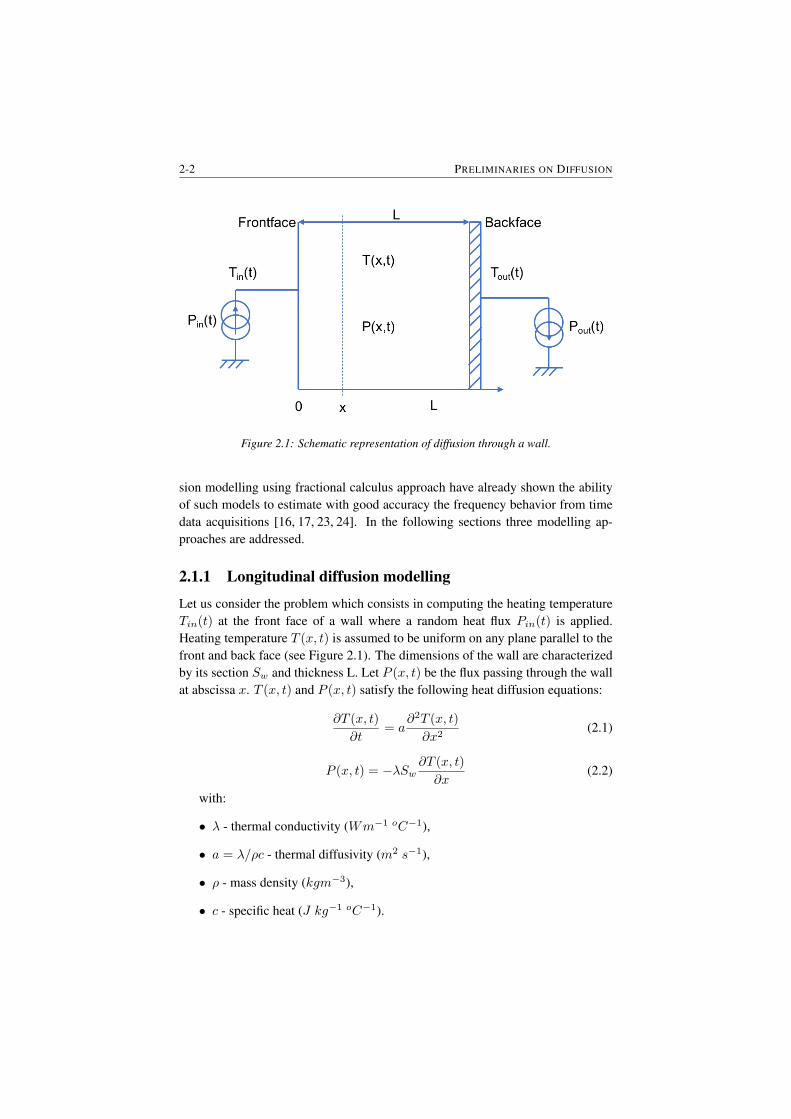
Figure 2.1: Schematic representation of diffusion through a wall.
sion modelling using fractional calculus approach have already shown the abilityof such models to estimate with good accuracy the frequency behavior from timedata acquisitions [16, 17, 23, 24]. In the following sections three modelling ap-proaches are addressed.
2.1.1 Longitudinal diffusion modelling
Let us consider the problem which consists in computing the heating temperatureTin(t) at the front face of a wall where a random heat flux Pin(t) is applied.Heating temperature T (x, t) is assumed to be uniform on any plane parallel to thefront and back face (see Figure 2.1). The dimensions of the wall are characterizedby its section Sw and thickness L. Let P (x, t) be the flux passing through the wallat abscissa x. T (x, t) and P (x, t) satisfy the following heat diffusion equations:
∂T (x, t)
∂t= a
∂2T (x, t)
∂x2(2.1)
P (x, t) = −λSw∂T (x, t)
∂x(2.2)
with:
• λ - thermal conductivity (Wm−1 oC−1),
• a = λ/ρc - thermal diffusivity (m2 s−1),
• ρ - mass density (kgm−3),
• c - specific heat (J kg−1 oC−1).
CHAPTER 2 2-3
Let Tout(t) be the back face temperature and Pout(t) the output flux. We writeTin(s), Pin(s) and Tout(s), Pout(s) the Laplace transforms of Tin(t), Pin(t) atx = 0 and Tout(t), Pout(t) at x = L. One can model the wall using a thermalquadrupole relating the inputs (Tin(s), Pin(s)) to the outputs (Tout(s), Pout(s))[25]: [
Tin(s)Pin(s)
]=
[A BC D
]∗[Tout(s)φout(s)
](2.3)
where the matrix coefficients A, B, C, D characterize the heat transfer phe-nomenon in the wall. By applying the Laplace transform to (2.1) and (2.2), oneobtains:
sT (x, s)− T (x, 0) = a∂2T (x, s)
∂x2(2.4)
P (x, s) = −λSw∂T (x, s)
∂x(2.5)
Assuming the longitudinal temperature profile is initially constant at time t = 0:
T (x, 0) = 0, 0 < x < L (2.6)
The solution set of the second order spatial differential equation (2.4) is given by:
T (x, s) = L1(s)cosh(δx) + L2 sinh(δx) (2.7)
with δ =√s/a. Using (2.5) and (2.7) and considering the boundary conditions
yields to:
Tin(s) = cosh(δL)Tout(s) + 1λSw
sinh(δL)δ Pout(s)
Pin(s) = λSwδ sinh(δL)Pout(s)(2.8)
Hence the wall thermal matrix coefficients are given by:
A = D = cosh(δL)B = 1
λSwsinhδL
δ
C = λSwδ sinh(δL)
(2.9)
If we consider the experiment where the back-face temperature is kept constant(i.e. Tout(s) = 0), the transfer function which can be interpreted as thermalimpedance is:
Zw(s) =Tin(s)
Pin(s)=B
D=
L
λSw
tanh(λL)
δL=
L
λSw
tanh(√
saL)
(√
saL)
(2.10)
The static gain of that transfer function corresponding to the thermal resistanceRthw has the following expression:
lims→0
Zs(s) =Tf (s)
Pin(s)= Rthw =
L
λSw(2.11)
2-4 PRELIMINARIES ON DIFFUSION
At high frequencies, the the wall behaves half order integrator:
lims→∞
Zs(s) =
√a
λSws0.5(2.12)
2.1.2 Spherical diffusion modelling
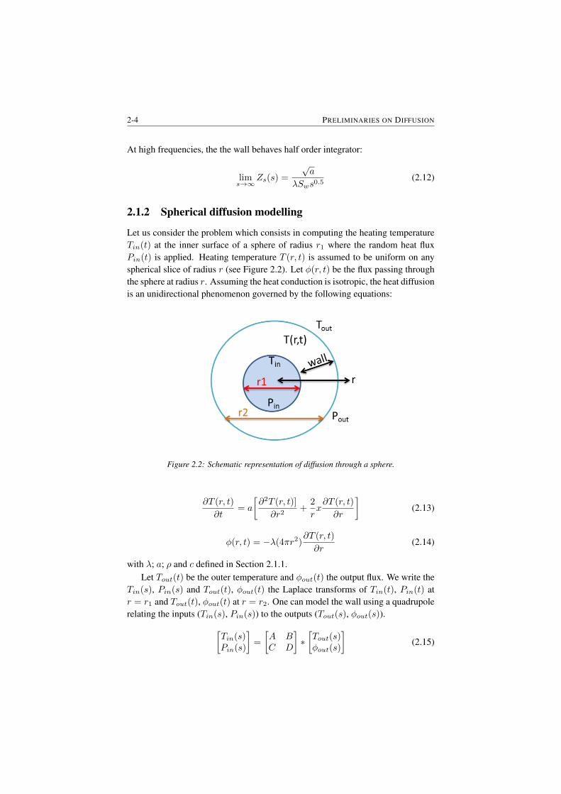
Let us consider the problem which consists in computing the heating temperatureTin(t) at the inner surface of a sphere of radius r1 where the random heat fluxPin(t) is applied. Heating temperature T (r, t) is assumed to be uniform on anyspherical slice of radius r (see Figure 2.2). Let φ(r, t) be the flux passing throughthe sphere at radius r. Assuming the heat conduction is isotropic, the heat diffusionis an unidirectional phenomenon governed by the following equations:
Figure 2.2: Schematic representation of diffusion through a sphere.
∂T (r, t)
∂t= a
[∂2T (r, t)]
∂r2+
2
rx∂T (r, t)
∂r
](2.13)
φ(r, t) = −λ(4πr2)∂T (r, t)
∂r(2.14)
with λ; a; ρ and c defined in Section 2.1.1.Let Tout(t) be the outer temperature and φout(t) the output flux. We write the
Tin(s), Pin(s) and Tout(t), φout(t) the Laplace transforms of Tin(t), Pin(t) atr = r1 and Tout(t), φout(t) at r = r2. One can model the wall using a quadrupolerelating the inputs (Tin(s), Pin(s)) to the outputs (Tout(s), φout(s)).[
Tin(s)Pin(s)
]=
[A BC D
]∗[Tout(s)φout(s)
](2.15)
CHAPTER 2 2-5
where the matrix coefficients A, B, C and D characterize the heat transfer phe-nomenon in the sphere. Applying the Laplace transform to (2.13) and (2.14) pro-vides:
sT (r, s)− T (r, 0) = a
[∂T (r, s)
∂r2+
2
rx∂T (r, s)
∂r
](2.16)
φ(r, s) = −λ(4πr2)∂T (r, s)
∂r(2.17)
Assuming the radial temperature profile is initially constant at time t=0:
T (r, 0) = 0, r1 < r < r2 (2.18)
The solution of the second order partial differential equation (2.16) is given by:
T (r, s) = r−0.5x[L1(s)I−0.5(δr) + L2(s)K−0.5(δr)
](2.19)
with δ =√s/a.
L1(s) and L2(s) are constant of integration and I−0.5(x) and K−0.5(x) aremodified Bessel functions of, respectively, first and second type given by [26]:
K−0.5(x) =( π
2x
)0.5e−x (2.20)
I−0.5(x) =( 2
πx
)0.5(2.21)
Considering the boundary conditions and using equations (2.19) and (2.17) thematrix terms A, B, C and D characterizing the heat transfer of the sphere can bedetermined [27]:
A = r1r2cosh(δ(r2 − r1))− sinh(δ(r2−r1))
δr1
B = 14πr1r2
sinh(δ(r2−r1))δλ
C = 4πr2λ[1− r1r2cosh(δ(r2 − r1)) + (λr1 − 1
λr2) sinh(δ(r2−r1))δr1
D = r1r2cosh(δ(r2 − r1)) + sinh(δ(r2−r1))
δr1
(2.22)
Considering that the heat flux Pin(t) is applied uniformly to the inner sphericalsurface of radius r1, the output temperature of the external spherical surface r2being kept constant (Tout(s) = 0), the following transfer function which can beinterpreted as a thermal impedance is obtained:
Zs(s) =Tin(s)
Pin(s)=B
D=
(1
4πr1λ
)1
1 +√
sar1
1
tanh(√
sa (r2−r1))
(2.23)
The thermal resistance Rths is given by considering the static gain:
lims→0
Zs(s) =Tin(s)
φin(s)= Tths =
1
4πλ
[1
r1− 1
r2
](2.24)
2-6 PRELIMINARIES ON DIFFUSION
At high frequencies, the thermal impedance of the sphere behaves like a non-integer integrator whose order is equal to 0.5:
lims→∞
Zs(s) =
√a
λ(4πr2i )s0.5
(2.25)
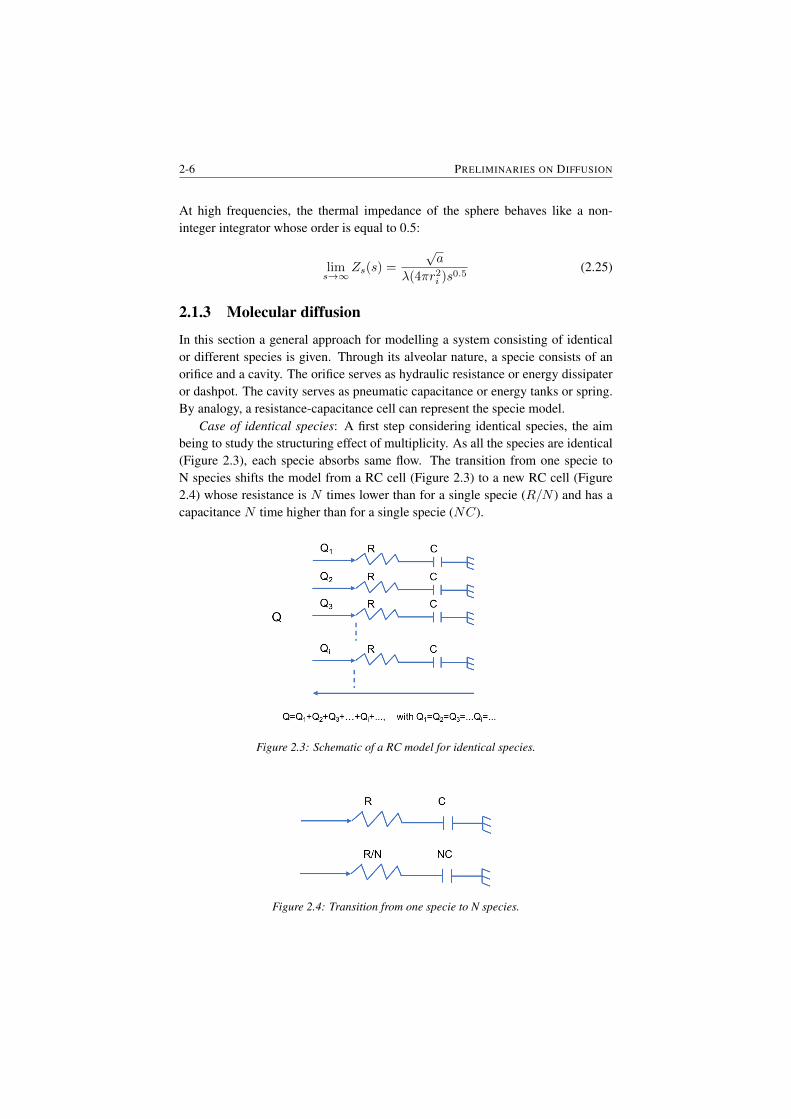
2.1.3 Molecular diffusion
In this section a general approach for modelling a system consisting of identicalor different species is given. Through its alveolar nature, a specie consists of anorifice and a cavity. The orifice serves as hydraulic resistance or energy dissipateror dashpot. The cavity serves as pneumatic capacitance or energy tanks or spring.By analogy, a resistance-capacitance cell can represent the specie model.
Case of identical species: A first step considering identical species, the aimbeing to study the structuring effect of multiplicity. As all the species are identical(Figure 2.3), each specie absorbs same flow. The transition from one specie toN species shifts the model from a RC cell (Figure 2.3) to a new RC cell (Figure2.4) whose resistance is N times lower than for a single specie (R/N ) and has acapacitance N time higher than for a single specie (NC).
Figure 2.3: Schematic of a RC model for identical species.
Figure 2.4: Transition from one specie to N species.
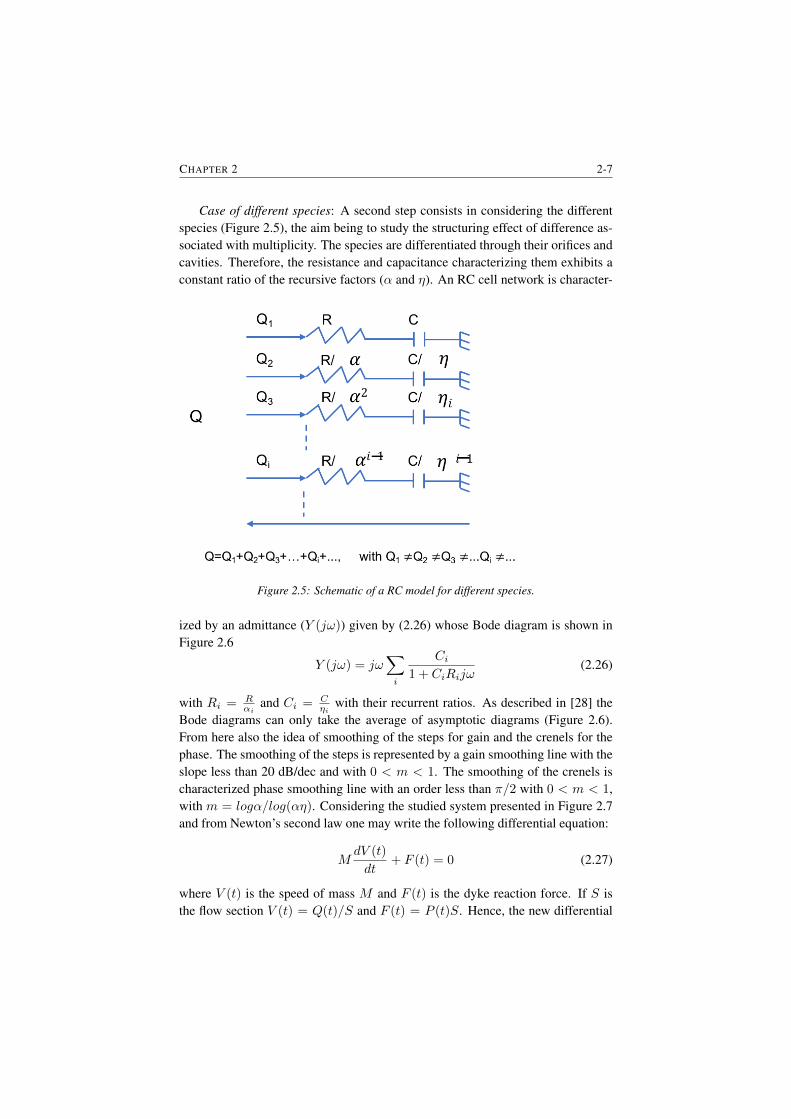
CHAPTER 2 2-7
Case of different species: A second step consists in considering the differentspecies (Figure 2.5), the aim being to study the structuring effect of difference as-sociated with multiplicity. The species are differentiated through their orifices andcavities. Therefore, the resistance and capacitance characterizing them exhibits aconstant ratio of the recursive factors (α and η). An RC cell network is character-
Figure 2.5: Schematic of a RC model for different species.
ized by an admittance (Y (jω)) given by (2.26) whose Bode diagram is shown inFigure 2.6
Y (jω) = jω∑i
Ci1 + CiRijω
(2.26)
with Ri = Rαi
and Ci = Cηi
with their recurrent ratios. As described in [28] theBode diagrams can only take the average of asymptotic diagrams (Figure 2.6).From here also the idea of smoothing of the steps for gain and the crenels for thephase. The smoothing of the steps is represented by a gain smoothing line with theslope less than 20 dB/dec and with 0 < m < 1. The smoothing of the crenels ischaracterized phase smoothing line with an order less than π/2 with 0 < m < 1,with m = logα/log(αη). Considering the studied system presented in Figure 2.7and from Newton’s second law one may write the following differential equation:
MdV (t)
dt+ F (t) = 0 (2.27)
where V (t) is the speed of mass M and F (t) is the dyke reaction force. If S isthe flow section V (t) = Q(t)/S and F (t) = P (t)S. Hence, the new differential
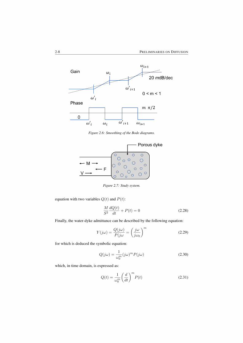
2-8 PRELIMINARIES ON DIFFUSION
Figure 2.6: Smoothing of the Bode diagrams.
Figure 2.7: Study system.
equation with two variables Q(t) and P (t):
M
S2
dQ(t)
dt+ P (t) = 0 (2.28)
Finally, the water-dyke admittance can be described by the following equation:
Y (jω) =Q(jω)
P (jω=
(jω
jω0
)m(2.29)
for which is deduced the symbolic equation:
Q(jω) =1
ωm0(jω)mP (jω) (2.30)
which, in time domain, is expressed as:
Q(t) =1
ωm0
(d
dt
)mP (t) (2.31)
CHAPTER 2 2-9
This equation represents the (dynamic) model of the porous interface and in-dicates that the flow Q(t) is proportional to the non-integer derivative of pressureP (t).
2.2 SummaryThis Chapter presented the theoretical aspects of diffusion processes. The theoret-ical aspects addressed in this chapter of the thesis are further employed to modelthe diffusion of gases in the lungs and drug diffusion in the human body. Diffu-sion in lungs is addressed in Chapter 3 and the tools presented in this chapter areemployed to model the gas exchange phenomena. For this, the theory presentedhere is used in order to model a network of alveoli. Both cases (i.e. identicaland different species/alveoli) presented in this section are used to model the dif-fusion process. Modelling of drug diffusion in the human body can be also mod-eled using the tools presented in this chapter. More specifically, in Chapter 5 thepharmacokinetic-pharmacodynamic model characterizing drug uptake and effectare based on theoretical aspects presented in this chapter.

3Diffusion in the Lungs
In this Chapter the importance of gas diffusion through the respiratory membraneis investigated. The theory described in Chapter 2 is further employed in Section3.4. First, the impedance of one alveolus has been simulated followed by a net-work of alveoli. The simulation results are then compared with measurements bymeans of derived parameters.
The main publications where this work has been presented are:
• D. Copot, C.M. Ionescu, R. De Keyser. Structural changes in the COPDlung and related changes in diffusion mechanism, PLOS ONE Journal, 12(5),doi.org/10.1371/journal.pone.0177969, 2017.
• D. Copot, C.M. Ionescu, R. De Keyser. Relation between fractional ordermodels and diffusion in the body, IFAC World Congress, Cape Town, SouthAfrica, 24-29 August, 9277-9282, 2014.
• C.M. Ionescu, D. Copot, R. De Keyser. A fractional order impedance modelto capture the structural changes in lungs, IFAC World Congress, CapeTown, South Africa, 24-29 August, 5363-5368, 2014.
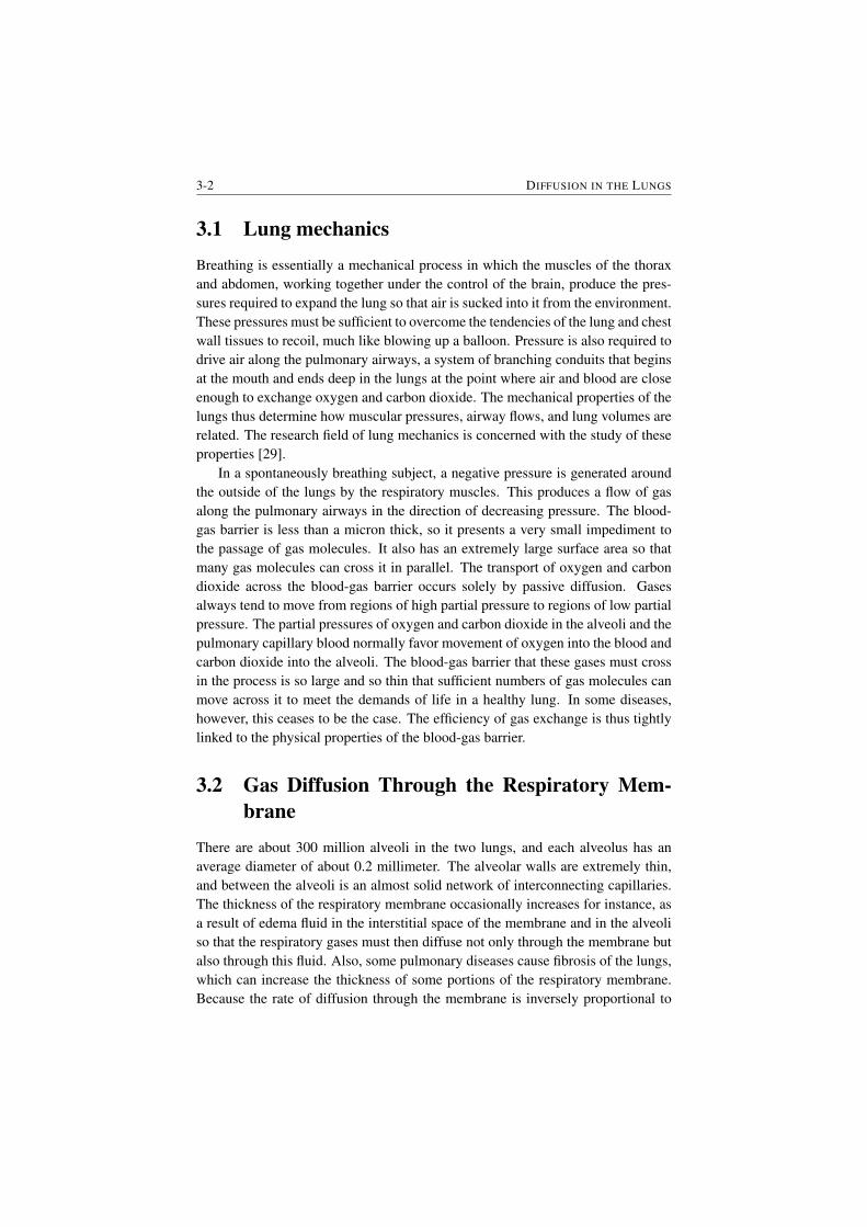
3-2 DIFFUSION IN THE LUNGS
3.1 Lung mechanics
Breathing is essentially a mechanical process in which the muscles of the thoraxand abdomen, working together under the control of the brain, produce the pres-sures required to expand the lung so that air is sucked into it from the environment.These pressures must be sufficient to overcome the tendencies of the lung and chestwall tissues to recoil, much like blowing up a balloon. Pressure is also required todrive air along the pulmonary airways, a system of branching conduits that beginsat the mouth and ends deep in the lungs at the point where air and blood are closeenough to exchange oxygen and carbon dioxide. The mechanical properties of thelungs thus determine how muscular pressures, airway flows, and lung volumes arerelated. The research field of lung mechanics is concerned with the study of theseproperties [29].
In a spontaneously breathing subject, a negative pressure is generated aroundthe outside of the lungs by the respiratory muscles. This produces a flow of gasalong the pulmonary airways in the direction of decreasing pressure. The blood-gas barrier is less than a micron thick, so it presents a very small impediment tothe passage of gas molecules. It also has an extremely large surface area so thatmany gas molecules can cross it in parallel. The transport of oxygen and carbondioxide across the blood-gas barrier occurs solely by passive diffusion. Gasesalways tend to move from regions of high partial pressure to regions of low partialpressure. The partial pressures of oxygen and carbon dioxide in the alveoli and thepulmonary capillary blood normally favor movement of oxygen into the blood andcarbon dioxide into the alveoli. The blood-gas barrier that these gases must crossin the process is so large and so thin that sufficient numbers of gas molecules canmove across it to meet the demands of life in a healthy lung. In some diseases,however, this ceases to be the case. The efficiency of gas exchange is thus tightlylinked to the physical properties of the blood-gas barrier.
3.2 Gas Diffusion Through the Respiratory Mem-brane
There are about 300 million alveoli in the two lungs, and each alveolus has anaverage diameter of about 0.2 millimeter. The alveolar walls are extremely thin,and between the alveoli is an almost solid network of interconnecting capillaries.The thickness of the respiratory membrane occasionally increases for instance, asa result of edema fluid in the interstitial space of the membrane and in the alveoliso that the respiratory gases must then diffuse not only through the membrane butalso through this fluid. Also, some pulmonary diseases cause fibrosis of the lungs,which can increase the thickness of some portions of the respiratory membrane.Because the rate of diffusion through the membrane is inversely proportional to
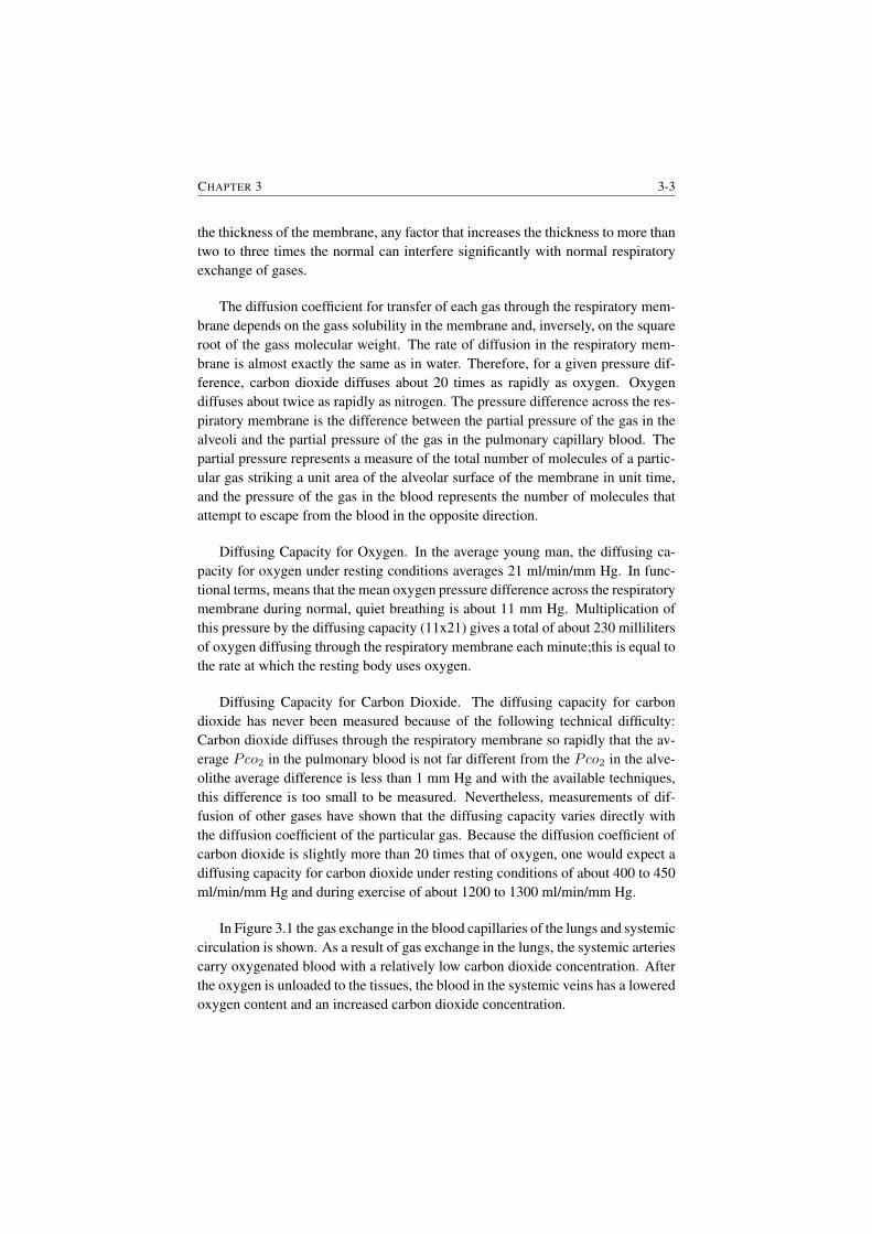
CHAPTER 3 3-3
the thickness of the membrane, any factor that increases the thickness to more thantwo to three times the normal can interfere significantly with normal respiratoryexchange of gases.
The diffusion coefficient for transfer of each gas through the respiratory mem-brane depends on the gass solubility in the membrane and, inversely, on the squareroot of the gass molecular weight. The rate of diffusion in the respiratory mem-brane is almost exactly the same as in water. Therefore, for a given pressure dif-ference, carbon dioxide diffuses about 20 times as rapidly as oxygen. Oxygendiffuses about twice as rapidly as nitrogen. The pressure difference across the res-piratory membrane is the difference between the partial pressure of the gas in thealveoli and the partial pressure of the gas in the pulmonary capillary blood. Thepartial pressure represents a measure of the total number of molecules of a partic-ular gas striking a unit area of the alveolar surface of the membrane in unit time,and the pressure of the gas in the blood represents the number of molecules thatattempt to escape from the blood in the opposite direction.
Diffusing Capacity for Oxygen. In the average young man, the diffusing ca-pacity for oxygen under resting conditions averages 21 ml/min/mm Hg. In func-tional terms, means that the mean oxygen pressure difference across the respiratorymembrane during normal, quiet breathing is about 11 mm Hg. Multiplication ofthis pressure by the diffusing capacity (11x21) gives a total of about 230 millilitersof oxygen diffusing through the respiratory membrane each minute;this is equal tothe rate at which the resting body uses oxygen.
Diffusing Capacity for Carbon Dioxide. The diffusing capacity for carbondioxide has never been measured because of the following technical difficulty:Carbon dioxide diffuses through the respiratory membrane so rapidly that the av-erage Pco2 in the pulmonary blood is not far different from the Pco2 in the alve-olithe average difference is less than 1 mm Hg and with the available techniques,this difference is too small to be measured. Nevertheless, measurements of dif-fusion of other gases have shown that the diffusing capacity varies directly withthe diffusion coefficient of the particular gas. Because the diffusion coefficient ofcarbon dioxide is slightly more than 20 times that of oxygen, one would expect adiffusing capacity for carbon dioxide under resting conditions of about 400 to 450ml/min/mm Hg and during exercise of about 1200 to 1300 ml/min/mm Hg.
In Figure 3.1 the gas exchange in the blood capillaries of the lungs and systemiccirculation is shown. As a result of gas exchange in the lungs, the systemic arteriescarry oxygenated blood with a relatively low carbon dioxide concentration. Afterthe oxygen is unloaded to the tissues, the blood in the systemic veins has a loweredoxygen content and an increased carbon dioxide concentration.
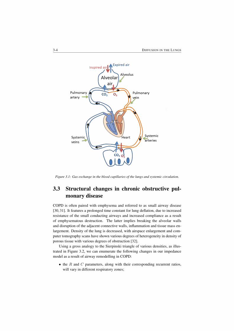
3-4 DIFFUSION IN THE LUNGS
Figure 3.1: Gas exchange in the blood capillaries of the lungs and systemic circulation.
3.3 Structural changes in chronic obstructive pul-monary disease
COPD is often paired with emphysema and referred to as small airway disease[30, 31]. It features a prolonged time constant for lung deflation, due to increasedresistance of the small conducting airways and increased compliance as a resultof emphysematous destruction. The latter implies breaking the alveolar wallsand disruption of the adjacent connective walls, inflammation and tissue mass en-largement. Density of the lung is decreased, with airspace enlargement and com-puter tomography scans have shown various degrees of heterogeneity in density ofporous tissue with various degrees of obstruction [32].
Using a gross analogy to the Sierpinski triangle of various densities, as illus-trated in Figure 3.2, we can enumerate the following changes in our impedancemodel as a result of airway remodelling in COPD:
• the R and C parameters, along with their corresponding recurrent ratios,will vary in different respiratory zones;
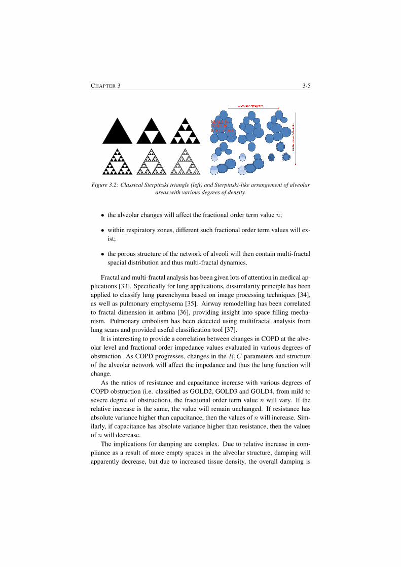
CHAPTER 3 3-5
Figure 3.2: Classical Sierpinski triangle (left) and Sierpinski-like arrangement of alveolarareas with various degrees of density.
• the alveolar changes will affect the fractional order term value n;
• within respiratory zones, different such fractional order term values will ex-ist;
• the porous structure of the network of alveoli will then contain multi-fractalspacial distribution and thus multi-fractal dynamics.
Fractal and multi-fractal analysis has been given lots of attention in medical ap-plications [33]. Specifically for lung applications, dissimilarity principle has beenapplied to classify lung parenchyma based on image processing techniques [34],as well as pulmonary emphysema [35]. Airway remodelling has been correlatedto fractal dimension in asthma [36], providing insight into space filling mecha-nism. Pulmonary embolism has been detected using multifractal analysis fromlung scans and provided useful classification tool [37].
It is interesting to provide a correlation between changes in COPD at the alve-olar level and fractional order impedance values evaluated in various degrees ofobstruction. As COPD progresses, changes in the R,C parameters and structureof the alveolar network will affect the impedance and thus the lung function willchange.
As the ratios of resistance and capacitance increase with various degrees ofCOPD obstruction (i.e. classified as GOLD2, GOLD3 and GOLD4, from mild tosevere degree of obstruction), the fractional order term value n will vary. If therelative increase is the same, the value will remain unchanged. If resistance hasabsolute variance higher than capacitance, then the values of n will increase. Sim-ilarly, if capacitance has absolute variance higher than resistance, then the valuesof n will decrease.
The implications for damping are complex. Due to relative increase in com-pliance as a result of more empty spaces in the alveolar structure, damping willapparently decrease, but due to increased tissue density, the overall damping is
3-6 DIFFUSION IN THE LUNGS
increasing. Notice that if alveolar surface is decreased with pathology, the timeconstant defined in previous section for the network will also increase. This is inline with the pathology of COPD which has long deflation periods. In conclusion,local structural changes are more important than the network spacial distributionin terms of impedance.
3.4 Diffusion at low frequencies
In the context of electrical analogy, one usually considers voltage as the equivalentfor respiratory pressure (P ) and current as the equivalent for airflow (Q). Thepressure in function of time is the accumulation of these components with thetrans-pulmonary pressure at end-expiration (P0):
P (t) =1
CV (t) +R
dV
dt+ I
d2V
dt2+ P0 (3.1)
where elastance (1/C) (the reciprocal of the compliance) is directly related tovolume (V ), the resistance (R) is related to airflow and the inertia (I) is relatedto accelerating particles. This equation represents the global relationship betweenairflow and pressure in the lungs. Its equivalent frequency domain form is therespiratory impedance as a function of oscillatory frequency [38].
This principle has been applied by means of Womersley theory and Navier-Stokes equations to elastic tubes preserving structure and morphology of the air-ways [39]. According to the seminal work of Weibel and Mandelbrot [40–42], thestructure of the lungs can be roughly approximated by a recurrent dichotomoustree of 24 levels, leading to a rough approximation of 224 alveolar ducts. At theend of each alveolar duct there is a porous bag called alveoli, which are groupedtogether like a lot of interlinked caves, rather than individual sacks.
A mathematical model of the respiratory tree up to 24th level has been pro-posed [39] and used in subsequent works in clinical studies [14]. The model isbased on the geometrical parameters: radius and wall thickness (r, h), on the me-chanical characteristics of the airway tube: complex elastic moduli (given by itsmodulus (|E|) and angle(ϕE)) on the Poisson coefficient (νP ), and on the air prop-erties: viscosity and density (µ, ρ). Over the length ` of an airway tube, we havethe corresponding definitions for electrical resistance:
Re = `µδ2
πr4M1sin(ε1), (3.2)
and for electrical capacitance
Ce = `2πr3(1− ν2P )2
|E|hcosϕE , (3.3)
CHAPTER 3 3-7
where, M1 is the modulus of the Bessel function of order 1, ε1 is the phase an-gle of the complex Bessel function of order 1, and δ =
√ωρ/µ the Womersley
parameter.We have shown that the geometry of the lungs leads to a piecewise fractal
structure, whose electrical equivalent leads to a recurrent ladder network. Theadmittance of such network has the form:
YN (s) ∼=1/Re1
1 +1/Re1Ce1s
1 +1/γRe1Ce1s
. . .. . .
1 +1/χN−2γN−1Re1Ce1s
1 + 1/χN−1γN−1Re1Ce1s
(3.4)
with Re1 and Ce1 denoting the resistance and compliance in the first airway (i.e.trachea), and γ the ratio of resistances per total levels, χ the ratio of compliancesper total levels and s the Laplace operator. This continuous fraction expansioncan be well-approximated for N → ∞ airway levels by the compact form ofadmittance [43]:
YN (s) ∼=1/Re1
K(γ, χ) · (1/Re1Ce1s)n(3.5)
with K(λ, χ) a gain factor depending on the values of the ratios and the fractionalorder n given by
n =log(γ)
log(γ) + log(χ)(3.6)
Notice that the impedance, ZN (s) will be the inverse of the admittance. In thefrequency domain, the fractional order will lead to a constant-phase behaviour, i.e.a phase-locking in the frequency range given by the convergence conditions [14,43]. The lumped version of this model is the well-known constant-phase elementmodel given by:
ZCP (sk) = R+ I(sk) +1
C(sβk)(3.7)
where R (kPa s/L) and I (kPa s2/L) denote the central airway resistance and in-ertance respectively, whereas the last term consists of a constant-phase elementwhich can be split into a real and imaginary part, denoting tissue damping andtissue elastance. These two latter properties are defined as averaged over the fre-quency range evaluated by the lung function test [44–46].
Gr =1
Cωβkcos(βπ/2)
Hr =1
Cωβksin(βπ/2)
ηr =GrHr
(3.8)

3-8 DIFFUSION IN THE LUNGS
and their ratio denotes the degree of heterogeneity present in the tissue [47]. Thisratio is in fact a characterization of sources for nonlinear contributions in the res-piratory dynamical properties. If changes in R are small, then any changes in Gr(kPa s(1−β)/L) will represent changes in parenchyma or in very small airways.The memory effects are introduced via s(1−β) [16]. These effects are observedin materials with viscoelastic properties. Chronic changes in Hr (kPa s(1−β)/L)reflect changes in the intrinsic mechanical properties of the parenchyma [48]. Thisparametric model has been shown to reliably estimate airway and tissue proper-ties and its sensitivity to bronchodilatation in dogs at low frequencies has beenassessed in [44]. The same model has been used to assess respiratory impedancein rats at low frequencies in [49]. The model has been used to evaluate respiratoryimpedance in healthy and sick patients [14, 47]. The reliability of the parameterestimates from model fitting to raw data has shown that the inertance I and theresistance R may contain a high degree of uncertainty , while the constant-phaseterm delivers a reliable estimate of peripheral tissue properties. The study alsoshowed that the steep dependency on frequency at low frequencies in the real partof impedance is consistently fitted by the constant-phase model from (3.7) whencompared to other models from literature.
In order to quantify the non-linear contributions the following index has beenintroduced [14]:
T =Peven + Podd
Pexc· UexcUeven + Uodd
(3.9)
where each variable represents the sum of the absolute values of all the contribu-tions in the pressure and flow signals a non-excited frequencies (even and odd) andthe odd excited frequencies. The index expresses the relative ration of the contri-butions at non-excited frequencies with respect to the contributions at the excitedfrequencies. For a detailed overview on filtering techniques applied to extract thecontributions see [14, 50].
To allow a systematic approach, we need to use an impedance model of onealveolus which will be later used for analysis of alveolar sac structures and theirrespective properties in presence of remodelling effects.
Impedance of one alveolus: Let us assume a spherical alveolus characterizedby an inner radius r1 and an outer radius r2. We may assume without loss ofgenerality that heat conduction is anisotropic, heat diffusion is unidirectional andspherical coordinates can be used for modelling. Following the line of thoughtpresented in [16, 17], approximating the spherical wall (i.e. difference betweeninner radius and outer radius) with many cells whose pressure is governed by:
dPidt
=1
RiCi(Pi−1 − 2Pi + Pi+1) (3.10)
with Ri and Ci representing the resistance and compliance properties of the cell
CHAPTER 3 3-9
i and Pi pressure profile assumed uniformly distributed along the cell face. Thethickness of each cell is then given by the relation: h = r2 − r1/N , with N thetotal number of cells and 0 ≤ i ≤ N . Introducing N0 = r1/h, it follows that theradii of each cell is given by ri = (N0 + i)h. The surface of the cell becomes:
Si = 4πr2i = 4πh2(N0 + i)2 (3.11)
and it follows that the resistance of each cell is given by:
Ri =h
λ · Si=
1
4πλh(N0 + i)2(3.12)
where λ is the thermal conductivity (W m−1 o C−1). The capacity per cell isdefined as:
Ci =4
3πh3[3(N0 + i)2 +
1
4]ρc (3.13)
with ρ mass density (kg m−3) and c specific heat (J kg−1 oC−1). The laddernetwork of series connected cells with resistance and capacity calculated in (3.12) -(3.13) in Laplace operator, provides the explicit impedance which can be evaluatedover a range of frequencies. This can be either a ladder network made of recurrentelements, either one with same element values per cell. In our case, the latterapplies since we assumed a homogeneous density of the alveolar wall.
Numerical simulation was performed using a linear state-space representationgiven in (3.14)-(3.15):
As(i, i− 1) =a
h2(N0 + i)2
(N0 + i)2 + 112
As(i, i) = − a
h2(N0 + i)2 + (N0 + i+ 1)2
(N0 + i)2 + 112
As(i, i− 1) =a
h2(N0 + i+ 1)2
(N0 + i)2 + 112
(3.14)
As(1, 1) =a
h2(N0 + 1)2
N20
2 + N0
2 + 124
As(1, 2) =a
h2(N0 + 1)2
N20
2 + N0
2 + 124
As(I, I − 1) =a
h2(N0 + I − 1)2
(N0 + I − 1)2 + 112
As(I, I) = − a
h2(N0 + I − 1)2 + (N0 + 1)2
(N0 + I − 1) + 112
(3.15)
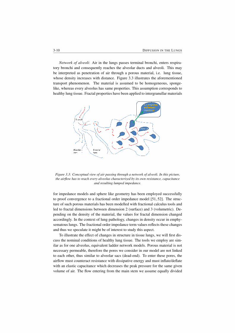
3-10 DIFFUSION IN THE LUNGS
Network of alveoli: Air in the lungs passes terminal bronchi, enters respira-tory bronchi and consequently reaches the alveolar ducts and alveoli. This maybe interpreted as penetration of air through a porous material, i.e. lung tissue,whose density increases with distance. Figure 3.3 illustrates the aforementionedtransport phenomenon. The material is assumed to be homogeneous, sponge-like, whereas every alveolus has same properties. This assumption corresponds tohealthy lung tissue. Fractal properties have been applied to intergranullar materials
Figure 3.3: Conceptual view of air passing through a network of alveoli. In this picture,the airflow has to reach every alveolus characterized by its own resistance, capacitance
and resulting lumped impedance.
for impedance models and sphere like geometry has been employed successfullyto proof convergence to a fractional order impedance model [51, 52]. The struc-ture of such porous materials has been modelled with fractional calculus tools andled to fractal dimensions between dimension 2 (surface) and 3 (volumetric). De-pending on the density of the material, the values for fractal dimension changedaccordingly. In the context of lung pathology, changes in density occur in emphy-sematous lungs. The fractional order impedance term values reflects these changesand thus we speculate it might be of interest to study this aspect.
To illustrate the effect of changes in structure in tissue lungs, we will first dis-cuss the nominal conditions of healthy lung tissue. The tools we employ are sim-ilar as for one alveolus, equivalent ladder network models. Porous material is notnecessary permeable, therefore the pores we consider in our model are not linkedto each other, thus similar to alveolar sacs (dead-end). To enter these pores, theairflow must counteract resistance with dissipative energy and must inflate/deflatewith an elastic capacitance which decreases the peak pressure for the same givenvolume of air. The flow entering from the main stem we assume equally divided
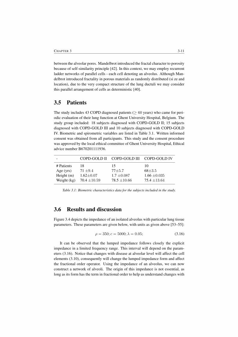
CHAPTER 3 3-11
between the alveolar pores. Mandelbrot introduced the fractal character to porositybecause of self-similarity principle [42]. In this context, we may employ recurrentladder networks of parallel cells - each cell denoting an alveolus. Although Man-delbrot introduced fractality in porous materials as randomly distributed (si ze andlocation), due to the very compact structure of the lung ductuli we may considerthis parallel arrangement of cells as deterministic [40].
3.5 Patients
The study includes 43 COPD diagnosed patients (≥ 60 years) who came for peri-odic evaluation of their lung function at Ghent University Hospital, Belgium. Thestudy group included: 18 subjects diagnosed with COPD-GOLD II; 15 subjectsdiagnosed with COPD-GOLD III and 10 subjects diagnosed with COPD-GOLDIV. Biometric and spirometric variables are listed in Table 3.1. Written informedconsent was obtained from all participants. This study and the consent procedurewas approved by the local ethical committee of Ghent University Hospital, Ethicaladvice number B670201111936.
- COPD-GOLD II COPD-GOLD III COPD-GOLD IV
# Patients 18 15 10Age (yrs) 71 ±9.4 77±5.7 68±3.5Height (m) 1.62±0.07 1.7 ±0.087 1.66 ±0.035Weight (kg) 70.4 ±10.59 78.5 ±10.66 75.4 ±13.64
Table 3.1: Biometric characteristics data for the subjects included in the study.
3.6 Results and discussion
Figure 3.4 depicts the impedance of an isolated alveolus with particular lung tissueparameters. These parameters are given below, with units as given above [53–55]:
ρ = 350; c = 5000;λ = 0.05; (3.16)
It can be observed that the lumped impedance follows closely the explicitimpedance in a limited frequency range. This interval will depend on the param-eters (3.16). Notice that changes with disease at alveolar level will affect the cellelements (3.10), consequently will change the lumped impedance form and affectthe fractional order operator. Using the impedance of an alveolus, we can nowconstruct a network of alveoli. The origin of this impedance is not essential, aslong as its form has the term in fractional order to help us understand changes with
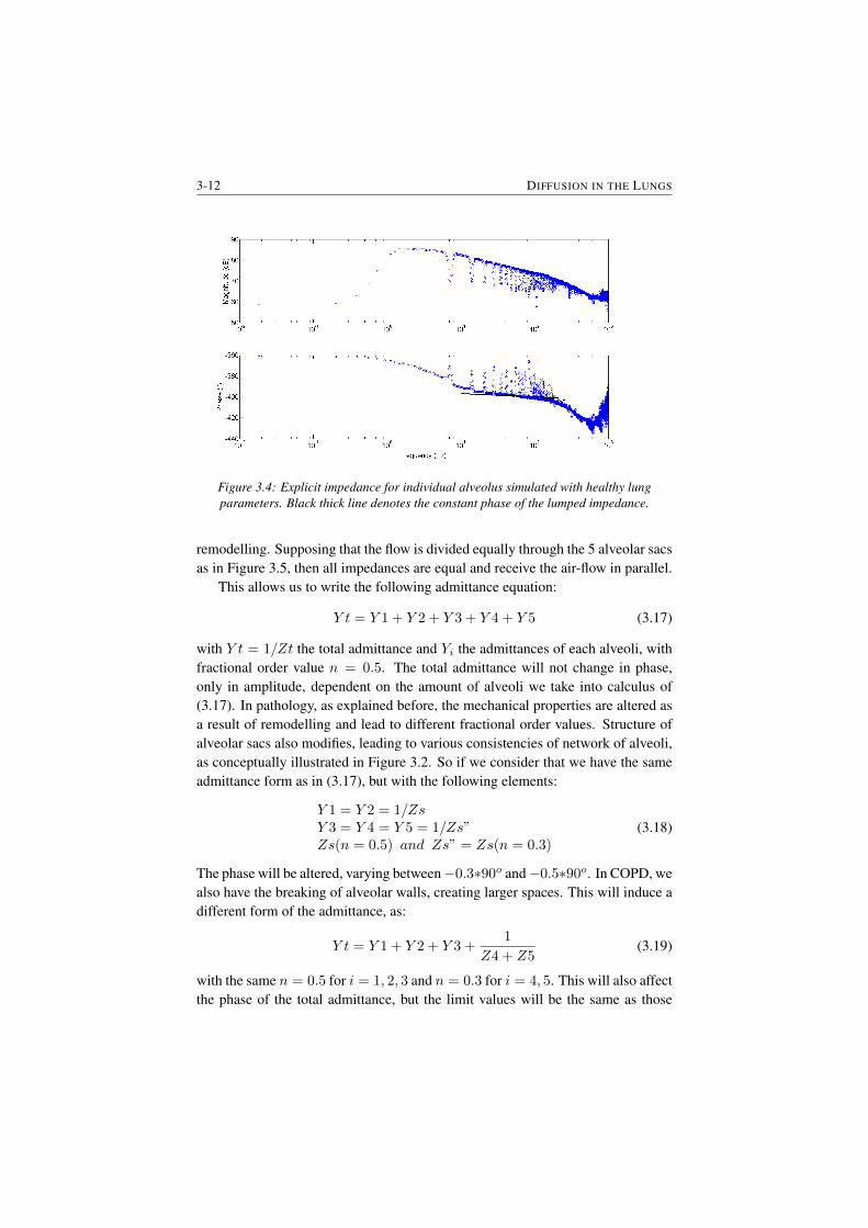
3-12 DIFFUSION IN THE LUNGS
Figure 3.4: Explicit impedance for individual alveolus simulated with healthy lungparameters. Black thick line denotes the constant phase of the lumped impedance.
remodelling. Supposing that the flow is divided equally through the 5 alveolar sacsas in Figure 3.5, then all impedances are equal and receive the air-flow in parallel.
This allows us to write the following admittance equation:
Y t = Y 1 + Y 2 + Y 3 + Y 4 + Y 5 (3.17)
with Y t = 1/Zt the total admittance and Yi the admittances of each alveoli, withfractional order value n = 0.5. The total admittance will not change in phase,only in amplitude, dependent on the amount of alveoli we take into calculus of(3.17). In pathology, as explained before, the mechanical properties are altered asa result of remodelling and lead to different fractional order values. Structure ofalveolar sacs also modifies, leading to various consistencies of network of alveoli,as conceptually illustrated in Figure 3.2. So if we consider that we have the sameadmittance form as in (3.17), but with the following elements:
Y 1 = Y 2 = 1/ZsY 3 = Y 4 = Y 5 = 1/Zs”Zs(n = 0.5) and Zs” = Zs(n = 0.3)
(3.18)
The phase will be altered, varying between−0.3∗90o and−0.5∗90o. In COPD, wealso have the breaking of alveolar walls, creating larger spaces. This will induce adifferent form of the admittance, as:
Y t = Y 1 + Y 2 + Y 3 +1
Z4 + Z5(3.19)
with the same n = 0.5 for i = 1, 2, 3 and n = 0.3 for i = 4, 5. This will also affectthe phase of the total admittance, but the limit values will be the same as those
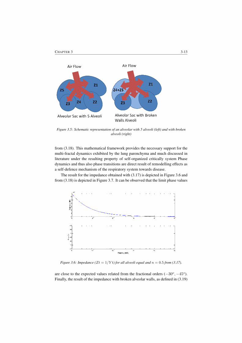
CHAPTER 3 3-13
Figure 3.5: Schematic representation of an alveolar with 5 alveoli (left) and with brokenalveoli (right)
from (3.18). This mathematical framework provides the necessary support for themulti-fractal dynamics exhibited by the lung parenchyma and much discussed inliterature under the resulting property of self-organized critically system Phasedynamics and thus also phase transitions are direct result of remodelling effects asa self-defence mechanism of the respiratory system towards disease.
The result for the impedance obtained with (3.17) is depicted in Figure 3.6 andfrom (3.18) is depicted in Figure 3.7. It can be observed that the limit phase values
Figure 3.6: Impedance (Zt = 1/Y t) for all alveoli equal and n = 0.5 from (3.17).
are close to the expected values related from the fractional orders (−30o,−45o).Finally, the result of the impedance with broken alveolar walls, as defined in (3.19)
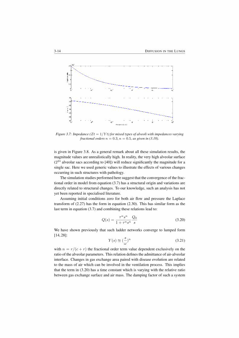
3-14 DIFFUSION IN THE LUNGS
Figure 3.7: Impedance (Zt = 1/Y t) for mixed types of alveoli with impedances varyingfractional orders n = 0.3, n = 0.5, as given in (3.18).
is given in Figure 3.8. As a general remark about all these simulation results, themagnitude values are unrealistically high. In reality, the very high alveolar surface(224 alveolar sacs according to [40]) will reduce significantly the magnitude for asingle sac. Here we used generic values to illustrate the effects of various changesoccurring in such structures with pathology.
The simulation studies performed here suggest that the convergence of the frac-tional order in model from equation (3.7) has a structural origin and variations aredirectly related to structural changes. To our knowledge, such an analysis has notyet been reported in specialised literature.
Assuming initial conditions zero for both air flow and pressure the Laplacetransform of (2.27) has the form in equation (2.30). This has similar form as thelast term in equation (3.7) and combining these relations lead to:
Q(s) =τnsn
1 + τnsnQ0
s(3.20)
We have shown previously that such ladder networks converge to lumped form[14, 28]:
Y (s) u (s
ω)n (3.21)
with n = r/(c + r) the fractional order term value dependent exclusively on theratio of the alveolar parameters. This relation defines the admittance of air-alveolarinterface. Changes in gas exchange area paired with disease evolution are relatedto the mass of air which can be involved in the ventilation process. This impliesthat the term in (3.20) has a time constant which is varying with the relative ratiobetween gas exchange surface and air mass. The damping factor of such a system
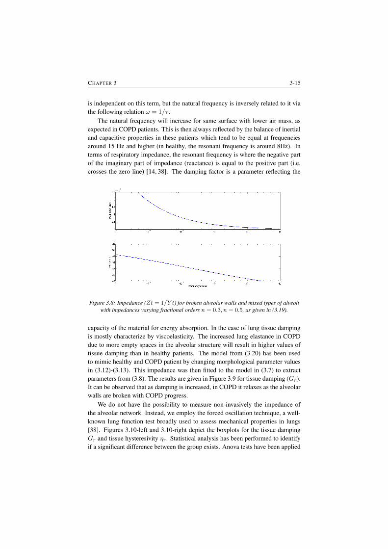
CHAPTER 3 3-15
is independent on this term, but the natural frequency is inversely related to it viathe following relation ω = 1/τ .
The natural frequency will increase for same surface with lower air mass, asexpected in COPD patients. This is then always reflected by the balance of inertialand capacitive properties in these patients which tend to be equal at frequenciesaround 15 Hz and higher (in healthy, the resonant frequency is around 8Hz). Interms of respiratory impedance, the resonant frequency is where the negative partof the imaginary part of impedance (reactance) is equal to the positive part (i.e.crosses the zero line) [14, 38]. The damping factor is a parameter reflecting the
Figure 3.8: Impedance (Zt = 1/Y t) for broken alveolar walls and mixed types of alveoliwith impedances varying fractional orders n = 0.3, n = 0.5, as given in (3.19).
capacity of the material for energy absorption. In the case of lung tissue dampingis mostly characterize by viscoelasticity. The increased lung elastance in COPDdue to more empty spaces in the alveolar structure will result in higher values oftissue damping than in healthy patients. The model from (3.20) has been usedto mimic healthy and COPD patient by changing morphological parameter valuesin (3.12)-(3.13). This impedance was then fitted to the model in (3.7) to extractparameters from (3.8). The results are given in Figure 3.9 for tissue damping (Gr).It can be observed that as damping is increased, in COPD it relaxes as the alveolarwalls are broken with COPD progress.
We do not have the possibility to measure non-invasively the impedance ofthe alveolar network. Instead, we employ the forced oscillation technique, a well-known lung function test broadly used to assess mechanical properties in lungs[38]. Figures 3.10-left and 3.10-right depict the boxplots for the tissue dampingGr and tissue hysteresivity ηr. Statistical analysis has been performed to identifyif a significant difference between the group exists. Anova tests have been applied
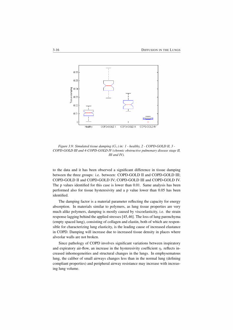
3-16 DIFFUSION IN THE LUNGS
Figure 3.9: Simulated tissue damping (Gr) in: 1 - healthy, 2 - COPD-GOLD II, 3 -COPD-GOLD III and 4-COPD-GOLD IV (chronic obstructive pulmonary disease stage II,
III and IV).
to the data and it has been observed a significant difference in tissue dampingbetween the three groups: i.e. between: COPD-GOLD II and COPD-GOLD III;COPD-GOLD II and COPD-GOLD IV; COPD-GOLD III and COPD-GOLD IV.The p values identified for this case is lower than 0.01. Same analysis has beenperformed also for tissue hysteresivity and a p value lower than 0.05 has beenidentified.
The damping factor is a material parameter reflecting the capacity for energyabsorption. In materials similar to polymers, as lung tissue properties are verymuch alike polymers, damping is mostly caused by viscoelasticity, i.e. the strainresponse lagging behind the applied stresses [45,46]. The loss of lung parenchyma(empty spaced lung), consisting of collagen and elastin, both of which are respon-sible for characterizing lung elasticity, is the leading cause of increased elastancein COPD. Damping will increase due to increased tissue density in places wherealveolar walls are not broken.
Since pathology of COPD involves significant variations between inspiratoryand expiratory air-flow, an increase in the hysteresivity coefficient ηr reflects in-creased inhomogeneities and structural changes in the lungs. In emphysematouslung, the caliber of small airways changes less than in the normal lung (definingcompliant properties) and peripheral airway resistance may increase with increas-ing lung volume.
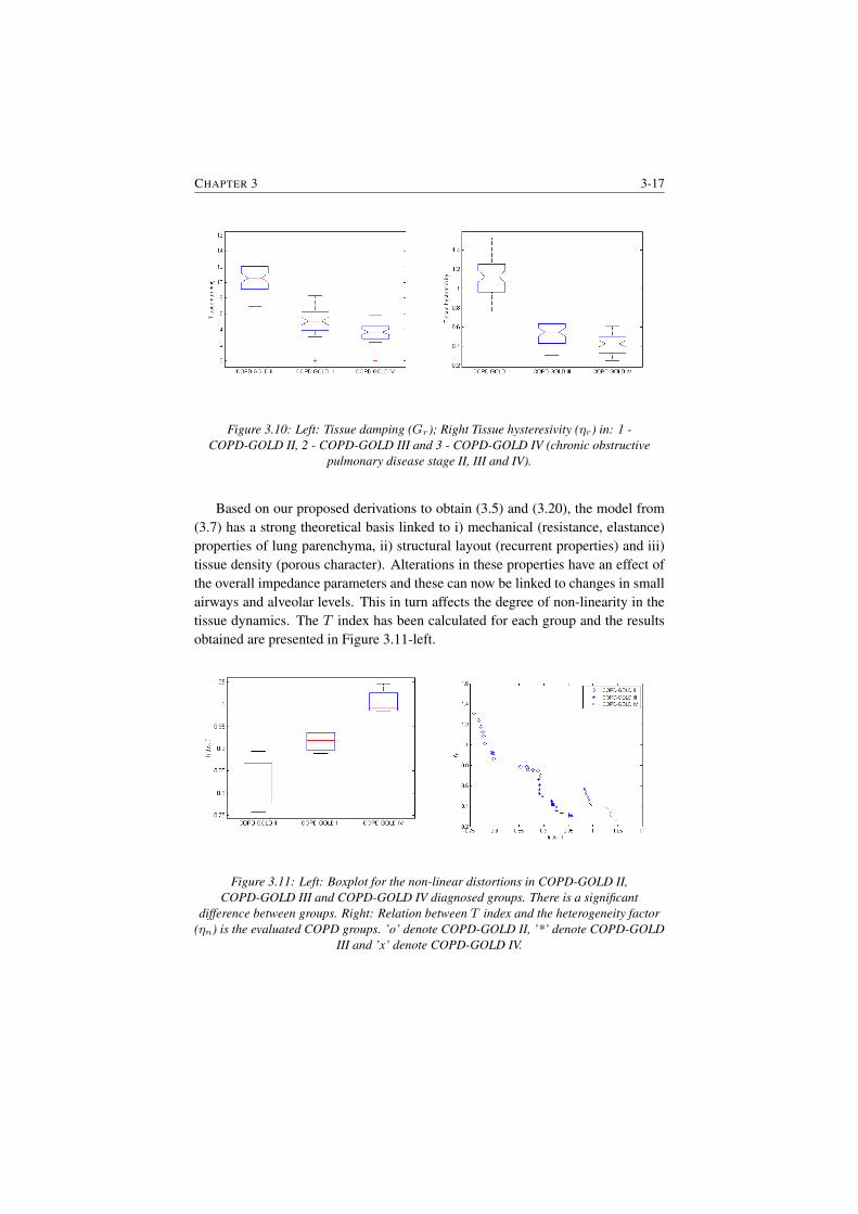
CHAPTER 3 3-17
Figure 3.10: Left: Tissue damping (Gr); Right Tissue hysteresivity (ηr) in: 1 -COPD-GOLD II, 2 - COPD-GOLD III and 3 - COPD-GOLD IV (chronic obstructive
pulmonary disease stage II, III and IV).
Based on our proposed derivations to obtain (3.5) and (3.20), the model from(3.7) has a strong theoretical basis linked to i) mechanical (resistance, elastance)properties of lung parenchyma, ii) structural layout (recurrent properties) and iii)tissue density (porous character). Alterations in these properties have an effect ofthe overall impedance parameters and these can now be linked to changes in smallairways and alveolar levels. This in turn affects the degree of non-linearity in thetissue dynamics. The T index has been calculated for each group and the resultsobtained are presented in Figure 3.11-left.
Figure 3.11: Left: Boxplot for the non-linear distortions in COPD-GOLD II,COPD-GOLD III and COPD-GOLD IV diagnosed groups. There is a significant
difference between groups. Right: Relation between T index and the heterogeneity factor(ηn) is the evaluated COPD groups. ’o’ denote COPD-GOLD II, ’*’ denote COPD-GOLD
III and ’x’ denote COPD-GOLD IV.
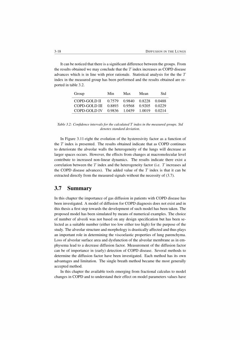
3-18 DIFFUSION IN THE LUNGS
It can be noticed that there is a significant difference between the groups. Fromthe results obtained we may conclude that the T index increases as COPD diseaseadvances which is in line with prior rationale. Statistical analysis for the the Tindex in the measured group has been performed and the results obtained are re-ported in table 3.2.
Group Min Max Mean Std
COPD-GOLD II 0.7579 0.9840 0.8228 0.0488COPD-GOLD III 0.8893 0.9568 0.9205 0.0229COPD-GOLD IV 0.9836 1.0459 1.0019 0.0214
Table 3.2: Confidence intervals for the calculated T index in the measured groups. Stddenotes standard deviation.
In Figure 3.11-right the evolution of the hysteresivity factor as a function ofthe T index is presented. The results obtained indicate that as COPD continuesto deteriorate the alveolar walls the heterogeneity of the lungs will decrease aslarger spaces occurs. However, the effects from changes at macromolecular levelcontribute to increased non-linear dynamics. The results indicate there exist acorrelation between the T index and the heterogeneity factor (i.e. T increases adthe COPD disease advances). The added value of the T index is that it can beextracted directly from the measured signals without the necessity of (3.7).
3.7 SummaryIn this chapter the importance of gas diffusion in patients with COPD disease hasbeen investigated. A model of diffusion for COPD diagnosis does not exist and inthis thesis a first step towards the development of such model has been taken. Theproposed model has been simulated by means of numerical examples. The choiceof number of alveoli was not based on any design specification but has been se-lected as a suitable number (either too low either too high) for the purpose of thestudy. The alveolar structure and morphology is drastically affected and thus playsan important role in determining the viscoelastic properties of lung parenchyma.Loss of alveolar surface area and dysfunction of the alveolar membrane as in em-physema lead to a decrease diffusion factor. Measurement of the diffusion factorcan be of importance in (early) detection of COPD disease. Several methods todetermine the diffusion factor have been investigated. Each method has its ownadvantages and limitation. The single breath method became the most generallyaccepted method.
In this chapter the available tools emerging from fractional calculus to modelchanges in COPD and to understand their effect on model parameters values have

CHAPTER 3 3-19
been presented. The theoretical basis helps in understanding the interplay betweenall these structural and dynamical changes. The results obtained indicate that thereis a direct relation between the T index and the heterogeneity in COPD lungs. Alimitation of this study is that effects of decrease in vascularisation associated withbroken alveolar walls are not investigated. This implies an augmentation of themodel with complex mathematical description of diffusion phenomena. However,these are pertinent next steps in further developing the mathematical of fundamentsrespiratory mechanics. The obtained results are promising and is definitely worthto further investigate this hypothesis.

4Towards a Pain Nociceptor Model
This chapter makes the soft transition from modeling diffusion in the lungs (Chap-ter 3) to modeling drug diffusion (Chapter 5). However, before investigating theuse of diffusion models to characterize drug effect and uptake its necessity is ad-dressed. Therefore, in this chapter the existing tools/methods/techniques and de-vices available to assess pain are presented. The contribution of this chapter to theremaining of the thesis is to indicate the gaps towards an objective pain assessment.
The publications related to this chapter are:
1. D. Copot, C.M. Ionescu, Objective Pain Assessement: How far are we?, ECronicon Anesthesia Journal, Special Issue on Critical Care and Importanceof Anaesthesia for Pain Relief, SI 01, 11-14, 2018,
2. D. Copot, C. Ionescu, Pain monitoring tools: a systematic review, Journalof Clinical Monitoring and Computing, 2018, submitted.
4-2 TOWARDS A PAIN NOCICEPTOR MODEL
4.1 Introduction
Despite the importance of pain in medicine and biology, it is astonishing to dis-cover that the word ”pain” has been never defined satisfactorily.
• First definition states that ”pain is that sensory experience evoked by stimulithat injure or threaten to destroy tissue” [56].
• Second definition describe pain as an abstract concept which refers to 1) apersonal, private sensation of hurt; 2) a harmful stimulus which destroy thetissues; 3) a pattern of responses which operate to protect the organism fromharm” [57].
• Third definition is much better, but still falls short from being acceptableto all. Merskey et al. define pain as an unpleasant sensory and emotionalexperience associated with actual or potential tissue damage, or describedin terms of such damage [58].
Pain is a highly personal experience and the patient is thus the best infor-mant [59–62]. Pain is a multidimensional phenomenon that includes physiologic,sensory, affective, cognitive, behavioral, and sociocultural aspects. Several factorssuch as: age, race, gender etc. seem to modify patients’ pain perception and re-porting [63–66]. Despite modern techniques, pain remains a subjective experienceand health care professionals have to rely on patients ratings [67]. Methods to ac-curately characterize patients pain level during unconsciousness are needed. Forthe case of intensive care unit there is no objective tool to evaluate the level of painthat the patient is experiencing.
Therefore, optimal pain assessment in intensive care units (ICU) is essentialsince it has been reported that 35% to 55% of nurses underrate patients pain[68, 69]. Moreover, in [70] has been reported that 64% of the patients did notreceive any medications before or during painful procedures. In the SUPPORT(Study to Understand Prognoses and Preferences for Outcomes and Risks of Treat-ment) report [62], nearly 50% of patients reported pain, 15% reported moderatelyor extremely severe pain that occurred at least half of the time of the procedure,and nearly 15% were dissatisfied with their pain control. Inaccurate pain assess-ment and the resulting inadequate treatment of pain in critically ill adults can havesignificant physiologic consequences [71].
Hitherto, patient self-report is the best indicator of pain, e.g. using the nu-meric pain rating scale ranging from 0 to 10. However, many critically ill patientsare unable to communicate effectively because of cognitive impairment, sedation,paralysis, or mechanical ventilation. Identification of the optimal pain scale insuch patients is ongoing, and no single tool is universally accepted for use in the
CHAPTER 4 4-3
non-communicative (anesthetized) patient [72, 73]. When a patient cannot ex-press himself, observable indicators - both physiologic and behavioral - have beentreated as pain-related indicators to evaluate pain level [74]. A more detailed de-scription of the available tools is presented is given in section 2.
Therefore, there is a clear evidence that no accurate physiologic or clinicalsigns that can be used to objectively measure pain exists. Reliance on healthcareworker assessment of patient pain results in underestimation of the intensity ofpain. According to the National Institutes for Health (NIH), patient self- reportingis the ”most reliable indicator of the existence and intensity of pain” [75] Subjec-tive pain measures that may need to be quantified include intensity, time course,quality, impact, and personal meaning. The ideal tool in the assessment of painshould include the identification of the presence of pain, as well as the progressof pain with time or treatment [76]. Also, this ideal tool should be applicable toany individual, regardless of psychologic, emotional, or cultural background. Tothat end, unidimensional pain scales have been developed. Because of their easeof use, these scales have become popular tools used to quantify pain relief andpain intensity. The most frequently used tools to assess acute pain are the numericrating scale (NRS) and the visual analogue scale (VAS).
Although popular for study purposes, unidimensional pain scales have short-comings. They were initially developed for use in experimental pain trials in whichpain was limited and controlled. Clinical pain is different in the sense that it maybecome persistent, unbearable, and beyond the individual’s control. It is also oftenassociated with a strong emotional component not observed in the experimentalsetting. Pain scales tend to focus only on pain intensity, with increased risk ofoversimplification of this complex experience. Furthermore, actual measurementsare relative only to the individual being assessed. Identical stimuli applied to dif-ferent individuals can yield to significantly different scores. Thus the numbers aresimply estimates of the perception of the pain, based on past personal experience.Quantification of the experience requires the individual to abstract and quantify thesensation. The use of unidimensional pain scales is more appropriate in the settingof acute pain (caused by surgery, broken bone, burns, etc.) than chronic pain (e.g.headache, cancer pain, low back pain, etc.). Chronic pain is usually associatedwith other events such as degree of support and depression. The assessment ofchronic pain often requires more complex evaluation tools.
Hence, pain is an subjective experience, and hitherto no objective tools existsto measure it. When possible, the existence and intensity of pain are measuredby the patients self-report (i.e. conscious patients). Unfortunately, some patientscannot provide a self-report of pain either verbally, in writing, or by other means,such as finger span [77] or blinking their eyes to answer yes or no questions [78].
Effective management of analgesia in the ICU units requires an assessment ofthe needs of the patient, subjective and/or objective measurement of the key vari-
4-4 TOWARDS A PAIN NOCICEPTOR MODEL
ables (such as pain, agitation, and level of consciousness), and titration of therapyto achieve specific targets [72, 79, 80]. It is important to admit that patient needscan differ depending on clinical circumstances, and that for any given patient ther-apeutic targets are likely to change over time. Thus, achieving patient comfort andensuring patient safety, including avoidance of over- and under-dosage, relies onaccurately measuring pain, agitation, sedation, and other related variables. Thisshould be evaluated with validated tools that are easy to use, precise, accurate, andsufficiently robust to include a wide range of behaviors. From the point view ofanalgesia there is still a missing puzzle piece with respect to the existence of a ob-jective pain measurement tool for general anesthesia. In this chapter a systematicreview describing instruments/tools developed for pain measurement in consciousand unconscious patients will be reported.
4.2 Pain measurement during consciousness
Wide variation in the experience of chronic and neuropathic pain has led to thedevelopment of a broad range of pain measurement instruments. In general, painmeasures can be classified into four groups: i) measures of pain intensity; ii) paincharacteristics; iii) pain interference; iv) pain relief or global change. In addition,there are multiquestion measures to differentiate between types of pain (chronicand acute).
A first class of tools used for pain measurement include: NRSs, VASs, ver-bal rating scales (VRSs), percentage scale and graphical scales. In research andclinical settings, the above mentioned tools are being predominantly used to eval-uate pain intensity. All tools produce good results as long as they are properlyadministered [83, 84] and all are highly correlated. These pain scales are reliablefor multiple measurements within a single individual, but there is high variabilityamong individuals with chronic pain. This variability makes it difficult to interpretthe clinical importance of single pain measurements, but the change over time is areliable and valid outcome for clinical trials. The improvement of pain assessment(expressed as a percent change to control for different baseline pain intensities) ishighly correlated with his or her overall condition [86, 87].
Verbal rating scales typically consist of a series of verbal pain descriptors or-dered from least to most intense (e.g., no pain, mild, moderate, or severe) [88].Patients read the list and choose the word that best describes the intensity of theirpain. A score of 0 is assigned to the descriptor with the lowest rank, a score of 1is assigned to the descriptor with the next lowest rank, and so on. Numeric ratingscales typically consist of a series of numbers ranging from 0 to 10 or 0 to 100 withendpoints intended to represent the extremes of the possible pain experience andlabeled no pain and worst possible pain respectively. Patients choose the numberthat best corresponds to the intensity of their pain. Although VRSs and NRSs are
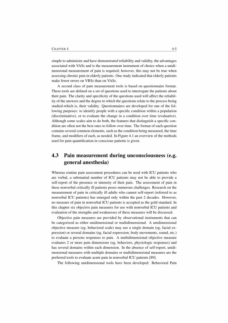
CHAPTER 4 4-5
simple to administer and have demonstrated reliability and validity, the advantagesassociated with VASs and is the measurement instrument of choice when a unidi-mensional measurement of pain is required; however, this may not be true whenassessing chronic pain in elderly patients. One study indicated that elderly patientsmake fewer errors on VRSs than on VASs.
A second class of pain measurement tools is based on questionnaire format.These tools are defined on a set of questions used to interrogate the patients abouttheir pain. The clarity and specificity of the questions used will affect the reliabil-ity of the answers and the degree to which the questions relate to the process beingstudied-which is, their validity. Questionnaires are developed for one of the fol-lowing purposes: to identify people with a specific condition within a population(discriminative), or to evaluate the change in a condition over time (evaluative).Although some scales aim to do both, the features that distinguish a specific con-dition are often not the best ones to follow over time. The format of each questioncontains several common elements, such as the condition being measured, the timeframe, and modifiers of each, as needed. In Figure 4.1 an overview of the methodsused for pain quantification in conscious patients is given.
4.3 Pain measurement during unconsciousness (e.g.general anesthesia)
Whereas routine pain assessment procedures can be used with ICU patients whoare verbal, a substantial number of ICU patients may not be able to provide aself-report of the presence or intensity of their pain. The assessment of pain inthese nonverbal critically ill patients poses numerous challenges. Research on themeasurement of pain in critically ill adults who cannot self-report (referred to asnonverbal ICU patients) has emerged only within the past 2 decades. However,no measure of pain in nonverbal ICU patients is accepted as the gold standard. Inthis chapter six objective pain measures for use with nonverbal ICU patients andevaluation of the strengths and weaknesses of these measures will be discussed.
Objective pain measures are provided by observational instruments that canbe categorized as either unidimensional or multidimensional. A unidimensionalobjective measure (eg, behavioral scale) may use a single domain (eg, facial ex-pression) or several domains (eg, facial expression, body movements, sound, etc.)to evaluate a persons responses to pain. A multidimensional objective measureevaluates 2 or more pain dimensions (eg, behaviors, physiologic responses) andhas several domains within each dimension. In the absence of self-report, unidi-mensional measures with multiple domains or multidimensional measures are thepreferred tools to evaluate acute pain in nonverbal ICU patients [89].
The following unidimensional tools have been developed: Behavioral Pain
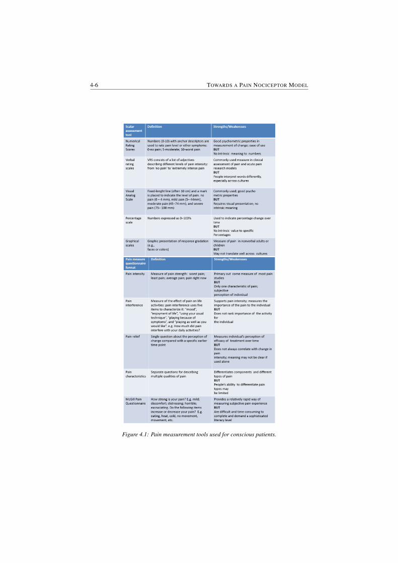
4-6 TOWARDS A PAIN NOCICEPTOR MODEL
Figure 4.1: Pain measurement tools used for conscious patients.
CHAPTER 4 4-7
Rating Scale (BPRS), Behavioral Pain Scale (BPS), Pain Behavior AssessmentTool (PBAT) and Critical-Care Pain Observational Tool (CPOT).
The BPRS is a unidimensional objective measure that assesses 4 behavioraldomains: restlessness, tense muscles, frowning or grimacing, and patient sounds.Each domain contains 3 descriptors that indicate a progressive increase in painseverity and are scored on a scale that ranges from 0 (normal behaviors) to 3 (ex-treme pain behaviors). The total BPRS score (the sum of all domains scores)ranges from 0 (no pain) to 12 (most pain). Although the BPRS appears to pos-sess satisfactory internal consistency, generalization of the BPRS findings [90–92]to nonverbal ICU patients is limited because it was tested in small homogeneoussamples of post-anesthesia care unit (PACU) patients. In fact, patients with majorcomplications and neurological problems were excluded from the studies. More-over, the BPRS requires a patient to vocalize and to show discernible movements,which is limiting its use in a substantial percentage of nonverbal ICU patients whomay be intubated, have an altered level of consciousness (LOC), unconscious pa-tients or who have received neuromuscular blocking agents.
The BPS evaluates 3 behavioral domains (ie, facial expression, movements ofupper limbs, compliance with ventilation). Each domain contains 4 descriptorsthat are rated on a 1 to 4 scale and the total BPS score can range from 3 (no pain)to 12 (most pain). Findings from 3 studies [90, 91, 93] suggest that the BPS is avalid and reliable measure for use in nonverbal ICU patients. However, attentionto a number of factors would improve its clinical utility. First, the range of scoreson the BPS (ie, 3 = no pain to 12 = most pain) should be revised so that a scoreof 0 reflects no pain behavior. Second, on the BPS, the lack of body movementequates with a pain-free state which is not most of the time the case for the ICUward. Moreover, during general anesthesia none of this tools can be used toevaluate pain during surgery for computerized closed loop drug titration.
The PBAT unidimensional assessment tool was developed for a large-scale de-scriptive study of patients pain perceptions and behaviors associated with commonhospital procedures in acute and critical care settings [94]. This tool consists of3 behavioral domains with several descriptors within each domain (ie, facial ex-pressions = 10 descriptors; body movement = 15 descriptors; verbal responses =7 descriptors). The PBAT contains a number of features that enhances its clinicalutility. The assessment procedure is simple (ie, mark the presence of a behavior)and not subject to interpretation. This approach contrasts with conventional ob-jective pain measures that assign scores at the item level and use a sum score toindicate patients level of pain. To increase its applicability for use in nonverbalICU patients, the tool requires modifications to the verbal response domain andthe body movement domain because certain descriptors (eg, moaning, guarding,massaging) are not applicable in nonverbal patients with a decreased LOC. Addi-tional evaluation is needed to confirm responsiveness of the PBAT to other sources
4-8 TOWARDS A PAIN NOCICEPTOR MODEL
of acute pain, as well as to the administration of analgesics.The CPOT is a unidimensional measure designed for use with intubated and
nonintubated ICU patients. It evaluates four behavioral domains (ie, facial expres-sions, movements, muscle tension, ventilator compliance). Each CPOT domain isscored from 0 to 2, and the total score ranges from 0 (no pain) to 8 (most pain) [93].However, the responsiveness of CPOT behaviors to painful stimuli in deeply se-dated patients remains to be determined.
The following multidimensional tools have been developed: Pain Assessmentand Intervention Notation (PAIN) Algorithm and Nonverbal Pain Scale (NVPS).
The PAIN Algorithm is a systematic pain assessment and management tooldeveloped for research testing with critical care nurses. This tool consists of3 parts: pain assessment; assessment of patients ability to tolerate opioids; andguidelines for analgesic treatment decisions and documentation. The pain assess-ment prompts nurses to observe the patient for the presence or absence of 6 be-havioral domains (ie, facial expression, movement, posture, vocal sounds, pallor,perspiration) and 3 physiologic indicators (ie, heart rate (HR), blood pressure (BP),respiration). Then, the tool prompts nurses, based on their appraisal of these di-mensions of pain, to rate the severity of the patients pain on a 0 (no pain) to 10(most pain). The PAIN Algorithm may be a useful tool to standardize pain as-sessment and management in the ICU. However, the length of the tool limits itsclinical utility [93]. Another limitation of this tool is that it does not standardizethe measurements of behavioral and physiologic responses.
The NVPS includes 3 behavioral domains (ie, facial expression, body move-ment, guarding). Additionally, 4 physiologic domains were added based on a re-view of literature and grouped into 2 categories: Changes in vital sign over 4hours and changes in skin color, warmth, and pupil dilation. Each NVPS domainis scored from 0 to 2 and the total score can range from 0 (no pain) to 10 (mostpain). The NVPS has limited content validity and reliability as a pain measure fornonverbal ICU patients. First, certain NVPS behavioral descriptors such as smileor lying in normal position cannot be equated with a nonpainful state. Moreover,measurement of the physiologic indicators (eg, pupil dilation, perspiration) wasnot defined or standardized. In addition, the authors did not describe the rationalefor their selection of vital sign parameters for pain (eg, respiratory rate increasedby >10 breaths/min over 4 hours, SBP increased by >20 mm Hg over 4 hours).
Despite advances in pain research and management, the measurement ofpain in nonverbal ICU patients remains an immense challenge for critical careclinicians. The dilemma of adequate versus inadequate pain management in thesehigh-risk patients is largely attributed to the lack of vigorously tested valid andreliable pain measures. This critical review demonstrates that although 2 objec-tive pain measures (ie, BPS, CPOT) showed validity and reliability, they have notreceived rigorous evaluation to consider them as a robust pain measure for use in
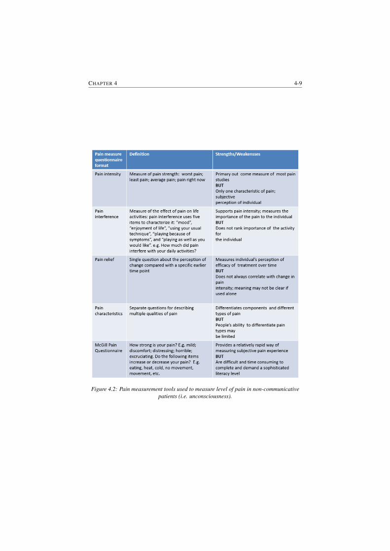
CHAPTER 4 4-9
Figure 4.2: Pain measurement tools used to measure level of pain in non-communicativepatients (i.e. unconsciousness).
4-10 TOWARDS A PAIN NOCICEPTOR MODEL
nonverbal ICU patients. Although the discussed tools are mentioned as an objec-tive way to measure pain, there is much room for improvement due to the factthat these tools are based on several domains and they are still depending on theexperience of the nurse. Therefore, it cannot be claimed that with these tools theactual pain the patient is experiencing is being also the measured pain. In Figure4.2 an overview of the available tools for pain assessment during unconsciousnessis presented.
In conclusion, pain assessment is largely depended on the ability to rate per-sonal subjective pain. Moreover, pain scales can be difficult to use during medicalprocedures. Several techniques have been developed for conscious and uncon-scious patients. For the first category (i.e. consciousness) most optimal tools forpain measurement are the VAS and NRS, but also the other techniques presentedin this review are being used to evaluate pain level. For the second category (i.e.unconsciousness) several devices/tools have been developed in order to evaluatepain level. Even if effort has been made to develop an objective and individualizedpain measurement device for unconscious/non-communicative patients there is nosuch tool is used in clinical practice. The first steps towards the development ofsuch an objective pain assessment tool have been undertaken in this thesis.
4.4 Commercial Devices
In the last fifteen years the research effort on developing a device for objectivemeasurement of pain has increased. As a result, nowadays there are three medicaldevices available on the market for pain assessment. Each of them is designed fora certain category of patients. A description of the available devices along withtheir advantages and disadvantages is given hereafter.
Med-Storm Pain Monitor is designed for infants, children and adults, withmore focus on infants and children. This device is based on the measurement ofskin conductance (SC) to monitor nociceptive stimulation, awareness and pain.Various methods of pain assessment in infants have been trialled in the search forobjective, specific, physiologic measures of responses to pain. SC measured in thepalm of the hand or on the plantar area of the foot may be one such measure. SC inthese sites reflects the emotional sweating due to sympathetic nerve activity. Theskin conductance response (SCR), which results from filling and reabsorption ofsweat in the sweat glands, has previously been suggested to be the most sensitiveSC parameter of sympathetic nerve activity in response to painful stimulation [95].
SC activity is caused by the release of sweat from the sweat glands upon activa-tion of the sympathetic nervous system which in turn acts on muscarinic receptorsin the sweat glands [96]. On cessation of this gland stimulation, fluid is reabsorbedfrom the ducts and the conductance decreases. This can be recorded as a ‘wave’
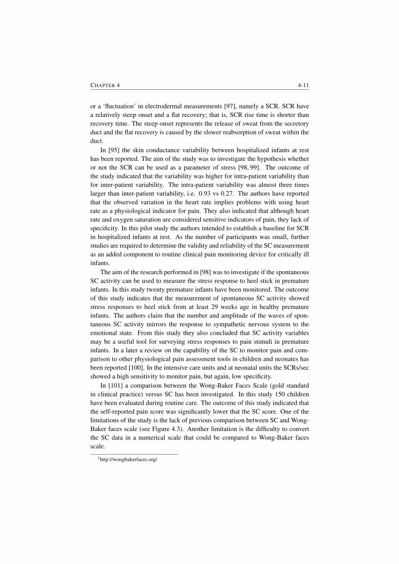
CHAPTER 4 4-11
or a ‘fluctuation’ in electrodermal measurements [97], namely a SCR. SCR havea relatively steep onset and a flat recovery; that is, SCR rise time is shorter thanrecovery time. The steep onset represents the release of sweat from the secretoryduct and the flat recovery is caused by the slower reabsorption of sweat within theduct.
In [95] the skin conductance variability between hospitalized infants at resthas been reported. The aim of the study was to investigate the hypothesis whetheror not the SCR can be used as a parameter of stress [98, 99]. The outcome ofthe study indicated that the variability was higher for intra-patient variability thanfor inter-patient variability. The intra-patient variability was almost three timeslarger than inter-patient variability, i.e. 0.93 vs 0.27. The authors have reportedthat the observed variation in the heart rate implies problems with using heartrate as a physiological indicator for pain. They also indicated that although heartrate and oxygen saturation are considered sensitive indicators of pain, they lack ofspecificity. In this pilot study the authors intended to establish a baseline for SCRin hospitalized infants at rest. As the number of participants was small, furtherstudies are required to determine the validity and reliability of the SC measurementas an added component to routine clinical pain monitoring device for critically illinfants.
The aim of the research performed in [98] was to investigate if the spontaneousSC activity can be used to measure the stress response to heel stick in prematureinfants. In this study twenty premature infants have been monitored. The outcomeof this study indicates that the measurement of spontaneous SC activity showedstress responses to heel stick from at least 29 weeks age in healthy prematureinfants. The authors claim that the number and amplitude of the waves of spon-taneous SC activity mirrors the response to sympathetic nervous system to theemotional state. From this study they also concluded that SC activity variablesmay be a useful tool for surveying stress responses to pain stimuli in prematureinfants. In a later a review on the capability of the SC to monitor pain and com-parison to other physiological pain assessment tools in children and neonates hasbeen reported [100]. In the intensive care units and at neonatal units the SCRs/secshowed a high sensitivity to monitor pain, but again, low specificity.
In [101] a comparison between the Wong-Baker Faces Scale (gold standardin clinical practice) versus SC has been investigated. In this study 150 childrenhave been evaluated during routine care. The outcome of this study indicated thatthe self-reported pain score was significantly lower that the SC score. One of thelimitations of the study is the lack of previous comparison between SC and Wong-Baker faces scale (see Figure 4.3). Another limitation is the difficulty to convertthe SC data in a numerical scale that could be compared to Wong-Baker facesscale.
1http://wongbakerfaces.org/
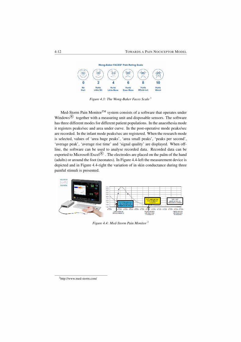
4-12 TOWARDS A PAIN NOCICEPTOR MODEL
Figure 4.3: The Wong-Baker Faces Scale 1
Med-Storm Pain MonitorTM system consists of a software that operates underWindows R© together with a measuring unit and disposable sensors. The softwarehas three different modes for different patient populations. In the anaesthesia modeit registers peaks/sec and area under curve. In the post-operative mode peaks/secare recorded. In the infant mode peaks/sec are registered. When the research modeis selected, values of ‘area huge peaks’, ‘area small peaks’, ‘peaks per second’,‘average peak’, ‘average rise time’ and ‘signal quality’ are displayed. When off-line, the software can be used to analyse recorded data. Recorded data can beexported to Microsoft Excel R© . The electrodes are placed on the palm of the hand(adults) or around the foot (neonates). In Figure 4.4-left the measurement device isdepicted and in Figure 4.4-right the variation of in skin conductance during threepainful stimuli is presented.
Figure 4.4: Med-Storm Pain Monitor 2
2http://www.med-storm.com/
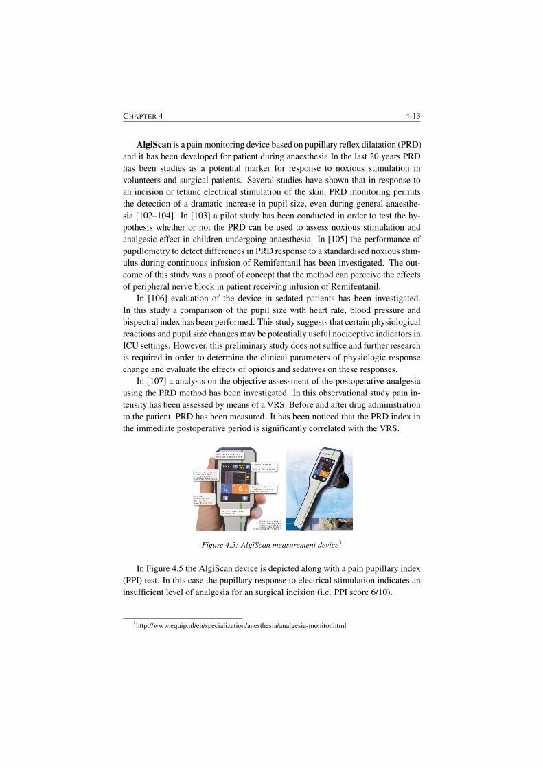
CHAPTER 4 4-13
AlgiScan is a pain monitoring device based on pupillary reflex dilatation (PRD)and it has been developed for patient during anaesthesia In the last 20 years PRDhas been studies as a potential marker for response to noxious stimulation involunteers and surgical patients. Several studies have shown that in response toan incision or tetanic electrical stimulation of the skin, PRD monitoring permitsthe detection of a dramatic increase in pupil size, even during general anaesthe-sia [102–104]. In [103] a pilot study has been conducted in order to test the hy-pothesis whether or not the PRD can be used to assess noxious stimulation andanalgesic effect in children undergoing anaesthesia. In [105] the performance ofpupillometry to detect differences in PRD response to a standardised noxious stim-ulus during continuous infusion of Remifentanil has been investigated. The out-come of this study was a proof of concept that the method can perceive the effectsof peripheral nerve block in patient receiving infusion of Remifentanil.
In [106] evaluation of the device in sedated patients has been investigated.In this study a comparison of the pupil size with heart rate, blood pressure andbispectral index has been performed. This study suggests that certain physiologicalreactions and pupil size changes may be potentially useful nociceptive indicators inICU settings. However, this preliminary study does not suffice and further researchis required in order to determine the clinical parameters of physiologic responsechange and evaluate the effects of opioids and sedatives on these responses.
In [107] a analysis on the objective assessment of the postoperative analgesiausing the PRD method has been investigated. In this observational study pain in-tensity has been assessed by means of a VRS. Before and after drug administrationto the patient, PRD has been measured. It has been noticed that the PRD index inthe immediate postoperative period is significantly correlated with the VRS.
Figure 4.5: AlgiScan measurement device3
In Figure 4.5 the AlgiScan device is depicted along with a pain pupillary index(PPI) test. In this case the pupillary response to electrical stimulation indicates aninsufficient level of analgesia for an surgical incision (i.e. PPI score 6/10).
3http://www.equip.nl/en/specialization/anesthesia/analgesia-monitor.html
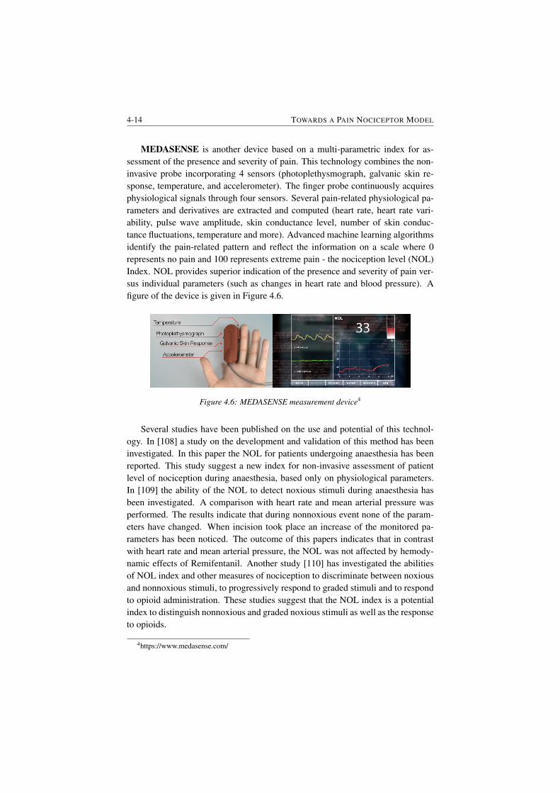
4-14 TOWARDS A PAIN NOCICEPTOR MODEL
MEDASENSE is another device based on a multi-parametric index for as-sessment of the presence and severity of pain. This technology combines the non-invasive probe incorporating 4 sensors (photoplethysmograph, galvanic skin re-sponse, temperature, and accelerometer). The finger probe continuously acquiresphysiological signals through four sensors. Several pain-related physiological pa-rameters and derivatives are extracted and computed (heart rate, heart rate vari-ability, pulse wave amplitude, skin conductance level, number of skin conduc-tance fluctuations, temperature and more). Advanced machine learning algorithmsidentify the pain-related pattern and reflect the information on a scale where 0represents no pain and 100 represents extreme pain - the nociception level (NOL)Index. NOL provides superior indication of the presence and severity of pain ver-sus individual parameters (such as changes in heart rate and blood pressure). Afigure of the device is given in Figure 4.6.
Figure 4.6: MEDASENSE measurement device4
Several studies have been published on the use and potential of this technol-ogy. In [108] a study on the development and validation of this method has beeninvestigated. In this paper the NOL for patients undergoing anaesthesia has beenreported. This study suggest a new index for non-invasive assessment of patientlevel of nociception during anaesthesia, based only on physiological parameters.In [109] the ability of the NOL to detect noxious stimuli during anaesthesia hasbeen investigated. A comparison with heart rate and mean arterial pressure wasperformed. The results indicate that during nonnoxious event none of the param-eters have changed. When incision took place an increase of the monitored pa-rameters has been noticed. The outcome of this papers indicates that in contrastwith heart rate and mean arterial pressure, the NOL was not affected by hemody-namic effects of Remifentanil. Another study [110] has investigated the abilitiesof NOL index and other measures of nociception to discriminate between noxiousand nonnoxious stimuli, to progressively respond to graded stimuli and to respondto opioid administration. These studies suggest that the NOL index is a potentialindex to distinguish nonnoxious and graded noxious stimuli as well as the responseto opioids.
4https://www.medasense.com/
CHAPTER 4 4-15
The devices presented in this chapter have been evaluated mostly on sedatedpatients. Therefore, there is still much room for improvement. Although, clini-cally needed and theoretically promising, currently there is not enough evidence(i.e. clinical trials) to support the widespread use of any physiological sensors as”objective” measures of pain. Another drawback is that none of these devices arebased on mathematical interpretations/descriptions/models of pain.
4.5 SummaryIn this chapter a detailed overview of the existing methods and devices availablefor pain assessment has been given. From here, one may conclude that the exist-ing methods are subjective (i.e. based on patient feedback). With respects to theavailable devices two main conclusions can be drawn: 1) these devices are not yetemployed in clinical settings as standard tools for pain assessment. This is dueto the lack of large clinical trials but also, because each of them is for a certainclass of patients. 2) none of them is based on a mathematically-physiologicallybased model. The challenges identified in this chapter are further exploited in theremaining of this thesis.

5Pharmacokinetics-Pharmacodynamics
Models of Drug Uptake and DrugEffect
In this chapter drug diffusion in the human body by means of compartmental mod-els is presented. Fractional calculus tools are employed to characterize the profilesof drug concentration in each compartment.
The main publications where this work has been presented are:
• D. Copot, R. Magin, R. De Keyser, C. Ionescu, Data-driven modelling ofdrug tissue trapping using anomalous kinetics, Chaos, Solitons and Fractals,102, 441-446, 2017.
• D. Copot, A. Chevalier, C.M. Ionescu, R. De Keyser. A Two-CompartmentFractional Derivative Model for Propofol Diffusion in Anesthesia, IEEEMulti-Conference on Systems and Control, Hyderabad, India, 28-30 Au-gust, 264-269, 2013.
• C.M. Ionescu, D. Copot, On the use of fractional order PK-PD models,European Workshop on Advanced Control and Diagnosis, Lille, France, 17-18 July, 1-12, 2017.
5-2 PK-PD MODELS OF DRUG UPTAKE AND DRUG EFFECT
5.1 Introduction
Selecting appropriate models is a crucial step in capturing complex biological andphysiological phenomena. Any choice of a model structure implies a simplifiedview of the interaction among the various elements that may characterise a dy-namical system. In pharmacokinetics, a popular choice is that of compartmentalmodels, due to their implicit simplicity and ease of understanding in relation to themass balance equations and assumptions for uniform distribution, homogeneoustransient times and immediate response to drug bolus administration [111]. Nu-merous works and decades of research have tailored their applicability for optimaldrug delivery assist devices in several domains of medical applications, e.g. di-abetes [112], cancer [113, 114], anaesthesia [115], immunodeficiency [116] andhormonal treatment [117].
Providing a best fit to data from observed drug concentration profiles impliesthe existence of some error tolerance intervals. Emerging tools from fractional cal-culus have proven useful to improve to a great degree the accuracy of dynamicalmodels with respect to classical integer order modelling theory [118, 119]. Theacceptance of these tools within the engineering community has led perhaps to asignificant step forward in terms of data driven modelling and numerical simula-tion [120, 121]. However, their acceptance in clinical practice may require furthertailoring for a better characterization of patient variability [122–124].
Compartmental models are a traditional tool for modelling drug pharmacoki-netics (PK) in applications of general anaesthesia. The depth of anaesthesia regu-latory problem consists of optimal calculation via such patient PK models of theamount of drug necessary to achieve a desired sedation level, irrespective of arte-facts and disturbances [125]. Attempts to fractionalise PK compartmental modelsfor anaesthesia have been done with simulated data. A net advantage however hasnot been shown, since secondary effects due to drug trapping were not accountedfor at that time [126, 127].
Pharmacokinetic model gives information about the concentration profile ofa drug as a function of time, in the body fluid (i.e. blood) as a result of a doseadministration (e.g. bolus injection). Compartmental models seems to be widelyused, while they provide a continuous description of the concentration that canserve as a input function for the pharmacodynamic part. In general, the pathwayof a drug through the body can be separated into three distinct phases: uptake,distribution, and elimination.
Uptake: Different routes of administration produce variability in the rate ofdrug uptake and amount of drug delivered effectively to the body. Intravenousadministration of a drug results in the entire dose entering the plasma immediately,although it must pass initially through the pulmonary circulation and some drugs(e.g. fentanyl) have significant take-up by the lungs [128].
CHAPTER 5 5-3
Distribution: After intravenous administration of a drug, the peak blood con-centration is determined by the dose, the rate of administration, and the cardiacoutput. With a high cardiac output, the effective volume of blood in which thedrug is initially diluted is larger, leading to a lower peak concentration. A highcardiac output transports the drug fast to the vessel-rich tissues (including brain),and for highly lipid-soluble drugs, fast equilibration takes place, leading to a fastonset of action. Therefore, a low cardiac output leads to a higher initial peakconcentration, because the drug is mixed with a smaller volume of blood duringinjection, though it will take longer to reach its target site [128]. All the aspectsmentioned above explains why a smaller dose of induction agent is required in anelderly or shocked patient but may have a slower onset of action, while a youngpatient may require a much larger dose, but they will start to feel the effects morequickly.
Elimination: Full recovery depends on the removal of the drug from the body.Such elimination may result from excretion, metabolism, or a combination of ofthe two drugs. Large molecular weight drugs are often excreted in the bile, butmost drugs are renally excreted. In order for the kidneys to handle lipid-solubledrugs, they need to be metabolized into a polar, water-soluble form. Most of thismetabolism occurs in the liver and can be divided into two phases reactions. Phaseone is the reaction which consist in oxidation, reduction, and hydrolysis, whilein the second phase reaction consist in conjugating the resulting metabolites withsulphate, glucuronide, or other groups. For most drugs, elimination occurs in anexponentially declining manner, the rate of elimination being proportional to theplasma concentration, as the downstream end of the gradient remains at zero [128].This system (i.e. the amount of drug being removed is a constant fraction in unittime rather than a constant amount) is known as first-order kinetics. The phar-macokinetic model represented in Figure 5.1 is represented traditionally by thefollowing equations (5.1)-(5.4).
From the point-of-view of regulating anesthesia, mathematical modeling ofdrug diffusion can be very useful to better understand the mechanism of drug de-livery systems. Therefore, the description of drug transport into the human bodycan be highly beneficial [18–20] from two points-of-view: (i) allows one to under-stand the insight of the mechanism and (ii) allows one to do quantitative predic-tion of the effects of formulation and processing parameters on the resulting drugrelease kinetics. The major challenge in the development or optimization of auto-mated drug delivery systems is to achieve optimal drug concentration at the site ofaction. In order to have the optimal concentration-time-profile at the site of actionthe release of the drug must be controlled as accurately as possible.
Pharmacokinetic/pharmacodynamics (PK/PD) models represents an importantstep in the process of drug development and this modeling tool also brought asignificant contribution to anesthesia. PK/PD models are a set of mathematical
5-4 PK-PD MODELS OF DRUG UPTAKE AND DRUG EFFECT
equations used to predict the drug effect in time. PK models describe what thebody does to the drug in terms of ADME parameters (i.e. Absorption, Distribu-tion, Metabolism and Elimination). PK modeling for analgesic, opioid and mus-cle relaxants drugs has been studied by several authors. In its classical version,compartmental analysis is based on mathematical models, typically in the formof systems of ordinary differential equations (see equations (5.1)-(5.4)) that arewidely used to characterize the uptake, distribution and elimination of a drug intothe body.
q1(t) = K21q2(t) +K31q3(t)−K12q1(t)−K13q1(t)−K10q1(t)−K1eq1(t) + U(t)
(5.1)
q2(t) = K12q1(t)−K21q2(t)−K20q2(t) (5.2)
q3(t) = K13q1(t)−K31q3(t)−K30q3(t) (5.3)
qe(t) = K1eq1(t)−K0eqe(t) (5.4)
where: q1, q2 and q3 [mg] denotes the amount of drug in the three compartmentsand V1, V2 and V3 represents the volume in the three compartments. The drugconcentration in the blood is expressed by q1/V1, respectively q2/V2 and q3/V3for compartment 2 and 3. The peripheral compartments 2 (muscle) and 3 (fat)represents the drug exchange of the blood with well and poorly diffused bodytissues. The parameters Kij denote the drug transfer frequency from the i− th tothe j − th compartment and U(t) [mg/s] is the infusion rate of the drug into thefirst compartment. The parameters Kij of the PK models depend on age, weight,height and gender and can be calculated for Propofol as follows: V3 represents thevolume of fat and is calculated using equation (5.5), while V1 and V2 are known(V1=4.27 (L) and V3=2.38 (L)).
V2 = 18.9− 0.391(age− 53) (5.5)
Clearance is calculated as follows:
Cl1 = 1.89 + 0.456(weight− 77)− 0.0681(lbm− 59) + 0.0264(height− 177)(5.6)
Cl2 = 1.29 + 0.024(age− 53) (5.7)
and Cl3 = 0.836 (l/min). where Cl1 is the rate at which the drug is cleared fromthe body, and Cl2 and Cl3 are the rates at which the drug is removed from thecentral compartment to the other two compartments by distribution.
The lean body mass (lbm) for men and women has the following expressions:
bmman = 1.1 ∗ weight− 128weight2
height2
lbmwomen = 1.07 ∗ weight− 148weight2
height2(5.8)
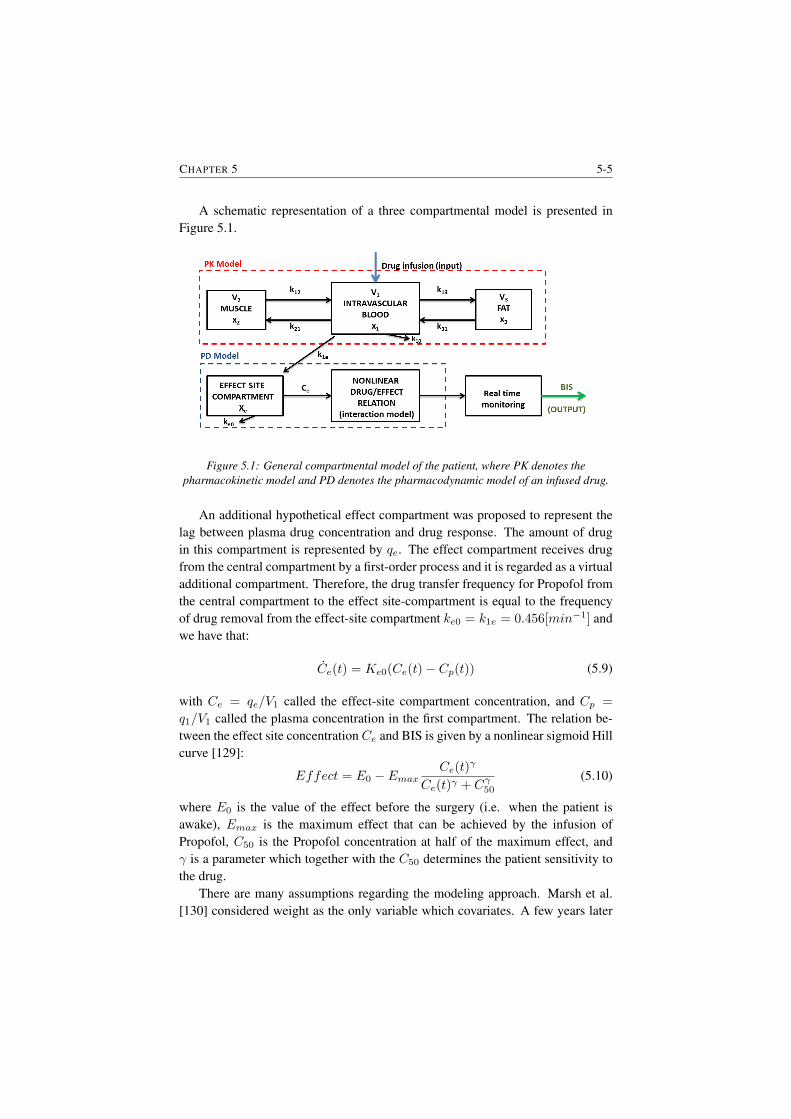
CHAPTER 5 5-5
A schematic representation of a three compartmental model is presented inFigure 5.1.
Figure 5.1: General compartmental model of the patient, where PK denotes thepharmacokinetic model and PD denotes the pharmacodynamic model of an infused drug.
An additional hypothetical effect compartment was proposed to represent thelag between plasma drug concentration and drug response. The amount of drugin this compartment is represented by qe. The effect compartment receives drugfrom the central compartment by a first-order process and it is regarded as a virtualadditional compartment. Therefore, the drug transfer frequency for Propofol fromthe central compartment to the effect site-compartment is equal to the frequencyof drug removal from the effect-site compartment ke0 = k1e = 0.456[min−1] andwe have that:
Ce(t) = Ke0(Ce(t)− Cp(t)) (5.9)
with Ce = qe/V1 called the effect-site compartment concentration, and Cp =
q1/V1 called the plasma concentration in the first compartment. The relation be-tween the effect site concentration Ce and BIS is given by a nonlinear sigmoid Hillcurve [129]:
Effect = E0 − EmaxCe(t)
γ
Ce(t)γ + Cγ50(5.10)
where E0 is the value of the effect before the surgery (i.e. when the patient isawake), Emax is the maximum effect that can be achieved by the infusion ofPropofol, C50 is the Propofol concentration at half of the maximum effect, andγ is a parameter which together with the C50 determines the patient sensitivity tothe drug.
There are many assumptions regarding the modeling approach. Marsh et al.[130] considered weight as the only variable which covariates. A few years later
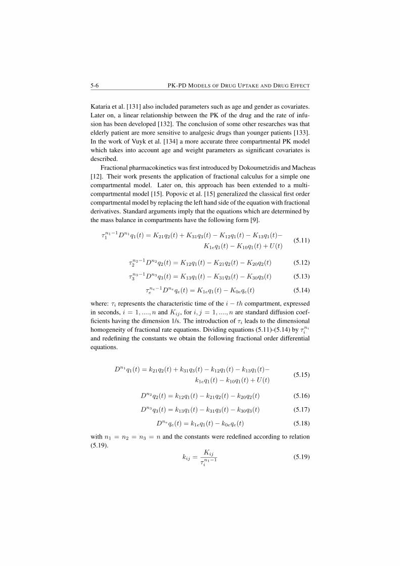
5-6 PK-PD MODELS OF DRUG UPTAKE AND DRUG EFFECT
Kataria et al. [131] also included parameters such as age and gender as covariates.Later on, a linear relationship between the PK of the drug and the rate of infu-sion has been developed [132]. The conclusion of some other researches was thatelderly patient are more sensitive to analgesic drugs than younger patients [133].In the work of Vuyk et al. [134] a more accurate three compartmental PK modelwhich takes into account age and weight parameters as significant covariates isdescribed.
Fractional pharmacokinetics was first introduced by Dokoumetzidis and Macheas[12]. Their work presents the application of fractional calculus for a simple onecompartmental model. Later on, this approach has been extended to a multi-compartmental model [15]. Popovic et al. [15] generalized the classical first ordercompartmental model by replacing the left hand side of the equation with fractionalderivatives. Standard arguments imply that the equations which are determined bythe mass balance in compartments have the following form [9].
τn1−11 Dn1q1(t) = K21q2(t) +K31q3(t)−K12q1(t)−K13q1(t)−
K1eq1(t)−K10q1(t) + U(t)(5.11)
τn2−12 Dn2q2(t) = K12q1(t)−K21q2(t)−K20q2(t) (5.12)
τn3−13 Dn3q3(t) = K13q1(t)−K31q3(t)−K30q3(t) (5.13)
τne−1e Dneqe(t) = K1eq1(t)−K0eqe(t) (5.14)
where: τi represents the characteristic time of the i − th compartment, expressedin seconds, i = 1, ...., n and Kij , for i, j = 1, ...., n are standard diffusion coef-ficients having the dimension 1/s. The introduction of τi leads to the dimensionalhomogeneity of fractional rate equations. Dividing equations (5.11)-(5.14) by τniiand redefining the constants we obtain the following fractional order differentialequations.
Dn1q1(t) = k21q2(t) + k31q3(t)− k12q1(t)− k13q1(t)−k1eq1(t)− k10q1(t) + U(t)
(5.15)
Dn2q2(t) = k12q1(t)− k21q2(t)− k20q2(t) (5.16)
Dn3q3(t) = k13q1(t)− k31q3(t)− k30q3(t) (5.17)
Dneqe(t) = k1eq1(t)− k0eqe(t) (5.18)
with n1 = n2 = n3 = n and the constants were redefined according to relation(5.19).
kij =Kij
τn1−1i
(5.19)
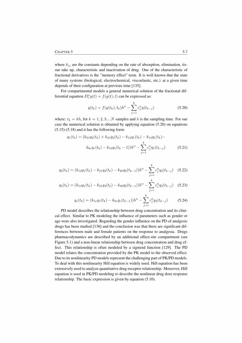
CHAPTER 5 5-7
where kij are the constants depending on the rate of absorption, elimination, tis-sue take up, characteristic and inactivation of drug. One of the characteristic offractional derivatives is the ”memory effect” term. It is well known that the stateof many systems (biological, electrochemical, viscoelastic, etc.) at a given timedepends of their configuration at previous time [135].
For compartmental models a general numerical solution of the fractional dif-ferential equation Dn
t y(t) = f(y(t), t) can be expressed as:
y(tk) = f(y(tk), tk)hn −k∑j=1
cnj y(tk−j) (5.20)
where: tk = kh, for k = 1, 2, 3....N samples and h is the sampling time. For ourcase the numerical solution is obtained by applying equation (5.20) on equations(5.15)-(5.18) and it has the following form:
q1(tk) = (k21q2(tk) + k31q3(tk)− k12q1(tk)− k13q1(tk)−
k0eqe(tk)− k10q1(tk − 1))hn −k∑j=1
cnj q1(tk−j) (5.21)
q2(tk) = (k12q1(tk)− k21q2(tk)− k20q2(tk−1))hn −k∑j=i
cnj q2(tk−j) (5.22)
q3(tk) = (k13q1(tk)− k31q3(tk)− k30q3(tk−1))hn −k∑j=i
cnj q3(tk−j) (5.23)
qe(tk) = (k1eq1(tk)− k0eqe(tk−1))hn −k∑j=i
cnj q3(tk−j) (5.24)
PD model describes the relationship between drug concentration and its clini-cal effect. Similar to PK modeling the influence of parameters such as gender orage were also investigated. Regarding the gender influence on the PD of analgesicdrugs has been studied [136] and the conclusion was that there are significant dif-ferences between male and female patients on the response to analgesia. Drugspharmacodynamics are described by an additional effect-site compartment (seeFigure 5.1) and a non-linear relationship between drug concentration and drug ef-fect. This relationship is often modeled by a sigmoid function [129]. The PDmodel relates the concentration provided by the PK model to the observed effect.Due to its nonlinearity PD models represent the challenging part of PK/PD models.To deal with this nonlinearity Hill equation is widely used. Hill equation has beenextensively used to analyze quantitative drug-receptor relationship. Moreover, Hillequation is used in PK/PD modeling to describe the nonlinear drug dose responserelationship. The basic expression is given by equation (5.10).
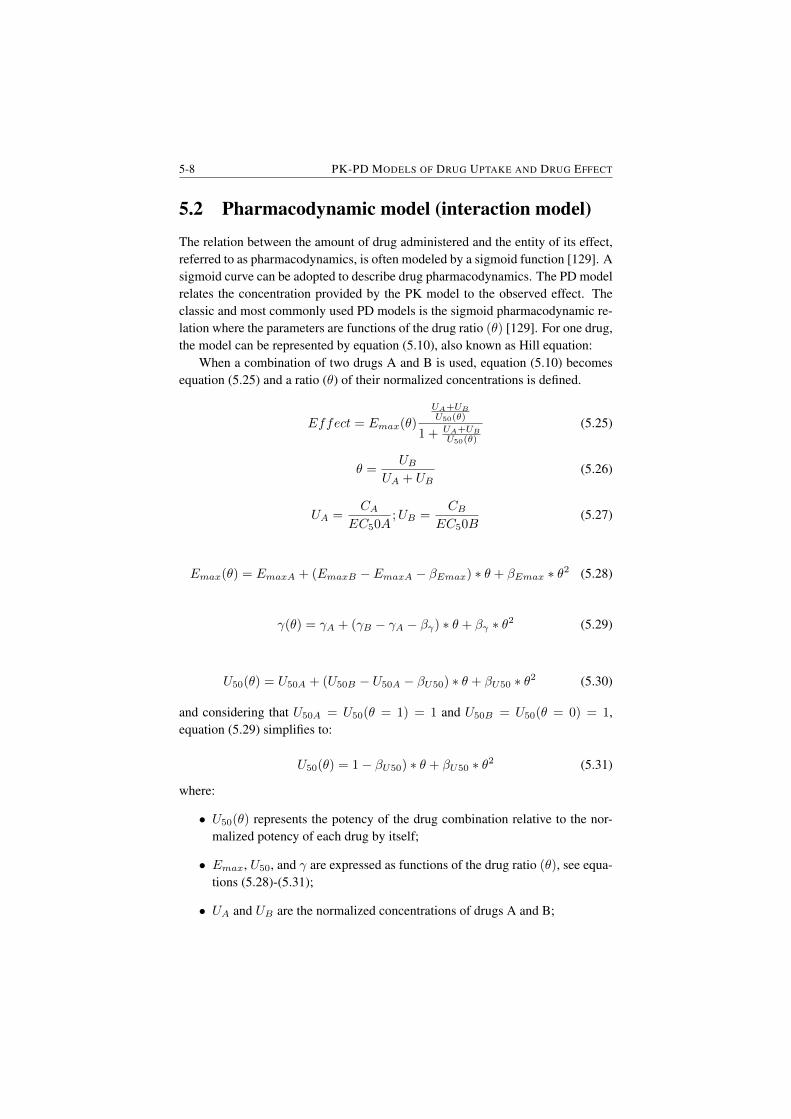
5-8 PK-PD MODELS OF DRUG UPTAKE AND DRUG EFFECT
5.2 Pharmacodynamic model (interaction model)
The relation between the amount of drug administered and the entity of its effect,referred to as pharmacodynamics, is often modeled by a sigmoid function [129]. Asigmoid curve can be adopted to describe drug pharmacodynamics. The PD modelrelates the concentration provided by the PK model to the observed effect. Theclassic and most commonly used PD models is the sigmoid pharmacodynamic re-lation where the parameters are functions of the drug ratio (θ) [129]. For one drug,the model can be represented by equation (5.10), also known as Hill equation:
When a combination of two drugs A and B is used, equation (5.10) becomesequation (5.25) and a ratio (θ) of their normalized concentrations is defined.
Effect = Emax(θ)
UA+UBU50(θ)
1 + UA+UBU50(θ)
(5.25)
θ =UB
UA + UB(5.26)
UA =CA
EC50A;UB =
CBEC50B
(5.27)
Emax(θ) = EmaxA + (EmaxB − EmaxA − βEmax) ∗ θ + βEmax ∗ θ2 (5.28)
γ(θ) = γA + (γB − γA − βγ) ∗ θ + βγ ∗ θ2 (5.29)
U50(θ) = U50A + (U50B − U50A − βU50) ∗ θ + βU50 ∗ θ2 (5.30)
and considering that U50A = U50(θ = 1) = 1 and U50B = U50(θ = 0) = 1,equation (5.29) simplifies to:
U50(θ) = 1− βU50) ∗ θ + βU50 ∗ θ2 (5.31)
where:
• U50(θ) represents the potency of the drug combination relative to the nor-malized potency of each drug by itself;
• Emax, U50, and γ are expressed as functions of the drug ratio (θ), see equa-tions (5.28)-(5.31);
• UA and UB are the normalized concentrations of drugs A and B;
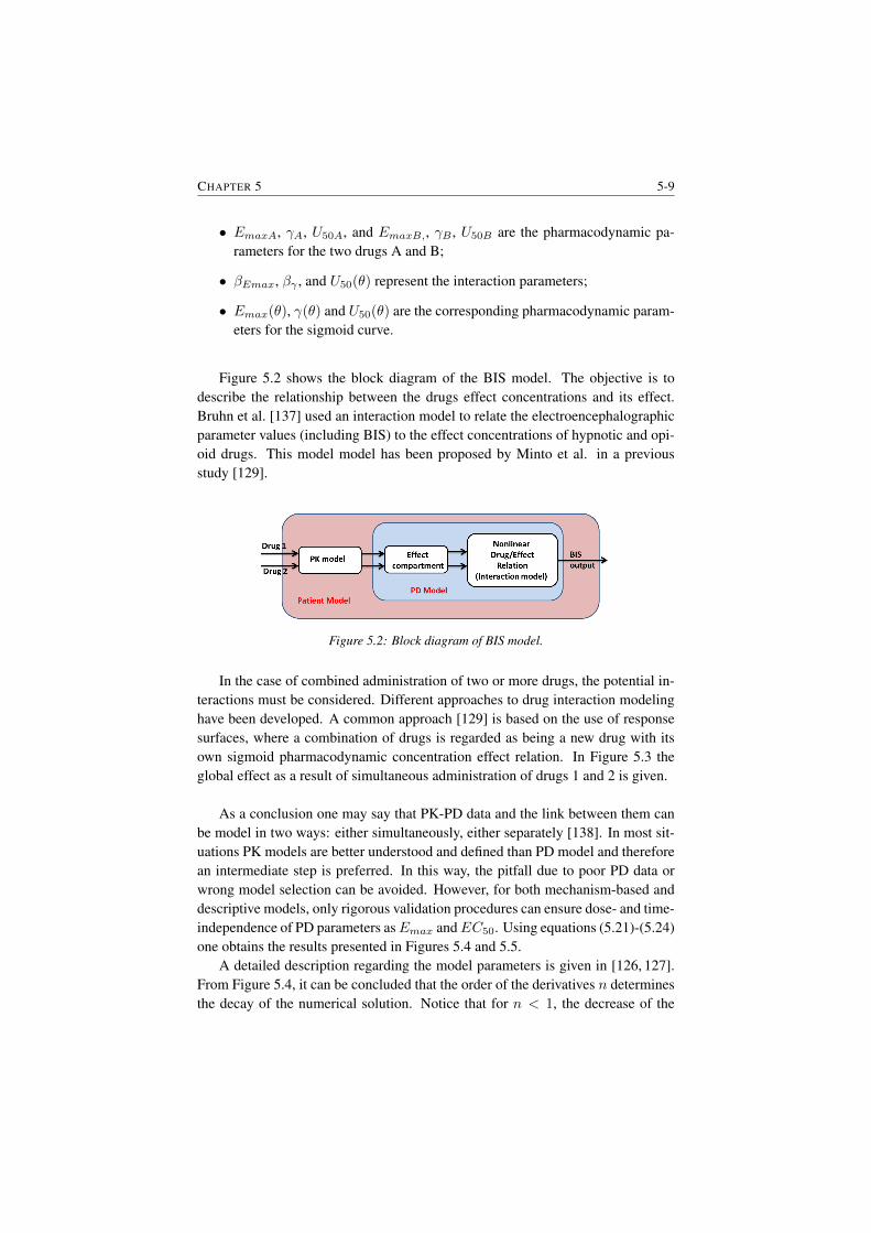
CHAPTER 5 5-9
• EmaxA, γA, U50A, and EmaxB,, γB , U50B are the pharmacodynamic pa-rameters for the two drugs A and B;
• βEmax, βγ , and U50(θ) represent the interaction parameters;
• Emax(θ), γ(θ) and U50(θ) are the corresponding pharmacodynamic param-eters for the sigmoid curve.
Figure 5.2 shows the block diagram of the BIS model. The objective is todescribe the relationship between the drugs effect concentrations and its effect.Bruhn et al. [137] used an interaction model to relate the electroencephalographicparameter values (including BIS) to the effect concentrations of hypnotic and opi-oid drugs. This model model has been proposed by Minto et al. in a previousstudy [129].
Figure 5.2: Block diagram of BIS model.
In the case of combined administration of two or more drugs, the potential in-teractions must be considered. Different approaches to drug interaction modelinghave been developed. A common approach [129] is based on the use of responsesurfaces, where a combination of drugs is regarded as being a new drug with itsown sigmoid pharmacodynamic concentration effect relation. In Figure 5.3 theglobal effect as a result of simultaneous administration of drugs 1 and 2 is given.
As a conclusion one may say that PK-PD data and the link between them canbe model in two ways: either simultaneously, either separately [138]. In most sit-uations PK models are better understood and defined than PD model and thereforean intermediate step is preferred. In this way, the pitfall due to poor PD data orwrong model selection can be avoided. However, for both mechanism-based anddescriptive models, only rigorous validation procedures can ensure dose- and time-independence of PD parameters asEmax andEC50. Using equations (5.21)-(5.24)one obtains the results presented in Figures 5.4 and 5.5.
A detailed description regarding the model parameters is given in [126, 127].From Figure 5.4, it can be concluded that the order of the derivatives n determinesthe decay of the numerical solution. Notice that for n < 1, the decrease of the
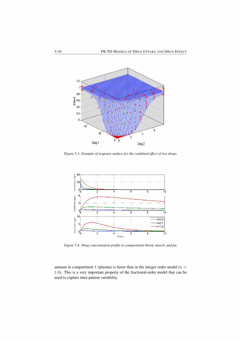
5-10 PK-PD MODELS OF DRUG UPTAKE AND DRUG EFFECT
Figure 5.3: Example of response surface for the combined effect of two drugs.
Figure 5.4: Drug concentration profile in compartment blood, muscle and fat.
amount in compartment 1 (plasma) is faster than in the integer order model (n =
1.0). This is a very important property of the fractional-order model that can beused to capture inter-patient variability.
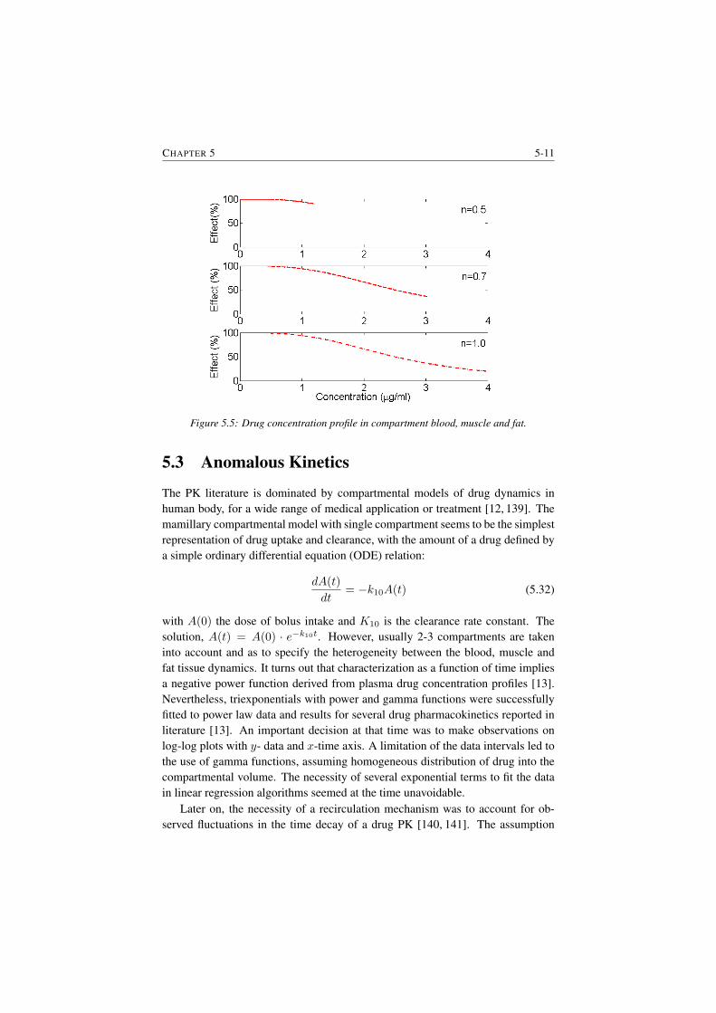
CHAPTER 5 5-11
Figure 5.5: Drug concentration profile in compartment blood, muscle and fat.
5.3 Anomalous Kinetics
The PK literature is dominated by compartmental models of drug dynamics inhuman body, for a wide range of medical application or treatment [12, 139]. Themamillary compartmental model with single compartment seems to be the simplestrepresentation of drug uptake and clearance, with the amount of a drug defined bya simple ordinary differential equation (ODE) relation:
dA(t)
dt= −k10A(t) (5.32)
with A(0) the dose of bolus intake and K10 is the clearance rate constant. Thesolution, A(t) = A(0) · e−k10t. However, usually 2-3 compartments are takeninto account and as to specify the heterogeneity between the blood, muscle andfat tissue dynamics. It turns out that characterization as a function of time impliesa negative power function derived from plasma drug concentration profiles [13].Nevertheless, triexponentials with power and gamma functions were successfullyfitted to power law data and results for several drug pharmacokinetics reported inliterature [13]. An important decision at that time was to make observations onlog-log plots with y- data and x-time axis. A limitation of the data intervals led tothe use of gamma functions, assuming homogeneous distribution of drug into thecompartmental volume. The necessity of several exponential terms to fit the datain linear regression algorithms seemed at the time unavoidable.
Later on, the necessity of a recirculation mechanism was to account for ob-served fluctuations in the time decay of a drug PK [140, 141]. The assumption
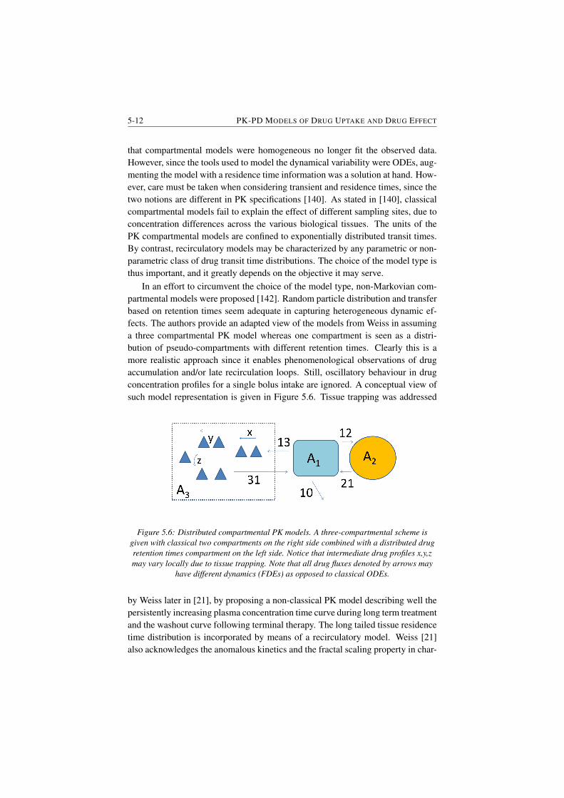
5-12 PK-PD MODELS OF DRUG UPTAKE AND DRUG EFFECT
that compartmental models were homogeneous no longer fit the observed data.However, since the tools used to model the dynamical variability were ODEs, aug-menting the model with a residence time information was a solution at hand. How-ever, care must be taken when considering transient and residence times, since thetwo notions are different in PK specifications [140]. As stated in [140], classicalcompartmental models fail to explain the effect of different sampling sites, due toconcentration differences across the various biological tissues. The units of thePK compartmental models are confined to exponentially distributed transit times.By contrast, recirculatory models may be characterized by any parametric or non-parametric class of drug transit time distributions. The choice of the model type isthus important, and it greatly depends on the objective it may serve.
In an effort to circumvent the choice of the model type, non-Markovian com-partmental models were proposed [142]. Random particle distribution and transferbased on retention times seem adequate in capturing heterogeneous dynamic ef-fects. The authors provide an adapted view of the models from Weiss in assuminga three compartmental PK model whereas one compartment is seen as a distri-bution of pseudo-compartments with different retention times. Clearly this is amore realistic approach since it enables phenomenological observations of drugaccumulation and/or late recirculation loops. Still, oscillatory behaviour in drugconcentration profiles for a single bolus intake are ignored. A conceptual view ofsuch model representation is given in Figure 5.6. Tissue trapping was addressed
Figure 5.6: Distributed compartmental PK models. A three-compartmental scheme isgiven with classical two compartments on the right side combined with a distributed drugretention times compartment on the left side. Notice that intermediate drug profiles x,y,zmay vary locally due to tissue trapping. Note that all drug fluxes denoted by arrows may
have different dynamics (FDEs) as opposed to classical ODEs.
by Weiss later in [21], by proposing a non-classical PK model describing well thepersistently increasing plasma concentration time curve during long term treatmentand the washout curve following terminal therapy. The long tailed tissue residencetime distribution is incorporated by means of a recirculatory model. Weiss [21]also acknowledges the anomalous kinetics and the fractal scaling property in char-
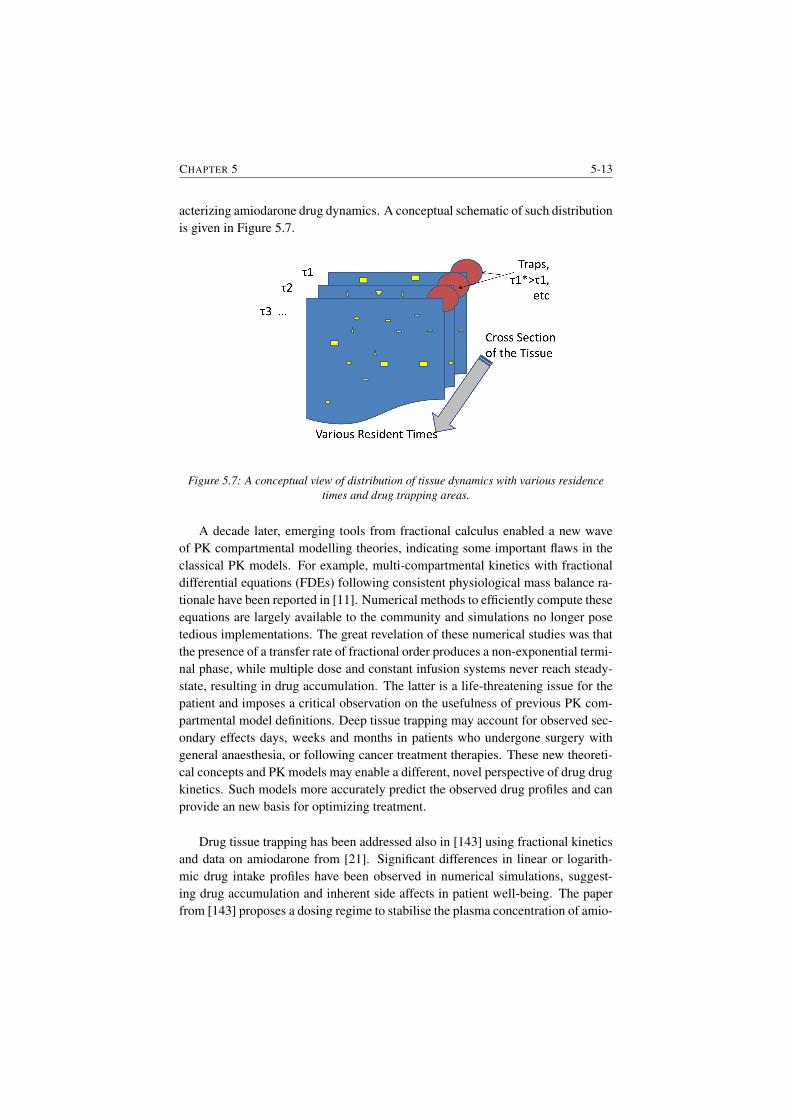
CHAPTER 5 5-13
acterizing amiodarone drug dynamics. A conceptual schematic of such distributionis given in Figure 5.7.
Figure 5.7: A conceptual view of distribution of tissue dynamics with various residencetimes and drug trapping areas.
A decade later, emerging tools from fractional calculus enabled a new waveof PK compartmental modelling theories, indicating some important flaws in theclassical PK models. For example, multi-compartmental kinetics with fractionaldifferential equations (FDEs) following consistent physiological mass balance ra-tionale have been reported in [11]. Numerical methods to efficiently compute theseequations are largely available to the community and simulations no longer posetedious implementations. The great revelation of these numerical studies was thatthe presence of a transfer rate of fractional order produces a non-exponential termi-nal phase, while multiple dose and constant infusion systems never reach steady-state, resulting in drug accumulation. The latter is a life-threatening issue for thepatient and imposes a critical observation on the usefulness of previous PK com-partmental model definitions. Deep tissue trapping may account for observed sec-ondary effects days, weeks and months in patients who undergone surgery withgeneral anaesthesia, or following cancer treatment therapies. These new theoreti-cal concepts and PK models may enable a different, novel perspective of drug drugkinetics. Such models more accurately predict the observed drug profiles and canprovide an new basis for optimizing treatment.
Drug tissue trapping has been addressed also in [143] using fractional kineticsand data on amiodarone from [21]. Significant differences in linear or logarith-mic drug intake profiles have been observed in numerical simulations, suggest-ing drug accumulation and inherent side affects in patient well-being. The paperfrom [143] proposes a dosing regime to stabilise the plasma concentration of amio-
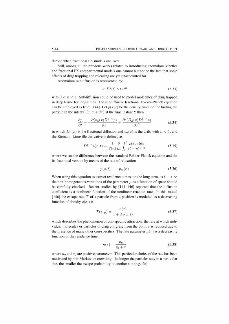
5-14 PK-PD MODELS OF DRUG UPTAKE AND DRUG EFFECT
darone when fractional PK models are used. .Still, among all the previous works related to introducing anomalous kinetics
and fractional PK compartmental models one cannot but notice the fact that someeffects of drug trapping and releasing are yet unaccounted for.
Anomalous subdiffusion is represented by:
< X2(t) >≈ tn (5.33)
with 0 < n < 1. Subdiffusion could be used to model molecules of drug trappedin deep tissue for long times. The subdiffusive fractional Fokker-Planck equationcan be employed as from [144]. Let p(x, t) be the density function for finding theparticle in the interval (x, x+ dx) at the time instant t; then
∂p
∂t= −∂(vn(x)D1−n
t p)
∂x+∂2(Dµ(x)D1−n
t p)
∂x2(5.34)
in which Dn(x) is the fractional diffusion and vn(x) is the drift, with n < 1, andthe Riemann-Liouville derivative is defined as
D1−nt p(x, t) =
1
Γ(n)
∂
∂t
∫ t
0
p(x, u)du
(t− u)1−n(5.35)
where we see the difference between the standard Fokker-Planck equation and theits fractional version by means of the rate of relaxation
p(x, t) −→ pst(x) (5.36)
When using this equation to extract residence times, on the long term, as t −→∞the non-homogeneous variations of the parameter µ as a function of space shouldbe carefully checked. Recent studies by [144–146] reported that the diffusioncoefficient is a nonlinear function of the nonlinear reaction rate. In this model[146] the escape rate T of a particle from a position is modeled as a decreasingfunction of density ρ(x, t):
T (τ, ρ) =n(τ)
1 +Aρ(x, t)(5.37)
which describes the phenomenon of con-specific attraction: the rate at which indi-vidual molecules or particles of drug emigrate from the point x is reduced due tothe presence of many other con-specifics. The rate parameter µ(τ) is a decreasingfunction of the residence time:
n(τ) =n0
τ0 + τ(5.38)
where n0 and τ0 are positive parameters. This particular choice of the rate has beenmotivated by non-Markovian crowding: the longer the particles stay in a particularsite, the smaller the escape probability to another site (e.g. fat).
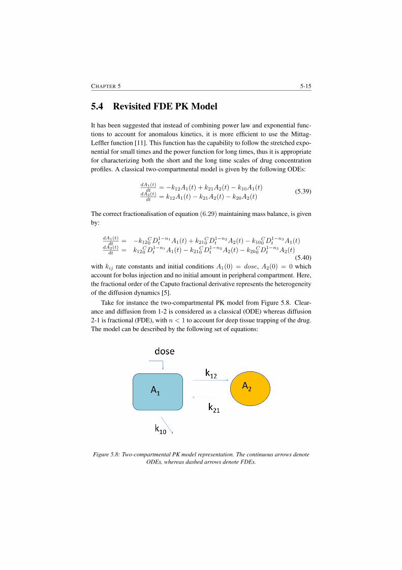
CHAPTER 5 5-15
5.4 Revisited FDE PK Model
It has been suggested that instead of combining power law and exponential func-tions to account for anomalous kinetics, it is more efficient to use the Mittag-Leffler function [11]. This function has the capability to follow the stretched expo-nential for small times and the power function for long times, thus it is appropriatefor characterizing both the short and the long time scales of drug concentrationprofiles. A classical two-compartmental model is given by the following ODEs:
dA1(t)dt = −k12A1(t) + k21A2(t)− k10A1(t)
dA2(t)dt = k12A1(t)− k21A2(t)− k20A2(t)
(5.39)
The correct fractionalisation of equation (6.29) maintaining mass balance, is givenby:
dA1(t)dt = −k12C0 D
1−n1t A1(t) + k21
C0 D
1−n2t A2(t)− k10C0 D
1−n3t A1(t)
dA2(t)dt = k12
C0 D
1−n1t A1(t)− k21C0 D
1−n2t A2(t)− k20C0 D
1−n3t A2(t)
(5.40)with kij rate constants and initial conditions A1(0) = dose, A2(0) = 0 whichaccount for bolus injection and no initial amount in peripheral compartment. Here,the fractional order of the Caputo fractional derivative represents the heterogeneityof the diffusion dynamics [5].
Take for instance the two-compartmental PK model from Figure 5.8. Clear-ance and diffusion from 1-2 is considered as a classical (ODE) whereas diffusion2-1 is fractional (FDE), with n < 1 to account for deep tissue trapping of the drug.The model can be described by the following set of equations:
Figure 5.8: Two-compartmental PK model representation. The continuous arrows denoteODEs, whereas dashed arrows denote FDEs.
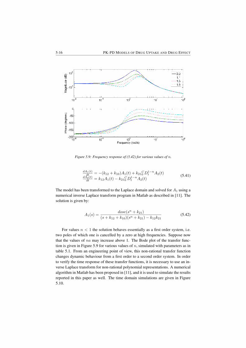
5-16 PK-PD MODELS OF DRUG UPTAKE AND DRUG EFFECT
Figure 5.9: Frequency response of (5.42) for various values of n.
dA1(t)dt = −(k12 + k10)A1(t) + k21
C0 D
1−nt A2(t)
dA2(t)dt = k12A1(t)− k21C0 D1−n
t A2(t)(5.41)
The model has been transformed to the Laplace domain and solved for A1 using anumerical inverse Laplace transform program in Matlab as described in [11]. Thesolution is given by:
A1(s) =dose(sn + k21)
(s+ k12 + k10)(sn + k21)− k12k21(5.42)
For values n < 1 the solution behaves essentially as a first order system, i.e.two poles of which one is cancelled by a zero at high frequencies. Suppose nowthat the values of na may increase above 1. The Bode plot of the transfer func-tion is given in Figure 5.9 for various values of n, simulated with parameters as intable 5.1. From an engineering point of view, this non-rational transfer functionchanges dynamic behaviour from a first order to a second order system. In orderto verify the time response of these transfer functions, it is necessary to use an in-verse Laplace transform for non-rational polynomial representations. A numericalalgorithm in Matlab has been proposed in [11], and it is used to simulate the resultsreported in this paper as well. The time domain simulations are given in Figure5.10.
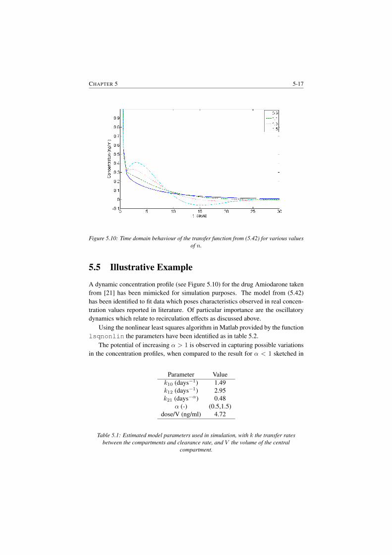
CHAPTER 5 5-17
Figure 5.10: Time domain behaviour of the transfer function from (5.42) for various valuesof n.
5.5 Illustrative Example
A dynamic concentration profile (see Figure 5.10) for the drug Amiodarone takenfrom [21] has been mimicked for simulation purposes. The model from (5.42)has been identified to fit data which poses characteristics observed in real concen-tration values reported in literature. Of particular importance are the oscillatorydynamics which relate to recirculation effects as discussed above.
Using the nonlinear least squares algorithm in Matlab provided by the functionlsqnonlin the parameters have been identified as in table 5.2.
The potential of increasing α > 1 is observed in capturing possible variationsin the concentration profiles, when compared to the result for α < 1 sketched in
Parameter Valuek10 (days−1) 1.49k12 (days−1) 2.95k21 (days−α) 0.48
α (-) (0.5,1.5)dose/V (ng/ml) 4.72
Table 5.1: Estimated model parameters used in simulation, with k the transfer ratesbetween the compartments and clearance rate, and V the volume of the central
compartment.
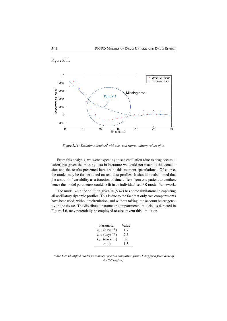
5-18 PK-PD MODELS OF DRUG UPTAKE AND DRUG EFFECT
Figure 5.11.
Figure 5.11: Variations obtained with sub- and supra- unitary values of α.
From this analysis, we were expecting to see oscillation (due to drug accumu-lation) but given the missing data in literature we could not reach to this conclu-sion and the results presented here are at this moment speculations. Of course,the model may be further tuned on real data profiles. It should be also noted thatthe amount of variability as a function of time differs from one patient to another,hence the model parameters could be fit in an individualised PK model framework.
The model with the solution given in (5.42) has some limitations in capturingall oscillatory dynamic profiles. This is due to the fact that only two compartmentshave been used, without recirculation, and without taking into account heterogene-ity in the tissue. The distributed parameter compartmental models, as depicted inFigure 5.6, may potentially be employed to circumvent this limitation.
Parameter Valuek10 (days−1) 1.7k12 (days−1) 2.5k21 (days−α) 0.6
α (-) 1.5
Table 5.2: Identified model parameters used in simulation from (5.42) for a fixed dose of4.7268 (ng/ml).
CHAPTER 5 5-19
5.6 Discussion and Perspectives
Naturally, tissue porosity, molecular binding and permeability vary within the or-gan, within the system and within the assumed compartment. Taking tissue speci-ficity into account when modelling PK dynamic profiles may lead to increasedmodel complexity. A trade-off between the usefulness and computational effi-ciency of such models must be made when evaluating the model objectives. Ifprediction for treatment optimisation is envisaged, then one may include as manydetails as possible to account for a personalised healthcare plan. If mere evalu-ation of dosing profiles and observational studies are involved, tissue specificitymay be limited to the strictly necessary number of details (e.g. Occam’s Razor ap-proach). Obviously, large population data sets will be necessary to provide somereference baseline values for initial start-up. However, if data is available, datadriven modelling/identification may be performed and model parameters tuned tofit the specificity of the case.
Applications of augmented PK models with FDEs are numerous and not lim-ited in the number of turns. One may freely consider their application to modellingany drug PK dynamics. Multiples types of dosing intake may be assumed, eitheras a single type, or as combinations hereof: single dose, bolus, multiple dose, con-tinuous infusion. When using FDEs in PK models, care must be taken for intakeprofiles may lead to drug accumulation and possibly over-dosing in some time in-tervals. Linear or power-law dosing profiles may be investigated to optimally usethe dynamic model properties.
As such, time FDEs have been considered hitherto. However, tissue hetero-geneity is also structural, geometric, and not only present in dynamic fluctuations.It may be worth considering introducing a time-space mathematical formulation(e.g. by employing fractional order space derivatives) to account for drug intakewhereas time and location may be specified. This is of great importance in pathol-ogy cases, where changes in tissue structure and morphology affects directly thedynamic profiles of drug diffusion, permeability and molecular binding. Specificstructural changes with disease may also reveal various paths of deep tissue trap-ping of drug and latency nodes which could explain effects observed in long-tailedobservations.
5.7 Summary
In this chapter the existing compartmental modelling approaches have been re-visited and their usefulness has been extended by employing emerging tools fromfractional calculus . Undoubtedly, the fractional kinetics approach outperforms theclassical ODE models while maintaining the link to physiological phenomena. It isworth mentioning that the assumption of a homogeneous compartment representa-

5-20 PK-PD MODELS OF DRUG UPTAKE AND DRUG EFFECT
tion is no longer limiting in view of modelling objectives. Instead, tissue trappingand heterogeneous resident times may be taken into account by using distributedcompartmental models with various diffusion rates. The combination of classicalPK models and with fractional PK models is then the natural next step in the questto improve their ability to mimic complex observed physiological phenomena.
6Proposed Models and Their Validation
In this chapter the proposed models to characterize the nociceptor pathways arepresented. These models have been validated (in vitro and in vivo) and have thepotential to unlock the current state of art in this specific area of applications.
The main publications where this work has been presented are:
1. D. Copot, R. De Keyser, J. Juchem, C. Ionescu, Fractional order impedancemodel to estimate glucose concentration: in vitro analysis. Acta Polytech-nica Hungarica, 14(1), 207-220, 2017.
2. D. Copot, C. Muresan, R. De Keyser, C. Ionescu, Fractional order modelingof diffusion processes: a new approach for glucose concentration estimation,International Conference on Automation, Quality and Testing, Robotics,Cluj-Napoca, Romania, 19-21 May, 407-712, 2016.
3. D. Copot, R. De Keyser, C. Ionescu, In vitro glucose concentration esti-mation by means of fractional order impedance models, IEEE InternationalConference on Systems, Man, and Cybernetics (SMC), 9-12 October, Bu-dapest, Hungary, 2711-2716, 2016.
6-2 PROPOSED MODELS AND THEIR VALIDATION
6.1 Introduction
Nociceptor pathway: relation between potassium channels and pain signallingPotassium is one of the most common cation in the body and the principal intra-cellular cation. Approximately 3500 mmol of potassium are present in the body.The distribution of Na+ and K+ can be thought of as opposite: one is in highconcentration and the other is at low concentration. Sodium is the most prevalentcation in the extracellular fluid (ECF), with a normal level of around 140 mmol/L,but has a typical intracellular concentration of around 10 mmol/L. In contrast,potassium is the most prevalent cation in the intracellular uid, with a concentra-tion around 150 mmol/L and about 5 mmol/L in the ECF [81, 147]. Because theintracellular space is the largest fluid compartment in the body, this makes it themost abundant cation overall. Hence, Na+ and K+ can only cross where specificcarrier proteins allow them to do so. Excitable cells can change their permeabilityto allow the in flux and efflux of ions that constitute an action potential. At rest,the large concentration gradients for Na+ and K+ are maintained by the actionof Na+/K+ pump [147]. This also maintains the net negative resting membranepotential, since it involves a net transfer of one positive charge out of the cell oneach cycle [148, 149].
The observed increase in potassium concentration in the ECF varies between0.1 and 10.0 mmol/L and depends on stimulation frequency, intensity, and duration[150]. An increase of 0.1-0.5 mmol/L has been found after a single electricalstimulus applied to the dorsal root, to peripheral nerve, or after a single adequatestimulus (light touch or pinch) applied to the skin. Repeated stimulation leads tosummation of responses. For example, an increase of about 6-7 mmol/L was foundin spinal cord after 15 seconds of high-frequency electrical stimulation (100 Hz) ofperipheral nerves. When stimulation is continued, no greater changes in potassiumconcentration are found because a steady state is established, which is the resultof concurrent release and clearance of K+. This so called ”ceiling level” can beexceeded only during epileptic seizures, anoxia or spreading depression, whenK+
can reach levels as high as 20-50 mmol/L [147,149]. Because of the threshold, theaction potential can be likened to a digital event, i.e. it either happens or it does not.If the threshold is not reached, then no action potential occurs. Action potentialsare based on all or nothing law: either the membrane reaches the threshold andeverything occurs as described or the membrane does not reach the threshold andnothing else happens.
While an action potential is in progress, another one cannot be initiated. Thateffect is referred to as the refractory period. There are two phases of the refractoryperiod: the absolute refractory period and the relative refractory period. Duringthe absolute phase, another action potential will not start. This is because of theinactivation gate of the voltage-gated Na+ channel. Once that channel is back to
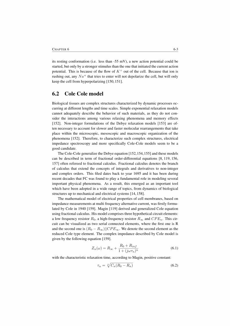
CHAPTER 6 6-3
its resting conformation (i.e. less than -55 mV), a new action potential could bestarted, but only by a stronger stimulus than the one that initiated the current actionpotential. This is because of the flow of K+ out of the cell. Because that ion isrushing out, any Na+ that tries to enter will not depolarize the cell, but will onlykeep the cell from hyperpolarizing [150, 151].
6.2 Cole Cole modelBiological tissues are complex structures characterized by dynamic processes oc-curring at different lengths and time scales. Simple exponential relaxation modelscannot adequately describe the behavior of such materials, as they do not con-sider the interactions among various relaxing phenomena and memory effects[152]. Non-integer formulations of the Debye relaxation models [153] are of-ten necessary to account for slower and faster molecular rearrangements that takeplace within the microscopic, mesoscopic and macroscopic organization of thephenomena [152]. Therefore, to characterize such complex structures, electricalimpedance spectroscopy and more specifically Cole-Cole models seem to be agood candidate.
The Cole-Cole generalize the Debye equation [152,154,155] and these modelscan be described in term of fractional order-differential equations [8, 119, 156,157] often refereed to fractional calculus. Fractional calculus denotes the branchof calculus that extend the concepts of integrals and derivatives to non-integerand complex orders. This filed dates back to year 1695 and it has been duringrecent decades that FC was found to play a fundamental role in modeling severalimportant physical phenomena. As a result, this emerged as an important toolwhich have been adopted in a wide range of topics, from dynamics of biologicalstructures up to mechanical and electrical systems [14, 158].
The mathematical model of electrical properties of cell membranes, based onimpedance measurements at multi frequency alternative current, was firstly formu-lated by Cole in 1940 [159]. Magin [119] derived and generalized Cole equationusing fractional calculus. His model comprises three hypothetical circuit elements:a low frequency resistor R0, a high-frequency resistor R∞ and CPEn. This cir-cuit can be visualized as two serial connected elements, where the first one is Rand the second one is (R0 − R∞)||CPE∞. We denote the second element as thereduced Cole type element. The complex impedance described by Cole model isgiven by the following equation [159].
Zα(ω) = R∞ +R0 +Rinf
1 + (jωτn)n(6.1)
with the characteristic relaxation time, according to Magin, positive constant:
τα = n√Cn(R0 −Rn) (6.2)
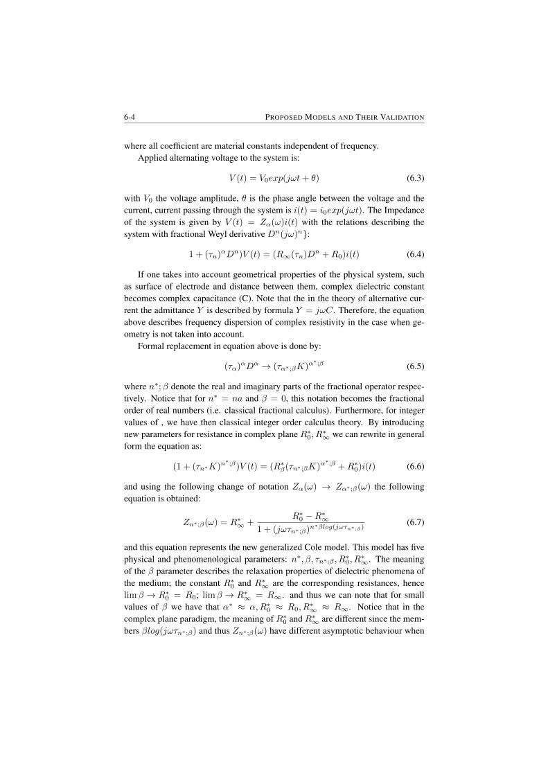
6-4 PROPOSED MODELS AND THEIR VALIDATION
where all coefficient are material constants independent of frequency.Applied alternating voltage to the system is:
V (t) = V0exp(jωt+ θ) (6.3)
with V0 the voltage amplitude, θ is the phase angle between the voltage and thecurrent, current passing through the system is i(t) = i0exp(jωt). The Impedanceof the system is given by V (t) = Zα(ω)i(t) with the relations describing thesystem with fractional Weyl derivative Dn(jω)n:
1 + (τn)αDn)V (t) = (R∞(τn)Dn +R0)i(t) (6.4)
If one takes into account geometrical properties of the physical system, suchas surface of electrode and distance between them, complex dielectric constantbecomes complex capacitance (C). Note that the in the theory of alternative cur-rent the admittance Y is described by formula Y = jωC. Therefore, the equationabove describes frequency dispersion of complex resistivity in the case when ge-ometry is not taken into account.
Formal replacement in equation above is done by:
(τα)αDα → (τα∗;βK)α∗;β (6.5)
where n∗;β denote the real and imaginary parts of the fractional operator respec-tively. Notice that for n∗ = na and β = 0, this notation becomes the fractionalorder of real numbers (i.e. classical fractional calculus). Furthermore, for integervalues of , we have then classical integer order calculus theory. By introducingnew parameters for resistance in complex plane R∗0, R
∗∞ we can rewrite in general
form the equation as:
(1 + (τn∗K)n∗;β)V (t) = (R∗β(τn∗;βK)α
∗;β +R∗0)i(t) (6.6)
and using the following change of notation Zα(ω) → Zα∗;β(ω) the followingequation is obtained:
Zn∗;β(ω) = R∗∞ +R∗0 −R∗∞
1 + (jωτn∗;β)n∗βlog(jωτn∗;β)
(6.7)
and this equation represents the new generalized Cole model. This model has fivephysical and phenomenological parameters: n∗, β, τn∗;β , R
∗0, R
∗∞. The meaning
of the β parameter describes the relaxation properties of dielectric phenomena ofthe medium; the constant R∗0 and R∗∞ are the corresponding resistances, hencelimβ → R∗0 = R0; limβ → R∗∞ = R∞. and thus we can note that for smallvalues of β we have that α∗ ≈ α,R∗0 ≈ R0, R
∗∞ ≈ R∞. Notice that in the
complex plane paradigm, the meaning of R∗0 and R∗∞ are different since the mem-bers βlog(jωτn∗;β) and thus Zn∗;β(ω) have different asymptotic behaviour when
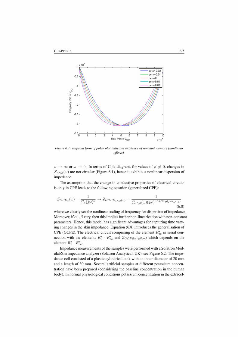
CHAPTER 6 6-5
Figure 6.1: Elipsoid form of polar plot indicates existence of remnant memory (nonlineareffects).
ω → ∞ or ω → 0. In terms of Cole diagram, for values of β 6= 0, changes inZn∗;β(ω) are not circular (Figure 6.1), hence it exhibits a nonlinear dispersion ofimpedance.
The assumption that the change in conductive properties of electrical circuitsis only in CPE leads to the following equation (generalized CPE):
ZCPEα(ω) =1
Cα(jω)α→ ZGCPEα∗;β(ω) =
1
Cα∗;β(ω)(jω)α∗+βlog(jωτα∗;β)
(6.8)where we clearly see the nonlinear scaling of frequency for dispersion of impedance.Moreover, ifα∗, β vary, then this implies further non-linearization with non-constantparameters. Hence, this model has significant advantages for capturing time vary-ing changes in the skin impedance. Equation (6.8) introduces the generalisation ofCPE (GCPE). The electrical circuit comprising of the element R∗∞ in serial con-nection with the elements R∗0 - R∗∞ and ZGCPEα∗;β(ω) which depends on theelement R∗0 - R∗∞.
Impedance measurements of the samples were performed with a Solatron Mod-ulabXm impedance analyzer (Solatron Analytical, UK), see Figure 6.2. The impe-dance cell consisted of a plastic cylindrical tank with an inner diameter of 20 mmand a length of 30 mm. Several artificial samples at different potassium concen-tration have been prepared (considering the baseline concentration in the humanbody). In normal physiological conditions potassium concentration in the extracel-
6-6 PROPOSED MODELS AND THEIR VALIDATION
lular fluid is about 4-5 mmol/L. Deionised water and potassium chloride was usedto prepare the samples. Through the Solatron analyzer a 100 mV r.m.s. sinusoidalvoltage has been applied to the outer couple of electrodes of the measurementprobe which was immersed into the glass tube containing the analyzed sample.Impedance of the samples has been analyzed in the 1Hz-0.1MHz frequency range.
Figure 6.2: Solatron ModulabXm impedance analyzer.
ModuLab XM ECS is an Xtreme Measurement electrochemical test systemthat is capable of measuring ultra-low, micro-ohm impedance cells (latest gener-ation batteries and fuel cells, for example), while able to accurately characterizeultra-high impedance corrosion coatings at the other extreme. The system uses aunique AC calibration method that ensures ultimate accuracy in all cases.
The results obtained using the Cole-Cole model (6.7) are given in Figure 6.3.
(a) (b) (c)
Figure 6.3: Cole-Cole model (blue line) and measured data (red line) for differentpotassium concentrations (a) 3.2 mmol/L; b) 4.9 mmol/L and c) 7.5mmol/L). The analysis
has been performed in the frequency interval 1Hz - 0.1 MHz
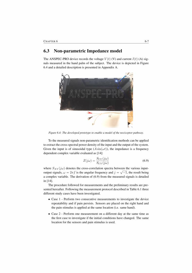
CHAPTER 6 6-7
6.3 Non-parametric Impedance modelThe ANSPEC-PRO device records the voltage V (t) (V) and current I(t) (A) sig-nals measured in the hand palm of the subject. The device is depicted in Figure6.4 and a detailed description is presented in Appendix A.
Figure 6.4: The developed prototype to enable a model of the nociceptor pathway.
To the measured signals non-parametric identification methods can be appliedto extract the cross-spectral power density of the input and the output of the system.Given the input is of sinusoidal type (A sin(ωt)), the impedance is a frequencydependent complex variable evaluated as [14]:
Z(jω) =SUU (jω)
SUY (jω)(6.9)
where SXY (jω) denotes the cross-correlation spectra between the various input-output signals, ω = 2πf is the angular frequency and j =
√−1, the result being
a complex variable. The derivation of (6.9) from the measured signals is detailedin [14].
The procedure followed for measurements and the preliminary results are pre-sented hereafter. Following the measurement protocol described in Table 6.1 threedifferent study cases have been investigated.
• Case 1 - Perform two consecutive measurements to investigate the devicerepeatability and if pain persists. Sensors are placed on the right hand andthe pain stimulus is applied at the same location (i.e. same hand).
• Case 2 - Perform one measurement on a different day at the same time asthe first case to investigate if the initial conditions have changed. The samelocation for the sensors and pain stimulus is used.
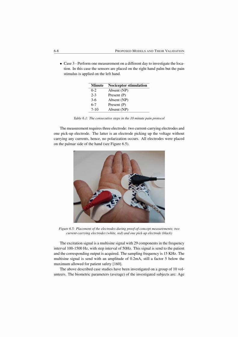
6-8 PROPOSED MODELS AND THEIR VALIDATION
• Case 3 - Perform one measurement on a different day to investigate the loca-tion. In this case the sensors are placed on the right hand palm but the painstimulus is applied on the left hand.
Minute Nociceptor stimulation0-2 Absent (NP)2-3 Present (P)3-6 Absent (NP)6-7 Present (P)7-10 Absent (NP)
Table 6.1: The consecutive steps in the 10 minute pain protocol
The measurement requires three electrode: two current-carrying electrodes andone pick-up electrode. The latter is an electrode picking up the voltage withoutcarrying any currents, hence, no polarization occurs. All electrodes were placedon the palmar side of the hand (see Figure 6.5).
Figure 6.5: Placement of the electrodes during proof-of-concept measurements; twocurrent-carrying electrodes (white, red) and one pick-up electrode (black)
The excitation signal is a multisine signal with 29 components in the frequencyinterval 100-1500 Hz, with step interval of 50Hz. This signal is send to the patientand the corresponding output is acquired. The sampling frequency is 15 KHz. Themultisine signal is send with an amplitude of 0.2mA, still a factor 5 below themaximum allowed for patient safety [160].
The above described case studies have been investigated on a group of 10 vol-unteers. The biometric parameters (average) of the investigated subjects are: Age
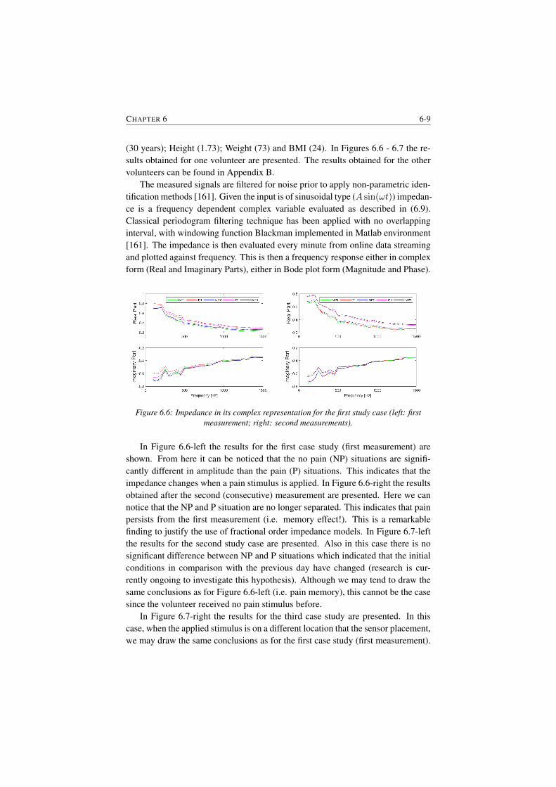
CHAPTER 6 6-9
(30 years); Height (1.73); Weight (73) and BMI (24). In Figures 6.6 - 6.7 the re-sults obtained for one volunteer are presented. The results obtained for the othervolunteers can be found in Appendix B.
The measured signals are filtered for noise prior to apply non-parametric iden-tification methods [161]. Given the input is of sinusoidal type (A sin(ωt)) impedan-ce is a frequency dependent complex variable evaluated as described in (6.9).Classical periodogram filtering technique has been applied with no overlappinginterval, with windowing function Blackman implemented in Matlab environment[161]. The impedance is then evaluated every minute from online data streamingand plotted against frequency. This is then a frequency response either in complexform (Real and Imaginary Parts), either in Bode plot form (Magnitude and Phase).
Figure 6.6: Impedance in its complex representation for the first study case (left: firstmeasurement; right: second measurements).
In Figure 6.6-left the results for the first case study (first measurement) areshown. From here it can be noticed that the no pain (NP) situations are signifi-cantly different in amplitude than the pain (P) situations. This indicates that theimpedance changes when a pain stimulus is applied. In Figure 6.6-right the resultsobtained after the second (consecutive) measurement are presented. Here we cannotice that the NP and P situation are no longer separated. This indicates that painpersists from the first measurement (i.e. memory effect!). This is a remarkablefinding to justify the use of fractional order impedance models. In Figure 6.7-leftthe results for the second study case are presented. Also in this case there is nosignificant difference between NP and P situations which indicated that the initialconditions in comparison with the previous day have changed (research is cur-rently ongoing to investigate this hypothesis). Although we may tend to draw thesame conclusions as for Figure 6.6-left (i.e. pain memory), this cannot be the casesince the volunteer received no pain stimulus before.
In Figure 6.7-right the results for the third case study are presented. In thiscase, when the applied stimulus is on a different location that the sensor placement,we may draw the same conclusions as for the first case study (first measurement).
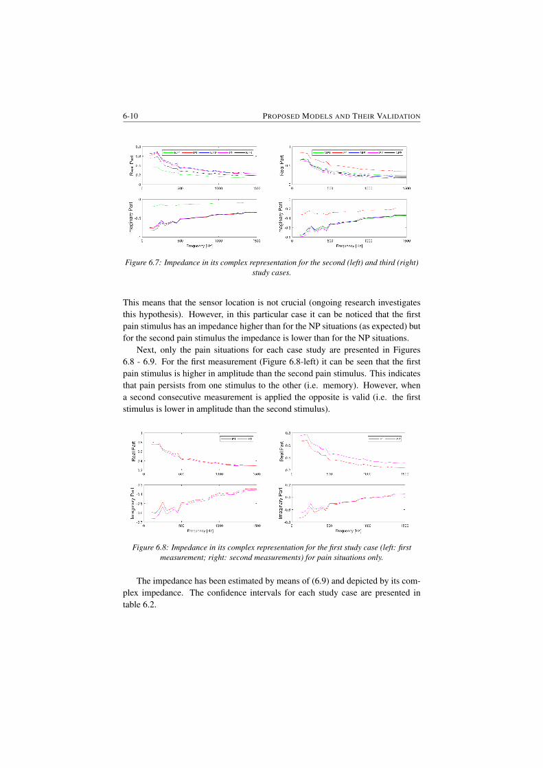
6-10 PROPOSED MODELS AND THEIR VALIDATION
Figure 6.7: Impedance in its complex representation for the second (left) and third (right)study cases.
This means that the sensor location is not crucial (ongoing research investigatesthis hypothesis). However, in this particular case it can be noticed that the firstpain stimulus has an impedance higher than for the NP situations (as expected) butfor the second pain stimulus the impedance is lower than for the NP situations.
Next, only the pain situations for each case study are presented in Figures6.8 - 6.9. For the first measurement (Figure 6.8-left) it can be seen that the firstpain stimulus is higher in amplitude than the second pain stimulus. This indicatesthat pain persists from one stimulus to the other (i.e. memory). However, whena second consecutive measurement is applied the opposite is valid (i.e. the firststimulus is lower in amplitude than the second stimulus).
Figure 6.8: Impedance in its complex representation for the first study case (left: firstmeasurement; right: second measurements) for pain situations only.
The impedance has been estimated by means of (6.9) and depicted by its com-plex impedance. The confidence intervals for each study case are presented intable 6.2.
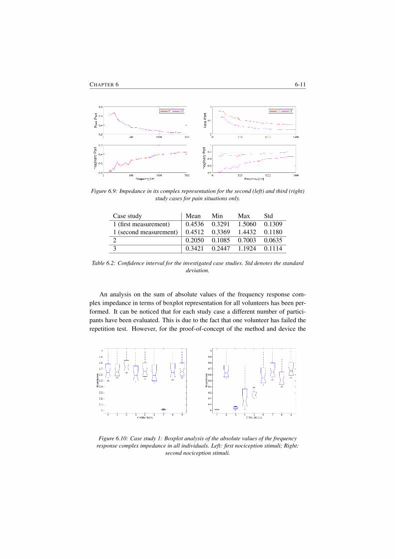
CHAPTER 6 6-11
Figure 6.9: Impedance in its complex representation for the second (left) and third (right)study cases for pain situations only.
Case study Mean Min Max Std1 (first measurement) 0.4536 0.3291 1.5060 0.13091 (second measurement) 0.4512 0.3369 1.4432 0.11802 0.2050 0.1085 0.7003 0.06353 0.3421 0.2447 1.1924 0.1114
Table 6.2: Confidence interval for the investigated case studies. Std denotes the standarddeviation.
An analysis on the sum of absolute values of the frequency response com-plex impedance in terms of boxplot representation for all volunteers has been per-formed. It can be noticed that for each study case a different number of partici-pants have been evaluated. This is due to the fact that one volunteer has failed therepetition test. However, for the proof-of-concept of the method and device the
Figure 6.10: Case study 1: Boxplot analysis of the absolute values of the frequencyresponse complex impedance in all individuals. Left: first nociception stimuli; Right:
second nociception stimuli.
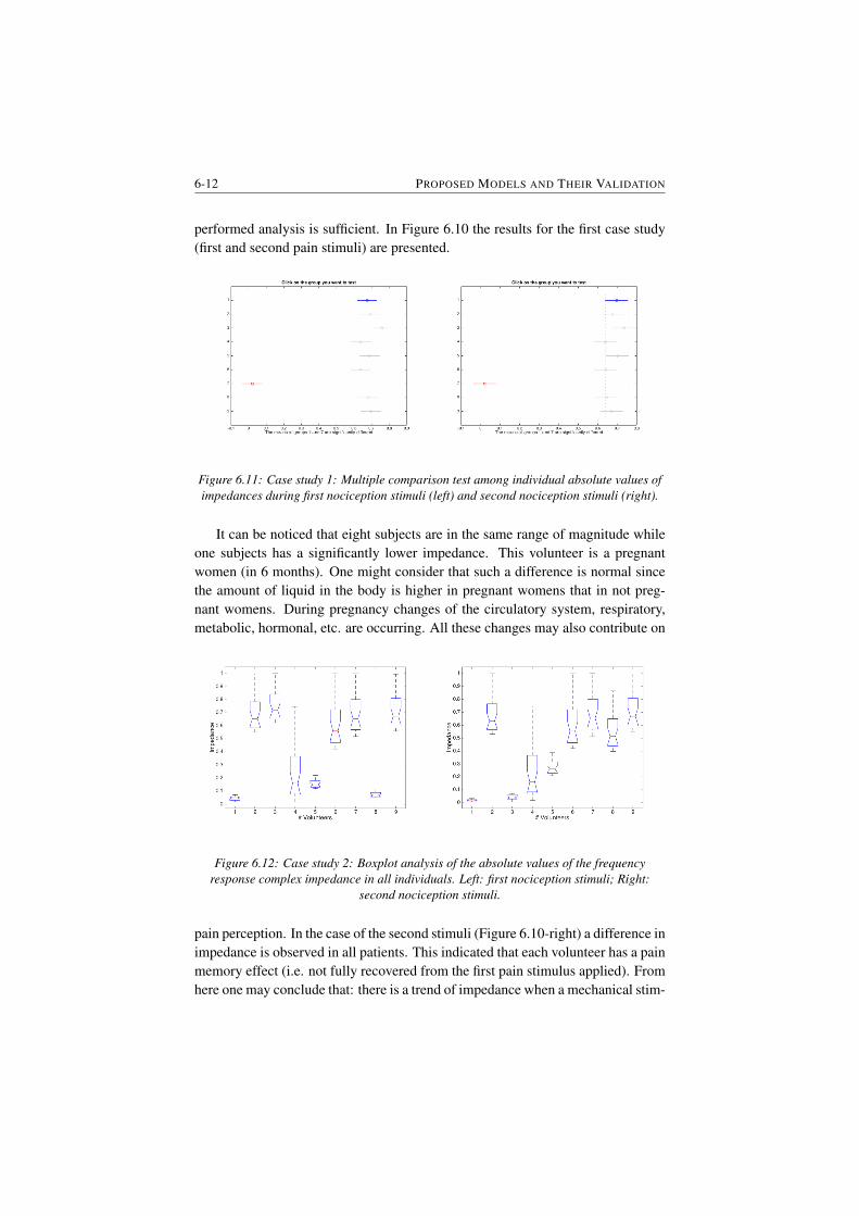
6-12 PROPOSED MODELS AND THEIR VALIDATION
performed analysis is sufficient. In Figure 6.10 the results for the first case study(first and second pain stimuli) are presented.
Figure 6.11: Case study 1: Multiple comparison test among individual absolute values ofimpedances during first nociception stimuli (left) and second nociception stimuli (right).
It can be noticed that eight subjects are in the same range of magnitude whileone subjects has a significantly lower impedance. This volunteer is a pregnantwomen (in 6 months). One might consider that such a difference is normal sincethe amount of liquid in the body is higher in pregnant womens that in not preg-nant womens. During pregnancy changes of the circulatory system, respiratory,metabolic, hormonal, etc. are occurring. All these changes may also contribute on
Figure 6.12: Case study 2: Boxplot analysis of the absolute values of the frequencyresponse complex impedance in all individuals. Left: first nociception stimuli; Right:
second nociception stimuli.
pain perception. In the case of the second stimuli (Figure 6.10-right) a difference inimpedance is observed in all patients. This indicated that each volunteer has a painmemory effect (i.e. not fully recovered from the first pain stimulus applied). Fromhere one may conclude that: there is a trend of impedance when a mechanical stim-
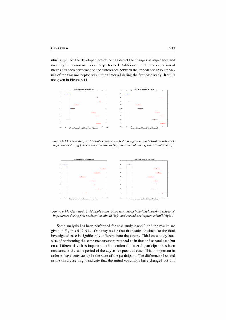
CHAPTER 6 6-13
ulus is applied; the developed prototype can detect the changes in impedance andmeaningful measurements can be performed. Additional, multiple comparison ofmeans has been performed to see differences between the impedance absolute val-ues of the two nociceptor stimulation interval during the first case study. Resultsare given in Figure 6.11.
Figure 6.13: Case study 2: Multiple comparison test among individual absolute values ofimpedances during first nociception stimuli (left) and second nociception stimuli (right).
Figure 6.14: Case study 3: Multiple comparison test among individual absolute values ofimpedances during first nociception stimuli (left) and second nociception stimuli (right).
Same analysis has been performed for case study 2 and 3 and the results aregiven in Figures 6.12-6.14. One may notice that the results obtained for the thirdinvestigated case is significantly different from the others. Third case study con-sists of performing the same measurement protocol as in first and second case buton a different day. It is important to be mentioned that each participant has beenmeasured in the same period of the day as for previous case. This is important inorder to have consistency in the state of the participant. The difference observedin the third case might indicate that the initial conditions have changed but this
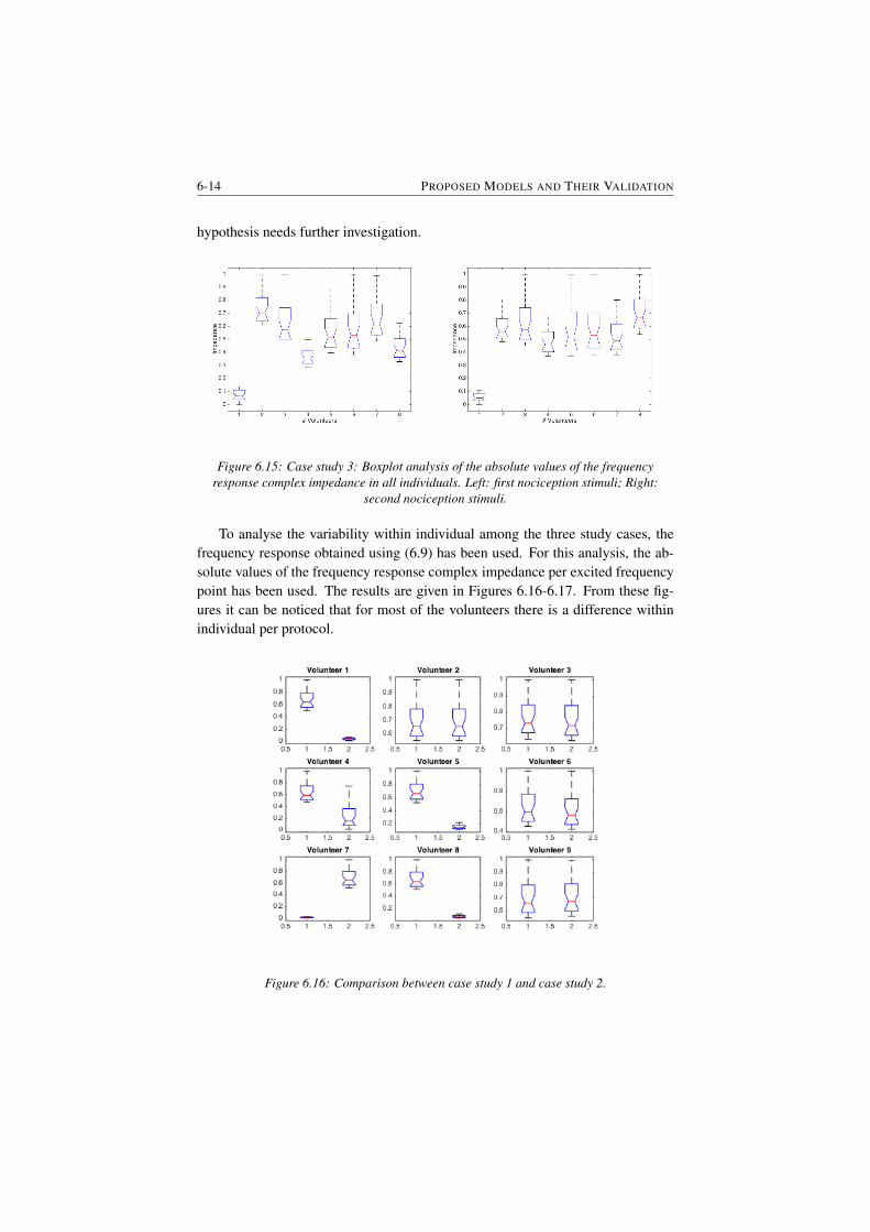
6-14 PROPOSED MODELS AND THEIR VALIDATION
hypothesis needs further investigation.
Figure 6.15: Case study 3: Boxplot analysis of the absolute values of the frequencyresponse complex impedance in all individuals. Left: first nociception stimuli; Right:
second nociception stimuli.
To analyse the variability within individual among the three study cases, thefrequency response obtained using (6.9) has been used. For this analysis, the ab-solute values of the frequency response complex impedance per excited frequencypoint has been used. The results are given in Figures 6.16-6.17. From these fig-ures it can be noticed that for most of the volunteers there is a difference withinindividual per protocol.
Figure 6.16: Comparison between case study 1 and case study 2.
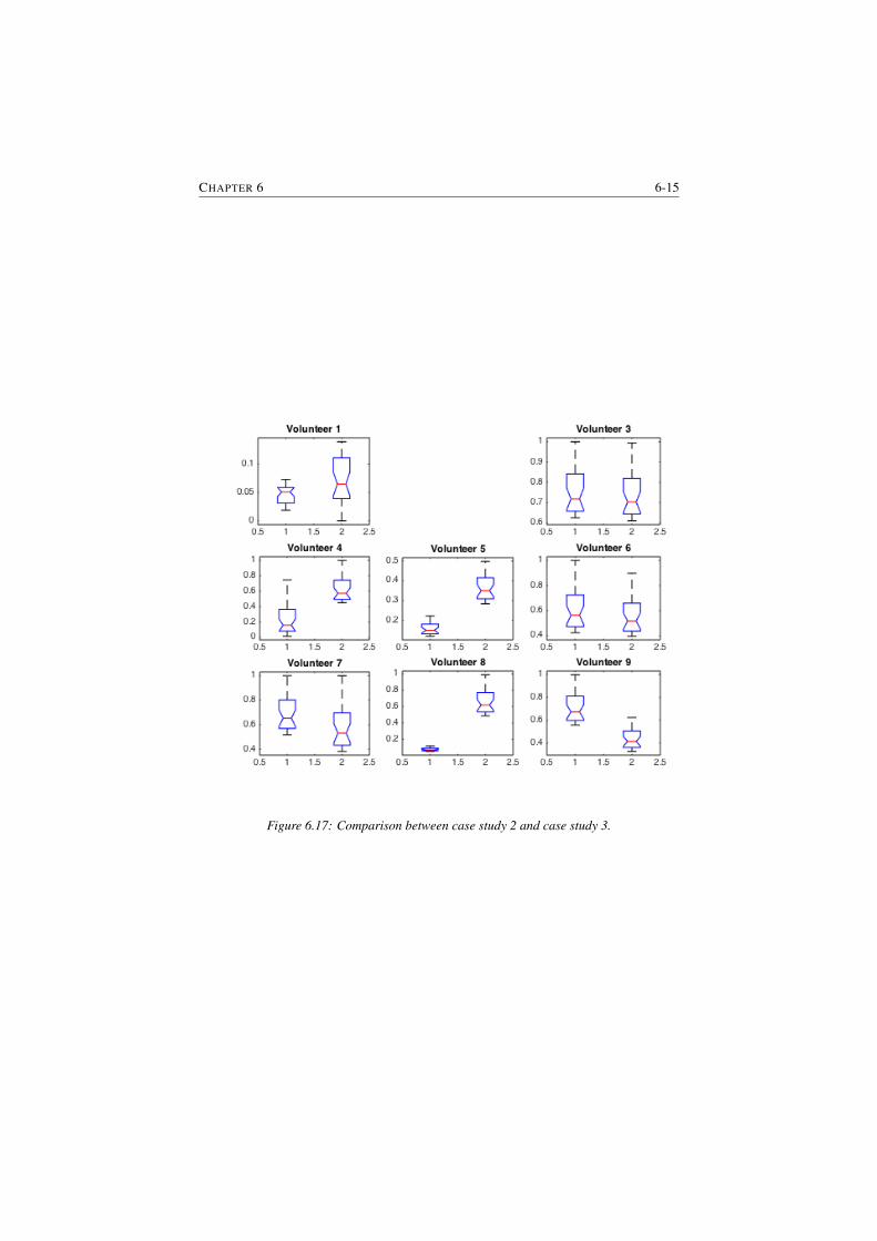
CHAPTER 6 6-15
Figure 6.17: Comparison between case study 2 and case study 3.
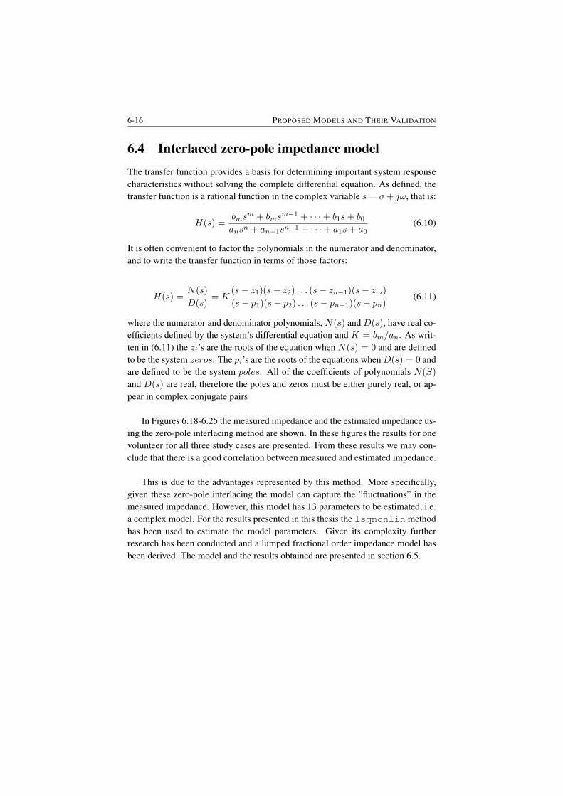
6-16 PROPOSED MODELS AND THEIR VALIDATION
6.4 Interlaced zero-pole impedance modelThe transfer function provides a basis for determining important system responsecharacteristics without solving the complete differential equation. As defined, thetransfer function is a rational function in the complex variable s = σ+ jω, that is:
H(s) =bms
m + bmsm−1 + · · ·+ b1s+ b0
ansn + an−1sn−1 + · · ·+ a1s+ a0(6.10)
It is often convenient to factor the polynomials in the numerator and denominator,and to write the transfer function in terms of those factors:
H(s) =N(s)
D(s)= K
(s− z1)(s− z2) . . . (s− zn−1)(s− zm)
(s− p1)(s− p2) . . . (s− pn−1)(s− pn)(6.11)
where the numerator and denominator polynomials, N(s) and D(s), have real co-efficients defined by the system’s differential equation and K = bm/an. As writ-ten in (6.11) the zi’s are the roots of the equation when N(s) = 0 and are definedto be the system zeros. The pi’s are the roots of the equations whenD(s) = 0 andare defined to be the system poles. All of the coefficients of polynomials N(S)
and D(s) are real, therefore the poles and zeros must be either purely real, or ap-pear in complex conjugate pairs
In Figures 6.18-6.25 the measured impedance and the estimated impedance us-ing the zero-pole interlacing method are shown. In these figures the results for onevolunteer for all three study cases are presented. From these results we may con-clude that there is a good correlation between measured and estimated impedance.
This is due to the advantages represented by this method. More specifically,given these zero-pole interlacing the model can capture the ”fluctuations” in themeasured impedance. However, this model has 13 parameters to be estimated, i.e.a complex model. For the results presented in this thesis the lsqnonlin methodhas been used to estimate the model parameters. Given its complexity furtherresearch has been conducted and a lumped fractional order impedance model hasbeen derived. The model and the results obtained are presented in section 6.5.
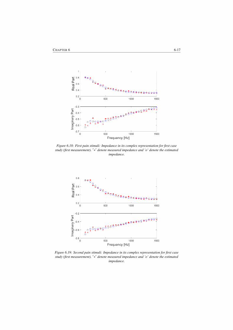
CHAPTER 6 6-17
Figure 6.18: First pain stimuli: Impedance in its complex representation for first casestudy (first measurement). ′∗′ denote measured impedance and ’o’ denote the estimated
impedance.
Figure 6.19: Second pain stimuli: Impedance in its complex representation for first casestudy (first measurement). ′∗′ denote measured impedance and ’o’ denote the estimated
impedance.
6-18 PROPOSED MODELS AND THEIR VALIDATION
Figure 6.20: First pain stimuli: Impedance in its complex representation for first casestudy (second measurement). ′∗′ denote measured impedance and ’o’ denote the estimated
impedance.
Figure 6.21: Second pain stimuli: Impedance in its complex representation for first casestudy (second measurement). ′∗′ denote measured impedance and ’o’ denote the estimated
impedance.

CHAPTER 6 6-19
Figure 6.22: First pain stimuli: Impedance in its complex representation for second casestudy. ′∗′ denote measured impedance and ’o’ denote the estimated impedance.
Figure 6.23: Second pain stimuli: Impedance in its complex representation for second casestudy. ′∗′ denote measured impedance and ’o’ denote the estimated impedance.
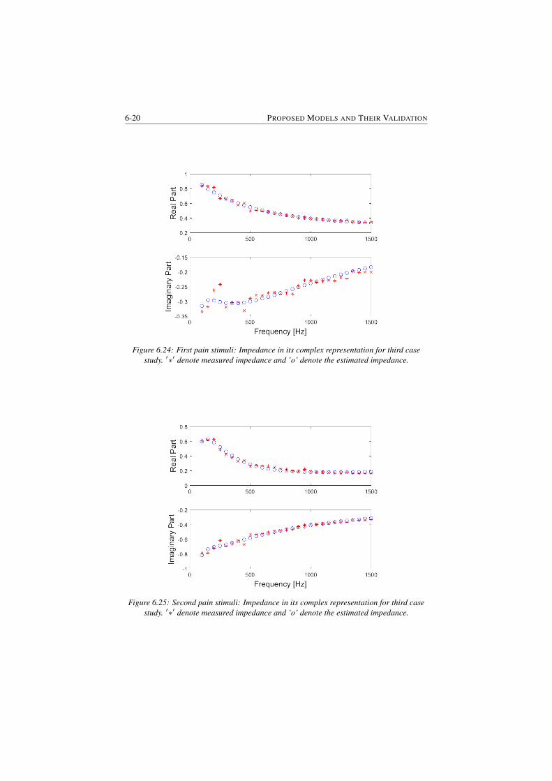
6-20 PROPOSED MODELS AND THEIR VALIDATION
Figure 6.24: First pain stimuli: Impedance in its complex representation for third casestudy. ′∗′ denote measured impedance and ’o’ denote the estimated impedance.
Figure 6.25: Second pain stimuli: Impedance in its complex representation for third casestudy. ′∗′ denote measured impedance and ’o’ denote the estimated impedance.
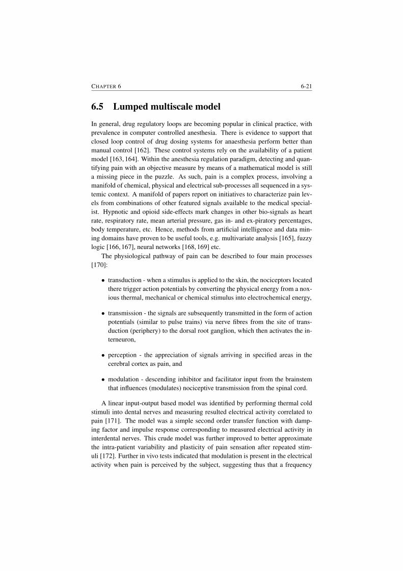
CHAPTER 6 6-21
6.5 Lumped multiscale model
In general, drug regulatory loops are becoming popular in clinical practice, withprevalence in computer controlled anesthesia. There is evidence to support thatclosed loop control of drug dosing systems for anaesthesia perform better thanmanual control [162]. These control systems rely on the availability of a patientmodel [163, 164]. Within the anesthesia regulation paradigm, detecting and quan-tifying pain with an objective measure by means of a mathematical model is stilla missing piece in the puzzle. As such, pain is a complex process, involving amanifold of chemical, physical and electrical sub-processes all sequenced in a sys-temic context. A manifold of papers report on initiatives to characterize pain lev-els from combinations of other featured signals available to the medical special-ist. Hypnotic and opioid side-effects mark changes in other bio-signals as heartrate, respiratory rate, mean arterial pressure, gas in- and ex-piratory percentages,body temperature, etc. Hence, methods from artificial intelligence and data min-ing domains have proven to be useful tools, e.g. multivariate analysis [165], fuzzylogic [166, 167], neural networks [168, 169] etc.
The physiological pathway of pain can be described to four main processes[170]:
• transduction - when a stimulus is applied to the skin, the nociceptors locatedthere trigger action potentials by converting the physical energy from a nox-ious thermal, mechanical or chemical stimulus into electrochemical energy,
• transmission - the signals are subsequently transmitted in the form of actionpotentials (similar to pulse trains) via nerve fibres from the site of trans-duction (periphery) to the dorsal root ganglion, which then activates the in-terneuron,
• perception - the appreciation of signals arriving in specified areas in thecerebral cortex as pain, and
• modulation - descending inhibitor and facilitator input from the brainstemthat influences (modulates) nociceptive transmission from the spinal cord.
A linear input-output based model was identified by performing thermal coldstimuli into dental nerves and measuring resulted electrical activity correlated topain [171]. The model was a simple second order transfer function with damp-ing factor and impulse response corresponding to measured electrical activity ininterdental nerves. This crude model was further improved to better approximatethe intra-patient variability and plasticity of pain sensation after repeated stim-uli [172]. Further in vivo tests indicated that modulation is present in the electricalactivity when pain is perceived by the subject, suggesting thus that a frequency
6-22 PROPOSED MODELS AND THEIR VALIDATION
dependence is necessary. Nonlinear terms in sine and cosine functions have beenintroduced in [173] to predict this nonlinear effect.
Somewhat later, a review of multi-scale processes involved in nociception andpain sensation has been made, summarizing all steps from thermal stimuli [174].Although the review makes an excellent overview, it concludes that the mech-anistic processes are far from being well understood and that engineering toolsneed to be further employed for delivering useful models for assessing pain inman. A model for electrical activity aroused from thermal nociceptor detectionand transmission at neuronal level is then given. The model captures in part thepain pathway and thus is limited in its use to the anesthesia regulation paradigm.Later studies on thermal pain indicated the presence of adaptability and variabilityin pain sensation as a result of noxious stimulus intensity degree and pattern ofstimulation [175]. In engineering terms, this is due to variability of disturbanceprofiles (i.e. stimuli) and thus the excitatory input to the measured response varia-tion provides a spatio-temporal change in the path pathway. Simple linear modelsof classical system engineering theory can no longer capture such changes withoutincreasing the complexity of the problem formulation.
In this chapter we present a view from system engineering standpoint makinguse of multi-scale models to obtain a lumped minimal parameter characterisationof nociception and pain pathways. We employ tools from mathematics, physicsand chemistry to equivalent electrical circuit analogues beyond classical linear sys-tem theory. Fractional calculus and diffusion in heterogeneous medium is a keyingredient in this paper. The originality of the approach is in the integrative mannerin which all sequences of nociception and pain related pathways are modelled, tomaintain a minimal number of parameters to be later identified from experimentaldata. The tools used in this model derivation are borrowed from mathematics, i.e.fractional calculus, since they are a generalization of the classical linear systemtheory known in systems engineering. To the author’s knowledge, a mathematicalmodel based on such systematic derivation does not yet exist in literature.
Gate Control Theory:
The gate control theory (GCT) is a successful way to explain important featuresof the pain process [150]. This theory says that the small fibres (Aδ and C) thatcarry the information about noxious stimuli, while the larger (L) fibres (Aβ) carryinformation about less-intense mechanical stimuli. As the signal from the smallfibres is routed through substantia gelatinosa (SG) to the central transmission cells(T-cell) and onwards, the double inhibition (indicated by the minus signs) strength-ens the signal, resulting that the sensation of pain is more easily evoked. However,the signal from A-fibres activates the inhibitory function of substantia gelatinosa,which will reduce the firing to transmission cells and suppress the pain in the end.This theory was modified later in that it included excitatory (indicated by the plus
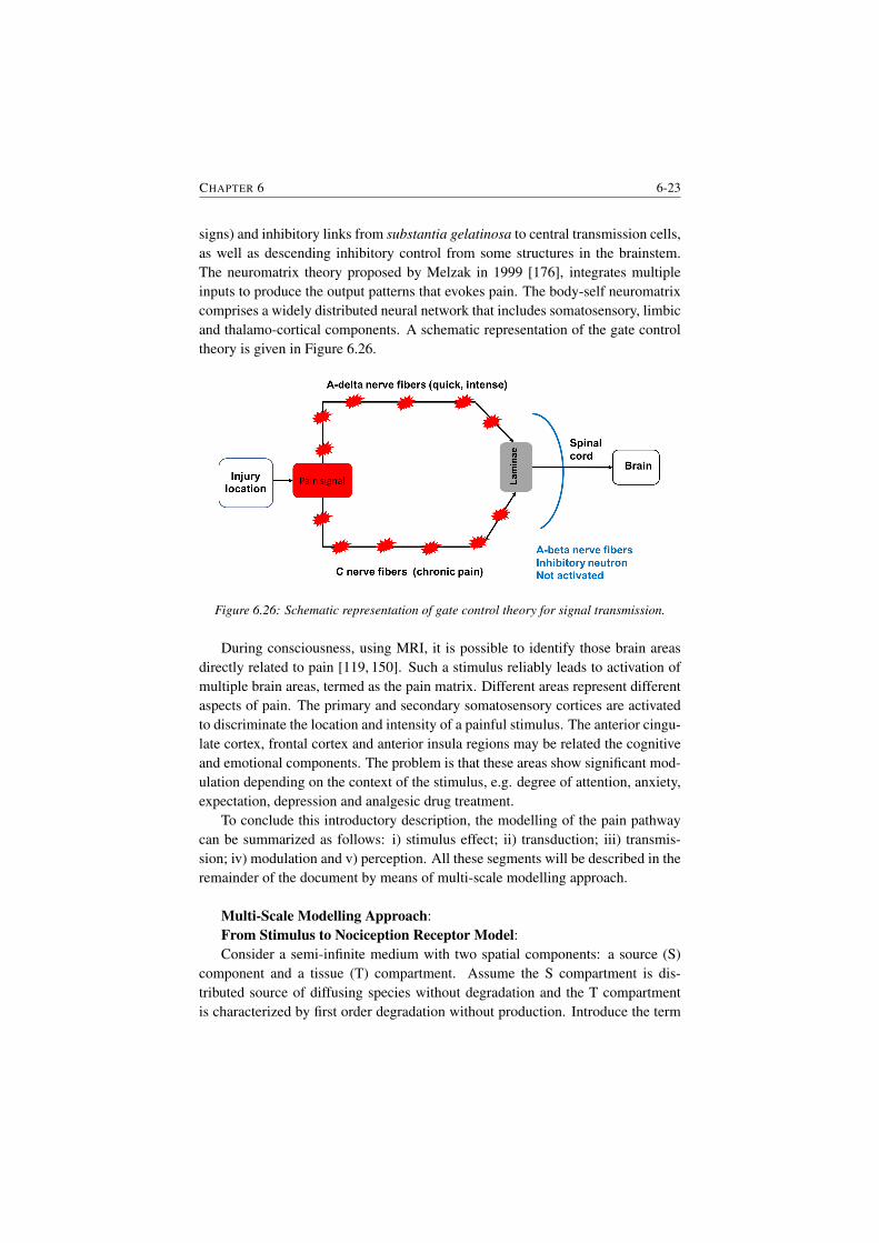
CHAPTER 6 6-23
signs) and inhibitory links from substantia gelatinosa to central transmission cells,as well as descending inhibitory control from some structures in the brainstem.The neuromatrix theory proposed by Melzak in 1999 [176], integrates multipleinputs to produce the output patterns that evokes pain. The body-self neuromatrixcomprises a widely distributed neural network that includes somatosensory, limbicand thalamo-cortical components. A schematic representation of the gate controltheory is given in Figure 6.26.
Figure 6.26: Schematic representation of gate control theory for signal transmission.
During consciousness, using MRI, it is possible to identify those brain areasdirectly related to pain [119, 150]. Such a stimulus reliably leads to activation ofmultiple brain areas, termed as the pain matrix. Different areas represent differentaspects of pain. The primary and secondary somatosensory cortices are activatedto discriminate the location and intensity of a painful stimulus. The anterior cingu-late cortex, frontal cortex and anterior insula regions may be related the cognitiveand emotional components. The problem is that these areas show significant mod-ulation depending on the context of the stimulus, e.g. degree of attention, anxiety,expectation, depression and analgesic drug treatment.
To conclude this introductory description, the modelling of the pain pathwaycan be summarized as follows: i) stimulus effect; ii) transduction; iii) transmis-sion; iv) modulation and v) perception. All these segments will be described in theremainder of the document by means of multi-scale modelling approach.
Multi-Scale Modelling Approach:From Stimulus to Nociception Receptor Model:Consider a semi-infinite medium with two spatial components: a source (S)
component and a tissue (T) compartment. Assume the S compartment is dis-tributed source of diffusing species without degradation and the T compartmentis characterized by first order degradation without production. Introduce the term

6-24 PROPOSED MODELS AND THEIR VALIDATION
cs as the accumulated concentration of the S compartment (i.e. as a result of thestimulus) and cf the concentration in the T compartment. The overall solution isthe sum of the two terms
c(x) = cs(x) + cf (x) (6.12)
with the two domains assumed to be orthogonal, i.e. cs(x) = 0, in the distalcompartment x > L and cf (x) = 0 in the proximal compartment x < L, withL the depth of the tissue layers. A continuous and smooth solution implies theequilibrium conditions:
cs(x)|x=L− = cf (x)|x=L+ (6.13)∂cs∂x
(x)|x=L− =∂cf∂x
(x)|x=L+ (6.14)
and boundary conditions c(0) = 0; c(∞) = 0.The amount of extracellular space (ECS) varies as a function of tissue structure,
function, and geometry within a system or an organ, i.e liver, arteries, heart, lungs,brain, muscle, fat, etc. Impeded diffusion can be thus modelled either by usingclassical diffusion laws, or by anomalous laws following fractional calculus tools.
Classical diffusion considers that the medium imposes only a spatial impedi-ment on the diffusing species and does not change the diffusion law. For example,in [177] the densely packed cells of the brain and their interstitial spaces resemblea porous medium with two phases, i.e. an intra- and an extra- cellular phase. Dif-fusion in the permeable phase of the porous media is analogous to the diffusion inthe narrow spaces between brain cells, i.e. the ECS. In our case, we consider thepermeable phase as that being with fast time constants, i.e. the fat cells and othermediums without fast electrical conductivity are thus representing the ECS.
Volume transport of species having concentration c is governed by rescaledreaction-diffusion equation:
∂c
∂t =
D
λ2∇2c+
s
α− κc, with λ =
√D
D(6.15)
where the stimulus source term is denoted by s, the clearance term by k(c) = κc
is assumed to be first order decay and D is the diffusion coefficient (i.e. defined aslength2/time). Additionally, we have the dimensionless parameters of tortuosityλ and porosity α, and the clearance rate κ (1/time). Tortuosity can be consideredas the linear correction for the anomalous diffusion in a complex medium [178].
Rename D = Dλ2 and s = s
α and the transport equation can be redefined usingfractional calculus as
∂c
∂t= D∇∇βc+ s− κc (6.16)
where ∇β denotes the fractional order Fick’s law, i.e. the fractional flux in themedium. This form of diffusion naturally implies spatial non-locality and can bederived rigorously using spatial averaging theorems [179, 180].
CHAPTER 6 6-25
Introducing the Caputo definition of an differ-integral as [5]:
Dβaf(x) =1
Λ(1− β)
∫ x
a
f ′(t)
(x− t)βdt (6.17)
where Λ is the Euler gamma function and reducing the system of coordinates to theaxial variable it follows that diffusion is given by −DDβa c, as following from thederivation presented in [181]. Introducing a mass conservation law for the particleconcentrations it follows that
∂c
∂t= D
∂
∂xDβ0 c+ s+ κc (6.18)
whose explicit solutions have been given in [181].Hence, we have that the model from stimulus to nociceptor receptor is gov-
erned by a diffusion equation in heterogeneous medium depending on time alongsingle linear spatial dimension. At this point we can describe the contact surface ofthe stimulus as an ultracapacitor whose impedance can be formulated as a functionof the porous nature of medium [182].
The Impedance Model:Signalling pathways is limited by ionic diffusion and electrical cellular stimu-
lation above a minimal threshold value. Geometry dependent diffusion impedanceshave been derived in [16,17] for several particle geometries: planar, cylindrical andspherical. In our case, the specific geometry is due to that localization of noxiousstimuli on different types of tissue structures, e.g. skin (planar), muscle (cylindri-cal) or organ (spherical). Sufficiently low frequencies it appeared that impedancesbehave as a resistor in series with a capacitor with specific terms according to ge-ometrical features. The electrochemical impedance of the Na+/K+ pump forsignalling pathways of nociceptor stimulus involves activation of material parti-cles and can be considered as a charge transfer process. At high frequencies (i.e.above 1 Hz in most ultracapacitor cases) the overall impedance does not depend ongeometrical features and follows the frequency dependence of its complex valuesas in a modified circuit:
Z(s) = R+Rc
1 + τcs+ Zm(s) (6.19)
where R is a threshold value (i.e. the gate control theory on-off signalising con-dition), Rc and τc values related to the overall cellular impedance and Zm thebounded diffusion impedance from molecular level dependent on anomalous dif-fusion geometry. The charge transfer characteristic pulsation frequency is thenωc = 1
τc.
The fractional differ-integral operator can be expressed as a continuous integerorder system approximating the fractional term in a limited bandwidth, synthesized
6-26 PROPOSED MODELS AND THEIR VALIDATION
by cascading elementary phase-delay filters within the bandwidth [183]. This ap-proximated filter is truncated at low and at high frequency boundaries. When con-sidering the asymptotic behaviour of bounded diffusion impedance models at lowand high frequencies, it can be observed that they behave as a classical integratorand an integrator of non-integer order n=1/2. The blocking diffusive behaviour isthus modelled by a gain b0 and a fractional integrator I:
Zm(s) =b0s
+ b1I(ωb, s) (6.20)
The asymptotic behaviour at low frequencies (i.e. ω wb) is
Zm|ωb =b0s
+ b1ω−nb (6.21)
with n the fractional order which for homogeneously diffusion patterns is close tothe value of 0.5. It follows thus the overall fractional impedance model as
Z(s) = R+Rc
1 + τcs+b0s
+ b1I(ωb, s) (6.22)
The Signalling Pathway Model:Typical dynamic processes observed in the neuron include diffusion phenom-
ena [184, 185], electrochemisty [186] and bistability [187]. Each of these featureshas been shown previously to be captured by power law models or fractional orderderivatives [119]. A typical feature of the fractional order dynamics is a phaseconstancy observed over a limited frequency range. Intuitively, one expects thatthe lumped simplification of the complex dynamics governing the neuronal mech-anisms would also exhibit a phase constancy. Our previous results confirm thisexpectation and the ladder network model presented in [188] can be employedwith complex elements to capture specific neural structures (e.g. visual cortex,hippocampus, corpus callosum, etc).
The further use of the cable theory and consequently the equivalent recurrentladder network for information transmission of nociceptor activity implies knowl-edge of some time-space dependent features. The geometrical and morphologi-cal features of the neural structure for propagating pathway determine the globaldynamic behaviour of the transmission network. By changing the neuron inter-connectivity (i.e. selective connectivity), the properties and dynamics of the struc-ture may vary, hence adapt for various purposes. In this way, adaptability andvariability in sensitivity can be captured.
The longitudinal and transversal impedances can be defined as a function ofvoltage and current:
Zlm(s) =Um−1(s)− Um(s)
Im−1(s)(6.23)
CHAPTER 6 6-27
and
Ztm(s) =Um(s)
Im−1(s)− Im(s)(6.24)
from which we can use: Um(s)− Um+1(s) = Zlm+1(s)Im(s), leading to:
Im(s)
Um(s)=
1/Zlm+1(s)
1 + Um+1(s)Im(s)Zlm+1(s)
(6.25)
and respectively Im(s)− Im+1(s) = Um+1(s)Ztm+1(s)
, leading to:
Um+1(s)
Im(s)=
Ztm+1(s)
1 + Ztm+1(s) Im+1(s)Um+1(s)
(6.26)
From (6.25)-(6.26), the total admittance of the ladder at level m = 0 is given by:
Y1(s) =1/Zl1(s)
1 +Zt1(s)/Zl1(s)
1 + Zt1(s)I1(s)
U1(s)
(6.27)
If we calculate the total admittance until m = 1, we have that:
Y2(s) =1/Zl1(s)
1 +Zt1(s)/Zl1(s)
1 +Zt1(s)/Zl2(s)
1 +U2(s)
I1(s)Zl2(s)
(6.28)
or, equivalently,
Y2(s) =1/Zl1(s)
1 +Zt1(s)/Zl1(s)
1 +Zt1(s)/Zl2(s)
1 +Zt2(s)/Zl2(s)
1 + Zt2(s)I2(s)
U2(s)
(6.29)
From (6.27)-(6.29) one may generalize via recurrence the form of the total admit-tance with m = N cells, for N →∞:
YN (s) =1/Zl1(s)
1 +Zt1(s)/Zl1(s)
1 +Zt1(s)/Zl2(s)
1 +Zt2(s)/Zl2(s)
. . .. . .
1 +ZtN−1(s)/ZlN (s)
1 + ZtN (s)/ZlN (s)
(6.30)
6-28 PROPOSED MODELS AND THEIR VALIDATION
which is, in fact, a continued fraction expansion. If in this network, we can ex-press each compartment as a recurrent function of the first compartment, then thetotal impedance of such a network exhibits a phase–constancy [189]. This phaseconstancy can be positive or negative, depending on the values of Zt and Zl as afunction of the frequency. We shall make use of such generalized network modelto determine the neuron network impedance model.
Considering any combination of cellular composition it follows the generalform of this continuous fraction expansion:
YN (s) =W ′(s)
1 +W (s)
1 +W (s)/α
1 +W (s)/αη
1 +W (s)/α2η
. . .. . .
1 +W (s)/αN−1ηN−2
1 +W (s)/αN−1ηN−1
(6.31)
which is a generally valid form, irrespective of the definitions ofW (s) andW ′(s).For any |W (s)| > 1, this general form (6.31) can be approximated by a lumpedadmittance whose form depend on the functions W (s) and W ′(s) in which existsat least one term in fractional-order given by:
γ =log(α)
log(α) + log(η)(6.32)
The frequency interval where the convergence to this form is valid, hence theconstant-phase behavior in the frequency response of such a ladder network, isgiven by the condition imposed via |W (s)| > 1.
In [190], an early study on fractional dynamics for distributed relaxation pro-cesses in sensory adaptation, the authors found that the fractional derivative andits Fourier transform sα = jωα were able to capture the wide dynamic range ofsensory adaptations. Distributed relaxation processes are common in cells and tis-sues, involving electrochemical reactions. The latter have been shown to be wellcharacterized by the fractional order circuit element Z = Z0ω
−α × e(jatg(πα2 ))
which exhibits constant phase dynamics [119]. The link from the frequency do-main to time domain of such a fractional order element can be derived by meansof the fractional derivative definition. Suppose the impedance written in Laplacedomain:
z(s) =v(s)
i(s)= R+
1
sαC(s)(6.33)
then the transient voltage response to a step in the applied current is described intime domain by
V (t) = I0R+I0t
α
CΓ(α+ 1)(6.34)
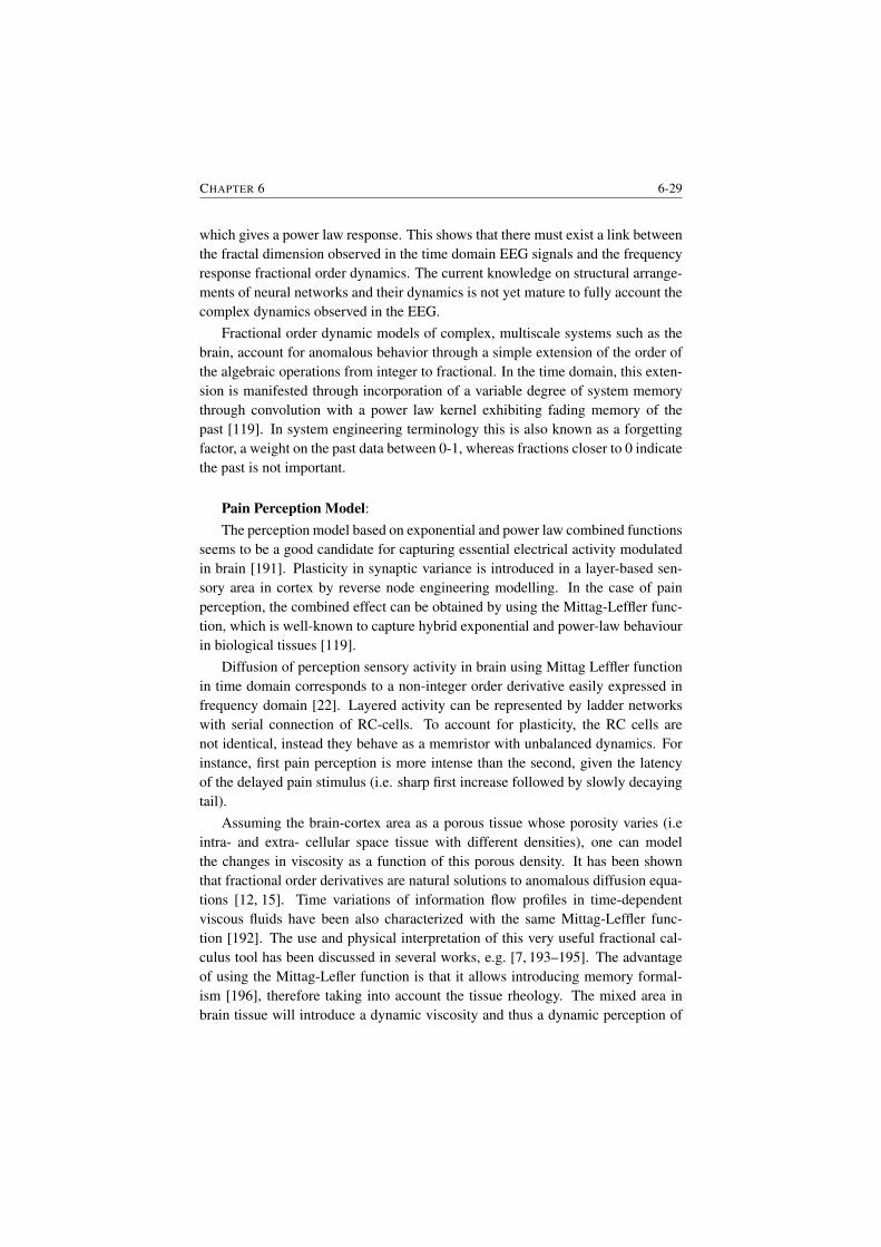
CHAPTER 6 6-29
which gives a power law response. This shows that there must exist a link betweenthe fractal dimension observed in the time domain EEG signals and the frequencyresponse fractional order dynamics. The current knowledge on structural arrange-ments of neural networks and their dynamics is not yet mature to fully account thecomplex dynamics observed in the EEG.
Fractional order dynamic models of complex, multiscale systems such as thebrain, account for anomalous behavior through a simple extension of the order ofthe algebraic operations from integer to fractional. In the time domain, this exten-sion is manifested through incorporation of a variable degree of system memorythrough convolution with a power law kernel exhibiting fading memory of thepast [119]. In system engineering terminology this is also known as a forgettingfactor, a weight on the past data between 0-1, whereas fractions closer to 0 indicatethe past is not important.
Pain Perception Model:The perception model based on exponential and power law combined functions
seems to be a good candidate for capturing essential electrical activity modulatedin brain [191]. Plasticity in synaptic variance is introduced in a layer-based sen-sory area in cortex by reverse node engineering modelling. In the case of painperception, the combined effect can be obtained by using the Mittag-Leffler func-tion, which is well-known to capture hybrid exponential and power-law behaviourin biological tissues [119].
Diffusion of perception sensory activity in brain using Mittag Leffler functionin time domain corresponds to a non-integer order derivative easily expressed infrequency domain [22]. Layered activity can be represented by ladder networkswith serial connection of RC-cells. To account for plasticity, the RC cells arenot identical, instead they behave as a memristor with unbalanced dynamics. Forinstance, first pain perception is more intense than the second, given the latencyof the delayed pain stimulus (i.e. sharp first increase followed by slowly decayingtail).
Assuming the brain-cortex area as a porous tissue whose porosity varies (i.eintra- and extra- cellular space tissue with different densities), one can modelthe changes in viscosity as a function of this porous density. It has been shownthat fractional order derivatives are natural solutions to anomalous diffusion equa-tions [12, 15]. Time variations of information flow profiles in time-dependentviscous fluids have been also characterized with the same Mittag-Leffler func-tion [192]. The use and physical interpretation of this very useful fractional cal-culus tool has been discussed in several works, e.g. [7, 193–195]. The advantageof using the Mittag-Lefler function is that it allows introducing memory formal-ism [196], therefore taking into account the tissue rheology. The mixed area inbrain tissue will introduce a dynamic viscosity and thus a dynamic perception of
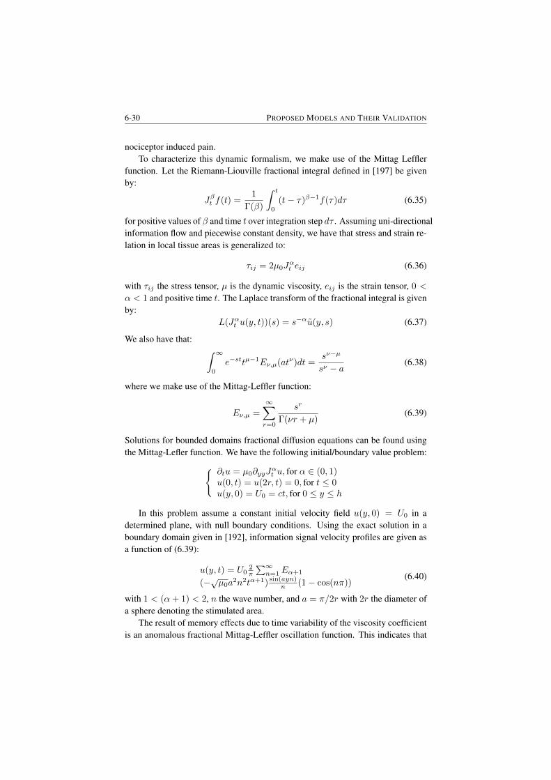
6-30 PROPOSED MODELS AND THEIR VALIDATION
nociceptor induced pain.To characterize this dynamic formalism, we make use of the Mittag Leffler
function. Let the Riemann-Liouville fractional integral defined in [197] be givenby:
Jβt f(t) =1
Γ(β)
∫ t
0
(t− τ)β−1f(τ)dτ (6.35)
for positive values of β and time t over integration step dτ . Assuming uni-directionalinformation flow and piecewise constant density, we have that stress and strain re-lation in local tissue areas is generalized to:
τij = 2µ0Jαt eij (6.36)
with τij the stress tensor, µ is the dynamic viscosity, eij is the strain tensor, 0 <
α < 1 and positive time t. The Laplace transform of the fractional integral is givenby:
L(Jαt u(y, t))(s) = s−αu(y, s) (6.37)
We also have that: ∫ ∞0
e−sttµ−1Eν,µ(atν)dt =sν−µ
sν − a(6.38)
where we make use of the Mittag-Leffler function:
Eν,µ =
∞∑r=0
sr
Γ(νr + µ)(6.39)
Solutions for bounded domains fractional diffusion equations can be found usingthe Mittag-Lefler function. We have the following initial/boundary value problem: ∂tu = µ0∂yyJ
αt u, for α ∈ (0, 1)
u(0, t) = u(2r, t) = 0, for t ≤ 0u(y, 0) = U0 = ct, for 0 ≤ y ≤ h
In this problem assume a constant initial velocity field u(y, 0) = U0 in adetermined plane, with null boundary conditions. Using the exact solution in aboundary domain given in [192], information signal velocity profiles are given asa function of (6.39):
u(y, t) = U02π
∑∞n=1Eα+1
(−√µ0a2n2tα+1) sin(ayn)
n (1− cos(nπ))(6.40)
with 1 < (α+ 1) < 2, n the wave number, and a = π/2r with 2r the diameter ofa sphere denoting the stimulated area.
The result of memory effects due to time variability of the viscosity coefficientis an anomalous fractional Mittag-Leffler oscillation function. This indicates that
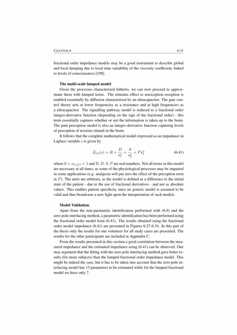
CHAPTER 6 6-31
fractional order impedance models may be a good instrument to describe globaland local damping due to local time variability of the viscosity coefficient, linkedto levels of consciousness [198].
The multi-scale lumped model:Given the processes characterized hitherto, we can now proceed to approx-
imate them with lumped terms. The stimulus effect to nociception reception isenabled essentially by diffusion characterised by an ultracapacitor. The gate con-trol theory acts at lower frequencies as a resistance and at high frequencies asa ultracapacitor. The signalling pathway model is reduced to a fractional orderintegro-derivative function (depending on the sign of the fractional order) - thisterm essentially captures whether or not the information is taken up to the brain.The pain perception model is also an integro-derivative function capturing levelsof perception of noxious stimuli in the brain.
It follows that the complete mathematical model expressed as an impedance inLaplace variable s is given by
Ztot(s) = R+D
sα1+
S
sα2+ Psα3 (6.41)
where 0 < α1,2,3 < 1 andR,D, S, P are real numbers. Not all terms in this modelare necessary at all times, as some of the physiological processes may be impairedin some applications (e.g. analgesia will put zero the effect of the perception termin P ). The units are arbitrary, as the model is defined as a difference to the initialstate of the patient - due to the use of fractional derivatives - and not as absolutevalues. This enables patient specificity since no generic model is assumed to bevalid and thus broadcasts a new light upon the interpretation of such models.
Model Validation:Apart from the non-parametric identification performed with (6.9) and the
zero-pole interlacing method, a parametric identification has been performed usingthe fractional order model from (6.41). The results obtained using the fractionalorder model impedance (6.41) are presented in Figures 6.27-6.34. In this part ofthe thesis only the results for one volunteer for all study cases are presented. Theresults for the other participants are included in Appendix C.
From the results presented in this section a good correlation between the mea-sured impedance and the estimated impedance using (6.41) can be observed. Onemay argument that the fitting with the zero-pole interlacing method gave better re-sults (for more subjects) than the lumped fractional order impedance model. Thismight be indeed the case, but it has to be taken into account that the zero-pole in-terlacing model has 13 parameters to be estimated while for the lumped fractionalmodel we have only 7.
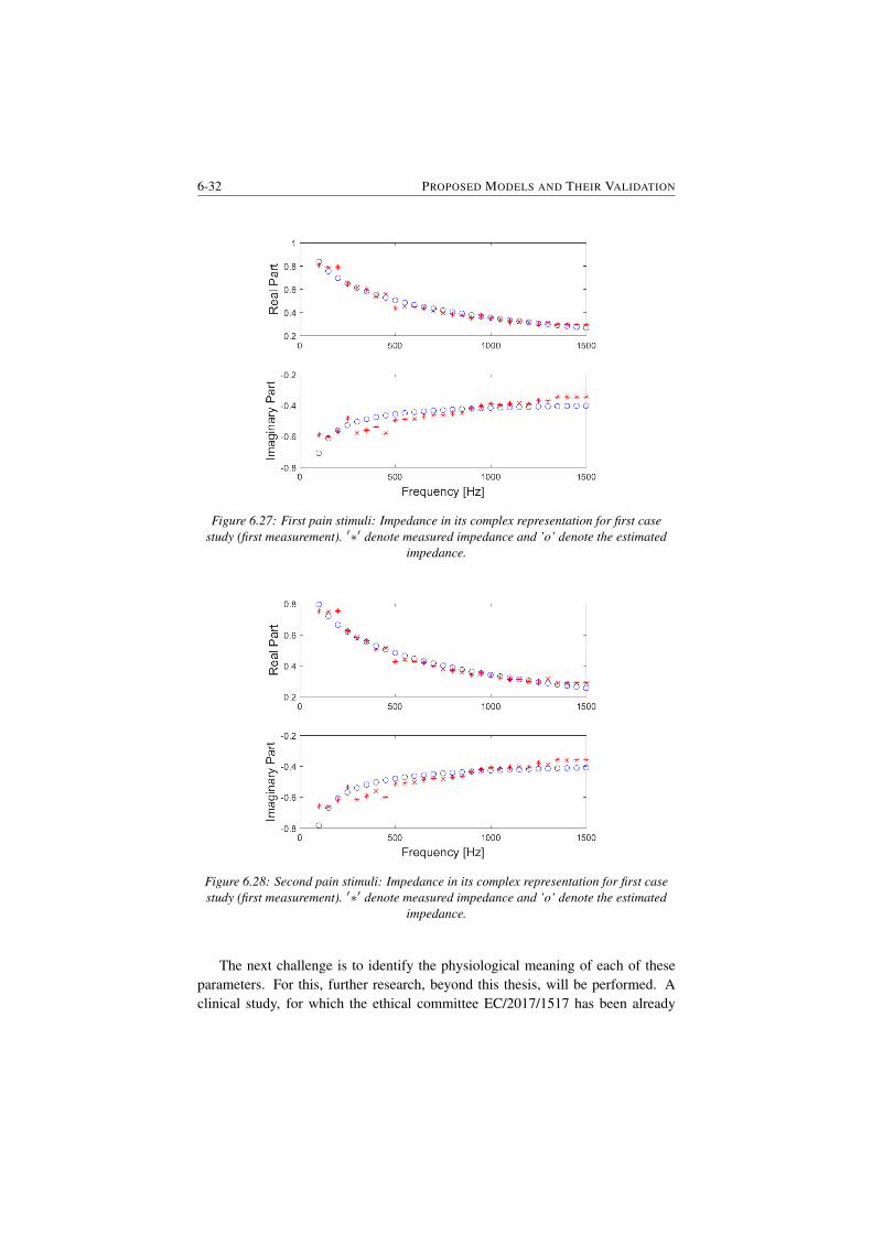
6-32 PROPOSED MODELS AND THEIR VALIDATION
Figure 6.27: First pain stimuli: Impedance in its complex representation for first casestudy (first measurement). ′∗′ denote measured impedance and ’o’ denote the estimated
impedance.
Figure 6.28: Second pain stimuli: Impedance in its complex representation for first casestudy (first measurement). ′∗′ denote measured impedance and ’o’ denote the estimated
impedance.
The next challenge is to identify the physiological meaning of each of theseparameters. For this, further research, beyond this thesis, will be performed. Aclinical study, for which the ethical committee EC/2017/1517 has been already
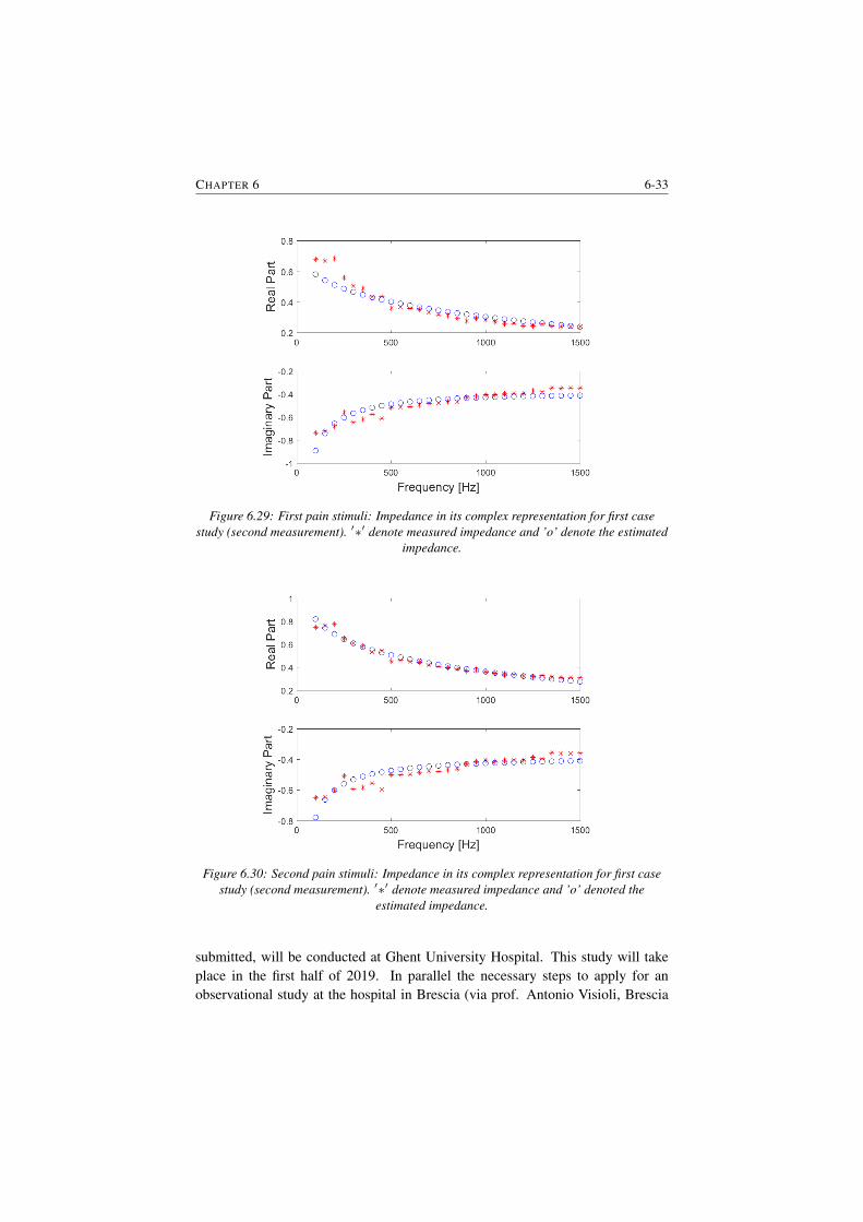
CHAPTER 6 6-33
Figure 6.29: First pain stimuli: Impedance in its complex representation for first casestudy (second measurement). ′∗′ denote measured impedance and ’o’ denote the estimated
impedance.
Figure 6.30: Second pain stimuli: Impedance in its complex representation for first casestudy (second measurement). ′∗′ denote measured impedance and ’o’ denoted the
estimated impedance.
submitted, will be conducted at Ghent University Hospital. This study will takeplace in the first half of 2019. In parallel the necessary steps to apply for anobservational study at the hospital in Brescia (via prof. Antonio Visioli, Brescia
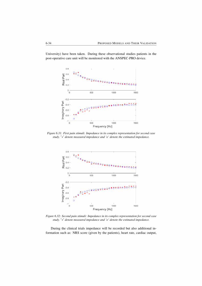
6-34 PROPOSED MODELS AND THEIR VALIDATION
University) have been taken. During these observational studies patients in thepost-operative care unit will be monitored with the ANSPEC-PRO device.
Figure 6.31: First pain stimuli: Impedance in its complex representation for second casestudy. ′∗′ denote measured impedance and ’o’ denote the estimated impedance.
Figure 6.32: Second pain stimuli: Impedance in its complex representation for second casestudy. ′∗′ denote measured impedance and ’o’ denote the estimated impedance.
During the clinical trials impedance will be recorded but also additional in-formation such as: NRS score (given by the patients), heart rate, cardiac output,
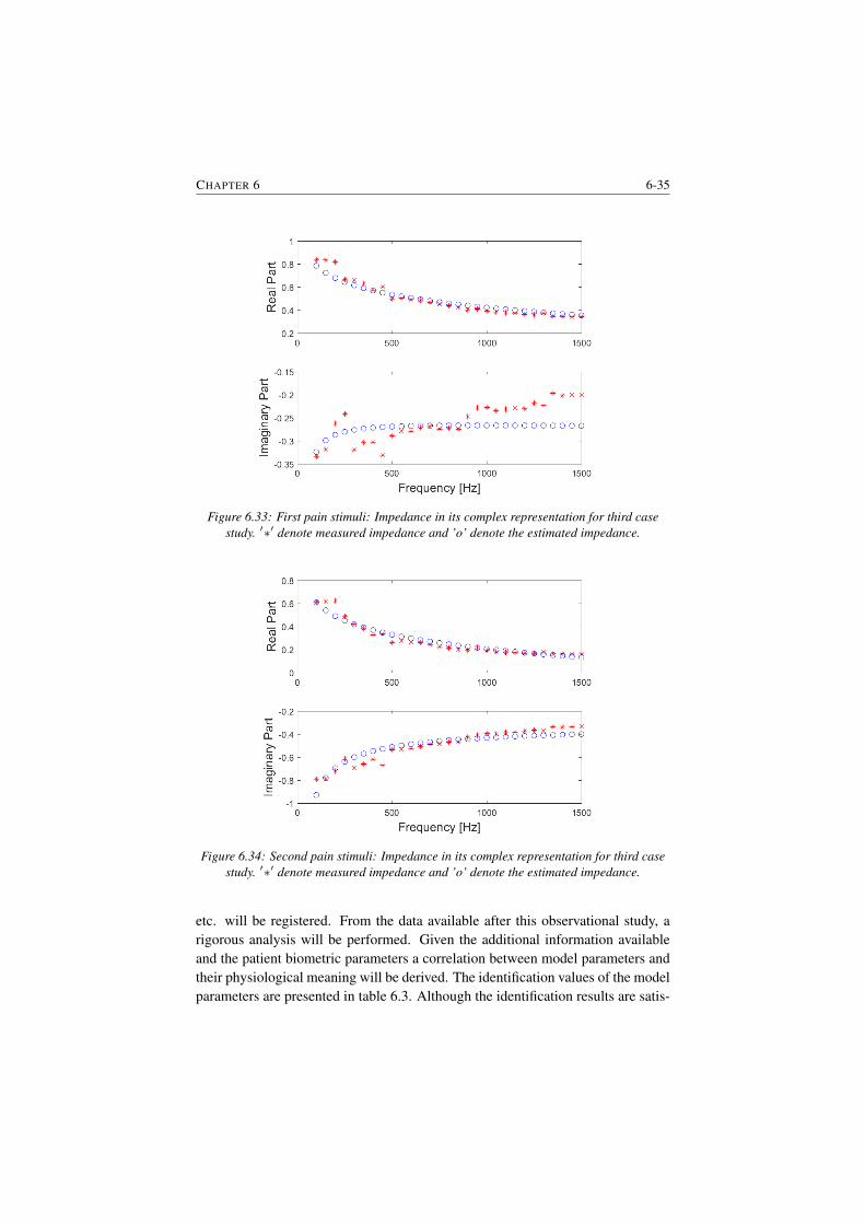
CHAPTER 6 6-35
Figure 6.33: First pain stimuli: Impedance in its complex representation for third casestudy. ′∗′ denote measured impedance and ’o’ denote the estimated impedance.
Figure 6.34: Second pain stimuli: Impedance in its complex representation for third casestudy. ′∗′ denote measured impedance and ’o’ denote the estimated impedance.
etc. will be registered. From the data available after this observational study, arigorous analysis will be performed. Given the additional information availableand the patient biometric parameters a correlation between model parameters andtheir physiological meaning will be derived. The identification values of the modelparameters are presented in table 6.3. Although the identification results are satis-

6-36 PROPOSED MODELS AND THEIR VALIDATION
factory and we have noticed that there are differences in model parameters betweenthe investigated case studies a more in depth analysis is needed. Therefore, furtherresearch with respect to the fractional order model parameters will be conducted.Also, an analysis between fractional order model parameter and the biometric pa-rameters has been conducted in order to identify if there is any correlation betweenthem. From this analysis no clear conclusion could be taken. We have noticed thatfor some of the fractional order parameter there is a correlation for others not.Therefore, these results have not been included in this chapter of the thesis but inAppendix A. Further research with respect to this particular item will be performedafter this thesis when also a higher number of subjects will be investigated suchthat statistically significant conclusions can be taken.
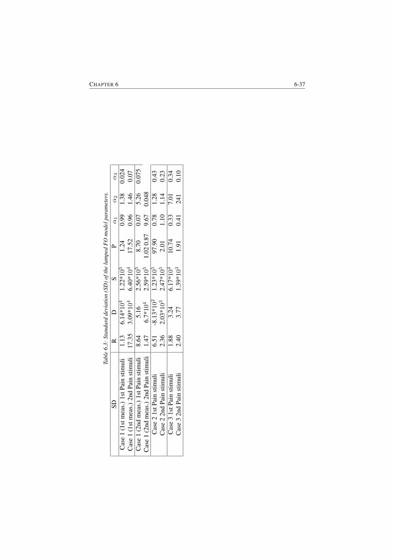
CHAPTER 6 6-37
Tabl
e6.
3:St
anda
rdde
viat
ion
(SD
)oft
helu
mpe
dF
Om
odel
para
met
ers.
SDR
DS
Pα1
α2
α3
Cas
e1
(1st
mea
s.)
1stP
ain
stim
uli
1.13
6.14
*104
1.22
*105
1.24
0.99
1.38
0.02
4C
ase
1(1
stm
eas.
)2n
dPa
inst
imul
i17
.35
3.09
*104
6.40
*104
17.5
20.
961.
460.
07C
ase
1(2
ndm
eas.
)1s
tPai
nst
imul
i8.
645.
162.
56*1
05
8.70
0.07
5.26
0.07
5C
ase
1(2
ndm
eas.
)2n
dPa
inst
imul
i1.
476.
7*104
2.59
*105
1.02
0.87
9.67
0.04
8C
ase
21s
tPai
nst
imul
i6.
51-8
.13*
102
1.23
*105
97.9
00.
781.
280.
43C
ase
22n
dPa
inst
imul
i2.
362.
03*1
032.
47*1
05
2.01
1.10
1.14
0.23
Cas
e3
1stP
ain
stim
uli
1.88
3.24
6.17
*104
10.7
40.
337.
010.
34C
ase
32n
dPa
inst
imul
i2.
403.
771.
39*1
03
1.91
0.41
241
0.10
6-38 PROPOSED MODELS AND THEIR VALIDATION
6.6 SummaryIn this Chapter the proposed model and their validation are presented. Four modelshave been investigated: Cole-Cole model, non-parametric impedance model, zero-pole interlacing model and lumped fractional order impedance model. All thesemodels have been validated on real data and the outcome of this chapter is thatthe fractional order impedance model can capture the changes in impedance whena pain stimulus is applied. Although the obtained results are satisfactory furtherresearch is needed and the following tasks need to be performed:
• measurements on larger number of participants to enable statistical mean-ingful conclusions;
• a clinical study where patients are standardly treated for pain (i.e. not acontrollable environment, pain is already present);
• perform a rigorous analysis of these measurements to extract the required in-formation for a physisological interpretation of each parameter in the model;
• an index needs to be derived to indicate the level of pain;
All these tasks are beyond the scope of this thesis.
7Conclusions
In this Chapter the conclusions of the work presented in this thesis are addressed.The main contributions and further work are emphasized. The conclusions aredrawn from two perspectives: diffusion model of gas exchange in the lungs and amodel to characterize the nociceptor pathways.
Diffusion of gas in the lungs is a passive physical process that exchanges oxy-gen and carbon dioxide between the alveoli and the blood (in the lungs) and be-tween the blood an the cells (in the periphery). Based on the theory presented inChapter 2 and the results given in Chapter 3 we have shown that the complex phe-nomenon of gas exchange in the lungs can be approximated with a fractional ordermodel. In this thesis, the importance of diffusion in patients with COPD diseasehas been investigated. Measurement of the diffusion factor might be of importancein (early) detection of COPD disease. The single breath method became the mostgenerally accepted method. In this thesis emerging tools from fractional calculushave been used to capture changes in COPD disease and to understand their effecton the model parameters.
The results presented in this thesis indicate a direct link relation between theT index and the heterogeneity in COPD lungs. Although the results obtained arepromising there are still challenges to be solved. The model presented in thisthesis is an approximation based on analogy, hence the theoretical link betweendiffusion in the lungs and the model presented in Chapter 2 will be further inves-tigated. Moreover, in this thesis a relatively small study in a somewhat heteroge-neous group of COPD patients has been performed.
7-2 CONCLUSION
According to the literature, detection and parameterization of nociceptor activ-ity is of crucial importance for treatment in chronic pain patients, in post-surgerypatients, rehabilitation and follow up studies of new medication development. Thelack of system engineering tools to capture the most important multi-scale pro-cesses involved in the reception, transmission and perception of pain has kept ona slow pace the potential development of pain management services. A specificdomain of application where such models are greatly needed is the depth of anes-thesia regulatory paradigm. As such, the model presented in this thesis enablesnew horizons and has the potential to unlock the current state of art in this specificarea of application.
Patient specificity implies the ability to characterise changes in the variousprocess dynamics involved in nociceptor pathways and perception. The proposedparametric model is unique in its formalism and systems engineering approach.The lumped model provides the most versatile features to capture changes in dy-namic responses, with the minimal number of parameter values. This keeps thenumerical complexity to a low level, enabling deployment on real-time platformsand fast computation rates for identification from real-life data.
The proposed model considers a time-frequency mathematical formulation. Ithas been shown that many biomedical signals may benefit from time-frequencyanalysis. Since the frequency content of many biomedical signals can fast withtime (i.e. changes in impedance when a pain stimulus is applied are very fast),the time-frequency analysis allows us to capture these changes. This is of greatimportance in pathology cases, where changes in tissue structure and morphologyaffects directly the dynamic profiles of drug diffusion, permeability and molecularbinding. Specific structural changes with disease may also reveal various pathsof deep tissue trapping of drug and latency nodes which could explain effects ob-served in long-tailed observations. This work enables a mapping of the variouscomponents of the pain pathways. The description follows the micro- and macro-structural elements. The end result is an innovative and original methodology tocapture the signalling pathways and deliver an objective, independent and usefulmeasure for pain.
In this thesis, the first steps towards a sensor to measure the pain level in anobjective manner and a model of nociception pathway have been made. The resultis the ANSPEC-PRO monitor, non-invasively measuring pain by means of skinimpedance. The prototype has been validated at this moment only in awake volun-teers with self-induced nociceptor excitation (i.e. mechanical pain stimuli). Giventhe low subjects number and the controlled environment in which the device hasbeen tested, an ethical committee application (EC/2017/1517) has been submit-ted for measurements at the University Hospital Ghent. In parallel, the necessarysteps for submitting an ethical committee application at Brescia University Hospi-tal have been taken. The aim of these observational studies is to observe patients

CHAPTER 7 7-3
in the post-operative care unit. These patients are treated for pain following thestandard procedure (i.e. based on NRS scale).
7.1 Future perspectivesAnesthesia paradigm consists of three main components: hypnosis, neuromuscularblockade and analgesia. The first two components are well now mature for integra-tion in a single environment. Hence, the missing piece is analgesia. The results ofthis thesis will enable the next steps towards a complete regulatory dynamic systemfor controlling general anesthesia by means of its all three components. However,the proposed model cannot be yet used in closed loop and a further developmentis required. More specifically, a correlation with drug concentration needs to bemade. This aspect has not been addressed in this thesis. A possibility to measuredrug concentration is using blood sample. However, to include this informationin closed loop continuous measurement of drug concentration is necessary. Giventhe technological advances nowadays a non-invasive or minimally invasive mea-surement of drug concentration would be ideal. This is not yet available and afirst hypothesis to be investigated is similar to continuous measurement of glu-cose concentration. More specifically, a thing wire sensor is inserted under theskin and measures the glucose concentration in the interstitial fluid. Studies haveshown that there is no significant time lag among the interstitial fluid, capillaryand venous glucose levels. At this moment the model can be used as disturbance.For instance if we know the surgery profile we can used the developed model as adisturbance to predict that an increase in the nociception level will occur.
The aim beyond this doctoral thesis is to develop a bullet-proof analysis of acomplete regulatory dynamic system for controlling general anesthesia by meansof all its three components: hypnosis, analgesia and neuromuscular blockade. Todate, nowhere worldwide exist such a complete system in simulation studies, letalone in practice. This system will feature multiple input and multiple outputvariable analysis, model development and adaptation and robust, stable, adaptivecontrol algorithms. Safety loops will be mimicked into the system, as well as sur-gical disturbances and noxious stimulation profiles. All these independent featuresare available in their single regulatory loop. Their combination and the effect oftheir combination on the patient state profiles is yet unknown.
The longer term objective will be to implement a clinical onset for this com-plete regulatory system following EC advise and policies at Ghent University Hos-pital. This is a challenging and unconventional research which requires the collab-oration and acceptance from the medical practitioners. Given our long-standingcollaboration with Ghent University Hospital and other hospitals in Europe (i.e.Breascia University) ethical committee files will be submitted to validate the de-veloped automated anesthesia system.


AANSPEC-PRO Device
In this Appendix the development of a measurement device for continuous mon-itoring of changes in skin impedance as a function of an applied stimulus is pre-sented. This proof of concept device has been developed starting from the per-spective that a pain stimulus can be detected from a change in skin impedance as afunction of time and frequency. The skin is a black box and in order to obtain theimpedance the skin is excited with a known voltage and simultaneous measuringthe current flowing through the skin. The relation between this input voltage V (s)
and output current I(s) is:
Z(s) =V (s)
I(s)(A.1)
Notice that skin impedance Z(s), input voltage V (s) and output current I(s) are infunction of s = jω and, thus, are dependent on frequency (ω = 2πf ) of the exci-tation signal [201]. To obtain a wide range of information on the behaviour of theskin impedance the skin is excited at different frequencies. For this identificationmethod with multiple exciting frequencies a multisine signal is used [202]. Thissignal is a superposition of a number of sines with different frequencies. UsingNon-Parametric Identification techniques the impedance Z(s) can be estimated.As mentioned before, this transfer function Z(s) will change in time, due to painstimuli or other external influences [203]. This will increase the complexity of theNon-Parametric Identification as a time factor will be introduced.
The device will consist of the following subsystems that will work together:hardware, software and data analysis. Measuring current is not easy compared tovoltages and therefore the signal is conditioned and the current is transformed to

A-2 ANSPEC-PRO DEVICE
a voltage which can be interpreted by the measuring device (see Figure A.1). Asignal is designed off-line (a priori). This signal v(t) is sampled and needs to besent to an analogue output port, using zero-order hold, with a certain samplingfrequency, fs. Simultaneously, the current i(t) coming from the skin needs to bemeasured. The voltage v(t) and current i(t) are saved in a file that is defined bythe user.
Figure A.1: Block diagram with the skin impedance Z(s, k) as black box system; Thebioimpedance is in function of the frequency and discretised time k.
General description of the investigational device and its components includingmaterials used: The developed device is non-invasive, as electrodes are temporar-ily attached to the skin of the human body. The electrodes and electrode con-nectors are CE-marked (according to MDD93/42/EEC). The National InstrumentsCompactRIO that is used to measure the patient fulfills the following electricalequipment safety standards:
• IEC 61010-1, EN 61010-1
• UL 61010-1, CSA 61010-1
• EN 60079-0:2012, EN 60079-15:2010
• IEC 60079-0: Ed 6, IEC 60079-15, Ed 4
• UL 60079-0; Ed 5, UL 60079-15; Ed 3
• CSA 60079-0:2011, CSA 60079-15:2012
Regarding the electromagnetic compatibility the cRIO meets the requirements ofthe following EMC standards for electrical equipment:
• EN 61326 (IEC 61326): Class A emissions; Industrial immunity
• EN 55011 (CISPR 11): Group 1, Class A emissions
• AS/NZS CISPR 11: Group 1, Class A emissions
• FCC 47 CFR Part 15B: Class A emissions
• ICES-001: Class A emissions
The devices meets the essential requirements of applicable European Directives,and therefore receiving the CE Mark, as follows:
APPENDIX A A-3
• 2014/35/EU; Low-Voltage Directive (safety)
• 2014/30/EU; Electromagnetic Compatibility Directive (EMC)
• 94/9/EC; Potentially Explosive Atmospheres (ATEX)
The device is built while taking into account the A.R.E.I. (Algemeen Regle-ment op de elektrische installaties) regulations, that provides rules of thumbs forsafety of electrical equipment, regarding electrical shocks, safety, grounding, etc.The device consists of two hardware parts: a laptop and a data-acquisition cir-cuit. The two parts are interconnected through Ethernet cables that links the twodevices to a common network. The laptop is a standard laptop with the operat-ing system Windows 7 Enterprise 64-bit and a INTEL(R) Core(TM) [email protected] processor.
Data-acquisition circuit consists of two DC-converters with galvanic separa-tors, step-down transformers, that will output 24 V DC and +/-15 V DC. The +/-15V DC will supply the power to the electrodes. The power is 3.75 VA and the trans-former is approved according to the ENEC 10 (VDE) legislations. The safety classof the transformer is class II, which indicates that it has a double insulation. Thevoltage is rectified and a voltage regulator provides a short-circuit protection in itspackage. A National Instruments (Texas, USA) device (cRIO9074 with NI9201-and NI9263-slots) is used to excite a part of the skin with an off-line designed volt-age signal. This voltage will induce a current in the circuit related to the impedanceof the human body. This current is captured and saved onto the laptop. A voltagebuffer limits the supplied current to +/-20 mA.
The user interface has been developed in LabView and the main block dia-grams behind figure A.2 are presented below. In this interface, the following num-bers are depicted:
1. Load the input signal;
2. Set the sampling frequency in Hz;
3. Set the frequency resolution in Hz;
4. Set the amplitude of output signal. This is to control saturation of the inputsignal to the patient (see 10);
5. The number of seconds that are saved per data file.
6. After fields 1 to 5 and 7 are filled in, start acquiring by pressing 6 - Startacquisition;
7. Create the paths and file name where to save the data. Remark that the datais only saved when 9 - Save is selected;
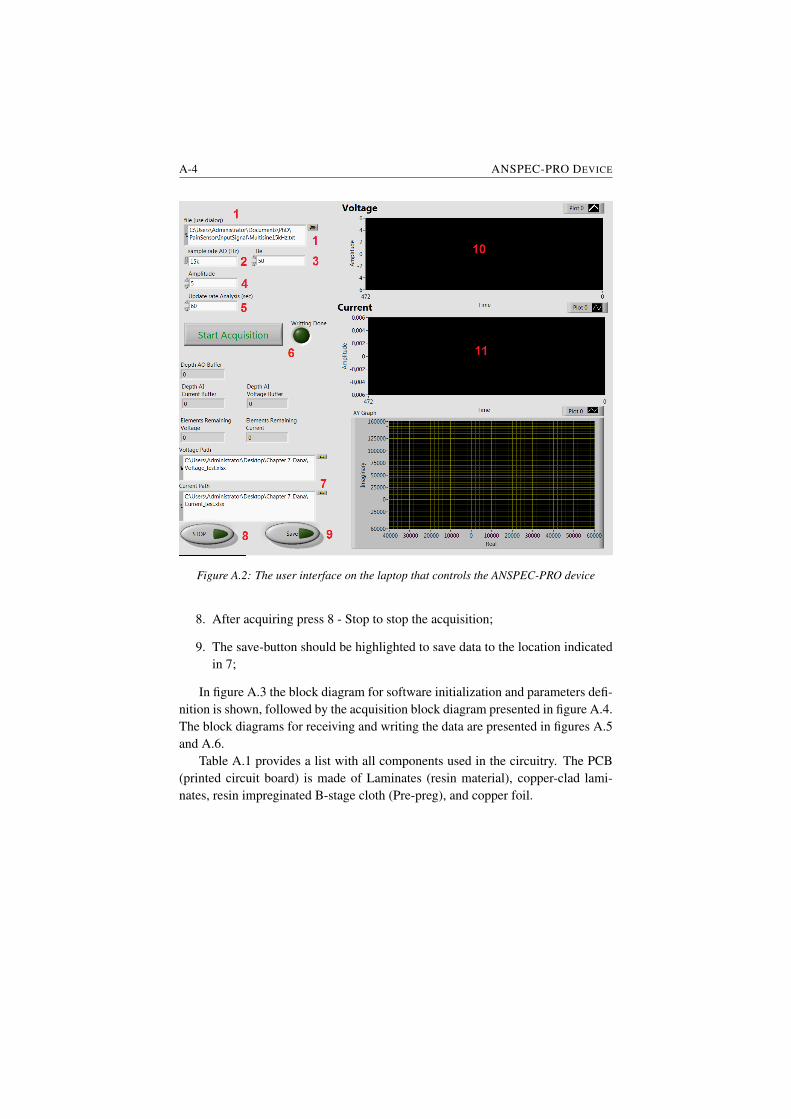
A-4 ANSPEC-PRO DEVICE
Figure A.2: The user interface on the laptop that controls the ANSPEC-PRO device
8. After acquiring press 8 - Stop to stop the acquisition;
9. The save-button should be highlighted to save data to the location indicatedin 7;
In figure A.3 the block diagram for software initialization and parameters defi-nition is shown, followed by the acquisition block diagram presented in figure A.4.The block diagrams for receiving and writing the data are presented in figures A.5and A.6.
Table A.1 provides a list with all components used in the circuitry. The PCB(printed circuit board) is made of Laminates (resin material), copper-clad lami-nates, resin impreginated B-stage cloth (Pre-preg), and copper foil.
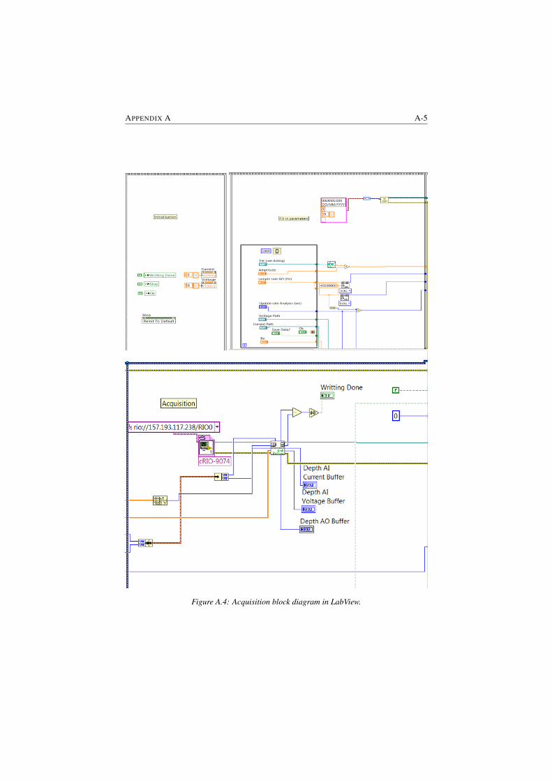
APPENDIX A A-5
Figure A.4: Acquisition block diagram in LabView.
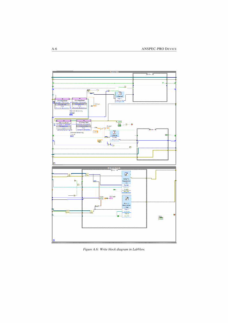
A-6 ANSPEC-PRO DEVICE
Figure A.6: Write block diagram in LabView.
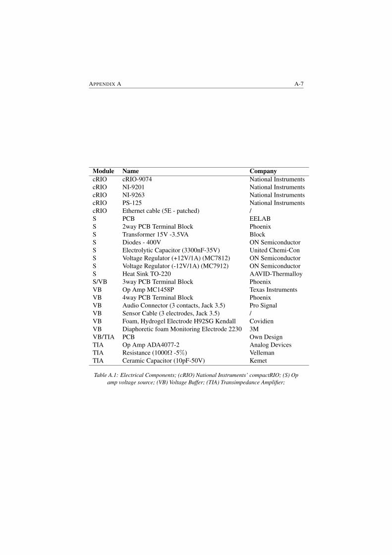
APPENDIX A A-7
Module Name CompanycRIO cRIO-9074 National InstrumentscRIO NI-9201 National InstrumentscRIO NI-9263 National InstrumentscRIO PS-125 National InstrumentscRIO Ethernet cable (5E - patched) /S PCB EELABS 2way PCB Terminal Block PhoenixS Transformer 15V -3.5VA BlockS Diodes - 400V ON SemiconductorS Electrolytic Capacitor (3300nF-35V) United Chemi-ConS Voltage Regulator (+12V/1A) (MC7812) ON SemiconductorS Voltage Regulator (-12V/1A) (MC7912) ON SemiconductorS Heat Sink TO-220 AAVID-ThermalloyS/VB 3way PCB Terminal Block PhoenixVB Op Amp MC1458P Texas InstrumentsVB 4way PCB Terminal Block PhoenixVB Audio Connector (3 contacts, Jack 3.5) Pro SignalVB Sensor Cable (3 electrodes, Jack 3.5) /VB Foam, Hydrogel Electrode H92SG Kendall CovidienVB Diaphoretic foam Monitoring Electrode 2230 3MVB/TIA PCB Own DesignTIA Op Amp ADA4077-2 Analog DevicesTIA Resistance (1000Ω -5%) VellemanTIA Ceramic Capacitor (10pF-50V) Kemet
Table A.1: Electrical Components; (cRIO) National Instruments’ compactRIO; (S) Opamp voltage source; (VB) Voltage Buffer; (TIA) Transimpedance Amplifier;

BMeasurement results
Results obtained using the non-parametric impedance modelIn Figures B.1 - B.6 the measurement results obtained for the first case study
are reported followed by the results for the second case study in Figures B.7 - B.9and third case study in Figures B.10 - B.12. Next, the results only showing thepain intervals are presented in Figures B.13 - B.18 for the first case study followedby the results for the second case study in Figures B.19 - B.21 and for the thirdcase study in Figures B.22 - B.24.
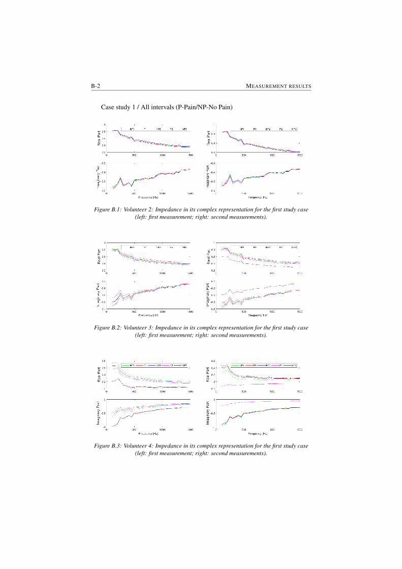
B-2 MEASUREMENT RESULTS
Case study 1 / All intervals (P-Pain/NP-No Pain)
Figure B.1: Volunteer 2: Impedance in its complex representation for the first study case(left: first measurement; right: second measurements).
Figure B.2: Volunteer 3: Impedance in its complex representation for the first study case(left: first measurement; right: second measurements).
Figure B.3: Volunteer 4: Impedance in its complex representation for the first study case(left: first measurement; right: second measurements).
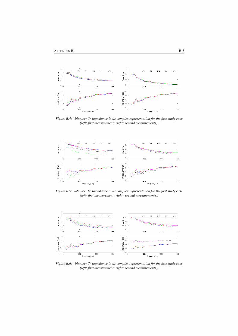
APPENDIX B B-3
Figure B.4: Volunteer 5: Impedance in its complex representation for the first study case(left: first measurement; right: second measurements).
Figure B.5: Volunteer 6: Impedance in its complex representation for the first study case(left: first measurement; right: second measurements).
Figure B.6: Volunteer 7: Impedance in its complex representation for the first study case(left: first measurement; right: second measurements).
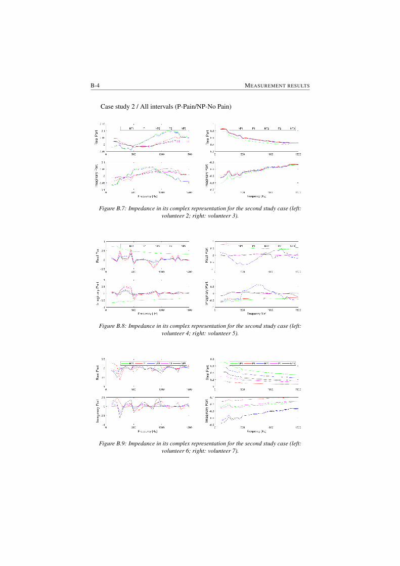
B-4 MEASUREMENT RESULTS
Case study 2 / All intervals (P-Pain/NP-No Pain)
Figure B.7: Impedance in its complex representation for the second study case (left:volunteer 2; right: volunteer 3).
Figure B.8: Impedance in its complex representation for the second study case (left:volunteer 4; right: volunteer 5).
Figure B.9: Impedance in its complex representation for the second study case (left:volunteer 6; right: volunteer 7).
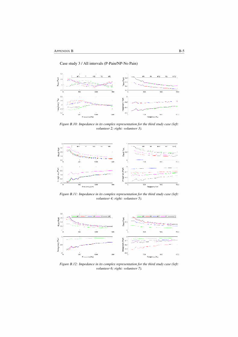
APPENDIX B B-5
Case study 3 / All intervals (P-Pain/NP-No Pain)
Figure B.10: Impedance in its complex representation for the third study case (left:volunteer 2; right: volunteer 3).
Figure B.11: Impedance in its complex representation for the third study case (left:volunteer 4; right: volunteer 5).
Figure B.12: Impedance in its complex representation for the third study case (left:volunteer 6; right: volunteer 7).
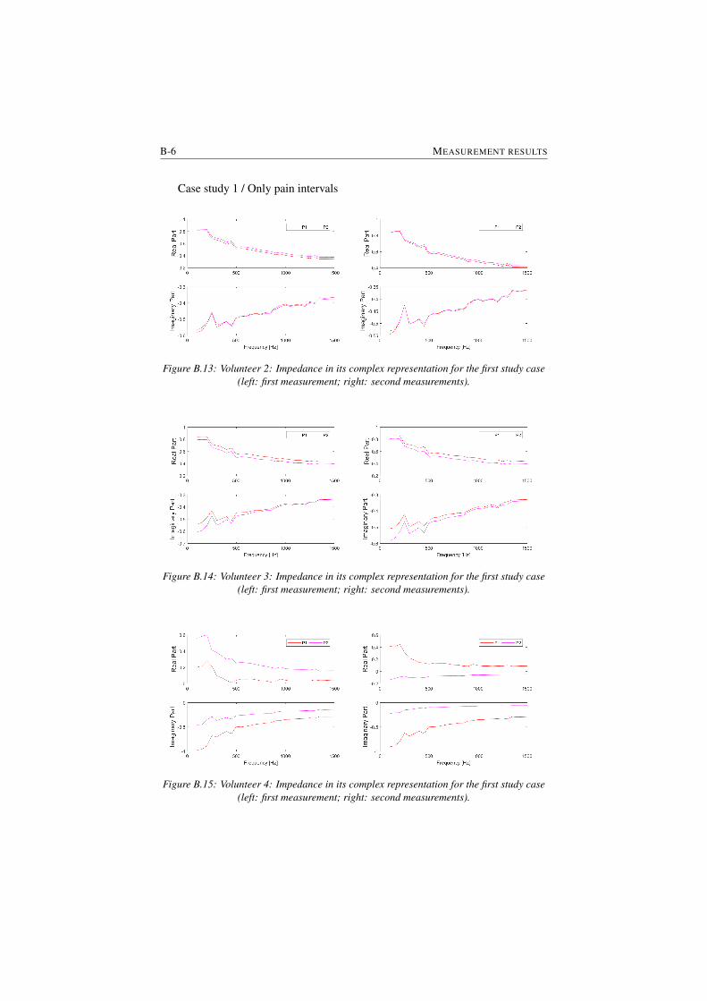
B-6 MEASUREMENT RESULTS
Case study 1 / Only pain intervals
Figure B.13: Volunteer 2: Impedance in its complex representation for the first study case(left: first measurement; right: second measurements).
Figure B.14: Volunteer 3: Impedance in its complex representation for the first study case(left: first measurement; right: second measurements).
Figure B.15: Volunteer 4: Impedance in its complex representation for the first study case(left: first measurement; right: second measurements).
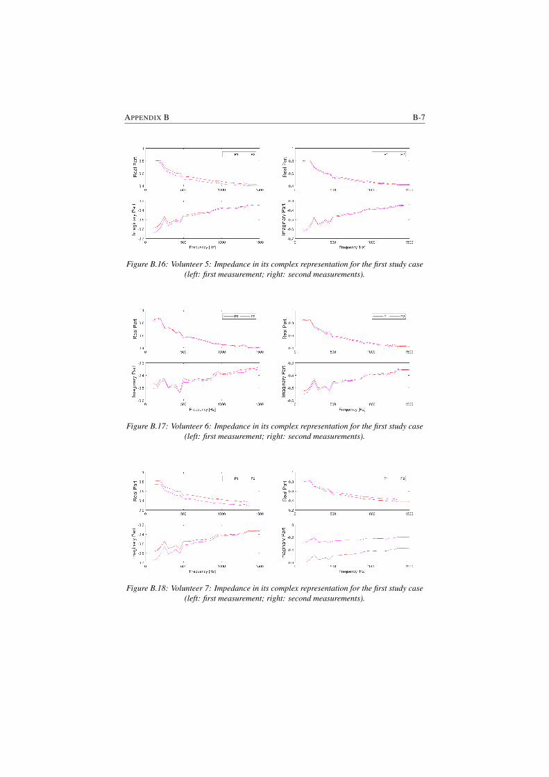
APPENDIX B B-7
Figure B.16: Volunteer 5: Impedance in its complex representation for the first study case(left: first measurement; right: second measurements).
Figure B.17: Volunteer 6: Impedance in its complex representation for the first study case(left: first measurement; right: second measurements).
Figure B.18: Volunteer 7: Impedance in its complex representation for the first study case(left: first measurement; right: second measurements).
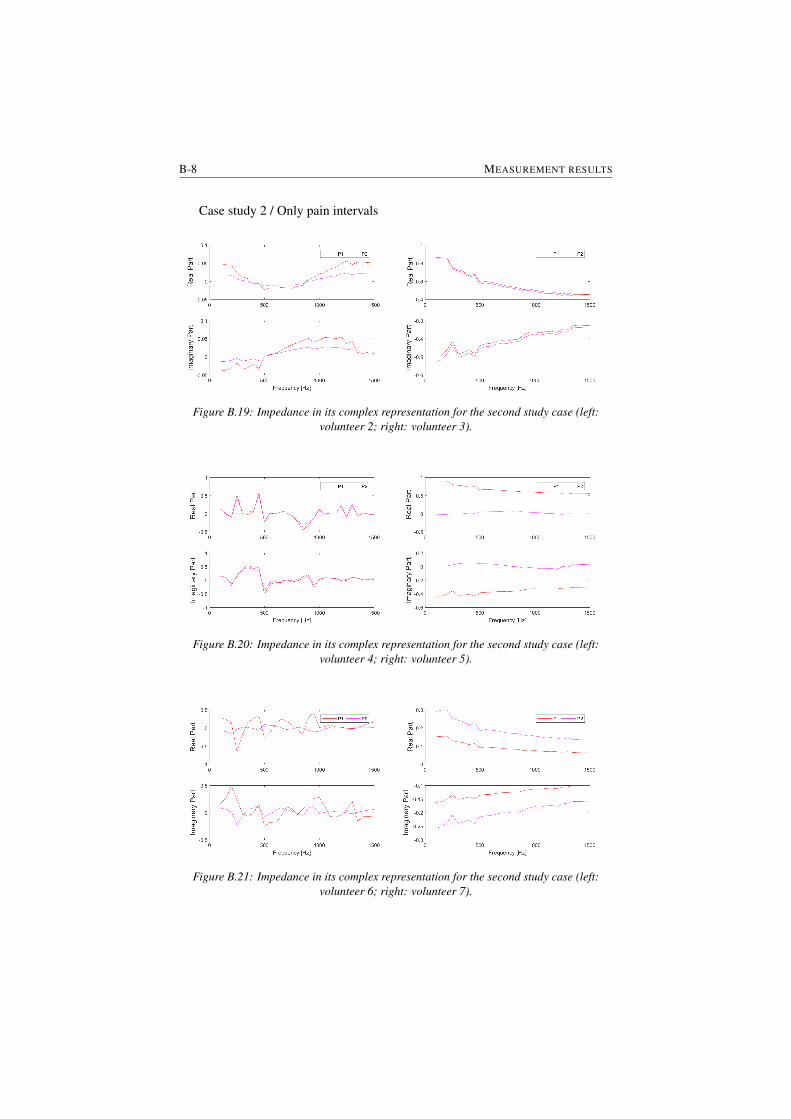
B-8 MEASUREMENT RESULTS
Case study 2 / Only pain intervals
Figure B.19: Impedance in its complex representation for the second study case (left:volunteer 2; right: volunteer 3).
Figure B.20: Impedance in its complex representation for the second study case (left:volunteer 4; right: volunteer 5).
Figure B.21: Impedance in its complex representation for the second study case (left:volunteer 6; right: volunteer 7).
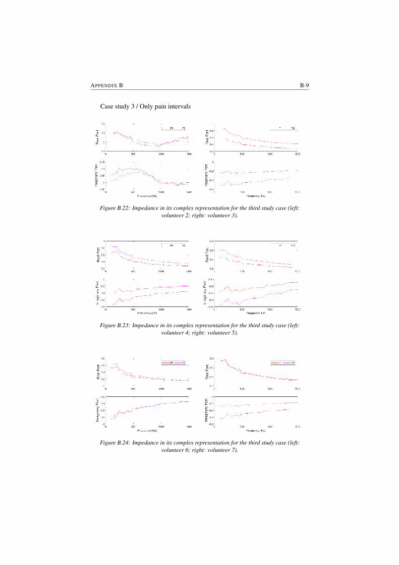
APPENDIX B B-9
Case study 3 / Only pain intervals
Figure B.22: Impedance in its complex representation for the third study case (left:volunteer 2; right: volunteer 3).
Figure B.23: Impedance in its complex representation for the third study case (left:volunteer 4; right: volunteer 5).
Figure B.24: Impedance in its complex representation for the third study case (left:volunteer 6; right: volunteer 7).

CIdentification results
In this appendix the results obtained for the zero pole model and the fractional or-der impedance model are presented. Both models have been validated on real dataand the outcome of this chapter is that the fractional order impedance model cancapture the changes in impedance when a pain stimulus is applied. An iterativeidentification procedure has been performed in order to fit the model to the mea-sured data. Iteration has been performed to avoid local minimum and the numberof iterations between the identified results varied between 2 and 4 in all data. Theiteration stopped when the model parameters have changed less than 5%. As forthe case of the non-iterative method, the using the iterative method the fitting of themodel to the real data did not worked for all cases. From the analysis performedin this thesis we could not conclude is there is a correlation between the biomet-ric data of the volunteers and model parameters. This can be due to the limitednumber of volunteers but also given the homogeneity of the group. This will befurther investigated based on the data recorded during the clinical trial that willtake place at the UZ Gent. In this case the variety of patient type (e.g. body massindex) will be more significant than in our group of volunteers and an analysis onthe variability among patients can be performed.
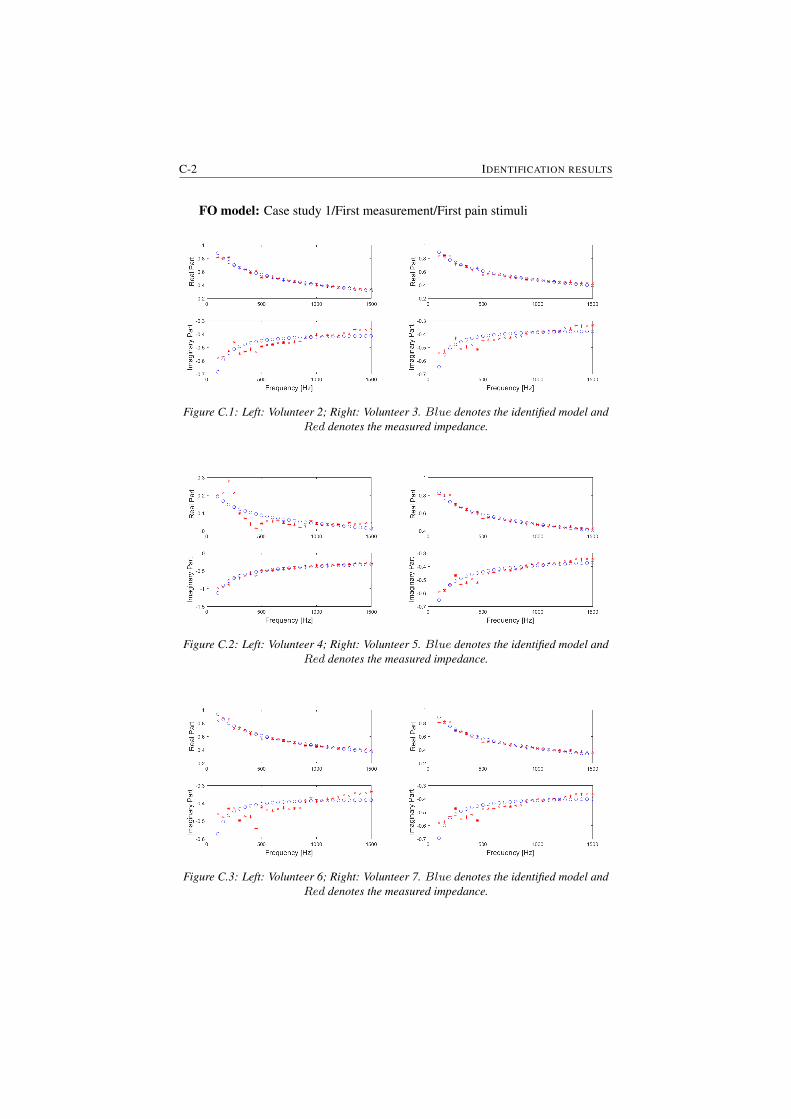
C-2 IDENTIFICATION RESULTS
FO model: Case study 1/First measurement/First pain stimuli
Figure C.1: Left: Volunteer 2; Right: Volunteer 3. Blue denotes the identified model andRed denotes the measured impedance.
Figure C.2: Left: Volunteer 4; Right: Volunteer 5. Blue denotes the identified model andRed denotes the measured impedance.
Figure C.3: Left: Volunteer 6; Right: Volunteer 7. Blue denotes the identified model andRed denotes the measured impedance.
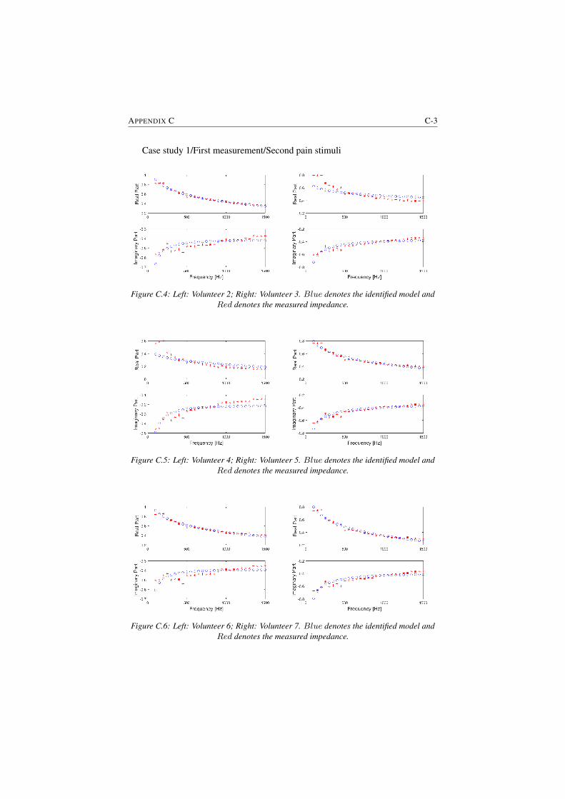
APPENDIX C C-3
Case study 1/First measurement/Second pain stimuli
Figure C.4: Left: Volunteer 2; Right: Volunteer 3. Blue denotes the identified model andRed denotes the measured impedance.
Figure C.5: Left: Volunteer 4; Right: Volunteer 5. Blue denotes the identified model andRed denotes the measured impedance.
Figure C.6: Left: Volunteer 6; Right: Volunteer 7. Blue denotes the identified model andRed denotes the measured impedance.
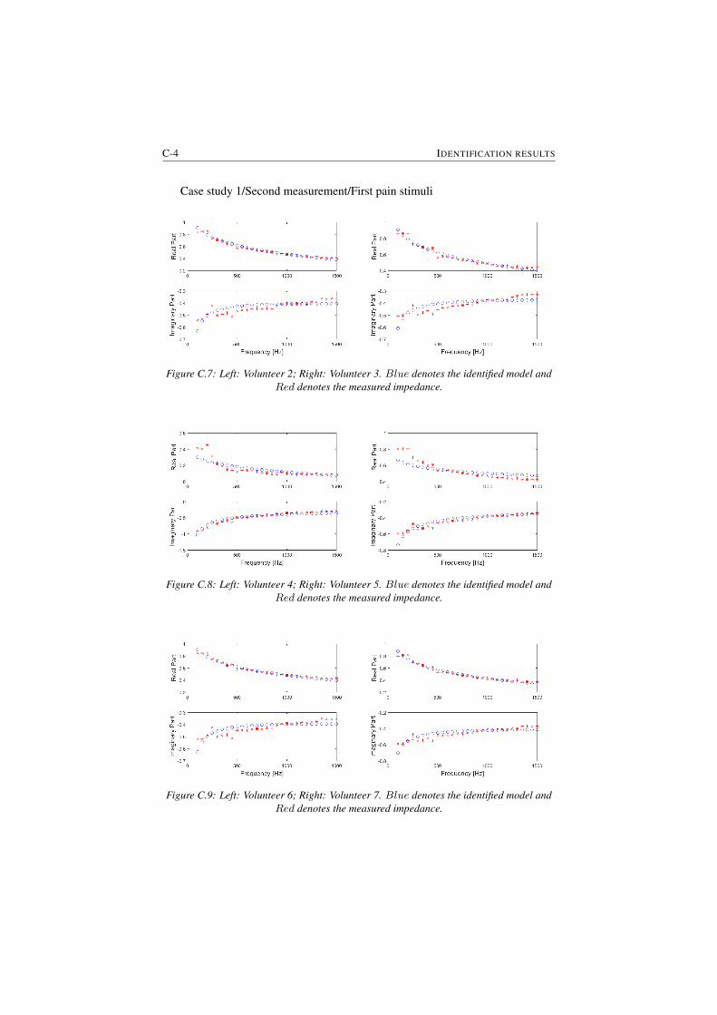
C-4 IDENTIFICATION RESULTS
Case study 1/Second measurement/First pain stimuli
Figure C.7: Left: Volunteer 2; Right: Volunteer 3. Blue denotes the identified model andRed denotes the measured impedance.
Figure C.8: Left: Volunteer 4; Right: Volunteer 5. Blue denotes the identified model andRed denotes the measured impedance.
Figure C.9: Left: Volunteer 6; Right: Volunteer 7. Blue denotes the identified model andRed denotes the measured impedance.
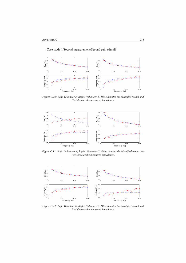
APPENDIX C C-5
Case study 1/Second measurement/Second pain stimuli
Figure C.10: Left: Volunteer 2; Right: Volunteer 3. Blue denotes the identified model andRed denotes the measured impedance.
Figure C.11: tLeft: Volunteer 4; Right: Volunteer 5. Blue denotes the identified model andRed denotes the measured impedance.
Figure C.12: Left: Volunteer 6; Right: Volunteer 7. Blue denotes the identified model andRed denotes the measured impedance.
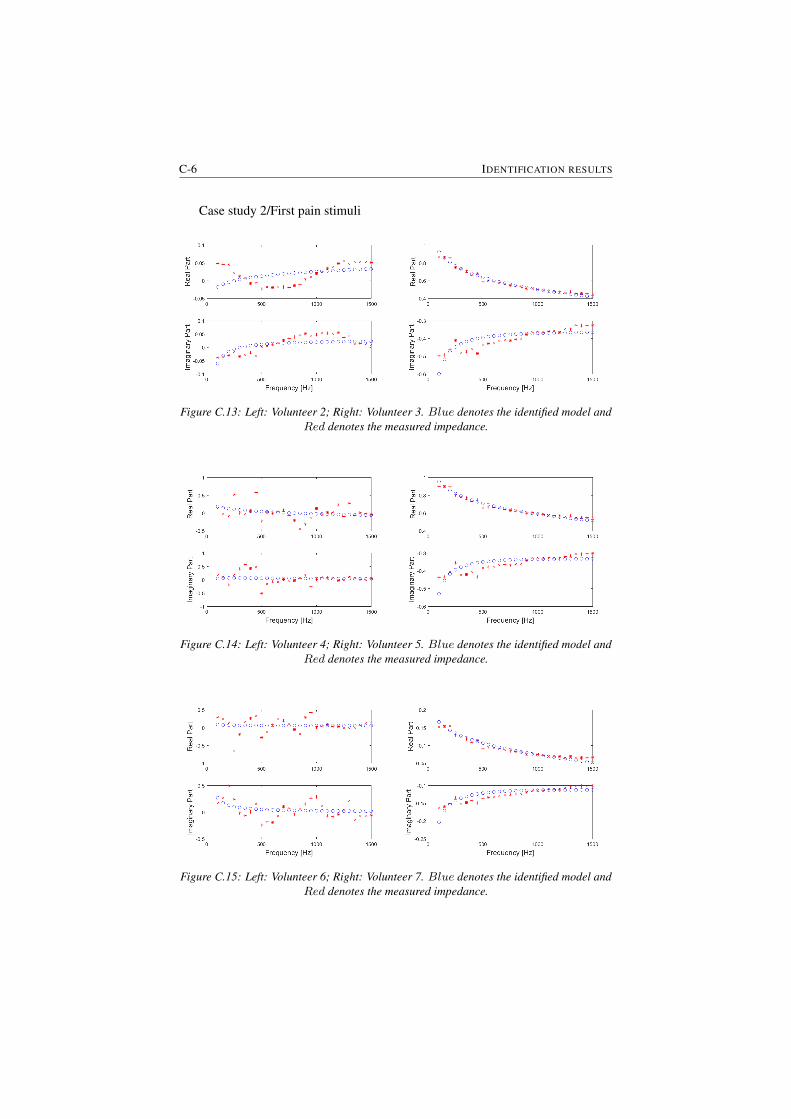
C-6 IDENTIFICATION RESULTS
Case study 2/First pain stimuli
Figure C.13: Left: Volunteer 2; Right: Volunteer 3. Blue denotes the identified model andRed denotes the measured impedance.
Figure C.14: Left: Volunteer 4; Right: Volunteer 5. Blue denotes the identified model andRed denotes the measured impedance.
Figure C.15: Left: Volunteer 6; Right: Volunteer 7. Blue denotes the identified model andRed denotes the measured impedance.
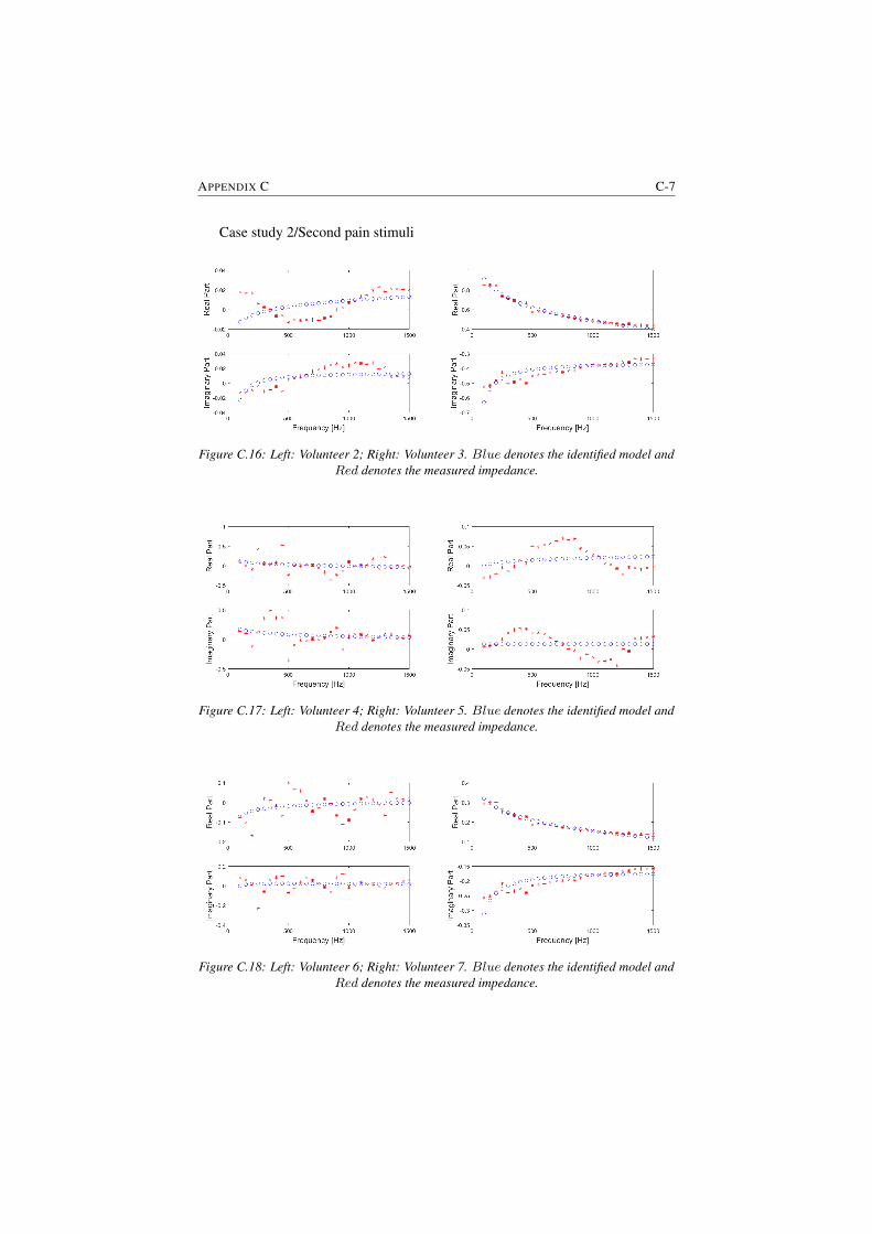
APPENDIX C C-7
Case study 2/Second pain stimuli
Figure C.16: Left: Volunteer 2; Right: Volunteer 3. Blue denotes the identified model andRed denotes the measured impedance.
Figure C.17: Left: Volunteer 4; Right: Volunteer 5. Blue denotes the identified model andRed denotes the measured impedance.
Figure C.18: Left: Volunteer 6; Right: Volunteer 7. Blue denotes the identified model andRed denotes the measured impedance.
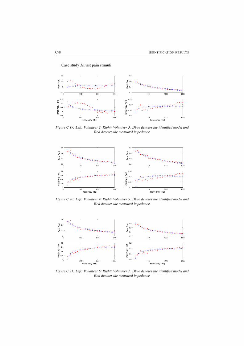
C-8 IDENTIFICATION RESULTS
Case study 3/First pain stimuli
Figure C.19: Left: Volunteer 2; Right: Volunteer 3. Blue denotes the identified model andRed denotes the measured impedance.
Figure C.20: Left: Volunteer 4; Right: Volunteer 5. Blue denotes the identified model andRed denotes the measured impedance.
Figure C.21: Left: Volunteer 6; Right: Volunteer 7. Blue denotes the identified model andRed denotes the measured impedance.
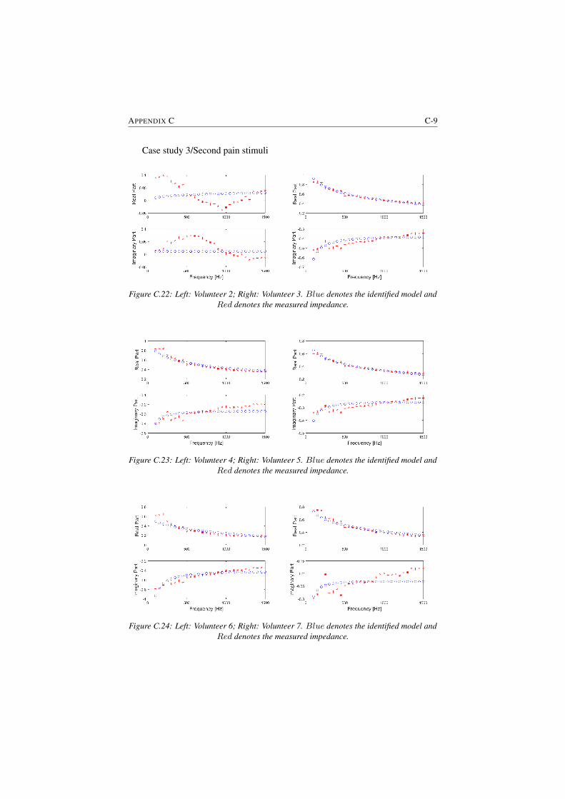
APPENDIX C C-9
Case study 3/Second pain stimuli
Figure C.22: Left: Volunteer 2; Right: Volunteer 3. Blue denotes the identified model andRed denotes the measured impedance.
Figure C.23: Left: Volunteer 4; Right: Volunteer 5. Blue denotes the identified model andRed denotes the measured impedance.
Figure C.24: Left: Volunteer 6; Right: Volunteer 7. Blue denotes the identified model andRed denotes the measured impedance.
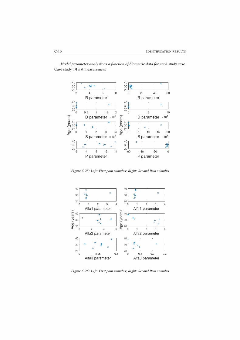
C-10 IDENTIFICATION RESULTS
Model parameter analysis as a function of biometric data for each study case.Case study 1/First measurement
Figure C.25: Left: First pain stimulus; Right: Second Pain stimulus
Figure C.26: Left: First pain stimulus; Right: Second Pain stimulus
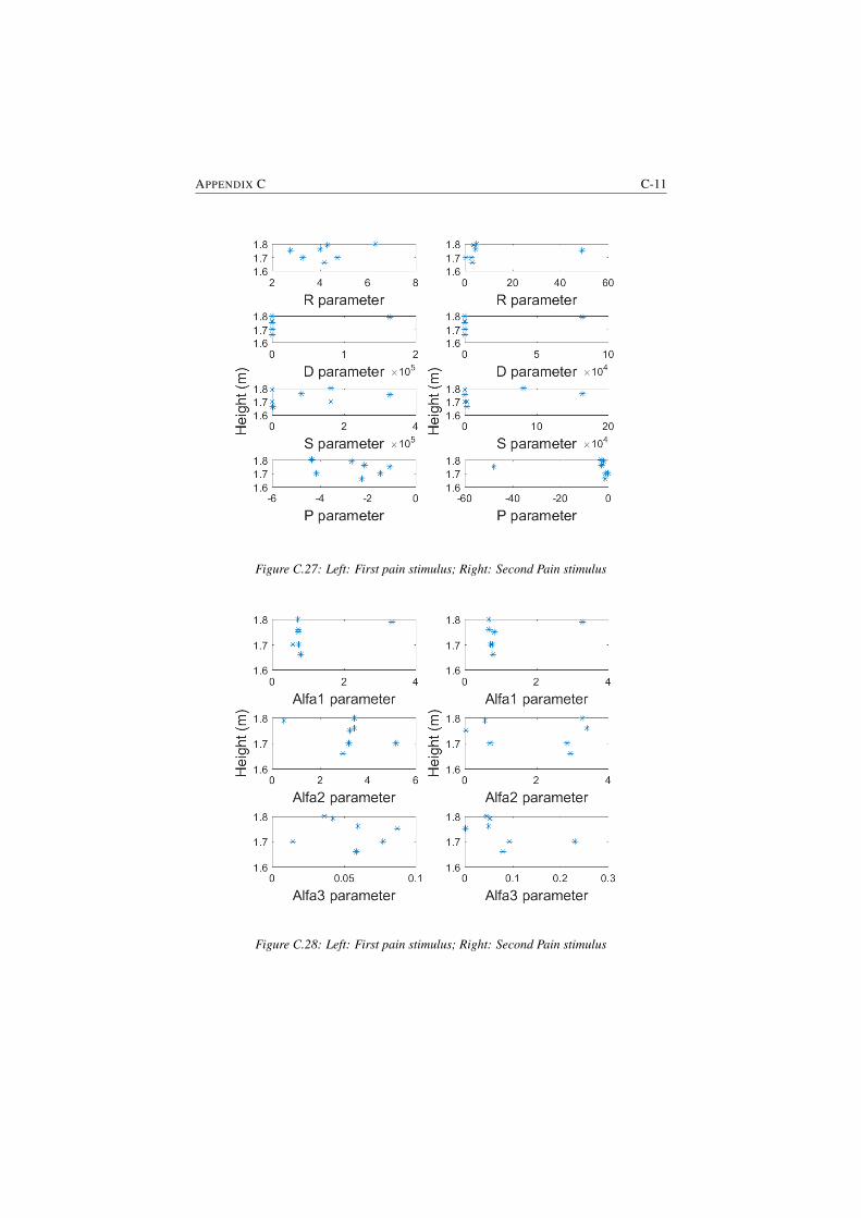
APPENDIX C C-11
Figure C.27: Left: First pain stimulus; Right: Second Pain stimulus
Figure C.28: Left: First pain stimulus; Right: Second Pain stimulus
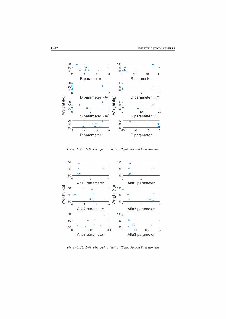
C-12 IDENTIFICATION RESULTS
Figure C.29: Left: First pain stimulus; Right: Second Pain stimulus
Figure C.30: Left: First pain stimulus; Right: Second Pain stimulus
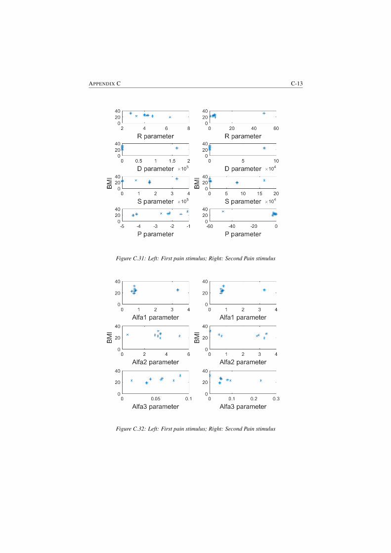
APPENDIX C C-13
Figure C.31: Left: First pain stimulus; Right: Second Pain stimulus
Figure C.32: Left: First pain stimulus; Right: Second Pain stimulus
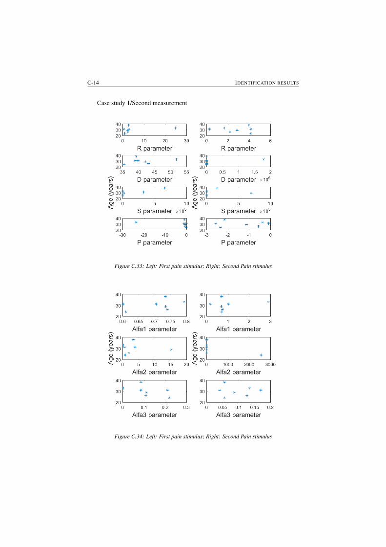
C-14 IDENTIFICATION RESULTS
Case study 1/Second measurement
Figure C.33: Left: First pain stimulus; Right: Second Pain stimulus
Figure C.34: Left: First pain stimulus; Right: Second Pain stimulus
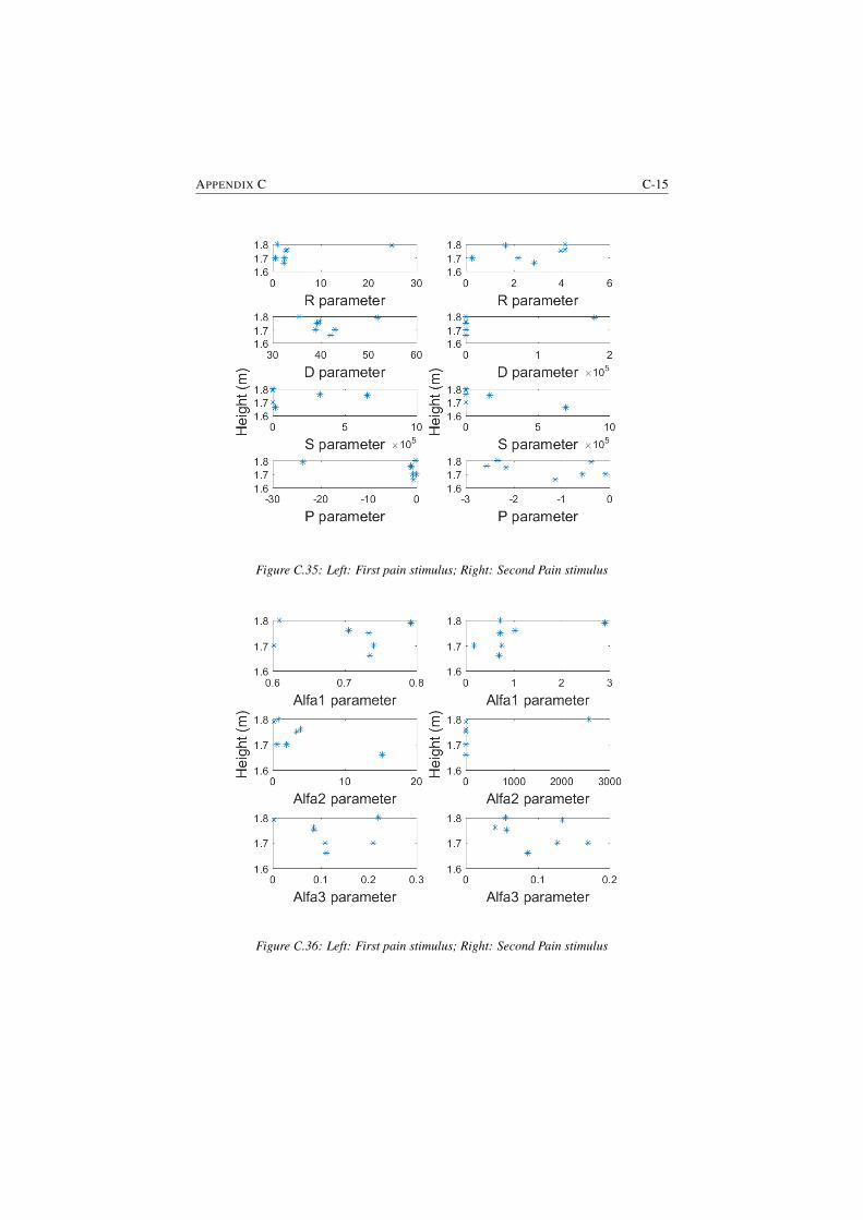
APPENDIX C C-15
Figure C.35: Left: First pain stimulus; Right: Second Pain stimulus
Figure C.36: Left: First pain stimulus; Right: Second Pain stimulus
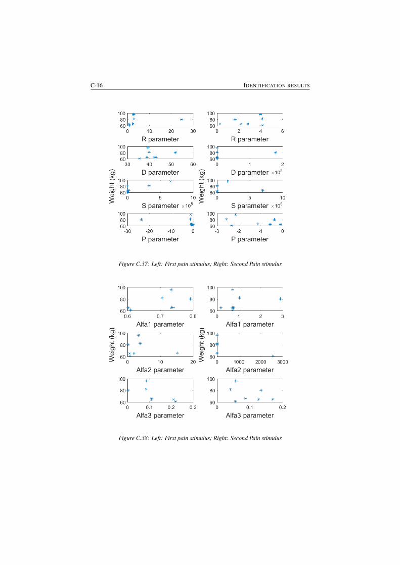
C-16 IDENTIFICATION RESULTS
Figure C.37: Left: First pain stimulus; Right: Second Pain stimulus
Figure C.38: Left: First pain stimulus; Right: Second Pain stimulus
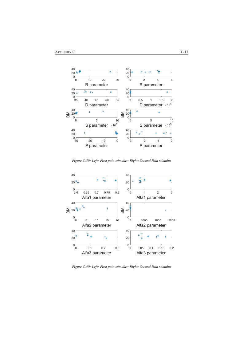
APPENDIX C C-17
Figure C.39: Left: First pain stimulus; Right: Second Pain stimulus
Figure C.40: Left: First pain stimulus; Right: Second Pain stimulus

C-18 IDENTIFICATION RESULTS
Case study 2
Figure C.41: Left: First pain stimulus; Right: Second Pain stimulus
Figure C.42: Left: First pain stimulus; Right: Second Pain stimulus

APPENDIX C C-19
Figure C.43: Left: First pain stimulus; Right: Second Pain stimulus
Figure C.44: Left: First pain stimulus; Right: Second Pain stimulus
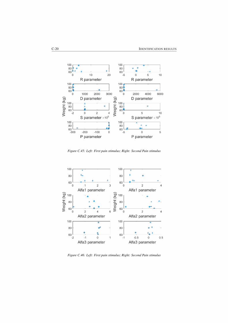
C-20 IDENTIFICATION RESULTS
Figure C.45: Left: First pain stimulus; Right: Second Pain stimulus
Figure C.46: Left: First pain stimulus; Right: Second Pain stimulus
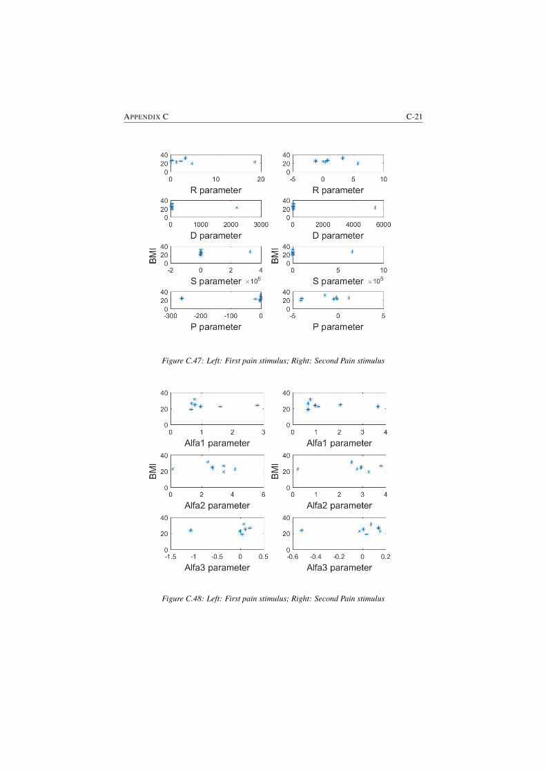
APPENDIX C C-21
Figure C.47: Left: First pain stimulus; Right: Second Pain stimulus
Figure C.48: Left: First pain stimulus; Right: Second Pain stimulus
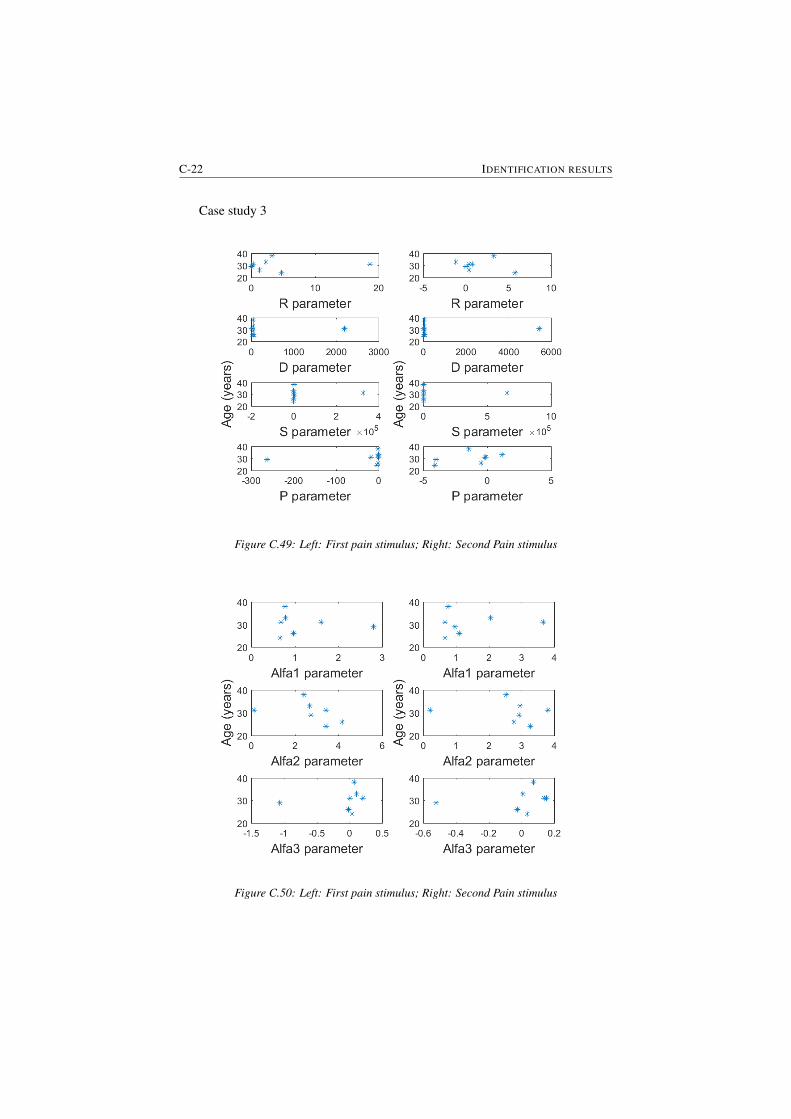
C-22 IDENTIFICATION RESULTS
Case study 3
Figure C.49: Left: First pain stimulus; Right: Second Pain stimulus
Figure C.50: Left: First pain stimulus; Right: Second Pain stimulus
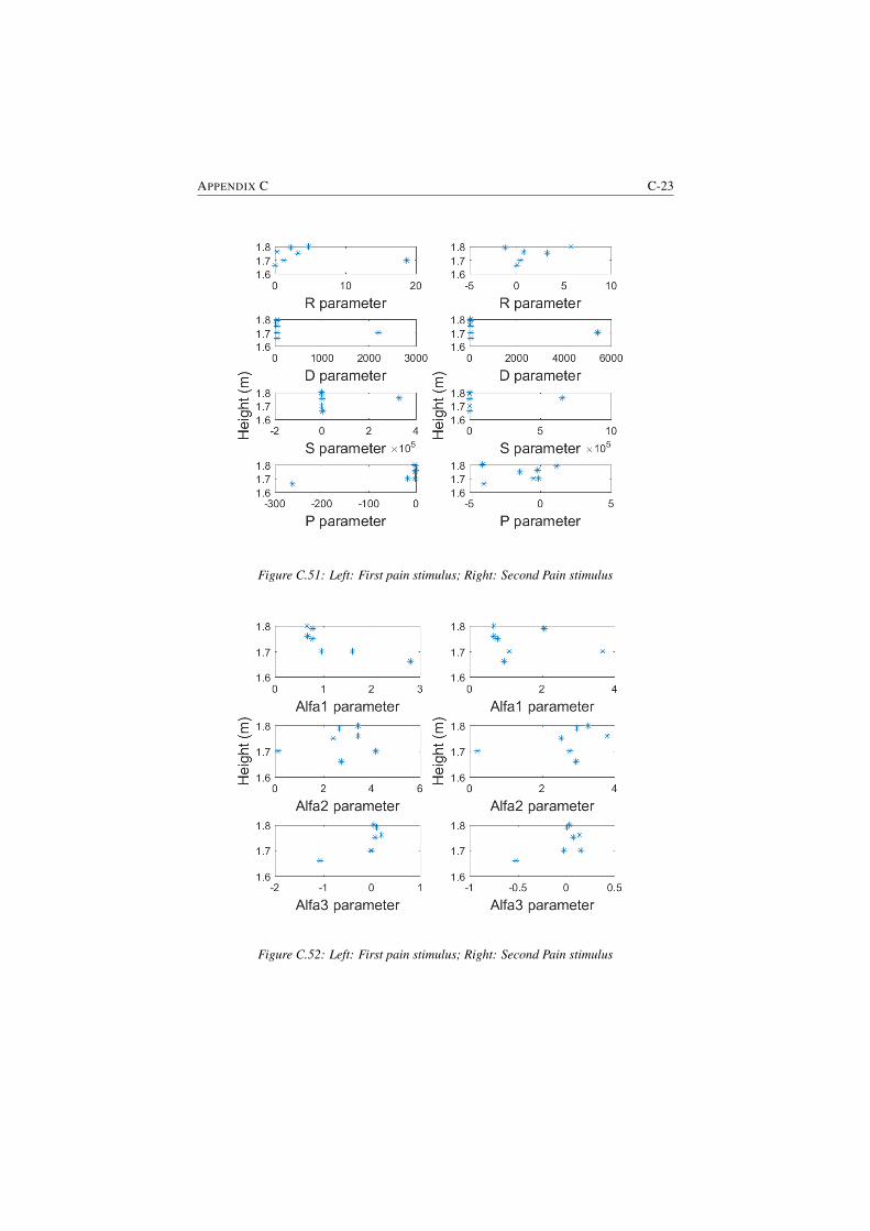
APPENDIX C C-23
Figure C.51: Left: First pain stimulus; Right: Second Pain stimulus
Figure C.52: Left: First pain stimulus; Right: Second Pain stimulus
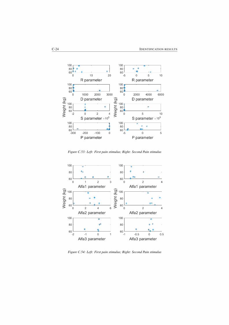
C-24 IDENTIFICATION RESULTS
Figure C.53: Left: First pain stimulus; Right: Second Pain stimulus
Figure C.54: Left: First pain stimulus; Right: Second Pain stimulus

APPENDIX C C-25
Figure C.55: Left: First pain stimulus; Right: Second Pain stimulus
Figure C.56: Left: First pain stimulus; Right: Second Pain stimulus
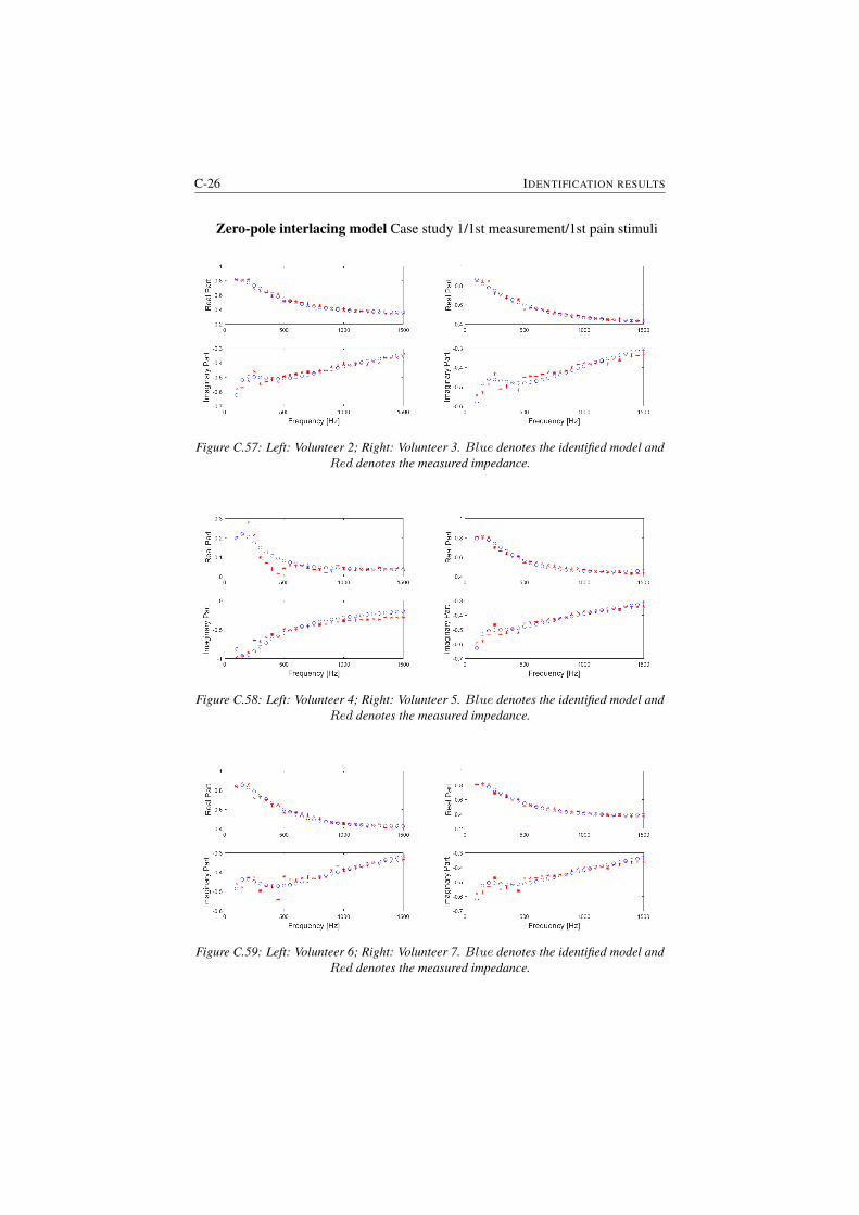
C-26 IDENTIFICATION RESULTS
Zero-pole interlacing model Case study 1/1st measurement/1st pain stimuli
Figure C.57: Left: Volunteer 2; Right: Volunteer 3. Blue denotes the identified model andRed denotes the measured impedance.
Figure C.58: Left: Volunteer 4; Right: Volunteer 5. Blue denotes the identified model andRed denotes the measured impedance.
Figure C.59: Left: Volunteer 6; Right: Volunteer 7. Blue denotes the identified model andRed denotes the measured impedance.
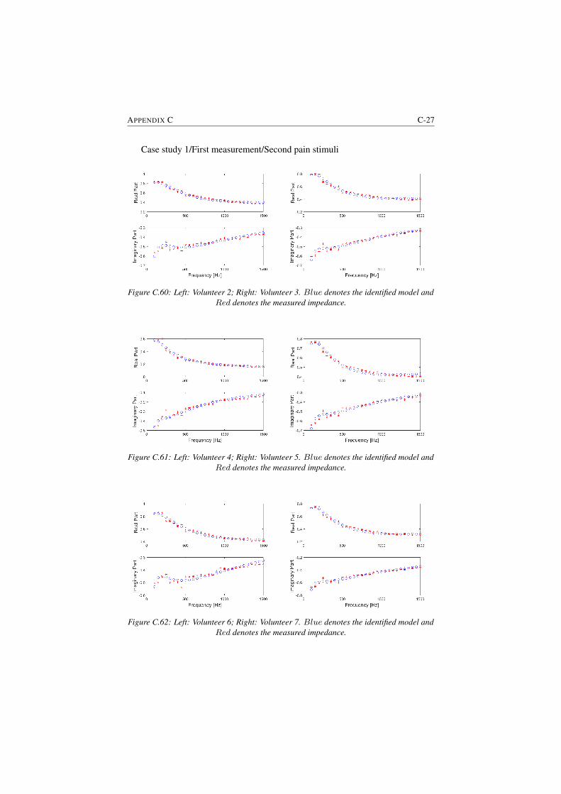
APPENDIX C C-27
Case study 1/First measurement/Second pain stimuli
Figure C.60: Left: Volunteer 2; Right: Volunteer 3. Blue denotes the identified model andRed denotes the measured impedance.
Figure C.61: Left: Volunteer 4; Right: Volunteer 5. Blue denotes the identified model andRed denotes the measured impedance.
Figure C.62: Left: Volunteer 6; Right: Volunteer 7. Blue denotes the identified model andRed denotes the measured impedance.
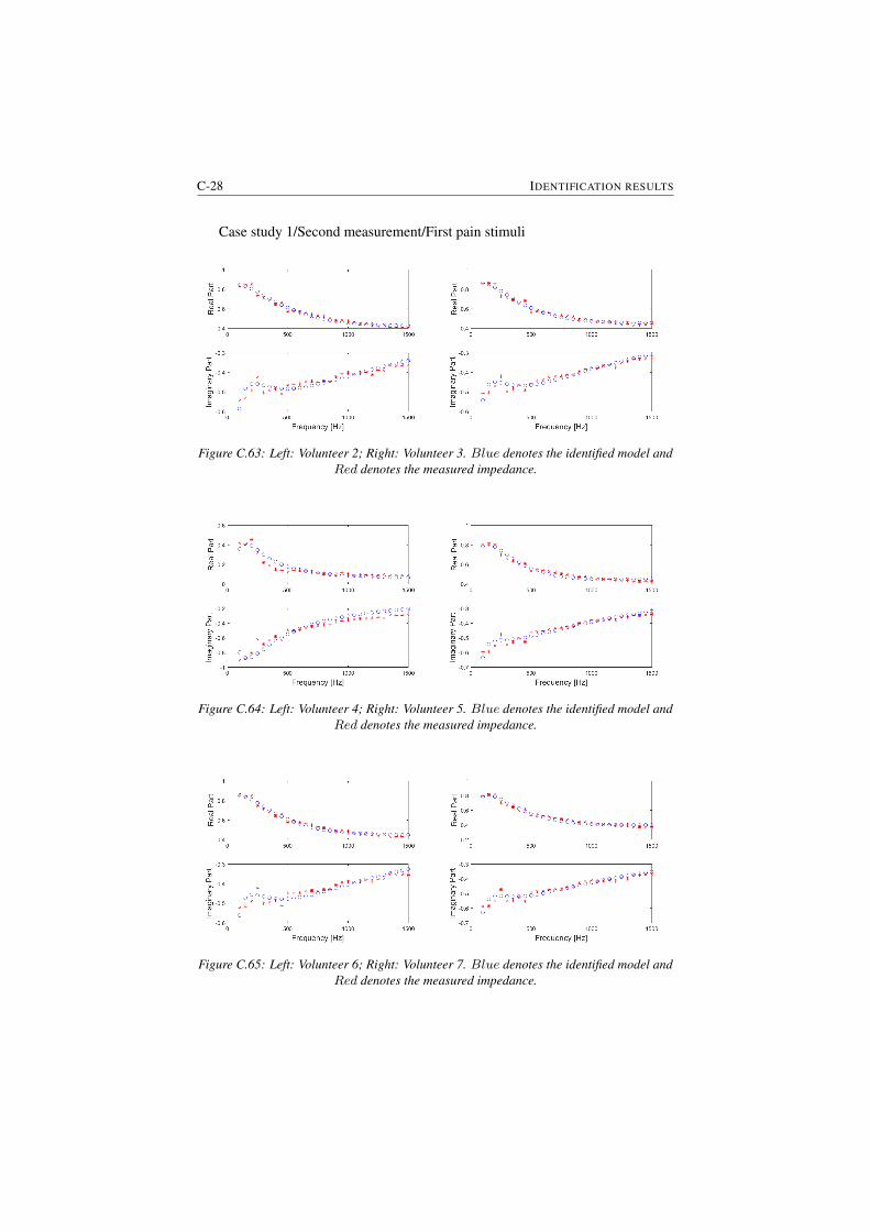
C-28 IDENTIFICATION RESULTS
Case study 1/Second measurement/First pain stimuli
Figure C.63: Left: Volunteer 2; Right: Volunteer 3. Blue denotes the identified model andRed denotes the measured impedance.
Figure C.64: Left: Volunteer 4; Right: Volunteer 5. Blue denotes the identified model andRed denotes the measured impedance.
Figure C.65: Left: Volunteer 6; Right: Volunteer 7. Blue denotes the identified model andRed denotes the measured impedance.
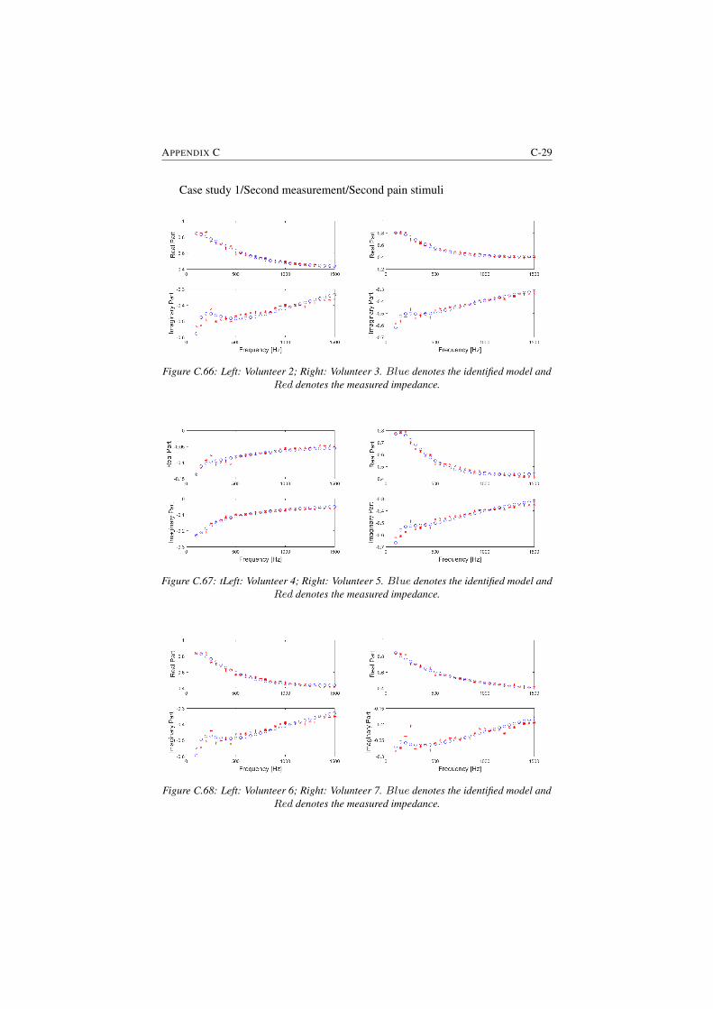
APPENDIX C C-29
Case study 1/Second measurement/Second pain stimuli
Figure C.66: Left: Volunteer 2; Right: Volunteer 3. Blue denotes the identified model andRed denotes the measured impedance.
Figure C.67: tLeft: Volunteer 4; Right: Volunteer 5. Blue denotes the identified model andRed denotes the measured impedance.
Figure C.68: Left: Volunteer 6; Right: Volunteer 7. Blue denotes the identified model andRed denotes the measured impedance.
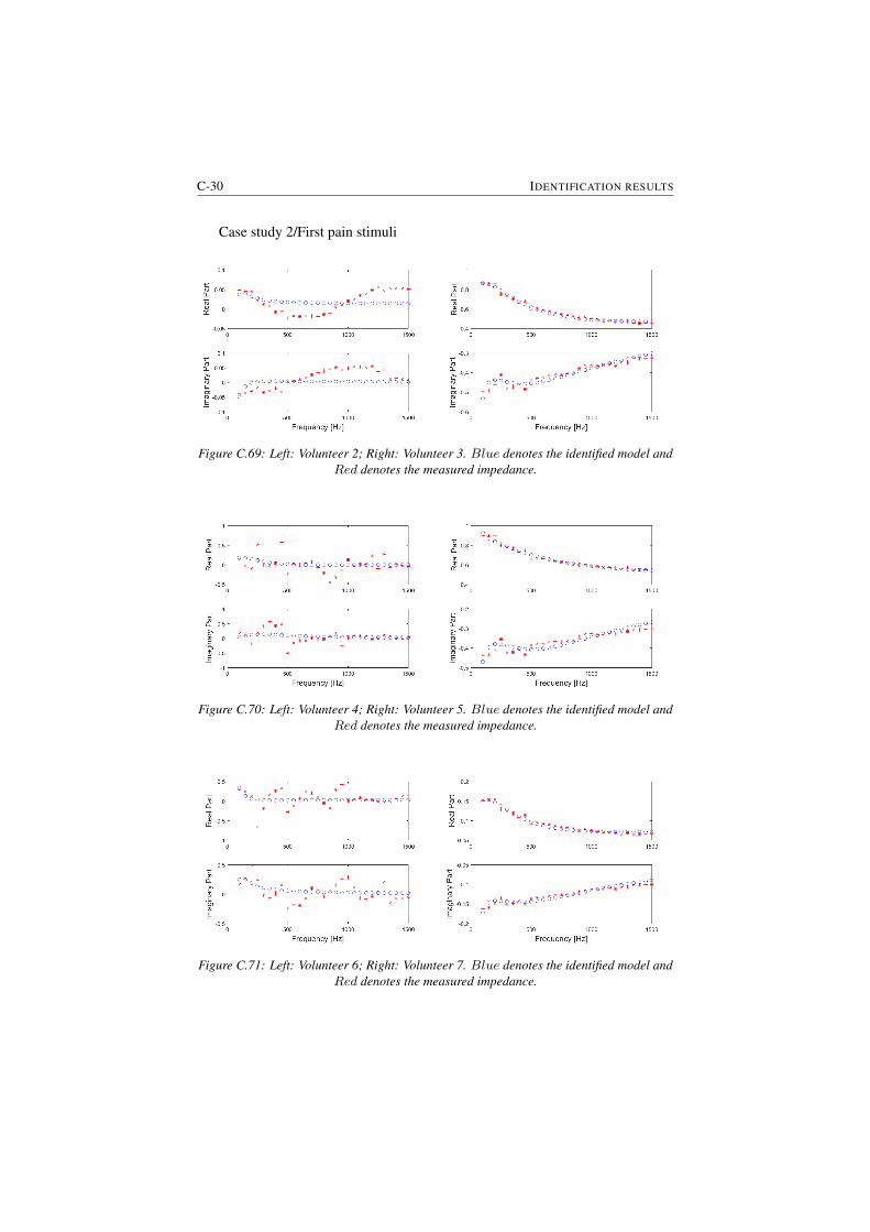
C-30 IDENTIFICATION RESULTS
Case study 2/First pain stimuli
Figure C.69: Left: Volunteer 2; Right: Volunteer 3. Blue denotes the identified model andRed denotes the measured impedance.
Figure C.70: Left: Volunteer 4; Right: Volunteer 5. Blue denotes the identified model andRed denotes the measured impedance.
Figure C.71: Left: Volunteer 6; Right: Volunteer 7. Blue denotes the identified model andRed denotes the measured impedance.
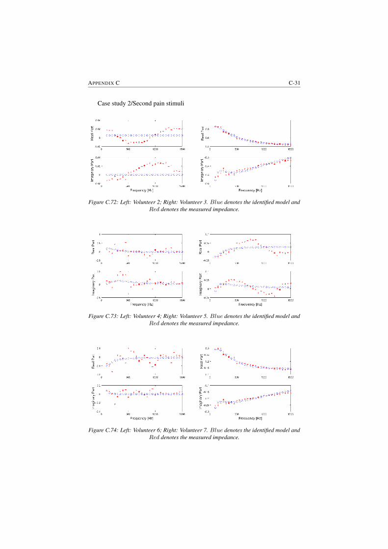
APPENDIX C C-31
Case study 2/Second pain stimuli
Figure C.72: Left: Volunteer 2; Right: Volunteer 3. Blue denotes the identified model andRed denotes the measured impedance.
Figure C.73: Left: Volunteer 4; Right: Volunteer 5. Blue denotes the identified model andRed denotes the measured impedance.
Figure C.74: Left: Volunteer 6; Right: Volunteer 7. Blue denotes the identified model andRed denotes the measured impedance.
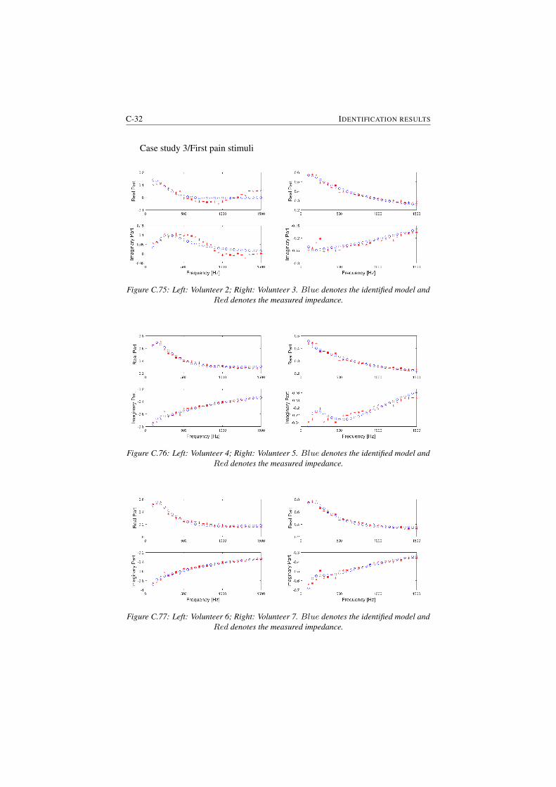
C-32 IDENTIFICATION RESULTS
Case study 3/First pain stimuli
Figure C.75: Left: Volunteer 2; Right: Volunteer 3. Blue denotes the identified model andRed denotes the measured impedance.
Figure C.76: Left: Volunteer 4; Right: Volunteer 5. Blue denotes the identified model andRed denotes the measured impedance.
Figure C.77: Left: Volunteer 6; Right: Volunteer 7. Blue denotes the identified model andRed denotes the measured impedance.
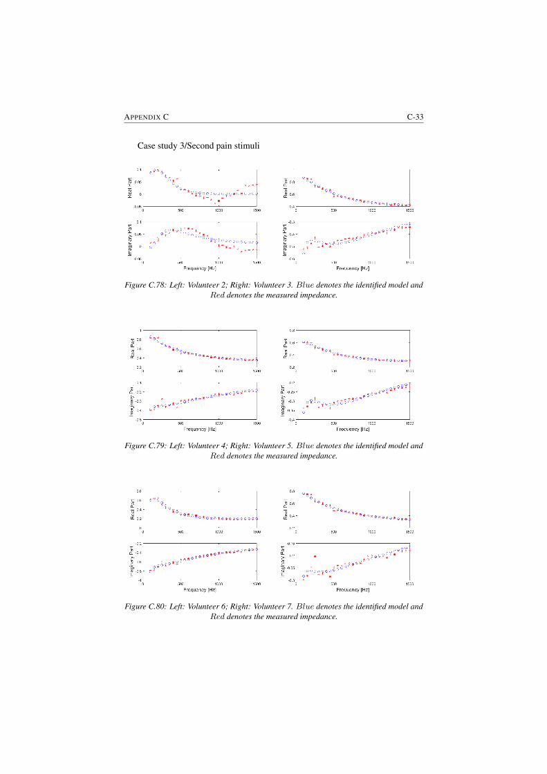
APPENDIX C C-33
Case study 3/Second pain stimuli
Figure C.78: Left: Volunteer 2; Right: Volunteer 3. Blue denotes the identified model andRed denotes the measured impedance.
Figure C.79: Left: Volunteer 4; Right: Volunteer 5. Blue denotes the identified model andRed denotes the measured impedance.
Figure C.80: Left: Volunteer 6; Right: Volunteer 7. Blue denotes the identified model andRed denotes the measured impedance.


DList of additional publications
Publications in international journals (A1)
1. A. Maxim, D. Copot, C. Ionescu, Model predictive control with minimalprocess information for interacting sub-system, Journal of Process Control,in revision.
2. N. Nicolai, F. De Leersnyder, D. Copot, M. Stock, C. Ionescu, I. Nopens,T. De Beer, Development of a PAT-based advanced process control solutionfor continuous twin-screw wet granulation, AIChE Journal, in print.
Publications in international conferences (P1)
1. A. Chevalier, C. Copot, D. Copot, C.M. Ionescu, R. De Keyser. Fractional-order feedback control of a poorly damped system. 19th IEEE InternationalConference on Automation, QualityandTesting, Robotics, Cluj-Napoca, Ro-mania, 22-24 May, 2014.
2. D. Copot, C. Ionescu, A. Hernandez, J. Thybaut, R. De Keyser, Develop-ment of a control strategy for efficient operation of a CSTR reactor. In-ternational Conference on System Theory Control and Computing, Sinaia,Romania, 14-17 October, 17-722, 2015.
3. Ionescu, C. Muresan, D. Copot, R. De Keyser, Constrained multivariablepredictive control of a train of cryogenic 13C separation columns, 11th IFACSymposium on Dynamics and Control of Process Systems, Trondheim, Nor-way, 6-8 June, 1103-1108, 2016.
D-2 LIST OF ADDITIONAL PUBLICATIONS
4. D. Copot, A. Maxim, R. De Keyser, C. Ionescu, Multivariable control ofsextuple tank system with non-minimum phase dynamics, International Con-ference on Automation, Quality and Testing, Robotics (AQTR), Cluj-Napoca,Romania, 19-21 May, 399-404, 2016.
5. D. Copot, C. Ionescu, I. Nascu, R. De Keyser, Online weight estimation ina robotic gripper arm, International Conference on Automation, Quality andTesting, Robotics (AQTR), Cluj-Napoca, Romania, 19-21 May, 151-156,2016.
6. Clara Ionescu, Dana Copot, Anca Maxim, Eva Dulf, Robin De Keyser,Robust Autotuning MPC for chemical process applications, InternationalConference on Automation, Quality and Testing, Robotics (AQTR), Cluj-Napoca, Romania, 19-21 May, 369-374, 2016.
7. I. Birs, S. Folea, D. Copot, O. Prodan, C. Muresan, Comparative analysisand experimental results of advanced control strategies for vibration sup-pression in aircraft wings, European Workshop on Advanced Control andDiagnosis, Lille, France, 17-18 July, 2017.
8. A. Maxim, D. Copot, C.M. Ionescu, R. De Keyser, A methodology for con-trol structure adaptation in presence of varying, unknown sub-system in-teraction degree, IEEE International Conference on Emerging Technologiesand Factory Automation-ETFA, Limassol, Cyprus, 2-5 September, 2017.
9. C.M. Ionescu, N. Van Oevelen, D. Copot, B. Paijmans, R. De Keyser, Con-trol of LPV Mechatronic Systems in Presence of Dynamic Uncertainties,IEEE International Conference on Intelligent Engineering Systems, Lar-naca, Cyprus, 20-23 October, 125-130, 2017.
Publications in international conferences (C1)
1. D. Copot, C. Ionescu, T. Vannecke, E. Volcke, R. De Keyser, An approachtowards multivariable control of anaerobic digestion using the EPSAC pre-dictive control strategy, 11th IWA Conference on Control and Automation,142-149, 2013.
2. A. Chevalier, D. Copot, C. Ionescu, R. De Keyser. A Theoretical Study onModeling the Nonlinear Dynamics of a Knee Emulator, International Con-ference on Mathematical methods in engineering, July 22-26, Porto, Portu-gal, 142-149, 2013.
3. A. Chevalier, C. Copot, D. Copot, C. Ionescu, R. De Keyser, FractionalPID control of a poorly damped system based on a 3-parameter designmethod. International Conference on Systems and Signals, 1-3 October,Cluj-Napoca, Romania, 2015.

APPENDIX D D-3
4. C. Ionescu, C. Copot, A. Chevalier, D. Copot, R. De Keyser, Adaptive slid-ing mode control with non-integer order reference function. InternationalConference on Systems and Signals, 1-3 October, Cluj-Napoca, Romania,2015.

References
[1] K.B. Oldham and J. Spanier. The Fractional Calculus. IEEE Transactionson Parallel and Distributed Systems, 14:369–382, 2003.
[2] K.S. Miller and B. Ross. An Introduction to the Fractional Calculus andFractional Deferential Equations. John Wiley and Sons Inc., New York,1993.
[3] R. Gorenflo and S. Vessella. Abel Integral Equations: Analysis and Appli-cations, Lecture Notes in Mathematics. Springer, Berlin Heidelberg, 1991.
[4] M. Lazarevic. Advanced Topics on Application of Fractional Calculus onControl Problem, System Stability and Modeling. WSEAS Press, 2012.
[5] M. Caputo. Linear models of dissipation whose Q is almost frequency in-dependent. Journal of Royal Australian Society, 13:529–539, 1967.
[6] B. West. Fractal physiology and the fractional calculus: a perspective.2010.
[7] Podlubny I. Geometric and physical interpretation of fractional integrationand fractional differentiation. Fractional Calculus and Applied Analysis,5(4):367–386, 2002.
[8] S. Samko, A. Kilbas, and O. Marichev. Fractional Integrals and Deriva-tives - Theory and Applications. Gordon and Breach Science Publishers,Amsterdam, 1993.
[9] R. Hilfer. Applications of Fractional Calculus in Physics. World ScientificPublishing Co., 2000.
[10] R. Magin, M. Ortigueira, I. Podlubny, and J. Trujillo. On the fractionalsignals and systems. Signal Processing, 91:350–371, 2011.
[11] A. Dokoumetzidis, R. Magin, and P. Macheras. Fractional kinetics in multi-compartmental systems. Journal of Pharmacokinetics and Pharmacodynam-ics, 37:507–524, 2010.
D-6 REFERENCES D
[12] A. Dokoumetzidis and P. Macheras. Fractional kinetics in drug absorptionand disposition processes. Journal of Pharmacokinetics and Pharmacody-namics, 36:165–178, 2009.
[13] M. Wise. Negative Power Functions of Time in Pharmacokinetics andTheir Implications. Journal of Pharmacokinetics and Biopharmaceutics,13(3):309–346, 1985.
[14] C. Ionescu. The human respiratory system: an analysis of the interplay be-tween anatomy, structure, breathing and fractal dynamics. Springer, Seriesin BioEngineering, 2013.
[15] J. Popovic, M. Atanackovic, A. Pilipovic, M. Rapaic, and S. Pilipovic. Anew approach to the compartmental analysis in pharmacokinetics: frac-tional time evolution of diclofenac. Journal of Pharmacokinetics and Phar-macodynamics, 37(4):119–138, 2010.
[16] J. Gabano and T. Poinot. Fractional modelling and identification of thermalsystems. Signal Processing, 91:531–541, 2011.
[17] J. Gabano and T. Poinot. Estimation of thermal parameters using fractionalmodelling. Signal Processing, 91:938–948, 2011.
[18] J. Siepman and F. Siepmann. Mathematical modeling of drug delivery,.International Journal of Pharmaceutics, 364:328–343, 2008.
[19] J. Siepmann and A. Goepferich. Mathematical modeling of bioerodible,polymeric drug delivery systems. Advanced Drug Delivery Review, 48:229–247, 2001.
[20] R. Baker. Controlled Release of Biologically Active Agents. John Wiley &Sons, New York, 1987.
[21] M. Weiss. The anomalous pharmacokinetics of amiodarone explained bynonexponential tissue trapping. Journal of Pharmacokinetics and Biophar-maceutics, 27(4):383–396, 1999.
[22] X.J. Zhou, Q. Gao, O. Abdullah, and R.L. Magin. Studies of anomalousdiffusion in the human brain using fractional order calculus. Magnetic Res-onance in Medicine, 63(3):562–569, 2010.
[23] A. Benchellal, T. Poinot, and J. Trigeassou. Approximation and identi-fication of diffusive interfaces by fractional models. Signal processing,86:2712–2727, 2006.
REFERENCES D-7
[24] T. Poinot and J. Trigeassou. Modelling and simulation of fractional systems.In Workshop on fractional differetiation and its applications, pages 656–663, 2004.
[25] H. Wang, A. Degiovanni, and C. Moyne. Periodic thermal contact: aquadrupole model and an experiment. International Journal of ThermalSciences, 41:125–135, 2002.
[26] G. Andrews, R. Askey, and R. Roy. Encyclopedia of mathematics and itsapplications. Cambridge University Press, 2001.
[27] D. Maillet, S. Andre, J. Batsale, A. Degiovanni, and C. Mayone. Thermalquadrupoles: Solving the heat equation through integral transforms. Wiley,2000.
[28] A. Oustaloup. Diversity and non-integer differentiation for system dynam-ics. Wiley and Sons, 2014.
[29] A. Guyton and J. Hall. Textbook of medical Physiology. Elsevier, 2006.
[30] J. Hogg. Pathophysiology of airflow limitation in chronic obstructive pul-monary disease. Lancet, 364:709–721, 2004.
[31] P. Barnes. Chronic Obstructive pulmonary disease. New England Journalof Medicine: Medical Progress, 343:269–280, 2000.
[32] H. Parameswaran, A. Majumdar, S. Ito, A. Alencar, and B. Suki. Quanti-tative characterization of airspace enlargement in emphysema. Journal ofApplied Physiology, 100:186–193, 2006.
[33] R. Lopes and N. Betrouni. Fractal and multifractal analysis: A review.Medical Image Analysis, 13:634–639, 2009.
[34] L. Sorensen and M. de Bruijne. Dissimilarity representation in lungparenchyma classification. In proceedings of the Spie digital library Con-ference, Medical Imaging, Computer-Aided Diagnosis, 2009.
[35] L. Sorensen, S. Shaker, and M. de Bruijne. Quantitative analysis of pul-monary emphysema using local binary patterns. IEEE Transactions onMedical Imaging, 29:559–569, 2010.
[36] S. Boser, H. Park, S. Perry, M. Menache, and F. Green. Fractal geometry ofairway remodeling in human asthma. American Journal of respiratory andCritical Care Medicine, 172:817–823, 2005.
D-8 REFERENCES D
[37] G. Tourassi, E. Frederick, C. Floyd, and R. Coleman. Multifractal textureanalysis of perfusion lung scans as a potential diagnostic tool for acute pul-monary embolism. Computers in Biology and Medicine, 31:15–25, 2001.
[38] E. Oostveen, D. Macleod, H. Lorino H, R. Farr, Z. Hantos Z, K. De-sager, and F. Marchal. The forced oscillation technique in clinical prac-tice: Methodology, recommendations and future developments. EuropeanRespiratory Journal, 22:1026–1041, 2003.
[39] C. Ionescu, P. Segers, and R. De Keyser. Mechanical Properties of theRespiratory System Derived From Morphologic Insight. IEEE Transactionon Biomedical Engineering, 56:949–959, 2009.
[40] E. Weibel. Morphometry of the human lung. Springer-Verlag, New York,1963.
[41] E. Weibel. Fractal geometry: a design principle for living organism. Amer-ican Journal of Physiology, 261:L361–L369, 1991.
[42] B. Mandelbrot. The Fractal Geometry of Nature. Freeman, New York,1983.
[43] A. Oustaloup. La derivation non entiere. Hermes, Paris, 1995.
[44] Z. Hantos, B. Daroczy, B. Suki, G. Galgoczy, and T. Csendes. Forced os-cillatory impedance of the respiratory system at low frequencies. Journal ofApplied Physiology, 60:123–132, 1986.
[45] Z. Hantos and B. Suki. Viscoelastic properties of the visceral pleura andits contribution to lung impedance. Respiratory Physiology, 90:271–287,1992.
[46] B. Suki B, A. Barabasi, Z. Hantos, F. Petak, and H. Stanley. Avalanches andpower law behaviour in lung inflation. Nature, 368:615–618, 1994.
[47] C. Ionescu, D. Copot, and R. De Keyser. A fractional order impedancemodel to capture the structural changes in lungs. In 19th World CongressThe International Federation of Automatic Control Cape Town, SouthAfrica, pages 5362–5368, 2014.
[48] G. Irvin, J. Pak, and R. Martin. Airway-parenchyma uncoupling in noc-turnal asthma. American Journal Respiratory and Critical Care Medicine,161:50–56, 2000.
[49] F. Petak, G. Hall, and P. Sly. Repeated measurements of airway andparenchymal mechanism in rats by using low frequency oscillation. Journalof Applied Physiology, 84:1616–1625, 1998.
REFERENCES D-9
[50] C. Ionescu, J. Schoukens, and R. De Keyser. Detecting and analyzing non-linear effects in respiratory impedance measurements. In American ControlConference, San Francisco, USA, pages 5412–5417, 2011.
[51] V. Mitic, V. Pavlovic, L. Kocic, V. Paunovic, and D. Mancic. Applications ofthe intergranular impedance model in correlating microstructure and elec-trical properties of Doped BaTiO3. Science of Sintering, 41:247–256, 2009.
[52] J. Liou, C. Tsai, and J. Lin. A microcontact model developed for sphereand cylinder based fractal bodies in contact with a rigid flat surface. Wear,268:431–442, 2010.
[53] R. Karimi, G. Tornling, H. Forsslund H, M. Mikko, A. Wheelock, andS. Nyren. Lung density on high resolution computer tomography (HRCT)reflects degree of inflammation in smokers. Respiratory Research, 15, 2014.
[54] E. Ponder. The coefficient of thermal conductivity of blood and varioustissues. The Journal of General Physiology, 45:454–451, 1962.
[55] R. Magleby, A. Schallop, E. Schulman, and J. Sterling. The effect of vas-cularization and tissue type on cryosurgical procedure. Computer AidedEngineering: Applications to Biomedical Processes, 453:410–413, 2008.
[56] V.B. Mountcastle. Medical Physiology. C. V. Mosby Company, St. Louis,Missouri, 1980.
[57] R.A. Sternbach. Pain: a Psychophysiological Analysis. Academic PressInc. (London) Ltd., New York, 1968.
[58] H. Marskey and N. Bogduk. Classification of Chronic Pain: Descriptionsof Chronic Pain Syndromes and Definitions of Pain Terms. IASP Press,Seattle, Washington, 1994.
[59] T. Sokka. Assessment of Pain in Rheumatic Diseases. Clin Exp Rheumatol,23:S77–S84, 2005.
[60] C.S. Rodriguez. Pain Measurement in Elderly: A Review. Pain ManagementNursing, 2(2):38–46, 2001.
[61] P. Wall and R. Melzack. The Challenge of Pain. Penguin, London, UnitedKingdom, 1996.
[62] N. Desbiens, A. Wu, S. Broste, N. Wenger, A. Connors, J. Lynn, Y. Yasui,R.S. Phillips, and W. Fulkerson. Pain and Satisfaction with Pain Controlin seriously ill hospitalized Adults: findings from the SUPPORT research
D-10 REFERENCES D
investigations. For the SUPPORT investigators. Study to understand Prog-noses and Preferences for Outcomes and Risks of Treatment. Critical CareMedicine, 24(12):1953–1961, 1996.
[63] I.A Harris, J.M. Young, H. Rae, B.B. Jalaludin, and M.J. Solomon. Factorsassociated with Back Pain after Physical Injury. Spine, 32(14):1561–1565,2007.
[64] M. Bates, W. Edwards, and K. Anderson. Ethnocultural Influences on Vari-ation in Chronic Pain Perception. Pain, 52(1):101–112, 1993.
[65] I. Lund, T. Lundeberg, J. Kowalski, and E. Svensson. Gender Differencesin Electrical Pain Threshold Responses to Transcutaneous Electrical NerveStimulation (TENS). Neuroscience Letters, 375(2):75–80, 2005.
[66] K. Herr, K. Spratt, P. Mobily, and G. Richardson. Pain Intensity assessmentin older Adults: use of experimental Pain to compare Psychometric Proper-ties and Usability of selected Pain Scales with younger Adults. The ClinicalJournal of Pain, 20(4):207–219, 2004.
[67] E. Flaherty. Using Pain-Rating Scales with Older Adults. American Journalof Nursing, 108(6):40–47, 2008.
[68] R. Hamill-Ruth and M. Marohn. Evaluation of Pain in the Critically IllPatient. Critical Care Clinics, 15(1):35–54, 1999.
[69] K. Puntillo, D. Stannard, C. Miaskowski, K. Kehrle, and S. Gleeson. Useof a Pain Assessment and Intervention Notation (P.A.I.N.) tool in criticalCare Nursing Practice: Nurses’ Evaluations. Heart and Lung: the journalof Critical Care, 31(4):303–314, 2002.
[70] K. Puntillo, C. Miaskowski, K. Kehrle, D. Stannard, S. Gleeson, and P. Nye.Relationship between Behavioral and Physiological Indicators of Pain,Critical Care Patients’ Self-reports of Pain, and Opoid Administration. Crit-ical Care Medicine, 25(7):1159–1166, 1997.
[71] P. McArdle. Intravenous Analgesia. Critical Care Clinics, 15(1):89–104,1999.
[72] J. Jacobi, G. Fraser, D. Coursin, R. Riker, D. Fountaine, E.T. Wittbrodt,D.B. Chalfin, M.F. Masica, H.S. Bjerke, W.M. Coplin, D.W. Crippen, B.D.Fuchs, R.M. Kelleher, P.E. Marik, S.A. Nasraway, M.J. Murray, W.T. Pe-ruzzi, and P.D. Lumb. Clinical Practice Guidlines for the Sustained use ofSedatives and Analgesics in the Critically Ill Adult. Critical Care Medicine,30(1):119–141, 2002.
REFERENCES D-11
[73] K. Herr, P. Coyne, T. Key, R. Manworren, M. McCaffery, S. Merkel,J. Pelosi, and L. Wild. Pain Assessment in the Non-verbal Patient: Posi-tion Statement with Clinical Practice Recommendations. Pain ManagementNursing, 7(2):44–52, 2006.
[74] T. Hadjistavropoulos, D. Chapelle, H. Hadjistavropoulos, S. Green, andG. Asmundson. Using Facial Expressions to assess Musculoskeletal Painin older Persons. European Journal of Pain, 6(3):179–187, 2002.
[75] United States. Agency for Health Care Policy, Research, and United States.Acute Pain Management Guideline Panel. Acute Pain Management: Oper-ative or Medical Procedures and Trauma. U.S. Department of Health andHuman Services, Public Health Service, Agency for Health Care Policy andResearch, Acute Pain Management Guideline Panel, Washington DC, 1992.
[76] W.E. Fordyce, D.C. Turk, and R. Melzack. Pain Measurement and Assess-ment. Raven Press, New York, New York, 1983.
[77] S. Merkel. Pain assessment in infants and young children: the finger spanscale. The American Journal of Nursing, 102:55–56, 2002.
[78] C. Pasero and M. McCaffery. Pain in the critically ill. The American Journalof Nursing, 102:59–60, 2002.
[79] C. Sessler, M. Grap, and G.Brophy. Multidisciplinary management of se-dation and analgesia in critical care. Seminars in Respiratory and CriticalCare Medicine, 22:211–225, 2001.
[80] J. Kress and J. Hall. Sedation in the mechanically ventilated patient. CriticalCare Medicine, 22:2541–2546, 2006.
[81] M. Ocana, C. Cendan, E. Cobos, J. Entrena, and J. Baeyens. PotassiumChannels and Pain: present Realities and future Opportunities. EuropeanJournal of Pharmacology, 500(1–3):203–219, 2004.
[82] M.P. Jensen and C.A. McFarland. Increasing the Reliability and Validity ofPain Intensity Measurement in Chronic Pain Patients. Pain, 55(2):195–203,1993.
[83] C. Hurny, J. Bernhard, A. Coates, H. Peterson, M. Castiglione-Gertsch,R.D. Gelber, C.M. Rudenstam, J. Collins, J. Lindtner, A. Goldhirsch, andH.J. Senn. Responsiveness of a single-item Indicator versus a multi-itemScale: Assessment of emotional Well-being in an International AdjuvantBreast Cancer Trial. Medical Care, 34(3):234–248, 1996.
D-12 REFERENCES D
[84] E. Breivik, G. Bjornsson, and E. Skovlund. A Comparison of Pain RatingScales by Sampling from Clinical Trial Data. The Clinical Journal of Pain,16(1):22–28, 2000.
[85] I. McDowell. Measuring Health: A Guide to Rating Scales and Question-naires. Oxford University Press, New York, New York, 2006.
[86] J.T. Farrar, R.K. Portenoy, J.A. Berlin, J.L. Kinman, and B.L. Strom. Defin-ing the clinically important Differences in Pain Outcome Measures. Pain,88(3):287–294, 2000.
[87] J.T. Farrar, J.P. Young, L. LaMoreaux, J.L. Werth, and R.M. Poole. Clinicalimportance of Changes in Chronic Pain Intensity measured on an 11-pointNumerical Pain Rating Scale. Pain, 94(2):149–158, 2001.
[88] M.P. Jensen, P. Karoly, D.C. Turk, and R. Melzac. Handbook of Pain As-sessment. Guilford Press, New York, 1992.
[89] J. Labus, F. Keefe, and M. Jensen. Self-reports of pain intensity and directobservations of pain behavior: When are they correlated? Journal of Pain,102:109–124, 2003.
[90] J. Payen, O. Bru, J. Bosson, A. Lagrasta, I. Deschaux E. Novel, P. Lavagne,and C. Jacquot. Assessing pain in critically ill sedated patients by using abehavioral pain scale. Critical Care Medicine, 29:2258–2263, 2001.
[91] Y. Aissaoui, A. Zeggwagh, A. Zekraoui, K. Abidi, and R. Abouqal. Valida-tion of a behavioral pain scale in critically ill, sedated, and mechanicallyventilated patients. Anesthesia and Analgesia, 101:1470–1476, 2005.
[92] J. Young, J. Siffleet, S. Nikoletti, and T. Shaw. Use of a behavioral painscale to assess pain in ventilated, unconscious and/or sedated patients. In-tensive Critical Care Nursing, 22:32–39, 2006.
[93] C. Gelinas, L. Fillion, K. Puntillo, C. Viens, and M. Fortier. Validation of theCritical-Care Pain Observation Tool in adult patients. American Journal ofCritical Care, 15:420–427, 2006.
[94] K. Puntillo, A. Morris, C. Thompson, J. Stanik-Hutt, C. White, and L. Wild.Pain behaviors observed during six common procedures: Result form Thun-der Project II. Critical Care Medicine, 32:421–427, 2004.
[95] I. Roeggen, H. Storm, and D. Harrison. Skin Conductance Variability be-tween and within Hospitalised Infants at Rest. Early Human Development,87(1):37–42, 2011.
REFERENCES D-13
[96] K.E. Hagbarth, R.G. Hallin, A. Hongell, H.E. Torebjork, and B.G. Wallin.General Characteristics of Sympathetic Activity in Human Skin Nerves.Acta Physiologica Scandinavica, 84(2):164–176, 1972.
[97] G.F. Goddard. A pilot study of the Changes of Skin Electrical Conduc-tance in Patients undergoing General Anaesthesia and Surgery. Anaesthe-sia, 37(4):408–415, 1982.
[98] H. Storm. Skin Conductance and the Stress Response from Heel Stick inPreterm Infants. Archives of Disease in Chidlhood - Fetal and NeonatalEdition, 83(2):F143–F147, 2000.
[99] D. Harrison, S. Boyce, P. Loughnan, P. Dargaville, H. Storm, and L. John-ston. Skin Conductance as a measure of Pain and Stress in HospitalisedInfants. Early Human Development, 82(9):603–608, 2006.
[100] H. Storm. The Capability of Skin Conductance to Monitor Pain Comparedto Other Physiological Pain Assessment Tools in Children and Neonates.Pediatrics and Therapeutics, 3(4):168–173, 2013.
[101] F. Savino, L. Vagliano, S. Ceratto, F. Viviani, R. Miniero, and F. Ricceri.Pain Assessment in Children undergoing Venipuncture: the Wong-BakerFaces Scale versus Skin Conductance Fluctuations. Early Human Devel-opment, 82(9):603–608, 2013.
[102] M.D. Larson, D.I. Sessler, D.E. Washington, B.R. Merrifield, J.A. Hynson,and J. McGuire. Pupillary Response to Noxious Stimulation during Isoflu-rane and Propofol Anesthesia. Anaesthesia and Analgesia, 76(5):1072–1078, 1993.
[103] I. Constant, M.C. Nghe, L. Boudet, J. Berniere, S. Schrayer, R. Seeman,and I. Murat. Reflex Pupillary Dilatation in Response to Skin Incision andAlfentanil in Children Anaesthetized with Servoflurane: a more sensitivemeasure of Noxious Stimulation than the commonly used Variables. BritishJournal of Anaesthesia, 96(5):614–619, 2006.
[104] M.D. Larson, P.D. Berry, J. May, A. Bjorksten, and D. Sessler. Autonomiceffects of Epidural and Intravenous Fentanyl. British Journal of Anaesthe-sia, 98(2):263–269, 2007.
[105] S. Isnardon, M. Vinclair, C. Genty, A. Hebrard, P. Albaladejo, and J.F.Payen. Pupillometry to detect Pain Response during general Anaesthesiafollowing Unilateral Popliteal Sciatic Nerve Block. European Journal ofAnaesthesiology, 30(7):429–434, 2013.
D-14 REFERENCES D
[106] D. Li, C. Miaskowski, D. Burkhardt, and K. Puntillo. Evaluations of Physi-ologic Reactivity and Reflexive Behaviors during Noxious Procedures in Se-dated Critically Ill Patients. Journal of Critical Care, 24(3):472.e9–472.e13,2009.
[107] M. Aissou, A. Snauwaert, C. Dupuis, A. Atchabahian, F. Aubrun, andM. Beaussier. Objective Assessment of the Immediate Postoperative Anal-gesia using Pupillary Reflex Measurements. Anesthesiology, 116(5):1006–1012, 2012.
[108] N. Ben-Israel, M. Kliger, G. Zuckerman, Y. Katz, and R. Edry. Monitoringthe Nociception Level: a Multi-Parameter Approach. Journal of ClinicalMonitoring and Computing, 27(6):659–668, 2013.
[109] C.H. Martini, M. Boon, S.J. Broens, E.F. Hekkelman, L.A. Oudhoff,A.W. Buddeke, and A. Dahan. Ability of the Nociception Level, a Multi-Parameter Composite of Autonomic Signals, to Detect Noxious Stimuli dur-ing Propofol-Remifentanil Anesthesia. Anesthesiology, 123(3):524–534,2015.
[110] R. Edry, V. Recea, Y. Dikust, and D. Sessler. Preliminary InteroperativeValidation of the Nociception Level Index. Anesthesiology, 125(1):193–203, 2016.
[111] K. Godfrey. Compartmental models and their applications. AcademicPress, London, 1983.
[112] L. Kovacs, B. Benyo, J. Bokor, and Z. Benyo. Induced L 2-norm mini-mization of glucoseinsulin system for Type I diabetic patients. ComputerMethods and Programs in Biomedicine, 102(2):105–118, 2011.
[113] D. Drexler, L. Kovacs, J. Sapi, I. Harmati, and Z. Benyo. Model-basedanalysis and synthesis of tumor growth under angiogenic inhibition: a casestudy. IFAC Proceedings, 44(1):3753–3759, 2011.
[114] B. Kiss, J. Sapi, and L. Kovacs. Imaging method for model-based controlof tumor diseases. Proceedings of the IEEE 11th International Symposiumon Intelligent Systems and Informatics (SISY), -:271–275, 2013.
[115] D. Copot and C. Ionescu. Drug delivery system for general anesthesia:Where are we? Proceedings of the IEEE International Conference on Sys-tems, Man, and Cybernetics (SMC), pages 2452–2457, 2014.
[116] J. K. Popovic, D.T. Spasic, J.Tovic, J.L. Kolarovic, R. Malti, I. M. Mitic,S. Pilipovic, and T.M. Atanackovic. Fractional model for pharmacokinetics
REFERENCES D-15
of high dose methotrexate in children with acute lymphoblastic leukaemia.Communications in Nonlinear Science and Numerical Simulation, 22:451–471, 2015.
[117] A. Churilov, A. Medvedev, and A. Shepeljavyi. Mathematical model ofnon-basal testosterone regulation in the male by pulse modulated feedback.Automatica, 45:78–85, 2009.
[118] G.A. Losa, D. Merlini, T.F. Nonnenmacher, and E.R. Weibel. Fractals inBiology and Medicine. Birkhauser, Berlin, 2002.
[119] R.L. Magin. Fractional calculus in bioengineering. Begell House, Con-necticut, 2006.
[120] J. Machado, V. Kiryakova, and F. Mainardi. Recent history of fractionalcalculus. Communications in Nonlinear Science and Numerical Simulation,16(3):1140–1153, 2011.
[121] J. Machado, V. Kiryakova, and F. Mainardi. Que vadis? Fractional CalculusAnalysis and Applications, page in press, 2017.
[122] C. Ionescu, D. Copot, and R. De Keyser. Modelling for control of depthof hypnosis: a patient friendly approach. Proceedings of the IEEE Inter-national Conference on Systems, Man, and Cybernetics, pages 2653–2658,2016.
[123] F. Padula, C. Ionescu, N. Latronico, M. Paltenghi, A. Visioli, and G. Vivac-qua. Inversion-based propofol dosing for intravenous induction of hypnosis.Communications in Nonlinear Science and Numerical Simulation, 39:481–494, 2016.
[124] C. Ionescu, J. T. Machado, R. De Keyser, J. Decruyenaere, and M. MRFStruys. Nonlinear dynamics of the patients response to drug effect duringgeneral anesthesia. Communications in nonlinear science and numericalsimulation, 20(3):914–926, 2015.
[125] C. Ionescu, I. Nascu, and R. De Keyser. Lessons learned from closedloops in engineering: towards a multivariable approach regulating depthof anaesthesia. Journal of clinical monitoring and computing, 28(6):537–546, 2014.
[126] D. Copot, A. Chevalier, C. Ionescu, and R. De Keyser. A two-compartmentfractional derivative model for propofol diffusion in anesthesia. Proceed-ings of the 2013 IEEE International Conference on Control Applications(CCA), pages 264–269, 2013.

D-16 REFERENCES D
[127] D. Copot, R. De Keyser, and C. Ionescu. Drug Interaction Between Propo-fol and Remifentanil in Individualised Drug Delivery Systems. Proceedingsof the IFAC-PapersOnLine, 48(20):64–69, 2015.
[128] G. Wilkinson. The dynamics of drug absorption, distribution, and elimina-tion. New York, 2002.
[129] C. F. Minto, T. Schnider, T. G. Short, K. M. Gregg, A. Gentilini, and S. L.Shafer. Response surface model for anesthetic drug interactions. Anesthe-siology, 92:1603–1616, 2000.
[130] B. Marsh, M. White, N. Morton, and G. N. Kenny. Pharmacokinetic modeldriven infusion of Propofol in children. British Journal of Anaesthesia,67:41–48, 1991.
[131] B. Kataria, S. Ved, and H. Nicodemus. The pharmacokinetics of propofolin children using three different data analysis approaches. Anesthesiology,80:104–1022, 1994.
[132] T. Schnider, C. Minto, and P. Gambus. The influence of method of ad-ministration and covariates on the pharmacokinetics of propofol in adultvolunteers. Anesthesiology, 88:1170–1182, 1998.
[133] T. Schnider, C. Minto, and S. Shafer. The influence of age on propofolpharmacodynamics. Anesthesiology, 90:1502–1516, 1999.
[134] J. Vuyk J, T. Schnider, and F. Engbers. Population pharmacokinetics ofpropofol for target-controlled infusion (TCI) in the elderly. Anesthesiology,93:1557–1558, 2000.
[135] D. Sierociuk, T. Skovranek, M. Macias, I. Podlubny, I. Petras, A. Dzielin-ski, and P. Ziubinski. Diffusion process modeling by using fractional-ordermodels. Applied Mathematics and Computation, 257:2–11, 2015.
[136] M. Gandhi, F. Aweeka, R. Greenblatt, and T. Blaschke. Sex differences inpharmacokinetics and pharmacodynamics. Annual Review of Pharmacol-ogy and Toxicology, 44:499–523, 2004.
[137] J. Bruhn, T. Bouillon, L. Radulesco, A. Hoeft, E. Bertaccini, and S. Shafer.Correlation of approximate entropy, bispectral index, and spectral edge fre-quency 95 (SEF95) with clinical signs of ”Anesthetic Depth” during coad-ministration of propofol and remifentanil. Anesthesiology, 98:621–627,2003.
[138] N.H. Holford and L.B. Sheiner. Pharmacokinetic and pharmacodynamicmodeling in vivo. CRC Critical Reviews in Bioengineering, 5:273–322,1981.
REFERENCES D-17
[139] L.M. Pereira. Fractal Pharmacokinetics. Computational and MathematicalMethods in Medicine, 11(2):161–184, 2010.
[140] M. Weiss. Commentary to ”Pharmacokinetics from a dynamical systempoint of view”. Journal of Pharmacokinetics and Pharmacodynamics, pages393–397, 1989.
[141] M. Weiss. Comparison of distributed and compartmental models of drugdisposition: assessment of tissue uptake kinetics. J. Pharmacokinetics andPharmacodynamics, 43:505–512, 2016.
[142] J. Matis and T. Wehrly. A general approach to non-markovian compartmen-tal models. Journal of Pharmacokinetics and Biopharmaceutics, 26(4):437–456, 1998.
[143] M. Hennion and E. Hanert. How to avoid unbounded drug accumulationwith fractional pharmacokinetics. Journal of Pharmacokinetics and Phar-macodynamics, 40:691–700, 2013.
[144] S. Fedotov. Subdiffusion, chemotaxis, and anomalous aggregation. PhysicalReview E, 83:1–6, 2011.
[145] S. Fedotov and S. Falconer. Subdiffusive master equation with space-dependent anomalous exponent and structural instability. Physical ReviewE, 85:1–6, 2012.
[146] S. Fedotov, A. Tan, and A. Zubarev. Persistent random walk of cells in-volving anomalous effects and random death. Physical Review E, 91:1–6,2015.
[147] C. Tsantoulas and McMahon X. Opening paths to novel analgesics:the roleof potassium channels in chronic pain. Trends in Neurosciences, 37(3):146–158, 2014.
[148] M. Liu and J.N. Wood. The roles of sodium channels in nociception: im-plications for mechanisms of neuropathic pain. Pain Med., 12(3):S93–S99,2011.
[149] E. Sykova. Extracellular potassium accumulation in the central nervoussystem. Progress in Biophysics and Molecular Biology, 42:135–189, 1983.
[150] S. McMahon, M. Koltzenburg, I. Tracey, and D Turk. Wall and Melzack’sTextbook of Pain. Elsevier Saunders, 2013.
[151] C.M. Ionescu. The phase constancy in neural dynamics. IEEE Trans SystMan Cyb, part A Systems and Humans, 42(6):1543–1551, 2012.
D-18 REFERENCES D
[152] Y. Feldman anf A. Puzenko and Y. Ryabov. Non-Debye dielectric relaxationin complex materials. Chemical Physics, 284:139–168, 2002.
[153] C. Bottcher, C. Van Belle, P. Bordewijk, A. Rip, and D. Yue. Theory ofelectric polarization. Journal of the Electrochemical Society, 121:211C,1974.
[154] A. Elwakil and B. Maundy. Extracting the Cole-Cole impedance modelparameters without direct impedance measurement. Electronics Letters,46:1367–1368, 2010.
[155] S. Emmert, M. Wolf, R. Gulich, S. Krohns, S. Kastner, P. Lunkenheimer,and A. Loidl. Electrode polarization effects in broadband dielectric spec-troscopy. The European Physical Journal B, 83:157–165, 2011.
[156] K. Diethelm. The analysis of fractional differential equations. Springer,2010.
[157] F. Mainardi. Fractional calculus and waves in linear viscoelasticity: anintroduction to mathematical models. Imperial College Press, 2010.
[158] R. Nigmatulin. Fractional kinetic equation and universal decoupling of amemory function in mesoscale region. Physica A: Statistical Mechanics andits Applications, 363:299–313, 2006.
[159] K. Cole. Permeability and impermeability of cell membranes for ions. ColdSpring Harbor Symposium Quantum Biology, 8:110–122, 1940.
[160] R. Fish and L. Geddes. Conduction of electrical current to and through thehuman body: a review. OA J of Plastic Surgery, 9:407–421, 2009.
[161] R.Pintelon and J.Schoukens. System Identification: a frequency domainapproach. 2001.
[162] M. Neckebroek, T. De Smet, and M. Struys. Automated drug delivery inanesthesia. Curr Anesthesiol Rep, 3:18–26, 2013.
[163] C. Ionescu, R. De Keyser, B. Claure-Torrico, T. De Smet, M.M.R.F. Struys,and J.E. Normey-Rico. Robust predictive control strategy applied forPropofol using BIS as a controlled variable during Anesthesias. IEEETransactions on Biomedical Engineering, 55(9):2161–2170, 2008.
[164] C. Ionescu, J.A.T. Machado, R. De Keyser, J. Decruyenaere, and M.M.R.F.Struys. Nonlinear dynamics of the patient’s response to drug effect duringgeneral anesthesia. Communications in Nonlinear Science and NumericalSimulation, 20(3):914–926, 2015.

REFERENCES D-19
[165] I. Caroll, R. Gaeta, and S. Mackey. Multivariate Analysis of Chronic PainPatients Undergoing Lidocaine Infusions: Increasing Pain Severity and Ad-vancing Age Predict Likelihood of Clinically Meaningful Analgesia. Clini-cal Journal of Pain, 28(3):702–706, 2007.
[166] J.S. Shieh, M. Fu, S.J. Huang, and M.C. Kao. Comparison of the applica-bility of rule-based and self-organizing fuzzy logic controllers for sedationcontrol of intracranial pressure pattern in a neurosurgical intensive careunit. IEEE Transactions on Biomedical Engineering, 53(8):1700–1705,2006.
[167] J.S. Shieh, D.A. Linkens, and A.J. Ashbury. A hierarchical system of on-lineadvisory for monitoring and controlling the depth of anaesthesia using self-organizing fuzzy logic. Engineering Applications of Artificial Intelligence,18:307–316, 2005.
[168] R. Allen and D. Smith. Neuro-fuzzy closed-loop control of depth of anaes-thesia. Artificial Intelligence in Medicine, 21:185–191, 2001.
[169] W.M. Haddad, J.M. bailey, T. Hayakawa, and N. Hovakimyan. Neural Net-work Adaptive Output Feedback Control for Intensive Care Unit Sedationand Intraoperative Anesthesia. IEEE Trans Neural Networks, 18(4):1049 –1066, 2007.
[170] J. Schuttler and H. Schwilden. Modern Anesthetics. Springer: Berlin Hei-delberg, 2008.
[171] U.G.H. Fors, M.L. Ahlquist, R. Skagerwall, G.A. L. Edwall, and G.A.T.Haegerstam. Relation between intradentall nerve activity and estimatedpain in man - a mathematical model. Pain, 18:397–408, 1984.
[172] U.G.H. Fors, M.L. Ahlquist, G.A. L. Edwall, and G.A.T. Haegerstam. Eval-uation of a mathematical model analysing the relation between intradentalnerve impulse activity and perceived pain in man. International Journal ofBio-Medical Computing, 19:261–277, 1986.
[173] U.G.H. Fors, G.A. L. Edwall, and G.A.T. Haegerstam. The ability of a math-ematical model to evaluate the effects of two pain modulating procedures onpulpal pain in man. Pain, 33:253–264, 1988.
[174] Y.J. Zhu and T.J. Lu. A multi-scale view of skin thermal pain: from noci-ception to pain sensation. Philosophical Transactions of the Royal Societyof London A, 368:521–559, 2010.
D-20 REFERENCES D
[175] C.D. Morch, K.S. Frahm, R.C. Coghill, L. Arendt-Nielsen, and O.K. Ander-sen. Distinct temporal filtering mechanisms are engaged during dynamic in-creases and decreases of noxious stimulus intensity. Pain, 156:1906–1912,2015.
[176] R. Melzack. From the gate to the neuromatrix. Pain, 82:S121–S126, 1999.
[177] C. Nicholson, P. Kamali-Zare, and L. Tao. Brain extracellular space as adiffusion barrier. Computing and Visualization in Science, 14(7):309–325,2011.
[178] C. Nicholson. Diffusion and related transport properties in brain tissue.Reports on Progress in Physics, 64:815–884, 2001.
[179] M.M. Meerschaert, J. Mortensen, and S.W. Wheatcraft. Fractional vectorcalculus for fractional advection-dispersion. Physica A: Statistical Mechan-ics and its Applications, 367:181–190, 2006.
[180] S.W. Wheatcraft and M.M. Meerschaert. Fractional conservation of mass.Advances in Water Resources, 31(10):1377–1381, 2008.
[181] D. Prodanov and J. Delbeke. A model of space-fractional-order diffusion inthe gliar scar. Journal of Theoretical Biology, 403:97–109, 2016.
[182] J. Gabano, T. Poinot, and H. Kanoun. LPV Continuous fractional modellingapplied to ultracapacitor impedance identification. Control EngineeringPractice, 45:89–97, 2015.
[183] R. De Keyser, C. Muresan, and C. Ionescu. An efficient algorithm for low-order direct discrete-time implementation of fractional order transfer func-tions. ISA Transactions, -:–, in review.
[184] D.N. Wheatley. Diffusion theory, the cell and the synapse. BioSystems,45:151–163, 1998.
[185] S. Fedotov, H. Al-Shamsi, AL. Ivanov, and A. Zubarev. Anomalous trans-port and nonlinear reactions in spiny dendrites. Physical Review, E-82:041103, 2010.
[186] B. Rigaud, L. Hamzaoui, M. Frikha, N. Chauveau, and J. Morucci. In vitrotissue characterization and modelling using electrical impedance measure-ments in the 100 Hz-10 MHz frequency range. Physiological Measurement,16, 1995.
[187] S. Kalitzin, B.W. van Dijk, and H. Spekreijse. Self-organized dynamics inplastic neural networks: bistability and coherencee. Biological Cybernet-ics, 83:139–150, 2000.
REFERENCES D-21
[188] C. Ionescu, J.A.T Machado, and R. De Keyser. Modeling of the LungImpedance Using a Fractional-Order Ladder Network With Constant PhaseElements. IEEE Transaction on Biomedical Circuits and Systems, 5(1):83–89, 2011.
[189] C. Ionescu, I. Muntean, J. Machado, R. De Keyser, and M. Abrudean. Atheoretical study on modelling the respiratory tract with ladder networksby means of intrinsic fractal geometry. IEEE Transactions on BiomedicalEngineering, 57(2):246–253, 2010.
[190] J. Thorson and M. Biederman-Thorson. Distributed relaxation processes insensory adaptation. Science, 183:161–172, 1974.
[191] R. Bogacz. A tutorial on the free-energy framework for modelling percep-tion and learning. Journal of Mathematical Psychology, 76:198–211, 2017.
[192] Garra R. and Polito F. Fractional calculus modelling for unsteady unidirec-tional flow of incompressible fluids with time-dependent viscosity. CommunNonlinear Sci Numer Simulat, 17:5073–507, 2012.
[193] Li Y, Chen Y-Q, and Podlubny I. MittagLeffler stability of fractional ordernonlinear dynamic systems. Automatica, 45(8):1965–1969, 2009.
[194] Li Y, Chen Y-Q, and Podlubny I. Stability of fractional-order nonlineardynamic systems: Lyapunov direct method and generalized MittagLefflerstability. Computers & Mathematics with Applications, 59(5):1810–1821,2010.
[195] C.M. Ionescu. A memory-based model for blood viscozity. Communicationson Nonlinear Science and Numerical Simulation, 45:29–34, 2017.
[196] J. Trujillo. Fractional models: Sub and super-diffusives, and undifferen-tiable solutions. Innovation in Engineering Computational Technology, -:371–401, 2006.
[197] Heymans N. and Podlubny I. Physical interpretation of initial conditions forfractional differential equations with Riemann-Liouville fractional deriva-tives. Rheologica Acta, 45(5):765–771, 2006.
[198] G. Tononi. An information integration theory of consciousness. BMC Neu-rosci, 5:42, 2004.
[199] F. Padula, C. Ionescu, N. Lantronico, M. Paltenghi, A. Visioli, and G. Vivac-qua. Optimized PID control of depth of hypnosis in anesthesia. ComputerMethods and Programs in Biomedicine, 144:21–35, 2017.

D-22 REFERENCES D
[200] T. Mendoca, J. Lemos, H. Magahales, P. Rocha, and S. Esteves. Drug deliv-ery for neuromuscular blockade with supervised multimodal adaptive con-trol. IEEE Transactions on Control System Technology, 17:1237–1244,2009.
[201] D. Lykken. Square-wave analysis of Skin Impedance. Psychophysiology,7(2):262–275, September 1970.
[202] Y. Yang, F. Zhang, K. Tao, L. Wang, H. Wen, and Z. Teng. Multi-frequencysimultaneous measurement of Bioimpedance Spectroscopy based on lowcrest factor Multisine excitation. Physiological Measurement, 36(3):489–501, February 2015.
[203] A. Hodgkin and A. Huxley. A quantitative description of membrane currentand its application to conduction and excitation in nerve. The Journal ofPhysiology, 117(4):500–544, 1952.