Untitled - Fulvio Frisone

Advances in

MARINE BIOLOGY

VOLUME 46

This Page Intentionally Left Blank

Advances in

MARINE BIOLOGY

Edited by

A. J. SOUTHWARD

Marine Biological Association, The Laboratory, Citadel Hill, Plymouth, PL1 2PB, UK

P. A. TYLER

School of Ocean and Earth Science, University of Southampton, SouthamptonOceanography Centre, European Way, Southampton, SO14 3ZH, UK

C. M. YOUNG

Oregon Institute of Marine Biology, University of Oregon P.O. Box 5389,Charleston, Oregon 97420, USA

and

L. A. FUIMAN

Marine Science Institute, University of Texas at Austin, 750 Channel View Drive,Port Aransas, Texas 78373, USA

Amsterdam – Boston – Heidelberg – London – New York – Oxford

Paris – San Diego – San Francisco – Singapore – Sydney – Tokyo

This book is printed on acid-free paper.

� 2003 Elsevier Science Ltd. All rights reserved.

No part of this publication may be reproduced or transmitted in any form or by any

means, electronic or mechanical, including photocopy, recording, or any information

storage and retrieval system, without permission in writing from the Publisher.

The appearance of the code at the bottom of the first page of a chapter in this book

indicates the Publisher’s consent that copies of the chapter may be made for personal

or internal use of specific clients. This consent is given on the condition, however,

that the copier pay the stated per copy fee through the Copyright Clearance Center,

Inc. (222 Rosewood Drive, Danvers, Massachusetts 01923), for copying beyond

that permitted by Sections 107 or 108 of the U.S. Copyright Law. This consent

does not extend to other kinds of copying, such as copying for general distribution,

for advertising or promotional purposes, for creating new collective works, or for

resale. Copy fees for pre-2002 chapters are as shown on the title pages. If no fee

code appears on the title page, the copy fee is the same as for current chapters.

0065-2881/02 $35.00

Academic Press

An Elsevier Science Imprint

84 Theobald’s Road, London WC1X 8RR, UK

http://www.academicpress.com

Academic Press

An Elsevier Science Imprint

525 B Street, Suite 1900, San Diego, California 92101-4495, USA

http://www.academicpress.com

International Standard Book Number: 0-12-026146-4

A catalogue record for this book is available from the British Library

Typeset by Keyword Publishing Services, Barking, UK

Printed in Great Britain by MPG Books, Bodmin, Cornwall

03 04 05 06 07 08 MP 9 8 7 6 5 4 3 2 1

LIST OF CONTRIBUTORS

BARBARA E. BROWN Department of Marine Sciences and Coastal

Management, University of Newcastle on Tyne, Newcastle on Tyne NE1

7RU, UK; Present address: Ling Cottage, Mickleton, Barnard Castle,

Co. Durham DL12 OLL, UK

S. L. COLES, Department of Natural Sciences, Bishop Museum, 1525 Bernice

St., Honolulu, HI 96734, USA

ANNE-JOHANNE TANG DALSGAARD, University of Copenhagen, c/o Danish

Institute for Fisheries Research, Charlottenlund Castle, DK-2920

Charlottenlund, Denmark.

ANDREW J. GOODAY, Southampton Oceanography Centre, European Way,

Southampton SO14 3ZH, UK

V. GUNAMALAI, Unit of Invertebrate Reproduction and Aquaculture,

Department of Zoology, University of Madras, Guindy Campus,

Chennai – 600 025, India.

WILHELM HAGEN, Universitat Bremen (NW2A), Postfach 330440, D-28334

Bremen, Germany

GERHARD KATTNER, Alfred Wegener Institute for Polar and Marine Research,

Am Handelshafen 12, D-27570 Bremerhaven, Germany.

DORTHE MULLER-NAVARRA, University of Hamburg, Center for Marine and

Climate Research, Institute for Hydrobiology and Fisheries Research,

Olbersweg 24, D-22767 Hamburg, Germany.

MICHAEL ST. JOHN, University of Hamburg, Center for Marine and Climate

Research, Institute for Hydrobiology and Fisheries Research, Olbersweg 24,

D-22767 Hamburg, Germany.

T. SUBRAMONIAM, Unit of Invertebrate Reproduction and Aquaculture,

Department of Zoology, University of Madras, Guindy Campus,

Chennai – 600 025, India

v

CONTENTS

CONTRIBUTORS TO VOLUME 46 . . . . . . . . . . . . . . . . . . . . . . . . . . . . . . . . . . . . . . . . . . . . . . . . . v

SERIES CONTENTS FOR LAST TEN YEARS . . . . . . . . . . . . . . . . . . . . . . . . . . . . . . . . . . . . . . . . ix

Benthic Foraminifera (Protista) as Tools inDeep-water Palaeoceanography: Environmental

Influences on Faunal Characteristics

Andrew J. Gooday

1. Introduction . . . . . . . . . . . . . . . . . . . . . . . . . . . . . . . . . . . . . . . . . . . . . . . . . . . . . . . . . . . 3

2. Deep-sea Environments . . . . . . . . . . . . . . . . . . . . . . . . . . . . . . . . . . . . . . . . . . . . . . . . 5

3. Methodology: Sieve Sizes, Sampling Devices and Replication . . . . . . . . . . . 6

4. Aspects of Deep-sea Foraminiferal Ecology . . . . . . . . . . . . . . . . . . . . . . . . . . . . 7

5. Faunal Approaches to Reconstructing Palaeoceanography . . . . . . . . . . . . . . 15

6. Organic Matter Fluxes . . . . . . . . . . . . . . . . . . . . . . . . . . . . . . . . . . . . . . . . . . . . . . . . . 18

7. Oxygen Concentrations . . . . . . . . . . . . . . . . . . . . . . . . . . . . . . . . . . . . . . . . . . . . . . . . 33

8. Bottom-water Hydrography . . . . . . . . . . . . . . . . . . . . . . . . . . . . . . . . . . . . . . . . . . . . 39

9. Water Depth . . . . . . . . . . . . . . . . . . . . . . . . . . . . . . . . . . . . . . . . . . . . . . . . . . . . . . . . . . 43

10. Species Diversity Parameters as Tools in Palaeoceanography . . . . . . . . . . . 45

11. Summary of Environmental Influences on Live Assemblages . . . . . . . . . . . 54

12. Relationship of Modern and Fossil Assemblages . . . . . . . . . . . . . . . . . . . . . . . 56

13. Problems and Future Directions . . . . . . . . . . . . . . . . . . . . . . . . . . . . . . . . . . . . . . . 62

Acknowledgements . . . . . . . . . . . . . . . . . . . . . . . . . . . . . . . . . . . . . . . . . . . . . . . . . . . . 69

References . . . . . . . . . . . . . . . . . . . . . . . . . . . . . . . . . . . . . . . . . . . . . . . . . . . . . . . . . . . . . 70

Breeding Biology of the Intertidal Sand Crab,Emerita (Decapoda: Anomura)

T. Subramoniam and V. Gunamalai

1. Introduction . . . . . . . . . . . . . . . . . . . . . . . . . . . . . . . . . . . . . . . . . . . . . . . . . . . . . . . . . . . . 92

2. Distribution and Natural History . . . . . . . . . . . . . . . . . . . . . . . . . . . . . . . . . . . . . . . 93

3. Sex Ratio and Size at Sexual Maturity . . . . . . . . . . . . . . . . . . . . . . . . . . . . . . . . . . 95

4. Neoteny . . . . . . . . . . . . . . . . . . . . . . . . . . . . . . . . . . . . . . . . . . . . . . . . . . . . . . . . . . . . . . . . 96

5. Protandric Hermaphroditism in E. asiatica . . . . . . . . . . . . . . . . . . . . . . . . . . . . . . 99

6. Mating Habits . . . . . . . . . . . . . . . . . . . . . . . . . . . . . . . . . . . . . . . . . . . . . . . . . . . . . . . . . . 104

7. Spermatophores and Sperm Transfer . . . . . . . . . . . . . . . . . . . . . . . . . . . . . . . . . . . . 106

8. Moulting Pattern of E. asiatica—A Case Study . . . . . . . . . . . . . . . . . . . . . . . . . . 112

9. Reproductive Cycle . . . . . . . . . . . . . . . . . . . . . . . . . . . . . . . . . . . . . . . . . . . . . . . . . . . . . 122

vii

10. Interrelationship Between Moulting and Reproduction . . . . . . . . . . . . . . . . . 135

11. Biochemistry of Eggs . . . . . . . . . . . . . . . . . . . . . . . . . . . . . . . . . . . . . . . . . . . . . . . . . . 139

12. Yolk Utilisation . . . . . . . . . . . . . . . . . . . . . . . . . . . . . . . . . . . . . . . . . . . . . . . . . . . . . . . 146

13. Larval Development . . . . . . . . . . . . . . . . . . . . . . . . . . . . . . . . . . . . . . . . . . . . . . . . . . . 161

14. Emerita as Indicator Species . . . . . . . . . . . . . . . . . . . . . . . . . . . . . . . . . . . . . . . . . . . 168

15. Conclusions . . . . . . . . . . . . . . . . . . . . . . . . . . . . . . . . . . . . . . . . . . . . . . . . . . . . . . . . . . . 170

Acknowledgements . . . . . . . . . . . . . . . . . . . . . . . . . . . . . . . . . . . . . . . . . . . . . . . . . . . . 171

References . . . . . . . . . . . . . . . . . . . . . . . . . . . . . . . . . . . . . . . . . . . . . . . . . . . . . . . . . . . . . 172

Coral Bleaching – Capacity for Acclimatization andAdaptation

S. L. Coles and Barbara E. Brown

1. Introduction . . . . . . . . . . . . . . . . . . . . . . . . . . . . . . . . . . . . . . . . . . . . . . . . . . . . . . . . . . . . 184

2. Coral Upper Temperature Tolerance Thresholds . . . . . . . . . . . . . . . . . . . . . . . . 186

3. The Coral Bleaching Process . . . . . . . . . . . . . . . . . . . . . . . . . . . . . . . . . . . . . . . . . . . . 188

4. Coral Bleaching Protective Mechanisms . . . . . . . . . . . . . . . . . . . . . . . . . . . . . . . . . 190

5. Coral and Zooxanthellae Thermal Acclimation, Acclimatization, and

Adaptation: Empirical Observations . . . . . . . . . . . . . . . . . . . . . . . . . . . . . . . . . . . . . 195

6. Coral Bleaching Recovery . . . . . . . . . . . . . . . . . . . . . . . . . . . . . . . . . . . . . . . . . . . . . . . 201

7. Bleaching and Coral Disease, Reproduction, and Recruitment . . . . . . . . . . . 204

8. Long-Term Ecological Implications of Coral Bleaching . . . . . . . . . . . . . . . . . . 207

9. Conclusions . . . . . . . . . . . . . . . . . . . . . . . . . . . . . . . . . . . . . . . . . . . . . . . . . . . . . . . . . . . . 209

Acknowledgements . . . . . . . . . . . . . . . . . . . . . . . . . . . . . . . . . . . . . . . . . . . . . . . . . . . . . 211

References . . . . . . . . . . . . . . . . . . . . . . . . . . . . . . . . . . . . . . . . . . . . . . . . . . . . . . . . . . . . . . 212

Fatty Acid Trophic Markers in the Pelagic MarineEnvironment

Johanne Dalsgaard, Michael St. John, Gerhard Kattner,

Dorthe Muller-Navarra and Wilhelm Hagen

1. Introduction . . . . . . . . . . . . . . . . . . . . . . . . . . . . . . . . . . . . . . . . . . . . . . . . . . . . . . . . . . . . 227

2. Fatty Acid Dynamics in Marine Primary Producers . . . . . . . . . . . . . . . . . . . . . 238

3. Fatty Acid Dynamics in Crustaceous Zooplankton . . . . . . . . . . . . . . . . . . . . . . 255

4. Fatty Acid Dynamics in Fish . . . . . . . . . . . . . . . . . . . . . . . . . . . . . . . . . . . . . . . . . . . 269

5. Applications of Fatty Acid Trophic Markers in Major Food Webs . . . . . . 278

6. Summary and Conclusions . . . . . . . . . . . . . . . . . . . . . . . . . . . . . . . . . . . . . . . . . . . . . . 313

Acknowledgements . . . . . . . . . . . . . . . . . . . . . . . . . . . . . . . . . . . . . . . . . . . . . . . . . . . . . 318

References . . . . . . . . . . . . . . . . . . . . . . . . . . . . . . . . . . . . . . . . . . . . . . . . . . . . . . . . . . . . . . 318

Taxonomic Index . . . . . . . . . . . . . . . . . . . . . . . . . . . . . . . . . . . . . . . . . . . . . . . . . . . . . . . 341

Subject Index . . . . . . . . . . . . . . . . . . . . . . . . . . . . . . . . . . . . . . . . . . . . . . . . . . . . . . . . . . . 347

viii Contents

Series Contents for Last Ten Years*

VOLUME 30, 1994.

Vincx, M., Bett, B. J., Dinet, A., Ferrero, T., Gooday, A. J., Lambshead,

P. J. D., Pfannkuche, O., Soltweddel, T. and Vanreusel, A. Meiobenthos

of the deep Northeast Atlantic. pp. 1–88.

Brown, A. C. and Odendaal, F. J. The biology of oniscid Isopoda of the

genus Tylos. pp. 89–153.

Ritz, D. A. Social aggregation in pelagic invertebrates. pp. 155–216.

Ferron, A. and Legget, W. C. An appraisal of condition measures for

marine fish larvae. pp. 217–303.

Rogers, A. D. The biology of seamounts. pp. 305–350.

VOLUME 31, 1997.

Gardner, J. P. A. Hybridization in the sea. pp. 1–78.

Egloff, D. A., Fofonoff, P. W. and Onbe, T. Reproductive behaviour of

marine cladocerans. pp. 79–167.

Dower, J. F., Miller, T. J. and Leggett, W. C. The role of microscale

turbulence in the feeding ecology of larval fish. pp. 169–220.

Brown, B. E. Adaptations of reef corals to physical environmental stress.

pp. 221–299.

Richardson, K. Harmful or exceptional phytoplankton blooms in the

marine ecosystem. pp. 301–385.

VOLUME 32, 1997,

Vinogradov, M. E. Some problems of vertical distribution of meso- and

macroplankton in the ocean. pp. 1–92.

Gebruk, A. K., Galkin, S. V., Vereshchaka, A. J., Moskalev, L. I. and

Southward, A. J. Ecology and biogeography of the hydrothermal vent

fauna of the Mid-Atlantic Ridge. pp. 93–144.

Parin, N. V., Mironov, A. N. and Nesis, K. N. Biology of the Nazca and

Sala y Gomez submarine ridges, an outpost of the Indo-West Pacific

fauna in the eastern Pacific Ocean: composition and distribution of the

fauna, its communities and history. pp. 145–242.

Nesis, K. N. Goniatid squids in the subarctic North Pacific: ecology,

biogeography, niche diversity and role in the ecosystem. pp. 243–324.

Vinogradova, N. G. Zoogeography of the abyssal and hadal zones.

pp. 325–387.

Zezina, O. N. Biogeography of the bathyal zone. pp. 389–426.

Sokolova, M. N. Trophic structure of abyssal macrobenthos. pp. 427–525.

ix

Semina, H. J. An outline of the geographical distribution of oceanic

phytoplankton. pp. 527–563.

VOLUME 33, 1998.

Mauchline, J. The biology of calanoid copepods. pp. 1–660.

VOLUME 34, 1998.

Davies, M. S. and Hawkins, S. J. Mucus from marine molluscs. pp. 1–71.

Joyeux, J. C. and Ward, A. B. Constraints on coastal lagoon fisheries.

pp. 73–199.

Jennings, S. and Kaiser, M. J. The effects of fishing on marine ecosystems.

pp. 201–352.

Tunnicliffe, V., McArthur, A. G. and McHugh, D. A biogeographical

perspective of the deep-sea hydrothermal vent fauna. pp. 353–442.

VOLUME 35, 1999.

Creasey, S. S. and Rogers, A. D. Population genetics of bathyal and abyssal

organisms. pp. 1–151.

Brey, T. Growth performance and mortality in aquatic macrobenthic

invertebrates. pp. 153–223.

VOLUME 36, 1999.

Shulman, G. E. and Love, R. M. The biochemical ecology of marine fishes.

pp. 1–325.

VOLUME 37, 1999.

His, E., Beiras, R. and Seaman, M. N. L. The assessment of marine

pollution – bioassays with bivalve embryos and larvae. pp. 1–178.

Bailey, K. M., Quinn, T. J., Bentzen, P. and Grant, W. S. Population

structure and dynamics of walleye pollock, Theragra chalcogramma.

pp. 179–255.

VOLUME 38, 2000.

Blaxter, J. H. S. The enhancement of marine fish stocks. pp. 1–54.

Bergstrom, B. I. The biology of Pandalus. pp. 55–245.

VOLUME 39, 2001.

Peterson, C. H. The ‘‘Exxon Valdez’’ oil spill in Alaska: acute indirect and

chronic effects on the ecosystem. pp. 1–103.

Johnson, W. S., Stevens, M. and Watling, L. Reproduction and develop-

ment of marine peracaridans. pp. 105–260.

Rodhouse, P. G., Elvidge, C. D. and Trathan, P. N. Remote sensing of the

global light-fishing fleet: an analysis of interactions with oceanography,

other fisheries and predators. pp. 261–303.

x Series Contents for Last Ten Years

VOLUME 40, 2001.

Hemmingsen, W. and MacKenzie, K. The parasite fauna of the Atlantic

cod, Gadus morhua L. pp. 1–80.

Kathiresan, K. and Bingham, B. L. Biology of mangroves and mangrove

ecosystems. pp. 81–251.

Zaccone, G., Kapoor, B. G., Fasulo, S. and Ainis, L. Structural, histo-

chemical and functional aspects of the epidermis of fishes. pp. 253–348.

VOLUME 41, 2001.

Whitfield, M. Interactions between phytoplankton and trace metals in the

ocean. pp. 1–128.

Hamel, J.-F., Conand, C., Pawson, D. L. and Mercier, A. The sea cucumber

Holothuria scabra (Holothuroidea: Echinodermata): its biology and

exploitation as beche-de-Mer. pp. 129–223.

VOLUME 42, 2002.

Zardus, J. D. Protobranch bivalves. pp. 1–65.

Mikkelsen, P. M. Shelled opisthobranchs. pp. 67–136.

Reynolds, P. D. The scaphopoda, pp. 137–236.

Harasewych, M. G. Pleurotomarioidean gastropods. pp. 237–294.

VOLUME 43, 2002.

Rohde, K. Ecology and biogeography of marine parasites. pp. 1–86.

Ramirez Llodra, E. Fecundity and life-history strategies in marine

invertebrates. pp. 87–170.

Brierley, A. S. and Thomas, D. N. Ecology of southern ocean pack ice.

pp. 171–276.

Hedley, J. D. and Mumby, P. J. Biological and remote sensing perspectives

of pigmentation in coral reef organisms. pp. 277–317.

VOLUME 44, 2003.

Hirst, A. G., Roff, J. C. and Lampitt, R. S. A Synthesis of growth rates in

epipelagic invertebrate zooplankton. pp. 3–142.

Boletzky, S. von. Biology of early life stages in cephalopod molluscs.

pp. 143–203.

Pittman, S. J. and McAlpine, C. A. Movements of marine fish and decapod

crustaceans: process, theory and application. pp. 205–294.

Cutts, C. J. Culture of harpacticoid copepods: potential as live feed for

rearing marine fish. pp. 295–315.

VOLUME 45, 2003.

Cumulative and Subject Index.

Series Contents for Last Ten Years xi

Benthic Foraminifera (Protista) as Tools

in Deep-water Palaeoceanography:

Environmental Influences on

Faunal Characteristics

Andrew J. Gooday

Southampton Oceanography Centre, European Way,

Southampton SO14 3ZH, UK

E-mail: [email protected]

1. Introduction . . . . . . . . . . . . . . . . . . . . . . . . . . . . . . . . . . . . . . . . . . . . . . . . . . . . . . . . . . . . . . . . . . . 3

2. Deep-sea Environments . . . . . . . . . . . . . . . . . . . . . . . . . . . . . . . . . . . . . . . . . . . . . . . . . . . . . . . 5

3. Methodology: Sieve Sizes, Sampling Devices and Replication . . . . . . . . . . . . . . . 6

4. Aspects of Deep-sea Foraminiferal Ecology . . . . . . . . . . . . . . . . . . . . . . . . . . . . . . . . . . . 7

4.1. Introduction . . . . . . . . . . . . . . . . . . . . . . . . . . . . . . . . . . . . . . . . . . . . . . . . . . . . . . . . . . . . . . 7

4.2. Small-scale patterns . . . . . . . . . . . . . . . . . . . . . . . . . . . . . . . . . . . . . . . . . . . . . . . . . . . . . 8

4.3. Regional patterns . . . . . . . . . . . . . . . . . . . . . . . . . . . . . . . . . . . . . . . . . . . . . . . . . . . . . . . . 14

5. Faunal Approaches to Reconstructing Palaeoceanography . . . . . . . . . . . . . . . . . . . 15

6. Organic Matter Fluxes . . . . . . . . . . . . . . . . . . . . . . . . . . . . . . . . . . . . . . . . . . . . . . . . . . . . . . . . . 18

6.1. General considerations . . . . . . . . . . . . . . . . . . . . . . . . . . . . . . . . . . . . . . . . . . . . . . . . . . 18

6.2. Reconstructing annual flux rates . . . . . . . . . . . . . . . . . . . . . . . . . . . . . . . . . . . . . . . . 19

6.3. Responses to seasonally varying fluxes . . . . . . . . . . . . . . . . . . . . . . . . . . . . . . . . . 29

6.4. Are calcareous species more responsive than other foraminifera? . . . . . 31

7. Oxygen Concentrations . . . . . . . . . . . . . . . . . . . . . . . . . . . . . . . . . . . . . . . . . . . . . . . . . . . . . . . 33


7.2. Qualitative approaches . . . . . . . . . . . . . . . . . . . . . . . . . . . . . . . . . . . . . . . . . . . . . . . . . . 35

7.3. Quantitative approaches . . . . . . . . . . . . . . . . . . . . . . . . . . . . . . . . . . . . . . . . . . . . . . . . . 37

8. Bottom-water Hydrography . . . . . . . . . . . . . . . . . . . . . . . . . . . . . . . . . . . . . . . . . . . . . . . . . . . 39


8.2. Carbonate undersaturation . . . . . . . . . . . . . . . . . . . . . . . . . . . . . . . . . . . . . . . . . . . . . . 40

8.3. Current flow . . . . . . . . . . . . . . . . . . . . . . . . . . . . . . . . . . . . . . . . . . . . . . . . . . . . . . . . . . . . . 41

9. Water Depth . . . . . . . . . . . . . . . . . . . . . . . . . . . . . . . . . . . . . . . . . . . . . . . . . . . . . . . . . . . . . . . . . . . 43

ADVANCES IN MARINE BIOLOGY VOL 46 Copyright � 2003 Academic Press0-12-026146-4 All rights of reproduction in any form reserved

10. Species Diversity Parameters as Tools in Palaeoceanography . . . . . . . . . . . . . . 45

11. Summary of Environmental Influences on Live Assemblages . . . . . . . . . . . . . . . 54

12. Relationship of Modern and Fossil Assemblages . . . . . . . . . . . . . . . . . . . . . . . . . . . . 56

13. Problems and Future Directions . . . . . . . . . . . . . . . . . . . . . . . . . . . . . . . . . . . . . . . . . . . . . 62

13.1. Relationship between environmental factors and spatial scales . . . . . . 62

13.2. Calibration of proxies . . . . . . . . . . . . . . . . . . . . . . . . . . . . . . . . . . . . . . . . . . . . . . . . . 64

13.3. Microhabitat studies . . . . . . . . . . . . . . . . . . . . . . . . . . . . . . . . . . . . . . . . . . . . . . . . . . 66

13.4. Problems in taxonomy . . . . . . . . . . . . . . . . . . . . . . . . . . . . . . . . . . . . . . . . . . . . . . . . 67

13.5. Biological–geological synergy in foraminiferal research? . . . . . . . . . . . . 68

Acknowledgements . . . . . . . . . . . . . . . . . . . . . . . . . . . . . . . . . . . . . . . . . . . . . . . . . . . . . . . . . . . . . . . . 69

References . . . . . . . . . . . . . . . . . . . . . . . . . . . . . . . . . . . . . . . . . . . . . . . . . . . . . . . . . . . . . . . . . . . . . . . . . 70

Foraminiferal research lies at the border between geology and biology. Benthic

foraminifera are a major component of marine communities, highly sensitive to

environmental influences, and the most abundant benthic organisms preserved

in the deep-sea fossil record. These characteristics make them important tools

for reconstructing ancient oceans. Much of the recent work concerns the

search for palaeoceanographic proxies, particularly for the key parameters of

surface primary productivity and bottom-water oxygenation. At small spatial

scales, organic flux and pore-water oxygen profiles are believed to control the

depths at which species live within the sediment (their ‘microhabitats’).

Epifaunal/shallow infaunal species require oxygen and labile food and prefer

relatively oligotrophic settings. Some deep infaunal species can tolerate anoxia

and are closely linked to redox fronts within the sediment; they consume more

refractory organic matter, and flourish in relatively eutrophic environments.

Food and oxygen availability are also key factors at large (i.e. regional)

spatial scales. Organic flux to the sea floor, and its seasonality, strongly

influences faunal densities, species compositions and diversity parameters.

Species tend to be associated with higher or lower flux rates and the annual

flux range of 2–3 g Corg m�2 appears to mark an important faunal boundary.

The oxygen requirements of benthic foraminifera are not well understood. It

has been proposed that species distributions reflect oxygen concentrations up

to fairly high values (3ml l�1 or more). Other evidence suggests that oxygen

only begins to affect community parameters at concentrations <0.5ml l�1.

Different species clearly have different thresholds, however, creating species

successions along oxygen gradients. Other factors such as sediment type,

hydrostatic pressure and attributes of bottom-water masses (particularly

carbonate undersaturation and current flow) influence foraminiferal distribu-

tions, particularly on continental margins where strong seafloor environmental

gradients exist. Epifaunal species living on elevated substrata are directly

exposed to bottom-water masses and flourish where suspended food particles

are advected by strong currents. Biological interactions, e.g. predation and

competition, must also play a role, although this is poorly understood

and difficult to quantify. Despite often clear qualitative links between

2 ANDREW J. GOODAY

environmental and faunal parameters, the development of quantitative

foraminiferal proxies remains problematic. Many of these difficulties arise

because species can tolerate a wide range of non-optimal conditions and do not

exhibit simple relationships with particular parameters. Some progress has

been made, however, in formulating proxies for organic fluxes and bottom-

water oxygenation. Flux proxies are based on the Benthic Foraminiferal

Accumulation Rate and multivariate analyses of species data. Oxygen proxies

utilise the relative proportions of epifaunal (oxyphilic) and deep infaunal

(low-oxygen tolerant) species. Yet many problems remain, particularly those

concerning the calibration of proxies, the closely interwoven effects of oxygen

and food availability, and the relationship between living assemblages and

those preserved in the permanent sediment record.

1. INTRODUCTION

The oceans are of fundamental importance to the functioning of the planet

and its ecosystems. The global climate is closely coupled with the

thermohaline circulation and surface productivity of the oceans. This

climate/ocean system has fluctuated radically in the geological past, most

recently during the last 2.6 million years (my), the period of the late Pliocene

and Quaternary ice ages. Recently, it has become apparent that major

changes in the earth’s climate have occurred over time scales as short as

decades or even years (Alley et al., 1993; Committee on Abrupt Climate

Change, 2002) and that such changes can rapidly impact the ocean floor

environment through deep-water production (Dokken and Jansen, 1999;

Schonfeld et al., in press). Present concerns about global warming have

heightened awareness of these rapid climatic oscillations and the need to

understand them. This, in turn, has promoted attempts to decipher the

history of the oceans, as revealed by records preserved in the deep-sea

sediments (Clark et al., 1999; Wefer et al., 1999; Schafer et al., 2001).

Benthic foraminifera convey a substantial amount of information about

conditions on the ocean floor and have played an important part in efforts

to understand these conditions. Indeed, much of the recent research by

geologists on modern deep-sea faunas has been driven by a desire to develop

reliable tools for use in palaeoceanography. Many earlier approaches were

qualitative or semi-quantitative and aimed at obtaining a general under-

standing of past environmental conditions. They were often based on

‘‘total’’ (live plus dead) assemblages that may not have represented the living

fauna accurately (Douglas and Woodruff, 1981). In more recent years, there

has been a spate of publications describing ‘‘live’’ (rose Bengal stained)

deep-sea faunas. These have been more quantitative in nature and focussed

BENTHIC FORAMINIFERA 3

on the development of proxies (Loubere, 1994; Mackensen et al., 1995;

Murray, 2001), particularly for primary productivity and organic matter

fluxes to the sea floor. Planktonic foraminiferal assemblages have long been

used to estimate sea-surface temperatures over the last few hundred

thousand years (Imbrie and Kipp, 1971; Hale and Pflaumann, 1999).

Despite their more complex ecology, benthic foraminifera also have the

potential to be good proxies. They are widely distributed, highly sensitive to

environmental conditions, and are by far the most abundant benthic

organisms preserved in the Cenozoic and Cretaceous deep-sea sediments.

There are two contrasting types of proxy based on benthic foraminifera. The

first utilises faunal characteristics such as species and species assemblages,

diversity parameters and test morphotypes; the second depends on the

elemental and isotopic chemistry of calcareous tests. Only the former is

considered here.

This review developed from an investigation, conducted under the U.K.

Natural Environment Research Council’s BENBO (BENthic BOundary

layer study) programme, of foraminifera and their test geochemistry at three

oceanographically dissimilar sites situated at water depths of 1100m, 1950m,

and 3600m on the UK continental margin. Results from the BENBO study

are used to illustrate some of the points discussed below. The discussion

builds on recent accounts of foraminiferal ecology by Bernhard and Sen

Gupta (1999), Jorissen (1999), van der Zwaan et al. (1999) and Loubere and

Fariduddin (1999b), Murray’s (2001) critical examination of some of the

basic concepts underlying the use of foraminifera in palaeoceanographic

reconstructions, and Mackensen’s (1997) review of the application of

benthic foraminiferal proxies in high latitude palaeoceanography. Some of

the ideas developed in this paper were prompted by Levin et al.’s (2001)

synthesis of regional diversity patterns in the deep sea. The overall goal is to

present an overview of faunal approaches based on benthic foraminifera and

to discuss factors that generate and modify the proxy signal. Unlike previous

reviews, I have attempted, where possible, to integrate observations made at

large and small spatial scales and utilise the insights of benthic ecologists into

the responses of organisms to environmental gradients.

Foraminifera are sarcodine protists characterised by a network of

pseudopodia that contain numerous granules (termed granuloreticulate

pseudopodia) and by complex life cycles that often involve sexual and

asexual generations (Goldstein, 1999). Although naked taxa exist

(Pawlowski et al., 2002), the cell body is usually enclosed within a single-

chambered (monothalamous) or multi-chambered (polythalamous) test

(‘shell’) composed of agglutinated particles collected from the surrounding

environment or of organic material or calcium carbonate (usually calcite)

secreted by the organism. The main subdivisions of the foraminifera are

based almost entirely on test characteristics, particularly the composition

4 ANDREW J. GOODAY

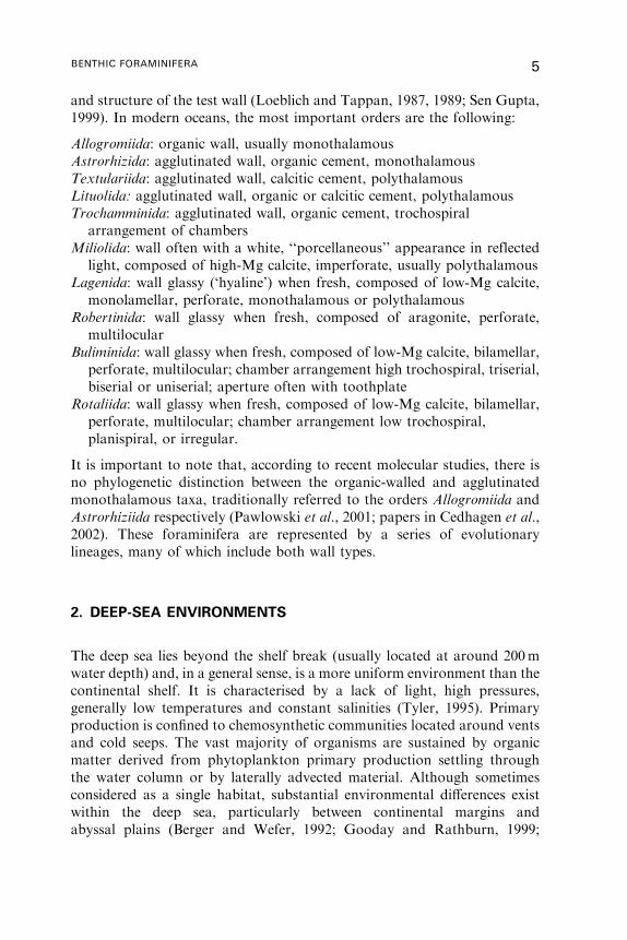
and structure of the test wall (Loeblich and Tappan, 1987, 1989; Sen Gupta,

1999). In modern oceans, the most important orders are the following:

Allogromiida: organic wall, usually monothalamous

Astrorhizida: agglutinated wall, organic cement, monothalamous

Textulariida: agglutinated wall, calcitic cement, polythalamous

Lituolida: agglutinated wall, organic or calcitic cement, polythalamous

Trochamminida: agglutinated wall, organic cement, trochospiral

arrangement of chambers

Miliolida: wall often with a white, ‘‘porcellaneous’’ appearance in reflected

light, composed of high-Mg calcite, imperforate, usually polythalamous

Lagenida: wall glassy (‘hyaline’) when fresh, composed of low-Mg calcite,

monolamellar, perforate, monothalamous or polythalamous

Robertinida: wall glassy when fresh, composed of aragonite, perforate,

multilocular

Buliminida: wall glassy when fresh, composed of low-Mg calcite, bilamellar,

perforate, multilocular; chamber arrangement high trochospiral, triserial,

biserial or uniserial; aperture often with toothplate

Rotaliida: wall glassy when fresh, composed of low-Mg calcite, bilamellar,

perforate, multilocular; chamber arrangement low trochospiral,

planispiral, or irregular.

It is important to note that, according to recent molecular studies, there is

no phylogenetic distinction between the organic-walled and agglutinated

monothalamous taxa, traditionally referred to the orders Allogromiida and

Astrorhiziida respectively (Pawlowski et al., 2001; papers in Cedhagen et al.,

2002). These foraminifera are represented by a series of evolutionary

lineages, many of which include both wall types.

2. DEEP-SEA ENVIRONMENTS

The deep sea lies beyond the shelf break (usually located at around 200m

water depth) and, in a general sense, is a more uniform environment than the

continental shelf. It is characterised by a lack of light, high pressures,

generally low temperatures and constant salinities (Tyler, 1995). Primary

production is confined to chemosynthetic communities located around vents

and cold seeps. The vast majority of organisms are sustained by organic

matter derived from phytoplankton primary production settling through

the water column or by laterally advected material. Although sometimes

considered as a single habitat, substantial environmental differences exist

within the deep sea, particularly between continental margins and

abyssal plains (Berger and Wefer, 1992; Gooday and Rathburn, 1999;


Etter and Mullineaux, 2000). Bathyal continental slopes and rises are

physically much more heterogeneous than abyssal plains. They are often

topographically complex (Mellor and Paull, 1994) and subject to vigorous

current activity and catastrophic mass movements (Masson et al., 1996).

Compared with abyssal plains, sedimentation rates are usually higher on the

continental slope and the sediments are more heterogeneous, less well

oxidised and richer in animal life (Etter and Grassle, 1992; Bett, 2001).

Continental slopes have experienced dramatic oceanographic changes linked

to global climatic fluctuations in the geologic past, particularly during the

Pliocene and Pleistocene glacial cycles. By comparison, the abyssal sea floor

is relatively uniform and quiescent with gently undulating topography.

Because the amount of organic matter reaching the ocean floor decreases

with increasing depth, abyssal environments are typically more food limited

than continental margins that also receive laterally advected organic matter

from the continental shelf. High productivity areas associated with upwelling

or major river discharges are more common on continental margins (Diaz

and Rosenburg, 1995; Rogers, 2000). These environmental contrasts have

ecological consequences for benthic communities. In a general sense, one

would expect sediment types, near-bottom currents and oxygen depletion

coupled with organic enrichment to exert a greater influence on continental

margins (e.g. Schaff et al., 1992; Schmiedl et al., 1997; Levin et al., 2000), and

patterns of food inputs derived from surface production to be more

important on abyssal plains (e.g. Loubere, 1991; Smith et al., 1997).

3. METHODOLOGY: SIEVE SIZES, SAMPLING DEVICES

AND REPLICATION

Most analyses of living foraminiferal faunas are based on sieved residues

stained with rose Bengal which colours the protoplasm red. Wet sorting (i.e.

in a dish of water) makes it easier to see stained protoplasm and therefore

yields more accurate results than dry sorting. Sieve sizes strongly influence

the abundance of individual species and hence assemblage composition and

diversity. Many studies are based on sediment fractions >125, >150 or

even >250 mm, which can be analysed relatively quickly. However, some

dominant species are small and therefore concentrated in the finer (63–125

or 63–150 mm) residues (Schroder et al., 1987; Sen Gupta et al., 1987;

Rathburn and Corliss, 1994; Kurbjeweit et al., 2000). In the ice-covered

central Arctic, the average size of foraminiferal tests is �70 mm and many of

the important species pass through a 125 mm mesh (Wollenburg and

Mackensen, 1998). Small epifaunal species may be very abundant and

important for detecting responses to freshly deposited, labile organic matter

6 ANDREW J. GOODAY

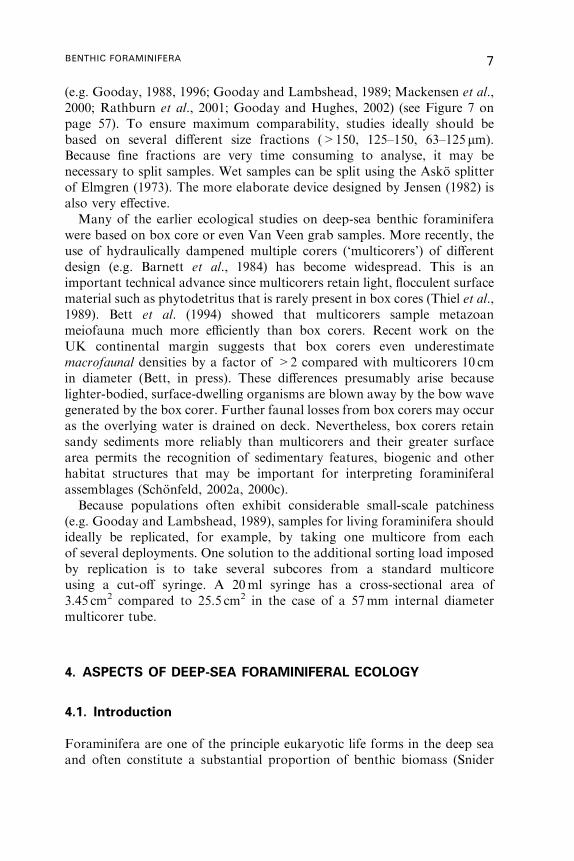
(e.g. Gooday, 1988, 1996; Gooday and Lambshead, 1989; Mackensen et al.,

2000; Rathburn et al., 2001; Gooday and Hughes, 2002) (see Figure 7 on

page 57). To ensure maximum comparability, studies ideally should be

based on several different size fractions (>150, 125–150, 63–125 mm).

Because fine fractions are very time consuming to analyse, it may be

necessary to split samples. Wet samples can be split using the Asko splitter

of Elmgren (1973). The more elaborate device designed by Jensen (1982) is

also very effective.

Many of the earlier ecological studies on deep-sea benthic foraminifera

were based on box core or even Van Veen grab samples. More recently, the

use of hydraulically dampened multiple corers (‘multicorers’) of different

design (e.g. Barnett et al., 1984) has become widespread. This is an

important technical advance since multicorers retain light, flocculent surface

material such as phytodetritus that is rarely present in box cores (Thiel et al.,

1989). Bett et al. (1994) showed that multicorers sample metazoan

meiofauna much more efficiently than box corers. Recent work on the

UK continental margin suggests that box corers even underestimate

macrofaunal densities by a factor of >2 compared with multicorers 10 cm

in diameter (Bett, in press). These differences presumably arise because

lighter-bodied, surface-dwelling organisms are blown away by the bow wave

generated by the box corer. Further faunal losses from box corers may occur

as the overlying water is drained on deck. Nevertheless, box corers retain

sandy sediments more reliably than multicorers and their greater surface

area permits the recognition of sedimentary features, biogenic and other

habitat structures that may be important for interpreting foraminiferal

assemblages (Schonfeld, 2002a, 2000c).

Because populations often exhibit considerable small-scale patchiness

(e.g. Gooday and Lambshead, 1989), samples for living foraminifera should

ideally be replicated, for example, by taking one multicore from each

of several deployments. One solution to the additional sorting load imposed

by replication is to take several subcores from a standard multicore

using a cut-off syringe. A 20ml syringe has a cross-sectional area of

3.45 cm2 compared to 25.5 cm2 in the case of a 57mm internal diameter

multicorer tube.

4. ASPECTS OF DEEP-SEA FORAMINIFERAL ECOLOGY

4.1. Introduction

Foraminifera are one of the principle eukaryotic life forms in the deep sea

and often constitute a substantial proportion of benthic biomass (Snider


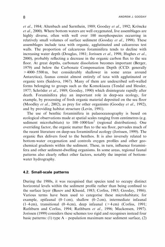
et al., 1984; Altenbach and Sarnthein, 1989; Gooday et al., 1992; Kroncke

et al., 2000). Where bottom waters are well oxygenated, live assemblages are

highly diverse, often with well over 100 morphospecies occurring in

relatively small volumes of surface sediment (Gooday et al., 1998). These

assemblages include taxa with organic, agglutinated and calcareous test

walls. The proportion of calcareous foraminifera tends to decline with

increasing water depth (Douglas, 1981; Jorissen et al., 1998; Hughes et al.,

2000), probably reflecting a decrease in the organic carbon flux to the sea

floor. At great depths, carbonate dissolution becomes important (Berger,

1979) and below the Carbonate Compensation Depth (CCD: generally

>4000–5500m, but considerably shallower in some areas around

Antarctica), faunas consist almost entirely of taxa with agglutinated or

organic tests (Saidova, 1967). Many of them are undescribed soft-walled

forms belonging to groups such as the Komokiacea (Tendal and Hessler,

1977; Schroder et al., 1989; Gooday, 1990) which disintegrate rapidly after

death. Foraminifera play an important role in deep-sea ecology, for

example, by processing of fresh organic material deposited on the sea floor

(Moodley et al., 2002), as prey for other organisms (Gooday et al., 1992),

and by providing habitat structure (Levin, 1991).

The use of benthic foraminifera in palaeoceanography is based on

ecological observations made at spatial scales ranging from centimetres (e.g.

sediment microhabitats) to 100–1000 km2 (regional distributions). One

overriding factor, the organic matter flux to the sea floor, pervades much of

the recent literature on deep-sea foraminiferal ecology (Jorissen, 1999). The

organic flux delivers food to the benthos. It is also inversely related to

bottom-water oxygenation and controls oxygen profiles and other geo-

chemical gradients within the sediment. These, in turn, influence foramini-

fera and other sediment-dwelling organisms. In some areas, regional faunal

patterns also clearly reflect other factors, notably the imprint of bottom-

water hydrography.

4.2. Small-scale patterns

During the 1980s, it was recognised that species tend to occupy distinct

horizontal levels within the sediment profile rather than being confined to

the surface layer (Basov and Khusid, 1983; Corliss, 1985; Gooday, 1986).

Various terms have been used to categorise these microhabitats; for

example, epifaunal (0–1 cm), shallow (0–2 cm), intermediate infaunal

(1–4 cm), transitional (0–4 cm), deep infaunal (>4 cm) (Corliss, 1991;

Rathburn and Corliss, 1994; Rathburn et al., 1996; Mackensen, 1997).

Jorissen (1999) considers these schemes too rigid and recognises instead four

basic patterns: (1) type A – population maximum near sediment surface, (2)

8 ANDREW J. GOODAY

type B – fairly stable populations in the upper part (several centimetres) of

the sediment column followed by a fairly sharp decline in deeper layers,

(3) type C – one or more subsurface maxima, (4) type D – an irregular

pattern with a surface maximum and one or more subsurface maxima.

Comparisons between these faunal patterns and geochemical profiles

suggest that they reflect differential species responses to geochemical

gradients (e.g. pore-water oxygen, H2S) within the sediment and therefore,

ultimately, the flux of organic matter to the sea floor. Other factors that may

be involved in controlling foraminiferal microhabitats, but for which there

is little direct evidence, include the intensity of competitive interactions,

the redistributing effects of bioturbation, the creation of microhabitats by

burrowing macro- and mega-fauna, and possibly sequences of different

bacterial food types related to redox boundaries (Moodley et al., 1998b;

Jorissen 1999; Schonfeld, 2001; Fontanier et al., 2002).

Foraminiferal microhabitats are not necessarily static (Linke and Lutze,

1993). Direct observations of specimens in aquaria (e.g. Gross, 2000), and

analyses of carbon isotopes in carbonate shells (Mackensen et al., 2000),

indicate that some deep-sea species move within the sediments. Species that

are deeply infaunal in well-oxygenated settings occur close to the sediment

surface in eutrophic, oxygen-depleted environments (Mackensen and

Douglas, 1989; Kitazato, 1994; Rathburn and Corliss, 1994). Infaunal

species also move up and down in the sediment in response to seasonal

fluctuations in the food supply and corresponding changes in the depth of the

oxygenated layer (Barmawidjaja et al., 1992; Kitazato and Ohga, 1995; Ohga

and Kitazato, 1997). These field observations are supported by laboratory

studies such as those of Nomaki (2002) and Nomaki, pers. comm. who

demonstrated that infaunal species from Sagami Bay, Japan (1426m water

depth) migrate vertically within the sediment profile following a food pulse.

These movements may be responses either to the availability of food at the

sediment surface, or to changes in oxygen concentrations within sediment

pore-waters. The experiments of Heinz et al. (2002), using sediment

from 919m water depth in the Mediterranean Sea, suggest that oxygen

availability is the main factor. They found that, when pore-water oxygen

levels remained constant, foraminiferal distributions did not change

following a food pulse. Earlier experiments based on samples from coastal

waters also suggested that shallow-water, infaunal species respond to

changing oxygen gradients (Alve and Bernhard, 1995;Moodley et al., 1998b).

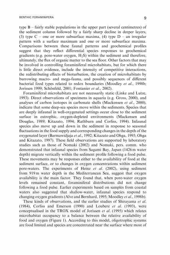
These kinds of observations, and the earlier studies of Shirayama et al.

(1984), Corliss and Emerson (1990) and Loubere et al. (1993), were

conceptualised in the TROX model of Jorissen et al. (1995) which relates

microhabitat occupancy to a balance between the relative availability of

food and oxygen (Figure 1). According to this model, oligotrophic systems

are food limited and species are concentrated near the surface where most of


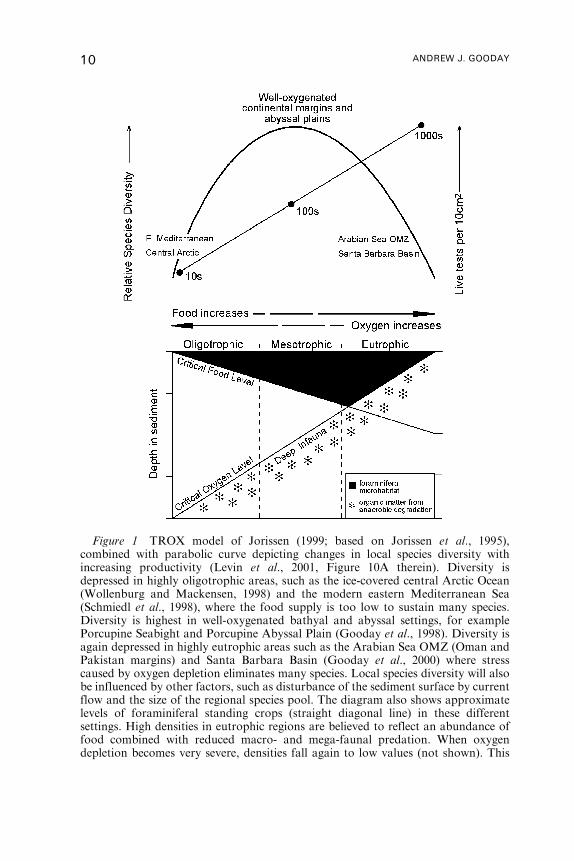
Figure 1 TROX model of Jorissen (1999; based on Jorissen et al., 1995),combined with parabolic curve depicting changes in local species diversity withincreasing productivity (Levin et al., 2001, Figure 10A therein). Diversity isdepressed in highly oligotrophic areas, such as the ice-covered central Arctic Ocean(Wollenburg and Mackensen, 1998) and the modern eastern Mediterranean Sea(Schmiedl et al., 1998), where the food supply is too low to sustain many species.Diversity is highest in well-oxygenated bathyal and abyssal settings, for examplePorcupine Seabight and Porcupine Abyssal Plain (Gooday et al., 1998). Diversity isagain depressed in highly eutrophic areas such as the Arabian Sea OMZ (Oman andPakistan margins) and Santa Barbara Basin (Gooday et al., 2000) where stresscaused by oxygen depletion eliminates many species. Local species diversity will alsobe influenced by other factors, such as disturbance of the sediment surface by currentflow and the size of the regional species pool. The diagram also shows approximatelevels of foraminiferal standing crops (straight diagonal line) in these differentsettings. High densities in eutrophic regions are believed to reflect an abundance offood combined with reduced macro- and mega-faunal predation. When oxygendepletion becomes very severe, densities fall again to low values (not shown). This

10 ANDREW J. GOODAY

the food is located. Eutrophic systems are oxygen limited and species are

concentrated near the surface into order to avoid anoxic conditions deeper

in the sediment profile. Maximum penetration is found in intermediate

(‘mesotrophic’) settings where both food and oxygen are available well

below the sediment/water interface. This basic scheme has been refined by

Jorissen et al. (1998), Jorissen (1999), van der Zwaan et al. (1999) and

Fontanier et al. (2002) who make the following suggestions: (1) the organic

flux is the pre-eminent parameter controlling foraminiferal microhabitats;

(2) Oxygen is not a limiting factor for deep infaunal (Type C) species that

occur below the subsurface oxic/anoxic interface. These species may be more

closely linked to subsurface accumulations of organic matter (Rathburn and

Corliss, 1994) or to populations of anaerobic bacteria associated with redox

boundaries (Jorissen et al., 1998; Fontanier et al., 2002), (3) Biological

interactions, particularly competition for labile food material, play a role in

determining where foraminifera live within the sediment profile. The TROX

model and its successors provide a useful framework for understanding

how various factors may interact to control foraminiferal microhabitats,

although they are qualitative and cannot be used to reconstruct values for

parameters such as organic fluxes directly.

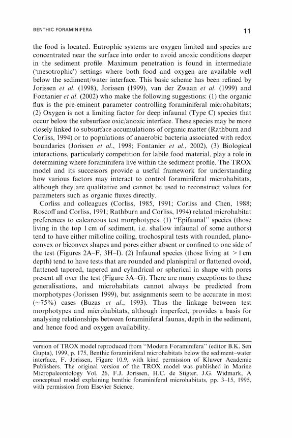
Corliss and colleagues (Corliss, 1985, 1991; Corliss and Chen, 1988;

Roscoff and Corliss, 1991; Rathburn and Corliss, 1994) related microhabitat

preferences to calcareous test morphotypes. (1) ‘‘Epifaunal’’ species (those

living in the top 1 cm of sediment, i.e. shallow infaunal of some authors)

tend to have either milioline coiling, trochospiral tests with rounded, plano-

convex or biconvex shapes and pores either absent or confined to one side of

the test (Figures 2A–F, 3H–I). (2) Infaunal species (those living at >1 cm

depth) tend to have tests that are rounded and planispiral or flattened ovoid,

flattened tapered, tapered and cylindrical or spherical in shape with pores

present all over the test (Figure 3A–G). There are many exceptions to these

generalisations, and microhabitats cannot always be predicted from

morphotypes (Jorissen 1999), but assignments seem to be accurate in most

(�75%) cases (Buzas et al., 1993). Thus the linkage between test

morphotypes and microhabitats, although imperfect, provides a basis for

analysing relationships between foraminiferal faunas, depth in the sediment,

and hence food and oxygen availability.

version of TROX model reproduced from ‘‘Modern Foraminifera’’ (editor B.K. SenGupta), 1999, p. 175, Benthic foraminiferal microhabitats below the sediment–waterinterface, F. Jorissen, Figure 10.9, with kind permission of Kluwer AcademicPublishers. The original version of the TROX model was published in MarineMicropaleontology Vol. 26, F.J. Jorissen, H.C. de Stigter, J.G. Widmark, Aconceptual model explaining benthic foraminiferal microhabitats, pp. 3–15, 1995,with permission from Elsevier Science.


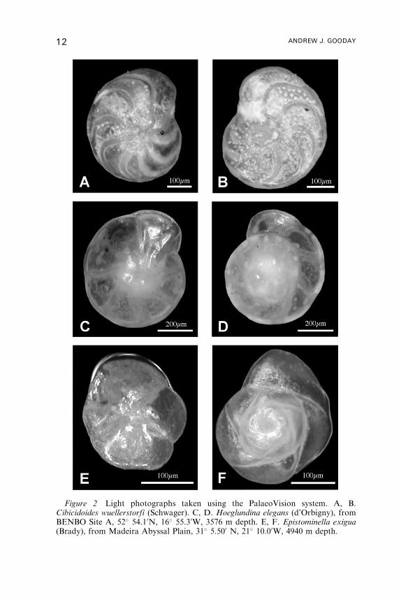
Figure 2 Light photographs taken using the PalaeoVision system. A, B.Cibicidoides wuellerstorfi (Schwager). C, D. Hoeglundina elegans (d’Orbigny), fromBENBO Site A, 52� 54.10N, 16� 55.30W, 3576 m depth. E, F. Epistominella exigua(Brady), from Madeira Abyssal Plain, 31� 5.500 N, 21� 10.00W, 4940 m depth.

12 ANDREW J. GOODAY

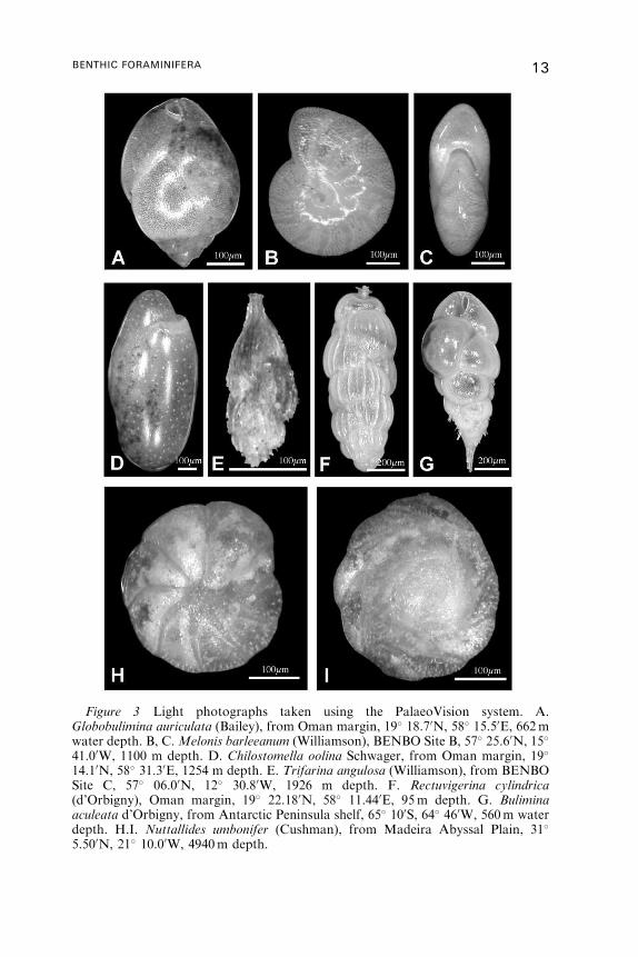
Figure 3 Light photographs taken using the PalaeoVision system. A.Globobulimina auriculata (Bailey), from Oman margin, 19� 18.70N, 58� 15.50E, 662mwater depth. B, C.Melonis barleeanum (Williamson), BENBO Site B, 57� 25.60N, 15�

41.00W, 1100 m depth. D. Chilostomella oolina Schwager, from Oman margin, 19�

14.10N, 58� 31.30E, 1254 m depth. E. Trifarina angulosa (Williamson), from BENBOSite C, 57� 06.00N, 12� 30.80W, 1926 m depth. F. Rectuvigerina cylindrica(d’Orbigny), Oman margin, 19� 22.180N, 58� 11.440E, 95m depth. G. Buliminaaculeata d’Orbigny, from Antarctic Peninsula shelf, 65� 100S, 64� 460W, 560m waterdepth. H.I. Nuttallides umbonifer (Cushman), from Madeira Abyssal Plain, 31�

5.500N, 21� 10.00W, 4940m depth.


4.3. Regional patterns

At regional scales, foraminiferal species distributions are influenced by a

variety of environmental factors, including temperature, salinity, food and

oxygen availability, sediment type, current and wave action (Murray, 1991).

These often vary spatially and temporally, particularly in complex,

energetic, continental shelf and coastal settings, making it difficult to

identify straightforward, predictable relationship between species and single

parameters. In the deep sea, where the physico-chemical environment is

generally more uniform, it is often easier to recognise the influence of a few

variable parameters on foraminiferal distributions (Murray, 2001). During

the last two decades, the view has become popular that the organic matter

flux to the ocean floor is a crucial parameter in this food-limited

environment (e.g. Grassle and Morse-Porteous, 1987; Nees and Struck,

1999; Loubere and Fariduddin, 1999b; van der Zwaan et al., 1999;

Wollenburg and Kuhnt, 2000; Morigi et al., 2001). Both the intensity of

the flux and its seasonal variations appear to be important (Loubere and

Fariduddin, 1999a). Work conducted in the 1970s and 1980s off the NW

African margin by G.F. Lutze and colleagues at Kiel University (Germany)

generated a vast body of faunal data and played a major part in the

development of this paradigm (Lutze, 1980; Lutze and Coulbourne, 1984;

Lutze et al., 1986; Altenbach, 1988; Altenbach and Sarnthein 1989;

Altenbach et al., 1999). Earlier researchers also made contributions but

based on much smaller databases (e.g. Osterman and Kellogg, 1979; Sen

Gupta et al., 1981; Miller and Lohmann, 1982).

Where organic fluxes are high, or circulation restricted, oxygen depletion

in the bottom water and sediment pore water becomes a significant

ecological factor. Foraminifera are more tolerant of oxygen depletion than

most metazoan taxa (Josefson and Widbom, 1988; Moodley et al., 1997),

but the degree of tolerance varies substantially between species. Tolerant

species usually have ‘‘infaunal’’ morphologies and occur in deeper, oxygen-

depleted or anoxic sediment layers. In dysoxic, organically enriched settings,

epifaunal/shallow infaunal species disappear and deep infaunal species take

advantage of the enhanced food supply and reduced macrofaunal predation

to develop dense, low-diversity populations close to the sediment–water

interface.

The current emphasis on food and oxygen availability should not obscure

the impact of other factors on foraminiferal species distributions, particu-

larly on continental slopes. Mackensen et al. (1993), Mackensen (1997) and

Schnitker (1994) focus on the influence of hydrography and suggest that

epifaunal species assemblages reflect the characteristics of bottom-water

masses. This is particularly true of foraminifera living on ‘elevated epifaunal’

microhabitats above the sediment surface. In the deep sea, substrates include

14 ANDREW J. GOODAY

stones, manganese nodules (Mullineaux, 1987; Schonfeld, 2002a), sponges,

hydroids, corals and other sessile animals (Lutze and Thiel, 1989; Rogers,

1999; Beaulieu, 2001), and even mobile animals such as pycnogonids and

isopods (Linke and Lutze, 1993; Svavarsson and Olafsdottir, 2000). These

species are in direct contact with the bottom water and clearly respond to

hydrographic factors, particularly current flow and the associated flux of

food particles. Other parameters that may help to explain deep-sea species

distributions include sediment characteristics (e.g. grain size and porosity),

temperature, water depth (i.e. hydrostatic pressure) (Hermelin and

Shimmield, 1990; Kurbjeweit et al., 2000; Hayward et al., 2002) and the

disturbance of sediment communities by ‘‘benthic storms’’, turbidity currents

and volcanic ash falls (Kaminski, 1985; Hess and Kuhnt, 1996; Hess et al.,

2001). Biotic factors are also likely to play a role. Predation, for example,

may limit foraminiferal standing stocks in areas where deposit feeders are

abundant (Douglas, 1981; Buzas et al., 1989).

5. FAUNAL APPROACHES TO RECONSTRUCTING

PALAEOCEANOGRAPHY

Observations made at these different spatial scales contribute to the use of

foraminifera in palaeoceanographic reconstructions. Faunas are usually

analysed at the species level and abundance patterns attributed to the

influence of one or more environmental factors. This approach is easily

applicable to Quaternary sediments where extant species are common.

Analyses of test morphotypes and diversity parameters can also yield

information about palaeoenvironments and are particularly useful in older

deposits where most species are extinct. In addition to these qualitative

approaches, a considerable effort has been devoted to developing

foraminiferal proxies for key environmental factors, particularly organic

carbon fluxes to the sea floor (Mackensen and Bickert, 1999; Wefer et al.,

1999; Weinelt et al., 2001). In the following sections, I review some of the

environmental attributes that are believed to control the abundance,

composition and diversity of foraminiferal assemblages. Faunal indicators

that have proved useful for reconstructing these parameters are summarised

in Table 1. Some are related to bottom-water hydrography, others either

directly or indirectly to the organic flux to the sea floor. In all cases, a central

problem concerns the development of reliable, quantitative relationships

(transfer functions) between environmental parameters and faunal attri-

butes. The review focusses on parameters that are used widely in

palaeoceanographic studies and is not intended to be comprehensive.


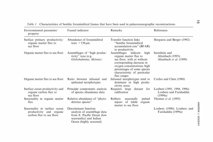
Table 1 Characteristics of benthic foraminiferal faunas that have been used in palaeoceanographic reconstructions.

Environmental parameter/property

Faunal indicator Remarks References

Surface primary productivity/organic matter flux tosea floor

Abundance of foraminiferaltests >150mm

Transfer function links‘‘benthic foraminiferalaccumulation rate’’ (BFAR)to productivity

Herguera and Berger (1992)

Organic matter flux to sea floor Assemblages of ‘‘high produc-tivity’’ taxa (e.g.Globobulimina, Melonis)

Assemblages indicate highorganic matter flux tosea floor, with or withoutcorresponding decrease inoxygen concentrations; highpercentages of some speciescharacteristic of particularflux ranges

Sarnthein andAltenbach (1995);Altenbach et al. (1999)

Organic matter flux to sea floor Ratio between infaunal andepifaunal morphotypes

Infaunal morphotypes tend todominate in high produ-ctivity areas

Corliss and Chen (1988)

Surface ocean productivity andorganic carbon flux tosea floor

Principle components analysisof species abundance data

Requires large dataset forcalibration

Loubere (1991, 1994, 1996);Loubere and Fariduddin(1999a)

Seasonality in organic matterflux

Relative abundance of ‘‘phyto-detritus species’’

Reflects seasonally pulsedinputs of labile organicmatter to sea floor

Thomas et al. (1995)

Seasonality in surface oceanproductivity and organiccarbon flux to sea floor

Discriminant functionanalysis of assemblage datafrom E. Pacific Ocean (lowseasonality) and IndianOcean (highly seasonal)

Loubere (1998); Loubere andFariduddin (1999a)

16

ANDREW

J.GOODAY

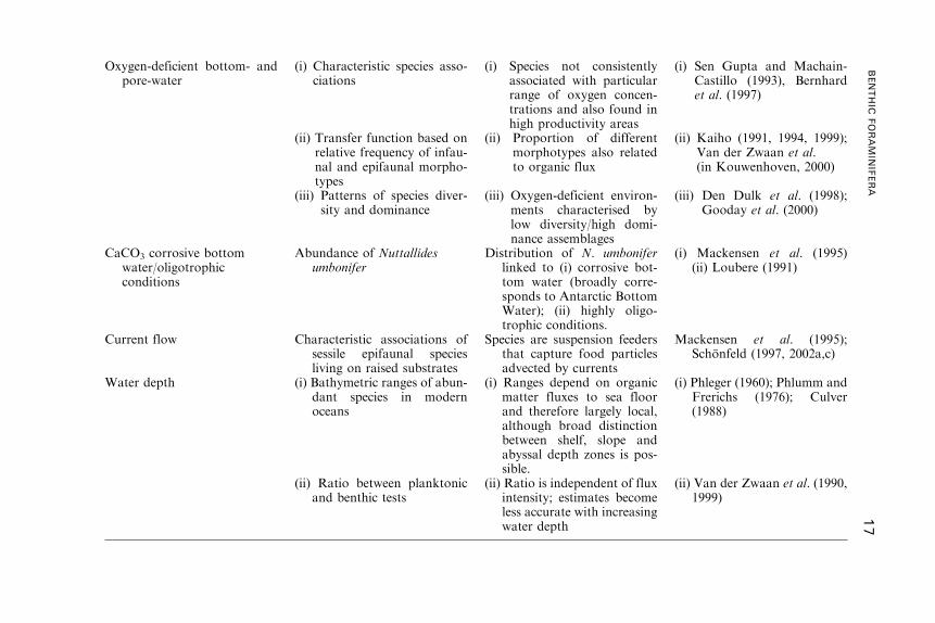
Oxygen-deficient bottom- andpore-water

(i) Characteristic species asso-ciations

(i) Species not consistentlyassociated with particularrange of oxygen concen-trations and also found inhigh productivity areas

(i) Sen Gupta and Machain-Castillo (1993), Bernhardet al. (1997)

(ii) Transfer function based onrelative frequency of infau-nal and epifaunal morpho-types

(ii) Proportion of differentmorphotypes also relatedto organic flux

(ii) Kaiho (1991, 1994, 1999);Van der Zwaan et al.(in Kouwenhoven, 2000)

(iii) Patterns of species diver-sity and dominance

(iii) Oxygen-deficient environ-ments characterised bylow diversity/high domi-nance assemblages

(iii) Den Dulk et al. (1998);Gooday et al. (2000)

CaCO3 corrosive bottomwater/oligotrophicconditions

Abundance of Nuttallidesumbonifer

Distribution of N. umboniferlinked to (i) corrosive bot-tom water (broadly corre-sponds to Antarctic BottomWater); (ii) highly oligo-trophic conditions.

(i) Mackensen et al. (1995)(ii) Loubere (1991)

Current flow Characteristic associations ofsessile epifaunal speciesliving on raised substrates

Species are suspension feedersthat capture food particlesadvected by currents

Mackensen et al. (1995);Schonfeld (1997, 2002a,c)

Water depth (i) Bathymetric ranges of abun-dant species in modernoceans

(i) Ranges depend on organicmatter fluxes to sea floorand therefore largely local,although broad distinctionbetween shelf, slope andabyssal depth zones is pos-sible.

(i) Phleger (1960); Phlumm andFrerichs (1976); Culver(1988)

(ii) Ratio between planktonicand benthic tests

(ii) Ratio is independent of fluxintensity; estimates becomeless accurate with increasingwater depth

(ii) Van der Zwaan et al. (1990,1999)

BENTHIC

FORAMIN

IFERA

17

In particular, sediment characteristics, temperature, substrate disturbance,

and biotic interactions are not treated in detail.

6. ORGANIC MATTER FLUXES

6.1. General considerations

The search for proxies of particulate organic matter (POM) fluxes to the

sea floor is a major goal in palaeoceanography. Much of the recent

geologically orientated research on deep-sea benthic foraminifera has

addressed this issue (e.g. Jorissen et al., 1998; papers in Jorissen and

Rohling, 2000; Morigi et al., 2001). On continental margins, refractory

organic material is transported down the continental slope by various

mechanisms, including nepheloid layers, turbidity currents and down-

canyon currents. A large proportion of the labile POM arriving at the ocean

floor, however, originates from phytoplankton primary production in the

overlying water column. This is particularly true in central oceanic areas

where the POM flux largely reflects the intensity of surface primary

production and lateral advection from slope and shelf areas is not a

significant factor. The material that settles out below the zone of winter

mixing constitutes the long-term export production to the ocean interior

(Berger and Wefer, 1990). In open-ocean settings, only a small fraction

(0.01–1.0%) of this exported material reaches the bottom and this fraction

decreases with increasing water depth (Suess, 1980; Berger et al., 1988, 1989;

Berger and Wefer, 1992). The flux at 2000m shows a linear relation with

levels of primary production below production levels of 200 gCm�2 y�1, but

at higher levels the flux remains constant, for reasons that are not well

understood (Lampitt and Antia, 1997).

Although the complex processes by which organic matter derived from

surface production is delivered to the ocean floor (‘bentho-pelagic coupling’)

are understood in general terms, actual rates of supply are more difficult to

determine accurately (Berger and Wefer, 1992; Murray, 2001). Estimates are

often derived from empirical equations that incorporate primary produc-

tion, export production, and flux rate data obtained from sediment traps

(Suess, 1980; Pace et al., 1987; Berger et al., 1988, 1989; Berger and Wefer,

1990, 1992). These parameters are not necessarily well constrained. In

particular, primary productivity estimates may vary by a factor of 2–3 and

exhibit considerable variability, both spatially and temporally (Berger et al.,

1988; Herguera, 2000). Oxygen fluxes across the sediment–water interface,

obtained by measuring either sediment pore water oxygen profiles or

sediment community oxygen consumption (SCOC), provide a more direct

18 ANDREW J. GOODAY

and time-averaged measure of POM fluxes (e.g. Loubere et al., 1993; Graf

et al., 1995; Jahnke, 1996, 2002; Rowe et al., 1997; Sauter et al., 2001). Even

this approach is not without problems since oxygen fluxes reflect inputs of

refractory carbon (e.g. redeposited material) of limited nutritional value to

foraminifera, as well as labile material. These data are still relatively scarce,

although they can be extrapolated using other measures as proxies (Jahnke,

1996). Thus, despite considerable improvements in our knowledge of ocean-

wide and global patterns of POC fluxes, values at particular localities will

often be subject to substantial uncertainties, a fact that complicates the task

of calibrating flux proxies (Berger et al., 1994).

Another complicating factor is that primary production and export flux

usually have a more or less distinct seasonal component (Berger and Wefer,

1990; Lampitt and Antia, 1997) that is transmitted down through the

oceanic water column (Asper et al., 1992; Turley et al., 1995), leading to the

seasonally pulsed deposition of phytodetritus on the sea floor (Billett et al.,

1983). In the temperate abyssal NE Atlantic Ocean, these deposits deliver an

estimated 2–4% of spring-bloom production to the benthos (Turley et al.,

1995). The strength of seasonality in the vertical flux is related to the nature

of the pelagic ecosystem (Lampitt and Antia, 1997), i.e. the ‘‘plankton

climate’’ provinces of Longhurst (1996, 1998). It is most intense at high

latitudes and least intense in tropical regions (Fischer et al., 1988; Berger

and Wefer, 1990; Wefer and Fischer, 1991; Ramseier et al., 1999). Berger

and Wefer (1990) suggest that export production is higher in strongly

seasonal systems compared with more constant ones, although this is not

confirmed by sediment trap data (Lampitt and Antia, 1996).

6.2. Reconstructing annual flux rates

6.2.1. Species abundances

Total foraminiferal standing stocks reflect food availability (Phleger, 1964,

1976; Douglas, 1981) while particular species tend to be associated with

either higher or lower levels of organic flux (e.g. Lutze, 1980; Rathburn and

Corliss, 1994; Mackensen, 1997; Altenbach et al., 1999; Fontanier et al.,

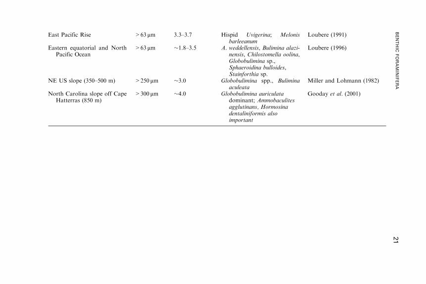
2002). So-called ‘‘high productivity assemblages’’ have received particular

attention (Table 2). They occur in areas that receive a strong and relatively

continuous input of organic matter, usually derived from intense primary

production associated with upwelling, hydrographic fronts, or major rivers

discharges (although material from the latter source is usually dominated

by refractory material of limited food value). Characteristic taxa include

Bulimina spp., Bolivina spp., Cassidulina spp., Chilostomella oolina Schwager

1878, Globobulimina spp., Melonis barleeanum (Williamson), M. zaandami


Table 2 Some examples of modern foraminiferal species and assemblages associated with high productivity areas. Ammobaculitesagglutinans and Hormosina dentaliniformis are agglutinated, all other species are calcareous.

Area (water depth) Size fraction Oxygen (ml l�1) Characteristic species Reference

NW African margin off CapBarbas & Cap Blanc

>250 mm >1.0 Bulimina marginata,Chilostomella oolina,Globobulimina spp.,Uvigerina peregrina

Lutze (1980),Lutze and Coulbourne(1984)

NW Africa off Cap Blanc >150 mm 4.5 Globobulimina pyrula, Melonisbarleeanum, Uvigerinaperegrina

Jorissen et al. (1998)

Tropical Atlantic >63 mm 5.0 Alabaminella weddellensis Fariduddin andLoubere (1997)

Eastern South Atlantic:lower slope off CuneneRiver (800–2000 m)

>125 mm 2.7–5.1 Bulimina spp., Uvigerinaauberiana, Fursenkoinamexicana, Valvulinerialaevigata

Schmiedl andMackensen (1997)

Lower slope off Cunene River(3000–4000m)

>125 mm 5.2 Melonis spp., U. peregrina,Globobulimina turgida,Chilostomella oolina,Nonionella opima,Cassidulina reniforme

Schmiedl andMackensen (1997)

20

ANDREW

J.GOODAY

East Pacific Rise >63 mm 3.3–3.7 Hispid Uvigerina; Melonisbarleeanum

Loubere (1991)

Eastern equatorial and NorthPacific Ocean

>63 mm �1.8–3.5 A. weddellensis, Bulimina alazi-nensis, Chilostomella oolina,Globobulimina sp.,Sphaeroidina bulloides,Stainforthia sp.

Loubere (1996)

NE US slope (350–500 m) >250 mm �3.0 Globobulimina spp., Buliminaaculeata

Miller and Lohmann (1982)

North Carolina slope off CapeHatterras (850 m)

>300 mm �4.0 Globobulimina auriculatadominant; Ammobaculitesagglutinans, Hormosinadentaliniformis alsoimportant

Gooday et al. (2001)

BENTHIC

FORAMIN

IFERA

21

(Van Voorthuyen), Nonionella stella Cushman & Moyer, Sphaeroidina

bulloides Deshayes, and Uvigerina spp. (usually U. peregrina Cushman)

(Figure 3A–G).

High productivity taxa are infaunal and tolerate varying degree of oxygen

depletion. Some (e.g. Globobulimina spp., Bolivina spp., Brizalina spp.)

withstand dysoxic or anoxic conditions better than others (e.g. Uvigerina

spp.) (Miller and Lohmann, 1982; Sen Gupta et al., 1981; Corliss et al., 1986;

Rathburn and Corliss, 1994; Bernhard et al., 1997; Schmiedl et al., 1997).

Species of Melonis apparently prefer more degraded food material than

Bulimina exilis Brady (Caralp, 1989). Evidence from strongly dysoxic

or anoxic settings, and from environments where a strong organic flux is

combined with well-oxygenated bottom water, suggests that Chilostomella

oolina and Nonion scaphum (Fitchel & Moll) are associated with labile

organic carbon inputs, Globobulimina affinis (d’Orbigny) and Melonis

barleeanum with more refractory material (Fontanier et al., 2002).

Laboratory experiments in which algae were added to sediments recovered

from the centre of Sagami Bay, Japan, tend to contradict these field

observations (Nomaki, 2002; Nomaki, pers. comm.). Another Chilostomella

species, C. ovoidea Reuss, did not respond at all whereas G. affinis migrated

upwards in the sediment following the addition of food, and ingested fresh

algae. In situ feeding experiments at the same locality using 13C labelled algae

support these results (Nomaki, 2002; Kitazato et al., in press) and suggest

that C. ovoidea and G. affinis may have different diets in Sagami Bay. Other

foraminifera, many of them epifaunal or shallow infaunal, are associated

with lower flux rates. Such species include Cibicidoides wuellerstorfi

(Schwager), Hoeglundina elegans (d’Orbigny), Oridorsalis umbonatus

(Reuss), Nuttallides umbonifer (Cushman), Globocassidulina subglobosa

(Brady) (Figures 2A–F, 3H–I) (Altenbach, 1988; Sarnthein and Altenbach,

1995; Altenbach et al., 1999; Loubere and Fariddudin, 1999b; Morigi et al.,

2001). As discussed below, these species are believed to feed largely on fresh

POM and are relatively intolerant of dysoxic conditions.

Can species abundances be used as indicators of absolute flux rates?

Altenbach et al. (1999) addressed this question by analysing the relationship

between flux to the sea floor and percentage species abundances in 382

samples from the equatorial eastern Atlantic to the Arctic. Species occurred

over a range of annual flux values spanning between 1 and 3 orders of

magnitude, and only 4–64% of total abundance was explained by flux rates.

When only high percentage occurrences were considered, however, the range

was much smaller. Thus, the abundant occurrence of particular species

(presumably reflecting their optimum habitat) may be typical of particular

flux regimes (Table 3), although mere occurrences, or even moderate

abundances, are of little significance. The percentage abundance of a few

species (e.g.Cibicidoides wuellerstorfi in the>250 mm fraction) can be used to

22 ANDREW J. GOODAY

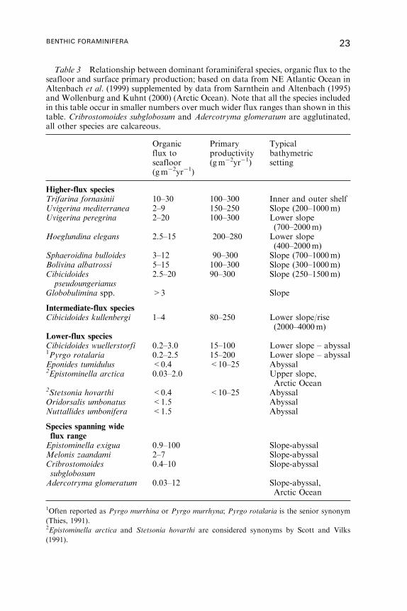
Table 3 Relationship between dominant foraminiferal species, organic flux to theseafloor and surface primary production; based on data from NE Atlantic Ocean inAltenbach et al. (1999) supplemented by data from Sarnthein and Altenbach (1995)and Wollenburg and Kuhnt (2000) (Arctic Ocean). Note that all the species includedin this table occur in smaller numbers over much wider flux ranges than shown in thistable. Cribrostomoides subglobosum and Adercotryma glomeratum are agglutinated,all other species are calcareous.

Organicflux toseafloor(gm�2yr�1)

Primaryproductivity(gm�2yr�1)

Typicalbathymetricsetting

Higher-flux speciesTrifarina fornasinii 10–30 100–300 Inner and outer shelfUvigerina mediterranea 2–9 150–250 Slope (200–1000m)Uvigerina peregrina 2–20 100–300 Lower slope

(700–2000m)Hoeglundina elegans 2.5–15 200–280 Lower slope

(400–2000m)Sphaeroidina bulloides 3–12 90–300 Slope (700–1000m)Bolivina albatrossi 5–15 100–300 Slope (300–1000m)Cibicidoidespseudoungerianus

2.5–20 90–300 Slope (250–1500m)

Globobulimina spp. >3 Slope

Intermediate-flux speciesCibicidoides kullenbergi 1–4 80–250 Lower slope/rise

(2000–4000m)Lower-flux speciesCibicidoides wuellerstorfi 0.2–3.0 15–100 Lower slope – abyssal1Pyrgo rotalaria 0.2–2.5 15–200 Lower slope – abyssalEponides tumidulus <0.4 <10–25 Abyssal2Epistominella arctica 0.03–2.0 Upper slope,

Arctic Ocean2Stetsonia hovarthi <0.4 <10–25 AbyssalOridorsalis umbonatus <1.5 AbyssalNuttallides umbonifera <1.5 Abyssal

Species spanning wideflux rangeEpistominella exigua 0.9–100 Slope-abyssalMelonis zaandami 2–7 Slope-abyssalCribrostomoidessubglobosum

0.4–10 Slope-abyssal

Adercotryma glomeratum 0.03–12 Slope-abyssal,Arctic Ocean

1Often reported as Pyrgo murrhina or Pyrgo murrhyna; Pyrgo rotalaria is the senior synonym

(Thies, 1991).2Epistominella arctica and Stetsonia hovarthi are considered synonyms by Scott and Vilks

(1991).


estimate flux rates <2 gCorg m�2 with reasonable confidence. In addition,

some infaunal species (e.g. Uvigerina mediterranea Hofker 1932) tend to be

associated with a specific range of flux values irrespective of their abundance.

Sarnthein and Altenbach (1995) and Altenbach et al. (1999) suggest that the

annual flux range of 2–3 gCorg m�2 marks an upper threshold of dominance

for many species characteristic of oligotrophic abyssal settings and a lower

threshold of dominance for species adapted to more eutrophic shelf and

bathyal environments. Other authors have also reported evidence for an

ecological boundary around the same flux levels (De Rijk et al., 2000;

Jian et al., 1999; Morigi et al., 2001; Weinelt et al., 2001).

6.2.2. Morphotype approaches

These approaches rely on the relationship between organic fluxes and the

relative abundance of infaunal and epifaunal morphotypes. The use of

morphotypes as flux indicators is complicated by the fact that they are also

related to oxygen availability, at least at low oxygen concentrations. This is

discussed in Section 7.

Corliss and Chen (1988) reanalysed the data of Mackensen et al. (1985)

from the Norwegian margin (dead assemblage, 0–1 cm layer, >125 mm

fraction), assigning the species to either infaunal or epifaunal morphotypes.

Both categories occurred between 200m and 500m water depth, infaunal

morphotypes predominated between 500m and 1500m, epifaunal morpho-

types were most abundant below this depth (Corliss and Chen, 1988).

A similar pattern was observed by Roscoff and Corliss (1991) in the

Greenland-Norwegian Sea. Below 800m depth, these patterns correlated

well with the organic carbon content of surface sediments; high organic

carbon values were associated with dominance by infaunal morphotypes,

low carbon values with epifaunal morphotypes. Corliss and Chen (1988)

suggest that the switch from infaunal to epifaunal dominance occurs within

the yearly organic carbon flux range 3–6 gCorgm�2. Despite the imperfect

relationship between microhabitats and morphotypes referred to above, the

Corliss and Chen (1988) approach can provide a general indication of

organic fluxes levels. The quality of the available food is also important.

Deep infaunal species living below the level at which oxygen disappears

from the sediment pore water apparently consume more degraded organic

matter than epifaunal and shallow-infaunal species (Goldstein and Corliss,

1994; Fontanier et al., 2002). The abundance of the former and scarcity of

the latter at a site off Cap Blanc (NW African margin) overlain by well-

oxygenated bottom water (4.5ml/l) was attributed by Jorissen et al. (1998)

to the lack of freshly deposited labile detritus compared to the relatively

large amounts of more degraded material available deeper in the sediment.

24 ANDREW J. GOODAY

Thus, as van der Zwaan et al. (1999) conclude, infaunal morphotypes reflect

the abundance of organic matter stored within the sediment, rather than the

flux of fresh material.

6.2.3. Benthic Foraminiferal Accumulation Rate (BFAR)

The population density and biomass of different components of the deep-sea

benthic fauna, from bacteria to megafauna, are related to food availability

(Rowe, 1983; Lampitt et al., 1986; Altenbach, 1988; Lochte, 1992; Tietjen,

1992; van der Zwaan et al., 1999; Wollenburg and Kuhnt, 2000; Fontanier

et al., 2002). This relationship provides the basis for an equation, proposed

by Herguera and Berger (1991), linking the abundance, or more accurately

the accumulation rate, of benthic foraminifera (BFAR) to the total organic

matter flux reaching the sea floor (Figure 4) (see also Berger and Herguera,

1992; Herguera, 1992). BFAR is the number of foraminiferal tests >150 mm

that accumulate per cm2 per 103 years [¼ (no. benthic foraminifera g of dry

Figure 4 Relationship between the benthic foraminiferal (BF) accumulation rate(BFAR) and the organic matter flux to the sea floor (Jsf), based on data from theOntong Java Plateau. Filled circles are core-top (i.e. modern) samples; diamonds arefrom sediment deposited during the last glacial maximum; squares are fromsediments deposited during the transition from glacial to interglacial conditions.Small white symbols inset into larger black symbols show water depths; the two insetopen circles (above the line) indicate depths from 4000–4500m, the inset opentriangles indicate depths >4500m. Reproduced from Geology Vol. 19, J.C.Herguera and W.H. Berger, Paleoproductivity from benthic foraminifera abun-dance: glacial to post-glacial change in west-equatorial Pacific, p. 1175, Figure 2,with thanks to the Geological Society of America.


sediment�1) x (sed. rate in cm kyr�1) x (dry bulk density in g cm�3)]. The

calculation depends on the sedimentation rate being constant during the

time interval examined. Struck (1992) used the term INDAR (Individual

Accumulation Rate) in much the same sense as BFAR. By applying

equations that describe the loss or decomposition of organic particles during

their passage through the water column (Herguera and Berger, 1991),

BFAR can be used to estimate surface primary productivity, although such

estimates involve important assumptions and considerable errors (Herguera,

2000). The BFAR approach appears to work adequately in well-oxygenated

sediments (Herguera and Berger, 1991; Nees et al., 1997; Schmiedl and

Mackensen, 1997; Nees and Struck, 1999; Herguera, 2000) but fails to yield

realistic palaeoproductivity estimates where oxygen depletion is a limiting

factor (Naidu and Malmgren, 1995). It can also be compromised by post-

mortem taphonomic processes such as the dissolution of calcareous tests

(Loubere and Fariduddin, 1999b). For example, Wollenburg and Kuhnt

(2000) report that highest BFAR values in the Arctic Ocean were derived

from areas under permanent ice where the Corg flux was lowest whereas

seasonally ice-free areas subject to carbonate dissolution yielded dispro-

portionately low values. Severe dissolution substantially limits the use of

BFAR to reconstruct Quaternary and Holocene paleoproductivity in this

region (Wollenburg et al., 2001).

An additional problem is that BFAR assumes a steady rain of sinking

material (Murray, 2001). In fact, a high proportion of the flux may be

delivered episodically in the form of phytodetritus aggregates (reviewed by

Beaulieu, 2002), larger phytoplankton mats (Kemp et al., 2000), large faecal

pellets (Pfannkuche and Lochte, 1993) and animal carcasses (e.g.

Christiansen and Boetius, 2000). Because they sink rapidly, these particles

have a greater food value and therefore support a higher benthic biomass

than more refractory, slowly descending particles. Small (<150 mm),

opportunistic foraminifera are often abundant in areas where the organic

flux is strongly pulsed. Much of the foraminiferal production supported

by this labile organic material will therefore pass through a 150 mm sieve.

If finer fractions (<150 mm) are incorporated into BFAR calculations, the

organic flux values will be overestimated since small foraminifera have a

much smaller biomass than larger ones (Ohkushi et al., 2000).

Nevertheless, there is evidence that BFAR values are sensitive to

differences in the quality of deposited organic matter. Guichard et al.

(1997) found a generally good correlation between BFAR (>150 mm

fraction) and flux rates for organic carbon (gC cm�2 10�3 years) in a core

from the NW African upwelling area. Deviations observed in certain

horizons were interpreted as reflecting fluctuations in the quality of organic

material reaching the sea floor. BFAR values that were disproportionately

high in relation to the Corg flux values were probably due to strong

26 ANDREW J. GOODAY

phytodetrital inputs derived from intense spring blooms while dispropor-

tionately low BFAR values probably reflected periods when the flux was

of poor food quality due to enhanced lateral advection. Schmiedl and

Mackensen (1997) also reported deviations from a linear relation between

BFAR (>125 mm fraction) and palaeo-export in the eastern South Atlantic.

BFAR values during glacial stage 12 were more than ten times higher than

interglacial values and translated into unrealistically high palaeoproductiv-

ity estimates. These results suggest that opportunistic epifaunal species that

respond to phytodetrital pulses add dead shells to the sediments at a higher

rate than deeper infaunal species (de Stigter et al., 1999). Refinements of the

BFAR method will need to take account of different rates of production

(Schonfeld, 2002b).

6.2.4. Multivariate analysis of assemblage data

Multivariate statistical techniques such as Principal Components Analysis

and Factor Analysis have been widely used to extract environmental signals

from large fauna datasets (Loubere and Qian, 1997). Loubere and

colleagues used multivariate analyses of relative species abundances in

surficial sediments to directly estimate ocean surface productivity (reviewed

by Loubere and Fariduddin, 1999b). In order to minimise the effects of

other environmental parameters, samples were selected from a relatively

narrow range of water depths. Regression of modern species abundances

against estimated average annual surface productivity, based on synthetic

maps, satellite measurements of surface ocean pigment concentrations, and

sediment trap data, yielded transfer functions with r2 values of 0.97 (eastern

Pacific) and 0.89 (World Ocean). This approach was first developed on a

transect along the East Pacific Rise where surface productivity is the only

significant variable (Loubere, 1991). It was later applied in the eastern

equatorial Pacific (Loubere, 1994), the Atlantic Ocean (Fariduddin and

Loubere, 1997), the Indian Ocean (Loubere, 1998) and the World Ocean

(Loubere and Fariduddin, 1999a). The functions obtained yielded estimates

of surface productivity that could be tested by comparing them with

observed values (Loubere, 1994; Loubere and Fariduddin, 1999a). Analyses

were based on >63 mm fractions that included small opportunists, making it

possible also to differentiate (using Discriminant Function Analysis)

between assemblages associated with high and low degrees of seasonality

(Loubere, 1998; Loubere and Fariduddin, 1999b). Recently, Loubere (2000)

has applied this method to cores in the eastern Equatorial Pacific to infer

fluctuations in palaeoproductivity over the last 130,000 years.

A similar approach was used by Kuhnt et al. (1999) to investigate

organic carbon flux rates in the South China Sea. In this case,


Correspondence Factor Analysis (AFC) of selected species (those with a

potential fossil record) from the dead assemblages (>150 mm fraction of

surficial box-core sediments) was used to derive a number of factors.

Factor 1 depended mainly on the relative abundance of calcareous species

and was correlated with water depth and organic carbon flux. Negative

values were due to the abundance of high productivity taxa (Uvigerina

spp.) while positive values were associated with oligotrophic taxa. Kuhnt

et al. (1999) used factor 1 values derived from two gravity cores as a proxy

for carbon fluxes in the South China Sea during the Holocene. In a later

paper, Jian et al. (2001) reconstructed Late Quaternary changes in

monsoon-driven upwelling intensity in the same area based on BF flux

values [estimated carbon flux values in g m�2 calculated from AFC factor

1 using regression in Kuhnt et al. (1999, Figure 4A)]. Wollenburg and

Kuhnt (2000) used AFC to examine the relation between benthic

foraminiferal assemblages and organic carbon flux, based on a large

faunal dataset from the Arctic Ocean. Again, there was a close correlation

between factor 1 and the organic flux, suggesting that this relationship

may prove to be a reliable transfer function for palaeoproductivity.

Wollenburg et al. (2001) applied it to two sediment cores collected to the

north of Svalbard (81–82�N) and reconstructed a convincing palaeopro-

ductivity record for the last 145 kyr.

The interpretation of ancient assemblages using the multivariate

approaches requires very large datasets based on modern faunas from

which to derive the multiple regression equations. These methods work

fairly well if the fossil assemblages have counterparts, or their close

equivalents, in the modern calibration dataset (Loubere and Qian, 1997;

Wollenburg et al., 2001). However, where there is no counterpart

(‘no-analogue’ conditions), substantial errors may occur in the estimation

of ancient environmental parameters such as palaeoproductivity. These

situations are not easy to recognise and present methods for extrapolating

from the calibration dataset to no-analogue conditions are less than

satisfactory (Mekik and Loubere, 1999). Also, because the transfer

function must be calibrated using modern surface ocean productivity

values that are difficult to measure accurately, the multivariate methods

are better suited to reconstructing relative changes in palaeoproductivity

rather than absolute values (Loubere, 2000). An additional problem is that

productivity is estimated over short time scales (a few years at most)

whereas dead foraminiferal assemblages in surface sediments represent

hundreds or thousands of years of accumulation. There is no certainty

that modern productivity values, even if measured accurately, are

representative of the entire period over which the dead assemblage has

accumulated.

28 ANDREW J. GOODAY

6.3. Responses to seasonally varying fluxes

As well as the overall scale of the flux (i.e. the annual flux rate), the degree

of seasonality in its delivery to the sea floor is an important parameter

(Gooday, 2002; Hayward et al., 2002; Loubere and Fariddudin, 1999b).

Seasonal delivery of food leads to temporal fluctuation in the population

densities of some benthic foraminiferal species that are not reflected in dead

assemblages (Douglas et al., 1980). Indeed, seasonality generally is a difficult

parameter to detect in the palaeoceanographic record (Smart et al., 1994;

Thomas and Gooday, 1996).

Pulsed fluxes of phytodetritus, usually reflecting seasonal surface

production, occur in the temperate North Atlantic Ocean (Hecker, 1990b;

Rice et al., 1994), the Greenland-Norwegian Sea (Graf et al., 1995), the

Southern Ocean (Mackensen et al., 1993), the monsoon-influenced Arabian

Sea (Pfannkuche et al., 2000) and the NE Pacific Ocean (Smith and Druffel,

1998). Beaulieu (2002) provides a detailed review of the occurrence,

composition and origin of phytodetritus, its geochemical significance and

fate on the seafloor. A limited number of small foraminiferal species are

physically associated with phytodetrital deposits. In open-ocean areas,

where the overall organic matter flux is not too high, the best-known are

Epistominella exigua (Brady) (Figure 2E–F) and Alabaminella weddellensis

(Earland), both species with cosmopolitan distributions at abyssal depths.

In the temperate NE Atlantic Ocean, individuals are commonly found living

within phytodetrital aggregates (Gooday, 1988, 1993, 1996). Epistominella

exigua is also associated with strong seasonality in primary production in

the Indian Ocean (Loubere, 1998). These ‘‘phytodetritus species’’ are

probably enrichment opportunists that undergo rapid population increase

when presented with a good food supply (Gooday and Rathburn, 1999).

Experiments suggest that shallow-water foraminiferal species grow con-

tinuously and rapidly when adequate food is available but slowly when food

is scarce (Bradshaw, 1961). Deep-water species also undergo rapid

population growth when presented with a pulse of algal food under

experimental conditions (Heinz et al., 2001, 2002).

On bathyal continental margins, where conditions are more eutrophic,

other small benthic species respond to phytodetritus. In the NE Atlantic

Ocean, the two most common are Nonionella iridea Heron-Allen & Earland

and Eponides pusillus Parr (¼ Eilohedra nipponica (Kuwano) of Wollenburg

andMackensen, 1998), both of which are abundant at BENBOSite C (1900m

water depth) and at a 1340-m site in the Porcupine Seabight (Gooday and

Lambshead, 1989; Gooday and Hughes, 2002). In the high Arctic,

Epistominella arctica Green 1960 is an opportunist that reproduces rapidly

during short-pulsed, local phytoplankton blooms (Wollenburg and Kuhnt,

2000). It apparently prefers more oligotrophic conditions than either


E. exigua or Eponides pusillus. Mackensen et al. (1993, 1995) described a

Northern High Productivity fauna dominated by Bulimina aculeata

d’Orbigny (Figure 3G) from parts of the Southern Ocean characterised by

highly seasonal production leading to a large pulse of phytodetritus deposited

within a very short period of time. This assemblage occurs at depths<2600m

between the Polar Front and southern boundary of Antarctic Circumpolar

Current, an area with fine-grained sediments and low current velocities. In

Sagami Bay, Japan (1430m water depth), calcareous (Bolivina pacifica

Cushman & McCulloch, Stainforthia apertura (Uchio)) and agglutinated

(Textularia kattegatensis Hoglund) species colonise the phytodetrital layer

(Ohga and Kitazato, 1997; Kitazato et al., 2000). Tiny juvenile specimens

(2 chambers) were common in the phytodetritus duringMay but rare at other

times of the year, suggesting a reproductive response (Kitazato et al., 2000).

Rathburn et al. (2001) reported dramatic increases in the abundance of

Nonionella fragilis, corresponding to periods of enhanced surface production,

at a 900-m site in the Southern Californian Bight. Other examples were

reviewed by Gooday and Rathburn (1999).

The recognition of ‘phytodetritus species’ was based largely on detailed

studies of fine sieve fractions (>63 or >32 mm) conducted at single sites

(Gooday and Rathburn, 1999; Kitazato et al., 2000). Regional studies

suggest thatEpistominella exigua is adapted to a greater range of productivity

values than many deep-sea taxa (Altenbach et al., 1999), possibly reflecting

its opportunistic life history. Because of its small size (mean test diameter

�120–130 mm), the apparent distribution of this species is strongly influenced

by the sieve fraction analysed (Kurbjeweit et al., 2000). Generally, it avoids

areas of high productivity. In the South Atlantic, an E. exigua assemblage

is associated with the core of highly saline North Atlantic Deep Water

(NADW) above the lysocline. It typically replaces high productivity species

in areas where the organic flux is diminished, and is replaced in turn by the

Nuttallides umbonifer assemblages in highly oligotrophic regions between the

lysocline and the CCD (Mackensen et al., 1993, 1995). Off SW Africa, the E.

exigua assemblage coincides with areas of low and seasonally fluctuating

organic matter fluxes on the flanks of Walvis Ridge and lower part of the

continental slope (Schmiedl et al., 1997). This species appears to prefer lower

carbon flux levels in the SW Pacific Ocean east of New Zealand (Hayward

et al., 2002). Kurbjeweit et al. (2000) recognised an E. exigua assemblage in

the western, northern and central Arabian Sea. Population densities

fluctuated seasonally and were positively correlated with the organic

carbon flux. Epistominella exigua is abundant in the eastern equatorial

Pacific Ocean (Loubere, 1994, 1996) where phytodetritus deposition is spread

over a longer time period and is not strongly seasonal (Smith, 1994; Smith

et al., 1996). Thus E. exigua appears to flourish in areas where a good supply

of fresh phytodetritus, seasonally pulsed or otherwise, is combined with a

30 ANDREW J. GOODAY

modest annual flux intensity. Other ‘‘phytodetritus species’’ may have rather

different ecological requirements. Statistical analyses of samples from the

Atlantic (Fariduddin and Loubere, 1997), Pacific (Loubere, 1996; Hayward

et al., 2002), and Indian (Loubere, 1998) Oceans tend to group Alabaminella

weddellensis with high productivity species, rather than with E. exigua. Fossil

occurrences support the view thatA. weddellensis andE. exigua have different

ecological characteristics (Nees and Struck, 1999; Okhushi et al., 2000).

Species do not always exhibit the same response to pulsed food inputs

across their entire range. Epistominella arctica is an opportunist in the High

Arctic (Wollenburg and Kuhnt, 2000) but at the temperate BENBO Site C it

shows only a modest numerical increase in post-bloom (July 1998) samples

with phytodetritus compared to pre-bloom (May 1998) samples devoid of

phytodetritus, and is never associated directly with these deposits (Gooday

and Hughes, 2002). If this tiny species is adapted to very low productivity

combined with extremely short pulses of phytodetritus, as suggested by

Thomas et al. (1995), then conditions at Site C are probably not ideal for it.

Similarly, Stainforthia fusiformis (Williamson) occurs in relatively low

number in ‘‘live’’ assemblages at this seasonal bathyal site but is reported to

be highly opportunistic in shallower, continental shelf settings (Alve, 1994).

These observations suggest that foraminiferal species may exhibit different

life-history characteristics in different areas. Where conditions are optimal,

they may react opportunistically to a fluctuating food supply. Near the

edges of their range, however, factors close to the tolerance limit exert

strong controls that dampen opportunistic responses.

6.4. Are calcareous species more responsive than

other foraminifera?

In general terms, hyaline calcareous foraminifera (orders Rotaliida and

Buliminida) appear to be more closely linked to organic matter fluxes than

agglutinated and allogromiid taxa. This probably explains the generally

observed decrease in abundance of calcareous taxa with increasing water

depth beyond the shelf break (Jorissen et al., 1998; Hughes et al., 2000;

Kurbjeweit et al., 2000). Many phytodetrital species are rotaliids (Gooday,

1988; Gooday and Lambshead, 1989; Gooday and Hughes, 2002). At two

bathyal NE Atlantic sites, the Porcupine Seabight and BENBO Site C

(1345m and 1960m water depth respectively), hyaline species increased

in absolute and relative abundance in samples collected in the summer

(i.e. after the spring bloom) compared with samples collected in the

spring (before the bloom) (Figure 5). There was no increase, however, in

the case of agglutinated and allogromiid foraminifera; indeed, some groups

(saccamminids/psammosphaerids, hormosinaceans, Lagenammina spp.)


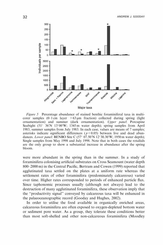
were more abundant in the spring than in the summer. In a study of

foraminifera colonising artificial substrates on Cross Seamount (water depth

800–2000m) in the Central Pacific, Bertram and Cowen (1999) reported that

agglutinated taxa settled on the plates at a uniform rate whereas the

settlement rates of other foraminifera (predominately calcareous) varied

over time. Higher rates corresponded to periods of enhanced particle flux.

Since taphonomic processes usually (although not always) lead to the

destruction of many agglutinated foraminifera, these observation imply that

the ‘‘productivity signal’’ conveyed by calcareous taxa will be enhanced in

the palaeoceanographic record (Gooday and Hughes, 2002).

In order to utilise the food available in organically enriched areas,

calcareous foraminifera are often exposed to oxygen-depleted bottom water

or sediment pore water. As a group, they tolerate these conditions better

than most soft-shelled and other non-calcareous foraminifera (Moodley

Figure 5 Percentage abundance of stained benthic foraminiferal taxa in multi-corer samples (0–1 cm layer >63 mm fraction) collected during spring (lightornamentation) and summer (dark ornamentation). Upper panel: PorcupineSeabight (51� 360N 13�000W; 1345m water depth); spring samples from April1983, summer samples from July 1983. In each case, values are means of 7 samples;asterisks indicate significant differences ( p<0.05) between live and dead abun-dances. Lower panel: BENBO Site C (57� 07.500N 12�30.300W; 1950m water depth);Single samples from May 1998 and July 1998. Note that in both cases the rotaliidsare the only group to show a substantial increase in abundance after the springbloom.

32 ANDREW J. GOODAY

et al., 1997; Gooday et al., 2000). However, calcareous foraminifera living in

low-oxygen environments must also withstand the acidic conditions often

associated with organic enrichment. In contrast, metazoans with calcareous

hard parts (e.g. molluscs and echinoderms) are often rare in dysoxic

environments, presumably because they find it difficult to prevent the

dissolution of their shells and skeletons (Rhoades and Morse, 1971;

Thompson et al., 1985).

7. OXYGEN CONCENTRATIONS


Modern oceans are generally well oxygenated and persistent large-scale

oxygen depletion is confined to coastal, continental shelf and slope settings.

These extreme conditions are usually associated with high productivity or

with weak bottom-water circulation; for example, off large rivers, Oxygen

Minimum Zones (OMZs), silled basins and fjords (Diaz and Rosenberg,

1995). Bottom-water oxygen concentrations are tightly coupled with organic

matter fluxes, making it difficult to separate the effects of these two variables

on benthic communities (Levin and Gage, 1998).

Many of the ideas about how oxygen affects faunal parameters have been

developed by macrofaunal ecologists (e.g. Sanders, 1969; Pearson and

Rosenberg, 1978; Levin and Gage, 1998; Levin et al., 2000, 2001, 2002).

Macro- and mega-faunal animals usually live on the sediment surface, or

can extend body parts above the sediment–water interface, and are directly

affected by oxygen concentrations in the bottom water. Foraminifera

attached to elevated substrata are also in direct contact with bottom water

(Lutze and Thiel, 1989; Schonfeld, 2002a, 2002c). However, in the case of

foraminifera and other meiofauna living within the sediments, it is the

concentration of oxygen in the sediment pore water that matters (Gooday

et al., 2000; Pike et al., 2001; Schonfeld, 2001). Because of oxygen

consumption within the sediment, deeper infaunal species will typically

encounter dysoxic or anoxic conditions, even when the bottom water is well

oxygenated (Murray, 2001; Fontanier et al., 2002). Unlike organic matter

fluxes, it is relatively easy to measure sediment pore-water oxygen profiles

directly and accurately, although processes such as bioturbation, and the

possibility that foraminifera extend their pseudopodia into overlying, more

strongly oxygenated sediment layers (Bernhard and Sen Gupta, 1999),

make it difficult to determine the amount of oxygen actually available to

individual specimens.


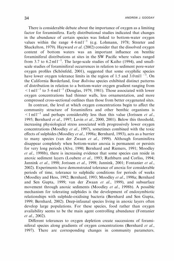
There is considerable debate about the importance of oxygen as a limiting

factor for foraminifera. Early distributional studies indicated that changes

in the abundance of certain species was linked to bottom-water oxygen

values within the range 4–6ml l�1 (e.g. Lohmann, 1978; Streeter and

Shackelton, 1979). Hayward et al. (2002) consider that the dissolved oxygen

content of bottom waters was an important influence on benthic

foraminiferal distributions at sites in the SW Pacific where values ranged

from 3.7 to 6.2ml l�1. The large-scale studies of Kaiho (1994), and small-

scale studies of foraminiferal occurrences in relation to sediment pore-water

oxygen profiles (Schonfeld, 2001), suggested that some oxyphilic species

have lower oxygen tolerance limits in the region of 1.5 and 3.0ml l �1. On

the California Borderland, four Bolivina species exhibited distinct patterns

of distribution in relation to a bottom-water oxygen gradient ranging from

<1ml l�1 to 5–6ml l�1 (Douglas, 1979, 1981). Those associated with lower

oxygen concentrations had thinner walls, less ornamentation, and more

compressed cross-sectional outlines than those from better oxygenated sites.

In contrast, the level at which oxygen concentrations begin to affect the

community structure of foraminifera and other benthic organisms is

<1ml l�1 and perhaps considerably less than this value (Jorissen et al.,

1995; Bernhard et al., 1997; Levin et al., 2000, 2001). Below this threshold,

increasing physiological stress associated with progressively lower oxygen

concentrations (Moodley et al., 1997), sometimes combined with the toxic

effects of sulphides (Moodley et al., 1998a; Bernhard, 1993), acts as a barrier

to many species (van der Zwaan et al., 1999). Although foraminifera

disappear completely when bottom-water anoxia is permanent or persists

for very long periods (Alve, 1990; Bernhard and Riemers, 1991; Moodley

et al., 1998b), there is increasing evidence that some species can reside in

anoxic sediment layers (Loubere et al., 1993; Rathburn and Corliss, 1994;

Jannink et al., 1998; Jorissen et al., 1998; Jannink, 2001; Fontanier et al.,

2002). Experiments have demonstrated tolerance of anoxia for considerable

periods of time, tolerance to sulphidic conditions for periods of weeks

(Moodley and Hess, 1992; Bernhard, 1993; Moodley et al., 1998a; Bernhard

and Sen Gupta, 1999; van der Zwaan et al., 1999), and subsurface

movement through anoxic sediments (Moodley et al., 1998b). A possible

mechanism for tolerating sulphides is the development of endosymbiotic

relationships with sulphide-oxidising bacteria (Bernhard and Sen Gupta,

1999; Bernhard, 2002). Deep-infaunal species living in anoxic layers often

develop large populations. For these species, food rather than oxygen

availability seems to be the main agent controlling abundance (Fontanier

et al., 2002).

Different tolerances to oxygen depletion create successions of forami-

niferal species along gradients of oxygen concentrations (Bernhard et al.,

1997). There are corresponding changes in community parameters.

34 ANDREW J. GOODAY

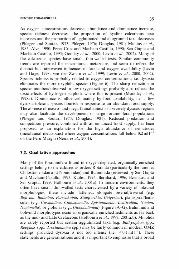
As oxygen concentrations decrease, abundance and dominance increase,

species richness decreases, the proportion of hyaline calcareous taxa

increases and the proportion of agglutinated and allogromiid taxa decreases

(Phleger and Soutar, 1973; Phleger, 1976; Douglas, 1981; Mullins et al.,

1985; Alve, 1990; Perez-Cruz and Machain-Castillo, 1990; Sen Gupta and

Machain-Castillo, 1993; Gooday et al., 2000; Levin et al., 2002). Many of

the calcareous species have small, thin-walled tests. Similar community

trends are reported for macrofaunal metazoans and seem to reflect the

distinct but interwoven influences of food and oxygen availability (Levin

and Gage, 1998; van der Zwaan et al., 1999; Levin et al., 2000, 2002).

Species richness is probably related to oxygen concentrations; i.e. dysoxia

eliminates the more oxyphilic species (Figure 6). The sharp reduction in

species numbers observed in low-oxygen settings probably also reflects the

toxic effects of hydrogen sulphide where this is present (Moodley et al.,

1998a). Dominance is influenced mainly by food availability; i.e. a few

dysoxia-tolerant species flourish in response to an abundant food supply.

The absence of macro- and mega-faunal animals in severely dysoxic regions

may also facilitate the development of large foraminiferal populations

(Phleger and Soutar, 1973; Douglas, 1981). Reduced predation and

competition pressure, combined with an enhanced food supply, has been

proposed as an explanation for the high abundance of nematodes

(meiofaunal metazoans) where oxygen concentrations fall below 0.2ml l�1

on the Peru Margin (Neira et al., 2001).

7.2. Qualitative approaches

Many of the foraminifera found in oxygen-depleted, organically enriched

settings belong to the calcareous orders Rotaliida (particularly the families

Chilostomellidae and Nonionidae) and Buliminida (reviewed by Sen Gupta

and Machain-Castillo, 1993; Kaiho, 1994; Bernhard, 1996; Bernhard and

Sen Gupta, 1999; Holbourn et al., 2001a). In modern environments, they

often have small, thin-walled tests characterised by a variety of infaunal

morphologies; these include flattened, elongate biserial/triserial (e.g.

Bolivina, Bulimina, Fursenkoina, Stainforthia, Uvigerina), planispiral/lenti-

cular (e.g. Cassidulina, Chilostomella, Epistominella, Lenticulina, Nonion,

Nonionella), or globular (e.g., Globobulimina) (Figure 3A–G). Buliminid and

bolivinid morphotypes occur in organically enriched sediments as far back

as the mid- and Late Cretaceous (Holbourn et al., 1999, 2001a,b). Miliolids

are rarely reported but certain agglutinated taxa (e.g. Bathysiphon spp.,

Reophax spp., Trochammina spp.) may be fairly common in modern OMZ

settings, provided dysoxia is not too intense (i.e. <0.1ml l�1). These

statements are generalisations and it is important to emphasise that a broad


Figure 6 Schematic representation of the effect of an oxygen gradient onforaminiferal species richness. Each horizontal line represents the distribution of asingle hypothetical species in relation to oxygen concentrations; the filled circlerepresents its lower oxygen tolerance limit. Most of the hypothetical species are foundin oxic environments, but one or two are absent where O2 values exceed 0.5–1.0ml l�1.Note that there is currently no evidence that obligate dysaerobic species actually exist,although low-oxygen tolerant species may be eliminated by competition withoxyphilic species at higher oxygen concentrations. There is good evidence, however,that species are progressively eliminated when oxygen concentrations fall below acertain threshold (�1.0–0.5ml l�1). Foraminifera disappear entirely when regionalanoxia is persistent (Alve, 1990). The presence of sulphides may be another factoreliminating species at low oxygen concentrations. The oxygen gradient is unspecifiedin this diagram; it may be on small spatial scale (i.e. across-sediment pore waterprofiles) or on regional scales (e.g. across an oxygen minimum zone). Oxygengradients may be associated with different food types; for example, well-oxygenated,sediment surface microhabitats are characterised by labile material, deep-infaunalmicrohabitats by more refractory material. The availability of food will influence theabundance of particular species. The quality of the food (labile near the sedimentsurface, more refractory in deeper layers) may influence rates of reproduction and testproduction (Ohga and Kitazato, 1997; de Stigter et al., 1999; Jorissen and Wittling,1999). Note that oxygen itself does not influence abundance, except by providing anincreased living space for oxyphilic species (Jannink, 2000).

36 ANDREW J. GOODAY

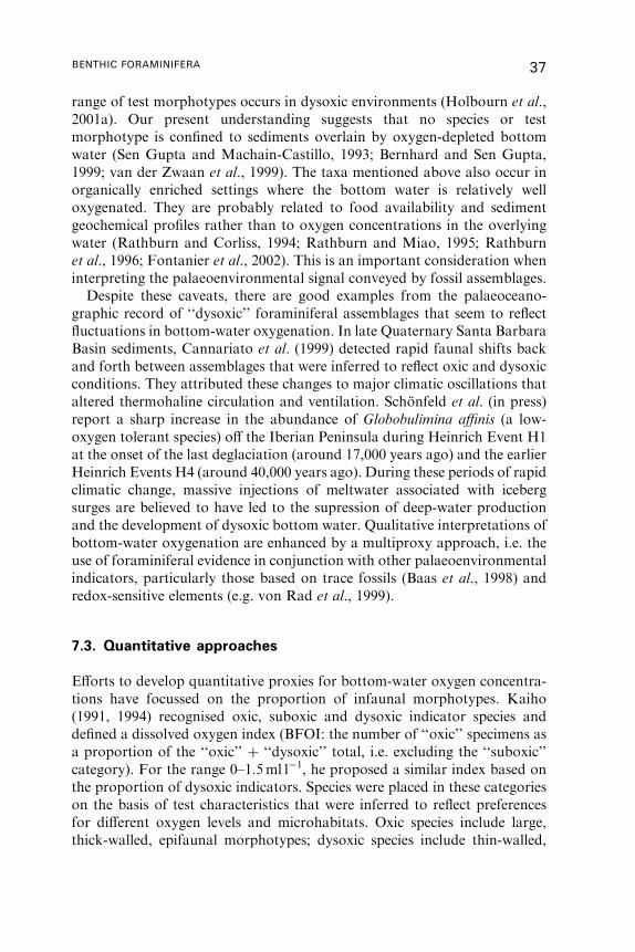
range of test morphotypes occurs in dysoxic environments (Holbourn et al.,

2001a). Our present understanding suggests that no species or test

morphotype is confined to sediments overlain by oxygen-depleted bottom

water (Sen Gupta and Machain-Castillo, 1993; Bernhard and Sen Gupta,

1999; van der Zwaan et al., 1999). The taxa mentioned above also occur in

organically enriched settings where the bottom water is relatively well

oxygenated. They are probably related to food availability and sediment

geochemical profiles rather than to oxygen concentrations in the overlying

water (Rathburn and Corliss, 1994; Rathburn and Miao, 1995; Rathburn

et al., 1996; Fontanier et al., 2002). This is an important consideration when

interpreting the palaeoenvironmental signal conveyed by fossil assemblages.

Despite these caveats, there are good examples from the palaeoceano-

graphic record of ‘‘dysoxic’’ foraminiferal assemblages that seem to reflect

fluctuations in bottom-water oxygenation. In late Quaternary Santa Barbara

Basin sediments, Cannariato et al. (1999) detected rapid faunal shifts back

and forth between assemblages that were inferred to reflect oxic and dysoxic

conditions. They attributed these changes to major climatic oscillations that

altered thermohaline circulation and ventilation. Schonfeld et al. (in press)

report a sharp increase in the abundance of Globobulimina affinis (a low-

oxygen tolerant species) off the Iberian Peninsula during Heinrich Event H1

at the onset of the last deglaciation (around 17,000 years ago) and the earlier

Heinrich Events H4 (around 40,000 years ago). During these periods of rapid

climatic change, massive injections of meltwater associated with iceberg

surges are believed to have led to the supression of deep-water production

and the development of dysoxic bottom water. Qualitative interpretations of

bottom-water oxygenation are enhanced by a multiproxy approach, i.e. the

use of foraminiferal evidence in conjunction with other palaeoenvironmental

indicators, particularly those based on trace fossils (Baas et al., 1998) and

redox-sensitive elements (e.g. von Rad et al., 1999).

7.3. Quantitative approaches

Efforts to develop quantitative proxies for bottom-water oxygen concentra-

tions have focussed on the proportion of infaunal morphotypes. Kaiho

(1991, 1994) recognised oxic, suboxic and dysoxic indicator species and

defined a dissolved oxygen index (BFOI: the number of ‘‘oxic’’ specimens as

a proportion of the ‘‘oxic’’ þ ‘‘dysoxic’’ total, i.e. excluding the ‘‘suboxic’’

category). For the range 0–1.5ml l�1, he proposed a similar index based on

the proportion of dysoxic indicators. Species were placed in these categories

on the basis of test characteristics that were inferred to reflect preferences

for different oxygen levels and microhabitats. Oxic species include large,

thick-walled, epifaunal morphotypes; dysoxic species include thin-walled,


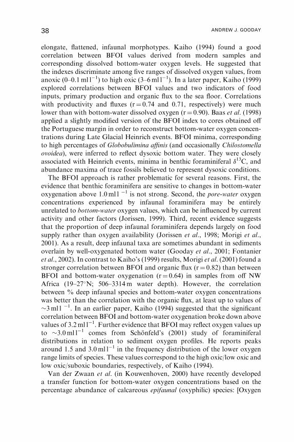
elongate, flattened, infaunal morphotypes. Kaiho (1994) found a good

correlation between BFOI values derived from modern samples and

corresponding dissolved bottom-water oxygen levels. He suggested that

the indexes discriminate among five ranges of dissolved oxygen values, from

anoxic (0–0.1ml l�1) to high oxic (3–6ml l�1). In a later paper, Kaiho (1999)

explored correlations between BFOI values and two indicators of food

inputs, primary production and organic flux to the sea floor. Correlations

with productivity and fluxes (r¼ 0.74 and 0.71, respectively) were much

lower than with bottom-water dissolved oxygen (r¼ 0.90). Baas et al. (1998)

applied a slightly modified version of the BFOI index to cores obtained off

the Portuguese margin in order to reconstruct bottom-water oxygen concen-

trations during Late Glacial Heinrich events. BFOI minima, corresponding

to high percentages of Globobulimina affinis (and occasionally Chilostomella

ovoidea), were inferred to reflect dysoxic bottom water. They were closely

associated with Heinrich events, minima in benthic foraminiferal �13C, and

abundance maxima of trace fossils believed to represent dysoxic conditions.

The BFOI approach is rather problematic for several reasons. First, the

evidence that benthic foraminifera are sensitive to changes in bottom-water

oxygenation above 1.0ml l �1 is not strong. Second, the pore-water oxygen

concentrations experienced by infaunal foraminifera may be entirely

unrelated to bottom-water oxygen values, which can be influenced by current

activity and other factors (Jorissen, 1999). Third, recent evidence suggests

that the proportion of deep infaunal foraminifera depends largely on food

supply rather than oxygen availability (Jorissen et al., 1998; Morigi et al.,

2001). As a result, deep infaunal taxa are sometimes abundant in sediments

overlain by well-oxygenated bottom water (Gooday et al., 2001; Fontanier

et al., 2002). In contrast to Kaiho’s (1999) results, Morigi et al. (2001) found a

stronger correlation between BFOI and organic flux (r¼ 0.82) than between

BFOI and bottom-water oxygenation (r¼ 0.64) in samples from off NW

Africa (19–27�N; 506–3314m water depth). However, the correlation

between % deep infaunal species and bottom-water oxygen concentrations

was better than the correlation with the organic flux, at least up to values of

�3ml l �1. In an earlier paper, Kaiho (1994) suggested that the significant

correlation between BFOI and bottom-water oxygenation broke down above

values of 3.2ml l�1. Further evidence that BFOI may reflect oxygen values up

to �3.0ml l�1 comes from Schonfeld’s (2001) study of foraminiferal

distributions in relation to sediment oxygen profiles. He reports peaks

around 1.5 and 3.0ml l�1 in the frequency distribution of the lower oxygen

range limits of species. These values correspond to the high oxic/low oxic and

low oxic/suboxic boundaries, respectively, of Kaiho (1994).

Van der Zwaan et al. (in Kouwenhoven, 2000) have recently developed

a transfer function for bottom-water oxygen concentrations based on the

percentage abundance of calcareous epifaunal (oxyphilic) species: [Oxygen

38 ANDREW J. GOODAY

content mmol l�1]¼ 7.9602þ 5.95 [% oxyphilic species]. This proxy, which

was calibrated using modern foraminiferal data from the Mediterranean Sea

and Atlantic and Indian Oceans, depends on the fact that oxyphilic species

require free oxygen and therefore are confined to fully oxic microenviron-

ments close to the sediment surface. Kouwenhoven (2000) used this method

to provide a generally convincing reconstruction of oxygenation history of

the late Miocene (6.3–8.1 million years ago) Mediterranean (Monte del

Casino section in Northern Italy). However, in places, it yielded oxygen

estimates that were either unrealistically low or peaked to unrealistically high

values, depending on whether or not particular species were included in

the calculations. Jannink et al. (in Jannink, 2001) proposed a very similar

transfer function [Oxygen content mmol l�1]¼ 7.23þ 5.62 [% oxyphilic

species] with an R2 value of 0.66, also based on Mediterranean and

Atlantic and Indian Ocean material representing a wide variety of product-

ivity regimes. They argued that the abundance of oxyphilic taxa is regulated

by the volume of aerated sediment (i.e. living space) rather than bottom-

water oxygen values as such. When applied to a core from the North

Adriatic, this proxy yielded oxygenation estimates for the past 160 years that

corresponded well with historical data. This method seems to produce

plausible results when applied cautiously, although it may require further

refinement.

8. BOTTOM-WATER HYDROGRAPHY


Foraminiferal distributions on continental shelves are often related to major

water masses (Phleger, 1960, 1964; Culver and Buzas, 2000). Correlations

between modern foraminiferal distributions and deep-sea, bottom-water

masses, such as North Atlantic Deep Water and Antarctic Bottom Water,

were first reported based on samples from the North Atlantic Ocean

(Streeter, 1973; Schnitker, 1974) and numerous other studies were

conducted during the 1970s and 1980s (reviewed by Douglas and

Woodruff, 1981; Schnitker, 1994). On continental margins, where the

water column is highly stratified and strong environmental gradients

impinge on the sea floor, there are often clear relationships between

bottom-water hydrography and foraminiferal assemblages (e.g. Douglas,

1979, 1981; Denne and Sen Gupta, 1991; Schmiedl et al., 1997). Mackensen

et al. (1995) and Mackensen (1997) suggest that three deep-sea foraminiferal

associations in the Atlantic and Southern Oceans reflect hydrographic

influences: (1) assemblages dominated by the epifaunal species Cibicidoides


wuellerstorfi are associated with young, well-oxygenated water masses, for

example, North Atlantic Deep Water; (2) Nuttallides umbonifer is closely

linked to carbonate corrosive bottom water; (3) Lobatula lobatula (Walker

and Jacob) and Trifarina angulosa (Williamson) are associated with strong

currents. Occasionally, temperature contrasts between adjacent basins seem

to provide the best explanation for faunal differences (Rathburn et al.,

1996). In one of the earliest deep-sea biological studies, Carpenter (1869)

and Carpenter et al. (1870) invoked contrasting temperature regimes to

explain differences between the foraminiferal assemblages to the north and

south of the Wyville-Thomson Ridge on the Scottish continental margin.

Below, I consider two of these characteristics, carbonate undersaturation

and current flow, in more detail.

8.2. Carbonate undersaturation

An abyssal assemblage dominated by Nuttallides umbonifer (Figure 3H–I)

has been recognised in areas overlain by Antarctic Bottom Water (AABW),

or its equivalents, in various parts of the world (Murray, 1991); for example,

deep basins in the southern part of the North Atlantic (Streeter, 1973;

Schnitker, 1974, 1980; Weston and Murray, 1984), on the Rio Grande Rise

in the SW Atlantic (Lohmann, 1978), the SE and SW Indian Oceans

(Corliss, 1979, 1983), and the eastern and western Pacific Ocean (Burke,

1981; Douglas and Woodruff, 1981, Table II therein; Nienstedt and Arnold,

1988). In the South Atlantic, it is restricted to the deep Cape and Angola

Basins (Schmiedl et al., 1997), at water depths below 3800m north of 51�S

and east of the Mid-Atlantic Ridge (Mackensen et al., 1993), and

3500–4000m in the eastern Weddell Sea (Mackensen et al., 1990). Species

that occur with N. umbonifer in the South Atlantic include Cribrostomoides

subglobosa (Cushman), Epistominella exigua, Adercotryma glomerata

(Brady) and Ammobaculites agglutinans (d’Orbigny) (Schmiedl et al., 1997).

Nuttallides umbonifer is most closely associated not with AABW as such

but with carbonate corrosive bottom water (Bremer and Lohmann, 1982).

In the SE Atlantic Ocean and the Southern Ocean, it is restricted to

carbonate-corrosive environments between the lysocline and the CCD

(Mackensen et al., 1990, 1993, 1995; Harloff and Mackensen, 1997;

Schmiedl et al., 1997). Mackensen concludes that ‘‘U. umbonifer is a

characteristic constituent of dead assemblage on most of the world ocean

floor over which AABW flows, i.e. between carbonate lysocline and CCD’’

(Mackensen et al., 1990) and that ‘‘this species unequivocally indicates

abyssal carbonate-aggressive bottom water masses’’ (Mackensen et al.,

1995). Carbonate dissolution is known to have a deleterious effect on

calcareous foraminifera. Green et al. (1998) incubated shallow-water

40 ANDREW J. GOODAY

sediments containing meiofaunal organisms under conditions of carbonate

saturation and undersaturation. Foraminifera exhibited significantly higher

mortality in the undersaturated treatments than in the saturated treatments.

Other experiments indicate that N. umbonifer is as susceptible to dissolution

as other hyaline calcareous species, suggesting that its distribution is

probably not related directly to carbonate undersaturation (Corliss and

Honjo, 1981; Kurbjeweit et al., 2000).

In the NE Atlantic Ocean, the distribution of N. umbonifer lies to the

south of temperate areas that experience strong seasonal phytodetrital

pulses (Gooday, 1993). Schmiedl et al. (1997) report a negative correlation

between the N. umbonifer assemblage and organic matter flux and sediment

TOC values in the eastern South Atlantic. In the eastern Equatorial Pacific,

an assemblage dominated by N. umbonifer occurs in low-productivity areas

situated well above the CCD (Loubere, 1991). Hence this species may be

adapted to the highly oligotrophic conditions that prevail in deep, abyssal

basins (Gooday, 1993; Altenbach et al., 1999) and associated only

incidentally with corrosive bottom water. However, the observation by

Kurbjeweit et al. (2000) of a N. rugosa (¼N. umbonifer) assemblage

associated with phytodetritus at a bathyal site (WAST-T; 1920m water

depth) in the western Arabian Sea make it clear that the ecology of this

important species is still not fully understood.

8.3. Current flow

Although much of the ocean floor is relatively quiescent, near-bottom

currents occur in certain areas, particularly those with sloped topography

such as continental slopes and seamounts (Heezen and Hollister, 1971;

Hollister et al., 1984; Hollister and Nowell, 1991). Such currents can modify

the structure and composition of benthic communities (Hall, 1994),

particularly if the flow is strong enough to transport sediment (Levin

et al., 1994). For example, strong bottom flow often depresses species

diversity but can also enhance it (reviewed in Levin et al., 2001). Sessile

suspension-feeding megafauna, such as the sponge Pheronema carpenteri

(Thomson) and the deep-water coral Lophelia pertusa (Linneaus), are

common on the upper continental slope around the NW European

continental margin in areas where bottom-water hydrography and

topography interact to enhance current flow (Rice et al., 1990; Rogers,

1999). These large organisms provide an important substrate for attached

organisms, including suspension-feeding foraminifera (Lutze and Thiel,

1989; Klitgaard, 1995; Rogers, 1999).

Associations between certain epifaunal foraminiferal species and

currents are well established, particularly in upper bathyal settings


(Mackensen, 1997). Sessile epifaunal suspension feeders are often common

where the flow is strong, suggesting that species benefit from food

delivered by currents. Schonfeld (1997) analysed living and dead

foraminiferal assemblages (>250-mm fraction) on the Portuguese con-

tinental margin. This region is strongly impacted by the Mediterranean

Outflow Water (MOW) which flows as a contour current along the slope

between 600m and 1500m water depth with sufficient velocity to transport

sediment and create mud ripples. Attached epibenthic species (Cibicides

lobatulus, Discanomalina coronata (Parker & Jones), Epistominella exigua,

Hanzawaia concentrica (Cushman), Planulina ariminensis d’Orbigny,

Vulvulina pennatula (Batsch)) that are presumed to be suspension feeders

were common within this depth interval. Past changes in MOW flow

patterns during the late Glacial and Holocene periods can be inferred from

downcore changes in the abundance of this ‘‘Epibenthos Group’’

(Schonfeld and Zahn, 2000).

In later papers, Schonfeld (2002a, c) described similar assemblages from

the Gulf of Cadiz off southern Spain, where current activity is more intense

and elevated epibenthic species correspondingly more abundant. Very high

current velocities (up to 50 cm s�1) were encountered in the eastern Gulf of

Cadiz, close to the Straits of Gibraltar. Here, epibenthic suspension feeders

such as Deuterammina ochracea, Discanomalina semipunctata (Bailey), C.

lobatulus and Cibicides refulgens de Montfort constituted 60–90% of the

living foraminiferal assemblage. They were attached to hydroid colonies and

to the tops of relatively large, heavy, stable objects, giving them access to a

high food flux. In the western part of the Gulf, where current velocities were

lower (4–25 cm s�1), attached epibenthic species (e.g. Crithionina mamilla

Goes, Trochammina squamata Parker and Jones, Saccammina sphaerica

Brady, Hanzawaia concentrica, Rosalina anomala Terquem) were relatively

less abundant (7–21% of live assemblage) and confined to lower substrates

(<3 cm above sea floor). Agglutinated tubes, mainly Rhabdammina

abyssorum M. Sars, constituted up to 60% of the assemblages in these

areas. Schonfeld (2002a) suggested that these faunal and ecological

differences were related to the optimisation of food acquisition. Only at

higher current velocities will the concentration of advected food particles

increase at elevations >3 cm above the sea floor. Dead assemblages in the

Gulf of Cadiz reflected the faunal differences apparent in the live faunas,

suggesting that the proportion of elevated epibenthic species may provide

the basis for a current velocity proxy that is independent of sedimentary

parameters (Schonfeld, 2002c).

Epibenthic foraminiferal faunas also occur on other parts of the NW

European continental margin. An assemblage associated with MOW at

water depths of 900–1200m in the Bay of Biscay (Pujos, 1970) includes

species that are found elsewhere living on Pheronema carpenteri (Lutze and

42 ANDREW J. GOODAY

Thiel, 1989). On the Norwegian margin, the attached suspension-feeding

calcareous foraminiferan Rupertina stabilis (Wallich) is abundant at

600–700m water depth in a border zone between two water masses where

current speeds are enhanced (Lutze and Altenbach, 1988). Another attached

species, Cibicides lobatula, occurs with the free-living Trifarina angulosa

(Figure 3E) in areas of enhanced flow on the upper slope off SW Norway

(Mackensen et al., 1985) and with the agglutinated species Reophax guttifer

in seasonally ice-free parts of the Arctic Ocean (<500m water depth)

(Wollenburg and Kuhnt, 2000). The tiny rotaliid Stetsonia hovarthi

dominates in current-affected regions at much greater water depths

(>2700m) under permanent ice cover in the Arctic Ocean (Wollenburg

and Kuhnt, 2000). This species may be associated with very low flux rates

(Altenbach et al., 1999), rather than current activity as such. A Trifarina

angulosa association is also typical of the shelf edge and upper slope areas

affected by strong bottom currents in the Southern Ocean (Mackensen et al.,

1995; Harloff and Mackensen, 1997). Finally, Globocassidulina subglobosa is

associated with areas of elevated topography and sandy sediments on the

Walvis Ridge in the SE Atlantic (Schmiedl et al., 1997).

Current flow impacts foraminiferal assemblages in a variety of other

ways; for example, by physically transporting small individuals (Alve, 1999;

Weinelt et al., 2001), modifying sediment characteristics, increasing or

decreasing sediment heterogeneity, or by transporting oxygen into areas that

would otherwise be oxygen depleted (Gage, 1997). Thus, on the Norwegian

margin and eastern Weddell Sea, Trifarina angulosamay be related to coarse

sediment rather than, or in addition to, current flow itself (Mackensen et al.,

1985, 1995). An association with terrigenous sand is reported on the edge of

the continental shelf to the east of South Island, New Zealand (Hayward

et al., 2002). Schonfeld (2002a) suggests that T. angulosa occupies interstitial

microhabitats in coarse-grained sediments which provide shelter from

turbulent water in high-energy environments.

9. WATER DEPTH

Early investigators of deep-sea foraminiferal ecology were preoccupied with

the bathymetric distribution of species (Phleger, 1960; Culver, 1988).

However, water depth itself has no influence on benthic faunas, although it is

related directly to hydrostatic pressure, a parameter which must set ultimate

limits to the bathymetric ranges of species through its control on cellular

biochemistry (Bradshaw, 1961; Belanger and Streeter, 1980; Somero, 1991,

1992). Within these physiological boundaries, actual species distributions

are likely to reflect a variety of other environmental factors, such as water-

mass characteristics, temperature, carbonate dissolution, and substrate


characteristics, all of which are also to some extent related to water depth

(Hayward et al., 2002). It seems likely that organic fluxes to the sea floor are

particularly important in determining the bathymetric distributions of

foraminiferal species (Haake et al., 1982; van der Zwaan et al., 1999). Fluxes

decrease with increasing water depth at any particular locality, and also vary

from region to region. Analysing the relation between the percentage

abundance of species and flux intensity, Altenbach et al. (1999) concluded

that, down to a water depth of about 1000 m, species ‘‘patterns are depth

dependent with reduced influence from organic matter flux’’. Below this

limit, patterns of species abundance follow flux values down to depths of

2000 m, below which species tend to be very widely distributed. In the

Mediterranean Sea, there is a clear relation between flux and bathymetric

distribution of species. De Rijk et al. (2000) described a shallowing of the

lower water depth limit for many species from west to east, corresponding

to a change from eutrophic to oligotrophic conditions. They conclude that

‘‘...the bathymetric distribution of the dominant foraminiferal taxa seems

indeed to be controlled by the level of the organic flux to the sea floor.’’

De Stigter et al. (in De Stigter, 1996, Chapter 6 therein) found that

foraminiferal species lived at greater water depths in the South Adriatic

Basin during the late Pleistocene compared with their present-day

distributions. They attributed this upward bathymetric shift to a decrease

in primary productivity and POC flux to the sea floor since the late

Pleistocene.

These results imply that benthic foraminifera can provide only a broad

indication of bathymetry (Murray, 1991). Although sucessions of species

invariably occur with increasing water depth along continental margin

transects (Pujos-Lamy, 1972; Pflumm and Frerichs, 1976; Haake, 1980;

Lutze, 1980; Douglas and Woodruff, 1981), species depth ranges are not

consistent between regions. The distributions of modern foraminiferal

species and species assemblages can therefore be used to reconstruct

palaeobathymetry only when applied to fossil faunas in the same study area

(e.g. Culver, 1988; Hayward, 1990; Kamp et al., 1998; Akimoto et al., 2002).

A more generalised approach to estimating palaeodepths exploits the

relation between the abundance of planktonic and benthic foraminifera and

organic fluxes. Building on the ideas of earlier authors (e.g. Berger and

Diester Haas, 1988), van der Zwaan et al. (1990, 1999) suggested that the

planktonic/benthic ratio (P/B ratio¼ the percentage of planktonic forami-

niferal tests in the total assemblage) reflects water depth. A better relation

between the P/B ratio and water depth was obtained when infaunal species,

which are less closely linked to the freshly settled flux, were excluded. This

relationship can be used to determine approximate palaeodepths and works

fairly well as long as the ratios are not distorted by selective dissolution or

by high inputs of organic matter and oxygen depletion. It has been used, for

44 ANDREW J. GOODAY

example, to estimate bathymetric changes within the Palaeocene El Kef

Formation in Tunisia (Kouwenhoven et al., 1997) and the Miocene Monte

del Casino section in Italy (van der Meulen et al., 1999).

Explanations of metazoan distributional patterns in relation to water

depth often involve food availability. Billett (1991) concluded that food

availability, and hydrographic factors such as temperature, control on the

distribution of holothurians in the Porcupine Seabight (NE Atlantic). Cartes

and Sarda (1993) emphasised the influence of decreasing food resources with

increasing depth on the bathymetric ranges of decapod crustacean species

in the Western Mediterranean. Hecker (1990) likewise invoked food

availability, together with parameters such as sediment type and current

intensity, to explain the bathymetric occurrence of megafaunal species on

the New England slope. Biological interactions, particularly predation and

competition have also been mentioned as factors contributing to the depth

distribution patterns of macro- and mega-faunal metazoans. Rex (1977)

argues that competition between species operating at lower trophic levels

will be reduced by predation, allowing them to have broader depth ranges

than predators. Although Rex’s hypothesis is problematical (e.g. Carney

et al., 1983), biological influences should not be overlooked when

considering controls on the distribution of deep-sea foraminiferal species,

many of which feed at low trophic levels.

10. SPECIES DIVERSITY PARAMETERS AS TOOLS IN

PALAEOCEANOGRAPHY

Species diversity parameters typically exhibit trends in relation to

environmental gradients. On a global scale, diversity appears to decrease

from low to high latitudes in a number of macrofaunal taxa (Rex et al.,

1997, 2000) and in foraminifera (Culver and Buzas, 2000). At regional

scales, species richness, diversity and dominance are influenced by, among

other factors, the organic flux to the sea floor, bottom-water oxygenation,

current activity and sediment heterogeneity (Etter and Grassle, 1992; Gage,

1997; Levin and Gage, 1998; Lambshead et al., 2001; Levin et al., 2001).

Food and oxygen availability are often the most important parameters.

Based on their analysis of macrofaunal diversity patterns in relation to

sediment organic matter content (considered a proxy for food availability),

Levin and Gage (1998) concluded that reduced macrofaunal species richness

in eutrophic/dysoxic settings is due largely to lack of oxygen whereas the

corresponding increase in dominance reflects increased food availability.

The overall result is a decrease in diversity, although the effects may

not become evident until oxygen concentrations fall below �0.5ml l�1


Table 4 Species richness data for foraminifera at localities characterised by differing oxygen regimes. L ¼ live populations; D ¼

dead populations. E(S100) ¼ expected number of species per 100 specimens; R1D ¼ rank 1 dominance (percentage abundance of top-ranked species). Sources of data: A ¼ Bernhard et al. (1997); B ¼ Gooday et al. (2000); C ¼ Jannink et al. (1998); D ¼ Rathburn andCorliss (1994); E ¼ Gooday et al. (1998); F ¼Fontanier et al. (2002); G ¼ Jorissen et al. (1998); H ¼ Hughes et al. (2001); I ¼ Goodayand Hughes (2002); J ¼ Schmiedl et al. (1997); K ¼ Wollenburg and Kuhnt (2000); L ¼ Gooday unpublished.

Locality, sizefraction, depth ofcore fraction,depth of sample

Bottom-wateroxygenml l-1

Oxygenpenetrationofsediment

Calcareousspecies

All hard-shelled4

speciesSource

Specimens Species E(S100) R1D(%) Specimens Species E(S100) R1D(%)

L D L D L D L D L D L D L D L D

Santa Barbara Basin:>63mm; 0–1 cm339m 0.50 28 5 – 28.6 31 7 – 25.8431m 0.34 238 8 7.5 40.3 255 11 9.7 37.6522m 0.08 355 7 6.1 29.0 470 10 8.4 25.5537m 0.04 218 8 7.7 48.6 323 12 10.3 32.8 A578m 0.02 756 7 5.8 35.8 828 10 7.8 32.3591m 0.06 360 7 5.4 74.4 450 9 6.7 59.6

Santa Barbara Basin>63mm, 0–1 cm590m 0.05 796 10 8.1 53.6 854 11 7.2 50.0610m 0.15 239 16 12.3 36.0 328 31 19.8 26.2 B

Oman margin:>125mm, 0–1 cm412m 0.13 4414 28 37.9 5505 41 30.4 B3350mm 3.0 18 15 12.5 406 61 13.1

46

ANDREW

J.GOODAY

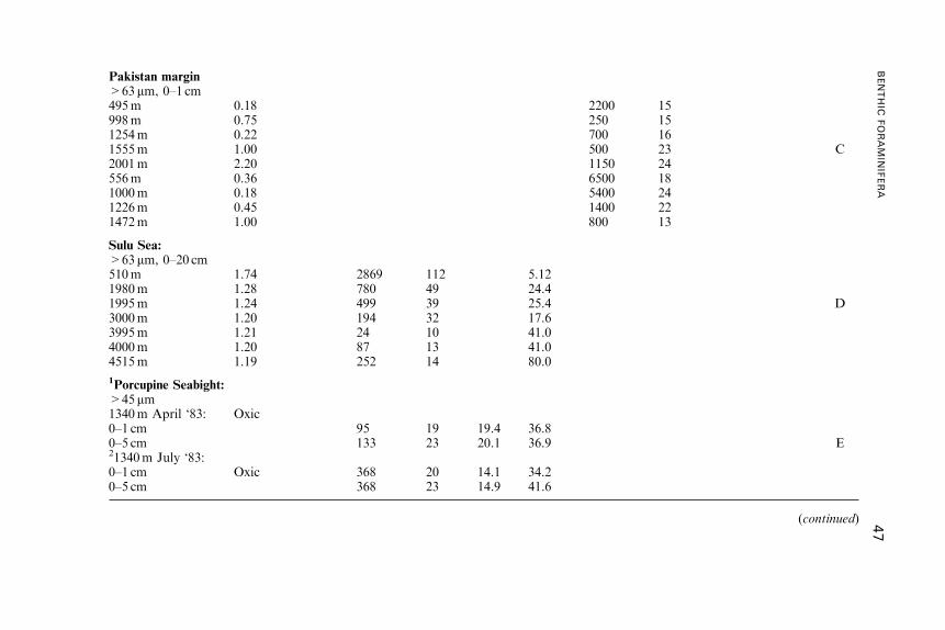
Pakistan margin>63 mm, 0–1 cm495m 0.18 2200 15998m 0.75 250 151254m 0.22 700 161555m 1.00 500 23 C2001m 2.20 1150 24556m 0.36 6500 181000m 0.18 5400 241226m 0.45 1400 221472m 1.00 800 13

Sulu Sea:>63 mm, 0–20 cm510m 1.74 2869 112 5.121980m 1.28 780 49 24.41995m 1.24 499 39 25.4 D3000m 1.20 194 32 17.63995m 1.21 24 10 41.04000m 1.20 87 13 41.04515m 1.19 252 14 80.0

1Porcupine Seabight:>45 mm1340m April ‘83: Oxic0–1 cm 95 19 19.4 36.80–5 cm 133 23 20.1 36.9 E21340m July ‘83:0–1 cm Oxic 368 20 14.1 34.20–5 cm 368 23 14.9 41.6

(continued)

BENTHIC

FORAMIN

IFERA

47

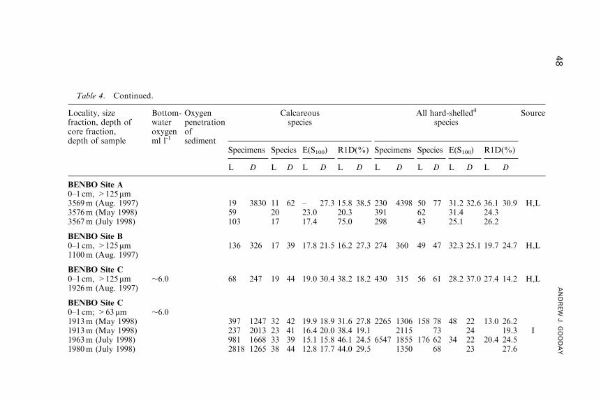
Table 4. Continued.




Calcareousspecies

All hard-shelled4

speciesSource



BENBO Site A0–1 cm, >125mm3569m (Aug. 1997) 19 3830 11 62 – 27.3 15.8 38.5 230 4398 50 77 31.2 32.6 36.1 30.9 H,L3576m (May 1998) 59 20 23.0 20.3 391 62 31.4 24.33567m (July 1998) 103 17 17.4 75.0 298 43 25.1 26.2

BENBO Site B0–1 cm, >125mm 136 326 17 39 17.8 21.5 16.2 27.3 274 360 49 47 32.3 25.1 19.7 24.7 H,L1100m (Aug. 1997)

BENBO Site C0–1 cm, >125mm �6.0 68 247 19 44 19.0 30.4 38.2 18.2 430 315 56 61 28.2 37.0 27.4 14.2 H,L1926m (Aug. 1997)

BENBO Site C0–1 cm; >63mm �6.01913m (May 1998) 397 1247 32 42 19.9 18.9 31.6 27.8 2265 1306 158 78 48 22 13.0 26.21913m (May 1998) 237 2013 23 41 16.4 20.0 38.4 19.1 2115 73 24 19.3 I1963m (July 1998) 981 1668 33 39 15.1 15.8 46.1 24.5 6547 1855 176 62 34 22 20.4 24.51980m (July 1998) 2818 1265 38 44 12.8 17.7 44.0 29.5 1350 68 23 27.6

48

ANDREW

J.GOODAY

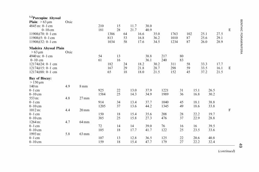
1,2Porcupine AbyssalPlain: >63 mm Oxic4845m: 0–1 cm 210 15 11.7 38.0

0–10 cm 181 28 21.7 40.9 E11908#70: 0–1 cm 1386 64 16.6 35.0 1763 102 25.1 27.511908#5: 0–1 cm 813 53 16.8 36.2 1010 87 25.6 29.111908#32: 0–1 cm 1034 58 17.6 34.5 1234 87 26.0 28.9

Madeira Abyssal Plain>63 mm Oxic4940m: 0–1 cm 54 13 38.8 217 800–10 cm 61 16 36.1 240 8312174#24: 0–1 cm 182 24 18.2 30.2 311 58 33.3 17.712174#15: 0–1 cm 167 29 21.8 28.7 298 59 33.5 16.1 E12174#88: 0–1 cm 65 18 18.0 21.5 152 45 37.2 21.5

Bay of Biscay:>150 mm140m 4.9 8mm0–1 cm 925 22 13.0 37.9 1221 31 15.1 26.50–10 cm 1584 25 14.3 34.9 1989 36 16.8 30.2553m: 4.8 27mm0–1 cm 914 34 13.4 37.7 1040 45 18.1 38.80–10 cm 1205 37 13.6 44.2 1345 49 18.6 33.81012m: 4.4 20mm F0–1 cm 150 18 15.4 35.6 208 28 22.2 19.70–10 cm 385 25 15.8 27.3 476 37 22.9 28.81264m: 4.7 64mm0–1 cm 72 14 14 39.0 76 16 16 39.50–10 cm 105 18 17.7 41.7 122 25 23.5 33.61993m: 5.8 63mm0–1 cm 107 13 12.8 36.5 125 22 20.6 40.80–10 cm 159 18 15.4 47.7 179 27 22.2 32.4

(continued)

BENTHIC

FORAMIN

IFERA

49

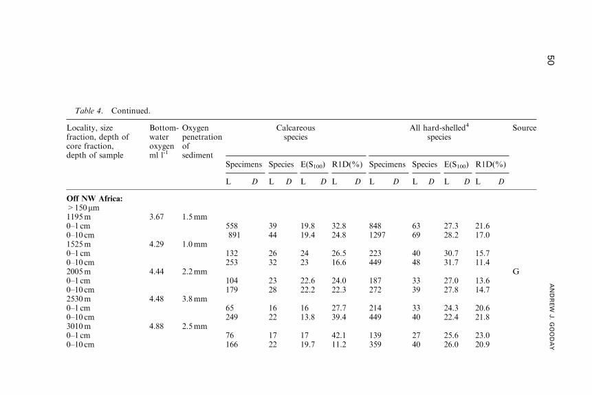
Table 4. Continued.




Calcareousspecies

All hard-shelled4

speciesSource



Off NW Africa:>150mm1195m 3.67 1.5mm0–1 cm 558 39 19.8 32.8 848 63 27.3 21.60–10 cm 891 44 19.4 24.8 1297 69 28.2 17.01525m 4.29 1.0mm0–1 cm 132 26 24 26.5 223 40 30.7 15.70–10 cm 253 32 23 16.6 449 48 31.7 11.42005m 4.44 2.2mm G0–1 cm 104 23 22.6 24.0 187 33 27.0 13.60–10 cm 179 28 22.2 22.3 272 39 27.8 14.72530m 4.48 3.8mm0–1 cm 65 16 16 27.7 214 33 24.3 20.60–10 cm 249 22 13.8 39.4 449 40 22.4 21.83010m 4.88 2.5mm0–1 cm 76 17 17 42.1 139 27 25.6 23.00–10 cm 166 22 19.7 11.2 359 40 26.0 20.9

50

ANDREW

J.GOODAY

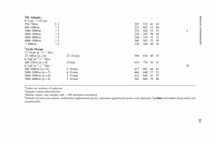
3SE Atlantic:0–1 cm; >125 mm250–700m 2–3 287 572 41 43400–1000m >3 225 602 35 401000–2000m >3 235 426 52 53 I2000–3000m >3 230 343 50 643000–4000m >3 264 334 53 534000–5000m >3 300 543 52 59>5000m >3 330 360 44 38

3Arctic Ocean:17–38 gCm�2 y�1 flux:37–100m (n¼ 4) 27–33mm 594 676 49 376–8 gCm�2 y�1 flux:200–250m (n¼ 4) 25mm 616 756 56 510–2 gCm�2 y�1 flux: K500–1000m (n¼ 9) 3–30mm 657 691 66 631000–2000m (n¼ 7) 4–35mm 464 640 57 512000–3000m (n¼ 8) 2–13mm 612 648 41 473000–4000m (n¼ 4) 3–10mm 503 604 39 40

1Values are medians of replicates.2Samples contain phytodetritus.3Median values; only samples with >200 specimens considered.4Includes all calcareous species, multilocular agglutinated species, unilocular agglutinated species with rigid tests; 5excludes soft-walled allogromiids and

saccamminids.

BENTHIC

FORAMIN

IFERA

51

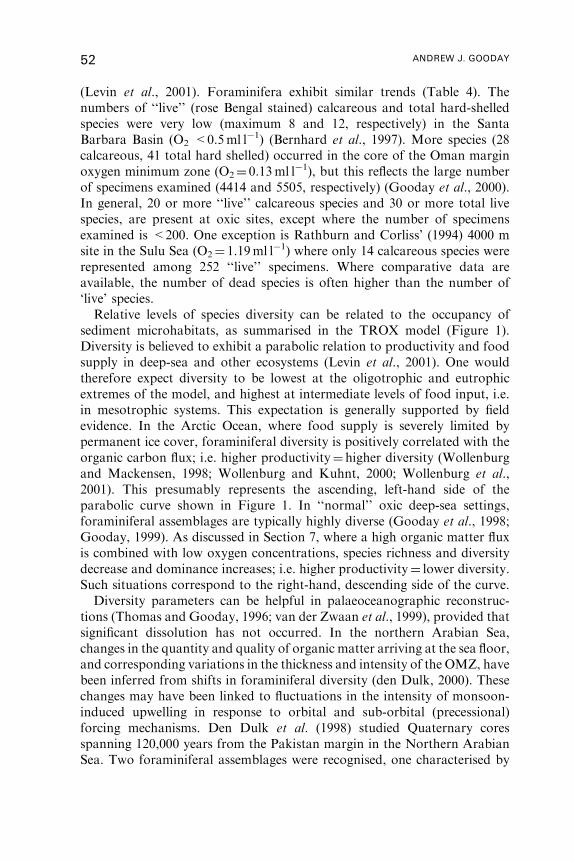
(Levin et al., 2001). Foraminifera exhibit similar trends (Table 4). The

numbers of ‘‘live’’ (rose Bengal stained) calcareous and total hard-shelled

species were very low (maximum 8 and 12, respectively) in the Santa

Barbara Basin (O2 <0.5ml l�1) (Bernhard et al., 1997). More species (28

calcareous, 41 total hard shelled) occurred in the core of the Oman margin

oxygen minimum zone (O2¼ 0.13ml l�1), but this reflects the large number

of specimens examined (4414 and 5505, respectively) (Gooday et al., 2000).

In general, 20 or more ‘‘live’’ calcareous species and 30 or more total live

species, are present at oxic sites, except where the number of specimens

examined is <200. One exception is Rathburn and Corliss’ (1994) 4000 m

site in the Sulu Sea (O2¼ 1.19ml l�1) where only 14 calcareous species were

represented among 252 ‘‘live’’ specimens. Where comparative data are

available, the number of dead species is often higher than the number of

‘live’ species.

Relative levels of species diversity can be related to the occupancy of

sediment microhabitats, as summarised in the TROX model (Figure 1).

Diversity is believed to exhibit a parabolic relation to productivity and food

supply in deep-sea and other ecosystems (Levin et al., 2001). One would

therefore expect diversity to be lowest at the oligotrophic and eutrophic

extremes of the model, and highest at intermediate levels of food input, i.e.

in mesotrophic systems. This expectation is generally supported by field

evidence. In the Arctic Ocean, where food supply is severely limited by

permanent ice cover, foraminiferal diversity is positively correlated with the

organic carbon flux; i.e. higher productivity¼ higher diversity (Wollenburg

and Mackensen, 1998; Wollenburg and Kuhnt, 2000; Wollenburg et al.,

2001). This presumably represents the ascending, left-hand side of the

parabolic curve shown in Figure 1. In ‘‘normal’’ oxic deep-sea settings,

foraminiferal assemblages are typically highly diverse (Gooday et al., 1998;

Gooday, 1999). As discussed in Section 7, where a high organic matter flux

is combined with low oxygen concentrations, species richness and diversity

decrease and dominance increases; i.e. higher productivity¼ lower diversity.

Such situations correspond to the right-hand, descending side of the curve.

Diversity parameters can be helpful in palaeoceanographic reconstruc-

tions (Thomas and Gooday, 1996; van der Zwaan et al., 1999), provided that

significant dissolution has not occurred. In the northern Arabian Sea,

changes in the quantity and quality of organic matter arriving at the sea floor,

and corresponding variations in the thickness and intensity of the OMZ, have

been inferred from shifts in foraminiferal diversity (den Dulk, 2000). These

changes may have been linked to fluctuations in the intensity of monsoon-

induced upwelling in response to orbital and sub-orbital (precessional)

forcing mechanisms. Den Dulk et al. (1998) studied Quaternary cores

spanning 120,000 years from the Pakistan margin in the Northern Arabian

Sea. Two foraminiferal assemblages were recognised, one characterised by

52 ANDREW J. GOODAY

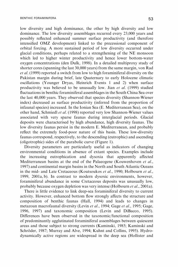
low diversity and high dominance, the other by high diversity and low

dominance. The low diversity assemblages recurred every 23,000 years and

possibly reflected enhanced summer surface productivity (and therefore

intensified OMZ development) linked to the precessional component of

orbital forcing. A more sustained period of low diversity occurred under

glacial conditions, perhaps related to a strengthening of the NE monsoon

which led to higher winter productivity and hence lower bottom-water

oxygen concentrations (den Dulk, 1998). In a detailed multiproxy study of

shorter cores (spanning the last 30,000 years) from the same margin, von Rad

et al. (1999) reported a switch from low to high foraminiferal diversity on the

Pakistan margin during brief, late Quaternary to early Holocene climatic

oscillations (Younger Dryas, Heinrich Events 1 and 2) when surface

productivity was believed to be unusually low. Jian et al. (1999) studied

fluctuations in benthic foraminiferal assemblages in the South China Sea over

the last 40,000 years. They observed that species diversity (Shannon-Wiener

index) decreased as surface productivity (inferred from the proportion of

infaunal species) increased. In the Ionian Sea (E. Mediterranean Sea), on the

other hand, Schmiedl et al. (1998) reported very low Shannon-Wiener values

associated with very sparse faunas during interglacial periods. Glacial

deposits were characterised by high abundance, high diversity faunas. The

low diversity faunas persist in the modern E. Mediterranean, and probably

reflect the extremely food-poor nature of this basin. These low-diversity

faunas correspond, respectively, to the descending (eutrophic) and ascending

(oligotrophic) sides of the parabolic curve (Figure 1).

Diversity parameters are particularly useful as indicators of changing

environmental conditions in absence of extant species. Examples include

the increasing eutrophication and dysoxia that apparently affected

Mediterranean basins at the end of the Palaeogene (Kouwenhoven et al.,

1997) and continental margin basins in the North and South Atlantic Oceans

in the mid- and Late Cretaceous (Koutsoukos et al., 1990; Holbourn et al.,

1999, 2001a, b). In contrast to modern dysoxic environments, however,

foraminiferal abundance in some Cretaceous deposits was unusually low,

probably because oxygen depletion was very intense (Holbourn et al., 2001a).

There is little evidence to link deep-sea foraminiferal diversity to current

activity. However, enhanced bottom flow strongly affects the structure and

composition of benthic faunas (Hall, 1994) and leads to changes in

metazoan macrofaunal diversity (Levin et al., 1994; Gage et al., 1995; Gage,

1996, 1997) and taxonomic composition (Levin and DiBacco, 1995).

Differences have been observed in the taxonomic/functional composition

of predominantly agglutinated foraminiferal assemblages between quiescent

areas and those subject to strong currents (Kaminski, 1985; Kaminski and

Schroder, 1987; Murray and Alve, 1994; Kuhnt and Collins, 1995). Hydro-

dynamically active regions are widespread in the deep sea (Hollister and


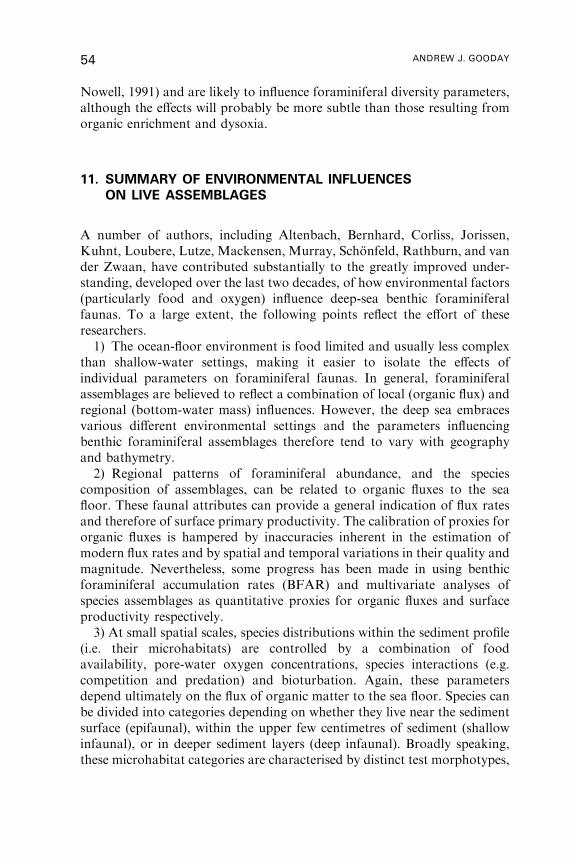
Nowell, 1991) and are likely to influence foraminiferal diversity parameters,

although the effects will probably be more subtle than those resulting from

organic enrichment and dysoxia.

11. SUMMARY OF ENVIRONMENTAL INFLUENCES

ON LIVE ASSEMBLAGES

A number of authors, including Altenbach, Bernhard, Corliss, Jorissen,

Kuhnt, Loubere, Lutze, Mackensen, Murray, Schonfeld, Rathburn, and van

der Zwaan, have contributed substantially to the greatly improved under-

standing, developed over the last two decades, of how environmental factors

(particularly food and oxygen) influence deep-sea benthic foraminiferal

faunas. To a large extent, the following points reflect the effort of these

researchers.

1) The ocean-floor environment is food limited and usually less complex

than shallow-water settings, making it easier to isolate the effects of

individual parameters on foraminiferal faunas. In general, foraminiferal

assemblages are believed to reflect a combination of local (organic flux) and

regional (bottom-water mass) influences. However, the deep sea embraces

various different environmental settings and the parameters influencing

benthic foraminiferal assemblages therefore tend to vary with geography

and bathymetry.

2) Regional patterns of foraminiferal abundance, and the species

composition of assemblages, can be related to organic fluxes to the sea

floor. These faunal attributes can provide a general indication of flux rates

and therefore of surface primary productivity. The calibration of proxies for

organic fluxes is hampered by inaccuracies inherent in the estimation of

modern flux rates and by spatial and temporal variations in their quality and

magnitude. Nevertheless, some progress has been made in using benthic

foraminiferal accumulation rates (BFAR) and multivariate analyses of

species assemblages as quantitative proxies for organic fluxes and surface

productivity respectively.

3) At small spatial scales, species distributions within the sediment profile

(i.e. their microhabitats) are controlled by a combination of food

availability, pore-water oxygen concentrations, species interactions (e.g.

competition and predation) and bioturbation. Again, these parameters

depend ultimately on the flux of organic matter to the sea floor. Species can

be divided into categories depending on whether they live near the sediment

surface (epifaunal), within the upper few centimetres of sediment (shallow

infaunal), or in deeper sediment layers (deep infaunal). Broadly speaking,

these microhabitat categories are characterised by distinct test morphotypes,

54 ANDREW J. GOODAY

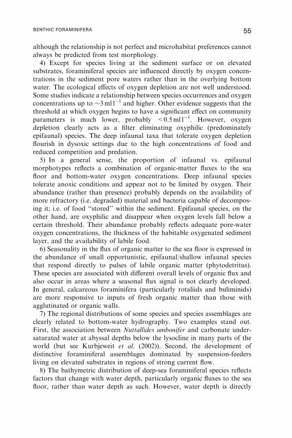
although the relationship is not perfect and microhabitat preferences cannot

always be predicted from test morphology.

4) Except for species living at the sediment surface or on elevated

substrates, foraminiferal species are influenced directly by oxygen concen-

trations in the sediment pore waters rather than in the overlying bottom

water. The ecological effects of oxygen depletion are not well understood.

Some studies indicate a relationship between species occurrences and oxygen

concentrations up to �3ml l�1 and higher. Other evidence suggests that the

threshold at which oxygen begins to have a significant effect on community

parameters is much lower, probably <0.5ml l�1. However, oxygen

depletion clearly acts as a filter eliminating oxyphilic (predominately

epifaunal) species. The deep infaunal taxa that tolerate oxygen depletion

flourish in dysoxic settings due to the high concentrations of food and

reduced competition and predation.

5) In a general sense, the proportion of infaunal vs. epifaunal

morphotypes reflects a combination of organic-matter fluxes to the sea

floor and bottom-water oxygen concentrations. Deep infaunal species

tolerate anoxic conditions and appear not to be limited by oxygen. Their

abundance (rather than presence) probably depends on the availability of

more refractory (i.e. degraded) material and bacteria capable of decompos-

ing it; i.e. of food ‘‘stored’’ within the sediment. Epifaunal species, on the

other hand, are oxyphilic and disappear when oxygen levels fall below a

certain threshold. Their abundance probably reflects adequate pore-water

oxygen concentrations, the thickness of the habitable oxygenated sediment

layer, and the availability of labile food.

6) Seasonality in the flux of organic matter to the sea floor is expressed in

the abundance of small opportunistic, epifaunal/shallow infaunal species

that respond directly to pulses of labile organic matter (phytodetritus).

These species are associated with different overall levels of organic flux and

also occur in areas where a seasonal flux signal is not clearly developed.

In general, calcareous foraminifera (particularly rotaliids and buliminids)

are more responsive to inputs of fresh organic matter than those with

agglutinated or organic walls.

7) The regional distributions of some species and species assemblages are

clearly related to bottom-water hydrography. Two examples stand out.

First, the association between Nuttallides umbonifer and carbonate under-

saturated water at abyssal depths below the lysocline in many parts of the

world (but see Kurbjeweit et al. (2002)). Second, the development of

distinctive foraminiferal assemblages dominated by suspension-feeders

living on elevated substrates in regions of strong current flow.

8) The bathymetric distribution of deep-sea foraminiferal species reflects

factors that change with water depth, particularly organic fluxes to the sea

floor, rather than water depth as such. However, water depth is directly


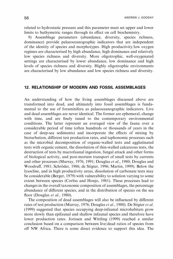
related to hydrostatic pressure and this parameter must set upper and lower

limits to bathymetric ranges through its effect on cell biochemistry.

9) Assemblage parameters (abundance, diversity, species richness,

dominance) provide palaeoceanographic indicators that are independent

of the identity of species and morphotypes. High productivity/low oxygen

regimes are characterised by high abundance, high dominance and relatively

low species richness and diversity. More oligotrophic, well-oxygenated

settings are characterised by lower abundance, low dominance and high

levels of species richness and diversity. Highly oligotrophic environments

are characterised by low abundance and low species richness and diversity.

12. RELATIONSHIP OF MODERN AND FOSSIL ASSEMBLAGES

An understanding of how the living assemblages discussed above are

transformed into dead, and ultimately into fossil assemblages is funda-

mental to the use of foraminifera as palaeoceanographic indicators. Live

and dead assemblages are never identical. The former are ephemeral, change

with time, and are finely tuned to the contemporary environmental

conditions. The latter represent an averaged view of the fauna over a

considerable period of time (often hundreds or thousands of years in the

case of deep-sea sediments) and incorporate the effects of mixing by

bioturbation, different test production rates, and taphonomic processes such

as the microbial decomposition of organic-walled tests and agglutinated

tests with organic cement, the dissolution of thin-walled calcareous tests, the

destruction of tests by macrofaunal ingestion, fungal attack and other forms

of biological activity, and post-mortem transport of small tests by currents

and other processes (Murray, 1976, 1991; Douglas et al., 1980; Douglas and

Woodruff, 1981; Schroder, 1986; de Stigter, 1996; Martin, 1999). Below the

lysocline, and in high productivity areas, dissolution of carbonate tests may

be considerable (Berger, 1979) with vulnerability to solution varying to some

extent between species (Corliss and Honjo, 1981). These processes lead to

changes in the overall taxonomic composition of assemblages, the percentage

abundance of different species, and in the distribution of species on the sea

floor (Douglas et al., 1980).

The composition of dead assemblages will also be influenced by different

rates of test production (Murray, 1976; Douglas et al., 1980). De Stigter et al.

(1999) suggested that species occupying deep-infaunal microhabitats grow

more slowly than epifaunal and shallow infaunal species and therefore have

lower production rates. Jorissen and Wittling (1999) reached a similar

conclusion based on a comparison between live/dead ratios of species from

off NW Africa. There is some direct evidence to support this idea. The

56 ANDREW J. GOODAY

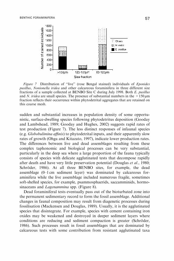
sudden and substantial increases in population density of some opportu-

nistic, surface-dwelling species following phytodetritus deposition (Gooday

and Lambshead, 1989; Gooday and Hughes, 2002) suggests rapid rates of

test production (Figure 7). The less distinct responses of infaunal species

(e.g. Globobulimina affinis) to phytodetrital inputs, and their apparently slow

rates of growth (Ohga and Kitazato, 1997), indicate lower production rates.

The differences between live and dead assemblages resulting from these

complex taphonomic and biological processes can be very substantial,

particularly in the deep sea where a large proportion of the fauna typically

consists of species with delicate agglutinated tests that decompose rapidly

after death and have very little preservation potential (Douglas et al., 1980;

Schroder, 1986). At all three BENBO sites, for example, the dead

assemblage (0–1 cm sediment layer) was dominated by calcareous for-

aminifera while the live assemblage included numerous fragile, sometimes

soft-shelled species, for example, psammosphaerids, saccamminids, hormo-

sinaceans and Lagenammina spp. (Figure 8).

Dead foraminiferal tests eventually pass out of the bioturbated zone into

the permanent sedimentary record to form the fossil assemblage. Additional

changes in faunal composition may result from diagenetic processes during

fossilisation (Mackensen and Douglas, 1989). Usually, it is the agglutinated

species that disintegrate. For example, species with cement containing iron

oxides may be weakened and destroyed in deeper sediment layers where

conditions are reducing and sediment compaction is greater (Schroder,

1986). Such processes result in fossil assemblages that are dominated by

calcareous tests with some contribution from resistant agglutinated taxa

Figure 7 Distribution of ‘‘live’’ (rose Bengal stained) individuals of Eponidespusillus, Nonionella iridea and other calcareous foraminifera in three different sizefractions of a sample collected at BENBO Site C during July 1998. Both E. pusillusand N. iridea are small species. The presence of substantial numbers in the >150mmfraction reflects their occurrence within phytodetrital aggregates that are retained onthis coarse mesh.


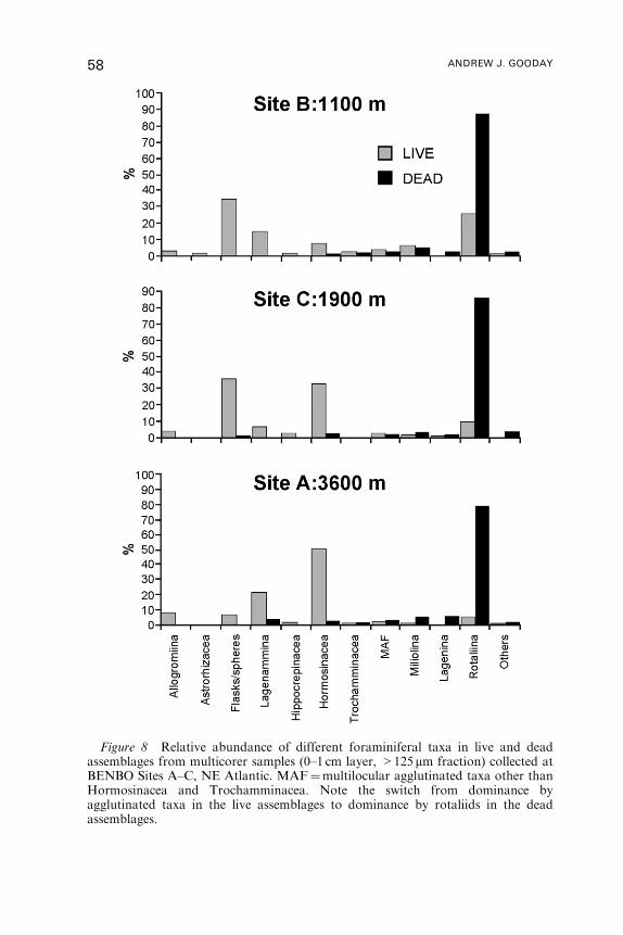
Figure 8 Relative abundance of different foraminiferal taxa in live and deadassemblages from multicorer samples (0–1 cm layer, >125 mm fraction) collected atBENBO Sites A–C, NE Atlantic. MAF¼multilocular agglutinated taxa other thanHormosinacea and Trochamminacea. Note the switch from dominance byagglutinated taxa in the live assemblages to dominance by rotaliids in the deadassemblages.

58 ANDREW J. GOODAY

with calcitic cement. In order to bridge the gap between dead and fossil

assemblages, Mackensen et al. (1990) introduced the concept of ‘‘potential

fossil assemblages’’, derived from modern dead assemblages by subtracting

the non-resistant agglutinated species. Potential fossil assemblages do not

reflect the effects of dissolution and other destructive processes and

must therefore be considered as ‘‘ideal’’ fossil assemblages. Calcareous

tests may also disappear as a result of dissoluton by corrosive pore waters

(Mackensen and Douglas, 1989), leaving a predominately or entirely

agglutinated assemblage (Gradstein and Berggren, 1981; Murray and Alve,

1994).

Loubere (1989) and Loubere and Gary (1990) presented computer models

and evidence from box cores (Gulf of Mexico, 1020–1170m water depth)

suggesting that microhabitat preferences can also influence the susceptibility

of a species to taphonomic destruction. They argue that much of the

destruction of foraminiferal tests occurs in the surface 1–2 cm of sediments

where disturbance by benthic animals is most intense (see also de Stigter,

1996). It therefore has a particular impact on epifaunal and shallow infaunal

species. Deep infaunal species live below this surface zone and therefore

largely escape these destructive processes. Loubere et al. (1993) developed

these arguments further, emphasising the ways in which the organic flux and

bottom-water oxygenation interact to influence the formation of fossil

assemblages. They suggested that assemblage generation depends on: (1) the

distribution of living foraminifera within the sediment profile, (2) the rates

of test production in different sediment layers, (3) the rates of destructive

taphonomic processes (the ‘taphonomic filter’) and the variation of these

rates within the sediment profile, (4) the style of bioturbation and the depth

to which it extends (among other things, this will influence the extent to

which deep-infaunal tests are exposed to taphonomic processes in surface

sediments). The final fossil assemblage reflects a combination of these four

processes (Figure 9), the importance of which change along gradients of

organic carbon flux, oxygen availability, and depth in the sediment profile.

On the basis of these ideas, Loubere et al. (1993) and Loubere (1997)

suggested that in well-oxygenated, low-flux settings (e.g. central oceanic

regions), most test production will occur close to the sediment surface and

be subject to intense and uniform taphonomic processes leading to a

substantial loss of tests in the fossil assemblage. In these environments, low

sedimentation rates will also promote the formation of a homogeneous dead

assemblage (de Stigter, 1996). Where a moderate organic flux is combined

with well-oxygenated bottom water (e.g. bathyal continental margins),

the fossil assemblage will form over a thicker sediment layer, species will

be distinctly stratified within this habitable zone, and deep infaunal

foraminifera will be subject to less taphonomic loss than those originating

in near-surface layers. In high flux, low-oxygen settings (e.g. oxygen


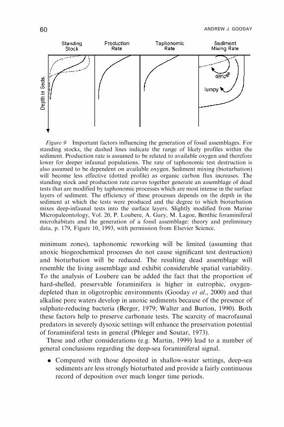
minimum zones), taphonomic reworking will be limited (assuming that

anoxic biogeochemical processes do not cause significant test destruction)

and bioturbation will be reduced. The resulting dead assemblage will

resemble the living assemblage and exhibit considerable spatial variability.

To the analysis of Loubere can be added the fact that the proportion of

hard-shelled, preservable foraminifera is higher in eutrophic, oxygen-

depleted than in oligotrophic environments (Gooday et al., 2000) and that

alkaline pore waters develop in anoxic sediments because of the presence of

sulphate-reducing bacteria (Berger, 1979; Walter and Burton, 1990). Both

these factors help to preserve carbonate tests. The scarcity of macrofaunal

predators in severely dysoxic settings will enhance the preservation potential

of foraminiferal tests in general (Phleger and Soutar, 1973).

These and other considerations (e.g. Martin, 1999) lead to a number of

general conclusions regarding the deep-sea foraminiferal signal.

. Compared with those deposited in shallow-water settings, deep-sea

sediments are less strongly bioturbated and provide a fairly continuous

record of deposition over much longer time periods.

Figure 9 Important factors influencing the generation of fossil assemblages. Forstanding stocks, the dashed lines indicate the range of likely profiles within thesediment. Production rate is assumed to be related to available oxygen and thereforelower for deeper infaunal populations. The rate of taphonomic test destruction isalso assumed to be dependent on available oxygen. Sediment mixing (bioturbation)will become less effective (dotted profile) as organic carbon flux increases. Thestanding stock and production rate curves together generate an assemblage of deadtests that are modified by taphonomic processes which are most intense in the surfacelayers of sediment. The efficiency of these processes depends on the depth in thesediment at which the tests were produced and the degree to which bioturbationmixes deep-infaunal tests into the surface layers. Slightly modified from MarineMicropaleontology, Vol. 20, P. Loubere, A. Gary, M. Lagoe, Benthic foraminiferalmicrohabitats and the generation of a fossil assemblage: theory and preliminarydata, p. 179, Figure 10, 1993, with permission from Elsevier Science.

60 ANDREW J. GOODAY

. The resolution of this record will depend largely on the sedimentation

rate and the thickness of the bioturbated zone. In the deep sea,

sedimentation rates will normally be slow (a few cm 1000 yr�1) and the

bioturbated zone will span several thousands of years of accumulation.

Thus, the resolution of the palaeoceanographic record will normally

be less detailed than in shallow-water settings where sedimentation

rates are generally higher. Exceptions are bathyal dysoxic basins and

oxygen minimum zones, where higher sedimentation rates combined

with reduced macrofaunal activity yield a high resolution record (e.g.

Cannariato et al., 1999).

. In oligotrophic settings, only a small proportion of the living

foraminiferal assemblage, which consists largely of non-fossilisable

agglutinated forms, will be preserved. The residual fossil assemblage

will be dominated by the shells of epifaunal/shallow infaunal species

that originate in the surface sediments where taphonomic processes

operate intensively.

. Rapidly growing, opportunistic, epifaunal/shallow infaunal species

add dead tests to the sediment at a faster rate than slower growing,

deep infaunal species. These opportunists also have small, thin-walled

shells and are therefore susceptible to dissolution and destruction by

macro- and mega-faunal activity in the surface sediments.

. In eutrophic, oxygen-limited continental margin habitats, a greater

proportion of the living assemblage will be preserved than in more

oligotrophic, well-oxygenated environments. To a large extent, this

reflects the high proportion of fossilisable calcareous forms combined

with limited taphonomic reworking.

Considering the range and complexity of the biological and physico-

chemical processes that intervene between the live and fossil assemblages, it

is surprising that any information at all passes into the permanent record.

Infact, Murray’s (1976) ‘‘palaeoecological’’ analysis of dead assemblages

from a variety of coastal and shelf environments yielded interpretations that

were at least moderately accurate, even when sharp differences existed

between the live and dead assemblages. Further encouraging evidence for

the resilience of the foraminiferal signal is provided by a series of

experiments in which dilute acids were used to remove calcareous tests

and agglutinated tests with calcareous cement from the original dead

assemblage (ODA), leaving only agglutinated species with organic cement

(Murray and Alve, 1994, 1999, 2001; Alve and Murray, 1995). The samples

originated from environments ranging from deep-sea (>4000m water

depth) to intertidal. Remarkably, the acid-treated assemblages (ATAs) still

conveyed a substantial amount of environmental information (for example,

in the form of diversity patterns) despite the fact that they represented <5%


of the ODA. ATAs from slope, rise and abyssal plain settings were

interpreted in terms of organic inputs, current flow, and water mass

properties (Murray and Alve, 1994). Nevetheless, some modification of the

signal must occur in deep-sea settings. Harloff and Mackensen (1997)

reported that live and dead assemblages in the Scotian Sea and Argentine

Basin correspond fairly closely. However, the potential fossil assemblages

(sensu Mackensen et al., 1990), defined on the basis of Principal Component

Analysis and consisting of species likely to fossilise, were generally more

extensive than the corresponding dead assemblages and therefore embraced

a wider range of environmental conditions.

13. PROBLEMS AND FUTURE DIRECTIONS

13.1. Relationship between environmental factors

and spatial scales

Murray (2001) emphasised the multifaceted nature of foraminiferal ecology,

and the need to understand its complexities when attempting to develop

reliable proxies for use in palaeoceanography. One of his central points is

that proxies require a clear, simple relationship between foraminiferal

species and the environmental factors of interest, whereas in reality, species

will be influenced by different factors, singly or in combination, at different

times and in different parts of their ranges. As a result, abundance will only

be related directly to a particular factor at times and in places where that

factor is limiting. Experimental and field studies suggest that foraminifera

do not have rigid ecological requirements and species will live where they

can, not only where conditions are optimum for them (Bradshaw, 1961;

Altenbach et al., 1999). This leads to wide geographical ranges and overlap

between species that have different environmental preferences. For example,

the co-occurrence of Uvigerina spp. (a high productivity taxon) and

Epistominella exigua (a phytodetritus species) (Corliss 1979; Nees and

Struck, 1999) reflect their relatively broad tolerances to organic carbon flux

rates, particularly at low percentage abundances (Altenbach et al., 1999).

Figure 10 represents some of the main environmental factors, biotic as well

as abiotic, that lead to the formation of living deep-sea foraminiferal

assemblages. In addition to affecting species directly, these factors interact

with each other, sometimes making it difficult to disentangle their separate

effects. To take just one example, elevated current flow can lead to the

winnowing of fine sediment and increased mean grain size, the increased

availability of suspended food particles, and the transport of oxygen into

dysoxic environments. It can thereby influence faunal abundance, diversity,

62 ANDREW J. GOODAY

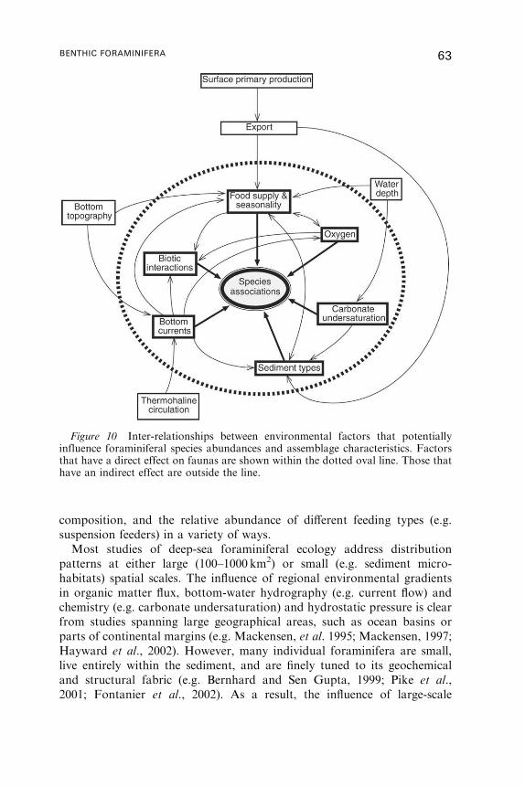
composition, and the relative abundance of different feeding types (e.g.

suspension feeders) in a variety of ways.

Most studies of deep-sea foraminiferal ecology address distribution

patterns at either large (100–1000 km2) or small (e.g. sediment micro-

habitats) spatial scales. The influence of regional environmental gradients

in organic matter flux, bottom-water hydrography (e.g. current flow) and

chemistry (e.g. carbonate undersaturation) and hydrostatic pressure is clear

from studies spanning large geographical areas, such as ocean basins or

parts of continental margins (e.g. Mackensen, et al. 1995; Mackensen, 1997;

Hayward et al., 2002). However, many individual foraminifera are small,

live entirely within the sediment, and are finely tuned to its geochemical

and structural fabric (e.g. Bernhard and Sen Gupta, 1999; Pike et al.,

2001; Fontanier et al., 2002). As a result, the influence of large-scale

Figure 10 Inter-relationships between environmental factors that potentiallyinfluence foraminiferal species abundances and assemblage characteristics. Factorsthat have a direct effect on faunas are shown within the dotted oval line. Those thathave an indirect effect are outside the line.


environmental gradients, particularly organic fluxes, bottom-water oxygen

concentrations and perhaps current flow, rather than being direct, is

mediated through their effects on small-scale gradients within the sediment

milieu (Loubere, 1997). Thus, changes in organic fluxes and oxygen

concentrations extending over horizontal distances of 10s–100s of kilo-

metres act on local foraminiferal assemblages by altering centimetre-scale

vertical gradients in physical, geochemical and microbiological parameters

within the sediment. It is these small-scale gradients that directly influence

foraminiferal assemblage characteristics.

Figure 11 attempts to summarise the various routes by which regional

environmental gradients impinge on the local assemblages that form the

basis for the fossil record (Loubere et al., 1993; Loubere, 1997). Not all

large-scale environmental gradients act indirectly. Some, for example

hydrostatic pressure, have a more immediate influence on local faunas.

Geochemical gradients within the sediment, and hence foraminiferal species,

also respond directly to processes that occur across large geographical areas

but over short time periods, e.g., seasonally pulsed inputs of organic matter

(reviewed by Beaulieu, 2002). In addition to physico-chemical parameters,

biotic interactions such as competition, predation, facilitation, biological

disturbance, and recruitment, undoubtedly help to structure sediment

communities (Gooday, 1986; Jorissen, 1999; Levin et al., 2001), although

their role is poorly understood and difficult to quantify. This web of direct

and indirect effects frustrates efforts to establish straightforward relation-

ships between species assemblages and environmental parameters.

13.2. Calibration of proxies

The quantification of proxies, particularly for organic flux to the sea floor

and bottom-water oxygen concentrations, remains a central challenge for

palaeoceanographers. Reliable, globally applicable, quantitative, proxies for

these parameters based on benthic foraminifera may always remain elusive

because foraminiferal biology is so complex. Nevertheless, considerable

progress has been made recently in a number of areas. Studies based on

samples collected over a wide geographical area (e.g. Mackensen et al., 1995;

Wollenburg and Mackensen, 1998) reveal qualitative relationships between

faunal patterns and environmental parameters. Large data sets relating

species abundances to a single parameter along an environmental gradient

provide the basis for a more quantitative approach. For example, the per-

centage abundance of species in the NE Atlantic Ocean has been related to

the organic carbon flux to the sea floor (Altenbach et al., 1999) and multi-

variate approaches have been used to develop transfer functions linking

species assemblages to surface primary productivity (e.g. Loubere, 1994;

64 ANDREW J. GOODAY

Wollenburg and Kuhnt, 2000). However, the calibration of these proxies

requires reliable values for modern surface productivity and fluxes to the sea

floor (Berger et al., 1994), both of which involve substantial errors. The

good correlations obtained in some studies are encouraging but the large

data sets required for calibration are not often available (Morigi et al., 2001).

Figure 11 Environmental gradients that act over regional spatial scales (outerrectangle) and their effects on foraminiferal faunas at local scales (inner rectangle).Some of the regional gradients (carbonate undersaturation, current flow, oxygena-tion) are water mass attributes. Organic fluxes and bottom-water oxygen act tomodify local geochemical gradients within the sediment and these, in turn, influencefaunal characteristics (species, morphotype composition, relative abundance ofepifaunal/shallow infaunal vs. deep infaunal species) by accelerating or deceleratingrates of reproduction. Current flow, organic fluxes, hydrostatic pressure andcarbonate undersaturation have a more direct effect on faunal characteristics. Bioticinteractions involving metazoan meio- and macro-fauna (not shown) will alsoinfluence foraminiferal faunas.


Another problem is that ancient assemblages may represent conditions that

have no analogue in the calibration dataset. These are difficult to recognise

and interpret (Mekik and Loubere, 1999). Clearly, there is a need for more

precise calibration methods, for example using sediment oxygen profiles as

measures of the flux actually arriving at the sea floor (Jahnke, 1996). For the

present, it may be more realistic to report changes in relative productivity or

flux rather than attempt to estimate absolute values when applying these

approaches in palaeoceanography (Herguera, 2000; Loubere, 2000).

Oxygen is a problematic parameter. Being tightly coupled to organic flux,

it is difficult to determine whether faunas are influenced by these two factors

acting together or by one of them acting alone. Dysoxic conditions are

clearly associated with particular foraminiferal assemblage characteristics

(e.g. low species diversity and high dominance) but there is less agreement

about whether more subtle, species-level effects occur at higher oxygen

concentrations (>1ml l�1). Experiments may provide one way to explore

these issues. Epifaunal/shallow infaunal species are most sensitive to oxygen

depletion and therefore probably offer the best basis for developing bottom-

water oxygen proxies. Again, large data sets, in this case spanning a wide

range of oxygenation regimes, are required in order to calibrate such

proxies.

13.3. Microhabitat studies

Studies of the small-scale distribution patterns of benthic foraminifera are

valuable because they provide detailed information on the environmental

preferences of individual species that cannot be gained by examining large-

scale distribution patterns. Examples include the colonisation of phyto-

detrital layers (Gooday, 1988) and elevated substrates (Lutze and Thiel,

1989; Schonfeld, 2002a, c) by some epifaunal species, the association of

species with particular ranges of pore-water oxygen values (Schonfeld,

2001), and the occurrence of deep infaunal species within anoxic sediment

layers (Jorissen et al., 1998; Fontanier et al., 2002). Such investigations are

leading to a better understanding of the ecological requirements of deep-sea

foraminifera and the relation of species to organic flux rates, oxygen

concentrations, and food sources. In addition to direct observations, �13C

values (i.e. the deviation of the observed 13C : 12C ratio from an arbitrary

standard) obtained from calcareous foraminiferal tests yield insights into the

depth in the sediment at which calcification occurs and the relative mobility

of different infaunal species (Rathburn et al., 1996; McCorkle et al., 1997;

Mackensen et al., 2000).

Despite these advances, many questions remain. Are infaunal taxa really

tolerant of anoxia over long time periods or are they able to obtain oxygen

66 ANDREW J. GOODAY

by deploying pseudopodia into overlying oxygenated layers, as suggested

by Bernhard and Sen Gupta (1999)? More information about diets is

particularly crucial for understanding the balance between inputs of labile

and refractory organic carbon. What do epifaunal/shallow infaunal and

deep infaunal species feed on? Do the deep infaunal species consume

anaerobic bacteria (e.g. Jorissen et al., 1998; Schonfeld, 2001; Fontanier

et al., 2002), degraded organic matter (Goldstein and Corliss, 1994) or fresh

phytodetritus (Kitazato et al., 2000) or can they utilise different food

sources according to their availability? New approaches may help to resolve

such questions. Lipid biomarkers can provide insights into the diets of

infaunal and epifaunal foraminifera (Gooday et al., 2002; Suhr pers.

comm.). In situ experiments using 13C-labelled algal substrates have

considerable potential for investigating the utilisation of labile carbon

sources by foraminifera in both shallow-water (Moodley et al., 2000) and

deep-water environments (Levin et al., 1999; Moodley et al., 2002; Nomaki,

2002; Kitazato et al., 2003). Laboratory-based experiments can also provide

information about aspects of deep-sea foraminiferal biology which

otherwise would be very difficult to obtain (e.g. Kitazato, 1989; Hemleben

and Kitazato, 1995; Gross, 2000; Heinz et al., 2001, 2002; Nomaki, 2002;

Nomaki, pers. comm.). Finally, sediment impregnation techniques, when

combined with fluorescent probes (Bernhard and Bowser, 1996; Pike et al.,

2001), can reveal sub-millimetre details of the relationship between

individual foraminifera and the sedimentary fabric in which they reside.

13.4. Problems in taxonomy

The accurate and consistent recognition of species is of fundamental

importance in ecological studies. Considerable confusion has arisen over the

application of names to some deep-sea foraminiferal species. To take one

example, a small rotaliid that is common in the NE Atlantic Ocean and

elsewhere has been variously referred to Eponides pusillus Parr,

Epistominella pusillus (Parr), Alabaminella weddellensis (Earland),

Eilohedra nipponica (Kuwano), Eilohedra levicula (Resig), Epistominella

levicula Resig and Eponides leviculus (Resig) (Gooday and Lambshead,

1989; Gooday and Hughes, 2002). These problems were emphasised in a

number of papers by Boltovskoy (e.g. Boltovskoy, 1978, 1983) who

suggested that illustrations of species accompanied by references to the

original description and, if necessary, brief remarks would avoid some of the

confusion. This approach has been adopted by journals such as Marine

Micropaleontology which publish taxonomic appendices and extensive

illustrations of foraminiferal species.


Modern advances in molecular genetics are providing a new understanding

of species and their biogeography. There is increasing evidence for genetic

differentiation among deep-sea metazoan species (Creasey and Rogers,

1999), particularly on topographically complex continental margins (France

and Kocher, 1996; Chase et al., 1998; Etter et al., 1999; Quattro et al., 2001).

Almost all benthic foraminiferal species currently described are morphos-

pecies, i.e. they are based on test morphology. It is possible that some, for

example, those occurring across a broad bathymetric range, include a

number of cryptic species rather than being single genetic entities.

Intraspecific morphological changes sometimes occur along bathymetric

gradients (e.g. Boltovskoy, 1991; Spencer, 1992) and may reflect genetic

differentiation. Molecular studies have revealed widespread cryptic specia-

tion among planktonic foraminifera (e.g. Huber et al., 1997; De Vargas et al.,

1999, 2001, 2002; Darling et al., 2000) and in the shallow-water benthic genus

Ammonia (Holzmann and Pawlowski, 1997). Cryptic speciation remains to

be demonstrated among deep-sea benthic taxa, although slightly different

morphotypes have been recognised in some species, for example, Uvigerina

peregrina (Loubere et al., 1995). In planktonic foraminifera, the distribution

of cryptic species appears to be related to water masses of different

productivity and hence to mesoscale upper ocean hydrography (de Vargas

et al., 2001, 2002). This suggests that cryptic speciation is more likely to occur

among benthic foraminifera on environmentally complex continental

margins than on the more uniform abyssal plains, where species geographical

ranges are probably very broad. If cryptic benthic foraminiferal species do

exist in the deep sea, they should exhibit subtle morphological differences that

could be used to distinguish them in the fossil record. Tests of otherwise

almost identical planktonic species can be separated on the basis of porosity

(Huber et al., 1997; de Vargas et al., 1999) and morphometric characteristics

(de Vargas et al., 2001).

13.5. Biological–geological synergy in foraminiferal research?

Research by biologists and geologists has contributed to our under-

standing of deep-sea foraminiferal ecology. The two disciplines tend to

have different scientific aims and approaches. Biologists are concerned

with the principles that govern the structure and functioning of ecosystems

and therefore examine the effects of biological processes such as

dispersion, interactions such as competition, predation and facilitation,

and as physico-chemical factors like oxygen, food availability and

currents. For geologists, the overriding aim is often the development

and refinement of proxies for measurable physical and chemical variables

that are important for understanding how ancient oceans functioned. As a

68 ANDREW J. GOODAY

result, they usually look for relations between species and groups of

species (rather than assemblage parameters) and particular physical and

chemical variables.

Despite these contrasting approaches, there is considerable potential for

synergy between palaeoceanography and biology (Gooday, 1994; Nees and

Struck, 1999). Biologists and geologists share a common interest in many

basic issues in deep-sea ecology and have often addressed them in the

same geographical settings. Biology underpins the accurate reading of

palaeoenvironmental signals, both faunal and geochemical, carried by fossil

foraminifera. Palaeoceanographic studies, in turn, provide a record of

faunal responses to changes in the environment over time scales that are

much longer than those available to biologists (Cronin and Raymo, 1997;

Den Dulk et al., 1998). It has long been known that deep-sea foraminiferal

assemblages have responded over geological time to environmental

fluctuations and recent studies reveal just how sensitive they are to rapid

climatic oscillations (Cannariato et al., 1999). The long temporal perspective

(103 to 106 or more years) provided by the palaeoceanographic record offers

unique insights into the historical and macroecological processes that have

helped to shape modern communities (Lawton, 1999). These are only now

beginning to be exploited by marine biologists, for example, in the

interpretation of large-scale patterns of genetic differentiation and species

diversity in the deep sea (Rex et al., 1997; Quattro et al., 2001; Stuart et al.,

2002). A broad perspective that combines biological and geological

approaches to the study of benthic foraminifera (e.g. Loubere and

Fariduddin, 1999b; Levin et al., 2001) may ultimately lead to a more

complete understanding of the biology of these remarkable and immensely

successful organisms.

ACKNOWLEDGEMENTS

I thank Frans Jorissen, John Murray, Joachim Schonfeld and an

anonymous referee for critiques of various drafts of this paper and

Alexander Altenbach, Elisabeth Alve, Joan Bernhard, Kerry Howell,

Hiroshi Kitazato and Richard Lampitt for their comments on particular

sections. I’m grateful to Lisa Levin, Hiroshi Kitazato and John Murray for

discussions that helped in the formulation of ideas. Andy Henderson took

the light photographs (Figures 2–3) using the PalaeoVision system at the

Natural History Museum, London. Kate Davis prepared most of the

figures. Financial support was provided by NERC Research Grant

GST021749.


REFERENCES

Akimoto, K., Hattori, M. and Oda, M. (2002). Late Cenozoic paleobathymetry andpaleogeography in the South Fossa-Magna and Enshunada regions, Japan, basedon planktic and benthic foraminifera. Marine Geology 187, 89–118.

Alley, R. B., Meese, D. A., Shuman, C. A., Gow, A. J., Taylor, K. C., Grootes, P.M., White, J. W. C., Ram, M., Waddington, E. D., Mayewski, P. A. and Zielinski,A. G. A. (1993). Abrupt increase in Greenland snow accumulation at the end ofthe Younger Dryas event. Nature 362, 527–529.

Altenbach, A. V. (1988). Deep-sea foraminifera and flux rates of organic carbon.Revue Paleobiologie, Vol. Spec. 2, 719–720.

Altenbach, A. V. and Sarnthein, M. (1989). Productivity record in benthicforaminifera. In ‘‘Productivity of the Oceans: Past and Present’’ (W. H. Berger,V. S. Smetacek and G. Wefer, eds.), pp. 255–269, Wiley-Interscience, Chichester.

Altenbach, A. V., Pflaumann, U., Schiebel, R., Thies, A., Timm, S. and Trauth, M.(1999). Scaling percentages and distributional patterns of benthic foraminiferawith flux rates of organic carbon. Journal of Foraminiferal Research 29,173–185.

Alve, E. (1990). Variations in estuarine foraminiferal biofacies with diminishingoxygen conditions in Drammensfjord, SE Norway. In ‘‘Paleoecology,Biostratigraphy, Paleoceanography and Taxonomy of AgglutinatedForaminifera.’’ (C. Hemleben, M. A. Kaminski, W. Kuhnt and D. B. Scott,eds.), pp. 661–694, Kluwer Academic Publishers, Dordrecht, Boston, London.

Alve, E. (1994). Opportunistic features of the foraminifer Stainforthia fusiformis(Williamson): evidence from Frierfjord, Norway. Journal of Micropalaeontology13, 24.

Alve, E. (1999). Colonization of new habitats by benthic foraminifera: a review.Earth Sciences Reviews 46, 167–185.

Alve, E. and Bernhard, J. M. (1995). Vertical migratory response of benthicforaminifera to controlled oxygen concentrations in an experimental mesocosm.Marine Ecology Progress Series 116, 137–151.

Alve, E. and Murray, J. W. (1995). Experiments to determine the origin andpalaeoenvironmental significance of agglutinated foraminiferal assemblages. In‘‘Proceedings of the Fourth International Workshop on AgglutinatedForaminifera, Krakow, Poland, September 12–19, 1993’’ (M. A. Kaminski, S.Geroch, M. A. Gasinski, eds.), pp. 1–11, Grzybowski Foundation SpecialPublication no. 3, Krakow, Poland.

Asper, V. L., Deuser, W. G., Knauer G. A. and Lohrenz, S. E. (1992). Rapidcoupling of sinking particles between surface and deep ocean waters. Nature 357,670–672.

Baas, J. H., Schonfeld, J. and Zahn, R. (1998). Mid-depth oxygen drawdown duringHeinrich events: evidence from benthic foraminiferal community structure, trace-fossil tiering, and benthic �

13C at the Portuguese Margin. Marine Geology 152,25–55.

Barmawidjaja, D. M., Jorissen, F. J., Puskaric, S. and van der Zwaan, G. J. (1992).Microhabitat selection by benthic foraminifera in the Northern Adriatic Sea.Journal of Foraminiferal Research 22, 297–317.

Barnett, P. R. O., Watson, J. and Connelly, D. (1984). A multiple corer for takingvirtually undisturbed samples from shelf, bathyal and abyssal sediments.Oceanologica Acta 7, 401–408.

70 ANDREW J. GOODAY

Basov, I. A. and Khusid, T. A. (1983). Biomass of benthic foraminifera in thesediments of the Sea of Okhotsk. Oceanology 33, 489–495.

Beaulieu, S. E. (2001). Colonization of habitat islands in the deep sea: recruitment toglass sponge stalks. Deep-Sea Research 48, 1121–1137.

Beaulieu, S. R.(2002). Accumulation and fate of phytodetritus on the sea floor.Oceanography and Marine Biology an Annual Review 40, 171–232.

Belanger, P. E. and Streeter, S.S. (1980). Distribution and ecology of benthic foramini-fera in the Norwegian-Greenland Sea. Marine Micropaleontology 5, 401–428.

Berger, W. H. (1979). Preservation of foraminifera. In ‘‘Foraminiferal Ecology andPaleoecology’’ (J. H. Lipps, W. H. Berger, M. A. Buzas, R. H. Douglas and C. A.Ross, eds.), pp. 105–155, Society of Economic Petrologists and MineralogistsShort Course No. 6, Houston, Texas.

Berger, W. H. and Diester-Haas, H. (1988). Paleoproductivity: the benthic/planktonicratio in foraminifera as a productivity index. Marine Geology 81, 15–25.

Berger, W. H. and Herguera, J. C. (1992). Reading the sedimentary record of theocean’s productivity. In ‘‘Primary Productivity and Biogeochemical Cycles inthe Sea’’ (P. G. Falkowsky and A. D. Woodhead, eds.), pp. 455–486, PlenumPress, New York.

Berger, W. H. and Wefer, G. (1990). Export production: seasonality andintermittency, and paleoceanographic implications. Palaeogeography,Palaeoclimatology, Palaeoecology (Global and Planetary Change Section) 89,245–254.

Berger, W. H. and Wefer, G. (1992). Flux of biogenous materials to the seafloor:open questions. In ‘‘Use and Misuse of the Seafloor’’ (K. J. Hsu and J. Thiede,eds.), pp. 285–304, John Wiley and Sons, Ltd., Chichester.

Berger, W. H., Fischer, K., Lai, C. and Wu, G. (1988). Ocean carbon flux: globalmaps of primary production and export production. In ‘‘Biogeochemical Cyclingand Fluxes Between the Deep Euphotic Zone and Other Oceanic Realms’’ (C. R.Agegian, ed.), pp. 131–176, National Undersea Research Program – ResearchReport 88-1.

Berger, W. H., Smetacek, V. S. and Wefer, G. (1989). Ocean productivity andpaleoproductivity - an overview. In ‘‘Productivity of the Oceans: Present andPast’’ (W. H. Berger, V. S. Smetacek and G. Wefer, eds.) pp. 1–34, Wiley,Chichester.

Berger, W. H., Herguera, J. C., Lange, C. B. and Schneider, R. (1994).Paleoproductivity: flux versus nutrient proxies and other problems concerningthe Quaternary productivity record. In ‘‘Carbon Cycling in the Glacial Ocean:Constraints on the Ocean’s Role in Global Change.’’ (R. Zahn, T. F. Pederson, M.A. Kaminski and L. Labeyrie, eds.), pp. 385–412, Springer-Verlag, Berlin,Heidelberg.

Bernhard, J. M. (1993). Experimental and field evidence of Antarctic foraminiferaltolerance to anoxia and hydrogen sulphide. Marine Micropaleontology 20,203–213.

Bernhard, J. M. (1996). Microaerophilic and faculative anaerobic benthicforaminifera: a review of experimental and ultrastructural evidence. Revue dePaleobiologie 15, 261–275.

Bernhard, J. M. (2002). The anoxic Cariaco Basin has benthic foraminifers:preliminary observations on the ecology and ultrastructure of Virgulinella fragilis.In ‘‘Forams 2002. International Symposium on Foraminifera. The University ofWestern Australia, Perth, 4–8 February 2002. Abstracts’’ (S. A. Revets, ed.),pp. 24–25.


Bernhard, J. M. and Bowser, S. S. (1996). Novel epifluorescence microscopy methodto determine life position of foraminifera in sediments. Journal ofMicropalaeontology 15, 68.

Bernhard, J. M. and Riemers, C. E. (1991). Benthic foraminiferal populationfluctuations related to anoxia: Santa Barbara Basin. Biogeochemistry 15, 127–149.

Bernhard, J. H. and Sen Gupta, B. K. (1999). Foraminifera in oxygen-depletedenvironments. In ‘‘Modern Foraminifera’’ (B. K. Sen Gupta, ed.), pp. 201–216,Kluwer Academic Publishers, Dordrecht, Boston, London.

Bernhard, J. M., Sen Gupta, B. K. and Borne, P. F. (1997). Benthic foraminiferalproxy to estimate dysoxic bottom-water oxygen concentrations: Santa BarbaraBasin, U. S. Pacific continental margin. Journal of Foraminiferal Research 27,301–310.

Bertram, M. A. and Cowen, J. P. (1999). Temporal variations in the deep-watercolonization rates of small benthic foraminifera: the results of an experiment onCross Seamount. Deep-Sea Research I 46, 1021–1049.

Bett, B. J. (2001). UK. Atlantic Margin Environmental Survey: introduction andoverview of bathyal benthic ecology. Continental Shelf Research 21, 917–956.

Bett, B. J. (in press). Sampler bias in the quantitative study of deep-seamacrobenthos. Marine Ecology Progress Series.

Bett, B. J., Vanreusel, A., Vincx, M., Soltwedel, T., Pfannkuche, O., Lambshead, P.J. D., Gooday, A. J., Ferrero, T. and Dinet, A. (1994). Sampler bias in thequantitative study of deep-sea meiobenthos. Marine Ecology Progress Series 104,197–203.

Billett, D. S. M. (1991). Deep-sea holothurians. Oceanography and Marine Biology,an Annual Review 29, 259–317.

Billett, D. M. S., Lampitt, R. S., Rice, A. L. and Mantoura, R. F. C. (1983). Seasonalsedimentation of phytodetritus to the deep-sea benthos. Nature 302, 520–522.

Boltovskoy, E. (1978). Late Cenozoic benthonic foraminifera of the NinetyeastRidge (Indian Ocean). Marine Geology 26, 139–175.

Boltovskoy, E. (1983). Late Cenozoic deep-sea benthic Foraminifera off the coast ofnorthwest Africa (D. D. Site 369). Journal of African Earth Sciences 1, 83–102.

Boltovskoy, E., Scott, D. B. and Medioli, F. S. (1991). Morphological variations ofbenthic foraminiferal tests in response to changes in ecological parameters: areview. Journal of Paleontology 65, 175–185.

Bradshaw, J. S. (1961). Laboratory experiments on the ecology of foraminifera.Contributions from the Cushman Foundation for Foraminiferal Research 12, 87–106.

Bremer, M. L. and Lohmann, G. P. (1982). Evidence for primary control of thedistribution of certain Atlantic benthonic foraminifera by degree of carbonatesaturation. Marine Micropaleontology 29, 987–998.

Burke, S. C. (1981). Recent benthic foraminifera of the Ontong Java Plateau. Journalof Foraminiferal Research 11, 1–19.

Buzas, M. A., Collins, L. S., Richardson, S. L. and Severin, K. P. (1989).Experiments on predation, substrate preference, and colonization of benthicforaminifera at the shelfbreak off the Ft. Pierce Inlet, Florida. Journal ofForaminiferal Research 19, 146–152.

Buzas, M. A., Culver, S. J. and Jorissen, F. J. (1993). A statistical evaluation of themicrohabitats of living (stained) infaunal benthic foraminifera. MarineMicropaleontology 20, 311–320.

Cannariato, K. G., Kennett, J. P. and Behl, R. J. (1999). Biotic response to lateQuaternary rapid climate switches in Santa Barbara Basin: ecological andevolutionary implications. Geology 27, 63–66.

72 ANDREW J. GOODAY

Caralp, M. (1989). Abundance of Bulimina exilis and Melonis barleeanum:Relationship to the quality of marine organic matter. Geo-Marine Letters 9, 37–43.

Carney, R. S., Haedrich, R. L. and Rowe, G. T. (1983). Zonation of fauna in thedeep sea. In ‘‘The Sea. Vol. 8. Deep-Sea Biology’’ (G. T. Rowe, ed.), pp. 371–398,Wiley-Interscience, New York.

Carpenter, W. B. (1869). Preliminary report of dredging operations in the seas to thenorth of the British Isles, carried out in Her Majesty’s steam-vessel ‘‘Lightning’’ byDr Carpenter and Dr Wyville Thomson. Proceedings of the Royal Society ofLondon 17, 168–197.

Carpenter, W. B., Jeffreys, J. G. and Thomson, W. (1870). Preliminary report of thescientific exploration of the deep sea in H. M. surveying-vessel ‘Porcupine’, duringthe summer of 1862. Proceedings of the Royal Society of London 18, 397–453.

Cartes, J. E. and Sarda, F. (1993). Zonation of deep-sea decapod fauna in theCatalan Sea (Western Mediterranean). Marine Ecology Progress Series 94, 27–34.

Cedhagen, T., Goldstein, S. T. and Gooday, A. J. (eds.) (2002). Biodiversity ofAllogromiid Foraminifera. Journal of Foraminiferal Research, 32.

Chase, M. R., Etter, R. J., Rex, M. A. and Quattro, J. M. (1998). Bathymetricpatterns of genetic differentiation in a deep-sea protobranch bivalve, Deminuculaatacellana. Marine Biology 131, 301–308.

Christiansen, B. and Boetius, A. (2000). Mass sedimentation of the swimming crabCharybdis smithii (Crustacea: Decapoda) in the deep Arabian Sea. Deep-SeaResearch II 47, 2673–2685.

Clark, P. U., Alley, R. B. and Pollard, D. (1999). Northerm hemisphere ice-sheetinfluences on global climate change. Science 286, 1104–1111.

Committee on Abrupt Climate Change (2002). ‘‘Abrupt Climate Change: InevitableSurprises’’ National Academy Press, Washington DC, 230 pp.

Corliss, B. H. (1979). Recent deep-sea benthonic foraminiferal distributions in thesoutheast Indian Ocean: inferred bottom-water routes and ecological implications.Marine Geology 31, 115–138.

Corliss, B. H. (1983). Quaternary circulation of the Antarctic Circumpolar Current.Deep-Sea Research 30, 47–61.

Corliss, B. H. (1985). Microhabitats of benthic foraminifera within deep-seasediments. Nature 314, 435–438.

Corliss, B. H. (1991). Morphology and microhabitat preferences of benthicforaminifera from the northwest Atlantic Ocean. Marine Micropaleontology 17,195–236.

Corliss, B. H. and Chen, C. (1988). Morphotype patterns of Norwegian Sea deep-seabenthic foraminifera and ecological implications. Geology 16, 716–719.

Corliss, B. H. and Emerson, S. (1990). Distribution of Rose Bengal stained deep-seabenthic foraminifera from the Nova Scotian continental margin and Gulf ofMaine. Deep-Sea Research 37, 381–400.

Corliss, B. H. and Honjo, S. (1981). Dissolution of deep-sea benthonic foraminifera.Micropaleontology 27, 356–378.

Corliss, B. H., Martinson, D. and Keffer, T. (1986). Late Quaternary deep oceancirculation. Bulletin of the Geological Society of America 97, 1106–1121.

Creasey, S. S. and Rogers, A. D. (1999). Population genetics of bathyal and abyssalorganisms. Advances in Marine Biology 35, 1–151.

Cronin, T. M. and Raymo, M. E. (1997). Orbital forcing of deep-sea benthic speciesdiversity. Nature 385, 624–627.

Culver, S. J. (1988). New foraminiferal depth zonation of the northwest Gulf ofMexico. Palaios 3, 69–85.


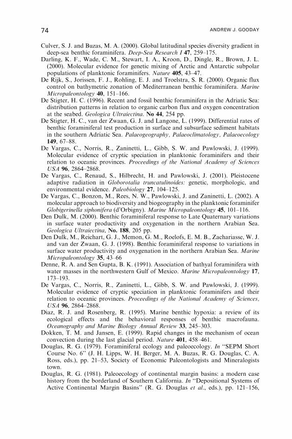
Culver, S. J. and Buzas, M. A. (2000). Global latitudinal species diversity gradient indeep-sea benthic foraminifera. Deep-Sea Research I 47, 259–175.

Darling, K. F., Wade, C. M., Stewart, I. A., Kroon, D., Dingle, R., Brown, J. L.(2000). Molecular evidence for genetic mixing of Arctic and Antarctic subpolarpopulations of planktonic foraminifers. Nature 405, 43–47.

De Rijk, S., Jorissen, F. J., Rohling, E. J. and Troelstra, S. R. (2000). Organic fluxcontrol on bathymetric zonation of Mediterranean benthic foraminifera. MarineMicropaleontology 40, 151–166.

De Stigter, H. C. (1996). Recent and fossil benthic foraminifera in the Adriatic Sea:distribution patterns in relation to organic carbon flux and oxygen concentrationat the seabed. Geologica Ultraiectina. No 44, 254 pp.

De Stigter, H. C., van der Zwaan, G. J. and Langone, L. (1999). Differential rates ofbenthic foraminiferal test production in surface and subsurface sediment habitatsin the southern Adriatic Sea. Palaeogeography, Palaeoclimatology, Palaeoecology149, 67–88.

De Vargas, C., Norris, R., Zaninetti, L., Gibb, S. W. and Pawlowski, J. (1999).Molecular evidence of cryptic speciation in planktonic foraminifers and theirrelation to oceanic provinces. Proceedings of the National Academy of SciencesUSA 96, 2864–2868.

De Vargas, C., Renaud, S., Hilbrecht, H. and Pawlowski, J. (2001). Pleistoceneadaptive radiation in Globorotalia truncatulinoides: genetic, morphologic, andenvironmental evidence. Paleobiology 27, 104–125.

De Vargas, C., Bonzon, M., Rees, N. W., Pawlowski, J. and Zaninetti, L. (2002). Amolecular approach to biodiversity and biogeography in the planktonic foraminiferGlobigerinella siphonifera (d’Orbigny). Marine Micropaleontology 45, 101–116.

Den Dulk, M. (2000). Benthic foraminiferal response to Late Quaternary variationsin surface water productivity and oxygenation in the northern Arabian Sea.Geologica Ultraiectina, No. 188, 205 pp.

Den Dulk, M., Reichart, G. J., Memon, G. M., Roelofs, E. M. B., Zachariasse, W. J.and van der Zwaan, G. J. (1998). Benthic foraminiferal response to variations insurface water productivity and oxygenation in the northern Arabian Sea. MarineMicropaleontology 35, 43–66

Denne, R. A. and Sen Gupta, B. K. (1991). Association of bathyal foraminifera withwater masses in the northwestern Gulf of Mexico. Marine Micropaleontology 17,173–193.

De Vargas, C., Norris, R., Zaninetti, L., Gibb, S. W. and Pawlowski, J. (1999).Molecular evidence of cryptic speciation in planktonic foraminifers and theirrelation to oceanic provinces. Proceedings of the National Academy of Sciences,USA 96, 2864–2868.

Diaz, R. J. and Rosenberg, R. (1995). Marine benthic hypoxia: a review of itsecological effects and the behavioral responses of benthic macrofauna.Oceanography and Marine Biology Annual Review 33, 245–303.

Dokken, T. M. and Jansen, E. (1999). Rapid changes in the mechanism of oceanconvection during the last glacial period. Nature 401, 458–461.

Douglas, R. G. (1979). Foraminiferal ecology and paleoecology. In ‘‘SEPM ShortCourse No. 6’’ (J. H. Lipps, W. H. Berger, M. A. Buzas, R. G. Douglas, C. A.Ross, eds.), pp. 21–53, Society of Economic Paleontologists and Mineralogiststown.

Douglas, R. G. (1981). Paleoecology of continental margin basins: a modern casehistory from the borderland of Southern California. In ‘‘Depositional Systems ofActive Continental Margin Basins’’ (R. G. Douglas et al., eds.), pp. 121–156,

74 ANDREW J. GOODAY

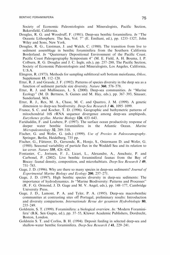
Society of Economic Paleontologists and Mineralogists, Pacific Section,Bakersfield, California.

Douglas, R. G. and Woodruff, F. (1981). Deep-sea benthic foraminifera. In ‘‘TheOceanic Lithosphere. The Sea, Vol. 7’’ (E. Emiliani, ed.), pp. 1233–1327, JohnWiley and Sons, New York.

Douglas, R. G., Liestman, J. and Walch, C. (1980). The transition from live tosediment assemblage in benthic foraminifera from the Southern CaliforniaBorderland. In ‘‘Quaternary Depositional Environment of the Pacific Coast.Pacific Coast Paleogeography Symposium 4’’ (M. E. Field, A. H. Bouma, I. P.Colburn, R. G. Douglas and J. C. Ingle, eds.), pp. 257–280, The Pacific Section,Society of Economic Paleontologists and Mineralogists, Los Angeles, California,U.S.A.

Elmgren, R. (1973). Methods for sampling sublittoral soft bottom meiofauna, Oikos,Supplement 15, 112–120.

Etter, R. J. and Grassle, J. F. (1992). Patterns of species diversity in the deep sea as afunction of sediment particle size diversity. Nature 360, 576–578.

Etter, R. J. and Mullineaux, L. S. (2000). Deep-sea communities. In ‘‘MarineEcology’’ (M. D. Bertness, S. Gaines and M. Hay, eds.), pp. 367–393, Sinauer,Sunderland, MA.

Etter, R. J., Rex, M. A., Chase, M. C. and Quattro, J. M. (1999). A geneticdimension to deep-sea biodiversity. Deep-Sea Research I 46, 1095–1099.

France, S. C. and Kocher, T. D. (1996). Geographic and bathymetric patterns ofmitochondrial 16S rRNA sequence divergence among deep-sea amphipods,Eurythenes gryllus. Marine Biology 126, 633–643.

Fariduddin, F. and Loubere, P. (1997). The surface ocean productivity response ofdeeper water benthic foraminifera in the Atlantic Ocean. MarineMicropaleontology 32, 289–310.

Fischer, G. and Wefer, G. (eds.) (1999). Use of Proxies in Paleoceanography.Springer, Berlin, Heidelberg, 735 pp.

Fischer, G., Futterer, D., Gersonde, R., Honjo, S., Ostermann D. and Wefer, G.(1988). Seasonal variability of particle flux in the Weddell Sea and its relation toice cover. Nature 335, 426–428.

Fontanier, C., Jorissen, F. J., Licari, L., Alexandre, A., Anschutz, P. andCarbonel, P. (2002). Live benthic foraminiferal faunas from the Bay ofBiscay: faunal density, composition, and microhabitats. Deep-Sea Research I 49,751–785.

Gage, J. D. (1996). Why are there so many species in deep-sea sediments? Journal ofExperimental Marine Biology and Ecology 200, 257–271.

Gage, J. D. (1997). High benthic species diversity in deep-sea sediments: Theimportance of hydrodynamics. In ‘‘Marine Biodiversity: Patterns and Processes’’(R. F. G. Ormond, J. D. Gage and M. V. Angel, eds.), pp. 148–177, CambridgeUniversity Press.

Gage, J. D., Lamont, P. A. and Tyler, P. A. (1995). Deep-sea macrobenthiccommunities at contrasting sites off Portugal, preliminary results: Introductionand diversity comparisons. Internationale Revue der gesamten Hydrobiologie 80,235–249.

Goldstein, S. T. (1999). Foraminifera: a biological overview. In: ‘Modern Foramini-fera’ (B.K. Sen Gupta, ed.), pp. 37–55, Kluwer Academic Publishers, Dordrecht,Boston, London.

Goldstein S. T. and Corliss, B. H. (1994). Deposit feeding in selected deep-sea andshallow-water benthic foraminifera. Deep-Sea Research I 41, 229–241.


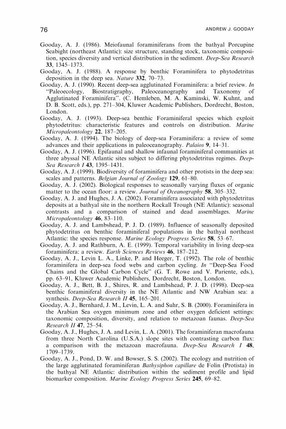
Gooday, A. J. (1986). Meiofaunal foraminiferans from the bathyal PorcupineSeabight (northeast Atlantic): size structure, standing stock, taxonomic composi-tion, species diversity and vertical distribution in the sediment. Deep-Sea Research33, 1345–1373.

Gooday, A. J. (1988). A response by benthic Foraminifera to phytodetritusdeposition in the deep sea. Nature 332, 70–73.

Gooday, A. J. (1990). Recent deep-sea agglutinated Foraminifera: a brief review. In‘‘Paleoecology, Biostratigraphy, Paleoceanography and Taxonomy ofAgglutinated Foraminifera’’. (C. Hemleben, M. A. Kaminski, W. Kuhnt, andD. B. Scott, eds.), pp. 271–304, Kluwer Academic Publishers, Dordrecht, Boston,London.

Gooday, A. J. (1993). Deep-sea benthic Foraminiferal species which exploitphytodetritus: characteristic features and controls on distribution. MarineMicropaleontology 22, 187–205.

Gooday, A. J. (1994). The biology of deep-sea Foraminifera: a review of someadvances and their applications in paleoceanography. Palaios 9, 14–31.

Gooday, A. J. (1996). Epifaunal and shallow infaunal foraminiferal communities atthree abyssal NE Atlantic sites subject to differing phytodetritus regimes. Deep-Sea Research I 43, 1395–1431.

Gooday, A. J. (1999). Biodiversity of foraminifera and other protists in the deep sea:scales and patterns. Belgian Journal of Zoology 129, 61–80.

Gooday, A. J. (2002). Biological responses to seasonally varying fluxes of organicmatter to the ocean floor: a review. Journal of Oceanography 58, 305–332.

Gooday, A. J. and Hughes, J. A. (2002). Foraminifera associated with phytodetritusdeposits at a bathyal site in the northern Rockall Trough (NE Atlantic): seasonalcontrasts and a comparison of stained and dead assemblages. MarineMicropaleontology 46, 83–110.

Gooday, A. J. and Lambshead, P. J. D. (1989). Influence of seasonally depositedphytodetritus on benthic foraminiferal populations in the bathyal northeastAtlantic: the species response. Marine Ecology Progress Series 58, 53–67.

Gooday, A. J. and Rathburn, A. E. (1999). Temporal variability in living deep-seaforaminifera: a review. Earth Sciences Reviews 46, 187–212.

Gooday, A. J., Levin L. A., Linke, P. and Heeger, T. (1992). The role of benthicforaminifera in deep-sea food webs and carbon cycling. In ‘‘Deep-Sea FoodChains and the Global Carbon Cycle’’ (G. T. Rowe and V. Pariente, eds.),pp. 63–91, Kluwer Academic Publishers, Dordrecht, Boston, London.

Gooday, A. J., Bett, B. J., Shires, R. and Lambshead, P. J. D. (1998). Deep-seabenthic foraminiferal diversity in the NE Atlantic and NW Arabian sea: asynthesis. Deep-Sea Research II 45, 165–201.

Gooday, A. J., Bernhard, J. M., Levin, L. A. and Suhr, S. B. (2000). Foraminifera inthe Arabian Sea oxygen minimum zone and other oxygen deficient settings:taxonomic composition, diversity, and relation to metazoan faunas. Deep-SeaResearch II 47, 25–54.

Gooday, A. J., Hughes, J. A. and Levin, L. A. (2001). The foraminiferan macrofaunafrom three North Carolina (U.S.A.) slope sites with contrasting carbon flux:a comparison with the metazoan macrofauna. Deep-Sea Research I 48,1709–1739.

Gooday, A. J., Pond, D. W. and Bowser, S. S. (2002). The ecology and nutrition ofthe large agglutinated foraminiferan Bathysiphon capillare de Folin (Protista) inthe bathyal NE Atlantic: distribution within the sediment profile and lipidbiomarker composition. Marine Ecology Progress Series 245, 69–82.

76 ANDREW J. GOODAY

Gradstein, F. M. and Berggren, W. A. (1981). Flysch-type agglutinated Foraminiferaand the Maastrichtian to Paleogene history of the Labrador and North Sea.Marine Micropaleontology 6, 211–268.

Graf, G., Gerlach, S. A., Linke, P., Queisser, W., Ritzrau, W., Scheltz, A., Thomsen,L. and Witte, U. (1995). Benthic-pelagic coupling in the Greenland-Norwegian Seaand its effect on the geological record. Geologische Rundschau 84, 49–58.

Grassle, J. F. and Morse-Porteous, L. S. (1987). Macrofaunal colonization ofdisturbed deep-sea environments and the structure of deep-sea benthic commu-nities. Deep-Sea Research 34, 1911–1950.

Green, M. A., Aller, R. C. and Aller, J. Y. (1998). Influence of carbonate dissolutionon survival of shell-bearing meiobenthos in nearshore sediments. Limnology andOceanography 43, 18–28.

Gross, O. (2000). Influence of temperature, oxygen and food availability on themigrational activity of bathyal benthic foraminifera: evidence by microcosmexperiments. Hydrobiologia 426, 123–137.

Guichard, S., Jorissen, F., Bertrand, P., Gervais, A., Martinez, P., Peypouquet, J.-P.,Pujol, C. and Vergnaud-Grazzini, C. (1997). Foraminiferes benthiques etpaleoproductivite: reflexions sur une carotte de l’upwelling (NW Africain).Compte Rendus de l’Acadamie des Sciences, Paris, Sciences de la Terre et desPlanets 325, 65–70.

Haake, F.-W. (1980). Benthische Foraminiferen in Oberflachen-Sedimenten undKernen des Ostatlantiks vor Senegal/Gambia (Westafrika). ‘Meteor’-Forschungs-Ergebnisse C32, 1–29.

Haake, F.-W., Coulbourn, W. T. and Berger, W. H. (1982). Benthic foraminifera:depth distribution and redeposition. In ‘‘Geology of the Northwest AfricanContinental Margin’’ (U. von Rad, K. Hinz, M. Sarnthein, E. Seibold, eds.),pp. 632–657, Springer-Verlag, Berlin, Heidelberg, New York.

Hale, W. and Pflaumann, U. (1999). Sea-surface temperature estimations using amodern analogue technique with foraminiferal assemblages from Western AtlanticQuaternary sediments. In ‘‘Use of Proxies in Paleoceanography’’ (G. Fischer andG. Wefer, eds.), pp. 69–90, Springer, Berlin, Heidelberg.

Hall, S. J. (1994). Physical disturbance and marine benthic communities: life inunconsolidated sediments. Oceanography and Marine Biology, an Annual Review32, 179–239.

Harloff, J. and Mackensen, A. (1997). Recent benthic foraminiferal associations andecology of the Scotia Sea and Argentine Basin. Marine Micropaleontology 31,1–29.

Hayward, B.W. (1990). Use of foraminiferal data in analysis of Taranaki Basin, NewZealand. Journal of Foraminiferal Research 20, 71–83.

Hayward, B. W., Neil, H., Carter, R., Grenfell, H. R., Hayward, J. (2002). Factorsinfluencing the distribution of Recent deep-sea benthic foraminifera, east of NewZealand, southwest Pacific Ocean. Marine Micropaleontology 46, 139–176.

Hecker, B. (1990a). Variation in megafaunal assemblages on the continental marginsouth of New England. Deep-Sea Research 37, 37–57.

Hecker, B. (1990b). Photographic evidence for the rapid flux of particles to theseafloor and their transport down the continental slope. Deep-Sea Research 37,1773–1782.

Heezen, B. C. and Hollister, C. D. (1971). ‘‘The face of the deep.’’ Oxford UniversityPress: New York.

Heinz, P., Kitazato, H., Schmiedl, G. and Hemleben, Ch. (2001). Response ofdeep-sea benthic Foraminifera from the Mediterranean Sea to simulated


phytoplankton pulses under laboratory conditions. Journal of ForaminiferalResearch 31, 210–227.

Heinz, P., Hemleben, Ch. and Kitazato, H. (2002). Time-response of cultured deep-sea benthic Foraminifera to different algal diets. Deep-Sea Research I 49, 517–537.

Hemleben, C. and Kitazato, H. (1995). Deep-sea foraminifera under long timeobservation in the laboratory. Deep-Sea Research I 42, 827–832.

Herguera, J. C. (1992). Deep-sea benthic foraminifera and biogenic opal: glacial topostglacial productivity changes in the western equatorial Pacific. MarineMicropaleontology 19, 79–98.

Herguera, J. C. (2000). Late glacial paleoproductivity patterns in the easternequatorial Pacific: benthic foraminifera records. Marine Micropaleontology 40,259–275.

Herguera, J. C. and Berger, W. H. (1991). Paleoproductivity from benthicforaminifera abundance: glacial to post-glacial change in west-equatorial Pacific.Geology 19, 1173–1176.

Hess, S. and Kuhnt, W. (1996). Deep-sea benthic foraminiferal recolonization of the1991 Mt. Pinatubo ash layer in the South China Sea. Marine Micropaleontology28, 171–197.

Hess, S., Kuhnt, W., Hill, S., Kaminski, M. A., Holbourn, A. and de Leon, M.(2001). Monitoring the recolonization of the Mt Pinatubo 1991 ash layer bybenthic foraminifera. Micropaleontology 43, 119–142.

Hermelin, J. O. R. and Shimmield, G. B. (1990). The importance of the oxygenminimum zone and sediment geochemistry in the distribution of Recent benthicforaminifera in the northwest Indian Ocean. Marine Geology 91, 1–29.

Holbourn, A., Kuhnt, W., El Albani, A., Pletsch, T., Luderer, F. and Wagner, T.(1999). Upper Cretaceous palaeoenvironments and benthonic foraminiferalassemblages of potential source rocks from the western African margin, CentralAtlantic. In ‘‘The Oil and Gas Habitats of the South Atlantic’’ (N. R., Cameron,R. H. Bate and V. S. Clure, eds.), pp. 195–222, Geological Society, London,Special Publication 153, 195–222.

Holbourn, A., Kuhnt, W. and Erbacher, J. (2001a). Benthic foraminifers from lowerAlbian black shales (Site 1049, ODP Leg 171): evidence for a non ‘uniformitarian’record. Journal of Foraminiferal Research 31, 60–74.

Holbourn, A., Kuhnt, W. and Soeding, E. (2001b). Atlantic paleobathymetry,paleoproductivity and paleocirculation in the late Albian: the benthic forami-niferal record. Palaeogeography, Palaeoclimatology, Palaeoecology 173, 171–196.

Hollister, C. D. and Nowell, A. R. M. (1991). HEBBLE epilogue. Marine Geology99, 445–460.

Hollister, C. D., Nowell, A. R. M. and Jumars, P. A. (1984). The dynamic abyss.Scientific American 250, 42–53.

Holzmann, M. and Pawlowski, J. (1997). Molecular, morphological and ecologicalevidence for species recognition in Ammonia (Foraminifera). Journal ofForaminiferal Research 27, 311–318.

Huber, B. T., Bijma, J. and Darling, K. (1997). Cryptic speciation in the livingplanktonic foraminifer Globigerinella siphonifera (d’Orbigny). Paleobiology 23,33–62.

Hughes, J. A., Gooday, A. J. and Murray, J. W. (2000). The distribution of livebenthic foraminifera at three oceanographically dissimilar sites in the northeastAtlantic: preliminary results. Hydrobiologia 440, 227–238.

Imbrie, J. and Kipp, N. G. (1971). A new micropaleontological method forquantitative paleoclimatology: application to a Late Pleistocene core. In ‘‘The Late

78 ANDREW J. GOODAY

Cenozoic Glacial Ages’’ (Turekian, K., ed.), pp. 71–181, Yale University Press,New Haven, Connecticut.

Jahnke, R. A. (1996). The global ocean flux of particulate organic carbon: Arealdistribution and magnitude. Global Biogeochemical Cycles 10, 71–88.

Jahnke, R. A. (2002). Global distribution and magnitude of deep particulate organiccarbon fluxes estimated by benthic flux measurements (abstract). In ‘‘InternationalWorkshop on Global Ocean Productivity and the Fluxes of Carbon and Nutrients:Combining Observations and Models’’ (R. Schlitzer, P. Monfray and N.Hoepfner, eds), pp. 16–17. JRC-ISPRA, Italy 24–27 June 2002.

Jannink, N. T. (2001). Seasonality, biodiversity and microhabitats in benthicforaminiferal communities. Geologica Ultraiectina, no. 203, 1–192.

Jannink, N. T., Zachariasse, W. J. and van der Zwaan, G. J. (1998). Living (RoseBengal stained) benthic Foraminifera from the Pakistan continental margin(northern Arabian Sea). Deep-Sea Research I 45, 1483–1513.

Jensen, P. (1982). A new meiofaunal splitter. Annales Zoologici Fennici 19,233–236.

Jian, Z., Wang, L., Kienast, M., Sarnthein, M., Kuhnt, W., Lin, H. and Wang, P.(1999). Benthic foraminiferal paleoceanography of the South China Sea over thelast 40,000. Marine Geology 156, 159–186.

Jian, Z., Huang, B., Kuhnt, W. and Lin, H.-L. (2001). Late Quaternary upwellingintensity and East Asian monsoon forcing in the South China Sea. QuaternaryResearch, 55, 363–370.

Jorissen, F. (1999). Benthic foraminiferal microhabitats below the sediment-waterinterface. In ‘‘Modern Foraminifera’’ (B. K. Sen Gupta, ed.), pp. 161–179. KluwerAcademic Publishers, Dordrecht, Boston, London.

Jorissen, F. and Rohling, E. T. (eds.), (2000). Foraminiferal proxies of paleopro-ductivity. Marine Micropalaeontology 40, 131–344.

Jorissen, F. J. and Wittling, I. (1999). Ecological evidence from live-deadcomparisons of benthic foraminiferal faunas off Cape Blanc (Northwest Africa).Palaeogeography, Palaeoclimatology, Palaeoecology 149, 151–170.

Jorissen, F. J., de Stigter, H. C. and Widmark, J. G. V. (1995). A conceptual modelexplaining benthic foraminiferal microhabitats. Marine Micropaleontology 26,3–15.

Jorissen, F., Wittling, I., Peypouquet, J. P., Rabouille, C. and Relexans, J. C. (1998).Live benthic foraminiferal faunas off Cap Blanc, NW Africa: community structureand microhabitats. Deep-Sea Research I 45, 2157–2188.

Josefson, A. B. and Widbom, B. (1988). Differential response of benthic macrofaunaand meiofauna to hypoxia in the Gullmar fjord basin. Marine Biology 100,31–40.

Kaiho, K. (1991). Global changes of Paleogene aerobic/anaerobic benthicforaminifera and deep-sea circulation. Palaeogeography, Palaeoclimatology,Palaeoecology 83, 65–85.

Kaiho, K. (1994). Benthic foraminiferal dissolved-oxygen levels in the modern ocean.Geology 22, 719–722.

Kaiho, K. (1999). Effect of organic carbon flux and dissolved oxygen on the benthicforaminiferal oxygen index (BFOI). Marine Micropaleontology 37, 67–76.

Kaminski, M. A. (1985). Evidence for control of abyssal agglutinated foraminiferalcommunity structure by substrate disturbance: results from the HEBBLE area.Marine Geology 66, 113–131.

Kaminski, M. A. and Schroder, C. J. (1987). Environmental analysis of deep-sea agglutinated foraminifera: can we distinguish tranquil from disturbed


environments? Gulf Coast Section SEPM Foundation Eighth Annual ResearchConference. Selected papers and illustrated abstracts, pp. 90–93.

Kamp, P. J. J., Journeaux. T. D. and Morgans, H. E. G. (1998). Cyclostratigraphy ofmiddle Pliocene mid shelf to upper slope strata, eastern Wanganui Basin (NewZealand): correlations to the deep sea isotope record. Sedimentary Geology 117,165–192.

Kemp, A. E. S., Pike, J., Pearce, R. B., Lange, C. B. (2000). The ‘‘Fall dump’’ – a newperspective on the role of a ‘‘shade flora’’ in the annual cycle of diatom productionand export flux. Deep-Sea Research II 47, 2129–2154.

Kitazato, H. (1989). Vertical distribution of benthic foraminifera within sediments(preliminary report). Benthos Research, Bulletin of the Japanese Association ofBenthology 35/36, 41–51.

Kitazato, H. (1994). Foraminiferal microhabitats in four environments aroundJapan. Marine Micropaleontology 24, 29–41.

Kitazato, H. and Ohga, T. (1995). Seasonal changes in deep-sea benthicforaminiferal populations: Results of long-term observations at Sagami Bay,Japan. In: ‘Biogeochemical Processes and Ocean Flux in the Western Pacific’ (H.Sakai and Y. Nozami, eds), pp. 331–342, Terra Scientific Publishing Company(TERRAPUB), Tokyo.

Kitazato, H., Nomaki, H., Heinz, P. and Nakatsuka, T. (2003). The role of benthicforaminifera in deep-sea food webs at the sediment-water interface: results from insitu feeding experiments in Sagami Bay. Fonfier Research on Earth Evolution 1,227–232.

Kitazato, H., Shirayama, Y., Nakatsuka, T., Fujiwara, S., Shimanaga, M., Kato, Y.,Okada, Y., Kanda, J., Yamaoka, A., Masuzawa, T. and Suzuki, K. (2000).Seasonal phytodetritus deposition and responses of bathyal benthic foraminiferalpopulations in Sagami Bay, Japan: preliminary results from ‘‘Project Sagami’’1996–1999. Marine Micropaleontology 40, 135–149.

Klitgaard, A. B. (1995). The fauna associated with outer shelf and upper slopesponges (Porifera, Demospongiae) at the Faroe Islands, northeastern Atlantic.Sarsia 80, 1–22.

Koutsoukos, E. A. M., Leary, P. N. and Hart, M. B. (1990). Latest Cenomanian-earliest Turonian low-oxygen tolerant benthonic foraminifera: a case-study fromthe Sergipe basin (N.E. Brazil) and the western Anglo-Paris basin (southernEngland). Palaeogeography, Palaeoclimatology, Palaeoecology 77, 145–177.

Kouwenhoven, T. J. (2000). Survival under stress: benthic foraminiferal patterns andCenozoic biotic crises. Geologica Ultraiectina 186, 206 pp.

Kouwenhoven, T. J., Speijer, R. P., van Oosterhout, C. W. M. and van der Zwaan,G. J. (1997). Benthic foraminiferal assemblages between two major extinctionevents: the Paleocene El Kef section, Tunisia. Marine Micropaleontology 29,105–127.

Kroncke, I., Vanreusel, A., Vincx, M., Wollenburg, J., Mackensen, A., Liebezeit, G.and Behrends, B. (2000). Different benthic size-compartments and their relation-ship to sediment chemistry in the deep Eurasian Arctic Ocean. Marine EcologyProgress Series 199, 31–41.

Kuhnt, W. and Collins, W. (1995). Fragile abyssal foraminifera from thenorthwestern Sargasso Sea: distribution, ecology and paleoceanographicsignificance. In ‘‘Proceedings of the Fourth International Workshop onAgglutinated Foraminifera’’ (M. A. Kaminski, S. Geroch, and M. A. Gasinski,eds.), pp. 159–172. Grzybowski Foundation Special Publication No. 3, Krakow,Poland.

80 ANDREW J. GOODAY

Kuhnt, W., Hess, H. and Jian, Z. (1999). Quantitative composition of benthicforaminiferal assemblages as a proxy indicator for organic carbon flux rates in theSouth China Sea. Marine Geology 156, 123–157.

Kurbjeweit, F., Schmiedl, G., Schiebel, R., Hemleben, Ch., Pfannkuche, O.,Wallmann, K. and Schafer, P. (2000). Distribution, biomass and diversity ofbenthic foraminifera in relation to sediment geochemistry in the Arabian Sea.Deep-Sea Research II 47, 2913–2955.

Lambshead, P. J. D., Brown, C. J., Ferrero, T. J., Mitchell, N. J., Smith, C. J.,Hawkins, L. E. and Tietjen, J. (2001). Latitudinal diversity patterns of deep-seamarine nematodes and organic fluxes: a test from the central equatorial Pacific.Marine Ecology Progress Series 236, 129–135.

Lampitt, R. S. and A. N. Antia (1997). Particle flux in deep seas: regionalcharacteristics and temporal variability. Deep-Sea Research I 44, 1377–1403.

Lampitt, R. S., Billett, D. S. M. and Rice, A. L. (1986). Biomass of the invertebratemegabenthos from 500 to 4100m in the northeast Atlantic Ocean. Marine Biology93, 69–81.

Lawton, J. H. (1999). Are there general laws in ecology? Oikos 84, 177–192.Levin, L. A. (1991). Interactions between metazoans and large, agglutinatedprotozoans: implications for the community structure of deep-sea benthos.American Zoologist 31, 886–900.

Levin, L. A. and DiBacco, C. (1995). Influence of sediment transport on short-term recolonization by seamount infauna. Marine Ecology Progress Series 123,163–175.

Levin, L. A. and Gage, J. D. (1998). Relationships between oxygen, organic matterand the diversity of bathyal macrofauna. Deep-Sea Research II 45, 129–163.

Levin, L. A., Leithold, E. L., Gross, T. F., Huggett, C. L. and DiBacco, C. (1994).Contrasting effects of substrate mobility on infaunal assemblages inhabiting twohigh-energy settings on Fieberling Guyot. Journal of Marine Research 52, 489–522.

Levin, L. A., Blair, N. E., Martin, C. M., DeMaster, D. J., Plaia, G. and Thomas,C. J. (1999). Macrofaunal processing of phytodetritus at two sites on the Carolinamargin: in situ experiments using 13C-labeled detritus. Marine Ecology ProgressSeries 182, 37–54.

Levin, L. A., Gage, J. D., Martin, C. and Lamont, P. A. (2000). Macrobenthiccommunity structure within and beneath the oxygen minimum zone, Arabian Sea.Deep-Sea Research II 47, 189–226.

Levin, L.A., Etter, R. J., Rex,M.A.,Gooday,A. J., Smith, C.R., Pineda, J., Stuart, C.T., Hessler, R. R. and Pawson, D. (2001). Environmental influences on regionaldeep-sea species diversity.Annual Review of Ecology and Systematics 2001 32, 51–93.

Levin, L. A., Gutierrez, D., Rathburn, A., Neira, C., Sellanes, J., Munoz, P.,Gallardo, V. and Salamanca, M. (2002). Benthic processes on the Peru margin: atransect across the oxygen minimum zone during the 1997-98 El Nino. Progress inOceanography 53, 1–27.

Linke, P. and Lutze, G. F. (1993). Microhabitat preferences of benthic foraminifera -a static concept or a dynamic adaptation to optimise food acquisition? MarineMicropaleontology 20, 215–234.

Lochte, K. (1992). Bacterial standing stock and consumption of organic carbon inthe benthic boundary layer of the abyssal North Atlantic. In ‘‘Deep-sea FoodChains and the Global Carbon Cycle’’ (G. T. Rowe and V. Pariente, eds.),pp. 1–10, Kluwer Academic, Dordrecht, Boston, London.

Loeblich, A. J. R. and Tappan, H. (1987). ‘‘Foraminiferal Genera and theirClassification, Vol. 1–2’’. Van Nostrand Reinhold, NewYork.


Loeblich, A. J. R. and Tappan, H. (1989). Implication of wall compositionand structure in agglutinated foraminifers. Journal of Paleontology 63,769–777.

Lohmann, G. P. (1978). Abyssal benthonic foraminifera as hydrographicindicators in the western South Atlantic ocean. Journal of ForaminiferalResearch 8, 6–34.

Longhurst, A. (1996). Seasonal cycles of pelagic production and consumption.Progress in Oceanography 36, 77–167.

Longhurst, A. (1998). ‘‘Ecological Geography of the Sea’’. Academic Press, SanDiego, London, Boston, New York, Sydney, Tokyo, Toronto.

Loubere, P. (1989). Bioturbation and sedimentation rate control of benthic taxonabundances in surface sediments: a theoretical approach to the analysis of speciesmicrohabitats. Marine Micropaleontology 14, 317–325.

Loubere, P. (1991). Deep-sea benthic foraminiferal assemblage response to a surfaceocean productivity gradient: a test. Paleoceanography 6, 193–204.

Loubere, P. (1994). Quantitative estimation of surface ocean productivity andbottom water oxygen concentration using benthic foraminifera. Paleoceanography9, 727–737.

Loubere, P. (1996). The surface ocean productivity and bottom water oxygen signalsin deep water benthic foraminiferal assemblages. Marine Micropaleontology 28,247–261.

Loubere, P. (1997). Benthic foraminiferal assemblage formation, organic carbon fluxand oxygen concentrations on the outer continental shelf and slope. Journal ofForaminiferal Research 27, 93–100.

Loubere, P. (1998). The impact of seasonality on the benthos as reflected in theassemblages of deep-sea foraminifera. Deep-Sea Research I 45, 409–432.

Loubere, P. (2000). Marine control of biological production in the eastern equatorialPacific. Nature 406, 497–500.

Loubere, P. and Fariduddin, M. (1999a). Quantitative estimation of globalpatterns of surface ocean biological productivity and its seasonal variationon timescales from centuries to millennia. Global Biogeochemical Cycles 13,115–133.

Loubere, P. and Fariduddin, M. (1999b). Benthic Foraminifera and the flux oforganic carbon to the seabed. In ‘‘Modern Foraminifera’’ (B. K. Sen Gupta, ed.),pp. 181–199, Kluwer Academic Publishers, Dordrecht, Boston, London.

Loubere, P. and Gary, A. (1990). Taphonomic process and species microhabitatsin the living to fossil assemblage transition of deeper water benthic foraminifera.Palaios 5, 375–381.

Loubere, P. and Qian, H. (1997). Reconstructing paleoecology and paleoenviron-mental variables using factor analysis and regression: some limitations. MarineMicropaleontology, 31, 205–217.

Loubere, P., Gary, A. and Lagoe, M. (1993). Benthic foraminiferal microhabitatsand the generation of a fossil assemblage: theory and preliminary data. MarineMicropaleontology 20, 165–181.

Loubere, P., Meyers, P. and Gary, A. (1995). Benthic foraminiferal microhabitatselection, carbon isotope values, and association with larger animals: a test withUvigerina peregrina. Journal of Foraminiferal Research 25, 83–95.

Lutze, G. F. (1980). Depth distribution of benthic foraminifera on the continentalmargin off NW Africa. Meteor Forschungs-Ergebnisse C32, 31–80.

Lutze, G. F. and Altenbach, A. V. (1988). Rupertina stabilis (Wallich), a highlyadapted, suspension feeding foraminifer. Meyniana 40, 55–69.

82 ANDREW J. GOODAY

Lutze, G. F. and Coulbourne, W. T. (1984). Recent benthic foraminifera from thecontinental margin of northwest Africa: community structure and distribution.Marine Micropaleontology 8, 361–401.

Lutze, G. F. and Thiel, H. (1989). Epibenthic foraminifera from elevatedmicrohabitats: Cibicidoides wuellerstorfi and Planulina ariminensis. Journal ofForaminiferal Research 19, 153–158.

Lutze, G. F., Pflaumann, U. and Weinholz, P. (1986). Jungquartare Fluktuationender benthischen Foraminiferenfaunen in Tiefsee-Sedimenten vor NW-Afrika –Eine Reaktion auf Produktivitatsanderungen im Oberflachenwasser. MeteorForschungs-Ergebnisse C40, 163–180.

Masson, D. G., Kenyon, N. H. and Weaver, P. P. E. (1996). Slides, debris flows, andturbidity currents. In ‘‘Oceanography, An Illustrated Guide’’ (C. P. Summerhayesand S. A. Thorpe, eds.), pp. 136–151. Manson Publishing, London.

Mackensen, A. (1997). Zur Palaoozeanographie hoher Breiten: Stellvertreterdatenaus Foraminiferen. Berichte Polarforschung 243, 1–146.

Mackensen, A. and Bickert, T. (1999). Stable carbon isotopes in benthicforaminifera: proxies for deep and bottom water circulation and new production.In ‘Use of Proxies in Paleoceanography’ (G. Fischer and G. Wefer, eds),pp. 229–254. Springer, Berlin, Heidelberg.

Mackensen, A. and Douglas, R. G. (1989). Down-core distribution of live and deaddeep-water benthic foraminifera in box cores from the Weddell Sea and theCalifornia Borderland. Deep-Sea Research 36, 879–900.

Mackensen, A., Sejrup, H. P. and Jansen, E. (1985). The distribution of livingbenthic foraminifera on the continental margin and rise off southwest Norway.Marine Micropaleontology, 9, 275–306.

Mackensen,A.,Grobe,H.,Kuhn,G. andFutterer,D.K. (1990). Benthic foraminiferalassemblages from the eastern Weddell Sea between 68 and 73�S: Distribution,ecology and fossilization potential. Marine Micropaleontology 16, 241–283.

Mackensen, A., Futterer, D. K., Grobe, H. and Schmiedl, G. (1993). Benthicforaminiferal assemblages from the eastern South Atlantic Polar Front regionbetween 35� and 57�S: distribution, ecology and fossilization potential. MarineMicropaleontology 22, 33–69.

Mackensen, A., Schmiedl, G., Harloff, J. and Giese, M. (1995). Deep-seaforaminifera in the South Atlantic Ocean: Ecology and assemblage generation.Micropaleontology 41, 342–358.

Mackensen, A., Schumacher, S., Radke, J. and Schmidt, D. N. (2000). Microhabitatpreferences and stable carbon isotopes of endobenthic foraminifera: clue toquantitative reconstruction of oceanic new production? Marine Micropaleontology40, 233–258.

McCorkle, D. C., Corliss, B. H. and Farnham, C. A. (1997). Vertical distributionsand stable isotope compositions of live (stained) benthic foraminifera from theNorth Carolina and California continental margins. Deep-Sea Research I 44,983–1024.

Martin, R. E. (1999). Taphonomic and temporal resolution of foraminiferalassemblages. In ‘‘Modern Foraminifera’’ (B. K. Sen Gupta, ed.), pp. 281–298,Kluwer Academic Publishers, Dordrecht, Boston, London.

Mekik, F. and Loubere, P. (1999). Quantitative paleo-estimation: hypotheticalexperiments with extrapolation and the no-analogue problem. MarineMicropaleontology 36, 225–248.

Mellor, C. A. and Paull, C. K. (1994). Sea beam bathymetry of the Manteo 467 leaseblock off Cape Hatteras, North Carolina. Deep-Sea Research I 41, 711–718.


Miller, K. G. and Lohmann, G. P. (1982). Environmental distribution of recentbenthic foraminifera on the northeast United States continental slope. GeologicalSociety of America Bulletin 93, 200–206.

Moodley, L. and Hess, C. (1992). Tolerance of infaunal benthic foraminifera for lowand high oxygen concentrations. Biological Bulletin 183, 94–98.

Moodley, L., van der Zwaan, G.J., Herman, P. M. J., Kempers, L. and van Breugel,P. (1997). Differential response of benthic meiofauna to anoxia with specialreference to Foraminifera (Protista: Sarcodina). Marine Ecology Progress Series158, 151–163.

Moodley, L., Schaub, B. E. M., van der Zwaan, G. J. and Herman, P. M. L. (1998a).Tolerance of benthic foraminifera (Protista: Sarcodina) to hydrogen sulphide.Marine Ecology Progress Series 169, 77–86.

Moodley, L., van der Zwaan, G. J., Rutten, G. M. W., Boom, R. C. E. andKempers, A. J. (1998b). Subsurface activity of benthic foraminifera in relation toporewater oxygen content: laboratory experiments. Marine Micropaleontology 34,91–106.

Moodley, L., Boschker, H. T. S., Middelburg, J. J., Pel, R., Herman, P. M. J., deDeckere, E. and Heip, C. H. R. (2000). Ecological significance of benthic foram-inifera: 13C labelling experiments. Marine Ecology Progress Series 202, 289–295.

Moodley, L., Middelburg, J. J., Boschker, H. T. S., Duineveld, G. C. A., Pel, R.,Herman, P. M. J. and Heip, C. H. R. (2002). Bacteria and Foraminifera: keyplayers in a short-term deep-sea benthic response to phytodetritus. MarineEcology Progress Series 236, 23–29.

Morigi, C., Jorissen, E. J., Gervais, A., Guichard, S. and Borsetti, A. M. (2001).Benthic foraminiferal faunas in surface sediments off NW Africa: relationship withorganic flux to the ocean floor. Journal of Foraminiferal Research 31, 350–368.

Mullineaux, L. S. (1987). Organisms living on manganese nodules and crusts:distribution and abundance at three North Pacific sites. Deep-Sea Research 34,165–184.

Mullins, H. T., Thompson, J. B. McDougall, K. and Vercoutere, T. L. (1985).Oxygen-minimum zone edge effects: Evidence from the central California coastalupwelling system. Geology 13, 491–494.

Murray, J. W. (1976). Comparative studies of living and dead benthic foraminiferaldistributions. In ‘‘Foraminifera Vol. 2’’ (R. H. Hedley and C. G. Adams, eds.),pp. 45–109, Academic Press, London, New York, San Francisco.

Murray, J. W. (1991). ‘‘Ecology and Palaeoecology of Benthic Foraminifera’’.Longman Scientific and Technical, Harlow.

Murray, J. W. (2001). The niche of benthic foraminifera, critical thresholds andproxies. Marine Micropaleontology 41, 1–7.

Murray, J. W. and Alve, E. (1994). High diversity agglutinated foraminiferalassemblages from the NE Atlantic: dissolution experiments. Cushman FoundationSpecial Publication 22, 33–51.

Murray, J. W. and Alve, E. (1999). Taphonomic experiments on marginal marineforaminiferal assemblages: how much ecological information is preserved?Palaeogeography, Palaeoclimatology, Palaeoecology 149, 183–197.

Murray, J. W. and Alve, E. (2001). Do calcareous dominated shelf foraminiferalassemblages leave worthwhile ecological information after their dissolution? In‘‘Proceedings of the Fifth International Workshop on Agglutinated Foraminifera,Krakow (Plymouth, U.K., September 6–16, 1997)’’ (M. B. Hart, M. A. Kaminskiand C. W. Smart, eds.), pp. 311–331, Grzybowski Foundation Special PublicationNo. 7, Krakow, Poland.

84 ANDREW J. GOODAY

Naidu, P. D. and Malmgren, B. A. (1995). Do benthic foraminifer records representa productivity index in oxygen minimum zone areas? An evaluation from theOman Margin, Arabian Sea. Marine Micropaleontology 26, 49–55.

Nees, S. and Struck, U. (1999). Benthic foraminiferal response to majorpaleoceanographic changes. In ‘‘Reconstructing Ocean History: A Window intothe Future’’ (Abrantes, F. and A. Mix, eds.), pp. 195–216, Kluwer Academic/Plenum Publishers, New York.

Nees, S., Altenbach, A. V., Kassens, H. and Thiede, J. (1997). High-resolutionrecord of foraminiferal response to late Quaternary sea-ice retreat in theNorwegian-Greenland Sea. Geology 25, 659–662.

Nienstedt, J. C. and Arnold, A. J. (1988). The distribution of benthic foraminifera onseamounts near the East Pacific Rise. Journal of Foraminiferal Research 18,237–249.

Neira, C., Sellanes, J., Levin, L. A. and Arntz, W. E. (2001). Meiofaunaldistributions on the Peru margin: relationship to oxygen and organic matteravailability. Deep-Sea Research 48, 2453–2472.

Nomaki, H. (2002). A role of deep-sea benthic foraminifera in the carbon budget atsediment-water interface: results from laboratory and in situ experiments. M.ScThesis, University of Shizuoka, 37 pp.

Okhushi, K., Thomas, E. and Kawahata, H. (2000). Abyssal benthic foraminiferafrom the northwestern Pacific (Shatsky Rise) during the last 298 kyr. MarineMicropaleontology 38, 119–147.

Ohga, T. and Kitazato, H. (1997). Seasonal changes in bathyal foraminiferalpopulations in response to the flux of organic matter (Sagami Bay, Japan). TerraNova 9, 33–37.

Osterman, L. and Kellogg, T. (1979). Recent benthic foraminiferal distributionsfrom the Ross Sea, Antarctica: relation to ecologic and oceanographic conditions.Journal of Foraminiferal Research 9, 250–269.

Pace, M. L., Knauer, G. A., Karl, D. M. and Martin, J. H. (1987). Primaryproduction, new production and vertical flux in the eastern Pacific Ocean. Nature325, 803–804.

Pawlowski, J., Bolivar, I., Fahrni, J., de Vargas, C., Bowser, S. S. (1999). Nakedforaminiferans revealed. Nature 339, 27.

Pawlowski, J., Fahrni, J. F., Brykcznska, U., Habura, A. and Bowser, S. S. (2002).Molecular data reveal high taxonomic diversity of allogromiid Foraminifera inExplorers Cove (McMurdo Sound, Antarctica). Polar Biology 25, 96–105.

Pearson, T. H. and Rosenberg, R. (1978). Macrobenthic succession in relation toorganic enrichment and pollution in the marine environment. Oceanography andMarine Biology, an Annual Review 16, 229–311.

Perez-Cruz, L. L. and Machain-Castillo, M. L. (1990). Benthic Foraminifera of theoxygen minimum zone, continental shelf of the Gulf of Tehuantepec, Mexico.Journal of Foraminiferal Research 20, 312–325.

Pfannkuche, O. and Lochte, K. (1993). Open ocean pelago-benthic coupling:cyanobacteria as tracers of sedimenting salp faeces.Deep-Sea Research 40, 727–737.

Pfannkuche, O., Sommer, S. and Kahler, A. (2000). Coupling between phytodetritusdeposition and the small-sized benthic biota in the deep Arabian Sea: analyses ofbiogenic sediment compounds. Deep-Sea Research II 47, 2805–2833.

Phleger, F. B. (1960). ‘‘Ecology and Distribution of Recent Foraminifera’’. JohnHopkins, Baltimore.

Phleger, F. B. (1964). Foraminiferal ecology and marine geology. Marine Geology 1,16–43.


Phleger, F. B. (1976). Benthic foraminiferids as indicators of organic production inmarginal marine areas. Maritime Sediments Special Publication 1, 107–117.

Phleger, F. B. and Soutar, A. (1973). Production of benthic foraminifera in three eastPacific oxygen minima. Micropaleontology 19, 110–115.

Pflumm, C. E. and Frerichs, W. E. (1976). Gulf of Mexico deep-water foraminifers.Cushman Foundation for Foraminiferal Research, Special Publication 14, 1–108.

Pike, J., Bernhard, J. M., Moreton, S. G. and Butler, I. B. (2001). Microbioirrigationof marine sediments in dysoxic environments: implications for early sedimentfabric formation and diagenetic processes. Geology 29, 923–926.

Pujos, M. (1970). Influence des eaux de type Mediterraneen sur la repatition decertains foraminiferes benthiques dans le Golfe de Gascogne. Cahiers del’Oceanographie 22, 827–831.

Pujos-Lamy, A. (1972). Repartition bathymetrique des Foraminiferes benthiquesprofonds du Golfe de Gascogne, comparaison avec d’autres aires oceaniques.Revista Espanola Micropalaeontologie 5, 213–234.

Quattro, J. M., Chase, M. R., Rex, M. A. and Grieg, T. W. (2001). Extrememitochondrial DNA divergence within populations of the deep-sea gastropodFrigidoalvania brychia. Marine Biology 139, 1107–1113.

Ramseier, R. O., Garrity, C., Bauerfeind, R. and Peinert, R. (1999). Sea-ice impacton long-term particle flux in the Greenland Sea’s Is Odden-Nordbukta region.Journal of Geophysical Research 104, 5329–5343.

Rathburn, A. E. and Corliss, B. H. (1994). The ecology of living (stained) deep-seabenthic foraminifera from the Sulu Sea. Paleoceanography 9, 87–150.

Rathburn, A. E. and Miao, Q. (1995). The taphonomy of deep-sea benthicforaminifera: comparisons of living and dead assemblages from box and gravitycores taken in the Sulu Sea. Marine Micropaleontology 25, 127–149.

Rathburn, A. E., Corliss, B. H., Tappa, K. D. and Lohmann, K. C. (1996).Comparisons of the ecology and stable isotopic compositions of living (stained)deep-sea benthic foraminifera from the Sulu and South China Seas. Deep-SeaResearch I 43, 1617–1646.

Rathburn, A. E., Perez, M. E. and Lange, C. B. (2001). Benthic-pelagic couplingin the Southern California Bight: Relationships between sinking organicmaterial, diatoms and benthic foraminifera. Marine Micropaleontology 43,261–271.

Rex, M. A. (1977). Zonation in deep-sea gastropods: the importance of biologicalinteractions to rates of zonation. In ‘‘Biology in Benthic Organisms, Proceedings11th European Marine Biology Symposium’’ (B. F. Keegan, P. O’Ceidigh andP. Boaden, eds.), pp. 521–530, Pergamon Press, Oxford.

Rex, M. A., Etter, R. J. and Stuart, C. T. (1997). Large-scale patterns of speciesdiversity in the deep-sea benthos. In ‘‘Marine Biodiversity’’ (R. F. G. Ormond,J. D. Gage and M. V. Angel, eds.), pp. 94–121, Cambridge University Press,Cambridge, Melbourne.

Rex, M. A., Stuart, C. T. and Coyne, G. (2000). Latitudinal gradients of speciesrichness in the deep-sea benthos of the North Atlantic. Proceedings of the NationalAcademy of Sciences, U.S.A. 97, 4082–4085.

Rhoads, D. C. and Morse, J. W. (1971). Evolutionary and ecological significance ofoxygen-deficient marine basins. Lethaia 4, 413–428.

Rice, A. L., Thurston, M. H. and New, A. L. (1990). Dense aggregations of ahexactinellid sponge, Pheronema carpenteri, in the Porcupine Seabight(northeast Atlantic Ocean), and possible causes. Progress in Oceanography 24,179–196.

86 ANDREW J. GOODAY

Rice, A. L., Thurston, M. H. and Bett, B. J. (1994). The IOSDL DEEPSEASprogramme: introduction and photographic evidence for the presence and absenceof a seasonal input of phytodetritus at contrasting abyssal sites in the northeasternAtlantic. Deep-Sea Research I 41, 1305–1320.

Rogers, A. D. (1999). The biology of Lophelia pertusa (LINNAEUS, 1758) and otherdeep-water reef-forming corals and impacts from human activities. InternationalReview of Hydrobiology 84, 315–406.

Rogers, A. D. (2000). The role of oceanic oxygen minima in generating biodiversityin the deep sea. Deep-Sea Research II 47, 119–148.

Roscoff, D. B. and Corliss, B. H. (1991). An analysis of Recent deep-sea benthicforaminiferal morphotypes from the Norwegian and Greenland Seas.Palaeogeography, Palaeoclimatology, Palaeoecology 91, 13–20.

Rowe, G. T. (1983). Biomass and production of the deep-sea macrobenthos. In ‘‘TheSea, Vol. 8’’ (G. T. Rowe, ed.), pp. 97–121. Wiley Interscience, New York.

Rowe, G. T., Boland, G. S., Escobar Briones, E. G., Cruz-Kaegi, M. E., Newton, A.,Piepenburg, D., Walsh, I. and Deming, J. (1997). Sediment community biomassand respiration in the Northeast Water Polynya, Greenland: a numericalsimulation of benthic lander and spade core data. Journal of Marine Systems 10,497–515.

Saidova, H. M. (1967). Sediment stratigraphy and paleogeography of the PacificOcean by benthonic foraminifera during the Quaternary. Progress inOceanography 4, 143–151.

Sanders, H. L. (1969). Benthic marine diversity and the time-stability hypothesis.Brookhaven Symposia on Biology 22, 71–81.

Sarnthein, M. and Altenbach, A. V. (1995). Late Quaternary changes in surfacewater and deep water masses of the Nordic Seas and north-eastern North Atlantic:a review. Geologische Rundschau 84, 89–107.

Sauter, E. J., Schluter, M. and Suess, E. (2001). Organic carbon and mineralizationin surface sediments from the northern North Atlantic derived from pore-wateroxygen microprofiles. Deep-Sea Research I 48, 529–553.

Schafer, P., Thiede, J., Gerlach, S., Graf, G., Suess, E. and Zeitschel, B. (2001). Theenvironment of the northern North Atlantic Ocean: modern depositionalprocesses and their historical documentation. In ‘‘The Northern North Atlantic:A Changing Environment’’ (P. Schafer, W. Ritzrau, M. Schluter and J. Thiede,eds.), pp. 319–352, Springer, Berlin, Heidelberg.

Schaff, T., Levin, L., Blair, N., DeMaster, D., Pope, R. and Boehme, S. (1992).Spatial heterogeneity of benthos on the Carolina continental slope: large (100 km)-scale variation. Marine Ecology Progress Series 88, 143–160.

Schmiedl, G. and Mackensen, A. (1997). Late Quaternary paleoproductivity anddeep water circulation in the eastern South Atlantic Ocean: evidence from benthicforaminifera. Palaeogeography, Palaeoclimatology, Palaeoecology 130, 43–80.

Schmiedl, G., Mackensen, A. and Muller, P. J. (1997). Recent benthic foraminiferafrom the eastern South Atlantic Ocean: dependence on food supply and watermasses. Marine Micropaleontology 32, 249–287.

Schmiedl, G., Hemleben, C., Keller, J. and Segl, M. (1998). Impact of climaticchanges on the benthic foraminiferal fauna in the Ionian Sea during the last330,000 years. Paleoceanography 13, 447–458.

Schnitker, D. (1974). West Atlantic abyssal circulation during the past 120,000 years.Nature 247, 385–387.

Schnitker, D. (1980). Quaternary deep-sea benthic foraminifers and water masses.Annual Review of Earth and Planetary Sciences 8, 343–370.


Schnitker, D. (1994). Deep-sea benthic foraminifers: food and bottom watermasses. In ‘‘Carbon Cycling in the Global Ocean: Constraints on the Ocean’sRole in Global Change’’ (R. Zahn, ed.), pp. 539–554, Springer-Verlag, Berlin,Heidelberg.

Schonfeld, J. (1997). The impact of the Mediterranean Outflow Water (MOW) onbenthic foraminiferal assemblages and surface sediments at the southernPortuguese continental margin. Marine Micropaleontology 29, 211–236.

Schonfeld, J. (2001). Benthic foraminifera and pore-water oxygen profiles.A re-assessment of species boundary conditions at the western Iberian margin.Journal of Foraminiferal Research 31, 86–107.

Schonfeld, J. (2002a). Recent benthic foraminiferal assemblages in deep high-energyenvironments from the Gulf of Cadiz (Spain). Marine Micropaleontology 44,141–162.

Schonfeld, J. (2002b). Benthic foraminifera scaling flux and decomposition oforganic material in slope to deep-sea sediments from the northeastern Atlantic(abstract). Newsletter of Micropalaeontology 66, 18.

Schonfeld, J. (2002c). A new benthic foraminiferal proxy for near-bottom currentvelocities in the Gulf of Cadiz, northeastern Atlantic Ocean. Deep-Sea Research I,49, 1853–1875.

Schonfeld, J. and Zahn, R. (2000). Late Glacial to Holocene history of theMediterranean Outflow: Evidence from benthic foraminiferal assemblages andstable isotopes at the Portuguese margin. Palaeogeography, Palaeoclimatology,Palaeoecology 159, 85–111.

Schonfeld, J., Zahn, R. and de Abreu, L. (2003). Surface and deep water response torapid climate changes at the Western Iberian Margin. Global and Planetary Change36, 237–264.

Schroder, C.J. (1986). Deep-water arenaceous foraminifera in the northwest AtlanticOcean. Canadian Technical Report of Hydrography and Ocean Sciences 71, 1–191.

Schroder, C. J., Scott, D. B. and Medioli, F. S. (1987). Can smaller foraminifera beignored in paleoenvironmental analyses? Journal of Foraminiferal Research 17,101–105.

Schroder, C. J., Scott, D. B. and Medioli, F. S. (1989). Fragile abyssal foraminifera(including new Komokiacea) from the Nares Abyssal Plain. Micropaleontology 35,10–48.

Scott, D. B. and Vilks, G. (1991). Benthic foraminifera in the surfacesediments of the deep-sea Arctic Ocean. Journal of Foraminiferal Research 21,20–38.

Sen Gupta, B. K. (1999). Systematics of modern foraminifera. In ‘‘ModernForaminifera’’ (B. K. Sen Gupta, ed.), pp. 7–36. Kluwer Academic Publishers,Dordrecht, Boston, London.

Sen Gupta, B. K. and Machain-Castillo, M. L. (1993). Benthic foraminifera inoxygen-poor habitats. Marine Micropaleontology 20, 183–201.

Sen Gupta, B. K., Lee, R. F. and May, M. S. (1981). Upwelling and an unusualassemblage of benthic foraminifera on the northern Florida continental slope.Journal of Paleontology 55, 853–857.

Shirayama, Y. (1984). Vertical distribution of meiobenthos in the sediment profile inbathyal, abyssal and hadal deep-sea systems of the Western Pacific. OceanologicaActa 7, 120–129.

Smart, C. M., King, S., Gooday, A. J., Murray, J. W. and Thomas, E. (1994). Abenthic foraminiferal proxy for pulsed organic matter palaeofluxes. MarineMicropaleontology 23, 89–99.

88 ANDREW J. GOODAY

Smith, C. R. (1994). Tempo and mode in deep-sea benthic ecology: punctuatedequilibrium revisited. Palaios 9, 3–13.

Smith, C. R., Hoover, D. J., Doan, S. E., Pope, R. H., DeMaster, D. J., Dobbs, F. C.and Altabet, M. A. (1996). Phytodetritus at the abyssal seafloor across 10�

of latitude in the central equatorial Pacific. Deep-Sea Research II 43,1309–1338.

Smith, C. R., Berelson, W., DeMaster, D. J., Dobbs, F. C., Hammond, D., Hoover,D. J., Pope, R. H. and Stephens, M. (1997). Latitudinal variations in benthicprocesses in the abyssal equatorial Pacific: control by biogenic particle flux.Deep-Sea Research II 44, 2295–2317.

Smith, K. L. and Druffel, E. R. M. (1998). Long time-series monitoring of an abyssalsite in the NE Pacific: an introduction. Deep-Sea Research II 45, 573–586.

Somero, G. N. (1991). Adaptations to high hydrostatic pressure. Annual Review ofPhysiology, 1992 54, 557–577.

Somero, G. N. (1992). Biochemical ecology of deep-sea animals. Experimentia 48,537–543.

Spencer, R. (1992). Quantified intraspecific variation of some common benthicforaminifera from the northwest Gulf of Mexico: a potential paleobathymetricindicator. Journal of Foraminiferal Research 22, 274–292.

Snider, L. J., Burnett, B. R. and Hessler, R. R. (1984). The composition anddistribution of meiofauna and nanobiota in a central North Pacific deep-sea area.Deep-Sea Research 31, 1225–1249.

Stuart, C. T., Rex, M. A. and Etter, R. J. (2003). Large-scale spatial andtemporal patterns of deep-sea benthic species diversity. In ‘‘Ecosystems of theWorld: Ecosystems of Deep Oceans’’ (P. A. Tyler, ed.). Elsevier Science,Amsterdam, 295–311.

Streeter, S. S. (1973). Bottom water and benthonic foraminifera in the NorthAtlantic - glacial-interglacial contrasts. Quaternary Research 3, 131–141.

Streeter, S. S. and Shackleton, N. J. (1979). Paleocirculation of the deep NorthAtlantic: 150,000-year record of benthic foraminifera and oxygen-18. Science 203,168–171.

Struck, U. (1992). Zur Palao-okologie benthischer Foraminiferen im europaischenNordmeer wahrend der letzten 600,000 Jahre. Berichte aus demSondersforschungsbereich 313, Universtat Kiel 38, 1–139.

Suess, E. (1980). Particulate organic carbon flux in the oceans – surface productivityand oxygen utilization. Nature 288, 260–263.

Svavarsson, J. and Olafsdottir, S. H. (2000). Foraminiferan (Protozoa) epizoites ondeep-water arcturids (Crustacea, Isopoda). Hydrobiologia 440, 229–247.

Tendal, O. S. and Hessler, R. R. (1977). An introduction to the biology andsystematics of Komokiacea: Galathea Report 14, 165–194, pls 9–26.

Thiel, H., Pfannkuche, O., Schriever, G., Lochte, K., Gooday, A. J., Hemleben, Ch.,Mantoura, R. F. C., Turley, C. M., Patching, J. W. and Riemann, F. (1989).Phytodetritus on the deep-sea floor in a central oceanic region of the northeastAtlantic. Biological Oceanography 6, 203–239.

Thomas, E. and Gooday, A. J. (1996). Cenozoic deep-sea benthic foraminifera:tracers for changes in oceanic productivity. Geology 24, 355–358.

Thomas, E., Booth, L., Maslin, M. and Shackleton, N. J. (1995). NortheasternAtlantic benthic foraminifera during the last 45,000 years: changes in productivityseen from the bottom up. Paleoceanography 10, 545–562.

Thompson, J. B., Mullins, H. T., Newton, C. R. and Vercoutere, T. L. (1985).Alternative biofacies model for dysaerobic communities. Lethaia 18, 167–179.


Thies, A. (1991). Die Benthos-Foraminiferen im europaischen Nordmeer. Berichteaus dem Sonderforschungsbereich 313 No. 31, 1–97.

Tietjen, J. (1992). Abundance and biomass of metazoan meiobenthos in the deep sea.In ‘‘Deep-sea Food Chains and the Global Carbon Cycle’’ (G. T. Rowe andV. Pariente, eds.), pp. 45–62, Kluwer Academic, Dordrecht, Boston, London.

Turley, C. M., Lochte, K. and Lampitt, R. S. (1995). Transformations of biologicalparticles during sedimentation in the northeastern Atlantic. PhilosophicalTransactions of the Royal Society of London, Series B 348, 179–189.

Tyler, P. A. (1995). Conditions for the existence of life at the deep-sea floor: anupdate. Oceanography and Marine Biology, an Annual Review 33, 221–244.

Van der Meulen, M. J., Kouwenhoven, J. E., Van der Zwaan, G. J., Meulenkamp,J. E. and Wortel, M. J. R. (1999). Late Miocene uplift in the RomagnanApennines and the detachment of subducted lithosphere. Tectonophysics. 315,319–335.

Van der Zwaan, G. J., Jorissen, F. J. and de Stigter, H. (1990). The depthdependency of planktonic/benthic foraminiferal ratios: constraints and applica-tions. Marine Geology 95, 1–16.

Van der Zwaan, G. J., Duijnstee, I. A. P., den Dulk, M., Ernst, S. R., Jannink, N. T.and Kouwenhoen, T. J. (1999). Benthic foraminifers: proxies or problems? Areview of paleoecological concepts. Earth Sciences Review 46, 213–236.

Von Rad, U., Schulz, H., Riech, V., Den Dulk, M., Berner, U. and Sirocko, F.(1999). Multiple monsoon-controlled breakdown of oxygen-minimum conditionsduring the past 30,000 years documented in laminated sediments off Pakistan.Palaeogeography, Palaeoclimatology, Palaeoecology 152, 129–61

Walter, L. M. and Burton, E. A. (1990). Dissolution of Recent platform carbonatesediments in marine pore fluids. American Journal of Science, 290, 601–643.

Wefer, G. and G. Fisher (1991). Annual production and export flux in the SouthernOcean from sediment trap data. Marine Chemistry 35, 597–613.

Wefer, G., Berger, W. H., Bijma, J. and Fischer, G. (1999). Clues to ocean history: abrief overview of proxies. In ‘‘Use of Proxies in Paleoceanography’’ (G. Fischerand G. Wefer, eds.), pp. 1–68, Springer, Berlin, Heidelberg.

Weinelt, M., Kuhnt, W., Sarnthein, M., Altenbach, A., Costello, O., Erlenkeuser, H.,Plaumann, U., Simstich, J., Thies, A., Trauth, M. H. and Vogelsand, E. (2001).Paleoceanographic proxies in the northern North Atlantic. In ‘‘The NorthernNorth Atlantic: A Changing Environment’’ (P. Schafer, W. Ritzrau, M. Schluterand J. Thiede, eds.), pp. 319–352, Springer, Berlin, Heidelberg.

Weston, J. F. and Murray, J. W. (1984). Benthic foraminifera as water massindicators. In H. J. Oertli (ed.) Benthos 83, pp. 605–610.

Wollenburg, J. E. and Kuhnt, W. (2000). The response of benthic foraminifers tocarbon flux and primary production in the Arctic Ocean. MarineMicropaleontology 40, 189–231.

Wollenburg, J. E. and Mackensen, A. (1998). Living benthic foraminifers from thecentral Arctic Ocean: faunal composition, standing stock and diversity. MarineMicropaleontology 34, 153–185.

Wollenburg, J. E., Kuhnt, W. and Mackensen, A (2001). Changes in Arctic Oceanpaleoproductivity and hydrography during the last 145 kyr: the benthicforaminiferal record. Paleoceanography 16, 65–77.

90 ANDREW J. GOODAY

Breeding Biology of the Intertidal Sand Crab,

Emerita (Decapoda: Anomura)

T. Subramoniam and V. Gunamalai

Unit of Invertebrate Reproduction and Aquaculture, Department of

Zoology,UniversityofMadras,GuindyCampus,Chennai–600 025, India

E-mail: [email protected]

1. Introduction . . . . . . . . . . . . . . . . . . . . . . . . . . . . . . . . . . . . . . . . . . . . . . . . . . . . . . . . . . . . . . . . . . . . . 92

2. Distribution and Natural History . . . . . . . . . . . . . . . . . . . . . . . . . . . . . . . . . . . . . . . . . . . . . . . 93

3. Sex Ratio and Size at Sexual Maturity . . . . . . . . . . . . . . . . . . . . . . . . . . . . . . . . . . . . . . . . . 95

4. Neoteny . . . . . . . . . . . . . . . . . . . . . . . . . . . . . . . . . . . . . . . . . . . . . . . . . . . . . . . . . . . . . . . . . . . . . . . . . 96

5. Protandric Hermaphroditism in E. asiatica . . . . . . . . . . . . . . . . . . . . . . . . . . . . . . . . . . . . . 99

6. Mating Habits . . . . . . . . . . . . . . . . . . . . . . . . . . . . . . . . . . . . . . . . . . . . . . . . . . . . . . . . . . . . . . . . . . . 104

7. Spermatophores and Sperm Transfer . . . . . . . . . . . . . . . . . . . . . . . . . . . . . . . . . . . . . . . . . . 106

7.1. Morphology of spermatophores . . . . . . . . . . . . . . . . . . . . . . . . . . . . . . . . . . . . . . . . . . . 106

7.2. Histochemistry of spermatophoric components . . . . . . . . . . . . . . . . . . . . . . . . . . 107

7.3. Origin of spermatophores . . . . . . . . . . . . . . . . . . . . . . . . . . . . . . . . . . . . . . . . . . . . . . . . . 111

7.4. Spermatophore dehiscence . . . . . . . . . . . . . . . . . . . . . . . . . . . . . . . . . . . . . . . . . . . . . . . 111

7.5. Adaptive role of spermatophores in sperm transfer . . . . . . . . . . . . . . . . . . . . . . 111

8. Moulting Pattern of E. asiatica—A Case Study . . . . . . . . . . . . . . . . . . . . . . . . . . . . . . . . . 112

8.1. Moult cycle stages . . . . . . . . . . . . . . . . . . . . . . . . . . . . . . . . . . . . . . . . . . . . . . . . . . . . . . . . . 113

8.2. Size-related moulting frequency in E. asiatica . . . . . . . . . . . . . . . . . . . . . . . . . . . . . 117

8.3. Endocrine regulation of moulting . . . . . . . . . . . . . . . . . . . . . . . . . . . . . . . . . . . . . . . . . 117

8.4. Nutritional control of moulting in Emerita . . . . . . . . . . . . . . . . . . . . . . . . . . . . . . . . 121

9. Reproductive Cycle . . . . . . . . . . . . . . . . . . . . . . . . . . . . . . . . . . . . . . . . . . . . . . . . . . . . . . . . . . . . . 122

9.1. Method of estimating reproductive cycle . . . . . . . . . . . . . . . . . . . . . . . . . . . . . . . . . 123

9.2. Reproductive cycle in E. asiatica . . . . . . . . . . . . . . . . . . . . . . . . . . . . . . . . . . . . . . . . . . . 124

9.3. Reproductive cycle of E. asiatica in relation to size . . . . . . . . . . . . . . . . . . . . . . . 128

9.4. Egg production . . . . . . . . . . . . . . . . . . . . . . . . . . . . . . . . . . . . . . . . . . . . . . . . . . . . . . . . . . . . 129

9.5. Effect of temperature on egg development on the pleopods . . . . . . . . . . . . . 131

10. Interrelationship Between Moulting and Reproduction . . . . . . . . . . . . . . . . . . . . . . . 135

10.1. Role of haemolymph lipoproteins in moulting and reproduction . . . . . . . 136

10.2. Endocrine regulation of moulting and reproduction . . . . . . . . . . . . . . . . . . . . . 138


11. Biochemistry of Eggs . . . . . . . . . . . . . . . . . . . . . . . . . . . . . . . . . . . . . . . . . . . . . . . . . . . . . . . . . . 139

11.1. Emerita yolk protein . . . . . . . . . . . . . . . . . . . . . . . . . . . . . . . . . . . . . . . . . . . . . . . . . . . . . . 139

11.2. Carotenoid pigments in the eggs and yolk proteins . . . . . . . . . . . . . . . . . . . . . 143

11.3. Metal content of the yolk protein . . . . . . . . . . . . . . . . . . . . . . . . . . . . . . . . . . . . . . . . 144

11.4. Hormonal conjugation to yolk protein . . . . . . . . . . . . . . . . . . . . . . . . . . . . . . . . . . . 145

11.5. Mechanism of yolk formation . . . . . . . . . . . . . . . . . . . . . . . . . . . . . . . . . . . . . . . . . . . . 145

12. Yolk Utilisation . . . . . . . . . . . . . . . . . . . . . . . . . . . . . . . . . . . . . . . . . . . . . . . . . . . . . . . . . . . . . . . . 146

12.1. Enzyme activity during yolk utilisation . . . . . . . . . . . . . . . . . . . . . . . . . . . . . . . . . . . 148

12.2. Energy utilisation in Emerita eggs . . . . . . . . . . . . . . . . . . . . . . . . . . . . . . . . . . . . . . . 153

12.3. Carotenoid metabolism during embryogenesis . . . . . . . . . . . . . . . . . . . . . . . . . . 155

12.4. Embryonic ecdysteroids . . . . . . . . . . . . . . . . . . . . . . . . . . . . . . . . . . . . . . . . . . . . . . . . . . 158

12.5. Occurrence and utilisation of vertebrate steroids

in Emerita eggs . . . . . . . . . . . . . . . . . . . . . . . . . . . . . . . . . . . . . . . . . . . . . . . . . . . . . . . . . . . 160

13. Larval Development . . . . . . . . . . . . . . . . . . . . . . . . . . . . . . . . . . . . . . . . . . . . . . . . . . . . . . . . . . . 161

13.1. Larval description in Emerita talpoida . . . . . . . . . . . . . . . . . . . . . . . . . . . . . . . . . . . . 161

13.2. Larval dispersal and megalopa settlement . . . . . . . . . . . . . . . . . . . . . . . . . . . . . . . 165

14. Emerita as Indicator Species . . . . . . . . . . . . . . . . . . . . . . . . . . . . . . . . . . . . . . . . . . . . . . . . . . 168

14.1. Parasitisation of egg mass and ovary . . . . . . . . . . . . . . . . . . . . . . . . . . . . . . . . . . . . 170

15. Conclusions . . . . . . . . . . . . . . . . . . . . . . . . . . . . . . . . . . . . . . . . . . . . . . . . . . . . . . . . . . . . . . . . . . . 170

References . . . . . . . . . . . . . . . . . . . . . . . . . . . . . . . . . . . . . . . . . . . . . . . . . . . . . . . . . . . . . . . . . . . . . . . . . 172

Emerita is a burrowing mole crab or sand crab, adapted to life in wave-washed

sandy beaches of temperate and tropical seas. The reproductive biology of this

anomuran crab presents several peculiarities, all contributing to its adaptation

to this harsh environmental niche. We discuss the following aspects: 1) sex

ratio and size at sexual maturity, 2) neoteny and protandric hermaphroditism,

3) mating behaviour and sperm transfer strategy, 4) synchronisation of

moulting and reproduction, 5) environmental impact on reproductive cycle and

egg production, 6) biochemistry of yolk utilisation and energetics, 7) larval

development, dispersal and settlement and 8) the value of Emerita as indicator

species. These aspects are discussed in the light of the life history pattern,

comprising a sedentary adult and pelagic larval phases. The successful

colonisation of the physically challenging habitat of the sandy beach by

Emerita is attributable largely to reproductive strategy and the larval

developmental and recruitment pattern. Sensitivity to changing environmental

conditions, including pollution, make this intertidal crab an indicator species

for monitoring anthropogenic impact.

1. INTRODUCTION

Crabs belonging to the genus Emerita burrow into wave-washed sandy

shores and exhibit a high degree of adaptation to this precarious environ-

ment. The morphological and behavioural features include modification of

the appendages for fast burrowing, and filter feeding by means of modified

92 T. SUBRAMONIAM AND V. GUNAMALAI

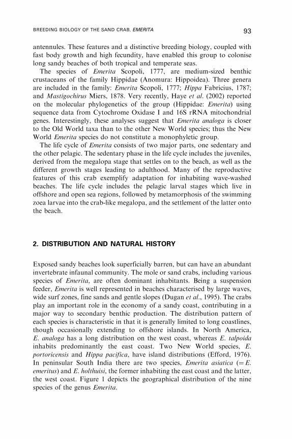
antennules. These features and a distinctive breeding biology, coupled with

fast body growth and high fecundity, have enabled this group to colonise

long sandy beaches of both tropical and temperate seas.

The species of Emerita Scopoli, 1777, are medium-sized benthic

crustaceans of the family Hippidae (Anomura: Hippoidea). Three genera

are included in the family: Emerita Scopoli, 1777; Hippa Fabricius, 1787;

and Mastigochirus Miers, 1878. Very recently, Haye et al. (2002) reported

on the molecular phylogenetics of the group (Hippidae: Emerita) using

sequence data from Cytochrome Oxidase I and 16S rRNA mitochondrial

genes. Interestingly, these analyses suggest that Emerita analoga is closer

to the Old World taxa than to the other New World species; thus the New

World Emerita species do not constitute a monophyletic group.

The life cycle of Emerita consists of two major parts, one sedentary and

the other pelagic. The sedentary phase in the life cycle includes the juveniles,

derived from the megalopa stage that settles on to the beach, as well as the

different growth stages leading to adulthood. Many of the reproductive

features of this crab exemplify adaptation for inhabiting wave-washed

beaches. The life cycle includes the pelagic larval stages which live in

offshore and open sea regions, followed by metamorphosis of the swimming

zoea larvae into the crab-like megalopa, and the settlement of the latter onto

the beach.

2. DISTRIBUTION AND NATURAL HISTORY

Exposed sandy beaches look superficially barren, but can have an abundant

invertebrate infaunal community. The mole or sand crabs, including various

species of Emerita, are often dominant inhabitants. Being a suspension

feeder, Emerita is well represented in beaches characterised by large waves,

wide surf zones, fine sands and gentle slopes (Dugan et al., 1995). The crabs

play an important role in the economy of a sandy coast, contributing in a

major way to secondary benthic production. The distribution pattern of

each species is characteristic in that it is generally limited to long coastlines,

though occasionally extending to offshore islands. In North America,

E. analoga has a long distribution on the west coast, whereas E. talpoida

inhabits predominantly the east coast. Two New World species, E.

portoricensis and Hippa pacifica, have island distributions (Efford, 1976).

In peninsular South India there are two species, Emerita asiatica (¼E.

emeritus) and E. holthuisi, the former inhabiting the east coast and the latter,

the west coast. Figure 1 depicts the geographical distribution of the nine

species of the genus Emerita.

BREEDING BIOLOGY OF THE SAND CRAB, EMERITA 93

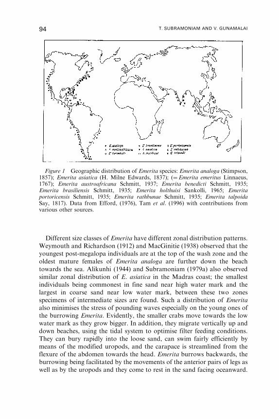
Different size classes of Emerita have different zonal distribution patterns.

Weymouth and Richardson (1912) and MacGinitie (1938) observed that the

youngest post-megalopa individuals are at the top of the wash zone and the

oldest mature females of Emerita analoga are further down the beach

towards the sea. Alikunhi (1944) and Subramoniam (1979a) also observed

similar zonal distribution of E. asiatica in the Madras coast; the smallest

individuals being commonest in fine sand near high water mark and the

largest in coarse sand near low water mark, between these two zones

specimens of intermediate sizes are found. Such a distribution of Emerita

also minimises the stress of pounding waves especially on the young ones of

the burrowing Emerita. Evidently, the smaller crabs move towards the low

water mark as they grow bigger. In addition, they migrate vertically up and

down beaches, using the tidal system to optimise filter feeding conditions.

They can bury rapidly into the loose sand, can swim fairly efficiently by

means of the modified uropods, and the carapace is streamlined from the

flexure of the abdomen towards the head. Emerita burrows backwards, the

burrowing being facilitated by the movements of the anterior pairs of legs as

well as by the uropods and they come to rest in the sand facing oceanward.

Figure 1 Geographic distribution of Emerita species: Emerita analoga (Stimpson,1857); Emerita asiatica (H. Milne Edwards, 1837); (¼Emerita emeritus Linnaeus,1767); Emerita austroafricana Schmitt, 1937; Emerita benedicti Schmitt, 1935;Emerita brasiliensis Schmitt, 1935; Emerita holthuisi Sankolli, 1965; Emeritaportoricensis Schmitt, 1935; Emerita rathbunae Schmitt, 1935; Emerita talpoidaSay, 1817). Data from Efford, (1976), Tam et al. (1996) with contributions fromvarious other sources.


The filter-feeding behaviour of Emerita is unique among arthropods

(Weymouth and Richardson, 1912). Snodgrass (1952) described the

anatomical modifications of the antennae in E. talpoida for filter feeding.

They are feather-like structures with four rows of diverging setae, armed

with inwardly directed secondary setae. When they unfold, the water passing

over the animal from behind is filtered through the fine mesh of the setae.

The mandibles of Emerita are much reduced structures. Zobell and Feltham

(1938) suggested that sand crabs fed by ingesting sand and digesting the

organic material including the bacteria mixed with it. However, detailed

studies by Efford (1966) confirmed antennal filter feeding and comparisons

were made with filter feeding by barnacles.

3. SEX RATIO AND SIZE AT SEXUAL MATURITY

Wenner (1972) proposed a size-related sex ratio for crustaceans and

classified the male–female size relationships into four patterns. These are (1)

standard (male–female ratios equal), (2) reverse (smaller individuals are all

males and the larger ones, all females or vice versa), (3) intermediate (sex-

ratios are intermediate between standard and reverse patterns and (4)

anomalous (male–female overlap in a narrow size range). The anomalous

pattern may also arise from factors such as differential growth rate and

mortality as well as migration. In E. analoga, sex ratios based on size classes

fit well in the anomalous pattern. Barnes and Wenner (1968) suggested that

this close overlap between males and females, especially in the mid-size

classes, could be interpreted as protandric hermaphroditism, by which the

males change sex to females. However, Diaz (1981), from a population

analysis of E. talpoida in the north Carolina beaches, concluded that sex

ratio, calculated on the basis of the relative frequency of females in the

population, fluctuated with season as well as recruitment pulses of the

megalopa stage.

For the tropical species E. asiatica, Subramoniam (1977b) calculated the

size-related sex ratio, following the method of Wenner (1972). As seen from

Figure 2 the overlap in size range between males and mature females is too

wide to suggest a possible sex reversal in this species. Whereas the increased

percentage of small size-group males indicates differential body growth of

males and females, the declining percentage of males above 8mm carapace

length (CL) might be due to their death, as reported for the American

species E. analoga (Efford, 1967). Further, the observation that males with

distinct genital papillae and juvenile females devoid of genital papillae are

found in almost equal proportions among the post-larval stages during

settlement in the beach indicates that males and females develop


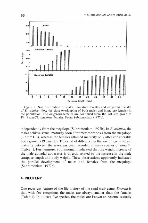
independently from the megalopa (Subramoniam, 1977b). In E. asiatica, the

males achieve sexual maturity soon after metamorphosis from the megalopa

(3.5mmCL), whereas the females attained maturity only after considerable

body growth (19mmCL). This kind of difference in the size or age at sexual

maturity between the sexes has been recorded in many species of Emerita

(Table 1). Furthermore, Subramoniam indicated that the weight increase of

the male gonadal apparatus is directly related to the increase in the male

carapace length and body weight. These observations apparently indicated

the parallel development of males and females from the megalopa

(Subramoniam, 1977b).

4. NEOTENY

One recurrent feature of the life history of the sand crab genus Emerita is

that with few exceptions the males are always smaller than the females

(Table 1). In at least five species, the males are known to become sexually

Figure 2 Size distribution of males, immature females and ovigerous femalesof E. asiatica. Note the close overlapping of both males and immature females inthe population. The ovigerous females are continued from the last size group of18–19mmCL immature females. From Subramoniam (1977b).


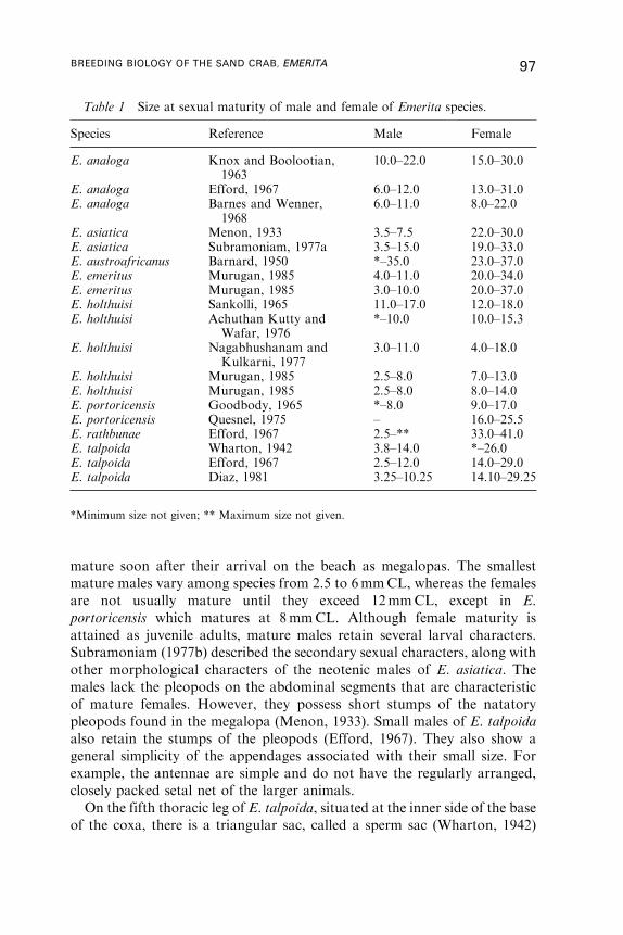
mature soon after their arrival on the beach as megalopas. The smallest

mature males vary among species from 2.5 to 6mmCL, whereas the females

are not usually mature until they exceed 12mmCL, except in E.

portoricensis which matures at 8mmCL. Although female maturity is

attained as juvenile adults, mature males retain several larval characters.

Subramoniam (1977b) described the secondary sexual characters, along with

other morphological characters of the neotenic males of E. asiatica. The

males lack the pleopods on the abdominal segments that are characteristic

of mature females. However, they possess short stumps of the natatory

pleopods found in the megalopa (Menon, 1933). Small males of E. talpoida

also retain the stumps of the pleopods (Efford, 1967). They also show a

general simplicity of the appendages associated with their small size. For

example, the antennae are simple and do not have the regularly arranged,

closely packed setal net of the larger animals.

On the fifth thoracic leg of E. talpoida, situated at the inner side of the base

of the coxa, there is a triangular sac, called a sperm sac (Wharton, 1942)

Table 1 Size at sexual maturity of male and female of Emerita species.

Species Reference Male Female

E. analoga Knox and Boolootian,1963

10.0–22.0 15.0–30.0

E. analoga Efford, 1967 6.0–12.0 13.0–31.0E. analoga Barnes and Wenner,

19686.0–11.0 8.0–22.0

E. asiatica Menon, 1933 3.5–7.5 22.0–30.0E. asiatica Subramoniam, 1977a 3.5–15.0 19.0–33.0E. austroafricanus Barnard, 1950 *–35.0 23.0–37.0E. emeritus Murugan, 1985 4.0–11.0 20.0–34.0E. emeritus Murugan, 1985 3.0–10.0 20.0–37.0E. holthuisi Sankolli, 1965 11.0–17.0 12.0–18.0E. holthuisi Achuthan Kutty and

Wafar, 1976*–10.0 10.0–15.3

E. holthuisi Nagabhushanam andKulkarni, 1977

3.0–11.0 4.0–18.0

E. holthuisi Murugan, 1985 2.5–8.0 7.0–13.0E. holthuisi Murugan, 1985 2.5–8.0 8.0–14.0E. portoricensis Goodbody, 1965 *–8.0 9.0–17.0E. portoricensis Quesnel, 1975 – 16.0–25.5E. rathbunae Efford, 1967 2.5–** 33.0–41.0E. talpoida Wharton, 1942 3.8–14.0 *–26.0E. talpoida Efford, 1967 2.5–12.0 14.0–29.0E. talpoida Diaz, 1981 3.25–10.25 14.10–29.25

*Minimum size not given; ** Maximum size not given.


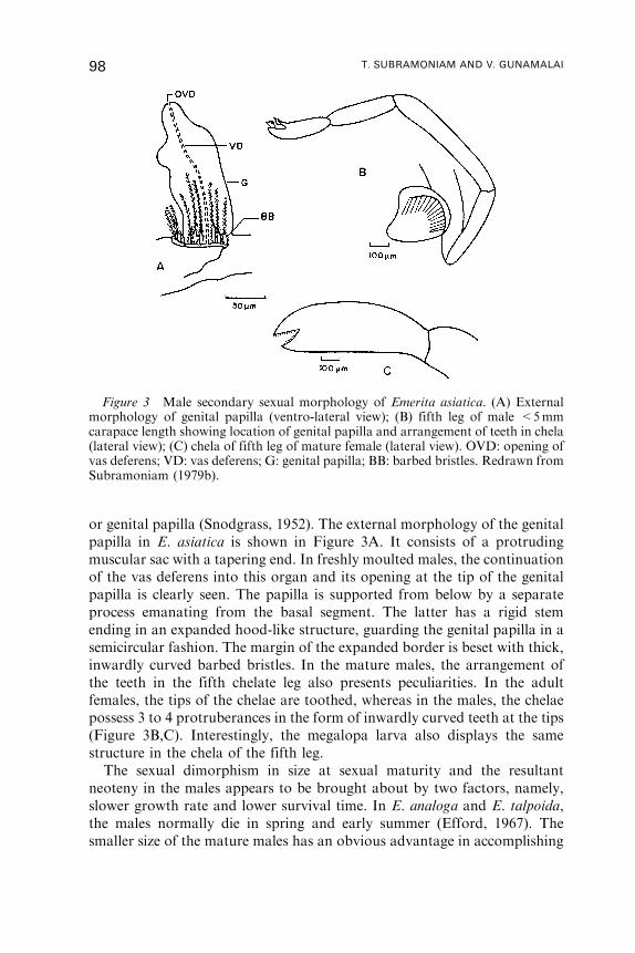
or genital papilla (Snodgrass, 1952). The external morphology of the genital

papilla in E. asiatica is shown in Figure 3A. It consists of a protruding

muscular sac with a tapering end. In freshly moulted males, the continuation

of the vas deferens into this organ and its opening at the tip of the genital

papilla is clearly seen. The papilla is supported from below by a separate

process emanating from the basal segment. The latter has a rigid stem

ending in an expanded hood-like structure, guarding the genital papilla in a

semicircular fashion. The margin of the expanded border is beset with thick,

inwardly curved barbed bristles. In the mature males, the arrangement of

the teeth in the fifth chelate leg also presents peculiarities. In the adult

females, the tips of the chelae are toothed, whereas in the males, the chelae

possess 3 to 4 protruberances in the form of inwardly curved teeth at the tips

(Figure 3B,C). Interestingly, the megalopa larva also displays the same

structure in the chela of the fifth leg.

The sexual dimorphism in size at sexual maturity and the resultant

neoteny in the males appears to be brought about by two factors, namely,

slower growth rate and lower survival time. In E. analoga and E. talpoida,

the males normally die in spring and early summer (Efford, 1967). The

smaller size of the mature males has an obvious advantage in accomplishing

Figure 3 Male secondary sexual morphology of Emerita asiatica. (A) Externalmorphology of genital papilla (ventro-lateral view); (B) fifth leg of male <5mmcarapace length showing location of genital papilla and arrangement of teeth in chela(lateral view); (C) chela of fifth leg of mature female (lateral view). OVD: opening ofvas deferens; VD: vas deferens; G: genital papilla; BB: barbed bristles. Redrawn fromSubramoniam (1979b).


mating with larger females in a turbulent marine environment such as the

intertidal region (see below). Efford (1970) considered the generalisation

that neoteny in the male is characteristic of Emerita, after examining several

sources of published information. De Beer (1951) defined neoteny as

precocious sexual maturity in which there is a relative retardation of body

growth compared with the reproductive growth and maturation.

5. PROTANDRIC HERMAPHRODITISM IN E. ASIATICA

The problem of sex reversal in the sand crab Emerita is a story in itself. The

occurrence of neoteny in several species of Emerita and the fact that the

males die before reaching the size at which the females become sexually

mature, result in considerable deviation from the 1 : 1 sex ratio. By applying

a size-related sex ratio method, Barnes and Wenner (1968) found a sigmoid

curve, characteristic of protandry in other crustaceans such as the deep sea

prawns (Yaldwyn, 1966), and proposed for the first time a sex reversal

hypothesis for E. analoga. In support, Eickstaedt, (1969) and Knapp and

Wenner (as reported in Barnes and Wenner, 1968) postulated that some

males, kept under laboratory conditions, changed sex. However, a series of

laboratory culture experiments as well as natural environment observations

on E. analoga (Auyong, 1981; Wenner and Haley, 1981; Conan et al., 1975),

E. asiatica (Subramoniam, 1977b), E. talpoida (Diaz, 1981), E. portoricensis

(Sastre, 1991) and an Island species, Hippa pacifica (Haley, 1979) suggest

that the apparent anomaly in the sex ratio results only from the differential

growth of males and females. Wenner and Haley (1981) summarised the

arguments in favour of and against the sex reversal hypothesis for the hippid

mole crabs, basing them mainly on population and sex ratio studies and

laboratory experiments on differential growth and moult increments of

males and females in different size groups. In all the above studies, there was

no direct observation of the male gonads during the period when they might

change to females, and hence the possibility of sex-reversal in Emerita

species was at that time not resolved.

Unequivocal existence of functional protandric hermaphroditism was

demonstrated in E. asiatica by Subramoniam (1979c, 1981). The main

reproductive events enumerated in the Figure 4 indicate that neotenous

males continue to grow after serving an active normal male life, deviate

from normal sexual behaviour, gradually lose their secondary and primary

sexual characters, and undergo sex reversal by acquiring female characters

around 19mmCL. The disappearance of genital papillae around 15mmCL,

is the first visible sign of sex reversal. Concurrently, spermatogonial

activity in testes ceases but hyperactivity of the mesodermic cells ensues


(Figure 5A). Such hyperactivity of the mesodermal cells in the testis during

periods of sexual inactivity has also been shown in the crayfish Pontastacus

leptodactylus leptodactylus (Amato and Payen, 1978). In the size range of

19–22mmCL, these males possess a gonad comprising inactive testicular

and active ovarian portions. The ovarian anlagen spread along the mid-

dorsal line of the paired testis. During sex reversal, following the formation

of separate ovarian anlagen, the ovarian structure contains typical follicle

cells that have either migrated from the testicular region or differentiated

from a prefollicular mesodermic tissue of the gonad (Figure 5B). These cells

attach themselves to the vitellogenic oocytes, probably mediating uptake of

yolk proteins from the haemolymph (Charniaux-Cotton, 1975b). The newly

Figure 4 Chronology of sexualisation in female and male Emerita asiatica. FromSubramoniam (1981). A.G.¼ androgeni gland.


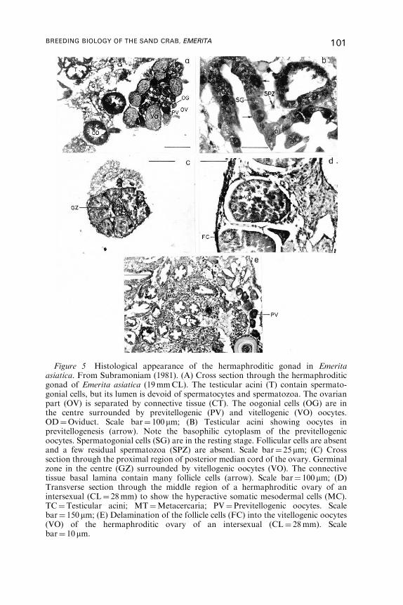
Figure 5 Histological appearance of the hermaphroditic gonad in Emeritaasiatica. From Subramoniam (1981). (A) Cross section through the hermaphroditicgonad of Emerita asiatica (19mmCL). The testicular acini (T) contain spermato-gonial cells, but its lumen is devoid of spermatocytes and spermatozoa. The ovarianpart (OV) is separated by connective tissue (CT). The oogonial cells (OG) are inthe centre surrounded by previtellogenic (PV) and vitellogenic (VO) oocytes.OD¼Oviduct. Scale bar¼ 100mm; (B) Testicular acini showing oocytes inprevitellogenesis (arrow). Note the basophilic cytoplasm of the previtellogenicoocytes. Spermatogonial cells (SG) are in the resting stage. Follicular cells are absentand a few residual spermatozoa (SPZ) are absent. Scale bar¼ 25mm; (C) Crosssection through the proximal region of posterior median cord of the ovary. Germinalzone in the centre (GZ) surrounded by vitellogenic oocytes (VO). The connectivetissue basal lamina contain many follicle cells (arrow). Scale bar¼ 100mm; (D)Transverse section through the middle region of a hermaphroditic ovary of anintersexual (CL¼ 28mm) to show the hyperactive somatic mesodermal cells (MC).TC¼Testicular acini; MT¼Metacercaria; PV¼Previtellogenic oocytes. Scalebar¼ 150mm; (E) Delamination of the follicle cells (FC) into the vitellogenic oocytes(VO) of the hermaphroditic ovary of an intersexual (CL¼ 28mm). Scalebar¼ 10mm.


formed median limb beyond the fused posterior extremity of the testis,

however, lacks testicular elements (Figure 5C). It is composed of a central

germarium surrounded by previtellogenic and vitellogenic oocytes. The vas

deferens in these intersexuals is intact but its opening is occluded. They also

begin to possess three pairs of pleopods and a pair of functional oviducts

formed at the base of the coxae of the third walking legs. The external

morphology of the reproductive system in the intersexual animals as

compared with the testis and ovary of the normal crabs is depicted in Figure

6. These intersexuals with a functional ovary could be easily identified by the

possession of only a few eggs on the pleopods.

The malacostracan crustaceans are generally gonochoristic with geneti-

cally determined sex. The genes for male morphogenesis act in the presence

of an androgenic hormone and for females in its absence (Charniaux-

Cotton, 1960). Sex reversal via protandric hermaphroditism has also been

reported in other crustaceans (Ghiselin, 1969; Policansky, 1982). Inversion

of sexual phenotype is influenced by epigamous factors exerted during

growth (Gallien, 1959). In malacostracan crustaceans, the hermaphroditic

potentialities are governed by the androgenic gland hormone (Charniaux-

Cotton, 1965a). The sequential disappearance of primary and secondary

male characters during the changeover phase of E. asiatica reported above,

and the concomitant assumption of female characters strongly suggest

Figure 6 Diagrammatic representation of the testis, ovary and the hermaphro-ditic ovary of Emerita asiatica. t-testis; a.v.d.-anterior vas deferens; m.v.d.-mid vasdeferens; p.v.d.-posterior vas deferens; a.l.o.-anterior ovarian lobe; m.l.o.-middleovarian lobe; o.d.-oviduct; p.m.l.o.-posterior median ovarian limb; o-ovary; v.d.-vasdeferens. Redrawn from Subramoniam (1981).


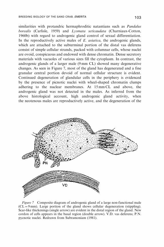
similarities with protandric hermaphroditic natantians such as Pandalus

borealis (Carlisle, 1959) and Lysmata seticaudata (Charniaux-Cotton,

1960b) with regard to androgenic gland control of sexual differentiation.

In the reproductively active males of E. asiatica, the androgenic glands,

which are attached to the subterminal portion of the distal vas deferens

consist of simple cellular strands, packed with columnar cells, whose nuclei

are ovoid, conspicuous and endowed with dense chromatin. Dense secretory

materials with vacuoles of various sizes fill the cytoplasm. In contrast, the

androgenic glands of a larger male (9mm CL) showed many degenerative

changes. As seen in Figure 7, most of the gland has degenerated and a fine

granular central portion devoid of normal cellular structure is evident.

Continued degeneration of glandular cells in the periphery is evidenced

by the presence of picnotic nuclei with wheel-shaped chromatin clumps

adhering to the nuclear membranes. At 15mmCL and above, the

androgenic gland was not detected in the males. As inferred from the

above histological account, high androgenic gland activity, when

the neotenous males are reproductively active, and the degeneration of the

Figure 7 Composite diagram of androgenic gland of a large non-functional male(CL¼ 9mm). Large portion of the gland shows cellular degeneration (stippling).Scar-like thickenings (single arrow) are evident in the distal region of the gland. Newcordon of cells appears in the basal region (double arrow). V.D. vas deferens; P.N.pycnotic nuclei. Redrawn from Subramoniam (1981).


androgenic gland during the gradual disappearance of male secondary

sexual characters and stoppage of spermatogonial activity in large males,

clearly suggest that a fall in circulating androgenic gland hormone may be

responsible for these changes in E. asiatica. Extirpation and grafting

experiments on the androgenic gland in Lysmata seticaudata have yielded

similar results (Charniaux-Cotton, 1959; Berrear-Bonnentant, 1963).

From a series of experimental studies on the hermaphroditic prawn

L. seticaudata, Touir (1977a, b, c) suggested a bihormonal control over the

androgenic gland as well as the gonadal activity from the brain

neurosecretory factors. Interestingly, Subramoniam (1981) also came

across instances of incomplete transformation of sex, as found in large

females of E. asiatica (28, 29mmCL). In these crabs, histological

examination indicates that a separate ovarian portion is never found

above the non-functional testis. However, the anterior half of the paired

tubular gonad is dominated by oocytic differentiation, whereas the posterior

half possessed inactive testicular tissues (Figure 5E). The mature oocytes in

the anterior portion undergo oosorption, accomplished by the infiltrating

follicle cells, which on entry into the ooplasm, turn phagocytic (Figure 5D).

Interestingly, these intersexuals retain the vas deferens, but the genital

papilla is absent. Paired oviducts are also present, but are incompletely

differentiated, compared to the functional oviduct of the secondary females

arising from successful sex reversal of E. asiatica. The bihormonal control

of brain neurosecretory factors over sex reversal, as suggested by Touir

(Touir, 1977a,b,c) for L. seticaudata may also explain the incomplete

gonadal transformation in E. asiatica (see Subramoniam, 1981, for

discussion).

Protandric hermaphroditism in E. asiatica is significant and points to the

high probability of sex reversal in other species of Emerita in which the

males attain precocious sexual maturity in the post-larval stage.

6. MATING HABITS

Mating behaviour has been described in many species of Emerita.

MacGinitie (1938) detailed the mating habits of E. analoga from both

field and laboratory observations. He found mating to occur mostly in late

spring or early summer. Males apparently gather around the egg-laying

females as much as two to five days before coupling and remain in contact

with the female. The males attach to the female by the dactyls of their fourth

legs, which according to MacGinitie (1938) are equipped with a sort of

sucker pad surrounded by stiff hairs. As the female burrows in the sand, the

males collect on her ventral side and remain there until they deposit their


sticky spermatophores. This author also observed that spermatophore

deposition occurred on the just-moulted females. He also reported a

laboratory observation that the soft-shelled female was found to lie on top

of the sand with its abdomen unflexed, while two to four males deposit

sperm on the ventral surface in the cervix between the third and fourth pairs

of legs. An interesting observation by the same author was that the males

were more commonly found in the upper part of the surf zone; but during

the mating season (late spring and early summer) they occurred with the

female lower down on the beach.

The behaviour of the males in the ventral region of the females has also

been reported for other species of Emerita. According to Wharton (1942),

the small males were found in the gill chambers, clamped between the coxae

of the thoracic appendages, or attached to egg masses, and some even

seemed to roam about on the ventral surface of the larger females. The

relationship between the clinging males and the female is such that some

males were found to moult whilst associated with the females, as recorded in

E. asiatica (Menon, 1933). This kind of mating behaviour in the Emerita

species has been termed ‘‘incipient parasitism’’ by Wharton (1942).

In the temperate species, the occurrence of the males has been reported

to be seasonal, limiting the mating season to late spring and early summer,

as in E. analoga (Efford, 1967); however, in the tropical species where

the reproduction and embryonic development in the pleopods go on

uninterruptedly throughout the year, small functional males in the size

range of 3.75 and 5mmCL, occur throughout the year (Subramoniam,

1977b). This observation is at variance with an earlier finding on E. asiatica,

from another location on the east coast of peninsular India, viz.,

Visakapatnam, that males occur only during the summer months

(Ganapathi and Lakshmana Rao, 1959). From the Madras coast on the

east coast of India, Subramoniam (1977b) has not only observed the year

round occurrence of small functional males, but also observed the continued

growth of the males to a larger size of up to 11mm CL. However, these

larger males have not been found to take part in mating with larger egg-

laying females, although they possessed well-developed spermatophores

in the swollen vas deferens. This author suggested that the sexually active

smaller males, once metamorphosed from the megalopa, not only attain

precocious sexual maturity without body growth, but also undergo a certain

degree of growth regression during subsequent moults. Understandably,

since these males are inside the burrow, clinging on to the females, they have

no chance of active feeding by antennal filtering, thus resulting in

considerable growth retardation. Furthermore, the smaller size is advanta-

geous for their hide out on the ventral region of the burrowing females.

More importantly, the females accept these smaller males, rather than the

bigger males, for mating since they will not disturb normal activities such as


burrowing and reburrowing when the tides are in and out, as well as filter

feeding. Again, mating between equally sized partners would be a

cumbersome process in the intertidal region, as the larger males clinging

onto females could be brushed off by waves, or by sand when the female

burrows. Coupled with aggregation behaviour (Efford, 1965; Cubit, 1969),

the neotenous male of Emerita species has probably evolved as a means to

increase the chance of fertilisation in the unstable habitat.

The occurrence of large non-functional but sexually mature males in the

population of E. asiaticamerits further comments on their sexual behaviour.

The size-increase of non-functional large males suggests that the specialisa-

tion towards neoteny in this species is still incomplete (Subramoniam,

1977b). A peculiar mating behaviour of these larger males has also been

reported by Subramoniam (1979b). A male of 8.5mm CL was observed to

deposit a spermatophore ribbon on the ventral side of a freshly moulted

immature female. Deposition of spermatophores by larger males on

immature, helpless freshly moulted females indicates indiscriminate copula-

tion, amounting to raping, in E. asiatica. Incidentally, Kittredge et al. (1971)

provided some experimental evidence for sex pheromonal activity of the

moulting hormone, crustecdysone, in a number of decapods. Whether such

pheromonal attraction to the moulting females could trigger spermato-

phoral deposition by males on the freshly moulted female E. asiatica

is conjectural and needs experimental support.

7. SPERMATOPHORES AND SPERM TRANSFER

One of the significant reproductive attributes of Emerita in the successful

colonisation of the sandy beach is the mode of sperm transfer and the

epizoic fertilisation of the eggs deposited externally on the pleopodal hairs.

As with most marine crustaceans, excepting the free-spawning penaeid

shrimps, spermatophore production in sand crabs is a specialisation to

transfer semen in the marine environment (Subramoniam, 1993). Emerita

lacks an intromittent organ and hence spermatophores can be considered to

be the alternative vehicle to transfer sperm. As in other decapod

crustaceans, the spermatozoa of Emerita are not motile. Hence, the

production of complex spermatophores is imperative for effective sperm

transfer by the neotenous male.

7.1. Morphology of spermatophores

Early workers on E. talpoida and E. analoga reported deposition of a sperma-

tophoric ribbon on the ventral sternum of the females (MacGinitie, 1938;


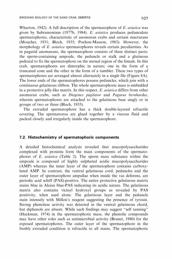
Wharton, 1942). A full description of the spermatophore of E. asiatica was

given by Subramoniam (1977b, 1984). E. asiatica produces pedunculate

spermatophores, characteristic of anomuran crabs and certain macrurans

(Mouchet, 1931; Bloch, 1935; Pochon-Masson, 1983). However, the

morphology of E. asiatica spermatophores reveals certain peculiarities. As

in pagurid anomurans, the spermatophore consists of three distinct parts:

the sperm-containing ampoule, the peduncle or stalk and a glutinous

pedestal to fix the spermatophore on the sternal region of the female. In this

crab, spermatophores are dimorphic in nature; one in the form of a

truncated cone and the other in the form of a tumbler. These two types of

spermatophores are arranged almost alternately in a single file (Figure 8A).

The lower ends of the spermatophores possess peduncles, which join with a

continuous gelatinous ribbon. The whole spermatophoric mass is embedded

in a protective jelly-like matrix. In this respect, E. asiatica differs from other

anomuran crabs, such as Diogenes pugilator and Pagurus bernhardus,

wherein spermatophores are attached to the gelatinous base singly or in

groups of two or three (Bloch, 1935).

The extruded spermatophore has a thick double-layered refractile

covering. The spermatozoa are glued together by a viscous fluid and

packed closely and irregularly inside the spermatophore.

7.2. Histochemistry of spermatophoric components

A detailed histochemical analysis revealed that mucopolysaccharides

complexed with proteins form the main components of the spermato-

phores of E. asiatica (Table 2). The sperm mass substance within the

ampoule is composed of highly sulphated acidic mucopolysaccharides

(AMP) whereas the inner layer of the spermatophore contains carboxy-

lated AMP. In contrast, the ventral gelatinous cord, peduncles and the

outer layer of spermatophore ampullae when inside the vas deferens, are

periodic acid schiff (PAS)-positive. The entire protective gelatinous matrix

stains blue in Alcian blue-PAS indicating its acidic nature. The gelatinous

matrix also contains vicinyl hydroxyl groups as revealed by PAS

positivity, when used alone. The gelatinous layer and the peduncle

stain intensely with Millon’s reagent suggesting the presence of tyrosin.

Strong phenolase activity was detected in the ventral gelatinous chord,

but diphenols are absent. While such findings may suggest ‘‘self tanning’’

(Hackman, 1974) in the spermatophoric mass, the phenolic compounds

may have other roles such as antimicrobial activity (Brunet, 1980) for the

exposed spermatophores. The outer layer of the spermatophore in the

freshly extruded condition is refractile to all stains. The spermatophoric


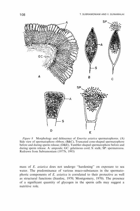
mass of E. asiatica does not undergo ‘‘hardening’’ on exposure to sea

water. The predominance of various muco-substances in the spermato-

phoric components of E. asiatica is correlated to their protective as well

as structural functions (Jeanloc, 1970; Montgomery, 1970). The presence

of a significant quantity of glycogen in the sperm cells may suggest a

nutritive role.

Figure 8 Morphology and dehiscence of Emerita asiatica spermatophores. (A)Side view of spermatophore ribbon; (B&C), Truncated cone-shaped spermatophorebefore and during sperm release; (D&E), Tumbler-shaped spermatophore before andduring sperm release. A: ampoule; GC: gelatinous cord; S: stalk; SP: spermatozoa.Redrawn from Subramoniam (1977b, 1993)


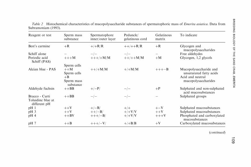
Table 2 Histochemical characteristics of mucopolysaccharide substances of spermatophoric mass of Emerita asiatica. Data fromSubramoniam (1993).

Reagent or test Sperm masssubstance

Spermatophoreinner/outer layer

Peduncle/gelatinous cord

Gelatinousmatrix

To indicate

Best’s carmine þR þ/þR/R þþ/þþR/R þR Glycogen andmucopolysaccharides

Schiff alone � �/� �/� � Free aldehydesPeriodic acidSchiff (PAS)

þþþM þþþ/þM/M þþ/þþM/M þM Glycogen, 1,2 glycols

Sperm cellsAlcian blue - PAS þþM þþ/þM/M þ/þM/M þþþ�B Mucopolysaccharide and

Sperm cells unsaturated fatty acidsþB Acid and neutralSperm masssubstance

mucopolysaccharides

Aldehyde fuchsin þþBB þ/�P/ �/� þP Sulphated and non-sulphatedacid mucosubstances

Bracco - Curti þþBB �/� �/� � Sulphated groupsToluidine blue atdifferent pH

pH 1 þþV þ/�B/ þ/þ þ�V Sulphated mucosubstancespH 3 þþV þþ/�B/ þ/þV/V þþV Sulphated mucosubstancespH 4 þþBV þþþ/�B/ þ/þV/V þþþV Phosphated and carboxylated

mucosubstancespH 7 þþB þþþ/�V/ þ/þB/B þV Carboxylated mucosubstances

(continued)

BREEDIN

GBIO

LOGYOFTHESAND

CRAB,EMERITA

109

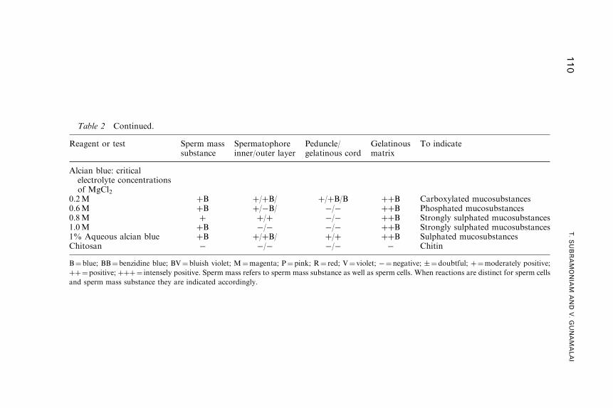
Table 2 Continued.

Reagent or test Sperm masssubstance

Spermatophoreinner/outer layer

Peduncle/gelatinous cord

Gelatinousmatrix

To indicate

Alcian blue: criticalelectrolyte concentrationsof MgCl2

0.2M þB þ/þB/ þ/þB/B þþB Carboxylated mucosubstances0.6M þB þ/�B/ �/� þþB Phosphated mucosubstances0.8M þ þ/þ �/� þþB Strongly sulphated mucosubstances1.0M þB �/� �/� þþB Strongly sulphated mucosubstances1% Aqueous alcian blue þB þ/þB/ þ/þ þþB Sulphated mucosubstancesChitosan � �/� �/� � Chitin

B¼blue; BB¼benzidine blue; BV¼bluish violet; M¼magenta; P¼ pink; R¼ red; V¼ violet; �¼ negative; �¼doubtful; þ¼moderately positive;

þþ¼ positive; þþþ¼ intensely positive. Sperm mass refers to sperm mass substance as well as sperm cells. When reactions are distinct for sperm cells

and sperm mass substance they are indicated accordingly.

110

T.SUBRAMONIA

MAND

V.GUNAMALAI

7.3. Origin of spermatophores

The spermatophore originates in the anterior region of the vas deferens. In

the proximal region, the spermatozoa, as released from the testis, are

agglutinated into many clusters, which are enveloped by a gelatinous

membrane emanating from the columnar epithelial cells. The peduncle as

well as the ventral gelatinous cord is secreted from the ventral epithelium of

the distal vas deferens. In the dorsal region of the distal vas deferens the

inner epithelial cells produce a typhlosole-like projection, which secretes a

frothy substance, constituting the protective gelatinous matrix of the

spermatophoric ribbon.

7.4. Spermatophore dehiscence

The mechanism of sperm release from the pedunculate spermatophores

of anomuran crabs is controversial. In E. asiatica, sperm release in

the deposited spermatophores does not occur until egg release from the

oviduct. Spermatophores in different stages of sperm release have

been recovered from the egg masses of freshly ovulated E. asiatica

(Subramoniam, 1977b). Sperm release occurs only through a definite

spermatophore opening. In the truncated cone-like spermatophores,

the opening is made through the nipple-like projection found at the

opposite end of the peduncle (Figure 8B,C). In the other larger type,

the wider region is rimmed by a well-defined lip which is firmly closed

before sperm release. During dehiscence, streaming of spermatozoa was

first observed in the gaps formed at the corners of the wider end and then

in several sites of the centre, resulting in the complete opening of the

lips. After extrusion of all spermatozoa, the lips remain completely apart

(Figure 8D,E). The fact that the spermatozoa release occurs only after

contact with the eggs suggests that an oviductal secretion may be responsible

for the digestion of the cementing material closing the lip of the

spermatophore.

7.5. Adaptive role of spermatophores in sperm transfer

Spermatophore extrusion occurs through the muscular genital papillae

situated at the inner side of the base of the fifth thoracic leg. In E. asiatica,

the spermatophore deposition occurs only in the fresh moult condition and

the sticky nature of the mucoid spermatophoric ribbon enables fast and firm

attachment to the sternum of the females. Further, in E. asiatica, spawning


rapidly follows spermatophore deposition (Subramoniam, 1977b) and hence

spermatophore ribbon remains as a jelly, enabling the dehiscence of

the spermatophores by the oviductal secretion, as mentioned earlier. As the

interim between spermatophore deposition and ovulation is brief, the

spermatophoric ribbon does not undergo hardening, as in the lobster.

Incidentally, mating via spermatophore deposition may also provide a

stimulus for ovulation in Emerita.

The highly adaptive nature of Emerita spermatophores in effecting

epizoic fertilisation in a turbulent environment is also reflected in their

possible evolution from the macruran type of spermatophoric mass. In the

Macrura, the tubular spermatophores are enveloped in several acellular

accessory mucoid secretions which protect the enclosed sperm cells during

their prolonged epizoic storage on the female body (Radha and

Subramoniam, 1985). Although anomuran crabs possess a pedunculate

type of spermatophore, a sand crab species, Albunea symnista, also

belonging to the family Hippidae, and co-existing with E. asiatica in the

sandy beach possesses a macruran type of spermatophoric ribbon

(Subramoniam, 1984). The spermatophoric tube of A. symnista, however,

shows node-like constrictions giving rise to internal discontinuities. Such

a breaking up of a continuous spermatophoric tube by constrictions

(Albunea) and distinct spermatophoric ampullae with drawn-out peduncles

set on a basal filamentous pedestal (Emerita) suggests that these anomuran

sand crabs may be mid-way forms in the evolution of discrete pedunculate

spermatophores of the anomurans from the tubular spermatophores of

Macrura (Subramoniam, 1993).

8. MOULTING PATTERN OF E. ASIATICA—A CASE STUDY

Moulting facilitates continued body growth by periodic shedding of

the old cuticle and secretion of a new cuticle. A characteristic feature,

which is uncommon among other arthropod groups, is the continuation

of moulting even after attaining sexual maturity in many crustacean species.

In general, moulting and reproductive activities are temporally separated

in large-bodied crustaceans such as lobsters and brachyuran crabs.

On the contrary, crustaceans with high fecundity and faster body

growth exhibit closeness in their moulting and reproductive cycles. In

E. asiatica, there exists a close synchronisation between moulting

and the female reproductive cycle (Gunamalai and Subramoniam,

2002). Hence, in order to evaluate the interrelationship between moulting

and reproduction, a detailed delineation of different moult cycle stages is

required.


8.1. Moult cycle stages

The moult cycle stages have been determined in E. asiatica using the criteria

of changes in the cuticular morphology, epidermal retraction and setagenic

events occurring in the pleopod. Furthermore, an aggregation of hemocytes

characteristic of moulting stages was also evaluated throughout the moult

cycle stages in E. asiatica, using microscopic observation on the pleopodal

lumen (Gunamalai and Subramoniam, 2002). Four major stages, namely

postmoult, intermoult, premoult and ecdysis have been distinguished. The

defining features of different moult cycle stages are given in Table 3.

8.1.1. Postmoult (Stages A and B)

Postmoult stage refers to the crab immediately after ecdysis. During this

period, the soft and pliable new cuticle undergoes hardening. The moulted

animal is inactive during this phase, which lasts for 30min; thereafter, it

regains activity and burrows in the sand. The pleopods are soft and

transparent. The setae are thin-walled, and their lumen is wide and

prominent with a granular matrix filling up the space (Figure 9). This stage

is further divided into A1, A2 and B.

8.1.2. Intermoult (Stage C)

As in many malacostracan crustaceans, the intermoult stage is the longest of

all moult cycle stages. The exoskeleton has become progressively hard and

calcified, making further subdivision of this stage difficult. The character-

istic feature of the intermoult stage is that the setal development on the

pleopods has been completed (Figure 9). Nevertheless, the intermoult stage

can be divided into three substages (C1, C2 and C3) based on the hardness as

well as the rigidity of the exoskeleton both on the dorsal and lateral sides.

8.1.3. Premoult (Stage D)

This is the preparatory stage to ecdysis and includes several substages

(D0–D4). This stage starts with apolysis, the retraction of epidermis from the

cuticle, creating a moulting space for the formation of new cuticle. The

epidermal retraction followed by the secretion of new cuticle is easily seen

in the pleopods. Hence, several substages characterising the extent of the

epidermal retraction and the formation of new cuticle within the pleopodal

tip can be examined microscopically. It may be seen from the Figure 9D–I

that a setal groove originates as a deep depression in the retracted epidermis


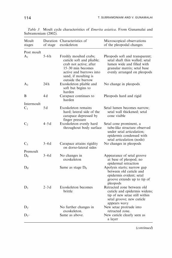
Table 3 Moult cycle characteristics of Emerita asiatica. From Gunamalai andSubramoniam (2002).

Moultstages

Durationof stage

Characteristics ofexoskeleton

Microscopical observationsof the pleopodal changes

Post moultA1 5–6 h Freshly moulted crabs;

cuticle soft and pliable;crab not active; after15–30 min becomesactive and burrows intosand, if moulting isoutside the burrow

Pleopods soft and transparent;setal shaft thin walled; setallumen wide and filled withgranular matrix; setal baseevenly arranged on pleopods

A2 24 h Exoskeleton pliable andsoft but begins toharden

No change in pleopods

B 4 d Carapace continues toharden

Pleopods hard and rigid

IntermoultC1 5 d Exoskeleton remains

hard; lateral side of thecarapace depressed byfinger pressure

Setal lumen becomes narrow;setal wall thickened; setalcone visible

C2 4–5 d Exoskeleton evenly hardthroughout body surface

Setal cone prominent, atube-like structure observedunder setal articulation;epidermis condensed withsetal articulation (node)

C3 3–4 d Carapace attains rigidityon dorso-lateral sides

No changes in pleopods

PremoultD0 3–4 d No changes in

exoskeletonAppearance of setal grooveat base of pleopod; noepidermal retraction

D00 Same as stage D0 Apolysis starts; narrow gapbetween old cuticle andepidermis evident; setalgroove extends up to tip ofpleopods

D1 2–3 d Exoskeleton becomesbrittle

Retracted zone between oldcuticle and epidermis widens;tip of new setae still withinsetal groove; new cuticleappears wavy

D10 No further changes inexoskeleton.

New setae protrude intoretracted zone.

D10 0 Same as above. New cuticle clearly seen asa layer

(continued)


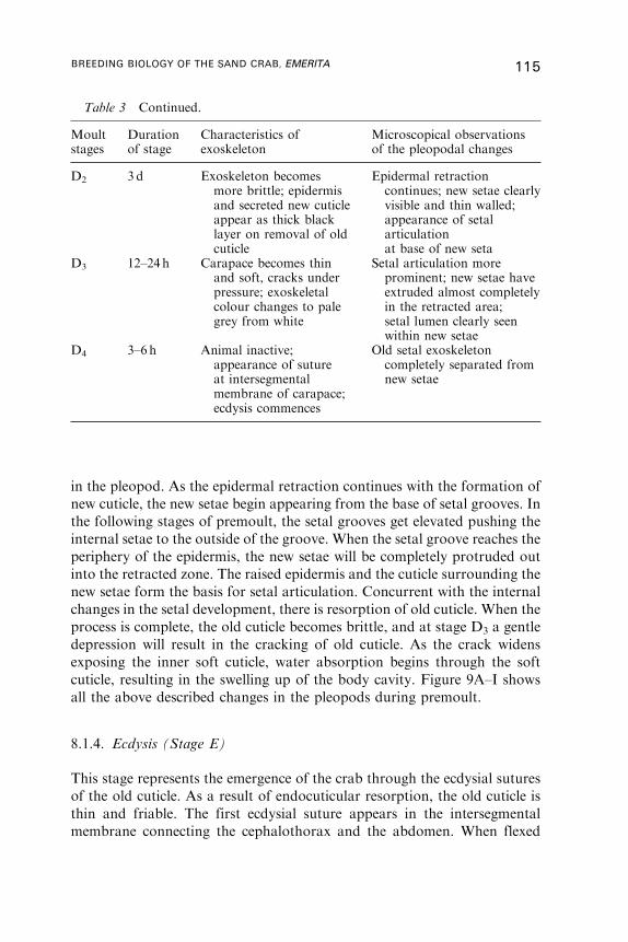
in the pleopod. As the epidermal retraction continues with the formation of

new cuticle, the new setae begin appearing from the base of setal grooves. In

the following stages of premoult, the setal grooves get elevated pushing the

internal setae to the outside of the groove. When the setal groove reaches the

periphery of the epidermis, the new setae will be completely protruded out

into the retracted zone. The raised epidermis and the cuticle surrounding the

new setae form the basis for setal articulation. Concurrent with the internal

changes in the setal development, there is resorption of old cuticle. When the

process is complete, the old cuticle becomes brittle, and at stage D3 a gentle

depression will result in the cracking of old cuticle. As the crack widens

exposing the inner soft cuticle, water absorption begins through the soft

cuticle, resulting in the swelling up of the body cavity. Figure 9A–I shows

all the above described changes in the pleopods during premoult.

8.1.4. Ecdysis (Stage E)

This stage represents the emergence of the crab through the ecdysial sutures

of the old cuticle. As a result of endocuticular resorption, the old cuticle is

thin and friable. The first ecdysial suture appears in the intersegmental

membrane connecting the cephalothorax and the abdomen. When flexed

Table 3 Continued.

Moultstages

Durationof stage

Characteristics ofexoskeleton

Microscopical observationsof the pleopodal changes

D2 3 d Exoskeleton becomesmore brittle; epidermisand secreted new cuticleappear as thick blacklayer on removal of oldcuticle

Epidermal retractioncontinues; new setae clearlyvisible and thin walled;appearance of setalarticulationat base of new seta

D3 12–24 h Carapace becomes thinand soft, cracks underpressure; exoskeletalcolour changes to palegrey from white

Setal articulation moreprominent; new setae haveextruded almost completelyin the retracted area;setal lumen clearly seenwithin new setae

D4 3–6 h Animal inactive;appearance of sutureat intersegmentalmembrane of carapace;ecdysis commences

Old setal exoskeletoncompletely separated fromnew setae


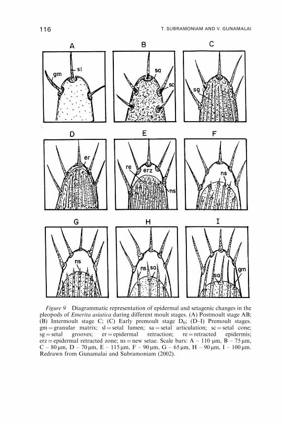
Figure 9 Diagrammatic representation of epidermal and setagenic changes in thepleopods of Emerita asiatica during different moult stages. (A) Postmoult stage AB;(B) Intermoult stage C; (C) Early premoult stage D0; (D–I) Premoult stages.gm¼ granular matrix; sl¼ setal lumen; sa¼ setal articulation; sc¼ setal cone;sg¼ setal grooves; er¼ epidermal retraction; re¼ retracted epidermis;erz¼ epidermal retracted zone; ns¼ new setae. Scale bars: A – 110 mm, B – 75 mm,C – 80 mm, D – 70 mm, E – 115 mm, F – 90mm, G – 65mm, H – 90 mm, I – 100 mm.Redrawn from Gunamalai and Subramoniam (2002).


ventrally the suture ruptures in a transverse direction allowing the animal

to escape. When the crab emerges, the old exoskeleton along with all

appendages is intact. After emergence, the animal remains inactive for about

5–10min. On no occasion was the moulted crab found to consume the

exuvium. The new cuticle continues to expand by water absorption, thereby

increasing the body volume. Figure 10 depicts the sequences in the ecdysis of

E. asiatica.

8.2. Size-related moulting frequency in E. asiatica

Growth in decapod crustaceans is facilitated by periodic moulting. As a

rule, the frequency of moulting is high in the immature animals and, after

the onset of reproduction, it declines considerably in order to facilitate the

reproductive activities which are normally completed within an extended

period of intermoult. In E. asiatica moulting continues even beyond sexual

maturity facilitating simultaneous body growth and reproduction. We

determined the size-related moulting frequency in both immature and

mature females. The results are shown in Figure 11 which clearly

demonstrates differences in the moulting frequency between three major

size classes, namely immature (10–17mmCL), actively reproducing females

(18–22mm CL) and large size females (23–33mmCL). The percentage

occurrence of moulting animals (as represented by premoult) is higher

(52–72%) than that of non-moulting females (intermoult) in the first size

class representing immature females. However, the percentage occurrence of

premoult animals declines (30–40%) from 21mmCL onwards with slight

increase at 22 and 25mmCL. In the actively reproducing females, the

intermoult frequency is considerably higher (40–60%) in between

21–29mmCL. Similarly, the large size group females ranging from

30–33mmCL showed a high frequency of non-moulting females. Thus,

the ratio of moulting and non-moulting forms is always higher in the smaller

size group of females, whereas in the actively reproducing females and large

size females, the percentage of intermoult animals slightly exceeds the

percentage of premoult females (Figure 11).

8.3. Endocrine regulation of moulting

In decapod crustaceans moulting is usually controlled by a bihormonal

system consisting of moulting gland (Y-organ, ecdysteroids) and eyestalk

X-organ/sinus gland complex (moult inhibiting hormone) (Subramoniam,

2000). Whereas the ecdysteroids promote moulting, the neuropeptides from

the eyestalk neurosecretory centres inhibit the synthesis of ecdysteroids by

Y-organ. For Emerita species, although the moulting physiology has been


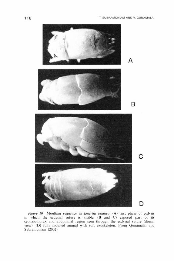
Figure 10 Moulting sequence in Emerita asiatica. (A) first phase of ecdysisin which the ecdysial suture is visible; (B and C) exposed part of itscephalothorax and abdominal region seen through the ecdysial suture (dorsalview); (D) fully moulted animal with soft exoskeleton. From Gunamalai andSubramoniam (2002).


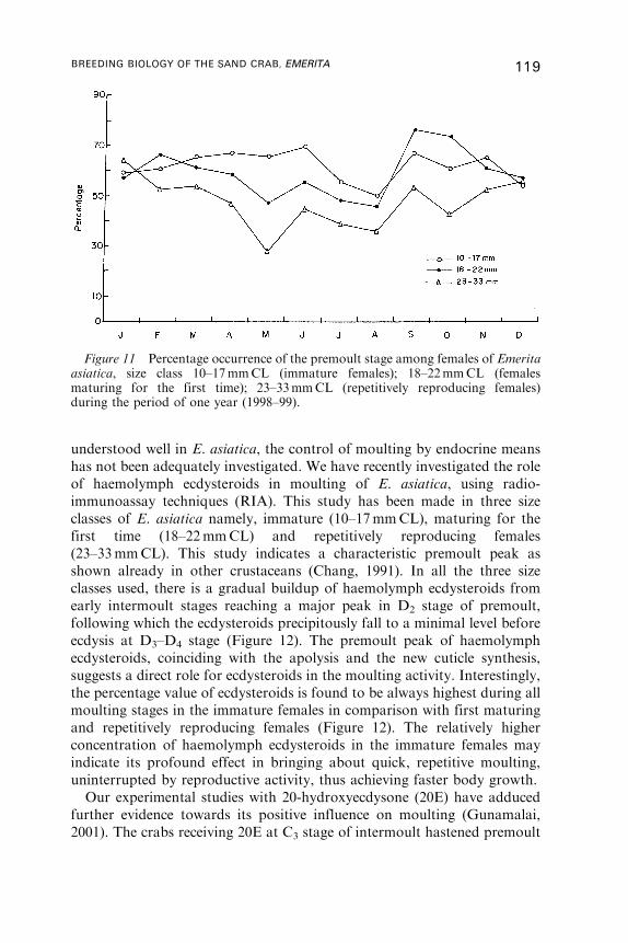
understood well in E. asiatica, the control of moulting by endocrine means

has not been adequately investigated. We have recently investigated the role

of haemolymph ecdysteroids in moulting of E. asiatica, using radio-

immunoassay techniques (RIA). This study has been made in three size

classes of E. asiatica namely, immature (10–17mmCL), maturing for the

first time (18–22mmCL) and repetitively reproducing females

(23–33mmCL). This study indicates a characteristic premoult peak as

shown already in other crustaceans (Chang, 1991). In all the three size

classes used, there is a gradual buildup of haemolymph ecdysteroids from

early intermoult stages reaching a major peak in D2 stage of premoult,

following which the ecdysteroids precipitously fall to a minimal level before

ecdysis at D3–D4 stage (Figure 12). The premoult peak of haemolymph

ecdysteroids, coinciding with the apolysis and the new cuticle synthesis,

suggests a direct role for ecdysteroids in the moulting activity. Interestingly,

the percentage value of ecdysteroids is found to be always highest during all

moulting stages in the immature females in comparison with first maturing

and repetitively reproducing females (Figure 12). The relatively higher

concentration of haemolymph ecdysteroids in the immature females may

indicate its profound effect in bringing about quick, repetitive moulting,

uninterrupted by reproductive activity, thus achieving faster body growth.

Our experimental studies with 20-hydroxyecdysone (20E) have adduced

further evidence towards its positive influence on moulting (Gunamalai,

2001). The crabs receiving 20E at C3 stage of intermoult hastened premoult

Figure 11 Percentage occurrence of the premoult stage among females of Emeritaasiatica, size class 10–17mmCL (immature females); 18–22mmCL (femalesmaturing for the first time); 23–33mmCL (repetitively reproducing females)during the period of one year (1998–99).


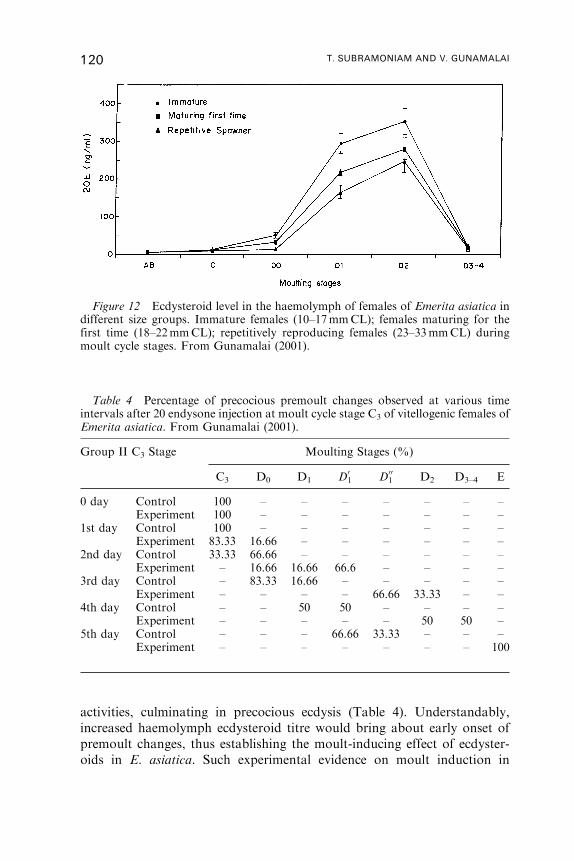
activities, culminating in precocious ecdysis (Table 4). Understandably,

increased haemolymph ecdysteroid titre would bring about early onset of

premoult changes, thus establishing the moult-inducing effect of ecdyster-

oids in E. asiatica. Such experimental evidence on moult induction in

Table 4 Percentage of precocious premoult changes observed at various timeintervals after 20 endysone injection at moult cycle stage C3 of vitellogenic females ofEmerita asiatica. From Gunamalai (2001).

Group II C3 Stage Moulting Stages (%)

C3 D0 D1 D01 D00

1 D2 D3–4 E

0 day Control 100 – – – – – – –Experiment 100 – – – – – – –

1st day Control 100 – – – – – – –Experiment 83.33 16.66 – – – – – –

2nd day Control 33.33 66.66 – – – – – –Experiment – 16.66 16.66 66.6 – – – –

3rd day Control – 83.33 16.66 – – – – –Experiment – – – – 66.66 33.33 – –

4th day Control – – 50 50 – – – –Experiment – – – – – 50 50 –

5th day Control – – – 66.66 33.33 – – –Experiment – – – – – – – 100

Figure 12 Ecdysteroid level in the haemolymph of females of Emerita asiatica indifferent size groups. Immature females (10–17mmCL); females maturing for thefirst time (18–22mmCL); repetitively reproducing females (23–33mmCL) duringmoult cycle stages. From Gunamalai (2001).


E. asiatica is in agreement with earlier results on other decapod crustaceans

such as Homarus americanus (Rao et al., 1973).

Although the role of ecdysteroids in moulting of E. asiatica is well

illustrated in the preceding account, not much is known on the negative

control of moulting by the neurosecretary centres of X-organ/sinus gland

complex. Emerita is a burrowing crab and hence the paired eyestalks are

secondarily reduced. Our unpublished observation indicates the absence of

ganglionic structures such as the medulla externa, medulla interna and

medulla terminalis in the eyestalk of E. asiatica. In the stalk-eyed decapods,

the X-organ, the seat of major neuropeptide synthesis is found in the

medulla terminalis and the neuronal ends of their neurosecretory cells

establish connection with the neurohaemal storage organ, the sinus gland,

found in between the medulla externa and medulla interna (Subramoniam

et al., 1998). In the absence of any neurosecretory centres in the eyestalk

of E. asiatica it is possible that the X-organ/sinus gland complex

is embedded in the brain, as in the isopods, which also lack stalked

eyes (Hanstrom, 1939). Indirect evidence to this effect is provided

by Vasantha (1995) who found that the brain extract of E. asiatica

contained the crustacean hyperglycemic hormone, which forms the principal

neuropeptide (as much as 60% of all eyestalk neuropeptides) (Keller, 1992).

The abbreviation of neurosecretory centres within the eyestalk has

reached an extreme stage in Albunia symnista, another species of

mole crab (family Albunidae) coexisting with E. asiatica in the

Madras Coast. This species is totally blind and hence lacks eyestalks

altogether (personal observation). Understandably, the moult-inhibiting

neuropeptides are produced from the abbreviated X-organ/sinus gland

complex embedded in the brain of E. asiatica and exert their inhibitory

effects on ecdysteroid synthesis in the Y-organ, as in other malacostracan

crustaceans.

8.4. Nutritional control of moulting in Emerita

Despite the fact that moulting is under hormonal control, environment may

also play a significant role in determining the seasonality of moulting

frequency at population level. For marine invertebrates in general,

temperature, photoperiod, salinity and availability of food are known to

exert influence on the vital physiological processes relating to growth and

reproduction (Giese and Pearse, 1974). In Emerita species, the evidence

indicates that abundance of food materials and the accumulation of

nutrients have an influence on the seasonality and intensity of moulting

(Siegel, 1984). As a filter feeder, Emerita might thus depend on the seasonal

abundance of plankton to control the moulting process. While studying the


size-specific moult synchrony in E. analoga on the coast of California, Siegel

(1984) concluded that physical factors such as temperature and lunar phase,

and biological factors like reproductive seasonality or pheromones did not

play any role in maintaining the intensity and synchrony of moulting in this

crab. The moult frequency of the female crabs reared in the tank showed

a peak during June–August; and a corresponding field observation also

indicated high frequency of moulting during these months when food

availability was high. In the same species of Emerita, Eickstaedt (1969)

reported that the intensity of moulting coincided with the period of peak

reproductive activity, suggesting that both reproduction and moulting at

population level are controlled by a common environmental factor such as

availability of food. Siegel (1984) also concluded that egg production did

not affect moult synchrony, under laboratory conditions. In an elegant

experiment of altering feeding regimen, using fresh and plankton-filtered

sea water, he showed that synchronisation and desynchronisation of

moulting could be achieved in the laboratory conditions.

In a recent study on the size-related frequency of moulting in E. asiatica

from the Madras Coast, India, Gunamalai (2001) observed continuous

moulting all through the year. She found that during the months of

September–December (1998–99) the frequency of moulting in all the three

size classes studied was high (see Figure 11). Higher moulting rate during

these months may be explained in terms of meteorological factors, including

upwelling, influencing the availability of phytoplankton nutrients, with an

overall increased production of plankton (Muthu, 1956).

9. REPRODUCTIVE CYCLE

The worldwide distribution of Emerita in tropical and subtropical sandy

beaches has resulted in the acquisition of different reproductive periodicities

for the different species. There are two major types of reproductive cycles;

those inhabiting the tropical beaches show continuous reproductive cycles

and the species occurring in temperate regions have an annual breeding

cycle (Table 5). According to Semper (1881) all reproductive periodicities

ought to be obliterated in tropical marine invertebrates, since in the tropics

annual changes in temperature are minimal. Orton (1920) also supported the

idea that all tropical marine animals breed continuously irrespective of the

seasons. In agreement with Orton’s rule, two tropical species of Emerita, one

from Jamaica (E. portoricensis) and the other from the east coast of India

(E. asiatica) have been shown to breed continuously (Goodbody, 1965;

Subramoniam, 1977a). Conversely, all the temperate species inhabiting the


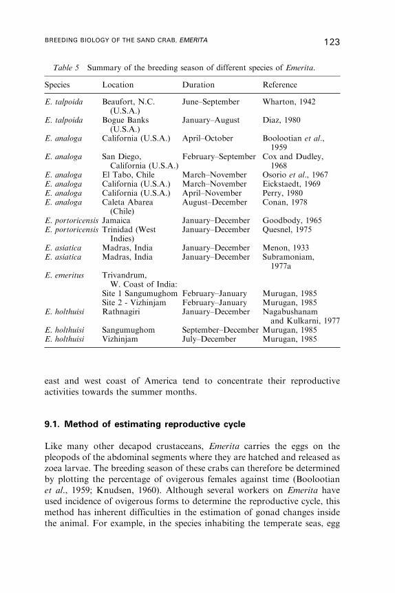
east and west coast of America tend to concentrate their reproductive

activities towards the summer months.

9.1. Method of estimating reproductive cycle

Like many other decapod crustaceans, Emerita carries the eggs on the

pleopods of the abdominal segments where they are hatched and released as

zoea larvae. The breeding season of these crabs can therefore be determined

by plotting the percentage of ovigerous females against time (Boolootian

et al., 1959; Knudsen, 1960). Although several workers on Emerita have

used incidence of ovigerous forms to determine the reproductive cycle, this

method has inherent difficulties in the estimation of gonad changes inside

the animal. For example, in the species inhabiting the temperate seas, egg

Table 5 Summary of the breeding season of different species of Emerita.

Species Location Duration Reference

E. talpoida Beaufort, N.C.(U.S.A.)

June–September Wharton, 1942

E. talpoida Bogue Banks(U.S.A.)

January–August Diaz, 1980

E. analoga California (U.S.A.) April–October Boolootian et al.,1959

E. analoga San Diego,California (U.S.A.)

February–September Cox and Dudley,1968

E. analoga El Tabo, Chile March–November Osorio et al., 1967E. analoga California (U.S.A.) March–November Eickstaedt, 1969E. analoga California (U.S.A.) April–November Perry, 1980E. analoga Caleta Abarea

(Chile)August–December Conan, 1978

E. portoricensis Jamaica January–December Goodbody, 1965E. portoricensis Trinidad (West

Indies)January–December Quesnel, 1975

E. asiatica Madras, India January–December Menon, 1933E. asiatica Madras, India January–December Subramoniam,

1977aE. emeritus Trivandrum,

W. Coast of India:Site 1 Sangumughom February–January Murugan, 1985Site 2 - Vizhinjam February–January Murugan, 1985

E. holthuisi Rathnagiri January–December Nagabushanamand Kulkarni, 1977

E. holthuisi Sangumughom September–December Murugan, 1985E. holthuisi Vizhinjam July–December Murugan, 1985


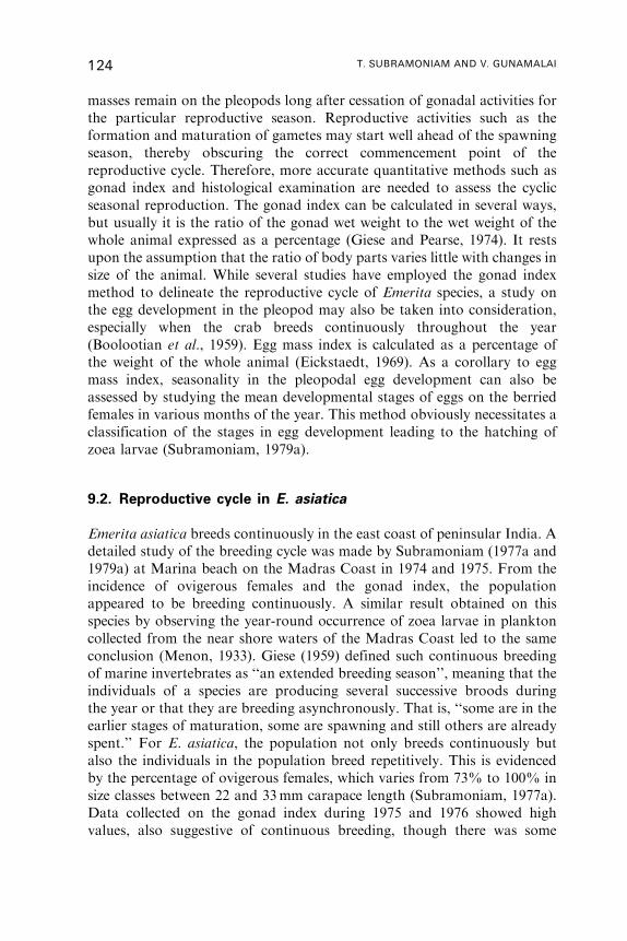
masses remain on the pleopods long after cessation of gonadal activities for

the particular reproductive season. Reproductive activities such as the

formation and maturation of gametes may start well ahead of the spawning

season, thereby obscuring the correct commencement point of the

reproductive cycle. Therefore, more accurate quantitative methods such as

gonad index and histological examination are needed to assess the cyclic

seasonal reproduction. The gonad index can be calculated in several ways,

but usually it is the ratio of the gonad wet weight to the wet weight of the

whole animal expressed as a percentage (Giese and Pearse, 1974). It rests

upon the assumption that the ratio of body parts varies little with changes in

size of the animal. While several studies have employed the gonad index

method to delineate the reproductive cycle of Emerita species, a study on

the egg development in the pleopod may also be taken into consideration,

especially when the crab breeds continuously throughout the year

(Boolootian et al., 1959). Egg mass index is calculated as a percentage of

the weight of the whole animal (Eickstaedt, 1969). As a corollary to egg

mass index, seasonality in the pleopodal egg development can also be

assessed by studying the mean developmental stages of eggs on the berried

females in various months of the year. This method obviously necessitates a

classification of the stages in egg development leading to the hatching of

zoea larvae (Subramoniam, 1979a).

9.2. Reproductive cycle in E. asiatica

Emerita asiatica breeds continuously in the east coast of peninsular India. A

detailed study of the breeding cycle was made by Subramoniam (1977a and

1979a) at Marina beach on the Madras Coast in 1974 and 1975. From the

incidence of ovigerous females and the gonad index, the population

appeared to be breeding continuously. A similar result obtained on this

species by observing the year-round occurrence of zoea larvae in plankton

collected from the near shore waters of the Madras Coast led to the same

conclusion (Menon, 1933). Giese (1959) defined such continuous breeding

of marine invertebrates as ‘‘an extended breeding season’’, meaning that the

individuals of a species are producing several successive broods during

the year or that they are breeding asynchronously. That is, ‘‘some are in the

earlier stages of maturation, some are spawning and still others are already

spent.’’ For E. asiatica, the population not only breeds continuously but

also the individuals in the population breed repetitively. This is evidenced

by the percentage of ovigerous females, which varies from 73% to 100% in

size classes between 22 and 33mm carapace length (Subramoniam, 1977a).

Data collected on the gonad index during 1975 and 1976 showed high

values, also suggestive of continuous breeding, though there was some


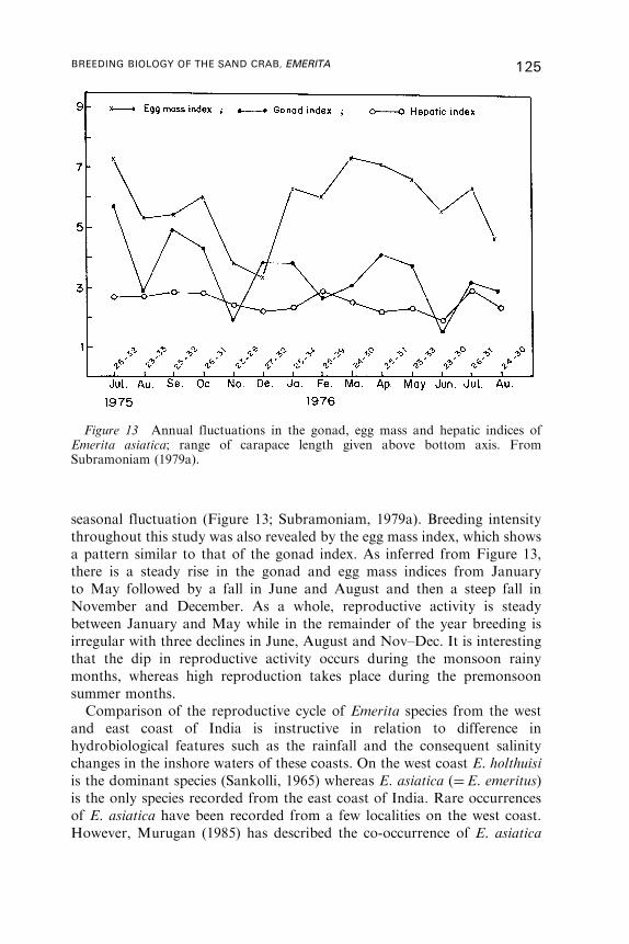
seasonal fluctuation (Figure 13; Subramoniam, 1979a). Breeding intensity

throughout this study was also revealed by the egg mass index, which shows

a pattern similar to that of the gonad index. As inferred from Figure 13,

there is a steady rise in the gonad and egg mass indices from January

to May followed by a fall in June and August and then a steep fall in

November and December. As a whole, reproductive activity is steady

between January and May while in the remainder of the year breeding is

irregular with three declines in June, August and Nov–Dec. It is interesting

that the dip in reproductive activity occurs during the monsoon rainy

months, whereas high reproduction takes place during the premonsoon

summer months.

Comparison of the reproductive cycle of Emerita species from the west

and east coast of India is instructive in relation to difference in

hydrobiological features such as the rainfall and the consequent salinity

changes in the inshore waters of these coasts. On the west coast E. holthuisi

is the dominant species (Sankolli, 1965) whereas E. asiatica (¼E. emeritus)

is the only species recorded from the east coast of India. Rare occurrences

of E. asiatica have been recorded from a few localities on the west coast.

However, Murugan (1985) has described the co-occurrence of E. asiatica

Figure 13 Annual fluctuations in the gonad, egg mass and hepatic indices ofEmerita asiatica; range of carapace length given above bottom axis. FromSubramoniam (1979a).


and E. holthuisi in equal proportions on the south-west tip of the Indian

peninsula. On the north-west coast of India, at Rathnagiri, E. holthuisi was

shown to be a continuous breeder, but with two peaks of berried females

occurring in the months of March and September (Nagabushanam and

Kulkarni, 1977). These two peaks coincide with the pre- and postmonsoon

seasons on the west coast. Murugan (1985) made extensive studies on the

reproductive cycles of both E. asiatica and E. holthuisi, coexisting in two

locations, Thiruvanandapuram and Vizhinjam on the south-west coast of

India. For E. asiatica he found continuous breeding with three distinct peak

periods at April–May, July and September–October, as determined by the

percentage of ovigerous females in the population. However, the gonadoso-

matic index indicated that the same population showed major peaks in July

and March. Interestingly, E. holthuisi, which breeds more or less

continuously on the north-west coast of India, shows only an extended

breeding period from July–December on the south east coast of

Thiruvanandapuram (Murugan, 1985). This season coincided with the

postmonsoonal months.

In Indian waters a major factor that influences intertidal as well as

offshore life is the monsoon rain that differs in time and intensity on the two

coasts (Panikkar and Jeyaraman, 1966). On the west coast, the southwest

monsoon brings abundant rain during May and August. This results in the

lowering of salinity in coastal waters, especially in the brackish water

lagoons that also receive fresh water from many large rivers. On the

east coast of India, the slow, retreating monsoon normally brings rain

around October in places from 19� to15�N, but in places south of 15�N it

rains later, in November (Hu-Cheng, 1967). Varadarajan and Subramoniam

(1982) made an estimate of breeding intensities of 78 marine invertebrates

from both east and west coasts. Figure 14 indicates that each month

between 60–80% of the east coast species are breeding continuously and

there is no seasonal pattern of peak activity. In contrast, most breeding

activity on the west coast occurs between September and March. While the

deterrent action of the heavy summer rain checks reproduction on the west

coast, its milder intensity than the retreating monsoon on the east coast,

especially near Madras, without any swift flowing rivers, may enhance

reproduction, as in E. asiatica.

An interesting difference from the continuous reproduction found in

E. asiatica from Madras occurs in another sand crab, Albunea symnista,

belonging to the family Hippidae, coexisting with E. asiatica. Although

this species does breed continuously on the Madras coast, there are two

distinct reproductive peaks, one in January and another in July, which

indicate a semiannual breeding pattern (Subramoniam and Panneerselvam,

1985). Examination of the ovary of this species during the rainy months of

October to December showed cessation of reproductive activity in the


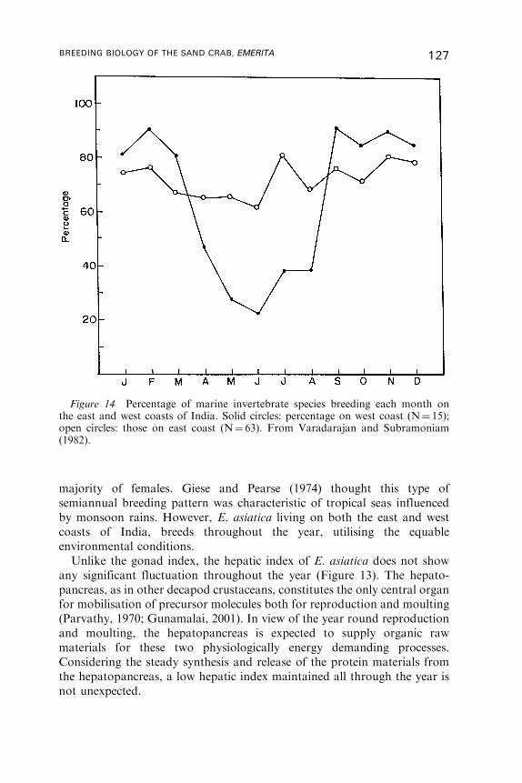
majority of females. Giese and Pearse (1974) thought this type of

semiannual breeding pattern was characteristic of tropical seas influenced

by monsoon rains. However, E. asiatica living on both the east and west

coasts of India, breeds throughout the year, utilising the equable

environmental conditions.

Unlike the gonad index, the hepatic index of E. asiatica does not show

any significant fluctuation throughout the year (Figure 13). The hepato-

pancreas, as in other decapod crustaceans, constitutes the only central organ

for mobilisation of precursor molecules both for reproduction and moulting

(Parvathy, 1970; Gunamalai, 2001). In view of the year round reproduction

and moulting, the hepatopancreas is expected to supply organic raw

materials for these two physiologically energy demanding processes.

Considering the steady synthesis and release of the protein materials from

the hepatopancreas, a low hepatic index maintained all through the year is

not unexpected.

Figure 14 Percentage of marine invertebrate species breeding each month onthe east and west coasts of India. Solid circles: percentage on west coast (N¼ 15);open circles: those on east coast (N¼ 63). From Varadarajan and Subramoniam(1982).


9.3. Reproductive cycle of E. asiatica in relation to size

A reinvestigation on the reproductive cycle of E. asiatica on the Marina

beach at Madras, using a combination of gonad index (GI) and direct

microscopic observation of the maturing ovary has yielded a better

understanding of size-related breeding pattern in this locality. For this, we

have classified the ovarian maturation stages into four categories on the

basis of the colour changes and direct microscopic measurement of the

oocyte diameter in the maturing ovary. Increase in the oocyte diameter is a

function of ovarian maturation as indicated in Table 6. In this study, we

have examined up to 1000 females with carapace length ranging from

16–33mm. The frequency occurrence of four ovarian stages has been plotted

against different size classes as a percentage value at each ovarian stage

(Figure 15). The first stage of ovarian maturity has been obtained from

16mmCL onwards with two peaks, one centred at 18mmCL and a second

at 25mmCL. The first peak coincides with the maximum number of animals

maturing for the first time at 18mmCL and the second large peak coincides

with the peak reproductive size class of 25mmCL. Ovarian stage II appears

to start from 19mmCL onwards with a small peak at 20mmCL and a larger

peak at 25mmCL. Similarly, stage III also appears to start from 20mmCL

with a gradual rise resulting in a flattened peak in the size range of

24–25mmCL. The stage IV ovary appears to start from 21mmCL with

a broader peak reaching over 75% at 25mmCL. This peak gradually

declined to reach a minimum value at 32–33mmCL. The overall data

comprising the percentage frequency of four ovarian stages against the size

classes indicates that the peak ovarian activity in Emerita occurs between

21–29mmCL. Thereafter, the frequency of all the stages declined. It may be

further inferred that the animals start the ovarian maturation at 16mmCL

onwards but continue maturation up to 21mm, when the first ovulation

is witnessed. From 22mmCL onwards the frequency of all the four stages

increases very steeply to reach the maximum at 25mmCL, thereby

Table 6 Classification of the ovarian stages of Emerita asiatica. From Gunamalai(2001).

Ovarianstages

Colour Oocyte diameter(mm)

Gonadosomaticindex

Stage I Whitish yellow 242.50� 12.99 1.05� 0.27Stage II Yellow 248.00� 19.39 1.06� 0.28Stage III Orange 257.50� 42.64 2.12� 0.58Stage IV Bright orange 361.66� 27.93 3.65� 0.89


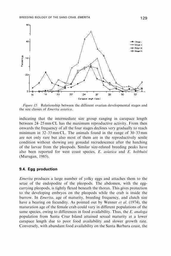
indicating that the intermediate size group ranging in carapace length

between 24–25mmCL has the maximum reproductive activity. From then

onwards the frequency of all the four stages declines very gradually to reach

minimum in 32–33mmCL. The animals found in the range of 30–33mm

are not only rare but also most of them are in the reproductively senile

condition without showing any gonadal recrudescence after the hatching

of the larvae from the pleopods. Similar size-related breeding peaks have

also been reported for west coast species, E. asiatica and E. holthuisi

(Murugan, 1985).

9.4. Egg production

Emerita produces a large number of yolky eggs and attaches them to the

setae of the endopodite of the pleopods. The abdomen, with the egg-

carrying pleopods, is tightly flexed beneath the thorax. This gives protection

to the developing embryos on the pleopods while the crab is inside the

burrow. In Emerita, age of maturity, breeding frequency, and clutch size

have a bearing on fecundity. As pointed out by Wenner et al. (1974), the

maturation age of the female crab could vary in different populations of the

same species, owing to differences in food availability. Thus, the E. analoga

population from Santa Cruz Island attained sexual maturity at a lower

carapace length due to poor food availability and slower growth rate.

Conversely, with abundant food availability on the Santa Barbara coast, the

Figure 15 Relationship between the different ovarian developmental stages andthe size classes of Emerita asiatica.


growth rate was not only high but there was also an increase in size of the

females at sexual maturity. A season-dependent size at sexual maturity is

also suggested for E. analoga by Eickstaedt (1969).

Wenner et al. (1987) studied egg production in E. analoga in reference to

the size and the year class at three California locations. They found that the

overall pattern of egg number as a function of size was similar for the first

two year classes, but egg production by the few third year crabs was highly

variable at the San Clemente site. Interestingly, the slope of the regressions

of size and egg number for each year class showed significant variation. The

slope was quite steep for first year and less so for the second year, but in the

third year the slope decreased considerably. This may suggest that the egg

laying intensity is inversely proportional to the size of the crab. However,

the number of eggs per spawning by the individual crabs always increased

linearly with the size of the laying female. Several authors who worked on E.

analoga at different beaches in north and south America also provided data

on the number of eggs produced as a function of size, although the number

per brood varied with season and locality (Osorio et al., 1967; Efford, 1969;

Eickstaedt, 1969). The size-related fecundity has also been determined

for the tropical species E. asiatica (Figure 16) indicating again that the egg-

laying capacity increases in direct relation to its body mass (Subramoniam,

1977a). In another population of E. asiatica from the east coast of India,

Figure 16 Relationship between carapace length and the number of eggs carriedin the pleopods of Emerita asiatica. From Subramoniam (1977a).


some 50 km south of Madras, the egg-laying adults reach a maximum size of

39mmCL. Correspondingly, the number of eggs laid by these bigger

females are also more than that of the females inhabiting Marina beach at

Madras (unpublished observation).

Table 7 summarises data on the fecundity of Emerita species inhabiting

tropical and temperate beaches. In general, the number of eggs produced by

the female per body size in the tropics far exceeds that of the temperate

species. For example E. asiatica inhabiting the Madras coast produces 4000

eggs at a body size of 25mmCL, whereas, the same sized temperate species

E. analoga, in California produces a maximum of 2500 eggs. This is

indicative of a temperature-dependent egg production in the Emerita

species. Apart from temperature effect, other local environmental factors

such as salinity and availability of food may also influence the rate of

egg production. This is evident in E. analoga with a wide distribution on

the west coast of America, ranging from Canada in the North to Mexico

in the South. A major difference between the north and south living

species is that in the south, the crabs grow to a larger size than those in

the north. A corresponding difference in the number of eggs per female

is also noticeable. In addition, on the east coast of southern peninsular

India at Madras, E. asiatica produces a higher number of eggs when

compared with its counterpart on the southwest coast of Trivandrum.

Again, E. holthuisi inhabiting the west coast, not only grows to a lesser body

size but also produces fewer eggs than E. asiatica coexisting in the same

beach.

9.5. Effect of temperature on egg development on the pleopods

Using several sets of published and unpublished data on the sand crab

E. analoga, which is widely distributed along the west coast of the Americas,

Wenner et al. (1991) plotted the egg development time as a function of

temperature. They found that the egg development time varied from 40 days

at 25�C to 100 days at 12�C. Furthermore, the duration of embryonic

development on the pleopod may also have a direct relation to the frequency

of spawning in these crabs. Fusaro (1980) provided experimental evidence

that decreased egg development time resulting from increased seawater

temperature has a positive effect on the number of egg batches produced per

female. Understandably, egg production by populations of E. analoga living

in cooler waters may be depressed relative to those populations experiencing

warmer water conditions.

Eickstaedt (1969) calculated the monthly mean egg development of the

berried females in the natural population to estimate the variation in the

time of egg development, as influenced by environmental factors such as


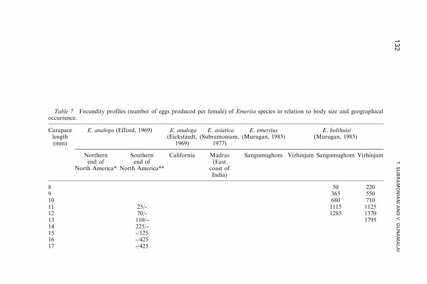
Table 7 Fecundity profiles (number of eggs produced per female) of Emerita species in relation to body size and geographicaloccurrence.

Carapacelength(mm)

E. analoga (Efford, 1969) E. analoga(Eickstaedt,

1969)

E. asiatica(Subramoniam,

1977)

E. emeritus(Murugan, 1985)

E. holthuisi(Murugan, 1985)

Northernend of

North America*

Southernend of

North America**

California Madras(East

coast ofIndia)

Sangumughom Vizhinjam Sangumughom Vizhinjam

8 50 2209 365 55010 680 71011 25/- 1115 112512 70/- 1285 137013 110/- 179514 225/-15 -/12516 -/42517 -/425

132

T.SUBRAMONIA

MAND

V.GUNAMALAI

18 -/55019 700/22520 1000/5252122 280023 7000 3100 1000 200024 1150/2300 370025 14000 4000 2800 352526 1750/3000 460027 17000 5000 5750 535028 1850/3750 550029 6100 8050 780030 2300/- 625031 6500 11500 985032 730033 7900 13100 118003435 16300

*La Jolla to Tofino; **Garibaldi to Playa De La Mission.

BREEDIN

GBIO

LOGYOFTHESAND

CRAB,EMERITA

133

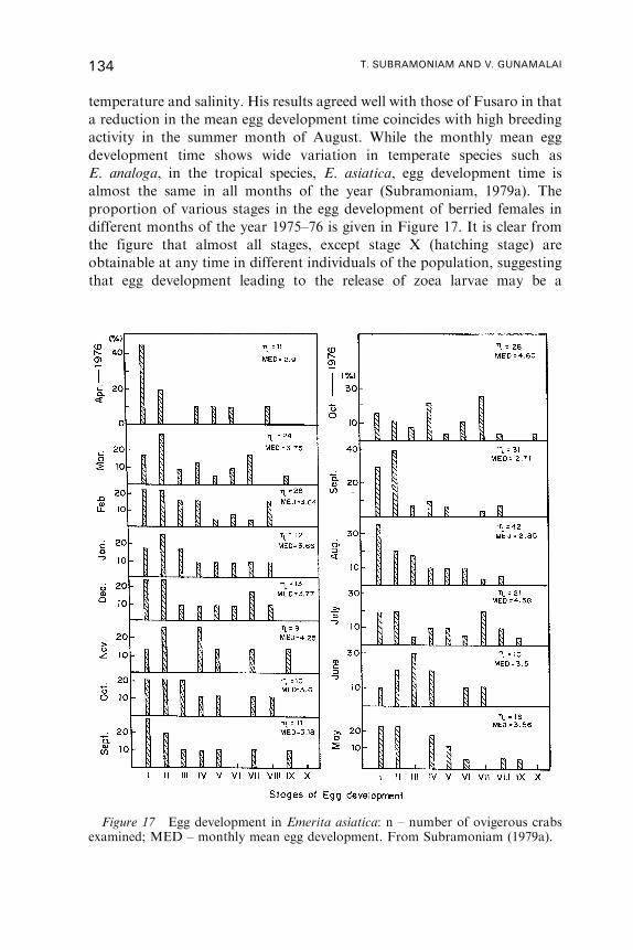
temperature and salinity. His results agreed well with those of Fusaro in that

a reduction in the mean egg development time coincides with high breeding

activity in the summer month of August. While the monthly mean egg

development time shows wide variation in temperate species such as

E. analoga, in the tropical species, E. asiatica, egg development time is

almost the same in all months of the year (Subramoniam, 1979a). The

proportion of various stages in the egg development of berried females in

different months of the year 1975–76 is given in Figure 17. It is clear from

the figure that almost all stages, except stage X (hatching stage) are

obtainable at any time in different individuals of the population, suggesting

that egg development leading to the release of zoea larvae may be a

Figure 17 Egg development in Emerita asiatica: n – number of ovigerous crabsexamined; MED – monthly mean egg development. From Subramoniam (1979a).


continuous process in accordance with the year-round breeding activity in

the population (Subramoniam, 1977a). Obviously, on the east coast of India

at Madras, the ambient seawater temperature as well as the other conditions

such as optimum salinity and the availability of food both for the adult

and the released larvae are conducive to promote and maintain both egg

production and egg development on the pleopods at a high profile

throughout the year (Panikkar and Jayaraman, 1966). By contrast, on the

west coast of India, where the monsoonal rains as well as the swift flowing

rivers lower the salinity of the coastal waters significantly, the intensity of

breeding declines during June–August.

10. INTERRELATIONSHIP BETWEEN MOULTING

AND REPRODUCTION

In the majority of the crustaceans, reproductive physiology is greatly

influenced by somatic growth, permitted by periodic moulting in the adults.

As evident from the preceding account, E. asiatica is not only a continuous

breeder but also exhibits year-round moulting. A detailed analysis of the

ovarian and moult cycle stages in the adult crab has not only indicated a

close correlation between moulting and reproduction, but also provides

evidence that some of the processes are closely linked and overlapping. In

female E. asiatica, the reproductive cycle is repetitive; when the pleopodal

embryos undergo development, there is a concurrent maturation of oocytes

within the ovary, making it ready for the next spawning. Moulting

invariably occurs after hatching of the larvae from the pleopods and

before spawning. It was believed earlier that the presence of pleopodal

embryos exerts an inhibitory effect on the onset of moulting in embryo-

carrying malacostracan crustaceans (Adiyodi, 1988). However, in E.

asiatica, initiation of the moulting process, such as the apolysis, invariably

starts almost midway through the development of the brood. The premoult

changes advance further up to D1, at the time when the pleopodal embryos

hatch out as zoea larvae. No females examined at the time of embryo

hatching are found in the intermoult stage. Tirumalai (1996) and Gunamalai

and Subramoniam (2002) have also observed the occurrence of the yolk

precursor protein vitellogenin in the haemolymph throughout intermoult

and premoult stages in E. asiatica suggesting that the process of

vitellogenesis continues well into the premoult stage. Evidently, there is

a perfect synchronisation of moulting and ovarian cycles, thus allowing

body growth and reproduction to occur simultaneously.

The overlapping of moulting and reproductive activities in E. asiatica is

further reflected in the haemolymph and ovarian total protein levels


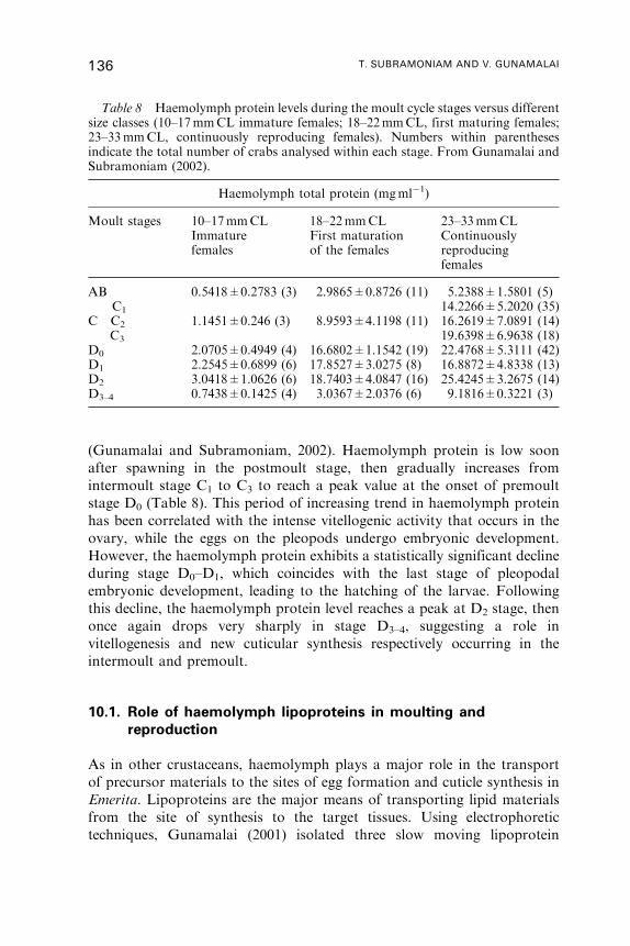
(Gunamalai and Subramoniam, 2002). Haemolymph protein is low soon

after spawning in the postmoult stage, then gradually increases from

intermoult stage C1 to C3 to reach a peak value at the onset of premoult

stage D0 (Table 8). This period of increasing trend in haemolymph protein

has been correlated with the intense vitellogenic activity that occurs in the

ovary, while the eggs on the pleopods undergo embryonic development.

However, the haemolymph protein exhibits a statistically significant decline

during stage D0–D1, which coincides with the last stage of pleopodal

embryonic development, leading to the hatching of the larvae. Following

this decline, the haemolymph protein level reaches a peak at D2 stage, then

once again drops very sharply in stage D3–4, suggesting a role in

vitellogenesis and new cuticular synthesis respectively occurring in the

intermoult and premoult.

10.1. Role of haemolymph lipoproteins in moulting and

reproduction

As in other crustaceans, haemolymph plays a major role in the transport

of precursor materials to the sites of egg formation and cuticle synthesis in

Emerita. Lipoproteins are the major means of transporting lipid materials

from the site of synthesis to the target tissues. Using electrophoretic

techniques, Gunamalai (2001) isolated three slow moving lipoprotein

Table 8 Haemolymph protein levels during the moult cycle stages versus differentsize classes (10–17mmCL immature females; 18–22mmCL, first maturing females;23–33mmCL, continuously reproducing females). Numbers within parenthesesindicate the total number of crabs analysed within each stage. From Gunamalai andSubramoniam (2002).

Haemolymph total protein (mgml�1)

Moult stages 10–17mmCLImmaturefemales

18–22mmCLFirst maturationof the females

23–33mmCLContinuouslyreproducingfemales

AB 0.5418±0.2783 (3) 2.9865±0.8726 (11) 5.2388±1.5801 (5)C1 14.2266±5.2020 (35)

C C2 1.1451±0.246 (3) 8.9593±4.1198 (11) 16.2619±7.0891 (14)C3 19.6398±6.9638 (18)

D0 2.0705±0.4949 (4) 16.6802±1.1542 (19) 22.4768±5.3111 (42)D1 2.2545±0.6899 (6) 17.8527±3.0275 (8) 16.8872±4.8338 (13)D2 3.0418±1.0626 (6) 18.7403±4.0847 (16) 25.4245±3.2675 (14)D3–4 0.7438±0.1425 (4) 3.0367±2.0376 (6) 9.1816±0.3221 (3)


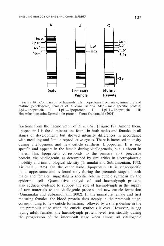
fractions from the haemolymph of E. asiatica (Figure 18). Among them,

lipoprotein I is the dominant one found in both males and females in all

stages of development; but showed intensity differences in accordance

with moulting and female reproductive cycles. There is increased intensity

during vitellogenesis and new cuticle synthesis. Lipoprotein II is sex-

specific and appears in the female during vitellogenesis, but is absent in

males. This lipoprotein corresponds to the primary yolk precursor

protein, viz. vitellogenin, as determined by similarities in electrophoretic

mobility and immunological identity (Tirumalai and Subramoniam, 1992;

Tirumalai, 1996). On the other hand, lipoprotein III is stage-specific

in its appearance and is found only during the premoult stage of both

males and females, suggesting a specific role in cuticle synthesis by the

epidermal cells. Quantitative analysis of total haemolymph proteins

also adduces evidence to support the role of haemolymph in the supply

of raw materials to the vitellogenic process and new cuticle formation

(Gunamalai and Subramoniam, 2002). In the immature female and first

maturing females, the blood protein rises steeply in the premoult stage,

corresponding to new cuticle formation, followed by a sharp decline in the

late premoult stage when the cuticle synthesis is over. However, in egg

laying adult females, the haemolymph protein level rises steadily during

the progression of the intermoult stage when almost all vitellogenic

Figure 18 Comparison of haemolymph lipoproteins from male, immature andmature (Vitellogenic) females of Emerita asiatica. Msp¼male specific protein;LpI¼ lipoprotein I; LpII¼ lipoprotein II; LpIII¼ lipoprotein III;Hcy¼ hemocyanin; Sp¼ simple protein. From Gunamalai (2001).


activities occur and, from the onset of premoult stage the protein registers

yet another peak followed by a sharp decline in the late premoult stages

(Table 8).

10.2. Endocrine regulation of moulting and reproduction

The close relationship between moulting and female reproduction in

E. asiatica discussed above could imply common influencing endocrine

factors. In several decapod species the moulting hormones, ecdysteroids,

also subserve functions in the control of reproduction and embryogenesis

(see Subramoniam, 2000, for references). As shown in Figure 12, the level of

haemolymph ecdysteroids in the postmoult stage is minimal but it begins to

rise gradually throughout the intermoult stage. From D0 onwards the titre

demonstrates a sharp increase in the haemolymph to reach a maximum level

in D2. From then onwards, the ecdysteroid level declines again to reach the

basal level at D3–4 of the premoult stage. Analysis of ovarian ecdysteroids

during the moult cycle stages also shows accumulation of ecdysteroids

within the ovary (Gunamalai unpublished observations). Again, the titre of

ecdysteroids in the haemolymph and the ovary exhibits a reciprocal

relationship during the moulting stages, thus suggesting that the haemo-

lymph ecdysteroids, when present in excess, could be sequestered in the

ovary. The rising trend in the haemolymph ecdysteroids during the premoult

stages also implies that vitellogenin synthesis and uptake by the ovary could

occur under a high titre of ecdysteroids. In this context, it is of interest to

note the studies by Okumura et al. (1992) in the fresh water prawn

Macrobrachium nipponense and by Wilder et al. (1991) in Macrobrachium

rosenbergii, where there is a close correlation between moulting and

reproduction. However, in M. rosenbergii, two types of moulting namely,

reproductive and non-reproductive moulting occur. The non-reproductive

moult signifies repetitive moulting outside the ovarian cycle. During the

reproductive moult, the ovarian cycle is completed within the intermoult

stage and spawning occurs soon after ecdysis, as in the case of E. asiatica.

The overlapping of moulting and ovarian cycle in the Macrobrachium

species is further reflected in a parallel rise of vitellogenin and haemolymph

ecdysteroids right up to the D1 stage of the premoult (Okumura et al., 1992).

This study supports our observation in E. asiatica that vitellogenesis and the

new cuticle synthesis during the premoult stage occur under high titre of

haemolymph ecdysteroids. In other decapods also, such as Penaeus

monodon, active vitellogenesis has been shown to occur during the extended

premoult period (Crocos, 1991). Although the independent role of

ecdysteroids in stimulating and maintaining vitellogenesis cannot be

confirmed from these data on E. asiatica, it is evident that the ovary


accumulates large quantities of ecdysteroids both in free and bound forms

(Subramoniam et al., 1999). Obviously, the stored ecdysteroids in the egg,

derived maternally, may have a role during embryogenesis (see below).

Experimental studies involving the exogenous injection of 20 hydro-

xyecdysone (20E) in E. asiatica show the common influence of this hormone

on moulting and reproduction (Gunamalai unpublished observations).

Injection of ecdysteroids at the C3 stage resulted in precocious commence-

ment of premoult changes as evidenced by new cuticular synthesis and

pleopodal setagenesis (Table 4). More interestingly, in the ecdysteroid

injected crabs, embryonic development on the pleopods was also enhanced.

Injection of 20E stimulated protein synthesis in tissues such as ovary,

hepatopancreas and integumentary tissue together with an increase in

haemolymph total proteins (Table 9). This may again suggest that, in

addition to their controlling effect on moult induction, 20E also acts as a

metabolic hormone by inducing protein synthesis related to vitellogenesis

and new cuticle synthesis, obviously under different titres.

11. BIOCHEMISTRY OF EGGS

11.1. Emerita yolk protein

Emerita asiatica lays a large number of yolky eggs at each spawning. As in

other decapod crustaceans, the yolk proteins, also called lipovitellins, are

high-density lipoproteins with carbohydrate as the major covalently linked

prosthetic group. They are invariably conjugated to a carotenoid pigment.

Tirumalai and Subramoniam (1992 and 2001) have characterised E. asiatica

yolk proteins. These comprise two lipovitellins (Lv I and Lv II) constituting

as much as 90% of the total egg proteins. In SDS-PAGE analysis, Lv I

yielded two subunits with molecular weights of approximately 109,000 and

105,000 Daltons respectively; whereas, Lv II resolved into six subunits with

molecular weights of 65,000, 54,000, 50,000, 47,000, 44,000 and 42,000

Daltons, respectively.

The carbohydrate component of the yolk exists in three forms, namely

free carbohydrate, protein- and lipid-bound carbohydrates (Table 10). The

protein-bound carbohydrates are dominated by hexose, hexosamine and

galactosamine. The Lv II contains the higher amount of N-linked

oligosaccharides than the O-linked oligosaccharides. Sialic acid is absent.

It is assumed that the abundant O-linked oligosaccharides of Emerita

lipovitellin may play a role in the secretion of yolk precursor protein during

yolk synthesis and recognition of its receptors on the oocyte membrane

during yolk accumulation. In addition, the O-glycosylation may also render


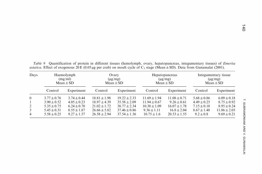
Table 9 Quantification of protein in different tissues (hemolymph, ovary, hepatopancreas, integumentary tissues) of Emeritaasiatica. Effect of exogenous 20E (0.05 mg per crab) on moult cycle of C3 stage (Mean� SD). Data from Gunamalai (2001).

Days Haemolymph(mg/ml)

Mean� SD

Ovary(mg/mg)

Mean� SD

Hepatopancreas(mg/mg)

Mean� SD

Integumentary tissue(mg/mg)

Mean� SD

Control Experiment Control Experiment Control Experiment Control Experiment

0 3.77� 0.76 3.74� 0.44 18.81� 1.98 19.22� 2.33 11.69� 1.94 11.08� 0.71 5.68� 0.86 6.09� 0.181 3.90� 0.52 4.05� 0.23 18.97� 4.39 35.58� 2.09 11.94� 0.67 9.26� 0.61 4.49� 0.25 8.75� 0.922 5.35� 0.75 6.24� 0.70 21.02� 1.72 38.77� 2.34 10.38� 1.09 16.07� 1.78 7.15� 0.18 8.95� 0.243 5.45� 0.31 8.55� 1.87 26.66� 5.82 37.46� 0.86 9.36� 1.11 16.8� 2.04 8.67� 1.48 11.86� 2.034 5.58� 0.25 9.27� 1.57 26.58� 2.94 37.54� 1.36 10.75� 1.6 20.53� 1.55 9.2� 0.8 9.69� 0.21

140

T.SUBRAMONIA

MAND

V.GUNAMALAI

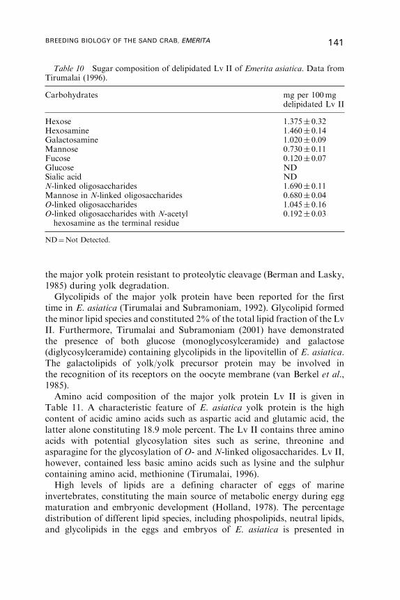
the major yolk protein resistant to proteolytic cleavage (Berman and Lasky,

1985) during yolk degradation.

Glycolipids of the major yolk protein have been reported for the first

time in E. asiatica (Tirumalai and Subramoniam, 1992). Glycolipid formed

the minor lipid species and constituted 2% of the total lipid fraction of the Lv

II. Furthermore, Tirumalai and Subramoniam (2001) have demonstrated

the presence of both glucose (monoglycosylceramide) and galactose

(diglycosylceramide) containing glycolipids in the lipovitellin of E. asiatica.

The galactolipids of yolk/yolk precursor protein may be involved in

the recognition of its receptors on the oocyte membrane (van Berkel et al.,

1985).

Amino acid composition of the major yolk protein Lv II is given in

Table 11. A characteristic feature of E. asiatica yolk protein is the high

content of acidic amino acids such as aspartic acid and glutamic acid, the

latter alone constituting 18.9 mole percent. The Lv II contains three amino

acids with potential glycosylation sites such as serine, threonine and

asparagine for the glycosylation of O- and N-linked oligosaccharides. Lv II,

however, contained less basic amino acids such as lysine and the sulphur

containing amino acid, methionine (Tirumalai, 1996).

High levels of lipids are a defining character of eggs of marine

invertebrates, constituting the main source of metabolic energy during egg

maturation and embryonic development (Holland, 1978). The percentage

distribution of different lipid species, including phospolipids, neutral lipids,

and glycolipids in the eggs and embryos of E. asiatica is presented in

Table 10 Sugar composition of delipidated Lv II of Emerita asiatica. Data fromTirumalai (1996).

Carbohydrates mg per 100mgdelipidated Lv II

Hexose 1.375� 0.32Hexosamine 1.460� 0.14Galactosamine 1.020� 0.09Mannose 0.730� 0.11Fucose 0.120� 0.07Glucose NDSialic acid NDN-linked oligosaccharides 1.690� 0.11Mannose in N-linked oligosaccharides 0.680� 0.04O-linked oligosaccharides 1.045� 0.16O-linked oligosaccharides with N-acetylhexosamine as the terminal residue

0.192� 0.03

ND¼Not Detected.


Table 12. Phospholipids formed by far the greatest fraction of the total

lipids in both freshly laid eggs and Lv II, as has been reported for the ovary

of many crustaceans (Teshima and Kanazawa, 1983; Lautier and

Lagarrigue, 1988; Teshima et al., 1989). As many as seven phospholipid

species have been separated from the lipovitellin and eggs of E. asiatica,

using thin layer chromatography (Tirumalai and Subramoniam, 1992). They

are: (1) lysophosphatidylecholine; (2) sphingomylin; (3) phosphatidyl-

choline; (4) phosphatidylenositol; (5) phosphatidylserine; (6) phosphatidy-

lethanolamine and (6) cardiolipin. However, phosphatidyl choline and

phosphatidyl serine were the predominant phospholipid species. These

phospholipid species, accumulated within the eggs, have an important role

Table 11 Amino acid composition of delipidated Lv IIof Emerita asiatica. Data from Tirumalai (1996).

Amino acids Mole percent

Aspartic acid 8.7925Glutamic acid 18.9271Asparagine 8.2362Serine 10.9370Histidine 3.7342Glycine 3.6943Threonine 5.4295Arginine 4.2299Alanine 7.5289Tyrosine 6.1480Methionine 0.3951Valine 5.1130Phenylalanine 4.3210Isoleucine 5.3851Leucine 6.7835Lysine 0.3446

Table 12 Relative percentage composition of different lipids in theegg (Stage I) and Lv II of E. asiatica. From Tirumalai (1996).

Lipid Species Egg Lv II

Neutral lipids 35 33±0.21Cholesterol 4 3±0.11Glycolipids 3 2±0.22Galactolipids ND 0.038±0.009Phospholipids 58 62±0.41

ND¼Not done.


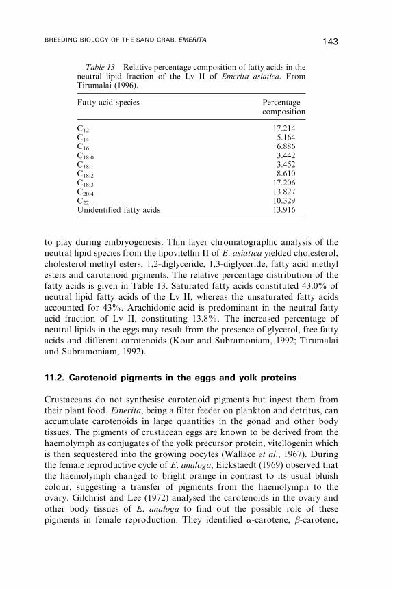
to play during embryogenesis. Thin layer chromatographic analysis of the

neutral lipid species from the lipovitellin II of E. asiatica yielded cholesterol,

cholesterol methyl esters, 1,2-diglyceride, 1,3-diglyceride, fatty acid methyl

esters and carotenoid pigments. The relative percentage distribution of the

fatty acids is given in Table 13. Saturated fatty acids constituted 43.0% of

neutral lipid fatty acids of the Lv II, whereas the unsaturated fatty acids

accounted for 43%. Arachidonic acid is predominant in the neutral fatty

acid fraction of Lv II, constituting 13.8%. The increased percentage of

neutral lipids in the eggs may result from the presence of glycerol, free fatty

acids and different carotenoids (Kour and Subramoniam, 1992; Tirumalai

and Subramoniam, 1992).

11.2. Carotenoid pigments in the eggs and yolk proteins

Crustaceans do not synthesise carotenoid pigments but ingest them from

their plant food. Emerita, being a filter feeder on plankton and detritus, can

accumulate carotenoids in large quantities in the gonad and other body

tissues. The pigments of crustacean eggs are known to be derived from the

haemolymph as conjugates of the yolk precursor protein, vitellogenin which

is then sequestered into the growing oocytes (Wallace et al., 1967). During

the female reproductive cycle of E. analoga, Eickstaedt (1969) observed that

the haemolymph changed to bright orange in contrast to its usual bluish

colour, suggesting a transfer of pigments from the haemolymph to the

ovary. Gilchrist and Lee (1972) analysed the carotenoids in the ovary and

other body tissues of E. analoga to find out the possible role of these

pigments in female reproduction. They identified �-carotene, �-carotene,

Table 13 Relative percentage composition of fatty acids in theneutral lipid fraction of the Lv II of Emerita asiatica. FromTirumalai (1996).

Fatty acid species Percentagecomposition

C12 17.214C14 5.164C16 6.886C18:0 3.442C18:1 3.452C18:2 8.610C18:3 17.206C20:4 13.827C22 10.329Unidentified fatty acids 13.916


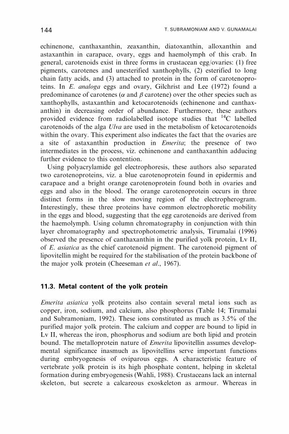
echinenone, canthaxanthin, zeaxanthin, diatoxanthin, alloxanthin and

astaxanthin in carapace, ovary, eggs and haemolymph of this crab. In

general, carotenoids exist in three forms in crustacean egg/ovaries: (1) free

pigments, carotenes and unesterified xanthophylls, (2) esterified to long

chain fatty acids, and (3) attached to protein in the form of carotenopro-

teins. In E. analoga eggs and ovary, Gilchrist and Lee (1972) found a

predominance of carotenes (� and � carotene) over the other species such as

xanthophylls, astaxanthin and ketocarotenoids (echinenone and canthax-

anthin) in decreasing order of abundance. Furthermore, these authors

provided evidence from radiolabelled isotope studies that 14C labelled

carotenoids of the alga Ulva are used in the metabolism of ketocarotenoids

within the ovary. This experiment also indicates the fact that the ovaries are

a site of astaxanthin production in Emerita; the presence of two

intermediates in the process, viz. echinenone and canthaxanthin adducing

further evidence to this contention.

Using polyacrylamide gel electrophoresis, these authors also separated

two carotenoproteins, viz. a blue carotenoprotein found in epidermis and

carapace and a bright orange carotenoprotein found both in ovaries and

eggs and also in the blood. The orange carotenoprotein occurs in three

distinct forms in the slow moving region of the electropherogram.

Interestingly, these three proteins have common electrophoretic mobility

in the eggs and blood, suggesting that the egg carotenoids are derived from

the haemolymph. Using column chromatography in conjunction with thin

layer chromatography and spectrophotometric analysis, Tirumalai (1996)

observed the presence of canthaxanthin in the purified yolk protein, Lv II,

of E. asiatica as the chief carotenoid pigment. The carotenoid pigment of

lipovitellin might be required for the stabilisation of the protein backbone of

the major yolk protein (Cheeseman et al., 1967).

11.3. Metal content of the yolk protein

Emerita asiatica yolk proteins also contain several metal ions such as

copper, iron, sodium, and calcium, also phosphorus (Table 14; Tirumalai

and Subramoniam, 1992). These ions constituted as much as 3.5% of the

purified major yolk protein. The calcium and copper are bound to lipid in

Lv II, whereas the iron, phosphorus and sodium are both lipid and protein

bound. The metalloprotein nature of Emerita lipovitellin assumes develop-

mental significance inasmuch as lipovitellins serve important functions

during embryogenesis of oviparous eggs. A characteristic feature of

vertebrate yolk protein is its high phosphate content, helping in skeletal

formation during embryogenesis (Wahli, 1988). Crustaceans lack an internal

skeleton, but secrete a calcareous exoskeleton as armour. Whereas in


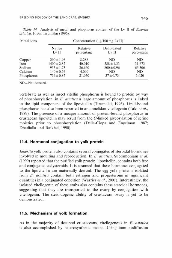
vertebrate as well as insect vitellin phosphorus is bound to protein by way

of phosphorylation, in E. asiatica a large amount of phosphorus is linked

to the lipid component of the lipovitellin (Tirumalai, 1996). Lipid-bound

phosphorus has also been reported in an annelidan vitellogenin (Taki et al.,

1989). The presence of a meagre amount of protein-bound phosphorus in

crustacean lipovitellin may result from the O-linked glycosylation of serine

moieties prior to phosphorylation (Della-Ciopa and Engelman, 1987;

Dhadialla and Raikhel, 1990).

11.4. Hormonal conjugation to yolk protein

Emerita yolk protein also contains several conjugates of steroidal hormones

involved in moulting and reproduction. In E. asiatica, Subramoniam et al.

(1999) reported that the purified yolk protein, lipovitellin, contains both free

and conjugated ecdysteroids. It is assumed that these hormones conjugated

to the lipovitellin are maternally derived. The egg yolk proteins isolated

from E. asiatica contain both estrogen and progesterone in significant

quantities in a conjugated condition (Warrier et al., 2001). Interestingly, the

isolated vitellogenin of these crabs also contains these steroidal hormones,

suggesting that they are transported to the ovary by conjugation with

vitellogenin. The steroidogenic ability of crustacean ovary is yet to be

demonstrated.

11.5. Mechanism of yolk formation

As in the majority of decapod crustaceans, vitellogenesis in E. asiatica

is also accomplished by heterosynthetic means. Using immunodiffusion

Table 14 Analysis of metal and phophorus content of the Lv II of Emeritaasiatica. From Tirumalai (1996).

Metal ions Concentration (mg/100mg Lv II)

NativeLv II

Relativepercentage

DelipidatedLv II

Relativepercentage

Copper 290±1.96 8.288 ND NDIron 1400±2.87 40.010 388±1.33 31.673Sodium 933±1.73 26.660 800±0.96 65.306Calcium 140±0.56 4.000 ND NDPhosphorus 736±0.87 21.030 37±0.73 3.020

ND¼Not detected.


techniques, Tirumalai (1996) showed that the anti-Vg antibodies prepared

against the purified vitellogenin of E. asiatica produced two precipitin lines

with the supernatants obtained from the mature ovary. Interestingly, these

two precipitin lines correspond to column chromatographically purified

lipovitellin I and II. However, the anti-Vg antibodies of E. asiatica did

not cross-react with the supernatants of any somatic tissue such as

hepatopancreas, muscle and subepidermal tissues. Thus in Emerita, the

final site of vitellogenin synthesis is still elusive. Perhaps molecular

techniques such as Northern blotting (Yang et al., 2000) and real-time

RT-PCR (Jayasankar et al., 2002) could unravel the ultimate site of

vitellogenin synthesis in this highly fecund sand crab. Interestingly, the

lipovitellin of another anomuran sand crab, Albunea symnista also cross-

reacted with anti-Vg antibodies of E. asiatica suggesting the immunological

and molecular similarities of the lipovitellins of these conspecific anomuran

crabs. Homology in the amino acid sequences of vitellogenin of different

decapod crustaceans as well as immunological relatedness between the

lipovitellin and mammalian serum low density lipoproteins have also been

revealed in recent studies (See Wilder et al., 2002; Warrier and

Subramoniam, 2003).

12. YOLK UTILISATION

Emerita species fasten the eggs to the pleopodal hairs where the eggs

develop and hatch out as larvae. The biochemical composition

of E. asiatica eggs shows them to be a rich source of nutrition. The

yolk comprises a glycolipocarotenoprotein complex, free lipids and

glycogen granules. During maturation in the ovary the eggs also acquire

various other organic and inorganic components needed for embryogen-

esis and also early larval development. The embryos also absorb water

and salts from the environment during the course of their development.

A special feature of Emerita eggs is the large proportion of lipid in the

yolk, forming as much as 30% of the lipovitellin (Tirumalai and

Subramoniam, 1992), in addition to a significant quantity of free lipids.

Lipid accumulation is a strategy to decrease density and to reduce

energy cost of egg carriage in pelagic crustaceans, which are characterised

by abbreviated development coupled with an extended period of

incubation (Herring, 1973), but this has little bearing on benthic species

such as Emerita. Studies on yolk utilisation in Emerita are limited to only

two species, namely E. holthuisi (Vijayaraghavan et al., 1976) and E.

asiatica (Subramoniam, 1991).


Emerita embryos also contain hemocyanin (Gilchrist and Lee, 1972;

Gunamalai, 2001). The functional importance of haemocyanin,

accumulated during vitellogenesis, in embryogenesis is not clear, but

in other crustaceans haemocyanins are known to provide a source of

protein and copper during yolk utilisation (Terwilliger, 1991). In Emerita,

as in other ovigerous crabs, embryonic development occurs within a

mass consisting of several thousand eggs. Hence, the embryos in the centre

of the egg mass may experience a lower partial pressure of oxygen than do

embryos on the outer surface. Embryonic accumulation of haemocyanin

may help in oxygen transport or diffusion (Terwilliger, 1991). In freshwater

prawns, Pandian (1994) observed grooming and aeration of the egg mass by

the legs of the female. The same behaviour may also occur in Emerita, but

direct observations are lacking.

Yolk utilisation has been studied in several crustaceans, with particular

regard to energy transformation during embryogenesis and the ecophysiol-

ogy of the organism (Pandian, 1970a, b). During vitellogenesis, besides

the accumulation of the yolk components, other metabolically important

substances such as RNA, and a host of hydrolytic enzymes, are also

synthesised and stored within the eggs (Adiyodi and Subramoniam, 1983).

Taking advantage of the year-round availability of the berried females with

eggs in different stages of embryonic development, Subramoniam (1991)

made a thorough investigation into the biochemcal changes in the egg

components of E. asiatica during embryogenesis. The eggs in the brood

exhibit changes in colouration during embryonic development, thus

facilitating an easy classification of development stages (Table 15). This

table also summarises other microscopic observations such as percentage

yolk clearance, appearance of morphological characters such as the eye

spots, beating heart and the development of appendages. The time taken for

each stage during egg development was also estimated by maintaining the

freshly ovulated females in the laboratory (Temp. 26�C; Salinity 34%).

Changes in percentage values of protein, lipid and carbohydrates, calculated

on wet weight and dry weight basis are summarised in Table 16 and 17.

Protein value steadily declined from stage I to IX, corresponding to

increasing water content. On the other hand, lipid content remained almost

unaltered up to stage V; thereupon, the value fell precipitously, reaching a

minimum of 0.49mg per 10mg in stage IX. Compared to protein and lipid,

the total carbohydrate content was low, but different carbohydrate compo-

nents exhibited an interesting pattern of fluctuation during egg develop-

ment. The total free carbohydrates increased from a low value of 0.12mg

per 10mg in stage I to 0.72mg per 10mg in stage IX. The free glycogen also

exhibited a similar increase during egg development. Conversely, the

protein-bound polysaccharides decreased from an initial high value of

0.072mg per 10mg in stage I to 0.021mg per 10mg in stage IX.


12.1. Enzyme activity during yolk utilisation

Commensurate with storage of complex yolk proteins in E. asiatica eggs, a

host of hydrolytic enzymes are available to release the component substrates

in utilisable form. Table 18 summarises the stage-specific enzyme activity of

esterases, proteases and glycosidases during embryogenesis in E. asiatica.

Interestingly, the activity of all the three enzymes peaks during stage V and

VI, coinciding with break down of the major yolk proteins into simpler

subunits. Esterase activity involved in the breakdown of various lipids

exhibits an interesting pattern during yolk utilisation. It starts only in stage

III and attains a peak value during stage V. Thereafter, activity slowly

declines to a very low value in stage VIII. The esterase activity correlates

with lipid utilisation during embryogenesis. Inactivity of the enzyme before

stage III may be caused by the proenzyme nature of esterases or there may

Table 15 Classification of egg development in Emerita asiatica. Adapted fromSubramoniam (1991).

Stage Approximatenumber ofdays

Description

I 5 Yellow yolk granules seen; egg mass bright orange in colourII 5 Cleavage has taken place and blastomeres are seen; egg

mass bright orange in colourIII 1 A yolk-free white streak makes its appearance at the animal

poleIV 1 One quarter of the yolk cleared; the white band encircles

the yolk material which is now in the centre; at the animalpole a periodic twitching is recognised; red pigments areseen at the edge of the yolk; colour of the egg mass is dullorange

V 2 One third of the yolk is cleared; two eye spots appear; redspots prominent and seen at the end of the animal pole;colour of the egg mass dull orange

VI 2 Egg mass brownish orange in colour; eyes well developed;yolk is found in the vegetal pole; two-thirds of the yolk iscleared; red pigments seen all over the white space

VII 1 Egg mass greyish orange in colour; yellow yolk is found astwo clusters in the centre; appendages of the embryo aredeveloped; heart beat seen; eye spots are very welldeveloped

VIII 1 Egg mass pale grey in colour; heart beat more prominent;embryo almost developed

IX 1 Embryo fully formed; egg mass white in colour; no yolkglobules seen; colourless yolk in the form of oil globulesseen just below the eyes; about to hatch


Table 16 Major organic composition of eggs during different stages of development in Emerita asiatica. Values expressed asmg/10mg wet weight (mean� SD). Esterase activity expressed as nM naphthol/mg protein/min. Data from Subramoniam (1991).

Biochemical

constituents

Stages of eggs

I II III IV V VI VII VIII IX

Protein 1.32±0.150 1.09±0.143 0.949±0.107 0.90±0.03 0.77±0.09 0.66±0.043 0.44±0.08 0.28±.0.021 0.16±0.029

Free

carbohydrates

0.12±0.013 0.24±0.009 0.28±0.012 0.32±0.012 0.36±0.010 0.48±0.012 0.52±0.008 0.68±0.009 0.72±0.015

Glycogen 0.005±0.001 0.0057±0.0001 0.0119±0.0002 0.0168±0.003 0.0109±0.0002 0.026±0.0022 0.0231±0.0013 0.0197±0.002 0.0207±0.0017

Protein

bound

sugar

0.0729±0.00 0.0849±0.0024 0.0467±0.0032 0.0457±0.0014 0.0205±0.0071 0.0339±0.0021 0.0261±0.0018 0.0250±0.007 0.0210±0.003

Lipid 31 1.88±0.014 1.87±0.010 1.85±0.014 1.80±0.012 0.64±0.009 0.52±0.014 0.51±0.015 0.49±0.009

Non-specific

esterases

1.89±0.014 – – 0.670±0.123 1.08±0.214 1.73±0.530 0.89±0.090 0.62±0.035 0.29±0.055

BREEDIN

GBIO

LOGYOFTHESAND

CRAB,EMERITA

149

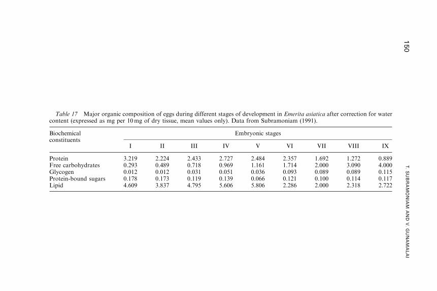
Table 17 Major organic composition of eggs during different stages of development in Emerita asiatica after correction for watercontent (expressed as mg per 10mg of dry tissue, mean values only). Data from Subramoniam (1991).

Biochemicalconstituents

Embryonic stages

I II III IV V VI VII VIII IX

Protein 3.219 2.224 2.433 2.727 2.484 2.357 1.692 1.272 0.889Free carbohydrates 0.293 0.489 0.718 0.969 1.161 1.714 2.000 3.090 4.000Glycogen 0.012 0.012 0.031 0.051 0.036 0.093 0.089 0.089 0.115Protein-bound sugars 0.178 0.173 0.119 0.139 0.066 0.121 0.100 0.114 0.117Lipid 4.609 3.837 4.795 5.606 5.806 2.286 2.000 2.318 2.722

150

T.SUBRAMONIA

MAND

V.GUNAMALAI

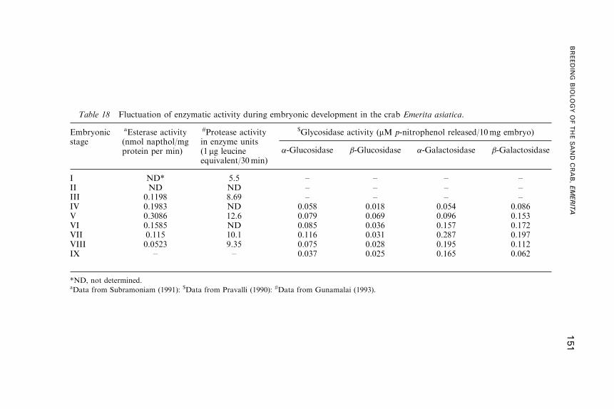
Table 18 Fluctuation of enzymatic activity during embryonic development in the crab Emerita asiatica.

Embryonicstage

aEsterase activity(nmol napthol/mgprotein per min)

#Protease activityin enzyme units(1 mg leucineequivalent/30min)

$Glycosidase activity (mM p-nitrophenol released/10mg embryo)

�-Glucosidase �-Glucosidase �-Galactosidase �-Galactosidase

I ND* 5.5 – – – –II ND ND – – – –III 0.1198 8.69 – – – –IV 0.1983 ND 0.058 0.018 0.054 0.086V 0.3086 12.6 0.079 0.069 0.096 0.153VI 0.1585 ND 0.085 0.036 0.157 0.172VII 0.115 10.1 0.116 0.031 0.287 0.197VIII 0.0523 9.35 0.075 0.028 0.195 0.112IX – – 0.037 0.025 0.165 0.062

*ND, not determined.aData from Subramoniam (1991): $Data from Pravalli (1990): #Data from Gunamalai (1993).

BREEDIN

GBIO

LOGYOFTHESAND

CRAB,EMERITA

151

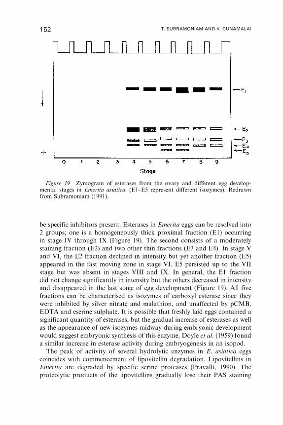
be specific inhibitors present. Esterases in Emerita eggs can be resolved into

2 groups; one is a homogeneously thick proximal fraction (E1) occurring

in stage IV through IX (Figure 19). The second consists of a moderately

staining fraction (E2) and two other thin fractions (E3 and E4). In stage V

and VI, the E2 fraction declined in intensity but yet another fraction (E5)

appeared in the fast moving zone in stage VI. E5 persisted up to the VII

stage but was absent in stages VIII and IX. In general, the E1 fraction

did not change significantly in intensity but the others decreased in intensity

and disappeared in the last stage of egg development (Figure 19). All five

fractions can be characterised as isozymes of carboxyl esterase since they

were inhibited by silver nitrate and malathion, and unaffected by pCMB,

EDTA and eserine sulphate. It is possible that freshly laid eggs contained a

significant quantity of esterases, but the gradual increase of esterases as well

as the appearance of new isozymes midway during embryonic development

would suggest embryonic synthesis of this enzyme. Doyle et al. (1959) found

a similar increase in esterase activity during embryogenesis in an isopod.

The peak of activity of several hydrolytic enzymes in E. asiatica eggs

coincides with commencement of lipovitellin degradation. Lipovitellins in

Emerita are degraded by specific serine proteases (Pravalli, 1990). The

proteolytic products of the lipovitellins gradually lose their PAS staining

Figure 19 Zymogram of esterases from the ovary and different egg develop-mental stages in Emerita asiatica. (E1–E5 represent different isozymes). Redrawnfrom Subramoniam (1991).


properties, suggestive of dissociation of the carbohydrate prosthetic groups

from the vitellins (Tirumalai, 1996). Activity of two glycosidases,

glucosidases and galactosidase, is increased in embryos at a time when the

PAS staining subsides in the vitellin fractions (Gunamalai, 1993). These

glycosidases may be required to release bound glucose and galactose from

the glycolipid and oligosaccharide components of the major yolk proteins,

as well as to hydrolyse stored glycogen during embryogenesis in E. asiatica.

Another enzyme that is active at the time of vitellin degradation in

E. asiatica is phospholipase C (Ramachandran, 1992).

Yolk utilisation in Emerita eggs necessitates extensive reshuffling of

substrates, especially during the early stages of embryonic development.

Such changes in the metabolic pathways involving interconversion of

already stored substrates within the closed system of egg development of

decapod crustaceans increase our understanding of embryonic development

in the non-cleidoic eggs of marine invertebrates. The initial high content

of lipid in Emerita egg is characteristic of lecithotrophic eggs. However, lipid

utilisation starts only from stage V onwards, suggesting that protein may

be the chief source of energy for initial embryonic development. On the

contrary, the eggs of a freshwater crab Paratelphusa hydrodromus expend

enormous reserves of lipid continuously during embryogenesis with a

concomitant increase in the protein level (Pillai and Subramoniam, 1985).

Suppression of protein utilisation and enhanced lipid metabolism is

characteristic of cleidoic eggs, a feature found also in many crustacean

species (see Pandian, 1970a). Conversely, in the bony fishes, protein is

preferentially used during the entire course of embryogenesis (Lasker, 1962).

Egg development of E. asiatica represents a condition intermediate between

cleidoic and non-cleidoic developmental extremes.

In spite of the increased utilisation of lipids in the second half of

embryogenesis, lipid is retained in the form of colourless yolk globules in the

embryo at hatching. These lipid reserves not only increase the buoyancy of

the pelagic larvae on their release, but also are useful in delaying starvation

during the rather protracted larval life of E. asiatica. In general, the protein/

lipid ratio is high in typically planktotrophic larvae such as cirripedes

(Achituv and Wortzlavski, 1983), whereas lipids form the major reserves in

lecithotrophic eggs. Although E. asiatica releases planktotrophic zoea with a

long pelagic life, it produces many yolky eggs in which the lipid/protein ratio

is much higher.

12.2. Energy utilisation in Emerita eggs

Conventionally, yolk utilisation in crustaceans and other animals has been

expressed in terms of energy value (Pandian, 1994). Therefore, we have


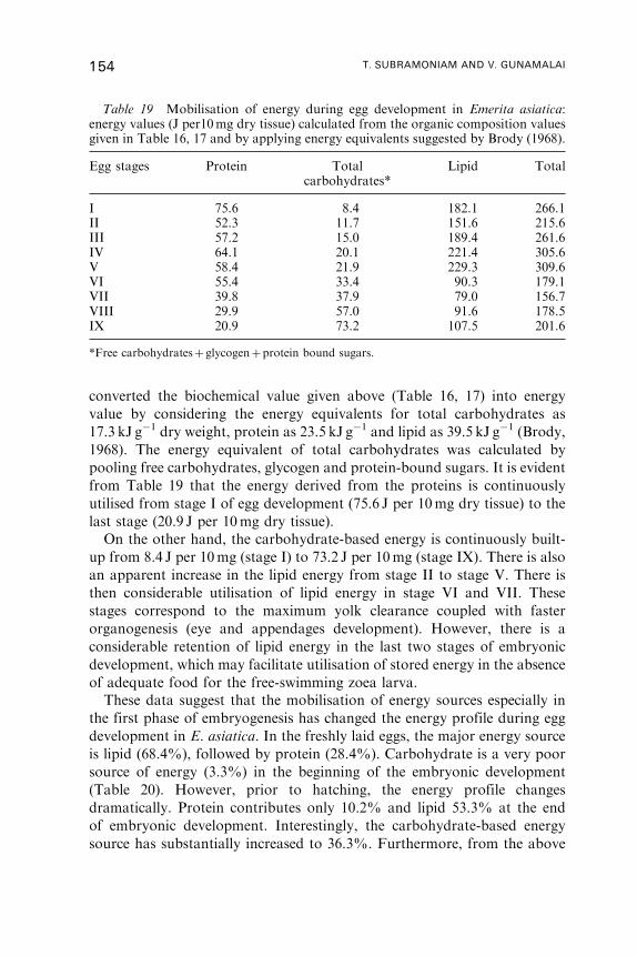
converted the biochemical value given above (Table 16, 17) into energy

value by considering the energy equivalents for total carbohydrates as

17.3 kJ g�1 dry weight, protein as 23.5 kJ g�1 and lipid as 39.5 kJ g�1 (Brody,

1968). The energy equivalent of total carbohydrates was calculated by

pooling free carbohydrates, glycogen and protein-bound sugars. It is evident

from Table 19 that the energy derived from the proteins is continuously

utilised from stage I of egg development (75.6 J per 10mg dry tissue) to the

last stage (20.9 J per 10mg dry tissue).

On the other hand, the carbohydrate-based energy is continuously built-

up from 8.4 J per 10mg (stage I) to 73.2 J per 10mg (stage IX). There is also

an apparent increase in the lipid energy from stage II to stage V. There is

then considerable utilisation of lipid energy in stage VI and VII. These

stages correspond to the maximum yolk clearance coupled with faster

organogenesis (eye and appendages development). However, there is a

considerable retention of lipid energy in the last two stages of embryonic

development, which may facilitate utilisation of stored energy in the absence

of adequate food for the free-swimming zoea larva.

These data suggest that the mobilisation of energy sources especially in

the first phase of embryogenesis has changed the energy profile during egg

development in E. asiatica. In the freshly laid eggs, the major energy source

is lipid (68.4%), followed by protein (28.4%). Carbohydrate is a very poor

source of energy (3.3%) in the beginning of the embryonic development

(Table 20). However, prior to hatching, the energy profile changes

dramatically. Protein contributes only 10.2% and lipid 53.3% at the end

of embryonic development. Interestingly, the carbohydrate-based energy

source has substantially increased to 36.3%. Furthermore, from the above

Table 19 Mobilisation of energy during egg development in Emerita asiatica:energy values (J per10mg dry tissue) calculated from the organic composition valuesgiven in Table 16, 17 and by applying energy equivalents suggested by Brody (1968).

Egg stages Protein Totalcarbohydrates*

Lipid Total

I 75.6 8.4 182.1 266.1II 52.3 11.7 151.6 215.6III 57.2 15.0 189.4 261.6IV 64.1 20.1 221.4 305.6V 58.4 21.9 229.3 309.6VI 55.4 33.4 90.3 179.1VII 39.8 37.9 79.0 156.7VIII 29.9 57.0 91.6 178.5IX 20.9 73.2 107.5 201.6

*Free carbohydratesþ glycogenþprotein bound sugars.


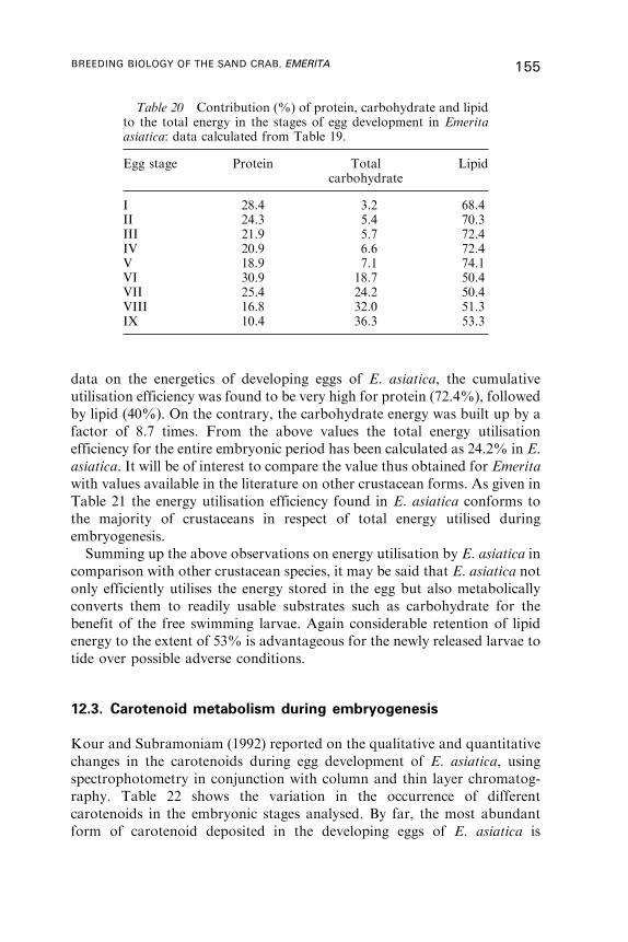
data on the energetics of developing eggs of E. asiatica, the cumulative

utilisation efficiency was found to be very high for protein (72.4%), followed

by lipid (40%). On the contrary, the carbohydrate energy was built up by a

factor of 8.7 times. From the above values the total energy utilisation

efficiency for the entire embryonic period has been calculated as 24.2% in E.

asiatica. It will be of interest to compare the value thus obtained for Emerita

with values available in the literature on other crustacean forms. As given in

Table 21 the energy utilisation efficiency found in E. asiatica conforms to

the majority of crustaceans in respect of total energy utilised during

embryogenesis.

Summing up the above observations on energy utilisation by E. asiatica in

comparison with other crustacean species, it may be said that E. asiatica not

only efficiently utilises the energy stored in the egg but also metabolically

converts them to readily usable substrates such as carbohydrate for the

benefit of the free swimming larvae. Again considerable retention of lipid

energy to the extent of 53% is advantageous for the newly released larvae to

tide over possible adverse conditions.

12.3. Carotenoid metabolism during embryogenesis

Kour and Subramoniam (1992) reported on the qualitative and quantitative

changes in the carotenoids during egg development of E. asiatica, using

spectrophotometry in conjunction with column and thin layer chromatog-

raphy. Table 22 shows the variation in the occurrence of different

carotenoids in the embryonic stages analysed. By far, the most abundant

form of carotenoid deposited in the developing eggs of E. asiatica is

Table 20 Contribution (%) of protein, carbohydrate and lipidto the total energy in the stages of egg development in Emeritaasiatica: data calculated from Table 19.

Egg stage Protein Totalcarbohydrate

Lipid

I 28.4 3.2 68.4II 24.3 5.4 70.3III 21.9 5.7 72.4IV 20.9 6.6 72.4V 18.9 7.1 74.1VI 30.9 18.7 50.4VII 25.4 24.2 50.4VIII 16.8 32.0 51.3IX 10.4 36.3 53.3


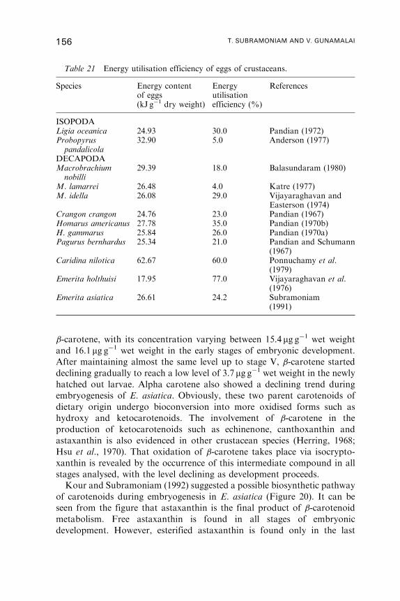
�-carotene, with its concentration varying between 15.4 mg g�1 wet weight

and 16.1 mg g�1 wet weight in the early stages of embryonic development.

After maintaining almost the same level up to stage V, �-carotene started

declining gradually to reach a low level of 3.7 mg g�1 wet weight in the newly

hatched out larvae. Alpha carotene also showed a declining trend during

embryogenesis of E. asiatica. Obviously, these two parent carotenoids of

dietary origin undergo bioconversion into more oxidised forms such as

hydroxy and ketocarotenoids. The involvement of �-carotene in the

production of ketocarotenoids such as echinenone, canthoxanthin and

astaxanthin is also evidenced in other crustacean species (Herring, 1968;

Hsu et al., 1970). That oxidation of �-carotene takes place via isocrypto-

xanthin is revealed by the occurrence of this intermediate compound in all

stages analysed, with the level declining as development proceeds.

Kour and Subramoniam (1992) suggested a possible biosynthetic pathway

of carotenoids during embryogenesis in E. asiatica (Figure 20). It can be

seen from the figure that astaxanthin is the final product of �-carotenoid

metabolism. Free astaxanthin is found in all stages of embryonic

development. However, esterified astaxanthin is found only in the last

Table 21 Energy utilisation efficiency of eggs of crustaceans.

Species Energy contentof eggs(kJ g�1 dry weight)

Energyutilisationefficiency (%)

References

ISOPODALigia oceanica 24.93 30.0 Pandian (1972)Probopyruspandalicola

32.90 5.0 Anderson (1977)

DECAPODAMacrobrachiumnobilli

29.39 18.0 Balasundaram (1980)

M. lamarrei 26.48 4.0 Katre (1977)M. idella 26.08 29.0 Vijayaraghavan and

Easterson (1974)Crangon crangon 24.76 23.0 Pandian (1967)Homarus americanus 27.78 35.0 Pandian (1970b)H. gammarus 25.84 26.0 Pandian (1970a)Pagurus bernhardus 25.34 21.0 Pandian and Schumann

(1967)Caridina nilotica 62.67 60.0 Ponnuchamy et al.

(1979)Emerita holthuisi 17.95 77.0 Vijayaraghavan et al.

(1976)Emerita asiatica 26.61 24.2 Subramoniam

(1991)


Table 22 Carotenoid content in different egg developmental stages of Emerita asiatica (mg/g wet weight). Data from Kour andSubramoniam (1992).

Carotenoids Stage

I III V VII VIII IX X

�-carotene 0.853±0.056 0.921±0.189 1.490±0.026 0.833±0.013 0.960±0.012 0.031±0.002 -�-carotene 15.560±0.122 16.072±0.141 15.445±0.087 14.320±0.097 12.220±0.034 7.220±0.034 3.700±0.069Lutein 2.080±0.067 – – – – – –Echinenone 0.846±0.031 1.960±0.036 3.540±0.036 – – – –Isozeaxanthin 4.373±0.068 1.500±0.019 3.540±0.039 3.380±0.048 0.031±0.010 – –Zeaxanthin 4.034±0.045 – 4.510±0.058 4.093±0.248 – 5.971±0.372 –Canthaxanthin – – – 2.972±0.323 5.806±0.528 4.613±0.264 2.606±0.264�-doradexanthin – – – – – – 0.666±0.117Isocryptoxanthin 6.712±0.198 5.100±0.197 3.910±0.153 3.630±0.161 2.540±0.236 2.136±0.142 2.104±0.173Free astaxanthin 0.600±0.022 0.216±0.016 0.686±0.034 0.608±0.016 1.192±0.055 2.440±0.100 0.848±0.044Esterified astaxanthin – – – – – – 4.280±0.018

BREEDIN

GBIO

LOGYOFTHESAND

CRAB,EMERITA

157

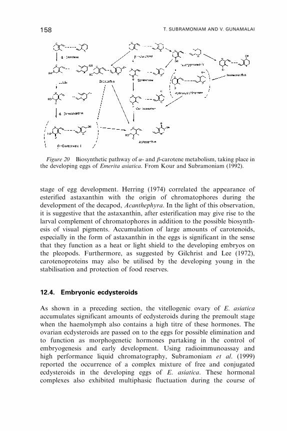
stage of egg development. Herring (1974) correlated the appearance of

esterified astaxanthin with the origin of chromatophores during the

development of the decapod, Acanthephyra. In the light of this observation,

it is suggestive that the astaxanthin, after esterification may give rise to the

larval complement of chromatophores in addition to the possible biosynth-

esis of visual pigments. Accumulation of large amounts of carotenoids,

especially in the form of astaxanthin in the eggs is significant in the sense

that they function as a heat or light shield to the developing embryos on

the pleopods. Furthermore, as suggested by Gilchrist and Lee (1972),

carotenoproteins may also be utilised by the developing young in the

stabilisation and protection of food reserves.

12.4. Embryonic ecdysteroids

As shown in a preceding section, the vitellogenic ovary of E. asiatica

accumulates significant amounts of ecdysteroids during the premoult stage

when the haemolymph also contains a high titre of these hormones. The

ovarian ecdysteroids are passed on to the eggs for possible elimination and

to function as morphogenetic hormones partaking in the control of

embryogenesis and early development. Using radioimmunoassay and

high performance liquid chromatography, Subramoniam et al. (1999)

reported the occurrence of a complex mixture of free and conjugated

ecdysteroids in the developing eggs of E. asiatica. These hormonal

complexes also exhibited multiphasic fluctuation during the course of

Figure 20 Biosynthetic pathway of �- and �-carotene metabolism, taking place inthe developing eggs of Emerita asiatica. From Kour and Subramoniam (1992).


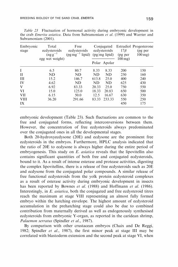
embryonic development (Table 23). Such fluctuations are common to the

free and conjugated forms, reflecting interconversions between them.

However, the concentration of free ecdysteroids always predominated

over the conjugated ones in all the developmental stages.

Both 20-hydroxyecdysone (20E) and ecdysone are the prominent free

ecdysteroids in the embryos. Furthermore, HPLC analysis indicated that

the ratio of 20E to ecdysone is always higher during the entire period of

embryogenesis. This study on E. asiatica reveals that the lipovitellin also

contains significant quantities of both free and conjugated ecdysteroids,

bound to it. As a result of intense esterase and protease activities, digesting

the complex lipovitellins, there is a release of free ecdysteroids such as 20E

and ecdysone from the conjugated polar compounds. A similar release of

free functional ecdysteroids from the yolk protein ecdysteroid complexes

as a result of esterase activity during embryonic development in insects

has been reported by Bownes et al. (1988) and Hoffmann et al. (1986).

Interestingly, in E. asiatica, both the conjugated and free ecdysteroid titres

reach the maximum at stage VIII representing an almost fully formed

embryo within the hatching envelope. The highest amount of ecdysteroid

accumulation in the prehatching stage could also be due to combined

contribution from maternally derived as well as endogenously synthesised

ecdysteroids from embryonic Y-organ, as reported in the caridean shrimp,

Palaemon serratus (Spindler et al., 1987).

By comparison with other crustacean embryos (Chaix and De Reggi,

1982; Spindler et al., 1987), the first minor peak at stage III may be

correlated with blastoderm extension and the second peak at stage VI, when

Table 23 Fluctuation of hormonal activity during embryonic development inthe crab Emerita asiatica. Data from Subramoniam et al. (1999) and Warrier andSubramoniam (2001).

Embryonicstage

Totalecdysteroids

(ng g�1

egg wet weight)

Freeecdysteroids

(pgmg�1 lipid)

Conjugatedecdysteroids(pg/mg lipid)

Estradiol17�

(pg per100mg)

Progesterone(pg per100mg)

Polar Apolar

I 6.5 80.7 8.33 8.33 200 150II ND ND ND ND 250 160III 15.2 146.7 613.8 25.0 400 240IV 4.62 ND ND ND 625 430V 6.92 83.33 20.33 25.0 750 550VI 15.0 125.0 18.33 20.83 650 500VII 6.15 50.0 12.5 16.67 630 350VIII 36.20 291.66 83.33 233.33 550 250IX 450 175


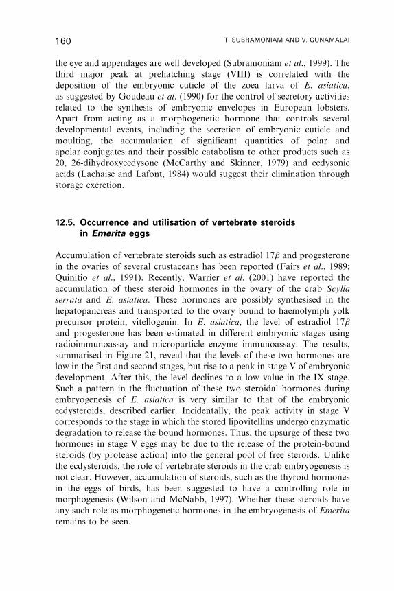
the eye and appendages are well developed (Subramoniam et al., 1999). The

third major peak at prehatching stage (VIII) is correlated with the

deposition of the embryonic cuticle of the zoea larva of E. asiatica,

as suggested by Goudeau et al. (1990) for the control of secretory activities

related to the synthesis of embryonic envelopes in European lobsters.

Apart from acting as a morphogenetic hormone that controls several

developmental events, including the secretion of embryonic cuticle and

moulting, the accumulation of significant quantities of polar and

apolar conjugates and their possible catabolism to other products such as

20, 26-dihydroxyecdysone (McCarthy and Skinner, 1979) and ecdysonic

acids (Lachaise and Lafont, 1984) would suggest their elimination through

storage excretion.

12.5. Occurrence and utilisation of vertebrate steroids

in Emerita eggs

Accumulation of vertebrate steroids such as estradiol 17� and progesterone

in the ovaries of several crustaceans has been reported (Fairs et al., 1989;

Quinitio et al., 1991). Recently, Warrier et al. (2001) have reported the

accumulation of these steroid hormones in the ovary of the crab Scylla

serrata and E. asiatica. These hormones are possibly synthesised in the

hepatopancreas and transported to the ovary bound to haemolymph yolk

precursor protein, vitellogenin. In E. asiatica, the level of estradiol 17�

and progesterone has been estimated in different embryonic stages using

radioimmunoassay and microparticle enzyme immunoassay. The results,

summarised in Figure 21, reveal that the levels of these two hormones are

low in the first and second stages, but rise to a peak in stage V of embryonic

development. After this, the level declines to a low value in the IX stage.

Such a pattern in the fluctuation of these two steroidal hormones during

embryogenesis of E. asiatica is very similar to that of the embryonic

ecdysteroids, described earlier. Incidentally, the peak activity in stage V

corresponds to the stage in which the stored lipovitellins undergo enzymatic

degradation to release the bound hormones. Thus, the upsurge of these two

hormones in stage V eggs may be due to the release of the protein-bound

steroids (by protease action) into the general pool of free steroids. Unlike

the ecdysteroids, the role of vertebrate steroids in the crab embryogenesis is

not clear. However, accumulation of steroids, such as the thyroid hormones

in the eggs of birds, has been suggested to have a controlling role in

morphogenesis (Wilson and McNabb, 1997). Whether these steroids have

any such role as morphogenetic hormones in the embryogenesis of Emerita

remains to be seen.


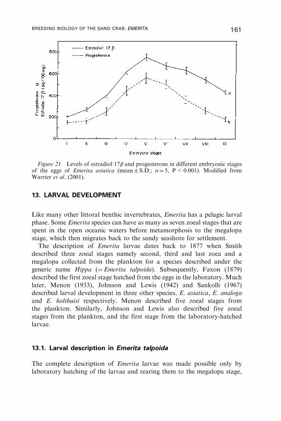
13. LARVAL DEVELOPMENT

Like many other littoral benthic invertebrates, Emerita has a pelagic larval

phase. Some Emerita species can have as many as seven zoeal stages that are

spent in the open oceanic waters before metamorphosis to the megalopa

stage, which then migrates back to the sandy seashore for settlement.

The description of Emerita larvae dates back to 1877 when Smith

described three zoeal stages namely second, third and last zoea and a

megalopa collected from the plankton for a species described under the

generic name Hippa (¼Emerita talpoida). Subsequently, Faxon (1879)

described the first zoeal stage hatched from the eggs in the laboratory. Much

later, Menon (1933), Johnson and Lewis (1942) and Sankolli (1967)

described larval development in three other species, E. asiatica, E. analoga

and E. holthuisi respectively. Menon described five zoeal stages from

the plankton. Similarly, Johnson and Lewis also described five zoeal

stages from the plankton, and the first stage from the laboratory-hatched

larvae.

13.1. Larval description in Emerita talpoida

The complete description of Emerita larvae was made possible only by

laboratory hatching of the larvae and rearing them to the megalopa stage,

Figure 21 Levels of estradiol 17� and progesterone in different embryonic stagesof the eggs of Emerita asiatica (mean� S.D.; n¼ 5, P<0.001). Modified fromWarrier et al. (2001).


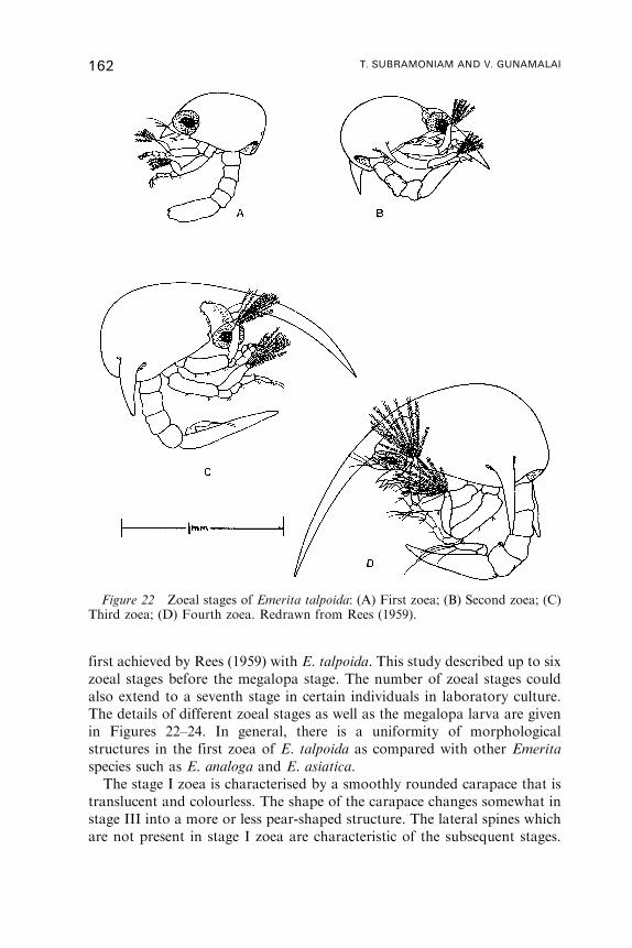
first achieved by Rees (1959) with E. talpoida. This study described up to six

zoeal stages before the megalopa stage. The number of zoeal stages could

also extend to a seventh stage in certain individuals in laboratory culture.

The details of different zoeal stages as well as the megalopa larva are given

in Figures 22–24. In general, there is a uniformity of morphological

structures in the first zoea of E. talpoida as compared with other Emerita

species such as E. analoga and E. asiatica.

The stage I zoea is characterised by a smoothly rounded carapace that is

translucent and colourless. The shape of the carapace changes somewhat in

stage III into a more or less pear-shaped structure. The lateral spines which

are not present in stage I zoea are characteristic of the subsequent stages.

Figure 22 Zoeal stages of Emerita talpoida: (A) First zoea; (B) Second zoea; (C)Third zoea; (D) Fourth zoea. Redrawn from Rees (1959).


The rostrum is short and broad in stage I zoea and continues to elongate

and reaches about one and a half times the length of the carapace. The

eyestalks are short and thick and lie close against the carapace, directed

somewhat posteriorly. In the subsequent zoeal stages, the eyestalks increase

in length and the eyes are carried somewhat farther forward than in the first

stage. In the megalopa stage, which resembles the adult, the eyes are still

relatively large as compared to the adult.

The antennules in stage I zoea are short unjointed appendages which are

thick at the base and taper to a blunt point where three setae of about equal

Figure 23 Zoeal stages of Emerita talpoida: (E) Fifth zoea; (F) Sixth zoea.Redrawn from Rees (1959).


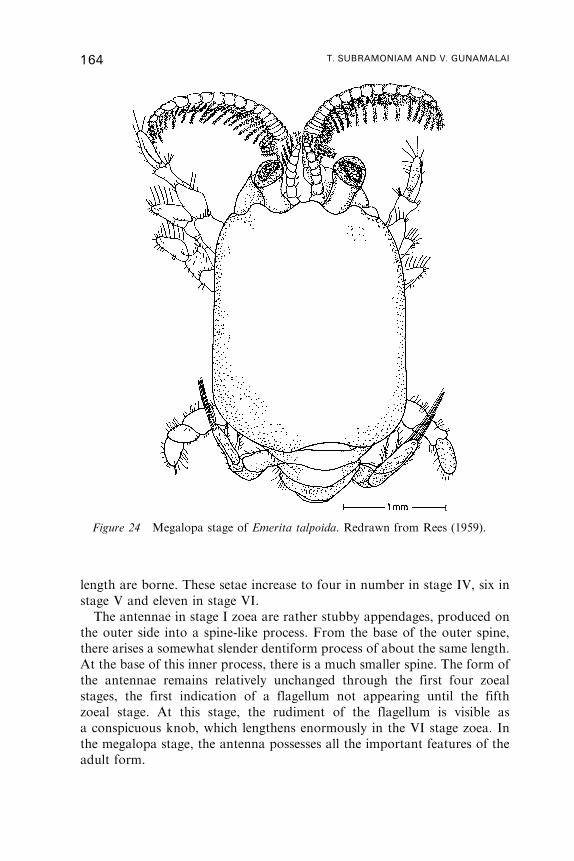
length are borne. These setae increase to four in number in stage IV, six in

stage V and eleven in stage VI.

The antennae in stage I zoea are rather stubby appendages, produced on

the outer side into a spine-like process. From the base of the outer spine,

there arises a somewhat slender dentiform process of about the same length.

At the base of this inner process, there is a much smaller spine. The form of

the antennae remains relatively unchanged through the first four zoeal

stages, the first indication of a flagellum not appearing until the fifth

zoeal stage. At this stage, the rudiment of the flagellum is visible as

a conspicuous knob, which lengthens enormously in the VI stage zoea. In

the megalopa stage, the antenna possesses all the important features of the

adult form.

Figure 24 Megalopa stage of Emerita talpoida. Redrawn from Rees (1959).


The mandible in the stage I zoea consists of an armed crown on its ventral

edge followed by sharp triangular teeth. These appendages change very

little, except for a general increase in size, throughout the zoeal stages. In the

megalopa stage, the mandible has undergone a complete change in structure

and function. It is no longer an organ of mastication but is adapted, as in

the adult, for the purpose of scraping the antennae and passing food to

the mouth.

In the case of the maxillae and the maxillipeds, the structures remain more

or less unchanged in the zoeal stages except for the increase in the number of

setae in the second maxilla and the maxillipeds. In the megalopa stage, these

structures possess all the parts of the adult appendage.

The abdomen in the stage I zoea is composed of five segments projecting

almost straight downward from the carapace, and is flexed so that the telson

is carried beneath and parallel to the carapace. At this stage, no rudiments

of the abdominal appendages are visible. The sixth segment is consolidated

with the telson; this becomes apparent when the uropods appear in the III

stage zoea. The uropod consists of a short basal segment with a long,

flattened lobe extending from it. In stage IV zoea, the four free segments

of the abdomen bears two small round thickenings on its inner side, the

evidence of future pleopods, which eventually appear in the stage VI zoea.

The pleopods are uniramous, unsegmented and appear on the second

through fifth abdominal segments. The abdomen in the megalopa stage is

composed of six segments, which are similar in form and proportion to

those of the adult. In contrast to the uniramous pleopods of the zoeal stages,

the megalopa stage bears four pairs of biramous pleopods.

13.2. Larval dispersal and megalopa settlement

In the temperate species, such as E. analoga, eggs are laid in the summer

months and after incubation on the pleopods for about a month, give rise to

zoeae, which are released into the plankton. Johnson (1940) estimated the

time spent as zoea in the plankton to be about four and a half months, after

analysing planktonic materials collected from tows off the coast of

California. Following this, Johnson and Lewis (1942) described the zoeal

stages of E. analoga from the plankton and suggested that they passed

through at least five stages before moulting to the megalopa. The duration

of larval development is also variable; for E. talpoida the laboratory rearing

took 30 days (Rees, 1959) whereas, E. rathbunae took about 90 days

(Knight, 1967). From laboratory rearing, Efford (1970) observed that the

zoea larvae of E. analoga passed through as many as 9 moults in a total time

duration of 130 days, before metamorphosing into megalopa. He also


observed that moulting into megalopa could occur at 8th or 9th zoeal moult.

Although Hanson (1969) contended that the larval development in the

Hippidae was temperature dependent, such variations in the larval duration,

especially from the estimates of laboratory rearing and plankton analysis

could not be explained in terms of temperature difference. The duration

of the later stages is also so variable that there is a possibility that one or

two stages from metamorphosis to megalopa are skipped if conditions are

ideal for settlement on the beach. Similarly, the larvae may have the

ability to delay metamorphosis if settlement conditions are unfavourable.

This feature increases the chances for selection of a suitable substratum,

thus contributing to the success of the population (Thorson, 1950; Wilson,

1952).

Along the ocean coasts where the shelf is rather narrow and the deep sea

is not far off, strong currents may carry the larvae away from their littoral

and shallow water habitat. Johnson (1939), correlated water movements and

the dispersal of pelagic zoea larvae of E. analoga along the southern

Californian coast. He observed that the fourth zoeal stage of this sand crab

is taken in plankton hauls at a distance of 125–130miles from the mainland

shores. However, the first zoeal stage, with a 4 week larval life in laboratory

rearing, was found in plankton taken less than 20miles from the shore.

Evidently, such a long journey offshore for development and metamor-

phosis into megalopa would cause a large wastage of larvae as suggested for

oyster larvae by Korringa (1947).

After spending a varying period of time in the plankton, zoea larvae

of E. analoga metamorphose into megalopae and start arriving in large

numbers in early April with a peak influx in early June at the Scripps beach,

La Jolla (Efford, 1965). However, Wenner (personal communication quoted

by Efford, 1970) observed the arrival of megalopae in the winter months of

1965–1966 on the beaches at Goleta, just south of Point Conception. Such

differences in the recruitment period on different beaches along the west

coast of North America may suggest that the timing of maximum

recruitment perhaps depends largely on the distribution of the later zoeal

stages in relation to local hydrographic conditions (Johnson, 1940; Efford,

1965; Barnes and Wenner, 1968; Cox and Dudley, 1968).

Seasonality of the megalopa settlement in temperate species can be

related to the seasonal reproductive cycle. With tropical species, such as

the E. asiatica, that breed all through the year, we would expect to have a

continuous or near continuous settlement pattern of megalopae. Year-

round egg laying, coupled with continuous embryonic development of

pleopodal eggs results in uninterrupted release of zoea larvae into the

plankton. Hence, larval availability for metamorphosis to the megalopa

stage and settlement occurs throughout the year. Yet, even on tropical

beaches, seasonality in the megalopa settlement has been reported,


probably influenced by factors other than temperature. Menon (1933), by

studying the occurrence of planktonic larvae of E. asiatica from the

offshore waters of the Madras coast found the early stage zoea larvae

abundant in September to November while in the succeeding months only

the advanced stage larvae were present. The settlement of the megalopa

larvae on this beach subsequently took place in April. This author

apparently assumed that the planktonic larvae released from the same

beach undergo development in the offshore waters and that they return to

the same beach to restock the parent population. This would suggest an

annual growth pattern for E. asiatica. However, later work by

Subramoniam (1979a) on E. asiatica from the same locality has shown a

year-round egg production coupled with uninterrupted zoea larval release.

Consequently, their larval stock is more or less equally distributed in the

plankton all year round. The megalopa settlement of E. asiatica on

the Marina beach at Madras takes place first in June, corresponding to the

onset of southwest monsoon rain and the second one in October and

November, when the northeast monsoon brings heavy rain to this region

(Subramoniam, 1979a). Similarly, Ansell et al., (1972) have documented

the seasonal recruitment pattern during the premonsoon and monsoon

months for E. holthuisi from the west coast of south India, suggesting a

relationship between the monsoon rains and the megalopa settlement on

the Indian coasts. Evidently, hydrographical conditions prevailing on the

sandy beach determine the settlement time of the megalopa larvae.

It is clear from the above account that the development, dispersion and

settlement of the Emerita larvae depends mostly on hydrographic factors.

Different species of Emerita inhabit long coastlines and hence, the dispersive

power of their larvae not only augments the existing population, but also

establishes new colonies in the beach. High exchange of genetic characters

between populations is predictable as a result of this larval dispersal.

Furthermore, gene flow may be enhanced by the possibility of multiple

fertilisation of the females. Gene flow could offset the expected Hardy-

Weinberg equilibrium in genotype frequencies in different populations.

Despite these factors, Corbin (1977) found distinct allelic groups of

E. talpoida colonising locations in North and South Carolina, based on

polymorphisms of the phosphoglucoisomerase enzymes. Distinct allelic

groups of local populations could be traced back to the Florida coast. This

indicates that, besides a certain degree of horizontal gene flow amongst

different regions, local selection pressures might favour different allelic

groups in different local populations. An interesting observation in this

connection is that the female population of E. asiatica at Marina beach in

Madras grows to a maximum size of 33mmCL, whereas the population of

the same species at Kovalam and Kalpakkam coasts, just 40 km to the

south, invariably reaches sizes of up to 40mmCL.


Beckwitt’s (1985) studies on E. analoga populations of southern

California revealed lack of genetic differentiation among six samples of

the study area indicating free horizontal gene flow within the species related

to their dispersal abilities. The greatest difference in allelic frequencies was

observed within two regions separated by only 7 km, indicating that local

selection pressures might be involved.

14. EMERITA AS INDICATOR SPECIES

Extensive data on the biology of Emerita may contribute to their suitability

as ‘‘indicator species’’ to investigate pollution on sandy beaches. Ever since

Burnett (1971) reported on the bioaccumulation of DDT residues in E.

analoga, this intertidal crab has served to indicate high pollution levels of

DDT in Santa Monica Bay, California. Interestingly, the bioaccumulated

DDT in the body tissues is transferred to the eggs, which after spawning and

attachment to the pleopodal hairs remain undeveloped. That pollution on

the sandy beach could cause abnormal reproduction in the sand crab has

been clearly indicated by Siegel and Wenner (1984). These authors, studying

the fecundity potentials of E. analoga in the vicinity of a nuclear generating

station in Southern California (SONGS), found that a reduction in

reproduction was not related to thermal enhancement associated with the

operation of nuclear generating facilities. Instead it seemed to result from

multifarious factors such as runoff of agricultural pesticides from a creek

3 km north of the nuclear generating plant, and the release of metals into

nearshore waters.

High levels of copper and zinc were reported in the body tissues of E.

analoga in the vicinity of SONGS, near Santa Barbara, implying specifically

that harmful metal contaminants in the environment might affect egg

production and egg quality in these crabs (Siegel and Wenner, 1984). In the

impacted area, egg membranes of the egg masses were found to be ruptured

soon after egg extrusion. A similar incidence of egg disruption was reported

by Wenner (1982) for a crab population at San Clemente Beach. When the

sand crabs from the impacted area were brought back to the laboratory,

they produced normal eggs, which underwent normal development to hatch

into healthy zoeae. Apparently, some factors emanating from metal

pollution in the beach could be responsible for the disruption of egg

membranes of the sand crabs. In addition, Wenner et al. (1985) found that

the size at onset of egg production was reduced in the crabs living in a

stressed habitat, in comparison with those living in nonimpacted areas.

Furthermore, Auyong (1981) found that the egg production season in the

impacted area was shorter. Evidently, both organic and inorganic pollutants


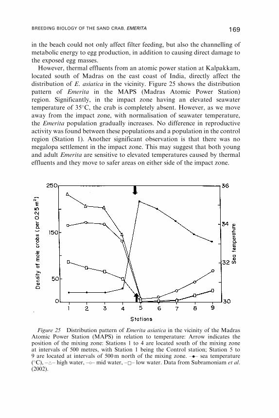
in the beach could not only affect filter feeding, but also the channelling of

metabolic energy to egg production, in addition to causing direct damage to

the exposed egg masses.

However, thermal effluents from an atomic power station at Kalpakkam,

located south of Madras on the east coast of India, directly affect the

distribution of E. asiatica in the vicinity. Figure 25 shows the distribution

pattern of Emerita in the MAPS (Madras Atomic Power Station)

region. Significantly, in the impact zone having an elevated seawater

temperature of 35�C, the crab is completely absent. However, as we move

away from the impact zone, with normalisation of seawater temperature,

the Emerita population gradually increases. No difference in reproductive

activity was found between these populations and a population in the control

region (Station 1). Another significant observation is that there was no

megalopa settlement in the impact zone. This may suggest that both young

and adult Emerita are sensitive to elevated temperatures caused by thermal

effluents and they move to safer areas on either side of the impact zone.

Figure 25 Distribution pattern of Emerita asiatica in the vicinity of the MadrasAtomic Power Station (MAPS) in relation to temperature: Arrow indicates theposition of the mixing zone: Stations 1 to 4 are located south of the mixing zoneat intervals of 500 metres, with Station 1 being the Control station; Station 5 to9 are located at intervals of 500m north of the mixing zone. –�– sea temperature(�C), –i– high water, –�– mid water, –&– low water. Data from Subramoniam et al.(2002).


14.1. Parasitisation of egg mass and ovary

Reproductive failure may also be caused by natural agents such as egg

predators (Kuris, 1991) or other parasites. In E. asiatica, the eggs attached

to the pleopods have been found to be occasionally parasitised by nemertean

worms: these worms eat the eggs and assume their bright orange colour

(Subramoniam, 1979a). Although the occurrence of nemertean worms has

been recorded in the egg masses of the crabs Portumanus ocellatus and

Carcinus maenas (MacGinitie and MacGinitie, 1949) and in the kelp crab

Pugettia producta (Boolootian et al., 1959), only in E. asiatica have these

worms been found to feed on the eggs. In addition, a vorticellid has also

been associated with the egg-carrying pleopods (Krishnaswamy, 1954). The

ovary of E. asiatica is invariably infested with numerous metacercaria of a

larval trematode belonging to the genus Microphallus (Anantharaman and

Subramoniam, 1976). The metacercariae are lodged only in the connective

tissue epithelium surrounding the ovary and do not enter the ovary proper

(Figure 5E); the midgut gland tubules are not infected except in extreme

parasitisation, suggesting that the ovary is the primary tissue of infection.

However, Young (1938) has observed that the midgut gland is the main site

of metacercarial infection in E. analoga. Apparently, metacercarial

association with the ovary of Emerita has no effect on oogenesis, but

under heavy infestation, ovulation is incomplete, many ripe eggs remaining

unspawned (Subramoniam, 1977a). Helminth infections on the ovary of the

sand crabs also include the capsules of a tetraphyllidean larvae, belonging to

the genus Phyllobothrium (Anantharaman and Subramoniam, 1980).

Obviously, these crustaceans constitute the second intermediate host for

these parasites that reach their final host in fishes and sea birds.

15. CONCLUSIONS

Mole crabs belonging to the genus Emerita are exclusively inhabitants of

exposed sandy beaches in certain temperate and tropical seas. The main

adaptive features for the sandy beach environment are the burrowing

behaviour and the mode of filter feeding with a pair of long plumose

antennules. While the morphology and behaviour of the mole crabs

reflect the adaptive attributes of the species to the environment,

peculiarities found in their sexual and reproductive biology imply a

complex life history pattern. Filter feeding in Emerita species, coupled

with the continuous availability of detrital food in the intertidal zone

confers a favourable nutritional status to help ensure successful

reproduction and moulting throughout the year, as shown in E. asiatica.


A perfect endocrine coordination of these two energy-demanding

processes is assumed to bring about the continued body growth even in

egg laying adults. Detailed analysis of the egg components and of

their efficient utilisation during embryogenesis, has unravelled the crab’s

ability to produce healthy larvae, to be released into the open ocean for

their subsequent development and metamorphosis. The protracted

larval development, coupled with their dispersion, aided by ocean and

nearshore water currents, enable them to spread far with the water

masses, to settle in new areas and found new populations. Nevertheless,

hydrographical conditions prevailing over the sandy beach intertidal zone

may have a deciding role in the recruitment of the megalopa stage to the

beach.

The occurrence of neotenic males in the majority of Emerita species is

again an adaptation to achieve easy sperm transfer via spermatophores

deposited on the females, without affecting their normal activities.The sticky

nature of the mucoid spermatophoric ribbon ensures fast and firm

attachment to the ventral sternum of the females. Yet another feature of

interest in the reproductive biology of a tropical species, E. asiatica is the

occurrence of functional protandric hermaphroditism. This pattern of

sexuality in the life history of this mole crab is of great adaptive significance

because it vastly augments fecundity, by introducing the secondary females

into the egg-laying female population. Obviously, natural selection

has favoured a smaller size of males to accomplish mating in a turbulent

environment, whereas the sex reversal of males at a larger size to enter

the egg-laying population of female Emerita increases fecundity. Emerita

is an ideal intertidal genus in which to investigate environmental influences

on the growth and reproductive performance in an otherwise harsh

substratum which provides habitation only to a few specialised invertebrate

forms.

ACKNOWLEDGEMENTS

We thank the Council of Scientific and Industrial Research, New Delhi

for financial support (Grant no. 21(0492)01/EMR-II/dt. 27.4.01). Grateful

thanks are also due to Dr. E. Vivekanandan of the Central Marine

Fisheries Institute substation at Chennai and Prof. Jeyaraman,

Department of Genetics, IBMS, University of Madras and to former

student Dr. R. Tirumalai for discussion during the preparation of this

article. We also thank Mr. Sunil Israel and Ms. Santhoshi of the Unit

of Invertebrate Reproduction and Aquaculture for their editorial

assistance.


REFERENCES

Achituv, Y. and Wortzlavski, A. (1983). Studies in the biochemistry of cirripede eggsVII. Changes in the general biochemical composition during development ofChthamalus dentatus Krauss and Octomeris angulosa Sowerby. Journal ofExperimental Marine Biology and Ecology 69, 137–144.

Achuthankutti, C. T. and Wafar, M. V. M. (1976). Ecology of sandy beach at SanCoale, Goa: Part II. Population model and production of Emerita holthuisiSankolli. Indian Journal of Marine Sciences 5, 98–102.

Adiyodi, R. G. (1988). Reproduction and development. In ‘‘Biology of the LandCrabs’’ (W. W. Burggren and B. R. McMahon, eds.), pp. 139–185, CambridgeUniversity Press, New York.

Adiyodi, R. G. and Subramoniam, T. (1983). Oogenesis, oviposition and oosorption,Arthropoda - Crustacea. In ‘‘Reproductive Biology of Invertebrates (K. G.Adiyodi and R. G. Adiyodi, eds.), Vol. I, pp. 443–495, John Wiley and Sons Ltd.,Chichester.

Alikunhi, K. H. (1944). Zonal distribution of Emerita. Journal of the BombayNatural History Society 45, 94–96.

Amato, G. D. and Payen, G. G. (1978). Mise en evidence du controle endocrine desdifferentes etapes de la spermatogenise chez l’ecrevisse Pontastacus leptodactylusleptodactylus (Eschscholtz, 1823) Crustace, Decapode, Reptantia. General andComparative Endocrinology 36, 487–496.

Anantharaman, S. and Subramoniam, T. (1976). On a microphallidmetacercaria occurring in the ovaries of the sand crabs Emerita asiatica andAlbunia symnista on the Madras coast. Proceedings of the Indian Academyof Sciences 84B, 192–199.

Anantharaman, S. and Subramoniam, T. (1980). A tetraphyllidean larva(Genus Phyllobothrium) from the ovaries of the sand crabs, AlbuneaSymnista and Emerita asiatica of the Madras coast. Current Science 49,449–450.

Anderson, G. (1977). The effects of parasitism on energy flow through laboratoryshrimp populations. Marine Biology 42, 235–252.

Ansell, A. D., Sivadas, P., Narayanan, B. and Trevallion, A. (1972). The ecology oftwo sandy beaches in south western India, II. Notes on Emerita holthuisi. MarineBiology 17, 311–317.

Auyong, J. (1981). Comparison of population structure of sand crab (Emeritaanaloga Stimpson) living at increasing distances from a power plant. M. Sc. Thesis,University of California, Santa Barbara, 90 pp.

Balasundaram, C. (1980). Ecophysiological studies in prawn culture (Macrobrachiumnobilli), Ph. D. Thesis, Madurai Kamaraj University, India.

Barnard, K. H. (1950). Descriptive catalogue of South African decapod Crustacea.Annals of the South African Museum 38, 1–837.

Barnes, N. B. and Wenner, A. M. (1968). Seasonal variation in the sand crab Emeritaanaloga (Decapoda: Hippidae) in the Santa Barbara area of California. Limnologyand Oceanography 13, 465–476.

Beckwitt, R. (1985). Population genetics of the sand crab, Emerita analoga Stimpsonin southern California. Journal of Experimental Marine Biology and Ecology 91,45–52.

Berman, P. W. and Lasky, L. A. (1985). Engineering glycoproteins for use aspharmaceuticals. Trends in Biotechnology 3, 51–53.


Berreur-Bonnenfant, J. (1963). Autodifferentiation ovarienne dans les gonades malesde Crustaces en culture in vitro. Bulletin de la Societe zoologique de France 88,235–238.

Bloch, F. (1935). Contribution a l’ etude des gametes et de la fecondation chezles crustaces decapodes. Travaux de la Station Zoologique de Wimereux12, 185–279.

Boolootian, R. A., Giese, A. C., Farmanfarmian, A. and Tucker, J.(1959). Reproductive cycles of five west coast crabs. Physiological Zoology32, 213–220.

Bownes, M., Shirras, A., Blair, M., Collins, J. and Coulson, A. (1988). Evidence thatinsect embryogenesis is regulated by ecdysteroids released from yolk proteins.Proceedings of the National Academy of Sciences, USA 85, 1554–1557.

Brody, S. (1968). Bioenergetics and growth. Hafner Publishing Corporation,New York, 1023 pp.

Brunet, P. C. J. (1980). The metabolism of the aromatic amino acids concerned in thecross-linking of insect cuticle. Insect Biochemistry 10, 467–500.

Burnett, R. (1971). DDT residues: distribution of concentration in Emerita analoga(Stimpson) along coastal California. Science 174, 606–608.

Carlisle, D. B. (1959). On the sexual biology of Pandalus borealis (Crustacea:Decapoda). I. Histology of incretory elements. Journal of the Marine BiologicalAssociation of the United Kingdom 38, 381–394.

Chaix, J. C. and De Reggi, M. (1982). Ecdysteroid levels during ovariandevelopment and embryogenesis in the spider crab Acanthonyx lunulatus.General and Comparative Endocrinology 47, 7–14.

Chang, E. S. (1991). Crustacean moulting hormones: cellular effects, role inreproduction and regulation by moult-inhibiting hormone. In ‘‘Frontiers inShrimp Research’’ (M. A. Davidson and W. J. Dougherty, eds.), pp. 83–105,Elsevier Science Publishers, Amsterdam, Netherlands.

Charniaux-Cotton, H. (1959). Masculinisation des femelles de la Crevette ahermaphrodisme Proterandrique Lysmata seticaudata, Par greff de glandesandrogenes. Interpretation de l’hermaphrodisme chez les Decapodes. Notepreliminaire. Competes Rendus de l’Academie des Sciences, Paris 249, 1580–1582.

Charniaux-Cotton, H. (1960a). Sex determination. In ‘‘The Physiology ofCrustacea’’ (T. H. Waterman, ed.), Vol. I, pp. 411–447, Academic Press,New York.

Charniaux-Cotton, H. (1960b). Physiologie de l’inversion sexuelle chez la Crevette ahermaphrodisme proterandrique functionnel, Lysmata seticaudata. ComptesRendus de l’Academie des Sciences, Paris 250, 4046–4048.

Charniaux-Cotton, H. (1965a). Hormonal control of sex differentiation ininvertebrates. In ‘‘Organogenesis’’ (R. L. DeHaan and H. Ursprung, eds.),pp. 701–740, Holt, Rinehart and Winston, New York. 804 pp.

Charniaux-Cotton, H. (1975b). L’ovogenese et sa regulation chez les crustacessuperieurs. Annales Biologie Animaux, Biochimie, Biophysique 15, 715–724.

Cheesman, D. F., Lee, W. L. and Zagalski, P. F. (1967). Carotenoproteins ininvertebrates. Biological Reviews 42, 131–160.

Conan, G. Y. (1978). Life history, growth, production and biomass modelling ofEmerita analoga, Nephrops norvegicus, and Homarus vulgaris (Crustacea,Decapoda). Ph. D. Thesis, University of California, San Diego.

Conan, G., Melo, C. and Yany, G. (1975). Evaluation de la production d’ unepopulation littorale de crabe Hippidae Emerita analoga (Stimpson) par integrationdes parametres de croissance et de mortalite. In ‘‘Proceedings of the10th European


Symposium on Marine Biology, Ostend, Belgium, September 1, (G. Persoone andE. Jaspers, eds.), Volume 2, pp. 129–150, Universa Press, Wetteren, Belgium.

Corbin, K. W. (1977). Phosphoglucoisomerase polymorphism and natural selectionin the sand crab, Emerita talpoida. Evolution 31, 331–340.

Cox, G. W. and Dudley, G. H. (1968). Seasonal pattern of reproduction of the sandcrab, Emerita analoga, in Southern California. Ecology 49, 746–751.

Crocos, P. J. (1991). Reproductive dynamics of three species of Penaeidae in tropicalAustralia, and the role of reproductive studies in fisheries management.Crustacean Issues 7, 317–331.

Cubit, J. (1969). Behaviour and physical factors causing aggregation in the sand crabEmerita analoga (Stimpson). Ecology 50, 118–123.

De Beer, G. R. (1951). Embryos and ancestors. Oxford University Press, London.Della-Cioppa, G. and Engelmann, F. (1987). The vitellogenin of Leucophaeamaderae: synthesis as a large phosphorylated precursor. Insect Biochemistry17, 401–415.

Dhadialla, T. S. and Raikhel, A. S. (1990). Biosynthesis of mosquito vitellogenin.Journal of Biological Chemistry 265, 9924–9933.

Diaz, H. (1981). The mole crab Emerita talpoida (Say): a case of changing life historypattern. Ecological Monographs 50, 437–456.

Doyle, W. L., Rappaprort, R. and Doyle, M. E. (1959). Formation and distributionof esterase in gammarids. Physiological Zoology 32, 246–255.

Dugan, J. E., Hubbard, D. M. and Page, H. M. (1995). Scaling population density tobody size: tests in two soft sediment intertidal communities. Journal of CoastalResearch 11, 849–857.

Efford, I. E. (1965). Aggregation in the sand crab, Emerita analoga (Stimpson).Journal of Animal Ecology 34, 63–75.

Efford, I. E. (1966). Feeding in the sand crab, Emerita analoga (Stimpson)(Decapoda, Anomura). Crustaceana 10, 167–182.

Efford, I. E. (1967). Neoteny in sand crabs of the genus Emerita (Anomura,Hippidae), Crustaceana 13, 81–93.

Efford, I. E. (1969). Egg size in the sand crab, Emerita analoga (Decapoda,Hippidae). Crustaceana 16, 15–26.

Efford, I. E. (1970). Recruitment to sedentary marine population as exemplifiedby the sand crab, Emerita analoga (Decapoda: Hippidae). Crustaceana 18,293–308.

Efford, I. E. (1972). The distribution of the sand crabs Hippa strigillata (Stimpson)and Hippa pacifica (Dana) in the eastern Pacific Ocean (Decapoda, Anomura).Crustaceana 23, 119–122.

Efford, I. E. (1976). Distribution of the sand crabs in the genus Emerita (Decapoda,Hippidae). Crustaceana 30, 169–183.

Eickstaedt, L. (1969). The reproductive biology of the sand crab Emerita analogaStimpson. Ph. D. Thesis, Stanford University, 100 pp.

Fairs, N. J., Evershed, R. P., Quinlan, P. T. and Goad, L. J. (1989). Detection ofunconjugated and conjugated steroids in the ovary, eggs and haemolymph of thedecapod crustacean Nephrops norvegicus. General and Comparative Endocrinology74, 199–208.

Faxon, W. (1879). On some young stages in the development of Hippa,Porcellana and Pinnixa. Bulletin of the Museum of Comparative Zoology,Harvard 5, 253–268.

Fusaro, C. (1980). Diel distribution differences in the sand crab, Emerita analoga(Stimpson) (Decapoda, Hippidea). Crustaceana 39, 287–300.


Gallien, L. (1959). Sex determination. In ‘‘The Cell, Biochemistry, Physiology andMorphology’’ (S. Brachet and A. E. Mirsky, eds.), Vol. I, pp. 399–446, AcademicPress, New York.

Ganapati, P. N. and Lakshmana Rao, M. V. (1959). Studies on the ecology ofintertidal sands of the Visakhapatnam coast. Proceedings of the All-India Congressof Zoology 1, 14–25.

Ghiselin, M. T. (1969). The evolution of hermaphroditism among animals. QuarterlyReview of Biology 44, 189–208.

Giese, A. C. (1959). Comparative physiology: annual reproductive cycles of marineinvertebrates. Annual Review of Physiology 21, 547–576.

Giese, A. C. and Pearse, J. S. (1974). Acoelomate and Pseudocoelomate metazoans.In ‘‘Reproduction in Marine Invertebrates’’ (A. C. Giese and J. S. Pearse, eds.),Vol. 1, pp. 1–49, Academic Press, New York.

Gilchrist, B. M. and Lee, W. L. (1972). Carotenoid pigments and their possible rolein reproduction in the sand crab, Emerita analoga (Stimpson, 1857). ComparativeBiochemistry and Physiology 42B, 263–294.

Goodbody, I. (1965). Continuous breeding in populations of tropical crustaceans,Mysidium columbiae (Zimmer) and Emerita portoricensis Schmitt. Ecology46, 195–197.

Goudeau, M., Lachaise, F., Carpenter, G. and Goxe, B. (1990). High titers ofecdysteroids are associated with the secretory process of embryonic envelopes inthe European lobster. Tissue and Cell 22, 269–281.

Gunamalai, V. (1993). Enzyme studies in the developing egg of Emerita asiatica(Milne Edwards) with special reference to carbohydrates. M. Phil. Dissertation,University of Madras, India, 43 pp.

Gunamalai, V. (2001). Studies on the moulting and female reproductive biology ofthe intertidal mole crab Emerita asiatica (Milne Edwards). Ph.D. Thesis,University of Madras, Chennai, India, 103 pp.

Gunamalai, V. and Subramoniam, T. (2002). Synchronisation of moulting andoogenic cycles in a continuously breeding population of the sand crab Emeritaasiatica on the Madras Coast, South India. Journal of Crustacean Biology22, 398–410.

Gunther, G. (1957). Temperature. In ‘‘Treatise on Marine Ecology andPaleoecology’’ (J. W. Hedgpeth, ed.), Vol. 1, pp. 159–184, Geological Society ofAmerica, Memoir 67.

Hackman, R. H. (1974). Chemistry of insect cuticle. In ‘‘The Physiology of Insecta’’(M. Rockstein, ed.), Vol. 6, pp. 216–270. Academic Press, New York.

Haley, S. R. (1979). Sex ratio as a function of size inHippa pacificaDana (Crustacea:Anomura, Hippidae). A test of the sex reversal and differential growth ratehypothesis. American Naturalist 113, 391–397.

Hanson, A. J. (1969). The larval development of the sand crab Hippa cubensis(De Saussure) in the laboratory (Decapoda: Anomura). Crustaceana 16, 143–157.

Hanstrom,B. (1939). ‘‘Hormones in Invertebrates’’. OxfordUniversity Press, London.Haye, P. A., Tam, Y. K. and Kornfield, I. (2002). Molecular phylogenetics of molecrabs (Hippidae: Emerita). Journal of Crustacean Biology 22, 903–915.

Herring, P. J. (1968). The carotenoid pigments of Daphnia magna Straus II.Aspects of pigmentary metabolism. Comparative Biochemistry and Physiology24, 205–221.

Herring, P. J. (1973). Depth distribution of pigment and lipid in some oceanicanimals. 2. Decapod crustaceans. Journal of Marine Biological Association of theUnited Kingdom 53, 327–334.


Herring, P. J. (1974). Observation on the embryonic development of some deep-living decapod crustaceans with particular reference to the species of Acanthephrya.Marine Biology 25, 25–33.

Hoffmann, J. A., Laguex, M., Hetru, C., Kappler, C., Goltzene, F., Lanot, R. andThiebold, J. (1986). Role of ecdysteroids in reproduction of insects: a criticalanalysis. In ‘‘Advances in Invertebrate Reproduction’’ (M. Porchet, J. C. Andriesand A. Dainaut, eds.), Vol. 4, pp. 9–21. Elsevier, Amsterdam.

Holland, L. (1978). Lipid reserves and energy metabolism in the larvae of benthicmarine invertebrates. In ‘‘Biochemical and Biophysical perspective in MarineBiology’’ (D. C. Malins and J. R. Sargent, eds.), Vol. 4, pp. 85–123, AcademicPress, New York.

Hsu, W., Chichester, C. O. and Davies, B. H. (1970). The metabolism of�-carotene and other carotenoids in the brine shrimp, Artemia salina L.(Crustacea: Branchiopoda). Comparative Biochemistry and Physiology 32 (B),69–79.

Hu-Cheng, J. (1967). The Indian summer monsoon. Geographical Review57, 371–396.

Jayasankar, V., Tsutsui, N., Jasmani, S., Sakanaka, H. S., Yang, W., Hien, T. T.,Aida, K. and Wilder, M. N. (2002). Dynamics of vitellogenin mRNA expressionand changes in haemolymph vitellogenin levels during ovarian maturation in thegiant freshwater prawn Macrobrachium rosenbergii. Journal of ExperimentalZoology 293, 675–682.

Jeanloz, R. W. (1970). Mucopolysaccharides of higher animals. In ‘‘TheCarbohydrates’’ (W. Pigman and D. Horton, eds.), Vol. IIB, pp. 590–627,Academic Press, New York.

Johnson, M. W. (1940). The correlation of water movements and dispersal of larvalstages of certain littoral animals, specially the sand crab Emerita. Journal ofMarine Research 2, 236–245.

Johnson, M. W. and Lewis, W. M. (1942). Pelagic larval stages of the sand crabsEmerita analoga (Stimpson), Blephiropoda occidentalis Randall, and Lepidopemyops Stimpson. Biological Bulletin 83, 67–87.

Katre, S. (1977). Yolk utilisation in the freshwater prawn, Macrobrachium lamarrei.Journal of Animal Morphology and Physiology 24, 13–20.

Keller, R. (1992). Crustacean neuropeptides: structure, functions and comparativeaspects. Experientia 48, 439–448.

Kittredge, J. S., Terry, M. and Takahashi, F. T. (1971). Sex pheromone activityof the moulting hormone, crustecdysone on male crabs (Pachygrapsus crassipes,Cancer antennarius and C. anthonyi), Fishery Bulletin, US 69, 94–96.

Knight, M. D. (1967). The larval development of the sand crab Emerita rathbunaeSchmitt (Decapoda: Hippidae). Pacific Science 21, 58–76.

Knox, C. and Boolootian, R. A. (1963). Functional morphology of the externalappendages of Emerita analoga. Bulletin of the South California Academy ofSciences 62, 45–68.

Knudsen, J. W. (1960). Observations of the reproductive cycles and ecology ofthe common Brachyura and crab-like Anomura of Puget Sound, Washington.Pacific Science 18, 3–33.

Korringa, P. (1947). Relations between the moon and periodicity in the breeding ofmarine animals. Ecological Monographs 17, 347–381.

Kour, V. R. D. and Subramoniam, T. (1992). Carotenoid metabolism duringembryonic development of a marine crab, Emerita asiatica (Milne-Edwards).Invertebrate Reproduction and Development 21, 99–106.


Krishnaswamy, S. (1954). Studies on the copepods of Madras. Ph. D. Thesis,University of Madras, India. 224 pp.

Kuris, A. M. (1991). A review of patterns and causes of crustacean brood mortality.Crustacean Issues 7, 117–141.

Lachaise, F. and Lafont, R. (1984). Ecdysteroid metabolism in a crab, Carcinusmaenas L. Steroids 43, 243–260.

Lasker, R. (1962). Efficiency and rate of yolk utilization by developing embryosand larvae of the Pacific sardine Sardinops caerulea (Girard). Journal of the FisheryResearch Board of Canada 19, 867–875.

Lautier, J. and Lagarrigue, J. G. (1988). Lipid metabolism in the crab, Pachygrapsusmarmoratus during vitellogenesis. Biochemical Systematics and Ecology16, 203–212.

MacGinitie, G. E. (1938). Movements and mating habits of the sand crab, Emeritaanaloga. American Midland Naturalist 19, 471–481.

MacGinitie, G. E. and MacGinitie, (1949). ‘‘Natural History of Marine Animals’’.McGraw-Hill, New York.

Matthews, D. C. (1955). Feeding habits of the sand crab Hippa pacifica (Dana).Pacific Science 9, 382–386.

McCarthy, J. F. and Skinner, D. M. (1979). Changes in the ecdysteroids duringembryogenesis of the blue crab, Callinectes sapidus Rathbun. DevelopmentalBiology 69, 627–633.

Menon, M. K. (1933). The life histories of decapod Crustacea from Madras. Bulletinof the Madras Government Museum (N.S.) 3, 1–45.

Montgomery, R. (1970). Glycoproteins. In ‘‘The Carbohydrates’’(W. Pigman and D. Horton, eds.), Vol. IIB, pp. 628–710, Academic Press,New York.

Mouchet, S. (1931). Spermatophores des crustaces decapodes, anomureset brachyoures et castration parasitaire chez quelques pagures. Annales de laStation Oceanographique de Salammbo 6, 1–203.

Murugan, T. (1985). Studies on the biology of the sand crabs of Kerala. Ph. D.Thesis, University of Kerala, India, 393 pp.

Muthu, M. S. (1956). Studies on plankton. M. Sc. Dissertation, University ofMadras, India.

Nagabushanam, R. and Kulkarni, K. M. (1977). Reproductive biology of the sandcrab Emerita holthuisi. Journal of the Marine Biological Association of India19, 50–57.

Okumura, T., Han, C. H., Suzuki, Y. and Aida, K. (1992). Changes in haemolymphvitellogenin and ecdysteroid levels during the reproductive and non-reproductivemoult cycles in the giant freshwater prawn, Macrobrachium rosenbergii. ZoologicalScience 9, 37–45.

Orton, J. H. (1920). Sea temperature, breeding and distribution in marineanimals. Journal of the Marine Biological Association of the United Kingdom12, 339–366.

Osorio, C., Bahamonde, N. and Lopez, Y. M. T. (1967). En limanche Emeritaanaloga (Stimpson) en Chile. Boletin. Museo Nacional de Historia Natural(Santiago de Chile) 29, 61–116.

Pandian, T. J. (1967). Changes in chemical composition and caloric content ofdeveloping eggs of the shrimp, Crangon crangon. Helgolander WissentschaftlicheMeeresuntersuchungen 16, 216–224.

Pandian, T. J. (1970a). Ecophysiological studies on developing eggs and embryos ofthe European lobster Homarus gammarus. Marine Biology 5, 153–157.


Pandian, T. J. (1970b). Yolk utilisation and hatching time in the Canadian lobsterHomarus americanus. Marine Biology 7, 249–254.

Pandian, T. J. (1972). Egg incubation and yolk utilisation in theisopod Ligia oceanica. Proceedings of the Indian National Science Academy38, 430–441.

Pandian, T. J. (1994). Arthropoda-Crustacea. In ‘‘Reproductive Biology ofInvertebrates’’ (K. G. Adiyodi and R. G. Adiyodi, eds.), Vol. VI, Part B,pp. 39–166.

Pandian, T. J. and Schumann, K. H. (1967). Chemical composition and caloriccontent of egg and zoea of the hermit crab, Eupagurus bernhardus. HelgolanderWissenschaftliche Meeresuntersuchungen 16, 225–230.

Panikkar, N. K. and Jeyaraman, R. (1966). Biological and oceanographic differencesbetween the Arabian Sea and Bay of Bengal as observed from the Indian region.Proceedings of the Indian Academy of Sciences 64B, 231–240.

Parvathy, K. (1970). Blood sugars in relation to chitin synthesis during cuticleformation in Emerita asiatica. Marine Biology 5, 108–112.

Perry, D. M. (1980). Factors influencing aggregation patterns in the sand crabEmerita analoga (Crustacea: Hippidae). Oecologia 45, 379–384.

Pillai, C. K. and Subramoniam, T. (1985). Yolk utilization as an adaptive strategy ofterrestrialization in the freshwater crab, Paratelphusa hydrodromus (Herbst).Physiological Zoology 58, 445–457.

Pochon-Masson, J. (1983). Arthropoda-Crustacea. In ‘‘Reproductive Biology ofInvertebrates, Vol. II. Spermatogenesis and Sperm Function’’ (K. G. Adiyodi andR. G. Adiyodi, eds.), pp. 407–449. John Wiley, Chichester.

Policansky, D. (1982). Sex change in plants and animals. Annual Review of Ecologyand Systematics 13, 471–495.

Ponnuchamy, R., Ayyappan, A., Reddy, S. R. and Katre, S. (1979). Yolk and copperutilisation during embryogenesis of the freshwater prawn, Caridina nilotica.Proceedings of the Indian Academy of Science 88, 353–362.

Pravalli, A. S. (1990). Protease activity in the developing eggs of Emerita asiatica(Milne Edwards). M. Phil. Dissertation, University of Madras, India.

Quesnel, V. C. (1975). Breeding season and breeding size of female Emeritaportoricensis Schmitt (Crustacea: Anomura) in Trinidad, West Indies. Journal ofthe Trinidad and Tobago Field Naturalists Club 1, 54–59.

Quinitio, E. T., Yamauchi, K., Harra, A. and Fugi, A. (1991). Profiles ofprogesterone and estradiol-like substances in the haemolymph of femalePandalus kessleri during an annual reproductive cycle. General and ComparativeEndocrinology 81, 343–348.

Radha, T. and Subramoniam, T. (1985). Origin and nature of spermatophoric massof the spiny lobster, Panulirus homarus. Marine Biology 86, 13–19.

Ramachandran, N. (1992). Phospholipase activity in the developing eggs of Emeritaasiatica (Milne Edwards). M. Phil. Dissertation, University of Madras, India.57 pp.

Rao, R. K., Fingerman, S. W. and Fingerman, M. (1973). Effects of exogenousecdysones on the moult cycles of fourth and fifth stage Americanlobsters, Homarus americanus. Comparative Biochemistry and Physiology 44A,1105–1120.

Rees, G. H. (1959). Larval development of the sand crab Emerita talpoida (Say) inthe laboratory. Biological Bulletin 117, 356–370.

Sankolli, N. K. (1965). On a new species of Emerita (Decapoda: Anomura) fromIndia, with a note on Emerita emeritus (L). Crustaceana 8, 48–54.


Sankolli, K. N. (1967). Studies on larval development in anomura (Crustacea,Decapoda). Proceedings of the Symposium on Crustacea. Marine BiologicalAssociation of India, Part II, 744–776.

Sastre, M. P. (1991). Sex-specific growth and survival in the mole crab Emeritaportoricensis (Schmitt). Journal of Crustacean Biology 11, 103–112.

Semper, K. (1881). Animal Life. The International Science Series, 30, D. Appleton,New York.

Siegel, P. R. (1984). Food-induced size-specific moult synchrony of the sand crab,Emerita analoga (Stimpson). Biological Bulletin 167, 579–589.

Siegel, P. R. and Wenner, A. M. (1984). Abnormal reproduction of the sand crabEmerita analoga in the vicinity of a nuclear generating station in SouthernCalifornia. Marine Biology 80, 341–345.

Snodgrass, R. E. (1952). The sand crab Emerita talpoida (Say) and some of itsrelatives. Smithsonian Miscellaneous Collections 117, 1–34.

Spindler, K. D., Van Wormhoudt, A., Sellos, D. and Spindler-Barth, M. (1987).Ecdysteroid levels during embryogenesis in the shrimp, Palaemon serratus(Crustacea: Decapoda): quantitative and qualitative changes. General andComparative Endocrinology 66, 116–122.

Subramoniam, T. (1977a). Continuous breeding in the tropical anomuran crab,Emerita asiatica Milne Edwards from the Madras coast. In ‘‘Advances inInvertebrate Reproduction’’ (K. G. Adiyodi and R. G. Adiyodi, eds.), Vol. 1,pp. 166–174. Peralam-Kenoth, Karivellur, Kerala.

Subramoniam, T. (1977b). Aspects of sexual biology of the anomuran crab Emeritaasiatica. Marine Biology 43, 369–377.

Subramoniam, T. (1979a). Some aspects of reproductive ecology of a mole crab,Emerita asiatica Milne Edwards. Journal of Experimental Marine Biology andEcology 36, 259–268.

Subramoniam, T. (1979b). Heterosexual raping in the mole crab, Emerita asiatica.International Journal of Invertebrate Reproduction 1, 197–199.

Subramoniam, T. (1979c). Sex reversal in a mole crab Emerita asiatica. In ‘‘Advancesin Invertebrate Reproduction’’ (W. Clark and T. S. Adams, eds.), Proceedings ofthe Second International Symposium of the International Society of InvertebrateReproduction, California. Vol. II, pp. 373, (Abstract only).

Subramoniam, T. (1981). Protandric hermaphroditism in a mole crab, Emeritaasiatica (Decapoda: Anomura). Biological Bulletin 160, 161–174.

Subramoniam, T. (1984). Spermatophore formation in two intertidal anomurancrabs Albunia symnista and Emerita asiatica (Decapoda: Anomura). BiologicalBulletin 166, 78–95.

Subramoniam, T. (1986). Breeding biology and life history pattern of an intertidalmole crab, Emerita asiatica (Decapoda: Anomura). In ‘‘Biology of Benthic MarineOrganisms’’ (M. F. Thomson, R. Sarojini and R. Nagabushanam, eds.), pp.35–45, Oxford & IBH Publishing Co., New Delhi, India.

Subramoniam, T. (1991). Yolk utilization and esterase activity in the mole crab,Emerita asiatica Milne Edwards. Crustacean Issues 7, 19–29.

Subramoniam, T. (1993). Spermatophores and sperm transfer in marine crustaceans.Advances in Marine Biology 29, 129–214.

Subramoniam, T. (2000). Crustacean ecdysteroids in reproduction and embryogen-esis. Comparative Biochemistry and Physiology 125(C), 135–156.

Subramoniam, T. and Panneerselvam, M. (1985). Semi-annual breeding pattern inthe burrowing sand crab, Albunea symmysta (L.) (¼ symnista) of Madras coast.Indian Journal of Marine Sciences 14, 226–227.


Subramoniam, T., Reichwein, B., Dircksen, H. and Keller, R. (1998). On theisolation and characterisation of a crustacean hyperglycaemic hormone in theeyestalk of the shrimp Penaeus indicus. Aquaculture 162, 99–111.

Subramoniam, T., Tirumalai, R., Gunamalai, V. and Hoffmann, K. H. (1999).Embryonic ecdysteroids in a mole crab, Emerita asiatica Milne-Edwards. Journalof Biosciences 24, 91–96.

Subramoniam, T., Sathish, R., Sunil Israel., Munuswamy, N., Venugopalan, V. T.and Narasimhan, S. V. (2002). Environmental influence on thepopulation structure of Emerita asiatica in the sandy beaches of Madras Coast.Proceedings of DAE-BRNS National Symposium on Thermal Ecology. Tirunelveli.95 pp.

Taki, H., Baert, J. L. and Dhainaut, A. (1989). Synthesis and release of vitellogenin-associated phospholipids by the coelomocytes of Perinereis cultrifera (Annelida,Polychaeta). Comparative Biochemistry and Physiology. 92B, 167–173.

Tam, Y. K., Kornfield, I. and Ojeda, F. P. (1996). Divergence and zoogeography ofmole crabs, Emerita spp. (Decapoda: Hippidae), in the Americas. Marine Biology125, 489–497.

Terwilliger, N. B. (1991). Hemocyanins in crustacean oocytes and embryos.Crustacean Issues 7, 31–39.

Teshima, S. and Kanazawa, A. (1983). Variation in lipid compositions during theovarian maturation of the prawn. Bulletin of Japanese Society of Science andFisheries 49, 957–962.

Teshima, S., Kanazawa, A., Koshio, S. and Horinouchi, K. (1989). Lipidmetabolism of the prawn Penaeus japonicus during maturation: variation in lipidprofiles of the ovary and hepatopancreas. Comparative Biochemistry andPhysiology 92B, 45–49.

Thorson, G. (1950). Reproductive and larval ecology of marine bottom inverte-brates. Biological Reviews 25, 1–45.

Tirumalai, R. (1996). Some molecular aspects of vitellogenesis in decapodcrustaceans. Ph. D. Thesis, University of Madras, Chennai, India. 132 pp.

Tirumalai, R. and Subramoniam, T. (1992). Purification and characterizationof vitellogenin and lipovitellins of the sand crab Emerita asiatica:molecular aspects of crab yolk proteins. Molecular Reproduction andDevelopment 33, 16–26.

Tirumalai, R. and Subramoniam, T. (2001). Carbohydrate components oflipovitellin of the sand crab Emerita asiatica. Molecular Reproduction andDevelopment 58, 54–62.

Touir, A. (1977a). Donnees nouvelles concernant l’endocrinologie sexuelle desCrustaces decapodes Natantia hermaphrodites et gonochoriques. II. Maintien desgonies et evolution des gametogeneses in vivo et in vitro. Comptes Rendus del’Academie des Sciences, Paris 284, 2515–2518.

Touir, A. (1977b). Donnees nouvelles concernant l’endocrinologie sexuelle desCrustaces decapodes Natantia hermaphrodites et gonochoriques. III. Mise enevidence d’un controle neurohormonal du maintien de l’appareil genital male etdes glandes androgenes exerce par le protocerebron median. Comptes Rendus del’ Academie des Sciences, Paris 285, 539–542.

Touir, A. (1977c). Donnees nouvelles concernant I’endocrinologie sexuelle descrustaces decapodes Natantia hermaphrodites et gonochoriques. I. Maintiendes glandes androgenes et role de ces glandes dans le controle des gametogeneseset des caracteres sexuels externes males. Bulletin de la Societe Zoologique de France102, 375–400.


van Berkel, T. J. C., Kruijt, J. K. and Kempen, H. J. M. (1985). Specific targetingof high density lipoproteins to liver hepatocytes by incorporation of a tris-galactoside-terminated cholesterol derivative. Journal of Biological Chemistry260, 12203–12207.

Varadarajan, S. and Subramoniam, T. (1982). Reproduction of the continuouslybreeding tropical hermit crab, Clibanarius clibanarius. Marine Ecology ProgressSeries 8, 197–201.

Vasantha, S., (1995). Glucose metabolism in the intertidal sand crab, Emeritaasiatica. M.Phil. dissertation, University of Madras, India. 95 pp.

Vijayaraghavan, S. and Easterson, D. C. V. (1974). Biochemical changes andenergy utilisation in developing stages of the estuarine prawn, Macrobrachiumidella (Hilgendorf). Journal of the Marine Biological Association of India,16, 275–279.

Vijayaraghavan, S., Wafar, M. V. M. and Royan, J. P. (1976). Changes inbiochemical composition and energy utilization in developmental stages of themole crab, Emerita holthuisi Sankolli. Mahasagar 8, 165–170.

Wahli, W. (1988). Evolution and expression of vitellogenin genes. Trends in Genetics.4, 227–232.

Wallace, R. A., Walker, S. L. and Hauschka, P. V. (1967). Crustacean lipovitellin.Isolation and characterization of the major high-density lipoprotein from the eggsof decapods. Biochemistry 6, 1582–1590.

Warrier, S. and Subramoniam, T. (2003). Instability of crab vitellogenin and itsimmunological relatedness with mammalian atherogenic lipoproteins. MolecularReproduction and Development 64, 329–340.

Warrier, S., Tirumalai, R. and Subramoniam, T. (2001). Occurrence of vertebratesteroids, estradiol 17� and progesterone in the reproducing females of the mudcrab Scylla serrata. Comparative Biochemistry and Physiology 130A, 283–294.

Wenner, A. M. (1972). Sex ratio as a function of size in marine Crustacea. TheAmerican Naturalist 106, 321–350.

Wenner, A. M. (1982). Sand crab population structure. Technical Report to theMarine Review Committee of the California Coastal Commission, Santa Barbara,California. 120 pp.

Wenner, A. M., and Haley, S. R. (1981). On the question of sex reversal in molecrabs (Crustacea, Hippidae). Journal of Crustacean Biology 1, 506–517.

Wenner, A. M., Fusario, C. and Oaten, A. (1974). Size at onset of sexual maturityand growth rate in crustacean populations. Canadian Journal of Zoology52, 1095–1106.

Wenner, A. M., Page, H. M. and Siegel, P. R. (1985). Variation in size at onset of eggproduction. Crustacean Issues 3, 149–164.

Wenner, A. M., Hubbard, D. M., Dugan, J., Shoffner, J. and Jellison, K. (1987). Eggproduction by sand crabs (Emerita analoga) as a function of size and year class(Decapoda: Hippidae). Biological Bulletin 172, 225–235.

Wenner, A. M., Dugan, J. and Wells, H. (1991). Estimating egg production in multi-brooding populations. Crustacean Issues 7, 333–355

Weymouth, F. W. and Richardson, C. H. (1912). Observations on the habits of thecrustacean Emerita analoga. Smithsonian Miscellaneous Collections 59, 1–13.

Wharton, G.W. (1942). A typical beach animal, the mole crab Emerita talpoida (Say).In ‘‘Ecology of Sand Beaches at Beaufort’’. Ecological Monographs 12, 137–181.

Wilder, N. M., Okumura, T. and Aida, K. (1991). Accumulation of ovarianecdysteroids in synchronization with gonadal development in the giant fresh-waterprawn Macrobrachium rosenbergii. Zoological Science 8, 919–927.


Wilder, M. N., Subramoniam, T. and Aida, K. (2002). Yolk proteins of Crustacea.In ‘‘Advances in Invertebrate Reproduction’’ (A. S. Raikhel and T. W.Sappington, eds.), Vol. IX, pp. 135–178, Science Publishers, Inc., Enfield, NewHampshire, USA and Plymouth, UK.

Wilson, D. P. (1952). The influence of the nature of the substratum on themetamorphosis of the larvae of marine animals. Annales de l’InstituteOceanographique, Monaco 27, 49–156.

Wilson, C. M. and McNabb, F. M. A. (1997). Maternal thyroid hormones inJapanese quail eggs and their influence on embryonic development. General andComparative Endocrinology 46, 81–92.

Yaldwyn, J. C. (1966). Protandrous hermaphroditism in decapod prawns of thefamilies Hippolytidae and Campylonotidae. Nature 209, 1366.

Yang, W. J., Ohira, T., Tsutsui, N., Subramoniam, T., Huong, D. T., Aida, K. andWilder, M. N. (2000). Determination of amino acid sequence and site of mRNAexpression of four vitellins in the giant freshwater prawn, Machrobrachiumrosenbergii. Journal of Experimental Zoology 287, 413–422.

Young, R. T. (1938). The life history of a trematode (Levinseniella cruzi) from theshore birds Limosa fedoa and Catoptrophorus semipalmatus inornatus. BiologicalBulletin 74, 319–329.

Zobell, C. E. and Feltham, C. B. (1938). Bacteria as a food for certain marineinvertebrates. Journal of Marine Research 1, 312–327.


Coral Bleaching – Capacity for

Acclimatization and Adaptation

S. L. Coles1 and Barbara E. Brown2

1Department of Natural Sciences, Bishop Museum,

1525 Bernice St., Honolulu, HI 96734, USA2School of Biology, University of Newcastle on Tyne,

Newcastle on Tyne NE1 7RU, UK

1. Introduction . . . . . . . . . . . . . . . . . . . . . . . . . . . . . . . . . . . . . . . . . . . . . . . . . . . . . . . . . . . . . . . . . . . . . 184

2. Coral Upper Temperature Tolerance Thresholds . . . . . . . . . . . . . . . . . . . . . . . . . . . . . . . 186

3. The Coral Bleaching Process . . . . . . . . . . . . . . . . . . . . . . . . . . . . . . . . . . . . . . . . . . . . . . . . . . . 188

4. Coral Bleaching Protective Mechanisms . . . . . . . . . . . . . . . . . . . . . . . . . . . . . . . . . . . . . . . 190

5. Coral and Zooxanthellae Thermal Acclimation, Acclimatization, and

Adaptation: Empirical Observations . . . . . . . . . . . . . . . . . . . . . . . . . . . . . . . . . . . . . . . . . . . . 195

6. Coral Bleaching Recovery . . . . . . . . . . . . . . . . . . . . . . . . . . . . . . . . . . . . . . . . . . . . . . . . . . . . . . 201

7. Bleaching and Coral Disease, Reproduction, and Recruitment . . . . . . . . . . . . . . . . 204

8. Long-Term Ecological Implications of Coral Bleaching . . . . . . . . . . . . . . . . . . . . . . . . 207

9. Conclusions . . . . . . . . . . . . . . . . . . . . . . . . . . . . . . . . . . . . . . . . . . . . . . . . . . . . . . . . . . . . . . . . . . . . . 209

Acknowledgments . . . . . . . . . . . . . . . . . . . . . . . . . . . . . . . . . . . . . . . . . . . . . . . . . . . . . . . . . . . . . . . . . 211

References . . . . . . . . . . . . . . . . . . . . . . . . . . . . . . . . . . . . . . . . . . . . . . . . . . . . . . . . . . . . . . . . . . . . . . . . . 212

Coral bleaching, i.e., loss of most of the symbiotic zooxanthellae normally

found within coral tissue, has occurred with increasing frequency on coral reefs

throughout the world in the last 20 years, mostly during periods of El Nino

Southern Oscillation (ENSO). Experiments and observations indicate that

coral bleaching results primarily from elevated seawater temperatures under

high light conditions, which increases rates of biochemical reactions associated

with zooxanthellar photosynthesis, producing toxic forms of oxygen that

interfere with cellular processes. Published projections of a baseline of

increasing ocean temperature resulting from global warming have suggested

that annual temperature maxima within 30 years may be at levels that will


cause frequent coral bleaching and widespread mortality leading to decline of

corals as dominant organisms on reefs. However, these projections have not

considered the high variability in bleaching response that occurs among corals

both within and among species. There is information that corals and their

symbionts may be capable of acclimatization and selective adaptation to

elevated temperatures that have already resulted in bleaching resistant coral

populations, both locally and regionally, in various areas of the world. There

are possible mechanisms that might provide resistance and protection to

increased temperature and light. These include inducible heat shock proteins

that act in refolding denatured cellular and structural proteins, production of

oxidative enzymes that inactivate harmful oxygen radicals, fluorescent coral

pigments that both reflect and dissipate light energy, and phenotypic

adaptations of zooxanthellae and adaptive shifts in their populations at

higher temperatures. Such mechanisms, when considered in conjunction with

experimental and observational evidence for coral recovery in areas that have

undergone coral bleaching, suggest an as yet undefined capacity in corals and

zooxanthellae to adapt to conditions that have induced coral bleaching.

Clearly, there are limits to acclimatory processes that can counter coral

bleaching resulting from elevated sea temperatures, but scientific models will

not accurately predict the fate of reef corals until we have a better

understanding of coral–algal acclimatization/adaptation potential. Research

is particularly needed with respect to the molecular and physiological

mechanisms that promote thermal tolerance in corals and zooxanthellae and

identification of genetic characteristics responsible for the variety of responses

that occur in a coral bleaching event. Only then will we have some idea of the

nature of likely responses, the timescales involved and the role of ‘experience’

in modifying bleaching impact.

1. INTRODUCTION

‘‘Coral bleaching’’ was first described in detail by Yonge and Nicholls

(1931a) as a reduction in cellular concentrations of symbiotic zooxanthellae

in corals that had been exposed to elevated temperature at Low Islands,

Great Barrier Reef, Australia. Their experiments also showed that bleaching

could result from a variety of stresses acting on the coral–algal symbiotic

association, such as exclusion of light or starvation. Earlier observations

(Vaughan, 1914) had described loss of coral pigmentation as a result

of reduced salinity and light exclusion. However, coral bleaching has

been most frequently linked with elevated temperature, generally considered

to be the primary stress causing coral bleaching worldwide and to be

associated with global warming of the earth’s atmosphere and ocean

184 S. L. COLES AND BARBARA E. BROWN

temperatures (see reviews by Brown, 1987, 1997b; Jokiel and Coles, 1990;

Williams and Bunkley-Williams, 1990; Glynn, 1991, 1993; Goreau, 1992;

Pittock, 1999; Boesch et al., 2000; Westmacott et al., 2000; Wilkinson, 2000;

Fitt et al., 2001).

The world’s mean ocean temperature has increased approximately 0.5�C

in the last century (Pittock, 1999), and various atmospheric models predict

another 1–3�C warming worldwide by the mid-21st century (Boesch et al.,

2000). Reef corals have long been described as living at temperatures near

their upper limits of thermal tolerance (Mayer, 1914; Edmondson, 1928).

Maximum temperatures that have occurred in the tropics in the past two

decades have coincided with episodes of coral bleaching that exceeded

previous bleaching events in both frequency and magnitude. Coral

bleaching reported in 1997–98 in the Indo-Pacific and the Caribbean was

very widespread and was followed by extensive coral mortality in many

areas (Cohen et al., 1997; Baird and Marshall, 1998; Spencer et al., 1998;

Berkelmans and Oliver, 1999; Berkelmans and Willis, 1999; Fabricius, 1999;

Hoegh-Guldberg, 1999; Mumby, 1999; Wilkinson et al., 1999; Aronson et

al., 2000, Marshall and Baird, 2000; McClanahan, 2000; Mumby et al.,

2000, 2001; Westmacott et al., 2000; Podesta and Glynn, 2001; Reyes

Bonilla, 2001; 2002; Bruno et al., 2001; Carriquiry et al., 2001; Edwards

et al., 2001; Feingold, 2001; Glynn et al., 2001; Guzman and Cortes, 2001;

Jimenez et al., 2001; Lindahl et al., 2001; McClanahan et al., 2001; Vargas-

Angel et al., 2001; Wellington et al., 2001). Periods of intense coral

bleaching have often been preceded by ‘‘El Nino’’ episodes associated with

the El Nino Southern Oscillation (ENSO) (Williams and Bunkley-Williams,

1990; Glynn, 1993; Spencer et al., 1998; Wilkinson et al., 1998; Hoegh-

Guldberg, 1999; Mumby et al., 2001), when reduced mid-latitude high

pressure systems result in weakened wind systems, less cloud cover, and

lower evaporative cooling at the ocean’s surface both regionally and locally.

However, there are equally as many recent bleaching phenomena that do

not seem to follow ENSO signals (Brown, 1987). Bleaching episodes have

apparently increased in their frequency and severity in the last 20 years

(Glynn, 1993; Hoegh-Guldberg, 1999), initiating concern that, with

maximum yearly temperatures increasing through the next century, thermal

tolerance thresholds of corals throughout the world could be exceeded on an

annual basis by 2030 (Hoegh-Guldberg, 1999).

Corals and coral reefs therefore appear to be undergoing a historically

unprecedented period of stress from elevated temperatures that may result

in their ultimate decline as one of the major biotopes on the planet. Table 1

shows the range of dates projected by four global climate models for

the dates when sea temperatures may increase to levels where coral

bleaching temperature thresholds could be exceeded on an annual basis

if acclimatization or adaptation does not occur (Hoegh-Guldberg, 1999).

CORAL BLEACHING 185

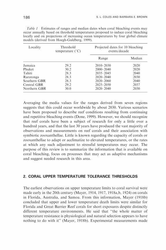
Averaging the media values for the ranges derived from seven regions

suggests that this could occur worldwide by about 2030. Various scenarios

have been proposed to describe reef conditions resulting from continuing

and repetitive bleaching events (Done, 1999). However, we should recognize

that reef corals have been a subject of research for only a little over a

hundred years, and that the last 30 years have produced the vast majority of

observations and measurements on reef corals and their association with

symbiotic zooxanthellae. Little is known regarding the capacity of corals or

zooxanthellae to adapt or acclimatize to elevated temperatures, or the rates

at which any such adjustment to stressful temperatures may occur. The

purpose of this review is to summarize the information that is available on

coral bleaching, focus on processes that may act as adaptive mechanisms

and suggest needed research in this area.

2. CORAL UPPER TEMPERATURE TOLERANCE THRESHOLDS

The earliest observations on upper temperature limits to coral survival were

made early in the 20th century (Mayer, 1914, 1917, 1918a,b, 1924) on corals

in Florida, Australia, and Samoa. From this information, Mayer (1918b)

concluded that upper and lower temperature death limits were similar for

Florida and Great Barrier Reef corals for short exposures despite distinctly

different temperature environments. He said that ‘‘the whole matter of

temperature resistance is physiological and natural selection appears to have

nothing to do with it’’ (Mayer, 1918b). Experimental measurements made

Table 1 Estimates of ranges and median dates when coral bleaching events mayoccur annually based on threshold temperatures proposed to induce coral bleachinglocally and on projections of increasing ocean temperatures by four global climatemodels (derived from Hoegh-Guldberg, 1999).

Locality Thresholdtemperature (�C)

Projected dates for 10 bleachingevents/decade

Range Median

Jamaica 29.2 2010–2030 2020Phuket 30.2 2000–2040 2020Tahiti 28.3 2035–2045 2040Raratonga 28.3 2020–2040 2030Southern GBR 28.3 2020–2060 2040Central GBR 29.2 2025–2050 2037Northern GBR 30.0 2020–2040 2030


by Yonge and Nicholls (1931a) on the Great Barrier Reef and by

Edmondson (1928) in Hawaii showed similar short-term upper temperature

tolerances. However, these results were limited by the experiments being

performed in static aquaria that allowed accumulation of toxic metabolites

that limited the applicability of the results to the natural environment.

Experiments using controlled temperatures in flowing systems were

conducted in Hawaii (Coles, 1973; Jokiel and Coles, 1977; Coles and

Jokiel, 1978; Jokiel and Guinther, 1978) and in Guam (Jones and Randall,

1973), and experimental results were compared to observations made in the

vicinity of power station thermal discharges (Jokiel and Coles, 1974; Coles,

1975; Neudecker, 1981). Using these techniques, experimental comparisons

were made between subtropical Hawaiian corals and tropical Pacific corals

at Enewetak, leading to the conclusions that differences in coral thermal

tolerances correspond to predictable differences in the ambient temperature

patterns between geographic areas, and that ‘‘in both subtropical and

tropical environments large populations of corals are exposed to tempera-

tures precariously close (within 1–2�C) to their upper lethal limit during the

summer months’’ (Coles et al., 1976).

Further experiments relating effects of temperature on energetic processes

using measurements of oxygen flux suggested that there was a possibility of

metabolic adaptation by corals to their ambient temperature regime (Coles,

1973; Coles and Jokiel, 1977). Comparisons of net photosynthesis and

respiration across a temperature range of 18–31�C for four coral species in

Hawaii and Enewetak showed that P :R ratios differed between Hawaii and

Enewetak specimens, resulting in linearly decreasing net photosynthesis with

increasing temperature for Hawaiian specimens, compared with a response

for Enewetak corals that suggested adaptation to the higher ambient

temperature regime at Enewetak. P :R ratios throughout the tested

temperature range also differed among species and corresponded to their

different tolerances to increased temperature.

Repeated coral bleaching episodes and additional experiments during the

past 25 years have verified that upper temperature tolerances of corals are

linked to geographic location and ambient temperature conditions.

Increases of 1–3�C above mean long-term annual maximum temperatures

have consistently induced coral bleaching (Hudson, 1981; Glynn, 1984;

Lasker et al., 1984; Harriott, 1985; Jaap, 1985; Brown and Suharsono, 1990;

Cook et al., 1990; Gates, 1990; Glynn and D’Croz, 1990; Gleason, 1993;

Brown et al., 1995; Cohen et al., 1997; Jones et al., 1997; Spencer et al.,

1998; Berkelmans and Oliver, 1999; Berkelmans and Willis, 1999; Quinn and

Kojis, 1999; Marshall and Baird, 2000; Berkelmans, 2001; Bruno et al.,

2001; Edwards et al., 2001; Glynn et al., 2001; Podesta and Glynn, 2001;

Vargas-Angel et al., 2001; Wellington et al., 2001). The threshold

temperatures which induce coral bleaching and mortality range over 8�C

CORAL BLEACHING 187

worldwide, from 27�C in Rapa Nui (Easter Island) during 2000 where

summer ambient maximum is normally about 25�C (Wellington et al., 2001)

to 35–36�C during 1998 in the Arabian Gulf (George and John, 1998;

Wilkinson et al., 1998; Riegl, 1999, 2002), where normal ambient summer

open water maxium usually ranges up to 34�C (Coles, 1988). Clearly,

maximum water temperatures normally occurring in particular geographic

areas have principally determined the upper temperature tolerances

of corals, indicating that the corals are adjusted to ambient conditions

(Figure 1). This implies a capacity for reef corals and/or their algal

symbionts to adapt to higher temperatures over as yet unknown periods of

time. What is not clear is whether adjustment can occur through phenotypic

acclimatization to acute stress conditions and the mechanisms involved,

or require longer-term adaptation involving selection and breeding of

eurythermal genotypes.

3. THE CORAL BLEACHING PROCESS

Various mechanisms of zooxanthellae loss from corals have been reported,

including exocytosis, apoptosis (or programmed cell death), necrosis, and

host detachment (Gates et al., 1992; Brown et al., 1995). The earliest

description of zooxanthellae leaving a host coral’s cells was made by

Boschma (1925, 1926), who concluded that this was a process of coral

polyps digesting the algal symbionts at the mesenterial filaments where

the zooxanthellae had aggregated. Yonge and Nicholls (1931a,b)

reinterpreted this process to be an active removal of the zooxanthellae, or

‘‘bleaching’’ of the coral that could occur in response to a variety of stresses,

including but not limited to increased temperature.

Following earlier experiments on the effects of elevated temperature on

Hawaiian corals (Edmondson, 1928), studies using a flowing seawater

system with altered temperature and light regimes showed that high light

levels interact with increased temperature in producing coral bleaching

(Coles, 1973; Jokiel and Coles, 1977; Coles and Jokiel, 1978). A number of

subsequent studies increased our understanding of the molecular processes

which lead to zooxanthellar loss, coral bleaching, and the interaction of

the effects of light and temperature (Iglesias-Prieto et al., 1992; Fitt and

Warner, 1995; Jones et al., 1998, 2000; Warner et al., 1996, 1999; Brown,

1997b; Hoegh-Guldberg, 1999; Brown et al., 2000b; Fitt et al., 2001). The

basis of the temperature–light interaction has recently been reviewed by Fitt

et al. (2001). Briefly, under nonstressful temperatures and light, zoox-

anthellar photosynthesis proceeds through a normal process of uptake of

dissolved carbon dioxide and water and transfer of protons through the


photochemical systems of the light reaction, with the release of oxygen, and

fixation of organic carbon in the dark reaction. At higher light intensities the

rates of processes can become saturated, with photosaturation occurring as

early as 09:00 h in shallow water corals (Brown, 1997b). With elevated

temperatures, the rates of these processes increase to a level where more

protons are produced in the light reaction than can be utilized to form

organic carbon in the dark reaction. In the first studies of bleaching-related

Figure 1 Semilogarithmic plots of survival of Pocillopora corals with stresstemperatures in Hawaii (thick line) and the tropical Pacific (thin line), from Figure 2in Coles et al. (1976). Data from: Edmondson (1928) for Hawaii P. meandrina (solidcircles) and P. caespitosa (syn. P. damicornis) (solid hexagons); Mayer (1918) forGreat Barrier Reef P. bulbosa (syn. P. damicornis), open triangle; Mayer (1924) forAmerican Samoa P. damicornis (open diamond); Jones and Randall (1973) for GuamP. damicornis (open circles); Jokiel and Coles (1977) for Hawaii P. damicornis (soliddiamonds); Coles et al. (1976) for Enewetak P. elegans (open squares), HawaiiP. meandrina (solid square) and Hawaiian Podamicornis (solid triangle).

CORAL BLEACHING 189

molecular processes, Lesser (Lesser et al., 1990; Lesser, 1997) demonstrated

that bleaching in corals and other cnidarians was preceded by the

production of oxygen free radicals or other toxic forms of oxygen in the

dinoflagellate symbionts and coral host tissues, subsequently causing

cellular damage and expulsion of symbionts.

Photoinhibition under the influence of increased temperature is therefore

a primary factor influencing coral bleaching, and both internal and external

processes that effectively reduce light levels or alter light quality to longer,

less damaging wavelengths may reduce coral bleaching with increased

temperatures. In experiments on Pocillopora damicornis at Heron Island,

damage to zooxanthellae occurred with exposures of only 7 h in high light

conditions (1000–1500 mmole quantam�2 s�1) (Salih et al., 1998a; Salih,

2001), suggesting that the process of coral bleaching starts well before it

manifests itself as actual zooxanthellae loss. A large proportion of algal cells

showed greatly reduced chloroplasts, increased vacuolation and presence of

lipid globules and increasing cell degradation along with coral bleaching two

days after the high light exposure. Remarkably, these symptoms of cell

damage occurred at both 26 and 32�C, although bleaching was more

pronounced in combined high illumination at 32�C, and these corals

continued to show progressive decline. These responses indicate that coral

bleaching is not simply a direct result of increased temperature, but rather

a result of combined stresses that include, but are not necessarily limited

to, temperature and light conditions. Evidence from various studies has

substantiated that high light levels are important in inducing coral bleaching

(Hoegh-Guldberg and Smith, 1989; Fitt and Warner, 1995; Brown et al.,

1999a). Individual corals usually show more pronounced bleaching and

mortality on upper surfaces and on terminal branches than lower down on

the colony. On a larger scale, corals at shallow depths are usually more

sensitive to bleaching at a given temperature than those at greater depths

(Marshall and Baird, 2000), and corals in offshore areas with high water

clarity are usually more highly impacted during major bleaching events than

corals in nearshore areas with higher turbidity (Phongsuwan, 1995).

4. CORAL BLEACHING PROTECTIVE MECHANISMS

Coral symbiotic algae must meet the challenge of all photosynthetic

organisms in harvesting solar radiation efficiently while simultaneously

safely disposing of dangerous excess excitation energy that would ultimately

be harmful to both algae and coral host. Normally, when excess solar

radiation is absorbed by the algae, an alternative dissipating pathway is

activated that safely returns excited chlorophyll to ground state. In this


process the excitation energy is dissipated as heat via the xanthophyll cycle

in a process termed nonphotochemical quenching (NPQ), which is well

documented in both higher plants and algae (Demmig-Adams and Adams,

1993; Olaizola and Yamamoto, 1994; Olaizola et al., 1994; Owens, 1994;

Wilkinson, 2000). In coral symbiotic zooxanthellae, heat dissipation is

achieved by the reversible interconversion of the xanthophylls, diadino-

xanthin, and diatoxanthin. These xanthophylls were first identified in coral

zooxanthellae by Jeffrey and Haxo (1968), and an active xanthophyll cycle

in corals was described by Ambarsari et al. (1997) and Brown et al. (1999b).

Figure 2 shows a pronounced cycling of photoprotective xanthophylls in

response to diurnal irradiance changes which induce photoinhibition in the

shallow water coral Goniastrea aspera. When sea temperatures rise above

the normal ambient maxima, corals become more susceptible to the effects

of damaging solar radiation (Brown, 1997b; Hoegh-Guldberg, 1999); thus

the xanthophyll cycle becomes a key photoprotective defense. Indeed it

has been claimed that those corals more capable of dissipating excess

excitation energy through NPQ are less prone to temperature bleaching

(Warner et al., 1996).

Another possible protective mechanism against stressful light levels may

be fluorescent coral pigments, which have been indicated to reduce coral

bleaching by reflecting and/or fluorescing absorbed light (Salih et al., 1998b,

2000; Dove et al., 2001). A total of 124 species of corals were found to have

morphs containing fluorescent pigments on the Great Barrier Reef, often

growing alongside of morphs of the same species without such pigments

(Salih et al., 2000). Corals containing such fluorescent capacity were found

to bleach significantly less than nonfluorescent colonies of the same species

growing in the same area. Nonfluorescent corals were significantly more

photoinhibited during peak irradiance periods, and bleaching resistance

measured as tissue dinoflagellate biomass correlated significantly with

fluorescent pigment concentrations in coral tissue. The protective capacity

of these pigments may have important implications for long-term survival of

corals exposed to thermal stress. At Phuket Thailand, Brown et al. (2002c)

found abundant fluorescent pigment in cores from bleaching-resistant west-

facing surfaces of G. aspera compared with low concentrations in bleaching-

prone east-facing surfaces. Fluorescent pigments were most abundant in the

endoderm surrounding the symbiotic algae, suggesting a photoprotective

function. Such potential protective capacity has far-ranging implications for

long-term survival of corals when additionally stressed by high temperature,

although recent preliminary work by Dove (pers. comm. to BEB) suggests

that some of these pigments are easily denatured by elevated sea

temperature.

An internal defense mechanism that may substantially influence coral

tolerance to bleaching and mortality is change in heat shock proteins (Hsps)

CORAL BLEACHING 191

induced by increased temperature. The Hsps act as ‘‘molecular chaperones’’

(Hartl, 1996), preventing detrimental aggregation of structurally nonnative

proteins, helping to refold reversibly heat damaged proteins and aiding

in the insertion of proteins into organelles (Lindquist and Craig 1988;

Figure 2 Underwater photosynthetically active radiation (PAR), effectivequantum yield of photosystem II (iF/Fm0), and xanthophyll ratios of diatoxanthinto diadinoxanthinþ diatoxanthinin for the coral Goniastrea aspera in January 1998at Phuket, Thailand. Points and bars represent means� one standard deviation(from Figure 2 in Brown et al., 1999b).


Morimoto et al., 1994). Induction of a suite of Hsps is a well-characterized

response to heat shock (and other stresses) in many marine organisms, e.g.,

Mytilus californianus (Roberts et al., 1997), the anemone Anemonia viridis,

and various marine invertebrates, including scleractinian corals. In corals,

Hsp 70 has been recognized during heat shock in Goniopora djiboutiensis

and Goniopora pandoraensis (Sharp, 1995; Sharp et al., 1997), Montastraea

annularis (Hayes and King, 1995), Montastraea franksi (Gates and

Edmunds, 1999), Montastraea faveolata (Downs et al., 2000), Acropora

grandis (Fang et al., 1997), and G. aspera (Brown et al., 2002c). Hsp 60 has

been demonstrated in M. faveolata (Downs et al., 2000), A. grandis (Fang

et al., 1997), and G. aspera (Brown et al., 2002c), while Hsps 27, 28, 33, 74,

78, 90, and 95 have been shown to occur in M. faveolata (Black et al., 1995).

Fang et al. (1997) identified Hsp 35 in A. grandis as heme oxygenase,

previously known to be induced by UV radiation and oxidative stress. In

model organisms such as the fruit fly Drosophila spp., maximum rates of

Hsp synthesis are achieved 1 h after initial heat shock; the rate of Hsp

synthesis then declines, but if the high-temperature treatment is continued,

Hsps accumulate since they have long half-lives. By 6–8 h they form up to

10% of the cell’s total proteins (Ashburner and Bonner, 1979). Similar

temporal fluctuations have been observed in synthesis of Hsp 70 in the coral

M. franksi (Gates and Edmunds, 1999), though detailed resolution of shifts

in protein turnover in heat-stressed corals is lacking. In higher plant

chloroplasts small Hsps are produced in response to many environmental

stresses, with recent work showing that chloroplast small Hsps are

important determinants of both photosynthetic and whole plant thermo-

tolerance (Heckathorn et al., 1999). Chloroplast small Hsps are also present

in coral symbiotic algae and in M. faveolata (Downs et al., 2000) are

upregulated 3.5 fold compared to controls by an increase in temperature of

6�C in dim light and as much as 50 fold in G. aspera by a temperature

increase of 4�C in bright light (Brown et al., 2002c).

Important coral defenses against high light and elevated temperature also

occur with oxidative enzymes which include copper/zinc superoxidase

(SOD), manganese SOD, iron SOD, ascorbate peroxidase, and catalase,

thereby preventing subsequent cellular damage from active species of

oxygen. Both enzyme activity and concentration may be increased as a result

of exposure to elevated temperature (Lesser et al., 1990; Fang et al., 1997;

Downs et al., 2000).

Changes in zooxanthellae symbionts may influence adaptive responses

by the coral–algal association to thermal stress. Although all coral

zooxanthellae were originally considered to be a single species described

as Symbiodinium microadriaticum, numerous species and types of zoo-

xanthellae are now recognized, and their environmental tolerances

or composition may fluctuate with environmental conditions. This could

CORAL BLEACHING 193

occur through changes in the phenotypic adaptation of the biochemical–

physiological processes of the resident zooxanthellae (Brown, 1997b), or by

rapid changes in their cladal composition (Coffroth et al., 2001). The latter

possibility, first proposed over 25 years ago when Jokiel and Coles (1977)

stated ‘‘a different strain of algal symbiont may inhabit the tropical

representative of the various coral species,’’ was later formalized as the

Adaptive Bleaching Hypothesis (ABH) (Buddemeier and Fautin, 1993;

Ware et al., 1996). The ABH postulated that the loss of resident

zooxanthellae in response to stress provides an opportunity for stress-

adapted types to repopulate the coral, imparting greater resistance to the

stress and competitive advantage for the coral–algal complex.

A number of laboratory and field studies of the genetic diversity of

symbiotic algae in corals and other cnidarians provide limited but

inconclusive support for the ABH (Baker, 2001; Kinzie et al., 2001).

These studies indicate consistent latitudinal differences that suggest the

existence of thermo-tolerant zooxanthellae phylotypes (Loh et al., 2001;

Rodriguez-Lanetty et al., 2001; Savage et al., 2002a). Glynn et al. (2001)

found differences in bleaching resistance that corresponded to zooxanthellae

symbiont genotypes in P. damicornis during the 1997–98 bleaching event.

These examples suggest that inducible variations in genetic composition

of zooxanthellae, as well as the capacity of the symbionts for phenotypic

adaptation to stress events (Brown, 1997a,b), may contribute to adaptive

selection of thermally resistant coral species and varieties. Some of these

observations, however, should be viewed with caution. Baker (2001) argues

that transplant experiments indicate that bleaching provides an opportunity

for corals to rid themselves of suboptimal algae and acquire new partners.

However, this work has been criticized by others (Hoegh-Guldberg et al.,

2002) who believe that Baker’s data do not support the ABH. Although

several criticisms were made, the main issue was that transplantation of

corals to different depths confused interpretation of the results obtained.

Most importantly, we are far from understanding the physiological traits of

symbiotic algal genotypes. The photosynthetic characteristics of coral

symbiotic algae cannot be deduced from the commonly used method of

molecular typing of r-RNA genes (Savage et al., 2002b). Therefore,

generalizations about photosynthetic traits of different algal genotypes

based on these results are unconvincing. Indeed, Kinzie et al. (2001) showed

that variability in physiological response to temperature (in this case growth

rate) within a genotype might be as great or greater than between genotypes.

Clearly, finer genetic differentiation will be required to understand not only

the physiological tolerances of the algae but also their dynamics within the

coral colony. Until this is achieved, the case for or against the ABH will not

be determined.


5. CORAL AND ZOOXANTHELLAE THERMAL ACCLIMATION,

ACCLIMATIZATION, AND ADAPTATION: EMPIRICAL

OBSERVATIONS

The capacity of corals and reefs to adapt to elevated temperatures has been

the subject of a number of reviews (Gates, 1990; Buddemeier and Fautin,

1993; Glynn, 1993; Brown, 1997a,b; Buddemeir and Smith, 1999; Done,

1999), and the mechanisms of phenotypic adaptation for corals have been

discussed in Brown (1997a) and Gates and Edmunds (1999). As reviewed in

Brown (1997a), adaptations by corals to elevated temperature or light

regimes can occur under a range of time scales and conditions. Terms

referring to these adjustments have been variously used, and we herein

follow the terminology of Brown (1997a) and Gates and Edmunds (1999).

Although acclimation has been used ambiguously to refer to adaptation

over the long term, e.g., Ware (1997), acclimation more properly means

changes in tolerances under laboratory or other experimental conditions,

generally over the short term. Acclimatization refers to phenotypic

changes by an organism to stresses in the natural environment that result

in the readjustment of the organism’s tolerance levels. These phenotypic

responses are usually reversible and are limited by the organism’s genotype,

which determines the boundaries beyond which acclimatization

cannot occur. Finally, selective adaptation occurs when the more stenotopic

members of a population are eliminated by the environmental stress,

leaving the more tolerant organisms to reproduce and recruit to available

habitat.

The primary evidence of long-term selection for temperature tolerant

corals is based upon the linkage of thermal thresholds to maximum ambient

temperature environments previously described, and reports of corals

surviving temperatures well in excess of normally accepted limits. Gardiner

(1903) observed abundant corals in a tidepool in the Laccadives at water

temperatures up to 56�C, and Kinsman (1964) noted massive Porites at over

40�C near Abu Dhabi, Arabian Gulf. Motoda (1940), Orr and Moorhouse

(1933), and Vaughan (1914) reported corals surviving temperatures up to

38–39�C in Palau, Australia, and Florida, respectively. More recently

Tomascik et al. (1997) reported a variety of corals living at 34–37�C near a

thermal vent in Indonesia, with one species growing in the vent at 42�C. On

Ofu Island, American Samoa, Craig et al. (2001) found 52 coral species,

including nine Acropora taxa, to survive daily temperatures as high as

34.5�C for up to 3 h exposures daily for 35 days during the summer of

1998–99 with virtually no bleaching. Meesters and Bak (1993) found

recovery of experimentally damaged bleached Porites asteroides in the

thermal effluent of a power station in Curacao to be just as high as that of

CORAL BLEACHING 195

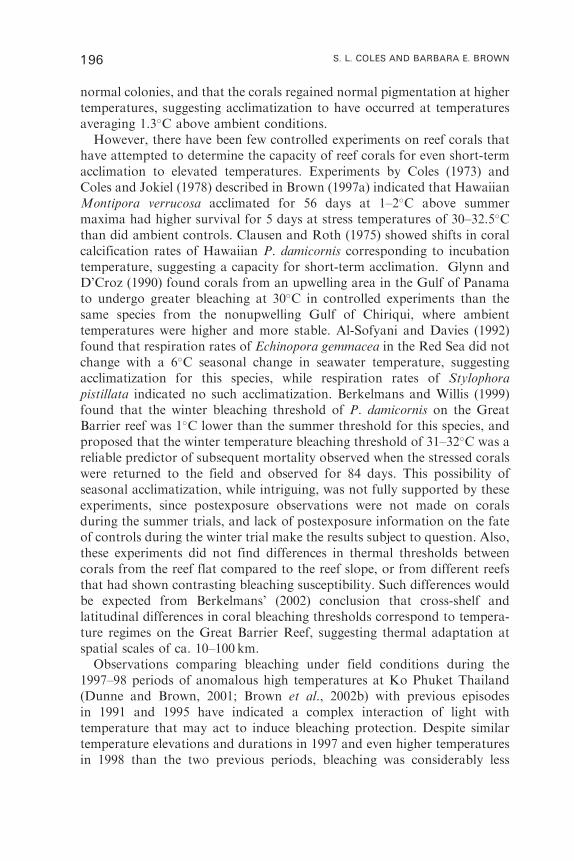
normal colonies, and that the corals regained normal pigmentation at higher

temperatures, suggesting acclimatization to have occurred at temperatures

averaging 1.3�C above ambient conditions.

However, there have been few controlled experiments on reef corals that

have attempted to determine the capacity of reef corals for even short-term

acclimation to elevated temperatures. Experiments by Coles (1973) and

Coles and Jokiel (1978) described in Brown (1997a) indicated that Hawaiian

Montipora verrucosa acclimated for 56 days at 1–2�C above summer

maxima had higher survival for 5 days at stress temperatures of 30–32.5�C

than did ambient controls. Clausen and Roth (1975) showed shifts in coral

calcification rates of Hawaiian P. damicornis corresponding to incubation

temperature, suggesting a capacity for short-term acclimation. Glynn and

D’Croz (1990) found corals from an upwelling area in the Gulf of Panama

to undergo greater bleaching at 30�C in controlled experiments than the

same species from the nonupwelling Gulf of Chiriqui, where ambient

temperatures were higher and more stable. Al-Sofyani and Davies (1992)

found that respiration rates of Echinopora gemmacea in the Red Sea did not

change with a 6�C seasonal change in seawater temperature, suggesting

acclimatization for this species, while respiration rates of Stylophora

pistillata indicated no such acclimatization. Berkelmans and Willis (1999)

found that the winter bleaching threshold of P. damicornis on the Great

Barrier reef was 1�C lower than the summer threshold for this species, and

proposed that the winter temperature bleaching threshold of 31–32�C was a

reliable predictor of subsequent mortality observed when the stressed corals

were returned to the field and observed for 84 days. This possibility of

seasonal acclimatization, while intriguing, was not fully supported by these

experiments, since postexposure observations were not made on corals

during the summer trials, and lack of postexposure information on the fate

of controls during the winter trial make the results subject to question. Also,

these experiments did not find differences in thermal thresholds between

corals from the reef flat compared to the reef slope, or from different reefs

that had shown contrasting bleaching susceptibility. Such differences would

be expected from Berkelmans’ (2002) conclusion that cross-shelf and

latitudinal differences in coral bleaching thresholds correspond to tempera-

ture regimes on the Great Barrier Reef, suggesting thermal adaptation at

spatial scales of ca. 10–100 km.

Observations comparing bleaching under field conditions during the

1997–98 periods of anomalous high temperatures at Ko Phuket Thailand

(Dunne and Brown, 2001; Brown et al., 2002b) with previous episodes

in 1991 and 1995 have indicated a complex interaction of light with

temperature that may act to induce bleaching protection. Despite similar

temperature elevations and durations in 1997 and even higher temperatures

in 1998 than the two previous periods, bleaching was considerably less


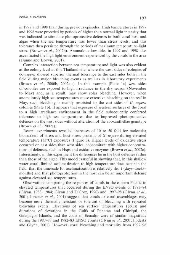
in 1997 and 1998 than during previous episodes. High temperatures in 1997

and 1998 were preceded by periods of higher than normal light intensity that

was indicated to stimulate photoprotective defenses in both coral host and

algae when the sea temperature was lower than stress levels, and this

tolerance then persisted through the periods of maximum temperature–light

stress (Brown et al., 2002b). Anomalous low tides in 1997 and 1998 also

accentuated the high light environment experienced by the corals in the area

(Dunne and Brown, 2001).

Complex interaction between sea temperature and light was also evident

at the colony level at this Thailand site, where the west sides of colonies of

G. aspera showed superior thermal tolerance to the east sides both in the

field during major bleaching events as well as in laboratory experiments

(Brown et al., 2000b, 2002a,c). In this example (Plate 1a) west sides

of colonies are exposed to high irradiance in the dry season (November

to May) and, as a result, may show solar bleaching. However, when

anomalously high sea temperatures cause extensive bleaching on the reef in

May, such bleaching is mainly restricted to the east sides of G. aspera

colonies (Plate 1b). It appears that exposure of western surfaces of the coral

to a high irradiance environment in the field subsequently conferred

tolerance to high sea temperatures due to improved photoprotective

defences on the west sides without alteration of the zooxanthellae genotype

(Brown et al., 2002a).

Recent experiments revealed increases of 10 to 50 fold for molecular

biomarkers of stress and host stress proteins of G. aspera during elevated

temperature (33�C) exposures (Figure 3). Higher levels of oxidative stress

occurred on east sides than west sides, concomitant with higher concentra-

tions of defenses, such as Hsps and oxidative enzymes (Brown et al., 2002c).

Interestingly, in this experiment the differences lie in the host defenses rather

than those of the algae. This model is useful in showing that, in this shallow

water coral, limited acclimatization to high temperature does occur in the

field, that the timescale for acclimatization is relatively short (days–weeks–

months) and that photoprotection in the host can be an important defense

against elevated sea temperatures.

Observations comparing the responses of corals in the eastern Pacific to

elevated temperatures that occurred during the ENSO events of 1983–84

(Glynn, 1983, 1984; Glynn and D’Croz, 1990) and 1997–98 (Glynn et al.,

2001; Jimenez et al., 2001) suggest that corals or coral assemblages may

become more thermally resistant or tolerant of bleaching with repeated

bleaching events. Elevations of sea surface temperatures (SSTs) and

durations of elevations in the Gulfs of Panama and Chiriqui, the

Galapagos Islands, and the coast of Ecuador were of similar magnitude

during the 1987–88 and 1982–83 ENSO events (Glynn et al., 2001; Podesta

and Glynn, 2001). However, coral bleaching and mortality from 1997–98

CORAL BLEACHING 197

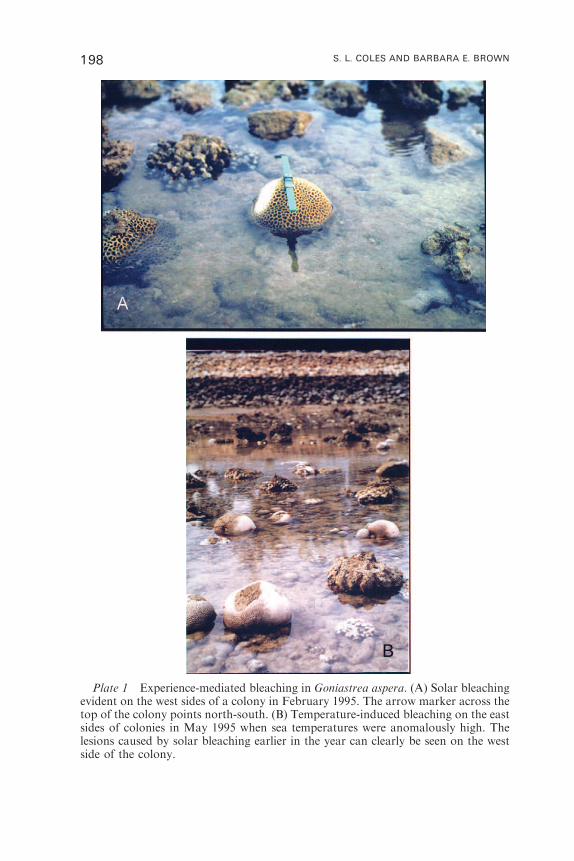
Plate 1 Experience-mediated bleaching in Goniastrea aspera. (A) Solar bleachingevident on the west sides of a colony in February 1995. The arrow marker across thetop of the colony points north-south. (B) Temperature-induced bleaching on the eastsides of colonies in May 1995 when sea temperatures were anomalously high. Thelesions caused by solar bleaching earlier in the year can clearly be seen on the westside of the colony.


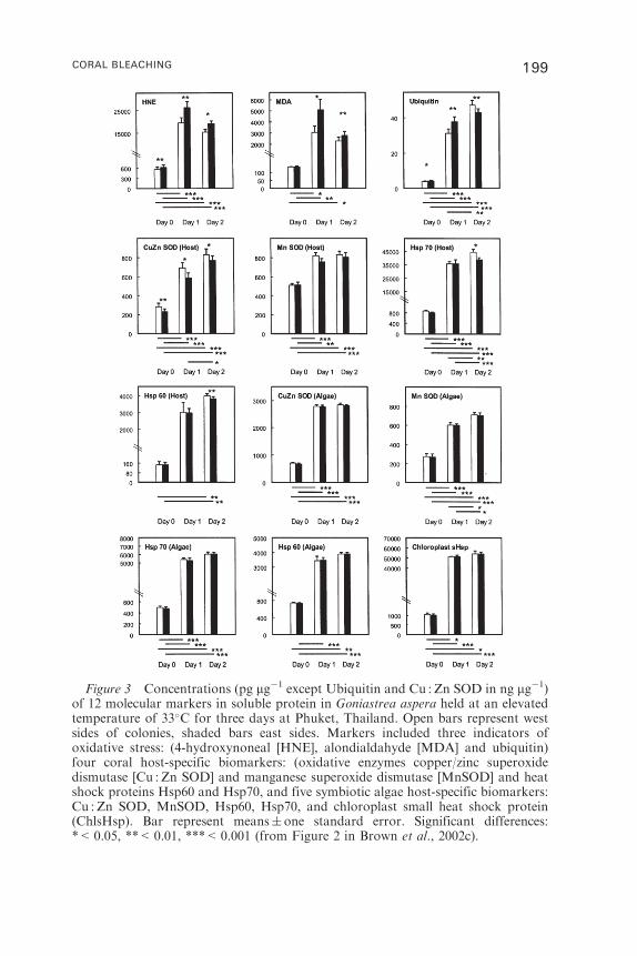
Figure 3 Concentrations (pg mg�1 except Ubiquitin and Cu : Zn SOD in ng mg�1)of 12 molecular markers in soluble protein in Goniastrea aspera held at an elevatedtemperature of 33�C for three days at Phuket, Thailand. Open bars represent westsides of colonies, shaded bars east sides. Markers included three indicators ofoxidative stress: (4-hydroxynoneal [HNE], alondialdahyde [MDA] and ubiquitin)four coral host-specific biomarkers: (oxidative enzymes copper/zinc superoxidedismutase [Cu : Zn SOD] and manganese superoxide dismutase [MnSOD] and heatshock proteins Hsp60 and Hsp70, and five symbiotic algae host-specific biomarkers:Cu : Zn SOD, MnSOD, Hsp60, Hsp70, and chloroplast small heat shock protein(ChlsHsp). Bar represent means� one standard error. Significant differences:*<0.05, **<0.01, ***<0.001 (from Figure 2 in Brown et al., 2002c).

CORAL BLEACHING 199

was substantially less than in 1982–83 (Glynn et al., 2001; Podesta and

Glynn, 2001). Coral mortality from the 1982–83 event was 97–99% in the

Galapagos Islands, 85% in the Gulf of Panama, and 75% in the Gulf of

Chiriqui. By contrast, mortality in 1987–88 was 26% in the Galapagos, 13%

in the Gulf of Chiriqui, and undetectable in Gulf of Panama (Glynn et al.,

2001). Although these comparisons are not unequivocal due to differences

in seasonal timing of anomalies, duration of exposures (Podesta and Glynn,

2001) or upwelling (Glynn et al., 2001), the lower bleaching and mortality

that occurred in 1997–98 suggest that selection for resistant species or

genotypes of corals and zooxanthellae may have occurred during prior

ENSO-related temperature events (Podesta and Glynn, 2001). Jimenez

et al. (2001) also report higher bleaching and mortality to corals on

Costa Rican reefs in 1982–83 than in 1997–98, despite the temperature stress

from the later event having been as strong or stronger than in 1982–83.

Unfortunately, no information is provided concerning the prevailing light

climates in this region for the two major El Nino events that would clarify

whether differences in solar radiation might have influenced the generally

lower bleaching that occurred in 1997–98.

Coral bleaching was also minimal in the Society Islands during the 1998

event, but the cause there was attributed to reduced light during the event.

Mumby et al. (2001) found no coral bleaching in the Society Islands in 1998

despite high temperature anomalies, but attributed lack of bleaching to high

cloud cover and reduced light levels during the period of elevated

temperatures. Statistical analyses of bleaching occurrence based on

cumulative temperature elevations, wind speed, and cloud cover predicted

the correct scenario for the 1998 event only when high cloud cover was

included in the analysis, indicating that the interactive effect of cloud cover

can reverse bleaching predictions based solely on temperature elevation.

Other findings suggest that coral populations can adapt to localized

temperature conditions. Cook et al. (1990) found that Bermuda corals at

lagoon and inshore sites, where they were subject to higher and more

variable temperatures, were more resistant to bleaching in 1987 than the

same species at offshore sites. Similar patterns have been observed on the

Great Barrier Reef (Marshall and Baird, 2000) and the East Pacific

(Guzman and Cortes, 2001). Berkelmans (2002) proposed that thermal

adaptation had taken place over both local (10s of km) and regional (100s to

1000s of km) scales in the Great Barrier Reef, although Berkelmans and

Oliver (1999) concluded that inshore reefs were more prone to bleaching

than offshore reefs because of higher inshore temperatures and probably

reduced circulation. An indication of localized thermal adaptation was

found in the Colombian Pacific (Vargas-Angel et al., 2001), where coral

responses to the 1997–98 elevated temperatures showed less bleaching and

lower mortality in an area where long-term temperatures were consistently


higher by 0.5–1.0�C. Although Bruno et al. (2001) did not find significant

differences in bleaching between sites at 3–5m compared with 10–12m

depths from the severe 1997–98 ENSO event in Palau, Coles (unpublished

report) found high coral survival in nearshore compared with offshore areas

in August 1999, one year after the event. Corals at various nearshore sites

around the island of Babeldoab in 1999 were abundant, well pigmented, and

in apparently healthy condition at temperatures up to 31.7�C, equivalent to

the temperatures that occurred during the bleaching event (Bruno et al.,

2001). Coral coverage and species composition in these nearshore areas

was indistinguishable from observations made on surveys in 1997. By con-

trast, virtually all Acropora and many other species on offshore reefs were

dead in 1999.

These examples indicate a capacity for selective adaptation by various

coral species to elevated temperatures. However, nothing is known about

the conditions or time frame under which this capacity was acquired. The

critical question pertaining to large-scale survival of corals and continued

viability of coral reefs over the next century is whether the temperature

tolerances of corals and their symbionts can adjust rapidly enough to

a changing ocean temperature environment, and whether the maximum

temperatures that ultimately occur will exceed adaptation capacity.

Attempts to predictively model reef conditions that may result from rising

sea temperatures have usually used fixed coral thermal tolerances (Hoegh-

Guldberg, 1999) predicting coral declines and phase shifts to algal-

dominated reefs over the next century. However, models comparing

projected global seawater change with various estimates of acclimation

(i.e., adaptation) times (Ware et al., 1996) suggest that, although probable

bleaching events are likely to increase over the next century, development

of higher temperature thresholds in 25–50 years may dramatically reduce

bleaching probabilities and frequencies. This suggests that models projecting

future conditions for reef corals and coral reefs could utilize specific

information relative to thermal acclimatization and adaptation of corals and

their symbionts. Especially needed are data on the timeframe required for

selective adaptation to both gradually increasing temperature and to

infrequent temperature increases in order to project the eventual impacts of

both global warming and El Nino events.

6. CORAL BLEACHING RECOVERY

In contrast to the limited experimental evidence for corals adapting to

higher temperatures, there are numerous instances of repeated coral

recovery from bleaching events, and recolonization and substantial

CORAL BLEACHING 201

regrowth of corals in areas denuded by coral bleaching can occur as rapidly

as within two years (Plate 2). The most documented area is the central Great

Barrier Reef, where bleaching occurred in 1979–80, 1981–82, 1986–87,

1992–93, 1993–94 (Harriott, 1985; Oliver, 1985; Jones et al., 1997), and 1998

(Berkelmans and Oliver, 1999; Marshall and Baird, 2000; Berkelmans,

2002). The bleaching episode that occurred in January–March 1982 resulted

in an estimated 50% mortality (Oliver, 1985) or more (Harriott, 1985)

by November 1983. Despite this and lesser impacts that occurred with

bleaching episodes every 2–5 years, recolonization and recovery was

sufficient to reestablish a coral community by 1998 prior to the most

extensive bleaching that has occurred there to date. Berkelmans and Oliver

(1999) reported 65% of inshore reefs and 7% of offshore reefs in the central

GBR to have had bleaching levels of 30% or more, with subsequent

mortality of up to 60–80% on the reef flats at Orpheus Island. Marshall and

Baird (2000) reported 53% of all coral colonies on Magnetic and Orpheus

Island to have been affected by the 1998 bleaching event, with a preliminary

report of mortality up to 16% on replicate transects and substantial

differences among species and spatial variation in bleaching resistance. On a

larger scale, Berkelmans (2001) reported good recovery only 6–8 months

following the severe 1998 bleaching event on most GBR inshore reefs, where

bleaching had been heaviest. Mortality was greatest in the Palm Islands

region with up to 73% on the reef flat at Rattlesnake Island, but coral cover

in the Magnetic Island and Whitsunday Islands region was generally

unchanged with no significant decreases on these reefs over time. Mortality

was highly variable and generally less extensive on most offshore reefs,

where maximum mortality was 50–55% at Otter and Little Kelso Reefs.

On the Heron Island reef flat, where 80% of corals showed bleaching

discoloration during the 1998 event (Jones et al., 2000), observations in

July 2001 (SLC, pers. obs.) indicated a flourishing coral community with

>50% total coverage.

Similar recurrent bleaching and recovery occurred in Moorea, French

Polynesia in 1984, 1987, 1991, and 1994 (Salvat, 1992; Fagerstrom and

Rougerie, 1994; Hoegh-Guldberg and Salvat, 1995) with sharp reductions

observed following the 1991 but not the 1994 event. Minimal bleaching

occurred again in 1998 (Wilkinson, 2000). In the Andaman Sea off the coast

of Thailand, bleaching occurred in 1988, 1991, and 1995 (Phongsuwan,

1995; Brown et al., 1996; Brown, 1997b). However, little mortality occurred

that could be attributed directly to these bleaching events, although coral

coverage decreased substantially on the outer reef flat due to high sediment

loading from a deep water port development (Brown, 1997b; Brown et al.,

2002b). Little bleaching or mortality occurred from similar to higher

temperatures in this area in 1997–98 (Dunne and Brown, 2001; Brown et al.,

2002b). Guzman and Cortes (2001) describe low-level coral recovery on


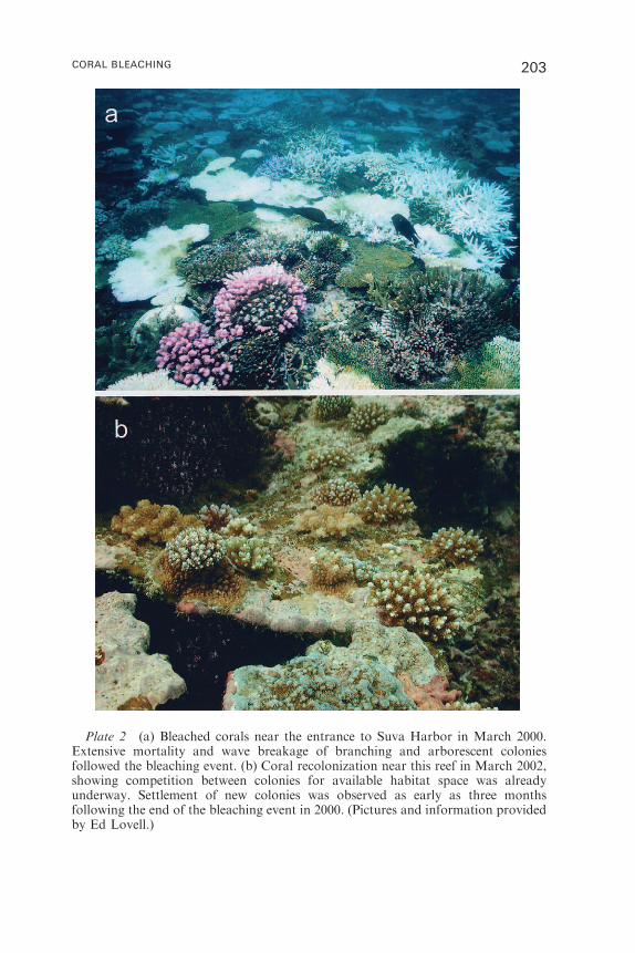
Plate 2 (a) Bleached corals near the entrance to Suva Harbor in March 2000.Extensive mortality and wave breakage of branching and arborescent coloniesfollowed the bleaching event. (b) Coral recolonization near this reef in March 2002,showing competition between colonies for available habitat space was alreadyunderway. Settlement of new colonies was observed as early as three monthsfollowing the end of the bleaching event in 2000. (Pictures and information providedby Ed Lovell.)

CORAL BLEACHING 203

Pacific reefs of Costa Rica following the 1982–83 ENSO. They attribute this

recovery to corals more tolerant of thermal stress, and note that mortality of

such corals was very limited during the 1997–98 ENSO warming. Kayanne

et al. (2002) noted that recovery of Montipora to prebleaching conditions

two years after the 1998 bleaching event had resulted in high mortality in the

southern Ryukus, although Montipora patches with coverage of less than

10% did not recover in that time period. Mortality and recovery varied

among the other genera surveyed, with low mortality and little overall

change shown for Heliopora and massive Porites, high mortality and

moderate recovery for branching Porites and Acropora, and high mortality

with no recovery shown for Pavona.

7. BLEACHING AND CORAL DISEASE, REPRODUCTION, AND

RECRUITMENT

A major consideration in recovery and maintenance of coral assemblages

and coral reef integrity following bleaching events is the impact of thermal

stress on coral resistance to disease, reproduction, and recruitment.

Observations and experiments have suggested infectious disease to be

both a cause and an effect of coral bleaching. A series of studies (Kushmaro

et al., 1996, 1998, 2001; Toren et al., 1998; Banin et al., 2000; 2001; Israely et

al., 2001; Fine et al., 2002a,b) in the Mediterranean have linked bleaching of

an introduced coral, Oculina patagonica, at elevated temperature with the

growth of the bacterium Vibrio shiloi. Recent experiments have indicated a

similar relationship between Pocillipora damicornis and the bacterium Vibrio

coralyticus in Zanzibar (Ben-Haim and Rosenberg, 2002). These pathogens

can be isolated in culture, and are experimentally transferable between coral

colonies. They cause lysis of coral host tissues, especially when temperatures

are elevated above normal ambient maxima (Ben-Haim and Rosenberg,

2002). Vibrio coralyticus has been isolated from diseased P. damicornis in the

Red Sea, and bacterial strains from bivalve larvae in the North and South

Atlantic were found to be pathogenic to this coral species. These findings

offer a new perspective that requires consideration for its implications

regarding widespread coral bleaching events. However, it is unlikely

that such bacterial processes are the primary cause for most of the

coral bleaching events that have been reported worldwide, which have

been found to be reversible if temperature–light stresses are not too extreme

or long lasting. As indicated by results and figures in Ben-Haim

and Rosenberg (2002), these bacterial infections lead to partial tissue

lysis scattered throughout the coral colony within seven days after

infection, followed by 100% lysis and mortality within three weeks.


In contrast, temperature–light induced bleaching produces aggregation of

zooxanthellae to polyp mouths and zooxanthellae expulsion, which may be

followed by recovery if the stress subsides. Even so, these findings on

temperature-correlated bacterial infections suggest an additional factor to

be considered within the general context of coral bleaching and its

ramifications.

Lower energy reserves caused by prolonged and repeated coral bleaching

are probably related to the extensive outbreaks of coral diseases that have

occurred in Florida and Caribbean waters in the last decade (Cervino et al.,

1998; Richardson et al., 1998). Chronic decreases in energy reserves of

bleached corals have also been indicated to reduce the long-term

reproductive capability of corals on reefs. Experiments on hard corals in

Florida (Szmant and Gassman, 1990) and Jamaica (Mendes and Woodley,

2002) and a soft coral on the Great Barrier Reef (Michalek-Wagner and

Willis, 2001a,b) have shown reduced fecundity of bleached corals that

resulted in reproductive failure or delay in spawning of one year and

reduced ability to complete gametogenesis, long after the symptoms of

bleaching had ended in the adults. Reduced fecundity appears to result from

lower energy resources available to a coral that has survived and recovered

from a bleaching episode (Szmant and Gassman, 1990). This potential

impact of bleaching on coral vitality, reproduction, and planula release has

serious long-term implications, especially if bleaching events increase in

frequency.

The limited information available also indicates that temperature

increases are as stressful to coral planulae as to adult stages.

Experimental exposure of P. asteroides planulae in Florida to 33�C for

24 h (Edmunds et al., 2001) significantly increased mortality and shortened

metamorphosis time compared with exposures at ambient temperatures

(28�C). Also P :R ratios decreased with short-term exposures to elevated

temperatures in these experiments, similar to that found for adult

Hawaiian corals (Coles, 1973; Coles and Jokiel, 1977). This suggests that

overall coral recruitment may be reduced through lower energy

availability, reduced lower planula survival, and restricted planktonic

dispersal following premature metamorphosis. For postlarval stages,

contrasting results have been reported for the impact of thermal stress

on settlement and recruitment of coral larvae that have been exposed to

temperatures that can induce coral bleaching. Experiments in Hawaii

found coral settlement to be highly sensitive to long term temperature

increases (Jokiel and Guinther, 1978), with 10-fold reductions at an

increase of 1�C above the annual temperature maximum. However,

Edmondson (1946) and later Coles (1985) demonstrated that brief

exposures to elevated temperatures significantly increased settlement and

survival of coral recruits, with a temperature optimum for settlement of

CORAL BLEACHING 205

P. damicornis at approximately 34�C for 10-min exposures, or about

7�C above annual maximum ambient (Coles, 1985). Coral recruitment

near a thermal outfall in Hawaii, where long-term mean temperature

elevation was 0.63�C above ambient, was 10 times greater than rates

elsewhere in Hawaii (Coles, 1984), and coral abundance adjacent to the

outfall remains the highest in the area (Coles, pers. obs.). Mumby (1999)

determined that the 1998 3.5-month long bleaching event which caused

70–90% bleaching of adult corals in Belize produced only 25% bleaching

of recruits 2–20mm in diameter, with ‘‘no measurable effect on recruit

density or community structure,’’ comparing conditions before and after

the event. Similar reduced susceptibility to bleaching in juvenile corals was

also noted by Loya et al. (2001) during extensive bleaching in Japan in

1997–98. Observations by Edwards et al. (2001) showed high recovery

by recently settled juveniles compared with adults following the 1998

bleaching in the Maldives. They noted recruitment of 202 branching

acroporid and pocilloporid corals within 10 months after bleaching

had eliminated 98% of nearly 1500 corals counted on artificial structures

in 1994.

These findings suggest that, although elevated temperature may reduce

planula survival and restrict planktonic dispersal, exposure to thermal stress

may also increase coral settlement rates and perhaps select for more

resistant surviving planulae. The apparently lower susceptibility of juvenile

corals to bleaching at elevated sea temperatures compared with adults

is interesting in terms of their molecular defence mechanisms. Preliminary

experiments comparing the temperature tolerances of adult and juvenile

corals reveal that juvenile corals show a greater defensive response

(in terms of concentrations of Hsps and oxidative enzymes) than adults

(Brown, unpublished). These differences may be the result of age-related

energetic costs (i.e., reproduction and/or lesion healing processes) that

reduce the defensive ability of adults and/or their capacity to maintain

homeostasis in the face of stress as the organism ages (Beckman and Ames,

1988; Halliwell and Gutteridge, 1999). Whatever the mechanisms involved,

these findings have important bearing on the recovery potential of some reef

sites following bleaching events and the ultimate community structure that

might result.

The weight of the available evidence therefore suggests that the

reproductive problems posed by coral bleaching are of greater concern

than impacts on adult corals, but that survival of recruits is less affected.

Given the importance of reproduction and recruitment to long-term

reef viability and the contrasting results that have been obtained for some

of the studies, it is clear that substantial further research is needed in

this area.


8. LONG-TERM ECOLOGICAL IMPLICATIONS OF CORAL

BLEACHING

A recent review (Fitt et al., 2001) has emphasized that reliable conclusions

about coral bleaching and mortality should be based on measurements of a

variety of environmental factors, such as duration of thermal stress, light

intensity, and quality (Warner et al., 2002). It was considered that

substantial reductions in algal symbiont concentrations, i.e., subliminal

bleaching, can be normal annual events. Fitt et al. (2001) also question

whether bleaching is a meaningful indicator for coral mortality, given the

lack of information linking zooxanthellae loss to coral death. Going further,

the available information is, in our view, insufficient to provide definitive

conclusions about the long-term fate of corals and reefs impacted by coral

bleaching. Uncertainties remain concerning the tropical seawater tempera-

ture environment and frequency of thermal events in the next century. We

are only beginning to acquire basic information on bleaching thresholds,

and the capacity of corals and their symbionts to acclimatize or adapt to

increasing temperatures or thermal events. Limited information is available

concerning linkages between bleaching and mortality, reproduction,

recruitment, and the capability of coral assemblages to recover and

reestablish after a bleaching event. Even less information is available as to

whether coral acclimatization and adaptation can occur sufficiently fast to

adjust to temperature anomalies that may occur.

Uncertainties also remain concerning the interaction of the stresses which

induce coral bleaching with other sources of coral stress and reef alteration

(Buddemeir and Smith, 1999), such as nitrification and eutrophication,

increased macroalgal growth that may result from overfishing of herbivores

and reduced coral growth rates that result from ocean pH changes related to

increased atmospheric CO2 (Pittock, 1999). The combined effects of these

and other important factors with temperature and light effects on coral

survival and propagation may be additive, synergistic, or neutral, but not

necessarily negative in all cases. Turbid environments, generally considered

to inhibit coral growth and survival, may shield corals from high light

intensities and act as refugia for corals during times of thermal stress, and

contribute to acclimatization and adaptation (Meesters et al., 2002). This

attests to the potential importance of nonreef communities containing

resistant corals, both locally and globally, in providing recruits during

periods of large-scale disturbance (Buddemeir and Smith, 1999).

Various scenarios resulting from mass coral bleaching have been

presented by Done (1999), which include coral tolerance and adaptation,

shifting of coral populations to smaller size classes, changing of species,

compositions toward more tolerant coral species with decreasing diversity,

CORAL BLEACHING 207

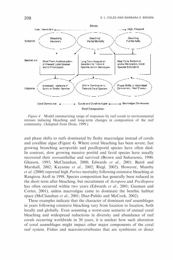
and phase shifts to reefs dominated by fleshy macroalgae instead of corals

and coralline algae (Figure 4). Where coral bleaching has been severe, fast

growing branching acroporids and pocilloporid species have often died.

In contrast, slow growing massive poritid and favid species have usually

recovered their zooxanthellae and survived (Brown and Suharsono, 1990;

Gleason, 1993; McClanahan, 2000; Edwards et al., 2001; Baird and

Marshall, 2002; Kayanne et al., 2002; Riegl, 2002). However, Mumby

et al. (2000) reported high Porites mortality following extensive bleaching at

Rangiroa Atoll in 1998. Species composition has generally been reduced in

the short term after bleaching, but recruitment of Acropora and Pocillopora

has often occurred within two years (Edwards et al., 2001; Guzman and

Cortes, 2001), unless macroalgae came to dominate the benthic habitat

space (McClanahan et al., 2001; Diaz-Pulido and McCook, 2002).

These examples indicate that the character of dominant reef assemblages

in years following extensive bleaching vary from location to location, both

locally and globally. Even assuming a worst-case scenario of annual coral

bleaching and widespread reductions in diversity and abundance of reef

corals occurring worldwide in 30 years, it is unclear how such alteration

of coral assemblages might impact other major components of the coral

reef system. Fishes and macroinvertebrates that are symbionts or direct

Figure 4 Model summarizing range of responses by reef corals to environmentalstresses inducing bleaching and long-term changes in composition of the reefcommunity. (Adapted from Done, 1999.)


consumers of living corals would be as diminished as their coral hosts, but

for the majority of reef organisms not directly linked to corals, the total

result of pervasive coral bleaching is difficult to foretell. Although all of

these alternatives are likely to result in less aesthetically attractive reefs, we

do not know that the reefs would be functionally diminished as biotic

systems, at least in the short term. Species diversity and abundance of small

invertebrates would be likely to increase initially as new habitat spaces

opened up in recently dead corals (Coles, 1980), and benthic macroalgae

would become more abundant. In the year after the 1998 bleaching event in

the Indian Ocean, McClanahan et al. (2001) found a 75–85% decrease

in hard and soft corals on Kenyan reefs and 88–220% increases in turf and

fleshy algae. Diaz-Pulido and McCook (2002) found a similar shift in

dominance to macroalgae on Porites that had undergone severe bleaching

and mortality on the Great Barrier Reef.

Regarding fish assemblages, studies of postcoral bleaching event

conditions have sometimes found shifts in dominant feeding groups but

no overall population decreases. Wellington and Victor (1985) found no

significant change in a damselfish population in the Gulf of Panama after

coral mortality from the 1982–83 El Nino caused massive increases in

available algal food and nesting sites. Lindahl et al. (2001) found that fish

community diversity was unchanged after the 1998 bleaching event that

killed 88% of corals on Tanzanian reef plots, but fish abundance rose 39%,

mostly due to increase in herbivores apparently responding to a greater

availability of macroalgae. Halford (1997) reported herbivorous scarids to

become the dominant fish taxa within a northwestern Australian bay where

the dominant benthos had shifted from corals to macroalgae following

large-scale coral and fish mortality due to hypoxia. Three years after

a bleaching event on the southern Great Barrier Reef, which had reduced

coral cover >75%, Doherty et al. (1997) found fish recruitment to be

indistinguishable in both numbers and diversity from when coral cover was

high. Victor et al. (2001) found that fish populations on East Pacific reefs

were not reduced by the 1997–97 ENSO event.

9. CONCLUSIONS

For the last 20 years corals and coral reefs have globally undergone repeated

stress from periodic elevation of seawater temperatures that is unprece-

dented in approximately one hundred years during which scientists have

been studying corals and their environmental responses. If these stresses

continue and seawater baseline temperature increases in the next century,

the tolerances of corals and their symbiotic zooxanthellae will be severely

CORAL BLEACHING 209

tested in many parts of the world where corals and coral reefs are the

dominant biotope.

There is ample evidence that global temperature, including SST, has risen

substantially and that the rise is continuing (Wigley et al., 1997; National

Research Council, 2002; Hansen, 2003). Responses to this warming have

been shown by both terrestrial and aquatic ecosystems (Parmesan and

Yohe, 2003). However, the rise has been most pronounced in the Atlantic

and at higher latitudes in the northern hemisphere (Hansen, 2003), and

changes have been less obvious in some tropical seas. Recent analyses of

satellite SST and in situ seawater temperatures (Liu et al., 2002; Strong et al.,

pers. comm.) suggest that, with ENSO events excluded, the overall trend in

SSTs in certain tropical waters, notably the western tropical Pacific, has

been stable for the last two decades and in some regions temperature has

fallen. There has also been some controversy about tropical temperatures

during past ‘‘greenhouse’’ periods in the Eocene and Cretaceous (Zachos

et al., 2002).

Thus, projections of a steadily increasing baseline of SSTs underlying

periodic ENSO events (Hoegh-Guldberg, 1999) may not apply to all tropical

regions. Even if SST warming occurs generally in the tropics and

temperature anomalies associated with ENSO periods continue, there is

evidence that a degree of adaptability, not yet rigorously defined, exists for

corals and their zooxanthellae, suggesting that these organisms could

continue to dominate coral reefs. We base this conclusion on demonstrated

differences in coral thermal thresholds linked to ambient temperatures, both

locally and regionally, on experimentally demonstrated protective mecha-

nisms such as HSPs, coral fluorescent pigments, and zooxanthellae

adaptability, on limited experimental evidence for acclimatization and/or

adaptation, and on the rapid recovery of corals and reefs that has been

observed following bleaching events.

Repeated bleaching events followed by various levels of coral mortality

during the last two decades has led to the perception among many reef

scientists and the general public that coral bleaching is likely to result in

degradation and demise of coral reefs as a major tropical biotope within the

next 50 years. Althoughmost of the available information and projections are

not encouraging in terms of the environmental stresses that are likely to

occur, there are also indications that reef corals have ‘‘potential for greater

physiological tolerance than might have been previously expected’’ (Done,

1999), and ‘‘possess effective mechanisms of adaptation and acclimation that

have ensured their survival and recurrence over geologic time’’ (Buddemeir

and Smith, 1999). Additional research is needed to clarify the potential for

corals and zooxanthellae to adapt to increasing temperatures occurring in

both brief events and over the long term. Since recruitment plays a major

function in reef recovery after bleaching events, it will be critically important


to clarify the tolerance of coral larvae and newly settled juvenile corals versus

adult stages, and determine the importance of habitat diversity in providing

refuges for juveniles, both during and after bleaching events. Carefully

managed, long-termmonitoring programs with high statistical power need to

be established or continued on reefs worldwide to clarify initial and long-term

impacts of coral bleaching events, and to test whether certain environmental

factors may provide resistance and resilience to coral bleaching (Done, 1999;

West, 2001; West and Salm, in press). This information could then be used to

establish criteria for protected areas to provide refugia as sources of

recruitment for coral reef recovery after bleaching events (Salm and Coles,

2001; Salm et al., 2001). Only after considerably more basic research has been

completed will we be able to make meaningful projections of the long-term

impacts of coral bleaching.

The biologist’s scope for understanding the complex interactions of

environmental stresses on coral bleaching and the equally complex

responses of the coral/algal symbiosis to these stresses may be significantly

expanded in the future by the application of environmental genomics.

Recent developments in DNA and protein-based technologies offer an

enormous increase in the efficiency of gene discovery and characterization,

placing focus specifically upon those genes that are upregulated as a result of

stress. Attempts to understand just how well corals may adjust to rising

seawater temperatures will need to focus increasingly on genetic variation,

both in terms of selection and phenotypic plasticity for ecophysiological

traits. Regarding phenotypic plasticity, Pigliucci (1996) comments ‘‘the old

metaphor of genes as blueprints for the organism has to be abandoned in

favor of a more complex view that sees organismal properties emerging from

local and limited genetic effects.’’ Work on noncoral organisms has shown

that there is considerable genetic variation for phenotypic plasticity in

natural populations and that this variation is both character and

environment specific (Via et al., 1993; Ackerly et al., 2000). Targeting

those ecophysiological processes that appear to confer thermal tolerance

in corals (e.g., xanthophyll cycling capability, HSPs, and oxidative enzyme

production to name but a few) and identifying the genes responsible for

plasticity in these traits in coral/algal symbioses from different environments

would be major advances in our understanding of the scope of corals to

survive an era of global warming.

ACKNOWLEDGEMENTS

These concepts expressed in this review have been influenced through many

years of observations and discussions with researchers in the field of coral

CORAL BLEACHING 211

biology, including those who may not totally agree with all of the

conclusions. These include stimulating conversations on coral bleaching

that occurred among participants in the workshop on Coral Bleaching and

Marine Protected Areas. Mitigating Coral Bleaching Impact Through MPA

Design, held at Bishop Museum in May 2001, namely R. Salm, B. Causey,

T. Done, P. Glenn, W. Heyman, P. Jokiel, G. Llewellyn, D. Obura, J. Oliver,

and J. West. Important input has also come from A. Salih, T. Nahaky,

T. McCleod, and E. Lovell, who kindly provided the photos for Plate 2.

Two anonymous reviewers and A.J. Southward provided very helpful

comments and suggested changes that resulted in major improvements to

the article. Figure 1 is reprinted by permission of University of Hawaii

Press, and Figures 2 and 3 by permission of Inter-Research. Thanks to

The Natural Environment Research Council, The Royal Society, and The

Leverhulme Trust in the United Kingdom for supporting research

conducted by BEB in Thailand over the last 23 years that has provided

insight to some of the issues raised by this review. Contribution No. 2003-

001 to the Pacific Biological Survey.

REFERENCES

Ackerly, D. D., Dudley, S. A., Sultan, S. E., Schimitt, J., Coleman, J. S., Linder,C. R., Sandquist, D. R., Geber, M. A., Evans, A. S., Dawson, T. E. andLechowicz, M. J. (2000). The evolution of plant ecophysiological traits: recentadvances and future directions. BioScience 50, 979–995.

Al-Sofyani, A. and Davies, P. S. (1992). Seasonal variation in production andrespiration of Red Sea corals. ‘‘Proceedings of the Seventh International CoralReef Symposium, Guam’’, Vol. 1, pp. 351–357.

Ambarsari, I., Brown, B. E., Barlow, R. G., Britton, G. and Cummings, D. G.(1997). Fluctuations in algal chlorophylls and carotenoid pigments during solarbleaching in the coral Goniastrea aspera at Phuket, Thailand. Marine EcologyProgress Series 159, 303–307.

Aronson, R. B., Precht, W. F., Macintyre, I. G. and Murdoch, T. J. T. (2000). Coralbleachout in Belize. Nature 405, 36.

Aronson, R. B., Precht, W. F., Toscano, M. A. and Koltes, K. H. (2002). The 1998bleaching event and its aftermath on a coral reef in Belize. Marine Biology 141,435–447.

Ashburner, M. and Bonner, J. J. (1979). The induction of gene activity in Drosophilaby heat shock. Cell 17, 241–254.

Baird, A. H. and Marshall, P. A. (1998). Mass bleaching of corals on the GreatBarrier Reef. Coral Reefs 17, 376.

Baird, A. H. and Marshall, P. A. (2002). Mortality, growth and reproduction inscleractinian corals following bleaching on the Great Barrier Reef.Marine EcologyProgress Series 237, 133–141.

Baker, A. C. (2001). Reef corals bleach to survive change. Nature 411, 765–766.


Banin, E., Israely, T., Kushmaro, A., Loya, Y., Orr, E. and Rosenberg, E. (2000).Penetration of the coral-bleaching bacterium Vibrio shiloi into Oculina patagonica.Applied Environmental Microbiology 66, 3031–3036.

Banin, E., Israely, T., Fine, M., Loya, Y. and Rosenberg, E. (2001). Role of endo-symbiotic zooxanthellae and coral mucus in the adhesion of the coral-bleachingpathogen Vibrio shiloi to its host. FEMS Microbiology Letters 199, 33–37.

Beckman, K. B. and Ames, B. N. (1988). The free radical theory of aging matures.Physiological Reviews 78, 547–581.

Ben-Haim, Y. and Rosenberg, E. (2002). A novel Vibrio sp. pathogen of the coralPocillopora damicornis. Marine Biology 141, 47–55.

Berkelmans, R. (2001). Bleaching, upper thermal limits and temperature adaptationin reef coral. Ph. D. thesis, James Cook University, Townsville, 178 pp.

Berkelmans, R. (2002). Time-integrated thermal bleaching thresholds of reefs andtheir variation on the Great Barrier Reef. Marine Ecology Progress Series 229,73–82.

Berkelmans, R. and Oliver, J. K. (1999). Large-scale bleaching of corals on the GreatBarrier Reef. Coral Reefs 18, 55–60.

Berkelmans, R. and Willis, B. L. (1999). Seasonal and local spatial patterns in theupper thermal limits of corals on the inshore Central Great Barrier Reef. CoralReefs 18, 219–228.

Black, N. A., Voellmy, R. and Szmant, A. M. (1995). Heat shock protein inductionin Montastrea faveolata and Aiptasia pallida exposed to elevated temperatures.Biological Bulletin 188, 234–240.

Boesch, D. F., Field, J. C. and Scavia’D (2000). ‘‘The potential consequences ofclimate variability and change on coastal areas and marine resources’’. NOAACoastal Ocean Program. Decision Analysis Series No. 21.

Boschma, H. (1925). The nature of the association between Anthozoaand zooxanthellae. Proceedings of the National Academy of Science, USA 11,65–67.

Boschma, H. (1926). On the food of reef corals. Proceedings of the Academy ofScience, Amsterdam 29, 993–997.

Brown, B. E. (1987). Worldwide death of corals – natural cyclical events or man-made pollution? Marine Pollution Bulletin 18, 9–13.

Brown, B. E. (1997a). Adaptations of reef corals to physical environmental stress.Advances in Marine Biology 31, 222–299.

Brown, B. E. (1997b). Coral bleaching: causes and consequences. Coral Reefs 16,S129–S138.

Brown, B. E. and Suharsono (1990). Damage and recovery of coral reefs affected byEl Nino related seawater warming in the Thousand Islands, Indonesia. Coral Reefs8, 163–170.

Brown, B. E., Ambarsari, I., Warner, M. E., Fitt, W. K., Dunne, R. P., Gibb, S. W.and Cummings, D. G. (1999b). Diurnal changes in photochemical efficiency andxanthophyll concentrations in shallow water reef corals: evidence for photoinhibi-tion and photoprotection. Coral Reefs 18, 99–105.

Brown, B. E., Clarke, K. R. and Warwick, R. M. (2002b). Serial patterns ofbiodiversity change in corals across shallow reef flats in Ko Phuket, Thailand, dueto the effects of local (sedimentation) and regional (climatic) perturbations.Marine Biology 141, 21–29.

Brown, B. E., Downs, C. A., Dunne, R. P. and Gibb, S. W. (2002c). Exploring thebasis of thermotolerance in the reef coral Goniastrea aspera. Marine EcologyProgress Series 242, 119–129.

CORAL BLEACHING 213

Brown, B. E., Dunne, R. P., Ambarsari, I., Le Tissier, M. D. A. and Satapoomin, U.(1999a). Seasonal fluctuations in environmental factors and variations insymbiotic algae and chlorophyll pigments in four Indo-Pacific coral species.Marine Ecology Progress Series 191, 53–69.

Brown, B. E., Dunne, R. P. and Chansang, H. (1996). Coral bleaching relative toelevated seawater temperature in the Andaman Sea (Indian Ocean) over the last50 years. Coral Reefs 15, 151–152.

Brown, B. E., Dunne, R. P., Goodson, M. S. and Douglas, A. E. (2000a). Bleachingpatterns in reef corals. Nature 404, 142–143.

Brown, B. E., Dunne, R. P., Goodson, M. S. and Douglas, A. E. (2002a). Experienceshapes the susceptibility of a reef coral to bleaching. Coral Reefs 21, 119–126.

Brown, B. E., Dunne, R. P., Warner, M. E., Ambarsari, I., Fitt, W. K., Gibb, S. W.and Cummings, D. G. (2000b). Damage and recovery of Photosystem II during amanipulative field experiment on solar bleaching in the coral Goniastrea aspera.Marine Ecology Progress Series 195, 117–124.

Brown, B. E., Le Tissier, M. D. A. and Bythell, J. C. (1995). Mechanisms ofbleaching deduced from histological studies of reef samples during a naturalbleaching event. Marine Biology 122, 655–663.

Bruno, J. F., Siddon, C. E., Witman, J. D., Colin, P. L. and Toscano, M. A. (2001).El Nino related coral bleaching in Palau, Western Caroline Islands. Coral Reefs20, 127–136.

Buddemeier, R. W. and Fautin, D. G. (1993). Coral bleaching as an adaptivemechanism – a testable hypothesis. Bioscience 43, 320–326.

Buddemeir, R. W. and Smith, S. V. (1999). Coral adaptation and acclimatization:a most ingenious paradox. American Zoologist 39, 1–9.

Carriquiry, J. D., Cupul-Magana, A. L., Rodriguez-Zaragoza, F. and Medina-Rosas, P. (2001). Coral bleaching and mortality in the Mexican Pacific during the1997–98 El Nino and prediction from a remote sensing approach. Bulletin ofMarine Science 69, 237–249.

Cervino, J. M., Goreau, T. J., Hayes, R. I., Kaufman, L., Nagelkerken, I., Paterson,K., Porter, J. W., Smith, G. W. and Quirolo, C. (1998). Coral disease. Science280, 499.

Clausen, C. D. and Roth, A. A. (1975). Effect of temperature and temperatureadaptation on calcification rate in the hermatypic coral Pocillopora damicornis.Marine Biology 33, 93–100.

Coffroth, M. A., Santos, S. R. and Goulet, T. L. (2001). Early ontogeneticexpression of specificity in a cnidarian-algal symbiosis. Marine Ecology ProgressSeries 222, 85–96.

Cohen, A. L., Lobel, P. S. and Tomasky, G. L. (1997). Coral bleaching on JohnstonAtoll, Central Pacific Ocean. Biological Bulletin 193, 276–279.

Coles, S. L. (1973). Some effects of temperature and related physical factors onHawaiian reef corals. Ph. D. thesis, University of Hawaii, Honolulu, 133 pp.

Coles, S. L. (1975). A comparison of effects of elevated temperature versustemperature fluctuations on reef corals at Kahe Point, Oahu. Pacific Science29, 15–18.

Coles, S. L. (1980). Species diversity of Decapoda associated with living anddead reef coral Pocillopora meandrina. Marine Ecology Progress Series 2,281–291.

Coles, S. L. (1984). Colonization of Hawaiian reef corals on new and denudedsubstrata in the vicinity of a Hawaiian power station. Coral Reefs 3,123–130.


Coles, S. L. (1985). The effects of elevated temperature on reef coral planulasettlement as related to power station entrainment. In ‘‘Proceedings of the FifthInternational Coral Reef Congress, Tahiti’’ (B. Delasalle and B. Salvat, eds.),Vol. 4, pp. 171–176. Antenne-Museum – EPHE, Moorea, French Polynesia.

Coles, S. L. (1988). Limitations on reef coral development in the Arabian Gulf:temperature or algal competition? In ‘‘Proceedings of the 6th International CoralReef Symposium, Townsville, Australia’’ (J. H. Choat, D. Barnes, M. A.Borowitzka, J. C. Coll, P. J. Davies, P. Flood, B. G. Hatcher and D. Hopley,eds.), Vol. 3, pp. 211–216, Townsville, Australia.

Coles, S. L. and Jokiel, P. L. (1977). Effects of temperature on photosynthesis andrespiration in hermatypic corals. Marine Biology 43, 209–216.

Coles, S. L. and Jokiel, P. L. (1978). Synergistic effects of temperature, salinity andlight on the hermatypic coral Montipora verrucosa. Marine Biology 49, 187–195.

Coles, S. L., Jokiel, P. L. and Lewis, C. R. (1976). Thermal tolerance in tropicalversus subtropical Pacific reef corals. Pacific Science 30, 159–166.

Cook, C. B., Logan, A., Ward, J., Luckburst, B. and Berg, C. J., Jr. (1990). Elevatedtemperatures and bleaching on a high latitude coral reef – the 1988 Bermudaevent. Coral Reefs 9, 45–49.

Craig, P., C., B. and S., B. (2001). High temperatures tolerated by a diverseassemblage of shallow-water corals in American Samoa. Coral Reefs 20, 185–189.

Demmig-Adams, B. and Adams, W. W. (1993). The xanthophyll cycle.In ‘‘Carotenoids in Photosynthesis’’ (A. Young and G. Britton, eds.),pp. 206–251. Chapman and Hall, London.

Diaz-Pulido, G. and McCook, L. J. (2002). The fate of bleached corals: patterns anddynamics of algal recruitment. Marine Ecology Progress Series 232, 115–128.

Doherty, P. J., Meekan, M. G., Miller, I. R., Osborne, K. and Thompson, A. A.(1997). Catastrophic loss of coral cover from reefs in the southern Great BarrierReef and the impact on fish recruitment. In ‘‘Proceedings of the 8th InternationalCoral Reef Symposium’’, (H. A. Lessios and I. G. Macintyre, eds.), SmithsonianTropical Research Institute, Panama.Vol. 1, pp. 1005–1010.

Done, T. J. (1999). Coral community adaptability to environmental change at thescales of regions, reefs and reef zones. American Zoologist 39, 66–79.

Dove, S. G., Hoegh-Guldberg and Ranganathan, S. (2001). Major colour patterns ofreef-building corals are due to a family of GFP-like proteins. Coral Reefs 19,197–204.

Downs, C. A., Mueller, E., Philipps, S., Fauth, J. E. and Woodley, C. M. (2000).A molecular biomarker system for assessing the health of coral (Montastraeafaveolata) during heat stress. Marine Biotechnology 2, 533–544.

Dunne, R. P. and Brown, B. E. (2001). The influence of solar radiation on bleaching ofshallow water reef corals in the Andaman Sea, 1993–1998.Coral Reefs 20, 201–210.

Edmondson, C. H. (1928). The ecology of an Hawaiian coral reef. Bernice P. BishopMuseum Bulletin 45, 3–64.

Edmondson, C. H. (1946). Behavior of coral planulae under altered saline andthermal conditions. Bernice P. Bishop Museum Occasional Papers 18, 283–304.

Edmunds, P. J., Gates, R. D. and Gleason, M. G. (2001). The biology of larvae fromthe reef coral Porites asteroides and their response to temperature disturbances.Marine Biology 139, 981–989.

Edwards, A. J., Clark, S., Zahir, H., Rajasuriya, A., Naseer, A. and Rubens, J.(2001). Coral bleaching and mortality on artificial and natural reefs in Maldives in1998, sea surface temperature anomalies and initial recovery. Marine PollutionBulletin 42, 7–15.

CORAL BLEACHING 215

Fabricius, K. E. (1999). Tissue loss and mortality in soft corals following mass-bleaching. Coral Reefs 18, 54.

Fagerstrom, J. A. and Rougerie, A. (1994). 1994 Coral Bleaching Event, SocietyIslands, French Polynesia. Marine Pollution Bulletin 29, 34–35.

Fang, L., Huang, S. and Lin, K. (1997). High temperature induces the synthesis ofheat-shock proteins and the elevation of intercellular calcium in the coral Acroporagrandis. Coral Reefs 16, 127–131.

Feingold, J. S. (2001). Responses of three coral communities to the 1997–98 El Nino-Southern oscillation: Galapagos Islands, Equador. Bulletin of Marine Science 69,61–77.

Fine, M., Banin, E., Israely, T., Rosenberg, E. and Loya, Y. (2002a). Ultravioletradiation prevents bleaching in the Mediterranean coral Oculina patagonica.Marine Ecology Progress Series 226, 249–254.

Fine, M., Oren, U. and Loya, Y. (2002b). Bleaching effect on regeneration andresource translocation in the coral Oculina patagonica. Marine Ecology ProgressSeries 234, 119–125.

Fitt, W. K. and Warner, M. E. (1995). Bleaching patterns of four species ofCaribbean reef corals. Biological Bulletin 189, 298–307.

Fitt, K., Brown, B. E., Warner, M. E. and Dunne, R. P. (2001). Coral bleaching:interpretation of thermal tolerance limits and thermal thresholds in tropical corals.Coral Reefs 20, 51–65.

Gardiner, J. S. (1903). ‘‘The Fauna and Geography of the Maldive and LaccadiveArchipelagoes’’. University Press, Cambridge.

Gates, R. D. (1990). Seawater temperature and sublethal coral bleaching in Jamaica.Coral Reefs 8, 193–197.

Gates, R. D. and Edmunds, P. J. (1999). The physiological mechanisms ofacclimatization in tropical reef corals. American Zoologist 39, 30–43.

Gates, R. D., Baghdasarian, G. and Muscatine, L. (1992). Temperature stress causeshost cell detachment in symbiotic cnidarians: implications for coral bleaching.Biological Bulletin 182, 324–332.

George, D. and John, D. (1998). High sea temperatures along the coast of AbuDhabi (UAE), Arabian Gulf – their impact upon corals and macroalgae. ReefEncounter 25, 21–23.

Gleason, M. G. (1993). Effects of disturbance on coral communities: bleaching inMoorea, French Polynesia. Coral Reefs 12, 193–201.

Glynn, P. W. (1983). Extensive ‘‘bleaching’’ and death of reef corals on the Pacificcoast of Panama. Environmental Conservation 10, 149–153.

Glynn, P. W. (1984). Widespread coral mortality and the 1982–83 El Nino warmingevent. Environmental Conservation 11, 133–146.

Glynn, P. W. (1991). Coral reef bleaching in the 1980s and possible connections withglobal warming. Trends in Ecology and Evolution 6, 175–178.

Glynn, P. W. (1993). Coral reef bleaching: ecological perspectives. Coral Reefs 12,1–17.

Glynn, P. W. and D’Croz, L. (1990). Experimental evidence for high temperaturestress as the cause of El Nino-coincident coral mortality. Coral Reefs 8, 181–191.

Glynn, P. W., Mate, J. L., Baker, A. C. and Calderon, M. O. (2001). Coral bleachingand mortality in Panama and Equador during the 1997–98 El Nino SouthernOscillation event: spatial/temporal patterns and comparisons with the 1982–1983event. Bulletin of Marine Science 69, 79–109.

Goreau, T. J. (1992). Bleaching and reef community change in Jamaica: 1951–1991.American Zoologist 32, 683–695.


Guzman, H. M. and Cortes, J. (2001). Changes in reef community structure afterfifteen years of natural disturbances in the eastern Pacific (Costa Rica). Bulletin ofMarine Science 69, 133–149.

Halford, A. (1997). Recovery of a fish community six years after a catastrophicmortality event. In ‘‘Proceedings of the 8th International Coral Reef Symposium’’(H. A. Lessios and I. G. Macintyre, eds.), Smithsonian Tropical ResearchInstitute, Panama. Vol. 1, pp. 1011–1016.

Halliwell, B. and Gutteridge, J. M. C. (1999). ‘‘Free Radicals in Biology andMedicine’’. Oxford Science Publications, New York.

Hansen, J. (2003). Global temperature trends: 2002 summation. Goddard Institutefor Space Studies. www.giss.nasa.gov/research/observe/surftemp/.

Harriott, V. J. (1985). Mortality rates of scleractinian corals before and during amass bleaching event. Marine Ecology Progress Series 21, 81–88.

Hartl, F. U. (1996). Molecular chaperones in cellular protein folding. Nature 381,571–580.

Hayes, R. L. and King, C. M. (1995). Induction of 70-kD heat shock protein inscleractinian corals by elevated temperature: significance for coral bleaching.Molecular Marine Biology and Biotechnology 4, 36–42.

Heckathorn, S. A., Downs, C. A. and Coleman, J. S. (1999). Small heat shockproteins protect electron transport in chloroplasts and mitochondria during stress.American Zoologist 39, 865–876.

Hoegh-Guldberg, O. (1999). Climate change, coral bleaching and the future of theworld’s coral reefs. Marine and Freshwater Research 50, 839–866.

Hoegh-Guldberg, O. and Salvat, B. (1995). Periodic mass-bleaching and elevated seatemperatures: bleaching of outer reef slop communities in Moorea, FrenchPolynesia. Marine Ecology Progress Series 121, 181–190.

Hoegh-Guldberg, O. and Smith, G. J. (1989). The effect of sudden changesin temperature, light and salinity on the population density and exportof zooxanthellae from the reef corals Stylophora pistillata Esper andSeriatopora hystrix Dana. Journal of Experimental Marine Biology and Ecology129, 279–303.

Hoegh-Guldberg, O., Jones R. J., Ward, S., Loh, W. K. (2002). Is coral bleachingreally adaptive? Nature 415, 601–602.

Hudson, J. H. (1981). Response of Montastrea annularis to environmentalchange in the Florida Keys. In ‘‘Proceedings of the Fourth InternationalCoral Reef Symposium, Manila’’. (E. D. Gomer, C. E. Birkeland, R. W.Buddmeier, R. E. Johannes, J. A. Marsh and R. T. Tsuda, eds.), Vol. 2,pp. 233–240.

Iglesias-Prieto, R., Matta, J., Robins, W. A. and Trench, R. K. (1992).Photosynthetic response to elevated temperature in the symbiotic dinoflagellateSymbiodinium microadriaticum in culture. Proceedings of the National Academy ofScience, USA 89, 10302–10305.

Israely, T., Banin, E. and Rosenberg, E. (2001). Growth, differentiation and death ofVibrio shiloi in coral tissue as a function of seawater temperature. AquaticMicrobial Ecology 24, 1–8.

Jaap, W. C. (1985). An epidemic zooxanthellae expulsion during 1983 in the lowerFlorida Keys. In ‘‘Proceedings of the Fifth International Coral Reef Congress,Tahiti’’ (B. Delasalle and B. Salvat, eds.), Vol. 6, pp. 143–148. Antenne-Museum –EPHE, Moorea, French Polynesia.

Jeffrey, S. W. and Haxo, F. T. (1968). Photosynthetic pigments of dinoflagellates(Zooxanthellae) from corals and clams. Biological Bulletin 135, 149–165.

CORAL BLEACHING 217

Jimenez, C., Cortes, J., Leon, A. and Ruiz, E. (2001). Coral bleaching and mortalityassociated with the 1997–98 El Nino in an upwelling environment in the easternPacific (Gulf of Papagyo, Costa Rica). Bulletin of Marine Science 69, 151–169.

Jokiel, P. L. and Coles, S. L. (1974). Effects of heated effluent on hermatypic coralsat Kahe Point, Oahu. Pacific Science 28, 18.

Jokiel, P. L. and Coles, S. L. (1977). Effects of temperature on the mortality andgrowth of Hawaiian reef corals. Marine Biology 43, 201–208.

Jokiel, P. L. and Coles, S. L. (1990). Response of Hawaiian and other Indo-Pacificreef corals to elevated temperature. Coral Reefs 8, 155–162.

Jokiel, P. L. and Guinther, E. B. (1978). Effects of temperature on reproduction inthe hermatypic coral Pocillopora damicornis. Bulletin of Marine Science 28,786–789.

Jones, R. S. and Randall, R. H. (1973). A study of biological impact caused bynatural and man-induced changes on a tropical reef. Marine Laboratory,University of Guam, Technical Report 7.

Jones, R. J., Berkelmans, R. and Oliver, J. K. (1997). Recurrent bleaching of coralsat Magnetic Island (Australia) relative to air and seawater temperature. MarineEcology Progress Series 158, 289–292.

Jones, R. J., Hoegh-Guldberg, O., Larkum, W. D. and Schreiber, U. (1998).Temperature-induced bleaching of corals begins with impairment of the carbondioxide fixation mechanism in zooxanthellae. Plant, Cell and Environment 21,1219–1230.

Jones, R. J., Ward, S., Amri, A. Y. and Hoegh-Guldberg, O. (2000). Changes inquantum efficiency of Photosystem II of symbiotic dinoflagellates after heat stress,and of bleached corals sampled after the 1998 Great Barrier Reef mass bleachingevent. Marine and Freshwater Research 51, 63–71.

Kayanne, H., Harii, S., Yoichi, I. and Akimoto, F. (2002). Recovery of coralpopulations after the 1998 bleaching on Shiraho Reef, in the southern Ryukyus,NW Pacific. Marine Ecology Progress Series 239, 93–103.

Kinsman, D. J. J. (1964). Reef coral tolerance of high temperatures and salinities.Nature 202, 1280–1282.

Kinzie, R. A., III, Takayama, M., Santos, S. R. and Coffroth, M. A. (2001). Theadaptive bleaching hypothesis: experimental tests of critical assumptions.Biological Bulletin 200, 51–58.

Kushmaro, A., Banin, E., Loya, Y., Stackebrandt, E. and Rosenberg, E. (2001).Vibrio shiloi sp. nov., the causative agent of bleaching of the coral Oculinapatagonica. International Journal of Systematic and Evolutionary Microbiology 51,1383–1388.

Kushmaro, A., Loya, Y., Fine, M. and Rosenberg, E. (1996). Bacterial infection andcoral bleaching. Nature 380, 396.

Kushmaro, A., Rosenberg, E., Fine, M., Haim, Y. and Loya, Y. (1998). Effect oftemperature on bleaching of the coral Oculina patagonica by Vibrio AK-1. MarineEcology Progress Series 171, 131–137.

Lasker, H. R., Peters, E. C. and Coffroth, M. A. (1984). Bleaching of reefcoelenterates in the San Blas Islands, Panama. Coral Reefs 3, 183–190.

Lesser, M. P. (1997). Oxidative stress causes coral bleaching during exposure toelevated temperatures. Coral Reefs 16, 187–192.

Lesser, M. P., Stochaj, W. R., Tapley, W. R. and Schick, J. M. (1990). Bleaching incoral reef anthozoans: effects of irradiance, ultraviolet radiation, and temperatureon the activities of protective enzymes against active oxygen. Coral Reefs 8,225–232.


Lindahl, U., Ohman, M. C., and Schelten, C. K. (2001). The 1997/1998 massmortality of corals: effects on fish communities on a Tanzanian coral reef. MarinePollution Bulletin 422, 127–131.

Lindquist, S., and Craig , E. A. (1988). The heat shock proteins. Annual Review ofGenetics 22, 631–677.

Liu, G., Strong, A. E., and Casey, K. (2002). Investigation of sea surface temperaturetendencies during 1985–1999 using NOAA/NASA satellite AVHRRoceans pathfinder data set. In ‘‘Abstracts of the 2002 Ocean Sciences Meeting,Honolulu’’.

Loh, W. K. W., Loi, T., Carter, D., and Hoegh-Guldberg, O. (2001). Geneticvariability of the symbiotic dinoflagellates from the wide ranging coral speciesSeriatopora hystrix and Acropora longicyathus in the Indo-West Pacific. MarineEcology Progress Series 222, 97–107.

Loya, Y., Sakai, K., Yamzato, K., Nakano, Y., Gambali, H., and van Woesik, R.(2001). Coral bleaching, the winners and the losers. Ecology Letters 4, 122–131.

Marshall, P. A., and Baird, A. H. (2000). Bleaching of corals on the Great BarrierReef: differential susceptibilities among taxa. Coral Reefs 19, 155–163.

Mayer, A. G. (1914). The effects of temperature on tropical marine animals.Publications of the Carnegie Institution, Washington 183, 3–24.

Mayer, A. G. (1917). Is death from high temperature due to accumulation ofacid in the tissues? Proceedings of the National Academy of Science, USA3, 626–627.

Mayer, A. G. (1918a). Toxic effects due to high temperature. Papers from theCarnegie Institution, Washington 12, 173–178.

Mayer, A. G. (1918b). Ecology of the Murray Island coral reef. Publications of theCarnegie Institution, Washington 213, 1–48.

Mayer, A. G. (1924). Structure and ecology of Samoan reefs. Publications of theCarnegie Institution, Washington 340, 1–25.

McClanahan, T. R. (2000). Bleaching damage and recovery potential of Maldiviancoral reefs. Marine Pollution Bulletin 40, 587–597.

McClanahan, T. R., Muthiga, N. A., and Mangi, S. (2001). Coral and algal changesafter the 1998 coral bleaching: interaction with reef management and herbivoreson Kenyan reefs. Coral Reefs 19, 380–391.

Meesters, E. H., and Bak, R. P. M. (1993). Effects of coral bleaching on tissueregeneration potential and colony survival. Marine Ecology Progress Series96, 189–198.

Meesters, E. H., Nieuwland, G., Duineveld, G. C. A., Kok, A., and Bak, R. P. M.(2002). RNA/DNA ratios of scleractinian corals suggest acclimatisation/adapta-tion in relation to light gradients and turbidity regimes. Marine Ecology ProgressSeries 227, 233–239.

Mendes, J. M., and Woodley, J. D. (2002). Effect of the 1995–1996 bleaching eventon polyp tissue depth, growth, reproduction and skeletal band formation inMontastraea annularis. Marine Ecology Progress Series 235, 93–102.

Michalek-Wagner, K., and Willis, B. L. (2001a). Impacts of bleaching on the softcoral Lobophytum compactum. I. Fecundity, fertilization and offspring viability.Coral Reefs 19, 231–239.

Michalek-Wagner, K., and Willis, B. L. (2001b). Impacts of bleaching on the softcoral Lobophytum compactum. II. Biochemical changes in adults and their eggs.Coral Reefs 19, 240–246.

Morimoto, R. I., Jurivich, D. A., Kroeger, P. E., Mathur, S. K., Murphy, S. P.,A. N., Sarge, K., Abravaya, K., and Sistonen, L. T. (1994). Regulation of heat

CORAL BLEACHING 219

shock gene transcription by a family of heat shock factors. In ‘‘The Biology ofHeat Shock Proteins and Molecular Chaperones’’ (R. I. Morimoto, A. Tissieresand C. Georgopoulos, eds.), pp. 417–455. Cold Spring Harbor Press, Cold SpringHarbor, N.Y.

Motoda, S. (1940). The environment and the life of massive reef coral, Goniastreaaspera Verrill, inhabiting the reef flat in Palao. Palao Tropical Biological StationStudies 2, 61–104.

Mumby, P. J. (1999). Bleaching and hurricane disturbances to populations of coralrecruits in Belize. Marine Ecology Progress Series 190, 27–35.

Mumby, P. J., Chisholm, J. R. M., Edwards, A. J., Andrefouet, S., and Jaubert, J.(2001). Cloudy weather may have saved Society Island reef corals during the 1998ENSO event. Marine Ecology Progress Series 222, 209–216.

Mumby, P. J., Chisholm, J. R. M., Edwards, A., Clark, C. D., Roarrk, E. B., J.,Andrefouet, S., and Jaubert, J. (2000). Unprecedented bleaching-inducedmorality in Porites spp. at Rangiroa Atoll, French Polynesia. Marine Biology139, 183–189.

National Research Council, 2002. ‘‘Reconciling Observations of GlobalTemperature Change’’. National Academic Press, Washington, DC, USA.www.nap.edu/catalog/9755.html.

Neudecker, S. (1981). Growth and survival of scleractinian corals exposed to thermaleffluents at Guam. In ‘‘Proceedings of the Fourth International Coral ReefSymposium, Manila’’ (E. D. Gomer, C. E. Birkeland, R. W. Buddmeier, R. E.Johannes, J. A. Marsh and R. T. Tsuda, eds.), Vol. 1, pp. 173–180.

Olaizola, M., and Yamamoto, H. Y. (1994). Short-term response of thediadinoxanthin cycle and fluorescence yield to high irradiance in diatoms(Bacillariophceae). Journal of Phycology 30, 606–612.

Olaizola, M., Roche, J. L., Zbigniew, K., and Falkowski, P. G. (1994).Non–photochemical fluorescence quenching and the diadinoxanthin cycle in amarine diatom. Photosynthesis Research 41, 357–370.

Oliver, J. (1985). Recurrent seasonal bleaching and mortality of corals on the GreatBarrier Reef. In ‘‘Proceedings of the Fifth International Coral Reef Congress,Tahiti’’ (B. Delasalle and B. Salvat, eds), Vol. 6, pp. 143–148. Antenne-Museum –EPHE, Moorea, French Polynesia.

Orr, A. P., and Moorhouse, F. W. (1933). Variations in physical and chemicalconditions. Scientific Reports of the Great Barrier Reef Expedition 2(4), 87–98.

Owens, T. G. (1994). Excitation energy transfer between chlorophylls andcarotenoids. A proposed molecular mechanism for non-photochemical quenching.In ‘‘Photoinhibition of photosynthesis from molecular mechanisms to the field’’(N. R. Baker and J. R. Bowyer, eds.), pp. 95–109. Bios Scientific Publishers,Oxford.

Parmesan, C. and Yohe, G. (2003). A globally coherent fingerprint of climate changeimpacts across natural systems. Nature 421, 37–42.

Phongsuwan, N. (1995). Extensive coral mortality as a result of bleaching in theAndaman Sea in 1995. Coral Reefs 17, 70.

Pigliucci, M. (1996). How organisms respond to environmental changes: from pheno-types to molecules (and vice versa). Trends in Ecology and Evolution 11, 168–173.

Pittock, A. B. (1999). Coral reefs and environmental change: adaptation to what?American Zoologist 39, 10–29.

Podesta, G. P., and Glynn, P. W. (2001). The 1997–98 El Nino event in Panama andGalapagos: an update of thermal stress indices relative to coral bleaching. Bulletinof Marine Science 69, 43–59.


Quinn, N. J., and Kojis, B. L. (1999). Subsurface seawater temperature variation andthe recovery of corals from the 1993 coral bleaching event in waters off St.Thomas, U. S. Virgin Islands. Bulletin of Marine Science 65, 201–214.

Reyes Bonilla, H. (2001). Effects of the 1997–98 El Nino-Southern Oscillation oncoral communities of the Gulf of California, Mexico. Bulletin of Marine Science69, 251–266.

Richardson, L. L., Goldberg, W. M., Kuta, K. G., Aronson, R. B., Smith, G. W.,Halas, J. C., and Miller, S. L. (1998). Florida’s mystery coral-killer identified.Nature 392, 557–558.

Riegl, B. (1999). Corals in a non-reef setting in the southern Arabian Gulf (Dubai,UAE): fauna and community structure in response to recurring mass mortality.Coral Reefs 18, 63–73.

Riegl, B. (2002). Effects of the 1996 and 1998 positive sea-surface temperatureanomalies on corals, coral diseases and fish in the Arabian Gulf (Dubai, UAE).Marine Biology 140, 29–40.

Roberts, D. A., Hofmann, G. E., and Somero, G. N. (1997). Heat-shock expressionin Mytilus californianus: acclimatization (seasonal and tidal-height comparison)and acclimation effects. Biological Bulletin 192, 309–320.

Rodriguez-Lanetty, M., Loh, W., Carter, D., Hoegh-Guldberg, O. (2001).Latitudinal variability in symbiont specificity within the widespread scleractiniancoral Plesiastrea versipora. Marine Biology 138, 1175–1181.

Salih, A. (2001). Mechanisms of light and temperature-induced bleaching of coralsand the sunscreening role of their fluorescent pigments. Ph. D. thesis, University ofSydney, Sydney, 236 pp.

Salih, A., Hoegh-Guldberg, O., and Cox, G. (1998a). Bleaching responses ofsymbiotic dinoflagellates in corals: the effects of light and elevated temperature ontheir Morphology and Physiology. In ‘‘Proceedings of the Australian Coral ReefSociety 75th Anniversary Conference, Heron Island October 1997’’ (J. G.Greenwood and N. J. Hall, eds.), pp. 199–216. School of Marine Science,University of Queensland, Brisbane, Australia.

Salih, A., Hoegh-Guldberg, O., and Cox, G. (1998b). Photoprotection of symbioticdinoflagellates by fluorescent pigments in reef corals. In ‘‘Proceedings of theAustralian Coral Reef Society 75th Anniversary Conference, Heron IslandOctober’’ (J. G. Greenwood and N. J. Hall, eds.), pp. 217–230. School ofMarine Science, The University of Queensland, Brisbane, Australia.

Salih, A., Larkum, A., Cox, G., Kuhl, M., and Hoegh-Guldberg, O. (2000).Fluorescent pigments in corals are photoprotective. Nature 408, 850–853.

Salm, R. V., and Coles, S. L., eds. (2001). ‘‘Coral Bleaching and Marine ProtectedAreas. Mitigating Coral Bleaching Impact Through MPA Design’’. BishopMuseum, Honolulu, 29–31 May. The Nature Conservancy Asia Pacific CoastalMarine Program Report No. 0102. Honolulu.

Salm, R. V., Smith, S. E., and Llewellyn, G. (2001). Mitigating the impact of coralbleaching through marine protected area design. In ‘‘Coral Bleaching: Causes,Consequences and Response. Selected papers presented at the 9th InternationalCoral Reef Symposium on Coral Bleaching: Assessing and Linking Ecological andSocioeconomic Impacts, Future Trends and Mitigation Planning’’ (H. Z.Schuttenberg, ed.), Vol. Coastal Management Report 2230, pp. 81–88. CoastalResources Center, University of Rhode Island, Narragansett.

Salvat, B. (1992). The 1991 bleaching event in the Society islands, French Polynesia.Proceedings of the 7th International Coral Reef Symposium, (R. H. Richmond, ed.),University of Guam Press, VOG Station, Guam 1, 73.

CORAL BLEACHING 221

Savage, A. M., Goodson, M. S., Visram, S., Trapido-Rosenthal, H., Wiedenmann,J., Douglas, A. E. (2002a). Molecular diversity of symbiotic algae at the latitudinalmargins of their distribution: dinoflagellates of the genus Symbiodinium in coralsand sea anemones. Marine Ecology Progress Series 244, 17–26.

Savage, A. M., Trapido-Rosenthal, H., Douglas, A. E. (2002b). On the functionalsignificance of molecular variation in Symbiodinium, the symbiotic algae ofCnidaria: photosynthetic response to irradiance. Marine Ecology Progress Series244, 27–37.

Sharp, V. A. 1995. Temperature tolerance and heat shock protein production bytemperate and tropical cnidarians. Ph. D. Thesis, University of Newcastle uponTyne, Newcastle, U.K., 170 pp.

Sharp, V. A., Brown, B. E., and Miller, D. (1997). Heat shock protein (hsp 70)expression in the tropical; reef coral Goniopora djiboutiensis. Journal of ThermalBiology 22, 11–19.

Spencer, T., Teleki, K., Bradshaw, C., and Spalding, M. (1998). Coral bleaching inthe southern Seychelles during the 1997–99 Indian Ocean warm event. MarinePollution Bulletin 40, 569–586.

Szmant, A. M., and Gassman, N. J. (1990). The effects of prolonged ‘‘bleaching’’ onthe tissue biomass and reproduction of the reef coral Montastrea annularis. CoralReefs B, 217–224.

Tomascik, T., Mah, A. J., Nontji, A., and Moosa, M. K. (1997). ‘‘The Ecology of theIndonesian Seas, Part One’’. The Ecology of the Indonesian Seas, Vol. VII.Periplus Additions, Hong Kong.

Toren, A., Landau, L., Kushmaro, A., Loya, Y., and Rosenberg, E. (1998). Effect oftemperature on adhesion of Vibrio strain AK-1 to Oculina patagonica and on coralbleaching. Applied Environmental Microbiology 64, 1379–1384.

Vargas-Angel, B., Zapata, F. A., Herncindez, H., and Jimenez, J. M. (2001). Coraland coral reef responses to the 1997–98 El Nino event on the Pacific coast ofColumbia. Bulletin of Marine Science 69, 111–132.

Vaughan, T. W. (1914). Reef corals of the Bahamas and of Southern Florida.Carnegie Institution Washington Year Book 13, 222–226.

Via, S., Gomulkiewicz, R., De Jong, G., Scheiner, S. M., Schlichting, C. D., and VanTienderen, P. H. (1993). Adaptive phenotypic plasticity: consensus andcontroversy. Trends in Ecology and Evolution 10, 212–217.

Victor, B. C., Wellington, G. M., Robertson, D. R., and Ruttenberg, B. I. (2001).The effect of the El Nino-Southern Oscillation event on the distribution of reef-associated labrid fishes in the eastern Pacific Ocean. Bulletin of Marine Science 69,279–288.

Ware, J. W. (1997). The effect of global warming on coral reefs: acclimate or die.Proceedings of the 8th International Coral Reef Symposium, (H. A. Lessios and I.G.Macintyre, eds.), Smithsonian Tropical Research Institute, Panama. 1, 327–332.

Ware, J. W., Fautin, D. G., and Buddemeier, R. W. (1996). Patterns of coralbleaching: modeling the adaptive-bleaching hypothesis. Ecological Modelling84, 199–214.

Warner, M. E., Chilcoat, G. C., McFarland, F. K., and Fitt, W. K. (2002). Seasonalfluctuations in the photosynthetic capacity of photosystem II in symbioticdinoflagellates in the Caribbean reef-building coral Montastraea. Marine Biology141, 31–38.

Warner, M. E., Fitt, W. K., and Schmidt, G. W. (1996). The effects of elevatedtemperature on the photosynthetic efficiency of zooxanthellae in hospite from fourspecies of reef coral: a novel approach. Plant, Cell and Environment 19, 291–299.


Warner, M. E., Fitt, W. K., and Schmidt, G. W. (1999). Damage to photosystem IIin symbiotic dinoflagellates: a determinant of coral bleaching. Proceedings of theNational Academy of Science, USA 96, 8007–8012.

Wellington, G. M., and Victor, B. C. (1985). El Nino mass coral mortality: a test ofresource limitation in a coral damselfish population. Oecologica 68,15–19.

Wellington, G. M., Glynn, P. W., Strong, A. E., Nauarrete, S. A., Wieters, E., andHubbard, D. (2001). Crisis on coral reefs linked to climate change. EOS 82, 1–7.

West, J. (2001). Environmental determinants of resistance to coral bleaching:implications for management of marine protected areas. In ‘‘Coral Bleaching andMarine Protected Areas. Mitigating Coral Bleaching Impact Through MPADesign’’ (R. V. Salm and S. L. Coles, eds.), pp. 53–69. Bishop Museum, Honolulu,The Nature Conservancy Asia Pacific Coastal Marine Program Report No. 0102.Honolulu.

West, J. M. and Salm, R. V. (2003). Resistance and resilience to coral bleaching:implications for coral reef conservation and management. Conservation Biology,17(4): 1–13.

Westmacott, S., Teleki, K., Wells, S., and West, J. (2000). ‘‘Management of Bleachedand Severely Damaged Coral Reefs’’. IUCN, Cambridge, 35 p.

Wigley, T. M. L., Jones, P. D. and Raper, S. C. B. (1997). The observed globalwarming record: What does it tell us? Proceedings of the National Academy ofScience, USA 94, 8314–8320.

Wilkinson, C. (2000). ‘‘Status of Coral Reefs of the World: 2000’’. AustralianInstitute of Marine Science, Townsville.

Wilkinson, C., Linden, O., Cesar, H., Hodgson, G., Rubens, J., and Strong, A. E.(1999). Ecological and socioeconomic impacts of 1998 coral mortality in theIndian Ocean: an ENSO impact and a warning of future change? Ambio 28,188–196.

Williams, E. H., Jr., and Bunkley-Williams, L. (1990). The world-wide coral reefbleaching cycle and related sources of coral mortality. Atoll Research Bulletin 335,1–71.

Yonge, C. M., and Nicholls, A. G. (1931a). Studies on the physiology of corals. IV.The structure, distribution and physiology of the zooxanthellae. Scientific Reportsof the Great Barrier Reef Expedition 1(6), 152–176.

Yonge, C. M., and Nicholls, A. G. (1931b). Studies on the physiology of corals. V.The effect of starvation in light and in darkness on the relationship between coralsand zooxanthellae. Scientific Reports of the Great Barrier Reef Expedition 1(7),178–210.

Zachos, J. C., Arthur, M. A., Bralower, T. J. and Spero, H. J. (2002).Palaeoclimatology (Communications arising): tropical temperatures in greenhouseepisodes. Nature 419, 897–898.

CORAL BLEACHING 223

Fatty Acid Trophic Markers in the Pelagic

Marine Environment

Johanne Dalsgaard,1 Michael St. John,2 Gerhard Kattner,3

Dorthe Muller-Navarra2 and Wilhelm Hagen4

1University of Copenhagen c/o Danish Institute for

Fisheries Research, Charlottenlund Castle, DK-2920

Charlottenlund, Denmark2University of Hamburg, Center for Marine and Climate

Research, Institute for Hydrobiology and Fisheries

Research, Olbersweg 24, D-22767 Hamburg, Germany3Alfred Wegener Institute for Polar and Marine Research,

Am Handelshafen 12, D-27570 Bremerhaven, Germany4Marine Zoology, University of Bremen, P.O. Box 330440,

D-28334 Bremen, Germany

1. Introduction . . . . . . . . . . . . . . . . . . . . . . . . . . . . . . . . . . . . . . . . . . . . . . . . . . . . . . . . . . . . . . . . . . . . . 227

1.1. Purpose and structure of the review . . . . . . . . . . . . . . . . . . . . . . . . . . . . . . . . . . . . . . 227

1.2. The trophic marker concept . . . . . . . . . . . . . . . . . . . . . . . . . . . . . . . . . . . . . . . . . . . . . . . 230

1.3. Applications of fatty acid trophic markers in marine research . . . . . . . . . . . . 231

1.4. Lipids and fatty acids in higher organisms . . . . . . . . . . . . . . . . . . . . . . . . . . . . . . . . 235

1.5. Fatty acid biochemistry . . . . . . . . . . . . . . . . . . . . . . . . . . . . . . . . . . . . . . . . . . . . . . . . . . . . 236

2. Fatty Acid Dynamics in Marine Primary Producers . . . . . . . . . . . . . . . . . . . . . . . . . . . . 238

2.1. General aspects . . . . . . . . . . . . . . . . . . . . . . . . . . . . . . . . . . . . . . . . . . . . . . . . . . . . . . . . . . . . 238

2.2. Biosynthesis of fatty acids . . . . . . . . . . . . . . . . . . . . . . . . . . . . . . . . . . . . . . . . . . . . . . . . . 239

2.3. Impact of growth, environmental and hydrodynamic factors . . . . . . . 240

2.4. Specific fatty acid markers of primary producers . . . . . . . . . . . . . . . . . . . . . . . . . 241

2.5. Specific fatty acid markers of heterotrophic

bacteria and terrestrial matter . . . . . . . . . . . . . . . . . . . . . . . . . . . . . . . . . . . . . . . . . . . . . 251

3. Fatty Acid Dynamics in Crustaceous Zooplankton . . . . . . . . . . . . . . . . . . . . . . . . . . . . . 255

3.1. General aspects . . . . . . . . . . . . . . . . . . . . . . . . . . . . . . . . . . . . . . . . . . . . . . . . . . . . . . . . . . . . 255


3.2. Uptake of dietary fatty acids and de novo biosynthesis of specific

fatty acid markers . . . . . . . . . . . . . . . . . . . . . . . . . . . . . . . . . . . . . . . . . . . . . . . . . . . . . . . . . . 256

3.3. Mobilization of fatty acids during starvation and reproduction . . . . . . . 264

3.4. Validation of the fatty acid trophic marker approach in

crustaceous zooplankton . . . . . . . . . . . . . . . . . . . . . . . . . . . . . . . . . . . . . . . . . . . . . . . . . . 266

4. Fatty Acid Dynamics in Fish . . . . . . . . . . . . . . . . . . . . . . . . . . . . . . . . . . . . . . . . . . . . . . . . . . . . 269

4.1. General aspects . . . . . . . . . . . . . . . . . . . . . . . . . . . . . . . . . . . . . . . . . . . . . . . . . . . . . . . . . . . . 269

4.2. Incorporation of dietary fatty acids . . . . . . . . . . . . . . . . . . . . . . . . . . . . . . . . . . . . . . . . 269

4.3. Modifications and de novo biosynthesis of fatty acids . . . . . . . . . . . . . . . . . . . . 271

4.4. Mobilization of fatty acids during starvation and reproduction . . . . . . . 273

4.5. Validation of the fatty acid trophic marker approach in fish . . . . . . . . . . . . . . 275

5. Applications of Fatty Acid Trophic Markers in Major Food Webs . . . . . . . . . . . . . 278

5.1. General aspects . . . . . . . . . . . . . . . . . . . . . . . . . . . . . . . . . . . . . . . . . . . . . . . . . . . . . . . . . . . . 278

5.2. The Arctic . . . . . . . . . . . . . . . . . . . . . . . . . . . . . . . . . . . . . . . . . . . . . . . . . . . . . . . . . . . . . . . . . . 281

5.3. The Antarctic . . . . . . . . . . . . . . . . . . . . . . . . . . . . . . . . . . . . . . . . . . . . . . . . . . . . . . . . . . . . . . . 291

5.4. Northwest Atlantic . . . . . . . . . . . . . . . . . . . . . . . . . . . . . . . . . . . . . . . . . . . . . . . . . . . . . . . . . 298

5.5. The North Sea . . . . . . . . . . . . . . . . . . . . . . . . . . . . . . . . . . . . . . . . . . . . . . . . . . . . . . . . . . . . . 305

5.6. Gulf of Alaska . . . . . . . . . . . . . . . . . . . . . . . . . . . . . . . . . . . . . . . . . . . . . . . . . . . . . . . . . . . . . . 308

5.7. Mediterranean Sea . . . . . . . . . . . . . . . . . . . . . . . . . . . . . . . . . . . . . . . . . . . . . . . . . . . . . . . . 310

5.8. Upwelling and sub-tropical/tropical systems . . . . . . . . . . . . . . . . . . . . . . . . . . . . . . 312

6. Summary and Conclusions . . . . . . . . . . . . . . . . . . . . . . . . . . . . . . . . . . . . . . . . . . . . . . . . . . . . . 313

6.1. State-of-the-art . . . . . . . . . . . . . . . . . . . . . . . . . . . . . . . . . . . . . . . . . . . . . . . . . . . . . . . . . . . . . 313

6.2. Future applications . . . . . . . . . . . . . . . . . . . . . . . . . . . . . . . . . . . . . . . . . . . . . . . . . . . . . . . . 316

Acknowledgments . . . . . . . . . . . . . . . . . . . . . . . . . . . . . . . . . . . . . . . . . . . . . . . . . . . . . . . . . . . . . . . . . 318

References . . . . . . . . . . . . . . . . . . . . . . . . . . . . . . . . . . . . . . . . . . . . . . . . . . . . . . . . . . . . . . . . . . . . . . . . . 318

Fatty acids have been used as qualitative markers to trace or confirm

predator–prey relationships in the marine environment for more than thirty

years. More recently, they have also been used to identify key processes

impacting the dynamics of some of the world’s major ecosystems.

The fatty acid trophic marker (FATM) concept is based on the observation

that marine primary producers lay down certain fatty acid patterns that may

be transferred conservatively to, and hence can be recognized in, primary

consumers. To identify these fatty acid patterns the literature was surveyed

and a partial least squares (PLS) regression analysis of the data was

performed, validating the specificity of particular microalgal FATM.

Microalgal group specific FATM have been traced in various primary

consumers, particularly in herbivorous calanoid copepods, which accumulate

large lipid reserves, and which dominate the zooplankton biomass in high

latitude ecosystems. At higher trophic levels these markers of herbivory are

obscured as the degree of carnivory increases, and as the fatty acids originate

from a variety of dietary sources. Such differences are highlighted in a PLS

regression analysis of fatty acid and fatty alcohol compositional data (the

components of wax esters accumulated by many marine organisms) of key

Arctic and Antarctic herbivorous, omnivorous and carnivorous copepod

species. The analysis emphasizes how calanoid copepods separate from other

copepods not only by their content of microalgal group specific FATM, but

226 JOHANNE DALSGAARD ET AL.

also by their large content of long-chain monounsaturated fatty acids and

alcohols. These monounsaturates have been used to trace and resolve food web

relationships in, for example, hyperiid amphipods, euphausiids and fish, which

may consume large numbers of calanoid copepods. Results like these are

extremely valuable for enabling the discrimination of specific prey species

utilized by higher trophic level omnivores and carnivores without the

employment of invasive techniques, and thereby for identifying the sources

of energetic reserves.

A conceptual model of the spatial and temporal dominance of group-specific

primary producers, and hence the basic fatty acid patterns available to higher

trophic levels is presented. The model is based on stratification, which acts on

phytoplankton group dominance through the availability of light and nutrients.

It predicts the seasonal and ecosystem specific contribution of diatom and

flagellate/microbial loop FATM to food webs as a function of water column

stability.

Future prospects for the application of FATM in resolving dynamic ecosystem

processes are assessed.

1. INTRODUCTION

1.1. Purpose and structure of the review

At present, one of the key issues for both marine and terrestrial ecologists as

well as resource managers is to resolve and predict the impacts of global

change on ecosystem dynamics. The objective of these activities is the

development of ecosystem-based management strategies with the ultimate

goal of preserving the structure and functioning of ecosystems and

contributing to the sustainable management of natural resources.

Contingent upon developing such strategies is a clear understanding of

the bottleneck processes (both biotic and abiotic) that impact the population

dynamics of key trophic level species, and which are influenced by global

change. Resolution of these bottleneck processes has to date been

determined primarily via an approach whereby the growth and overall

condition as well as trophic links of individuals are related to in situ

conditions and assumptions about the survival potential of the individual

are scaled up to the population level. Such classical approaches to the

resolution of key processes are limited, as they are reliant upon temporal

snapshots of complex and highly variable (both spatially and temporally)

interactions obtained from individuals that might never survive to become

part of the reproductive population. In order to expand the temporal

window of resolution of key processes, an approach termed ‘‘characteristics

FATTY ACID TROPHIC MARKERS 227

of survivors’’ (Fritz et al., 1990; Taggart and Frank, 1990; St. John et al.,

2000), has recently been used to identify processes leading to enhanced

survival success. This approach is based upon the examination of

phenotypic and genotypic characteristics of individuals before and after

experiencing an event. If, after exposure to a specific process, a random

subset of survivors exists from the initial population, no phenotypic or

genotypic selective advantage exists with respect to that process. However,

if a particular characteristic results in an increased survival success, this

characteristic can be described as increasing the individual’s fitness. To date,

the characteristics of survivors approach has primarily been used to identify

survivors in terms of growth rates (Miller et al., 1988; Meekan and Fortier,

1996), food webs (St. John and Lund, 1996; Storr-Paulsen et al., 2003) and

transport processes (St. John et al., 2000). All of these studies employ a

biomarker approach to identify in situ processes contributing to enhanced

growth, condition and survival success. Specific biomarkers included in

these studies comprise otolith microstructure (e.g., Meekan and Fortier,

1996) and fatty acid trophic markers (e.g., St. John and Lund, 1996). The

application of otolith microstructure for the study of larval, juvenile and

adult fish is now a common tool in fish ecology (e.g., Campana, 1996),

however, the application of fatty acid trophic markers (FATM) to address

issues in marine science is so far relatively limited. Hence, the major

objective of this review is to summarize applications of fatty acids (FA) as

trophic markers in marine ecosystems and furthermore, to assess the future

prospects for their application in resolving ecosystem dynamic processes.

For three decades, detailed information on the FA composition of marine

organisms has been generated under the assumption that, among other

things, such data may provide valuable insight into predator–prey

relationships. Studies employing FATM have taken place in both marine

and freshwater pelagic systems as well as in demersal and deep-sea

applications. In order to constrain this review and avoid duplication we

will focus on applications in the pelagic marine system, and will not consider

other lipid biomarkers such as sterols and hydrocarbons (but see, e.g.,

Sargent and Whittle, 1981; Volkman et al., 1998). Furthermore, for an

introduction to FATM in freshwater ecosystems we refer readers to

Desvilettes et al. (1997) and Napolitano (1999).

In the first part of this review, we introduce the FATM concept and give

a chronological synopsis of the development and application of FATM in

marine food web research. General FA biochemistry is briefly presented and

the distribution of lipids and FA in marine organisms is discussed.

Subsequently, the dynamics of lipids and FA at the various trophic levels

(i.e., primary producers, zooplankton and fish) are described in more detail.

At the first trophic level microalgae are given most emphasis, as they are the

principal primary producers in the marine environment, supporting both


pelagic and offshore benthic food webs (Parsons, 1963; Kayama et al.,

1989). In order to summarize and compare the information on algal groups,

the characteristic FA patterns of various marine microalgal classes are

visualized through a partial least squares (PLS) regression analysis based

on published laboratory culture studies, and the conclusions compared to

natural plankton communities. We comment briefly on macroalgae, which

are largely confined to shallow coastal regions. Here they may support local

benthic food webs (Ackman et al., 1968 and references therein), while they

generally have little importance in the pelagic marine environment. Finally,

FATM of heterotrophic bacteria and terrestrially derived organic matter are

summarized. In general, bacteria make important contributions in the

marine environment, particularly in microbial loop food webs, which

develop primarily in stratified and nutrient depleted areas (e.g., Cushing,

1989 and references therein). Terrestrial matter can be important in coastal

and estuarine ecosystems, and differences in the FA pattern between the

terrestrial and marine environment have been used to detect the entrainment

of terrestrial organic matter into coastal food webs. We look therefore

briefly at characteristic terrigenous FATM.

At the next trophic level, zooplankton form an essential link between

primary producers and higher order consumers (Sargent, 1976; Sargent and

Henderson, 1986). We focus on herbivorous calanoid copepods, as they are

the best studied group of zooplankton with respect to FATM. We describe

the uptake, incorporation and modification of dietary FA during different

life history stages, and give examples of studies that have verified the

conservative incorporation of specific phytoplankton-derived FATM by

copepods. Moreover, apart from incorporating and transferring dietary FA

from primary producers to higher trophic levels, calanoid copepods are

themselves important producers of specific FA and fatty alcohols (the

moieties of wax esters). Hence, we discuss their capacity to biosynthesize

such compounds de novo, focusing on those FA and fatty alcohols that can

be used to elucidate predator–prey relationships at higher trophic levels. The

FA characteristics of omnivorous and carnivorous copepods are subse-

quently discussed, and FA that have been used as markers of carnivory are

summarized. Lastly, the information on herbivorous, omnivorous and

carnivorous copepods is summarized and compared in a PLS regression

analysis based on FA and fatty alcohol compositional data of key Arctic

and Antarctic copepod species.

Next, we review the dynamics of FA in fish, primarily teleosts, which

principally catabolize and transform dietary FA (Sargent and Henderson,

1986). We describe the processes of uptake, incorporation and modification

of dietary FA, de novo biosynthesis, mobilization of FA during starvation

and reproduction, and summarize studies that have validated the FATM

approach in this group of organisms.


Finally, in the last section of the paper, we review major marine food webs

in which FA have been used to trace or confirm predator–prey relationships

and key processes impacting on ecosystem dynamics, i.e. the Arctic, the

Antarctic, northwest Atlantic Ocean, the North Sea, the Gulf of Alaska,

Mediterranean Sea, upwelling and subtropical–tropical systems. The section

is introduced by a comparison between these different systems based on the

influence of stratification processes on phytoplankton group dominance.

1.2. The trophic marker concept

The perfect trophic marker is a compound whose origin can be uniquely and

easily identified, that is inert and nonharmful to the organisms, that is not

selectively processed during food uptake and incorporation, and that is

metabolically stable and hence transferred from one trophic level to the next

in both a qualitative and quantitative manner. Such a marker would provide

essential insight into the dynamics of ecosystems by presenting unique

information on pathways of energy flows, i.e., crucial information on which

all ecosystem models are eventually built. However, such markers are

unfortunately rare if nonexistent and instead we have to be content with less

ideal components, a category to which FA belong.

In the case of FATM, these lipid components are in many circumstances

incorporated into consumers in a conservative manner, thereby providing

information on predator–prey relations. Moreover, contrary to the more

traditional gut content analyses, which provide information only on recent

feeding, FA provide information on the dietary intake and the food

constituents leading to the sequestering of lipid reserves over a longer period

of time (e.g., Hakanson, 1984; St. John and Lund, 1996; Kirsch et al., 1998;

Auel et al., 2002). This integrating effect helps to resolve the importance

of specific prey items and can validate prey utilization strategies based on

traditional stomach content analyses (Graeve et al., 1994b). Furthermore,

traditional stomach analyses suffer from the fact that food items in the gut

are frequently difficult to identify and are quantitatively biased due to

differential digestion rates of soft and hard parts. For example, exoskeletons

and otoliths may be retained in the stomachs whereas softer tissue parts are

rapidly digested, and hence, seldom observed (e.g., Iverson et al., 1997a

and references therein; Budge et al., 2002). These problems are partly

circumvented by FA but unfortunately replaced by other constraints. For

example, no single FA can be assigned uniquely to any one species and

depending on the condition and metabolic strategy of the consumer, FA are

not necessarily metabolically stable (e.g., Section 3.2 and 4.3). In addition,

the temporal dynamics, i.e., turnover rate of individual FA, can be species-

specific and are often linked to the metabolic condition or reproductive


status of the organism (Section 3.3 and 4.4), and have seldom been

quantified (St. John and Lund, 1996; Kirsch et al., 1998). Consequently, FA

have so far only been used as qualitative and ‘‘semi-quantitative’’ food web

markers, the latter in concert with other tracers such as stable isotopes

(Kiyashko et al., 1998; Kharlamenko et al., 2001). It still remains to be

established whether they can be used for more than that. This is a serious

challenge given the fact that whereas the FA composition may be used to

elucidate the dietary source of lipid reserves, it is not possible to discern

whether an individual is incorporating or depleting reserves in its current

situation, using a marker which gives no indication of the temporal

dynamics of growth or conditional status.

1.3. Applications of fatty acid trophic markers in marine research

The concept of FA being transferred conservatively through aquatic food

webs was first suggested in 1935 by Lovern. This seminal work found that

Calanus finmarchicus could be distinguished from three freshwater copepod

species based on lower proportions of C16 and C18 unsaturated FA and

higher concentrations of C20 and especially C22 unsaturated FA. Similar

relationships had previously been observed in fish from the two habitats,

and the author speculated that the ‘‘whole character of fish fats’’ was

derived from the crustacean diet, suggesting further that these differences

propagate all the way down to the algae. Almost 30 years later, Kayama

et al. (1963) performed one of the first experiments demonstrating the

transfer of FA through a linear, experimental food web consisting of

Chaetoceros simplex (diatom) – Artemia salina (branchiopod) – Lebistes

reticulatus (freshwater guppy). The FA profile of the branchiopods and

guppies clearly showed the transfer as well as endogenous modifications of

dietary FA. In particular, the branchiopods were able to elongate and

further desaturate C18 polyunsaturated fatty acids into 20:51. In addition,

the guppies contained both 22:5 and 22:6, with more of the latter when the

water temperature had been lowered from 24�C to 17�C. These results were

supported by Jezyk and Penicnak (1966), who examined a discontinuous,

1The IUPAC-IUB Commission on Biochemical Nomenclature (1967, 1977) short-

hand notation of fatty acids z:y(n-x) is employed throughout the paper. Here,

z¼ number of carbon atoms in the acyl chain; y¼ number of double bonds;

n¼ chain length; x¼ number of carbon atoms from the last double bond to the

terminal methyl group, i.e., (n-x) defines the position of the first double bond

counting from the terminal methyl group of the acyl chain. In some, particularly

older studies, FA isomers were not determined and are cited accordingly.


linear, experimental food web consisting of (i) algae - brine shrimp, and (ii)

brine shrimp nauplii - Hydra at 10�C and 20�C. These authors found that

the FA composition of the neutral lipid (NL) fraction resembled the diet

more closely than did that of the polar lipid fraction, and that

polyunsaturated fatty acids (PUFA) were predominantly concentrated

within the polar lipid fraction.

In a study involving the culturing of twelve species of unicellular marine

algae from the phytoplankton classes Chrysophyceae, Cryptophyceae,

Bacillariophyceae (diatoms), Dinophyceae (dinoflagellates), Chlorophyceae

(green algae), Prasinophyceae, Rhodophyceae (red algae) and

Xanthophyceae, Ackman et al. (1968) discovered that despite large

variations of individual FA within the different taxonomic classes,

common features could still be recognized. Subsequently, consistent with

these findings, Jeffries (1970) performed the seminal work on the changes in

the FA composition accompanying a succession of species within a

natural plankton community (Figure 1). In this study, a succession from

diatoms to flagellates in Narragansett Bay, Rhode Island, was found to

be associated with a decrease in the 16:1/16:0 ratio from >2 to <0.3.

This trend was, furthermore, partly mirrored in locally abundant Acartia

sp., assumed to feed on the algae. Complementary but much less

pronounced trends were also evident in the 18:4/18:1 ratio, highest when

the 16:1/16:0 ratio was lowest and commensurate with the peak in flagellate

dominance.

Shortly thereafter, Lee et al. (1971b) demonstrated that dietary FA were

incorporated conservatively into the wax ester (WE) fraction of marine

copepods. In this study, Calanus helgolandicus fed on either diatoms

(Lauderia borealis, Chaetoceros curvisetus, Skeletonema costatum) or

dinoflagellates (Gymnodinium splendens) showed a WE fatty acid composi-

tion very similar to its prey. Such similarities were, however, not observed

between the diet and the WE fatty alcohol composition, which consisted

primarily of saturated and monounsaturated fatty alcohols, purported to

be biosynthesized de novo by the copepods. Subsequently, Sargent (1976)

concluded that calanoid copepods differ from phytoplankton in containing

high proportions of C20 and C22 monounsaturated FA and fatty alcohols

biosynthesized de novo, and that these moieties can be recognized (as FA) in

copepod predators.

To verify the potential of phytoplankton FA as trophic markers, Graeve

et al. (1994a) performed a feeding experiment with herbivorous, Arctic

calanoid copepods (see also Section 3.4). After 42 days on a diet of

Thalassiosira antarctica (diatom), the level of 16:1(n-7) in Calanus

finmarchicus had strongly increased, whereas 18:4(n-3) was almost depleted.

Opposite trends were observed in C. hyperboreus fed on Amphidinium


carterae (dinoflagellate), i.e., the level of 16:1(n-7) had decreased, while the

level of 18:4(n-3) had increased.

Kharlamenko et al. (1995) demonstrated how a combination of FA

identified in samples of pelagic diatoms, seston, microbial mats, sediments

and macroalgae collected in an isolated shallow-water hydrothermal

ecosystem in Kurile Islands, east Pacific, could be used to identify potential,

major food sources of locally abundant macrozoobenthic species. Their

ratio of 16:1(n-7)/16:0 and the 20:5(n-3) content indicated that diatoms were

a major food source of all species. Furthermore, some of the deposit and

Figure 1 Seasonal distributions of particular FA within the phytoplankton andzooplankton community of Narragansett Bay, Rhode Island. Redrawn withpermission after Jeffries (1970).


suspension feeders studied contained higher than average levels of bacterial

markers (branched and odd-chain FA; see also Section 2.5) indicating a

significant dietary input, whereas the gastropod Littorina kurila had a FA

profile comparable to that of the locally abundant brown macroalgae Fucus

evanescens.

Despite several applications, the 16:1(n-7)/16:0 ratio was first validated as

a specific food web tracer in 1996 by St. John and Lund, who performed a

controlled laboratory experiment with first-feeding North Sea cod larvae

(Gadus morhua; see also Section 4.5). The larvae were maintained on either

a Heterocapsa triquetra (dinoflagellate) or Skeletonema costatum (diatom)

based food web or a mixture of the two. Using Acartia tonsa nauplii as an

intermediary, the larvae mirrored the tracer index of their respective diets

within thirteen days of feeding (Figure 2).

Recently, FA combined with stable isotope analyses have proven to be

particularly helpful for identifying major sources of organic matter con-

tributing to the diet of marine benthic invertebrates (Kiyashko et al., 1998;

Figure 2 Validation of the 16:1(n� 7)/16:0 specific food web tracer in larvalNorth Sea cod (Gadus morhua) raised on food webs based on either Skeletonemacostatum, Heterocapsa triquetra, a 50% mix of the two or starved. The algae were fedto Acartia tonsa and the resultant nauplii fed to the cod larvae. Each point representsan average of five cod larvae. Redrawn with permission after St. John andLund (1996).


Kharlamenko et al., 2001), warranting a possible future direction of this

approach.

1.4. Lipids and fatty acids in higher organisms

Fatty acids are ubiquitous components of all living organisms where they

form an essential and integral part of neutral and polar lipids and constitute

important precursors of ‘‘local’’ hormones (eicosanoids). One major role of

polar lipids is to provide the basic matrix of the cellular membranes into

which cholesterol, proteins and other membrane constituents are embedded

(Spector and Yorek, 1985; Stubbs and Smith, 1990; Cook, 1996; Vance,

1996). The dual structural and functional role of polar lipids limits the type

of FA that are incorporated, consisting principally of PUFA of the (n-3)

and (n-6) series (reviewed by Vaskovsky, 1989). These particular FA provide

special conformational properties to the biomembranes, and assist tissue

specific cells in reacting to external stimuli such as, e.g., changing

environmental temperatures and light regimes (Sargent et al., 1993; Cook,

1996).

The principal role of neutral lipids (NL), which in marine systems consist

predominantly of triacylglycerols (TAG) and WE, is as an energetic reserve

of FA that are destined either for oxidation to provide energy (ATP) or for

incorporation into phospholipids (PL) (Sargent and Whittle, 1981; Hølmer,

1989; Lee and Patton, 1989). The NL content and the constituent FA is

linked to the physiological status of the organism, and is determined by the

rate of turnover of the lipid depots, i.e., the coupled processes of anabolism

and catabolism. An organism experiencing a dietary surplus of energy may

accumulate lipids either directly, in which case the FA composition is similar

to the diet (Ackman and McLachlan, 1977; Sargent and Whittle, 1981), or

after modifying the FA to suit particular physiological needs, e.g., for the

formation of reproductive tissue. The former situation underpins the belief

that FA in many cases can be used to explore predator–prey relationships,

i.e., that they can be used as trophic markers.

In reviewing the literature and the use of FATM, it has become apparent

that different approaches have been used for detecting dietary relationships.

Either the total lipid (TL) composition has been analysed, or individual lipid

classes have been evaluated separately. Neutral lipids are preferred for

resolving dietary contributions in ‘‘end’’ predators, since the FA composi-

tion of this lipid class usually reflects trophic influences much better than PL

(e.g., Bell and Dick, 1990; Stubbs and Smith, 1990; Parrish et al., 1995).

However, if the objective of the study is to characterize the FA signature of

potential prey organisms, and as most predators consume their prey whole,


analyses of TL of these potential prey species are preferable (e.g., Iverson

et al., 1997b; Kirsch et al., 1998).

1.5. Fatty acid biochemistry

The biochemistry of lipid classes and their FA components as well as WE

fatty alcohols has been thoroughly described in the literature. For a general

introduction to the biochemistry of lipids in living organisms consult for

instance Gurr and Harwood (1991) and Vance and Vance (1996). In

particular, Christie (1982, 1989, 1992, 1993, 1996, 1997) and Hamilton and

Hamilton (1992) are excellent sources of information on methodologies

applied in lipid research, while Ackman (1989a, b) contains an impressive

compilation and summary of work relating to (i) marine lipid classes, (ii) the

distribution of marine lipids in plants, invertebrates, fish, mammals and

seabirds, and (iii) utilization of marine oils and lipids. Lastly, a

comprehensive summary of the recent status of knowledge on the roles of

lipids in aquatic ecosystems, with emphasis on freshwater systems, can be

found in Arts and Wainman (1999). In the following, we limit the discussion

to the basic processes of FA biosynthesis in primary producers and marine

animals with emphasis on their potential as trophic markers.

The de novo biosynthesis of FA generally follows the common lipid

pathway, i.e., the Type I fatty acid synthetase. The major end product of this

pathway is 16:0 but FA with 14, 18 and 20 carbon atoms may also be

released or produced by further chain elongation (the latter referring to acyl

chains with 18 and 20 carbon atoms). The most universal pathway for the

formation of monounsaturated fatty acids (MUFA), which most organisms

are capable of, is aerobic desaturation catalysed by the enzyme �9

desaturase (the delta nomenclature, where carbon atoms are numbered

from the carboxylic acid end of the acyl chain, is used for describing

biochemical reactions; Figure 3). This leads to the introduction of a double

bond between carbon atom 9 and 10 to form 16:1(n-7), 18:1(n-9) and

20:1(n-11) (Sargent and Henderson, 1986; Gurr and Harwood, 1991; Cook,

1996). In animals, these MUFA may also be biosynthesized from 14:0 and

16:0 precursors obtained from the diet and undergoing further chain

elongation and desaturation, rather than by de novo biosynthesis. These

basic patterns of FA biosynthesis and modification leave enough flexibility

for different species to select specific pathways best suited for their

metabolic requirements (Kattner and Hagen, 1995). The processes of

chain elongation and desaturation lead to major FA end products, which

have been widely used to infer trophic relationships. For example, the

de novo biosynthesis of the long-chain MUFA, i.e., 20:1 and 22:1, is par-

ticularly pronounced in herbivorous calanoid copepod species (Figure 4B)


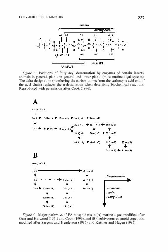
Figure 4 Major pathways of FA biosynthesis in (A) marine algae, modified afterGurr and Harwood (1991) and Cook (1996), and (B) herbivorous calanoid copepods,modified after Sargent and Henderson (1986) and Kattner and Hagen (1995).

Figure 3 Positions of fatty acyl desaturation by enzymes of certain insects,animals in general, plants in general and lower plants (most marine algal species).The delta-designation (numbering the carbon atoms from the carboxylic acid end ofthe acyl chain) replaces the n-designation when describing biochemical reactions.Reproduced with permission after Cook (1996).


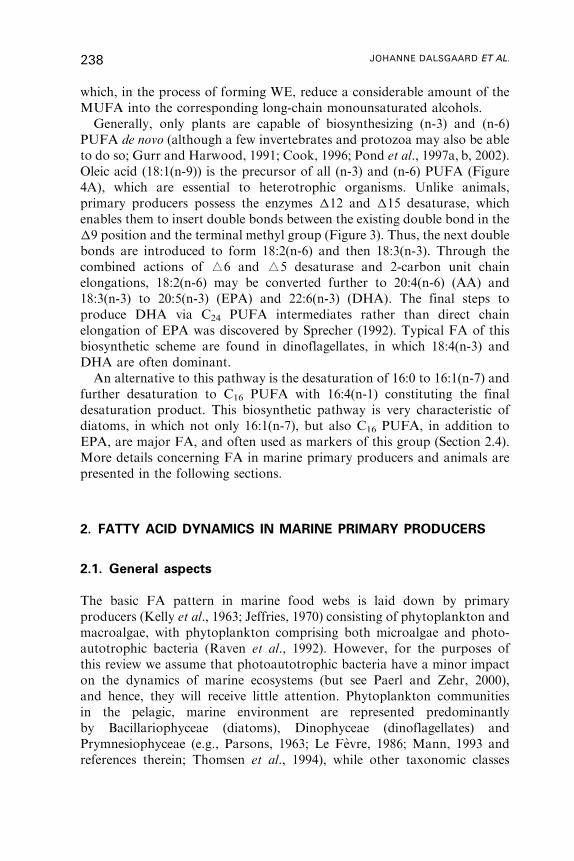
which, in the process of forming WE, reduce a considerable amount of the

MUFA into the corresponding long-chain monounsaturated alcohols.

Generally, only plants are capable of biosynthesizing (n-3) and (n-6)

PUFA de novo (although a few invertebrates and protozoa may also be able

to do so; Gurr and Harwood, 1991; Cook, 1996; Pond et al., 1997a, b, 2002).

Oleic acid (18:1(n-9)) is the precursor of all (n-3) and (n-6) PUFA (Figure

4A), which are essential to heterotrophic organisms. Unlike animals,

primary producers possess the enzymes �12 and �15 desaturase, which

enables them to insert double bonds between the existing double bond in the

�9 position and the terminal methyl group (Figure 3). Thus, the next double

bonds are introduced to form 18:2(n-6) and then 18:3(n-3). Through the

combined actions of i6 and i5 desaturase and 2-carbon unit chain

elongations, 18:2(n-6) may be converted further to 20:4(n-6) (AA) and

18:3(n-3) to 20:5(n-3) (EPA) and 22:6(n-3) (DHA). The final steps to

produce DHA via C24 PUFA intermediates rather than direct chain

elongation of EPA was discovered by Sprecher (1992). Typical FA of this

biosynthetic scheme are found in dinoflagellates, in which 18:4(n-3) and

DHA are often dominant.

An alternative to this pathway is the desaturation of 16:0 to 16:1(n-7) and

further desaturation to C16 PUFA with 16:4(n-1) constituting the final

desaturation product. This biosynthetic pathway is very characteristic of

diatoms, in which not only 16:1(n-7), but also C16 PUFA, in addition to

EPA, are major FA, and often used as markers of this group (Section 2.4).

More details concerning FA in marine primary producers and animals are

presented in the following sections.

2. FATTY ACID DYNAMICS IN MARINE PRIMARY PRODUCERS

2.1. General aspects

The basic FA pattern in marine food webs is laid down by primary

producers (Kelly et al., 1963; Jeffries, 1970) consisting of phytoplankton and

macroalgae, with phytoplankton comprising both microalgae and photo-

autotrophic bacteria (Raven et al., 1992). However, for the purposes of

this review we assume that photoautotrophic bacteria have a minor impact

on the dynamics of marine ecosystems (but see Paerl and Zehr, 2000),

and hence, they will receive little attention. Phytoplankton communities

in the pelagic, marine environment are represented predominantly

by Bacillariophyceae (diatoms), Dinophyceae (dinoflagellates) and

Prymnesiophyceae (e.g., Parsons, 1963; Le Fevre, 1986; Mann, 1993 and

references therein; Thomsen et al., 1994), while other taxonomic classes


(see below) are much less abundant except in bloom conditions (e.g., Parrish

et al., 1995; Cripps et al., 1999).

Phytoplankton are the major providers of metabolic energy in pelagic

food webs (Parsons, 1963), which is transferred to higher trophic levels via

grazing by herbivorous and omnivorous planktivorous species including the

larvae of fish and larger invertebrates. Similarly, phytoplankton support

benthic food webs that, in addition, may receive considerable inputs from

macroalgae (seaweeds), belonging to one of the three classes: Chlorophyceae

(green algae), Rhodophyceae (red algae) or Phaeophyceae (brown algae)

(Raven et al., 1992). While a few species of the brown algae Sargassum are

free-floating (Raven et al., 1992), the dominant life phase in most macro-

algal species is benthic, and because of limited light availability they are

restricted to the shallower coastal areas (Levring, 1979; Kristiansen et al.,

1981). Here, they constitute an important refuge for fish and invertebrates

and are either grazed directly or, as is mostly the case, enter the detrital food

webs via microheterotrophs (Dunstan et al., 1988; Sherr and Sheer, 2000

and references therein; Graeve et al., 2002 and references therein).

2.2. Biosynthesis of fatty acids

Autotrophic organisms biosynthesize all of their cellular constituents de

novo including a great diversity of FA (Sargent and Henderson, 1995; Cook,

1996). A description of the structure of these lipids and FA in algae can be

found in Pohl and Zurheide (1979) and in Wood (1988), while algal

metabolism is discussed by Harwood and Jones (1989). In summary, FA are

biosynthesized in the chloroplasts comprising the thylakoid membranes

(Harwood and Russell, 1984; Raven et al., 1992). They consist predomi-

nantly of even-numbered, straight-chain, saturated or cis-unsaturated

compounds with 12 to 24 carbon atoms (Pohl and Zurheide, 1979, 1982;

Wood, 1988; Cobelas and Lechado, 1989; Harwood and Jones, 1989;

Kayama et al., 1989). Low amounts of more unusual FA with more than

24 carbon atoms, as well as some trans-unsaturated (particularly trans-

16:1(n-13)) and odd-chain FA of varying chain length, are also biosynthe-

sized by some species (Pohl and Zurheide, 1979; Volkman et al., 1980a;

Harwood and Jones, 1989; Mansour et al., 1999a). The FA are esterified

chiefly to glycolipids (particularly rich in (n-3) PUFA and the major

constituents of the thylakoid membranes), whereas PL and NL are

comparatively minor lipid constituents of algae (Pohl and Zurheide, 1979;

Sargent et al., 1987, 1989; Wood, 1988; Harwood and Jones, 1989).

As mentioned in Section 1.5, plants are usually the only organism within

the system that can biosynthesize 18:2(n-6) and 18:3(n-3) de novo. These

particular PUFA and their derivatives (i.e., AA, EPA and DHA) are


essential constituents of heterotrophic organisms, stressing the central

position of algae within marine food webs (Pohl and Zurheide, 1979; Gurr

and Harwood, 1991; Cook, 1996; Smith and Fitzpatrick, 1996). Consistent

with this, recent experimental evidence (particularly in freshwater research)

has shown that the level of (n-3) PUFA is an important food quality

indicator (Jonasdottir et al., 1995; Muller-Navarra, 1995; Muller-Navarra

et al., 2000; Wacker and von Elert, 2001), which may affect trophodynamic

relationships (Muller-Navarra and Lampert, 1996; Sterner and Schulz,

1998; Muller-Navarra et al., 2000). Consequently, (n-3) PUFA may

determine the rates at which carbon (Brett and Muller-Navarra, 1997),

and hence other marker FA, are channeled through the food web.

2.3. Impact of growth, environmental and

hydrodynamic factors

The FA signature of microalgae is an expression of both genotypic (Alonso

et al., 1994) and phenotypic characteristics. Large qualitative and

particularly quantitative fluctuations, both within and between species,

are observed that can be related to the combined effects of environmental

conditions and the physiological state of the algae (see below).

Variations in the biomass, distribution and species composition of

microalgae, and hence the basic FA pattern in the marine environment, are

ultimately driven by hydrodynamic processes. The reason for this is that

hydrodynamic processes affect both the availability of nutrients and light,

and influence the distribution of microalgae through horizontal and vertical

circulation patterns coupled with behavioral or buoyancy characteristics

(e.g., Franks, 1992). Nutrient and light availability are tightly coupled to

water column stability, which can be simplified into two extreme

hydrodynamic regimes in the pelagic environment: stratified and mixed

water columns. Stratified water columns arise in areas characterized by low

turbulent energy, and primary production in these areas is typically nutrient

limited. The primary producer community is generally composed of small,

autotrophic flagellates and cyanobacteria (<10 mm) that form the basis

of low biomass, microbial loop food webs. In contrast, areas of high

turbulence result in mixed or weakly stratified water columns with a

consistent influx of nutrients. As a consequence, primary producers in these

areas are light limited rather than nutrient limited due to the increased

depth of mixing. Primary production is usually carried out by relatively

large diatoms (>10 mm) giving rise to ‘‘simple’’ food webs with an efficient

transfer of energy to higher trophic levels. Algal growth within these

regimes is largely controlled by the local environmental conditions, with


temperature, light and nutrient availability being the three key factors

affecting the FA pattern of the local community.

The impact of these environmental factors has been studied primarily in

laboratory cultures, and has been reviewed, e.g., by Pohl and Zurheide

(1979), Cobelas (1989), Kayama et al. (1989), and Roessler (1990). Typically,

lower water temperatures result in an increase in the level of unsaturation

(e.g., Ackman et al., 1968; Pohl and Zurheide, 1982), whereas the impact of

light is ambiguous and more species-specific. In general, however, the level of

glycolipids, and hence (n-3) PUFA, increases under nonlimiting light

conditions, whereas photo-inhibition and reduced light intensities reportedly

lead to the accumulation of TAG (the major lipid storage product in algae),

which is richer in saturated fatty acids (SFA) andMUFA (Cohen et al., 1988;

Harrison et al., 1990; Mayzaud et al., 1990 and references therein; Thompson

et al., 1990; Sukenik and Wahnon, 1991; Smith et al., 1993; Parrish et al.,

1994). Algal growth, as previously mentioned, is influenced by the

availability of limiting nutrients (principally nitrogen, phosphorus or

silicate), which influence the transition from the exponential phase (non-

nutrient limited) to the stationary growth phase (nutrient limited), the latter

being characterized by the accumulation of TAG (see above for consequences

on FA patterns; Kattner et al., 1983; Morris et al., 1983; Ben-Amotz et al.,

1985; Harrison et al., 1990; Kattner and Brockmann, 1990; Mayzaud et al.,

1990; Fahl and Kattner, 1993; Reitan et al., 1994; Falk-Petersen et al., 1998;

Henderson et al., 1998). During the exponential growth phase of

phytoplankton blooms, carbon fixed through photosynthesis is allocated to

growth and cell division rather than lipid storage (e.g., Morris, 1981; Kattner

et al., 1983; Parrish and Wangersky, 1990). As a consequence, the relative

proportion of glycolipids is particularly high in this phase (Sargent and

Henderson, 1986; Roessler, 1990), and the concentration of (n-3) PUFAmay

approach 50% of the TL content (e.g., Napolitano et al., 1997; Claustre et al.,

1989; Sargent et al., 1989; Falk-Petersen et al., 1998; Henderson et al., 1998).

This exponential algal growth phase occurs during spring bloom conditions

and the FA pattern of the exponentially growing algae is particularly evident

in field examinations of phytoplankton lipid dynamics (e.g., Kattner et al.,

1983; Hama, 1991).

2.4. Specific fatty acid markers of primary producers

2.4.1. Microalgae

It is well established that whereas FA cannot be used as taxonomic indicators

at the species-specific level, the presence and combinations of certain FA can

be characteristic of particular algal classes and thus have potential as markers


(e.g., Ackman et al., 1968; Chuecas andRiley, 1969; Pohl and Zurheide, 1979;

Kattner et al., 1983; Sargent et al., 1987; Cobelas and Lechado, 1989;

Mayzaud et al., 1990;Mourente et al., 1990; Fahl andKattner, 1993; Viso and

Marty, 1993; Napolitano, 1999; Volkman et al., 1998).

Since the early 1960s, a large number of laboratory studies have examined

the FA composition of marine microalgae (reviewed by Ackman et al., 1968;

Pohl and Zurheide, 1979; Cobelas and Lechado, 1989; Kayama et al., 1989).

In these studies, the algae have been cultured under a wide range of

treatment conditions, and have been analyzed using standard, organic-

solvent extraction and methylation procedures combined with thin layer

chromatography (TLC) and gas chromatography (GC) later combined with

mass spectrometry (GC-MS) (Ackman, 2002; Traitler, 1987). Many of the

earliest studies were characterized by incomplete compound separation and

loss of PUFA due to improper sample handling and storage protocols.

Hence, the results from these studies should be interpreted with caution

(discussed by Ackman et al., 1968; Chuecas and Riley, 1969; Conte et al.,

1994). Subsequently, techniques have improved (especially column technol-

ogy), resulting in a higher degree of sensitivity. As a consequence, more

precise estimates of total FA contents may be obtained, and in addition,

more FA have been identified. For example, trace amounts of the very-long-

chain, highly-unsaturated-fatty-acids (VLC-HUFA) 28:7(n-6) and 28:8(n-3)

have been identified in several species of dinoflagellates (Mansour et al.,

1999a, b). Intriguingly, octacosaheptaenoic acid (28:7(n-6)) and other VLC-

HUFA had previously been detected in Baltic herring where they were

suspected to originate from the diet (Linko and Karinkanta, 1970).

However, except for a few examples like this, these more unusual FA

usually occur only in trace amounts in phytoplankton (e.g., Nichols et al.,

1986), and are even more difficult to recognize in the consumers due to the

low levels of occurrence, limiting their potential as trophic markers (see also

Section 5.7.2; Ackman and Mclachlan, 1977; Mayzaud et al., 1999).

Aside from sample treatment and identification procedures, another

obstacle associated with the application of FATM has been the interpreta-

tion of the large data sets routinely produced in these types of analyses

(typically arrays of more than 30 FA determined simultaneously from one

or more samples). With the development of computer power, easily

accessible, multivariate statistical methods have advanced to become

particularly useful for interpreting such large data sets (e.g., Wold et al.,

1988; Frank, 1989; Kaufmann, 1992; Smith et al., 1997, 1999; Legendre

and Legendre, 1998). Here, we present the results of such an analysis,

indicating the patterns of FA similarities within and among eight classes

of microalgae (Bacillariophyeae, Chlorophyceae, Cryptophyceae,

Dinophyceae, Eustigmatophyceae, Prymnesiophyceae, Prasinophyceae and

Raphidophyceae). The outcome of the analysis is visualized in Figure 5,


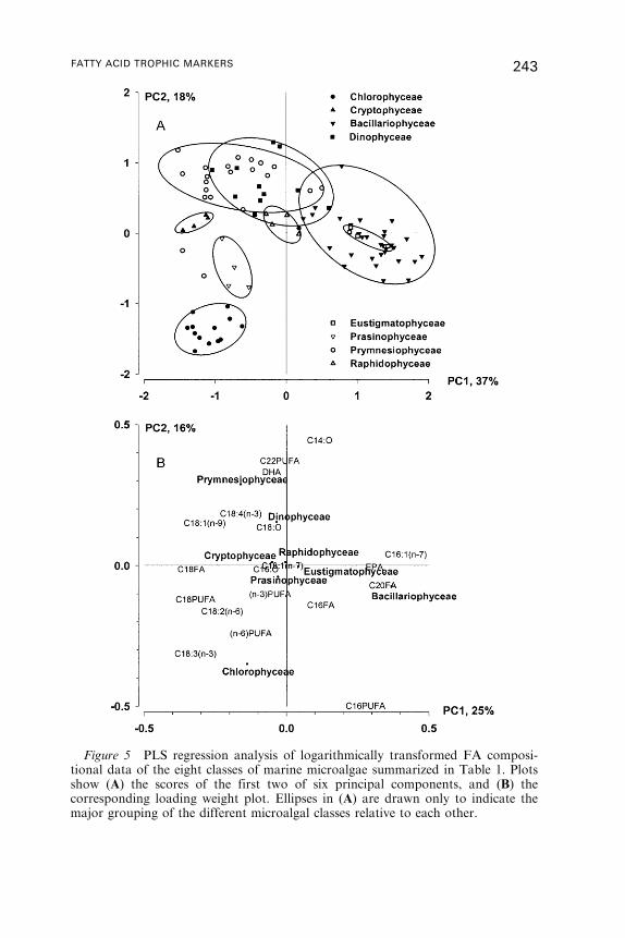
Figure 5 PLS regression analysis of logarithmically transformed FA composi-tional data of the eight classes of marine microalgae summarized in Table 1. Plotsshow (A) the scores of the first two of six principal components, and (B) thecorresponding loading weight plot. Ellipses in (A) are drawn only to indicate themajor grouping of the different microalgal classes relative to each other.


which was constructed by applying a PLS regression analysis2 to

logarithmically transformed FA compositional data compiled from

laboratory culture studies reported in the literature3. The analysis was

performed on nineteen FA variables summarized in Table 1. The variables

comprise both individual FA as well as combinations (sums) of FA selected

based on the presence in the compiled data set, i.e., only FA that were

identified in all studies were included.

In this analysis, the first six PLS components (linear combinations of the

variables) explained 89% of the variance of the FA compositional data

(predictor variables) and 61% of the variance contributed to microalgal

‘‘class-affiliation’’ (response variables). Despite considerable overlap,

particularly between dinophytes and prymnesiophytes and between bacil-

lariophytes and eustigmatophytes, the eight classes of microalgae can

still be recognized in the score plot of the first two principal components

(Figure 5A). The corresponding loading weight plot4 (Figure 5B) shows

the importance of the different FA variables for the two first PLS

components. Fatty acids roughly in the same direction from the center as

the microalgal classes are positively linked to and particularly important

predictors of those classes, whereas FA in the opposite direction

are negatively linked with the algal classes. Figure 5B shows that

bacillariophytes clearly separate from the other classes along the first PLS

component linking positively with 16:1(n-7), C16 FA, C16 PUFA, C20 FA

and EPA and negatively with C18 FA (see also Mayzaud et al., 1990).

Although not included in the analysis, another important FA is 16:4(n-1),

which has been suggested as a specific marker of this microalgal class (Viso

and Marty, 1993). It has been detected in most of the species of

Bacillariophyceae studied to date, whereas it is more or less absent in

2This particular analysis models simultaneously the FA composition and microalgal

‘‘class-affiliation’’, and can be perceived as a PC-hyperplane tilted slightly so as to

make microalgal ‘‘class-affiliation’’ better explained by the latent variables of the FA

matrix (Wold et al., 1988). Analyses were performed using The Unscrambler� v7.6

SR-1 CAMO ASA software.3The model is only preliminary and not adopted for predictive purposes by applying

it on an independent test set.4 ‘‘Loading weights are specific to PLS . . . and express how the information in each

X-variable [predictor variables] relates to the variation in Y [response variables]

summarized by the u-scores. They are called loading weights because they also express,

in the PLS algorithm, how the t-scores are to be computed from the X-matrix to obtain

an orthogonal decomposition. The loading weights are normalized, so that their lengths

can be interpreted as well as their directions. Variables with large loading weight values

are important for the prediction of Y.’’ Copyright � 1996-2000 CAMO ASA. All

rights reserved.


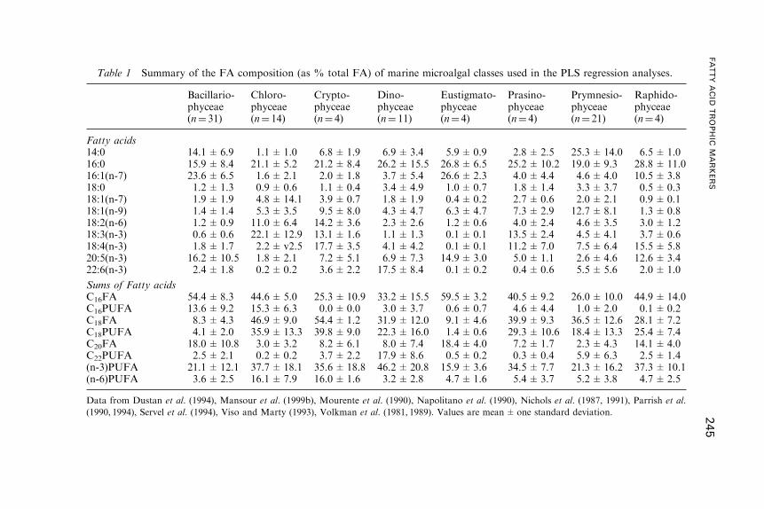
Table 1 Summary of the FA composition (as % total FA) of marine microalgal classes used in the PLS regression analyses.

Bacillario-phyceae(n¼ 31)

Chloro-phyceae(n¼ 14)

Crypto-phyceae(n¼ 4)

Dino-phyceae(n¼ 11)

Eustigmato-phyceae(n¼ 4)

Prasino-phyceae(n¼ 4)

Prymnesio-phyceae(n¼ 21)

Raphido-phyceae(n¼ 4)

Fatty acids14:0 14.1±6.9 1.1±1.0 6.8±1.9 6.9±3.4 5.9±0.9 2.8±2.5 25.3±14.0 6.5±1.016:0 15.9±8.4 21.1±5.2 21.2±8.4 26.2±15.5 26.8±6.5 25.2±10.2 19.0±9.3 28.8±11.016:1(n-7) 23.6±6.5 1.6±2.1 2.0±1.8 3.7±5.4 26.6±2.3 4.0±4.4 4.6±4.0 10.5±3.818:0 1.2±1.3 0.9±0.6 1.1±0.4 3.4±4.9 1.0±0.7 1.8±1.4 3.3±3.7 0.5±0.318:1(n-7) 1.9±1.9 4.8±14.1 3.9±0.7 1.8±1.9 0.4±0.2 2.7±0.6 2.0±2.1 0.9±0.118:1(n-9) 1.4±1.4 5.3±3.5 9.5±8.0 4.3±4.7 6.3±4.7 7.3±2.9 12.7±8.1 1.3±0.818:2(n-6) 1.2±0.9 11.0±6.4 14.2±3.6 2.3±2.6 1.2±0.6 4.0±2.4 4.6±3.5 3.0±1.218:3(n-3) 0.6±0.6 22.1±12.9 13.1±1.6 1.1±1.3 0.1±0.1 13.5±2.4 4.5±4.1 3.7±0.618:4(n-3) 1.8±1.7 2.2±v2.5 17.7±3.5 4.1±4.2 0.1±0.1 11.2±7.0 7.5±6.4 15.5±5.820:5(n-3) 16.2±10.5 1.8±2.1 7.2±5.1 6.9±7.3 14.9±3.0 5.0±1.1 2.6±4.6 12.6±3.422:6(n-3) 2.4±1.8 0.2±0.2 3.6±2.2 17.5±8.4 0.1±0.2 0.4±0.6 5.5±5.6 2.0±1.0

Sums of Fatty acidsC16FA 54.4±8.3 44.6±5.0 25.3±10.9 33.2±15.5 59.5±3.2 40.5±9.2 26.0±10.0 44.9±14.0C16PUFA 13.6±9.2 15.3±6.3 0.0±0.0 3.0±3.7 0.6±0.7 4.6±4.4 1.0±2.0 0.1±0.2C18FA 8.3±4.3 46.9±9.0 54.4±1.2 31.9±12.0 9.1±4.6 39.9±9.3 36.5±12.6 28.1±7.2C18PUFA 4.1±2.0 35.9±13.3 39.8±9.0 22.3±16.0 1.4±0.6 29.3±10.6 18.4±13.3 25.4±7.4C20FA 18.0±10.8 3.0±3.2 8.2±6.1 8.0±7.4 18.4±4.0 7.2±1.7 2.3±4.3 14.1±4.0C22PUFA 2.5±2.1 0.2±0.2 3.7±2.2 17.9±8.6 0.5±0.2 0.3±0.4 5.9±6.3 2.5±1.4(n-3)PUFA 21.1±12.1 37.7±18.1 35.6±18.8 46.2±20.8 15.9±3.6 34.5±7.7 21.3±16.2 37.3±10.1(n-6)PUFA 3.6±2.5 16.1±7.9 16.0±1.6 3.2±2.8 4.7±1.6 5.4±3.7 5.2±3.8 4.7±2.5

Data from Dustan et al. (1994), Mansour et al. (1999b), Mourente et al. (1990), Napolitano et al. (1990), Nichols et al. (1987, 1991), Parrish et al.

(1990, 1994), Servel et al. (1994), Viso and Marty (1993), Volkman et al. (1981, 1989). Values are mean±one standard deviation.

FATTYACID

TROPHIC

MARKERS

245

other algal classes (e.g., Volkman et al., 1989; Napolitano et al., 1990;

Parrish et al., 1990; Thompson et al., 1990; Dunstan et al., 1994). Trace

amounts have, however, been detected in a few species of chlorophytes

(Chuecas and Riley, 1969), dinophytes (Mansour et al., 1999b), prasino-

phytes (Chuecas and Riley, 1969), prymnesiophytes (Ackman et al., 1968;

Chuecas and Riley, 1969) and rhodophytes (macroalgae; Graeve et al.,

2002).

Prymnesiophytes (except for two species of Hymenomonas) and dino-

phytes separate from the other classes by positive anomalies of 18:0, 18:1

(n-9), 18:4(n-3), C22 PUFA and DHA. Another important FA of these

two classes, though not included in the analysis, is 18:5(n-3). This FA

was identified for the first time by Joseph (1975) in several species of

Dinophyceae. Later, it has been identified in species of prymnesiophytes

(Volkman et al., 1981, 1989; Sargent et al., 1985; Claustre et al., 1990;

Napolitano et al., 1990; Viso and Marty, 1993), raphidophytes (Nichols

et al., 1987; Viso and Marty, 1993), prasinophytes (Viso and Marty, 1993)

and bacillariophytes (Reitan et al., 1994).

Chlorophytes (except for one species of Nannochloris) are discriminated

by 18:3(n-3), 18:2(n-6) and other (n-6) PUFA. The close association of the

chlorophytes with prasinophytes in Figure 5A is consistent with both classes

belonging to the same division of Chlorophyta (Viso and Marty, 1993). A

characteristic FA of both these classes is 16:4(n-3) (not included in the

analysis; Ackman et al., 1968; Viso and Marty, 1993), whereas the presence

of >C20 FA in prasinophytes distinguishes them from the chlorophytes

(Viso and Marty, 1993).

Cryptophytes, raphidophytes and eustigmatophytes can be distinguished

as more or less separate groups. However, together with prasinophytes their

variations are poorly explained by the model, clustering around the center

on the loading weight plot (Figure 5B). It should be emphasized that limited

FA compositional data were available for these four classes of microalgae.

Hence, they were only represented by four observations each, which are

really too few for ensuring stability of the model (Albano et al., 1981; Wold

et al., 1988).

This was taken into account in a second analysis, considering only

Bacillariophyceae, Dinophyceae, Prymnesiophyceae and Chlorophyceae,

which all contributed sufficient sample sizes and, as mentioned in Section

2.1, dominate the phytoplankton biomass in most marine ecosystems

(except for Chlorophyceae). In this analysis, the first four PLS components

now explain 83% of the variance of the FA compositional data and 76% of

the variance contributed by microalgal ‘‘class-affiliation’’. A plot of the

second vs. third principal component (Figure 6A) reveals that apart from

two species of Hymenomonas, two large clusters of prymnesiophytes can be

recognized consisting predominantly of Isochrysis spp. (upper ellipse), and


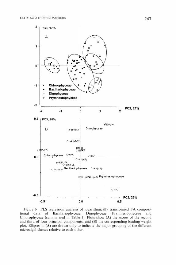
Figure 6 PLS regression analysis of logarithmically transformed FA composi-tional data of Bacillariophyceae, Dinophyceae, Prymnesiophyceae andChlorophyceae (summarized in Table 1). Plots show (A) the scores of the secondand third of four principal components, and (B) the corresponding loading weightplot. Ellipses in (A) are drawn only to indicate the major grouping of the differentmicroalgal classes relative to each other.


Phaeocystis spp. and Chrysotila spp. (lower ellipse). Consistent with their

position in Figure 6A close to the Dinophyceae, species of Isochrysis are

characterized by a low 16:1/16:0 ratio, and high concentrations of C18

PUFA and EPA (Conte et al., 1994). The loading weight plot (Figure 6B)

shows that the prymnesiophytes in general separate from the dinophytes by

higher, positive anomalies of 14:0, 16:1(n-7), 18:1(n-9) and 18:4(n-3) while

the dinophytes link positively with DHA, C22PUFA and (n-3) PUFA.

These analyses re-emphasize that individual FA cannot be used as

taxonomic indicators of particular algal species or classes, whereas

combinations of FA reveal certain patterns when microalgae are compared

class-wise. This conclusion confirms the statement of Viso and Marty (1993)

who identified the need to combine several FA criteria to distinguish natural

assemblages of microalgae belonging to different taxonomic classes. To

date, most of the criteria (ratios of FA) that have been developed have

focused on bacillariophytes and dinophytes, reflecting the relative impor-

tance of these two classes in the marine environment. Here, in particular,

high values of 16:1(n-7)/16:0 (typically >1) and �C16/�C18 have been

associated with a dominance of bacillariophytes (e.g., Miyazaki, 1983;

Claustre et al., 1988, 1989; Mayzaud et al., 1990; Viso and Marty, 1993;

Budge and Parrish, 1998; Budge et al., 2001; Reuss and Poulsen, 2002),

whereas high values of 18:5(n-3)/18:3(n-3) and � (C18PUFA, C22PUFA)

have been associated with a dominance of dinophytes (Nichols et al.,

1984; Viso and Marty, 1993). Combining these criteria, i.e., high values of

�C16/�C18 together with low values of 18:5(n-3)/18:3(n-3), has been

proposed as a means whereby bacillariophytes can be distinguished from

dinophytes (Viso and Marty, 1993). This could be further strengthened

by examining the ratio of 22:6(n-3)/20:5(n-3) as suggested by Budge

and Parrish (1998). Here, a value �1 signals a dominance in the

contribution of dinophytes while conversely, a value <1 is suggestive of a

greater contribution of bacillariophytes.

A quantitative summary of the PLS analyses and the criteria discussed

above is presented in Table 2 with mean values for the eight classes of

microalgae included in the analyses. It must be recognised that the figures in

the table should be perceived only as a very rough guideline of potentially

useful FATM.

2.4.2. Macroalgae

Compared to microalgae, most of the information on macroalgae

(belonging to one of the three classes: Chlorophyceae, Rhodophyceae

and Phaeophyceae) originates from field studies (reviewed by Kayama

et al., 1989), rather than laboratory experiments (e.g., Ahern et al., 1983;


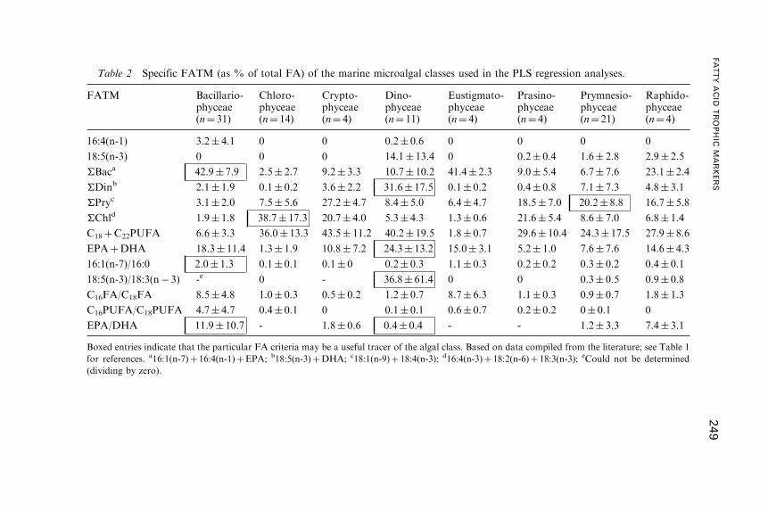
Table 2 Specific FATM (as % of total FA) of the marine microalgal classes used in the PLS regression analyses.

FATM Bacillario-phyceae(n¼ 31)

Chloro-phyceae(n¼ 14)

Crypto-phyceae(n¼ 4)

Dino-phyceae(n¼ 11)

Eustigmato-phyceae(n¼ 4)

Prasino-phyceae(n¼ 4)

Prymnesio-phyceae(n¼ 21)

Raphido-phyceae(n¼ 4)

16:4(n-1) 3.2� 4.1 0 0 0.2� 0.6 0 0 0 0

18:5(n-3) 0 0 0 14.1� 13.4 0 0.2� 0.4 1.6� 2.8 2.9� 2.5

�Baca 42.9� 7.9 2.5� 2.7 9.2� 3.3 10.7� 10.2 41.4� 2.3 9.0� 5.4 6.7� 7.6 23.1� 2.4

�Dinb 2.1� 1.9 0.1� 0.2 3.6� 2.2 31.6� 17.5 0.1� 0.2 0.4� 0.8 7.1� 7.3 4.8� 3.1

�Pryc 3.1� 2.0 7.5� 5.6 27.2� 4.7 8.4� 5.0 6.4� 4.7 18.5� 7.0 20.2� 8.8 16.7� 5.8

�Chld 1.9� 1.8 38.7� 17.3 20.7� 4.0 5.3� 4.3 1.3� 0.6 21.6� 5.4 8.6� 7.0 6.8� 1.4

C18þC22PUFA 6.6� 3.3 36.0� 13.3 43.5� 11.2 40.2� 19.5 1.8� 0.7 29.6� 10.4 24.3� 17.5 27.9� 8.6

EPAþDHA 18.3� 11.4 1.3� 1.9 10.8� 7.2 24.3� 13.2 15.0� 3.1 5.2� 1.0 7.6� 7.6 14.6� 4.3

16:1(n-7)/16:0 2.0� 1.3 0.1� 0.1 0.1� 0 0.2� 0.3 1.1� 0.3 0.2� 0.2 0.3� 0.2 0.4� 0.1

18:5(n-3)/18:3(n� 3) -e 0 - 36.8� 61.4 0 0 0.3� 0.5 0.9� 0.8

C16FA/C18FA 8.5� 4.8 1.0� 0.3 0.5� 0.2 1.2� 0.7 8.7� 6.3 1.1� 0.3 0.9� 0.7 1.8� 1.3

C16PUFA/C18PUFA 4.7� 4.7 0.4� 0.1 0 0.1� 0.1 0.6� 0.7 0.2� 0.2 0� 0.1 0

EPA/DHA 11.9� 10.7 - 1.8� 0.6 0.4� 0.4 - - 1.2� 3.3 7.4� 3.1

Boxed entries indicate that the particular FA criteria may be a useful tracer of the algal class. Based on data compiled from the literature; see Table 1

for references. a16:1(n-7)þ 16:4(n-1)þEPA; b18:5(n-3)þDHA; c18:1(n-9)þ 18:4(n-3); d16:4(n-3)þ 18:2(n-6)þ 18:3(n-3); eCould not be determined

(dividing by zero).

FATTYACID

TROPHIC

MARKERS

249

Honya et al., 1994). Some general trends distinguishing the three classes

have been recognized, which are largely independent of geographical

locations and morphological differences (e.g. Ackman and McLachlan, 1977

(Nova Scotia); Chuecas and Riley, 1966 (Isle of Man); Dembritsky et al.,

1993 (Caspian Sea); Fleurence et al., 1994 (French Brittany coast); Graeve

et al., 2002 (Arctic and Antarctic); Khotimchenko et al., 2002 (Pacific

coast); Li et al., 2002 (Bohai Sea); Pohl and Zurheide, 1982 (Baltic Sea)). C18

and C20 FA constitute the principal PUFA in macroalgae whereas C22

PUFA are more abundant in microalgae (Chuecas and Riley, 1966; Graeve

et al., 2002). Moreover, the (n-6) family (particularly AA) is more prevalent

in macroalgae than in microalgae. High concentrations of AA combined

with insignificant amounts of C18 PUFA distinguish rhodophytes from

phaeophytes in which both C18 PUFA (particularly 18:4(n-3)) and C20

PUFA (principally EPA and AA) are major FA constituents. The FA

pattern of chlorophyte macroalgae is similar to that of chlorophyte

microalgae. Overall, the chlorophytes differ from the rest of the eukaryotic

algae by a FA composition more similar to that of higher plants (Pohl and

Zurheide, 1979; Wood, 1988; Kayama et al., 1989). For example, few of the

constituent FA have more than three double bonds and most species have

only modest amounts of >C20 PUFA, while the proportion of C16 and C18

PUFA is generally high (see Table 1; Wood, 1988; Lechevalier and

Lechevalier, 1988; Volkman et al., 1998; Graeve et al., 2002). A particular

trait of chlorophytes is the high content of 18:3(n-3) regarded as a

characteristic of the phylum Chlorophyta (Li et al., 2002). Furthermore,

several species exhibit a 18:1(n-7)/18:1(n-9) ratio >1 (Khotimchenko et al.,

2002; Li et al., 2002), which in combination with 18:2(n-3) and 18:3(n-3)

may potentially serve as a biomarker of this algal class.

2.4.3. Comparisons with natural plankton communities

Natural plankton communities consist of a mixture of species and dead

organic matter that are exposed to concurrent fluctuations of different

environmental factors. This makes comparisons and extrapolations of

results obtained in the laboratory to the field situation extremely difficult.

The proportion of PUFA is, for example, usually lower in natural

phytoplankton communities than in algal cultures (e.g., Kattner et al.,

1983; Morris, 1984; Morris et al., 1985; Kattner and Brockmann, 1990; Fahl

and Kattner, 1993), and the FA signature of lipid-deficient algae is often

masked by the signature of more abundant and lipid rich species such as

diatoms (e.g., Skerratt et al., 1995; Budge et al., 2001).

Despite these uncertainties, studies of natural phytoplankton communities

generally confirm the characteristic FA patterns summarized above. Hence,


elevated concentrations of 14:0, 16:1(n-7), C16 PUFA (particularly 16:4(n-1)),

and EPA are characteristically measured in diatom-dominated enclosure

studies (Morris et al., 1985; Kattner and Brockmann, 1990; Mayzaud

et al., 1990; Pond et al., 1998), during temporal spring blooms (Kattner et al.,

1983; Claustre et al., 1988, 1989; Napolitano et al., 1997; Budge and Parrish,

1998; Budge et al., 2001), in open waters of polar and boreal systems (Lewis,

1969; Sargent et al., 1985; Kattner and Brockmann, 1990; Pond et al., 1993;

Skerratt et al., 1995; Cripps et al., 1999; Cripps and Atkinson, 2000; Reuss

and Poulsen, 2002) and in Arctic and Antarctic attached sea-ice algae (Fahl

and Kattner, 1993; Nichols et al., 1993; Falk-Petersen et al., 1998; Henderson

et al., 1998). Similarly, typical dinoflagellate markers, i.e., particularly high

levels of 18:4(n-3), 18:5(n-3) and DHA are consistent within dinoflagellate

dominated communities both at temperate (e.g., Kattner et al., 1983;

Mayzaud et al., 1990; Napolitano et al., 1997; Budge and Parrish, 1998;

Budge et al., 2001) and at high latitudes (Falk-Petersen et al., 1998).

Consistent with the PLS analysis in Section 2.4.1, the FA composition of

blooms dominated by prymnesiophytes is more variable. In several regions,

such blooms have been associated with elevated levels of 14:0, 16:0, 18:0 and

18:1(n-9) and low levels of (n-3) PUFA (Al-Hasan et al., 1990 (Kuwait Bay);

Claustre et al., 1990 (the Irish Sea); Skerratt et al., 1995 (Antarctic);

Cotonnec et al., 2001 (the English Channel); Reuss and Poulsen, 2002 (west

Greenland)). The low concentration of (n-3) PUFA makes Phaeocystis in

these regions of low nutritional value for grazers. For example, Claustre

et al. (1990) estimated that Phaeocystis constituted only a minor dietary

component of Temora longicornis in the Irish Sea. Cotonnec et al. (2001),

however, found that T. longicornis, Acartia clausi and Pseudocalanus

elongatus, sampled in the English Channel during a Phaeocystis-dominated

spring bloom, had all consumed large quantities. They argued that this was

a result of low rejection of the algae due to its very high concentration in the

field. In contrast, Phaeocystis blooms have in other regions been associated

with high concentrations of 18:4(n-3), 18:5(n-3), EPA and DHA (Sargent

et al., 1985; Hamm et al., 2001 (Balsfjord)), and are here heavily grazed

(e.g., Sargent et al., 1987; Tande and Bamstedt, 1987; Sargent and Falk-

Petersen, 1988).

2.5. Specific fatty acid markers of heterotrophic

bacteria and terrestrial matter

2.5.1. Bacteria

Marine heterotrophic bacteria are particularly abundant in sediments

(Sargent et al., 1987) and as colonizers of settling particulate matter


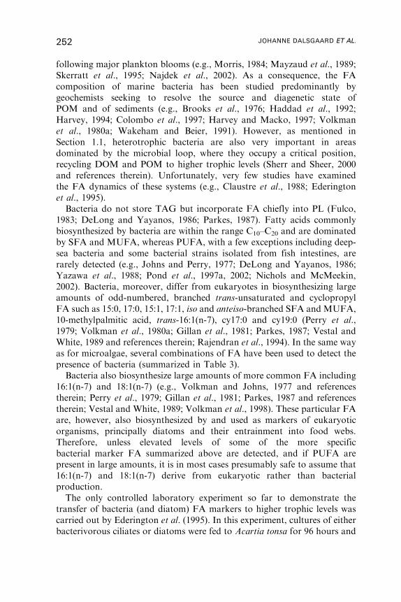
following major plankton blooms (e.g., Morris, 1984; Mayzaud et al., 1989;

Skerratt et al., 1995; Najdek et al., 2002). As a consequence, the FA

composition of marine bacteria has been studied predominantly by

geochemists seeking to resolve the source and diagenetic state of

POM and of sediments (e.g., Brooks et al., 1976; Haddad et al., 1992;

Harvey, 1994; Colombo et al., 1997; Harvey and Macko, 1997; Volkman

et al., 1980a; Wakeham and Beier, 1991). However, as mentioned in

Section 1.1, heterotrophic bacteria are also very important in areas

dominated by the microbial loop, where they occupy a critical position,

recycling DOM and POM to higher trophic levels (Sherr and Sheer, 2000

and references therein). Unfortunately, very few studies have examined

the FA dynamics of these systems (e.g., Claustre et al., 1988; Ederington

et al., 1995).

Bacteria do not store TAG but incorporate FA chiefly into PL (Fulco,

1983; DeLong and Yayanos, 1986; Parkes, 1987). Fatty acids commonly

biosynthesized by bacteria are within the range C10–C20 and are dominated

by SFA and MUFA, whereas PUFA, with a few exceptions including deep-

sea bacteria and some bacterial strains isolated from fish intestines, are

rarely detected (e.g., Johns and Perry, 1977; DeLong and Yayanos, 1986;

Yazawa et al., 1988; Pond et al., 1997a, 2002; Nichols and McMeekin,

2002). Bacteria, moreover, differ from eukaryotes in biosynthesizing large

amounts of odd-numbered, branched trans-unsaturated and cyclopropyl

FA such as 15:0, 17:0, 15:1, 17:1, iso and anteiso-branched SFA and MUFA,

10-methylpalmitic acid, trans-16:1(n-7), cy17:0 and cy19:0 (Perry et al.,

1979; Volkman et al., 1980a; Gillan et al., 1981; Parkes, 1987; Vestal and

White, 1989 and references therein; Rajendran et al., 1994). In the same way

as for microalgae, several combinations of FA have been used to detect the

presence of bacteria (summarized in Table 3).

Bacteria also biosynthesize large amounts of more common FA including

16:1(n-7) and 18:1(n-7) (e.g., Volkman and Johns, 1977 and references

therein; Perry et al., 1979; Gillan et al., 1981; Parkes, 1987 and references

therein; Vestal and White, 1989; Volkman et al., 1998). These particular FA

are, however, also biosynthesized by and used as markers of eukaryotic

organisms, principally diatoms and their entrainment into food webs.

Therefore, unless elevated levels of some of the more specific

bacterial marker FA summarized above are detected, and if PUFA are

present in large amounts, it is in most cases presumably safe to assume that

16:1(n-7) and 18:1(n-7) derive from eukaryotic rather than bacterial

production.

The only controlled laboratory experiment so far to demonstrate the

transfer of bacteria (and diatom) FA markers to higher trophic levels was

carried out by Ederington et al. (1995). In this experiment, cultures of either

bacterivorous ciliates or diatoms were fed to Acartia tonsa for 96 hours and


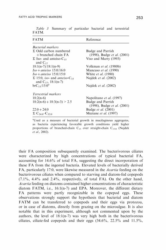
their FA composition subsequently examined. The bacterivorous ciliates

were characterized by high concentrations of typical bacterial FA,

accounting for 14.6% of total FA, suggesting the direct incorporation of

these FA from the ingested bacteria. Elevated levels of bacterially derived

FA, particularly 17:0, were likewise measured in the Acartia feeding on the

bacterivorous ciliates when compared to starving and diatom-fed copepods

(7.1%, 4.4% and 2.4%, respectively, of total FA). On the other hand,

Acartia feeding on diatoms contained higher concentrations of characteristic

diatom FATM, i.e., 16:1(n-7) and EPA. Moreover, the different dietary

FA patterns were partly recognizable in the copepod eggs. These

observations strongly support the hypothesis that bacterial and diatom

FATM can be transferred to copepods and their eggs via protozoa,

or in case of diatoms, directly from grazing on the microalgae. It is also

notable that in this experiment, although not commented upon by the

authors, the level of 18:1(n-7) was very high both in the bacterivorous

ciliates, ciliate-fed copepods and their eggs (34.6%, 22.5% and 11.5%,

Table 3 Summary of particular bacterial and terrestrialFATM.

FATM Reference

Bacterial markers� Odd carbon numbered

þ branched chain FABudge and Parrish(1998), Budge et al. (2001)

� Iso- and anteiso-C15

and C17

Viso and Marty (1993)

18:1(n-7)/18:1(n-9) Volkman et al. (1980b)Isoþ anteiso 15:0/16:0 Mancuso et al. (1990)Isoþ anteiso 15:0/15:0 White et al. (1980)� 15:0, iso- and anteiso-C15

and C17, 18:1(n-7)Najdek et al. (2002)

brC15/15:0a Najdek et al. (2002)

Terrestrial markers18:2(n-6) Napolitano et al. (1997)18:2(n-6)þ 18:3(n-3)>2.5 Budge and Parrish

(1998), Budge et al. (2001)22:0þ 24:0 Budge et al. (2001)� C24:0–C32:0 Meziane et al. (1997)

aUsed as a measure of bacterial growth in mucilaginous aggregates,

as bacteria experiencing favorable growth conditions yield higher

proportions of branched-chain C15 over straight-chain C15:0 (Najdek

et al., 2002).


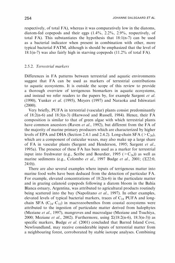
respectively, of total FA), whereas it was comparatively low in the diatoms,

diatom-fed copepods and their eggs (1.4%, 2.2%, 2.9%, respectively, of

total FA). This substantiates the hypothesis that 18:1(n-7) can be used

as a bacterial indicator when present in combination with other, more

typical bacterial FATM, although is should be emphasized that the level of

18:1(n-7) was also fairly high in starving copepods (11.2% of total FA).

2.5.2. Terrestrial markers

Differences in FA patterns between terrestrial and aquatic environments

suggest that FA can be used as markers of terrestrial contributions

to aquatic ecosystems. It is outside the scope of this review to provide

a thorough overview of terrigenous biomarkers in aquatic ecosystems,

and instead we refer readers to the papers by, for example Sargent et al.

(1990), Yunker et al. (1995), Meyers (1997) and Naraoka and Ishiwatari

(2000).

Very briefly, PUFA in terrestrial (vascular) plants consist predominantly

of 18:2(n-6) and 18:3(n-3) (Harwood and Russell, 1984). Hence, their FA

composition is similar to that of green algae with which terrestrial plants

have common ancestors (Raven et al., 1992), but different from the FA of

the majority of marine primary producers which are characterized by higher

levels of EPA and DHA (Section 2.4.1 and 2.4.2). Long-chain SFA (>C20),

which are a component of cuticular waxes, may also make up a large share

of FA in vascular plants (Sargent and Henderson, 1995; Sargent et al.,

1995a). The presence of these FA has been used as a marker for terrestrial

input into freshwater (e.g., Scribe and Bourdier, 1995 (>C26)) as well as

marine sediments (e.g., Colombo et al., 1997 Budge et al., 2001; (�22:0,

24:0)).

There are also several examples where inputs of terrigenous matter into

marine food webs have been deduced from the detection of particular FA.

For example, elevated concentrations of 18:2(n-6) in the particulate matter

and in grazing calanoid copepods following a diatom bloom in the Bahıa

Blanca estuary, Argentina, was attributed to agricultural products routinely

being scattered into the bay (Napolitano et al., 1997). In other examples,

elevated levels of typical bacterial markers, traces of C18 PUFA and long-

chain SFA (C24–C32) in macrozoobenthos from coastal ecosystems were

attributed to the ingestion of particulate matter derived from halophytes

(Meziane et al., 1997), mangroves and macroalgae (Meziane and Tsuchiya,

2000; Meziane et al., 2002). Furthermore, using �(18:2(n-6), 18:3(n-3)) as

specific markers, Budge et al. (2001) concluded that Barred Island Cove,

Newfoundland, may receive considerable inputs of terrestrial matter from

a neighbouring forest, corroborated by stable isotope analyses. Combining


FA and lipid class biomarkers, hydrocarbons, sterols and carbon stable

isotope ratios, Canuel et al. (1997) concluded that the largest input of

organic matter into Cape Lookout Bight, North Carolina, originated

from phytoplankton and sedimentary bacteria, whereas vascular plants

contributed a comparatively smaller fraction.

These studies confirm that coastal and estuarine ecosystems can receive

considerable inputs of terrestrial organic matter, which is characterized by

the presence of particular terrestrial marker FA (summarized in Table 3).

Terrigenous inputs can be traced as far out as to the continental slope using

sterol rather than FA markers, as the latter are broken down or reworked

rapidly (Harvey, 1994; Prahl et al., 1994). In order to estimate the fluxes

of terrigenous matter between the water column and the sediment, an

understanding of the processes leading to sediment production and

diagenesis is crucial, especially regarding the incorporation and/or alteration

of biomarker signatures. For example, Ahlgren et al. (1997) found a

significantly lower content of PUFA (2–40% depending on season) in

sediment trapped at just 15m depth, 2m above the bottom in Lake Erken,

when compared to net plankton. Likewise, Fredrickson et al. (1986) showed

that phytoplankton-derived FA were efficiently metabolized in the oxic part

of the water column of Lake Vechten. In addition, a tremendous shift in

the distribution of FA may take place across the oxic–anoxic interface.

For example, whereas algal-derived FA (e.g., 16:3, 16:4, 18:3, 18:4) were

abundant under oxic conditions in a coastal salt pond, they were completely

replaced by bacterial FATM (e.g. 16:1(n-7), 18:1(n-7), anteiso-C15) in the

anoxic layers (Wakeham and Canuel, 1989).

3. FATTY ACID DYNAMICS IN CRUSTACEOUS ZOOPLANKTON


The concept of FATM has been frequently applied to marine invertebrates,

especially herbivorous zooplankton that represent a key link between

primary producers and higher trophic levels (Lee et al., 1971b; Sargent et al.,

1977; Falk-Petersen et al., 1987, 1990). There is a large body of information

on the lipids of ‘‘juicy’’ larger calanoid copepods (reviewed by Sargent and

Henderson, 1986), which dominate the zooplankton biomass in large parts

of the world’s oceans (e.g., Geynrikh, 1986; Smith and Schnack-Schiel,

1990; Boysen-Ennen et al., 1991; Hirche et al., 1994), and which are

particularly important in northern temperate and polar latitude pelagic food

webs (Sargent and Henderson, 1986). More recently, lipid and FA research

has also focused on euphausiids, especially from the Antarctic, where they


are very prevalent and often constitute the major prey of squids, fish, marine

mammals and seabirds (Pond et al., 1993; Virtue et al., 1993; Hagen et al.,

2001; Saito et al., 2002). In contrast, very little information is available on

FA of cyclopoid and poeicilostomatoid ‘‘microcopepods’’, which usually

dominate in terms of copepod abundance but not in terms of biomass

(Paffenhofer, 1993; Metz, 1998; Bottger-Schnack et al., 2001). This holds

true also for other invertebrate groups of noncommercial interest such as,

e.g., pteropods and amphipods, which nevertheless are essential members

of marine food webs (Joseph, 1989; Kattner et al. 1998; Hagen and

Auel, 2001). However, there is a large body of literature on the general

distribution and composition of lipids in marine invertebrates, and a

comprehensive compilation was provided by Joseph (1982, 1989).

In this next section, we deal predominantly with the dynamics of FA in

calanoid copepods for which most information is available. A discussion

of fatty alcohols is also included, since these are the constituents of WE

accumulated in large amounts by some of the species. Some fatty alcohols

are unique to certain copepods, and therefore, of potential biomarker value.

The lipid and FA dynamics of other zooplankton groups are mentioned

where pertinent, but otherwise confined to Section 5, where they are

discussed in conjunction with major food webs.

3.2. Uptake of dietary fatty acids and de novo biosynthesis

of specific fatty acid markers

3.2.1. Herbivorous calanoid copepods

Given their central position within the food web, a key aspect of FA

dynamics in copepods and other zooplankton is whether they modify

dietary FA, and if so, to what extent do these modifications take place, and

how might this interfere with the interpretation of FATM? On the basis of

controlled laboratory experiments (Section 3.4), it is generally accepted that

phytoplankton FATM are incorporated largely unaltered by phytopha-

geous species, allowing conclusions to be drawn on the major type of food

ingested. Herbivorous calanoid copepods from higher latitudes are classical

examples of this. They typically accumulate large lipid reserves as an

adaptation to the pronounced seasonality and strongly pulsed supply of

food in these regions (Lee et al., 1971a; Lee and Hirota, 1973). The lipid

reserves consist predominantly of WE, and may contain considerable

amounts of specific FA such as 16:1(n-7), 18:4(n-3) and EPA, presumably

incorporated directly from the consumption of microalgae (e.g., Sargent and

Henderson, 1986; Graeve et al., 1994a). Moreover, calanoid copepods are so

far the only known organisms that biosynthesize de novo considerable


amounts of MUFA and monounsaturated fatty alcohols with 20 and 22

carbon atoms. Consequently, the latter may be used to resolve food web

relationships at higher trophic levels, and have, for example, been detected

in euphausiids and fish which typically consume large quantities of calanoid

copepods (e.g., Sargent, 1978; Falk-Petersen et al., 1987).

The lipid biochemistry of calanoid copepods was reviewed in detail by

Sargent and Henderson (1986), who also discussed the possible pathways

involved in WE biosynthesis. The long-chain MUFA are biosynthesized

following the common pathway (section 1.5.). Strictly herbivorous

copepods, such as species of the genus Calanus and Calanoides, biosynthe-

size large amounts of 20:1(n-9) and 22:1(n-11), which are produced by one-

step chain elongation of 18:1(n-9) and 20:1(n-11), respectively (Figure 4B;

Sargent and Henderson, 1986; Kattner and Hagen, 1995). A large fraction

of these long-chain MUFA are subsequently reduced to their fatty alcohol

homologues.

Clear species-specific differences in the type and ratios of these MUFA

and monounsaturated fatty alcohols are observed. Hence, highest amounts

of 22:1(n-11) and highest ratios of 22:1(n-11) to 20:1(n-9) have, for example,

been detected in Calanus hyperboreus (Falk-Petersen et al., 1987; Kattner

et al., 1989; Albers et al., 1996; Scott et al., 2002), whereas the 20:1(n-9)

component comprises the largest fraction in Calanoides acutus and Calanus

glacialis (Tande and Henderson, 1988; Albers et al., 1996; Scott et al., 2002).

C. propinquus, which deviates from the other herbivorous Calanus species by

storing TAG rather than WE (Hagen et al., 1993), has evolved a slightly

modified biosynthetic pathway unique to this species, elongating 20:1(n-9)

further into 22:1(n-9), (Kattner et al., 1994). The other major FA

biosynthesized by C. propinquus, 22:1(n-11), is an end product of the

common pathway. C. propinquus is known to switch to omnivorous feeding

during winter (Bathmann et al., 1993; Hagen et al., 1993; Kattner et al.,

1994), a strategy apparently evolved by this species to cope with the seasonal

availability of primary production in lieu of accumulating large WE

reserves. Moreover, contrary to other calanoid species, C. propinquus does

not store large proportions of typical microalgal FATM, and it is

hypothesized that it catabolizes such dietary FA to provide energy for the

biosynthesis of long-chain MUFA, which are then incorporated into TAG

(Kattner and Hagen, 1995). Another interesting biosynthetic pathway is

followed by Neocalanus cristatus and N. flemingeri. These species, in

addition to 22:1(n-11), produce considerable amounts of the 20:1(n-11)

rather than the 20:1(n-9) isomer (Lee and Nevenzel, 1979; Saito and Kotani,

2000), resulting from the desaturation of 20:0 to 20:1(n-11).

Fatty acids can be synthesized de novo from nonlipoidal dietary

components such as monosaccharides and amino acids. In addition, it is

also possible that shorter-chain saturated dietary FA such as 14:0 and 16:0


enter the biosynthetic pathway (Section 1.5) and are modified to longer-

chain SFA and MUFA (Sargent and Henderson, 1986). The entrainment

of such short-chain SFA probably varies with the dietary regime, e.g.,

throughout a phytoplankton bloom. This may account for some of the

variation observed within the WE fatty alcohol composition of a given

species as well as the differences observed between different developmental

stages of copepods (Sargent and Falk-Petersen, 1988; Tande and

Henderson, 1988). However, dietary 16:1(n-7), which is used as a specific

diatom tracer, does probably not enter this internal biosynthetic pathway as

it may only be elongated to longer-chain (n-7) isomers (Figure 4B), which

are generally not detected in large amounts in calanoid copepods (Sargent

and Falk-Petersen, 1981, 1988).

The reduction of SFA and MUFA to fatty alcohols is presumably

mediated by a NADPH-fatty acyl coenzyme A oxidoreductase specific

to WE producing animals, and once formed they may subsequently be

esterified to dietary FA by a nonspecific ester synthetase (reviewed by

Sargent and Henderson, 1986). Through these processes, dietary carbohy-

drates, proteins and FA may effectively be converted to WE even in periods

of high intakes of dietary FA. In contrast, this situation usually causes a

feedback inhibition of FA biosynthesis in other organisms such as fish (e.g.,

Sargent et al., 1989; Section 4.3). Hence, the possession of this specific

biosynthetic pathway is presumably largely restricted to higher latitude

herbivorous species. These species have both to accumulate enough energy

reserves during the short feeding season to survive the prolonged periods of

starvation, and to fuel reproductive processes starting prior to the onset of

phytoplankton spring blooms (Sargent and Falk-Petersen, 1988; Hagen and

Schnack-Schiel, 1996). Altogether, these processes sustain the hypothesis

that the FA component of WE in herbivorous calanoid copepods is largely

derived from the diet (i.e., phytoplankton), whereas the fatty alcohols are

derived from the animal’s internal biosynthesis (Sargent and Henderson,

1986).

The conservative incorporation of dietary FA into WE has been

established through controlled laboratory experiments (Section 3.4), even

though it has also been demonstrated that herbivorous marine invertebrates

can modify dietary 18:3(n-3) to EPA and DHA at very slow rates (e.g.,

Moreno et al., 1979; Sargent and Whittle, 1981 and references therein). As

the natural diet of herbivorous copepods is typically rich in EPA and DHA

and relatively poor in C18 PUFA (e.g., Scott et al., 2002), they presumably

do not need to undertake these modifications to sustain their growth

requirements (Sargent and Henderson, 1986). In all circumstances, FATM

are most ‘‘applicable’’ to herbivorous copepods sampled in mid- or late-

summer (Sargent and Henderson, 1986) when they are actively accumulat-

ing lipid reserves, whereas specimens sampled from mid-winter and onwards


will be mobilizing their energy reserves (for moulting and gonad

development; see Section 3.3).

3.2.2. Omnivorous and carnivorous crustaceous zooplankton

Not all zooplankton are characterized by suitable FATM as are the

calanoids. This is true of omnivorous and carnivorous copepods for which

FA biosynthesis is rather simple. It typically ends with carbon chain

elongation to 18:0, which is almost completely desaturated to 18:1(n-9).

Moreover, considerable amounts of SFA, especially 16:0, are often

produced. Omnivorous and carnivorous copepods accumulate lipids in the

form of TAG but may also produce large amounts of WE. In contrast to

herbivorous copepods, the fatty alcohols are composed largely of 14:0 and

16:0, reduced from the corresponding FA (Sargent and Henderson, 1986;

Graeve et al., 1994b; Kattner and Hagen, 1995; Albers et al., 1996). Only

the euphausiid Thysanoessa macrura is known to reduce large amounts of

18:1(n-7) and 18:1(n-9) to the corresponding 18:1 alcohols (Kattner et al.,

1996).

The reason why long-chain MUFA are not biosynthesized by omnivorous

and carnivorous copepods is still under discussion. It has been hypothesized

that these species are provided with a less efficient lipid ‘‘economy’’, and

that they are less dependent on the seasonal pulse of phytoplankton

production in high-latitude ecosystems (Graeve et al., 1994b). Carnivorous

and omnivorous polar copepods may also take up large amounts of WE

from their diet (Sargent et al., 1977). However, by comparing the lipid

composition of Euchaeta antarctica with that of its potential prey, Hagen

et al. (1995) concluded that the WE moieties are biosynthesized de novo

rather than incorporated directly from the prey (see also Sargent, 1978).

Substantiating this conclusion, gut tissue from Euchaeta has been shown to

oxidize fatty alcohols to FA as well as to biosynthesize fatty alcohols de novo

(reviewed by Sargent, 1978; Sargent and Henderson, 1986).

Tracking trophodynamic relationships in omnivorous and carnivorous

species in general, using FATM, is more complex than for herbivores. A

major reason for this is that the lipid signatures may originate from a variety

of different dietary sources. Hence, it generally applies that markers of

herbivory become ‘‘blurred’’ and trophic relations become less clear with

increasing trophic levels (Auel et al., 2002). However, other FATM may

increase in importance, reflecting the changes in feeding behavior (see also

Section 3.2.2). Typical algal FATM may be ingested either directly from

phytoplankton or indirectly via herbivorous prey species, which themselves

may exhibit very different lipid characteristics (e.g., calanoid copepods) that

may be transferred to higher trophic levels as well.


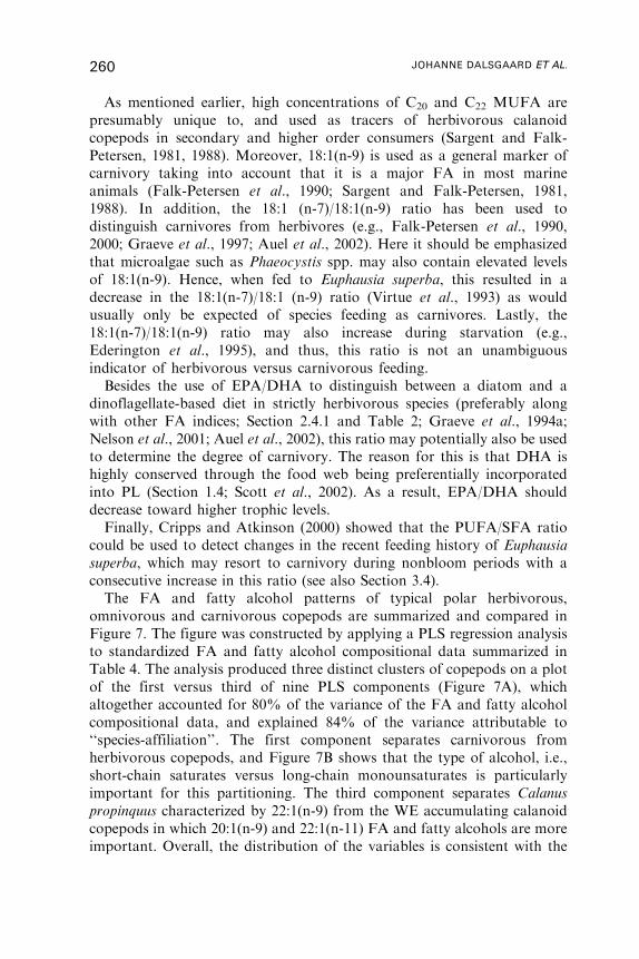
As mentioned earlier, high concentrations of C20 and C22 MUFA are

presumably unique to, and used as tracers of herbivorous calanoid

copepods in secondary and higher order consumers (Sargent and Falk-

Petersen, 1981, 1988). Moreover, 18:1(n-9) is used as a general marker of

carnivory taking into account that it is a major FA in most marine

animals (Falk-Petersen et al., 1990; Sargent and Falk-Petersen, 1981,

1988). In addition, the 18:1 (n-7)/18:1(n-9) ratio has been used to

distinguish carnivores from herbivores (e.g., Falk-Petersen et al., 1990,

2000; Graeve et al., 1997; Auel et al., 2002). Here it should be emphasized

that microalgae such as Phaeocystis spp. may also contain elevated levels

of 18:1(n-9). Hence, when fed to Euphausia superba, this resulted in a

decrease in the 18:1(n-7)/18:1 (n-9) ratio (Virtue et al., 1993) as would

usually only be expected of species feeding as carnivores. Lastly, the

18:1(n-7)/18:1(n-9) ratio may also increase during starvation (e.g.,

Ederington et al., 1995), and thus, this ratio is not an unambiguous

indicator of herbivorous versus carnivorous feeding.

Besides the use of EPA/DHA to distinguish between a diatom and a

dinoflagellate-based diet in strictly herbivorous species (preferably along

with other FA indices; Section 2.4.1 and Table 2; Graeve et al., 1994a;

Nelson et al., 2001; Auel et al., 2002), this ratio may potentially also be used

to determine the degree of carnivory. The reason for this is that DHA is

highly conserved through the food web being preferentially incorporated

into PL (Section 1.4; Scott et al., 2002). As a result, EPA/DHA should

decrease toward higher trophic levels.

Finally, Cripps and Atkinson (2000) showed that the PUFA/SFA ratio

could be used to detect changes in the recent feeding history of Euphausia

superba, which may resort to carnivory during nonbloom periods with a

consecutive increase in this ratio (see also Section 3.4).

The FA and fatty alcohol patterns of typical polar herbivorous,

omnivorous and carnivorous copepods are summarized and compared in

Figure 7. The figure was constructed by applying a PLS regression analysis

to standardized FA and fatty alcohol compositional data summarized in

Table 4. The analysis produced three distinct clusters of copepods on a plot

of the first versus third of nine PLS components (Figure 7A), which

altogether accounted for 80% of the variance of the FA and fatty alcohol

compositional data, and explained 84% of the variance attributable to

‘‘species-affiliation’’. The first component separates carnivorous from

herbivorous copepods, and Figure 7B shows that the type of alcohol, i.e.,

short-chain saturates versus long-chain monounsaturates is particularly

important for this partitioning. The third component separates Calanus

propinquus characterized by 22:1(n-9) from the WE accumulating calanoid

copepods in which 20:1(n-9) and 22:1(n-11) FA and fatty alcohols are more

important. Overall, the distribution of the variables is consistent with the


Figure 7 PLS regression analysis of standardized FA and fatty alcoholcompositional data of eight key species of polar copepods summarized in Table 4.Plots show (A) the scores of the first vs. third of nine principal components, and (B)the corresponding loading weight plot. Ellipses in (A) are drawn to indicate themajor clusters of zooplankton species.


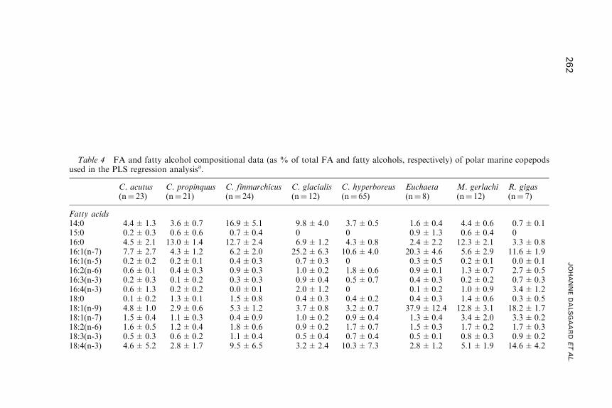
Table 4 FA and fatty alcohol compositional data (as % of total FA and fatty alcohols, respectively) of polar marine copepodsused in the PLS regression analysisa.

C. acutus(n¼ 23)

C. propinquus(n¼ 21)

C. finmarchicus(n¼ 24)

C. glacialis(n¼ 12)

C. hyperboreus(n¼ 65)

Euchaeta(n¼ 8)

M. gerlachi(n¼ 12)

R. gigas(n¼ 7)

Fatty acids14:0 4.4±1.3 3.6±0.7 16.9±5.1 9.8±4.0 3.7±0.5 1.6±0.4 4.4±0.6 0.7±0.115:0 0.2±0.3 0.6±0.6 0.7±0.4 0 0 0.9±1.3 0.6±0.4 016:0 4.5±2.1 13.0±1.4 12.7±2.4 6.9±1.2 4.3±0.8 2.4±2.2 12.3±2.1 3.3±0.816:1(n-7) 7.7±2.7 4.3±1.2 6.2±2.0 25.2±6.3 10.6±4.0 20.3±4.6 5.6±2.9 11.6±1.916:1(n-5) 0.2±0.2 0.2±0.1 0.4±0.3 0.7±0.3 0 0.3±0.5 0.2±0.1 0.0±0.116:2(n-6) 0.6±0.1 0.4±0.3 0.9±0.3 1.0±0.2 1.8±0.6 0.9±0.1 1.3±0.7 2.7±0.516:3(n-3) 0.2±0.3 0.1±0.2 0.3±0.3 0.9±0.4 0.5±0.7 0.4±0.3 0.2±0.2 0.7±0.316:4(n-3) 0.6±1.3 0.2±0.2 0.0±0.1 2.0±1.2 0 0.1±0.2 1.0±0.9 3.4±1.218:0 0.1±0.2 1.3±0.1 1.5±0.8 0.4±0.3 0.4±0.2 0.4±0.3 1.4±0.6 0.3±0.518:1(n-9) 4.8±1.0 2.9±0.6 5.3±1.2 3.7±0.8 3.2±0.7 37.9±12.4 12.8±3.1 18.2±1.718:1(n-7) 1.5±0.4 1.1±0.3 0.4±0.9 1.0±0.2 0.9±0.4 1.3±0.4 3.4±2.0 3.3±0.218:2(n-6) 1.6±0.5 1.2±0.4 1.8±0.6 0.9±0.2 1.7±0.7 1.5±0.3 1.7±0.2 1.7±0.318:3(n-3) 0.5±0.3 0.6±0.2 1.1±0.4 0.5±0.4 0.7±0.4 0.5±0.1 0.8±0.3 0.9±0.218:4(n-3) 4.6±5.2 2.8±1.7 9.5±6.5 3.2±2.4 10.3±7.3 2.8±1.2 5.1±1.9 14.6±4.2

262

JOHANNEDALSGAARD

ETAL.

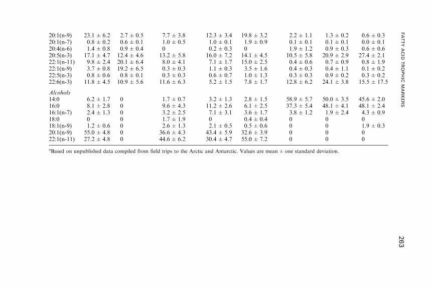
20:1(n-9) 23.1±6.2 2.7±0.5 7.7±3.8 12.3±3.4 19.8±3.2 2.2±1.1 1.3±0.2 0.6±0.320:1(n-7) 0.8±0.2 0.6±0.1 1.0±0.5 1.0±0.1 1.9±0.9 0.1±0.1 0.1±0.1 0.0±0.120:4(n-6) 1.4±0.8 0.9±0.4 0 0.2±0.3 0 1.9±1.2 0.9±0.3 0.6±0.620:5(n-3) 17.1±4.7 12.4±4.6 13.2±5.8 16.0±7.2 14.1±4.5 10.5±5.8 20.9±2.9 27.4±2.122:1(n-11) 9.8±2.4 20.1±6.4 8.0±4.1 7.1±1.7 15.0±2.5 0.4±0.6 0.7±0.9 0.8±1.922:1(n-9) 3.7±0.8 19.2±6.5 0.3±0.3 1.1±0.3 3.5±1.6 0.4±0.3 0.4±1.1 0.1±0.222:5(n-3) 0.8±0.6 0.8±0.1 0.3±0.3 0.6±0.7 1.0±1.3 0.3±0.3 0.9±0.2 0.3±0.222:6(n-3) 11.8±4.5 10.9±5.6 11.6±6.3 5.2±1.5 7.8±1.7 12.8±6.2 24.1±3.8 15.5±17.5

Alcohols14:0 6.2±1.7 0 1.7±0.7 3.2±1.3 2.8±1.5 58.9±5.7 50.0±3.5 45.6±2.016:0 8.1±2.8 0 9.6±4.3 11.2±2.6 6.1±2.5 37.3±5.4 48.1±4.1 48.1±2.416:1(n-7) 2.4±1.3 0 3.2±2.5 7.1±3.1 3.6±1.7 3.8±1.2 1.9±2.4 4.3±0.918:0 0 0 1.7±1.9 0 0.4±0.4 0 0 018:1(n-9) 1.2±0.6 0 2.6±1.3 2.1±0.5 0.5±0.6 0 0 1.9±0.320:1(n-9) 55.0±4.8 0 36.6±4.3 43.4±5.9 32.6±3.9 0 0 022:1(n-11) 27.2±4.8 0 44.6±6.2 30.4±4.7 55.0±7.2 0 0 0

aBased on unpublished data compiled from field trips to the Arctic and Antarctic. Values are mean±one standard deviation.

FATTYACID

TROPHIC

MARKERS

263

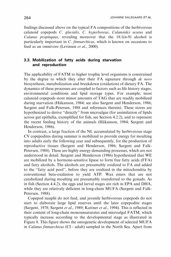
findings discussed above on the typical FA compositions of the herbivorous

calanoid copepods C. glacialis, C. hyperboreus, Calanoides acutus and

Calanus propinquus, revealing moreover that the 18:1(n-9) alcohol is

particularly important in C. finmarchicus, which is known on occasions to

feed as an omnivore (Levinsen et al., 2000).

3.3. Mobilization of fatty acids during starvation

and reproduction

The applicability of FATM to higher trophic level organisms is constrained

by the degree to which they alter their FA signature through de novo

biosynthesis, metabolization and breakdown (oxidation) of dietary FA. The

dynamics of these processes are coupled to factors such as life history stages,

environmental conditions and lipid storage types. For example, most

calanoid copepods store minor amounts of TAG that are readily mobilized

during starvation (Hakanson, 1984; see also Sargent and Henderson, 1986;

Sargent and Falk-Petersen, 1988 and references therein). These stores are

hypothesized to derive ‘‘directly’’ from microalgae (for assimilation of lipids

across gut epithelia, exemplified for fish, see Section 4.2.2), and to represent

the recent feeding history of the animals (Hakanson, 1984; Sargent and

Henderson, 1986).

In contrast, a large fraction of the NL accumulated by herbivorous stage

CV copepodites during summer is mobilized to provide energy for moulting

into adults early the following year and subsequently, for the production of

reproductive tissues (Sargent and Henderson, 1986; Sargent and Falk-

Petersen, 1988). These are highly energy demanding processes, which are not

understood in detail. Sargent and Henderson (1986) hypothesized that WE

are mobilized by a hormone-sensitive lipase to form free fatty acids (FFA)

and fatty alcohols. The alcohols are presumably oxidized to FA and added

to the ‘‘fatty acid pool’’, before they are oxidized in the mitochondria by

conventional beta-oxidation to yield ATP. Wax esters that are not

catabolized during moulting are presumably transferred to the gonads. As

in fish (Section 4.4.2), the eggs and larval stages are rich in EPA and DHA,

while they are relatively deficient in long-chain MUFA (Sargent and Falk-

Petersen, 1988).

Copepod nauplii do not feed, and juvenile herbivorous copepods do not

start to elaborate large lipid reserves until the later copepodite stages

(Sargent, 1978; Sargent et al., 1989; Kattner et al., 1994). This is reflected in

their content of long-chain monounsaturates and microalgal FATM, which

typically increase according to the developmental stage as illustrated in

Figure 8. This figure shows the ontogenetic development of selected MUFA

in Calanus finmarchicus (CI - adult) sampled in the North Sea. Apart from


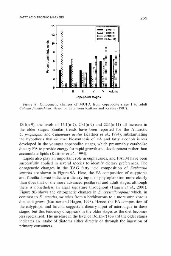
18:1(n-9), the levels of 16:1(n-7), 20:1(n-9) and 22:1(n-11) all increase in

the older stages. Similar trends have been reported for the Antarctic

C. propinquus and Calanoides acutus (Kattner et al., 1994), substantiating

the hypothesis that de novo biosynthesis of FA and fatty alcohols is less

developed in the younger copepodite stages, which presumably catabolize

dietary FA to provide energy for rapid growth and development rather than

accumulate lipids (Kattner et al., 1994).

Lipids also play an important role in euphausiids, and FATM have been

successfully applied in several species to identify dietary preferences. The

ontogenetic changes in the TAG fatty acid composition of Euphausia

superba are shown in Figure 9A. Here, the FA composition of calyptopis

and furcilia larvae indicate a dietary input of phytoplankton more clearly

than does that of the more advanced postlarval and adult stages, although

there is nonetheless an algal signature throughout (Hagen et al., 2001).

Figure 9B shows the ontogenetic changes in E. crystallorophias which, in

contrast to E. superba, switches from a herbivorous to a more omnivorous

diet as it grows (Kattner and Hagen, 1998). Hence, the FA composition of

the calyptopis and furcilia suggests a dietary input of microalgae in these

stages, but this tendency disappears in the older stages as the diet becomes

less specialized. The increase in the level of 16:1(n-7) toward the older stages

indicates an intake of diatoms either directly or through the ingestion of

primary consumers.

Figure 8 Ontogenetic changes of MUFA from copepodite stage I to adultCalanus finmarchicus. Based on data from Kattner and Krause (1987).


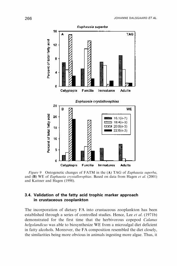
3.4. Validation of the fatty acid trophic marker approach

in crustaceous zooplankton

The incorporation of dietary FA into crustaceous zooplankton has been

established through a series of controlled studies. Hence, Lee et al. (1971b)

demonstrated for the first time that the herbivorous copepod Calanus

helgolandicus was able to biosynthesize WE from a microalgal diet deficient

in fatty alcohols. Moreover, the FA composition resembled the diet closely,

the similarities being more obvious in animals ingesting more algae. Thus, it

Figure 9 Ontogenetic changes of FATM in the (A) TAG of Euphausia superba,and (B) WE of Euphausia crystallorophias. Based on data from Hagen et al. (2001)and Kattner and Hagen (1998).


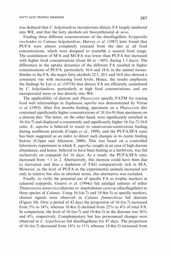
was deduced that C. helgolandicus incorporates dietary FA largely unaltered

into WE, and that the fatty alcohols are biosynthesized de novo.

Feeding three different concentrations of the dinoflagellate Scrippsiella

trochoidea to Calanus helgolandicus, Harvey et al. (1987) later found that

PUFA were almost completely retained from the diet at all food

concentrations, which were designed to resemble a natural food range.

The assimilation of SFA and MUFA was lower than PUFA but increased

with higher food concentrations (from 60 to �80% during 1.5 days). The

differences in the uptake dynamics of the different FA resulted in higher

concentrations of PUFA, particularly 16:4 and 18:4, in the animal tissues.

Similar to the FA, the major fatty alcohols 22:1, 20:1 and 16:0 also showed a

consistent rise with increasing food levels. Hence, the results emphasize

the findings by Lee et al. (1971b) that dietary FA are efficiently assimilated

by C. helgolandicus, particularly at high food concentrations, and are

incorporated more or less directly into WE.

The applicability of diatom and Phaeocystis specific FATM for tracing

food web relationships in Euphausia superba was demonstrated by Virtue

et al. (1993). After five months feeding, specimens on a Phaeocystis diet

contained significantly higher concentrations of 18:1(n-9) than specimens on

a diatom diet. The latter, on the other hand, were significantly enriched in

16:1(n-7) and displayed a consistently and significantly higher 16:1(n-7)/16:0

ratio. E. superba is believed to resort to omnivorous-carnivorous feeding

during nonbloom periods (Cripps et al., 1999), and the PUFA/SFA ratio

has been suggested as an index to detect such changes in its recent feeding

history (Cripps and Atkinson, 2000). This was based on a controlled

laboratory experiment in which E. superba, caught in an area of high diatom

abundance, and hence, believed to have been feeding as a herbivore, was fed

exclusively on copepods for 16 days. As a result, the PUFA/SFA ratio

increased from <1 to 2. Alternatively, this increase could have been due

to starvation and thus a depletion of TAG comparatively rich in SFA.

However, as the level of PUFA in the experimental animals increased not

only in relative but also in absolute terms, this alternative was excluded.

Finally, to verify the potential use of specific FA as trophic markers in

calanoid copepods, Graeve et al. (1994a) fed unialgal cultures of either

Thalassiosira antarctica (diatom) or Amphidinium carterae (dinoflagellate) to

three species of Calanus. Using 16:1(n-7) and 18:4(n-3) as specific markers,

clearest signals were observed in Calanus finmarchicus fed diatoms

(Figure 10). Over a period of 42 days the proportion of 16:1(n-7) increased

from 3% to 14%, whereas 18:4(n-3) declined from 22% to 4% of total FA.

In comparison, the level of 16:1(n-7) and 18:4(n-3) in the diatoms was 36%

and 4%, respectively. Complementary but less pronounced changes were

observed in C. hyperboreus fed dinoflagellates for 47 days. The proportion

of 16:1(n-7) decreased from 14% to 11% whereas 18:4(n-3) increased from


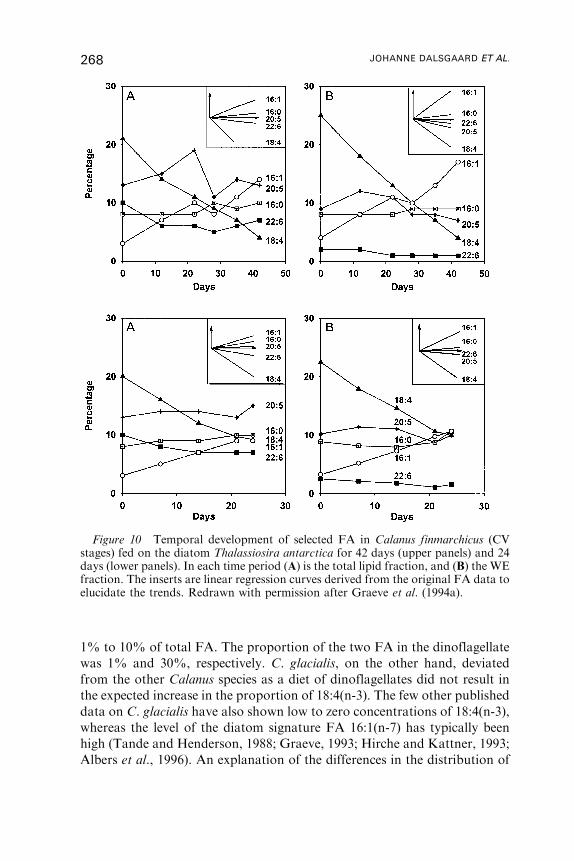
1% to 10% of total FA. The proportion of the two FA in the dinoflagellate

was 1% and 30%, respectively. C. glacialis, on the other hand, deviated

from the other Calanus species as a diet of dinoflagellates did not result in

the expected increase in the proportion of 18:4(n-3). The few other published

data on C. glacialis have also shown low to zero concentrations of 18:4(n-3),

whereas the level of the diatom signature FA 16:1(n-7) has typically been

high (Tande and Henderson, 1988; Graeve, 1993; Hirche and Kattner, 1993;

Albers et al., 1996). An explanation of the differences in the distribution of

Figure 10 Temporal development of selected FA in Calanus finmarchicus (CVstages) fed on the diatom Thalassiosira antarctica for 42 days (upper panels) and 24days (lower panels). In each time period (A) is the total lipid fraction, and (B) the WEfraction. The inserts are linear regression curves derived from the original FA data toelucidate the trends. Redrawn with permission after Graeve et al. (1994a).


18:4(n-3) between species might be that C. glacialis readily converts 18:4(n-

3) to EPA, whereas C. finmarchicus incorporates 18:4(n-3) directly. It

should, however, also be noted that all animals were losing weight

(measured as wax ester content) during the experiment, in particular C.

glacialis, and the results may simply be due to C. glacialis starving on the

experimental diet.

4. FATTY ACID DYNAMICS IN FISH


A review on the dynamics of lipids in fish, focusing on marine species, was

first presented by Shul’man (1960), who pointed out that many of the major

conclusions could have been drawn from data obtained by the end of the

18th century, and that little fundamentally new knowledge had been added

from then until 1960.

Subsequently, a large body of literature on the dynamics of lipid and FA

metabolism in marine fish has been generated. This research has focused in

particular on the optimization of artificial diets for meeting the nutritional

requirements, and improving the growth and development of cultured

species. However, as pointed out by Ackman (1980), much of this literature

is of little relevance for natural systems because of the ‘‘designed’’ lipid

composition of artificial diets, and the ‘‘unnatural’’ growth rates and fat

levels achieved by cultured species. We therefore focus on the literature that

is pertinent for the interpretation of FATM in fish, i.e., the uptake,

incorporation and modification of dietary FA as well as mobilization of FA

during periods of starvation and maturation. Finally, we summarize studies

that have demonstrated the incorporation of FATM in fish.

4.2. Incorporation of dietary fatty acids

4.2.1. Lipids and enzyme specificity

Marine fish use lipids as a chief metabolic energy source (Shul’man, 1960),

fulfilling their energetic requirements primarily through the oxidation of

cellular lipids and proteins rather than carbohydrates (Cowey and Sargent,

1977; Jobling, 1994; Sargent et al., 1993). TAG is the primary mode of lipid

storage in most species whereas WE are usually much less important

(Shul’man, 1960; Love, 1970; Owen et al., 1972; Ackman, 1980; Navarro

and Gutierrez, 1995; Sargent and Henderson, 1995). Many meso- and


bathypelagic species, such as the lantern fish (Myctophidae) and bristle-

mouths (Gonostomatidae), however, accumulate large amounts of WE

reserves (>10%; reviewed by Lee and Patton, 1989), consisting of relatively

simple FA and fatty alcohols, i.e., primarily 16:0 and 18:1 (Sargent, 1976;

Sargent et al., 1977). The exact role of these WE is not known but they most

probably serve either as long-term energy stores in species living in an

environment characterized by irregular food supply, or as a means to

provide buoyancy since WE have a lower specific gravity than TAG (Lee

and Patton, 1989; Sargent, 1976).

Laboratory experiments have established that the FA composition of fish

can be highly affected by their diet (Section 4.5). On a biochemical basis, this

may be due to the low enzyme–substrate specificity of the FA converting

enzymes of the common lipid pathway, which rely on weaker ‘‘hydro-

phobic’’ interactions contrary to, for example, amino acid and protein

metabolism that depends on stronger ionic and hydrogen-bond interactions

(Sargent et al., 1993). Hence, whereas the amino acid composition of

proteins is controlled by highly specific transfer RNAs, �6 desaturase

(which is central to the common lipid pathway) may readily desaturate a

number of dietary FA (Sargent et al., 1993). The introduction of polar

groups, however, enhances slightly the specificity of the enzyme–substrate

complex, as demonstrated by the selective incorporation of PUFA rather

than SFA and MUFA into PL (Sargent et al., 1993). Still, the acylases and

transacylases that esterify PUFA to PL do not have absolute specificity for

any one FA in particular, and a dietary excess of, e.g., EPA may lead to

elevated levels of this FA at the expense of DHA if the latter is present in

lower concentrations (Sargent et al., 1999). These processes largely explain

why storage lipids are generally more similar and respond more readily to

the diet than specialized tissues such as the heart and brain, which are

comparatively rich in polar lipids (Navarro et al., 1995; Grahl-Nielsen and

Mjaavatten, 1992; Mjaavatten et al., 1998).

4.2.2. Uptake of dietary fatty acids

The digestion, absorption and deposition of lipids and FA in fish has been

studied in detail and thoroughly reviewed (Cowey and Sargent, 1977, 1979;

Sargent, 1978; Henderson and Tocher, 1987; Sheridan, 1988; Sargent et al.,

1989, 1993). Briefly, upon consumption the dietary lipids are emulsified by

bile salts and hydrolysed by pancreatic lipases in the gut to form FFA in

addition to 2-monoacylglycerols and glycerol (from dietary TAG), alcohols

(from dietary WE) and lysophospholipids (from dietary PL). Wax esters

are more hydrophobic than TAG and PL and therefore more difficult to

emulsify. Hence, fish consuming large quantities of WE generally exhibit a


longer retention time of food in their gut presumably to facilitate hydrolysis

and absorption (e.g., Cowey and Sargent, 1979). The various lipid

components are absorbed into intestinal epithelial cells where they are

re-esterified into TAG and PL. Dietary fatty alcohols are oxidized to the

corresponding FA by a NAD-dependent dehydrogenase prior to esterifica-

tion (with glycerol) to form TAG. Shortage of preformed glycerol in the diet

is compensated for by converting nonessential amino acids and glucose to

triacylglycerol-glycerol (see also Sargent and Henderson, 1986). The lipids

are concurrently assembled into lipoprotein particles and transported to the

liver or extra-hepatic adipose tissues by the blood or lymphatic system. In

most species the liver, rather than the adipose tissues, is the principal site of

lipogenic activity including de novo biosynthesis and modification of dietary

FA (see also Henderson and Sargent, 1985).

This short summary explains how zooplanktivorous fish, which may

consume large quantities of WE rich calanoid copepods, are able to

accumulate TAG rich in 20:1(n-9) and 22:1(n-11) (see also Sargent, 1978;

Sargent and Henderson, 1986). However, whereas the ratio of 20:1(n-9) and

22:1(n-11) is typically 1:2 in the copepods, it decreases to 2:3 in clupeids

(Ackman and Eaton, 1966b) and is close to one, e.g., in capelin, indicating a

preferential catabolism of 22:1(n-11) (Pascal and Ackman, 1976; see also

Henderson et al., 1984). Moreover, both MUFA are essentially absent from

fish PL suggesting that they are used preferably for the provision of

metabolic energy rather than involved in biomembrane functioning

(reviewed by Sargent and Whittle, 1981; Henderson and Sargent, 1985).

These observations sustain that the FA composition of storage lipids resem-

bles the diet more closely than does the FA composition of polar lipids.

Larval fish may not be capable of biosynthesizing the glycerophospho-

base backbone of phosphoglycerides de novo, but presumably obtain these

moieties from their diet. They may, however, readily exchange FA between

and within dietary-derived PL and TAG (reviewed by Sargent et al., 1999),

consistent with the findings that larval fish consuming large amounts of

microalgae and microzooplankton have a total FA composition very similar

to their prey (e.g., Klungsøyr et al., 1989; St. John and Lund, 1996).

4.3. Modifications and de novo biosynthesis of fatty acids

Like most other organisms, fish can readily biosynthesize SFA with up to 18

carbon atoms de novo (Ackman, 1980; Henderson and Sargent, 1985) and

desaturate them into monounsaturates following the common lipid pathway

(Section 1.5). However, in contrast to calanoid copepods discussed in

Section 3.2.1, a dietary excess of FA (>10%) apparently suppresses de novo


biosynthesis while the deposition of dietary FA continues (reviewed by

Sargent et al., 1989, 1993).

Fish incorporate dietary FA either directly or after modifying them

slightly through further elongation and desaturation. To date, detailed

research has been conducted mostly on the ability of fish to convert

18:2(n-6) and 18:3(n-3) to AA, EPA and DHA, which are essential for their

normal growth and development (e.g., Bell et al., 1986; Sargent et al.,

1995a, b, 1999). Early experimental evidence from rainbow trout (Castell

et al., 1972a, b, c), and later from numerous other studies of freshwater

species (reviewed by Cowey and Sargent, 1977; Watanabe, 1982; Henderson

and Tocher, 1987; Sargent et al., 1989, 1993), has established that freshwater

fish can generally carry out these modifications. In contrast, most marine

species studied so far cannot undertake these conversions at any significant

rates (e.g., juvenile gilthead sea bream, Mourente and Tocher, 1993a;

juvenile golden grey mullet, Mourente and Tocher, 1993b; plaice, Owen

et al., 1972; red sea bream, rockfish and globefish, Kanazawa et al., 1979;

and turbot, Owen et al., 1975; Cowey et al., 1976; Scott and Middleton,

1979; Linares and Henderson, 1991). It has been hypothesized that since the

diet of both larval and adult marine fish is naturally rich in (n-3) PUFA, a

deficiency or impairment of the �5 fatty acid desaturase necessary for

converting C18 PUFA to EPA and DHA has evolved in these species

(reviewed by Sargent et al., 1993, 1995a). However, it has also been argued

that the ability to undertake these conversions is a matter of feeding

habit rather than water salinity (Sargent, 1995; Sargent et al., 1995a).

For example, similarly to marine piscivores, freshwater pike (Esox lucius)

do not convert C18 PUFA to EPA and DHA at any significant rate

(Henderson et al., 1995). Moreover, the capacity to undertake these

conversions might be coupled to ontogenetic changes in the diet composi-

tion (Sargent, 1995; Sargent et al., 1995a). Rapidly growing salmon fry in

freshwater can, e.g., readily convert 18:3(n-3) ingested from aquatic insects

to DHA, whereas slower growing juveniles entering the marine environment

and turning into piscivores, do not need to undertake these conversions, as

they have a ready dietary source of DHA (Sargent, 1995; see also Lovern,

1934 and Mjaavatten et al., 1998).

In a comparative study of 56 fresh and brackish-water fish species,

Ahlgren et al. (1994) found that differences in FA patterns were a matter of

overall lipid content rather than water salinity. Hence, they found strong

correlations between the total FA content and SFA, MUFA and (n-6)

PUFA, respectively, in all species. In contrast, the concentration of (n-3)

PUFA was independent of the total FA content after a breakpoint at about

100mgFAg�1 dry mass (DM).

PUFA are preferentially incorporated into polar lipids, and high

concentrations of (n-3) PUFA in the biomembranes of fish have been


linked to the generally low temperature in the aquatic environment

(e.g., Cowey and Sargent, 1977, 1979). The fluidity of biomembranes is

largely determined by the degree of membrane FA unsaturation and

by selectively incorporating (n-3) PUFA, fish may ensure the functional

integrity of their biomembranes at lower water temperatures (reviewed by

Cowey and Sargent, 1977, 1979; Henderson and Sargent, 1985; Bell et al.,

1986; Sargent et al., 1989). More recently, the abundance of (n-3) PUFA in

fish membranes has been related to their structural rather than fluidizing role

(reviewed by Sargent and Henderson, 1995; Sargent et al., 1995b). High

concentrations of di-22:6(n-3) phosphatidylethanolamine and di-22:6(n-3)

phosphatidylserine in the retinal rod outer segment membranes and brain

synaptosomal membranes of fish are believed to provide a unique and highly

ordered bi-layer that remains relatively constant despite changing environ-

mental temperatures and pressure, while facilitating fast conformational

changes undergone by membrane signaling proteins (reviewed by Sargent

and Henderson, 1995; Sargent et al., 1993, 1995a, b). Substantiating this

hypothesis, Bell et al. (1995) showed that herring larvae (Clupea harengus)

reared on a diet deficient in DHA fed less actively at different light intensities

than larvae reared on a diet supplemented in DHA (see also Navarro and

Sargent, 1992).

In summary, the FA composition of fish lipids is a blend of endogenous

and exogenous sources, determined by (i) de novo biosynthesis of short-

chain SFA and MUFA, (ii) selective uptake and ‘‘direct’’ incorporation of

dietary FA and fatty alcohols, and (iii) uptake and modification of dietary

FA and fatty alcohols prior to incorporation.

4.4. Mobilization of fatty acids during starvation

and reproduction

4.4.1. Starvation

The metabolism of lipids and FA in fish is strongly linked to physiological

and behavioral traits such as size, age, sex, state of maturity, spawning,

depth distribution and migration as well as to biotic and abiotic factors such

as food abundance, water temperature, salinity, etc. (e.g., Shul’man, 1960,

1974; Friedrich and Hagen, 1994; Sargent and Henderson, 1995; Anthony

et al. 2000). Prolonged periods of starvation are common in fish and have

often evolved as part of their reproductive cycle, for example in spawning-

migrating salmon (Henderson and Tocher, 1987). Starvation is accompa-

nied by a reduction in FA biosynthesis (reviewed by Sargent et al., 1989),

and increased mobilization of energy stores. TAG is mobilized either

simultaneously or after carbohydrates, but usually before proteins and


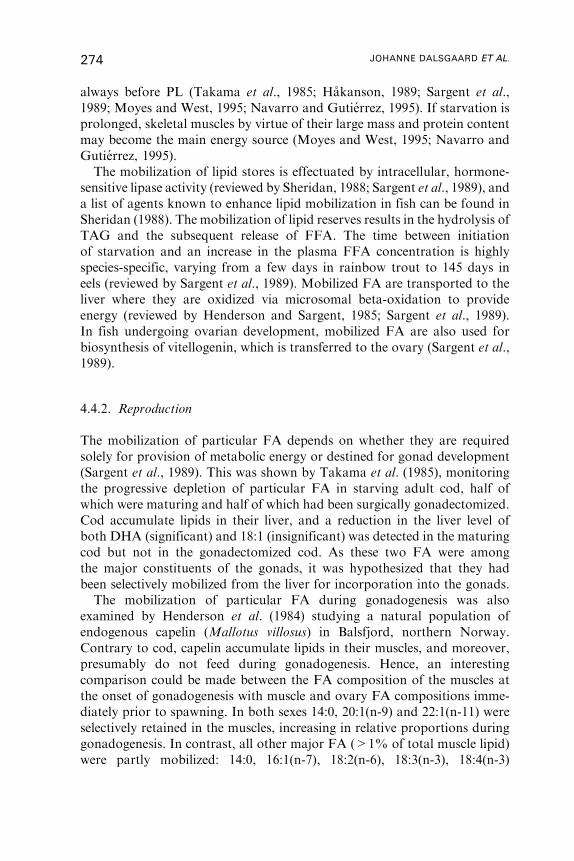
always before PL (Takama et al., 1985; Hakanson, 1989; Sargent et al.,

1989; Moyes and West, 1995; Navarro and Gutierrez, 1995). If starvation is

prolonged, skeletal muscles by virtue of their large mass and protein content

may become the main energy source (Moyes and West, 1995; Navarro and

Gutierrez, 1995).

The mobilization of lipid stores is effectuated by intracellular, hormone-

sensitive lipase activity (reviewed by Sheridan, 1988; Sargent et al., 1989), and

a list of agents known to enhance lipid mobilization in fish can be found in

Sheridan (1988). The mobilization of lipid reserves results in the hydrolysis of

TAG and the subsequent release of FFA. The time between initiation

of starvation and an increase in the plasma FFA concentration is highly

species-specific, varying from a few days in rainbow trout to 145 days in

eels (reviewed by Sargent et al., 1989). Mobilized FA are transported to the

liver where they are oxidized via microsomal beta-oxidation to provide

energy (reviewed by Henderson and Sargent, 1985; Sargent et al., 1989).

In fish undergoing ovarian development, mobilized FA are also used for

biosynthesis of vitellogenin, which is transferred to the ovary (Sargent et al.,

1989).

4.4.2. Reproduction

The mobilization of particular FA depends on whether they are required

solely for provision of metabolic energy or destined for gonad development

(Sargent et al., 1989). This was shown by Takama et al. (1985), monitoring

the progressive depletion of particular FA in starving adult cod, half of

which were maturing and half of which had been surgically gonadectomized.

Cod accumulate lipids in their liver, and a reduction in the liver level of

both DHA (significant) and 18:1 (insignificant) was detected in the maturing

cod but not in the gonadectomized cod. As these two FA were among

the major constituents of the gonads, it was hypothesized that they had

been selectively mobilized from the liver for incorporation into the gonads.

The mobilization of particular FA during gonadogenesis was also

examined by Henderson et al. (1984) studying a natural population of

endogenous capelin (Mallotus villosus) in Balsfjord, northern Norway.

Contrary to cod, capelin accumulate lipids in their muscles, and moreover,

presumably do not feed during gonadogenesis. Hence, an interesting

comparison could be made between the FA composition of the muscles at

the onset of gonadogenesis with muscle and ovary FA compositions imme-

diately prior to spawning. In both sexes 14:0, 20:1(n-9) and 22:1(n-11) were

selectively retained in the muscles, increasing in relative proportions during

gonadogenesis. In contrast, all other major FA (>1% of total muscle lipid)

were partly mobilized: 14:0, 16:1(n-7), 18:2(n-6), 18:3(n-3), 18:4(n-3)


and DHA were preferentially deposited in the ovaries, whereas 16:0, 18:0,

18:1(n-7), 18:1(n-9), 22:1(n-11), 22:5(n-3) and EPA were catabolized after

mobilization.

These results emphasize that the FA patterns of fish depleting their lipid

reserves are highly distorted, reflecting internal metabolic processes rather

than potential dietary signals. In fish roe, EPA and DHA typically

constitute 50% of the TL, suggesting an essential need of the developing

embryo for the formation of cellular membranes. Interestingly, the FA

composition of fish roe is remarkably similar among species and presumably

optimized nutritionally for the growth of the developing embryo and yolk-

sac larvae until first-feeding (Kaitaranta and Linko, 1984; Tocher and

Sargent, 1984; Klungsøyr et al., 1989). The dietary FA composition of the

parent fish typically has little impact on the FA composition of the eggs.

However, when comparing the roe of Atlantic and Baltic herring

(Kaitaranta and Linko, 1984), relatively large proportions of 20:1(n-9)

and 22:1(n-11) (i.e., 3.1% and 1.5% of total FA, respectively) were detected

in the Atlantic herring roe, whereas these FA were absent in Baltic herring

eggs. Calanoid copepods are much less common in the Baltic Sea compared

to the Atlantic, presumably because the lower salinity in this system

(Ackman, 1980), and this probably explains the absence of these tracers in

Baltic herring roe. In another example, Lasker and Theilacker (1962) found

a relatively close similarity between the FA composition of the ovary of

Pacific sardine (Sardinops caerulea) and the diet of the adult fish, consisting

mostly of Calanus. However, apart from a few such exceptions, it may be

anticipated that FA add a limited amount of information useful for

resolving the trophodynamic processes resulting ultimately in the

production of offspring.

4.5. Validation of the fatty acid trophic marker approach in fish

Only a handful of studies have validated the FATM approach in fish,

examining the FA composition of prey and predators under controlled

experimental conditions either in the laboratory or in mesocosms. Such

studies are nevertheless essential for the application of any trophic marker

in studies of ecosystem dynamics. Two laboratory studies have been

performed. In the first case, St. John and Lund (1996) examined the

potential of 16:1(n-7)/16:0 as a specific food web tracer in a study with

the overall objective of identifying the dominant microalgal class, and

hence the hydrographic regime (Section 2.3), contributing to the condition

of juvenile North Sea cod (Gadus morhua). In order to establish a

relationship between lipid tracer content and food utilization in situ, the

tracer was first validated in the laboratory. Using Acartia tonsa nauplii


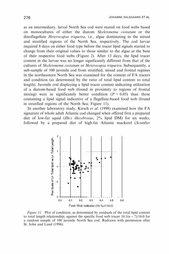
as an intermediary, larval North Sea cod were reared on food webs based

on monocultures of either the diatom Skeletonema costatum or the

dinoflagellate Heterocapsa triquetra, i.e., algae dominating in the mixed

and stratified regions of the North Sea, respectively. The cod larvae

required 8 days on either food type before the tracer lipid signals started to

change from their original values to those similar to the algae at the base

of their respective food webs (Figure 2). After 13 days, the lipid tracer

content in the larvae was no longer significantly different from that of the

cultures of Skeletonema costatum or Heterocapsa triquetra. Subsequently, a

sub-sample of 100 juvenile cod from stratified, mixed and frontal regimes

in the northeastern North Sea was examined for the content of FA tracers

and condition (as determined by the ratio of total lipid content to total

length). Juvenile cod displaying a lipid tracer content indicating utilization

of a diatom-based food web (found in proximity to regions of frontal

mixing) were in significantly better condition (P>0.05) than those

containing a lipid signal indicative of a flagellate-based food web (found

in stratified regions of the North Sea; Figure 11).

In another laboratory study, Kirsch et al. (1998) examined how the FA

signature of whole adult Atlantic cod changed when offered first a prepared

diet of low-fat squid (Illex illecebrosus, 2% lipid DM) for six weeks,

followed by a prepared diet of high-fat Atlantic mackerel (Scomber

Figure 11 Plot of condition, as determined by residuals of the total lipid contentto total length relationship, against the specific food web tracer 16:1(n� 7)/16:0 fora random sample of 100 juvenile North Sea cod. Redrawn with permission afterSt. John and Lund (1996).


scombrus, 16% lipid DM) for another eight weeks. Intriguingly, after only 3

weeks on the squid diet, and despite the absence of any mass gain, the FA

composition of the cod had changed significantly toward that of the squid,

changing no further after 6 weeks of feeding. When switched to the mackerel

diet, the overall tissue lipid content of the cod increased from 2% to 4%.

Furthermore, the FA patterns had reversed toward that of the mackerel diet

within 5 weeks of first feeding, with no further changes during the last three

weeks. Applying a classification and regression tree analysis (CART) to the

FA compositional data, the authors showed that the cod treatment groups,

despite the influence of dietary FA, were still readily differentiated from

each other and from their diet.

The results of these two studies demonstrate the relevance of dietary FA

as qualitative markers for resolving trophic interactions in both larval and

adult fish. Moreover, the latter study supports the application of FATM

for assessing the diet of yet higher trophic level predators such as marine

mammals (e.g., Iverson et al., 1997b).

A series of enclosure studies have been carried out in Loch Ewe, Scotland,

demonstrating the impact of ontogeny and varying dietary regimes on the

FA composition of herring larvae (Clupea harengus). In the first study,

Gatten et al. (1983) observed that a switch in the diet of herring larvae from

microalgae and nauplii (as determined from gut analyses) to WE rich stages

of copepodites and adult calanoid copepods, was accompanied by a gradual

replacement of typical dinoflagellate and flagellate FATM (18:4(n-3), EPA,

DHA) by calanoid FATM. Considering the condition of the herring

larvae, Fraser et al. (1987) later found that a dietary resemblance was much

more pronounced in well-nourished larvae, which were accumulating

TAG, than in under-nourished larvae. Finally, using 18:4(n-3) as a specific

flagellate tracer, Fraser et al. (1989) were able to follow a natural succes-

sion in the enclosed microalgal community from dinoflagellates and

flagellates to diatoms, and furthermore, could detect the signal, presumably

through zooplankton, to herring larvae (Figure 12). However, whereas the

zooplankton community closely mirrored the temporal development in the

phytoplankton, the peak in the tracer content was delayed by 23 days in

herring larvae. This delay suggests that the fish larvae either continued

feeding selectively on dinoflagellates and flagellates rather than on diatoms

or zooplankton, or that the turnover rates of the tissue lipid pools decreased

as the larvae grew (see also Section 5.2.5). The authors did not, however,

discuss this.

Apart from the studies summarized above, several studies of natural

fish populations have been carried out, comparing the FA composition of fish

and their potential prey, and assuming simply a conservative transfer of FA

from prey to predators. These studies will be summarized in Section 5.


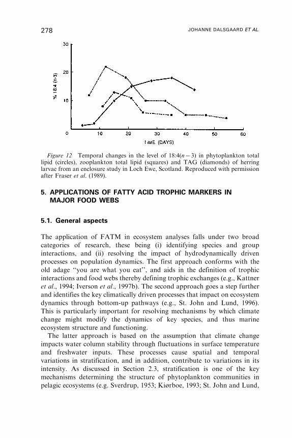
5. APPLICATIONS OF FATTY ACID TROPHIC MARKERS IN

MAJOR FOOD WEBS


The application of FATM in ecosystem analyses falls under two broad

categories of research, these being (i) identifying species and group

interactions, and (ii) resolving the impact of hydrodynamically driven

processes on population dynamics. The first approach conforms with the

old adage ‘‘you are what you eat’’, and aids in the definition of trophic

interactions and food webs thereby defining trophic exchanges (e.g., Kattner

et al., 1994; Iverson et al., 1997b). The second approach goes a step further

and identifies the key climatically driven processes that impact on ecosystem

dynamics through bottom-up pathways (e.g., St. John and Lund, 1996).

This is particularly important for resolving mechanisms by which climate

change might modify the dynamics of key species, and thus marine

ecosystem structure and functioning.

The latter approach is based on the assumption that climate change

impacts water column stability through fluctuations in surface temperature

and freshwater inputs. These processes cause spatial and temporal

variations in stratification, and in addition, contribute to variations in its

intensity. As discussed in Section 2.3, stratification is one of the key

mechanisms determining the structure of phytoplankton communities in

pelagic ecosystems (e.g. Sverdrup, 1953; Kiørboe, 1993; St. John and Lund,

Figure 12 Temporal changes in the level of 18:4(n� 3) in phytoplankton totallipid (circles), zooplankton total lipid (squares) and TAG (diamonds) of herringlarvae from an enclosure study in Loch Ewe, Scotland. Reproduced with permissionafter Fraser et al. (1989).


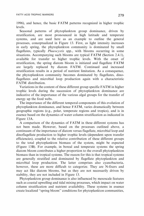
1996), and hence, the basic FATM patterns recognized in higher trophic

levels.

Seasonal patterns of phytoplankton group dominance, driven by

stratification, are most pronounced in high latitude and temperate

systems, and are used here as an example to outline the general

processes, conceptualized in Figure 13. First, as light intensity increases

in early spring, the phytoplankton community is dominated by small

flagellates, typically Phaeocystis spp., with blooms occurring in some

situations. Accompanying such blooms are typical FATM (Section 2.4.1),

available for transfer to higher trophic levels. With the onset of

stratification, the spring diatom bloom is initiated and flagellate FATM

are largely replaced by diatom FATM. Continued and increased

stratification results in a period of nutrient limitation. As a consequence,

the phytoplankton community becomes dominated by flagellates, dino-

flagellates and microbial loop production again with a characteristic

FATM distribution.

Variations in the content of these different group specific FATM in higher

trophic levels during the succession of phytoplankton dominance are

indicative of the importance of the various algal groups for the transfer of

energy up the food webs.

The importance of the different temporal components of this evolution of

phytoplankton dominance, and hence FATM, varies dramatically between

geographic regions (e.g., polar, temperate regions and tropics), and is in

essence based on the dynamics of water column stratification as indicated in

Figure 13A.

A comparison of the dynamics of FATM in these different systems has

not been made. However, based on the processes outlined above, a

continuum of the importance of diatom versus flagellate, microbial loop and

dinoflagellate production to higher trophic levels (dependent upon transfer

efficiencies), coupled to the relative contribution of these different groups

to the total phytoplankton biomass of the system, might be expected

(Figure 13B). For example, in boreal and temperate systems the spring

diatom bloom contributes a higher proportion to the overall phytoplankton

biomass than in tropical systems. The reason for this is that tropical systems

are generally stratified and dominated by flagellate phytoplankton and

microbial loop production. The latter comprises also cyanobacteria,

however, these are more difficult to categorize. They are N-fixers and

may act like diatom blooms, but as they are not necessarily driven by

stability, they are not included in Figure 13.

Phytoplankton group dominance is also influenced by mesoscale features

such as coastal upwelling and tidal mixing processes, which impact on water

column stratification and nutrient availability. These systems in essence

create localized ‘‘spring bloom’’ conditions for phytoplankton communities,


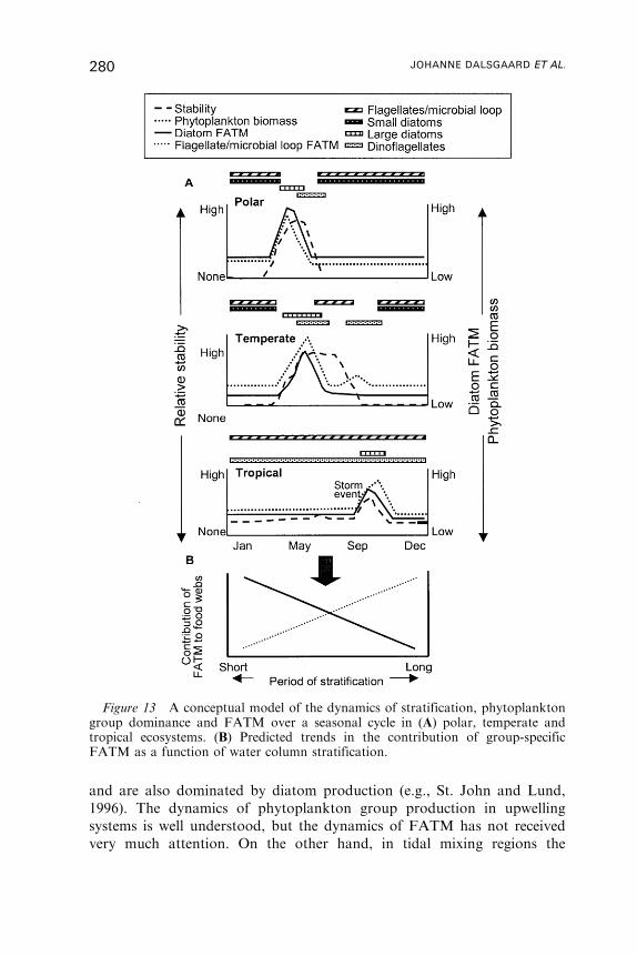
and are also dominated by diatom production (e.g., St. John and Lund,

1996). The dynamics of phytoplankton group production in upwelling

systems is well understood, but the dynamics of FATM has not received

very much attention. On the other hand, in tidal mixing regions the

Figure 13 A conceptual model of the dynamics of stratification, phytoplanktongroup dominance and FATM over a seasonal cycle in (A) polar, temperate andtropical ecosystems. (B) Predicted trends in the contribution of group-specificFATM as a function of water column stratification.


distribution of FATM relative to water column structure and phytoplank-

ton group dominance has been studied, and links to higher trophic level

condition have been identified (St. John and Lund, 1996).

The following section describes the state-of-the-art of FATM in pelagic

marine ecosystems.

5.2. The Arctic

5.2.1. Primary producers

Light, nutrients and stratification are the major driving forces in the Arctic,

controlling the short but intensive period of primary production with

60–70% of the total annual primary production taking place between mid-

March and early July (Falk-Petersen et al., 1990 and references therein). The

pelagic spring bloom is initiated in fjords (where fresh water run-offs result

in early stratification), followed by blooms in the open water of the marginal

ice zone (MIZ) (Falk-Petersen et al., 1998 and references therein). Ice algae

consist predominantly of diatoms, whereas open water phytoplankton

communities are relatively richer in dinoflagellates and smaller flagellates

(Falk-Petersen et al., 1998; Henderson et al., 1998). In particular,

Phaeocystis spp. often dominate at the onset of the open water spring

bloom (Sargent et al., 1985; Falk-Petersen et al., 1990, 2000 and references

therein; Marchant and Thomsen, 1994; Hamm et al., 2001). The different

phytoplankton communities are accompanied by typical FA signatures

reflecting the dominant algal classes (Section 2.4.1). A notable exception is

Phaeocystis pouchetii in Balsfjord (Sargent et al., 1985; Hamm et al., 2001),

which contained a FA pattern quite different from that observed in other

areas (Section 2.4.3), i.e., high proportions of 18:4(n-3), 18:5(n-3), EPA and

DHA combined with relatively low levels of C16 PUFA.

The FA signature of size-fractionated plankton samples collected during

the spring and post-plankton bloom off the west coast of Greenland was

recently combined with detailed microscopic analyses of biomass and

species level composition of microalgae (Reuss and Poulsen, 2002). This

study revealed that most of the spring bloom biomass was contained within

the 11–300 mm size-fraction and was dominated by diatoms, while 80% of

the biomass in the 6–11 mm size-fraction was composed of Phaeocystis

pouchetii. The spring plankton bloom was succeeded by flagellates

(Haptophyceae; <11 mm) with the total biomass of FA being an order of

magnitude lower and significantly different (r¼ 0.95, P<0.001) from the

spring bloom. On this basis, specific FATM were coupled with the

phytoplankton species composition. The biomass of diatoms correlated

significantly and positively with 16:1(n-7)/16:0, �C16/�C18, 16:1(n-7) and


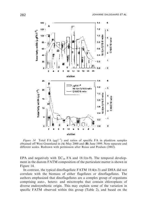
EPA and negatively with �C18 FA and 18:1(n-9). The temporal develop-

ment in the diatom FATM composition of the particulate matter is shown in

Figure 14.

In contrast, the typical dinoflagellate FATM 18:4(n-3) and DHA did not

correlate with the biomass of either flagellates or dinoflagellates. The

authors emphasized that dinoflagellates are a complex group of organisms

comprising auto-, hetero- and mixotrophs that contain chloroplasts of

diverse endosymbiotic origin. This may explain some of the variation in

specific FATM observed within this group (Table 2), and based on the

Figure 14 Total FA (mg l�1) and ratios of specific FA in plankton samplesobtained off West Greenland in (A) May 2000 and (B) June 1999. Note separate anddifferent scales. Redrawn with permission after Reuss and Poulsen (2002).


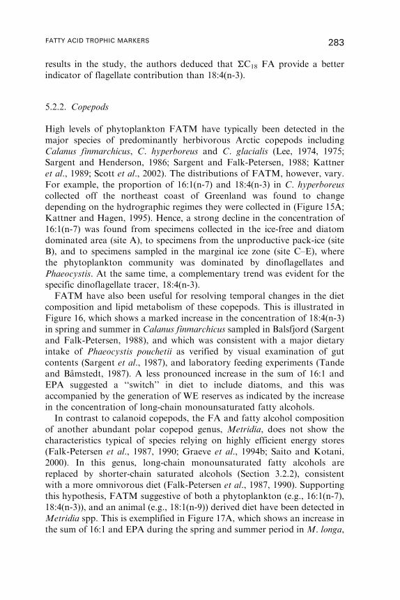
results in the study, the authors deduced that �C18 FA provide a better

indicator of flagellate contribution than 18:4(n-3).

5.2.2. Copepods

High levels of phytoplankton FATM have typically been detected in the

major species of predominantly herbivorous Arctic copepods including

Calanus finmarchicus, C. hyperboreus and C. glacialis (Lee, 1974, 1975;

Sargent and Henderson, 1986; Sargent and Falk-Petersen, 1988; Kattner

et al., 1989; Scott et al., 2002). The distributions of FATM, however, vary.

For example, the proportion of 16:1(n-7) and 18:4(n-3) in C. hyperboreus

collected off the northeast coast of Greenland was found to change

depending on the hydrographic regimes they were collected in (Figure 15A;

Kattner and Hagen, 1995). Hence, a strong decline in the concentration of

16:1(n-7) was found from specimens collected in the ice-free and diatom

dominated area (site A), to specimens from the unproductive pack-ice (site

B), and to specimens sampled in the marginal ice zone (site C–E), where

the phytoplankton community was dominated by dinoflagellates and

Phaeocystis. At the same time, a complementary trend was evident for the

specific dinoflagellate tracer, 18:4(n-3).

FATM have also been useful for resolving temporal changes in the diet

composition and lipid metabolism of these copepods. This is illustrated in

Figure 16, which shows a marked increase in the concentration of 18:4(n-3)

in spring and summer in Calanus finmarchicus sampled in Balsfjord (Sargent

and Falk-Petersen, 1988), and which was consistent with a major dietary

intake of Phaeocystis pouchetii as verified by visual examination of gut

contents (Sargent et al., 1987), and laboratory feeding experiments (Tande

and Bamstedt, 1987). A less pronounced increase in the sum of 16:1 and

EPA suggested a ‘‘switch’’ in diet to include diatoms, and this was

accompanied by the generation of WE reserves as indicated by the increase

in the concentration of long-chain monounsaturated fatty alcohols.

In contrast to calanoid copepods, the FA and fatty alcohol composition

of another abundant polar copepod genus, Metridia, does not show the

characteristics typical of species relying on highly efficient energy stores

(Falk-Petersen et al., 1987, 1990; Graeve et al., 1994b; Saito and Kotani,

2000). In this genus, long-chain monounsaturated fatty alcohols are

replaced by shorter-chain saturated alcohols (Section 3.2.2), consistent

with a more omnivorous diet (Falk-Petersen et al., 1987, 1990). Supporting

this hypothesis, FATM suggestive of both a phytoplankton (e.g., 16:1(n-7),

18:4(n-3)), and an animal (e.g., 18:1(n-9)) derived diet have been detected in

Metridia spp. This is exemplified in Figure 17A, which shows an increase in

the sum of 16:1 and EPA during the spring and summer period in M. longa,


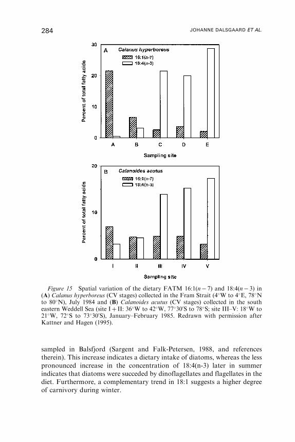
sampled in Balsfjord (Sargent and Falk-Petersen, 1988, and references

therein). This increase indicates a dietary intake of diatoms, whereas the less

pronounced increase in the concentration of 18:4(n-3) later in summer

indicates that diatoms were succeded by dinoflagellates and flagellates in the

diet. Furthermore, a complementary trend in 18:1 suggests a higher degree

of carnivory during winter.

Figure 15 Spatial variation of the dietary FATM 16:1(n� 7) and 18:4(n� 3) in(A) Calanus hyperboreus (CV stages) collected in the Fram Strait (4�W to 4�E, 78�Nto 80�N), July 1984 and (B) Calanoides acutus (CV stages) collected in the southeastern Weddell Sea (site Iþ II: 36�W to 42�W, 77�300S to 78�S; site III–V: 18�W to21�W, 72�S to 73�300S), January–February 1985. Redrawn with permission afterKattner and Hagen (1995).


Metridia longa and M. okhotensis may, however, deviate from the general

fatty alcohol pattern summarized above, and their WE contain substantial

amounts of C20 and C22 monounsaturates. It is not clear whether these

long-chain monounsaturates are biosynthesized de novo or derived from

feeding on calanoid copepods (Falk-Petersen et al., 1987; Albers et al.,

1996). Assuming that the latter is true, Figure 17B indicates an uptake of

calanoid copepods in late winter by M. longa. Similarly, the WE fatty acid

composition of another carnivorous Arctic copepod, Pareuchaeta norvegica,

indicated that this species also feeds on calanoid copepods (Sargent and

McIntosh, 1974). Interestingly, the WE of the Antarctic congeners, Metridia

gerlachei (Graeve et al., 1994b) and Euchaeta antarctica (Hagen et al., 1995),

were characterized by the near absence of calanoid FATM. E. antarctica

has been observed to prey on Calanus acutus (Øresland, 1991), and Metridia

gerlachei is believed to show similar feeding behavior. Hence, it is not

fully understood why long-chain monounsaturates are apparently entirely

catabolized in these Antarctic species (Hagen et al., 1995), while retained

in the Arctic congeners (Auel, 1999). However, it obviously weakens

the potential of these long-chain monounsaturates as calanoid FATM,

particularly in the southern hemisphere, due to the uncertainty of their

dietary and biosynthetic origin.

Figure 16 Seasonal development in specific WE fatty acids and alcoholsin Calanus finmarchicus from Balsfjord, northern Norway. Based on datafrom Falk-Petersen et al. (1988) cited and reproduced in Sargent and Falk-Petersen (1988).


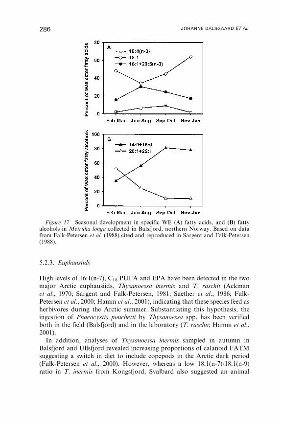
5.2.3. Euphausiids

High levels of 16:1(n-7), C18 PUFA and EPA have been detected in the two

major Arctic euphausiids, Thysanoessa inermis and T. raschii (Ackman

et al., 1970; Sargent and Falk-Petersen, 1981; Saether et al., 1986; Falk-

Petersen et al., 2000; Hamm et al., 2001), indicating that these species feed as

herbivores during the Arctic summer. Substantiating this hypothesis, the

ingestion of Phaeocystis pouchetii by Thysanoessa spp. has been verified

both in the field (Balsfjord) and in the laboratory (T. raschii; Hamm et al.,

2001).

In addition, analyses of Thysanoessa inermis sampled in autumn in

Balsfjord and Ullsfjord revealed increasing proportions of calanoid FATM

suggesting a switch in diet to include copepods in the Arctic dark period

(Falk-Petersen et al., 2000). However, whereas a low 18:1(n-7)/18:1(n-9)

ratio in T. inermis from Kongsfjord, Svalbard also suggested an animal

Figure 17 Seasonal development in specific WE (A) fatty acids, and (B) fattyalcohols in Metridia longa collected in Balsfjord, northern Norway. Based on datafrom Falk-Petersen et al. (1988) cited and reproduced in Sargent and Falk-Petersen(1988).


dietary input, low proportions of calanoid FATM indicated that these

copepods did not make important contributions to the diet of T. inermis in

this area (Falk-Petersen et al., 2000).

The seasonal and spatial changes in the FATM pattern of Thysanoessa

raschii generally resemble those of T. inermis, though this species stores

TAG rather than WE, suggesting a slightly more omnivorous feeding

behavior (Falk-Petersen et al., 1981, 2000).

5.2.4. Other zooplankters and nekton

Amphipods perform an essential role in the Arctic, linking sympagic (ice

fauna) and pelagic production to higher trophic levels (Scott et al., 1999;

Auel et al., 2002). Here, FA analyses have allowed the identification of both

interspecific and regional differences in trophic interactions (Falk-Petersen

et al., 1987; Scott et al., 1999; Auel et al., 2002). Amphipods are considered

opportunistic feeders (Hagen, 1999), and have been observed to store both

WE and TAG in varying amounts. Auel et al. (2002) suggested that WE in

these animals are stored mainly to provide buoyancy. Intriguingly, the WE

often contain considerable amounts of 20:1 and 22:1 MUFA and

monounsaturated fatty alcohols. Hence, either amphipods have evolved a

mechanism for depositing WE directly from preying on calanoid copepods,

or they are capable of biosynthesizing these monounsaturates de novo (Falk-

Petersen et al., 1987). If the latter is the case, it seriously undermines the case

for the use of these compounds as calanoid FATM.

Assuming that amphipods cannot biosynthesize 20:1 and 22:1 de novo,

and considering the varying amounts of typical diatom or flagellate tracers,

it has been deduced that many of these species, including Themisto libellula,

T. abyssorum, Gammarus wilkitzkii, Onisimus nanseni and O. glacialis feed as

omnivores (Scott et al., 1999; Auel et al., 2002). Furthermore, on the basis

of lower 18:1(n-7)/18:1(n-9) and EPA/DHA ratios in the deeper-living

Themisto abyssorum relative to the epipelagic and ice-associated T. libellula,

it has been hypothesized that the latter is a secondary consumer whereas

T. abyssorum is a tertiary consumer (Auel et al., 2002). Using similar

reasoning, Scott et al. (1999), in a study of ice-fauna, suggested that

Gammarus wilkitzkii is a secondary consumer while Onisimus spp. are

tertiary consumers.

FATM have also been applied in studies on the feeding preferences of

Arctic ctenophores. Hence, in Raudfjord, Svalbard, Clarke et al. (1987)

found a remarkably similar FA composition in the TAG of all three levels of

a presumably simple food web comprising: Calanus glacialis - Bolinopsis

infundibulum (ctenophore) - Beroe cucumis (ctenophore). However, the FA

patterns were not consistent within the WE fraction, which constituted the


dominant lipid class in all three species. These observations conform to the

hypothesis that TAG represents the recent feeding history of animals

whereas WE integrate over a longer period of time (Hakanson, 1984;

Sargent and Henderson, 1986). Alternatively, Bolinopsis infundibulum is not

a ‘‘true’’ intermediate link between Calanus glacialis and Beroe cucumis. This

hypothesis is proposed based on a closer examination of the data in the

paper, revealing a quite similar WE fatty acid composition of Calanus

glacialis and Beroe cucumis, i.e., suggesting that Bolinopsis infundibulum is

not part of the food web. Support for this hypothesis may be found in the

paper by Falk-Petersen et al. (2002), where a close coupling of the FA

composition of the NL, mostly WE, between the dominant calanoid

copepods Calanus hyperboreus, C. glacialis and C. finmarchicus, the

ctenophores Mertensia ovum and Beroe cucumis was found. Based on the

presence of calanoid FATM these authors suggested that WE moieties are

transmitted unmodified from Calanus spp. via Mertensia ovum to Beroe

cucumis.

The chaetognath Sagitta elegans is another active carnivore in the Arctic,

and high abundances have been observed, e.g., in Balsfjord. S. elegans stores

moderate amounts of TAG with a low 18:1(n-7)/18:1(n-9) ratio and high

proportions of calanoid FATM (Falk-Petersen et al., 1987), suggesting that

it is an important predator of these copepods.

Finally, stomach content analyses of different age-groups of the deep-

water prawn Pandalus borealis, collected during spring and summer in

Balsfjord, revealed very clear ontogenetic changes in diet composition

(Hopkins et al., 1993). Age-groups 0–1 were found to consume mostly

calanoid copepods whereas older prawns (II–IV) contained remains of

euphausiids (Thysanoessa spp.) and scales from capelin (probably from fish

discarded by prawn trawlers). These observations were substantiated by

FATM showing that the concentration of calanoid FATM was highest

in the youngest age-classes, whereas in the more mature prawns, higher

proportions of 18:1(n-9), EPA and DHA were found.

5.2.5. Fish

Balsfjord has a large resident population of Thysanoessa inermis and T.

raschii, which constitute the major prey of indigenous capelin (Mallotus

villosus; Falk-Petersen et al., 1986b). As mentioned in Section 5.2.3, these

euphausiids feed primarily as herbivores during the Arctic summer and are

therefore relatively deficient in calanoid FATM (Sargent and Falk-Petersen,

1981; Falk-Petersen et al., 1982). This pattern was also reflected in the

capelin (Henderson et al., 1984; Falk-Petersen et al., 1987), and was a trait

that distinguishes them from offshore Norwegian (Falk-Petersen et al.,


1986b) and eastern Canadian (Ackman et al., 1969; Eaton et al., 1975)

capelin populations (see also summary table by Jangaard, 1974).

Furthermore, in capelin caught off Novaya Zemlya, northern Norway, a

similar FA signature to that seen in Balsfjord was observed (i.e., low levels

of calanoid FATM and elevated proportions of 16:0 and 18:1), consistent

with a mixed diet of calanoid copepods and locally abundant Thysanoessa

inermis (Falk-Petersen et al., 1986b, 1990).

In contrast, large proportions of calanoid FATM were detected in

Maurolicus muelleri and Benthosema glaciale, important members of

the pelagic fish community in Ullsfjord located adjacent to Balsfjord

(Falk-Petersen and Sargent, 1986a; Falk-Petersen et al., 1987). Calanus

finmarchicus, C. hyperboreus and the predatory amphipod Themisto

abyssorum are common species in this fjord (Falk-Petersen et al., 1986a,

1987), and based on FA signatures are all hypothesized to contribute to the

diet of these fish.

In another study including FATM in fish, the 16:1(n-7)/16:0 ratio was

applied as a food web tracer to clarify the impact of food quantity and

quality on the condition of juvenile snail fish (Liparis sp.) off west

Greenland (Pedersen et al., 1999). On the assumption that mesozooplankton

>400 mm (consisting predominantly of Calanus) constituted the major prey,

the 16:1(n-7)/16:0 tracer was observed to follow the same spatial pattern in

the fish and in the mesozooplankton (Figure 18). Hence, the ratio of the

diatom tracer in the fish increased significantly (T-test, P<0.001) toward

the northern part of the region, and in addition, correlated significantly

(T-test, P<0.001) with the condition of the fish. Concurrent analyses of

size-fractionated plankton samples revealed a succession from a hetero-

trophic dinoflagellate and nanoflagellate dominated plankton community in

the south to a late spring bloom, diatom dominated community in the north,

consistent with the withdrawal of sea ice in this area. Intriguingly, the

16:1(n-7)/16:0 ratio did not show a significant south–north trend in

the phytoplankton, and it was therefore deduced that the tracer signal in

the mesozooplankton in the north (high 16:1(n-7)/16:0, low DHA)

originated from a recent diatom bloom (which was not sampled), reflecting

a lower turnover rate of FATM with increasing body size (see also Section

4.5). The effect was carried over to the snail fish, whose FA composition

suggested that they had been feeding on a flagellate-based food web in the

south and a diatom-based food web in the north.

The Arcto-Norwegian cod, Gadus morhua, utilizes the Lofoten area,

northern Norway, as an important spawning site, and FATM of first-

feeding cod larvae have been examined to ascertain the contribution

of phytoplankton to their diet (Klungsøyr et al., 1989). Close similarities

between the FA compositions of the phytoplankton community, composed

primarily of diatoms and Phaeocystis pouchetii, and the cod larvae were


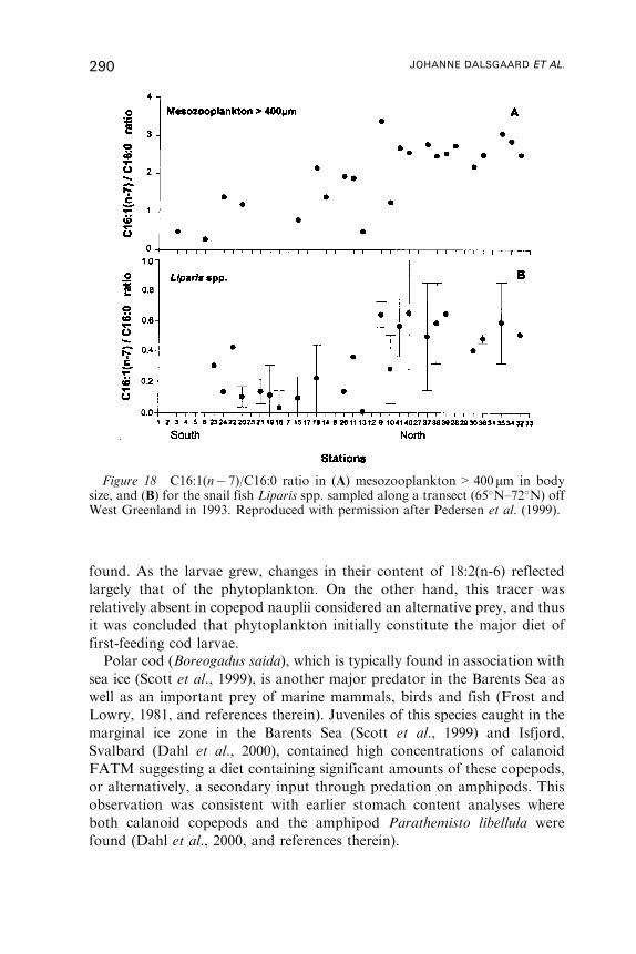
found. As the larvae grew, changes in their content of 18:2(n-6) reflected

largely that of the phytoplankton. On the other hand, this tracer was

relatively absent in copepod nauplii considered an alternative prey, and thus

it was concluded that phytoplankton initially constitute the major diet of

first-feeding cod larvae.

Polar cod (Boreogadus saida), which is typically found in association with

sea ice (Scott et al., 1999), is another major predator in the Barents Sea as

well as an important prey of marine mammals, birds and fish (Frost and

Lowry, 1981, and references therein). Juveniles of this species caught in the

marginal ice zone in the Barents Sea (Scott et al., 1999) and Isfjord,

Svalbard (Dahl et al., 2000), contained high concentrations of calanoid

FATM suggesting a diet containing significant amounts of these copepods,

or alternatively, a secondary input through predation on amphipods. This

observation was consistent with earlier stomach content analyses where

both calanoid copepods and the amphipod Parathemisto libellula were

found (Dahl et al., 2000, and references therein).

Figure 18 C16:1(n� 7)/C16:0 ratio in (A) mesozooplankton>400mm in bodysize, and (B) for the snail fish Liparis spp. sampled along a transect (65�N–72�N) offWest Greenland in 1993. Reproduced with permission after Pedersen et al. (1999).


5.2.6. Marine mammals

FATM have also been used to assess the potential prey of white whales

(Delphinapterus leucas; Dahl et al., 2000). Comparing blubber FA signatures

derived from biopsies of white whales foraging close to Svalbard with FA

compositional data of potential prey species by principal component

analyses, Dahl et al. (2000) deduced that juvenile polar cod, capelin, Calanus

hyperboreus and Pandalus borealis constituted the most likely prey. From

observations of feeding behavior and stomach content analyses it was,

however, suggested that copepods are not ingested directly but represent a

secondary input via predation on polar cod and capelin.

5.3. The Antarctic


A large share of primary production in the Antarctic takes place in the sea-

ice. Here, as in the Arctic, the microalgal communities are dominated by

diatoms (Fahl and Kattner, 1993; Nichols et al., 1993), although a variety of

autotrophic flagellates, particularly Phaeocystis, are also present (Marchant

and Thomsen, 1994). Most of the pelagic primary production occurs in the

marginal ice zone rather than in the open ocean (Marchant and Thomsen,

1994, and references therein). Pelagic phytoplankton is also composed

largely of diatoms superimposed on a background of Phaeocystis and

dinoflagellates. Moreover, Phaeocystis spp. typically bloom in the marginal

ice zone in the spring prior to the increase in diatoms (Pond et al., 1993;

Marchant and Thomsen, 1994; Skerratt et al., 1995; Cripps et al., 1999;

Cripps and Atkinson, 2000, and references therein).

As in other regions, the phytoplankton biomass in the Antarctic is typified

by characteristic signature FA reflecting the prevailing class of microalgae

(Section 2.4.3). However, in contrast to the Arctic and as discussed in Section

2.4.3, Phaeocystis spp. in this region are much less rich in (n-3) PUFA, which

together with a low 16:1(n-7)/16:0 ratio and an elevated concentration of

18:1(n-9) distinguishes them from diatoms (Skerratt et al., 1995).

5.3.2. Copepods

Herbivorous and omnivorous copepods in the Antarctic deviate in several

ways from their Arctic counterparts. Many species such as Calanus

propinquus (Hagen et al., 1993; Kattner et al., 1994; Falk-Petersen et al.,

1999), C. simillimus and Euchirella rostromagna (Hagen et al., 1995; Ward

et al., 1996), store TAG rather than WE. This storage pattern suggests that


these copepods feed throughout the year and have evolved a more

opportunistic feeding strategy than strictly herbivorous species. In WE-

storing copepods, long-chain monounsaturated fatty alcohols are typically

replaced either by short-chain saturated fatty alcohols (e.g., Rhincalanus

gigas, Graeve et al., 1994b) or the concentration of 20:1(n-9) is higher than

that of 22:1(n-11) (Calanoides acutus, Graeve et al., 1994b; Kattner and

Hagen, 1995; Falk-Petersen et al., 1999; Section 3.2). FATM are typically

less evident in Antarctic copepods as compared to Arctic copepods (e.g.,

Calanus propinquus, Kattner et al., 1994; Falk-Petersen et al., 1999;

C. simillimus and Euchirella rostromagna, Hagen et al., 1995; Ward et al.,

1996), though this does not apply to all species. High concentrations of

16:1(n-7) and 18:4(n-3) have, for example, been detected in the dominant

circum-Antarctic species, Calanoides acutus (Graeve et al., 1994b). This is

illustrated in Figure 15B, which was based on samples of C. acutus from the

Weddell Sea. Here, specimens from site III–V contained very high

concentrations of 18:4(n-3) probably as a result of the uptake of

Phaeocystis, which was the dominant microalgae in these areas at the time

of sampling (Kattner and Hagen, 1995, and references therein). Lower levels

of 18:4(n-3) combined with elevated concentrations of 16:1(n-7) at site I

suggested a higher uptake of diatoms there, whereas the resolution of group-

specific phytoplankton contributing to the diet of specimens from site II

was less easy to interpret, suggesting a more mixed diet. These observations

were supported by data from the Lazarev Sea, where the FA signature of

C. acutus indicated extensive feeding on a mixed but probably diatom-

dominated phytoplankton diet, with seasonal differences in the uptake of

dinoflagellates and Phaeocystis (Falk-Petersen et al., 1999).

Fatty acid trophic markers have also been used to resolve the diet

composition of the Antarctic copepod Rhincalanus gigas revealing char-

acteristics of both a herbivorous and omnivorous feeding behavior (Graeve

et al., 1994b; Ward et al., 1996). Hence, the WE fatty acid composition of

specimens from the Weddell Sea revealed a mixture of 18:1(n-9), typical

of a carnivorous diet, and 16:1(n-7), 18:4(n-3), EPA and DHA indicating

additional uptake of phytoplankton (Graeve et al., 1994b). Omnivorous

feeding behavior by R. gigas on phytoplankton, detritus and zooplankton

has indeed been reported by Arashkevich (1978, in Bathmann et al., 1993).

Hence, utilizing FATM, R. gigas has been suggested to be a facultative

herbivore able to switch to nonphytoplankton food when algae are scarce.

Similarly, the predominance of 16:1(n-7) and 18:1(n-9) in the WE of older,

lipid-rich specimens of another Southern Ocean species, Pareuchaeta

antarctica, collected in the southeastern Weddell Sea (Hagen et al., 1995),

suggested omnivorous feeding behavior by this species as well. Older stages

of P. antarctica are, however, known to feed as carnivores consuming only

small amounts of phytoplankton (Hopkins, 1987). Hence, whereas the


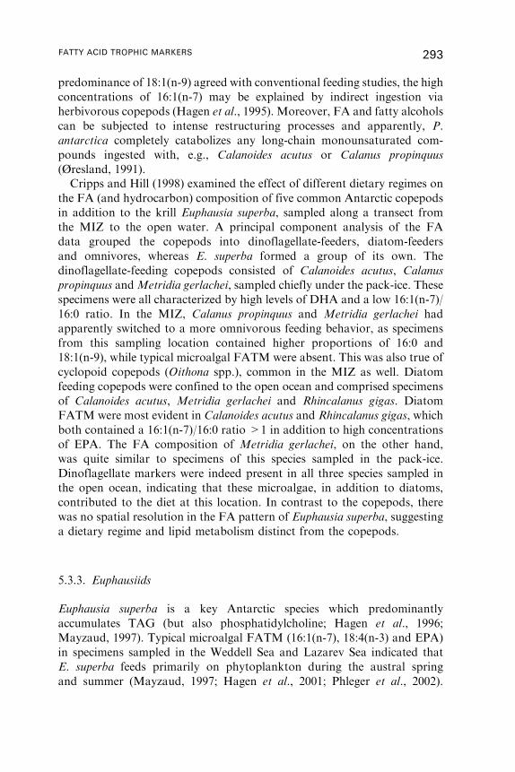
predominance of 18:1(n-9) agreed with conventional feeding studies, the high

concentrations of 16:1(n-7) may be explained by indirect ingestion via

herbivorous copepods (Hagen et al., 1995). Moreover, FA and fatty alcohols

can be subjected to intense restructuring processes and apparently, P.

antarctica completely catabolizes any long-chain monounsaturated com-

pounds ingested with, e.g., Calanoides acutus or Calanus propinquus

(Øresland, 1991).

Cripps and Hill (1998) examined the effect of different dietary regimes on

the FA (and hydrocarbon) composition of five common Antarctic copepods

in addition to the krill Euphausia superba, sampled along a transect from

the MIZ to the open water. A principal component analysis of the FA

data grouped the copepods into dinoflagellate-feeders, diatom-feeders

and omnivores, whereas E. superba formed a group of its own. The

dinoflagellate-feeding copepods consisted of Calanoides acutus, Calanus

propinquus andMetridia gerlachei, sampled chiefly under the pack-ice. These

specimens were all characterized by high levels of DHA and a low 16:1(n-7)/

16:0 ratio. In the MIZ, Calanus propinquus and Metridia gerlachei had

apparently switched to a more omnivorous feeding behavior, as specimens

from this sampling location contained higher proportions of 16:0 and

18:1(n-9), while typical microalgal FATM were absent. This was also true of

cyclopoid copepods (Oithona spp.), common in the MIZ as well. Diatom

feeding copepods were confined to the open ocean and comprised specimens

of Calanoides acutus, Metridia gerlachei and Rhincalanus gigas. Diatom

FATM were most evident in Calanoides acutus and Rhincalanus gigas, which

both contained a 16:1(n-7)/16:0 ratio >1 in addition to high concentrations

of EPA. The FA composition of Metridia gerlachei, on the other hand,

was quite similar to specimens of this species sampled in the pack-ice.

Dinoflagellate markers were indeed present in all three species sampled in

the open ocean, indicating that these microalgae, in addition to diatoms,

contributed to the diet at this location. In contrast to the copepods, there

was no spatial resolution in the FA pattern of Euphausia superba, suggesting

a dietary regime and lipid metabolism distinct from the copepods.

5.3.3. Euphausiids

Euphausia superba is a key Antarctic species which predominantly

accumulates TAG (but also phosphatidylcholine; Hagen et al., 1996;

Mayzaud, 1997). Typical microalgal FATM (16:1(n-7), 18:4(n-3) and EPA)

in specimens sampled in the Weddell Sea and Lazarev Sea indicated that

E. superba feeds primarily on phytoplankton during the austral spring

and summer (Mayzaud, 1997; Hagen et al., 2001; Phleger et al., 2002).


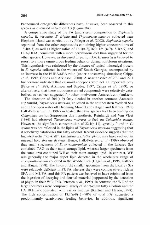
Pronounced ontogenetic differences have, however, been observed in this

species as discussed in Section 3.3 (Figure 9A).

A comparative study of the FA (and sterol) composition of Euphausia

superba, E. tricantha, E. frigida and Thysanoessa macrura collected near

Elephant Island was carried out by Phleger et al. (2002). Euphausia superba

separated from the other euphausiids containing higher concentrations of

18:4(n-3) as well as higher ratios of 16:1(n-7)/16:0, 18:1(n-7)/18:1(n-9) and

EPA/DHA, consistent with a more herbivorous diet than suggested for the

other species. However, as discussed in Section 3.4, E. superba is believed to

resort to a more omnivorous feeding behavior during nonbloom situations.

This hypothesis was reinforced by the absence of typical microalgal tracers

in E. superba collected in the waters off South Georgia, accompanied by

an increase in the PUFA/SFA ratio (under nonstarving situations; Cripps

et al., 1999; Cripps and Atkinson, 2000). A near absence of 20:1 and 22:1

furthermore indicated that calanoid copepods were not an important prey

(Price et al. 1988; Atkinson and Snyder, 1997; Cripps et al., 1999), or

alternatively, that these monounsaturated compounds were selectively cata-

bolized as has been suggested for other omnivorous Antarctic zooplankters.

The detection of 20:1(n-9) fatty alcohol in another common Antarctic

euphausiid, Thysanoessa macrura, collected in the southeastern Weddell Sea

and in the open water off Dronning Maud Land (Hagen and Kattner, 1998;

Falk-Petersen et al., 1999) indicated that this species had been feeding on

Calanoides acutus. Supporting this hypothesis, Reinhardt and Van Vleet

(1986) had observed Thysanoessa macrura to feed on Calanoides acutus.

However, the significant concentration of 22:1(n-11) typically found in C.

acutus was not reflected in the lipids of Thysanoessa macrura suggesting that

it selectively catabolizes this fatty alcohol. Recent evidence suggests that the

high-Antarctic ‘‘ice-krill’’, Euphausia crystallorophias, may have evolved an

unusual lipid storage strategy. Hence, Falk-Petersen et al. (1999) observed

that small specimens of E. crystallorophias collected in the Lazarev Sea

contained TAG as their main storage lipid, whereas larger specimens from

the same area contained WE as their main storage lipid. In contrast, WE

was generally the major depot lipid detected in the whole size range of

E. crystallorophias collected in the Weddell Sea (Hagen et al., 1996; Kattner

and Hagen, 1998). The lipids of the smaller specimens from the Lazarev Sea

were relatively deficient in PUFA whereas they were comparatively rich in

SFA and MUFA, and this FA pattern was believed to have originated from

the ingestion of decaying and detrital material (supported by the detection

of phytol in their WE; Falk-Petersen et al., 1999). In contrast, the WE of the

large specimens were composed largely of short-chain fatty alcohols and the

FA 18:1(n-9), consistent with earlier findings (Kattner and Hagen, 1998).

The high concentration of 18:1(n-9) (>70% of total FA) suggested a

predominantly carnivorous feeding behavior. In addition, significant


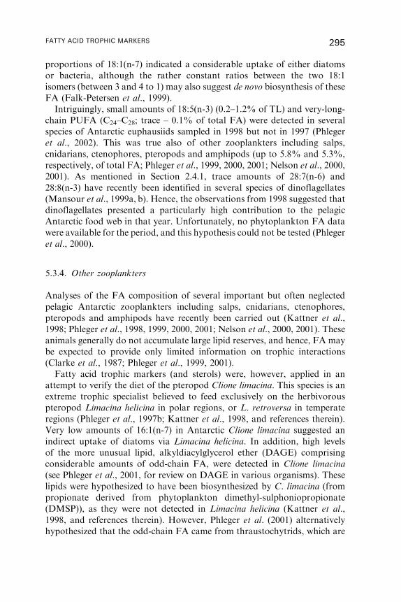
proportions of 18:1(n-7) indicated a considerable uptake of either diatoms

or bacteria, although the rather constant ratios between the two 18:1

isomers (between 3 and 4 to 1) may also suggest de novo biosynthesis of these

FA (Falk-Petersen et al., 1999).

Intriguingly, small amounts of 18:5(n-3) (0.2–1.2% of TL) and very-long-

chain PUFA (C24–C28; trace – 0.1% of total FA) were detected in several

species of Antarctic euphausiids sampled in 1998 but not in 1997 (Phleger

et al., 2002). This was true also of other zooplankters including salps,

cnidarians, ctenophores, pteropods and amphipods (up to 5.8% and 5.3%,

respectively, of total FA; Phleger et al., 1999, 2000, 2001; Nelson et al., 2000,

2001). As mentioned in Section 2.4.1, trace amounts of 28:7(n-6) and

28:8(n-3) have recently been identified in several species of dinoflagellates

(Mansour et al., 1999a, b). Hence, the observations from 1998 suggested that

dinoflagellates presented a particularly high contribution to the pelagic

Antarctic food web in that year. Unfortunately, no phytoplankton FA data

were available for the period, and this hypothesis could not be tested (Phleger

et al., 2000).

5.3.4. Other zooplankters

Analyses of the FA composition of several important but often neglected

pelagic Antarctic zooplankters including salps, cnidarians, ctenophores,

pteropods and amphipods have recently been carried out (Kattner et al.,

1998; Phleger et al., 1998, 1999, 2000, 2001; Nelson et al., 2000, 2001). These

animals generally do not accumulate large lipid reserves, and hence, FA may

be expected to provide only limited information on trophic interactions

(Clarke et al., 1987; Phleger et al., 1999, 2001).

Fatty acid trophic markers (and sterols) were, however, applied in an

attempt to verify the diet of the pteropod Clione limacina. This species is an

extreme trophic specialist believed to feed exclusively on the herbivorous

pteropod Limacina helicina in polar regions, or L. retroversa in temperate

regions (Phleger et al., 1997b; Kattner et al., 1998, and references therein).

Very low amounts of 16:1(n-7) in Antarctic Clione limacina suggested an

indirect uptake of diatoms via Limacina helicina. In addition, high levels

of the more unusual lipid, alkyldiacylglycerol ether (DAGE) comprising

considerable amounts of odd-chain FA, were detected in Clione limacina

(see Phleger et al., 2001, for review on DAGE in various organisms). These

lipids were hypothesized to have been biosynthesized by C. limacina (from

propionate derived from phytoplankton dimethyl-sulphoniopropionate

(DMSP)), as they were not detected in Limacina helicina (Kattner et al.,

1998, and references therein). However, Phleger et al. (2001) alternatively

hypothesized that the odd-chain FA came from thraustochytrids, which are


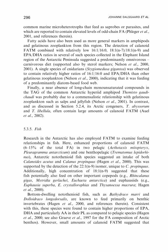
common marine microheterotrophs that feed as saprobes or parasites, and

which are reported to contain elevated levels of odd-chain FA (Phleger et al.,

2001, and references therein).

Fatty acids have also been used as more general markers in amphipods

and gelatinous zooplankton from this region. The detection of calanoid

FATM combined with relatively low 16:1/16:0, 18:1(n-7)/18:1(n-9) and

EPA/DHA ratios in several of such species collected in the Elephant Island

region of the Antarctic Peninsula suggested a predominantly omnivorous –

carnivorous diet (supported also by sterol markers; Nelson et al., 2000,

2001). A single species of cnidarians (Stygiomedusa gigantea) was observed

to contain relatively higher ratios of 16:1/16:0 and EPA/DHA than other

gelatinous zooplankton (Nelson et al., 2000), indicating that it was feeding

of a predominantly diatom-based food web.

Finally, a near absence of long-chain monounsaturated compounds in

the TAG of the common Antarctic hyperiid amphipod Themisto gaudi-

chaudi was probably due to a commensalistic relationship with gelatinous

zooplankton such as salps and jellyfish (Nelson et al., 2001). In contrast,

and as discussed in Section 5.2.4, its Arctic congeners, T. abyssorum

and T. libellula, often contain large amounts of calanoid FATM (Auel

et al., 2002).

5.3.5. Fish

Research in the Antarctic has also employed FATM to examine feeding

relationships in fish. Here, enhanced proportions of calanoid FATM

(6–15% of the total FA) in two pelagic (Aethotaxis mitopteryx,

Pleuragramma antarcticum) and one benthopelagic (Trematomus lepidorhi-

nus), Antarctic notothenioid fish species suggested an intake of both

Calanoides acutus and Calanus propinquus (Hagen et al., 2000). This was

supported by the detection of the 22:1(n-9) isomer, unique to C. propinquus.

Additionally, high concentration of 18:1(n-9) suggested that these

fish potentially also feed on other important copepods (e.g., Rhincalanus

gigas, Metridia gerlachei, Euchaeta antarctica) and euphausiids (e.g.,

Euphausia superba, E. crystallorophias and Thysanoessa macrura; Hagen

et al., 2000).

Bottom-dwelling notothenioid fish, such as Bathydraco marri and

Dolloidraco longedorsalis, are known to feed primarily on benthic

invertebrates (Hagen et al., 2000, and references therein). Consistent

with this, these species were found to contain higher proportions of EPA,

DHA and particularly AA in their PL as compared to pelagic species (Hagen

et al., 2000; see also Graeve et al., 1997 for the FA composition of Arctic

benthos). However, small amounts of calanoid FATM suggested that


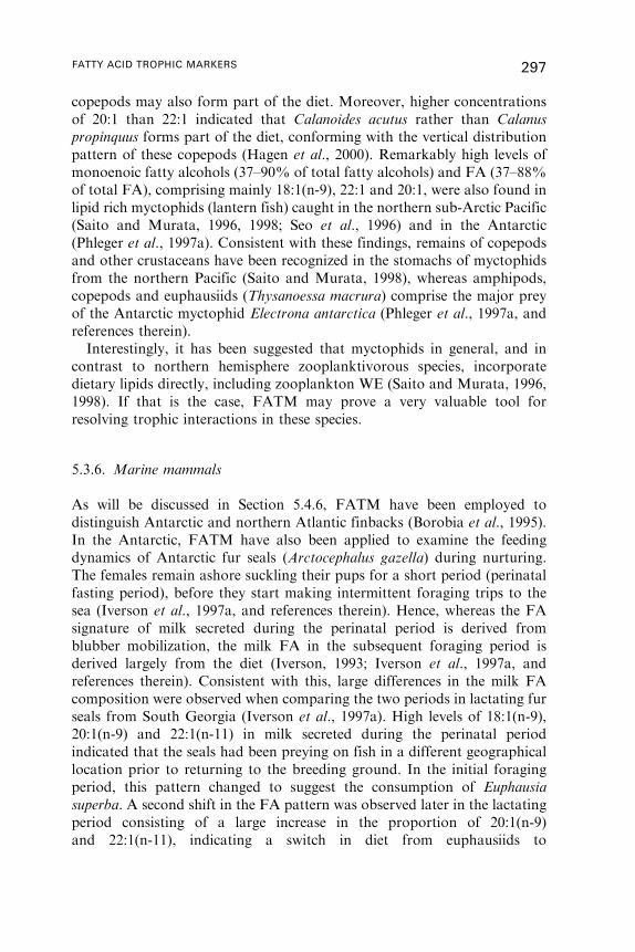
copepods may also form part of the diet. Moreover, higher concentrations

of 20:1 than 22:1 indicated that Calanoides acutus rather than Calanus

propinquus forms part of the diet, conforming with the vertical distribution

pattern of these copepods (Hagen et al., 2000). Remarkably high levels of

monoenoic fatty alcohols (37–90% of total fatty alcohols) and FA (37–88%

of total FA), comprising mainly 18:1(n-9), 22:1 and 20:1, were also found in

lipid rich myctophids (lantern fish) caught in the northern sub-Arctic Pacific

(Saito and Murata, 1996, 1998; Seo et al., 1996) and in the Antarctic

(Phleger et al., 1997a). Consistent with these findings, remains of copepods

and other crustaceans have been recognized in the stomachs of myctophids

from the northern Pacific (Saito and Murata, 1998), whereas amphipods,

copepods and euphausiids (Thysanoessa macrura) comprise the major prey

of the Antarctic myctophid Electrona antarctica (Phleger et al., 1997a, and

references therein).

Interestingly, it has been suggested that myctophids in general, and in

contrast to northern hemisphere zooplanktivorous species, incorporate

dietary lipids directly, including zooplankton WE (Saito and Murata, 1996,

1998). If that is the case, FATM may prove a very valuable tool for

resolving trophic interactions in these species.


As will be discussed in Section 5.4.6, FATM have been employed to

distinguish Antarctic and northern Atlantic finbacks (Borobia et al., 1995).

In the Antarctic, FATM have also been applied to examine the feeding

dynamics of Antarctic fur seals (Arctocephalus gazella) during nurturing.

The females remain ashore suckling their pups for a short period (perinatal

fasting period), before they start making intermittent foraging trips to the

sea (Iverson et al., 1997a, and references therein). Hence, whereas the FA

signature of milk secreted during the perinatal period is derived from

blubber mobilization, the milk FA in the subsequent foraging period is

derived largely from the diet (Iverson, 1993; Iverson et al., 1997a, and

references therein). Consistent with this, large differences in the milk FA

composition were observed when comparing the two periods in lactating fur

seals from South Georgia (Iverson et al., 1997a). High levels of 18:1(n-9),

20:1(n-9) and 22:1(n-11) in milk secreted during the perinatal period

indicated that the seals had been preying on fish in a different geographical

location prior to returning to the breeding ground. In the initial foraging

period, this pattern changed to suggest the consumption of Euphausia

superba. A second shift in the FA pattern was observed later in the lactating

period consisting of a large increase in the proportion of 20:1(n-9)

and 22:1(n-11), indicating a switch in diet from euphausiids to


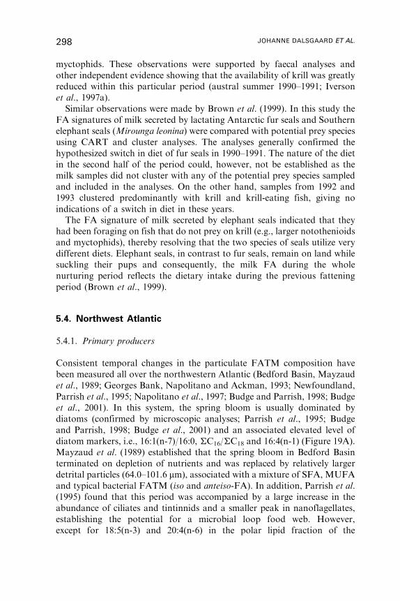
myctophids. These observations were supported by faecal analyses and

other independent evidence showing that the availability of krill was greatly

reduced within this particular period (austral summer 1990–1991; Iverson

et al., 1997a).

Similar observations were made by Brown et al. (1999). In this study the

FA signatures of milk secreted by lactating Antarctic fur seals and Southern

elephant seals (Mirounga leonina) were compared with potential prey species

using CART and cluster analyses. The analyses generally confirmed the

hypothesized switch in diet of fur seals in 1990–1991. The nature of the diet

in the second half of the period could, however, not be established as the

milk samples did not cluster with any of the potential prey species sampled

and included in the analyses. On the other hand, samples from 1992 and

1993 clustered predominantly with krill and krill-eating fish, giving no

indications of a switch in diet in these years.

The FA signature of milk secreted by elephant seals indicated that they

had been foraging on fish that do not prey on krill (e.g., larger notothenioids

and myctophids), thereby resolving that the two species of seals utilize very

different diets. Elephant seals, in contrast to fur seals, remain on land while

suckling their pups and consequently, the milk FA during the whole

nurturing period reflects the dietary intake during the previous fattening

period (Brown et al., 1999).

5.4. Northwest Atlantic


Consistent temporal changes in the particulate FATM composition have

been measured all over the northwestern Atlantic (Bedford Basin, Mayzaud

et al., 1989; Georges Bank, Napolitano and Ackman, 1993; Newfoundland,

Parrish et al., 1995; Napolitano et al., 1997; Budge and Parrish, 1998; Budge

et al., 2001). In this system, the spring bloom is usually dominated by

diatoms (confirmed by microscopic analyses; Parrish et al., 1995; Budge

and Parrish, 1998; Budge et al., 2001) and an associated elevated level of

diatom markers, i.e., 16:1(n-7)/16:0, �C16/�C18 and 16:4(n-1) (Figure 19A).

Mayzaud et al. (1989) established that the spring bloom in Bedford Basin

terminated on depletion of nutrients and was replaced by relatively larger

detrital particles (64.0–101.6 mm), associated with a mixture of SFA, MUFA

and typical bacterial FATM (iso and anteiso-FA). In addition, Parrish et al.

(1995) found that this period was accompanied by a large increase in the

abundance of ciliates and tintinnids and a smaller peak in nanoflagellates,

establishing the potential for a microbial loop food web. However,

except for 18:5(n-3) and 20:4(n-6) in the polar lipid fraction of the


microzooplankton, no significant correlations with typical microalgal

FATM within this period were detected. Later in the summer, a second

bloom composed of small (2.0–6.4 mm) dinoflagellates and flagellates usually

develops, characterized by increasing proportions of C18 FA and DHA

(Mayzaud et al., 1989; Parrish et al., 1995).

Figure 19 Values of various FA indicators in net-tows collected during a springbloom in Trinity Bay, Newfoundland in 1996 (mean� S.D., n¼ 9). (A) diatomindicators, and (B) dinoflagellate and bacterial indicators (the latter equal to the sumof 15:0, 17:0 and all iso and anteiso-branched chain FA expressed as percent of totalFA). Redrawn with permission after Budge and Parrish (1998).


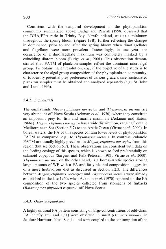
Consistent with the temporal development in the phytoplankton

community summarized above, Budge and Parrish (1998) observed that

the DHA/EPA ratio in Trinity Bay, Newfoundland, was at a minimum

throughout the spring bloom (Figure 19B), further reflecting the changes

in dominance, prior to and after the spring bloom when dinoflagellates

and flagellates were more prevalent. Interestingly, in one year, the

occurrence of a dinoflagellate maximum was completely masked by a

coinciding diatom bloom (Budge et al., 2001). This observation demon-

strated that FATM of plankton samples reflect the dominant microalgal

group. To obtain higher resolution, e.g., if the objective of the study is to

characterize the algal group composition of the phytoplankton community,

or to identify potential prey preferences of various grazers, size-fractionated

plankton samples must be obtained and analyzed separately (e.g., St. John

and Lund, 1996).

5.4.2. Euphausiids

The euphausiids Meganyctiphanes norvegica and Thysanoessa inermis are

very abundant off Nova Scotia (Ackman et al., 1970), where they constitute

an important prey for fish and marine mammals (Ackman and Eaton,

1966a).Meganyctiphanes norvegica has a wide distribution, ranging from the

Mediterranean Sea (Section 5.7) to the Arctic Ocean (Virtue et al., 2000). In

boreal waters, the FA of this species contain lower levels of phytoplankton

FATM as compared, e.g., to Thysanoessa inermis. In contrast, calanoid

FATM are usually highly prevalent in Meganyctiphanes norvegica from this

region (but see Section 5.7). These observations are consistent with data on

the feeding ecology of this species, which is known to feed preferentially on

calanoid copepods (Sargent and Falk-Petersen, 1981; Virtue et al., 2000).

Thysanoessa inermis, on the other hand, is a boreal-Arctic species storing

large amounts of WE with a FA and fatty alcohol composition suggestive

of a more herbivorous diet as discussed in Section 5.2.3. The differences

between Meganyctiphanes norvegica and Thysanoessa inermis were already

established in the late 1960s when Ackman et al. (1970) reported on the FA

composition of the two species collected from stomachs of finbacks

(Balaenoptera physalus) captured off Nova Scotia.

5.4.3. Other zooplankters

A highly unusual FA pattern consisting of large concentrations of odd-chain

FA (chiefly 15:1 and 17:1) were observed in smelt (Osmerus mordax) in

Jeddore Harbour, Nova Scotia, and were coupled to the consumption of the


amphipod Pontoporeia femorata (Paradis and Ackman, 1976). This

amphipod contains extremely high levels of these FA (�50%), and stomach

content analyses of smelt moving into the harbor prior to their spring

spawning runs revealed that they had been preying heavily on P. femorata.

The conservative propagation of the odd-chain FA through this short food

web was substantiated by a nearly identical distribution of monoethylenic

isomers in the amphipod and the fish, whereas the isomeric ratio of more

common even-chain FA was quite different. Intriguingly, high levels of

similar odd-chain FA (i.e., 15:0 and 17:1(n-8)) have later been reported for

Clione limacina (pteropod; Kattner et al., 1998), which is an extreme trophic

specialist as discussed in Section 5.3.4. Since the prey of C. limacina con-

tained only traces of these odd-chain FA, and because of the close trophic

coupling, it was deduced that C. limacina biosynthesize these FA de novo

(Kattner et al., 1998), or alternatively, obtain them from thaustochytrids

(Microheterotrophs; Phleger et al., 2001). The situation may be similar for

Pontoporeia femorata, however, this remains to be examined.

Another less well studied organism, which periodically occurs in very large

abundances in the North Atlantic, is the tunicate Dolioletta gegenbauri. This

species is known to graze on a wide variety of microplankton ranging from

bacteria to diatoms, and is believed to contribute significantly to the diet of

many larval fish (Pond and Sargent, 1998, and references therein). However,

being gelatinous, this prey is difficult to detect in stomach content analyses

and here, FA may provide additional information. Free-swimming, sexual

stages of D. gegenbauri sampled in the western Atlantic off central America

(58�W, 20�N) contained high concentrations of EPA, DHA and C18 PUFA.

This FA pattern was consistent with a primary producer community

dominated by coccolithophores and smaller contributions of diatoms,

dinoflagellates, flagellates and picoplankton (Pond and Sargent, 1998). On

the basis of the high growth and mortality rates observed in D. gegenbauri, it

was hypothesized that the tunicates sediment rapidly to the deep ocean,

bringing with them large amounts of labile PUFA to the benefit of

bathypelagic and deep-sea benthic ecosystems.

5.4.4. Macrobenthos

Measuring the organ-specific FA composition of the sea scallop Placopecten

magellanicus, a major local primary consumer in Trinity Bay,

Newfoundland, Napolitano et al. (1997) found that the digestive gland

(which is the major NL storage site and is composed of 60% TAG)

exhibited a series of compositional shifts, reflecting the temporal develop-

ment in the phytoplankton. In this study, the digestive gland prior to the

spring bloom was characterized by dinoflagellate- and flagellate-specific


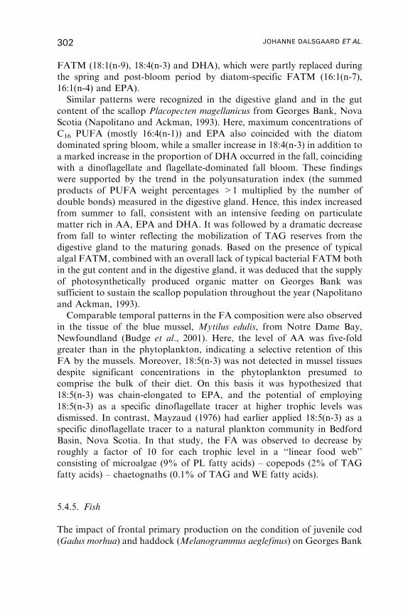
FATM (18:1(n-9), 18:4(n-3) and DHA), which were partly replaced during

the spring and post-bloom period by diatom-specific FATM (16:1(n-7),

16:1(n-4) and EPA).

Similar patterns were recognized in the digestive gland and in the gut

content of the scallop Placopecten magellanicus from Georges Bank, Nova

Scotia (Napolitano and Ackman, 1993). Here, maximum concentrations of

C16 PUFA (mostly 16:4(n-1)) and EPA also coincided with the diatom

dominated spring bloom, while a smaller increase in 18:4(n-3) in addition to

a marked increase in the proportion of DHA occurred in the fall, coinciding

with a dinoflagellate and flagellate-dominated fall bloom. These findings

were supported by the trend in the polyunsaturation index (the summed

products of PUFA weight percentages >1 multiplied by the number of

double bonds) measured in the digestive gland. Hence, this index increased

from summer to fall, consistent with an intensive feeding on particulate

matter rich in AA, EPA and DHA. It was followed by a dramatic decrease

from fall to winter reflecting the mobilization of TAG reserves from the

digestive gland to the maturing gonads. Based on the presence of typical

algal FATM, combined with an overall lack of typical bacterial FATM both

in the gut content and in the digestive gland, it was deduced that the supply

of photosynthetically produced organic matter on Georges Bank was

sufficient to sustain the scallop population throughout the year (Napolitano

and Ackman, 1993).

Comparable temporal patterns in the FA composition were also observed

in the tissue of the blue mussel, Mytilus edulis, from Notre Dame Bay,

Newfoundland (Budge et al., 2001). Here, the level of AA was five-fold

greater than in the phytoplankton, indicating a selective retention of this

FA by the mussels. Moreover, 18:5(n-3) was not detected in mussel tissues

despite significant concentrations in the phytoplankton presumed to

comprise the bulk of their diet. On this basis it was hypothesized that

18:5(n-3) was chain-elongated to EPA, and the potential of employing

18:5(n-3) as a specific dinoflagellate tracer at higher trophic levels was

dismissed. In contrast, Mayzaud (1976) had earlier applied 18:5(n-3) as a

specific dinoflagellate tracer to a natural plankton community in Bedford

Basin, Nova Scotia. In that study, the FA was observed to decrease by

roughly a factor of 10 for each trophic level in a ‘‘linear food web’’

consisting of microalgae (9% of PL fatty acids) – copepods (2% of TAG

fatty acids) – chaetognaths (0.1% of TAG and WE fatty acids).

5.4.5. Fish

The impact of frontal primary production on the condition of juvenile cod

(Gadus morhua) and haddock (Melanogrammus aeglefinus) on Georges Bank


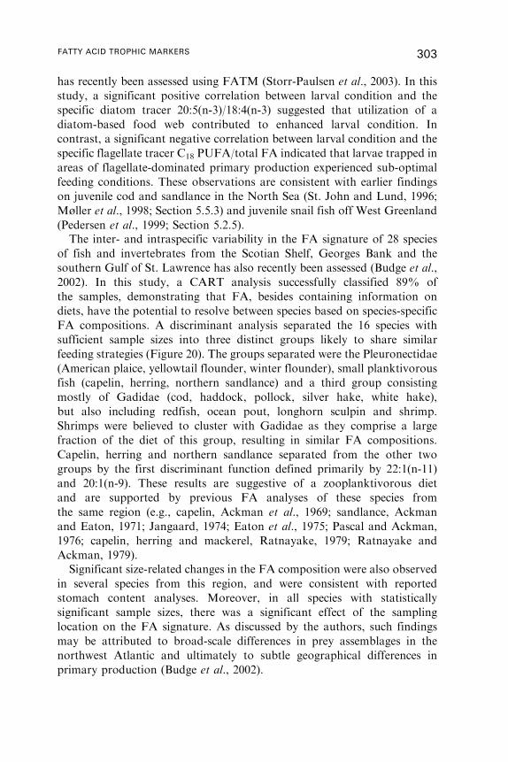
has recently been assessed using FATM (Storr-Paulsen et al., 2003). In this

study, a significant positive correlation between larval condition and the

specific diatom tracer 20:5(n-3)/18:4(n-3) suggested that utilization of a

diatom-based food web contributed to enhanced larval condition. In

contrast, a significant negative correlation between larval condition and the

specific flagellate tracer C18 PUFA/total FA indicated that larvae trapped in

areas of flagellate-dominated primary production experienced sub-optimal

feeding conditions. These observations are consistent with earlier findings

on juvenile cod and sandlance in the North Sea (St. John and Lund, 1996;

Møller et al., 1998; Section 5.5.3) and juvenile snail fish off West Greenland

(Pedersen et al., 1999; Section 5.2.5).

The inter- and intraspecific variability in the FA signature of 28 species

of fish and invertebrates from the Scotian Shelf, Georges Bank and the

southern Gulf of St. Lawrence has also recently been assessed (Budge et al.,

2002). In this study, a CART analysis successfully classified 89% of

the samples, demonstrating that FA, besides containing information on

diets, have the potential to resolve between species based on species-specific

FA compositions. A discriminant analysis separated the 16 species with

sufficient sample sizes into three distinct groups likely to share similar

feeding strategies (Figure 20). The groups separated were the Pleuronectidae

(American plaice, yellowtail flounder, winter flounder), small planktivorous

fish (capelin, herring, northern sandlance) and a third group consisting

mostly of Gadidae (cod, haddock, pollock, silver hake, white hake),

but also including redfish, ocean pout, longhorn sculpin and shrimp.

Shrimps were believed to cluster with Gadidae as they comprise a large

fraction of the diet of this group, resulting in similar FA compositions.

Capelin, herring and northern sandlance separated from the other two

groups by the first discriminant function defined primarily by 22:1(n-11)

and 20:1(n-9). These results are suggestive of a zooplanktivorous diet

and are supported by previous FA analyses of these species from

the same region (e.g., capelin, Ackman et al., 1969; sandlance, Ackman

and Eaton, 1971; Jangaard, 1974; Eaton et al., 1975; Pascal and Ackman,

1976; capelin, herring and mackerel, Ratnayake, 1979; Ratnayake and

Ackman, 1979).

Significant size-related changes in the FA composition were also observed

in several species from this region, and were consistent with reported

stomach content analyses. Moreover, in all species with statistically

significant sample sizes, there was a significant effect of the sampling

location on the FA signature. As discussed by the authors, such findings

may be attributed to broad-scale differences in prey assemblages in the

northwest Atlantic and ultimately to subtle geographical differences in

primary production (Budge et al., 2002).



A comparative analysis on the blubber FA composition of sympatric

populations of finbacks (Balaenoptera physalus) and humpbacks

(Megaptera novaeangliae) from the Gulf of St. Lawrence was carried out

by Borobia et al. (1995). Blubber FA data from earlier studies on finbacks

from the Antarctic, Nova Scotia and a single sample from Spain were

incorporated in the analysis as well, as was data on stable carbon isotope

ratios. Calanoid FATM clearly separated the northern hemisphere baleens

from Antarctic finbacks. Consistent with these finding, Antarctic finbacks

are known to feed heavily on Euphausia superba, which are relatively

deficient in long-chain MUFA (Section 5.3.3; Ackman and Eaton, 1966a).

Furthermore, Gulf of St. Lawrence humpbacks separated from finbacks in

the same area on the basis of higher than average levels of EPA and DHA.

Based on this and a slightly more depleted stable carbon isotope ratio in

humpbacks as compared to finbacks, it was deduced that the humpbacks fed

slightly lower in the food web than finbacks.

Figure 20 Discriminant analysis of FA compositional data of 16 common speciesof fish and invertebrates from the Scotian Shelf, Georges Bank and the Gulf of St.Lawrence. The plot shows the average scores of the first two of 15 discriminantfunctions that classified individuals to species with a 98% success rate. Ellipsessurround the three major clusters of groups and are based on the data point clouds ofindividuals. Reproduced with permission after Budge et al. (2002).


5.5. The North Sea


The temporal dynamics of primary production in this area is similar to that

in the northwest Atlantic (Section 5.4.1). In a study on Fladen Ground,

northern North Sea, Kattner et al. (1983) performed one of the first

systematic determinations of the particulate FA composition during the

course of a natural spring plankton bloom (but see also Jeffries, 1970). A

clear relationship between the species composition of microalgae and the

FA profile of the particulate matter was found. The initial bloom was

dominated by diatoms and was associated with peak proportions of 14:0,

C16 FA, 18:4(n-3), EPA and DHA as illustrated in Figure 21. The bloom

was terminated with the exhaustion of nutrients and was shortly followed

by a second, smaller bloom consisting mostly of dinoflagellates, which was

accompanied by a temporary increase in the proportions of C18 FA and 22:6

(Figure 21B).

In another study on the coupling between FATM and larval and juvenile

cod, St. John and Lund (1996) examined the distribution of phytoplankton

and their associated FA composition across a frontal system in the northern

North Sea. Here, in situ, size-fractionated plankton samples analyzed

for phytoplankton species and concurrent FA composition, verified the

co-occurrence of diatom and dinoflagellate species and their representative

FATM across a tidal mixing region.

5.5.2. Copepods

In general, little information exists on the lipid and FA composition of small

copepods either in this or other regions, although they can be important

members of zooplankton communities (Schnack et al., 1985; Morales et al.,

1991). The majority of small zooplankters, such as Acartia, Pseudocalanus,

Temora and Centropages from temperate regions are omnivorous and their

feeding behavior is tightly coupled to food availability. This was shown, e.g.,

by Cotonnec et al. (2001) who, using a combination of phytoplankton

pigments and FA, found that Temora longicornis, Acartia clausi and

Pseudocalanus elongatus all had consumed large quantities of low quality

Phaeocystis during a Phaeocystis dominated spring bloom in the English

Channel. In addition, the specific diatom marker 16:1(n-7) and the PUFA,

EPA and DHA have been detected in specimens sampled in the southern

North Sea and Wadden Sea, and may give some indication of seasonal

variations in food availability (Kattner et al., 1981).


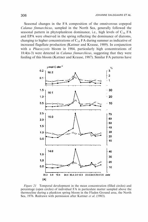
Seasonal changes in the FA composition of the omnivorous copepod

Calanus finmarchicus, sampled in the North Sea, generally followed the

seasonal pattern in phytoplankton dominance, i.e., high levels of C16 FA

and EPA were observed in the spring reflecting the dominance of diatoms,

changing to higher concentrations of C18 FA during summer as indicative of

increased flagellate production (Kattner and Krause, 1989). In conjunction

with a Phaeocystis bloom in 1984, particularly high concentrations of

18:4(n-3) were detected in Calanus finmarchicus, suggesting that they were

feeding of this bloom (Kattner and Krause, 1987). Similar FA patterns have

Figure 21 Temporal development in the mean concentration (filled circles) andpercentage (open circles) of individual FA in particulate matter sampled above thethermocline during a plankton spring bloom in the Fladen Ground area, the NorthSea, 1976. Redrawn with permission after Kattner et al. (1983).


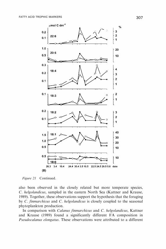
also been observed in the closely related but more temperate species,

C. helgolandicus, sampled in the eastern North Sea (Kattner and Krause,

1989). Together, these observations support the hypothesis that the foraging

by C. finmarchicus and C. helgolandicus is closely coupled to the seasonal

phytoplankton production.

In comparison with Calanus finmarchicus and C. helgolandicus, Kattner

and Krause (1989) found a significantly different FA composition in

Pseudocalanus elongatus. These observations were attributed to a different

Figure 21 Continued.


feeding strategy utilized by P. elongatus, as this species is known to consume

large amount of detritus (Kattner and Krause, 1989, and references therein).

A high concentration of 18:1(n-9) both in P. elongatus (see also Cotonnec

et al., 2001) and in the particulate FA was observed in this study, and

thereby proposed to confirm the utilization of detritus by this species

(Kattner et al., 1983).

5.5.3. Fish

The links between phytoplankton class composition, copepod consumption

and larval fish growth and condition in the North Sea have also been

examined using FATM (St. John and Lund, 1996; Møller et al., 1998). Here,

the enhanced condition of juvenile North Sea cod was linked to diatom

production in frontal regimes, using the 16:1(n-7)/16:0 ratio as a food web

tracer. Juvenile cod with a higher-than-average-tracer content suggestive of

a diatom-based food web were found to be in significantly better condition

than fish with a lower tracer content indicative of a flagellate-based food

web (Figure 11). Similar findings have been made for larval and juvenile

sandlance using 20:5(n-3)/18:4(n-3) as a specific diatom tracer (Møller et al.,

1998). Larvae with a higher than average tracer content, indicative of a

diatom-based food web and hence a frontal mixing regime, were larger and

in better condition than predicted from the size-specific mean of the

population.

5.6. Gulf of Alaska


Unfortunately, there is a lack of FATM related studies with focus on lower

trophic levels in this region. Intriguingly, however, research on higher trophic

levels (Iverson et al., 1997b, 2002) has revealed that in contrast to food webs

in the northern Atlantic, 20:1(n-11) is more abundant than 20:1(n-9). This

‘‘unusual’’ isomer ratio has been observed in species of Neocalanus (Saito

and Kotani, 2000), and has been recognized all the way up to harbor

seals (Phoca vitulina), indicating that the FA composition at the base of the

food web is very different in the two regions (Iverson et al., 1997b).

5.6.2. Fish

A few studies on the FA composition of secondary and higher order

consumers in the Gulf of Alaska have recently been carried out (Iverson


et al., 1997b, 2002). In one study, 22 common species of forage fish and

invertebrates were sampled within Prince William Sound (PWS) over a four

year period (1994–1998). The species were readily distinguished by their

total FA composition via a CART analysis (92% classified correctly;

Iverson et al., 2002). Species with partly overlapping diets such as walleye

pollock (Theragra chalcogramma), Pacific herring (Clupea harengus pallasi)

and Pacific sandlance (Ammodytes hexapterus) were, however, less success-

fully classified. These observations were supported by a discriminant

analysis in which the three species tended to cluster together on a plot of the

first two discriminant functions. Flatfishes, which presumably also share a

similar diet and life history, constituted another cluster. Ontogenetic

changes in specific dietary FATM (14:0, 20:1(n-11), 22:1(n-11), EPA,

DHA) were also observed in this system. Hence, herring showed a shift in

FA composition commensurate with a dietary switch from zooplankton in

earlier life stages to a more piscivorous diet as the fish grew larger, an

observation consistent with stomach content analyses. Similar changes have

previously been reported for both herring and pollock in PWS (see below,

Iverson et al., 1997b), and more lately for several species of fish in the

northwest Atlantic (Section 5.4.5).

Finally, unusually high levels of 20:1(n-11) and 22:1(n-11) were found in

young herring, pollock and sandlance sampled in the spring and summer

1995/1996. These changes in FA composition were attributed to a more

highly stratified ocean surface layer contributing to a reduced biomass of

calanoid copepods in these two years, an occurrence which was hypothe-

sized to have forced a dietary shift in the young fish (Iverson et al., 2002).


In a study of harbor seals (Phoca vitulina) from this system, Iverson et al.

(1997b) employed a CART analysis on blubber FA. The analysis readily

classified the seals according to region (PWS, Kodiak Island, Southeast

Alaska) and even specific haulout sites within PWS, suggesting site-specific

diets (Iverson et al., 1997b). Moreover, herring and pollock were classified

according to size (length) and sampling location in a CART analysis on the

FA composition of potential prey, and the authors commented: ‘‘One result

of these findings is that given a fatty acid composition of an unknown herring

or pollock, one could essentially determine its size-class and location within the

study area with reasonable certainty... This could provide an important tool for

studying foraging ecology and stock structure of fish species’’.

In a preliminary analysis, the FA data of the seals were subjected to the

classification rules derived from the FA composition of their potential prey.

Intriguingly, the seals separated into two groups suggesting possible prey


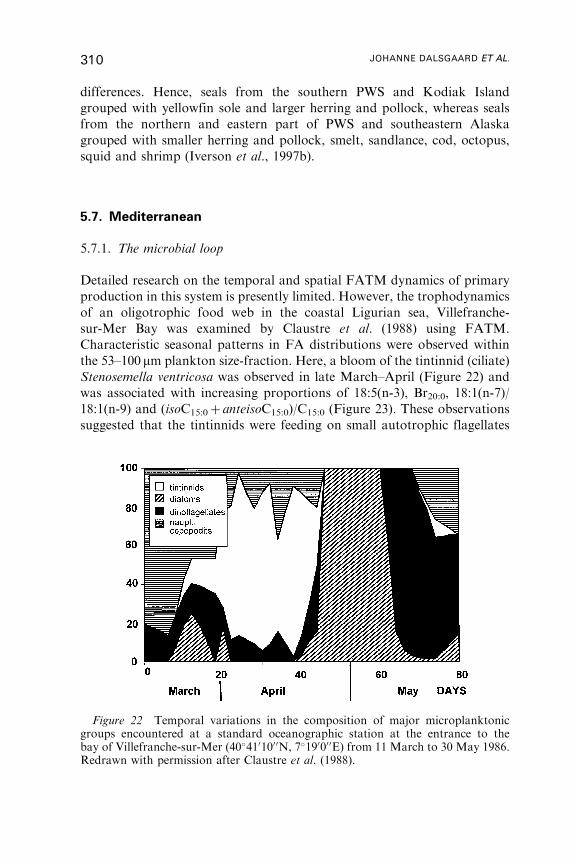
differences. Hence, seals from the southern PWS and Kodiak Island

grouped with yellowfin sole and larger herring and pollock, whereas seals

from the northern and eastern part of PWS and southeastern Alaska

grouped with smaller herring and pollock, smelt, sandlance, cod, octopus,

squid and shrimp (Iverson et al., 1997b).

5.7. Mediterranean

5.7.1. The microbial loop

Detailed research on the temporal and spatial FATM dynamics of primary

production in this system is presently limited. However, the trophodynamics

of an oligotrophic food web in the coastal Ligurian sea, Villefranche-

sur-Mer Bay was examined by Claustre et al. (1988) using FATM.

Characteristic seasonal patterns in FA distributions were observed within

the 53–100 mm plankton size-fraction. Here, a bloom of the tintinnid (ciliate)

Stenosemella ventricosa was observed in late March–April (Figure 22) and

was associated with increasing proportions of 18:5(n-3), Br20:0, 18:1(n-7)/

18:1(n-9) and (isoC15:0þ anteisoC15:0)/C15:0 (Figure 23). These observations

suggested that the tintinnids were feeding on small autotrophic flagellates

Figure 22 Temporal variations in the composition of major microplanktonicgroups encountered at a standard oceanographic station at the entrance to thebay of Villefranche-sur-Mer (40�4101000N, 7�190000E) from 11 March to 30 May 1986.Redrawn with permission after Claustre et al. (1988).


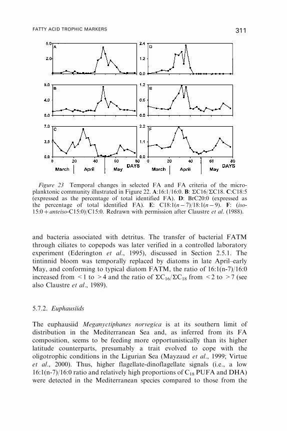
and bacteria associated with detritus. The transfer of bacterial FATM

through ciliates to copepods was later verified in a controlled laboratory

experiment (Ederington et al., 1995), discussed in Section 2.5.1. The

tintinnid bloom was temporally replaced by diatoms in late April–early

May, and conforming to typical diatom FATM, the ratio of 16:1(n-7)/16:0

increased from <1 to >4 and the ratio of �C16/�C18 from <2 to >7 (see

also Claustre et al., 1989).

5.7.2. Euphausiids

The euphausiid Meganyctiphanes norvegica is at its southern limit of

distribution in the Mediterranean Sea and, as inferred from its FA

composition, seems to be feeding more opportunistically than its higher

latitude counterparts, presumably a trait evolved to cope with the

oligotrophic conditions in the Ligurian Sea (Mayzaud et al., 1999; Virtue

et al., 2000). Thus, higher flagellate-dinoflagellate signals (i.e., a low

16:1(n-7)/16:0 ratio and relatively high proportions of C18 PUFA and DHA)

were detected in the Mediterranean species compared to those from the

Figure 23 Temporal changes in selected FA and FA criteria of the micro-planktonic community illustrated in Figure 22. A:16:1/16:0. B: �C16/�C18. C:C18:5(expressed as the percentage of total identified FA). D: BrC20:0 (expressed asthe percentage of total identified FA). E: C18:1(n� 7)/18:1(n� 9). F: (iso-15:0þ anteiso-C15:0)/C15:0. Redrawn with permission after Claustre et al. (1988).


Clyde Sea and Kattegat, which contained higher diatom signals (a high

16:1(n-7)/16:0 ratio and high EPA). The latter also contained higher

concentrations of calanoid FATM suggesting that they were relying heavily

on copepods. In contrast, M. norvegica from the Ligurian Sea contained

significantly lower concentrations of long-chain MUFA, although copepods

from this area were also relatively deficient in these compounds. Hence, 20:1

and 22:1 cannot be used as copepod FATM in this area (Virtue et al., 2000).

Mayzaud et al. (1999) emphasized that one should exercise caution when

interpreting FATM in omnivorous species such as M. norvegica. They

wrote: ‘‘To be of practical use under natural conditions, fatty acid tracers in

omnivorous species should at least be present at concentrations higher than 1%

of the total fatty acids (below that the tracer is likely to be a contaminant from

ingested grazers) and display over time a pattern coherent with that of the food

supply’’.

5.8. Upwelling and sub-tropical/tropical systems

There are comparatively few studies on the dynamics of lipids and FA in

food webs from lower latitude temperate and tropical regions despite the

fact that these areas comprise the world’s largest pelagic fisheries, centered

on major upwelling systems (e.g., Cushing, 1989; Kiørboe, 1993). These

systems are regions of highly turbulent mixing and are generally dominated

by diatoms, which are consumed either directly by the major fish stocks in

the region (i.e., Peruvian anchovy) or by meso- and macrozooplankton,

which are then consumed by fish predators. The application of FATM has

primarily focused on identifying the feeding ecology of zooplanktivorous

fish. As a result, it has been determined that planktivorous fish from

northwest African waters are typically rich in DHA and particularly EPA,

whereas they contain only traces of calanoid FATM (e.g., Njinkoue et al.,

2002), reflecting their closer association to the base of the food web

(reviewed by Sargent et al., 1989; Sargent and Henderson, 1995).

Low levels of fat (<2% of wet mass) combined with high levels of (n-3)

PUFA, (n-6) PUFA (particularly AA) and trace amounts of calanoid

FATM are common traits of low latitude fish species apart from upwelling

systems, as shown for Malaysian and temperate – tropical Australian

coastal species (Gibson, 1983; Gibson et al., 1984; Evans et al., 1986;

Dunstan et al., 1988). Such observations are consistent with the more

regular food supply experienced by these species, and therefore, the absence

of need for them to accumulate large lipid reserves.

Dunstan et al. (1988) noted that macroalgae from Australian waters are

grazed directly by omnivorous and herbivorous fish species. This observa-

tion was supported using FATM, as the authors found that omnivorous


teleosts could be differentiated from carnivorous teleosts by higher

concentrations of AA, EPA and a lower (n-3)/(n-6) ratio, suggesting that

they were feeding partly on macroalgae. Among the cartilaginous species

examined in the same study, highest levels of AA were found in Port

Jackson sharks (Heterodontus portusjacksoni), which presumably feeds on

macroalgae via predation on sea urchins and snails. Lowest concentrations

of AA were found in piked dogfish (Squalus megalops), which feeds

primarily on cephalopods believed to rely on a microalgal-based (and hence

low AA) food web.

Subjecting FA compositional data of either black bream (Acanthopagrus

australis) or red fish (Centroberyx affinis) to principal component analyses,

Armstrong et al. (1994) found distinct seasonal clusters on the scatter plots

of the first two principal components (explaining 59.5% and 64.6%,

respectively, of the total variance). Corresponding bi-plots revealed that

specimens caught in spring correlated positively with (n-3) and (n-6) PUFA,

whereas those caught in autumn correlated positively with SFA and

MUFA. These results were consistent with a higher concentration of storage

lipids in specimens caught in autumn at the end of the feeding season,

whereas specimens caught in spring had used up their lipid reserves, and as a

consequence, contained relatively higher proportions of PL rich in PUFA.

Supporting this hypothesis, the FA composition of John dory (Zeus faber)

and ling (Genypterus blacodes) failed to reveal similar seasonal clusters,

consistent with the lack of seasonal lipid accumulation in these species.

Finally, when comparing the 22:1(n-11) to 20:1(n-9) fatty alcohol ratio in

specimens of orange roughy (Hoplostethus atlanticus) and deep-sea oreo

(Oreosomatidae) from Australian waters with that of their north Atlantic

counterparts, significant differences were observed reflecting different FA

compositions at the base of the food web in the two regions (Bakes et al.,

1995). Hence, in specimens from the north Atlantic the ratio ranged from

1.4 to 2.2 indicating a significant dietary contribution from calanoid

copepods. In contrast, the ratio was much lower in the Australian

specimens, ranging from 0.2 to 0.9 and consistent with the relatively lower

concentration of the two monounsaturates in copepods from the southern

hemisphere (Section 5.3.2).

6. SUMMARY AND CONCLUSIONS

6.1. State-of-the-art

In a sense, the state-of-the-art in the field of FATM research remains

at the level indicated by Sargent (1976) over 25 years ago: ‘‘At the present


state of our knowledge it would appear that fatty acid analyses represent

a rather blunt tool in defining food chain inter-relationships. Until further

knowledge is accumulated it would appear best to apply fatty acid analyses

as a corroborative method to support prey–predator relationships already

indicated on independent grounds, such as the analyses of stomach

contents’’.

Fraser et al. (1989) later added that: ‘‘to clarify the transfer of lipid

biomarkers up the food web, the availability of tracer lipids in algae and the

zooplankton prey of larval fish must be established before these tracers may be

employed either quantitatively or qualitatively’’. St. John and Lund (1996),

while recognizing the statement of Fraser et al. (1989), were more specific

about problems concerning the quantitative application of FATM. They

stated: ‘‘these biomarkers may be suitable as a qualitative index of utilization

of a specific food source in field studies, however, quantitative estimates of

transfer between trophic levels in the field may prove to be difficult for a

number of reasons. It is evident that a better understanding of the dynamics of

lipid incorporation and utilization with respect to environmental conditions

such as temperature, light and nutrients in phytoplankton as well as during

ontogeny in zooplankton and larval and juvenile fish is required before these

biomarkers may be used quantitatively’’.

With the recommendations of these authors in mind, it is clear that to

quantify relationships using FATM, information would need to be

available on a number of aspects of the dynamics of FA in marine

animals, including not least, time scales for incorporation of new FA

signatures into tissues. This has been examined in a few laboratory

studies of copepods, larval and adult cod (Graeve et al., 1994a; St. John

and Lund, 1996; Kirsch et al., 1998) and in one field experiment on

mussels (Mytilus galloprovincialis; Freites et al., 2002), but there is still a

long way to go, considering the physiological status of the organisms

(i.e., adding or depleting lipid reserves), growth rates and ontogenetic

state of development, the impact of mixed diets, etc. Given the resolution

of FATM, we question whether turning FATM into a quantitative tool is

worth the effort, although in some studies a quantitative approach has

been considered (e.g., Desvilettes et al., 1997).

Resolution of ecological niches is the strength of the FATM approach

and a key to resolving complex trophic interactions. FATM are

incorporated largely unaltered into the NL pool of primary consumers,

especially in periods of low catabolic activity, as when the animals are

accumulating lipid reserves. In particular, 16:1(n-7), C16 PUFA and EPA

have been used as indicators of diatom-based diets, whereas 18:4(n-3), C18

PUFA and DHA are used as dietary tracers of dinoflagellates and

prymnesiophytes. Secondary and higher order consumers may also

incorporate dietary FA largely unaltered into their NL reserves, but the


signals of herbivory are obscured as the degree of carnivory increases and

FA may derive from many different sources (Auel et al., 2002). Markers of

herbivory may be replaced by markers of carnivory, reflecting changes in

feeding behavior such as during ontogeny. This is most obvious at higher

latitudes, where the mesozooplankton communities are dominated by

herbivorous and omnivorous calanoid copepods. These copepods usually

accumulate large WE reserves containing large amounts of C20 and C22

MUFA and monounsaturated fatty alcohols, which they are believed to

biosynthesize de novo. These particular monounsaturates have been used to

trace and resolve food web relationships at higher trophic levels, for

example in hyperiid amphipods, euphausiids and zooplanktivorous fish that

typically consume large quantities of calanoid copepods (e.g. Sargent, 1978;

Falk-Petersen et al., 1987; Kattner and Hagen, 1998; Hagen et al., 2001;

Auel et al., 2002).

Additional information on the ecological niches occupied by various

zooplankton species may be obtained by combining FATM and lipid class

compositions. Hence, at higher latitudes, the largest concentrations of WE

are typically found in strictly herbivorous zooplankton, which are directly

and immediately linked to primary production in these regions. The level of

WE generally decreases from herbivores through omnivores to carnivores

(Sargent and Falk-Petersen, 1988), and is partly replaced by TAG. Ratios of

particular FA have also been used to assess the extent to which various

species occupy different ecological niches. The proportion of 18:1(n-7) to

18:1(n-9) (as a marker of primary or heterotrophic bacterial production vs.

animal production) was, for example, found to decrease in Arctic benthic

organisms when considering a ‘‘succession’’ from suspension feeders

via predatory decapods to scavenging amphipods (Graeve et al., 1997). As

an example of how to combine this criterion with the various FATM

summarized above, in addition to lipid class compositions, Falk-Petersen

et al. (2000) used all these indices to classify seven common species of Arctic

and Antarctic krill into different ecological niches. Hence, based on the

results they concluded that Thysanoessa inermis and Euphausia crystal-

lorophias are true herbivores, whereas Thysanoessa raschii, T. macrura and

Euphausia superba are omnivores, and Thysanoessa longicaudata and

Meganyctiphanes norvegica are carnivores.

At higher trophic levels, i.e., in fish and marine mammals, specific FATM

are often less evident than in zooplankton and consequently more difficult

to interpret. The advancement of multivariate statistical methods of pattern

recognition has, however, proven particularly valuable for resolving trophic

interactions in these organisms (Smith et al., 1997; Iverson et al., 1997b,

2002; Budge et al., 2002), and we urge that this becomes an integrated tool in

future applications of FATM at all trophic levels.


6.2. Future applications

FATM are obviously good tools for assessing trophic interactions in the

marine environment, adding information that is at times difficult, and in

some instances impossible, to derive from more traditional techniques, such

as stomach content analyses. In particular, FA provide information on the

origin of lipid reserves generated over a period of time.

Primary producer communities in the marine environment are

dominated by diatoms, dinoflagellates and prymnesiophytes, which can

be distinguished based on the presence and combinations of particular

FA (as summarized in Table 2; see also Mayzaud et al., 1990). The

spatial and temporal resolution of the various phytoplankton groups,

and hence the basic FA pattern in the marine environment, is largely

determined by macro and mesoscale stratification processes acting on

phytoplankton group dominance through affecting light and nutrient

availability. Large concentrations of phytoplankton biomass, essentially

dominated by diatoms, evolve under spring bloom type conditions and

form the basis for an efficient transfer of energy to higher trophic levels.

Flagellates, on the other hand, typically dominate the phytoplankton

communities before and after diatom bloom events when either light or

nutrients are limiting, establishing the potential for microbial loop food

webs. This coupling between hydrodynamic processes and the transfer of

group-specific phytoplankton production to higher trophic levels has

been established using FATM. For example, St. John and Lund (1996)

showed a coupling between the growth and condition of larval and

juvenile fish to spatial variations in frontal primary production, linking

ultimately with physical frontal mixing processes, using 16:1(n-7)/16:0

as a food web tracer. Hence, applied in this manner, in examination of

the potential impact of mesoscale processes, FATM may provide a tool

for resolving the impact of global change on marine ecosystem

dynamics. To further develop this approach, we suggest that it could

be combined with the analyses of larval fish otolith microstructures.

These allow an indication of the growth history of the individuals,

thereby contributing to the identification of the potential dynamics of

FATM incorporation.

Fatty acids have principally been used as qualitative markers of

trophic interactions in shelf sea ecosystems with an emphasis on higher

latitudes. In contrast, very few FATM studies have been carried out

in upwelling and open ocean, oligotrophic areas, including tropical systems.

Primary producers in oligotrophic systems are composed largely of small,

autotrophic flagellates and cyanobacteria, forming the basis of low biomass,

microbial loop food webs. As microorganisms usually do not accumulate

large lipid reserves, FATM may be of less relevance here. However, despite


their lack of storage lipids, heterotrophic bacteria, which contribute

significantly to these systems, are still recognizable by specific FA.

Considering the fast turnover rates of microorganisms, we therefore

hypothesize that FATM may help resolve trophic interactions in microbial

loop food webs, and we support the strengthening of FA research in this

area, as suggested also by Strom (2000), recognizing the importance of these

systems in the global carbon budget.

The combination of FATM and stable isotope analyses may provide

additional information for resolving trophic interactions in marine

ecosystems (e.g., Kiyashko et al., 1998; Kharlamenko et al., 2001). This

approach has proven particularly helpful in identifying the contribution of

major sources of organic matter contributing to detrital food webs, and

hence, the diet of, e.g., detritivorous benthic invertebrates, which cannot be

inferred from stomach content analyses. Using this approach Kiyashko et al.

(1998), for example, established that in addition to bacteria, benthic rather

than pelagic diatoms, which are characterized by similar FA signatures,

constituted the major food source of sea urchins in Vostok Bay, Sea of

Japan.

Another interesting approach that can be used to characterize carbon

fluxes between prey and predators as well as to validate the applicability of

FATM, involves feeding experiments with 13C-enriched experimental diets.

Such studies provide information on carbon accumulation, transfer and

turnover rates as well as biosynthesis of lipids and individual FA. Hence, in

a preliminary study involving 13C-enriched phytoplankton, it was shown

that long-chain MUFA and monounsaturated fatty alcohols synthesized

de novo by herbivorous copepods feeding on the 13C-enriched phytoplank-

ton were also enriched in 13C isotopes (Albers, 1999).

In general, studies applying FATM have been dominated by those

correlating individual FA with the dynamics of individuals, for example

growth or reproductive output. In many instances the biological relevance

of the FA employed is not clear. This points to a key issue in the field, which

is a general lack of validation, and at times an uncritical application of

FATM. Many of the studies cited in Section 5 have, for example, applied

FATM on the assumption that they derive from certain prey species or

groups of species, without testing the validity of this assumption (e.g., often

as simple as examining stomach contents). A second flaw within FATM

research is that this technique has been applied in a fragmentary manner,

i.e., employed in studies in which the FATM results have not been validated

by other approaches. Hence, future applications of FATM should form part

of integrated research programs, with FATM as an ecological tool to

establish trophic interactions on an ecosystem level. It is here that their

strength lies.


ACKNOWLEDGEMENTS

The first author thanks Dr. B. Jørgensen for fruitful discussions on

multivariate statistical analyses, Dr. H. A. Thomsen for advice on

microalgal taxonomy and G. Møller, C. Anderberg and K. Prentow for

excellent library service. We wish to thank Prof. A. J. Southward and an

anonymous reviewer for very constructive comments on the manuscript.

The authors would like in addition to thank the GLOBEC Focus Group 2

on Process Studies for convincing Gerhard Kattner and Michael St. John of

the necessity of this review. The Danish Institute for Fisheries Research, the

Danish Research Agency and the European Union Fifth Frame Work

Programme, Quality and management of living resources, Q5RS-2000-

30183 (LIFECO) provided funding for the first author.

REFERENCES

Ackman, R. G. (1980). Fish Lipids. Part 1. In ‘‘Advances in Fish Science andTechnology’’ (J. J. Connell, ed.), pp. 86–103, Fishing News Books, Farnham.

Ackman, R. G. (ed.) (1989a). ‘‘Marine biogenic lipids, fats, and oils’’, Vol. I. CRCPress, Boca Raton, Florida.

Ackman, R. G. (ed.) (1989b). ‘‘Marine biogenic lipids, fats, and oils’’, Vol. II. CRCPress, Boca Raton, Florida.

Ackman, R. G. (2002). The gas chromatograph in practical analysis of common anduncommon fatty acids for the 21st century. Analytica Chimica Acta 465, 175–192.

Ackman, R. G. and Eaton, C. A. (1966a). Lipids of the fin whale (Balaenopteraphysalus) from North Atlantic waters. III. Occurrence of eicosenoic anddocosenoic fatty acids in the zooplankter Meganyctiphanes norvegica (M. Sars)and their effect on whale oil composition. Canadian Journal of Biochemistry 44,1561–1566.

Ackman, R. G. and Eaton, C. A. (1966b). Some commercial Atlantic herring oils;fatty acid composition. Journal of the Fisheries Research Board of Canada 23,991–1006.

Ackman, R. G. and Eaton, C. A. (1971). Investigation of the fatty acid compositionof oils and lipids from the sand launce (Ammodytes americanus) from Nova ScotiaWaters. Journal of the Fisheries Research Board of Canada 28, 601–606.

Ackman, R. G. and McLachlan, J. (1977). Fatty acids in some Nova Scotian marineseaweeds: a survey for octadecapentaenoic and other biochemically novel fattyacids. Proceedings of the Nova Scotian Institute of Science 28, 47–64.

Ackman, R. G., Tocher, C. S. and McLachlan, J. (1968). Marine phytoplankter fattyacids. Journal of the Fisheries Research Board of Canada 25, 1603–1620.

Ackman, R. G., Ke, P. J., MacCallum, W. A. and Adams, D. R. (1969).Newfoundland capelin lipids: fatty acid composition and alterations duringfrozen storage. Journal of the Fisheries Research Board of Canada 26, 2037–2060.

Ackman, R. G., Eaton, C. A., Sipos, J. C., Hooper, S. N. and Castell, J. D. (1970).Lipids and fatty acids of two species of North Atlantic krill (Meganyctiphanes


norvegica and Thysanoessa inermis) and their role in the aquatic food web. Journalof the Fisheries Research Board of Canada 27, 513–533.

Ahern, T. J., Katoh, S. and Sada, E. (1983). Arachidonic acid production by the redalgae Porphyridium cruentum. Biotechnology and Bioengineering 15, 1057–1070.

Ahlgren, G., Blomqvist, P., Boberg, M. and Gustafsson, I.-B. (1994). Fatty acidcontent of the dorsal muscle - an indicator of fat quality in freshwater fish. Journalof Fish Biology 45, 131–157.

Ahlgren, G., Goedkoop, W., Markensten, H., Sonesten, L. and Boberg, M. (1997).Seasonal variations in food quality for pelagic and benthic invertebrates in LakeErken – the role of fatty acids. Freshwater Biology 38, 555–570.

Albano, C., Blomqvist, G., Coomans, D., Dunn III, W. J., Edlund, U., Eliasson, B.,Hellberg, S., Johansson, E., Norden, B., Sjostrom, M., Soderstrom, B., Wold, H.and Wold, S. (1981). Pattern recognition by means of disjoint principalcomponents models (SIMCA). Philosophy and methods. In ‘‘Proceedings of thesymposium on applied statistics’’ (A. Hoskuldsson, K. Conradsen, B. Sloth-Jensenand K. Esbesen, eds.), pp. 183–218, Danmarks Tekniske Højskole, Lyngby,Denmark.

Albers, C. (1999). ‘‘Lipidstoffwechsel polarer Copepoden: Laborexperimente undFelduntersuchungen’’. Ph.D. Thesis, University of Bremen.

Albers, C. S., Kattner, G. and Hagen, W. (1996). The compositions of wax esters,triacylglycerols and phospholipids in Arctic and Antarctic copepods: evidence ofenergetic adaptations. Marine Chemistry 55, 347–358.

Alonso, D. L., Segura del Castillo, C. I., Garcıa Sanchez, J. L. Sanchez Perez, J. A.and Garcıa Camacho, F. (1994). Quantitative genetics of fatty acid variation inIsochrysis galbana (Prymnesiophyceae) and Phaeodactylum tricornutum(Bacillariophyceae). Journal of Phycology 30, 553–558.

Al-Hasan, R. H., Ali, A. M. and Radwan, S. S. (1990). Lipids, and their constituentfatty acids, of Phaeocystis sp. from the Arabian Gulf. Marine Biology 105, 9–14.

Anthony, J. A., Roby, D. D. and Turco, K. R. (2000). Lipid content and energydensity of forage fishes from the northern Gulf of Alaska. Journal of ExperimentalMarine Biology and Ecology 248, 53–78.

Armstrong, S. G., Wyllie, S. G. and Leach, D. N. (1994). Effects of season andlocation of catch on the fatty acid compositions of some Australian fish species.Food Chemistry 51, 295–305.

Arts, M. T. and Wainman, B. C. (eds.). (1999). ‘‘Lipids in freshwater ecosystems’’.Springer, New York.

Atkinson, A. and Snyder, R. (1997). Krill-copepod interactions at South Georgia,Antarctica, I. Omnivory by Euphausia superba. Marine Ecology Progress Series160, 63–76.

Auel, H. (1999). The ecology of Arctic deep-sea copepods (Euchaetidae andAetideidae). Aspects of their distribution, trophodynamics and effect on thecarbon flux. Berichte zur Polarforschung 319, 1–97.

Auel, H., Harjes, M., da Rocha, R., Stubing, D. and Hagen, W. (2002). Lipidbiomarkers indicate different ecological niches and trophic relationships of theArctic hyperiid amphipods Themisto abyssorum and T. libellula. Polar Biology 25,374–383.

Bakes, M. J., Elliott, N. G., Green, G. J. and Nichols, P. D. (1995). Variation in lipidcomposition of some deep-sea fish (Teleostei: Oreosomatidae andTrachichthyidae). Comparative Biochemistry and Physiology 111B, 633–645.

Bathmann, U. V., Makarov, R. R., Spiridonov, V. A. and Rohardt, G. (1993).Winter distribution and overwintering strategies of the Antarctic copepod species


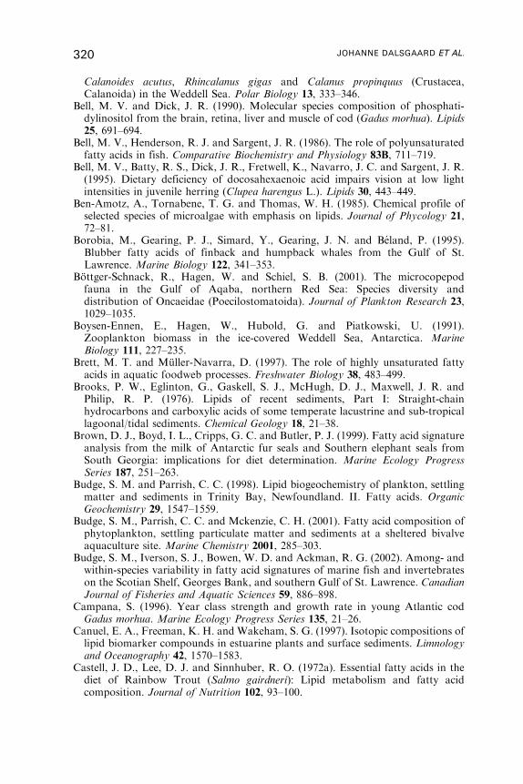
Calanoides acutus, Rhincalanus gigas and Calanus propinquus (Crustacea,Calanoida) in the Weddell Sea. Polar Biology 13, 333–346.

Bell, M. V. and Dick, J. R. (1990). Molecular species composition of phosphati-dylinositol from the brain, retina, liver and muscle of cod (Gadus morhua). Lipids25, 691–694.

Bell, M. V., Henderson, R. J. and Sargent, J. R. (1986). The role of polyunsaturatedfatty acids in fish. Comparative Biochemistry and Physiology 83B, 711–719.

Bell, M. V., Batty, R. S., Dick, J. R., Fretwell, K., Navarro, J. C. and Sargent, J. R.(1995). Dietary deficiency of docosahexaenoic acid impairs vision at low lightintensities in juvenile herring (Clupea harengus L.). Lipids 30, 443–449.

Ben-Amotz, A., Tornabene, T. G. and Thomas, W. H. (1985). Chemical profile ofselected species of microalgae with emphasis on lipids. Journal of Phycology 21,72–81.

Borobia, M., Gearing, P. J., Simard, Y., Gearing, J. N. and Beland, P. (1995).Blubber fatty acids of finback and humpback whales from the Gulf of St.Lawrence. Marine Biology 122, 341–353.

Bottger-Schnack, R., Hagen, W. and Schiel, S. B. (2001). The microcopepodfauna in the Gulf of Aqaba, northern Red Sea: Species diversity anddistribution of Oncaeidae (Poecilostomatoida). Journal of Plankton Research 23,1029–1035.

Boysen-Ennen, E., Hagen, W., Hubold, G. and Piatkowski, U. (1991).Zooplankton biomass in the ice-covered Weddell Sea, Antarctica. MarineBiology 111, 227–235.

Brett, M. T. and Muller-Navarra, D. (1997). The role of highly unsaturated fattyacids in aquatic foodweb processes. Freshwater Biology 38, 483–499.

Brooks, P. W., Eglinton, G., Gaskell, S. J., McHugh, D. J., Maxwell, J. R. andPhilip, R. P. (1976). Lipids of recent sediments, Part I: Straight-chainhydrocarbons and carboxylic acids of some temperate lacustrine and sub-tropicallagoonal/tidal sediments. Chemical Geology 18, 21–38.

Brown, D. J., Boyd, I. L., Cripps, G. C. and Butler, P. J. (1999). Fatty acid signatureanalysis from the milk of Antarctic fur seals and Southern elephant seals fromSouth Georgia: implications for diet determination. Marine Ecology ProgressSeries 187, 251–263.

Budge, S. M. and Parrish, C. C. (1998). Lipid biogeochemistry of plankton, settlingmatter and sediments in Trinity Bay, Newfoundland. II. Fatty acids. OrganicGeochemistry 29, 1547–1559.

Budge, S. M., Parrish, C. C. and Mckenzie, C. H. (2001). Fatty acid composition ofphytoplankton, settling particulate matter and sediments at a sheltered bivalveaquaculture site. Marine Chemistry 2001, 285–303.

Budge, S. M., Iverson, S. J., Bowen, W. D. and Ackman, R. G. (2002). Among- andwithin-species variability in fatty acid signatures of marine fish and invertebrateson the Scotian Shelf, Georges Bank, and southern Gulf of St. Lawrence. CanadianJournal of Fisheries and Aquatic Sciences 59, 886–898.

Campana, S. (1996). Year class strength and growth rate in young Atlantic codGadus morhua. Marine Ecology Progress Series 135, 21–26.

Canuel, E. A., Freeman, K. H. and Wakeham, S. G. (1997). Isotopic compositions oflipid biomarker compounds in estuarine plants and surface sediments. Limnologyand Oceanography 42, 1570–1583.

Castell, J. D., Lee, D. J. and Sinnhuber, R. O. (1972a). Essential fatty acids in thediet of Rainbow Trout (Salmo gairdneri): Lipid metabolism and fatty acidcomposition. Journal of Nutrition 102, 93–100.


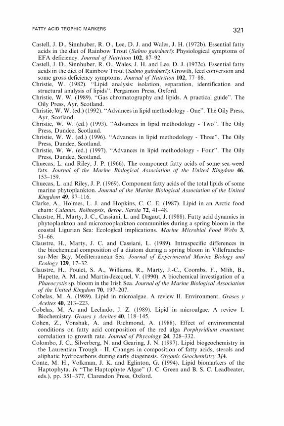
Castell, J. D., Sinnhuber, R. O., Lee, D. J. and Wales, J. H. (1972b). Essential fattyacids in the diet of Rainbow Trout (Salmo gairdneri): Physiological symptoms ofEFA deficiency. Journal of Nutrition 102, 87–92.

Castell, J. D., Sinnhuber, R. O., Wales, J. H. and Lee, D. J. (1972c). Essential fattyacids in the diet of Rainbow Trout (Salmo gairdneri): Growth, feed conversion andsome gross deficiency symptoms. Journal of Nutrition 102, 77–86.

Christie, W. (1982). ‘‘Lipid analysis: isolation, separation, identification andstructural analysis of lipids’’. Pergamon Press, Oxford.

Christie, W. W. (1989). ‘‘Gas chromatography and lipids. A practical guide’’. TheOily Press, Ayr, Scotland.

Christie, W. W. (ed.) (1992). ‘‘Advances in lipid methodology - One’’. The Oily Press,Ayr, Scotland.

Christie, W. W. (ed.) (1993). ‘‘Advances in lipid methodology - Two’’. The OilyPress, Dundee, Scotland.

Christie, W. W. (ed.) (1996). ‘‘Advances in lipid methodology - Three’’. The OilyPress, Dundee, Scotland.

Christie, W. W. (ed.) (1997). ‘‘Advances in lipid methodology - Four’’. The OilyPress, Dundee, Scotland.

Chuecas, L. and Riley, J. P. (1966). The component fatty acids of some sea-weedfats. Journal of the Marine Biological Association of the United Kingdom 46,153–159.

Chuecas, L. and Riley, J. P. (1969). Component fatty acids of the total lipids of somemarine phytoplankton. Journal of the Marine Biological Association of the UnitedKingdom 49, 97–116.

Clarke, A., Holmes, L. J. and Hopkins, C. C. E. (1987). Lipid in an Arctic foodchain: Calanus, Bolinopsis, Beroe. Sarsia 72, 41–48.

Claustre, H., Marty, J. C., Cassiani, L. and Dagaut, J. (1988). Fatty acid dynamics inphytoplankton and microzooplankton communities during a spring bloom in thecoastal Ligurian Sea: Ecological implications. Marine Microbial Food Webs 3,51–66.

Claustre, H., Marty, J. C. and Cassiani, L. (1989). Intraspecific differences inthe biochemical composition of a diatom during a spring bloom in Villefranche-sur-Mer Bay, Mediterranean Sea. Journal of Experimental Marine Biology andEcology 129, 17–32.

Claustre, H., Poulet, S. A., Williams, R., Marty, J.-C., Coombs, F., Mlih, B.,Hapette, A. M. and Martin-Jezequel, V. (1990). A biochemical investigation of aPhaeocystis sp. bloom in the Irish Sea. Journal of the Marine Biological Associationof the United Kingdom 70, 197–207.

Cobelas, M. A. (1989). Lipid in microalgae. A review II. Environment. Grases yAceites 40, 213–223.

Cobelas, M. A. and Lechado, J. Z. (1989). Lipid in microalgae. A review I.Biochemistry. Grases y Aceites 40, 118–145.

Cohen, Z., Vonshak, A. and Richmond, A. (1988). Effect of environmentalconditions on fatty acid composition of the red alga Porphyridium cruentum:correlation to growth rate. Journal of Phycology 24, 328–332.

Colombo, J. C., Silverberg, N. and Gearing, J. N. (1997). Lipid biogeochemistry inthe Laurentian Trough - II. Changes in composition of fatty acids, sterols andaliphatic hydrocarbons during early diagenesis. Organic Geochemistry 3/4.

Conte, M. H., Volkman, J. K. and Eglinton, G. (1994). Lipid biomarkers of theHaptophyta. In ‘‘The Haptophyte Algae’’ (J. C. Green and B. S. C. Leadbeater,eds.), pp. 351–377, Clarendon Press, Oxford.


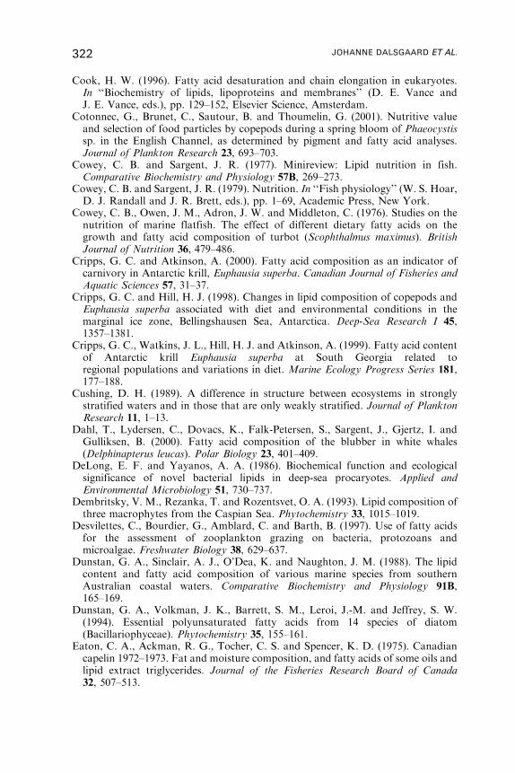
Cook, H. W. (1996). Fatty acid desaturation and chain elongation in eukaryotes.In ‘‘Biochemistry of lipids, lipoproteins and membranes’’ (D. E. Vance andJ. E. Vance, eds.), pp. 129–152, Elsevier Science, Amsterdam.

Cotonnec, G., Brunet, C., Sautour, B. and Thoumelin, G. (2001). Nutritive valueand selection of food particles by copepods during a spring bloom of Phaeocystissp. in the English Channel, as determined by pigment and fatty acid analyses.Journal of Plankton Research 23, 693–703.

Cowey, C. B. and Sargent, J. R. (1977). Minireview: Lipid nutrition in fish.Comparative Biochemistry and Physiology 57B, 269–273.

Cowey, C. B. and Sargent, J. R. (1979). Nutrition. In ‘‘Fish physiology’’ (W. S. Hoar,D. J. Randall and J. R. Brett, eds.), pp. 1–69, Academic Press, New York.

Cowey, C. B., Owen, J. M., Adron, J. W. and Middleton, C. (1976). Studies on thenutrition of marine flatfish. The effect of different dietary fatty acids on thegrowth and fatty acid composition of turbot (Scophthalmus maximus). BritishJournal of Nutrition 36, 479–486.

Cripps, G. C. and Atkinson, A. (2000). Fatty acid composition as an indicator ofcarnivory in Antarctic krill, Euphausia superba. Canadian Journal of Fisheries andAquatic Sciences 57, 31–37.

Cripps, G. C. and Hill, H. J. (1998). Changes in lipid composition of copepods andEuphausia superba associated with diet and environmental conditions in themarginal ice zone, Bellingshausen Sea, Antarctica. Deep-Sea Research I 45,1357–1381.

Cripps, G. C., Watkins, J. L., Hill, H. J. and Atkinson, A. (1999). Fatty acid contentof Antarctic krill Euphausia superba at South Georgia related toregional populations and variations in diet. Marine Ecology Progress Series 181,177–188.

Cushing, D. H. (1989). A difference in structure between ecosystems in stronglystratified waters and in those that are only weakly stratified. Journal of PlanktonResearch 11, 1–13.

Dahl, T., Lydersen, C., Dovacs, K., Falk-Petersen, S., Sargent, J., Gjertz, I. andGulliksen, B. (2000). Fatty acid composition of the blubber in white whales(Delphinapterus leucas). Polar Biology 23, 401–409.

DeLong, E. F. and Yayanos, A. A. (1986). Biochemical function and ecologicalsignificance of novel bacterial lipids in deep-sea procaryotes. Applied andEnvironmental Microbiology 51, 730–737.

Dembritsky, V. M., Rezanka, T. and Rozentsvet, O. A. (1993). Lipid composition ofthree macrophytes from the Caspian Sea. Phytochemistry 33, 1015–1019.

Desvilettes, C., Bourdier, G., Amblard, C. and Barth, B. (1997). Use of fatty acidsfor the assessment of zooplankton grazing on bacteria, protozoans andmicroalgae. Freshwater Biology 38, 629–637.

Dunstan, G. A., Sinclair, A. J., O’Dea, K. and Naughton, J. M. (1988). The lipidcontent and fatty acid composition of various marine species from southernAustralian coastal waters. Comparative Biochemistry and Physiology 91B,165–169.

Dunstan, G. A., Volkman, J. K., Barrett, S. M., Leroi, J.-M. and Jeffrey, S. W.(1994). Essential polyunsaturated fatty acids from 14 species of diatom(Bacillariophyceae). Phytochemistry 35, 155–161.

Eaton, C. A., Ackman, R. G., Tocher, C. S. and Spencer, K. D. (1975). Canadiancapelin 1972–1973. Fat and moisture composition, and fatty acids of some oils andlipid extract triglycerides. Journal of the Fisheries Research Board of Canada32, 507–513.


Ederington, M. C., McManus, G. B. and Harvey, H. R. (1995). Trophic transfer offatty acids, sterols, and a triterpenoid alcohol between bacteria, a ciliate, and thecopepod Acartia tonsa. Limnology and Oceanography 40, 860–867.

Evans, A. J., Fogerty, A. C. and Sainsbury, K. J. (1986). The fatty acid compositionof fish from the North West Shelf of Australia. CSIRO Food Research Quarterly46, 40–45.

Fahl, K. and Kattner, G. (1993). Lipid content and fatty acid composition of algalcommunities in sea-ice and water from the Weddell Sea (Antarctica). PolarBiology 13, 405–409.

Falk-Petersen, S., Gatten, R. R., Sargent, J. R. and Hopkins, C. C. E. (1981).Ecological investigations on the zooplankton community in Balsfjorden, northernNorway: seasonal changes in the lipid class composition of Meganyctiphanesnorvegica (M. Sars), Thysanoessa raschii (M. Sars) and T. inermis (Krøyer).Journal of Experimental Marine Biology and Ecology 54, 209–224.

Falk-Petersen, S., Sargent, J. R., Hopkins, C. C. E. and Vaja, B. (1982). Ecologicalinvestigations on the zooplankton community of Balsfjorden, northern Norway:Lipids in the euphausiids Thysanoessa raschi and T. inermis during spring. MarineBiology 68, 97–102.

Falk-Petersen, I.-B., Falk-Petersen, S. and Sargent, J. R. (1986a). Nature, originand possible roles of lipid deposits in Maurolicus muelleri (Gmelin) andBenthosema glaciale (Reinhart) from Ullsfjorden, Northern Norway. PolarBiology 5, 235–240.

Falk-Petersen, S., Sargent, J. R. and Middleton, C. (1986b). Level and compositionof triacylglycerols and wax esters in commercial capelin oils from the Barents Seafishery, 1983. Sarsia 71, 49–54.

Falk-Petersen, S., Sargent, J. R. and Tande, K. S. (1987). Lipid compositionof zooplankton in relation to the sub-Arctic food web. Polar Biology 8,115–120.

Falk-Petersen, S., Hopkins, C. C. E. and Sargent, J. R. (1990). Trophic relationshipsin the pelagic, Arctic food web. In ‘‘Trophic relationships in marine environments’’(M. Barnes and R. N. Gibson, eds.), Proceedings of the 24th European MarineBiology Symposium, Oban, Scotland, pp. 315–333. Aberdeen University Press.

Falk-Petersen, S., Sargent, J. R., Henderson, J., Hegseth, E. N., Hop, H. andOkolodkov, Y. B. (1998). Lipids and fatty acids in ice algae and phytoplanktonfrom the Marginal Ice Zone in the Barents Sea. Polar Biology 20, 41–47.

Falk-Petersen, S., Sargent, J. R., Lønne, O. J. and Timofeev, S. (1999). Functionalbiodiversity of lipids in Antarctic zooplankton: Calanoides acutus, Calanuspropinquus, Thysanoessa macrura and Euphausia crystallorophias. Polar Biology21, 37–47.

Falk-Petersen, S., Hagen, W., Kattner, G., Clarke, A. and Sargent, J. (2000). Lipids,trophic relationships, and biodiversity in Arctic and Antarctic krill. CanadianJournal of Fisheries and Aquatic Sciences 57, 178–191.

Falk-Petersen, S., Dahl, T. M., Scott, C. L., Sargent, J. R., Gulliksen, B.,Kwasniewski, S., Hop, H. and Millar, R.-M. (2002). Lipid biomarkers andtrophic linkages between ctenophores and copepods in Svalbard waters. MarineEcology Progress Series 227, 187–194.

Fleurence, J., Gutbier, G., Mabeau, S. and Leray, C. (1994). Fatty acids from 11marine macroalgae of the French Brittany coast. Journal of Applied Phycology6, 527–532.

Frank, I. (1989). Classification models: Discriminant Analysis, SIMCA, CART.Chemometrics and Intelligent Laboratory Systems 5, 247–256.


Franks, P. J. S. (1992). Sink or swim: accumulation of biomass at fronts. MarineEcology Progress Series 82, 1–12.

Fraser, A. J., Sargent, J. R., Gamble, J. C. and MacLachlan, P. (1987). Lipidclass and fatty acid composition as indicators of the nutritional condition of larvalAtlantic herring. American Fisheries Society Symposium 2, 129–143.

Fraser, A. J., Sargent, J. R., Gamble, J. C. and Seaton, D. D. (1989). Formation andtransfer of fatty acids in an enclosed marine food chain comprising phytoplank-ton, zooplankton and herring (Clupea harengus L.) larvae. Marine Chemistry 27,1–18.

Fredrickson, H. L., Cappenberg, T. E. and de Leeuw, J. W. (1986). Polar lipid ester-linked fatty acid composition of Lake Vechten seston: an ecological application oflipid analysis. FEMS Microbiology Ecology 38, 381–396.

Freites, L., Labarta, U. and Fernandez-Reiriz, M. J. (2002). Evolution of fatty acidprofiles of subtidal and rocky shore mussel seed (Mytilus galloprovincialis, Lmk.).Influence of environmental parameters. Journal of Experimental Marine Biologyand Ecology 268, 185–204.

Friedrich, C. and Hagen, W. (1994). Lipid contents of five species of notothenioidfish from high-Antarctic waters and ecological implications. Polar Biology 14,359–369.

Fritz, E. S., Crowder, L. B. and Francis R. C. (1990). The National Oceanic andAtmospheric Administration plan for recruitment fisheries oceanographicresearch. Fisheries 15, 25–31.

Frost, K. J. and Lowry, L. F. (1981). Trophic importance of some marine gadids innorthern Alaska and their body-otolith size relationships. Fishery Bulletin, US 79,187–192.

Fulco, A. J. (1983). Fatty acid metabolism in bacteria. Progress in Lipid Research22, 133–160.

Gatten, R. R., Sargent, J. R. and Gamble, J. C. (1983). Diet-induced changesin fatty acid composition of herring larvae reared in enclosed ecosystems.Journal of the Marine Biological Association of the United Kingdom 63,575–584.

Geynrikh, A. K. (1986). Mass species of oceanic phytophagous copepods andtheir ecology. Oceanology of the Academy of Sciences of the USSR 26: 213–217(English translation).

Gibson, R. A. (1983). Australian fish - An excellent source of both arachidonic acidand !-3-polyunsaturated fatty acids. Lipids 18, 743–752.

Gibson, R. A., Kneebone, R. and Kneebone, G. M. (1984). Comparative levels ofarachidonic acid and eicosapentaenoic acid in Malaysian fish. ComparativeBiochemistry and Physiology 78C, 325–328.

Gillan, F. T., Johns, R. B., Verheyen, T. V., Nichols, P. D., Esdaile, R. J. and Bavor,H. J. (1981). Monounsaturated fatty acids as specific bacterial markers in marinesediments. In ‘‘Advances in Organic Geochemistry 1981’’ (M. Bjorøy et al., ed),Proceedings of the 10th International Meeting on Organic Geochemistry,University of Bergen, Norway, pp. 198–206, John Wiley and Sons Limited,Chichester.

Graeve, M. (1993). Umsatz und Verteilung von Lipiden in Arktischen marinenOrganismen unter besonderer Berucksichtigung unterer trophischer Stufen.Reports on Polar Research 124, 1–141.

Graeve, M., Kattner, G. and Hagen, W. (1994a). Diet-induced changes in the fattyacid composition of Arctic herbivorous copepods: Experimental evidence of trophicmarkers. Journal of Experimental Marine Biology and Ecology 182, 97–110.


Graeve, M., Hagen, W. and Kattner, G. (1994b). Herbivorous or omnivorous? Onthe significance of lipid compositions as trophic markers in Antarctic copepods.Deep-Sea Research 41, 915–924.

Graeve, M., Kattner, G. and Piepenburg, D. (1997). Lipids in Arctic benthos: doesthe fatty acid and alcohol composition reflect feeding and trophic interactions?Polar Biology 18, 53–61.

Graeve, M., Kattner, G., Wiencke, C. and Karsten, U. (2002). Fatty acidcomposition of Arctic and Antarctic macroalgae: indicator of phylogenetic andtrophic relationships. Marine Ecology Progress Series 231, 67–74.

Grahl-Nielsen, O. and Mjaavatten, O. (1992). Discrimination of striped bass stocks:A new method based on chemometry of the fatty acid profile in heart tissue.Transactions of the American Fisheries Society 121, 307–314.

Gurr, M. I. and Harwood, J. L. (1991). ‘‘Lipid Biochemistry, an introduction’’.Chapman and Hall, London.

Haddad, R. I., Martens, C. S. and Farrington, J. (1992). Quantifying early diagenesisof fatty acids in a rapidly accumulating coastal marine sediment. OrganicGeochemistry 19, 206–216.

Hagen, W. (1999). Reproductive strategies and energetic adaptations of polarzooplankton. International Journal of Invertebrate Reproduction and Development36, 25–34.

Hagen, W. and Auel, H. (2001). Seasonal adaptations and the role of lipids inoceanic zooplankton. Zoology 104, 313–326.

Hagen, W. and Kattner, G. (1998). Lipid metabolism of the Antarctic euphausiidThysanoessa macrura and its ecological implications. Limnology and Oceanography43, 1894–1901.

Hagen, W. and Schnack-Schiel, S. B. (1996). Seasonal lipid dynamics of dominantAntarctic copepods: energy for overwintering or reproduction? Deep-Sea Research43, 139–158.

Hagen, W., Kattner, G. and Graeve, M. (1993). Calanoids acutus and Calanuspropinquus, Antarctic copepods with different lipid storage modes via wax esters ortriacylglycerols. Marine Ecology Progress Series 97, 135–142.

Hagen, W., Kattner, G. and Graeve, M. (1995). On the lipid biochemistry ofpolar copepods: Compositional differences in the Antarctic calanoids Euchaetaantarctica and Euchirella rostromagna. Marine Biology 123, 451–457.

Hagen, W., Van Vleet, E. S. and Kattner, G. (1996). Seasonal lipid storage as over-wintering strategy of Antarctic krill. Marine Ecology Progress Series 134, 85–89.

Hagen, W., Kattner, G. and Friedrich, C. (2000). The lipid composition of high-Antarctic notothenioid fish species with different life strategies. Polar Biology23, 785–791.

Hagen, W., Kattner, G., Terbruggen, A. and Van Vleet, E. S. (2001). Lipidmetabolism of the Antarctic krill Euphausia superba and its ecological implica-tions. Marine Biology 139, 95–104.

Hakanson, J. L. (1984). The long and short term feeding condition in field-caughtCalanus pacificus, as determined from the lipid content. Limnology andOceanography 29, 794–804.

Hakanson, J. L. (1989). Analysis of lipid components for determining the conditionof anchovy larvae, Engraulis mordax. Marine Biology 102, 143–151.

Hamilton, R. J. and Hamilton, S. (1992). ‘‘Lipid Analysis. A Practical Approach’’(D. Rickwood and B. D. Hames, eds.). Oxford University Press, Oxford.

Hama, T. (1991). Production and turnover rates of fatty acids in marine particulatematter through phytoplankton photosynthesis. Marine Chemistry 33, 213–227.


Hamm, C., Reigstad, M., Riser, C. W., Muhlebach, A. and Wassmann, P. (2001). Onthe trophic fate of Phaeocystis pouchetii. VII. Sterols and fatty acids revealsedimentation of P. pouchetii-derived organic matter via krill fecal strings. MarineEcology Progress Series 209, 55–69.

Harrison, P. J., Thompson, P. A. and Calderwood, G. S. (1990). Effects of nutrientand light limitation on the biochemical composition of phytoplankton. Journal ofApplied Phycology 2, 45–56.

Harvey, H. R. (1994). Fatty acids and sterols as source markers of organic matter insediments of the North Carolina continental slope. Deep-Sea Research II 41,783–796.

Harvey, H. R. and Macko, S. A. (1997). Catalysts or contributors? Trackingbacterial mediation of early diagenesis in the marine water column. OrganicGeochemistry 26, 531–544.

Harvey, H. R., Eglinton, G., O’Hara, S. C. M. and Corner, E. D. S. (1987).Biotransformation and assimilation of dietary lipids by Calanus feeding on adinoflagellate. Geochimica et Cosmochimica Acta 51, 3031–3040.

Harwood, J. L. and Jones, A. L. (1989). Lipid metabolism in algae. Advances inBotanical Research 16, 1–53.

Harwood, J. L. and Russell, N. J. (1984). ‘‘Lipids in plants and microbes’’. GeorgeAllen and Unwin, London.

Henderson, R. J. and Sargent, J. R. (1985). Fatty acid metabolism in fish. In‘‘Nutrition and feeding in fish’’ (C. B. Cowey, A. M. Mackie and J. G. Bell, eds.),pp. 349–364, Academic Press, London.

Henderson, R. J. and Tocher, D. R. (1987). The lipid composition and biochemistryof freshwater fish. Progress in Lipid Research 26, 281–347.

Henderson, R. J., Sargent, J. R. and Hopkins, C. C. E. (1984). Changes in thecontent and fatty acid composition of lipid in an isolated population of the capelinMallotus villosus during sexual maturation and spawning. Marine Biology 78,255–263.

Henderson, R. J., Park, M. T. and Sargent, J. R. (1995). The desaturation andelongation of 14C-labelled polyunsaturated fatty acids by pike (Esox lucius L.)in vivo. Fish Physiology and Biochemistry 14, 223–235.

Henderson, R. J., Hegseth, E. N. and Park, M. T. (1998). Seasonal variation in lipidand fatty acid composition of ice algae from the Barents Sea. Polar Biology 20,48–55.

Hirche, H.-J. and Kattner, G. (1993). Egg production and lipid content of Calanusglacialis in spring: indication of a food-dependent and food-independentreproductive mode. Marine Biology 117, 615–622.

Hirche, H.-J., Hagen, W., Mumm, N. and Richter, C. (1994). The Northeast Waterpolynya, Greenland Sea. III: Meso- and macrozooplankton distribution andproduction of dominant herbivorous copepods during spring. Polar Biology 14,491–503.

Honya, M., Kinoshita, T., Ishikawa, M., Mori, H. and Nisizawa, K. (1994).Seasonal variation in the lipid content of cultured Laminaria japonica: fattyacids, sterols, �-carotene and tocopherol. Journal of Applied Phycology 6, 25–29.

Hopkins, T. L. (1987). Midwater food web in McMurdo Sound, Ross Sea,Antarctica. Marine Biology 96, 93–106.

Hopkins, C. C. E., Sargent, J. R. and Nilssen, E. M. (1993). Total lipid content, andlipid and fatty acid composition of the deep-water prawn Pandalus borealis fromBalsfjord, northern Norway: growth and feeding relationships. Marine EcologyProgress Series 96, 217–228.


Hølmer, G. (1989). Triglycerides. In ‘‘Marine Biogenic lipids, fats, and oils’’, Vol. I(R. G. Ackman, ed.), pp. 139–173, CRC Press, Boca Raton, Florida.

IUPAC-IUB Commission on Biochemical Nomenclature (1967). The nomenclatureof lipids. The Journal of Biological Chemistry, 242, 4845–4849.

IUPAC-IUB Commision on Biochemical Nomenclature (CBN)(1977). The nomen-clature of lipids. Recommendations, 1976. European Journal of Biochemistry 79,11–21.

Iverson, S. J. (1993). Milk secretion in marine mammals in relation to foraging: canmilk fatty acids predict diet? Symposia of the Zoological Society of London 66,263–291.

Iverson, S. J., Arnould, J. P. Y. and Boyd, I. L. (1997a). Milk fatty acid signaturesindicate both major and minor shifts in the diet of lactating Antarctic fur seals.Canadian Journal of Zoology 75, 188–197.

Iverson, S. J., Frost, K. J. and Lowry, L. F. (1997b). Fatty acid signatures reveal finescale structure of foraging distribution of harbor seals and their prey in PrinceWilliam Sound, Alaska. Marine Ecology Progress Series 151, 255–271.

Iverson, S. J., Frost, K. J. and Lang, S. L. C. (2002). Fat content and fatty acidcomposition of forage fish and invertebrates in Prince William Sound, Alaska:Factors contributing to among and within species variability. Marine EcologyProgress Series 241, 161–181.

Jangaard, P. M. (1974). The capelin (Mallotus villosus). Biology, distribution,exploitation, utilization, and composition. Bulletin of the Fisheries Research Boardof Canada 186, 1–70.

Jeffries, H. P. (1970). Seasonal composition of temperate plankton communities:fatty acids. Limnology and Oceanography 15, 419–426.

Jezyk, P. F. and Penicnak, A. J. (1966). Fatty acid relationships in aquatic foodchain. Lipids 1, 427–429.

Jobling, M. (1994). ‘‘Fish bioenergetics’’. Chapman and Hall, London.Johns, R. B. and Perry, G. J. (1977). Lipids of the marine bacterium Flexibacterpolymorphus. Archives of Microbiology 114, 267–271.

Jonasdottir, S. H., Fields, D. and Pantoja, S. (1995). Copepod egg production inLong Island Sound USA, as a function of the chemical composition of seston.Marine Ecology Progress Series 119, 87–98.

Joseph, J. D. (1975). Identification of 3, 6, 9, 12, 15-octadecapentaenoic acid inlaboratory-cultured photosynthetic dinoflagellates. Lipids 10, 395–403.

Joseph, J. D. (1982). Lipid composition of marine and estuarine invertebrates. PartII: Mollusca. Progress in Lipid Research 21, 109–153.

Joseph, J. D. (1989). Distribution and composition of lipids in marine invertebrates.In ‘‘Marine biogenic lipids, fats, and oils’’, Vol. II. (R. G. Ackman, ed.),pp. 49–143, CRC Press, Boca Raton, Florida.

Kaitaranta, J. K. and Linko, R. R. (1984). Fatty acids in the roe lipids of commonfood fishes. Comparative Biochemistry and Physiology 79B, 331–334.

Kanazawa, A., Teshima, S. I. and Ono, K. (1979). Relationship between essentialfatty acid requirements of aquatic animals and the capacity for bioconversion oflinolenic acid to highly unsaturated fatty acids. Comparative Biochemistry andPhysiology 63B, 295–298.

Kattner, G. and Brockmann, U. H. (1990). Particulate and dissolved fatty acids in anenclosure containing a unialgal Skeletonema costatum (Greve) Cleve culture.Journal of Experimental Marine Biology and Ecology 141, 1–13.

Kattner, G. and Hagen, W. (1995). Polar herbivorous copepods – different pathwaysin lipid biosynthesis. ICES Journal of Marine Science 52, 329–335.


Kattner, G. and Hagen, W. (1998). Lipid metabolism of the Antarctic euphausiidEuphausia crystallorophias and its ecological implications. Marine EcologyProgress Series 170, 203–213.

Kattner, G. and Krause, M. (1987). Changes in lipids during the development ofCalanus finmarchicus s.l. from copepodid I to adult. Marine Biology 96, 511–518.

Kattner, G. and Krause, M. (1989). Seasonal variation of lipids (wax esters, fattyacids and alcohols) in calanoid copepods from the North Sea. Marine Chemistry26, 261–275.

Kattner, G., Krause, M. and Trahms, J. (1981). Lipid composition of some typicalNorth Sea copepods. Marine Ecology Progress Series 4, 69–74.

Kattner, G., Gercken, G. and Eberlein, K. (1983). Development of lipids during aspring plankton bloom in the northern North Sea. I. Particulate fatty acids.Marine Chemistry 14, 149–162.

Kattner, G., Hirche, H.-J. and Krause, M. (1989). Spatial variability in lipidcomposition of calanoid copepods from Fram Strait, the Arctic. Marine Biology102, 473–480.

Kattner, G., Graeve, M. and Hagen, W. (1994). Ontogenetic and seasonal changes inlipid and fatty acid/alcohol compositions of the dominant Antarctic copepodsCalanus propinquus, Calanoides acutus and Rhincalanus gigas. Marine Biology 118,637–644.

Kattner, G., Hagen, W., Falk-Petersen, S., Sargent, J. R. and Henderson, R. J.(1996). Antarctic krill Thysanoessa macrura fills a major gap in marine lipogenicpathways. Marine Ecology Progress Series 134, 295–298.

Kattner, G., Hagen, W., Graeve, M. and Albers, C. (1998). Exceptional lipids andfatty acids in the pteropod Clione limacina (Gastropoda) from both polar oceans.Marine Chemistry 61, 219–228.

Kaufmann, P. (1992). Chemometrics in lipid analysis. In ‘‘Advances in lipid methodo-logy - One’’ (W. W. Christie, ed.), pp. 149–180, The Oily Press, Ayr, Scotland.

Kayama, M., Tsuchiya, Y. and Mead, J. F. (1963). A model experiment of aquaticfood chain with special significance in fatty acid conversion. Bulletin of theJapanese Society of Scientific Fisheries 29, 452–458.

Kayama, M., Araki, S. and Sato, S. (1989). Lipids of marine plants. In ‘‘Marinebiogenic lipids, fats and oils’’, Vol. II (R. G. Ackman, ed.), pp. 3–48, CRC Press,Boca Raton, Florida.

Kelly, R. B., Reiser, R. and Hood, D. W. (1963). The origin of the marinepolyunsaturated fatty acids. Composition of some marine plankton. Journal of theAmerican Oil Chemists’ Society 36, 104–106.

Kharlamenko, V. I., Zhukova, N. V., Khotimchenko, S. V., Svetashev, V. I. andKamenev, G. M. (1995). Fatty acids as markers of food sources in a shallow-waterhydrothermal ecosystem (Kraternaya Bight, Yankich Island, Kurile Islands).Marine Ecology Progress Series 120, 231–241.

Kharlamenko, V. I., Kiyashko, S. I., Imbs, A. B. and Vyshkvartzev, D. I. (2001).Identification of food sources of invertebrates from the seagrass Zostera marinacommunity using carbon and sulfur stable isotope ratio and fatty acid analyses.Marine Ecology Progress Series 220, 103–117.

Khotimchenko, S. V., Vaskovsky, V. E. and Titlyanova, T. V. (2002). Fatty acidsof marine algae from the Pacific coast of North California. Botanica Marina45, 17–22.

Kirsch, P. E., Iverson, S. J., Bowen, W. D., Kerr, S. R. and Ackman, R. G. (1998).Dietary effects on the fatty acid signature of whole Atlantic cod (Gadus morhua).Canadian Journal of Fisheries and Aquatic Sciences 55, 1378–1386.


Kiørboe, T. (1993). Turbulence, phytoplankton cell size, and the structure of pelagicfood webs. Advances in Marine Biology 29, 1–72.

Kiyashko, S. I., Kharlamenko, V. I. and Imbs, A. B. (1998). Stable isotope ratios andfatty acids as food source markers of deposit-feeding invertebrates. RussianJournal of Marine Biology 24, 170–174.

Klungsøyr, J., Tilseth, S., Wilhelmsen, S., Falk-Petersen, S. and Sargent, J. R.(1989). Fatty acid composition as an indicator of food intake in cod larvae Gadusmorhua from Lofoten, Northern Norway. Marine Biology 102, 183–188.

Kristiansen, A., Moestrup, Ø. and Nielsen, H. (1981). ‘‘Introduktion til alger ogbakterier’’. Nucleus, Arhus, Denmark.

Lasker, R. and Theilacker, G. H. (1962). The fatty acid composition of the lipids ofsome Pacific sardine tissues in relation to ovarian maturation and diet. Journal ofLipid Research 3, 60–64.

Le Fevre, J. (1986). Aspects of the biology of frontal systems. Advances in MarineBiology 23, 163–299.

Lechevalier, H. and Lechevalier, M. P. (1988). Chemotaxonomic use of lipids - anoverview. In ‘‘Microbial lipids’’, Vol. 1 (C. Ratledge and S. G. Wilkinson, eds.),pp. 869–902, Academic Press, London.

Lee, R. F. (1974). Lipid composition of the copepod Calanus hyperboreusfrom the Arctic Ocean. Changes with depth and season. Marine Biology 26,313–318.

Lee, R. F. (1975). Lipids of Arctic zooplankton. Comparative Biochemistry andPhysiology 51B, 263–266.

Lee, R. F. and Hirota, J. (1973). Wax esters in tropical zooplankton and nekton andthe geographical distribution of wax esters in marine copepods. Limnology andOceanography 18, 227–239.

Lee, R. F. and Nevenzel, J. C. (1979). Wax esters in the marine environment: originand composition of the wax from Bute Inlet, British Columbia. Journal of theFisheries Research Board of Canada 36, 1519–1523.

Lee, R. F. and Patton, J. S. (1989). Alcohol and waxes. In ‘‘Marine biogenic lipids,fats, and oils’’, Vol. I (R. G. Ackman, ed.), pp. 73–102, CRC Press, Boca Raton,Florida.

Lee, R. F., Hirota, J. and Barnett, A. M. (1971a). Distribution and importance ofwax esters in marine copepods and other zooplankton. Deep-Sea Research18, 1147–1165.

Lee, R. F., Nevenzel, J. C. and Paffenhofer, G.-A. (1971b). Importance of wax estersand other lipids in the marine food chain: phytoplankton and copepods. MarineBiology 9, 99–108.

Legendre, P. and Legendre, L. (1998). ‘‘Numerical ecology’’. Elsevier Science,Amsterdam.

Levinsen, H., Turner, J. T., Nielsen, T. G. and Hansen, B. W. (2000). On the trophiccoupling between protists and copepods in Arctic marine ecosystems. MarineEcology Progress Series 204, 65–77.

Levring, T. (1979). The vegetation in the sea. In ‘‘Marine algae in pharmaceuticalscience’’, Vol. 1 (H. A. Hoppe, T. Levring and Y. Tanaka, eds.), pp. 3–23, Walterde Gruyter, Berlin.

Lewis, R. W. (1969). The fatty acid composition of Arctic marine phytoplankton andzooplankton with special reference to minor acids. Limnology and Oceanography14, 35–40.

Li, X., Fan, X., Han, L. and Lou, Q. (2002). Fatty acids of some algae from theBohai Sea. Phytochemistry 59, 157–161.


Linares, F. and Henderson, R. J. (1991). Incorporation of 14C-labelled polyunsa-turated fatty acids by juvenile turbot, Scophthalmus maximus (L.) in vivo. Journalof Fish Biology 38, 335–347.

Linko, R. R. and Karinkanta, H. (1970). Fatty acids of long chain lengthin Baltic Herring lipids. Journal of the American Oil Chemists’ Society 47, 42–46.

Love, R. M. (1970). ‘‘The chemical biology of fishes’’. Academic Press, London.Lovern, J. A. (1934). CCLVI. Fat metabolism in fishes. V. The fat of the salmon inits young freshwater stages. Biochemical Journal 28, 1961–1963.

Lovern, J. A. (1935). C. Fat metabolism in fishes. VI. The fats of some planktoncrustacea. Biochemical Journal 29, 847–849.

Mancuso, C. A., Franzmann, P. D., Burton, H. R. and Nichols, P. D. (1990).Microbial community structure and biomass estimates of a methanogenicAntarctic lake ecosystem as determined by phospholipid analysis. MicrobialEcology 19, 73–95.

Mann, K. H. (1993). Physical oceanography, food chains, and fish stocks: a review.ICES Journal of Marine Science 50, 105–119.

Mansour, M. P., Volkman, J. K., Holdsworth, D. G., Jackson, A. E. and Blackburn,S. I. (1999a). Very-long-chain (C28) highly unsaturated fatty acids in marinedinoflagellates. Phytochemistry 50, 541–548.

Mansour, M. P., Volkman, J. K., Jackson, A. E. and Blackburn, S. I. (1999b). Thefatty acid and sterol composition of five marine dinoflagellates. Journal ofPhycology 35, 710–720.

Marchant, H. J. and Thomsen, H. A. (1994). Haptophytes in polar waters. In ‘‘TheHaptophyte Algae’’ (J. C. Green and B. S. C. Leadbeater, eds.), pp. 209–228,Clarendon Press, Oxford.

Mayzaud, P. (1976). The occurrence and distribution of octadecapentaenoicacid in a natural plankton population. A possible food chain index. Lipids 11,858–862.

Mayzaud, P. (1997). Spatial and life cycle changes in lipid and fatty acid structure ofthe Antarctic euphausiid Euphausia superba. In ‘‘Antarctic Communities. Species,structure and survival’’ (B. Battaglia, J. Valencia and D. W. H. Walton, eds.),pp. 284–294, Cambridge University Press, Cambridge.

Mayzaud, P., Chanut, J. P. and Ackman, R. G. (1989). Seasonal changes of thebiochemical composition of marine particulate matter with special reference tofatty acids and sterols. Marine Ecology Progress Series 56, 189–204.

Mayzaud, P., Claustre, H. and Augier, P. (1990). Effect of variable nutrient supplyon fatty acid composition of phytoplankton growth in an enclosed experimentalecosystem. Marine Ecology Progress Series 60, 123–140.

Mayzaud, P., Virtue, P. and Albessard, E. (1999). Seasonal variations in the lipid andfatty acid composition of the euphausiid Meganyctiphanes norvegica from theLigurian Sea. Marine Ecology Progress Series 186, 199–210.

Meekan M. G. and Fortier, L. (1996). Selection for fast growth during the larval lifeof Atlantic cod Gadus morhua on the Scotian Shelf. Marine Ecology ProgressSeries 137, 25–37.

Metz, C. (1998). Feeding of Oncaea curvata (Poecilostomatioida, Copepoda).MarineEcology Progress Series 169, 229–235.

Meyers, P. A. (1997). Organic geochemical proxies of paleoceanographic,paleolimnologic, and paleoclimatic processes. Organic Geochemistry 27, 213–250.

Meziane, T. and Tsuchiya, M. (2000). Fatty acids as tracers of organic matter in thesediment and food web of a mangrove/intertidal flat ecosystem, Okinawa, Japan.Marine Ecology Progress Series 200, 49–57.


Meziane, T., Bodineau, L., Retiere, C. and Thoumelin, G. (1997). The use of lipidmarkers to define sources of organic matter in sediment and food web of theintertidal salt-marsh-flat ecosystem of Mont-Saint-Michel Bay, France. Journal ofSea Research 38, 47–58.

Meziane, T., Sanabe, M. C. and Tsuchiya, M. (2002). Role of fiddler crabs of asubtropical intertidal flat on the fate of sedimentary fatty acids. Journal ofExperimental Marine Biology and Ecology 270, 191–201.

Miller T. J., Crowder L. B., Rice J. A. and Marschall E. A. (1988). Larval size andrecruitment in fishes: toward a conceptual framework. Canadian Journal ofFisheries and Aquatic Sciences 45, 1657–1670.

Miyazaki, T. (1983). Compositional changes of fatty acids in particulate matter andwater temperature, and their implications to the seasonal succession ofphytoplankton in a hypereutrophic lake, Lake Kasumigaura, Japan. Archiv furHydrobiologie 99, 1–14.

Mjaavatten, O., Levings, C. D. and Poon, P. (1998). Variation in the fatty acidcomposition of juvenile chinook and coho salmon from Fraser River Estuarydetermined by multivariate analysis; role of environment and genetic origin.Comparative Biochemistry and Physiology 120B, 291–309.

Møller, P., St. John, M., Lund, T. and Madsen, K. P. (1998). Identifying the effect offrontal regimes on condition in larval and juvenile sand lance (Ammodytes sp.):Utilisation of food web specific tracer lipids. International Council for theExploration of the Sea, Council Meeting 1998/R:8.

Morales, C. E., Bedo, A., Harris, R. P. and Tranter P. R. G. (1991). Grazing ofcopepods assemblages in the north-east Atlantic: the importance of the small sizefraction. Journal of Plankton Research 13, 455–472.

Moreno, V. J., Moreno, J. E. A. and Brenner, R. R. (1979). Fatty acid metabolism inthe calanoid copepod Paracalanus parvus: 1. Polyunsaturated fatty acids. Lipids14, 313–317.

Morris, I. (1981). Photosynthetic products, physiological state, and phyto-plankton growth. Canadian Bulletin of Fisheries and Aquatic Sciences 210,83–102.

Morris, R. J. (1984). Studies of a spring phytoplankton bloom in an enclosedexperimental ecosystem. II. Changes in the component fatty acids and sterols.Journal of Experimental Marine Biology and Ecology 75, 59–70.

Morris, R. J., McCartney, M. J. and Robinson, G. A. (1983). Studies of a springphytoplankton bloom in an enclosed experimental ecosystem. I. Biochemicalchanges in relation to the nutrient chemistry of water. Journal of ExperimentalMarine Biology and Ecology 70, 249–262.

Morris, R. J., McCartney, M. J., Joint, I. R. and Robinson, G. A. (1985). Furtherstudies of a spring phytoplankton bloom in an enclosed experimental ecosystem.Journal of Experimental Marine Biology and Ecology 86, 151–170.

Mourente, G. and Tocher, D. R. (1993a). Incorporation and metabolism of14C-labelled polyunsaturated fatty acids in juvenile gilthead sea bream Sparusaurata L. in vivo. Fish Physiology and Biochemistry 10, 443–453.

Mourente, G. and Tocher, D. R. (1993b). Incorporation and metabolismof 14C-labelled polyunsaturated fatty acids in wild-caught juveniles ofgolden grey mullet, Liza aurata, in vivo. Fish Physiology and Biochemistry 12,119–130.

Mourente, G., Lubian, L. M. and Odriozola, J. M. (1990). Total fatty acidcomposition as a taxonomic index of some marine microalgae used as food inmarine aquaculture. Hydrobiologia 203, 147–154.


Moyes, C. D. and West, T. G. (1995). Exercise metabolism of fish. In ‘‘Biochemistryand molecular biology of fishes’’, Vol. 4 (P.W. Hochachka and T.P. Mommsen,eds.), pp. 367–392, Elsevier Science, Amsterdam.

Muller-Navarra, D. C. (1995). Biochemical versus mineral limitation in Daphnia.Limnology and Oceanography 40, 1209–1214.

Muller-Navarra, D. and Lampert, W. (1996). Seasonal patterns of food limitation inDaphnia galeata: separating food quantity and food quality effects. Journal ofPlankton Research 18, 1137–1157.

Muller-Navarra, D., Brett, M. T., Liston, A. M. and Goldman, C. R. (2000). Ahighly unsaturated fatty acid predicts carbon transfer between primary producersand consumers. Nature 403, 74–77.

Najdek, M., Debobbis, D., Miokovic, D. and Ivancic, I. (2002). Fatty acid andphytoplankton compositions of different types of mucilaginous aggregates in thenorthern Adriatic. Journal of Plankton Research 24, 494–441.

Napolitano, G. (1999). Fatty acids as trophic and chemical markers in freshwaterecosystems. In ‘‘Lipids in freshwater ecosystems’’ (M. T. Arts and B. C. Wainman,eds.), pp. 21–44, Springer, New York.

Napolitano, G. E. and Ackman, R. G. (1993). Fatty acid dynamics in sea scallopsPlacopecten magellanicus (Gmelin, 1791) from Georges Bank, Nova Scotia.Journal of Shellfish Research 12, 267–277.

Napolitano, G. E., Ackman, R. G. and Ratnayake, W. M. N. (1990). Fatty acidcomposition of three cultured algal species (Isochrysis galbana, Chaetocerosgracilis and Chaetoceros calcitrans) used as food for bivalve larvae. WorldAquaculture Society 21, 122–130.

Napolitano, G. E., Pollero, R. J., Gayoso, A. M., MacDonald, B. A. and Thompson,R. J. (1997). Fatty acids as trophic markers of phytoplankton blooms in the BahiaBlanca estuary (Buenos Aires, Argentina) and in Trinity Bay (Newfoundland,Canada). Biochemical Systematics and Ecology 25, 739–755.

Naraoka, H. and Ishiwatari, R. (2000). Molecular and isotopic abundances of long-chain n-fatty acids in open marine sediments of the western North Pacific.Chemical Geology 165, 23–36.

Navarro, I. and Gutierrez. (1995). Fasting and starvation. In ‘‘Biochemistry andmolecular biology of fishes’’, Vol. 4 (P. W. Hochachka and T. P. Mommsen, eds),pp. 393–434. Elsevier Science, Amsterdam.

Navarro, J. C. and Sargent, J. R. (1992). Behavioural differences in starving herringClupea harengus L. larvae correlate with body levels of essential fatty acids.Journal of Fish Biology 41, 509–513.

Navarro, J. C., McEvoy, L. A., Amat, F. and Sargent, J. R. (1995). Effects of diet onfatty acid composition of body zones in larvae of the sea bass Dicentrarchuslabrax: a chemometric study. Marine Biology 124, 177–183.

Nelson, M. M., Phleger, C. F., Mooney, B. D. and Nichols, P. D. (2000). Lipidsof gelatinous Antarctic zooplankton: cnidaria and ctenophora. Lipids 35, 551–559.

Nelson, M. M., Mooney, B. D., Nichols, P. D. and Phleger, C. F. (2001). Lipids ofAntarctic ocean amphipods: food chain interactions and the occurrence of novelbiomarkers. Marine Chemistry 73, 53–64.

Nichols, D. S. and McMeekin, T. A. (2002). Biomarker techniques to screen forbacteria that produce polyunsaturated fatty acids. Journal of MicrobiologicalMethods 48, 161–170.

Nichols, D. S., Nichols, P. D. and Sullivan, C. W. (1993). Fatty acid, sterol andhydrocarbon composition of Antarctic sea ice diatom communities during thespring bloom in McMurdo Sound. Antarctic Science 5, 271–278.


Nichols, P. D., Jones, G. J., de Leeuw, J. W. and Johns, R. B. (1984). The fatty acidand sterol composition of two marine dinoflagellates. Phytochemistry 23,1043–1047.

Nichols, P. D., Palmisano, A. C., Smith, A. and White, D. C. (1986). Lipidsof the Antarctic sea ice diatom Nitzschia cylindrus. Phytochemistry 25,1649–1654.

Nichols, P. D., Volkman, J. K., Hallegraeff, G. M. and Blackburn, S. I. (1987).Sterols and fatty acids of the red tide flagellates Heterosigma akashiwo andChattonella antiqua (Raphidophyceae). Phytochemistry 26, 2537–2541.

Nichols, P. D., Skerratt, J. H., Davidson, A., Burton, H. and McMeekin, T. A.(1991). Lipids of cultured Phaeocystis pouchetii: signatures for food-web,biogeochemical and environmental studies in Antarctica and the SouthernOcean. Phytochemistry 30, 3209–3214.

Njinkoue, J.-M., Barnathan, G., Miralles, J., Gaydou, E.-M. and Samb, A. (2002).Lipids and fatty acids in muscle, liver and skin of three edible fish from theSenegalese coast: Sardinella maderensis, Sardinella aurita and Cephalopholistaeniops. Comparative Biochemistry and Physiology 131B, 395–402.

Øresland, V. (1991). Feeding of the carnivorous copepod Euchaeta antarctica inAntarctic waters. Marine Ecology Progress Series 78, 41–47.

Owen, J. M., Adron, J. W., Sargent, J. R. and Cowey, C. B. (1972). Studies on thenutrition of marine flatfish. The effect of dietary fatty acids on the tissue fatty-acids of the plaice Pleuronectes platessa. Marine Biology 13, 160–166.

Owen, J. M., Adron, J. W., Middleton, C. and Cowey, C. B. (1975). Elongation anddesaturation of dietary fatty acids in turbot Scophthalmus maximus L., andrainbow trout, Salmo gairdnerii Rich. Lipids 10, 528–531.

Paerl, H. W. and Zehr, J. P. (2000). Marine nitrogen fixation. In ‘‘Microbial Ecologyof the Oceans’’ (D. L. Kirchman, ed.), pp. 387–426. Wiley-Liss, New York.

Paffenhofer, G.-A. (1993). On the ecology of marine cyclopoid copepods (Crustacea,Copepoda). Journal of Plankton Research 15, 37–55.

Paradis, M. and Ackman, R. G. (1976). Localization of a source of marine oddchain-length fatty acids. II. Seasonal propagation of odd chain-length mono-ethylenic fatty acids in a marine food chain. Lipids 11, 871–876.

Parkes, R. J. (1987). Analysis of microbial communities within sedimentsusing biomarkers. In ‘‘Ecology of microbial communities’’ (M. Fletcher,T. R. G. Gray and J. G. Jones, eds.), pp. 147–177, Cambridge University Press,Cambridge.

Parrish, C. C. andWangersky, P. J. (1990). Growth and lipid class composition of themarine diatom, Chaeterceros gracilis, in laboratory and mass culture turbidostats.Journal of Plankton Research 12, 1011–1021.

Parrish, C. C., Freitas, A., Bodennec, G., Macpherson, E. J. and Ackman, R. G.(1990). Unusual fatty acid composition of the toxic marine diatom Nitzschiapungens. Bulletin of the Aquaculture Association of Canada 90, 15–18.

Parrish, C. C., Bodennec, G. and Gentien, P. (1994). Time courses of intracellularand extracellular lipid classes in batch cultures of the toxic dinoflagellate,Gymnodium cf. nagasakiense. Marine Chemistry 48, 71–82.

Parrish, C. C., McKenzie, C. H., MacDonald, B. A. and Hatfield, E. A. (1995).Seasonal studies of seston lipids in relation to microplankton species compositionand scallop growth in South Broad Cove, Newfoundland. Marine EcologyProgress Series 129, 151–164.

Parsons, T. R. (1963). Suspended organic matter in sea water. Progress inOceanography 1, 205–293.


Pascal, J.-C. and Ackman, R. G. (1976). Long chain monoethylenic alcohol and acidisomers in lipids of copepods and capelin. Chemistry and Physics of Lipids 19,219–223.

Pedersen, L., Jensen, H. M., Burmeister, A. D. and Hansen, B. W. (1999). Thesignificance of food web structure for the condition and tracer lipid content ofjuvenile snail fish (Pisces: Liparis spp.) along 65–72�N off West Greenland. Journalof Plankton Research 21, 1593–1611.

Perry, G. J., Volkman, J. K., Johns, R. B. and Bavor Jr., H. J. (1979). Fatty acids ofbacterial origin in contemporary marine sediments. Geochimica et CosmochimicaActa 43, 1715–1725.

Phleger, C. F., Nichols, P. D. and Virtue, P. (1997a). The lipid, fatty acid and fattyalcohol composition of the myctophid fish Electrona antarctica: high level of waxesters and food-chain implications. Antarctic Science 9, 258–265.

Phleger, C. F., Nichols, P. D. and Virtue, P. (1997b). Lipids and buoyancy inSouthern Ocean pteropods. Lipids 32, 1093–1100.

Phleger, C. F., Nichols, P. D. and Virtue, P. (1998). Lipids and trophodynamicsin Antarctic zooplankton. Comparative Biochemistry and Physiology 120B,311–323.

Phleger, C. F., Nelson, M. M., Mooney, B. and Nichols, P. D. (1999). Lipids ofabducted Antarctic pteropods, Spongiobranchaea australis, and their hypriidamphipod host. Comparative Biochemistry and Physiology 124B, 295–307.

Phleger, C. F., Nelson, M. M., Mooney, B. and Nichols, P. D. (2000). Lipids ofAntarctic salps and their commensal hyperiid amphipods. Polar Biology 23,329–337.

Phleger, C. F., Nelson, M. M., Mooney, B. D. and Nichols, P. D. (2001). Interannualvariations in the lipids of the Antarctic pteropods Clione limacina and Cliopyramidata. Comparative Biochemistry and Physiology 128, 553–564.

Phleger, C. F., Nelson, M. M., Mooney, B. D. and Nichols, P. D. (2002). Interannualand between species comparison of the lipids, fatty acids and sterols of Antarctickrill from the US AMLR Elephant Island survey area. Comparative Biochemistryand Physiology 131B, 733–747.

Pohl, P. and Zurheide, F. (1979). Fatty acids and lipids of marine algae and thecontrol of their biosynthesis by environmental factors. In ‘‘Marine algae inpharmaceutical science’’, Vol. 1 (H. A. Hoppe, T. Levring and Y. Tanaka, eds.),pp. 473–523. Walter de Gruyter, Berlin.

Pohl, P. and Zurheide, F. (1982). Fat production in freshwater and marine algae. In‘‘Marine algae in pharmaceutical science’’, Vol. 2 (H. A. Hoppe and T. Levring,eds.), pp. 65–80. Walter de Gruyter and Co., Berlin.

Pond, D. W. and Sargent, J. R. (1998). Lipid composition of the pelagic tunicateDolioletta gegenbauri (Tunicata, Thaliacea). Journal of Plankton Research 20,169–174.

Pond, D., Priddle, J., Sargent, J. and Watkins, J. L. (1993). Lipid composition ofAntarctic microplankton in relation to the nutrition of krill. Antarctic SpecialTopic, 133–139.

Pond, D. W., Dixon, D. R., Bell, M. V., Fallick, A. E. and Sargent, J. R. (1997a).Occurrence of 16:2(n-4) and 18:2(n-4) fatty acids in the lipids of the hydrothermalvent shrimps Rimicaris exoculata and Alvinocaris markensis: Nutritional andtrophic implications. Marine Ecology Progress Series 156, 167–174.

Pond, D. W., Segonzac, M., Bell, M. V., Dixon, D. R., Fallick, A. E. andSargent, J. R. (1997b). Lipid and lipid carbon stable isotope composition ofthe hydrothermal vent shrimp Microcaris fortunata: evidence for nutritional


dependence on photosynthetically fixed carbon. Marine Ecology Progress Series157, 221–231.

Pond, D. W., Bell, M. V., Harris, R. P. and Sargent, J. R. (1998). Microplanktonicpolyunsaturated fatty acid markers: a mesocosm trial. Estuarine, Coastal and ShelfScience 46, 61–67.

Pond, D. W., Allen, C. E., Bell, M. V., Van Dover, C. L., Fallick, A. E., Dixon, D. R.and Sargent, J. R. (2002). Origins of long-chain polyunsaturated fatty acids in thehydrothermal vent worms Ridgeia piscesae and Protis hydrothermica. MarineEcology Progress Series 225, 219–226.

Prahl, F. G., Ertel, J. R., Goni, M. A., Sparrow, M. A. and Eversmeyer, B. (1994).Terrestrial organic carbon contributions to sediments on the Washington margin.Geochimica et Cosmochimica Acta 58, 3035–3048.

Price, H. J., Boyd, K. R. and Boyd, C. M. (1988). Omnivorous feeding behavior ofthe Antarctic krill Euphausia superba. Marine Biology 97, 67–77.

Rajendran, N., Matsuda, O., Urushigawa, Y. and Simidu, U. (1994).Characterization of microbial community structure in the surface sediment ofOsaka Bay, Japan, by phospholipid fatty analysis. Applied and EnvironmentalMicrobiology 60, 248–257.

Ratnayake, W. N. (1979). Fatty alcohols in capelin, herring and mackerel oils andmuscle lipids: I. Fatty alcohol details linking dietary copepod fat with certain fishdepot fats. Lipids 14, 795–803.

Ratnayake, W. N. and Ackman, R. G. (1979). Fatty alcohols in capelin, herring andmackerel oils and muscle lipids: II. A comparison of fatty acids from wax esterswith those of triglycerides. Lipids 14, 804–810.

Raven, P. H., Evert, R. F. and Eichhorn, S. (1992). ‘‘Biology of plants’’. WorthPublishers, New York.

Reinhardt, S. B. and Van Vleet, E. S. (1986). Lipid composition of twenty-two species of Antarctic midwater zooplankton and fish. Marine Biology 91,149–159.

Reitan, K. I., Rainuzzo, J. R. and Olsen, Y. (1994). Effect of nutrient limitation onfatty acid and lipid content of marine microalgae. Journal of Phycology 30,972–979.

Reuss, N. and Poulsen, L. K. (2002). Evaluation of fatty acids as biomarkers for anatural plankton community. A field study of a spring bloom and a post-bloomoff West Greenland. Marine Biology 141, 423–434.

Roessler, P. G. (1990). Environmental control of glycerolipid metabolism inmicroalgae. Commercial implications and future research directions. Journal ofPhycology 26, 393–399.

Saether, O., Ellingsen, T. E. and Mohr, V. (1986). Lipids of North Atlantic krill.Journal of Lipid Research 27, 274–285.

Saito, H. and Kotani, Y. (2000). Lipids of four boreal species of calanoidcopepods: origin of monoene fats of marine animals at higher trophic levels inthe grazing food chain in the subarctic ocean ecosystem. Marine Chemistry 71,69–82.

Saito, H. and Murata, M. (1996). The high content of monoene fatty acids in thelipids of some midwater fishes: family Myctophidae. Lipids 31, 757–763.

Saito, H. and Murata, M. (1998). Origin of the monoene fats in the lipid of midwaterfishes: relationship between the lipids of myctophids and those of their prey.Marine Ecology Progress Series 168, 21–33.

Saito, H., Kotani, Y., Keriko, J. M., Xue, C., Taki, K., Ishihara, K., Ueda, T. andMiyata, S. (2002). High levels of n-3 polyunsaturated fatty acids in Euphausia


pacifica and its role as a source of docosahexaenoic and eicosapentaenoic acids forhigher trophic levels. Marine Chemistry 78, 9–28.

Sargent, J. R. (1976). The structure, metabolism and function of lipids in marineorganisms. In ‘‘Biochemical and biophysical perspectives in marine biology’’,Vol. 3 (D. C. Malins and J. R. Sargent, eds.), pp. 150–212, Academic Press,London.

Sargent, J. R. (1978). Marine wax esters. Science Progress 65, 437–458.Sargent, R. J. (1995). Origins and functions of egg lipids: Nutritional implications. In‘‘Broodstock management and egg and larval quality’’ (N. R. Bromage and R. J.Roberts, eds.), pp. 353–372, Blackwell Science, London.

Sargent, J. R. and Falk-Petersen, S. (1981). Ecological investigations on thezooplankton community in Balsfjorden, Northern Norway: lipids and fatty acidsin Meganyctiphanes norvegica, Thysanoessa raschi and T. inermis during mid-winter. Marine Biology 62, 131–137.

Sargent, J. R. and Falk-Petersen, S. (1988). The lipid biochemistry of calanoidcopepods. Hydrobiologia 167/168, 101–114.

Sargent, J. R. and Henderson, R. J. (1986). Lipids. In ‘‘The biological chemistry ofmarine copepods’’, Vol. 1 (E. D. S. Corner and S. C. M. O’Hara, eds.), pp. 59–108,Clarendon Press, Oxford.

Sargent, J. R. and Henderson, R. J. (1995). Marine (n-3) polyunsaturated fatty acids.In ‘‘Developments in oils and fats’’ (R. J. Hamilton, ed.), pp. 32–65. BlackieAcademic and Professional, London.

Sargent, J. R. and McIntosh, R. (1974). Studies on the mechanism of biosynthesis ofwax esters in Euchaeta norvegica. Marine Biology 25, 271–277.

Sargent, J. R. and Whittle, K. J. (1981). Lipids and hydrocarbons in the marine foodweb. In ‘‘Analysis of marine ecosystems’’ (A. R. Longhurst, ed.), pp. 491–533.Academic Press.

Sargent, J. R., Gatten, R. R. and McIntosh, R. (1977). Wax esters in the marineenvironment – their occurrence, formation, transformation and ultimate fates.Marine Chemistry 5, 573–584.

Sargent, J. R., Eilertsen, H. C., Falk-Petersen, S. and Taasen, J. P. (1985). Carbonassimilation and lipid production in phytoplankton in northern Norwegian fjords.Marine Biology 85, 109–116.

Sargent, J. R., Parkes, R. J., Mueller-Harvey, I. and Henderson, R. J. (1987). Lipidbiomarkers in marine ecology. In ‘‘Microbes in the sea.’’ (M. A. Sleigh, ed.),pp. 119–138, Ellis Horwood Ltd., Chichester.

Sargent, J., Henderson, R. J. and Tocher, D. R. (1989). The lipids. In ‘‘Fishnutrition’’ (J. E. Halver, ed.), pp. 153–218, Academic Press, San Diego.

Sargent, J. R., Bell, J. G., Bell, M. V., Henderson, R. J. and Tocher, D. R. (1990).Polyunsaturated fatty acids in marine and terrestrial food webs. ComparativePhysiology 5, 11–23.

Sargent, J. R., Bell, J. G., Bell, M. V., Henderson, R. J. and Tocher, D. R.(1993). The metabolism of phospholipids and polyunsaturated fatty acidsin fish. In ‘‘Aquaculture: Fundamental and applied research’’ (B. Lahlouand P. Vitiello, eds.), pp. 103–124, American Geophysical Union, Washington,D.C.

Sargent, J. R., Bell, J. G., Bell, M. V., Henderson, R. J. and Tocher, D. R. (1995a).Requirement criteria for essential fatty acids. Journal of Applied Ichthyology 11,183–198.

Sargent, J. R., Bell, M. V., Bell, J. G., Henderson, R. J. and Tocher, D. R. (1995b).Origins and functions of n-3 polyunsaturated fatty acids in marine organisms.


In ‘‘Phospholipids: characterization, metabolism and novel biological applica-tions’’, Vol. III (G. Cevc and F. Paltauf, eds.), pp. 248–259, American Oil andChemical Society Press, Champaign, USA.

Sargent, J., McEvoy, L., Estevez, A., Bell, G., Bell, M., Henderson, J. and Tocher,D. (1999). Lipid nutrition of marine fish during early development: current statusand future directions. Aquaculture 179, 217–229.

Schnack, S. B., Marshall, S. and Mizdalski, E. (1985). On the distribution ofcopepods and larvae of Euphausia superba in Antarctic waters during February1982. Kieler Meeresforschung 30, 251–263.

Scott, A. P. and Middleton, C. (1979). Unicellular algae as a food for turbot(Scophthalmus maximus L.) larvae - the importance of dietary long-chainpolyunsaturated fatty acids. Aquaculture 18, 227–240.

Scott, C. L., Falk-Petersen, S., Sargent, J. R., Hop, H., Loenne, O. J. andPoltermann, M. (1999). Lipids and trophic interactions of ice fauna andpelagic zooplankton in the marginal ice zone of the Barents Sea. Polar Biology21, 65–70.

Scott, C. L., Kwasniewski, S., Falk-Petersen, S. and Sargent, J. R. (2002). Speciesdifferences, origins and functions of fatty alcohols and fatty acids in the wax estersand phospholipids of Calanus hyperboreus, C. glacialis and C. finmarchicus fromArctic waters. Marine Ecology Progress Series 235, 127–134.

Scribe, P. and Bourdier, G. (1995). La matiere organique lacustre: approache par lesmarqueurs -moleculaires. In ‘‘Limnologie generale’’ (R. Pourriot and M.Meybeck, eds.), pp. 157–184, Masson Ed., Paris.

Seo, H.-S., Endo, Y., Fujimoto, K., Watanabe, H. and Kawaguchi, K. (1996).Characterization of lipid in Myctophid fish in the Subarctic and tropical PacificOcean. Fisheries Science 62, 447–453.

Servel, M.-O., Claire, C., Derrien, A., Coffard, L. and De Roeck-Holtzhauer, Y.(1994). Fatty acid composition of some marine microalgae. Phytochemistry 36,691–693.

Sheridan, M. A. (1988). Lipid dynamics in fish: aspects of absorption, transporta-tion, deposition and mobilization. Comparative Biochemistry and Physiology 90B,679–690.

Sherr, E. and Sheer, B. (2000). Marine microbes. An overview. In ‘‘MicrobialEcology of the Oceans’’ (D. L. Kirchman, ed.), pp. 13–46, Wiley-Liss, New York.

Shul’man, G. E. (1960). Dynamics of the fat content of the body of fish. RussianReview of Biology 49, 209–222.

Shul’man, G. E. (1974). ‘‘Life cycles of fish: Physiology and biochemistry’’. JohnWiley and Sons, New York.

Skerratt, J. H., Nichols, P. D., McMeekin, T. A. and Burton, H. (1995). Seasonaland inter-annual changes in planktonic biomass and community structure ineastern Antarctica using signature lipids. Marine Chemistry 51, 93–113.

Smith, R. E. H., Cavaletto, J. F., Eadie, B. J. and Gardner, W. S. (1993).Growth and lipid composition of high Arctic ice algae during the spring bloom atResolute, Northwest Territories, Canada. Marine Ecology Progress Series 97,19–29.

Smith, S. J., Iverson, S. J. and Bowen, W. D. (1997). Fatty acid signatures andclassification trees: new tools for investigating the foraging ecology of seals.Canadian Journal of Fisheries and Aquatic Sciences 54, 1377–1386.

Smith, S. J., Iverson, S. J. and Bowen, W. D. (1999). Reply: Fatty acid signatures andclassification trees: new tools for investigation the foraging ecology of seals.Canadian Journal of Fisheries and Aquatic Sciences 56, 2224–2226.


Smith, S. L. and Schnack-Schiel, S. B. (1990). Polar zooplankton. In ‘‘PolarOceanography, part B: chemistry, biology, and geology’’ (W. O. Smith, ed.),pp. 527–598, Academic Press, San Diego.

Smith, W. L. and Fitzpatrick, F. A. (1996). The eicosanoids: cyclooxygenase,lipoxygenase, and epoxygenase pathways. In ‘‘Biochemistry of lipids, lipoproteinsand membranes’’ (D. E. Vance and J. E. Vance, eds.), pp. 283–308, ElsevierScience, Amsterdam.

Spector, A. A. and Yorek, M. A. (1985). Membrane lipid composition and cellularfunction. Journal of Lipid Research 26, 1015–1035.

Sprecher, H. (1992). A reevaluation of the pathway for the biosynthesis of 4, 7, 10,13, 16, 19- docosahexaenoic acid. Omega 3 News 7, 1–3.

St. John, M. A. and Lund, T. (1996). Lipid biomarkers: linking the utilization offrontal plankton biomass to enhanced condition of juvenile North Sea cod.Marine Ecology Progress Series 131, 75–85.

St. John, M. A., Mosegaard, H., Hinrichsen, H.-H., Grønkjær, P., Koster F., Hussy,K. and Nielsen, R. (2000). Baltic Cod: Resolving processes determining spatial andtemporal windows of survival. International Council for the Exploration of theSea, Council Meeting 2000/N:27.

Sterner R. W. and Schulz, K. L. (1998). Zooplankton nutrition: Recent progress anda reality check. Aquatic Ecology 32, 261–279.

Storr-Paulsen, M., St. John, M., Calderone, E., Buckley, L., Lough, G. and Lund, T.(2003). Comparison of the condition and lipid biomarker content in Cod (Gadusmorhua) and haddock (Melanogrammus aeglefinus) larvae on Georges Bank. Inprep.

Strom, S. L. (2000). Bacterivory: interactions between bacteria and their grazers. In‘‘Microbial Ecology of the Oceans’’ (D. L. Kirchman, ed.), pp. 351–386, Wiley-Liss, New York.

Stubbs, C. D. and Smith, A. D. (1990). Essential fatty acids in membrane: physicalproperties and function. Biochemical Society Transaction 18, 779–781.

Sukenik, A. and Wahnon, R. (1991). Biochemical quality of marine unicellular algaewith special emphasis on lipid composition. I. Isochrysis galbana. Aquaculture 97,61–72.

Sverdrup, H. U. (1953). On conditions for the vernal blooming of phytoplankton.Journal du Conseil 18, 287–295.

Taggart, C. T. and Frank, K. T. (1990). Perspectives on larval fish ecology andrecruitment processes: probing the scales of relationships. In ‘‘Large MarineEcosystems: Patterns, Processes and Yields’’ (K. Sherman, L. M. Alexander andB. D. Gold, eds.), pp. 151–164, American Association for the Advancement ofScience, Washington D.C.

Takama, K., Malcolm Love, R. and Smith, G. L. (1985). Selectivity in mobilisationof stored fatty acids by maturing cod, Gadus morhua L.. Comparative Biochemistryand Physiology 80B, 713–718.

Tande, K. S. and Bamstedt, U. (1987). On the trophic fate of Phaeocystis pouchetii. I.Copepod feeding rates on solitary cells and colonies of P. pouchetii. Sarsia 72,313–320.

Tande, K. S. and Henderson, R. J. (1988). Lipid composition of copepodite stagesand adult females of Calanus glacialis in Arctic waters of the Barents Sea. PolarBiology 8, 333–339.

Thompson, P. A., Harrison, P. J. and Whyte, J. N. C. (1990). Influence ofirradiance on the fatty acid composition of phytoplankton. Journal of Phycology26, 278–288.


Thomsen, H. A., Buck, K. R. and Chavez, F. P. (1994). Haptophytes as componentsof marine phytoplankton. In ‘‘The haptophyte algae’’ (J. C. Green and B. S. C.Leadbeater, eds.), pp. 187–208, Clarendon Press, Oxford.

Tocher, D. R. and Sargent, J. R. (1984). Analyses of lipids and fatty acids in ripe roesof some Northwest European marine fish. Lipids 19, 492–499.

Traitler, H. (1987). Recent advances in capillary gas chromatography applied to lipidanalysis. Progress in Lipid Research 26, 257–280.

Vance, D. E. (1996). Glycerolipid biosynthesis in eukaryotes. In ‘‘Biochemistry oflipids, lipoproteins and membranes’’ (D. E. Vance and J. E. Vance, eds.),pp. 153–181, Elsevier Science, Amsterdam.

Vance, D. E. and Vance, J. E. (1996). ‘‘Biochemistry of lipids, lipoproteins andmembranes’’. Elsevier Science, Amsterdam.

Vaskovsky, V. E. (1989). Phospholipids. In ‘‘Marine biogenic lipids, fats, and oils’’,vol. I. (R. G. Ackman, ed.), pp. 199–242, CRC Press, Boca Raton, Florida.

Vestal, J. R. and White, D. C. (1989). Lipid analysis in microbial ecology. BioScience39, 535–541.

Virtue, P., Nichols, P. D., Nicol, S., McMinn, A. and Sikes, E. L. (1993). The lipidcomposition of Euphausia superba Dana in relation to the nutritional value ofPhaeocystis pouchetii (Hariot) Lagerheim. Antarctic Science 5, 169–177.

Virtue, P., Mayzaud, P., Albessard, E. and Nichols, P. (2000). Use of fatty acids asdietary indicators in northern krill, Meganyctiphanes norvegica, from northeasternAtlantic, Kattegat, and Mediterranean waters. Canadian Journal of Fisheries andAquatic Sciences 57, 104–114.

Viso, A.-C. and Marty, J.-C. (1993). Fatty acids from 28 marine microalgae.Phytochemistry 34, 1521–1533.

Volkman, J. K. and Johns, R. B. (1977). The geochemical significance of positionalisomers of unsaturated acids from an intertidal zone sediment. Nature 267,693–694.

Volkman, J. K., Johns, R. B., Gillan, F. T., Perry, G. J. and Bavor, H. J. J. (1980a).Microbial lipids of an intertidal sediment - I. Fatty acids and hydrocarbons.Geochimica et Cosmochimica Acta 44, 1133–1143.

Volkman, J. K., Eglinton, G. and Corner, E. D. S. (1980b). Sterols and fatty acids ofthe marine diatom Biddulphia sinensis. Phytochemistry 19, 1809–1813.

Volkman, J. K., Smith, D. J., Eglinton, G., Forsberg, T. E. V. and Corner, E. D. S.(1981). Sterol and fatty acid composition of four marine haptophycean algae.Journal of the Marine Biological Association of the United Kingdom 61, 509–527.

Volkman, J. K., Jeffrey, S. W., Nichols, P. D., Rogers, G. I. and Garland, C. D.(1989). Fatty acid and lipid composition of 10 species of microalgae used inmariculture. Journal of Experimental Marine Biology and Ecology 128, 219–240.

Volkman, J. K., Barrett, S. M., Blackburn, S. I., Mansour, M. P., Sikes, E. L.and Gelin, F. (1998). Microalgal biomarkers: A review of recent researchdevelopments. Organic Geochemistry 29, 1163–1179.

Wacker, A. and von Elert, E. (2001). Polyunsaturated fatty acids: evidence fornon-substitutable biochemical resources in Daphnia galeata. Ecology 82,2507–2520.

Wakeham, S. G. and Beier, J. A. (1991). Fatty acid and sterol biomarkers asindicators of particulate matter source and alteration processes in the Black Sea.Deep-Sea Research 38, S943–S968.

Wakeham, S. G. and Canuel, E. A. (1989). Fatty acids and sterols of particulatematter in a brackish and seasonally anoxic coastal salt pond. Advances in OrganicGeochemistry 16, 703–713.


Ward, P., Shreeve, R. S. and Cripps, G. C. (1996). Rhincalanus gigas and Calanussimillimus: lipid storage patterns of two species of copepod in the seasonally ice-free zone of the Southern Ocean. Journal of Plankton Research 18, 1439–1454.

Watanabe, T. (1982). Lipid nutrition in fish. Comparative Biochemistry andPhysiology 73B, 3–15.

White, D. C., Bobbie, R. J., Nickels, J. S., Fazio, S. D. and Davis, W. M. (1980).Nonselective biochemical methods for the determination of fungal mass andcommunity structure in estuarine detrital microflora. Botanica Marina 23,239–250.

Wold, S., Albano, C., Dunn III, W. J., Esbensen, K., Hellberg, S., Johansson, E. andSjostrom, M. (1988). Pattern recognition: finding and using regularities inmultivariate data. In ‘‘Food research and data analysis’’ (H. Martens and H.Russwurth Jr., eds.), pp. 147–188, Applied Science Publishers, London.

Wood, B. J. B. (1988). Lipids of algae and protozoa. In ‘‘Microbial lipids’’, Vol. 1(C. Ratledge and S. G. Wilkinson, eds.), pp. 807–867, Academic Press, London.

Yazawa, K., Araki, K., Watanabe, K., Ishikawa, C., Inoue, A., Kondo, K., Watabe,S. and Hashimoto, K. (1988). Eicosapentaenoic acid productivity of the bacteriaisolated from fish intestines. Nippon Suisan Gakkaishi 54, 1835–1838.

Yunker, M. B., Macdonald, R. W., Veltkamp, D. J. and Cretney, W. J. (1995).Terrestrial and marine biomarkers in a seasonally ice-covered Arctic estuary –integration of multivariate and biomarker approaches. Marine chemistry 49, 1–50.


TAXONOMIC INDEX

Acanthopagrus australis 313

Acanthephyra 158

Acartia 253, 305

Acartia clausi 251, 305

Acartia tonsa 252, 275

Acropora 195, 201, 204, 208

Acropora grandis 193

Adercotryma glomerata 40

Adercotryma glomeratum 23

Aethotaxis mitopteryx 296

Alabaminella weddellensis 20, 21,

29, 31, 67

Albunea symnista 112, 121, 126, 146

Allogromiida 5

Ammobaculites agglutinans 20, 21, 40

Ammodytes hexapterus 309

Ammonia 68

Amphidinium carterae 233, 267

Anemonia viridis 193

Arctocephalus gazella 297

Artemia salina 231

Astrorhizida 5

Balaenoptera physalus 300, 304

Bathydraco marri 296

Bathysiphon spp. 35

Benthosema glaciale 289

Beroe cucumis 287, 288

Bolinopsis infundibulum 287, 288

Bolivina albatrossi 23

Bolivina pacifica 30

Bolivina spp. 19, 22, 34, 35

Boreogadus saida 290

Brizalina spp. 22

Bulimina aculeata 13, 21, 30

Bulimina alazinensis 21

Bulimina exilis 22

Bulimina marginata 20

Bulimina spp. 20, 35

Buliminida 5

Bullimina spp. 19

Calanoides 257

Calanoides acutus 257, 264, 265, 284,

285, 292, 293, 294, 296, 297

Calanus 257, 267, 268, 275, 289

Calanus acutus 285

Calanus finmarchicus 231, 232, 264,

265, 267, 268, 269, 283, 285, 288,

289, 306, 307

Calanus glacialis 257, 264, 268, 269,

283, 287, 288

Calanus helgolandicus 232, 266, 267, 307

Calanus hyperboreus 232, 257, 264, 267, 283,

284, 288, 289, 291

Calanus propinquus 257, 260, 264, 265, 291,

292, 293, 296, 297

Calanus simillimus 291, 292

Calanus spp. 288

Carcinus maenus 170

Caridina nilotica 156

Cassidulina reniforme 20

Cassidulina spp. 19, 35

Centroberyx affinis 313

Chaetoceros curvisetus 232

Chaetoceros simplex 231

Chilostomella oolina 13, 19, 20, 21, 22

Chilostomella ovoidea 22, 38

Chilostomella spp. 35

Chrysotila spp. 248

Cibicides lobatula 43

Cibicides lobatulus 42

Cibicides refulgens 42

Cibicidoides kullenbergi 23

Cibicidoides pseudoungerianus 23

Cibicidoides wuellerstorfi 12, 22–4, 40

Clione limacina 295, 301

Clupea harengus 277

Clupea harengus pallasi 309

Crangon crangon 156

Cribrostomoides subglobosum 23

Crithionina mamilla 42

Delphinapterus leucas 291

Deuterammina ochracea 42

Diogenes pugilator, spermatophores 107

Discanomalina coronata 42

Discanomalina semipunctata 42

Dolioletta gegenbauri 301

Dolloidraco longedorsalis 296

Drosophila spp. 193

Echinopora gemmacea 196

Eilohedra levicula 67

Eilohedra nipponica 29, 67

Electrona antarctica 297

Emerita 91–182

as indicator species 168–71

astaxanthin production in 144

behavioural features 92–3

biochemistry of eggs,

yolk protein 139–46

breeding season 123

carotenoid pigments in eggs and yolk

proteins of 143–4

distribution 93–5

egg production 129–31

energy utilisation in eggs 153–5

fecundity profiles 131

filter-feeding behaviour 95

life cycle 93

male–female size relationship

patterns 95

morphological features 92–3

natural history 93–5

neotenic males 171

neotony 96–9

nutritional control of moulting 121–2

occurrence and utilisation

of vertebrate steroids in eggs 160

overview 92–3

reproductive cycle 122–35

role of haemolymph lipoproteins in

moulting and reproduction 136–8

sex ratio 95–6

size at sexual maturity 95–6

of male and female species 96–7

stimulus for ovulation 112

yolk utilisation 146–60

zonal distribution patterns 94

Emerita analoga 93, 94, 97–9, 105, 122, 123,

130, 161, 170

allelic frequencies 168

carotenoids in ovary and egg 143–4

copper and zinc levels 168

effect of temperature on egg development

on pleopods 131–5

egg production 131

fecundity profiles 132–3

larval dispersal and megalopa settlement

165–8

mating habits 104–6

morphology of spermatophores 106–7

sex ratios based on size

classes 95

Emerita antarctica 285

Emerita asiatica 93, 94, 98–102, 105, 106, 113,

114, 121, 123, 126, 129, 130

amino acid composition

of Lv II 141–2

androgenic glands 103

annual fluctuations in gonad, egg mass and

hepatic indices 125

biosynthetic pathway of �- and �-carotene

metabolism taking place in developing

eggs 158

carotenoid content in different

egg developmental stages 157

carotenoid metabolism during

embryogenesis 155–8

chronology of sexualisation in female

and male 100

classification of egg development 148

classification of ovarian stages 128

contribution (%) of protein,

carbohydrated and lipid

to total energy in stages

of egg development 155

deposition of embryonic cuticle of

zoea larva 160

diagrammatic representation of testis,

ovary and hermaphroditic ovary 102

distribution pattern 169

ecdysteroid level in haemolymph

of females 120

342 TAXONOMIC INDEX

egg development 134

egg production 131

embryogenesis 147, 153, 156

embryonic ecdysteroids in 158–60

enzymatic activity during embryonic

development 151

enzyme activity during yolk

utilisation 148

epidermal and setagenic changes

in pleopods during

moult stages 116

esterases in 152


fluctuation of hormonal activity during

embryonic

development 159

functional protandric

hermaphroditism 171

glycolipids 141

haemolymph lipoproteins

from male, immature

and mature 137

hepatic index 127

histochemical characteristics

of mucopolysaccharide

substances of

spermatophoric mass 109–10

histological appearance

of hermaphodite gonad 101

hormonal conjugation to

yolk protein 145

levels of estradiol 17 � and

progesterone in different embryonic

stages 161

major organic composition of eggs during

different stages of

development 149, 150

mechanism of yolk formation 145–6

metal content of yolk protein 144–5

mobilisation of energy during egg

development 154

moult cycle stages 113–17

moulting pattern 112–22

moulting sequence 118

parasitisation of egg mass and ovary 170

percentage of precocious premoult

changes 120

planktonic larvae 167

premoult stage 119

protandric hermaphroditism 99–104

quantification of protein 140

relationship between carapace length and

number of eggs carried in pleopods 130

relative composition of fatty acids in

neutral lipid fraction

of Lv II 143

relative percentage composition of

different lipids in egg 142

reproductive cycle 124–7

in relation to size 128

sex reversal 99–100, 104

size distribution of males,

immature females and

ovigerous females 96

size-related moulting frequency 117, 122

size-related sex ratio 95

sperm release 111–12

spermatophore 107

spermatophores 108

sugar composition of delipidated Lv II 141

vitellogenin of 146

year-round moulting 135

yolk protein 139–43

yolk utilisation 146

Emerita austroafricana 94

Emerita austroafricanus 97

Emerita benedicti 94

Emerita brasiliensis 94

Emerita crystallorophias 265, 296

Emerita emeritus 94, 97, 123, 125


Emerita frigida 294

Emerita holthuisi 93, 94, 97, 123, 125, 126,

129, 156, 161, 167


yolk utilisation 146

Emerita portoricensis 93, 94, 97,

99, 122, 123

Emerita rathbunae 94


165–8

Emerita Scopoli 1777 93

Emerita talpoida 93–5, 97, 98, 99, 123

allelic groups 167

larval description in 161–5


165–8

megalopa stage 164

morphology of spermatophores 106–7

sperm sac or genital

papilla 97–8

zoeal stages 162, 163

TAXONOMIC INDEX 343

Emerita tricantha 294

Epistominella arctica 23, 29, 31

Epistominella exigua 12, 23, 29, 30,

31, 40, 42, 62

Epistominella levicula 67

Epistominella pusillus 67

Epistominella spp. 35

Eponides leviculus 67

Eponides pusillus 29, 30, 57, 67

Eponides tumidulus 23

Euchaeta antarctica 259, 296

Euchirella rostromagna 291, 292

Euphausia crystallorophias 266, 294, 315

Euphausia superba 260, 265, 266, 267, 293,

294, 296, 297, 304, 315

Euphausiids 311

Fucus evanescens 234

Fursenkoina mexicana 20

Fursenkoina spp. 35

Gadus morhua 234, 275, 289, 302

Gammarus wilkitzkii 287

Genypterus blacodes 313

Globobulimina 19

Globobulimina affinis 22, 37, 38, 57

Globobulimina auriculata 13, 21

Globobulimina pyrula 20

Globobulimina turgida 20

Globobulimina spp. 16, 20, 21, 22, 23, 35

Globocassidulina subglobosa 22, 43

Goniastrea aspera 191, 192, 193, 197, 198, 199

Goniopora djiboutiensis 193

Goniopora pandoraensis 193

Hanzawaia concentrica 42

Heliopora 204

Heterocapsa triquetra 234, 276

Heterodontus portusjacksoni 313

Hippa 1787 93

Hippa pacifica 93, 99

Hoeglundina elegans 12, 22, 23

Homarus americanus 121, 156

Homarus garmmarus 156

Hoplostethus atlanticus 313

Hormosina dentaliniformis 20, 21

Hydra 232

Hymenomonas 246

Illex illecebrosus 276

Isochrysis spp. 246, 248

Lagenammina spp. 31, 57

Lagenida 5

Lauderia borealis 232

Lebistes reticulatus 231

Lenticulina spp. 35

Ligia oceanica 155

Limacina helicina 295

Limacina retroversa 295

Liparis sp. 289

Littorina kurila 234

Lituolida 5

Lobatula lobatula 40

Lophelia pertusa 41

Lysmata seticaudata 103

androgenic gland 104

Macrobrachium idella 156

Macrobrachium lamarrei 156

Macrobrachium nipponense 138

Macrobrachium nobilli 156

Macrobrachium rosenbergii 138

Mallotus villosus 274, 288

Mastigochirus Miers 1878 93

Maurolicus muelleri 289

Meganyctiphanes norvegica

300, 311, 315

Megaptera novaeangliae 304

Melanogrammus aeglefinus 302

Melonis barleeanum 13, 19, 20, 21, 22

Melonis zaandami 19, 23

Melonis spp. 16, 20, 22

Mertensia ovum 288

Metridia gerlachei 285, 293, 296

Metridia longa 283, 285, 286

Metridia okhotensis 285

Metridia spp. 283

Microphallus 170

Miliolida 5

Mirounga leonina 298

Montastraea annularis 193

Montastraea faveolata 193

Montastraea franksi 193

Montipora verrucosa 196

Montipora spp. 204

Mytilus edulis 302

Mytilus californianus 193

Mytilus galloprovincialis 314

Nannochloris 246

Neocalanus cristatus 257

Neocalanus flemengeri 257

344 TAXONOMIC INDEX

Neocalanus spp. 308

Nonion scaphum 22

Nonion spp. 35

Nonionella iridea 57

Nonionella fragilis 30

Nonionella iridea 29

Nonionella opima 20

Nonionella stella 22

Nonionella spp. 35

Nuttallides rugosa 41

Nuttallides umbonifer 13, 17, 22, 23,

30, 40, 41, 55

Oculina patagonica 204

Onisimus glacialis 287

Onisimus nanseni 287

Onisimus spp. 287

Oridorsalis umbonatus 22, 23

Osmerus mordax 300

Pagettia producta 170

Pagurus bernhardus 156

spermatophores 107

Palaemon serratus 159

Pandalus borealis 103, 288, 291

Paratelphusa hydrodromus 153

Parathemisto libellula 290

Pareuchaeta antarctica 292, 293

Pareuchaeta norvegica 285

Pavona 204

Penaeus monodon 138

Phaeocystis pouchetii 281, 283,

286, 289

Phaeocystis spp. 248, 251, 260,

267, 291, 292, 305, 306

Pheronema carpenteri 41, 42

Phoca vitulina 308, 309

Phyllobothrium 170

Placopecten magellanicus 301, 302

Planulina ariminensis 42

Pleuragramma antarcticum 296

Pocillipora damicornis 204, 205

Pocillopora bulbosa 189

Pocillopora caespitosa 189

Pocillopora damicornis 189, 190, 194, 196

Pocillopora elegans 189

Pocillopora meandrina 189

Pocillopora spp. 189, 208

Pontastuacus leptodactylus

leptodactylus 100

Pontoporeia femorata 301

Porites 195, 204, 208, 209

Porites asteroides 195, 205

Portumanus ocellatus 170

Probopyrus pandalicola 156

Pseudocalanus 305

Pseudocalanus elongatus 251, 305, 307, 308

Pyrgo murrhina 23

Pyrgo murrhyna 23

Pyrgo rotalaria 23

Rectuvigerina cylindrica 13

Reophax guttifer 43

Reophax spp. 35

Rhabdammina abyssorum 42

Rhincalanus gigas 292, 293, 296

Robertinida 5

Rotaliida 5

Rupertina stabilis 43

Saccammina sphaerica 42

Sagitta elegans 288

Sardinops caerulea 275

Scomber scombrus 276

Scrippsiella trochoidea 267

Skeletonema costatum 232, 234, 276

Sphaeroidina bulloides 21–3

Squalus megalops 313

Stainforthia apertura 30

Stainforthia fusiformis 31

Stainforthia spp. 21, 35

Stenosemella ventricosa 310

Stetsonia hovarthi 23, 43

Stygiomedusa gigantea 296

Stylophora pistillata 196

Symbiodinium

microadriaticum 193

Temora 305

Temora longicornis 251, 305

Textularia kattegatensis 30

Textulariida 5

Thalassiosira antarctica 232, 267, 268

Themisto abyssorum 287, 289, 296

Themisto gaudichaudi 296

Themisto libellula 287, 296

Theragra chalcogramma 309

Thysanoessa inermis 286, 287, 288,

289, 300, 315

Thysanoessa longicaudata 315

TAXONOMIC INDEX 345

Thysanoessa macrura 259, 294, 296,

297, 315

Thysanoessa raschii 286, 287, 315

Thysanoessa spp. 286, 288

Trematomus lepidorhinus 296

Trifarina angulosa 13, 40, 43

Trifarina fornasinii 23

Trochammina squamata 42

Trochammina spp. 35

Trochamminida 5

Uvigerina auberiana 20

Uvigerina mediterranea 23, 24

Uvigerina peregrina 20, 23, 68

Uvigerina spp. 21, 28, 35, 62

Valvulineria laevigata 20

Vibrio coralyticus 204

Vibrio shiloi 204

Valvulina pennatula 42

346 TAXONOMIC INDEX

SUBJECT INDEX

abyssal environments 6

acid-treated assemblages (ATAs) 61–2

acidic mucopolysaccharides (AMP) 107

Adaptive Bleaching Hypothesis (ABH) 194

agglutinated foraminifera 31

alkyldiacylglycerol ether (DAGE) 295

allogromiid foraminifera 31

amino acid composition of Lv II in

E. asiatica 141–2

androgenic gland 103

androgenic gland hormone 104

annual flux rates, reconstruction 19–28

Antarctic Bottom Water (AABW) 39, 40

Antarctic Circumpolar Current 30

Arabian Sea 10, 29

Arctic Ocean 28, 43, 52

Argentine Basin 62

Asko splitter 7

assemblage data, multivariate

analysis 27–8

assemblage parameters as

palaeoceanographic indicators 56

astaxanthin production in Emerita 144

Atlantic Ocean 27, 31, 39–40

bathyal continental margins 29

bathymetric distribution of deep-sea

foraminiferal species 55–6

Bay of Biscay 42

BENBO programme 4

BENBO Site A–C 58

BENBO Site C 31, 32, 57

benthic foraminifera 1–90

as proxies 4

faunal approaches based on 4

in palaeoceanography 8

overview 7–8

small-scale distribution patterns 66–7

see also foraminiferal species

benthic foraminiferal accumulation rate

(BFAR) 25–7, 54

and differences in quality of deposited

organic matter 26–7

and organic matter flux to sea floor 25

benthic foraminiferal faunas used in

palaeoceanographic reconstructions 16–17

benthic storms 15

bentho-pelagic coupling 18

biological–geological synergy in foraminiferal

research 68–9

bottom-water hydrography 39–43, 55

current flow effects 41–3

water depth effect 43–5

box corers 7

Buliminida 35

calcareous foraminifera 8

calcareous species 31–3

calcareous test morphotypes 11

calibration dataset 28

calibration of proxies 64–6

California Borderland 34

Carbonate Compensation Depth (CCD) 8,

30, 40, 41

carbonate undersaturation 40–1

carnivorous crustaceous

zooplankton 259–64

carotenoid pigments in eggs and yolk proteins

of Emerita 143–4

carotenoids

in ovary and egg of E. analoga 143–4

metabolism during embryogenesis in

E. asiatica 155–8

Central Pacific 32

characteristics of survivors 227–8

Chilostomellidae 35

classification and regression tree analysis

(CART) 277

climate/ocean system 3

Colombian Pacific 200

continental slopes 14

copepods, FATM in 283–5, 291–3, 305–8

copper : zinc SOD 199

coral–algal association 193

coral–algal symbiotic association 184

coral bleaching 183–223

and ENSO events 183, 185, 197, 200, 201,

204, 210

and fish assemblages 209

and global warming 184–5

and photoinhibition under the influence of

increased temperature 190

early studies 184

future studies 211

internal defense mechanism 191

link with elevated temperature 184–5

long-term ecological implications 207–9

observations under field conditions 196

present studies 185

process 188–90

protective mechanisms 190–4

range estimates and projected median dates

186–7

recovery 201–4

scenarios resulting from 207

uncertainties concerning interaction of

stresses inducing 207

corals

acclimatization and adaptation to elevated

temperatures or light regimes 195–201

adjustment to ambient conditions 188

and metabolic adaptation to ambient

temperature regime 187

defenses against high light and elevated

temperature 193

fluorescent pigments 210

long-term selection for temperature

tolerance 195

mechanisms of zooxanthellae loss 188–9

mortality 210

resistance to disease, reproduction and

recruitment 204–6

symbiotic algae 190

upper temperature tolerance

thresholds 186–8

correspondence factor analysis (AFC) 28

crab see Emerita in Taxonomic Index

crayfish 100

Cross Seamount 32

current flow 15

DDT pollution levels 168

deep-infaunal species 34

deep-sea environments 5–6

deep-sea faunas 3

deep-sea foraminiferal diversity and current

activity 53

deep-sea foraminiferal ecology 7–15, 63

deep-sea foraminiferal signal 60–1

deep-sea foraminiferal species, problems in

taxonomy 67–8

deep-sea sediments 3, 4

deep-water production 3

discriminant function analysis 27

dissolved oxygen index (BFOI) 37–8

dysoxic conditions 66

dysoxic foraminiferal assemblages 37

ecdysis stage 115–17

ecdysteroids, moult-inducing

effect of 120–1

ecosystem dynamics and global change 227

egg production, Emerita 129–31

El Kef Formation 45

El Nino Southern Oscillation

(ENSO) and coral bleaching 183,

185, 197, 200, 201, 204, 209, 210

embryonic ecdysteroids in

E. asiatica 158–60

endocrine regulation

of moulting 117–21, 138–9

of reproduction 138–9

environmental factors and

spatial scales 62–4

environmental gradients 64

environmental influences on

live assemblages 54–6

enzyme activity during yolk utilisation

in E. asiatica 148

enzyme specificity in fish 269–70

epibenthic foraminiferal faunas 42

epifaunal/shallow infaunal species 14

epifaunal species 11, 14

esterases

activity 148

in E. asiatica 152

348 SUBJECT INDEX

euphausiids, FATM in 286–7,

293–5, 300, 311–12

eutrophic systems 11

factor analysis 27

fatty acid trophic markers (FATM) 225–340

applications in major food webs 278–313

Antarctic 291–8

Arctic 281–98

Mediterranean 310–12

North Sea 305–8

Northwest Atlantic 298–304

upwelling and sub-tropical/tropical

systems 312–13

applications in marine research 231–5

bacterial 251–4

concept 230–1

crustaceous zooplankton 266–9

de novo biosynthesis 256–64

future applications 316–17

Gulf of Alaska 308–10

heterotrophic bacteria and terrestrial

matter 251–5

in copepods 283–5, 291–3, 305–8

in euphausiids 286–7, 293–5, 300, 311–12

in fish 288–90, 296–7, 302–3, 308–9

in macrobenthos 301–2

in primary producers 281–3

interpretation of large data sets 242

of marine microalgal classes used in PLS

regression analyses 249

primary producers 241–51

state-of-the-art 313–15

terrestrial 253–5

validation in fish 275–7

fatty acids (FA)

basic pattern in marine food webs 238

biochemistry 236–8

biosynthesis 237, 239–40

in primary producers and marine

animals 236

combined with stable isotope analyses 234

composition of marine microalgal

classes 245

de novo biosynthesis 236, 257–8, 271–3

dietary 269–71

dynamics in crustaceous zooplankton

255–69

dynamics in fish 269–77

dynamics in marine primary producers

238–55

impact of growth, environmental and

hydrodynamic factors 240–1

in higher organisms 235–6

mobilization during reproduction

264–5, 274–5

mobilization during starvation 264–5,

273–4

modifications 271–3

seasonal distributions 233

temporal development 268

uptake of dietary 256–64, 270–1

fatty acyl desaturation 237

fatty alcohols 264

faunal approaches

based on benthic foraminifera 4

to reconstructing palaeoceanography

15–18

faunal indicators 15

fish

enzyme specificity in 269–70

FATM in 288–90, 296–7, 302–3, 308–9

fatty acid dynamics in 269–77

food availability 11, 14, 19, 25, 32, 45, 129

foraminifera, characterisation 4

foraminiferal abundance, regional

patterns of 54

foraminiferal distributions 14

foraminiferal ecology 4

foraminiferal microhabitats 9

foraminiferal proxies 15

foraminiferal research, biological–geological

synergy in 68–9

foraminiferal species

and assemblages associated with high

productivity areas 20–1

relationship with organic flux to the

seafloor and surface primary

production 23

see also benthic foraminifera

foraminiferal standing stocks 19

fossil assemblages

factors influencing generation 60

living assemblages relationship to 56–62

free fatty acids (FFA) 264, 274

genotypic characteristics 228

global change and ecosystem dynamics 227

global climate 3

global warming 3, 201

and coral bleaching 184–5

glycolipids, E. asiatica 141

SUBJECT INDEX 349

granuloreticulate pseudopodia 4

Great Barrier Reef 186–7, 209

Greenland-Norwegian Sea 24

Gulf of Alaska, FATM 308–10

Gulf of Cadiz 42

haemolymph 100–2

haemolymph protein levels during moulting

136–8

heat shock proteins (HSPs) 191–3, 210

Heinrich Event, H1 and H4 37

herbivorous calanoid copepods 256–9

heterotrophic bacteria 251–4

high performance liquid

chromatography 158

high productivity areas, foraminiferal species

and assemblages associated with 20–1

high productivity assemblages 19

hormonal conjugation to yolk protein in

E. asiatica 145

hyaline calcareous foraminifera 31

hydrographic factors 14–15

hydroxyecdysone (20E) 139

Iberian Peninsula 37

INDAR (Individual Accumulation Rate) 26

India 127

Indian Ocean 27, 31

infaunal morphologies 14

infaunal morphotypes 25

vs. epifaunal morphotypes 55

infaunal species 9, 11

intermoult stage 113

Intertidal Sand Crab see Emerita in

Taxonomic Index

isopods 15

Italy 45

Kalpakkam 169

larval description in E. talpoida 161–5

lipid biomarkers 67

lipids

in higher organisms 235–6

in marine fish 269–70

lipoproteins 136–8

lipovitellins (Lv I and Lv II) 139

living assemblages, relationship to fossil

assemblages 56–62

low-oxygen environments 33

macroalgae 248–50

macrobenthos, FATM in 301–2

Madras 135

malacostracan crustaceans, hermaphroditic

potentialities 102

Maldives 206

manganese superoxide dismutase

(MnSOD) 199

MAPS (Madras Atomic Power Station) 169

mating habits in E. analoga 104–6

Mediterranean Outflow Water (MOW) 42

mesodermal cells 100

mesotrophic settings 11

metazoan distributional patterns 45

microalgae 241–8

microhabitat preferences 11

microhabitat studies 66–7

microparticle enzyme immunoassay 160

monounsaturated fatty acids (MUFA) 236–8,

241, 252, 257–9, 267, 270, 271, 294,

304, 315

Monte del Casino 45

morphotypes as flux indicators 24–5

moult-inducing effect of ecdysteroids 120–1

moulting 112

and reproduction interrelationship 135–9

cycle stages 113–17

endocrine regulation 117–21

frequency 117

haemolymph protein levels during 136–8

in decapod crustaceans 117

nutritional control 121–2

postmoult stage 113

premoult stage 113

multicorers 7

multilocular agglutinated taxa 58

multivariate analysis of assemblage data 27–8

Narragansett Bay, Rhode Island 232

natural plankton communities 250–1

NE Alantic 58

NE Atlantic 29, 31, 41, 64

NE Pacific 29

neutral lipids (NL) 235

Nonionidae 35

nonphotochemical quenching (NPQ) 191

North Atlantic 29

North Atlantic Deep Water

(NADW) 30, 39, 40

Northern Arabian Sea 52

Northern blotting 146

350 SUBJECT INDEX

ocean-floor environment 3, 54

ocean surface productivity 27

ocean temperature increase 185

oligotrophic systems 9

omnivorous crustaceous zooplankton 259–64

oocytic differentiation 104

organic carbon flux rates 27–8

organic-matter fluxes 18–33, 55

original dead assemblage (ODA) 61–2

otolith microstructure 228

oxic species 37–8

oxygen, as limiting factor for foraminifera 34

oxygen availability 11, 14

oxygen concentrations 33–9, 55

qualitative approaches 35–7

quantitative approaches 37–9

oxygen depletion 14, 33–5

oxygen fluxes across sediment–water

interface 18

oxygen gradients 9

effect on foraminiferal species richness 36

Oxygen Minimum Zones (OMZs) 33

oxygenation regimes 66

Pacific Ocean 31

Pakistan margin 52–3

palaeoceanography 3

benthic foraminiferal faunas used in

reconstructions 16–17

faunal approaches to reconstructing 15–18

species diversity parameters as tools in

45–54

palaeoecological analysis of

dead assemblages 61

PalaeoVision system 12, 13

particulate organic matter (POM) fluxes

18–19, 22

pelagic ecosystem 19

periodic acid shift (PAS) 107

phenotypic characteristics 228

phospholipid species 142

photosynthetic characteristics of coral sym-

biotic algae 194

photosynthetically active radiation (PAR) 192

physico-chemical factors 68

phytodetritus, pulsed fluxes 29

phytodetritus deposition 19

phytodetritus species 29–31

planktonic/benthic ratio (P/B ratio) 44

planktonic foraminiferal assemblages 4

PLS regression analysis 244–8, 261, 262–3

POC flux 44

Polar Front 30

polar marine copepods 262–3

polyacrylamide gel electrophoresis 144

polyunsaturated fatty acids (PUFA) 232, 235,

238–42, 248, 250–2, 255, 267, 270, 272–3,

291, 294, 302, 312

Porcupine Seabight 31, 32, 45

postmoult stage 113

premoult stage 113

principal components analysis 27

productivity signal 32

protandric hermaphroditism 99–104

E. asiatica 104

proxies

calibration of 64–6

quantification 64–6

pseudopodia 67

pycnogonids 15

Quaternary sediments 15

radioimmunoassay (RIA) 119, 158, 160

regional distributions of species and species

assemblages 55

regional patterns 14–15

foraminiferal abundance 54

replication 7

reproduction and moulting relationship 135–9

Rotaliida 35

RT-PCR 146

Sagami Bay, Japan 9

sampling devices 6–7

San Clemente Beach 168

Santa Barbara 129, 168

Santa Barbara Basin 10, 37

Santa Cruz Island 129

Santa Monica Bay 168

saturated fatty acids (SFA) 241, 252, 258, 267,

270, 294

Scotia Sea 62

sea-surface temperatures 4

seasonality in flux of organic matter to sea

floor 55

seasonally varying fluxes 29–31

sediment characteristics 15

sediment community oxygen consumption

(SCOC) 18

sediment fractions 6

SUBJECT INDEX 351

sediment porewater oxygen profiles 18

sediment–water interface, oxygen fluxes

across 18

sieve sizes 6–7

small-scale patterns 8–11

Society Islands 200

South Atlantic 30

South China Sea 27–8, 53

Southern Californian Bight 30

Southern Ocean 29, 40

spatial scales and environmental factors 62–4

species abundances 19

as indicators of absolute flux rates 22

species distributions within

sediment profile 54

species diversity parameters as tools in

palaeoceanography 45–54

species richness data for foraminifera at

localities characterised by differing oxygen

regimes 46–51

sperm transfer 106–12

spermatophores in 111–12

spermatogonial cells (SG) 101

spermatophores 106–12

dehiscence 111

deposition 105

histochemistry of components 107–8

in sperm transfer 111–12

morphology 106–7

origin 111

SSTs 210

sulphate-reducing bacteria 60

sulphides, toxic effects 34

surficial sediments 27

Suva Harbor 203

SW Pacific 30, 34

thermohaline circulation 3

triacylglycerols (TAG) 235, 241, 269

Trinity Bay, Newfoundland 299

TROX model 9, 52

Tunisia 45

turbidity currents 15

very-long-chain,

highly-unsaturated-fatty-acids

(VLC-HUFA) 242

vitellogenin of E. asiatica 146

volcanic ash falls 15

WAST-T 41

wax ester (WE) fraction 232

Western Mediterranean 45

World Ocean 27

yolk proteins 100–2

yolk utilisation

in E. asiatica, enzyme activity during 148

in Emerita 146–60

zooxanthellae

adaptability 210

symbionts 193

thermal acclimation 195

zooxanthellar, photosynthesis in coral

bleaching 188–9

352 SUBJECT INDEX

Untitled - Fulvio Frisone

Documents

Transcript of Untitled - Fulvio Frisone