Universality in voting behavior: an empirical analysis
19
arXiv:1212.2142v2 [physics.soc-ph] 24 Jan 2013 Universality in voting behavior: an empirical analysis Arnab Chatterjee, Marija Mitrovi´ c, and Santo Fortunato * Department of Biomedical Engineering and Computational Science, Aalto University School of Science, P.O. Box 12200, FI-00076, Finland Election data represent a precious source of information to study human behavior at a large scale. In proportional elections with open lists, the number of votes received by a candidate, rescaled by the average performance of all competitors in the same party list, has the same distribution regardless of the country and the year of the election. Here we provide the first thorough assessment of this claim. We analyzed election datasets of 15 countries with proportional systems. We confirm that a class of nations with similar election rules fulfill the universality claim. Discrepancies from this trend in other countries with open-lists elections are always associated with peculiar differences in the election rules, which matter more than differences between countries and historical periods. Our analysis shows that the role of parties in the electoral performance of candidates is crucial: alternative scalings not taking into account party affiliations lead to poor results. Keywords: elections, universality I. INTRODUCTION We know from statistical physics that systems of many particles exhibit, in the aggregate, a behavior which is en- forced by a few basic features of the individual particles, but independent of all other characteristics. This result is particularly striking in critical phenomena, like contin- uous phase transitions and is known as universality [1]. Empirical evidence shows that a number of social phe- nomena are also characterized by simple emergent behav- ior out of the interactions of many individuals. The most striking example is collective motion [2–4]. Therefore, in the last years a growing community of scholars have been analyzing large-scale social dynamics and propos- ing simple microscopic models to describe it, alike the minimalistic models used in statistical physics. Such sci- entific endeavour, initially known by the name of socio- physics [5–7], has been meanwhile augmented by scholars and tools of other disciplines, like applied mathematics, social and computer science, and is currently referred to as computational social science [8]. Elections are among the largest social phenomena. In India, USA and Brazil hundreds of million voters cast their preferences on election day. Fortunately, datasets can be freely downloaded from institutional sources, like the Ministry of Internal Affairs of many countries. There- fore, it is not surprising that elections have been among the most studied social phenomena of the last decade [9]. By now, several aspects of voting behavior have been ex- amined, like statistics of turnout rates [10, 11], detection of election anomalies [12, 13], polarization and tactical voting in mayoral elections [14, 15], the relation between party size and temporal correlations [16], the relation be- tween number of candidates and number of voters [17], the emergence of third parties in bipartisan systems [18], the correlation between the score of a party and the num- * Email: santo.fortunato@aalto.fi ber of its members [19], the classification of electoral cam- paigns [20], etc. The most studied feature is the distribution of the number of votes of candidates [21–35]. In the first analy- sis by Costa Filho et al. [21], the distribution of the frac- tion of votes received by candidates in Brazilian federal and state elections seems to decay as a power law with exponent -1 in the central region. Following this finding several similar analyses have been performed on election data of various countries, like India [25], Indonesia [26] and Mexico [28]. However, Fortunato and Castellano observed that the analysis by Costa Filho et al. treats all candidates equally, neglecting the role of the party in the electoral performance [30]. This assumptions appears too strong and unjustified, as the final score of the candidate is likely to depend on whether his/her party is popular or not. For this reason Fortunato and Castellano argued that characterizing and modelling the competition of candi- dates of the same party is more promising, as the perfor- mance of the candidates would be mostly depending on their own activity, rather than on external factors. Such competition occurs in a peculiar type of voting system, viz. proportional elections with open lists, where people may vote for a party and one or more candidates. In this system, people may actually choose their represen- tatives by voting directly for them, whereas the number of candidates entering the Parliament for a given party typically depends on the strength of the party at the na- tional and/or regional level. In these elections, it was found that the distributions of the number of votes of a candidate, divided by the average number of votes of all party competitors in the same list, appear to be the same regardless of the country and the year of the election [30]. This claim has been recently disputed by Araripe and Costa Filho, who found that the universal curve com- puted in Ref. [30] does not follow well the profile of the distribution of Brazilian elections, which are also propor- tional and with open lists. Here we carry out the first comprehensive analysis of
-
Upload
independent -
Category
Documents
-
view
4 -
download
0
Transcript of Universality in voting behavior: an empirical analysis

arX
iv:1
212.
2142
v2 [
phys
ics.
soc-
ph]
24
Jan
2013
Universality in voting behavior: an empirical analysis
Arnab Chatterjee, Marija Mitrovic, and Santo Fortunato∗
Department of Biomedical Engineering and Computational Science,Aalto University School of Science, P.O. Box 12200, FI-00076, Finland
Election data represent a precious source of information to study human behavior at a large scale.In proportional elections with open lists, the number of votes received by a candidate, rescaledby the average performance of all competitors in the same party list, has the same distributionregardless of the country and the year of the election. Here we provide the first thorough assessmentof this claim. We analyzed election datasets of 15 countries with proportional systems. We confirmthat a class of nations with similar election rules fulfill the universality claim. Discrepancies fromthis trend in other countries with open-lists elections are always associated with peculiar differencesin the election rules, which matter more than differences between countries and historical periods.Our analysis shows that the role of parties in the electoral performance of candidates is crucial:alternative scalings not taking into account party affiliations lead to poor results.
Keywords: elections, universality
I. INTRODUCTION
We know from statistical physics that systems of manyparticles exhibit, in the aggregate, a behavior which is en-forced by a few basic features of the individual particles,but independent of all other characteristics. This resultis particularly striking in critical phenomena, like contin-uous phase transitions and is known as universality [1].Empirical evidence shows that a number of social phe-nomena are also characterized by simple emergent behav-ior out of the interactions of many individuals. The moststriking example is collective motion [2–4]. Therefore,in the last years a growing community of scholars havebeen analyzing large-scale social dynamics and propos-ing simple microscopic models to describe it, alike theminimalistic models used in statistical physics. Such sci-entific endeavour, initially known by the name of socio-physics [5–7], has been meanwhile augmented by scholarsand tools of other disciplines, like applied mathematics,social and computer science, and is currently referred toas computational social science [8].
Elections are among the largest social phenomena. InIndia, USA and Brazil hundreds of million voters casttheir preferences on election day. Fortunately, datasetscan be freely downloaded from institutional sources, likethe Ministry of Internal Affairs of many countries. There-fore, it is not surprising that elections have been amongthe most studied social phenomena of the last decade [9].By now, several aspects of voting behavior have been ex-amined, like statistics of turnout rates [10, 11], detectionof election anomalies [12, 13], polarization and tacticalvoting in mayoral elections [14, 15], the relation betweenparty size and temporal correlations [16], the relation be-tween number of candidates and number of voters [17],the emergence of third parties in bipartisan systems [18],the correlation between the score of a party and the num-
∗Email: [email protected]
ber of its members [19], the classification of electoral cam-paigns [20], etc.
The most studied feature is the distribution of thenumber of votes of candidates [21–35]. In the first analy-sis by Costa Filho et al. [21], the distribution of the frac-tion of votes received by candidates in Brazilian federaland state elections seems to decay as a power law withexponent −1 in the central region. Following this findingseveral similar analyses have been performed on electiondata of various countries, like India [25], Indonesia [26]and Mexico [28].
However, Fortunato and Castellano observed that theanalysis by Costa Filho et al. treats all candidatesequally, neglecting the role of the party in the electoralperformance [30]. This assumptions appears too strongand unjustified, as the final score of the candidate is likelyto depend on whether his/her party is popular or not.For this reason Fortunato and Castellano argued thatcharacterizing and modelling the competition of candi-dates of the same party is more promising, as the perfor-mance of the candidates would be mostly depending ontheir own activity, rather than on external factors. Suchcompetition occurs in a peculiar type of voting system,viz. proportional elections with open lists, where peoplemay vote for a party and one or more candidates. Inthis system, people may actually choose their represen-tatives by voting directly for them, whereas the numberof candidates entering the Parliament for a given partytypically depends on the strength of the party at the na-tional and/or regional level. In these elections, it wasfound that the distributions of the number of votes of acandidate, divided by the average number of votes of allparty competitors in the same list, appear to be the sameregardless of the country and the year of the election [30].This claim has been recently disputed by Araripe andCosta Filho, who found that the universal curve com-puted in Ref. [30] does not follow well the profile of thedistribution of Brazilian elections, which are also propor-tional and with open lists.
Here we carry out the first comprehensive analysis of

2
the distribution of candidates’ performance, using elec-tion results of 15 countries. We focus on proportionalelections, as they feature the open-list system that al-low voters to choose their representatives, enabling a realcompetition between candidates. We conclude that therelative performance, i.e. the ratio between the numberof votes of a candidate and the average score of his/herparty competitors in a given list has indeed the same dis-tribution for countries with similar voting systems, andthat discrepancies from the universal distribution emergewhen the election has markedly different features (e.g.large districts, compulsory voting and weak role of partiesin Brazil). We also show that party affiliations cannot beneglected: statistics of the absolute performance of can-didates of different parties, like that investigated in theoriginal analysis by Costa Filho et al., do not comparewell between countries.
II. RESULTS
A. Proportional elections
The electoral system we wish to study is proportionalrepresentation (PR) [36]. We analyze data from parlia-mentary elections of 15 countries: Italy (before 1992),Poland, Finland, Denmark, Estonia, Sweden, Belgium,Switzerland, Slovenia, Czech Republic, Greece, Slovakia,Netherlands, Uruguay and Brazil. The basic principleis that all voters deserve representation and all politi-cal groups deserve to be represented in legislatures inproportion to their strength in the electorate. In orderto achieve this ‘fair’ representation, the country is usu-ally divided into multi-member districts, each district inturn allocating a certain number of seats. Most coun-tries having a PR system use a party list voting schemeto allocate the seats among the parties – each politicalparty presents a list of candidates for each district. Onthe ballot the voters indicate their preference to a polit-ical party by selecting one or more candidates from thelist. The number of seats assigned to each party in a dis-trict is proportional to the number of votes. The partylist systems can be categorized into open, semi-open andclosed.Open lists Open lists enable voters to express their
preference not only among parties but also among candi-dates. A party presents an unordered, random or alpha-betically ordered list of candidates. Voters choose one ormore candidates, and not the party. The position of eachcandidate depends entirely on the number of votes thathe/she receives. In this category, we have studied datafrom Italy (before 1994, when a new system was intro-duced), Poland, Finland, Denmark, Estonia (since 2002),Greece, Switzerland, Slovenia, Brazil, Uruguay.Semi-open lists Semi-open lists impose some restric-
tions on voters directly or indirectly. The voter votes foreither a party or a candidate within a party list. Theparties usually put up a list of candidates according to
their ‘initial’ preference, which depends on internal partyrankings, etc. Candidates conquer parliamentary seatsin the order they are ranked in the list, from the firstto the last. However, if a candidate gets a number ofvotes exceeding a threshold, then he/she climbs up theranking even if he/she was initially at the bottom of thelist. The final order of the candidates is decided basedon the ‘initial’ ordering and the actual votes received bythe candidates. Sweden, Slovakia, Czech Republic, Bel-gium, Estonia (until 2002) and Netherlands fall in thiscategory.Closed lists In the closed list system the party fixes
the order in which the candidates are listed and elected.The voter casts a vote to a party as a whole and cannotexpress his/her preference for any candidate or group ofcandidates. The representatives are then selected as theyappear on the list, in the order defined before the elec-tions. Countries voting with this system include Russia,Italy (since 2006), Spain, Angola, South Africa, Israel,Sri Lanka, Hong Kong, Argentina, etc. We did not con-sider this type of elections in our analysis, as there is noreal competition between the candidates.The allocation of seats to the parties takes place
according to some pre-defined method, e.g. d’Hondt,Hagenbach-Bischoff, Sainte-Lague, or some modified ver-sion of these [37].
B. Distribution of candidates’ performance: open
lists
In every proportional election, the country is dividedinto districts and each party presents a list with Q can-didates. Voters typically choose one of the parties andexpress their preference among the candidates of the se-lected party. The seat allocation depends on the country(see Section A of Appendix) and has a large influence onhow voters choose who they will vote for. The data setswe considered contain information about the number ofvotes vi that each candidate i received and the numberof candidates Qi of the party list li including candidatei. From this information one can derive the total numberof votes Nli collected by the Qi candidates of list li. Bysumming over all party lists in the district Di of candi-date i we obtain the number of votes NDi in the district.The total number of votes cast during the whole electionis indicated as NT .Our analysis consists in computing the probability dis-
tribution of the number of votes received by candidates,suitably normalized. We use the following normaliza-tions:
• The scaling by Fortunato and Castellano [30],where the number of votes vi of a candidate is di-vided by the average number of votes v0 = Nli/Q
i
of all candidates in his/her party list. We shall in-dicate it as FC scaling.
• The scaling by Costa Filho, Almeida, Andrade and

3
10-5
10-4
10-3
10-2
10-1
100
10-2 10-1 100 101
P(v
/v0)
Italy
A
19581972197619791987
10-5
10-4
10-3
10-2
10-1
100
10-2 10-1 100 101
Poland
B
2001200520072011
10-5
10-4
10-3
10-2
10-1
100
10-2 10-1 100 101
Finland
C
1995199920032007
10-5
10-4
10-3
10-2
10-1
100
10-2 10-1 100 101
P(v
/v0)
v/v0
Denmark
D
1990199419982001200520072011
10-5
10-4
10-3
10-2
10-1
100
10-2 10-1 100 101
v/v0
Estonia I
E
200320072011
10-5
10-4
10-3
10-2
10-1
100
10-2 10-1 100 101
v/v0
F
Italy 1987Poland 2011Finland 2003
Denmark 2005Estonia 2007
FIG. 1: Distribution of electoral performance of candidates in proportional elections with open lists, according to FC scaling.Italy (until 1992), Poland, Finland, Denmark and Estonia (after 2002) follow essentially the same rules, which is reflected bythe data collapse of panel F. The historical evolution of the countries does not seem to affect the shape of the distribution(panels A to E).
10-5
10-4
10-3
10-2
10-1
100
101
10-4 10-3 10-2 10-1 100 101
P(v
/v0)
Slovenia
A
200420082011
10-5
10-4
10-3
10-2
10-1
100
101
10-4 10-3 10-2 10-1 100 101
Greece
B
20072009
10-5
10-4
10-3
10-2
10-1
100
101
10-4 10-3 10-2 10-1 100 101
Switzerland
C
20072011
10-5
10-4
10-3
10-2
10-1
100
101
10-4 10-3 10-2 10-1 100 101
P(v
/v0)
v/v0
Brazil
D
200220062010
10-5
10-4
10-3
10-2
10-1
100
101
10-4 10-3 10-2 10-1 100 101
v/v0
Uruguay
E
20042009
10-5
10-4
10-3
10-2
10-1
100
101
10-4 10-3 10-2 10-1 100 101
v/v0
F
Slovenia 2008Greece 2007
Switzerland 2007Brazil 2002
Uruguay 2009Italy 1987
FIG. 2: Same analysis as in Fig. 1, for Slovenia, Greece, Switzerland, Brazil and Uruguay. Curves are fairly stable at thenational level, but they do not compare well across countries and with the universal curves of Fig.1 (represented in panel F bythe distribution for the Italian elections in 1987). Such discrepancies are likely to be due to the different election rules of thesecountries as compared to each other and to the ones examined in Fig. 1, although they all adopt open lists.
Moreira (CAAM) [21], where one considers thefraction of votes received by a candidate. Sinceit is unclear to us what one exactly means by that,we consider two possible normalizations: a) thefraction of the total votes in the district, vi/NDi ;b) the fraction of the total votes in the countryvi/NT . We shall refer to them as to CAAMd andCAAMn, respectively. We rule out the fraction ofvotes in the party list because the authors madeclear that they do not consider party affiliations.The most sensible definition appears the normal-ization at the district level, which will be thus re-
ported here. The results for CAAMn are shown inthe Appendix (Figs. B.1, B.2, B.3).
The universality discovered in Ref. [30] referred to elec-tions held in Finland, Poland and Italy in various years.Here we confirm the result with a larger number of datasets (Fig. 1). Panels A, B and C display the distributionsfor Italy, Poland and Finland, respectively, in differentyears. The stability of the curve within the same countryis remarkable, especially on the tail. In panel F we com-pare the distributions across the countries, yielding thecollapse found in Ref. [30]. Elections data in Denmark

4
and Estonia (detailed in panels D and E), appear to fol-low the universal curve as well. We indicate this class ofcountries as Group U in the following. In Ref. [30] it wasshown that this universal curve is very well representedby a log-normal function.
Italy (until 1992), Poland, Finland, Denmark and Es-tonia (after 2002) use open lists [36], in which voters canexpress their preference toward certain candidates withinthe party list and have a direct influence on the list or-dering. These lists use the plurality method for the al-location of the seats within the party lists: candidateswith the largest number of nominative votes are declaredelected. There are just small differences in the number ofcandidates that a voter can indicate, the ordering of thecandidates on the ballot, but the systems are basicallythe same, justifying the observed universality.
Other countries using open lists are Slovenia, Greece,Switzerland, Brazil, Uruguay. The results of the FC scal-ing are illustrated in Fig 2. While there is a histori-cal persistence of the distribution at the national level,the curves do not really follow a common pattern, anddo not match well the behavior of the universal distri-bution found for Italy, Poland, Finland, Denmark andEstonia. We distinguish here two classes of behaviors:Slovenia, Greece and Switzerland are characterized by apronounced peak at v/v0 = 1, and their tails match eachother quite well. Brazil and Uruguay exhibit a monotonicpattern, quite different from the other three curves. TheBrazilian curve follows quite closely the profile of the uni-versal curve of Fig. 1 on the tail (v/v0 > 1).
We conclude that open list systems do not guaran-tee identical distributions, but can be grouped in classesof behaviors. A close inspection of the election sys-tems, however, may explain why we observe discrepan-cies. Slovenia divides its territory into eight districtswhich in turn are partitioned into 11 electoral units, eachgiving one candidate in the district. The voters can castthe vote for any of the candidates in the district, but theelection of the candidate depends on the number of voteshe/she won in his/her unit, i.e. the performance of thecandidate in the unit is more important than the numberof votes won in the district, which may affect both thecandidates’ campaigns and the voters’ choices.
Greece uses a very complex seat allocation methodamong party lists and individual candidates. Althoughthe ranking of the candidates on the list and the seatsreallocation depends on the number of votes collected bythe candidate, if one of the candidates happens to be thehead of a party or a current or ex Prime Minister he/sheis set automatically at the top of the party list, regardlessof his/her electoral performance. Additionally, voting iscompulsory, so many people cast a vote because theyhave to, without an informed opinion and/or motivationto participate in the election.
In Switzerland, voters may cast as many votes as thereare seats in the district. They may vote for all members ofthe list, or for candidates of more than one party. Votersare also allowed to cast two votes per candidate. This
type of list is classified as free list.In Brazil, like in Greece, voting is compulsory, and we
cannot exclude that this plays a role on the shape ofthe distribution. In addition, each state is just one dis-trict, which then comprises a number of voters orders ofmagnitude larger than the typical districts in all otherelections. This explains why the Brazilian curve spans amuch larger range of values for the performance variablethan all other curves. The huge number of voters in thesame district also explains why parties present very longlists of candidates (often with over one hundred names).Finally, the role of parties is very weak; the political con-stellation frequently changes, with new parties being cre-ated and old ones being reshaped.In Uruguay voters cannot choose candidates, but lists
of candidates presented by the parties, the so-called sub-lemas. Therefore our analysis focuses on the distributionof performance of sub-lemas, instead of that of singlecandidates.Figs. 3 and 4 show the analogues of Figs. 1 and 2 ob-
tained by using CAAMd scaling. The historical stabilityof the corresponding distributions at the national levelholds, however the comparison across countries is poor:curves appear to cross, not to collapse (panel F). Accord-ing to Costa Filho et al. [21] the central part of the Brazil-ian curve follows a power law, with exponent close to 1;power law fits of the central region of the other distribu-tions yield exponents sensibly different from each other,which confirms the crossing of the curves (see Table C.1of Appendix). In particular, we cound not identify anyportion of the Polish curve resembling a power law. Weconclude that the fraction of votes v/ND collected by acandidate in his/her electoral district does not follow thesame probability distribution in different countries, noteven when they have essentially identical voting schemes,as in Figs. 1 and 3.
C. Distribution of candidates’ performance:
semi-open lists
The other countries we considered use semi-open lists,with different thresholds for the number of preferencesthat candidates are required to collect in order to se-cure a seat in the Parliament. The higher the electoralquota is, the harder is for a candidate to reach the re-quired number of votes. In this case the position of thecandidate within the party, as it appears on the ballot,has more influence on his/her final rank than the num-ber of votes he/she collected. This can drastically effectthe motivation of the candidate to lead a personal cam-paign. Also, high quotas diminish the influence of thevoter on the final list ordering, which affects both thedegree of a candidate’s involvement in his/her personalcampaign and the way people cast their preference votes.Therefore there is hardly an open competition betweencandidates, and this may be reflected in the shape of thedistribution of performance. Figure 5 shows the prob-

5
10-310-210-1100101102103
10-5 10-4 10-3 10-2 10-1
P(v
/ND
)Italy
A
195819761979 10-3
10-2
10-1
100
101
102
103
10-5 10-4 10-3 10-2 10-1
Poland
B
200120072011 10-3
10-2
10-1
100
101
102
103
10-5 10-4 10-3 10-2 10-1
Finland
C
1995199920032007
10-310-210-1100101102103
10-5 10-4 10-3 10-2 10-1
P(v
/ND
)
v/ND
Denmark
D
199019941998200520072011 10-3
10-2
10-1
100
101
102
103
10-5 10-4 10-3 10-2 10-1
v/ND
Estonia I
E
200320072011 10-3
10-2
10-1
100
101
102
103
10-5 10-4 10-3 10-2 10-1
v/ND
F
Italy 1976Poland 2011Finland 2003
Denmark 1998Estonia 2011
Brazil 2010
FIG. 3: Same analysis as in Fig. 1, with CAAMd scaling. Curves are stable at the national level, but they do not comparewell across countries.
10-310-210-1100101102103104
10-5 10-4 10-3 10-2 10-1 100
P(v
/ND
)
Slovenia
A
200420082011 10-3
10-2
10-1
100
101
102
103
104
10-5 10-4 10-3 10-2 10-1 100
Greece
B
20072009 10-3
10-2
10-1
100
101
102
103
104
10-5 10-4 10-3 10-2 10-1 100
Switzerland
C
20072011
10-310-210-1100101102103104
10-5 10-4 10-3 10-2 10-1 100
P(v
/ND
)
v/ND
Brazil
D
20062010 10-3
10-2
10-1
100
101
102
103
104
10-5 10-4 10-3 10-2 10-1 100
v/ND
Uruguay
E
20042009 10-3
10-2
10-1
100
101
102
103
104
10-5 10-4 10-3 10-2 10-1 100
v/ND
F
Slovenia 2011Greece 2009
Switzerland 2011Brazil 2010
Uruguay 2009
FIG. 4: Same analysis as in Fig. 2, with CAAMd scaling. Curves are stable at the national level, but they do not comparewell across countries.
ability density distributions for different countries withsemi-open lists, according to FC scaling. The electionsin Czech Republic held in 2010 had the lowest electoralquota and P (v/v0) (Fig. 5D) turns out to be very sim-ilar to the curve obtained for Greek elections (Fig. 3B).The country with the highest electoral quota are theNetherlands, where each candidate has to win 10% ofvotes cast on the national level in order to be directlyelected. Voters in Netherlands have little or no influenceon the ordering of candidates, which is essentially frozenby the party, and they often vote for the top-ranked can-didate and the first several names on the list, as they arethe most popular and appreciated members of the party.This resembles the rich-gets-richer effect, which is char-acterized by power-law behavior of the distribution ofthe relevant quantities [38–42]. Indeed, the distribution
of performance of Dutch candidates follow an approxi-mate power-law behavior over most of the range of theperformance v/v0 (Fig. 5F).
Besides the values of the electoral threshold, thesecountries also differ in the number of nominative pref-erences a voter can cast, in the size and number ofmulti-member districts, as well as in the electoral for-mula that determines the final rankings (see Section A ofAppendix). Any change in the electoral system, i.e. theseseveral factors, might influence the shape of P (v/v0). Forinstance, in 1994 Slovakia changed the number of multi-member districts, leading to appreciable changes in theshape of the distribution (Fig. 5C). The change in theelectoral quota and the number of nominative votes de-cided in Czech Republic in 2006, may be the responsiblefor the variation of the curve before and after that year

6
10-4
10-3
10-2
10-1
100
101
10-2 10-1 100 101 102
P(v
/v0)
Sweden
A
20062010
10-4
10-3
10-2
10-1
100
101
10-2 10-1 100 101 102
Belgium
B
20072010
10-4
10-3
10-2
10-1
100
101
10-2 10-1 100 101 102
Slovakia
C
19941998200220102012
10-4
10-3
10-2
10-1
100
101
10-2 10-1 100 101 102
P(v
/v0)
v/v0
Czech Republic D
200220062010
10-4
10-3
10-2
10-1
100
101
10-2 10-1 100 101 102
v/v0
Estonia II
E
199219951999
10-4
10-3
10-2
10-1
100
101
10-2 10-1 100 101 102
v/v0
F
Netherlands20102012
FIG. 5: Distribution of electoral performance of candidates in proportional elections with semi-open lists, according to FCscaling. Voters may express preferences for the candidates, but this plays a role for the final seat assignments only if thenumber of votes obtained by a candidate exceeds a given threshold, which varies from a country to another. At the nationallevel curves are mostly stable, significant discrepancies correspond to changes in the election rules, like in Slovakia (C), CzechRepublic (D) and Estonia (E). The apparent power law of the Dutch curve (F) might be generated by a rich-gets-richermechanism, since the threshold is very high (10% at the national level) and voters typically tend to support the candidatesbased on their popularity. We stress that Estonia since 2002 has adopted open lists, which is why distributions of Estonianelections after 2002 are illustrated in Figs. 1 and 2 (labeled as Estonia I).
10-310-210-1100101102103104
10-6 10-5 10-4 10-3 10-2 10-1
P(v
/ND
)
Sweden
A
20062010
10-3
10-2
10-1
100
101
102
103
104
10-6 10-5 10-4 10-3 10-2 10-1
Belgium
B
20072010
10-3
10-2
10-1
100
101
102
103
104
10-6 10-5 10-4 10-3 10-2 10-1
Slovakia
C
19941998200220102012
10-310-210-1100101102103104
10-6 10-5 10-4 10-3 10-2 10-1
P(v
/ND
)
v/ND
Czech Republic
D
200220062010
10-3
10-2
10-1
100
101
102
103
104
10-6 10-5 10-4 10-3 10-2 10-1
v/ND
Estonia II
E
199219951999
10-3
10-2
10-1
100
101
102
103
104
10-6 10-5 10-4 10-3 10-2 10-1
v/ND
F
Netherlands20102012
FIG. 6: Same as Fig. 5, with CAAMd scaling.
(Fig. 5D). The transition from semi-open to open listsintroduced in Estonia in 2002, might explain why thecurves before and after that year look different (Fig. 1Eversus Fig. 5E). Interestingly, after the introduction ofopen lists in Estonia, the distribution of performancematches the universal distribution of the other countrieswith similar election systems (Fig. 1F), while before 2002we find clear discrepancies.
The corresponding distributions with CAAMd scalingalso show marked differences between different countries(Fig. 6).
D. Estimating the similarity of the distributions
So far the estimation of the agreement or disagreementof different curves has been basically visual. In this sec-tion we would like to attempt a quantitative assessmentof this issue. We build two matrices, whose entries arethe values of the average distanceDavg and the maximumdistance Dmax between the distributions for any pair ofcountries for which we gathered election data (see Meth-ods). The dissimilarity values for elections in the samecountry are reported on one diagonal of the matrix. Since

7
average distance
It Fi
Pl
Dk
Ee I
Ee IIS
iG
rC
hB
rU
yS
eB
eS
kC
zN
l
ItFiPl
DkEe I
Ee IISiGrChBrUySeBeSkCzNl
0
0.1
0.2
0.3
0.4
0.5
0.6
0.7
0.8
0.9
FCA
maximum distance
It Fi
Pl
Dk
Ee I
Ee IIS
iG
rC
hB
rU
yS
eB
eS
kC
zN
l
ItFiPl
DkEe I
Ee IISiGrChBrUySeBeSkCzNl
0
0.1
0.2
0.3
0.4
0.5
0.6
0.7
0.8
0.9B
average distance
It Fi
Pl
Dk
Ee I
Ee IIS
iG
rC
hB
rU
yS
eB
eS
kC
zN
l
ItFiPl
DkEe IEe II
SiGrChBrUySeBeSkCzNl
0
0.1
0.2
0.3
0.4
0.5
0.6
0.7
0.8
0.9
1
CAAMdC
maximum distance
It Fi
Pl
Dk
Ee I
Ee IIS
iG
rC
hB
rU
yS
eB
eS
kC
zN
lItFiPl
DkEe IEe II
SiGrChBrUySeBeSkCzNl
0
0.1
0.2
0.3
0.4
0.5
0.6
0.7
0.8
0.9
1D
average distance
It Fi
Pl
Dk
Ee I
Ee IIS
iG
rC
hB
rU
yS
eB
eS
kC
zN
l
ItFiPl
DkEe IEe II
SiGrChBrUySeBeSkCzNl
0
0.1
0.2
0.3
0.4
0.5
0.6
0.7
0.8
0.9
1
CAAMnE
maximum distance
It Fi
Pl
Dk
Ee I
Ee IIS
iG
rC
hB
rU
yS
eB
eS
kC
zN
l
ItFiPl
DkEe IEe II
SiGrChBrUySeBeSkCzNl
0
0.1
0.2
0.3
0.4
0.5
0.6
0.7
0.8
0.9
1F
FIG. 7: Quantitative assessment of the similarity between distributions at the national level and between countries. Thematrices in the top row indicate the values of the average K-S distance between datasets of different countries. On thebottom row the maximum distances are reported. Each column corresponds to one of the three types of distributions we haveexamined, by using FC, CAAMd and CAAMn scaling. A color code is adopted to better distinguish the low values of thedistance (indicated by the blue), indicating a big similarity between the curves, from the larger values, corresponding to poorcollapses. The bluish square on the bottom left of the matrices obtained via FC scaling confirm that the distributions of thosecountries are pretty close to each other, as illustrated in Fig. 1F. Conversely, the similarity between distributions obtained viaCAAMd and CAAMn scaling appears rather modest for most pairs of countries.
we have adopted three different types of scaling for theelectoral performance of candidates, FC, CAAMd andCAAMn, we end up with six matrices, which are illus-trated in Fig. 7. In each column we display the pair ofmatrices corresponding to one type of scaling, the firstrow contains the average distances, the second row themaximum distances. We built 16 × 16 matrices, even ifwe studied 15 countries, because we considered two setsof elections for Estonia, because of their transition fromsemi-open lists (Ee II) to open lists (Ee II), which tookplace in 2002.
Potential data collapses are indicated by low values ofDavg and Dmax, which are easier to spot by using a colorcode, as we did in the figure. Numerical values are listedin the Appendix in the Tables C.2, C.3, C.4, C.5, C.6,C.7. Dark squares (black-blue) correspond to the lowestvalues ofDavg andDmax, so to very similar distributions.The data collapse for the countries of Group U (Fig. 1F)is illustrated by the bottom left block of A and B. In-terestingly, we see that only the Estonian elections heldafter 2002 (Ee I) are very similar to the other curves ofGroup U; before 2002 Estonians used semi-open lists, thecorresponding curves do not match well with the univer-sal distribution.
We see that also the Brazilian and the Uruguayan dis-tributions are fairly similar, on average, to the universalcurve, mostly on the tail, although they considerably dif-
fer in the initial part, especially the Brazilian distribu-tions. The strong similarity between the results of elec-tions in the nations of Group U persists even if we con-sider the maximum distance (panel B), as the dark blockis still there, though blurred. Slovenia and Greece appearvery similar to each other but sensibly different from theother countries. The diagonal from bottom left to topright shows the values of the distance for datasets in thesame country. In general, the distances are pretty low,but we also find fairly large values. These correspond tocountries which introduced changes in the election rules,reflected in the shape of the distributions, as describedabove.
If we move to CAAMd scaling (panels C and D) thescenario is considerably worse, in that the curves aremuch more dissimilar to each other than the ones ob-tained with FC scaling. In panel C, the average distancebetween the countries of Group U is still low, thoughhigher than for FC scaling (panel A), but when one movesto the maximum distance the block disappears (panel D).For CAAMn (panels E and F) the curves are even moredissimilar to each other.
We are not giving here any indication on the signifi-cance of the measured values of the K-S distance. Largevalues indicate with certainty that the corresponding dis-tributions are really different curves, but low values couldstill have high significance. As a matter of fact, all val-

8
ues that we found, for all types of scaling, indicate asignificant discrepancy between the corresponding distri-butions. However, we stress that here we are consideringthe whole profile of the distribution, from the lowest tothe highest value of the performance variable. The mostinteresting part of the distributions, and the one which islikely to reflect collective social dynamics, is certainly thetail, because it is where one has the largest cascades ofvotes for the same individual. On the contrary, the initialpart of the curve corresponds to poorly voted candidates,and there are many ways to get to such modest outcomes(like being voted solely by closest family members andfriends), hardly susceptible of a mathematical modelling.But at this stage we did not want to identify the most“interesting” part of the distribution by constraining therange of the variable, which is always tricky. Thereforewe decided to compare the full distributions.We finally remark that in social dynamics one can
hardly get the same striking data collapses obtained inphysical systems and models. Even if the social atomhypothesis implies that just a few features of the socialactors and their interactions determine the large-scalebehavior, the complexity of human nature and context-dependent factors may still have some influence, albeitsmall. For instance, in the Polish distributions of Fig.1B there is a hump for v/v0 ≈ 5, which occurs system-atically at the national level, but which is absent in theother distributions of the same class. Therefore, obtain-ing the agreement of the distributions shown in Fig. 1F,despite all differences between countries and historicalages, is truly remarkable.
III. DISCUSSION
We have performed an empirical analysis of electionsheld in 15 countries in various years. We focused on thecompetition between candidates, which is a truly opencompetition when the voters can indicate their favouriterepresentatives in the ballot and candidates with thelargest number of votes are ranked the highest. Thisoccurs in proportional elections with open lists. Of thecountries for which we found data, 10 adopt open lists.Five of them (Group U), Italy, Finland, Poland, Den-mark and Estonia (since 2002) have very similar electionrules, the other five are characterized by important dif-ferences (e.g. compulsory vote, huge districts and weakrole of parties in Brazil), which are likely to affect thebehavior of voters and candidates, leading to measur-able differences in the statistical properties of the elec-toral outcomes. Indeed, the distribution of the numberof votes received by a candidate, normalized by the av-erage number of votes gained by his/her competitors inthe same party list, seems to be the same for the nationsof Group U, while there are marked differences from thecurves obtained from the other countries. This result,originally found by Fortunato and Castellano for Italy,Finland and Poland [30], is confirmed here on a much
larger data collections and holds for Denmark and Esto-nia as well.Different patterns are found for countries adopting
semi-open lists, in which in principle voters can choosethe candidates, but the main ranking criterion is stillimposed by their party, regardless of the final electoralscore of the candidate, unless it exceeds a given threshold.In this system the competition among the candidates istherefore not really open, and it is no wonder that thedistribution of electoral performance does not follow theprofile of the curves of Group U.In general we found that the shape of the distribution is
much more sensitive to the specific election rules adoptedin the countries than to the historical and cultural con-text where the election took place. This is evident whenone considers the evolution in time of distributions of anygiven country, which remain essentially identical even af-ter many years, if the voting system does not change,but display visible variations following the introductionand/or modification of election rules as it happened inEstonia in 2002, Slovakia in 1994, Czech Republic in2006. The case of Estonia is spectacular: before 2002it used semi-open lists, and the distributions of relativeperformance of a candidate with respect to his/her partycompetitors did not compare well with the curves of theother countries of Group U. After the introduction ofopen lists, instead, the distributions became very similarto the universal curve. Such sensitivity of the distribu-tions might allow to detect anomalies, e.g. large-scalefraud, in future elections [12, 13].Our analysis proves that the success of a candidate,
measured by the number of votes, strongly depends onthe party he/she belongs to, and that only when oneconsiders the competition among candidates of the sameparty universal signatures may emerge. Indeed, neglect-ing the party affiliation does not seem to take us veryfar: the two party-independent normalizations we haveconsidered, following the procedure by Costa Filho etal. [21, 23, 32], do not seem to reveal strong common fea-tures among distributions of different countries, not evenwhen the latter follow nearly identical election schemes(e.g. the nations of Group U).
IV. METHODS
A. Election data
Here we consider the data sets for parliamentaryelections from 15 countries with open and semi-openlists: Italy (1958, 1972, 1976, 1979 and 1987) [43],Poland (2001, 2005, 2007 and 2011) [44], Finland(1995, 1999, 2003 and 2007) [45], Denmark (1990,1994, 1998, 2001, 2005, 2007 and 2011) [46], Estonia(1992, 1995, 1999, 2003, 2007 and 2011) [47], Slovenia(2004, 2008 and 2011) [48], Greece (2007 and 2009)[49], Switzerland (2007 and 2011) [50], Brazil (elec-tions for state deputies in 2002, 2006 and 2010) [51],
9
Uruguay (2004 and 2009) [52], Sweden (2006 and 2010)[53], Belgium (2007 and 2010) [54], Slovakia (1994,1998, 2002, 2010 and 2012) [55, 56], Czech Republic(2002, 2006 and 2010) [57] and the Netherlands (2010and 2012) [58]. Further details and sources for eachfile are given in Table C.8 in Appendix, while thecompiled and cleaned data maybe be downloaded athttp://becs.aalto.fi/en/research/complex_systems/elections/.
B. Comparing distributions
We use the Kolmogorov-Smirnov (K-S) distance [59] tomeasure the dissimilarity of two empirical distributions.The K-S distance D is defined as the maximum value ofthe absolute difference between the corresponding cumu-lative distribution functions, i.e.
D = maxx
|SN1(x) − SN2
(x)| (1)
where SN1(x) and SN2
(x) are the cumulative distribu-tions for two data sets of size N1 and N2.
Since we have multiple datasets for each country, inorder to compute the dissimilarity of the distributions atthe national level and across countries we proceed as fol-lows. For a given country X we compute the distancebetween any two distributions for elections of X . For apair of countries X and Y we compute the distance be-tween any pair of distributions PX and PY , correspond-ing to one dataset of X and one of Y , respectively. Inboth cases we take the average Davg and the maximumDmax of the resulting values. In this way we estimatethe average and the maximum distance between distri-butions of the same country and between distributions oftwo different countries.
Acknowledgments
We thank Lauri Loiskekoski for helping us to collectthe election data. We also thank Claudio Castellano andRaimundo N. Costa Filho for useful comments on themanuscript.
[1] Binney, J., Dowrick, N., Fisher. A. & Newman. M. TheTheory of Critical Phenomena: An Introduction to theRenormalization Group. (Oxford University Press, Ox-ford, UK, 1992).
[2] Helbing, D. Traffic and related self-driven many-particlesystems. Rev. Mod. Phys., 73, 1067–1141 (2001).
[3] Helbing, D., Farkas, I., Molnar, P. & Vicsek, T. Pedes-trian and Evacuation Dynamics, Eds. Schreckenberg, M,& Sharma, S. D. 19–58 (Springer Verlag, Berlin, Ger-many, 2002)
[4] Vicsek, T. & Zafeiris, A. Collective motion. Physics Re-ports, 517, 71 – 140 (2012).
[5] Ball, P. Critical mass. (Farrar, Straus and Giroux, NewYork, USA, 2004).
[6] Buchanan, M. The social atom (Marshall CavendishBusiness, London, UK, 2007).
[7] Castellano, C., Fortunato, S. & Loreto, V. ) Statisticalphysics of social dynamics. Rev. Mod. Phys., 81, 591–646(2009).
[8] Lazer, D. et al. Computational social science. Science,323, 721–723 (2009).
[9] Fortunato, S. & Castellano, C. Physics peeks into theballot box. Physics Today, 65, 74–75 (2012).
[10] Borghesi, C. & Bouchaud, J-P. Spatial correlationsin vote statistics: a diffusive field model for decision-making. Eur. Phys. J. B, 75, 395–404 (2010).
[11] Borghesi, C., Raynal, J. C. & Bouchaud, J-P. Electionturnout statistics in many countries: Similarities, differ-ences, and a diffusive field model for decision-making.PLoS ONE, 7, e36289 (2012).
[12] Baez, G., Hernandez-Saldana, H. & Mendez-Sanchez, R.A. On the reliability of voting processes: the mexicancase. Eprint arxiv:physics/0609114 (2006).
[13] Klimek, P., Yegorov, Y., Hanel, R. & Thurner, S. Statis-tical detection of systematic election irregularities. Proc.
Natl. Acad. Sci., 109, 16469–16473 (2012).[14] Araripe, L. E., Costa Filho, R. N., Herrmann, H. J.,
Andrade, J. S. Plurality Voting:. the Statistical Laws ofDemocracy in Brazil. Int. J. Mod. Phys.C, 17, 1809–1813(2006).
[15] Araujo, N. A. M., Andrade Jr, J. S. & Herrmann, H.J. Tactical voting in plurality elections. PLoS ONE, 5,e12446 (2010).
[16] Andresen, C. A., Hansen, H. F., Hansen, A., Vasconcelos,G. L. & Andrade Jr, J. S. Correlations between politicalparty size and voter memory: A statistical analysis ofopinion polls. Physica A, 19, 1647–1658 (2008).
[17] Mantovani, M. C., Ribeiro, H. V., Moro, M. V. &Mendes, R. S. Scaling laws and universality in the choiceof election candidates. Europhys. Lett., 96, 48001 (2011).
[18] Romero, D., Kribs-Zaleta, C., Mubayi, A. & Orbe, C. Anepidemiological approach to the spread of political thirdparties. Discrete and Continuous Dynamical Systems-Series B (DCDS-B), 15, 707–738 (2011).
[19] Schneider, J. J. & Hirtreiter, C. The Impact of ElectionResults on the Member Numbers of the Large Parties inBavaria and Germany. Int. J. Mod. Phys. C, 16, 1165–1215 (2005).
[20] Sadovsky, M. G. & Gliskov, A. A. Towards a typology ofelections at Russia. Eprint arXiv:0706.3521 (2007).
[21] Costa Filho, R. N., Almeida, M. P., Andrade Jr, J. S. &Moreira, J. E. Scaling behavior in a proportional votingprocess. Phys. Rev. E, 60, 1067–1068 (1999).
[22] Bernardes, A. T., Stauffer, D. & Kertesz, J. Election re-sults and the Sznajd model on Barabasi network. Eur.Phys. J. B, 25, 123–127 (2002).
[23] Costa Filho, R. N., Almeida, M. P., Moreira, J. E. &Andrade Jr, J. S. Brazilian elections: voting for a scalingdemocracy. Physica A, 322, 698–700 (2003).
[24] Lyra, M. L., Costa, U. M. S. & Costa Filho R. N. Gen-

10
eralized zipf’s law in proportional voting processes. Eu-rophys. Lett., 62, 131–137 (2003).
[25] Gonzalez, M. C., Sousa, A. O. & Herrmann, H. J. Opin-ion formation on a deterministic pseudo-fractal network.Int. J. Mod. Phys. C, 15, 45–57 (2004).
[26] Situngkir, H. Power Law Signature in Indonesian Leg-islative Election 1999-2004. Eprint arxiv:nlin/0405002(2004).
[27] Sousa, A. Consensus formation on a triad scale-free net-work. Physica A, 348, 701–710 (2005).
[28] Morales, O., Martinez, M. & Tejeida, R. Mexican voternetwork as a dynamic complex system. Proceedings of the50th Annual Meeting of the ISSS (2006).
[29] Travieso, G. & da Fontoura Costa, L. Spread of opin-ions and proportional voting. Phys. Rev. E, 74, 036112(2006).
[30] Fortunato, S. & Castellano, C. Scaling and universalityin proportional elections. Phys. Rev. Lett., 99, 138701(2007).
[31] Gradowski, T. M. & Kosinski, R. A. Statistical propertiesof the proportional voting process. Acta Phys. Pol., 114,575–580 (2008).
[32] Araripe, L. E. & Costa Filho, R. N. Role of parties inthe vote distribution of proportional elections. PhysicaA, 388, 4167 – 4170 (2009).
[33] Hernandez-Saldana, H. On the corporate votes and theirrelation with daisy models. Physica A, 388, 2699 – 2704(2009).
[34] Chou, C. I. & Li, S. P. Growth model for vote distribu-tions in elections. Eprint arXiv:0911.1404 (2009).
[35] Banisch, S. & Araujo, T. On the empirical relevance ofthe transient in opinion models. Phys. Lett. A, 374, 3197– 3200 (2010).
[36] Ortega Villodes, C. Preference voting systems and theirimpact on the personalisation of politics. in Compara-tive studies of electoral systems meeting (CSES), Sevilla,Spain, 2006.
[37] Colomer, J. M. in Handbook of Electoral System Choice,Ed. Colomer, J. M., pp 3–78 (Palgrave-Macmillan, Lon-don, 2004).
[38] Eggenberger, F. & Polya, G. Uber die Statistik verketterVorgange. Zeitschrift fur Angewandte Mathematik undMechanik, 3, 279–289 (1923).
[39] Simon, H. A. On a class of skew distribution functions.Biometrika, 42, 425–440 (1955).
[40] Merton, R. The Matthew Effect in Science. Science, 159,56–63 (1968).
[41] de Solla Price, D. A general theory of bibliometric andother cumulative advantage processes. J. Am. Soc. In-form. Sci., 27, 292–306 (1976).
[42] Albert, R. & Barabasi, A. L. Statistical mechanics ofcomplex networks. Rev. Mod. Phys., 74, 47–97 (2002).
[43] Ministero dell’Interno, Archivio Storico delle Elezionihttp://elezionistorico.interno.it. 7 December2012.
[44] Panstwowa Komisja Wyborcza (National Election Com-mision) http://pkw.gov.pl. 7 December 2012.
[45] Statistics Finland http://tilastokeskus.fi. 7 Decem-ber 2012.
[46] Statistics Denmark http://www.dst.dk. 7 December2012.
[47] Estonian National Electoral Committee http://vvk.ee.7 December 2012.
[48] Republika Slovenija - odlocanje drzavljank in drzavljanovna volitvah in referendumih (The Republic of Slove-nia - decisions of citizens in elections and referendums)http://volitve.gov.si. 7 December 2012.
[49] Hellenic Republic, Ministry of Interior: ELection Resultshttp://www.ypes.gr/en/Elections/NationalElections/Results.7 December 2012.
[50] Swiss Statistics - Swiss Federal Statistical Officehttp://www.bfs.admin.ch. 7 December 2012.
[51] Tribunal Superior Eleitoral - Brazil (Superior ElectoralCourt - Brazil) http://www.tse.jus.br. 7 December2012.
[52] Corte Electoral, Republica Oriental del Uruguay(Electoral Court, Oriental Republic of Uruguay)http://www.corteelectoral.gub.uy. 7 December 2012.
[53] Valmyndigheten (Election Authority)http://www.val.se. 7 December 2012.
[54] General Directorate of Institutions and Populationhttp://www.ibz.rrn.fgov.be. 7 December 2012.
[55] Political Transformation and the Elec-toral Process in Post-Communist Europehttp://www.essex.ac.uk/elections. 7 December2012.
[56] Statistical Office of the Slovak Republichttp://portal.statistics.sk. 7 December 2012.
[57] Czech Statistical Office http://www.volby.cz. 7 Decem-ber 2012.
[58] Databank Verkiezingsuitslagen (Election ResultsDatabase) http://www.verkiezingsuitslagen.nl. 7December 2012.
[59] Press, W. H., Teukolsky, S. A., Vetterling, W. T. & Flan-nery, B. P. Numerical Recipes 3rd Edition: The Art ofScientific Computing , 3rd ed. (Cambridge UniversityPress, New York, NY, USA, 2007).
[60] Grofman, B., Mikkel, E., & Taagepera, R. Electoralsystems change in Estonia, 19891993. Journal of BalticStudies, 30, 227–249 (1999).
[61] Renwick, A. Electoral Reform in Europe since 1945. WestEuropean Politics, 34, 456–477 (2011).

11
Appendix A: Description of election systems
a. Italy During 1948 to 1992, the members of the Chamber of Deputies (Camera dei Deputati) were elected byproportional representation (PR) in multi-member electoral districts, except in Valle d’Aosta where one member waselected by simple majority. Over this legislative period, Italy used an open-list PR system in which voters could decideto use as many as 3 (4 for very large districts) preference votes for individual candidates on the party list of theirchoice. However, in 1992 this number was limited to unity. In each constituency, seats were divided between openlists using the largest remainder method with the Imperiali quota, and the remaining votes and seats were transferredto the national level, where special closed lists of national leaders received the last seats using the Hare quota.b. Poland The lower chamber of the Polish parliament, the Sejm, has 460 seats out of which 391 are elected
in the multi-member districts and 69 at the national level. The seats within the district are allocated to a party orindependent list according to d’Hondt method, and reallocation to the candidates on each list is done according toplurality rule.c. Finland The Finnish parliament, Eduskunta, has 200 seats, distributed among 15 multi-member districts.
The candidates are nominated by a political party. A political party presents a list for each district, with at least 14candidates. In Finland there is no electoral threshold and all seats are allocated within the electoral constituencies.The voter is presented with the ballots from each party, and he/she cast a vote for one candidate only, expressing thisway a preference toward a certain candidate, but also towards a certain party. The allocation of the seats is accordingto d’Hondt constituency list system.d. Denmark The parliament of the Kingdom of Denmark, the Folketing, is composed of 179 members directly
elected by a two-tier, six-stage proportional representation system. 135 of the total 175 members that representmetropolitan Denmark are chosen in multi-member electoral districts grouped into three electoral regions, while theremaining 40 seats are allocated to ensure proportionality at a national level. Voters may cast a ballot for a districtparty list, or for a specific candidate. From 1970 to 2005 the seats within the constituencies were distributed accordingto the modified Sainte-Lague method of PR, while since 2007 the seats are distributed according to the d’Hondt orlargest average method of PR. The seats on the national level are apportioned among political parties that obtainat least one district seat, or obtained as many votes as on average were cast per constituency seat in at least twoof the three regions, or at least two percent of all valid votes cast at the national level. The total number of seatsto which each cartel is entitled is determined using the d’Hondt method. From this total number is then subtractedthe number of constituency seats won by associated lists within each district. The difference gives the number of theforty supplemental seats to which the party is entitled. Seats awarded on the national level are reallocated to eachparty’s component constituency lists by a two-step procedure. Seats are first allocated to regions, by the Sainte-Laguemethod. Then, within regions, they are allocated to constituencies by another divisor method. These seats are thenre reallocated to each list’s candidates, by three different procedures.e. Estonia We consider the data from the elections to the Estonian parliament (Riigikogu) for the period of two
decades (1992-2012) during which there were two reforms in the electoral system in 1994 and 2002 [61]. Keeping inmind the years of these reforms, the data sets for Estonian elections can be categorized into three groups: 1992 asthe first group, the second consists of the data from the elections held in 1995 and 1999, and in the third we considerelections after the second reform, that of 2003. The rules used in elections in 1992 were partly similar to those used inFinland [60]. The country was divided into 12 multi-member districts whose magnitudes ranged from five to thirteenseats, whereas the whole Estonian parliament consists of 101 members. Each party presented a list of candidates andvoters voted for an individual candidate. Candidates who received a Hare quota were certified as personally elected.The remainder of votes were added by the list, and if full quota materialized, the top voted candidates on the listreceived district seats. Unlike Finland, where the seats are allocated in the district, the remained unallocated seatswere compiled nationwide and appointed to closed lists of parties that received at least five percent of the votes onnational level. For the allocation on the national level the quasi-d’Hondt quota was used [60]. This kind of systemled to selection of candidate which had only 51 personal votes. For this reasons, a restriction for district seats wasintroduced for the elections held in 1995: in order to be chosen, a candidate had to win at least the number of votesequal to 0.1 of quota. The reform in 2002 was related to lists at the national level, the ordering of the candidates wasaccording to the number of their personal votes. In this sense the later reform, the transition from semi-open to openlists led to a greater personalization of the electoral system in Estonia [61].f. Slovenia In Slovenia, the deputies of the National Assembly (Drzavni zbor), with the exception of the two
representatives of minorities, are elected by proportional representation, with a 4% electoral threshold required at thenational level. The country is divided into eight territorial constituencies, each represented by eleven elected deputies.For the elections of the representatives of the Italian and Hungarian ethnic communities, two special constituenciesare formed, one for each minority. The deputies representing the minorities are elected on the basis of the majorityprinciple. The seat allocation within the districts is as follows: each list gets as many seats as there are whole Harequotas contained in its vote within the district. Seats unallocated within the districts are aggregated at the national

12
level and distributed by PR-d’Hondt rule, on the basis of each party remainder vote (the sum of all remainders fromassociated constituency lists). Only lists which won at least three seats are eligible to participate in this step of seatallocation. The party seats won on the national level are reallocated to the lists according to their ranking. The listswithin the party are ranked according to their remainder is expressed as a fraction of the quota in its constituency.The lists from constituencies all of whose seats have already been allocated are not considered in the apportionmentof national seats. The seats awarded to the lists are reallocated to each list’s candidates as follows and candidates oneach list are associated with one (or two) geographically defined sub-districts. The candidates on each list are rankedin terms of the percentage of the total vote each has received in his or her sub-district. The top candidates on thelist get the seats to which their list is entitled.
g. Greece The Hellenic Parliamnet is composed of 300 deputies elected for four-year term through reinforcedproportional representation system. Greece is divided into 56 districts, out of which 48 have more than one rep-resentatives in the Parliament. The winning party on the national level in Greece receives a majority bonus of 40in 2007 (50 in 2009), while the remaining 260 (250 in 2009) seats are distributed by the largest remainder method(Hagenbach-Bischoff) of proportional representation (PR) on a nationwide basis among parties polling at least 3%of the vote. The voters can express their preference toward certain candidates on the the party list. The numberof preference votes depends on the number of seats in constituency. Single-member seats were filled by the pluralityor first-past-the-post method, in which the candidate obtaining the largest number of votes in the constituency waselected to office. In multimember districts the seats won by party are reallocated to each list’s candidates by plurality.The only exception are the party heads and acting or past Prime Ministers who are automatically placed at the topof their party list.
h. Switzerland The National Council (Nationalrat/Conseil National/Consiglio Nazionale/Cussegl Naziunal) iscomposed of 200 members elected for a 4-year term of office in 26 constituencies - the cantons of Switzerland. Theelectors have as many votes as there are allocated seats for the district. These votes can be given to all candidateson a single list or to candidates from different lists. The seats apportionment within the constituency is based onHagenbach-Bischoff method, while the list seats are assigned to the candidates with the largest vote totals withineach list. Like in Poland, Finland, Denmark and Estonia, the voters have total control on who will represent them inparliament.
i. Brazil In Brazil, the elections for the 513 seats of the Chamber of Deputies (Camara dos Deputados) of theNational Congress are conducted in 27 multi-member (8 to 70 seats, based on population) constituencies correspondingto the country’s 26 states and the Federal district, using the party-list proportional system with seats allotted accordingto the simple quotient and highest average calculations. The seats won by each list are in turn awarded to thecandidates on the basis of preferential votes cast by the electorate. Vacancies arising between general elections arefilled by substitutes elected at the same time as titular members. If no substitute is available and there remain atleast 15 months before the end of the term of the member concerned, by-elections are held. Furthermore, voting iscompulsory, and abstention being punishable by a fine.
j. Uruguay The Chamber of Deputies (Camara de Diputados) in Uruguay has 99 seats allocated in 19 multi-member districts through a list proportional representation system. The members of the Chamber are elected for5 year term. Voting is compulsory in Uruguay and unjustified abstention is penalized by a fine. The elections forChamber are in the same time as the elections for the Senate and presidential elections. For each district the partycan present more then one list, so called sub-lemas containing usually a pair of candidates or more. Uruguay usesthe rule of the double simultaneous vote (DSV), which means that the voter must vote for one of the sub-lemas ofthe party he/she has chosen in a Presidential contest. The distribution of seats between political parties or cartels isdecided by tallying the votes of each sub-lemas. The allocation of the seats is done according to variation of d’Hondtformula devised by Borelli. The possible remaining seats are distributed on the national level. Although the voterscan not cast a vote for a single member but for the sub-lemas, we can use the quantity v/v0 for measuring performanceof the sub-lemas since the parties propose several sub-lemas which usually contain two or three names. The data weconsider here, have information about the number of votes cast for each of the lists. The performance of the sub-lemais expressed as the relation between the number of votes won by sub-lema and number of votes won in average by allsub-lemas proposed by a party or cartel in the district.
k. Sweden The elections to the Swedish parliament (Riksdag) uses open lists system, but unlike in countriespreviously discussed, the voters can choose between three different types of ballots papers: the party ballot paperwhich has simply the name of the party, the name ballot paper has a party name followed by a list of candidates andalternatively, a voter can take blank ballot paper and write a party name on it. Voters in Sweden can either vote fora party without expressing a preference towards any candidate, or can vote for a person on the list, thereby givingthe voice to one candidate and indirectly to his/her party. Seats are allocated among the Swedish political partiesproportionally using a modified form of the Saint-Lague method. The candidates from the each party are determinedaccording by two factors: the candidate’s ranking by their party and the number of preference votes the obtainedin the elections. If the candidate receives a number of personal votes equal or greater than 8% of the party’s total
13
amount of votes, he/she will be automatically shifted to the top of the list, regardless of the previous ranking. Thistype of system gives the voters a degree of power in choosing candidates from the list, but not as much as in thecase of Poland. This is reflected in the way people cast their votes and how the performance of the candidates aredistributed.l. Belgium In Belgium, the Chamber (Kamer van Volksvertegenwoordigers/Chambre des Reprsen-
tants/Abgeordnetenkammer) seats are filled in eleven constituencies. The political parties present the lists ofcandidates and voters can either indicate a preference for one or more of them, or vote for a party. The seats aredistributed in each district among the lists that receive at least of all valid votes cast in the constituency accordingto d’Hondt system. The ordering of the candidates on the lists is similar to Sweden, i.e. it is a combination of partyordering and nominative votes.m. Slovakia For Slovakia we consider several election years 1994, 1998, 2002, 2010 and 2012 during which there
were three reforms of electoral system, 1998, 1999 and 2004 [61]. The National council (Narodna rada) of the Slovakianparliament consists of 150 members chosen for four year term on proportional representation elections. For the electionsin 1994 the country was divided into four multi-member constituencies. Each political party was nominating theircandidates, by submitting the list of not more than 50 candidates in each constituency. The voters were allowed tovote for four candidates on the list of the same party, expressing this way their preference toward certain candidates.The seat allocation among the parties within the constituency was according to the Hagenbach-Bischoff system. Allparties with more than 5% of the votes on national level took part in the seat distribution. Within individual politicalparties the mandates were distributed among candidates nominated by these parties in the order of priority of thelist of candidates. If some of the candidates gained at least 10% of preferential votes of the total number of votes castfor a political party within a constituency, he/she had an advantage over other candidates on the list, regardless ofhis/hers previously determined order. If the political party had the right to several mandates, and several candidatesmet the conditions specified in the previous sentence, then the candidates obtained mandates in the order whichwas determined by the largest number of preferential votes, cast for them. In case of equal preferential votes, theposition of candidate for Deputy in the list of candidates was decisive. After the elections in 1994, Slovakia becameone, nationwide electoral constituency, where political parties or coalitions could submit lists of 150 candidates. Thissemi-open list system puts elections in Slovakia between elections in Netherlands, where the voters do not have aninfluence on the seat allocation within the party, and countries like Finland and Poland, where the ordering of thecandidates solely depends on the preference of the voters.n. Czech Republic The lower house of the Czech Republic, the Chamber of deputies (Poslanecka snemovna) is
composed of 200 members directly elected by proportional elections. The apportionment of Chamber seats in each ofthe fourteen multi-member districts among competing lists is done using d’Hondt rule. In order to participate in thedistribution of constituency seats, a party must obtain at least 5% of all valid votes cast at the national level, whilecoalitions of 2, 3 and 4 or more parties are required to obtain at least 10, 15 and 20 percent of the vote (previously7, 9 and 11 percent) respectively. The electoral reforms of 2000 changed the number of preferences to 2 and the seatswithin the list are allocated to candidates in the order in which they appear on the list, but the candidates whichreceived at least 7% (reduced from 10%) of the votes cast for their party list have priority in the allocation of seats,regardless of their position on the list. This was followed in the elections of 2002 and 2006. However in 2010, thepreferences were set to 4 and the amount of necessary preferences for the relevant candidate was reduced to 5%.o. Netherlands The House of Representatives (Tweede Kamer) has a particular way of allocating seats. Each
party can represent the list of 50 candidates (80 if the party had more than 15 seats in the previous term) withpredetermined ordering of the candidates. The first person on the list, list puller, is usually appointed by the party tolead its election campaign and is a candidate for the Prime Minister. Although, parties may choose to compete withthe different candidates in each district, the seat allocation on the national level results in nationwide lists. Since, thevoters cannot influence the ordering of the candidates, i.e. the lists are of closed types, they often vote for the listpuller and first several candidates on the list, as the more popular and appreciated members of the party.

14
Appendix B: CAAMn scaling
10-210-1100101102103104105
10-6 10-5 10-4 10-3 10-2
P(v
/NT)
Italy
A
19581972197619791987
10-2
10-1
100
101
102
103
104
105
10-6 10-5 10-4 10-3 10-2
Poland
B
2001200520072011
10-2
10-1
100
101
102
103
104
105
10-6 10-5 10-4 10-3 10-2
Finland
C
1995199920032007
10-210-1100101102103104105
10-6 10-5 10-4 10-3 10-2
P(v
/NT)
v/NT
Denmark
D
1990199419982001200520072011
10-2
10-1
100
101
102
103
104
105
10-6 10-5 10-4 10-3 10-2
v/NT
Estonia I
E
200320072011
10-2
10-1
100
101
102
103
104
105
10-6 10-5 10-4 10-3 10-2
v/NT
F
Italy 1987Poland 2011Finland 2003
Denmark 2005Estonia 2007
FIG. B.1: Distributions of the fraction of votes obtained by a candidate within the entire country for different election yearsfor (A) Italy, (B) Poland, (C) Finland, (D) Denmark, (E) Estonia (2003, 2007, 2011). A comparison of the scaling curves forthese countries is shown in (F).
10-1
100
101
102
103
104
105
10-6 10-5 10-4 10-3 10-2 10-1
P(v
/NT)
Slovenia
A
200420082011 10-1
100
101
102
103
104
105
10-6 10-5 10-4 10-3 10-2 10-1
Greece
B
20072009 10-1
100
101
102
103
104
105
10-6 10-5 10-4 10-3 10-2 10-1
Switzerland C
20072011
10-1
100
101
102
103
104
105
10-6 10-5 10-4 10-3 10-2 10-1
P(v
/NT)
v/NT
Brazil
D
200220062010 10-1
100
101
102
103
104
105
10-6 10-5 10-4 10-3 10-2 10-1
v/NT
Uruguay
E
20042009 10-1
100
101
102
103
104
105
10-6 10-5 10-4 10-3 10-2 10-1
v/NT
F
Slovenia 2011Greece 2009
Switzerland 2011Brazil 2010
Uruguay 2009
FIG. B.2: Distributions of the fraction of votes obtained by a candidate within the whole country for different election yearsfor Slovenia, ( Greece, (C) Switzerland, (D) Brazil and (E) Uruguay. A comparison of the scaling curves for these countries isshown in (F).

15
10-210-1100101102103104105
10-6 10-5 10-4 10-3 10-2
P(v
/NT)
Sweden
A
20062010
10-2
10-1
100
101
102
103
104
105
10-6 10-5 10-4 10-3 10-2
Belgium
B
20072010
10-2
10-1
100
101
102
103
104
105
10-6 10-5 10-4 10-3 10-2
Slovakia
C
19941998200220102012
10-210-1100101102103104105
10-6 10-5 10-4 10-3 10-2
P(v
/NT)
v/NT
Czech Republic
D
200220062010
10-2
10-1
100
101
102
103
104
105
10-6 10-5 10-4 10-3 10-2
v/NT
Estonia II
E
199219951999
10-2
10-1
100
101
102
103
104
105
10-6 10-5 10-4 10-3 10-2
v/NT
F
Netherlands20102012
FIG. B.3: Distributions of the fraction of votes obtained by a candidate within the whole country for different election yearsin (A) Sweden, (B) Belgium, (C) Slovakia, (D) Czech Republic, (E) Estonia (1992, 1995, 1999), and (F) Netherlands.

16
Appendix C: Tables
TABLE C.1: The estimates of γ exponent for CAAMd scaling for open-list electoral systems. For Poland and Uruguay, it isnot possible to find any finite range of values for which a power-law could be fitted.
Country Year xmin xmax γ
Italy 1958 0.00021 0.04871 −1.27(4)Poland n.d. n.d. n.d.Finland 1999 0.00036 0.02879 −1.11(3)Denmark 2007 0.00063 0.02959 −1.08(3)Estonia 2011 0.00330 0.08730 −1.47(5)Greece 2007 0.00008 0.03403 −1.10(4)Switzerland 2007 0.00063 0.02795 −1.21(4)Brazil 2006 0.00007 0.00968 −1.12(1)Uruguay n.d. n.d. n.d.
TABLE C.2: FC scaling: Average distance D between datasets from different countries.It Fi Pl Dk EeI EeII Si Gr Ch Br Uy Se Be Sk Cz Nl
It 0.03801 0.06560 0.05380 0.09199 0.07412 0.15788 0.37039 0.29121 0.45663 0.23223 0.14801 0.19722 0.28724 0.27584 0.12724 0.65437
Fi 0.02592 0.10756 0.06669 0.11274 0.16889 0.31749 0.23889 0.40258 0.25590 0.14209 0.23261 0.23913 0.30750 0.07937 0.67421
Pl 0.04236 0.12456 0.07161 0.15240 0.41216 0.33374 0.49942 0.21605 0.18217 0.17276 0.32289 0.25497 0.16750 0.64148
Dk 0.08410 0.12214 0.16958 0.31303 0.23599 0.39847 0.23272 0.13046 0.23501 0.23729 0.29784 0.09915 0.64581
EeI 0.05032 0.11546 0.40584 0.32818 0.48532 0.20248 0.13599 0.14914 0.34322 0.22991 0.17743 0.62883
EeII 0.14210 0.43881 0.36203 0.51480 0.14974 0.16591 0.11289 0.37911 0.19494 0.21826 0.56205
Si 0.06288 0.08608 0.11806 0.46576 0.33138 0.52184 0.18294 0.56076 0.25497 0.82169
Gr 0.02087 0.17273 0.39836 0.26706 0.44342 0.14608 0.48803 0.18109 0.77310
Ch 0.17259 0.53076 0.39489 0.59665 0.22172 0.63361 0.34065 0.86106
Br 0.08174 0.16535 0.12180 0.42645 0.16871 0.28469 0.43365
Uy 0.11100 0.23317 0.29583 0.27973 0.16721 0.55188
Se 0.07814 0.45601 0.14886 0.29123 0.49503
Be 0.16144 0.51014 0.18404 0.80793
Sk 0.18281 0.35344 0.45883
Cz 0.11962 0.69293
Nl 0.10844
TABLE C.3: FC scaling: Maximum distance D between datasets from different countries.It Fi Pl Dk EeI EeII Si Gr Ch Br Uy Se Be Sk Cz Nl
It 0.07070 0.09998 0.10859 0.16108 0.10361 0.21909 0.43408 0.31982 0.54035 0.31357 0.20025 0.24036 0.33814 0.40206 0.26237 0.69261
Fi 0.03241 0.14086 0.13231 0.13737 0.25200 0.35904 0.24493 0.46759 0.33103 0.16655 0.27059 0.26516 0.42020 0.19063 0.71052
Pl 0.05897 0.19237 0.08694 0.19499 0.47491 0.36068 0.57986 0.29779 0.24170 0.22232 0.37147 0.38301 0.29832 0.67978
Dk 0.18642 0.20043 0.30713 0.45101 0.33843 0.54346 0.34308 0.18052 0.32110 0.36328 0.44594 0.28313 0.69737
EeI 0.07077 0.18239 0.45052 0.34142 0.54968 0.28357 0.18697 0.20743 0.37557 0.36842 0.29624 0.67421
EeII 0.20064 0.55498 0.44567 0.64241 0.27050 0.26773 0.21713 0.48052 0.36279 0.40379 0.64199
Si 0.06963 0.12116 0.18554 0.55632 0.38073 0.57478 0.20762 0.66732 0.34597 0.85289
Gr 0.02087 0.23365 0.46823 0.27242 0.46320 0.16256 0.57763 0.23186 0.79092
Ch 0.17259 0.62214 0.45975 0.65662 0.34539 0.73473 0.45101 0.88318
Br 0.11955 0.23797 0.16632 0.51099 0.22314 0.43536 0.50603
Uy 0.11100 0.27942 0.31512 0.35771 0.23877 0.59656
Se 0.07814 0.49512 0.23553 0.41632 0.56354
Be 0.16144 0.62021 0.24679 0.83190
Sk 0.30812 0.54228 0.58983
Cz 0.17079 0.77514
Nl 0.10844

17
TABLE C.4: CAAMd scaling: Average distance D between datasets from different countries.It Fi Pl Dk EeI EeII Si Gr Ch Br Uy Se Be Sk Cz Nl
It 0.06929 0.24181 0.19605 0.43669 0.39816 0.37895 0.71540 0.16986 0.20398 0.15814 0.49786 0.19310 0.17631 0.51498 0.13853 0.82727
Fi 0.04488 0.09237 0.22718 0.17321 0.18166 0.54486 0.12413 0.07568 0.34413 0.38077 0.20539 0.13957 0.59584 0.31366 0.90123
Pl 0.05296 0.30310 0.24112 0.21381 0.62367 0.10381 0.05648 0.31814 0.44676 0.17102 0.07638 0.59226 0.28284 0.89917
Dk 0.14625 0.14076 0.23600 0.34091 0.28756 0.28417 0.50810 0.23662 0.40870 0.35072 0.71065 0.48959 0.93467
EeI 0.16015 0.20126 0.41525 0.26706 0.23025 0.49047 0.31402 0.35743 0.29123 0.70049 0.46403 0.94112
EeII 0.27932 0.49650 0.26027 0.20853 0.48211 0.36498 0.32008 0.25375 0.69835 0.45156 0.94359
Si 0.12409 0.55850 0.59761 0.75097 0.27246 0.70531 0.66668 0.87455 0.74770 0.98217
Gr 0.02514 0.08957 0.23211 0.37571 0.18430 0.12873 0.53297 0.22762 0.85404
Ch 0.03784 0.31057 0.40198 0.16720 0.09645 0.57467 0.27950 0.89779
Br 0.04599 0.53713 0.20996 0.31572 0.42003 0.09011 0.77025
Uy 0.07334 0.50697 0.48601 0.75089 0.54306 0.93769
Se 0.31276 0.19498 0.51565 0.20655 0.82880
Be 0.07014 0.60935 0.27882 0.92955
Sk 0.37043 0.45729 0.64184
Cz 0.14945 0.79005
Nl 0.11057
TABLE C.5: CAAMd scaling: Maximum distance D between datasets from different countries.It Fi Pl Dk EeI EeII Si Gr Ch Br Uy Se Be Sk Cz Nl
It 0.09564 0.31050 0.27939 0.59191 0.51746 0.56189 0.79147 0.21808 0.25947 0.20313 0.54676 0.29096 0.24784 0.59231 0.19929 0.83707
Fi 0.06399 0.12927 0.37020 0.25594 0.31480 0.60435 0.14990 0.10232 0.38160 0.40233 0.32485 0.17915 0.75149 0.40082 0.91477
Pl 0.07079 0.46116 0.33911 0.40269 0.69504 0.11828 0.07156 0.34448 0.46076 0.29170 0.13499 0.72876 0.36182 0.91553
Dk 0.27609 0.28350 0.46215 0.52053 0.38945 0.41921 0.61449 0.31473 0.61296 0.50386 0.89750 0.65247 0.95876
EeI 0.16015 0.32867 0.52946 0.32185 0.31209 0.55802 0.33626 0.53202 0.39225 0.87834 0.58936 0.95553
EeII 0.40882 0.70318 0.35761 0.36411 0.59422 0.47135 0.57410 0.44274 0.90111 0.62867 0.96391
Si 0.15834 0.60628 0.65331 0.79363 0.30116 0.81381 0.72674 0.97543 0.83624 0.98663
Gr 0.02514 0.09492 0.24590 0.38503 0.23799 0.13999 0.62957 0.28286 0.86564
Ch 0.03784 0.32906 0.41469 0.27331 0.10927 0.69802 0.34844 0.92066
Br 0.04599 0.55228 0.37209 0.36614 0.46050 0.18873 0.78936
Uy 0.07334 0.56762 0.49001 0.86231 0.59356 0.94393
Se 0.31276 0.30932 0.74055 0.38563 0.87916
Be 0.07014 0.75194 0.36306 0.93611
Sk 0.82481 0.56383 0.93643
Cz 0.20000 0.82044
Nl 0.11057
TABLE C.6: CAAMn scaling: Average distance D between datasets from different countries.It Fi Pl Dk EeI EeII Si Gr Ch Br Uy Se Be Sk Cz Nl
It 0.09735 0.40966 0.14123 0.58838 0.61612 0.58557 0.85043 0.11092 0.41552 0.11946 0.51910 0.20152 0.39650 0.25389 0.13287 0.45861
Fi 0.04351 0.35011 0.23342 0.24521 0.21334 0.64307 0.31078 0.13590 0.47827 0.24283 0.34281 0.31376 0.31712 0.33150 0.74166
Pl 0.09321 0.55354 0.57673 0.52816 0.87547 0.12517 0.31186 0.21890 0.51622 0.18065 0.34107 0.18941 0.14757 0.55727
Dk 0.12727 0.10739 0.23872 0.45690 0.49039 0.34408 0.62871 0.13951 0.54174 0.45328 0.44034 0.50761 0.82775
EeI 0.08995 0.23476 0.47561 0.51604 0.36519 0.65453 0.14583 0.56573 0.47355 0.45637 0.53249 0.85558
EeII 0.31559 0.56396 0.48834 0.29685 0.63564 0.26306 0.51877 0.45609 0.45362 0.50424 0.84092
Si 0.12035 0.78621 0.71714 0.88896 0.42180 0.86111 0.75142 0.75679 0.81878 0.95440
Gr 0.04070 0.32655 0.17752 0.43189 0.16606 0.36930 0.20312 0.11543 0.46402
Ch 0.09460 0.49885 0.32350 0.30518 0.32525 0.31319 0.34490 0.76336
Br 0.04866 0.54868 0.22568 0.44326 0.33406 0.18699 0.39566
Uy 0.06401 0.50106 0.39542 0.42237 0.45469 0.73689
Se 0.29447 0.34396 0.25998 0.20101 0.51794
Be 0.39807 0.36546 0.36481 0.59617
Sk 0.28602 0.23325 0.62914
Cz 0.17667 0.52661
Nl 0.11067

18
TABLE C.7: CAAMn scaling: Maximum distance D between datasets from different countries.It Fi Pl Dk EeI EeII Si Gr Ch Br Uy Se Be Sk Cz Nl
It 0.16596 0.50374 0.26781 0.71614 0.69386 0.77979 0.90781 0.18572 0.49951 0.19006 0.57505 0.35774 0.48851 0.71299 0.30706 0.52575
Fi 0.06925 0.44934 0.33086 0.29380 0.41589 0.69992 0.35526 0.19113 0.51624 0.25757 0.46646 0.39807 0.36838 0.44178 0.74807
Pl 0.15795 0.69344 0.65574 0.77212 0.92970 0.15241 0.41221 0.29297 0.55847 0.24358 0.39807 0.68071 0.23487 0.60646
Dk 0.25816 0.22690 0.38805 0.63695 0.57707 0.46020 0.71573 0.19562 0.69262 0.60308 0.62669 0.66268 0.87907
EeI 0.12580 0.35347 0.57749 0.55147 0.40626 0.69928 0.17781 0.66887 0.55584 0.57848 0.64139 0.87960
EeII 0.46472 0.76296 0.64484 0.53917 0.77335 0.32213 0.76560 0.67811 0.70570 0.72553 0.91809
Si 0.15350 0.82560 0.78469 0.92936 0.50423 0.91929 0.83452 0.89726 0.88466 0.96836
Gr 0.04070 0.34150 0.20807 0.43647 0.21221 0.39807 0.56949 0.15117 0.48829
Ch 0.09460 0.52232 0.34134 0.44541 0.39807 0.43729 0.42843 0.76747
Br 0.05984 0.57857 0.38059 0.51411 0.71360 0.33074 0.41760
Uy 0.06401 0.55696 0.46762 0.50409 0.51926 0.75746
Se 0.29447 0.42572 0.68662 0.27888 0.65408
Be 0.39807 0.58983 0.39807 0.79575
Sk 0.60654 0.65949 0.87480
Cz 0.23837 0.58946
Nl 0.11067
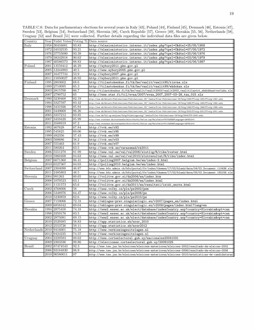
19
TABLE C.8: Data for parliamentary elections for several years in Italy [43], Poland [44], Finland [45], Denmark [46], Estonia [47],Sweden [53], Belgium [54], Switzerland [50], Slovenia [48], Czech Republic [57], Greece [49], Slovakia [55, 56], Netherlands [58],Uruguay [52] and Brazil [51] were collected. Further details regarding the individual data files are given below.
Country Year Valid Votes Voting % Data source
Italy 1958 30434681 93.83 http://elezionistorico.interno.it/index.php?tpel=C&dtel=25/05/1958
1972 34532535 93.21 http://elezionistorico.interno.it/index.php?tpel=C&dtel=07/05/1972
1976 37755090 93.39 http://elezionistorico.interno.it/index.php?tpel=C&dtel=20/06/1976
1979 38242918 90.62 http://elezionistorico.interno.it/index.php?tpel=C&dtel=03/06/1979
1987 40586573 88.83 http://elezionistorico.interno.it/index.php?tpel=C&dtel=14/06/1987
Poland 2001 13559412 46.29 http://wybory2011.pkw.gov.pl
2005 12244903 40.5 http://www.wybory2005.pkw.gov.pl
2007 16477734 53.9 http://wybory2007.pkw.gov.pl
2011 15050027 48.92 http://wybory2011.pkw.gov.pl
Finland 1995 2803602 68.6 http://tilastokeskus.fi/tk/he/vaalit/vaalit95/risvaa.xls
1999 2710095 65.3 http://tilastokeskus.fi/tk/he/vaalit/vaalit99/ehdokas.xls
2003 2815700 66.7 http://tilastokeskus.fi/tk/he/vaalit/vaalit2003/vaalit2003_vaalitilastot_ehdokkaatverluku.xls
2007 2790752 65 http://www.stat.fi/til/evaa/2007/evaa_2007_2007-03-28_tau_015.xls
Denmark 1990 3239468 82.19 http://sum.dk/Aktuelt/Publikationer/Publikationer_IN/~/media/Filer-Publikationer-IN/Valg/1996/FTvalg-1990/FTvalg-1990.ashx
1994 3327597 83.42 http://sum.dk/Aktuelt/Publikationer/Publikationer_IN/~/media/Filer-Publikationer-IN/Valg/1996/FTvalg-1994/FTvalg-1994.ashx
1998 3431926 85.94 http://sum.dk/Aktuelt/Publikationer/Publikationer_IN/~/media/Filer-Publikationer-IN/Valg/1999/FTvalg-1998/FTvalg-1998.ashx
2001 3449668 86.26 http://sum.dk/Aktuelt/Publikationer/Publikationer_IN/~/media/Filer-Publikationer-IN/Valg/2003/FTvalg-2001/FTvalg-2001.ashx
2005 3357212 83.85 http://sum.dk/Tal-og-analyser/Valg/Folketingsvalg/~/media/Filer-Publikationer-IN/Valg/2006/FTV-2005.ashx
2007 3459420 85.99 http://www.statbank.dk/statbank5a/SelectVarVal/Define.asp?MainTable=FV07KAND&PLanguage=1&PXSId=0
2011 3588919 87.2 http://www.statbank.dk/statbank5a/SelectVarVal/Define.asp?MainTable=FV11KAND&PLanguage=1&PXSId=0
Estonia 1992 467628 67.84 http://vvk.ee/r92
1995 545825 69.06 http://vvk.ee/r95
1999 492356 57.43 http://vvk.ee/r99
2003 500686 58.2 http://vvk.ee/r03
2007 555463 61.9 http://vvk.ee/r07
2011 580264 63.5 http://www.vvk.ee/varasemad/rk2011
Sweden 2006 5551278 81.99 http://www.val.se/val/val2006/slutlig/R/rike/roster.html
2010 5960408 84.63 http://www.val.se/val/val2010/slutresultat/R/rike/index.html
Belgium 2007 6671360 86.41 http://polling2007.belgium.be/en/index-2.html
2010 6527367 84.03 http://polling2010.belgium.be/en/index.html
Switzerland 2007 2304090 46.87 http://www.bfs.admin.ch/bfs/portal/fr/index/themen/17/02/blank/data/04/02.Document.110436.xls
2011 2485803 48.5 http://www.bfs.admin.ch/bfs/portal/fr/index/themen/17/02/blank/data/05/02.Document.155156.xls
Slovenia 2004 991263 60.65 http://volitve.gov.si/dz2004/en/index.htm
2008 1070523 63.1 http://volitve.gov.si/dz2008/en/index.html
2011 1121573 65.6 http://volitve.gov.si/dz2011/en/rezultati/izidi_enote.html
Czech 2002 4768006 58 http://www.volby.cz/pls/ps2002/psm
2006 5348976 64.47 http://www.volby.cz/pls/ps2006/ps
2010 5230859 62.6 http://www.volby.cz/pls/ps2010/ps
Greece 2007 7159006 72.18 http://ekloges-prev.singularlogic.eu/v2007/pages_en/index.html
2009 6858342 69.04 http://ekloges-prev.singularlogic.eu/v2009/pages/index.html?lang=en
Slovakia 1994 2875458 74.18 http://www2.essex.ac.uk/elect/database/indexCountry.asp?country=Slovakia&opt=can
1998 3359176 83.5 http://www2.essex.ac.uk/elect/database/indexCountry.asp?country=Slovakia&opt=can
2002 2875081 69.15 http://www2.essex.ac.uk/elect/database/indexCountry.asp?country=Slovakia&opt=can
2010 2529385 58.83 http://app.statistics.sk/nrsr_2010
2012 2553726 59.11 http://app.statistics.sk/nrsr2012
Netherlands 2010 9416001 75.18 http://www.verkiezingsuitslagen.nl
2012 9424235 74.57 http://www.verkiezingsuitslagen.nl
Uruguay 2004 2229583 89.62 http://www.corteelectoral.gub.uy/nacionales20041031
2009 2303336 89.86 http://elecciones.corteelectoral.gub.uy/20091025
Brazil 2002 87474543 92.3 http://www.tse.jus.br/eleicoes/eleicoes-anteriores/eleicoes-2002/resultado-da-eleicao-2002
2006 93184830 88.9 http://www.tse.jus.br/eleicoes/eleicoes-anteriores/eleicoes-2006/resultado-da-eleicao-2006
2010 96580011 87 http://www.tse.jus.br/eleicoes/eleicoes-anteriores/eleicoes-2010/estatisticas-de-candidaturas