University of Catania - Department of Economics

Working Paper Series

n° 2010/06 – December 201o

Satisfaction and adaptation in voting behavior: an empirical

exploration

by

Marco F. MartoranaIsidoro Mazza

Corso Italia 55, Catania – Italy | www.demq.unict.it | e-mail: demqseg@unict.it

Satisfaction and adaptation in voting behavior:

an empirical exploration

Marco F. Martorana - Isidoro Mazza1

University of Catania

Abstract.

Dynamic models of learning and adaptation have provided realistic predictions in terms of voting

behavior. This study aims at contributing to their scant empirical verification. We develop a

learning algorithm based on bounded rationality estimating the pattern of learning process through a

two-stage econometric model. The analysis links voting behavior to past choices and economic

satisfaction derived from previous period election and state of the economy. This represents a

novelty in the literature on voting that assumes given voter preferences. Results show that

persistence is positively affected by the combination of income changes and past behavior and by union membership.

Keywords: voting, bounded rationality, learning, political accountability.

JEL Classification: D030, D720, C230, C250.

FIRST PRELIMINARY VERSION. NOT TO BE QUOTED.

1 Corresponding author. Address: University of Catania, DEMQ, Corso Italia 55, 95129 Catania (Italy). E-mail:

marco.martorana@unict.it.

1

1. Introduction

The voting paradox (Downs, 1957; Riker and Ordeshook, 1968) highlights a contrast between

economic theory of voting and actual voting behavior. The paradox occurs because voting costs are

generally higher than the expected benefits, originating when the favorite between two parties wins,

which are negligible as the probability of casting the decisive vote is close to nil. According to the

so-called calculus of voting, if individuals are rational and voting is purely instrumental to obtain

the preferred electoral outcome, voting turnout should be negligible. However, voting is definitely

more common than abstaining in democratic systems. A substantial literature has provided several

potential solutions to the voting paradox, without infringing the assumption of fully rational forward

looking voters.2

A rather customary tenet of these voting models is that individual preferences for

candidates are exogenous. Therefore, the focus is almost exclusively on the act of voting

disregarding the impact of feedbacks form past political and economic performance.

In a dynamic perspective, a reasonable presumption would be that people may adjust their

preferences along successive elections according to their satisfaction with their party politics and

the economic outcome.3 A class of voting models based on bounded rationality suggests that voting

can be viewed as a dynamic process based on adaptation, driven either at individual - learning

voting (LV) models - or aggregate level - evolutionary game-theoretic voting (EV) models. Namely,

voters are believed to act in on the basis of previous actions and election outcomes. A well known

example of individual-based stochastic learning process is developed by Macy (1990, 1992, 1994).

This paper refers to Macy‟s process, more specifically to its application by Kanazawa (1998; 2000),

and the related aspiration-based-adaptation rule (ABAR) developed by Bendor, et al. (2003). Their

2 With fully rational voters, a simple solution to the paradox would be that individuals are driven by a consumption

benefit, a warm glow associated with the act of voting itself (expressive voting approach). This approach has some

conceptual limits, in spite of the received empirical support (Blais and Young, 2000). Mueller (2003a, 2003b) and

Aldrich (1993; 1997) argue that this solution is inevitably tautological, as individuals end up voting when they feel they

should vote. People may also regret not having voted. The minimax regret (Ferejohn and Fiorina, 1974) states that

individuals try to minimize the regret they could have by choosing the wrong option. Unfortunately, the minimax regret

leads to very unrealistic, ultra-cautious individual behavior. other solutions, within the fully rational framework,

predicting a positive levels of turnout include the game-theoretical models (Palfrey and Rosenthal, 1983; 1985), info-

based models (Larcinese, 2006) and group-based models (Ulhaner, 1989; Feddersen 2004; Feddersen and Sandroni, 2006; Fowler, 2005). Theoretical and empirical surveys of rational solutions are provided, among others, by Blais

(2000), Blais and Young (2000), Mueller (2003a) and Geys (2006).

3 The link between political decision-making and economic performance is central in the political economy literature.

Here we do not deal with the determinants of political accountability. We just admit that individual (dis)satisfaction

with a party politics may affect her decisions concerning voting.

2

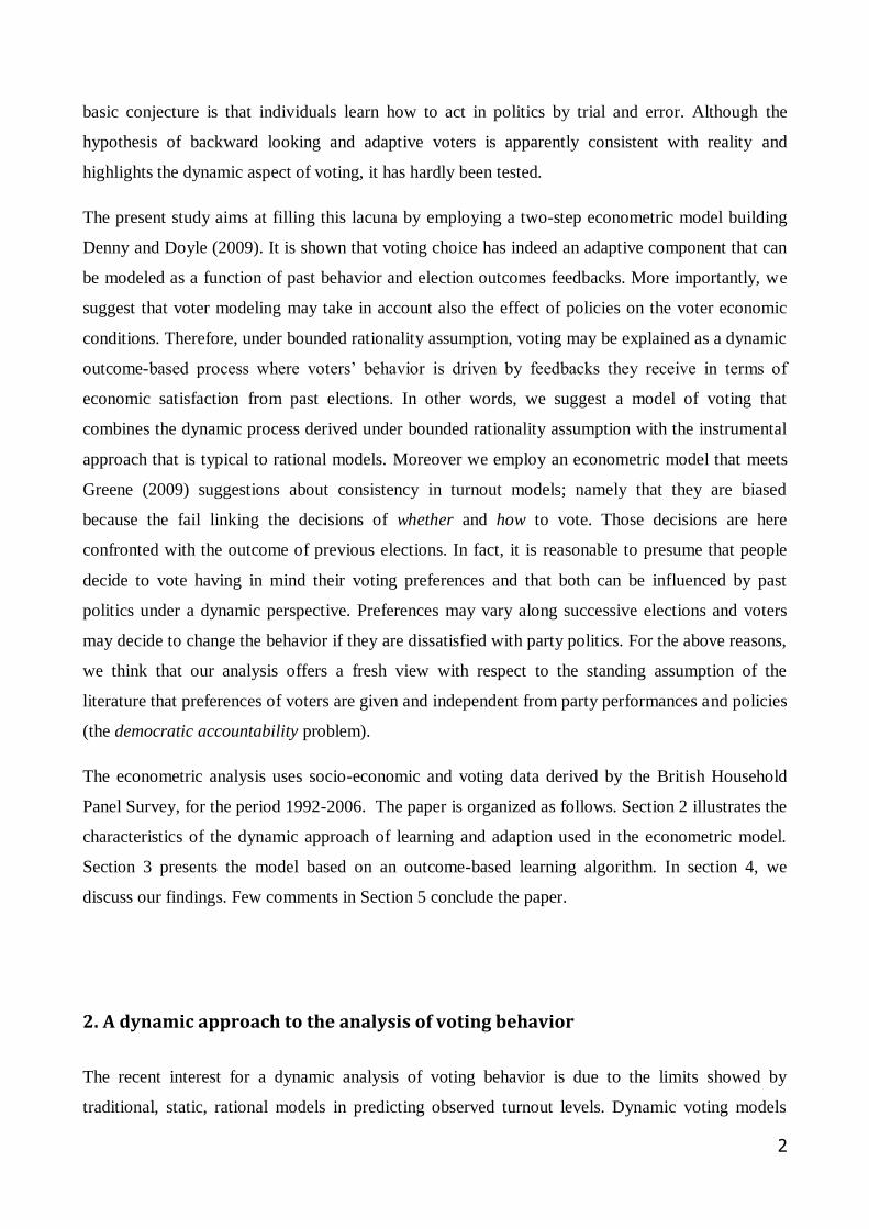
basic conjecture is that individuals learn how to act in politics by trial and error. Although the

hypothesis of backward looking and adaptive voters is apparently consistent with reality and

highlights the dynamic aspect of voting, it has hardly been tested.

The present study aims at filling this lacuna by employing a two-step econometric model building

Denny and Doyle (2009). It is shown that voting choice has indeed an adaptive component that can

be modeled as a function of past behavior and election outcomes feedbacks. More importantly, we

suggest that voter modeling may take in account also the effect of policies on the voter economic

conditions. Therefore, under bounded rationality assumption, voting may be explained as a dynamic

outcome-based process where voters‟ behavior is driven by feedbacks they receive in terms of

economic satisfaction from past elections. In other words, we suggest a model of voting that

combines the dynamic process derived under bounded rationality assumption with the instrumental

approach that is typical to rational models. Moreover we employ an econometric model that meets

Greene (2009) suggestions about consistency in turnout models; namely that they are biased

because the fail linking the decisions of whether and how to vote. Those decisions are here

confronted with the outcome of previous elections. In fact, it is reasonable to presume that people

decide to vote having in mind their voting preferences and that both can be influenced by past

politics under a dynamic perspective. Preferences may vary along successive elections and voters

may decide to change the behavior if they are dissatisfied with party politics. For the above reasons,

we think that our analysis offers a fresh view with respect to the standing assumption of the

literature that preferences of voters are given and independent from party performances and policies

(the democratic accountability problem).

The econometric analysis uses socio-economic and voting data derived by the British Household

Panel Survey, for the period 1992-2006. The paper is organized as follows. Section 2 illustrates the

characteristics of the dynamic approach of learning and adaption used in the econometric model.

Section 3 presents the model based on an outcome-based learning algorithm. In section 4, we

discuss our findings. Few comments in Section 5 conclude the paper.

2. A dynamic approach to the analysis of voting behavior

The recent interest for a dynamic analysis of voting behavior is due to the limits showed by

traditional, static, rational models in predicting observed turnout levels. Dynamic voting models

3

include EV and LV models. These adaptive models have two main common features: bounded

rationality, and the time-dependence. In contrast to rational models, agents learn how to behave

through experience. While EV models of voting behavior (Sieg and Schulz, 1995; Linzer and

Honaker, 2003 and Conley and Toossi, 2006) assume evolution to be driven at aggregate level, LV

models (Kanazawa 1998, 2000; Bendor 2001; Bendor et al. 2003) keep the agent as autonomous

and evolution is drawn at individual level: agents adapt on the basis of their and others‟ experience,

modifying their behavior over time (Selten, 1991; Fudenberg and Levine, 1998).

In particular, Bendor et al. (2003) presents a model where each individual i, at time t, has a starting

propensity to vote denoted by pit and an aspiration level ait. Propensity probabilistically determines

who votes and who is the winning candidate at time t. Given voting costs cij and a benefit bij (bij >

cij>0) for the voters of the winning candidate j,4 individuals compare obtained payoffs (πij) and

aspiration levels, and eventually adjust their propensity in the next stage.5 The adjustment direction

depends on the received feedback. Their aspiration-based adjustment rule (ABAR) is defined as

follows:

, , i,t , 1 ,, 1 ,

, , , 1 ,

, , i,t , 1 ,, 1 ,

Pr 1 and Pr 1

Pr 1

Pr 1 and Pr 1

i t i t i t i ti t i t

i t i t i t i t

i t i t i t i ti t i t

p pa a a

a a a

p pa a a

(1)

They also allow for individuals to be partially or fully inertial. Nevertheless, Bendor et al. (2003)

has been strongly criticized by Fowler (2006). He rejects their use of Bush-Mosteller (1995)

reinforcement rule for the model simulation because it would lead to a biased outcome. That is, the

reinforcement rule indeed has incoherent effects on individual propensity to vote so that individuals

engage in casual voting.6 This bias occurs as adaptation varies with the initial level of pit.

Solutions with full or bounded rational voters generally fail modeling the act of voting as an

outcome-based process. We suggest that voting behavior could follow an adaptation process that

links election outcome to feedbacks that voters receives from party activities as well as on

4 In Bendor et al. (2003), the benefit B is attributed only to the those who have preferences aligned to the winner,

independently from the fact that they actually voted. 5 Net payoff is equal to bij -cij if individual i voted and is of the same faction as the winning candidate j (bij, if i did not vote); or -cij if individual i voted and is not in the same faction as the winning candidate j (0, if i did not vote). 6 Casual voting is also rejected by the empirical evidence for habitual voting (HV), thoroughly surveyed by Plutzer

(2002). Habitual voting can be interpreted as an alternative dynamic explanation for voting still based on a

reinforcement rule. However, in this case, the reinforcement rule is not based on a learning process but rather on voting

reinforcement itself. Although this solution has received empirical evidences both by econometric studies (Green and

Shachar, 2000) and experiments (Gerber et al., 2003), it presents a major shortcoming. On one hand, it confirms

individual behavior to be an evolving process where dynamics play a relevant role; on the other hand, it overlooks the

relation between voting and the political and economic situation.

4

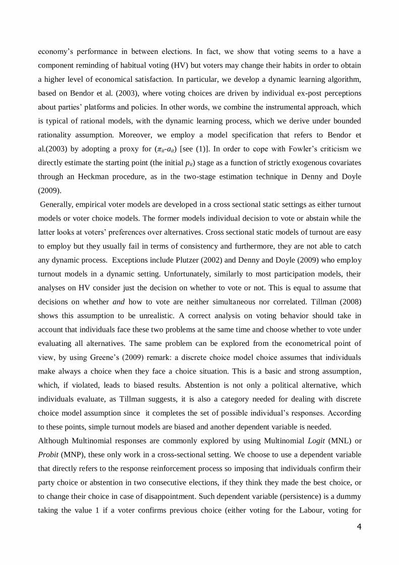
economy‟s performance in between elections. In fact, we show that voting seems to a have a

component reminding of habitual voting (HV) but voters may change their habits in order to obtain

a higher level of economical satisfaction. In particular, we develop a dynamic learning algorithm,

based on Bendor et al. (2003), where voting choices are driven by individual ex-post perceptions

about parties‟ platforms and policies. In other words, we combine the instrumental approach, which

is typical of rational models, with the dynamic learning process, which we derive under bounded

rationality assumption. Moreover, we employ a model specification that refers to Bendor et

al.(2003) by adopting a proxy for (πit-ait) [see (1)]. In order to cope with Fowler‟s criticism we

directly estimate the starting point (the initial pit) stage as a function of strictly exogenous covariates

through an Heckman procedure, as in the two-stage estimation technique in Denny and Doyle

(2009).

Generally, empirical voter models are developed in a cross sectional static settings as either turnout

models or voter choice models. The former models individual decision to vote or abstain while the

latter looks at voters‟ preferences over alternatives. Cross sectional static models of turnout are easy

to employ but they usually fail in terms of consistency and furthermore, they are not able to catch

any dynamic process. Exceptions include Plutzer (2002) and Denny and Doyle (2009) who employ

turnout models in a dynamic setting. Unfortunately, similarly to most participation models, their

analyses on HV consider just the decision on whether to vote or not. This is equal to assume that

decisions on whether and how to vote are neither simultaneous nor correlated. Tillman (2008)

shows this assumption to be unrealistic. A correct analysis on voting behavior should take in

account that individuals face these two problems at the same time and choose whether to vote under

evaluating all alternatives. The same problem can be explored from the econometrical point of

view, by using Greene‟s (2009) remark: a discrete choice model choice assumes that individuals

make always a choice when they face a choice situation. This is a basic and strong assumption,

which, if violated, leads to biased results. Abstention is not only a political alternative, which

individuals evaluate, as Tillman suggests, it is also a category needed for dealing with discrete

choice model assumption since it completes the set of possible individual‟s responses. According

to these points, simple turnout models are biased and another dependent variable is needed.

Although Multinomial responses are commonly explored by using Multinomial Logit (MNL) or

Probit (MNP), these only work in a cross-sectional setting. We choose to use a dependent variable

that directly refers to the response reinforcement process so imposing that individuals confirm their

party choice or abstention in two consecutive elections, if they think they made the best choice, or

to change their choice in case of disappointment. Such dependent variable (persistence) is a dummy

taking the value 1 if a voter confirms previous choice (either voting for the Labour, voting for

5

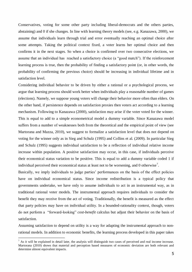
Conservatives, voting for some other party including liberal-democrats and the others parties,

abstaining) and 0 if she changes. In line with learning theory models (see, e.g. Kanazawa, 2000), we

assume that individuals learn through trial and error eventually reaching an optimal choice after

some attempts. Taking the political context fixed, a voter learns her optimal choice and then

confirms it in the next stages. So when a choice is confirmed over two consecutive elections, we

assume that an individual has reached a satisfactory choice (a “good match”). If the reinforcement

learning process is true, then the probability of finding a satisfactory point (or, in other words, the

probability of confirming the previous choice) should be increasing in individual lifetime and in

satisfaction level.

Considering individual behavior to be driven by either a rational or a psychological process, we

argue that learning process should work better when individuals play a reasonable number of games

(elections). Namely, we suppose young voters will change their behavior more often than elders. On

the other hand, if persistence depends on satisfaction proxies then voters act according to a learning

mechanism. Following to Kanazawa (2000), satisfaction may arise if the voter voted for the winner.

This is equal to add to a simple econometrical model a dummy variable. Since Kanazawa model

suffers from a number of weaknesses both from the theoretical and the empirical point of view (see

Martorana and Mazza, 2010), we suggest to formalize a satisfaction level that does not depend on

voting for the winner only as in Sieg and Schulz (1995) and Collins et al. (2009). In particular Sieg

and Schulz (1995) suggests individual satisfaction to be a reflection of individual relative income

increase within population. A positive satisfaction may occur, in this case, if individuals perceive

their economical status variation to be positive. This is equal to add a dummy variable coded 1 if

individual perceived their economical status at least not to be worsening, and 0 otherwise7.

Basically, we imply individuals to judge parties‟ performances on the basis of the effect policies

have on individual economical status. Since income redistribution is a typical policy that

governments undertake, we have only to assume individuals to act in an instrumental way, as in

traditional rational voter models. The instrumental approach requires individuals to consider the

benefit they may receive from the act of voting. Traditionally, the benefit is measured as the effect

that party policies may have on individual utility. In a bounded-rationality context, though, voters

do not perform a “forward-looking” cost-benefit calculus but adjust their behavior on the basis of

satisfaction.

Assuming satisfaction to depend on utility is a way for adapting the instrumental approach to non-

rational models. In addition to economic benefits, the learning process developed in this paper takes

7 As it will be explained in detail later, the analysis will distinguish two cases of perceived and real income increase.

Martorana (2010) shows that material and perception based measures of economic deviation are both relevant and

determine almost equivalent impacts.

6

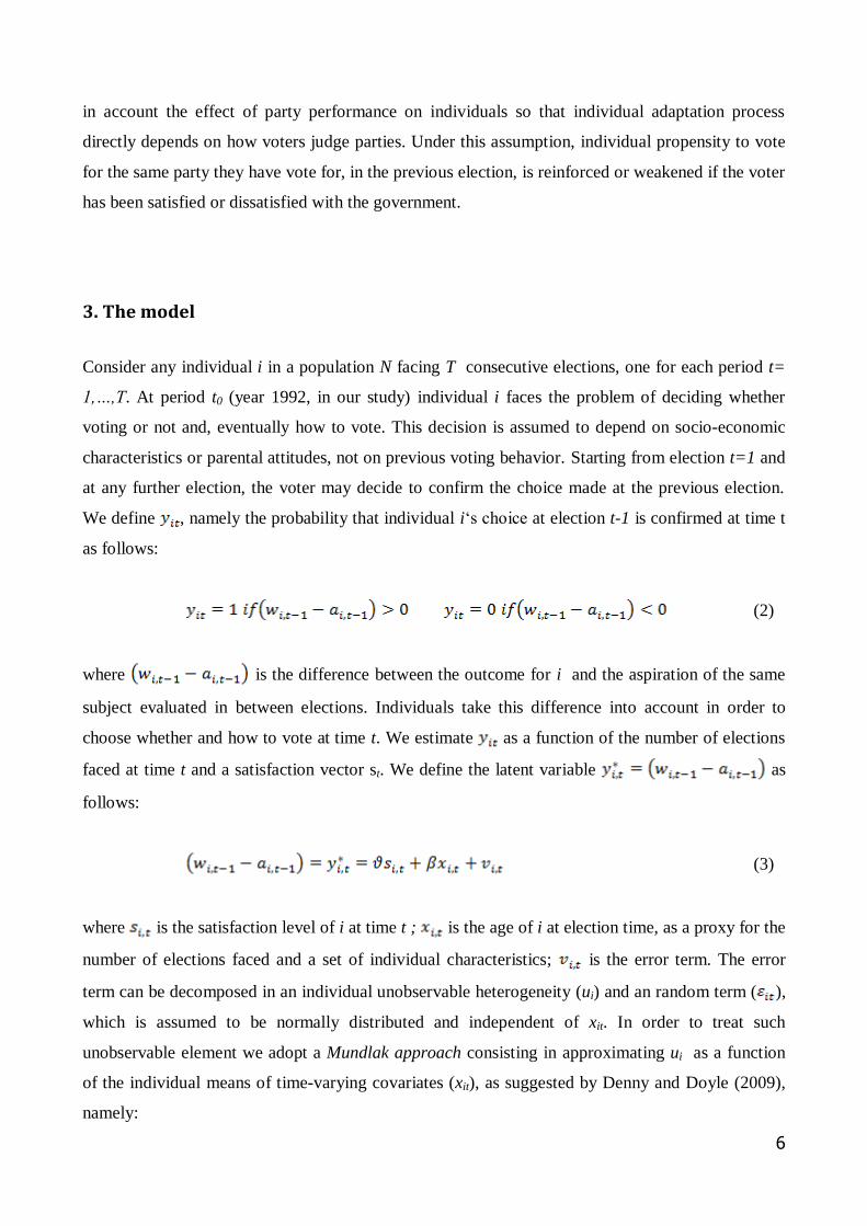
in account the effect of party performance on individuals so that individual adaptation process

directly depends on how voters judge parties. Under this assumption, individual propensity to vote

for the same party they have vote for, in the previous election, is reinforced or weakened if the voter

has been satisfied or dissatisfied with the government.

3. The model

Consider any individual i in a population N facing T consecutive elections, one for each period t=

1,…,T. At period t0 (year 1992, in our study) individual i faces the problem of deciding whether

voting or not and, eventually how to vote. This decision is assumed to depend on socio-economic

characteristics or parental attitudes, not on previous voting behavior. Starting from election t=1 and

at any further election, the voter may decide to confirm the choice made at the previous election.

We define , namely the probability that individual i„s choice at election t-1 is confirmed at time t

as follows:

(2)

where is the difference between the outcome for i and the aspiration of the same

subject evaluated in between elections. Individuals take this difference into account in order to

choose whether and how to vote at time t. We estimate as a function of the number of elections

faced at time t and a satisfaction vector st. We define the latent variable as

follows:

(3)

where is the satisfaction level of i at time t ; is the age of i at election time, as a proxy for the

number of elections faced and a set of individual characteristics; is the error term. The error

term can be decomposed in an individual unobservable heterogeneity (ui) and an random term ( ),

which is assumed to be normally distributed and independent of xit. In order to treat such

unobservable element we adopt a Mundlak approach consisting in approximating ui as a function

of the individual means of time-varying covariates (xit), as suggested by Denny and Doyle (2009),

namely:

7

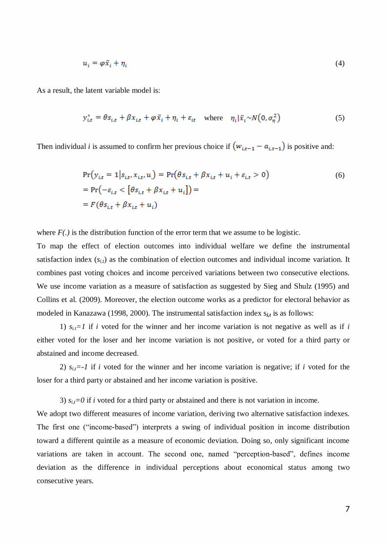
(4)

As a result, the latent variable model is:

where (5)

Then individual i is assumed to confirm her previous choice if is positive and:

(6)

where F(.) is the distribution function of the error term that we assume to be logistic.

To map the effect of election outcomes into individual welfare we define the instrumental

satisfaction index (si,t) as the combination of election outcomes and individual income variation. It

combines past voting choices and income perceived variations between two consecutive elections.

We use income variation as a measure of satisfaction as suggested by Sieg and Shulz (1995) and

Collins et al. (2009). Moreover, the election outcome works as a predictor for electoral behavior as

modeled in Kanazawa (1998, 2000). The instrumental satisfaction index si,t is as follows:

1) si.t=1 if i voted for the winner and her income variation is not negative as well as if i

either voted for the loser and her income variation is not positive, or voted for a third party or

abstained and income decreased.

2) si,t=-1 if i voted for the winner and her income variation is negative; if i voted for the

loser for a third party or abstained and her income variation is positive.

3) si,t=0 if i voted for a third party or abstained and there is not variation in income.

We adopt two different measures of income variation, deriving two alternative satisfaction indexes.

The first one (“income-based”) interprets a swing of individual position in income distribution

toward a different quintile as a measure of economic deviation. Doing so, only significant income

variations are taken in account. The second one, named “perception-based”, defines income

deviation as the difference in individual perceptions about economical status among two

consecutive years.

8

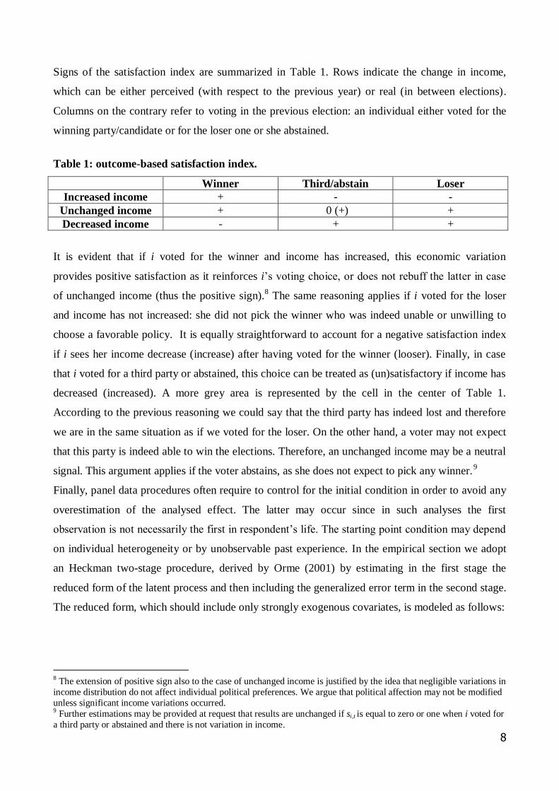
Signs of the satisfaction index are summarized in Table 1. Rows indicate the change in income,

which can be either perceived (with respect to the previous year) or real (in between elections).

Columns on the contrary refer to voting in the previous election: an individual either voted for the

winning party/candidate or for the loser one or she abstained.

Table 1: outcome-based satisfaction index.

Winner Third/abstain Loser

Increased income + - -

Unchanged income + 0 (+) +

Decreased income - + +

It is evident that if i voted for the winner and income has increased, this economic variation

provides positive satisfaction as it reinforces i‟s voting choice, or does not rebuff the latter in case

of unchanged income (thus the positive sign).8 The same reasoning applies if i voted for the loser

and income has not increased: she did not pick the winner who was indeed unable or unwilling to

choose a favorable policy. It is equally straightforward to account for a negative satisfaction index

if i sees her income decrease (increase) after having voted for the winner (looser). Finally, in case

that i voted for a third party or abstained, this choice can be treated as (un)satisfactory if income has

decreased (increased). A more grey area is represented by the cell in the center of Table 1.

According to the previous reasoning we could say that the third party has indeed lost and therefore

we are in the same situation as if we voted for the loser. On the other hand, a voter may not expect

that this party is indeed able to win the elections. Therefore, an unchanged income may be a neutral

signal. This argument applies if the voter abstains, as she does not expect to pick any winner.9

Finally, panel data procedures often require to control for the initial condition in order to avoid any

overestimation of the analysed effect. The latter may occur since in such analyses the first

observation is not necessarily the first in respondent‟s life. The starting point condition may depend

on individual heterogeneity or by unobservable past experience. In the empirical section we adopt

an Heckman two-stage procedure, derived by Orme (2001) by estimating in the first stage the

reduced form of the latent process and then including the generalized error term in the second stage.

The reduced form, which should include only strongly exogenous covariates, is modeled as follows:

8 The extension of positive sign also to the case of unchanged income is justified by the idea that negligible variations in

income distribution do not affect individual political preferences. We argue that political affection may not be modified

unless significant income variations occurred. 9 Further estimations may be provided at request that results are unchanged if si,t is equal to zero or one when i voted for

a third party or abstained and there is not variation in income.

9

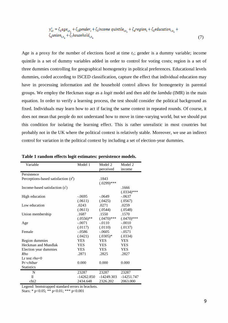
(7)

Age is a proxy for the number of elections faced at time t1; gender is a dummy variable; income

quintile is a set of dummy variables added in order to control for voting costs; region is a set of

three dummies controlling for geographical homogeneity in political preferences. Educational levels

dummies, coded according to ISCED classification, capture the effect that individual education may

have in processing information and the household control allows for homogeneity in parental

groups. We employ the Heckman stage as a logit model and then add the lambda (IMR) in the main

equation. In order to verify a learning process, the test should consider the political background as

fixed. Individuals may learn how to act if facing the same context in repeated rounds. Of course, it

does not mean that people do not understand how to move in time-varying world, but we should put

this condition for isolating the learning effect. This is rather unrealistic in most countries but

probably not in the UK where the political context is relatively stable. Moreover, we use an indirect

control for variation in the political context by including a set of election-year dummies.

Table 1 random effects logit estimates: persistence models.

Variable Model 1 Model 2

perceived

Model 2

income

Persistence

Perceptions-based satisfaction (sp) .1843

(.0299)***

Income-based satisfaction (si) .1666

(.0334)***

High education -.0695

(.0611)

-.0649

(.0425)

-.0637

(.0567)

Low education .0243

(.0611)

.0271

(.0544)

.0259

(.0548)

Union membership .1687

(.0556)**

.1550

(.0470)***

.1570

(.0470)*** Age -.0071

(.0117)

-.0110

(.0110)

-.0010

(.0137)

Female -.0586

(.0421)

-.0605

(.0305)*

-.0571

(.0334)

Region dummies YES YES YES

Heckman and Mundlak YES YES YES

Election year dummies YES YES YES

Rho

Lr test rho=0

Pr>chibar

.2871

0.000

.2825

0.000

.2827

0.000

Statistics

N 23287 23287 23287

ll -14262.850 -14249.303 -14251.747

chi2 2434.648 2326.202 2063.000

Legend: bootstrapped standard errors in brackets.

Stars: * p<0.05; ** p<0.01; *** p<0.001

10

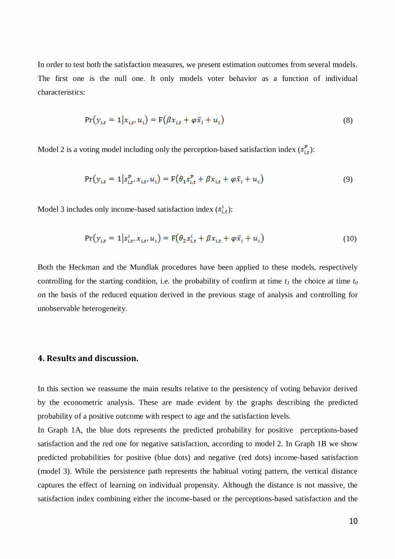
In order to test both the satisfaction measures, we present estimation outcomes from several models.

The first one is the null one. It only models voter behavior as a function of individual

characteristics:

(8)

Model 2 is a voting model including only the perception-based satisfaction index ( ):

(9)

Model 3 includes only income-based satisfaction index ( ):

(10)

Both the Heckman and the Mundlak procedures have been applied to these models, respectively

controlling for the starting condition, i.e. the probability of confirm at time t1 the choice at time t0

on the basis of the reduced equation derived in the previous stage of analysis and controlling for

unobservable heterogeneity.

4. Results and discussion.

In this section we reassume the main results relative to the persistency of voting behavior derived

by the econometric analysis. These are made evident by the graphs describing the predicted

probability of a positive outcome with respect to age and the satisfaction levels.

In Graph 1A, the blue dots represents the predicted probability for positive perceptions-based

satisfaction and the red one for negative satisfaction, according to model 2. In Graph 1B we show

predicted probabilities for positive (blue dots) and negative (red dots) income-based satisfaction

(model 3). While the persistence path represents the habitual voting pattern, the vertical distance

captures the effect of learning on individual propensity. Although the distance is not massive, the

satisfaction index combining either the income-based or the perceptions-based satisfaction and the

11

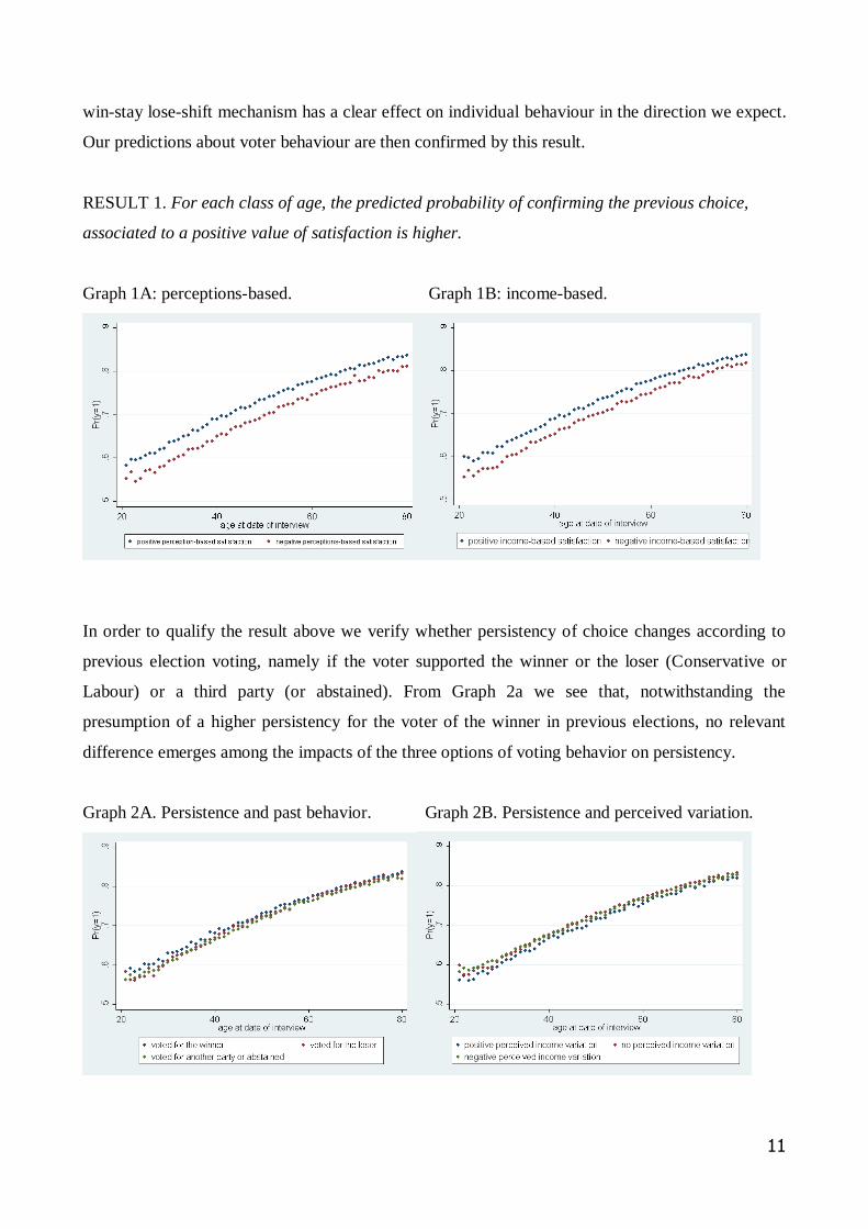
win-stay lose-shift mechanism has a clear effect on individual behaviour in the direction we expect.

Our predictions about voter behaviour are then confirmed by this result.

RESULT 1. For each class of age, the predicted probability of confirming the previous choice,

associated to a positive value of satisfaction is higher.

Graph 1A: perceptions-based. Graph 1B: income-based.

In order to qualify the result above we verify whether persistency of choice changes according to

previous election voting, namely if the voter supported the winner or the loser (Conservative or

Labour) or a third party (or abstained). From Graph 2a we see that, notwithstanding the

presumption of a higher persistency for the voter of the winner in previous elections, no relevant

difference emerges among the impacts of the three options of voting behavior on persistency.

Graph 2A. Persistence and past behavior. Graph 2B. Persistence and perceived variation.

12

Interestingly, also perceived variation in economic status alone does not seem to have an impact on

persistency, as shown by Graph 2b. Reassuming, we obtain the following result.

RESULT 2. The probability of persisting in choices depends neither on past behaviour nor on

economical variation but only on their interaction.

The interaction between past behaviour and instrumental voting (perceived or income based) is

highlighted by the impact of si.t, described in Graphs 1a and 1b. Comparison between Result 1 and

Result 2 proves that economic variations per se are not fundamental to ascertain persistency. In fact,

voters adapt their behaviour along elections on the basis of how they evaluate election outcomes in

terms of economic satisfaction. These results also offer useful insights for empirical and theoretical

studies investigating the influence of economic trend on elections.

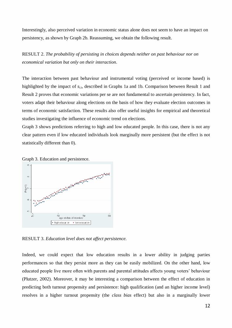
Graph 3 shows predictions referring to high and low educated people. In this case, there is not any

clear pattern even if low educated individuals look marginally more persistent (but the effect is not

statistically different than 0).

Graph 3. Education and persistence.

RESULT 3. Education level does not affect persistence.

Indeed, we could expect that low education results in a lower ability in judging parties

performances so that they persist more as they can be easily mobilized. On the other hand, low

educated people live more often with parents and parental attitudes affects young voters‟ behaviour

(Plutzer, 2002). Moreover, it may be interesting a comparison between the effect of education in

predicting both turnout propensity and persistence: high qualification (and an higher income level)

resolves in a higher turnout propensity (the class bias effect) but also in a marginally lower

13

persistence. A reason for this outcome could be that more educated people are more informed; thus

their reaction to perceived changes would be more elastic and induce more frequent changes. An

interesting result concerns the effects of unionization on persistence.

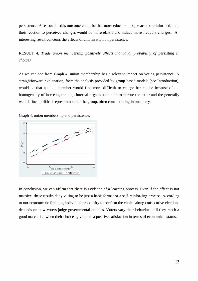
RESULT 4. Trade union membership positively affects individual probability of persisting in

choices.

As we can see from Graph 4, union membership has a relevant impact on voting persistence. A

straightforward explanation, from the analysis provided by group-based models (see Introduction),

would be that a union member would find more difficult to change her choice because of the

homogeneity of interests, the high internal organization able to pursue the latter and the generally

well defined political representation of the group, often concentrating in one party.

Graph 4. union membership and persistence.

In conclusion, we can affirm that there is evidence of a learning process. Even if the effect is not

massive, these results deny voting to be just a habit format or a self-reinforcing process. According

to our econometric findings, individual propensity to confirm the choice along consecutive elections

depends on how voters judge governmental policies. Voters vary their behavior until they reach a

good match, i.e. when their choices give them a positive satisfaction in terms of economical status.

14

5. Concluding comments

This study has provided an empirical analysis of a dynamic model of voting as an outcome based

process. Voters learn and adapt from feedbacks of previous voting and economic satisfaction

determined by past elections. Regarding the latter, a distinction has been made between perceived

variation in individual economic conditions, consistent with bounded rationality, and real changes

of income quintile, in line with the with the instrumental approach typical of rational models.

The results confirm that voters adapt along elections on the basis of the evaluation of past election

outcomes in terms of economic satisfaction, which in turn depends on previous voting choices.

Interestingly, persistency of voting behavior is not affected by education or the kind of voting: who

voted for the winner is as likely to confirm her choice as who voted for the loser. Finally, economic

improvements alone have an ambiguous effect on persistency: they support the choice of who

voted for the winner but wane the choice of who voted for the loser. This result contributes to

qualify the identification of swing voters as those who adapt their (partisan) preferences according

to the performance of their party or the opponent.

This study presents two main novelties with respect to most models on voting behavior. First, it

allows voting preferences to adapt along elections depending on the voter‟s satisfaction with party

politics. This contrasts with previous analysis generally presuming given preferences. Second, the

dynamic approach presented connects the decisions concerning the act of voting and the choice of

the party, or candidate. In this way, it deals with the criticism of Fowler (2006) and Greene (2009)

about consistency in turnout models. This approach may also provide new interesting insights for

further explorations on the voting paradox. In particular, the outcome of previous elections is likely

to affect the benefits of voting and then represents a determinant of abstention whose relevance

requires additional empirical investigation.

15

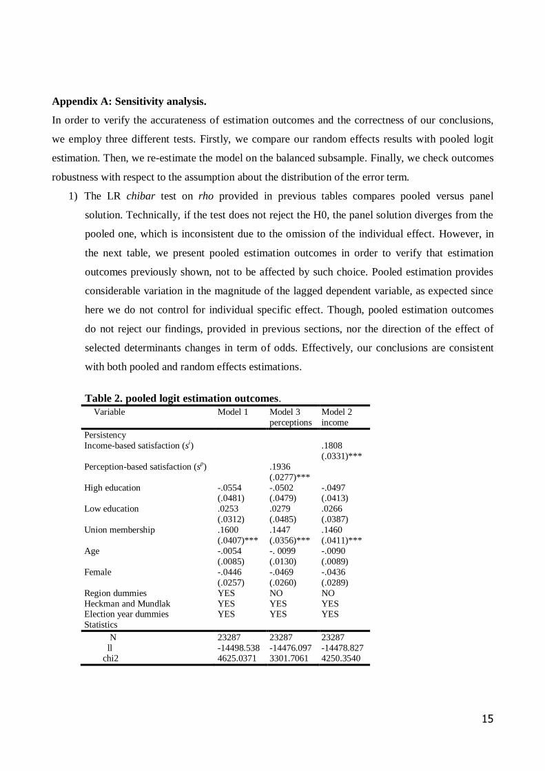
Appendix A: Sensitivity analysis.

In order to verify the accurateness of estimation outcomes and the correctness of our conclusions,

we employ three different tests. Firstly, we compare our random effects results with pooled logit

estimation. Then, we re-estimate the model on the balanced subsample. Finally, we check outcomes

robustness with respect to the assumption about the distribution of the error term.

1) The LR chibar test on rho provided in previous tables compares pooled versus panel

solution. Technically, if the test does not reject the H0, the panel solution diverges from the

pooled one, which is inconsistent due to the omission of the individual effect. However, in

the next table, we present pooled estimation outcomes in order to verify that estimation

outcomes previously shown, not to be affected by such choice. Pooled estimation provides

considerable variation in the magnitude of the lagged dependent variable, as expected since

here we do not control for individual specific effect. Though, pooled estimation outcomes

do not reject our findings, provided in previous sections, nor the direction of the effect of

selected determinants changes in term of odds. Effectively, our conclusions are consistent

with both pooled and random effects estimations.

Table 2. pooled logit estimation outcomes.

Variable Model 1 Model 3

perceptions

Model 2

income

Persistency

Income-based satisfaction (si) .1808

(.0331)***

Perception-based satisfaction (sp) .1936

(.0277)***

High education -.0554 (.0481)

-.0502 (.0479)

-.0497 (.0413)

Low education .0253

(.0312)

.0279

(.0485)

.0266

(.0387)

Union membership .1600

(.0407)***

.1447

(.0356)***

.1460

(.0411)***

Age -.0054

(.0085)

-. 0099

(.0130)

-.0090

(.0089)

Female -.0446

(.0257)

-.0469

(.0260)

-.0436

(.0289)

Region dummies YES NO NO

Heckman and Mundlak YES YES YES Election year dummies YES YES YES

Statistics

N 23287 23287 23287

ll -14498.538 -14476.097 -14478.827 chi2 4625.0371 3301.7061 4250.3540

16

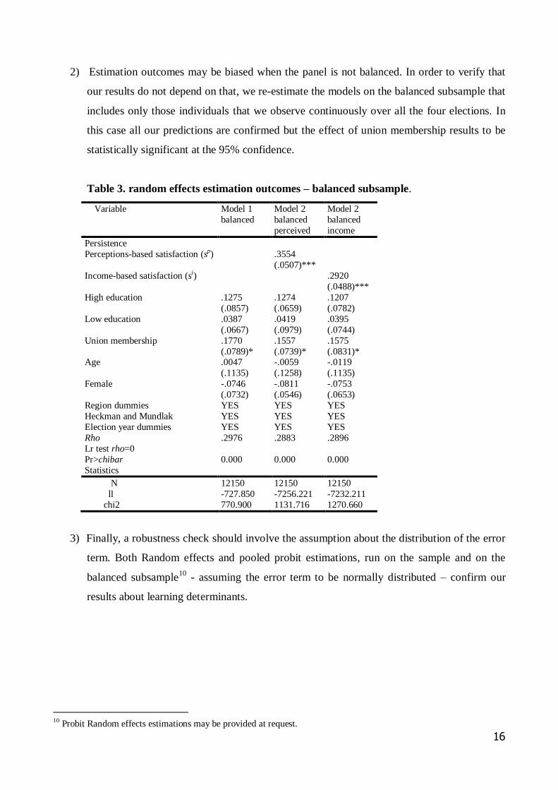
2) Estimation outcomes may be biased when the panel is not balanced. In order to verify that

our results do not depend on that, we re-estimate the models on the balanced subsample that

includes only those individuals that we observe continuously over all the four elections. In

this case all our predictions are confirmed but the effect of union membership results to be

statistically significant at the 95% confidence.

Table 3. random effects estimation outcomes – balanced subsample.

Variable Model 1

balanced

Model 2

balanced

perceived

Model 2

balanced

income

Persistence

Perceptions-based satisfaction (sp) .3554

(.0507)***

Income-based satisfaction (si) .2920

(.0488)***

High education .1275

(.0857)

.1274

(.0659)

.1207

(.0782)

Low education .0387

(.0667)

.0419

(.0979)

.0395

(.0744)

Union membership .1770

(.0789)*

.1557

(.0739)*

.1575

(.0831)* Age .0047

(.1135)

-.0059

(.1258)

-.0119

(.1135)

Female -.0746

(.0732)

-.0811

(.0546)

-.0753

(.0653)

Region dummies YES YES YES

Heckman and Mundlak YES YES YES

Election year dummies YES YES YES

Rho

Lr test rho=0

Pr>chibar

.2976

0.000

.2883

0.000

.2896

0.000

Statistics

N 12150 12150 12150

ll -727.850 -7256.221 -7232.211

chi2 770.900 1131.716 1270.660

3) Finally, a robustness check should involve the assumption about the distribution of the error

term. Both Random effects and pooled probit estimations, run on the sample and on the

balanced subsample10

- assuming the error term to be normally distributed – confirm our

results about learning determinants.

10 Probit Random effects estimations may be provided at request.

17

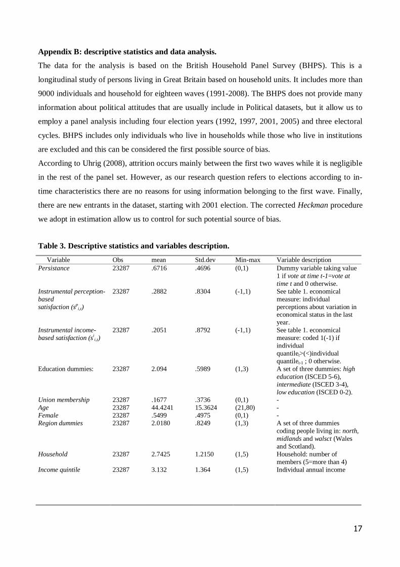
Appendix B: descriptive statistics and data analysis.

The data for the analysis is based on the British Household Panel Survey (BHPS). This is a

longitudinal study of persons living in Great Britain based on household units. It includes more than

9000 individuals and household for eighteen waves (1991-2008). The BHPS does not provide many

information about political attitudes that are usually include in Political datasets, but it allow us to

employ a panel analysis including four election years (1992, 1997, 2001, 2005) and three electoral

cycles. BHPS includes only individuals who live in households while those who live in institutions

are excluded and this can be considered the first possible source of bias.

According to Uhrig (2008), attrition occurs mainly between the first two waves while it is negligible

in the rest of the panel set. However, as our research question refers to elections according to in-

time characteristics there are no reasons for using information belonging to the first wave. Finally,

there are new entrants in the dataset, starting with 2001 election. The corrected Heckman procedure

we adopt in estimation allow us to control for such potential source of bias.

Table 3. Descriptive statistics and variables description.

Variable Obs mean Std.dev Min-max Variable description

Persistance 23287 .6716 .4696 (0,1) Dummy variable taking value

1 if vote at time t-1=vote at

time t and 0 otherwise.

Instrumental perception-

based

satisfaction (spi,t)

23287 .2882 .8304 (-1,1) See table 1. economical

measure: individual

perceptions about variation in economical status in the last

year.

Instrumental income-

based satisfaction (sii,t)

23287 .2051 .8792 (-1,1) See table 1. economical

measure: coded 1(-1) if

individual

quantilet>(<)individual

quantilet-1 ; 0 otherwise.

Education dummies: 23287 2.094 .5989 (1,3) A set of three dummies: high

education (ISCED 5-6),

intermediate (ISCED 3-4),

low education (ISCED 0-2). Union membership 23287 .1677 .3736 (0,1) -

Age 23287 44.4241 15.3624 (21,80) -

Female 23287 .5499 .4975 (0,1) -

Region dummies 23287 2.0180 .8249 (1,3) A set of three dummies

coding people living in: north,

midlands and walsct (Wales

and Scotland).

Household 23287 2.7425 1.2150 (1,5) Household: number of

members (5=more than 4)

Income quintile 23287 3.132 1.364 (1,5) Individual annual income

18

Data source.

University of Essex. Institute for Social and Economic Research, British Household Panel Survey:

Waves 1-15, 1991-2006 [computer file]. 3rd Edition. Colchester, Essex: UK Data Archive

[distributor], June 2007. SN: 5151.

References

Aldrich, J. H. (1993). "Rational Choice and Turnout." American Journal of Political Science 37(1):

246-278.

Aldrich, J. H. (1997). When is it Rational to Vote? Perspectives on Public Choice: A Handbook. D.

C. Mueller. Cambridge, Cambridge University Press: 373-390.

Bendor, J. (2001). Aspiration-based Reinforcement Learning in Repeated Interaction Games an

Overview. International Game Theory Review. 3: 159-174.

Bendor, J., D. Diermeier, M. Ting (2003). "A Behavioral Model of Turnout." American Political

Science Review 97(2): 261-280.

Blais, A. (2000). To Vote or not to Vote?: the merits and limits of rational choice theory. Pittsburgh,

Pa, University of Pittsburgh Press.

Blais, A., R. Young, and M. Lapp (2000). The calculus of voting: An empirical test. European

Journal of Political Research. 37: 181-201.

Bush, R. R. and F. Mosteller (1955). Stochastic Models of Learning. New York, Wiley.

Chamberlain, G. (1984). Panel Data in S. G. M. Intriligator (Ed.) Handbook of Econometrics,

Amsterdam: North-Holland: 1247–1318.

Collins, N. A., S. Kumar,and J. Bendor (2009). The Adaptive Dynamics of Turnout, The Journal of

Politics. 71: 457-472.

Conley, J., A. Toossi, et al. (2006). "Memetics and voting: how nature may make us public

spirited." International Journal of Game Theory 35(1): 71-90.

Denny, K. and O. Doyle (2009). Does Voting History Matter? Analysing Persistence in Turnout.

American Journal of Political Science 53: 17-35.

Downs, A. (1957). An Economic Theory of Democracy. New York, Harper.

Feddersen, T.J. (2004). “Rational Choice Theory and the Paradox of Not Voting”, Journal of

Economic Perspectives 18(1): 99-112.

Feddersen, T.J. and A. Sandroni (2006). “A Theory of Participation in Elections”, American

Economic Review, 96(4): 1271-1282.

19

Ferejohn, J. A. and M. P. Fiorina (1974). "The Paradox of Not Voting: A Decision Theoretic

Analysis." American Political Science Review 68(2): 525-536.

Fowler, J. H. (2006). Habitual Voting and Behavioral Turnout. The Journal of Politics 68: 335-344.

Fudenberg, D. and D. K. Levine (1998). The Theory of Learning in Games. Cambridge, MA, The

Mit Press.

Gerber, A. S., D. P. Green, and R. Shashar (2003). "Voting may be habit-forming: Evidence from a

randomized field experiment." American Journal of Political Science 47: 540-550.

Geys, B. (2006). "'Rational' Theories of Voter Turnout: A Review." Political Studies Review 4(1).

Green, D. P. and R. Shachar (2000). "Habit Formation and Political Behaviour: Evidence of

Consuetude in Voter Turnout " British Journal of Political Science 30(4): 561-573.

Greene, W. H. (2009). Discrete Choice Modelling, T. C. Mills and K. Patterson (Eds.) Palgrave

Handbook of Econometrics: Vol. 2, Applied Econometrics., Palgrave Macmillan.

Heckman, J. J. (1981). The Incidental Parameters Problem and the Problem of Initial Conditions in

Estimating a Discrete Time-Discrete Data Stochastic Process. Structural Analysis of Discrete Data

with Econometric Analysis. C. F. M. a. D. McFadden. Cambridge, MIT Press: 179–95.

Kanazawa, S. (1998). "A Possible Solution to the Paradox of Voter Turnout." The Journal of

Politics 60(974-995).

Kanazawa, S. (2000). "A New Solution to the Collective Action Problem: The Paradox of Voter

Turnout." American Sociological Review 65: 433-442.

Martorana, M.F. (2010), “Material Conditions, Economic Perceptions and Voting Behavior”,

mimeo.

Martorana M.F. and Mazza, I. (2010), “A Note on the Paradox of Voter Turnout”, mimeo.

Linzer, D. and J. Honaker (2003). A Theory of the Evolution of Voting: Turnout Dynamics and the

Importance of Groups. annual meeting of the American Political Science Association. Philadelphia

Marriott Hotel, Philadelphia, PA.

Mueller, D. C. (2003a). Public Choice III. Cambridge, Cambridge University Press.

Mueller, D.C. (2003b). Perspectives in Public Choice: an Handbook. Cambridge, Cambridge

University Press.

Mundlak, Y. (1978). "On the Pooling of Time Series and Cross Section Data." Econometrica 46(1).

Orme, C. D. (2001). The Initial Conditions Problem and Two-Step Estimation in Discrete Panel

Date Models. Department of Economics Discussion Paper University of Manchester.

Palfrey, T. R. and H. Rosenthal (1983). "A strategic calculus of voting." Public Choice 41(1): 7-53.

Palfrey, T. R. and H. Rosenthal (1985). "Voter Participation and Strategic Uncertainty." American

Political Science Review 79(1): 62-78.

20

Plutzer, E. (2002). "Becoming a Habitual Voter: Inertia, Resources, and Growth in Young

Adulthood." American Political Science Review 96(1): 41-56.

Poi, B. P. (2004). “From the Help Desk: Some Bootstrapping Techniques.” Stata Journal 4(3): 312-

328.

Riker, W. H. and P. C. Ordeshook (1968). "A Theory of the Calculus of Voting." American

Political Science Review 62(1): 25-42.

Schram, A. and J. Sonnemans (1996a). "Voter turnout as a participation game: an experimental

investigation." International Journal of Game Theory 25(3): 385-406.

Schram, A. and J. Sonnemans (1996b). "Why People vote: Experimental evidence." Journal of

Economic Psychology 17(4): 417-422.

Selten, R. (1991). "Evolution, learning, and economic behavior." Games and Economic Behavior

3(1): 3-24.

Sieg, G. and C. Schulz (1995). "Evolutionary dynamics in the voting game." Public Choice 85(1):

157-172.

Simon, H. A. (1957). Models of Man: Social and Rational; Mathematical Essays on Rational

Human Behavior in a Social Setting. New York, John Wiley and Sons.

Tillman, E. R. (2008). "Economic Judgments, Party Choice and Voter Abstention in Cross-National

Perspective." Comparative Political Studies 41(9): 1290-1309.

Uhlaner, C.J. (1989). “Rational Turnout: the Neglected Role of Groups”, American Journal of

Political Science 33 (2): 390-422.

Uhrig, N. S. C. (2008). The Nature and the Causes of Attrition in the British Household Panel

Survey. ISER working Paper Colchester, ISER.

University of Catania - Department of Economics

Corso Italia 55, Catania – Italy.

www.demq.unict.it

E-mail: demqseg@unict.it

Working Paper Series

Previous 10 papers of the series:• 2010/05 – G. Coco and G. Pignataro, “Inequality of Opportunity in the Credit Market”• 2010/04 – P. Platania, “Generalization of the financial systems of management in

actuarial techniques affecting insurance of individuals”• 2010/03 – L. Gitto, “Multiple sclerosis patients’ preferences: a preliminary study on

disease awareness and perception”• 2010/02 – A. Cristaldi, “Convergenza e costanza del sentiero di consumo ottimo

intertemporale in presenza di incertezza e lasciti”• 2010/01 – A. E. Biondo and S. Monteleone, “Return Migration in Italy: What do we

Know?”• 2009/04 – S. Angilella, A. Giarlotta and F. Lamantia “A linear implementation of

PACMAN” • 2009/03 – G. Torrisi, “A multilevel analysis on the economic impact of public

infrastructure and corruption in Italian regions”• 2009/02 – L. Bonaventura and A. Consoli, “La scelta dei criteri di priorità per il giudice

penale: effetti sui carichi pendenti e sul costo sociale” • 2009/01 – G. I. Bischi and F. Lamantia, “R&D collaboration networks in oligopoly

competition with spillovers”• 2008/03 – C. Guccio and I. Mazza, “Determinants of Regional Spending for Heritage

Conservation and Valorization in Sicily: a Political-economy Approach”