arX

iv:0

903.

1833

v1 [

hep-

th]

10

Mar

200

9

Preprint typeset in JHEP style - HYPER VERSION ITP-UU-09-10

SPIN-09-10

Universal blocks of the AdS/CFT Scattering Matrix

G. Arutyunov∗, M. de Leeuw, A. Torrielli †

Institute for Theoretical Physics and Spinoza Institute,

Utrecht University, 3508 TD Utrecht, The Netherlands

Abstract: We identify certain blocks in the S-matrix describing the scattering of bound

states of the AdS5 × S5 superstring that allow for a representation in terms of univer-

sal R-matrices of Yangian doubles. For these cases, we use the formulas for Drinfeld’s

second realization of the Yangian in arbitrary bound-state representations to obtain the

explicit expressions for the corresponding R-matrices. We then show that these expressions

perfectly match with the previously obtained S-matrix blocks.

∗Correspondent fellow at Steklov Mathematical Institute, Moscow.†E-mail: G.E.Arutyunov,M.deLeeuw,A.Torrielli@uu.nl

Contents

1. Introduction 1

2. Structure of the bound state S-matrix 3

3. Invariant subspaces 5

3.1 The su(2) subspace 5

3.2 The su(1|1) subspace 6

4. Drinfeld’s realizations of the Yangian 7

5. Universal R-matrix for su(2) 8

6. Universal R-matrix for gl(1|1) 13

A. Revisiting the Y (su(2)) computation 17

A.1 The Factor RF 17

A.2 The Factor RH 19

A.3 The Factor RE 20

1. Introduction

The study of integrable structures in the AdS/CFT correspondence [1–11] has now devel-

oped to a point where the exact solution of the planar spectral problem seems to be a

concrete possibility [12–24]. A recent step in this direction was taken in [25], where the

S-matrix describing the scattering of arbitrary bound states of the theory [26] has been

obtained by employing the Yangian symmetry1 [28–38] . In turn, the knowledge of the

exact scattering matrix for generic states in the spectrum might be essential for better

understanding the TBA approach [39].

The S-matrix found in [25] has a very interesting yet complicated structure. Under-

standing this structure could reveal a great deal of information on the underlying theory,

by adopting the same ideology as for the case of the S-matrix for fundamental magnons.

One immediate consequence of the result of [25] is that the S-matrix for arbitrary bound

states is, by construction, given by a formula of the type

R = ΛopΛ−1

1For interesting recent developments connecting Yangian symmetry and scattering amplitudes, see [27].

– 1 –

for a certain (super)matrix Λ. This naturally realizes the idea of factorizing (Drinfeld’s)

twists [40], and expresses the “triangular” factorization of the S-matrix2.

Given the overall difficulty of the problem, it is natural to start from reducing the

S-matrix to smaller subsectors, and trying to reconduct them to well-understood mathe-

matical objects. One expects the complete algebraic structure responsible for integrability

to be some complicated and likely new type of quantum supergroup, whose properties have

so far only appeared as pieces of a bigger puzzle. We intend to provide here another set of

such pieces, coming from selected subsectors of the bound state S-matrix.

Our first focus will be on a particular subspace of states, which was the essential

starting point of the construction in [25]. This is the space of bound states of the form

(2.1) (Case I). The S-matrix transforms these states among themselves, with amplitudes

controlled by a hypergeometric function (see (3.2) below). Since only the bosonic indices are

allowed to be transformed, these states naturally host a representation of one of the su(2)

(the “bosonic” one) inside the (centrally-extended) psu(2|2) Yangian, and it is a natural

question to ask whether the S-matrix in this subspace is the representation of the universal

R-matrix of the su(2) Yangian double, DY (su(2)). We will show that this is indeed the

case. This will be done by using the suitable evaluation representations for Drinfeld’s

second realization of DY (su(2)), originally obtained by [41], in the operator formalism of

[42]. We will then obtain explicit expressions for the corresponding R-matrices in terms of

hypergeometric functions.

We remark that the universal R-matrix and its realization in concrete representations

is a well-studied subject in the mathematical literature, see e.g. [41, 43]. Here we will

work out the expression for the universal R-matrix evaluated in generic finite-dimensional

representations of su(2) in our particular basis, suitable for comparison with the blocks of

the bound-state scattering matrix. After completing the necessary steps, we will provide

satisfactory evidence that these expressions match with our formula for the S-matrix (3.2)

governing the scattering of Case I states. This matching ought also to be expected in view

of the connection of the hypergeometric function in (3.2), shown to be related to a certain

6j-symbol in [25], with knot theory and the general theory of solutions of the Yang-Baxter

equation [44].

Moreover, one can notice, by analyzing the result of [25], how ubiquitous the amplitudes

Xk,l

n (3.2) are in the S-matrix for both Case II and Case III, since by construction they are

derived from the Case I amplitudes. These factors basically encode how the tail of bosonic

states composing the bound states transform, with the fermions acting temporarily as

spectators. The fact that we can interpret these fundamental building blocks as coming

from the universal R-matrix of su(2) suggests that the latter could be a genuine factor of

the full universal R-matrix.

As a second task, we will focus on subspaces consisting of states with only one species

of bosons and one species of fermions. These are other (four) subspaces, closed under

the action of the S-matrix, and “transversal” to the Cases listed in [25]: namely, they

2We remark that, even in the case of the fundamental magnon S-matrix, this fact had not been explicitly

shown before.

– 2 –

contain vectors from Case I, II and III, as we will explain below. These subspaces host

representations of gl(1|1), and we will show that the S-matrix in these blocks can be

obtained from the universal R-matrix of the gl(1|1) Yangian double, DY (gl(1|1)). We

will construct the general bound state representation for (Drinfeld’s second realization of)

DY (gl(1|1)), and then match with our results from [25]. The novelty with respect to the

su(2) case is represented by the necessity of making an unusual choice of the evaluation

parameter of the Yangian. This is an indication that these states, when scattering among

themselves, respect an “effective” gl(1|1) Yangian symmetry, whose parameters somehow

encode the effect of the yet-unknown superior structure of the full universal R-matrix.

The paper is organized as follows. We will first summarize the structure and the main

features of the bound state S-matrix constructed in [25]. We will also concisely review some

notions concerning Drinfeld’s first and second realization of the Yangian. We will then

single out the su(2) and the various gl(1|1) subspaces, respectively. We will summarize the

corresponding Yangian representations for arbitrary bound states, and explicitly evaluate

their universal R-matrices, matching with our previously obtained results. We will conclude

with an appendix, containing some computational details.

2. Structure of the bound state S-matrix

In this section, we report a summary of the results of [25], with the aim of fixing the

notation and as a motivation to investigate the universal structure of the bound state

scattering matrix.

We denote the bound state numbers of the scattering particles as ℓ1 and ℓ2, respec-

tively. Because of su(2) × su(2) invariance, when the S-matrix acts on the bound state

representation space it leaves five different subspaces invariant. Two pairs of them are

simply related to each other, therefore only three non-equivalent cases are given, which we

list here below.

Case I

The standard basis for this vector space, which we will concisely call V I, is

|k, l〉I ≡ θ3wℓ1−k−11 wk

2︸ ︷︷ ︸Space1

ϑ3vℓ2−l−11 vl

2︸ ︷︷ ︸Space2

, (2.1)

for all k + l = N . The range of k, l here and in the cases below is straightforwardly read

off from the definition of the states. For fixed N , this gives in this case N + 1 different

vectors. We get another copy of Case I if we exchange the index 3 with 4 in the fermionic

variable, with the same S-matrix.

– 3 –

Case II

The standard basis for this space V II is

|k, l〉II1 ≡ θ3wℓ1−k−11 wk

2︸ ︷︷ ︸ vℓ2−l1 vl

2︸ ︷︷ ︸,

|k, l〉II2 ≡ wℓ1−k1 wk

2︸ ︷︷ ︸ ϑ3vℓ2−l−11 vl

2︸ ︷︷ ︸, (2.2)

|k, l〉II3 ≡ θ3wℓ1−k−11 wk

2︸ ︷︷ ︸ ϑ3ϑ4vℓ2−l−11 vl−1

2︸ ︷︷ ︸,

|k, l〉II4 ≡ θ3θ4wℓ1−k−11 wk−1

2︸ ︷︷ ︸ ϑ3vℓ2−l−11 vl

2︸ ︷︷ ︸,

where k + l = N as before3. It is easily seen that we get in this case 4N + 2 states. Once

again, exchanging 3 with 4 in the fermionic variable gives another copy of Case II, with

the same S-matrix.

Case III

For fixed N = k + l, the dimension of this vector space V III is 6N . The standard basis is

|k, l〉III1 ≡ wℓ1−k1 wk

2︸ ︷︷ ︸ vℓ2−l1 vl

2︸ ︷︷ ︸,

|k, l〉III2 ≡ wℓ1−k1 wk

2︸ ︷︷ ︸ ϑ3ϑ4vℓ2−l−11 vl−1

2︸ ︷︷ ︸,

|k, l〉III3 ≡ θ3θ4wℓ1−k−11 wk−1

2︸ ︷︷ ︸ vℓ2−l1 vl

2︸ ︷︷ ︸,

|k, l〉III4 ≡ θ3θ4wℓ1−k−11 wk−1

2︸ ︷︷ ︸ ϑ3ϑ4vℓ2−l−11 vl−1

2︸ ︷︷ ︸, (2.3)

|k, l〉III5 ≡ θ3wℓ1−k−11 wk

2︸ ︷︷ ︸ ϑ4vℓ2−l1 vl−1

2︸ ︷︷ ︸,

|k, l〉III6 ≡ θ4wℓ1−k1 wk−1

2︸ ︷︷ ︸ ϑ3vℓ2−l−11 vl

2︸ ︷︷ ︸ .

The different cases are mapped into one another by use of the (opposite) coproducts

of the (Yangian) symmetry generators.

The S-matrix has the following block-diagonal form:

S =

X

Y 0

Z0 Y

X

. (2.4)

The outer blocks scatter states from V I

X : V I −→ V I (2.5)

|k, l〉I 7→k+l∑

m=0

Xk,l

m |m,k + l − m〉I, (2.6)

3We will from now on, with no risk of confusion, omit indicating “Space 1” and “Space 2” under the

curly brackets.

– 4 –

where Xk,l

m is given by Eq. (4.11) in [25]. We will report its explicit expression in the next

section, formula (3.2). The blocks Y describe the scattering of states from V II

Y : V II −→ V II (2.7)

|k, l〉IIj 7→k+l∑

m=0

4∑

j=1

Yk,l;j

m;i |m,k + l − m〉IIj . (2.8)

These S-matrix elements are given in Eq. (5.18) of [25], but we will not need their explicit

expression here. Finally, the middle block deals with the third case

Z : V III −→ V III (2.9)

|k, l〉IIIj 7→k+l∑

m=0

6∑

j=1

Zk,l;jm;i |m,k + l − m〉IIIj , (2.10)

with Zk,l;jm;i from Eq. (6.11) in [25]. Similarly, these expressions are not needed for the sake

of the present discussion, and we refer to [25] for their details.

We recall that the full AdS5 × S5 string bound state S-matrix is then obtained by

taking two copies of the above S-matrix, and multiplying the result by the square of the

following phase factor [42, 45]:

S0(p1, p2) =

(x−1x+

1

) ℓ22

(x+

2

x−2

) ℓ12

σ(x1, x2) ×

×√

G(ℓ2 − ℓ1)G(ℓ2 + ℓ1)

ℓ1−1∏

q=1

G(ℓ2 − ℓ1 + 2q), (2.11)

where, in our conventions,

G(Q) =u1 − u2 + Q

2

u1 − u2 −Q2

. (2.12)

Here, u is given in the standard variables by

u ≡g

4i

(x+ +

1

x++ x− +

1

x−

). (2.13)

3. Invariant subspaces

We will describe here in detail the two type of subspaces of states we will be focussing our

attention on.

3.1 The su(2) subspace

The first subspace is given by states belonging to Case I in the above classification. We

remind that the psu(2|2) algebra has two (“bosonic” and “fermionic”, according to the

– 5 –

indices they transform) su(2) subalgebras, with generators Lab and Rα

β , respectively. The

first ones satisfy the following commutation relations:

[L ba , Jc] = δb

cJa −1

2δbaJc,

[L ba , Jc] = −δc

aJb +1

2δbaJc. (3.1)

The states from Case I form a natural representation on which the “bosonic” su(2) sub-

algebra of Lab ’s acts. The latter transforms the bosonic variables, and leaves the only two

(equal-type) fermions presents as spectators. Furthermore, the Case I S-matrix satisfies

the Yang-Baxter equation by itself, and it is of difference form. This means that such

S-matrix should naturally come from the universal R-matrix of the su(2) Yangian double

[41]. The Case I S-matrix is given by [25]

Xk,l

n = (−1)k+n πDsin[(k − ℓ1)π] Γ(l + 1)

sin[ℓ1π] sin[(k + l − ℓ2 − n)π] Γ(l − ℓ2 + 1)Γ(n + 1)×

Γ(n + 1 − ℓ1)Γ(l + ℓ1−ℓ2

2 − n − δu)

Γ(1 − ℓ1+ℓ2

2 − δu)

Γ(k + l − ℓ1+ℓ2

2 − δu + 1)

Γ(

ℓ1−ℓ22 − δu

) × (3.2)

4F3

(−k,−n, δu + 1 −

ℓ1 − ℓ2

2,ℓ2 − ℓ1

2− δu; 1 − ℓ1, ℓ2 − k − l, l − n + 1; 1

),

where one has defined 4F3(x, y, z, t; r, v, w; τ) = 4F3(x, y, z, t; r, v, w; τ)/[Γ(r)Γ(v)Γ(w)] and

D =x−1 − x+

2

x+1 − x−2

eip12

eip22

. (3.3)

The quantity δu equals u1 − u2, with u given by (2.13). One can check that this S-matrix

satisfies the YBE, and we will indeed show that this formula coincides with what one

obtains from the Yangian universal R-matrix [41], with the same evaluation parameter u

(2.13).

3.2 The su(1|1) subspace

The other subspace we will consider is obtained by restricting the bound states to having

bosonic and fermionic indices of only one respective type. For definiteness, we will take

the bosonic index to be 1 and the fermionic index to be 3. There are four copies of this

subspace, corresponding to the four different choices of these indices we can make. The

embedding of this subspace in the full bound state representation is spanned by the vectors

{|0, 0〉III1 , |0, 0〉II1 , |0, 0〉II2 , |0, 0〉I

}. (3.4)

As one can see, this subspace takes particular states from all three Cases listed above,

yet being closed under the action of the S-matrix. This means that the S-matrix for this

subsector corresponds to a block-diagonal 4 × 4 matrix. The two Case II states mix with

an S-matrix given by formula (3.15) in [25]. The amplitude for the Case III state present

– 6 –

is normalized to 1, while for the Case I state it is simply the factor D (3.3). Putting this

together, one obtains

S =

1 0 0 0

0 e−ip22

x+1 −x+

2

x+1 −x−

2

√ℓ1η(p1)√ℓ2η(p2)

x+2 −x−

2

x+1 −x−

2

0

0 eip12

eip22

√ℓ2η(p2)√ℓ1η(p1)

x+1 −x−

1

x+1 −x−

2

eip12

x−1 −x−

2

x+1 −x−

2

0

0 0 0x−1 −x+

2

x+1 −x−

2

eip12

eip22

. (3.5)

We remark that, taken in the fundamental representation, and suitably un-twisted in order

to eliminate the braiding factors coming from the nontrivial coproduct [46–48], this matrix

coincides with the S-matrix of [49]. It is readily checked that this matrix satisfies the Yang-

Baxter equation by itself, therefore it is natural to ask whether it is the representation of

a known (Yangian) universal R-matrix.

In the remainder of the paper we will discuss the universal R-matrices for the Yan-

gian doubles associated to su(2) and gl(1|1), and show that they coincide with the above

discussed bound state S-matrix blocks [25]. The construction relies on Drinfeld’s second

realization of the Yangian, which we will review in the next section.

4. Drinfeld’s realizations of the Yangian

In this section we report, for convenience of the reader, the defining relations of the Yangian

of a simple Lie algebra g, in Drinfeld’s first and second realization4. For a thorough

treatment of the subject, the reader is referred for instance to [44, 53–55].

The first realization [56] is obtained as follows. Let g be a finite dimensional simple Lie

algebra generated by JA with commutation relations [JA,JB ] = fABC JC , and equipped with

a non-degenerate invariant bilinear form. The Yangian is the infinite-dimensional (Hopf)

algebra generated by level zero generators Ja and level one generators Ja

[JA,JB ] = fABC JC , (4.1)

[JA, JB ] = fABC JC , (4.2)

subject to certain (Serre-relations type of) constraints.

The second realization [57] is given in terms of generators κi,m, ξ±i,m, i = 1, . . . , rankg,

4When superalgebras will be involved, all formulas will be understood in their natural graded general-

ization (see for example [34, 50–52]). The non-simplicity of gl(1|1) will not be an obstacle, as its Yangian

satisfies a similar set of defining relations.

– 7 –

m = 0, 1, 2, . . . and relations

[κi,m, κj,n] = 0, [κi,0, ξ+j,m] = aij ξ+

j,m,

[κi,0, ξ−j,m] = −aij ξ−j,m, [ξ+

j,m, ξ−j,n] = δi,j κj,n+m,

[κi,m+1, ξ+j,n] − [κi,m, ξ+

j,n+1] =1

2aij{κi,m, ξ+

j,n},

[κi,m+1, ξ−j,n] − [κi,m, ξ−j,n+1] = −

1

2aij{κi,m, ξ−j,n},

[ξ±i,m+1, ξ±j,n] − [ξ±i,m, ξ±j,n+1] = ±

1

2aij{ξ

±i,m, ξ±j,n},

i 6= j, nij = 1 + |aij |, Sym{k}[ξ±i,k1

, [ξ±i,k2, . . . [ξ±i,knij

, ξ±j,l] . . . ]] = 0. (4.3)

In these formulas, aij is the (symmetric) Cartan matrix.

Drinfeld [57] gave the isomorphism between the two realizations as follows. Let us

define a Chevalley-Serre basis for g as composed of Cartan generators Hi, and positive

(negative) simple roots E+i (E−i , respectively). Also, let us define the corresponding Cartan-

Weyl basis for g, composed of generators Hi and E±β . One has then

κi,0 = Hi, ξ+i,0 = E+

i , ξ−i,0 = E−i ,

κi,1 = Hi − vi, ξ+i,1 = E+

i − wi, ξ−i,1 = E−i − zi, (4.4)

where

vi =1

4

∑

β∈∆+

(αi, β) (E−β E+β + E+

β E−β ) −1

2H2

i , (4.5)

wi =1

4

∑

β∈∆+

(E−β ad

E+i(E+

β ) + adE

+i(E+

β )E−β

)−

1

4{E+

i ,Hi}, (4.6)

zi =1

4

∑

β∈∆+

(adE−

β(E−i )E+

β + E+β adE−

β(E−i )

)−

1

4{E−i ,Hi}. (4.7)

Here ∆+ denotes the set of positive root vectors, and the adjoint action is defined as

adx(y) = [x, y].

The double of the Yangian admits a universal R-matrix which endows it with a quasi-

triangular structure. Explicit formulas have been given in [41] by making use of Drinfeld’s

second realization. In the general case the expressions are rather complicated, therefore we

will not report them here. We will instead report in what follows the concrete examples

relevant to our subspaces of interest.

5. Universal R-matrix for su(2)

We will now proceed to compute the universal R-matrix for the su(2) block of our bound

state S-matrix, following [41]. The derivation is split up into three parts, corresponding to

the factorization

R = RERHRF , (5.1)

– 8 –

RE and RF being “root” factors, while RH is a purely diagonal “Cartan” factor. As we

mentioned in the above, one works in Drinfeld’s second realization of the Yangian. The

map (4.4) between the first and the second realization becomes in this case

h0 = h, e0 = e, f0 = f,

h1 = h − v, e1 = e − w, f1 = f − z, (5.2)

where

v =1

2({f, e} − h2), w = −

1

4{e, h}, z = −

1

4{f, h}. (5.3)

The first realization is given by

[h, e] = 2e, [h, f ] = −2f, [e, f ] = h,

[h, e] = [h, e] = 2e, [h, f ] = [h, f ] = −2f, [e, f ] = [e, f ] = h, (5.4)

and in evaluation representation one has h = uh = u(w2∂w2 − w1∂w1), e = ue = u(w2∂w1)

and f = uf = u(w1∂w2). By applying Drinfeld’s map (5.2) to this evaluation represen-

tation, one first finds the level 0 and 1 generators of the second realization. For generic

bound state representations they depend on second order derivatives. After some manipu-

lations, one can put the level 1 generators in a simple form, very suggestive of the possible

generalization at level n. This form reads

fn = f(u +h − 1

2)n, (5.5)

en = e(u +h + 1

2)n, (5.6)

hn = efn − fen. (5.7)

These generators coincide with what obtained in [41] for generic highest-weight represen-

tations of Y (su(2)).

It is easy to check that these generators satisfy the correct defining relations obtained

by specializing (4.3):

[hm, hn] = 0, [em, fn] = hn+m,

[h0, em] = 2 em, [h0, fm] = −2 fm,

[hm+1, en] − [hm, en+1] = {hm, en},

[hm+1, fn] − [hm, fn+1] = −{hm, fn},

[em+1, en] − [em, en+1] = {em, en},

[fm+1, fn] − [fm, fn+1] = −{fm, fn}. (5.8)

The universal R-matrix for the double of the Yangian of sl(2) reads

R = RERHRF , (5.9)

– 9 –

where

RE =

→∏

n≥0

exp(−en ⊗ f−n−1), (5.10)

RF =

←∏

n≥0

exp(−fn ⊗ e−n−1), (5.11)

RH =∏

n≥0

exp

{Resu=v

[d

du(logH+(u)) ⊗ logH−(v + 2n + 1)

]}. (5.12)

One has defined

Resu=v (A(u) ⊗ B(v)) =∑

k

ak ⊗ b−k−1 (5.13)

for A(u) =∑

k aku−k−1 and B(u) =

∑k bku

−k−1, and the so-called Drinfeld’s currents are

given by

E±(u) = ±∑

n≥0n<0

enu−n−1 , F±(u) = ±∑

n≥0n<0

fnu−n−1

H±(u) = 1 ±∑

n≥0n<0

hnu−n−1 . (5.14)

The arrows on the products indicate the ordering one has to follow in the multipli-

cation, and are a consequence of the normal ordering prescription for the root factors in

the universal R-matrix [41]. For the generic bound state representations which we have

described above, the ordering will be essential to get the correct result, and cannot be

ignored as it accidentally happens for the case of the fundamental representation of su(2).

We will review the computation of the three relevant factors of the universal R-matrix in

Appendix A, and report here only the final results in our conventions.

We define the state 〈A,B〉〈C,D〉 as made of an A number of w1’s, a B number of w2’s

in the first space, and analogously C and D for v1, v2 in the second space. We also define

ci = u1 −A − B + 1

2− i,

di = u2 −C − D − 1

2+ i,

ci = u2 −C − D + 1

2− i,

di = u1 −A − B − 1

2+ i, (5.15)

and

δu = u1 − u2.

One has for the factor RF

←∏

n≥0

exp[−fn ⊗ e−1−n]|k, l〉 =∑

m

Am(A,B,C,D) |k − m, l + m〉, (5.16)

– 10 –

with

Am(A,B,C,D) = m!

(B

m

)(C

m

) m−1∏

i=0

1

c0 − d0 − i − m + 1. (5.17)

The Cartan part is then given by

RH〈A,B〉 〈C,D〉 =21−2δu π Γ

(2δu+A+B+C−D+2

2

)Γ(

2δu+B−A+C+D+22

)

Γ( δu−A+B+C−D2 )Γ( δu−A+B+C−D+2

2 )Γ(2δu−A−B−C−D4 )

×

×Γ(

2δu−A+B−C−D2

)Γ(

2δu−A−B+C−D2

)

Γ(2δu+A+B−C−D+24 )Γ(2δu−A−B+C+D+2

4 )Γ(2δu+A+B+C+D+44 )

〈A,B〉〈C,D〉

≡ H(A,B,C,D) 〈A,B〉〈C,D〉. (5.18)

Finally, the factor RE is given by

→∏

n≥0

exp[−en ⊗ f−1−n]|k, l〉 =∑

m

Bm|k + m, l − m〉, (5.19)

where

Bm(A,B,C,D) = m!

(A

m

)(D

m

) m−1∏

i=0

1

d0 − c0 − i + m − 1. (5.20)

We are now ready to put things together and evaluate the action of the universal

R-matrix of su(2) on Case I states. From formulas (5.16), (5.18) and (5.19), we obtain

R|k, l〉 =

min(B,C)∑

m=0

min(A,D)+m∑

n=0

Bn(A + m,B − m,C − m,D + m) (5.21)

×H(A + m,B − m,C − m,D + m)Am(A,B,C,D) |k − m + n, l + m − n〉,

where

A = ℓ1 − k − 1, B = k,

C = ℓ2 − l − 1, D = l, (5.22)

and the various factors are given by formulas (5.17), (5.18) and (5.20). It is now easy to

convert the above expression into

R|k, l〉 =

k+l∑

n=0

Rn |n, k + l − n〉. (5.23)

In order to find the amplitudes Rn, we proceed as follows. Taking into account the presence

of binomial factors in the expressions for Am and Bn, which naturally truncate the sum

when m,n lie outside the correct intervals, we can extend the summation indices to run

– 11 –

from −∞ to ∞. In this way, manipulations of the above sums are easier, and one ends up

with

Rn =

∞∑

m=−n+k

Am(ℓ1 − k − 1, k, ℓ2 − l − 1, l)

×H(ℓ1 − k − 1 + m,k − m, ℓ2 − l − 1 − m, l + m)

×Bn−k+m(ℓ1 − k − 1 + m,k − m, ℓ2 − l − 1 − m, l + m). (5.24)

The result of the summation can be obtained by restriction to the suitable integer

values of the parameters of the following meromorphic function, expressed in terms of

hypergeometric functions:

Rn = a1 [ 6F5(α1, α2, α3, α4, α5, α6;β1, β2, β3, β4, β5; 1) + y×

6F5(α1 − 1, α2 − 1, α3 − 1, α4 − 1, α5 − 1, α6 − 1;β1 − 1, β2 − 1, β3 − 1, β4 − 1, β5 − 1; 1)],

where

α1 = 2 + N − n, α2 = 1 − n, α3 = 1 + ℓ1 − n,

α4 = 2 + N − n − ℓ2, α5 = 1 + N − 2n − δu + ℓ1−ℓ22 , α6 = 1 + l − n − δu + ℓ1−ℓ2

2 ,

and

β1 = α1 − l, β2 = 2 + N − ℓ1+ℓ22 − n − δu,

β3 = 1 + ℓ1−ℓ22 − n − δu, β4 = 2 + N − n − δu + ℓ1−ℓ2

2 , β5 = 1 + ℓ1+ℓ22 − n − δu.

We have also defined

y =(k−n+1)(2N−ℓ1−ℓ2−2n−2δu+2)(2N+ℓ1−ℓ2−2(n+δu−1))((ℓ1−2(n+δu))2−ℓ22)

16(N−n+1)(N−ℓ2−n+1)n(n−ℓ1)(2l+ℓ1−ℓ2−2(n+δu)) , (5.25)

and

a1 = − (−1)k−nπ sin((n+1)π)(N−n+1)(N−ℓ2−n+1)(n−ℓ1)(2(N−2n−δu)+ℓ1−ℓ2)(2(n−l+δu)−ℓ1+ℓ2)(k−n+1)(2(N−n−δu+1)−ℓ1−ℓ2)(2(N−n−δu+1)+ℓ1−ℓ2)

×

sin“

π(2(N−2n−δu−2)+ℓ1−ℓ2)

4

”

sin2“

π(2(N−2n−δu−1)+ℓ1−ℓ2)

4

”

sin“

π(2(N−2n−δu)+ℓ1−ℓ2)

4

”

sin“

π(2(n+δu+1)−ℓ1+ℓ2)2

”

sin“

π(2(n−N+δu)−ℓ1+ℓ2)2

”

sin“

π(2(n−N+δu)+ℓ1+ℓ2)2

”

sin“

π(ℓ1+ℓ2−2(n+δu+1))2

” ×

Γ(k+1)Γ(ℓ2−l)Γ(1−n)Γ(N−ℓ2−n+1)Γ“

N+ℓ1−ℓ2

2−2n−δu

”

Γ“

l+ℓ1−ℓ2

2−n−δu

”

Γ(k−n+1)Γ“

N− ℓ1+ℓ22−n−δu+1

”

Γ“

N+ℓ1−ℓ2

2−n−δu+1

”

Γ“

2δu+2−ℓ1−ℓ24

”

Γ“

2δu+4−ℓ1−ℓ24

” ×

42−δuD sin((n−N+ℓ2)π)

Γ“

ℓ1+ℓ2+2δu

4

”

Γ“

ℓ1+ℓ2+2δu+2

4

”

Γ“

ℓ1−ℓ2−2(n+δu−1)

2

”

Γ“

ℓ1+ℓ2−2(n+δu−1)

2

” . (5.26)

The quantity N is again here equal to k + l.

We have checked that this coincides with the r.h.s. of (3.2) for a large selection of

choices of the integer parameters, when taking into account the proper normalization. We

have in fact, with the notations of [25],

DΓ

(14(2 + ℓ1 − ℓ2 + 2δu)

)Γ

(14(2 + ℓ2 − ℓ1 + 2δu)

)

Γ(

14(4 − ℓ1 − ℓ2 + 2δu)

)Γ

(14 (ℓ1 + ℓ2 + 2δu)

) Rn = Xk,l

n . (5.27)

– 12 –

The ratio of gamma functions appearing in the above formula is the (inverse of the) so-

called “character” of the universal R-matrix in evaluation representations [41], namely its

action on states of highest-weight λi = li − 1.

As a remark, we notice that the formulas for the coproducts of the generators of

DY (su(2)) (as well as for DY (gl(1|1)) which will be studied next) are explicitly known at

arbitrary level n in Drinfeld’s second realization. It is easy to see that the coproducts of

the level n = 1 generators discussed in this section coincide with the truncation to su(2) of

the general expressions obtained in [34]. This indicates how this smaller Yangian we have

been discussing here can be embedded in the psu(2|2) one.

6. Universal R-matrix for gl(1|1)

In this section, we focus on four other subsectors of the entire bound state representation

space, closed under the action of the S-matrix. We will show that the S-matrix block(s)

scattering these sectors can be obtained from the universal R-matrix of a Yangian double,

in suitable evaluation representations.

Each of these sectors is obtained by considering bound states made of only one type

of boson and one type of fermion. The algebra transforming the states inside these sectors

is an sl(1|1). As it is known, this type of superalgebras (with a degenerate Cartan matrix)

do not admit a universal R-matrix, therefore we will introduce an extra Cartan generator

[58] and study the Yangian of the algebra gl(1|1) instead5. Let us start with the canonical

derivation, and adapt the representation later in order to exactly match with our S-matrix.

We will follow [41, 59]. The super Yangian double DY (gl(1|1)) is the Hopf algebra

generated by the elements en, fn, hn, kn, with n an integer number, satisfying (Drinfeld’s

second realization)

[hm , hn] = [hm , kn] = [km , kn] = 0,

[km , en] = [km , fn] = 0,

[h0 , en] = −2en , [h0 , fn] = 2fn,

[hm+1 , en] − [hm , en+1] + {hm , en} = 0,

[hm+1 , fn] − [hm , fn+1] − {hm , fn} = 0,

{em , en} = {fm , fn} = 0,

{em , fn} = −km+n. (6.1)

Drinfeld’s currents are given by

E±(t) = ±∑

n≥0n<0

ent−n−1 , F±(t) = ±∑

n≥0n<0

fnt−n−1, (6.2)

H±(t) = 1 ±∑

n≥0n<0

hnt−n−1 , K±(t) = 1 ±∑

n≥0n<0

knt−n−1. (6.3)

5For the purposes of the universal R-matrix, it will not make any difference to consider real forms of the

algebras when needed.

– 13 –

The universal R-matrix reads

R = R+R1R2R−, (6.4)

where

R+ =

→∏

n≥0

exp(−en ⊗ f−n−1), (6.5)

R− =←∏

n≥0

exp(fn ⊗ e−n−1), (6.6)

R1 =∏

n≥0

exp

{Rest=z

[(−1)

d

dt(logH+(t)) ⊗ lnK−(z + 2n + 1)

]}, (6.7)

R2 =∏

n≥0

exp

{Rest=z

[(−1)

d

dt(logK+(t)) ⊗ lnH−(z + 2n + 1)

]}, (6.8)

and again

Rest=z (A(t) ⊗ B(z)) =∑

k

ak ⊗ b−k−1 (6.9)

for A(t) =∑

k akt−k−1, B(z) =

∑k bkz

−k−1.

One can show that the following bound state representation, acting on monomials

made of a generic bosonic state v and a generic fermionic state θ, satisfies all the defining

relations of the second realization (6.1):

en = λn a θ∂v, fn = λn d v∂θ,

kn = −λn ad (v∂v + θ∂θ), hn = (λ + ℓ − 1)n(v∂v − θ∂θ). (6.10)

As usual, we denote by ℓ the number of components of the bound state. At this stage, a

and d are arbitrarily chosen representation labels, and λ is a generic spectral parameter

independent of a, d. We will later specify the values they have to take in order to match

with the bound state S-matrix in these subsectors. Let us start by selecting w1 as our

boson v, and θ3 as our fermion θ. Let us also define a basis of this first subsector in the

following way:

{|0, 0〉III1 , |0, 0〉II1 , |0, 0〉II2 , |0, 0〉I

}. (6.11)

We first compute

R− =

←∏

n≥0

exp[fn ⊗ e−n−1] (6.12)

– 14 –

in our bound state representation. Because of the fermionic nature of the operators fn ⊗

e−n−1, the above expression simplifies to

R− = 1 +∑

n≥0

fn ⊗ e−n−1

= 1 +∑

n≥0

un1

un+12

f ⊗ e

= 1 −f ⊗ e

δλ(6.13)

Considering that this term will act non-trivially only on a state with a fermion in the first

space6, we easily obtain

R− =

1 0 0 0

0 1 0 0

0 a2d1ℓ2δλ 1 0

0 0 0 1

. (6.14)

We have defined

δλ = λ1 − λ2. (6.15)

Similarly, one finds

R+ = 1 −∑

n≥0

en ⊗ f−n−1

= 1 +e ⊗ f

δλ, (6.16)

which, written in matrix form, looks like

R+ =

1 0 0 0

0 1 a1d2ℓ1δλ 0

0 0 1 0

0 0 0 1

. (6.17)

Let us now turn to the Cartan part. For this, we first need to compute the currents. They

are found to be

H± = 1 +h

1 + λ − ℓ − t, (6.18)

K± = 1 +k

λ − t, (6.19)

where we used the fact that both h and k are diagonal operators. In appropriate domains

one then has in particular

−d

dtlog H+ =

∞∑

m=1

{(λ + ℓ − 1)m − (λ + ℓ − 1 − h)m} t−m−1 (6.20)

6Tensor products of generators act according to the rule (X ⊗ Y )|a〉 ⊗ |b〉 = (−)[Y ][a]X|a〉 ⊗ Y |b〉, where

[x] denotes the fermionic grading of x.

– 15 –

and

log K−(z + 2n + 1) = log K−(2n + 1) + (6.21)

+

∞∑

m=1

{1

(λ − 1 − 2n)m−

1

(λ − 1 − 2n − k)m

}zm

m.

Straightforwardly computing the residue and performing the sum yields, in matrix form,

R1 =Γ

(δλ+ℓ1

2

)Γ

(δλ−a2d2ℓ2

2

)

Γ(

δλ2

)Γ

(δλ+ℓ1−a2d2ℓ2

2

)

1 0 0 0

0 δλ−a2d2ℓ2δλ 0 0

0 0 1 0

0 0 0 δλ−a2d2ℓ2δλ

. (6.22)

One can perform an analogous derivation for R2 and find

R2 =Γ

(δλ+a1d1ℓ1+2

2

)Γ

(δλ−ℓ2+2

2

)

Γ(

δλ+22

)Γ

(δλ+a1d1ℓ1−ℓ2+2

2

)

1 0 0 0

0 1 0 0

0 0 δλδλ+a1d1ℓ1

0

0 0 0 δλδλ+a1d1ℓ1

. (6.23)

Multiplying everything out finally gives us the universal R-matrix in our bound state

representation:

R = A

1 0 0 0

0 1 − a2d2ℓ2δλ+a1d1ℓ1

a1d2ℓ1δλ+a1d1ℓ1

0

0 a2d1ℓ2δλ+a1d1ℓ1

δλδλ+a1d1ℓ1

0

0 0 0 δλ−a2d2ℓ2δλ+a1d1ℓ1

, (6.24)

where

A =Γ

(δλ+ℓ1

2

)Γ

(δλ+a1d1ℓ1+2

2

)Γ

(δλ−ℓ2+2

2

)Γ

(δλ−a2d2ℓ2

2

)

Γ(

δλ2

)Γ

(δλ+2

2

)Γ

(δλ+a1d1ℓ1−ℓ2+2

2

)Γ

(δλ+ℓ1−a2d2ℓ2

2

) . (6.25)

For ai = di = ℓi = 1 this reduces to the formula in [59],

R ∝ 1+P

δλ, (6.26)

where P is the graded permutation matrix.

But we can also take a, d to be the representation labels of the supercharges in the

centrally extended psu(2|2) superalgebra, i.e.

a =

√g

2ℓη, d =

√g

2ℓ

x+ − x−

iη. (6.27)

This corresponds to considering the generators e, f as the restriction to this subsector of

the two supercharges Q31 and G1

3. It is now readily seen that by choosing λ to be g2ix−, we

– 16 –

can exactly reproduce7 the 4×4 block (3.5) from (6.24), after we properly normalize it and

introduce the appropriate braiding factors. To normalize, we simply divide the formula

coming from the universal R-matrix by A (6.25). To introduce the braiding factors, we

need to twist it by [42]

U−12 (p1)RU1(p2),

with U(p) = diag(1, e−ip/2).

There is also another choice for a, d from the psu(2|2) algebra. Namely, one can also

restrict the supercharges Q42 and G2

4 to this sector. This means that our parameters a, d

will now become the c, b from the bound state representation

b =√

g2ℓ

iζη

(x+

x− − 1)

, c = −√

g2ℓ

ηζx+ . (6.28)

Remarkably, in order to match with (3.5), one has to choose λ = ig2x− and ζ1 = ζ2. The

correct braiding factors can be incorporated by means of the inverse of the above mentioned

twist [42].

A similar argument can finally be seen to hold for all the other subsectors corresponding

to different fixed bosonic and fermionic indices.

While it is likely that in the full universal R-matrix (where one is supposed to have at

once all generators of psu(2|2)) some kind of “average” of the two situations will occur8,

we have shown here that the S-matrix in these subspaces can be “effectively” described

by the universal R-matrix of DY (gl(1|1)) taken in (two inequivalent choices of) evaluation

representations.

Acknowledgments

One of us (A.T.) would like to thank J. Plefka and F. Spill for an early time collaboration

on the gl(1|1) sector. The work of G. A. was supported in part by the RFBI grant 08-

01-00281-a, by the grant NSh-672.2006.1, by NWO grant 047017015 and by the INTAS

contract 03-51-6346.

A. Revisiting the Y (su(2)) computation

In this Appendix, we give the computational details for the su(2) case.

A.1 The Factor RF

Let us first compute how RF acts on an arbitrary Case I state. We find

←∏

n≥0

exp[−fn ⊗ e−1−n]|k, l〉 =∑

m

Am|k − m, l + m〉. (A.1)

The term Am is built up out of m copies of −f ⊗ e acting on the state 〈A,B〉〈C,D〉, which

is made of an A number of w1’s, a B number of w2’s in the first space, and analogously C

7This is similar to the observation in [49] for the the case of the fundamental representation.8In the fundamental representation, this is exemplified by some of the formulas in [60].

– 17 –

and D for v1, v2 in the second space. In view of (A.1), we find that such terms can come

from different exponentials, i.e. with different n’s, or from the same exponential. One first

needs to know how the product of m f ’s acts on the state 〈A,B〉.

We conveniently define as in the main text

ci = u1 −A − B + 1

2− i, (A.2)

di = u2 −C − D − 1

2+ i. (A.3)

In general one has

fnm . . . fn2fn1〈A,B〉 = fnm . . . f

(u +

h − 1

2

)n2

f

(u +

h − 1

2

)n1

〈A,B〉

= fnm . . . f

(u +

h − 1

2

)n2

f (c0)n1 〈A,B〉

= B (c0)n1 fnm . . . f

(u +

h − 1

2

)n2

〈A + 1, B − 1〉

= B(B − 1) (c0)n1 (c1)

n2 fnm . . . fn3〈A + 2, B − 2〉

=B!

(B − m)!cn10 . . . cnm

m−1〈A + m,B − m〉. (A.4)

Similar expressions hold for en acting on 〈C,D〉, but with di instead of ci, and producing

the state 〈C − m,D + m〉. When we consider terms like this coming from the ordered

exponential (A.1), we always have that ni ≥ ni−1. In case ni = ni+1, we also pick up a

combinatorial factor coming from the series of the exponential. Putting all of this together,

we find

Am = (−)mB!

(B − m)!

C!

(C − m)!

∑

n1≤...≤nm

1

N({n1, . . . , nm})

cn10

dn1+10

. . .cnmm−1

dnm+1m−1

,

N({n1, . . . , nm}) =1

ordS({n1, . . . , nm}). (A.5)

N is a combinatorial factor which is defined as the inverse of the order of the permutation

group of the set {n1, . . . , nm}. For example, N({1, 1, 2}) = 12 and N({1, 1, 1, 2, 3, 3, 4, 5}) =

13!

12! = 1

12 . By using the fact that ci = ci+1 + 1, di = di+1 − 1, one can evaluate this sum

explicitly and find

Am(A,B,C,D) = m!

(B

m

)(C

m

) m−1∏

i=0

1

c0 − d0 − i − m + 1, (A.6)

where we have indicated the dependence on the parameters A,B,C,D of the state we are

acting on. As one can easily see using (5.15), the resulting expression is manifestly of

difference form.

– 18 –

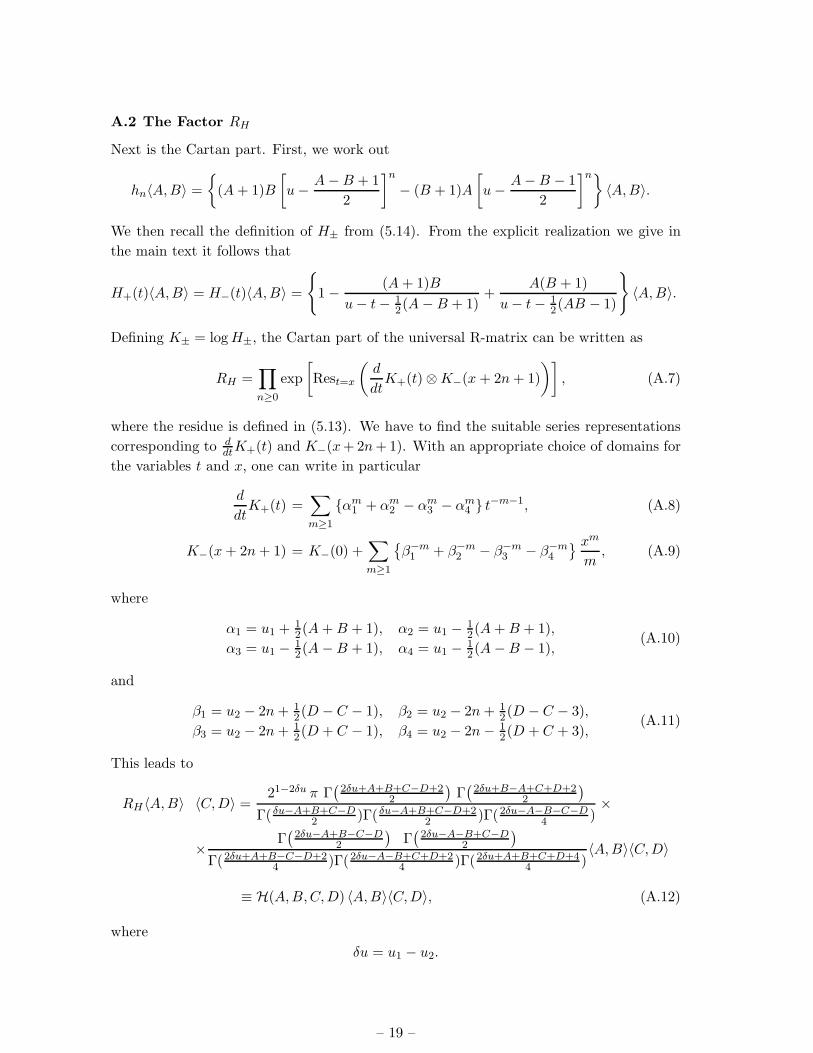
A.2 The Factor RH

Next is the Cartan part. First, we work out

hn〈A,B〉 =

{(A + 1)B

[u −

A − B + 1

2

]n

− (B + 1)A

[u −

A − B − 1

2

]n}〈A,B〉.

We then recall the definition of H± from (5.14). From the explicit realization we give in

the main text it follows that

H+(t)〈A,B〉 = H−(t)〈A,B〉 =

{

1 −(A + 1)B

u − t − 12(A − B + 1)

+A(B + 1)

u − t − 12(AB − 1)

}

〈A,B〉.

Defining K± = log H±, the Cartan part of the universal R-matrix can be written as

RH =∏

n≥0

exp

[Rest=x

(d

dtK+(t) ⊗ K−(x + 2n + 1)

)], (A.7)

where the residue is defined in (5.13). We have to find the suitable series representations

corresponding to ddtK+(t) and K−(x + 2n + 1). With an appropriate choice of domains for

the variables t and x, one can write in particular

d

dtK+(t) =

∑

m≥1

{αm1 + αm

2 − αm3 − αm

4 } t−m−1, (A.8)

K−(x + 2n + 1) = K−(0) +∑

m≥1

{β−m

1 + β−m2 − β−m

3 − β−m4

} xm

m, (A.9)

where

α1 = u1 + 12(A + B + 1), α2 = u1 −

12(A + B + 1),

α3 = u1 −12(A − B + 1), α4 = u1 −

12(A − B − 1),

(A.10)

and

β1 = u2 − 2n + 12(D − C − 1), β2 = u2 − 2n + 1

2(D − C − 3),

β3 = u2 − 2n + 12(D + C − 1), β4 = u2 − 2n − 1

2(D + C + 3),(A.11)

This leads to

RH〈A,B〉 〈C,D〉 =21−2δu π Γ

(2δu+A+B+C−D+2

2

)Γ(

2δu+B−A+C+D+22

)

Γ( δu−A+B+C−D2 )Γ( δu−A+B+C−D+2

2 )Γ(2δu−A−B−C−D4 )

×

×Γ(

2δu−A+B−C−D2

)Γ(

2δu−A−B+C−D2

)

Γ(2δu+A+B−C−D+24 )Γ(2δu−A−B+C+D+2

4 )Γ(2δu+A+B+C+D+44 )

〈A,B〉〈C,D〉

≡ H(A,B,C,D) 〈A,B〉〈C,D〉, (A.12)

where

δu = u1 − u2.

– 19 –

A.3 The Factor RE

We will now compute RE. One has

→∏

n≥0

exp[−en ⊗ f−1−n]|k, l〉 =∑

m

Bm|k + m, l − m〉. (A.13)

Let us define as in the main text

ci = u2 −C − D + 1

2− i, (A.14)

di = u1 −A − B − 1

2+ i. (A.15)

The term Bm is this time built up out of m copies of −e⊗f acting on the state 〈A,B〉〈C,D〉.

One has

enm . . . en2en1〈A,B〉 = enm . . . e

(u +

h + 1

2

)n2

e

(u +

h + 1

2

)n1

〈A,B〉

= enm . . . e

(u +

h + 1

2

)n2

e(d0

)n1

〈A,B〉

= A(d0

)n1

enm . . . e

(u +

h + 1

2

)n2

〈A − 1, B + 1〉

= A(A − 1)(d0

)n1(d1

)n2

enm . . . en3〈A − 2, B + 2〉

=A!

(A − m)!dn10 . . . dnm

m−1〈A − m,B + m〉. (A.16)

Similar expressions hold for fn acting on 〈C,D〉, with ci instead of di, and producing the

state 〈C + m,D − m〉. From the ordered exponential (A.13) we have now ni ≤ ni−1. In

case ni = ni+1, we again pick up the same combinatorial factor as in the calculation of RF ,

coming from the series of the exponential. Putting all of this together, we find

Bm =A!

(A − m)!

D!

(D − m)!

∑

n1≥...≥nm

1

N({n1, . . . , nm})

dn10

cn1+10

. . .dnm

m−1

cnm+1m−1

,

N({n1, . . . , nm}) =1

ordS({n1, . . . , nm}), (A.17)

where N is defined as in the formulas for RF . The sum evaluates at

Bm(A,B,C,D) = m!

(A

m

)(D

m

) m−1∏

i=0

1

d0 − c0 − i + m − 1. (A.18)

References

[1] J. A. Minahan and K. Zarembo, The Bethe-ansatz for N = 4 super Yang-Mills, JHEP 03

(2003) 013, [hep-th/0212208].

[2] V. A. Kazakov, A. Marshakov, J. A. Minahan, and K. Zarembo, Classical / quantum

integrability in AdS/CFT , JHEP 05 (2004) 024, [hep-th/0402207].

– 20 –

[3] N. Beisert, V. Dippel, and M. Staudacher, A novel long range spin chain and planar N = 4

super Yang- Mills, JHEP 07 (2004) 075, [hep-th/0405001].

[4] G. Arutyunov, S. Frolov, and M. Staudacher, Bethe ansatz for quantum strings, JHEP 10

(2004) 016, [hep-th/0406256].

[5] M. Staudacher, The factorized S-matrix of CFT/AdS, JHEP 05 (2005) 054,

[hep-th/0412188].

[6] N. Beisert and M. Staudacher, Long-range psu(2, 2|4) Bethe ansaetze for gauge theory and

strings, Nucl. Phys. B727 (2005) 1–62, [hep-th/0504190].

[7] N. Beisert, The su(2|2) dynamic S-matrix, Adv. Theor. Math. Phys. 12 (2008) 945,

[hep-th/0511082].

[8] D. M. Hofman and J. M. Maldacena, Giant magnons, J. Phys. A39 (2006) 13095–13118,

[hep-th/0604135].

[9] G. Arutyunov, S. Frolov, J. Plefka, and M. Zamaklar, The off-shell symmetry algebra of the

light-cone AdS5 × S 5 superstring, J. Phys. A40 (2007) 3583–3606, [hep-th/0609157].

[10] T. Klose, T. McLoughlin, R. Roiban, and K. Zarembo, Worldsheet scattering in AdS5 × S 5,

JHEP 03 (2007) 094, [hep-th/0611169].

[11] G. Arutyunov and S. Frolov, Foundations of the AdS5 × S 5 Superstring. Part I,

arXiv:0901.4937.

[12] R. A. Janik, The AdS5 × S 5 superstring worldsheet S-matrix and crossing symmetry, Phys.

Rev. D73 (2006) 086006, [hep-th/0603038].

[13] N. Beisert, R. Hernandez, and E. Lopez, A crossing-symmetric phase for AdS5 × S 5 strings,

JHEP 11 (2006) 070, [hep-th/0609044].

[14] N. Beisert, B. Eden, and M. Staudacher, Transcendentality and crossing, J. Stat. Mech. 0701

(2007) P021, [hep-th/0610251].

[15] Z. Bajnok and R. A. Janik, Four-loop perturbative Konishi from strings and finite size effects

for multiparticle states, Nucl. Phys. B807 (2009) 625–650, [arXiv:0807.0399].

[16] F. Fiamberti, A. Santambrogio, C. Sieg, and D. Zanon, Wrapping at four loops in N=4 SYM,

Phys. Lett. B666 (2008) 100–105, [arXiv:0712.3522].

[17] B. I. Zwiebel, Iterative Structure of the N=4 SYM Spin Chain, JHEP 07 (2008) 114,

[arXiv:0806.1786].

[18] Z. Bajnok, R. A. Janik, and T. Lukowski, Four loop twist two, BFKL, wrapping and strings,

arXiv:0811.4448.

[19] G. Arutyunov and S. Frolov, String hypothesis for the AdS 5 × S 5 mirror, arXiv:0901.1417.

[20] N. Gromov, V. Kazakov, and P. Vieira, Integrability for the Full Spectrum of Planar

AdS/CFT, arXiv:0901.3753.

[21] T. Bargheer, N. Beisert, and F. Loebbert, Long-Range Deformations for Integrable Spin

Chains, arXiv:0902.0956.

[22] D. Bombardelli, D. Fioravanti, and R. Tateo, Thermodynamic Bethe Ansatz for planar

AdS/CFT: a proposal, arXiv:0902.3930.

– 21 –

[23] N. Gromov, V. Kazakov, A. Kozak, and P. Vieira, Integrability for the Full Spectrum of

Planar AdS/CFT II, arXiv:0902.4458.

[24] G. Arutyunov and S. Frolov, Thermodynamic Bethe Ansatz for the AdS 5 × S 5 Mirror Model,

arXiv:0903.0141.

[25] G. Arutyunov, M. de Leeuw, and A. Torrielli, The Bound State S-Matrix for AdS5 × S 5

Superstring, arXiv:0902.0183.

[26] N. Dorey, Magnon bound states and the AdS/CFT correspondence, J. Phys. A39 (2006)

13119–13128, [hep-th/0604175].

[27] J. M. Drummond, J. M. Henn, and J. Plefka, Yangian symmetry of scattering amplitudes in

N=4 super Yang-Mills theory, arXiv:0902.2987.

[28] A. Torrielli, Classical r-matrix of the su(2|2) SYM spin-chain, Phys. Rev. D75 (2007)

105020, [hep-th/0701281].

[29] N. Beisert, The S-Matrix of AdS/CFT and Yangian Symmetry, PoS SOLVAY (2006) 002,

[0704.0400].

[30] M. de Leeuw, Bound States, Yangian Symmetry and Classical r-matrix for the AdS5 × S 5

Superstring, JHEP 06 (2008) 085, [arXiv:0804.1047].

[31] S. Moriyama and A. Torrielli, A Yangian Double for the AdS/CFT Classical r-matrix, JHEP

06 (2007) 083, [0706.0884].

[32] T. Matsumoto, S. Moriyama, and A. Torrielli, A Secret Symmetry of the AdS/CFT S-matrix,

JHEP 09 (2007) 099, [arXiv:0708.1285].

[33] N. Beisert and F. Spill, The Classical r-matrix of AdS/CFT and its Lie Bialgebra Structure,

Commun. Math. Phys. 285 (2009) 537–565, [arXiv:0708.1762].

[34] F. Spill and A. Torrielli, On Drinfeld’s second realization of the AdS/CFT su(2|2) Yangian,

J. Geom. Phys. (in press) [arXiv:0803.3194].

[35] T. Matsumoto and S. Moriyama, An Exceptional Algebraic Origin of the AdS/CFT Yangian

Symmetry, JHEP 04 (2008) 022, [arXiv:0803.1212].

[36] M. de Leeuw, The Bethe Ansatz for AdS5 × S 5 Bound States, JHEP 01 (2009) 005,

[arXiv:0809.0783].

[37] F. Spill, Weakly coupled N=4 Super Yang-Mills and N=6 Chern-Simons theories from u(2|2)

Yangian symmetry, arXiv:0810.3897.

[38] T. Matsumoto and S. Moriyama, Serre Relation and Higher Grade Generators of the

AdS/CFT Yangian Symmetry, arXiv:0902.3299.

[39] G. Arutyunov and S. Frolov, On String S-matrix, Bound States and TBA, JHEP 12 (2007)

024, [0710.1568].

[40] V. G. Drinfeld, Quasi-Hopf algebras, Leningrad Math. J. 1 (1990) 1419.

[41] S. M. Khoroshkin and V. N. Tolstoy, Yangian double and rational R matrix, hep-th/9406194.

[42] G. Arutyunov and S. Frolov, The S-matrix of String Bound States, Nucl. Phys. B804 (2008)

90–143, [arXiv:0803.4323].

[43] P. P. Kulish, N. Y. Reshetikhin, and E. K. Sklyanin, Yang-Baxter Equation and

Representation Theory. 1, Lett. Math. Phys. 5 (1981) 393–403.

– 22 –

[44] V. Chari and A. Pressley, A Guide To Quantum Groups, Cambridge, UK: Univ. Press (1994).

[45] H.-Y. Chen, N. Dorey, and K. Okamura, On the scattering of magnon boundstates, JHEP 11

(2006) 035, [hep-th/0608047].

[46] C. Gomez and R. Hernandez, The magnon kinematics of the AdS/CFT correspondence,

JHEP 11 (2006) 021, [hep-th/0608029].

[47] J. Plefka, F. Spill, and A. Torrielli, On the Hopf algebra structure of the AdS/CFT S-matrix,

Phys. Rev. D74 (2006) 066008, [hep-th/0608038].

[48] G. Arutyunov, S. Frolov, and M. Zamaklar, The Zamolodchikov-Faddeev algebra for

AdS 5 × S 5 superstring, JHEP 04 (2007) 002, [hep-th/0612229].

[49] N. Beisert, An SU(1|1)-invariant S-matrix with dynamic representations, Bulg. J. Phys.

33S1 (2006) 371–381, [hep-th/0511013].

[50] V. Stukopin, Yangians of classical lie superalgebras: Basic constructions, quantum double and

universal R-matrix, Proceedings of the Institute of Mathematics of NAS of Ukraine 50 (2004)

1195.

[51] I. Heckenberger, F. Spill, A. Torrielli, and H. Yamane, Drinfeld second realization of the

quantum affine superalgebras of D(1)(2, 1 : x) via the Weyl groupoid, RIMS Kokyuroku

Bessatsu B8 (2008) 171–216, [arXiv:0705.1071].

[52] L. Gow, Gauss Decomposition of the Yangian Y (gl(m|n)), Commun. Math. Phys. 276 (2007)

799–825.

[53] P. Etingof and O. Schiffman, Lectures on Quantum Groups, Lectures in Mathematical

Physics, International Press, Boston (1998).

[54] N. J. MacKay, Introduction to Yangian symmetry in integrable field theory, Int. J. Mod.

Phys. A20 (2005) 7189–7218, [hep-th/0409183].

[55] A. Molev, Yangians and Classical Lie Algebras, Mathematical Surveys and Monographs 143,

American Mathematical Society, Providence, RI (2007).

[56] V. G. Drinfeld, Quantum groups, Proc. of the International Congress of Mathematicians,

Berkeley, 1986, American Mathematical Society (1987) 798.

[57] V. G. Drinfeld, A new realization of Yangians and quantum affine algebras, Soviet Math.

Dokl. 36 (1988) 212.

[58] S. M. Khoroshkin and V. N. Tolstoy, Universal R-matrix for quantized (super)algebras,

Commun. Math. Phys. 276 (1991) 599–617.

[59] J. Cai, S. Wang, K. Wu, and C. Xiong, Universal R-matrix Of The Super Yangian Double

DY (gl(1|1)), Comm. Theor. Phys. 29 (1998) 173–176, [q-alg/9709038].

[60] A. Torrielli, Structure of the string R-matrix, J. Phys. A42 (2009) 055204,

[arXiv:0806.1299].

– 23 –