UNIT-IV NOTES

Basic Concepts

Frequent pattern mining searches for recurring relationships in a given data set. It introduces the basic concepts of

frequent pattern mining for the discovery of interesting associations and correlations between itemsets in transactional and

relational databases.

Market Basket Analysis: A Motivating Example

Figure 5.1 Market basket analysis.

A typical example of frequent itemset mining is market basket analysis. This process analyzes customer buying habits

by finding associations between the different items that customers place in their ―shopping baskets‖ (Figure 5.1). The discovery

of such associations can help retailers develop marketing strategies by gaining insight into which items are frequently

purchased together by customers. For instance, if customers are buying milk, how likely are they to also buy bread (and what

kind of bread) on the same trip to the supermarket? Such information can lead to increased sales by helping retailers do

selective marketing and plan their shelf space.

www.getmyuni.com

UNIT IV ASSOCIATION RULE MINING AND CLASSIFICATION 11

Mining Frequent Patterns, Associations and Correlations – Mining Methods – Mining

Various Kinds of Association Rules – Correlation Analysis – Constraint Based

Association Mining – Classification and Prediction – Basic Concepts – Decision Tree

Induction – Bayesian Classification – Rule Based Classification – Classification by

Backpropagation – Support Vector Machines – Associative Classification – Lazy

Learners – Other Classification Methods – Prediction

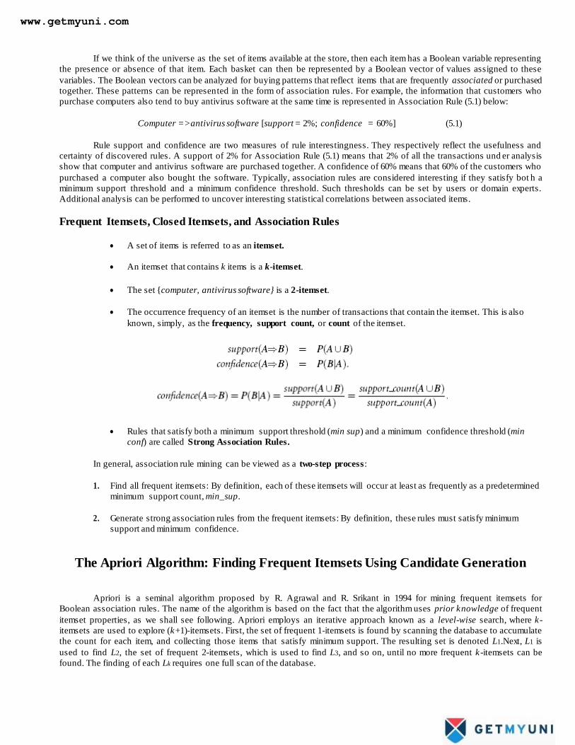
If we think of the universe as the set of items available at the store, then each item has a Boolean variable representing

the presence or absence of that item. Each basket can then be represented by a Boolean vector of values assigned to these

variables. The Boolean vectors can be analyzed for buying patterns that reflect items that are frequently associated or purchased

together. These patterns can be represented in the form of association rules. For example, the information that customers who

purchase computers also tend to buy antivirus software at the same time is represented in Association Rule (5.1) below:

Computer =>antivirus software [support = 2%; confidence = 60%] (5.1)

Rule support and confidence are two measures of rule interestingness. They respectively reflect the usefulness and

certainty of discovered rules. A support of 2% for Association Rule (5.1) means that 2% of all the transactions und er analysis

show that computer and antivirus software are purchased together. A confidence of 60% means that 60% of the customers who

purchased a computer also bought the software. Typically, association rules are considered interesting if they satisfy bot h a

minimum support threshold and a minimum confidence threshold. Such thresholds can be set by users or domain experts.

Additional analysis can be performed to uncover interesting statistical correlations between associated items.

Frequent Itemsets, Closed Itemsets, and Association Rules

A set of items is referred to as an itemset.

An itemset that contains k items is a k-itemset.

The set {computer, antivirus software} is a 2-itemset.

The occurrence frequency of an itemset is the number of transactions that contain the itemset. This is also

known, simply, as the frequency, support count, or count of the itemset.

Rules that satisfy both a minimum support threshold (min sup) and a minimum confidence threshold (min

conf) are called Strong Association Rules.

In general, association rule mining can be viewed as a two-step process:

1. Find all frequent itemsets: By definition, each of these itemsets will occur at least as frequently as a predetermined

minimum support count, min_sup.

2. Generate strong association rules from the frequent itemsets: By definition, these rules must satisfy minimum

support and minimum confidence.

The Apriori Algorithm: Finding Frequent Itemsets Using Candidate Generation

Apriori is a seminal algorithm proposed by R. Agrawal and R. Srikant in 1994 for mining frequent itemsets for

Boolean association rules. The name of the algorithm is based on the fact that the algorithm uses prior knowledge of frequent

itemset properties, as we shall see following. Apriori employs an iterative approach known as a level-wise search, where k-

itemsets are used to explore (k+1)-itemsets. First, the set of frequent 1-itemsets is found by scanning the database to accumulate

the count for each item, and collecting those items that satisfy minimum support. The resulting set is denoted L1.Next, L1 is

used to find L2, the set of frequent 2-itemsets, which is used to find L3, and so on, until no more frequent k-itemsets can be

found. The finding of each Lk requires one full scan of the database.

www.getmyuni.com

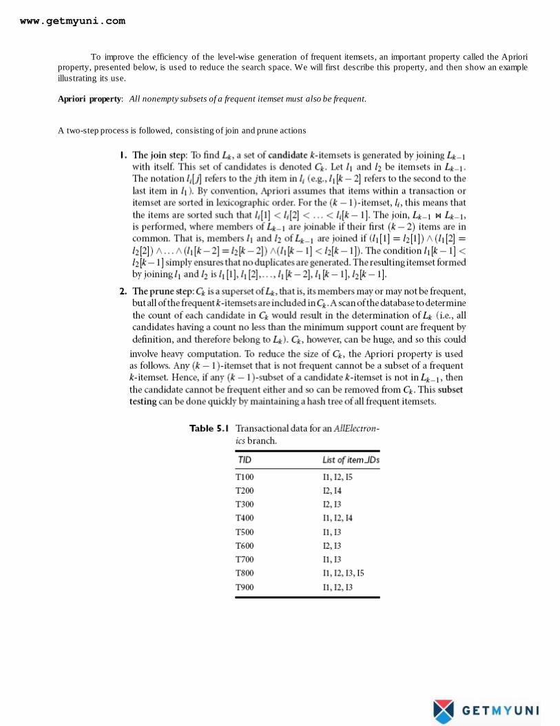
To improve the efficiency of the level-wise generation of frequent itemsets, an important property called the Apriori

property, presented below, is used to reduce the search space. We will first describe this property, and then show an example

illustrating its use.

Apriori property: All nonempty subsets of a frequent itemset must also be frequent.

A two-step process is followed, consisting of join and prune actions

www.getmyuni.com

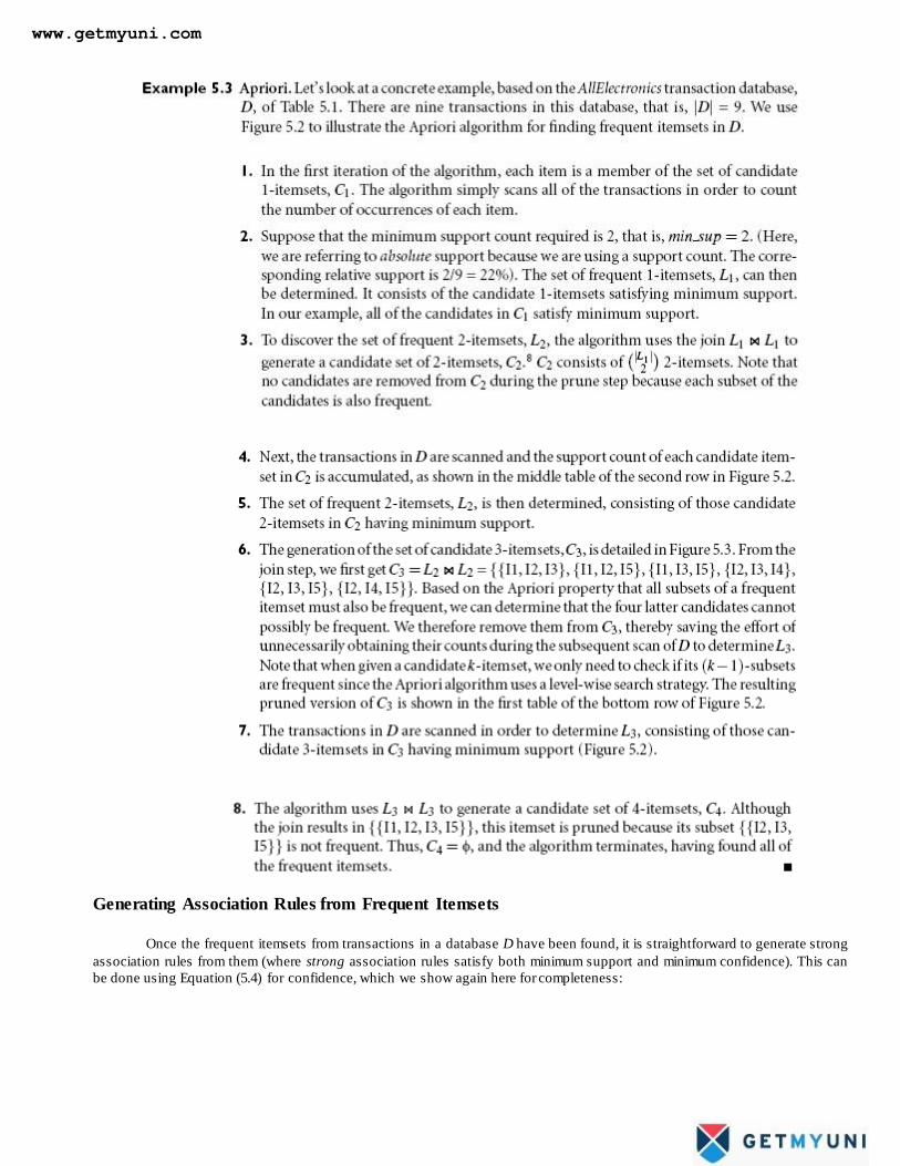
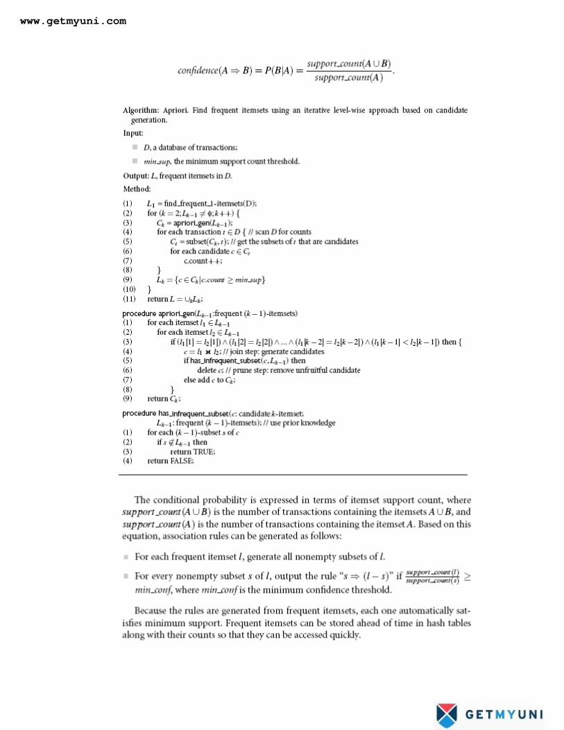
Generating Association Rules from Frequent Itemsets

Once the frequent itemsets from transactions in a database D have been found, it is straightforward to generate strong

association rules from them (where strong association rules satisfy both minimum support and minimum confidence). This can

be done using Equation (5.4) for confidence, which we show again here for completeness:

www.getmyuni.com

www.getmyuni.com

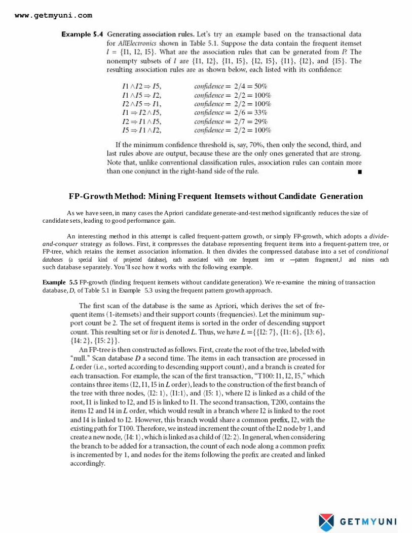
FP-Growth Method: Mining Frequent Itemsets without Candidate Generation

As we have seen, in many cases the Apriori candidate generate-and-test method significantly reduces the size of

candidate sets, leading to good performance gain.

An interesting method in this attempt is called frequent-pattern growth, or simply FP-growth, which adopts a divide-

and-conquer strategy as follows. First, it compresses the database representing frequent items into a frequent-pattern tree, or

FP-tree, which retains the itemset association information. It then divides the compressed database into a set of conditional

databases (a special kind of projected database), each associated with one frequent item or ―pattern fragment,‖ and mines each

such database separately. You’ll see how it works with the following example.

Example 5.5 FP-growth (finding frequent itemsets without candidate generation). We re-examine the mining of transaction

database, D, of Table 5.1 in Example 5.3 using the frequent pattern growth approach.

www.getmyuni.com

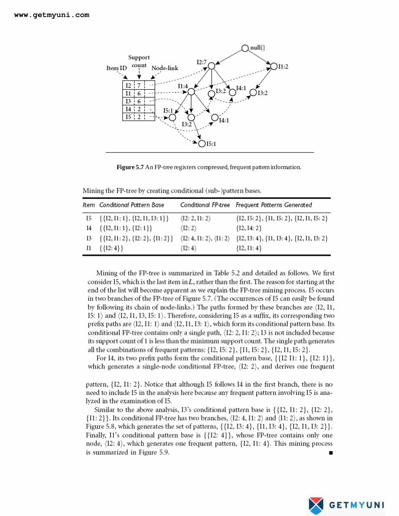
Figure 5.7 An FP-tree registers compressed, frequent pattern information.

www.getmyuni.com

Figure 5.9 The FP-growth algorithm for discovering frequent itemsets without candidate generation.

Also Read Example problems which we solved in Class Lecture

Mining Various Kinds of Association Rules

1) Mining Multilevel Association Rules

For many applications, it is difficult to find strong associations among data items at low or primitive levels of

abstraction due to the sparsity of data at those levels. Strong associations discovered at high levels of abstraction may represent

commonsense knowledge. Moreover, what may represent common sense to one user may seem novel to another. Therefore,

data mining systems should provide capabilities for mining association rules at multiple levels of abstraction, with sufficient

flexibility for easy traversal among different abstraction spaces.

Let’s examine the following example.

Mining multilevel association rules. Suppose we are given the task-relevant set of transactional data in Table for sales

in an AllElectronics store, showing the items purchased for each transaction. The concept hierarchy for the items is shown in

Figure 5.10. A concept hierarchy defines a sequence of mappings from a set of low-level concepts to higher level, more general

concepts. Data can be generalized by replacing low-level concepts

within the data by their higher-level concepts, or ancestors, from a concept hierarchy.

www.getmyuni.com

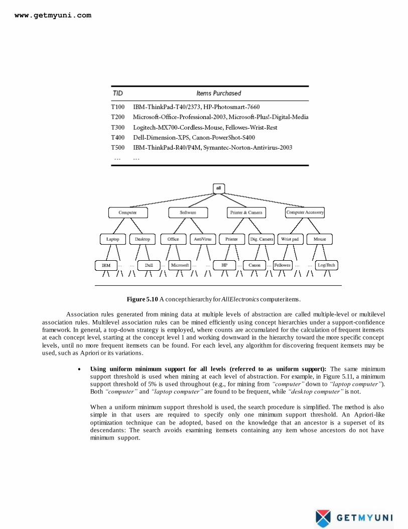
Figure 5.10 A concept hierarchy for AllElectronics computer items.

Association rules generated from mining data at multiple levels of abstraction are called multiple-level or multilevel

association rules. Multilevel association rules can be mined efficiently using concept hierarchies under a support-confidence

framework. In general, a top-down strategy is employed, where counts are accumulated for the calculation of frequent itemsets

at each concept level, starting at the concept level 1 and working downward in the hierarchy toward the more specific concept

levels, until no more frequent itemsets can be found. For each level, any algorithm for discovering frequent itemsets may be

used, such as Apriori or its variations.

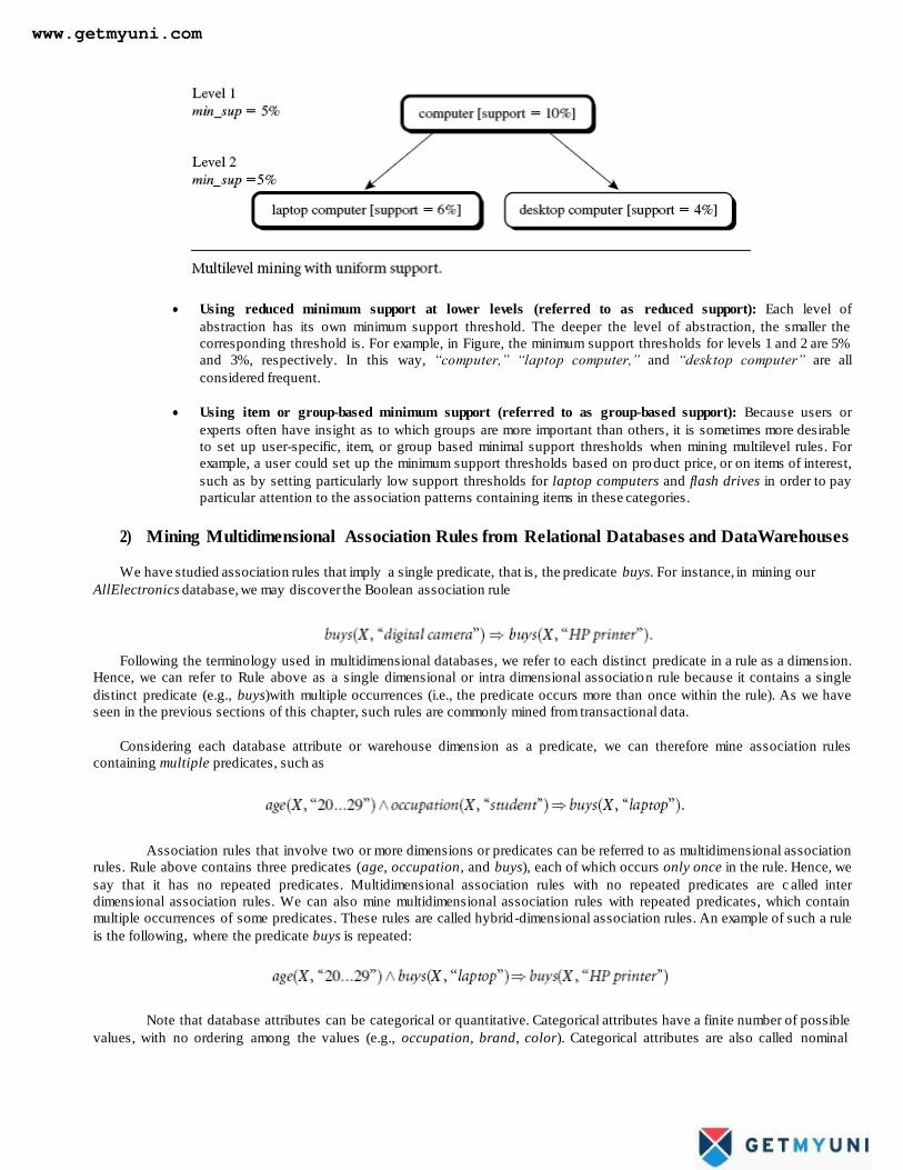
Using uniform minimum support for all levels (referred to as uniform support): The same minimum

support threshold is used when mining at each level of abstraction. For example, in Figure 5.11, a minimum

support threshold of 5% is used throughout (e.g., for mining from “computer” down to “laptop computer”).

Both “computer” and “laptop computer” are found to be frequent, while “desktop computer” is not.

When a uniform minimum support threshold is used, the search procedure is simplified. The method is also

simple in that users are required to specify only one minimum support threshold. An Apriori-like

optimization technique can be adopted, based on the knowledge that an ancestor is a superset of its

descendants: The search avoids examining itemsets containing any item whose ancestors do not have

minimum support.

www.getmyuni.com

Using reduced minimum support at lower levels (referred to as reduced support): Each level of

abstraction has its own minimum support threshold. The deeper the level of abstraction, the smaller the

corresponding threshold is. For example, in Figure, the minimum support thresholds for levels 1 and 2 are 5%

and 3%, respectively. In this way, “computer,” “laptop computer,” and “desktop computer” are all

considered frequent.

Using item or group-based minimum support (referred to as group-based support): Because users or

experts often have insight as to which groups are more important than others, it is sometimes more desirable

to set up user-specific, item, or group based minimal support thresholds when mining multilevel rules. For

example, a user could set up the minimum support thresholds based on product price, or on items of interest,

such as by setting particularly low support thresholds for laptop computers and flash drives in order to pay

particular attention to the association patterns containing items in these categories.

2) Mining Multidimensional Association Rules from Relational Databases and DataWarehouses

We have studied association rules that imply a single predicate, that is, the predicate buys. For instance, in mining our

AllElectronics database, we may discover the Boolean association rule

Following the terminology used in multidimensional databases, we refer to each distinct predicate in a rule as a dimension.

Hence, we can refer to Rule above as a single dimensional or intra dimensional association rule because it contains a single

distinct predicate (e.g., buys)with multiple occurrences (i.e., the predicate occurs more than once within the rule). As we have

seen in the previous sections of this chapter, such rules are commonly mined from transactional data.

Considering each database attribute or warehouse dimension as a predicate, we can therefore mine association rules

containing multiple predicates, such as

Association rules that involve two or more dimensions or predicates can be referred to as multidimensional association

rules. Rule above contains three predicates (age, occupation, and buys), each of which occurs only once in the rule. Hence, we

say that it has no repeated predicates. Multidimensional association rules with no repeated predicates are c alled inter

dimensional association rules. We can also mine multidimensional association rules with repeated predicates, which contain

multiple occurrences of some predicates. These rules are called hybrid -dimensional association rules. An example of such a rule

is the following, where the predicate buys is repeated:

Note that database attributes can be categorical or quantitative. Categorical attributes have a finite number of possible

values, with no ordering among the values (e.g., occupation, brand, color). Categorical attributes are also called nominal

www.getmyuni.com

attributes, because their values are ―names of things.‖ Quantitative attributes are numeric and have an implicit ordering among

values (e.g., age, income, price). Techniques for mining multidimensional association rules can be categorized into two basic

approaches regarding the treatment of quantitative attributes.

Mining Multidimensional Association Rules Using Static Discretization of

Quantitative Attributes

Quantitative attributes, in this case, are discretized before mining using predefined concept hierarchies or data

discretization techniques, where numeric values are replaced by interval labels. Categorical attributes may also be generalized

to higher conceptual levels if desired. If the resulting task-relevant data are stored in a relational table, then any of the frequent

itemset mining algorithms we have discussed can be modified easily so as to find all frequent predicate sets rather than freq uent

itemsets. In particular, instead of searching on only one attribute like buys, we need to search through all of the relevant

attributes, treating each attribute-value pair as an itemset.

Mining Quantitative Association Rules

Quantitative association rules are multidimensional association rules in which the numeric attributes are dynamically

discretized during the mining process so as to satisfy some mining criteria, such as maximizing the confidence or compactness

of the rules mined. In this section, we focus specifically on how to mine quantitative association rules having two quantitative

attributes on the left-hand side of the rule and one categorical attribute on the right-hand side of the rule. That is,

where Aquan1 and Aquan2 are tests on quantitative attribute intervals (where the intervals are dynamically determined), and Acat

tests a categorical attribute from the task-relevant data. Such rules have been referred to as two-dimensional quantitative

association rules, because they contain two quantitative dimensions. For instance, suppose you are curious about the association

relationship between pairs of quantitative attributes, like customer age and income, and the type of television (such as high-

definition TV, i.e., HDTV) that customers like to buy. An example of such a 2-D quantitative association rule is

www.getmyuni.com

Binning: Quantitative attributes can have a very wide range of values defining their domain. Just think about how big a 2-D

grid would be if we plotted age and income as axes, where each possible value of age was assigned a unique position on one

axis, and similarly, each possible value of income was assigned a unique position on the other axis! To keep grids down to a

manageable size, we instead partition the ranges of quantitative attributes into intervals. These intervals are dynamic in that

they may later be further combined during the mining process. The partitioning process is referred to as binning, that is, wh ere

the interv als are conside re d ―bin s.‖ Three comm o n binnin g strate gie s area as follow s:

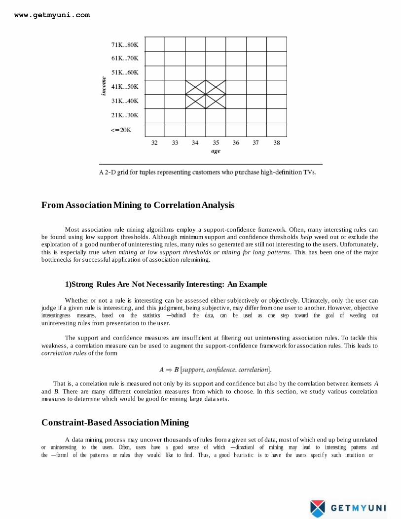
Finding frequent predicate sets: Once the 2-D array containing the count distribution for each category is set up, it can be

scanned to find the frequent predicate sets (those satisfying minimum support) that also satisfy minimum confidence. Strong

association rules can then be generated from these predicate sets, using a rule generation algorithm.

www.getmyuni.com

From Association Mining to Correlation Analysis

Most association rule mining algorithms employ a support-confidence framework. Often, many interesting rules can

be found using low support thresholds. Although minimum support and confidence thresholds help weed out or exclude the

exploration of a good number of uninteresting rules, many rules so generated are still not interesting to the users. Unfortunately,

this is especially true when mining at low support thresholds or mining for long patterns . This has been one of the major

bottlenecks for successful application of association rule mining.

1)Strong Rules Are Not Necessarily Interesting: An Example

Whether or not a rule is interesting can be assessed either subjectively or objectively. Ultimately, only the user can

judge if a given rule is interesting, and this judgment, being subjective, may differ from one user to another. However, objective

interestingness measures, based on the statistics ―behind‖ the data, can be used as one step toward the goal of weeding out

uninteresting rules from presentation to the user.

The support and confidence measures are insufficient at filtering out uninteresting association rules. To tackle this

weakness, a correlation measure can be used to augment the support -confidence framework for association rules. This leads to

correlation rules of the form

That is, a correlation rule is measured not only by its support and confidence but also by the correlation between itemsets A

and B. There are many different correlation measures from which to choose. In this section, we study various correlation

measures to determine which would be good for mining large data sets.

Constraint-Based Association Mining

A data mining process may uncover thousands of rules from a given set of data, most of which end up being unrelated

or uninteresting to the users. Often, users have a good sense of which ―direction‖ of mining may lead to interesting patterns and

the ―form‖ of the patte rn s or rules they would like to find. Thus, a good heuristic is to have the users speci f y such intuit io n or

www.getmyuni.com

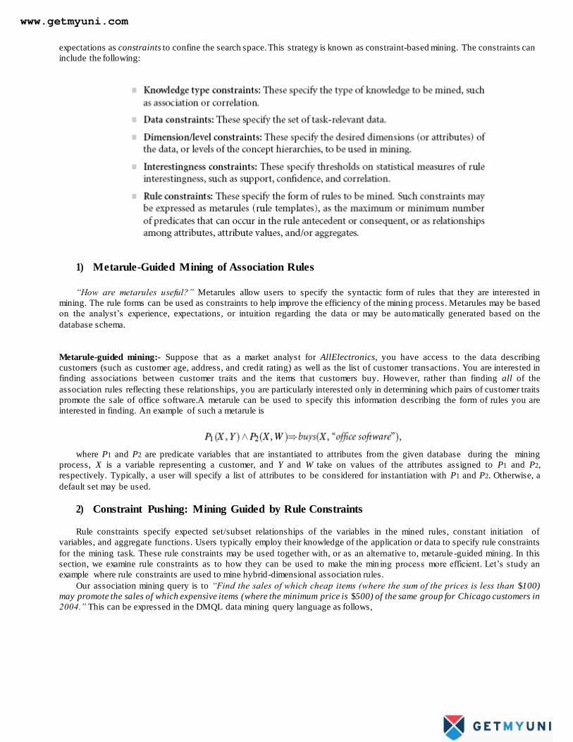
expectations as constraints to confine the search space. This strategy is known as constraint-based mining. The constraints can

include the following:

1) Metarule-Guided Mining of Association Rules

“How are metarules useful?” Metarules allow users to specify the syntactic form of rules that they are interested in

mining. The rule forms can be used as constraints to help improve the efficiency of the mining process. Metarules may be based

on the analyst’s experience, expectations, or intuition regarding the data or may be automatically generated based on the

database schema.

Metarule-guided mining:- Suppose that as a market analyst for AllElectronics, you have access to the data describing

customers (such as customer age, address, and credit rating) as well as the list of customer transactions. You are interested in

finding associations between customer traits and the items that customers buy. However, rather than finding all of the

association rules reflecting these relationships, you are particularly interested only in determining which pairs of customer traits

promote the sale of office software.A metarule can be used to specify this information describing the form of rules you are

interested in finding. An example of such a metarule is

where P1 and P2 are predicate variables that are instantiated to attributes from the given database during the mining

process, X is a variable representing a customer, and Y and W take on values of the attributes assigned to P1 and P2,

respectively. Typically, a user will specify a list of attributes to be considered for instantiation with P1 and P2. Otherwise, a

default set may be used.

2) Constraint Pushing: Mining Guided by Rule Constraints

Rule constraints specify expected set/subset relationships of the variables in the mined rules, constant initiation of

variables, and aggregate functions. Users typically employ their knowledge of the application or data to specify rule constraints

for the mining task. These rule constraints may be used together with, or as an alternative to, metarule -guided mining. In this

section, we examine rule constraints as to how they can be used to make the min ing process more efficient. Let’s study an

example where rule constraints are used to mine hybrid-dimensional association rules.

Our association mining query is to “Find the sales of which cheap items (where the sum of the prices is less than $100)

may promote the sales of which expensive items (where the minimum price is $500) of the same group for Chicago customers in

2004.” This can be expressed in the DMQL data mining query language as follows,

www.getmyuni.com

Classification and Prediction

What Is Classification? What Is Prediction?

A bank loans officer needs analysis of her data in order to learn which loan applicants are ―safe‖ and which are ―risky‖

for the bank. A marketing manager at AllElectronics needs data analysis to help guess whether a customer with a given profile

will buy a new computer. A medical researcher wants to analyze breast cancer data in order to predict which one of three

specific treatments a patient should receive. In each of these examples, the data analysis task is classification, where a model or

classifier is constructed to predict categorical labels, such as ―safe‖ or ―risky‖ for the loan application data; ―yes‖ or ―no‖ for

the marketing data; or ―treatment A,‖ ―treatment B,‖ or ―treatment C‖ for the medical data. These categories can be represented

by discrete values, where the ordering among values has no meaning. For example, the values 1, 2, and 3 may be used to

represent treatments A, B, and C, where there is no ordering implied among this group of treatment regimes.

Suppose that the marketing manager would like to predict how much a given cus tomer will spend during a sale at

AllElectronics. This data analysis task is an example of numeric prediction, where the model constructed predicts a continuous-

valued function, or ordered value, as opposed to a categorical label. This model is a predictor

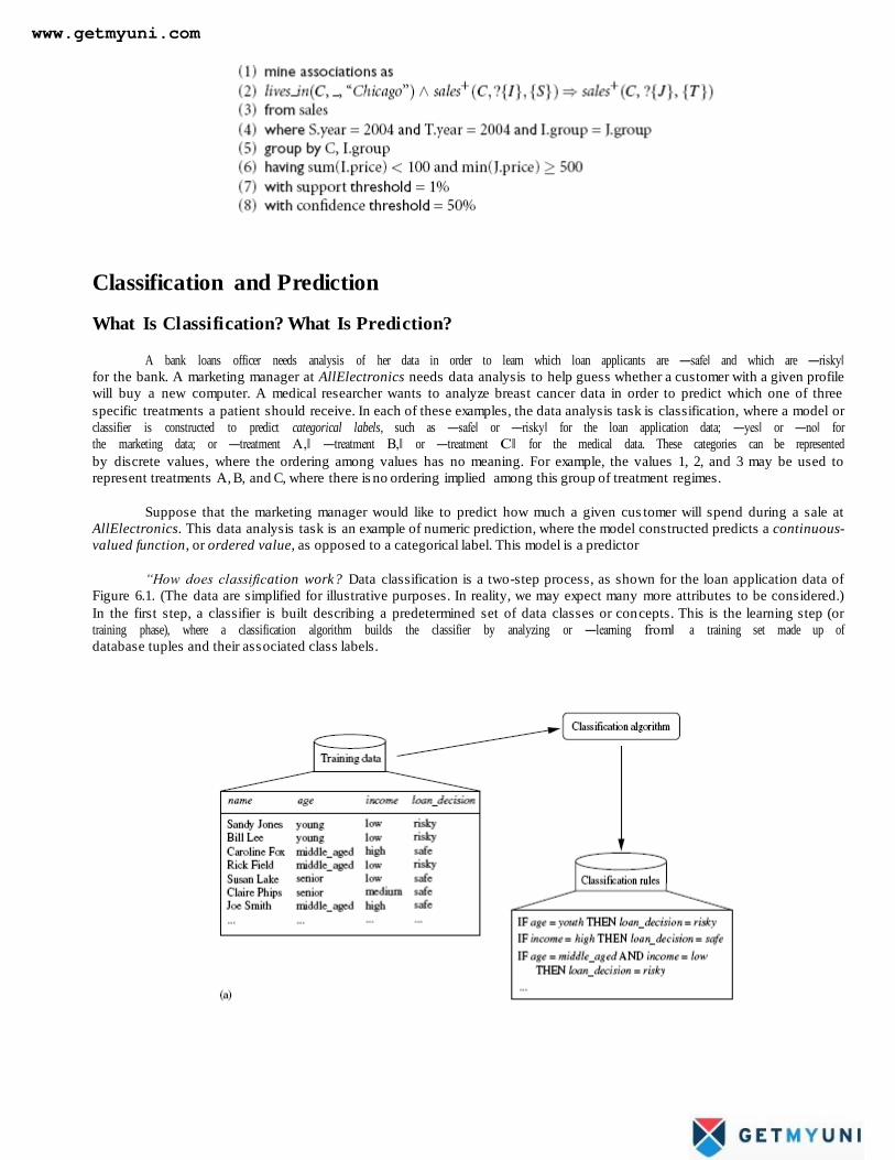
“How does classification work? Data classification is a two-step process, as shown for the loan application data of

Figure 6.1. (The data are simplified for illustrative purposes. In reality, we may expect many more attributes to be considered.)

In the first step, a classifier is built describing a predetermined set of data classes or concepts. This is the learning step (or

training phase), where a classification algorithm builds the classifier by analyzing or ―learning from‖ a training set made up of

database tuples and their associated class labels.

www.getmyuni.com

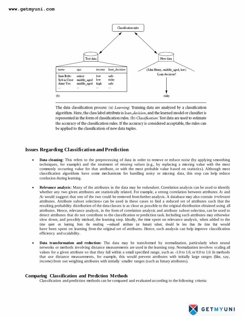
Issues Regarding Classification and Prediction

Data cleaning: This refers to the preprocessing of data in order to remove or reduce noise (by applying smoothing

techniques, for example) and the treatment of missing values (e.g., by replacing a missing value with the most

commonly occurring value for that attribute, or with the most probable value based on statistics). Although most

classification algorithms have some mechanisms for handling noisy or missing data, this step can help reduce

confusion during learning.

Relevance analysis : Many of the attributes in the data may be redundant. Correlation analysis can be used to identify

whether any two given attributes are statistically related. For example, a strong correlation between attributes A1 and

A2 would suggest that one of the two could be removed from further analysis. A database may also contain irrelevant

attributes. Attribute subset selection4 can be used in these cases to find a reduced set of attributes such that the

resulting probability distribution of the data classes is as close as possible to the original distribution obtained using all

attributes. Hence, relevance analysis, in the form of correlation analysis and attribute subset selection, can be used to

detect attributes that do not contribute to the classification or prediction task. Including such attributes may otherwise

slow down, and possibly mislead, the learning step. Ideally, the time spent on relevance analysis, when added to the

time spent on learning from the resulting ―reduced‖ attribute (or feature) subset, should be less than the time that would

have been spent on learning from the original set of attributes. Hence, such analysis can help improve classification

efficiency and scalability.

Data transformation and reduction: The data may be transformed by normalization, particularly when neural

networks or methods involving distance measurements are used in the learning step. Normalization involves scaling all

values for a given attribute so that they fall within a small specified range, such as -1.0 to 1.0, or 0.0 to 1.0. In methods

that use distance measurements, for example, this would prevent attributes with initially large ranges (like, say,

income) from out weighing attributes with initially smaller ranges (such as binary attributes).

Comparing Classification and Prediction Methods Classification and prediction methods can be compared and evaluated according to the following criteria:

www.getmyuni.com

Accuracy

Speed

Robustness

Scalability

Interpretability

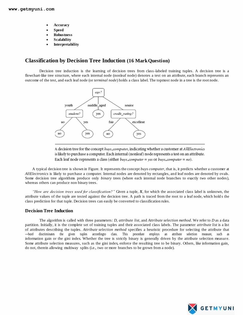
Classification by Decision Tree Induction (16 Mark Question)

Decision tree induction is the learning of decision trees from class -labeled training tuples. A decision tree is a

flowchart-like tree structure, where each internal node (nonleaf node) denotes a test on an attribute, each branch represents an

outcome of the test, and each leaf node (or terminal node) holds a class label. The topmost node in a tree is the root node.

A typical decision tree is shown in Figure. It represents the concept buys computer, that is, it predicts whether a customer at

AllElectronics is likely to purchase a computer. Internal nodes are denoted by rectangles, and leaf nodes are denoted by ovals.

Some decision tree algorithms produce only binary trees (where each internal node branches to exactly two other nodes),

whereas others can produce non binary trees.

“How are decision trees used for classification?” Given a tuple, X, for which the associated class label is unknown, the

attribute values of the tuple are tested against the decision tree. A path is traced from the root to a leaf node, which hold s the

class prediction for that tuple. Decision trees can easily be converted to classification rules.

Decision Tree Induction

The algorithm is called with three parameters: D, attribute list, and Attribute selection method. We refer to D as a data

partition. Initially, it is the complete set of training tuples and their associated class labels. The parameter attribute list is a list

of attributes describing the tuples. Attribute selection method specifies a heuristic procedure for selecting the attribute that

―best‖ discriminates the given tuples accordingto class. This procedure employs an attribute selection measure, such as

information gain or the gini index. Whether the tree is strictly binary is generally driven by the attribute selection measure.

Some attribute selection measures, such as the gini index, enforce the resulting tree to be binary. Others, like information gain,

do not, therein allowing multiway splits (i.e., two or more branches to be grown from a node).

www.getmyuni.com

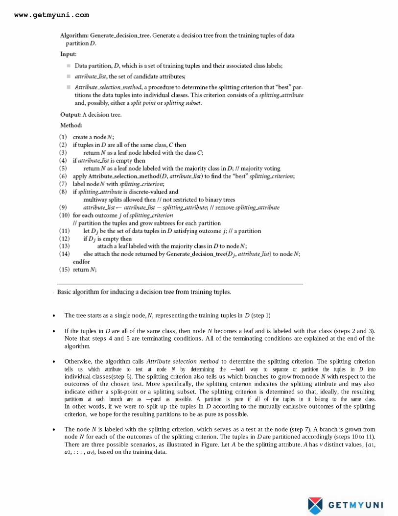
The tree starts as a single node, N, representing the training tuples in D (step 1)

If the tuples in D are all of the same class, then node N becomes a leaf and is labeled with that class (steps 2 and 3).

Note that steps 4 and 5 are terminating conditions. All of the terminating conditions are explained at the end of the

algorithm.

Otherwise, the algorithm calls Attribute selection method to determine the splitting criterion. The splitting criterion

tells us which attribute to test at node N by determining the ―best‖ way to separate or partition the tuples in D into

individual classes(step 6). The splitting criterion also tells us which branches to grow from node N with respect to the

outcomes of the chosen test. More specifically, the splitting criterion indicates the splitting attribute and may also

indicate either a split-point or a splitting subset. The splitting criterion is determined so that, ideally, the resulting

partitions at each branch are as ―pure‖ as possible. A partition is pure if all of the tuples in it belong to the same class.

In other words, if we were to split up the tuples in D according to the mutually exclusive outcomes of the splitting

criterion, we hope for the resulting partitions to be as pure as possible.

The node N is labeled with the splitting criterion, which serves as a test at the node (step 7). A branch is grown from

node N for each of the outcomes of the splitting criterion. The tuples in D are partitioned accordingly (steps 10 to 11).

There are three possible scenarios, as illustrated in Figure. Let A be the splitting attribute. A has v distinct values, {a1,

a2, : : : , av}, based on the training data.

www.getmyuni.com

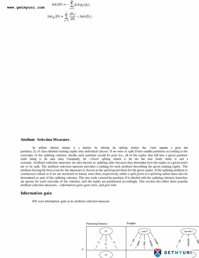
Attribute Selection Measures

An attribute selection measure is a heuristic for selecting the splitting criterion that ―best‖ separates a given data

partition, D, of class-labeled training tuples into individual classes. If we were to split D into smaller partitions according to the

outcomes of the splitting criterion, ideally each partition would be pure (i.e., all of the tuples that fall into a given partition

would belong to the same class). Conceptually, the ―best‖ splitting criterion is the one that most closely results in such a

scenario. Attribute selection measures are also known as splitting rules because they determine how the tuples at a given nod e

are to be split. The attribute selection measure provides a ranking for each attribute describing the given training tuples. The

attribute having the best score for the measure6 is chosen as the splitting attribute for the given tuples. If the splitting attribute is

continuous-valued or if we are restricted to binary trees then, respectively, either a split point or a splitting subset must also be

determined as part of the splitting criterion. The tree node created for partition D is labeled with the splitting criterion, branches

are grown for each outcome of the criterion, and the tuples are partitioned accordingly. This section des cribes three popular

attribute selection measures—information gain, gain ratio , and gini inde

Information gain

ID3 uses information gain as its attribute selection measure.

www.getmyuni.com

Information gain is defined as the difference between the original information requirement (i.e., based on just the

proportion of classes) and the new requirement (i.e., obtained after partitioning on A). That is,

In other words, Gain(A) tells us how much would be gained by branching on A. It is the expected reduction in the information

requirement caused by knowing the value of A. The attribute A with the highest information gain, (Gain(A)), is chosen as the

splitting attribute at node N.

Example 6.1 Induction of a decision tree using information gain.

Table 6.1 presents a training set, D, of class-labeled tuples randomly selected from the AllElectronics customer

database. (The data are adapted from [Qui86]. In this example, each attribute is discrete -valued. Continuous-valued attributes

have been generalized.) The class label attribute, buys computer, has two distinct values (namely, {yes, no}); therefore, there

are two distinct classes (that is, m = 2). Let class C1 correspond to yes and class C2 correspond to no. There are nine tuples of

class yes and five tuples of class no. A (root) node N is created for the tuples in D. To find the splitting criterion for these tuples,

we must compute the information gain of each attribute. We first use Equation (6.1) to compute the expected information

needed to classify a tuple in D:

The expected information needed to classify a tuple in D if the tuples are partitioned according to age is

www.getmyuni.com

Hence, the gain in information from such a partitioning would be

Similarly, we can compute Gain(income) = 0.029 bits, Gain(student) = 0.151 bits, and Gain(credit rating) = 0.048 bits.

Because age has the highest information gain among the attributes, it is selected as the splitting attribute. Node N is labeled

with age, and branches are grown for each of the attribute’s values. The tuples are then partitioned accordingly, as shown in

Figure 6.5. Notice that the tuples falling into the partition for age = middle aged all belong to the same class. Because they all

belong to class “yes,” a leaf should therefore be created at the end of this branch and labeled with “yes.” The final decision tree

returned by the algorithm is shown in Figure 6.5.

Bayesian Classification (16 mark Question )

“What are Bayesian classifiers?” Bayesian classifiers are statistical classifiers. They can predict class membership

probabilities, such as the probability that a given tuple belongs to a particular class.

Bayesian classification is based on Bayes’ theorem, described below. Studies comparing classification algorithms have found a

simple Bayesian classifier known as the naïve Bayesian classifier to be comparable in performance with decision tree and

www.getmyuni.com

selected neural network classifiers. Bayesian classifiers have also exhibited high accu racy and speed when applied to large

databases.

1) Bayes’ Theorem

Bayes’ theorem is named after Thomas Bayes, a nonconformist English clergyman who did early work in probability

and decision theory during the 18th century. Let X be a data tuple. In Bayesian terms, X is considered ―evidence.‖ As usual, it is

described by measurements made on a set of n attributes. Let H be some hypothesis, such as that the data tuple X belongs to a

specified class C. For classification problems, we want to determine P(HjX), the probability that the hypothesis H holds given

the ―evidence‖ or observed data tuple X. In other words, we are looking for the probability that tuple X belongs to class C, given

that we know the attribute description of X.

“How are these probabilities estimated?” P(H), P(XjH), and P(X) may be estimated from the given data, as we shall

see below. Bayes’ theorem is useful in that it provides a way of calculating the posterior probability, P(HjX), from P(H),

P(XjH), and P(X). Bayes’ theorem is

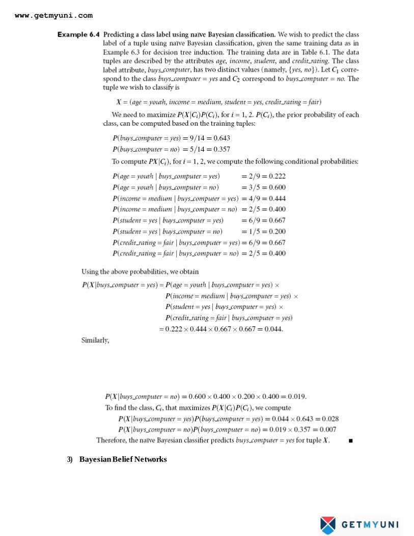
2) Naïve Bayesian Classification

www.getmyuni.com

3) Bayesian Belief Networks

www.getmyuni.com

The naïve Bayesian classifier makes the assumption of class conditional indepen dence, that is, given the class label of

a tuple, the values of the attributes are assumed to be conditionally independent of one another. This simplifies computation .

When the assumption holds true, then the naïve Bayesian classifier is the most accurate in comparison with all other classifiers.

In practice, however, dependencies can exist between variables. Bayesian belief networks specify joint conditional probabilit y

distributions. They allow class conditional independencies to be defined between subsets of variables. They provide a graphic al

model of causal relationships, on which learning can be performed. Trained Bayesian belief networks can be used for

classification. Bayesian belief networks are also known as belief networks, Bayesian networks, and probabilistic networks. Fo r

brevity, we will refer to them as belief networks.

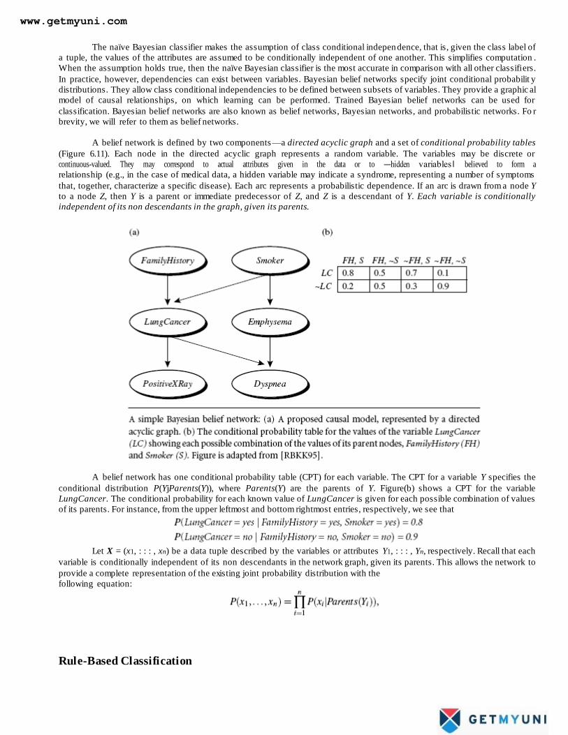
A belief network is defined by two components —a directed acyclic graph and a set of conditional probability tables

(Figure 6.11). Each node in the directed acyclic graph represents a random variable. The variables may be discrete or

continuous-valued. They may correspond to actual attributes given in the data or to ―hidden variables‖ believed to form a

relationship (e.g., in the case of medical data, a hidden variable may indicate a syndrome, representing a number of symptoms

that, together, characterize a specific disease). Each arc represents a probabilistic dependence. If an arc is drawn from a node Y

to a node Z, then Y is a parent or immediate predecessor of Z, and Z is a descendant of Y. Each variable is conditionally

independent of its non descendants in the graph, given its parents.

A belief network has one conditional probability table (CPT) for each variable. The CPT for a variable Y specifies the

conditional distribution P(YjParents(Y)), where Parents(Y) are the parents of Y. Figure(b) shows a CPT for the variable

LungCancer. The conditional probability for each known value of LungCancer is given for each possible combination of values

of its parents. For instance, from the upper leftmost and bottom rightmost entries, respectively, we see that

Let X = (x1, : : : , xn) be a data tuple described by the variables or attributes Y1, : : : , Yn, respectively. Recall that each

variable is conditionally independent of its non descendants in the network graph, given its parents. This allows the network to

provide a complete representation of the existing joint probability distribution with the

following equation:

Rule-Based Classification

www.getmyuni.com

We look at rule-based classifiers, where the learned model is represented as a set of IF-THEN rules. We first examine

how such rules are used for classification. We then study ways in which they can be generated, either from a decision tree or

directly from the training data using a sequential covering algorithm.

1) Using IF-THEN Rules for Classification

Rules are a good way of representing information or bits of knowledge. A rule-based classifier uses a set of IF-THEN rules for

classification. An IF-THEN rule is an expression of the form

IF condition THEN conclusion.

An example is rule R1,

R1: IF age = youth AND student = yes THEN buys computer = yes.

The ―IF‖-part (or left-hand side)of a rule is known as the rule antecedent or precondition. The ―THEN‖-part (or right-

hand side) is the rule consequent. In the rule antecedent, the condition consists of one or more attribute tests (such as age =

youth, and student = yes) that are logically ANDed. The rule’s consequent contains a class prediction (in this case, we are

predicting whether a customer will buy a computer). R1 can also be written as

If the condition (that is, all of the attribute tests) in a rule antecedent holds true for a given tuple, we say that the rule

antecedent is satisfied (or simply, that the rule is satisfied) and that the rule covers the tuple.

A rule R can be assessed by its coverage and accuracy. Given a tuple, X, from a class labeled data set D, let ncovers be

the number of tuples covered by R; ncorrect be the number of tuples correctly classified by R; and |D| be the number of tuples in

D. We can define the coverage and accuracy of R as

That is, a rule’s coverage is the percentage of tuples that are covered by the rule (i.e. whose attribute values hold true

for the rule’s antecedent). For a rule’s accuracy, we look at the tuples that it covers and see what percentage of them the rule

can correctly classify.

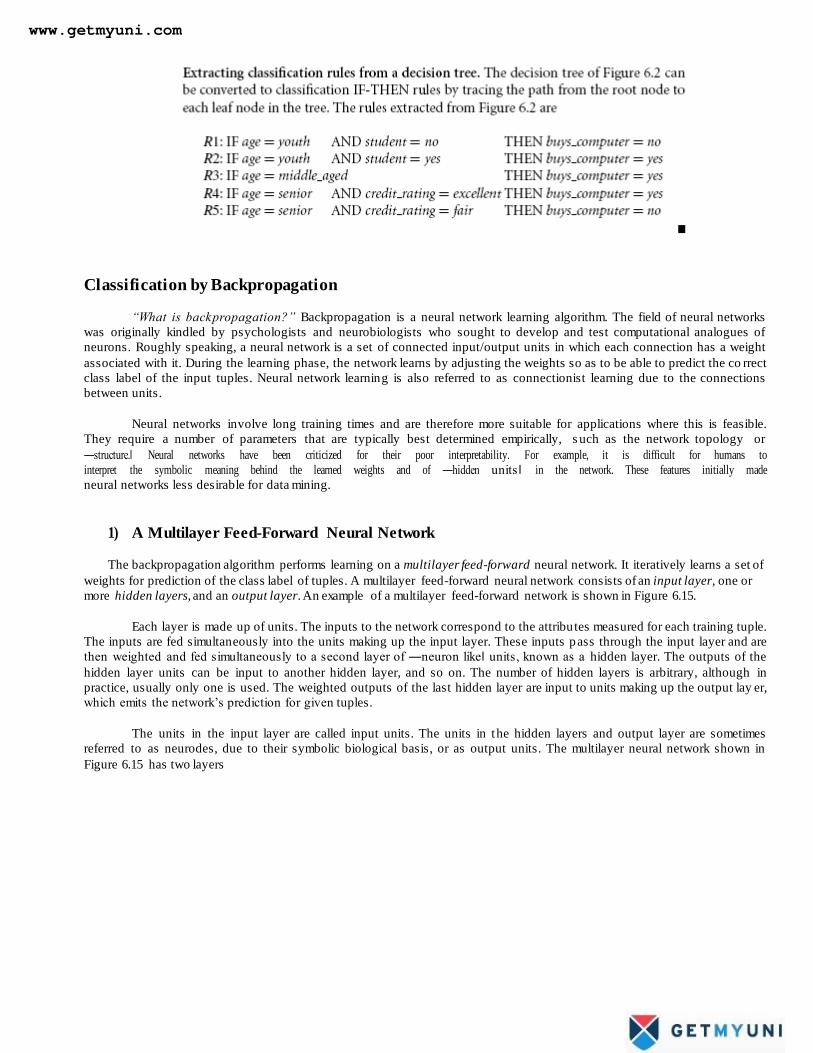
2) Rule Extraction from a Decision Tree

We learned how to build a decision tree classifier from a set of training data. Decision tree classifiers are a popular method

of classification—it is easy to understand how decision trees work and they are known for their accuracy. Decision trees can

become large and difficult to interpret. In this subsection, we look at how to build a rule based classifier by extracting IF-THEN

rules from a decision tree. In comparison with a decision tree, the IF-THEN rules may be easier for humans to understand,

particularly if the decision tree is very large.

To extract rules from a decision tree, one rule is created for each path from the root to a leaf node. Each splitting

criterion along a given path is logically ANDed to form the rule antecedent (―IF‖ part). The leaf node holds the class prediction,

formin g the rule conseq ue nt (―T H E N ‖ part ) .

www.getmyuni.com

Classification by Backpropagation

“What is backpropagation?” Backpropagation is a neural network learning algorithm. The field of neural networks

was originally kindled by psychologists and neurobiologists who sought to develop and test computational analogues of

neurons. Roughly speaking, a neural network is a set of connected input/output units in which each connection has a weight

associated with it. During the learning phase, the network learns by adjusting the weights so as to be able to predict the co rrect

class label of the input tuples. Neural network learning is also referred to as connectionist learning due to the connections

between units.

Neural networks involve long training times and are therefore more suitable for applications where this is feasible.

They require a number of parameters that are typically best determined empirically, s uch as the network topology or

―structure.‖ Neural networks have been criticized for their poor interpretability. For example, it is difficult for humans to

interpret the symbolic meaning behind the learned weights and of ―hidden units‖ in the network. These features initially made

neural networks less desirable for data mining.

1) A Multilayer Feed-Forward Neural Network

The backpropagation algorithm performs learning on a multilayer feed-forward neural network. It iteratively learns a set of

weights for prediction of the class label of tuples. A multilayer feed-forward neural network consists of an input layer, one or

more hidden layers, and an output layer. An example of a multilayer feed-forward network is shown in Figure 6.15.

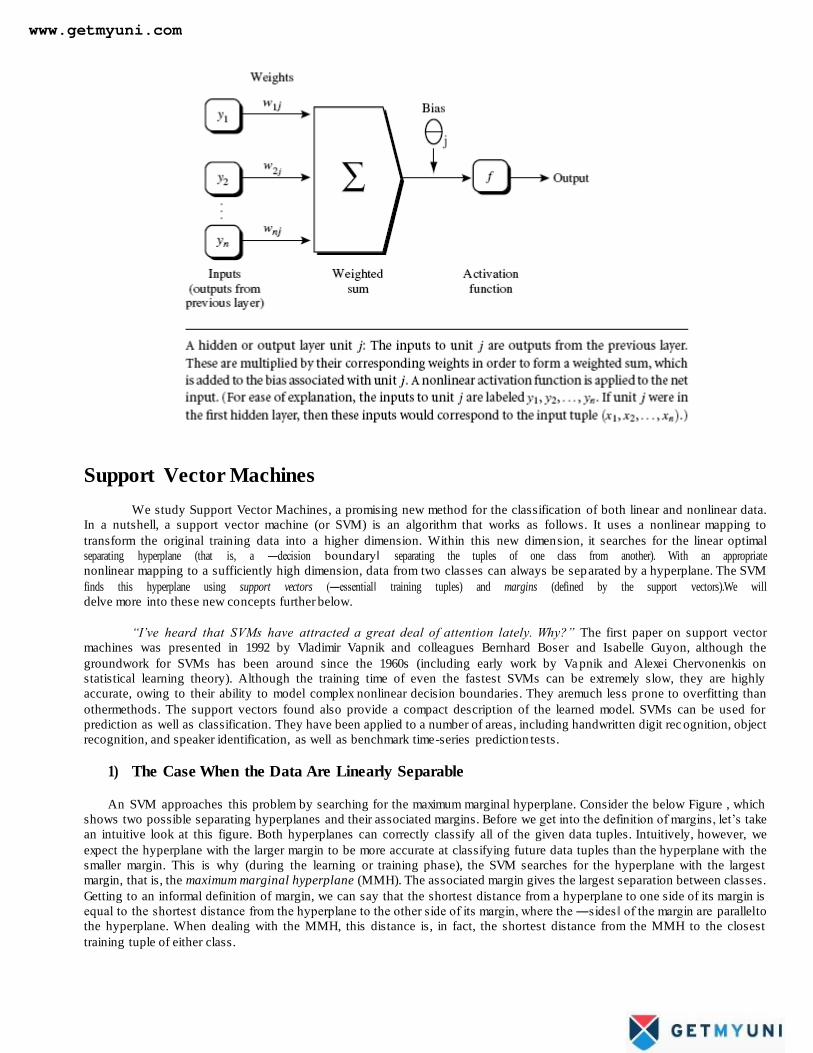
Each layer is made up of units. The inputs to the network correspond to the attributes measured for each training tuple.

The inputs are fed simultaneously into the units making up the input layer. These inputs pass through the input layer and are

then weighted and fed simultaneously to a second layer of ―neuron like‖ units, known as a hidden layer. The outputs of the

hidden layer units can be input to another hidden layer, and so on. The number of hidden layers is arbitrary, although in

practice, usually only one is used. The weighted outputs of the last hidden layer are input to units making up the output lay er,

which emits the network’s prediction for given tuples.

The units in the input layer are called input units. The units in the hidden layers and output layer are sometimes

referred to as neurodes, due to their symbolic biological basis, or as output units. The multilayer neural network shown in

Figure 6.15 has two layers

www.getmyuni.com

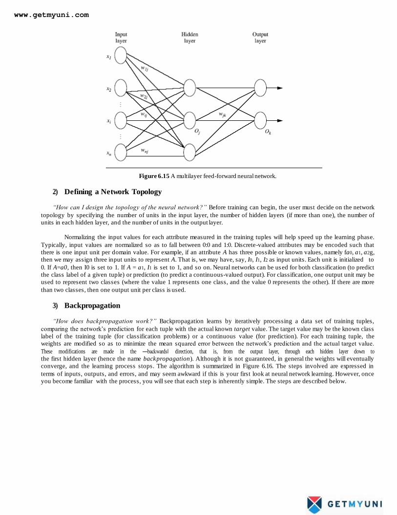
Figure 6.15 A multilayer feed-forward neural network.

2) Defining a Network Topology

“How can I design the topology of the neural network?” Before training can begin, the user must decide on the network

topology by specifying the number of units in the input layer, the number of hidden layers (if more than one), the number of

units in each hidden layer, and the number of units in the output layer.

Normalizing the input values for each attribute measured in the training tuples will help speed up the learning phase.

Typically, input values are normalized so as to fall between 0:0 and 1:0. Discrete-valued attributes may be encoded such that

there is one input unit per domain value. For example, if an attribute A has three possible or known values, namely fa0, a1, a2g,

then we may assign three input units to represent A. That is, we may have, say, I0, I1, I2 as input units. Each unit is initialized to

0. If A=a0, then I0 is set to 1. If A = a1, I1 is set to 1, and so on. Neural networks can be used for both classification (to predict

the class label of a given tuple) or prediction (to predict a continuous-valued output). For classification, one output unit may be

used to represent two classes (where the value 1 represents one class, and the value 0 represents the other). If there are more

than two classes, then one output unit per class is used.

3) Backpropagation

“How does backpropagation work?” Backpropagation learns by iteratively processing a data set of training tuples,

comparing the network’s prediction for each tuple with the actual known target value. The target value may be the known class

label of the training tuple (for classification problems) or a continuous value (for prediction). For each training tuple, the

weights are modified so as to minimize the mean squared error between the network’s prediction and the actual target value.

These modifications are made in the ―backwards‖ direction, that is, from the output layer, through each hidden layer down to

the first hidden layer (hence the name backpropagation). Although it is not guaranteed, in general the weights will eventually

converge, and the learning process stops. The algorithm is summarized in Figure 6.16. The steps involved are expressed in

terms of inputs, outputs, and errors, and may seem awkward if this is your first look at neural network learning. However, once

you become familiar with the process, you will see that each step is inherently simple. The steps are described below.

www.getmyuni.com

www.getmyuni.com

Support Vector Machines

We study Support Vector Machines, a promising new method for the classification of both linear and nonlinear data.

In a nutshell, a support vector machine (or SVM) is an algorithm that works as follows. It uses a nonlinear mapping to

transform the original training data into a higher dimension. Within this new dimension, it searches for the linear optimal

separating hyperplane (that is, a ―decision boundary‖ separating the tuples of one class from another). With an appropriate

nonlinear mapping to a sufficiently high dimension, data from two classes can always be separated by a hyperplane. The SVM

finds this hyperplane using support vectors (―essential‖ training tuples) and margins (defined by the support vectors).We will

delve more into these new concepts further below.

“I’ve heard that SVMs have attracted a great deal of attention lately. Why?” The first paper on support vector

machines was presented in 1992 by Vladimir Vapnik and colleagues Bernhard Boser and Isabelle Guyon, although the

groundwork for SVMs has been around since the 1960s (including early work by Vapnik and Alexei Chervonenkis on

statistical learning theory). Although the training time of even the fastest SVMs can be extremely slow, they are highly

accurate, owing to their ability to model complex nonlinear decision boundaries. They aremuch less prone to overfitting than

othermethods. The support vectors found also provide a compact description of the learned model. SVMs can be used for

prediction as well as classification. They have been applied to a number of areas, including handwritten digit rec ognition, object

recognition, and speaker identification, as well as benchmark time-series prediction tests.

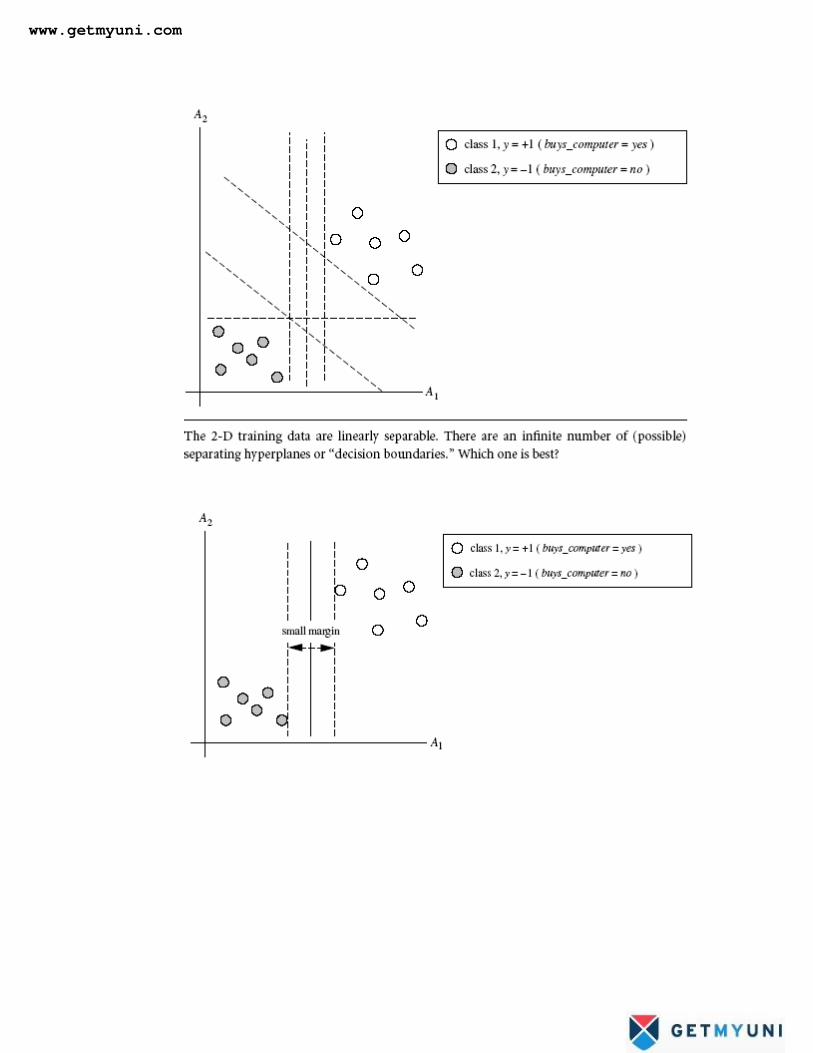
1) The Case When the Data Are Linearly Separable

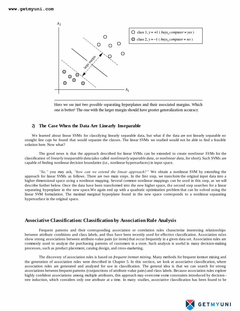
An SVM approaches this problem by searching for the maximum marginal hyperplane. Consider the below Figure , which

shows two possible separating hyperplanes and their associated margins. Before we get into the definition of margins, let’s take

an intuitive look at this figure. Both hyperplanes can correctly classify all of the given data tuples. Intuitively, however, we

expect the hyperplane with the larger margin to be more accurate at classifying future data tuples than the hyperplane with the

smaller margin. This is why (during the learning or training phase), the SVM searches for the hyperplane with the largest

margin, that is, the maximum marginal hyperplane (MMH). The associated margin gives the largest separation between classes.

Getting to an informal definition of margin, we can say that the shortest distance from a hyperplane to one side of its margin is

equal to the shortest distance from the hyperplane to the other side of its margin, where the ―sides‖ of the margin are parallel to

the hyperplane. When dealing with the MMH, this distance is, in fact, the shortest distance from the MMH to the closest

training tuple of either class.

www.getmyuni.com

www.getmyuni.com

2) The Case When the Data Are Linearly Inseparable

We learned about linear SVMs for classifying linearly separable data, but what if the data are not linearly separable no

straight line cajn be found that would separate the classes. The linear SVMs we studied would not be able to find a feasible

solution here. Now what?

The good news is that the approach described for linear SVMs can be extended to create nonlinear SVMs for the

classification of linearly inseparable data (also called nonlinearly separable data, or nonlinear data, for short). Such SVMs are

capable of finding nonlinear decision boundaries (i.e., nonlinear hypersurfaces) in input space.

“So,” you may ask, “how can we extend the linear approach?” We obtain a nonlinear SVM by extending the

approach for linear SVMs as follows. There are two main steps. In the first step, we trans form the original input data into a

higher dimensional space us ing a nonlinear mapping. Several common nonlinear mappings can be used in this step, as we will

describe further below. Once the data have been transformed into the new higher space, the second step searches for a linear

separating hyperplane in the new space.We again end up with a quadratic optimization problem that can be solved using the

linear SVM formulation. The maximal marginal hyperplane found in the new space corresponds to a nonlinear separating

hypersurface in the original space.

Associative Classification: Classification by Association Rule Analysis

Frequent patterns and their corresponding association or correlation rules characterize interesting relationships

between attribute conditions and class labels, and thus have been recently used for effective classification. Association rules

show strong associations between attribute-value pairs (or items) that occur frequently in a given data set. Association rules are

commonly used to analyze the purchasing patterns of customers in a store. Such analysis is useful in many decision-making

processes, such as product placement, catalog design, and cross-marketing.

The discovery of association rules is based on frequent itemset mining. Many methods for frequent itemset mining and

the generation of association rules were described in Chapter 5. In this sectio n, we look at associative classification, where

association rules are generated and analyzed for use in classification. The general idea is that we can search for strong

associations between frequent patterns (conjunctions of attribute-value pairs) and class labels. Because association rules explore

highly confident associations among multiple attributes, this approach may overcome some constraints introduced by decision -

tree induction, which considers only one attribute at a time. In many studies, associative classification has been found to be

www.getmyuni.com

we study three main methods: CBA,

more accurate than some traditional classification methods, such as C4.5. In particular,

CMAR, and CPAR.

Lazy Learners (or Learning from Your Neighbors)

The classification methods discussed so far in this chapter—decision tree induction, Bayesian classification, rule-based

classification, classification by backpropagation, support vector machines, and classification based on association rule mining—

are all examples of eager learners. Eager learners, when given a set of training tuples, will construct a generalization (i.e.,

classification) model before receiving new (e.g., test) tuples to classify. We can think of the learned model as being ready and

eager to classify previously unseen tuples.

1) k-Nearest-Neighbor Classifiers

The k-nearest-neighbor method was first described in the early 1950s. The method is labor intensive when given large

training sets, and did not gain popularity until the 1960s when increased computing power became available. It has since been

widely used in the area of pattern recognition.

Nearest-neighbor classifiers are based on learning by analogy, that is, by comparing a given test tuple with training

tuples that are similar to it. The training tuples are described by n attributes. Each tuple represents a point in an n-dimensional space. In this way, all of the training tuples are stored in an n-dimensional pattern space. When given an unknown tuple, a k-

nearest-neighbor classifier searches the pattern space for the k training tuples that are closest to the unknown tuple. These k

training tuples are the k ―nearest neighbors‖ of the unknown tuple.

―Closeness‖ is defined in terms of a distance metric, such as Euclidean distance. The Euclidean distance between two points or tuples, say, X1 = (x11, x12, : : : , x1n) and X2 = (x21, x22, : : : , x2n), is

2) Case-Based Reasoning

Case-based reasoning (CBR) classifiers use a database of problem solutions to so lve new problems. Unlike nearest-

neighbor classifiers, which store training tuples as points in Euclidean space, CBR stores the tuples or ―cases‖ for problem

solving as complex symbolic descriptions. Business applications of CBR include problem resolution for customer service help

desks, where cases describe product-related diagnostic problems. CBR has also been applied to areas such as engineering and

law, where cases are either technical designs or legal rulings, respectively. Medical education is another area for CBR, where

patient case histories and treatments are used to help diagnose and treat new patients.

When given a new case to classify, a case-based reasoner will first check if an identical training case exists. If one is

found, then the accompanying solution to that case is returned. If no identical case is found, then the case -based reasoner will

search for training cases having components that are similar to those of the new case. Conceptually, these training cases may be

considered as neighbors of the new case. If cases are represented as graphs, this involves searching for subgraphs that are

similar to subgraphs within the new case. The case-based reasoner tries to combine the solutions of the neighboring training

cases in order to propose a solution for the new case. If incompatibilities arise with the individual solutions, then backtra cking

to search for other solutions may be necessary. The case-based reasoner may employ background knowledge and problem-

solving strategies in order to propose a feasible combined solution.

Other Classification Methods

1) Genetic Algorithms

www.getmyuni.com

Genetic algorithms attempt to incorporate ideas of natural evolution. In general, genetic learning starts as follows. An

initial population is created consisting of randomly generated rules. Each rule can be represented by a string of bits. As a simple

example, suppose that samples in a given training set are described by two Boolean attributes, A1 and A2, and that there are two

classes,C1 andC2. The rule ―IF A1 AND NOT A2 THEN C2‖ can be encoded as the bit string ―100,‖ where the two leftmost bits

represent attributes A1 and A2, respectively, and the rightmost bit represents the class. Similarly, the rule ―IF NOT A1 AND NOT

A2 THEN C1‖ can be encoded as ―001.‖ If an attribute has k values, where k > 2, then k bits may be used to encode the

attribute’s values. Classes can be encoded in a similar fashion.

Based on the notion of survival of the fittest, a new population is formed to consist of the fittest rules in the current

population, as well as offspring of these rules. Typically, the fitness of a rule is assessed by its classification accuracy on a set

of training samples.

Offspring are created by applying genetic operators such as crossover and mutation. In crossover, substrings from

pairs of rules are swapped to form new pairs of rules. In mutation, randomly selected bits in a rule’s string are inverted. The

process of generating new populations based on prior populations of rules continues until a population, P, evolves where each

rule in P satisfies a prespecified fitness threshold.

Genetic algorithms are easily parallelizable and have been used for classification as well as other optimization

problems. In data mining, they may be used to evaluate the fitness of other algorithms.

2) Rough Set Approach

Rough set theory can be used for classification to discover structural relationships within imprecise or noisy data. It

applies to discrete-valued attributes. Continuous-valued attributes must therefore be discretized before its use.

Rough set theory is based on the establishment of equivalence classes within the given training data. All of the data

tuples forming an equivalence class are indiscernible, that is, the samples are identical with respect to the attributes describing

the data. Given real world data, it is common that some classes cannot be distinguished in terms of the available attributes.

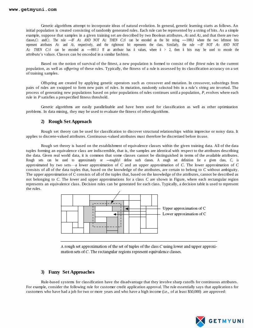
Rough sets can be used to approximately or ―roughly‖ define such classes. A rough set definition for a given class, C, is

approximated by two sets—a lower approximation of C and an upper approximation of C. The lower approximation of C

consists of all of the data tuples that, based on the knowledge of the attributes, are certain to belong to C without ambiguity.

The upper approximation of C consists of all of the tuples that, based on the knowledge of the attributes, cannot be described as

not belonging to C. The lower and upper approximations for a class C are shown in Figure, where each rectangular region

represents an equivalence class. Decision rules can be generated for each class. Typically, a decision table is used to represent

the rules.

3) Fuzzy Set Approaches

Rule-based systems for classification have the disadvantage that they involve sharp cutoffs for continuous attributes.

For example, consider the following rule for customer credit application approval. The rule essentially says that application s for

customers who have had a job for two or more years and who have a high income (i.e., of at least $50,000) are approved:

www.getmyuni.com

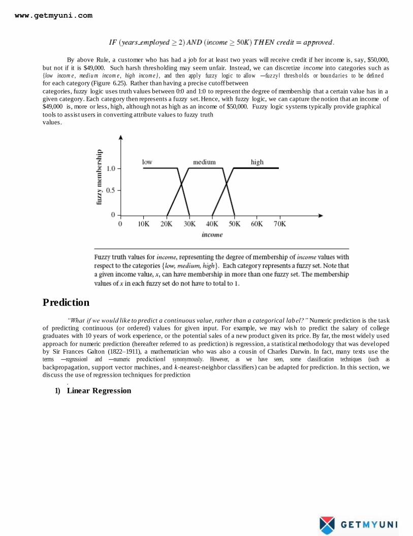
By above Rule, a customer who has had a job for at least two years will receive credit if her income is, say, $50,000,

but not if it is $49,000. Such harsh thresholding may seem unfair. Instead, we can discretize income into categories such as

{low incom e , mediu m incom e , high incom e } , and then apply fuzzy logic to allow ―fuz zy‖ thresh olds or boun da rie s to be define d

for each category (Figure 6.25). Rather than having a precise cutoff between

categories, fuzzy logic uses truth values between 0:0 and 1:0 to represent the degree of membership that a certain value has in a

given category. Each category then represents a fuzzy set. Hence, with fuzzy logic, we can capture the notion that an income of

$49,000 is, more or less, high, although not as high as an income of $50,000. Fuzzy logic systems typically provide graphical

tools to assist users in converting attribute values to fuzzy truth

values.

Prediction

“What if we would like to predict a continuous value, rather than a categorical label?” Numeric prediction is the task

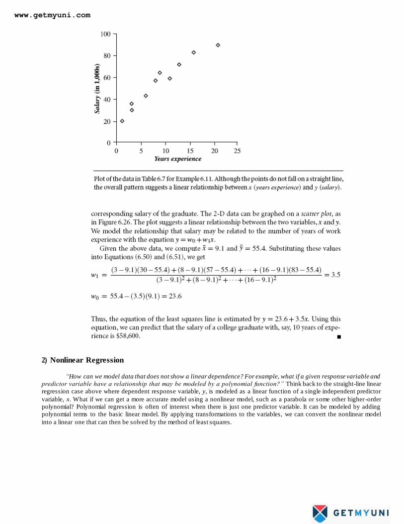
of predicting continuous (or ordered) values for given input. For example, we may wis h to predict the salary of college

graduates with 10 years of work experience, or the potential sales of a new product given its price. By far, the most widely used

approach for numeric prediction (hereafter referred to as prediction) is regression, a statistical methodology that was developed

by Sir Frances Galton (1822–1911), a mathematician who was also a cousin of Charles Darwin. In fact, many texts use the

terms ―regression‖ and ―numeric prediction‖ synonymously. However, as we have seen, some classification techniques (such as

backpropagation, support vector machines, and k-nearest-neighbor classifiers) can be adapted for prediction. In this section, we

discuss the use of regression techniques for prediction

.

1) Linear Regression

www.getmyuni.com

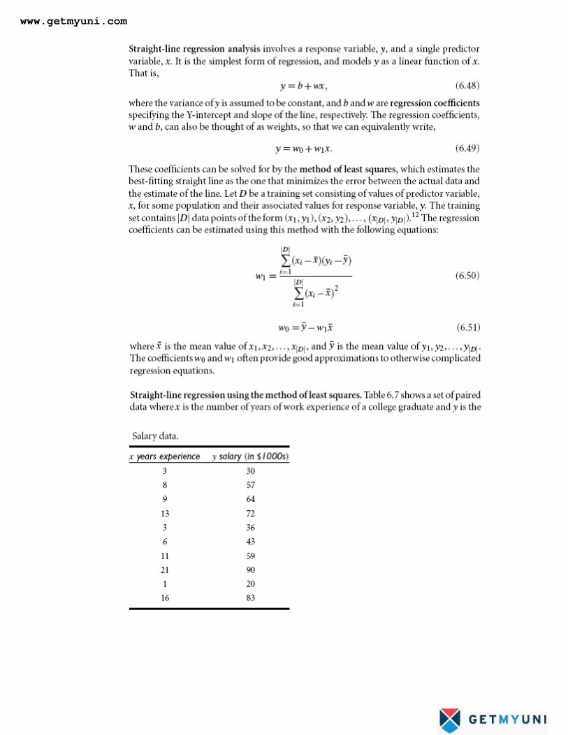
www.getmyuni.com

2) Nonlinear Regression

“How can we model data that does not show a linear dependence? For example, what if a given response variable and

predictor variable have a relationship that may be modeled by a polynomial function?” Think back to the straight-line linear

regression case above where dependent response variable, y, is modeled as a linear function of a single independent predictor

variable, x. What if we can get a more accurate model using a nonlinear model, such as a parabola or some other higher-order

polynomial? Polynomial regression is often of interest when there is just one predictor variable. It can be modeled by adding

polynomial terms to the basic linear model. By applying transformations to the variables, we can convert the nonlinear model

into a linear one that can then be solved by the method of least squares.

www.getmyuni.com

Important 16 mark Questions in Unit-IV

Explain Associations Rule Mining

Or

Explain how to generate strong association rule mining Or

Explain the mining methods for association rule generation

Or Explain Apriori and FP-Growth Method with Example.

Explain Mining Various Kinds of Association Rules

Explain decision tree induction (Attribute Oriented Induction) Explain Bayesian Classification.

Explain Rule Based Classification Explain Classification by Backpropagation Write short notes on Support Vector Machines and Lazy Learners

Write short notes on Prediction

www.getmyuni.com