Unit 2: Probability and Random Variables - Harvard Canvas

Unit 2: Probability and Random

Variables

Section 2.1-2.2 in the Text (sorta)

2

Unit 2 Outline

• General Probability Review

• Random Variables: PMFs, PDFs, and CDFs

• Means (Expected value) and Variances of r.v.s

• Definitions & Interpretations

• Rules

• Two Named Distributions

• Sample Statistics: X and S2 as r.v.s

3

Probability Axioms and Results

• Axioms of Probability

Axiom 1: P(A) ≥ 0

Axiom 2: P(S) = 1.

Axiom 3: If A1, A2,… are disjoint events, then:

• Result 1: P(Ac) = 1 – P(A).

• Result 2: If A ⊆ B, then P(A) ≤ P(B).

• Result 3: P(A ⋃ B) = P(A) + P(B) – P(A ∩ B).

*Note: If A and B are disjoint or mutually exclusive events

then P(A ⋃ B) = P(A) + P(B).

11

)(j

j

j

j APAP

4

Counting and Combinatorics

• Sampling with replacement: n objects and making k choices from them, one at a time with replacement. (order matters)

nk possible outcomes

• Sampling without replacement: n objects and making k choices from them, one at a time without replacement. (order matters)

n(n – 1) (n – 2)…(n – k + 1) possible outcomes

• How many ordered ways can n unique people form a line? (order matters)

n! = n(n-1)(n-2)…1 possible outcomes

• How many ways can you form a group of k people (everyone in the group are equivalent) from a population of n people? (order doesn’t matters)

!

))1()...(2)(1(

)!(!

!

k

knnnn

knk

n

k

n

5

Conditional Probability

• conditional probability: the probability of one event occurring

under the condition that we know the outcome of another event

• Conditional probability is probability! Follows all the rules!

• General multiplication rule: P(A∩B∩C) = P(A)P(B|A)P(C|A∩B)

• Law of Total Probability (LOTP): For a partition, A1,…, An:

)(

)B()|(

BP

APBAP

n

i

ii

n

i

i

APABP

ABPBP

1

1

)()| (

) ()(

)()|()()|() ( APABPBPBAPBAP

6

Bayes’ Rule

• Bayes’ rule (formula) provides a way to go from P(B | A)

to P(A | B) (in general they are not equal).‏

• If A and B are two events whose probabilities are

not 0 or 1, then:

• It is often written using the law of total probability:

• Or:

)(

)()|()|(

BP

APABPBAP

)()|()()|(

)()|()|(

CC APABPAPABP

APABPBAP

n

i

ii APABP

APABPBAP

1

111

)()| (

)()|()|(

7

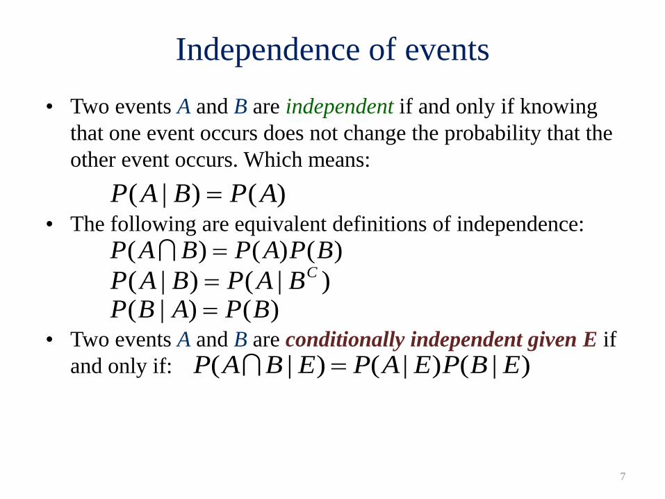
Independence of events

• Two events A and B are independent if and only if knowing

that one event occurs does not change the probability that the

other event occurs. Which means:

• The following are equivalent definitions of independence:

• Two events A and B are conditionally independent given E if

and only if:

)()|( APBAP

)()()( BPAPBAP

)()|( BPABP )|()|( CBAPBAP

)|()|()|( EBPEAPEBAP

8

Example #1

• There is a bag with 3 balls in it: 1 is red, and 2

are black

• You draw two balls out of the bag, one at a

time (without replacement). Define the events:

A: the first ball drawn is black

B: the second ball drawn is black

• Are A and B independent?

• What is P(B | A)? P(A | B)? P(B ∩ A)?

9

Example #2

It is known that approximately 20% of men and 3% of women

are taller than 6 feet in the US.

Let F = the event that someone is female and T = taller than 6

feet.

a) What is P(T | F)? What is P(T | FC)?

b) What is the probability that the next person walking through

the door is a woman and 6 feet tall?

c) What is the probability that the next person walking through

the door is 6 feet tall?

d) What is the probability that a person known to be 6 feet tall is

a woman?

10

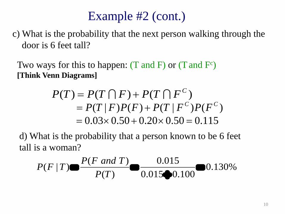
Example #2 (cont.)

c) What is the probability that the next person walking through the

door is 6 feet tall?

Two ways for this to happen: (T and F) or (T and Fc) [Think Venn Diagrams]

) () ()( CFTPFTPTP

)()|()() | ( CC FPFTPFPFTP

115.050.020.050.003.0

d) What is the probability that a person known to be 6 feet

tall is a woman?

%130.0100.0015.0

015.0

)(

)()|(

TP

TandFPTFP

11

Unit 2 Outline





• Rules



12

Random Variables and Discrete r.v.s

• A random variable (r.v.): a function that maps the outcomes in a sample space S to the real line.

• The distribution of X is the collection of all probabilities of the form P(X ∈ C) for all sets C of real numbers ({X ∈ C} = event).

• A probability mass function (PMF) of a discrete r.v. X is defined as the function f such that for every real number x

• The support of a dist. of X is the closure of the set {x: f(x) > 0}.

• The cumulative distribution function (CDF) of a r.v. X is the function FX given by FX(x) = P(X ≤ x). It is often written as just capital F without the subscript, or F(x).

)()( xXPxf

13

Continuous Random Variables

• A r.v. has a continuous distribution if its CDF is differentiable.

• The probability density function (PDF) of a continuous r.v. X is the derivative, f, of the CDF, given by f(x) = F’(x): The support of X and its distribution is the set of all x where f(x) > 0.

• So to calculate the probability that X fall within (a,b):

• What does f(x) represent?

• In general, we can think of f(x)dx as the probability of X being

in an infinitesimally small interval containing x, of length dx.

• What is P(X = x) for a continuous r.v.?

x

dttfxF )()(

b

adxxfaFbFbXaP )()()()(

14

Unit 2 Outline





• Rules



15

Expectation

• Definition:

• For a discrete r.v.:

• Expected value/expectation/mean (μX):

• For a continuous RV:

• Interpretation:

xall

xXxPXE )()(

dxxxfXE )()(

16

Properties of Expectation

• Linearity:

• LOTUS (Expectation of a function):

• Discrete:

• Continuous:

)()()( YEXEYXE bXaEbaXE )()(

xall

xXPxgXgE )()()(

dxxfxgXgE )()()(

17

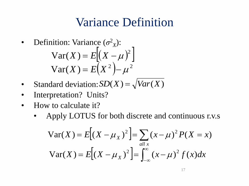
Variance Definition

• Definition: Variance (σ2X):

• Standard deviation:

• Interpretation? Units?

• How to calculate it?

• Apply LOTUS for both discrete and continuous r.v.s

2)(Var XEX

)()( XVarXSD

22)(Var XEX

dxxfxXEX X )()()()(Var 22

xall

X xXPxXEX )()()()(Var 22

18

Properties of Variance

• Properties of Variance:

• Var(X + c) = Var(X)

• Var(cX) = c2Var(X)

• Var(X) ≥ 0

• General linear combination form:

• If X and Y are independent, this simplifies to:

Var(X + Y) = Var(X) + Var(Y)

XYYXabYbXa

YXabYbXabYaX

2)(Var)(Var

),(Cov2)(Var)(Var)(Var

22

22

19

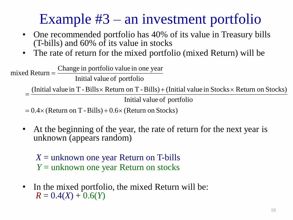
Example #3 – an investment portfolio • One recommended portfolio has 40% of its value in Treasury bills

(T-bills) and 60% of its value in stocks • The rate of return for the mixed portfolio (mixed Return) will be

• At the beginning of the year, the rate of return for the next year is

unknown (appears random)‏ X = unknown one year Return on T-bills Y = unknown one year Return on stocks • In the mixed portfolio, the mixed Return will be:

R = 0.4(X) + 0.6(Y)

)Stockson Return (6.0)Bills-Ton Return (4.0

portfolio of valueInitial

Stocks)on Return Stocksin value(InitialBills)-Ton Return Bills-Tin value(Initial

portfolio of valueInitial

year onein valueportfolioin ChangeReturnmixed

20

What is volatility (aka σ) of a mixed portfolio? Solution

Some `modeling’ assumptions:

X = return on T-bills: μX = 5.2%, σX = 2.9%,

Y = return on stocks: μY = 13.3%, σY = 17.0%

Correlation between X and Y: ρXY = – 0.3

• Expected return (average) of this portfolio is:

• Variance of the portfolio return is:

So, the volatility of the portfolio (its standard deviation) is σR = 10.15%

Note: smaller expected return than stocks alone, but WAY less volatility

%06.10)3.13(6.0)2.5(4.06.04.0 YXR

02.103

)0.17)(9.2)(6.0)(4.0)(3.0(2)0.17()6.0()9.2()4.0(

))((2

2222

22222

YXYXR baba

21

Unit 2 Outline





• Rules



Normal Distribution

22

• A random variable Y with probability density function

(PDF)

for -∞ < y < ∞ is called Normal (or Gaussian) r.v. with

mean ϵ (-∞ , ∞) and variance σ2.

• We often use the following notation

• What is the distribution of ?

22 2/)(

2

1)(

y

Y eyf

),(~ 2NY

YZ

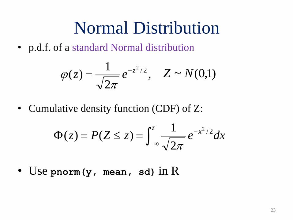
Normal Distribution

23

• p.d.f. of a standard Normal distribution

• Cumulative density function (CDF) of Z:

• Use pnorm(y, mean, sd) in R

,2

1)( 2/2zez

dxezZPzz

x

2/2

2

1)()(

)1,0(~ NZ

Normal Distribution: Linear combinations

24

• If Y1, …, Yn are independent normal r.v.’s,

• and a1, …, an are constants, then the linear combination

• has the following distribution

niNY iii ,...,1),,(~ 2

n

i

iiYaX1

n

i

ii

n

i

ii aaNX1

22

1

,~

25

The Binomial Distribution

• Think Coin Flips (counting heads)

• 4 Major characteristics

– Dichotomous outcome, n fixed, p fixed, independent trials

• Shorthand: X ~ Bin(n, p)

• PMF :

• E(X) = np, Var(X) = np(1 – p)

•

n

Xp ˆ

knk ppk

nkXP

)1()(

Binomial Random Variables (Normal approximation to the binomial)

• Let X ~ Bin(n, p). Then approximately:

• This approximation is a good one if:

– np ≥ 10 and n(1 – p) ≥ 10

0.0

00

.02

0.0

40

.06

0.0

8

n

pppNp

)1(,~ˆ

)1(,~ pnpnpNX

27

Unit 2 Outline





• Rules



28

Mean and Variance of X

• A very important sample statistic (which is often used as

an estimator) is the sample mean X :

• In contrast, the population mean or true mean is μ = E(Xi),

the mean of the distribution from which the Xi were drawn.

• Let X1,…, Xn be i.i.d. random variables with mean μ and

variance σ2. Then X is unbiased for estimating μ. That is:

• And the variance of X is:

28

n

i

iXn

X1

1

XE

n

X2

Var

29

Sample Variance, S2

• Let X1,…, Xn be i.i.d. random variables with mean and

variance . Then the sample variance is the r.v.:

• And the sample standard deviation is the square root of

the sample variance.

• Why the (n-1)? Because that way it is unbiased for

estimating σ2.

• Heuristic Proof:

• Note: more about this in the next unit (including R code).

29

n

i

i XXn

S1

22 )(1

1

Recall: Sampling Distribution

30

• Sampling distribution of a statistic is the (reference)

distribution that arises from a chance mechanism used to select

a random sample from a population.

• This is equivalent to thinking it is the distribution of the

statistic in a theoretical repeated sampling.

• So if we were able to repeatedly sample the r.v. many, many

times, the histogram of the results would be its sampling

distribution.

• A sampling dist. may depend on underlying population

distribution, statistic, sampling procedure, and sample size.

Sampling distribution of X

31

• Let X1, …, Xn be independent and identically distributed

Normal r.v.s. This can be written as:

• What is the distribution of the sample average, X ?

– It is Normal and it can be derived exactly:

• What if the population is not Normal?

– We need to rely on Limit Theorems.

),(~ 2...

NXdii

i

nNX

XX

22,~

32

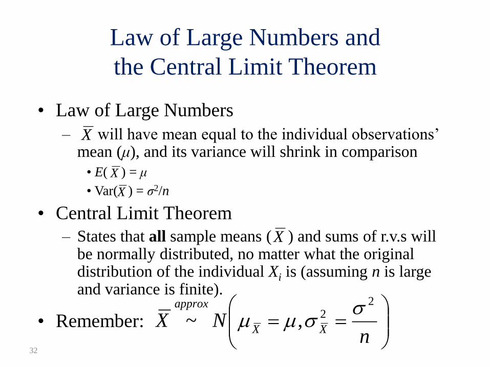
Law of Large Numbers and

the Central Limit Theorem

• Law of Large Numbers

– will have mean equal to the individual observations’ mean (μ), and its variance will shrink in comparison

• E( ) = μ

• Var( ) = σ2/n

• Central Limit Theorem

– States that all sample means ( ) and sums of r.v.s will be normally distributed, no matter what the original distribution of the individual Xi is (assuming n is large and variance is finite).

• Remember:

X

X

X

X

nNX

XX

approx 22,~

• What this means is, no matter what the underlying

distribution of the individual observations of X is, if you

take a large enough sample, and under the right conditions

(finite variance is more than enough), then the sampling

distribution of the r.v. will be approximately: X

Central Limit Theorem

Normally

Distributed!!!

33

http://www.socr.ucla.edu/applets.dir/samplingdistributionapplet.html

Sampling distribution of 𝑋

34

• So if the population is not normal, will the CLT always apply?

– In most cases, yes!

– But n may have to be prohibitively large, especially if the underlying distribution is extremely skewed or contains outliers, or if the observations are not independent

• And, the approximation is very good near the peak, but does a much poorer job out in the tails.

• So it requires much large number of observations to approximate the tails well

– and that is where we need it the most (think small p-values)!

How large is “large enough”?

35

Depends! – consider CLT assumptions:

1. Violation of independence:

– Serial effect – dependence between measurements

collected close in time (including seasonality);

– Cluster effect – dependence between measurements

within subgroups of similar units.

2. Deviations of Xi from Normality: skewness & outliers

3. Heterogeneity of the population - applies to all

characteristics of a measurement distributions:

– Variable expectations among population units;

– Heteroscedasticity - violation of equal variances.

For binary data: p = X

36

• So what about for the binomial setting?

• If we let independent X1,…, Xn ~ Bern(p).

• then each Xi can take on value either 1 with probability

p, or 0, with probability 1 - p.

• Then the distribution of X = Σ Xi truly follows what

distribution?

• Then define:

• Thus, the CLT applies to , and will thus be [approx]

Normally distributed!

• Key: think coin flips!

n

X

n

XXp

i

ˆ

p̂

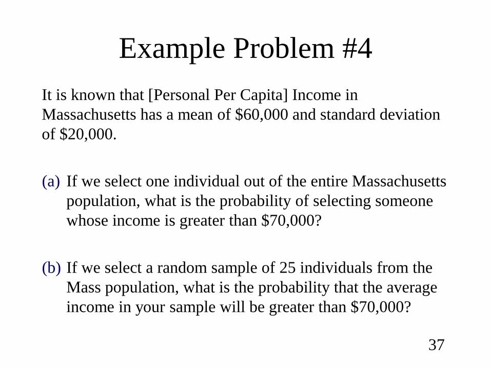
Example Problem #4

It is known that [Personal Per Capita] Income in

Massachusetts has a mean of $60,000 and standard deviation

of $20,000.

(a) If we select one individual out of the entire Massachusetts

population, what is the probability of selecting someone

whose income is greater than $70,000?

(b) If we select a random sample of 25 individuals from the

Mass population, what is the probability that the average

income in your sample will be greater than $70,000?

37

38

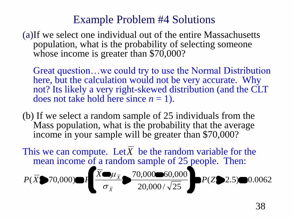
Example Problem #4 Solutions

(a)If we select one individual out of the entire Massachusetts population, what is the probability of selecting someone whose income is greater than $70,000?

Great question…we could try to use the Normal Distribution here, but the calculation would not be very accurate. Why not? Its likely a very right-skewed distribution (and the CLT does not take hold here since n = 1).

(b) If we select a random sample of 25 individuals from the Mass population, what is the probability that the average income in your sample will be greater than $70,000?

This we can compute. Let be the random variable for the mean income of a random sample of 25 people. Then:

X

0062.0)5.2(25/000,20

000,60000,70)000,70(

ZP

XPXP

X

X

The Last Word

39

Unit 2: Probability and Random Variables - Harvard Canvas

Documents

Transcript of Unit 2: Probability and Random Variables - Harvard Canvas