Emulsion Templating: Unexpected Morphology of

Monodisperse Macroporous Polymers

Von der Fakultät Chemie der Universität Stuttgart

zur Erlangung der Würde eines Doktors der

Naturwissenschaften (Dr. rer. nat.) genehmigte Abhandlung

Vorgelegt von

Lukas Koch

aus Anger

Hauptberichterin: Prof. Dr. Cosima Stubenrauch

Mitberichter: Prof. Dr. Michael D. Gilchrist

Prüfungsvorsitzender: Prof. Dr. Michael R. Buchmeiser

Tag der mündlichen Prüfung: 31.03.2021

Institut für Physikalische Chemie

der Universität Stuttgart

2021

für Conny und Franz Koch

I

Acknowledgements

First and foremost, I would like to express my deep gratitude to Prof. Dr. Cosima Stubenrauch

for giving me the opportunity to do my PhD thesis under her outstanding supervision. She

guided me in the beginning of my research when experiments had to be planned and later played

a vital role in the discussion of the results. Because of her advice, I was able to improve my

writing skills and became a better scientist in general. Moreover, I am thankful for all the

national and international conferences I was able to attend because of her support.

Furthermore, I would like to thank Prof. Dr. Michael D. Gilchrist for taking on the role as the

second examiner of my PhD thesis and Prof. Dr. Michael R. Buchmeiser for being my

GRADUS mentor as well as accepting the chairmanship of my PhD defense.

I would like to further express my gratitude to Dr. Wiebke Drenckhan who greatly assisting my

research with uncountable fruitful discussions. Moreover, I would like to thank her and her

whole research group for welcoming me in Strasbourg when I was residing with them. Special

thanks to Dr. Sebastian Andrieux for supporting me as my “local contact” in Strasbourg.

I am also very grateful to all the people who supported my work over these recent years. I am

thankful to Prof. Dr. Alexander Fels and Dr. Yaseen Qawasmi for their support during the SEM

measurements, to Apl. Prof. Dr. Thomas Sottmann, Diana Zauser, Shih-Yu Tseng, Karina

Abitaev, and Julian Fischer for their roles in the SANS measurements, to Maximilian Krappel

for his help with the DLS measurements, and to Dr. Natalie Preisig for recording the FFEM

pictures. I also want to thank the CTAs Birgit Feucht and Diana Zauser as well as the staff of

the electrical, mechanical, and glass workshops for their support in the lab. I would like to

further express my gratitude to my students Sabrina Beyer, Benjamin Kordes, Sophia Botsch,

and Manfred Stenzel who greatly assisted my PhD thesis with their work. Moreover, I want to

give a big “thank you” to Miriam Dabrowski for supporting my work by her contributions in

the lab and office. In general, I also want thank all former and current members of the

Stubenrauch and Sottmann groups for the pleasant atmosphere during my time in Stuttgart.

To Clarissa Dietrich, Julian Fischer, and all the other people who practiced sports with me, I

want to express my gratitude for helping me achieve a work-life-balance during my PhD thesis.

Finally, I want to thank my friends and family at home who supported me during both my

studies and my PhD thesis. My parents Cornelia and Franz Koch deserve the greatest gratitude,

because without their never-ending support, neither my studies nor my PhD thesis would have

been possible.

II

1 Introduction ............................................................................................ - 1 -

1.1 Motivation .............................................................................................................. - 1 -

1.2 Task Description ..................................................................................................... - 4 -

2 Theoretical Background ........................................................................ - 7 -

2.1 Emulsions ............................................................................................................... - 7 -

2.2 Microfluidics ........................................................................................................ - 14 -

2.3 Polymers and Porous Polymers ............................................................................ - 23 -

2.3.1 Polymers ........................................................................................................ - 23 -

2.3.2 Porous Polymers ............................................................................................ - 30 -

2.4 Templating Routes ................................................................................................ - 37 -

3 Results and Discussion ......................................................................... - 43 -

3.1 Disproof of Osmotic Transport ............................................................................. - 43 -

3.1.1 Variation of Styrene Mass Fraction βstyrene .................................................... - 44 -

3.1.2 Variation of KPS Mass Fraction βKPS ........................................................... - 56 -

3.2 New Mechanism: Surfactant Diffusion ................................................................ - 65 -

3.2.1 Experimental Results ..................................................................................... - 65 -

3.2.2 Discussion of Experimental Results .............................................................. - 81 -

3.3 Mechanical Behavior ............................................................................................ - 85 -

4 Conclusions and Outlook ..................................................................... - 95 -

4.1 Conclusion ............................................................................................................ - 95 -

4.2 Outlook ............................................................................................................... - 101 -

5 Experimental ...................................................................................... - 103 -

5.1 Materials ............................................................................................................. - 103 -

5.2 Synthesis of Macroporous PS/polyDVB ............................................................ - 103 -

5.3 Analysis of Macroporous PS/polyDVB ............................................................. - 105 -

5.3.1 Analysis of Morphology .............................................................................. - 105 -

5.3.2 Analysis of Mechanical Behavior ............................................................... - 106 -

III

5.4 Phase Diagram .................................................................................................... - 107 -

5.5 Interfacial Tension .............................................................................................. - 107 -

5.6 Small angle neutron scattering ........................................................................... - 107 -

5.7 Freeze Fracture Electron Microscopy ................................................................. - 108 -

5.8 Dynamic Light Scattering ................................................................................... - 108 -

6 Appendix ............................................................................................. - 109 -

6.1 Supplementary Calculations ............................................................................... - 109 -

6.2 Supplementary Figures ....................................................................................... - 115 -

References ................................................................................................... - 121 -

IV

Abbreviations and Symbols

Abbreviations

2D two dimensional

3D three dimensional

AIBN azobisisobutyronitrile

APD avalanche photodiode

CFCs chlorofluorocarbons

cont continuous (phase)

D2O deuterated water

disp dispersed (phase)

DLS dynamic light scattering

DNA deoxyribonucleic acid

DSC differential scanning calorimetry

DTA differential thermal analysis

DVB divinylbenzene

EPS expanded polystyrene

ETFE ethylene tetrafluoroethylene

FEP fluorinated ethylene propylene

FFEM freeze fracture electron microscopy/microscope

g/o gas-in-oil

g/w gas-in-water

HIPE high internal phase emulsion

IUPAC International Union of Pure and Applied Chemistry

KPS potassium peroxodisulfate

LAS linear alkylbenzene sulphonate

V

LIPE low internal phase emulsion

MIPE medium internal phase emulsion

mol% mol percent

n unspecified, large number

o/w oil-in-water (emulsion)

o/w/o oil-in-water-in-oil (emulsion)

PEG polyethylene glycol

PDI polydispersity index

PDMS polydimethylsiloxane

PE polyethylene

PET polyethylene terephthalate

Ph Phenyl rest

PhD philosophiae doctor (Doctor of Philosophy)

PMMA poly(methyl methacrylate)

polyDVB polydivinylbenzene

polyHIPE polymerized high internal phase emulsion

PS polystyrene

PVC polyvinyl chloride

R aliphatic rest

SANS small angle neutron scattering

SEI secondary electron imaging

SEM scanning electron microscopy/microscope

TEM transmission electron microscopy/microscope

UV ultraviolet

vol% volume percent

VI

wt.% weight percent

w/o water-in-oil

w/o/w water-in-oil-in-water

XPS extruded polystyrene

Constants, Numbers and Units

Å ångström (10-10 m)

g gravitational constant of earth (9.81 m s-2)

N Newton (kg m s-2)

NA Avogadro number (6.022 · 1023 mol-1)

Pa Pascal (N m-2)

Greek Symbols

βi mass fraction of component i / wt.%

γ interfacial tension / mN m-1

Δh height difference / m

Δp pressure difference / N m-2

ε strain / %

θ angle at which two channels meet in microfluidic cross-flow geometry / °

ηi dynamic viscosity of component i / kg m-1 s-1

κ curvature / m-1

λ viscosity ratio

ν* Poisson’s ratio

ρi density of component i / kg m-3 or g cm-3

ρrel relative density

VII

σ stress / N

σys yield strength / MPa

φ flow ratio

Φi volume fraction of component i / vol%

χi molar fraction of component i / mol%

Roman Symbols

Ai area of object i / m2

Ainterface interfacial area / m2

Bo Bond number

Ca Capillary number

CC / C1 / C1´ proportionality constants

Ci circumference of object i / m

daverage average diameter / m

di diameter of object i / m

dsd standard deviation of diameter / m

Ei Young’s Modulus of component i / MPa

F force / N

Fmax point at which the linear elastic region goes over into the plateau region in stress-

strain-curves / N

fc force of capillary pressure / kg m-1 s-2

fg gravitational force / kg m-1 s-2

fi inertial force / kg m-1 s-2

fv viscous force / kg m-1 s-2

G Gibbs free energy / J

VIII

h height / m

h0 initial height / m

H enthalpy / J

I measured intensity in SANS

I(q) calculated intensity in SANS

L characteristic length scale of microfluidic chip / m

p pressure / N m-2

p0 initial (gas) pressure / N m-2

P porosity / %

P(q) form factor in SANS

q scattering vector / Å-1

Qi flow rate of component i / m3 s-1

ri radius of object i / m

rHyd hydrodynamic radius / m

Re Reynolds number

S shape factor

S(q) structure factor in SANS

Std thermodynamic entropy / J K-1

ti thickness of object i / m

T temperature / K or °C

Tg glass transition temperature / K or °C

Tm melting temperature / K or °C

vi velocity of component i / m s-1

Vi volume of component i / m3

We Weber number

IX

Abstract

The polymerization and drying of monodisperse water-in-styrene/divinylbenzene (DVB) high

internal phase emulsions (HIPEs) leads to monodisperse macroporous polystyrene

(PS)/polydivinylbenzene (polyDVB). When the monomer-soluble azobisisobutyronitrile

(AIBN) is used as initiator, spherical and interconnected pores and porous pore walls are

obtained. In contrast, when the water-soluble potassium peroxodisulfate (KPS) is used,

polyhedral and closed pores are obtained and the pore walls are comprised of two similar

looking outer layers and one different inner layer. The aim of this work was to identify the

mechanism (1) that transforms spherical droplets into polyhedral pores and (2) that creates a

three-layered pore wall when the polymerization is initiated from the water/monomer interface

with KPS.

The styrene/DVB mass ratio and the KPS mass fraction were varied to test the existing

hypothesis, i.e. an osmotic transport of DVB. Scanning electron microscopy (SEM) pictures

revealed that the morphology of the samples does not change in the way it is expected if osmotic

transport of DVB was the acting mechanism. Therefore, the existing hypothesis was rejected

and a new explanation had to be found. Experiments in which the surfactant mass fraction

βsurfactant was varied revealed that the relative size of the inner layer increases and the relative

size of the outer layers decreases when βsurfactant is increased. Moreover, it was found that the

outer layers are non-porous and that the inner layer is porous. With the help of a model ternary

phase diagram consisting of styrene, surfactant, and PS, it was shown that the surfactant is not

soluble in partially polymerized styrene/PS mixtures. The experimental results allow suggesting

a mechanism that is based on surfactant diffusion. Since the polymerization starts at the

water/monomer interface with KPS, a partially polymerized layer forms close to the interface.

From this layer, surfactant molecules that are dissolved in the continuous phase diffuse either

(1) to the water/monomer interface or (2) to the interior of the continuous phase. (1) Surfactant

diffusion to the interface induces an overpopulation of surfactant. This enables the interface to

increase its area, which, in turn, transforms the spherical droplets to polyhedral pores. (2)

Surfactant diffusion to the interior of the continuous phase leads to an accumulation of

surfactant, while the regions close to the interface become surfactant-free. When the surfactant

is washed out during purification, a porous inner and two non-porous outer layers are obtained.

Additionally, the mechanical properties of monodisperse macroporous PS/polyDVB were

investigated. It was found that the samples are only elastomeric when the amount of DVB is

low, while they are elastic-brittle for all other monomer compositions.

X

Kurzzusammenfassung

Durch Polymerisation und Trocknen wird aus monodispersen Wasser-in-Styrol/Divinylbenzol

(DVB) Emulsionen monodisperses, makroporöses Polystyrol (PS)/Polydivinylbenzol. Mit

monomerlöslichem Azobis(isobutyronitril) (AIBN) als Initiator werden sphärische und offene

Poren sowie poröse Porenwände erhalten. Dagegen entstehen mit wasserlöslichem

Kaliumperoxodisulfat (KPS) polyedrische und geschlossene Poren und die Porenwände

bestehen aus zwei ähnlich aussehenden äußeren Schichten und einer inneren Schicht. Das Ziel

dieser Arbeit war es, den Mechanismus zu identifizieren, (1) der sphärische Tropfen in

polyedrische Poren verwandelt und (2) der eine dreilagige Porenwand erzeugt, wenn die

Polymerisation durch KPS an der Wasser/Monomer Grenzfläche beginnt.

Das Styrol/DVB Massenverhältnis und der KPS Massenbruch wurden variiert, um die

bestehende Hypothese zu überprüfen, die auf osmotischen Transport von DVB basiert.

Rasterelektronenmikroskopie (REM) Aufnahmen zeigten, dass sich die Morphologie der

Proben nicht in der Art verändert, wie sie es tun sollte, wenn osmotischer Transport von DVB

der wirkende Mechanismus ist. Somit wurde die bestehende Hypothese verworfen und eine

neue Erklärung musste gefunden werden. In Experimenten, in denen der Tensidmassenbruch

βTensid erhöht wurde, nahm die relative Größe der inneren Schicht zu und die relative Größe der

äußeren Schichten ab. Zudem wurde herausgefunden, dass die äußeren Schichten nicht porös

sind, sehr wohl aber die innere Schicht. Mithilfe eines ternären Phasendiagrams bestehend aus

Styrol, Tensid und PS wurde gezeigt, dass das Tensid nicht in partiell polymerisiertem

Styrol/PS löslich ist. Der anhand der experimentellen Ergebnisse vorgeschlagene Mechanismus

basiert auf Tensiddiffusion. Da die Polymerisation durch KPS an der Wasser/Monomer

Grenzfläche beginnt, entsteht in deren Nähe eine partiell polymerisierte Schicht. In der

kontinuierlichen Phase gelöste Tensidmoleküle diffundieren aus dieser Schicht entweder (1)

zur Grenzfläche oder (2) ins Innere der kontinuierlichen Phase. (1) Tensiddiffusion zur

Grenzfläche verursacht dort eine Übersättigung, wodurch sich die Grenzfläche vergrößern kann

und aus sphärischen Tropfen polyedrische Poren werden. (2) Tensid Diffusion ins Innere der

kontinuierlichen Phase verursacht dort eine Anreicherung mit Tensid, während nahe der

Grenzfläche kein Tensid mehr vorhanden ist. Wenn das Tensid während der Reinigung

ausgewaschen wird, entstehen eine poröse innere und zwei nicht-poröse äußere Schichten.

Zusätzlich wurden die mechanischen Eigenschaften von monodispersen, makroporösem

PS/polyDVB untersucht. Dieses ist nur dann elastomerisch, wenn der DVB Anteil niedrig ist,

während es bei allen anderen Monomerzusammensetzungen elastisch-brüchig ist.

- 1 -

1 Introduction

1.1 Motivation

Polymers have been used by humans indirectly or directly for a long time in the form of bio-

polymers like proteins, polysaccharides, and deoxyribonucleic acid (DNA). The discovery of

synthetic polymers in the 19th century has fundamentally changed modern society. Since 1909,

when the first industrially produced plastic, Bakelite [Bae09], was introduced, a wide range of

products has been made from synthetic polymers. Among these products are, for example,

porous polymers where the dispersed phase is a gas and the continuous phase is a polymer.

They are employed in a broad variety of areas ranging from construction (insulation material)

and vehicles (dashboard) to sports (protective gear) and hygiene (polyurethane sponges), to

mention just a few. Compared with their bulk counterparts, one big advantage of porous

polymers is the fact that the density ρ can be adjusted by changing the amount of the dispersed

gas. The gamut of densities includes not only the dense bulk polymer itself where the volume

percentage of gas is very small (ρporous polymer ~ 103 kg m-3), but also materials that consist almost

entirely of gas (ρporous polymer ~ 100 kg m-3) [Lan95]. As the mechanical properties of porous

polymers strongly depend on their density, this opens up the possibility of producing a large

number of distinct materials using only one type of polymer [Lee07].

The volume fraction of the dispersed phase is only one parameter that affects the morphology.

By changing other parameters like the average pore size, the pore size distribution, the pore

wall thickness, or the interconnectivity of the pores, the properties of porous polymers can be

modified even further. For instance, in buoyancy products like floatation aids, closed-pore

porous polymers are required since penetration of water into the material has to be avoided

[Mil07]. Open-pore porous polymers, on the other hand, are used as acoustic damping materials

for example [Ban11]. However, the interconnectivity, the average pore size, and the pore size

distribution are difficult to control when the porous polymer is produced industrially. One

method for solving this problem is the use of templates. These consist of a dispersed phase that

acts as placeholder for the pores and a continuous phase which is a precursor to the polymer.

Since the templates are liquid, their structure is easier to control and manipulate compared to

the solid porous polymer. By preserving the generated structure during solidification, the

structure of the porous polymer is controlled as well.

If emulsion droplets are used as placeholders in a template, the term “emulsion templating” is

used. The continuous phase consists of the monomer(s), the surfactant, and in some cases a

- 2 -

solvent, while a liquid that is immiscible with the continuous phase serves as the dispersed

phase. By monitoring the volume fraction Φdisp of the dispersed phase, the density of the porous

polymer is adjustable: the higher the amount of the dispersed phase is, the lower is the density.

If Φdisp is at least 74 vol%, the emulsion is called a high internal phase emulsion (HIPE)

[Cam96]. HIPEs were first used to produce porous polymers by Bartl et al. in 1962 [Bar62].

They formulated “reverse emulsions” where water was the dispersed phase, styrene or methyl

methacrylate were the two investigated monomers, and a graft copolymer of styrene and

polyethylene oxide was used as surfactant. It took another 20 years before a patent was filed for

this specific kind of synthesis [Bar85] and the terms HIPE and polyHIPE (polymerized high

internal phase emulsion) were introduced although, strictly speaking, the final porous polymer

is not an emulsion anymore. Since then, numerous research groups have used this method to

prepare porous polymers where the final morphology can be controlled to a certain point

[Wil88a, Wil88b, Wil89, Wil90a, Wil90b, Hai91, Cam96, Cam97, Bar00, Cam00, Tai01a,

Tai01b, Cam05, Sil05, Kim11, Sil14].

Talha Gokmen et al. first combined HIPEs with microfluidics, which enables the formation of

droplets with a uniform size. However, they used this concept to produce monodisperse

polymer beads by polymerizing the monomeric droplets in an oil-in-water (o/w) emulsion

[Tal09]. In contrast, Costantini et al. synthesized porous polymers with uniform sized pores by

polymerizing the hydrophilic continuous phase of an o/w emulsion formed with microfluidics

[Cos14]. Quell et al. used the same method with the hydrophobic monomers styrene and

divinylbenzene (DVB) as continuous phase and water as dispersed phase. The polymerization

Figure 1.1: Schematic depiction of the synthesis of monodisperse macroporous PS/polyDVB

(right) from a monodisperse water-in-styrene/DVB HIPE template (middle) which itself was

synthesized with microfluidics (left).

- 3 -

of this water-in-styrene/DVB HIPE and subsequent drying led to porous polystyrene (PS)/poly-

divinylbenzene (polyDVB) with a monodisperse pore size [Que15, Que16a, Que16b, Els17,

Que17a, Que17b]. The schematic process of producing monodisperse porous PS/polyDVB with

monodisperse water-in-styrene/DVB HIPEs is shown in Figure 1.1. By varying the flow rates

of both phases in the microfluidic chip, the synthesis of porous PS/polyDVB with pore sizes

ranging from 55 µm to 80 µm was possible. Due to the pore size being larger than 50 nm, the

material is classified as macroporous PS/PDVB [Eve72, Bur76]. Furthermore, by changing the

type of initiator, both open-pore and closed-pore macroporous PS/polyDVB were obtained.

With water-soluble potassium peroxydisulfate (KPS) as initiator, polyhedral and closed pores

with granular pore surfaces and layered pore walls are formed (see Figure 1.2 (top)). Note that

in the 2D pore cross-sections of Figure 1.2, the polyhedral pores appear as hexagons, while the

pores are shaped like rhombic dodecahedrons in 3D.

Figure 1.2: Scanning electron microscope (SEM) pictures of macroporous PS/polyDVB

obtained from monodisperse water-in-styrene/DVB HIPEs and initiated with (top) KPS and

(bottom) AIBN. This Figure was copied from [Que17b]. Reprinted with permission from Quell,

A.; Sottmann, T.; Stubenrauch, C.; Diving into the Finestructure of Macroporous Polymer

Foams Synthesized via Emulsion Templating: A Phase Diagram Study, Langmuir 2017, 33,

537-542. Copyright (2021) American Chemical Society.

With oil-soluble azobisisobutyronitrile (AIBN) as initiator, on the other hand, spherical and

interconnected pores with smooth pore surfaces and porous pore walls are formed (see Figure

1.2 (bottom)). For the samples seen in Figure 1.2, the styrene/DVB mass ratio is 50/50, the

surfactant mass fraction 10 wt.%, and the initiator molar concentration 1.28 mol%. Since the

emulsion templates are spherical droplets, the difference observed for the two initiators raises

- 4 -

the question of how and why the spherical droplets become polyhedral pores when KPS is used.

Quell et al. explained this transformation with osmotic transport of DVB [Que17a]. According

to Schwachula [Sch75], the polymerization of the crosslinker DVB is faster than that of the

monomer styrene, which is why Quell et al. argue that a DVB-rich polymer layer forms at the

interface. Assuming that the major part of the monomer styrene only reacts after DVB has

polymerized, Quell et al. concluded that layered pore walls with two polyDVB-rich outer layers

and a PS-rich inner layer form. Furthermore, a concentration gradient of DVB between the

Plateau borders (initial DVB concentration) and the films (DVB depleted) is believed to be the

reason for the change from a spherical to a polyhedral pore shape. This gradient causes osmotic

transport of DVB molecules from the Plateau borders into the films. As a result, the size of the

Plateau borders is reduced and the thickness of the films is increased. Thus, the shape of the

interface changes from spherical to polyhedral. Furthermore, Quell et al. showed that quite

uniform pore wall thicknesses are built. Note that the osmotic transport has to work against the

desire of the droplets to minimize their surface since the surface area of a rhombic dodecahedron

is ~10% larger than the surface area of a sphere [Que16b, Que17a].

1.2 Task Description

Although the experimental results obtained by Quell et al. [Que17a] support the idea of an

osmotic transport of DVB as the reason for the transformation from spherical droplets to

polyhedral pores, resounding proof for this hypothesis is still lacking. Thus, the main focus of

this PhD thesis is put on either proving or disproving this hypothesis. To achieve this, logical

deductions are drawn about what ought to happen to the morphology of monodisperse

macroporous PS/polyDVB when the concentration of a component is changed systematically.

(1) When the styrene/DVB mass ratio is changed from 50/50 towards pure styrene, the extent

of osmotic transport of DVB is expected to decrease. Thus, the shape of the pores ought to

become more spherical. Additionally, since less DVB is present in the continuous phase, the

thickness of the supposedly polyDVB-rich outer layers is expected to decrease. (2) When the

KPS concentration is increased, the polymerization rate ought to increase as well. Thus, osmotic

transport of DVB has less time to occur and the pores ought to become more spherical as well.

In both cases, analogous experiments are conducted with AIBN as initiator for the sake of

comparison.

If the hypothesis of osmotic transport of DVB is confirmed, the large number of new

experimental results may allow a quantitative description of the mechanism. On the other hand,

- 5 -

if the experiments reveal that osmotic transport of DVB is not responsible for the transformation

of spherical droplets to polyhedral pores, this hypothesis was to be dismissed. Consequently, a

new hypothesis would have to be developed by conducting further experiments. The new

hypothesis would have to comply with both old and new experimental results.

Finally, the mechanical properties of monodisperse macroporous PS/polyDVB are examined.

Focus is put on how the type and amount of initiator, the styrene/DVB mass ratio, and the

amount of surfactant influence the mechanical properties. The goal is to obtain structure-

property-relationships. Moreover, both monodisperse and polydisperse macroporous

PS/polyDVB are investigated to see if their mechanical properties are different.

- 6 -

- 7 -

2 Theoretical Background

2.1 Emulsions

If two pure liquids are brought in contact, there are three possibilities for what can happen: a

chemical reaction, mixing, and separation. In the latter case, the mixtures are typically

composed of a hydrophilic liquid, in most cases water, and a hydrophobic liquid which is often

called “oil”. To enable the mixing of immiscible liquids, a third component is required which

is at least partially soluble in either liquid. Such molecules typically consist of a hydrophilic

and a hydrophobic part. In a ternary mixture, this causes an accumulation of this molecule at

the interface between water and oil, thereby reducing the interfacial tension between them. The

same is true when the hydrophobic liquid is substituted by a gas which transforms the interface

into a surface. This type of molecule is therefore called “surfactant” (surface active agent) or

“amphiphile”. Mixtures of water and oil stabilized with surfactants are called “emulsions”,

while the surfactant is called “emulsifier”. Emulsions have found their way into modern life via

cosmetics like creams, shampoos, make-up, or perfume as well as into industrial processes.

Typical emulsions either consist of water droplets dispersed in a continuous oil phase (w/o-

emulsions, see Figure 2.1 (left)) or of oil droplets dispersed in a continuous water phase (o/w-

emulsions see Figure 2.1 (right)).

Figure 2.1: Schematic structure of (left) a water-in-oil emulsion and (right) an oil-in-water

emulsion.

- 8 -

More complex systems like o/w/o- or w/o/w-emulsions also exist but less common. The type

of emulsion depends on the type of surfactant, the temperature, the concentration of electrolytes

in the water phase, the volume fractions, and the concentration of the surfactant. To test which

type of emulsion has formed, two easy experiments can be conducted. One the one hand, if low

amounts of salt are added and the conductivity is measured, o/w-emulsions show a high

conductivity while the value is close to zero in the case of w/o-emulsions. On the other hand, a

dye which is only soluble in one phase can be added. The color can only be seen if the dye is

dissolved in the continuous phase [Bin98, Eva99, Lyk05, Ros12].

In general, most emulsions appear white since the droplets of the dispersed phase have a

diameter between 200 nm and 100 μm, thus scattering visible light. However, emulsions can

also be transparent, namely if the dispersed droplets are diluted enough or the if their diameter

is smaller than 200 nm. In this case, the Tyndall effect [Whi20] can be observed. When a ray

of light is shone through a sample, light scattering in the liquid is visible if particles with a

diameter in the micrometer range are present which of course is true for emulsions. In

homogeneous liquids, in contrast, no ray of light is observable [Sch05].

Influence of Interfacial Tension on Emulsions

The surfactant molecules between the dispersed and the continuous phase form a skin-like layer

around the dispersed droplets which enables a kinetic stabilization of the interface. No matter

how well an emulsion might be stabilized kinetically, its ultimate fate is always phase

separation. The reason behind this lays in the change of the Gibbs free energy G which in the

case of emulsions holds

𝐺 = 𝐻 − 𝑇 · 𝑆td + 𝛾 · 𝐴interface . (2.1)

In equation (2.1), H represents the enthalpy, T the temperature, Std the thermodynamic entropy,

γ the interfacial tension, and Ainterface the interfacial area. Note that thermodynamic systems

always try to minimize G [Eva99]. Since the difference in enthalpy is zero between an emulsion

and two separated phases, only the second and third term are important for the stability of

emulsions. On the one hand, by emulsifying two originally separated phases, S increases which

leads to a decrease of G. However, now Ainterface has been increased as well which, in turn,

increases G. Thus, the deciding factor is how far the surfactant can reduce the value of γ. This

decrease is by far not enough in the case of emulsions (typically γ ≈ 30 mN m-1), thus making

- 9 -

them overall thermodynamically unstable [Lyk05]. In microemulsions, in contrast, the

interfacial tension is reduced to γ ≈ 1 mN m-1 or lower. For example, the system H2O – linear

alkylbenzene sulphonate (LAS) – decane with 0.1 g L-1 LAS has an interfacial tension of γ ≈

0.5 mN m-1 [Stu09]. In this case, the increase in S matters and the system becomes

thermodynamically stable. Furthermore, microemulsions appear transparent because droplets

with typical diameters between 10 nm and 100 nm form and are thus not able to scatter light

[Stu09].

Another point where γ matters is the shape of emulsion droplets. For a given volume, a sphere

has the lowest surface area and since a minimized surface area is required energetically, the

droplets in emulsions are spherical. The diameter of the droplets is determined by the interfacial

tension and the pressure difference between the inner and the outer liquid. This pressure

difference tries to increase the diameter of the droplets, while the surface tension works against

this effort. The two counteracting forces lead to an equilibrium droplet diameter which can be

described with the Young-Laplace equation. It holds

𝛥𝑝 = 2 · 𝛾 · 𝜅 (2.2)

where Δp represents the pressure difference between the inner and the outer liquid and κ the

mean curvature of the droplets. It holds

𝜅 = 1

2· (

1

𝑟1+

1

𝑟2) , (2.3)

where r1 and r2 are the two radii of an ellipsoidal body. In the case of spheres, the two radii are

equal (rsphere) which simplifies the curvature to the reciprocal radius and transforms equation

(2.2) to [Sch05]

𝛥𝑝 = 2𝛾

𝑟𝑠𝑝ℎ𝑒𝑟𝑒 . (2.4)

Disintegrating Mechanisms

Since emulsions are only kinetically stabilized but not thermodynamically stable, they will

eventually disintegrate. There are three different routes for how that can occur, namely

sedimentation (or creaming), coalescence, and Ostwald ripening (see Figure 2.2).

- 10 -

Figure 2.2: Schematic depictions of the three disintegrating mechanisms (top) sedimentation,

(middle) coalescence, and (bottom) Ostwald-ripening for a o/w emulsion. Note that in o/w

emulsions, sedimentation is usually replaced by creaming.

One way how emulsions can decompose is by an accumulation of droplets. If the dispersed

phase has a higher density than the continuous phase, which is typically the case for

w/o-emulsions, the droplets sediment towards the bottom due to gravity (see Figure 2.2 (top)).

On the other hand, if the dispersed phase is less dense than the continuous phase, which usually

applies for o/w-emulsions, the opposite happens. The droplets than cream towards the top of

the emulsion. Eventually, these processes lead to a phase separation if the sedimented or

creamed droplets merge. An approach to at least slow down sedimentation or creaming is the

use of two liquids with similar densities or to artificially modify the densities via additives

[Bin98, Eva99].

Another route of decomposing is the coalescence of droplets. This can happen when they are

brought close enough together through Brownian motion or flocculation. Note that flocculation

can serve as its own disintegrating route if the droplets aggregate irreversible. Due to gravity,

this would cause sedimentation or creaming at some point. Coalescence, on the other hand, is

- 11 -

a process where two droplets fuse together to form one bigger droplet (see Figure 2.2 (middle)).

This can only occur if the surfactant film is not stable enough to prevent this, i.e. if the surfactant

concentration is not high enough. The merging of two droplets is energetically favored since

the Laplace pressure of the larger droplet is smaller (see equation (2.4)). The coalescence of

more and more droplets eventually leads to phase separation. A way to avert coalescence is

using a sufficient concentration of surfactant. The steric repulsion of non-ionic surfactants or

the electrostatic repulsion of ionic surfactants, respectively, pushes the droplets apart if they

come to close together [Bin98, Eva99, Sch05].

Finally, an emulsion can decompose via Ostwald ripening. Named after its discoverer W.

Ostwald [Ost00], this effect describes a process where bigger droplets increase their size at the

expense of smaller ones (see Figure 2.2 (bottom)). Note that Ostwald ripening is not exclusive

to emulsions but also occurs in foams. The underlying principle is the Young-Laplace equation

(see equation (2.4)). For smaller droplets, the pressure difference between inner and outer phase

is higher than for bigger droplets because κ is larger for smaller droplets. Since the dispersed

liquid has a finite solubility in the continuous one, single molecules can inter-diffuse between

droplets. Additionally, their concentration close to a droplet is dependent on the diameter of the

droplet, being higher in the case of smaller droplets. As a result, a concentration gradient

between the outside of small droplets – where the concentration of solubilized molecules is high

– and the outside of large droplets – where the concentration of solubilized molecules is low –

forms. Therefore, molecules of the dispersed phase will net-diffuse from the small droplets

through the continuous phase into large droplets. Eventually, this leads to a disappearance of

smaller droplets, while the bigger droplets grow larger and larger, finally also resulting in phase

separation. The easiest way to avoid Ostwald ripening is creating a monodisperse emulsion, i.e.

creating droplets that all have the same Laplace pressure. The droplets then retain the same size

for a long time. This can be achieved by preparing the emulsion via microfluidics (see Chapter

2.2) or by preparing a solution already assembled from all three components (water, oil, and

amphiphile) and rapidly adding more oil or water. Once the system crosses into the two-phase

region, uniform sized droplets form via nucleation. The ouzo effect observed in many alcoholic

beverages derived from plants containing essential oils is a famous practical example for this

method [Vit03]. Another route to prevent Ostwald ripening is to dissolve an additive in the

dispersed phase which is completely insoluble in the continuous phase, e.g. for w/o emulsions

a salt like sodium chloride NaCl. In the beginning, the concentration of NaCl is equal in all

droplets. However, if a net diffusion of molecules of the dispersed phase into the bigger droplets

occurs, a reverse chemical potential arises as well. Therefore, an osmotic transport forces a

- 12 -

back-diffusion into the smaller droplets, thus counterbalancing Ostwald ripening. In the case of

o/w-emulsions, the same effect can be achieved if long hydrocarbons like hexadecane are used

[Bin98, Sch05].

Polydispersity, Volume Fraction, Packing, and Ordering in Emulsions

The polydispersity and the volume fractions of the dispersed and the continuous phase,

respectively, also have an influence on the structure and stability of emulsions. The

polydispersity index (PDI) describes how large the droplet size distribution in an emulsion is.

With dsd as the standard deviation of the measured droplet diameters and daverage as the average

droplet diameter, it holds [Cla16]

𝑃𝐷𝐼 = 100% · 𝑑𝑠𝑑

𝑑𝑎𝑣𝑒𝑟𝑎𝑔𝑒 . (2.5)

Typical emulsions have a PDI of around 50% and are therefore polydisperse. Ideal

monodisperse emulsions, on the other hand, would have an PDI of 0. However, because “true”

monodispersity is virtually impossible, the term monodispersity is typically used when the PDI

is equal to or smaller than 5% [Mae13].

Furthermore, the volume fraction of the dispersed phase (Φdisp) is used to classify different types

of emulsions. It holds

𝛷𝑑𝑖𝑠𝑝 = 𝑉𝑑𝑖𝑠𝑝

𝑉𝑑𝑖𝑠𝑝 + 𝑉𝑐𝑜𝑛𝑡 =

𝑉𝑑𝑖𝑠𝑝

𝑉𝑡𝑜𝑡𝑎𝑙 , (2.6)

with Vdisp denoting the volume of the dispersed phase, Vcont denoting the volume of the

continuous phase, and Vtotal denoting the total volume. If Φdisp ≈ 25%, the emulsion is called

low internal phase emulsion (LIPE, see Figure 2.3 (first column)). For 30% < Φdisp < 70% and

for Φdisp > 74%, the terms medium internal phase emulsion (MIPE see Figure 2.3 (second

column)) and high internal phase emulsion (HIPE, see Figure 2.3 (third column)) are used.

- 13 -

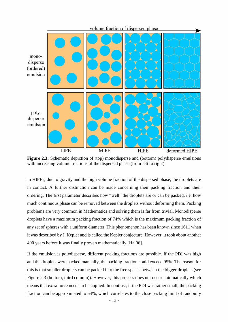
Figure 2.3: Schematic depiction of (top) monodisperse and (bottom) polydisperse emulsions

with increasing volume fractions of the dispersed phase (from left to right).

In HIPEs, due to gravity and the high volume fraction of the dispersed phase, the droplets are

in contact. A further distinction can be made concerning their packing fraction and their

ordering. The first parameter describes how “well” the droplets are or can be packed, i.e. how

much continuous phase can be removed between the droplets without deforming them. Packing

problems are very common in Mathematics and solving them is far from trivial. Monodisperse

droplets have a maximum packing fraction of 74% which is the maximum packing fraction of

any set of spheres with a uniform diameter. This phenomenon has been known since 1611 when

it was described by J. Kepler and is called the Kepler conjecture. However, it took about another

400 years before it was finally proven mathematically [Hal06].

If the emulsion is polydisperse, different packing fractions are possible. If the PDI was high

and the droplets were packed manually, the packing fraction could exceed 95%. The reason for

this is that smaller droplets can be packed into the free spaces between the bigger droplets (see

Figure 2.3 (bottom, third column)). However, this process does not occur automatically which

means that extra force needs to be applied. In contrast, if the PDI was rather small, the packing

fraction can be approximated to 64%, which correlates to the close packing limit of randomly

- 14 -

packed monodisperse spheres [Ber60]. Another term that can be used instead of ‘randomly

packed’ is disordered. If the droplets are ordered, however, they reach their maximum packing

fraction at 74%. Since the dispersed phase is not composed of hard spheres but liquid droplets,

the packing fraction can exceed 64 % or 74%, respectively. In that case, the droplets need to be

deformed and start to become polyhedral (see Figure 2.3 (fourth column)).

2.2 Microfluidics

Describing “[t]he science and technology of systems that process or manipulate small (10-9 –

10-18 liters) amounts of fluids, using channels with dimensions of tens to hundreds of

micrometers” [Whi06], systematic studies of microfluidics date back as far as the 1970s. At

that time, microfluidic devices were fabricated with micromechanics technology and were

employed in research on gas chromatography and ink jet printing [Gra93, Tab05]. However, it

was not until the early 1990s that progress in the field of microfluidics really picked up [Jon06,

Whi06]. In essence, the applications of microfluidics can be divided into (a) the synthesis of

chemicals and materials and (b) the analysis of mostly biological samples. All types of

applications avail themselves of the numerous advantages of this technique. Among these are

the low consumption of chemicals and samples, the enhanced separation and detection of

samples with remaining high resolution and sensitivity, the low cost, the short time for analysis,

and the small footprint on analytical devices [Man92, Bee02, Whi06, Zha11, Zha16]. Another

advantage of microfluidic devices is the fact that the fluids show laminar (“sheet-like“) flow,

which can be exploited for specific applications and will be discussed to a greater extent later.

Laminar flow means that the hypothetical sheets inside a fluid flow parallelly and do not

automatically mix with each other.

Commonly, polydimethylsiloxane (PDMS) is used as the base material from which the

microfluidic devices are manufactured by means of soft lithography techniques. PDMS has

several advantages, namely it is a moldable elastomeric polymer, it is inexpensive, and it is

optically transparent. Nevertheless, glass, steel, silicone, and thiolene can also be used when

more chemical or mechanical resistance is required. These materials do not deform or swell

when they come into contact with strong organic solvents or when they are exposed to higher

temperatures [Whi06, Chr07, Teh08]. Sometimes, it is necessary to change the wettability of

the microfluidic chip, i.e. to render its surface hydrophobic or hydrophilic. In order to transform

a hydrophilic surface into a hydrophobic one, it can be silanized or siliconized. On the other

hand, to transform a hydrophobic surface into a hydrophilic one, it can be exposed to oxygen

- 15 -

plasma, polyvinyl alcohol (PVA), or polyethylene glycol (PEG). Another way of changing the

surface wettability is the use of surfactants which absorb at the surface, thus rendering the chip

hydrophobic or hydrophilic [Chr07, Teh08].

A particular subtopic of microfluidics is droplet-based microfluidics where two phases are used

instead of one. They are either partially miscible or immiscible [Zha11]. When the two phases

meet at the so-called “junction”, monodisperse emulsion droplets are formed. In general, the

fluids are pushed through the microfluidic device by means of pressure pumps or syringe

pumps. At this point, it is necessary to take a closer look at the way the droplets are generated

inside the microfluidic device. By and large, the droplet generation is determined by (a) the

channel geometry and (b) the forces acting upon the fluids as well as upon the arising interface.

The ratio of two of these forces can be expressed in the form of dimensionless numbers, which,

along with other parameters, help to subdivide the droplet generation into different regimes.

Channel Geometry

Most of the used channel designs can be classified into cross-flow geometry, co-flow geometry,

and flow-focusing geometry, the last of which also being referred to as elongated flow geometry

[Chr07, Bar10, Zha11, Zha16]. Further arrangements dealing with step emulsification,

microchannel emulsification, and membrane emulsification are less common [Zhu16] and will

not be discussed here. A visual representation of cross-flow, co-flow, and flow-focusing

geometry is given in Figure 2.4. In cross-flow geometry, the two phases meet at an angle θ of

between 0° – 180° (see Figure 2.4 (top left)). In most cases, θ = 90° and this particular

arrangement is called “T-junction” (see Figure 2.4 (top right)). The dispersed phase and the

continuous phase ought to have similar flow rates in order to enable droplet generation. If the

flow rate of the dispersed phase is much lower than that of the continuous phase, the former

will not enter the downstream channel and hence, no droplets will form. If, on the other hand,

the flow rate of the continuous phase is too low compared to that of the dispersed phase, both

of them will stream uninterruptedly into the downstream channel and hence, droplets will not

form either. If the ratio between the two phases is set to an appropriate and constant value,

uniform-sized droplets will form periodically. This was first achieved by Thorsen et al. in 2001

[Tho01], who generated an w/o emulsion with a PDI as low as 2%. Since then, the cross-flow

geometry and especially the T-junction have been widely used due to their easy handling

[Chr07, Zhu16].

- 16 -

Figure 2.4: Schematic depiction of the general cross-flow geometry (top left), the T-junction

geometry (top right), the 2D-planar co-flow geometry (middle left), the 3D-coaxial co-flow

geometry (middle right), the 2D-planar flow-focusing geometry (bottom left), and the 3D-

coaxial flow-focusing geometry (bottom right).

As its name already suggests, in the co-flow geometry the two phases flow coexistingly

(parallelly) with the channel of the dispersed phase being surrounded by the larger channel of

the continuous phase (see Figure 2.4 (middle row)). Typically, the size of the generated droplets

is larger than the size of the channel of the dispersed phase. With a co-flow geometry, the first

monodisperse droplets were produced by Umbanhower et al. [Umb00], who were able to

minimize the PDI in their o/w emulsion to 3%. When focusing on the “depth” of the channels,

co-flow geometry can either be two dimensional (2D)-planar or three dimensional (3D)-coaxial

(see Figure 2.4 (middle left and middle right)) [Chr07, Zhu16].

Finally, in flow-focusing / elongated flow geometry both phases are pushed through a narrow

constriction (see Figure 2.4, bottom row). Moreover, the dispersed phase is flanked by two

streams of the continuous phase with a velocity flow field of the continuous phase focusing the

dispersed phase. At the highest point of shear, the result is a consistent breakup of the dispersed

phase into uniform-sized droplets. In general, this geometry offers an even more controlled

droplet break-up than the other two that were discussed previously. As is case for co-flow

- 17 -

geometry, the channels can either be 2D-planar or 3D-coaxial (see Figure 2.4 (bottom left and

bottom right)). In 2001, Gañàn-Calvo et al. [Gan01] were the first to use this geometry for

producing gas-in-water (g/w) bubbles. One year later, Anna et al. [Ann02] employed the same

arrangement for generating monodisperse w/o emulsion droplets [Chr07, Teh08, Zhu16].

Forces, Dimensionless Numbers, and Droplet Break-Up

In essence, there are four forces1 that act upon the fluids inside a microfluidic device. They all

depend on the characteristic length scale L of the microfluidic device – most often simply the

channel thickness – and/or the velocity vi of the fluid. The index ‘i’ thereby denotes the type of

phase that is examined with ‘c’ indicating the continuous phase and ‘d’ indicating the dispersed

phase. The first force acting upon a fluid is the inertial force fi which holds

𝑓i = ρi · 𝑣i2 , (2.7)

with ρi being the density of the fluid. This force stems from the pressure/syringe pump that sets

the liquid in motion inside the microfluidic device. At the junction where the two phases meet,

this force squeezes both of them downstream towards the channel outlet. The second force that

has the same orientation is the viscous force fv which holds

𝑓v =ηi · 𝑣i

𝐿 , (2.8)

with ηi being the dynamic viscosity. As its name presumes, this force is caused by the viscosity

of the fluid which itself stems from molecular diffusion and intermolecular interactions. The

third force that becomes especially important once the two immiscible phases get into contact

with each other is the capillary pressure fc which holds

𝑓c =γ

𝐿 , (2.9)

with γ being the interfacial tension between the two phases. If only one phase is present, γ

denotes the surface tension of the fluid. Finally, gravity has an influence on the fluids inside a

microfluidic device as well. Its force fg holds

𝑓g = ρi · 𝑔 · 𝐿 , (2.10)

1 Note that the four forces only nominally carry the name “force”, but are not forces in terms of physics.

- 18 -

with g being the gravitational constant of the earth [Zhu16]. In order to determine which type

of flow is present inside a microfluidic channel – laminar or turbulent – the so-called Reynolds

number Re is calculated. This dimensionless number is given by the ratio between the inertial

force fi and the viscous force fv and thus,

𝑅𝑒 =𝑓𝑖

𝑓v=

ρi · 𝑣i2

ηi · 𝑣i𝐿⁄

=ρi · 𝑣i · 𝐿

ηi (2.11)

[Bee02, Gar05, Zhu16]. If the viscous force fv greatly exceeds the inertial force fi, Re is small

and the flow is laminar. On the other hand, if the inertial force fi greatly exceeds the viscous

force fv, Re is large and the flow is turbulent. The boundary between laminar and turbulent flow

is typically put at Re = 2300 [Bee02, Zha16]. However, in microfluidic channels Re is usually

between 10-6 and 101 [Zhu16] and therefore, the flow is always laminar in microfluidic

channels. Fortunately, the famous Navier-Stokes-equation for incompressible fluids can be

solved linearly for laminar flow. For turbulent flows, solving the Navier-Stokes-equation

requires non-linear differential equations [Whi01, Squ05].

When droplets are generated, an interface between the two phases is formed. Thus, the force of

the capillary pressure fc, which contains the interfacial tension γ becomes essential. The energy

for developing the interface is provided by the pressure / syringe pumps that set the fluid in

motion. All the other three forces in relation to the force of the capillary pressure fc can be

expressed as dimensionless numbers. The Bond number Bo gives the ratio of the gravitational

force fg to the force of the capillary pressure fc and thus,

𝐵𝑜 =𝑓g

𝑓c=

Δρ · 𝑔 · 𝐿γ

𝐿⁄=

Δρ · 𝑔 · 𝐿2

γ . (2.12)

Here, Δρ is the difference in density between the two phases. When emulsion droplets are

formed inside a microfluidic device, both L and Δρ are small, which, in turn, decreases Bo to

miniscule values. Consequently, the influence of gravity can be neglected for droplet generation

in a microfluidic device [Tab05, Chr07, Zha11, Zhu16]. Note that for bubble generation, Δρ

has a higher value since the dispersed phase is a gas, which also increases Bo to some extent.

Here, gravity can have an influence on bubble generation [Chr07].

As already discussed for the Reynolds number Re, the inertial force fi can usually be disregarded

on the microfluidic scale. The ratio of this force to the force of the capillary pressure fc is

expressed by the Weber number We. Therefore, this dimensionless number is given as

- 19 -

𝑊𝑒 =𝑓i

𝑓c=

ρi · 𝑣i2

γ𝐿⁄

=ρi · 𝑣i

2 · 𝐿

γ . (2.13)

As the Reynolds number Re before, We has small values when droplets are generated in a

microfluidic device and is therefore not of high relevance [Chr07, Zha11, Zhu16].

The most important dimensionless number in microfluidics is the Capillary number Ca which

expresses the ratio between the two dominating forces on the microfluidic scale, fv and fc. It

holds

𝐶𝑎 =𝑓v

𝑓c=

ηi · 𝑣i𝐿⁄

γ𝐿⁄

=ηi · 𝑣i

γ . (2.14)

Consequently, Ca is independent of the length scale L. In microfluidic droplet generation, Ca

typically takes up values between 10-3 and 101 [Zhu16] and helps to differentiate between three

droplet generation regimes [Squ05, Chr07, Teh08, Zhu16]. These will be discussed thoroughly

in the upcoming paragraphs.

Two further dimensionless numbers that are sometimes used and do not depend on the four

previously introduced forces are the viscosity ratio λ and the flow ratio φ. They hold

λ =η𝑑

𝜂c (2.15)

and

φ =𝑄d

𝑄c , (2.16)

with ηd and ηc representing the viscosities of the dispersed and the continuous phase and Qd and

Qc representing the flow rates of the dispersed and the continuous phase, respectively [Chr07,

Teh08, Zhu16].

Droplet generation in microfluidic devices can be divided into three major regimes. These are

squeezing, dripping, and jetting and are depicted in Figure 2.5. Note that since the geometry of

the microfluidic device in this PhD thesis was flow-focusing geometry, the three regimes

accessible with this particular geometry are described. Nevertheless, the concepts are very

similar in cross-flow and co-flow geometry. Two further, less common regimes are tip-

streaming and tip-multibreaking. These are modifications of the jetting regime and will not be

- 20 -

Figure 2.5: Schematic depiction of the generation of one droplet in the squeezing regime (top),

in the dripping regime (bottom left), and the jetting regime (bottom right).

discussed here. As already mentioned, the Capillary number Ca can be used to define the

boundaries between the three regimes. In general, the viscous force fv and to smaller extend

also the inertial force fi try to deform the interface in order to continue flowing downstream,

while the capillary pressure tries to minimize the interfacial area. Since fi can be neglected, the

Capillary number Ca is a good indicator for distinguishing between the three regimes and is

therefore conventionally used. When the Capillary number of the continuous phase Cac is smal-

ler than 10-2, droplet generation occurs in the squeezing regime. When Cac is between 10-2 –

100, droplet generation occurs in the dripping regime. Finally, when Cac is larger than 100,

droplet generation occurs in the jetting regime [Ann16, Zhu16]. Together, they are all part of

the larger concept of passive droplet generation where droplet break-up is only determined by

the flow rates. In contrast, in active droplet generation auxiliary energy is put into the system.

For instance, electrical, magnetical, or centrifugal fields or optical stimuli assist the

destabilization of the interface which, in turn, facilitates droplet breakup. Another technique of

active droplet generation is altering the intrinsic properties of the fluids. Among these intrinsic

- 21 -

properties are the velocity, the viscosity, the interfacial tension, the channel wettability, and the

fluid density [Zhu16]. However, in this PhD thesis only the interfacial tension was influenced

by adding a surfactant and hence, only this way of active droplet generation will be discussed

to a greater extend later.

Coming back to the squeezing, dripping, and jetting regimes, the first one is different from the

latter two in that its droplet breakup is not determined by capillary instabilities. In contrast, the

confinement of the channel is dominating here and droplet breakup is governed by a quasi-static

mechanism. In the beginning, the dispersed phase starts to fill up the downstream channel

(cross-flow and co-flow geometry) or the constriction (flow-focusing geometry), respectively

(see Figure 2.5 (top a, b, and c)). Thereby, the available volume for the continuous phase to

continue flowing downstream becomes increasingly limited. This, in turn, creates a pressure

gradient of the continuous phase between the downstream channel (lower pressure) and the

upstream channel (higher pressure). Once the pressure gradient is large enough, the upstream

pressure of the continuous phase surmounts the pressure inside the dispersed phase. Now, the

continuous phase can enter the downstream channel/constriction again and thereby deforms

(“squeezes”) the interface (see Figure 2.5 (top d)). This continues until finally, droplet breakup

occurs (see Figure 2.5 (top e)) and the process starts again (see Figure 2.5 (top a)). Since droplet

breakup is mainly determined by the channel geometry, this regime is sometimes called the

“geometry-controlled” regime. Typically, the droplets are larger than the dimension of the

channel/constriction and are highly monodisperse [Bar10, Zha11, Zhu16].

As already mentioned before, the droplet breakup in the dripping and the jetting regime is

governed by capillary instabilities. This means that instead of a pressure gradient, the viscous

force of the continuous phase that streams alongside the droplet deforms the interface.

Moreover, droplet breakup already occurs before the channel/constriction is filled completely

with the dispersed phase (see Figure 2.5 (bottom left a, b, and c and bottom right a, b, and c)).

However, like the pressure gradient before, the viscous force increases when the dispersed

phase more and more fills the downstream channel/constriction. The droplet breakup of the

dripping and jetting regime is also similar to that of the squeezing regime in that the droplets

are formed when the continuous phase starts to deform the interface (see Figure 2.5 (bottom

left d and bottom right d)). In the dripping regime, breakup occurs close to the nozzle of the

dispersed phase (cross-flow and co-flow geometry) or close to the constriction (flow-focusing

geometry) (see Figure 2.5 (bottom left e)). In the jetting regime, on the other hand, there is an

extended stream of the dispersed phase into the downstream channel (see Figure 2.5 (bottom

- 22 -

right e)). The droplet breakup is then caused by Rayleigh-Plateau instabilities. However, this

severely limits the monodispersity so that the droplets are less monodisperse. In contrast, the

droplets are monodisperse when they are formed in the dripping regime. In both the dripping

and the jetting regime, the droplets are typically smaller than the dimension of the

channel/constriction [Zhu 16].

Apart from the flow rates, the droplet generation regimes can be influenced by adjusting the

interfacial tension. Most commonly, this is done by adding a surfactant to the continuous phase

which lowers the interfacial tension of the interface once droplet generation starts. Thus, it

becomes easier to deform the interface and hence, to generate droplets. By lowering the

interfacial tension, the Capillary number Ca is increased. This means that in order to remain in

the same droplet generation regime, the flow rates have to be decreased accordingly. An

important aspect of surfactant addition is the adsorption-desorption kinetics towards the

interface which include surfactant mass transfer time. When the time for forming one droplet

is much larger than the time for the surfactant to diffuse to the newly created interface, an

equilibrium surfactant concentration at the interface is obtained. In the inverted case, on the

other hand, the surfactant concentration at the interface remains quite low during droplet

formation as if no surfactant was present at all. For the case of similar time frames, the result is

a dynamic interfacial tension that changes during the droplet formation. Here, it becomes

possible to change the droplet size by small shifts in the flow rates or the surfactant

concentration [Ann16, Zhu16].

Though the geometries, forces, dimensionless numbers, and droplet generation regimes have

been discussed now, what is lacking are advantages and applications of droplet-based

microfluidics compared to microfluidics in general. Since the droplets offer even smaller

volumes than the microfluidic channel themselves, processes can be scaled down even further.

For example, the droplets can act as microreactors that prevent their content from leaving the

reaction site, while also having a high interfacial area-to-volume ratio to accelerate reactions

that require transfer between two droplets. Moreover, the monodisperse droplets can be

produced in high numbers. Various geometries and droplet generation regimes offer a tight

control over a wide range of droplet sizes, which helps to monitor the stoichiometry of a

reaction. Furthermore, as the droplets can adopt the size of organelles and cells, the former ones

can mimic the latter ones for studying biological processes. Two further examples for

applications are the investigation of reaction kinetics, commonly of enzymes, and the synthesis

of molecules with a highly exothermic energy profile where the temperature has to be precisely

- 23 -

controlled. Most of the applications are difficult to undertake with any other technique if not

even completely impossible. Finally, the droplets can also serve as templates for the synthesis

of microcapsules, microparticles, and microfibers that themselves are used in pharmaceutics,

cosmetics, and food. When the continuous phase is solidified after the droplet generation and

the droplets are removed afterwards, monodisperse porous materials can be produced which

was done in this PhD thesis [Chr07, Bar10, Teh08, Zhu16].

2.3 Polymers and Porous Polymers

2.3.1 Polymers

According to the International Union of Pure and Applied Chemistry (IUPAC), a polymer is

defined as “[a] molecule of high relative molecular mass, the structure of which essentially

comprises the multiple repetition of units derived, actually or conceptually, from molecules of

low molecular mass” [www1]. This ‘high relative molecular mass’ is typically at least above

1000 g mol-1 and often even above 10000 g mol-1 [Lec10]. Therefore, adding or removing one

unit does not significantly change the properties of a polymer. In the form of wood, fur, horn,

proteins, or carbohydrates, naturally occurring biopolymers have been known to and used by

mankind for millenia [Tie14]. In contrast, scientific research on synthetic polymers started only

about 200 years ago and their widespread industrial production began roughly 80 years ago

[Tie14]. Today, the most commonly used synthetic polymers are polyethylene (PE),

polystyrene (PS), polyvinylchloride (PVC), poly(methyl methacrylate) (PMMA), polytetra-

fluoroethylene (PTFE), and polyvinyl alcohol (PVA) [Lec10].

Types of Polymers and Polymerizations

If a polymer only consists of one singular repeating unit, it is called a homopolymer, while two

or three repeating units mean that the polymer is a copolymer or terpolymer, respectively

[Tie14]. Furthermore, using the example of a copolymer, four different types can be

distinguished by the alternating sequence of the two monomers inside the polymer. These four

types are statistical/random copolymers, alternating copolymers, block copolymers, and graft

copolymers and are all schematically depicted in Figure 2.6 (left) [Tie14].

- 24 -

Figure 2.6: Schematical depiction of (left) statistical/random (1a), alternating (1b), block (1c),

graft (1d) copolymers and of (right) linear (2a), branched (2b), crosslinked (2c), star-shaped

(2d) polymers.

Moreover, polymers can be distinguished according to their constitution. Here, four types exist

as well. These are linear polymers, branched polymers, crosslinked polymers, and star-shaped

polymers and are all depicted in Figure 2.6 (right) [Lec10, Tie14]. Another way to characterize

polymers is by the manner in which they are synthesized. In general, step-polymerization and

chain-polymerization can be distinguished. In step-polymerizations, the link between two

monomers is made through a reaction of their two respective functional groups. These are

typically hydroxy (-OH), carboxyl (-COOH), amine (-NH2), and aldehyde (-CHO) groups

[Lec10] and every monomer has at least two functional groups [Lec10, Su13]. At first, two

monomers are linked to form a dimer which itself then reacts with another monomer or dimer

to become a trimer or tetramer, respectively. Over time, more and more smaller units are linked

to form oligomers and finally polymers [Lec10, Tie14]. Step-polymerization can be further sub-

divided into polycondensation and polyaddition [Lec10, Tie14]. In polycondensations, every

reaction step produces a low-molecular byproduct which is often H2O. Examples for polymers

synthesized via polycondensation are polyesters like polyethylene terephthalate (PET) and

polyamides like Nylon®. In contrast, no byproduct is formed in polyadditions. Here, the most

prominent example are polyurethanes [Lec10].

In chain-polymerizations, the monomers typically contain at least one double or triple bond

whose electrons are used to connect two molecules by forming a new bond [Su13]. However,

initiators that activate some of the monomers by forming radicals are required to start the

polymerization. The newly formed radical at the monomer then can react with the next

monomer which itself now becomes a radical. Only at these ‘active centers’ other monomers

- 25 -

can be added to the growing polymer chain. The most common initiators are molecules that

dissociate into radicals when they are exposed to UV-light or heat and are called radical

initiators [Su13]. In turn, the polymerization is called a radical polymerization. Other initiator

types include anionic initiators, cationic initiators, and coordinative initiators [Tie14]. Chain-

polymerizations are comprised of three main reaction steps: initiation, propagation, and

termination. For the sake of convenience, the formation of a linear homopolymer with a radical

initiator will be used as an example to explain the three reaction steps. Overall, the three reaction

steps can be distinguished by how the concentration of radicals changes during each step.

During initiation, initiator molecules dissociate into radicals and thus, the concentration of

radicals increases. These radicals then activate the double bonds of the monomers by forming

a new bond with one carbon atom and creating a radical at the other carbon atom. The new

radical, in turn, bonds to the next monomer molecule and thereby continues the process. Figure

2.7 depicts this process for the first few steps with styrene as monomer and

azobisisobutyronitrile (AIBN) as radical initiator.

Figure 2.7: (top) Dissociation of the radical initiator AIBN by light or heat into two radicals

and nitrogen, (middle) reaction of the monomer styrene with one radical, (bottom) continuing

polymerization with two more styrene monomers.

- 26 -

These last two steps are still part of the initiation as long as the overall concentration of radicals

still increases. However, the formation of new radicals is always counteracted by radical

recombination where two radicals react and thus eliminate each other. Each of the two radicals

can be located at a large polymer chain, at a smaller oligomer, or still at the original dissociated

initiator. After the polymerization has continued for a certain time, the formation of new

radicals is compensated by radical recombination. Thus, the concentration of radicals remains

constant. This is known as propagation where the overall length of the polymer chains increases.

Once most of the monomer molecules are consumed, radical recombination becomes ever more

likely and thus, the concentration of radicals decreases. This is further supported by the fact that

with ongoing polymerization, the system will run out of initiator molecules at some point. The

final step is known as termination after which the polymerization is finished [Lec10, Su13,

Tie14].

Polymerization Media

Another important factor in any polymerization is the medium in which it takes place.

Polymerizations without a solvent are rarely used because it is virtually impossible to remove

the excess energy created by the exothermic polymerization process. This problem becomes

worse when the viscosity of the solution increases due to the formation of large molecules

during the polymerization. Even for polymerizations that take place in a non-polymerizable

medium, the increase in viscosity during the polymerization can be problematic. The diffusion

of large molecules becomes slower with increasing size. This, in turn, decreases the likelihood

of radical recombination because two large and active polymer chains do not come into contact

with each other anymore. However, since new radicals still form by initiator dissociation and

monomers can still diffuse to the immobile, yet active polymer chains, the exothermic

polymerization gets accelerated. This creates a lot of excess, uncompensated energy that

manifests as a sharp increase in temperature. Overall, this phenomenon is known as the

Trommsdorff/gel effect. To limit the extent of the Trommsdorff/gel effect and to maintain a

comparatively low viscosity during polymerization, the monomer is usually dispersed in H2O

or other media. The two most prominent methods here are emulsion polymerization and

suspension polymerization. In this chapter, they will be explained with styrene as hydrophobic

monomer and H2O as dispersing medium and are depicted schematically in Figure 2.8.

- 27 -

Figure 2.8: (top) Schematic depiction of emulsion polymerization: The surfactant forms

micelles and stabilizes the styrene droplets. The water-soluble initiator reacts with dissolved

styrene molecules to form oligomers which diffuse into the micelles. More styrene molecules

diffuse into the micelles and thereby continue the polymerization. (bottom) Schematic depiction

of suspension polymerization: Large, suspended styrene droplets also contain the monomer-

soluble initiator. Therefore, the polymerization takes place in the styrene droplets. Note that the

sizes of the droplets, micelles, and surfactant molecules are not to scale.

Other, more special methods such as miniemulsion polymerization, monomolecular plain

polymerization, and interphase polymerization will not be discussed here. For more information

on this subject, the reader is referred to [Lec10]. In emulsion polymerization, the surfactant

plays two roles, i.e. it stabilizes monomer droplets and it forms micelles in H2O (see Figure 2.8

(top left)). As already mentioned, the monomer is hydrophobic, but note that it still has a non-

negligible solubility in H2O. The polymerization is started by a water-soluble initiator and

mainly happens inside the micelles because the number of micelles (~ 1018 L-1 – 1021 L-1) is se-

veral orders of magnitude higher than the number of monomer droplets (~ 1010 L-1 – 1014 L-1)

[Lec10, Su13]. Because of this difference in numbers, it is far more likely that an active polymer

chain and a monomer meet inside a micelle than for an active polymer chain to diffuse into a

monomer droplet. Note that the first reaction steps between the water-soluble initiator and a

- 28 -

small number of monomer molecules occurs outside the micelles in H2O [Lec10 (page 167)].

When these short molecules grow in size, they become more hydrophobic and diffuse into

close-by micelles (see Figure 2.8 (top left)). Via the surfactant concentration, the number of

micelles can be adjusted which, in turn, controls the size of the resulting polymer globules.

Typically, their size is between 0.05 – 5 µm (see Figure 2.8 (top right)). In contrast, the final

globules produced by suspension polymerization are much bigger with sizes between 0.01 –

0.5 cm (see Figure 2.8 (bottom right)). Suspension polymerization does not use surfactants,

though the suspended monomer droplets can be stabilized by protective colloids. Furthermore,

a monomer-soluble initiator is used which means that the polymerization occurs inside the

suspended monomer droplets (see Figure 2.8 (bottom left)). Subsequently, these droplets

solidify over the course of the polymerization and transform into the already mentioned

polymer globules. Because the polymerization takes place in the large monomer droplets, heat

dissipation is more challenging than in emulsion polymerization. This can result in the

emergence of the Trommsdorff/gel effect. To prevent or limit the extent of the Trommsdorff/gel

effect, constant stirring is indispensable [Lec10, Su13, Tie14].

Crystallinity of Polymers

Finally, polymers can be differentiated by their mechanical behavior and their response to

temperature. Both factors depend on how the polymer chains are interconnected and if the

polymer is amorphous, crystalline, or a mixture of these two (= semicrystalline). One distinction

is between thermoplastics, thermosets, and elastomers. Before discussing the features of these

three types of polymers, the terms ‘glass transition temperature’ (Tg) and ‘melting temperature’

(Tm) have to be explained. While amorphous polymers show a Tg, crystalline polymers exhibit

a Tm. Semicrystalline polymers show both a Tg and a Tm. When the amorphous part of a

semicrystalline polymer or an amorphous polymer reaches its Tg, it transforms from a glassy

into a rubber-like state. On the other hand, when the crystalline part of a semicrystalline polymer

or a crystalline polymer reaches its Tm, it transforms from a crystalline state into an isotropic

melt. Note that since the size of the amorphous regions or crystals varies, both Tg and Tm are

not exact temperatures but rather temperature ranges. The temperature ranges at which Tm and

Tm appear, respectively, can be measured by differential scanning calorimetry (DSC) or

differential thermal analysis (DTA). Thermoplastics consist of linear, non-crosslinked polymer

chains and are usually amorphous or semicrystalline. They are frequently soluble in organic

solvents and can be converted into a polymer melt at high enough temperatures. In this state, it

- 29 -

is possible to re-shape a thermoplastic which will then remain in its new shape once cooled

down again. In contrast, thermosets cannot be re-shaped at all. Even if they are heated up to

several hundred degrees centigrade, they will rather decompose than undergo a Tg or Tm. The

reason for this behavior is that thermosets consist of highly crosslinked polymer networks. This

feature also explains why thermosets cannot be dissolved in any solvent and show no or only

very limited swelling. Both thermoplastics and thermosets respond rigidly when they are

compressed or stretched, while elastomers show – as their name already implies – elastic

behavior. The reason for this is that elastomers have a Tg that lies below room temperature

[Gib97], which means that they are in a rubber-like state. Elastomers consist of amorphous,

lightly crosslinked polymer chains and cannot be molten. Furthermore, they are not soluble in

solvents, but can be swollen by them [Gib97, Lec10, Tie14].

Polystyrene and Polydivinylbenzene

In this PhD thesis, only styrene and divinylbenzene (DVB) were used as monomers which is

why a closer look is taken at the polymerization of styrene/DVB mixtures. Since DVB has two

vinyl groups, it can be used for crosslinking. Similar to other factors like temperature, initiator

concentration, and type of polymerization, the styrene/DVB ratio affects the kinetics of the

polymerization. Firstly, the rate of polymerization increases linearly by a factor of ~ 2.5 when

one changes from pure styrene to pure DVB [Sto65, Zou90]. Secondly, when both styrene and

DVB are present, it is more likely for DVB to join a growing polymer chain [Sch75]. Thirdly,

in bulk or suspension polymerization, the addition of DVB has an influence on the onset of the

Trommsdorff/gel effect. By crosslinking with DVB, one increases the molecular weight of the

polymers which simultaneously increases the viscosity of the system. Therefore, the gel point

appears at lower conversion rates compared to the polymerization of pure styrene [Sto65]. This

effect is most perceptible below 10 wt.% DVB, while there is essentially no change anymore

above 10 wt.% DVB and the viscosity at a certain conversion rate even slightly decreases above

20 wt.% [Sto65]. The reason for this behavior is the twofold role of DVB during polymerization

which depends on the styrene/DVB ratio. For DVB fractions < 10 wt.%, the chains become

connected chemically and thus, the mechanical stability of the whole polymer system increases

[Hay83, Sun93]. Though, the polymerization is still occurring homogeneously everywhere

[Sto65, Kun68, Wie82]. Above 10 wt.% DVB, on the other hand, the crosslinker becomes a co-

monomer. Now, microgel particles with a net-like structure and a high degree of crosslinking

are formed in the beginning of the polymerization. These structures are separated from each

- 30 -

other by a pseudo-phase of monomers. Simultaneously, the monomers swell the microgel

particles, thereby continuing the localized, inhomogeneous polymerization. As a rule of thumb,

the extent of swelling decreases with increasing DVB fraction since it becomes increasingly

difficult for molecules to diffuse into the ever more tightly crosslinked structure [Sto65, Kun68,

Wil75, Hil85b]. Only when the polymerization in the microgel particles is finished, they start

to become connected with each other. However, these links between the microgel particles are

mechanically weaker than the interconnections inside them [Wie82] and thus, the copolymer

has a lower mechanical stability than at lower DVB fractions [Sun93]. Summarized, at high

DVB fractions, a sort of phase separation occurs during polymerization [Sto65, Dus67, Kun68,

Wie82, Sun93]. Since the viscosity remains comparatively low during the polymerization of

the microgel particles and only increases significantly once their connection starts, a precise gel

point is observed here [Sto65]. In contrast, a broader gel point exists when the DVB fraction is

lower since the crosslinking and therefore also the increase in viscosity happens more gradually

[Sto65]. The styrene/DVB ratio furthermore determines the probability for intra- versus

interchain polymerization and the fraction of pendant double bonds, i.e. double bonds that

remain unreacted after the polymerization is finished. At low DVB fractions, DVB acts solely

as crosslinker and mainly interchain polymerization occurs. The fraction of pendant double

bonds is very low as nearly all extra vinyl groups are used for crosslinking. At high DVB

fractions, on the other hand, intrachain polymerization inside the microgel particles dominates

over interchain polymerization. Thus, cyclizations occur that prevent a lot of extra vinyl groups

from polymerizing which, in turn, increases the fraction of pendant double bonds [Sto65,

Sop72, Hil85a, Hil85b, Sun93]. Finally, the styrene/DVB ratio influences the glass transition

temperature Tg. At first, adding DVB to pure styrene increases the Tg. For example, Zou et al.

[Zou90] found that the Tg of crosslinked monodisperse polystyrene beads increases from 104,4

°C to 133 °C when up to 10 wt.% of DVB were added. At higher DVB fractions, no Tg can be

observed anymore since it is impossible to transform a highly crosslinked polymer into a

flowable polymer glass [Wie82].

2.3.2 Porous Polymers

By converting polymers into porous polymers, the spectrum of possible applications broadens

immensely. Porous polymers – or polymer foams as they are often called as well – are part of

the larger group of cellular solids. These colloidal materials consist of a solid continuous phase

and a gaseous dispersed phase. While the gas is typically air, a wide range of solids like metals,

- 31 -

ceramics, glasses, and polymers can be used to create a cellular solid. Though this chapter

focusses solely on porous polymers, the reader can find information on cellular solids with other

materials in Gibson et al. [Gib97]. The properties of porous polymers are given by (a) the

chemistry of the polymer, (b) the volume fraction of the dispersed phase Φgas, and (c) the

morphology. As for the chemistry of the polymer, the chemical composition of the polymer –

i.e. the type of monomer(s) – is not solely decisive. Factors like the degree of crystallinity, the

degree of crosslinking, and the extent of the chain length distribution of the polymer play their

parts as well. The volume fraction of the dispersed gas Φgas, i.e. how much gas is dissolved in

the polymer matrix, is closely related to the relative density of the porous polymer ρrel and the

porosity of the porous polymer P. It holds

ρrel =ρporous polymer

ρpolymer (2.17)

with ρporous polymer and ρpolymer being the density of the porous polymer and the polymer,

respectively. In turn, P is calculated from ρrel via

𝑃 = 1 − ρrel . (2.18)

When neglecting the mass of the dispersed gas mgas, ρrel and P can easily be expressed with

Φgas. It holds,

ρrel = 1 − Φgas (2.19)

and

𝑃 = Φgas . (2.20)

A detailed derivation of how Φgas relates to ρrel and P is given in the Appendix in Section 6.1

(a). The ‘morphology’ summarizes all characteristic features that are associated with the

structure. These are the average pore size and pore size distribution, the pore shape, the texture

and thickness of the pore walls, and the interconnectivity of the pores. The last term describes

whether the pores are connected by windows or closed off from each other and what size the

windows have. Note that while this PhD thesis uses the terms ‘pores’ and ‘windows’, other

works [Gib97, Lan95, Lee07, Mil07] use the terms ‘cells’ for the larger voids and ‘pores’ for

the interconnections between these voids, respectively. Furthermore, note that the pore size sub-

divides porous polymers into macroporous polymers (pore width > 50 nm), mesoporous

- 32 -

polymers (2 nm ≤ pore width ≤ 50 nm), and microporous polymers (pore width < 2 nm) [Eve72,

Bur76]. In this PhD thesis, only macroporous polymers were synthesized [Gib97, Lan95].

Applications of Porous Polymers

Since porous polymers display a broad range of properties different from their bulk

counterparts, this opens up numerous different applications and explains their widespread use.

The most important benefit of porous polymers is that they are much lighter than the bulk

polymer. However, porous polymers can still exhibit a substantial mechanical stability which

is why they are widely used as packaging materials where they protect commodities from

physical damage by absorbing impact energy. Apart from commodities, it is also possible to

protect body parts with porous polymers which is used in protective sports gear like shin guards

for football players or helmets for cyclists, construction workers, skiers, etc. If a porous polymer

is more elastic than stiff, it can be utilized for applications that involve cushioning like cushions

or the sole of running shoes. Another property of porous polymers is their insulation potential

that depends on the interconnectivity of the pores. Open-pore porous polymers are used for

acoustic insulation. While sound waves can enter the porous polymer, they cannot leave it on

the opposite side and instead get damped by the pore walls. On the other hand, closed-pore

porous polymers are used for thermal insulation. Convection from one side to the other is

suppressed by the porous structure by repeated absorption and reflection at the pore walls.

While the polymer might have a non-neglectable heat conductivity, the volume fraction of the

porous polymer Φpolymer is usually low compared to Φgas. The gas itself has virtually no heat

conductivity. Thermal insulation is employed in buildings to reduce energy costs and for the

refrigeration of food and chemicals. Another type of insulation for which both open-pore and

closed-pore porous polymers can be used is electric insulation. Similar to thermal insulation, it

relies on the virtually non-existing electric conductivity of the gas inside the porous polymer.

Closed-pore porous polymers can also be utilized for their buoyancy since water cannot

penetrate the porous polymer and the density of the porous polymer is lower than the density

of water. Water wings for small children or additional floating support for water vehicles are

areas of application. Another field of application for open-pore porous polymers are filters and

water-repellent membranes. In filters, a liquid or gas flows through the open-pore structure

which causes a retardation or even retention of some of the components. This method is used

for the treatment of tap water or in gas masks. Water-repellent membranes are employed in

breathable fabrics or shoes. While liquid water cannot enter from the outside because of the

- 33 -

hydrophobicity of the polymer, air can pass through the material freely [Gib97, Lan95, Lee07,

Mil07].

Foaming Techniques

An important aspect of porous polymers is the manner in which the gas is introduced into the

polymer, i.e. how they are foamed. Here, three basic methods can be distinguished: mechanical,

physical, and chemical foaming. In general, the continuous phase has to be a liquid in order to

allow gas to be inserted and dispersed. Therefore, the gas is either introduced before the

polymerization, i.e. into a monomeric solution, or the polymer is molten. Once the gas bubbles

have formed and stabilized, a solid porous polymer is obtained by polymerization or cooling

down, respectively. A straightforward foaming technique is mechanical foaming where the

continuous phase is simply stirred or frothed intensively to submerse air into it and to break up

this air into bubbles. As for physical foaming, both inert gases and liquids with a low boiling

point can be used. Inert gases like N2 or CO2 are solubilized in a polymer melt at high

temperatures and high pressures. By releasing the pressure and cooling down, the inert gas

forms bubbles which are simultaneously immobilized by the solidifying polymer. Foaming with

liquids with a low boiling point works similarly. The polymer melt is mixed with the liquid

blowing agent which remains liquid even at high temperatures because of high pressure. When

the pressure is released, the blowing agent vaporizes and thus forms gaseous bubbles. Finally,

the melt is cooled down again to solidify the polymer. Initially, chlorofluorocarbons (CFCs)

were used as blowing agents. After their ban, hydrocarbons like butane and pentane were

chosen as replacement. However, the drawback of these compounds is that they are flammable

and explosive. In chemical foaming, the blowing agent is formed either (a) during the heating

of the reaction mixture or (b) during polymerization. In the first case, additives are mixed into

the monomer solution or polymer melt which decompose and release a gas at higher

temperatures. In the second case, a byproduct is formed during polymerization which can act

as a blowing agent. For example, if the temperature and pressure are adjusted to appropriate

levels, i.e. to above 100 °C and atmospheric pressure, the byproduct of most polycondensations,

H2O, can act as blowing agent [Lan95, Mil07].

- 34 -

Mechanical Properties of Porous Polymers

As already mentioned, the mechanical properties of porous polymers play a crucial role for their

applications. In applications such as packaging/protection, insulation, or floatation, the

mechanical properties are important since the material will always have to resist some kind of

stress. The mechanical behavior is primarily determined by the relative density ρrel of the porous

polymer, secondarily by the chemistry of the polymer, and marginally by other factors that

include the temperature, the type of gas, the strain rate, and anisotropy. Anisotropy can here

describe morphological anisotropy like pore size and shape, structural anisotropy like the

existence of pore size gradients, or material anisotropy [Gib97]. The two most important

mechanical characteristics of porous polymers are the Young’s Modulus E and the yield

strength σys. To determine these parameters, stress-strain-curves of porous polymers are

measured, where the mechanical response of a porous polymer is recorded by a load cell (≙

force censor) while being compressed via a hydraulic press. Depending on the progression of

the stress-strain-curve, three general types can be distinguished: elastomeric, elastic-plastic, and

Figure 2.9: Schematic stress-strain-curves of (top left) an elastomeric porous polymer, (top

right) an elastic-plastic porous polymer, and (bottom left) an elastic-brittle porous polymer.

- 35 -

elastic-brittle. Their stress-strain-curves are drawn schematically in Figure 2.9. All three types

of stress-strain-curves run through (a) a linear elastic region, (b) a plateau region, and (c) a

densification region with increasing strain. The linear elastic region and the densification region

look alike for all three types (see Figure 2.9 (top left a and c, top right a and c, and bottom left

a and c)), while the main difference lies in the shape of the plateau region (see Figure 2.9 (top

left b, top right b, and bottom left b)). In the linear elastic region, the stress σ increases

proportionally with the strain ε. This region is dominated by the bending of pore walls (open-

pore) / stretching of pore faces (closed-pore) and the performed compression is usually

recoverable, i.e. the porous polymer will return to its original shape once the compression is

stopped. Here, the Young’s Modulus E is determined via the slope of the stress-strain-curve

(see Figure 2.9 (top left E, top right E, and bottom left E)). It holds for the stress

σ =𝐹

𝐴 (2.21)

with F being the force acting upon the porous polymer and A being the area upon which the

compression is put. It holds for the strain

ε =Δℎ

ℎ0 (2.22)

with Δh being the difference in height and h0 being the initial height of the porous polymer.

Thus, it holds

𝐸 =σ

ε=

𝐹𝐴⁄

Δℎℎ0

⁄=

𝐹 · ℎ0

𝐴 · Δℎ (2.23)

The higher the value of E is, the more rigid is the porous polymer. Note that in order to obtain

accurate results, the initial height h0 of the porous polymers ought to be neither to large nor to

small compared to the diameter or width/length of the examined sample. Furthermore, the

sample ought to have dimensions at least 20 times greater than the average pore size to avoid

size effects [Mil07]. For porous polymers, Eporous polymer is typically in the order of ~ 1 MPa,

though Eporous polymer can be as low as ~ 10-3 MPa for elastomeric porous polymers. For example,

porous polystyrene with ρ = 50 kg m-3 has a Eporous polystyrene = 2.8 MPa and porous polystyrene

with ρ = 100 kg m-3 has a Eporous polystyrene = 4.8 MPa [Rin71]. In contrast, the Young’s Modulus

of the bulk polymer Epolymer usually is ~ 103 MPa. For non-porous polystyrene with ρ = 1050

- 36 -

kg m-3, Epolystyrene = {1400-3000} MPa [Gib97, page 57]. For open-pore porous polymers, the

ratio between Eporous polymer and Epolymer is proportional to the squared relative density ρrel. It holds

𝐸porous polymer

𝐸polymer= 𝐶C · 𝜌rel

2 = 𝐶C · (𝜌porous polymer

𝜌polymer)

2

(2.24)

with CC being the proportionality constant which is typically ≈ 1. For closed-cell porous

polymers, an equation similar to equation (2.24) exists, although it is more complex. While

equation (2.24) only takes into account pore edge bending, for closed-cell porous polymers pore

face stretching and gas compression inside the pores also contribute to the mechanical behavior.

It holds

𝐸porous polymer

𝐸polymer= 𝐶1Φ2𝜌rel

2 + 𝐶1′(1 − Φ)𝜌rel +

𝑝0(1 − 2𝜈∗)

𝐸polymer(1 − 𝜌rel) . (2.25)

Similar to equation (2.24), C1 and C1’ are proportionality constants which are both ≈ 1. Φ is the

fraction of the polymer that comprises the pore edges and thus (1 – Φ) represents the fraction

of the polymer residing in the pore faces. p0 is the initial gas pressure and ν* is the Poisson’s

ratio which is a measure for the “negative ratio of lateral to axial stress” [Gib97, page 187], in

other words how much the pores get stretched perpendicular to and get compressed parallel to

the direction of loading. For more information on the derivation of equation (2.25), the reader

is referred to Gibson et al. [Gib97, pages 192-197]. At the end of the linear elastic region which

is typically at a maximum strain of ε = 5%, the stress-strain-curve crosses over into the plateau

region. At this transition, the yield strength σys is determined (see Figure 2.9 (top left σys, top

right σys, and bottom left σys)). σys ranges between 10-2 MPa and 10-1 MPa for porous polymers

and between 101 MPa and 102 MPa for bulk polymers. For example, porous polystyrene with ρ

= 50 kg m-3 has a σys = 0.027 MPa and porous polystyrene with ρ = 100 kg m-3 has a σys = 0.062

MPa [Rin71]. For non-porous polystyrene with ρ = 1050 kg m-3, σys = {30-35} MPa [Gib97,

page 57]. σys is a measure for the maximum stress to which the porous polymer can be

compressed elastically. In the plateau region, though ε is successively increased, σ remains

more or less constant because pore collapse circumvents an increase of σ. For elastomeric

porous polymers, pore collapse occurs via elastic buckling of the pore walls and is recoverable.

In contrast, pore collapse for elastic-plastic and elastic-brittle porous polymers is irreversible.

For elastic-plastic porous polymers, pore collapse occurs via plastic hinges that eventually give

way to strain, while for elastic-brittle porous polymers, brittle crushing of the pore walls takes

place. Eventually, the stress-strain-curve reaches the densification region once all pore walls

- 37 -

have collapsed. Now, a compression of the solid polymer starts which leads to an abrupt and

steep increase in σ. Other, more specialized mechanical properties like shear modulus,

compressive stiffness, bending stiffness, or torsional stiffness to name but a few exist as well,

but are not discussed here. Commonly, porous polymers are only used for their properties in

compression, while stretching of porous polymers is rare. [Gib97, Mil07]

Porous Polystyrene

Like in Chapter 2.3.1, a closer look will be taken at porous polymers consisting of the monomers

styrene and DVB. Typically, the fraction of DVB is very low (< 1 %) or even zero as too much

DVB would make foaming of the molten polymer impossible. Porous polystyrene (PS) is a

light-weight material with closed pores, a low thermal conductivity, and a high water resistance.

This is why it is used in packaging, thermal insulation, and buoyancy products [Lan95, Lee07,

Mil07]. The two commercially most prominent types of porous PS are expanded polystyrene

(EPS) and extruded polystyrene (XPS). EPS is manufactured via suspension polymerization of

styrene that contains ~ 5 – 7 wt.% of pentane as chemical blowing agent. Pentane decreases the

Tg of PS from ~ 100 °C to ~ 60 °C, thus enabling the expansion of the PS beads by the

volatilization of pentane when the mixture is heated above the boiling temperature of pentane

[Lan95, Mil07, Tie14]. XPS is produced by first melting PS, secondly adding a blowing agent,

and thirdly putting the mixture under elevated temperature and pressure. Extruding the mixture

leads to a decrease in pressure which volatilizes the blowing agent and a decrease in temperature

which solidifies polystyrene [Lan95].

2.4 Templating Routes

A more specialized and indirect way of producing macroporous polystyrene in particular and

of macroporous polymers in general is the use of templates. The reason for this detour is that it

is easier to control and manipulate the structure of the template than to induce the desired

structure/morphology by direct foaming. Obviously, the structure of the template has to be

retained in the final macroporous polymer in order for this technique to be effective. At first,

an emulsion or a liquid foam is formed which acts as the template for the macroporous polymer.

The continuous phase is or contains the precursor for the solid polymer, i.e. the liquid monomer

or the dissolved polymer. In turn, the droplets or bubbles of the dispersed phase act as

placeholders for the future pores. After the formation of the template, it is solidified to fixate

- 38 -

its structure. Solidification is achieved by polymerization (monomers) or gelation (polymers).

Note that when emulsion templates are used, an additional drying step which removes the

dispersed droplets is necessary. Figure 2.10 schematically depicts the synthesis of a porous

(hydrophobic) polymer via a water-in-monomer template.

Figure 2.10: Schematic depiction of the synthesis of a porous (hydrophobic) polymer via a

water-in-monomer emulsion template.

In both foam and emulsion templating, the gas/liquid or liquid/liquid interface has to be

stabilized by a surfactant for at least as long as it takes to solidify the template. Therefore, no

hydrophobic monomers/polymers can be used in foam templating since no surfactants that can

stabilize gas-in-oil (g/o) interfaces exist. In contrast, surfactants that stabilize g/w, o/w, or w/o

interfaces are well-known. In order to be able to produce highly porous materials, the volume

fraction of the dispersed phase Φdisp is much higher than the volume fraction of the continuous

phase Φcont. As was already described in Section 2.1 (Figure 2.3), polydisperse (or

monodisperse and disordered) droplets/bubbles become close-packed at Φdisp = 64 vol%

[Dre15]. For monodisperse and ordered droplets/bubbles, the packing limit is Φdisp = 74 vol%.

When Φdisp > 64 vol% or Φdisp > 74 vol%, respectively, the droplets/bubbles lose their spherical

shape and get deformed. In this PhD thesis, monodisperse water-in-styrene/DVB HIPEs were

produced via microfluidics and consequently polymerized and dried to end up with

monodisperse macroporous polystyrene/poly-DVB. Therefore, the next paragraph is about the

development of (1) emulsion templating with polydisperse water-in-styrene/DVB emulsions

and of (2) monodisperse foam/emulsion templating.

Though Bartl et al. published their study on what they called “umgekehrte Emulsionen”

(German, in English “reversed emulsions”) as early as 1962 [Bar62], it took until 1985 for

Barby et al. to file for a patent on the preparation of “low density porous crosslinked polymeric

materials” [Bar85]. In the following decades, the research groups of Williams [Wil88a, Wil88b,

Wil89, Wil90a, Wil90b], Sherrington and Cameron [Hai91, Cam96, Cam97, Bar00, Cam00,

- 39 -

Cam05, Kim11], and Silverstein [Tai01a, Tai01b, Sil05, Sil14] advanced the science of

emulsion templating with styrene and DVB as the main monomers enormously. They

investigated the influence of the surfactant, of the monomer/crosslinker ratio, and of Φdisp on

emulsion stability, morphology, and pore size. Moreover, they investigated the effect of

additives like additional porogens or other co-monomers on the morphology of macroporous

polystyrene and measured their mechanical behavior. Figure 2.11 shows a scanning electron

microscope (SEM) picture of macroporous polystyrene synthesized with emulsion templating

by Barbetta et al. [Bar00].

Figure 2.11: Scanning electron microscope (SEM) picture of macroporous polystyrene that

was synthesized via emulsion templating by Barbetta et al. This Figure was copied from

[Bar00]. Order License ID: 1096628-1.

Parallel to the development of emulsion templating, advances in microfluidics enabled

researchers to produce monodisperse emulsions or foams. Talha Gokmen et al. used a

monodisperse HIPE where the dispersed phase was polymerized to end up with monodisperse

particles [Tal09]. In contrast, by solidifying the continuous phase and – if necessary – removing

the dispersed phase, monodisperse porous materials were achieved from monodisperse foam

templates [Cho09, Chu09, Lin11, Wan11, Sun12] or from a monodisperse oil-in-water

emulsion template [Cos14]. Combining water-in-styrene/DVB emulsion templating with

microfluidics, Quell et al. produced monodisperse macroporous polystyrene [Que15, Que16a,

Que16b, Els17, Que17a, Que17b]. A schematic depiction of the synthesis route was already

displayed in Figure 1.1. The most striking result was that the type of initiator – monomer-

- 40 -

soluble or water-soluble – has an immense impact of the morphology. With monomer-soluble

azobisisobutyronitrile (AIBN), (a) spherical pores, (b) an open-pore structure, and (c) porous

pore walls with (d) smooth pore surfaces were obtained (see Figure 2.12 (bottom)). In contrast,

with water-soluble potassium peroxodisulfate (KPS), (a) polyhedral pores, (b) a closed-pore

structure, and (c) a three-layered pore wall with (d) small globules on the pore surfaces were

obtained (see Figure 2.12 (top)). In Figure 2.12, the styrene/DVB mass ratio in the water-in-

styrene/DVB HIPE was 50/50, the surfactant mass fraction was 10 wt.%, and the initiator molar

fraction was 1.28 mol%. This composition was used in all works of Quell et al.

Figure 2.12: SEM pictures of macroporous PS/polyDVB obtained from monodisperse water-

in-styrene/DVB HIPEs where the initiator was either (top row) water-soluble KPS or (bottom

row) monomer-soluble AIBN. This Figure was copied from [Que17b]. Reprinted with

permission from Quell, A.; Sottmann, T.; Stubenrauch, C.; Diving into the Finestructure of

Macroporous Polymer Foams Synthesized via Emulsion Templating: A Phase Diagram Study,

Langmuir 2017, 33, 537-542. Copyright (2021) American Chemical Society.

Note that the polyhedral pores appear as hexagons in two-dimensional (2D) scanning electron

microscopy (SEM) pictures, while they more or less resemble rhombic dodecahedrons in three

dimensions (3D). Further note that with both types of initiator, the pores remain close-packed.

For monomer-soluble AIBN, the pore openings can be explained by the shrinkage of the

continuous phase when styrene/DVB (ρ ~ 0.94 g cm-3) polymerizes to polystyrene/poly-DVB

(ρ ~ 1.05 g cm-3) and consequently ruptures at its thinnest points, the films [Cam96]. Except for

the pore openings, the template structure is essentially retained with monomer-soluble AIBN.

With water-soluble KPS, however, two main questions arise: (1) why do the spherical droplets

transform into polyhedral pores when the continuous phase is polymerized. Note that for a given

- 41 -

volume, the surface area of a rhombic dodecahedron is ~ 10.5% larger than that of a sphere (see

Appendix Section 6.1 (b)). Therefore, a mechanism/force exists that increases the interfacial

area and thereby counteracts the capillary pressure. The second main question is (2) why the

pore walls are made up of three layers where the two outer layers appear dark and the inner

layer appears lighter in SEM pictures. Quell et al. answered both questions with one

explanation, namely osmotic transport of DVB from the Plateau borders into the films [Que16b,

Que17a, Que17b]. According to Schwachula, it is more likely for DVB to be built into the

polymer than for styrene. This means that in the beginning of the polymerization, the decrease

of the DVB concentration is greater than the decrease of the styrene concentration [Sch75].

Additionally, since the polymerization starts at the water/monomer interface when water-

soluble KPS is used, the decrease of the DVB concentration occurs more extensively in the

films compared to the Plateau borders. Therefore, a DVB concentration gradient between the

films and the Plateau borders arises because of which DVB molecules diffuse from the Plateau

borders into the films. As a consequence, the size of the Plateau borders decreases, while the

size of the films increases resulting in the hexagonal shape of the pore cross-sections. The three-

layered pore walls were explained by Quell et al. with two outer, poly-DVB-rich layers and an

inner, polystyrene-rich layer. Experiments conducted by Quell et al. [Que16b, Que17a] were in

line with their hypothesis, though a quantitative way to describe the osmotic transport was

missing. This is where this PhD thesis starts.

- 42 -

- 43 -

3 Results and Discussion

3.1 Disproof of Osmotic Transport

Assuming that osmotic transport of DVB as described previously at the end of Section 2.4 is

indeed responsible for the transformation of spherical droplets into polyhedral pores, one can

draw the following two conclusions: (1) If the styrene/DVB mass ratio was systematically

changed from 50/50 towards pure styrene, the extent of osmotic transport of DVB would

decrease because the concentration gradient of DVB between the Plateau borders and the films

would be lower. If the extent of osmotic transport of DVB decreases, (1a) the shape of the 2D

pore cross-sections ought to change from hexagonal to more circular (polyhedral to more

spherical for 3D pores). Simultaneously, (1b) the diameters of the layers inside the pore walls

ought to change as well. When the styrene/DVB mass ratio is varied towards pure styrene, the

diameter of the outer layers touter layer (supposed to be polyDVB-rich) ought to decrease, while

the diameter of the inner layer tinner layer (supposed to be PS-rich) ought to increase. In Section

3.1.1, the styrene/DVB mass ratio was varied in steps of 10 wt.% from 50 wt.% styrene

(styrene/DVB mass ratio = 50/50) to 90 wt.% styrene (styrene/DVB mass ratio = 90/10). From

now on, the styrene mass fraction βstyrene / wt.% will be used instead of styrene/DVB mass ratio

to avoid confusion. Note that it is not possible to polymerize a water-in-(pure) styrene HIPE as

it disintegrates into two separate phases during the early stages of solidification. Further note

that when βstyrene is decreased towards 10 wt.% instead of increasing it towards 90 wt.%,

analogous results are expected. Here, the shape of the 2D pore cross-sections ought to become

more circular as well since the continuous phase mainly consists of DVB, i.e. the extent of

osmotic transport of DVB ought to decrease, too. Simultaneously, the thickness of the outer

layer touter layer ought to increase and the thickness of the inner layer tinner layer ought to decrease.

In Section 3.1.1, only the change from 50 wt.% styrene to 90 wt.% styrene will be discussed in

detail, while the change from 50 wt.% styrene to 10 wt.% styrene will be presented via selected

samples in the Appendix in Section 6.2 (a).

The second conclusion that can be drawn if one believes in the existence of osmotic transport

of DVB is connected to the KPS mass fraction βKPS. (2) When βKPS is increased from its initial

2.98 wt.%, the polymerization is sped up. Therefore, there ought to be less time for the

comparatively slow diffusion process (osmotic transport of DVB). Thus, (2a) the shape of the

2D pore cross-sections should be more circular and (2b) the apparent visual difference between

outer and inner layer should be less pronounced. When βKPS is decreased from its initial 2.98

wt.%, it is not immediately clear what should happen, i.e. if the 2D pore cross-sections remain

- 44 -

hexagons or if they are transformed into some other shape. The corresponding experiments will

be discussed in Section 3.1.2. Note that Quell et al. [Que15, Que16a, Que16b, Els17, Que17a,

Que17b] used initiator molar fractions χinitiator 2, while in this PhD thesis initiator mass fractions

βinitiator 3 were used. Thus, the values of Quell et al. were converted to βinitiator (e.g. χKPS = 1.28

mol% corresponds to βKPS = 2.98 wt.% 4 and χAIBN = 1.28 mol% corresponds to βAIBN = 1.82

wt.%) as described in the Appendix in Section 6.1 (c). Overall, the intention behind the variation

of both βstyrene and βKPS was two-fold. The first purpose was to test the hypothesis of osmotic

transport of DVB. The second purpose was to collect more data about the morphology of the

polymerized monodisperse water-in-styrene/DVB HIPEs and to ideally develop a more

quantitative description of the osmotic transport of DVB. The results of Section 3.1 were also

published in a paper in Colloid and Polymer Science [Koc20].

3.1.1 Variation of Styrene Mass Fraction βstyrene

In this Section, βstyrene of the water-in-styrene/DVB HIPEs was varied from 50 wt.% to 90 wt.%

in steps of 10 wt.%. βKPS was set to a constant value of 2.98 wt.% and βsurfactant (mass surfactant

divided by combined mass of monomers styrene and DVB) was set to a constant value of 10

wt.%. For a better overview, the corresponding mass fractions are listed in Table 3.1.

Table 3.1: Type of initiator, βstyrene, βinitiator, and βsurfactant of the samples. βstyrene was varied,

while βinitiator and βsurfactant were kept constant.

Type of Initiator βstyrene / wt.% βinitiator / wt.% βsurfactant / wt.%

water-soluble KPS 50 2.98 10

water-soluble KPS 60 2.98 10

water-soluble KPS 70 2.98 10

water-soluble KPS 80 2.98 10

water-soluble KPS 90 2.98 10

monomer-soluble AIBN 50 1.82 10

monomer-soluble AIBN 70 1.82 10

monomer-soluble AIBN 90 1.82 10

For the sake of comparison, some samples were synthesized with the monomer-soluble AIBN

as initiator. The corresponding mass fractions are also listed in Table 3.1. The way in which the

2 χinitiator is calculated by dividing the molar amount of the initiator by the combined molar amount of the monomers

styrene and DVB. 3 βinitiator is calculated by dividing the mass of the initiator by the mass of the solvent. 4 The conversion was calculated with m(styrene) + m(DVB) = m(H2O). Quell et al. always used this mass ratio for

their samples as well [Que15, Que16a, Que16b, Els17, Que17a, Que17b].

- 45 -

Figure 3.1: SEM pictures of macroporous PS/poly-DVB obtained via polymerization of

monodisperse water-in-styrene/DVB HIPEs with βKPS = 2.98 wt.%, βsurfactant = 10 wt.%, and

βstyrene = 50 wt.%, = 60 wt.%, = 70 wt.%, = 80 wt.%, and = 90 wt.%. The magnifications are

100-fold (left column), 500-fold (middle column), and 1000-fold (right column).

- 46 -

samples were synthesized, polymerized, and processed is described in the Experimental

Section. In Figure 3.1, the SEM pictures of the KPS samples from Table 3.1 are presented with

a 100-fold (left column), a 500-fold (middle column), and a 1000-fold magnification (right

column). Looking at Figure 3.1, one instantly sees – contrary to the expectations – that the

shape of the 2D pore cross-sections is not becoming more circular when βstyrene is increased

from 50 wt.% to 90 wt.%. Instead, the shape of the 2D pore cross-sections appears to be even

more “angular”, i.e. it deviates even more from a circular shape. The left column of Figure 3.1

indicates that this observation is not due to a failure of the templating method since the pores

are still close-packed and fairly monodisperse.

For the templating method to be fully successful, the size of the pores has to be same as the size

of the preceding droplets. For both the water droplets and the pores, the diameter d was

calculated via the area A of the 2D cross-sections. For circles, it holds

𝑑 = 2 · 𝑟 = 2 · √𝐴

π , (3.1)

with r being the radius. Equation (3.1) was used to calculate ddroplet and dpore. This means that

although the shape of the pore cross-sections is not circular, dpore was calculated as if the pore

cross-sections were circular. Thus, the calculation of dpore contains a systematic error. However,

the “correct” diameter of the hexagonal 2D pore cross-sections is not clear. The distance edge-

to-edge, the distance corner-to-corner, or an average of the first two can all be viewed as viable

definitions for the diameter of a hexagon. In any case, the relative differences between these

three values and the calculation via equation (3.1) are comparatively small as can be seen in the

exemplary calculations in Appendix Section 6.1 (d). If the shape of the 2D pore cross-sections

is modified from a hexagon, the determination of dpore via the edges and/or the corners becomes

impossible. Therefore, the calculation of dpore that was used in this PhD thesis is a reasonable

compromise because the occurring error is not significant. In Figure 3.2, the average diameter

of the water droplets ddroplet (black circles) in the water-in-styrene/DVB HIPEs before

polymerization and the average diameter of the pores dpore (white squares) in the macroporous

PS/polyDVB samples after polymerization are plotted as function of βstyrene.

- 47 -

Figure 3.2: Average emulsion droplet diameter ddroplet (black circles) and average pore diameter

dpore (pink squares) as function of βstyrene for macroporous PS/poly-DVB at βKPS = 2.98 wt.%

and βsurfactant = 10 wt.%.

Figure 3.2 shows that the polymerization slightly changes the average diameter and decreases

the monodispersity. Before polymerization, ddroplet is always ~ 72 µm and the water droplets are

very monodisperse since the standard deviation (black error bars in Figure 3.2) is only 1 – 2

µm. In contrast, after polymerization the standard deviation of dpore has increased to values

between 8 – 12 µm. Though this means that the polydispersity increases during polymerization,

the pores are still far from being actually polydisperse. Concerning the change in average

diameter from ddroplet to dpore, no continuous trend could be found. For βstyrene = 60 wt.%, dpore is

smaller than ddroplet. For all four other βstyrene, however, dpore is larger than ddroplet. The extent of

the increase is very small for βstyrene = 70 wt.%, a little larger for βstyrene = 50 wt.% and βstyrene =

80 wt.%, and largest for βstyrene = 90 wt.%. For all five samples, dpore is nevertheless always still

in the range of ddroplet. Figure 6.1 in the Appendix Section 6.2 (a) shows the development of the

morphology of macroporous PS/polyDVB where βstyrene was lower than 50 wt.%. At first

glance, the 2D pore cross-sections remain hexagons independent of βstyrene. Overall, the results

from Figure 3.1 and Figure 6.1 are contrary to what should have happened if osmotic transport

of DVB was the reason for the transformation from spherical droplets to polyhedral pores.

- 48 -

When instead of KPS the monomer-soluble initiator AIBN is used, the 2D pore cross-sections

are always circular. This can be seen in Figure 3.3 where the SEM pictures of macroporous

PS/polyDVB samples that were polymerized from monodisperse water-in-styrene/DVB HIPEs

with AIBN as initiator are displayed. βAIBN was set to a constant value of 1.82 wt.%, βsurfactant

was set to a constant value of 10 wt.%, and βstyrene was 50 wt.%, 70 wt.%, and 90 wt.%. The

magnifications in Figure 3.3 are 100-fold (left column), 500-fold (middle column), and 1000-

fold (right column).

Figure 3.3: SEM pictures of macroporous PS/poly-DVB obtained via polymerization of

monodisperse water-in-styrene/DVB HIPEs with βAIBN = 1.82 wt.%, βsurfactant = 10 wt.%, and

βstyrene = 50 wt.%, = 70 wt.%, and = 90 wt.%. The magnifications are 100-fold (left column),

500-fold (middle column), and 1000-fold (right column).

In all cases, the pores are close-packed, fairly monodisperse, and interconnected in Figure 3.3.

Figure 3.4 depicts ddroplet (black circles) before polymerization and dpore (pink squares) after

polymerization of these samples as function of βstyrene.

- 49 -

Figure 3.4: Average emulsion droplet diameter ddroplet (black circles) and average pore diameter

dpore (pink squares) as function of βstyrene for macroporous PS/poly-DVB at βstyrene = 1.82 wt.%

and βstyrene = 10 wt.%.

As was already the case in Figure 3.2, ddroplet ~ 72 µm for all samples and the droplets are very

monodisperse with standard deviations of only 2 µm. After polymerization, the standard

deviation increases to values between 6 – 8 µm, meaning that the pores are still fairly

monodisperse, and dpore has also increased compared to ddroplet. The reason for this increase

might be that the water droplets are more susceptible to Ostwald ripening compared to water

droplets that contain a water-soluble salt, namely KPS (see Section 2.1). Overall, it is evident

that changing βstyrene has little to no effect on the morphology when AIBN is used as initiator,

while the morphology changes considerably as function of βstyrene when KPS is used as initiator

(see Figure 3.1).

Shape of Pore Cross-Sections: Shape Factor S

Although it is obvious from Figure 3.1 that the 2D pore cross-sections are not becoming more

circular when βstyrene is increased, it would be helpful to have a quantitative value to express

how “circular” or “angular” the 2D pore cross-sections are. To achieve this, the ratio between

the circumference C and the area A of a pore cross-section are taken into account. Since a circle

- 50 -

has the lowest circumference-to-area ratio, this value is lowest for a circle and then increases

when the shape gets more angular. The idea for such a quantitative value stems from foam

science where something analogous is done in 3D with the surface area and volume of foam

bubbles [Kra04, Hil04, Kra05, Kra06, Dre15]. Though only the 2D circumference C and area

A of the pore cross-sections are used in this PhD thesis, the result can be taken as a

representative for the 3D pores. An exemplary picture on how C and A were determined in one

sample via the image processing software ImageJ is presented in Appendix Section 6.2 (b),

Figure 6.2 (left)). However, the ratio between C and A is not taken directly, but two alterations

are undertaken. Firstly, since C scales linearly and A quadratically with size, the ratio between

them depends on the size of the pore cross-sections. To avoid this, the square root of A is used

instead of A. For a geometric circle, it holds

𝐶circle

√𝐴circle

=2π𝑟

√π𝑟2= √

4π2𝑟2

π𝑟2= √4π = 2 · √π ≈ 3.545. (3.2)

Next, the result of equation (3.2) is inverted to serve as a normalizing factor. This constitutes

the second alteration and yields the final form to describe the shape of the 2D pore cross-

sections. In this PhD thesis, this value is denominated “shape factor S”. It holds

𝑆 =1

2 · √π·

𝐶

√𝐴 . (3.3)

For a circle, S = 1 (see Figure 3.5 (bottom left)). For a geometric hexagon, S can be calculated

from its circumference Chexagon and its area Ahexagon. It holds

𝐶hexagon = 6 · 𝑎 (3.4)

and

𝐴hexagon =3 · √3

2· 𝑎2 (3.5)

with a being the length of one edge of the hexagon. Thus,

𝑆hexagon =1

2 · √π·

6𝑎

√3√32 · 𝑎2

= √36𝑎2 · 2

4π · 3√3 · 𝑎2= √

6

√3 · π≈ 1.050. (3.6)

- 51 -

Consequently, S ought to be ~ 1.05 (see Figure 3.5 (middle left)) for the hexagonal shapes found

in the 2D pore cross-sections in Figure 3.1. For shapes that are distorted from a hexagon, S ≥

1.05 (see Figure 3.5 (top left)). Figure 3.5 (right) depicts S as function of βstyrene.

Figure 3.5: (left) Exemplary values of the shape factor S for a sphere (bottom), a hexagon

(middle), and a distorted hexagon (top). (right) S as function of βstyrene for macroporous PS/poly-

DVB at βKPS = 2.98 wt.% and βsurfactant = 10 wt.%.

When βstyrene is increased, S increases from ~ 1.09 ± 0.04 for βstyrene = 50 wt.% to ~ 1.34 ± 0.13

for βstyrene = 90 wt.%. Thus, Figure 3.5 (right) quantifies the observations from Figure 3.1, i.e.

that increasing βstyrene leads to more “angular” pore cross-sections. Note that S is not exactly

1.05 for the apparent hexagons at βstyrene = 50 wt.% or βstyrene = 60 wt.%. Instead, S ~ 1.10. This

can be explained by looking at the middle and right column of Figure 3.1. The 2D pore cross-

sections are not geometric hexagons with perfectly straight edges, but the edges are somewhat

distorted. Thus, C is larger than that of a hexagon, while A stays more or less constant. As a

consequence, the ratio between C and A is also larger and thus S > 1.05.

Thickness of Pore Wall and Layers

As already mentioned, the development of the shape of the 2D pore cross-sections is

incompatible with the results that should have been obtained when osmotic transport of DVB

was responsible for the transformation from spherical droplets to polyhedral pores. Another

- 52 -

logical consequence of this hypothesis was that the thickness of the supposedly polyDVB-rich

outer layers touter layer ought to decrease and the thickness of the supposedly PS-rich inner layer

tinner layer ought to increase when βstyrene is increased. From Figure 3.1, it is not possible to

determine the development of the thickness of the pore wall tpore wall, touter layer, and tinner layer as

function of βstyrene. The magnification in the left column of Figure 3.1 is not high enough to

directly measure the thicknesses and the middle and right column of Figure 3.1 only show a

small section of the sample. Therefore, tpore wall, touter layer, and tinner layer were determined using a

SEM picture of the whole sample and consequently zooming in at various locations. An

example of this method is presented in Appendix Section 6.2 (b), Figure 6.2 (right). By

determining the desired length perpendicular to the direction the pore wall/layer is running

along, tpore wall, touter layer, and tinner layer were measured. An example for this can be seen in Figure

3.6.

Figure 3.6: Picture of how the thickness of the whole pore wall (black), of the two outer layers

(blue), and of the inner layer (red) were determined.

Figure 3.7 (top) depicts the development of tpore wall (black circles), touter layer (blue squares), and

tinner layer (red diamonds) as function of βstyrene. Figure 3.7 (bottom) depicts the fraction of the

outer layer (blue squares) which is the ratio between touter layer and tpore wall and the fraction of the

inner layer (red diamonds) which is the ratio between tinner layer and tpore wall.

- 53 -

Figure 3.7: (top) Average thickness of the whole pore wall tpore wall (black circles), of the outer

layers touter layer (blue squares), and of the inner layer tinner layer (red diamonds) as function of βstyrene

for macroporous PS/poly-DVB at βKPS = 2.98 wt.% and βsurfactant = 10 wt.%. (bottom) Ratio touter

layer to tpore wall (blue squares) and ratio tinner layer to tpore wall (red diamonds) as function of βstyrene.

Since two outer layers exist, the two ratios in the bottom graph do not add up to 1. For the sake

of clarity, the blue squares and the red diamonds are shifted to lower and higher βstyrene,

respectively.

Again, the results are not in line with what was to be expected if osmotic transport of DVB was

responsible for the transformation from spherical droplets to polyhedral pores. Even though

- 54 -

touter layer decreases as function of βstyrene (as was expected), the same trend is observable for tinner

layer and tpore wall. Thus, the fraction of the outer layer and the fraction of the inner layer remain

more or less constant when βstyrene is increased (see Figure 3.7 (bottom)). For osmotic transport

of DVB to be the correct hypothesis, the fraction of the outer layer should have decreased and

the fraction of the inner layer should have increased. Overall, this means that the development

of the layer thicknesses or their fractions, respectively, as function of βstyrene serves as a second

counterevidence to the hypothesis of osmotic transport of DVB. Note that in Figure 3.7

(bottom), the two fractions do not add up to 1. The reason for this can be explained with the

help of Figure 3.6. Every time tpore wall and tinner layer are determined once, touter layer is determined

twice. However, in the end only one average touter layer is calculated. Thus, touter layer has to be

doubled before adding it to tinner layer in order to yield tpore wall. The same is true for the addition

of the fraction of the outer layer to the fraction of the inner layer to end up at 1. Strikingly, the

standard deviations of tpore wall and tinner layer are much larger than the standard deviation of touter

layer (see Figure 3.7 (top)). The same can be said about the large standard deviation of the fraction

of the inner layer and the small standard deviation of the fraction of the outer layer. (see Figure

3.7 (bottom)). Again, the reason for this can be found in Figure 3.6 when looking at the

thicknesses close to the struts5 (see Figure 3.6 (left)) and at the thicknesses in the films (see

Figure 3.6 (right)). When moving from the struts into the films, tpore wall becomes smaller.

However, tpore wall was determined at several positions that were close to the struts, in the films,

or between these two (see Appendix Section 6.2 (b), Figure 6.2 (right)). Therefore, tpore wall has

a relatively high standard deviation. Looking at the development of touter layer and tinner layer

between the struts and the films, it becomes apparent that touter layer remains roughly the same

value independent of the location where it is measured. In contrast, and tinner layer changes from

larger to smaller values when tpore wall changes from larger (close to struts) to smaller values

(films). Thus, the standard deviation of touter layer is small and the standard deviation of tinner layer

is large. These trends continue for the fraction of the outer layer and the fraction of the inner

layer in Figure 3.7 (bottom).

When combining the trends from Figure 3.5 (right) and Figure 3.7 (top), it is noticeable that the

overall surface of the pores increases as function of βstyrene, while tpore wall, touter layer, and tinner layer

decrease as function of βstyrene. Indeed, this makes sense: since the amount of available polymer

is finite and the same independent of βstyrene, tpore wall, touter layer, and tinner layer have to decrease in

order for the surface area to be able to increase. In other words, tpore wall, touter layer, and tinner layer

5 A strut corresponds to a former Plateau border which is now solidified.

- 55 -

are spread out over a larger area. This relation can be expressed via a formula. For this purpose,

both S and tpore wall, touter layer, and tinner layer are normalized. This is done by dividing them by the

respective values of the initial βstyrene which is 50 wt.%. Moreover, the normalized shape factor

S/S50 has to be squared since the key factor, the available volume of polymer, is a product of

tpore wall, touter layer, or tinner layer and the surface area of a pores. The latter term is a quadratically

scaling parameter that is determined from 3D. In contrast, S/S50 scales linearly and is determined

from 2D. By squaring S/S50, this problem is easily solved and the desired relation is achieved.

The product of t/t50 and (S/S50)2 as function of βstyrene is depicted for the pore wall (black circles),

for the outer layer (blue squares), and for the inner layer (red diamonds) in Figure 3.8.

Figure 3.8: Normalized average thickness of the whole pore wall tpore wall/tpore wall, 50 wt.% styrene

(black circles), of the outer layer touter layer/touter layer, 50 wt.% styrene (blue squares), and of the inner

layer tinner layer/tinner layer, 50 wt.% styrene (red diamonds) multiplied with the squared normalized shape

factor S/S50 wt.% styrene as function of βstyrene for macroporous PS/poly-DVB at βKPS = 2.98 wt.%

and βsurfactant = 10 wt.%. For the sake of clarity, the blue squares and the red diamonds are shifted

to lower and higher βstyrene, respectively.

Summed up, Figure 3.8 indeed shows that when βstyrene is increased, the increase in surface area

of the pores is compensated by the decrease in tpore wall, touter layer, and tinner layer. In other words,

the total volume of the pore wall, of the outer layer, and of the inner layer remain constant, but

they are spread out over a larger surface area.

- 56 -

3.1.2 Variation of KPS Mass Fraction βKPS

In Section 3.1.2, the KPS mass fraction βKPS of the water-in-styrene/DVB HIPEs was varied

from 0.37 wt.% to 4.96 wt.%. The first (0.37 wt.%), second (0.75 wt.%), and third (1.49 wt.%)

values of βKPS are one eight, one fourth, and one half of the initial βKPS of 2.98 wt.%. The fifth

βKPS represents the maximum solubility of KPS in H2O [www2]. βstyrene was kept constant at 50

wt.% and βsurfactant was kept constant at 10 wt.%. For a better overview, the corresponding mass

fractions are listed in Table 3.2.

Table 3.2: Type of initiator, βstyrene, βinitiator, and βsurfactant of the samples. βinitiator was varied,

while βstyrene and βsurfactant were kept constant.

Type of Initiator βstyrene / wt.% βinitiator / wt.% βsurfactant / wt.%

water-soluble KPS 50 0.37 10

water-soluble KPS 50 0.75 10

water-soluble KPS 50 1.49 10

water-soluble KPS 50 2.98 10

water-soluble KPS 50 4.96 10

monomer-soluble AIBN 50 0.23 10

monomer-soluble AIBN 50 0.45 10

monomer-soluble AIBN 50 0.91 10

monomer-soluble AIBN 50 1.82 10

As in Section 3.1.1, samples were also prepared with the monomer-soluble initiator AIBN.

However, now the AIBN mass fraction βAIBN was varied between 0.23 – 1.82 wt.%. Note that

for unknown reasons, it was not possible to produce a monodisperse water-in-styrene/DVB

HIPE at βAIBN = 3.02 wt.%. Therefore, only four βAIBN values were studied. The way in which

the samples were synthesized, polymerized, and processed can be found in the Experimental

Section. Figure 3.9 depicts the SEM pictures of macroporous PS/polyDVB samples that were

obtained from the polymerization of the monodisperse HIPEs listed in Table 3.2 with KPS as

initiator. The magnifications are 100-fold (left column), 500-fold (middle column), and 1000-

fold (right column). At first glance, the shape of the 2D pore cross-sections is always hexagonal

independent of βKPS. Since Section 3.1.1 already revealed that osmotic transport of DVB cannot

be the reason for the transformation from spherical droplets to polyhedral pores, it is not

surprising that the expectations stated in the introduction of Section 3.1 did not come true. As

a reminder, a higher βKPS was supposed to lead to more circular 2D pore cross-sections since

the polymerization would be sped up and osmotic transport of DVB would have less time to

occur. When taking a closer look at the middle and right column of Figure 3.9, it is observable

that the edges of the hexagons in the 2D pore cross-sections are nearly perfectly straight at low

βKPS and get more distorted at higher βKPS.

- 57 -

Figure 3.9: SEM pictures of macroporous PS/poly-DVB obtained via polymerization of

monodisperse water-in-styrene/DVB HIPEs with βstyrene = 50 wt.%, βsurfactant = 10 wt.%, and

βKPS = 0.37 wt.%, = 0.75 wt.%, = 1.49 wt.%, = 2.98 wt.%, and = 4.96 wt.%. The magnifications

are 100-fold (left column), 500-fold (middle column), and 1000-fold (right column).

- 58 -

The diameter of the water droplets ddroplet (black circles) before polymerization and the diameter

of the pores dpore (pink squares) after polymerization as function of βKPS is depicted in Figure

3.10. Note that logarithmic plotting is used for the abscissa in Figure 3.10. The same will be

true for the abscissae of Figure 3.12, Figure 3.13 (right), Figure 3.14 (top) and (bottom), and

Figure 3.15.

Figure 3.10: Average emulsion droplet diameter ddroplet (black circles) and average pore

diameter dpore (pink squares) as function of βKPS for macroporous PS/poly-DVB at βstyrene = 50

wt.% and βsurfactant = 10 wt.%.

Even though ddroplet varies a bit more compared to Figure 3.2, the droplets were monodisperse.

As before, polymerization leads to an increase of the error bars, but the pore cross-sections are

still fairly monodisperse. Except for βKPS = 1.49 wt.% where dpore is ~ 11 µm smaller than ddroplet,

the change from ddroplet to dpore is minimal for the four other values of βKPS. As explained in

Section 3.1.1, dpore was calculated from the area A of the pore cross-sections (see equation (3.1)).

Unfortunately, βKPS cannot be set to values higher than ~ 5 wt.% since this represents the

maximum solubility of KPS in H2O [www2]. However, ammonium peroxodisulfate (APS) has

a much higher solubility in H2O [www3] and is chemically very similar to KPS since only the

counter-cation is different. Note that no experiments about were carried out and it was assumed

that KPS and APS have similar reactivities. With APS as initiator, βAPS was set to values

- 59 -

between 0.32 – 39.44 wt.%. Here, βAPS = 0.32 wt.%, = 0.63 wt.%, = 1.26 wt.%, = 2.52 wt.%,

and = 4.20 wt.% are molarly equivalent to the five values of βKPS in Figure 3.9. Additionally,

samples with βAPS = 9.86 wt.%, = 19.72 wt.%, and = 39.44 wt.% were produced. The SEM

pictures of these eight samples are depicted in Figure 6.3 and Figure 6.4 in Appendix Section

6.2 (c). Without going into too much detail, it is apparent that for molarly equal mass fractions,

the morphology is roughly the same if either KPS or APS is used. Up to βAPS = 9.86 wt.%, the

shape of the 2D pore cross-sections can roughly be described as hexagonal. With a further in-

Figure 3.11: SEM pictures of macroporous PS/poly-DVB obtained via polymerization of

monodisperse water-in-styrene/DVB HIPEs with βstyrene = 50 wt.%, βsurfactant = 10 wt.%, and

βAIBN = 0.23 wt.%, = 0.45 wt.%, = 0.91 wt.%, and = 1.82 wt.%. The magnifications are 100-

fold (left column), 500-fold (middle column), and 1000-fold (right column).

- 60 -

crease of βAPS, the pores become more and more disordered as well as polydisperse. At the

highest value for βAPS = 39.44 wt.%, the interconnectivity changes from closed-pore to open-

pore. Note that such high initiator mass fractions are far from any reasonable field of application

and were only used to test the limits of the system.

When βAIBN is varied, the shape of the pore cross-sections is always circular. This is depicted

in Figure 3.11 where the magnifications were 100-fold (left column), 500-fold (middle column),

and 1000-fold (right column). The corresponding mass fractions were listed in Table 3.2. As in

Figure 3.4 where the morphology was largely independent of βstyrene, it is also independent of

βAIBN. However, looking at the diameters of the pore cross-sections in Figure 3.11, it is obvious

that at βAIBN = 0.91 wt.% dpore is much larger than for the three other values of βAIBN. This can

also be seen in Figure 3.12 where ddroplet (black circles) before polymerization and dpore (pink

squares) after polymerization are depicted as function of βAIBN.

Figure 3.12: Average emulsion droplet diameter ddroplet (black circles) and average pore

diameter dpore (pink squares) as function of βAIBN for macroporous PS/poly-DVB at βstyrene = 50

wt.% and βsurfactant = 10 wt.%.

For βAIBN = 0.23 wt.% and βAIBN = 0.45 wt.%, the high monodispersity of the droplets is largely

conserved in the pores, while dpore is slightly smaller than ddroplet. For βAIBN = 0.91 wt.%, the

high monodispersity is also mostly retained, while dpore increases tremendously compared to

- 61 -

ddroplet. Finally, for βAIBN = 1.82 wt.%, the pores did not maintain the high monodispersity of

the droplets, though dpore is closer to ddroplet compared to βAIBN = 0.91 wt.%. Overall, it appears

as if the transition from HIPE to macroporous PS/polyDVB gets more susceptible to changes

when βAIBN is increased. This is further supported by the fact that it was not possible to produce

a sample with βAIBN = 3.02 wt.% where the droplets were already polydisperse when they were

generated in the microfluidic chip. Nevertheless, Figure 3.11 shows that βAIBN has at least no

influence on the shape of the pore cross-sections and on the interconnectivity of the pores.

Shape of Pore Cross-Sections: Shape Factor S

Looking again at Figure 3.9, one sees that the edges of the hexagons in the 2D pore cross-

sections are nearly perfectly straight for small values of βKPS and get more distorted at higher

values of βKPS.6 Therefore, the shape factor S should be very close to 1.05 for small βKPS and

somewhat higher for larger βKPS which is indeed the case as can be seen in Figure 3.13 (right).

As a reminder, Figure 3.13 (left) shows values of S for a distorted hexagon, for a hexagon, and

for a circle.

Figure 3.13: (left) Exemplary values of the shape factor S for a sphere (bottom), a hexagon

(middle), and a distorted hexagon (top). (right) S as function of βKPS for macroporous PS/poly-

DVB at βstyrene = 50 wt.% and βsurfactant = 10 wt.%.

6 The same is true for APS as initiator.

- 62 -

When βKPS = 0.37 wt.% and βKPS = 0.75 wt.%, S is exactly 1.05 as was expected for the

hexagonal shape with nearly perfectly straight edges. In contrast, for βKPS = 1.49 wt.%, = 2.98

wt.%, and = 4.96 wt.%, S is around 1.10 as was already the case for the hexagonal pore cross-

sections in Figure 3.1 and Figure 3.5 (right). Again, the reason for this increase is that changing

the edges from straight to distorted results in an increase of C without simultaneously increasing

A which, in turn, increases S from 1.05 to 1.10.

Thickness of Pore Wall and Layers

Next, the development of the thickness of the pore wall tpore wall, of the thickness of the outer

layer touter layer, and of the thickness of the inner layer tinner layer as function of βKPS will be

investigated. Again, the development of the fraction of the outer layer (touter layer/tpore wall) and of

the fraction of the inner layer (tinner layer/tpore wall) as function of βKPS will be examined as well.

Looking at Figure 3.9, one sees that the three-layered structure of the pore walls is independent

of βKPS. As a reminder, an increase of βKPS – or βAPS – was supposed to diminish the differences

between outer layer and inner layer when assuming an osmotic transport of DVB. Figure 3.14

(top) depicts the development of tpore wall (black circles), touter layer (blue squares), and tinner layer

(red diamonds) as function of βKPS. Figure 3.14 (bottom) depicts the development of the fraction

of the outer layer (blue squares) and of the fraction of the inner layer (red diamonds) as function

of βKPS. Figure 3.14 (top) shows that there is no apparent trend for either diameter when βKPS is

varied. Except for βKPS = 2.98 wt.% where tpore wall, touter layer, and tinner layer are larger than for the

remaining four values of βKPS, the thicknesses are more or less constant. Therefore, it is no

surprise that in Figure 3.14 (bottom), the fraction of the outer layer and the fraction of the inner

layer are constant and independent of βKPS. As a reminder, the two fractions in Figure 3.14

(bottom) do not add up to 1 because for this to happen, the fraction of the outer layer has to be

doubled (see Section 3.1.1, Figure 3.6). The reason for why the values of the standard deviation

are much smaller for touter layer and for the fraction of the outer layer compared to tpore wall, to tinner

layer and to the fraction of the inner layer was also already discussed in Section 3.1.1 with the

help of Figure 3.6. Finally, a multiplication of the normalized values of tpore wall, of touter layer, and

of tinner layer with the normalized value of S akin to Figure 3.8 was performed here as well. Since

the initial βKPS was 2.98 wt.%, tpore wall, touter layer, tinner layer, and S of this βKPS were chosen as the

values the other four respective values were normalized to. The product of t/t2.98 and (S/S2.98)2

for the pore wall (black circles), for the outer layer (blue squares), and for the inner layer (red

diamonds) is plotted in Figure 3.15 as function of βKPS.

- 63 -

Figure 3.14: (top) Average thickness of the whole pore wall tpore wall (black circles), of the outer

layers touter layer (blue squares), and of the inner layer tinner layer (red diamonds) as function of βKPS

for macroporous PS/poly-DVB at βstyrene = 50 wt.% and βsurfactant = 10 wt.%. (bottom) Ratio touter

layer to tpore wall (blue squares) and ratio tinner layer to tpore wall (red diamonds) as function of βKPS.

Since two outer layers exist, the two ratios in the bottom graph do not add up to 1. For the sake

of clarity, the blue squares and the red diamonds are shifted to lower and higher βKPS,

respectively.

Unfortunately, since tpore wall, touter layer, and tinner layer are considerably higher for βKPS = 2.98 wt.%

compared to the other values of βKPS (see Figure 3.14 (top)), the product of t/t2.98 and (S/S2.98)2

- 64 -

Figure 3.15: Normalized average diameter of the whole pore wall tpore wall/tpore wall, 2.98 wt.% KPS

(black circles), of the outer layer touter layer/touter layer, 2.98 wt.% KPS (blue squares), and of the inner

layer tinner layer/tinner layer, 2.98 wt.% KPS (red diamonds) multiplied with the squared normalized shape

factor S/S2.98 wt.% KPS as function of βKPS for macroporous PS/poly-DVB at βstyrene = 50 wt.% and

βsurfactant = 10 wt.%. For the sake of clarity, the blue squares and the red diamonds are shifted to

lower and higher βKPS, respectively.

is not close to 1 for these four values of βKPS. Nevertheless, Figure 3.15 shows that overall, the

total volume of the pore wall, of the outer layer, and of the inner layer is constant. The reasons

why the normalized shape factor S/S2.98 has to be squared and why the error bars are this large

was discussed in Section 3.1.1.

- 65 -

3.2 New Mechanism: Surfactant Diffusion

3.2.1 Experimental Results

While Section 3.1 focused on disproving the osmotic transport of DVB, this Section is about

developing and experimentally proving a new hypothesis. The results of this Section were also

published in a paper in the Journal of Colloid and Interface Science [Koc21]. The influence of

βstyrene and βKPS on the morphology of macroporous PS/polyDVB was investigated in the

previous Section. Thus, Section 3.2 starts with the variation of a third parameter, namely

βsurfactant, which was changed from its initial value of 10 wt.% to βsurfactant = 5 wt.%, = 15 wt.%,

and = 20 wt.%. As a reminder, βsurfactant is the surfactant mass divided by the combined mass of

the monomers styrene and DVB. In turn, βstyrene was kept constant at 50 wt.% and βKPS was kept

constant at 2.98 wt.%. As before, the corresponding mass fractions are listed in Table 3.3.

Table 3.3: Type of initiator, βstyrene, βinitiator, and βsurfactant of the samples. βsurfactant was varied,

while βstyrene and βinitiator were kept constant.

Type of Initiator βstyrene / wt.% βinitiator / wt.% βsurfactant / wt.%

water-soluble KPS 50 2.98 5

water-soluble KPS 50 2.98 10

water-soluble KPS 50 2.98 15

water-soluble KPS 50 2.98 20

monomer-soluble AIBN 50 1.82 5

monomer-soluble AIBN 50 1.82 10

monomer-soluble AIBN 50 1.82 15

monomer-soluble AIBN 50 1.82 20

As in Section 3.1, samples were also prepared with the monomer-soluble initiator AIBN. Table

3.3 gives an overview of the corresponding samples. The way in which the samples in Table

3.3 were synthesized, polymerized, and processed is described in the Experimental Section.

Figure 3.16 depicts the SEM pictures of the KPS samples from Table 3.3 at a 100-fold (left

column), a 500-fold (middle column), and a 1000-fold magnification (right column). Looking

at the left column of Figure 3.16, it is obvious that the pores are close-packed and fairly

monodisperse for all four values of βsurfactant. Additionally, the shape of the 2D pore cross-

sections is always hexagonal (see Figure 3.16 (middle column and right column)) and the pore

walls are always made up of three layers (see Figure 3.16 (right column)). As a reminder, a

hexagonal shape of the pore cross-sections means that the area of the water/monomer interface

increases during polymerization.

- 66 -

Figure 3.16: SEM pictures of macroporous PS/poly-DVB obtained via polymerization of

monodisperse water-in-styrene/DVB HIPEs with βstyrene = 50 wt.%, βKPS = 2.98 wt.%, and

βsurfactant = 5 wt.%, = 10 wt.%, = 15 wt.%, and = 20 wt.%. The magnifications are 100-fold (left

column), 500-fold (middle column), and 1000-fold (right column).

As in Section 3.1, the average diameter of the water droplets ddroplet before polymerization and

the average diameter of the pores dpore after polymerization were determined. In Figure 3.17,

ddroplet (black circles) and dpore (pink squares) are plotted as function of βsurfactant. Looking at

ddroplet, one sees that highly monodisperse droplets with a uniform diameter between 71 – 73

µm and with standard deviations of only 1 – 2 µm were generated. After the polymerization,

the polydispersity is slightly higher with a standard deviation for dpore of 3 – 4 µm. Thus, the

- 67 -

Figure 3.17: Average emulsion droplet diameter ddroplet (black circles) and average pore

diameter dpore (pink squares) as function of βsurfactant for macroporous PS/poly-DVB at βstyrene =

50 wt.% and βKPS = 2.98 wt.%.

pores can still be regarded as highly monodisperse. The polymerization furthermore influences

the transition from ddroplet to dpore in that dpore is slightly higher than ddroplet for βsurfactant = 5 wt.%

and for βsurfactant = 10 wt.%. For βsurfactant = 15 wt.%, dpore is somewhat larger than ddroplet and for

βsurfactant = 20 wt.%, dpore is slightly lower than ddroplet. As a reminder, since dpore is calculated as

if the pore cross-sections were circular, dpore always carries a small, systematic error. This

means that the small differences between ddroplet and dpore can be neglected.

The composition of the samples where KPS was substituted by AIBN are given in Table 3.3.

The SEM pictures that were obtained from polymerizing and processing these samples are

depicted in Figure 3.18. The magnifications were 100-fold (left column), 500-fold (middle

column), and 1000-fold (right column). Looking at the left column of Figure 3.18, one sees that

while the pores are close-packed and ordered for βsurfactant = 5 wt.%, the packing density and the

order of the pores decreases when βsurfactant is increased. Nevertheless, the shape of the 2D pore

cross-sections is always circular. Moreover, an open-pore morphology is found independent of

βsurfactant. The development of ddroplet (black circles) and dpore (pink squares) are plotted as

function of βsurfactant in Figure 3.19. Again, it was possible to generate monodisperse water drop-

- 68 -

Figure 3.18: SEM pictures of macroporous PS/poly-DVB obtained via polymerization of

monodisperse water-in-styrene/DVB HIPEs with βstyrene = 50 wt.%, βAIBN = 1.82 wt.%, and

βsurfactant = 5 wt.%, = 10 wt.%, = 15 wt.%, and = 20 wt.%. The magnifications are 100-fold (left

column), 500-fold (middle column), and 1000-fold (right column).

lets with microfluidics. The values of ddroplet lie between 72 – 77 µm and the droplets were fairly

monodisperse with standard deviations of 2 – 5 µm. For βsurfactant = 15 wt.% and βsurfactant = 20

wt.%, polymerization changed neither the diameter nor the standard deviation in a significant

way. However, note that very large pores were excluded from the determination of dpore at

βsurfactant = 20 wt.%. If these very large pores were to be included, dpore and especially the stan-

- 69 -

Figure 3.19: Average emulsion droplet diameter ddroplet (black circles) and average pore

diameter dpore (pink squares) as function of βsurfactant for macroporous PS/poly-DVB at βstyrene =

50 wt.% and βAIBN = 1.82 wt.%.

dard deviation would increase significantly. For βsurfactant = 5 wt.% and βsurfactant = 10 wt.%, the

pore cross-sections remain monodisperse after polymerization. Though, polymerization

tremendously increases dpore compared to ddroplet. The reason for this increase is not known.

Possible explanations are droplet coalescence or Ostwald ripening.

Shape of Pore Cross-Sections: Shape Factor S

As before in Section 3.1.1 and Section 3.1.2, the shape factor S was calculated for the samples

shown in Figure 3.16. Since the shape of the 2D pore cross-sections is always hexagonal, it

could be expected that S would lie between 1.05 (straight edges) and 1.10 (distorted edges).

Figure 3.20 (right) depicts S as function of βsurfactant and Figure 3.20 (left) again shows S for a

distorted hexagon, for a hexagon, and a circle. Figure 3.20 (right) shows S is indeed between

1.05 and 1.10. The discussion of these results will follow in Section 3.2.2.

- 70 -

Figure 3.20: (left) Exemplary values of the shape factor S for a sphere (bottom), a hexagon

(middle), and a distorted hexagon (top). (right) S as function of βsurfactant for macroporous

PS/poly-DVB at βstyrene = 50 wt.% and βKPS = 2.98 wt.%.

Area of Pore Wall and Layers

In Section 3.1, the thickness of the pore wall (tpore wall) and of the layers (touter layer and tinner layer)

was determined. In Section 3.2, however, the area of the pore wall Apore wall, the area of the outer

Figure 3.21: Exemplary determination of the area of the outer layer (blue) and of the inner

layer (red) for one strut.

- 71 -

layer Aouter layer, and the area of the inner layer Ainner layer were determined instead. Measuring the

area turned out to be a bit more accurate than measuring the thicknesses. Figure 3.21 shows an

exemplary SEM picture for how Aouter layer (blue areas) and Ainner layer (red area) were determined

in one strut. Apore wall is obtained by adding Aouter layer, and Ainner layer. To determine average values

Figure 3.22: (top) Average area of the whole pore wall Apore wall (black circles), the outer layers

Aouter layer (blue squares), and the inner layer Ainner layer (red diamonds) as function of βsurfactant for

macroporous PS/poly-DVB at βstyrene = 50 wt.% and βKPS = 2.98 wt.%. (bottom) Ratio Aouter layer

to Apore wall (blue squares) and ratio Ainner layer to Apore wall (red diamonds) as function of βsurfactant.

- 72 -

of Apore wall, Aouter layer, and Ainner layer, several struts are examined for each sample. In Figure 3.22

(top), Apore wall (black circles), Aouter layer (blue squares), and Ainner layer (red diamonds) are plotted

as function of βsurfactant. In Figure 3.22 (bottom), the areal fractions of the outer layer Aouter layer/

Apore wall and of the inner layer Ainner layer/ Apore wall are plotted as function of βsurfactant. Figure 3.22

(top) shows that Apore wall and Aouter layer decrease as function of βsurfactant. In contrast, Ainner layer

remains more or less constant when βsurfactant is varied. A slight exception to these trends is

found for βsurfactant = 10 wt.%. Here, Apore wall, Aouter layer, and Ainner layer are smaller than what the

overall trend would suggest. Nevertheless, Figure 3.22 (bottom) shows a clear trend: The

fraction of the outer layer decreases as function of βsurfactant, while the fraction of the inner layer

increases. Again, the detailed discussion of the results will follow in Section 3.2.2.

Texture of Outer Layer and Inner Layer

So far, it was not possible to investigate the texture of the outer and the inner layers. With a

100-fold, a 500-fold, and a 1000-fold magnification, the two layers could only be distinguished

because of their different colors. While the outer layer appears dark grey, the inner layer appears

in light grey (see Figure 3.1, Figure 3.9, and Figure 3.16). However, the texture of the outer and

the inner layers becomes visible at higher magnifications. In Figure 3.23, the magnifications

are 2500-fold (left column), 5000-fold (middle column), and 10000-fold (right column). The

samples that were used are the KPS samples of Table 3.3 and their SEM pictures were already

shown with lower magnifications in Figure 3.16. Note that for the middle and right column in

Figure 3.23, another SEM had to be used in order to achieve the desired magnifications. The

specifications of both SEMs can be found in the Experimental Section. Looking at the middle

and right column of Figure 3.23, one sees that the outer layer appears non-porous, while the

inner layer appears porous. A porous inner layer implies that material is removed at some point,

while this does not happen in the outer layers. The texture of the outer layer does not change

when βsurfactant is varied. The texture of the inner layer also does not look different for βsurfactant

= 10 wt.%, = 15 wt.%, and = 20 wt.%, while it appears less porous at βsurfactant = 5 wt.%. This

observation suggests that the porosity of the inner layer is related to or even caused by the

surfactant which is why the behavior of the surfactant during the polymerization was further

investigated.

- 73 -

Figure 3.23: SEM pictures of macroporous PS/poly-DVB obtained via polymerization of

monodisperse water-in-styrene/DVB HIPEs with βstyrene = 50 wt.%, βKPS = 2.98 wt.%, and

βsurfactant = 5 wt.%, = 10 wt.%, = 15 wt.%, and = 20 wt.%. The samples are the same as in Figure

3.16. The magnifications are 2500-fold (left column), 5000-fold (middle column), and 10000-

fold (right column).

Behavior of Surfactant during Polymerization

Assuming that the porosity of the inner layer is indeed caused by the surfactant, the question

arises: why is only the inner layer porous, while the outer layer is non-porous/compact? Even

for the lowest βsurfactant of 5 wt.%, the amount of surfactant is much higher than what is needed

to stabilize the water/monomer interface in the HIPEs. Thus, the remaining amount of surfactant

- 74 -

is simply dissolved in the continuous phase since the surfactant is insoluble in H2O. Using

geometrical considerations, βsurfactant at interface as function of ddroplet and of the head group area

Ahead group can be calculated (see Appendix Section 6.1 (e) and 6.2 (d)). Ahead group describes the

area one surfactant molecule covers at the water/monomer interface. Figure 6.5 in the Appendix

shows βsurfactant at interface as function of Ahead group for three different droplet diameters, namely

ddroplet = 60 µm (dashed line), ddroplet = 80 µm (continuous line), and ddroplet = 100 µm (dotted

line). As Ahead group increases, βsurfactant at interface decreases. Ahead group can be assumed to lie between

50 Å2 and 250 Å2 [Wet01, Dom07] which leads to values of βsurfactant at interface between 0.06 wt.%

and 0.01 wt.%. Therefore, only a small fraction of the surfactant is located at the

water/monomer interface, while the majority of the surfactant is dissolved in the continuous

phase.7

Since the majority of the surfactant molecules are simply dissolved in the continuous phase, the

next question is what happens to them during polymerization. To simulate this process, a model

ternary phase diagram was measured. The three components were the monomer styrene, the

Figure 3.24: Model ternary phase diagram of the monomer styrene, the surfactant Hypermer

2296, and the polymer polystyrene at 70 °C. The black dots mark the positions of the measured

phase boundaries between the homogeneous one-phase (1Φ) and inhomogeneous two-phase

(2Φ) region. The arrows indicate the direction of the simulated polymerization.

7 βsurfactant was not decreased to values below 5 wt.% because a too low βsurfactant tampers with the generation of

monodisperse droplets via microfluidics. The reason for this not understood yet.

- 75 -

(technical, non-ionic) surfactant Hypermer 2296, and the polymer polystyrene (PS). The model

ternary phase diagram was recorded at 70 °C, the temperature of polymerization.

Surfactant/styrene mixtures with varying compositions simulated different βsurfactant. By

dissolving purchasable PS in these mixtures, the polymerization was simulated which was much

more practical than actually polymerizing the mixtures, stopping halfway, and then determining

how far the polymerization had progressed. DVB was not included because no purchasable

polyDVB could be found. H2O was also not included because the focus lay on the behavior of

the surfactant during polymerization and not on its emulsification properties. PS was dissolved

in the surfactant/styrene mixtures until phase separation occurred. At this point, the original

surfactant/styrene mixture was added again to get back into the homogeneous one-phase region

which allowed a more accurate determination of the phase boundary. Figure 3.24 shows the

results of these experiments. The black dots represent the phase boundary and the two arrows

indicate the direction of the simulated polymerization. In Figure 3.24, the relation between the

position of the phase boundary and βsurfactant is clearly seen. When βsurfactant is low, high amounts

of PS can be dissolved in the surfactant/styrene mixture before phase separation occurs (see

Figure 3.24 (dashed arrow)). In contrast, when βsurfactant is high, only low amounts of PS can be

added before phase separation occurs (see Figure 3.24 (dotted arrow)). This implies that the

surfactant and PS are immiscible, i.e. the polymerization leads to an increasingly bad solvent

for the surfactant. The consequences of this observation will be discussed in Section 3.2.2.

Formation of Water Droplets

There was one last thing to be clarified, namely whether the porosity of the inner layer stems

only from the surfactant or from a combination of surfactant and H2O. In the latter case, the

surfactant would have to extract H2O from the dispersed phase and form small structures – most

likely droplets – in the continuous monomer phase. During polymerization, these droplets

would then leave the regions close to the water/monomer interface and accumulate in the

continuous phase. Since no additional energy is put into the system, the droplets would have to

form spontaneously. For the KPS samples used in this Section (see Table 3.3), the interfacial

tension γ between the dispersed phase and the continuous phase was measured with Spinning

Drop Tensiometry. This was done to assess if spontaneous droplet formation is possible which

is typically only the case for microemulsions for which γ can be as low as 10-3 – 10-5 mN m-1.

However, such low values are only reached at the phase inversion temperature, while γ can

increase up to 10-1 – 1 mN m-1 at other temperatures [Stu09]. For the four samples studied in

- 76 -

this Section, γ was between 0.5 mN m-1 and 1.0 mN m-1 for temperatures between 25 – 70 °C.

It was found that γ decreases with increasing βsurfactant and increases with increasing temperature.

Since spontaneous droplet formation is thus theoretically possible, this hypothesis was put to

the test with a simple visual experiment. If spontaneous droplet formation actually occurs, a

monomer phase that is brought into contact with H2O will eventually become turbid if the

droplets become big enough to scatter light. At first, the two phases were prepared separately.

The monomer phase consisted of styrene, DVB, and surfactant with βstyrene being kept constant

Figure 3.25: Visual development of styrene/DVB mixtures with surfactant mass fractions of 0

wt.% (A), 5 wt.% (B), 10 wt.% (C), 15 wt.% (D), and 20 wt.% (E) exposed to H2O. When both

surfactant molecules and H2O are present (B-E), the monomer phases become turbid. When

either surfactant (A) or H2O (F) is missing, the monomer phases remain clear. The surfactant

mass fraction in the sample without H2O (F) was 10 wt.%.

- 77 -

at 50 wt.% and βsurfactant being varied between 0 – 20 wt.%. Next, the monomer phase was

carefully put over H2O to limit mixing of the two phases which would result in unwanted

emulsification. Figure 3.25 (top A – E) depicts the appearance of the samples directly after the

two phases were put together. Figure 3.25 (top F) shows a monomer phase with βsurfactant = 10

wt.% where no H2O was added. This sample was prepared to serve as a comparison to the other

five samples. Figure 3.25 (bottom) depicts the same samples as in the top row after 24 h. Figure

3.25 (F) shows than when no H2O is made available to the monomer phase, it remains clear

after 24 h. Note that this is also the case for βsurfactant = 5 wt.%, 15 wt.%, and 20 wt.%. The

monomer phase also remains clear when βsurfactant = 0 wt.% (see Figure 3.25 (A)). In contrast,

the monomer phase becomes turbid and later even white when βsurfactant is between 5 – 20 wt.%

(see Figure 3.25 (B – E)). Thus, both surfactant and H2O need to be present for the turbidity to

develop, i.e. for droplets to form. It was observed that the turbidity and the whiteness of the

monomer phases developed faster for lower βsurfactant. The reason for this observation is

discussed in Section 3.2.2.8

To better understand the droplet formation, small angle neutron scattering (SANS) experiments

were performed. For this purpose, the two monomers styrene and DVB were replaced by

deuterated styrene and H2O was replaced by D2O. After preparing a sample with βsurfactant = 10

wt.%, small fractions of the monomer phase were removed after 8 minutes, 13.5 hours, and 1.5

days and SANS spectra were recorded. Figure 3.26 depicts the I-q-curve (black circles) of the

sample that was removed after 8 minutes. The curve was fitted to determine the shape and size

of the structures which were so far assumed to be droplets. The fit was done with a Gaussian

shell model [Fos08] where I(q) (blue line) is calculated by combining a form factor P(q) (red

line) and a structure factor S(q) (light green line). Figure 3.26 (inset) depicts the intensity I of

the samples removed after 8 minutes (black circles), after 13.5 hours (orange squares), and after

1.5 days (dark green diamonds) as function of the scattering vector q. The fit of the I(q)-curve

in Figure 3.26 is in line with vesicles that consist of surfactant bilayers and contain only a very

small amount of water. The diameter of the vesicles was determined to be 11 ± 5 nm. However,

the calculated I(q)-curve (blue line) describes the experimental data only for small q, while it

deviates a bit for higher q. Thus, the structure derived from the fitting procedure should be

handled with care. Looking at Figure 3.26 (inset), one sees that the three measured I(q)-curves

look similar. This implies that the shape and size of the structures does not change significantly

8 The length scale and volume of the samples shown in Figure 3.25 (cm and cm3) is not comparable to that of the

real samples (µm and µm3). Thus, the time frame of Figure 3.25 it not transferable to the real samples.

- 78 -

Figure 3.26: Measured intensity Imeas after 8 minutes (black circles), form factor P(q) (red line),

structure factor S(q) (light green line), and calculated intensity I(q) (blue line) as function of the

scattering vector q. (inset) Measured intensities I after 8 minutes (black circles), after 13.5 hours

(orange squares), and after 1.5 days (dark green diamonds) as function of the scattering vector

q. For the sake of clarity, the intensities of the curves measured after 13.5 hours (orange squares)

and after 1.5 days (dark green diamonds) were multiplied by a factor of 10 and 100,

respectively.

even after 13.5 hours or 1.5 days. Since the findings from the SANS measurements are not

completely convincing, the sample was additionally investigated with freeze fracture electron

microscopy (FFEM) and dynamic light scattering (DLS).

For FFEM, the sample shown in Figure 3.25 (C) was prepared again, i.e. βsurfactant was set to 10

wt.% and βstyrene = 50 wt.%. Small fractions of the monomer phase were removed, frozen, and

coated with carbon. The exact process is described in the Experimental Section. The resulting

samples were investigated with a transmission electron microscope (TEM). Three exemplary

pictures are shown in Figure 3.27. When looking at the FFEM pictures in Figure 3.27, one sees

two structures with different size ranges. Both structures appear circular in the 2D FFEM

pictures and are therefore spherical in 3D. Though the vesicles that were suggested from fitting

the SANS data are spherical as well, their imprint in FFEM would have another, ring like

appearance. The imprints found in Figure 3.27 are more likely caused by droplets. The smaller

- 79 -

Figure 3.27: FFEM pictures of a 50/50 styrene/DVB mixture with a surfactant mass fraction

of 10 wt.% that was placed over H2O.

structures are ~ 25 nm in diameter and thus roughly match the size already determined by

SANS. The larger structures have a diameter of ~ 100 nm. The top of Figure 3.27 shows that

there is no gradual change between the two sizes, but an abrupt one. The reason for this is not

known.

Finally, the sample containing βsurfactant = 10 wt.% at βstyrene = 50 wt.% was prepared again.

Immediately after preparing the sample, the monomer phase was placed into the beam path of

a DLS device and scattered light was recorded at a fixed angle of 90°. With the help of a

correlation function, the hydrodynamic radius rHyd (white points) as well as its deviation (black

bars) were calculated by the software Z.1 from LS Instruments. The evolution of rHyd was deter-

- 80 -

Figure 3.28: DLS curve of a 50/50 styrene/DVB mixture with a surfactant mass fraction of 10

wt.% that was put over H2O. The white dots are the measured hydrodynamic radius rHyd and

the black bars are the measured width.

mined for a duration of 24 h which is depicted in Figure 3.28. Figure 3.28 shows that moments

after the sample was prepared, the detected structures have an average rHyd of 11 nm. As time

passes, rHyd increases rapidly in the beginning and slower towards the end of the measurement.

After 24 h, rHyd has increased to ~ 24 nm. The deviation from the average rHyd also increases

with time. In the beginning, the deviation is ~ 4 nm and increases up to ~ 7 nm after 24 h have

passed. Note that the results strongly depend on the distance between the water/monomer

interface and the height at which the laser beam crosses the monomer phase. When this distance

is larger, the increase of rHyd in Figure 3.28 requires more time to occur. These results as well

as of all other results of Section 3.2.1 will be discussed in Section 3.2.2.

- 81 -

3.2.2 Discussion of Experimental Results

The results of Section 3.1 disproved the idea of osmotic transport of DVB as the reason for the

transformation from spherical droplets to polyhedral pores when KPS is used as initiator.

Nevertheless, two main questions remained unanswered. The first of these is (1) why the shape

of the pore cross-sections is hexagonal after the polymerization. This requires the area of the

water/monomer interface to increase during the polymerization and thus, a certain mechanism

counteracts capillary pressure. The second question is (2) why the pore walls consist of two

quite similar looking non-porous outer layers and one porous inner layer. To answer these

questions, the experiments in Section 3.2.1 were conducted. The surfactant mass fraction

βsurfactant was varied to investigate its influence on the morphology of the macroporous

PS/polyDVB samples. More precisely, the shape of the pore cross-sections and the development

of the layer areas was examined with SEM. Regardless of which βsurfactant is used, the pore cross-

sections are always hexagonal when KPS is used as initiator. Therefore, the mechanism that

increases the area of the water/monomer interface occurs regardless of how large βsurfactant is.

However, the area of the pore wall and its layers depend on βsurfactant. While Apore wall and Aouter

layer decrease as function of βsurfactant, Ainner layer remains constant. Thus, the areal fraction of the

outer layer decreases with βsurfactant, while the areal fraction of the inner layer increases. When

AIBN is used as initiator, the pore cross-sections are always circular and the pore walls are

porous. To determine the effect of the polymerization on the solubility of the surfactant

molecules in the continuous phase, a ternary phase diagram of surfactant, styrene, and

polystyrene (PS) was measured. It was found that the surfactant is insoluble in PS, which

implies that the polymerization drives the surfactant out of the continuous phase. By and large,

the results and their interpretations allow the construction of a mechanism that illustrates what

is happening during polymerization (see Figure 3.29). The surfactant molecules consist of a

hydrophilic head (dark blue) and a hydrophobic tail (red). The water droplets of the dispersed

phase are depicted in light blue and the continuous phase is shown in orange. The

polymerization is illustrated by the gradual change in color from orange (unpolymerized) via

light brown (partially polymerized) to black (fully polymerized). Note that the sizes of the

surfactant molecules, of the water droplets, and of the space between two droplets are not to

scale.

- 82 -

Figure 3.29: Schematic drawing of the mechanism that increases the area of the water/mono-

mer interface and that creates non-porous outer layers and a porous inner layer in the pore wall.

Before polymerization starts, the shape of the droplets is spherical (circular in 2D scheme of

Figure 3.29) and the surfactant either stabilizes the water/monomer interface or is evenly

distributed in the continuous phase (see Figure 3.29 (a)). Since the polymerization starts at the

interface with the water-soluble initiator KPS, a small layer of partially polymerized continuous

phase forms close to the water/monomer interface (see Figure 3.29 (b), light brown layer). The

- 83 -

surfactant is now less soluble here compared to other regions where no polymerization has

taken place so far. Thus, the polymerization close to the water/monomer interface prompts the

surfactant molecules in this region to diffuse away. Here, two options exist, namely diffusion

(1) to the water/monomer interface or (2) to the interior of the monomer phase.

(1) The water/monomer interface is very close to the polymerization zone and diffusion towards

it is possible at the beginning since the continuous phase is only partially polymerized (see

Figure 3.29 (b) arrow upwards). At the interface, surfactant molecules create an oversaturation

which, in turn, increases the interfacial area [Jia99, Pat12, Giu17]. Note that the surfactant will

remain at the interface because it is insoluble in H2O. By increasing its area, the shape of the

interface changes from spherical to polyhedral. In Figure 3.29, this is illustrated by the change

of the droplet cross-sections from circular (see Figure 3.29 (a)) via an intermediary state (see

Figure 3.29 (b)) to hexagonal (see Figure 3.29 (c)). Note that the ongoing polymerization

prevents further surfactant diffusion towards the water/monomer interface since the continuous

phase becomes too polymerized for diffusion to happen (see Figure 3.29 (c), brown layers).

(2) The second option for the surfactant molecules is to diffuse in the opposite direction, i.e. to

the unpolymerized continuous phase (see Figure 3.29 (b) arrow downwards). In contrast to

diffusion towards the interface, this process continues with the ongoing polymerization. In the

course of the polymerization, the region close to the water/monomer interface becomes more

polymerized (see Figure 3.29 (b), light brown layers → (c), dark brown layers → (d), black

layers)) and the polymerization proceeds further into the continuous phase (see Figure 3.29 (b),

light brown layers → (c), light brown layers → (d), light brown layers)). Thus, two surfactant-

free layers adjacent to the water droplets of the dispersed phase and one surfactant-rich inner

layer in the interior of the continuous phase form (see Figure 3.29 (d)). Once the surfactant

molecules are trapped inside the continuous phase, they remain there until eventually

polymerization catches up (see Figure 3.29 (d → e → f)). When the samples are later purified

by Soxhlet extraction, the surfactant is washed out. This causes the porosity of the inner layer,

while the outer layer remains non-porous. When βsurfactant increases, more surfactant molecules

can accumulate in the interior of the continuous phase. Thus, the thickness of the inner layer

increases with increasing βsurfactant as observed in the experiments in Section 3.2.1. Note that the

overall size of the pore wall decreases as a function of βsurfactant because less polymerizable

material is available at higher βsurfactant.

In conclusion, surfactant diffusion towards the water/monomer interface is responsible for the

polyhedral shape of the pores, while surfactant diffusion towards the interior of the continuous

- 84 -

phase is responsible for the layered structure of the pore walls. Complementary experiments

were conducted to examine whether the surfactant is solely responsible for the porosity of the

inner layer. It was found that small droplets form in the continuous phase which grow in size

over time. Initially, the radius of the droplets is ~ 10 nm and they consist only of surfactant.

Over time, the droplets grow in size by taking up water. Thus, the porosity of the inner layer is

not solely caused by the surfactant, but by a combination of surfactant and water. The small

water droplets are not shown in Figure 3.29 for the sake of clarity.

- 85 -

3.3 Mechanical Behavior

The mechanical properties of macroporous PS/polyDVB obtained from polymerizing

monodisperse water-in-styrene/DVB HIPEs are dealt with in Section 3.3. More precisely, the

focus is put on how (a) the type of initiator, (b) the styrene/DVB mass ratio (βstyrene), (c) the

amount of initiator (βinitiator), and (d) the amount of surfactant (βsurfactant) influence the yield

strength σys and the Young’s Modulus Eporous polymer. However, instead of calculating σys, the

stress at which the linear elastic region goes over into the Plateau region Fmax was determined.

Emphasis is also put on the question whether monodisperse macroporous PS/polyDVB has

enhanced mechanical properties compared to polydisperse macroporous PS/polyDVB. The

morphology was determined from investigating one sample with SEM, while the stress-strain-

curves were recorded from four other samples of the same composition.

Though the influence (a) of the type of initiator, (b) of βstyrene, (c) of βinitiator, and (d) of βsurfactant

were all investigated, only (b) the variation of βstyrene resulted in a meaningful trend. This is why

only stress-strain-curves where βstyrene was varied are shown in this Section. All results will be

summed up in Table 3.9 at the end of this Section. The largest differences were found between

βstyrene = 90 wt.% and βstyrene ≤ 70 wt.%. The most striking difference were not the values of

Fmax or Eporous polymer, but the development of the stress-strain-curves. Table 3.4 gives an

overview of the compositions whose stress-strain-curves will be shown in Figure 3.30 – Figure

3.33. βstyrene was either 50 wt.% or 90 wt.% and the initiator was either KPS or AIBN. βsurfactant

was kept at a constant value of 10 wt.%.

Table 3.4: Type of initiator, βstyrene, βinitiator, and βsurfactant of the samples whose the stress-strain-

curves are shown in Figure 3.30 – Figure 3.33.

Type of Initiator βstyrene / wt.% βinitiator / wt.% βsurfactant / wt.% Figure

water-soluble KPS 50 2.98 10 Figure 3.30

monomer-soluble AIBN 50 1.82 10 Figure 3.31

water-soluble KPS 90 2.98 10 Figure 3.32

monomer-soluble AIBN 90 1.82 10 Figure 3.33

Each Figure shows both the complete development of the measured stress-strain-curves (top

left) and the stress-strain-curves at low strains (top right) since this is the range where Fmax and

Eporous polymer are determined. Note that measurements of the stress-strain-curves were either

stopped automatically by the software when the stress dropped to 80% of its maximum value

or manually by the experimenter. In Figure 3.30 and Figure 3.31, measurements were manually

stopped at some point in the plateau region once several pieces of each sample had broken off

from the sample. Most often, these pieces originated from the top of the sample which was in

- 86 -

contact with the load cell and broke off at the rim of the sample. In Figure 3.32 and Figure 3.33,

measurements were manually stopped once the densification region of the stress-strain-curves

had been reached. In addition to the stress-strain-curves, each Figure also shows the SEM

pictures of a sample with the same composition. The magnifications of the SEM pictures were

100-fold (bottom left), 500-fold (bottom middle), and 1000-fold (bottom right). Figure 3.30

shows the stress-strain-curves and SEM pictures for βstyrene = 50 wt.% and βKPS = 2.98 wt.%.

Figure 3.30: (top) Stress-strain-curves and (bottom) SEM pictures of macroporous PS/poly-

DVB obtained via polymerization of monodisperse water-in-styrene/DVB HIPEs with βstyrene =

50 wt.%, βKPS = 2.98 wt.%, and βsurfactant = 10 wt.%. The stress-strain-curves on the top right

are magnifications of the stress-strain-curves on the top left at lower strain. The magnifications

of the SEM pictures are 100-fold (bottom left), 500-fold (bottom middle), and 1000-fold

(bottom right).

The SEM pictures in Figure 3.30 (bottom) show that the pores are close-packed and fairly

monodisperse (dpore = 77 ± 4 µm)9. Furthermore, the 2D pore cross-sections are hexagonal (S =

1.10 ± 0.03) and the pore walls consist of three layers. Ideally, the porosity P is 74% since this

9 dpore was calculated as if the pore cross-section were circular with equation (3.1).

- 87 -

is the volume fraction of the dispersed phase in the monodisperse HIPEs. If P < 74%, the pores

are not close-packed in the whole sample. If P > 74%, an additional porosity like the one found

in the inner layer of the pore walls must be taken into account. In Section 2.3.2 it was explained

that for open-pore porous polymers, Eporous polymer/Epolymer ought to be directly proportional to

(ρporous polymer/ρpolymer)2 (see equation (2.24)) and that the proportionality constant CC ought to be

= 1. For closed-pore porous polymers, the relation between the relative Young’s Modulus and

ρrel is more difficult (see equation (2.25)). Since the necessary parameters Φ and ν* are not

known, equation (2.24) is used also for the closed-pore polymer. Non-porous samples that were

polymerized from pure styrene/DVB mixtures were used to determine ρpolymer and Epolymer. The

determined values for P, Eporous polymer, Fmax, and CC as well as their average values are summed

up in Table 3.5.

Table 3.5: Porosity P, Eporous polymer, Fmax, and CC of the samples shown in Figure 3.30 where

βstyrene = 50 wt.% and βKPS = 2.98 wt.%.

Porosity P / % Eporous polymer / MPa Fmax / N CC

black stress-strain-curve 76 ± 1 39 8 1.76 ± 0.36

red stress-strain-curve 71 ± 1 27 36 0.91 ± 0.18

green stress-strain-curve 70 ± 1 87 43 2.56 ± 0.52

average 73 ± 4 51 ± 36 29 ± 21 1.9 ± 1.2

Since the average porosity is P = 70 ± 3 %, the samples were obviously not fully sedimented.

The average mechanical values one obtains from the stress-strain-curves are Eporous polymer = 51

± 36 MPa and Fmax = 29 ± 21 N. However, for both Eporous polymer and Fmax, the individual values

deviate largely from each other. An explanation for this cannot be given. The same is true for

CC since CC = 1.9 ± 1.2. Figure 3.30 (top) shows that the stress-strain-curves are elastic-brittle.

This is also true when KPS is substituted by AIBN (see Figure 3.31). Here, βAIBN = 1.82 wt.%

and βstyrene remains at 50 wt.%.

- 88 -

Figure 3.31: (top) Stress-strain-curves and (bottom) SEM pictures of macroporous PS/poly-

DVB obtained via polymerization of monodisperse water-in-styrene/DVB HIPEs with βstyrene =

50 wt.%, βAIBN = 1.82 wt.%, and βsurfactant = 10 wt.%. The stress-strain-curves on the top right

are magnifications of the stress-strain-curves on the top left at lower strain. The magnifications

of the SEM pictures are 100-fold (bottom left), 500-fold (bottom middle), and 1000-fold

(bottom right).

Compared to the samples were KPS was used as initiator (see Figure 3.30), the individual values

of Fmax, Eporous polymer and P are closer together when AIBN is used as initiator. All results as

well as the average values are summed up in Table 3.6.

Table 3.6: Porosity P, Eporous polymer, Fmax, and CC of the samples shown in Figure 3.31 where

βstyrene = 50 wt.% and βAIBN = 1.82 wt.%.

Porosity P / % Eporous polymer / MPa Fmax / N CC

black stress-strain-curve 77 ± 1 89 30 4.55 ± 0.92

red stress-strain-curve 78 ± 1 97 25 5.53 ± 1.12

green stress-strain-curve 77 ± 1 102 32 5.07 ± 1.02

blue stress-strain-curve 77 ± 1 114 35 5.85 ± 1.18

average 78 ± 2 102 ± 13 30 ± 5 5.3 ± 1.7

- 89 -

In Figure 3.31 (top right), one can see that the red, green, and blue stress-strain-curves closely

resemble each other in the linear region. In contrast, the black stress-strain-curve deviates from

the other three. The porosity P = 78 ± 2 % and therefore slightly higher than the ideal P = 74%.

This can be explained when looking at Figure 3.31 (bottom right) where it is apparent that the

struts of the pore walls have an additional porosity. Moreover, the pores are fairly monodisperse

(dpore = 78 ± 2 µm), close-packed, and spherical. The values of Eporous polymer = 102 ± 13 MPa

and of Fmax = 30 ± 5 N are much higher compared to the values of the KPS initiated porous

polymers (see Figure 3.30). The calculated average value of CC is CC = 5.3 ± 1.7 which is much

larger than the expected CC = 1. The reason for this enormous deviation lies in the values of

Eporous polymer that are too high for the found porosities. The reason why such high values were

found for Eporous polymer is not known. In Figure 3.32, the initiator is changed back to KPS, βKPS

= 2.98 wt.%, and βstyrene is increased to 90 wt.%.

Figure 3.32: (top) Stress-strain-curves and (bottom) SEM pictures of macroporous PS/poly-

DVB obtained via polymerization of monodisperse water-in-styrene/DVB HIPEs with βstyrene =

90 wt.%, βKPS = 2.98 wt.%, and βsurfactant = 10 wt.%. The stress-strain-curves on the top right

are magnifications of the stress-strain-curves on the top left at lower strain. The magnifications

of the SEM pictures are 100-fold (bottom left), 500-fold (bottom middle), and 1000-fold

(bottom right).

- 90 -

Most strikingly, the stress-strain-curves are elastomeric for βstyrene = 90 wt.% and βKPS = 2.98

wt.%, while they are elastic-brittle independent of the type of initiator for βstyrene = 50 wt.% (see

Figure 3.30 (top) and Figure 3.31 (top)). This can be explained by the change in crosslinking

density when βDVB is decreased from 50 wt.% to 10 wt.% (βstyrene increased from 50 wt.% to 90

wt.%). A high crosslinking density as is the case for βDVB = 50 wt.% (βstyrene = 50 wt.%) creates

a more rigid continuous polymer phase [Wie82]. Therefore, it ruptures at higher strains. At low

crosslinking densities, the polymer is more elastic and is thus able to deform at higher strains.

Figure 3.32 (bottom) shows that the pores are close-packed and fairly monodisperse (dpore = 79

± 7 µm)10. The shape of the 2D pore cross-sections is strongly deformed from the initially

circular shape (S = 1.24 ± 0.09). All determined values and the calculated average values are

summed up in Table 3.7.

Table 3.7: Porosity P, Eporous polymer, Fmax, and CC of the samples shown in Figure 3.32 where

βstyrene = 90 wt.% and βKPS = 2.98 wt.%.

Porosity P / % Eporous polymer / MPa Fmax / N CC

black stress-strain-curve 79 ± 1 36 20 0.90 ± 0.27

red stress-strain-curve 80 ± 1 36 20 1.01 ± 0.30

green stress-strain-curve 83 ± 1 21 14 0.80 ± 0.24

blue stress-strain-curve 80 ± 1 31 15 0.90 ± 0.27

average 81 ± 3 29 ± 8 17 ± 3 0.9 ± 0.4

The calculated average values for Eporous polymer and Fmax were Eporous polymer = 29 ± 8 MPa and

Fmax = 17 ± 3 N. A comparison with the values obtained when βstyrene = 50 wt.% is difficult to

do since with βstyrene = 50 wt.%, the calculated values came along with a high uncertainty. The

porosity of the inner layer of the pore walls is the reason why P = 81 ± 3 % and thus higher

than the ideal P = 74%. Even if the pores are closed-pore, CC was again calculated as if they

were open-pore (see equation (2.24)) because the necessary parameters Φ and ν* to calculate

C1 and C1’ are not known (see equation (2.25)). The calculated average value was CC = 0.9 ±

0.4 and thus closer to the expected value of CC = 1. Finally, in Figure 3.33, AIBN was used as

initiator, βAIBN = 1.82 wt.%, and at the higher styrene content of βstyrene = 90 wt.% was used.

10 dpore was calculated as if the pore cross-section were circular with equation (3.1).

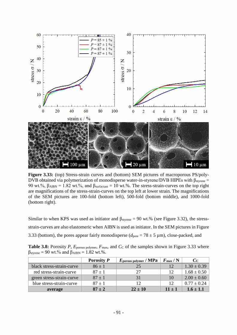
- 91 -

Figure 3.33: (top) Stress-strain curves and (bottom) SEM pictures of macroporous PS/poly-

DVB obtained via polymerization of monodisperse water-in-styrene/DVB HIPEs with βstyrene =

90 wt.%, βAIBN = 1.82 wt.%, and βsurfactant = 10 wt.%. The stress-strain-curves on the top right

are magnifications of the stress-strain-curves on the top left at lower strain. The magnifications

of the SEM pictures are 100-fold (bottom left), 500-fold (bottom middle), and 1000-fold

(bottom right).

Similar to when KPS was used as initiator and βstyrene = 90 wt.% (see Figure 3.32), the stress-

strain-curves are also elastomeric when AIBN is used as initiator. In the SEM pictures in Figure

3.33 (bottom), the pores appear fairly monodisperse (dpore = 78 ± 5 µm), close-packed, and

Table 3.8: Porosity P, Eporous polymer, Fmax, and CC of the samples shown in Figure 3.33 where

βstyrene = 90 wt.% and βAIBN = 1.82 wt.%.

Porosity P Eporous polymer / MPa Fmax / N CC

black stress-strain-curve 86 ± 1 25 12 1.30 ± 0.39

red stress-strain-curve 87 ± 1 27 12 1.68 ± 0.50

green stress-strain-curve 87 ± 1 31 10 2.00 ± 0.60

blue stress-strain-curve 87 ± 1 12 12 0.77 ± 0.24

average 87 ± 2 22 ± 10 11 ± 1 1.6 ± 1.1

- 92 -

spherical. All determined values and the calculated average values are summed up in Table 3.8.

The measured porosity was P = 87 ± 1 % and thus much higher than the expected P = 74%.

This implies that the continuous polymer phase has a relatively high additional porosity. The

calculated average values for Eporous polymer and Fmax were Eporous polymer = 22 ± 10 MPa and Fmax

= 11 ± 1 N. Compared to when βstyrene = 50 wt.% (see Figure 3.31), Eporous polymer and Fmax are

much lower. On the one hand, this could be expected since the porosity is higher for βstyrene =

90 wt.% compared to βstyrene = 50 wt.%. On the other hand, the crosslinking density is also lower

for βstyrene = 90 wt.% (βDVB = 10 wt.%) compared to βstyrene = 50 wt.% (βDVB = 50 wt.%). Thus,

the polymer matrix is less rigid for βstyrene = 90 wt.% (βDVB = 10 wt.%) and consequently, Eporous

polymer and Fmax are smaller. The calculated average value for CC was CC = 1.6 ± 1.1 which is

also lower than when βstyrene = 50 wt.%, but still higher than the expected CC = 1. Compared to

when KPS was used as initiator (see Figure 3.32), Eporous polymer and Fmax are slightly smaller

when AIBN was used as initiator. Though, the porosity is higher when AIBN was used as

initiator. When the porosity is included for the calculation of CC, CC is higher when AIBN was

used as initiator. This suggests that the close-packed spherical morphology found when AIBN

is used as initiator is stiffer than the disordered, polyhedral morphology found when KPS is

used as initiator.

Summarized, the stress-strain-curves are elastomeric for βstyrene = 90 wt.% and elastic-brittle for

βstyrene = 50 wt.%. This is independent of the type of initiator. The stress-strain-curves are also

elastic-brittle when βstyrene = 70 wt.%, = 30 wt.%, and = 10 wt.%. They are not shown here, but

are similar to the stress-strain-curves obtained for βstyrene = 50 wt.%. When AIBN is used as

initiator, Eporous polymer is much higher for βstyrene = 50 wt.% compared to βstyrene = 90 wt.%. This

is still true when the higher porosities at βstyrene = 90 wt.% are considered. For βstyrene = 50 wt.%

and AIBN as initiator, the values of Eporous polymer are also much higher compared to the KPS

initiated porous polymers. The reason for this is not known. When KPS is used as initiator, no

such trend could be observed since the values were too far spread for βstyrene = 50 wt.%. For

βstyrene = 90 wt.%, it appears as if the close-packed spherical morphology obtained with AIBN

as initiator is stiffer than the disordered, polyhedral morphology with KPS as initiator. The

summary of all average values is presented in Table 3.9.

- 93 -

Table 3.9: Type of initiator, βstyrene, porosity P, Eporous polymer, Fmax, and CC of the sample whose

results were shown in Section 3.3.

type of

initiator

βstyrene /

wt.%

Porosity P /

%

Eporous polymer /

MPa Fmax / N CC

KPS 50 73 ± 4 51 ± 36 29 ± 21 1.9 ± 1.2

AIBN 50 78 ± 2 102 ± 13 30 ± 5 5.3 ± 1.7

KPS 90 81 ± 3 29 ± 8 17 ± 3 0.9 ± 0.4

AIBN 90 87 ± 2 22 ± 10 11 ± 1 1.6 ± 1.1

When βinitiator or βsurfactant were varied, no significant trends could be found. The stress-strain-

curves and thus also Fmax and Eporous polymer often differed more greatly between the samples

within one composition than between two compositions. The same is true when one searched

for differences between monodisperse macroporous PS/polyDVB and polydisperse

macroporous PS/polyDVB. While differing porosities were sometimes the explanation for the

differences within one composition, they cannot explain all observations. As above-mentioned,

no direct structure-property-relationships could be determined since the morphology was

determined with SEM from one sample, while the stress-strain-curves were recorded from other

samples with the same composition. Additionally, with SEM only a small part of the whole

sample can be looked at. While the sample height is ~ 7 mm (7000 µm), with SEM the

morphology of only 1-2 layers can be visualized (~ 80 – 160 µm). Thus, SEM does not provide

the structure of the whole sample which is why structure-property-relationships are difficult to

draw from the combination of SEM and stress-strain-curves. Overall, it was therefore not

possible to examine how small changes in the morphology affect the mechanical properties.

The potentially existing differences could not be detected with the method used in this PhD

thesis. The solution to this problem would be the use of micro-computed tomography (µ-CT)

while compressing the samples. Thus, both the stress-strain-curve and the morphology of the

whole sample could be determined simultaneously. However, this combination requires a lot of

time and was moreover not available for this PhD thesis. Determining the morphology with µ-

CT while simultaneously measuring the mechanical properties could be the focus of future

research.

- 94 -

- 95 -

4 Conclusions and Outlook

4.1 Conclusion

Starting Situation

Using microfluidics, it is possible to generate monodisperse water-in-styrene/divinylbenzene

(DVB) emulsions. Because the water droplets have a uniform size and a higher density than the

surrounding monomer phase, their sedimentation results in a high internal phase emulsion

(HIPE) with a water volume fraction of Φdisp = 74 vol%. By polymerizing and drying the HIPE,

its structure is retained and monodisperse porous polystyrene (PS)/polydivinylbenzene

(polyDVB) is produced. Because the average pore diameter is ~ 80 µm and thus much larger

than 50 nm, the material is classified as macroporous [Eve72, Bur76]. The morphology of

monodisperse macroporous PS/polyDVB strongly depends on which type of initiator is used.

With monomer-soluble azobisisobutyronitrile (AIBN), the pores are spherical and

interconnected and the pore walls exhibit an additional porosity (see Figure 4.1 (left)). With

water-soluble potassium peroxydisulfate (KPS), on the other hand, the pores are polyhedral and

not interconnected and the pores walls are comprised of two similar looking outer layers and

one inner layer (see Figure 4.1 (right)). Thus, two questions arise: (1) Firstly, why are spherical

droplets transforming into polyhedral pores during the polymerization? This requires a certain

mechanism to increase the area of the water/monomer interface and thus counteract capillary

pressure. (2) Secondly, why are the pore walls made up of three layer?

Hypothesis 1: Osmotic Transport of DVB

In previous works, Quell et al. [Que16b, Que17a] answered both questions with a mechanism

that revolves around osmotic transport of DVB (see Figure 4.2 (right)). When the

polymerization starts at the interface because a water-soluble initiator is used, a polyDVB-rich

layer forms close to the interface since DVB polymerizes faster than styrene [Sch75] (see Figure

4.2 (right), purple layer). This induces a concentration gradient of DVB between the films

where DVB has been depleted and the Plateau borders where the DVB concentration is still at

its initial value. As a consequence, osmotic transport of DVB from the Plateau borders into the

films thins out the Plateau borders and increases the thickness of the films (see Figure 4.2

(right), red arrows). Overall, this leads to a change of the shape of the interface from spherical

to polyhedral. The three layers of the pore walls were explained in that the two outer layers are

- 96 -

Figure 4.1: Polymerization and drying of a (top) monodisperse water-in-styrene/DVB HIPE

leads to (left) open-pore monodisperse macroporous PS/polyDVB with spherical pores and

porous pore walls when monomer-soluble AIBN is used and (right) closed-pore monodisperse

macroporous PS/polyDVB with polyhedral pores and three-layered pore walls when water-

soluble KPS is used. This Figure was copied from [Que17a]. License number 5004850663340.

polyDVB-rich, while the inner layer is PS-rich because of the slower polymerization of styrene

(see Figure 4.2 (right), yellow layer). Though Quell et al. found experimental support of this

hypothesis [Que17a], a satisfying and quantitative proof was still missing. Thus, this PhD

thesis’ goal was to either prove or disprove the above-explained hypothesis. This was tackled

by drawing up logical deductions about what ought to happen to the morphology of

monodisperse macroporous PS/polyDVB when the concentration of a component is varied

systematically (see Section 3.1). If the experimental results support the existing hypothesis, a

quantitative description of it might become feasible from the large number of new findings. If,

- 97 -

Figure 4.2: Explanation of the morphologies depicted in Figure 4.1 as described by [Que17a].

(Left) With monomer-soluble AIBN, the polymerization is occurring homogeneously

throughout the continuous phase and the droplet shape is retained. The shrinkage of the

continuous phase during polymerization causes mechanic stress and a consequent film rupture.

(Right) With water-soluble KPS, the polymerization startes locally at the water/monomer

interface and a polyDVB-rich layer is formed. The depletion of DVB in the films is balanced

by osmotic-driven flow of DVB from the Plateau borders into the films. This induces a

deformation of the droplet shape from spherical to polyhedral. The shrinkage of the continuous

phase during polymerization causes internal mechanic stress which wrinkles the polyDVB-rich

outer layer. This Figure was copied from [Que17a]. License number 5004850663340.

on the other hand, the experimental results contradict the existing hypothesis, it has to be

rejected and a new explanation has to be worked out. (1) Firstly, the styrene mass fraction βstyrene

was varied between the initial 50 wt.% (styrene/DVB mass ratio 50/50) and 90 wt.%

(styrene/DVB mass ratio 90/10) in steps of 10 wt.% (see Section 3.1.1). When the monomer

composition is increased towards pure styrene, (1a) the extent of osmotic transport of DVB

ought to decrease. As a consequence, the mechanism that transforms the shape of the pores

ceases and thus, the pores ought to remain spherical. However, when βstyrene was varied,

scanning electron microscopy (SEM) pictures did not support the expectations. In fact, the pores

- 98 -

became even more distorted from the spherical shape when βstyrene was increased from 50 wt.%

to 90 wt.%. To quantify this observation, a so-called shape factor S was introduced where the

circumference C of a 2D pore cross-section is divided by the square root of its area A. Thus, S

is lowest for a circular shape and increases with increasing distortion from the circular shape.

In the samples, S increased from values found for hexagons at βstyrene = 50 wt.% to much higher

values at βstyrene = 90 wt.%, thus indeed quantifying the SEM observations. When βstyrene was

decreased from 50 wt.% to 10 wt.%, the shape of the 2D pore cross-sections ought to become

circular as well if one assumes osmotic transport of DVB. However, the shape of the pore cross-

sections remained hexagonal. Therefore, the development of the pore shape as function of

βstyrene is the first counterargument to osmotic transport of DVB. Apart from the shape of the

pores, changing βstyrene also ought to have an influence on the thickness of the layers in the pore

walls. When βstyrene is increased from 50 wt.% to 90 wt.%, (1b) the thickness of the supposedly

polyDVB-rich outer layers ought to decrease and the thickness of the supposedly PS-rich inner

layer ought to increase. However, the expectations were not supported here either. The pore

wall thickness tpore wall, the outer layer thickness touter layer, and the inner layer thickness tinner layer

all decreased when βstyrene was increased from 50 wt.% to 90 wt.%. Thus, the relative

thicknesses of the outer and inner layer remained constant as function of βstyrene which serves as

the second counterargument to osmotic transport of DVB. When AIBN was used as initiator

for the sake of comparison, the morphology did not change when βstyrene was varied.

(2) Secondly, the KPS mass fraction βKPS was changed (see Section 3.1.2). The reasoning

behind was that an increase of the amount of KPS increases the polymerization rate. Thus, the

comparatively slow diffusion process of DVB from the Plateau borders into the films has less

time to occur. Consequently, the pores ought to remain more spherical. However, when βKPS

was increased, the hexagonal shape of the 2D pore cross-sections became slightly more

distorted. This observation was quantified by the shape factor S. Therefore, the development of

the pore shape as function of βKPS is the third counterargument against osmotic transport of

DVB. The measurement of tpore wall, touter layer, and tinner layer as function of βKPS revealed that the

thicknesses are independent of βKPS. When KPS was substituted by AIBN for the sake of

comparison, the morphology did not change when βAIBN was varied. The results of Section 3.1

were published in a paper in Colloid and Polymer Science [Koc20].

- 99 -

Hypothesis 2: Surfactant Diffusion

Overall, the variation of βstyrene and βKPS demonstrated that osmotic transport of DVB does not

exist. Thus, the new goal of this PhD thesis was to find the real mechanism that answers (1)

why spherical droplets become polyhedral pores and (2) why the pore walls are comprised of

three layers (see Section 3.2.1). As a first step, the surfactant mass fraction βsurfactant was varied

between 5 – 20 wt.% in steps of 5 wt.%. In the 2D pore cross-sections of the SEM pictures, the

shape was always hexagonal. This means that the mechanism that increases the interfacial area

during polymerization is independent of βsurfactant. To determine if and how the size of the layers

in the pore walls change when βsurfactant is varied, their areas Aouter layer and Ainner layer as well as

the total area of the pore wall Apore wall were measured. It was found that Apore wall and Aouter layer

decrease as function of βsurfactant, while Ainner layer remains constant. To determine how Aouter layer

and Ainner layer develop independent of Apore wall, the relative area of the outer layer Aouter layer/Apore

wall and the relative area of the inner layer Ainner layer/Apore wall were calculated. Here, a clear trend

was observed: The relative area of the outer layer decreases as function of βsurfactant, while the

relative area of the inner layer increases. This finding indicates that the formation of the layers

is linked to the surfactant. SEM pictures at higher magnifications revealed that the outer layers

are non-porous, while the inner layer is porous. This implies that the porosity of the inner layer

is caused by the surfactant since the relative area of the porous inner layer increases with

increasing βsurfactant.

The intended use of the surfactant is to stabilize the water/monomer interface. However, with

the help of an educated guess for the head group area Ahead group of the surfactant [Wet01,

Dom07], the amount of surfactant actually necessary to cover the interface βsurfactant at interface was

calculated. This value is below 0.1 wt.% which means that the majority of the surfactant is dis-

solved in the continuous phase. Thus, the surfactant can cause a porosity in the pore walls when

it is removed after the polymerization. However, this opens up the question why there is only a

porous inner layer and not a porous pore wall. To investigate what happens to the surfactant

during the polymerization, a model ternary phase diagram consisting of styrene, surfactant, and

PS was used to simulate the polymerization. Here, surfactant/styrene mixtures simulated

different βsurfactant and the styrene/PS ratio simulated the polymerization. When PS was added

and dissolved in the surfactant/styrene mixtures, the initially clear mixtures eventually

separated into two phases. When βsurfactant was low, high amounts of PS could be dissolved,

while phase separation occurred much earlier when βsurfactant was high. This means that the

surfactant is neither soluble in PS nor in partially polymerized styrene/PS mixtures. Finally, it

- 100 -

was investigated whether the porosity of the inner layer is solely caused by the surfactant or if

the surfactant forms small water droplets that add to the porosity. In experiments where

monomer phases were placed over water, the initially clear monomer phases became turbid and

white over time. Thus, small water droplets surrounded by surfactant formed and grew in size

over time. Small angle neutron scattering, freeze fracture electron microscopy, and dynamic

light scattering experiments showed that the surfactant already forms structures (inverse

micelles) in the low nanometer range without water. However, to be able to grow in size, these

structures require water and thus turn into small water droplets by incorporating water.

Therefore, the porosity of the inner layer stems from both surfactant and small water droplets.

Figure 4.3: Schematic drawing of the mechanism that increases the area of the water/mono-

mer interface and that creates non-porous outer layers and a porous inner layer in the pore wall.

- 101 -

From all results, a mechanism that answers (1) why spherical droplets become polyhedral pores

and (2) why the pore walls are comprised of three layers was concluded (see Section 3.2.2).

When the polymerization starts at the water/monomer interface because water-soluble KPS is

used, a small and partially polymerized layer forms close to the interface (see Figure 4.3 (b)).

Since the surfactant is not soluble in this layer, it diffuses away from there. One option is to

diffuse to the nearby water/monomer interface, where the surfactant overpopulates the interface

which causes an increase of the interface [Jia99, Pas12, Giu17]. This increase changes the shape

of the interface from spherical to polyhedral (see Figure 4.3 (a → b → c)). Another option for

the surfactant is to diffuse into the interior of the continuous phase. Thus, the surfactant

accumulates in the interior of the continuous phase, while the regions close to the interface

become surfactant-free (see Figure 4.3 (b → c → d)). When the macroporous material is

purified after the polymerization, the surfactant is washed out, which creates the porosity of the

inner layer. In turn, the outer layers remain non-porous. Since the small water droplets are

surrounded by surfactant, they diffuse along with the surfactant. Thus, they either diffuse back

into the dispersed phase or remain in the interior of the continuous phase. There, they add to

the porosity of the inner layer when they are washed and dried out. The results of Section 3.2

were published in a paper in the Journal of Colloid and Interface Science [Koc21].

Another focus of this PhD thesis was the investigation of the mechanical properties of

monodisperse macroporous PS/polyDVB (see Section 3.3). The influence of the type and

amount of initiator, of the styrene/DVB mass ratio, of the amount of surfactant, and of the

change between mono- and polydispersity were investigated. It was found that for βstyrene = 90

wt.% the samples were elastomeric, while they were elastic-brittle for βstyrene ≤ 70 wt.%. No

further significant trends could be found because it was not possible to determine the

morphology of a whole sample and to also record the mechanical properties of that sample. As

a consequence, it was impossible to obtain structure-property-relationships.

4.2 Outlook

To solve the just-mentioned problem for the determination of structure-property-relationships,

a combination of methods that simultaneously investigate the morphology of a whole sample

and determine the mechanical properties has to be used. Instead of only examining 1-2 layers

of a sample with SEM, with micro-computed tomography (µ-CT) the morphology of a whole

sample can be determined. Therefore, if µ-CT is coupled to a universal testing machine, the

determination of structure-property-relationships becomes possible. Thierry Roland and the

- 102 -

work group of Wiebke Drenckhan have such a piece of equipment at their disposal at the Institut

Charles Sadron (ICS) in Strasbourg. Thus, by cooperating with them, the mechanical properties

of monodisperse and polydisperse macroporous PS/polyDVB can be recorded and

differentiated. The only drawback of µ-CT is that it takes quite a long time to record one sample

which is why only selected samples can be investigated.

The use of µ-CT could also help with two smaller issues concerning the transformation of

spherical droplets into polyhedral pores. Firstly, the mechanism shown in Figure 4.3 suggests

that the transformation of the shape happens in the early stages of the polymerization. At this

point, the interface is already overpopulated with surfactant, but the continuous phase is only

partially polymerized and can thus still comply with the change of the shape. By monitoring

the polymerization with µ-CT, this assumption can be tested. Secondly, it has not been clarified

yet why the pore walls between two pores are much thicker than they were initially between

two droplets. This means that during the polymerization, material diffuses into the films.

Monitoring the polymerization with µ-CT could help investigating this question.

Another aspect that has to be improved is the output rate at which monodisperse macroporous

PS/polyDVB can be produced. For this, two options exist: On the one hand, an upscaling of the

microfluidic process would result in higher amounts of monodisperse HIPEs while maintaining

a very high monodispersity. An example of how the output of microfluidics can be increased

was shown by Nisisako et al. [Nis12] who developed a microfluidic parallelization chip. In this

device, an output rate of 180 mL h-1 is enabled by having parallel droplet generation in up to

144 constrictions. The workgroup of Wiebke Drenckhan at the ICS in Strasbourg built such a

parallelization device where preliminary tests have already been undertaken. On the other hand,

the output rate can be drastically increased to several mL min-1 with membrane emulsification.

However, this is accompanied by a loss in monodispersity. Nevertheless, the generated droplets

are still far from being polydisperse with PDIs between 10 – 26% [Kos05, Egi08, Gas08,

Hol10] and the average droplet size can also still be controlled. Thus, if it turns out that the

mechanical properties of monodisperse macroporous PS/polyDVB are not better compared to

those of polydisperse ones, membrane emulsification offers a promising alternative.

- 103 -

5 Experimental

5.1 Materials

Styrene (99%), divinylbenzene (DVB, technical grade 80%, residual 20% is mostly

ethylstyrene), potassium peroxydisulfate (KPS, 99%), ammonium peroxydisulfate (APS, 99%),

azobisisobutyronitrile (AIBN, 99%), and polystyrene (PS, average MW = 35 000 g mol-1) were

purchased from Sigma-Aldrich. For the SANS measurements, deuterated Styrene (98%) was

purchased from Cambridge Isotopes and D2O (>99%) was purchased from Eurisotop. Double

distilled water was produced with a Bi 18E distillery from QCS. The technical, non-ionic

surfactant Hypermer 2296 was kindly supplied by Croda. The surfactant primarily consists of

polyisobutylene succinic anhydride sorbitan esters [Gra13]. All chemicals were used without

further purification.

5.2 Synthesis of Macroporous PS/polyDVB

The continuous monomer phases consisted of styrene, DVB, and surfactant. The styrene mass

fraction βstyrene was calculated by dividing the styrene mass by the combined monomer mass. It

holds

βstyrene =𝑚(styrene)

𝑚(styrene) + 𝑚(DVB)· 100% . (5.1)

The surfactant mass fraction βsurfactant was calculated by dividing the surfactant mass by the

combined monomer mass. It holds

βsurfactant =𝑚(surfactant)

𝑚(styrene) + 𝑚(DVB)· 100% . (5.2)

If AIBN was added to the continuous phase, the AIBN mass fraction βAIBN was calculated by

dividing the AIBN mass by the combined monomer mass. It holds

βAIBN =𝑚(AIBN)

𝑚(styrene) + 𝑚(DVB)· 100% . (5.3)

The combined monomer mass was kept constant at 10 g. In the dispersed phase, the H2O mass

was likewise kept constant at 10 g. This was done to have similar conditions in the microfluidic

chip for droplet generation. If KPS was added to the dispersed phase, the KPS mass fraction

βKPS was calculated by dividing the KPS mass by the H2O mass. It holds

- 104 -

βKPS =𝑚(KPS)

𝑚(H2O)· 100% . (5.4)

To better illustrate how the weighed in masses relate to the above-mentioned mass fractions,

two exemplary samples are shown in Table 5.1. These are the standard samples with either KPS

or AIBN as initiator from which βstyrene, βinitiator, or βsurfactant was varied. For KPS as initiator, the

initial values are βstyrene = 50 wt.%, βKPS = 2.98 wt.%, and βsurfactant = 10 wt.%. For AIBN as

initiator, βAIBN = 1.82 wt.%, while βstyrene and βsurfactant are kept constant.

Table 5.1: Type of initiator, m(styrene), m(DVB), βstyrene, m(initiator), βinitiator, m(surfactant),

βsurfactant, and m(H2O) for the standard sample with KPS and the standard sample with AIBN.

standard sample with KPS standard sample with AIBN

type of initiator KPS AIBN

m(styrene) 5 g 5 g

m(DVB) 5 g 5 g

βstyrene 50 wt.% 50 wt.%

m(initiator) 0.298 g 0.182 g

βinitiator 2.98 wt.% 1.82 wt.%

m(surfactant) 1 g 1 g

βsurfactant 10 wt.% 10 wt.%

m(H2O) 10 g 10 g

Both the dispersed and the continuous phase were prepared by weighing in all components with

a high precision scale (accuracy 0.0001 g) into 100 mL screw top DURAN® borosilicate

containers from Schott. By carefully shaking the containers, a homogeneous mixture was

obtained. The dispersed and the continuous phase were then connected with the pressure

controller OB I MkII (maximum pressure 2 bar, software control ESI) from Elveflow with

DURAN® multipart connector caps and Tygon tubes. The two phases were furthermore

connected with the microfluidic chip with FEP (fluorinated ethylene propylene) tubing (inner

diameter 0.5 mm). The continuous phase was additionally split into two channels with a T-

connector (ethylene tetrafluoroethylene (ETFE), 0.5 mm). The microfluidic chip consisted of

quartz glass and was purchased from Dolomite. It had a hydrophobic coating, a constriction

size of 100 x 105 µm, and flow-focussing geometry. The microfluidic chip was embedded into

a H-interface from Dolomite and connected to the sample vial with FEP tubing (inner diameter

0.5 mm). Monodisperse droplet generation was achieved by adjusting the pressures of both

phases such that the droplets formed in the dripping regime. For monodisperse droplet

generation, the two pressures were kept constant, while for polydisperse droplet generation, a

sinusoidal pressure profile was used for the dispersed phase [And18, Dab20]. The droplet

- 105 -

generation was monitored with a Nikon SMZ – 800 N optical microscope from Nikon coupled

to an Optronis CL600X2 high speed camera from Stemmer Imaging.

Before collecting the emulsion in the sample vial, the average droplet diameter ddroplet was

determined. If necessary, the pressures were adjusted such that the desired ddroplet was obtained.

The emulsion was poured onto a glass disk and examined with the optical microscope. A picture

of the emulsion was taken and processed with the free of charge image processing software

ImageJ from National Institutes of Health (NIH, USA). The picture was converted into a binary

picture which allowed ImageJ to automatically determine the area Adroplet of each droplet cross-

section. From this value, ddroplet and its standard deviation was calculated. Next, the emulsion

was collected in a vial until the desired amount was reached. Depending on vial size, this took

roughly between 30 – 90 min. During collection, the droplets already sedimented in the vial

and thus formed a high internal phase emulsion (HIPE) with Φdisp = 74 vol% at the bottom of

the vial. After the collection was finished, complete sedimentation of all droplets was achieved

by waiting ~ 30 min. The excess continuous monomer phase was removed with a syringe. The

vial was sealed with a cap, though air holes were pierced into the caps to allow pressure equali-

zation. Then, the vial was placed into an oil bath at 70 °C. The HIPE was polymerized for 48 h

(KPS as initiator) or 24 h (AIBN as initiator). After polymerization, the samples were removed

from the vial with a bench vise and then purified with Soxhlet extraction for at least 12 h with

ethanol as solvent. Finally, the samples were dried in a drying oven at 60 °C for 72 h.

5.3 Analysis of Macroporous PS/polyDVB

5.3.1 Analysis of Morphology

The morphology of the samples was examined with scanning electron microscopy (SEM). The

samples had to be cut open with a scalpel. To facilitate cutting and ideally have a cut parallel

to one layer of pores, the samples were cooled with liquid nitrogen. Pieces of ~ 5 x 5 mm in

area and ~ 2 mm in height were glued onto Aluminium Specimen Stubs from Agar Scientific

with Carbon adhesive discs from Agar Scientific. Vacuum was then applied and the samples

were sputtered with a thin layer of gold. If the sputtering device was out of order, the samples

were steamed with carbon instead. Sputtering with gold or steaming with carbon did not have

significant influence on the quality of the SEM pictures later. A CamScan CS44 SEM from

Tescan with secondary electron imaging (SEI) was used for the determination of the average

pore diameter dpore, the shape-factor S of the pore cross-sections, and the thickness/area of the

- 106 -

pore wall and layers tpore wall/Apore wall, touter layer/Aouter layer, and tinner layer/Ainner layer. To enable the

determination of dpore and S, the circumference Cpore and area Apore were determined with

ImageJ. The outline of a pore cross-section was retraced manually which allowed ImageJ to

calculate Cpore and Apore. Apore wall, Aouter layer, and Ainner layer were determined analogously in one

strut. tpore wall, touter layer, and tinner layer were determined by measuring the respective thickness

perpendicular to the direction the pore wall or layer is running along. For the analysis of the

texture of the layers in the pore wall, a Zeiss GeminiSEM 500 SEM from Zeiss was used.

5.3.2 Analysis of Mechanical Behavior

The mechanical behavior of the macroporous PS/polyDVB samples as well as of the bulk

samples used for normalization was examined with a universal testing machine. The samples

were cut such that a cylindrical shape was obtained. Before cutting, the samples were cooled

with liquid nitrogen. The main focus was put on cutting the sample such that the top and bottom

of the cylinder were as parallel and as flat as possible. To calculate the density of the samples,

the diameter and the height were measured with a caliper (accuracy 0.02 mm). The diameter of

the cylindrical samples was typically between 3.3 – 3.5 mm and their height was between 6 –

8 mm. The mass of the sample was determined with a high precision scale (accuracy 0.0001 g).

By dividing the density of the samples by the density of the bulk polymer, ρrel was obtained

(see equation (2.17)). Next, the samples were placed into the universal testing machine. A

zwickiLine Z5.0 (maximum capacity 5 kN) and the software testXpert III from ZwickRoell were

used to record the stress-strain-curves. The compression rate was 1 mm min-1 and a Xforce HP

load cell measured the stress. The Young’s Modulus E was determined from the slope of the

linear elastic region of the stress-strain-curve. Fmax was determined at the position where the

linear elastic region goes over into the Plateau region.

Five samples were prepared for each composition. Of these five samples, one was used for the

determination of the morphology with SEM, while the other four samples were used for the

compression tests. This was done to connect a determined morphology to the recorded stress-

strain-curves, i.e. to obtain structure-property-relationships. When a sample fractured during

preparation, it could no longer be used in the compression tests, but was still viable to be

examined with SEM. If more than one sample fractured, the compression tests were conducted

with less than four samples. The reason why compression tests were conducted with more than

one sample was to determine average values of Fmax and Eporous polymer.

- 107 -

5.4 Phase Diagram

To investigate the response of the surfactant to polymerization, surfactant/styrene mixtures

were prepared by weighing in the two components in a glass tube. A stirring bar was added to

the mixture and the glass tube was placed over a magnetic stirrer and into a water bath. The

temperature of the water bath was 70 °C to simulate the temperature of the polymerization.

Small polystyrene (PS) pellets were added and dissolved stepwisely until the mixture changed

from clear to turbid. This change indicated that the phase boundary had been crossed. The

amount of added PS was determined by weighing the glass tube and subtracting the initial mass.

Finally, the original surfactant/styrene mixture was added dropwisely until the mixture returned

to the clear, one-phase region. After again weighing the glass tube, the phase boundary was

determined more accurately.

5.5 Interfacial Tension

The interfacial tension γ was measured with the Spinning Drop Video Tensiometer SVT 15 from

DataPhysics Instruments. First, the capillary was filled bubble-free with H2O. Next, ~ 100 µL

of a surfactant/monomer mixture was injected into the capillary. By spinning the capillary, a

droplet consisting of the surfactant/monomer mixture formed. βsurfactant was varied between 5 –

20 wt.% in steps of 5 wt.%, the temperature was varied between 25 – 70 °C in steps of 15 °C,

and spinning rates were varied between 3000 – 13000 rpm in steps of 2000 rpm. βstyrene was

kept constant at 50 wt.%. LaPlace Young Fitting was used by the software SVT20_uEye to

calculate γ from the shape of the droplet. For LaPlace Young Fitting, the density of both H2O

and the surfactant/monomer mixtures had to be known. For H2O, the temperature-dependent

values were already known by the software. For the surfactant/monomer mixtures, the Density

Meter DMA 5000 A from Anton Paar was used to measure the temperature-dependent density.

5.6 Small angle neutron scattering

The small angle neutron scattering (SANS) spectra were recorded at the KWS-1 spectrometer

at the Heinz Maier-Leibnitz Zentrum (MLZ) in Munich, Germany. A mixture of surfactant and

deuterated styrene with βsurfactant = 10 wt.% was prepared and placed over D2O without allowing

the two phases to mix and form an emulsion. After 8 minutes, 13.5 hours, and 1.5 days, a small

amount of the upper monomer phase was removed from the sample, transferred into a cuvette,

and placed into the beam path of the SANS device. The neutron wavelength was 4.93 Å and

- 108 -

the scattering intensity q was varied between 0.00978 – 0.669 Å-1. To enable this,

collimation/detector distances of 8 m / 8 m and 8 m / 1.5 m were used. The normalization of

the scattering density to an absolute scale was achieved by the incoherent scattering of reference

materials. These were H2O and Perspex (trade name of poly(methyl methacrylate) (PMMA)).

The evaluation software QtiKWS was used for raw data treatment, masking, and radial

averaging. As a result, one-dimensional scattering curves were obtained. The fitting of the

SANS spectrum was achieved with a Gaussian shell model [Fos08] where the addition of a

form factor P(q) and a structure factor S(q) yield a simulated I(q) spectrum.

5.7 Freeze Fracture Electron Microscopy

A mixture of surfactant, styrene, and DVB was prepared and placed over H2O without mixing

the two phases, where βsurfactant = 10 wt.% and βstyrene = 50 wt.%. After a small fraction of the

monomer phase was removed, a replica of it was made by using the EM BAF060 freeze-fracture

and etching system from Leica. For this purpose, the sample was placed into a sandwich-like

structure consisting of two copper grids and two copper plates and consequently frozen in liquid

ethane. Next, the sample was fractured and its surface was first shadowed at 45° with a ~ 2 nm

thick platinum-carbon layer and secondly covered at 90° with a ~ 20 nm thick pure carbon

layer. This process was conducted in the vacuum chamber of the BAF060 and at a temperature

of –150 °C. Finally, the replicas were washed with ethanol, dried, and examined at room

temperature with the transmission electron microscope (TEM) EM10 from Zeiss.

5.8 Dynamic Light Scattering

As in Section 5.7, a mixture of surfactant, styrene, and DVB with βsurfactant = 10 wt.% and βstyrene

= 50 wt.% was prepared. The mixture was placed over H2O inside a capillary without mixing

the two phases. The capillary was placed into the beam path of the dynamic light scattering

(DLS) spectrometer 3DLS Spectrometer from LS Instruments such that the beam path crossed

through the monomer phase. A helium/neon laser with a wavelength of λ = 561 nm was used

and the scattering angle was kept constant at 90°. The scattering intensity was measured as

count rate of photons with an avalanche photodiode (APD) detector. The software of the DLS

spectrometer, LS spectrometer, automatically calculated the hydrodynamic radius rHyd as well

as its deviation from the slope of an intensity-time-correlation function g2-(τ). Values were

determined from 120 s time intervals for a total time span of 24 h.

- 109 -

6 Appendix

6.1 Supplementary Calculations

(a) Relation between Φgas and ρrel / P

In Section 2.3.2, it was stated that the relative density of a porous polymer ρrel equals one minus

the volume fraction of the gas Φgas (see equation (2.19)). Furthermore, it was stated that the

porosity P equals Φgas (see equation (2.20)). These relations are deduced in detail here. It holds

Φgas =𝑉gas

𝑉gas + 𝑉polymer=

𝑉gas

𝑉total= 1 −

𝑉polymer

𝑉total (6.1)

with Vgas being the volume of the gas, Vpolymer being the volume of the polymer, and Vtotal being

the combined volume of the gas and the polymer. The relative density ρrel depends on the

density of the porous polymer ρporous polymer and the density of the bulk polymer ρpolymer. In turn,

ρporous polymer and ρpolymer can be expressed by their respective masses mporous polymer / mpolymer and

their respective volumes Vporous polymer / Vpolymer. It holds

ρrel =𝜌porous polymer

𝜌polymer=

𝑚porous polymer𝑉porous polymer

⁄

𝑚polymer

𝑉polymer⁄

=𝑚porous polymer · 𝑉polymer

𝑚polymer · 𝑉porous polymer=

(𝑚gas + 𝑚polymer) · 𝑉polymer

𝑚polymer · (𝑉gas + 𝑉polymer) .

(6.2)

Next, the approximation is made that mgas is insignificant compared to mpolymer. It holds

𝑚gas + 𝑚polymer ≅ 𝑚polymer . (6.3)

This enables a simplification of equation (6.2). It holds

ρrel ≅𝑚polymer · 𝑉polymer

𝑚polymer · (𝑉polymer + 𝑉gas)=

𝑉polymer

𝑉polymer + 𝑉gas=

𝑉polymer

𝑉total . (6.4)

Thus, the result of equation (6.4) can be inserted into equation (6.1). It holds

Φgas = 1 −𝑉polymer

𝑉total= 1 − 𝜌rel . (6.5)

- 110 -

Finally, the relation between ρrel and P was already stated in equation (2.18). Thus, for the

relation between P and Φgas, it holds

𝑃 = 1 − 𝜌rel = Φgas . (6.6)

(b) Volume and Surface Area of a Rhombic Dodecahedron compared to a Sphere

In Section 2.4, it was stated that for a constant volume, the surface area of a rhombic

dodecahedron-shaped pore is roughly 10.5% larger than the surface area of a spherical droplet.

In this paragraph, this value is calculated. For the surface area Asphere and volume Vsphere of a

sphere, it holds

𝐴sphere = 4𝜋𝑟2 (6.7)

and

𝑉sphere =4

3𝜋𝑟3 (6.8)

with r being the radius of the sphere. For the surface area Arhombic dodecahedron and volume Vrhombic

dodecahedron of a rhombic dodecahedron, it holds

𝐴rhombic dodecahedron = 8 · √2 · 𝑎2 (6.9)

and

𝑉rhombic dodecahedron =16 · √3

9𝑎3 (6.10)

with a being the edge length of the rhombic dodecahedron [www4, www5]. Approximately,

the volume of a droplet Vdroplet is that of a sphere and the volume of a pore Vpore is that of a

rhombic dodecahedron. Assuming that the volume does not change during polymerization, it

holds

𝑉sphere ≡ 𝑉droplet = 𝑉pore ≡ 𝑉rhombic dodecahedron . (6.11)

Thus, by rearranging equation (6.8) and equation (6.10), a can be expressed with a coefficient

and r. It holds

- 111 -

16 · √3

9𝑎3 =

4

3𝜋𝑟3

𝑎 = √4𝜋 · 9

3 · 16 · √3𝑟3

3

= √√3𝜋

4

3

𝑟 .

(6.12)

Next, the result of equation (6.12) is inserted into equation (6.9). It holds

𝐴rhombic dodecahedron = 8 · √2 · 𝑎2 = 8 · √2 · (√√3𝜋

4

3

𝑟)

2

= 8 · √2 · √3𝜋2

16

3

· 𝑟2 .

(6.13)

Thus, both Arhombic dodecahedron (see equation (6.13)) and Asphere (see equation (6.7)) are expressed

as a coefficient multiplied by r2. Finally, their ratio shows how much larger Arhombic dodecahedron is

compared to Asphere. It holds

𝐴rhombic dodecahedron

𝐴sphere≅ 1.105 . (6.14)

(c) Conversion of mol% to wt.%

In Section 3.1, an AIBN molar fraction χAIBN = 1.28 mol% was converted into an AIBN mass

fraction βAIBN = 1.82 wt.%. Furthermore, a KPS molar fraction χKPS = 1.28 mol% was converted

into a KPS mass fraction βKPS = 2.98 wt.%. In this paragraph, these conversions are calculated.

It holds

χAIBN = 1.28 mol% = 0.0128 =𝑛AIBN

𝑛styrene + 𝑛DVB

𝑛AIBN = 0.0128 · (𝑛styrene + 𝑛DVB)

(6.15)

with nAIBN, nstyrene and nDVB being the molar amounts of AIBN, styrene, and DVB, respectively.

It holds

βAIBN =𝑚AIBN

𝑚styrene + 𝑚DVB (6.16)

- 112 -

with mAIBN, mstyrene and mDVB being the masses of AIBN, styrene, and DVB, respectively. In the

samples by Quell et al. [Que15, Que16a, Que16b, Els17, Que17a, Que17b], the styrene/DVB

mass ratio was kept constant at 50/50, Thus, it holds

𝑚styrene = 𝑚DVB = 𝑚monomer . (6.17)

Next, the results of equation (6.15) and equation (6.17) are inserted into equation (6.16).

Additionally, the molar masses MAIBN = 164.21 g mol-1, Mstyrene = 104.15 g mol-1, and MDVB =

130.19 g mol-1 of AIBN, styrene, and DVB are used to convert the respective masses into molar

amounts. It holds

βAIBN =𝑛AIBN · 𝑀AIBN

𝑚styrene + 𝑚DVB=

0.0128 · (𝑛styrene + 𝑛DVB) · 𝑀AIBN

2 · 𝑚monomer

=0.0128 · 𝑀𝐴𝐼𝐵𝑁

2·

𝑚monomer𝑀styrene

⁄ +𝑚monomer

𝑀DVB⁄

𝑚monomer

= 0.0064 · 𝑀AIBN · (1

𝑀styrene+

1

𝑀DVB) = 0.0182 .

(6.18)

For the conversion of χKPS to βKPS, analogous calculations are conducted. It holds

χKPS = 1.28 mol% = 0.0128 =𝑛KPS

𝑛styrene + 𝑛DVB

𝑛KPS = 0.0128 · (𝑛styrene + 𝑛DVB)

(6.19)

with nKPS being the molar amount of KPS. Since KPS is dissolved in H2O, βKPS is calculated

with the KPS mass mKPS and the H2O mass mH2O. It holds

βKPS =𝑚KPS

𝑚H2O . (6.20)

The statement of equation (6.17) applies here as well. Additionally, mH2O was equal to the

combined mass of monomers in the experiments of Quell et al. [Que15, Que16a, Que16b,

Els17, Que17a, Que17b]. Thus, it holds

𝑚H20 = 𝑚styrene + 𝑚DVB = 2 · 𝑚monomer . (6.21)

- 113 -

Finally, the results of equation (6.19) and equation (6.21) are inserted into equation (6.20). To

convert masses into molar amounts, Mstyrene = 104.15 g mol-1 and MDVB = 130.19 g mol-1 are

used again. The KPS molar mass MKPS = 270.32 g mol-1. It holds

βKPS =𝑛KPS · 𝑀KPS

𝑚H2O=

0.0128 · (𝑛styrene + 𝑛DVB) · 𝑀KPS

2 · 𝑚monomer

=0.0128 · 𝑀𝐾𝑃𝑆

2·

𝑚monomer𝑀styrene

⁄ +𝑚monomer

𝑀DVB⁄

𝑚monomer

= 0.0064 · 𝑀KPS · (1

𝑀styrene+

1

𝑀DVB) = 0.0298 .

(6.22)

(d) Different determinations of dpore

In Section 3.1.1, the diameter of the pores dpore was calculated as if the pore cross-sections were

circular (see equation (3.1)). Here, this method is compared to the determination of dpore in a

hexagon as the corner-to-corner distance, edge-to-edge distance, and the mean value of these

two distances. Using the edge length a of a hexagon, for the diameter corner-to-corner dcorner-to-

corner it holds

𝑑corner−to−corner = 2𝑎 . (6.23)

For the diameter edge-to-edge, it holds

𝑑edge−to−edge = √3𝑎 ≈ 1.732𝑎 . (6.24)

For the mean value of equation (6.23) and equation (6.24), it holds

𝑑mean =2𝑎 + √3𝑎

2= (1 +

√3

2) 𝑎 ≈ 1.866𝑎 . (6.25)

For the calculation of the diameter as if the pore cross-sections were circular, the area of a

hexagon AHexagon is required. It holds

𝐴Hexagon =3

2· √2 · 𝑎2 . (6.26)

The result of equation (6.26) is now inserted into equation (3.1). It holds

- 114 -

𝑑circular = 2 · √𝐴Hexagon

𝜋= 2 · √

32⁄ · √2 · 𝑎2

𝜋

= √6 · √2

𝜋· 𝑎 ≈ 1.643𝑎

(6.27)

Thus, when dpore is calculated as if the pore cross-section was circular, the obtained result is

17.85% (equation (6.23)) smaller than if it was calculated from the distance corner-to-corner.

For the distance edge-to-edge or the mean value of the former two, the difference is 5.14%

(equation (6.24)) or 11.95% (equation (6.25)), respectively.

(e) Calculation of βsurfactant at interface

In Section 3.2.1, it was stated that even for the lowest surfactant mass fraction βsurfactant, the

majority of the surfactant molecules are dissolved in the continuous phase and not located at

the water/monomer interface. Here, the surfactant mass fraction necessary to cover the interface

βsurfactant at interface is estimated. This is done by combining geometrical considerations with

reasonable assumptions about the head group area Ahead group of the surfactant. From the radius

rdroplet of a water droplet inside a HIPE, its surface area

𝐴droplet = 4 · π · 𝑟droplet2 (6.28)

and its volume

𝑉droplet =4

3· π · 𝑟droplet

3 (6.29)

can be calculated. Since the droplets are monodiperse and reside in a HIPE, it is also possible

to calculate the volume of the continuous monomer phase Vcontinuous phase surrounding one

droplet. It holds

𝑉continuous phase = 0.26

0.74· 𝑉droplet . (6.30)

Next, the molar amount of surfactant necessary to cover the interface of a droplet

𝑛surfactant at interface =𝐴droplet

𝐴head group· 𝑁Avogadro

−1 (6.31)

- 115 -

is calculated from Adroplet, Ahead group, and the Avogadro number NAvogadro. Here, reasonable

values for Ahead group have to be assumed. As an educated guess, Ahead group lies between 50 Å2

and 250 Å2 [Wet01, Dom07]. βsurfactant at interface can now be calculated with the help of equation

(6.28), equation (6.29), equation (6.30), the density of the continuous phase ρcontinuous phase, and

the molar mass of the surfactant MHypermer which is 833 g mol-1 [Gra13]. It holds

βsurfactant at interface =𝑚surfactant at interface

𝑚continuous phase

=𝑛surfactant at interface · 𝑀Hypermer

𝑉continuous phase · 𝜌continuous phase

=𝐴droplet · 𝑀Hypermer

𝐴head group · 𝑁Avogadro · 𝑉continuous phase · 𝜌continuous phase

=4 · 𝜋 · 𝑟droplet

2 · 𝑀Hypermer

𝐴head group · 𝑁Avogadro · 0.260.74⁄ · 4

3⁄ · 𝜋 · 𝑟droplet3 · 𝜌continuous phase

=0.74 · 3 · 𝑀Hypermer

𝐴head group · 𝑁Avogadro · 0.26 · 𝑟droplet · 𝜌continuous phase.

(6.32)

Since MHypermer, NAvogadro, and ρcontinuous phase are all constant and known, βsurfactant at interface only

depends on Ahead group and rdroplet. For example, for rdroplet = 40 µm (ddroplet = 80 µm) and Ahead

group = 50 Å2 or = 250 Å2, βsurfactant at interface = 0.065 wt.% or = 0.013 wt.%. These values are

much lower than βsurfactant total which is between 5 – 20 wt.%. A graph of calculated values for

βsurfactant at interface as a function of the head group areas Ahead group for droplet diameters of 60 µm,

80 µm, and 100 µm is shown in Figure 6.5.

6.2 Supplementary Figures

(a) Variation of βstyrene between 50 – 10 wt.%

Section 3.1.1 only depicted the SEM pictures where βstyrene was varied between 50 – 90 wt.%.

The SEM pictures of samples where βstyrene = 50 wt.%, = 30 wt.%, and = 10 wt.% are depicted

in Figure 6.1. βKPS is kept constant at 2.98 wt.% and βsurfactant is kept constant at 10 wt.%. The

magnifications are 100-fold (left column), 500-fold (middle column), and 1000-fold (right

column). In Figure 6.1, the 2D pore cross-sections fairly monodisperse and close-packed (see

Figure 6.1 (left column)). Furthermore, the shape of the pore cross-sections is always hexagonal

(see Figure 6.1 (middle column)) and the pore walls consist of three layers (see Figure 6.1 (right

- 116 -

Figure 6.1: SEM pictures of macroporous PS/poly-DVB obtained via polymerization of

monodisperse water-in-styrene/DVB HIPEs with βKPS = 2.98 wt.%, βsurfactant = 10 wt.%, and

βstyrene = 50 wt.%, = 30 wt.%, and = 10 wt.%.

column)). This means that the morphology does not change when βstyrene is decreased from 50

wt.% to 10 wt.%, while the pore cross-sections became increasingly polyhedral and disordered

when βstyrene was increased from 50 wt.% to 90 wt.%.

(b) Determination of C, A, tpore wall, touter layer, and tinner layer

To better illustrate how the circumference C, the area A, the pore wall thickness tpore wall, the

outer layer thickness touter layer, and the inner layer thickness tinner layer were measured, two

exemplary pictures are presented. Figure 6.2 (left) depicts how C and A were determined by

manually encircling the pore cross-sections. From the encirclements, the image processing

software ImageJ calculated C and A. C and A were determined from as many pore cross-sections

as possible. Figure 6.2 (right) depicts how tpore wall, touter layer, and tinner layer were determined from

taking the respective thickness perpendicular to direction the pore wall / layer is running along.

- 117 -

Figure 6.2: (left) Exemplary determination of the circumference C and area A of the pore cross-

sections and (right) exemplary determination of the pore wall thickness tpore wall, of the outer

layer thickness touter layer, and of the inner layer thickness tinner layer.

tpore wall, touter layer, and tinner layer were determined close to the struts, in the films, and between

these two. Furthermore, as many pore walls as possible were used to determine tpore wall, touter

layer, and tinner layer.

(c) Variation of βAPS between 0.32 – 39.44 wt.%

In Section 3.1.2, KPS was used as initiator. However, the maximum solubility of KPS in water

is only 5 wt.%, while that of APS is 62 wt.% [www2, www3]. To further examine if the shape

of the pore cross-sections remains hexagonal if the initiator amount is raised to above 5 wt.%,

KPS was substituted by APS. The assumption was made that KPS and APS have roughly the

same reactivity, though no experiments were conducted on that matter. In Figure 6.3, βAPS is

varied between 0.32 – 2.52 wt.%. In Figure 6.4, βAPS is varied between 4.20 – 39.44 wt.%. In

both Figures, βstyrene was kept constant at 50 wt.% and βsurfactant was kept constant at 10 wt.%.

- 118 -

Figure 6.3: SEM pictures of macroporous PS/poly-DVB obtained via polymerization of

monodisperse water-in-styrene/DVB HIPEs with βstyrene = 50 wt.%, βsurfactant = 10 wt.%, and

βAPS = 0.32 wt.%, = 0.63 wt.%, = 1.26 wt.%, and = 2.52 wt.%.

Note that βAPS between 0.32 – 4.20 wt.% is molarly equivalent to βKPS between 0.37 – 4.96

wt.%. In contrast, βAPS between 9.86 – 39.44 wt.% has no counterpart with KPS. In Figure 6.3,

the pores are always close-packed and fairly monodisperse. The shape of the pore cross-sections

is hexagonal and the pore walls are comprised of three layers. Thus, these samples are very

similar to their KPS counterparts in Figure 3.9. This implies that KPS and APS behave similar.

In Figure 6.4, the pores become increasingly disordered and polydisperse when βAPS is

increased. For βAPS = 4.20 wt.% and = 9.86 wt.%, the shape of the pore cross-sections is still

- 119 -

Figure 6.4: SEM pictures of macroporous PS/poly-DVB obtained via polymerization of

monodisperse water-in-styrene/DVB HIPEs with βstyrene = 50 wt.%, βsurfactant = 10 wt.%, and

βAPS = 4.20 wt.%, = 9.86 wt.%, = 19.72 wt.%, and = 39.44 wt.%.

more or less hexagonal and three layers are observed in the pore walls. For βAPS = 19.72 wt.%,

the pore cross-sections have no regular shape anymore and no layers in the pore walls can be

found. For βAPS = 39.44 wt.%, the pores are polydisperse and the interconnectivity changed

from closed-pore to open-pore. Overall, the SEM pictures in Figure 6.3 and Figure 6.4 show

that even when βAPS is increased to absurd levels, the pore cross-sections do not become

circular. Thus, these results also conflict with the idea of an osmotic transport of DVB as the

reason for the transformation from spherical droplets to polyhedral pores.

- 120 -

(d) Calculation of βsurfactant at interface

In Section 6.1 (e), βsurfactant at interface was calculated for an exemplary rdroplet = 40 µm (ddroplet = 80

µm) and for two exemplary Ahead group area = 50 Å2 and = 250 Å2. MHypermer, NAvogadro, and ρcontinuous

phase were constant and known (see equation (6.32)). For a better overview, in Figure 6.5 βsurfactant

at interface is calculated as function of Ahead group area. The chosen droplet diameters are ddroplet = 60

µm (dashed line), = 80 µm (continuous line), and = 100 µm (dotted line). These droplet

diameters are in the range of the droplet diameter generated in this PhD thesis. Ahead group area was

chosen between 10 – 300 Å2 which ought to include the actual, but unknown Ahead group area of

the surfactant Hypermer 2296 that was used in this PhD thesis. Figure 6.5 shows that even for

the smallest Ahead group area and smallest ddroplet, βsurfactant at interface is still much lower than the

surfactant mass fractions that were used in this PhD thesis.

Figure 6.5: Calculated surfactant mass fraction βsurfactant at interface necessary to cover the

interfacial area of a water droplet with diameters of 60 µm, 80 µm, and 100 µm inside a HIPE

as function of the head group area Ahead group area of the surfactant.

- 121 -

References

[And18] Andrieux, S.; Drenckhan, W.; Stubenrauch, C.; Generation of Solid Foams with

Controlled Polydispersity Using Microfluidics, Langmuir 2018, 34(4), 1581-

1590.

[Ann02] Anna, S. L.; Bontoux, N.; Stone, H. A.; Formation of dispersions using „flow

focusing“ in microchannels, Applied Physics Letters 2002, 82(3), 364-366.

[Ann16] Anna, S. L.; Droplets and Bubbles in Microfluidic Devices, Annual Review of

Fluid Mechanics 2016, 48, 285-309.

[Bae09] Baekeland, L. H.; US942699 (A) – method of making insoluble products of

phenol and formaldehyde, 1909.

[Ban11] Bandarian, M.; Shojaeia, A.; Rashidi, A. M.; Thermal, mechanical and acoustic

damping properties of flexible open-cell polyurethane/multi-walled carbon

nanotube foams: effect of surface functionality of nanotubes, Polymer

International 2011, 60, 475-482.

[Bar62] Bartl, H; von Bonin, W.; Über die Polymerisation in umgekehrter Emulsion,

Macromolecular Chemistry and Physics 1962, 57, 74-95.

[Bar85] Barby, D.; Haq, Z.; EP 0060138 – Low Density Porous Cross-Linked Polymeric

Materials and Their Preparation, 1985.

[Bar00] Barbetta, A.; Cameron, N. R.; Cooper, S. J.; High internal phase emulsions

(HIPEs) containing divinylbenzene and 4-vinylbenzyl chloride and the

morphology of the resulting PolyHIPE materials, Chemical Communications

2000, 0, 221-222.

[Bar10] Baroud, C. N.; Gallaire, F.; Dangla, R.; Dynamics of microfluidic droplets, Lab

on a Chip 2010, 10, 2032-2045.

[Bee02] Beebe, D. J.; Mensing, G. A.; Walker, G. M.; Physics and Applications of

Microfluidics in Biology, Annual Review of Biomedical Engineering 2002, 4,

261-286.

[Ber60] Bernal, J. D.; Mason, J.; Packing of Spheres: Co-ordination of Randomly Packed

Spheres, Nature 1960, 188, 910-911.

- 122 -

[Bin98] Binks, B. P.; Modern Aspects of Emulsion Science; The Royal Society of

Chemistry, Cambridge, 1998.

[Bur76] Burwell, R. L. Jr.; Manual of Symbols and Terminology for Physiochemical

Quantities and Units, Appendix III: Definitions, Terminology and Symbols in

Colloid and Surface Chemistry – Part II: Heterogeneous Catalysis, Pure and

Applied Chemistry 1976, 46(1), 71-90. (page 79)

[Cam96] Cameron, N. R.; Sherrington, D. C.; Albiston, L.; Gregory, D. P.; Study of the

formation of the open-cellular morphology of poly(styrene/divinylbenzene)

polyHIPE materials by cryo-SEM, Colloid & Polymer Science 1996, 274(6),

592-595.

[Cam97] Cameron, N. R.; Sherrington, D. C.; Preparation and glass transition

temperatures of elastomeric PolyHIPE materials, Journal of Material Chemistry

1997, 7(11), 2209–2212.

[Cam00] Cameron, N. R.; Barbetta, A.; The influence of porogen type on the porosity,

surface area and morphology of poly(divinylbenzene) PolyHIPE foams, Journal

of Materials Chemistry 2000, 10, 2466-2471.

[Cam05] Cameron, N. R.; High internal phase emulsion templating as a route to well-

defined porous polymers, Polymer 2005, 46, 1439-1449.

[Cho09] Choi, S.-W.; Cheong, I. W.; Kim, J.-H.; Xia, Y.; Preparation of Uniform

Microspheres Using a Simple Device and Their Crystallization into Close-

Packed Lattices, Small 2009, 5(4), 454-459.

[Chr07] Christopher, G. F.; Anna, S. L.; Microfluidic methods for generating continuous

droplet streams, Journal of Physics D: Applied Physics 2007, 40, R319-R336.

[Chu09] Chung, K.-Y.; Mishra, N. C.; Wang, C.-C.; Lin, F.-H.; Lin, K.-H.; Fabricating

scaffolds by microfluidics, Biomicrofluidics 2009, 3, 022403-(1-8).

[Cla16] Clayton, K. N.; Salameh, J. W.; Wereley, S. T.; Kinzer-Ursem, T. L.; Physical

characterization of nanoparticle size and surface modification using particle

scattering diffusometry; Biomicrofluidics 2016, 10 (5), 054107-(1-14).

[Cos14] Costantini, M.; Colosi, C.; Guzowski, J.; Barbetta, A.; Jaroszewicz, J.;

Swieszkowski, W.; Dentinia, M.; Garstecki, P.; Highly ordered and tunable

- 123 -

polyHIPEs by using microfluidics, Journal of Material Chemistry B 2014, 2,

2290-2300.

[Dab20] Dabrowski, M.; Jenkins, D; Cosgriff-Hernandez, E.; Stubenrauch, C.;

Methacrylate-based polymer foams with controllable connectivity, pore shape,

pore size and polydispersity, Physical Chemistry Chemical Physics 2020, 22,

155-168.

[Dom07] Dominguez, H.; Self-Aggregation of the SDS Surfactant at a Solid-Liquid

Interface, Journal of Physical Chemistry B 2007, 111, 4054-4059.

[Dre15] Drenckhan, W.; Hutzler, S.; Structure and energy of liquid foams, Advances in

Colloid and Interface Science 2015, 224, 1-15.

[Dus67] Dusek, K.; Phase Separation During the Formation of Three-Dimensional

Polymers, Journal of Polymer Science: Part C 1967, 16, 1289-1299.

[Egi08] Egidi, E.; Gasparini, G.; Holdich, R.G.; Vladisavljević, G.T.; Kosvintsev, S.R.;

Membrane emulsification using membranes of regular pore spacing: Droplet size

and uniformity in the presence of surface shear, Journal of Membrane Science

2008, 323, 414-420.

[Els17] Elsing, J.; Quell, A.; Stubenrauch, C.; Toward Functionally Graded Polymer

Foams Using Microfluidics, Advanced Engineering Materials 2017, 19,

1700195.

[Eva99] Evans, D. F.; Wernerström, H.; The Colloidal Domain – Where Physics,

Chemistry, Biology, and Technology meet; Wiley-VCH, New York, 1999.

[Eve72] Everett, D. H.; Manual of Symbols and Terminology for Physicochemical

Quantities and Units, Appendix II: Definitions, Terminology and Symbols in

Colloid and Surface Chemistry – Part I, Pure and Applied Chemistry 1972,

31(4), 579-638. (page 585)

[Fos08] Foster, T.; Sottmann, T.; Schweins, R.; Strey, R.; Small-angle neutron scattering

from giantwater-in-oil microemulsion droplets. I. Ternary system, The Journal

of Chemical Physics 2008, 128, 054502-(1-13).

[Gan01] Gañán-Calvo, A. M.; Gordillo, J. M.; Perfectly Monodisperse Microbubbling by

Capillary Flow Focusing, Physical Review Letters 2001, 87(27), 274501-(1-4).

- 124 -

[Gar05] Garstecki, P.; Gañán-Calvo, A. M, Whitesides, G. M.; Formation of bubbles and

droplets in microfluidic systems, Bulletin of the Polish Academy of Sciences:

Technical Sciences 2005, 53(4), 361-372.

[Gas08] Gasparini, G.; Kosvintsev, S.; Stillwell, M.; Holdich, R.; Preparation and

characterization of PLGA particles for subcutaneous controlled drug release by

membrane emulsification, Colloids and Surfaces B: Biointerfaces 2008, 61, 199-

207.

[Gib97] Gibson, L. J.; Ashby, M. F.; Cellular solids – Structure and properties,

Cambridge University Press, Cambrigde, 2nd edition, 1997.

[Giu17] Giustiniani, A.; Drenckhan, W.; Poulard, C.; Interfacial tension of reactive,

liquid interfaces and its consequences, Advances in Colloid and Interface

Science 2017, 247, 185-197.

[Gra93] Gravesen P.; Branebjerg, J.; Jensen, O. S.; Microfluidics – a review, Journal of

Micromechanics and Microengineering 1993, 3, 168-182.

[Gra13] Graeber, N.; A Study of Fundamentals in Emulsion Templating for the

Preparation of Macroporous Polymer Foams, Imperial College London, PhD

Thesis, 2013 (p. 85).

[Hai91] Hainey, P.; Huxham, I. M.; Rowatt, B.; Sherrington, D. C.; Tetley, L.; Synthesis

and Ultrastructural Studies of Styrene-Divinylbenzene Polyhipe Polymers,

Macromolecules 1991, 24, 117-121.

[Hay83] Hayashi, T.; Ito, J.; Mitani, K.; Mizutani, Y.; Dynamic Mechanical Properties

and Morphology of Styrene-Divinylbenzene Copolymer/Poly(vinyl Chloride)

Systems, Journal of Applied Polymer Science 1983, 28, 2867-2880.

[Hal06] Hales, T. C.; Ferguson, S. P.; A Formulation of the Kepler Conjecture, Discrete

& Computational Geometry 2006, 36 (1), 21-69.

[Hil85a] Hild, G.; Okasha, R.; Kinetic investigation of the free radical crosslinking

copolymerization in the pre-gel state, 1, Styrene/m- and p-divinylbenzene

systems, Makromolekulare Chemie 1985, 186, 93-110.

- 125 -

[Hil85b] Hild, G.; Okasha, R.; Rempp, P.; Free radical crosslinking copolymerization in

the post-gel state, 3, Swelling and mechanical properties of polystyrene

networks, Makromolekulare Chemie 1985, 186, 407-422.

[Hil04] Hilgenfeldt, S.; Kraynik, A. M.; Reinelt, D. A.; Sullivan, J. M.; The structure of

foam cells: Isotropic Plateau polyhedra, Europhysics Letters 2004, 67(3), 484-

490.

[Hol10] Holdich, R.G.; Dragosavac, M.M.; Vladisavljević G.T.; Kosvintsev, S.R.;

Membrane Emulsification with Oscillating and Stationary Membranes,

Industrial & Engineering Chemical Research 2010, 49, 3810-3817.

[Jia99] Jiao, J.; Kramer, E. J.; de Vos, S.; Möller, M.; Koning, C.; Polymer interface

instability caused by grafting reaction, Polymer 1999, 40, 3585-3588.

[Jon06] de Jong, J.; Lammertink, R. G. H.; Wessling, M.; Membranes and microfluidics:

a review, Lab on a Chip 2006, 6, 1125-1139.

[Kim11] Kimmins, S. D.; Cameron, N. R.; Functional Porous Polymers by Emulsion

Templating: Recent Advances, Advanced Functional Materials 2011, 21, 211-

225.

[Koc20] Koch, L.; Drenckhan, W.; Stubenrauch, C.; Porous polymers via emulsion

templating: pore deformationduring solidification cannot be explained by an

osmotic transport!, Colloid and Polymer Science 2020.

[Koc21] Koch, L.; Botsch, S.; Stubenrauch, C.; Emulsion templating: Unexpected

morphology of monodisperse macroporous polymers, Journal of Colloid and

Interface Science 2021, 582(B), 834-841.

[Kos05] Kosvintsev, S.R.; Gasparini, G.; Holdich, R.G.; Cumming, I.W.; Stillwell, M.T.;

Liquid−Liquid Membrane Dispersion in a Stirred Cell with and without

Controlled Shear, Industrial & Engineering Chemical Research 2005, 44, 9323-

9330.

[Kra04] Kraynik, A. M.; Reinelt, D. A.; van Swol, F.; Structure of Random Foam,

Physical Review Letters 2004, 93(20), 208301-(1-4).

- 126 -

[Kra05] Kraynik, A. M.; Reinelt, D. A.; van Swol, F.; Structure of random bidisperse

foam, Colloids and Surfaces A: Physicochemical and Engineering Aspects 2005,

263, 11-17.

[Kra06] Kraynik, A. M.; The Structure of Random Foam, Advanced Engineering

Materials 2006, 8(9), 900-906.

[Kun68] Kun, K. A.; Kunin, R.; Macroreticular Resins. III. Formation of Macroreticular

Styrene-Divinylbenzene Copolymers, Journal of Polymer Science: Part A-1

1968, 6, 2689-2701.

[Lan95] Landrock, A. H.; Handbook of Plastic Foams – Types, Properties, Manufacture

and Applications, Noyes Publications, Park Ridge, 1995.

[Lec10] Lechner, M. D.; Gehrke, K.; Nordmeier, E. H.; Makromolekulare Chemie – Ein

Lehrbuch für Chemiker, Physiker, Materialwissenschaftler und

Verfahrenstechniker; Birkhäuser Verlag, Basel – Boston- Berlin, 4th edition,

2010.

[Lee07] Lee, S.-T.; Park, C. B.; Ramesh, N. S.; Polymeric foams, Taylor & Francis

Group, Boca Raton, 2007.

[Lin11] Lin, J.-Y.; Lin, W.-J.; Hong, W.-H.; Hung, W.-C.; Nowotarski, S. H.;

Montenegro Gouveai, S.; Cristo, I.; Lin, K.-H.; Morphology and organization of

tissue cells in 3D microenvironment of monodisperse foam scaffolds, Soft

Matter 2011, 7, 10010-10016.

[Lyk05] Lykema, J.; Fundamentals of Interface and Colloid Science – Volume V: Soft

Colloids; Elsevier, Amsterdam, 2005.

[Mae13] Maestro, A.; Drenckhan, W.; Rio, E.; Höhler, R.; Liquid dispersions under

gravity: volume fraction profile and osmotic pressure, Soft Matter 2013, 9, 2531-

2540.

[Man92] Manz, A.; Harrison, D. J.; Verpoorte, E. M. J.; Fettinger, J. C.; Paulus, A.; Lüdi,

H.; Widmer, H. M.; Planar chips technology for miniaturization and integration

of separation techniques into monitoring systems – Capillary electrophoresis on

a chip, Journal of Chromatography 1992, 593, 253-258.

- 127 -

[Mil07] Mills, N.; Polymer Foams Handbook: Engineering and Biomechanics

Applications and Design Guide, Elsevier, Amsterdam, 2007.

[Nis12] Nisisako, T.; Ando, T.; Hatsuzawa, T.; High-volume production of single and

compound emulsions in a microfluidic parallelization arrangement coupled with

coaxial annular world-to-chip interfaces, Lab on a chip 2012, 12, 3426-3435.

[Ost00] Ostwald, W.; Über die vermeintliche Isomerie des roten und gelben

Quecksilberoxyds und die Oberflächenspannung fester Körper, Zeitschrift für

Physikalische Chemie 1900, 34 (1), 495-503.

[Pat12] Patashinski, A. Z.; Orlik, R.; Paclawski, K.; Ratner, M. A.; Grzybowski, B. A.;

The unstable and expanding interface between reacting liquids: theoretical

interpretation of negative surface tension, Soft Matter 2012, 8, 1601-1608.

[Que15] Quell, A.; Elsing, J.; Drenckhan, W.; Stubenrauch, C.; Monodisperse

Polystyrene Foams via Microfluidics – A Novel Templating Route, Advanced

Engineering Materials 2015, 17, 604-609.

[Que16a] Quell, A.; de Bergolis, B.; Drenckhan, W.; Stubenrauch, C.; How the Locus of

Initiation Influences the Morphology and the Pore Connectivity of a

Monodisperse Polymer Foam, Macromolecules 2016, 49, 5059-5067.

[Que16b] Quell, A.; Monodisperse Emulsions as Template for Highly Structured Polymer

Foams, University of Stuttgart, PhD Thesis, 2016.

[Que17a] Quell, A.; Heitkam, S.; Drenckhan, W.; Stubenrauch, C.; Creating Honeycomb

Structures in Porous Polymers by Osmotic Transport, ChemPhysChem 2017, 18,

451-454.

[Que17b] Quell, A.; Sottmann, T.; Stubenrauch, C.; Diving into the Finestructure of

Macroporous Polymer Foams Synthesized via Emulsion Templating: A Phase

Diagram Study, Langmuir 2017, 33, 537-542.

[Rin71] Rinde, J. A.; Hoge, K. G.; Time and Temperature Dependence of the Mechanical

Properties of Polystyrene Bead Foam, Journal of Applied Polymer Science 1971,

15, 1377-1395.

[Ros12] Rosen, M. J.; Kunjappu, J. T.; Surfactants and Interfacial Phenomena, John

Wiley & Sons, 4th edition, Hoboken, 2012.

- 128 -

[Sch75] Schwachula, G.; Calculation of the copolymerization parameters in the ternary

copolymerization system of styrene/m-divinyl-benzene/p-divinylbenzene,

Journal of Polymer Science: Polymer Symposia 1975, 53, 107-112.

[Sch05] Schramm, L. L.; Emulsions, Foams, and Suspensions – Fundamentals and

Applications, Wiley-VCH, Weinheim, 2005.

[Sil05] Silverstein, M. S.; Tai, H.; Sergienko, A.; Lumelsky, Y.; Pavlovsky, S.;

PolyHIPE: IPNs, hybrids, nanoscale porosity, silica monoliths and ICP-based

sensors, Polymer 2005, 46, 6682-6694.

[Sil14] Silverstein, M. S.; PolyHIPEs: Recent advances in emulsion-templated porous

polymers, Progress in Polymer Science 2014, 39, 199-234.

[Sop72] Soper, B.; Haward, R. N.; White, E. F. T.; Intramolecular Cyclization of

Styrene-p-Divinylbenzene Copolymers, Journal of Polymer Science: Part A-1

1972, 10, 2545-2464.

[Squ05] Squires, T. M.; Quake, S. R.; Microfluidics: Fluid physics at the nanoliter scale,

Reviews of Modern Physics 2005, 77, 977-1025.

[Sto65] Storey, B. T.; Copolymerization of Styrene and p-Divinylbenzene. Initial Rates

and Gel Points, Journal of Polymer Science: Part A 1965, 3, 265-282.

[Stu09] Stubenrauch, C.; Microemulsions – Background, New Concepts, Applications,

Perspectives; Wiley-VCH, Oxford, 2009.

[Su13] Su, W.-F.; Principles of Polymer Design and Synthesis, Springer, Berlin –

Heidelberg, 2013.

[Sun93] Sundell, M. J.; Pajunen, E. O.; Hormi, O. O. E.; Näsman, J. H.; Crosslinked

Polystyrene with Improved Mechanical Properties, Journal of Polymer Science:

Part A: Polymer Chemistry 1993, 31, 2305-2311.

[Sun12] Sun, Y.-S.; Peng, S.-W.; Lin, K.-H.; Cheng, J.-Y.; Electrotaxis of lung cancer

cells in ordered three-dimensional scaffolds, Biomicrofluidics 2012, 6, 014102-

(1-14).

[Tab05] Tabeling, P.; Introduction to Microfluidics, Oxford University Press, Oxford

2005.

- 129 -

[Tai01a] Tai, H.; Sergienko, A.; Silverstein, M. S.; Organic-inorganic networks in foams

from high internal phase emulsion polymerizations, Polymer 2001, 42, 4473-

4482.

[Tai01b] Tai, H.; Sergienko, A.; Silverstein, M. S.; High Internal Phase Emulsion Foams:

Copolymers and Interpenetrating Polymer Networks, Polymer Engineering and

Science 2001, 41(9), 1540-1552.

[Tal09] Talha Gokmen, M.; Van Camp, W.; Colver, P. J.; Bon, S. A. F.; Du Prez, F. E.;

Fabrication of Porous “Clickable” Polymer Beads and Rods through Generation

of High Internal Phase Emulsion (HIPE) Droplets in a Simple Microfluidic

Device, Macromolecules 2009, 42, 9289–9294.

[Teh08] Teh, S.-Y.; Lin, R.; Hung, L.-H.; Lee, A. P.; Droplet microfluidics, Lab on a

Chip 2008, 8, 198-220.

[Tho01] Thorsen, T.; Roberts, R. W.; Arnold, F. H.; Quake, S. R.; Dynamic Pattern

Formation in a Vesicle-Generating Microfluidic Device, Physical Review

Letters 2001, 86(18), 4163-4166.

[Tie14] Tieke, B.; Makromolekulare Chemie – Eine Einführung, Wiley-VCH,

Weinheim, 3rd edition, 2014.

[Umb00] Umbanhowar, P. B.; Prasad, V.; Weitz, D. A.; Monodisperse Emulsion

Generation via Drop Break Off in a Coflowing Stream, Langmuir 2000, 16, 347-

351.

[Vit03] Vitale, S. A.; Katz, J. L.; Liquid Droplet Dispersions Formed by Homogeneous

Liquid-Liquid Nucleation: The Ouzo Effect; Langmuir 2003, 19 (10), 4105-

4110.

[Wan11] Wang, C-C.; Yang, K.-C.; Lin, K.-H.; Liu, H.-C.: Lin, F.-H.; A highly organized

three-dimensional alginate scaffold for cartilage tissue engineering prepared by

microfluidic technology, Biomaterials 2011, 32, 7118-7126.

[Wet01] Wettig, S. D.; Verrall, R. E.; Thermodynamic Studies of Aqueous m–s–m

Gemini Surfactant Systems, Journal of Colloid and Interface Science 2001, 235,

310–316.

- 130 -

[Whi20] Whitmore Smith, A.; John Tyndall (1820-1893), The Scientific Monthly 1920,

331-340.

[Whi01] Whitesides, G. M.; Stroock, A. D.; Flexible Methods for Microfluidics, Physics

Today 2001, 42-47.

[Whi06] Whitesides, G. M.; The origins and the future of microfluidics, Nature 2006,

442, 368-373.

[Wie82] Wieczorek, P. P.; Ilavsky, M.; Kolarz, B. N.; Dusek, K.; Mechanical Behavior

and Structure of Single Beads of Homogeneous and Macroporous Styrene-

Divinylbenzene Copolymers, Journal of Applied Polymer Science 1982, 27,

277-288.

[Wil75] Wiley, R. H.; Crosslinked Styrene/Divinylbenzene Network Systems, Pure and

Applied Chemistry 1975, 43(1-2), 57-75.

[Wil88a] Williams, J. M.; Wrobleski, D. A.; Spatial Distribution of the Phases in Water-

in-Oil Emulsions. Open and Closed Microcellular Foams from Cross-Linked

Polystyrene, Langmuir 1988, 4, 656-662.

[Wil88b] Williams, J. M.; Toroidal Microstructures from Water-in-Oil Emulsions,

Langmuir 1988, 4(1), 44-49.

[Wil89] Williams, J. M.; Wrobleski, D. A.; Microstructures and properties of some

microcellular foams, Journal of Materials Science Letters 1989, 24, 4062-4067.

[Wil90a] Williams, J. M.; Gray, A. J.; Wilkerson, M. H.; Emulsion Stability and Rigid

Foams from Styrene or Divinylbenzene Water-in-Oil Emulsions, Langmuir

1990, 6, 437-444.

[Wil90b] Williams, J. M., Bartos III, J. J.; Wilkerson, M. H.; Elastic modulus dependence

on density for polymeric foams with systematic changing microstructures,

Journal of Materials Science 1990, 25, 5134-5141.

[www1] https://goldbook.iupac.org/terms/view/M03667 (15.02.2021)

[www2] https://gestis.dguv.de/data?name=001180 (15.02.2021)

[www3] https://gestis.dguv.de/data?name=002310 (15.02.2021)

[www4] http://www.mathematische-basteleien.de/sechseck.htm (15.02.2021)

- 131 -

[www5] https://www.wolframalpha.com/input/?i=rhombic+dodecahedron&x=0&y=0

(15.02.2021)

[Zha11] Zhao, C.-X.; Middelberg, A. P. J.; Two-phase microfluidic flows, Chemical

Engineering Science 2011, 66, 1394-1411.

[Zha16] Zhang, J.; Yan, S.; Yuan, D.; Alici, G.; Nguyen, N.-T.; Warkian, M. E, Li, W.;

Fundamentals and applications of inertial microfluidics: a review, Lab on a Chip

2016, 16, 10-34.

[Zhu16] Zhu, P.; Wang, L.; Passive and active droplet generation with microfluidics: a

review, Lab on a Chip 2017, 17, 34-75.

[Zou90] Zou, D.; Derlich, V.; Gandhi, K.; Park, M.; Sun, L.; Kriz, D.; Lee, Y. D.; Kim,

G.; Aklonis, J. J.; Salovey, R.; Model Filled Polymers. I. Synthesis of

Crosslinked Monodisperse Polystyrene Beads, Journal of Polymer Chemistry:

Part A: Polymer Chemistry 1990, 28, 1909-1921.

- 132 -

- 133 -

Declaration of Authorship

I hereby certify that the dissertation entitled

Emulsion Templating: Unexpected Morphology of Monodisperse Macroporous

Polymers

is entirely my own work except where otherwise indicated. Passages and ideas from other

sources have been clearly indicated.

Name: Lukas Koch

Signed:

Date: 6th of May 2021

- 134 -

- 135 -

Curriculum Vitae

Lukas Koch

born 28th November 1993 in Bad Reichenhall, Germany

11/2017 – 03/2021 Institute of Physical Chemistry, University of Stuttgart

PhD Thesis (magna cum laude) „Emulsion Templating: Unexpected

Morphology of Monodisperse Macroporous Polymers”

Two papers as leading author, two papers as co-author

Participation with presentation or poster at three national and two

international conferences

Supervisor of three Bachelor theses and one lab internship, co-supervisor

of one Master thesis

10/2015 – 09/2017 University of Regensburg

Master of Science (1,2) in Complex Condensed Materials and Soft

Matter

Master Thesis (1,0) „Temperature-induced extraction and separation of

lanthanides in pre-ouzo systems”

02/2017 – 07/2017 Institut de Chimie Séparative de Marcoule

Lab internship within the scope of the Master Thesis

10/2012 – 08/2015 University of Regensburg

Bachelor of Science (1,9) in Chemistry

Bachelor Thesis (1,0) „Extraktion von Rosmarinus officinialis L:

Antioxidative Stärke von Extrakten“

09/2005 – 06/2012 Karlsgymnasium Bad Reichenhall

University Entrance Diploma (1,2) in natural scientific and modern

language branches