Utah State University Utah State University

DigitalCommons@USU DigitalCommons@USU

All Graduate Theses and Dissertations Graduate Studies

5-2016

Understanding Pyrotechnic Shock Dynamics and Response Understanding Pyrotechnic Shock Dynamics and Response

Attenuation Over Distance Attenuation Over Distance

Richard J. Ott Utah State University

Follow this and additional works at: https://digitalcommons.usu.edu/etd

Part of the Mechanical Engineering Commons

Recommended Citation Recommended Citation Ott, Richard J., "Understanding Pyrotechnic Shock Dynamics and Response Attenuation Over Distance" (2016). All Graduate Theses and Dissertations. 5071. https://digitalcommons.usu.edu/etd/5071

This Dissertation is brought to you for free and open access by the Graduate Studies at DigitalCommons@USU. It has been accepted for inclusion in All Graduate Theses and Dissertations by an authorized administrator of DigitalCommons@USU. For more information, please contact digitalcommons@usu.edu.

UNDERSTANDING PYROTECHNIC SHOCK DYNAMICS AND RESPONSE

ATTENUATION OVER DISTANCE

by

Richard J. Ott

A dissertation submitted in partial fulfillmentof the requirements for the degree

of

DOCTOR OF PHILOSOPHY

in

Mechanical Engineering

Approved:

Steven Folkman, Ph.D. Thomas Fronk, Ph.D.Major Professor Committee Member

David Geller, Ph.D. Marvin Halling, Ph.D.Committee Member Committee Member

Benjamin Goldberg, Ph.D. Mark R. McLellan, Ph.D.Committee Member Vice President for Research and

Dean of the School of Graduate Studies

UTAH STATE UNIVERSITYLogan, Utah

2016

ii

ABSTRACT

Understanding Pyrotechnic Shock Dynamics and Response Attenuation Over Distance

by

Richard J. Ott, Doctor of Philosophy

Utah State University, 2016

Major Professor: Steven Folkman, Ph.D.Department: Mechanical and Aerospace Engineering

Pyrotechnic shock events used during stage separation on rocket vehicles produce high

amplitude short duration structural response that can lead to malfunction or degradation

of electronic components, cracks and fractures in brittle materials, local plastic deforma-

tion, and can cause materials to experience accelerated fatigue life. These transient loads

propagate as waves through the structural media losing energy as they travel outward from

the source. This work assessed available test data in an effort to better understand attenua-

tion characteristics associated with wave propagation and attempted to update a historical

standard defined by the Martin Marietta Corporation in the late 1960’s using out of date

data acquisition systems. Two data sets were available for consideration. The first data set

came from a test that used a flight like cylinder used in NASA’s Ares I-X program, and the

second from a test conducted with a flat plate. Both data sets suggested that the historical

standard was not a conservative estimate of shock attenuation with distance, however, the

variation in the test data did not lend to recommending an update to the standard.

Beyond considering attenuation with distance an effort was made to model the flat

plate configuration using finite element analysis. The available flat plate data consisted

of three groups of tests, each with a unique charge density linear shape charge (LSC)

used to cut an aluminum plate. The model was tuned to a representative test using the

iii

lowest charge density LSC as input. The correlated model was then used to predict the

other two cases by linearly scaling the input load based on the relative difference in charge

density. The resulting model predictions were then compared with available empirical data.

Aside from differences in amplitude due to nonlinearities associated with scaling the charge

density of the LSC, the model predictions matched the available test data reasonably well.

Finally, modeling best practices were recommended when using industry standard software

to predict shock response on structures. As part of the best practices documented, a

frequency dependent damping schedule that can be used in model development when no

data is available is provided.

(155 pages)

iv

PUBLIC ABSTRACT

Understanding Pyrotechnic Shock Dynamics and Response Attenuation Over Distance

Richard J. Ott

Component requirements govern design and production in the aerospace industry. One

such potential requirement for a component is the survival and continued function upon

exposure to shock environments. A shock event is a high amplitude, short duration travel-

ing wave that induces large loads on components in its path that can cause degradation of

electronic components, cracks and fractures in brittle materials, local plastic deformation,

and materials to experience accelerated fatigue life. In defining these environments for new

structures, industry experts rely mainly on empirical data. Measurements from similar

structures are scaled and enveloped to create a predicted bounding case. This enveloping

process is often times conservative which leads to increased design and risk reduction costs.

This work focuses on two ways to aid in the reduction of shock environments. First, atten-

uation with distance is considered. Second, the development and correlation of a model to

empirical data was conducted in order to establish modeling best practices and provide a

frequency dependent damping schedule that could be used in modeling efforts where data

is not available in an effort to reduce model uncertainty in predicting shock response.

Attenuation with distance is considered in an attempt at validating or updating a

historical standard that provides knock down factors that can be used to aid in the reduction

of high shock environments defined for components that may not feel the full effects of the

environment due to their spatial separation from the source of the shock event. To assess

this, two sets of test data were analyzed using two methods for which the results were

compared to the historical standard developed in the 1960’s based on data collected on

technologically obsolete data acquisition systems. The data sets assessed were composed of

measurements from two different structural configurations. The first set of data was from

v

a full scale flight like structure simulating a portion of NASA’s Ares I-X vehicle, while the

second set comes from a series of tests performed on a flat plate and conducted as part

of the same NASA program. The first analysis method followed the historical standard

approach such that a direct comparison with the standard could be completed. Here a

ratio of the peak shock response spectrum as a function of distance from the source was

used. The second approach ratioed an approximate energy calculation in a similar fashion.

Both approaches resulted in similar results, with the approximate energy method better

aligning with the historical standard. Though there was some agreement with the historical

standard, the data generally suggested that the historical standard is not a conservative

estimate of attenuation with distance. The variation in the test results, however, was large

enough to require further testing to provide an updated standard.

In developing and correlating the model, there were several goals. First, as part of the

development and correlation process, any best practices associated with modeling shock re-

sponse were documented. This included defining a frequency dependent damping schedule

that can be used as a basis when modeling other structures for which no data is available.

Second, use a wavelet transform in the correlation process. Rather than relying on time

history and spectral density comparisons only, a different tool, the harmonic wavelet trans-

form, was used to correlate the model from a time-frequency stand point. Third, the model

was used to extrapolate the same structural configuration with different loading conditions

to determine how well the correlated damping schedule and overall response characteristics

could be simulated using the identified best practices. Finally, an investigation into a split

peak response characteristic that was discovered as part of the flat plate data quality review

was conducted.

In model development, several best practices could be determined. First, plate elements

provided the quickest solution time combined with overall good response characteristics

making them the recommend element type. Second, when the load on the structure is due

to a linear shaped charge, not including the finite detonation velocity of the charge was

determined to alter the response, leading to the recommendation that this be included in

vi

future modeling efforts. Third, in defining the applied load, it is best to keep as short as a

duration load application as feasible and to use a forcing function shape with a finite rise

and fall rate. Lastly a frequency dependent damping schedule was provided for use in other

modeling efforts where correlation data may not be available.

The spit peak response characteristic of the flat plate data was determined to be wave

reflection from the edge of the plate. This was determined by investigation with the har-

monic wavelet, and the realization that the traveling wave speed was not driven by the

elastic modulus, but rather the shear modulus.

Three general conclusions can be taken away from this work. First, based on com-

parison with the available test data, the historical standard should be further investigated.

Second, when modeling structural shock response it is important to use as short of a du-

ration forcing function as feasible, incorporate the appropriate detonation velocity of the

explosive input when appropriate, and to use a forcing function with a finite rise and fall

rate. Furthermore, plate elements provide the best balance of solution time and good re-

sponse characteristics. Lastly, the harmonic wavelet transform provides a better tool for

shock characterization, model correlation, and data investigation than the shock response

spectrum. The transform requires no damping assumptions, and it maintains the connec-

tion between the time and frequency domains of the forcing function, both of which are not

captured when using a shock response spectrum.

vii

To my parents, without whom my success would not be possible;

To my wife, for her unwavering love, support, belief, and understanding;

To my son, that your dreams come true.

viii

ACKNOWLEDGMENTS

I would like to express my gratitude to my advisor Dr. Steven Folkman, for his guidance

and feedback, to my committee members for their time and willingness to listen, and to

Chris Spall for her assistance in organizing and ensuring all requirements were satisfied. I’d

like to thank Orbital ATK for providing the data to analyze and for their financial support,

and Matt King at Altair for providing Hyermesh and other hyperworks products that were

used as part of the modeling effort. Thanks are also due to my friends and family for their

support.

Lastly, I want to acknowledge the contribution of my wife, Bethany. Without her self-

lessness and support, this work would not have been possible. She is a great wife and a

better mother.

ix

CONTENTS

Page

ABSTRACT . . . . . . . . . . . . . . . . . . . . . . . . . . . . . . . . . . . . . . . . . . . . . . . . . . . . . . ii

PUBLIC ABSTRACT . . . . . . . . . . . . . . . . . . . . . . . . . . . . . . . . . . . . . . . . . . . . . . . iv

ACKNOWLEDGMENTS . . . . . . . . . . . . . . . . . . . . . . . . . . . . . . . . . . . . . . . . . . . . viii

LIST OF TABLES . . . . . . . . . . . . . . . . . . . . . . . . . . . . . . . . . . . . . . . . . . . . . . . . . xi

LIST OF FIGURES . . . . . . . . . . . . . . . . . . . . . . . . . . . . . . . . . . . . . . . . . . . . . . . . xii

1 Introduction . . . . . . . . . . . . . . . . . . . . . . . . . . . . . . . . . . . . . . . . . . . . . . . . . . . 1

2 Literature Survey . . . . . . . . . . . . . . . . . . . . . . . . . . . . . . . . . . . . . . . . . . . . . . . . 2

3 Signal Energy and Parseval’s Theorem . . . . . . . . . . . . . . . . . . . . . . . . . . . . . . . . 15

4 General Harmonic Wavelet Theory . . . . . . . . . . . . . . . . . . . . . . . . . . . . . . . . . . . 194.1 Background and General Harmonic Wavelet Definition . . . . . . . . . . . . 194.2 Multi-Resolution Analysis . . . . . . . . . . . . . . . . . . . . . . . . . . . . 264.3 Numerical Implementation of the Transform . . . . . . . . . . . . . . . . . . 29

5 Shock Attenuation with Distance on a Cylindrical Shell . . . . . . . . . . . . . . . . . . . . 355.1 Background . . . . . . . . . . . . . . . . . . . . . . . . . . . . . . . . . . . . 355.2 SRS Approach . . . . . . . . . . . . . . . . . . . . . . . . . . . . . . . . . . 475.3 Approximate Energy Approach . . . . . . . . . . . . . . . . . . . . . . . . . 495.4 General Conclusions . . . . . . . . . . . . . . . . . . . . . . . . . . . . . . . 51

6 Flat Plate Shock Response Modeling and Attenuation Characteristics . . . . . . . . . . 576.1 Background . . . . . . . . . . . . . . . . . . . . . . . . . . . . . . . . . . . . 576.2 Modeling and The Split Peak Phenomena . . . . . . . . . . . . . . . . . . . 60

6.2.1 Model Development and Correlation . . . . . . . . . . . . . . . . . . 616.2.2 Model Extrapolation . . . . . . . . . . . . . . . . . . . . . . . . . . . 826.2.3 The Split Peak Phenomena . . . . . . . . . . . . . . . . . . . . . . . 90

6.3 Attenuation with Distance . . . . . . . . . . . . . . . . . . . . . . . . . . . . 966.4 Modeling Best Practices and Conclusions . . . . . . . . . . . . . . . . . . . 104

7 Conclusions . . . . . . . . . . . . . . . . . . . . . . . . . . . . . . . . . . . . . . . . . . . . . . . . . . . . 106

REFERENCES . . . . . . . . . . . . . . . . . . . . . . . . . . . . . . . . . . . . . . . . . . . . . . . . . . . 113

x

APPENDICES . . . . . . . . . . . . . . . . . . . . . . . . . . . . . . . . . . . . . . . . . . . . . . . . . . . . 118A Continuous - Discrete Comparison: Circular Scaling and Wavelet Functions 119B Proof of Parseval’s Theorem for the Generalized Harmonic Wavelet Transform122C Algorithm Reliability Study . . . . . . . . . . . . . . . . . . . . . . . . . . . 125

C.1 Shock Response Spectrum Algorithm Reliability Study . . . . . . . . 125C.2 Generalized Harmonic Wavelet Transform Algorithm Reliability Study 128

D Trajectory Summary of Ares I-X Booster After Operation. . . . . . . . . . . 133E Flat Plate Data Quality Summary . . . . . . . . . . . . . . . . . . . . . . . 135

CURRICULUM VITAE . . . . . . . . . . . . . . . . . . . . . . . . . . . . . . . . . . . . . . . . . . . . . 137

xi

LIST OF TABLES

Table Page

5.1 Accelerometer Location By Test. This table shows the locations of theaccelerometers of interest to this assessment. [12] . . . . . . . . . . . . . . . 40

5.2 Accelerometer Distance to Source Standardization. This table showsthe locations of the accelerometers relative to the separation plane and thestandardized location used for comparison with historical standard. [12] Ad-ditionally, it shows the magnitude of the ratio of peaks for all channels relativeto the axially measurement nearest the separation plane. . . . . . . . . . . . 44

6.1 Accelerometer Location. This table shows the locations of the accelerom-eters of interest to this assessment. Xrel and Yrel are defined relative to chan-nel A04N, the measurement that experiences the shock pulse first when theLSC is detonated. Note: Channels A11N and A12N were not present in manyof the data sets used in this analysis, as a result they were not assessed. [12] 59

6.2 Mesh Density Frequency Content. This table shows the approximatecutoff frequency for each element type and mesh density modeled. . . . . . 65

6.3 Correlated Damping Schedule. This table shows the damping scheduleused in the final correlated model. Between data points NASTRAN linearlyinterpolates to provide continuity for the solver. . . . . . . . . . . . . . . . . 75

6.4 Normal Modes Correlation. This table compares the first five experi-mentally obtained normal modes to the normal mode model prediction. . . 79

D.1 Trajectory Summary of ARES I-X Booster After Operation. Thisimage shows an artist rendition of the sequence of events the booster ex-perienced after operation. The FSE to frustum separation and the FSE toforward skirt separation were duplicated as part of [2]. Image taken from [67].134

E.1 Data Quality and Charge Density By Test. KEY: B - Bad Channel, S- Saturated, P - Peak Outside Range, No Clipping, Blank - Indicates ReliableData . . . . . . . . . . . . . . . . . . . . . . . . . . . . . . . . . . . . . . . . 136

xii

LIST OF FIGURES

Figure Page

2.1 Expected Shock Transient Time History Shape. Notice the smoothexponential decay as time goes on and the symmetry of the response, theseare two key aspects that help distinguish good from suspect data. [2] . . . . 3

2.2 A bank of sdof systems used in an SRS generation. . . . . . . . . . 4

2.3 SRS input comparison. Five radically different time histories are passedinto the SRS algorithm, symbolized in the top right by the bank of sdofsystems, that generate the same SRS. The figure is taken directly from [4]. . 5

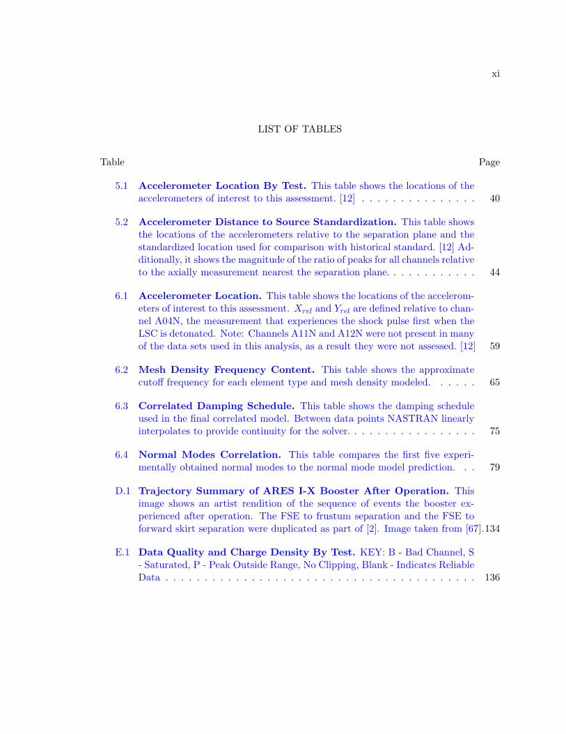
2.4 Martin Marietta Cylindrical Shell Shock Distance Attenuation Curve.Figure 3.1 in [5]. . . . . . . . . . . . . . . . . . . . . . . . . . . . . . . . . . 7

2.5 Comparison of the ARES I and ARES I-X Configurations. Fig.taken from [11]. . . . . . . . . . . . . . . . . . . . . . . . . . . . . . . . . . . 8

2.6 Ares Partial Stack Description. Fig. taken from [13]. . . . . . . . . . . 9

2.7 Ares I-X Flight Vehicle Configuration. Fig. taken from [14]. . . . . . 10

2.8 Ares I-X Flight FSE Separation Test. Image taken from [15]. . . . . . 11

2.9 Ares I-X Flight FSE Separation Test. Image taken from [16]. . . . . . 12

4.1 Spectral Leakage of a Sine Wave. The plot of the left shows a 7 Hz sinewave and the plot on the right shows the fast Fourier transform of that samesine wave. Image taken from [63]. . . . . . . . . . . . . . . . . . . . . . . . . 22

4.2 Harmonic Wavelet. The two figures show the real and imaginary parts ofthe harmonic wavelet. . . . . . . . . . . . . . . . . . . . . . . . . . . . . . . 24

4.3 Fourier Transform of Harmonic Wavelet Levels. [23] . . . . . . . . . 25

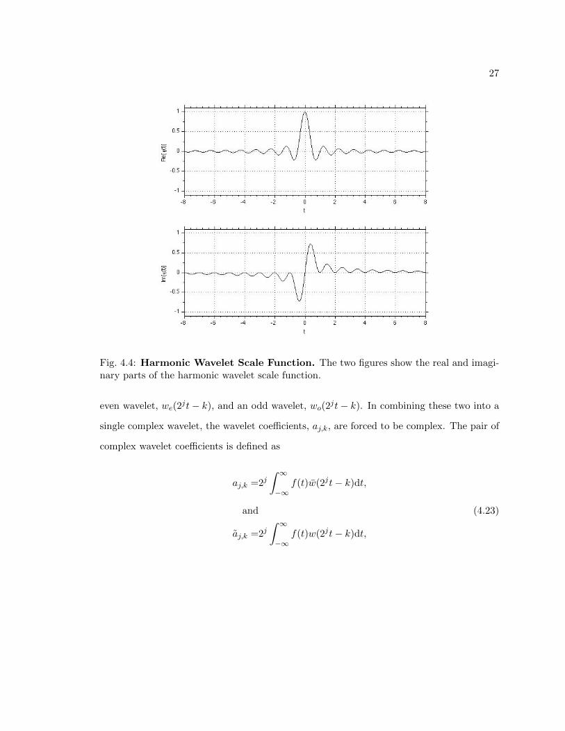
4.4 Harmonic Wavelet Scale Function. The two figures show the real andimaginary parts of the harmonic wavelet scale function. . . . . . . . . . . . 27

4.5 Harmonic Wavelet Transform Algorithm For Real Inputs. The im-age shows a graphical description of the algorithm used to calculate theharmonic wavelet transform for real inputs. Image taken from [23]. . . . . . 34

xiii

4.6 Harmonic Wavelet Transform Algorithm For Complex Inputs. Theimage shows a graphical description of the algorithm used to calculate theharmonic wavelet transform for real inputs. Image taken from [23]. . . . . . 34

5.1 Main Parachute Support System Description. (a) The image showsthe main parachute support system arms and plate that tie into the cylindri-cal shell or what would the outer case in flight. [12] (b) The image shows apictorial representation of the main parachute support system arms that tieinto the cylindrical shell. The azimuthal location of the accelerometers usedthis assessment is represented by the red star. Based on a diagram in [12]. . 38

5.2 General MPSS Location During Both Ground Tests. The red boxillustrates the general location of the MPSS in both ground tests. Modifiedimage from [15]. . . . . . . . . . . . . . . . . . . . . . . . . . . . . . . . . . . 39

5.3 Azimuthal Coordinate System. This image shows a cartoon depictionof the top view of the azimuthal coordinate system on the shell and thedetonation path followed by the pyrotechnic devices used to severe the FSEfrom the forward skirt and FSE from the frustum joints. Image based onwork done in [12]. . . . . . . . . . . . . . . . . . . . . . . . . . . . . . . . . . 41

5.4 Axial Station Locations of Interest. (a) The image shows the relativestation locations of key locations on the test article. The separation plane islocated at station -4 in. [12] (b) The image shows the relative station locationsof key locations on the test article. The separation plane is located at station72.6 in. [12] . . . . . . . . . . . . . . . . . . . . . . . . . . . . . . . . . . . . 42

5.5 Digitized Martin Marietta Standard. The figure shows a digitized veri-sion of Fig. 2.4. . . . . . . . . . . . . . . . . . . . . . . . . . . . . . . . . . . 45

5.6 Wave Paths Following to Measurement Locations. The image showsthe possible paths that can be taken by the wave front once the LSC isdetonated. . . . . . . . . . . . . . . . . . . . . . . . . . . . . . . . . . . . . . 47

5.7 FSE to Forward Skirt Separation Test Attenuation. The plots showthe attenuation with distance for the measurements taken as part of the FSEto frustum separation test using the peak SRS approach for (a) all directionsand (b) for the axial direction. . . . . . . . . . . . . . . . . . . . . . . . . . 53

5.8 FSE to Frustum Separation Test Attenuation. The plots show theattenuation with distance for the measurements taken as part of the FSEto forward skirt separation test using the peak SRS approach for (a) alldirections and (b) for the axial direction. Channel A008T required additionalprocessing to bring it in family with the other data’s time histories, andchannel A109A’s location required the traveling wave to pass through a boltedjoint prior to reaching the measurement location. . . . . . . . . . . . . . . . 54

xiv

5.9 FSE to Forward Skirt Separation Test Attenuation. The plots showthe attenuation with distance for the measurements taken as part of the FSEto frustum separation test using the peak SRS approach for (a) all directionsand (b) for the axial direction. . . . . . . . . . . . . . . . . . . . . . . . . . 55

5.10 FSE to Frustum Separation Test Attenuation.The plots show the at-tenuation with distance for the measurements taken as part of the FSE toforward skirt separation test using the peak SRS approach for (a) all di-rections and (b) for the axial direction. Channel A008T required additionalprocessing to bring it in family with the other data’s time histories, and chan-nel A109A’s location required the traveling wave to pass through a boltedjoint prior to reaching the measurement location. . . . . . . . . . . . . . . . 56

6.1 Cartoon Depiction of Test Article and Stand. The red star pointsout the location of the origin used with the accelerometers in the full testconfiguration. This location is consistent with the location shown in Fig. 6.2.Image based on figures in [18]. . . . . . . . . . . . . . . . . . . . . . . . . . 58

6.2 Accelerometer Locations. The image shows the accelerometer locationsrelative to the selected origin. All measurements are normal to the plate.Table 6.1 provides the actual distances from the origin. Image based onfigures in [12]. . . . . . . . . . . . . . . . . . . . . . . . . . . . . . . . . . . . 59

6.3 Example Flat Plate Time History Response. The two arrows illustratethe two peaks that are atypical of the expected response. [18] . . . . . . . . 61

6.4 Test T3 Channel A04N Peak Normalized Frequency Cutoff Deter-mination. . . . . . . . . . . . . . . . . . . . . . . . . . . . . . . . . . . . . 64

6.5 Mesh Density Study. Peak Normalized Model Time History for (a) PlateElements (b) Solid Brick Elements. The responses shown in these figures arenormalized using the peak model response. . . . . . . . . . . . . . . . . . . 66

6.6 Element Type Time History Comparison. Plate and solid element timehistory response at the A04N location are compared with test data to aid indetermining which element is more appropriate for use. The amplitude wasnormalized relative to the peak model response in this case. . . . . . . . . 67

6.7 Element Type FFT Comparison. (a) Plate and (b) solid element spectraldensity at the A04N location are compared with test data spectral density toaid in determining which element is more appropriate for use. The amplitudewas normalized relative to the peak model response in this case. . . . . . . 68

6.8 0.5 in. by 0.5 in. Plate Element Model. . . . . . . . . . . . . . . . . . 69

6.9 Input Shape Sensitivity Study. The three input shapes shown here wereused to provide a better understanding of how the input shape affected theimpulse response of the plate. . . . . . . . . . . . . . . . . . . . . . . . . . 69

xv

6.10 Mesh Density Study. Peak normalized time history comparing test T3,channel A04N response to the solid brick element model response for a (a)triangular shaped load (b) half sine shaped load, and (c) step shaped load 71

6.11 Detonation Velocity Inclusion Study. The three spectral density plotswere normalized relative to the peak response of test T3 cannel A04N. Fromthis it is clear that the detonation velocity must be included in the model. 72

6.12 Peak Normalized Input Load. . . . . . . . . . . . . . . . . . . . . . . . 73

6.13 Load Duration Study. The time histories here have been normalized bytheir peak values. . . . . . . . . . . . . . . . . . . . . . . . . . . . . . . . . 74

6.14 Damped Time History Comparison and Correlation, t = 0 to 0.01s. The time history shown here has been normalized relative to the peakresponse of test T3 at channel A04N and shows the effect of the applieddamping given in Table 6.3 on model response. . . . . . . . . . . . . . . . . 76

6.15 Damped Spectral Density Comparison and Correlation. The spectraldensity shown here has been normalized relative to the peak response of testT3 at channel A04N and shows the effect of the applied damping given inTable 6.3 on the spectral content of the model. . . . . . . . . . . . . . . . . 77

6.16 Damped Model Harmonic Wavelet Transform Comparison and Cor-relation. The wavelet transforms shown here have been normalized relativeto channel A04N of test T3 and show the effects of the applied damping onthe system response over the time period t = 0 to 0.01 s for (a) test T3 chan-nel A04N and (b) the modal nodal response representing channel A04N’slocation. . . . . . . . . . . . . . . . . . . . . . . . . . . . . . . . . . . . . . 78

6.17 Model Nodal Time History Response Compared to Test T3 Chan-nel A06N, t = 0 to 0.01 s. The time histories shown here have been nor-malized relative to the peak response of test T3 at channel A04N and providea point of comparison for the model response away from the correlation point. 80

6.18 Comparison of Model Nodal Output for A06N to Test. The wavelettransforms shown here have been normalized relative to channel A04N oftest T3 and provide a comparison for the model away from the correlationpoint. The transforms are shown both for (a) the test data and (b) the modeloutput over the time period between t = 0 to 0.01 s. . . . . . . . . . . . . . 81

6.19 Model Nodal Time History Response Compared to Test T2 Chan-nel A04N, t = 0 to 0.01 s. The time histories shown here have beennormalized relative to the peak response of test T2 at channel A04N andprovide a point of comparison for the model response when extrapolating fora load case similar to the correlation load. . . . . . . . . . . . . . . . . . . 83

xvi

6.20 Model Nodal Spectral Density Compared to Test T2 Channel A04NThe spectral densities shown here have been normalized relative to the peakresponse of test T2 at channel A04N and provide a point of comparison for themodel response when extrapolating for a load case similar to the correlationload. . . . . . . . . . . . . . . . . . . . . . . . . . . . . . . . . . . . . . . . 84

6.21 Comparison of Model Nodal Output for A04N to Test. The wavelettransforms shown here have been normalized relative to channel A04N of testT2 and provide a comparison for the model when extrapolating for a loadcase similar to the correlation load. The transforms are shown both for (a)the test data and (b) the model output over the time period between t = 0to 0.01 s. . . . . . . . . . . . . . . . . . . . . . . . . . . . . . . . . . . . . . 85

6.22 Model Nodal Time History Response Compared to Test T10 Chan-nel A04N, t = 0 to 0.01 s. The time histories shown here have beennormalized relative to the peak response of test T10 at channel A04N andprovide a point of comparison for the model response when extrapolating fora load case significantly different than the correlation load. . . . . . . . . . 87

6.23 Model Nodal Spectral Density Compared to Test T10 ChannelA04N The spectral densities shown here have been normalized relative tothe peak response of test T10 at channel A04N and provide a point of compar-ison for the model response when extrapolating for a load case significantlydifferent than the correlation load. . . . . . . . . . . . . . . . . . . . . . . . 88

6.24 Comparison of Model Nodal Output for A04N to Test. The wavelettransforms shown here have been normalized relative to channel A04N oftest T10 and provide a comparison for the model when extrapolating for aload case significantly different than the correlation load. The transformsare shown both for (a) the test data and (b) the model output over the timeperiod between t = 0 to 0.01 s. . . . . . . . . . . . . . . . . . . . . . . . . . 89

6.25 Test T3 Channel A04N Time History. The time history shown here hasbeen normalized relative to the peak response of test T3 at channel A04Nand provides an estimate of the arrival times of the primary and secondarypeaks. . . . . . . . . . . . . . . . . . . . . . . . . . . . . . . . . . . . . . . . 91

6.26 Full Scale Separation Test Data Investigation - Time History. Theimages show the response time histories for measurements on the (a) FSE toforward skirt test and (b) frustum to FSE test. . . . . . . . . . . . . . . . 94

6.27 Full Scale Separation Test Data Investigation - Harmonic WaveletTransform. The images show the response harmonic wavelet transform formeasurements on the (a) FSE to forward skirt test and (b) frustum to FSEtest. . . . . . . . . . . . . . . . . . . . . . . . . . . . . . . . . . . . . . . . . 95

xvii

6.28 Attenuation With Distance, SRS Method, LSC Charge Density:1.0 gr./ft. (Q = 50). . . . . . . . . . . . . . . . . . . . . . . . . . . . . . 98

6.29 Attenuation With Distance, SRS Method, LSC Charge Density:1.125 gr./ft. (Q = 50). . . . . . . . . . . . . . . . . . . . . . . . . . . . . . 99

6.30 Attenuation With Distance, SRS Method, LSC Charge Density:4.125 gr./ft. (Q = 50). . . . . . . . . . . . . . . . . . . . . . . . . . . . . . 100

6.31 Attenuation With Distance, Energy Method, LSC Charge Density:1.0 gr./ft.. . . . . . . . . . . . . . . . . . . . . . . . . . . . . . . . . . . . . 101

6.32 Attenuation With Distance, Energy Method, LSC Charge Density:1.125 gr./ft.. . . . . . . . . . . . . . . . . . . . . . . . . . . . . . . . . . . 102

6.33 Attenuation With Distance, Energy Method, LSC Charge Density:4.125 gr./ft.. . . . . . . . . . . . . . . . . . . . . . . . . . . . . . . . . . . 103

C.1 SRS Input. The plot shows the graphical representation of Eqn. C.1, forτ = 0.01 s, ξ0 = 5000 g, and T = 1

f , where f is the frequency of interest. . . 126

C.2 SRS Input. The plot shows the graphical representation of Eqn. C.2 com-pared to the algorithm generated SRS for several different processing, forτ = 0.01 s, ξ0 = 5000 g, and T = 1

f , where f is the frequency of interest. . . 127

C.3 Sinusoidal Input. The plot shows the first half second of data for a 35s long sinusoidal input described in Eqn. C.3 with parameters defined asξ1 = ξ2 = 50 g, ω1 = 2π200, and ω2 = 2π550. . . . . . . . . . . . . . . . . . 129

C.4 Harmonic Wavelet Transform of Sinusoidal Input. The plot showsthe harmonic wavelet transform for a sinusoidal input of the form given inEqn. C.3 with the parameters defined as ξ1 = ξ2 = 50 g, ω1 = 2π200, andω2 = 2π550, for different processing bandwidths. Fig. C.3 shows the input. 130

C.5 Chirp Input. The plot shows the first second of data for a 4 s long chirp(sine sweep) input. . . . . . . . . . . . . . . . . . . . . . . . . . . . . . . . . 131

C.6 Harmonic Wavelet Transform of Chirp Input. The plot shows theharmonic wavelet transform for a chirp input for different processing band-widths. Fig. C.5 shows the input. . . . . . . . . . . . . . . . . . . . . . . . . 132

1

CHAPTER 1

Introduction

As in any industry, component requirements govern design and production in the

aerospace industry. In order to show compliance to these requirements, components must

be qualified. Qualification is the process of demonstrating positive margins for different

loading scenarios either through analysis or by test for a component.

Dynamic loads qualification is one subset of the qualification process and dynamic en-

vironments directly feed these loads. Self-induced random vibration and shock (ignition

and separation) are two primary environments that induce loads on components. Scaling

methodologies and mass loading techniques can be used to predict random vibration en-

vironments; however, predicting shock environments is much more difficult. Modeling and

extrapolation methods do exist for shock prediction; however they often produce unrealistic

results when generating levels for a new design [1]. As a result, shock levels from several

similar motors are typically enveloped during environment development on new programs.

This leads to added conservatism which leads to increased costs in risk reduction tasks prior

to qualification testing; the standard for shock qualification.

With the added conservatisms in the environment development, attenuation for dis-

tance, joints, and other structural features becomes important. Current industry stan-

dards are based on data collected nearly 50 years ago on archaic data acquisition systems

and processed using the shock response spectrum (SRS) - an analysis tool that has major

limitations. Advancements in computing, improvements in testing technology, and newly

developed processing tools warrant the need to validate current standards, however, any

validation effort done by industry professionals is likely not wide spread due to proprietary

concerns.

2

CHAPTER 2

Literature Survey

Shock is a local transient mechanical loading characterized by its short duration, high

amplitude, and high frequency response. Events such as the impact of a falling body,

earthquake, near miss of an underwater explosion, or a pyroshock from an explosive device

can all be characterized as a shock event. The time scale of such events can be as long

as several minutes or as short as a few microseconds. The focus of this work will be on

pyroshock events in aerospace applications. Fig. 2.1 shows an example of an expected time

series response to one of these events. The structural environment developed in response to

shock loading can induce major failure resulting in total or partial loss of equipment. On

a component basis, malfunction or degradation of electronic components can occur. On a

larger more global scale, cracks and fractures in brittle materials can develop, local plastic

deformation can occur, or materials can experience an accelerated fatigue life.

One way of representing this type of load is the shock response spectrum or SRS. The

SRS was first developed by Maurice Biot in 1932 to describe the response of a building

during an earthquake [3]. This analysis tool is still widely used in dynamic subfields such as

earthquake engineering or the aerospace industry today. The SRS is a graphical represen-

tation of an array of single degree of freedom (sdof) systems each having a unique natural

frequency. It is calculated by determining the maximum response of each sdof system in the

array, to the same transient base excitation. In order to calculate an SRS, as assumption

about damping has to be made. The dynamic amplification, Q, is essentially a measure of

damping and is defined as the ratio of the critical damping to twice the system damping

of a sdof system and is often used in SRS algorithms. Fig. 2.2 visualizes one such bank of

sdof systems.

Focusing on solid rocket applications, SRS curves are used to characterize ignition and

pyrotechnic device transients that occur as part of a system level launch vehicles. Examples

3

Fig. 2.1: Expected Shock Transient Time History Shape. Notice the smooth expo-nential decay as time goes on and the symmetry of the response, these are two key aspectsthat help distinguish good from suspect data. [2]

of these pyrotechnic devices include explosive bolts and the linear shaped charge (LSC).

An example of an explosive bolt application was the connection between the solid rocket

boosters and the core stage of NASA’s Space Shuttle program. An LSC is a linear chevron

shaped plastic explosive device that is used in several applications. Two such examples are

thrust termination and during staging. As part of thrust termination the LSC stretches

along the case of the motor and is used to cut the case releasing pressure in the event the

flight needs to be terminated. As part of staging, the LSC is wrapped circumferentially

around an interstage and is used to cut the case separating adjacent stages of the rocket.

This work will focus on the response of structural systems where an LSC is used.

In practice, several sources, including an ignition transient at the start of burn for

a solid rocket may be present in any one system. Although each source may be charac-

terized individually, they are often enveloped to determine a bounding environment. The

4

Fig. 2.2: A bank of sdof systems used in an SRS generation.

enveloping procedure, however, can result in an overly conservative environment, especially

when predicting environments for new programs. This bounding case is then used to define

load factors or as an input for dynamic qualification testing. The industry standard used

to characterize shock environments is the SRS. Though it is the standard, it does have

its limitations. Its biggest limitation is that it fails to address the temporal nature of a

transient event. For every SRS generated, there are an infinite number of potential inputs.

The example in Fig. 2.3 shows five radically different time series, that when passed through

the SRS algorithm, generate the same shock response. The lower right corner of the figure

shows the resulting outputs of these different time series. This indicates the loss of tem-

poral information about the transient event in the calculation of the SRS. Ideally, when

defining a bounding environment for structural loads determination or qualification testing,

the environment should capture both spectral and temporal aspects of the flight environ-

ment. There are two additional limitations of the SRS. The first, as previously mentioned,

is that the SRS requires an assumption about damping. Secondly, is does not account for

5

any modal interactions or coupling that can occur in physical systems. This is a result of

treating each frequency as its own independent sdof system.

Fig. 2.3: SRS input comparison. Five radically different time histories are passed intothe SRS algorithm, symbolized in the top right by the bank of sdof systems, that generatethe same SRS. The figure is taken directly from [4].

With the dissipative mechanisms inherent to physical systems, it is easy to conclude a

traveling wave such as a shock wave, would undergo energy loss as it propagates. Combining

the inherent high-level structural response that shock events cause with the conservatisms

associated with the enveloping process, it is easy to see the need for a reduction factor that

can be used to reduce loads the further a component is from the source. Or more appro-

priately, it points to the need to understand the attenuation characteristics of these waves

as they propagate through open media and joints. In March of 1970 The Martin Marietta

Corporation, under a contract with NASA’s Goddard Space Flight Center published a re-

port entitled Aerospace Systems Pyrotechnic Shock Data (Ground Test and Flight) [5]. In

this report the authors present attenuation guidelines for structures and equipment being

designed to pyrotechnic environments. They consider attenuation for distance and several

types of jointed interfaces. These guidelines have since been the industry standard for shock

attenuation. Fifteen years later in 1985, a survey of pyroshock prediction methods was done

6

by Van Ert [6]. His survey primarily focused on prediction methodologies; however, a sub-

section on attenuation references the Martin Marietta report. Further work was completed

by Spann et al. looking at shock attenuation through joints in [7–9]. In 2001 and 2011 the

latest versions of the NASA Handbook 7005: Dynamic Environmental Criteria (2001), [1],

and NASA Technical Standard 7003: Pyroshock Test Criteria (2011), [10], still cite the

work completed by Martin Marietta. In addition, the same two NASA technical documents

provide two scaling relationships. The first accounts for source energy differences,

SRSn(x) = SRSr(x)

√EnEr, (2.1)

where En and Er is the total explosive energy of the new and reference structure respectively,

and x is the distance from the source. The second provides an alternative for the distance

attenuation of a point source on a complex structure,

SRS(D2, fn) = SRS(D1, fn)e(−8∗10−4f

2.4f−0.105n

n )(D2−D1), (2.2)

where D1 and D2 are the distances from the pyrotechnic source to the reference and new

locations respectively, and fn is the nth natural frequency. Both Eqn. 2.1 and Eqn. 2.2

share the limitation of using the SRS in their definition, and furthermore, Eqn. 2.2 was

developed using a point source at ground level and may not be representative of other

sources in different conditions such as in the upper atmosphere or in space. Additionally,

a point source is only applicable in limited situations such as an explosive bolt or hammer

strike [1].

Focusing on the attenuation over distance, the Martin Marietta document discusses

several structural configurations ranging from a cylindrical shell with no stringers (verti-

cal stiffeners), rings, or frames, to a honeycomb structure. For each configuration, the

documented attenuation curve was calculated using the SRS peak spectrum response over

the frequency range of interest. The curves were normalized to a factor of one at the

measurement nearest the source. In most cases, the nearest measurement available was ap-

7

proximately 5 in. from the source. Thus, the attenuation curves presented in the document

are arbitrarily normalized to a distance of 5 in. Fig. 2.4 summarizes the findings for the

cylindrical shell. This structural configuration is of most interest in the solid rocket motor

structures. Two primary concerns arise from the plotted data: first the curve was generated

with limited data (as is self-stated within the report) using old data acquisition technology,

and second, the SRS was used to determine the spectrum peaks; and the short comings of

this analysis technique have already been pointed out.

Fig. 2.4: Martin Marietta Cylindrical Shell Shock Distance Attenuation Curve.Figure 3.1 in [5].

As recent as 2009 and 2011 two sets of LSC separation development tests were con-

ducted by Orbital ATK as part of NASA’s ARES I and ARES I-X programs. Fig. 2.5 gives

an overview of the differences between the two vehicles [11]. In 2009, a full scale separation

8

test plan, [2], was executed and documented in [12] to demonstrate the functionality of the

ARES I-X LSC severance system. The test consisted of an ARES I-X full scale flight-like

cylindrical segment that jointed the frustum to the forward skirt. The test was conducted

in two parts, the forward skirt extension (FSE) to forward skirt joint was cut followed by a

cut of the FSE to frustum joint. During each event accelerometers recorded the response on

the cylinder at various locations; the data will be discussed in depth in a later chapter. Figs.

2.6 and 2.7 show the various structural components of the vehicle and give an indication of

where the separation events occur [13, 14]. Figs. 2.8 and 2.9 show the test article prior to

ordinance detonation and just after detonation of the FSE - frustum LSC [15, 16]. A high

speed video of the FSE - frustum separation test can be found in [16].

Fig. 2.5: Comparison of the ARES I and ARES I-X Configurations. Fig. takenfrom [11].

In 2011, a series of flat plate LSC development tests were conducted by Orbital ATK.

In these tests a large flat aluminum plate was used to demonstrate cutting abilities of

different LSC strengths. In addition, the tests were used to help characterize source shock

levels for different staging events that were specific to the program. The test plan and final

report [17,18] discuss the test description and results.

Though both the 2009 and 2011 sets of data are ideal for determining attenuation as

9

a function of distance, no analysis was done to verify the findings in the Martin Marietta

document. In both tests, the data were characterized at a top level by the time history and

the SRS. The only dynamics interest in the data was to estimate the environment produced

by such events, not to investigate the underlying physics of the traveling wave.

Fig. 2.6: Ares Partial Stack Description. Fig. taken from [13].

Though the shock response spectrum is still widely used as an analysis tool, and is the

basis for characterizing the events in the previously discussed tests, time-frequency methods

incorporate both temporal and spectral aspects of a transient signal. These methods are

signal processing techniques that present amplitude and phase as a function of time and

frequency simultaneously. They provide a way to characterize the time evolving spectral na-

ture of a transient event. Cohen provides an excellent discussion as to why these techniques

are needed in his book [19].

Recently, the use of wavelets has increased in the time-frequency analysis of vibration

and shock characterization [4, 20–26]. Wavelets, developed in the 1980’s, are used for nu-

merous applications throughout the literature. Bettella et al. used a wavelet transform to

10

Fig. 2.7: Ares I-X Flight Vehicle Configuration. Fig. taken from [14].

investigate wave propagation on thin aluminum plate and all aluminum honeycomb sand-

wich panels due to high velocity impacts [20]. Gendelman et al. used them to characterize

passive targeted energy transfer in strongly nonlinear mechanical oscillators [21], and Phu

Le and Argoul uses a similar transform for modal identification purposes [22]. These works

show how widely applicable wavelets are.

One specific wavelet, the harmonic wavelet, has the unique property of preserving

signal strength in the frequency domain. Newland created this wavelet in 1993 [23] with

multi-resolution analysis in mind. One of his first published applications of the new wavelet

was approved in 1994 and discusses the extension of harmonic wavelets into music and

the applications it has in that discipline [24]. He extends the applications in 1999 where

he discussed four nonrelated topics: transmission of bending waves in a beam subjected

11

Fig. 2.8: Ares I-X Flight FSE Separation Test. Image taken from [15].

to an impact, pressure fluctuations in acoustic waveguides, ground response analysis for

vibration recorded near an underground train in London, and computing the time varying

cross-spectra for multi-channel measurements of soil vibration in a centrifuge [25]. More

recently, Edwards looked at correcting accelerometer data when zero shift occurred, [26],

and Hacker proposed a replacement for the SRS in shock characterization, [4]. In this work,

the harmonic wavelet transform will be used to characterize shock attenuation as a function

of distance from the source. A more complete history and development will be provided

shortly.

To aid in better understanding the intricacies of the type of short time, high energy

event that pyroshock is, finite element analysis (FEA) modeling techniques can be employed

to best simulate available test data when unexpected response characteristics are present

in measured data. Although FEA provides a flexible way to analyze complex structures,

assumptions about the forcing function and damping must be made when considering py-

roshock events. Standard approaches for direct and modal transient solutions that include

damping can be found in the documentation accompanying the industry standard pack-

12

Fig. 2.9: Ares I-X Flight FSE Separation Test. Image taken from [16].

ages [27]. However, both of these methods have limitations in damping control that prevent

one from accurately modeling a transient event. In addition, file size often becomes an

issue when fine time steps and mesh densities are used. Even with these limitations, FEA

provides a quick way to gain an qualitative understanding of the response of simple systems

and will be used as tool to help explore unexpected response characteristics in this work.

The models that will be discussed should in no way be taken as state of the art in shock

modeling; rather the models are used merely as a tool used to gain insight in the response

of these simplified systems.

The literature is full of different approaches to modeling impulse response on structures.

In Ugural’s book, [28], he formulates a closed form solution using a series expansion for

rectangular plates with different loading conditions. His approach however follows the

typical pattern: resolve the associated eigenvalue problem and then form the solution by

modal super position. This type of approach works well for simple boundary conditions,

however when other, more difficult boundary conditions apply, approximate methods must

13

be used. Pavic uses a boundary forming approach where the analytical response of an

infinite plate is used to obtain a solution by superposing two excitations, the original and a

secondary one which has a continuously distributed outside contour bounding the original

plate [29]. The secondary solution has the role of creating the proper boundary conditions

for the original plate. Botta and Cerri use Reissner-Mindlin theory to investigate a plate

under an impulse load and influence of the impulse (rise time and function) along with

geometric parameters play on the response [30]. They correlate their work using the SRS,

however, a seemingly incomplete way to correlate a model. Various other techniques for

modeling simple and orthotropic plates as well as cylindrical shells have been developed [31–

36]. More recent analytical modeling procedures involving Hydrocodes have surfaced. These

codes model the time history details of the explosive or propellent ignition and burning

process and use the results to excite a nonlinear structural deformation or separation model

that generate propagating structural waves [37–39]. Unfortunately, the implementation

of these types of analyses is generally expensive and produce predictions that are often

poor [1, 10].

An alternative to Hydrocodes is Transient Statistical Energy Analysis (SEA). SEA

methods are typically applied to steady state vibration problems, however when used with

transient excitations the steady-state power balance equation is replaced with the corre-

sponding transient equation that incorporates time dependent power and a term describing

the time varying dynamic modal energies. When the input power involves a nonlinear pro-

cess, which is often the case for local structural responses with a pyrotechnic excitation, this

type of analysis fails due to its modal nature. Examples of this analysis are found in [40–48].

One common numerical implantation of this technique is called TRANSTAR for Transient

Analysis Storage and Retrieval. Further information on this can be found in [49–51].

Related to Transient SEA is Virtual Mode Synthesis and Simulation (VMSS). The

process estimates the steady state frequency response magnitude at a selected location due

to an input excitation at a different location. Then at high frequencies it is assumed that

the frequency response envelope can be represented as the peak response from a collection

14

of localized modes spaced according to the estimated modal density of the local structure.

Virtual mode coefficients are then generated that can be used to simulate a time response

of the dynamical system by convolving a measurement or simulated transient excitation

with the output. VMSS has several advantages over Transient SEA. In VMSS, there are no

quasi-stationary requirements for the excitation and if the structure is reasonably linear, the

near-field response estimate may be estimated. VMSS also provides a time domain solution

and an SRS (if desired) as opposed to the peak value and spectral envelope estimate that

transient SEA provides. More information about VMSS can be found in [52–55].

With numerous sources in the literature describing a variety of ways to model such

transient events, it is clear that modeling such events is quite difficult. Each method has

strengths and weakness and the application of a method should be chosen to be in line with

the desired results of a defined analysis. Regardless of the method, this collection of work

show the need for better modeling methods of pyrotechnic excitation of complex structures.

15

CHAPTER 3

Signal Energy and Parseval’s Theorem

The signal energy for an arbitrary input function, f(t), is defined as

Es =

∫ t2

t1

|f(t)|2dt, (3.1)

where the total signal energy, Es, can be found by integrating over all time [56]. From Eqn.

3.1 it is easy to see the units of signal energy are U2s, where U are the engineering units of

the specific application. In the electrical world, f(t) is typically a voltage (V); giving the

signal energy units of V2s. In this case, the signal energy is proportional to the physical

energy through the impedance of the electrical system. The impedance is a measure of the

effective resistance of a circuit and is reported in units of Ohm’s (Ω) [57]. The physical

energy is the ratio of the signal energy to the system impedance, producing a value with

units of energy, Joules (J). It is important to note, that the signal energy is proportional

to the physical energy, so a loss in one, results in a loss in the other, regardless of the time

dependent form of the impedance. Take the case of resonance for example, there may be

significantly higher system response at a particular frequency, but the overall energy output

is still less than the input. Resonance and dynamic amplification does not imply an increase

in total system energy, but rather a particular energy density shape [19].

This same approach can be extended to mechanical systems. Voltage can be thought

of as analogous to force. Both provide an input to their respective systems; voltage is

associated with current, while a force is associated with acceleration. Masses and springs

store energy in both kinetic and potential forms, just as capacitors and inductors, while

dampers dissipate energy just as resistors [57]. Using this analogy, the signal energy of a

measured acceleration signal can be converted to the physical energy by multiplying by the

mass squared and dividing by the mechanical impedance. For a single degree of freedom

16

system, the mechanical impedance is defined as

Zmech =K

iω+ C + iωM, (3.2)

where ω is the natural frequency, K the spring constant, C the damping coefficient, and

M the mass [58]. In the mechanical world, impedance can be thought of as a generalized

inertia, or as a measure of the resistance of motion. To illustrate the analogy, consider

the units: (in SI) acceleration is meters per second squared, mass is kilograms, and the

impedance is kilograms per second. An acceleration signal produces a signal energy having

units of meters squared per second cubed that when multiplied by the mass squared and

divided by the mechanical impedance results in units of Joules, just as before, energy units

are obtained. Notice again that the signal energy goes as the physical energy.

Obviously, the analogy does not translate exactly, as the acceleration varies spatially

as well as temporally and in general would require integration over space; whereas a voltage

can be measured at a point in a circuit and treated as only varying in time. Even with these

limitations, acceleration is often treated in the same manner as voltage so that vibration

engineers can extract modal response information from measured data. The same approach

will be taken here; in the coming chapters the relationship between the signal energy and

physical energy is assumed and the signal energy is treated and referred to as a measure of

the system physical energy, even though the units do not explicitly agree with the treatment.

In vibration analysis, and in other fields, it is often the case that signals are analyzed

using their frequency response. This requires a transformation between the time and fre-

quency domains. This transformation should have no effect on the signal or system energy.

Parseval’s theorem demonstrates this.

Theorem 1. Parseval’s Theorem. Let x(t) be a complex valued function that is suffi-

ciently smooth, that decays sufficiently quickly near infinity so that its integrals exist, and

has Fourier transform

X(ω) =1

2π

∫ ∞−∞

x(t)e−iωtdt, (3.3)

17

where ω = 2πf , and inverse Fourier transform

x(t) =

∫ ∞−∞

X(ω)eiωtdω. (3.4)

Then, ∫ ∞−∞|x(t)|2dt =

1

2π

∫ ∞−∞|X(ω)|2dω. (3.5)

Proof. Let δ(t) be the well-known Dirac delta function. Its Fourier transform is then

∆(ω) =

∫ ∞−∞

δ(t)e−iωtdt = 1 (3.6)

and it’s inverse Fourier transform is

δ(t) =1

2π

∫ ∞−∞

eiωtdω. (3.7)

The proof of Eqn. 3.5 starts by rewriting the left hand side of Eqn. 3.5 using the inverse

Fourier transform

∫ ∞−∞|x(t)|2dt =

∫ ∞−∞

(1

2π

∫ ∞−∞

X(χ)eiχtdχ

)(1

2π

∫ ∞−∞

X(ξ)eiξtdξ

)dt, (3.8)

where the over bar denotes the complex conjugate. Rearranging the order of integration in

Eqn. 3.8 gives,

∫ ∞−∞|x(t)|2dt =

∫ ∞−∞

X(χ)

(1

2π

∫ ∞−∞

X(ξ)

(1

2π

∫ ∞−∞

ei(χ−ξ)tdt︸ ︷︷ ︸δ(χ−ξ)

)dξ

)dχ, (3.9)

and using Eqn. 3.7 the integral over t is evaluated leaving

∫ ∞−∞|x(t)|2dt =

∫ ∞−∞

X(χ)

(1

2π

∫ ∞−∞

X(ξ) δ(χ− ξ)dξ)

dχ (3.10)

=1

2π

∫ ∞−∞

X(χ)X(χ)dχ, (3.11)

18

or, just as in Eqn. 3.5 ∫ ∞−∞|x(t)|2dt =

1

2π

∫ ∞−∞|X(ω)|2dω. (3.12)

19

CHAPTER 4

General Harmonic Wavelet Theory

4.1 Background and General Harmonic Wavelet Definition

Summarizing the work done by Gao in [59], the first reference of wavelets goes back

to the early twentieth century when Alfred Haar wrote his dissertation in 1909. His work

on orthogonal systems of functions led to the development of a set of rectangular basis

functions which later led to the entire Haar wavelet family. The Haar wavelet family is the

simplest family of wavelets and consists of a short positive pulse followed by a short negative

pulse. This wavelet family has been used for a variety of applications. Initially developed

to illustrate a countable orthonormal system for the space of square-integrable functions

on the real line, they were later used in image compression and to investigate Brownian

motion. Since Haar’s initial work, numerous individuals have contributed to advancing the

field. Major contributions came from Jean Morlet in the mid 1970’s. Morlet developed

and implemented a technique to scale and shift the analysis window functions in analyzing

acoustic echoes while working for an oil company. This work was the foundation of what

later became the Morlet wavelet family. Later, around 1988, Ingrid Daubechies created

her own family of wavelets with multi-resolution analysis in mind. Since then, wavelet

applications have become more widespread ranging from image and speech processing to

signal analysis in manufacturing.

At their core, all wavelets are based on integral transforms, similar to the well-known

Fourier transform. These transforms expand an arbitrary function with respect to some

set of chosen basis functions. The Fourier transform uses sines and cosines as the basis

set, where wavelets use other functions. Wavelets and wavelet families can be continuous

or discrete, real or complex, but in general the choice of a basis set used to define the

wavelet or wavelet family is arbitrary; ideally, however, the chosen basis has some form of

20

physical meaning. The sines and cosines used as the Fourier basis, for example, are related

to frequency making them useful in spectral analysis. Furthermore, it is well known that

choosing a set of basis functions that are normalizable, invertible, orthogonal, and form a

complete set is advantageous when defining a wavelet transform.

In time-frequency analysis, a subset of multi-resolution analysis, a signal is decomposed

in time and frequency simultaneously. At the heart of this transformation, the input signal

is decomposed into sub-signals or different size resolution levels. The term level refers to

one of these sub-signals. There can be as many levels as the number of times the input

signal can be divided by two [60]. The series expansion of such a transformation requires an

expansion in two variables. A general series expansion and wavelet transform of this form

is

x(t) =∑m

∑n

αm,nφm,n(t) (4.1)

αm,n =1√m

∫x(t)φm,n

(t− nm

)dt, (4.2)

where φm,n(t) are the basis functions related to time (n) and frequency (m) respectively. A

general wavelet transform of a function, x(t), is a transform of the function from t into a

function of m and n, where m is a scaling parameter and is related to frequency and n is a

translation parameter and is related to time. Scaling makes the basis function more localized

in time shortening the duration of the wavelet, which effectively increases its frequency. This

allows for correlation with events that occur at higher frequencies. Translation shifts the

basis function such that it correlates with events that occur later in time [4].

The general harmonic wavelet is a unique wavelet developed by David Newland in

1993, and will be referred to as the harmonic wavelet in this work. Newland developed

the transform with multi-resolution analysis of vibration problems in mind. His goal was

to develop a wavelet whose spectrum is confined exactly to an octave band. By doing

so he eliminated all spectral leakage. Spectral leakage is the smearing of energy across a

frequency spectrum that occurs when a signal is not periodic in the sample interval [61]. An

21

example of spectral leakage can be seen in Fig. 4.1. A wavelet having a spectrum confined

to an octave band allows the level of a signal’s multi-resolution analysis to be interchanged

with its frequency band. This lead Newland to look for a wavelet whose Fourier transform

is compact and which could be constructed from simple functions [23]. Along with its

compactness1, the wavelet is orthogonal, normalizable, and invertible [23].

Another benefit of the harmonic wavelet is that it captures both signal dispersion and

dissipation without making any assumptions about the system damping [4]. Dispersion

is a conservative mechanism by which energy in a traveling wave spreads out over time.

Dispersion occurs when the group velocity is different than the phase velocity of the traveling

wave. Generally, the group and phase velocities are frequency dependent, and when they are

different, waves at different frequencies travel at different speeds. The velocity differences

spread the waves out and the peak power of the traveling wave group decreases. Hacker

demonstrates this application in his work, [4]. Dissipation is a decrease in peak power as well;

however, it stems from the conversion of mechanical energy into heat and is non-conservative

in nature. As will be discussed shortly, the harmonic wavelet satisfies Parseval’s theorem,

and therefore, the transform inherently captures any dissipation present in the data being

analyzed.

Following Newland [23], we will develop the harmonic wavelet from its infancy. Certain

details such as the normalization and orthogonality will be assumed. The proof of these

properties can be found in Newland’s work, [23]. Consider the functions we(x) and wo(x)

whose Fourier transforms are defined by

We(ω) =

14π for − 4π ≤ ω < −2π and 2π ≤ ω < 4π

0 otherwise,

(4.3)

1Compactness is a mathematical property that generalizes the notion of a subset of Euclidean spacebeing closed and bounded. This means the space contains all its limit points and those points all lie withinsome fixed distance of each other. Where a limit point, z ∈ Z, is a point of set S, if every neighborhood ofz contains at least one point of S different from z itself. [62]

22

Fig. 4.1: Spectral Leakage of a Sine Wave. The plot of the left shows a 7 Hz sine waveand the plot on the right shows the fast Fourier transform of that same sine wave. Imagetaken from [63].

and

Wo(ω) =

i4π for − 4π ≤ ω < −2π,

− i4π for 2π ≤ ω < 4π,

0 otherwise,

(4.4)

where the subscript e denotes an even function and o denotes an odd function. The inverse

Fourier transform,

f(t) =

∫ ∞−∞

F (ω)eiωtdω, (4.5)

of We(ω) and Wo(ω) are

we(t) =1

2πt

(sin(4πt)− sin(2πt)

)(4.6)

and

wo(t) =− 1

2πt

(cos(4πt)− cos(2πt)

), (4.7)

respectively. Combining Eqns. 4.6 and 4.7 into a single complex function as

w(t) = we(t) + i wo(t), (4.8)

23

we obtain

w(t) =1

i2πtei4πt − ei2πt, (4.9)

where w(t) defines the harmonic wavelet. Fig. 4.2 shows the real and imaginary parts of

the harmonic wavelet as functions of time. Based on its definition, the Fourier transform,

W (ω), of the harmonic wavelet is given by

W (ω) = We(ω) + iWo(ω). (4.10)

Using Eqns. 4.3 and 4.4 we have

W (ω) =

12π for 2π ≤ ω < 4π,

0 otherwise.

(4.11)

To incorporate scaling and translation, as discussed in Eqn. 4.2, we need to replace t

with (2jt− k) in Eqn. 4.9:

w(2jt− k) =1

i2π(2jt− k)

(ei4π(2

jt−k) − ei2π(2jt−k)), (4.12)

where j and k are integers. The shape of the harmonic wavelet described in Eqn. 4.12 does

not change, it is simply scaled or translated. Its horizontal scale is compressed by a factor

of 2j , and its position is translated by k units at a new scale of k/2j units of the original

scale. j determines the level of the wavelet. At level j = 0, the wavelet’s Fourier transform

occupies the bandwidth between 2π and 4π; at level j = J , it occupies the bandwidth

between 2π2J and 4π2J , which is J octaves higher up the frequency scale. j and k act in

the same manner as m and n in Eqn. 4.2, they simply scale and translate the harmonic

wavelet. With the simplicity of the wavelet’s Fourier transform, orthogonality can easily be

shown, but will be left to Newland [23].

As the octave band widens, successive levels of the harmonic wavelet decrease in pro-

portion to this increasing bandwidth. Fig. 4.3 shows this relationship for j ≥ 0. For those

24

Fig. 4.2: Harmonic Wavelet. The two figures show the real and imaginary parts of theharmonic wavelet.

octave bands or levels defined by j < 0, the same sequence as in Fig. 4.3 is maintained.

These levels see ω → −∞. As part of multi-resolution analysis, all frequencies can be rolled

together into a single wavelet level for this case. Following the standard terminology, this

level is referred to as level -1, and it serves to cover the residual frequency band between

0 and 2π in Fig. 4.3. The function that describes this frequency band is called the scaling

function in wavelet theory, and the inverse Fourier transform of the even scaling function is

Φe(ω) =

14π for − 2π ≤ ω < 2π,

0 otherwise,

(4.13)

25

Fig. 4.3: Fourier Transform of Harmonic Wavelet Levels. [23]

Taking the inverse transform of Eqn. 4.13 gives

φe(t) =sin(2πt)

2πt. (4.14)

Similarly, the odd function defined by

Φo(ω) =

i4π for − 2π ≤ ω < 0,

− i4π for 0 ≤ ω < 2π,

0 otherwise,

(4.15)

gives an odd scaling function,

φo(t) =−(cos(2πt)− 1)

2πt. (4.16)

Combining Eqns. 4.14 and 4.16 in the same manner as Eqn. 4.8, the complex scaling

function is defined,

φ(t) =ei2πt − 1

i2πt, (4.17)

26

and its Fourier transform, from Eqn. 4.13 and 4.15, is

Φ(ω) =

12π for 0 ≤ ω < 2π,

0 otherwise.

(4.18)

Fig. 4.4 shows the real and imaginary part of φ(t) as functions of time. Just as in the case

of the other levels, the scale function φ(t) can be shown to be orthogonal [23].

As was mentioned previously the harmonic wavelet can be normalized, the details of

which will be left to Newland, [23]. The result used in normalization of w(t) and φ(t) in

Eqns. 4.9 and 4.17 is ∫ ∞−∞|w(2jt− k)|2dt =

1

2j, (4.19)

and ∫ ∞−∞|φ(t− k)|2dt = 1. (4.20)

4.2 Multi-Resolution Analysis

The general expansion formulas of wavelet theory shown in Eqn. 4.1 and 4.2 applied

to a function, f(t), using the harmonic wavelet and keeping all levels is written as

f(t) =∞∑

j=−∞

∞∑k=−∞

aj,k w(2jt− k). (4.21)

If the negative levels are replaced by the scale function, Eqn. 4.21 becomes

f(t) =∞∑

k=−∞aφ,k φ(t− k) +

∞∑j=0

∞∑k=−∞

aj,k w(2jt− k). (4.22)

Both Eqn. 4.21 and 4.22 assume that the wavelets expanding f(t) are derived from the

solution of two-scale dilation equations2 with real coefficients, and that there is only one

wavelet for each j, k pair. Recall though that the harmonic wavelet is composed of both an

2A two parameter dilation equation is an equation that includes two parameters to shift and scale theindependent variable and requires solution for coefficients. [64]

27

Fig. 4.4: Harmonic Wavelet Scale Function. The two figures show the real and imagi-nary parts of the harmonic wavelet scale function.

even wavelet, we(2jt− k), and an odd wavelet, wo(2

jt− k). In combining these two into a

single complex wavelet, the wavelet coefficients, aj,k, are forced to be complex. The pair of

complex wavelet coefficients is defined as

aj,k =2j∫ ∞−∞

f(t)w(2jt− k)dt,

and (4.23)

aj,k =2j∫ ∞−∞

f(t)w(2jt− k)dt,

28

where the over bar indicates the complex conjugate. Similarly, the corresponding pair of

complex coefficients for the scaling function are

aφ,k =

∫ ∞−∞

f(t)φ(t− k)dt,

and (4.24)

aφ,k =

∫ ∞−∞

f(t)φ(t− k)dt.

When f(t) is real, aj,k = aj,k, thus aj,k is not a new coefficient. Allowing f(t) to be complex

requires that aj,k be distinguished separately from aj,k. The contribution of a single complex

wavelet to the expansion of function, f(t), is

aj,k w(2jt− k) + aj,k w(2jt− k). (4.25)

As a result, the expansion formulas given in Eqn. 4.21 and 4.22 become

f(t) =∞∑

j=−∞

∞∑k=−∞

aj,k w(2jt− k) + aj,k w(2jt− k)

, (4.26)

and

f(t) =∞∑

k=−∞

aj,k φ(2jt−k)+aj,k φ(2jt−k)

+∞∑j=0

∞∑k=−∞

aj,k w(2jt−k)+aj,k w(2jt−k)

.

(4.27)

Using the band-limited structure of the Fourier transform of w(2jt−k), it can be shown

(see Appendix B) that Parseval’s theorem is satisfied:

∞∑j=−∞

∞∑k=−∞

2−j(|aj,k|2 + |aj,k|2

)=

∫ ∞−∞|f(t)|2dt. (4.28)

This, in the terminology of wavelet theory, states that the set of functions, w(2jt − k),

forms a tight frame. Or that the band-limited harmonic wavelet defined in Eqn. 4.12

provides a complete set of basis functions for the expansion of an arbitrary function, f(t),

29

provided that f(t) decays to zero as t→ ±∞, which implies

∫ ∞−∞|f(t)|2dt <∞, (4.29)

or that the arbitrary function has finite energy.

4.3 Numerical Implementation of the Transform

An algorithm to compute w(2jt−k) and φ(t−k) from their defining Fourier transforms

and the coefficient integrals can be set up in a straight forward way. There is, however,

a more numerically efficient way these functions can be calculated [23]. This alternative

method starts by considering a real, discretely sampled function, f(t), represented by the

sequence

fr, r = 0, 1, 2, · · · , N − 1, (4.30)

where N = 2n. Using the discrete Fourier transform, the corresponding Fourier coefficients

of fr are

Fm =1

N

N−1∑r=0

fr e− i2πmr

N , m = 0, 1, 2, · · · , N − 1, (4.31)

where FN−m = Fm, and all the Fm are generally complex with the exception of F0 and

FN2

, which are always real. Now suppose that the corresponding complex wavelet coefficients

are known and are represented by,

as, s = 0, 1, 2, · · · , N − 1, (4.32)

The Fourier coefficients repeat themselves in the second half of the sequence so that aN−s =

as, and they are generally complex, except for a0 and aN2

which are both always real. The

coefficients can be arranged in octave bands or synonymously wavelet levels, as follows:

30

Wavelet Level Coefficient in Wavelet Transform

-1 a0

0 a1

1 a2, a3

2 a4, a5, a6, a7

3 a8, a9...

...

j a2j to a2j+1−1...

...

n− 2 aN4

to aN2−1

n− 1 aN2,

where level j has 2j coefficients, a2j+k, and k = 0, 1, 2, · · · , 2j −1. Each of these coefficients

defines the complex amplitude of a wavelet whose Fourier transform is described by the

Fourier coefficients in the band. For k = 0, 1, 2, · · · , 2j − 1, the coefficients are F2j+k.

The first wavelet in the sequence has a constant spectral density of relative level 12j

with

amplitude a2j ; this implies it contributesa2j

2jto the general coefficient, Fm, where 2j ≤

m < 2j+1. The second wavelet at level j has amplitude a2j+1 and is translated by 12j

with

respect to its neighbor. This results in a rotation of its Fourier transform by e− iωk

2j when

k = 1. Fm is the Fourier coefficient at frequency ω = 2πm, so each Fm has a contribution

ofa2j+1

2je− iωk

2j . Combining all contributions from k = 0 to k = 2j − 1 we get

Fm = 2−j2j−1∑k=0

a2j+ke− i2πmk

2j . (4.33)

31

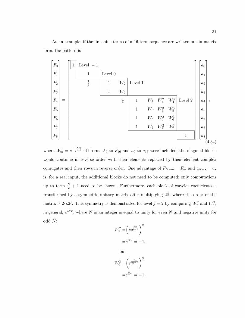
As an example, if the first nine terms of a 16 term sequence are written out in matrix

form, the pattern is

F0

F1

F2

F3

F4

F5

F6

F7

F8

=

1 Level − 1

1 Level 0

12 1 W2 Level 1

1 W3

14 1 W4 W 2

4 W 34 Level 2

1 W5 W 25 W 3

5

1 W6 W 26 W 3

6

1 W7 W 27 W 3

7

1

a0

a1

a2

a3

a4

a5

a6

a7

a8

,

(4.34)

where Wm = e− iπm

2j−1 . If terms F9 to F16 and a9 to a16 were included, the diagonal blocks

would continue in reverse order with their elements replaced by their element complex

conjugates and their rows in reverse order. One advantage of FN−m = Fm and aN−s = as

is, for a real input, the additional blocks do not need to be computed; only computations

up to term N2 + 1 need to be shown. Furthermore, each block of wavelet coefficients is

transformed by a symmetric unitary matrix after multiplying 2j2 , where the order of the

matrix is 2jx2j . This symmetry is demonstrated for level j = 2 by comparing W 27 and W 3

6 ;

in general, eiNπ, where N is an integer is equal to unity for even N and negative unity for

odd N :

W 27 =

(ei7π

2j−1

)2

=ei7π = −1,

and

W 36 =

(ei6π

2j−1

)3

=ei9π = −1.

32

Thus, the inverse of the matrix is just its complex conjugate. This results in the wavelet

coefficients being easily calculated using the Fourier coefficients. In practice, all the coeffi-

cients other than those that are unity in Eqn. 4.34, can easily be calculated using the fast

Fourier transform (FFT). As such, Eqn. 4.33 can be rewritten in the standard form of the

discrete Fourier transform after substituting n = 2j and s = m− n,

F2j+ss=0,1,2,··· ,n−1

=1

n

n−1∑k=0

a2j+ke− i2πsk

n , (4.35)

since e−2πk = 1 for all k. Aside from those coefficients which are unity (and will be consid-

ered next), the wavelet coefficients can be obtained by computing the inverse discrete Fourier

transform of successive blocks of the Fourier coefficients of the signal being decomposed.

The first unitary block in Eqn. 4.34 is related to the band of frequencies between zero

and 2π and is the contribution of the scaling function. Obtaining unity for this block requires

an assumption about the input signal. In the continuous case, the function characterizing

the input is considered to overlap the unit interval. That the function is assumed to wrap

around the interval appearing at the opposite side. Because of this wrap around effect,

the scaling function is replaced by unity in the discrete case and therefore ao = F0, the

mean value of fr. This is shown in Appendix A. The second unit block in Eqn. 4.34 comes

from the frequencies in level 0 and is the FFT of a single term sequence. The last block in

Eqn. 4.34 indicates FN2

= aN2

; this term must be included to pick-up the Nyquist frequency

component of the signal.

For a discrete transform of sequence length N = 2n, only wavelet levels up to n − 2

can be included, because both coefficients, aj,k and aj,k (Eqns. 4.26 and 4.27), must be

computed. As a result, there is no space for a level n − 1 wavelet and only one harmonic

can be fitted with the Nyquist frequency, Nπ. This defines the wavelet

fr =N−1∑k=0

Frei2πkrN

=FN2eiπr, (4.36)

33

for r = 0, 1, 2, · · · , N − 1. Since all other Fk are zero, this produces the saw-tooth sequence

f = [1 − 1 1 − 1 1 − 1 · · · ], (4.37)

when FN2

= 1. The saw-tooth wavelet can be shown to be orthogonal to the other discrete

sequences that describe the harmonic wavelets [23]. This last term, aN2

, is important because

it serves to pick up any additional energy at the Nyquist frequency ensuring Parseval’s

theorem is satisfied, just as in Eqn. 4.28:

1

N

N−1∑r=0

|fr|2 = |a0|2 +n−2∑j=0

1

2j

2j−1∑k=0

(|a2j+k|2 + |aN−2j−k|2

)+ |aN

2|2, (4.38)

where N = 2n. The algorithm is described graphically in Fig. 4.5. When the input

sequence, fr, has complex elements, the wavelet sequence as no longer satisfies aN−s = as,

but rather aN−s = as. As a result, the second half of the sequence can no longer be written

across as shown in Fig. 4.5. In this case, the block pattern in Eqn. 4.34 must continue to fill

the complete NxN matrix, where each block of order 2jx2j in the lower half of the matrix

is the complex conjugate of the block of the same order in the upper half of the matrix,

with the rows in reverse order. The corresponding version of the algorithm for a complex

input shown is shown in Fig. 4.6. Additionally, Newland provides an alternative to these

algorithms in [65], which uses an interpolation technique that reduces the processing time

required to provide the wavelet coefficients.

34

Fig. 4.5: Harmonic Wavelet Transform Algorithm For Real Inputs. The imageshows a graphical description of the algorithm used to calculate the harmonic wavelet trans-form for real inputs. Image taken from [23].

Fig. 4.6: Harmonic Wavelet Transform Algorithm For Complex Inputs. Theimage shows a graphical description of the algorithm used to calculate the harmonic wavelettransform for real inputs. Image taken from [23].

35

CHAPTER 5

Shock Attenuation with Distance on a Cylindrical Shell

5.1 Background

In March of 1970, The Martin Marietta Corporation, under a contract with NASA’s

Goddard Space Flight Center, published a report entitled Aerospace Systems Pyrotechnic

Shock Data (Ground Test and Flight) [5]. In this report, the authors present attenuation

guidelines for structures and equipment being designed to pyroshock environments. Their

work discusses several structural configurations, each having a specific attenuation curve.

The attenuation curves they generated were based on an omni-directional envelope of the

directional specific ratio of SRS peak spectrum responses over the frequency range of interest

at various distances away from the source shock, normalized to the measurement nearest

the source.

Of particular interest are the attenuation characteristics of a cylindrical shell. This

type of structure is common place in the rocket industry and knowing the attenuation

along the cylinder is useful in defining design loads for components and structures attached

to a cylindrical case. Fig. 2.4 summarizes the findings of the work conducted in the late

1960’s. As has been previously stated, there are two primary concerns that arise when

reviewing this figure. First, the curve was generated based on limited data (as is self-stated

within the report) using old data acquisition technology, and second, the SRS was used to

determine the spectrum peaks.

In 2009, Orbital ATK conducted a full scale separation test as part of NASA’s ARES I

and ARES I-X programs [2, 12]. The test objectives were to demonstrate the functionality

of the ARES I-X Linear Shaped Charge (LSC) severance system and to capture data to

help understand the structural dynamic response of the detonation. The test used LSCs to

separate the forward skirt to forward skirt extension (FSE) joint and the FSE to frustum

36

joint. The first test conducted separated the FSE from the forward skirt, while the second

separated the frustum from the FSE. Fig. 2.6 shows these joints and where they fall with

respect to the larger system. The nominal core design of the LSCs used an explosive ni-

troamine, RDX [12], with a detonation velocity of approximately 345,000 in/s [66]. Though

the data set was used to help characterize the structural response, attenuation with distance

was never considered. As the data is assessed, keep in mind the limitations associated with

using an archived data set - changes in test configuration to verify or highlight findings is

not possible. Furthermore, the type of data used in this assessment is expensive to collect

and of limited availability in many archives. The costs associated with this type of test

often prohibit similar tests from being performed. The data available is the best available

to the author for this type of assessment at the current time.

Each test consisted of three basic pieces of hardware, an LSC severance system, the

FSE, and a mass simulator used to represent either the forward skirt or frustum depending

on the test. In each test, the LSC severance system was bolted onto the FSE, which was

in turn bolted onto the appropriate mass simulator. The LSC severance system consisted

of the LSC, which sat inside an aluminum retaining ring (the gold ring in Fig. 2.8), an

initiator manifold that the flexible confined detonating cord (FCDC) ran into, and a set of

aluminum plates that acted as debris shields. During the actual test, the LSC severance

system was where the severance actually occurred. By designing the test in this fashion the

FSE was preserved and available for use in both test configurations.

In addition, the FSE contained flight like features such as the main parachute support

system (MPSS). The MPSS was the anchor location for the drogue parachute used as part

of atmospheric reentry and consisted of interior arms that attached to the outer shell of

the cylinder along with a plate that covered the aft end of the cylindrical segment. Fig.

5.1(a) shows these interior arms and plate and Fig. 5.1(b) shows the azimuthal attachment

locations of the arms. The separation events that were duplicated during the ground test

were conducted in the opposite order as they occurred in flight. During flight, following

the upper stage separation between the frustum and an interstage segment, the frustum

37

was severed from the FSE. On top of the FSE, a nose cap contained the pilot and drogue

parachutes. Once the nose cap was jettisoned, the pilot parachute served to deploy the

drogue chute. Then, when conditions were appropriate, the FSE to forward skirt was

severed and the main parachute system would deploy slowing the booster until water impact

sometime later [67]. A pictorial representation of the flight sequence leading to water impact

is provided in Appendix D. During both ground tests, the MPSS was located on the side of

the FSE near the ground [12]. Despite the order of separation events being backwards, and

the hardware oriented with the aft end of the separation joints pointing up, the hardware

was consistent with the flight configuration. Fig. 5.2 shows an image describing where the

MPSS was located during both ground tests.

Accelerometers were located at several locations on the shell outer radius at varied

distances from the cut plane of the LSC line in each test. Each measurement location

collected the structural response in three mutually perpendicular axes. These axes were

defined using a cylindrical system with the origin located at the center of the shell on the

plane defined by FSE to frustum joint. Fig. 2.7 shows the relative location of the FSE

to frustum joint. The station of a measurement refers to the axial distance away from the

origin, while the azimuth of a measurement refers to the angular distance from the zero

reference point. Fig. 5.3 shows the top view of the azimuthal coordinate system relative

to the incoming FCDC initiation lines connecting the LSCs. Figs. 5.4(a) and 5.4(b) show

station locations of interest for the FSE to forward skirt test and FSE to frustum test

respectively. The separation plane for the FSE to forward skirt test was at station -4 in,

while the separation plane for the FSE to frustum test was at station 72.6 in. Table 5.1

summarizes the accelerometer locations on the shell, along with the axial distance away

from the separation plane. Though the origin was located at the same location on the

hardware in both tests, the FSE to frustum test configuration dictated that the test article

was roughly 8 in. higher off the ground than during the FSE to forward skirt separation

test.

38

(a) Interior View of Test Article Showing the Main ParachuteSupport System.

(b) Pictorial Representation of the Main Parachute Support Sys-tem Azimuthally Attachment Locations.

Fig. 5.1: Main Parachute Support System Description. (a) The image shows themain parachute support system arms and plate that tie into the cylindrical shell or whatwould the outer case in flight. [12] (b) The image shows a pictorial representation of themain parachute support system arms that tie into the cylindrical shell. The azimuthallocation of the accelerometers used this assessment is represented by the red star. Basedon a diagram in [12].

All measurements, except channel A109A, used an Endevco model 7270A-200K ac-

celerometer, while channel A109A used a PCB model 350C02 accelerometer. All channels

39

Fig. 5.2: General MPSS Location During Both Ground Tests. The red box illus-trates the general location of the MPSS in both ground tests. Modified image from [15].

were ranged to ±100, 000 g’s, and the sample rate varied based on the test and location.

Generally, the sample rate ranged between 1,000,000 and 25,000,000 samples per second.

Again channel A109A was the anomaly; here the sample rate was 102,400 samples per sec-

ond. Regardless of the sample rate, the data available for analysis was decimated as part of

posttest procedures to expedite the analysis. The FSE to forward skirt separation data was

decimated to a 100 kHz sample rate and the FSE to frustum separation test was decimated

to a 200 kHz sample rate. In either case, the decimated data sample rates are sufficiently

high to characterize the frequency range between 10 and 10,000 Hz1.

Channel A008T had a severe mean offset present throughout the recorded time history.

Looking at the noise level prior to the shock transient for this channel, it was clear the offset

was roughly 86,000 g. As a result, a mean of 86,000 g was assumed and subtracted over the

complete time history. Doing so brought the channel in family with all other data. There

were no other channels that exhibited obvious data quality issues. All measurements were

located on the FSE during both tests aside from channel A109A. As part of the FSE to

frustum separation test, channel A109A was located at station -2.1 in, putting it on the

forward skirt tooling ring. The tooling ring is an adapter that simulated the attachment of

the forward skirt and was used as the support point of the structure during the test. Based

1The frequency band used in the calculation of the SRS is consistent with the approach used in [5].

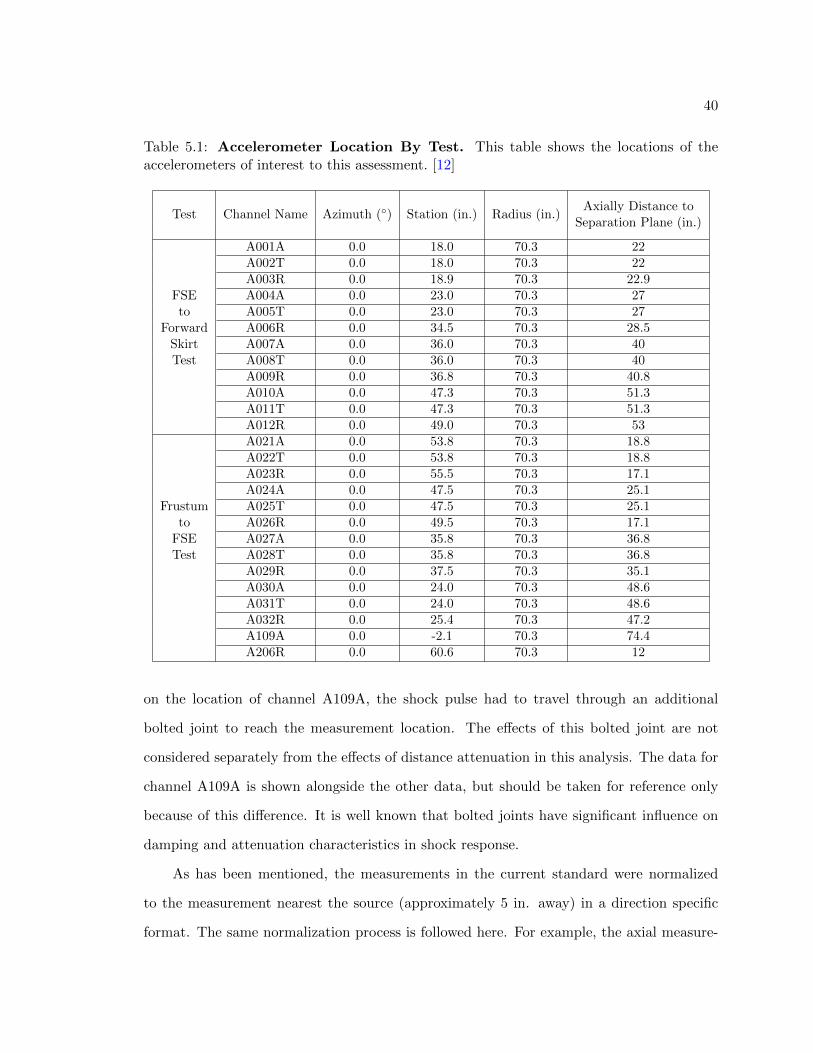
40

Table 5.1: Accelerometer Location By Test. This table shows the locations of theaccelerometers of interest to this assessment. [12]

Test Channel Name Azimuth () Station (in.) Radius (in.)Axially Distance to

Separation Plane (in.)

A001A 0.0 18.0 70.3 22A002T 0.0 18.0 70.3 22A003R 0.0 18.9 70.3 22.9

FSE A004A 0.0 23.0 70.3 27to A005T 0.0 23.0 70.3 27

Forward A006R 0.0 34.5 70.3 28.5Skirt A007A 0.0 36.0 70.3 40Test A008T 0.0 36.0 70.3 40

A009R 0.0 36.8 70.3 40.8A010A 0.0 47.3 70.3 51.3A011T 0.0 47.3 70.3 51.3A012R 0.0 49.0 70.3 53A021A 0.0 53.8 70.3 18.8A022T 0.0 53.8 70.3 18.8A023R 0.0 55.5 70.3 17.1A024A 0.0 47.5 70.3 25.1

Frustum A025T 0.0 47.5 70.3 25.1to A026R 0.0 49.5 70.3 17.1

FSE A027A 0.0 35.8 70.3 36.8Test A028T 0.0 35.8 70.3 36.8

A029R 0.0 37.5 70.3 35.1A030A 0.0 24.0 70.3 48.6A031T 0.0 24.0 70.3 48.6A032R 0.0 25.4 70.3 47.2A109A 0.0 -2.1 70.3 74.4A206R 0.0 60.6 70.3 12

on the location of channel A109A, the shock pulse had to travel through an additional

bolted joint to reach the measurement location. The effects of this bolted joint are not

considered separately from the effects of distance attenuation in this analysis. The data for

channel A109A is shown alongside the other data, but should be taken for reference only

because of this difference. It is well known that bolted joints have significant influence on

damping and attenuation characteristics in shock response.

As has been mentioned, the measurements in the current standard were normalized

to the measurement nearest the source (approximately 5 in. away) in a direction specific

format. The same normalization process is followed here. For example, the axial measure-

41

Fig. 5.3: Azimuthal Coordinate System. This image shows a cartoon depiction of thetop view of the azimuthal coordinate system on the shell and the detonation path followedby the pyrotechnic devices used to severe the FSE from the forward skirt and FSE from thefrustum joints. Image based on work done in [12].

ments for a particular test are normalized based on the peak SRS or approximate energy

of the axial measurement nearest the source.

The relative distance to the source of the heritage measurements is different than that

of the measurements nearest the source given in Table 5.1. As a result, the measurements

in the data set were shifted to account for the difference, and just as in the case of the

amplitude, this was performed in a direction specific fashion. The relative distance between

measurement locations was determined by subtracting the axial station of the measurement

nearest the source from each successive location (including the measurement nearest the

source). This translated the data points to the left, positioning the measurement nearest

the source as if it were located directly above the pyrotechnic charge, or having an axial

difference of zero. Finally, to standardize the current data set with the historical standard,

the measurement locations were translated right by adding the station location of the nearest

point measured in the historical standard (roughly 5 in. away). This allows for a direct

42

(a) FSE to Forward Skirt Separation Test.

(b) FSE to Frustum Separation Test.

Fig. 5.4: Axial Station Locations of Interest. (a) The image shows the relative stationlocations of key locations on the test article. The separation plane is located at station-4 in. [12] (b) The image shows the relative station locations of key locations on the testarticle. The separation plane is located at station 72.6 in. [12]

comparison with the historically accepted standard. The standardized distance, or the

translated distance to source, are used in the work that follows. As an example, consider

channel A003R, here the axial distance to the source, 22.9 in., was subtracted from itself,

placing it at 0 in., and then the 6.93 in. accounting for the historical standard was added.

Thus the standardized distance from the source is 6.93 in. Table 5.2 shows the standardized

43

distance compared with actual distance to the separation plane for all accelerometers.

There is a significant draw back to normalizing the measurements in this fashion, in

doing so, the relationship between the directional responses is lost. In order to provide an

understanding of the relative differences between response directions, the peak acceleration

from each measurement was normalized relative to the peak axial measurement nearest

the source for each test. That is, for the FSE to forward skirt test, all measurements

were normalized relative to channel A001A and for the frustum to FSE test; the channels

were normalized relative to A021A. This ratio is presented alongside the axial distance

to the separation plane and the standardized distance to the separation plane in Table

5.2. Based on the data in Table 5.2, there is a significant difference in the relative peak

response with distance between the FSE to forward skirt test and FSE to frustum test.

The most significant difference between these two tests is the MPSS location relative to the

separation plane. In the FSE to forward skirt test, the MPSS was located on the opposite

end of the FSE from the separation plane, while the FSE to frustum test separation plane

was on the same end of the FSE as the MPSS. The data suggest that the response dynamics

are significantly different for an excitation near the MPSS compared to one further away.

Figs. 5.1(a) and 5.1(b) show the relative location of the accelerometers being used in the

assessment compared to the attachment points of the MPSS. The measurements used in

the assessment are roughly 15 away from the attachment point of one of the arms, and

although the separation from the measurement locations is reasonably far, their presences

affects the global stiffness of the structure, and locally, they act as an artificial boundary

condition to the response characteristics nearby. As a result, the unexpected peak response

characteristics in Table 5.2 could be due to the presence of the MPSS proximity to the

separation plane. Based on this, it is not unreasonable to assume difference between the

attenuation characteristics in the two tests will exist.

The remainder of this chapter looks at the available data from the two tests documented

in [12] and compares the attenuation with distance exhibited in the data with the historical

standard in [5]. The attenuation with distance in the data sets is characterized in two ways:

44

Table 5.2: Accelerometer Distance to Source Standardization. This table shows thelocations of the accelerometers relative to the separation plane and the standardized locationused for comparison with historical standard. [12] Additionally, it shows the magnitude ofthe ratio of peaks for all channels relative to the axially measurement nearest the separationplane.

Test Channel NameAxial Distance to Standardized Distance to |Normalized Peak

Separation Plane (in.) Separation Plane (in.) Time History|

A001A 22 6.93 1.00A002T 22 6.93 0.69A003R 22.9 6.93 0.69

FSE A004A 27 11.93 0.62to A005T 27 11.93 0.63

Forward A006R 28.5 12.53 0.79Skirt A007A 40 24.93 1.07Test A008T 40 24.93 1.01

A009R 40.8 24.83 0.54A010A 51.3 36.23 0.95A011T 51.3 36.23 0.62A012R 53 37.03 0.55A021A 18.8 6.93 1.00A022T 18.8 6.93 0.89A023R 17.1 12.03 1.60A024A 25.1 13.23 2.21

Frustum A025T 25.1 13.23 1.54to A026R 17.1 18.03 2.59

FSE A027A 36.8 24.93 1.36Test A028T 36.8 24.93 1.12

A029R 35.1 81.99 1.70A030A 48.6 36.73 2.25A031T 48.6 36.73 1.34A032R 47.2 42.13 1.98A109A 74.4 62.83 1.98A206R 12 6.93 2.21

first, following the historical standard, the peak SRS response over the frequency band

between 10 and 10,000 Hz is used, secondly, an alternative method using the approximate

energy of the time history (Eqn. 3.1) is used. In both cases, keeping with the historical

standard, measurements are ratioed with the directionally consistent measurement nearest

the source to determine the percent of the shock remaining. In order to compare the

attenuation characteristics of the ARES I-X data with the historical standard, the Martin

Marietta attenuation with distance curve, Fig. 2.4, had to be digitized from the available

45

PDF file. Fig. 5.5 shows the result. The red curve is a curve fit based on a four parameter

fit to the sum of two exponential functions having general form: y = a1ea2x +a3e

a4x, where

ai are the fit parameters. The curve fit was developed based on the black solid points, which

were the digitized points from a screen capture of Fig. 2.4.

Fig. 5.5: Digitized Martin Marietta Standard. The figure shows a digitized verisionof Fig. 2.4.

The primary response direction of interest for the available test data is the axial di-

rection. Although the first wave to arrive at a given measurement location is not from the

LSC detonation directly in line with the measurement, the test configuration used in the

FSE to forward skirt and FSE to frustum separation tests lends itself to primarily an axial

excitation at each measurement point. Fig. 5.6 shows a pictorial representation of the test

set up. Point A is some azimuthal distance away from the projection of the measurement

location onto the separation plane (point B). There are two paths from which waves arrive

at the measurement location early in time. They follow either path one, which follows the

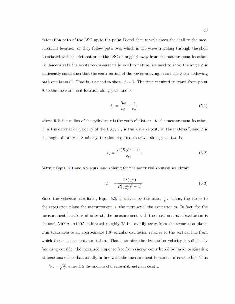
46

detonation path of the LSC up to the point B and then travels down the shell to the mea-

surement location, or they follow path two, which is the wave traveling through the shell

associated with the detonation of the LSC an angle φ away from the measurement location.

To demonstrate the excitation is essentially axial in nature, we need to show the angle φ is

sufficiently small such that the contribution of the waves arriving before the waves following

path one is small. That is, we need to show, φ ∼ 0. The time required to travel from point

A to the measurement location along path one is

t1 =Rφ

vd+

z

vm, (5.1)

where R is the radius of the cylinder, z is the vertical distance to the measurement location,

vd is the detonation velocity of the LSC, vm is the wave velocity in the material2, and φ is

the angle of interest. Similarly, the time required to travel along path two is

t2 =

√(Rφ)2 + z2

vm. (5.2)

Setting Eqns. 5.1 and 5.2 equal and solving for the nontrivial solution we obtain

φ = −2z(vmvd )

R[(vmvd )2 − 1

] . (5.3)

Since the velocities are fixed, Eqn. 5.3, is driven by the ratio, zR . Thus, the closer to

the separation plane the measurement is, the more axial the excitation is. In fact, for the

measurement locations of interest, the measurement with the most non-axial excitation is

channel A109A. A109A is located roughly 75 in. axially away from the separation plane.

This translates to an approximate 1.8 angular excitation relative to the vertical line from

which the measurements are taken. Thus assuming the detonation velocity is sufficiently

fast as to consider the measured response free from energy contributed by waves originating

at locations other than axially in line with the measurement locations, is reasonable. This

2vm =√

Eρ

, where E is the modulus of the material, and ρ the density.

47

makes the axial response the most relevant data set to compare to the historical standard.

Fig. 5.6: Wave Paths Following to Measurement Locations. The image shows thepossible paths that can be taken by the wave front once the LSC is detonated.

5.2 SRS Approach

The Martin Marietta document does not explicitly specify the length of time used in

the attenuation work, as a result two assessments using two time periods were completed

using the peak SRS approach. Based on the fact that the SRS was first developed as a

tool to capture a peak design load, the full time history of the impulse will be kept for

the first assessment. This ensures all energy due to the excitation is accounted for and

captured in data processing. The second time period considers trying to characterize the

traveling wave only and as a result is significantly shorter than the first. A review of the

time histories indicated the peak response measured by the accelerometer furthest from the

source in either test occurred before t = 0.0025 s. In actuality, both of these time periods

should produce similar results. The basis of the SRS is to determine the peak response

due to some basis excitation at a particular frequency. Theoretically, that means finding

the peak response of a single degree of freedom system at each frequency of interest. If the

peak input acceleration is captured in the input, the peak response for a particular natural

48

frequency will be captured as well. This is basically a statement of the conservation of

energy, the only energy sink or source after the initial excitation are the dissipative effects

modeled as a viscous damper in the SRS determination. This implies an exponential decay

in the response over time. Therefore, regardless of the time varying nature of the input,

if the peak input base excitation is captured in the time period used as the input to the

SRS, the response spectrum should very similar for different time periods. This just serves

to illustrate a known short coming of the SRS; the SRS does not account for the temporal

nature of the excitation.

Figs. 5.7 and 5.8 show the attenuation with distance for both time periods for the

FSE to forward skirt and FSE to frustum separation tests respectively3. As expected, the

results for the time periods are similar, and although the plots show results for the three

directions, the axial direction is of primary interest based on the essentially axial nature of

the excitation demonstrated in Eqn. 5.3. Consider the axial data for the FSE to forward

skirt test and FSE to frustum test, the FSE to forward skirt data set suggest the historical

standard over estimates the attenuation with distance, while the FSE to frustum test tends

to increase with distance, an unexpected result. This behavior is likely due to the proximity

of the MPSS to the separation plane, similar to what was seen in Table 5.2. The radial and

tangential attenuation characteristics are peculiar as well. The odd behavior in the radial

and tangential directions could also be an implication of the MPSS; however, there is no

conclusive evidence upon which to tie the behavior too. Keep in mind, channels A109A

and A008T deserve special consideration, either due to their location, or extra processing

needed. Also note that some data points in Figs. 5.7 and 5.8 may fall directly on top of

one another, causing it to look like data has been excluded; this however, is not the case.

The results of both data sets do not lend themselves to making strong conclusions about

the historically accepted Martin Marietta attenuation standards. There are three primary

sources of concern that could be sources of the anomalous results produced. First, as was

3Note: Some data points overlap for both time periods, causing it to seem as if data were omitted; thishowever, is not the case. A good example of this is at the location nearest the source, here, all directionsand time periods overlap one another, causing it to seem as if only one data point is plotted, when in reality,all directions and time periods are at this point.

49

previously discussed, the test article used in this assessment was not a true cylindrical

shell, whereas, the Martin Marietta test configuration was a true cylindrical shell. Any

change in configuration can result in a significant response differences which likely influence

attenuation with distance. Second, many decimation schemes use filtering as part of the

process. The “decimate.m” function in Matlab, for example, uses an eighth order Chebyshev

type I low pass filter by default. If this were the function used in the decimation process, it is

likely there would be little effect over the frequency range used in this assessment, however,

without knowing the decimation process followed in the post processing of the data, it is

hard to completely rule out filtering effects on the data set. Lastly, there is always the

possibility of data quality concerns that stem from instrumentation related issues such as

misaligned accelerometers or accelerometer cross axis bleed that contribute to uncertainty

in the analysis of any experimental data; however, quantizing these effects is difficult when

data is pulled from an archive and the analyst is not involved in the data collection process.

5.3 Approximate Energy Approach

Two assessments using two time periods were completed following the approximate

energy approach. As a comparison to the SRS approach, the first time period keeps the

portion of the response between, t = 0 to 0.0025 s. The second time period was based

on the understanding of how the approximate energy changes in time. As longer periods

of time are kept, the more likely the modal standing response is to influence the attenua-

tion characteristics. If a measurement happens to be located on a node of a high energy

mode, the approximate energy of the response can be skewed. As a result, trying to corre-

late wave propagation attenuation over some distance becomes unreliable. Measurements

further away from the source maybe located away from a node of a high energy mode,

while measurements more near the source may be located on one, causing the measurement

further from the source to appear as if it has more energy, artificially skewing the wave prop-

agation attenuation estimate. The next logical idea is to keep the time period prior to the

modal response being active. Isolating the traveling wave from the modal response requires

knowing exactly when the modal response of the system is actively starting to influence the

50

energy, which is extremely difficult. The modal response is inherently tied to any excitation

and determining an adequate cut off time may be nearly impossible. Working under the

assumption that the previously analyzed time period is too long and incorporated portions

of the modal response, the data was reprocessed over two distinct time periods, one specific

to each test. The time periods were determined by selecting the portion of time starting

just before the first wave arrival at the measurement nearest the source and ending after

the time required for the response at the measurement furthest from the source to complete

roughly one full period. By choosing this time period, the noise floor contribution prior to

wave arrival is eliminated, but more importantly, it ensures the modal response contribution

is negligible. The time period focuses solely on the first pulse of the shock that is exciting

the system. The time period used in the case of the FSE to forward skirt test was between

t = 0.0008 to 0.00104 s and the time period used in the case of the FSE to frustum test

was between t = 0.001 to 0.00122 s. Before any conclusions are drawn, the reader should

be reminded again about subtle differences associated with channels A008T and A109A.

Figs. 5.9 and 5.10 show the attenuation with distance for both time periods for the FSE to

forward skirt and FSE to frustum separation tests respectively. Looking only at the axial

data, the shorter time period better represents the expected behavior for sets of test data.

For the FSE to forward skirt test, and depending on which time period is considered, the

data points to two opposing conclusions. The longer time period data suggest that the

historical standard over estimates the attenuation with distance; a similar result as was in

the case of the SRS approach, while the shorter time period suggests the exact opposite

conclusion. Here the data suggest the historical standard is overly conservative and the

attenuation with distance could be increased. Additionally of note, there is evidence that

the modal standing response may have started to skew the longer time period data even for

the relatively short duration that it is. Channel A007A increases relative to A004A, which

could be due to nodal effects of the modal response.

The results are similar for the FSE to frustum test. The shorter time period data

here again suggests the historical standard is overly conservative and the attenuation with

51

distance could be increased; where as in the case of the longer time period, the potential

effects of the modal response and proximity of the MPSS to the separation plane make it

difficult to draw any conclusions. Attempting to determine the relative impact of the nodal

effects and the MPSS proximity to the separation plane for the longer time period data

would be very difficult; however, based on the slight differences between the longer and

short time periods in the FSE to forward skirt test and the similar differences seen between

the two tests’ attenuation characteristics using the SRS approach and shown in Table 5.2,

it is likely that the MPSS proximity to the separation plane plays a larger role than the

modal effects.

5.4 General Conclusions

Though the results do not lend themselves to being definitive, several general conclu-

sions can be established.

• First, the time period used in the SRS approach is of little importance in the deter-

mination of the expected attenuation with distance, so long as the peak acceleration

of the system is captured and input into the SRS algorithm.

• Second, processing the data with either approach, clear differences between the FSE

to forward skirt and FSE to frustum tests can be seen. These differences are likely

due to the proximity of the MPSS to the separation plane and the corresponding

structural response differences.

• Third, based on the comparison of the standard to the test data, and the inconclusive

nature of the results, further testing should be conducted to either validate or update

the attenuation with distance standards.

• Fourth, the two methods used in the analysis, the peak SRS response and approximate

energy approach, both produce results that are similar. When using a short time

period, the approximate energy method generally produces results indicating there is

more attenuation then the historical standard. Though both methods follow similar

52

trends, the results do not lend themselves to one particular method. The benefit of

the approximate energy method however, is that it requires no assumptions about

system damping, or a frequency band to implement.

• Lastly, the need for a method that isolates a traveling shock wave from a generic

response is highlighted here. In the tests considered, the excitation is due only to the

impulse from the pyroshock event, however in practice, responses often have other

superimposed excitations, such as random or sinusoidal excitation, making it even

more difficult to distinguish between a modal response and the shock response.

53

(a) All Directions.

(b) Axial.

Fig. 5.7: FSE to Forward Skirt Separation Test Attenuation. The plots show theattenuation with distance for the measurements taken as part of the FSE to frustum sepa-ration test using the peak SRS approach for (a) all directions and (b) for the axial direction.

54

(a) All Directions.

(b) Axial.

Fig. 5.8: FSE to Frustum Separation Test Attenuation. The plots show the at-tenuation with distance for the measurements taken as part of the FSE to forward skirtseparation test using the peak SRS approach for (a) all directions and (b) for the axialdirection. Channel A008T required additional processing to bring it in family with theother data’s time histories, and channel A109A’s location required the traveling wave topass through a bolted joint prior to reaching the measurement location.

55

(a) All Directions.

(b) Axial.

Fig. 5.9: FSE to Forward Skirt Separation Test Attenuation. The plots show theattenuation with distance for the measurements taken as part of the FSE to frustum sepa-ration test using the peak SRS approach for (a) all directions and (b) for the axial direction.

56

(a) All Directions.

(b) Axial.

Fig. 5.10: FSE to Frustum Separation Test Attenuation.The plots show the attenua-tion with distance for the measurements taken as part of the FSE to forward skirt separationtest using the peak SRS approach for (a) all directions and (b) for the axial direction. Chan-nel A008T required additional processing to bring it in family with the other data’s timehistories, and channel A109A’s location required the traveling wave to pass through a boltedjoint prior to reaching the measurement location.

57

CHAPTER 6

Flat Plate Shock Response Modeling and Attenuation Characteristics

6.1 Background

The Ares I launch vehicle had several separation events using linear shaped charges

(LSC) that occurred throughout flight. These type events inherently create large shock

levels which can affect avionics and other sensitive electrical components nearby. In order

to better understand the impact of these events, a series of pyrotechnic shock tests were

performed by Orbital ATK in October of 2010. The primary purposes of the test series was

to demonstrate cutting capability of the LSC units to the designed thickness of the case, and

to measure and characterize the shock environment produced from such events. The test

series saw three different linear shape charges used, however, due to International Traffic

in Arms Regulatory (ITAR) restrictions the specific values of these cannot be released.

As a result, the baseline LSC is ‘normalized’ and labeled as having a charge density of 1

grain/foot (gr./ft.). The two additional LSC configurations were more densely concentrated

and are designated as 1.125 gr./ft. and 4.125 gr./ft. The relative charge density relationship

between the three LSC configurations is preserved in the definitions here, that is to say the

third configuration had 4.125 times more charge per length than the baseline configuration

did.

The flat plate test article consisted of three primary pieces. A sacrificial or scar plate,

the LSC severance system, and the primary aluminum plate that is joined to the scar plate

using a butt joint interface. The LSC was attached to the scar plate; by attaching the

LSC on a separate scar plate, the primary test article was able to be reused indefinitely.

The thicknesses of the scar plate varied based on the cut depth goals of the test plan and

were thicker relative to the main plate thickness. The main plate was 4 ft. wide, 8 ft.

long, and 1 in. thick and although the test configuration was designed to simulate free

58

boundary conditions, four cables supported the primary plate in a test stand. A cartoon

description of the test set up is shown in Fig. 6.1. Though the test set up does not provide

the desired free boundary conditions, the presences of the cables minimally influences the

collected data. The shock response of the primary plate is driven by the high frequency

transient produced by the blast, while the boundary condition affects typically affect the

low frequency response (<∼ 100 Hz) of any system.

Fig. 6.1: Cartoon Depiction of Test Article and Stand. The red star points outthe location of the origin used with the accelerometers in the full test configuration. Thislocation is consistent with the location shown in Fig. 6.2. Image based on figures in [18].

There were 24 tests performed during the test series, each with a designation between

T1 and T24, and all having the initial LSC detonation near the origin, which is designated on

Fig. 6.1. Upon initiation, the LSC detonation propagated up the scar plate ending at the full

width of the plate. In each case, the accelerometers used to measure the plate response were

placed in the same locations and were configured the same in the data acquisition system.

Fig. 6.2 shows the placement of each accelerometer along with the channel name associated

with it and the reference location designated as the origin. The accelerometer type and

59

relative location to the origin are shown in Table 6.1. All accelerometer measurements were

normal to the plate, were ranged at ±50,000 G, and were sampled at 1,000,000 samples per

second.

Fig. 6.2: Accelerometer Locations. The image shows the accelerometer locations relativeto the selected origin. All measurements are normal to the plate. Table 6.1 provides theactual distances from the origin. Image based on figures in [12].

Table 6.1: Accelerometer Location. This table shows the locations of the accelerometersof interest to this assessment. Xrel and Yrel are defined relative to channel A04N, themeasurement that experiences the shock pulse first when the LSC is detonated. Note:Channels A11N and A12N were not present in many of the data sets used in this analysis,as a result they were not assessed. [12]

Channel X (in.) Y (in.) Xrel (in.) Yrel (in.)√

X2rel + Y2

rel (in.) Accelerometer Type

A01N 18 38 0 28 28 Endevco 7270A-60K M6A02N 18 36 0 28 28 PCB 350C02A03N 18 12 0 2 2 PCB 350C02A04N 18 10 – – – Endevco 7270A-60K M6A05N 55 38 37 28 46.4 PCB 350C02A06N 55 10 37 0 66.85 PCB 350C02A07N 59 38 41 28 59.84 PCB 350C02A08N 59 10 41 0 70.18 PCB 350C02A09N 71.5 38 53.5 28 60.38 Endevco 7270A-60K M6A10N 71.5 10 53.5 0 80.97 PCB 350C02

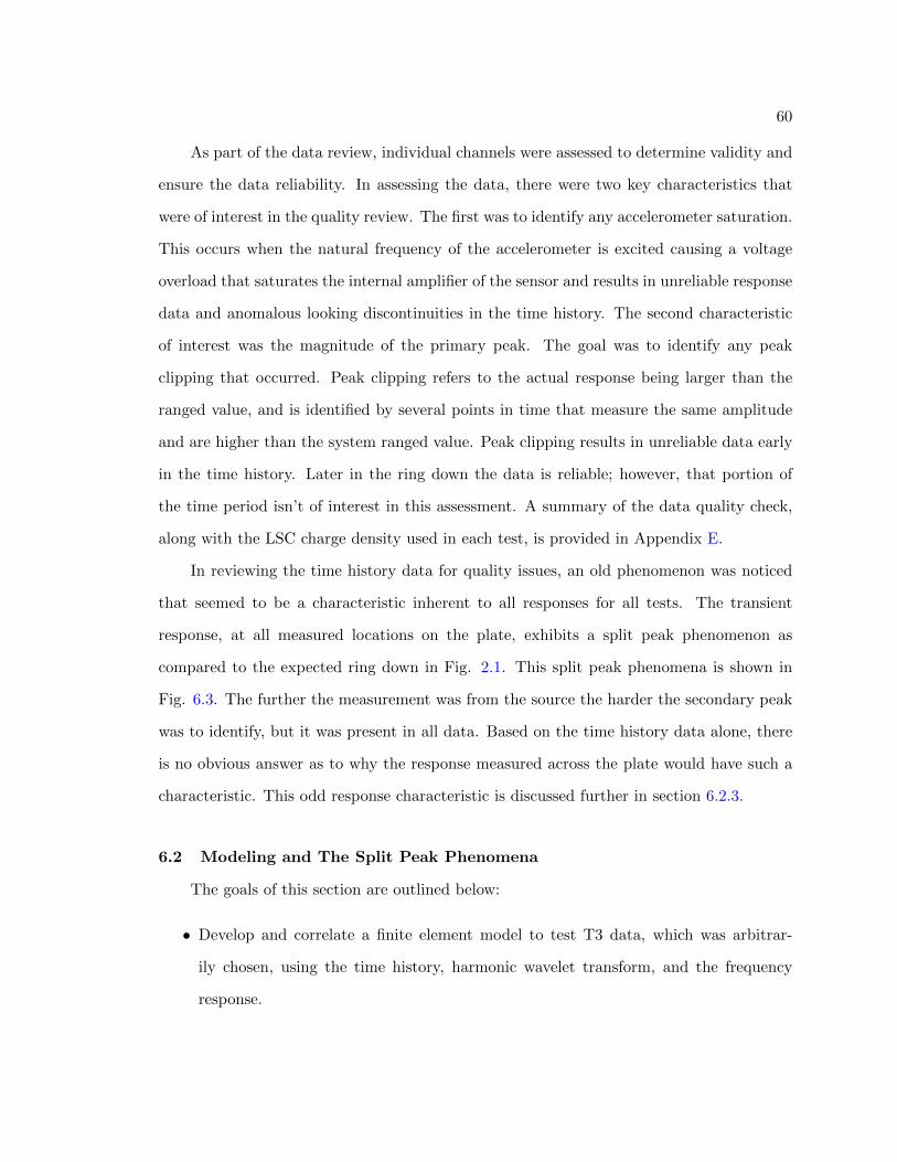
60

As part of the data review, individual channels were assessed to determine validity and

ensure the data reliability. In assessing the data, there were two key characteristics that

were of interest in the quality review. The first was to identify any accelerometer saturation.

This occurs when the natural frequency of the accelerometer is excited causing a voltage

overload that saturates the internal amplifier of the sensor and results in unreliable response

data and anomalous looking discontinuities in the time history. The second characteristic

of interest was the magnitude of the primary peak. The goal was to identify any peak

clipping that occurred. Peak clipping refers to the actual response being larger than the

ranged value, and is identified by several points in time that measure the same amplitude

and are higher than the system ranged value. Peak clipping results in unreliable data early

in the time history. Later in the ring down the data is reliable; however, that portion of

the time period isn’t of interest in this assessment. A summary of the data quality check,

along with the LSC charge density used in each test, is provided in Appendix E.

In reviewing the time history data for quality issues, an old phenomenon was noticed

that seemed to be a characteristic inherent to all responses for all tests. The transient

response, at all measured locations on the plate, exhibits a split peak phenomenon as

compared to the expected ring down in Fig. 2.1. This split peak phenomena is shown in

Fig. 6.3. The further the measurement was from the source the harder the secondary peak

was to identify, but it was present in all data. Based on the time history data alone, there

is no obvious answer as to why the response measured across the plate would have such a

characteristic. This odd response characteristic is discussed further in section 6.2.3.

6.2 Modeling and The Split Peak Phenomena

The goals of this section are outlined below:

• Develop and correlate a finite element model to test T3 data, which was arbitrar-

ily chosen, using the time history, harmonic wavelet transform, and the frequency

response.

61

• Use the correlated model to predict the response of the plate for an increased charge

density LSC load case and comment on the reliability of such prediction capability.

• Identify any best practices associated with the use of industry standard software in

modeling pyroshock structural response.

• Use finite element modeling and data processing techniques to investigate and under-

stand the source of the split peak phenomena shown in Fig. 6.3.

Fig. 6.3: Example Flat Plate Time History Response. The two arrows illustrate thetwo peaks that are atypical of the expected response. [18]

6.2.1 Model Development and Correlation

As in the case with building any finite element model, simplifications are made to

approximate reality. In this case, three primary simplifying assumptions exist between the

model and the test set up. First, the model does not include a sacrificial attachment plate

and butt joint. Joints, being inherently difficult to model, only add complexity to a model

whose purpose is for shock response prediction and not joint modeling. Additionally, the

62

lack of data across the joint precludes any correlation of the joint that could be done.

The second simplification was to model the plate using free boundary conditions. As was

previously stated, the boundary conditions in the test influence the low frequency portion

of the response and will have minimal impact on the high frequency shock response due to

the LSC. The third and final simplifying assumption is the damping schedule dependence.

In general, damping is a function of amplitude, time, frequency, and space. The work here

correlates the model response amplitude using damping, but the limitations of standard

software preclude being able to capture all dependencies associated with damping.

In transient simulation using industry standard software, there are two solution types:

a direct transient solution and a modal transient solution. These solution types each have

a different way of implementing damping, however, both have limitations in their represen-

tation of reality. If a direct transient solution is used, damping is typically modeled using a

structural approach. This works by specifying an equivalent viscous damping at a specified

frequency generating a damping matrix that is proportional to the stiffness matrix. Direct

integration of the system of equations then provides the selected damping. Because the

damping is only specified at a single frequency, this often results in the higher frequency

range being overly damped. The alternative modal transient solution applies damping as

a function of frequency allowing for a more control of the system damping. The solution

processes uses a sum of normal modes to estimate the total response as opposed to directly

integrating for the solution like the direct transient solution. The damping associated with

the shock transient response is amplitude, time, and frequency dependent in general. As

a result, the standard damping simplifications often do not provide as desirable prediction

capabilities as one might like. This is one of the primary difficulties in predicting shock

response for structures.

Before tuning the model to better match the test data, a mesh density study must be

performed. The goal in completing this to determine what element size is needed to achieve

the desired fidelity output. In this case, the goal is to identify the cutoff frequency of the

mesh, which will be below the Nyquist frequency defined by the sample rate of the test data.

63

This type of study can be performed using either of the methods discussed previously. When

using a modal solution, the number of modes included in the solution determines the high

frequency limit of the solution, and is independent of the time step used. If however, the

time step used in not short enough in duration, higher order modes may not be visible in

the plotted output. Here the time step used in the model development is consistent with the

test data. The data was sampled at 1,000,000 samples a second, which defines the Nyquist

frequency at 500,000 Hz, and sets the time step to 1.0x10−6 s. In this case, the limit of

the mesh fidelity will likely be well below that of the Nyquist frequency. Understanding

this cutoff point is the goal in performing a mesh density study. Using the modal solution

method, the model time history will converge to the same output once the frequency cutoff

limit of the mesh density has been reached.

A direct transient solution mesh density study can be performed in a similar manner.

No cutoff frequency variation is available here though. The direct solution format integrates

the equations of motion and by doing so, attempts to capture all frequency content of the

response. In general, a direct solution mesh density study is dependent on both the time

step used and the mesh fidelity in the model. Here a sufficiently small time step is assumed

in order to match the sample rate of the test data. This implies the mesh density sets the

frequency limit of the solution. As a result, to identify the frequency limitations associated

with a particular mesh density, looking at the spectral density of the model output will

provide a clear cutoff point. If the highest frequency of the mesh density being considered

is under what is desired, the mesh can be refined until the desired fidelity is achieved. As

the mesh is refined, it is important to keep in mind the dimensional dependence of the

mesh. That is refining one direction might provide quicker convergence than the other. As

an example, the brick elements used as part of this work, required more refinement in one

direction than the other to achieve convergence.

Fig. 6.4 shows the spectral density of channel A04N of test T3. From the figure it is

clear that there is a significant drop in contribution to overall response above 55,000 Hz.

As a result, the final mesh density, regardless of other modeling parameters, should be able

64

to characterize frequency content up to roughly 60,000 Hz to provide some margin. Both

linear solid brick elements and plate (or shell) elements were initially used to determine if

one better replicated the frequency response than the other. These two element types were

chosen for two distinct reasons. The plate elements were chosen because their expedited

solution speed, while the brick elements were chosen based on the applied load. It is well

known that brick elements handle shear load well, and being that the load is essentially

shear in nature, these were a natural choice for comparison sake.

Fig. 6.4: Test T3 Channel A04N Peak Normalized Frequency Cutoff Determina-tion.

In the mesh density study performed the convergence criteria required a converged

time history and frequency content up to 60,000 Hz. All initial studies were performed for

both types of elements using a direct solution approach with a triangular load shape1, and

no damping. Table 6.2 shows the approximate frequency cutoff for each mesh density and

element type modeled. Fig. 6.5 shows the time histories produced for each of the modeled

1Load shape will be further evaluated shortly.

65

mesh densities. The plate elements had converged time histories and the desired frequency

content when using a 0.5 in. by 0.5 in. density and the 1 in. thickness property. The solid

elements produced much higher frequency content; however, it took several attempts to get

an approximate time history convergence. A mesh density of 0.5 in. by 0.25 in. by 0.33 in.

was needed to achieve the desired frequency content and a converged time history using the

solid brick elements.

Table 6.2: Mesh Density Frequency Content. This table shows the approximate cutofffrequency for each element type and mesh density modeled.

Element Type X Mesh Width (in.) Y Mesh Width (in.) Z Mesh Width (in.) Approximate Cutoff Frequency (Hz.)

Plate 1 1 N/A - 1 in. Property Used 30,800Plate 0.5 0.5 N/A - 1 in. Property Used 66,100

Solid Brick 1 1 0.33 185,000Solid Brick 1 0.5 0.33 185,000Solid Brick 1 0.25 0.33 170,000Solid Brick 0.5 0.5 0.33 185,000Solid Brick 0.5 0.25 0.33 180,000Solid Brick 0.5 0.5 0.25 220,000

Fig. 6.6 compares the time histories of the solid and plate elements to channel A04N

of test T3 over the first three milliseconds of the response. Fig. 6.7 compares the spectral

density of the solid and plate elements to the spectral density of the same data, over the

same time period. The choice of three milliseconds over which to compare the responses

was chosen for quick solution time coupled with a duration long enough to account for the

split peak response characteristic seen in the test data. Neither the solid elements nor the

plate elements respond significantly different when comparing the model time histories to

the test data (Fig. 6.6).

Now consider the frequency domain. In using this short time period, it does limit the

low frequency response that can be compared. Using the 0.003 s time period set the low

frequency cut off at about 300 Hz. Although this limits the comparison range, shock events

like this are typically much higher in frequency, so there isn’t much loss in this assumption.

In looking at Fig. 6.7, the plate elements seem to better characterize the frequency response

near 20,000 Hz than the solid elements. Additionally, the solid elements seem to respond

with more energy in the higher frequency range (∼80,000 Hz) than is desired.

66

(a) Peak Normalized Plate Element Mesh Density Convergence.

(b) Peak Normalized Solid Element Mesh Density Convergence.

Fig. 6.5: Mesh Density Study. Peak Normalized Model Time History for (a) PlateElements (b) Solid Brick Elements. The responses shown in these figures are normalizedusing the peak model response.

67

Fig. 6.6: Element Type Time History Comparison. Plate and solid element timehistory response at the A04N location are compared with test data to aid in determiningwhich element is more appropriate for use. The amplitude was normalized relative to thepeak model response in this case.

From a run time stand point, the plate element model for the chosen time segment

and frequency content completed in roughly eight minutes, while the solid element model

required nearly 12 times longer, or roughly an hour and forty minutes. The significant time

differences are primarily due to the significant difference in the number of elements required

convergence between the two models. Where the plate elements are capable of accounting

for rotational components of the response with a single layer of elements, the solid elements

require a minimum of three elements through the thickness in order to accurately char-

acterize any rotational response. Combining the significantly longer run time and relative

inaccuracy of the energy distribution in the frequency domain of the solid elements, it seems

that plate elements are a stronger choice for use in further sensitivity studies and the final

model correlation. As a result, unless otherwise explicitly stated, when a model is discussed,

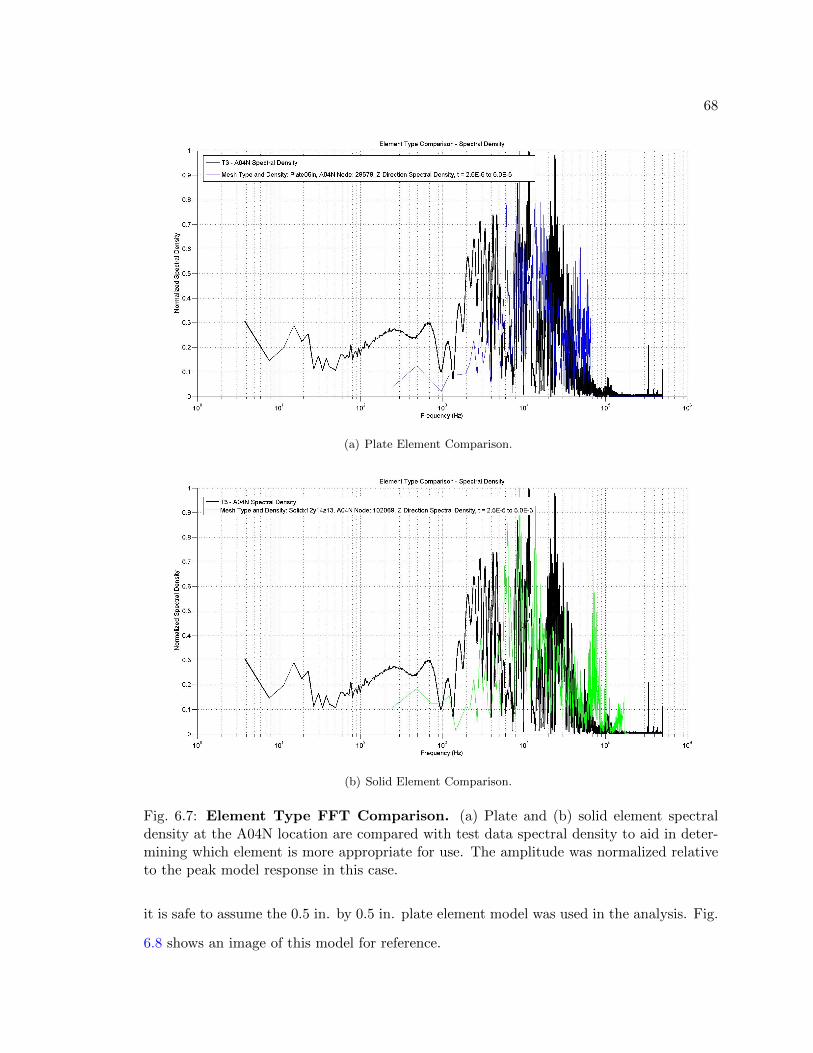
68

(a) Plate Element Comparison.

(b) Solid Element Comparison.

Fig. 6.7: Element Type FFT Comparison. (a) Plate and (b) solid element spectraldensity at the A04N location are compared with test data spectral density to aid in deter-mining which element is more appropriate for use. The amplitude was normalized relativeto the peak model response in this case.

it is safe to assume the 0.5 in. by 0.5 in. plate element model was used in the analysis. Fig.

6.8 shows an image of this model for reference.

69

Fig. 6.8: 0.5 in. by 0.5 in. Plate Element Model.

Fig. 6.9: Input Shape Sensitivity Study. The three input shapes shown here were usedto provide a better understanding of how the input shape affected the impulse response ofthe plate.

With element choice and mesh density concerns addressed, the next important aspect

of any model is determining how to best represent the load. With the destructive nature

of a pyroshock event, it is extremely difficult to capture the response resulting from the

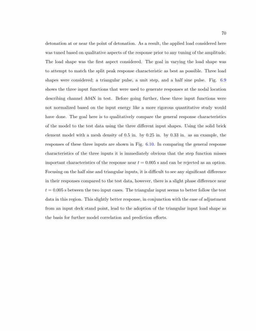
70

detonation at or near the point of detonation. As a result, the applied load considered here

was tuned based on qualitative aspects of the response prior to any tuning of the amplitude.

The load shape was the first aspect considered. The goal in varying the load shape was

to attempt to match the split peak response characteristic as best as possible. Three load

shapes were considered; a triangular pulse, a unit step, and a half sine pulse. Fig. 6.9

shows the three input functions that were used to generate responses at the nodal location

describing channel A04N in test. Before going further, these three input functions were

not normalized based on the input energy like a more rigorous quantitative study would

have done. The goal here is to qualitatively compare the general response characteristics

of the model to the test data using the three different input shapes. Using the solid brick

element model with a mesh density of 0.5 in. by 0.25 in. by 0.33 in. as an example, the

responses of these three inputs are shown in Fig. 6.10. In comparing the general response

characteristics of the three inputs it is immediately obvious that the step function misses

important characteristics of the response near t = 0.005 s and can be rejected as an option.

Focusing on the half sine and triangular inputs, it is difficult to see any significant difference

in their responses compared to the test data, however, there is a slight phase difference near

t = 0.005 s between the two input cases. The triangular input seems to better follow the test

data in this region. This slightly better response, in conjunction with the ease of adjustment

from an input deck stand point, lead to the adoption of the triangular input load shape as

the basis for further model correlation and prediction efforts.

71

(a) Peak Normalized Time History: Test T3 - Channel A04N vs. Triangular Input.

(b) Peak Normalized Time History: Test T3 - Channel A04N vs. Half Sine Input.

(c) Peak Normalized Time History: Test T3 - Channel A04N vs. Step Input.

Fig. 6.10: Mesh Density Study. Peak normalized time history comparing test T3, channel

A04N response to the solid brick element model response for a (a) triangular shaped load

(b) half sine shaped load, and (c) step shaped load

72

Initially, it was assumed the detonation velocity of the LSC was infinite. This assump-

tion meant the load was modeled as a uniform shear load applied at the nodes along the

edge of the plate in the location the butt joint was in test. In reality, the detonation of

the RDX explosive used in the LSC is approximately 345,000 in/s [66]. In comparing the

response of the model with and without the detonation velocity included, it was clear the

detonation velocity needed to be accounted for. Fig. 6.11 shows the spectral density if

the model with and without the detonation velocity included in the model. The model

solution only includes the first three milliseconds of time, which was done to reduce run

time, however, this plot clearly shows that higher frequency portions of the response, near

∼ 40, 000 Hz, are missed when the detonation velocity is not included in the model.

Fig. 6.11: Detonation Velocity Inclusion Study. The three spectral density plots were

normalized relative to the peak response of test T3 cannel A04N. From this it is clear that

the detonation velocity must be included in the model.

To model the load in NASTRAN, the TLOAD1 card was used. The benefit of using this

73

card lies in the incorporation of the detonation velocity. The TLOAD1 card has an optional

delay feature in its definition. This feature only requires knowing the time delay at the load

application site. To obtain this, the time required for detonation to propagate across one

element is determined by multiplying the element width and the detonation velocity. This

is then multiplied by the number of elements out to each successive nodal application site

giving the needed delay at a particular node. The delay is obviously a function of the mesh

density; an important reason for element type choice and obtaining response convergence

prior to any other model development. In the case of the 0.5 in. by 0.5 in. plate element

model, there was a 1.4x10−6 s delay between each successive nodal load application.

Fig. 6.12: Peak Normalized Input Load.

During the process of including the detonation velocity in the load definition, the model

was discovered to be sensitive to the load application duration. The model response seemed

to exhibit a lead-follow effect that varied based on the load duration. As an example,

consider the similar shape of the response in Fig. 6.5 to that of the triangular input shape

used in the model, shown in Fig. 6.12. Notice the sharp rise and fall in the response

74

that is similar to the load shape. A sensitivity study was performed using a 1 in. by 1

in. plate element model to reduce solution time, the results of which are shown in Fig.

6.13. The effect is worse for longer applied load duration. As the load duration decreased,

the sharpness of the primary peak in the response increases. When the load duration is

sufficiently small, the plate is unable to respond quickly enough to follow the load shape

itself, producing a result more in line with the test data.

Fig. 6.13: Load Duration Study. The time histories here have been normalized by theirpeak values.

The last two aspects to consider in model development are the amplitude of the response

and the model damping. Both are intimately tied together. Damping is energy loss, which

inherently decreases amplitude. Until now, damping has been neglected in all modeling

decisions to eliminate a parameter and qualitatively assess general response characteristics

first. It is well known that typical damping values for metal structures range between 0.5%

to 3%, depending on the metal type and preparation. In considering the test configuration,

75

it seems reasonable to assume the plate (and it’s restraints) are a lightly damped system,

which implies using a value near the lower end of the typical range. Additionally, to provide

better control over damping application, a modal transient solution is now used. The

solution uses a 60,000 Hz cutoff frequency and initially assumed 1% damping across the

spectrum. After numerous runs, the damping was tuned so to best represent the frequency

content of the test data response using the harmonic wavelet transform and the spectral

density. The resulting damping schedule is provided in Table 6.3.

Now that damping has been accounted for, the amplitude of the time history can be

adjusted to match the test data. To do this, the peak response of the test data was ratioed

with the peak response of the model so the model loading amplitude could be adjusted

linearly by the appropriate percentage. Fig. 6.14 shows the final result of this adjustment

process. The primary peak is well correlated with the test data, however, the secondary

peak and the decaying ring down seem to miss higher frequency components of the response

which likely contribute to the slight differences between test and model response amplitude

over the later time ranges.

Table 6.3: Correlated Damping Schedule. This table shows the damping scheduleused in the final correlated model. Between data points NASTRAN linearly interpolates toprovide continuity for the solver.

Frequency (Hz) Modal Damping (%)

0.0 1.010,000.0 1.010,000.01 0.520,000.0 0.520,000.01 0.240,000.0 0.240,000.01 0.860,000.0 0.8

Figs. 6.15 and 6.16 show the spectral density and harmonic wavelet transform re-

spectively. These figures compare the model output to the test data using the correlated

damping schedule. Though the model spectral density aligns well with the test data in

both amplitude and spectral content, there are clear deficiencies in the wavelet transform.

The model misses some of the higher frequency response near t = 0.002 s and seems to

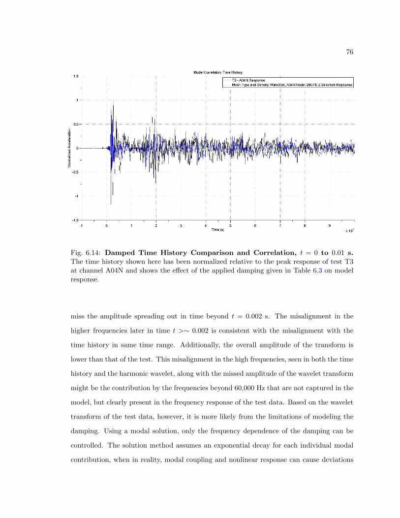
76

Fig. 6.14: Damped Time History Comparison and Correlation, t = 0 to 0.01 s.The time history shown here has been normalized relative to the peak response of test T3at channel A04N and shows the effect of the applied damping given in Table 6.3 on modelresponse.

miss the amplitude spreading out in time beyond t = 0.002 s. The misalignment in the

higher frequencies later in time t >∼ 0.002 is consistent with the misalignment with the

time history in same time range. Additionally, the overall amplitude of the transform is

lower than that of the test. This misalignment in the high frequencies, seen in both the time

history and the harmonic wavelet, along with the missed amplitude of the wavelet transform

might be the contribution by the frequencies beyond 60,000 Hz that are not captured in the

model, but clearly present in the frequency response of the test data. Based on the wavelet

transform of the test data, however, it is more likely from the limitations of modeling the

damping. Using a modal solution, only the frequency dependence of the damping can be

controlled. The solution method assumes an exponential decay for each individual modal

contribution, when in reality, modal coupling and nonlinear response can cause deviations

77

from the assumed single degree of freedom damping model used in the solution process.

Additionally, the initial transient seems to have more energy higher in frequency than the

test data. Even with these deficiencies, the model generally aligns well with the test data.

Fig. 6.15: Damped Spectral Density Comparison and Correlation. The spectral

density shown here has been normalized relative to the peak response of test T3 at channel

A04N and shows the effect of the applied damping given in Table 6.3 on the spectral content

of the model.

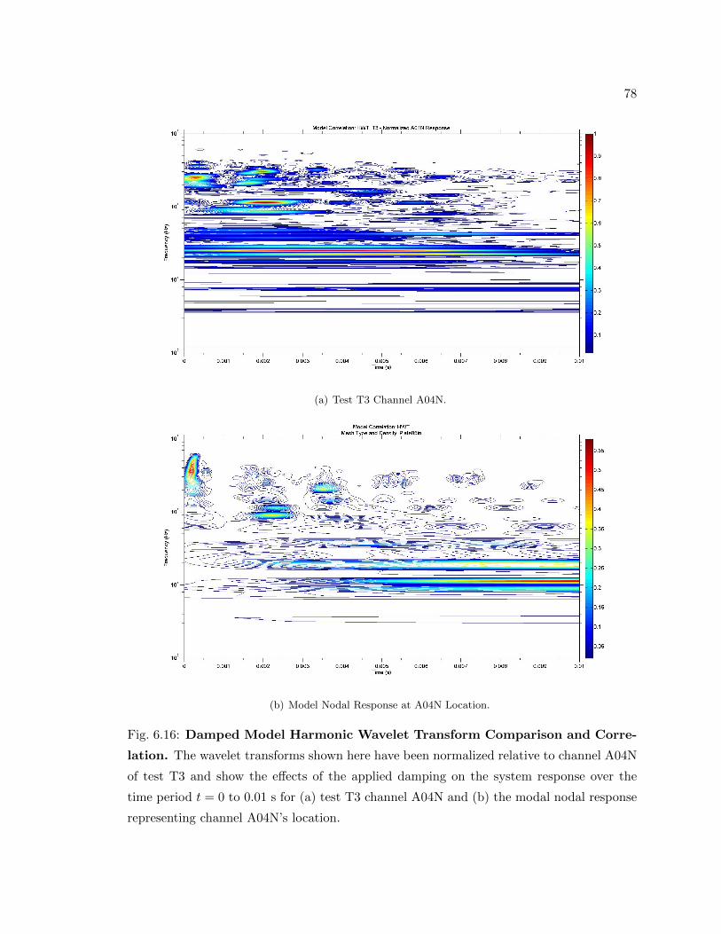
78

(a) Test T3 Channel A04N.

(b) Model Nodal Response at A04N Location.

Fig. 6.16: Damped Model Harmonic Wavelet Transform Comparison and Corre-

lation. The wavelet transforms shown here have been normalized relative to channel A04N

of test T3 and show the effects of the applied damping on the system response over the

time period t = 0 to 0.01 s for (a) test T3 channel A04N and (b) the modal nodal response

representing channel A04N’s location.

79

There is one final correlation step left to complete; a comparison between the normal

modes of the plate determine as part of a modal survey on the test article and a normal

modes run on the model can be performed. Ideally, a modal assurance criterion (MAC)

would be used to compare the mode shapes of the model and test data, allowing for a

decisive conclusion about frequency alignment. Unfortunately, however, the required data

files were not available from the test to do this. The available test data did provide frequency

response functions, however. Using these frequency response functions the primary response

peaks were identified and compared with the model output assuming the mode shapes for

corresponding mode numbers were similar. Table 6.4 summarizes the comparison between

the empirically collected modal survey data and the normal modes model results generated

using NASTRAN. The fifth predicted mode is low compared to the test data; however, the

sixth predicted mode occurred at 103.54 Hz and better aligns with the empirically collected

mode. Likely, the predicted fifth mode is a different mode shape than that of the empirical

mode, however, a MAC comparison is needed to determine this hypothesis. Even with this

slight discrepancy, the overall accuracy of the model modes prediction aligns well with the

collected test data, providing confidence in the model.

Table 6.4: Normal Modes Correlation. This table compares the first five experimentallyobtained normal modes to the normal mode model prediction.

Mode Number Experimental Normal Mode (Hz) Model Prediction (Hz)

1 23.75 22.152 28.75 26.973 60.00 59.494 64.38 61.535 102.50 91.182

To provide further confidence in the model, a comparison of the model response to test

data at a different spatial location was considered. Using the same test, T3, channel A06N

is compared with the equivalent nodal response from the model. Figs. 6.17 and 6.18 show

the time history and harmonic wavelet transform comparisons. Both figures are normalized

relative to the peak response of channel A04N to provide an understanding of the relative

2Model predicts a 103.54 Hz mode that might better align with this particular frequency.

80

amplitude difference further from the source. Fig. 6.17 shows a slight difference in arrival

time between the test and model responses. Additionally, the primary peak amplitude

of the model misses the test response. The amplitude differences are likely due to the

limitations associated with modeling the damping of the system. In general, however, the

model response represents the test data reasonably well. Comparing the model to test

wavelet transform in Fig. 6.18, there are similar issues as seen in Fig. 6.16. The model

seems to miss the higher frequency portion of the response. Additionally, near t = 0.002 s,

the test data shows higher amplitude contours compared to the model. Again, the model

transform amplitude does not align well with that of the test data. In general, however, the

model does reasonably well at predicting the response at a far field location that was not

directly correlated to the test data. This provides additional confidence in the model and

confidence that any additional predictions will provide reasonable results.

Fig. 6.17: Model Nodal Time History Response Compared to Test T3 Channel

A06N, t = 0 to 0.01 s. The time histories shown here have been normalized relative to

the peak response of test T3 at channel A04N and provide a point of comparison for the

model response away from the correlation point.

81

(a) Test T3 Channel A06N.

(b) Model Nodal Response at A06N Location.

Fig. 6.18: Comparison of Model Nodal Output for A06N to Test. The wavelet

transforms shown here have been normalized relative to channel A04N of test T3 and

provide a comparison for the model away from the correlation point. The transforms are

shown both for (a) the test data and (b) the model output over the time period between

t = 0 to 0.01 s.

82

6.2.2 Model Extrapolation

The primary purpose of model correlation is to use the correlated model to extrapo-

late and predict response on a structure that may have slight configuration differences, or

different load cases. Using the correlated 0.5 in. by 0.5 in. mesh density plate model, with

a triangular pulse applied as a shear load having a duration of 5.0x10−7 s on each applied

node and accounting for the detonation velocity of the LSC, the load amplitude was scaled

up by 12.5% and 412.5% to attempt to extrapolate and predict the response of the other

collected load cases during the test series. The scaling method assumes the LSC charge

density scales linearly with the impulsive output in the structure. Test T2 and T10 are

taken as a basis for comparison to the 1.125 and 4.125 gr./ft. charge density LSC test sets,

respectively. The test data and model response were normalized in a test consistent fashion,

relative to the test data measured by channel A04N. The time histories, spectral densities,

and harmonic wavelet transform of the different cases are compared and commented on.

Extrapolation to 1.125 gr./ft. Charge Density LSC Input - Test T2 Comparison

Figs. 6.19, 6.20, and 6.21 show the time history, spectral density, and harmonic wavelet

comparisons between the test T2 channel A04N and a model whose load has been linearly

scaled for charge density, respectively. Comparing the time history between test and model

in Fig. 6.19, the peak amplitudes align well with one another. The model slightly over

predicts the max response, but the overall model time history represents the test data well.

Similarly, the spectral density, shown in Fig. 6.20, agrees well with the test data. In general,

the amplitude of the model spectral density aligns well with the test data. Additionally,

within the bounds of the 60,000 Hz limit of the model, the predicted spectral content is

similar to that of the test data. Comparing the wavelet transforms of the test data and

model data in Fig. 6.21 shows the model transform under predicts the amplitude and

spreads the energy out in lower frequency bands that are not present in the test data. The

agreement here could be better, however, it does seem to capture characteristics associated

with the split peak response characteristic of the test data well.

Overall there are amplitude alignment concerns between test and model prediction,

83

however, the time history response and spectral density content align well between test

and model. The wavelet transform comparison highlights some of the short comings of the

model, but the model does reasonably well in predicting the structural response for a load

case that is similar in magnitude to the correlated model.

Fig. 6.19: Model Nodal Time History Response Compared to Test T2 ChannelA04N, t = 0 to 0.01 s. The time histories shown here have been normalized relative tothe peak response of test T2 at channel A04N and provide a point of comparison for themodel response when extrapolating for a load case similar to the correlation load.

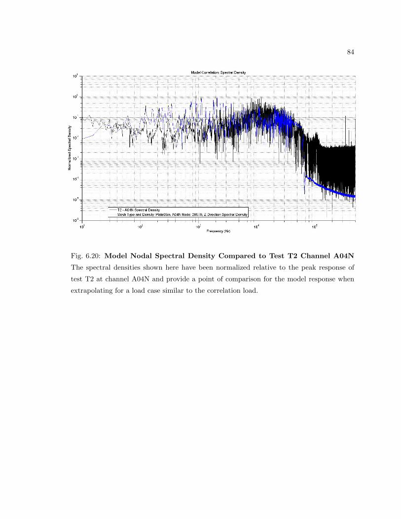
84

Fig. 6.20: Model Nodal Spectral Density Compared to Test T2 Channel A04N

The spectral densities shown here have been normalized relative to the peak response of

test T2 at channel A04N and provide a point of comparison for the model response when

extrapolating for a load case similar to the correlation load.

85

(a) Test T2 Channel A04N.

(b) Model Nodal Response at A04N Location.

Fig. 6.21: Comparison of Model Nodal Output for A04N to Test. The wavelet

transforms shown here have been normalized relative to channel A04N of test T2 and provide

a comparison for the model when extrapolating for a load case similar to the correlation

load. The transforms are shown both for (a) the test data and (b) the model output over

the time period between t = 0 to 0.01 s.

86

Extrapolation to 4.125 gr./ft. Charge Density LSC Input - Test T10 Comparison

Comparing the time history between test and model in Fig. 6.19, the peak amplitudes

align well with one another. The model slightly over predicts the max response, but the

overall model time history represents the test data well. Similarly, the spectral density,

shown in Fig. 6.20, agrees well with the test data. In general, the amplitude of the model

spectral density aligns well with the test data. Additionally, within the bounds of the

60,000 Hz limit of the model, the predicted spectral content is similar to that of the test

data. Comparing the wavelet transforms of the test data and model data in Fig. 6.21

shows the model transform under predicts the amplitude and spreads the energy out in

lower frequency bands that are not present in the test data. The agreement here could

be better, however, it does seem to capture characteristics associated with the split peak

response characteristic of the test data well.

Overall there are amplitude alignment concerns between test and model prediction,

however, the time history response and spectral density content align well between test

and model. The wavelet transform comparison highlights some of the short comings of the

model, but the model does reasonably well in predicting the structural response for a load

case that is similar in magnitude to the correlated model.

Figs. 6.22, 6.23, and 6.24 show the time history, spectral density, and harmonic wavelet

comparisons between the test T10 channel A04N and a model whose load has been linearly

scaled for charge density, respectively. Comparing the time history between test and model

in Fig. 6.22, the peak amplitude of the model prediction does not align well with the test

data. From this, it is clear there is not a linear relationship between the charge density

and impulsive output of the LSC. The model prediction does capture the general response

characteristics of the test data well, outside the amplitude alignment issues. A similar

result is present in Fig. 6.23. Here the frequency response matches reasonably well with

the test data, with the exception of the amplitude. The higher frequencies, >∼ 35, 000 Hz,

show signs of a difference in the damping between test and model prediction, however, the

general shape of the spectral density is similar to the test data. The suspected damping

87

differences between test and model are further exhibited in the wavelet transforms. Here

the amplitudes do not align well, and the wavelet transform of the model response shows

far more low frequency response than the test data.

Using a linear scaling methodology to define the mode load condition does not result in

reliable response prediction for load cases significantly different than those of the correlated

model. In general, the model captures many of the qualitative response features of the test

data. If the input loads are more appropriately scaled for larger charge density differences

of the LSC used, the model will likely perform better than has been demonstrated here. A

model’s reliability is often restricted to the reliability of its inputs.

Fig. 6.22: Model Nodal Time History Response Compared to Test T10 Channel

A04N, t = 0 to 0.01 s. The time histories shown here have been normalized relative to the

peak response of test T10 at channel A04N and provide a point of comparison for the model

response when extrapolating for a load case significantly different than the correlation load.

88

Fig. 6.23: Model Nodal Spectral Density Compared to Test T10 Channel A04N

The spectral densities shown here have been normalized relative to the peak response of

test T10 at channel A04N and provide a point of comparison for the model response when

extrapolating for a load case significantly different than the correlation load.

89

(a) Test T10 Channel A04N.

(b) Model Nodal Response at A04N Location.

Fig. 6.24: Comparison of Model Nodal Output for A04N to Test. The wavelet

transforms shown here have been normalized relative to channel A04N of test T10 and

provide a comparison for the model when extrapolating for a load case significantly different

than the correlation load. The transforms are shown both for (a) the test data and (b) the

model output over the time period between t = 0 to 0.01 s.

90

6.2.3 The Split Peak Phenomena

Fig. 6.3 shows an example of the split peak phenomena. Throughout model develop-

ment different aspects of the test set up were simulated and adjusted in order to obtain a

correlated model. In the end, the model accurately predicted the same response character-

istic. As part of the model development process, two noticeable sensitivities affecting the

split peak response characteristic were identified. First, when the detonation velocity of the

LSC was incorporated the high frequency response of the model more accurately matched

the test data. Fig. 6.11 illustrates this. Second, when damping was introduced, a drastic

decrease in the amplitude of the secondary peak in the model response could be seen. Fig.

6.14 shows this. Based on the behavior of the model, and considering the parameters that

affect the split peak response characteristic the greatest, no definitive conclusions could be

drawn about the response characteristics source. As a result, a deeper look at the test data

was required to better understand the origin of the unexpected response.

The harmonic wavelet transform was used to decompose the response measured by

channel A04N of test T3, and is shown in Fig. 6.16(a). Here distinct high amplitude

response bands can be seen at specific periods of time. Furthermore, these bands align

with the timing of the primary and secondary peaks occurring in the time history response

(Fig. 6.14). Initially one might expect the secondary peak to be a reflection of the traveling

wave off the opposite end of the plate. For channel A04N, the wave must travel the 18

in. to the accelerometer, down another 78 in. to the end of the plate and then the 78 in.

back to the accelerometer location. In total the wave travels roughly 174 in. The speed at

which the wave propagates can be estimated using the speed of sound in aluminum. Using

the square root of the ratio of the elastic modulus to the density can be used to provide a

theoretical estimate. Using a modulus of 1.0x107 psi and a density of 2.52x10−4 lbf-s2/in.4

the theoretical wave speed is roughly 199,000 in./s. This gives an estimated arrival time

for the secondary peak relative to the primary peak of approximately ∆t = 0.000874 s.

Comparing this to the approximate arrival time shown in Fig. 6.25, it’s clear that the

arrival of the peak occurs after the predicted estimate by roughly one-half millisecond.

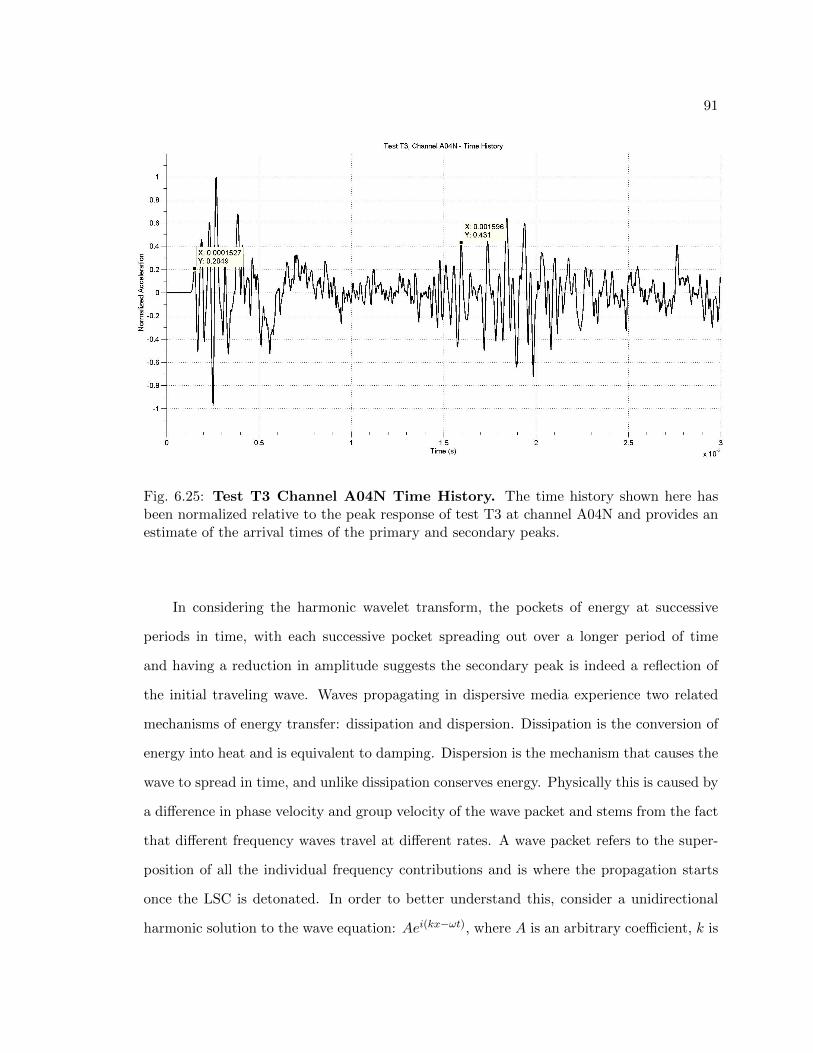
91

Fig. 6.25: Test T3 Channel A04N Time History. The time history shown here hasbeen normalized relative to the peak response of test T3 at channel A04N and provides anestimate of the arrival times of the primary and secondary peaks.

In considering the harmonic wavelet transform, the pockets of energy at successive

periods in time, with each successive pocket spreading out over a longer period of time

and having a reduction in amplitude suggests the secondary peak is indeed a reflection of

the initial traveling wave. Waves propagating in dispersive media experience two related

mechanisms of energy transfer: dissipation and dispersion. Dissipation is the conversion of

energy into heat and is equivalent to damping. Dispersion is the mechanism that causes the

wave to spread in time, and unlike dissipation conserves energy. Physically this is caused by

a difference in phase velocity and group velocity of the wave packet and stems from the fact

that different frequency waves travel at different rates. A wave packet refers to the super-

position of all the individual frequency contributions and is where the propagation starts

once the LSC is detonated. In order to better understand this, consider a unidirectional

harmonic solution to the wave equation: Aei(kx−ωt), where A is an arbitrary coefficient, k is

92

the wave vector and is related to the wavelength, and ω is the angular frequency (ω = 2πf)

of the traveling wave. Based on this wave form, it is clear that the propagation speed of

the wave is dependent on k and ω in general. When the phase between these two pieces is

constant, kx − ωt = const., there is no phase difference between the spatial and temporal

components of the wave; hence the name ’phase velocity’. If however, ω depends on k,

the group velocity arises. The group velocity describes the speed of the wave packet as

a function of frequency. The wave velocity dependence on frequency is what causes the

wave packet to spread in time [68]. This spreading effect can be seen in Fig. 6.16(a) at

the secondary and each successive pocket of energy. In comparing the test data with the

model output, it’s clear that the misalignments mentioned in the correlation portion of

this chapter are likely due to nonlinearities associate the dispersion and damping, which

manifest themselves by the elimination of the reflected waves earlier in time in the model

wavelet transform when compared to the test data.

Based on the evidence from the wavelet transform, the secondary peak seems to be

the reflection of the traveling wave, however, the theoretical arrival time doesn’t align well

with the test data. The misalignment in time could be due to an imperfect dispersion

relationship in which there are actual losses in reality, however, it’s difficult to be believe

this would cause such a significant difference in arrival time. A closer look at the system,

however, yields a pointed fact; the applied load is essentially a shear load. This indicates

that the wave might be a shear wave in nature and the propagation speed might be better

predicted using a shear modulus as opposed to the elastic modulus. The shear modulus for

aluminum is roughly 3.77x106 psi. When accounting for this, the rough propagation speed

of the wave is 122,000 in./s, resulting in a predicted relative arrival time of ∆t = 0.00142

s after the primary peak. Comparing this to the test data, it aligns well with the arrival

time of the secondary peak. Based on this, the secondary peak is in fact a reflection of the

traveling wave off the plate boundaries, but it is not an in plane wave like initially thought.

More interestingly, however, is the amplitude of the secondary peak. Fig. 6.25 shows

that the secondary peak exhibits roughly a 40% reduction compared to the primary peak

93

in the time history. This is in direct conflict with the Martin Marietta standard, which

suggests that beyond 110 inches the amplitude of the traveling wave should be lower than

10% of its original peak. Here, however, the wave has traveled approximately 18 inches to

the location of channel A04N, another approximately 78 inches to the edge of the plate,

reflected, and then traveled another 78 inches back to the measurement location and still

has an amplitude of roughly 60% of its peak. This further highlights the need to reassess

the Martin Marietta distance attenuation standard.

The conclusions here suggest a similar response may be present in the full scale cylinder

data. The configuration differences between the two tests, however, may make it difficult

to identify. Additionally, intervening structures of the test article will surely cause more

reduction and change the path of the traveling waves. Even with these differences, there

might still be evidence of this event in the data. Figs. 6.26 and 6.27 show the time history

and harmonic wavelet transform for both sets of full scale test data for channels A001A

and A021A between t = 0 and t = 0.01 s respectively. In comparing the wavelet transform

of the two tests, there is a significant difference in the measurement nearest the source.

The FSE to forward skirt test exhibits evidence of the secondary peak near t = 0.003 s,

while the frustum to FSE test data provides little evidence of this feature. The differences

highlighted here are likely due to the internal structure in the test article and its relative

position to the detonation plane. The frustum to FSE test positioned the detonation plane

more near the internal structure of the test article than the FSE to forward skirt test. In

comparing the flat plate and full scale test data responses, the relative prominence of this

effect between the two configurations is quite interesting. It provides an ideal example of

how a change in geometry can drastically affect the structural response and corresponding

wave propagation of shock events.

94

(a) FSE to Forward Skirt Test, Channel A001A.

(b) Frustum to FSE Test, Channel A021A.

Fig. 6.26: Full Scale Separation Test Data Investigation - Time History. The

images show the response time histories for measurements on the (a) FSE to forward skirt

test and (b) frustum to FSE test.

95

(a) FSE to Forward Skirt Test, Channel A001A.

(b) Frustum to FSE Test, Channel A021A.

Fig. 6.27: Full Scale Separation Test Data Investigation - Harmonic Wavelet

Transform. The images show the response harmonic wavelet transform for measurements

on the (a) FSE to forward skirt test and (b) frustum to FSE test.

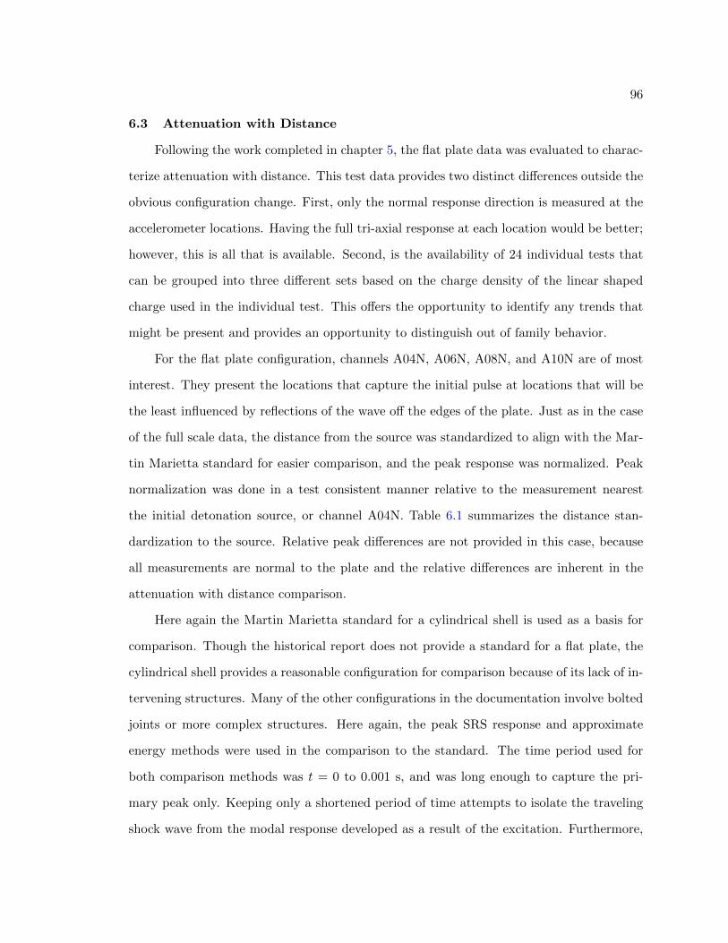
96

6.3 Attenuation with Distance

Following the work completed in chapter 5, the flat plate data was evaluated to charac-

terize attenuation with distance. This test data provides two distinct differences outside the

obvious configuration change. First, only the normal response direction is measured at the

accelerometer locations. Having the full tri-axial response at each location would be better;

however, this is all that is available. Second, is the availability of 24 individual tests that

can be grouped into three different sets based on the charge density of the linear shaped

charge used in the individual test. This offers the opportunity to identify any trends that

might be present and provides an opportunity to distinguish out of family behavior.

For the flat plate configuration, channels A04N, A06N, A08N, and A10N are of most

interest. They present the locations that capture the initial pulse at locations that will be

the least influenced by reflections of the wave off the edges of the plate. Just as in the case

of the full scale data, the distance from the source was standardized to align with the Mar-

tin Marietta standard for easier comparison, and the peak response was normalized. Peak

normalization was done in a test consistent manner relative to the measurement nearest

the initial detonation source, or channel A04N. Table 6.1 summarizes the distance stan-

dardization to the source. Relative peak differences are not provided in this case, because

all measurements are normal to the plate and the relative differences are inherent in the

attenuation with distance comparison.

Here again the Martin Marietta standard for a cylindrical shell is used as a basis for

comparison. Though the historical report does not provide a standard for a flat plate, the

cylindrical shell provides a reasonable configuration for comparison because of its lack of in-

tervening structures. Many of the other configurations in the documentation involve bolted

joints or more complex structures. Here again, the peak SRS response and approximate

energy methods were used in the comparison to the standard. The time period used for

both comparison methods was t = 0 to 0.001 s, and was long enough to capture the pri-

mary peak only. Keeping only a shortened period of time attempts to isolate the traveling

shock wave from the modal response developed as a result of the excitation. Furthermore,

97

to be consistent with the Martin Marietta standard, the frequency band between 10 and

10,000 Hz is used in the SRS development, even though spectral analysis of this data shows

frequency response well above the 10,000 Hz cutoff.

Figs. 6.28 to 6.30 show the attenuation with distance using the peak SRS method

in a charge density consistent format. Similarly, Figs. 6.31 to 6.33 show the attenuation

with distance using the energy method. In general, both methods behave as one would

expect; the larger the separation from the source, the lower the amplitude response. There

are a few outliers indicating an increase in energy or peak response, which is likely due to

any number of measurement or data collection issues. In comparing with the cylindrical

Martin Marietta standard, the 1.0 and 1.125 gr./ft. test sets seem to align better with the

standard than the 4.125 gr./ft. test set, for both methods. In general, the data do not align

as well as one might like. This disagreement could be in part to the configuration differences

between the plate and cylindrical shell used in the standard in addition to the circular load

application on the cylindrical shell. The full scale cylinder LSC applied a shear load which

followed the circumference of the cut plane, giving the load an angular component; where

the load case applied to the flat plate was essentially completely shearing in nature. The

investigation into the split peak response characteristic tends to support this claim. In

looking for a similar response characteristic in the full scale test data there were significant

response differences between the configuration differences.

In looking at the three subdivided data sets from the flat plate test series, there are three

primary conclusions that can be made. First, the 1.0 and 1.125 gr./ft. test sets seem to align

better with the standard than the 4.125 gr./ft. test set, however, it is difficult to make any

definitive conclusions based on the variation in the results. Second, although only normal

measurements were available in this configuration, in determining the source of the split

peak characteristic of the response, it provides confidence that only considering the normal

response direction is appropriate in the case of the flat plate. Lastly, the disagreement

present in comparing the test data to the Martin Marietta standard suggests further testing

and analysis should be done to either validate or update the current standard. Furthermore,

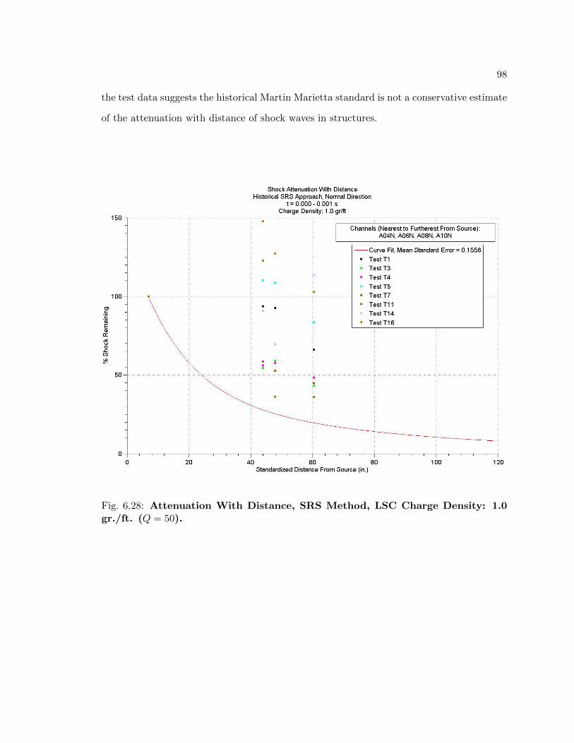
98

the test data suggests the historical Martin Marietta standard is not a conservative estimate

of the attenuation with distance of shock waves in structures.

Fig. 6.28: Attenuation With Distance, SRS Method, LSC Charge Density: 1.0gr./ft. (Q = 50).

99

Fig. 6.29: Attenuation With Distance, SRS Method, LSC Charge Density: 1.125

gr./ft. (Q = 50).

100

Fig. 6.30: Attenuation With Distance, SRS Method, LSC Charge Density: 4.125

gr./ft. (Q = 50).

101

Fig. 6.31: Attenuation With Distance, Energy Method, LSC Charge Density: 1.0

gr./ft..

102

Fig. 6.32: Attenuation With Distance, Energy Method, LSC Charge Density:

1.125 gr./ft..

103

Fig. 6.33: Attenuation With Distance, Energy Method, LSC Charge Density:

4.125 gr./ft..

104

6.4 Modeling Best Practices and Conclusions

Modeling shock propagation is inherently difficult. The time and frequency depen-

dencies associated with the damping and wave propagation characteristics are aspects of

a model that must often just be accepted as a best effort. There are however, some best

practices that can be gleaned from this work. First, plate elements provide adequate re-

sponse, even to an essentially shear load, and solve much faster than solid brick elements

when modeling transient events. Second, when there is a lack of data for model correlation,

the damping schedule provided in Table 6.3 can be used as an assumed damping profile.

Though there are certainly instances where geometry affects damping and wave propaga-

tion, this provides a reasonable set of values over a broad frequency range. Moreover, the

damping correlation effort here suggests higher frequency components of the response, are

better modeled with less damping. Lastly, the harmonic wavelet transform provides better

insight about the model response than just a time history and spectral density plot. It

allows for investigation and potentially correlation via comparing both time and frequency

content of a signal simultaneously.

The model correlation effort provided a model that was used to extrapolate to two

other cases in which a higher charge density LSC was used as part of the flat plate test

series. Using the correlated model as a basis, and scaling for the increased charge density

of the LSC, model predictions were compared with available test data to aid in trying to

better understand the predictability of pyroshock response. The results made it clear that

a nonlinear relationship between the charge density in an LSC and the impulsive load it

provides exists. Better understanding this relationship would likely better align the model

predicted response with available test data, and would provide better reliability for future

modeling efforts. However, understating the relationship between the charge density of an

LSC and the impulse load it provides is out of scope for this work; as such the task is taken

as forward work. In general, the model predictions did reasonably well in representing the

two additional load cases. There was evidence that the assumed damping schedule (defined

in the correlated model) does not capture all the subtleties associated with this type of

105

scenario, however, the damping schedule did provide reasonable results in all modeled cases,

providing confidence to its use in general practice when there is a lack of better data.

The split peak phenomenon was determined to reflection of the shear wave off the plate

boundaries. In general, the loss in overall amplitude of the secondary peak in the test data

is due to both dispersion and dissipation. Dispersion causes a spread in the time domain

stemming from a traveling waves’ velocity frequency dependence, while dissipation converts

energy into heat and is equivalent to damping. When investigating the full scale data for

similar response characteristics, evidence was found in the FSE to forward skirt test, but not

in the frustum to FSE test. This difference between the two full scale tests is contributed

to the relative location differences of the internal structure to the separation plane of the

shell.

In looking at attenuation with distance for the flat plate configuration, both the peak

SRS and approximate energy methods produce similar results. In general, the 1.0 and

1.125 gr./ft. test sets seem to align better with the Martin Marietta standard than the

4.125 gr./ft. test set. Though some individual tests were agreed better with the standard

than others, in general the data did not align well with the standard. Furthermore, the data

suggested the historical standard was not a conservative estimate of the attenuation with

distance for shock events. Thus further testing should be conducted to validate or update

the current standards.

106

CHAPTER 7

Conclusions

Component requirements govern design and production in the aerospace industry. In

order to show compliance to requirements components are qualified. Qualification is the

process of demonstrating positive margins for different loading conditions either through

analysis or test. Self-induced random vibration and shock are two primary environments

that induce load on components. Scaling methodologies and mass loading techniques can

be used to predict random vibration environments, however, shock environments are much

more difficult to predict. Modeling and extrapolation methods do exist for shock prediction;

however, they often produce unrealistic results when generating levels for new designs [1].

Because of the deficiencies associated with these techniques, shock environments are often

defined by scaling structural response from several similar structures and enveloping these

predictions. This leads to conservative environments which increases cost by adding addi-

tional risk reduction tasks prior to qualification testing; the standard for shock qualification.

With the added conservatisms of the enveloping process, understanding the attenuation

characteristics associated with the traveling shock wave over distance and through joints

becomes an important way to reduce these environments. Current industry standards are

based on data collected nearly 50 years ago on data acquisition systems that are technolog-

ically obsolete and based on the SRS - an analysis tool that has major limitations. With

the improvement of today’s technology, verification of these standard knock down factors

seems a valid concern, however, any validation efforts done by industry professionals are

likely not wide spread due to proprietary concerns.

The test data required for this type of standards validation or model development

effort is difficult to come by, but sources do exist. Two tests governed by two separate tests

plans were made available for assessment in this work. Both data sets were collected as

part of the Ares I-X program by Orbital ATK and were used to aid in shock environment

107

development for the launch vehicle. The first set of test data was collected on a full scale,

flight-like, cylindrical structure and provided two sets of response data. The second set of

data was collected as part of an LSC severance capability investigation. This test provided

24 individual sets of data that could be grouped together into three functional groups based

on the charge density of the LSC used in each test.

The available test data was used to aid in satisfying the primary goals of this work,

which are: First, investigate the attenuation with distance characteristics associated with

a cylindrical shell using the same process the historical standard was defined with, and

by using an alternative approximate energy approach based on the signal energy of the

response. Second, investigate the attenuation with distance characteristics associated with

the flat plate configuration using the same processing methods as the cylindrical shell.

Third, build and correlate a model based on the flat plate configuration, which can be

used to predict response for different load cases. Forth, as part of model generation and

correlation, identify any best practices associated with shock response prediction using

industry standard software. Lastly, using the model and other processing tools attempt to

better understand the unexpected split peak response identified during preliminary review

of the flat plate data. An example of this split peak response is shown in Fig. 6.3.

As mentioned, both sets of full scale test data were analyzed using two different pro-

cessing techniques. As part of the investigation, different time periods were used to try and

isolate the traveling wave response from the developing modal response of the structure. In

the end, the peak SRS approach was found to produce similar results regardless of the time

period kept, which is in line with the assumptions of how the processing method is defined.

The approximate energy approach highlighted the need for a method to better isolate the

modal standing contribution from the transient traveling wave contribution to the struc-

tural response. Using shorter time segments when processing the data with the approximate

energy approach provided results that were more in line with the Martin Marietta standard.

Comparing the two sets of data available to the Martin Marietta standard, there were

clear differences between the two configurations tested. The FSE to forward skirt test

108

initiated the separation further away from an internal structure designed to carry the loads

associated with parachute deployment as part of reentry, while the FSE to frustum test

initiated the separation more near this structure. The differences were contributed to the

near field structural differences altering the propagation path of the traveling wave. In either

case, the peak SRS and approximately energy method produced similar trends, for which

the results do not lend themselves to one particular method being better than the other.

The benefit of the approximate energy method, however, is that it requires no assumptions

about the damping of the system to calculate. The results using both processing methods

were generally inconclusive, which could be related to the internal structure of the MPSS.

This, however, points to the need to conduct further testing in an effort to validate or

update the historical Martin Marietta standard.

The flat plate test series was evaluated in a similar fashion, however, only normal

response measurements were available in this case. The test series was broken into three

subsets each having a unique charge density LSC that was used as the severance charge.

Both the peak SRS and approximate energy methods were used to assess attenuation with

distance. In general, the 1.0 and 1.125 gr./ft. test sets seem to align better with the Martin

Marietta standard than the 4.125 gr./ft. test set, however, none of the test data aligned

well with the standard using either processing method. Based on the relative disagreement

between the test data and standard, further testing should be undertaken to either validate

or update the current standards. The test data analyzed in this case suggests the historical

Martin Marietta standard is not a conservative estimate of the attenuation with distance

characteristics of similar shock events.

Using the same flat plate configuration, the model development and correlation effort

started by first investigating the effects of the mesh density on the model. The time step

was assumed to be small enough that the mesh density of the model was the driving factor

in the frequency content produced in the output. The mesh density study was performed

for both solid brick elements and plate elements, and based on solution time and minor

frequency content differences, the plate elements both solve quicker, and better represent

109

the available test data. The forcing function was the next item to consider. Here the shape,

duration, and detonation velocity were investigated to determine response sensitivities in

the model. Model response was extremely sensitive to the load application duration, and

mildly sensitive to the forcing shape. In addition, including the detonation velocity better

accounted for the high frequency response of the test data. In general, it is good practice

to include the detonation velocity in modeling shock response, as well as to use as short

of application load duration as feasible, and either a half sine pulse, or triangular shaped

input. Lastly, the damping and amplitude of the model was tuned based on the harmonic

wavelet transform and the peak time history response. Though the amplitude of the wavelet

transform of the model output and test data did not align well and the transform of the

test data indicated underlying pieces of physics related to damping were missing, the model

proved to be well correlated.

Using the correlated model with a linearly scaled input, the model was used to predict

the response of the same plate under higher loads due to charge density increases in the

input LSC. In the case that the scaled input was similar in magnitude to the correlated load,

the model performed well in predicting the structural response when compared with the

available test data. In the case the load was scaled by a significant amount, the model over

predicted the response amplitudes, but did provide a reasonable estimate of the frequency

content and the spectral density. For both extrapolated cases, the damping schedule devel-

oped in the model correlation did seem to provide decent results in appropriately weighting

the spectral content of other similar tests. Just as in the case with the correlated model,

the wavelet transform of the model data compared to test in both extrapolation cases saw

misalignment of the transform amplitudes. Furthermore, the transform demonstrated sim-

ilar physics related to damping that was missed by the extrapolated models. Even with

these deficiencies, the extrapolated models did reasonably well at predicting the spectral

content of both load cases along with the general characteristics of the time histories. These

results suggest that the defined damping schedule in Table 6.3 can be used as a baseline

assumption for work when no data is available.

110

Lastly, the split peak phenomenon was determined to be reflection of the shear wave

off the edge of the plate. In general, the loss in overall amplitude of the secondary peak in

the test data is due to both dispersion and dissipation. Dispersion causes a spread in the

time domain stemming from the traveling wave’s velocity dependence on frequency, while

dissipation converts energy into heat and is equivalent to damping. When investigating the

full scale data for similar response characteristics, evidence could be found in the FSE to

forward skirt test, but not in the frustum to FSE test. The difference between the two full

scale tests is contributed to the relative location of the internal intervening structure to the

separation plane.

Three general conclusions can be drawn from the contributions put forth here. First,

based on the available data, the Martin Marietta attenuation with distance standard should

be further investigated. Both the full scale separation test data and series of flat plate

tests suggest that the Martin Marietta distance attenuation standard is not a conservative

estimate of the attenuation with distance for these types of pyrotechnic excitations. This

points to the need for further testing to update the standard’s attenuation with distance

scale factors, and points to the need to investigate the other defined scale factors for bolted

joints and intervening structure. Second, several modeling best practices have been set forth.

When modeling the structural response to shock events of this nature, it is important to use

as short of a load duration as feasible, incorporate the detonation velocity of the explosive

input when appropriate, and us a forcing function with a finite rise and fall rate (like that of

a half sine or triangular shaped pulse). Furthermore, plate (or shell) elements provide good

response prediction and solve significantly faster than solid elements. Lastly, the harmonic

wavelet transform provides a better tool for shock characterization, model correlation, and

data investigation than the SRS. It’s use in model correlation here provides an example of

the transforms usefulness compared to the SRS. The wavelet transform allowed for a better

understanding of the fundamental damping characteristics of the test data, highlighting the

need for a finite element scheme that incorporates both time and frequency dependence in

damping definition at a minimum.

111

Throughout the course of this work, several additional points of interest came to light.

First, based on the understanding that the split peak characteristic of the response in the

flat plate data is wave reflection, it suggests a similar response characteristic should be

present in the response of a truly cylindrical shell. Using the available flat plate data and

with additional testing on a truly cylindrical shell, it would be interesting to establish a

method that isolates the primary peak from the secondary peak and considers the energy

loss relative to one another. This approach would provide not only a better definition for

the attenuation with distance, but also might provide insight about the damping of the

system. Further testing should simulate a free boundary condition case by supporting a

cylindrical shell via cabling and should include tri-axial acceleration measurements at five

to ten inch increments away from the source separation plane; with the final measurement

being at least 110 inches from the separation plane. By configuring the test in this fash-

ion it allows for a more well-defined attenuation with distance curve for comparison with

and update of the standard. Second, though the correlated model performed reasonably

well in predicting response to different load cases, it would be beneficial to have a solution

method which could account for amplitude, time, and frequency dependence of damping

in transient analysis. As such, it would be interesting to try and better understand these

dependencies analytically, in order to facilitate the development of a finite element approach

that attempts to incorporate all the dependencies of damping. This study would start by

considering a simple geometry such as the plate, and develop the full equations of motion

using shell theory. The theory would contain several terms responsible for damping. These

include a viscous damping term to simulate modal damping of the structure, a drag term

to account for the atmospheric drag on the structure from the air, a term describing the

transfer of energy from the propagating wave into heat, and a term attempting to account

for the energy loss at the boundary conditions, in the case of the flat plate, the cable attach-

ment points would be treated as energy sinks and modeled as discrete attachments to the

primary plate. By including these additional terms, it allows to a deeper understand of the

relative importance between the different damping mechanisms and potentially allows for an

112

effective damping definition which simplifies the contribution of all sources to a single term.

Lastly, based on the poor amplitude alignment when comparing the extrapolated models to

available test data, having a better scaling method to better account for input differences

corresponding with charge density in LSC would provide better prediction capability for

future modeling efforts. This final effort would use the available flat plate test series as a

basis, but would require additional testing with different charge density LSCs. The addi-

tional testing should have at a minimum ten repetitions per charge density. Additionally,

the testing should vary only the charge density of the LSC, items such as standoff distance

should not be varied. The additional testing would provide more data points to develop

a better understanding of the nonlinear relationship between the charge density and peak

amplitude recorded on the structure and would allow for a more complete scaling practice

to be developed. Having multiple tests within each charge density subset of the test would

allow for better characterization of uncertainty in the test series, and it would allow for

the use of normal tolerance techniques to define a statistically predicted peak response that

could be used to help bound the final recommendations on scaling.

113

Bibliography

[1] H. Himelblau, D. Kern, J. M. A. P. and Rubin, S., “Dynamic Environmental Criteria,”March 2001, NASA Technical Handbook 7005.

[2] Crockett, R., “ARES I-X Seperation Functional Demonstration,” Tech. Rep.ETP40302B, Orbital ATK, 2009.

[3] Alexander, J. E., “Shock Response Spectrum - A Primer,” Journal of Sound and Vi-bration, June 2009, [Online; accessed 16-Feb-2016].

[4] Hacker, J. E., “Using Time-Frequency Analysis to Characterize Shock,” 27th AerospaceTesting Seminar , Vol. 6, Oct. 2012, pp. 109–123.

[5] W. J. Kacena III, D. M. B. M. and Rader, W. P., “Aerospace Systems PyrotechnicShock Data (Ground Test and Flight),” Tech. rep., NASA Contractor Report -116437,-116450, -116401, -116402, -116403, -116406, and -116019, 1970.

[6] VanErt, D. L., “Survey of Pyroshock Prediction Methodology,” Vol. 31st Annual Tech-nical Meeting, Inst. Envir. Sc., Institute of Environmental Sciences Pyrotechnic ShockTutorial Program, Apr. - May 1985.

[7] F.W. Spann, R. H. and Beck, C., “IUS Program Shock Analyses,” Tech. rep., BoeingDoc. D290-75303-2 Vol. I, 1982.

[8] F.W. Spann, R. H. and Beck, C., “IUS Program Shock Analyses,” Tech. rep., BoeingDoc. D290-75303-2 Vol. II, 1982.

[9] F.W. Spann, R. H. and Beck, C., “IUS Program Shock Analyses,” Tech. rep., BoeingDoc. D290-75303-2 Vol. III, 1993.

[10] Ryschkewitsch, M. G., “Pyroshock Test Criteria,” December 2011, NASA TechnicalStandard 7003.

[11] Bergin, C., “Ares I-X passes FTRR for Tuesday launch week-end simulation set,” http://www.nasaspaceflight.com/2009/10/

ares-i-x-passes-ftrr-weekend-simulation-set/, October 2009, [Online; ac-cessed 14-Feb-2016].

[12] Crockett, R., “Final Test Report for ETP40302, ARES I-X Seperation FunctionalDemonstration Test,” Tech. Rep. TR018809, Orbital ATK, 2009.

[13] Henry, K. and Martin, K., “NASA’s Slender New Rocket to be Tested for Stabil-ity Before Launch,” http://www.nasa.gov/mission_pages/constellation/ares/

flighttests/aresIx/aresIX_modal_test.html, May 2009, [Online; accessed 14-Feb-2016].

114

[14] Spaceflightnow.com, http://spaceflightnow.com/ares1x/081221ares1x.html,2014, [Online; accessed 14-Feb-2016].

[15] Grey Hautaluoma, Ashley Edwards, D. K. and Patterson, T., “Test in Developmentof NASA’s New Crew Rocket is Successful,” http://www.nasa.gov/mission_pages/

constellation/ares/flighttests/aresIx/skirt_test.html, January 2009, [On-line; accessed 14-Feb-2016].

[16] Grey Hautaluoma (NASA), Ashley Edwards (NASA), D. K. N. and (ATK), T. P.,“Test in Development of NASA’s New Crew Rocket is Successful,” http://www.nasa.

gov/mov/312076main_Ares_Sep_Test_105_Deg_Small.mov, January 2009, [Online;accessed 14-Feb-2016].

[17] Salas, R., “Ares I Flat Plate LSC Source Shock Testing,” Tech. Rep. ETP70276A,Orbital ATK, 2010.

[18] Salas, R., “Final Test Report for ETP70276A: Ares I Flat Plate LSC Source ShockTesting,” Tech. Rep. TR025920, Orbital ATK, 2011.

[19] Cohen, L., Time-Frequency Analysis, chap. 5, 6, Prentice Hall PTR, Upper SaddleRiver, New Jersey, 1995.

[20] A Bettella, A. Francesconi, D. P. C. G. and Angrilli, F., “Application of Wavelet Trans-form to analyze acceleration signals generated by HVI on thin aluminum plates andall-aluminum honeycomb sandwich panels,” International Journal of Impact Engineer-ing , Vol. 35, 2008, pp. 1427–1434.

[21] O. V. Gendelman, T. Sapsis, A. F. V. and Bergman, L., “Enhanced passive targetedenergy transfer in strongly nonlinear mechanical oscillators,” Journal of Sound andVibration, Vol. 330, 2011, pp. 1–8.

[22] Le, T.-P. and Argoul, P., “Continuous wavelet transform for modal identification usingfree decay response,” Journal of Sound and Vibration, Vol. 277, Aug. 2004, pp. 73–100.

[23] Newland, D. E., “Harmonic Wavelet analysis,” Proc. R. Soc. Lond., Vol. 443, 1993,pp. 203–255.

[24] Newland, D. E., “Harmonic and musical wavelets,” Proc. R. Soc. Lond., Vol. 444, 1994,pp. 605–620.

[25] Newland, D. E., “Harmonic wavelets in vibrations and acoustics,” Phil. Trans. R. Soc.Lond., Vol. 357, 1999, pp. 2607–2625.

[26] Edwards, T. S., “An improved wavelet correction for zero shifted accelerometer data,”Shock and Vibration, Vol. 10, 2003, pp. 159–167.

[27] Blakely, K., MSC/NASTRAN User’s Guide: Basic Dynamic Analysis, Vol. 68, chap.6,8,10, The Macneal-Schwendler Corporation, Los Angeles, CA, 1993, pp. 153–200,227–250, 273–298.

115

[28] Ugural, A. C., Stresses in Beams, Plates, and Shells, chap. 3, 5, 15, CRC Press, BocaRaton, FL, 3rd ed., 2009, pp. 87–121, 171–221, 507–543.

[29] Pavic, G., “Analytical modeling of flexural vibration of arbitrary flat plates by theboundary forming approach,” Journal of Sound and Vibration, Vol. 364, Feb. 2015,pp. 376–401.

[30] Botta, F. and Cerri, G., “Analytical modeling of flexural vibration of arbitrary flatplates by the boundary forming approach,” Journal of Sound and Vibration, Vol. 308,April 2007, pp. 563–578.

[31] Kang, S. W. and Lee, J. M., “Free vibration analysis of arbitrarily shaped plates withdamped edges using wave-type functions,” Journal of Sound and Vibration, Vol. 242,2001, pp. 9–26.

[32] Shuyu, L., “Study on the flexural vibration of rectangular thin plates with free bound-ary conditions,” Journal of Sound and Vibration, Vol. 239, 2001, pp. 1063–1071.

[33] S. Huberlaus, L. G. and Wang, J.-S., “An exact series solution for calculating theeigenfrequencies of orthotropic plates with completely free boundary,” Journal of Soundand Vibration, Vol. 244, 2001, pp. 747–759.

[34] X. M. Zhang, G. R. L. and Lam, K. Y., “Vibration analysis of thin cylindrical shellsusing wave propagation approach,” Journal of Sound and Vibration, Vol. 239, 2001,pp. 397–403.

[35] Amebili, M., Nonlinear Vibrations and Stability of Shells and Plates, chap. 1, 4, 5,Cambridge University Press, Cambridge, NY, 2008, pp. 6–19, 120–139, 141–156.

[36] Ding Hao-jiang, W. H.-m. and Wei-qiu, C., “A Theoretical Solution of CylindricalShells for Axisymmetric Plain Strain Elastodynamic Problems,” Applied Mathematicsand Mechanics, Vol. 23, No. 2, Feb. 2002, pp. 138–145.

[37] S. Hancock, e. a., “Numerical Simulation of Atlas-Centaur Stage-Separation ShapedCharge Firing and Structural Response,” Shock and Vibration Bulletin, , No. 56, Aug.1986, pp. 45–57.

[38] S. Goldstein, Y.-M. L. and Wong, T., “Importance of Enhanced Test Data for Com-puter Modeling of Explosive Activated Devices,” AIAA Paper 95-2852 , July 1995.

[39] J.D. Frey, F. Janicot, V. R. and Movillat, P., “Pyrotechnic Separation of the VEBStructure, Shock Propagation,” Proc. Symp. Europeen, Ariane-5 Structures and Tech-nologies, May 1993.

[40] Lyon, R. and DeJong, R., Theory and Application of Statistical Energy Analysis,chap. 14, Butterworth-Heinemann, Newton, MA, 2nd ed., 1995.

[41] Manning, J. and Lee, K., “Predicting Mechanical Shock Transmission,” Shock andVibration Bulletin, , No. 37, Jan. 1968, pp. 65 – 70.

116

[42] Powell, R. and Quartararo, L. R., “Statistical Energy Analysis of Transient Vibration,”Statistical Energy Analysis (Hsu, K.H., Nefske, D.J., and Akay, A., Ed.), ASME NCA,Vol. 3, No. 37, 1987, pp. 3–8.

[43] Pinnington, R. and Lednick, D., “Transient Statistical Energy Analysis of an Impul-sively Excited Two Oscillator System,” Journal of Sound and Vibration, Vol. 189,No. 2, 1996, pp. 249–264.

[44] Pinnington, R. and Lednick, D., “Transient Energy Flow between Two CoupledBeams,” Journal of Sound and Vibration, Vol. 189, No. 2, 1996, pp. 265–287.

[45] Pinnington, R. and Lednick, D., “A Comparison between Wave Propagation Tech-niques and Transient SEA for the Prediction of Shock Response in One DimensionalSystems,” Proc. Inter-Noise 96 (Eds: Hill, F.A., and Lawrence, R.), July 1996,pp. 1343–1348.

[46] Lai, M. and Soom, A., “Prediction of Transient Vibration Envelopes using Statisti-cal Energy Analysis Techniques,” Journal of Vibration and Acoustics, Trans. ASME ,Vol. 112, No. 1, 1990, pp. 127–137.

[47] Lai, M. and Soom, A., “Statistical Energy Analysis for the Time-Integrated TransientResponse of Vibrating Systems,” Journal of Vibration and Acoustics, Trans. ASME ,Vol. 112, No. 2, 1990, pp. 206–213.

[48] Honda, I. and Irie, Y., “Transient Structure Borne Energy Analysis Using SEA,” Proc.Inter-Noise 95 , July 1995, pp. 1233–1238.

[49] Singh, A., “Impact Analysis by TRANSTAR Statistical Energy Method,” 2nd Intern.Cong. of Air- and Structure-Born Sound and Vibration, Mar. 1992.

[50] Singh, A., “Shock Source Characterization Methods for TRANSTAR SEA Program,”Proc. 63rd Shock and Vibration Symp., Vol. 1, Oct. 1992, pp. 439–450.

[51] Singh, A., “Multiple Impact Analysis by TRANSTAR SEA Program,” Proc. 63rd Shockand Vibration Symp., Vol. 1, Oct. 1992, pp. 451–463.

[52] Dalton, E., “Ballistic Shock Response Analysis by an Extension of Statistical EnergyAnalysis,” Proc. 63rd Shock and Vibration Symp., Vol. 1, Oct. 1992, pp. 411–424.

[53] Dalton, E., “High Frequency Shock Prediction in Multiply-Connected Plate Struc-tures,” Proc. 64rd Shock and Vibration Symp., Vol. 2, Oct. 1993, pp. 81–91.

[54] E.C. Dalton, B.S. Chambers III, B. K. and White, M., “Analysis of Shock in a Py-rotechnically Separated Missile Structure,” Proc. 66rd Shock and Vibration Symp.,Vol. 2, Oct. - Nov. 1995, pp. 195–201.

[55] Dalton, E. and III, B. C., “Analysis and Validation Testing of Impulsive Load Responsein Complex, Multi-Compartmented Structures,” AIAA Paper 95-1243 , 1995.

[56] “Lecture 5: Signal Energy and Parseval’s Formula,” http://ocw.usu.edu/

Electrical_and_Computer_Engineering/Signals_and_Systems/5_10node10.

html, May 2006, [Online; accessed 16-Mar-2016].

117

[57] Kelly, S. G., System Dynamics and Response, chap. 2,3,7, CL Engineering.

[58] Ginsberg, J. H., Mechanical and Structural Vibrations Theory and Applications, JohnWiley & Sons, Inc., 2001, p. 122.

[59] Gao, R. X. and Yan, R., Wavelets Theory and Applications in Manufacturing , chap. 2,Springer, 2011, p. 42.

[60] Walker, J. S., A Primer on Wavelets and Their Scientific Applications, chap. 1, Chap-man & Hall/CRC, Boca Raton, FL, 2nd ed., 2008.

[61] de Silva, C. W., Vibration and Shock Handbook , CRC Press, Taylor & Francis Group,LLC., Boca Raton, FL, 2005.

[62] Rosen, K., Discrete Mathematics and Its Applications, McGraw-Hill Education, NewYork, NY, 7th ed., June 2011.

[63] “Gaussian Waves: FFT and Spectral Leakage,” http://www.gaussianwaves.com/

2011/01/fft-and-spectral-leakage-2/, Jan. 2011, [Online; accessed 11-Mar-2016].

[64] Strang, G., “Wavelets and Dilation Equations: A Brief Introduction,” SIAM Review ,Vol. 31, No. 4, Dec. 1989, pp. 614–627, [Online; accessed 1-Apr-2016].

[65] Newland, D. E., “Ridge and Phase Identification in the Frequency Analysis of TransientSignals by Harmonic Wavelets,” Journal of Vibration and Acoustics, Vol. 121, April1999, pp. 149–155.

[66] Cooper, P. W., Explosives Engineering , chap. 3, Wiley-VCH, Inc., Cambridge, NY,1996, p. 42.

[67] NASA, “ARES I-X Press Kit,” http://www.nasa.gov/pdf/396682main_Ares_

I-X-pk.pdf, October 2009, [Online; accessed 6-June-2016].

[68] John R, P., Almost All About Waves, chap. 4, Dover Publications, Inc., Mineola, NY,1974, pp. 22–38.

[69] Lighthill, M. J., An introduction to Fourier analysis and generalised functions, Cam-bridge University Press, 1962, pp. 67–68.

[70] Smallwood, D. O., “An Improved Recursive Formula For Calculating Shock ResponseSpectra,” Shock and Vibration Bulletin, , No. 51, Apr. 1981, [Online; accessed 12-Apr-2016].

[71] Harris, C. and Crede, C., Shock and Vibration Handbook , chap. 8, McGraw-Hill BookCompany, New York, NY, 2nd ed., 1976.

118

APPENDICES

119

Appendix A

Continuous - Discrete Comparison: Circular Scaling and Wavelet Functions

Again following Newland in [23], comparing the continuous and discrete wavelet trans-

form assumes the discrete transform covers a unit interval of t, and that the function being

analyzed is periodic in t with a period of unity. When a continuous function overlaps the

interval, they are considered to be wrapped around and to reappear at the opposite side

of the interval. Each continuous function that overlaps the interval sides must be replaced

by a corresponding circular continuous function. In the case of the scale function, φ(t), the

circular scaling function, φc(t), is defined as

φc(t) =

∞∑k=−∞

φ(t− k). (A.1)

Substituting φ(t− k) with its Fourier transform we obtain

φc(t) =

∞∑k=−∞

∫ ∞−∞

Φ(ω)eiω(t−k)dω. (A.2)

Then according to Poisson’s summation formula1 [69],

∞∑k=−∞

e−iωk = 2π∞∑

m=−∞δ(ω − 2πm). (A.3)

Since the scaling function is defined as zero outside the frequency band [0, 2π], only the

m = 0 term must be retained in Eqn. A.3, giving

φc(t) = 2π

∫ ∞−∞

Φ(ω)eiω(t)δ(ω)dω, (A.4)

1Poisson’s summation formula relates the Fourier series coefficients of a periodic summation of a functionto values of the function’s continuous Fourier transform.

120

which, with the definition of Φ(ω) in Eqn. 4.18, gives

φc(t) = 1. (A.5)

When φ(t − k) is replaced by its complex conjugate in Eqn. A.1, the same argument can

be used, yielding the same result.

In the discrete case, the expansion of a circular function, fc(t), by the discrete transform

has only one term derived from the contribution of the scaling function. From Eqn. 4.22

the term can be seen to be a0 = aφφc(t) + aφφc(t), which, from A.5 is a0 = aφ + aφ, a single

constant. In the case of a general wavelet, w(2jt− k), its circular equivalent is

wc,j(2jt− k) =

∞∑m=−∞

w(2j(t−m)− k)

=

∞∑m=−∞

2−j∫ ∞−∞

e− iωk

2j eiω(t−m)W (2−jω)dω, (A.6)

for k = 0, 1, 2, · · · , 2j − 1

where W (2−jω) is of the same functional form as in Eqn. 4.18. Since W (2−jω) = 12π

over the domain 2π2j ≤ ω < 2π2j+1, and zero elsewhere, the only terms required to be

considered are m = 2j to 2j+1 − 1. Substituting Eqn. A.3 into Eqn. A.6 and integrating

gives

wc,j(2jt− k) = 2−j

2j+1−1∑m=2j

ei2πm(t− k

2j), (A.7)

for k = 0, 1, 2, · · · , 2j − 1.

When j = 0 in Eqn. A.7 and only one wavelet per unit interval is kept we have

wc,0(t) = ei2πt. (A.8)

Similarly, the two circular wavelets at level 1 are given by

wc,1(2t− k) =1

2

[ei2π(2t−k) + ei6π(t−

k2)

], (A.9)

121

for k = 0, 1 and so on for higher levels. Based on the form of Eqn. A.7, it is clear that

the circular wavelet of level j has 2j discrete harmonics whose frequencies are 2π2j , 2π(2j +

1), 2π(2j + 2), · · · , 2π(2j+1 − 1).

122

Appendix B

Proof of Parseval’s Theorem for the Generalized Harmonic Wavelet Transform

Prove Eqn. 4.28:

∞∑j=−∞

∞∑k=−∞

2−j(|aj,k|2 + |aj,k|2

)=

∫ ∞−∞|f(t)|2dt (B.1)

Proof. Following Newland [23], we start by defining some useful quantities. Let W (ω)

and V (ω) be the Fourier transform of Eqns. 4.9 and 4.12 respectively. Next, we make a

coordinate transformation so V (ω) can be written in a slightly different way, let z = 2jt−k,

so that, dz = 2jdt, this gives

V (ω) =1

2π

∫ ∞−∞

w(z)e−iω(z+k)2−j

2−jdz

= 2−je−iωk2−jW( ω

2j), (B.2)

so that w(2jt− k) can be written as:

w(2jt− k) = 2−j∫ ∞−∞

W( ω

2j)e−iω(2

−jk+t)dω. (B.3)

The proof starts by making no assumptions about the wavelet expansion in Eqn. 4.21.

Using the coefficient definitions in Eqn. 4.23, writing f(t) as the inverse Fourier transform,

F (ω), and using the result in Eqn. B.3 it can be shown the coefficients (Eqn. 4.23) can be

written as

aj,k =2π

∫ ∞−∞

F (ω)W( ω

2j)eiωk

2j dω,

and (B.4)

aj,k =2π

∫ ∞−∞

F (−ω)W( ω

2j)e

−iωk2j dω,

123

where F (ω) = 12π

∫∞−∞ f(t)e−iωtdt, and F (−ω) = 1

2π

∫∞−∞ f(t)eiωtdt. The modulus squared

of the coefficients in Eqn. B.4 is

|aj,k|2 =

∫ ∞−∞

2πF (ω1)W(ω1

2j)dω1

∫ ∞−∞

2πF (ω2)W(ω2

2j)ei(ω1−ω2)k

2j dω2,

and (B.5)

|aj,k|2 =

∫ ∞−∞

2πF (−ω1)W(ω1

2j)dω1

∫ ∞−∞

2πF (−ω2)W(ω2

2j)e− i(ω1−ω2)k

2j dω2.

We now sum over all j and k. The summation over k involves only two terms,∑∞

k=−∞ ei(ω2−ω1)k

2j ,

and its complex conjugate. According to Poisson’s summation1 [69],

1

2L

∞∑k=−∞

e−ixkπL = 2π

∞∑m=−∞

δ(x− 2mL). (B.6)

If, from Eqn. B.6, one takes x = ω2 − ω1 and L = 2jπ, they find

∞∑k=−∞

ei(ω1−ω2)k

2j = 2π2j∞∑

m=−∞δ(ω2 − ω1 − 2mπ2j). (B.7)

The summation over k in Eqn.B.5 is of the form in Eqn. B.7 and is multiplied by the product

W(ω1

2j

)W(ω2

2j

), or its complex conjugate, which because of the band limited spectrum of

the harmonic nature (its orthogonality), is zero unless ω1 and ω2 fall within an interval

2π2j ≤ ω < 4π2j . It then follows that W(ω1

2j

)W(ω2

2j

)will be zero for all values of m in the

summation in Eqn. B.7, except for m = 0. This result implies

∞∑j=−∞

∞∑k=−∞

2−j |aj,k|2 =∞∑

j=−∞(2π)3

∫ ∞−∞

F (ω)F (ω)W( ω

2j)W( ω

2j)dω,

and (B.8)

∞∑j=−∞

∞∑k=−∞

2−j |aj,k|2 =

∞∑j=−∞

(2π)3∫ ∞−∞

F (−ω)F (−ω)W( ω

2j)W( ω

2j)dω.

The Fourier transform of the harmonic wavelet, Eqn. 4.11, is zero except over 2π ≤ ω < 4π,

where, W (ω) = 12π . Thus, W

(ω2j

)W(ω2j

)= 1

(2π)2over 2π2j ≤ ω < 4π2j , and its summation

overall j is the constant, 1(2π)2

, for 0 ≤ ω <∞. Using this result, and adding the expressions

1Poisson’s summation formula relates the Fourier series coefficients of a periodic summation of a functionto values of the function’s continuous Fourier transform.

124

in Eqn. B.8, we have

∞∑j=−∞

∞∑k=−∞

2−j(|aj,k|2 + |aj,k|2

)=2π

∫ ∞0

(F (ω)F (ω) + F (−ω)F (−ω)

)dω

=2π

∫ ∞−∞

F (ω)F (ω)dω. (B.9)

Finally, using the result from Chapter 3, Eqn. 3.12, we have proven Eqn. B.1:

∞∑j=−∞

∞∑k=−∞

2−j(|aj,k|2 + |aj,k|2

)=

∫ ∞−∞|f(t)|2dt. (B.10)

125

Appendix C

Algorithm Reliability Study

The discussion in the coming sections speaks to inputting signals into the both the SRS

and generalized harmonic wavelet transform algorithms that produce an expected output.

By inputting a signal with a known frequency or time-frequency response the reliability of

the algorithms in use can be assessed.

C.1 Shock Response Spectrum Algorithm Reliability Study

In 1981, Smallwood presented a filtering method for calculating the SRS [70]. His

approach has sense become the aerospace industry standard. In following with standard

practice, the algorithm developed for this analysis is based on the Smallwood approach. The

method uses a ramp invariant filter to approximate the system response at each frequency

of interest. The filtering technique greatly improves computation time, but being an ap-

proximation, the algorithm is expected to produce slightly different output when compared

to an analytically exact solution.

Using the work done by Harris and Crede in [71] as a basis, a check of the algorithm

in use is simple. Inputting a step function with a constant rise time,

ξ(t) =

ξ0

tτ 0 ≤ t ≤ τ,

ξ0 τ ≤ t,(C.1)

the expected output is described by the normalized relationship

ν

ξ0= 1 +

∣∣∣∣ Tπτ sinπτ

T

∣∣∣∣, (C.2)

where T is the period, and τ is the rise time. Setting τ = 0.01 s, ξ0 = 5000 g, and

T = 1f , where f is the frequency of interest, Eqn. C.1 is shown graphically in Fig. C.1.

Fig. C.2 compares the analytically expected result given in Eqn. C.2, to the algorithm

126

generated SRS for several different processing bandwidths. Dividing the spectrum into

bandwidths essentially bins the spectrum; resulting in the output only being calculated at

evenly spaced1 discrete points over each band. The industry standard bandwidth is 16

th

octave. This results in six response points being calcuated for each octave bandwidth.

As expected, the algorithm produces slightly different results than the analytically exact

solution given in Eqn. C.2, however, the results are reasonable and generally reproduce the

expected output.

Fig. C.1: SRS Input. The plot shows the graphical representation of Eqn. C.1, for

τ = 0.01 s, ξ0 = 5000 g, and T = 1f , where f is the frequency of interest.

1The points are only evenly spaced using a log scale.

127

Fig. C.2: SRS Input. The plot shows the graphical representation of Eqn. C.2 compared

to the algorithm generated SRS for several different processing, for τ = 0.01 s, ξ0 = 5000

g, and T = 1f , where f is the frequency of interest.

128

C.2 Generalized Harmonic Wavelet Transform Algorithm Reliability Study

Since there are no closed form results to compare the wavelet transform algorithm to, a

slightly different approach will be used here. Two sinusoidal based inputs will be input and

the results compared against what would be expected. For a sinusoidal input of the form,

sin(2πft), the output in the time-frequency domain is expected to only have a frequency

component, f , throughout the period of the time in question.

Starting with a sinusoidal input of the form

ξ(t) = ξ1sin(ω1t) + ξ2sin(ω2t), (C.3)

where ωi = 2πfi, we expect to see two linear bands in time-frequency space, one for each

frequency component. Fig. C.3 shows the input sinusoid as a function of time when ξ1 =

ξ2 = 50 g, ω1 = 2π200, and ω2 = 2π550. Fig. C.4 shows the generalized harmonic wavelet

transform of the sinusoidal input for the same values using several processing bandwidths.

As expected, there are two bands in the output. The bandwidth differences serve only to

localize the response - that is for smaller processing bandwidths, the response energy is

spread over fewer frequencies in each band.

129

Fig. C.3: Sinusoidal Input. The plot shows the first half second of data for a 35 s

long sinusoidal input described in Eqn. C.3 with parameters defined as ξ1 = ξ2 = 50 g,

ω1 = 2π200, and ω2 = 2π550.

130

Fig. C.4: Harmonic Wavelet Transform of Sinusoidal Input. The plot shows the

harmonic wavelet transform for a sinusoidal input of the form given in Eqn. C.3 with the

parameters defined as ξ1 = ξ2 = 50 g, ω1 = 2π200, and ω2 = 2π550, for different processing

bandwidths. Fig. C.3 shows the input.

131

The same check can be done for a chirp input. A chirp input is sinusoidal in nature,

with the frequency in the sinusoid being time dependent. The definition of a chirp goes

as sin(2πt2). It is essentially a sine sweep over some time period. In the time-frequency

domain, the output is expected to be quadratic in time. Fig. C.5 shows the first second of

a chirp function that was used as an input. Fig. C.6 shows the harmonic wavelet transform

of the chirp shown in Fig. C.5. As expected, the frequency response is quadratic in time.

Here again, several bandwidths are shown.

Fig. C.5: Chirp Input. The plot shows the first second of data for a 4 s long chirp (sine

sweep) input.

132

Fig. C.6: Harmonic Wavelet Transform of Chirp Input. The plot shows the harmonic

wavelet transform for a chirp input for different processing bandwidths. Fig. C.5 shows the

input.

133

Appendix D

Trajectory Summary of Ares I-X Booster After Operation.

134

Tab

leD

.1:

Tra

jecto

ryS

um

mary

of

AR

ES

I-X

Boost

er

Aft

er

Op

era

tion

.T

his

imag

esh

ows

anar

tist

ren

dit

ion

ofth

ese

qu

ence

of

even

tsth

eb

oost

erex

per

ien

ced

afte

rop

erat

ion

.T

he

FS

Eto

fru

stu

mse

par

atio

nan

dth

eF

SE

tofo

rwar

dsk

irt

sep

arat

ion

wer

ed

up

lica

ted

as

part

of[2

].Im

age

take

nfr

om[6

7].

135

Appendix E

Flat Plate Data Quality Summary

136

Tab

leE

.1:

Data

Qu

ality

an

dC

harg

eD

en

sity

By

Test

.K

EY

:B

-B

adC

han

nel

,S

-S

atu

rate

d,

P-

Pea

kO

uts

ide

Ran

ge,

No

Cli

pp

ing,

Bla

nk

-In

dic

ates

Rel

iab

leD

ata

Test

Nam

eT

1T

2T

3T

4T

5T

6T

7T

8T

9T

10

T11

T12

T13

T14

T15

T16

T17

T18

T19

T20

T21

T22

T23

T24

Ch

arg

eD

en

sity

(gr/

ft)

11.1

251

11

1.12

51

4.12

51.

125

4.12

51

1.1

25

4.1

25

14.

125

14.

125

4.1

25

4.1

25

4.1

25

4.1

25

4.1

25

4.1

25

4.1

25

Ch

an

nel

T1

T2

T3

T4

T5

T6

T7

T8

T9

T10

T11

T12

T13

T14

T15

T16

T17

T18

T19

T20

T21

T22

T23

T24

A01

NS

PP

PP

PP

PP

P

A02

NS

PP

A03

NP

A04

N

A05

N

A06

NS

A07

N

A08

NS

A09

NP

A10

N

137

CURRICULUM VITAE

Richard J. Ott

Professional Experience

• Senior Loads and Environments Engineer

- Orbital ATK, August 2013 - present

• Graduate Research Assistant

- University of Akron, August 2010 - August 2013

Professional Memeberships

• AIAA Member, December 2015 - present

Published Journal Articles

• Ott, R.J., “Random Vibration Environment Standard Deviation Variation Verifica-

tion for Solid Rocket Motors,” Journal of Spacecraft and Rockets, July 2016. Under

Review.

• Ott, R.J. and S. Folkman., “Full Scale Pyroschock Separation Test Attenuation with

Distance,” Journal of Spacecraft and Rockets, July 2016. Under Review.

• Wierschem, N., Luo, J., AL-Shudeifat, M., Hubbard, S., Ott, R.J., Fahnestock, L.,

Quinn, D., McFarland, D., Spencer, B., Jr., Vakakis, A., and Bergman, L. (2014). ”Ex-

perimental Testing and Numerical Simulation of a Six-Story Structure Incorporating

Two-Degree-of-Freedom Nonlinear Energy Sink.” J. Struct. Eng., 10.1061/(ASCE)

ST.1943-541X.0000978, 04014027.

138

• Wierschem, N.E., Lou, J., Al-Shudeifat, M., Hubbard, S., Ott, R.J., Fahnestock,

L.A., Quinn, D.D., McFarland, D.M., Spencer Jr., B.F., Vakakis, A., and Bergman,

L.A., “Equivalent modal damping, stiffening, and energy exchanges in multi-degree-of-

freedom systems with strongly nonlinear attachments,” Proceedings of the Institution

of Mech. Engineers, Part K: Journal of Multi-body Dynamics, vol. 226, no. 2, pp.

122-146, Jan. 2012.

Published Conference Papers

• Ott, R.J., “Random Vibration Environment Standard Deviation Variation Verification

for Solid Rocket Motors,” Proceedings of the 52nd AIAA/SAE/ASEE Joint Propul-

sion Conference, AIAA Propulsion and Energy Forum and Exposition, AIAA, Salt

Lake City, UT, 2016.

• Wierschem, N.E., Lou, J., Al-Shudeifat, M., Hubbard, S., Ott, R.J., Fahnestock, L.A.,

Quinn, D.D., McFarland, D.M., Spencer Jr., B.F., Vakakis, A., and Bergman, L.A.,

“Simulation and Testing of a 6-Story Building Incorporating a Coupled Two Mass

Nonlinear Energy Sink,” Proceedings of 24th Conference on Mechanical Vibration

and Noise, ASME, DETC2012-71442, Chicago, Il, Aug. 2012.

• Quinn, D.D., Ott, R.J., Hubbard, S., McFarland, D.M., Bergman, L.A., and Vakakis,

A.F., “Identification of Equivalent Modal Damping and Frequencies in Mutli-degree

of Freedom Nonlinear Systems,” in Proceedings of ASME Int. Design Eng. Technical

Conf. & Computers and Info. in Eng. Conf., ASME, DETC2001-48956, Washington,

DC, Aug. 2011.