Ultimate Compression After Impact Load Prediction in Graphite
230
Dissertations and Theses Spring 2011 Ultimate Compression After Impact Load Prediction in Graphite/ Ultimate Compression After Impact Load Prediction in Graphite/ Epoxy Coupons Using Neural Network and Multivariate Statistical Epoxy Coupons Using Neural Network and Multivariate Statistical Analyses Analyses Alexandre David Grégoire Embry-Riddle Aeronautical University - Daytona Beach Follow this and additional works at: https://commons.erau.edu/edt Part of the Aerospace Engineering Commons Scholarly Commons Citation Scholarly Commons Citation Grégoire, Alexandre David, "Ultimate Compression After Impact Load Prediction in Graphite/Epoxy Coupons Using Neural Network and Multivariate Statistical Analyses" (2011). Dissertations and Theses. 77. https://commons.erau.edu/edt/77 This Thesis - Open Access is brought to you for free and open access by Scholarly Commons. It has been accepted for inclusion in Dissertations and Theses by an authorized administrator of Scholarly Commons. For more information, please contact [email protected].
-
Upload
khangminh22 -
Category
Documents
-
view
1 -
download
0
Transcript of Ultimate Compression After Impact Load Prediction in Graphite

Dissertations and Theses
Spring 2011
Ultimate Compression After Impact Load Prediction in Graphite/Ultimate Compression After Impact Load Prediction in Graphite/
Epoxy Coupons Using Neural Network and Multivariate Statistical Epoxy Coupons Using Neural Network and Multivariate Statistical
Analyses Analyses
Alexandre David Grégoire Embry-Riddle Aeronautical University - Daytona Beach
Follow this and additional works at: https://commons.erau.edu/edt
Part of the Aerospace Engineering Commons
Scholarly Commons Citation Scholarly Commons Citation Grégoire, Alexandre David, "Ultimate Compression After Impact Load Prediction in Graphite/Epoxy Coupons Using Neural Network and Multivariate Statistical Analyses" (2011). Dissertations and Theses. 77. https://commons.erau.edu/edt/77
This Thesis - Open Access is brought to you for free and open access by Scholarly Commons. It has been accepted for inclusion in Dissertations and Theses by an authorized administrator of Scholarly Commons. For more information, please contact [email protected].

ULTIMATE COMPRESSION AFTER IMPACT LOAD PREDICTION
IN GRAPHITE/EPOXY COUPONS USING NEURAL NETWORK AND
MULTIVARIATE STATISTICAL ANALYSES
by
Alexandre David Grégoire
A thesis submitted in partial fulfillment of the requirements for the degree of
Master of Science in Aerospace Engineering
Embry Riddle Aeronautical University
Daytona Beach, Florida Spring 2011

ii

iii
ULTIMATE COMPRESSION AFTER IMPACT LOAD PREDICTION
IN GRAPHITE/EPOXY COUPONS USING NEURAL NETWORK AND
MULTIVARIATE STATISTICAL ANALYSES
by
Alexandre David Grégoire
This thesis was prepared under the direction of the candidate‟s thesis committee chairman, Dr.
Eric Hill, Department of Aerospace Engineering, and has been approved by the members of his
thesis committee. It was submitted to the School of Graduate Studies and Research and was
accepted in partial fulfillment of the requirements for the degree of Master of Science in
Aerospace Engineering.
THESIS COMMITTEE
________________________
Dr. Eric v. K. Hill
Chairman
________________________
Dr. Fady F. Barsoum
Member
________________________
Anthony M. Gunasekera
Member
_________________________________________________
Executive Vice President & Chief Academic Officer, ERAU
________________________________
Graduate Program Coordinator, MSAE
__________________________________ ____________ Department Chair, Aerospace Engineering Date

iv
In presenting this thesis in partial fulfillment of the requirements for a Master‟s degree at
Embry Riddle Aeronautical University, I agree that the library shall make its copies freely
available for inspection. I further agree that extensive copying of this thesis is allowable only for
scholarly purposes, consistent with „‟fair use‟‟ as prescribed in the U.S. Copyright Law. Any
other reproduction for any purposes or by any means shall not be allowed without my written
permission.
Signature ________________________
Date ____________________________

v
ABSTRACT
Author: Alexandre David Grégoire
Title: Ultimate Compression After Impact Load Prediction in Graphite/Epoxy Coupons
Using Neural Network and Multivariate Statistical Analyses
Institution: Embry Riddle Aeronautical University
Degree: Master of Science in Aerospace Engineering
Year: 2011
The goal of this research was to accurately predict the ultimate compressive load of
impact damaged graphite/epoxy coupons using a Kohonen self-organizing map (SOM) neural
network and multivariate statistical regression analysis (MSRA). An optimized use of these data
treatment tools allowed the generation of a simple, physically understandable equation that
predicts the ultimate failure load of an impacted damaged coupon based uniquely on the acoustic
emissions it emits at low proof loads. Acoustic emission (AE) data were collected using two 150
kHz resonant transducers which detected and recorded the AE activity given off during
compression to failure of thirty-four impacted 24-ply bidirectional woven cloth laminate
graphite/epoxy coupons. The AE quantification parameters duration, energy and amplitude for
each AE hit were input to the Kohonen self-organizing map (SOM) neural network to accurately
classify the material failure mechanisms present in the low proof load data. The number of
failure mechanisms from the first 30% of the loading for twenty-four coupons were used to
generate a linear prediction equation which yielded a worst case ultimate load prediction error of
16.17%, just outside of the ±15% B-basis allowables, which was the goal for this research.
Particular emphasis was placed upon the noise removal process which was largely responsible for
the accuracy of the results.

vi
ACKNOWLEDGMENTS
I would like to thank Dr. Eric v. K. Hill for the honor of working with him: for his
guidance, confidence, rigorous mindset and support throughout my thesis at Embry-Riddle
Aeronautical University. I acknowledge Anthony Michael Gunasekera for sharing his precious
experience, time and data and also for his infallible support throughout the progress of this thesis.
Acknowledgement should also go to Dr. Fady F. Barsoum for being on my thesis committee.
I especially thank all my family for all these years of true moral and financial support
without which none of this would have been possible. I thank my father Philippe Grégoire, my
mother Murielle Courtaud Grégoire, my sister Elodie Grégoire Gomez and her first baby, my
niece, Cléa. I also thank Brigitte Terrier, Jean Pierre Courtaud and Bruno Gomez.
I should recognize Matthew Morlando Bailey for his several reviews of this thesis and for
his undeniable friendship and support throughout the Embry-Riddle Aeronautical University/EPF
École d‟Ingenieurs Exchange Program. I also wish to thank all my close friends, too numerous to
be all mentioned, for constantly believing in my ability to successfully complete my studies, their
unconditional friendship and true support. Finally, I express my gratitude to all the amazing
international people that I met during my studies for shaping another definition of the word
globalization.

1
TABLE OF CONTENTS
ABSTRACT ....................................................................................................................................... V
ACKNOWLEDGMENTS .............................................................................................................. VI
TABLE OF CONTENTS ................................................................................................................... 1
LIST OF TABLES ............................................................................................................................. 4
LIST OF EQUATIONS ..................................................................................................................... 5
CHAPTER 1 : INTRODUCTION .................................................................................................... 6 1.1. INDUSTRIAL CONTEXT ............................................................................................... 6
1.2. PREVIOUS RESEARCH .................................................................................................. 8
1.3. RESEARCH OBJECTIVE .............................................................................................. 10
CHAPTER 2 : THEORETICAL BACKGROUND ...................................................................... 12 2.1. ACOUSTIC EMISSION ................................................................................................. 12
2.1.1. Introduction ......................................................................................................... 12
2.1.2. Capturing technique ............................................................................................ 13
2.2. NEURAL NETWORKS .................................................................................................. 19
2.2.1. Introduction ......................................................................................................... 19
2.2.2. Kohonen self organizing maps ............................................................................ 23
2.3. MULTIVARIATE STASTISTICAL REGRESSION ANALYSIS ................................ 31
CHAPTER 3 : COMPOSITE COUPONS MANUFACTURE AND TESTING ........................ 36 3.1. SPECIMEN MANUFACTURING ................................................................................. 36
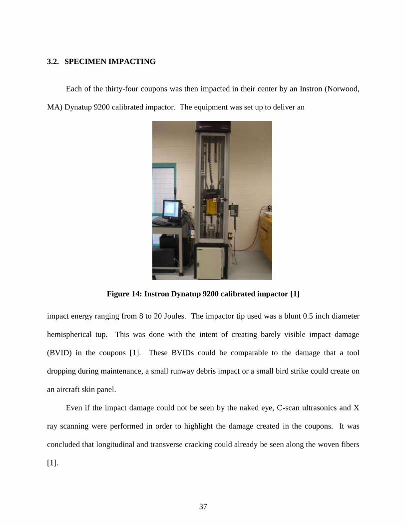
3.2. SPECIMEN IMPACTING .............................................................................................. 37
3.3. SPECIMEN COMPRESSION TESTING ....................................................................... 38
CHAPTER 4 : DATA ANALYSIS PROCESS .............................................................................. 40 4.1. OVERVIEW .................................................................................................................... 40
4.1.1. Data input ............................................................................................................ 40
4.1.2. Analysis parameters ............................................................................................ 41
4.1.2.1. Percentage of recorded acoustic emission data ..................................... 42
4.1.2.2. Number of training coupons .................................................................. 42
4.1.2.3. Type of multivariate statistical regression analysis equation ................ 44
4.1.2.4. Acoustic emission parameters for failure mechanism description ........ 45
4.1.2.5. Type of Kohonen Self Organizing Map ................................................ 45
4.1.2.6. Kohonen SOM data classification parameters ...................................... 45
4.1.2.7. Number of Kohonen SOM output clusters ............................................ 46
4.1.3. Programming aspects .......................................................................................... 46
4.1.3.1. Output results ........................................................................................ 47
4.1.3.2. Visual results ......................................................................................... 47
4.1.3.3. Results variables saving ........................................................................ 49
4.2. NOISE REMOVAL PROCESSES.................................................................................. 50
4.2.1. Noise removal by boundaries filtration ............................................................... 50
4.3. DATA CLUSTERING .................................................................................................... 55
4.3.1. Use of Kohonen self-organizing maps ................................................................. 55
4.3.2. Failure mechanisms identification ...................................................................... 58
4.3.3. Clustering visualization ....................................................................................... 63

2
4.4. APPLIED MULTIVARIATE STATISTICAL REGRESSION ANALYSIS ................. 71
CHAPTER 5 : RESULTS ................................................................................................................ 79 5.1. B-basis allowables ........................................................................................................... 79
5.2. Average frequency filtration optimization ...................................................................... 83
5.3. Number of Kohonen SOM clusters optimization ............................................................ 85
5.4. B-basis allowables minimum conditions ......................................................................... 86
5.4.1. Surface errors and R2 value trends .................................................................................. 86
5.5. Optimized prediction equation ........................................................................................ 92
5.6. Type of MSRA equation influence.................................................................................. 97
CHAPTER 6 : CONCLUSIONS ................................................................................................... 100 6.1. SUMMARY .................................................................................................................. 100
6.2. PERSPECTIVES ........................................................................................................... 102
6.3. RECOMMENDATIONS .............................................................................................. 102
REFERENCES ............................................................................................................................... 103
APPENDIX ..................................................................................................................................... 105 A. Failure Loads ................................................................................................................. 105
B. Code visual outputs ....................................................................................................... 106
C. Results exploitation example ......................................................................................... 118
D. Analysis source code ..................................................................................................... 128

3
LIST OF FIGURES
Figure 1: Typical broadband piezoelectric transducer cross section [2] ........................................ 14
Figure 2: Acoustic emission acquisition process ........................................................................... 15
Figure 3: Pocket AE by Physical Acoustics Corporation® ........................................................... 16
Figure 4: Idealized acoustic emission waveform parameters ......................................................... 17
Figure 5: Energy measurement of typical acoustic emission waveform ........................................ 17
Figure 6: Representation of a neural network typical organization ............................................... 20
Figure 7: Artificial Neural Network processing element or neuron ............................................... 21
Figure 8: Kohonen Self Organizing Maps typical architecture ...................................................... 24
Figure 9: Front view of a Kohonen SOM output map .................................................................. 25
Figure 10: Orthogonal type of Kohonen SOM output map............................................................ 28
Figure 11: Hexagonal type of Kohonen SOM output map .......................................................... 28
Figure 12: Random type of Kohonen SOM output map ................................................................ 28
Figure 13: 4 by 6 in. laminated graphite/epoxy coupon [1] ........................................................... 36 Figure 14: Instron Dynatup 9200 calibrated impactor [1] .............................................................. 37
Figure 15: Compression after impact test setup [1] ....................................................................... 38
Figure 16: Architecture of iterative analysis process ..................................................................... 46
Figure 17: Energy boundaries definition ........................................................................................ 51
Figure 18: Average frequency boundaries definition ..................................................................... 52
Figure 19: Static noise test result [1] .............................................................................................. 53
Figure 20 : Number of minimum Kohonen SOM training iterations determination...................... 57
Figure 21: Failure mechanisms distribution through loading ........................................................ 60
Figure 22: Duration vs counts before Kohonen SOM classification.............................................. 64
Figure 23: Duration vs counts with 4 clusters Kohonen SOM classification ................................ 64
Figure 24: Duration vs counts with 9 clusters Kohonen SOM classification ................................ 65
Figure 25: Amplitude vs Energy vs Duration of non-classified AE data ....................................... 66
Figure 26: Amplitude vs Energy vs Duration of AE data classified in 4 clusters .......................... 67
Figure 27: Amplitude vs Energy vs Duration of AE data classified in 9 clusters .......................... 67
Figure 28: Amplitude distribution of a coupon AE data before classification ............................... 68
Figure 29: Amplitude distribution of a coupon AE hits after classification into 4 clusters ........... 69
Figure 30: Amplitude distribution of a coupon AE hits after classification into 9 clusters ........... 69
Figure 31: Training coupons predicted loads distribution.............................................................. 77
Figure 32: Prediction coupons predicted loads distribution ........................................................... 78
Figure 33: B-basis allowables ........................................................................................................ 80
Figure 34: Modified B-basis allowables ........................................................................................ 82
Figure 35: Lower average frequency boundary optimization ........................................................ 84
Figure 36: Number of Kohonen SOM ouput clusters influence study ........................................... 85
Figure 37: Absolute value of training worst case error evolution .................................................. 87
Figure 38: Training R2 value evolution .......................................................................................... 88
Figure 39: Absolute value of prediction worst case error evolution .............................................. 89
Figure 40: Prediction R2 value evolution ....................................................................................... 91
4
LIST OF TABLES
Table 1: Acoustic emission waveform parameters ........................................................................ 18
Table 2: Distance function definitions ........................................................................................... 29
Table 3: Kohonen SOM combinations ........................................................................................... 30
Table 4: Acoustic emission input data format (Coupon 2A example) ........................................... 41
Table 5: Coupons repartition .......................................................................................................... 43
Table 6: Visualization plots AE parameters couple axis ................................................................ 48
Table 7: Results plots axis .............................................................................................................. 49
Table 8: Filter boundary values ...................................................................................................... 54
Table 9: Failure mechanisms in composite materials .................................................................... 56
Table 10: Kohonen SOM 4 output clusters parameters: Energy (aJ) ............................................. 59
Table 11: Kohonen SOM 4 output clusters parameters: Duration (μs) .......................................... 59
Table 12: Kohonen SOM 4 output clusters parameters: Amplitude (dB) ...................................... 59
Table 13: Kohonen SOM 4 output clusters parameters: Average frequency (KHz)...................... 59
Table 14: Kohonen SOM 9 output clusters parameters: Energy (aJ) ............................................. 61
Table 15: Kohonen SOM 9 output clusters parameters: Duration (μs) .......................................... 61
Table 16: Kohonen SOM 9 output clusters parameters: Amplitude (dB) ...................................... 62
Table 17: Kohonen SOM 9 output clusters parameters: Average frequency (KHz)...................... 62
Table 18: Cluster identification in failure mechanisms ................................................................. 63
Table 19: Example of response variables matrix ........................................................................... 71
Table 20: Example of predictor variables matrix ........................................................................... 72
Table 21: β coefficients example set .............................................................................................. 75
Table 22: MSRA results example .................................................................................................. 76
Table 23: B-basis allowable calculations ....................................................................................... 79
Table 24: B-basis allowables percentage error............................................................................... 81
Table 25: Modified B-basis allowables calculation ....................................................................... 82
Table 26: Modified B-basis allowables percentage error ............................................................... 83
Table 27: Worst case training error ................................................................................................ 87
Table 28: Worst case R2 for training coupons ................................................................................ 88
Table 29: Modified B-basis allowables compliance ...................................................................... 90
Table 30: Minimum number of training coupons for above 50% prediction R2
value .................. 91
Table 31: Prediction equation sensitivity to number of training coupons ...................................... 94
Table 32: Training and prediction errors ........................................................................................ 96
Table 33: Training and prediction errors using a type 2 MSRA prediction equation .................... 98

5
LIST OF EQUATIONS
Equation 1: Artificial neural network processing element output calculation ............................... 21
Equation 2: Kohonen SOM winning neuron determination ........................................................... 25
Equation 3: Kohonen SOM weight adaptation calculation ............................................................ 26
Equation 4: Euclidean distance calculation .................................................................................... 29
Equation 5: Manhattan distance calculation ................................................................................... 29
Equation 6: MSRA equation of type 1 ........................................................................................... 31
Equation 7: MSRA equation of type 2 ........................................................................................... 31
Equation 8: Typical MSRA matrix system for equation of type 1 ................................................. 32
Equation 9: Typical MSRA matrix system for equation of type 2 ................................................. 33
Equation 10: Condition on the matrix system dimensions for MSRA equation of type 1 ............. 34
Equation 11: Condition on the matrix system dimensions for MSRA equation of type 2 ............. 34
Equation 12: β matrix calculation .................................................................................................. 34
Equation 13: Residual error calculation ......................................................................................... 35
Equation 14: MSRA equation of type 2 ......................................................................................... 73
Equation 15: MSRA equation of type 2 ......................................................................................... 74
Equation 16: MSRA equation of type 2 ......................................................................................... 74
Equation 17: MSRA equation of type 2 ......................................................................................... 79
Equation 18: Output format of a MSRA equation of type 1 .......................................................... 92
Equation 19: Calculation example of a prediction failure load ...................................................... 95

6
CHAPTER 1 : INTRODUCTION
1.1. INDUSTRIAL CONTEXT
Composite materials have been of growing interest in the transportation industry and more
particularly the aerospace industry for several years. The idea of reinforcing a material by
combining it with another in order to improve its overall mechanical properties has been used for
decades in field of aerospace engineering. The recent intensive study and development of
composites is essentially driven by the aerospace industry‟s constant need to increase the
strength-to-weight ratio of any material being used in aerospace structures, while conserving or
improving upon its mechanical properties. Throughout the years, composite materials have been
the primary answer for improving strength-to-weight ratios of structures. This is mainly
accomplished through the use of materials such as carbon fiber that have a considerably lower
density than all of the high strength metals. On the other hand, it has been proven that even when
composite materials meet all of the aerospace industry requirements in terms of mechanical
properties, they can be strongly degraded by environmental effects and especially impact damage
[15].
The current absolute necessity of lighter materials pushed the aerospace industry towards
the extensive use of composite materials on the new generation of both civil and military aircraft.
Two famous examples, particularly highlighted for their high percentage of composite material
use, are the Boeing 787 Dreamliner and the upcoming Airbus A350. By taking into
consideration the fact that both these projects included more than 50% of composite materials in
their structures, one can see the need for a thorough understanding of these materials. Hence,
knowing the aforementioned sensitivities of these materials to their environment becomes crucial

7
in order to be able to certify that any aircraft part made out of composite materials is able to
sustain its maximum design load throughout its service life.
Solutions have been researched and developed in order to monitor material condition at
any time during its service life without affecting the material itself. This set of non-intrusive
monitoring solutions are known as nondestructive testing methods and have been of particular
interest for the petroleum for pipeline integrity inspections and the aerospace industry for aircraft
structural integrity inspections [2]. The nondestructive testing methods that have been developed
are primarily based on the nature of the material to be inspected in order to be efficient. Even if
efforts have been put into the development of nondestructive testing methods, the non-metallic
nature of composite materials reduces the number of usable inspection methods. One of the most
promising yet undeveloped methods for composite materials nondestructive inspection is based
on the analysis of the acoustic emissions (AE) generated by loading the structure to be inspected.
Recently, efforts have also been made in the field of structural health monitoring. This
type of live monitoring becomes feasible when the transducers are built into the structure,
preferably during the manufacturing process. This evolution of nondestructive inspection
methods could strongly redefine aerospace systems from regularly inspected, inert mechanical
structures to constantly self-evaluated structures. This continuous evaluation would provide
crucial information about the vehicle structural integrity and determine its maintenance needs in
real time. The research presented in this thesis is designed to further this end.

8
1.2. PREVIOUS RESEARCH
Numerous research projects have been conducted in the past in order to gain knowledge
about composite materials used in the aerospace industry. The mechanical behavior of composite
materials during their mechanics of failure is still not well understood or described by any
mathematical model. Thus, much effort was put into the study of the mechanics of failure of
these materials from a molecular to a macro-mechanical scale. Artificial neural networks
(ANNs) have also been investigated for their ability to analyze such highly complex problems.
The Department of Aerospace Engineering at Embry-Riddle Aeronautical University
(ERAU) has successfully conducted several studies on the failure mechanisms associated with
composite materials, including coupons, beams and pressure vessels, by combining the
nondestructive monitoring technique of acoustic emission with the artificial neural network
technology and multivariate statistical analysis as data analysis tools [1,3-4].
The present research is closely related to a previous research project conducted in 2009 by
Gunasekera, an ERAU alumnus [1]. This research project consisted in predicting, within the B-
basis allowables for composite materials, the ultimate load of graphite/epoxy coupons degraded
by previous impact and subjected to compression loading until failure. A set of thirty-four 24-ply
graphite/epoxy coupons were manufactured and impacted at various levels of impact energy
varying from 8 to 20 Joules. These impacts were intentionally delivered in order to recreate
barely visible impact damage (BVID) like that experienced by an aircraft skin panel when
exposed to a tool drop during maintenance, runway debris impact, or small bird strikes during
operation. The present research then focused on the mechanical behavior of these impacted
coupons under a constantly increasing compressive load. While each coupon was undergoing

9
compression, the emitted acoustic emission data were captured and recorded by an AE analyzer
system along with the concomitant ultimate failure load.
The study of composite materials undergoing compression is of particular interest with
regard to the little knowledge available when compared to its behavior in tension. As opposed to
a composite material undergoing tension, in which the load is mainly carried by the fibers, a
composite material under compression will rely on both its fibers and matrix to sustain the load.
It is now well understood that, due to unexpected manufacturing defects and unpredictable
physical degradations of the material throughout its lifetime, any anticipation of the behavior of
any real composite coupon or part approaching its failure will be difficult and, in any case,
unique [5].
Further comprehensive data analysis has been conducted using the Kohonen self-
organizing map (SOM) type of ANN for data classification and backpropagation neural networks
(BPNNs) for ultimate load prediction [1]. The overall goal of Gunasekera‟s research was to
demonstrate the capability of accurately predicting the ultimate compressive loads in impact
damaged coupons by only using the acoustic emissions emitted by the coupons loaded at levels
well below their ultimate failure loads. This previous research project was successfully
concluded by an ultimate load prediction worst case error of -11.53% using 24 coupons to train
the BPNN and the remaining 10 coupons for ultimate load prediction.

10
1.3. RESEARCH OBJECTIVE
As with any new technique or technology, it is of primary interest to have a good
understanding and knowledge prior to any industrial application. The problem of the present
research project is to extend the physical understanding of the nondestructive acoustic emission
technique by reproducing the real life service conditions in a laboratory. The presence of
composite material skin panels being exposed to environmental aggressions and subjected to
complex loading is increasing in aircraft structures. Thus, it is of interest to study the behavior of
degraded composite coupons undergoing, at first, simple compression in order to determine if the
use of acoustic emission is a viable technique that should be used in the future. This laboratory
experiment could be easily compared to a real life situation, where a flat skin panel on the upper
surface area of a wing was previously degraded by a tool drop during maintenance and then
subjected to a constant compressive load during flight. The choice of the acoustic emission
nondestructive method to acquire data in the laboratory stands to reason in this example since this
technique has already been used for in-flight data acquisition for metal structures [2].
The present research project proposes to demonstrate the feasibility of an ultimate load
prediction using the acoustic emission data recorded during the previously discussed research
project. This prediction will be accomplished by using ANNs for data classification and a
multivariate statistical analysis (in place of the backpropagation neural network [1]) for an
accurate compressive failure load prediction. The prevalent aim of joining these two methods is
the ability to generate a linear equation, which will mathematically define the relationship
between the low proof load (≤30% Pult) acoustic emission observed during a coupon compression
and its ultimate failure load.

11
The main difficulty in combining the acoustic emission capturing technique and the
multivariate statistical analysis is that these methods possess disadvantages that can be
considered, at first blush, as incompatible. Indeed, the acoustic emission capturing technique is a
noise sensitive technique, which captures noise as part of its output data. In order to produce
accurate results, these captured AE data need to be almost noise free when introduced to the
multivariate statistical analysis process. The analyzing process described hereinafter was
designed by the author with the intention of being automatic and easily reproducible for any
future composite aircraft parts. In order to do so, several subsequent requirements were defined
and constantly sought:
- Be able to run an analysis starting uniquely with raw acoustic emission data directly after
their capture on several specimens.
- Identify the analysis parameters.
- Evaluate the influence of each analysis parameter on the final prediction.
- Allow a physical interpretation of the data manipulation step by step by means of
graphical representation understandable by any NDT engineer.
- Determine the optimized set of parameters allowing a prediction error within the B-basis
allowables for the composite material.
- Obtain, in this particular case, a best fitting equation predicting the ultimate load as
accurately as possible.

12
CHAPTER 2 : THEORETICAL BACKGROUND
2.1. ACOUSTIC EMISSION
2.1.1. Introduction
Any material that is subjected to an external stress will react according to the laws of
physics in order to reach an equilibrium state. An applied external load will create stress
concentrations within the material that will be released by different means. The stress release
mechanisms can manifest themselves in different variations of the materials physical properties.
For example a stressed material can redistribute the energy it is subjected to by varying its
temperature, deforming itself on a large scale, or even by failing at stress concentration points
created within the material. In the last case, the sudden dislocation of material at those failure
points will generate mechanical waves that will propagate within the material according to its
mechanical properties. Thus, a correlation can be established between the observation of the
stress releasing ultrasonic mechanical waves, known as acoustic emission, and the physical
events occurring in the failing material [2].
Since this statement is valid regardless of the material type, a universal technique has
been developed to accurately observe these stress releasing waves. This nondestructive technique
is known as acoustic emission. Because the mechanical waves propagating throughout the
material will reach the external surfaces of the material, it is feasible to observe them in a non-
intrusive manner by the acoustic emission technique. Furthermore, in this technique, the stress
that the failing material is subjected to is uniquely provided by the material loading environment.

13
Thus, the acoustic emission technique is a passive nondestructive technique that simply captures
acoustic emissions that naturally occur in a material stressed by its loading environment.
Knowing the physical events occurring in a structure well before its failure can inform the
trained NDT engineer of the physical state of the observed structure and with some analysis allow
him to predict its point of failure and ultimate failure load. This has been successfully
accomplished on a number of occasions in the past [1-4].
2.1.2. Capturing technique
The acoustic emission monitoring technique consists in capturing the mechanical waves
propagating throughout a material, by sensing and measuring the vertical displacement of the
aforementioned material‟s surface. In order to do so, resonant piezoelectric transducers are
placed on the surface of the specimen to observe mechanical waves that are travelling within the
material. A typical acoustic emission resonant piezoelectric transducer is composed of a ceramic
element that is extremely sensitive to any displacement. The transducer is coupled to the surface,
here with hot melt glue. Any surface displacements are transformed by the piezoceramic
element into an electrical signal that can be read by a computer or an electronic device. A
typical broadband resonant piezoelectric transducer cross section is presented in Figure 1.
Acoustic emission transducers typically do not include the damping material and are therefore
allowed to resonate at frequencies consistent with the geometry of the piezoceramic element..

14
Figure 1: Typical broadband piezoelectric transducer cross section [2]
As with any measuring technique, the choice of the transducer most adapted to the
considered application is of primary importance. The large spectrum of acoustic emission
applications led to the design of several types of acoustic emission transducers specifically
adapted to their respective purposes and environments. The numerous types of transducers that
are available today vary in terms of size, shape, frequency spectrum and sensitivity. These
transducers can be either wideband or resonant, depending upon the frequency range that is to be
recorded. An enlightened selection requires an experience shared by both the manufacturer and
the NDT engineer [6].
Another crucial parameter for an accurate measurement is the use of a wave conducting
medium, known as a couplant, between the material surface and the sensitive surface of the
acoustic emission transducer. This is done in order to reduce the impedance difference between
the transducer and specimen materials. Couplants are often water based liquids or gels that
replace an air interface. Indeed, the lack of couplant or the presence of too many air bubbles
trapped in it would lower the overall interface impedance and ultimately degrade the
measurement. In addition, the couplant can also be selected for its adhesive properties in order to
15
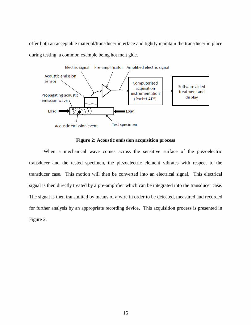
offer both an acceptable material/transducer interface and tightly maintain the transducer in place
during testing, a common example being hot melt glue.
Figure 2: Acoustic emission acquisition process
When a mechanical wave comes across the sensitive surface of the piezoelectric
transducer and the tested specimen, the piezoelectric element vibrates with respect to the
transducer case. This motion will then be converted into an electrical signal. This electrical
signal is then directly treated by a pre-amplifier which can be integrated into the transducer case.
The signal is then transmitted by means of a wire in order to be detected, measured and recorded
for further analysis by an appropriate recording device. This acquisition process is presented in
Figure 2.

16
Figure 3: Pocket AE by Physical Acoustics Corporation®
The acoustic emission recording devices today are compact and transportable. As a
practical example, the acoustic emission recording device used in the present case is the hand-
held Pocket AE® designed and distributed by Physical Acoustics Corporation® [6] as shown in
Figure 3.
Acoustic emission is the elastic energy spontaneously released by the material when it
undergoes deformation. An acoustic emission hit is the individual signal burst produced by a
localized material change. A captured acoustic emission hit can be represented by an idealized
sinusoidal signal as shown in Figures 4 and 5 [2].

17
Figure 4: Idealized acoustic emission waveform parameters
Figure 5: Energy measurement of typical acoustic emission waveform
This signal can be characterized by several waveform parameters that the recording
device can measure directly on reception of the acoustic emission hit. These parameters, visually
represented in Figures 4 and 5, are defined as described in Table 1.

18
Table 1: Acoustic emission waveform parameters
# Parameter Unit Definition
1 Counts N/A Number of times the acoustic emission signal passes
above a specified threshold amplitude level
2 Duration Micro seconds (μs) Time elapsed between the first and last threshold crossing
of the acoustic emission signal
3 Energy Atto Joules (aJ)
Defined as the Mean Area under the Rectified Signal
Envelope (MARSE) from beginning to end and represents
the energy delivered by the acoustic emission signal
4 Average
Frequency Hertz (Hz) Defined as the ratio of counts over duration
5 Amplitude Decibel (dB) Amplitude of the maximum peak within the sinusoidal
acoustic emission signal
6 Rise time Micro seconds (μs) Time elapsed between the first threshold crossing and the
peak amplitude
The acoustic emission technique offers the advantage of being able to record the acoustic
emission hits generated during the compression of a test specimen from the initial loading to
ultimate compressive failure. Thus, particular attention should be paid to the transducer
placement to ensure that it is consistent from specimen to specimen throughout the testing. Also,
the correct bonding of the transducer through the testing process should be verified by inspecting
the attachment of the transducer to the specimen both prior to and after testing. Hot melt glue is
used in the present case to ensure correct bonding throughout the loading process.
This allows the NDT engineer to record the acoustic emission hits occurring within the
material and to store the data for further comprehensive analysis. The main disadvantage of the
acoustic emission technique resides in the fact that it does capture all the acoustic emission that
occurs during a specimen testing, which typically includes a certain amount of unwanted acoustic
emission hits due to mechanical and electromagnetic noises [2]. Even if the Pocket AE®
allows
the user to set bandpass filters on the data inputs, noise will still be part of the output data.

19
2.2. NEURAL NETWORKS
2.2.1. Introduction
The human brain massively interconnects neural cells capable of transmitting information
that results in some action or decision making process. Models have been similarly developed in
order to recreate this complex infrastructure with the final intention of being capable of executing
either complex classifications or complex predictions [7,9]. Such computerized models, known
as artificial neural networks (ANNs), are nowadays broadly used for many different types of
applications. For example, in the image processing field, ANNs can be used for automatic target
recognition, signature authentication and handwritten character recognition. In the signal
processing industry, ANNs can be applied in many different fields from sonar signature
recognition to seismic event prediction, from animal species classification to disease diagnostics,
etc. [7-8].
ANNs can be easily seen as black boxes, in which the user enters a set of inputs and
requires an output relative to their specific application. The given ANN will then be trained to
produce a requested prediction result or classification. This fundamental phase of training
confers to ANNs a high degree of adaptability and a certain universality in their applications.
The training phase is essential in this process since it is the period wherein the neural network
will be iteratively modified to produce the best relationship between the input data and the
required output [7]. Notably, ANNs can be applied to nonlinear problems of prediction where
no analytical solution can readily be found [7]. ANNs are also advantageous with regard to their
ability to confer a less significant importance to input data that counterproductively affects the
required output. Thus, a limited amount of noise can oftentimes be ignored by the ANN in
prediction applications [7]. On the other hand, the use of an ANN requires a certain minimal
20
knowledge base concerning their operation in order to clean up input data and make adjustments
to their training parameters in order to optimize their performance [1].
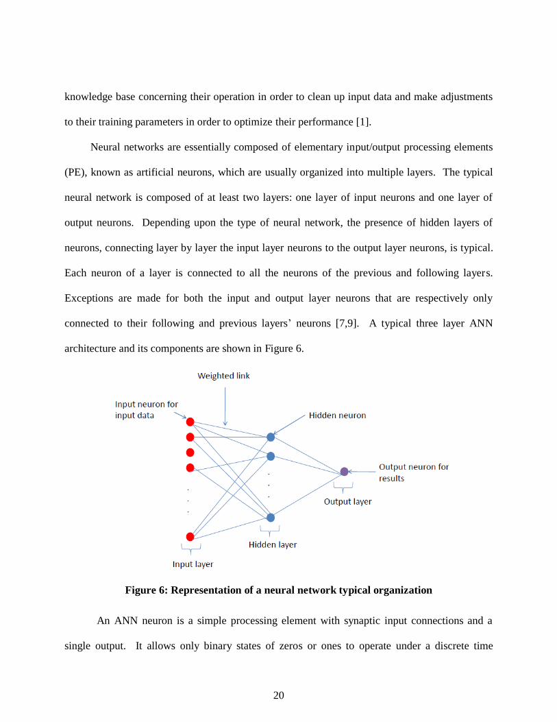
Neural networks are essentially composed of elementary input/output processing elements
(PE), known as artificial neurons, which are usually organized into multiple layers. The typical
neural network is composed of at least two layers: one layer of input neurons and one layer of
output neurons. Depending upon the type of neural network, the presence of hidden layers of
neurons, connecting layer by layer the input layer neurons to the output layer neurons, is typical.
Each neuron of a layer is connected to all the neurons of the previous and following layers.
Exceptions are made for both the input and output layer neurons that are respectively only
connected to their following and previous layers‟ neurons [7,9]. A typical three layer ANN
architecture and its components are shown in Figure 6.
Figure 6: Representation of a neural network typical organization
An ANN neuron is a simple processing element with synaptic input connections and a
single output. It allows only binary states of zeros or ones to operate under a discrete time

21
assumption and works in synchronization with the other neurons of the overall network [9]. A
representation of a typical artificial neuron or processing is presented in Figure 7. The
Figure 7: Artificial Neural Network processing element or neuron
ANN neuron function is to produce a single output calculated from its input data and its weighted
input links as shown in Equation 1.
Equation 1: Artificial neural network processing element output calculation
where
f is the activation function
wi is the link weight
xi is the input value
i is a subscript covering all the output neurons
n is the number of neuron.
The function f is called the transfer or activation function, which determines the terms of
the input data and weights and the state that the neuron output takes. Numerous activation
functions are available, linear or nonlinear, unipolar or bipolar, and their interest is highly related
to the type of ANN that is used [9].

22
The ANN can be classified according to its architecture, competitiveness and learning
process. The type of architecture depends notably upon the number of layers and processing
elements. The competitiveness is related to learning process mode, which can be cooperative or
suppressive while adjusting the connection weights. As mentioned previously, the learning
process of any ANN is crucial to its efficiency. During the learning or training phase, the ANN
will iteratively modify the weight of each PE connection in order to reach the desired output.
The learning process can be of two types: supervised and unsupervised.
In the case of a supervised learning, a set of training inputs and their known output are used
to train the network. Iteration by iteration, the ANN calculates the output solely based upon the
input and the current setting of the links‟ weight, finds the output error by comparing it to the
targeted or actual output, and finally, back propagates adjustments to the network weights based
on the error for an improved output. The backpropagation of the error in terms of weight
adjustments is mathematically accomplished by following a user adopted learning rule. This
iterative optimization procedure is repeated until stability in the output variation is reached
around the targeted output.
In the case of unsupervised learning, since the ANN is not given any output target, it cannot
use any output error to adjust its set of PE connection weights. The ANN will then only use the
set of input data to train. This explains why most of the unsupervised learning processes are used
for classification problems. The ANN will try to find patterns or similarities between the input
data in order to classify them into clusters or groups of data having similar characteristics. In
both cases, the ANN is given an initial set of arbitrary weights, between 0 and 1, that the learning
process will modify until stability in the output is reached [9].

23
There are mainly five different types of neural networks available today: perceptron
classifiers, feedforward, backpropagation, associative memory and self-organizing networks [9].
These networks find their application in data filtering, data clustering and prediction tools [7-8].
The present research focuses on the data clustering type of neural network, the Kohonen self
organizing map (SOM), which helps in the data filtering process to remove noise in preparation
for multivariate statistical regression analysis (MRSA) ultimate load prediction.
2.2.2. Kohonen self organizing maps
The Kohonen self organizing map (SOM) is a data clustering algorithm developed by
Teuvo Kohonen that is commonly used for data classification. While in the feedforward and
backpropagation networks the set of inputs is transformed layer by layer into a set of outputs, in
the Kohonen SOM, the neurons of the single output layer are organized in a map where each
neuron can interact laterally with its neighboring neurons. This allows all output neurons to be in
competition with their neighboring neurons and to turn themselves through a learning process
into an input data pattern detector [7].
Kohonen SOMs are two layered, unsupervised and competitive ANNs. In terms of
architecture, the Kohonen SOM is composed of an input layer in which every input neuron
contains a data point to classify and an output layer in which the data points will be clustered
based on their similarities. The number of input neurons is defined by the number of data
parameters used to classify, in this case, the acoustic emission quantification parameters:
amplitude, energy, duration, rise time and counts. The number of output neurons can be defined
by the user and represents the number of clusters the data points will be classified into. Here
these will be the failure mechanisms associated with compressive failure of composite structures.
These two layers are then connected by weighted links that will be in competition during a

24
learning process in order to determine the appropriate cluster for each input data point. A typical
Kohonen SOM can be represented as shown in Figure 8.
Figure 8: Kohonen Self Organizing Maps typical architecture
Since a Kohonen SOM performs the simple task of classifying a complex set of data, it is
implied that the output is unknown; thus, the Kohonen SOM learning process has to be
unsupervised. Moreover, since each input data point (value contained in an input neuron) has to
be classified into only one cluster (contained in one output neuron), the learning process will use
competition to determine, iteration by iteration, the weight that should be associated with each
connecting link.
The peculiarity of the Kohonen SOM resides in the fact that it produces an output layer
that can be seen as a spatially organized map that divides the input data points into clusters. The
spatial proximity of these clusters implies a higher similarity between the data points. A front
view of the Kohonen SOM output map presented in Figure 8, as the output layer is presented in
Figure 9.

25
Figure 9: Front view of a Kohonen SOM output map
The typical learning process for a Kohonen SOM will be described in the following
paragraph. First, the SOM is initialized with a random set of weights (0 to 1), connecting the
input layer neurons to the output layer neurons. Then, every time an input data point is presented
to the SOM, it is presented to all the output neurons. The best matching neuron is determined
based on the configuration of the current connection weights, and the input data/output neuron
proximity that is determined from Equation 2 [9].
Equation 2: Kohonen SOM winning neuron determination
where
x represents the data input
w represents the link weight
i is a subscript covering all the output neurons
m is the subscript of the winning output neuron.
26
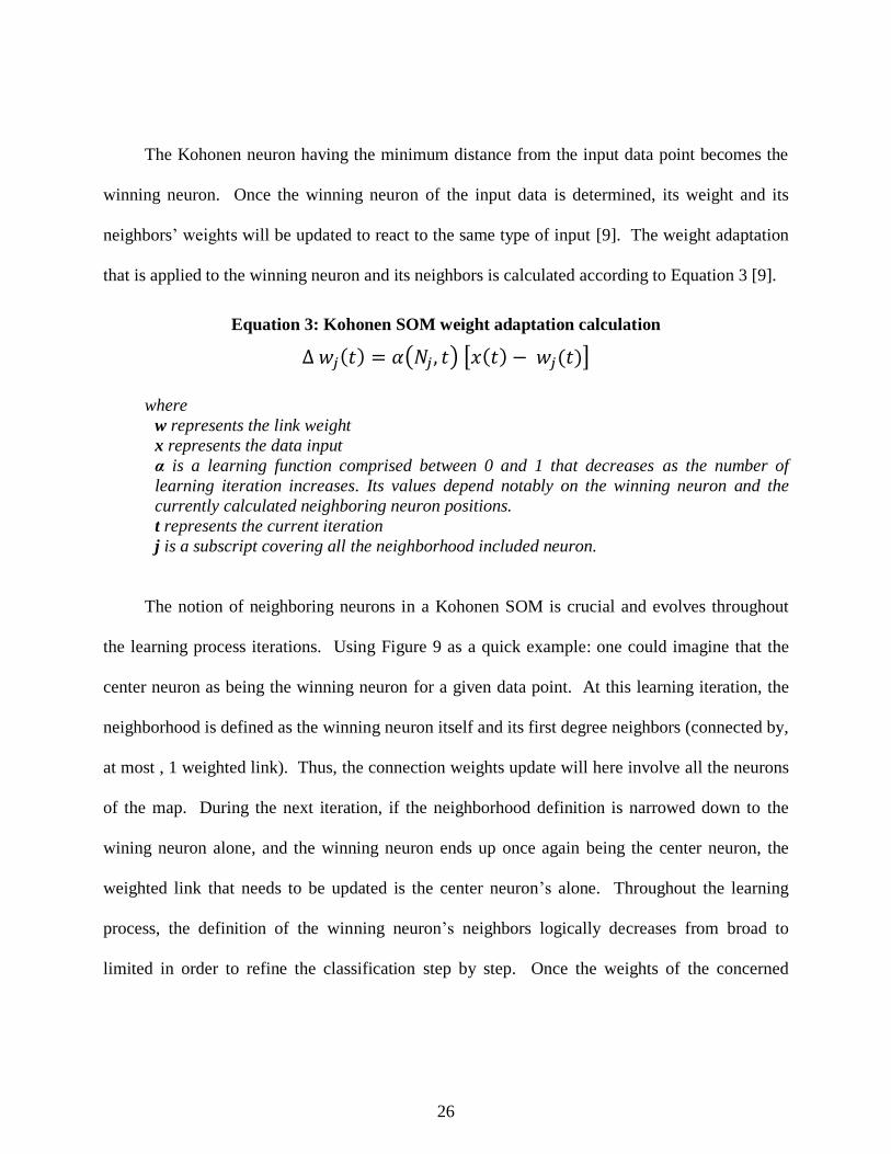
The Kohonen neuron having the minimum distance from the input data point becomes the
winning neuron. Once the winning neuron of the input data is determined, its weight and its
neighbors‟ weights will be updated to react to the same type of input [9]. The weight adaptation
that is applied to the winning neuron and its neighbors is calculated according to Equation 3 [9].
Equation 3: Kohonen SOM weight adaptation calculation
where
w represents the link weight
x represents the data input
α is a learning function comprised between 0 and 1 that decreases as the number of
learning iteration increases. Its values depend notably on the winning neuron and the
currently calculated neighboring neuron positions.
t represents the current iteration
j is a subscript covering all the neighborhood included neuron.
The notion of neighboring neurons in a Kohonen SOM is crucial and evolves throughout
the learning process iterations. Using Figure 9 as a quick example: one could imagine that the
center neuron as being the winning neuron for a given data point. At this learning iteration, the
neighborhood is defined as the winning neuron itself and its first degree neighbors (connected by,
at most , 1 weighted link). Thus, the connection weights update will here involve all the neurons
of the map. During the next iteration, if the neighborhood definition is narrowed down to the
wining neuron alone, and the winning neuron ends up once again being the center neuron, the
weighted link that needs to be updated is the center neuron‟s alone. Throughout the learning
process, the definition of the winning neuron‟s neighbors logically decreases from broad to
limited in order to refine the classification step by step. Once the weights of the concerned

27
neurons have been updated, and all the data inputs presented, an iteration is concluded. This
process is repeated over and over again until stability in the classification is reached.
In the present case, twelve different SOM configurations were identified to be of interest in
the classification process of the acoustic emission data. These twelve configurations combine
three different types of map organization and four different distance functions [10]. The three
possible Kohonen SOM output maps architectures are thus presented in Figures 10, 11 and 12
[10].

28
Figure 10: Orthogonal type of Kohonen SOM
output map
Figure 11: Hexagonal type of Kohonen
SOM output map
Figure 12: Random type of Kohonen SOM output map

29
The distance functions are used to determine if a neuron is considered to be the winning
neuron. A neuron is in the neighborhood of the winning neuron if its distance to the winning
neuron is less than a certain value. This maximum distance value decreases throughout the
learning process [10]. The four identified distance functions employed herein are described in
Table 2.
Table 2: Distance function definitions
Distance function Definition
Euclidean distance
Equation 4: Euclidean distance calculation
where
p and q are two points
i is the dimension subscript
n is the number of dimensions.
Link distance The degree of neighborhood is defined by the minimum number of
links connecting a neighboring neuron to the winning neuron.
Manhattan
distance
Equation 5: Manhattan distance calculation
where
p and q are two points
i is the dimension subscript
n is the number of dimensions.
Box distance The degree of neighborhood is defined by a box including all neurons
surrounding the winning neurons (in line, column and diagonal).

30
Table 3 presents the twelve possible combinations of map architecture and distance functions
employed in this research to classify the acoustic emission data.
Table 3: Kohonen SOM combinations
Type of SOM
number
Map
architecture Distance function
1
Orthogonal grid
Euclidean distance
2 Link distance
3 Manhattan distance
4 Box distance
5
Hexagonal grid
Euclidean distance
6 Link distance
7 Manhattan distance
8 Box distance
9
Random grid
Euclidean distance
10 Link distance
11 Manhattan distance
12 Box distance
In the present case, the Kohonen SOMs have been used in order to classify the large
amount of acoustic emission data acquired after compression testing of the graphite/epoxy
coupons. Each data point represents an acoustic emission hit that possesses a value for each of
the six acoustic emission waveform quantification parameters presented in Table 1. This
complex set of data has to be classified into clusters representative of the composite failure
mechanisms from the compression after impact specimens in order to be able to generate an
ultimate load equation using multivariate statistical regression analysis.

31
2.3. MULTIVARIATE STASTISTICAL REGRESSION ANALYSIS
Multivariate statistical regression analysis (MSRA) is a statistical tool that, as implied in its
name, establishes the relationship between several variables based on a statistical regression. The
variables enrolled in a MSRA are of two types. The first type is called the independent variables
or predictors. There are, logically, in a MSRA, several of them. The second type of variable is
called the dependent variable or response variable [12-13].
It is assumed that a response variable can be written in terms of a combination of the
predictors as presented in Equation 6. This will be denoted as a MSRA equation of type 1.
Equation 6: MSRA equation of type 1
where
Y is the dependent response variable
βi are constant terms
Xi are the independent predictor variables
n is the number of independent predictor variables
ε is a random error.
Another form of such a combination includes the cross product terms of each pair of two
predictors. This will be further denoted as a MSRA equation of type 2.
Equation 7: MSRA equation of type 2
where
Y is the dependent response variable
βi are constant terms
Xi are the independent predictor variables
n is the number of independent predictor variables
m is the number of independent predictor variables cross products of two:
ε is the residual prediction error.

32
This second type of equation will take into account the correlation or interdependency that
exists between the predictor variables. In the present research, where the independent variables
are the failure mechanisms of the composite material (matrix cracking, delamination, fiber
breaks, etc.), the cross product terms could take into account the coupling that exists between the
various failure mechanisms.
MSRA is applied in problems where the dependency between multiple response variables
and a set of predictor variables is to be found by a unique set of βi constant coefficients in order
to evaluate the overall impact of each predictor on the response. This is, for example, the case in
social, physical, atmospheric, ancient civilization and species survival types of problems where
the effects of different parameters are to be studied to understand a phenomenon [11-12]. The
domains of application are unlimited as long as a sufficient number of measurements are
available.
When the number of response variables is larger than one, the problem can be seen as the
following matrix system. This system is valid for a MSRA equation of type 1.
Equation 8: Typical MSRA matrix system for equation of type 1
where
Yi are the known response dependent variables
Xij are the known predictor variables
βi are the constant coefficients to be determined
εi are the residual prediction errors
n is the number of independent predictor variables
m is the number of independent predictor variables cross products of two:
.

33
For a MSRA equation of type 2 the previous system becomes [12-13]
Equation 9: Typical MSRA matrix system for equation of type 2
where
Yi are the known response dependent variables
Xij are the known predictor variables
βi are the constant coefficients to be determined
εi are the residual prediction errors
n is the number of independent predictor variables
m is the number of independent predictor variables cross products of two:
.
In these two systems, the matrices of response variables Yi and predictor variables Xij are
known. The MSRA solves the system by determining the unique set of constant coefficients βi
that best fit all the system equations. The residual error εi due to this unique best fitting set of
coefficients βi is then determined for each single equation of the system. It should be noted that
the presence of a first column of ones in the predictor variables matrix is mandatory to obtain a
first constant coefficient β0, as shown in Equations 6 and 7. It is also important to understand that
the solving of a system of k equations, containing n+1 unknown constant coefficients βi for a
MSRA equation of type 1 and n+m+1 unknown constant coefficients βi for a MSRA equation of
type 2, creates a condition on the minimum number of equations k required as shown in
Equations 10 and 11. In order to run a MSRA, this condition can be simply expressed as shown
in Equation 10.

34
Equation 10: Condition on the matrix system dimensions for MSRA equation of type 1
where
k is the number of equations in the system
n is the number predictor variables.
Equation 11: Condition on the matrix system dimensions for MSRA equation of type 2
where
k is the number of equations in the system
n is the number predictor variables
m is the number of independent predictor variables cross products of two:
.
The condition on the number of lines k of the system means that in order to run a MSRA
analysis, one should have two more cases providing a set of predictors and response variables
than the number of predictors, or the number of predictors plus the number of predictors cross
products, for respectively an equation of type 1 or 2.
Once the matrices of predictors and response variables are provided, the MSRA
determines the β matrix by solving the system as shown in Equation 12 [12-13]
Equation 12: β matrix calculation
where
β is the matrix of the constant coefficients βi
X is the matrix of predictor coefficients Xij
Y is the matrix of response coefficients Yi .
The residual error is then determined by calculating the actual response variables values
and the calculated responses variables‟ values as presented in Equation 13 [12-13]

35
Equation 13: Residual error calculation
where
ε is the matrix of residual errors εi
β is the matrix of the constant coefficients βi
X is the matrix of predictor coefficients Xij
Y is the matrix of response coefficients Yi .
One of the goals of the present research was to efficiently determine the X matrix of
predictor variables in order to minimize the values contained in the residual matrix ε. The use of
the MSRA and its specific application in the present project will be presented later on.

36
CHAPTER 3 : COMPOSITE COUPONS MANUFACTURE AND TESTING
3.1. SPECIMEN MANUFACTURING
Thirty-four graphite/epoxy laminated coupons were fabricated, impacted and compressed
while recording acoustic emissions by Gunasekera for a previous research project [1]. The
coupons were fabricated following the ASTM standard D7137/D 7137M-07, defining the
specimen coupons for compression after impact testing. A Cycom ® (Cytec, Woodland Park,
New Jersey) 985 GF3070PW bidirectional woven prepreg cloth was used to fabricate the entire
set of coupons. Nine 14 x 9 inch laminates were fabricated, out of which thirty-four 4 x 6 inch
coupons were cut out. The ASTM standard requires the compression coupons to be of a
thickness of 0.20 inch, which in this case required 24 prepeg layers per laminate. The nine
laminates were then manufactured by laying 24 layers of prepeg woven cloth onto a wooden
plate, clamping them between two aluminum caul plates by C clamps, and finally, curing the
laminate in an oven at 355°F for two hours in conformance with the prepeg curing specifications.
The oven was then turned off, and the laminates were allowed to gradually cool to ambient
temperature. Each of the nine laminates were then cut into four 4 x 6 inch coupons using a
diamond tip wet saw.
Figure 13: 4 by 6 in. laminated graphite/epoxy coupon [1]
37
3.2. SPECIMEN IMPACTING
Each of the thirty-four coupons was then impacted in their center by an Instron (Norwood,
MA) Dynatup 9200 calibrated impactor. The equipment was set up to deliver an
Figure 14: Instron Dynatup 9200 calibrated impactor [1]
impact energy ranging from 8 to 20 Joules. The impactor tip used was a blunt 0.5 inch diameter
hemispherical tup. This was done with the intent of creating barely visible impact damage
(BVID) in the coupons [1]. These BVIDs could be comparable to the damage that a tool
dropping during maintenance, a small runway debris impact or a small bird strike could create on
an aircraft skin panel.
Even if the impact damage could not be seen by the naked eye, C-scan ultrasonics and X
ray scanning were performed in order to highlight the damage created in the coupons. It was
concluded that longitudinal and transverse cracking could already be seen along the woven fibers
[1].

38
3.3. SPECIMEN COMPRESSION TESTING
Once all the specimens have been manufactured and impacted, each of them was mounted
on a Tinius-Olsen (Willow Grove, PA) model 290 Lo Cap testing machine for compression until
failure. A representation of the test setup is presented in Figure 15 [1].
Figure 15: Compression after impact test setup [1]
This Boeing compression after impact testing machine was used in order to conform to the
same ASTM standard D7137/D 7137M-07 used previously for the coupon manufacture. The
tested graphite/epoxy coupon was then equipped with two 150 kHz transducers (R15α A157 and
A158) placed on the coupon centerline at 1.5 inches from the bottom and top edges. The two
transducers were then connected to an Enviroacoustics (Physical Acoustics Cooperation,
Princeton Junction, New Jersey) Pocket AE-1 (Figure 3) for acoustic emission data acquisition.

39
The interface between the transducers and the specimen was made of a thin layer of hot melt
glue, ensuring both a role of couplant and bonding to maintain the transducers in place during the
testing. In order to prevent any unwanted disbonding during the specimen failure, the transducers
were also taped to the specimen. A compressive load was then applied at a rate of 4,000 lbf/min
until failure. It should be noted that the Pocket AE allowed the continuous recording of the
Tinius-Olsen compressive load at each instant on an input channel matching the current acoustic
emission data recording to the current compressive load. The maximum applied load was then
recorded [1].

40
CHAPTER 4 : DATA ANALYSIS PROCESS
4.1. OVERVIEW
The purpose of the current research was to demonstrate the feasibility of an automated
treatment of raw acoustic emission data from their capture until development of a failure load
prediction equation. Matlab R2009b® was used herein to develop a code that automatically
analysed the acoustic emission data and generated an ultimate compression after impact load
equation based on the amount of the various failure mechanisms that occurred at a low proof
load.
4.1.1. Data input
It has been defined as a requirement that the analysis process of the acoustic emission data
set should start with raw data directly extracted from the Pocket AE acquisition instrument. After
impacting the coupons, the Pocket AE was set to record the following list of AE parameters:
counts, duration, energy, amplitude and rise time for each signal waveform or hit. The ratio of
counts over duration or average frequency was then calculated for each acoustic emission hit.
Finally, the compressive load was also recorded for each acoustic emission hit.
After each compression test, the recorded acoustic emission data were exported in a single
file for further analysis. A total of 34 files were generated. Each of these files was formatted as
shown in Table 4.

41
Table 4: Acoustic emission input data format (Coupon 2A example)
Acoustic
emission
hit
number
Counts Duration
(μs)
Energy
(aJ)
Load
(lb)
Average
Frequency
(KHz)
Amplitude
(dB)
Rise
time
(μs)
1 24 180 1 169 133 44 10
2 17 284 1 169 60 49 18
3 24 629 1 178 38 38 67
… … … … … … … …
3804 217 2956 12 24676 73 50 701
These acoustic emission data were classified in a chronological order with respect to their
occurrence during the compression test. This can be seen in the load values that continue to
increase throughout the specimen compression. The spreadsheets logically contain the AE data
occurring at the beginning of the compression in the first rows up to the AE data occurring in the
vicinity of the failure in the last rows. For the purpose of this research, the totality of the acoustic
emission hits from compression initiation up to failure were saved in the data processing
environment even though, as it will be explained later on, only a small percentage of these data
were used for ultimate load prediction.
4.1.2. Analysis parameters
Several analysis parameters have been identified as potentially impacting the prediction
results.

42
4.1.2.1. Percentage of recorded acoustic emission data
Since the purpose of this research was to produce an accurate prediction of the failure
load of a specimen compressed well below its ultimate load, the first analysis parameter of
interest was the percentage of acoustic emission data recorded that should be used in the
prediction. In other words, the compression testing output file made available for each of the
compressed coupon contained the entire acoustic emission data set occurring before the coupon
failure, or 100% of the recorded data, but only a certain percentage of these data were used for
ultimate compression after impact load prediction. The existence of a minimum recorded data
percentage that should be used for accurate results was then researched.
4.1.2.2. Number of training coupons
Since the acoustic emission data of thirty-four coupons were available, it was decided to
divide the tested coupons into two groups. On one hand, a group of coupons were used as
training coupons. Only the acoustic emission from these coupons were used to train the Kohonen
SOM and to determine the set of β constant coefficients in the MSRA equation. On the other
hand, the remaining coupons were used as test or prediction coupons. The acoustic emission
from these prediction coupons was used to predict their failure loads by applying them to the
optimized set of β coefficients in the trained MSRA ultimate load equation.
The second identified analysis parameter was thus the number of training coupons used.
The repartition of the coupons throughout the impact energy levels are presented in Table 5 and
will help to understand how the minimum number of training coupons was determined.

43
Table 5: Coupons repartition
Impact Energy (J)
Coupon Number
Coupon Identification Code
Failure Load (lbf)
Mean Failure Load (lbf)
8 1 1A 22583
23541 2 2A 24498
10
5 5A 19916
21791
3 4A 20162
23 25A 21815
27 26A 22190
18 23C 22470
19 24A 24195
12
26 25D 17249
20008
20 24B 19782
6 7A 20434
7 8A 20827
24 25B 21749
13 9 11A 17226
17695 8 10A 18163
14 10 13A 18660
19818 11 14A 20975
15 13 17A 16685
17048 12 16A 17410
16
14 19A 15805
18147
15 20A 16734
21 24C 17944
34 27D 18742
32 27B 18825
28 26B 20833
18
17 23A 17322
19468
33 27C 18986
16 22A 19503
25 25C 20010
31 27A 20255
29 26C 20729
20
22 24D 17250
18816 4 4B 19175
30 26D 20024
When a multivariate statistical regression analysis is used as a prediction tool, it is
essential to train on at least the maximum and minimum ultimate loads within the set of available
data points. In the present case the 34 available coupons were divided into nine groups of

44
different impact energy levels, the most restrictive training set naturally contains the coupons of
maximum and minimum failure loads in each of these groups. As such, the minimum number of
training coupons was determined to be 18 coupons and contained those coupons colored in green
(minimum value) or red (maximum value) in Table 5. The maximum number of training
coupons of thirty-four was determined by the necessity of having at least one prediction coupon
for each impact energy level. In between these two boundaries, a variation in the number of
training coupons was possible.
The number of training coupons could then vary in between these two boundaries. In
order to be comprehensive, for a certain number of training coupons, all the combinations of
training coupons (and their associated remaining prediction coupons set) were analyzed. This
was done in order to prevent any fortuitous result due to some “randomly good” selection of
training coupons.
4.1.2.3. Type of multivariate statistical regression analysis equation
The MSRA method provides a relationship between multiple predictors and a response
variable in terms of an equation. Two types of equations were considered in the present research,
Equations 6 and 7. However, the use of the second type of equation influences the minimum
number of training coupons to be used and the maximum number of failure mechanisms into
which the data can be divided. The second type of equation will become unusable with only 34
coupons if a large number of failure mechanisms have been identified.
45
4.1.2.4. Acoustic emission parameters for failure mechanism description
An important emphasis has been put onto the research of the best representation of the
failure mechanisms of the composite specimens through the recorded acoustic emission data.
Indeed, six AE parameters being available, each of them was subjected to investigation. Each of
them was thus used to feed the MSRA, making those AE parameters used as input to the SOM an
important analysis parameter.
4.1.2.5. Type of Kohonen Self Organizing Map
Another important analysis parameter is found in the type of Kohonen SOM that is used
to classify the acoustic emission data. The twelve different types of Kohonen SOM have been
previously presented in Table 2. It was thought that the type of Kohonen SOM classifying the
acoustic emission data might influence the AE hits classification and therefore the failure load
prediction.
4.1.2.6. Kohonen SOM data classification parameters
The Kohonen SOM classification process is based on similarities between data input. In
the present case, the input data are acoustic emission hits comprised of six AE parameter values.
The Kohonen SOM allows the use of multidimensional input per data point in order to
appropriately classify the data point. In the present case, the Kohonen SOM offers the possibility
of evaluating the impact of the AE parameters used to classify the AE hits. An optimization of
the AE classification parameters to be used has been done.

46
4.1.2.7. Number of Kohonen SOM output clusters
The last analysis parameter is the number of Kohonen SOM output clusters. As will be
further explained, the number of Kohonen SOM parameters to use depends, in this research, on
the purpose of the Kohonen SOM. The number of Kohonen SOM output clusters can be directly
set by the user but is subjected to a particular caution. Indeed, the number of Kohonen SOM
output clusters directly affects the MSRA output equation format by defining the number of
predictor variables. As such, it also directly affects the minimum number of training coupons to
use.
4.1.3. Programming aspects
Since numerous parameters have been identified as potentially affecting the prediction
error, a rigorous methodology has been developed in order to investigate the influence of each of
these aforementioned parameters.
Figure 16: Architecture of iterative analysis process

47
Three of the analysis parameters have been investigated by a trial and error method in
order to determine their best combination. These three analysis parameters are denoted in Figure
16 as analysis predetermined input parameters. The remaining four analysis parameters were
investigated by means of an iterative process, testing all the possible different combinations. As
it can be seen in Figure 16, a system of loops within each other allowed the coverage of all the
possible values of each of the parameters, and all the combinations were developed. Once the
complete study of all the parameters variation is done, the results are directly exploitable.
4.1.3.1. Output results
Particular attention was focused on the analysis results format to make it easily
understandable by any NDT engineer who would run such an analysis. Indeed, the amount of
acoustic emission hits being so large, correct visualization is necessary in order to perform the
analysis.
4.1.3.2. Visual results
Many acoustic emission data plots are automatically were generated throughout the
analysis in order to to allow the NDT engineer to understand the manipulation performed on the
data and determine the physical meaning connecting the AE hits to the failure of the specimens.
These visual outputs were saved in independent files and are consultable after an analysis has
been run. One typical example of each of the subsequently mentioned plots is presented in
Appendix B. The large number of AE data representations made available can be decomposed
into four groups.
The first group allowed the visualization of the six AE parameter distributions for all the
specimens. These plots are made available before and after a first degree noise filtration and also
after a certain percentage of filtered AE data have been extracted from the totality of filtered AE

48
data set. These plots are useful since it allows the NDT engineer to define the filtration
boundaries of the first degree filtration as subsequently explained. Each of these plots is a three-
dimensional histogram spreading on their X axis the thirty-four specimens, on their Y axis the
AE parameter range and finally on the Z axis the number of AE hits at each AE parameter.
The second group of plots allows the visualization of AE data parameters with respect to
each other for four interesting AE parameters couples. These four couples are summarized in
Table 6 and are frequently used for a physical understanding of the AE hits.
Table 6: Visualization plots AE parameters couple axis
AE parameter on X axis AE parameter on Y
axis
Counts vs Duration
Average Frequency vs Amplitude
Time vs Amplitude
Amplitude vs Energy
The third group helps to visualize the AE hits once the classification in composite
material failure mechanisms by the Kohonen SOM has been done. The plot of duration versus
counts with classified AE data is helpful to understand the Kohonen SOM classification process.
The amplitude, duration and frequency distributions per failure mechanism are also made
available.
The remaining group displays the training and prediction errors of ultimate loads,
respectively, in the groups of training coupons and prediction coupons. Three types of plots are
made available as summarized in Table 7.
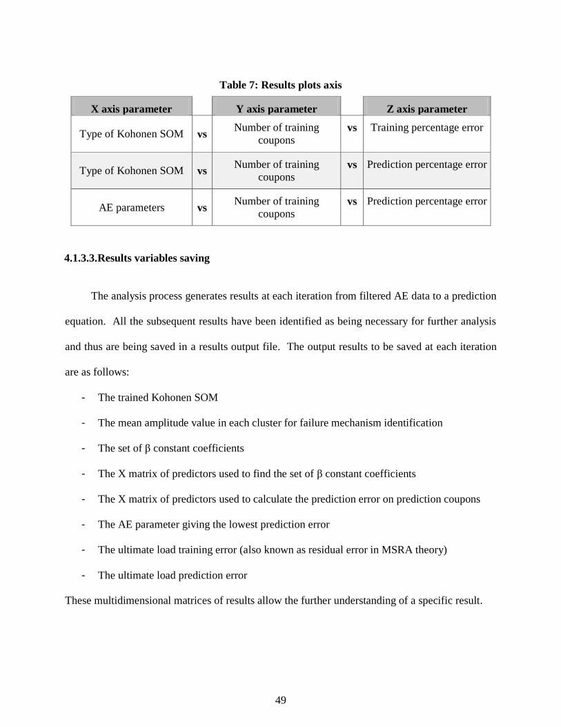
49
Table 7: Results plots axis
X axis parameter Y axis parameter Z axis parameter
Type of Kohonen SOM vs Number of training
coupons vs Training percentage error
Type of Kohonen SOM vs Number of training
coupons vs Prediction percentage error
AE parameters vs Number of training
coupons vs Prediction percentage error
4.1.3.3. Results variables saving
The analysis process generates results at each iteration from filtered AE data to a prediction
equation. All the subsequent results have been identified as being necessary for further analysis
and thus are being saved in a results output file. The output results to be saved at each iteration
are as follows:
- The trained Kohonen SOM
- The mean amplitude value in each cluster for failure mechanism identification
- The set of β constant coefficients
- The X matrix of predictors used to find the set of β constant coefficients
- The X matrix of predictors used to calculate the prediction error on prediction coupons
- The AE parameter giving the lowest prediction error
- The ultimate load training error (also known as residual error in MSRA theory)
- The ultimate load prediction error
These multidimensional matrices of results allow the further understanding of a specific result.
50
4.2. NOISE REMOVAL PROCESSES
The joint use of the acoustic emission technique and MSRA presupposes an almost entire
elimination of the AE data noise.
4.2.1. Noise removal by boundaries filtration
The data filtration process consists in a simple filtration by boundaries. This filtration is
applied before the AE data classification process begins. Practically, the AE data distribution
with respect to each AE parameter is visualized with all the coupons at once. The limits
under/above which the data points are really sparse and seem to be irrelevant with respect to the
specimen failure mechanisms are then determined. Determination of typical boundaries can be
seen on Figure 17. This figure is a three-dimensional plot where the energy distribution is
presented on the Y and Z axis while each X axis position contains AE hits of a single coupon,
thus creating a simultaneous visualization of all the coupons. A two dimensional view of such a
plot shows the data overlaps, allowing the user to define the domains of consistent AE data
versus the domains of noise.
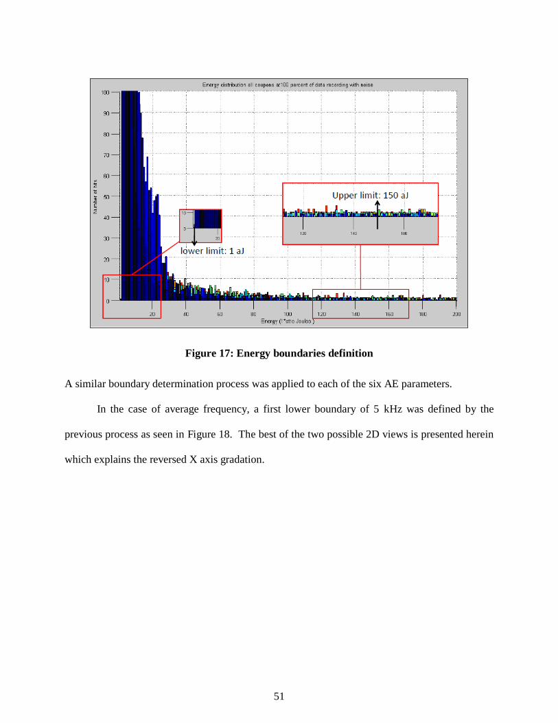
51
Figure 17: Energy boundaries definition
A similar boundary determination process was applied to each of the six AE parameters.
In the case of average frequency, a first lower boundary of 5 kHz was defined by the
previous process as seen in Figure 18. The best of the two possible 2D views is presented herein
which explains the reversed X axis gradation.

52
Figure 18: Average frequency boundaries definition
However, as it can be seen on Figure 18 a lower boundary of 5 kHz would leave a large
amount of noise still embedded in the useful data. Thus, further analysis was done in order to
determine precisely the lower average frequency boundary between noise and useful data.
A static noise test, where a coupon test was set up and acoustic emission recorded without
applying any compressive load, was performed previously [1]. The results of this static test are
presented in Figure 19.

53
Figure 19: Static noise test result [1]
It can be seen that the AE hits from the static noise due to the naturally noisy laboratory
environment (hydraulic machines, electromagnetic interference, external vibrations, etc.) were
captured when no compressive load was applied. This static noise can be identified by its
characteristic low average frequency (low counts and long durations). This test suggests that any
data point having an average frequency below 18 kHz is probably noise.
However, as can be seen in Figure 18, a lower limit of 18 kHz would still leave a part of
the noise data in the resulting data set. This extra noise may be due to either the friction between
the clamping edges of the compression machines and the specimen or the hydraulic pistons in the
actuator. A higher value of average frequency lower limit of 45 kHz was determined to improve
the prediction results, as will be explained later on.
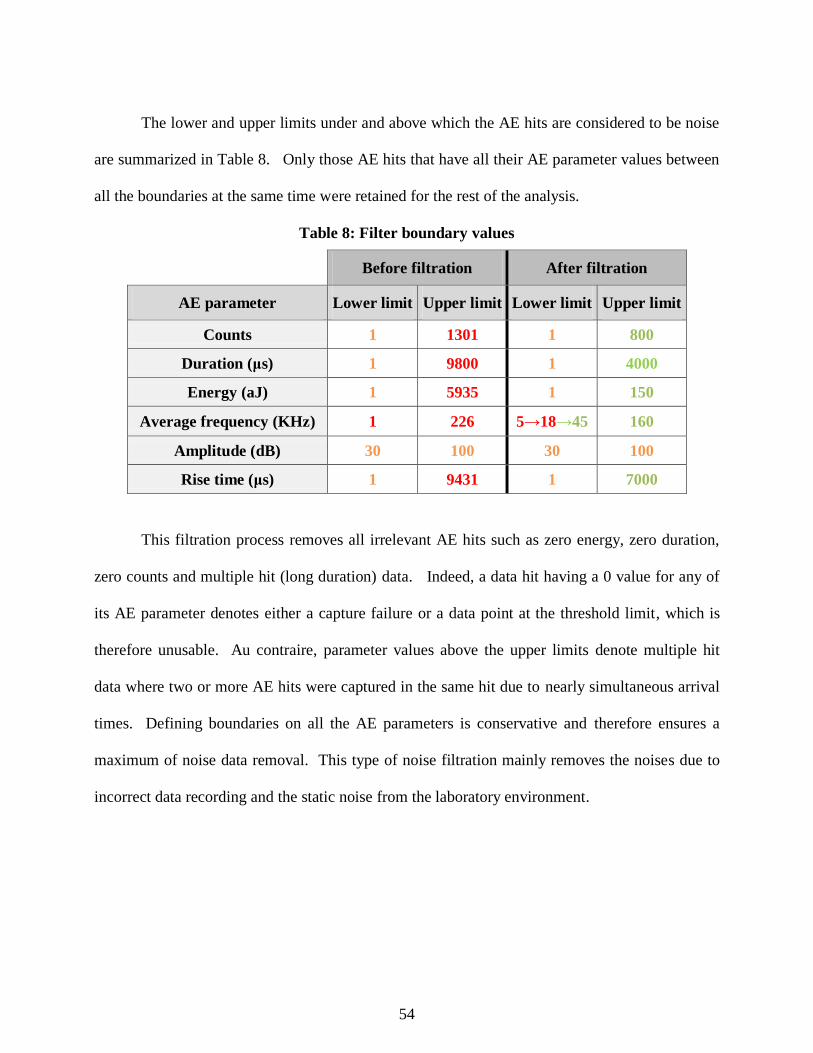
54
The lower and upper limits under and above which the AE hits are considered to be noise
are summarized in Table 8. Only those AE hits that have all their AE parameter values between
all the boundaries at the same time were retained for the rest of the analysis.
Table 8: Filter boundary values
Before filtration After filtration
AE parameter Lower limit Upper limit Lower limit Upper limit
Counts 1 1301 1 800
Duration (μs) 1 9800 1 4000
Energy (aJ) 1 5935 1 150
Average frequency (KHz) 1 226 5→18→45 160
Amplitude (dB) 30 100 30 100
Rise time (μs) 1 9431 1 7000
This filtration process removes all irrelevant AE hits such as zero energy, zero duration,
zero counts and multiple hit (long duration) data. Indeed, a data hit having a 0 value for any of
its AE parameter denotes either a capture failure or a data point at the threshold limit, which is
therefore unusable. Au contraire, parameter values above the upper limits denote multiple hit
data where two or more AE hits were captured in the same hit due to nearly simultaneous arrival
times. Defining boundaries on all the AE parameters is conservative and therefore ensures a
maximum of noise data removal. This type of noise filtration mainly removes the noises due to
incorrect data recording and the static noise from the laboratory environment.

55
4.3. DATA CLUSTERING
4.3.1. Use of Kohonen self-organizing maps
The heterogeneous and brittle nature of a composite materials leads to a complex process
of progressive failure of the material when subjected to an external compressive load. Moreover,
the type of material considered in the present application has been damaged by low velocity
impacts. A certain failure process has thus been initiated by suddenly compressing the fiber
layers and inevitably breaking some of the fibers in the impact area. Furthermore, it is known
that in composite materials under compression, the material‟s response will be due both to the
matrix and the fiber mechanical properties. In tension, the material properties will mainly appeal
to the fiber‟s properties. Several failure mechanisms are nowadays known from the extensive
study of the composite material failure that has been conducted for years [14-16]. These failure
mechanisms are based, on one hand, on the failure of the matrix itself, particularly present in a
case of material compression and, on another hand, on the failure of the fibrous phase present in
the material. Also, failure occurs at the fiber/matrix interface. A nonexhaustive list of the
principal failure mechanisms appearing in composite materials subjected to an external load is
presented in Table 9 [1, 14-17].
The presence of such failure mechanisms and their magnitude is believed to be strongly
related to the ultimate failure of the compressed specimens. In other words, if the presence and
magnitude of such failure mechanisms could be extracted from the collected AE data, their
individual influence on the failure load of the specimen would be reflected by the coefficients of
the MSRA ultimate load prediction equation.

56
Table 9: Failure mechanisms in composite materials
Domain Failure
mechanism Sources
AE Hit Characteristics [1, 17]
Amplitude Duration Energy
Fiber Fiber breaks
Localized stress concentration
around fibers
Brittleness of the fiber
Load redistribution from
adjacent broken fibers
High Short High
Matrix
Matrix
longitudinal
cracking
Stress concentration between
the fibers
Matrix brittleness
Low Long Low-
Medium
Matrix
transverse
cracking
Stress concentration
Matrix brittleness Low Short Low
Fiber-
Matrix
Interface
Delamination
Inter laminar tension
Inter laminar shear
Transverse and longitudinal
matrix cracks joining
Medium Medium
Long
Medium-
High
Fiber pullout Matrix / fiber disbonding High Short High
The Kohonen SOM is used in the present case to classify the AE data collected from the
specimen testing into the various failure mechanisms present. As has been previously explained,
a Kohonen SOM has to be trained in order to be an effective classification tool. The specimens
are divided into two groups: a group of training coupons and a group of prediction coupons. The
training coupons‟ AE data are used to train the Kohonen SOM by presenting them all at once to
iteratively train the network until convergence of the classifications. The convergence of a
Kohonen SOM can be set as a maximum number of iterations, a time limit, or a maximum weight
change criterion.
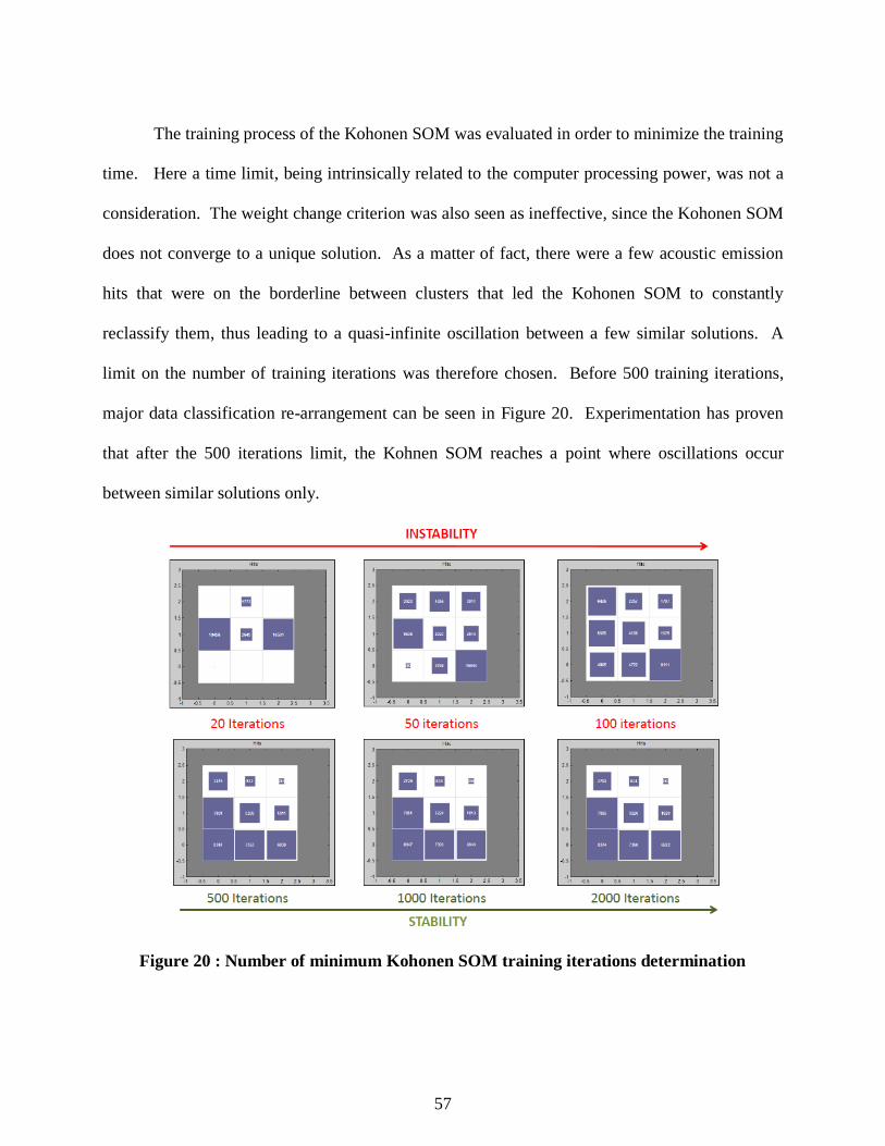
57
The training process of the Kohonen SOM was evaluated in order to minimize the training
time. Here a time limit, being intrinsically related to the computer processing power, was not a
consideration. The weight change criterion was also seen as ineffective, since the Kohonen SOM
does not converge to a unique solution. As a matter of fact, there were a few acoustic emission
hits that were on the borderline between clusters that led the Kohonen SOM to constantly
reclassify them, thus leading to a quasi-infinite oscillation between a few similar solutions. A
limit on the number of training iterations was therefore chosen. Before 500 training iterations,
major data classification re-arrangement can be seen in Figure 20. Experimentation has proven
that after the 500 iterations limit, the Kohnen SOM reaches a point where oscillations occur
between similar solutions only.
Figure 20 : Number of minimum Kohonen SOM training iterations determination

58
The state of the classification can be visually followed while the data were being
classified into 9 different clusters, the colored square dimensions in each cluster being
proportional to the number of AE data points it contained. (Example parameters: 9 Kohonen
SOM output clusters, 40% of recorded data, 18 training coupons.)
The best combination of AE parameters to be used as input parameters for the Kohonen
SOM was researched through numerous trials. It was found that the AE parameters amplitude,
duration, and energy gave the best results when used in combination. Also, in order to ensure no
domination of one classification parameter over the other ones, the order of the AE classification
parameters inputs were changed. As had been hoped, changing the order yielded the same
classification results. Once the Kohonen SOM was trained to classify AE data using the training
coupon data, each training and prediction coupon were then presented to the network individually
for classification.
4.3.2. Failure mechanisms identification
The goal of the previously detailed classification process was to neatly separate the AE hits
generated by several failure mechanisms of the material based on their acoustic emission
parameter signatures. The following four tables present the characteristics of each Kohonen
SOM using 4 output clusters for respectively the energy, duration, amplitude and average
frequency of the contained data points. The said data points are the data points of the training
coupons used to train the Kohonen SOM.

59
Table 10: Kohonen SOM 4 output clusters parameters: Energy (aJ)
Mechanism # Cluster # Min value Max value Mean value Standard deviation # of Hits
1 2 1 18 1.60 1.08 28794
2 4 1 61 5.28 4.35 11007
3 3 3 149 14.68 14.97 3240
4 1 5 148 26.78 22.03 1323
Table 11: Kohonen SOM 4 output clusters parameters: Duration (μs)
Mechanism # Cluster # Min value Max value Mean value Standard deviation # of Hits
1 2 124 581 370.37 102.89 28794
2 4 582 1186 792.86 163.15 11007
3 3 1187 2264 1580.70 291.70 3240
4 1 2266 3999 2951.54 489.04 1323
Table 12: Kohonen SOM 4 output clusters parameters: Amplitude (dB)
Mechanism # Cluster # Min value Max value Mean value Standard deviation # of Hits
1 2 34 68 46.41 4.52 28794
2 4 33 78 51.28 6.56 11007
3 3 33 87 56.05 7.83 3240
4 1 33 85 59.01 8.12 1323
Table 13: Kohonen SOM 4 output clusters parameters: Average frequency (KHz)
Mechanism # Cluster # Min value Max value Mean value Standard deviation # of Hits
1 2 45 160 72.63 17.62 28794
2 4 45 151 63.85 12.91 11007
3 3 45 138 63.54 12.64 3240
4 1 45 156 63.88 11.98 1323
According to the cluster characteristics presented in Table 11, the Kohonen SOM
classifies the AE hits in layers of duration. As seen in Tables 10 and 12, this classification
separated these AE hits into clusters that ranged from low to high values of energy and
amplitude. In order to identify the failure mechanism associated with these groups of AE data,
two approaches were used. The first one was to analyze the level of energy of the AE hits
contained in each cluster. Using Table 9, it is understood that an increasing level of energy

60
classifies the failure mechanisms in the following order: matrix cracking, crack coupling,
delamination and fiber breaks. A second approach to identify the nature of the AE hits contained
in the four clusters was to observe their distribution as a function of loading [18]. Figure 21
presents the normalized evolution of the number of AE hits contained in each cluster with respect
to the percentage of data recording, where failure occurs at 100%.
Figure 21: Failure mechanisms distribution through loading
The failure mechanism distributions presented above clearly show two different trends.
The failure mechanism 1 presence increases throughout the loading until 70% of the failure load
is reached and then decreases past this point until failure. The behavior of these low energy AE
hits can be identified as matrix cracking. Failure mechanisms 2, 3 and 4 show an opposite trend.
These mechanisms decrease constantly after an abrupt initial jump until 60-70% of loading is

61
reached; after that, these mechanisms tend to become more active as failure progresses to
complete coupon failure. The behavior of these medium to high energy AE hits is associated
with the remaining three failure mechanisms: crack coupling, delamination and fiber breaks. It
can also be seen that the two main failure mechanisms that drastically increase at the approach of
failure (and therefore are responsible for failure) are delamination and fiber breaks.
Tables 14 through 17 present the Kohonen SOM output cluster characteristics with
respect to energy, duration, amplitude and average frequency when a classification into 9 clusters
is made.
Table 14: Kohonen SOM 9 output clusters parameters: Energy (aJ)
Mechanism # Cluster # Min value Max value Mean value Standard deviation # of Hits
1
3 1 5 1.13 0.38 13280
6 1 10 1.76 1.05 11674
2 1 24 3.17 2.12 7986
2 9 1 52 5.39 3.95 4643
5 2 61 8.57 6.62 2766
3 1 3 105 13.04 12.29 1663
8 4 149 19.84 19.65 1045
4 4 5 148 24.12 21.30 771
7 7 148 30.60 22.59 536
Table 15: Kohonen SOM 9 output clusters parameters: Duration (μs)
Mechanism # Cluster # Min value Max value Mean value Standard deviation # of Hits
1
3 124 348 278.30 45.89 13280
6 349 504 418.98 44.42 11674
2 505 699 590.17 55.55 7986
2 9 700 948 808.50 70.57 4643
5 949 1279 1089.28 95.05 2766
3 1 1280 1711 1469.01 123.08 1663
8 1711 2279 1951.44 160.99 1045
4 4 2281 3035 2607.94 219.04 771
7 3039 3999 3466.05 269.78 536

62
Table 16: Kohonen SOM 9 output clusters parameters: Amplitude (dB)
Mechanism # Cluster # Min value Max value Mean value Standard deviation # of Hits
1
3 34 62 45.67 3.51 13280
6 34 67 46.57 4.88 11674
2 34 72 49.16 5.85 7986
2 9 33 78 51.51 6.49 4643
5 33 77 53.80 7.00 2766
3 1 40 81 55.56 7.65 1663
8 37 87 57.66 8.31 1045
4 4 33 83 58.60 8.09 771
7 33 85 59.57 8.11 536
Table 17: Kohonen SOM 9 output clusters parameters: Average frequency (KHz)
Mechanism # Cluster # Min value Max value Mean value Standard deviation # of Hits
1
3 45 159 79.43 18.20 13280
6 45 160 67.30 14.94 11674
2 45 151 64.78 13.77 7986
2 9 45 131 63.61 12.71 4643
5 45 110 63.73 12.76 2766
3 1 45 138 63.07 12.53 1663
8 45 132 63.79 12.51 1045
4 4 45 108 63.77 11.78 771
7 45 156 63.89 12.06 536
According to the maximum and minimum energy, duration, and amplitude values of the 9
clusters, it can be seen that increasing the number of output clusters appears to subdivide the
previously presented 4 clusters in subgroups. An association of the output clusters with their
appropriate failure mechanism can thus be determined. This cluster identification is summarized
in Table 18.
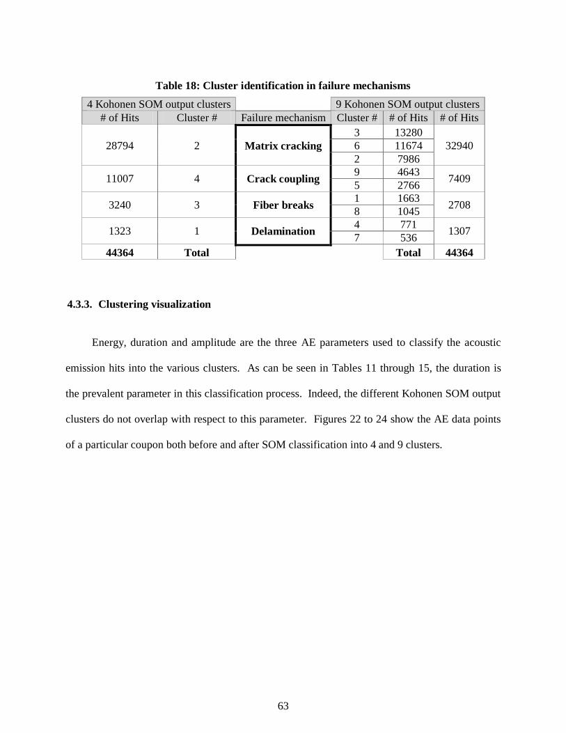
63
Table 18: Cluster identification in failure mechanisms
4 Kohonen SOM output clusters 9 Kohonen SOM output clusters
# of Hits Cluster # Failure mechanism Cluster # # of Hits # of Hits
28794 2 Matrix cracking
3 13280
32940 6 11674
2 7986
11007 4 Crack coupling 9 4643
7409 5 2766
3240 3 Fiber breaks 1 1663
2708 8 1045
1323 1 Delamination 4 771
1307 7 536
44364 Total Total 44364
4.3.3. Clustering visualization
Energy, duration and amplitude are the three AE parameters used to classify the acoustic
emission hits into the various clusters. As can be seen in Tables 11 through 15, the duration is
the prevalent parameter in this classification process. Indeed, the different Kohonen SOM output
clusters do not overlap with respect to this parameter. Figures 22 to 24 show the AE data points
of a particular coupon both before and after SOM classification into 4 and 9 clusters.
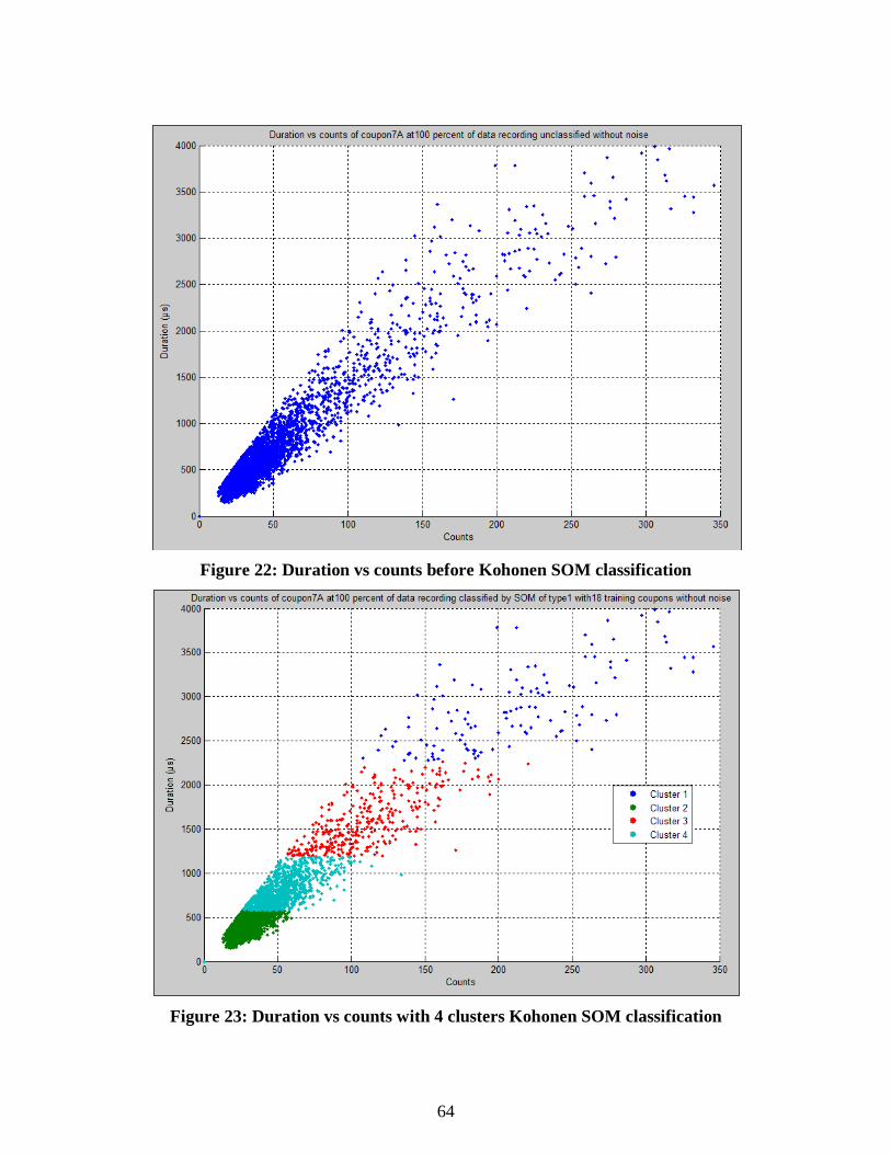
64
Figure 22: Duration vs counts before Kohonen SOM classification
Figure 23: Duration vs counts with 4 clusters Kohonen SOM classification

65
Figure 24: Duration vs counts with 9 clusters Kohonen SOM classification
As can be seen in Figures 22 through 24, the AE data are divided in layers of duration
from shortest to longest. The limits between these different clusters are then determined by the
other two classification parameters, amplitude and energy. Figures 25 to 27 show more clearly
how the AE data are separated between the classification parameters in a three dimensional
space.

66
Figure 25: Amplitude vs Energy vs Duration of non-classified AE data
Figures 26 and 27 show how the AE data are separated in clusters ranging gradually from
low amplitude, low energy and short duration to high amplitude, high energy and long duration.
This can also be seen in Tables 10 to 12 and 14 to 16 where the clusters are sorted according to
their ascending mean value of energy, amplitude and duration, respectively. The constant order
of the clusters seen in the first column of these tables indicates that the classification process
generates groups of AE data neatly separated from each other, which is what is seen in the figures
as well.

67
Figure 26: Amplitude vs Energy vs Duration of AE data classified in 4 clusters
Figure 27: Amplitude vs Energy vs Duration of AE data classified in 9 clusters
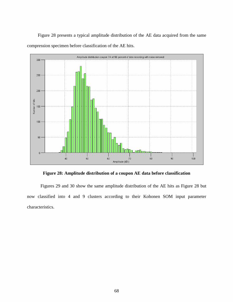
68
Figure 28 presents a typical amplitude distribution of the AE data acquired from the same
compression specimen before classification of the AE hits.
Figure 28: Amplitude distribution of a coupon AE data before classification
Figures 29 and 30 show the same amplitude distribution of the AE hits as Figure 28 but
now classified into 4 and 9 clusters according to their Kohonen SOM input parameter
characteristics.

69
Figure 29: Amplitude distribution of a coupon AE hits after classification into 4 clusters
Figure 30: Amplitude distribution of a coupon AE hits after classification into 9 clusters

70
In these two representations (Figures 29 and 30) the overlap between the failure mechanism
clusters becomes obvious, which reinforces the idea that AE data classification without using a
multi-input Kohonen SOM is impractical as the number of AE hits becomes large. It should be
brought to the reader‟s attention that the cluster data coloration is an automatic feature in the
software; thus, the color coding for the various failure mechanisms is not consistent between
Figures 29 and 30. It is also important to understand that the random weight initialization of the
Kohonen SOM converges to equivalent final classifications, where clusters containing similar
data points are adjacent, but due to output map vertical and horizontal symmetry, four different
AE data cluster/physical cluster associations are possible. In practice this leads to similar
solutions with different cluster numbering when a Kohonen SOM is repeatedly used. Tracking of
the cluster number and the type of data contained therein must then be employed.

71
4.4. APPLIED MULTIVARIATE STATISTICAL REGRESSION ANALYSIS
As has been mentioned before, the MSRA is a statistical tool that is highly sensitive to
noisy data. Its use is then recommended when the acoustic emission hits due to noise have been
completely removed. After the previously described filtration process, the AE data are
considered to be cleaned of the noise recorded during the data acquisition process.
The matrices used to feed the MSRA process are generated at this point. The first type of
matrix to be generated is the matrix of response variables denoted as Y in Equation 6. Two
matrices are generated, one containing the training coupons‟ ultimate failure loads and a second
one containing the prediction coupons‟ ultimate failure loads according to the current groups of
training and prediction coupons. An example of this first type of matrix is presented in Table 14
for a set of 18 training coupons.
Table 19: Example of response variables matrix
Coupon Number Coupon identification number Impact energy (J) Ultimate failure load (lbf)
1 1A 8 22583
2 2A 8 24498
5 5A 10 19916
8 10A 13 18163
9 11A 13 17226
10 13A 14 18660
11 14A 14 20975
12 16A 15 17410
13 17A 15 16685
14 19A 16 15805
17 23A 18 17322
19 24A 10 24195
22 24D 20 17250
24 25B 12 21749
26 25D 12 17249
28 26B 16 20833
29 26C 18 20729
30 26D 20 20024
Y matrix
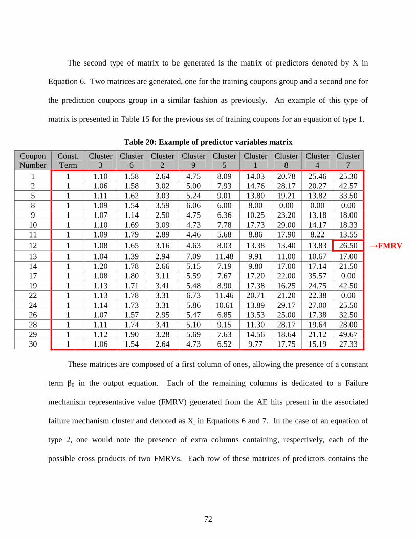
72
The second type of matrix to be generated is the matrix of predictors denoted by X in
Equation 6. Two matrices are generated, one for the training coupons group and a second one for
the prediction coupons group in a similar fashion as previously. An example of this type of
matrix is presented in Table 15 for the previous set of training coupons for an equation of type 1.
Table 20: Example of predictor variables matrix
Coupon
Number
Const.
Term
Cluster
3
Cluster
6
Cluster
2
Cluster
9
Cluster
5
Cluster
1
Cluster
8
Cluster
4
Cluster
7
1 1 1.10 1.58 2.64 4.75 8.09 14.03 20.78 25.46 25.30
2 1 1.06 1.58 3.02 5.00 7.93 14.76 28.17 20.27 42.57
5 1 1.11 1.62 3.03 5.24 9.01 13.80 19.21 13.82 33.50
8 1 1.09 1.54 3.59 6.06 6.00 8.00 0.00 0.00 0.00
9 1 1.07 1.14 2.50 4.75 6.36 10.25 23.20 13.18 18.00
10 1 1.10 1.69 3.09 4.73 7.78 17.73 29.00 14.17 18.33
11 1 1.09 1.79 2.89 4.46 5.68 8.86 17.90 8.22 13.55
12 1 1.08 1.65 3.16 4.63 8.03 13.38 13.40 13.83 26.50 →FMRV
13 1 1.04 1.39 2.94 7.09 11.48 9.91 11.00 10.67 17.00
14 1 1.20 1.78 2.66 5.15 7.19 9.80 17.00 17.14 21.50
17 1 1.08 1.80 3.11 5.59 7.67 17.20 22.00 35.57 0.00
19 1 1.13 1.71 3.41 5.48 8.90 17.38 16.25 24.75 42.50
22 1 1.13 1.78 3.31 6.73 11.46 20.71 21.20 22.38 0.00
24 1 1.14 1.73 3.31 5.86 10.61 13.89 29.17 27.00 25.50
26 1 1.07 1.57 2.95 5.47 6.85 13.53 25.00 17.38 32.50
28 1 1.11 1.74 3.41 5.10 9.15 11.30 28.17 19.64 28.00
29 1 1.12 1.90 3.28 5.69 7.63 14.56 18.64 21.12 49.67
30 1 1.06 1.54 2.64 4.73 6.52 9.77 17.75 15.19 27.33
These matrices are composed of a first column of ones, allowing the presence of a constant
term β0 in the output equation. Each of the remaining columns is dedicated to a Failure
mechanism representative value (FMRV) generated from the AE hits present in the associated
failure mechanism cluster and denoted as Xi in Equations 6 and 7. In the case of an equation of
type 2, one would note the presence of extra columns containing, respectively, each of the
possible cross products of two FMRVs. Each row of these matrices of predictors contains the

73
FMRV of one training/prediction coupon and their cross products if an equation of type 2 is
desired.
An investigation has been conducted in order to determine the best manner to represent the
presence of the failure mechanism through its FMRV. It is understood that these values are to be
calculated from the available AE data in the failure mechanisms clusters. Three possibilities have
been attempted. The first possibility was to simply sum up the values of the considered AE
parameters from the AE hits present in a failure mechanism. For example, in the case where the
energy is studied, the FMRV would be the summation of the energies released by all the AE hits
present in a specific failure mechanism. This calculation of FMRV is described by Equation 14.
Equation 14: MSRA equation of type 2
where
FMRV is the Failure Mechanism Representative Variable
i is the current failure mechanism
j is the current coupon
n is the number of AE data points in the mechanism i of the coupon j
X is the value of the used AE parameter for the current AE hit.
Unfortunately, this method suffered from the fact that the amount and level of captured AE data
varies widely for the different coupons. The data feeding the MSRA were therefore too scattered.
A second possibility was to attenuate the data dispersion by normalizing the FMRV within
each coupon. This was done by dividing the aforementioned FMRV of each cluster by the
summation of the FMRV throughout all the failure mechanisms. Following the previous
example, in the case where the energy is studied, the FMRV of a particular mechanism would be
the total amount of energy released in the failure mechanism divided by the total amount of

74
energy released by the coupon through all its failure mechanisms. This calculation of FMRV is
described by Equation 15.
Equation 15: MSRA equation of type 2
where
FMRV is the Failure Mechanism Representative Variable
i is the current failure mechanism
j is the current coupon
n is the number of AE data points in the mechanism i of the coupon j
m is the number of failure mechanisms
X is the value of the used AE parameter for the current AE hit.
This method generated FMRVs between 0 and 1, thus damping the difference of acoustic
emissions captured throughout the coupons. However, having values very close to each other
proved to be confusing to the MSRA.
A third solution was then adopted. This last solution consisted in taking the average value
of the AE hits in each of the failure mechanisms. Following the same example as before, the
mean energy of the AE hits contained in a failure mechanism was used as the FMRV. This
calculation of FMRV is described by Equation 16.
Equation 16: MSRA equation of type 2
where
FMRV is the Failure Mechanism Representative Variable
i is the current failure mechanism
j is the current coupon
n is the number of AE data points in the mechanism i of the coupon j
X is the value of the used AE parameter for the current AE hit.

75
This last solution has the advantage of damping the differences in the level of acoustic emission
captured (i.e., the number of AE hits) without bringing the FMRVs too close to each other such
that the MSRA analysis was still applicable.
Once the required matrices were generated, the pair of response and predictor training
matrices were used to feed a MSRA which generated the set of β coefficients following Equation
12. Table 16 presents the set of β coefficients calculated using the MSRA on the particular
example previously presented through the predictor and response variables matrices.
Table 21: β coefficients example set
β coefficients
Constant term 25465
Cluster 3 coefficient -10127
Cluster 6 coefficient -791
Cluster 2 coefficient 3723
Cluster 9 coefficient -1795
Cluster 5 coefficient 329
Cluster 1 coefficient -95
Cluster 8 coefficient -23
Cluster 4 coefficient 104
Cluster 7 coefficient 82
The residual training errors (or residual errors) were then calculated using the training
matrices and following Equation 13. Similarly, prediction errors were determined using the
prediction matrices. This error is representative of the error between the predicted ultimate loads
and the actual ultimate loads of the prediction coupons and will be known as prediction errors.
The worst case error will be observed in both the training and the prediction errors. The goal of
this research was to determine the conditions to obtain a worst case prediction error within the B-
basis allowables for composite materials. The errors were expressed as signed percentage errors
in order to know if the prediction overestimated or underestimated the failure load.

76
It is also important to note that during this analysis process the prediction coupon AE data
were only used to evaluate the prediction error and were not involved at any point in the training
of the Kohonen SOM or in the determination of the βi coefficients in the prediction equation.
Table 17 summarizes the results that were obtained once the MSRA was applied in the given
example.
Table 22: MSRA results example
Training Prediction
Coupon n
um
ber
Act
ual
fai
lure
load
(lb
f)
Pre
dic
ted f
ailu
re l
oad
(lb
f)
Per
centa
ge
of
trai
nin
g e
rror
Coupon n
um
ber
Act
ual
fai
lure
load
(lb
f)
Pre
dic
ted f
ailu
re l
oad
(lb
f)
Per
centa
ge
of
pre
dic
tion e
rror
1 22583 19933 -11.74 3 20162 19098 -5.28
2 24498 21937 -10.45 4 19175 23557 22.86
5 19916 20173 1.29 6 20434 19796 -3.12
8 18163 16937 -6.75 7 20827 22720 9.09
9 17226 17980 4.38 15 16734 19688 17.65
10 18660 19212 2.96 16 19503 17536 -10.08
11 20975 18365 -12.44 18 22470 21620 -3.78
12 17410 21301 22.35 20 19782 20115 1.69
13 16685 17150 2.79 21 17944 17543 -2.24
14 15805 17186 8.74 23 21815 20070 -8.00
17 17322 18723 8.09 25 20010 16693 -16.58
19 24195 22493 -7.04 27 22190 20797 -6.28
22 17250 16500 -4.35 31 20255 19298 -4.72
24 21749 20741 -4.64 32 18825 18991 0.88
26 17249 19448 12.75 33 18986 21125 11.27
28 20833 22041 5.80 34 18742 20385 8.77
29 20729 21634 4.37 R2 = 0.0751
30 20024 19522 -2.51
R2 = 0.5352

77
Figures 27 and 28 help to visualize the distribution of actual and predicted failure loads of the
training and prediction coupons sets, respectively.
Figure 31: Training coupons predicted loads distribution
± 15% interval

78
Figure 32: Prediction coupons predicted loads distribution
After testing of each of the six AE hit parameters, it was determined that the average
energy released in each failure mechanisms was the best FMRV to use for ultimate load
prediction. Also, it should be mentioned that an equation of type 2 (where cross products of
FMRV appears) is not suitable when a high number of Kohonen SOM output cluster is used. For
example, when the recorded AE data are classified into 9 clusters, the number of βi coefficients
would increase from 10 to 46. The minimum number of training coupons required to apply
MSRA would, in that case, be 48, which is greater than the available number of coupons.

79
CHAPTER 5 :RESULTS
5.1. B-basis allowables
The B-basis allowables are defined for a composite as being the interval within which 90% of
the population of specimens will fall with a confidence level of 95%. This interval is dependent
upon the number of specimens and the standard deviation of the failure loads in a test group (i.e.,
impact energy group) and can be determined using Equation 17.
Equation 17: MSRA equation of type 2
where
Interval is the failure load allowable interval
P is the fraction of population
C is the confidence level
N is the number of samples in the considered group
SX is the standard deviation of the considered group
K factor is a tabulated value dependent upon the N, P and C parameters.
The allowable interval is calculated separately for each of the energy impact groups.
Given the low number of coupons available per energy group, the B-basis allowables will be
large. Table 18 presents the results of the B-basis allowable calculations.
Table 23: B-basis allowable calculations
Impact
Energy
(J)
Number
of
coupons
Mean
failure load
(lbf)
Standard
deviation
Sx
K
factor
B-basis
allowables
(lbf)
Upper limit
(lbf)
Lower limit
(lbf)
8 2 23540.50 1354.11 18.80 ±25457.26 48997.76 -1916.76
10 6 21791.33 1585.52 3.72 ±5902.87 27694.21 15888.46
12 5 20008.20 1699.01 4.15 ±7054.27 27062.47 12953.93
13 2 17694.50 662.56 18.80 ±12456.11 30150.61 5238.39
14 2 19817.50 1636.95 18.80 ±30774.70 50592.20 -10957.20
15 2 17047.50 512.65 18.80 ±9637.87 26685.37 7409.63
16 6 18147.17 1763.58 3.72 ±6565.80 24712.97 11581.36
18 6 19467.50 1211.79 3.72 ±4511.48 23978.98 14956.02
20 3 18816.33 1421.36 6.92 ±9834.36 28650.69 8981.98
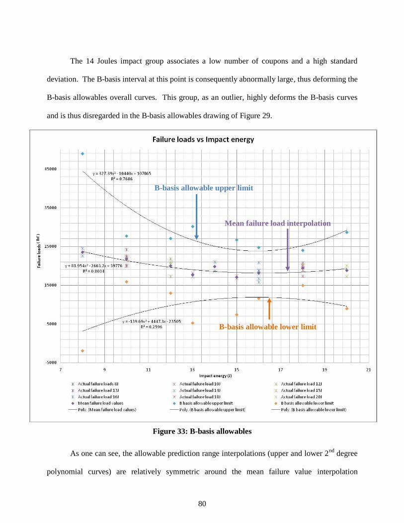
80
The 14 Joules impact group associates a low number of coupons and a high standard
deviation. The B-basis interval at this point is consequently abnormally large, thus deforming the
B-basis allowables overall curves. This group, as an outlier, highly deforms the B-basis curves
and is thus disregarded in the B-basis allowables drawing of Figure 29.
Figure 33: B-basis allowables
As one can see, the allowable prediction range interpolations (upper and lower 2nd
degree
polynomial curves) are relatively symmetric around the mean failure value interpolation
( lb
f )
B-basis allowable upper limit
B-basis allowable lower limit
Mean failure load interpolation

81
polynomial. A minimum interval is found at the 16 Joules impact group. Table 19 presents the
percentage interval error between the various mean failure loads and the B-basis interpolations.
Table 24: B-basis allowables percentage error
Impact
energy
(J)
Mean failure
value
interpolation
(lbf)
Upper limit
interpolation value
(lbf)
Lower limit
interpolation
value (lbf)
Percentage
error upper
limit (%)
Percentage
error lower
limit (%)
8 23715.456 44497.96 3133.24 87.63 -86.79
10 21339.4 35404 6999 65.91 -67.20
12 19618.976 28929.16 9747.24 47.45 -50.32
13 19004.626 26673.91 10702.29 40.35 -43.69
14 18554.184 25073.44 11377.96 35.14 -38.68
15 18267.65 24127.75 11774.25 32.08 -35.55
16 18145.024 23836.84 11891.16 31.37 -34.47
18 18391.496 25219.36 11286.84 37.13 -38.63
20 19293.6 29221 9565 51.45 -50.42
Average 47.61 -49.53
Due to a really low number of coupons available in each of the impact energy groups, the
B-basis allowables determined here are quite broad. Indeed, the interval of allowable prediction
error is close to ±48% on average. Since an accurate prediction of the ultimate failure load is
sought in this research project, the B-basis allowables were artificially narrowed to a more
restrictive interval error by assuming that the number of coupons available in each of the impact
energy groups was 30 instead of the actual number available. It has to be noted that the
allowables converge with a high number of coupons through the convergence of the K factor.
The modified B-basis allowables were then determined following the previous process.
Table 20, Figure 30 and Table 21 present the modified B-basis calculations where 30 coupons per
impact energy group were assumed.
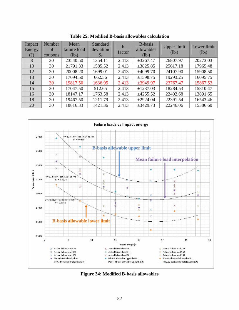
82
Table 25: Modified B-basis allowables calculation
Impact
Energy
(J)
Number
of
coupons
Mean
failure load
(lbf)
Standard
deviation
Sx
K
factor
B-basis
allowables
(lbf)
Upper limit
(lbf)
Lower limit
(lbf)
8 30 23540.50 1354.11 2.413 ±3267.47 26807.97 20273.03
10 30 21791.33 1585.52 2.413 ±3825.85 25617.18 17965.48
12 30 20008.20 1699.01 2.413 ±4099.70 24107.90 15908.50
13 30 17694.50 662.56 2.413 ±1598.75 19293.25 16095.75
14 30 19817.50 1636.95 2.413 ±3949.97 23767.47 15867.53
15 30 17047.50 512.65 2.413 ±1237.03 18284.53 15810.47
16 30 18147.17 1763.58 2.413 ±4255.52 22402.68 13891.65
18 30 19467.50 1211.79 2.413 ±2924.04 22391.54 16543.46
20 30 18816.33 1421.36 2.413 ±3429.73 22246.06 15386.60
Figure 34: Modified B-basis allowables
( lb
f )
B-basis allowable upper limit
Mean failure load interpolation
B-basis allowable lower limit
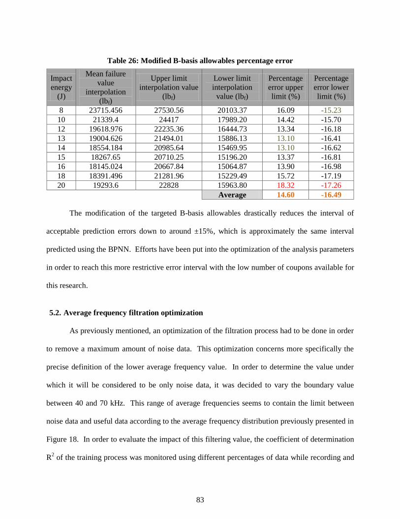
83
Table 26: Modified B-basis allowables percentage error
Impact
energy
(J)
Mean failure
value
interpolation
(lbf)
Upper limit
interpolation value
(lbf)
Lower limit
interpolation
value (lbf)
Percentage
error upper
limit (%)
Percentage
error lower
limit (%)
8 23715.456 27530.56 20103.37 16.09 -15.23
10 21339.4 24417 17989.20 14.42 -15.70
12 19618.976 22235.36 16444.73 13.34 -16.18
13 19004.626 21494.01 15886.13 13.10 -16.41
14 18554.184 20985.64 15469.95 13.10 -16.62
15 18267.65 20710.25 15196.20 13.37 -16.81
16 18145.024 20667.84 15064.87 13.90 -16.98
18 18391.496 21281.96 15229.49 15.72 -17.19
20 19293.6 22828 15963.80 18.32 -17.26
Average 14.60 -16.49
The modification of the targeted B-basis allowables drastically reduces the interval of
acceptable prediction errors down to around ±15%, which is approximately the same interval
predicted using the BPNN. Efforts have been put into the optimization of the analysis parameters
in order to reach this more restrictive error interval with the low number of coupons available for
this research.
5.2. Average frequency filtration optimization
As previously mentioned, an optimization of the filtration process had to be done in order
to remove a maximum amount of noise data. This optimization concerns more specifically the
precise definition of the lower average frequency value. In order to determine the value under
which it will be considered to be only noise data, it was decided to vary the boundary value
between 40 and 70 kHz. This range of average frequencies seems to contain the limit between
noise data and useful data according to the average frequency distribution previously presented in
Figure 18. In order to evaluate the impact of this filtering value, the coefficient of determination
R2 of the training process was monitored using different percentages of data while recording and

84
training on the minimum of 18 training coupons. The study of this influence is presented in
Figure 35.
Figure 35: Lower average frequency boundary optimization
It can first be concluded from these results that the lower average frequency boundary
value greatly affects the training efficiency. Indeed, the training coefficient of determination,
calculated between the actual and predicted failure loads of the training coupons, varies by 20%
over the average frequency range covered. As shown in Figure 31, 45 kHz was retained as the
value giving the maximum R2 training value most consistently throughout the percentage of data
recording used. This value of 45 kHz was then updated in the filtration process of the AE data as
previously shown in Table 8.

85
5.3. Number of Kohonen SOM clusters optimization
The number of Kohonen SOM output clusters also proved to be a crucial parameter that
significantly affected the prediction results. Great attention was brought to its optimization in
order to determine a value that both made physical sense and produced good results. Only four
main failure mechanisms are historically used: matrix cracking, crack coupling, delaminations
and fibers breaks. This led to the usual classification of the AE data into four Kohonen SOM
output clusters. Figure 32 presents the influence of the number of Kohonen SOM output clusters
on the training coefficient of determination or R2 value.
Figure 36: Number of Kohonen SOM ouput clusters influence study
A clear tendency can be observed in Figure 36: the higher the number of Kohonen SOM
output clusters, the higher the training R2 value. It can be surmised from the previous figure that
a number of clusters of 16, giving an R2 value close to one, is advantageous. However, this high
training R2 value suggests that the prediction equation is too tightly trained to predict the training

86
coupons failure loads using their AE data. This overtraining results in a drastic increase of the
prediction error when the previous equation is applied to the prediction coupons AE data. Thus a
lower number of Kohonen SOM output cluster was sought in order to give a maximum degree of
freedom between the training and the prediction AE data to decrease the prediction error. The
value of 9 Kohonen SOM output clusters was retained. This value corresponds to the minimum
number of clusters of the stabilized R2 region of the curve before overtraining began to occur.
5.4. B-basis allowables minimum conditions
The major goal of this research was to determine the minimum conditions required on
each of the identified variables affecting the results in order to reach a prediction precision within
the B-basis allowables which are typically applied to composites. The targeted B-basis
allowables for the prediction error was a ±15% error. The number of training coupons and the
type of Kohonen SOM were studied in order to determine the minimum conditions with respect
to each of these parameters to obtain a prediction error within the targeted B-basis allowables.
The absolute value of training and prediction worst case errors were followed with respect to
these parameters as well as the training and prediction R2 values. These R
2 value give an
estimation of the goodness of fit between the actual and predicted failure loads of the training and
prediction coupons sets.
5.4.1. Surface errors and R2 value trends
Constant trends were seen throughout the percentage of data recording used. The
following example presents the evolution of training and prediction errors and their associated R2
values when 50% of the data were used. Figures 37 and 38 present the training evolution with
respect to the type of Kohonen SOM used and the number of training coupons, while Figures 39
and 40 present the prediction evolution.

87
Figure 37: Absolute value of training worst case error evolution
As it can be seen in Figure 37, as the number of training coupons increases, the absolute
value of training error increases until stability is reached. This stabilization is visible when 27
training coupons or more are used; however, the absolute value of the training error remains
under 22% in the presented case. Table 27 presents the absolute value of the worst case training
error with respect to the percentage of recorded data used.
Table 27: Worst case training error
Percentage of AE data recording used 10% 30% 50% 70% 90%
Absolute value of worst case training error 28.49% 23.55% 21.59% 22.4% 24.58%
Type of SOM 7 6 10 9 9
Number of training coupons 20 23 26 24 25
From Table 27 it can be seen that starting as early as 30% of data recording, the training error
remains within a ±25% range.
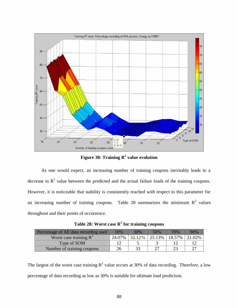
88
Figure 38: Training R2 value evolution
As one would expect, an increasing number of training coupons inevitably leads to a
decrease in R2 value between the predicted and the actual failure loads of the training coupons.
However, it is noticeable that stability is consistently reached with respect to this parameter for
an increasing number of training coupons. Table 28 summarizes the minimum R2 values
throughout and their points of occurrence.
Table 28: Worst case R2 for training coupons
Percentage of AE data recording used 10% 30% 50% 70% 90%
Worst case training R2 24.07% 32.12% 25.13% 18.57% 21.02%
Type of SOM 12 5 3 12 12
Number of training coupons 26 33 27 23 27
The largest of the worst case training R2 value occurs at 30% of data recording. Therefore, a low
percentage of data recording as low as 30% is suitable for ultimate load prediction.

89
Figure 39 presents the prediction error trend clearly identifiable throughout the use of an
increasing percentage recorded data.
Figure 39: Absolute value of prediction worst case error evolution
It has been constantly seen that the more training coupons used, the less the prediction error.
Also, the prediction error always decreases sufficiently to fall within the targeted prediction error
B-basis allowables of ±15%. Table 29 presents the minimum number of training coupons
necessary to predict within the modified B-basis allowables with respect to the percentage of
recorded data and the type of Kohonen SOM used.
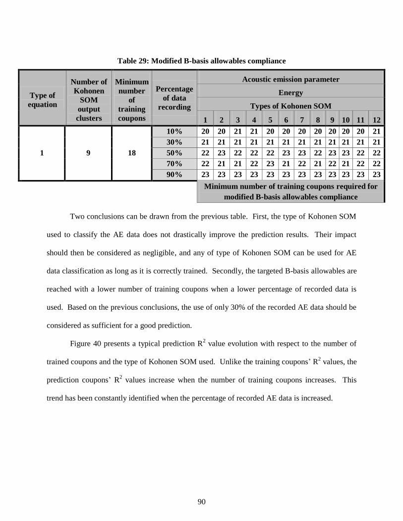
90
Table 29: Modified B-basis allowables compliance
Type of
equation
Number of
Kohonen
SOM
output
clusters
Minimum
number
of
training
coupons
Percentage
of data
recording
Acoustic emission parameter
Energy
Types of Kohonen SOM
1 2 3 4 5 6 7 8 9 10 11 12
1 9 18
10% 20 20 21 21 20 20 20 20 20 20 20 21
30% 21 21 21 21 21 21 21 21 21 21 21 21
50% 22 23 22 22 22 23 23 22 23 23 22 22
70% 22 21 21 22 23 21 22 21 22 21 22 22
90% 23 23 23 23 23 23 23 23 23 23 23 23
Minimum number of training coupons required for
modified B-basis allowables compliance
Two conclusions can be drawn from the previous table. First, the type of Kohonen SOM
used to classify the AE data does not drastically improve the prediction results. Their impact
should then be considered as negligible, and any of type of Kohonen SOM can be used for AE
data classification as long as it is correctly trained. Secondly, the targeted B-basis allowables are
reached with a lower number of training coupons when a lower percentage of recorded data is
used. Based on the previous conclusions, the use of only 30% of the recorded AE data should be
considered as sufficient for a good prediction.
Figure 40 presents a typical prediction R2 value evolution with respect to the number of
trained coupons and the type of Kohonen SOM used. Unlike the training coupons‟ R2 values, the
prediction coupons‟ R2 values increase when the number of training coupons increases. This
trend has been constantly identified when the percentage of recorded AE data is increased.

91
Figure 40: Prediction R2 value evolution
Table 30 presents the minimum number of training coupons to be used in order to reach a
prediction R2 value of 50% or more.
Table 30: Minimum number of training coupons for above 50% prediction R2
value
Percentage
of data
recording
Acoustic emission parameter
Energy
Types of Kohonen SOM
1 2 3 4 5 6 7 8 9 10 11 12
10% 26 26 26 26 26 26 26 26 26 26 26 26
30% 24 24 24 24 24 24 24 24 24 24 24 24
50% 27 27 26 27 27 26 27 27 26 26 27 27
70% 26 26 26 26 26 26 28 26 26 26 26 26
90% 32 32 32 32 29 29 32 32 31 32 31 31
92
As one can see, using only 30% of recorded AE data will allow a respectable prediction
R2 for a minimum number of training coupons and should be considered as the optimum
percentage of recorded AE data to use.
5.5. Optimized prediction equation
When the MSRA is applied to classified acoustic emission data, a certain physical meaning
is expected from the prediction equation coefficients. It has to be kept in mind that this
establishes the relationship between the representative values of a failure mechanism presence
and the ultimate load as recalled by Equation 18.
Equation 18: Output format of a MSRA equation of type 1
where
Fult is the compressive failure load
βi are constant terms determined by the MSRA
Mi are the failure mechanisms representative values (average energy of the AE hits
contained in the cluster )
The first constant coefficient β0 is an independent value setting a baseline value of the
failure load being subsequently affected by the presence of failure mechanisms increasing or
decreasing the failure load. It is then expected to obtain a set of βi either positive or negative with
respect to their influence on the failure load by respectively increasing it or decreasing each.
Also, the magnitude of the βi coefficients with respect to each other reflects the influence of the
associated failure mechanism on the failure load variation.
It has been previously determined that a prediction equation is optimized when only 30% of
the recorded AE data are classified into 9 clusters. Since impact of the type of Kohonen SOM
used to classify the recorded AE data is negligible, the Kohonen SOM of type 1 (orthogonal map,
Euclidian distance function) will be used in the following example.

93
Table 31 presents the prediction equations with respect to the number of training coupons.
The minimum number of training coupon presented is 21 which is the starting point of
predictions falling in the modified B-basis allowables of ±15%.

94
Table 31: Prediction equation sensitivity to number of training coupons
Number of training
coupons 21 22 23 24 25 26 27
Number of prediction
coupons 13 12 11 10 9 8 7
β0 34065 35468 36249 42522 42949 30948 35822
…
β3 -24026 -24997 -24866 -32039 -32407 -20197 -25096
β6 6247 6329 8550 9205 9416 7031 8944
β2 839 550 -1227 -717 -775 -185 -1107
β9 -716 -953 -854 -810 -924 -615 -682
β5 208 486 339 392 460 165 294
β1 -9 -88 73 -88 -100 46 18
β8 -25 -27 0 34 8 1 -10
β4 41 70 -7 14 44 3 24
β7 66 64 63 35 35 63 48
Worst case training
error (%) 17.66 18.53 23.27 16.17 17.24 19.78 21.69
R2 training value (%) 41.29 42.29 44.36 40.15 41.34 35.8 38.78
Worst case prediction
error (%) 12.55 11.33 -11.25 -7.64 -6.78 8.33 6.11
R2 prediction value
(%) 16.72 11.33 18.27 58.25 54.49 20.05 62.71
Number of training
coupons 28 29 30 31 32 33
Failure
Mechanism Number of prediction
coupons 6 5 4 3 2 1
β0 34334 32496 34820 33487 33591 34854 Constant coeff.
β3 -22712 -21489 -22760 -21634 -21880 -23145 Matrix cracking
coeff. β6 7075 7483 5928 5875 5998 6742
β2 -217 -369 865 984 779 141
β9 -794 -664 -1046 -998 -929 -829 Crack coupling
coeff. β5 255 231 342 287 277 264
β1 24 9 -106 -109 -80 -3 Fiber breaks
coeff. β8 -24 -4 -21 -15 -14 -21
β4 21 9 61 62 55 34 Delamination
coeff. β7 60 56 59 56 57 47
Worst case prediction
error (%) 19.77 18.42 19.34 18.82 18.38 18.95
R2 training value (%) 35.13 35.33 34.5 34.46 33.86 34.77
Worst case prediction
error (%) -5.72 -5.37 -3.96 -2.71 -1.49 -1.55
R2 prediction value
(%) 88.85 0.04 79.66 97.3 N/A N/A

95
Based on Table 31, it can be determined that using 24 training coupons is sufficient to
achieve low training and prediction errors while preserving relatively high training and prediction
R2 values. The worst case prediction error out of the remaining 10 prediction coupons will be at
that point of -7.64%, well within the targeted B-basis allowables.
The prediction tool can be considered optimized for the following conditions:
- 24 training coupons (10 remaining prediction coupons)
- Recorded AE data clustered into 9 clusters
- Use of only the first 30% of recorded AE data
- Type 1 prediction equation
- Average energy of AE hits contained in the cluster as the FMRV
Once the optimum set of equation coefficients have been determined, it is possible for
each coupon to calculate a prediction failure load. Indeed, each coupon released AE events that
have been filtered of the noise data and then classified by the optimized Kohonen SOM in 9
different clusters. Multiplying the 9 FMRV of a particular coupon by the set of equation
coefficients will give a prediction failure load. Equation 18 recalls the format of the prediction
equation while equation 19 shows such a calculation for the prediction coupon 4A.
Equation 19: Calculation example of a prediction failure load

96
Table 32 presents the actual and predicted failure loads of the training and predictions coupon
batches.
Table 32: Training and prediction errors

97
5.6. Type of MSRA equation influence
The influence of the two types of MSRA equations on the prediction accuracy can be
determined by comparing the prediction results at the optimized point. The two different types of
equation available when the MSRA method is applied have been presented as Equations 6 and 7.
The main difference is the presence or absence of the cross product of FMRV in the prediction
equation manifesting the physical correlation of the material failure mechanisms.
A large number of Kohonen SOM output cluster leads to a very high number of FMRV
cross products. If the MSRA is to be applied with 9 Kohonen SOM output clusters and a type of
MSRA prediction equation of type 2 (with presence of FMRV cross products), the required
number of training coupons will be of 47 as described by Equation 11. This number of required
training coupons exceeds the number of 34 available coupons and comparing the two types of
MSRA equations with the optimized number of Kohonen SOM output cluster of 9 is, in the
present case, impossible.
Thus, the comparison between the two types of MSRA prediction equations is done
between an MSRA equation of type 1 with 9 Kohonen SOM output clusters and an MSRA
equation of type 2 with 4 Kohonen SOM output clusters. The remaining analysis parameters are
kept at their respective optimum points. Table 33 presents the actual and predicted failure loads
of the training and predictions coupon batches when the second type of MSRA equation is used
with 4 Kohonen SOM output clusters.

98
Table 33: Training and prediction errors using a type 2 MSRA prediction equation

99
The use of the second type of MSRA equation leads to larger training and prediction
worst case errors than previously. Thus, it can be concluded that it is preferable to use an MSRA
equation of type 1 with a higher number (9) of Kohonen SOM output clusters than an MSRA
equation of type 2 with a fewer number (4) of Kohonen SOM output clusters.

100
CHAPTER 6 :CONCLUSIONS
6.1. SUMMARY
The goal of this research project was to prove the feasibility of combining the acoustic
emission technique and multivariate statistical regression analysis in order to accurately predict
the ultimate compressive failure load of impacted graphite/epoxy specimens. It was proven that
the combination of this nondestructive monitoring method and the developed data treatment
technique can lead to an accurate prediction of the ultimate failure load of the testing specimens
just outside the defined B-basis allowables for composite materials (±15% error). Here the worst
case prediction error of was found to be 16.17%.
The association of these two techniques remains subject to an important work on noise
elimination from the acoustic emission data. Indeed, the acoustic emission technique allows the
NDT engineer to record all the acoustic emission hits released by the loaded structure including a
large amount of noise. On the other hand, the multivariate statistical regression analysis
technique is highly sensitive to noise. Thus, emphasis was put on the optimization of the noise
filtration process in order to make feasible the joint use of these two techniques.
Furthermore, several parameters were identified as influencing greatly the prediction
results, and they should always be taken into consideration. The percentage of acoustic emission
data used, the number of training coupons, the AE parameters used as input to the Kohonen SOM
for failure mechanism classification, and the number of failure mechanism clusters used to
determine the ultimate load prediction equation are all crucial in the development of an accurate
prediction tool.

101
An optimum of 30% of the total amount of AE data collected until failure was determined
to be necessary for an accurate prediction. The duration, energy and the amplitude are the
acoustic emission parameters that are most likely to be used to successfully train the Kohonen
self-organizing maps to correctly classify the acoustic emission hits into the various failure
mechanisms. Also, the prediction accuracy is largely dependent upon the number of training
coupons used but not the type of Kohonen self organizing map neural network used. The mean
energy released throughout the AE hits of a failure mechanism cluster proved to be the best
failure mechanism representative value to be used in order to feed the multivariate statistical
regression analysis and establish an ultimate failure load prediction equation. In summary, the
overall analysis process described in the present research from the AE data capture until the
actual ultimate load prediction seems to provide a practical procedure leading to accurate
prediction results that should consequently be followed in the future.

102
6.2. PERSPECTIVES
It is thought that further research should be focusing on the ultimate load prediction of parts
of more complicated shapes. Since the MSRA process uses the similarities among the AE
patterns generated by similar loaded structures, it is believed that the ultimate loads should be
predicted as accurately as in the present research independently of the specimen geometrical
shape.
It is also believed that a next step in the analysis could be to detect outliers based on their
low level of acoustic emission and remove them from the batch of training coupon. If justified,
this outlier removal would have an effect of reducing the prediction error by removing directly
the worst cases. However, it was considered in this research that in order to test the robustness of
the method against the outlier data point, these particular low acoustic emission specimens should
be left in the batch of training and prediction coupons. Finally, it is desirable for further research
to produce a larger amount of test coupons in order to proof test the method on an industrial
scale.
6.3. RECOMMENDATIONS
The current data filtration process consists in removing any AE data having one of their AE
parameters outside of the defined boundaries. The limit between noise data and actual material
failure AE data being ambiguous particularly in terms of average frequency, it is possible to
improve the noise removal process by adding a second layer of data filtration. This second layer
of data filtration could involve a pre-classification of AE data using a Kohonen SOM with a noise
cluster identification and removal procedure. Once the optimization of this filtration layer is
done, the remaining noise free data could be used to feed the developed ultimate load prediction
process.
103
REFERENCES
1. Gunasekera, A.M., “Compression after impact load prediction in graphite/epoxy
laminates using acoustic emission and artificial neural networks.”, MSAE Thesis,
Embry-Riddle Aeronautical University, Daytona Beach, FL, 2009, pp. 22-33, 36-45,
55, 58-59.
2. Miller, R.K., Hill, E.v.K. and Moore, P.O. editors. Nondestructive testing handbook:
Acoustic emission testing, 3rd
edition, Vol 6, Columbus, Ohio: American Society for
Nondestructive Testing, 2005, pp. 32, 41-48, 52, 198-210, 360-376, 382-390.
3. Dorfman, M.D. “Ultimate strength prediction in fiberglass/epoxy beams subjected to
three-point bending using acoustic emission and neural networks.”, MSAE Thesis,
Embry-Riddle Aeronautical University, Daytona Beach, FL, 2004, pp. 36-43, 52-55.
4. Hill, E.v.K., Zhao, Y., Ebert, T., Kay, J.V. and Lewis, G.K. “Compression after impact
strength prediction in composites using acoustic emission and artificial neural
networks” 49th
AIAA/ASME/ASCE/AHS/ASC Structures, Structural Dynamics, and
Materials conference. 7-10 April 2008, Schaumburg, IL, AIAA 2008-2257.
5. Baker, A., Dutton, S., Kelly, D. “Composite materials for aircraft structures” 2nd
edition American Institute of Aeronautics and Astronautics Inc., VA, ISBN 1-56347-
540-5, 2004, pp. 128-131, 144, 157, 203-204, 482-485.
6. Physical Acoustic Corporation website, MISTRAS group Inc. Princeton, NJ.
http://www.pacndt.com
http://www.pacndt.com/index.aspx?go=products&focus=Pocket%20AE.htm
7. Vemuri V.R. “Artificial neural network : concepts and control applications”, IEEE
Computer Society Press, Los Alamitos, CA., 1992, pp. 1-10, 42, 229-244, 419-435.
8. Ripley B.D. “Pattern recognition and neural networks”, Cambridge University Press,
NY, 1996, pp. 10-15, 311-327.
9. Zurada, J.M. “Introduction to Artificial Neural Systems”, PWS publishing company,
ISBN 0-534-95460-X, 1992, pp. 1-3, 26-39, 55-74, 93-94.
10. Beale, M., Hagan, M. and Demuth, H. Neural Network ToolbowTM
7: User’s Guide.
The MathworksTM
Inc. Natick, MA, 2010.
http://www.mathworks.com/help/pdf_doc/nnet/nnet.pdf, pp. 275-300.
11. Manly B.F.J. “Multivariate Statistical methods: a primer”, 3rd
edition Chapman &
Hall a CRC Press company, ISBN 1-58488-414-2, 2005, pp. 1-16.
104
12. Mukhopadhyay P. Indian statistical institute. “Multivariate statistical analysis” ISBN:
978-981-279-175-7, World Scientific Publishing Co. Pte. Ltd., 2008, pp. 3-5, 183-
189.
13. Johnson, R.A. and Wichern D.W. “Applied multivariate statistical analysis”. 6th
edition, Prentice-Hall, Inc., NJ. ISBN: 0-131-87715-1, 2007, pp. 360, 387-401.
14. “Effects of defects in composite materials: A symposium” American Society for
Testing and Materials Special Technical Publication #386, ISBN 0803102186,1984,
pp. 104-124, 161-174.
15. Kelly A. “Concise encyclopedia of composite materials” MIT Press Cambridge, MA.
ISBN 0-262-11145-4, 1989, pp. 75-76, 165-173.
16. Reifsnider, K.L., “Damage in composite materials”, American Society for Testing and
Materials Special Technical Publication 775, 1982, pp. 41-46, 118-120.
17. Eisenblatter, J. “Acoustic emission” DGM Informationsgesellschaft mbH., ISBN 3-
88355-131-7, 1988, pp. 47-58, 69-76.
18. Zucchelli, A., Dal Re, V., Experimental analysis of composite laminate progressive
failure by AE monitoring, 12th International Conference on Experimental Mechanics,
29 August - 2 September, Politecnico di Bari, Bari, Italy, 2004.
19. "Standard test method for compressive residual strength properties of damaged
polymer matrix composite plates. D7137/D 7137 M" ASTM Standards. ASTM
International. Conshohocken, PA, 2007, pp. 1-14.
20. "Standard test method for measuring the damage resistance of a fiber-reinforced
polymer matrix composite to a drop-weight impact event. D7136/D 7136 M " ASTM
Standards. ASTM International. Conshohocken, PA, 2007, pp. 1-16.

105
APPENDIX
A. Failure Loads
Coupon name Coupon identification
number
Ultimate compressive
failure load (lbf)
Impact
energies (J)
1A 1 22583 8
2A 2 24498 8
4A 3 20162 10
4B 4 19175 20
5A 5 19916 10
7A 6 20434 12
8A 7 20827 12
10A 8 18163 13
11A 9 17226 13
13A 10 18660 14
14A 11 20975 14
16A 12 17410 15
17A 13 16685 15
19A 14 15805 16
20A 15 16734 16
22A 16 19503 18
23A 17 17322 18
23C 18 22470 10
24A 19 24195 10
24B 20 19782 12
24C 21 17944 16
24D 22 17250 20
25A 23 21815 10
25B 24 21749 12
25C 25 20010 18
25D 26 17249 12
26A 27 22190 10
26B 28 20833 16
26C 29 20729 18
26D 30 20024 20
27A 31 20255 18
27B 32 18825 16
27C 33 18986 18
27D 34 18742 16
AVERAGE FAILURE LOAD 19680

106
B. Code visual outputs
In this appendix are presented the typical visual outputs that are automatically generated
by the analysis code available in Appendix D: Analysis source code. One should note that these
plots are interactive and come with a set of visualization tools such as a zoom, data cursor and 3D
rotation for the multidimensional plots.
The next six plots present the six AE parameters distributions throughout all the 34
coupons. The x axis presents the 34 coupons, the y axis the current AE parameter graduation and
the Z axis the associated number of AE hits. For better visualization, the plots where zoomed in
with respect to the Y axis.
These plots are available at 100% of data recording before and after the first filter
application. Plots are also available after the first filter application with only a certain percentage
of recorded data below the 100%. The following six plots present the first set of plots at 100% of
recorded data and before the noise filter application.

107
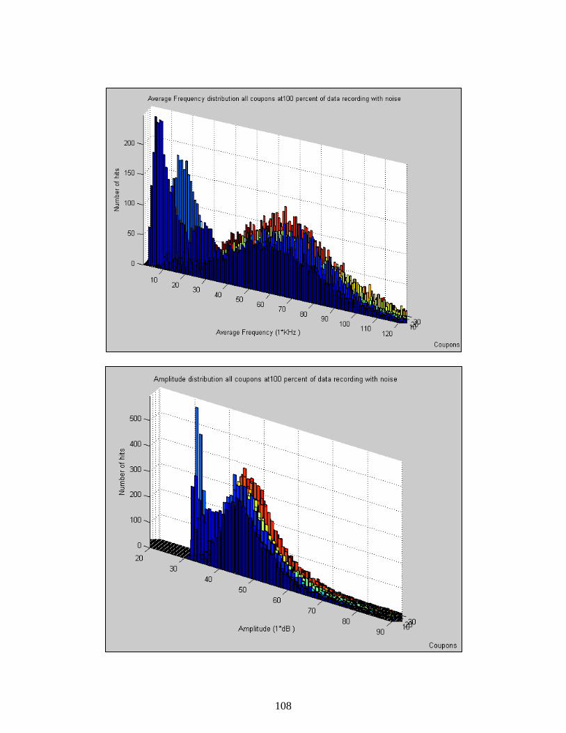
108

109
The next four plots give representations of the AE data remaining after the noise filter has
been applied and only a certain percent of recorded data taken out of the complete AE data.
These plots are available for all the training and prediction coupons and help the NDT engineer to
understand the AE data.

110

111

112
The next five plots help to visualize the AE data for each coupon once the classification
by Kohonen SOM has been done. It helps to understand where each cluster is in terms of the AE
parameters. These plots are available after the noise filtration and Kohonen SOM classification
processes.

113
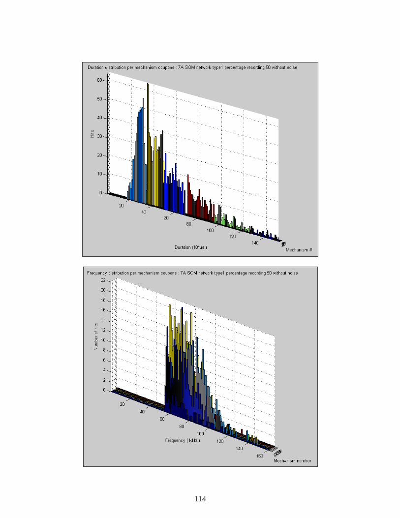
114

115
The following five plots are the visual output results of the analysis. These plots present by a surface the absolute training and prediction errors as well as the R
2 fitting coefficients
evolution with respect to the type of Kohonen SOM used, the number of training coupons and
lastly the AE parameter used in the MSRA.

116

117

118
C. Results exploitation example
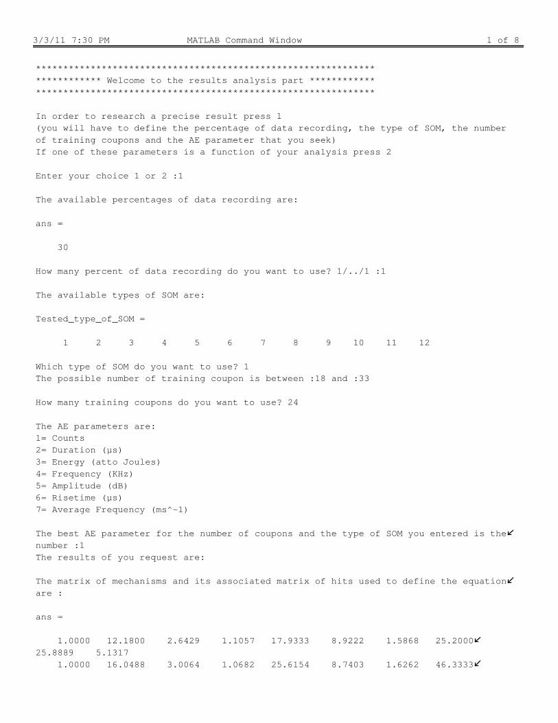
3/3/11 7:30 PM MATLAB Command Window 1 of 8
**************************************************************
************ Welcome to the results analysis part ************
**************************************************************
In order to research a precise result press 1
(you will have to define the percentage of data recording, the type of SOM, the number
of training coupons and the AE parameter that you seek)
If one of these parameters is a function of your analysis press 2
Enter your choice 1 or 2 :1
The available percentages of data recording are:
ans =
30
How many percent of data recording do you want to use? 1/../1 :1
The available types of SOM are:
Tested_type_of_SOM =
1 2 3 4 5 6 7 8 9 10 11 12
Which type of SOM do you want to use? 1
The possible number of training coupon is between :18 and :33
How many training coupons do you want to use? 24
The AE parameters are:
1= Counts
2= Duration (µs)
3= Energy (atto Joules)
4= Frequency (KHz)
5= Amplitude (dB)
6= Risetime (µs)
7= Average Frequency (ms^-1)
The best AE parameter for the number of coupons and the type of SOM you entered is the
number :1
The results of you request are:
The matrix of mechanisms and its associated matrix of hits used to define the equation
are :
ans =
1.0000 12.1800 2.6429 1.1057 17.9333 8.9222 1.5868 25.2000
25.8889 5.1317
1.0000 16.0488 3.0064 1.0682 25.6154 8.7403 1.6262 46.3333

3/3/11 7:30 PM MATLAB Command Window 2 of 8
25.0667 5.2478
1.0000 11.9778 3.0104 1.1047 21.3636 9.1196 1.6567 29.2000
15.0690 6.1339
1.0000 13.5000 3.7797 1.0923 0 11.0000 1.5526 0
0 5.7619
1.0000 10.7000 2.3478 1.0476 18.0000 5.9524 1.1538 20.0000
11.7143 4.8929
1.0000 20.0000 3.0630 1.1087 29.0000 8.4565 1.7841 18.3333
14.8000 4.6087
1.0000 7.2727 2.7732 1.0816 17.5455 5.8049 1.6963 11.2308
8.4444 4.3103
1.0000 12.6250 3.0156 1.1311 12.4000 8.6531 1.6242 26.5000
9.0909 4.8644
1.0000 10.1538 3.5577 1.0625 10.5000 10.4000 1.5750 17.0000
10.6667 7.4906
1.0000 9.1176 2.6400 1.2500 16.0000 7.9615 1.8302 20.6667
15.5556 5.5000
1.0000 8.2500 2.8305 1.0370 18.4167 7.1034 1.3455 23.0000
10.3333 4.6458
1.0000 19.3846 3.4318 1.1164 22.0000 6.9091 1.8278 0
44.0000 6.0833
1.0000 14.4615 3.5254 1.1261 16.8000 8.2500 1.8269 24.0000
10.1667 5.3778
1.0000 18.6400 3.2353 1.1216 29.2500 8.5682 1.7778 33.6667
25.5000 5.5510
1.0000 24.0000 3.6893 1.1638 19.0000 11.4219 1.8249 0
25.7273 6.9259
1.0000 16.2105 3.3135 1.1433 14.6667 9.0976 1.7120 22.0000
19.2857 4.8036
1.0000 13.0625 3.3356 1.1642 37.6667 12.4872 1.8596 27.3333
21.2500 6.2857
1.0000 13.1786 3.0679 1.1087 25.6667 6.5833 1.5163 32.5000
17.2000 5.8061
1.0000 10.3714 3.3556 1.1362 50.0000 9.3043 1.7913 28.0000
25.3846 5.1129
1.0000 12.7381 3.2353 1.1630 17.3000 9.9483 1.9731 40.2308
21.1481 5.5429
1.0000 9.2703 2.4921 1.0846 16.5714 7.2388 1.4279 24.3333
13.2778 5.0311
1.0000 20.0000 3.2336 1.1120 14.0000 8.0189 1.8242 29.0000
16.7500 5.1443
1.0000 17.5556 3.2281 1.1330 35.0000 11.5050 1.6198 51.0000
24.1333 5.2441
1.0000 17.1739 2.8405 1.1125 23.0000 8.9556 1.6983 49.1429
26.1111 4.4880
ans =
0 50 238 123 15 90 242 15 27 167
0 41 157 132 13 77 206 6 15 113

3/3/11 7:30 PM MATLAB Command Window 3 of 8
0 45 193 191 11 92 233 5 29 127
0 2 59 130 0 4 114 0 0 21
0 20 46 21 9 21 52 1 14 28
0 6 127 138 1 46 176 3 5 92
0 22 97 98 11 41 135 13 9 58
0 16 128 122 5 49 157 4 11 59
0 13 52 48 2 25 80 1 3 53
0 17 75 144 7 26 106 3 9 60
0 20 59 27 12 29 55 13 12 48
0 13 176 318 1 33 302 0 4 96
0 13 59 119 5 24 104 4 6 45
0 25 204 222 4 44 252 3 14 98
0 25 177 293 1 64 337 0 11 81
0 19 185 293 3 41 316 1 7 112
0 16 149 268 3 39 228 3 8 84
0 28 162 138 9 48 246 4 15 98
0 35 284 367 2 92 369 2 13 186
0 42 187 454 10 58 335 13 27 105
0 37 191 130 7 67 215 3 18 161
0 12 214 259 5 53 273 1 8 97
0 36 171 218 16 101 242 3 15 127
0 46 232 240 8 90 295 7 18 125
Where each line correspond to the following training coupons:
ans =
1
2
5
8
9
10
11
12
13
14
15
17
18
19
22
23
24
26
28
29
30
32
33
34

3/3/11 7:30 PM MATLAB Command Window 4 of 8
The actual failure load of training coupons are:
actual_failure_loads_training =
22583
24498
19916
18163
17226
18660
20975
17410
16685
15805
16734
17322
22470
24195
17250
21815
21749
17249
20833
20729
20024
18825
18986
18742
Their predicted load are:
predicted_failure_load_training =
1.0e+004 *
2.0097
2.1711
1.9607
1.7571
1.6676
2.0602
2.0564
1.8824
1.8653
1.6770
1.9362
1.9015
1.9763
2.0312
1.7297

3/3/11 7:30 PM MATLAB Command Window 5 of 8
1.9161
2.0810
1.7559
2.1334
2.1767
1.8613
2.0372
2.0631
2.1773
Percentage of training error is:
ans =
-11.0074
-11.3748
-1.5510
-3.2569
-3.1951
10.4083
-1.9589
8.1198
11.7966
6.1083
15.7040
9.7708
-12.0489
-16.0470
0.2696
-12.1670
-4.3155
1.7956
2.4065
5.0056
-7.0472
8.2186
8.6630
16.1723
The fitting coefficient R^2 is:
ans =
0.4015
The matrix of mechanisms and its associated matrix of hits used to predict with the
equation are:
ans =
1.0000 15.0000 3.0787 1.1076 17.3000 7.6739 1.6744 21.0000
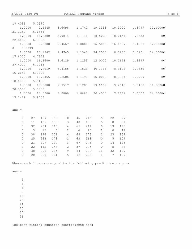
3/3/11 7:30 PM MATLAB Command Window 6 of 8
18.4091 5.0390
1.0000 9.4545 3.6698 1.1742 19.3333 10.3000 1.8797 20.4000
21.1250 6.1358
1.0000 16.2500 3.9014 1.1111 18.5000 10.0154 1.8333 0
22.8462 6.7865
1.0000 7.0000 2.4667 1.0000 16.5000 16.1667 1.1500 12.0000
0 5.5833
1.0000 10.1842 2.4745 1.1343 34.2500 8.3235 1.5201 14.5000
17.6000 4.7278
1.0000 16.3600 3.6119 1.1259 12.0000 10.2698 1.8397 0
37.4000 6.2018
1.0000 9.7619 3.4155 1.1523 40.3333 8.9104 1.7636 0
16.2143 6.3828
1.0000 10.5455 3.2606 1.1193 16.0000 8.3784 1.7709 0
18.6000 5.9186
1.0000 13.5000 2.9517 1.1283 19.6667 9.2619 1.7153 31.3636
20.9063 5.0388
1.0000 13.5000 3.0800 1.0663 20.4000 7.6667 1.6000 24.0000
17.1429 5.8705
ans =
0 27 127 158 10 46 215 5 22 77
0 11 106 155 3 40 158 5 8 81
0 32 284 315 4 65 414 0 13 178
0 5 15 6 2 6 20 1 0 12
0 38 196 201 4 68 273 2 25 169
0 25 268 278 2 63 368 0 5 109
0 21 207 197 3 67 275 0 14 128
0 22 142 243 2 37 275 0 5 86
0 38 207 265 9 84 288 11 32 129
0 28 200 181 5 72 285 1 7 139
Where each line correspond to the following prediction coupons:
ans =
3
4
6
7
16
20
21
25
27
31
The best fitting equation coefficients are:

3/3/11 7:30 PM MATLAB Command Window 7 of 8
ans =
1.0e+004 *
4.2522
-0.0088
-0.0717
-3.2039
0.0014
0.0392
0.9205
0.0035
0.0034
-0.0810
The actual failure load of prediction coupons are:
actual_failure_loads_prediction =
20162
19175
20434
20827
19503
19782
17944
20010
22190
20255
Their predicted load are:
predicted_failure_load =
1.0e+004 *
1.9457
1.9518
1.9046
2.1150
1.8520
1.9812
1.7968
1.9049
2.0495
1.9653
Percentage of prediction error is:
ans =

3/3/11 7:30 PM MATLAB Command Window 8 of 8
-3.4987
1.7868
-6.7914
1.5512
-5.0395
0.1540
0.1358
-4.8047
-7.6395
-2.9727
The fitting coefficient R^2 is:
ans =
0.5825
Percentage of worst prediction error is:
ans =
-7.6395
Do you want to request another result? Y/N [N]:


128
D. Analysis source code

129
Source code functions architecture:
MAIN_PROGRAM
constant_inputs
Load_AE_files
Load_load_energy_file
B_basis_allowable_calculation
Distributions_calculator_all_coupons
Plot_counts_distribution
Plot_duration_distribution
Plot_energy_distribution
Plot_frequency_distribution
Plot_amplitude_distribution
Plot_risetime_distribution
Plot_average_frequency_distribution
Filter_values
Filtration_of_data
Percentage_of_recording_data_generation
Plot_duration_vs_counts
Plot_amplitude_vs_average_frequency
Plot_duration_vs_energy_vs_amplitude_per_mechanism
Plot_amplitude_vs_time
Plot_energy_vs_amplitude
Prediction_and_training_coupons_combinations_generation
SOM_and_MSA_analysis
Classification_by_SOM
Clusters_parameters_determination
Generation_AE_mechanisms_per_coupon_matrix_SOM_classification
Amplitude_distribution_calculator_per_mechanism
Duration_distribution_calculator_per_mechanism
frequency_distribution_calculator_per_mechanism
Mean_amplitude_per_mechanism_research
Noise_clusters_research
Multivariate_satistical_regression_analysis
Plot_training_error
Plot_prediction_error
Plot_R2_values_training
Plot_R2_values_prediction
Plot_prediction_error_per_AE_parameter
Plot_training_error_per_AE_parameter
Plot_R2_values_training_per_AE_parameter
Plot_R2_values_prediction_per_AE_parameter
Results_exploitation
1
1
1
2
2

3/4/11 6:18 PM C:\Users\Alex-Dell\Desktop\workspace\MAIN_PROGRAM.m 1 of 9
%%%%%%%%%%%%%%%%%%%%%%%%%%%%%%%%%%%%%%%%%%%%%%%%%%%%%%%%%%%%%%%%%%%%%%%%%%%
% Failure load prediction of compressed graphite/epoxy coupons using %
% Kohonen Self Organizing Maps and Multivariate Statistical Analysis %
%%%%%%%%%%%%%%%%%%%%%%%%%%%%%%%%%%%%%%%%%%%%%%%%%%%%%%%%%%%%%%%%%%%%%%%%%%%
% Delete all the variables stored in matlab memory, close all the open
% windows and clear the matlab command window
close all force;
clear all;
clc;
% Read the analysis parameters in constant_inputs.m file
constant_inputs;
% Defines if the data should be loaded from a previous load (case
% preload=1) or not (case preload=0)
preload=0;
% Defines if the data should be loaded from a previous load (case
% preloaded_AE_files=1) or not (case preloaded_AE_files=0)
preloaded_AE_files=1;
%Differenciation in the loading process
if preload==0
%Existing preload file
if preloaded_AE_files==1
load loaded_AE_files.mat
else
% Load 100% recording of the Acoustic Emissions data available in the Excel
% spreadsheets for all the available coupons
[Matrix_of_files_100_percent]=Load_AE_files(Files_coupon_name, File_extension);
% Load the actual failure loads of all the loaded coupons
[ Actual_load,Actual_energies,Coupons_separated_in_energy_impact_groups,
Load_and_impact_energies_full,Number_of_coupon_per_energy_group] = Load_load_energy_file
( Actual_load_file);
B_basis_allowable_limits=B_basis_allowable_calculation(Actual_load,
Actual_energies);
filename='loaded_AE_files.mat';
save
(filename,'Matrix_of_files_100_percent','Actual_load','Actual_energies','B_basis_allowab
le_limits','Coupons_separated_in_energy_impact_groups','Load_and_impact_energies_full','
Number_of_coupon_per_energy_group')
end;
% Create 4 dimensions matrices that will contain the training and
% prediction error at the end of the analysis
Prediction_error_matrix_equation_1=zeros(Number_of_AE_parameters,length
(Files_coupon_name),length(Tested_type_of_SOM),length(Percentage_list));
Prediction_error_matrix_equation_2=zeros(Number_of_AE_parameters,length

3/4/11 6:18 PM C:\Users\Alex-Dell\Desktop\workspace\MAIN_PROGRAM.m 2 of 9
(Files_coupon_name),length(Tested_type_of_SOM),length(Percentage_list));
Training_error_matrix_equation_1=zeros(Number_of_AE_parameters,Max_nb_training_coupon,
length(Tested_type_of_SOM),length(Percentage_list));
Training_error_matrix_equation_2=zeros(Number_of_AE_parameters,Max_nb_training_coupon,
length(Tested_type_of_SOM),length(Percentage_list));
% Create 4 dimensions matrices that will contain the training and
% prediction error at the end of the analysis
R2_value_prediction_matrix_equation_1=zeros(Number_of_AE_parameters,
Max_nb_training_coupon,length(Tested_type_of_SOM),length(Percentage_list));
R2_value_prediction_matrix_equation_2=zeros(Number_of_AE_parameters,
Max_nb_training_coupon,length(Tested_type_of_SOM),length(Percentage_list));
R2_value_training_matrix_equation_1=zeros(Number_of_AE_parameters,
Max_nb_training_coupon,length(Tested_type_of_SOM),length(Percentage_list));
R2_value_training_matrix_equation_2=zeros(Number_of_AE_parameters,
Max_nb_training_coupon,length(Tested_type_of_SOM),length(Percentage_list));
% Create 4 dimensions matrices that will contain the worst case error
% in prediction equation
if Type_of_equation==1
Worst_case_error_prediction_equation=zeros
((Classification_plane_dimension_1*Classification_plane_dimension_2)+1-
nb_of_noise_cluster,Max_nb_training_coupon,length(Tested_type_of_SOM),length
(Percentage_list));
Matrix_of_mechanisms_for_worst_case_training=zeros(Max_nb_training_coupon,
(Classification_plane_dimension_1*Classification_plane_dimension_2)+2-
nb_of_noise_cluster,Max_nb_training_coupon,length(Tested_type_of_SOM),length
(Percentage_list));
Matrix_of_mechanisms_for_worst_case_prediction=zeros(length(Files_coupon_name)-
Min_nb_training_coupon,
(Classification_plane_dimension_1*Classification_plane_dimension_2)+2-
nb_of_noise_cluster,Max_nb_training_coupon,length(Tested_type_of_SOM),length
(Percentage_list));
Matrix_of_hits_for_worst_case_training=zeros(Max_nb_training_coupon,
(Classification_plane_dimension_1*Classification_plane_dimension_2)+2-
nb_of_noise_cluster,Max_nb_training_coupon,length(Tested_type_of_SOM),length
(Percentage_list));
Matrix_of_hits_for_worst_case_prediction=zeros(length(Files_coupon_name)-
Min_nb_training_coupon,
(Classification_plane_dimension_1*Classification_plane_dimension_2)+2-
nb_of_noise_cluster,Max_nb_training_coupon,length(Tested_type_of_SOM),length
(Percentage_list));
else
Worst_case_error_prediction_equation=zeros
((Classification_plane_dimension_1*Classification_plane_dimension_2)+1+nchoosek
((Classification_plane_dimension_1*Classification_plane_dimension_2)-
nb_of_noise_cluster,2)-nb_of_noise_cluster,Max_nb_training_coupon,length
(Tested_type_of_SOM),length(Percentage_list));
Matrix_of_mechanisms_for_worst_case_training=zeros(Max_nb_training_coupon,
(Classification_plane_dimension_1*Classification_plane_dimension_2)+2+nchoosek
((Classification_plane_dimension_1*Classification_plane_dimension_2)-
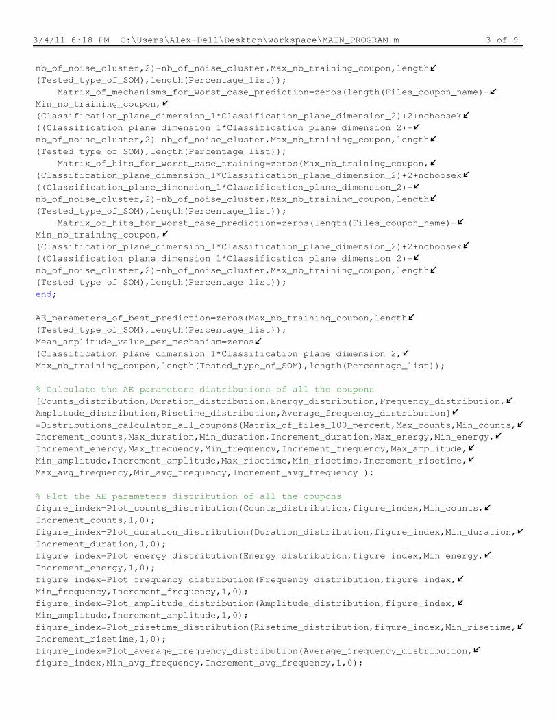
3/4/11 6:18 PM C:\Users\Alex-Dell\Desktop\workspace\MAIN_PROGRAM.m 3 of 9
nb_of_noise_cluster,2)-nb_of_noise_cluster,Max_nb_training_coupon,length
(Tested_type_of_SOM),length(Percentage_list));
Matrix_of_mechanisms_for_worst_case_prediction=zeros(length(Files_coupon_name)-
Min_nb_training_coupon,
(Classification_plane_dimension_1*Classification_plane_dimension_2)+2+nchoosek
((Classification_plane_dimension_1*Classification_plane_dimension_2)-
nb_of_noise_cluster,2)-nb_of_noise_cluster,Max_nb_training_coupon,length
(Tested_type_of_SOM),length(Percentage_list));
Matrix_of_hits_for_worst_case_training=zeros(Max_nb_training_coupon,
(Classification_plane_dimension_1*Classification_plane_dimension_2)+2+nchoosek
((Classification_plane_dimension_1*Classification_plane_dimension_2)-
nb_of_noise_cluster,2)-nb_of_noise_cluster,Max_nb_training_coupon,length
(Tested_type_of_SOM),length(Percentage_list));
Matrix_of_hits_for_worst_case_prediction=zeros(length(Files_coupon_name)-
Min_nb_training_coupon,
(Classification_plane_dimension_1*Classification_plane_dimension_2)+2+nchoosek
((Classification_plane_dimension_1*Classification_plane_dimension_2)-
nb_of_noise_cluster,2)-nb_of_noise_cluster,Max_nb_training_coupon,length
(Tested_type_of_SOM),length(Percentage_list));
end;
AE_parameters_of_best_prediction=zeros(Max_nb_training_coupon,length
(Tested_type_of_SOM),length(Percentage_list));
Mean_amplitude_value_per_mechanism=zeros
(Classification_plane_dimension_1*Classification_plane_dimension_2,
Max_nb_training_coupon,length(Tested_type_of_SOM),length(Percentage_list));
% Calculate the AE parameters distributions of all the coupons
[Counts_distribution,Duration_distribution,Energy_distribution,Frequency_distribution,
Amplitude_distribution,Risetime_distribution,Average_frequency_distribution]
=Distributions_calculator_all_coupons(Matrix_of_files_100_percent,Max_counts,Min_counts,
Increment_counts,Max_duration,Min_duration,Increment_duration,Max_energy,Min_energy,
Increment_energy,Max_frequency,Min_frequency,Increment_frequency,Max_amplitude,
Min_amplitude,Increment_amplitude,Max_risetime,Min_risetime,Increment_risetime,
Max_avg_frequency,Min_avg_frequency,Increment_avg_frequency );
% Plot the AE parameters distribution of all the coupons
figure_index=Plot_counts_distribution(Counts_distribution,figure_index,Min_counts,
Increment_counts,1,0);
figure_index=Plot_duration_distribution(Duration_distribution,figure_index,Min_duration,
Increment_duration,1,0);
figure_index=Plot_energy_distribution(Energy_distribution,figure_index,Min_energy,
Increment_energy,1,0);
figure_index=Plot_frequency_distribution(Frequency_distribution,figure_index,
Min_frequency,Increment_frequency,1,0);
figure_index=Plot_amplitude_distribution(Amplitude_distribution,figure_index,
Min_amplitude,Increment_amplitude,1,0);
figure_index=Plot_risetime_distribution(Risetime_distribution,figure_index,Min_risetime,
Increment_risetime,1,0);
figure_index=Plot_average_frequency_distribution(Average_frequency_distribution,
figure_index,Min_avg_frequency,Increment_avg_frequency,1,0);

3/4/11 6:18 PM C:\Users\Alex-Dell\Desktop\workspace\MAIN_PROGRAM.m 4 of 9
% Load the boundary values of all the AE parameter for first filtration
Filter_values;
% Apply a first filtration on the data
Matrix_of_files_100_percent_filtered=Filtration_of_data(Matrix_of_files_100_percent,
Max_counts,Min_counts,Max_duration,Min_duration,Max_energy,Min_energy,Max_frequency,
Min_frequency,Max_amplitude,Min_amplitude,Max_risetime,Min_risetime,Max_avg_frequency,
Min_avg_frequency);
% Calculate the AE parameters distributions of all the filtered coupons
[Counts_distribution,Duration_distribution,Energy_distribution,Frequency_distribution,
Amplitude_distribution,Risetime_distribution,Average_frequency_distribution]
=Distributions_calculator_all_coupons(Matrix_of_files_100_percent_filtered,Max_counts,
Min_counts,Increment_counts,Max_duration,Min_duration,Increment_duration,Max_energy,
Min_energy,Increment_energy,Max_frequency,Min_frequency,Increment_frequency,
Max_amplitude,Min_amplitude,Increment_amplitude,Max_risetime,Min_risetime,
Increment_risetime,Max_avg_frequency,Min_avg_frequency,Increment_avg_frequency );
% Plot the AE parameters distribution of all the filtered coupons
figure_index=Plot_counts_distribution(Counts_distribution,figure_index,Min_counts,
Increment_counts,1,1);
figure_index=Plot_duration_distribution(Duration_distribution,figure_index,Min_duration,
Increment_duration,1,1);
figure_index=Plot_energy_distribution(Energy_distribution,figure_index,Min_energy,
Increment_energy,1,1);
figure_index=Plot_frequency_distribution(Frequency_distribution,figure_index,
Min_frequency,Increment_frequency,1,1);
figure_index=Plot_amplitude_distribution(Amplitude_distribution,figure_index,
Min_amplitude,Increment_amplitude,1,1);
figure_index=Plot_risetime_distribution(Risetime_distribution,figure_index,Min_risetime,
Increment_risetime,1,1);
figure_index=Plot_average_frequency_distribution(Average_frequency_distribution,
figure_index,Min_avg_frequency,Increment_avg_frequency,1,1);
% Save all the loaded data at that point
save workspacepreload.mat
else
% Loads a previously loaded set of data
load workspacepreload.mat
end;
% Loop allowing the study of different percentage recording of the
% prediction coupons' Acoustic Emissions data
for Percentage_recording_index=1:1:length(Percentage_list)
clc;
% Progress of the percentage recording analysis vizualization
Percentage_of_data_recording_progress=(Percentage_recording_index/length
(Percentage_list))*100
% Generate a matrix containing a certain percent of the recorded
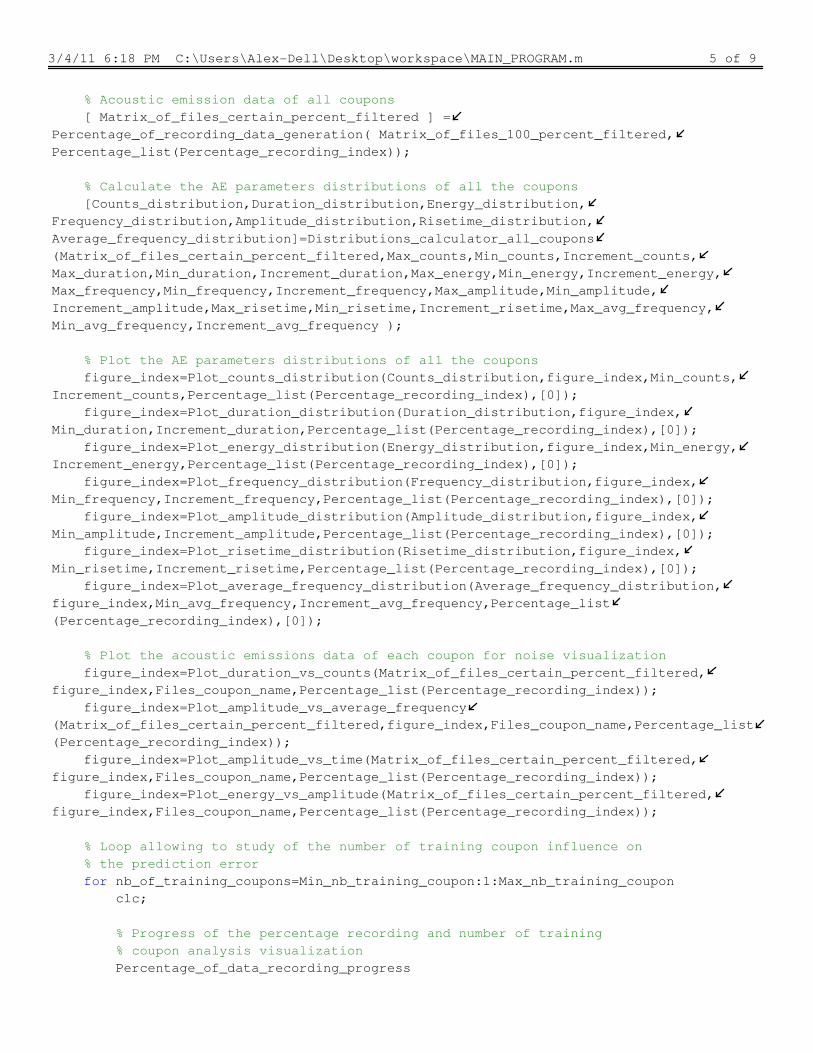
3/4/11 6:18 PM C:\Users\Alex-Dell\Desktop\workspace\MAIN_PROGRAM.m 5 of 9
% Acoustic emission data of all coupons
[ Matrix_of_files_certain_percent_filtered ] =
Percentage_of_recording_data_generation( Matrix_of_files_100_percent_filtered,
Percentage_list(Percentage_recording_index));
% Calculate the AE parameters distributions of all the coupons
[Counts_distribution,Duration_distribution,Energy_distribution,
Frequency_distribution,Amplitude_distribution,Risetime_distribution,
Average_frequency_distribution]=Distributions_calculator_all_coupons
(Matrix_of_files_certain_percent_filtered,Max_counts,Min_counts,Increment_counts,
Max_duration,Min_duration,Increment_duration,Max_energy,Min_energy,Increment_energy,
Max_frequency,Min_frequency,Increment_frequency,Max_amplitude,Min_amplitude,
Increment_amplitude,Max_risetime,Min_risetime,Increment_risetime,Max_avg_frequency,
Min_avg_frequency,Increment_avg_frequency );
% Plot the AE parameters distributions of all the coupons
figure_index=Plot_counts_distribution(Counts_distribution,figure_index,Min_counts,
Increment_counts,Percentage_list(Percentage_recording_index),[0]);
figure_index=Plot_duration_distribution(Duration_distribution,figure_index,
Min_duration,Increment_duration,Percentage_list(Percentage_recording_index),[0]);
figure_index=Plot_energy_distribution(Energy_distribution,figure_index,Min_energy,
Increment_energy,Percentage_list(Percentage_recording_index),[0]);
figure_index=Plot_frequency_distribution(Frequency_distribution,figure_index,
Min_frequency,Increment_frequency,Percentage_list(Percentage_recording_index),[0]);
figure_index=Plot_amplitude_distribution(Amplitude_distribution,figure_index,
Min_amplitude,Increment_amplitude,Percentage_list(Percentage_recording_index),[0]);
figure_index=Plot_risetime_distribution(Risetime_distribution,figure_index,
Min_risetime,Increment_risetime,Percentage_list(Percentage_recording_index),[0]);
figure_index=Plot_average_frequency_distribution(Average_frequency_distribution,
figure_index,Min_avg_frequency,Increment_avg_frequency,Percentage_list
(Percentage_recording_index),[0]);
% Plot the acoustic emissions data of each coupon for noise visualization
figure_index=Plot_duration_vs_counts(Matrix_of_files_certain_percent_filtered,
figure_index,Files_coupon_name,Percentage_list(Percentage_recording_index));
figure_index=Plot_amplitude_vs_average_frequency
(Matrix_of_files_certain_percent_filtered,figure_index,Files_coupon_name,Percentage_list
(Percentage_recording_index));
figure_index=Plot_amplitude_vs_time(Matrix_of_files_certain_percent_filtered,
figure_index,Files_coupon_name,Percentage_list(Percentage_recording_index));
figure_index=Plot_energy_vs_amplitude(Matrix_of_files_certain_percent_filtered,
figure_index,Files_coupon_name,Percentage_list(Percentage_recording_index));
% Loop allowing to study of the number of training coupon influence on
% the prediction error
for nb_of_training_coupons=Min_nb_training_coupon:1:Max_nb_training_coupon
clc;
% Progress of the percentage recording and number of training
% coupon analysis visualization
Percentage_of_data_recording_progress

3/4/11 6:18 PM C:\Users\Alex-Dell\Desktop\workspace\MAIN_PROGRAM.m 6 of 9
Nb_training_coupons_progress=((nb_of_training_coupons-Min_nb_training_coupon+1)/
(Max_nb_training_coupon-Min_nb_training_coupon+1))*100
% Generate matrices of all the training coupons combinations and
% their associated prediction coupons combinations
[Training_coupons_combinations,Prediction_coupon_combination,
number_of_training_coupon_combination]
=Prediction_and_training_coupons_combinations_generation(Max_nb_training_coupon,
nb_of_training_coupons,Possible_training_coupons,
Coupons_separated_in_energy_impact_groups,Number_of_coupon_per_energy_group,
Files_coupon_name);
% Specific set of training and prediction coupons combination (previous
research)
%Prediction_coupon_combination=[1,5,6,11,12,17,20,24,29,34];
%Training_coupons_combinations=
[2,3,4,7,8,9,10,13,14,15,16,18,19,21,22,23,25,26,27,28,30,31,32,33];
%number_of_training_coupon_combination=1;
% Classify the Acoustic emmission data of all coupons by using Kohonen Self
Organiwing Maps and predict the ultimate loads by using the
% Multivariate Statistical Analysis
[ Training_error_matrix_equation_1,Training_error_matrix_equation_2,
Prediction_error_matrix_equation_1,Prediction_error_matrix_equation_2,figure_index,
Number_of_mechanisms,Worst_case_error_prediction_equation,
AE_parameters_of_best_prediction,Matrix_of_mechanisms_for_worst_case_training,
Matrix_of_mechanisms_for_worst_case_prediction,Mean_amplitude_value_per_mechanism,
Matrix_of_hits_for_worst_case_training,Matrix_of_hits_for_worst_case_prediction,
R2_value_prediction_matrix_equation_1,R2_value_prediction_matrix_equation_2,
R2_value_training_matrix_equation_1,R2_value_training_matrix_equation_2] =
SOM_and_MSA_analysis( Matrix_of_files_certain_percent_filtered,
Matrix_of_files_100_percent_filtered,Number_of_AE_parameters,Actual_load,
Training_coupons_combinations,Prediction_coupon_combination,
Classification_plane_dimension_1,Classification_plane_dimension_2,nb_iteration,
nb_of_training_coupons,Min_amplitude,Max_amplitude,Min_duration,Max_duration,
Increment_duration,Min_frequency,Max_frequency,Nb_training_coupons_progress,
Percentage_of_data_recording_progress,figure_index,Training_error_matrix_equation_1,
Training_error_matrix_equation_2,Prediction_error_matrix_equation_1,
Prediction_error_matrix_equation_2,Tested_type_of_SOM,Percentage_list,
Percentage_recording_index,classification_AE_parameter,
Worst_case_error_prediction_equation,Files_coupon_name,nb_of_noise_cluster,remove_noise,
Min_average_frequency,Type_of_equation,AE_parameters_of_best_prediction,
Matrix_of_mechanisms_for_worst_case_training,
Matrix_of_mechanisms_for_worst_case_prediction,Max_nb_training_coupon,
Min_nb_training_coupon,Mean_amplitude_value_per_mechanism,
Matrix_of_hits_for_worst_case_training,Matrix_of_hits_for_worst_case_prediction,
R2_value_prediction_matrix_equation_1,R2_value_prediction_matrix_equation_2,
R2_value_training_matrix_equation_1,R2_value_training_matrix_equation_2);
% Saves all the workspace variables
save workspacefinal.mat
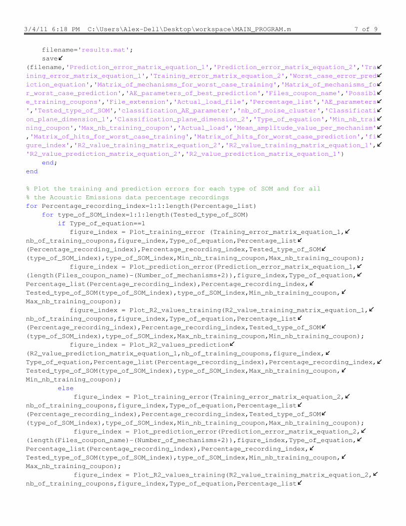
3/4/11 6:18 PM C:\Users\Alex-Dell\Desktop\workspace\MAIN_PROGRAM.m 7 of 9
filename='results.mat';
save
(filename,'Prediction_error_matrix_equation_1','Prediction_error_matrix_equation_2','Tra
ining_error_matrix_equation_1','Training_error_matrix_equation_2','Worst_case_error_pred
iction_equation','Matrix_of_mechanisms_for_worst_case_training','Matrix_of_mechanisms_fo
r_worst_case_prediction','AE_parameters_of_best_prediction','Files_coupon_name','Possibl
e_training_coupons','File_extension','Actual_load_file','Percentage_list','AE_parameters
','Tested_type_of_SOM','classification_AE_parameter','nb_of_noise_cluster','Classificati
on_plane_dimension_1','Classification_plane_dimension_2','Type_of_equation','Min_nb_trai
ning_coupon','Max_nb_training_coupon','Actual_load','Mean_amplitude_value_per_mechanism'
,'Matrix_of_hits_for_worst_case_training','Matrix_of_hits_for_worst_case_prediction','fi
gure_index','R2_value_training_matrix_equation_2','R2_value_training_matrix_equation_1',
'R2_value_prediction_matrix_equation_2','R2_value_prediction_matrix_equation_1')
end;
end
% Plot the training and prediction errors for each type of SOM and for all
% the Acoustic Emissions data percentage recordings
for Percentage_recording_index=1:1:length(Percentage_list)
for type_of_SOM_index=1:1:length(Tested_type_of_SOM)
if Type_of_equation==1
figure_index = Plot_training_error (Training_error_matrix_equation_1,
nb_of_training_coupons,figure_index,Type_of_equation,Percentage_list
(Percentage_recording_index),Percentage_recording_index,Tested_type_of_SOM
(type_of_SOM_index),type_of_SOM_index,Min_nb_training_coupon,Max_nb_training_coupon);
figure_index = Plot_prediction_error(Prediction_error_matrix_equation_1,
(length(Files_coupon_name)-(Number_of_mechanisms+2)),figure_index,Type_of_equation,
Percentage_list(Percentage_recording_index),Percentage_recording_index,
Tested_type_of_SOM(type_of_SOM_index),type_of_SOM_index,Min_nb_training_coupon,
Max_nb_training_coupon);
figure_index = Plot_R2_values_training(R2_value_training_matrix_equation_1,
nb_of_training_coupons,figure_index,Type_of_equation,Percentage_list
(Percentage_recording_index),Percentage_recording_index,Tested_type_of_SOM
(type_of_SOM_index),type_of_SOM_index,Max_nb_training_coupon,Min_nb_training_coupon);
figure_index = Plot_R2_values_prediction
(R2_value_prediction_matrix_equation_1,nb_of_training_coupons,figure_index,
Type_of_equation,Percentage_list(Percentage_recording_index),Percentage_recording_index,
Tested_type_of_SOM(type_of_SOM_index),type_of_SOM_index,Max_nb_training_coupon,
Min_nb_training_coupon);
else
figure_index = Plot_training_error(Training_error_matrix_equation_2,
nb_of_training_coupons,figure_index,Type_of_equation,Percentage_list
(Percentage_recording_index),Percentage_recording_index,Tested_type_of_SOM
(type_of_SOM_index),type_of_SOM_index,Min_nb_training_coupon,Max_nb_training_coupon);
figure_index = Plot_prediction_error(Prediction_error_matrix_equation_2,
(length(Files_coupon_name)-(Number_of_mechanisms+2)),figure_index,Type_of_equation,
Percentage_list(Percentage_recording_index),Percentage_recording_index,
Tested_type_of_SOM(type_of_SOM_index),type_of_SOM_index,Min_nb_training_coupon,
Max_nb_training_coupon);
figure_index = Plot_R2_values_training(R2_value_training_matrix_equation_2,
nb_of_training_coupons,figure_index,Type_of_equation,Percentage_list

3/4/11 6:18 PM C:\Users\Alex-Dell\Desktop\workspace\MAIN_PROGRAM.m 8 of 9
(Percentage_recording_index),Percentage_recording_index,Tested_type_of_SOM
(type_of_SOM_index),type_of_SOM_index,Max_nb_training_coupon,Min_nb_training_coupon);
figure_index = Plot_R2_values_prediction
(R2_value_prediction_matrix_equation_2,nb_of_training_coupons,figure_index,
Type_of_equation,Percentage_list(Percentage_recording_index),Percentage_recording_index,
Tested_type_of_SOM(type_of_SOM_index),type_of_SOM_index,Max_nb_training_coupon,
Min_nb_training_coupon);
end;
end;
for AE_displayed_parameter_index=1:1:Number_of_AE_parameters
if Type_of_equation==1
figure_index = Plot_prediction_error_per_AE_parameter
(Prediction_error_matrix_equation_1,(length(Files_coupon_name)-
(Number_of_mechanisms+2)),figure_index,Type_of_equation,Percentage_list
(Percentage_recording_index),Percentage_recording_index,AE_displayed_parameter_index,
Min_nb_training_coupon,Max_nb_training_coupon);
figure_index = Plot_training_error_per_AE_parameter
(Training_error_matrix_equation_1,(length(Files_coupon_name)-(Number_of_mechanisms+2)),
figure_index,Type_of_equation,Percentage_list(Percentage_recording_index),
Percentage_recording_index,AE_displayed_parameter_index,Min_nb_training_coupon,
Max_nb_training_coupon);
figure_index = Plot_R2_values_training_per_AE_parameter
(R2_value_training_matrix_equation_1,nb_of_training_coupons,figure_index,
Type_of_equation,Percentage_list(Percentage_recording_index),Percentage_recording_index,
Tested_type_of_SOM(type_of_SOM_index),type_of_SOM_index,Max_nb_training_coupon,
Min_nb_training_coupon,AE_displayed_parameter_index);
figure_index = Plot_R2_values_prediction_per_AE_parameter
(R2_value_prediction_matrix_equation_1,nb_of_training_coupons,figure_index,
Type_of_equation,Percentage_list(Percentage_recording_index),Percentage_recording_index,
Tested_type_of_SOM(type_of_SOM_index),type_of_SOM_index,Max_nb_training_coupon,
Min_nb_training_coupon,AE_displayed_parameter_index);
else
figure_index = Plot_prediction_error_per_AE_parameter
(Prediction_error_matrix_equation_2,(length(Files_coupon_name)-
(Number_of_mechanisms+2)),figure_index,Type_of_equation,Percentage_list
(Percentage_recording_index),Percentage_recording_index,AE_displayed_parameter_index);
figure_index = Plot_prediction_error_per_AE_parameter
(Prediction_error_matrix_equation_2,33,figure_index,Type_of_equation,Percentage_list
(Percentage_recording_index),Percentage_recording_index,AE_displayed_parameter_index,
Min_nb_training_coupon,Max_nb_training_coupon);
figure_index = Plot_training_error_per_AE_parameter
(Training_error_matrix_equation_2,(length(Files_coupon_name)-(Number_of_mechanisms+2)),
figure_index,Type_of_equation,Percentage_list(Percentage_recording_index),
Percentage_recording_index,AE_displayed_parameter_index,Min_nb_training_coupon,
Max_nb_training_coupon);
figure_index = Plot_R2_values_training_per_AE_parameter
(R2_value_training_matrix_equation_2,nb_of_training_coupons,figure_index,
Type_of_equation,Percentage_list(Percentage_recording_index),Percentage_recording_index,
Tested_type_of_SOM(type_of_SOM_index),type_of_SOM_index,Max_nb_training_coupon,
Min_nb_training_coupon,AE_displayed_parameter_index);
figure_index = Plot_R2_values_prediction_per_AE_parameter

3/4/11 6:18 PM C:\Users\Alex-Dell\Desktop\workspace\MAIN_PROGRAM.m 9 of 9
(R2_value_prediction_matrix_equation_2,nb_of_training_coupons,figure_index,
Type_of_equation,Percentage_list(Percentage_recording_index),Percentage_recording_index,
Tested_type_of_SOM(type_of_SOM_index),type_of_SOM_index,Max_nb_training_coupon,
Min_nb_training_coupon,AE_displayed_parameter_index);
end;
end;
end;
%Results analysis
reply_analyze = input('Do you want to analyze the results? Y/N [N]: ', 's');
if isempty(reply_analyze)
reply_analyze = 'N';
end
if reply_analyze=='Y'
reply_continuing='Y';
while reply_continuing=='Y'
Results_exploitation;
reply_continuing = input('Do you want to request another result? Y/N [N]: ',
's');
if isempty(reply_continuing)
reply_continuing = 'N';
end
end;
end;
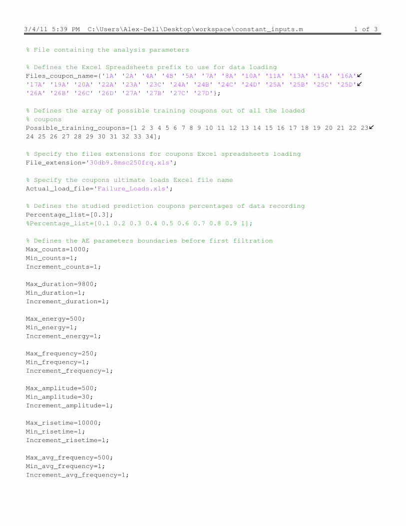
3/4/11 5:39 PM C:\Users\Alex-Dell\Desktop\workspace\constant_inputs.m 1 of 3
% File containing the analysis parameters
% Defines the Excel Spreadsheets prefix to use for data loading
Files_coupon_name={'1A' '2A' '4A' '4B' '5A' '7A' '8A' '10A' '11A' '13A' '14A' '16A'
'17A' '19A' '20A' '22A' '23A' '23C' '24A' '24B' '24C' '24D' '25A' '25B' '25C' '25D'
'26A' '26B' '26C' '26D' '27A' '27B' '27C' '27D'};
% Defines the array of possible training coupons out of all the loaded
% coupons
Possible_training_coupons=[1 2 3 4 5 6 7 8 9 10 11 12 13 14 15 16 17 18 19 20 21 22 23
24 25 26 27 28 29 30 31 32 33 34];
% Specify the files extensions for coupons Excel spreadsheets loading
File_extension='30db9.8msc250frq.xls';
% Specify the coupons ultimate loads Excel file name
Actual_load_file='Failure_Loads.xls';
% Defines the studied prediction coupons percentages of data recording
Percentage_list=[0.3];
%Percentage_list=[0.1 0.2 0.3 0.4 0.5 0.6 0.7 0.8 0.9 1];
% Defines the AE parameters boundaries before first filtration
Max_counts=1000;
Min_counts=1;
Increment_counts=1;
Max_duration=9800;
Min_duration=1;
Increment_duration=1;
Max_energy=500;
Min_energy=1;
Increment_energy=1;
Max_frequency=250;
Min_frequency=1;
Increment_frequency=1;
Max_amplitude=500;
Min_amplitude=30;
Increment_amplitude=1;
Max_risetime=10000;
Min_risetime=1;
Increment_risetime=1;
Max_avg_frequency=500;
Min_avg_frequency=1;
Increment_avg_frequency=1;

3/4/11 5:39 PM C:\Users\Alex-Dell\Desktop\workspace\constant_inputs.m 2 of 3
% Defines the first figure index
figure_index=1;
% Defines the AE parameters names as present in the coupons files
AE_parameters={'Counts' 'Duration (µs)' 'Energy (atto Joules)' 'Load (lb)' 'Average
Frequency (KHz)' 'Amplitude (dB)' 'Risetime (µs)'};
Number_of_AE_parameters=length(AE_parameters)-1;
% Specify the types of SOM studied in the analysis
Tested_type_of_SOM=[1];
%Tested_type_of_SOM=[1 2 3 4 5 6 7 8 9 10 11 12];
% Specify the number of noise cluster(s) after Kohonen Self Organizing
% Maps classification
nb_of_noise_cluster=0;
%Has to be one to enable the noise removal process
remove_noise=0;
%Set the noise average frequency lower limit
Min_average_frequency=45;
% Specify the AE parameters used to classify the Acoustic Emissions data
%#4 is the load so shouldn't be part of the classification AE parameters
% 1= 'Counts'
% 2= 'Duration (µs)'
% 3= 'Energy (atto Joules)'
% 4= 'Load (lb)'
% 5= 'Average Frequency (KHz)'
% 6= 'Amplitude (dB)'
% 7= 'Risetime (µs)'
% 8= 'Average Frequency (KHz)'
classification_AE_parameter=[2 3 6];
% Specify the number of iterations for the Kohonen Self Organizing Maps
% training process
nb_iteration=500;
% Specify the Kohonen Self Organizing Maps output width and height
% dimensions
Classification_plane_dimension_1=3;
Classification_plane_dimension_2=3;
%Defines the type of equation: 1 for simple linear equation 2 for equation
%with cross products
Type_of_equation=1;
% Defines the maximum number of training coupons in the analysis process
Max_nb_training_coupon=33;
%Max_nb_training_coupon=length(Possible_training_coupons)-1;
if Type_of_equation==1

3/4/11 5:39 PM C:\Users\Alex-Dell\Desktop\workspace\constant_inputs.m 3 of 3
Min_nb_training_coupon=18;
end;
if Type_of_equation==2
Min_nb_training_coupon=18;
%Min_nb_training_coupon=
(Classification_plane_dimension_1*Classification_plane_dimension_2)+nchoosek
((Classification_plane_dimension_1*Classification_plane_dimension_2)-
nb_of_noise_cluster,2)+2;
end;

3/4/11 5:43 PM C:\Users\Alex-Dell\Desktop\workspace\Load_AE_files.m 1 of 1
function [ Files_3D_matrix ] = Load_AE_files( Files_name, extension )
% Function that loads the acoustic emission data from excel spreadsheets to
% the matlab workspace
% Initialize internal variables for acoustic emission data loading
Max_number_of_rows=0;
Max_number_of_columns=0;
% Determining the largest number acoustic emission data throughout all the
% coupons
for i=1:1:length(Files_name)
File=xlsread(strcat(Files_name{i},extension));
if size(File,1)>Max_number_of_rows
Max_number_of_rows=size(File,1);
end;
if size(File,2)>Max_number_of_columns
Max_number_of_columns=size(File,2);
end;
end;
% Creation of output variable containing the Acoustic emission data
Files_3D_matrix=zeros(Max_number_of_rows,Max_number_of_columns,length(Files_name));
% Load the acoustic emission data
for i=1:1:length(Files_name)
Files_3D_matrix(1:size(xlsread(strcat(Files_name{i},extension)),1),1:size
(xlsread(strcat(Files_name{i},extension)),2),i)=xlsread(strcat(Files_name{i},
extension));
end;
end

3/4/11 5:46 PM C:\Users\Alex-Dell\Desktop\workspace\Load_load_energy_file.m 1 of 1
function [ Actual_loads_matrix,Actual_energies_matrix,
Coupons_separated_in_energy_impact_groups,Load_and_impact_energies_full,
Number_of_coupon_per_energy_group ] = Load_load_energy_file( Loads_energies_file)
% Function loading the load and impact energies of all the coupons in the
% matlab workspace
% Read the excel spreadsheet
Load_and_impact_energies = xlsread(Loads_energies_file);
%Order the data in a proper table
Load_and_impact_energies_full=zeros(size(Load_and_impact_energies,1),3);
for k=1:1:size(Load_and_impact_energies,1)
Load_and_impact_energies_full(k,1)=k;
end;
Load_and_impact_energies_full(:,2:3)=Load_and_impact_energies;
%Classify the coupons with respect to their impact energy group
Energy_groups=[8 10 12 13 14 15 16 18 20]';
ranks=ones(9);
Coupons_separated_in_energy_impact_groups=zeros(6,3,9);
for k=1:size(Load_and_impact_energies_full,1)
[Position,group]=ismember(Load_and_impact_energies_full(k,3),Energy_groups);
Coupons_separated_in_energy_impact_groups(ranks(group),:,group)
=Load_and_impact_energies_full(k,:);
ranks(group)=ranks(group)+1;
end;
%Calculates the number of coupons per enrgy group
Number_of_coupon_per_energy_group=ranks-1;
Number_of_coupon_per_energy_group=Number_of_coupon_per_energy_group(:,1)'
% Load impact energies and ultimate loads in separates variables
Actual_loads_matrix=Load_and_impact_energies(:,1);
Actual_energies_matrix=Load_and_impact_energies(:,2);
end
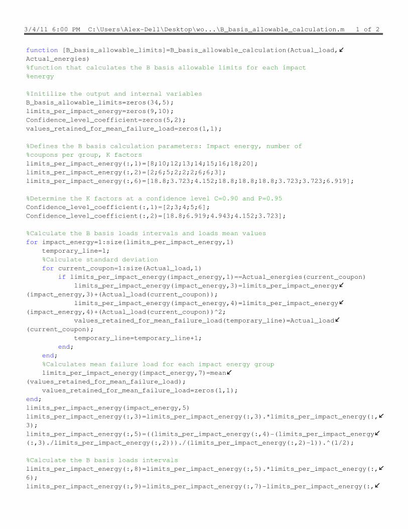
3/4/11 6:00 PM C:\Users\Alex-Dell\Desktop\wo...\B_basis_allowable_calculation.m 1 of 2
function [B_basis_allowable_limits]=B_basis_allowable_calculation(Actual_load,
Actual_energies)
%function that calculates the B basis allowable limits for each impact
%energy
%Initilize the output and internal variables
B_basis_allowable_limits=zeros(34,5);
limits_per_impact_energy=zeros(9,10);
Confidence_level_coefficient=zeros(5,2);
values_retained_for_mean_failure_load=zeros(1,1);
%Defines the B basis calculation parameters: Impact energy, number of
%coupons per group, K factors
limits_per_impact_energy(:,1)=[8;10;12;13;14;15;16;18;20];
limits_per_impact_energy(:,2)=[2;6;5;2;2;2;6;6;3];
limits_per_impact_energy(:,6)=[18.8;3.723;4.152;18.8;18.8;18.8;3.723;3.723;6.919];
%Determine the K factors at a confidence level C=0.90 and P=0.95
Confidence_level_coefficient(:,1)=[2;3;4;5;6];
Confidence_level_coefficient(:,2)=[18.8;6.919;4.943;4.152;3.723];
%Calculate the B basis loads intervals and loads mean values
for impact_energy=1:size(limits_per_impact_energy,1)
temporary_line=1;
%Calculate standard deviation
for current_coupon=1:size(Actual_load,1)
if limits_per_impact_energy(impact_energy,1)==Actual_energies(current_coupon)
limits_per_impact_energy(impact_energy,3)=limits_per_impact_energy
(impact_energy,3)+(Actual_load(current_coupon));
limits_per_impact_energy(impact_energy,4)=limits_per_impact_energy
(impact_energy,4)+(Actual_load(current_coupon))^2;
values_retained_for_mean_failure_load(temporary_line)=Actual_load
(current_coupon);
temporary_line=temporary_line+1;
end;
end;
%Calculates mean failure load for each impact energy group
limits_per_impact_energy(impact_energy,7)=mean
(values_retained_for_mean_failure_load);
values_retained_for_mean_failure_load=zeros(1,1);
end;
limits_per_impact_energy(impact_energy,5)
limits_per_impact_energy(:,3)=limits_per_impact_energy(:,3).*limits_per_impact_energy(:,
3);
limits_per_impact_energy(:,5)=((limits_per_impact_energy(:,4)-(limits_per_impact_energy
(:,3)./limits_per_impact_energy(:,2)))./(limits_per_impact_energy(:,2)-1)).^(1/2);
%Calculate the B basis loads intervals
limits_per_impact_energy(:,8)=limits_per_impact_energy(:,5).*limits_per_impact_energy(:,
6);
limits_per_impact_energy(:,9)=limits_per_impact_energy(:,7)-limits_per_impact_energy(:,

3/4/11 6:00 PM C:\Users\Alex-Dell\Desktop\wo...\B_basis_allowable_calculation.m 2 of 2
8);
limits_per_impact_energy(:,10)=limits_per_impact_energy(:,7)+limits_per_impact_energy(:,
8);
%Associate the B basis intervals to each coupons
B_basis_allowable_limits(:,1)=Actual_load;
B_basis_allowable_limits(:,2)=Actual_energies;
for current_coupon=1:size(Actual_load,1)
rank=find(limits_per_impact_energy(:,1)==Actual_energies(current_coupon));
B_basis_allowable_limits(current_coupon,3)=limits_per_impact_energy(rank,5);
B_basis_allowable_limits(current_coupon,4)=limits_per_impact_energy(rank,8);
B_basis_allowable_limits(current_coupon,5)=limits_per_impact_energy(rank,9);
end;
end

3/4/11 7:58 PM C:\Users\Alex-Dell\Des...\Distributions_calculator_all_coupons.m 1 of 4
function [Counts_distribution,Duration_distribution,Energy_distribution,
Frequency_distribution,Amplitude_distribution,Risetime_distribution,
Average_frequency_distribution] = Distributions_calculator_all_coupons
(Matrix_of_files_certain_percent,Max_counts,Min_counts,Increment_counts,Max_duration,
Min_duration,Increment_duration,Max_energy,Min_energy,Increment_energy,Max_frequency,
Min_frequency,Increment_frequency,Max_amplitude,Min_amplitude,Increment_amplitude,
Max_risetime,Min_risetime,Increment_risetime,Max_avg_frequency,Min_avg_frequency,
Increment_avg_frequency )
%Function calculating the Acoustic Emission parameters distributions
% Creation of internal variables for AE parameters distribution
% calculation
Counts_matrix=zeros(size(Matrix_of_files_certain_percent,1),size
(Matrix_of_files_certain_percent,3));
Duration_matrix=zeros(size(Matrix_of_files_certain_percent,1),size
(Matrix_of_files_certain_percent,3));
Energy_matrix=zeros(size(Matrix_of_files_certain_percent,1),size
(Matrix_of_files_certain_percent,3));
Frequency_matrix=zeros(size(Matrix_of_files_certain_percent,1),size
(Matrix_of_files_certain_percent,3));
Amplitude_matrix=zeros(size(Matrix_of_files_certain_percent,1),size
(Matrix_of_files_certain_percent,3));
Risetime_matrix=zeros(size(Matrix_of_files_certain_percent,1),size
(Matrix_of_files_certain_percent,3));
Average_frequency_matrix=zeros(size(Matrix_of_files_certain_percent,1),size
(Matrix_of_files_certain_percent,3));
% Initialization of the internal variables
for i=1:1:size(Matrix_of_files_certain_percent,3)
Counts_matrix(:,i)=Matrix_of_files_certain_percent(:,1,i);
Duration_matrix(:,i)=Matrix_of_files_certain_percent(:,2,i);
Energy_matrix(:,i)=Matrix_of_files_certain_percent(:,3,i);
Frequency_matrix(:,i)=Matrix_of_files_certain_percent(:,5,i);
Amplitude_matrix(:,i)=Matrix_of_files_certain_percent(:,6,i);
Risetime_matrix(:,i)=Matrix_of_files_certain_percent(:,7,i);
Average_frequency_matrix(:,i)=Matrix_of_files_certain_percent(:,8,i);
end;
% Creation of output variable for count distribution calculation
Counts_distribution=zeros((((Max_counts-Min_counts)/Increment_counts)+1),size
(Counts_matrix,2)+1);
% Definition of the count distribution range
for i=1:1:size(Counts_distribution,1)
Counts_distribution(i,1)=(Min_counts-1*Increment_counts)+i*Increment_counts;
end;
% Calculates the count distribution
for i=1:1:size(Counts_matrix,2)
for j=1:1:size(Counts_matrix,1)
if Counts_matrix(j,i)>=Min_counts && Counts_matrix(j,i)<=Max_counts
3/4/11 7:58 PM C:\Users\Alex-Dell\Des...\Distributions_calculator_all_coupons.m 2 of 4
if Counts_matrix(j,i)>0
row=ceil((Counts_matrix(j,i)-Min_counts)/Increment_counts)+1;
else
row=1;
end
Counts_distribution(row,i+1)=Counts_distribution(row,i+1)+1;
end;
end;
end;
% Creation of output variable for duration distribution calculation
Duration_distribution=zeros((((Max_duration-Min_duration)/Increment_duration)+1),size
(Duration_matrix,2)+1);
% Definition of the duration distribution range
for i=1:1:size(Duration_distribution,1)
Duration_distribution(i,1)=(Min_duration-1*Increment_duration)+i*Increment_duration;
end;
% Calculates the duration distribution
for i=1:1:size(Duration_matrix,2)
for j=1:1:size(Duration_matrix,1)
if Duration_matrix(j,i)>=Min_duration && Duration_matrix(j,i)<=Max_duration
if Duration_matrix(j,i)>0
row=ceil((Duration_matrix(j,i)-Min_duration)/Increment_duration)+1;
else
row=1;
end
Duration_distribution(row,i+1)=Duration_distribution(row,i+1)+1;
end;
end;
end;
% Creation of output variable for energy distribution calculation
Energy_distribution=zeros((((Max_energy-Min_energy)/Increment_energy)+1),size
(Energy_matrix,2)+1);
% Definition of the energy distribution range
for i=1:1:size(Energy_distribution,1)
Energy_distribution(i,1)=(Min_energy-1*Increment_energy)+i*Increment_energy;
end;
% Calculates the energy distribution
for i=1:1:size(Energy_matrix,2)
for j=1:1:size(Energy_matrix,1)
if Energy_matrix(j,i)>=Min_energy && Energy_matrix(j,i)<=Max_energy
if Energy_matrix(j,i)>0
row=ceil((Energy_matrix(j,i)-Min_energy)/Increment_energy)+1;
else
row=1;
end

3/4/11 7:58 PM C:\Users\Alex-Dell\Des...\Distributions_calculator_all_coupons.m 3 of 4
Energy_distribution(row,i+1)=Energy_distribution(row,i+1)+1;
end;
end;
end;
% Creation of output variable for frequency distribution calculation
Frequency_distribution=zeros((((Max_frequency-Min_frequency)/Increment_frequency)+1),
size(Frequency_matrix,2)+1);
% Definition of the frequency distribution range
for i=1:1:size(Frequency_distribution,1)
Frequency_distribution(i,1)=(Min_frequency-1*Increment_frequency)
+i*Increment_frequency;
end;
% Calculates the frequency distribution
for i=1:1:size(Frequency_matrix,2)
for j=1:1:size(Frequency_matrix,1)
if Frequency_matrix(j,i)>=Min_frequency && Frequency_matrix(j,i)<=Max_frequency
if Frequency_matrix(j,i)>0
row=ceil((Frequency_matrix(j,i)-Min_frequency)/Increment_frequency)+1;
else
row=1;
end
Frequency_distribution(row,i+1)=Frequency_distribution(row,i+1)+1;
end;
end;
end;
% Creation of output variable for amplitude distribution calculation
Amplitude_distribution=zeros((((Max_amplitude-Min_amplitude)/Increment_amplitude)+1),
size(Amplitude_matrix,2)+1);
% Definition of the amplitude distribution range
for i=1:1:size(Amplitude_distribution,1)
Amplitude_distribution(i,1)=(Min_amplitude-1*Increment_amplitude)
+i*Increment_amplitude;
end;
% Calculates the amplitude distribution
for i=1:1:size(Amplitude_matrix,2)
for j=1:1:size(Amplitude_matrix,1)
if Amplitude_matrix(j,i)>=Min_amplitude && Amplitude_matrix(j,i)<=Max_amplitude
if Amplitude_matrix(j,i)>0
row=ceil((Amplitude_matrix(j,i)-Min_amplitude)/Increment_amplitude)+1;
else
row=1;
end
Amplitude_distribution(row,i+1)=Amplitude_distribution(row,i+1)+1;
end;
end;

3/4/11 7:58 PM C:\Users\Alex-Dell\Des...\Distributions_calculator_all_coupons.m 4 of 4
end;
% Creation of output variable for risetime distribution calculation
Risetime_distribution=zeros((((Max_risetime-Min_risetime)/Increment_risetime)+1),size
(Risetime_matrix,2)+1);
% Definition of the risetime distribution range
for i=1:1:size(Risetime_distribution,1)
Risetime_distribution(i,1)=(Min_risetime-1*Increment_risetime)+i*Increment_risetime;
end;
% Calculates the risetime distribution
for i=1:1:size(Risetime_matrix,2)
for j=1:1:size(Risetime_matrix,1)
if Risetime_matrix(j,i)>=Min_risetime && Risetime_matrix(j,i)<=Max_risetime
if Risetime_matrix(j,i)>0
row=ceil((Risetime_matrix(j,i)-Min_risetime)/Increment_risetime)+1;
else
row=1;
end
Risetime_distribution(row,i+1)=Risetime_distribution(row,i+1)+1;
end;
end;
end;
% Creation of output variable for average frequency distribution calculation
Average_frequency_distribution=zeros((((Max_avg_frequency-Min_avg_frequency)
/Increment_avg_frequency)+1),size(Average_frequency_matrix,2)+1);
% Definition of the average frequency distribution range
for i=1:1:size(Average_frequency_distribution,1)
Average_frequency_distribution(i,1)=(Min_avg_frequency-1*Increment_avg_frequency)
+i*Increment_avg_frequency;
end;
% Calculates the average frequency distribution
for i=1:1:size(Average_frequency_matrix,2)
for j=1:1:size(Average_frequency_matrix,1)
if Average_frequency_matrix(j,i)>=Min_avg_frequency && Average_frequency_matrix
(j,i)<=Max_avg_frequency
if Average_frequency_matrix(j,i)>0
row=ceil((Average_frequency_matrix(j,i)-Min_avg_frequency)
/Increment_avg_frequency)+1;
else
row=1;
end
Average_frequency_distribution(row,i+1)=Average_frequency_distribution(row,
i+1)+1;
end;
end;
end;
end

3/4/11 6:05 PM C:\Users\Alex-Dell\Desktop\workspace\Plot_counts_distribution.m 1 of 1
function [ figure_index ] = Plot_counts_distribution(Counts_distribution,figure_index,
Min_counts,Increment_counts,Percentage_recording,before_after_filter)
% Function that plots counts distribution for all the coupons
%Opens a figure
figure (figure_index)
% Calculates the counts distributions of all the coupons
nb_extra_rows=floor(Min_counts/Increment_counts);
Counts_distribution_from_0=zeros(size(Counts_distribution,1)+nb_extra_rows,size
(Counts_distribution,2));
Counts_distribution_from_0((nb_extra_rows+1):size(Counts_distribution,1)
+nb_extra_rows,:)=Counts_distribution;
% Plots the counts distribution
bar3(Counts_distribution_from_0(:,[2:size(Counts_distribution_from_0,2)]),
0.75,'detached')
if before_after_filter==0
title(strcat('Counts distribution all coupons at ',int2str
(Percentage_recording*100),' percent of data recording with noise'))
else
title(strcat('Counts distribution all coupons at ',int2str
(Percentage_recording*100),' percent of data recording with noise removed by first
filter'))
end;
xlabel('Coupons')
ylabel(strcat('Counts ( ',int2str(Increment_counts),'*counts )'))
zlabel('Number of hits')
axis tight
grid on
hold on
% Saves and closes the plot
if before_after_filter==0
saveas(figure(figure_index),strcat('Counts distribution all coupons at ',int2str
(Percentage_recording*100),' percent of data recording with noise'),'fig');
else
saveas(figure(figure_index),strcat('Counts distribution all coupons at ',int2str
(Percentage_recording*100),' percent of data recording with noise removed by first
filter'),'fig');
end;
close(figure(figure_index));
%Increase the figure index
figure_index=figure_index+1;
end

3/4/11 6:06 PM C:\Users\Alex-Dell\Desktop\works...\Plot_duration_distribution.m 1 of 1
function [ figure_index ] = Plot_duration_distribution(Duration_distribution,
figure_index,Min_duration,Increment_duration,Percentage_recording,before_after_filter)
% Function that plots counts distribution for all the coupons
%Opens a figure
figure (figure_index)
% Calculates the duration distributions of all the coupons
nb_extra_rows=floor(Min_duration/Increment_duration);
Duration_distribution_from_0=zeros(size(Duration_distribution,1)+nb_extra_rows,size
(Duration_distribution,2));
Duration_distribution_from_0((nb_extra_rows+1):size(Duration_distribution,1)
+nb_extra_rows,:)=Duration_distribution;
% Plots the duration distribution
bar3(Duration_distribution_from_0(:,[2:size(Duration_distribution_from_0,2)]),
0.75,'detached')
if before_after_filter==0
title(strcat('Duration distribution all coupons at ',int2str
(Percentage_recording*100),' percent of data recording with noise'))
else
title(strcat('Duration distribution all coupons at ',int2str
(Percentage_recording*100),' percent of data recording with noise removed by first
filter'))
end;
xlabel('Coupons')
ylabel(strcat('Duration ( ',int2str(Increment_duration),'*micro seconds )'))
zlabel('Number of hits')
axis tight
grid on
hold on
% Saves and closes the plot
if before_after_filter==0
saveas(figure(figure_index),strcat('Duration distribution all coupons at ',
int2str(Percentage_recording*100),' percent of data recording with noise'),'fig');
else
saveas(figure(figure_index),strcat('Duration distribution all coupons at ',
int2str(Percentage_recording*100),' percent of data recording with noise removed by
first filter'),'fig');
end;
close(figure(figure_index));
%Increase the figure index
figure_index=figure_index+1;
end

3/4/11 6:06 PM C:\Users\Alex-Dell\Desktop\workspace\Plot_energy_distribution.m 1 of 1
function [ figure_index ] = Plot_energy_distribution(Energy_distribution,figure_index,
Min_energy,Increment_energy,Percentage_recording,before_after_filter)
% Function that plots the energy distribution throughout all the coupons
%Opens a figure
figure (figure_index)
% Calculates the energy distribution throughout all the coupons
nb_extra_rows=floor(Min_energy/Increment_energy);
Energy_distribution_from_0=zeros(size(Energy_distribution,1)+nb_extra_rows,size
(Energy_distribution,2));
Energy_distribution_from_0((nb_extra_rows+1):size(Energy_distribution,1)
+nb_extra_rows,:)=Energy_distribution;
% Plots the energy distribution
bar3(Energy_distribution_from_0(:,[2:size(Energy_distribution_from_0,2)]),
0.75,'detached')
if before_after_filter==0
title(strcat('Energy distribution all coupons at ',int2str
(Percentage_recording*100),' percent of data recording with noise'))
else
title(strcat('Energy distribution all coupons at ',int2str
(Percentage_recording*100),' percent of data recording with noise removed by first
filter'))
end;
xlabel('Coupon number')
ylabel(strcat('Energy ( ',int2str(Increment_energy),'*atto Joules )'))
zlabel('Number of hits')
axis tight
grid on
hold on
% Saves and closes the plot
if before_after_filter==0
saveas(figure(figure_index),strcat('Energy distribution all coupons at ',int2str
(Percentage_recording*100),' percent of data recording with noise'),'fig');
else
saveas(figure(figure_index),strcat('Energy distribution all coupons at ',int2str
(Percentage_recording*100),' percent of data recording with noise removed by first
filter'),'fig');
end;
close(figure(figure_index));
%Increase the figure index
figure_index=figure_index+1;
end

3/4/11 6:06 PM C:\Users\Alex-Dell\Desktop\work...\Plot_frequency_distribution.m 1 of 1
function [ figure_number_index ] = Plot_frequency_distribution(Frequency_distribution,
figure_number_index,Min_frequency,Increment_frequency,Percentage_recording,
before_after_filter)
% Function that plots the frequency distribution throughout all the coupons
%Opens a figure
figure (figure_number_index)
% Calculates the frequency distribution throughout all the coupons
nb_extra_rows=floor(Min_frequency/Increment_frequency);
Frequency_distribution_from_0=zeros(size(Frequency_distribution,1)+nb_extra_rows,
size(Frequency_distribution,2));
Frequency_distribution_from_0((nb_extra_rows+1):size(Frequency_distribution,1)
+nb_extra_rows,:)=Frequency_distribution;
% Plots the frequency distribution
bar3(Frequency_distribution_from_0(:,[2:size(Frequency_distribution_from_0,2)]),
0.75,'detached')
if before_after_filter==0
title(strcat('Frequency distribution all coupons at ',int2str
(Percentage_recording*100),' percent of data recording with noise'))
else
title(strcat('Frequency distribution all coupons at ',int2str
(Percentage_recording*100),' percent of data recording with noise removed by first
filter'))
end;
xlabel('Coupon number')
ylabel(strcat('Frequency ( ',int2str(Increment_frequency),'*KHz)'))
zlabel('Number of hits')
axis tight
grid on
hold on
% Saves and closes the plot
if before_after_filter==0
saveas(figure(figure_number_index),strcat('Frequency distribution all coupons at
',int2str(Percentage_recording*100),' percent of data recording with noise'),'fig');
else
saveas(figure(figure_number_index),strcat('Frequency distribution all coupons at
',int2str(Percentage_recording*100),' percent of data recording with noise removed by
first filter'),'fig');
end;
close(figure(figure_number_index));
%Increase the figure index
figure_number_index=figure_number_index+1;
end

3/4/11 6:07 PM C:\Users\Alex-Dell\Desktop\work...\Plot_amplitude_distribution.m 1 of 1
function [ figure_number_index ] = Plot_amplitude_distribution ( Amplitude_distribution,
figure_number_index,Min_amplitude,Increment_amplitude,Percentage_recording,
before_after_filter)
% Function that plots the amplitude distribution throughout all the coupons
%Opens a figure
figure (figure_number_index)
% Calculates the amplitude distribution
nb_extra_rows=floor(Min_amplitude/Increment_amplitude);
Amplitude_distribution_from_0=zeros(size(Amplitude_distribution,1)+nb_extra_rows,size
(Amplitude_distribution,2));
Amplitude_distribution_from_0((nb_extra_rows+1):size(Amplitude_distribution,1)
+nb_extra_rows,:)=Amplitude_distribution;
% Plots the amplitude distribution
bar3(Amplitude_distribution_from_0(:,[2:size(Amplitude_distribution_from_0,2)]),
0.75,'detached')
if before_after_filter==0
title(strcat('Amplitude distribution all coupons at ',int2str
(Percentage_recording*100),' percent of data recording with noise'))
else
title(strcat('Amplitude distribution all coupons at ',int2str
(Percentage_recording*100),' percent of data recording with noise removed by first
filter'))
end;
xlabel('Coupons')
ylabel(strcat('Amplitude ( ',int2str(Increment_amplitude),'*dB )'))
zlabel('Number of hits')
axis tight
grid on
hold on
% Saves and closes the figure
if before_after_filter==0
saveas(figure(figure_number_index),strcat('Amplitude distribution all coupons at ',
int2str(Percentage_recording*100),' percent of data recording with noise'),'fig');
else
saveas(figure(figure_number_index),strcat('Amplitude distribution all coupons at ',
int2str(Percentage_recording*100),' percent of data recording with noise removed by
first filter'),'fig');
end;
close(figure(figure_number_index));
%Increase the figure index
figure_number_index=figure_number_index+1;
end

3/4/11 6:07 PM C:\Users\Alex-Dell\Desktop\works...\Plot_risetime_distribution.m 1 of 1
function [ figure_index ] = Plot_risetime_distribution(Risetime_distribution,
figure_index,Min_risetime,Increment_risetime,Percentage_recording,before_after_filter)
% Function that plots the risetime distribution throuhout all the coupons
%Opens a figure
figure (figure_index)
% Calculates the risetime distribution
nb_extra_rows=floor(Min_risetime/Increment_risetime);
Risetime_distribution_from_0=zeros(size(Risetime_distribution,1)+nb_extra_rows,size
(Risetime_distribution,2));
Risetime_distribution_from_0((nb_extra_rows+1):size(Risetime_distribution,1)
+nb_extra_rows,:)=Risetime_distribution;
% Plots the risetime distribution
bar3(Risetime_distribution_from_0(:,[2:size(Risetime_distribution_from_0,2)]),
0.75,'detached')
if before_after_filter==0
title(strcat('Risetime distribution all coupons at ',int2str
(Percentage_recording*100),' percent of data recording with noise'))
else
title(strcat('Risetime distribution all coupons at ',int2str
(Percentage_recording*100),' percent of data recording noise filtered by first filter'))
end;
xlabel('Coupon number')
ylabel(strcat('Risetime ( ',int2str(Increment_risetime),' *micro seconds)'))
zlabel('Number of hits')
axis tight
grid on
hold on
%Saves and closes the plot
if before_after_filter==0
saveas(figure(figure_index),strcat('Risetime distribution all coupons at ',
int2str(Percentage_recording*100),' percent of data recording with noise'),'fig');
else
saveas(figure(figure_index),strcat('Risetime distribution all coupons at ',
int2str(Percentage_recording*100),' percent of data recording with noise removed by
first filter'),'fig');
end;
close(figure(figure_index));
%Increase the figure index
figure_index=figure_index+1;
end

3/4/11 6:07 PM C:\Users\Alex-Dell\Desk...\Plot_average_frequency_distribution.m 1 of 1
function [ figure_index ] = Plot_average_frequency_distribution
(Average_frequency_distribution,figure_index,Min_avg_frequency,Increment_avg_frequency,
Percentage_recording,before_after_filter)
% Function that plots the average frequency distribution of all the coupons
%Opens a figure
figure (figure_index)
% Calculates the average frequency distributions
nb_extra_rows=floor(Min_avg_frequency/Increment_avg_frequency);
Average_frequency_distribution_from_0=zeros(size(Average_frequency_distribution,1)
+nb_extra_rows,size(Average_frequency_distribution,2));
Average_frequency_distribution_from_0((nb_extra_rows+1):size
(Average_frequency_distribution,1)+nb_extra_rows,:)=Average_frequency_distribution;
% Plots the avergae frequency distribution
bar3(Average_frequency_distribution_from_0(:,[2:size
(Average_frequency_distribution_from_0,2)]),0.75,'detached')
if before_after_filter==0
title(strcat('Average Frequency distribution all coupons at ',int2str
(Percentage_recording*100),' percent of data recording with noise'))
else
title(strcat('Average Frequency distribution all coupons at ',int2str
(Percentage_recording*100),' percent of data recording with noise removed by first
filter'))
end;
xlabel('Coupons')
ylabel(strcat('Average Frequency ( ',int2str(Increment_avg_frequency),'*KHz )'))
zlabel('Number of hits')
axis tight
grid on
hold on
% Saves and closes the plot
if before_after_filter==0
saveas(figure(figure_index),strcat('Average Frequency distribution all coupons
at ',int2str(Percentage_recording*100),' percent of data recording with noise'),'fig');
else
saveas(figure(figure_index),strcat('Average Frequency distribution all coupons at
',int2str(Percentage_recording*100),' percent of data recording with noise removed by
first filter'),'fig');
end;
close(figure(figure_index));
%Increase the figure index
figure_index=figure_index+1;
end

3/4/11 6:11 PM C:\Users\Alex-Dell\Desktop\workspace\Filter_values.m 1 of 1
% Defines the Acoustic emission parameters filtration boundaries
% Defines counts new boundaries
Max_counts=800;
Min_counts=1;
Increment_counts=1;
% Defines duration new boundaries
%Max_duration=9800;
Max_duration=4000;
Min_duration=1;
Increment_duration=1;
% Defines energy new boundaries
Max_energy=150;
Min_energy=1;
Increment_energy=1;
% Defines frequency new boundaries
Max_frequency=160;
Min_frequency=1;
Increment_frequency=1;
% Defines amplitude new boundaries
Max_amplitude=100;
Min_amplitude=30;
Increment_amplitude=1;
% Defines risetime new boundaries
Max_risetime=7000;
Min_risetime=1;
Increment_risetime=1;
% Defines average frequency new boundaries
Max_avg_frequency=160;
Min_avg_frequency=45;
Increment_avg_frequency=1;

3/4/11 6:12 PM C:\Users\Alex-Dell\Desktop\workspace\Filtration_of_data.m 1 of 1
function [ Matrix_of_files_certain_percent_filtered ] = Filtration_of_data
(Matrix_of_files_certain_percent,Max_counts,Min_counts,Max_duration,Min_duration,
Max_energy,Min_energy,Max_frequency,Min_frequency,Max_amplitude,Min_amplitude,
Max_risetime,Min_risetime,Max_avg_frequency,Min_avg_frequency)
%Function removing all the acoustic emission data being outside of the
%filtration boundaries
% Initialization of variable containing filtered AE data
Matrix_of_files_certain_percent_filtered=zeros(size(Matrix_of_files_certain_percent,1),
size(Matrix_of_files_certain_percent,2),size(Matrix_of_files_certain_percent,3));
% Filtration process keeping only the AE data having all their AE
% parameters in between the predefined filtration boundaries
for i=1:1:size(Matrix_of_files_certain_percent,3)
new_row=1;
for j=1:1:size(Matrix_of_files_certain_percent,1)
if Matrix_of_files_certain_percent(j,1,i)>=Min_counts &&
Matrix_of_files_certain_percent(j,1,i)<=Max_counts
if Matrix_of_files_certain_percent(j,2,i)>=Min_duration &&
Matrix_of_files_certain_percent(j,2,i)<=Max_duration
if Matrix_of_files_certain_percent(j,3,i)>=Min_energy &&
Matrix_of_files_certain_percent(j,3,i)<=Max_energy
if Matrix_of_files_certain_percent(j,5,i)>=Min_frequency &&
Matrix_of_files_certain_percent(j,5,i)<=Max_frequency
if Matrix_of_files_certain_percent(j,6,i)>=Min_amplitude &&
Matrix_of_files_certain_percent(j,6,i)<=Max_amplitude
if Matrix_of_files_certain_percent(j,7,i)>=Min_risetime &&
Matrix_of_files_certain_percent(j,7,i)<=Max_risetime
if Matrix_of_files_certain_percent(j,8,i)
>=Min_avg_frequency && Matrix_of_files_certain_percent(j,8,i)<=Max_avg_frequency
Matrix_of_files_certain_percent_filtered(new_row,:,
i)=Matrix_of_files_certain_percent(j,:,i);
new_row=new_row+1;
end;
end;
end;
end;
end;
end;
end;
end;
end;
end

3/4/11 6:13 PM C:\Users\Alex-Dell\...\Percentage_of_recording_data_generation.m 1 of 2
function [ Matrix_of_percentage_recording_data ] =
Percentage_of_recording_data_generation( Matrix_of_files,Percentage_recording )
% Function tha copies only a certain percentage of the acoustic emission
% data
% Initialization of internal variables to detect the maximum number of
% acoustic emission hits in a coupon
max_row=0;
% Detection of the number of acoustic emission hit for 100% of recording
% for each coupon
for i=1:1:size(Matrix_of_files,3)
last_row=1;
last_row_detected=0;
for k=1:1:size(Matrix_of_files,1)
if Matrix_of_files(k,1,i)==0
if last_row_detected==0
last_row=k-1;
last_row_detected=1;
end;
end;
if last_row_detected==0;
if k==size(Matrix_of_files,1)
last_row=k;
end;
end;
end;
if last_row>max_row
max_row=last_row;
end;
end;
% Creation of the variable containing only a certain percentage of the
% acoustic emission data
Matrix_of_percentage_recording_data=zeros(floor(max_row*Percentage_recording),size
(Matrix_of_files,2),size(Matrix_of_files,3));
% Copy of only part of the data in the output variable
for j=1:1:size(Matrix_of_files,3)
last_row=1;
last_row_detected=0;
for m=1:1:size(Matrix_of_files,1)
if Matrix_of_files(m,1,j)==0
if last_row_detected==0
last_row=m-1;
last_row_detected=1;
end;
end;
if last_row_detected==0;
if m==size(Matrix_of_files,1)
last_row=m;

3/4/11 6:13 PM C:\Users\Alex-Dell\...\Percentage_of_recording_data_generation.m 2 of 2
end;
end;
end;
Matrix_of_percentage_recording_data(1:floor((last_row)*Percentage_recording),:,j)
=Matrix_of_files(1:floor((last_row)*Percentage_recording),:,j);
end;
end

3/4/11 6:16 PM C:\Users\Alex-Dell\Desktop\workspace\Plot_duration_vs_counts.m 1 of 1
function [ figure_number_index ] = Plot_duration_vs_counts( Matrix_of_data,
figure_number_index ,Files_coupon_name,Percentage_recording)
% Function that plots the duration versus counts of all the coupons
% Loop covering all the coupons
for i=1:1:size(Matrix_of_data,3)
%Opens a figure
figure (figure_number_index)
% Plots the duration vs counts of the current coupon
scatter(Matrix_of_data(:,1,i),Matrix_of_data(:,2,i),15,'blue','filled')
title(strcat('Duration vs counts of coupon ',Files_coupon_name(i),' at ',int2str
(Percentage_recording*100),' percent of data recording'))
xlabel('Counts')
ylabel('Duration (µs)')
axis tight
grid on
hold on
% Saves and closes the plot
saveas(figure(figure_number_index),strcat('Duration vs counts of coupon ',cell2mat
(Files_coupon_name(i)),' at ',int2str(Percentage_recording*100),' percent of data
recording'),'fig');
close(figure(figure_number_index));
%Increases the figure index
figure_number_index=figure_number_index+1;
end;
end

3/4/11 6:16 PM C:\Users\Alex-Dell\Desk...\Plot_amplitude_vs_average_frequency.m 1 of 1
function [ figure_number_index ] = Plot_amplitude_vs_average_frequency( Matrix_of_data,
figure_number_index,Files_coupon_name,Percentage_recording )
% Function that plots the amplitude versus average frequency of all the
% coupons
% Loop covering all the coupons
for i=1:1:size(Matrix_of_data,3)
%Opens a figure
figure (figure_number_index)
% Plots the amplitude versus average frequency
scatter(Matrix_of_data(:,8,i),Matrix_of_data(:,6,i),15,'blue','filled')
title(strcat('Amplitude vs Average frequency of coupon ',Files_coupon_name(i),' at
',int2str(Percentage_recording*100),' percent of data recording'))
xlabel('Average frequency (KHz)')
ylabel('Amplitude (dB)')
axis tight
grid on
hold on
% Saves and closes the plot
saveas(figure(figure_number_index),strcat('Amplitude vs Average frequency of coupon
',cell2mat(Files_coupon_name(i)),' at ',int2str(Percentage_recording*100),' percent of
data recording'),'fig');
close(figure(figure_number_index));
%Increases the figure index
figure_number_index=figure_number_index+1;
end;
end

3/4/11 6:17 PM C:\Users\Alex-Dell\Desktop\workspace\Plot_amplitude_vs_time.m 1 of 1
function [ figure_number_index ] = Plot_amplitude_vs_time( Matrix_of_data,
figure_number_index,Files_coupon_name,Percentage_recording )
% Function that plots amplitude versus time for all the coupons
% Loop covering all the coupons
for i=1:1:size(Matrix_of_data,3)
%Opens a figure
figure (figure_number_index)
% Plots the amplitude versus time
bar(1:1:size(Matrix_of_data(:,6,i),1),Matrix_of_data(:,6,i),0.75,'b','grouped')
title(strcat('Amplitude vs time of coupon ',Files_coupon_name(i),' at ',int2str
(Percentage_recording*100),' percent of data recording'))
xlabel('time (mmicro s)')
ylabel('Amplitude (dB)')
axis tight
grid on
hold on
% Saves and closes the current plot
saveas(figure(figure_number_index),strcat('Amplitude vs time of coupon ',cell2mat
(Files_coupon_name(i)),' at ',int2str(Percentage_recording*100),' percent of data
recording'),'fig');
close(figure(figure_number_index));
%Increases the figure index
figure_number_index=figure_number_index+1;
end;
end

3/4/11 6:17 PM C:\Users\Alex-Dell\Desktop\workspace\Plot_energy_vs_amplitude.m 1 of 1
function [ figure_number_index ] = Plot_energy_vs_amplitude( Matrix_of_data,
figure_number_index,Files_coupon_name,Percentage_recording )
% Function that plots the energy versus amplitude of all the coupons
% Loop covering all the coupons
for i=1:1:size(Matrix_of_data,3)
%Opens a figure
figure (figure_number_index)
% Plots the energy versus amplitude
scatter(Matrix_of_data(:,6,i),Matrix_of_data(:,3,i),15,'blue','filled')
title(strcat('Energy vs Amplitude of coupon ',Files_coupon_name(i),' at ',int2str
(Percentage_recording*100),' percent of data recording'))
xlabel('Amplitude (dB)')
ylabel('Energy (atto Joules)')
axis tight
grid on
hold on
% Saves and closes the plot
saveas(figure(figure_number_index),strcat('Energy vs Amplitude of coupon ',cell2mat
(Files_coupon_name(i)),' at ',int2str(Percentage_recording*100),' percent of data
recording'),'fig');
close(figure(figure_number_index));
%Increases the figure index
figure_number_index=figure_number_index+1;
end;
end

3/4/11 6:23 PM C:\...\Prediction_and_training_coupons_combinations_generation.m 1 of 2
function [Training_coupons_combinations,Prediction_coupon_combination,
number_of_training_coupon_combination]
=Prediction_and_training_coupons_combinations_generation(Max_nb_training_coupon,
nb_of_training_coupons,Possible_training_coupons,
Coupons_separated_in_energy_impact_groups,Number_of_coupon_per_energy_group,
Files_coupon_name)
% Function that generates all the possible training coupons combinations
% and their associated training coupons combinations
% Calculates the number of possible combinations
number_of_training_coupon_combination=nchoosek(Max_nb_training_coupon,
nb_of_training_coupons);
%Initialize output variable
Training_coupons_combinations=zeros(nchoosek(length(Possible_training_coupons)-18,
nb_of_training_coupons-18),nb_of_training_coupons);
%By default set of training coupons
max_min_training_coupons=[1 2 5 19 24 26 8 9 10 11 12 13 14 28 17 29 22 30];
%Remaining set of training coupons
completing_coupons=[3 4 6 7 15 16 18 20 21 23 25 27 31 32 33 34];
%Generates all the training coupons possible combinations
if nb_of_training_coupons>18
remaining_coupons=nchoosek(completing_coupons,nb_of_training_coupons-18);
Training_coupons_combinations(:,(size(max_min_training_coupons,2)+1):
nb_of_training_coupons)=remaining_coupons;
else
error('Too few training coupons. The minimum number of training coupons is 18
coupons');
end;
%Sorts the training coupons combinations
for a=1:size(Training_coupons_combinations,1)
Training_coupons_combinations(a,1:size(max_min_training_coupons,2))
=max_min_training_coupons;
end;
for a=1:size(Training_coupons_combinations,1)
Training_coupons_combinations(a,:)=sort(Training_coupons_combinations(a,:));
end;
% Creates the variables that will contain the prediction coupons
% combinations
Prediction_coupon_combination=zeros(size(Training_coupons_combinations,1),(length
(Files_coupon_name)-nb_of_training_coupons));
%Generates the associated prediction coupons combinations
for m=1:1:size(Prediction_coupon_combination,1)
n=1;
for o=1:1:length(Files_coupon_name)

3/4/11 6:23 PM C:\...\Prediction_and_training_coupons_combinations_generation.m 2 of 2
if ismember(Training_coupons_combinations(m,:),o)==zeros(1,size
(Training_coupons_combinations,2))
Prediction_coupon_combination(m,n)=o;
n=n+1;
end;
end;
end;
% Sorts the prediction coupons combinations
for a=1:size(Prediction_coupon_combination,1)
Prediction_coupon_combination(a,:)=sort(Prediction_coupon_combination(a,:));
end;
end
3/4/11 7:00 PM C:\Users\Alex-Dell\Desktop\workspace\SOM_and_MSA_analysis.m 1 of 10
function [ Training_error_matrix_equation_1,Training_error_matrix_equation_2,
Prediction_error_matrix_equation_1,Prediction_error_matrix_equation_2,figure_index,
Number_of_mechanisms,Worst_case_error_prediction_equation,
AE_parameters_of_best_prediction,Matrix_of_mechanisms_for_worst_case_training,
Matrix_of_mechanisms_for_worst_case_prediction,Mean_amplitude_value_per_mechanism,
Matrix_of_hits_for_worst_case_training,Matrix_of_hits_for_worst_case_prediction,
R2_value_prediction_matrix_equation_1,R2_value_prediction_matrix_equation_2,
R2_value_training_matrix_equation_1,R2_value_training_matrix_equation_2] =
SOM_and_MSA_analysis( Matrix_of_files_certain_percent,Matrix_of_files_100_percent,
Number_of_AE_parameters,Actual_load,Training_coupons_combinations,
Prediction_coupon_combination,Classification_plane_dimension_1,
Classification_plane_dimension_2,nb_iteration,nb_of_training_coupons,Min_amplitude,
Max_amplitude,Min_duration,Max_duration,Increment_duration,Min_frequency,Max_frequency,
Nb_training_coupons_progress,Percentage_of_data_recording_progress,figure_index,
Training_error_matrix_equation_1,Training_error_matrix_equation_2,
Prediction_error_matrix_equation_1,Prediction_error_matrix_equation_2,
Tested_type_of_SOM,Percentage_list,Percentage_recording_index,
classification_AE_parameter,Worst_case_error_prediction_equation,Files_coupon_name,
nb_of_noise_cluster,remove_noise,Min_average_frequency,Type_of_equation,
AE_parameters_of_best_prediction,Matrix_of_mechanisms_for_worst_case_training,
Matrix_of_mechanisms_for_worst_case_prediction,Max_nb_training_coupon,
Min_nb_training_coupon,Mean_amplitude_value_per_mechanism,
Matrix_of_hits_for_worst_case_training,Matrix_of_hits_for_worst_case_prediction,
R2_value_prediction_matrix_equation_1,R2_value_prediction_matrix_equation_2,
R2_value_training_matrix_equation_1,R2_value_training_matrix_equation_2)
% Function that classifies the Acoustic emission data and establish an
% equation between AE data and failure load using a multivariate
% statistical regression analysis
% Calculates the number of failure mechanisms based on the Self organizing
% map output characteristics
Number_of_mechanisms=Classification_plane_dimension_1*Classification_plane_dimension_2;
% Creates internal variable for the Acoutic emission parameters combinations
%Parameters_combinations=zeros(Number_of_AE_parameters,Number_of_mechanisms);
Parameters_combinations=zeros(1,Number_of_mechanisms);
% Generates the AE parameters possible combinations
% for m=1:1:3
% Parameters_combinations(m,:)=m*ones(1,Number_of_mechanisms);
% end;
% for m=5:1:(Number_of_AE_parameters+1)
% Parameters_combinations(m-1,:)=m*ones(1,Number_of_mechanisms);
% end;
%Test only the energy as AE parameter
Parameters_combinations(1,:)=3*ones(1,Number_of_mechanisms);
number_of_parameters_combination=size(Parameters_combinations,1);
% Loop covering the different types of SOM
3/4/11 7:00 PM C:\Users\Alex-Dell\Desktop\workspace\SOM_and_MSA_analysis.m 2 of 10
for type_of_SOM_index=1:1:length(Tested_type_of_SOM)
% Initialization progress bar indicators
initialization_SOM=0;
Type_of_SOM_progress=(type_of_SOM_index/length(Tested_type_of_SOM))*100;
% Creation of worst case error and MSRA matrices retaining variables
Training_worst_case_error_1=zeros(number_of_parameters_combination,size
(Training_coupons_combinations,1));
Training_worst_case_error_2=zeros(number_of_parameters_combination,size
(Training_coupons_combinations,1));
Prediction_worst_case_error_1=zeros(number_of_parameters_combination+1,size
(Prediction_coupon_combination,1));
Prediction_worst_case_error_2=zeros(number_of_parameters_combination+1,size
(Prediction_coupon_combination,1));
if Type_of_equation==1
Temporary_save_of_matrix_of_mechanisms_training=zeros(Max_nb_training_coupon,
(Classification_plane_dimension_1*Classification_plane_dimension_2)+2-
nb_of_noise_cluster,size(Training_coupons_combinations,1),
number_of_parameters_combination);
Temporary_save_of_matrix_of_mechanisms_prediction=zeros(length
(Files_coupon_name)-Min_nb_training_coupon,
(Classification_plane_dimension_1*Classification_plane_dimension_2)+2-
nb_of_noise_cluster,size(Training_coupons_combinations,1),
number_of_parameters_combination);
Temporary_save_of_matrix_of_hits_training=zeros(Max_nb_training_coupon,
(Classification_plane_dimension_1*Classification_plane_dimension_2)+2-
nb_of_noise_cluster,size(Training_coupons_combinations,1),
number_of_parameters_combination);
Temporary_save_of_matrix_of_hits_prediction=zeros(length(Files_coupon_name)-
Min_nb_training_coupon,
(Classification_plane_dimension_1*Classification_plane_dimension_2)+2-
nb_of_noise_cluster,size(Training_coupons_combinations,1),
number_of_parameters_combination);
Temporary_save_of_R2_value_prediction_matrix_equation_1=zeros
(number_of_parameters_combination,size(Prediction_coupon_combination,1));
Temporary_save_of_R2_value_training_matrix_equation_1=zeros
(number_of_parameters_combination,size(Prediction_coupon_combination,1));
else
Temporary_save_of_matrix_of_mechanisms_training=zeros(Max_nb_training_coupon,
(Classification_plane_dimension_1*Classification_plane_dimension_2)+2+nchoosek
((Classification_plane_dimension_1*Classification_plane_dimension_2)-
nb_of_noise_cluster,2)-nb_of_noise_cluster,size(Training_coupons_combinations,1),
number_of_parameters_combination);
Temporary_save_of_matrix_of_mechanisms_prediction=zeros(length
(Files_coupon_name)-Min_nb_training_coupon,
(Classification_plane_dimension_1*Classification_plane_dimension_2)+2+nchoosek
((Classification_plane_dimension_1*Classification_plane_dimension_2)-
nb_of_noise_cluster,2)-nb_of_noise_cluster,number_of_parameters_combination);
Temporary_save_of_matrix_of_hits_training=zeros(Max_nb_training_coupon,
(Classification_plane_dimension_1*Classification_plane_dimension_2)+2+nchoosek

3/4/11 7:00 PM C:\Users\Alex-Dell\Desktop\workspace\SOM_and_MSA_analysis.m 3 of 10
((Classification_plane_dimension_1*Classification_plane_dimension_2)-
nb_of_noise_cluster,2)-nb_of_noise_cluster,size(Training_coupons_combinations,1),
number_of_parameters_combination);
Temporary_save_of_matrix_of_hits_prediction=zeros(length(Files_coupon_name)-
Min_nb_training_coupon,
(Classification_plane_dimension_1*Classification_plane_dimension_2)+2+nchoosek
((Classification_plane_dimension_1*Classification_plane_dimension_2)-
nb_of_noise_cluster,2)-nb_of_noise_cluster,number_of_parameters_combination);
Temporary_save_of_R2_value_prediction_matrix_equation_2=zeros
(number_of_parameters_combination,size(Prediction_coupon_combination,1));
Temporary_save_of_R2_value_training_matrix_equation_2=zeros
(number_of_parameters_combination,size(Prediction_coupon_combination,1));
end;
% Creates a variables retaining the equations generated by
% the multivariate statistical analysis
Retained_equations=zeros(size(Worst_case_error_prediction_equation,1),
number_of_parameters_combination,size(Training_coupons_combinations,1));
% Loop covering all the training coupons combinations
for combination_index=1:1:size(Training_coupons_combinations,1)
% AE parameters combinations progress bar
Combination_progress=(combination_index/size(Training_coupons_combinations,
1))*100;
if ((((Classification_plane_dimension_1*Classification_plane_dimension_2)+2)
<=nb_of_training_coupons) && (Type_of_equation==1)) ||
((((Classification_plane_dimension_1*Classification_plane_dimension_2)+nchoosek
((Classification_plane_dimension_1*Classification_plane_dimension_2)-
nb_of_noise_cluster,2)+2)<=nb_of_training_coupons) && (Type_of_equation==2))
% Case where the Acoustic Emission data are not classified
if initialization_SOM==0
% Classifies the AE data using the Self Organizing Maps
%[Matrix_of_files_certain_percent_classified,updatedNet
%]= Classification_by_SOM_test(Matrix_of_files_certain_percent,
Matrix_of_files_100_percent,nb_iteration,Tested_type_of_SOM(type_of_SOM_index),
Training_coupons_combinations(combination_index,:),Classification_plane_dimension_1,
Classification_plane_dimension_2,classification_AE_parameter);
[Matrix_of_files_certain_percent_classified,updatedNet]=
Classification_by_SOM(Matrix_of_files_certain_percent,Matrix_of_files_100_percent,
nb_iteration,Tested_type_of_SOM(type_of_SOM_index),Training_coupons_combinations
(combination_index,:),Classification_plane_dimension_1,Classification_plane_dimension_2,
classification_AE_parameter);
% Saves the trained Self Organizing Map
Filename=strcat('SOM network trained on',int2str
(nb_of_training_coupons),' coupons type',int2str(Tested_type_of_SOM
(type_of_SOM_index)),' at ',int2str(Percentage_list(Percentage_recording_index)*100),'
percent of data recording.mat');

3/4/11 7:00 PM C:\Users\Alex-Dell\Desktop\workspace\SOM_and_MSA_analysis.m 4 of 10
save(Filename,'updatedNet');
% Generates a 4 Dimensions matrix with classified AE
% data
[Classified_mechanisms_per_coupon_4D_matrix]
=Generation_AE_mechanisms_per_coupon_matrix_SOM_classification
(Matrix_of_files_certain_percent_classified,Min_amplitude,Max_amplitude,Min_duration,
Max_duration,Increment_duration,Min_frequency,Max_frequency,Number_of_mechanisms);
%Research the average amplitude value per mechanism for
%further mechanisms identification
Mean_amplitude_value_per_mechanism=Mean_amplitude_per_mechanism_research
(Mean_amplitude_value_per_mechanism,Classified_mechanisms_per_coupon_4D_matrix,
type_of_SOM_index,nb_of_training_coupons,Percentage_recording_index);
% Plots the Classified AE data with noise removed by
% boundaries filtration
Noise_clusters=[0];
figure_index=Plot_duration_vs_counts_per_mechanism(
Classified_mechanisms_per_coupon_4D_matrix, figure_index ,Files_coupon_name,
Percentage_list(Percentage_recording_index),Noise_clusters,Tested_type_of_SOM,
type_of_SOM_index,nb_of_training_coupons);
figure_index=Plot_energy_vs_amplitude_per_mechanism(
Classified_mechanisms_per_coupon_4D_matrix, figure_index ,Files_coupon_name,
Percentage_list(Percentage_recording_index),Noise_clusters,Tested_type_of_SOM,
type_of_SOM_index,nb_of_training_coupons);
figure_index=Plot_amplitude_distribution_per_mechanism_per_coupon(
Classified_mechanisms_per_coupon_4D_matrix,figure_index,Max_amplitude,Min_amplitude,
Files_coupon_name,Tested_type_of_SOM(type_of_SOM_index),Percentage_list
(Percentage_recording_index),Noise_clusters);
figure_index=Plot_duration_vs_energy_vs_amplitude_per_mechanism(
Classified_mechanisms_per_coupon_4D_matrix,figure_index,Files_coupon_name,
Percentage_list(Percentage_recording_index),Noise_clusters,Tested_type_of_SOM
(type_of_SOM_index),type_of_SOM_index,nb_of_training_coupons);
figure_index=Plot_duration_distribution_per_mechanism_per_coupon(
Classified_mechanisms_per_coupon_4D_matrix,figure_index,Max_duration,Increment_duration,
Files_coupon_name,Tested_type_of_SOM(type_of_SOM_index),Percentage_list
(Percentage_recording_index),Noise_clusters);
figure_index=Plot_frequency_distribution_per_mechanism_per_coupon(
Classified_mechanisms_per_coupon_4D_matrix,figure_index,Max_frequency,Files_coupon_name,
Tested_type_of_SOM(type_of_SOM_index),Percentage_list(Percentage_recording_index),
Noise_clusters);
% Researches the noise clusters in classified AE data
% (Ready for future investigations)
%Noise_clusters=Noise_clusters_research
(Classified_mechanisms_per_coupon_4D_matrix,remove_noise,Min_average_frequency,
nb_of_noise_cluster)
%if size(Noise_clusters,2)<nb_of_noise_cluster

3/4/11 7:00 PM C:\Users\Alex-Dell\Desktop\workspace\SOM_and_MSA_analysis.m 5 of 10
% error('STOP: number of noise clusters detected insufficient')
%end;
% Plots the Classified AE data without noise cluster
%figure_index=Plot_duration_vs_counts_per_mechanism(
Classified_mechanisms_per_coupon_4D_matrix, figure_index ,Files_coupon_name,
Percentage_list(Percentage_recording_index),Noise_clusters,Tested_type_of_SOM,
type_of_SOM_index,nb_of_training_coupons);
%figure_index=Plot_energy_vs_amplitude_per_mechanism(
Classified_mechanisms_per_coupon_4D_matrix, figure_index ,Files_coupon_name,
Percentage_list(Percentage_recording_index),Noise_clusters,Tested_type_of_SOM,
type_of_SOM_index,nb_of_training_coupons);
%figure_index=Plot_amplitude_distribution_per_mechanism_per_coupon(
Classified_mechanisms_per_coupon_4D_matrix,figure_index,Max_amplitude,Min_amplitude,
Files_coupon_name,Tested_type_of_SOM(type_of_SOM_index),Percentage_list
(Percentage_recording_index),Noise_clusters);
%figure_index=Plot_duration_distribution_per_mechanism_per_coupon(
Classified_mechanisms_per_coupon_4D_matrix,figure_index,Max_duration,Increment_duration,
Files_coupon_name,Tested_type_of_SOM(type_of_SOM_index),Percentage_list
(Percentage_recording_index),Noise_clusters);
%figure_index=Plot_frequency_distribution_per_mechanism_per_coupon(
Classified_mechanisms_per_coupon_4D_matrix,figure_index,Max_frequency,Files_coupon_name,
Tested_type_of_SOM(type_of_SOM_index),Percentage_list(Percentage_recording_index),
Noise_clusters);
initialization_SOM=1;
end;
% Loop covering all the AE parameters combinations
for i=1:1:number_of_parameters_combination
% Loop covering the 2 types of equation
% (with/without cross products)
for Current_type_of_equation=Type_of_equation:1:
Type_of_equation
% Determine the coefficients of the
% equation linking the AE data and the
% failure load
[Training_worst_case_error,
Prediction_worst_case_error,Equation_coefficient,Mechanisms_matrix_of_training_coupons,
Mechanisms_matrix_of_prediction_coupons,Hits_matrix_of_training_coupons,
Hits_matrix_of_prediction_coupons,R2_training,R2_prediction] =
Multivariate_satistical_regression_analysis(Classified_mechanisms_per_coupon_4D_matrix,
Training_coupons_combinations(combination_index,:),Prediction_coupon_combination
(combination_index,:),Parameters_combinations(i,:),Actual_load,Current_type_of_equation,
Noise_clusters,type_of_SOM_index);
% Displays the analysis progress indicators
clc;
Percentage_of_data_recording_progress
Nb_training_coupons_progress
Type_of_SOM_progress
3/4/11 7:00 PM C:\Users\Alex-Dell\Desktop\workspace\SOM_and_MSA_analysis.m 6 of 10
Combination_progress
Noise_clusters
Prediction_worst_case_error
Equation_coefficient
% Retains worst case
% training/prediction errors and the
% worst case equation of the current coupons
combination
if Current_type_of_equation==1
Training_worst_case_error_1(i,
combination_index)=Training_worst_case_error;
Prediction_worst_case_error_1(i,
combination_index)=Prediction_worst_case_error;
Retained_equations(:,i,combination_index)
=Equation_coefficient;
Temporary_save_of_matrix_of_mechanisms_training(1:size(Training_coupons_combinations,2),
1,combination_index,i)=Training_coupons_combinations(combination_index,:)';
Temporary_save_of_matrix_of_mechanisms_training(1:size
(Mechanisms_matrix_of_training_coupons,1),2:(size(Mechanisms_matrix_of_training_coupons,
2)+1),combination_index,i)=Mechanisms_matrix_of_training_coupons;
Temporary_save_of_matrix_of_mechanisms_prediction(1:size(Prediction_coupon_combination,
2),1,combination_index,i)=Prediction_coupon_combination(combination_index,:)';
Temporary_save_of_matrix_of_mechanisms_prediction(1:size
(Mechanisms_matrix_of_prediction_coupons,1),2:(size
(Mechanisms_matrix_of_prediction_coupons,2)+1),combination_index,i)
=Mechanisms_matrix_of_prediction_coupons;
Temporary_save_of_matrix_of_hits_training(1:
size(Training_coupons_combinations,2),1,combination_index,i)
=Training_coupons_combinations(combination_index,:)';
Temporary_save_of_matrix_of_hits_training(1:
size(Mechanisms_matrix_of_training_coupons,1),2:(size
(Mechanisms_matrix_of_training_coupons,2)+1),combination_index,i)
=Hits_matrix_of_training_coupons;
Temporary_save_of_matrix_of_hits_prediction
(1:size(Prediction_coupon_combination,2),1,combination_index,i)
=Prediction_coupon_combination(combination_index,:)';
Temporary_save_of_matrix_of_hits_prediction
(1:size(Mechanisms_matrix_of_prediction_coupons,1),2:(size
(Mechanisms_matrix_of_prediction_coupons,2)+1),combination_index,i)
=Hits_matrix_of_prediction_coupons;
Temporary_save_of_R2_value_prediction_matrix_equation_1(i,combination_index)
=R2_prediction;
Temporary_save_of_R2_value_training_matrix_equation_1(i,combination_index)=R2_training;

3/4/11 7:00 PM C:\Users\Alex-Dell\Desktop\workspace\SOM_and_MSA_analysis.m 7 of 10
if nb_of_training_coupons==size
(Classified_mechanisms_per_coupon_4D_matrix,4)
Training_worst_case_error_1=Training_worst_case_error;
end;
else
Training_worst_case_error_2(i,
combination_index)=Training_worst_case_error;
Prediction_worst_case_error_2(i,
combination_index)=Prediction_worst_case_error;
Retained_equations(:,i,combination_index)
=Equation_coefficient;
Temporary_save_of_matrix_of_mechanisms_training(1:size(Training_coupons_combinations,2),
1,combination_index,i)=Training_coupons_combinations(combination_index,:)';
Temporary_save_of_matrix_of_mechanisms_training(1:size
(Mechanisms_matrix_of_training_coupons,1),2:(size(Mechanisms_matrix_of_training_coupons,
2)+1),combination_index,i)=Mechanisms_matrix_of_training_coupons;
Temporary_save_of_matrix_of_mechanisms_prediction(1:size(Prediction_coupon_combination,
2),1,combination_index,i)=Prediction_coupon_combination(combination_index,:)';
Temporary_save_of_matrix_of_mechanisms_prediction(1:size
(Mechanisms_matrix_of_prediction_coupons,1),2:(size
(Mechanisms_matrix_of_prediction_coupons,2)+1),combination_index,i)
=Mechanisms_matrix_of_prediction_coupons;
Temporary_save_of_matrix_of_hits_training(1:
size(Training_coupons_combinations,2),1,combination_index,i)
=Training_coupons_combinations(combination_index,:)';
Temporary_save_of_matrix_of_hits_training(1:
size(Mechanisms_matrix_of_training_coupons,1),2:(size
(Mechanisms_matrix_of_training_coupons,2)+1),combination_index,i)
=Hits_matrix_of_training_coupons;
Temporary_save_of_matrix_of_hits_prediction
(1:size(Prediction_coupon_combination,2),1,combination_index,i)
=Prediction_coupon_combination(combination_index,:)';
Temporary_save_of_matrix_of_hits_prediction
(1:size(Mechanisms_matrix_of_prediction_coupons,1),2:(size
(Mechanisms_matrix_of_prediction_coupons,2)+1),combination_index,i)
=Hits_matrix_of_prediction_coupons;
Temporary_save_of_R2_value_prediction_matrix_equation_2(i,combination_index)
=R2_prediction;
Temporary_save_of_R2_value_training_matrix_equation_2(i,combination_index)=R2_training;
if nb_of_training_coupons==size
(Classified_mechanisms_per_coupon_4D_matrix,4)
Training_worst_case_error_2=Training_worst_case_error;

3/4/11 7:00 PM C:\Users\Alex-Dell\Desktop\workspace\SOM_and_MSA_analysis.m 8 of 10
end;
end;
end;
end;
% Case where there is not enough training coupons
else
error_message=strcat('BEWARE: THERE IS NOT ENOUGH COUPONS TO USE
MULTIVARIATE STATISTICAL ANALYSIS. YOU NEED AT LEAST ',int2str(size
(Classified_mechanisms_per_coupon_4D_matrix,3)+2), ' COUPONS TO DETERMINE THE EQUATION
FOR ',int2str(size(Classified_mechanisms_per_coupon_4D_matrix,3)),' MECHANISMS IN THE
EQUATION OF TYPE 1 (SIMPLE LINEAR COMBINATION OF MECHANISMS)')
end;
end;
% Retains worst case training/prediction errors and the worst case
% equation over all the coupons combinations
if Current_type_of_equation==1
max(Temporary_save_of_R2_value_training_matrix_equation_1)
for j=1:1:size(Prediction_worst_case_error_1,2)
[current_min,rank]=min(abs(Prediction_worst_case_error_1(1:(size
(Prediction_worst_case_error_1,1)-1),j)));
Prediction_worst_case_error_1(size(Prediction_worst_case_error_1,1),j)
=Prediction_worst_case_error_1(rank,j);
end;
[Maximum,combination_number]=min(abs(Prediction_worst_case_error_1(size
(Prediction_worst_case_error_1,1),:)));
[Minimum_of_maximum,AE_parameter_of_minimum_prediction]=min(abs
(Prediction_worst_case_error_1(1:(size(Prediction_worst_case_error_1,1)-1),
combination_number)));
Training_error_matrix_equation_1(:,nb_of_training_coupons,type_of_SOM_index,
Percentage_recording_index)=Training_worst_case_error_1(:,combination_number);
Prediction_error_matrix_equation_1(:,nb_of_training_coupons,type_of_SOM_index,
Percentage_recording_index)=Prediction_worst_case_error_1(1:size
(Prediction_worst_case_error_1,1)-1,combination_number);
Worst_case_error_prediction_equation(:,nb_of_training_coupons,
type_of_SOM_index,Percentage_recording_index)=Retained_equations(:,
AE_parameter_of_minimum_prediction,combination_number);
R2_value_prediction_matrix_equation_1(:,nb_of_training_coupons,
type_of_SOM_index,Percentage_recording_index)
=Temporary_save_of_R2_value_prediction_matrix_equation_1(:,combination_number);
R2_value_training_matrix_equation_1(:,nb_of_training_coupons,
type_of_SOM_index,Percentage_recording_index)
=Temporary_save_of_R2_value_training_matrix_equation_1(:,combination_number);
AE_parameters_of_best_prediction(nb_of_training_coupons,type_of_SOM_index,
Percentage_recording_index)=AE_parameter_of_minimum_prediction;
Matrix_of_mechanisms_for_worst_case_training(:,:,nb_of_training_coupons,
type_of_SOM_index,Percentage_recording_index)
=Temporary_save_of_matrix_of_mechanisms_training(:,:,combination_number,
AE_parameter_of_minimum_prediction);
Matrix_of_mechanisms_for_worst_case_prediction(:,:,nb_of_training_coupons,
3/4/11 7:00 PM C:\Users\Alex-Dell\Desktop\workspace\SOM_and_MSA_analysis.m 9 of 10
type_of_SOM_index,Percentage_recording_index)
=Temporary_save_of_matrix_of_mechanisms_prediction(:,:,combination_number,
AE_parameter_of_minimum_prediction);
Matrix_of_hits_for_worst_case_training(:,:,nb_of_training_coupons,
type_of_SOM_index,Percentage_recording_index)=Temporary_save_of_matrix_of_hits_training
(:,:,combination_number,AE_parameter_of_minimum_prediction);
Matrix_of_hits_for_worst_case_prediction(:,:,nb_of_training_coupons,
type_of_SOM_index,Percentage_recording_index)
=Temporary_save_of_matrix_of_hits_prediction(:,:,combination_number,
AE_parameter_of_minimum_prediction);
else
max(Temporary_save_of_R2_value_training_matrix_equation_2)
for j=1:1:size(Prediction_worst_case_error_2,2)
[current_min,rank]=min(abs(Prediction_worst_case_error_2(1:(size
(Prediction_worst_case_error_2,1)-1),j)));
Prediction_worst_case_error_2(size(Prediction_worst_case_error_2,1),j)
=Prediction_worst_case_error_2(rank,j);
end;
[Maximum,combination_number]=min(abs(Prediction_worst_case_error_2(size
(Prediction_worst_case_error_2,1),:)))
[Minimum_of_maximum,AE_parameter_of_minimum_prediction]=min(abs
(Prediction_worst_case_error_2(1:(size(Prediction_worst_case_error_2,1)-1),
combination_number)));
Training_error_matrix_equation_2(:,nb_of_training_coupons,type_of_SOM_index,
Percentage_recording_index)=Training_worst_case_error_2(:,combination_number);
Prediction_error_matrix_equation_2(:,nb_of_training_coupons,type_of_SOM_index,
Percentage_recording_index)=Prediction_worst_case_error_2(1:size
(Prediction_worst_case_error_2,1)-1,combination_number);
Worst_case_error_prediction_equation(:,nb_of_training_coupons,
type_of_SOM_index,Percentage_recording_index)=Retained_equations(:,
AE_parameter_of_minimum_prediction,combination_number);
R2_value_prediction_matrix_equation_2(:,nb_of_training_coupons,
type_of_SOM_index,Percentage_recording_index)
=Temporary_save_of_R2_value_prediction_matrix_equation_2(:,combination_number);
R2_value_training_matrix_equation_2(:,nb_of_training_coupons,
type_of_SOM_index,Percentage_recording_index)
=Temporary_save_of_R2_value_training_matrix_equation_2(:,combination_number);
AE_parameters_of_best_prediction(nb_of_training_coupons,type_of_SOM_index,
Percentage_recording_index)=AE_parameter_of_minimum_prediction;
Matrix_of_mechanisms_for_worst_case_training(:,:,nb_of_training_coupons,
type_of_SOM_index,Percentage_recording_index)
=Temporary_save_of_matrix_of_mechanisms_training(:,:,combination_number,
AE_parameter_of_minimum_prediction);
Matrix_of_mechanisms_for_worst_case_prediction(:,:,nb_of_training_coupons,
type_of_SOM_index,Percentage_recording_index)
=Temporary_save_of_matrix_of_mechanisms_prediction(:,:,combination_number,
AE_parameter_of_minimum_prediction);
Matrix_of_hits_for_worst_case_training(:,:,nb_of_training_coupons,
type_of_SOM_index,Percentage_recording_index)=Temporary_save_of_matrix_of_hits_training
(:,:,combination_number,AE_parameter_of_minimum_prediction);
Matrix_of_hits_for_worst_case_prediction(:,:,nb_of_training_coupons,

3/4/11 7:00 PM C:\Users\Alex-Dell\Desktop\workspace\SOM_and_MSA_analysis.m 10 of 10
type_of_SOM_index,Percentage_recording_index)
=Temporary_save_of_matrix_of_hits_prediction(:,:,combination_number,
AE_parameter_of_minimum_prediction);
end;
end;
end
3/4/11 6:39 PM C:\Users\Alex-Dell\Desktop\workspace\Classification_by_SOM.m 1 of 3
function [ Matrix_of_files_certain_percent_classified,updatedNet] =
Classification_by_SOM(Matrix_of_files_certain_percent,Matrix_of_files_100_percent,
nb_iteration,type_of_SOM,Training_coupons_combinations,Classification_plane_dimension_1,
Classification_plane_dimension_2,classification_AE_parameter)
% Function classifying the Acoustic emission data using a Kohonen Self
% Organizing Map
% Two sets of data are defined, the training and the prediction set:
% The training set is used to train the map to classify the AE data
% Both the training and the prediction sets are then classified using the
% trained map
% Retains the number of AE hits of each coupons
retain_nb_row=zeros(1,size(Matrix_of_files_certain_percent,3));
% Loop covering all the coupons
for i=1:1:size(Matrix_of_files_100_percent,3)
nb_row=0;
% Test if the current coupon is a training coupon
if ismember(i,Training_coupons_combinations)==1
% Loop covering all the AE hits
for j=1:1:size(Matrix_of_files_100_percent,1)
% Test the hit validity
if Matrix_of_files_100_percent(j,6,i)~=0
% Increase by one the number of hit for the current coupon
nb_row=nb_row+1;
end;
end;
% Retains the number of hit of the current coupon
retain_nb_row(i)=nb_row;
end;
end;
Total_nb_row=sum(retain_nb_row);
%Initialize the training AE data matrix
All_coupons_AE_data_matrix=zeros(Total_nb_row,size(Matrix_of_files_100_percent,2));
% Creates a training data matrix combining all the training coupons AE data
All_coupons_AE_data_matrix(1:retain_nb_row(Training_coupons_combinations(1)),:)
=Matrix_of_files_100_percent(1:retain_nb_row(Training_coupons_combinations(1)),:,
Training_coupons_combinations(1));
for k=2:1:length(Training_coupons_combinations)
All_coupons_AE_data_matrix((sum(retain_nb_row(1:(Training_coupons_combinations(k)
-1)))+1):(sum(retain_nb_row(1:(Training_coupons_combinations(k)-1)))+retain_nb_row
(Training_coupons_combinations(k))),:)=Matrix_of_files_100_percent(1:retain_nb_row
(Training_coupons_combinations(k)),:,Training_coupons_combinations(k));
end;
%%%%%%%%%%%%%%%%%%%%%%%%%%%%%%%%%%%%%%%%%%%%%%%%%%%%%%%%%%%%%%%%%%%%%%%%%%%
%TRAINING OF THE NETWORK
%%%%%%%%%%%%%%%%%%%%%%%%%%%%%%%%%%%%%%%%%%%%%%%%%%%%%%%%%%%%%%%%%%%%%%%%%%%
3/4/11 6:39 PM C:\Users\Alex-Dell\Desktop\workspace\Classification_by_SOM.m 2 of 3
% Type of network selection
if type_of_SOM == 1
typology='gridtop';
distance_function='dist';
end;
if type_of_SOM == 2
typology='gridtop';
distance_function='linkdist';
end;
if type_of_SOM == 3
typology='gridtop';
distance_function='mandist';
end;
if type_of_SOM == 4
typology='gridtop';
distance_function='boxdist';
end;
if type_of_SOM == 5
typology='hextop';
distance_function='dist';
end;
if type_of_SOM == 6
typology='hextop';
distance_function='linkdist';
end;
if type_of_SOM == 7
typology='hextop';
distance_function='mandist';
end;
if type_of_SOM == 8
typology='hextop';
distance_function='boxdist';
end;
if type_of_SOM == 9
typology='randtop';
distance_function='dist';
end;
if type_of_SOM == 10
typology='randtop';
distance_function='linkdist';
end;
if type_of_SOM == 11
typology='randtop';
distance_function='mandist';
end;
if type_of_SOM == 12
typology='randtop';
distance_function='boxdist';
end;
% Creation of the Kohonen Self Organizing Map (SOM)
3/4/11 6:39 PM C:\Users\Alex-Dell\Desktop\workspace\Classification_by_SOM.m 3 of 3
SOM_network=newsom(All_coupons_AE_data_matrix(:,classification_AE_parameter)',
[Classification_plane_dimension_1 Classification_plane_dimension_2],typology,
distance_function,100,3);
% SOM network parameters
SOM_network.trainParam.epochs=nb_iteration;
SOM_network.trainParam.goal=0.1;
SOM_network.trainParam.show=1;
SOM_network.trainParam.showCommandLine=0;
SOM_network.trainParam.showWindow=1;
SOM_network.trainParam.time=inf;
% Training of the SOM network
[updatedNet,training_records,output] = train(SOM_network,All_coupons_AE_data_matrix
(:,classification_AE_parameter)');
% Closes the SOM training user interface
nntraintool('close');
output=sim(updatedNet,All_coupons_AE_data_matrix(:,classification_AE_parameter)');
[Duration_clusters_parameters,Amplitude_clusters_parameters,
Energy_clusters_parameters,Average_frequency_clusters_parameters]
=Clusters_parameters_determination(output,All_coupons_AE_data_matrix,
Classification_plane_dimension_1,Classification_plane_dimension_2);
%%%%%%%%%%%%%%%%%%%%%%%%%%%%%%%%%%%%%%%%%%%%%%%%%%%%%%%%%%%%%%%%%%%%%%%%%%%
% CLASSIFICATION OF EACH COUPON
%%%%%%%%%%%%%%%%%%%%%%%%%%%%%%%%%%%%%%%%%%%%%%%%%%%%%%%%%%%%%%%%%%%%%%%%%%%
% Copy of the unclassified data
Matrix_of_files_certain_percent_classified=Matrix_of_files_certain_percent;
% Classification of all the coupons (both training and prediction)
for i=1:1:size(Matrix_of_files_certain_percent,3);
% Classification of the AE hits
Output_sim= sim(updatedNet,Matrix_of_files_certain_percent(:,
classification_AE_parameter,i)');
SOM_classification_results=vec2ind(Output_sim);
% Add a column with the cluster number for each AE hit
Matrix_of_files_certain_percent_classified(:,size(Matrix_of_files_certain_percent,2)
+1,i)=SOM_classification_results';
end;
end

3/4/11 7:28 PM C:\Users\Alex-Dell\Deskto...\Clusters_parameters_determination.m 1 of 2
function [Duration_clusters_parameters,Amplitude_clusters_parameters,
Energy_clusters_parameters,Average_frequency_clusters_parameters] =
Clusters_parameters_determination(SOM_output,All_coupons_AE_data_matrix,
Classification_plane_dimension_1,Classification_plane_dimension_2)
%Function that calculates the Ae parameters of the Johonen SOm output
%clusters and output the results in Excel spreadsheets
%Calculates the number of clusters
nb_of_clusters=Classification_plane_dimension_1*Classification_plane_dimension_2;
%Initializes the output variables
Energy_clusters_parameters=zeros(nb_of_clusters,6);
Duration_clusters_parameters=zeros(nb_of_clusters,6);
Amplitude_clusters_parameters=zeros(nb_of_clusters,6);
Average_frequency_clusters_parameters=zeros(nb_of_clusters,6);
%Reatain the Kohonen SOM classification results
clusters_classification=vec2ind(SOM_output);
%Separates AE data points of each cluster
for i=1:1:nb_of_clusters
current_cluster_values=zeros(1,size(All_coupons_AE_data_matrix,2));
rank=1;
for k=1:1:size(All_coupons_AE_data_matrix,1)
if i==clusters_classification(k)
current_cluster_values(rank,:)=All_coupons_AE_data_matrix(k,:);
rank=rank+1;
end;
end;
%Calculates the clusters Energy parameters
Energy_clusters_parameters(i,1)=i;
Energy_clusters_parameters(i,2)=min(current_cluster_values(:,3));
Energy_clusters_parameters(i,3)=max(current_cluster_values(:,3));
Energy_clusters_parameters(i,4)=mean(current_cluster_values(:,3));
Energy_clusters_parameters(i,5)=std(current_cluster_values(:,3));
Energy_clusters_parameters(i,6)=size(current_cluster_values,1);
%Calculates the clusters Duration parameters
Duration_clusters_parameters(i,1)=i;
Duration_clusters_parameters(i,2)=min(current_cluster_values(:,2));
Duration_clusters_parameters(i,3)=max(current_cluster_values(:,2));
Duration_clusters_parameters(i,4)=mean(current_cluster_values(:,2));
Duration_clusters_parameters(i,5)=std(current_cluster_values(:,2));
Duration_clusters_parameters(i,6)=size(current_cluster_values,1);
%Calculates the clusters Amplitude parameters
Amplitude_clusters_parameters(i,1)=i;
Amplitude_clusters_parameters(i,2)=min(current_cluster_values(:,6));
Amplitude_clusters_parameters(i,3)=max(current_cluster_values(:,6));
Amplitude_clusters_parameters(i,4)=mean(current_cluster_values(:,6));

3/4/11 7:28 PM C:\Users\Alex-Dell\Deskto...\Clusters_parameters_determination.m 2 of 2
Amplitude_clusters_parameters(i,5)=std(current_cluster_values(:,6));
Amplitude_clusters_parameters(i,6)=size(current_cluster_values,1);
%Calculates the clusters Average frequency parameters
Average_frequency_clusters_parameters(i,1)=i;
Average_frequency_clusters_parameters(i,2)=min(current_cluster_values(:,5));
Average_frequency_clusters_parameters(i,3)=max(current_cluster_values(:,5));
Average_frequency_clusters_parameters(i,4)=mean(current_cluster_values(:,5));
Average_frequency_clusters_parameters(i,5)=std(current_cluster_values(:,5));
Average_frequency_clusters_parameters(i,6)=size(current_cluster_values,1);
end;
%Generates the clusters AE parameters output Excel spreadsheet
headers={'Mechanism #' 'Min value' 'Max value' 'Mean value' 'Standard deviation' '# of
Hits'};
filename=strcat('Clusters parameters for ',int2str(nb_of_clusters),' clusters.xls');
xlswrite(filename,headers,'Energy');
xlswrite(filename,Energy_clusters_parameters,'Energy','A2');
xlswrite(filename,headers,'Duration');
xlswrite(filename,Duration_clusters_parameters,'Duration','A2');
xlswrite(filename,headers,'Amplitude');
xlswrite(filename,Amplitude_clusters_parameters,'Amplitude','A2');
xlswrite(filename,headers,'Average_frequency');
xlswrite(filename,Average_frequency_clusters_parameters,'Average_frequency','A2');
end

3/4/11 8:00 PM C:\Users\Alex-Dell\Desktop\workspace\Generation_AE_mechanisms... 1 of 1
function [ Matrix_of_data_classified_per_mechanism_per_coupon] =
Generation_AE_mechanisms_per_coupon_matrix_SOM_classification (Matrix_of_data,
Min_amplitude,Max_amplitude,Min_duration,Max_duration,Duration_increment,Min_frequency,
Max_frequency,Number_of_mechanisms)
% Function generating the 4 dimensions matrix of filtered AE data
% Creates the internal variables for the 4D matrix generation
mechanisms_values=zeros(Number_of_mechanisms);
% Internal variables helping to recognize AE data classification
for i=1:1:size(mechanisms_values)
mechanisms_values(i)=i;
end;
% Creation of 4 dimensions matrix of classified AE data
Matrix_of_data_classified_per_mechanism_per_coupon=zeros(size(Matrix_of_data,1),size
(Matrix_of_data,2),Number_of_mechanisms,size(Matrix_of_data,3));
% Fills up the 4 dimensions matrix with the classified acoustic emissions
% data
for i=1:1:size(Matrix_of_data,3)
for j=1:1:size(Matrix_of_data,1)
for k=1:1:size(mechanisms_values,1)
if (Matrix_of_data(j,9,i)==mechanisms_values(k)) && (Matrix_of_data(j,9,i)
~=0)
m=1;
while Matrix_of_data_classified_per_mechanism_per_coupon(m,9,k,i)~=0
m=m+1;
end;
Matrix_of_data_classified_per_mechanism_per_coupon(m,:,k,i)
=Matrix_of_data(j,:,i);
end;
end;
end;
end;
% Calculates the Amplitude/duration/frequency distributions of the acoustic
% emissions classified data
Matrix_of_data_classified_per_mechanism_per_coupon=Amplitude_distribution_calculator_per
_mechanism( Matrix_of_data_classified_per_mechanism_per_coupon,Min_amplitude,
Max_amplitude );
Matrix_of_data_classified_per_mechanism_per_coupon=Duration_distribution_calculator_per_
mechanism( Matrix_of_data_classified_per_mechanism_per_coupon,Min_duration,Max_duration,
Duration_increment );
Matrix_of_data_classified_per_mechanism_per_coupon=frequency_distribution_calculator_per
_mechanism( Matrix_of_data_classified_per_mechanism_per_coupon,Min_frequency,
Max_frequency );
end

3/4/11 6:44 PM C:\Users\Al...\Amplitude_distribution_calculator_per_mechanism.m 1 of 1
function [ Classified_mechanisms_per_coupon_4D_matrix ] =
Amplitude_distribution_calculator_per_mechanism(
Classified_mechanisms_per_coupon_4D_matrix,Min_amplitude,Max_amplitude )
%Function calculating the amplitude distribution per mechanism and storing
%it into column 9 and 10 of the 4 dimensions matrix.
% Initialization of temporary amplitude distribution matrix
Amplitude_distribution=zeros((Max_amplitude+1-Min_amplitude),size
(Classified_mechanisms_per_coupon_4D_matrix,3)+1);
% Generation of the amplitude range
for i=1:1:(Max_amplitude+1-Min_amplitude)
Amplitude_distribution(i,1)=(Min_amplitude-1)+i;
end;
% Calculation and storage of the amplitude distribution for each mechanism
% of each coupon
% Loop covering each coupon
for i=1:1:size(Classified_mechanisms_per_coupon_4D_matrix,4)
% Initialisation of the amplitude distribution matrix
Amplitude_distribution(:,2:(size(Classified_mechanisms_per_coupon_4D_matrix,3)+1))
=zeros(size(Amplitude_distribution,1),size(Classified_mechanisms_per_coupon_4D_matrix,
3));
% Loop covering each mechanism
for j=1:1:size(Classified_mechanisms_per_coupon_4D_matrix,3)
% Loop covering each AE hit
for k=1:1:size(Classified_mechanisms_per_coupon_4D_matrix,1)
% Test if the AE hit amplitude is positive
if Classified_mechanisms_per_coupon_4D_matrix(k,6,j,i)>0
% Increase the number of hits for the particular AE hit
% amplitude
Amplitude_distribution(Classified_mechanisms_per_coupon_4D_matrix(k,6,j,
i)-Min_amplitude+1,j+1)=Amplitude_distribution
(Classified_mechanisms_per_coupon_4D_matrix(k,6,j,i)-Min_amplitude+1,j+1)+1;
end;
end;
end;
% Loop copying the final amplitude distribution
for m=1:1:size(Classified_mechanisms_per_coupon_4D_matrix,3)
Classified_mechanisms_per_coupon_4D_matrix(1:size(Amplitude_distribution,1),9,m,
i)=Amplitude_distribution(:,1);
Classified_mechanisms_per_coupon_4D_matrix(1:size(Amplitude_distribution,1),10,
m,i)=Amplitude_distribution(:,m+1);
end;
end;
end

3/4/11 8:01 PM C:\Users\Ale...\Duration_distribution_calculator_per_mechanism.m 1 of 1
function [ Classified_mechanisms_per_coupon_4D_matrix ] =
Duration_distribution_calculator_per_mechanism(
Classified_mechanisms_per_coupon_4D_matrix,Min_duration,Max_duration,Duration_increment
)
%Function calculating the amplitude distribution per mechanism and storing
%it into column 11 and 12 of the 4 dimensions matrix.
% Initialization of temporary duration distribution matrix
Duration_distribution=zeros((ceil((Max_duration-Min_duration)/Duration_increment)+2),
size(Classified_mechanisms_per_coupon_4D_matrix,3)+1);
% Generation of the duration range
for i=1:1:(ceil((Max_duration-Min_duration)/Duration_increment)+1)
Duration_distribution(i,1)=(i-1)*Duration_increment;
%((Min_duration-1)*Duration_increment)+i*Duration_increment;
end;
% Calculation and storage of the duration distribution for each mechanism
% of each coupon
% Loop covering each coupon
for i=1:1:size(Classified_mechanisms_per_coupon_4D_matrix,4)
% Initialisation of the duration distribution matrix
Duration_distribution(:,2:(size(Classified_mechanisms_per_coupon_4D_matrix,3)+1))
=zeros(size(Duration_distribution,1),size(Classified_mechanisms_per_coupon_4D_matrix,
3));
% Loop covering each mechanism
for j=1:1:size(Classified_mechanisms_per_coupon_4D_matrix,3)
% Loop covering each AE hit
for k=1:1:size(Classified_mechanisms_per_coupon_4D_matrix,1)
% Test if the AE hit duration is positive
if Classified_mechanisms_per_coupon_4D_matrix(k,2,j,i)>0
% Increase the number of hits for the particular AE hit
% duration
row=ceil((Classified_mechanisms_per_coupon_4D_matrix(k,2,j,i)-
Duration_increment)/Duration_increment)+2;
Duration_distribution(row,j+1)=Duration_distribution(row,j+1)+1;
end;
end;
end;
% Loop copying the final duration distribution
for m=1:1:size(Classified_mechanisms_per_coupon_4D_matrix,3)
Classified_mechanisms_per_coupon_4D_matrix(1:size(Duration_distribution,1),11,m,
i)=Duration_distribution(:,1);
Classified_mechanisms_per_coupon_4D_matrix(1:size(Duration_distribution,1),12,m,
i)=Duration_distribution(:,m+1);
end;
end;
end
3/4/11 6:45 PM C:\Users\Al...\frequency_distribution_calculator_per_mechanism.m 1 of 1
function [ Classified_mechanisms_per_coupon_4D_matrix ] =
frequency_distribution_calculator_per_mechanism(
Classified_mechanisms_per_coupon_4D_matrix,Min_frequency,Max_frequency )
%Function calculating the frequency distribution per mechanism and storing
%it into column 13 and 14 of the 4 dimensions matrix.
% Initialization of temporary amplitude distribution matrix
Frequency_distribution=zeros((Max_frequency+1-Min_frequency),size
(Classified_mechanisms_per_coupon_4D_matrix,3)+1);
% Generation of the frequency range
for i=1:1:(Max_frequency+1-Min_frequency)
Frequency_distribution(i,1)=(Min_frequency-1)+i;
end;
% Calculation and storage of the frequency distribution for each mechanism
% of each coupon
% Loop covering each coupon
for i=1:1:size(Classified_mechanisms_per_coupon_4D_matrix,4)
% Initialisation of the frequency distribution matrix
Frequency_distribution(:,2:(size(Classified_mechanisms_per_coupon_4D_matrix,3)+1))
=zeros(size(Frequency_distribution,1),size(Classified_mechanisms_per_coupon_4D_matrix,
3));
% Loop covering each mechanism
for j=1:1:size(Classified_mechanisms_per_coupon_4D_matrix,3)
% Loop covering each AE hit
for k=1:1:size(Classified_mechanisms_per_coupon_4D_matrix,1)
% Test if the AE hit frequency is positive
if Classified_mechanisms_per_coupon_4D_matrix(k,5,j,i)>0
% Increase the number of hits for the particular AE hit
% frequency
Frequency_distribution(Classified_mechanisms_per_coupon_4D_matrix(k,5,j,
i)-Min_frequency+1,j+1)=Frequency_distribution
(Classified_mechanisms_per_coupon_4D_matrix(k,5,j,i)-Min_frequency+1,j+1)+1;
end;
end;
end;
% Loop copying the final frequency distribution
for m=1:1:size(Classified_mechanisms_per_coupon_4D_matrix,3)
Classified_mechanisms_per_coupon_4D_matrix(1:size(Frequency_distribution,1),13,
m,i)=Frequency_distribution(:,1);
Classified_mechanisms_per_coupon_4D_matrix(1:size(Frequency_distribution,1),14,
m,i)=Frequency_distribution(:,m+1);
end;
end;
end

3/4/11 6:57 PM C:\Users\Alex-Dell\De...\Mean_amplitude_per_mechanism_research.m 1 of 1
function [ Mean_amplitude_value_per_mechanism ] = Mean_amplitude_per_mechanism_research
(Mean_amplitude_value_per_mechanism,Classified_mechanisms_per_coupon_4D_matrix,
type_of_SOM_index,nb_of_training_coupons,Percentage_recording_index)
% Function that calculates the mean Amplitude of the AE data points
% contained in the Kohonen SOM output clusters
%Select the amplitude as observed parameter
selected_parameter=6;
%Calculates the mean amplitude of each cluster
%Loop covering all the clusters
for current_mechanism=1:size(Classified_mechanisms_per_coupon_4D_matrix,3)
rank=1;
clear saved_values;
for current_coupon=1:size(Classified_mechanisms_per_coupon_4D_matrix,4)
for line=1:1:size(Classified_mechanisms_per_coupon_4D_matrix,1)
if Classified_mechanisms_per_coupon_4D_matrix(line,selected_parameter,
current_mechanism,current_coupon)~=0
saved_values(rank)=Classified_mechanisms_per_coupon_4D_matrix(line,
selected_parameter,current_mechanism,current_coupon);
rank=rank+1;
end;
end;
end;
Mean_amplitude_value_per_mechanism(current_mechanism,nb_of_training_coupons,
type_of_SOM_index,Percentage_recording_index)=mean(saved_values);
end;
end

3/4/11 6:47 PM C:\Users\Alex-Dell\Desktop\workspace\Noise_clusters_research.m 1 of 2
function [Noise_clusters]=Noise_clusters_research
(Classified_mechanisms_per_coupon_4D_matrix,remove_noise,Min_average_frequency,
nb_of_noise_cluster)
% Function that detects the noise clusters after a Self Organizing Map
% classification of the acoustic emission data
% Creation of an internal variable retaining the noise clusters
Noise_clusters_all_coupons=zeros(size(Classified_mechanisms_per_coupon_4D_matrix,4),size
(Classified_mechanisms_per_coupon_4D_matrix,3));
% Detection of the noise clusters
if remove_noise>0
% Loop covering all the coupons and all the failure mechanisms
for i=1:1:size(Classified_mechanisms_per_coupon_4D_matrix,4)
for j=1:1:size(Classified_mechanisms_per_coupon_4D_matrix,3)
nb_data=1;
% Detection of actual Acoustic emission data in the current mechanism
while Classified_mechanisms_per_coupon_4D_matrix(nb_data,8,j,i)~=0 &&
nb_data<size(Classified_mechanisms_per_coupon_4D_matrix,1)
nb_data=nb_data+1;
end;
% If there is data and the average of average frequencies of
% the mechanism is below a certain value then the mechanism is
% considered as a noise cluster
if nb_data>0
if mean(Classified_mechanisms_per_coupon_4D_matrix(1:nb_data,8,j,i))
<Min_average_frequency
Noise_clusters_all_coupons(i,j)=1;
end;
end;
end;
end;
Noise_detection_OK=1;
% If the noise clusters are the same throughout all the coupons then we
% correctly detected the noise clusters
% Detection of non correct noise clusters detection
for k=1:1:size(Classified_mechanisms_per_coupon_4D_matrix,3)
if Noise_clusters_all_coupons(1,k)==1
if Noise_clusters_all_coupons(:,k)~=ones(size(Noise_clusters_all_coupons,1),
1)
Noise_detection_OK=0;
end
else
if Noise_clusters_all_coupons(:,k)~=zeros(size(Noise_clusters_all_coupons,
1),1)
Noise_detection_OK=0;
end;
end;
end;
% Case of correct noise cluster detection

3/4/11 6:47 PM C:\Users\Alex-Dell\Desktop\workspace\Noise_clusters_research.m 2 of 2
if Noise_detection_OK==1
Noise_clusters=vec2ind(Noise_clusters_all_coupons(1,:)');
if size(Noise_clusters,2)>nb_of_noise_cluster
Noise_clusters_save=Noise_clusters;
Noise_clusters=zeros(1,nb_of_noise_cluster);
Noise_clusters=Noise_clusters_save(1,1:nb_of_noise_cluster);
end;
else
Error_message='Something went wrong with the noise clusters detection'
Noise_clusters=[0];
end;
% In case of no noise cluster detection
else
Noise_clusters=[0];
end;
end

3/4/11 6:59 PM C:\Users\Alex-D...\Multivariate_satistical_regression_analysis.m 1 of 7
function [ Training_worst_case_error,Prediction_worst_case_error,Equation_coefficient,
Mechanisms_matrix_of_training_coupons,Mechanisms_matrix_of_prediction_coupons,
Hits_matrix_of_training_coupons,Hits_matrix_of_prediction_coupons,R2_training,
R2_prediction] = Multivariate_satistical_regression_analysis
(Classified_mechanisms_per_coupon_4D_matrix,training_coupons,prediction_coupons,
selected_parameter,Actual_load,Type_of_equation,Noise_clusters,type_of_SOM_index)
% Function that calculates the ultimate failure load of all coupons using
% a multivariate statistical regression analysis
% Clears the internal variables used to feed the MSR analysis
clear Mechanisms_matrix_of_training_coupons;
clear Mechanisms_matrix_of_prediction_coupons;
% Initialization of the matrices containing the mechanism manifestation
% depending on the number of noise clusters and the type of needed equation
if Noise_clusters==zeros(size(Noise_clusters,1),size(Noise_clusters,2))
if Type_of_equation==1
Mechanisms_matrix_of_training_coupons=zeros(size(training_coupons,2),size
(Classified_mechanisms_per_coupon_4D_matrix,3)+1);
Mechanisms_matrix_of_prediction_coupons=zeros(size(prediction_coupons,2),size
(Classified_mechanisms_per_coupon_4D_matrix,3)+1);
Hits_matrix_of_training_coupons=zeros(size(training_coupons,2),size
(Classified_mechanisms_per_coupon_4D_matrix,3)+1);
Hits_matrix_of_prediction_coupons=zeros(size(prediction_coupons,2),size
(Classified_mechanisms_per_coupon_4D_matrix,3)+1);
else
Mechanisms_matrix_of_training_coupons=zeros(size(training_coupons,2),size
(Classified_mechanisms_per_coupon_4D_matrix,3)+nchoosek(size
(Classified_mechanisms_per_coupon_4D_matrix,3),2)+1);
Mechanisms_matrix_of_prediction_coupons=zeros(size(prediction_coupons,2),size
(Classified_mechanisms_per_coupon_4D_matrix,3)+nchoosek(size
(Classified_mechanisms_per_coupon_4D_matrix,3),2)+1);
Hits_matrix_of_training_coupons=zeros(size(training_coupons,2),size
(Classified_mechanisms_per_coupon_4D_matrix,3)+nchoosek(size
(Classified_mechanisms_per_coupon_4D_matrix,3),2)+1);
Hits_matrix_of_prediction_coupons=zeros(size(prediction_coupons,2),size
(Classified_mechanisms_per_coupon_4D_matrix,3)+nchoosek(size
(Classified_mechanisms_per_coupon_4D_matrix,3),2)+1);
end;
else
if Type_of_equation==1
Mechanisms_matrix_of_training_coupons=zeros(size(training_coupons,2),size
(Classified_mechanisms_per_coupon_4D_matrix,3)-size(Noise_clusters,2)+1);
Mechanisms_matrix_of_prediction_coupons=zeros(size(prediction_coupons,2),size
(Classified_mechanisms_per_coupon_4D_matrix,3)-size(Noise_clusters,2)+1);
Hits_matrix_of_training_coupons=zeros(size(training_coupons,2),size
(Classified_mechanisms_per_coupon_4D_matrix,3)-size(Noise_clusters,2)+1);
Hits_matrix_of_prediction_coupons=zeros(size(prediction_coupons,2),size
(Classified_mechanisms_per_coupon_4D_matrix,3)-size(Noise_clusters,2)+1);
else
Mechanisms_matrix_of_training_coupons=zeros(size(training_coupons,2),size
3/4/11 6:59 PM C:\Users\Alex-D...\Multivariate_satistical_regression_analysis.m 2 of 7
(Classified_mechanisms_per_coupon_4D_matrix,3)-size(Noise_clusters,2)+nchoosek(size
(Classified_mechanisms_per_coupon_4D_matrix,3)-size(Noise_clusters,2),2)+1);
Mechanisms_matrix_of_prediction_coupons=zeros(size(prediction_coupons,2),size
(Classified_mechanisms_per_coupon_4D_matrix,3)-size(Noise_clusters,2)+nchoosek(size
(Classified_mechanisms_per_coupon_4D_matrix,3)-size(Noise_clusters,2),2)+1);
Hits_matrix_of_training_coupons=zeros(size(training_coupons,2),size
(Classified_mechanisms_per_coupon_4D_matrix,3)-size(Noise_clusters,2)+nchoosek(size
(Classified_mechanisms_per_coupon_4D_matrix,3)-size(Noise_clusters,2),2)+1);
Hits_matrix_of_prediction_coupons=zeros(size(prediction_coupons,2),size
(Classified_mechanisms_per_coupon_4D_matrix,3)-size(Noise_clusters,2)+nchoosek(size
(Classified_mechanisms_per_coupon_4D_matrix,3)-size(Noise_clusters,2),2)+1);
end;
end;
% First columns of mechanism matrices need to be 1 to have a constant in
% the output equation
Mechanisms_matrix_of_training_coupons(:,1)=1;
Mechanisms_matrix_of_prediction_coupons(:,1)=1;
% fulfill the mechanism matrices of training coupons with the mechanism
% manifestation (number of hits of an AE parameter)
for i=1:1:size(training_coupons,2)
Total_nb_hits_training_coupon_j=0;
if Noise_clusters==zeros(size(Noise_clusters,1),size(Noise_clusters,2))
for j=1:1:size(Classified_mechanisms_per_coupon_4D_matrix,3)
clear saved_values;
saved_values=0;
rank=1;
for k=1:1:size(Classified_mechanisms_per_coupon_4D_matrix,1)
if Classified_mechanisms_per_coupon_4D_matrix(k,selected_parameter
(j),j,training_coupons(i))~=0
saved_values(rank)=Classified_mechanisms_per_coupon_4D_matrix(k,
selected_parameter(j),j,training_coupons(i));
Hits_matrix_of_training_coupons(i,j+1) =
Hits_matrix_of_training_coupons(i,j+1)+1;
rank=rank+1;
end;
end;
Mechanisms_matrix_of_training_coupons(i,j+1)=mean(saved_values);
end;
else
number_of_jumped_noise_cluster=0;
for j=1:1:size(Classified_mechanisms_per_coupon_4D_matrix,3)
if isequal(zeros(1,size(Noise_clusters,2)),ismember(Noise_clusters,j))==0
number_of_jumped_noise_cluster=number_of_jumped_noise_cluster+1;
else
clear saved_values;
saved_values=0;
rank=1;
for k=1:1:size(Classified_mechanisms_per_coupon_4D_matrix,1)

3/4/11 6:59 PM C:\Users\Alex-D...\Multivariate_satistical_regression_analysis.m 3 of 7
if Classified_mechanisms_per_coupon_4D_matrix(k,selected_parameter
(j),j,training_coupons(i))~=0
saved_values(rank)=Classified_mechanisms_per_coupon_4D_matrix(k,
selected_parameter(j),j,training_coupons(i));
Hits_matrix_of_training_coupons(i,j+1-
number_of_jumped_noise_cluster) = Hits_matrix_of_training_coupons(i,j+1-
number_of_jumped_noise_cluster)+1;
rank=rank+1;
end;
end;
Mechanisms_matrix_of_training_coupons(i,j+1-
number_of_jumped_noise_cluster)=mean(saved_values);
end;
end;
end;
end;
% fulfill the mechanism matrices of prediction coupons with the mechanism
% manifestation (number of hits of an AE parameter)
for i=1:1:size(prediction_coupons,2)
Total_nb_hits_prediction_coupon_j=0;
if Noise_clusters==zeros(size(Noise_clusters,1),size(Noise_clusters,2))
for j=1:1:size(Classified_mechanisms_per_coupon_4D_matrix,3)
clear saved_values;
number_of_jumped_noise_cluster=0;
saved_values=0;
rank=1;
for k=1:1:size(Classified_mechanisms_per_coupon_4D_matrix,1)
if Classified_mechanisms_per_coupon_4D_matrix(k,
selected_parameter(j),j,prediction_coupons(i))~=0
saved_values(rank)
=Classified_mechanisms_per_coupon_4D_matrix(k,selected_parameter(j),j,prediction_coupons
(i));
Hits_matrix_of_prediction_coupons(i,j+1) =
Hits_matrix_of_prediction_coupons(i,j+1)+1;
rank=rank+1;
end;
end;
Mechanisms_matrix_of_prediction_coupons(i,j+1-
number_of_jumped_noise_cluster)=mean(saved_values);
end;
else
number_of_jumped_noise_cluster=0;
for j=1:1:(size(Classified_mechanisms_per_coupon_4D_matrix,3))
if isequal(zeros(1,size(Noise_clusters,2)),ismember(Noise_clusters,j))==0
number_of_jumped_noise_cluster=number_of_jumped_noise_cluster+1;
else
clear saved_values;
saved_values=0;
rank=1;
for k=1:1:size(Classified_mechanisms_per_coupon_4D_matrix,1)

3/4/11 6:59 PM C:\Users\Alex-D...\Multivariate_satistical_regression_analysis.m 4 of 7
if Classified_mechanisms_per_coupon_4D_matrix(k,selected_parameter
(j),j,prediction_coupons(i))~=0
saved_values(rank)=Classified_mechanisms_per_coupon_4D_matrix(k,
selected_parameter(j),j,prediction_coupons(i));
Hits_matrix_of_prediction_coupons(i,j+1-
number_of_jumped_noise_cluster) = Hits_matrix_of_prediction_coupons(i,j+1-
number_of_jumped_noise_cluster)+1;
rank=rank+1;
end;
end;
Mechanisms_matrix_of_prediction_coupons(i,j+1-
number_of_jumped_noise_cluster)=mean(saved_values);
end;
end;
end;
end;
% In the case of a desired equation of type 2 (including cross products),
% fulfill the remaining columns of the training coupons matrix with the
% actual cross products
if Type_of_equation==2
if Noise_clusters==zeros(size(Noise_clusters,1),size(Noise_clusters,2))
Product_of_mechanisms=nchoosek(2:1:(size
(Classified_mechanisms_per_coupon_4D_matrix,3)+1),2);
for n=1:1:size(Product_of_mechanisms,1)
Mechanisms_matrix_of_training_coupons(:,size
(Classified_mechanisms_per_coupon_4D_matrix,3)+1+n)
=Mechanisms_matrix_of_training_coupons(:,Product_of_mechanisms(n,1)).
*Mechanisms_matrix_of_training_coupons(:,Product_of_mechanisms(n,2));
Hits_matrix_of_training_coupons(:,size
(Classified_mechanisms_per_coupon_4D_matrix,3)+1+n)=Hits_matrix_of_training_coupons(:,
Product_of_mechanisms(n,1)).*Hits_matrix_of_training_coupons(:,Product_of_mechanisms(n,
2));
end;
else
Product_of_mechanisms=nchoosek(2:1:(size
(Classified_mechanisms_per_coupon_4D_matrix,3)-size(Noise_clusters,2)+1),2);
for n=1:1:size(Product_of_mechanisms,1)
Mechanisms_matrix_of_training_coupons(:,size
(Classified_mechanisms_per_coupon_4D_matrix,3)-size(Noise_clusters,2)+1+n)
=Mechanisms_matrix_of_training_coupons(:,Product_of_mechanisms(n,1)).
*Mechanisms_matrix_of_training_coupons(:,Product_of_mechanisms(n,2));
Hits_matrix_of_training_coupons(:,size
(Classified_mechanisms_per_coupon_4D_matrix,3)-size(Noise_clusters,2)+1+n)
=Hits_matrix_of_training_coupons(:,Product_of_mechanisms(n,1)).
*Hits_matrix_of_training_coupons(:,Product_of_mechanisms(n,2));
end;
end;
end;
% In the case of a desired equation of type 2 (including cross products),

3/4/11 6:59 PM C:\Users\Alex-D...\Multivariate_satistical_regression_analysis.m 5 of 7
% fulfill the remaining columns of the prediction coupons matrix with the
% actual cross products
if Type_of_equation==2
if Noise_clusters==zeros(size(Noise_clusters,1),size(Noise_clusters,2))
Product_of_mechanisms=nchoosek(2:1:(size
(Classified_mechanisms_per_coupon_4D_matrix,3)+1),2);
for n=1:1:size(Product_of_mechanisms,1)
Mechanisms_matrix_of_prediction_coupons(:,size
(Classified_mechanisms_per_coupon_4D_matrix,3)+1+n)
=Mechanisms_matrix_of_prediction_coupons(:,Product_of_mechanisms(n,1)).
*Mechanisms_matrix_of_prediction_coupons(:,Product_of_mechanisms(n,2));
Hits_matrix_of_prediction_coupons(:,size
(Classified_mechanisms_per_coupon_4D_matrix,3)+1+n)=Hits_matrix_of_prediction_coupons(:,
Product_of_mechanisms(n,1)).*Hits_matrix_of_prediction_coupons(:,Product_of_mechanisms
(n,2));
end;
else
Product_of_mechanisms=nchoosek(2:1:(size
(Classified_mechanisms_per_coupon_4D_matrix,3)-size(Noise_clusters,2)+1),2);
for n=1:1:size(Product_of_mechanisms,1)
Mechanisms_matrix_of_prediction_coupons(:,size
(Classified_mechanisms_per_coupon_4D_matrix,3)-size(Noise_clusters,2)+1+n)
=Mechanisms_matrix_of_prediction_coupons(:,Product_of_mechanisms(n,1)).
*Mechanisms_matrix_of_prediction_coupons(:,Product_of_mechanisms(n,2));
Hits_matrix_of_prediction_coupons(:,size
(Classified_mechanisms_per_coupon_4D_matrix,3)-size(Noise_clusters,2)+1+n)
=Hits_matrix_of_prediction_coupons(:,Product_of_mechanisms(n,1)).
*Hits_matrix_of_prediction_coupons(:,Product_of_mechanisms(n,2));
end;
end;
end;
% Generate the matrix of ultimate loads of training coupons
Actual_load_of_training_coupons=zeros(length(training_coupons),1);
for q=1:1:length(training_coupons)
Actual_load_of_training_coupons(q)=Actual_load(training_coupons(q),1);
end;
% Generate the matrix of ultimate loads of prediction coupons
Actual_load_of_prediction_coupons=zeros(length(prediction_coupons),1);
for q=1:1:length(prediction_coupons)
Actual_load_of_prediction_coupons(q)=Actual_load(prediction_coupons(q),1);
end;
% Execute the multivariate statistical analysis with the training coupons
Equation_coefficient = mvregress (Mechanisms_matrix_of_training_coupons,
Actual_load_of_training_coupons);
% Initialise the internal variables for prediction loads of both training
% and prediction coupons
Predicted_training_load=zeros(size(Mechanisms_matrix_of_training_coupons,1),1);

3/4/11 6:59 PM C:\Users\Alex-D...\Multivariate_satistical_regression_analysis.m 6 of 7
Predicted_prediction_load=zeros(size(Mechanisms_matrix_of_prediction_coupons,1),1);
% Calculates the predicted loads of the training coupons using the equation
for r=1:1:size(Mechanisms_matrix_of_training_coupons,1)
Predicted_training_load(r)= Mechanisms_matrix_of_training_coupons(r,:)
*Equation_coefficient;
end;
% Calculates the predicted loads of the prediction coupons using the equation
for r=1:1:size(Mechanisms_matrix_of_prediction_coupons,1)
Predicted_prediction_load(r)= Mechanisms_matrix_of_prediction_coupons(r,:)
*Equation_coefficient;
end;
% Calculates the fitting coefficient R2 of training coupons load prediction
Average_training_coupons_failure_load=mean(Actual_load_of_training_coupons);
for k=1:1:size(Mechanisms_matrix_of_training_coupons,1)
SStot_training(k)=(Actual_load_of_training_coupons(k)-
Average_training_coupons_failure_load)^2;
SSerr_training(k)=(Actual_load_of_training_coupons(k)-Predicted_training_load(k))^2;
end;
R2_training=1-(sum(SSerr_training)/sum(SStot_training));
Correl_coeff_training=corrcoef(Actual_load_of_training_coupons,Predicted_training_load);
R2_training=Correl_coeff_training(1,2)*Correl_coeff_training(1,2);
% Calculates the fitting coefficient R2 of prediction coupons load prediction
Average_prediction_coupons_failure_load=mean(Actual_load_of_prediction_coupons);
for k=1:1:size(Mechanisms_matrix_of_prediction_coupons,1)
SStot_prediction(k)=(Actual_load_of_prediction_coupons(k)-
Average_prediction_coupons_failure_load)^2;
SSerr_prediction(k)=(Actual_load_of_prediction_coupons(k)-Predicted_prediction_load
(k))^2;
end;
R2_prediction=1-(sum(SSerr_prediction)/sum(SStot_prediction));
Correl_coeff_prediction=corrcoef(Actual_load_of_prediction_coupons,
Predicted_prediction_load);
if size(prediction_coupons,2)>1
R2_prediction=Correl_coeff_prediction(1,2)*Correl_coeff_prediction(1,2);
else
R2_prediction=1;
end;
% Calculates the error and the worst case error of training coupons load
% prediction
Training_percentage_error = ((Predicted_training_load-Actual_load_of_training_coupons).
/Actual_load_of_training_coupons)*100;
[max_training_error,rank_1]=max(abs(Training_percentage_error));
Training_worst_case_error=Training_percentage_error(rank_1);
% Calculates the error and the worst case error of training coupons load

3/4/11 6:59 PM C:\Users\Alex-D...\Multivariate_satistical_regression_analysis.m 7 of 7
% prediction
Prediction_percentage_error = ((Predicted_prediction_load-
Actual_load_of_prediction_coupons)./Actual_load_of_prediction_coupons)*100;
[max_prediction_error,rank_2]=max(abs(Prediction_percentage_error));
Prediction_worst_case_error=Prediction_percentage_error(rank_2);
end
3/4/11 8:01 PM C:\Users\Alex-Dell\Desktop\workspace\Plot_training_error.m 1 of 1
function [ index_of_figures ] = Plot_training_error (Error_matrix,nb_training_coupon,
index_of_figures,Equation_type,Percentage_recording,Percentage_recording_index,
Tested_type_of_SOM,type_of_SOM_index,Min_nb_training_coupon,Max_nb_training_coupon)
% Function that plots the training error in a 3D surface shape
% Creates an internal variables for the prediction error plot
Zeros_matrix=zeros(size(Error_matrix,1),size(Error_matrix,2),size(Error_matrix,3),size
(Error_matrix,4));
if Error_matrix==Zeros_matrix
else
%Opens a figure
figure (index_of_figures)
% Plots a 2D plot in case of single prediction coupon
if Min_nb_training_coupon==Max_nb_training_coupon
plot(abs(Error_matrix(:,Min_nb_training_coupon,type_of_SOM_index,
Percentage_recording_index)));
xlabel('AE parameter')
ylabel('Absolute value of percentage training error')
else
% Plots a 3D error surface in case of more than one number of
% prediction coupon
surf([Min_nb_training_coupon:1:nb_training_coupon],[1:1:size(Error_matrix,1)],
abs(Error_matrix(:,Min_nb_training_coupon:nb_training_coupon,type_of_SOM_index,
Percentage_recording_index)));
xlabel('Number of training coupons used')
ylabel('AE parameter')
zlabel('Absolute value of training error percentage')
colorbar
end;
title(strcat('Absolute value of training error for type ',int2str(Equation_type),'
equation and a percentage recording of ',int2str(Percentage_recording*100), ' percent
and type ',int2str(Tested_type_of_SOM),' SOM'))
axis tight
grid on
hold on
% Saves and closes the plot
saveas(figure(index_of_figures),strcat('Training error for type ',int2str
(Equation_type),' equation and a percentage recording of ',int2str
(Percentage_recording*100), ' percent and type ',int2str(Tested_type_of_SOM),'
SOM'),'fig');
close(figure(index_of_figures));
%Increases the figures index
index_of_figures=index_of_figures+1;
end;
end

3/4/11 7:09 PM C:\Users\Alex-Dell\Desktop\workspace\Plot_prediction_error.m 1 of 2
function [ index_of_figures ] = Plot_prediction_error (Error_matrix,
max_nb_prediction_coupon,index_of_figures,Equation_type,Percentage_recording,
Percentage_recording_index,Tested_type_of_SOM,type_of_SOM_index,Min_nb_training_coupon,
Max_nb_training_coupon)
% Function that plots the prediction error in a 3D surface shape
% Creates an internal variables for the prediction error plot
Zeros_matrix=zeros(size(Error_matrix,1),size(Error_matrix,2),size(Error_matrix,3),size
(Error_matrix,4));
if Error_matrix==Zeros_matrix
else
%Opens a figure
figure (index_of_figures)
% Plots a 2D plot in case of single prediction coupon
%if Error_matrix(:,1:(max_nb_prediction_coupon-1))==zeros(size(Error_matrix,1),
(max_nb_prediction_coupon-1))
if Min_nb_training_coupon==Max_nb_training_coupon
plot(abs(Error_matrix(:,Max_nb_training_coupon,type_of_SOM_index,
Percentage_recording_index)));
xlabel('AE parameter')
ylabel('Absolute value of prediction error percentage')
else
% Detection of the minimum and maximum number of prediction
% coupons
max_number_of_tested_coupons=0;
min_number_of_tested_coupons=0;
min_detected=0;
max_detected=0;
for i=1:1:size(Error_matrix,2)
if Error_matrix(:,i)~=zeros(size(Error_matrix,1),1)
if min_detected==0
min_number_of_tested_coupons=i;
min_detected=1;
end;
else
if Error_matrix(:,i)==zeros(size(Error_matrix,1),1)
if min_detected==1
if max_detected==0
max_number_of_tested_coupons=i-1;
max_detected=1;
end;
end;
end;
end;
end;
% Plots a 3D error surface in case of more than one number of
% prediction coupon

3/4/11 7:09 PM C:\Users\Alex-Dell\Desktop\workspace\Plot_prediction_error.m 2 of 2
surf([min_number_of_tested_coupons:1:max_number_of_tested_coupons],[1:1:size
(Error_matrix,1)],abs(Error_matrix(:,min_number_of_tested_coupons:
max_number_of_tested_coupons,type_of_SOM_index,Percentage_recording_index)));
hold on
B_basis_limit=(15*ones(size(Error_matrix,2),size(Error_matrix,1)));
surf([Min_nb_training_coupon:1:Max_nb_training_coupon],[1:size
(B_basis_limit,2)],B_basis_limit([Min_nb_training_coupon:Max_nb_training_coupon],:)');
xlabel('Number of training coupons')
ylabel('AE parameter')
zlabel('Absolute value of prediction error percentage')
colorbar
end;
title(strcat('Absolute value of prediction error percentage for type ',int2str
(Equation_type),' equations, a percentage recording of ',int2str
(Percentage_recording*100), ' percent and type ',int2str(Tested_type_of_SOM),' SOM'))
axis tight
grid on
hold on
% Saves and closes the plot
saveas(figure(index_of_figures),strcat('Prediction error for type ',int2str
(Equation_type),' equations and a percentage recording of ',int2str
(Percentage_recording*100), ' percent and type ',int2str(Tested_type_of_SOM),'
SOM'),'fig');
close(figure(index_of_figures));
%Increases the figures index
index_of_figures=index_of_figures+1;
end;
end

3/4/11 7:09 PM C:\Users\Alex-Dell\Desktop\workspace\Plot_R2_values_training.m 1 of 2
function [ index_of_figures ] = Plot_R2_values_training (R2_values_matrix,
nb_of_training_coupons,index_of_figures,Type_of_equation,Percentage_recording,
Percentage_recording_index,Tested_type_of_SOM,type_of_SOM_index,Max_nb_training_coupon,
Min_nb_training_coupon)
% Function that plots the training error in a 3D surface shape
% Creates an internal variables for the prediction error plot
Zeros_matrix=zeros(size(R2_values_matrix,1),size(R2_values_matrix,2),size
(R2_values_matrix,3),size(R2_values_matrix,4));
if R2_values_matrix==Zeros_matrix
else
%Opens a figure
figure (index_of_figures)
% Plots a 2D plot in case of single prediction coupon
if Min_nb_training_coupon==Max_nb_training_coupon
plot(R2_values_matrix(:,Max_nb_training_coupon,type_of_SOM_index,
Percentage_recording_index));
xlabel('AE Parameters number')
ylabel('Training R^2 value')
else
% Plots a 3D error surface in case of more than one number of
% prediction coupon
surf([Min_nb_training_coupon:1:Max_nb_training_coupon],[1:1:size
(R2_values_matrix,1)],100*R2_values_matrix(:,Min_nb_training_coupon:
Max_nb_training_coupon,type_of_SOM_index,Percentage_recording_index));
ninety_percent_limit=0.9*ones(size(R2_values_matrix,1),size(R2_values_matrix,
2));
hold on
surf([Min_nb_training_coupon:1:Max_nb_training_coupon],[1:1:size
(R2_values_matrix,1)],100*ninety_percent_limit(:,Min_nb_training_coupon:
Max_nb_training_coupon));
xlabel('Number of training coupons used')
ylabel('AE parameter')
zlabel('Training R^2 value')
colorbar
end;
title(strcat('Training R^2 value for type ',int2str(Type_of_equation),' equation and
a percentage recording of ',int2str(Percentage_recording*100), ' percent and type ',
int2str(Tested_type_of_SOM),' SOM'))
axis tight
grid on
hold on
% Saves and closes the plot
saveas(figure(index_of_figures),strcat('Training R^2 value for type ',int2str
(Type_of_equation),' equation and a percentage recording of ',int2str

3/4/11 7:09 PM C:\Users\Alex-Dell\Desktop\workspace\Plot_R2_values_training.m 2 of 2
(Percentage_recording*100), ' percent and type ',int2str(Tested_type_of_SOM),'
SOM'),'fig');
close(figure(index_of_figures));
%Increases the figures index
index_of_figures=index_of_figures+1;
end;
end
3/4/11 7:10 PM C:\Users\Alex-Dell\Desktop\workspace\Plot_R2_values_prediction.m 1 of 2
function [ index_of_figures ] = Plot_R2_values_prediction (R2_values_matrix,
nb_of_training_coupons,index_of_figures,Type_of_equation,Percentage_recording,
Percentage_recording_index,Tested_type_of_SOM,type_of_SOM_index,Max_nb_training_coupon,
Min_nb_training_coupon)
% Function that plots the training error in a 3D surface shape
% Creates an internal variables for the prediction error plot
Zeros_matrix=zeros(size(R2_values_matrix,1),size(R2_values_matrix,2),size
(R2_values_matrix,3),size(R2_values_matrix,4));
if R2_values_matrix==Zeros_matrix
else
%Opens a figure
figure (index_of_figures)
% Plots a 2D plot in case of single prediction coupon
if Min_nb_training_coupon==Max_nb_training_coupon
plot(R2_values_matrix(:,Max_nb_training_coupon,type_of_SOM_index,
Percentage_recording_index));
xlabel('AE Parameters number')
ylabel('Prediction R^2 value')
else
% Plots a 3D error surface in case of more than one number of
% prediction coupon
surf([Min_nb_training_coupon:1:Max_nb_training_coupon],[1:1:size
(R2_values_matrix,1)],100*R2_values_matrix(:,Min_nb_training_coupon:
Max_nb_training_coupon,type_of_SOM_index,Percentage_recording_index));
ninety_percent_limit=0.9*ones(size(R2_values_matrix,1),size(R2_values_matrix,
2));
hold on
surf([Min_nb_training_coupon:1:Max_nb_training_coupon],[1:1:size
(R2_values_matrix,1)],100*ninety_percent_limit(:,Min_nb_training_coupon:
Max_nb_training_coupon));
xlabel('Number of training coupons used')
ylabel('AE parameter')
zlabel('Prediction R^2 value')
colorbar
end;
title(strcat('Prediction R^2 value for type ',int2str(Type_of_equation),' equation,
a percentage recording of ',int2str(Percentage_recording*100), ' percent and type ',
int2str(Tested_type_of_SOM),' SOM'))
axis tight
grid on
hold on
% Saves and closes the plot
saveas(figure(index_of_figures),strcat('Prediction R^2 value for type ',int2str
(Type_of_equation),' equation and a percentage recording of ',int2str
(Percentage_recording*100), ' percent and type ',int2str(Tested_type_of_SOM),'

3/4/11 7:10 PM C:\Users\Alex-Dell\Desktop\workspace\Plot_R2_values_prediction.m 2 of 2
SOM'),'fig');
close(figure(index_of_figures));
%Increases the figures index
index_of_figures=index_of_figures+1;
end;
end

3/4/11 7:10 PM C:\Users\Alex-Dell\D...\Plot_prediction_error_per_AE_parameter.m 1 of 2
function [ figure_index ] =Plot_prediction_error_per_AE_parameter (Error_matrix,
max_nb_prediction_coupon,figure_index,Equation_type,Percentage_recording,
Percentage_recording_index,AE_displayed_parameter_index,Min_nb_training_coupon,
Max_nb_training_coupon)
% Function that plots the prediction error per Acoustic Emission parameter
% in a 3D surface shape
% Creates an internal variables for the prediction error plot
Zeros_matrix=zeros(size(Error_matrix,1),size(Error_matrix,2),size(Error_matrix,3),size
(Error_matrix,4));
if Error_matrix==Zeros_matrix
else
%Opens a figure
figure (figure_index)
%if Error_matrix(:,1:(max_nb_prediction_coupon-1),1)==zeros(size(Error_matrix,
1),(max_nb_prediction_coupon-1),1)
if Min_nb_training_coupon==Max_nb_training_coupon
% Plots a 2D plot in case of single prediction coupon
for type_of_SOM_index=1:1:size(Error_matrix,3)
Error_matrix_for_plot(type_of_SOM_index)=abs(Error_matrix
(AE_displayed_parameter_index,Max_nb_training_coupon,type_of_SOM_index,
Percentage_recording_index));
end;
plot(Error_matrix_for_plot);
xlabel('Type of SOM')
ylabel('Absolute value of prediction error percentage')
else
% Detection of the minimum and maximum number of prediction
% coupons
max_number_of_tested_coupons=0;
min_number_of_tested_coupons=0;
min_detected=0;
max_detected=0;
for i=1:1:size(Error_matrix,2)
if Error_matrix(:,i)~=zeros(size(Error_matrix,1),1)
if min_detected==0
min_number_of_tested_coupons=i;
min_detected=1;
end;
else
if Error_matrix(:,i)==zeros(size(Error_matrix,1),1)
if min_detected==1
if max_detected==0
max_number_of_tested_coupons=i-1;
max_detected=1;
end;
end;

3/4/11 7:10 PM C:\Users\Alex-Dell\D...\Plot_prediction_error_per_AE_parameter.m 2 of 2
end;
end;
end;
Error_saved_matrix=zeros(size(Error_matrix,3),max_number_of_tested_coupons-
min_number_of_tested_coupons+1);
for type_of_SOM=1:1:size(Error_matrix,3)
Error_saved_matrix(type_of_SOM,:)=Error_matrix
(AE_displayed_parameter_index,Min_nb_training_coupon:Max_nb_training_coupon,type_of_SOM,
Percentage_recording_index);
end;
% Plots a 3D error surface in case of more than one number of
% prediction coupon
surf([Min_nb_training_coupon:1:Max_nb_training_coupon],[1:1:size
(Error_matrix,3)],abs(Error_saved_matrix));
hold on
B_basis_limit=15*ones(Max_nb_training_coupon,size(Error_saved_matrix,1));
surf([Min_nb_training_coupon:1:Max_nb_training_coupon],[1:1:size
(B_basis_limit,2)],B_basis_limit(Min_nb_training_coupon:Max_nb_training_coupon,:)');
xlabel('Number of training coupons used')
ylabel('Type of SOM')
zlabel('Absolute value of prediction error percentage')
colorbar
end;
title(strcat('Absolute value of prediction error percentage for type ',int2str
(Equation_type),' equations and a percentage recording of ',int2str
(Percentage_recording*100), ' percent and number ',int2str
(AE_displayed_parameter_index),' AE parameter'))
axis tight
grid on
hold on
% Saves and closes the plot
saveas(figure(figure_index),strcat('Prediction error for type ',int2str
(Equation_type),' equations and a percentage recording of ',int2str
(Percentage_recording*100), ' percent and number ',int2str
(AE_displayed_parameter_index),' AE parameter'),'fig');
close(figure(figure_index));
%Increases the figures index
figure_index=figure_index+1;
end;
end

3/4/11 7:11 PM C:\Users\Alex-Dell\Des...\Plot_training_error_per_AE_parameter.m 1 of 2
function [ figure_index ] =Plot_training_error_per_AE_parameter (Error_matrix,
max_nb_prediction_coupon,figure_index,Equation_type,Percentage_recording,
Percentage_recording_index,AE_displayed_parameter_index,Min_nb_training_coupon,
Max_nb_training_coupon)
% Function that plots the prediction error per Acoustic Emission parameter
% in a 3D surface shape
% Creates an internal variables for the prediction error plot
Zeros_matrix=zeros(size(Error_matrix,1),size(Error_matrix,2),size(Error_matrix,3),size
(Error_matrix,4));
if Error_matrix==Zeros_matrix
else
%Opens a figure
figure (figure_index)
if Min_nb_training_coupon==Max_nb_training_coupon
% Plots a 2D plot in case of single prediction coupon
for type_of_SOM_index=1:1:size(Error_matrix,3)
Error_matrix_for_plot(type_of_SOM_index)=abs(Error_matrix
(AE_displayed_parameter_index,Max_nb_training_coupon,type_of_SOM_index,
Percentage_recording_index));
end;
Error_matrix_for_plot
plot(Error_matrix_for_plot);
xlabel('Type of SOM')
ylabel('Absolute value of prediction error percentage')
else
% Detection of the minimum and maximum number of prediction
% coupons
max_number_of_tested_coupons=0;
min_number_of_tested_coupons=0;
min_detected=0;
max_detected=0;
for i=1:1:size(Error_matrix,2)
if Error_matrix(:,i)~=zeros(size(Error_matrix,1),1)
if min_detected==0
min_number_of_tested_coupons=i;
min_detected=1;
end;
else
if Error_matrix(:,i)==zeros(size(Error_matrix,1),1)
if min_detected==1
if max_detected==0
max_number_of_tested_coupons=i-1;
max_detected=1;
end;
end;
end;
end;
3/4/11 7:11 PM C:\Users\Alex-Dell\Des...\Plot_training_error_per_AE_parameter.m 2 of 2
end;
for type_of_SOM=1:1:size(Error_matrix,3)
Error_saved_matrix(type_of_SOM,:)=abs(Error_matrix
(AE_displayed_parameter_index,Min_nb_training_coupon:Max_nb_training_coupon,type_of_SOM,
Percentage_recording_index));
end;
% Plots a 3D error surface in case of more than one number of
% prediction coupon
surf([Min_nb_training_coupon:1:Max_nb_training_coupon],[1:1:size
(Error_matrix,3)],abs(Error_saved_matrix));
hold on
B_basis_limit=15*ones(size(Error_matrix,2),size(Error_matrix,3))
surf([Min_nb_training_coupon:1:Max_nb_training_coupon],[1:1:size
(B_basis_limit,2)],B_basis_limit(Min_nb_training_coupon:1:Max_nb_training_coupon,:)');
xlabel('Number of training coupons used')
ylabel('Type of SOM')
zlabel('Absolute value of training error percentage')
colorbar
end;
title(strcat('Absolute value of training error percentage for type ',int2str
(Equation_type),' equations and a percentage recording of ',int2str
(Percentage_recording*100), ' percent and number ',int2str
(AE_displayed_parameter_index),' AE parameter'))
axis tight
grid on
hold on
% Saves and closes the plot
saveas(figure(figure_index),strcat('Training error for type ',int2str
(Equation_type),' equations and a percentage recording of ',int2str
(Percentage_recording*100), ' percent and number ',int2str
(AE_displayed_parameter_index),' AE parameter'),'fig');
close(figure(figure_index));
%Increases the figures index
figure_index=figure_index+1;
end;
end

3/4/11 7:11 PM C:\Users\Alex-Dell...\Plot_R2_values_training_per_AE_parameter.m 1 of 2
function [ index_of_figures ] = Plot_R2_values_training_per_AE_parameter
(R2_values_matrix,nb_of_training_coupons,index_of_figures,Type_of_equation,
Percentage_recording,Percentage_recording_index,Tested_type_of_SOM,type_of_SOM_index,
Max_nb_training_coupon,Min_nb_training_coupon,AE_displayed_parameter_index)
% Function that plots the training error in a 3D surface shape
% Creates an internal variables for the prediction error plot
Zeros_matrix=zeros(size(R2_values_matrix,1),size(R2_values_matrix,2),size
(R2_values_matrix,3),size(R2_values_matrix,4));
if R2_values_matrix==Zeros_matrix
else
%Opens a figure
figure (index_of_figures)
% Plots a 2D plot in case of single prediction coupon
if Min_nb_training_coupon==Max_nb_training_coupon
for type_of_SOM_index=1:1:size(R2_values_matrix,3)
R2_values_matrix_for_plot(type_of_SOM_index)=R2_values_matrix
(AE_displayed_parameter_index,Max_nb_training_coupon,type_of_SOM_index,
Percentage_recording_index);
end;
plot(R2_values_matrix_for_plot);
xlabel('Type of SOM')
ylabel('Training R^2 value')
else
% Plots a 3D error surface in case of more than one number of
% prediction coupon
for type_of_SOM_index=1:1:size(R2_values_matrix,3)
R2_values_saved_matrix(type_of_SOM_index,:)=R2_values_matrix
(AE_displayed_parameter_index,Min_nb_training_coupon:Max_nb_training_coupon,
type_of_SOM_index,Percentage_recording_index);
end;
surf([Min_nb_training_coupon:1:Max_nb_training_coupon],[1:1:size
(R2_values_matrix,3)],100*R2_values_saved_matrix);
ninety_percent_limit=0.9*ones(size(R2_values_matrix,3),size(R2_values_matrix,
2));
hold on
surf([Min_nb_training_coupon:1:Max_nb_training_coupon],[1:1:size
(R2_values_matrix,3)],100*ninety_percent_limit(:,Min_nb_training_coupon:
Max_nb_training_coupon));
xlabel('Number of training coupons used')
ylabel('Type of SOM')
zlabel('Training R^2 value')
colorbar
end;
title(strcat('Training R^2 value for type ',int2str(Type_of_equation),' equation, a
percentage recording of ',int2str(Percentage_recording*100), ' percent and AE parameter
number ',int2str(AE_displayed_parameter_index)))

3/4/11 7:11 PM C:\Users\Alex-Dell...\Plot_R2_values_training_per_AE_parameter.m 2 of 2
axis tight
grid on
hold on
% Saves and closes the plot
saveas(figure(index_of_figures),strcat('Training R^2 value for type ',int2str
(Type_of_equation),' equation, a percentage recording of ',int2str
(Percentage_recording*100), ' percent and AE parameter number ',int2str
(AE_displayed_parameter_index)),'fig');
close(figure(index_of_figures));
%Increases the figures index
index_of_figures=index_of_figures+1;
end;
end
3/4/11 7:11 PM C:\Users\Alex-De...\Plot_R2_values_prediction_per_AE_parameter.m 1 of 2
function [ index_of_figures ] = Plot_R2_values_prediction_per_AE_parameter
(R2_values_matrix,nb_of_training_coupons,index_of_figures,Type_of_equation,
Percentage_recording,Percentage_recording_index,Tested_type_of_SOM,type_of_SOM_index,
Max_nb_training_coupon,Min_nb_training_coupon,AE_displayed_parameter_index)
% Function that plots the training error in a 3D surface shape
% Creates an internal variables for the prediction error plot
Zeros_matrix=zeros(size(R2_values_matrix,1),size(R2_values_matrix,2),size
(R2_values_matrix,3),size(R2_values_matrix,4));
if R2_values_matrix==Zeros_matrix
else
%Opens a figure
figure (index_of_figures)
% Plots a 2D plot in case of single prediction coupon
if Min_nb_training_coupon==Max_nb_training_coupon
for type_of_SOM_index=1:1:size(R2_values_matrix,3)
R2_values_matrix_for_plot(type_of_SOM_index)=R2_values_matrix
(AE_displayed_parameter_index,Max_nb_training_coupon,type_of_SOM_index,
Percentage_recording_index);
end;
plot(R2_values_matrix_for_plot);
xlabel('Type of SOM')
ylabel('Prediction R^2 value')
else
% Plots a 3D error surface in case of more than one number of
% prediction coupon
for type_of_SOM_index=1:1:size(R2_values_matrix,3)
R2_values_saved_matrix(type_of_SOM_index,:)=R2_values_matrix
(AE_displayed_parameter_index,Min_nb_training_coupon:Max_nb_training_coupon,
type_of_SOM_index,Percentage_recording_index);
end;
surf([Min_nb_training_coupon:1:Max_nb_training_coupon],[1:1:size
(R2_values_matrix,3)],100*R2_values_saved_matrix);
ninety_percent_limit=0.9*ones(size(R2_values_matrix,3),size(R2_values_matrix,
2));
hold on
surf([Min_nb_training_coupon:1:Max_nb_training_coupon],[1:1:size
(R2_values_matrix,3)],100*ninety_percent_limit(:,Min_nb_training_coupon:
Max_nb_training_coupon));
xlabel('Number of training coupons used')
ylabel('Type of SOM')
zlabel('Prediction R^2 value')
colorbar
end;
title(strcat('Prediction R^2 value for type ',int2str(Type_of_equation),' equation,
a percentage recording of ',int2str(Percentage_recording*100), ' percent and AE
parameter number ',int2str(AE_displayed_parameter_index)))
3/4/11 7:11 PM C:\Users\Alex-De...\Plot_R2_values_prediction_per_AE_parameter.m 2 of 2
axis tight
grid on
hold on
% Saves and closes the plot
saveas(figure(index_of_figures),strcat('Prediction R^2 value for type ',int2str
(Type_of_equation),' equation, a percentage recording of ',int2str
(Percentage_recording*100), ' percent and AE parameter number ',int2str
(AE_displayed_parameter_index)),'fig');
close(figure(index_of_figures));
%Increases the figures index
index_of_figures=index_of_figures+1;
end;
end

3/4/11 7:35 PM C:\Users\Alex-Dell\Desktop\workspace\Results_exploitation.m 1 of 12
%File that interpret the test results from a results.mat file
%User request possible through user interaction
reply_continuing='Y';
while reply_continuing=='Y'
% Initialization and loading of results data
clear all
clf
close all
clc
load('results.mat')
figure_index=3;
percentage_data_recording=0;
type_of_SOM=0;
nb_training_coupon=0;
AE_parameter=0;
%Introduction
display('**************************************************************')
display('************ Welcome to the results analysis part ************')
display('**************************************************************')
display(' ')
display('In order to research a precise result press 1')
display('(you will have to define the percentage of data recording, the type of SOM, the
number ')
display('of training coupons and the AE parameter that you seek)')
display('If one of these parameters is a function of your analysis press 2')
display(' ')
%Selection through different results exploitation possibilities
reply_type_of_analysis_choice = input('Enter your choice 1 or 2 :');
display(' ')
while isempty(reply_type_of_analysis_choice)|| ((reply_type_of_analysis_choice~=1) &&
(reply_type_of_analysis_choice~=2))
display('Incorrect choice')
reply_type_of_analysis_choice = input('Enter your choice 1 or 2 :');
end;
% Specific result request
if reply_type_of_analysis_choice==1
display('The available percentages of data recording are: ')
display(Percentage_list*100)
reply_percentage_of_data_recording = input(strcat('How many percent of data
recording do you want to use? 1/../',int2str(length(Percentage_list)),' :'));
while isempty(reply_percentage_of_data_recording)||
(reply_percentage_of_data_recording<1) || (reply_percentage_of_data_recording>length
(Percentage_list))
display('Incorrect choice')
reply_percentage_of_data_recording = input(strcat('How many percent of data
recording do you want to use? 1/../',int2str(length(Percentage_list)),' :'));

3/4/11 7:35 PM C:\Users\Alex-Dell\Desktop\workspace\Results_exploitation.m 2 of 12
end;
display(' ')
percentage_data_recording=reply_percentage_of_data_recording;
display('The available types of SOM are: ')
display(Tested_type_of_SOM)
reply_type_of_SOM = input('Which type of SOM do you want to use? ');
while isempty(reply_type_of_SOM)|| (sum(ismember(Tested_type_of_SOM,
reply_type_of_SOM))~=1)
display('Incorrect choice')
reply_type_of_SOM = input('Which type of SOM do you want to use? ');
end;
[tf,type_of_SOM]=ismember(reply_type_of_SOM,Tested_type_of_SOM);
display(strcat('The possible number of training coupon is between :',int2str
(Min_nb_training_coupon),' and :',int2str(Max_nb_training_coupon)))
display(' ')
reply_nb_of_training_coupon = input('How many training coupons do you want to use?
');
while isempty(reply_nb_of_training_coupon) ||
(reply_nb_of_training_coupon<Min_nb_training_coupon) ||
(reply_nb_of_training_coupon>Max_nb_training_coupon)
display('Incorrect choice')
reply_nb_of_training_coupon = input('How many training coupons do you want to
use? ');
end;
display(' ')
nb_training_coupon=reply_nb_of_training_coupon;
display('The AE parameters are: ')
display('1= Counts ')
display('2= Duration (µs) ')
display('3= Energy (atto Joules) ')
display('4= Frequency (KHz)')
display('5= Amplitude (dB)')
display('6= Risetime (µs)')
display('7= Average Frequency (ms^-1)')
display(' ')
display(strcat('The best AE parameter for the number of coupons and the type of SOM
you entered is the number :',int2str(AE_parameters_of_best_prediction
(nb_training_coupon,type_of_SOM))))
AE_parameter=AE_parameters_of_best_prediction(nb_training_coupon,type_of_SOM);
display('The results of you request are: ')
display(' ')
display('The matrix of mechanisms and its associated matrix of hits used to define
the equation are :')
display(Matrix_of_mechanisms_for_worst_case_training(1:nb_training_coupon,2:size
(Matrix_of_mechanisms_for_worst_case_training,2),nb_training_coupon,type_of_SOM,
percentage_data_recording))
display(Matrix_of_hits_for_worst_case_training(1:nb_training_coupon,2:size
(Matrix_of_mechanisms_for_worst_case_training,2),nb_training_coupon,type_of_SOM,
percentage_data_recording))
display('Where each line correspond to the following training coupons: ')
display(Matrix_of_mechanisms_for_worst_case_training(1:nb_training_coupon,1,

3/4/11 7:35 PM C:\Users\Alex-Dell\Desktop\workspace\Results_exploitation.m 3 of 12
nb_training_coupon,type_of_SOM,percentage_data_recording))
display('The actual failure load of training coupons are: ')
actual_failure_loads_training=zeros(nb_training_coupon,1);
for i=1:(nb_training_coupon)
actual_failure_loads_training(i)=Actual_load
(Matrix_of_mechanisms_for_worst_case_training(i,1,nb_training_coupon,type_of_SOM,
percentage_data_recording));
end;
display(actual_failure_loads_training)
display('Their predicted load are: ')
predicted_failure_load_training=zeros(nb_training_coupon);
for j=1:(nb_training_coupon)
predicted_failure_load_training=Matrix_of_mechanisms_for_worst_case_training(1:
nb_training_coupon,2:size(Matrix_of_mechanisms_for_worst_case_training,2),
nb_training_coupon,type_of_SOM,percentage_data_recording)
*Worst_case_error_prediction_equation(:,nb_training_coupon,type_of_SOM,
percentage_data_recording);
end;
display(predicted_failure_load_training)
display('Percentage of training error is: ')
display(((predicted_failure_load_training-actual_failure_loads_training).
/actual_failure_loads_training)*100)
display('The fitting coefficient R^2 is: ')
if Type_of_equation==1
display(R2_value_training_matrix_equation_1(AE_parameters_of_best_prediction
(nb_training_coupon,type_of_SOM),nb_training_coupon,type_of_SOM,
percentage_data_recording))
else
display(R2_value_training_matrix_equation_2(AE_parameters_of_best_prediction
(nb_training_coupon,type_of_SOM),nb_training_coupon,type_of_SOM,
percentage_data_recording))
end;
% Training coupons prediction figure generation
figure(figure_index)
figure_index=figure_index+1;
errorbar(Matrix_of_mechanisms_for_worst_case_training(1:(nb_training_coupon),1,
nb_training_coupon,type_of_SOM,percentage_data_recording),actual_failure_loads_training,
(0.15*actual_failure_loads_training).*ones(size(actual_failure_loads_training,1),1),'--
ok')
hold on
scatter(Matrix_of_mechanisms_for_worst_case_training(1:(nb_training_coupon),1,
nb_training_coupon,type_of_SOM,percentage_data_recording),
predicted_failure_load_training,15,'filled','or')
hold on
if Type_of_equation==1
text(6,27000,strcat('R^2=',num2str(R2_value_training_matrix_equation_1
(AE_parameters_of_best_prediction(nb_training_coupon,type_of_SOM),nb_training_coupon,
type_of_SOM,percentage_data_recording))));
else
text(6,27000,strcat('R^2=',num2str(R2_value_training_matrix_equation_2
(AE_parameters_of_best_prediction(nb_training_coupon,type_of_SOM),nb_training_coupon,

3/4/11 7:35 PM C:\Users\Alex-Dell\Desktop\workspace\Results_exploitation.m 4 of 12
type_of_SOM,percentage_data_recording))));
end;
title('Actual vs predicted failure load of training coupons')
legend('Actual failure load','Predicted failure load')
xlabel('Coupon identification number')
ylabel('Failure load (lbf)')
axis tight
grid on
display('The matrix of mechanisms and its associated matrix of hits used to predict
with the equation are: ')
display(Matrix_of_mechanisms_for_worst_case_prediction(1:(length(Files_coupon_name)-
nb_training_coupon),2:size(Matrix_of_mechanisms_for_worst_case_training,2),
nb_training_coupon,type_of_SOM,percentage_data_recording))
display(Matrix_of_hits_for_worst_case_prediction(1:(length(Files_coupon_name)-
nb_training_coupon),2:size(Matrix_of_mechanisms_for_worst_case_training,2),
nb_training_coupon,type_of_SOM,percentage_data_recording))
display('Where each line correspond to the following prediction coupons: ')
display(Matrix_of_mechanisms_for_worst_case_prediction(1:(length(Files_coupon_name)-
nb_training_coupon),1,nb_training_coupon,type_of_SOM,percentage_data_recording))
display('The best fitting equation coefficients are: ')
display(Worst_case_error_prediction_equation(:,nb_training_coupon,type_of_SOM,
percentage_data_recording))
display('The actual failure load of prediction coupons are: ')
actual_failure_loads_prediction=zeros(length(Files_coupon_name)-nb_training_coupon,
1);
for i=1:(length(Files_coupon_name)-nb_training_coupon)
actual_failure_loads_prediction(i)=Actual_load
(Matrix_of_mechanisms_for_worst_case_prediction(i,1,nb_training_coupon,type_of_SOM,
percentage_data_recording));
end;
display(actual_failure_loads_prediction)
display('Their predicted load are: ')
predicted_failure_load=zeros(length(Files_coupon_name)-nb_training_coupon);
for j=1:(length(Files_coupon_name)-nb_training_coupon)
predicted_failure_load=Matrix_of_mechanisms_for_worst_case_prediction(1:(length
(Files_coupon_name)-nb_training_coupon),2:size
(Matrix_of_mechanisms_for_worst_case_training,2),nb_training_coupon,type_of_SOM,
percentage_data_recording)*Worst_case_error_prediction_equation(:,nb_training_coupon,
type_of_SOM,percentage_data_recording);
end;
display(predicted_failure_load)
display('Percentage of prediction error is: ')
display(((predicted_failure_load-actual_failure_loads_prediction).
/actual_failure_loads_prediction)*100)
display('The fitting coefficient R^2 is: ')
if Type_of_equation==1
display(R2_value_prediction_matrix_equation_1(AE_parameters_of_best_prediction
(nb_training_coupon,type_of_SOM),nb_training_coupon,type_of_SOM,
percentage_data_recording))
else
display(R2_value_prediction_matrix_equation_2(AE_parameters_of_best_prediction
3/4/11 7:35 PM C:\Users\Alex-Dell\Desktop\workspace\Results_exploitation.m 5 of 12
(nb_training_coupon,type_of_SOM),nb_training_coupon,type_of_SOM,
percentage_data_recording))
end;
display('Percentage of worst prediction error is: ')
if Type_of_equation==1
display(Prediction_error_matrix_equation_1(AE_parameter,nb_training_coupon,
type_of_SOM,percentage_data_recording))
else
display(Prediction_error_matrix_equation_2(AE_parameter,nb_training_coupon,
type_of_SOM,percentage_data_recording))
end;
% Prediction coupons prediction figure generation
figure(figure_index)
figure_index=figure_index+1;
errorbar(Matrix_of_mechanisms_for_worst_case_prediction(1:(length(Files_coupon_name)
-nb_training_coupon),1,nb_training_coupon,type_of_SOM,percentage_data_recording),
actual_failure_loads_prediction,(0.15*actual_failure_loads_prediction).*ones(size
(actual_failure_loads_prediction,1),1),'--ok')
hold on
scatter(Matrix_of_mechanisms_for_worst_case_prediction(1:(length(Files_coupon_name)-
nb_training_coupon),1,nb_training_coupon,type_of_SOM,percentage_data_recording),
predicted_failure_load,15,'filled','or')
hold on
if Type_of_equation==1
text(20,24000,strcat('R^2=',num2str(R2_value_prediction_matrix_equation_1
(AE_parameters_of_best_prediction(nb_training_coupon,type_of_SOM),nb_training_coupon,
type_of_SOM,percentage_data_recording))));
else
text(20,24000,strcat('R^2=',num2str(R2_value_prediction_matrix_equation_2
(AE_parameters_of_best_prediction(nb_training_coupon,type_of_SOM),nb_training_coupon,
type_of_SOM,percentage_data_recording))));
end;
title('Actual vs predicted failure load of prediction coupons')
legend('Actual failure load','Predicted failure load')
xlabel('Coupon identification number')
ylabel('Failure load (lbf)')
axis tight
grid on
else
%Results request with influence of a specific parameter
display('What parameter is your variable for a study of influence?')
display('1: percentage of data recording')
display('2: type of SOM')
display('3: number of training coupons')
display(' ')
reply_type_of_influence_study = input('Enter your choice 1/2/3 :');
display(' ')
while isempty(reply_type_of_analysis_choice)|| ((reply_type_of_analysis_choice~=1)
&& (reply_type_of_analysis_choice~=2)&& (reply_type_of_analysis_choice~=3))
reply_type_of_influence_study = input('Enter your choice 1/2/3 :');
display(' ')
3/4/11 7:35 PM C:\Users\Alex-Dell\Desktop\workspace\Results_exploitation.m 6 of 12
end;
% Influence of the percentage of data recording
if reply_type_of_influence_study==1
display('The available types of SOM are: ')
display(Tested_type_of_SOM)
reply_type_of_SOM = input('Which type of SOM do you want to use? ');
while isempty(reply_type_of_SOM)|| (sum(ismember(Tested_type_of_SOM,
reply_type_of_SOM))~=1)
display('Incorrect choice')
reply_type_of_SOM = input('Which type of SOM do you want to use? ');
end;
display(' ')
type_of_SOM=reply_type_of_SOM;
display(strcat('The possible number of training coupon is between :',int2str
(Min_nb_training_coupon),' and :',int2str(Max_nb_training_coupon)))
display(' ')
reply_nb_of_training_coupon = input('How many training coupons do you want
to use? ');
while isempty(reply_nb_of_training_coupon) ||
(reply_nb_of_training_coupon<Min_nb_training_coupon) ||
(reply_nb_of_training_coupon>Max_nb_training_coupon)
display('Incorrect choice')
reply_nb_of_training_coupon = input('How many training coupons do you
want to use? ');
end;
display(' ')
nb_training_coupon=reply_nb_of_training_coupon;
display('The best AE parameters to predict the ultimate load in function of
the percentage recording are :')
display(Percentage_list*100)
for k=1:length(Percentage_list)
Best_AE_parameters(k)=AE_parameters_of_best_prediction
(nb_training_coupon,type_of_SOM,k);
end;
display(Best_AE_parameters)
if Type_of_equation==1
for j=1:length(Percentage_list)
Training_error(j)=Training_error_matrix_equation_1
(AE_parameters_of_best_prediction(nb_training_coupon,type_of_SOM,Percentage_list(j)),
nb_training_coupon,type_of_SOM,Percentage_list(j));
Prediction_error(j)=Prediction_error_matrix_equation_1
(AE_parameters_of_best_prediction(nb_training_coupon,type_of_SOM,Percentage_list(j)),
nb_training_coupon,type_of_SOM,Percentage_list(j));
end;
display('The training errors are :')
display(Training_error)
display('The predictions errors are :')
display(Prediction_error)
end;
if Type_of_equation==2
for j=1:length(Percentage_list)

3/4/11 7:35 PM C:\Users\Alex-Dell\Desktop\workspace\Results_exploitation.m 7 of 12
Training_error(j)=Training_error_matrix_equation_2
(AE_parameters_of_best_prediction(nb_training_coupon,type_of_SOM,j),nb_training_coupon,
type_of_SOM,j);
Prediction_error(j)=Prediction_error_matrix_equation_2
(AE_parameters_of_best_prediction(nb_training_coupon,type_of_SOM,j),nb_training_coupon,
type_of_SOM,j);
end;
display('The training errors are :')
display(Training_error)
display('The predictions errors are :')
display(Prediction_error)
end;
display('The best fitting equations for these percentage recording are :')
for l=1:length(Percentage_list)
Best_fitting_equation(:,l)=Worst_case_error_prediction_equation(:,
nb_training_coupon,type_of_SOM,l);
end;
display(Best_fitting_equation)
reply_visualize_training_matrix = input('Do you want to visualize the matrix
of mechanisms and hits used to find the equation ? [Y]/[N] :','s');
while isempty(reply_visualize_training_matrix) ||
(reply_visualize_training_matrix~='Y' && reply_visualize_training_matrix~='N')
reply_visualize_training_matrix = input('Do you want to visualize
the matrix of mechanisms and hits used to find the equation ? [Y]/[N] :','s');
end;
if reply_visualize_training_matrix=='Y'
display('The first column correspond to the coupon number')
display('The matrix of mechanism is :')
display(Matrix_of_mechanisms_for_worst_case_training(1:
nb_training_coupon,:,nb_training_coupon,type_of_SOM,:))
display('The matrix of hits is :')
display(Matrix_of_hits_for_worst_case_training(1:nb_training_coupon,:,
nb_training_coupon,type_of_SOM,:))
end;
reply_visualize_prediction_matrix = input('Do you want to visualize the
matrix of mechanisms and hits used to predict ? [Y]/[N] :','s');
while isempty(reply_visualize_prediction_matrix) ||
(reply_visualize_prediction_matrix~='Y' && reply_visualize_prediction_matrix~='N')
reply_visualize_prediction_matrix = input('Do you want to visualize
the matrix of mechanisms and hits used to predict ? [Y]/[N] :','s');
end;
if reply_visualize_prediction_matrix=='Y'
display('The first column correspond to the coupon number')
display('The matrix of mechanism is :')
display(Matrix_of_mechanisms_for_worst_case_prediction(1:(length
(Files_coupon_name)-nb_training_coupon),:,nb_training_coupon,type_of_SOM,:))
display('The matrix of hits is :')
display(Matrix_of_hits_for_worst_case_prediction(1:(length
(Files_coupon_name)-nb_training_coupon),:,nb_training_coupon,type_of_SOM,:))
end;
end;

3/4/11 7:35 PM C:\Users\Alex-Dell\Desktop\workspace\Results_exploitation.m 8 of 12
% Influence of the type of Kohonen SOM used for classification
if reply_type_of_influence_study==2
display('The available percentages of data recording are: ')
display(Percentage_list*100)
reply_percentage_of_data_recording = input(strcat('How many percent of data
recording do you want to use? 1/../',int2str(length(Percentage_list)),' :'));
while isempty(reply_percentage_of_data_recording)||
(reply_percentage_of_data_recording<1) || (reply_percentage_of_data_recording>length
(Percentage_list))
display('Incorrect choice')
reply_percentage_of_data_recording = input(strcat('How many percent of
data recording do you want to use? 1/../',int2str(length(Percentage_list)),' :'));
end;
display(' ')
percentage_data_recording=reply_percentage_of_data_recording;
display(strcat('The possible number of training coupon is between :',int2str
(Min_nb_training_coupon),' and :',int2str(Max_nb_training_coupon)))
display(' ')
reply_nb_of_training_coupon = input('How many training coupons do you want
to use? ');
while isempty(reply_nb_of_training_coupon) ||
(reply_nb_of_training_coupon<Min_nb_training_coupon) ||
(reply_nb_of_training_coupon>Max_nb_training_coupon)
display('Incorrect choice')
reply_nb_of_training_coupon = input('How many training coupons do you
want to use? ');
end;
display(' ')
nb_training_coupon=reply_nb_of_training_coupon;
display('The best AE parameters to predict the ultimate load in function of
the type of SOM are :')
display(Tested_type_of_SOM)
for k=1:length(Tested_type_of_SOM)
Best_AE_parameters(k)=AE_parameters_of_best_prediction
(nb_training_coupon,k,percentage_data_recording);
end;
display(Best_AE_parameters)
if Type_of_equation==1
for j=1:length(Tested_type_of_SOM)
Training_error(j)=Training_error_matrix_equation_1
(AE_parameters_of_best_prediction(nb_training_coupon,Tested_type_of_SOM(j),
percentage_data_recording),nb_training_coupon,Tested_type_of_SOM(j),
percentage_data_recording);
Prediction_error(j)=Prediction_error_matrix_equation_1
(AE_parameters_of_best_prediction(nb_training_coupon,Tested_type_of_SOM(j),
percentage_data_recording),nb_training_coupon,Tested_type_of_SOM(j),
percentage_data_recording);
end;
display('The training errors are :')
display(Training_error)
display('The predictions errors are :')

3/4/11 7:35 PM C:\Users\Alex-Dell\Desktop\workspace\Results_exploitation.m 9 of 12
display(Prediction_error)
end;
if Type_of_equation==2
for j=1:length(Tested_type_of_SOM)
Training_error(j)=Training_error_matrix_equation_2
(AE_parameters_of_best_prediction(nb_training_coupon,Tested_type_of_SOM(j),
percentage_data_recording),nb_training_coupon,Tested_type_of_SOM(j),
percentage_data_recording);
Prediction_error(j)=Prediction_error_matrix_equation_2
(AE_parameters_of_best_prediction(nb_training_coupon,Tested_type_of_SOM(j),
percentage_data_recording),nb_training_coupon,Tested_type_of_SOM(j),
percentage_data_recording);
end;
display('The training errors are :')
display(Training_error)
display('The predictions errors are :')
display(Prediction_error)
end;
display('The best fitting equations for these types of SOM are :')
for l=1:length(Tested_type_of_SOM)
Best_fitting_equation(:,l)=Worst_case_error_prediction_equation(:,
nb_training_coupon,l,percentage_data_recording);
end;
display(Best_fitting_equation)
reply_visualize_training_matrix = input('Do you want to visualize the matrix
of mechanisms and hits used to find the equation ? [Y]/[N] :','s');
while isempty(reply_visualize_training_matrix) ||
(reply_visualize_training_matrix~='Y' && reply_visualize_training_matrix~='N')
reply_visualize_training_matrix = input('Do you want to visualize
the matrix of mechanisms and hits used to find the equation ? [Y]/[N] :','s');
end;
if reply_visualize_training_matrix=='Y'
display('The first column correspond to the coupon number')
display('The matrix of mechanism is :')
display(Matrix_of_mechanisms_for_worst_case_training(1:
nb_training_coupon,:,nb_training_coupon,:,percentage_data_recording))
display('The matrix of hits is :')
display(Matrix_of_hits_for_worst_case_training(1:nb_training_coupon,:,
nb_training_coupon,:,percentage_data_recording))
end;
reply_visualize_prediction_matrix = input('Do you want to visualize the
matrix of mechanisms and hits used to predict ? [Y]/[N] :','s');
while isempty(reply_visualize_prediction_matrix) ||
(reply_visualize_prediction_matrix~='Y' && reply_visualize_prediction_matrix~='N')
reply_visualize_prediction_matrix = input('Do you want to visualize
the matrix of mechanisms and hits used to predict ? [Y]/[N] :','s');
end;
if reply_visualize_prediction_matrix=='Y'
display('The first column correspond to the coupon number')
display('The matrix of mechanism is :')
display(Matrix_of_mechanisms_for_worst_case_prediction(1:(length

3/4/11 7:35 PM C:\Users\Alex-Dell\Desktop\workspace\Results_exploitation.m 10 of 12
(Files_coupon_name)-nb_training_coupon),:,nb_training_coupon,:,
percentage_data_recording))
display('The matrix of hits is :')
display(Matrix_of_hits_for_worst_case_prediction(1:(length
(Files_coupon_name)-nb_training_coupon),:,nb_training_coupon,:,
percentage_data_recording))
end;
end;
% Influence of the number of training coupons
if reply_type_of_influence_study==3
display('The available percentages of data recording are: ')
display(Percentage_list*100)
reply_percentage_of_data_recording = input(strcat('How many percent of data
recording do you want to use? 1/../',int2str(length(Percentage_list)),' :'));
while isempty(reply_percentage_of_data_recording)||
(reply_percentage_of_data_recording<1) || (reply_percentage_of_data_recording>length
(Percentage_list))
display('Incorrect choice')
reply_percentage_of_data_recording = input(strcat('How many percent of
data recording do you want to use? 1/../',int2str(length(Percentage_list)),' :'));
end;
display(' ')
percentage_data_recording=reply_percentage_of_data_recording;
display('The available types of SOM are: ')
display(Tested_type_of_SOM)
reply_type_of_SOM = input('Which type of SOM do you want to use? ');
while isempty(reply_type_of_SOM)|| (sum(ismember(Tested_type_of_SOM,
reply_type_of_SOM))~=1)
display('Incorrect choice')
reply_type_of_SOM = input('Which type of SOM do you want to use? ');
end;
display(' ')
[tf,type_of_SOM]=ismember(reply_type_of_SOM,Tested_type_of_SOM);
display('The number of training coupons used are :')
for m=1:(Max_nb_training_coupon-Min_nb_training_coupon+1)
number_of_training_coupons_variation(m)=Min_nb_training_coupon+m-1;
end;
display(number_of_training_coupons_variation)
display('The best AE parameters to predict the ultimate load in of the
number of training coupons are :')
for k=1:length(number_of_training_coupons_variation)
type_of_SOM
Best_AE_parameters(k)=AE_parameters_of_best_prediction
(number_of_training_coupons_variation(k),type_of_SOM,percentage_data_recording);
end;
display(Best_AE_parameters)
if Type_of_equation==1
for j=1:length(number_of_training_coupons_variation)
Training_error(j)=Training_error_matrix_equation_1
(AE_parameters_of_best_prediction(number_of_training_coupons_variation(j),type_of_SOM,
percentage_data_recording),number_of_training_coupons_variation(j),type_of_SOM,

3/4/11 7:35 PM C:\Users\Alex-Dell\Desktop\workspace\Results_exploitation.m 11 of 12
percentage_data_recording);
Prediction_error(j)=Prediction_error_matrix_equation_1
(AE_parameters_of_best_prediction(number_of_training_coupons_variation(j),type_of_SOM,
percentage_data_recording),number_of_training_coupons_variation(j),type_of_SOM,
percentage_data_recording);
end;
display('The training errors are :')
display(Training_error)
display('The predictions errors are :')
display(Prediction_error)
end;
if Type_of_equation==2
for j=1:length(number_of_training_coupons_variation)
Training_error(j)=Training_error_matrix_equation_2
(AE_parameters_of_best_prediction(number_of_training_coupons_variation(j),type_of_SOM,
percentage_data_recording),number_of_training_coupons_variation(j),type_of_SOM,
percentage_data_recording);
Prediction_error(j)=Prediction_error_matrix_equation_2
(AE_parameters_of_best_prediction(number_of_training_coupons_variation(j),type_of_SOM,
percentage_data_recording),number_of_training_coupons_variation(j),type_of_SOM,
percentage_data_recording);
end;
display('The training errors are :')
display(Training_error)
display('The predictions errors are :')
display(Prediction_error)
end;
display('The best fitting equations for these number of training coupons are
:')
for l=1:length(number_of_training_coupons_variation)
Best_fitting_equation(:,l)=Worst_case_error_prediction_equation(:,
number_of_training_coupons_variation(l),type_of_SOM,percentage_data_recording);
end;
display(Best_fitting_equation)
reply_visualize_training_matrix = input('Do you want to visualize the matrix
of mechanisms and hits used to find the equation ? [Y]/[N] :','s');
while isempty(reply_visualize_training_matrix) ||
(reply_visualize_training_matrix~='Y' && reply_visualize_training_matrix~='N')
reply_visualize_training_matrix = input('Do you want to visualize
the matrix of mechanisms and hits used to find the equation ? [Y]/[N] :','s');
end;
if reply_visualize_training_matrix=='Y'
display('The first column correspond to the coupon number')
for h=1:length(number_of_training_coupons_variation)
display(Matrix_of_mechanisms_for_worst_case_training(1:
number_of_training_coupons_variation(h),:,number_of_training_coupons_variation(h),
type_of_SOM,percentage_data_recording))
display(Matrix_of_hits_for_worst_case_training(1:
number_of_training_coupons_variation(h),:,number_of_training_coupons_variation(h),
type_of_SOM,percentage_data_recording))
end;
3/4/11 7:35 PM C:\Users\Alex-Dell\Desktop\workspace\Results_exploitation.m 12 of 12
end;
reply_visualize_prediction_matrix = input('Do you want to visualize the
matrix of mechanisms and hits used to predict ? [Y]/[N] :','s');
while isempty(reply_visualize_prediction_matrix) ||
(reply_visualize_prediction_matrix~='Y' && reply_visualize_prediction_matrix~='N')
reply_visualize_prediction_matrix = input('Do you want to visualize
the matrix of mechanisms and hits used to predict ? [Y]/[N] :','s');
end;
if reply_visualize_prediction_matrix=='Y'
display('The first column correspond to the coupon number')
for h=1:length(number_of_training_coupons_variation)
display(Matrix_of_mechanisms_for_worst_case_prediction(1:(length
(Files_coupon_name)-number_of_training_coupons_variation(h)),:,
number_of_training_coupons_variation(h),type_of_SOM,percentage_data_recording))
display(Matrix_of_hits_for_worst_case_prediction(1:(length
(Files_coupon_name)-number_of_training_coupons_variation(h)),:,
number_of_training_coupons_variation(h),type_of_SOM,percentage_data_recording))
end;
end;
end;
end;
%Loop for more results exploitation
reply_continuing = input('Do you want to request another result? Y/N [N]: ', 's');
close(figure(1))
close(figure(2))
display(' ')
if isempty(reply_continuing)
reply_continuing = 'N';
end;
end;

225