This content has been downloaded from IOPscience. Please scroll down to see the full text.

Download details:

IP Address: 128.101.206.125

This content was downloaded on 17/04/2014 at 21:47

Please note that terms and conditions apply.

True associations between resting fMRI time series based on innovations

View the table of contents for this issue, or go to the journal homepage for more

2011 J. Neural Eng. 8 046025

(http://iopscience.iop.org/1741-2552/8/4/046025)

Home Search Collections Journals About Contact us My IOPscience

IOP PUBLISHING JOURNAL OF NEURAL ENGINEERING

J. Neural Eng. 8 (2011) 046025 (20pp) doi:10.1088/1741-2560/8/4/046025

True associations between resting fMRItime series based on innovationsP Christova1,2, S M Lewis1,3, T A Jerde1,2,4, J K Lynch1,2 andA P Georgopoulos1,2,3,5,6,7

1 Brain Sciences Center, Veterans Affairs Health Care System (11B), Minneapolis, MN 55417, USA2 Department of Neuroscience, University of Minnesota Medical School, Minneapolis, MN 55455, USA3 Department of Neurology, University of Minnesota Medical School, Minneapolis, MN 55455, USA4 Current address: Department of Psychology, New York University, New York, NY 10003, USA5 Department of Psychiatry, University of Minnesota Medical School, Minneapolis, MN 55455, USA6 Center for Cognitive Sciences, University of Minnesota, Minneapolis, MN 55455, USA

E-mail: omega@umn.edu

Received 21 December 2010Accepted for publication 3 June 2011Published 29 June 2011Online at stacks.iop.org/JNE/8/046025

AbstractWe calculated voxel-by-voxel pairwise crosscorrelations between prewhitened resting-stateBOLD fMRI time series recorded from 60 cortical areas (30 per hemisphere) in 18 humansubjects (nine women and nine men). Altogether, more than a billion-and-a-quarter pairsof BOLD time series were analyzed. For each pair, a crosscorrelogram was computed bycalculating 21 crosscorrelations, namely at zero lag ± 10 lags of 2 s duration each. Foreach crosscorrelogram, in turn, the crosscorrelation with the highest absolute value wasfound and its sign, value, and lag were retained for further analysis. In addition, thecrosscorrelations at zero lag (irrespective of the location of the peak) were also analyzed as aspecial case. Based on known varying density of anatomical connectivity, we distinguishedfour general brain groups for which we derived summary statistics of crosscorrelationsbetween voxels within an area (group I), between voxels of paired homotopic areas acrossthe two hemispheres (group II), between voxels of an area and all other voxels in the same(ipsilateral) hemisphere (group III), and voxels of an area and all voxels in the opposite(contralateral) hemisphere (except those in the homotopic area) (group IV). We found thefollowing. (a) Most of the crosscorrelogram peaks occurred at zero lag, followed by ±1 lag;(b) over all groups, positive crosscorrelations were much more frequent than negative ones;(c) average crosscorrelation was highest for group I, and decreased progressively for groupsII–IV; (d) the ratio of positive over negative crosscorrelations was highest for group Iand progressively smaller for groups II–IV; (e) the highest proportion of positivecrosscorrelations (with respect to all positive ones) was observed at zero lag; and (f) thehighest proportion of negative crosscorrelations (with respect to all negative ones) wasobserved at lag = 2. These findings reveal a systematic pattern of crosscorrelationswith respect to their sign, magnitude, lag and brain group, as defined above. Given thatthese groups were defined along a qualitative gradient of known overall anatomicalconnectivity, our results suggest that functional interactions between two voxels may simplyreflect the density of such anatomical connectivity between the areas to which the voxelsbelong.

7 Author to whom any correspondence should be addressed.

1741-2560/11/046025+20$33.00 1 © 2011 IOP Publishing Ltd Printed in the UK

J. Neural Eng. 8 (2011) 046025 P Christova et al

1. Introduction

During the past 15 odd years, an increasing number ofstudies have been carried out on time series of functionalbrain neuroimaging data, especially obtained using functionalmagnetic resonance imaging (fMRI). In 1995, Biswal et al [1]were the first to report significant correlations between fMRItime courses (filtered <0.1 Hz) obtained for different voxelsin the motor cortex, in the absence of a task (resting) andduring bilateral finger tapping. Similar studies of correlatingfMRI time courses in the resting state in various brain areasbecame more and more frequent during the subsequent years;these studies are summarized in two recent reviews [2, 3]and will not be discussed here. The common methodologicalfeature of those studies is the correlation of raw time courses,commonly subjected to some pre-processing, including spatialsmoothing, corrections for global fluctuations, etc (see, forexample, [2, 4–6]). Unfortunately, no attention has been paidto the fundamental problem inherent in correlating any pair oftime series, namely the nonstationarity and autocorrelationof the individual series being correlated. The problem isthat, unless these issues are taken explicitly into account,correlations between such time series are most likely to bespurious, since they will reflect both the internal properties ofthe series as well as any ‘true’ relation between the two series.In addition, it is likely that the regression errors (residuals) willbe typically serially correlated, in violation of a fundamentalassumption in least-squares regression analysis, namely thatregression errors be independent, i.e. not serially correlated[7, 8]. Such a violation invalidates least-squares regression andis guaranteed to yield spurious correlations [7]. These pitfallswere first noted several decades ago [7, 10–18] in statistics[7, 9, 10, 13, 15, 17, 18]. A famous case in econometrics wasa paper with spurious results [11], refuted shortly thereafter[12] using prewhitening techniques. The recognition of theserious errors stemming from autocorrelated regression errorsand the application of proper analyses in econometrics werepioneered by Box, Newbold, Granger and others [12, 14, 16];the problem was also recognized, more recently, inneurophysiology [19]. Remarkably, the serious problem ofspurious correlations derived from correlating nonstationarytime series was specifically cited by the Nobel Prize committeein awarding the Nobel Prize in Economic Sciences to CliveW J Granger in 2003 [20] and was discussed by Grangerhimself in his Nobel Prize lecture [21]. The remedy, pioneeredby Box, Priestley, Newbold, Granger and others [7, 9, 12–18, 22–25], is to first render the individual, univariate timeseries, e.g. Xt and Yt , stationary and nonautocorrelated bysuitably modeling the series and taking the stationary andnonautocorrelated residuals (also called ‘innovations’), R(X)and R(Y): the correlation between these residuals is the truecorrelation between the two time series (see [15] for a lucidexposition). This preprocessing is called ‘prewhitening’of the series and is typically accomplished by fitting anAutoRegressive Integrative Moving Average (ARIMA) model[10, 25]. Without prewhitening, the correlations between rawtime series are very likely to be spurious, and, at least, do notreflect the true association between the two series (see [16],

pp 202–14 and pp 230–7, for a particularly lucid discussionof this issue). In previous studies, since 1995, we appliedthis method to fMRI data to detect task effects [26, 27](see also [28]) and perform brain network analyses duringcognitive processing [29–31]. In addition, we used thismethod of correlating prewhitened neural time series onmagnetoencephalographic (MEG) data to investigate taskdifferences [32] and assess the potential for such correlations todiscriminate among, and classify, brain diseases in the restingstate [33–36]. In this study, we applied this method on restingfMRI (rfMRI) data to assess true associations between voxelswithin a specific region of interest (ROI), between voxelsof a given ROI and voxels of the same ROI in the oppositehemisphere (homotopic ROI), between voxels of a given ROIand other voxels in the same hemisphere, and between voxelsof a given ROI and other voxels in the opposite hemisphere(excluding those in the homotopic ROI). We found systematiceffects on the strength and sign of correlations among thosefour groups which reveal a basic pattern of associations in atask-free state.

2. Materials and methods

2.1. Subjects

Eighteen healthy human subjects participated in theseexperiments as paid volunteers. They ranged in age from 21to 44 years; nine were men (32.9 ± 2.2 years, mean ± SEM;range: 25–44 years) and nine were women (25.2 ± 1.1 years;range 21–32 years). All subjects participated in the study afterproviding informed consent, in adherence to the Declaration ofHelsinki. The study protocol was approved by the respectiveInstitutional Review Boards.

2.2. Task

The experimental task was simple, short, did not require apractice session and engaged the brain in a stable condition.Subjects lay supine within the scanner and fixated their eyeson a spot in front of them in the center of the screen. Theabsence of eye movement during this fixation period wasverified by using an eye tracking system (ASL eye tracker,Applied Science Laboratories, Bedford, MA). Subjects wereasked to remain still. Participants wore earplugs to reduce thescanner noise.

2.3. Image acquisition

Blood oxygenation level dependent (BOLD) contrastfunctional images were acquired with a whole-body 3 T MRIscanner (Magnetom Trio, Siemens, Erlangen, Germany) at theCenter for Magnetic Resonance Research of the University ofMinnesota using a gradient echo echo-planar imaging (EPI)(T2∗) sequence with the following parameters: echo time(TE) = 23 ms; repetition time (TR) = 2 s; flip angle =90◦; in-plane resolution, 3 mm × 3 mm; slice thickness, 3 mmwithout inter slice gap. Whole-brain functional volumes (N =203) of 38 axial slices covering the whole brain, cerebellum,

2

J. Neural Eng. 8 (2011) 046025 P Christova et al

and brain stem were obtained for each subject. A high-resolution anatomical T1-weighted 3D flash scan was obtainedwith the following parameters: TE = 4.7 ms; TR = 20 ms;flip angle = 22◦; in-plane resolution = 1 mm × 1 mm; slicethickness = 1 mm; 176 slices in total.

2.4. Data extraction

All analyses were performed on the BOLD time series signalacquired per individual voxel in the whole brain of eachsubject. Coordinates in Talairach space for each voxel, as wellas the BOLD intensity for each voxel, were extracted usingBrain Voyager QX (v.1.10, Brain Innovation BV, Maastricht,The Netherlands). Slice scan time correction was performedusing sinc interpolation based on the information about TR andinterleaved order of slice scanning. Three-dimensional motioncorrection was performed to correct for small head movements,if present, by spatially aligning all volumes of a subject to thefirst volume using rigid body transformations. The estimatedparameters of translation and rotation were inspected and didnot exceed 3 mm or 2◦. The 3D volumes were then aligned withthe corresponding 3D anatomical volumes and normalized tostandard Talairach space [37]. Matlab (R2008b, Mathworks,Natick, MA, USA) programs were implemented to enableBOLD time series extraction from volume time course andanatomical mask available from Brain Voyager. For eachsubject, 203 functional images were acquired continuously,yielding a sequence of 203 BOLD signal values per voxel;of these, the first three volumes were discarded, leaving atime series of 200 BOLD values for analysis. Because thecoefficient of variation is higher in the vicinity of large vesselsand outside the brain [38], we analyzed only voxels withcoefficient of variation of no more than 5%.

A high-speed database server called Talairach Daemon[39, 40] was used for automatic brain segmentation ofindividual brains in Talairach space. Talairach coordinates ofeach voxel were used to search the Talairach Daemon database(www.talairach.org, v.2.4.2) for the Talairach label using the‘single point’ search option. All voxels of the gray matterof the following 30 areas of the cerebral cortex in the leftand right hemispheres were analyzed (for a total of 60 areas):precentral gyrus, superior frontal gyrus, middle frontal gyrus,inferior frontal gyrus, precentral lobule, medial frontal gyrus,rectal gyrus, subcallosal gyrus, orbital gyrus, postcentralgyrus, superior parietal lobule, inferior parietal lobule, angulargyrus, supramarginal gyrus, precuneus, superior occipitalgyrus, middle occipital gyrus, inferior occipital gyrus, cuneus,lingual gyrus, superior temporal gyrus, middle temporal gyrus,inferior temporal gyrus, transverse temporal gyrus, fusiformgyrus, cingulate gyrus, anterior cingulate, posterior cingulate,parahippocampal gyrus, uncus.

2.5. Data preprocessing: prewhitening the raw BOLD timeseries

Initial inspection of the BOLD time series from many voxelsrevealed that they were nonstationary with respect to the meanand highly autocorrelated. (The variance did not vary muchalong the series.) Since we were interested in calculating the

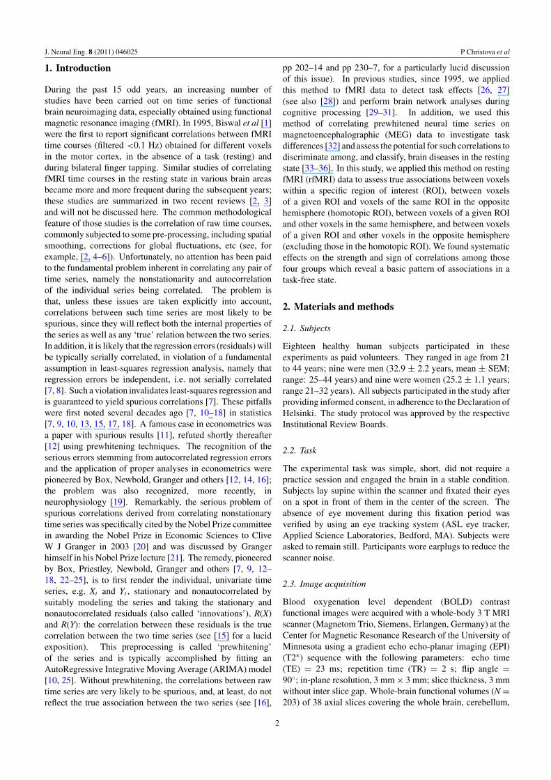
crosscorrelation function (CCF) between these time series, it isrequired, from first principles [10, 13–15, 17], that individualseries be rendered stationary and nonautocorrelated for theircrosscorrelation to be valid (i.e. not spurious). ‘Stationarity’implies that statistical parameters do not vary along the timeseries, i.e. they are more or less constant at different time pointst, i.e. for small time intervals centered at t. There are threeparameters of interest: mean, variance and autocovariance.A simple plot of the data and a plot of the autocorrelationfunction would typically go a long way to begin assessment ofthe time series and decide on initial steps to render it stationary.For example, inspection of the raw BOLD time series plotsfor the two voxels in the top panel of figure 1 shows thatBOLD values vary with time (indicating the presence of timetrends, i.e. that the series is ‘integrated’ [14, 16]); moreover,inspection of the corresponding autocorrelation plots of theseseries in figure 2 (top panel) shows a strong dependenceof BOLD values on previous values, up to 15 lags beingplotted. On the other hand, the variance of BOLD valuesdoes not seem to vary systematically with the time-varyingmean. This initial qualitative assessment suggests that theseries is nonstationary and autocorrelated. The objective nowis to render the series stationary and nonautocorrelated, i.e.convert it to white noise, hence the term ‘prewhitening’. Thestrategy [7, 10, 15, 17, 22, 25] is to model the series andthen apply the model and take the residuals; the better themodeling of the series is, the closer the residuals will beto white noise. This prewhitening is commonly achievedin two stages. The first stage is called model identificationand consists in identifying the factors that are relevant for theinternal structure of the series. The tools for this step consistof inspecting the series and plotting autocorrelation functions,including the raw autocorrelation (ACF, i.e. the correlationbetween Xt and Xt−k) and the partial autocorrelation (PACF,i.e. the correlation between Xt and Xt−k when all interveningrelations between Xt and Xt−k , namely between Xt and {Xt−1,. . ., Xt−k−1} have been accounted for, that is ‘partialed out’).Based on the data time series plot and the shape of ACF andPACF, a tentative model is suggested with respect to three kindsof basic factors: dependence of a value on previous values(‘AutoRegressive, AR’ component of the model), presenceof time trends (‘Integrative, I’ component of the model),and dependence of a value on the variation of previousvalues (‘Moving Average, MA’ component). Following thepioneering work of Box and Jenkins [10], this is called ARIMAmodeling of a time series (from the capitalized initials ofthe three model components above). An ARIMA model isconcisely described as of (p, d, q) orders, where p denotesthe AR orders (i.e. the number of AR lags in the model), ddenotes the I orders (i.e. the number of differencing in themodel), and q denotes the MA orders (i.e. the number of MAlags in the model). After a tentative choice of (p, d, q) orders,we proceed in the second stage, namely model parameterestimation. This stage involves computations which arecommonly implemented in several statistical packages andwhich yield coefficients for the AR and MA lags specified.Typical diagnostic checking of the model involves plotting theresiduals, their ACF and PACF, ensuring that the AR and MA

3

J. Neural Eng. 8 (2011) 046025 P Christova et al

Figure 1. Resting fMRI time series recorded from 2 voxels in the left superior parietal lobule of a single subject after various stages ofprocessing, as indicated.

coefficients are within bounds of stationarity and invertibility,respectively, and calculating some global measures, includingthe sums of the squares of residuals, Akaike’s informationcriterion, Schwartz’s Bayesian criterion, etc. The essentialpoint for our application is not really to model the seriesperfectly (this could be an ad hoc objective of another studyaimed to elucidate the various dependences in a BOLD timeseries) but to model it adequately enough so that the residualsobtained are stationary and nonautocorrelated. If indeed so,we retain them for the subsequent crosscorrelation analysis;

otherwise, the model is further refined iteratively by varyingthe (p, d, q) orders until this goal is attained.

Typically, we start with (p = 0, d = 1, q = 0) whichinvolves first-order differencing: Xt − Xt−1 (see below). Thisaims to remove nonperiodic time trends which are ubiquitous,even in random walks [14, 16]. (For a particularly instructiveexplication of this problem, see [14] and [16], pp 202–14and pp 230–7.) (Periodic trends, if present, say at lag k areremoved by differencing at that lag: Xt − Xt−k.) It can be seenin figure 1 (middle panel) that this process indeed removed

4

J. Neural Eng. 8 (2011) 046025 P Christova et al

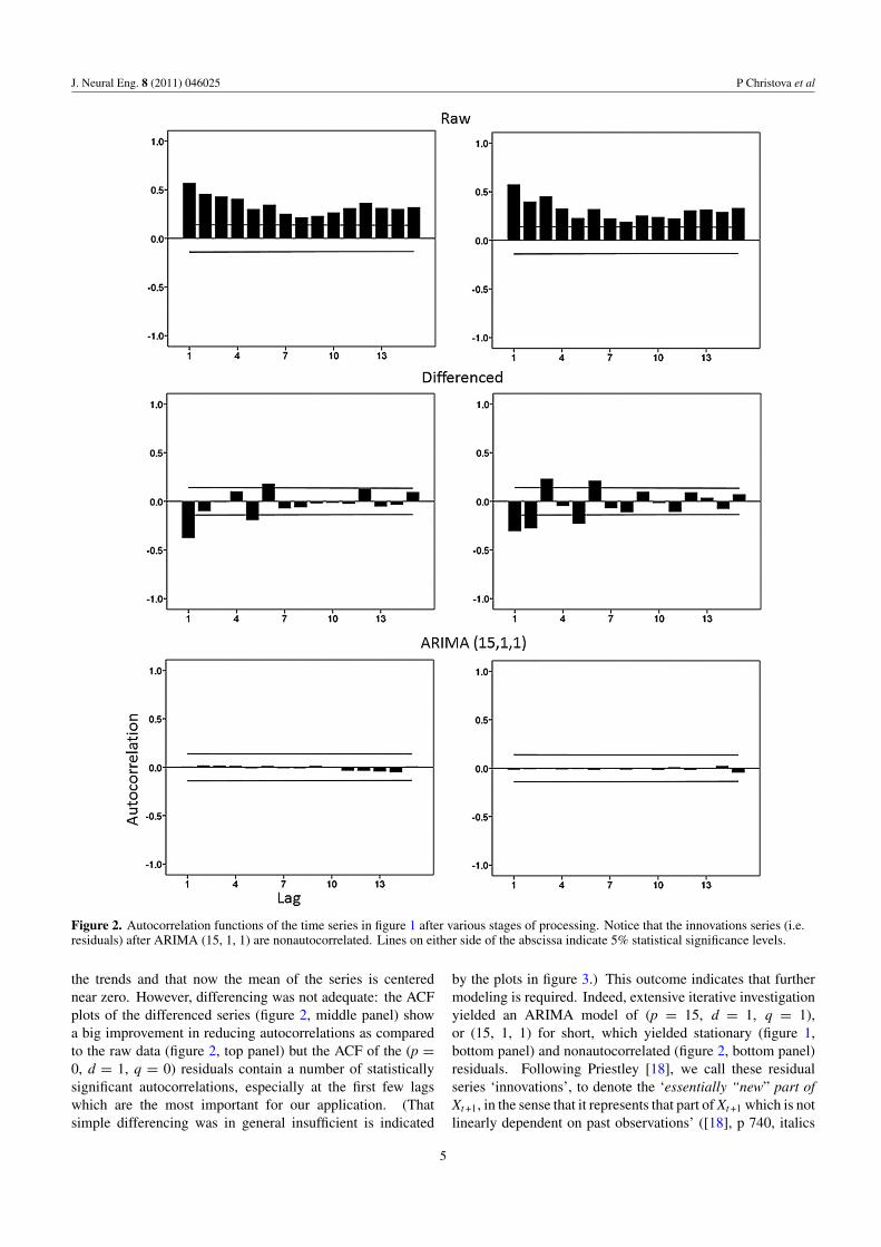
Figure 2. Autocorrelation functions of the time series in figure 1 after various stages of processing. Notice that the innovations series (i.e.residuals) after ARIMA (15, 1, 1) are nonautocorrelated. Lines on either side of the abscissa indicate 5% statistical significance levels.

the trends and that now the mean of the series is centerednear zero. However, differencing was not adequate: the ACFplots of the differenced series (figure 2, middle panel) showa big improvement in reducing autocorrelations as comparedto the raw data (figure 2, top panel) but the ACF of the (p =0, d = 1, q = 0) residuals contain a number of statisticallysignificant autocorrelations, especially at the first few lagswhich are the most important for our application. (Thatsimple differencing was in general insufficient is indicated

by the plots in figure 3.) This outcome indicates that furthermodeling is required. Indeed, extensive iterative investigationyielded an ARIMA model of (p = 15, d = 1, q = 1),or (15, 1, 1) for short, which yielded stationary (figure 1,bottom panel) and nonautocorrelated (figure 2, bottom panel)residuals. Following Priestley [18], we call these residualseries ‘innovations’, to denote the ‘essentially “new” part ofXt +1, in the sense that it represents that part of Xt +1 which is notlinearly dependent on past observations’ ([18], p 740, italics

5

J. Neural Eng. 8 (2011) 046025 P Christova et al

Figure 3. Percentages of autocorrelations in raw and differenced resting fMRI time series exceeding a ∼95% confidence interval asthreshold are plotted against the absolute lag (see the text). Notice (a) the very high percentage of autocorrelations exceeding threshold, and(b) that differencing is not sufficient to yield nonautocorrelated residuals, hence the need for additional (ARMA) components in the timeseries model.

in the original). (Priestley also provides a nice geometricalinterpretation of the innovations process in [18], figure 10.3,p 740.) We used the SPSS statistical package for Windows(version 15, SPSS Inc., Chicago, IL, 2006) to carry out theARIMA modeling. Our choice of 15 AR lags was dictatedby the fact that our crosscorrelation analysis extended up to10 lags, so we wanted to ensure lack of autocorrelation for afew lags beyond 10.

2.6. ARIMA equations

The formal ARIMA equations are given in practically everytextbook on time series (see [25] for the most recent textbookby Box et al). However, we give them here too for the purposeof clarity. We present below the standard equations. (In timeseries analysis, use is made frequently of the backshift and delnotation which can be found in time series textbooks.)

2.6.1. Integrative (I) model. Time series are oftennonstationary, i.e. typically show an average increase or adecrease in their value over time (see, e.g., the raw BOLD timeseries in figure 1, top panels). As mentioned in the precedingparagraph, the first step is to make the series stationary in itsmean. This is achieved by differencing. Consider a BOLDseries X(t) with TR = 2 s, where there is an upward lineartrend (e.g., top-right plot in figure 1). This means that every2 s the series increases on average (in expectation) by someconstant amount C. Since

Xt = C + Xt−1 + Nt (1)

where Nt is a random ‘noise’ component with expectation zero,

Xt − Xt−1 = C + Nt . (2)

Thus Nt + C, or just Nt , is a stationary process with the lineartrend removed. Let zt be the stationary series obtained bydifferencing series Xt :

zt = Xt − Xt−1. (3)

2.6.2. AutoRegressive (AR) model. The AR model refers todependence on past values of the series. Obviously, it canonly be applied to a stationary series, i.e. to a series withouttrend (otherwise, the estimated dependence on previous valueswould include the trend, and hence would be spurious andinvalid). Given the stationary series zt , the AR model impliesa linear dependence of zt on previous values {zt−1, zt−2, . . .,zt−k}, and is similar to a linear regression model. The highestlag k specifies the order p of the AR model. At any time

zt = C + �1zt−1 + �2zt−2 + · · · + �κzt−k + at , (4)

where C is the constant level, {zt−1, zt−2, . . ., zt−k} arepast series values (lags), the �s are coefficients (similar toregression coefficients) to be estimated, and at is a randomvariable with mean zero and constant variance. The ats areassumed to be independent and represent random errors orrandom shocks.

2.6.3. Moving Average (MA) model. The MA model refers tothe dependence on the past values of the random shocks above.(Again, this can only be applied to a suitably differenced,stationary series.) Given the stationary series zt , the MAmodel implies a linear dependence of zt on previous values{at−1, at−2, . . ., at−m}. The highest lag m specifies the orderq of the MA model. At any time,

zt = at − �1αt−1 − �2αt−2 − · · · − �καt−m. (5)

This model is called moving average because zt is assumed tobe a weighted average of the uncorrelated ats.

2.6.4. Combined ARMA model. The AR and MA models canbe combined to an ARMA model of the stationary series zt toaccount for both past values and past random shocks. Notethat, similar to the AR and MA cases, the ARMA model canonly be applied to a suitably differenced stationary process; itis incorrect and invalid to apply such a model to series with

6

J. Neural Eng. 8 (2011) 046025 P Christova et al

trends. Consider an ARMA model with (p = 3, q = 2) of thestationary series zt . The combined model is then

zt = C + �1zt−1 + �2zt−2 + �3zt−3 + at − �1αt−1 −�2αt−2.

(6)

Given that zt is a stationary, once-differenced series, thecomplete model for the original series Xt is an ARIMA modelwith (p = 3, d =1, q = 2).

2.7. Crosscorrelations

Crosscorrelations r between the innovations series of each pairof voxels were calculated for 10 lags, corresponding to 20 s,given TR = 2 s. (It should be noted that these crosscorrelationlags are unrelated to the autocorrelation lags used for ARIMAmodeling and diagnostics.) In addition to the lag-basedanalysis, we also analyzed the zero-lag crosscorrelations asa special case.

2.8. Data transformations

For statistical analyses, standard transformations were appliedto specific data as follows to stabilize their variance andnormalize their distributions [41].

(a) Correlations were z-transformed [42]: z = 0.5[loge(1+r) − loge(1 − r)].

(b) Ratios were log-transformed: ratio′ = loge(ratio).(c) Proportions were arcsin-transformed: proportion′ =

arcsin(proportion); for plotting purposes, proportionswere converted to percentages.

The double-precision functions of the IMSL statisticallibrary in FORTRAN were used for all computations usingpersonal computers (Compaq Visual Fortran ProfessionalEdition, version 6.6B) and a 512-core Linux cluster (Rocks 5.1,CentOS 5.2, Intel Fortran Compiler 10.0, IMSL 6.0).

2.9. Statistical analyses

Standard statistical analyses were performed [41], includinganalysis of covariance (ANCOVA), linear regression, t-test,etc. The SPSS statistical package for Windows (version 15)was used for this purpose. The Durbin–Watson test (and itsstatistical significance for testing the null hypothesis that serialcorrelation of regression residuals is zero) was computed usingMatlab R2010b, version 7.11.0.584 (64 bit).

2.10. Brain groups

Crosscorrelations were calculated for each pair of voxels.These voxel pairs were assigned as follows to one of fourgroups. In the intra-area group (group I), both voxels ina pair were located within the same area; in the homotopicgroup (group II), one voxel was located in a given area and theother in the same area of the opposite hemisphere; in the ipsi-hemispheric group (group III), one voxel was located in a givenarea and the other in any other area of the same hemisphere;finally, in the contra-hemispheric group (group IV), one voxelwas located in a given area of one hemisphere and the other in

any nonhomotopic area of the opposite hemisphere. Variousstatistics (e.g. means) were calculated for each group acrosssubjects.

3. Results

3.1. General

Data (i.e. BOLD time series) were available from 212 227voxels in the 60 brain areas above (30 areas for eachhemisphere) corresponding to 1 255 517 520 pairs. Given thatwe computed a crosscorrelogram with 21 values (0 ± 10 lags)for each pair, the total number of crosscorrelations calculatedwas 26 365 867 920.

3.2. ARIMA

The raw BOLD times series were typically nonstationaryand highly autocorrelated (figures 1 and 2, top panel).Following differencing, the series became centered on zero(figure 1, middle panel) but significant autocorrelationsremained (figure 2, middle panel). These were removed afterapplying the full ARIMA (15, 1, 1) model (see section 2) whichyielded innovations series (i.e. residuals) centered on zero withlower variance (figure 1, bottom panel) and nonautocorrelatedvalues (figure 2, bottom panel).

These changes in autocorrelations were quantified bycalculating the percentage of autocorrelations that exceededan arbitrary threshold, namely that the absolute value of anautocorrelation at a specific lag was higher than twice itsstandard error. (This threshold corresponds approximately toa 5% probability level for a single autocorrelogram.) Figure 3shows these percentages for different lags for the raw anddifferenced (i.e. detrended) data. It can be seen that veryhigh percentages of autocorrelations exceeded threshold forthe raw data, and that high percentages remained for the firsttwo lags in the detrended (differenced) data. This latter findingindicates that autocorrelations exceeding threshold are not justdue to time trends but are inherent to the BOLD time series. Incontrast, the percentages for the ARIMA (15, 1, 1) innovationsprocess exceeding threshold were extremely small and are notshown (for that reason). Specifically, the mean percentage(±SEM, N = 15 lags) of autocorrelations exceeding thresholdin the ARIMA innovations series was 0.0159% ± 0.008 24, ascompared to 74.3% ± 2.72 for the raw series and 20.34% ±5.57 for the differenced (detrended) series.

3.3. Crosscorrelations

As expected from the presence of trends and highautocorrelations above, crosscorrelations between raw BOLDtime series were very inflated (figure 4, upper panel),as compared to the crosscorrelations between the ARIMAinnovations series (figure 4, lower panel). In fact, differencesneed not be restricted to the magnitude of the correlation butthey affect its sign and lag, as illustrated in additional examplesin figure 5 (see also [16] pp 230–7). The correlations betweenraw time series are spurious, and those between the ARIMAinnovations series are correct.

7

J. Neural Eng. 8 (2011) 046025 P Christova et al

Figure 4. CCFs between the series illustrated in figure 1 for the rawand ARIMA innovations. Notice the spurious, widespread highcrosscorrelations in the raw data, as contrasted with the true, singlehigh zero-lag crosscorrelation of the innovation series.

3.3.1. Serial correlations in regression residuals. Thespuriousness of the correlations between raw time series (toppanel of figure 4 and left panel of figure 5) stems not onlyfrom first principles [10, 12–18], recognized in Granger’sNobel Prize Citation [21] and his Nobel Prize Lecture [20],but also from the fact that correlating nonstationary time seriestypically violates a fundamental assumption of least-squaresregression, namely that regression errors (i.e. residuals) beindependent [7, 8, 41]; if regression errors are seriallycorrelated, the correlation coefficient calculated is spurious.The estimates of any least-squares regression analysis withserially correlated errors are invalid, with typically lowestimates of standard errors and hence inflated statisticalsignificance of the slope and inflated correlation coefficient.These detrimental effects of serially correlated errors arebeing explicated in practically every standard textbook ofelementary (or sophisticated) statistics, for the problem isspecific to regression/correlation of any data, not just timeseries. For example, a standard textbook on regression [8]devoted 16 pages (pp 153–69) to just this issue. Fortunately,

there is a special test by which to detect serial correlationin regression residuals, namely the Durbin–Watson test[43, 44], developed 60 years ago. The Durbin–Watson testcan tell us whether a violation of error independence exists,and whether it is significant. Therefore, this is an objectivemeasure by which to test the validity of any analysis, includingany such analysis of neural associations reported in this paperas well as in the literature. Since we do not have access to datapublished in the literature from other groups, we carried out anextensive analysis of the residuals in a sample of 300 voxels(yielding 44 850 pairwise correlations) from our data, underthree conditions: (a) raw time series, (b) time series filteredas described by Fox et al [4] (0.009 < f < 0.08 Hz), and(c) prewhitened time series, as described above. For each pair,we calculated the autocorrelation function of the residuals andthe corresponding Durbin–Watson test statistic d. We illustratethe results in figures 6 and 7. In figure 6 (left panel), we plotthree CCFs for a pair of voxels. It can be seen that they aredrastically different, and that the crosscorrelations of the rawand filtered time series are very inflated. In fact, both thehigh values of the correlations and the smooth shape of thecrosscorrelograms of nonstationary series make them suspect,as succinctly discussed by Granger and Newbold: ‘Thus, notonly does one have to contend with the spurious regressionphenomenon of the size of the cross correlations, but alsothe shape of the cross correlogram is impossible to interpretsensibly’ ([16], p 232). In the right panel of figure 6, we plotthe autocorrelation functions of the residuals for the zero-lagcrosscorrelation: it can be seen that the residuals are highlyautocorrelated for both the raw and filtered data, with lag 1serial correlation close to 0.8. The Durbin–Watson statistic dwas 1.237 for the raw data regression, 0.281 for the filtereddata and 2.095 for the prewhitened data (the smaller the valueof d, the higher the serial correlation of the residual, the moresuspect the correlation coefficient [16]). The critical value(p < 0.05) of d in our sample is 1.753: any value below itrejects the null hypothesis that the serial correlation of theresiduals is zero, so only the prewhitened data yield correctestimates. The spuriousness of high correlations associatedwith low d is beautifully discussed and illustrated in [14, 16](see also [21, 20]). Finally, in figure 7, we plot histograms ofall Durbin–Watson d values obtained in this analysis of 44 850correlations: it can be seen that both raw and filtered data hadd values below critical significance threshold (vertical line),hence are providing wrong correlation estimates (99.6% forthe raw and 100% for the filtered data). By contrast, 100%of the prewhitened data had d values above the threshold, thusproviding correct estimates.

3.3.2. Neural connectivity maps. Both fundamentalstatistical considerations (discussed in the introduction andsection 4 below) as well as the results obtained above showthat correlations between nonstationary and/or autocorrelatedtime series are spurious. In this analysis we assessed theextent of this error and the effect it may have on inferencesabout neural connectivity by plotting the neural connectivitypattern obtained by correlating filtered and prewhitened series.

8

J. Neural Eng. 8 (2011) 046025 P Christova et al

(A) (A´)

(B) (B´)

(C) (C´)

Figure 5. Three additional examples of spurious CCF (A, B, C) between raw time series and corresponding true CCF (A′, B′, C′) betweenthe corresponding ARIMA innovations. Notice that the presence of a true significant CCF between innovations (C′) is missed in the rawseries (C).

Figure 8 plots the spatial pattern of significant (p < 0.05) zero-lag correlations obtained for the right superior parietal lobuleof one subject. As expected from first principles, the numberof significant correlations was much higher (3.5 times) in thefiltered than the prewhitened case. Even more importantly,it can be seen in figure 8 that the prewhitened analysisyielded an interesting pattern of functional connectivity

within the superior parietal lobule, consisting of two separatesubgroups linked by negative correlations; no such patternwas discernible in the filtered case. These results underscorethe power and prospect of the correct correlation analysis fordiscovering true neural connectivity patterns. Very similarresults were obtained for other areas and are currently underinvestigation.

9

J. Neural Eng. 8 (2011) 046025 P Christova et al

Figure 6. Left panel: crosscorrelograms of raw, filtered (see the text) and prewhitened BOLD time series of the same voxel pair. Rightpanel: color-coded autocorrelograms of the regression residuals for the zero-lag correlation.

10

J. Neural Eng. 8 (2011) 046025 P Christova et al

Figure 7. Frequency distributions of the Durbin–Watson d statisticin 44 850 cases of zero-lag crosscorrelations (all pairwisecorrelations between 300 voxels). The vertical line indicates thep < 0.05 threshold for rejecting the null hypothesis that the serialcorrelation of the regression residuals is zero. Values below thatlevel (i.e. to the left of the line) reject the null hypothesis (indicatingthat there exists a significant serial correlation).

3.4. Peak crosscorrelations

3.4.1. General. As mentioned above, a crosscorrelogramwas computed for each pair of voxels (0 lag ± 10 lags =21 crosscorrelations). For this analysis, we wanted toidentify the sign, magnitude and lag of the strongestcrosscorrelation in each crosscorrelogram, and how thesemeasures differed among the four brain groups defined above.For that purpose, the maximum absolute crosscorrelationwas found and its sign and lag noted and assigned to oneof the four brain groups, depending on the location ofthe crosscorrelated voxels. For each group, the followingsummary statistics were computed for each lag: (1) thenumber of positive crosscorrelations (Np), (2) the numberof negative crosscorrelations (Nn), (3) the positive/negativeratio: Np

Nn, (4) the percentage of positive crosscorrelations

(with respect to all positive crosscorrelations), (5) thepercentage of negative crosscorrelations (with respect toall negative crosscorrelations), (6) the mean positive z-transformed crosscorrelation, (7) the mean negative z-transformed crosscorrelation, and (8) the overall z-transformedmean. We found the following.

3.4.2. Sign and counts of peak crosscorrelations. Withrespect to the counts of the strongest crosscorrelations, therewere many more positive than negative crosscorrelations.Figure 9 shows the Np

Nnratio as a function of lag for each

group. (The positive and negative lags have been collapsed totheir absolute value, since the sign of the lag has no meaningwhen averaging.) It can be seen that this ratio was very highat zero lag, decreased at |lag| = 1, and practically becameunity for subsequent lags. In addition, there were systematicdifferences among the four brain groups, in that the Np

Nnratio

was highest for the intra-area group, and progressively lowerfor the homotopic, ipsi-hemispheric and contra-hemisphericgroups. These group differences were most prominent at zerolag and at |lag| = 1. An ANOVA on loge

(Np

Nn

)(see section 2)

showed highly significant effects of group (F3,1468 = 9.72,P < 0.001), |lag| (F10,1468 = 537.39, P < 0.001) and group×|lag| interaction (F30,1468 = 2.18, P = 0.002).

3.4.3. Lag distributions of peak crosscorrelations. Positiveand negative crosscorrelations were distributed unevenlyacross different lags. The percentage of positive (peak)crosscorrelations was highest at zero lag and decreasedsmoothly at longer lags, becoming practically flat at |lag| �3 (figure 10, upper panel). In addition, there were systematicgroup differences; an ANOVA on the arcsin-transformedproportions (see section 2) showed highly significant effectsof group (F3,1468 = 8.95, P < 0.001), |lag| (F10,1468 =1962.5, P < 0.001) and group x|lag| interaction (F30,1468 =19.73, P < 0.001). In contrast, the percentages of negativecrosscorrelations varied more widely across lags (figure 10,lower panel), with a peak at |lag| = 2. An ANOVA showeda highly significant effect only of |lag| (F10,1468 = 212.59,P < 0.001); neither group nor the group ×|lag| interactionwere statistically significant (P = 0.982 and P = 0.999,respectively). It can be seen in figure 10 (lower panel) that

11

J. Neural Eng. 8 (2011) 046025 P Christova et al

Figure 8. Network connectivity patterns of the right superior parietal lobule of a single subject derived using filtered (see the text) orprewhitened BOLD time series. Green and red lines indicate positive or negative zero-lag cross correlations, respectively. A nominalthreshold of p < 0.05 on the correlation coefficient was applied. There were 3.5 times more significant correlations in the filtered than theprewhitened series (N = 830 and 241, respectively).

Figure 9. Positive/negative ratio of the counts of peakcrosscorrelations for the four brain groups is plotted against theabsolute lag.

the percentage for the ipsi- and contra-hemispheric groups(blue and magenta color, respectively, almost superimposed)are lower than the other values. To test whether this wassignificant, we performed an additional ANOVA specificallyfor |lag| = 0. The group effect was not statistically significant(P = 0.873); in addition, none of the pairwise comparisonsbetween groups showed any statistically significant difference(P > 0.5 for all comparisons).

3.4.4. Strength of peak crosscorrelations. Figure 11 plotsthe mean (z-transformed, across subjects) crosscorrelationsfor different lags and groups. It can be seen that (a) positivecrosscorrelations were consistently stronger (i.e. in absolutevalue) than negative ones, (b) both positive and negative

crosscorrelations were strongest at zero lag and decreasedprogressively at longer lags, and (c) both positive and negativecrosscorrelations were strongest for the intra-area group andprogressively weaker for the homotopic, ipsi-hemispheric,and contra-hemispheric groups. Interestingly, the intra-areagroup seems to cluster with the homotopic group, whereasthe ipsi-hemispheric group seems to cluster with the contra-hemispheric group. An ANOVA on positive crosscorrelationsshowed highly significant effects of group (F3,1468 = 26.63,P < 0.001), |lag| (F10,1468 = 441.48, P < 0.001) and group×|lag| interaction (F30,1468 = 22.0, P < 0.001). An ANOVA onnegative crosscorrelations showed highly significant effects ofgroup (F3,1468 = 107.78, P < 0.001), |lag| (F10,1468 = 1175.4,P < 0.001) and a weaker group ×|lag| interaction (F30,1468 =1.59, P = 0.023).

3.5. Zero-lag crosscorrelations

3.5.1. General. In the previous section we focused onthe analysis of peak crosscorrelations with respect to theirvalues, sign, lag distribution and brain group differences. Inthis section we focused specifically on the crosscorrelationsobserved at zero lag, irrespective of the location of the peakcrosscorrelation. These two analyses provide different andcomplementary information.

3.5.2. Sign and counts of zero-lag crosscorrelations.Overall, there were approximately three times more positivethan negative correlations (figure 12); these proportionswere highly statistically significant (paired t-test on arcsin-transformed proportions, t71 = 33.29, P < 0.001, N = 18subjects × 4 groups = 72). In addition, there were systematicdifferences among the four brain groups, which are as follows(figure 13). With respect to the frequency of occurrenceof positive and negative correlations, (a) the percentage ofpositive correlations was highest for the intra-area group,

12

J. Neural Eng. 8 (2011) 046025 P Christova et al

Figure 10. Relative distributions of positive (upper panel) andnegative (lower panel) crosscorrelations are plotted against absolutelag for the four brain groups. Since the negative and positive werecollapsed (see the text), 100% = percentage at zero lag + (2 ×percentage at the other lags).

and progressively lower for the homotopic, ipsi-hemisphericand contra-hemispheric groups (ANOVA, group main effect,F3,68 = 6.14, P = 0.001) (figure 13, top panel); (b) conversely,the percentage of negative correlations was lowest in the intra-area group, and progressively higher for the homotopic, ipsi-hemispheric and contra-hemispheric groups (ANOVA, groupmain effect, F3,68 = 6.34, P = 0.001) (figure 13, middlepanel); (c) the positive/negative ratio was highest for the intra-area group, and progressively lower for the homotopic, ipsi-hemispheric and contra-hemispheric groups (ANOVA, groupmain effect, F3,68 = 6.00, P = 0.001) (figure 13, bottom panel).

3.5.3. Strength of zero-lag crosscorrelations (figure 15).Overall, the strength of the mean positive z-transformed zero-lag crosscorrelation (z0 = 0.13) was approximately two timesthat of the mean negative one (|z0| = 0.07) (figure 14). Inaddition, there were systematic differences among the fourbrain groups, which are as follows (figure 15). Specifically,

Figure 11. Mean z-transformed positive and negativecrosscorrelations for each brain group are plotted against absolutelag.

the z-transformed mean positive crosscorrelation was highestfor the intra-area group, and progressively lower for thehomotopic, ipsi-hemispheric and contra-hemispheric groups(ANOVA, group main effect, F3,68 = 13.83, P = 0.001)(figure 15, top panel). In contrast, the z-transformed meannegative crosscorrelation did not differ significantly amonggroups (ANOVA, group main effect, F3,68 = 0.974, P =0.41) although it was lowest in the intra-area group, andprogressively higher for the homotopic, ipsi-hemispheric andcontra-hemispheric groups (figure 15, middle panel). Finally,statistically significant differences with respect to brain groupswere observed for the overall mean (ANOVA, group maineffect, F3,68 =11.10, P < 0.001).

3.5.4. Relative brain groups contributions. A different issueconcerns the relative contributions of the various sources(i.e. the four brain groups) to the whole variance accountedfor by them. We derived approximate estimates of thesecontributions as follows. First, we calculated the mean of theabsolute values of the zero-lag z-transformed crosscorrelationsfor each group. This step ensured that all correlations are taken

13

J. Neural Eng. 8 (2011) 046025 P Christova et al

Figure 12. Percentages of positive and negative zero-lagcrosscorrelations (total N = 1255 517 520). Lines on top of the barsindicate one SEM calculated from across subjects and brain groups(N = 18 subjects × 4 groups = 72).

into account, irrespective of their sign. Next, we convertedthese z-transformed values to crosscorrelations. Then, wesquared these crosscorrelations to derive the proportion ofvariance accounted for by the crosscorrelation in each group.Finally, we added these proportions and re-expressed themas percentages of their sum. These percentages were 35%for the intra-area group, 27% for the homotopic group, 20%for the ipsi-hemispheric group, and 18% for the contra-hemispheric group (figure 16). These values can be consideredas approximate estimates of the overall relative strength ofassociation between zero-lag, BOLD voxel signals in thedifferent brain groups.

4. Discussion

4.1. Methodological considerations

4.1.1. Spuriousness of correlating nonstationaryautocorrelated time series. As mentioned in the introduction,previous studies of functional connectivity have typicallyrelied on correlating time series, variously preprocessed (e.g.filtered, adjusted, smoothed, averaged, etc) but without takinginto consideration the single most important aspect in a timeseries, namely their internal structure (i.e. nonstationarity andautocorrelation). The point is that the true value of such resultswith respect to the true association between the two time seriesis undetermined, since the computed correlations variouslyreflect a combination of factors, including the internal structureof the series, external influences and the true relation betweenthe two series [15]. Unless the time series being correlated arestationary and nonautocorrelated, their computed correlationswill be spurious, due, among other reasons, to autocorrelatederrors. It is this aspect which spoils any correlation betweennonstationary and/or nonautocorrelated time series and whichrenders any conclusions drawn from such analysis invalid. To

Figure 13. Mean percentages of positive, negative andpositive/negative ratio of zero-lag crosscorrelations for each braingroup, as indicated. Lines on top of the bars indicate one SEMcalculated from across subjects (N = 18).

14

J. Neural Eng. 8 (2011) 046025 P Christova et al

Figure 14. Mean positive, negative and overall z-transformedzero-lag crosscorrelations for each brain group, as indicated.Conventions as in figure 13

quote directly from a famous paper by Granger and Newbold[14] on work that was cited in the 2003 Clive Granger NobelPrize press release [21] and discussed by Granger in his NobelPrize lecture [20]:

‘There are, in fact, as is well known, three majorconsequences of autocorrelated errors in regression analysis:

(i) Estimates of the regression coefficients are inefficient.(ii) Forecasts based on the regression equations are sub-

optimal.(iii) The usual significance tests on the coefficients are invalid’

([14], p 111).

In fact, the detrimental effects of correlated errors hasbeen stressed repeatedly over the past several decades withrespect to regression in general [7, 8], correlation of rawtime series [10, 12–18], and forecasting in single time series[16]. And yet, all studies we know of on resting or task-related fMRI during the past 16 odd years have relied oncorrelations between raw (or filtered) nonstationary and/orautocorrelated time series. (Those studies are too manyto cite here; for typical examples, see [4] and [45] forresting and task fMRI studies, respectively.) The currentsituation in our field resembles very much the situation ineconometrics in the early 1970s. It is worth quoting againfrom the paper of Granger and Newbold [14], published37 years ago: ‘We find it very curious that whereasvirtually every textbook on econometric methodology containsexplicit warnings of the dangers of autocorrelated errors,this phenomenon crops up so frequently in applied work’([14], p 111).

The same considerations apply to time series analysesin the frequency (spectral) domain, since the two methods(time and frequency domains) are intimately related [9]. Forexample, the autospectrum is the Fourier transform of theautocovariance function, and, similarly, the cross spectrumis the Fourier transform of the crosscovariance function.

Figure 15. Mean positive and negative zero-lag z-transformedcrosscorrelations across all brain groups. Conventions as infigure 13.

Spectral analyses of times series have a long history (see, e.g.,[9, 18, 46–49]. All of this early work, as well as subsequentwork, has drawn attention to the detrimental effects of

15

J. Neural Eng. 8 (2011) 046025 P Christova et al

Figure 16. Relative contributions of the four brain groups to thezero-lag crosscorrelations (see the text for details).

nonstationarities and autocorrelations on estimating the truespectral coherency between two time series. We quote directlyfrom Jenkins and Watts [9]: for the time domain: ‘ . . . unlessa filtering operation is applied to both series to convert themto white noise, spurious cross correlations may arise’ ([9],p 321); and for the frequency domain: ‘ . . . the sample phaseand cross amplitude spectral estimators are derived, underthe assumption that the two processes are uncorrelated whitenoise processes’ ([9], p 363). The choice of the specificmethod to use depends on the problem; for example, frequencydomain analyses (i.e. cross spectral analyses) yield valuableinformation on relations between the two series across a rangeof frequencies, whereas time domain analyses (i.e. CCF)provide valuable information on the sign (positive or negative)of the relation. In fact, time-domain and frequency-domainanalyses can be used profitably on the same problem ([9],p 367). However, the important point is that for validinferences to be obtained regarding the relations betweentwo time series, both methods require that the time seriesbe stationary and nonautocorrelated.

4.1.2. Prewhitening. To find the true relation between twotime series, a two-stage approach is followed, explicatedlucidly in [15]. First, univariate models are fitted to eachseries and the residuals (innovations) taken, to strip the seriesof nonstationarities and autocorrelations before a correlation(or coherence) is computed. Thus the series are convertedto white noise [14–16], and hence the term ‘prewhitening’[46] (see also [49]). Prewhitening can be achieved eitherin the frequency domain [46, 47] or in the time domain[10, 25]. The latter procedure is called ARIMA [10], a termderived from the initials of three essential components thatdefine a time series, namely an AutoRegressive component(i.e. the dependence of a given value in the series on previousvalues), an Integrative component (e.g. a linear trend), and aMoving Average component (i.e. the dependence of a givenvalue on random shocks of previous values). This procedure is

standard in time series analysis, is straightforward, is describedin many time series analysis textbooks [10, 18, 22–25], and isreadily implemented in various statistical packages (e.g. SPSS,Matlab, SAS, R, etc). The main tool for model identificationis the autocorrelation and partial autocorrelation functions,assuming that the series is suitably differenced to be stationary.In the frequency domain, the tool is the spectrum which isthe Fourier transform of the autocorrelation function of thedifferenced (stationary) series. Prewhitening is a standardprocedure in many fields, especially in industrial engineeringand econometrics, where forecasting and control carry majorweight and where wrong statements and predictions carrysubstantial penalties.

4.1.3. Other approaches. Crosscorrelation analyses in fMRIresearch address directly the issue of dynamic connectivity;in contrast, the grouping of fMRI time courses into similarpatterns addresses the issue of similarity of spontaneous orevoked temporal fluctuations in the BOLD signal. It should benoted that these are two very different issues: (a) no inferenceson connectivity can be drawn from similarities in time courses,whereas, conversely, (b) no inferences on similarity of timecourses can be drawn from information on connectivity. Theformer case is undetermined, since many different quantitiescan have very similar time courses without been connected(e.g. trains moving north with the same speed time course inParis and Athens); and in the latter case, the relation betweenthe time courses in a pair of connected quantities is determinedby their transfer function (including feedback and delays), andmay or may not be similar.

Grouping of fMRI time courses according to their shapehas been carried out using principal component analysis(PCA) and independent component analysis (ICA) (seerecent reviews [2, 3]). These methods have provideduseful information concerning neural systems participating inpotentially common functions. However, as mentioned above,no inference on connectivity can be drawn from the degree ofsimilarity of time courses, and, hence, no such inferences onneural connectivity can be drawn from PCA or ICA analysisof BOLD time courses. Problems arise when correlations arecomputed between BOLD time series grouped together byprior PCA or ICA analyses (see [50] for an example): suchcorrelations are spurious if the raw (or filtered) data are used,as discussed above. The point is that the selection processof which time series are being correlated is irrelevant to thecorrelation itself: it makes no difference whether the two seriesare from the same or different ICA-based groups. The onlyaspect that matters is whether the series are stationary andnonautocorrelated in order for the correlations obtained to becorrect (i.e. not to be spurious). In fact, any grouping method,including PCA, ICA or other, could be very useful if coupledwith proper crosscorrelation analysis of prewhitened series.

4.2. Peak crosscorrelations across lags

In this study we carried out an extensive analysis ofvoxel-by-voxel pairwise crosscorrelations after each serieswas prewhitened to yield stationary, nonautocorrelated

16

J. Neural Eng. 8 (2011) 046025 P Christova et al

innovations. Therefore, the estimates of the interactions(i.e. crosscorrelations) obtained reflect the true associationsbetween voxel BOLD time series and are not spurious. As afirst step for this analysis, we focused on crosscorrelationsof voxels within the same area, between homotopic areas,between an area and all other voxels in the same hemisphere,and between an area and all voxels in the contralateralhemisphere (excluding the homotopic area). As shownin figure 5, individual crosscorrelograms varied widelyin shape. In order to evaluate their basic aggregatecharacteristics, we focused on the peak (i.e. highest absolutevalue) of the crosscorrelogram: analyzing the peaks enabledus to derive summary statistics on the highest possibleinteractions between single voxel BOLD time series. Weperformed analyses extending up to 10 lags (i.e. 20 s, givenTR = 2 s), as an upper limit of expected interactions,and collapsed the positive and negative sides of thecrosscorrelogram, since the sign of the lag has no meaning inpooled data. We then analyzed the prevalence of positive andnegative crosscorrelations, and their strength, as a function ofthe lag (figures 9–11). There were five major findings. First,positive interactions were much more frequent and strongerthan negative ones; second, the strongest interactions (meanabsolute values of crosscorrelations, figure 11) occurred atzero lag and decreased gradually at longer lags; third, thestrength of interactions varied systematically with the braingroup, such that intra-area > homotopic > ipsi-hemispheric >

contra-hemispheric; fourth, the relative distribution of positiveinteractions had a peak at zero lag, declined progressively atlonger lags, and differed among brain groups in the same orderas above; and fifth, and in contrast to the positive interactions,the relative distribution of negative interactions had a peak(tuned) at |lag| = 2 and did not differ significantly amongbrain groups. We discussed these findings in that sequencebelow.

These findings validate the resting, task-free BOLD signalas reflecting neural activity, since it is difficult to see how elsethis BOLD signal could be correlated between voxels of areasfar away, such as homotopic areas in opposite hemispheres.The finding that positive interactions occurred more frequentlyand were stronger than negative ones is not surprising, asit most probably reflects the more widespread excitatoryeffects in the cerebral cortex. For example, all long-rangecorticocortical projections are excitatory, whereas inhibitorymechanisms are local and, even there, more limited than theexcitatory ones. Also, the high percentages and values at zerolag are in accord with other findings [33] and are discussed inmore detail below. Perhaps the most remarkable findings ofthis analysis are (a) the discovery of the tuning of the negativeinteractions at |lag| = 2, i.e. at a relative shift of the timeseries by 4–6 s (given TR = 2 s), and (b) the fact that thistuning was invariant across all four brain groups. We interpretthis finding as reflecting the localized and uniform nature ofcortical inhibitory mechanisms, namely that such mechanismsare local and of the same nature and similar circuitry in variouscortical areas, hence the invariance across groups.

4.3. Zero-lag crosscorrelations

Interactions at zero lag (i.e. within an interval of TR =2 s) are a special case for two reasons. First, becausethey were most prevalent (as compared to other lags, seeabove) and second because synchronicity is a principleof brain function in its own merit. In this analysis, wefocused on zero-lag crosscorrelations as a time-snapshot, soto speak, irrespective of the location of the crosscorrelogrampeak. We found an orderly variation of zero-lagcrosscorrelations with respect to their sign, strength anddependence on brain groups. This indicates a robustunderlying organization of synchronous variation in restingneural activity. As pointed out in the discussion of the resultsfrom recent studies using magnetoencephalography (MEG)[32–36], the four most likely sources of synchronizationinclude recurrent axon collaterals of pyramidal cells [51],specific (parvalbumin) thalamocortical afferents [52, 53],divergent, multifocal (calbindin) thalamocortical afferents[52], and broadly distributed noradrenergic fibers [54]. Inaddition, since BOLD measurements were taken every 2 sin this study, it is likely that corticocortical interactions withsome lag (in the order of milliseconds) also contribute. Itis interesting that the sign of correlation also varied in asystematic fashion across the four brain groups, with theproportion of negative correlations increasing from group Ito group IV. This could reflect the similarity in the kind ofinformation being processed. For example, within an area(group I), negative interactions are low because local cellensembles perform similar operations; hence, they positivelycooperate. This would also hold, but to a lesser extent, forinteractions between a given area and its homotopic area inthe opposite hemisphere (group II). In contrast, other areasin the same hemisphere (group III), and certainly other areasin the opposite hemisphere (group IV) would be involved intheir own information processing; hence, they may be notexpected to cooperate (i.e. positively correlated) with thatgiven area. Such considerations would explain as follows theorderly trends observed for the variation of the percentage ofpositive and negative crosscorrelations across brain groups.The fact that the positive/negative ratio is always greaterthan 1 (i.e. the number of positive crosscorrelations is greaterthan the negative ones) underscores the greater preponderanceof excitatory (versus inhibitory) mechanisms in the cerebralcortex, as discussed above. However, the orderly decrease ofthat ratio across intra-area, homotopic, ipsi-hemispheric andcontra-hemispheric groups, in that order, suggests a differentoperating principle which, we propose, reflects the similarityof information being processed. In that sense, the categoricalbrain group horizontal axis in figure 13 would correspond to aqualitative axis of similarity in information processing. Thisidea can be further tested by analyzing data from specific areas,a work in progress in our laboratory.

Overall, these results indicate an orderly variation insynchronicity that seems to closely reflect the presenceand density of direct anatomical connections, an idea alsosuggested by other investigators (see, e.g., [55–59]). Theseare most dense within an area, substantial across homotopicareas and sparse across heterotopic areas (see, e.g., [60]).

17

J. Neural Eng. 8 (2011) 046025 P Christova et al

The covariation in activity comes from the fact that theseconnections are typically reciprocal, leading to a practicallysynchronous (within the 2 s of fMRI TR time) activationbetween interconnected areas. Thus, there may be nothingspecial about ‘default’ networks [see 2, 3] beyond theirreflection of existing anatomical connectivity.

Finally, our analysis provided an approximate quantitativeassessment of the relative contributions of the different kinds ofbrain groups (figure 16), as defined based on known anatomicalconnectivity. These relative contributions are broad estimatesderived from averaging large numbers of crosscorrelations.It is reasonable to suppose that interactions are actuallyspatially specific, in which case our measurements are likelyto underestimate such spatially restricted interactions. Weare currently investigating this issue by analyzing the fine-grain spatial distribution of the crosscorrelations obtained (seefigure 8 for an example).

4.4. State of the field: spurious correlations in functionalneuroimaging and what needs to be done

Talk about spurious or nonsense correlations between timeseries dates at least 85 years back, when G Udny Yule deliveredthe Presidential Address at the 1925–26 session of the RoyalStatistical Society in a lecture titled ‘Why do we sometimes getnonsense-correlations between time-series?’ [61]. His famousexample was the high positive correlation of 0.9512 betweenthe proportion of Church of England marriages to all marriagesfor the years 1866–1911 and the standardized mortality per1000 persons for the same years. Yule had the followingcomment on this finding: ‘Now I suppose it is possible,given a little ingenuity and goodwill, to rationalize very nearlyanything. And I can imagine some enthusiast arguing thatthe fall in the proportion of Church of England marriages issimply due to the Spread of Scientific Thinking since 1866,and the fall in mortality is also clearly to be ascribed to theProgress of Science; hence both variables are largely or mainlyinfluenced by a common factor and consequently ought to behighly correlated. But most people would, I think, agree withme that the correlation is simply sheer nonsense; that it hasno meaning whatever; that it is absurd to suppose that thetwo variables in question are in any sort of way, howeverindirect, causally related to one another’ ([61], p 2). Yuleastutely located the problem to the autocorrelations of the timeseries, and explored ways for correct analyses using techniquessimilar to modern prewhitening. Since Yule’s lecture, thetopic of spurious regressions resurfaced with force in appliedeconomics, leading to a false (spurious) prediction [11], itsrefutation using prewhitening [12], a simulation study [14],and a textbook [16]. By the end of the 1970s, the matter ofhow to analyze correctly relations between time series hadbeen settled in statistics and econometrics.

Now, this issue became prominent in functionalneuroimaging in the 1990s [62] and has continued to bein the foreground up to now unabated. As discussedabove, a large number of studies have been carried out inwhich correlations between raw (or filtered, averaged, etc)BOLD (and MEG [63]) time series have been performed as

the main tool to investigate dynamic, neural connectivity.Now, it is common practice in these studies to correlateBOLD time series in the resting or task-driven state withoutpaying attention to the serious errors in the correlationsobtained due to autocorrelated residuals. This can betested rigorously by (a) plotting the autocorrelogram of theseresiduals, and (b) calculating the Watson–Durbin test statistic[43]. Unfortunately, to our knowledge, no such informationhas been provided in the literature. Given the knownnonstationarity and autocorrelation of BOLD time series, itis obvious that correlations between such series are spurious[12, 14, 16]. The reason why ‘default’ brain networksinferred from such correlations may be found to be in accordwith known anatomical connectivity stems from the fact thatan existing, true relationship is part of the equation but itsrelative contribution is undetermined due to the influence ofnonstationarity and autocorrelation present in the individualseries. It is remarkable that history repeats itself and thatessentially we are facing the same problem that the field ofeconometrics faced 40 years earlier [12, 14, 16]. Indeed,we may paraphrase without loss of generality Granger andNewbold’s comment in 1974 [14]: We find it very curious thatwhereas virtually every textbook on time series methodologycontains explicit warnings of the dangers of autocorrelatederrors, this phenomenon crops up so frequently in functionalneuroimaging work.

Be that as it may, it is instructive to note how that problemwas dealt with in the field of econometrics when the flaws ofregression analysis with autocorrelated errors were exposed.The best and most succinct exposition was given by Grangerin his 2003 Nobel Prize Lecture. He said:

An example is a problem known as ‘spuriousregressions.’ It had been observed, by Paul Newboldand myself in a small simulation published in1974, that if two independent integrated series wereused in a regression, one chosen as the ‘dependentvariable’ and the other the ‘explanatory variable,’ thestandard regression computer package would veryoften appear to ‘find’ a relationship whereas in factthere was none. That is, standard statistical methodswould find a ‘spurious regression.’ This observationlead to a great deal of reevaluation of empirical work,particularly in macroeconomics, to see if apparentrelationships were correct or not. Many editors hadto look again at their list of accepted papers. Puttingthe analysis in the form of an error-correction modelresolves many of the difficulties found with spuriousregression. ([20], italics ours)

It seems appropriate and timely that such a reevaluation becarried out in the field of neuroscience. Reporting the Durbin–Watson statistic and providing the autocorrelogram of theregression residuals will clear the issue for a particular study,and prewhitening the time series will lead to the constructionof brain network models, including ‘default’ networks, basedon true, not spurious, correlations.

18

J. Neural Eng. 8 (2011) 046025 P Christova et al

Acknowledgments

This work was supported by United States Public HealthService grant NS32919 and the United States Department ofVeterans Affairs.

Note added in proof. It is frequently thought that the problems stemmingfrom autocorrelated BOLD time series can be dealt with by adjustingdegrees of freedom (see, for example, [4] p 9674). This is incorrect.Specifically, the reference by Fox et al [4] to Bartlett’s theory is misapplied.Bartlett’s general asymptotic expression for the variance of the samplecrosscorrelation coefficient assumes explicitly two jointly stationary timeseries with independent, identically distributed normal errors ([64]). Asdiscussed above, the basic problem stems from serially correlated regressionresiduals, i.e. from the violation of the assumption of error independence inleast squares regression, and not from the number of degrees of freedom;no adjustment of degrees of freedom can correct for serially correlatedresiduals. In addition, most problems in the literature stem from correlatingintegrated BOLD time series (i.e. time series with trends), in addition to theirautocorrelation. Again, it is not a matter of p-value but the fact that in suchcases the magnitude of the correlation itself and even the shape of the wholecrosscorrelogram are suspect [16].

References

[1] Biswal B, Yetkin F Z, Haughton V M and Hyde J S 1995Functional connectivity in the motor cortex of restinghuman brain using echo-planar MRI Magn. Reson. Med.34 5370–41

[2] Cole D M, Smith S M and Beckmann C F 2010 Advances andpitfalls in the analysis and interpretation of resting-stateFMRI data Front. Syst. Neurosci. 4 8

[3] van den Heuvel M P and Hulshoff Pol H E 2010 Exploring thebrain network: a review on resting-state fMRI functionalconnectivity Eur. J. Neuropsychopharmacol. 20 519–34

[4] Fox M D, Snyder A Z, Vincent J L, Corbetta M,Van Essen D C and Raichle M E 2005 The human brain isintrinsically organized into dynamic, anticorrelatedfunctional networks Proc. Natl Acad. Sci. USA 102 9673–8

[5] Fox M D, Zhang D, Snyder A Z and Raichle M E 2009 Theglobal signal and observed anticorrelated resting state brainnetworks J. Neurophysiol. 101 3270–83

[6] Murphy K, Birn R M, Handwerker D A, Jones T Band Bandettini P A 2009 The impact of global signalregression on resting state correlations: Are anti-correlatednetworks introduced? Neuroimage 44 893–905

[7] Box G E P, Hunter W G and Hunter J S 1978 Statistics forExperimenters (New York: Wiley)

[8] Draper N R and Smith H 1981 Applied Regression Analysis2nd edn (New York: Wiley)

[9] Jenkins G M and Watts D G 1968 Spectral Analysis and ItsApplications (Oakland, CA: Holden-Day)

[10] Box G E P and Jenkins G M 1970 Time Series Analysis:Forecasting and Control (San Francisco: Holden-Day)

[11] Coen P J, Gomme E D and Kendall M G 1969 Laggedrelationships in economic forecasting J. R. Stat. Soc. A132 133–63

[12] Box G E P and Newbold P 1971 Some comments on a paper ofCoen, Gomme and Kendall J. R. Stat. Soc. A 134 229–40

[13] Priestley M B 1971 Fitting relationships between time seriesBull. Inst. Int. Stat. 38 1–27

[14] Granger C W J and Newbold P 1974 Spurious regressions ineconometrics J. Econometrics 2 111–20

[15] Haugh L D 1976 Checking the independence of twocovariance-stationary time series: a univariate residualcross-correlation approach J. Am. Stat. Assoc. 71 378–85

[16] Granger C W J and Newbold P 1977 Forecasting EconomicTime Series (New York: Academic)

[17] Pierce D A 1979 R2 measures for time series J. Am. Stat.Assoc. 74 901–10

[18] Priestley M B 1981 Spectral Analysis and Time Series (SanDiego, CA: Academic)

[19] Schwartz A B and Adams J L 1995 A method for detecting thetime course of correlation between single-unit activity andEMG during a behavioural task J. Neurosci. Methods58 127–41

[20] Granger CWJ 2004 Time series analysis, cointegration, andapplications. Nobel Prize Lecture 2003 The Nobel Prizes2003 ed T Frangsmyr (Stockholm, Sweden: NobelFoundation) pp 360–6

[21] Nobel Prize in Economic Sciences, Press Release, 8 October2003 Statistical methods for economic time series TheRoyal Swedish Academy of Sciences. http://nobelprize.org/nobel_prizes/economics/laureates/2003/press.html

[22] Vandaele W 1983 Applied Time Series and Box–JenkinsModels (San Diego, CA: Academic)

[23] Pankratz A 1991 Forecasting with Dynamic RegressionModels (New York: Wiley)

[24] Yafee R and McGee M 2000 Introduction to Time SeriesAnalysis and Forecasting (San Diego, CA: Academic)

[25] Box G E P, Jenkins G M and Reinsel G C 2008 Time SeriesAnalysis: Forecasting and Control 4th edn (Hoboken, NJ:Wiley)

[26] Tagaris G A, Kim S-G, Ugurbil K and Georgopoulos A P 1995Box–Jenkins intervention analysis of functional MRI data3rd Scientific Meeting, and European Society for MagneticResonance in Medicine and Biology, 12th Annu. Meeting(Nice, France, 19–25 August 1995) p 814

[27] Tagaris G A, Richter W, Kim S-G and Georgopoulos A P 1997Box–Jenkins intervention analysis of functional magneticresonance imaging data Neurosci. Res. 27 289–94

[28] Locascio J J, Jennings P J, Moore C I and Corkin S 1997 Timeseries analysis in the time domain and resampling methodsfor studies of functional magnetic resonance brain imagingHum. Brain Mapp. 15 168–93

[29] Georgopoulos A P, Christova P S, Lewis S M, Slagle Eand Ugurbil K 2005 Co-processing of mental rotation andmemory scanning in the brain: a voxel-by-voxel analysis of4 Tesla fMRI activation 35th Annu. Meeting of the Societyfor Neuroscience (Washington, DC, 12–16 November 2005)640.16

[30] Georgopoulos A P, Christova P S and Lewis S M 2006Functional network analysis of brain areas using fMRI infour cognitive tasks 36th Annu. Meeting of the Society forNeuroscience (Atlanta, GA, 14–18 October 2006) 262.16

[31] Lewis S M, Jerde T A, Goerke U, Ugurbil Kand Georgopoulos A P 2006 Functional network analysis ofsuperior parietal lobule (SPL) in two spatial cognitive tasksusing fMRI at 7 Tesla 36th Annu. Meeting of the Society forNeuroscience (Atlanta, GA, 14–18 October 2006) 262.8

[32] Leuthold A C, Langheim F J P, Lewis S M andGeorgopoulos A P 2005 Time series analysis ofmagnetoencephalographic (MEG) data during copying Exp.Brain Res. 164 211–22

[33] Langheim F J, Leuthold A C and Georgopoulos A P 2006Synchronous dynamic brain networks revealed bymagnetoencephalography Proc. Natl Acad. Sci. USA103 455–9

[34] Georgopoulos A P et al 2007 Synchronous neural interactionsassessed by magnetoencephalography: a functionalbiomarker for brain disorders J. Neural Eng. 4 349–55

[35] Georgopoulos A P, Tan H-M, Lewis S M, Leuthold A C,Winskowski A M, Lynch J K and Engdahl B 2010 Thesynchronous neural interactions test as a functionalneuromarker for post-traumatic stress disorder (PTSD): arobust classification method based on the bootstrapJ. Neural Eng. 7 16011

19

J. Neural Eng. 8 (2011) 046025 P Christova et al

[36] Engdahl B, Leuthold A C, Tan H-M, Lewis S M,Winskowski A M, Dikel T N and Georgopoulos A P 2010The synchronous neural interactions test as a functionalneuromarker for post-traumatic stress disorder (PTSD): arobust classification method based on the bootstrapJ. Neural Eng. 7 066005

[37] Talairach J and Tournoux P 1988 Co-planar Stereotaxic Atlasof the Human Brain (New York: Thieme)

[38] Kim S G, Hendrich K, Hu X, Merkle H and Ugurbil K 1994Potential pitfalls of functional MRI using conventionalgradient-recalled echo techniques NMR Biomed.7 69–74

[39] Lancaster J L, Rainey L H, Summerlin J L, Freitas C S,Fox P T, Evans A C, Toga A W and Mazziotta J C 1997Automated labeling of the human brain: a preliminaryreport on the development and evaluation of aforward-transform method Hum. Brain Mapp.5 238–42

[40] Lancaster J L, Woldorff M G, Parsons L M, Liotti M,Freitas C S, Rainey L, Kochunov P V, Nickerson D, MikitenS A and Fox P T 2000 Automated Talairach Atlas labels forfunctional brain mapping Hum. Brain Mapp. 10 120–31

[41] Snedecor G W and Cochran W G 1989 Statistical Methods(Ames, IO: Iowa State University Press)

[42] Fisher R A 1958 Statistical Methods for Research Workers13th edn (Edinburgh: Oliver and Boyd)

[43] Durbin J and Watson G S 1951 Testing for serial correlation inleast squares regression: II Biometrica 38 159–77

[44] von Neumann J 1941 Distribution of the ratio of the meansquare successive difference to the variance Ann. Math.Stat. 12 367–95

[45] Just M A, Cherkassky V L, Keller T A and Minshew N J 2004Cortical activation and synchronization during sentencecomprehension in high-functioning autism: evidence ofunderconnectivity Brain 127 1811–21

[46] Press H and Tukey J W 1956 Power spectral methods ofanalysis and their application to problems in airplanedynamics Flight Test Manual NATO, Advisory Group forAeronautical Research and Development pp 1–41

[47] Blackman R B and Tukey J W 1959 The Measurement ofPower Spectra from the Point of View of CommunicationsEngineering (New York: Dover)

[48] Granger C W J and Hatanaka M 1964 Spectral Analysis ofEconomic Time Series (Princeton, NJ: Princeton UniversityPress)

[49] Brillinger D R 2002 John W Tukey’s work on time series andspectrum analysis Ann. Stat. 30 1595–618

[50] Kiviniemi V, Kantola J H, Jauhiainen J, Hyvarinen Aand Tervonen O 2003 Independent component analysis ofnondeterministic fMRI signal sources Neuroimage19 253–60

[51] Stefanis C and Jasper H 1964 Recurrent collateral inhibition inpyramidal tract neurons J. Neurophysiol. 27 855–77

[52] Jones E G 2001 The thalamic matrix and thalamocorticalsynchrony Trends Neurosci. 24 595–601

[53] Bruno R M and Sakmann B 2006 Cortex is driven by weak butsynchronously active thalamocortical synapses Science312 1622–7

[54] Morrison J H, Molliver M E and Grzanna R 1979Noradrenergic innervation of cerebral cortex: widespreadeffects of local cortical lesions Science 205 313–6

[55] Honey C J, Kotter R, Breakspear M and Sporns O 2007Network structure of cerebral cortex shapes functionalconnectivity on multiple time scales Proc. Natl Acad. Sci.USA 104 10240–5

[56] Honey C J, Sporns O, Cammoun L, Gigandet X, Thiran J P,Meuli R and Hagmann P 2009 Predicting humanresting-state functional connectivity from structuralconnectivity Proc. Natl Acad. Sci. USA 106 2035–40

[57] Greicius M D, Supekar K, Menon V and Dougherty R F 2008Resting-state functional connectivity reflects structuralconnectivity in the default mode network Cereb. Cortex19 72–8

[58] Hagmann P, Cammoun L, Gigandet X, Meuli R, Honey C J,Wedeen V J and Sporns O 2008 Mapping the structural coreof human cerebral cortex PLoS Biol. 6 e159

[59] van den Heuvel M P, Mandl R C, Luigjes J andHulshoff Pol H E 2008 Microstructural organization of thecingulum tract and the level of default mode functionalconnectivity J. Neurosci. 28 10844–51

[60] Hedreen J C and Yin T C 1981 Homotopic and heterotopiccallosal afferents of caudal inferior parietal lobule inMacaca mulatta J. Comp. Neurol. 197 605–21

[61] Yule G U 1926 Why do we sometimes get nonsense-correlations between time-series?—a study in sampling andthe nature of time-series J. R. Stat. Soc. 89 1–63

[62] Friston K J, Jezzard P and Turner R 1994 Analysis offunctional MRI time-series Hum. Brain Mapp. 2 69–78

[63] de Pasquale F et al 2010 Temporal dynamics of spontaneousMEG activity in brain networks scales Proc. Natl Acad. Sci.USA 107 6040–5

[64] Bartlett M S 1978 An Introduction to Stochastic Processeswith Special Reference to Methods and Applications 3rdedn (Cambridge: Cambridge University Press)

20