Tributaries of River Chenab - Pakistan Research Repository

Effect of Anthropogenic Activities on Water

Quality and Fish Fauna of Nullah Aik and Nullah

Palkhu - Tributaries of River Chenab, Pakistan

by

Abdul Qadir

A thesis submitted in partial fulfillment of

the requirements for the degree of

Doctor of Philosophy

In

Environmental Biology

DEPARTMENT OF PLANT SCIENCES

FACULTY OF BIOLOGICAL SCIENCES

QUAID-I-AZAM UNIVERSITY

ISLAMABAD, PAKISTAN

To

My wife

for her endless support,

encouragement and ardour

ACKNOWLEDGEMENTS

All prayers for Almighty Allah, the most merciful and beneficent, without whose consent and

consecration nothing would ever be imaginable. I am absolutely beholden by my Lord’s generosity in this

effort. Praises be to Holy Prophet for he is a beacon as I pace on in my life and work.

I take this dispensation to pay thanks to Dr. Riffat Naseem Malik, Assistant Professor,

Department of Plant Sciences for her guidance, untiring support, endorsement, and technical review of

this research project. I am deeply grateful to Dr. Tahira Ahmad, Professor of Ecology for her perseverance,

support and opinion, especially her help in development of methodology for this research. I am also

appreciative to Dr. Syed Zahoor Hussain for encouragement and support whenever needed. Words of

praise are also for Prof Dr. Asghri Bano Chairperson, Department of Plant Sciences and Dr. Mir Ajab

Khan, Dean Faculty of Biological Sciences, for being excellent facilitators for research and research

environment in the department.

I would also like to extend my appreciation to Higher Education Commission (HEC),

Pakistan for scholarship support and also to staff at Cleaner Production Centre (CPC), Sialkot for kind

permission to avail technical facilities for sample storage and analyses.

It was highly gratifying to have worked with courteous and empathetic colleagues at

Environmental Biology Lab. Quaid-i-Azam University, Islamabad especially, Zafeer Saqib, Maria Ali,

Masood Arshed, Mahjabeen Niazi, Ali Mustajab, Rizwan Ullah, Aman Ullah, Waqar Jadoon, Summya

Nazir, Hina Qayyum and Muhammad Nadeem. I am highly thankful for their assistance in chemical and

statistical analysis. I highly recognize my friends, Arshed Makhdoom Sabir, Muhammad Yaseen Mughal,

Sumaira Abbas, Dr. Habib Ali, Ahsan Feroze, Dr. Naseem, Saeed Ahmad, Asgher Abbas, Muhammad

Ramzan and Hammyun Shaheen for sharing my highs and lows during the research period, their

unquestionable backing and reassurance that proved to be a genuine driving force for me.

My thankfulness stretches out to all my colleagues at Govt Islamia College Sambrial, Sialkot,

particularly, Mirza Muhammad Iqbal (Principal), Muhammad Arshed Butter (Ex Principal), Arshid

Mehmood Mirza (Vice Principal) and Rana Farooq Ahmed (Assisstant Professor) for their invaluable

support in all the phases of this work.

I am highly indebted to all members of field crew during the tedious sampling periods

especially my younger brother Abdur Rehman and Adil Pervaiz, who rendered their services during water

and fish sampling. Thanks also due to fishermen Muhammad Hussain and Allah Ditta for doing

fatiguing work during sampling and transport of samples.

Nevertheless, it’s the inspiration that I derive from the unconditional love, care, and prayers

of my parents, wife, brothers, sisters, son and daughter that have propelled me as far as I have triumphed.

I cannot thank enough.

Abdul QadAbdul QadAbdul QadAbdul Qadiriririr

Table of Contents

Chapter # Title Page # List of Tables iv

List of Figures vi

List of Plates ix

List of Appendices x

List of abbreviations xi

Abstract xii

Chapter 1 General Introduction 1

Problem Statement 7

Objectives 11

Structure of Thesis 14

Chapter 2 Materials and Methods 16

Study area 16

Anthropogenic Activities and Sources of Pollutants 24

Sampling Methodology and Design 26

Selection of sampling sites 26

Water sampling and Laboratory Analysis 34

Fish Sampling 39

Metal Analysis in Fish Organs 40

Chapter 3 Spatial and temporal variations in water quality of Nullah Aik and Nullah

Palkhu

42

Introduction 42

Materials and Methods 45

Sampling Strategy 45

Statistical Analyses 45

Results 47 Stream Morphology 47

Physiochemical Variables of Stream Water 47

Nutrients in Stream Water 48

Dissolved Metal in Stream Water 48

Suspended Particulate Metals in Stream Water 49

Inter- Relationships among Metals 61

Classification of Sampling Sites 64

Spatial Variations in Surface Water Quality Of Nullah Aik and

Nullah Palkhu

65

ii

Chapter # Title Page # Temporal Variations in Surface Water Quality of Nullah Aik and

Nullah Palkhu

69

Principal component analysis/Factor analysis (PCA/FA) 74

Discussion 79

Spatial Variations in Surface Water Quality 79

Temporal Variations in Surface Water Quality 83

Conclusions 90

Chapter 4 Bioaccumulation of Heavy metals in some fishes of Nullah Aik and Nullah

Palkhu

91

Introduction 91


Statistical Analysis 94

Results 96 Bioaccumulation of Heavy Metals 96

Iron 96

Lead 104

Cadmium 107

Chromium 110

Nickel 113

Copper 116

Zinc 119

Discussion 122 Spatio-Temporal Variations in Accumulation of Metals 122

Inter-Specific Variations in Accumulation of Metals 127

Toxic Effect of Metals on Fishes 129

Comparison with Guidelines for Human Consumption 134

Conclusions 136

Chapter 5 Patterns of fish assemblage and distribution under the influence of

environmental variables in Nullah Aik and Nullah Palkhu

137

Introduction 137



Index for change in Scenarios of Fish Communities 141

Results 141 Fish diversity 142

Changes in Species Composition along longitudinal Gradient and 149

iii

Chapter # Title Page # Distributional Patterns of Feeding Guilds

Environmental Relationship of Fish Assemblage during post

monsoon and pre monsoon

150

Discussion 155

Conclusions 163

Chapter 6 Assessment of Stream Health of Nullah Aik and Nullah Palkhu Using an

Index of Biotic Integrity (IBI)

164

Introduction 164


Selection of Reference Sites 168


Assessment of Habitat Degradation and Identification of Reference

Sites in relation to underlying Ecological Gradients

169

Calculation of Index of Biological Integrity (IBI) 170

Application of IBI 173

Classification of Integrity Classes 175

Results 177

Classification of Sites and Species in Clusters based on Habitat

Degradation and Identification of Reference Sites

177

Identification of ecological gradients 179

Fish Abundance and Assemblage in relation to its Spatial Distribution 182

Metric Scores and IBI Scores 183

Assessment of IBI along Longitudinal Gradient of Nullah Aik and

Nullah Palkhu and relationship with Water Quality Parameters

189

Discussion 192

Variations in Individual IBI Metrics on Spatial Scale and Effect of

Environmental Factors on Fish Assemblages

192

Validation of Reference Sites and Variations in Overall IBI Scores 195

Conclusions 204

Chapter 7 General Discussion 205

Recommendations 213

Future Thrusts 215

References 216

Appendices 256

List of Publications 261

iv

List of Tables

Table # Title Page Table 2.1 Parameters, abbreviations, units and analytical methods as measured during

Sept., 2004 and July, 2006 for water quality assessment of Nullah Aik and

Nullah Palkhu

37

Table 2.2 Mean ± standard deviation of measured values in comparison with certified

values of the reference material

39

Table 2.3 Comparison of measured and certified values (Mean ± standard deviation) of

certified reference materials of during metal analysis

41

Table 3.1 Means ± S.D. and Ranges (min– max) of Physico-chemical parameters in

stream water at various sampling sites located on Nullah Aik and Nullah Aik

51

Table 3.2 Means ± S.D. and Ranges (min – max) of dissolved metals in stream water at

various sampling sites located on Nullah Aik and Nullah Palkhu

53

Table 3.3 Means ± S.D. and Ranges (min – max) of suspended metals in stream water at

various sampling sites located on Nullah Aik and Nullah Palkhu

54

Table 3.4 Pearson’s correlation matrix indicating the association within (a) dissolved

metals and (b)within suspended metals

63

Table 3.5 Classification functions for Discriminant Function Analysis of spatial

variations in water quality data of Nullah Aik and Nullah Palkhu

66

Table 3.6 Classification functions for discriminent function analysis of temporal


70

Table 3.7 Loadings of environmental variables on the first 10 VFs for RUR and IR, and

nine VFs for MIR water quality data collected from of Nullah Aik and Nullah

Palkhu.

77

Table 4.1a Means ± standard deviation of heavy metals in different organs of eight fish

species sampled from different sampling zones located at Nullah Aik and

Nullah Palkhu during post monsoon seasons (September, 2004 – April 2006)

98

Table 4.1b Means ± standard and deviation of heavy metals in different organs of eight

fish species sampled from different sampling zones located at Nullah Aik and

Nullah Palkhu during pre monsoon seasons from (Sept., 2004 – April, 2006)

100

Table 4.2 Significance of metal accumulation in organs, sampling zones, season and

species in eight fishes captured from Nullah Aik and Nullah Palkhu through

ANOVA

101

Table 5.1 Richness (S), evenness (E), Simpson’s diversity (H) and Shannon diversity (D)

indices of (a) site and (b) fish species from Nullah Aik and Nullah Palkhu

146

v

Table # Title Page Table 5.2 Relative abundance of different feeding group in up and downstream of Nullah

Aik and Nullah Palkhu

149

Table 5.3a Results of the canonical correspondence analysis on species abundance and

environmental variables on 14 site located on Nullah Aik and Nullah Palkhu

152

Table 5.3b Canonical coefficients (A) and Inter-set correlations (B) of environmental

variables canonical correspondence analysis on species abundance and

environmental variables matrices in Nullah Aik and Nullah Palkhu

152

Table 6.1 Families, species, relative abundance, feeding behaviour, tolerance level,

habitat preferences and origin of ichthyic-fauna recorded from Nullah Aik and

Nullah Palkhu: tributaries of River Chenab

174

Table 6.2 Scheme for rating of index of biological integrity (IBI) metrics for Nullah Aik

and Nullah Palkhu tributaries of River Chenab

176

Table 6.3 Stepped and continuous IBI metrics values and qualitative classification

evaluated on the basis of fish fauna recorded during Study period from Nullah


185

vi

List of Figures

Fig. # Title Page # Fig. 2.1 Map of study area showing the location of Nullah Aik and Nullah Palkhu 17

Fig. 2.2 Average stream discharge of Nullah Aik and Nullah Palkhu 18

Fig. 2.3 (a) Mean monthly minimum, maximum temperature (°C) (b) Mean monthly

rainfall (mm) in the catchment of Nullah Aik and Nullah Palkhu Sialkot

18

Fig. 2.4 Drainage pattern in catchment area of Nullah Aik and Nullah Palkhu

(a) Upstream of Nullah Aik (b) Downstream of Nullah Aik

(c) Upstream of Nullah Palkhu (d) Downstream of Nullah Palkhu

22

Fig. 2.5 Irrigation system developed on Nullah Aik during Sikh regime 23

Fig. 2.6 Activities in the catchment area of Nullah Aik and Nullah Palkhu 25

Fig. 2.7 Map of study area showing sampling sites on Nullah Aik and Nullah Palkhu 27

Fig. 2.8 Strategy to measure (a) stream width, (b) Stream flow and (c) Stream depth at a

sampling site

36

Fig. 3.1 Mean values of stream morphology (a), physiochemical (a-e), nutrients (g),

metals in dissolved form (g - k) and metals in suspended particulate form (l-p)

measured at various sites located on Nullah Aik and Nullah Palkhu

55

Fig. 3.2 Comparison of metals (a - j) in dissolved and suspended particulate form

measured in water samples collected from Nullah Aik and Nullah Palkhu

59

Fig. 3.3 Dendrogram showing association of metals (a) Dissolved form, (b) Suspended

form in water samples collected from Nullah Aik and Nullah Palkhu

62

Fig. 3.4 Dendrogram showing different clusters of sampling sites located on Nullah Aik

and Nullah Palkhu

64

Fig. 3.5 Box and Whisker plots of some variables (a. stream flow, b. stream depth, c. DO,

d. COD, e. TDS, f. NO3-, g. PO43-, h. Pb dis, i. Cr dis, j. Mg sus, and k. Ni sus)

separated by spatial Discriminant analysis associated with water quality data of

Nullah Aik and Nullah Palkhu

67

Fig. 3.6 Box and Whisker plots of some variables (a. stream flow, b. temperature, c. EC,

d. Salinity, e. Total hardness, f. Na, g. K, h.Ca, i. Mg, j. Fe dis, k. Cd dis, l. Cu

dis, m. Na sus) separated by temporal discriminant analysis associated with water

quality data of Nullah Aik and Nullah Palkhu

72

Fig. 4.1 Map of study area showing sampling zones on Nullah Aik and Nullah Palkhu 95

Fig. 4.2 Spatial variations in bioaccumulation of Fe(µg/g) in four organs (gills, kidney,

liver and muscle) of eight fish species during (a) post monsoon and (b) pre

monsoon at upstream and downstream of Nullah Aik and Nullah Palkhu

102

http://en.allmetsat.com/climate/pakistan-afghanistan.php?code=41600�

vii

Fig. # Title Page Fig. 4.3 Box and whisker plots of showing comparative accumulation of Fe(µg/g)

concentration in (a) organs, (b) seasons and (c) fish species collected from Nullah


103

Fig. 4.4 Spatial variations in bioaccumulation of Pb(µg/g) in four organs (gills, kidney,



105

Fig. 4.5 Box and whisker plots of showing comparative accumulation of Pb(µg/g)

concentration in (a) organs (b) sampling zone and (c) fish species collected from


106

Fig. 4.6 Spatial variations in bioaccumulation of Cd(µg/g) in four organs (gills, kidney,



107

Fig. 4.7 Box and whisker plots of showing comparative accumulation of Cd(µg/g)

concentration in (a) organs, (b) seasons, and (c) fish species collected from Nullah


108

Fig. 4.8 Spatial variations in bioaccumulation of Cr(µg/g) in four organs (gills, kidney,



111

Fig. 4.9 Box and whisker plots of showing comparative accumulation of Cr (µg/g)

concentration in organs, (b) sampling zone, (c) seasons and (d) fish species

collected from Nullah Aik and Nullah Palkhu

112

Fig. 4.10 Spatial variations in bioaccumulation of Ni(µg/g) in four organs (gills, kidney,



114

Fig. 4.11 Box and whisker plots of showing comparative accumulation of Ni(µg/g)

concentration in organs, (b) sampling zone and (c) fish species collected from


115

Fig. 4.12 Spatial variations in bioaccumulation of Cu(µg/g) in four organs (gills, kidney,



117

Fig. 4.13 Box and whisker plots of showing comparative accumulation of Cu(µg/g)

concentration in (a) organs and (b) fish species collected from Nullah Aik and

Nullah Palkhu

118

Fig. 4.14 Spatial variations in bioaccumulation of Zn(µg/g) in four organs (gills, kidney,


120

viii

Fig. # Title Page monsoon at upstream and downstream of Nullah Aik and Nullah Palkhu

Fig. 4.15 Box and whisker plots of showing comparative accumulation of Zn(µg/g)

concentration in (a) organs, (b) seasons and (c) fish species collected from Nullah


121

Fig. 5.1 (a) Species richness, (b) Shannon diversity Indices and (c) Simpson diversity

indices recorded from various sites recorded from Nullah Aik and Nullah Palkhu

147

Fig. 5.2 Canonical correspondence analysis (CCA) plots showing site scores (a & b) and

species (c & d) and effect of environmental factors on fish assemblages during

post monsoon

153

Fig. 5.3 Canonical correspondence analysis (CCA) plots showing site scores (a & b),

species (c & d) and effect of environmental factors on fish assemblages during

pre monsoon

154

Fig. 5.4 Change in Scenarios of Fish Communities in up and downstream of Nullah Aik

and Nullah Palkhu

161

Fig. 5.5 Possible scenarios for the community loss in the downstream of pollution source 162

Fig. 6.1 Dendrogram showing major three clusters viz: Cluster 1 (reference sites) Cluster

2 and (impaired sites) and Cluster 3 (moderately impaired sites)

178

Fig. 6.2 Two-dimensional plot of sampling sites located on Nullah Aik and Nullah Palkhu

showing the four groups based on ordination resulting from the NMDS based on a

similarity Bray-Curtis coefficient

178

Fig. 6.3 Two-dimensional plot showing distribution of different fish species in Nullah Aik

and Nullah Palkhu showing the four groups based on ordination resulting from

the NMDS based on a similarity Bray-Curtis coefficient

181

Fig. 6.4 Box and whisker plot showing scores individual IBI metrics in three integrity (a;

number of native species, b; native families, c; total number of individuals, d;

number of column dweller species, e; bottom dweller species, f; intolerant

species, g; proportion of individuals as tolerant species, h; proportion of

individuals as herbivore species, i; proportion of individuals as omnivore species,

j; proportion of individuals as invertevore species k; proportion of individuals as

carnivore species and l; proportion individuals as of exotic species)

188

Fig. 6.5 Showing trend of stepped (a) continuous (b) IBI scores along the longitudinal

distance from upstream to downstream of Nullah Aik and Nullah Palkhu

198

Fig. 6.6 Graphical representation depicting the relationships of IBI scores and water

quality parameters (a. Temp., b. pH, c. DO, d. COD, e. TDS, f. Turbidity, g.

NO3-, h. PO4

3-, i. Fe, j. Pb, k, Cd, l, Cr, m. Ni, n. Cu and o. Zn)

200

ix

List of Plates

Plate # Title Page Plate 1.1a Point source discharging effluents containing toxic effluent in Nullah Aik 12

Plate 1.1b Open discharge of untreated effluents of tanneries in fields near Sambrial,

Sialkot

12

Plate 1.2a Buffalo bathing in Nullah Aik Near Wazirabad 13

Plate 1.2b Foam dunes developed during irrigation with untreated polluted water from

Nullah Palkhu (near Chitti Sheikhan, Sialkot)

13

Plate 2.1a Devastating flood during monsoon season, 2006 in lower catchment area due

to over flow of Nullah Aik (Near Kotli Matalan)

19

Plate 2.1b Devastating flood during monsoon season, 2005 in lower catchment area due

to over flow of Nullah Palkhu (Near Kotli Cochran)

19

Plate 2.2 Aik crossing over the Maralla Ravi link canal located near Sahibkay (site 5) 19

Plate 2.3 Pictorial representation of sampling sites located on Nullah Aik and Nullah

Palkhu

31

Plate 3.1a An overview of Nullah Aik at Uoora (site 2) showing the reduced stream flow

during pre monsoon season, 2005

85

Plate. 3.1b An overview of Nullah Aik (site 2) at Uoora showing the highest stream

discharge (35,000Cs) during monsoon season, 2005

85

Plate 3.2a Stream water turn into black after erosion of deposited sediments at stream bed

during early monsoon season

86

Plate 3.2b Stream water return to its normal colour during monsoon season after heavy

rainfall in the catchment area

86

Plate 3.3a Solid waste (plastic bottles, rubber and packing material) at site 7 on Nullah

Aik

87

Plate 3.3b Entangled polythene bags on branches of stream bank plants during high

stream flow

87

Plate 4.1 Diseased specimens Channa punctata (a) and Mystus cavasius (b) captured

from Nullah Aik near Bhopalwala and Nullah Palkhu near Jathikay

132

Plate 4.2 Skin colour variations in two individuals of Wallago attu captured from (a)

upstream(less polluted site) and (b) downstream (polluted site) on Nullah Aik

132

Plate 4.3 A fish sale point at Sambrial town located in lower catchment area of Nullah

Aik and Nullah Palkhu.

135

Plate 5.1 Fish species captured from Nullah Aik and Nullah Palkhu during study period 145

List of Appendices

x

Appendix # Title Page Appendix 2.1 Monthly average minimum and maximum daily temperatures (°C)

Rainfall (mm) and Relative Humidity (%) at Sialkot located in the

catchment of Nullah Aik and Nullah Palkhu

256

Appendix 2.2 Longitude, latitude and altitude of 18 sampling sites located on Nullah Aik

and Nullah Palkhu

257

Appendix 2.3a Number of collected fish specimens, Number of dissected individuals,

body length and body weight of eight fish species sampled from different

sampling zones located at Nullah Aik and Nullah Palkhu during post

monsoon seasons.

258

Appendix 2.3b Number of collected fish specimens, Number of dissected individuals,


sampling zones located at Nullah Aik and Nullah Palkhu during pre

monsoon.

259

Appendix 6.1 Habitat structure and characteristics at sampling sites located on Nullah


260

List of Abbreviation

http://en.allmetsat.com/climate/pakistan-afghanistan.php?code=41600�

xi

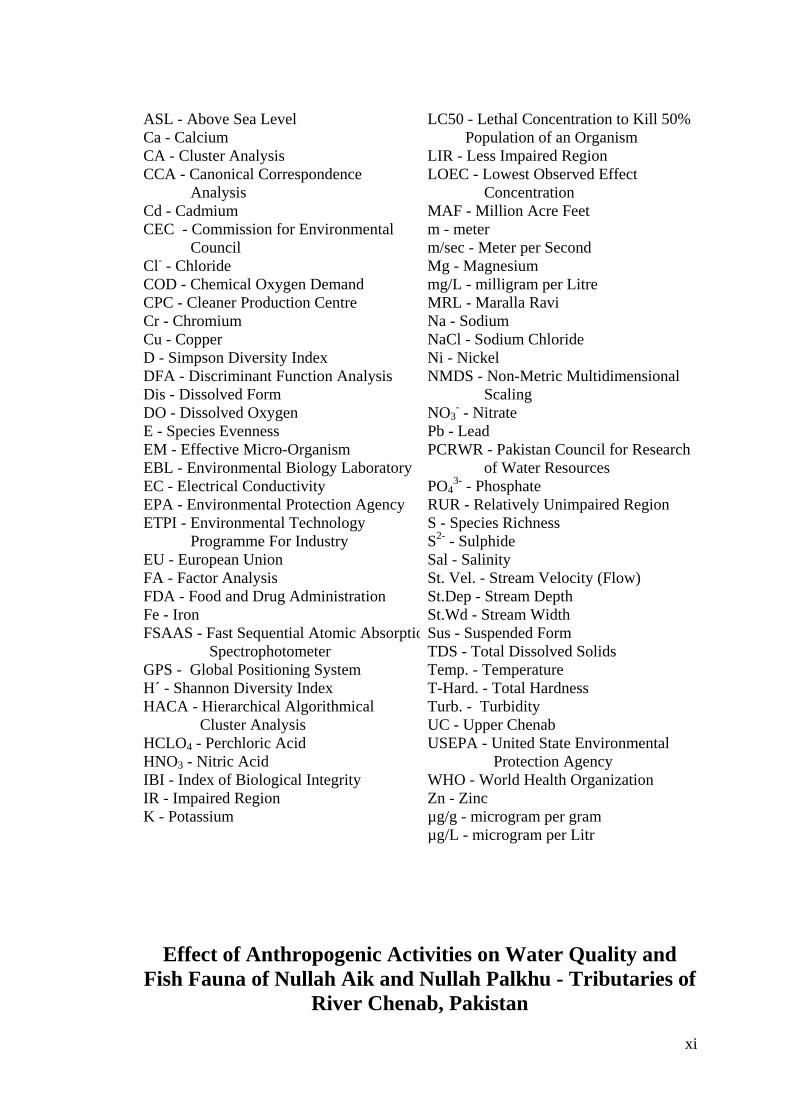
ASL - Above Sea Level Ca - Calcium CA - Cluster Analysis CCA - Canonical Correspondence

Analysis Cd - Cadmium CEC - Commission for Environmental

Council Cl- - Chloride COD - Chemical Oxygen Demand CPC - Cleaner Production Centre Cr - Chromium Cu - Copper D - Simpson Diversity Index DFA - Discriminant Function Analysis Dis - Dissolved Form DO - Dissolved Oxygen E - Species Evenness EM - Effective Micro-Organism EBL - Environmental Biology Laboratory EC - Electrical Conductivity EPA - Environmental Protection Agency ETPI - Environmental Technology

Programme For Industry EU - European Union FA - Factor Analysis FDA - Food and Drug Administration Fe - Iron FSAAS - Fast Sequential Atomic Absorptio

Spectrophotometer GPS - Global Positioning System H´ - Shannon Diversity Index HACA - Hierarchical Algorithmical

Cluster Analysis HCLO4 - Perchloric Acid HNO3 - Nitric Acid IBI - Index of Biological Integrity IR - Impaired Region K - Potassium

LC50 - Lethal Concentration to Kill 50% Population of an Organism

LIR - Less Impaired Region LOEC - Lowest Observed Effect

Concentration MAF - Million Acre Feet m - meter m/sec - Meter per Second Mg - Magnesium mg/L - milligram per Litre MRL - Maralla Ravi Na - Sodium NaCl - Sodium Chloride Ni - Nickel NMDS - Non-Metric Multidimensional

Scaling NO3

- - Nitrate Pb - Lead PCRWR - Pakistan Council for Research

of Water Resources PO4

3- - Phosphate RUR - Relatively Unimpaired Region S - Species Richness S2- - Sulphide Sal - Salinity St. Vel. - Stream Velocity (Flow) St.Dep - Stream Depth St.Wd - Stream Width Sus - Suspended Form TDS - Total Dissolved Solids Temp. - Temperature T-Hard. - Total Hardness Turb. - Turbidity UC - Upper Chenab USEPA - United State Environmental

Protection Agency WHO - World Health Organization Zn - Zinc µg/g - microgram per gram µg/L - microgram per Litr

Effect of Anthropogenic Activities on Water Quality and Fish Fauna of Nullah Aik and Nullah Palkhu - Tributaries of

River Chenab, Pakistan

xii

Abstract

Nullah Aik and Nullah Palkhu are major tributaries of River Chenab in Pakistan and

important water resources in district Sialkot. These streams receive industrial

effluents, municipal sewage from Sialkot City, which degrade the water quality and

disrupt the ecological integrity. Present study was designed to highlight the effects of

human activities on water quality and fish fauna of these streams. For this purpose,

water samples and fish samples were collected at 18 sampling sites on seasonal basis

from September 2004 to July 2006. Water samples were analyzed for 38 parameters.

Hierarchical Agglomerative Cluster Analysis (HACA) identified three different

classes of sites: relatively unimpaired, impaired and less impaired regions on the basis

of variations in water quality parameters. Discriminant Function Analysis (DFA)

identified 11 water quality parameters viz; stream flow, stream depth, DO, COD,

TDS, NO3-, PO4

3-, Pb(dis), Cr(dis), Mg(sus), and Ni(sus), which showed significant

spatial variations, whereas, major seasonal variations were observed in stream flow,

temperature, EC, salinity, total hardness, Na(dis), K(dis), Ca(dis), Mg(dis), Fe(dis),

Cd(dis), Cu(dis) and Na(sus). Factor Analysis (FA) identified the six sources of

contamination such as municipal waste, industrial effluents, tanneries effluents,

agricultural, urban runoff and parent rock material. COD, TDS, Fe (dis), Pb (dis), Cd

(dis), Cr (dis) and Ni (dis) were found to be higher than the permissible limits. Seven

heavy metals (Fe, Pb, Cd, Cr, Ni, Cu and Zn) were analysed in different organs (liver,

gills, kidneys and muscles) of eight fish species. Significant variations in heavy

metals accumulation were observed in organs of studied fish species. The

concentration of Pb and Cr was recorded significantly between fishes captured from

different sampling zones, whereas, Fe, Cd, Cr and Cu in fishes varied significantly

between post monsoon and pre monsoon. The muscles of Channa punctata, Labeo

rohita, Cirrhinus reba, Puntius sophore and Wallago attu captured from downstream

of Nullah Aik and Nullah Palkhu exceeded the international permissible limits of Pb,

Cd and Cr. A total of 24 fish species belonging to 12 families were recorded from

Nullah Aik and Nullah Palkhu. Highest diversity indices were calculated at upstream

of Nullah and downstream of Nullah Aik. Fish assemblage at upstream of Nullah Aik

was stable, whereas, other stream segments showed seasonal variations. CCA

identified the three groups of fishes viz., sensitive species, ubiquitous species and

tolerant species, which were grouped on the basis of related to stream flow, stream

depth, DO, COD, salinity, turbidity, NO3- and heavy metals. Biological Integrity index

xiii

(IBI) was developed for the assessment of stream ecosystem degradation. A total of

12 metrics were calculated on the basis of taxonomic richness, habitat preference,

trophic guild, stress tolerance and origin of species to develop stepped and continuous

IBI criteria. HACA segregated the sites based on species abundance into three groups

viz., reference, moderately impaired and impaired groups. Non-Metric

Multidimensional Scaling (NMDS) was applied to identify underlying ecological

gradient to highlight the habitat degradation. Sites located in upstream of Nullah Aik

showed higher IBI scores, which dropped to its lowest in downstream sites near

Sialkot city, which gradually improve far downstream. Spatial variability in IBI

values is related as a function of surface water quality degradation. The results

indicate that water quality and fish fauna of these streams are facing severe

degradation due to unwise anthropogenic in the catchment area. The findings of

present study are alarming and highlight that there is an urgent need to protect the

natural streams from further degradation. These results can be helpful for future

management of other polluted streams and small rivers in the same eco-region.

Chapter 1

General Introduction

Water is a primary driving force for major physical, chemical and biological

changes all over the world (Brady & Weil, 1996; Boyd, 2000). Oceans and seas

contain approximately 97%, whereas, freshwater resources consist of 3% of the entire

water reserve of the earth (Wilson & Carpenter, 1999). About 68.7% of freshwater is

locked up in glaciers and icecaps on poles, 30.1% in ground water, 0.3% in surface

water bodies and 0.9% in other forms (Gleick, 1996). It is not only main component of

biosphere but also a major part of the living organisms (Jackson et al., 2001b; Pandey,

2006). Life cannot be sustained more than few days without water, even inadequate

supply of water change the pattern of distribution of organisms as well as human

being (WHO, 2005).

Freshwater is a limited resource, which is essential not only for survival of

living organisms but also for human activities such as agriculture, industry and

domestic needs (Bartram & Balance, 1996). The history of freshwater resource

utilization is as old as human civilizations (Gleick et al., 2002). Water has also played

a vital role in the evolution of human civilizations. Human social cultural evolution

started in those areas, where adequate quantity and quality of freshwater was

available. Most of the ancient human civilizations established around the freshwater

resources such as rivers (Gupta et al., 2006). Early civilizations like Mesopotamian,

Egyptian, Chinese and Indo-Gangatic civilizations developed around rivers to fulfill

the needs of water for domestic, agriculture and irrigation. Several rivers such as

Euphrates, Tigris, Nile, Yangtze, Indus and Ganges have been the lifelines for ancient

civilizations (Wichelns & Oster, 2006).

Freshwater resources can be classified into three major categories such as lotic

(rivers and streams), lentic (lakes and ponds) and ground water (aquifer). Rivers and

streams are characterized by uni-directional flow with relatively high velocity > 0.1

m/sec (Meybeck et al., 1989; Shreshtha & Kazama, 2007). Pristine rivers and streams

exhibit stable aquatic ecosystem, which are rapidly degrading due to over exploitation

to fulfil human demands (Hinrichsen et al., 1998). Freshwater as a resource has never

been an issue of concern until recent population explosion that has caused an immense

pressure on water resources (Fischer et al., 1997), which became worst with the

Chapter 1

2

advent of industrial revolution and rapid expansion of urban areas (Douglas et al.,

2002). Rapid Industrialization, extensive urbanization, intensive agriculture practices

and burning of fossil fuel are amongst anthropogenic activities, which have increased

rapidly and have been considered important for changing the natural condition of an

aquatic ecosystem (Dale et al., 2005; Grimm et al., 2000). The adverse effect of

human activities have resulted in degradation of stream and riverine ecosystems

(Schleiger, 2000), which ultimately alter the water quality and structure and function

of aquatic biota (Stoddard et al., 2006). Streams and rivers are facing number of

environmental problems throughout the world largely associated with anthropogenic

activities in their catchment areas (Young et al., 2004). The pollution of freshwater

resources is a matter of concern all over the world, especially in developing and poor

countries. However, developed countries have adapted various technologies for the

protection of water ways from pollution. High intensity of aquatic pollution is more

critical in developing countries (Bozzetti & Schulz, 2004), where effluents are

indiscriminately discharged directly and/or indirectly into rivers and streams without

considering environmental protective measures (Pandey, 2006). Most of the

developing countries do not have infrastructure to control water pollution and enforce

water quality standards (Hinrichsen et al., 1998).

Natural as well as anthropogenic factors determine the water quality of an

aquatic ecosystem, which is essential for biological communities and maintain the

human demands (Scott et al., 2002; Schoonover et al., 2005; Pandey, 2006; Singh et

al., 2007). Information of surface water quality is an inevitable component for the

assessment of pollution and long-term environmental impacts assessment of human

activities in a particular area. Generally, pristine aquatic systems exhibit less variation

in water quality parameters in comparison to those of polluted aquatic ecosystems.

Any significant human activity in the catchment area can produce huge volume of

pollutants such as heavy metals, organic pollutants, nutrients, salts and other synthetic

compounds (Miller, 2002), which alter the water quality and consequently disintegrate

the ecological integrity of lotic ecosystems (Lytle & Peckarsky, 2001; Brown et al.,

2005).

Downstream ecology of streams and rivers moving across cities and industrial

areas are facing severe degradation; higher losses in biotic integrity and many of these

fresh water resources have become unsafe for human consumption (Gafny et al.,

2000; Lima-Junior et al., 2006). Among lotic system, streams are more at risk to

Chapter 1

3

anthropogenic activities in comparison to rivers because most of the streams

experience extreme fluctuation and discharge as compared to river (Paul & Meyer,

2001). Streams traversing from urban area are more vulnerable to human activities

and display irregular discharge, altered water chemistry, disturbed and disrupted food

chains (Brown et al., 2005).

Spatial and temporal variations in water quality of streams are shaped by

natural as well as human activities in the catchment area. The effects of pollutants are

mostly high near the source, however; it becomes diluted as water traverses the

distance (Qadir et al., 2008). Streams affected from industrial activities and

urbanization display more prominent spatial variations. Many authors have

highlighted the deleterious effects of natural and anthropogenic factors on water

quality on spatial and temporal basis worldwide (Simeonov el al., 2000; Alberto et

al., 2001; Fernández-Turie et al., 2003; Anazawa et al., 2004; Kotti et al., 2005; Singh

et al., 2004; Singh et al., 2005a; Zeng & Rasmussen, 2005; Qadir et al., 2008).

Natural processes such as rainfall, weathering of parent rock material, erosion, surface

runoff, sediment transport, changes in stream hydrology and flow influence water

quality on seasonal basis. Anthropogenic factors include a range of activities that can

degrade the water quality, depending upon the intensity and duration of contribution

from point and non-point sources (Tarvainen et al., 1997). A point source is a point at

which pollutants are discharged directly into surface water at a particular point and

can easily be recognized (Fang et al., 2005) such as industrial effluents and domestic

sewage discharged into streams or rivers without prior treatment (Connell et al.,

1999). Generally, more inlets of point sources are located in urban and industrialized

areas, compared to those in non-urban areas (Fitzpatrick et al., 1995). Point sources

contribution become very high, where people and authorities don’t follow the

environmental rules and regulations; such situations exist mainly in poor and

developing countries (Maillarda & Santos, 2008).

Non-point sources pour pollutants in streams from multiple locations or sites such

as after rainfall through surface runoff from urban and agricultural areas (Choi &

Blood, 1999; Kyriakeas & Watzin, 2006). The gaseous and suspended particulate

matter from burning of fossil fuels and industrial emissions can get deposited on soil

surface or on urban structures. During rainfall, these atmospheric deposits erode or

dissolve into rainwater and enter into streams via multiple inlets (Davis et al., 2001).

Fertilizers, pesticides and soil improving agents are used to increase the crop

Chapter 1

4

production. After heavy irrigation or rainfall, these additives get dissolved and leach

down to ground water or moves to streams/rivers with surface runoff after soil

saturation (Tsihrintzis & Hamid, 1997). The concentration of pollutants in surface run

off varies from one place to another e.g. surface runoff from industrial area possesses

high concentration as compared to un-inhabited areas (Sanger et al., 1999). Non-point

sources are usually scattered or diffused making the source identification a difficult

task.

Metals are one of the important contaminant group responsible for

deterioration of surface water quality, which either originate naturally from parent

rock material as a result of weathering or contributed from anthropogenic process

(Selin & Selin, 2006). Alkali metals (Na, K) and alkaline earth metals (Ca, Mg) are

found abundantly in earth’s crust, whereas, heavy metals are present in trace amount.

Heavy metals such as Fe, Cr, Ni, Cu and Zn are essential in living organisms because

of their structural and functional roles in various physiological processes (Wepener et

al., 2001), whereas, non-essential metals have no known role in metabolic functions of

the organisms and are toxic even in trace amount. Essential heavy metals are required

in trace quantities by organisms and if their concentration exceeds the threshold level

become toxic (Wright & Welbourn, 2002). Toxic effects of heavy metal vary

according to their position in food chain. At higher trophic levels, their effect of heavy

metals become more conspicuous among aquatic organisms (Devlin, 2006;

Rasmussen et al., 2008).

In an aquatic ecosystem, metals are present either in dissolved form or bind with

suspended particulate matter. Dissolved heavy metals are bio-available and highly

toxic to aquatic organisms, whereas, metals in particulate matter are comparatively

stable and less toxic (Morrison et al., 1990). It is difficult to estimate the biological

availability of metals; however, the dissolved content of metals gives a general

estimate of available metals (Charlesworth & Lees, 1999). Particulate metals settle

down in the form of sediments in stream bed may build up to high concentrations with

the passage of time (Colman & Sanzolone, 1992). Availability of heavy metals

depends upon several factors such as pH, organic matter, electrical conductivity,

salinity and total hardness (Wright & Welbourn, 2002). Other factors such as

turbidity, flow rates and size can also influence the availability of metals and metal

load in surface water (Caruso et al., 2003).

Chapter 1

5

Heavy metal pollution is a long term and irreversible process that affects the

productivity of aquatic ecosystem, may lead to complete loss of species and biological

communities and disrupt the structural and functional integrity (Majagi et al., 2007).

Heavy metals in aquatic medium are harmful for aquatic biota even at very low

concentration (Schüürmann & Markert, 1998). Aquatic organisms can absorb heavy

metals from their surrounding aquatic environment and accumulate in their bodies.

This process may accelerate if the concentrations become elevated in aquatic

environment. The absorbed heavy metals in organisms can bind with cellular

components (nucleic acids and proteins) and interfere with metabolic processes

(Zhang & Casey, 1996) that leads to genotoxic, neurotoxic, mutagenic and teratogenic

effects (Lachance et al., 1999; Das, 2007). Heavy metals disrupt the physiology and

histology of aquatic organisms that may leads to death (Sehgal & Saxena, 1986).

There are several physical and chemical factors, which affect the bioavailability of

heavy metals (Smolders et al., 2004), which are transferred from aquatic medium to

bodies via ingestion of food and suspended particulate matter while metal ion

exchange through gills and skin (Nussey et al., 2000). The level of heavy metal

accumulation depend on metal type, distance from the metal source, season, type of

species and trophic level (Asuquo et al., 2004; Terra et al., 2008). Accumulation of

heavy metals varies from species to species (Wright & Welbourn, 2002).

The loss of biological communities in any stream results due to deterioration

of water quality. Aquatic organisms are good biological indicators of water pollution

in a river or stream. Biological indicators are sensitive to any change in physical and

chemical change in stream water, which directly or indirectly influence the biological

communities. Ecological health of an aquatic ecosystem can be analysed through

biological indicators on the basis of their presence or absence, relative abundance,

community structure and function (Karr et al., 1986; Landres et al., 1988). Aquatic

organisms such as algae, invertebrates, fishes and amphibians are important organisms

for understanding the impacts of human activities on stream ecosystem.

Among aquatic organisms, fishes are good indicators of pollution stress and

have wide range of tolerance. Fishes respond to change in physical, chemical and

biological conditions of aquatic ecosystem caused by human activities (Plafkin et al.,

1989). The distribution of stream fishes is influenced by different local physical

characteristics, as well as regional interactions (Smith & Kraft, 2005). Fishes are

sensitive to any type of human disturbance such as inflow of industrial effluents,

Chapter 1

6

municipal waste, stream discharge, habitat alteration and fragmentation (Pont et al.,

2006). Sensitive species indicates the stream health in a better way in comparison to

tolerant species. However, tolerant fish species are adapted to unfavorable conditions

created by natural or anthropogenic factors and can recover rapidly as the stress

reduces. Natural factors viz; drought and flood conditions influence the structure and

function of fish communities. Flood increases diversity in fish assemblages in

irregular streams by connecting isolated pools and creating favourable conditions for

the fish movement barriers (Taylor & Warren, 2001). Anthropogenic activities

strongly influence the distribution, migration, colonization, and re-colonization of

fishes (Magalhães et al., 2002). In addition to water quality, physical characteristics of

stream also influence the distribution and pattern of fish assemblage (Ghosh &

Ponniah, 2001). Most of the temperate streams exhibit well marked spatial and

temporal variations in physical characteristics of water quality that also determines the

fish assemblage (Arunachalam, 2000). Unwise human activities in catchment area

have significant impact on species composition within ecological communities which

results in disappearance of native fish species and appearance of exotic species (Karr

et al., 1986; Lyons et al., 2000). Change in species composition in a stream converts

the complex and stable ecosystem into fragile one and disrupts the functional

ecological integrity of an aquatic ecosystem (Lyons et al., 2000).

Index of Biological Integrity (IBI) is an important index to determine the

stream health on the basis of information from various tiers of aquatic ecosystem such

as individual organism, population, community and ecosystem levels and express

health status of any aquatic ecosystem into an index (Karr et al., 1986). This index is

used to measure the intensity of anthropogenic impacts on natural environmental

processes inside stream ecosystem and to take the managerial decision about

restoration activities (Yeom & Adams, 2007). Different aquatic organisms have been

introduced as candidate organisms for the biological assessment of streams and rivers

but fishes and other invertebrates are frequently used as model organisms. Several

authors in different parts of the world used fish as organism to determine the health

conditions of stream and rivers (Ganasan & Hughes, 1998; Kleynhans, 1999; Wang et

al. 2003; Toham & Teugels 1999; Bozzetti & Schulz, 2004; Breine et al., 2004; Joy &

Death, 2004; Yeom & Adams, 2007).

IBI is formulated on the basis of various biological aspects such as species

diversity, stress tolerance, habitat preferences, feeding behaviours and origin of

Chapter 1

7

species (Ganasan & Hughes, 1998). IBI has been applied successfully on streams and

small rivers in various geographical areas all over the world since last two decades.

IBI provide overall information about fish species at community level in stream

ecosystem.

The importance of protection, restoration and management of aquatic resources

has been realized all over the world (Nakamura et al., 2005). Indiscriminate human

activities have destroyed the ecological and biological integrity of aquatic resources

and make unfit for resource utilization in many parts of the world (Karr & Chu, 1999).

Therefore, the protection and management of aquatic resources must be ensured for

sustainable agricultural, domestic, recreational and industrial uses. The knowledge

about biological integrity and impacts of anthropogenic activities in the catchment

area of urban streams provides an understanding for protection, conservation and

restoration of stream ecosystem. Unwise and indiscriminate industrialization,

urbanization and intensive agriculture in developing countries are putting the aquatic

resources under threat of degradation. Pakistan is also among those developing

countries, where aquatic resources are facing the severe degradation.

Problem Statement Pakistan exhibits diverse climatic conditions and is enriched with plenty of

freshwater resources (Khan, 1991). Rivers, canals, streams and dams, which are the

major surface water resources of Pakistan and lifeline of its irrigation system,

currently irrigates over 36 million hectares of land (Alam & Naqvi, 2003). About 7.8

million hectors of freshwater in Pakistan has been estimated, including 3.1 million

hectares of rivers and streams (Naik, 1985). Pakistan is among those few countries,

which have well developed irrigation system for irrigating its vast planes (Punjab and

Sindh). Rivers and streams are flowing down from Himalayas and Karakoram to

Indus plains provide base for the world largest irrigation system, which plays a vital

role in agriculture and energy generation (Alam & Naqvi, 2003).

Pakistan is struggling to develop its industrial sector along with agriculture to

fulfil demands for local population. Indiscriminate industrialization process and rapid

urbanization has created several environmental problems related to water, air and soil

resources. Untreated industrial effluents and raw municipal sewage are continuously

discharged into streams and rivers. Water quality of rivers and stream in Pakistan is

Chapter 1

8

generally poor and rapidly getting deteriorated due to pollution from industrial,

municipal, and agricultural sources (UNIDO, 2000). Pakistan is amongest water

stressed countries facing water scarcity due to human population pressures (World

Bank, 2005) and have shortage of over 40MAF (Million Acre feet) of water that will

increase over 151MAF by year 2025 (Mirjat & Chandio, 2001). This scarcity of water

needs protection and improvement of existing freshwater resources, otherwise, it will

face acute shortage of water for irrigation, domestic and industrial use. This is the

right time to recognize the intensity of problem and to take concrete steps towards its

sustainable utilization and protection of water resources.

About 80% of industrial and urban growth is restricted to major cities viz;

Karachi, Lahore, Faisalabad, Hyderabad, Multan, Sialkot, Gujranwala, Rawalpindi,

Peshawar and Kasur (Aftab et al., 2000). Away from the cities, in rural areas,

agriculture land is under an indiscriminate use of fertilizers and pesticides that makes

their way to rivers and streams through surface runoff. The intensity of human stress

is continuously amplifying with an increase in human population, which was 33.7

million in 1950, reached to 140 million in 2000 with an increase of 8 million persons

per annum (Qureshi, 2002). Urban settlements occupy about 1% of total land area;

contribute 48 % of the Gross National Productivity (GNP) and more than 80% of

industrial manufacturing (Khan, 1996). The urban centres of Pakistan are developing

rapidly, which are putting the natural water ways under stress.

Sialkot is the 9th largest city of Pakistan situated in north east of Punjab. It is

an important industrial city known worldwide for its leather garments, surgical

instruments and sports good production (Ghani, 2002). This city is in the grip of

pollution problem caused by industries, which are posing threat to the local

environment (Mehdi, 2005). These environmental issues have been emerged with

advent of industrial revolution since last three decades (Qadir et al., 2008). Exports of

tanned leather from Sialkot have been increased as a consequence of more stringent

environmental controls curtailing the process in western countries. At present, about

264 tanneries are scattered within and outside the city along with hundreds of other

industrial units. According to an estimate, tanneries located at Sialkot are producing

about 9400 m3/ day of heavily polluted tannery effluent (EM Research Organization,

2002). Industrial and municipal area generates huge volume of effluents and sewage,

which causes irreparable loss to local environment. Nullah Aik and Nullah Palkhu the

Chapter 1

9

important surface water resources of Sialkot more vulnerable to deleterious effects of

pollutants in effluents and sewage without treatment from industries and municipality.

Nullah Aik and Nullah Palkhu, two main natural tributaries of River Chenab

pass through the Sialkot. More than 2.5 million people are residing in the catchment of

Nullah Aik and Nullah Palkhu. In the past, these streams were an important water

resource for drinking, domestic use and irrigation purposes. Land around these

streams is alluvium deposits resulting from regular floods and is under cultivation

since pre historic times. Presently, these streams are receiving huge volume of

effluents, raw sewage and solid waste that influence physical, chemical and biological

characteristics of these streams. Major industrial activities are concentrated in and

around the urban areas and along the major roads/highways. A major share of

effluents is being contributed by tanneries, which produce a huge volume of liquid

waste containing about 130 chemicals, municipal sewage (Khan & Mahmood, 2007).

High flux of effluents containing toxic chemical including heavy metals drains

directly or indirectly into Nullah Aik and Nullah Palkhu (Mohtadullah et al., 1992;

Mehdi, 2005). Effluents from tanneries contain high chemical oxygen demand,

sulfides, chlorides, metals and salt content (Bajza & Vrcek, 2001). Among these

notorious chemicals, heavy metals such as Cr and its salts have been reported to

contaminate the stream water and aquifer (Bhalli & Khan (2006). Sialkot city generate

1503gallons per day of waste water, which directly or indirectly discharged into

Nullah Aik and Nullah Palkhu (Randhawa, 2002). The average effluents production of

each tannery in Sialkot district is 547- 814 m3/day (ETPI, 1998) with a total volume of

effluents as 11000m3 (Dawn Daily, 2006). Sialkot city generate 19million m3 waste

water per annum (WWF, 2007), which is drained into natural streams, ponds and

croplands. A complex mixture of industrial effluents, municipal sewage and surface

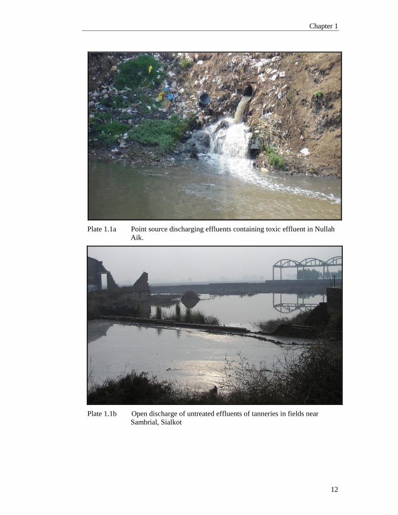
running water discharged directly or indirectly into drains (Plate 1.1a) and open

discharge to fields (Plate 1.1b). Most of the drains fall into the local sewerage system,

which ultimately finds their way into the Nullah Aik and Nullah Palkhu and finally

fall in River Chenab.

No industrial effluents and sewage treatment plants have been established to

treat the wastewater from multiple sources. Nullah Aik and Nullah Palkhu are

gradually turning into industrial and municipal drains. Large volume of industrial and

urban sewage is considered a major threat to aquatic life of the focussed streams.

Stream biota especially, fishes are facing severe impacts of toxic pollutants. This

Chapter 1

10

situation was more severe in close downstream sites of Nullah Aik and Nullah Palkhu,

where fishes were completely vanished due to high load of toxic pollutants. As a

result, fish population reported from upstream and downstream is spatially fragmented

due to barrier of pollutants. Downstream segment of streams are experiencing loss of

many native fish species. Extinction of sensitive species, introduction of exotic and

tolerant species, reductions in fish diversity, increasing the risk of diseases and

abnormalities in fishes are the negative impacts of elevated level of pollutants in

stream ecosystem.

Fishing is common activity in upstream and downstream of Nullah Aik and

Nullah Palkhu for human consumption. Several fish species (Channa punctata,

Wallago attu, Heteropneustes fossilis, Cirrhinus reba and Labeo rohita) are consumed

due to their palatable values. People, who consume contaminated fishes captured from

downstream of Nullah Aik and Nullah Palkhu, are more vulnerable to toxic effects of

pollutants. Domestic animals’ bathing in polluted water of Nullah Aik and Nullah

Palkhu is also common practice, which may cause health problems in domestic

animals (Plate 1.2a). In addition, along the banks of streams hundreds of pumps are

used to suck the polluted water for irrigation purposes in surrounding cropland putting

the agriculture and soil resources at risk (Plate 1.2b).

Conservation of freshwater fauna of Nullah Aik and Nullah Palkhu is a

challenge for environmental managers due to its rapidly increasing human population,

urbanization, agricultural and industrial activities in their catchment area (Qadir et al.,

2008). Human stress on streams has created an alarming situation, which needs an

immediate attention. Indiscriminate discharge of industrial effluents and municipal

sewage deteriorates the water quality and displace and/or vanish the ichthyo-fauna.

Unfortunately, no comprehensive scientific work, to date, is available about the water

quality, sources of pollutants and their impacts on distribution of fishes. There is an

urgent need to initiate concrete efforts to assess the impacts of human activities on

water quality and fish fauna of these streams.

Present research project was designed, keeping in view environmental

problems of Nullah Aik and Nullah Palkhu. For this purpose, a reliable and

statistically sound data was required that highlight the effect of the anthropogenic

activities on water quality and fish fauna in Nullah Aik and Nullah Palkhu. This is the

first attempt to uncover the environmental problems of these streams caused due to

anthropogenic activities in Pakistan. This research presents useful information about

Chapter 1

11

status of water quality and fish fauna and will highlight the various anthropogenic

threats responsible for degradation of stream ecology. These results will also provide

the information about the impacts of pollutants on fish distribution, which can be used

in decision making for re-introduction of extinct native fish species. The results of IBI

will be quite useful for ecological stream health and measure indirect intensity of

human activities in the catchment area, which will be useful for restoration and

management of these aquatic resources. This study will be the guideline for

sustainable watershed management, wise urbanization, environment friendly

industrialization and agro-ecosystems not only in the catchment area of Nullah Aik

and Nullah Palkhu but also for other streams in the same eco-region.

Objectives Following main objectives have been focused:

• to highlight the spatial and temporal variations in water quality of Nullah Aik and

Nullah Palkhu, identification of water quality parameters and contamination sources,

which bring variations in water quality.

• to assess heavy metals (Fe, Pb, Cd, Cr, Ni, Cu and Zn) accumulation patterns in

different organs of fish species on spatial and temporal scales.

• to study the effects of environmental variables on diversity and spatio-temporal

distribution of ichthyofauna.

• to develop an index of biological integrity for the quantification of stream habitat

degradation of fish dwelling in Nullah Aik and Palkhu.

Chapter 1

12

Plate 1.1a Point source discharging effluents containing toxic effluent in Nullah Aik.

Plate 1.1b Open discharge of untreated effluents of tanneries in fields near

Sambrial, Sialkot

Chapter 1

13

Plate 1.2a Buffalo bathing in Nullah Aik Near Wazirabad

Plate 1.2b Foam dunes developed during irrigation with untreated polluted water

from Nullah Palkhu near Chitti Sheikhan, Sialkot.

Chapter 1

14

Structure of Thesis

The main objectives of present thesis was to study the impacts of

anthropogenic activities on water quality and ichthyo-fauna of Nullah Aik and Palkhu

stream system and to achieve these objectives, the research thesis is divided into seven

chapters; each one will be focusing on specific objectives in details.

First Chapter describes the general introduction and background information that

reviews the role of anthropogenic factors deteriorating the water quality and affecting

the fish fauna. This chapter also describe the environmental problems in study area

and presents research objectives.

Second Chapter provides description of the study area in relation to topography,

climate, geology, history, drainage pattern, land use, human population and other

anthropogenic activities. This chapter also describes the sampling strategy for

collection, transportation, preservation and analysis of stream water and fish samples.

Third Chapter highlights the spatio-temporal variations in surface water quality of

Nullah Aik and Palkhu, identification of important variables responsible for variations

and their source of origin. Comparison of stream water quality with regional and

international standard has also been discussed.

Fourth Chapter describes heavy metal accumulation in different organs of selected

fishes on spatial and temporal basis. The results of heavy metal accumulation in

muscles of fishes were compared with international permissible limits of heavy metals

for human consumption.

Fifth Chapter describes the fish diversity, feeding guilds, spatio-temporal distribution

pattern of fish species in relation with environmental factors.

Sixth Chapter explains the stream fish assemblage at community level with the

application of index of biological integrity (IBI) to assess the impacts of

anthropogenic activities.

Chapter 1

15

Seventh Chapter concludes the findings of the research and provides guidelines for

restoration and management of Nullah Aik and Palkhu stream system. Finally, this

chapter also identifies the areas of future research programs.

Chapter 2

Materials and Methods Study Area

Present study focuses on Nullah Aik (32°63′N- 74°99′E and 32°45′N-

74°69′E) and Nullah Palkhu (32°69′N- 74°99′E and 32°37′N- 74°02′E) tributaries of

the River Chenab (Fig. 2.1) that originate from Lesser Himalayas in the Jammu and

Kashmir, at an altitude 530m and 290m, respectively. Nullah Aik and Nullah Palkhu

drain about 1,875km2 catchments area and travel a total distance of about 131.6km

and 98km with an average annual discharge of 315 and 288Cs per second,

respectively (Fig 2.2). Sialkot is the main city along with several towns such as

Sambrial, Bhopalwala, Ugoki, Jathekay, Sodhra, Begowala and Wazirabad located in

the catchment area. These streams traverse through the city of Sialkot from east to

west and converge at downstream near Wazirabad city in district Gujranwala before

falling in Chenab River.

The catchment area of studied streams experience four distinct seasons viz.,

summer (pre monsoon; April to mid-June), rainy season (monsoon; mid-June to mid-

September), autumn (post monsoon; mid-September to November), winter (December

to February) and a short spring (March). Climate is hot and humid during summer and

cold during winter. June is the hottest month of the year with maximum daily

temperature soaring to 40oC and above (Fig. 2.3a; Appendix 2.1). The temperature

during winter may usually drop to 4oC but occasionally may even decline to freezing

point during the month of January. The mean annual rainfall in the catchment is about

950mm of which maximum precipitation (~80%) occurs during the monsoon season

(Fig. 2.3b). During frequent rainfall in monsoon season, rain water flows into streams

through surface runoff and cause flooding which usually have devastating effects on

crops and human settlements (Plate 2.1a & b). Most of the floods result in deposition

of new alluvial soil in catchment area.

The catchment area of Nullah Aik and Nullah Palkhu is the part of upper

Rachna Doab (Region between River Chenab and Ravi). The great plain of Punjab

started from the upper parts of Rachna Doab with an average slope (0.37 m/km),

which gradually decrease from North East to South West (Jehangir et al., 2002).

Fig. 2.1 Map of study area showing the location of Nullah Aik and Nullah Palkhu- tributaries of River Chenab.

Chapter 2

18

0

200

400

600

800

1000

1200

Jan Feb Mar Apr May Jun Jul Aug Sep Oct Nov Dec

Stre

am d

isch

arge

(Cs/

sec)

Nullah Aik Nullah Palkhu

Fig. 2.2 Average stream discharge of Nullah Aik and Nullah Palkhu

(source; Anonymous, 2007)

(a)

0

5 0

1 0 0

1 5 0

2 0 0

2 5 0

3 0 0

Ja n F e b M a r A p r M a y Ju n J u l A u g S e p O ct N o v D e c

M o n th s

Rainfall (m

m)

(b)

Fig. 2.3 (a) Mean monthly minimum, maximum temperature (°C) (b) Mean monthly rainfall (mm) in the catchment of Nullah Aik

and Nullah Palkhu Sialkot

0

5

10

15

20

25

30

35

40

45

Jan Feb Mar Apr May Jun Jul Aug Sep Oct Nov DecTem

perature (oC

)

minimaxi

Winter Pre monsoon Monsoon Post monsoon

Winter

Chapter 2

19

Plate 2.1a Devastating flood during monsoon season, 2006 in lower catchment area due to over flow of Nullah Aik (Near Kotli Maralan).

Plate 2.1b Devastating flood during monsoon season, 2006 in lower catchment area due to over flow of Nullah Palkhu (Near Kotli Khokhran).

Plate 2.2 Aik crossing over the Maralla Ravi Link canal located near Sahibkay (Site 5). (arrows indicate the direction of flow)

Maralla Ravi Link Canal

Maralla Ravi Link

Nullah Aik

Chapter 2

20

The upper part of Punjab plain originated during late Pleistocene alluvial deposition

from Lesser Himalayas, which is approximately 200meter thick (Greenman et al.,

1967). The soil is predominantly alluvial of varying textural classes such as clay and

silt loam while sandy loam and sandy clay loam also prevail in the region. The soil

types in upper catchment area of Sialkot are mainly maira (light reddish- yellow

loam) and sandy loam in relict areas. In lower catchment, two types of soil i.e., rohi

(predominant in clay) and maira (loamy soil) are common.

The resource utilization of Nullah Aik and Nullah Palkhu started 5000 years

ago in Vedic Era, when Raja Sáliváhan founded the Sialkot named as Sakala

(Population and Censes organization, 2000). Raja Sáliváhan and his son (Raja Rasálu)

invited the people from various parts of Northern India to come and settle in Sialkot

(http://en.wikipedia.org). They also promoted the irrigation system around the Sialkot

city based on water resources of Nullah Aik. During Sikh regime (1800- 1849), many

small channels (Khands) were constructed on both side of Nullah Aik for irrigation

purposes (Fig. 2.5). Among these Khands, one of the major Khand (abandoned canal)

was constructed to irrigate the lands of Sikhs around the Daska city (Fig. 2.5). It

remained functional till the construction of Maralla Ravi Link (MRL) canal in 1955.

In British era (1857-1947), a small headwork was constructed on Nullah Aik at Wain

to divert the water of Nullah Aik for irrigation purposes in vicinity of Begowala

Town, which was destroyed during heavy floods in 1954. After signing of Indus water

treaty between Pakistan and India, riverine water irrigation system was expanded and

local (Khand) irrigation system become vanished due to construction of MRL canals.

Nullah Aik receives water from springs in eastern parts of Jammu district and

from heavy rains in its upper catchment area. Its maximum discharge level is

approximately 35,000Cs per second at upstream which gradually reduces as the

Nullah progresses towards downstream (Anonymous, 2007). Its maximum capacity to

retain the water in downstream at the crossing of MRL canal is approximately

5,000Cs per second (Plate 2.2) and at the Wain small headworks can retain

approximately 2000Cs per second. Nullah Aik exhibited maximum width in upper

catchment area that gradually narrows down in lower catchment area. During

monsoon season, heavy rains occur and rainwater drains into Nullah Aik and Nullah

Palkhu. Sometimes these streams cannot retain the rainwater that ultimately flow out

and spread over the vast area (Fig. 2.5). Floodwater brings large quantity of silt that

Chapter 2

21

deposits new layers of soil every year. This unique attribute is utilized by local

inhabitants in the downstream of Nullah Aik for irrigation through small distributaries

(Khands). At present only single irrigation channel is active that originates from small

headworks at Wain, which further divides into sub channels that irrigate the croplands

around the Begowala town. The surplus water from these sub-channels falls into

Begowala drain which finally descends into Nullah Aik.

In contrast to Nullah Aik, discharge capacity of Nullah Palkhu increases as the

stream moves from upstream towards downstream. At upstream, it has limited

discharge capacity and collects rain water from its upper catchment area. Sometimes,

in early summer season, it become dry and water inside the stream can be seen as

isolated ditches and pools. At downstream after crossing UC (Upper Chenab) canal it

receives water from many Saim Nullahs (Jourian and Roras out falls) and freshwater

streams (Neil Wah and Tannai Wah) resulting high discharge level. Before falling into

River Chenab, it joins Nullah Aik near Wazirabad.

According to Population and Censes Organization (2000) estimated population

density of catchment area is 903 persons/ km2 and one of the populous areas of

Pakistan. Most of the land in catchment area is under intensive cultivation. Major

crops grown in the area are wheat and rice. However, fodder crops and vegetables are

also cultivated to meet the local demands. According to an estimate, there are about

1,000,000 domestic animals including cattle, buffaloes, horses, donkeys, sheep and

goats in the rural areas (Population and Censes Organization, 2000). Application of

fertilizers, pesticides and soil improving agents is a common practice in the catchment

area. These synthetic chemicals make their way to streams after heavy rainfall or

irrigation. Three kinds of irrigation sources are common in the area which are tube

well irrigation (water from aquifer), stream water irrigation by pumping (hundreds of

pumps have been established along the sides of streams) and diversion of water into

small distributaries (this type of irrigation is restricted to the surroundings of

Begowala town).

Chapter 2

22

(a) Fig. 2.4 Drainage pattern in catchment area of Nullah Aik and Nullah Palkhu

(a) Upstream of Nullah Aik (b) Downstream of Nullah Aik (c) Upstream of Nullah Palkhu (d) Downstream of Nullah Palkhu.

Surface runoff

Nullah Aik

Overflow of water during flood

Nullah Aik

(b)

Nullah Palkhu

(c) Surface run off

Nullah Palkhu (d)

Flooding in lower catchment

Fig. 2.5 Irrigation system developed on Nullah Aik during Sikh regime

Nullah Palkhu

Nullah Aik

Main Aik Canal

(abandoned)

Small channelslocally called KHANDS

(abandoned)

Sialkot City

River Chenab Begowala channel (Active)

Small head works at Wain

Chapter 2

24

Anthropogenic Activities and Sources of Pollutants

The catchment area of the streams is densely populated and house a significant

number of industrial units in urban areas, whereas, rural areas are intensively used for

agricultural purposes (Fig. 2.6). Major industrial activities are concentrated in and

around the Sialkot city and along the roads. The industry of Sialkot consisted of small

and medium units that are scattered throughout the city. The major industries consist

of leather, sports goods and surgical instruments manufacturing. A total of 3,229

industrial units are present in Sialkot, comprising of 264 tanneries, 220 surgical

instruments producing factories and 900 sports goods manufacturing units (Qadir et

al., 2008). Among these industrial units, tanneries are the major contributors in the

production of effluents and sludge. Effluents of tanneries are also loaded with

different types of salts (containing metals such as chromium, sodium and calcium),

suspended solid matter and organic solvents. Most of the industries discharge their

effluents without any treatment into drains that directly or indirectly fall into Nullah

Aik and Nullah Palkhu.

According to an estimate of Cleaner Production Centre (CPC), Sialkot, the

optimum level of leather production is about 297tons/ day with a daily production of

9388m3of tanneries effluents. The average effluents production of each tannery in

Sialkot district is 547- 814 m3/day (ETPI, 1998) with a total volume of effluents as

11000m3 (Dawn daily, 2006). Surgical instruments manufacturing units produce acid

containing effluents which contain dissolved metals (used in electroplating) etc.

However, amount of effluents produced is very low as compared to the tanneries.

Surgical instruments producing units, sports goods production units are the least

contributors in effluent production.

Municipal sewage is another source of pollution of surface water. There is no

municipal waste treatment plant in Sialkot city and untreated raw sewage, organic and

inorganic pollutants along with high quantities of suspended organic matter as well as

animal and human excreta, which are discharged directly/ indirectly into streams.

Sialkot city generate 19million m3 waste water per annum (WWF, 2007), which is

drained into natural streams, ponds and croplands.

Fig. . 2.6 Activities in the catchment areaof Nullah Aik and Nullah Palkhu

Chapter 2

26

Sampling Methodology and Study Design

Selection of Sampling Sites

Nullah Aik and Nullah Palkhu stream system was selected on the basis of

similarities in topography, surface geology, relief and anthropogenic activities. A

preliminary survey of Nullah Aik and Nullah Palkhu was conducted during the

months of June and July, 2004 to extract information related to human impacts on

water quality and aquatic life. During the preliminary surveys, each site was marked

using a GPS (Global Positioning System, Garmin) for future sampling visits

(Appendix 2.2). The selection criteria for each site was based upon anthropogenic

activities in catchment area, variations in habitat, presence or absence of fish species

and accessibility of the sites. After preliminary survey, a total of 18 sites were selected

for water and fish sampling. Each stream consisted of nine sites and among these nine,

two sites were located in upstream of Sialkot city, whereas, seven sites in downstream

(Fig. 2.7; Plate 2.3). The sampling was started early in the morning usually

commencing from 5:00am to 12:00pm. Every day, three sites were taken into account

and whole sampling schedule lasted for one week. Before water and fish sampling, a

detailed weather forecast for study area was studied to avoid the rainy days. All

samplings were done during sunny days when the stream flow was at normal level.

From each site, water and fish samples were collected on seasonal basis from

September, 2004 to July, 2006. Water sampling was carried out from post monsoon

(September - October), winter (December - January), pre monsoon (April - May) and

monsoon (July), whereas, fish sampling during pre monsoon and post monsoon

season, respectively.

Brief description of each site is given below.

Nullah Aik

Site 1 (Umranwali, 74° 39′ 45″ E, 32° 30′ 21″ W and 247m ASL) was located on

working boundary (undecided international boundary) between Pakistan and Indian

held Jammu & Kashmir, the point, where Nullah Aik enters in Pakistan (Plate. 2.3).

This site was situated on upstream of Nullah Aik and least disturbed with relatively

good water quality. No point source of pollution was identified, however, agricultural

runoff and atmospheric disposition from Indian held Jammu district can be considered

as a non-point source of pollution.

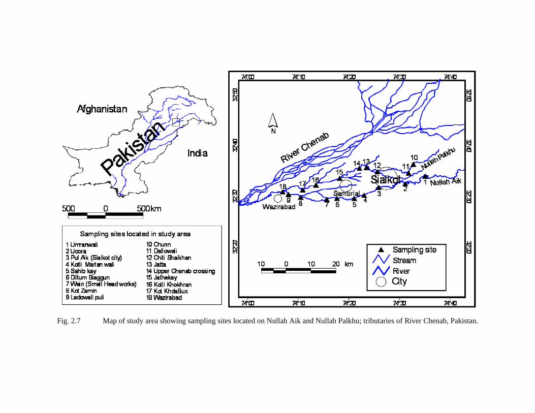
Fig. 2.7 Map of study area showing sampling sites located on Nullah Aik and Nullah Palkhu; tributaries of River Chenab, Pakistan.

Site 2 (Uoora, 74° 36′ 55″ E, 32° 29′ 30″W and 245m ASL) was selected at upstream

of Nullah Aik near a village Uoora (Plate 2.3). This site was represented by relatively

good water quality and inhabited by healthy aquatic life. Number of water pumps has

been installed on stream banks to pump the water for irrigation. No major point source

was found, however, it does receive some contaminants from agricultural runoff along

with atmospheric deposition.

Site3 (Pul Aik, Sialkot city, 74° 31′ 50″ E, 32° 30′ 39″ W and 242m ASL) was located

in Sialkot city (Plate 2.3) and receives effluents from small industries, tanneries,

municipals waste, urban surface runoff and solid waste from Sialkot city.

Site 4 (Kotli Marlanwali, 74° 29′ 05″ E, 32° 27′ 26″ W and 237m ASL) was situated

approximately seven km downstream of Sialkot city (Plate 2.3). The stretch between

site 3 and site 4 receives industrial and municipal wastes from Sialkot city.

Site 5 (Sahibkay, 74° 25′ 03″ E, 32° 25′ 58″ W and 233m ASL) was located on Nullah

Aik just after crossing the MRL canal (Plate 2.3). The water of Nullah Aik flows on

upper side from east to west, whereas, the MRL canal water passes through a siphon

underneath the Nullah Aik, which flows from north to south (Plate 2.2). The stream

does not receive any substantial amount of contamination from a significant point

source but agricultural activities and atmospheric deposition in the surrounding areas

may contribute contamination of surface water.

Site 6 (Dillum Blaggun 74° 21′ 22″ E, 32° 25′ 48″W and 230m ASL) was located

about 24km downstream of Sialkot (Plate 2.3) and site receives domestic sewage from

Dillum Blaggun and Bhopalwala town. The major activity in its catchment area was

agricultural farming.

Site 7 (Wain small head works 74° 18′ 03″ E, 32° 25′ 39″ W and 227m ASL) was

situated near Wain village (Plate 2.3). Small headworks have been constructed to

divert the water of Nullah Aik to irrigate fields around the Begowala town. Highest

stream depth was recorded at this site. Stream flow is regulated by small headworks at

downstream of Wain and remains low except monsoon season. Main sources of

surface water contamination at this site are mainly from non-point sources.

Chapter 2

29

Site 8 (Kot Zamin 74° 11′ 55″ E 32° 26′ 09″ W and 222m ASL) receives effluents

from Begowala drain that bring effluents from tanneries zone and Sambrial city after

traversing a distance of about 20km (Plate 2.3). This site was selected to highlight the

possible impacts of Begowala drain on the stream water quality of Nullah Aik.

Site 9 (Ladowali Puli 74° 09′ 95″ E 32° 27′ 02″ W and 219m ASL) was located near

Wazirabad city (Plate 2.3) and is the last site on Nullah Aik before it falls into Nullah

Palkhu. The site receives effluents from tanneries located along Sialkot-Wazirabd

road and municipal sewage from eastern part of Wazirabad city and surface runoff

from agricultural and urban area.

Nullah Palkhu

Site 10 (Chun 74° 37′ 54″ E 32° 33′ 34″ W and 250m ASL) was situated near the

origin of stream located near working boundary between Pakistan and Indian held

Kashmir on upstream of Nullah Palkhu (Plate 2.3). Agriculture is the main activity in

the upstream catchment area. Stream flow at this site is strongly influenced by rainfall,

which is high in monsoon season and low even dry in early summer season, however,

water remains in ditches and pools.

Site 11 (Dolluwali 74° 36′ 14″ E 32° 32′ 22″ W and 247m ASL) was situated at

upstream of Dolluwali and Sialkot Cantonment (Plate 2.3) and experiences occasional

summer drought. Main source of pollution at this site is the agricultural activities.

Site 12 (Chitti Sheikhan 74° 30′ 43″ E 32° 31′ 45″ W and 238m ASL) was located at

downstream of Sialkot Cantonment (Plate 2.3) and receives tannery effluents,

municipal waste from northern parts of Sialkot and its surrounding areas.

Site 13 (Jatta 74° 27′ 24″ E, 32° 32′ 30″ W and 232 ASL) was situated at downstream

of Sialkot (Plate 2.3) and strongly influenced by Nullah Bhed, which passes through

the center of Sialkot city and brings heavy load of pollutants from Sialkot City.

Site 14 (UC canal crossing 74° 25′ 20″ E, 32° 32′ 38″ W and 229m ASL) was located

on Nullah Palkhu after crossing the Upper Chenab canal (Plate 2.3). The water of

Nullah Palkhu passes under the UC canal through a siphon. No visible point source of

Chapter 2

30

pollutant discharge was found.

Site 15 (Jathekay 74° 19′ 47″ E, 32° 32′ 29″ W and 227m ASL) was located at the

junction of Nullah Palkhu and Jaurian out fall near Jathekay (Plate 2.3). Land in the

periphery of UC and MRL canal become waterlogged due to seepage from canals.

Jaurian out fall collects water from waterlogged land and drains into Nullah Palkhu,

which may dilutes the contaminants concentration and improve the water quality.

Farmers along each side of the stream pump stream water to irrigate their crops.

Site 16 (Kotli Khokhran 74° 16′ 40″ E, 32° 29′ 03″ W and 224m ASL) was situated

downstream of Nullah Palkhu (Plate 2.3) after joining Nullah Neil Wah, which further

dilute the concentration of contaminants in stream water. Agriculture was the major

human activity in its catchment area.

Site 17 (Kot Khuda Bux 74° 12′ 30″ E, 32° 27′ 45″ W and 221m ASL) was located in

the lower catchment area of Nullah Palkhu (Plate 2.3) and receives domestic sewage

from Sodrah town and surface runoff from agricultural fields.

Site 18 (Wazirabad 74° 07′ 08″ E, 32° 27′ 06″ W and 217m ASL) was located on

Nullah Palkhu after joining Nullah Aik (Plate 2.3) and collects effluents and

municipal wastes from Wazirabad city, known for cutlery production industry.

Chapter 2

31

Continued…


Palkhu.

Site 1 (Umanwali) Site 2 (Uoora)

Site 3 (Pul Aik Sialkot) Site 4 (Kotli Marlanwali)

Site 5 (Sahikay) Site 6 (Bhopalwala)

Chapter 2

31

Continued…

Site 7 (Wain small head Site 8 (Kot Zamin)

Site 9 (Ladowali Puli)

Site 12 (Chitti Sheikhan)

Site 10 (Chun)

Site 11 (Dolluwali)

Chapter 2

32


Palkhu.

Site 13 (Jatta) Site 14 (Upper Chenab canal crossing)

Site 15 (Jathekay) Site 16 (Kotli Khokhran)

Site 17 (Kot Khuda Bux) Site 18 (Wazirabad)

Chapter 2

34

Water Sampling and Laboratory Analysis Water sampling was carried out with the help of self-designed sampler which

was consisted of long plastic rod of adjustable length and angle. One end consisted of

two circles of stainless steel covered by rubber coating in which glass container was

fixed to get water sample from desired depth of stream water. Glass container was

washed with nitric acid and rinsed with deionised water at every site. Water samples

were taken 30cm below the water surface, within 100m range of a sampling site.

Sampling container was drained into sampling bottles up to the mouth without

trapping any bubble. From each site, three sub-samples of stream water were

collected, which were combined to obtain composite samples during sampling. The

water samples were stored in plastic bottles (pre cleaned with HNO3) and were tightly

sealed to avoid leakage during transportation. All water samples were preserved in ice

boxes and transported to laboratory according to prescribed standard method (APHA,

1998). All samples were transported to the laboratory of Cleaner Production Center

(CPC), Sialkot and stored in freezer to cease any probable physico-chemical changes.

All analyses on water except metal were performed in CPC laboratory. Water samples

were separated out for the dissolved metal contents and particulate matter. The water

samples for dissolved metals were acidified with few drops of HNO3 to make it

remain available in dissolved form during storage.

Stream width, depth and flow dissolved oxygen (DO), pH, Electrical

conductivity (EC), Salinity and Total Dissolved Solid (TDS) of the water samples

were measured in field at each site.

Stream Width was measured at four different points within sampling site. The

average distance between two points was 25m along the longitudinal direction of

stream. The mean stream width was calculated by averaging the readings of four

points (Fig. 2.8a) and expressed in meters (Arunachalam, 2000 and Bhat, 2004).

Stream Depth was measured at three points; one was taken at centre of stream, while

two measurements were taken at 1/3 distance from each bank of the stream. These

three measurements were taken in same transect that fall across the stream (Fig. 2.8c;

Arunachalam, 2000; Bhat, 2004).

Stream Velocity was measured at the point where stream flow was fastest. To

measure stream velocity two bamboo sticks were fixed at stream bed at the distance of

10 meter from each other. A cork was dropped at the point towards upstream and

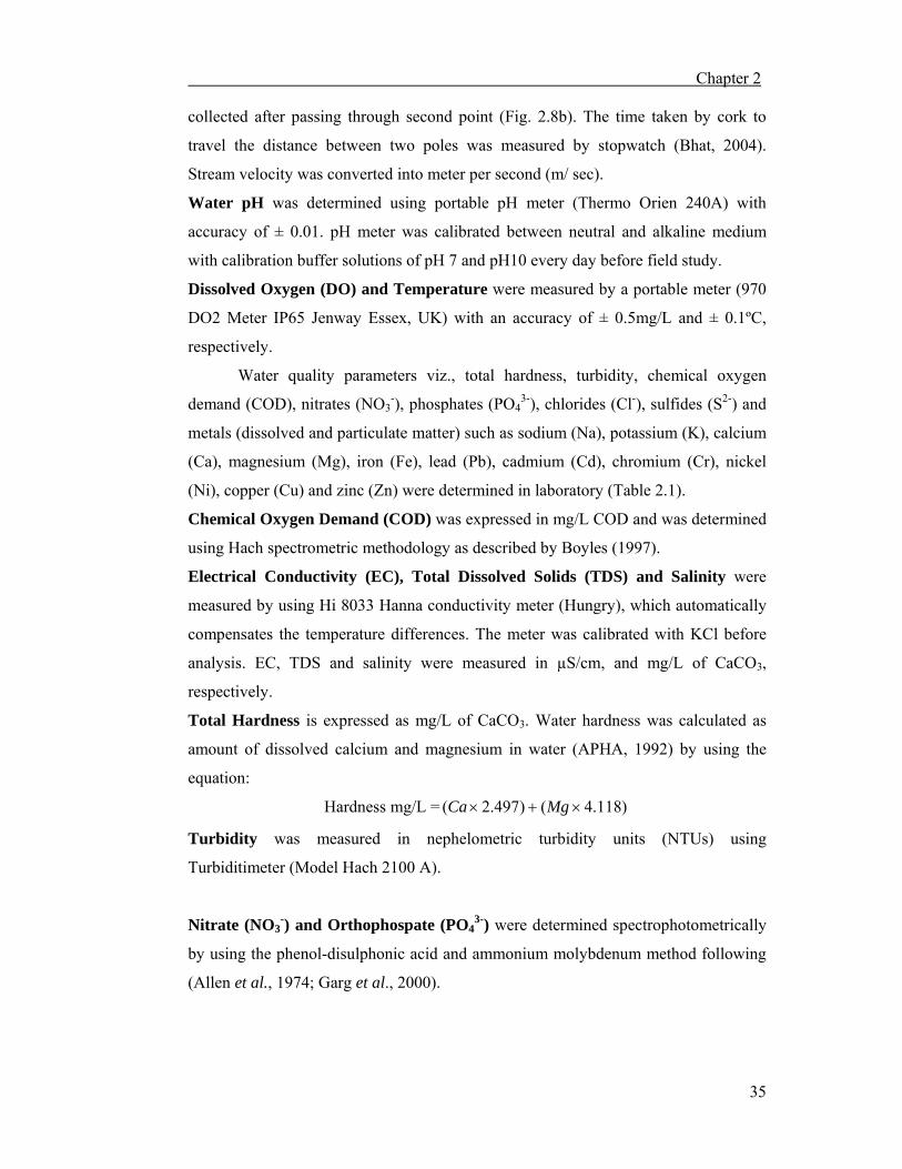
Chapter 2

35

collected after passing through second point (Fig. 2.8b). The time taken by cork to

travel the distance between two poles was measured by stopwatch (Bhat, 2004).

Stream velocity was converted into meter per second (m/ sec).

Water pH was determined using portable pH meter (Thermo Orien 240A) with

accuracy of ± 0.01. pH meter was calibrated between neutral and alkaline medium

with calibration buffer solutions of pH 7 and pH10 every day before field study.

Dissolved Oxygen (DO) and Temperature were measured by a portable meter (970

DO2 Meter IP65 Jenway Essex, UK) with an accuracy of ± 0.5mg/L and ± 0.1ºC,

respectively.

Water quality parameters viz., total hardness, turbidity, chemical oxygen

demand (COD), nitrates (NO3-), phosphates (PO4

3-), chlorides (Cl-), sulfides (S2-) and

metals (dissolved and particulate matter) such as sodium (Na), potassium (K), calcium

(Ca), magnesium (Mg), iron (Fe), lead (Pb), cadmium (Cd), chromium (Cr), nickel

(Ni), copper (Cu) and zinc (Zn) were determined in laboratory (Table 2.1).

Chemical Oxygen Demand (COD) was expressed in mg/L COD and was determined

using Hach spectrometric methodology as described by Boyles (1997).

Electrical Conductivity (EC), Total Dissolved Solids (TDS) and Salinity were

measured by using Hi 8033 Hanna conductivity meter (Hungry), which automatically

compensates the temperature differences. The meter was calibrated with KCl before

analysis. EC, TDS and salinity were measured in µS/cm, and mg/L of CaCO3,

respectively.

Total Hardness is expressed as mg/L of CaCO3. Water hardness was calculated as

amount of dissolved calcium and magnesium in water (APHA, 1992) by using the

equation:

Hardness mg/L = )118.4()497.2( ×+× MgCa

Turbidity was measured in nephelometric turbidity units (NTUs) using

Turbiditimeter (Model Hach 2100 A).

Nitrate (NO3-) and Orthophospate (PO4

3-) were determined spectrophotometrically

by using the phenol-disulphonic acid and ammonium molybdenum method following

(Allen et al., 1974; Garg et al., 2000).

Chapter 2

36

Stream flow

ABC

50 m

(a)

A

B

10 m

Stream flow

(b)

Stream level

Streambed

Stream bank Stream depth at 1/3 width

Stream depth at mid

(c)

Fig. 2.8 Strategy to measure (a) stream width, (b) Stream flow and (c) Stream depth measured at a sampling site

Chapter 2

37

Table 2.1 Parameters, abbreviations, units and analytical methods as measured during 2004- 2005 for water quality assessment of Nullah Aik and Nullah Palkhu.

Variables Abbreviations Units Analytical Methods Stream width St.Wd m Bhat,2004 Stream velocity (flow) St. vel. m/sec Bhat,2004 Stream depth St.dep m Bhat,2004 Temperature Temp ºC Thermometer inside DO meter pH pH pH pH-meter Dissolved oxygen DO mg/L DO meter Chemical oxygen demand COD mg/L Spectrophotometric Electrical conductivity EC µS/cm E.C. meter Total dissolved solids TDS mg/L TDS meter Salinity Sal mg/L of CaCO3 Titrimetric Total hardness T-Hard mg/L Ca and Mg based Turbidity Turb NTU Turbiditimeter Nitrates NO3

-, mg/L Spectrophotometric Phosphates PO4

3- mg/L Spectrophotometric Chlorides Cl- mg/L Titrimetric Sulphides S2- mg/L Spectrophotometric Sodium * Na mg/L FS AAS Potassium* K mg/L FS AAS Calcium* Ca mg/L FS AAS Magnesium* Mg mg/L FS AAS Iron* Fe mg/L FS AAS Lead* Pb mg/L FS AAS Cadmium* Cd mg/L FS AAS Chromium * Cr mg/L FS AAS Nickel* Ni mg/L FS AAS Copper* Cu mg/L FS AAS Zinc* Zn mg/L FS AAS *metals in dissolved form (mg/L) and suspended particulate matter (mg/L)

Chloride (Cl-) were measured in water samples by titration with standard solution of

silver nitrate with sulphuric acid using potassium chromate as an indicator in mg/L.

Cl- concentration was calculated by the following equation (Garg et al., 2000).

Cl- (mg/L) = 100x sample of volume

35.5 x N x AgNO3 of volume

Where N stands for normality of H2SO4

Sulfides (S2-) were measured by Methylene Blue method (Hach method # 8131)

adopted for the estimation of S2- using Hach DR5000 spectrophotometer as described

by Hach Company (2005).

Dissolved Metal Contents were measured by taking 250 ml of stream water samples

filtered through Whatman filter paper (No. 45) in the laboratory (APHA, 1998). The

Chapter 2

38

filtrate was acidified with 1-2 ml of ultra pure HNO3 to drop its pH below 2 and

preserved at 4 �C for dissolved metal analyses (De Carlo et al., 2004).

Metal Contents in Suspended Particulate Matter

Suspended particulate matter was separated from 250ml water sample on filter

paper (Whatman filter paper No.45). These filter papers were oven dried and weighted

before separation of suspended sediment from water samples. After separation of

Suspended particulate matter filters were oven dried (Herman et al., 2000). Suspended

particulate matter was digested according to the method of USEPA (1990). Oven

dried suspended particulate matter was transfered to 100ml Kjaldahl flask and

digested in 10 ml of HNO3 and HClO4 with ratio of 5:1, boiled for 20 - 30 minutes

until a transparent digest was appeared. Digests were filtered and volume of obtained

aliquot was raised up to 50ml in volumetric flask.

All prepared samples for dissolved, and suspended particulate matter were

subjected to metal analysis. Concentration of eleven metals (Na, K, Ca, Mg, Fe, Pb,

Cd, Cr, Ni, Cu and Zn) in prepared samples was determined by using flame atomic

absorption spectrophotometric technique. Fast Sequential Atomic Absorption

Spectrophotometer (FSAAS Varian AA-240) was used to determine metal

concentrations. A set of standards consisting of a series of standard that varies from

lowest concentration to highest concentration were prepared to obtain a calibration

curve (Hayes & Buckney, 1998). A blank was also prepared by repeating the same

process. The concentration of blank was subtracted from concentration of samples to

obtain a final concentration values (Vazquez et al., 1999). Three replicates of each

sample were prepared to obtain the precision in metal analyses and 5 - 10% standard

deviation was observed during analysis of metal concentration. For quality control and

to ensure the accuracy of running analysis BCR-714 reference materials (Waste water

influent) was used obtained from European Commission, DG JRC, Institute for

Reference Materials and Measurements (IRMM) Reference Materials Unit, Belgium.

About 5 - 15% variations in results of reference material for heavy metals were

observed after repeating it for six times. The measured and certified values of

reference material are given in Table 2.2.

Chapter 2

39

Table 2.2 Mean ± standard deviation of measured values in comparison with certified values of the reference material.

BCR-714 Wastewater (influent)

Metal (mg/L) Certified values Measured Fe 1.03 ± 0.11 0.988 ± 0.023 Pb 0.145 ± 0.011 0.162 ± 0. 020 Cd 0.019 ± 0.016 0.017± 0.005 Cr 0.123 ± 0.010 0.131 ± 0.045 Ni 0.108 ± 0.015 0.119 ± 0.013

Cu 0.309 ±0.023 0.324 ± 0.098 Zn 1.00 ± 0.010 0.984± 0. 031

Fish Sampling Fish samples were collected from each site using variety of fishing nets of

varying mesh sizes as suggested by Bhat (2003). Seine net (8 m × 1.5 m with mesh

size of 1cm), cast nets (circumference 15 m with 1.5 cm mesh size) and dragnets (7m

x 1m with mesh size of 1.5cm) were used within 100 meters reach of each sampling

site. Cast and dragnets were used to sample fish in water with depth less than 1.5 m,

while seine net was used where depth of water was more than 1.5 meter. The intensity

of sampling for each site was standardized as 20 efforts for cast net, three hours

duration for seine net and 10 trials for drag net covering the stream within 100m of

stream along longitudinal gradient (Bhat, 2003). All sampling sites were intensively

sampled in an effort to capture as many fish species as possible in proportion to their

abundance (Matthews, 1985). Captured fish specimens were transferred immediately

into stream water filled tubs place on stream bank to reduce the chances of fish

mortality. Minimum of four persons were the member of sampling crew, who handle

netting process. The whole process of sampling was done very carefully with fishing

nets traversing the distance from downstream to upstream. During collection of fishes,

the length and weight of each fish was measured (Appendix 2.3a & b). Maximum five

specimens of each species were packed, labelled in separate polythene bags, placed in

icebox and transported to laboratory within 12 hours for the purpose of identification

and further chemical analysis (Van Aardt & Erdmann, 2004). The remaining

specimens were released back into stream water at the same point from where fish was

captured (Ganasan & Hughes, 1998). Released fishes were only native, whereas,

exotic fishes were not returned back to the stream. The juvenile fishes, which have tail

length less than 20mm, were excluded because of inadequacy in their capturing

Chapter 2

40

(Helms et al., 2005). Taxonomic identification and classification was done on the

basis of morphometric characteristics up to the species level. Fish species were

identified following regional keys (Mirza & Bhatti, 1993; Mirza, 2003; Talwar &

Jhingran, 1991; http://www.fishbase.org).

Metal Analysis in Fish Organs

Out of 24 fish species (details are given in chapter 5), only eight abundant fish

species (Channa punctata, Cirrhinus reba, Labeo rohita, Heteropneustes fossilis,

Mystus cavasius, Oreochromis niloticus, Puntius sophore and Wallago attu) were

selected for heavy metal analysis indifferent organs. A total of seventy five and

seventy nine fish specimens were dissected during post monsoon and pre monsoon,

respectively.

Each specimen was dissected in laboratory to obtain different organs (Liver,

kidney, gills and muscle) with corrosion resistant stainless steel knives. These knives

were washed after dissection of each specimen with a detergent solution, rinsed in

50% HNO3 and finally by distilled water. First of all, gills were obtained from both

sides then homogenized to form a composite sample. After removal operculum,

epidermal and subcutaneous tissues were carefully removed to obtain sample of

muscle. To ensure uniformity, all samples were taken from dorso-lateral muscles of

the right side (Fréry et al., 2001). After opening the body cavity with a scalpel, liver

was identified in the presence of surrounding organs and the connective tissue around

the liver was removed to separate the liver along with gall bladder. Finally kidneys

were located and separated from connective tissues. Each dissected organs was placed

in polythene bag and provided with necessary information about identification code,

date, locality, season, species name and type of tissue. Polythene bags containing

different organs were stored at −20°C before digestion to avoid contamination

(Mormede & Davies, 2001).

One gram of wet fish tissue (liver, gills, kidneys and muscles) of different

species was digested (Zyadah & Chouikhi, 1999) by using 5ml of HNO3 and 1 ml

HClO4 in volumetric flask. Digestion of fish tissues was carried out on a hotplate (200

to 250°C) until digest of fish organs converted into colourless liquid and volume of

the digest raised up to 50ml (Nussey et al., 2000). Each digest was filtered through

0.42µm filter paper, transferred to polyethylene bottle and sealed to avoid

contamination and evaporation. Before heavy metal analyses, digested samples were

Chapter 2

41

stored at 4°C. The prepared samples were analyzed for heavy metals such as Fe, Pb,

Cd, Cr, Ni, Cu and Zn using Fast Sequential Atomic Absorption Spectrometer (Varian

Spectra AA-240). Metal concentration in fish tissues was determined in

microgram/gram (µg/g). Concentration of each metal was further confirmed using

external standard method (Bajc et al., 2005). The precision and accuracy of procedure

was evaluated by analyzing two standard reference materials (cod muscle BCR 422

and bovine liver BCR 185R) obtained from European Commission, DG JRC, Institute

for Reference Materials and Measurements (IRMM) Reference Materials Unit,

Belgium. The level of metal accuracy was checked for heavy metal as 83 - 96%

(Table 2.3).

Table 2.3 Comparison of measured and certified values (Mean ± standard deviation) of certified reference materials of during metal analysis

Bovine Kidney BCR 186R Cod Muscle BCR 422 Metals

(µg/g) Measured Certified Measured Certified Fe 217± 18 229 ± 10 5.21 ± 0.45 5.46 ± 0.30 Pb 314 ± 22 306 ± 11 0.07 ± 0.03 0.085 ± 0.015 Cd 2814 ± 234 2710 ± 150 1.24 ± 0.10 1.05 ± 0.07 Cr 71 - 115 58 -142 - - Ni 402 ± 39 420 - - Cu 27.4 ± 4.4 31.9 ± 0.4 - -

Chapter 3

Spatial and Temporal Variations in Water Quality of Nullah


Introduction Surface water quality of lotic ecosystems is influenced by natural processes

(erosion of parent rock material and precipitation) as well as anthropogenic activities

such as industrial, municipal and agricultural runoff (Singh et al., 2005a; Shrestha &

Kazama, 2007). The magnitude of this problem become further intensified due to

indiscriminate growth in industries, expansion of population and degradation of

natural aquatic systems (Ghosh & McBean, 1998). Streams and rivers characterized

by unidirectional water flow (Gafny et al., 2000) are often treated as easy dumping

sites and act as sink for industrial and municipal waste (Singh et al., 2007), which

makes them highly vulnerable (Korfali & Davies, 2003). Inflow of hazardous

pollutants such as heavy metals and other organic pollutants into streams and rivers

can be related to two main major sources (Honnen, et al., 2001; Gallo et al., 2006).

Point sources (industrial and municipal effluents) are released at specific points

throughout the year and non-point sources (atmospheric deposition, surface runoff

from urban and agricultural areas) are highly influenced by seasonal changes

(Sundaray et al., 2006).

Industrial effluents and municipal wastes contain heavy metals, which are

persistent in nature and cannot be removed or degraded by natural processes (Singh et

al., 2005b). In surface water heavy metals are present either in dissolved phase or in

suspended particulate phase (Saeedi et al., 2004) which exchange continuously as

water traverse the distance (Gallo et al., 2006). Dissolved metals are available to

aquatic organisms and determine the health of an ecosystem (Morrison et al., 1984).

Metals in suspended particulate phase are comparatively stable and less toxic

(Morrison et al., 1990).

Distribution of heavy metals in water and sediment is greatly influenced by

various physico-chemical characteristics such as pH, organic matter and mineral

compounds (Singh et al., 2005b; Gallo et al., 2006; Rothwell, et al., 2006). After the

introduction of heavy metals into aquatic ecosystem, heavy metals undergo the

Chapter 3

43

process of various chemical processes such as dissolution, sedimentation and re-

suspension along longitudinal gradient (Lee et al., 2003). There are different physical

or chemical factors that promote or reduce the adsorption process of dissolved

contents of metal to suspended particulate matter (Dojlido & Best, 1993; Saeedi et al.,

2004). Heavy metals are mainly transported in association with suspended particulate

matter, which settles down in streambed, when stream flow becomes slow with low

turbulence. Sedimentation process of highly polluted streambed sediment becomes

more pronounced especially where streams receive industrial and urban effluents (Tsai

et al., 2003). Stream suspended particulate matter consisted of many constituents such

as clay, organic matter, metals oxides that scavenge the heavy metals from the

environment (Rodrigues et al., 2006). Heavy metals in sediments are not permanently

fixed and can re-mobilize during flood period resulting changes in pH, organic matter

and TDS and may become available in the particulate or dissolved form (Lee et al.,

2003; Kucuksezgin et al., 2007). The distribution of heavy metals in particulate matter

varies along longitudinal gradient of stream and between different seasons.

Variations in stream water originate from catchment area as a result of

precipitation, surface run off, sub-surface inflow of water through aquifer and

drainage pattern. Other in-stream processes that affect the availability of heavy metals

is dilution of effluent by addition of water from associated streams, pumping of water

for irrigation, sediments formation, and re-mobilisation from sediments (Qadir et al.,

2008). These processes exhibits seasonal and spatial variations and have a strong

effect on the equilibrium of dissolved and suspended form of heavy metals in surface

water (Singh et al., 2005a). Distribution of heavy metals in running waters is generally

evaluated from limited number of points on spatial and temporal basis (Temnerud &

Bishop, 2005). Spatial and temporal variations of different heavy metals in streams are

highly variable and regulated by complex processes such as stream discharge, natural

and human activities (Simeonov et al., 2003). Temporal variations in water quality are

determined by precipitation, stream discharge level (Singh et al., 2005a) and become

more pronounced in streams of temperate region, where flow is regulated by rains

(Shah et al., 2007). Streams and rivers of Indo-gengatic plains are located in temperate

zone, with distinct seasonal pattern of rainfall. A number of regional studies on the

spatial and temporal variations in surface water of streams and rivers have been

conducted. Singh et al. (2005a) reported the spatio-temporal variations and source

Chapter 3

44

identification of contaminants in Gomuti River. Chakrapani (2005) highlighted spatial

and temporal variations in upper part of river Ganga, India. Ansari et al. (1999)

studied the impact of industrial effluents, domestic sewage and agricultural runoff on

water quality from River Ganga. Qadir et al. (2008) highlighted spatio-temporal

variations in water quality of Nullah Aik, which is an important tributary of River

Chenab, Pakistan.

Nullah Aik and Nullah Palkhu major tributaries of River Chenab, Pakistan,

receive untreated industrial and municipal discharge from different industrial units and

urban settlements of district Sialkot. These contaminants are putting ecological

integrity of these streams at risk and have been considered as major threat to

degradation of aquatic ecosystem, which are ultimately turning into municipal drains

(Qadir et al., 2008). High load of pollutants into studied streams are severely altering

the water quality and resulted degradation in its natural ecosystem. No previous data

and scientific work is available on water and sediment quality of Aik-Palkhu stream

system and no attempt has been made to assess the extent of contamination and

characterize the potential impacts on streams ecology of Nullah Aik and Nullah

Palkhu. There is dire need for comprehensive assessment to find out the trends and

variations in the water quality of these streams and to address the consequences of

present and future threats of contamination. It is also important that spatio-temporal

monitoring of water quality of these streams should be done for future water resource

management. A monitoring program was felt necessary to provide a representative

and reliable spatial and temporal dataset of water quality for future restoration of

stream ecology.

The main objectives of this chapter are

to measure the spatial and seasonal trends of heavy metals in dissolved and

suspended sediments of Aik- Palkhu stream system,

to highlight the most influencing variables that contribute in spatio-temporal

variations in water and suspended particulate matter and

to identify the possible sources of heavy metals along with physico-chemical

variables in surface water.

Chapter 3

45

Materials and Methods

Sampling Strategy Details of water sampling and analysis of 38 parameters of water quality are

given in Chapter 2.

Statistical Analyses

Basic Statistics analyses were performed by using Statistica 5.5 software (Stat

Soft, Inc. 1995) and for graphical representation of water quality data Microsoft Excel

97 (Microsoft Corporation 1985) was used. Three multivariate techniques such as

Hierarchical Algorithmical Cluster Analysis (HACA), Discriminant Function Analysis

(DFA) and Principal Component Analysis based on Factor Analysis (PCA/FA) were

used for the water quality assessment and interpretation of the results (Simeonov et

al., 2000; Wunderlin et al., 2001; Singh et al., 2005b). These multivariate statistical

techniques have been widely used in various studies for the explanation of spatio-

temporal variations and interpretation of chemical/physical characteristics of water

quality parameters (Simeonov et al., 2000; Wunderlin et al., 2001; Singh et al.,

2005b) in comparison to uni-variant techniques that usually fail to give adequate

information on multivariate dataset (Santos-Roman et al., 2003).

The stream water quality data set was subjected to HACA to identify clusters

of the sampling sites indicating their similarity based on water quality parameters

(Table 2.1). For this purpose, 38 water quality parameters measured from 18 sites (38

variables × 18 cases) were subjected to HACA analysis. HACA was performed on

the mean values of water quality parameters. Euclidean distances were chosen as a

measure of linkage that uses analysis of variance to evaluate the distances between

clusters, attempting to minimize the sum squares of any two clusters that can be

formed at each step (Kent & Coker, 1992). To determine the association of metals and

their possible sources in water quality data, eleven metals within dissolved and

suspended particulate form were also subjected to HACA. Pearson correlation was

used to confirm the results of HACA and to find association between different metals.

DFA was used to determine the water quality parameters that best discriminate

between spatial groups identified by HACA. The basic idea underlying DFA is to

determine whether groups differ with regard to mean of a variable, and then to use that

variable to predict group membership. DFA was applied to water quality data set (18

sites x 38 variables) without any standardization to define the spatial and temporal

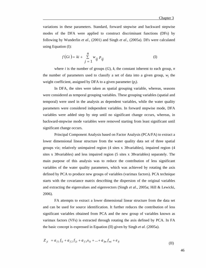
Chapter 3

46

variations in these parameters. Standard, forward stepwise and backward stepwise

modes of the DFA were applied to construct discriminant functions (DFs) by

following by Wunderlin et al., (2001) and Singh et al., (2005a). DFs were calculated

using Equation (I):

( ) ijpn

j ijwkiGif ∑=

+=1

(I)

where i is the number of groups (G), ki the constant inherent to each group, n

the number of parameters used to classify a set of data into a given group, wj the

weight coefficient, assigned by DFA to a given parameter (pj).

In DFA, the sites were taken as spatial grouping variable, whereas, seasons

were considered as temporal grouping variables. These grouping variables (spatial and

temporal) were used in the analysis as dependent variables, while the water quality

parameters were considered independent variables. In forward stepwise mode, DFA

variables were added step by step until no significant change occurs, whereas, in

backward-stepwise mode variables were removed starting from least significant until

significant change occurs.

Principal Component Analysis based on Factor Analysis (PCA/FA) to extract a

lower dimensional linear structure from the water quality data set of three spatial

groups viz; relatively unimpaired region (4 sites x 38variables), impaired region (4

sites x 38variables) and less impaired region (5 sites x 38variables) separately. The

main purpose of this analysis was to reduce the contribution of less significant

variables of the water quality parameters, which was achieved by rotating the axis

defined by PCA to produce new groups of variables (varimax factors). PCA technique

starts with the covariance matrix describing the dispersion of the original variables

and extracting the eigenvalues and eigenvectors (Singh et al., 2005a; Hill & Lewicki,

2006).

FA attempts to extract a lower dimensional linear structure from the data set

and can be used for source identification. It further reduces the contribution of less

significant variables obtained from PCA and the new group of variables known as

varimax factors (VFs) is extracted through rotating the axis defined by PCA. In FA

the basic concept is expressed in Equation (II) given by Singh et al. (2005a).

fimifmifififji efaxafafaZ +++++= ...332211 (II)

Chapter 3

47

Results

Stream Morphology

Basic descriptive statistics (range, mean and standard deviation) of stream

morphological parameters measured at 18 sites located on Nullah Aik and Nullah

Palkhu during 2004- 2006 are summarized in Table 3.1. Stream width ranged from

3.47 to 37.1m with an average of 13.12m. Maximum stream width (37.07m) was

recorded from Uoora located at upstream of Nullah Aik. Stream width of Nullah Aik

decreased from upstream to downstream, whereas, Nullah Palkhu exhibited an

increasing trend from upstream to downstream (Fig. 3.1a). Average value of stream

flow was 0.88 m/sec. A decreasing trend in stream width was observed in case of

Nullah Aik from upstream to downstream sites, whereas, in contrary to Nullah Aik,

Nullah Palkhu showed an increasing trend. Average depth of stream was measured as

1.54m; maximum depth (6.0m) of stream was recorded from Wain small headworks

and minimum stream depth (0.49m) at Dallowali. Generally stream depth increases

from upstream to downstream in both streams (Fig. 3.1a).

Physiochemical Variables of Stream Water

Mean and range values (min. – max.) of 16 Physico-chemical parameters of

water samples collected from different sites located on Nullah Aik and Nullah Palkhu

are given in Table 3.1. Variations in stream water temperature were recorded that

varied between 12 to 29oC during the study period. Maximum temperature was

recorded during monsoon season whereas minimum was recorded in winter season

(Fig. 3.1b).

Most of the stream water samples were alkaline in nature with pH varied

between 6.59 and 9.71. Maximum pH values were observed in upstream sites, which

gradually decreased towards downstream sites (Fig. 3.1b). The level of DO in stream

water was ranged between 0.1 to 10.9mg/L. The maximum values of DO were found

in the sample collected from upstream site (Uoora) of Nullah Aik and minimum

values at Chiti Sheikhan. The results showed decreasing trend of DO from upstream

sites to mid-stream sites near Sialkot city and gradual improvement in far downstream

sites (Fig. 3.1b). Average COD values varied between 4.82 and 1090 mg/L. The

maximum values were recorded from downstream sites such as Chiti Sheikan and Pul

Aik and minimum in upstream sites of both streams. Highest value of COD was

Chapter 3

48

measured in those stream segments, which pass through urban areas of Sialkot (Fig.

3.1c). EC and TDS also showed distinct variations and exhibited similar trend like

COD (Fig. 3.1c). Maximum values were recorded from Jatta situated at downstream

of Nullah Palkhu. Salinity and total hardness showed an increase in concentration

trend from upstream towards mid-stream sites and decrease in far downstream sites

(Fig. 3.1c). Maximum turbidity (1526NTU) was recorded near Upper Chenab- Palkhu

crossing and minimum (2.5 NTU) at Umeranwali at upstream of Nullah Aik (Fig.

3.1d). Highest concentrations of Cl- (2463mg/L) and S2- (3.412mg/L) were measured

at Chiti Sheikhan and Jatta located at downstream of Nullah Palkhu and minimum Cl-

(97.11mg/L) and S2- (0.169mg/L) at upstream sites of studied streams. Nullah Palkhu

exhibited marked variations in Cl- and S2- as compared to Nullah Aik (Fig. 3.1e).

Nutrients in Stream Water

The maximum concentration of NO3- (9.8mg/L) was recorded in water

samples collected from Dallowali at upstream of Nullah Palkhu site and minimum in

water samples taken from Wain small head works at downstream of Nullah Aik. The

results indicated high concentration of NO3- exhibited by the site located in

agricultural area (Fig. 3.1f). In contrast, high concentration of PO43- was measured at

those sites, which were located in industrial and urban areas (Fig. 3.1f).

Dissolved Metals in Stream Water

Mean and range values of 11 dissolved metals in water samples are given in Table 3.2. The average concentrations of major metals such as Na, K, Mg, and Ca in stream water were higher to those of heavy metals. Maximum concentration of dissolved Na (203.9mg/L) was measured in water sampled collected from Jatta whereas, minimum (5.45mg/L) from Uoora at upstream of Nullah Aik. Concentration of dissolved Na increased from upstream to downstream of Nullah Aik whereas, highest concentration was observed in sites receiving effluents form tanneries which gradually decrease in far downstream (Fig. 3.1g).

Like Na, K exhibited similar spatial pattern. Nullah Aik showed lesser concentration of K in comparison with Nullah Palkhu (Fig. 3.1g). An increasing trend in concentration of dissolved Ca was observed from upstream to mid-stream and decreased in downstream of studied streams (Fig. 3.1h), whereas, dissolved Mg did not show marked variations in water quality of Nullah Aik, whereas, comparatively, significant variations were observed in Nullah Palkhu (Fig. 3.1h).

Chapter 3

49

Sites located near downstream of Sialkot exhibited high concentration of dissolved Fe which gradually decreases in far downstream sites (Fig. 3.1i). Similarly, dissolved Pb concentration exhibited similar spatial pattern. High concentration of dissolved Pb was recorded at sites close to Sialkot city (Fig. 3.1i). High concentration of Cd (dissolved) was recorded at sites located far from human settlements (Fig. 3.1j). The spatial trend of Cr (dissolved) showed marked variations. Minimum concentration of Cr (dissolved) was found (0.001mg/L) at Umeranwali and maximum (1.146mg/L) at Jatta. High concentration was observed from sites, which receive effluents from tanneries such as Chitti Sheikhan, Jatta, Pul Aik and Wazirabad (Fig. 3.1j). Concentration of Ni in dissolved form increases from upstream sites towards downstream sites and highest concentration was found in water samples collected from far downstream sites (Fig. 3.1k). The highest concentration of Cu in dissolved form was observed at Wazirabad, whereas, lowest at sites downstream of Nullah Aik (Fig. 3.1k). Zn exhibited similar spatial pattern to that of Cr (Fig. 3.1k).

Suspended Particulate Metals in Stream Water

Mean and range values of 11 metals in suspended particulate form in water samples are given in Table 3.3. Suspended particulate matter exhibited average Na concentration (20.658mg/L), which showed an increasing trend from upstream to downstream with exception of three sites viz; Kot Zamin, Kot Khudabux and Wazirabad, which exhibited lower concentrations (Fig. 3.1l). Maximum concentration of K (123 mg/L) was recorded at Upper Chenab – Palkhu crossing and minimum concentration (0.075mg/L) at Kot Zamin located at downstream of Nullah Aik. The concentration of K in suspended form did not showed spatial variations pattern in Nullah Aik, however, an increasing trend was observed from upstream to downstream of Nullah Palkhu (Fig. 3.1l). Ca (suspended particulate form) exhibited maximum concentration (101.836mg/L) at Jathekay, whereas, minimum (0.987mg/L) at Kot Zamin. In case Nullah Aik, Ca in suspended particulate form decreased from upstream to downstream site, whereas, its highest concentration was recorded at midstream of Nullah Palkhu, which decreases towards downstream. Highest concentration (106.97mg/L) of Mg was recorded at Jatta and minimum (3.163mg/L) at Kot Zamin. Like Ca in suspended particulate form, Mg (suspended particulate form) showed high concentration at sites situated on mid-stream of Nullah Palkhu (Fig. 3.1m).

Average concentration of Fe in suspended form varied between 0.759 - 71.054

(mg/L). High concentration of Fe in suspended particulate matter recorded at sites

located in close vicinity of Sialkot city (Fig. 3.1m). Concentration of Pb in suspended

particulate form increases from upstream to downstream sites (Fig. 3.1n). Cd in

Chapter 3

50

suspended form varied from 0.001 to 0.832mg/L and sites with high concentration of

Cd were found near downstream of streams (Fig. 3.1o).

The concentration of suspended Cr was varied from between 0.017 and 26.47 mg/L and higher concentration was recorded at sites close to Sialkot city (Fig. 3.1o), which receive effluents from tanneries. The concentration of Ni in suspended form was ranged from 0.001 to 4.235 mg/L. Ni in suspended particulate form exhibited marked differences in its spatial distribution (Fig. 3.1p). High concentration of suspended Ni was recorded from sites where stream receive effluents from municipal waste. Cu in suspended particulate form showed the lowest value 0.001 at Urooa and highest 3.201mg/L at Jatta. Maximum concentration of Cu in suspended form was observed near downstream sites on Nullah Palkhu. Less variations of suspended Cu were recorded in Nullah Aik, in comparison to Nullah Palkhu which showed marked fluctuations (Fig. 3.1p). Mean concentration of Zn in suspended form was 1.322mg/L. Zn in suspended particulate form showed higher concentration near downstream of Nullah Palkhu (Fig. 3.1p).

Concentrations of metals in dissolved and suspended particulate matter is

depicted in Fig. 3.2(a – j). Higher concentrations of major metals were recorded in

dissolved form as compared to heavy metals. Na and Ca showed higher concentration

in dissolved form to those in suspended form, whereas, other metals (K and Mg)

showed highest concentration in suspended particulate form. The general trend of

alkali and alkaline earth metals in dissolved and suspended form was: Ca > Na > Mg

> K and Mg > Ca > Na > K, respectively. Among heavy metals, highest concentration

of Fe and lowest concentration of Cd was recorded in dissolved and suspended

particulate form. The general trend of metals in dissolved and suspended particulate

form was: Fe > Pb > Cr > Ni > Zn > Cu > Cd and Fe > Cr > Zn > Pb > Ni > Cu > Cd,

respectively.

Chapter 3

51

Table 3.1 Means ± S.D. and Ranges (min– max) of Physico-chemical parameters in stream water at various sampling sites located on Nullah Aik and Nullah Aik

St #

Stream width

Stream velocity

Stream depth Temp pH DO COD E.C.

1 Means ± S.D 25.46 ± 8.82 1.00 ± 0.61 1.10 ± 0.56 20.21 ± 5.73 8.26 ± 0.22 7.99 ± 1.69 24.3 ± 14.1 535.4 ± 98.3 Min - Max 3.77 - 9.67 0.40 - 0.74 0.49 - 1.50 14 - 22 6.59 - 8.59 0.1 - 2.8 71.6 - 2886.0 301.0 - 1868.0

2 Means ± S.D 30.64 ± 3.14 0.91 ± 0.35 1.00 ± 0.22 21.33 ± 5.88 8.16 ± 0.22 7.86 ± 2.04 33.7 ± 36.5 524.9 ± 99.3 Min - Max 4.39 - 9.66 0.35 - 1.21 1.10 - 1.80 14 - 30 7.13 - 8.64 0.23 - 2.01 54.2 - 1527.0 633.0 - 1693.0

3 Mean ± S.D 12.61 ± 1.73 1.00 ± 0.58 1.30 ± 0.15 21.88 ± 5.73 7.78 ± 0.31 2.03 ± 0.66 267.0 ± 327.6 753.5 ± 238.0 Min - Max 9.84 - 13.80 0.46 - 1.76 1.58 - 2.93 12--29 7.23 - 8.31 0.79 - 4.98 12.4 - 140.4 545.0 - 926.0

4 Mean ± S.D 17.03 ± 1.64 1.00 ± 0.47 1.26 ± 0.12 22.33 ± 5.88 7.65 ± 0.51 2.24 ± 0.51 215.5 ± 243.2 711.8 ± 165.4 Min - Max 23.73 - 29.07 0.40 - 1.98 0.60 - 2.10 11--29 7.89 - 8.67 5.25 - 10.58 4.8 - 59.0 411.0 - 31.0

5 Means ± S.D 11.18 ± 1.79 1.09 ± 0.50 1.26 ± 0.35 21.72 ± 5.87 7.88 ± 0.34 3.12 ± 0.85 202.6 ± 167.3 767.2 ± 170.2 Min - Max 3.70 - 21.27 0.43 - 1.08 0.50 - 1.73 12--30 3.38 - 9.28 4.1 - 8.96 11.5 - 67.1 505.0 - 971.0

6 Mean ± S.D 12.10 ± 1.19 1.12 ± 0.47 1.11 ± 0.53 21.21 ± 5.74 7.72 ± 0.30 3.67 ± 1.19 62.0 ± 39.8 696.5 ± 125.3 Min - Maxi 26.28 - 37.07 0.44 - 1.34 1.23 - 1.95 11--30 7.76 - 8.45 4.01 - 10.99 9.0 - 132.0 403.0 - 694.0

7 Mean ± S.D 11.72 ± 1.34 0.37 ± 0.72 3.89 ± 1.10 21.33 ± 5.87 7.93 ± 0.36 4.07 ± 1.30 57.8 ± 37.4 651.3 ± 139.3 Min - Max 10.83 - 15.91 0.43 - 1.26 1.09 - 1.61 13 - 30 7.34 - 8.38 1.03 - 3.84 28.4 - 1090.0 523.0 - 304.0

8 Means ± S.D 16.27 ± 1.33 0.90 ± 0.72 1.74 ± 0.40 20.33 ± 6.67 7.56 ± 0.19 2.65 ± 1.08 191.3 ± 129.5 718.7 ± 74.8 Min - Max 3.48 - 9.11 0.30 - 1.53 0.90 - 1.90 14 - 30 6.99 - 8.23 0.5 - 2.35 13.7 - 740.2 624.0 - 2531.0

9 Means ± S.D 19.43 ± 1.18 1.01 ± 0.65 1.72 ± 0.23 25.33 ± 3.67 7.91 ± 0.16 1.26 ± 0.87 52.1 ± 17.3 1051.7 ± 413.4 Min - Max 4.87 - 12.88 0.38 - 0.86 0.63 - 1.08 11--29 7.56 - 8.5 4.31 - 7.73 11.3 - 201.6 525.0 - 926.0

10 Means ±S.D 13.71 ± 6.75 0.67 ± 0.20 0.80 ± 0.44 21.21 ± 5.73 7.79 ± 1.05 6.01 ± 1.35 33.4 ± 15.8 768.0 ± 136.8 Min - Max 11.54 - 17.52 0.38 - 1.90 1.03 - 1.90 13 - 29 7.24 - 8.88 1.12 - 5.56 17.6 - 468.2 463.0 - 261.0

11 Means ±S.D 7.66 ± 2.78 0.60 ± 0.15 0.76 ± 0.17 21.33 ± 5.88 8.01 ± 0.28 6.20 ± 0.98 58.4 ± 53.4 744.3 ± 134.4 Min - Max 19.40 - 21.37 0.41 - 1.65 1.13 - 1.50 12 - 30 7.32 - 7.86 1.26 - 4.32 18.5 - 21.0 480.0 - 750.0

12 Mean ± S.D 5.10 ± 1.61 0.55 ± 0.13 1.06 ± 0.36 21.33 ± 5.87 7.72 ± 0.56 1.18 ± 0.77 496.5 ± 863.1 1190.7 ± 452.4 Min - Max 14.57 - 19.38 0.43 - 1.91 1.08 - 1.42 13 - 30 6.78 - 8.7 1.2 - 2.96 13.1 - 830.0 455.0 - 975.0

13 Mean ± S.D 6.21 ± 1.65 0.56 ± 0.23 1.34 ± 0.26 21.21 ± 5.74 7.76 ± 0.39 0.97 ± 0.56 507.9 ± 431.9 1253.6 ± 275.0 Min - Max 8.43 - 15.06 0.51 - 1.80 0.92 - 1.70 13 - 30 7.45 - 8.64 1.56 - 4.63 20.0 - 533.0 526.0 - 988.0

14 Mean ± S.D 5.24 ± 1.44 0.83 ± 0.35 1.48 ± 0.31 21.21 ± 5.73 7.69 ± 0.35 1.14 ± 0.52 313.2 ± 244.0 1345.3 ± 541.8 Min - Max 9.34 - 14.21 0.20 - 1.01 3.09 - 5.97 11--29 7.36 - 8.75 0.94 - 5.59 12.2 - 127.8 436.0 - 898.0

15 Mean ± S.D 12.36 ± 1.56 1.02 ± 0.46 1.52 ± 0.15 21.33 ± 5.88 7.91 ± 0.46 3.65 ± 1.39 127.6 ± 83.8 1159.4 ± 353.4 Min - Max 15.25 - 18.60 0.43 - 2.00 1.46 - 2.40 13 - 30 7.3 - 7.85 1.18 - 3.89 46.7 - 376.2 612.0 - 783.0

16 Mean ± S.D 15.71 ± 2.07 1.07 ± 0.51 1.59 ± 0.22 21.21 ± 5.73 7.89 ± 0.36 3.32 ± 1.56 102.4 ± 96.3 795.2 ± 227.1 Min - Max 17.50 - 20.87 0.41 - 1.67 1.50 - 2.00 12--30 7.58 - 8.01 0.31 - 2.13 20.8 - 68.0 680.0 - 563.0

17 Means ± S.D 19.59 ± 3.46 0.97 ± 0.62 1.33 ± 0.17 24.83 ± 3.25 7.55 ± 0.24 3.02 ± 1.38 139.6 ± 135.3 617.5 ± 143.4 Min - Max 9.35 - 14.59 0.29 - 1.85 1.24 - 1.70 14 - 29 7.41 - 9.71 0.9 - 5.99 24.4 - 246.1 605.0 - 1801.0

18 Means ±S.D 18.20 ± 3.05 0.80 ± 0.24 1.67 ± 0.32 21.50 ± 6.06 7.99 ± 0.46 3.08 ± 1.21 154.4 ± 147.5 763.4 ± 216.5 Min - Max 14.81 - 23.87 0.41 - 1.12 1.44 - 2.40 13 - 30 7.5 - 8.73 1.02 - 5.16 20.8 - 491.6 488.0 - 1096.0

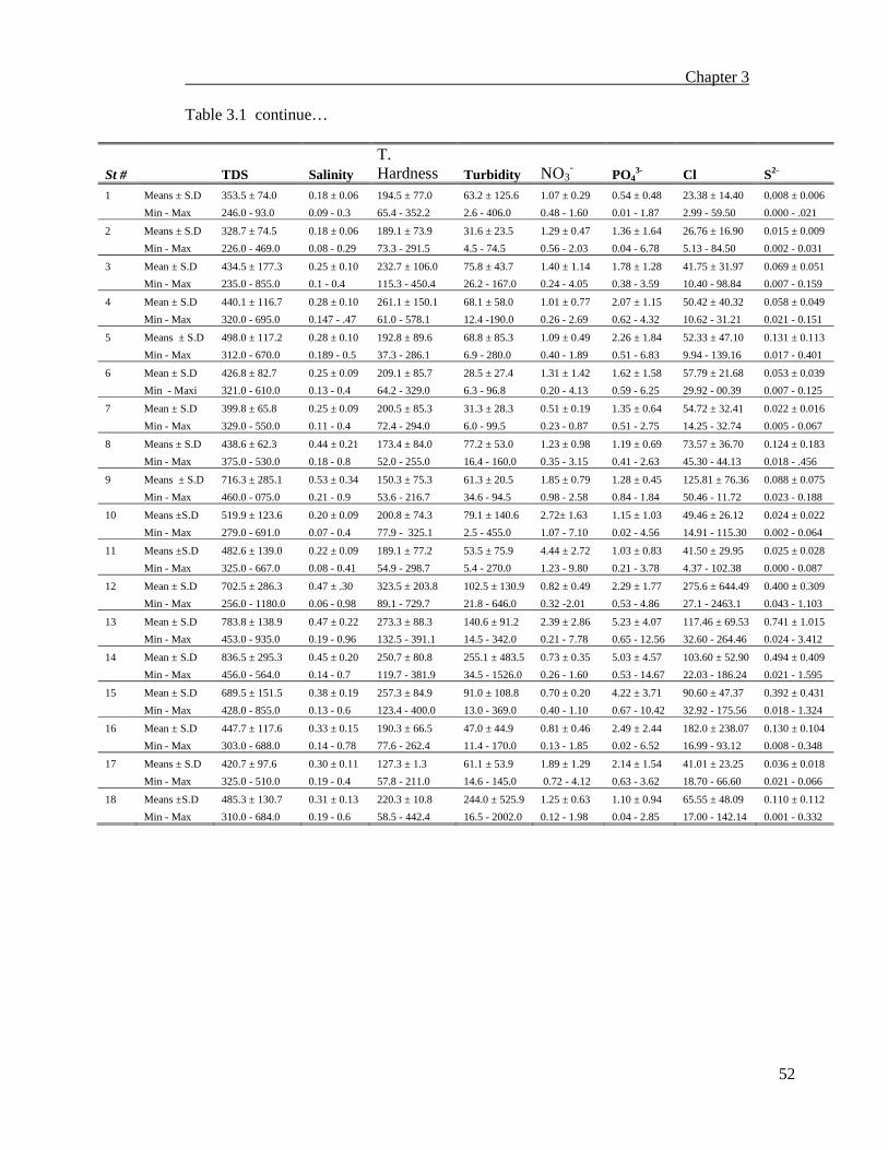
Chapter 3

52

Table 3.1 continue…

St # TDS Salinity T. Hardness Turbidity NO3

- PO43- Cl S2-

1 Means ± S.D 353.5 ± 74.0 0.18 ± 0.06 194.5 ± 77.0 63.2 ± 125.6 1.07 ± 0.29 0.54 ± 0.48 23.38 ± 14.40 0.008 ± 0.006 Min - Max 246.0 - 93.0 0.09 - 0.3 65.4 - 352.2 2.6 - 406.0 0.48 - 1.60 0.01 - 1.87 2.99 - 59.50 0.000 - .021

2 Means ± S.D 328.7 ± 74.5 0.18 ± 0.06 189.1 ± 73.9 31.6 ± 23.5 1.29 ± 0.47 1.36 ± 1.64 26.76 ± 16.90 0.015 ± 0.009 Min - Max 226.0 - 469.0 0.08 - 0.29 73.3 - 291.5 4.5 - 74.5 0.56 - 2.03 0.04 - 6.78 5.13 - 84.50 0.002 - 0.031

3 Mean ± S.D 434.5 ± 177.3 0.25 ± 0.10 232.7 ± 106.0 75.8 ± 43.7 1.40 ± 1.14 1.78 ± 1.28 41.75 ± 31.97 0.069 ± 0.051 Min - Max 235.0 - 855.0 0.1 - 0.4 115.3 - 450.4 26.2 - 167.0 0.24 - 4.05 0.38 - 3.59 10.40 - 98.84 0.007 - 0.159

4 Mean ± S.D 440.1 ± 116.7 0.28 ± 0.10 261.1 ± 150.1 68.1 ± 58.0 1.01 ± 0.77 2.07 ± 1.15 50.42 ± 40.32 0.058 ± 0.049 Min - Max 320.0 - 695.0 0.147 - .47 61.0 - 578.1 12.4 -190.0 0.26 - 2.69 0.62 - 4.32 10.62 - 31.21 0.021 - 0.151

5 Means ± S.D 498.0 ± 117.2 0.28 ± 0.10 192.8 ± 89.6 68.8 ± 85.3 1.09 ± 0.49 2.26 ± 1.84 52.33 ± 47.10 0.131 ± 0.113 Min - Max 312.0 - 670.0 0.189 - 0.5 37.3 - 286.1 6.9 - 280.0 0.40 - 1.89 0.51 - 6.83 9.94 - 139.16 0.017 - 0.401

6 Mean ± S.D 426.8 ± 82.7 0.25 ± 0.09 209.1 ± 85.7 28.5 ± 27.4 1.31 ± 1.42 1.62 ± 1.58 57.79 ± 21.68 0.053 ± 0.039 Min - Maxi 321.0 - 610.0 0.13 - 0.4 64.2 - 329.0 6.3 - 96.8 0.20 - 4.13 0.59 - 6.25 29.92 - 00.39 0.007 - 0.125

7 Mean ± S.D 399.8 ± 65.8 0.25 ± 0.09 200.5 ± 85.3 31.3 ± 28.3 0.51 ± 0.19 1.35 ± 0.64 54.72 ± 32.41 0.022 ± 0.016 Min - Max 329.0 - 550.0 0.11 - 0.4 72.4 - 294.0 6.0 - 99.5 0.23 - 0.87 0.51 - 2.75 14.25 - 32.74 0.005 - 0.067

8 Means ± S.D 438.6 ± 62.3 0.44 ± 0.21 173.4 ± 84.0 77.2 ± 53.0 1.23 ± 0.98 1.19 ± 0.69 73.57 ± 36.70 0.124 ± 0.183 Min - Max 375.0 - 530.0 0.18 - 0.8 52.0 - 255.0 16.4 - 160.0 0.35 - 3.15 0.41 - 2.63 45.30 - 44.13 0.018 - .456

9 Means ± S.D 716.3 ± 285.1 0.53 ± 0.34 150.3 ± 75.3 61.3 ± 20.5 1.85 ± 0.79 1.28 ± 0.45 125.81 ± 76.36 0.088 ± 0.075 Min - Max 460.0 - 075.0 0.21 - 0.9 53.6 - 216.7 34.6 - 94.5 0.98 - 2.58 0.84 - 1.84 50.46 - 11.72 0.023 - 0.188

10 Means ±S.D 519.9 ± 123.6 0.20 ± 0.09 200.8 ± 74.3 79.1 ± 140.6 2.72± 1.63 1.15 ± 1.03 49.46 ± 26.12 0.024 ± 0.022 Min - Max 279.0 - 691.0 0.07 - 0.4 77.9 - 325.1 2.5 - 455.0 1.07 - 7.10 0.02 - 4.56 14.91 - 115.30 0.002 - 0.064

11 Means ±S.D 482.6 ± 139.0 0.22 ± 0.09 189.1 ± 77.2 53.5 ± 75.9 4.44 ± 2.72 1.03 ± 0.83 41.50 ± 29.95 0.025 ± 0.028 Min - Max 325.0 - 667.0 0.08 - 0.41 54.9 - 298.7 5.4 - 270.0 1.23 - 9.80 0.21 - 3.78 4.37 - 102.38 0.000 - 0.087

12 Mean ± S.D 702.5 ± 286.3 0.47 ± .30 323.5 ± 203.8 102.5 ± 130.9 0.82 ± 0.49 2.29 ± 1.77 275.6 ± 644.49 0.400 ± 0.309 Min - Max 256.0 - 1180.0 0.06 - 0.98 89.1 - 729.7 21.8 - 646.0 0.32 -2.01 0.53 - 4.86 27.1 - 2463.1 0.043 - 1.103

13 Mean ± S.D 783.8 ± 138.9 0.47 ± 0.22 273.3 ± 88.3 140.6 ± 91.2 2.39 ± 2.86 5.23 ± 4.07 117.46 ± 69.53 0.741 ± 1.015 Min - Max 453.0 - 935.0 0.19 - 0.96 132.5 - 391.1 14.5 - 342.0 0.21 - 7.78 0.65 - 12.56 32.60 - 264.46 0.024 - 3.412

14 Mean ± S.D 836.5 ± 295.3 0.45 ± 0.20 250.7 ± 80.8 255.1 ± 483.5 0.73 ± 0.35 5.03 ± 4.57 103.60 ± 52.90 0.494 ± 0.409 Min - Max 456.0 - 564.0 0.14 - 0.7 119.7 - 381.9 34.5 - 1526.0 0.26 - 1.60 0.53 - 14.67 22.03 - 186.24 0.021 - 1.595

15 Mean ± S.D 689.5 ± 151.5 0.38 ± 0.19 257.3 ± 84.9 91.0 ± 108.8 0.70 ± 0.20 4.22 ± 3.71 90.60 ± 47.37 0.392 ± 0.431 Min - Max 428.0 - 855.0 0.13 - 0.6 123.4 - 400.0 13.0 - 369.0 0.40 - 1.10 0.67 - 10.42 32.92 - 175.56 0.018 - 1.324

16 Mean ± S.D 447.7 ± 117.6 0.33 ± 0.15 190.3 ± 66.5 47.0 ± 44.9 0.81 ± 0.46 2.49 ± 2.44 182.0 ± 238.07 0.130 ± 0.104 Min - Max 303.0 - 688.0 0.14 - 0.78 77.6 - 262.4 11.4 - 170.0 0.13 - 1.85 0.02 - 6.52 16.99 - 93.12 0.008 - 0.348

17 Means ± S.D 420.7 ± 97.6 0.30 ± 0.11 127.3 ± 1.3 61.1 ± 53.9 1.89 ± 1.29 2.14 ± 1.54 41.01 ± 23.25 0.036 ± 0.018 Min - Max 325.0 - 510.0 0.19 - 0.4 57.8 - 211.0 14.6 - 145.0 0.72 - 4.12 0.63 - 3.62 18.70 - 66.60 0.021 - 0.066

18 Means ±S.D 485.3 ± 130.7 0.31 ± 0.13 220.3 ± 10.8 244.0 ± 525.9 1.25 ± 0.63 1.10 ± 0.94 65.55 ± 48.09 0.110 ± 0.112 Min - Max 310.0 - 684.0 0.19 - 0.6 58.5 - 442.4 16.5 - 2002.0 0.12 - 1.98 0.04 - 2.85 17.00 - 142.14 0.001 - 0.332

Chapter 3

53

Table. 3.2 Means ± S.D. and Ranges (min– max) of dissolved metals in stream water at various sampling sites located on Nullah Aik and Nullah Palkhu

St # Na (dis) K (dis) Ca (dis) Mg (dis) Fe (dis) Pb (dis) Cd (dis) Cr(dis) Ni (dis) Cu (dis) Zn (dis) 1 Means ± S.D 29.41 ± 11.90 3.87 ± 3.07 57.92 ± 19.63 11.61 ± 9.59 0.198 ± 0.430 0.111 ± 0.070 0.023± 0.031 0.062 ± 0.083 0.090 ± 0.122 0.030 ± 0.062 0.038 ± 0.030 Min - Max 17.6 - 57.1 0.2 - 10.0 15.7 - 86.5 0.4 - 42.5 0.003 - .542 0.007 - .288 0.002 - .098 0.003 - .340 0.005 - .356 0.000 - .196 0.004 - .093

2 Means ± S.D 28.85 ± 10.12 5.84 ± 6.71 57.92 ± 18.80 12.18 ± 9.12 0.292 ± 0.406 0.129 ± 0.095 0.028 ± 0.029 0.091 ± 0.160 0.067 ± 0.069 0.025 ± 0.051 0.038 ± 0.029 Min - Max 19.3 - 58.9 0.6 - 23.1 19.5 - 86.9 0.1 - 29.9 0.018 - 1.330 0.029 - 0.421 0.003 - 0.098 0.002 - 0.504 0.008 - 0.256 0.000 - 0.173 0.002 - 0.085

3 Mean ± S.D 47.14 ± 30.57 8.02 ± 4.77 67.43 ± 28.19 14.98 ± 0.61 0.644 ± 0.769 0.660 ± 0.649 0.028 ± 0.032 0.267 ± 0.388 0.088 ± 0.063 0.034 ± 0.055 0.126 ± 0.183 Min - Max 14.5 - 130.4 0.4 - 5.7 30.9 - 130.6 1.6 - 31.2 0.002 - 2.526 0.031 - 1.922 0.003 - 0.108 0.006 - 1.146 0.004 - 0.224 0.000 - 0.187 0.015 - 0.689

4 Mean ± S.D 39.46 ± 16.32 9.25 ± 10.71 77.79 ± 42.36 15.49 ± 12.48 0.383 ± 0.513 0.445 ± 0.745 0.027 ± 0.031 0.116 ± 0.149 0.079 ± 0.078 0.039 ± 0.069 0.089 ± 0.088 Min - Max 12.0 - 69.0 1.0 - 37.9 16.7 - 170.3 1.7 - 37.2 0.020 - 1.693 0.039 - 2.605 0.001 - 0.109 0.006 - 0.489 0.002 - 0.239 0.001 - 0.203 0.018 - 0.415

5 Means ± S.D 52.01 ± 31.82 10.19 ± 15.41 55.60 ± 24.64 12.34 ± 8.19 0.423 ± 0.522 0.600 ± 0.818 0.029 ± 0.035 0.096 ± 0.139 0.105 ± 0.101 0.040 ± 0.069 0.094 ± 0.137 Min - Max 11.1 - 122.1 0.3 - 51.4 13.2 - 89.5 1.0 - 24.9 0.020 - 2.300 0.062 - 3.538 0.003 - 0.116 0.001 - 0.610 0.004 - 0.325 0.000 - 0.234 0.000 - 0.452

6 Mean ± S.D 50.92 ± 21.06 7.52 ± 2.51 56.53 ± 20.44 16.29 ± 10.92 0.349 ± 0.452 0.692 ± 0.904 0.021 ± 0.027 0.102 ± 0.153 0.072 ± 0.068 0.023 ± 0.041 0.054 ± 0.070 Min - Maxi 22.4 - 97.8 3.0 - 13.3 14.9 - 82.0 1.2 - 36.9 0.021 - 1.689 0.042 - 3.378 0.000 - 0.089 0.004 - 0.525 0.002 - 0.197 0.001 - 0.125 0.004 - 0.237

7 Mean ± S.D 42.20 ± 19.83 6.56 ± 2.17 54.95 ± 21.26 14.63 ± 10.26 0.346 ± 0.425 0.692 ± 0.849 0.022 ± 0.026 0.122 ± 0.178 0.104 ± 0.136 0.031 ± 0.055 0.050 ± 0.065 Min - Max 18.5 - 77.1 2.1 - 9.7 16.5 - 89.1 1.0 - 32.0 0.008 - 1.534 0.016 - 3.068 0.002 - 0.091 0.005 - 0.504 0.001 - 0.436 0.000 - 0.183 0.003 - 0.216

8 Means ± S.D 68.88 ± 56.10 6.92 ± 5.20 63.08 ± 10.11 9.45 ± 4.48 0.505 ± 0.647 0.747 ± 1.017 0.049 ± 0.058 0.046 ± 0.046 0.179 ± 0.189 0.141 ± 0.202 0.027 ± 0.023 Min - Max 19.8 - 173.5 0.2 - 12.6 45.1 - 76.5 3.2 - 13.6 0.045 - .405 0.044 - 2.162 0.001 - 0.130 0.014 - 0.108 0.001 - 0.424 0.011 - 0.532 0.000 - 0.056

9 Means ± S.D 66.60 ± 46.16 7.98 ± 8.43 61.46 ± 4.75 6.41 ± 3.41 0.862 ± 0.805 1.325 ± 1.239 0.067 ± 0.066 0.134 ± 0.145 0.055 ± 0.035 0.142 ± 0.150 0.019 ± 0.016 Min - Max 23.6 - 113.6 0.2 - 16.9 53.1 - 67.0 3.1 - 10.2 0.106 - 1.856 0.163 - 2.855 0.004 - 0.131 0.002 - 0.279 0.021 - 0.092 0.007 - 0.347 0.001 - 0.038

10 Means ±S.D 51.48 ± 25.28 10.05 ± 7.67 58.34 ± 21.85 12.37 ± 7.17 0.321 ± 0.532 0.210 ± 0.237 0.023 ± 0.030 0.195 ± 0.326 0.083 ± 0.092 0.043 ± 0.112 0.037 ± 0.029 Min - Max 16.5 - 112.0 0.2 - 26.5 20.6 - 96.4 1.2 - 20.9 0.020 - 1.784 0.021 - 0.989 0.001 - 0.099 0.011 - 1.013 0.003 - 0.281 0.000 - 0.475 0.001 - 0.096

11 Means ±S.D 49.03 ± 22.31 10.56 ± 7.63 56.92 ± 23.10 10.67 ± 6.88 0.553 ± 0.664 0.113 ± 0.083 0.022 ± 0.028 0.161 ± 0.250 0.072 ± 0.098 0.034 ± 0.078 0.042 ± 0.026 Min - Max 20.0 - 94.8 0.2 - 25.0 11.2 - 96.4 1.1 - 22.7 0.042 - 1.886 0.025 - .331 0.002 - 0.092 0.006 - 0.725 0.000 - 0.326 0.000 - 0.263 0.006 - 0.096

12 Mean ± S.D 67.44 ± 30.00 20.51 ± 12.52 87.25 ± 48.76 24.40 ± 20.44 0.682 ± 0.496 0.712 ± 0.774 0.027 ± 0.034 0.206 ± 0.328 0.071 ± 0.073 0.028 ± 0.055 0.070 ± 0.054 Min - Max 15.7 - 111.6 6.0 - 40.8 23.7 - 186.1 1.5 - 4.3 0.033 - 1.541 0.047 - 2.371 0.001 - 0.124 0.015 - 0.958 0.002 - 0.245 0.000 - 0.185 0.005 - 0.190

13 Mean ± S.D 79.09 ± 45.76 18.16 ± 8.20 65.07 ± 17.10 25.86 ± 13.38 0.673 ± 0.646 0.624 ± 0.959 0.024 ± 0.030 0.262 ± 0.302 0.072 ± 0.065 0.028 ± 0.050 0.088 ± 0.080 Min - Max 30.3 - 160.3 9.5 - 36.6 28.4 - 93.2 4.5 - 48.6 0.075 - 2.369 0.038 - 3.645 0.002 - 0.103 0.016 - 0.797 0.001 - 0.231 0.000 - 0.159 0.004 - 0.259

14 Mean ± S.D 84.63 ± 56.18 16.08 ± 7.10 62.39 ± 17.67 22.09 ± 11.96 0.787 ± 0.573 0.640 ± 0.790 0.022 ± 0.025 0.235 ± 0.258 0.104 ± 0.104 0.031 ± 0.057 0.110 ± 0.098 Min - Max 31.3 - 203.9 6.8 - 32.7 34.1 - 86.0 5.7 - 47.5 0.031 - 1.892 0.016 - 2.911 0.002 - 0.098 0.015 - 0.795 0.002 - 0.332 0.000 - 0.185 0.014 - 0.362

15 Mean ± S.D 67.32 ± 31.23 18.44 ± 14.47 59.50 ± 18.34 25.63 ± 13.85 0.446 ± 0.457 0.893 ± 0.914 0.023 ± 0.027 0.210 ± 0.255 0.106 ± 0.126 0.027 ± 0.056 0.095 ± 0.099 Min - Max 33.5 - 123.7 6.1 - 58.8 22.0 - 81.3 6.8 - 51.4 0.042 - 1.569 0.084 - 3.138 0.002 - 0.097 0.015 - 0.675 0.002 - 0.414 0.001 - 0.186 0.002 - 0.485

16 Mean ± S.D 54.10 ± 33.91 9.81 ± 6.16 50.63 ± 16.34 14.89 ± 8.20 0.382 ± 0.552 0.764 ± 1.104 0.024 ± 0.027 0.175 ± 0.202 0.115 ± 0.285 0.025 ± 0.050 0.079 ± 0.062 Min - Max 16.9 - 126.4 3.0 - 23.3 20.6 - 72.5 0.1 - 26.9 0.012 - 1.904 0.024 - 3.808 0.002 - 0.093 0.012 - 0.575 0.001 - 1.426 0.001 - 0.185 0.012 - 0.213

17 Means ± S.D 39.41 ± 15.73 2.58 ± 2.60 47.45 ± 5.88 8.86 ± 3.08 0.820 ± 0.775 1.640 ± 1.550 0.068 ± 0.067 0.028 ± 0.024 0.075 ± 0.093 0.109 ± 0.109 0.024 ± 0.009 Min - Max 24.8 - 58.1 0.2 - 5.4 42.6 - 58.4 3.8 - 12.6 0.086 - .693 0.172 - 3.386 0.004 - 0.131 0.006 - 0.053 0.000 - 0.231 0.007 - 0.215 0.014 - 0.036

18 Means ±S.D 68.95 ± 37.58 10.43 ± 6.13 54.00 ± 20.87 20.23 ± 21.79 0.357 ± 0.404 0.426 ± 0.618 0.028 ± 0.038 0.261 ± 0.321 0.123 ± 0.231 0.042 ± 0.101 0.082 ± 0.071 Min - Max 5.5 - 103.7 0.2 - 21.2 17.6 - s87.2 0.1 - 66.8 0.013 - 1.460 0.007 - 2.246 0.002 - 0.125 0.004 - 1.034 0.003 - 0.896 0.000 - 0.412 0.006 - 0.219

Chapter 3

54

Table 3.3 Means ± S.D. and Ranges (min – max) of suspended metals in stream water at various sampling sites located on Nullah Aik and Nullah Palkhu

St # Na (sus) K (sus) Ca (sus) Mg (sus) Fe (sus) Pb (sus) Cd (sus) Cr (sus) Ni (sus) Cu (sus) Zn (sus) 1 Means ± S.D 13.192 ± 10.224 6.580 ± 6.920 13.694 ± 10.201 17.181 ± 8.242 4.563 ± 2.716 0.651 ± 0.516 0.049 ± 0.035 0.180 ± 0.132 0.300 ± 0.224 0.076 ± 0.084 0.544 ± 0.805 Min - Max 1.755 - 31.097 0.124 - 22.457 0.987 - 39.064 0.531 - 26.97 2.011 - .718 0.000 - .700 0.008 - .129 0.022 - .375 0.070 - .774 0.003 - .344 0.000 - .415

2 Means ± S.D 11.708 ± 5.910 11.624 ± 8.379 36.284 ± 27.307 42.197 ± 30.688 10.600 ± 4.597 0.874 ± 0.360 0.056 ± 0.053 0.505 ± 0.465 0.348 ± 0.271 0.147 ± 0.210 0.802 ± 0.700 Min - Max 2.361 - 22.457 0.235 - 28.467 1.854 - 76.383 3.163 - 91.659 3.548 - 7.623 0.212 - 1.580 0.004 - 0.196 0.041 - 1.814 0.023 - 0.885 0.001 - 0.695 0.072 - 1.989 3 Mean ± S.D 14.017 ± 9.820 12.255 ± 7.626 31.143 ± 25.800 47.965 ± 28.789 22.382 ± 10.445 1.023 ± 0.381 0.070 ± 0.050 1.398 ± 1.044 0.631 ± 0.554 0.170 ± 0.094 1.306 ± 1.129 Min - Max 5.234 - 35.158 2.568 - 31.712 6.533 - 97.425 23.561 - 133.558 4.797 - 1.023 0.127 - 1.850 0.008 - 0.185 0.045 - 4.231 0.001 - 1.968 0.029 - 0.359 0.259 - 3.658

4 Mean ± S.D 16.717 ± 9.941 12.749 ± 9.674 28.187 ± 24.272 51.988 ± 30.511 30.940 ± 22.706 1.045 ± 0.435 0.102 ± 0.138 2.828 ± 2.782 0.806 ± 0.824 0.163 ± 0.111 2.427 ± 2.906 Min - Max 5.048 - 37.39 1.798 - 31.745 3.996 - 88.961 16.457 - 97.774 0.759 - 1.054 0.526 - 1.963 0.016 - 0.710 0.073 - 8.124 0.100 - 3.168 0.008 - 0.412 0.165 - 8.529

5 Means ± S.D 14.336 ± 9.356 9.202 ±10.725 32.535 ± 26.644 27.542 ± 8.813 10.386 ± 5.770 0.987 ± 0.289 0.061 ± 0.051 3.132 ± 3.044 0.626 ± 0.510 0.156 ± 0.149 0.898 ± 0.592 Min - Max 5.604 - 39.263 0.075 - 37.12 2.301 - 96.895 14.392 - 39.087 2.185 - 3.235 0.635 - 1.610 0.011 - 0.175 0.058 - 8.457 0.123 - 1.961 0.008 - 0.523 0.137 - 1.975

6 Mean ± S.D 23.966 ± 18.623 13.013 ± 9.973 29.785 ± 24.865 46.023 ± 26.316 10.208 ± 6.178 0.990 ± 0.550 0.073 ± 0.082 1.080 ± 0.781 0.581 ± 0.743 0.098 ± 0.133 0.724 ± 0.661 Min - Maxi 5.986 - 59.09 0.695 - 27.018 2.001 - 78.244 16.604 - 99.531 1.230 - 8.478 0.265 - 1.895 0.002 - 0.403 0.024 - 2.559 0.032 - 3.261 0.023 - 0.630 0.036 - 1.989

7 Mean ± S.D 23.873 ± 20.619 12.091 ± 10.496 24.883 ± 20.654 46.092 ± 41.057 7.369 ± 5.097 1.082 ± 0.691 0.055 ± 0.044 0.598 ± 0.510 0.376 ± 0.294 0.092 ± 0.080 0.680 ± 0.924 Min - Max 4.546 - 69.243 0.623 - 24.465 1.828 - 66.474 15.23 - 151.34 1.023 - 5.326 0.075 - 2.624 0.014 - 0.167 0.024 - 1.978 0.096 - 0.964 0.004 - 0.262 0.111 - 3.024

8 Means ± S.D 21.150 ± 12.441 10.569 ± 8.401 19.308 ±16.258 14.284 ± 1.235 7.528 ± 7.590 0.711 ± 0.643 0.083 ± 0.070 1.613 ± 1.991 0.634 ± 0.582 0.104 ± 0.110 0.220 ± 0.173 Min - Max 5.333 - 35.69 1.186 - 24.212 1.024 - 44.235 12.137 - 16.564 1.231 - 8.425 0.012 - 1.527 0.013 - 0.197 0.099 - 5.263 0.088 - 1.634 0.015 - 0.267 0.099 - 0.635

9 Means ± S.D 23.001 ± 10.279 9.954 ± 7.400 17.182 ± 22.836 25.374 ± 13.975 5.267 ± 0.755 0.186 ± 0.154 0.067 ± 0.071 0.542 ± 0.267 0.116 ± 0.037 0.081 ± 0.040 0.109 ± 0.043 Min - Max 9.959 - 36.457 1.207 - 19.457 1.23 - 49.863 12.71 - 45.718 4.127 - .351 0.029 - 0.433 0.001 - 0.141 0.089 - 0.859 0.074 - 0.174 0.040 - 0.126 0.056 - 0.152

10 Means ±S.D 13.681 ± 9.820 8.427 ± 5.941 27.940 ± 26.447 29.237 ±18.793 5.750 ± 2.909 0.805 ± 0.423 0.057 ± 0.064 0.308 ± 0.203 0.382 ± 0.264 0.090 ± 0.116 0.696 ± 0.554 Min - Max 3.04 - 33.034 0.862 - 19.413 1.024 - 85.284 9.451 - 77.531 1.665 - 10.156 0.021 - 1.968 0.005 - 0.229 0.017 - 0.630 0.121 - 0.924 0.005 - 0.395 0.052 - 1.815

11 Means ±S.D 18.745 ± 15.488 14.812 ± 15.236 23.603 ±14.575 39.201 ± 14.853 12.299 ± 10.015 0.749 ± 0.435 0.050 ± 0.049 0.549 ± 0.471 0.505 ± 0.419 0.106 ± 0.126 0.683 ± 0.547 Min - Max 4.912 - 48.4147 0.135 - 42.052 4.268 - 53.879 0.123 - 73.3676 3.485 - 37.124 0.089 - 1.536 0.007 - 0.197 0.071 - 1.856 0.121 - 1.745 0.006 - 0.456 0.109 - 1.634

12 Mean ± S.D 25.492 ± 15.333 23.265 ± 13.713 45.828 ± 30.462 75.650 ±70.124 16.877 ± 6.350 1.111 ± 0.356 0.062 ± 0.049 1.576 ± 2.373 0.660 ± 0.447 0.303 ± 0.486 1.217 ± 1.019 Min - Max 6.125 - 51.4635 3.562 - 42.004 1.181 - 92.283 33.257 - 310.804 2.486 - 29.780 0.568 - 1.953 0.012 - 0.196 0.032 - 8.503 0.163 - 1.523 0.040 - 1.856 0.068 - 3.624

13 Mean ± S.D 30.181 ± 16.114 31.831 ± 13.012 50.839 ± 29.865 112.28 ± 132.07 27.312 ± 11.148 1.053 ± 0.514 0.065 ± 0.046 10.13 ± 10.68 1.029 ± 0.565 0.734 ± 0.887 3.620 ± 2.984 Min - Max 8.96 - 59.4021 10.236 - 49.56 2.028 - 99.9731 50.291 - 468.716 10.172 - 45.124 0.055 - 1.908 0.014 - 0.175 0.082 - 25.17 0.368 - 2.206 0.065 - 3.201 0.596 - 9.562

14 Mean ± S.D 27.300 ±15.478 38.701 ± 32.960 51.879 ± 31.551 80.310 ± 60.146 20.942 ± 7.156 1.227 ± 0.681 0.106 ± 0.163 5.636 ± 6.264 0.912 ± 1.184 0.393 ± 0.284 3.180 ± 1.563 Min - Max 0.04 - 57.3971 4.025 - 123 5.267 - 89.741 43.039 - 279.253 10.080 - 32.512 0.485 - 3.456 0.001 - 0.832 0.10 - 20.948 0.121 - 4.213 0.145 - 1.054 0.426 - 6.126

15 Mean ± S.D 29.816 ± 19.109 19.507 ± 15.681 52.793 ± 33.945 68.216 ± 41.518 19.653 ± 15.372 1.089 ± 0.580 0.083 ± 0.047 4.569 ± 7.628 0.905 ± 1.079 0.138 ± 0.085 1.974 ± 1.675 Min - Max 1.96 - 68.784 2.013 - 48.121 2.014 - 94.71 44.912 - 189.16 3.458 - 53.596 0.289 - 2.361 0.009 - 0.161 0.119 - 26.47 0.025 - 4.235 0.023 - 0.295 0.129 - 5.012

16 Mean ± S.D 30.586 ± 25.374 13.866 ± 12.208 36.571 ± 26.956 62.306 ± 25.629 13.016 ± 6.831 0.907 ± 0.416 0.065 ± 0.042 0.794 ± 0.544 0.480 ± 0.356 0.125 ± 0.111 0.899 ± 0.897 Min - Max 6.275 - 85.486 1.042 - 32.095 1.024 - 82.653 23.421 - 106.97 3.002 - 2.728 0.314 - 1.789 0.013 - 0.175 0.054 - 2.001 0.045 - 1.086 0.042 - 0.459 0.123 - 3.457

17 Means ± S.D 16.518 ± 8.821 3.551 ± 2.539 14.178 ± 15.548 13.393 ± 2.104 6.560 ± 4.197 0.252 ± 0.207 0.079 ± 0.084 0.375 ± 0.322 0.225 ± 0.189 0.026 ± 0.019 0.188 ± 0.078 Min - Max 7.544 - 26.45 1.235 - 7.568 1.0784 - 39.564 11.421 - 16.124 2.421 - 11.450 0.069 - 0.544 0.001 - 0.163 0.062 - 0.845 0.051 - 0.416 0.008 - 0.052 0.089 - 0.313

18 Means ±S.D 16.170 ± 11.917 16.140 ± 14.929 29.973 ± 33.416 51.334 ± 34.691 9.891 ± 5.245 1.423 ± 1.004 0.073 ± 0.060 3.232 ± 5.593 0.720 ± 0.439 0.158 ± 0.097 1.615 ± 1.629 Min - Max 6.02 - 38.458 1.023 - 56.528 1.031 - 101.836 12.419 - 135.46 2.551 - 18.683 0.129 - 4.012 0.011 - 0.225 0.025 - 18.23 0.052 - 1.374 0.010 - 0.301 0.106 - 4.562

(a)

00.5

11.5

22.5

33.5

44.5

1 2 3 4 5 6 7 8 9 10 11 12 13 14 15 16 17 18

St. f

low

(m/s

ec)

St.d

epth

(m)

05101520253035

stre

am w

idth

(m)

St flow St depth St width

(b)

0

5

10

15

20

25

1 2 3 4 5 6 7 8 9 10 11 12 13 14 15 16 17 18

Tem

pera

ture

(C)

DO

(mg/

L)

7.27.47.67.888.28.4

pH

Temperature DO pH

(c)

0

200

400

600

800

1000

1200

1 2 3 4 5 6 7 8 9 10 11 12 13 14 15 16 17 18

EC

(uS/

cm) T

DS

(mg/

L)

050100150200250300350400

CO

D (m

g/L

)

EC TDS COD

d)

0

50

100

150

200

250

300

1 2 3 4 5 6 7 8 9 10 11 12 13 14 15 16 17 18

Tot

al h

ardn

ess (

mg/

L)

Tur

bidi

ty(N

TU

)

0

0.1

0.2

0.3

0.4

0.5

Salin

ity (m

g/L

)

T.hardness Turbidity Salinity

Nullah Palkhu Nullah Aik




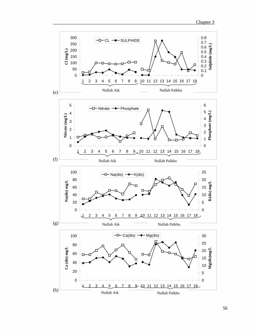
Chapter 3

56

(e)

050

100150200250300

1 2 3 4 5 6 7 8 9 10 11 12 13 14 15 16 17 18

Cl (

mg/

L)

00.10.20.30.40.50.60.70.8

Sulp

hide

(mg/

L)CL SULPHIDE

(f)

0

1

2

3

4

5

1 2 3 4 5 6 7 8 9 10 11 12 13 14 15 16 17 18

Nitr

ate

(mg/

L)

0

1

2

3

4

5

6

Phos

phat

e (m

g/L

)Nitrate Phosphate

(g)

0

20

40

60

80

100

1 2 3 4 5 6 7 8 9 10 11 12 13 14 15 16 17 18

Na(

dis)

mg/

L

0

5

10

15

20

25

K(d

is) m

g/L

Na(dis) K(dis)

(h)

0

20

40

60

80

100

1 2 3 4 5 6 7 8 9 10 11 12 13 14 15 16 17 18

Ca

(dis

) mg/

L

0

5

10

15

20

25

30

Mg(

dis)

mg/

L

Ca(dis) Mg(dis)





Chapter 3

57

(i)

00.10.20.30.40.50.60.70.80.9

1 2 3 4 5 6 7 8 9 10 11 12 13 14 15 16 17 18

Fe (d

is) m

g/L

00.050.10.150.20.250.30.350.4

Pb(d

is) m

g/L

Fe(dis) Pb(dis)

(j)

00.0050.01

0.0150.02

0.0250.03

0.035

1 2 3 4 5 6 7 8 9 10 11 12 13 14 15 16 17 18

Cd

(dis

) mg/

L

00.050.10.150.20.250.3

Cr

(dis

) mg/

L

Cd(dis) Cr(dis)

(k)

00.020.040.060.080.1

0.120.14

1 2 3 4 5 6 7 8 9 10 11 12 13 14 15 16 17 18

Ni(d

is) m

g/L

Cu(

dis)

mg/

L

00.020.040.060.080.10.120.14

Zn

(dis

) mg/

L

Ni(dis) Cu(dis) Zn(dis)

(l)

05

101520253035

1 2 3 4 5 6 7 8 9 10 11 12 13 14 15 16 17 18

Na(

sus)

mg/

L

051015202530354045

K(s

us) m

g/L

Na(sus)K(sus)




Chapter 3

58

(m)

0

10

20

30

40

50

60

1 2 3 4 5 6 7 8 9 10 11 12 13 14 15 16 17 18

Mg

(sus

) mg/

L

0

20

40

60

80

100

120

Ca(

sus)

mg/

L

Ca(sus) Mg(sus)

(n)

05

101520253035

1 2 3 4 5 6 7 8 9 10 11 12 13 14 15 16 17 18

Fe(s

us) m

g/L

0

0.5

1

1.5

Pb (s

us) m

g/L

Fe(sus) Pb(sus)

(o)

00.020.040.060.08

0.10.12

1 2 3 4 5 6 7 8 9 10 11 12 13 14 15 16 17 18

Cd(

sus)

mg/

L

024681012

Cr(

sus)

mg/

L

Cd(sus) Cr(sus)

(p)

00.20.40.60.8

11.2

1 2 3 4 5 6 7 8 9 10 11 12 13 14 15 16 17 18

Ni(s

us) m

g/L

Cu(

sus)

m

g/L

0

1

2

3

4

Zn(

sus)

mg/

LNi(sus) Cu(sus)Z ( )

Fig. 3.1 Mean values of stream morphology (a), physiochemical (a - e),

nutrients (g), metals in dissolved form (g-k) and metals in suspended particulate form (l- p) measured at various sites (names of sites are given in Fig 2.7) located on Nullah Aik and Nullah Palkhu





Chapter 3

59

2030405060708090

Na mg/l

Na (dis)

(a)

0

5

10

15

20

25

30

35

40

45

1 2 3 4 5 6 7 8 9 10 11 12 13 14 15 16 17 18

Sampling aites

K m

g/L

K (dis) K (sus)

(b)

0

10

20

30

40

50

60

70

8090

100

1 2 3 4 5 6 7 8 9 10 11 12 13 14 15 16 17 18

Sampling sites

Ca

mg/

L

Ca (dis) Ca (sus)

(c)

0

10

20

30

40

50

60

70

80

90

1 2 3 4 5 6 7 8 9 10 11 12 13 14 15 16 17 18

Sampling sites

Mg

mg/

L

Mg (dis) Mg (sus)

(d)

0

5

10

15

20

25

30

35

1 2 3 4 5 6 7 8 9 10 11 12 13 14 15 16 17 18

Sampling sites

Fe m

g/L

Fe (dis) Fe (sus)

(e)

0

0.2

0.4

0.6

0.8

1

1.2

1.4

1.6

1 2 3 4 5 6 7 8 9 10 11 12 13 14 15 16 17 18

Sampling sites

Pb m

g/L

Pb (dis) Pb (sus)

(f)

0

2

4

6

8

10

12

1 2 3 4 5 6 7 8 9 10 11 12 13 14 15 16 17 18

Sampling sites

Cr m

g/L

Cr (dis) Cr (sus)

0

0.02

0.04

0.06

0.08

0.1 0.12

1 2 3 4 5 6 7 8 9 10 11 12 13 14 15 16 17 18

Sampling sites

Cd (dis) Cd (sus)

Cd

mg/

L

Chapter 3

60

0

0.2

0.4

0.6

0.8

1

1.2

1 2 3 4 5 6 7 8 9 10 11 12 13 14 15 16 17 18

Sampling sites

Ni m

g/L

Ni (dis) Ni (sus)

(g)

0

0.05

0.1

0.15

0.2

0.25

0.3

0.35

0.4

1 2 3 4 5 6 7 8 9 10 11 12 13 14 15 16 17 18

Sampling sites

Cu

mg/

L

Cu (dis) Cu (sus)

(h)

(i)

0

0.5

1

1.5

2

2.5

3

3.5

4

1 2 3 4 5 6 7 8 9 10 11 12 13 14 15 16 17 18

Sampling sites

Zn m

g/L

Zn (dis) Zn (sus)

(j) Fig. 3.2 Comparison of metals (a- j) in dissolved and suspended particulate

form measured in water samples collected from Nullah Aik and Nullah Palkhu.

Chapter 3

61

Inter- relationships among Metals

The metal correlations were observed in two forms i.e. dissolved and

suspended particulate matter. Pearson correlation matrix of dissolved metals and

suspended particulate matter are given in Table 3.4a & b. In case of dissolved form of

metal, significant positive correlation of Fe (dis) was observed with Na (dis; r =

0.527), Pb (dis; r = 0.586) and Cu (dis; r = 0.481) Pb (dis) exhibited positive

correlations with K (dis; r = 0.432), Cr (dis; r = 0.516) and Zn (dis; r = 0.517). Cd

(dis) showed negative correlation with Mg (dis; r =-0.479) and Zn (dis; r =-0.479) and

positive with Cu (dis; r = 0.859). Cr (dis) exhibited strong positive correlation with K

(dis; r = 0.704) and Zn (dis; r = 0.684) while negative with Cu (dis; r = 0.445). Cu

(dis) was found to be negatively correlated with Mg (dis; r =0.445) and positively with

Zn (dis; r = 0.864). Zn (dis) showed positive correlation with K (dis; r = 0.543) and

Mg (dis; r = 0.667), Metals such as Ca and Ni were not correlated with any other

metal (Fig. 3.3a).

Fe (sus) exhibited strong positive correlation with K (sus; r = 0.598), Ca (sus;

r = 0.514), Mg (sus; r = 0.641), Ni (sus; r = 0.595), Cu (sus; r = 0.668) and Zn (sus; r

= 0.644). Cr (sus) was strongly correlated with Ca (sus; r = 0.624), Mg (sus; r =

0.759), Ni (sus; r = 0.757), Cu (sus; r = 0.843) and Zn (sus; r = 0.919). Ni (sus)

exhibited positive correlation with K (sus; r = 0.510), Mg (sus; r = 0.694), Cu (sus; r =

0.712) and Zn (sus; r = 0.737). Zn (sus) showed strong correlation with K (sus; r =

0.797), Ca (sus; r = 711) and Mg (sus; r = 0.877). A significant correlation was

observed between major metals (Na, K, Ca, and Mg). Similarly, among heavy metals

(Fe, Cr, Ni, Cu and Zn) also exhibited positive correlation.

The results of correlation analysis were further confirmed by HACA (Fig. 3.3).

Three clusters of dissolved metals were formed. Cluster 1 consisted of Na, K, Mg, Cr

and Zn. Second cluster was made up of Ca and Ni, whereas, third cluster comprised of

Fe, Pb, Cd and Cu. Metal in suspended particulate form showed two distinct clusters.

First cluster consisted of major metals (Na, K, Ca and Mg), whereas, heavy metals

such as Fe, Cr, Ni, Cu and Zn formed cluster 2. Pb and Cd in particulate matter were

identified as outlier.

Chapter 3

62

(Dlink/Dmax)*100 <45

Cu (dis)

Cd (dis)

Ni (dis)

Ca (dis)

Pb (dis)

Fe (dis)

Zn (dis)

Cr (dis)

Na (dis)

Mg (dis)

K (dis)

Na (dis)

0 20 40 60 80 100 120

(a)

(Dlink/Dmax)*100 <45

Cd (sus)

Cu (sus)

Zn (sus)

Cr (sus)

Ni (sus)

Fe (sus)

Pb (sus)

Ca (sus)

Mg (sus)

K (sus)

Na (sus)

0 20 40 60 80 100 120

(b) Fig. 3.3 Dendrogram showing association of metals (a) Dissolved form, (b)

Suspended form in water samples collected from Nullah Aik and Nullah Palkhu

Cluster 1

Cluster 3

Cluster 2

Cluster 1

Cluster 2

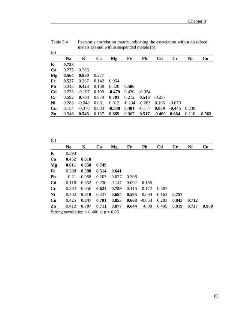
Chapter 3

63

Table 3.4 Pearson’s correlation matrix indicating the association within dissolved

metals (a) and within suspended metals (b) (a)

Na K Ca Mg Fe Pb Cd Cr Ni Cu K 0.733 Ca 0.275 0.386 Mg 0.564 0.850 0.277 Fe 0.527 0.287 0.142 0.054 Pb 0.313 0.423 0.188 0.320 0.586 Cd 0.233 -0.197 0.199 -0.479 0.426 -0.024 Cr 0.592 0.704 0.079 0.701 0.212 0.516 -0.237 Ni 0.283 -0.048 0.081 0.012 -0.234 -0.263 0.105 -0.079 Cu 0.154 -0.370 0.083 -0.588 0.481 -0.117 0.859 -0.445 0.239 Zn 0.346 0.543 0.137 0.669 0.067 0.517 -0.409 0.684 0.110 -0.563 (b)

Na K Ca Mg Fe Pb Cd Cr Ni Cu K 0.393 Ca 0.452 0.618 Mg 0.611 0.658 0.749 Fe 0.388 0.598 0.514 0.641 Pb 0.21 -0.058 0.203 -0.027 -0.306 Cd -0.118 0.352 -0.230 0.147 0.092 0.185 Cr 0.382 0.356 0.624 0.759 0.416 0.172 0.387 Ni 0.402 0.510 0.437 0.694 0.595 0.094 -0.163 0.757 Cu 0.425 0.847 0.701 0.855 0.668 -0.054 0.283 0.843 0.712 Zn 0.412 0.797 0.711 0.877 0.644 -0.08 0.405 0.919 0.737 0.900Strong correlation < 0.400 at p = 0.05

Chapter 3

64

Classification of Sampling Sites HACA performed on the water quality data set to evaluate spatial variation

among sampling sites resulted in grouping of sampling sites into three groups (Fig.

3.4). The sites within each group have similar water quality parameters. These groups

were designated based upon impairment of sites from different pollutants as relatively

unimpaired region (RUR), moderately impaired region (MIR) and impaired region

(IR). Sites 1, 2, 10 and 11 were classified in RUR group. Sites (1 and 2) were located

in upstream of Nullah Aik, whereas, remaining two sites (10 and 11) in upstream of

Nullah Palkhu. Sites grouped in this cluster were categorized with low level of COD,

EC, TDS, PO43-, Cl-, Pb, Cr, Ni and Zn and high level of DO. These sites were located

in upstream of the Sialkot city and were least affected from industrial effluents and

municipal sewage. Sites such as 3, 4, 5, 8, 9, 12, 13, 14, and 18 were grouped in IR

and located close to mid stream of Nullah Aik (3, 4, 5, 8 and 9) and Nullah Palkhu

(12, 13, 14, and 18). This group was regarded as impaired region (IR) of streams,

which exhibited low level of DO and high concentration of COD, EC, TDS, turbidity,

Cl-, S2-, Na, Fe, Pb, Cr, Ni and Zn. These sites received effluents from multiple

pollution sources.

(Dlin

k/D

max

)*10

0 <

40

0

20

40

60

80

100

120

18 9 8 14 5 13 12 4 3 17 16 7 15 6 11 10 2 1

Fig. 3.4 Dendrogram showing different clusters of sampling sites located on

Nullah Aik and Nullah Palkhu.

Impaired Region Moderately Impaired Region

Relatively Unimpaired Region

Chapter 3

65

This group exhibited relatively higher concentrations of the DO and lower

concentrations of COD, EC, TDS, turbidity, PO43-, Cl-, S2-, Na, Fe, Pb, Cr, Ni and Zn

compared to IR. Sites such as 6, 7, 15, 16 and 17 were included in MIR group,

whereas, located far downstream of Nullah Aik (6, 7) and Nullah Palkhu (15, 16 and

17).

Spatial Variations in Surface Water Quality of Nullah Aik and

Nullah Palkhu For spatial variations among different stream zones such as RUR, IR and LIR

defined by HACA. Table 3.5 presents DFs and spatial classification accuracies of

90.9%, 90.4% and 87.6% for standard and forward stepwise and backward stepwise

mode DFA. Backward stepwise mode DFA deleted least significant and discriminated

11 significant variables via; stream flow, stream depth, DO, COD, TDS, NO3-, PO4

3-,

Pb (dis), Cr (dis), Na (sus), and Ni (sus).

Box and whisker plots of significantly important parameters recognized by

backward step mode of spatial DFA are presented in Fig. 3.5. Stream flow gradually

improved from upstream towards downstream i.e. it was minimum in RUR and

maximum in MIR (Fig. 3.5a). Similar to stream flow, stream depth was also

maximum at MIR, whereas, minimum at RUR (Fig. 3.5b). Highest concentration of

DO was found in RUR which declined in IR and gradually increased in MIR (Fig.

3.5c). In contrary to DO, maximum value of COD was measured in IR, whereas,

minimum in RUR (Fig. 3.5d). TDS also exhibited similar spatial pattern (Fig. 3.5e).

In case of NO3-, highest concentration was measured in RUR followed by IR

reaching to its lowest level in MIR (Fig. 3.5f). RUR exhibited lowest concentration of

PO43- and highest concentration in IR (Fig. 3.5g). Lowest concentration of Pb (dis)

was found in RUR, which gradually increased in IR and reached at highest

concentration in MIR (Fig. 3.5h). Cr (dis) exhibited lowest concentration in RUR

followed by highest concentration in IR and decreasing trend was found in MIR (Fig.

3.5i). Minimum concentration of Mg in suspended particulate matter was recorded in

RUR that gradually increased towards IR and attain higher concentration in IR (Fig.

3.5j). Maximum concentration of Ni in suspended particulate matter was recorded in

IR, lowest concentration in RUR (Fig. 3.5k).

Chapter 3

66

Table 3.5 Classification functions for Discriminant Function Analysis of spatial


Standard Mode Forward Step Mode Backward Step Mode

Variable RUR

coefficient MIR

coefficient IR

coefficient RUR

coefficient MIR

coefficient IR

coefficient RUR

coefficient MIR

coefficient IR

coefficient

Stream width 0.668 0.543 0.477 0.636 0.517 0.453 Stream velocity -9.701 -3.714 -4.430 -4.241 -2.095 -0.411 -4.221 1.744 0.747 Stream depth -2.590 -0.459 1.230 -7.403 -1.408 -2.153 -0.630 1.144 2.741 Temperature 3.879 3.519 3.641 2.756 2.427 2.549 pH 53.723 53.748 52.605 50.445 50.526 49.367 45.797 46.112 44.874 DO 8.776 4.697 5.780 6.550 2.481 3.567 6.343 2.946 3.815 COD 0.062 0.067 0.060 0.046 0.050 0.043 0.011 0.016 0.011 E.C. 0.053 0.054 0.053 TDS -0.039 -0.025 -0.032 0.034 0.048 0.040 0.027 0.039 0.033 Salinity 20.011 18.249 20.054 Hardness 0.093 0.102 0.105 Turbidity -0.004 -0.001 -0.002 0.113 0.122 0.125 NO3

- 2.059 1.021 0.867 0.954 -0.062 -0.227 1.415 0.475 0.302 PO4

3- 1.012 0.233 0.330 2.872 2.028 2.110 0.286 -0.298 -0.293 Cl- 0.001 0.000 0.003 0.003 0.003 0.005 S2- -8.210 -6.403 -7.557 -6.989 -5.187 -6.229 Na (dis) 0.271 0.271 0.267 K (dis) 0.136 -0.016 0.032 0.344 0.187 0.239 Ca (dis) 0.074 0.028 0.041 0.090 0.043 0.055 Mg (dis) -0.416 -0.478 -0.422 Fe (dis) -8.479 -9.413 -9.843 -1.632 -1.627 -2.134 Pb (dis) -23.779 -19.640 -15.557 -14.751 -11.010 -7.2467 -5.798 -2.759 -1.196 Cd (dis) 0.565 31.683 47.448 -19.602 -15.650 -16.786 Cr (dis) 35.568 22.262 22.887 36.966 23.890 24.543 19.922 9.236 9.973 Ni (dis) -10.212 -6.328 -5.686 -2.927 1.274 1.861 Cu (dis) 57.323 56.200 44.735 50.880 48.580 38.993 Zn (dis) -49.897 -39.883 -38.945 -46.508 -35.664 -35.075 Na (sus) 0.257 0.279 0.335 0.237 0.255 0.305 K (sus) -0.252 -0.262 -0.280 Ca (sus) -0.017 0.024 0.001 -0.063 -0.023 -0.043 Mg (sus) 0.040 0.062 0.056 0.048 0.068 0.062 0.018 0.049 0.073 Fe (sus) 0.196 0.165 0.208 0.170 0.145 0.186 Pb (sus) 3.173 5.652 4.864 2.951 5.426 4.647 5.925 8.513 7.890 Cd (sus) 58.826 55.296 56.767 99.785 130.72 147.75 Cr (sus) -0.598 -0.497 -0.381 -0.083 -0.009 0.083 Ni (sus) 8.022 7.631 7.695 Cu (sus) 8.460 7.397 6.936 Zn (sus) -2.575 -2.604 -3.104 -3.005 -3.166 -3.745 Constant -322.92 -308.11 -304.09 -281.49 -268.21 -264.36 -52.56 -41.81 -41.52 Class Accuracy 97.917 92.063 82.353 97.917 92.063 84.314 93.750 90.476 76.471 Total Accuracy 90.956 91.473 87.597

RUR (Relatively Unimpaired Region), MIR (Moderately polluted Region), and IR (Impaired Region)

Chapter 3

67

Stream zone

Stre

am fl

ow m

/sec

0.2

0.4

0.6

0.8

1.0

1.2

1.4

1.6

1.8

RUR IR MIR

±Std. Dev.±Std. Err.Mean

(a) Stream zone

Stre

am d

epth

(m)

0.4

0.8

1.2

1.6

2.0

2.4

2.8

3.2

3.6

RUR IR MIR

(b)

Stream zone

DO

mg/

l

0

2

4

6

8

10

RUR IR MIR

(c) Stream zone

CO

D m

g/l

-200

0

200

400

600

800

RUR IR MIR

(d)

Stream zone

TDS

mg/

l

200

300

400

500

600

700

800

900

RUR IR MIR

(e)

Stream zone

NO

3- mg/

l

-0.5

0.5

1.5

2.5

3.5

4.5

5.5

RUR IR MIR

(f)

Streams zone

PO

43- m

g/l

-1

0

1

2

3

4

5

6

RUR IR MIR

(g)

Stream zone

Pb(

dis)

mg/

l

-0.3

-0.1

0.1

0.3

0.5

0.7

RUR IR MIR

(h)

Chapter 3

68

Stream zone

Cr(

dis)

mg/

l

-0.15

-0.05

0.05

0.15

0.25

0.35

0.45

0.55

RUR IR MIR

(i)

Stream zone

Mg

(sus

) mg/

l

5

20

35

50

65

80

RUR IR MIR

(j)

Stream zone

Ni (

sus)

mg/

l

-0.4

0.0

0.4

0.8

1.2

1.6

RUR IR MIR

(k) Fig. 3.5 Box and Whisker plots of some variables (a. stream flow, b. stream

depth, c. DO, d. COD, e. TDS, f. NO3-, g. PO4

3-, h. Pb dis, i. Cr dis, j. Mg sus, and k. Ni sus) separated by spatial Discriminant analysis associated with water quality data of Nullah Aik and Nullah Palkhu.

Chapter 3

69

Temporal Variations in Surface Water Quality of Nullah Aik and Nullah Palkhu

After segregating raw data into four seasonal groups (post monsoon, winter,

pre monsoon and monsoon), DFA was applied for the evaluation of temporal

variations. DFs and classification matrix for temporal variations were obtained from

standard, forward stepwise and backward stepwise of DFA for 38 water quality

variables (Table 3.6). Temporal classification accuracies ranged from 97.9% to 94.7%

for standard, forward stepwise and backward stepwise mode. Backward stepwise DFA

discriminated 13 variables viz; stream flow, temperature, EC, salinity, total hardness,

Na (dis), K (dis), Ca (dis), Mg (dis), Fe (dis), Cd (dis), Cu (dis) and Na (sus) as

significant variables.

Box and whisker plots of variables discriminated using DFA are given in Fig.

3.6. Streams exhibited maximum flow in monsoon season that gradually decreased till

pre monsoon season (Fig. 3.6a). Maximum temperature was found during monsoon

season and lowest in winter (Fig. 3.6b). Highest level of EC was observed in winter

season, which gradually reduced to its lowest level in monsoon season (Fig. 3.6c).

Like EC, Total hardness, salinity and Na also showed similar trend i.e. maximum in

pre monsoon and lowest in monsoon season (Fig. 3.6d, e, f). Highest concentration of

total hardness of stream water was recorded in winter season which decreases during

monsoon season. Concentration of K increases from post monsoon to pre monsoon,

when it reaches to its maximum level (Fig. 3.6g). Lowest concentration of Ca was

recorded in post monsoon, whereas, highest concentration in winter season followed

by pre monsoon and monsoon season (Fig. 3.6h). Highest concentration of Mg was

observed during pre monsoon, whereas lowest in monsoon season (Fig. 3.6i). Fe (dis),

Cd (dis) and Cu (dis) also exhibited seasonal differences, minimum concentrations

were recorded in post monsoon and maximum level during monsoon season (Fig. 3.6j

k & l). Among suspended particulate matter, Na varied significantly between seasons.

Minimum concentration of Na was recorded during monsoon, which increased till

winter when its concentration becomes at highest level (Fig.3.6m).

Table 3.6 Classification functions for discriminent function analysis of temporal variations in water quality data of Nullah Aik and Nullah Palkhu

Seasons

Standard mode Forward stepwise mode Backward stepwise mode Post Monsoon coefficient

Winter coefficient

Spring coefficient

Pre Monsoon coefficient

Post Monsoon coefficient

Winter coefficient

Spring coefficient



Winter coefficient

Spring coefficient


Stream width 0.618 0.871 0.994 0.991 0.549 0.786 0.917 0.929 Stream velocity 4.774 4.294 -0.181 15.161 5.989 5.135 1.073 16.425 4.249 4.841 0.748 11.103 Stream depth 0.998 1.724 1.490 1.323 Temperture 16.918 9.315 15.632 20.953 16.710 9.229 15.472 20.758 14.485 7.627 13.502 17.923 pH 54.212 54.893 54.234 56.852 53.377 53.997 53.316 56.055 DO 3.004 2.869 2.380 1.108 2.975 2.954 2.440 1.049 COD 0.038 0.057 0.053 0.033 0.034 0.051 0.048 0.029 E.C. 0.039 0.025 0.015 0.011 0.041 0.025 0.016 0.013 0.009 0.006 0.005 0.001 TDS -0.010 -0.003 0.012 0.013 -0.013 -0.004 0.010 0.011 Salinity -28.044 10.365 -3.579 -33.907 -28.592 11.317 -3.512 -34.321 -25.558 -2.250 -10.923 -23.813 Hardness 0.142 0.079 0.097 0.111 0.146 0.086 0.103 0.115 0.076 0.042 0.053 0.048 Turbidity -0.008 -0.001 -0.005 -0.007 NO3

- -0.462 1.404 0.389 0.694 -0.877 0.847 -0.083 0.236 PO4

3- -0.307 0.506 0.021 -0.085 -0.465 0.243 -0.212 -0.186 Cl- -0.009 -0.004 -0.008 -0.015 -0.010 -0.004 -0.008 -0.016 S2- 1.058 -4.076 -2.593 5.377 0.536 -4.676 -2.895 4.794 Na (dis) 0.289 0.261 0.370 0.231 0.268 0.231 0.342 0.209 0.069 0.030 0.131 0.036 K (dis) 0.392 0.361 0.423 0.816 0.472 0.426 0.506 0.885 0.175 0.099 0.099 0.538 Ca (dis) -0.086 0.126 0.054 0.041 -0.101 0.104 0.037 0.027 -0.020 0.127 0.067 0.079 Mg (dis) -1.134 -0.697 -0.824 -1.450 -1.174 -0.774 -0.891 -1.485 -0.465 -0.161 -0.257 -0.689 Fe (dis) -2.950 -2.505 -5.021 7.316 -2.175 -1.635 -4.222 8.025 -9.822 -6.556 -9.461 -4.221 Pb (dis) -24.591 -18.057 -18.735 -29.486 -24.601 -19.219 -19.034 -30.010

Continued …

Chapter 3

71

Seasons

Standard mode Forward stepwise mode Backward stepwise mode Post Monsoon coefficient

Winter coefficient

Spring coefficient



Winter coefficient

Spring coefficient



Winter coefficient

Spring coefficient


Cd (dis) 279.089 -19.136 137.604 154.050 343.614 56.249 208.393 215.908 390.341 126.883 275.472 345.717Cr (dis) 9.990 19.691 17.951 6.262 6.190 14.650 13.137 3.488 Ni (dis) 12.487 14.734 19.261 28.491 6.711 6.807 12.116 24.087 Cu (dis) 41.602 78.222 57.838 81.998 43.754 78.157 57.414 85.786 -57.949 -4.415 -34.313 -29.202 Zn (dis) -21.750 -35.185 -27.679 -19.046 Na (sus) 0.364 0.429 0.341 0.467 0.325 0.376 0.294 0.436 K (sus) 0.259 -0.143 0.077 0.335 0.212 -0.148 0.047 0.299 0.450 0.112 0.276 0.500 Ca (sus) -0.061 -0.027 -0.081 -0.073 -0.064 -0.036 -0.087 -0.078 Mg (sus) 0.084 0.082 0.076 0.109 0.111 0.107 0.104 0.136 Fe (sus) 0.254 0.205 0.270 0.235 6.712 7.011 7.900 8.749 Pb (sus) 6.690 7.297 8.073 8.529 Cd (sus) 63.252 56.811 58.677 62.917 Cr (sus) -0.164 -0.402 -0.271 -0.084 Ni (sus) 1.586 8.240 3.079 3.307 0.414 7.002 1.608 2.370 -3.023 3.446 -1.037 -1.355 Cu (sus) 17.088 14.653 15.231 21.451 14.884 10.888 11.795 20.020Zn (sus) -6.331 -5.638 -5.984 -8.663 -5.171 -4.811 -4.760 -7.611 Constant -456.695 -343.30 -435.88 -588.20 -447.45 -333.78 -426.16 -579.54 -180.19 -64.40 -159.97 -274.20 Accuracy (%) 96.774 100.000 98.039 100.000 96.774 100.000 98.039 100.000 96.774 100.000 95.098 100.000 Overall Accuracy (%) 98.708 98.708 97.933

Stre

am fl

ow (m

/sec

)

0.2

0.4

0.6

0.8

1.0

1.2

1.4

1.6

1.8

2.0

PM WN PR MN


S

Tem

pera

ture

(OC

)

10

14

18

22

26

30

34

PM WN PR MN

(a) Seasons (b) Seasons

Season

EC u

S/cm

300

500

700

900

1100

1300

1500

PM WN PR MNTo

tal h

ardn

ess

mg/

l50

100

150

200

250

300

350

400

450

PM WN PR MN (c) Seasons (d) Seasons

Sal

inity

mg/

l

0.05

0.15

0.25

0.35

0.45

0.55

0.65

PM WN PR MN

Na

(dis

) mg/

l

0

20

40

60

80

100

120

140

PM WN PR MN

(e) Seasons (f) Seasons

K (d

is) m

g/l

-6

0

6

12

18

24

30

PM WN PR MN

Ca

(dis

) mg/

l

10

30

50

70

90

110

130

PM WN PR MN

(g) Seasons (h) Seasons

Chapter 3

73

Mg

(dis

) mg/

l

-5

5

15

25

35

45

PM WN PR MN

Fe (d

is) m

g/l

-0.4

0.0

0.4

0.8

1.2

1.6

2.0

PM WN PR MN

(i) Seasons (j) Seasons

Cd

(dis

) mg/

l

-0.02

0.00

0.02

0.04

0.06

0.08

0.10

0.12

PM WN PR MN

Cu

(dis

) mg/

l

-0.04

0.02

0.08

0.14

0.20

0.26

PM WN PR MN

(k) Seasons (l) Seasons

Na

(sus

) mg/

l

-5

5

15

25

35

45

55

PM WN PR MN

(m) Seasons Fig. 3.6 Box and Whisker plots of some variables (a. stream flow, b. temperature, c.

EC, d. Salinity, e. Total hardness, f. Na, g. K, h.Ca, i. Mg, j. Fe dis, k. Cd dis, l. Cu dis, m. Na sus) separated by temporal discriminant analysis associated with water quality data of Nullah Aik and Nullah Palkhu. PM (post monsoon), WN (winter), PR (pre monsoon) and MN (Monsoon)

Chapter 3

74

Principal Component Analysis/ Factor Analysis (PCA/ FA)

PCA/FA was applied separately on raw water quality data matrix for the three

different regions, viz., RUR, IR and MIR identified by HACA to compare the

distribution pattern between water samples to recognize factors that influence water

quality of streams. The Data matrices used for PCA/FA were (38 × 96) for RUR, (38

× 186) for IR, and (38 × 108) for MIR. PCA/FA of the three regions produced 10 VFs

for RUR and IR and nine for MIR with eigenvalues greater than 1 and explained

81.7%, 73.6% and 79.8% of the total variance of water quality variables.

Ten VFs were found significant for RUR (Table 3.7). VF1 explained 19.5% of

total variance and was positively correlated with COD (r = 0.789), Ni (dis; r = 0.808)

and Ni (sus; r = 0.820). This factor represented industrial and municipal source of

pollution. VF2, explained 12.1% of the total variance, showed positive loadings on Zn

(dis; r = 0.789) and Na (sus, r = 0.870) representing the impact of tanneries effluents

and municipal sewage. VF3 was positively correlated with Cd (dis; r = 0.763) and Fe

(sus; r= 841), which contributed 10.7% of the total variance. This factor is related to

non-point source (surface runoff) and parent rock material. VF4 contributed 10.4% of

the total variation which was negatively correlated to turbidity(r = -0.746), Pb (dis; r =

-0.836), Cu (dis; r = - 0.918) and Cd (sus; r = - 0.808). This factor was related to

municipal sewage and urban runoff. VF5 explained 6.4% of total variance, was

negatively correlated to Cu (sus r = -0.760) which indicated the contribution from

municipal waste and surface runoff. VF6 shared 6.1% of the total variance and

negatively correlated to two variables stream width(r = -0.850) and stream depth(r = -

0.884), indicating the importance of stream morphology. VF7 contributed 5.3% of

total variation with negatively correlated to EC (r = - 0 907 and TDS (r = -0.850). This

factor can be related mainly with tanneries and from parent rock material (with lesser

extent). VF8 contributed 4.2% of total variation and showed significant positive

correlation to Cl- (r = 0.839), K (dis; r = 0.780) and Cr (dis; r = 0.767) and was related

to effluents coming from tanneries located in different locations in Sialkot. Presence

of Fe in suspended particulate matter can be associated mainly with parent rock

material. VF9 corresponded to 3.5% of the total explained variance and showed

negative correlation with Mg (dis r = -0.815) contributed by municipal sewage and

surface runoff. VF10, which accounted for 2.7% of total explained variance showed

Chapter 3

75

negative correlation with PO43-(r = -0.806) indicating the origin of PO4

3- is mainly

from municipal waste and also from tanneries effluent with lesser extent.

PCA/FA of IR separated eight significant VFs (Table 3.7). VF1 accounted for

24.01% of total explained variance and was positively correlated with PO43-(r =

0.772), S2-(r = 0.702) and K (dis r = 0.819). This factor can be related with municipal

waste and tanneries effluent. VF2 explained about 8.5% of total variation, negatively

correlated with Cr (dis; r = -0.841), Zn (dis; r = -0.793) and Cd (sus; r = -0.745)

attributed by miscellaneous sources. VF3, shared about 8.1% of total variation and

was positively correlated to Pb (dis; r = 0.841) and Zn (sus; r = 0.737) representing the

contribution of surface run off from roads and urban area. VF4 contributed 7.0% of

the total variations and showed positive correlation with Cr (dis r = 0.743), indicating

their source related with effluents from tanneries. VF5 showed positive correlation

with turbidity (r = 0.813), K (sus; r = 0.819) and Cr (sus; r = 0.764) explained 6.9% of

total variations along this factor may be due to due to load of suspended solid waste

from municipal sewage and tanneries effluents. VF6 was positively correlated to Na

(sus; r = 0.852) explaining 5.7% of total variations. This factor identified tanneries

effluents and municipal waste as major sources. VF7 contributed about 4.1% of total

variance, with positive loadings on EC (r = 0.788) and TDS (r = 0.860) indicating

from tanneries and parent rock material as major contributor. VF8 contributed about

3.8% of total variation showing negative correlation with Cl- (r = -0.714) influenced

from tanneries and municipal waste.

For MIR, FA/PCA segregated nine VFs as significant contributors (Table 3.7).

VF1 correspond to 24.6% of the total explained variance and showed negative

correlation with Pb (dis; r = -0.866) and Cu (dis; r = -0.882). This factor was found

related to non-point sources like surface runoff. VF2 accounted for 14.1% of the total

variance and showed negative correlation with Na (sus; r = -0.875), Mg (sus; r = -

0.820) and Ca (sus; r = -0.827) representing the contribution of parent rock material,

and tanneries effluents. VF3 was responsible for 9.1% of the total variance with

positive correlation with turbidity(r = 0.917), and Cr (sus; r = 0.921) indicating the

contribution of tanneries effluents. EC(r = 0.832) and TDS(r = 0.882) were positively

correlated with VF4, which accounted for 7.2% of the total variance associated with

untreated tanneries effluents and parent rock material. VF5 corresponds to 6.6% of the

total explained variance and showed positive correlation with Mg (dis; r = 0.876).

Chapter 3

76

This factor explained the load of Mg coming from municipal sewage and agricultural

runoff. VF6 accounted for 3.9% and showed positive correlation Ca (dis; r = 0.776),

Mg (sus; r = 0.815) and Cd (sus; r = 0.745) exhibiting the contribution of surface

runoff and parent rock material. No variable was found strongly correlated with VF7,

which is accounted for 3.9% of the total explained variance. VF8 corresponds to 3.5%

of the total explained variance and showed negative with stream width (r = -0.721)

and positive with stream depth (r = 0.778). This factor is influenced by stream

morphology. VF9, which accounts for 3.0% of the total explained variance showing

negative correlation with NO3- (r = 0.756) indicating the origin of this factor from

agricultural runoff.

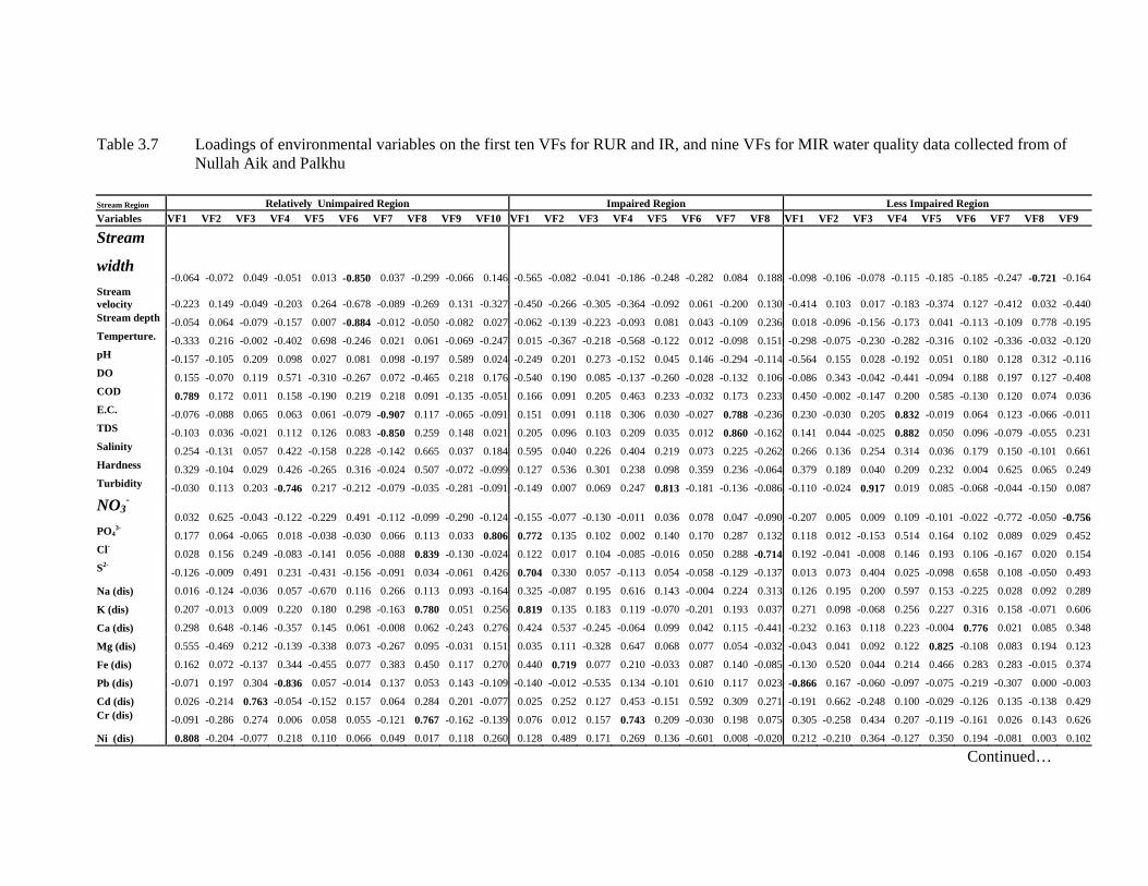
Table 3.7 Loadings of environmental variables on the first ten VFs for RUR and IR, and nine VFs for MIR water quality data collected from of Nullah Aik and Palkhu

Stream Region Relatively Unimpaired Region Impaired Region Less Impaired Region Variables VF1 VF2 VF3 VF4 VF5 VF6 VF7 VF8 VF9 VF10 VF1 VF2 VF3 VF4 VF5 VF6 VF7 VF8 VF1 VF2 VF3 VF4 VF5 VF6 VF7 VF8 VF9

Stream

width -0.064 -0.072 0.049 -0.051 0.013 -0.850 0.037 -0.299 -0.066 0.146 -0.565 -0.082 -0.041 -0.186 -0.248 -0.282 0.084 0.188 -0.098 -0.106 -0.078 -0.115 -0.185 -0.185 -0.247 -0.721 -0.164

Stream velocity -0.223 0.149 -0.049 -0.203 0.264 -0.678 -0.089 -0.269 0.131 -0.327 -0.450 -0.266 -0.305 -0.364 -0.092 0.061 -0.200 0.130 -0.414 0.103 0.017 -0.183 -0.374 0.127 -0.412 0.032 -0.440 Stream depth -0.054 0.064 -0.079 -0.157 0.007 -0.884 -0.012 -0.050 -0.082 0.027 -0.062 -0.139 -0.223 -0.093 0.081 0.043 -0.109 0.236 0.018 -0.096 -0.156 -0.173 0.041 -0.113 -0.109 0.778 -0.195 Temperture. -0.333 0.216 -0.002 -0.402 0.698 -0.246 0.021 0.061 -0.069 -0.247 0.015 -0.367 -0.218 -0.568 -0.122 0.012 -0.098 0.151 -0.298 -0.075 -0.230 -0.282 -0.316 0.102 -0.336 -0.032 -0.120 pH -0.157 -0.105 0.209 0.098 0.027 0.081 0.098 -0.197 0.589 0.024 -0.249 0.201 0.273 -0.152 0.045 0.146 -0.294 -0.114 -0.564 0.155 0.028 -0.192 0.051 0.180 0.128 0.312 -0.116 DO 0.155 -0.070 0.119 0.571 -0.310 -0.267 0.072 -0.465 0.218 0.176 -0.540 0.190 0.085 -0.137 -0.260 -0.028 -0.132 0.106 -0.086 0.343 -0.042 -0.441 -0.094 0.188 0.197 0.127 -0.408 COD 0.789 0.172 0.011 0.158 -0.190 0.219 0.218 0.091 -0.135 -0.051 0.166 0.091 0.205 0.463 0.233 -0.032 0.173 0.233 0.450 -0.002 -0.147 0.200 0.585 -0.130 0.120 0.074 0.036 E.C. -0.076 -0.088 0.065 0.063 0.061 -0.079 -0.907 0.117 -0.065 -0.091 0.151 0.091 0.118 0.306 0.030 -0.027 0.788 -0.236 0.230 -0.030 0.205 0.832 -0.019 0.064 0.123 -0.066 -0.011 TDS -0.103 0.036 -0.021 0.112 0.126 0.083 -0.850 0.259 0.148 0.021 0.205 0.096 0.103 0.209 0.035 0.012 0.860 -0.162 0.141 0.044 -0.025 0.882 0.050 0.096 -0.079 -0.055 0.231 Salinity 0.254 -0.131 0.057 0.422 -0.158 0.228 -0.142 0.665 0.037 0.184 0.595 0.040 0.226 0.404 0.219 0.073 0.225 -0.262 0.266 0.136 0.254 0.314 0.036 0.179 0.150 -0.101 0.661 Hardness 0.329 -0.104 0.029 0.426 -0.265 0.316 -0.024 0.507 -0.072 -0.099 0.127 0.536 0.301 0.238 0.098 0.359 0.236 -0.064 0.379 0.189 0.040 0.209 0.232 0.004 0.625 0.065 0.249 Turbidity -0.030 0.113 0.203 -0.746 0.217 -0.212 -0.079 -0.035 -0.281 -0.091 -0.149 0.007 0.069 0.247 0.813 -0.181 -0.136 -0.086 -0.110 -0.024 0.917 0.019 0.085 -0.068 -0.044 -0.150 0.087

NO3-

0.032 0.625 -0.043 -0.122 -0.229 0.491 -0.112 -0.099 -0.290 -0.124 -0.155 -0.077 -0.130 -0.011 0.036 0.078 0.047 -0.090 -0.207 0.005 0.009 0.109 -0.101 -0.022 -0.772 -0.050 -0.756 PO4

3- 0.177 0.064 -0.065 0.018 -0.038 -0.030 0.066 0.113 0.033 0.806 0.772 0.135 0.102 0.002 0.140 0.170 0.287 0.132 0.118 0.012 -0.153 0.514 0.164 0.102 0.089 0.029 0.452 Cl- 0.028 0.156 0.249 -0.083 -0.141 0.056 -0.088 0.839 -0.130 -0.024 0.122 0.017 0.104 -0.085 -0.016 0.050 0.288 -0.714 0.192 -0.041 -0.008 0.146 0.193 0.106 -0.167 0.020 0.154 S2- -0.126 -0.009 0.491 0.231 -0.431 -0.156 -0.091 0.034 -0.061 0.426 0.704 0.330 0.057 -0.113 0.054 -0.058 -0.129 -0.137 0.013 0.073 0.404 0.025 -0.098 0.658 0.108 -0.050 0.493

Na (dis) 0.016 -0.124 -0.036 0.057 -0.670 0.116 0.266 0.113 0.093 -0.164 0.325 -0.087 0.195 0.616 0.143 -0.004 0.224 0.313 0.126 0.195 0.200 0.597 0.153 -0.225 0.028 0.092 0.289

K (dis) 0.207 -0.013 0.009 0.220 0.180 0.298 -0.163 0.780 0.051 0.256 0.819 0.135 0.183 0.119 -0.070 -0.201 0.193 0.037 0.271 0.098 -0.068 0.256 0.227 0.316 0.158 -0.071 0.606

Ca (dis) 0.298 0.648 -0.146 -0.357 0.145 0.061 -0.008 0.062 -0.243 0.276 0.424 0.537 -0.245 -0.064 0.099 0.042 0.115 -0.441 -0.232 0.163 0.118 0.223 -0.004 0.776 0.021 0.085 0.348

Mg (dis) 0.555 -0.469 0.212 -0.139 -0.338 0.073 -0.267 0.095 -0.031 0.151 0.035 0.111 -0.328 0.647 0.068 0.077 0.054 -0.032 -0.043 0.041 0.092 0.122 0.825 -0.108 0.083 0.194 0.123

Fe (dis) 0.162 0.072 -0.137 0.344 -0.455 0.077 0.383 0.450 0.117 0.270 0.440 0.719 0.077 0.210 -0.033 0.087 0.140 -0.085 -0.130 0.520 0.044 0.214 0.466 0.283 0.283 -0.015 0.374

Pb (dis) -0.071 0.197 0.304 -0.836 0.057 -0.014 0.137 0.053 0.143 -0.109 -0.140 -0.012 -0.535 0.134 -0.101 0.610 0.117 0.023 -0.866 0.167 -0.060 -0.097 -0.075 -0.219 -0.307 0.000 -0.003

Cd (dis) 0.026 -0.214 0.763 -0.054 -0.152 0.157 0.064 0.284 0.201 -0.077 0.025 0.252 0.127 0.453 -0.151 0.592 0.309 0.271 -0.191 0.662 -0.248 0.100 -0.029 -0.126 0.135 -0.138 0.429 Cr (dis) -0.091 -0.286 0.274 0.006 0.058 0.055 -0.121 0.767 -0.162 -0.139 0.076 0.012 0.157 0.743 0.209 -0.030 0.198 0.075 0.305 -0.258 0.434 0.207 -0.119 -0.161 0.026 0.143 0.626

Ni (dis) 0.808 -0.204 -0.077 0.218 0.110 0.066 0.049 0.017 0.118 0.260 0.128 0.489 0.171 0.269 0.136 -0.601 0.008 -0.020 0.212 -0.210 0.364 -0.127 0.350 0.194 -0.081 0.003 0.102

Continued…

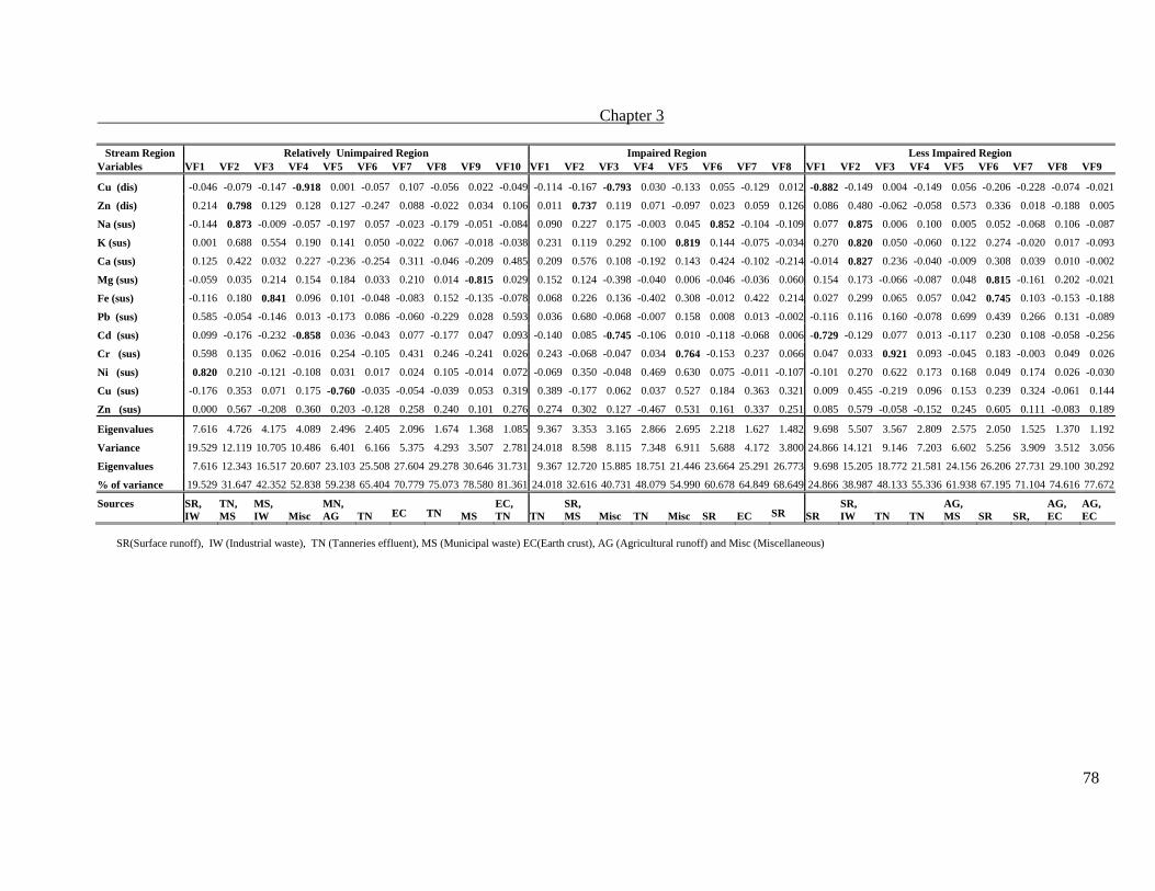
Chapter 3

78

Stream Region Relatively Unimpaired Region Impaired Region Less Impaired Region Variables VF1 VF2 VF3 VF4 VF5 VF6 VF7 VF8 VF9 VF10 VF1 VF2 VF3 VF4 VF5 VF6 VF7 VF8 VF1 VF2 VF3 VF4 VF5 VF6 VF7 VF8 VF9

Cu (dis) -0.046 -0.079 -0.147 -0.918 0.001 -0.057 0.107 -0.056 0.022 -0.049 -0.114 -0.167 -0.793 0.030 -0.133 0.055 -0.129 0.012 -0.882 -0.149 0.004 -0.149 0.056 -0.206 -0.228 -0.074 -0.021

Zn (dis) 0.214 0.798 0.129 0.128 0.127 -0.247 0.088 -0.022 0.034 0.106 0.011 0.737 0.119 0.071 -0.097 0.023 0.059 0.126 0.086 0.480 -0.062 -0.058 0.573 0.336 0.018 -0.188 0.005

Na (sus) -0.144 0.873 -0.009 -0.057 -0.197 0.057 -0.023 -0.179 -0.051 -0.084 0.090 0.227 0.175 -0.003 0.045 0.852 -0.104 -0.109 0.077 0.875 0.006 0.100 0.005 0.052 -0.068 0.106 -0.087

K (sus) 0.001 0.688 0.554 0.190 0.141 0.050 -0.022 0.067 -0.018 -0.038 0.231 0.119 0.292 0.100 0.819 0.144 -0.075 -0.034 0.270 0.820 0.050 -0.060 0.122 0.274 -0.020 0.017 -0.093

Ca (sus) 0.125 0.422 0.032 0.227 -0.236 -0.254 0.311 -0.046 -0.209 0.485 0.209 0.576 0.108 -0.192 0.143 0.424 -0.102 -0.214 -0.014 0.827 0.236 -0.040 -0.009 0.308 0.039 0.010 -0.002

Mg (sus) -0.059 0.035 0.214 0.154 0.184 0.033 0.210 0.014 -0.815 0.029 0.152 0.124 -0.398 -0.040 0.006 -0.046 -0.036 0.060 0.154 0.173 -0.066 -0.087 0.048 0.815 -0.161 0.202 -0.021

Fe (sus) -0.116 0.180 0.841 0.096 0.101 -0.048 -0.083 0.152 -0.135 -0.078 0.068 0.226 0.136 -0.402 0.308 -0.012 0.422 0.214 0.027 0.299 0.065 0.057 0.042 0.745 0.103 -0.153 -0.188

Pb (sus) 0.585 -0.054 -0.146 0.013 -0.173 0.086 -0.060 -0.229 0.028 0.593 0.036 0.680 -0.068 -0.007 0.158 0.008 0.013 -0.002 -0.116 0.116 0.160 -0.078 0.699 0.439 0.266 0.131 -0.089

Cd (sus) 0.099 -0.176 -0.232 -0.858 0.036 -0.043 0.077 -0.177 0.047 0.093 -0.140 0.085 -0.745 -0.106 0.010 -0.118 -0.068 0.006 -0.729 -0.129 0.077 0.013 -0.117 0.230 0.108 -0.058 -0.256

Cr (sus) 0.598 0.135 0.062 -0.016 0.254 -0.105 0.431 0.246 -0.241 0.026 0.243 -0.068 -0.047 0.034 0.764 -0.153 0.237 0.066 0.047 0.033 0.921 0.093 -0.045 0.183 -0.003 0.049 0.026

Ni (sus) 0.820 0.210 -0.121 -0.108 0.031 0.017 0.024 0.105 -0.014 0.072 -0.069 0.350 -0.048 0.469 0.630 0.075 -0.011 -0.107 -0.101 0.270 0.622 0.173 0.168 0.049 0.174 0.026 -0.030

Cu (sus) -0.176 0.353 0.071 0.175 -0.760 -0.035 -0.054 -0.039 0.053 0.319 0.389 -0.177 0.062 0.037 0.527 0.184 0.363 0.321 0.009 0.455 -0.219 0.096 0.153 0.239 0.324 -0.061 0.144

Zn (sus) 0.000 0.567 -0.208 0.360 0.203 -0.128 0.258 0.240 0.101 0.276 0.274 0.302 0.127 -0.467 0.531 0.161 0.337 0.251 0.085 0.579 -0.058 -0.152 0.245 0.605 0.111 -0.083 0.189

Eigenvalues 7.616 4.726 4.175 4.089 2.496 2.405 2.096 1.674 1.368 1.085 9.367 3.353 3.165 2.866 2.695 2.218 1.627 1.482 9.698 5.507 3.567 2.809 2.575 2.050 1.525 1.370 1.192

Variance 19.529 12.119 10.705 10.486 6.401 6.166 5.375 4.293 3.507 2.781 24.018 8.598 8.115 7.348 6.911 5.688 4.172 3.800 24.866 14.121 9.146 7.203 6.602 5.256 3.909 3.512 3.056

Eigenvalues 7.616 12.343 16.517 20.607 23.103 25.508 27.604 29.278 30.646 31.731 9.367 12.720 15.885 18.751 21.446 23.664 25.291 26.773 9.698 15.205 18.772 21.581 24.156 26.206 27.731 29.100 30.292

% of variance 19.529 31.647 42.352 52.838 59.238 65.404 70.779 75.073 78.580 81.361 24.018 32.616 40.731 48.079 54.990 60.678 64.849 68.649 24.866 38.987 48.133 55.336 61.938 67.195 71.104 74.616 77.672

Sources

SR, IW

TN, MS

MS, IW Misc

MN, AG TN

EC

TN MS

EC, TN TN

SR, MS Misc TN Misc SR EC

SR SR

SR, IW TN TN

AG, MS SR SR,

AG, EC

AG, EC

SR(Surface runoff), IW (Industrial waste), TN (Tanneries effluent), MS (Municipal waste) EC(Earth crust), AG (Agricultural runoff) and Misc (Miscellaneous)

Discussion

Spatial Variations in Surface Water Quality

The spatial and temporal variations in streams water quality are highly

influenced by natural and anthropogenic activities (Sullivan & Drever, 2001; De Carlo

et al, 2005). Anthropogenic activities in the catchment area of any stream highly

degrade the stream water quality. This process of degradation becomes severe in

streams traversing from densely populated and industrial areas (Paul & Meyer, 2001).

Nullah Aik and Nullah Palkhu are facing severe degradation from anthropogenic

activities in the catchment area. The water quality was relatively better in upstream of

Nullah Aik and Nullah Palkhu lies within 15 kilometres above the Sialkot city. The

upstream segment was least impacted from point sources receive pollutants from

agricultural runoff. Water quality of mid stream and downstream segments was

degraded as streams passes through Sialkot city, where they receive pollutants from

multiple point sources. Water quality at mid stream sites was highly degraded, which

improve as it flows towards far downstream due to sedimentation and dilution factors.

Less variations in water quality parameters were observed in RUR, whereas,

more variations exhibited by MIR and IR. In RUR, variations in water quality

parameters were resulted from seasonal variations in stream discharge and parent rock

material in IR. Effluents load from point sources decreased in MIR that reduced the

variations within water quality parameters. Most of the point sources are concentrated

in IR that drains effluents in streams. The sites in IR were located in downstream of

Sialkot city, which receive effluents and raw sewage throughout the year.

Spatial variations in water quality were due to stream flow, depth, DO, COD,

TDS, NO3-, PO4

3-, Pb (dis), Cr (dis), Mg (sus) and Ni (sus). Stream flow showed an

increasing trend from RUR to MIR. Qadir et al. (2008) reported that stream water

flow and discharge plays a vital role in determination of pollutants load. Stream depth

varies from site to site. Maximum stream depth was observed at site 7(Wain) located

in MIR due to construction of small headworks, which control and divert the stream

water for irrigation purposes.

The results showed that high concentration of DO in RUR (6.3mg/L), low

concentration at IR(1.97mg/L), which gradually increased in LIR(3.63mg/L). The

concentration of DO in IR and LIR were below the standard limits of fresh water

organisms like fishes (5.0 - 9.0mg/L) described by CEC (1978). The concentration of

Chapter 3

80

DO of present study were below the DO(7.4mg/L) as reported by Sharma & Ghosh

(1987) and above the concentration (0.51mg/L) in Hudiara drain (Khan et al., 2003).

Low concentration of DO in IR is associated with the direct discharge of untreated

industrial effluents and municipal sewage from Sialkot and Sambrial towns situated

along the Nullah Aik and Nullah Palkhu. Municipal sewage and industrial effluents

contain organic substances, which are biodegradable, require a large amount of

oxygen for oxidation process by micro-organisms and causes depletion of DO. In

aquatic systems, excessive organic and inorganic input (from industrial and urban

waste) may reduce the availability of DO. Recommended concentration of DO is 4.0

mg/L for fishes, however, most species are distressed when it falls between 2.0 - 4.0

mg/L. Low level of DO (less than 2.0 mg/L) can cause fish mortality (McNeil &

Closs, 2007).

Municipal sewage and industrial effluents decrease DO level and increase

COD level in stream water (Singh et al., 2005a). Lowest level of COD was recorded

in RUR (38.02 mg/L) and highest in IR (90.01 mg/L). High level of COD may be due

to the discharge of high volume of untreated industrial and municipal effluents into

streams. Khan et al. (2003) and Singh et al. (2005a) observed similar trend in COD

values in Hudiara drain (Pakistan) and Gomti River (India). The level of COD was

higher in IR, where its level exceeded the permissible level (50mg/L) of effluent

discharge in fresh water (UNEP, 2004). The COD level in present study was higher to

those reported by Singh et al. (2005a) and lower to those of Khan et al. (2003).

Similarly, high concentration of TDS was recorded in IR (585.1 mg/L), which

was below the permissible level (500mg/L) described by USEPA (1998), whereas,

concentration of TDS in RUR(418.9mg/L) and LIR ( 486.8 mg/L) were below the

permissible level. The level of TDS was high as compared to the concentration of

TDS recorded by PCRWR (2004) and Singh et al., (2005a), however, below TDS

values recorded by Khan et al. (2003). High values of TDS can be resulted due to

effluent containing higher concentration of soluble salts related with natural and

anthropogenic sources. Stream system of Nullah Aik and Nullah Palkhu receives

effluents from tanneries, which contain higher concentration of sodium chloride,

which affects the freshwater aquatic life, when its concentration becomes high.

Highest concentration of NO3- (2.19mg/L) was measured in RUR, which can

be associated with agricultural activities in the catchment area. Elevated concentration

Chapter 3

81

of NO3- comes from agricultural fields after surface runoff. Yang et al. (2004) and

Morrison et al. (2001) also reported similar reason of high level of NO3- in stream

water. The level of NO3- was reported in the present study was higher to those in

River Chenab (PCRWR, 2004) and Gomti River, India (Singh et al., 2005a).

Concentration of NO3- in stream water of Nullah Aik and Nullah Palkhu was also

higher than concentration (0.05 - 0.2mg/L) reported by Chapman (1996) for natural

stream water.

In contrast, highest level of PO43- was observed in IR (2.78mg/L) and lowest

in RUR (1.02mg/L). Municipal sewage was identified as the possible source of PO43-.

The elevated concentration of PO43- is due to human impacts on streams and may be

associated with direct discharge of raw sewage (Singh et al., 2005a). Higher level of

PO43- may also occur as a consequence of the use of detergents (Perona et al., 1999;

Sundaray et al., 2006). Debels et al. (2005) reported higher level of PO43- in

downstream sites as compared to upstream sites of Chillan River and municipal

sewage being blamed as its source. The level of PO43- concentration (2.19mg/L) in

surface water was higher than the concentration (0.002 - 0.025mg/L) measured in

pristine streams (Chapman et al., 1996). Higher concentration of PO43- was also

reported in River Chenab (0.3mg/L; PCRWR, 2004), River Ganga (0.21mg/L; Sharma

& Ghosh, 1987) and River Gomti (0.1 - 10mg/L). Higher concentrations of PO43- and

NO3- may cause eutrophication in streams and lakes (Morrison et al., 2001).

Pb in dissolved form was recorded maximum in MIR (0.812mg/L) and lowest

at RUR (0.141mg/L). Pb concentration increases from upstream towards downstream

sites. Atmospheric deposition in urban areas and surface runoff can be main sources of

Pb in stream water. During heavy rainfall, Pb on soil surface becomes dissolved,

which makes its way into the stream (Hurst et al., 1996; Sutherland et al., 2003).

Manufacturing processes (battery plants), paints and pigments, incineration of

municipal solid wastes and hazardous wastes are the other sources of Pb (FDA, 1993).

Pb comes from automobile exhaust and deposited on soil form atmosphere especially

near major highways (FDA, 1993; Tomazelli et al., 2003). Concentration of Pb in

water of Nullah Aik and Nullah Palkhu exceeded the permissible limits (0.01mg/L)

for freshwater (Chapman, 1996). In present study, high concentration of Pb was

compared to the studies of Khan et al. (2003), Singh et al. (2004) and Tariq et al.

Chapter 3

82

(1996), whereas, its concentrations were lower to those reported by Javed (1999) and

Khan et al. (2003).

High concentration of Cr measured in present study is mainly related with

effluents from tanneries and electroplating industries discharged into streams, which

may accumulated in sediment with higher concentrations (Nriagu & Nieboere, 1988).

Maximum concentration of Cr was recorded from those sites, which were close to the

Sialkot city. The results showed high level of Cr (dis) were recorded in IR

(0.196mg/L) and MIR (0.145mg/L), which can be attributed to heavy load of

contaminants from tanneries. Cr concentration in IR and MIR was above the

permissible limit (0.05mg/L) described by CEC (1978) and USEPA (1993). Large

volume of effluents is produced during tanning process, which contain high

concentration of chromium and soluble salts such as NaCl (Moten & Sami, 2000).

Indiscriminate use of Cr salts in tanneries is one of the main source of its increase

level in drains and streams of Sialkot. Cr is mainly found in industrial waste from the

chrome tanning process, about 70% of the total amount is taken up by the hides and

about 30% remains unabsorbed, which goes into the effluent and sludge. Continuous

discharges of Cr, even in low concentrations, have been reported to have toxic effects

on aquatic life and can disrupt the food chain in aquatic ecosystems (Bosnic et al.,

2000). High pH allows Cr to convert into complex substances and become part of

suspended particulate matter, which settles down as effluents travels the distance from

the source. Significantly higher concentration of Cr (0.196mg/L) was observed in IR

region. Higher concentration of Cr in sediment is toxic for aquatic organisms in

general and particularly for bottom dweller organisms. Cr concentration in studied

streams was higher than the permissible level (0.022mg/L) for freshwater described by

Wright & Welbourn, (2002). Similarly, concentration of present study was above to

those reported by Tariq et al. (1996), Javed (1999), Khan et al. (2003) and Abbas et

al. (2004).

The distribution of Mg in suspended particulate matter depicted an increasing

trend from upstream to downstream. The origin of Mg is from both natural and

anthropogenic activities. Relatively high concentrations of Mg in moderately impaired

sites may indicate the effect of human activities in the catchment area. Tzankov et al.

(2007) reported that higher concentration of Mg in stream water is strongly influenced

by weathering of parent materials.

Chapter 3

83

Ni is relatively less toxic to organism in comparison to other metals and

toxicity of Ni can be masked by other metals in aquatic environment (Kszos et al.,

1992; Wright & Welbourn, 2002). Ni is mainly used for alloy formation and metal

plating. Industrial effluent and municipal waste are the main sources that increases

level of Ni in stream water (Ntengwe & Maseka, 2006). Highest level of Ni in

suspended particulate matter was found in IR that can be as result of discharge of

municipal sewage and industrial effluents that contain waste from electroplating units,

where surgical instruments are manufactured. In alkaline pH, dissolved Ni metal

reacts with suspended particulate and organic matter that settles down in streambed.

The concentration of Ni decreases with an increase of distance from the source

(Wright & Welbourn, 2002). Sometimes, Ni deposited at remote sites from its sources

indicating that its source may be resulted from atmospheric deposition (Sarkar, 2002).

Concentrations of Ni recorded from all sampling zones were recorded within safe

limits (0.065mg/L) as described for freshwater by Chapman (1996). During present

study, concentration of Ni was recorded higher than the concentrations of Ni reported

by Tariq et al. (1996), Abbas et al. (2004) and Singh et al. (2005a). In contrary to

results of present study, Javed (1999) studied higher concentrations of Ni (0.8mg/L) in

River Ravi.

Temporal Variations in Surface Water Quality

The results highlight temporal variability of various pollutants. Pollutants from

non-point sources exhibited maximum concentration during monsoon season due to

surface runoff and pollutants from point sources showed highest concentration when

the stream flow reduced to its minimum level. In present study, stream flow,

temperature, EC, salinity, total hardness, Na (dis), K (dis), Ca (dis), Mg (dis), Fe (dis),

Cd (dis), Cu (dis) and Na( sus) showed marked seasonal variations. Distinct seasonal

variations in concentration of pollutants may be due to fluctuation in the stream

discharge level. During monsoon season, due to high discharge level the effect of

effluent becomes diluted, whereas, in winter and early summer, studied streams

experiences extreme low discharge level. The amount of effluents remains same

throughout the year in the catchment area and pollutants concentration is generally

higher during low stream flow. Similar results were obtained by Tsai et al. (2003).

Maximum stream discharge level was observed in monsoon season and minimum

discharge level was observed during winter and pre monsoon seasons (Fig. 3.7).

Chapter 3

84

During monsoon season, the catchment area receives major share of rainfalls. High

discharge level of streams during heavy rains causes local flooding (Plate. 3.1a & b).

This may result in dilution of toxic chemicals like heavy metals coming from point

sources, whereas, the concentration of metals coming from non-point sources

(atmospheric deposition, urban and agricultural runoff) increases in stream water

during rainy season. During dry season, heavy metals deposits on the soil surface

through atmospheric deposition and flushed away by surface runoff into streams

during rainy season. There is a strong relationship between stream flow and rainfall in

their catchment area. Low stream flow prevails in pre monsoon season (early summer)

that recovered rapidly in monsoon season (mid June - mid September). During winter

season, occasional rainfall may increases stream flow. About 80% of rainfalls occur

during monsoon season when streams flow at their full swing. During early monsoon

rains, fast flowing water erodes the contaminated sediments deposited in stream bed

and transported to River Chenab. Floodwater also carries a huge volume of non

degradable solid (plastic bottles, polythene bags and packing material) ultimately

discharged into River Chenab (Plate. 3.2a & b).

The results indicated marked seasonal variations in EC, which was recorded

high in winter (915.8µS/cm) and pre monsoon (974.5µS/cm) and lowest (622.5µS/cm)

in monsoon season. High values of EC can be due to high discharge of soluble salts

along with tanneries effluents. Stream system of Nullah Aik and Nullah Palkhu

receive effluents from tanneries, which contain higher concentration of sodium

chloride, which in turn affects freshwater aquatic life. EC value of present study was

relatively higher to those reported in different regional studies, such as, Khan et al.

(2003), Singh et al. (2005a) and PCRWR (2004).

Salinity and hardness affects the availability of metals to organism (Wright &

Welbourn, 2002). At high level of salinity trace metals present in dissolved form react

with suspended particulate matter and become insoluble, which settle down in

sediments. In natural stream, presence of soluble salts indicates that salts originate

from parent rock material in catchment area (Crosa et al., 2006). The results showed

that maximum salinity was recorded in pre monsoon (0.43mg/L) and minimum in

monsoon season (0.16mg/L). High stream discharge level reduce the level of salinity

in stream water thus, the temporal variations in salinity can be associated with high

quantity of soluble salts used in tanneries, which are discharged into streams.

Chapter 3

85

Plate 3.1a An overview of site 2 showing the reduced stream flow during pre

monsoon season, 2005.

Plate 3.1b An overview of site 2 showing the highest stream discharge (35,000Cs)

during monsoon season, 2005.

Chapter 3

86

Plate 3.2a. The stream water turn into black after erosion of deposited sediments at

stream bed during early monsoon season

Plate 3.2b. The stream water return to its normal colour during monsoon season after

heavy rainfall in the catchment area

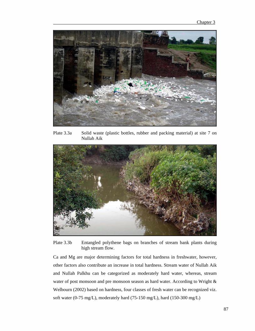
Chapter 3

87

Plate 3.3a Solid waste (plastic bottles, rubber and packing material) at site 7 on

Nullah Aik

Plate 3.3b Entangled polythene bags on branches of stream bank plants during

high stream flow. Ca and Mg are major determining factors for total hardness in freshwater, however,

other factors also contribute an increase in total hardness. Stream water of Nullah Aik

and Nullah Palkhu can be categorized as moderately hard water, whereas, stream

water of post monsoon and pre monsoon season as hard water. According to Wright &

Welbourn (2002) based on hardness, four classes of fresh water can be recognized viz.

soft water (0-75 mg/L), moderately hard (75-150 mg/L), hard (150-300 mg/L)

Chapter 3

88

and very hard (above 300 mg/L). The results depicted that maximum total hardness

was recorded in winter when the stream flow become low and effluents coming from

tanneries containing higher concentration of calcium salts discharge into streams.

Lowest values of total hardness were recorded in monsoon season, when streams flow

at full swing and dilute Ca level in water. Main natural sources of Ca are gypsum,

pyroxenes, calcite, dolomite, and clay minerals (Nanda, 2005). Generally, Ca content

of natural waters is less than 100 mg/L. Parent rock material contains higher level of

Ca in catchment area, which gets dissolved after weathering (Marofi & Maryanaji,

2007; Girija et al., 2007). In pristine water, concentration of Ca ranged between 0.06

to 210 mg/L (Chapman, 1996). PCRWR (2004) reported mean concentration of Ca

(30mg/L) in water samples collected from River Chenab. Highest level of Mg

(23.74mg/L) was recorded during winter, whereas, lowest concentration (6.959mg/L)

was recorded during monsoon season. In natural running water, concentration of Mg

ranged from 0.05 to 80mg/L (Chapman, 1996). The concentration of Mg recorded

during present study was within the range of natural waters (0.05 to 80mg/L). The

concentration of Mg was recorded in present study was higher to those of River

Chenab (12.0 mg/L; PCRWR 2004).

Concentration of K increases from post monsoon (6.903mg/L) to pre monsoon

(12.714mg/L), however, stream samples showed a slight decline during monsoon

season (10.715mg/L), probably due to dilution factor. The concentration of K was

higher to those reported by Chapman (1996) for natural streams. Possible source of K

are from human activities (municipal sewage and agricultural sources) and natural

input (Girija et al., 2007). Na has natural sources, but it is also be enriched by

anthropogenic processes. The concentration of Na was higher than K and is related

with TDS. Na and K are essential elements play vital role in various physiological

processes in organisms. Minimum concentration of Na (24.89mg/L) was recorded

during monsoon and maximum (91.49mg/L) during pre monsoon. Higher

concentration can be attributed by the use of NaCl in tanning activities and other

human uses. NaCl is used for hide and skin preservation process. Tanning industry in

Sialkot produces considerable quantities of salts, which may result in higher

concentration of Na in drinking water. Increased salt content in groundwater,

especially in areas of high industrial density has been reported to cause environmental

hazard (Bosnic et al., 2000). Concentration of Na measured in present study was

Chapter 3

89

lower to those reported by Chapman (1996). Similarly, the concentration of Na was

below the permissible level (200mg/L) and (150mg/L) as described by CEC (1978)

and USEPA (1993) for drinking purposes.

Maximum concentration of dissolved Fe (1.018mg/L) was recorded during

monsoon season, which is higher than the permissible value (0.3mg/L) for fresh water

(Wright & Welbourn, 2002). Similarly, Taboada-Castro et al. (2002) also reported

higher dissolved Fe content when stream flow was highest. This also support that

inflow of Fe in dissolved form can be as a result of its remobilisation from earth crust

in streams. Boman et al. (2002) stated that possible reason of higher concentration of

Fe in stream water can be linked to its geological origin. Alther (1981) also described

that presence of Fe in stream water is related to parent rock material. Fe may be

originated with either organic or inorganic wastewater generated from municipal and

industrial activities in the study area; however, major share of Fe comes from natural

sources. Fe concentration measured in present study was higher to those reported in

River Indus (Tariq et al., 1996) and lower to those of Gomti and Ravi rivers (Singh et

al., 2004; Javed (1999).

Mean concentration of Cd was very low at most of the sites but maximum

concentration was recorded during monsoon. The possible sources of Cd are

atmospheric deposition, surface runoff, electroplating industries, solid waste disposal

and the use of fertilizers (He & Singh, 1994; Jonsson et al., 2002). Highest mean

concentration of Cd (0.06mg/L) was recorded in monsoon season, which was above

the standards for drinking water as described by CEC (1978), USEPA (1993) and

WHO (1993) Similarly, Cd concentration was also above the permissible level of

freshwaters water (0.002mg/L) and for aquatic life (0.017mg/L) as described by

Wright & Welbourn (2002).

Like Cd, highest mean concentration of dissolved Cu (0.116mg/L) was also

recorded during monsoon season, which was higher than the threshold values for

surface water (0.043mg/L) and aquatic life (0.056mg/L). The major pathway of Cu in

stream water is from non-point sources (urban and agricultural runoff and atmospheric

deposition). Stream water is a main vector for Cu transportation to soil, ground water

and biota. Cu is less toxic in hard water whereas it has significant toxic effect in soft

water (Nriagu, 1980). Fish and crustaceans are susceptible to copper toxicity as

compared to birds and mammals (Wright & Welbourn, 2002). During present study,

Chapter 3

90

higher level of dissolved Fe, Cu and Cd were recorded in monsoon when water

discharge level becomes high. Kimball et al. (1995) studied increased concentration

of colloidal iron, copper, and lead loads during high flow, likely resulting from re-

suspension of iron colloids settled onto bed sediments.

Conclusions Water quality of Nullah Aik and Nullah Palkhu is highly impaired due to

unwise and wide spread human activities in the catchment area. The anthropogenic

activities have converted pristine condition of studied stream into fragile and

unacceptable state. On the basis of spatial classification, three groups of sites were

identified. First group (RUR) showed comparatively good water quality, second group

of sites (IR) indicated highest level of stream degradation and third group (MIR)

showed water quality was comparatively less degraded. Spatial and seasonal

variations were observed in water quality parameters. Multivariate techniques

discriminated the most influencing factors and identified their possible sources. DFA

identified 11 water quality parameters viz., stream flow, stream depth, DO, COD,

TDS, NO3-, PO4

3-, Pb (dis), Cr (dis), Mg (sus), and Ni (sus), which showed significant

variations along spatial gradient. Seasonal variations were recorded due to stream

flow, temperature, EC, salinity, total hardness, Na (dis), K (dis), Ca (dis), Mg (dis), Fe

(dis), Cd (dis), Cu (dis) and Na (sus). Main factors that bring changes in chemical

composition of water are either related to anthropogenic and/or natural factors. Point

sources such as industrial, tanneries, municipal sewage and non-point sources

(atmospheric deposition, urban and agricultural runoff) were identified the most

important factors. However, concentration of some contaminants such as Ca, Mg and

Fe were due to the contribution of parent rock material and related to geo-chemical

processes. The results of present study also showed parameters such as COD, TDS,

NO3- Fe, Pb, Cd, Cr and Cu exceeded the permissible level for fresh water, aquatic

life, irrigation and domestics use. Present study highlighted the spatio-temporal

variations in water quality of Nullah Aik and Nullah Palkhu caused due to

anthropogenic activities. The statistical techniques used in present study pointed out

the factors responsible for degradation of water quality. These results will help the

environmental managers to develop restoration activities with minimum operational

cost and expenditures.

Chapter 4

Bioaccumulation of Heavy Metals in Selected Fishes of


Introduction Higher level of pollutants had severe impact directly/ indirectly on the health

of an aquatic ecosystem. Aquatic organisms respond to changes in their environment,

which in turn reflect the prevailing health status of aquatic ecosystem (Kotze et al.,

1999). Heavy metals are important group of toxic pollutants (Amin, 1996), which are

chemicals of great concern (Qadir et al., 2008). Heavy metal pollution has gained

serious attention from public and scientific community in relation with their toxicity

to aquatic organisms and ultimate affect on well being of humans (Yayıntas et al.,

2007). Continuous release of heavy metals from point and non-point sources is putting

the aquatic ecosystem under stress (Dural et al., 2006). Heavy metals e.g. iron,

copper, chromium and zinc are essential for regulation of metabolic activities but

become toxic at higher concentrations, whereas, lead and cadmium have no

documented role in living organism (Canli & Atli, 2003). Essential and non-essential

metal at higher concentration can disrupt metabolic and physiological activities of

aquatic organisms (Batley, 1983). Essential metals also become toxic if their

concentration exceeds the permissible level (Wright & Welbourn, 2002).

Fishes are most important organisms in the aquatic food chain, which are

sensitive to heavy metals contamination (Pickering & Pottinger, 1995). Most of the

freshwater fishes are confined to specific microhabitat within inter connected river/

stream system. If such system becomes contaminated by heavy metals, fish species

either shift to less polluted segment of river/stream system or die off which ultimately

disturb the food chains (Rashed, 2001). High level of heavy metals has apparent lethal

and chronic effects on fishes (Kotze et al., 1999). Thus, fish not only indicates the

pollution status of aquatic ecosystem but have significant impact on the food web

(Qiao-qiao et al., 2007). It is one of the main source of protein-enriched food all over

the world (Mansour & Sidky, 2002). Consumption of contaminated fish with heavy

metals can result hazardous effects on human health (Mai et al., 2006).

Chapter 4

92

Various pathways of metal accumulation in fish include such as ingestion of

food, suspended particulate matter, metal ion exchange through gills and skin (Liang

et al., 1999; Wright & Welbourn, 2002). Nussey et al. (2000) also identified five

routes through which heavy metals enter into fish viz; food, suspended particle, gills,

intake of water and integuments. From these pathways, metals get absorbed into blood

and transported to various organs for either storage or excretion. Level of trace metals

in different organs of fish is used as an index of metal pollution in an ecosystem,

which is considered as an important tool to highlight the role of elevated level of

metals in aquatic organisms (Tarrio et al., 1991; Mendil et al., 2005). Concentration

of heavy metals in different tissues/organs of fishes is directly influenced by

contamination in aquatic environment, uptake, regulation and elimination inside the

fish body (Bervoets et al., 2001). Liver stores either heavy metals or excretes through

bile. Other routes of heavy metal regulation are either kidneys or gills (Heath, 1991;

Nussey et al., 2000). Accumulation of metals in various organs and tissues depends

upon the way of exposure such as through diet or their elevated level in surrounding

environment (Pourang, 1995, Nussey et al., 2000; Alam et al., 2002). Morphological

and behavioural abnormalities such as alteration in sensory reception, reduced

responses to normal olfactory function (feeding, mating, selection, or homing),

reduction in swimming performance, gills purge, ventilation, coughs, learning

impairment, loss of equilibrium that lapsed into paralysis, loss of reproductive

efficiency and irregular metamorphosis appeared as symptom of toxic exposure of

trace metals (Atchison et al., 1987). Concentration of metals becomes toxic to the fish

when its level exceeds the permissible level (Langston, 1990). This threshold limit not

only varies from metal to metal but also from one species to another (Langston, 1990;

Kalay & Canli, 2000). Toxic effects of metals become more pronounced when various

metabolic activities inside organism body fail to detoxify (Nussey et al., 2000).

Heavy metals exhibit different accumulation pattern in organs (Jezierska &

Witeska, 2007). Gills, liver and kidneys accumulate heavy metals in higher

concentration in comparison to muscles, which exhibit lowest levels of metals

accumulation (Jezierska & Witeska, 2007). Among different organs, liver

accumulates higher concentrations of metals comparatively and has been used widely

to investigate the process of bioaccumulation. Kidneys also play a vital role in

excretion of trace metal ions (Langston et al., 1998). Exchange of gases and

Chapter 4

93

absorption of heavy metals takes place from external aquatic to internal body

environment through gills (Wepener et al., 2001).

The concentration of heavy metals in fish is highly influenced by spatial and

seasonal variations, which are directly related to metal contents in different organs

(Farkas et al., 2002). The concentration of heavy metals in different fish species have

been studied on spatial and seasonal basis (Nussey et al., 2000; Avenant-Oldewage &

Marx, 2000). Besser et al. (2007) documented spatial and temporal variations in

heavy metal concentration in stream biota from mining areas, Viburnum, United

States. Tawari-Fufeyin & Ekaye (2007) highlighted metal pollution in different

segments of river Ikpoba River, Nigeria. Kojadinovic et al. (2007) studied

comparative concentration of heavy metal among different fishes. Bajc et al. (2005)

investigated distribution of heavy metals with in fish body and differences in heavy

metals accumulation among different fish species. Agarwal et al. (2007) studied

heavy metal accumulation pattern in wild fishes of Gomti River. However, no

systematic study has been conducted on spatial and temporal variations of heavy

metal contents in different fish species in Nullah Aik and Nullah Palkhu. Due to lack

of information about the bioaccumulation pattern of heavy metals in different fish

species, there is a dire need to investigate the deleterious effect of heavy metal on

local fish fauna. The focus of this chapter is to provide baseline information about

heavy metal contents (Fe, Pb, Cd, Cr, Ni, Cu and Zn) in eight species to regulate the

aquatic ecosystem for restoration and management.

The main objectives are:

• to highlight spatial, seasonal and specific variations of heavy metals in different

organs of selected eight fishes.

• to evaluate trends of heavy metal accumulation in fish species and compare with

international guidelines for human consumption.

Chapter 4

94


The details of fish sampling and metal analysis in fish organs are given in

Chapter 2. The bioaccumulation of heavy metals was studied in eight fish species

collected from upstream and downstream of Nullah Aik and Nullah Palkhu. All

samples of fish were collected on seasonal basis (post and pre monsoon) from 18 sites

located at Nullah Aik and Nullah Palkhu commencing from September, 2004 and

culminate at April, 2006. Out of 18 sampling sites, fish was recorded from only 14

sites and no fish was found from sites (3, 4, 12, and 14). Site 13 was also deleted

because only one specimen of Channa punctata was captured from this site. Sites with

no fish catch were located in close proximities of Sialkot city and were named as mid-

stream sites (Fig 4.1). The sites from where fishes were grouped into four zones.

1. Upstream of Nullah Aik (1and 2 site)

2. Upstream of Nullah Palkhu (10 and 11site)

3. Downstream of Nullah Aik (5, 6, 7, 8 and 9 site)

4. Downstream of Nullah Palkhu (15, 16, 17 and 18 site)

Statistical analysis

The basic statistics such as mean, standard deviation (SD) and range of heavy

metal concentration in fishes of Nullah Aik and Nullah Palkhu was calculated using

Microsoft Excel. Two-way analysis of variance ANOVA was used to indicate the

statistically significant differences in mean metal concentration between organs,

sampling zones, and species (Pourang, 1995; Besser et al., 2007).

Chapter 4

95

Fig. 4.1 Map of study area showing sampling sites located on Nullah Aik and

Nullah Palkhu; tributaries of River Chenab, Pakistan.

Downstream sites located at Nullah Aik

Downstream sites located at Nullah Palkhu

Upstream sites located at Nullah Aik

Fish species

Chapter 4

96

Results A total of eight fish species (Channa punctata, Cirrhinus reba, Labeo rohita,

Heteropneustes fossilis, Mystus cavasius, Oreochromis niloticus, Puntius sophore and

Wallago attu) were selected to highlight spatio-temporal variations in heavy metal

concentrations among different organs (gills, liver, kidneys and muscles). Mean

concentrations and standard deviations of metals (Fe, Pb, Cd, Cr, Ni, Cu and Zn) in

gills, kidneys, liver and muscles of fish from four sampling zones during post

monsoon and pre monsoon seasons are given in Table 4.1 a & b. Metals such as Fe,

Pb, Cd, Cr, Ni, Cu and Zn were statistically significant in four organs (gills, liver,

kidneys and muscles) between fish species. Similarly, significant spatial differences

were found in accumulation of Cr and Pb. Mean concentration of Fe, Cd, Cr and Cu

were also significantly different between two seasons (Table. 4.2).

Bioaccumulation of Heavy Metals

Iron

Significant seasonal and inter-specific variations in bioaccumulation of Fe

were found, whereas, non-significant spatial differences were found between

upstream and downstream (Table. 4.2). Highest accumulation of Fe was recorded

during pre monsoon and minimum in post monsoon. Maximum Fe accumulation was

recorded in Wallago attu, followed by Mystus cavasius and minimum concentration in

Labeo rohita (Fig. 4.2). Maximum mean concentration of Fe was analyzed in liver

and minimum mean concentration in muscles. The general trend of mean Fe

concentration in different organs of eight species was: liver > gills > kidneys >

muscles (Fig. 4.3a). Maximum mean Fe concentration (566.720 ± 30.376µg/g) was

recorded in liver of Wallago attu captured at downstream of Nullah Aik and minimum

(109.866 ± 86.149) in Oreochromis niloticus from same stream segment. In gills,

maximum mean Fe concentration (320.456 ± 57.362µg/g) was recorded of Puntius

sophore sampled from upstream of Nullah Aik and minimum (53.065 ± 46.058µg/g)

in Labeo rohita from downstream of Nullah Aik. Kidneys showed higher mean

concentration (249.007 ± 27.494µg/g) in Heteropneustes fossilis captured from

downstream of Nullah Palkhu, whereas, lowest mean concentration was measured in

Labeo rohita from downstream of Nullah Aik. Maximum mean Fe concentration

Chapter 4

97

(92.152 ± 22.399µg/g) in muscles was observed in Channa punctata from

downstream of Nullah Aik and minimum (24.421 ± 14.699µg/g) in Labeo rohita

sampled from downstream of Nullah Palkhu (Fig 4.2a).

During pre monsoon, maximum mean Fe (372.715 ± 55.331µg/g) was

accumulated in liver of Wallago attu captured from upstream of Nullah Aik followed

by Channa punctata (509.206 ± 41.827µg/g) collected from downstream of Nullah

Aik and minimum was recorded in liver (277.268 ± 36.824µg/g) of Labeo rohita

collected from upstream of Nullah Aik. Mean concentration of Fe in gills (370.215 ±

21.361µg/g) and kidneys (372.715 ± 55.331µg/g) maximum in Wallago attu was

observed in case of liver but minimum mean Fe contents were observed in gills

(130.808 ± 28.888µg/g) and kidneys (88.999 ± 68.293µg/g) of Cirrhinus reba

collected from upstream of Nullah Aik. Maximum mean Fe concentration (118.947 ±

45.122µg/g) in muscles were observed in Mystus cavasius while minimum

concentration (49.464 ± 52.862µg/g) was observed in Labeo rohita sampled from

upstream of Nullah Aik.

Chapter 4

98

Table 4.1a Means ± standard deviation of heavy metals (µg/g) in different organs of eight fish species sampled from four sampling zones located at Nullah Aik and Nullah Palkhu during post monsoon seasons (September, 2004 – April, 2006)

Species Zone Organ Fe Pb Cd Cr Ni Cu Zn Channa

punctata

1 gills 206.050 ± 33.703 12.356 ± 3.148 4.665 ± 0.588 6.328 ± 5.221 4.678 ± 0.933 2.149 ± 1.256 38.287 ± 16.926

Kidneys 186.280 ± 18.322 8.715 ± 2.114 4.085 ± 0.759 3.464 ± 2.144 5.027 ± 1.941 1.703 ± 0.776 33.358 ± 16.143

Liver 338.196 ± 46.844 11.575 ± 2.170 3.509 ± 0.898 6.649 ± 4.765 4.874 ± 1.950 5.955 ± 2.323 41.484 ± 17.411

Muscles 66.875 ± 35.733 1.719 ± 2.402 1.612 ± 1.131 2.160 ± 2.171 1.489 ± 0.588 0.406 ± 0.041 11.361 ± 3.322

2 gills 122.868 ± 48.426 11.878 ± 1.322 3.504 ± 0.607 4.312 ± 1.807 5.212 ± 0.358 3.162 ± 1.710 16.133 ± 10.750

kidneys 122.934 ± 28.201 5.323 ± 1.618 4.373 ± 0.254 3.762 ± 2.337 5.075 ± 2.648 2.457 ± 1.351 29.189 ± 12.389

Liver 214.874 ± 28.495 9.314 ± 2.205 4.453 ± 1.084 5.243 ± 1.218 3.937 ± 1.403 4.041 ± 1.563 43.844 ± 11.305

Muscles 51.367 ± 35.966 1.527 ± 2.019 1.112 ± .101 1.205 ± 0.957 1.253 ± 0.140 0.715 ± 0.146 14.659 ± 5.006

3 gills 202.740 ± 33.782 15.146 ± 2.719 4.093 ± 1.381 10.840 ± 3.467 6.926 ± 1.197 2.650 ± 1.122 47.633 ± 11.247

Kidneys 161.920 ± 28.674 7.153 ± 2.056 3.465 ± 0.564 5.794 ± 1.732 5.566 ± 4.014 2.254 ± 0.258 24.288 ± 8.864

Liver 377.373 ± 22.485 16.927 ± 2.162 4.366 ± 0.857 9.079 ± 1.295 5.365 ± 2.184 5.901 ± 1.382 39.541 ± 11.870

Muscles 92.152 ± 22.400 2.299 ± 2.285 1.509 ± 0.187 2.015 ± 0.559 1.596 ± 0.811 1.382 ± 0.149 19.554 ± 4.456

4 gills 189.785 ± 23.786 17.224 ± 3.061 3.833 ± 0.797 9.737 ± 4.006 6.852 ± 3.225 3.283 ± 1.991 36.414 ± 15.003

Kidneys 133.590 ± 16.021 9.273 ± 2.106 3.699 ± 1.620 8.979 ± 5.194 6.411 ± 2.101 2.828 ± 1.882 27.851 ± 13.924

Liver 227.225 ± 27.113 13.909 ± 2.233 4.697 ± 1.235 9.695 ± 2.896 6.539 ± 2.180 5.762 ± 2.014 31.883 ± 17.046

Muscles 64.062 ± 29.217 1.855 ± 2.387 1.480 ± 0.727 2.054 ± 1.200 1.473 ± 1.156 1.531 ± 0.389 15.796 ± 4.295

Cirrhinus reba

1 gills 108.128 ± 27.430 8.027 ± 4.478 5.101 ± 1.732 4.574 ± 3.296 4.452 ± 2.286 3.976 ± 1.910 22.331 ± 15.354

Kidneys 122.044 ± 22.642 6.181 ± 1.887 5.400 ± 1.558 4.310 ± 2.499 4.492 ± 2.455 6.080 ± 1.705 19.393 ± 13.738

Liver 171.076 ± 25.331 7.944 ± 2.491 5.650 ± 1.102 5.685 ± 2.262 3.507 ± 1.857 6.103 ± 2.225 34.080 ± 21.298

Muscles 68.444 ± 18.001 1.043 ± 1.045 2.093 ± 1.036 1.786 ± 0.869 0.909 ± 0.703 0.520 ± 0.496 13.691 ± 4.545

2 gills 146.467 ± 33.178 10.748 ± 1.632 5.286 ± 1.150 5.062 ± 2.606 9.815 ± 1.135 7.292 ± 4.043 23.707 ± 13.900

kidneys 136.867 ± 13.685 6.404 ± 1.694 5.412 ± 0.705 7.826 ± 8.146 9.323 ± 7.819 6.608 ± 1.301 16.166 ± 12.734

Liver 146.818 ± 29.816 9.350 ± 2.140 5.548 ± 0.742 7.268 ± 1.486 8.651 ± 2.169 8.344 ± 1.940 35.080 ± 18.442

Muscles 81.570 ± 17.452 1.633 ± 1.034 1.807 ± 0.180 3.187 ± 2.465 2.090 ± 1.213 1.018 ± 0.746 14.780 ± 2.565

4 gills 128.859 ± 39.284 11.687 ± 2.127 3.751 ± 0.286 5.427 ± 1.201 9.458 ± 0.329 7.154 ± 2.025 27.718 ± 10.597

Kidneys 169.117 ± 36.438 7.871 ± 1.371 5.439 ± 0.207 9.135 ± 1.012 8.819 ± 1.292 8.813 ± 2.037 18.600 ± 10.537

Liver 185.918 ± 46.714 10.960 ± 2.116 5.549 ± 0.615 2.918 ± 0.636 6.226 ± 2.233 9.197 ± 1.015 39.489 ± 10.278

Muscles 53.809 ± 33.046 3.105 ± 2.024 1.683 ± 0.127 1.830 ± 0.970 2.033 ± 0.186 1.527 ± 0.023 5.994 ± 3.173

Labeo rohita

1 gills 119.126 ± 50.819 14.602 ± 3.124 4.395 ± 1.741 6.234 ± 3.973 7.269 ± 1.436 5.199 ± 2.064 36.181 ± 17.391

Kidneys 83.924 ± 29.564 10.273 ± 4.386 3.223 ± 4.139 4.601 ± 6.967 6.946 ± 1.621 4.725 ± 1.951 32.352 ± 18.527

Liver 197.203 ± 36.117 7.473 ± 2.283 4.151 ± 1.500 6.215 ± 3.247 6.283 ± 3.938 9.874 ± 3.166 44.558 ± 17.974

Muscles 27.354 ± 16.327 3.738 ± 2.844 1.535 ± 1.821 3.659 ± 1.174 1.803 ± 1.594 1.306 ± 0.665 15.493 ± 6.196

3 gills 53.065 ± 46.058 15.062 ± 3.742 4.925 ± 0.186 22.036 ± 10.83 10.957 ± 1.376 8.169 ± 1.171 34.684 ± 11.001

Kidneys 75.845 ± 48.655 6.042 ± 1.228 2.199 ± 0.249 11.311 ± 1.728 9.994 ± 3.456 5.763 ± 1.276 41.455 ± 11.674

Liver 274.083 ± 8.454 8.611 ± 2.115 3.998 ± 0.610 16.757 ± 1.267 8.040 ± 0.376 12.183 ± 1.171 47.986 ± 10.893

Muscles 44.649 ± 23.768 4.353 ± 2.013 0.890 ± 0.069 3.639 ± 0.413 2.005 ± 0.117 1.854 ± 0.076 18.346 ± 7.395

4 gills 59.809 ± 41.547 11.615 ± 2.864 4.180 ± 1.648 15.517 ± 6.122 9.713 ± 1.249 7.746 ± 2.011 22.947 ± 10.321

Kidneys 93.523 ± 48.389 9.328 ± 1.034 4.896 ± 0.721 17.458 ± 1.935 8.622 ± 1.065 8.052 ± 3.030 32.903 ± 11.742

Liver 286.305 ± 13.202 9.117 ± 2.122 4.214 ± 0.647 17.822 ± 3.663 7.828 ± 3.090 12.081 ± 0.008 42.302 ± 10.881

Muscles 24.421 ± 14.699 3.338 ± 2.005 0.771 ± 0.027 3.604 ± 0.530 2.242 ± 1.214 1.479 ± 0.010 15.709 ± 4.328

Heteropneustes

fossilis

3 gills 124.842 ± 19.591 12.877 ± 2.293 2.837 ± 0.281 22.073 ± 6.368 7.934 ± 0.781 3.074 ± 1.351 29.089 ± 10.298

Kidneys 198.622 ± 21.328 7.647 ± 1.248 2.059 ± 0.261 8.619 ± 1.276 6.809 ± 2.516 3.696 ± 1.020 14.559 ± 10.419

Liver 223.295 ± 34.770 12.389 ± 2.077 3.146 ± 0.408 21.112 ± 1.747 5.577 ± 1.557 4.490 ± 1.006 35.085 ± 10.312

Muscles 38.492 ± 19.965 2.026 ± 2.343 0.308 ± 0.051 2.798 ± 0.214 1.573 ± 0.244 0.593 ± 0.016 6.343 ± 3.509

4 gills 198.690 ± 29.492 12.552 ± 1.884 2.960 ± 0.286 24.511 ± 7.386 6.687 ± 2.172 5.061 ± 5.082 27.785 ± 13.768

Kidneys 249.007 ± 27.494 10.038 ± 2.754 2.125 ± 0.331 7.013 ± 2.297 5.365 ± 3.032 3.114 ± 1.481 25.161 ± 14.917

Liver 358.440 ± 29.707 11.911 ± 2.268 1.968 ± 1.422 19.824 ± 3.971 5.699 ± 4.381 5.077 ± 1.471 36.916 ± 14.786

Muscles 75.534 ± 23.856 1.523 ± 2.063 0.640 ± 0.585 2.363 ± 3.646 1.515 ± 0.411 0.998 ± 0.206 11.218 ± 5.136

Mystus

cavasius

1 gills 236.519 ± 88.126 7.350 ± 2.705 5.303 ± 1.571 6.610 ± 1.901 4.658 ± 2.212 3.119 ± 2.005 28.744 ± 19.832

Kidneys 225.973 ± 36.501 10.368 ± 2.631 5.540 ± 1.157 5.740 ± 4.356 4.494 ± 2.163 4.009 ± 2.887 32.194 ± 17.738

Chapter 4

99

Liver 382.010 ± 27.173 8.918 ± 2.699 5.914 ± 1.702 4.698 ± 2.568 5.200 ± 1.477 3.835 ± 2.196 40.988 ± 11.884

Muscles 45.153 ± 67.773 1.926 ± 2.635 1.515 ± 0.716 1.260 ± 1.353 1.238 ± 3.760 1.130 ± 0.132 10.526 ± 3.568

Table 4.1a Continue … Species Zone Organ Fe Pb Cd Cr Ni Cu Zn Mystus

cavasius 2 gills 263.521 ± 49.888 6.561 ± 2.304 6.017 ± 0.538 7.618 ± 3.853 6.063 ± 1.689 2.451 ± 1.303 27.861 ± 12.609

kidneys 187.851 ± 27.430 6.024 ± 2.058 6.783 ± 1.124 5.703 ± 3.053 5.779 ± 1.412 3.381 ± 2.383 35.574 ± 13.648

Liver 362.318 ± 33.212 6.104 ± 2.079 5.434 ± 0.419 7.076 ± 2.382 4.818 ± 1.376 5.629 ± 2.126 43.159 ± 16.276

Muscles 27.353 ± 22.548 1.593 ± 2.024 1.396 ± 0.127 1.093 ± 0.390 1.231 ± 0.403 1.064 ± 0.162 8.096 ± 3.560

Mystus

cavasius

4 gills 218.660 ± 37.683 7.095 ± 1.749 3.983 ± 0.403 17.650 ± 4.005 6.633 ± 1.886 4.050 ± 1.388 45.851 ± 23.787

Kidneys 208.084 ± 38.045 7.165 ± 2.197 3.382 ± 0.491 16.000 ± 4.017 6.438 ± 2.594 3.274 ± 1.026 48.793 ± 16.550

Liver 459.230 ± 42.528 10.874 ± 2.085 13.137 ± 0.449 13.590 ± 6.099 5.179 ± 2.397 6.255 ± 0.241 60.389 ± 14.743

Muscles 42.094 ± 39.607 2.223 ± 2.406 2.799 ± 0.383 5.553 ± 1.669 1.532 ± 1.074 1.436 ± .177 9.397 ± 3.735

Oreochromis

niloticus

1 gills 184.787 ± 16.139 9.558 ± 1.847 4.651 ± 1.556 3.449 ± 2.934 5.281 ± 1.299 3.299 ± 3.423 23.310 ± 13.227

Kidneys 126.989 ± 33.997 6.860 ± 2.675 5.019 ± 0.928 2.813 ± 2.046 4.407 ± 1.954 3.294 ± 0.946 20.302 ± 13.046

Liver 449.212 ± 65.412 10.594 ± 2.108 4.520 ± 0.572 2.681 ± 2.640 3.715 ± 1.426 5.104 ± 5.523 36.876 ± 15.053

Muscles 55.559 ± 10.338 3.122 ± 2.640 1.567 ± 0.739 1.415 ± 1.344 1.556 ± 1.527 0.556 ± 0.103 8.579 ± 1.683

2 gills 180.774 ± 40.651 8.872 ± 3.164 4.703 ± 0.371 14.257 ± 4.324 7.226 ± 1.448 3.783 ± 4.360 16.819 ± 23.734

Kidneys 138.617 ± 46.894 6.794 ± 2.338 5.162 ± 1.791 2.531 ± 1.749 6.219 ± 2.959 3.940 ± 1.579 16.582 ± 18.491

Liver 482.107 ± 65.588 9.849 ± 2.306 4.819 ± 1.622 3.551 ± 2.306 4.056 ± 1.563 6.232 ± 4.758 61.206 ± 13.630

Muscles 59.413 ± 20.617 3.480 ± 3.072 1.100 ± 0.382 1.770 ± 0.986 1.453 ± 2.009 1.436 ± 3.031 11.414 ± 15.287

3 gills 179.856 ± 3.010 13.911 ± 1.148 6.851 ± 0.509 5.038 ± 3.769 7.842 ± 1.567 3.242 ± 1.005 15.658 ± 10.327

Kidneys 177.621 ± 50.812 7.431 ± 2.076 5.333 ± 0.403 3.664 ± 1.419 6.664 ± 3.101 4.391 ± 1.006 10.116 ± 10.142

Liver 109.866 ± 86.149 14.905 ± 2.039 5.460 ± 0.207 5.048 ± 1.774 5.201 ± 1.659 4.349 ± 0.002 53.060 ± 10.371

Muscles 56.631 ± 81.261 2.384 ± 2.018 2.569 ± 0.095 1.619 ± 0.122 2.194 ± 1.033 1.256 ± 0.007 9.461 ± 1.390

4 gills 140.852 ± 65.907 13.220 ± 1.747 6.173 ± 1.039 8.931 ± 2.419 7.942 ± 2.302 4.591 ± 1.429 22.272 ± 9.464

Kidneys 195.709 ± 20.090 8.497 ± 2.655 5.273 ± 0.819 4.170 ± 1.776 7.476 ± 2.455 5.019 ± 2.223 17.369 ± 11.505

Liver 206.221 ± 33.932 14.260 ± 2.192 5.774 ± 1.015 3.965 ± 0.946 6.267 ± 2.123 5.789 ± 1.511 33.361 ± 11.621

Muscles 52.528 ± 135.142 3.664 ± 2.028 1.506 ± 0.146 1.843 ± 0.714 1.977 ± 1.128 1.425 ± 0.138 10.177 ± 6.733

Puntius

sophore

1 gills 320.457 ± 57.362 18.997 ± 1.858 3.021 ± 0.347 6.093 ± 5.197 6.863 ± 1.785 7.456 ± 7.718 20.366 ± 16.796

Kidneys 180.438 ± 22.085 12.342 ± 2.273 2.735 ± 1.444 8.508 ± 3.170 5.445 ± 1.929 5.669 ± 1.372 23.175 ± 14.895

Liver 249.323 ± 26.569 14.843 ± 2.282 3.168 ± 1.495 5.293 ± 1.459 5.320 ± 1.712 10.262 ± 1.613 59.953 ± 15.263

Muscles 41.077 ± 21.086 2.743 ± 4.441 3.605 ± 6.435 2.985 ± 1.628 1.401 ± 0.490 1.048 ± 0.300 9.450 ± 4.640

2 gills 108.67 ± 104.900 8.577 ± 2.089 2.501 ± 1.580 5.490 ± 3.729 7.790 ± 3.854 8.586 ± 6.591 13.251 ± 3.427

kidneys 154.728 ± 20.628 12.766 ± 2.057 2.868 ± 0.299 5.548 ± 1.510 7.292 ± 1.371 6.679 ± 3.845 24.294 ± 16.480

Liver 248.742 ± 24.955 15.096 ± 3.120 4.586 ± 0.933 6.897 ± 6.622 6.452 ± 2.984 11.860 ± 3.704 57.986 ± 15.745

Muscles 36.462 ± 31.202 4.560 ± 2.526 1.473 ± 0.135 1.709 ± 1.697 1.398 ± 0.529 1.319 ± 0.081 15.627 ± 7.297

3 gills 256.409 ± 62.014 15.255 ± 1.574 2.600 ± 0.338 11.329 ± 2.406 9.261 ± 1.551 5.987 ± 1.290 12.690 ± 4.664

Kidneys 153.853 ± 23.185 8.386 ± 2.086 5.066 ± 0.456 14.203 ± 3.034 7.536 ± 1.993 6.755 ± 2.034 23.320 ± 10.679

Liver 346.898 ± 40.023 14.540 ± 2.057 2.053 ± 0.302 11.100 ± 1.809 7.679 ± 0.993 14.828 ± 2.162 67.123 ± 11.036

Muscles 53.939 ± 27.209 4.044 ± 2.030 1.828 ± 0.160 2.646 ± 0.098 1.581 ± 0.237 1.419 ± 0.012 15.534 ± 5.925

4 gills 162.934 ± 63.975 13.960 ± 1.619 4.410 ± 0.415 4.025 ± 1.569 10.185 ± 3.059 6.529 ± 1.875 18.780 ± 6.129

Kidneys 187.763 ± 25.530 6.577 ± 2.117 5.365 ± 0.622 3.281 ± 0.832 9.187 ± 2.079 6.450 ± 2.148 17.280 ± 11.368

Liver 373.609 ± 21.251 12.872 ± 2.063 4.053 ± 0.336 4.361 ± 1.844 7.707 ± 3.929 14.150 ± 2.012 46.559 ± 11.371

Muscles 42.254 ± 25.323 3.808 ± 2.360 1.206 ± 0.143 1.855 ± 0.525 1.773 ± 0.452 1.087 ± 0.111 11.642 ± 7.738

Wallago attu

1 gills 124.360 ± 50.393 15.655 ± 2.410 4.395 ± 1.818 12.700 ± 3.706 4.719 ± 1.265 0.824 ± 0.123 28.143 ± 10.201

Kidneys 130.604 ± 41.751 11.050 ± 3.130 4.492 ± 5.989 7.596 ± 3.204 4.551 ± 2.459 0.813 ± 0.105 29.596 ± 15.513

Liver 336.637 ± 32.230 16.003 ± 3.479 3.635 ± 2.339 13.689 ± 6.568 4.446 ± 1.411 0.944 ± 0.073 65.427 ± 29.669

Muscles 43.297 ± 36.069 2.470 ± 3.032 2.221 ± 1.970 1.977 ± 1.321 1.689 ± 0.645 0.471 ± 0.071 16.969 ± 4.494

3 gills 168.200 ± 42.077 20.596 ± 1.503 4.932 ± 0.551 31.274 ± 6.289 7.746 ± 3.278 2.284 ± 0.363 30.537 ± 15.960

Kidneys 159.214 ± 28.242 15.789 ± 2.079 4.020 ± 0.416 23.180 ± 8.740 5.008 ± 1.996 1.582 ± 0.335 27.141 ± 13.736

Liver 566.721 ± 30.377 18.734 ± 2.096 4.561 ± 0.506 25.716 ± 8.942 5.944 ± 1.164 2.675 ± 0.185 52.847 ± 12.447

Muscles 56.090 ± 14.050 4.053 ± 2.064 1.841 ± 0.339 5.173 ± 1.589 1.179 ± 0.305 0.959 ± 0.149 11.934 ± 4.180

4 gills 133.598 ± 42.628 12.411 ± 1.490 2.622 ± 1.794 14.022 ± 3.074 6.715 ± 2.270 1.234 ± 0.718 30.638 ± 17.848

Kidneys 136.948 ± 29.224 10.386 ± 2.158 5.409 ± 0.837 5.389 ± 3.360 6.679 ± 6.715 1.531 ± 0.115 42.512 ± 16.694

Chapter 4

100

Liver 335.899 ± 26.193 16.917 ± 2.149 5.589 ± 0.790 20.988 ± 4.065 6.210 ± 1.467 1.147 ± 0.265 51.774 ± 28.766

Muscles 59.494 ± 24.968 3.784 ± 2.708 1.377 ± 0.975 2.850 ± 1.611 1.783 ± 0.986 0.405 ± 0.084 8.364 ± 4.711

Table 4.1b Means ± standard and deviation of heavy metals (µg/g) in different organs of

eight fish species sampled from four sampling zones located at Nullah Aik and Nullah Palkhu during pre monsoon seasons from (September, 2004 – April, 2006)

Species Zone Organ Fe Pb Cd Cr Ni Cu Zn

Channa

punctata

1 gills 281.790 ± 40.691 16.497 ± 3.003 4.947 ± 3.270 7.745 ± 3.182 9.701 ± 1.385 3.281 ± 1.215 44.985 ± 10.71

Kidneys 245.793 ± 46.883 12.215 ± 4.627 4.831 ± 0.930 5.825 ± 1.863 10.538 ± 2.200 6.139 ± 1.855 52.010 ± 20.445

Liver 475.106 ± 23.631 13.294 ± 6.013 5.833 ± 0.600 5.720 ± 2.097 15.826 ± 2.270 12.32 ± 1.153 69.264 ± 8.59

Muscles 60.282 ± 64.962 3.987 ± 2.044 1.857 ± 0.865 2.735 ± 3.497 9.643 ± 1.350 1.772 ± 0.527 49.905 ± 4.865

2 gills 314.140 ± 71.233 22.142 ± 9.120 6.161 ± 3.463 11.380 ± 5.841 12.050 ± 3.445 4.923 ± 1.990 65.475 ± 12.375

Kidneys 224.066 ± 46.213 18.521 ± 4.871 4.881 ± 2.375 15.660 ± 5.474 11.001 ± 4.739 3.936 ± 2.138 51.944 ± 7.608

Liver 418.548 ± 225.20 15.640 ± 8.178 6.284 ± 0.628 9.620 ± 3.368 12.814 ± 1.250 6.688 ± 1.649 76.312 ± 11.96

Muscles 87.867 ± 35.289 4.236 ± 3.141 1.778 ± 0.653 3.881 ± 3.996 8.376 ± 3.163 1.566 ± 0.410 34.469 ± 8.35

3 gills 303.290 ± 45.448 29.912 ± 6.192 5.808 ± 1.990 19.730 ± 2.014 13.056 ± 2.810 5.119 ± 1.634 54.378 ± 14.93

Kidneys 272.311 ± 46.212 14.400 ± 3.064 5.364 ± 0.308 16.584 ± 5.583 4.726 ± 1.960 4.418 ± 1.176 60.425 ± 10.25

Liver 509.207 ± 41.828 15.773 ± 8.029 8.180 ± 0.580 18.868 ± 5.355 12.897 ± 4.013 5.470 ± 1.555 88.107 ± 9.405

Muscles 68.056 ± 33.298 6.961 ± 7.770 2.581 ± 2.263 13.693 ± 4.156 11.696 ± 2.703 1.646 ± 1.095 36.670 ± 11.79

4 gills 294.668 ± 26.103 18.713 ± 7.784 6.456 ± 1.630 16.862 ± 3.468 14.379 ± 2.426 4.466 ± 1.665 73.905 ± 12.433

Kidneys 218.348 ± 36.450 16.958 ± 1.564 6.060 ± 1.013 14.372 ± 3.805 5.282 ± 1.430 5.480 ± 2.238 60.378 ± 23.3

Liver 475.426 ± 24.361 13.805 ± 5.927 7.409 ± 1.395 14.537 ± 4.127 8.182 ± 2.220 5.649 ± 2.743 92.258 ± 11.672

Muscles 69.630 ± 44.018 5.674 ± 7.681 2.151 ± 1.715 8.834 ± 1.125 14.424 ± 2.338 1.603 ± 1.105 42.598 ± 10.78

Cirrhinus reba

1 gills 130.808 ± 28.889 18.334 ± 7.735 6.072 ± 3.183 16.791 ± 3.670 6.377 ± 2.720 4.104 ± 2.077 39.176 ± 18.2725

Kidneys 89.000 ± 68.293 15.001 ± 3.441 5.476 ± 0.705 8.051 ± 4.084 8.854 ± 1.998 5.756 ± .905 74.621 ± 7.61

Liver 295.784 ± 36.440 15.074 ± 5.317 6.017 ± 1.815 12.690 ± 2.624 16.236 ± 5.613 6.755 ± 1.296 90.237 ± 24.685

Muscles 55.525 ± 66.148 3.380 ± 6.136 1.627 ± 1.463 2.998 ± 5.573 14.536 ± 3.088 1.700 ± 1.069 33.010 ± 8.3975

2 gills 160.085 ± 28.601 17.15 ± 12.901 6.019 ± 1.695 19.939 ± 2.705 12.838 ± 3.705 3.248 ± 1.752 52.841 ± 20.165

Kidneys 83.431 ± 53.593 16.370 ± 7.574 5.883 ± 0.470 10.099 ± 5.472 5.761 ± 1.660 5.585 ± 1.239 72.970 ± 7.93

Liver 373.078 ± 22.328 14.009 ± 2.408 6.079 ± 1.485 14.987 ± 1.521 9.219 ± 1.315 4.794 ± 1.040 93.421 ± 22.28

Muscles 51.884 ± 57.702 4.764 ± 7.266 1.386 ± 2.120 5.305 ± 2.223 10.700 ± 2.305 1.360 ± 0.567 32.221 ± 9.765

4 gills 170.229 ± 33.803 18.302 ± 7.234 6.600 ± 3.400 19.331 ± 5.936 12.013 ± 3.885 4.433 ± 2.862 48.407 ± 9.705

Kidneys 130.205 ± 67.513 18.620 ± 4.725 4.418 ± 1.465 14.898 ± 3.749 11.292 ± 1.580 5.386 ± 2.169 75.986 ± 8.755

Liver 327.655 ± 50.854 15.030 ± 2.117 7.325 ± 1.050 16.683 ± 4.068 13.854 ± 2.585 6.300 ± 2.309 95.624 ± 36.375

Muscles 51.470 ± 32.970 3.732 ± 4.984 1.118 ± 1.385 1.647 ± 2.700 13.744 ± 2.960 1.849 ± 0.923 33.383 ± 7.4

Labeo rohita

1 gills 160.191 ± 38.913 18.688 ± 5.901 5.831 ± 1.373 10.163 ± 1.402 13.987 ± 2.988 5.401 ± 1.632 42.747 ± 10.7625

Kidneys 109.827 ± 44.778 14.099 ± 5.124 5.196 ± 1.565 6.320 ± 4.651 9.516 ± 2.015 3.625 ± 1.547 37.501 ± 11.925

Liver 277.269 ± 36.824 13.003 ± 3.504 7.713 ± 0.848 8.074 ± 0.650 8.790 ± 2.473 8.151 ± 0.428 40.954 ± 16.03

Muscles 49.464 ± 52.863 3.554 ± 8.741 1.602 ± 0.868 4.570 ± 2.405 12.642 ± 4.650 1.339 ± 0.526 13.250 ± 9.5575

Heteropneustes

fossilis

3 gills 212.803 ± 48.759 30.062 ± 10.645 2.860 ± 2.475 32.770 ± 4.856 9.940 ± 6.065 2.809 ± 1.742 50.536 ± 7.375

Kidneys 145.463 ± 45.274 18.824 ± 1.806 2.406 ± 0.470 12.635 ± 0.212 14.389 ± 3.005 2.688 ± 1.221 59.463 ± 10.93

Liver 323.298 ± 27.109 18.221 ± 5.456 1.734 ± 2.195 30.668 ± 1.881 8.780 ± 2.630 5.258 ± 1.929 68.809 ± 13.545

Muscles 92.911 ± 53.532 9.534 ± 5.131 0.309 ± 3.355 4.247 ± 1.292 15.345 ± 3.205 1.588 ± 0.572 11.130 ± 14.51

4 gills 211.882 ± 68.012 24.449 ± 6.264 2.983 ± 3.780 28.566 ± 6.854 9.563 ± 9.280 3.190 ± 2.804 49.359 ± 7.66

Kidneys 140.968 ± 31.953 21.799 ± 1.442 2.299 ± 1.285 12.472 ± 0.216 10.978 ± 1.575 4.390 ± 1.085 66.354 ± 6.04

Liver 361.893 ± 27.949 19.486 ± 4.784 1.712 ± 1.325 27.455 ± 6.318 7.507 ± 1.905 7.085 ± 0.396 69.166 ± 18.455

Muscles 85.995 ± 79.732 4.227 ± 9.037 0.908 ± 1.320 5.548 ± 0.185 14.609 ± 1.040 2.118 ± 0.485 47.745 ± 13.995

Chapter 4

101

Table 4.1b Continue…

Table 4.2 Significance of metal accumulation in organs, sampling zones, season and species in eight fishes captured from Nullah Aik and Nullah Palkhu through ANOVA.

Species Zone Organ Fe Pb Cd Cr Ni Cu Zn

Heteropneustes

fossilis

3 gills 212.803 ± 48.759 30.062 ± 10.645 2.860 ± 2.475 32.770 ± 4.856 9.940 ± 6.065 2.809 ± 1.742 50.536 ± 7.375

Kidneys 145.463 ± 45.274 18.824 ± 1.806 2.406 ± 0.470 12.635 ± 0.212 14.389 ± 3.005 2.688 ± 1.221 59.463 ± 10.93

Liver 323.298 ± 27.109 18.221 ± 5.456 1.734 ± 2.195 30.668 ± 1.881 8.780 ± 2.630 5.258 ± 1.929 68.809 ± 13.545

Muscles 92.911 ± 53.532 9.534 ± 5.131 0.309 ± 3.355 4.247 ± 1.292 15.345 ± 3.205 1.588 ± 0.572 11.130 ± 14.51

4 gills 211.882 ± 68.012 24.449 ± 6.264 2.983 ± 3.780 28.566 ± 6.854 9.563 ± 9.280 3.190 ± 2.804 49.359 ± 7.66

Kidneys 140.968 ± 31.953 21.799 ± 1.442 2.299 ± 1.285 12.472 ± 0.216 10.978 ± 1.575 4.390 ± 1.085 66.354 ± 6.04

Liver 361.893 ± 27.949 19.486 ± 4.784 1.712 ± 1.325 27.455 ± 6.318 7.507 ± 1.905 7.085 ± 0.396 69.166 ± 18.455

Muscles 85.995 ± 79.732 4.227 ± 9.037 0.908 ± 1.320 5.548 ± 0.185 14.609 ± 1.040 2.118 ± 0.485 47.745 ± 13.995

Mystus cavasius 1 gills 267.835 ± 44.795 18.607 ± 7.428 5.742 ± 1.485 6.398 ± 1.175 16.143 ± 4.475 3.091 ± 1.779 44.747 ± 21.79

Kidneys 240.935 ± 19.672 16.734 ± 5.446 5.512 ± 0.755 5.727 ± 0.923 14.463 ± 1.030 3.898 ± 1.180 70.134 ± 5.345

Liver 477.837 ± 24.441 15.488 ± 3.087 8.970 ± 0.290 8.661 ± 0.671 5.409 ± 1.500 4.814 ± 0.257 89.642 ± 9.295

Muscles 118.947 ± 45.122 3.863 ± 4.056 1.990 ± 0.405 4.453 ± 2.129 12.154 ± 2.865 1.608 ± 0.743 45.241 ± 9.89

2 gills 251.884 ± 37.702 15.764 ± 11.242 1.386 ± 0.840 5.305 ± 6.939 8.635 ± 1.310 1.360 ± 1.149 32.221 ± 11.91

Kidneys 217.033 ± 12.523 15.294 ± 6.916 6.487 ± 2.525 3.904 ± 1.017 8.065 ± 3.890 2.277 ± 3.281 76.613 ± 13.295

Liver 428.359 ± 36.427 14.548 ± 3.977 12.815 ± 0.785 9.445 ± 1.265 14.547 ± 2.080 5.342 ± 0.500 97.594 ± 21.56

Muscles 104.976 ± 32.939 3.755 ± 1.260 1.800 ± 0.200 4.784 ± 0.914 3.412 ± 3.720 1.933 ± 0.216 44.381 ± 7.42

Oreochromis niloticus

1 gills 226.342 ± 48.928 16.077 ± 9.958 3.690 ± 1.340 14.901 ± 2.207 6.306 ± 2.120 6.860 ± 2.037 27.070 ± 9.262

Kidneys 209.939 ± 38.339 15.005 ± 5.646 4.093 ± 1.478 12.010 ± 3.493 9.641 ± 3.450 4.328 ± 1.549 34.741 ± 15.542

Liver 332.253 ± 64.025 15.562 ± 8.682 6.384 ± 0.545 13.636 ± 2.571 5.673 ± 2.730 10.35 ± 0.162 59.133 ± 18.775

Muscles 72.081 ± 28.223 3.365 ± 2.426 1.683 ± 0.305 4.240 ± 2.113 2.966 ± 1.153 1.549 ± 0.463 17.446 ± 6.972

Puntius sophore 1 gills 292.593 ± 31.830 20.315 ± 5.491 4.949 ± 1.805 3.265 ± 2.934 13.437 ± 3.145 4.912 ± 2.086 32.379 ± 13.54

Kidneys 150.867 ± 45.479 18.759 ± 5.058 5.052 ± 0.585 3.469 ± 1.555 11.469 ± 1.703 3.910 ± 1.315 29.876 ± 22.757

Liver 439.446 ± 19.464 16.265 ± 2.560 6.519 ± 1.743 2.758 ± 0.866 8.504 ± 1.293 4.628 ± 0.689 55.501 ± 15.455

Muscles 54.348 ± 40.198 3.773 ± 3.559 1.305 ± 0.833 2.745 ± 1.321 2.822 ± 0.933 1.769 ± 0.162 23.409 ± 8.255

2 gills 324.055 ± 27.725 19.604 ± 9.851 4.034 ± 2.723 5.444 ± 2.108 11.114 ± 2.923 5.704 ± 3.427 31.396 ± 24.83

Kidneys 148.676 ± 47.499 17.033 ± 2.755 4.960 ± 0.570 4.307 ± 0.383 5.055 ± 1.255 3.735 ± 1.076 29.521 ± 8.982

Liver 489.738 ± 37.769 16.377 ± 3.889 5.607 ± 1.420 6.391 ± 1.517 7.452 ± 3.083 8.281 ± 0.857 68.563 ± 10.912

Muscles 57.500 ± 31.798 4.922 ± 6.832 1.655 ± 1.138 3.657 ± 0.414 1.855 ± 0.278 1.340 ± 0.368 16.660 ± 14.487

Wallago attu 1 gills 370.215 ± 21.361 15.71 ± 10.080 4.788 ± 2.065 14.195 ± 4.653 13.696 ± 1.610 1.725 ± 1.170 36.415 ± 6.095

Kidneys 372.715 ± 55.331 13.006 ± 4.732 5.771 ± 0.080 6.107 ± 0.707 4.885 ± 1.385 4.211 ± 1.243 30.334 ± 6.975

Liver 613.383 ± 20.318 14.442 ± 5.887 6.665 ± 1.255 11.866 ± 7.452 9.720 ± 15.310 6.175 ± 2.401 60.675 ± 26.785

Muscles 48.277 ± 20.079 2.824 ± 1.072 2.057 ± 0.445 1.804 ± 0.104 1.215 ± 0.175 1.494 ± 0.329 12.003 ± 12.585

Metals Organs Sampling Zone Season SpeciesF value

Prob. Sign. level

F value

Prob. Sign. level

F value

Prob. Sign. level

F value

Prob. Sign. level

Fe 100.8 0.000 ** 0.23 0.877 NS 9.13 0.003 ** 2.16 0.040 *Pb 74.00 0.000 ** 0.78 0.047 * 34.06 0.560 NS 1.39 0.091 *Cd 51.33 0.000 ** 1.31 0.273 NS 5.45 0.021 * 4.28 0.000 **Cr 19.35 0.000 ** 11.57 0.000 ** 6.26 0.013 * 6.50 0.000 **Ni 42.51 0.000 ** 2.75 0.210 NS 62.60 0.931 NS 2.08 0.059 *Cu 49.69 0.000 ** 0.30 0.825 NS 0.01 0.000 ** 5.75 0.000 **Zn 39.43 0.000 ** 0.19 0.905 NS 68.54 0.664 NS 2.71 0.011 *

Chapter 4

102

* Significance level at (p = 0.05) ** Significance level at (p = 0.01)

(a)

(b)

Fig. 4.2 Spatial variations in bioaccumulation of Fe (µg/g) in four organs (gills, kidneys, liver and muscles) of eight fish species during (a) post monsoon and (b) pre monsoon at upstream and downstream of Nullah Aik and Nullah Palkhu. Upstream of Nullah Aik (1), Upstream of Nullah Palkhu (2), Downstream of Nullah Aik (3) and Downstream of Nullah Palkhu (4).

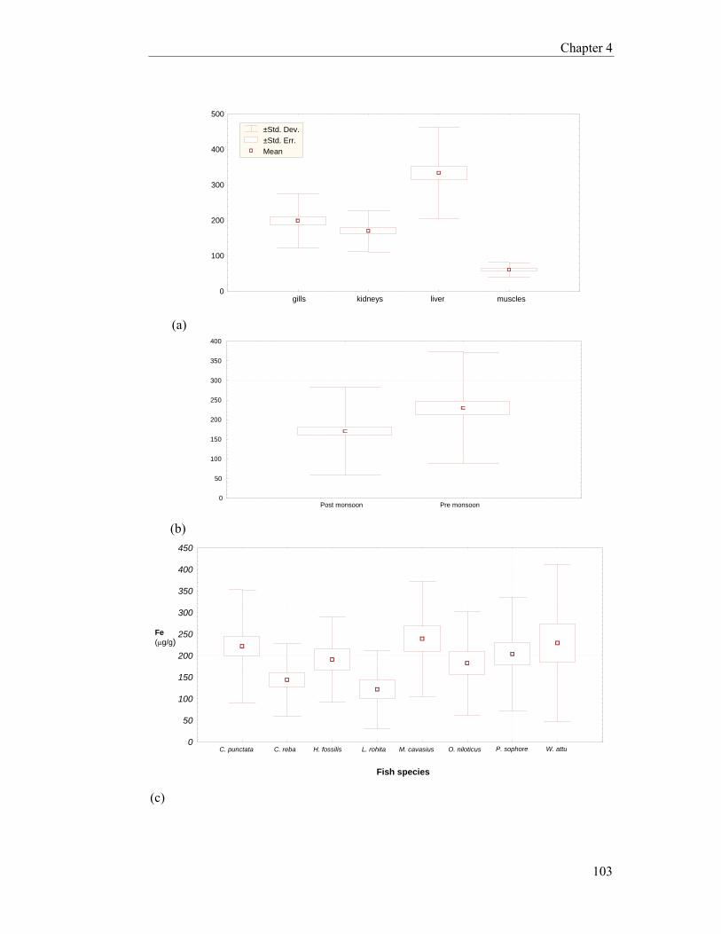
Chapter 4

103

(a)

(b)

(c)

Fish species

Fe (µg/g)

0 50

100 150 200 250 300 350 400 450

C. punctata C. reba H. fossilis L. rohita M. cavasius O. niloticus P. sophore W. attu

0 50

100

150

200

250

300

350

400

Post monsoon Pre monsoon

500

0

100

200

300

400

gills kidneys liver muscles


Chapter 4

104

Fig. 4.3 Box and whisker plots of showing comparative accumulation of Fe (µg/g) concentration in (a) organs, (b) seasons, and (c) fish species collected from Nullah Aik and Nullah Palkhu.

Lead

Mean Pb concentration was significantly different between up and

downstream zones. Maximum concentration of Pb was recorded in downstream of

Nullah Aik and minimum at upstream of Nullah Aik (Fig.4.5b). Similarly, significant

variations in mean concentration of Pb were found between species. Highest Pb

accumulation was recorded in Heteropneustes fossilis and Wallago attu, and lowest in

Mystus cavasius (Fig.4.5c).

Like Fe, highly significant variations in mean Pb concentration were observed

between various organs from pre and post monsoon seasons (Table 4.1a & b; Fig

4.5a). The results showed that the highest mean concentration of Pb was found in gills

followed by liver, kidneys and muscles during post monsoon. Maximum mean

concentration of Pb (20.595 ± 1.506µg/g) was measured in the gills and liver (18.734

± 2.095µg/g) of Wallago attu recorded from downstream of the Nullah Aik, whereas,

minimum in gills (6.561 ± 2.307µg/g) and liver (6.104 ± 2.079µg/g) was recorded in

Mystus cavasius captured from upstream of Nullah Palkhu. In kidneys, maximum

mean concentration of Pb (15.788 ± 2.078µg/g) was measured in Wallago attu

captured from downstream of Nullah Aik and minimum (1.033 ± 2.034µg/g) in

Cirrhinus reba from upstream of Nullah Palkhu. Maximum mean concentration of Pb

(4.56 ± 2.525µg/g) was found in muscles of Puntius sophore at upstream of Nullah

Palkhu, whereas, minimum mean concentration (1.043 ± 1.044µg/g) in Cirrhinus reba

sampled from upstream of Nullah Aik (Fig 4.4a).

In pre monsoon, highest concentration of Pb was recorded in gills (30.062

±10.645µg/g) and muscles (9.534 ± 5.131µg/g) of Heteropneustes fossilis sampled

from downstream of Nullah Aik and lowest concentration was recorded in gills

(15.717 ± 10.08µg/g) of Wallago attu and in muscles (4.227 ± 9.037µg/g) of Channa

punctata captured from upstream of Nullah Aik. In liver (19.486±4.784µg/g) and

kidneys (21.799 ± 11.442µg/g) highest Pb concentration was recorded in

Heteropneustes fossilis and lowest concentration in liver (12.215 ± 4.627µg/g) and

kidneys (13.006 ± 4.732µg/g) of Wallago attu from upstream of Nullah Aik (Fig.

4.4b).

Chapter 4

105

(a)

(b)

Fig. 4.4 Spatial variations in bioaccumulation of Pb (µg/g) in four organs (gills, kidneys, liver and muscles) of eight fish species during (a) post monsoon and (b) pre monsoon at upstream and downstream of Nullah Aik and Nullah Palkhu.

Chapter 4

106

(a)

(b)

Fig.4.5 Box and whisker plots of showing comparative accumulation of Pb

(µg/g) concentration in (a) organs (b) fish species collected from Nullah Aik and Nullah Palkhu.

2

6

10

14

18

22

26


Pb (µg/g)

Fish species

24

gills kidneys0

4

8

12

16

20

liver muscles

Pb (µg/g)

Chapter 4

107

Cadmium

Upstream and downstream sampling zones were non-significantly different in

Cd concentration; however, significant differences were recorded between two

seasons. Similarly, inter-specific variations in mean concentration of Cd were found

(Table 4.2). Minimum accumulation of Cd was recorded during post monsoon and

maximum in pre monsoon (Fig. 4.7b). Mystus cavasius showed highest level of Cd

accumulation followed by Cirrhinus reba and minimum concentration in

Heteropneustes fossilis (Fig. 4.7c).

Mean concentration of Cd in various organs was diminutive. Pattern of Cd

accumulation was in this order: liver> gills > kidneys > muscles (Fig. 4.7a). Mean

concentration of Cd (13.136 ± 0.448µg/g) was highest in the liver of Mystus cavasius

at downstream of Palkhu and lowest (1.968 ± 1.421µg/g) in liver of Heteropneustes

fossilis from downstream of Nullah Aik (Table 4.1a & b). Maximum mean

concentration of Cd (6.851 ± 0.509µg/g) in gills was recorded in Oreochromis

niloticus at downstream of Nullah Palkhu and minimum (2.837 ± 0.281µg/g) was

exhibited by Heteropneustes fossilis captured from downstream of Nullah Aik.

Maximum mean Cd concentration (6.782 ± 1.123µg/g) in kidneys of Mystus cavasius

at upstream of Nullah Palkhu and minimum (2.058 ± 0.261µg/g) was recorded in

Heteropneustes fossilis at downstream of Nullah Aik (Fig 4.6a). Maximum mean Cd

concentration (2.798 ± 0.383µg/g) was recorded in muscles of Mystus cavasius from

downstream of Nullah Palkhu and minimum (0.64 ± 0.285µg/g) in Heteropneustes

fossilis from downstream Nullah Aik.

Channa punctata accumulated highest mean concentration of Cd during pre

monsoon in gills (6.456 ± 1.63µg/g), kidneys (6.060 ± 1.0125µg/g) and muscles

(2.505 ± 1.715µg/g) captured from downstream of Nullah Palkhu. Mystus cavasius

also showed high mean concentration of Cd in liver (12.815 ± 0.785µg/g) from

upstream of Nullah Palkhu, whereas, minimum in liver (1.734 ± 2.195µg/g), gills

(2.86 ± 2.475µg/g), kidneys (2.406 ± 0.47µg/g) and muscles (1.309 ± 0.835µg/g) of

Heteropneustes fossilis captured from downstream of streams (Fig. 4.6b).

Chapter 4

108

(a)

(b)

Fig. 4.6 Spatial variations in bioaccumulation of Cd (µg/g) in four organs (gills, kidneys, liver and muscles) of eight fish species during (a) post monsoon and (b) pre monsoon at upstream and downstream of Nullah Aik and Nullah Palkhu.

Chapter 4

109

(a)

(b)

(c)

Fig. 4.7 Box and whisker plots of showing comparative accumulation of Cd (µg/g) concentration in (a) organs, (b) seasons, and (c) fish species collected from Nullah Aik and Nullah Palkhu

0

2

4

6

8

10


Cd (µg/g)

Fish species

1.5

2.5

3.5

4.5

5.5

6.5

7.5

Post monsoon Pre monoon

Cd (µg/g)

0

1

2

3

4

5

6

7

8

9


Cd (µg/g)

Chapter 4

110

Chromium

Mean Cr concentration varied significantly between seasons and species

(Table 4.2). Highest accumulation of Cr was observed in downstream of Nullah Aik

followed by Nullah Palkhu and lowest at upstream of Nullah Aik (Fig. 4.9b). Highest

mean concentration of Cr was recorded in Heteropneustes fossilis followed by

Wallago attu and minimum in Puntius sophore (Fig. 4.9d).

Gills, liver, kidneys and muscles showed marked variations of Cr

accumulation of Cr during post monsoon (Table 4.2). Overall Cr accumulation was in

order: gills ≥ liver> kidneys > muscles (Fig. 4.9a). In post monsoon, maximum mean

Cr concentration was recorded in gills (31.274 ± 6.289µg/g), followed by liver

(25.7155 ± 8.942µg/g) and kidneys (23.18 ± 8.739µg/g) in Wallago attu sampled

from downstream of Nullah Aik. Minimum mean Cr concentration was recorded in

gills (3.448 ± 2.933), liver (4.52 ± 0.572µg/g) and kidneys (1.415 ± 1.3435µg/g) of

Oreochromis niloticus inhabiting at upstream of Nullah Aik (Table 4.2a & b).

Maximum mean Cr concentration (5.173 ± 1.589µg/g) was measured in muscles of

Wallago attu from downstream of Nullah Aik and minimum (1.415 ± 1.343µg/g) in

Mystus cavasius captured from upstream of Nullah Aik (Fig. 4.8b).

In pre monsoon, maximum mean concentration of Cr was recorded in gills

(32.77 ± 4.855µg/g) and liver (30.668 ± 1.881µg/g) of Heteropneustes fossilis from

downstream of studied streams, whereas, highest mean concentration of Cr in kidneys

(16.584 ± 5.583µg/g) and muscles (13.693 ± 4.156µg/g) was recorded in Channa

punctata dwelling in downstream of Nullah Aik (Fig. 4.8b). Puntius sophore captured

from upstream showed lowest accumulation of Cr metals in gills (3.2645 ±

2.933µg/g) followed by liver (6.390 ± 1.5165µg/g), kidneys (3.468 ± 1.554µg/g) and

muscles (3.656 ± 0.414µg/g).

Chapter 4

111

(a)

(b) Fig. 4.8 Spatial variations in bioaccumulation of Cr (µg/g) in four organs (gills,

kidneys, liver and muscles) of eight fish species during (a) post monsoon and (b) pre monsoon at upstream and downstream of Nullah Aik and Nullah Palkhu.

Chapter 4

112

(a)

-2

2

6

10

14

18

22


Cr (µg/g)

Chapter 4

113

Bioaccumulation of Nickel

The accumulation of Ni among different sampling zones and seasons were

found non-significant differences, whereas, significant in inter-specific comparison

(Table 4.2). In case of inter-specific Ni accumulation, Cirrhinus reba and Labeo

rohita showed highest accumulation of Ni and minimum in Wallago attu (Fig. 4.11).

The pattern of Ni accumulation in different organs was: gills > kidneys > liver

> Muscles during post monsoon (Fig.11a). Maximum mean concentration of Ni in

(b)

(c)

-2

2

6

10

14

18

22

26

30


Cr (µg/g)

Fish species

0

4

8

12

16

20


Cr (µg/g)

0 4 8

12

16

20

24

Up Ak Up Pk Dn Ak Dn Pk

Cr(µg/g)

Fig. 4.9 Box and whisker plots of showing comparative accumulation of Cr (µg/g) concentration in organs, (b) sampling zone, (c) seasons and (d) fish species collected (d)from Nullah Aik and Nullah Palkhu

Chapter 4

114

gills (10.957±1.376µg/g), kidneys (9.994 ± 3.455µg/g) liver (8.04 ± 0.376µg/g) and

muscles (2.205 ± 0.117µg/g) was recorded in Labeo rohita inhabiting downstream of

Nullah Aik, whereas, minimum in gills (4.452 ± 2.285µg/g), kidneys (4.492 ±

2.45µg/g) liver (3.506 ± 1.857µg/g) and muscles (0.909 ± 0.703µg/g) of Cirrhinus

reba captured from upstream of Nullah Aik (Fig. 4.10a).

In pre monsoon, highest mean Ni concentration (14.379 ± 2.426µg/g) was

recorded in gills of Channa punctata collected from downstream of Nullah Palkhu

and kidneys (14.489 ± 3.005µg/g) of Heteropneustes fossilis and liver (16.236 ±

5.612µg/g) of Cirrhinus reba captured from downstream of Nullah Aik. Maximum

mean Ni concentration (6.335 ± 3.162µg/g) was reported in muscles of Labeo rohita

collected from upstream of Nullah Aik. Minimum mean Ni concentration in gills

(6.571 ± 1.61µg/g), kidneys (2.459 ± 1.385µg/g) liver (5.139 ± 1.31µg/g) and muscles

(1.215 ± 0.84µg/g) was accumulated in Wallago attu captured from downstream of

Nullah Palkhu (Fig. 4.10b).

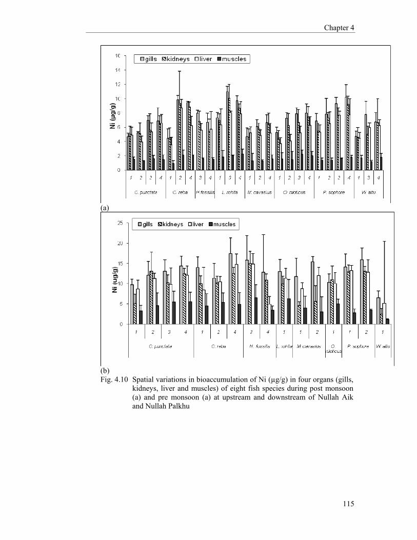
Chapter 4

115

(a)

(b) Fig. 4.10 Spatial variations in bioaccumulation of Ni (µg/g) in four organs (gills,

kidneys, liver and muscles) of eight fish species during post monsoon (a) and pre monsoon (a) at upstream and downstream of Nullah Aik and Nullah Palkhu

Chapter 4

116

(a)

(b)

Fig.4.11 Box and whisker plots of showing comparative accumulation of Ni (µg/g) concentration in organs, (b) sampling zone and (c) fish species collected from Nullah Aik and Nullah Palkhu.


Ni (µg/g)

0

2

4

6

8

10

12

14

0

2

4

6

8

10

12

14


Ni (µg/g)

Chapter 4

117

Copper

Non-significant variations in Cu concentration were recorded between

sampling zones as well as between two seasons (Table 4.2). However, significant

inter-specific variations for Cu concentration were observed. Maximum mean Cu

concentration was found in Puntius sophore, Labeo rohita and minimum in Wallago

attu (Fig. 4.13b).

The accumulation trend of Cu in different organs during post monsoon was

highest in liver followed by gills, kidneys and muscles (Fig. 4.13a). Maximum mean

Cu concentration (14.827 ± 2.161µg/g) was observed in liver of Puntius sophore

captured from downstream of Nullah Aik (Fig. 4.12a). Labeo rohita collected from

downstream of Aik showed maximum mean Cu concentration (8.169 ± 1.171µg/g) in

gills, whereas, maximum mean concentration (8.052 ± 3.030µg/g) in kidneys of

Labeo rohita captured from downstream of Nullah Palkhu (Table 4.1a & b).

Maximum mean Cu concentration (1.854 ± 0.076µg/g) in muscles was recorded in

Labeo rohita collected from downstream of Nullah Aik. Minimum mean Cu

concentration was accumulated in liver (0.943 ± 0.073µg/g), gills (0.823 ±

0.123µg/g), kidneys (0.813 ± 0.105µg/g) and muscles (0.471± 0.071µg/g) of Wallago

attu inhabiting in upstream of Nullah Aik.

During pre monsoon, maximum Cu concentration was accumulated in liver

(6.139 ± 1.855µg/g) and kidneys (5.795 ± 2.237µg/g) of Channa punctata, whereas,

maximum Cu concentration in gills (10.357 ± 0.162µg/g) was observed in

Oreochromis niloticus captured from upstream of Nullah Aik. Mystus cavasius

collected from upstream of Nullah Aik, showed minimum accumulation in liver

(4.814 ± 0.256µg/g), kidneys (2.277 ± 3.280µg/g), and gills (1.36 ± 1.048µg/g).

Maximum mean Cu concentration in muscles (2.118 ± 0.485 µg/g) of Heteropneustes

fossilis was recorded from downstream of Nullah Aik, whereas, minimum Cu

concentration in muscles (1.339 ± 0.526µg/g) of Labeo rohita captured from upstream

of Nullah Palkhu (Fig. 4.12b).

Chapter 4

118

(a)

(b) Fig. 4.12 Spatial variations in bioaccumulation of Cu (µg/g) in four organs (gills,

kidneys, liver and muscles) of eight fish species during (a) post monsoon and (b) pre monsoon at upstream and downstream of Nullah Aik and Nullah Palkhu

Chapter 4

119

(a) (b)

Fig. 4.13 Box and whisker plots of showing comparative accumulation of Cu (µg/g) concentration in (a) organs, and (b) fish species collected from Nullah Aik and Nullah Palkhu

-1

1

3

5

7

9

11


Cu (µg/g)

Fish species

0

2

4

6

8

10

12


Cu (µg/g)

Chapter 4

120

Zinc

Non-significant variations in accumulation of Zn were found between

sampling zones, whereas, significant seasonal and inter-specific variations were

recorded (Table. 4.3). Mystus cavasius, Channa punctata, Cirrhinus reba showed

higher accumulation of Zn and lowest in Wallago attu (Fig. 4.15c).

The accumulation of Zn in different organs during post monsoon was in the

order: liver > gills ≥ kidneys > muscles (Fig. 4.15a). Maximum mean Zn

concentration was recorded in liver (65.427 ± 29.669µg/g) of Wallago attu dwelling

in upstream of Nullah Aik. Maximum mean Zn concentration in gills (45.851 ±

23.787µg/g) and kidneys (48.793 ± 16.55µg/g) was recorded in Mystus cavasius

captured from downstream of Nullah Aik. Maximum mean concentration of Zn

(19.554 ± 4.456µg/g) was recorded in muscles of Channa punctata collected from

downstream of Nullah Aik. Minimum mean Zn concentration in liver (31.883 ±

17.046µg/g) of Channa punctata sampled from downstream of Nullah Palkhu,

whereas, minimum in kidneys (10.116 ± 10.142µg/g) of Oreochromis niloticus

captured from downstream of Nullah Aik. Minimum mean Zn concentration was

recorded in gills (13.251 ± 3.427µg/g) of Puntius sophore from downstream of Nullah

Aik (Fig. 4.14a). In muscles, minimum mean Zn concentration (6.343 ± 3.503µg/g)

was found in Heteropneustes fossilis captured from downstream of Nullah Palkhu

(Table 4.1a & b).

In pre monsoon, Zn accumulation pattern in different organs was: liver >

kidneys > gills > muscles. During pre monsoon, highest mean Zn concentration was

recorded in liver (97.594 ± 21.56µg/g), kidneys (76.613 ± 13.295µg/g) and muscles

(45.241 ± 9.890µg/g) of Mystus cavasius and highest mean concentration in gills

(73.905 ± 12.434µg/g) of Channa punctata collected from upstream of Nullah

Palkhu. Minimum mean concentration of Zn was observed in liver (55.501 ±

15.455µg/g) and kidneys (29.520 ± 8.982µg/g) of Puntius sophore, whereas,

minimum mean concentration of Zn was observed in gills (27.07±9.262µg/g) of

Oreochromis niloticus dwelling in upstream of Nullah Aik (Fig. 4.14b).

Heteropneustes fossilis showed minimum accumulation in muscles (21.13 ±

14.51µg/g) captured from downstream of Nullah Aik.

Chapter 4

121

(a)

(b) Fig. 4.14 Spatial variations in bioaccumulation of Zn (µg/g) in four organs (gills,

kidneys, liver and muscles) of eight fish species during (a) post monsoon and (b) pre monsoon at upstream and downstream of Nullah Aik and Nullah Palkhu

Chapter 4

122

(a)

(b)

(c)

Fig. 4.15 Box and whisker plots of showing comparative accumulation of Zn (µg/g) concentration in (a) organs, (b) seasons and (c) fish species collected from Nullah Aik and Nullah Palkhu.

0

10

20

30

40

50

60

70

80


Zn (µg/g)

Fish species

0

10

20

30

40

50

60

70

80


Zn (µg/g)

Season

0

10 20 30 40 50 60 70 80 90


Zn (µg/g))

Organ

Chapter 4

123

Discussion

Spatio-temporal Variations in Accumulation of Metals in Fish Organs

Fish intake heavy metals through different organs (gills and digestive tract),

which are transported by blood to various body parts where, metal ion bind with

different proteins (Kotze et al., 1999). Presence of metal-binding proteins is an

indication of toxic metal pollution in an aquatic environment (Hennig, 2008). Fish

regulate metal ions through excretion via kidneys and gills. Most of the organisms

regulate and maintain level of essential heavy metals due to metabolic requirements

(Sorensen, 1991). The intensity of heavy metals uptake is influenced by

physiochemical and ecological factors. Physiochemical factors such as temperature,

pH, TDS and salinity influenced the availability of heavy metals. Higher

concentrations of anions, chloride, fluoride and phosphate have been reported to play

a vital role in regulating concentration of metals in an aquatic ecosystem (Avenant-

Oldewage & Marx, 2000). Ecological requirements of every species differ from each

other in terms of habitat preferences, genetic variations, feeding and breeding

behaviour. Accumulation of metals in organs of different fish species can be related to

differences in physiological functions such as uptake, absorption, storage, regulation

and excretion abilities of fish species (Kotze et al., 1999).

The results highlighted that overall accumulation pattern of trace metals in

different organs (liver, gills, kidneys and muscles) was: Fe > Zn > Cr > Pb > Ni > Cu

> Cd. Similar accumulation pattern was found in the study of Javaid & Mehmood

(2000) and Zyadah & Chouikhi (1999) in fishes collected from Ravi River and

Aegean Sea (Turkey), respectively. Furthermore, Yilmaz et al. (2007) also described

the sequence of metal accumulation Zn > Fe > Cu > Pb > Co > Cd. According to

Terra et al. (2008) metal such as Fe and Zn, which are essential for the metabolic

activities accumulated in higher concentration. Cr, Ni and Cu which are required in

trace amounts for metabolic activities showed high bioaccumulation in fish species.

Higher Fe concentration was recorded in all organs as compared to Pb, Cd, Cr, Ni, Cu

and Zn. Avenant-Oldewage & Marx (2000) indicated that higher concentration of Fe

in water and sediments increases the rate of accumulation in fish organs. Wallago attu

accumulated relatively higher Fe concentration in liver. Fe is basic component of

haemoglobin protein, which is stored in liver and reuse in genesis of red blood cells.

Chapter 4

124

High concentration of Fe was accumulated in liver followed by gills indicating the

metabolic and physiological role in fish body (Avenant-Oldewage & Marx, 2000).

Kojadinovic et al. (2007) described the general principle for accumulation of

metal i.e., higher in liver, followed by gills, kidneys and muscles. Liver and gills

generally accumulated higher concentration of metals compared to other organs.

Similarly, the results of present studies indicated relatively high concentration of

heavy metals in liver and gills of all fishes captured from Nullah Aik and Nullah

Palkhu. All organs showed significant variations in accumulations of metals. Cd and

Zn showed similar accumulation pattern in fish organs as earlier recorded for Fe in

eight fish species.

Cadmium is highly toxic to organisms and its biological function is unknown

(Wright & Welbourn, 2002). Trace amount of Cd can cause anomalies such as

reduction in development and growth rates and skeletal ossification even death of

organism (Hollis et al., 1999). During present study lowest concentration of Cd was

detected in all organs as compare to the other metals.

Pb accumulated with higher concentration in gills, followed by liver, kidneys

and muscles. El-Shaikh et al. (2005); Canli & Kalay (1998); Akhtar et al. (2005);

Kargin (1998) also reported high concentration of Pb in gills in comparison to other

organs. According to Pastor et al. (1998) highest percentage of Pb accumulated in

gills, whereas, other tissues such as liver, kidneys and muscles accumulate least

quantity. Metals can easily enter into fish through gills from external medium (El-

Shaikh et al., 2005).

The results showed highest Cu concentration in liver which was followed by

gills, kidneys and muscles. Similar pattern of Cu accumulation was recorded by

Kargin (1998), Canli & Kalay (1998) and Avenant-Oldewage & Marx (2000).

However, Akhtar et al. (2005) reported maximum concentration of Cu in gills

followed by liver and muscles. McCarter & Roch (1983) also reported highest

accumulation of Cu in liver. Excessive amount of Cu in liver also excreted through

bile duct and kidneys (Heath, 1987). Gills can accumulate Cu due to large surface

area from aquatic medium and facilitates the absorption into blood (Stagg &

Shuttleworth, 1982). Cu in dissolved form may bind with respiratory surface directly

exposed to external medium water. The results demonstrated lowest concentration of

Cu in muscles. Avenant-Oldewage & Marx (2000) also indicated that muscles

accumulate less amount of Cu even if fish is exposed to high levels of metal

Chapter 4

125

contamination. In contrast, Campenhout et al. (2004); Chatterjee et al. (2006)

reported higher concentration of Cu in liver, followed by gills and muscles.

The concentration of Pb, Cr, Ni and Cu displayed accumulation in this order:

gills > liver > kidneys > muscles. Similar accumulation patterns among various

organs. Canli & Kalay (1998), Avenant-Oldewage & Marx (2000), Nussey et al.

(2000) and Akhtar et al. (2005) reported similar trend of metal concentration in

different organs. Cr absorbed readily by gills and liver as compared to kidneys and

muscles. Liver detoxifies and excretes Cr through digestive system to regulate the

concentration inside the body (Avenant-Oldewage & Marx, 2000). Fish dwelling in

contaminated water with higher load of Cr and Ni accumulate higher concentration in

gills and liver due to slow excretion rate (Avenant-Oldewage & Marx, 2000; Heath,

1991). Generally, fishes accumulate Cr to the largest extent in organs such as gills,

liver, kidneys and spleen, whereas, relatively lower concentration in muscles. Higher

concentration of Cr was observed at the lowest trophic levels (Eisler, 1986). Similar

accumulation pattern of Ni in different organs of fish species was reported by several

authors (Canli & Atli, 2003; Deheyn et al., 2005; Bajc et al., 2005; Kojadinovic et al.,

2007; Akhtar et al., 2005).

The results demonstrated higher concentration of Zn in liver followed by gills,

kidneys and muscles. Javaid & Mehmood (2000) described analogous pattern of Zn

accumulation in organs of fishes captured from River Ravi. Tekin-Özan & Kır (2006)

also reported high concentration of Zn in liver, gills and muscles of fishes. The study

of Deb & Santra (1997); Farkas et al. (2000); Andreji et al. (2006); Farombi et al.

(2007) also confirmed the findings of present study.

Metal accumulation in fish species provided evidences of constant exposure to

metals contaminated aquatic environment (Kotze et al., 1999). Mean concentration of

Cr and Pb was significantly different between upstream and downstream stream

zones. Distinct variations in metal accumulation were observed for metals originated

from point sources. Nullah Aik and Nullah Palkhu receive Cr from tanneries effluents.

The results showed non-significant spatial differences in mean concentration of

metals such as Fe, Cd, Ni, Cu and Zn, which were mainly related with non-point

sources of contamination. Van Eeden (2003) also reported non-significant variations

in accumulation of Pb, Ni and Cu between reference and least polluted sites.

The concentration of Fe, Cd, Cr and Cu were significantly different between

two seasons. During present study, maximum concentration of metals (Fe, Cd, Cr, and

Chapter 4

126

Cu) was recorded in pre monsoon, while lowest concentration in post monsoon. Non-

significant seasonal variations were recorded for Pb, Ni and Zn accumulation in fishes

of Nullah Aik and Nullah Palkhu. Differences in metal concentrations in fishes can be

attributed by the presence of metal contaminant in surrounding medium. Tekin-Özan

& Kir (2007) described that bioavailability of metals may influenced by physiological

activities of fish during different seasons. Nussey et al. (2000) indicated highest metal

accumulation in fish species during spring and summer as compared to autumn and

winter season. Farkas et al. (2000) also described that seasonal variations in metal

accumulation is related to feeding behaviour of fish species (Pourang, 1995). Kargin

(1998) reported an increasing trend of metal accumulation in fishes from autumn to

summer in Seyhan River in Turkey. Seasonal variations in metal accumulation may

be influenced by stream conditions, pollutants load, water chemistry and other

environmental factors which affect the availability of metal (Johnson, 1988; Heiny &

Tate, 1997).

Simkiss & Mason (1983) indicated that seasonal differences in temperature,

rainfall, salinity and stream flow can influence metal accumulation and their

bioavailability. Roesijadi & Robinson (1994) reported that metal concentration in

surface water varies due to sources of metal, rainfall pattern, surface runoff, feeding

behaviour and metabolic activities. High stream flow in post monsoon season may

dilute the concentration of contaminants. In winter, stream discharge is relatively low

and streams experience elevated level of heavy metals. Highest accumulation of

heavy metals was measured during pre monsoon season. Nussey et al. (2000) also

recorded high metal accumulation in pre monsoon, which can also be related with

high temperature favourable for optimum metabolic activities of surrounding medium

during pre monsoon season. High metabolic rate reduces oxygen concentration in

blood and increase accumulation of pollutants (Grobler et al., 1989; Nussey et al.,

2000). Most of the fish species breed during pre monsoon season and high metabolic

rate with elevated level of heavy metals in surrounding medium may influence the

embryonic development of fish individuals (Campbell, 1995).

Mean Fe concentration did not show significant variations between in

upstream and downstream zones. Similar results were reported by Avenant-Oldewage

& Marx, (2000). Fe in stream water originates from natural as well as anthropogenic

sources. Fe concentration varied significantly between seasons. Kargin (1998);

Ozmen et al. (2006); Avenant-Oldewage & Marx (2000) also reported that Fe

Chapter 4

127

accumulation varied significantly between seasons in freshwater fishes of South

Africa. Avenant-Oldewage & Marx, (2000) also stated that high concentration of Fe

in stream water can be related with high level of organic matter and humic acids.

Mean Pb concentration showed spatial significant variations in fish organs

from four sampling zones located on Nullah Aik and Nullah Palkhu. Minimum mean

Pb concentration in muscles was reported in upstream of Nullah Aik (8.774 µg/g) and

maximum at downstream of Nullah Aik (9.182µg/g) followed by Nullah Palkhu

(10.768 µg/g). Downstream of Nullah Aik (12.320µg/g) and Nullah Palkhu receive

pollutants from urban runoff and municipal sewage that increases the concentration of

Pb in stream water. Van Aardt & Erdmann (2004) reported significant spatial

variations in accumulation of Pb in fishes captured from polluted freshwater bodies.

Tryfonas et al. (2006) also reported the same results of Pb accumulation in fishes

dwelling in Yamuna River. Similarly, Canli & Kalay (1998); Javed (2005), Javid et

al. (2007), Karadede-Akin & Ünlü (2007) and Terra et al. (2008) reported high spatial

variations of Pb accumulation in less and high polluted streams and rivers. During

present study, non-significant seasonal variations in Pb accumulation were recorded.

In contrary, Mwashote (2003) and Mansour & Sidky (2002) reported significant

seasonal variations in Pb accumulation in fishes from African waters.

Mean Cd concentration did not show pronounced variations between upstream

and downstream zones. Campbell (1995), Nnaji et al. (2007) reported similar results.

Goldstein & DeWeese (1999) also found non-significant spatial variations of Cd

concentration in Red River. In contrary, Besser et al. (2007) reported significant

spatial variations of Cd concentration in fishes from streams polluted from cadmium

mines in United States. Cd accumulation was significantly different between post and

pre monsoon downstream seasons. Tekin-Özan & Kir (2007) reported seasonal

variations in Cd accumulation between fishes of Beyşehir Lake, Turkey. High

concentration of Cd in fish is an indicator of the environmental contamination of

surrounding medium (Kojadinovic et al., 2007).

Fish species captured from downstream of Nullah Aik showed high level of Cr

accumulation and low concentration in upstream sampling zone. Significant spatial

and seasonal variations were recorded in Cr concentration between fish species. In

contrary, Avenant-Oldewage & Marx (2000) and Ozmen et al. (2006) reported non-

significant spatial and seasonal variation in Cr accumulation. High concentrations of

Chapter 4

128

Cr in fishes indicate the contribution of tanneries effluents which bring large amount

of Cr salts that may concentrate in the aquatic organism like fishes.

Ni concentration in different fishes did not showed significant variations

between seasons. These results further confirmed the findings of Lefkovitz et al.

(2000) and Nussey et al. (2000), whereas, Canli & Kalay (1998) reported significant

spatial differences in Ni accumulation in the Seyhan River, Turkey. Nussey et al.

(2000) also reported significant seasonal variations in Ni accumulation.

Cu and Zn concentration in four sampling zones did not showed significant

differences in accumulation. Similar results were reported by Campbell (1995),

Goldstein & DeWeese (1999) and Youssef & Tayel (2004). However, Canli & Kalay

(1998), Kotze et al. (1999) and Beldi et al. (2006) found significant spatial differences

in Cu accumulation in fishes. In present study, Cu concentration in fishes was

significantly different between seasons. Avenant-Oldewage & Marx (2000) and

Tekin-Özan & Kir (2007) reported significant seasonal variations in Cu accumulation.

Harrison & KlaverkKamp (1990); Schmitt et al. (2002; 2007) reported

significant spatial variation in Zn accumulation in freshwater fishes. In present study,

non-significant seasonal variations were recorded. Similar results were also reported

by Velcheva (2006) and Tekin-Özan & Kir (2007).

Inter-specific Variations in Accumulation of Metals

Inter-specific variations in heavy metals accumulation are influenced by life

history patterns such as trophic position in food chain, geographic variations,

exposure to contaminated environment and internal metabolic activities (Allen-Gill &

Martynov, 1995). Fishes occupy various positions (herbivore to top carnivore) in the

food chain (Mansour & Sidky, 2002) and species at lower trophic level accumulate

low metal concentration in comparison to those occupy higher trophic level (Peakall

& Burger, 2003; Burger et al., 2001). Amundsen et al. (1997) and Canli & Kalay

(1998) reported inter-specific variation of heavy metal accumulation. Concentration

of metals such as Fe, Pb, Cd, Cr, Ni, Cu and Zn were significantly different between

fish species. Highest concentration of Fe accumulated in Wallago attu, whereas,

lowest in Labeo rohita. Similarly, Highest Fe concentration in carnivorous fish

species and lowest in herbivore fish species.

Chapter 4

129

Heteropneustes fossilis showed highest concentration of Pb and Mystus

cavasius accumulated lowest Pb concentration. Fishes are highly sensitive to Pb

toxicity. Higher concentrations of Pb in bottom feeder fish species was recorded

to those of predatory fishes (Campbell, 1995).

Among metals lowest level of Cd accumulation was recorded in all fish

species; though, it varies significantly from one fish species to another. Similarly

Youssef & Tayel (2004) found low concentration of Cd in Tilapias. In present study,

highest concentration of Cd was recorded in Mystus cavasius, which is carnivore

species and lowest concentration of Cd in Heteropneustes fossilis, which is an

omnivore species. Similar results were also reported by Amundsen et al. (1997) and

Andreji et al. (2006). Burger et al. (2001) and Terra et al. (2008) found higher level of

metals in carnivorous species instead of herbivores and omnivores. Furthermore,

bottom dweller fish species showed higher concentration of Cd.

Among fish species, Wallago attu and Heteropneustes fossilis showed highest

accumulation of Cr while lowest accumulation was recorded in Oreochromis

niloticus. Heteropneustes fossilis is a bottom dweller omnivore fish found in

downstream sites and Wallago attu feed on small fish species and macro-

invertebrates. Terra et al. (2008) and Tekin-Özan & Kir (2006) recorded high level of

Cr accumulation in carnivore species followed by omnivore species. Heteropneustes

fossilis and Oreochromis niloticus are omnivorous species but have different habitat

preferences. Heteropneustes fossilis is bottom dweller showed preferences for

downstream sites contaminated with industrial effluents and urban sewage and

Oreochromis niloticus is column dweller and prefer upstream sites (less polluted).

Fish dwelling in contaminated water with higher load of Cr metal from tanneries,

exhibit higher level of Cr in gills and liver due to slow excretion rate by liver under

stress conditions. Chromium in aquatic medium found in two forms trivalent (Cr+3) or

hexavalent (Cr+6). Cr+3 are less toxic as compared to Cr+6 and can disturb the

permeability of membrane by oxidation process (USEPA, 1980).

Highest concentration of Ni was recorded in Cirrhinus reba and lowest in

Wallago attu. Present study indicated that lowest Ni concentration in carnivorous

species as compared to herbivore, which can accumulate higher concentration.

Campbell (1995) also reported similar results.

Chapter 4

130

High Cu accumulation was recorded in invertevore (Puntius sophore) and

herbivore species (Labeo rohita), whereas, lowest accumulation in carnivore species

(Wallago attu). Silva & Shimizu (2004) reported omnivorous fishes can accumulate

higher Cu concentration as compared to carnivorous fishes. In contrary to our results,

Terra et al. (2008) reported that carnivore fishes accumulate highest level of Cu to

those of herbivore species. Phillips (1990) reported that carnivore fish species can

accumulate Cu at higher concentration than herbivorous and omnivorous and

indicated that this pattern could be changed due to pollution exposure, feeding habits

and fish breeding behaviour. Higher accumulation of Cu in omnivore species could be

due to pollution stress and feeding patterns (Phillips, 1990).

During present study, highest concentration of Zn was recorded in Mystus

cavasius and lowest in Oreochromis niloticus. According to Kotze et al. (1999) inter-

specific differences in Zn bioaccumulation could be due to differences in feeding

habits and behaviour of fish species. Oreochromis niloticus is an omnivore species

feeds on aquatic vegetation and detritus matter (Greger & Deacon, 1988), whereas,

Mystus cavasius feed on small fishes and small invertebrate. High concentration of Zn

was recorded in Channa punctata (Mirza & Bhatti, 1993).

Toxic Effects of Metals on Fishes

Elevated level of metals in different organs of fish is mainly absorbed from

aquatic resources polluted by industrial effluent and municipal sewage (Asuquo et al.,

2004). Heavy metals discharged from multiple sources into aquatic ecosystems are

responsible for fish physiological and histological abnormalities (Sehgal & Saxena,

1986). Toxic level of metals may affect growth, impaired movements, behavioural,

physiological and reproductive abnormalities in fishes (Atchison et al., 1987). During

present study, skin and fin rot diseases were observed Channa punctata and Mystus

cavasius (Plate 4.1). Species like Wallago attu captured from less polluted sites and

polluted sites also showed prominent variations in skin colour (Plate 4.2). These

negative effects of heavy metals affect fish health, leading to abnormalities and even

death.

Iron is rarely toxic (Atchison et al., 1987; USEPA, 1999) and hardly toxic to

aquatic ecosystem. Bury et al. (2003) reported that excessive amount of iron can be

harmful for fish health including gills clogging and respiratory perturbations. Mean Fe

Chapter 4

131

concentration in fishes of Nullah Aik and Nullah Palkhu ranged from 121.0 to 238.3

(µg/g).

The toxic effect of Pb decreases with an increase in water hardness. High level

of water hardness reduces bioavailability of heavy metal (Wright & Welbourn, 2002).

Factors such as age, sex and food and interference of Pb with other chemical present

in mixture of effluents affect the adsorption process of Pb in fishes (Eisler, 1988;

USEPA, 1999). In present study, mean dissolved Pb concentration varied from 188.2

to 206.9 (µg/L). USEPA (1999) reported chronic (11.86µg/L) and acute effect

(316.64µg/L) of Pb concentration for fish species at water hardness 290 (mg/L).

According to Davies et al. (1976) and Atchison et al. (1987) Pb concentration of 32

(µg/L) and LC 50 for fish species for 96 hours at 1320 (µg/L) of water hardness can

cause abnormalities such as hepatic lesions, splenic hemosiderosis and malfunctioning

of kidneys in freshwater fishes (Pattee et al., 2006). The LC50 (lethal concentration to

kill 50% population of an organism) of Pb concentration for fishes was 542 (mg/L) at

290 (mg/L) water hardness (USEPA, 1985). Pb concentration in water of Nullah Aik

and Nullah Palkhu was above Pb concentration that can cause chronic effects,

however, below the concentration that can cause acute effects on fish fauna. Sub-

lethal effects of Pb on fish fauna appears if its concentration ranged from 2300 to

145.72 (mg/L) in aquatic ecosystem (USEPA, 1999). Mean Pb concentration, which

ranged from 9.012 to 13.597 of (µg/g) in muscles of fishes captured from Nullah Aik

and Nullah Palkhu was above the permissible level (4.0µg/g) in fish muscles for

human consumption (USEPA, 1999).

Cd toxicity of fish varied from species to species, developmental stages,

interference of toxicants and water hardness (USEPA, 1999). Mean Cd concentration

in water of Nullah Aik and Nullah Palkhu ranged between 22.3 and 33.6 (µg/L) at

water hardness 122 to 288 (mg/L). These values were higher to Cd level, which can

produce chronic and acute effects in freshwater fishes (USEPA, 1999). Sastry &

Shukla (1994) described the LC50 of Cd, which is 11,200,000 (µg/L) for Channa

punctata at 165 (mg/L) level of water hardness for 96 hours exposure. Hontela et al.

(1996) noted abnormal production of fish thyroxin and cortisol hormones at exposure

of fish juveniles to Cd concentrations of 400-2,400 µg/L for 2 hours to 1 week at 110

mg/l water hardness. USEPA (1999) described Cd concentration (300- 400,000µg/L)

at which sub-lethal effects appears which altered normal functioning of enzymes and

physiological activities of catfishes, whereas, lethal effects appear at Cd concentration

Chapter 4

132

ranged from 338.3- 405,000µg/L. During present study, average concentration of Cd

in the fish body ranged from 1.953 to 5.295 (µg/g). Cd concentration should not

exceed the standards (5.0µg/g) for human consumption developed by Food and Drug

Administration (1993). Higher concentration of Cd was recorded in Mystus cavasius

captured from downstream sites of Nullah Palkhu.

According to (USEPA, 1980) Cr+6 concentration of 16 to 21(µg/L) in

freshwater can reduce growth in teleosts (bony fishes). Cr+6 have higher biological

activity and are more toxic to those of Cr+3. The Canadian water quality guideline

(Canadian Council for Ministers for Environment CCME, 1999) for Cr+3 for

freshwater fishes is 8.9 (µg/L), whereas, it’s least observed effect concentration

(LOEC) is 0.089 (µg/L). CCME (1999) reported chronic Cr toxicity appear in

freshwater fishes at concentration ranged from 6– 110000 (µg/L) while acute toxicity

appear at concentration ranged from 3300- 77500 (µg/L). In present study, the level of

Cr in surface water of Nullah Aik and Nullah Palkhu ranged between 76.7 – 196.8

(µg/L), which is below the concentration in freshwater that cause acute toxicity level

described by the Benoit (1975) and CCME (1999). In present study, mean

concentration of Cr in fish body ranged from 2.30 to 16.42(µg/g). Eisler (1986)

described the maximum permissible concentration of Cr (4.0 µg/g) in fishes for

human consumption. Higher concentration of Cr causes abnormal development of fish

embryos, over production of mucous and blood serum, malfunction of liver and

chromosomal aberration.

Nickel is considered less toxic in comparison to Cd and Pb (Clark, 2001). The

symptoms of nickel toxicity in fishes are fast mouth, opercula (Beraldo et al., 1995)

and convulsive movements and loss of equilibrium before death (Khangarot & Ray,

1990; Eisler, 1998). Higher concentration of Ni reduces respiration rate and causes

death due to blood hypoxia (Ellgaard et al., 1995; Eisler, 1998). Ni concentration in

water of Nullah Aik and Nullah Palkhu ranged from 78.8 to 100.8 (µg/L), which were

below the concentration that causes the chronic (160µg/L) and acute toxic effect

levels (1400µg/L) described by USEPA (1999). Higher Ni concentration affects

growth, reproduction, teratogenicity, and carcinogenicity (Eisler, 1998). Ni

concentration was also less than LOEC (134µg/L) and LC50 (8100µg/L) as given by

Nebeker et al. (1985). In present study, mean Ni concentration in fish muscles ranged

from 4.50 to 8.14(µg/g), which was below the permissible level of Ni (10.0µg/g) in

fishes for human consumption (Eisler, 1998).

Chapter 4

133

(a)

(b) Plate 4.1 Diseased specimens Channa punctata (a) and Mystus cavasius (b) captured from

Nullah Aik near Bhopalwala and Nullah Palkhu near Jathikay.

(a)

(b) Plate 4.2 Skin colour variations in two individuals of Wallago attu captured from (a)

upstream(less polluted site) and (b) downstream (polluted site) on Nullah Aik.

The level of Cu in fish tissues reflects indirectly its bio-availability in aquatic

environment. The toxic effect of Cu in fishes is highly influenced by water hardness,

Channa punctata

Mystus cavasius

Wallago attu

Wallago attu

Chapter 4

134

organic matter and developmental stage of freshwater fishes (USEPA, 1999). During

present study, concentration of dissolved Cu in stream water ranged between 27.5

(µg/L) and 46.1 (µg/L). These concentrations were below to the concentration that

can produce acute and chronic effects (USEPA, 1999). Pickering et al. (1977) studied

LOEC of Cu (37µg/L) and LC 50 (460mg/l). Buhl & Hamilton (1996) reported

mortality in sward fish at 363-10,000 (µg/L) of Cu concentration. According to

ANZFA (The Australian, New Zealand Food Authority), the concentration of Cu

should not exceed 10.0(µg/g) in fish body (Van den Broek et al., 2002). The

concentration of Cu muscles of fishes from Nullah Aik and Nullah Palkhu ranged

from 1.779 to 6.059 (µg/g) and was within the permissible (10.0µg/g) concentration

for human consumption (USEPA, 1999).

Zinc becomes toxic for fish in water with low pH, alkalinity, dissolved oxygen

and high temperature (Eisler, 1993). Majority of fish species accumulate excessive

amount of Zn than required for metabolic activities (USEPA, 1999). Shukla & Pandey

(1986) reported reduced growth of Channa punctata at Zn concentration of 12000

(µg/L) in surface water. According to Bengeri & Patil (1986) fishes showed reduced

production of liver glycogen at Zn concentration of 65,000 (µg/L). According to

USEPA (1999) chronic and acute toxic effects appear at Zn concentration of 10

(µg/L) and 100 (µg/L). The chronic effects of Zn such as changes in enzymes

production and alteration in blood and tissues appear when its concentration ranged

between 500 and 130,000 (µg/L) on catfishes (USEPA, 1999). USEPA (1987)

reported LC 50 of Zinc for freshwater fishes ranged from 840 to 22,600 (µg/L).

According to ANZFA (The Australian, New Zealand Food Authority) Zn

concentration in fish tissues should not exceed 150(µg/g) within tissues of fishes (Van

den Broek et al., 2002). Van den Broek et al. (2002) and Eisler (1993) reported that

the concentration of Zn in whole fish body should be below 80(µg/g). In present

study, mean concentration of Zn in fish body was ranged from 25.25 to 44.6(µg/g)

which is within safe limits for human consumption described by Van den Broek et al.

(2002) and Eisler (1993).

Comparison with Guidelines for Human Consumption

Chapter 4

135

Metal contents in muscles are most important because people, consume the

muscular parts of fish as food after removing liver, gills and kidneys (Mai et al.,

2006). Lowest accumulation of Fe, Pb, Cd, Cr, Ni, Cu and Zn was found in muscles.

Fish species such as Channa punctata, Wallago attu, Cirrhinus reba, Labeo rohita

and Heteropneustes fossilis are commonly used as food in the catchment area of

Nullah Aik and Nullah Palkhu either captured by game fishermen or professional

fishermen. Channa punctata is the most abundant species and is preferably used for

food (plate 4.3). The concentration of Fe in the muscles of all eight species during

post monsoon and pre monsoon was below the standards of (FAO/WHO, 1987;

USEPA, 1999) ranged from 20 to 150 (µg/g). However, Pb (4.0µg/g) and Cr

(8.0µg/g) during each season exceeded the permissible level described by USEPA

(1999) and FAO (1983). The Pb concentration in Labeo rohita (4.353 ± 2.013µg/g)

captured from downstream of Nullah Aik was higher to standard limits (4.0 µg/g),

whereas, Puntius sophore collected from upstream of Nullah Palkhu (4.044 ±

2.03µg/g) and downstream of Nullah Aik (4.560 ± 2.526µg/g) and Wallago attu (4.05

± 2.06µg/g) sampled from downstream of Nullah Aik also exceeded Pb concentration.

During pre monsoon season, Pb concentration in muscles of Channa punctata

captured from upstream (4.24 ± 3.14µg/g) and downstream (6.96 ± 7.77µg/g) of

Nullah Aik and Nullah Palkhu (5.67 ± 7.68µg/g) were above the standard limits of 4.0

(µg/g). Similarly, Pb concentration in muscles of Labeo rohita captured from

downstream of studied streams (9.534 ± 5.131µg/g, 4.227 ± 9.037µg/g) and Puntius

sophore (4.922 ± 6.832µg/g) dwelling in upstream of Nullah Palkhu exceeded the

standard limits (USEPA, 1999; FAO, 1983).

Cirrhinus reba (2.09 ± 1.04µg/g) captured from upstream of Nullah Aik and

Oreochromis niloticus (2.57 ± 0.10µg/g) from downstream of Nullah Aik during post

monsoon, whereas, Channa punctata from downstream of Nullah Aik (2.581 ±

2.26µg/g) and Nullah Palkhu (2.15 ± 1.71µg/g) during pre monsoon were higher than

the permissible limits (2.0µg/g) described by (FAO/WHO 1987). Cr concentration in

muscles of studied fish species did not exceed the standard limits (8.0µg/g) during

post monsoon, however, exceeded in Channa punctata captured from downstream of

Nullah Aik (13.693 ± 4.156µg/g) and Nullah Palkhu (8.834 ± 1.125µg/g) during pre

monsoon. The present study highlighted the intensity of heavy metal contamination in

fishes, which need to be addressed urgently.

Chapter 4

136

Plate 4.3 A fish sale point at Sambrial town located in lower catchment area of Nullah Aik and Nullah Palkhu.

Wallago attu

Channa punctata

Chapter 4

137

In Sialkot City, heavy metal contamination in Nullah Aik and Nullah Palkhu is

the consequence from industrial effluents, municipal sewage and surface runoff.

Effluents discharge into streams contains heavy metals (Qadir et al., 2008), which

may provide conducive condition for bio-concentration of metals in fish fauna of

Nullah Aik and Nullah Palkhu. The finding of present study indicated that fishes

dwelling in Nullah Aik and Nullah Palkhu are under risk of metal accumulation,

which is an ultimate threat to local human population. If existing situation remain

unchanged, it will not only affect the fish life but also well being of humans.

Conclusions

In conclusion, the results of this chapter indicated that all seven metals studies

showed significant variations in accumulation in different organs such as gills, liver,

kidneys and muscles. Significant spatial differences in Cr concentration were

observed, whereas, non-significant spatial variation were recorded in Fe, Pb, Cd, Ni

and Cu. All studied heavy metals showed significant variation between different fish

species. Among heavy metals, Fe showed high concentration and Cd lowest

concentration in fish species. Metals like Pb, Cr, Ni and Cu showed highest

accumulation in gills followed by liver, kidneys and lowest in muscles, whereas, Fe,

Cd and Zn showed metal accumulation pattern in order: liver > gills > kidneys >

muscles. General pattern of metal accumulation was: Fe > Zn > Cr > Pb > Ni > Cu >

Cd. Higher concentration of metals like Fe, Cd, Cr and Cu was recorded in pre

monsoon season. Most of the metals in stream water were above the LOEC and below

the level of acute toxic effects of heavy metals on fish species. Pb concentration in

muscles of Labeo rohita, Puntius sophore and Wallago attu, Cd concentration in

muscles of Cirrhinus reba, Oreochromis niloticus and Channa punctata and Cr

concentration in muscles of Channa punctata were recorded above the standard limits

for human consumption as described by FAO/WHO (1987) and USEPA (1999). These

findings suggested that consumption of fishes captured from downstream of Nullah

Aik and Nullah Palkhu may cause human health hazard. Therefore, it is recommended

that fishes captured from downstream sites of each stream should be avoided as

human diet.

Chapter 5

Patterns of Fish Assemblage and Distribution under the

Influence of Environmental Variables in Nullah Aik and

Nullah Palkhu

Introduction The diversity and spatio-temporal distribution pattern of fish assemblage in

stream is highly influenced by variations in lotic ecosystem (Taylor et al., 1997).

These variations are resulted due to environmental factors inside the stream (Taylor et

al., 2006). In intermittent streams environmental variations are of great importance for

fish assemblage as compared to continuously flowing streams (Pires et al., 1999).

Environmental factors such as physiochemical parameters of water quality and habitat

structure determine the structure and composition of fish assemblages inside the

stream (Casatti et al., 2006; Aparicio et al., 2000) and result in change of the

ecological equilibrium (Karr, 1996; Lyons, 1996). Habitat structure and

physiochemical quality of stream water have been widely used to explore the

relationships with fish assemblage (Casatti et al., 2006). Fishes aggregate into co-

existing groups to form complex assemblages of species in pristine aquatic ecosystem

(Pusey & Kennard 1996; Lamouroux et al., 2002). Association of different species in

food web is a delicate and complex phenomenon that has evolved over long time

period. Physical habitat and stream water quality are very sensitive to human pollution

(Casatti et al., 2006). Aquatic communities, especially fishes reflect the intensity of

degradation in streams and rivers (Wichert & Rapport, 1998; Das & Chakrabarty,

2007).

Streams which experience irregular flow are more vulnerable to anthropogenic

activities (Paul & Meyer, 2001) such as industrial effluents, municipal sewage, and

surface runoff from urban and agricultural land, which alter the water quality and

habitat structure of stream (Singh et al., 2005a; Qadir et al., 2008). Change in water

quality due to untreated industrial effluent and municipal sewage not only increases

the load of pollutants to streams but also put the fish fauna under stress (Matthews,

1998; Davis et al., 2003).

Chapter 5

138

Fish assemblages have been used as an indicator of environmental degradation

(Scott & Hall, 1997; Arunachalam, 2000). Fish diversity in streams and rivers is

considered as a diagnostic tool to highlight the impact of environmental changes (Das

& Chakrabarty, 2007). Loss of fish species diversity determines the severity of habitat

degradation of an aquatic ecosystem (Ganasan & Hughes, 1998).

Structure and composition of fish assemblage in temperate streams exhibit

prominent temporal variations influenced by habitat characteristics and physico-

chemical characteristics of water (Magalhães et al., 2002). The temporal distribution

patterns of fish assemblages and water quality are directily or indirectly influenced by

the flow regime (Grossman et al., 1990; Godoy et al., 2002). Most of the streams and

rivers in oriental region exhibit high flow during monsoon season and experience low

flow or drought during pre monsoon season, which determine the structure of fish

communities in the streams (Pires et al., 1999). Fish assemblages of such streams are

adapted to low and high stream flow to attain ecological equilibrium in fish

population. However, anthropogenic factors such as pollution load from industries and

municipalities, water abstraction and introduction of alien species highly destabilize

the equilibrium of fish assemblage (Pires et al., 1999). Unwise human activities in the

catchment area deteriorate the water quality and disrupt the integrity of fish

assemblage, which results, vanishing of native fish species or appearance of exotic

species in an ecosystem (Karr et al., 1986; Lyons, 1996). Any change in species

composition due to addition or deletion of species may disrupt the functional and

functional integrity of an aquatic ecosystem (Lyons, 1996).

Influence of environmental factors on structure and function of fish

assemblages in streams have been studied in several countries (Gafny et al., 2000;

Bhat, 2004; Magalhães et al., 2002; Li & Gelwick, 2005; Snodgrass et al., 1996;

Davis et al., 2003; Belliard et al., 1999). Diversity indices and multivariate statistical

techniques are commonly used to highlight the role of various important

environmental factors that contributes in explanation of fish diversity and distribution

along longitudinal gradients (Koel & Peterka, 2003). Multivariate techniques like

Canonical correspondence analysis (CCA) provide information regarding current

status of fish distribution in relation to environmental variables (Inoue & Nakano,

2001). Multivariate techniques have been useful in decision making for the restoration

and management of degraded streams and to assess the impact of disturbance and

identification of factors contribute in deterioration of stream ecosystem for effective

Chapter 5

139

stream management (Paul & Meyer, 2001). Major restoration efforts for intermittent

streams are underway in many parts of the world (Paul & Meyer, 2001) and

restoration efforts have been successfully implemented. Unfortunately, in developing

countries like Pakistan, no restoration efforts for streams and rivers have been made so

far. Information related to role of environmental factors in shaping the distribution

pattern of fishes in streams and rivers is completely lacking. It is important to collect

baseline data about biotic (fish assemblage) and abiotic (environmental) components

of stream/river ecosystem before taking any step towards restoration and management

of a streams or rivers. The objectives of this chapter are:

• to assess the fish species diversity in Nullah Aik and Nullah Palkhu,

• to explain the pattern of spatio-temporal variations in diversity and

composition of fish assemblage and

• to explore the role of environmental variables in fish distribution.

Chapter 5

140


Site Selection and Fish Sampling

Detailed information about the fish sampling and environmental variables is

given in Chapter 2.

Statistical Analysis Shannon index (H´) and Simpson index (D) were used to calculate fish species

diversity (Magurran, 1991; Lima-Junior, et al., 2006) at different sampling sites

during post and pre monsoon seasons.

CCA which is a direct gradient analysis was used to highlight the relationship

between fish distribution and environmental variables (Malik & Hussain, 2008). CCA

is an eigenvalue based technique applied on species abundance data in relation to

environmental variables (stream morphology, physiochemical and metal

concentration) during post monsoon and pre monsoon seasons at 18 sampling sites

located on Nullah Aik and Nullah Palkhu. Strongly correlated variables were excluded

from this analysis using Pearson correlation and 13 variables were used (Pires et al.,

1999). Environmental variables viz; stream morplogy (stream flow, depth and width),

physiochemical variables (DO, COD, turbidity and NO3-) and six metals (Na, Ca, Fe,

Pb, Cr and Cu) were subjected to CCA. The sites representing zero fish catch were

also excluded from CCA. Two separate CCAs were performed on fish abundance data

with environmental data sets recorded during post and pre monsoon season (Ter Braak

& Verdonschot, 1995). First CCA was applied to find out the relationship between (a)

sites and environmental variables (14 sites x 13environmental variables) and (b)

between species and environmental variables (24 species x 13environmental

variables) for post monsoon. CCA for pre monsoon season was performed on site

matrix including 12 sites and x 13 environmental variables and species matrix which

included 17 x 13 environmental variables (Eggleton, 2004; Malik & Hussain, 2008).

Monte Carlo permutation test with 1000 permutations was performed to check

wheather environmental parameters were significancantly correlated with fish species

composition of plots (Pires et al., 1999). For Fish diversity analysis and CCA,

Multivariate Statistical Package (MVSP) was used (Kovach, 1999).

Chapter 5

141

Index for Change in Scenarios of Fish Communities

The coefficient of community loss depict the range of scenarios to measure the

intensity of change caused by pollution which is a useful tool to take decision for the

management of species diversity in an aquatic ecosystem was calculated using

following formula as:

l = (a-c)/b

where (1) is coefficient of community loss, (a) total number of texa from

polluted section, (b) total number of texa from unpolluted section and (c) number of

texa common in polluted and unpolluted zones.

Chapter 5

142

Results

Fish Diversity

A total of 1506 individuals of 24 species (Plate 5.1) belonging to 12 families

and 19 genera were recorded in two seasons (post monsoon and pre monsoon) from

Nullah Aik and Nullah Palkhu (Table 5.1a & b). About 50.6% of individuals belonged

to ten species of family Cyprinidae followed by 19.6% of individual of Channa

punctata belonging to family Channidae. The remaining 29.8% of relative abundance

was contributed by family Bagridae (8.7%), Heteropneustidae (6.7%), Ambassidae

(2.7%), Notopteridae (2.3%), Siluridae (2.3%), Osphronemidae (1.7%),

Mastacembelidae (0.1%) and Sisoridae (0.1%). The highest species richness and

abundance was recorded in post monsoon after rainy season, whereas, lowest in pre

monsoon before rainy season.

During post monsoon season, 1141 fish specimens were captured from 14

sites. Maximum species richness (14), Simpson (2.29) and Shannon diversity index

(0.86 and 0.88) were recorded from upstream sites (1 and 2) of Nullah Aik, which

decrease to zero at sites located in close vicinity of Sialkot city. Fish species reappear

in far downstream of studied stream (Fig 5.1). Channa punctata and Puntius sophore

species were the dominant species recorded from 12 sites (Table 5.1b).

A total of 375 fish specimens were captured from 12 sites during pre monsoon.

None of fish was recorded from six sites (3, 4, 5, 12, 13 and 14). Maximum species

richness (13) was recorded at site 2 located at upstream of Nullah Aik with Simpson

(2.19) and Shannon (0.85) diversity indices and Channa punctata and Puntius ticto

were recorded in high abundance from nine and eight sampling sites, respectively (Fig

5.1).

Changes in Species Composition along longitudinal Gradient and

Distributional Patterns of Feeding Guilds

Four trophic groups of fishes were identified viz; invertivores, herbivores,

omnivores and carnivores from studied streams. Relative abundance for different

feeding groups recorded from Nullah Aik was in order: invertivores 36.2% >

herbivore 24.6 > Carnivore 24.0% > omnivore 15.1%, whereas, Nullah Palkhu

Chapter 5

143

exhibited different trend: Carnivore 44.9 % > invertivores 36.5% > omnivore 11.3% >

herbivore7.3%.

Labeo calbasu (Hamilton, 1822)

Labeo rohita (Hamilton, 1822)

Labeo dero (Hamilton, 1822)

Cyprinus carpio carpio (Linnaeus, 1758)

Puntius sophore (Hamilton, 1822)

Puntius ticto (Hamilton, 1822)

Salmostoma bacaila (Hamilton, 1822)

Garra gotyla (Gray, 1830)

Chapter 5

144

Cirrhinus reba (Hamilton, 1822)

Cirrhinus cirrhosus (Bloch, 1795)

Osteobrama cotio cotio (Hamilton, 1822)

Mystus cavasius (Hamilton, 1822)

Rita rita (Hamilton, 1822)

Sperata seenghala (Sykes, 1839)

Parambassis ranga (Hamilton, 1822)

Polyacanthus fasciatus (Bloch & Schneider, 1801)

Chapter 5

145

Heteropneustes fossilis (Bloch, 1794)

Gagata cenia (Hamilton, 1822)

Oreochromis niloticus niloticus (Linnaeus, 1758)

Notopterus notopterus (Pallas, 1769)

Channa punctata (Bloch, 1793)

Wallago attu (Bloch & Schneider, 1801)

Mastacembelus armatus (Hamilton, 1822)

Xenentodon cancila (Hamilton, 1822)

Plate 5.1 Fish species captured from Nullah Aik and Nullah Palkhu during study

period.

www.aqua‐art.spb.ru/.../xenentodon_cancila.jpg

Chapter 5

146

Table 5.1 Richness (S), evenness (E), Simpson’s diversity (H) and Shannon diversity (D) indices of (a) site and (b) fish species from Nullah Aik and Nullah Palkhu

(a) Season Post monsoon Pre monsoon Site # S H D` S H D` 1 14 2.20 0.86 8 1.4 0.67 2 14 2.29 0.88 13 2.19 0.85 5 4 1.22 0.65 0 0 0 6 4 1.15 0.62 1 0 0 7 7 1.47 0.68 3 0.99 0.60 8 3 1.01 0.61 1 0 0 9 4 1.09 0.58 1 0 0 10 7 1.76 0.80 4 1.23 0.66 11 5 1.39 0.73 2 0.68 0.48 13 1 0 0 0 0 015 13 2.16 0.84 3 1.02 0.62 16 10 1.99 0.83 3 0.9 0.56 17 12 2.10 0.84 1 0 0 18 5 1.39 0.72 2 0.34 0.19 (b)

Family Species

Post monsoon Pre monsoon S H D` S H D`

Ambassidae Parambassis ranga 2 0.29 0.15 1 0 0Bagridae Mystus cavasius 7 1.73 0.80 2 0.66 0.47 Rita rita 4 1.32 0.72 1 0 0 Sperata seenghala 2 0.56 0.37 0 0 0 Belonidae Xenentodon cancila 2 0.63 0.44 1 0 0 Channidae Channa punctata 12 2.17 0.86 8 1.69 0.78 Cichlidae Oreochromis niloticus 5 1.30 0.68 2 0.38 0.22 Cyprinidae Cirrhinus cirrhosus 5 1.49 0.75 1 0 0 Cyprinus carpio 5 1.46 0.74 0 0 0 Cirrhinus reba 1 0 0 3 0.80 0.49 Garra gotyla 1 0 0 0 0 0 Labeo calbasu 1 0 0 1 0 0 Labeo dero 1 0 0 1 0 0 Labeo rohita 4 1.18 0.64 2 0.58 0.39 Osteobrama cotio 2 0.69 0.49 1 0 0 Puntius ticto 11 2.22 0.87 9 2.06 0.85 Puntius sophore 12 2.29 0.88 4 1.11 0.59 Salmostoma bacaila 2 0.59 0.40 2 0.41 0.24 Heteropneustidae Heteropneustes

fossilis 7 1.69 0.79 2 0.69 0.49 Mastacembelidae Mastacembelus

armatus 1 0 0 0 0 0Notopteridae Notopterus notopterus 4 1.27 0.69 0 0 0 Osphronemidae Polyacanthus fasciatus 4 1.30 0.71 0 0 0 Siluridae Wallago attu 7 1.77 0.81 1 0 0 Sisoridae Gagata cenia 1 0 0 0 0 0

Chapter 5

147

(a)

(b)

(c)

Fig. 5.1 (a)Species richness, (b)Shannon diversity Indices and (c) Simson diversity indices recorded from various sites recorded from Nullah Aik and Nullah Palkhu.

Nullah Aik


Nullah Palkhu


Chapter 5

148

Invertivore fishes were generally small sized fishes, which mainly feed on

insect larvae and other small invertebrates. Among invertivores, two species (Puntius

ticto and Puntius sophore) were found as ubiquitous species in upstream and

downstream sites, whereas, Osteobrama cotio and Parambassis ranga showed

restricted distribution in upstream of Nullah Aik. Polyacanthus fasciatus, which an

invertevore species was distributed from upstream and downstream of Nullah Palkhu,

whereas, no specimen of this species was captured from Nulluh Aik. Five herbivore

fish species were sampled throughout the study area. Two species (Labeo calbasu and

Labeo dero) were restricted in upstream of Nullah Aik, whereas, other three species

(Labeo rohita, Cirrhinus reba and Cirrhinus cirrhosus) were ubiquitous in upstream

and downstream of studied streams. Omnivore trophic group of fishes was consisting

of four species. Out of these, two species (Oreochromis niloticus and Salmostoma

bacaila) were common in up and downstream sites but preferably present in upstream

sites. One omnivore species (Garra gotyla) was restricted to downstream of Nullah

Aik, whereas, Heteropneustes fossilis was common in downstream of Nullah Aik and

Nullah Palkhu. The largest trophic guild was carnivore species consisting of nine fish

species. Among these carnivore species, Channa punctata, Mystus cavasius, Rita rita

and Wallago attu were distributed in upstream and downstream of Nullah Aik and

Nullah Palkhu. Sperata seenghala and Xenentodon cancila were distributed at

upstream sites, whereas, Mastacembelus armatus, Gagata cenia and Notopterus

notopterus were restricted in downstream of Nullah Palkhu.

The relative abundance of feeding groups of fish in up and downstream of

streams in post monsoon and pre monsoon is given in Table 5.2. Among these feeding

groups, maximum relative abundance of herbivores (54.2%) captured from upstream

of Nullah Aik, whereas, no herbivorous species was recorded from downstream of

Nullah Aik and Palkhu during pre monsoon season. Highest relative abundance of

invertivores (57.4%) was recorded from downstream of Nullah Palkhu during pre

monsoon. Insectivorous individuals were more abundant in upstream during post

monsoon, whereas, abundant in downstream sites during pre monsoon. Highest

relative abundance of omnivores (21.6%) was observed in downstream of Nullah Aik

during pre monsoon season. Carnivore species were more abundant in downstream

zone throughout the sampling period.

Chapter 5

149

Table 5.2 Relative abundance of different feeding group in up and downstream of Nullah Aik and Nullah Palkhu

Season Sampling zone

Feeding group (%)

Carnivore Herbivore Invertivore Omnivore Post

monsoon

Upstream of Nullah Aik 20.2 16.8 49 14

Downstream of Nullah Palkhu 46.7 6.1 28 19.2

Upstream of Nullah Palkhu 34.3 8.7 54.7 2.1

Downstream of Nullah Palkhu 49.4 7.4 28.4 14.8

Pre

monsoon

Upstream of Nullah Aik 8.5 54.2 25.5 11.9

Downstream of Nullah Palkhu 56 0 21.6 21.6

Upstream of Nullah Palkhu 52.5 10 37.5 0

Downstream of Nullah Palkhu 27.7 0 57.4 14.8

Environmetal Relationship of Fish Assemblage during post monsoon and

pre monsoon

CCA was applied on 13 significant environmental variables to highlight their

relationship with distribution of fish during post monsoon and pre monsoon in studied

streams. The ordination plot of site and species scores produced from CCA shows the

distribution of sites and species in ordination (Fig. 5.2 & 5.3).

Post Monsoon First three axes of sites ordination for post monsoon accounted 51.38% of

total variance with more than 0.1 eigenvalues (Table 5.3a). First axis explained about

29.94 % of the total variations with 0.4 eigenvalue and was correlated to COD (r =

0.59), Pb (r = 0.51) and DO (r = -0.90). Axis 2 descibed 11.6 of the total variations

with 0.15 eigenvalue was correlated to stream width (r = 0.67), Cr (r = 0.59) and

stream depth (r = 0.75) (Table 5.3b).

CCA ordinations for sampling sites during post monsoon season are given in

Fig 5.2a-d). The sampling sites located at upstream of Nullah Aik and Nullah Palkhu

were closely associated and grouped together on the left side of CCA axis 1.

Furthermore, sampling sites located in downstream of Nullah Aik and Nullah Palkhu

on the right side of CCA axis 1. The sites located in downstream of Nullah were found

to be closely associated with each other and showing the similar composition of fish

assemblages, whereas, sites located at downstream of Nullah Aik were dispersed on

right side of CCA axis 1. These dispersed sites indicate variations in composition of

Chapter 5

150

fish assemblages of sites. Therefore, sites located close to each other on CA plot

exhibit the same fish species composition than sites located far from each other and

showed differences in fish species composition. Stream flow, stream width, DO and

NO3- and Pb were associated with upstream site of Nullah Aik and Nullah Palkhu,

whereas, stream depth, COD, Na, Ca, Fe, Cr and Cu were related with downstream of


CCA species ordination (species x environment) identified three different

groups of fish species for post monsoon (Fig. 5.2c-d). Group 1 comprised of species,

which were dwelling in upstream site consisting of seven species (Parambassis ranga,

Labeo rohita, Labeo dero, Labeo calbasu, Osteobrama cotio, Xenentodon cancila and

Sperata seenghala) highly correlated to DO, NO3- and stream flow. Out of seven, five

species (Parambassis ranga, Labeo rohita, Labeo dero, Labeo calbasu and

Osteobrama cotio) belonged to family Cyprinidae, whereas, remaining two

Xenentodon cancila and Sperata seenghala represented the families Belonidae and

Bagridae, respectively. Ten species (Cirrhinus reba, Cirrhinus cirrhosus, Puntius

sophore, Puntius ticto, Salmostoma bacaila, Mystus cavasius, Rita rita, Channa

punctata, Oreochromis niloticus and Wallago attu) were widely distributed in

upstream and downstream and clustered in group 2. Among these species, species

such as Cirrhinus reba, Cirrhinus cirrhosus, Puntius sophore, Puntius ticto and

Salmostoma bacaila were represented by family Cyprinidae, whereas, Mystus

cavasius and Rita rita belonged to family Bagridae. Remaining four species viz;

Channa punctata, Oreochromis niloticus and Wallago attu belonged to families viz;

Channidae, Cichlidae and Siluridae, respectively. These species were ubiquitous in

upstream and downstream and located at the centre of the biplot (Fig. 5.2c & d).

Group 3 was represented by Cyprinus carpio, Garra gotyla, Heteropneustes fossilis

Mastacembelus armatus, Notopterus notopterus and Gagata cenia belonged to

Cyprinidae, Mastacembelidae, Notopteridae and Sisoridae, which were distributed in

downstream sites and absent at upstream sites. Species belonging to third group were

tolerant to COD, turbidity, Na, Ca, Fe, Pb, Cr and Cu.

Pre Monsoon CCA plot ordination of pre monsoon season explained about 37.48% of the

total variation for first three axes with more than 0.1 eigenvalues (Table 5.3a). First

Chapter 5

151

axis explained 37.5% variation with 0.68 eigenvalue and positively correlated with

stream flow (r = 0.56), turbidity (r = 0.65), nitrates (r = 0.66), Na(r = 0.82) and Cr (r =

0.86), whereas, negative with DO (r = -0. 90). Second axis contributed about 20.30%

of the total variations with 0.36 and negatively correlated with stream flow (r = -0.75)

and nitrate (r = -0.55). COD (r = -0.65) exhibited positive correlation with third axis

that explained about 12.9 % variation with 0.23 eigenvalue (Table 5.3b).

CCA plot ordination for pre monsoon, sites located at upstream of Nullah Aik

were grouped together on the left side of CCA axis1 and were strongly influenced

with Stream flow, DO and NO3-. Sites located in upstream of Nullah Palkhu,

downstream of Nullah Aik and Palkhu were plotted on right side of CCA axis 1. The

upstream sites of Nullah Aik were correlated with stream width, DO and NO3- .

Stream depth, flow, COD, turbidity, Na, Ca, Fe, Cr and Cu were related to

downstream sites of studied streams.

CCA species ordination provides pattern of fish assemblage (Fig. 5.3c & d).

Three clusters of fish species were recognized. First group was represented by nine

species of upstream sites (Cirrhinus cirrhosus, Cirrhinus reba, Labeo dero, Labeo

calbasu, Labeo rohita, Osteobrama cotio, Parambassis ranga, Xenentodon cancila,

and Wallago attu). Out of nine species, six species (Cirrhinus cirrhosus, Cirrhinus

reba, Labeo dero, Labeo calbasu, Labeo rohita and Osteobrama cotio) were

represented by family Cyprinidae, whereas, remaining four species (Parambassis

ranga, Xenentodon cancila and Wallago attu) belong to families Ambassidae,

Belonidae and Siluridae, respectively. These species were positively correlated with

stream width, DO and NO3. Second group comprized of three species (Channa

punctata, Puntius sophore and Puntius ticto), which was evenly distributed in up and

downstream sites. Third group was represented by one fish species (Heteropneustes

fossilis), which belongs to family Heteropneustidae restricted in downstream sites.

Fish species showed correlation with COD, turbidity, Na, Ca, Fe, Pb, Cr and Cu. CCA

plot for pre monsoon season differ from pre monsoon. The upstream fish species did

not show significant variation, whereas, significant reduction in fish species richness

in second group (ubiquitous species) and in third group (downstream cluster) during

pre monsoon. However, species in first group showed an increase in number of

species and restricted to upstream area during pre monsoon season.

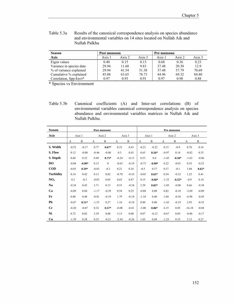
Chapter 5

152

Table 5.3a Results of the canonical correspondence analysis on species abundance

and environmental variables on 14 sites located on Nullah Aik and Nullah Palkhu

Season Post monsoon Pre monsoon Axis Axis 1 Axis 2 Axis 3 Axis 1 Axis 2 Axis 3Eigen values 0.40 0.15 0.13 0.68 0.36 0.23 Variance in species data 29.94 11.60 9.83 37.48 20.30 12.9 % of variance explained 29.94 41.54 51.38 37.48 57.79 70.69 Cumulative % explained 45.88 63.65 78.73 44.96 69.32 84.80 Correlation, Spp-Envt* 0.97 0.93 0.91 0.97 0.98 0.88

* Species vs Environment Table 5.3b Canonical coefficients (A) and Inter-set correlations (B) of

environmental variables canonical correspondence analysis on species abundance and environmental variables matrices in Nullah Aik and Nullah Palkhu.

Season Post monsoon Pre monsoon

Axis Axis 1 Axis 2 Axis 3 Axis 1 Axis 2 Axis 3

A B A B A B A B A B A B

S. Width -0.52 -0.17 0.77 0.67* 0.33 0.43 -0.21 -0.22 0.15 -0.9 0.76 0.16

S. Flow 0.12 -0.08 -0.46 -0.08 0.3 0.43 0.65 0.56* -0.97 0.14 -0.82 0.35

S. Depth 0.46 0.32 0.49 0.75* -0.24 -0.13 0.53 0.4 -1.45 -0.50* -1.63 -0.06

DO -0.84 -0.90* 0.12 0 -0.63 -0.19 -0.73 -0.90* 0.22 -0.01 0.55 -0.23

COD -0.03 0.59* -0.03 -0.1 0.21 0.16 -0.5 0.37 0.37 -0.1 1.04 0.65*

Turbidity 0.14 0.42 0.13 0.02 -0.78 -0.16 -0.05 0.65* 0.54 -0.32 1.25 0.41

NO3 0.2 -0.3 -0.03 0.05 0.65 0.47 0.15 -0.66* -1.33 -0.55* -0.9 0.14

Na -0.24 0.42 3.71 0.12 0.53 -0.24 2.29 0.82* -1.05 -0.08 8.66 -0.38

Ca -0.89 0.04 -1.17 -0.39 0.54 0.25 -0.88 0.08 0.82 -0.18 -3.69 -0.09

Fe 0.80 0.48 -0.81 -0.19 1.79 -0.18 -1.34 0.40 1.04 -0.36 -6.98 -0.45

Pb -0.47 0.51* -1.53 0.27 1.16 -0.18 0.80 0.40 -1.43 -0.19 2.95 -0.35

Cr -0.20 -0.07 0.32 0.57* -0.08 -0.41 -3.00 0.86* 4.15 0.05 -16.18 -0.04

Ni 0.72 0.02 3.39 0.08 3.13 0.00 0.07 -0.12 -0.67 0.05 -0.96 -0.17

Cu -1.39 0.28 0.55 -0.21 -2.54 -0.24 1.05 0.49 -1.25 0.35 3.12 0.27

Fig. 5.2 Canonical correspondence analysis (CCA) plots showing site scores (a &b) and species (c &d) and effect of environmental factors on fish assemblages during postmonsoon.

Axis 2

Axis 1

Par ran Mys cav

Spe see

Rit rit

Xen can

Cha pun

Ore nil

Lab roh

Cir cir

Cyp reb Cyp car

Gar gotLab cal

Pun sopPun tic

Lab der

Ost cot

Sal bas

Het fos

Mac panNot not

Pol fasWal att

Gag cen-0.7

-1.5

-2.2

0.7

1.5

2.2

3.0

3.7

-0.7 -2.2 1.5 2.2 3.0 3.7

Na

Ca

Fe

Pb

Cr

Cu

(d)

Ubiquitous group

Downstream group

Upstream group Axis 2

Axis 1

Par ran Mys cav

Spe see Rit rit

Xen can

Cha pun

Ore nil Lab roh

Cir cir

Cyp reb Cyp car Gar got

Lab cal Pun sop

Pun tic Lab der

Ost cot

Sal bas

Het fos

Mac pan

Not not

Pol fas

Wal att Gag cen

-0.5 -1.0 -1.6 -2.1 -2.6

0.5 1.0 1.6 2.1

-0.5 -1.0 -1.6 -2.1 -2.6 0.5 1.0 1.6 2.1

S.Width

S.Flow

S. Depth

DO

COD

TurbidityNO3

Downstream group

Upstream group Ubiquitous group

(c)

Axis 2

Axis 1

1 2

5

6

7

8

9

11

1013 17

16

15

18

-1.07

-2.14

-3.21

1.07

2.14

3.21

4.29

5.36

-1.07 -2.14 -3.21 2.14 3.21 4.29 5.36

Na

Ca

Fe

Pb

Cr

Cu

(b)

Axis 2

Axis 1

1

2

5

6

7

8

9 10

11

13

15

16

17

18

-0.7 -1.4 -2.1 -2.8 -3.5

0.7 1.4 2.1 2.8

-1.4 -2.1 -2.8 -3.5 0.7 1.4 2.1 2.8

S.Width

S.Flow

S. Depth

DO

COD

TurbidityNO3

(a)

Group 3 (downstream) Cyprinus carpio Garra gotyla Heteropneustes fossilis Macrognathus pancalus Notopterus notopterus and Gagata cenia

Group 2(Ubiquitous species)Mystus cavasius, Rita rita, Channa punctata, Oreochromis niloticus, Cirrhinus reba, Cirrhinus cirrhosus, Polyacanthus fasciatus, Labeo rohita, Puntius sophore, Puntius ticto, Salmostoma bacaila andWallago attu

Group 1 (upstream) Parambassis ranga, Sperata seenghala, Xenentodon cancila Labeo dero,Labeo calbasu and Osteobrama cotio.

Upstream of Nullah Aik Downstream of Nullah Aik Upstream of Nullah Palkhu Downstream of Nullah Aik

Chapter 5

154

Fig. 5.3 Canonical correspondence analysis (CCA) plots showing site scores (a & b) and species (c & d) and effect of environmental factors on fish assemblages during premonsoon.

Axis 2

Axis 1

Par ranMys cav

Rit rit

Xen can

Cha pun

Ore nil

Lab roh

Cir cir

Cyp car

Lab cal

Pun sop

Pun tic

Lab der

Ost cot

Sec gor

Het fos

Wal att

-0.6

-1.1

-1.7

0.6

1.1

1.7

2.3

2.8

-0.6 -1.1 -1.7 0.6 1.1 1.7 2.3 2.8NaCa

Fe

Pb

Cr

Cu

(d)

Downstream group

Ubiquitous groupUpstream group

Axis 2

Axis 1

Cha pun

Cir cir

Cyp reb

Het fos

Lab cal

Lab der

Lab roh

Mys cav

Ore nil

Ost cot Par ran

Pun tic

Pun sop

Rit rit

Sec gor

Wal

Xen cal

-0.4 -0.9 -1.3 -1.7 -2.2

0.4

0.9

1.3

1.7

2.2

-0.4 -0.9 -1.3 -1.7 -2.2 0.4 0.9 1.3 1.7 2.2

S.Width

S.Flow

S. Depth

DO COD

Turbidity

NO3

(c)

Upstream group

Ubiquitous group

Downstream group

Axis 2

Axis 1

1

2

6

7

8 9 10

11

15

16 17

18

-0.6

-1.2

-1.8

0.6

1.2

1.8

2.4

3.0

-0.6 -1.2-1.8 0.6 1.2 1.8 3.0NaCa

Fe

Pb

Cr

Cu

(b)

Axis 2

Axis 1

1

2

6

7

89

111 15

16

1718

-0.5

-0.9

-1.4

-1.9

-2.3

0.5

0.9

1.4

1.9

2.3

-0.5 -0.9-1.4 -1.9-2.3 0.5 1.4 1.9 2.3

S.Width

S.Flow

S. Depth

DO COD

Turbidity

NO3

Group 1 (downstream) Cirrhinus cirrhosus Cirrhinus reba, Labeo dero, Labeo calbasu, Labeo rohita, Parambassis ranga, Xenentodon cancila, Wallago attu. Xenentodon cancila and Osteobrama cotio

Group 3 (downstream)Heteropneustes fossilis

Axis 2

Axis 1

1

2

6

7

89

10

11

15

16

1718

-0.5

-0.9

-1.4

-1.9

-2.3

0.5 0.9

1.4 1.9 2.3

-0.5-0.9-1.4 -1.9-2.3 0.5 1.4 1.9 2.3

S.Width

S.Flow

S. Depth

DO

COD

Turbidity

NO3

Upstream of Nullah Aik Downstream of Nullah Aik Upstream of Nullah Palkhu Downstream of Nullah Aik

(a)

Group 2(Ubiquitous species) Channa punctata, Puntius sophore and Puntius ticto.

Discussion Fish responds to changes in its environment whether it is human induced or

natural (Han, et al., 2007). Local environmental factors play a vital role in structuring

stream fish assemblage (Pires et al., 1999) and have significant impacts on stream

habitat as well as fish assemblage (Wang et al., 2001). Poor water quality is one of the

important factor, which has been reported to alter abiotic and biotic component of

intermittent streams (Moses & Morris, 1998; Davis et al., 2003). During present

study, studied streams are facing natural and anthropogenic disturbances. Natural

disturbances are mainly based on climatic and geomorpholoical factors such as stream

flow, depth, width and rainfall pattern in the catchment area, whereas, discharge of

industrial effluents and municipal sewage are resulted due to human activities, which

remain throughout the year. During present study, major changes in fish assemblage

were resulted due to discharge of industrial effluents and municipal sewage from

Sialkot city. The severe impacts of anthropogenic activities were observed at sites (3,

4, 12 and 14) located in close vicinity of Sialkot, where no fish specimen was

captured. The continuous human stress on streams can completely vanish the whole

fish fauna, whereas, pristine streams exhibited little variations in fish assemblage over

long time period (Paller, 2002).

Deterioration of water quality due to anthropogenic activities has contributed

in replacement and disappearance of sensitive fish species in streams and rivers (Karr

et al., 1986). Degradation of water quality increases stress on fish assemblage that

reduces species diversity and abundance (Pollino et al., 2004). Boët et al. (1994) and

Belliard et al. (1999) highlighted that water quality degradation in downstream of

urban stream, profoundly affects distribution and movements of fishes. Extinction or

missing of any species provokes the ecological disturbance at the community as well

as ecosystem level. During present study, fish assemblage in upstream of Nullah Aik

was stable in post monsoon and pre monsoon season, whereas, fish assemblage in

upstream of Nullah Palkhu became affected due to reduced stream discharge, which

reduce the diversity of fishes during pre monsoon. The fish assemblage in downstream

of Nullah Aik and Nullah Palkhu are severely affected from increased level of

pollutant in stream water. Highest fish diversity was recorded at upstream sites of

Nullah Aik during post monsoon. In upstream of studied streams, 18 fish species

(Parambassis ranga, Sperata seenghala, Xenentodon cancila Labeo dero, Labeo

Chapter 5

156

calbasu, Osteobrama cotio, Mystus cavasius, Rita rita, Channa punctata,

Oreochromis niloticus, Cirrhinus reba, Cirrhinus cirrhosus, Polyacanthus

fasciatus, Labeo rohita, Puntius sophore, Puntius ticto, Salmostoma bacaila

and Wallago attu) were captured and species diversity reduced to 13 fish species

(Cirrhinus cirrhosus, Cirrhinus reba, Labeo dero, Labeo calbasu, Labeo rohita,

Parambassis ranga, Xenentodon cancila, Wallago attu, Channa punctata, Puntius

sophore, Puntius ticto and Osteobrama cotio) in pre monsoon. Highest variations in

species richness were recorded in downstream of Nullah Palkhu. Eighteen fish species

were recorded in downstream during post monsoon, whereas, only four fish species

(Channa punctata, Puntius sophore, Puntius ticto and Heteropneustes fossilis) were

recorded from down stream. Similarly, Paul & Meyer (2001) and Gafny et al. (2000)

reported significant reduction in fish diversity during dry season at close downstream

sites of cities. Decline in fish diversity and abundance become more pronounced in

downstream of towns and cities, however, the relative abundance of tolerant taxa

increases in moderately disturbed downstream (Paul & Meyer, 2001). In response to

pollution, sensitive species disappear sharply, whereas, individuals of tolerant fish

species can continue to exist in polluted water up to some extent (Gafny et al., 2000).

Gradual increase in species richness and distribution of fish assemblage, from

upstream to downstream have been reported in pristine streams and rivers (Bhat,

2004; Lima-Junior et al., 2006), however, in intermittent streams, species richness

decreases with increase in anthropogenic activities (Paul & Meyer, 2001). The results

showed that Nullah Aik has maximum diversity in upstream region that reaches to its

ebb (zero fish catch) at sampling sites (3 and 4) near to Sialkot city, which receive

high pollutant load from industries and municipalities. In downstream of Nullah Aik,

some species like Channa punctata, Puntius sophore and Wallago attu reappear to

establish fish assemblage. According to Bhat (2004) natural streams become modified

due to municipal and industrial effluents as well as construction of barriers for

divergences of water. Presence of small head works at site 7 (Wain) is also an

important reason for reduction of the fish diversity in downstream. Stream water of

Nullah Aik is diverted into sub-channels and hundreds of pumps have been

established on stream banks to suck stream water for the irrigation purpose. Reduced

of stream flow at downstream of Wain cannot support fish assemblage to re-establish,

resulting less diversity in downstream of Nullah Aik.

Chapter 5

157

Streams and rivers exhibit changes in distribution of different feeding groups

along longitudinal gradient (Bhat, 2004). High relative abundance of herbivore species

in upstream was due to presence of algae and other aquatic plants on which these

species feed. During pre monsoon season, herbivore fishes shift towards upstream

segment due to high load of pollutants in downstream segment. According to Ganasan

& Hughes (1998) herbivore species are sensitive as compared to invertivore, which

disappears as pollution stress increases. Bhat (2004) also reported that insectivorous

species are ubiquitous in upstream and downstream of rivers. The results indicated

seasonal variations in distribution of invertivore species. Hoyt et al. (2001) reported

that concentration of specific feeding guild at upstream or downstream depends upon

the feeding and reproductive activities. Omnivores and carnivores were found in up

and downstream but preferably present at downstream sites. Bhat (2004) calculated

higher relative abundance of carnivore in downstream sites. Generally, carnivore

species are sensitive and respond to any change in water quality. However, carnivore

species are also tolerant like Channa punctata can survive in unfavaourable conditions

by developing some adaptation to survive in turbid condition and low level of oxygen

(Anctil & Ali, 1976; Narayanan & Khan, 1995).

Streams exhibited great variations in stream morphological conditions

influenced by stream size and discharge (Vlach et al., 2005). Stream morphological

parameters include water flow; depth and width greatly influence the fish community

assemblages and are critical in the maintenance of fish populations (Pires et al., 1999;

Paul & Meyer, 2001). Bhat (2004) showed stream depth is correlated with species

richness in the stream of Western Ghat, India. Stream depth and width contributes in

structuring the fish assemblage (Lima-Junior et al., 2006). Stream depth also affects

on fish assemblage in streams facing regular wet and dry seasons (Mesquita et al.,

2006) and provides good spawning, feeding habitats and protection from predation

(Angermeier & Winston, 1998; Jackson et al., 2001a). During present study,

maximum depth was observed during post monsoon while minimum in pre monsoon

season due to variations in stream discharge. Stream sites exhibited depth ranged from

0.5 - 2.0m except, site 7.

Stream flow highly influences chemical properties of water and community

patterns of fishes (Reash & Pigg, 1990). The structure of fish assemblage is

characterized by the fluctuation in stream flow that is influenced by rainfall in the

catchment area (Fraser, 1997; Castillo-Rivera et al., 2002). Stream flow has

Chapter 5

158

significant effects on species composition, diversity and reproduction (Xenopoulos et

al., 2005). Regular stream flow provides better conditions for stability of fish

communities. Low stream flow causes reduction in diversity of fishes in intermittent

streams (Thompson & Larsen, 1994). Lowest stream flow rate was recorded in

upstream of Palkhu during summer season. Reduction in stream flow affects the

species richness and diversity in upstream of Nullah Palkhu and during dry period,

fishes restrict to ditches and small pools. These ditches and small pools act as refuge

sites, when water flow re-establishes in streams, fishes proliferate to maintain their

population (Pires et al., 1999). Only four species (Channa punctata, Puntius sophore,

Puntius ticto and Heteropneustes fossilis) were collected from downstream sites,

which can survive at low level of DO. Cirrhinus cirrhosus Cirrhinus reba,

Labeo rohita, Wallago attu and Osteobrama cotio) were common species in upstream

and downstream during post monsoon but restrict themselves in upstream due to input

of pollutants in pre monsoon. Streams flow with highest discharge level due to heavy

rains in the catchment area during monsoon season. High stream water flow dilutes

concentration of pollutants and allows the fish to move from river to upstream for

spawning and breeding. Movement of fishes from river to streams during monsoon

facilitates the re-colonization of fish species in upstream region. After monsoon

season catchment area experiences dry spell resulting reduced stream. High discharge

of pollutants from industries and urban sewage acts as barrier, which restrict the

sensitive fishes in upstream sites.

DO is one of the important variable in explaining the distribution of species

(Fraser, 1997; Castillo-Rivera et al., 2002). Depletion of DO makes the habitat

unsuitable for fish life (Slavík & Bartŏs, 2001). In streams and rivers, DO define the

pattern of fish assemblage on temporal and spatial scale (Mathews & Berg, 1997). DO

play a vital role in all developmental stages of fish from embryo to adult (Thompson

& Larsen, 1994). Low concentration of DO (below 4mg/L) causes reduced growth

rate increases the risk of disease and even death (Thompson & Larsen, 1994). Level

of DO (2.0 mg/L) in aquatic ecosystem is the minimum level to prevent the mortality

of fish Abegaz et al. (2005). Intolerant species cannot withstand extreme fluctuations

of DO. In disturbed stream; sensitive fishes disappear first or shift to least disturbed

conditions. Disappearance of sensitive species creates the space for tolerant and exotic

species to proliferate in such streams. The results showed that sites with less amount

of DO were least diverse. Depletion of DO is mainly caused by organic pollution

Chapter 5

159

resulting in the process of decomposition of organic component inducing instability of

DO concentration (Slavík & Bartŏs, 2001) and cause high COD value. High COD

values determine chemical and organic pollution that severely affect the fish

assemblage (Gafny et al., 2000).

High turbidity level was recorded at downstream sites due to discharge of

untreated effluents and sewage from Sialkot city. Preference of fish species varies

with the change in the level of turbidity in stream water (Ludsin et al., 2001).

Turbidity affects water color and reduces light penetration, which ultimately change

the composition of fish assemblage (Akin et al., 2005). According to Costa et al.

(2007) turbidity can influenced on the distribution of fishes in stream. Stream flow

directly affects stream turbidity level, which may restrict fish distribution and

movement of fish during breeding season. In present study, generally cyprinids

species preferred to live in clear water, whereas, Channa punctata and Heteropneustes

fossilis were found at turbid site with high relative abundance. Channa punctata and

Heteropneustes fossilis which are tolerant species can survive in turbid condition

(Ganasan & Hughes, 1998).

The concentration of nitrates in post monsoon and pre monsoon seasons was

found correlated with upstream sites of Nullah Aik and Nullah Palkhu. The high

concentration of nitrates in upstream sites was mainly contributed by fertilizers used

in agricultural land (Rashleigh, 2004). Nitrates make their way into stream through

surface runoff after heavy irrigation and rainfalls. Higher concentration of nitrates

instream increases the production of native fishes because nitrates increase the

production of aquatic plant especially algae (Wolgast & Stout, 1977). However,

excessive amount of nitrates in stream may cause eutrophication (Addiscott, 1996).

High concentration of metals recorded in downstream sites have negative

impacts on the fish assemblage, whereas, upstream sites with low level of metals

represented higher number of fish species. In post monsoon season, stream discharge

level becomes high, which dilute the concentration of heavy metals in stream water

coming from industrial effluents and municipal sewage. During this season, fishes

showed wide distribution in downstream sites especially in Nullah Palkhu, whereas, in

pre monsoon season, only four species were recorded in downstream of Nullah

Palkhu. Similar results were obtained by Tawari-Fufeyin & Ekaye (2007) in polluted

Ikpoba River, Nigeria. This reduction in species richness in downstream sites could be

attributed by human activities in the catchment area. Qadir et al. (2008) reported that

Chapter 5

160

downstream sites of Nullah Aik and Nullah Palkhu are heavily polluted by industrial

effluents coming from Sialkot city. These effluents contain many toxic metals such as

Pb, Cd and Cr. The sensitive species showed strong negative correlation with heavy

metals, if concentration of metals becomes high, fishes migrate to less polluted

segment of river or stream (Tawari-Fufeyin & Ekaye, 2007). Svecevièius (1999)

showed experimentally that sensitive fishes always avoid living in contaminated

waters with heavy metals. However, some tolerant species have developed the

tendency to tolerate the heavy metals up to certain limits. The reduction of fishes in

downstream is due to increasing industrial and urban pressure (Gafny et al., 2000).

Pinto et al. (2006) reported significant reduction in species richness and abundance of

fishes in downstream of Paraíba do Sul River in Brazil. Pfeiffer et al. (1986) studied

the loss of fish species and reduction in diversity of Fish species in downstream of

Volta Redonda city. Heavy metal pollution in stream has significant negative impacts

on structure of fish assemblage in downstream of Nullah Aik and Nullah Palkhu.

Similar results were obtained by Snodgrass & Meffe (1998) and Magalhães et al.

(2002).

Seventeen fish species were recorded from upstream sites, whereas, 11 species

were captured from downstream sites of Nullah Aik. Among these species, nine were

common to upstream and downstream sites (Fig. 5.4). Seven species were recorded

from upstream sites while seventeen species from downstream of Nullah Palkhu,

whereas, six species were found in upstream as well as downstream of Nullah Palkhu.

High coefficient of community loss was calculated for Nullah Palkhu as compared to

Nullah Aik (0.012).

Courtemanch & Davies (1987) and Wright & Welboum (2000) described three

possible scenarios (acceptable, criteria needed and unacceptable) of stream conditions

on the basis of fish communities in downstream segment (Table 5.4). According to

criteria developed by Courtemanch & Davies (1987) Nullah Aik is facing partial loss

and replacement of fish species at downstream sites. Partial loss of fish species was

observed in Nullah Palkhu and downstream showed maximum fish species. The

existing situation of fish diversity and water quality in studied streams are highly

degraded. Complete loss of fish species has been observed at mid stream sites, which

is an alarming situation and unacceptable from ecological point of view. Therefore,

this situation needs urgent measure to stop indiscriminate anthropogenic activities in

the catchment area to improve water quality and restore the fish communities.

Chapter 5

161

a c b 11 9 17

Coefficient of community loss = 0.012

Nullah Aik

a c b

17 6 7

Coefficient of community loss = 1.57

Nullah Palkhu

Fig. 5.4 Change in Scenarios of Fish Communities in up and

downstream of Nullah Aik and Nullah Palkhu

Chapter 5

162

No change

a b c

Acceptable

No loss of texa increased richness in downstream

a c b

Acceptable

Partial loss of texa Partial replacement in downstream

a c b

Certain managerial steps needed

Partial loss of texa Partial replacement in downstream

a c b


Partial loss of texa No replacement

a b c


Total loss of texa increased richness in downstream

a b

Unacceptable but improbable

Total loss of texa Partial replacement in downstream

a b

Unacceptable

Total loss of texa replacement in downstream

a

Unacceptable

Fig. 5.5 Possible scenarios for the community loss in the downstream of pollution source

(Courtemanch & Davis, 1987; Wright & Welbourn, 2002).

Chapter 5

163

Conclusions

Present study highlighted that stream habitat structure, water quality

parameters and metals highly influence the fish assemblage in Nullah Aik and Nullah

Palkhu. CCA results indicated strong relationship between species and environmental

factors such as stream flow, depth, width, DO, COD, turbidity, NO3-, Na, Ca, Fe, Pb,

Cr and Cu. Highest fish species richness was recorded in upstream of Nullah Aik and

minimum at downstream of Nullah Aik. The fish assemblage was studied in upstream

of Nullah Aik was least disturbed where fish assemblage did not showed significant

seasonal variations in term of fish diversity. Seasonal variations in fish assemblage

were observed at downstream of Nullah Aik and Nullah Palkhu due to anthropogenic

activities that change the stream habitat characteristics, degrade water quality and

become unfavourable for fishes. Industrial effluents and municipal sewage from

Sialkot acts as a barrier between upstream and downstream fish communities and

restrict the movement of fishes between stream segments. Present study highlighted

the impact of natural as well as human activities on the fish assemblage of Nullah Aik

and Nullah Palkhu. The coefficient of fish community loss indicated that there must

be management criteria to restore the fish species loss in Nullah Aik and Nullah

Palkhu.

Chapter 6

Assessment of Stream Health of Nullah Aik and Nullah Palkhu

Using an Index of Biotic Integrity (IBI)

Introduction

The biological response and sensitivity of different organisms/communities to

physical or chemical changes such as flow, depth and width of stream, light, turbidity,

temperature, organic and inorganic carbon, oxygen, nutrients, and metals can be used as

an indicator for the assessment of habitat quality (Karr, 1991). Physical and chemical

factors may be related directly or indirectly to biological changes (such as absence of

native species, intrusion of non-native species, decline in diversity and productivity, loss

of integrity in fish assemblage etc) and may contribute in complexity and integrity of

streams and rivers (Mullins, 1999). Biological indicators have significant importance in

evaluation of environmental degradation due to anthropogenic activities and have long

history of their use (Simon & Lyons, 1995). The use of biological indicators in freshwater

ecosystem is becoming popular (Davis & Simon, 1995; Joy & Death, 2004), which may

reflect the intensity of anthropogenic stress and have been used as a tool in risk

assessment and evaluation of human induced changes in fresh water ecosystem (Toham &

Teugels, 1999).

Assemblages of freshwater organisms such as fish, macro-invertebrates, and

periphytons which respond to both environmental contaminants and habitat changes are

commonly used to assess the biotic condition of streams, rivers lakes and wetlands

because the integrity of these assemblages provides a direct measure of ecological

conditions of water resources (Ode et al., 2005). Fish have been regarded as an effective

biological indicator of environmental quality and anthropogenic stress in aquatic

ecosystems (Fausch et al., 1990; Simon, 1991) not only because of its iconic value, but

also because of sensitivity to subtle environmental changes (Karr, 1981) and represents a

wide range of tolerance at community level (Plafkin et al., 1989). Fish is sensitive to

changes in water chemistry due to different anthropogenic activities from their catchment.

Chapter 6

165

Fish responses to environmental disturbances, including hydro-morphological factors, are

different in time and space in comparison to simpler organisms, as they tend to be

integrated over larger intervals. Fish has been identified as suitable for biological

assessment due to its easy identification and economic value (Simon & Lyons, 1995;

Smith et al., 1999; Siligato & Böhmer, 2001). Fish assemblages have widely been used as

ecological indicator to assess and evaluate the level of degradation and health of rivers

and streams at various spatial scales (Zampella et al., 2006). Plafkin et al., (1989)

observed that there are many advantages of using fish assemblage as biological indicator.

Most of the streams exhibit variations in different sections especially from upstream to

downstream and these variations become more remarkable in streams facing problem of

habitat degradation particularly from direct discharge from untreated industrial and

municipal effluents (Qadir et al., 2008). Upstream section are generally less degraded

with relatively less changed physical, chemical and biological conditions of habitats

(Drake, 2004). Sites located in upstream section have generally been considered as

reference sites and can be compared with rest of sites for assessment of stream health (Joy

& Death, 2004). Fish assemblages may differ on longitudinal gradient in streams

according to various biological aspects such as species diversity, stress tolerance, habitat

preferences, feeding behaviour and origin of species (Ganasan & Hughes, 1998). These

variations depict the level and severity of degradation in stream health.

Both multimetric and multivariate methods have been used to characterize biotic

conditions and to establish thresh holds of ecological impairment (Ode et al., 2005. The

Index of Biotic Integrity (IBI) is most commonly used to assess stream health based on

biological criteria (Mebane et al., 2003). It is an index for quantitative assessment of the

biological quality/health of streams (Ganasan & Hughes, 1998) and was formulated to

integrate information from various aspects of an ecosystem into numerical value that

indicate the quality rating for streams, rivers, lakes etc., (Ganasan & Hughes, 1998). This

criterion has been widely used to assess and categorize the condition of streams and rivers

by studying the structure and composition of fish assemblage (Simon & Lyons, 1995;

Bozzetti & Schulz, 2004). The concept of IBI was developed by Karr (1981) to assess the

ecological status of streams and rivers in mid western United States and has been widely

applied in other parts of the world with modification either addition or deletion of

Chapter 6

166

biological metrics depending upon biological conditions of an ecosystem (Ganasan &

Hughes 1998). Ganasan & Hughes (1998) applied IBI to determine level of degradation

in two rivers such as Khan and Kshipra in India. Fausch et al. (1990) and Simon & Lyons

(1995) applied IBI criteria to study lakes, streams and rivers with some modification

based on regional, geographic and climatic variation in fish distribution and assemblage

structure. Toham & Teugels (1999) used IBI to quantify the impact of deforestation on

freshwater biodiversity in Central African tropical streams. Kleynhans (1999) developed

IBI in the form of fish assemblage integrity index (FAII) using metrics to explain the

habitat quality of fish assemblages in different segments of Crocodile River, South

Africa. Araújo (1998) used IBI to recognize the impacts of the effluents (heavy metals,

pesticides and organic solvents) on fish assemblage from industrial areas into Paraiba do

Sul River. Bozzetti & Schulz (2004) highlighted the ecological conditions of sub-tropical

streams using IBI in southern parts of Brazil. Fish-based IBI was used to assess upstream

brooks in Flanders, Belgium (Breine et al., 2004). River conditions at varying spatial

scales were also evaluated in New Zealand (Joy & Death, 2004). In central India,

Ganasan & Hughes (1998) studied the impact of municipal and industrial effluents on fish

assemblage based on IBI criterion.

The IBI criteria used in this study is a combination of twelve metrics of fish

assemblage which are grouped into four categories viz., species diversity and

composition; trophic composition; and fish abundance and health (Ganasan & Hughes,

1998). IBI metrics were derived from previous studies conducted by various workers in

different regions of the world on streams and rivers. IBI was developed for two tributaries

of river Chenab: Nullah Aik and Nullah Palkhu which are under facing environmental

degradation due to indiscriminant industrial, urban and agricultural pollution. Theses

streams are located in densely populated and industrialized region of Punjab, Pakistan.

Major activities in upstream region are characterized by agriculture sector, whereas

industrial and municipal activities highly impacted the middle and downstream regions.

The results of this chapter will highlight the need for better future protection of fish fauna

in small streams from anthropogenic activities. This initiative will be helpful to measure

fish assemblage characteristics that are responsive to human-induced environmental

changes.

Chapter 6

167

Main objective of this chapter was

• to develop IBI for the tributaries of river Chenab to assess the impact of

anthropogenic activities on fish assemblage structure.

• to quantify the quality stream health of Nullah Aik and Nullah Palkhu, tributaries

of river Chenab in term of index of biotic integrity.

• to investigate the spatial variations of IBI in relation to biological conditions of

streams and water quality parameters.

Chapter 6

168


The details of fish and water sampling and chemical analysis of water quality

parameters is given in Chapter 2.

Selection of Reference sites

Reference condition of aquatic water resources such as streams and rivers

generally reflects natural conditions with minimal disturbance from anthropogenic

activities. Reference condition explains the undisturbed biological, chemical and physical

components of a site or group of sites. In ecological assessment of fresh water resources,

identification of reference sites is vital to highlight, the impact of human activities on

aquatic ecosystem (Zhu & Chang, 2008). Identification of reference sites helps in

understanding the relationship between human disturbance and biological condition of a

stream (Fritz, 2004) and to scale bio-metrics appropriately. Reference sites are the

segments of water bodies that reflect the natural conditions and least effected by

anthropogenic activities (Reynoldson et al., 1997). The choice of an appropriate reference

condition is a major problem in all ecological assessments (Hughes, 1994). The

knowledge of metric responses to human impact is also appropriate for the selection of

reference conditions. The reconstitution of a reference fish assemblage based on historical

data (Hughes, 1994) is impossible in the studied streams. Identification and selection of

reference sites in present study was difficult as the catchment area of Nullah Aik and

Nullah Palkhu is densely populated and its fish fauna is poorly known because ecological

and historical information about fish assemblage is extremely scarce / absent.

Quantitative physical, chemical, as well biological standards are needed against which

streams/rivers in the region can be compared to determine the influence of cumulative

stressor (Radwell & Kwak, 2005). Selection of reference sites was done based on

evaluation of the biological, physical habitat, and water quality data of streams as

suggested by USEPA (2005) and Springe et al. (2006). Similarly, Zhu & Chang (2008)

also used cumulative data set based on physical, chemical, and biological conditions of

upper Yangtze River to define reference sites for calculation of biotic integrity. There is

no information exists with regard of reference site identification in Pakistan and there is

Chapter 6

169

need to develop reference condition for streams and rivers. In present study, sites with

minimal disturbance or least impairment or best conditions in term of fish communities in

Nullah Aik and Nullah Palkhu were treated as reference sites. Reference sites possess a

maximum IBI score (Bozzetti & Schulz, 2004) which further compared with other sites

located on the same stream or sites located on other streams of the same eco-regions

(areas of homogenous ecological systems or areas that have the potential for similar

biological communities) to quantify the anthropogenic stress on biological integrity of the

ecosystem. Selection of least-disturbed/impairment sites was further confirmed by the

application of biological (fish) data to cluster analysis (CA).

Statistical Analysis Assessment of Habitat Degradation and Identification of Reference Sites in relation

to underlying Ecological Gradients

Sub-tropical and temperate streams are highly variables in fish diversity in

different seasons throughout the year (Ganasan & Hughes, 1998). It was highlighted that

fish composition of a single season gives inadequate information to evaluate the scores

for IBI metrics. Usually seasonal changes in fish assemblages are not considered

(Bozzetti & Schulz, 2004) since Karr et al. (1986) in his first IBI study (Karr, 1981) did

not find temporal dependence. Bozzetti & Schulz (2004) highlighted that seasonal

differences in species composition do not reflect to influence general IBI results. Other

studies of temporal variability in IBI score have also indicated minimal effects from

among years and within season fluctuations in species composition (Hughes et al., 1998;

McCormick et al., 2001). Pyron et al. (2008) addressed within temporal variation of IBI

scores for two sampling event and indicated non-significant differences in IBI scores.

Therefore, all fish individuals captured during different seasons from same site were used

for analysis (Ganasan & Hughes, 1998). Similarly, Kushlan (1976) also supported

pooling up seasonal species composition collected from the same site for further analysis

and suggested that information related to species composition collected during one season

may leads to inaccurate assessment of stream health. Each individual site should be

sampled for fish species abundance many times in year, especially when the life history

of different fish species is less known (LoweMcConnell, 1987). Long & Walker (2005)

Chapter 6

170

also combined the data collected from a site to avoid seasonal and inter-annual variations

for further analysis.

Cluster Analysis (CA) was used to group the sites on the basis of similarities

within fish assemblage and for identification of reference sites. Ward’s method was

selected as a linkage method and Euclidean matrix as dissimilarity distance measure.

Same method has been used to characterize fish abundance data by McCune & Grace

(2002) and Bozzetti & Schulz (2004) into classification of sites into groups with different

level of habitat degradation. Non-metric multidimensional scaling (NMDS) ordination

was calculated to highlight the intensity of stress on fish abundance along longitudinal

gradient and to confirm the sampling sites identified as reference sites using CA. Pair-

wise similarity metrics was used in ordination analysis to calculate the stress level

between the similarity matrix and ordination axes (Clarke & Warwick, 1994; Casatti et al.

2006). CA and NMDS ordination analysis was calculated using Statistica 5.5 (Soft stat

Inc., 1999) and PC ORD ver. 4.0 (McCune & Mefford, 1999), respectively.

Calculation of Index of Biological Integrity (IBI)

Biological or biotic integrity which encompasses compositional, structural and functional

levels of organization refers to the ability of biological system’s to function and maintain

itself and ultimately to evolve in the face of changes in environmental conditions

(Angermeier & Karr, 1994). Biotic integrity has played an important role in an

assessment of environmental health and in bio-monitoring of environmental degradation.

IBI is multimetric approach which uses combination of metrics (Mebane et al., 2003) for

biotic health of streams suffering with anthropogenic activities was developed to assess

the health condition of studied streams. Biotic indices based on fish have become

common tool in ecological monitoring (Scardi et al., 2008). While (multi-metric) biotic

indices are commonly used, even the most successful ones have been criticized due to

lack of their diagnostic capacity, unpredictable interactions between different metrics, the

inherent circularity of selecting indicators that are supposed to respond to anthropogenic

stressors (Scardi et al., 2008). In the present study, different metrics were calculated using

biological information of fish species either with the help of literature and personal

experiences. Twelve different metrics relevant to assessment of anthropogenic impacts on

fish communities were calculated based on structure, composition, assemblage pattern of

Chapter 6

171

fish species. IBI scoring criteria was modified as proposed by Ganasan & Hughes (1998).

IBI metrics were categorized into five main groups viz; fish species diversity, habitat

preference, stress tolerance, trophic composition and origin of fish species (Table 6.1).

The information about various different ecological aspects of a fish species was extracted

from existing local literature (Mirza, 2003; Talwar & Jhingran, 1991; Jayaram, 1999;

http://www.fishbase.org). Fish species were classified into different ecological groups on

the basis of taxonomic diversity, habitat preference, stress tolerance (intolerant,

moderately intolerant, and tolerant species), feeding habits and origin of species (native

and exotic species). The column and bottom feeder were included into the category of

habitat preference. Fish feeding habits were determined by the following into four trophic

groups (herbivore, omnivore, invertivore and carnivore) on the basis of their feeding

preferences (Matthews 1998). Another important parameter related to the biological

health streams i.e. infestation of exotic species was incorporated on the basis of origin of

species. Higher number of the exotic individual and species indicates the ecological

degradation of stream ecosystem (Moyle et al., 2003).

Species diversity metrics were calculated to express fish species diversity which

included number of native fish species, total number of fish families and total number of

individuals of species. Metrics for number of native species were calculated as introduced

by Steedman (1988) by replacing the total number of fish species used by Karr (1981).

Metrics of number of native species and families have been used as an indicator of

anthropogenic stress on fish assemblage by different authors. Sometimes due to long term

exposure to anthropogenic activities in the catchment may cause complete elimination of

a fish family or families from particular stream/river (Oberdorff & Hughes, 1992;

Ganasan & Hughes, 1998). Therefore, metrix of number of native families was included

as described by Ganasan & Hughes (1998). Matrix of total number of individuals of a

species in the site which indicates species richness level and ecological conditions of an

aquatic ecosystem was included without any modification as described by Ganasan &

Hughes (1998) and Karr (1981).

Habitat preferences metrics which relate habitat quality of the sampling sites in

term of water quality were calculated using number of benthic and water column species.

Originally, this matrix was used to incorporate number of darter species and sunfish

Chapter 6

172

species for mid-western streams of United States by Karr (1981). Later on Oberdorff &

Hughes (1992) replaced these two metrics with number of benthic dweller species and

number of column dweller species. Higher number of benthic and column dweller in

habitats is associated with good habitat quality and showed a decreasing trend with an

increase in turbidity, pollutants, reduced oxygen content and organic matter (Hughes et

al., 1998).

Fishes were grouped on the basis of stress tolerance into tolerant, moderately

tolerant and intolerant by following the Oberdorff et al. (2002). Intolerant species were

present at stream segment exhibiting good water quality and absent at degraded segment

of stream. Tolerant species were present at most of the sites ranging least disturbed to

moderately degraded sites dominant at moderately degraded sites. Moderately tolerant

species were those species which found at least degraded sites as well as moderately

degraded sites but have preferences for least degraded sites. Two metrics related to stress

tolerance were calculated to assess the sensitivity of different species viz., number of

intolerant species and proportion of individual as tolerant species. Number of intolerant

species which provides information regarding the sensitivity of fish species to

environmental degradation (Shinn, 2000) was calculated as described by Karr (1981).

Trophic composition related with trophic status of fish species were calculated

based on literature and information extracted from www.fishbase.com. Four metrics such

as proportion of individuals as herbivorous species, proportion of individuals as

omnivorous species, proportion of individuals as insectivorous species, and proportion of

individuals as carnivorous species were included as measure of trophic composition of a

fish assemblage based on their feeding patterns. Three metrics such as proportion of

individuals as omnivorous, invertivorous and carnivorous species were calculated as

described by Karr (1981). Presence of introduced species in a natural ecosystem is always

problematic for the equilibrium of ecosystem (Howard, 2002) and metric for proportion

of individuals as non-native species was calculated based on presence of introduced

species to assess the infestation intensity of non-native species in study area.

Chapter 6

173

Application of IBI

Two methods such as stepped and continuous scoring metrics were used to assess

biological health of stream at 18 monitoring sites. The scores values of different metrics

calculated for the evaluation of stream conditions for studied streams are given in Table

6.2. Continuous IBI was calculated as proposed by Minns et al. (1994) and Ganasan &

Hughes (1998) and ranged from 0 to 10 for metric score and 0 to 100 for IBI score. For

all metric scores upper thresholds value of 10 was used for least disturbed habitat

(reference condition) and lower values of 0 was used for highly degraded habitat. Each

metric score was calculated by a ratio of observed metric site score (O) and score at

reference site (R) and multiplied with 10 (Bozzetti & Schulz, 2004). For the tolerant,

carnivore and non-native metrics, scoring criteria was reciprocal to all other metrics and

calculated using equation (1).

( )⎣ ⎦x10RO- 10species) native-non and carnivore (tolerant, score IBI Individual = --- (1)

In case of these metric scores, highest score (10) was assigned to lowest proportions and

lowest score (0) to highest proportions of tolerant, carnivore and non-native species.

Overall continuous metric score for each site was computed by a ratio of total of metric

scores and total number of metrics and was multiplied by 100. Stepped IBI scoring

criteria was also used along with continuous IBI and derived from Ganasan & Hughes

(1998). All metric scores were treated the same as discussed in continuous IBI. Each

metric score was scored as 1(impaired), 3(moderately impaired) and 5(less impaired)

representing conditions of habitat that deviates from threshold level of reference sites

(Fausch et al., 1990; Kleynhans, 1999). For the carnivores, tolerant and non-natives

metrics scoring criteria was also reciprocal to all other metrics. Stepped IBI score for sites

were ranged between 0-50 and calculated by the following equation (2):

⎥⎦⎥

⎢⎣⎢

⎟⎠⎞⎜

⎝⎛= x50metrics ofnumber Total

metrics individual of score IBI stepped Score IBI Individual Stepped --- 2)

Chapter 6

174

Table 6.1 Families, species, relative abundance, feeding behavior, tolerance level, habitat preferences and origin of ichtho-fauna recorded from Nullah Aik and Nullah Palkhu: tributaries of River Chenab.

S#

Family Name Abbreviations Relative abundance (%)*

Habitat preferences

Tolerance level

Feeding Behaviour Origin

1 Ambassidae Parambassis ranga (Hamilton, 1822)

Para ran 2.39 BDa IT

Invertivorec Na

2 Bagridae Mystus cavasius (Hamilton, 1822) Mys cav 7.04 CDa MT

Carnivore Na

Sperata seenghala (Sykes, 1839) Spe see 0.53 BDa IT

Carnivore Na

Rita rita (Hamilton, 1822) Rit rit 1.13 BDa MT

Carnivore Na, b

3 Belonidae Xenentodon cancila (Hamilton, 1822)

Xen can 0.13 SFa MT

Carnivore Na

4 Channidae Channa punctata (Bloch, 1793) Cha pun 19.59 BDa Te

Carnivore Na

5 Cichlidae Oreochromis niloticus (Linnaeus, 1758)

Ore nil 6.11 CDa MTf

Omnivore c, d Ea, b

6 Cyprinidae Labeo rohita (Hamilton, 1822) Lab roh 6.31 CDa ITf

Herbivore c, d Na

Labeo calbasu (Hamilton, 1822) Lab cal 0.27 CDa ITf

Herbivore c, d Na

Labeo dero (Hamilton, 1822) Lab der 0.20 CDa ITf

Herbivore c, d Na

Cirrhinus reba Hamilton, 1822 Cir reba 8.83 CDa MTf

Herbivored Na

Cyprinus carpio (Linnaeus, 1758)

Cyp car 0.2 CDa MTf

Herbivored Ea,b

Cirrhinus cirrhosus (Bloch, 1795) Cir cir 1.26 CDa MTf

Herbivore c, d Na

Puntius sophore (Hamilton, 1822) Pun sop 16.93 CDa Tf

Invertivorec Na

Puntius ticto (Hamilton, 1822) Pun tic 11.49 CDa Tf

Invertivorec Na

Osteobrama cotio (Hamilton, 1822)

Ost cot 3.78 CDa ITf

Herbivorec, d Na

Salmostoma bacaila (Hamilton, 1822)

Sal bac 0.93 SFa MTf

Herbivore c, d Na

Garra gotyla (Gray, 1830) Gar got 0.4 BDa MTe

Omnivorousc

, d Na 7 Heteropneustidae Heteropneustes fossilis (Bloch,

1794) Het fos

6.04 BDa Te Omnivorousc

, d Na 8 Mastacembelidae Mastacembelus armatus (Hamilton,

1822) Mas arm

0.13 CDa MTe Carnivored

Na 9 Notopteridae Notopterus notopterus (Pallas,

1769) Not not

2.26 CDa MTe Carnivored

Na 10

Osphronemidae Polyacanthus fasciatus (Bloch & Schneider, 1801)

Pol fas 1.73 CDa MTf

Invertivorec Na

11

Siluridae Wallago attu (Bloch & Schneider, 1801)

Wat att 2.26 CDa MTe

Carnivored Na

12

Sisoridae Gagata cenia (Hamilton, 1822) Gaga cen 0.07 BDa ITf

Carnivored Na

BD : Bottom dweller, CD: column dweller, SF: surface Feeder, IT: Intolerant, MT: Moderately tolerant, T: Tolerant, N: Native and E: exotic (non native). * Relative abundance was calculated by this formula

⎥⎦⎥

⎢⎣⎢ ⎟

⎠⎞⎜

⎝⎛= species all of sindividual ofnumber Total

areastudy from species a of Individual abundance Relative

a (Information extracted from Mirza & Bhatti, 2003 and Talwar & Jhingran and 1991) b (origin of species extracted from www.fishbase.com and Mirza & Bhatti, 1993) c (Based on information provided by Mirza & Bhatti, 1993) d (Information retrieved from www.fishbase.com) e (Ganasan & Hughes, 1998) f (status assigned during study based on presence in wide range of habitats within streams)

Chapter 6

175

Classification of Integrity Classes

Many authors classified the integrity classes into three to five groups. For example

Karr et al. (1986) grouped the IBI classes into five groups. These classes were

categorized as very poor, poor, fair, good and excellent. Plafkin et al. (1989) classified

the IBI qualitative classes in to four groups viz; non-impaired, slightly impaired,

moderately impaired and severely impaired. In present study, on the basis of overall IBI

score, all sites were categorized into three qualitative classes such as less impaired,

moderately impaired and impaired as described by Ganasan & Hughes (1998). Overall

IBI scores were ranged between 0 to 80 and 0 to 45 for continuous and stepped IBI

classes, respectively. IBI scores for continuous integrity classes were characterized as

impaired (<43), moderately impaired (43-63) and less impaired (>63). Overall IBI scores

for three stepped integrity classes were ranged as impaired (<25), moderately impaired

(25-35) and less impaired (>35). In present study, for the qualitative assessment of sites in

terms of IBI were categorized into three classes. Large number of classes may cause some

problem during restoration process for managers to decide for the management actions

therefore, three classes were developed by following (Ganason & Hughes, 1998; Lyon et

al., 2000).

Chapter 6

176

Table 6.2 Scheme for rating of index of biological integrity (IBI) metrics for

Nullah Aik and Palkhu tributaries of River Chenab.

S#

Major Categories of Metrics Scoring Criteria

Continuous IBI metrics Score* Stepped IBI metrics Scores

Individual metrics 10 (Best)

0 (worst) 5 (Best) 3 (Fair) 1 (worst)

1 Species diversity Number of native Species 15 0 >12 12 - 6 <6 2 Number of Native Families 8 0 >7 4 - 7 <4 3 Total number of Individuals 306 0 >250 100 - 250 <100

4 Habitat preference Number of Bottom Feeder species 4 0 >4 2-4 <2

5 Number of Column Feeder species 11 0 >9 4 - 9 <4 6 Stress tolerance Number of intolerant species 4 0 >4 2- 4 <4

7 Proportion of individuals as

tolerant species 0 100 <40 40 - 70 >70 8

Trophic composition (%)a

Proportion of individuals as herbivore species 0 45 >40 20 - 40 <20

9

Proportion of individuals as omnivore species 0 28 >15 15 - 25 <25

10

Proportion of individuals as insectivore species 0 71 >40 20 - 40 <20

11

Proportion of individuals as carnivore species 100 20 <50 25 -50 >25

12

Origin of species (%)a Proportion of individuals as exotic

species 0 18 <5 5 - 10 >10 13

Health of fish Proportion of individual of with

abnormalities NA NA NA NA NA IBI score 80 0 >43 43 - 23 <23

Integrity Class Less

impaired Highly

impaired Less

impaired Impaired

Highly impaired

* The range of continuous IBI method is ranged between 0 – 10. The values for

each metrics were obtained from (n x 10). n= NA Not applied in present research paper.

a: information extracted from Karr (1986); Minns et al. (1994), Ganasan & Hughes (1998).

Chapter 6

177

Results Classification of Sites and Species in Clusters Based on Habitat Degradation and

Identification of Reference Sites

CA identified three groups/clusters of sites based on spatial difference of fish

abundance data (Fig. 6.1). Cluster 1 was consisted of two sites (1 and 2) situated in the

upstream of Nullah Aik. This cluster was distinguished from other clusters on the basis of

species diversity. Out of the total of 24 species recorded, a total of 58% and 63% species

were recorded at site 1 and 2 and constituted 39.7% of the total fish abundance recorded

from all studied sites. Among water quality parameters, highest average concentration of

dissolved oxygen contents, lowest COD, and dissolved metal content were recorded from

these sites. No point sources of pollution such effluents from municipal and industrial

waste was identified in their catchment and was relatively least disturbed with good water

quality. Only agricultural activities were found in the surrounding area. These sites were

comparatively more diverse, exhibited complex fish assemblage and reflected low level

of habitat degradation. Highest stream width of 28m was recorded to those of other

clusters. These sites were also considered as reference sites because of least disturbance

from anthropogenic activities. Cluster 2 comprised of seven sites which includes 3, 4, 5,

8, 10, 12 and 14 with highly degraded habitat condition with minimum species diversity.

These sites receive contamination from industrial and urban effluents and surface runoff

from urban area. Water quality of these sites was found highly contaminated (Qadir et al.,

2008). Lowest dissolved oxygen, highest values of COD, salts and heavy metals were

recorded in this cluster. These parameters make the habitat unsuitable for fish species.

Species richness ranged between zero catch to five species. Most of the sites in this

cluster represented the zero fish catch from four sites situated in close proximity of the

Sialkot city. These sites receive huge volume of industrial effluents (especially from

tanneries) and domestic sewages from different point sources. Cluster 3 consisted of nine

sites (6, 7, 9, 10, 11, 15, 16, 17 and 18) located in far downstream sites of Sialkot city and

showed moderate degradation of habitat conditions. After traversing distance, water

quality gradually become improved due to sedimentation of suspended solid and

improvement of dissolved oxygen contents in stream water. The major human activity in

the catchment area of these sites was agricultural practices along with small contribution

Chapter 6

178

of domestic sewage coming from small villages. These showed an improved ichtheo-

fauna ranging from the four to 12 species. More number of fish species was recorded

from sites located on Nullah Palkhu due to improvement of water quality through dilution

process, whereas, site located on Nullah Aik did not show improvement in species

diversity due to presence of small head works.

Fig. 6.1 Dendrogram showing major three clusters viz: Cluster 1 (reference sites) Cluster 2 and (impaired sites) and Cluster 3 (moderately impaired sites).

0

20

40

60

80

100

120

1 2 8 5 13 4 3 12 14 15 7 10 11 16 17 9 18 6

Highly degraded group

Moderately degraded group

Reference group

Chapter 6

179

Identification of Ecological Gradients

Fig. 6.2 represented site ordination of NMDS which explained 73% of the total

variance in relation to fish abundance at sites. First axis explained 39.8% of total variation

whereas second and third axes accounted 13.5% and 10.8% respectively. Two ecological

gradients were defined along first and second axes. First axis provided information

related to water quality degradation and habitat impairment. Degradation of water quality

and habitat impairment increases from lower to upper side along the axis of the ordination

plot. Highly impaired sites which were located in close vicinity of Sialkot city were found

on the lower side and least impaired sites on the upper side of the ordination plot. Second

axis provided information about species richness along longitudinal gradient of streams

(Fig. 6.3). NMDS grouped all sites into four groups. First group consisted of less

impaired sites (1 and 2) with high species diversity. Second group was comprised with 6-

14 fish species from sites (7, 9, 10, 11, 15, 16 and 17) and regarded as moderately

impaired group. Third group consisted of site (5, 6, 8, 9, 13 and 18) which represent less

than six species and considered as impaired group. Fourth group was made up of sites (3,

4, 12, and 14) with zero catch of fish specimen and ranked as highly impaired group.

Species ordination plot explained distribution and association of species dwelling

in different habitat. Three groups of fish species (intolerant, moderately tolerant and

tolerant) based on their ability to tolerate stress can be recognized (Fig. 6.4). First group

consisted of intolerant species (Labeo rohita, L. calbasu, L. dero, Osteobrama cotio,

Sperata seenghala and Parambassis ranga) which inhabiting at upstream sites. Second

group consisted of species (Mystus cavasius, Wallago attu, Cyprinus reba, Xenentodon

cancila, Cirrhinus cirrhosus, Puntius sophore, P. ticto and Oreochromis niloticus) which

were distributed in both upstream and downstream sites. Channa punctata,

Heteropneustes fossilis, Notopterus notopterus and Polyacanthus fasciatus were

resistant/tolerant species residing downstream sites and formed third group. Along first

axes tolerant species group was clearly segregated on right side whereas other two groups

showed overlap. Second axis explained the spatial gradient of species distribution. Two

groups of species which had the preferences in upstream and downstream can be

recognized along this axis. Intolerant species group was identified on the upper side of the

ordination diagram whereas other two groups showed overlap.

Chapter 6

180

Fig. 6.2 Two-dimensional plot of sampling sites located on Nullah Aik and Palkhu

showing the four groups based on ordination resulting from the NMDS based on a similarity Bray-Curtis coefficient.

6

7

16

15

14

13

12 3 4

5

2 1

11

10

18

8

17

9

-1.0

-1.5

-0.5 0.0 0.5 1.0

-0.5

0.5

1.5

NMDS 1 Water quality degradation and Habitat Impairment→

Reference group

Highly degraded group

Moderately degraded group

Group with out fish catch

NM

DS 2

←Species R

ichness

Chapter 6

181

Fig. 6.3 Two-dimensional plot showing distribution of different fish species in

Nullah Aik and Palkhu showing the four groups based on ordination resulting from the NMDS based on a similarity Bray-Curtis coefficient.

Chan pun

Cirr cir

Cyp car

Cyp reb

Gag cen

Gar got

Het fos

Lab calLab der

Lab roh

Mac pan

Mys cav

Not not

Ore nil

Ost cotPara ran

Pol fas

Pun sop

Pun tic

Rita rit

Sal bac

Spe see

Wal attXen can

-1.4

-0.8

-1.0 -0.6 -0.2 0.2

-0.4

0.0

0.4

0.8

Moderately tolerant group Tolerant group

Intolerant group

NMDS 1

Water quality degradation and Habitat impairment →

NM

DS 2

Stress tolerance →

Chapter 6

182

Fish Abundance and Assemblage in relation to its Spatial Distribution

A total of 24 fish species belonging to 12 families were identified from 18

sampling sites belonging to different habitats and trophic levels (Table 6.3). Five sites (3,

4, 12, 13 and 14) were recognized as the most polluted sites which do not support the fish

fauna. Two sites (1 and 2) in upstream of Nullah Aik were identified as the least polluted

sites which were treated as reference sites. The results showed that at most of the

sampling sites, native fish species dominated studied streams. Reference sites (1 and 2)

shared about 39.7% of the total relative fish abundance from all sites, whereas 61.3%

individuals were collected from other 16 sites. Out of 24 fish species, 22 species were

native which contributed 93.4% of the total fish species. Maximum number of fifteen

native species was recorded from site 2. Similarly, maximum number of native families

was also recorded from site 2. Two non-native species such as Oreochromis niloticus and

Cyprinus carpio were also recorded from different sites which contributed 6.3% of total

fish species. Among these, O. niloticus was found in upstream and downstream sites of

Nullah Palkhu whereas Cyprinus carpio was recorded only from site 17 located at

downstream of Nullah Palkhu. Among all fish species Channa punctata was the most

abundant species with relative abundance of 19.6% of the total fish diversity.

Sixteen column dweller, five bottom dweller, and two surface feeder species were

recorded which contributed 68.8%, 30.1%, and 1.1% of total fish abundance data of both

streams (Table 6.3). Majority of column feeder and bottom feeder species were confined

to upstream of Nullah Aik and downstream of Nullah Palkhu. Four resistant species such

as Channa punctata, Puntius sophore, P. ticto and Heteropneustes fossilis were recorded

which showed wide distribution from less impaired to impaired sites. These species

shared about 54.1% of the total fish abundance data. Fish species which were restricted to

upstream were categorized as intolerant/sensitive species. These species included

Labeo rohita, L. calbasu, L. dero, Osteobrama cotio, Gagata cenia, Sperata seenghala

and Parambassis ranga and contributed about 13.5% of the total fish abundance data.

Intolerant species were confined to less impaired part of streams and absent in moderately

and highly impaired section of the streams. Moderately tolerant species such as Mystus

cavasius, Wallago attu, Cyprinus reba, C. carpio, Rita rita, Polyacanthus fasciatus,

Salmostoma bacaila, Garra gotyla, Xenentodon cancila, Mastacembelus armatus,

Chapter 6

183

Cirrhinus cirrhosus, and Oreochromis niloticus contributed 32.4 % of the total

abundance data and dominated at less impaired sites but least abundant at moderately

impaired sites. Herbivore species such as L. rohita, L. calbasu, Cyprinus reba, C. carpio,

Cirrhinus cirrhosus, Osteobrama cotio, and Salmostoma bacaila showed

narrow/restricted distribution and were recorded at reference sites. Among three

omnivorous species, Oreochromis niloticus, and Garra gotyla were found in upstream

sites, whereas, Heteropneustes fossilis was restricted at moderately impaired sites in

downstream. Among four invertivore species; two species such as Puntius sophore and P.

ticto showed even distribution at less impaired and moderately impaired sites. Nine

carnivorous species were identified in downstream sites. These were Mystus cavasius,

Sperata seenghala, Rita rita, Xenentodon cancila, Mastacembelus armatus, Notopterus

notopterus, Wallago attu, Gagata cenia and Channa punctata.

Metric Scores and IBI Scores

The results of 12 individual metrics for continuous and stepped IBI criteria are

given in Tables 6.2 and 6.3. Species diversity metrics (such as number of native species,

number of native families and total number of species individuals) were used as a

measure of species diversity. In term of metric scores, different trends were observed.

Metric score for number of native species, number of native families and abundance of

species were highest in “less impaired” integrity class, and lowest in “impaired” integrity

class. In case of these three metrics of species diversity, minimum overlap was observed

for three integrity classes (Fig. 6.4a, b & c). Higher metric scores related to habitat

preferences (number of column and bottom dweller species) were recorded in “less

impaired” integrity class which gradually decreased in “moderately impaired” and

“impaired” integrity classes (Fig. 6.4d & e). This stresses that as the level of pollution

increases, the number of column and bottom dweller species decreases.

Intolerant species (sensitive native species) colonized at reference sites and were

rare at impaired sites. Metric score for stress intolerant species in “less impaired” integrity

class was highest as compared to “moderately impaired” and “impaired” integrity classes

(Fig. 6.4f). Absence of intolerant species from impaired sites reflected biological

degradation of habitat and poor water quality of the sites. Proportion of tolerant species

Chapter 6

184

was highest in “moderately impaired” integrity class and lowest in “less impaired”

integrity class (Fig. 6.4g). High proportion of tolerant species in “moderately impaired”

and “impaired” integrity classes and absence of intolerant species highlighted significant

change in structure of fish assemblage in studied streams.

IBI score for proportion of herbivorous species was highest in “less impaired”

integrity class which indicated that most of herbivorous species had preferences for the

less impaired sites. Herbivorous species contributed about 45% of the total fish

abundance in “less impaired” integrity class (Fig. 6.4h). Highest metric score for

proportion of omnivores and insectivore species was observed in “moderately impaired”

and “less impaired” integrity classes whereas lowest metric score in “impaired” integrity

class (Fig. 6.4i & j). No clear distribution pattern of omnivore and insectivore in different

integrity classes was observed. Higher proportion of carnivore was recorded in

“moderately impaired” integrity class in comparison to other classes. About 50% of total

abundance was shared by carnivore in “moderately impaired” integrity class (Fig. 6.4k).

“Moderately impaired” integrity class had lowest metric score for proportion of carnivore

and highest in “less impaired” integrity class. Box and whisker plots indicated that

carnivore species were abundant in downstream sites rather than upstream sites.

Maximum proportion of non-native species was recorded from less impaired site included

in “less impaired” integrity class. Higher proportion of non-native species was assigned

lowest metric score because presence of alien species represents biological disturbed

habitat (Fig. 6.4l). Minimum metric score was measured in “less impaired” integrity class

due to infestation by introduced species.

Three qualitative integrity classes viz; less impaired, moderately impaired,

impaired were obtained from sum of stepped and continuous IBI scores. The range of

scores for each class is given in Table. 6.3. Out of 18 sites, two sites (reference sites 1 and

2) depicted maximum score and were placed into less impaired integrity class. Five sites

(8, 10, 15, 16 and 17) fall into moderately impaired integrity class whereas eleven sites

(3, 4, 5, 6, 7, 9, 11, 12, 13, 14 and 18) were categorized in impaired integrity class (Table.

6.3).

Table 6.3 Stepped and continuous IBI metrics values and qualitative classification evaluated on the basis of fish fauna recorded during Study period from Nullah Aik and Palkhu: tributaries of river Chenab

eam Nullah Aik Nullah Palkhu

Region Upstream Down stream Upstream Down stream

Metrics/ Sampling sites 1 2 3 4 5 6 7 8 9 10 11 12 13 14 15 16 17 18

Number of native Species 14 15 0 0 4 4 7 4 3 6 5 0 1 0 11 10 10 5

A 9.3 10 0 0 3.3 2.7 4.7 2.7 2 4 3.3 0 0.7 0 7.3 6.7 8 3.3

B 5 5 0 0 1 1 3 1 1 3 1 0 1 0 3 3 5 1

Number of Native Families 7 8 0 0 4 3 5 3 3 4 4 0 1 0 7 8 7 4

A 8.8 10 0 0 5 3.8 6.3 3.8 3.8 5 5 0 1.3 0 8.8 10 8.8 5

B 5 5 0 0 3 1 3 1 1 3 3 0 1 0 5 5 5 3

Number of Bottom Feeder species 3 4 0 0 1 1 3 2 2 1 1 0 1 0 4 2 3 2

A 7.5 10 0 0 2.5 2.5 7.5 5 5 2.5 2.5 0 2.5 0 10 5 7.5 5

B 3 5 0 0 1 1 3 1 1 1 1 0 1 0 5 1 3 1

Number of Column Feeder species 11 10 0 0 2 3 3 2 2 6 4 0 0 0 9 8 8 3

A 10 9.1 0 0 1.8 2.7 2.7 1.8 1.8 5.5 3.6 0 0 0 8.2 7.3 7.3 2.7

B 5 5 0 0 1 1 1 1 1 3 3 0 1 0 5 5 5 1

Number of intolerant species 6 5 0 0 0 0 0 1 0 0 0 0 0 0 2 0 0 0

A 10 8.3 0 0 0 0 0 1.7 0 0 0 0 0 0 3.3 0 0 0

B 5 5 0 0 1 1 1 1 1 1 1 0 1 0 1 1 1 1

% Individual of tolerant species 46 30 0 0 68 94 86 57 100 56 89 0 100 0 74 71 58 83

A 5.4 7 0 0 3.2 0.6 1.4 4.3 0 4.4 1.2 0 0 0 2.6 2.9 4.2 1.7

B 5 5 0 0 3 1 1 3 1 3 1 0 1 0 1 1 1 1

% Individual of Carnivore 12.3 15.4 0 0 16.1 55.3 55.1 9.5 64.4 45.9 29.1 0 100 0 48.8 46 44 50

A 8.7 8.5 0 0 8.4 4.5 4.5 9.1 3.6 5.4 7.1 0 0 0 5.1 5.4 5.6 5

B 5 5 0 0 5 1 1 5 1 3 3 0 0 0 3 3 3 1

% Individual of Herbivore species 42.5 45.1 0 0 16.1 0 3.7 42.9 0 16.3 0 0 0 0 4.4 1.5 23.1 0

Chapter 6

186

Stream Nullah Aik Nullah Palkhu

Region Upstream Down stream Upstream Down stream

A 9.4 10 0 0 3.6 0 0.8 9.5 0 3.6 0 0 0 0 1 0.3 5.1 0

B 5 5 0 0 1 1 1 5 0 1 0 0 0 0 1 1 3 0

% Individual of Invertivorous species 27 33 0 0 68 45 13 33 11 35 71 0 0 0 28 40 18 48

A 3.8 4.6 0 0 9.6 6.3 1.8 4.6 1.5 4.9 10 0 0 0 3.9 5.6 2.5 6.8

B 3 3 0 0 5 3 1 3 1 3 5 0 0 0 3 3 1 3

% Individual of Omnivorous species 18 6 0 0 0 0 28 14 24 3 0 0 0 0 19 12 15 2

A 4.1 8.5 0 0 0 0 0 5.4 1.6 9.6 0 0 0 0 3.6 5.8 5 10

B 3 5 0 0 1 0 1 5 3 5 1 0 1 0 5 5 3 5

Total number of Individuals 292 306 0 0 31 47 107 21 45 98 79 0 1 0 205 137 91 46

A 9.5 10 0 0 1.0 1.5 3.5 0.7 1.5 3.2 2.6 0 0.0 0 6.7 4.5 2.8 1.5

B 5 5 0 0 1 1 3 1 1 1 1 0 1 0 3 3 1 1

% Individual of non native species 8 16 0 0 0 0 0 0 7 3 0 0 0 0 7 0 3 0

A 5 0 0 0 10 10 10 10 5.6 8.1 10 0 0 0 5.6 10 8.1 10

B 3 1 0 0 5 5 5 5 3 5 5 0 5 0 3 5 5 5

Cont. IBI score a 76 80 0 0 40 29 36 49 22 47 38 0 4 0 55 53 54 43

Stepped IBI Score b 43 45 0 0 23 14 20 27 13 27 21 0 11 0 32 30 30 19

Integrity Class a LI LI HI HI HI HI HI I HI I HI HI HI HI I I I HI

Integrity Class b LI LI HI HI HI HI HI I HI I HI HI HI HI I I I HI

a (Bold) individual continuous metrics and b (Italics) individual stepped metrics, Continuous integrity classes Highly impaired = below 46, impaired = 46 -66 and less impaired = above 66, Stepped integrity classes Highly impaired = below 25, impaired = 25 - 35 and less impaired = above 35

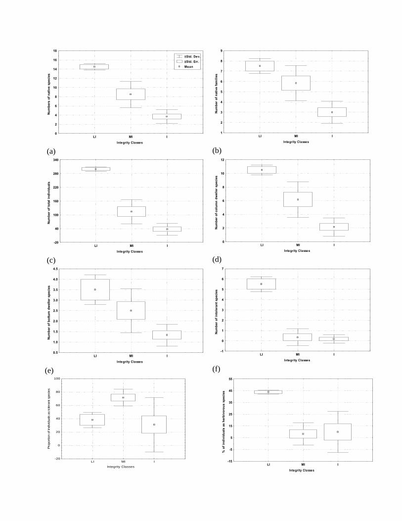
Integrity Classes

Num

bers

of n

ativ

e sp

ecie

s

0

2

4

6

8

10

12

14

16

18

LI MI I


(a) Integrity Classes

Num

ber o

f nat

ive

fam

ilies

1

2

3

4

5

6

7

8

9

LI MI I

(b)

Integrity Classes

Num

ber o

f tot

al in

divi

dual

s

-20

40

100

160

220

280

340

LI MI I

(c) Integrity Classes

Num

ber

of c

olum

n dw

elle

r sp

ecie

s

0

2

4

6

8

10

12

LI MI I

(d)

Integrity Classes

Num

ber o

f bot

tum

dw

elle

r spe

cies

0.5

1.0

1.5

2.0

2.5

3.0

3.5

4.0

4.5

LI MI I

(e) Integrity Classes

Num

ber o

f int

oler

ant s

peci

es

-1

0

1

2

3

4

5

6

7

LI MI I

(f)

Integrity Classes

Prop

ortio

n of

indi

vidu

als

as to

lera

nt s

peci

es

-20

0

20

40

60

80

100

LI MI I

Integrity Classes

% o

f ind

ivid

uals

as

herb

ivor

ous

spec

ies

-15

-5

5

15

25

35

45

55

LI MI I

Chapter 6

188

(g) (h)

Integrity Classes

% o

f ind

ivid

uals

as

omni

voro

us s

peci

es

-6

-2

2

6

10

14

18

22

26

LI MI I

(i)

Integrity Classes

% o

f ind

ivid

uals

as

inve

rtivo

rous

spe

cies

0

15

30

45

60

75

LI MI I

(j)

Integrity Classes

% o

f ind

ivid

uals

as

carn

ivou

rous

spe

cies

0

10

20

30

40

50

60

70

80

90

LI MI I

(k)

Integrity Classes

% o

f ind

ivid

uals

as

non

nativ

e sp

ecie

s

-4

0

4

8

12

16

20

LI MI I

(l)

LI = Less Impaired, I = Impaired and HI = Highly impaired Fig. 6.4 Box and whisker plot showing scores individual IBI metrics in three integrity (a; number

of native species, b; number of native families, c; total number of individuals, d; number of column dweller species, e; number of bottom dweller species, f; number of intolerant species, g; proportion of individuals as tolerant species, h; proportion of individuals as herbivore species, i; proportion of individuals as omnivore species, j; proportion of individuals as invertivore species k; proportion of individuals as carnivore species and l; proportion individuals as of exotic species).

Chapter 6

189

Assessment of IBI along Longitudinal Gradient of Nullah Aik and Nullah Palkhu

and Relationship with Water Quality Parameters

IBI scores for stepped and continuous integrity classes were highest in upstream

sites of Nullah Aik (1 and 2) which decreased to its ebb in the city (site 3 and 4) and

recovered in downstream sites such as 5, 6 and 7 (Fig. 6.5a and b). Maximum IBI scores

for Nullah Palkhu were observed in downstream sites 15, 16 and 17 respectively. Sites 10

and 11 of upstream were moderately rich with fish fauna. Minimum values were observed

at sites 12, 13 and 14 near the city. Upstream sites of Nullah Aik were the least disturbed

sites while sites close to the city towards downstream were highly polluted with untreated

discharge of industrial effluents as well as domestic sewage discharged from city. The IBI

score at downstream sites of Nullah Palkhu increases as these sites receive different

unpolluted water channels and gradually decrease till Wazirabad city. On the contrary to

Nullah Aik, IBI score for downstream of Nullah Palkhu was greater (55). IBI scores

varied along longitudinal gradient in both streams representing the intensity of

anthropogenic stress. The results of stepped and continuous IBI scores showed

longitudinal gradient for Nullah Aik and Palkhu (Fig: 6.5a & b). In case of Nullah Aik

maximum IBI scores (80 and 76) was recorded at upstream sites (1 and 2) which

decreased in mid-stream sites and regain in downstream sites.

Fig 6.6 showed that water quality parameters viz., COD, TDS, turbidity, and

metals had negative correlation with IBI scores. IBI score was significantly positively

correlated with DO and pH. Significantly negative correlation was found between DO,

COD and TDS. Metals such as Cr, Zn and Fe were negatively associated with IBI scores.

COD, TDS and turbidity showed positive correlation with temperature. The results of

physiochemical parameters (such as temperature, pH, DO, COD, EC, TDS, turbidity,

NO3-, PO4

3- and toxic metals such as Fe, Pb, Cd, Cr, Ni, Cu and Zn) of water quality of

different sampling sites are illustrated in Table 6.4 and indicated that variability in water

chemistry was related as a function of stream sites (i.e. unimpaired, moderately impaired,

and severely impaired) and depended on the chemical properties.

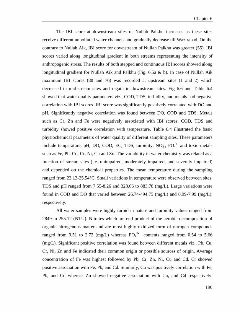
Chapter 6

190

The IBI score at downstream sites of Nullah Palkhu increases as these sites

receive different unpolluted water channels and gradually decrease till Wazirabad. On the

contrary to Nullah Aik, IBI score for downstream of Nullah Palkhu was greater (55). IBI

scores varied along longitudinal gradient in both streams representing the intensity of

anthropogenic stress. The results of both stepped and continuous IBI scores showed along

longitudinal gradient for Nullah Aik and Palkhu (Fig. 6.5a & b). In case of Nullah Aik

maximum IBI scores (80 and 76) was recorded at upstream sites (1 and 2) which

decreased in mid-stream sites and regain in downstream sites. Fig 6.6 and Table 6.4

showed that water quality parameters viz., COD, TDS, turbidity, and metals had negative

correlation with IBI scores. IBI score was significantly positively correlated with DO and

pH. Significantly negative correlation was found between DO, COD and TDS. Metals

such as Cr, Zn and Fe were negatively associated with IBI scores. COD, TDS and

turbidity showed positive correlation with temperature. Table 6.4 illustrated the basic

physiochemical parameters of water quality of different sampling sites. These parameters

include temperature, pH, DO, COD, EC, TDS, turbidity, NO3-, PO4

3- and toxic metals

such as Fe, Pb, Cd, Cr, Ni, Cu and Zn. The variability in water chemistry was related as a

function of stream sites (i.e. unimpaired, moderately impaired, and severely impaired)

and depended on the chemical properties. The mean temperature during the sampling

ranged from 23.13-25.54°C. Small variations in temperature were observed between sites.

TDS and pH ranged from 7.55-8.26 and 328.66 to 883.78 (mg/L). Large variations were

found in COD and DO that varied between 26.74-494.75 (mg/L) and 0.99-7.99 (mg/L),

respectively.

All water samples were highly turbid in nature and turbidity values ranged from

2849 to 255.12 (NTU). Nitrates which are end product of the aerobic decomposition of

organic nitrogenous matter and are most highly oxidized form of nitrogen compounds

ranged from 0.51 to 2.72 (mg/L) whereas PO43- contents ranged from 0.54 to 5.66

(mg/L). Significant positive correlation was found between different metals viz., Pb, Cu,

Cr, Ni, Zn and Fe indicated their common origin or possible sources of origin. Average

concentration of Fe was highest followed by Pb, Cr, Zn, Ni, Cu and Cd. Cr showed

positive association with Fe, Pb, and Cd. Similarly, Cu was positively correlation with Fe,

Pb, and Cd whereas Zn showed negative association with Cu, and Cd respectively.

Chapter 6

191

Concentration of metals such as Fe, Cr, and Zn was highest in highly impaired group

followed by impaired, moderately impaired and lowest in less impaired group. Similar

trend was observed for COD, TDS, salinity and turbidity values. The results also showed

DO and pH was highest in the least impaired and moderately impaired streams sites and

lowest in highly impaired streams sites. Variation in NO3-, and PO4

3- contents were

observed between different impaired groups.

Chapter 6

192

Discussion Variations in Individual IBI Metrics on Spatial Scale and Effect of Environmental

Factors on Fish Assemblages

Impacts of anthropogenic activities related with industrialization, population

expansion, urbanization and agriculture on biological integrity of water resources are very

complex and long-lasting (Hu et al., 2007). Human influences, such as changes in water

chemistry or physical habitat modifications, could alter fish assemblage and diversity by

disrupting their structures and functions. Variations in fish assemblage could be detected

through changes in components of the community, functional groups, species diversity,

and relative abundance. The results showed high fish abundance at reference sites (less

disturbed) in comparison to disturbed sites. These results are analogous to the results

obtained by Karr et al. (1986), Oberdorff & Hughes (1992) and Toham & Teugels (1999).

The results also illustrated that species diversity decreases as human impact increases

(Belpaire et al., 2000, Breine et al., 2004). Sites located on both streams were affected by

various anthropogenic stresses such as industrial effluents, municipal sewage,

atmospheric deposition and surface runoff from agricultural and urban areas. These

factors negatively influence the structure and composition of fish assemblage in streams

passing through cities and can adversely affect their habitat which becomes vulnerable for

fish survival. These results were in accordance with Wichert & Rapport (1998) and

Casatti et al. (2006). Large number of bottom and column dweller species was recorded

from least impaired sites and decreasing trend was observed towards downstream sites.

Column dwellers are generally sensitive to bottom depletion of oxygen and sedimentation

which affect their feeding; Oberdorff & Hughes (1992). Organic and inorganic chemicals

form industrial and domestic sewage (Kestemont et al., 2000) are indiscriminately

discharged into streams which consume dissolved oxygen during oxidation process

resulting depletion of oxygen (Eklöv et al., 1998). Heavy metals and Persistent Organic

Pollutants (POPs) in fresh water have been mainly associated with industrial and

agricultural sources. Accumulation of these pollutants in body tissues of fish species may

result in reduction of growth and cause disturbance in physiological processes (Lwanga et

al., 2003). Upstream sites were less disturbed from anthropogenic activities with large

number of intolerant species which declined toward downstream. Six intolerant species

Chapter 6

193

were recorded from reference sites which were absent from degraded sites. Kennard et al.

(2005) and Habit et al. (2006) also recorded intolerant species from reference sites which

gradually disappear from the sites with high level of contamination. Channa punctata,

Puntius sophore, P. ticto and Heteropneustes fossilis can tolerate pollution stress and

were encountered at moderately degraded sites. Presence of intolerant fish species

generally indicates species richness of sites which are relatively less disturbed by

anthropogenic activities (Karr et al., 1986) in contrast; higher proportion of tolerant

individuals reflects habitat degradation. Tolerant species are the last to disappear in

disturbance conditions and reappear first in comparison to other species as habitat become

favourable (Ganasan & Hughes, 1998). The percentage of carnivorous individuals was

higher at moderately degraded sites in downstream, whereas, minimum proportion was

recorded at least disturbed sites. High percentage of herbivore species was recorded at

reference sites. Similar, results were also reported by Bhat (2003). However, Ganasan &

Hughes (1998) found higher proportion of carnivorous species at reference sites. Stream

width has been identified as important factor which influence richness of herbivore

species i.e., more is the stream width, more will be the proportion of herbivorous species.

The results showed that stream width was higher at reference sites with low flow rate.

This in turn allows suspended sediment to settle down resulting clear water which favours

the establishment of phytoplankton that forms the food of herbivorous fishes (Borges et

al., 2003). Most herbivores species were found upstream and carnivores in the

downstream sites. These results highlighted that more detailed studies on the feeding

habits and preferences of these species are required for better understanding of spatial

pattern in feeding guilds. The relative abundance of insectivorous species found during

current study was almost the same at reference and degraded sites. These results are in

consistent with the findings of Bhat (2004). Among three omnivore species, O. niloticus

was found in the upstream, whereas, other two species such as Garra gotyla and

Heteropneustes fossilis in downstream sites. Oberdorff & Hughes (1992) showed that

omnivorous species had wide range of food selection and can switch from one food to

another. Relatively higher proportion of omnivorous species at reference site may be due

to more availability of food as compared to other sites. Toham & Teugels (1999)

described that omnivorous species are comparatively more successful at reference sites

Chapter 6

194

and degraded sites than any other trophic groups. Among non-native species, O. niloticus

showed wide distribution in upstream as well as downstream of Nullah Palkhu. It is

considered as a potential threat to diversity of native fish fauna of the studied streams. It

was introduced to fresh water resources of Pakistan from River Nile basin in 1985 and

now has been reported in most of rivers, streams, lakes and small ponds (Mirza, 2003). In

contrary to other non-native species, Cyprinus carpio was captured only from site 17,

located downstream of Nullah Palkhu. This species is intensively cultured in ponds and

fish farms to fulfill the local demand of white meat. During monsoon season, due to

heavy rains, fish farms overflow and this species makes its way to streams. According to

Kasulo (2000) non-native species have the ability to spread from one ecosystems to

another through inter connected water ways and have significant impact on local fish

species by predation, resource competition and interference with reproduction. These

species have been reported as a carrier of parasites of different diseases from one

ecosystem to another and used as an ecological indicator of biological health of stream

and river (Kennard et. al., 2005). High richness of non-native species can be correlated

with level of biological degradation. Intrusion of non-native species into freshwater

ecosystem disrupt the food webs making the aquatic ecosystem more vulnerable for

native fauna (Scrimgeour & Chambers, 2000; Wolter et al., 2000; Habit et al., 2006) and

their presence is considered problematic for management and conservation of water

recourses (Kennard et al., 2005).

The results highlighted that fish diversity increases as streams moves downstream.

Vila-Gispert et al., (2002) stated that fish diversity increases from upstream to

downstream of undisturbed streams. Pollutants from point and non-point source and other

factors such as introduction of alien species, exploitation of water for irrigation purpose

and habitat alteration by construction of dams and canals has been recognized as

significant threats for loss of species diversity and changes in spatial trends of species

distribution (Moyle & Leidy, 1992; Lyons et al., 2000; Kouamélan et al., 2003; Mebane

et al., 2003). Fish diversity of Nullah Aik and Palkhu was highly fragmented. Discharge

of untreated pollutants form industries and urban waste, pumping of stream water for

irrigation purposes and presence of small head works at site (7) are main causes of

fragmentation of fish species. These threats may increases the risk of local extinction of

Chapter 6

195

fish species (Cetra & Petrere, 2006). Surface water contamination could result in

reduction in fish diversity and abundance as few tolerant species can only thrive in highly

polluted water due to their adaptability and resistivity to water pollution (Pinto et al.,

2006). The results highlighted that upstream of Aik and Palkhu streams were mainly

affected by agricultural activities, whereas, downstream were heavily polluted from

discharge of untreated industrial effluents and domestic wastes. Walton et al. (2007)

concluded that streams which passed through human settlements generally receive

pollutants from point sources (industrial and municipal sewage) and non-point sources

including agricultural and urban runoff and atmospheric deposition. These pollution

sources inexorably affect directly or indirectly the biota of the streams in particular fish

fauna. Heavy load of industrial and municipal effluents have been recognized to have

negative effect on habitat conditions which become unfavorable for native/sensitive

species and favourable for the opportunist/tolerant species (Pinto et al., 2006). Tolerant

species generally have the ability to survive in organically enriched environment from

industrial and municipal discharges (Ganasan & Hughes, 1998). The results indicated that

upstream sites were dominated by intolerant species as relatively undisturbed habitat

conditions prevail. The fish diversity decreases as study streams passes through Sialkot

metropolitan which lies in midstream region generates large volume of untreated

industrial and municipal wastes. Impairment of sites also increases as study streams

moves from upstream towards downstream. Impairment of study sites can be related to

high level of COD, TDS, turbidity, and toxic metals viz., Cr, Zn, Cu, Pb, Ni, Fe, and Cd

(Qadir et al., 2008). The results found negative correlation of DO with turbidity, COD,

TDS and toxic metals. Less impaired groups showed better water quality in terms of high

level of DO, and low level of COD, turbidity, TDS and toxic metals.

Validation of Reference Sites and Variations in Overall IBI Scores

Defining a reference conditions against which other streams can be compared

present a unique challenge because most of aquatic ecosystems have been alter to some

extent by changes in physical, chemical or biological structure (e.g., impoundment,

pollution, or introduction of exotic species). The selection of reference sites was based on

findings of Sudaryanti et al., (2001), Hart et al. (2001) and Tejerina-Garro et al. (2005).

Chapter 6

196

Sudaryanti et al. (2001) assessed the impact of different human activities on riverine

ecology of river Brantas, Indonesia and indicated that it is difficult to find any un-

disturbed reference site in developing countries due to anthropogenic activities in

catchment area of aquatic resources. They suggested sites with relatively better ecological

characteristics can provide baseline for ecological change in streams and can be

considered as a reference sites because the choice of an appropriate reference condition is

a major problem in most of ecological assessments. The decision about the health of

stream is an essential part of biological assessment (Hughes, 1994). In order to study the

health status of any stream, it should be compared with those stream segments having

best ecological conditions such stream segments are called reference sites. These sites

represent the minimal disturbed conditions indicating the good physio-chemical and

biological quality of the stream (Qadir et al., 2008). In evaluation of ecological health of

streams, it is essential to study various characteristics of the reference site. No completely

undisturbed reference sites were identified in the catchment of Nullah Aik and Palkhu

because of intensive utilization of land resources for urbanization, industrial activities and

agriculture processes (Qadir et al., 2008). Site 1 and 2 were represented as reference sites

were located at 247m and 245m height from the sea level with no apparent source of

pollution in catchment. However, some agricultural activities were found. Thus runoff

from agricultural field and atmospheric deposition of pollutants can be considered the

only source of contamination. These sites showed relatively similar physical, chemical

and biological characteristics. Maximum average width (25.46 and 30.64m) was recorded

from these sites with an average depth (1.10m and 1.00m). Stream bank vegetation of the

two site was very similar dominated by tall grasses mainly Saccharum spp. stream bed

sediment were pre-dominantly sandy with least organic substances. From these sites fresh

water bivalves were also recorded which were absent from other sites and water was clear

with no unpleasant odor which is produced during decomposition process. Thus represent

habitat condition suitable for flourishing of Fish fauna. The results also indicated that

highest fish abundance was recorded from these sites and depicted relatively better

ecological conditions with least impact from anthropogenic processes. The selection of

reference sites was also validated by multivariate techniques such as CA and NMDS.

Among three clusters of sites from streams (viz., less degraded, moderately degraded and

Chapter 6

197

degraded sites) classified using CA, less degraded sites were considered as reference

sites. Similarly, NMDS also separated sites into four groups based on the intensity of

habitat impairment due to anthropogenic stress. Thus least impacted sites selected as

reference sites were treated as threshold level of biological conditions of habitat in terms

of quantitative values of IBI scores.

IBI provides multiple indicator evaluation system to describe biological conditions

of streams (Groom et al., 2005) and has been used to assess the level of impairment at

different spatial scales. The results of metric scores and IBI scores indicated that

degradation of the studied streams can strongly be related to anthropogenic activities. The

results revealed upstream sites with better water quality had higher IBI scores than sites

located midstream and downstream regions. Low IBI scores were related with

environmental degradation and decline in site quality with downstream distance primarily

to increasing impacts from direct discharge of industrial and municipal effluents in the

streams. There is no treatment plant for industrial and sewage treatment in Sialkot city

(Qadir et al., 2008). The effluents are directly discharged either into nearby streams,

drains, ponds or/and agricultural land. Gammon (1998) also attributed agriculture and

urban discharge as major factor responsible for habitat degradation in downstream to

those of upstream region. Anthropogenic disturbance has been recognized as a major

contributor for changing chemical composition of stream water (Qadir et al., 2008) which

ultimately disturbs the ecological integrity of an ecosystem. The results showed

significantly negative correlation of IBI scores with COD, TDS, turbidity, Fe, Cr, Zn and

positive correlation with DO and pH (Fig. 6.6 and Table 6.4). The results stress the role of

industrial and municipal effluents in deterioration of water quality which negatively

influence ecological health of streams.

Chapter 6

198

(a)

(b)

Fig. 6.5 Showing trend of stepped (a) and continuous (b) IBI scores along the

longitudinal distance from upstream to downstream of Nullah Aik and Nullah Palkhu

Chapter 6

199

(a)

R2 = 0.0843

22

23

24

25

26

0 20 40 60 80 100

IBI Score

Tem

p (°

C)

(b)

R2 = 0.3096

7.5

8

8.5

0 20 40 60 80 100IBI Score

pH

(c)

R2 = 0.6325

0

2

4

6

8

10

0 20 40 60 80 100IBI Score

DO

(mg/

L)

(d)

R2 = 0.4884

0

100

200

300

400

500

600

0 20 40 60 80 100

IBI Score

CO

D (m

g/L)

(e)

R2 = 0.3369

300

400

500

600

700

800

0 20 40 60 80 100

IBI Score

TDS

(mg/

L)

(f)

R2 = 0.1286

0

50

100

150

200

250

300

0 20 40 60 80 100

IBI Score

Turb

idity

(NTU

)

(g)

R2 = 0.0002

0

0.5

1

1.5

2

0 20 40 60 80 100

IBI Score

NO

3 (m

g/L)

(h)

R2 = 0.1692

0

1

2

3

4

5

6

0 20 40 60 80 100

IBI Score

PO4

(mg/

L)

Chapter 6

200

R2 = 0.3165

0.1

0.3

0.5

0.7

0.9

0 20 40 60 80 100

IBI Score

Fe (m

g/L)

(i)

(j)

R2 = 0.0138

0.2

0.3

0.4

0.5

0.6

0 20 40 60 80 100

IBI Score

Pb (m

g/L)

(k)

(l)

(m)

(n)

(o)

Fig. 6.6 Graphical representation depicting the relationships of IBI scores and water quality parameters (a. Temp., b. pH, c. DO, d. COD, e. TDS, f. Turbidity, g. NO3

-, h. PO4

3-, i. Fe, j. Pb, k, Cd, l, Cr, m. Ni, n. Cu and o.

Zn).

Chapter 6

201

Factors such as stream discharge, width, depth, and substrate also influence integrity of

aquatic resources and have shown correlation with IBI scores (Casatti et al., 2006).

Regular stream discharge rate and large width of streams generally favour higher IBI

score due to presence of high diversity of intolerant and column dweller species

(Oberdorff & Porchcr, 1992; Tejerina-Garro et al., 2005). Stream discharge, width, depth,

and substrate influence the distribution of fish species (Casatti et al., 2006, Oberdorff &

Porchcr, 1992). Similarly, Radwell & Kwak (2005) also highlighted that physical

attributes of river system are highly influential and play major role in discriminating

among rivers to assess their spatial integrity. Width of Nullah Palkhu increases toward

downstream and sites located downstream showed higher IBI scores. Depth of stream and

rivers also influence the overall IBI scores and is difficult to portray the exact picture of

fish assemblage in deep water due to inadequacy in sampling efforts as cited by Ganasan

& Hughes (1998). Thus, large sized streams with good water quality should have

significantly more species than a small, poor quality stream. Sites located in upstream of

Nullah Aik (reference sites) had higher IBI score and had maximum width which

decreases towards downstream sites. Sites with high IBI scores were least disturbed

which were characterized by complex and sensitive fish assemblages sensitive to changes

in habitat quality. Sensitive species generally avoid polluted sites by relocating their niche

to the sites which are relatively less disturbed (Mebane et al., 2003). Based on

quantitative overall IBI score, three qualitative classes were developed (impaired,

moderately impaired and less impaired). Ganason & Hughes (1998) also adopted

classification system for assessment of ecological integrity of aquatic habitats which

comprised of three qualitative classes (poor, fair and good). The use of less number of

classes has been proven more beneficial for restoration of aquatic ecosystem in

comparison to use of large number of classes (Ganason & Hughes, 1998; Lyons et al.,

2000). Most of sites in two tributaries of Chenab river were impacted with anthropogenic

stress expects sites (1 and 2) located upstream of Nullah Aik. Sites located in upstream

were classified as “less impaired” integrity class on the basis of their high IBI score.

These sites were also characterized with high level of DO and pH in comparison to other

integrity classes. Sites with lowest IBI score placed in impaired integrity classes were

located in downstream, close to Sialkot city, a major source of industrial and municipal

Chapter 6

202

pollution. These sites also had high contents of toxic metal related with anthropogenic

origin such as Cr, Zn, Fe, Ni, Cd, Pb and Cu and lower level of DO and high level of

COD, TDS and turbidity. Ganasan & Hughes (1998) also found minimum IBI scores near

sources of pollution and highest in extreme downstream sites. Water quality of Nullah

Palkhu improves as it stream moves away from the midstream towards downstream to the

Sialkot city in comparison to Nullah Aik. IBI scores for downstream of Nullah Aik did

not improve as it move downstream, probably due to pumping of water from streams for

irrigation purposes (Qadir et al., 2008). Pumping of stream water for irrigation is a known

practice in Pakistan because it’s a cheap source for crops irrigation. Large number of

water pumps was found during sampling. Upstream sites of Nullah Palkhu experience

low flow rate throughout the year especially in early summer and IBI scores for these

sites were in medium range (25 – 35 for stepped IBI and 45 – 65 continuous IBI) and

classified into “moderately impaired” integrity class. As the streams moves away from

Sialkot city towards downstream on the west, water quality gradually improves as small

water channels add in before these streams fall into river Chenab. Improvement of IBI

scores for sites located downstream far from Sialkot city on Nullah Palkhu was observed

which could be related to better water quality and habitat conditions. Many small

channels collecting water from seepage of canals join Nullah Palkhu resulting

improvement of surface water which becomes favorable for re-establishment of fish

assemblages.

During present study, stepped and continuous IBI criteria depicted the similar

results. Stepped and continues IBI criteria were found useful for the quantification of fish

biological integrity of studied streams. Stepped IBI scoring method was developed by

Karr et al., (1986) and later adopted by different authors (Oberdorff & Hughes, 1992;

Minns et al., 1994; Hughes et al., 1998; Toham & Teugels, 1999; McCormick et al.,

2001) with some modification. Dauwalter & Jackson (2004) and Bozzetti & Schulz

(2004) applied the continuous scoring method for the calculation of IBI scores. Mebane et

al. (2003) used continuous IBI scoring method and indicated that it is good for graphical

representation. Ganasan & Hughes (1998) applied the both traditional (stepped) IBI

scoring method as developed by Karr et al. (1986) and continuous IBI scoring methods.

The results of this study supported the use of IBI for the assessment of fish assemblage

Chapter 6

203

and habitat condition. IBI is more practicable index for the assessment and monitoring of

fish assemblage in small streams rather than big rivers and lakes due to sampling

inadequacies (Lyons et al., 2000). These inadequacies are due to more depth of water in

which incomplete fish sampling might have resulted. Other comprehensive and precise

sampling methods such as electro-fishing should be adopted to minimize the sampling

errors (Ganason & Hughes, 1998). Before application of IBI, ecological managers must

consider methods of their sampling effort, selection of reference site, and richness of

native and non-native species to minimize the errors to extract more reliable results

(Mebane et al., 2003). Habitat quality of study of streams is essential to understand the

overall impact of human activities (Spence et al., 1999). This approach is an important

step toward assessment at ecosystem level considering human and environmental factors

(Joy & Death, 2004). Urbanization, ill-planed industrialization in catchment and

discharge of effluent without any treatment into Nullah Aik and Nullah Palkhu is putting

fish assemblage under stress and are constant threat to local streams. This study highlights

the importance of an integrated effort for management and restoration of such ecosystems

using an integrated approach of IBI and multivariate techniques.

Chapter 6

204

Conclusions IBI can be used for assessment and monitoring of fish assemblage in small streams of

Pakistan. The results highlighted that to study the habitat quality study of streams is

essential to understand the overall impact of human activities (Spence et al., 1999). The

results of this study supported the use of IBI as an important tool for ecological

assessment at ecosystem level with consideration of human related environmental factors

and IBI can be used as an indicator for fish assemblage and habitat condition. IBI was

successfully developed and applied for Nullah Aik and Palkhu; tributaries of River

Chenab to assess the stream health of streams at 18 selected sites to portray a wide range

of anthropogenic impacts on fish assemblage. Assessment of stream health using IBI

provided an appropriate approach about habitat condition and its relationships to the

human activities in catchment area and can be used as indicator of freshwater ecosystem

degradation. Comparative assessment of biotic conditions in streams allows along spatial

gradient. Stepped and continuous IBI criteria evaluated the sites from quantitative

information of IBI into qualitative integrity classes (less impaired, moderately impaired

and impaired) with least error. Most of the sampling sites were included in impaired

integrity class, which indicated that fish assemblage of both streams have been altered by

human activities. Finally, it was concluded that IBI based on fish assemblages is the most

useful criteria for the assessment of habitat quality and streams health. Urbanization, ill-

planed industrialization in catchment of study area and discharge of effluent without any

treatment into Nullah Aik and Nullah Palkhu had negative impact on fish assemblage and

diversity. These factors are considered important contributor to wipe out the local aquatic

fauna and constant threat to local streams. The study highlighted the importance of an

integrated effort for management and restoration of stream ecosystems and stresses the

importance to initiate concrete steps to control the indiscriminate discharge of industrial

and municipal waste into the streams from further degradation.

Chapter 7

General Discussion

Anthropogenic activities cause multiple interlinked ecological problems of

Nullah Aik and Nullah Palkhu stream system. Degradation of these streams becomes

intensified after industrial revolution in the catchment area. Direct or indirect

discharge of industrial effluents, municipal sewage and surface runoff are considered

as the main sources of surface water pollution that have deleterious impact on the

physical, chemical and biological components of Nullah Aik and Nullah Palkhu.

It is necessary to quantify the adverse impact of the multiple anthropogenic

activities on ecological integrity of streams for effective management. These multiple

factors are Industrialization, urbanization, atmospheric deposition and surface runoff,

which affect the health status of streams and rivers (Allan, 2004; Kodarkar, 2004).

Human stress is prominent in streams of those regions, where rainfall occurs with

distinct seasonal pattern. This phenomenon is generally observed in temperate

streams, which show wide range of variations in annual flow as well as water quality.

In pristine streams, natural variations such as stream flow, rainfall and temperature

occur after regular intervals and operates stream ecosystem with in natural range of

variations to attain the state of equilibrium (Kauffman et al., 1997) and changes in

natural aquatic system can disrupt its ecological functions (Resh et al., 1988), as well

as structural integrity of an aquatic ecosystem (Kauffman et al., 1997). Industrialization,

urbanization, and intensive agriculture production are the major human activities that

are responsible for deterioration and degradation of stream ecosystem (Sahasrabuddhe

et al., 2003). Ecological factors such as habitat degradation, barrier or abstraction for

water divergence and introduction of alien species in aquatic ecosystems influence the

biological state of streams and rivers (Rahel et al., 2008). Physical, chemical or

biological characteristics have been used world wide for ecosystem management and

restoration (Bundi et al., 2000).

Upstream of Nullah Aik showed good water as well as biological quality, whereas,

middle segment receive huge volume of effluents that acts as chemical barrier, which

restrict the movement of fishes from downstream to upstream. In downstream segment of

Nullah Aik, a small headworks is present that is used to divert stream water for irrigation

Chapter 7

206

purposes. Downstream segment of Nullah Aik also receive effluents from Begowala drain

that bring effluent from tanneries of Sambrial and discharged into Nullah Aik. Therefore,

presence of small headworks, Begowala drain and stream flow regulations are the main

obstacle in improvement of water quality. Upstream of Nullah Palkhu experiences dry

spell during summer season resulting reduction in stream flow even it may become dry

and fishes get refuge in riffle and pools. This dry spell culminates with start of monsoon

rainfalls. Stream fish fauna proliferate during monsoon season to re-establish the fish

community in upstream of Nullah Palkhu. Higher stream flow improves water quality in

downstream of Nullah Palkhu, which is favourable for higher diversity of fishes. Water

logged area in surroundings of UC and MRL canals drain water into downstream of

Nullah Palkhu, which resulted high stream flow. High stream flow dilutes the

concentration of pollutants coming from Sialkot city and stream water quality gets

improved. This improved water quality favours the organization of fish assemblage in

downstream.

Spatial and temporal variations provided better understanding about the

pollutants dynamics in stream water (Podgorney et al., 2000). The first objective of

the present study was to highlight the spatial and temporal variations in stream water

quality and source identification of contaminants. Multivariate statistical techniques

such as HACA, DFA and FA/PCA segregated important variables that explained most

of the spatial and temporal variations and highlighted the contribution of

contamination from different sources. Three classes of sampling sites viz., relatively

unimpaired region (RUR), impaired region (IR) and moderately impaired region

(MIR) were identified on the basis of water quality parameters of stream water using

CA. RUR consisted of upstream sites, which were least contaminated and IR was

highly contaminated.

Discriminant analysis highlighted most important variables, which causes

variations in surface water on spatial and temporal scale. Water quality parameters

identified 11 important parameters viz., stream flow, stream depth, DO, COD, TDS,

NO3-, PO4

3-, Pb (dis), Cr (dis), Mg (sus), and Ni (sus) were important to bring

variations along spatial gradient. Seasonal variations were related with stream flow,

temperature, EC, salinity, total hardness, Na (dis), K (dis), Ca (dis), Mg (dis), Fe (dis),

Cd (dis), Cu (dis) and Na (sus). Spatial variations in water quality are the results of

anthropogenic stress along the longitudinal stretch of the studied streams while,

seasonal variations are mainly derived from natural factors. Low and high stream flow

Chapter 7

207

are controlled by rainfall in the catchment area. Stream flow, discharge and rainfall

determine the concentration of contaminants on seasonal basis. The pollutants from

non-point sources are more pronounced when streams flow at full swing, while point

sources showed marked variations when streams experienced lowest flow rate. Stream

discharge of Nullah Aik and Nullah Palkhu become high during monsoon season,

which causes dilution of contaminant concentration coming from point sources. In dry

period, different pollutants like heavy metals deposited on the soil surface and process

of deposition continue throughout the year. Heavy rainfall during monsoon season

washed away deposited pollutants and increases the concentration in stream water.

Therefore, concentration of pollutants from atmospheric deposition becomes high

during monsoon season.

FA/PCA identified six main sources of different contaminant such as (i)

municipal waste (COD, EC, TDS, turbidity, PO43-, S2-, Na, K, Mg, Pb, Ni and Zn), (ii)

industrial effluents (Fe, Ni, Pb, Cr and Zn), (iii) tanneries effluents (COD, EC, TDS,

turbidity, S2-, Na, Ca, Cr, Zn), (iv) agricultural runoff (NO3-, Pb, Cd, Cu and Zn), (v)

urban runoff (Pb, Cd, Cu and Zn) and (iv) parent rock material (Na, K, Ca and Fe).

Heavy metals contamination is related to multiple sources mainly through industrial,

municipal, atmospheric deposition and surface runoff (Singh et al., 2005a). The

impacts of human degradation on water quality were high during winter and pre

monsoon season when streams flow reduced to lowest level. This reduction in stream

flow makes the situation more critical from ecological as well as aesthetic view.

Higher concentration of heavy metals was measured in suspended particulate matter,

whereas, low concentration was present in dissolved form due to slightly alkaline pH,

high salinity and water hardness level (Wright & Welboun, 2004).

Higher levels of metals in mid-stream region are largely due to tanneries

effluents and municipal sewage along with waste from surgical instrument

manufacturing units. Metals such as Cr, Ni and Zn were associated with point sources

and showed high concentration during dry season, when stream experience low flow.

The state of metals (dissolved and suspended particulate matter) is highly influenced

by physiochemical water quality parameters. High concentration of heavy metals in

dissolved form is considered as potential threat for aquatic organisms (Guéguen &

Dominik, 2003). Among metals in dissolved form Fe, Pb, Cd, Cr and Ni were

recorded higher to those of permissible levels. The high load of heavy metals in

stream water is one of the major concerns for aquatic biota of the studied stream.

Chapter 7

208

Second objective of the present study was the assessment of bioaccumulation

patterns of heavy metals in different organs (liver, gills, kidneys and muscles) of fish

species on spatial and temporal scales. Highest metal accumulation was recorded in

liver followed by gills, kidneys and muscles. Significant variations of heavy metals

accumulation were observed in different organs within same and among different

species. The physiology of healthy fish do not allow the accumulation of metals in its

organs and excrete the large amounts of heavy metals (Pourang, 1995) resulting in low

accumulation of metals in fish. The results revealed that elevated concentration in

various organs like liver and gills is influenced by contaminated environment with

heavy metals for longer time periods (Goldstein & DeWeese, 1999). Elevated level of

heavy metals reduces the growth and disturbed body physiology (Maity et al., 2008).

Fishes with elevated level of metals represent the degraded health of freshwater

ecosystem. Feeding habits and trophic position in food chain also contributes to

differences in bioaccumulation of different metals (Tawari-Fufeyin & Ekaye, 2007).

Bioavailability of heavy metals is also influenced by metal form (either dissolved or

suspended) in surrounding medium (Rainbow, 1995). Dissolved form of metals,

which are readily available to fishes cause toxic effects on physiological equilibrium

of fishes (Playle, 1998). The cumulative affect of heavy metals usually lead to acute or

chronic stress and eventually causes the death of fish species (Fromm, 1980).

Accumulation of Pb and Cr in different organs of fishes was significantly

different between upstream and downstream segments of streams, whereas, Fe, Cd,

Ni, Cu and Zn did not show significant spatial variations in different fish species.

Metal accumulation was highest at down stream of Nullah Aik and Nullah Palkhu and

lowest at upstream of Nullah Aik and Nullah Palkhu. High metal concentration in

fishes captured from downstream sites was due to increased concentration in ambient

stream water. The mid stream and downstream sites were contaminated with heavy

metals especially Pb and Cr, which were related with industrial effluent and municipal

sewage discharged from tanneries and municipalities in catchment area. Concentration

of Fe, Cd, Cr and Cu showed significant seasonal variations. High concentrations of

heavy metals were recorded during pre monsoon season, when stream water exhibited

elevated level of metals.

Significant inter-specific variations in the bioaccumulation pattern of heavy

metals were recorded. Pb, Cd and Cr in muscles of Channa punctata, Labeo rohita,

Cirrhinus reba, Puntius sophore and Wallago attu captured from downstream of

Chapter 7

209

Nullah Aik and Nullah Palkhu exceeded the permissible level described by United

States Environmental Protection Agency (1999).

Fish muscles are important for human consumption point of view (Alibabić et

al., 2007). Metals viz., Pb, Cd and Cr were recorded above the permissible limits of

heavy metals in muscles of Labeo rohita, Puntius sophore, Channa punctata,

Oreochromis niloticus and Wallago attu. The concentration of Pb was reported higher

in Labeo rohita, Puntius sophore, Channa punctata and Wallago attu. Higher

concentration of Cd and Cr was reported in muscles of Cirrhinus reba, Channa

punctata and Oreochromis niloticus. Higher concentration of Pb and Cd can be

related to non-point sources. Metals absorbed by fish through gills and digestive

system while Cr is related to tanneries into stream water. High concentration of heavy

metals in stream water increases the process of bioaccumulation in fish species,

particularly, intolerant species that can survive in polluted water. However, further

investigations are required to predict the distribution pattern of heavy metals in fish

species at various trophic levels.

Third objective of present study was to describe the diversity and temporal

distribution pattern of different fish assemblage in relation to stream water quality.

Fish assemblage in the regular streams exhibited fewer variations in flow regime

remains stable through out the year (Casatti, 2005). However, flow of intermittent

streams varies from season to season through natural annual cycle that affects the fish

assemblage (Grossman et al., 1990). Anthropogenic disturbance, which is more

pronounced in studied streams, may disturb the fish assemblage (Franssen et al.,

2006). When streams exhibited low flow along the high level of human disturbance,

this unfavorable condition force the fish assemblage to move in least polluted segment

of stream (Vila-Gispert et al., 2002). Due to pollution stress, sensitive fish species

become vanished from polluted stream and their biological niche become occupied by

invasive species. However, if particular segment of stream is less diverse, fish

assemblage will regain during favourable season like monsoon.

A total of 24 fish species belonging to 12 families were recorded from Nullah

Aik and Nullah Palkhu. Maximum diversity were recorded in upstream sites and

lowest at downstream of Nullah Aik. Channa punctata and Puntius sophore were the

most dominant species and found at most of the sites. Upstream of Nullah Aik showed

better and least disturbed conditions that favour the proliferation of fishes. The

upstream fish assemblage was comparatively stable in different seasons under natural

Chapter 7

210

conditions but stream segment faces the anthropogenic stress in urban area do not

support the fish life due to high degradation of surface water. As streams traverse

through Sialkot city, receives a large volume of industrial effluent (especially from

tanneries) and municipal sewage resulting in deterioration of water quality, which has

negative impacts on fish species.

The present study concluded that municipal and industrial activities are putting

fishes of stream under stress in comparison to non-point sources. Municipal and

industrial effluents decrease the level of DO and increase the COD level and heavy

metals. Most of the fish species cannot tolerate the low concentration of DO and high

level of COD and heavy metals in stream water. In downstream sites, only those

species were found, which can tolerate fluctuations in DO level and high level of

COD, turbidity and heavy metals. Fish species richness increases as water quality

improves in downstream. Comparatively less improvement in fish fauna in

downstream of Nullah Aik was observed. This may be due to the presence of small

headworks, diversion of water for irrigation and Begowala drain that bring large

volume of tanneries effluents. As a result of such constraints these sites remain

impaired for re-appearance of native fish fauna, however, those species, which can

tolerant pollution stress may reappear. In comparison downstream sites of Nullah

Palkhu, showed maximum diversity especially in post monsoon season due to

improved water quality.

The fourth objective of present study was to develop and apply an index of

biological integrity for quantification of ecological degradation of Aik and Palkhu

streams. Two kinds of IBI scoring criteria (continuous IBI and stepped IBI) were

developed. Three spatial groups of sites were obtained based on fish abundance data.

This group includes least impaired sites (1 and 2), which exhibited most of the

characteristics of reference conditions, impaired sites (3, 4, 5, 8, 12, 13 and 14) and

moderately impaired sites (6, 7, 9, 10, 11, 15, 16, 17 and 18). Three major guilds of

spatial preference groups were identified on the basis of fish associations viz.,

upstream guild, evenly distributed guild and downstream guild. NMDS identified the

four groups of sites on the basis of habitat impairment and species richness. Based on

NMDS species ordination, three groups were identified on the basis of stress tolerance

and habitat impairment. Maximum IBI score was calculated from upstream sites of

Nullah Aik, whereas, minimum of zero score was calculated from those sites where no

fish specimen was recorded.

Chapter 7

211

One of the main constrain in present study was the absence of an ideal

reference site in the catchment area. Following the studies of Sudaryanti et al. (2001),

Hart et al. (2001) and Tejerina-Garro et al. (2005) reference sites were identified on

the basis of fish diversity data and subjected to cluster analysis. Two sites located in

upstream of Nullah Aik showed maximum species richness and abundance and were

considered as reference sites i.e., least disturbed sites. Sites in close downstream of

Sialkot city showed minimum fish species richness and abundance. These sites

showed highest level of contaminants in stream water. On the other hand, the sites

located in far downstream of streams represent intermediate range of fish species

richness and abundance. Sensitive species were recorded at reference sites. No fish

species was recorded in close premises of point sources located in Sialkot city. As

stream water traverse the distance toxic substances settle down in stream sediments

and water quality improves. Only tolerant fish species were found in far downstream

sites due to the improvement of stream conditions.

Improvement in IBI scores in downstream sites of Nullah Palkhu was evident

in contrast to Nullah Aik, which was due to presence of small head works at Wain and

Begowala drain discharge huge volume of tanneries effluents into Nullah Aik at Kot

Zamin (Fig. 2.1) after traversing 25km. Last site located on Nullah Aik receives

effluents from few tanneries located at Sialkot-Wazirabad road municipal sewage

from Wazirabad city. Low IBI scores were recorded from the sites located in upstream

of Nullah Palkhu as stream flow become reduced even stream become dry during pre

monsoon season, when fishes refuge in small ditches and pools which restrict the

proliferation of fish communities. IBI index appears quite useful for understanding

and interpreting the stream health and the human impacts on aquatic ecosystem. The

IBI score for each site was found to be more reliable in response to human impact on

aquatic ecosystem. The results of present study supported the use of IBI for the

quantitative assessment of fish assemblage and human pressure on stream health.

Therefore, fish communities in various segments of a stream are the best indicators of

overall biological integrity. These streams are also facing a serious infestation of

exotic species in upstream and downstream sites which indicate stream ecosystem is

fragile. Habitat degradation of streams provided an opportunity for the invasion of exotic

fish species. Two exotic species in upstream as well downstream sites were recorded.

Invasion of exotic species is another critical issue for the stream health in Nullah Aik and

Nullah Palkhu.

Chapter 7

212

This study presents an integrative approach about the impacts assessment of

human activities on natural aquatic ecosystem of two streams. This document provides

information related to impacts of human activities on water quality and fish fauna and

a guideline document for future research endeavours on various aspects of Nullah Aik

and Nullah Palkhu. The behaviour of contaminants was investigated on spatial and

temporal basis and their impacts on the fish fauna residing in Nullah Aik and Nullah

Palkhu, which was not previously studied. Human activities such as industrial,

urbanization and agriculture are rapidly increasing in the catchment area of Nullah

Aik and Nullah Palkhu. As a result of these activities, a huge volume of effluents

containing many toxic pollutants such as heavy metals are directly or/and indirectly

discharged into Nullah Aik and Nullah Palkhu, which are degrading physical,

chemical and biological integrity and these effects were at the sites, which were

located near the point sources with low stream flow rate. Fishes dwelling in such

polluted stream segment are under stress of heavy metals, which have led to

fragmentation of fishes into upstream and downstream of streams. This encourages the

invasion of exotic fish species that severely change the structure and function of

ecosystem and reduce the stream biodiversity. Nullah Aik and Nullah Palkhu are one

of the main water sources for human use since long time and important natural source

for local community but present health status indicates that it is unacceptable for

human, domestic, and agricultural usage. The restoration of Nullah Aik and Nullah

Palkhu is necessary not only for the well being of local area but also for aquatic

integrity of River Chenab. This is the need of hour, peep into the matter of water

quality deterioration and loss of fish fauna in Nullah Aik and Nullah Palkhu for

restoration of polluted stream ecosystems and protection of human health at large.

This alarming situation demands dire attention of concerning authorities like Govt.

authorities, municipalities and environmental agencies to come and play effective role

in protection, management and conservation of streams. The results of this research

can be used for effective restoration of Aik-Nullah system.

Chapter 7

213

Recommendations For the improvement of conditions in stream and catchment area

Following are the proposed recommendations to improve the environmental

conditions in catchment area and instream conditions of Nullah Aik and Nullah

Palkhu:

• Concerned authorities (National, Provisional, District Govt., Environmental

department etc.) should take immediate measures (such as complete ban on

discharge of untreated industrial effluent and municipal sewage) for restoration of


• There should be proper regulations for the production and dumping of effluents

produced as a result of anthropogenic activities in the catchment area.

• Environmental impact assessment should be done before the construction of any

industrial unit, housing colonies and other structures.

• Heavy fines should be imposed on those authorities, industries and individuals

which discharge wastes whether it is liquid or in solid form.

• Taxes should be charged from authorities; industries and individuals on the basis

of pollute and pay principle.

• Stream management activities should be implemented on the priority basis in

stream segments traversing in urban and industrial area.

• People residing in proximity of the Nullah Aik and Palkhu should be educated

about the negative impacts of stream pollution in relation to human health and

broadly at ecosystem level.

For the improvement of stream water quality

The recommendations for the improvement of water quality of Nullah Aik and

Nullah Palkhu are as under:

• Effective measures (proper legislation, implementation of environmental laws,

stream management etc.) should be adapted to reduce the deleterious contributions

of point sources that degrade the water quality of Nullah Aik and Nullah Palkhu

especially, focusing on those water quality attributes that are contributing to major

spatio-temporal variations and their concentration above the international

environmental standards.

Chapter 7

214

• Strict criteria should be developed and applied to treat the effluents at their

generation site.

• Waste treatment plants should be established for the effective treatment of

industrial and municipal waste.

• All industrial units should be encouraged to adopt the effluent treatment

techniques at the source and those units which are violating and discharging their

effluent without treatment should be punished.

• There should be a regular monitoring of industrial units, municipal sewage into

stream water.

• People belonging to various segments of the community (stakeholders) should be

encouraged to highlight the aquatic pollution problems and educate people about

the deleterious effects of pollutants on aquatic ecosystem and their harmful

impacts on human life.

• Guidelines of stream water should be developed not only for Nullah Aik and

Palkhu but also for other streams and rivers at national level. This requires

repeated experiments to establish the local water quality standards.

For the protections and regrouping of fish assemblage

Following recommendations are based on the information extracted from

results and discussion to improve the conditions for fish assemblage in Nullah Aik and

Nullah Palkhu:

• If above mentioned recommendations are followed, ultimately it will lead towards

reorganization of biological communities in Nullah Aik and Palkhu.

• There should be a regular assessment of metal contents in different organs of fish

species dwelling in Nullah Aik and Nullah Palkhu to educate the people about

consequences consumption of contaminated fish meat.

• There should not be physical barriers like headworks to divert water for irrigation,

which restrict the movement of fishes. If such structures are inevitable then there

should be a fish ladder for the movement of fishes from downstream to upstream.

• The stream habitat should be managed to provide better conditions for nesting and

breeding sites of fishes within streams.

Chapter 7

215

Future Thrusts

Pakistan is among those countries, which have little or no baseline data and

information for its stress stricken water bodies. The economy of Pakistan is readily

growing with rapid industrialization, urbanization and extensive agriculture, which

have placed the aquatic resources under immense stress. Scientific studies and

investigations such as the present one is necessary for the environmental management

and conservation activities. It is strongly recommended that current study should be

continued in term of physiochemical and biological components of focused streams.

• Comprehensive survey should be conducted to assess the volume of effluents

that are discharged through different point sources into stream system.

• The focus of future studies should be broadened to assess the status of

persistent organic pollutants (POPs) along with heavy metal contamination.

• Macro-invertebrates such as aquatic crustaceans and mollusks founded at the

upstream sites should be investigated as potential biological indicators on

spatial and seasonal scales.

• Birds and turtles are other important group of vertebrate residing in and along

the streamside could be studied as good biological indicators for the bio-

magnification of heavy metals and organic pollutants.

• Fish sampling should be done with help of electro-fisher and compared with

traditional netting at regular intervals conducted during post monsoon and pre

monsoon seasons to find out pattern of fish assemblage.

• The IBI criteria should be applied not only for fishes but also for macro-

invertebrates, birds and aquatic plants to assess the more accurate information

about the degradation of an aquatic ecosystem.

• Newly developed IBI criteria for streams under focus should be applied on

other streams of the same region to test its efficacy and utility.

• There should be a comprehensive study on the invasion of exotic species in

natural streams and their potential impacts on the aquatic ecosystems.

References Abbas ST, Mehdi SM, Sarfraz M & Hassan G (2004). Contents of heavy-metals in

waters of Nullahs Dek, Bisharat & Aik and their effect on soil-health. Science

Vision, 9: 1 - 11.

Abegaz T, Legesse W & Tiku S (2005). Determination of critical concentration and

diurnal variation of dissolved oxygen (DO) in relation to physicochemical

variables in Boye Pond, South Western Ethiopia. African Journal of

Environmental Assessment and Management, 10: 66 - 76.

Addiscott TM (1996). Fertilizers and nitrate leaching. Issues in Environmental

Science and Technology, 5: 1 - 26.

Aftab Z, Ali L, Khan AM, Robinson AC & Irshad IA (2000). Industrial Policy and the

Environment in Pakistan. United Nations Industrial Development Organization.

Agarwal R, Kumar R & Behari JR (2007). Mercury and lead content in fish species

from the River Gomti, Lucknow, India, as biomarkers of contamination.

Bulletin of Environmental Contamination and Toxicology, 78: 108- 112.

Akhtar N, Ahmad T, Gulfraz M & Khanum R (2005). Adverse effects of metal ions

pollution on aquatic biota and seasonal variations. Pakistan Journal of

Biological Sciences, 8: 1086 - 1089.

Akin S, Buhan E, Winemiller KO & Yilmaz H (2005). Fish assemblage structure of

Koycegiz Lagoon-Estuary, Turkey: Spatial and temporal distribution patterns

in relation to environmental variation Estuarine, coastal and shelf science, 64:

671- 684.

Alam MGM, Tanaka A, Allinson G, Laurenson LJB & Stagnitti F (2002). A

comparison of trace element concentrations in cultured and wild carp

(Cyprinus carpio) of Lake Kasumigaura, Japan. Ecotoxicology and

Environmental Safety, 53: 348 - 354.

Alam SM & Naqvi MH (2003). Water Scenario and Pakistan. NIA, Tandojam,

Pakistan. Available on http://www.pakistaneconomist.com/pagesearch/Search-

Engine2003/S.E180.asp

Alberto WD, Delpilar DM, Valeria AM, Fabiana PS, Cecilia HA & De Los Angeles,

BM (2001). Pattern recognition techniques for the evaluation of spatial and

temporal variations in water quality. A Case Study: Suquia River Basin (Co´

Rdoba – Argentina). Water Research, 35: 2881 - 2894.

References

217

Alibabić V, Vahčić N & Bajramović M (2007) . Bioaccumulation of Metals in Fish of

Salmonidae Family and the Impact on Fish Meat Quality Environmental

Monitoring and Assessment, 131: 349 - 364.

Allan JD (2004). Landscapes and Riverscapes: The Influence of Land Use on Stream

Ecosystems. Annual Review of Ecological Evolutionary Systematics, 35: 257-

84.

Allen SE, Parkinssons HMJA & Ouarmby C (1974). Chemical Analysis Ecological

Material. Blackwell Scientific Publication, Oxford, UK.

Allen-Gill SM & Martynov VG (1995). Heavy metal burdens in nine species of

freshwater and anadromous fish from the Pechora River, northern Russia.

Science of the Total Environment, 160-161: 653 - 659.

Alther GR (1981). The use of stream sediments to infer water quality on a stream in

northwestern Ohio. Ohio Journal of Sciences, 81: 247- 252.

Amin O (1996). Heavy metal concentrations in litteral sediments from the Beagle

Channel, Tierra Del Fuego, Argentina. Environmental Monitoring and

Assessment, 4: 219- 231.

Amundsen PA, Staldvik FJ, Lukin AA, Kashulin NA, Popova OA & Reshetnikov YS

(1997). Heavy metal contamination in freshwater fish from the border region

between Norway and Russia. Science of the Total Environment, 201: 211- 224.

Anazawa K, Kaido Y, Shinomura Y, Tomiyasu T & Sakamoto H (2004). Heavy metal

distribution in river waters and sediments around a “ firefly village,” Shikoku,

Japan: Application of multivariate analysis. Analytical Sciences, 20: 79- 84.

Anctil M & Ali MA (1976). Cone droplets of mitochondrial origin in the retina of

Fundulus heteroclitus (Pisces: Cyprinodontidae). Zoomorphology, 84: 103 -

111.

Andreji J, Stránai I, Massányi P & Valent M (2006). Accumulation of some metals in

muscles of five fish species from Lower Nitra River. Journal of Environmental

Health, Part A, 41: 2607 - 2622.

Angermeier PL & Karr JR (1994). Biological integrity versus biological diversity as

policy directives, protecting biotic resources. Biosciences, 44: 690 - 697.

Angermeier PL & Winston MR (1998). Local vs. regional influences on local

diversity in stream fish communities of Virginia. Ecology, 79: 911 – 927.

Anonymous (2007). Discharge data of drains in Ruchna drainage division,

Sheikupuara, Punjab Irrigation Department, Lahore, Pakistan.

References

218

Ansari AA, Singh IB & Tobschall HJ (1999). Status of anthropogenically induced

metal pollution in the Kanpur-Unnao industrial region of the Ganga Plain,

India. Environmental Geology, 38: 25 - 33.

Aparicio E, Vargas MJ, Olmo JM & de Sostoa A (2000). Decline of native freshwater

fishes in a Mediterranean watershed on the Iberian Peninsula: a quantitative

assessment. Environmental Biology of Fishes, 59: 11 - 19.

APHA (1992). Standard methods for the examination of water and waste water, 18th

edition. American Public Health Association, American Water Works

Association (AWWA) and Water Pollution Control Federation (WPCF),

Washington DC, USA.

APHA (1998). Standard methods for the examination of water and waste water, 20th

ed., American Public Health Association, Washington DC, USA.

Araújo FG (1998). Adaptação do índice de integridade biótica usando a comunidade

de peixes para o rio Paraíba do Sul. Revista Brasileira Biologia, 58: 547 - 558.

Arunachalam M (2000). Assemblage structure of stream fishes in the Western Ghats

(India). Hydrobiologia, 430: 1 - 31.

Asuquo FE, Ewa-Oboho I, Asuquo EF & Udo PJ (2004). Fish species used as

biomarker for heavy metal and hydrocarbon contamination for Cross River,

Nigeria. The Environmentalist, 24: 29 - 37.

Atchison GJ, Henry MG & Sandheinrich MB (1987). Effects of metals on fish

behavior: A Review. Environmental Biology of Fishes, 18: 11 - 25.

Avenant-Oldewage A & Marx HM (2000). Bioaccumulation of chromium, copper and

iron in the organs and tissues of Clarias gariepinus in the Olifants River,

Kruger National Park. Water Sanitation, 26: 569 - 582.

Bajc ZKŠ, Gačnik JV & Doganoc DZ (2005). The contents of Cu, Zn, Fe and Mn in

Slovenian Freshwater Fish. Slovenian Veterinary Research, 42: 15 - 21.

Bajza Z & Vrcek IV (2001). Water quality analysis of mixtures obtained from tannery

waste effluents. Ecotoxicology and Environmental Safety, 50: 15 - 18.

Bartram J & Balance R (1996). Water quality monitoring - A practical guide to the

design and implementation of freshwater quality studies and monitoring

programmes. Published on behalf of United Nations Environment Programme

and the World Health Organization.

References

219

Batley GE (1983). The current status of trace element speciation studies in natural

waters. In Trace element speciation in surface waters and its ecological

implication. Plenum Press, New York, USA.

Beldi H, Gimbert F, Maas S, Scheifler R & Soltani N (2006). Seasonal variations of

Cd, Cu, Pb and Zn in the edible mollusc Donax trunculus (Mollusca, Bivalvia)

from the gulf of Annaba, Algeria. African Journal of Agricultural Research, 1:

85 - 90.

Belliard J, Thomas RB & Monnier D (1999). Fish communities and river alteration in

the Seine Basin and nearby coastal streams, Hydrobiologia, 400: 155 - 166.

Belpaire C, Smolders R, Vanden AI, Ercken D, Breine J, Van Thuyne G & Ollevier F

(2000). An index of biotic integrity characterizing fish populations and the

ecological quality of Flandrian waterbodies. Hydrobiologia, 434: 17- 33.

Bengeri KV & Patil HS (1986). Respiration, liver glycogen and bioaccumulation in

Labeo rohita exposed to zinc. Indian Journal Comparative Animal Physiology,

4: 79 - 84.

Benoit DA (1975). Chronic effects of copper on survival, growth and reproduction of

the bluegill (Lepomis macrochirped). Transactions of the American Fisheries

Society, 104: 353- 358.

Beraldo P, Pinosa M, Tibaldi E & Canavese B (1995). Abnormalities of the

operculum in Gilthead Sea bream (Sparus aurata). Pollution Bulletin, 31: 183

- 192.

Bervoets L, Blust R & Verheyen R (2001). Accumulation of metals in the tissues of

three Spined Stickelback (Gasterosteus aculeatus) from Natural Fresh Waters.

Ecotoxicology and Environmental Safety, 48: 117- 127.

Besser JM, Brumbaugh WG, May TW & Schmitt CJ (2007). Biomonitoring of Lead,

Zinc and Cadmium in streams draining Lead-mining and non-nining areas,

Southeast Missouri, USA. Environment Monitoring and Assessment, 129: 227

- 241.

Bhalli JA & Khan QM (2006). Pollution analysis in tanneries effluents collected from

three different cities of Punjab, Pakistan. Pakistan Journal of Biological

Sciences, 9: 418 - 421.

Bhat A (2003). Diversity and composition of freshwater fishes in river systems of

Central Western Ghats, India. Environmental Biology of Fishes, 68: 25 - 38.

References

220

Bhat A (2004). Patterns in the distribution of freshwater fishes in rivers of Central

Western Ghats, India and their associations with environmental gradients.

Hydrobiologia, 529: 83 - 97.

Boët P, Duvoux B, Allardi J & Belliard J (1994). Incidence des orages estivaux sur les

peuplements pi de la Seine à l’aval de l’agglomération parisienne (bief

Andrésy - Méricourt). La Houille Blanche, 1- 2: 141- 147.

Boman BJ, Wilson PC & Ontermaa EA (2002). Understanding water quality

parameters for citrus irrigation and drainage systems, Circular 1406, U.S.

Department of Agriculture, Cooperative Extension Service, University of

Florida, IFAS, Florida, USA.

Borges PAF, Rodrigues CL, Pagioro TA & Train S (2003). Spatial variation of

phytoplankton and some abiotic variables in the Pirapó River - PR (Brazil) in

August 1999: A preliminary study. Acta Scientiarium, 25: 1 - 8.

Bosnic M, Buljan J & Daniels RP (2000). Pollutants in tannery effluents: definitions

and environmental impact limits for discharge into water bodies and sewers,

Regional Programme for Pollution Control in the Tanning Industry in South-

East Asia, United Nations Industrial Development Organization pp 1- 26.

Available on https://www.unido.org/userfiles/ PuffK/L _pollutants.pdf

Boyd CE & Massaut L (1999). Risks associated with the use of chemicals in pond

aquaculture. Aquacultural Engineering, 20: 113 - 132.

Boyd CE (2000). Water quality: An introduction. Kluwer Academic Publishers

Boston, MA, USA.

Boyles W (1997). The science of chemical oxygen demand bluebook. Hach Company,

USA.

Bozzetti M & Schulz UH (2004). An index of biotic integrity based on fish

assemblages for subtropical streams in southern Brazil. Hydrobiologia, 529:

133 - 144.

Brady NC & Weil RR (1996). The Nature and Properties of Soils. 11th Edition,

Prentice-Hall, Upper Saddle River, NJ, USA.

Breine J, Simoens I, Goethals P, Quataert P, Ercken D, Liefferinghe CV &

Liefferinghe CV & Belpaire C (2004). A fish-based index of biotic integrity

for upstream brooks in Flanders (Belgium). Hydrobiologia, 522: 133- 148.

References

221

Brown LR, Gray RH, Hughes RM & Meador MR (2005). Introduction to effects of

urbanization on stream ecosystems. American Fisheries Society Symposium,

47: 1 - 8.

Buhl KJ & Hamilton SJ (1996). Toxicity of inorganic contaminants, individually and

in environmental mixtures, to three endangered fishes (Colorado squawfish,

bonytail and razorback sucker). Archives of Environ- mental Contamination

and Toxicology, 30: 84 - 92.

Bundi U, Peter A, Frutiger A, Hütte M, Liechti P & Sieber U (2000). Assessing the

Ecological Integrity of Running Waters. Scientific base and modular concept

for comprehensive assessment of streams in Switzerland. Hydrobiologia

422/423: 477- 487.

Burger J, Gaines KF, Boring CS, Warren L, Stephens Jr, Snodgrass J & Gochfeld M

(2001). Mercury and Selenium in Fish from the Savannah River: Species,

Trophic Level and Locational Differences. Environmental Research Section A,

87: 108- 118.

Bury NR, Walker PA & Glover CN (2003). Nutritive metal uptake in teleost fish:

Review. The Journal of Experimental Biology, 206: 11- 23.

Campbell KR (1995). Bioaccumulation of Heavy Metals in Fish living in stormwater

treatment ponds. Technical Publication SJ95-1St. Johns River Water

Management District Palatka, Florida, USA.

Campenhout KV, Infante HG, Adams F & Blust R (2004). Induction and Binding of

Cd, Cu and Zn to Metallothionein in Carp (Cyprinus carpio) Using HPLC-

ICP-TOFMS. Toxicological Sciences, 80, 276 - 287.

Canadian Council of Ministers of the Environment CCME (1999). Canadian water

quality guidelines for the protection of aquatic life: Chromium- Hexavalent

chromium and trivalent chromium. In: Canadian environmental quality

guidelines, Publication No. 1299; ISBN 1- 896997- 34- 1. Canadian Council of

Ministers of the Environment, Winnipeg, MB, Canada.

Canli M & Atli G (2003). The relationships between heavy metal (Cd, Cr, Cu, Fe, Pb,

Zn) levels and the size of six Mediterranean fish species. Environmental

Pollution, 121: 129 - 136.

Canli M, Ay Ö & Kalay M (1998). Levels of heavy metals (Cd, Pb, Cu, Cr and Ni) in

tissue of Cyprinus carpio, Barbus capito and Chondrostoma regium from the

Seyhan River, Turkey. Turkish Journal of Zoology, 22: 149 - 157.

References

222

Caruso JA, Klaue B, Michalke B & Rocked DM (2003). Group assessment: Elemental

speciation. Special Issue on Methodologies for Assessing Exposures to Metals:

peciation, bioaccessibility and bioavailability in the environment, food and

feed. Ecotoxicology and Environmental Safety, 56: 32- 44.

Casatti L (2005). Fish assemblage structure in a first order stream, southeastern Brazil:

longitudinal distribution, seasonality, and microhabitat diversity. Biota

Neotropical, 5: 75 - 83.

Casatti L, Langeani F & Ferreira CP (2006). Effects of physical habitat degradation on

the stream fish assemblage structure in a Pasture Region. Environmental

Management, 38: 974- 982.

Castillo-Rivera M, Zavala-Hurtado JA & Rocýo Z (2002). Exploration of spatial and

temporal patterns of fish diversity and composition in a tropical estuarine

system of Mexico. Reviews in Fish Biology and Fisheries, 12: 167-177.

CEC (1978). Council Directive of 18 July 1978 on the quality of fresh waters needing

protection or improvement in order to support fish life, (78/659/EEC). Official

Journal, L/222, 1-10.

Cetra M & Petrere M (2006). Fish-assemblage structure of the Corumbatai river basin,

São Paulo state, Brazil: Characterization and anthropogenic disturbances.

Brazilian Journal of Biology, 66: 431 - 439.

Chakrapani GJ (2005). Major and trace element geochemistry in upper Ganga river in

Himalayas, India. Environmental Geology, 48: 189 - 201.

Chapman D (1996). Water quality assessments. A guide to the use of biota, sediments

and water in environmental monitoring. 2nd edition. UNESCO/WHO/UNEP.

Charlesworth SM & Lees JA (1999). The transport of particulate-associated heavy

metals from source to deposit in the urban environment, Coventry, UK.

Science of the Total Environment, 235: 351 - 353.

Chatterjee SB, Chattopadhyay SK & Mukhopadhyay (2006). Trace Metal distribution

in Tissues of Cichlids (Oreochromis niloticus and O. mossambicus) collected

from Wastewater-fed Fish ponds in East Calcutta Wetlands, A Ramsar site.

Acta Ichthyologica et Piscatoria, 36: 119 - 125.

Choi KS & Blood E (1999). Modeling developed coastal watersheds with the

agricultural non-point source model. Journal of the American Water Resources

Association, 35: 233 - 244.

References

223

Clark RB (2001). Marine pollution (5th Edition). Oxford, England: Oxford University

Press, England, UK.

Clarke KR & Warwick RM (1994). Change in Marine Communities: An Approach to

Statistical Analysis and Interpretation. Plymouth Marine Laboratory, Plymouth,

UK.

Colman JA & Sanzolone RF (1992). Geochemical characterization of streambed

sediment in the upper Illinois river basin. Journal of the American Water

Resources Association, 28: 933 - 950.

Connell D, Lam P, Richardson B & Wu R (1999). Introduction to Ecotoxicology.

Blackwell Science, Oxford, UK.

Costa MJ, Vasconcelos R, Costa JL & Cabral HN (2007). River flow influence on the

fish community of the Tagus estuary (Portugal). Hydorbiologia, 587: 113 - 123.

Courtemanch DL, Davies SP & Laverty EB (1987). Incorporation of biological

information in water quality planning. Environmental Management, 13: 35- 41.

Crosa G, Froebrichb J, Nikolayenkoc V, Stefanid F, Gallid P & Calamaria D (2006).

Spatial and seasonal variations in the water quality of the Amu Darya River

(Central Asia). Archives of Environmental Contamination and Toxicology, 40:

2237 - 2245.

Dale VS, Chang M & Ojima D (2005). Ecological Impacts and Mitigation Strategies

for Rural Land Management. Ecological Applications, 15: 1879 - 1892.

Das M (2007). Environmental Biochemistry: Food Contamination and Adulteration

Food Toxicology Laboratory Industrial Toxicology Research Centre Luckow-

226001, India.

Das SK & Chakrabarty D (2007). The use of fish community structure as a measure of

ecological degradation: A case study in two tropical rivers of India.

BioSystems 90: 188 - 196.

Dauwalter DC & Jackson JR (2004). A Provisional Fish Index of Biotic Integrity for

Assessing Ouachita Mountains Streams in Arkansas, U.S.A. Environmental

Monitoring and Assessment, 91, 27 - 57.

Davies PH, Goettl JP, Sinley JR & Smith NF (1976). Acute and chronic toxicity of

lead to rainbow trout Salmo gairdneri in hard and soft water. Water Research,

10: 199 - 206.

References

224

Davis AP, Shokouhian M & Ni S (2001). Loading estimates of Lead, Copper,

Cadmium and Zinc in urban runoff from specific sources. Chemosphere, 44:

997- 1009.

Davis NM, Weaver V, Parks K & Lydy MJ (2003). An assessment of water quality,

physical habitat, and biological integrity of an urban stream in wichita, Kansas,

prior to restoration improvements (Phase I). Archives of Environmental

Contamination and Toxicology, 44: 351 - 359.

Davis WS & Simon TP (1995). Biological assessment and criteria: Building on the

past W. S. Davis T. P. Simon (Davis) Biological assessment and criteria: Tools

for water resource planning and decision making, Lewis Publishers Boca

Raton, Florida, USA.

Dawn Daily (2006). No step taken to check tanneries pollution (p. 12). March 26.

Published from Karachi, Pakistan.

De Carlo EH, Beltran VL & Tomlinson MS (2004). Composition of water and

suspended sediment in streams of urbanized subtropical watersheds in Hawaii.

Applied Geochemistry, 19: 1011 - 1037.

De Carlo EH, Tomlinson MS & Anthony, SS (2005). Trace elements in streambed

sediments of small subtropical streams on Oahu, Hawai: Results from the

USGS NAWQA program. Applied Geochemistry, 20: 2157 - 2188.

Deb SC & Santra SC (1997). Bioaccumulation of metals in Fishes: an in vivo

experimental study of a sewage fed ecosystem. The Environmentalist, 17: 27 -

32.

Debels P, Figueroa R, Urrutia R, Barra R, & Niell X (2005). Evaluation of water

quality in the Chillán River (Central Chile) using physicochemical parameters

and a modified water quality index. Environmental Monitoring and

Assessment, 110: 301 - 322.

Deheyn DD, Gendreau P, Baldwin, RJ & Latz MI (2005). Evidence for enhanced

bioavailability of trace elements in the marine ecosystem of Deception Island,

a volcano in Antarctica. Marine. Environmental Research, 60: 1 - 33.

Devlin EW (2006). Acute toxicity, uptake and histopathology of aqueous Methyl

Mercury to Fathead minnow Embryos. Ecotoxicology, 15: 97- 110.

Dojlido J & Best GA (1993). Chemistry of Water and Water Pollution. Ellis Horwood,

New York, USA.

References

225

Douglas I, Hodgson R & Lawson N (2002). Industry, environment and health through

200 years in Manchester special section: European Environmental History and

Ecological Economics. Ecological Economics, 41: 235- 255.

Drake D (2004). Selecting Reference Condition Sites: An approach for biological

criteria and watershed assessment; Technical Report WAS04-002, Watershed

Assessment Section, Laboratory Division Oregon Department of

Environmental Quality, USA, Retrieved from

http://www.deq.state.or.us/lab/techrpts/docs/ WSA04002.pdf.

Dural M, Goksu MZL, Akif A & Zak O (2006). Bioaccumulation of some heavy

metals in different tissues of Dicentrarchus labrax L, 1758, Sparus aurata L,

1758 and Mugil cephalus L, 1758 from the Camlik Lagoon of the eastern cost

of Mediterranean (Turkey). Environmental Monitoring and Assessment, 118:

65- 74.

Eggleton MA, Gido KB, Matthews WJ & Schnell GD (2004). Assessment of

anthropogenic influences on littoral-zone aquatic communities of Lake

Texoma, Oklahoma-Texas, USA. Ecohydrology & Hydrobiology, 4:103-117

Eisler R (1986). Chromium hazards to fish, wildlife, and invertebrates: A synoptic

review. Biological Report, 85 U.S. Fish and Wildlife Service. Washington, DC,

USA.

Eisler R (1988). Hazards to fish. Wildlife and intervertebrates: A synoptic review.

Biological Report, 85: 82- 92. United States Fish and Wildlife Service.

Washington, DC, USA.

Eisler R (1993). Zinc hazards to fish, wildlife, and invertebrate: a synoptic review. In

Biological Report 10. US Department of Interior, Fish and Wildlife Service,

Washington, DC, USA.

Eisler R (1998). Nickel Hazards to Fish, Wildlife, and Invertebrates: A Synoptic

Review. Biological Science Report USGS/BRD/BSR-1998-0001Patuxent

Wildlife Research Center, US Geological Survey, USA.

Eklöv AG, Greenberg LA, Brönmark C, Larsson P & Berglund O (1998). Response of

stream fish to improved water quality: a comparison between the 1960s and

1990s. Freshwater Biology, 40: 771 - 782.

Ellgaard EG, Ashley SE & Langford AE (1995). Kinetic analysis of the swimming

behavior of the goldfish, Carassius auratus, exposed to nickel: Hypoactivity

References

226

induced by sublethal concentrations Bulletin of Environmental Contamination

and Toxicology, 55: 929 - 935.

El-Shaikh K, Nada AS & Yousief ZA (2005). Assessment of Cadmium and Lead in

water, sediment and different organs of Procambarus clarkii (Girard, 1852) in

the river Nile. Medical Journal of Islamic World Academy of Sciences, 15:

161- 167.

EM Research Organization (2002). In-Situ Treatment Of Tanneries Pollution Odor,

Effluent And Sludge In Sialkot Using Em Technology. Technical Proposal for

Six Months Pilot Project. Em Research Organization for Middle East &

Central Asia, Lahore, Pakistan. Available on http://www.embiotech.org.

ETPI (1998). The leather sector: Environmental report, Environmental Technology

Programme For Industry (ETPI), Federation of Pakistan Chamber of Pakistan.

Available on http://www.cpp.org.pk/ etpirpt/ LeatherSectorReport.pdf

Fang F, Easter KW & Brezonik PL (2005). Point-nonpoint source water quality

trading: a case study in the Minnesota River basin. Journal of the American

Water Resources Association, 41: 645 - 657.

FAO (Food and Agriculture Organization) 1983. Compilation of legal limits for

hazardous substances in fish and fishery products, FAO fishery circular No.

464, pp. 5–100.

FAO/WHO (1987). Principles of the Safety Assessment of Food Additives and

Contaminants in Food Environmental Health Criteria, Geneva, No: 70.

Farkas A, Salánki J & Specziár A (2002). Relation between growth and the heavy

metal concentration in organs of Bream Abramis brama L. populating lake

Balaton. Archives of Environmental Contamination and Toxicology, 43: 236–

243.

Farkas A, Salánki J & Varanka I (2000). Heavy metal concentrations in fish of Lake

Balaton. Lakes & Reservoirs: Research and Management, 5: 271 - 279.

Farombi EO, Adelowo OA & Ajimoko YR (2007). Biomarkers of oxidative stress and

heavy metal levels as indicators of environmental pollution in african cat fish

(Clarias gariepinus) from Nigeria Ogun River. International Journal of

Environmental Research and Public Health, 4: 158- 165.

Fausch KD, Lyons JD, Angermeier PL & Karr JR (1990). Fish communities as

indicators of environmental degradation. American Fisheries Society

Symposium, 8: 123 - 144.

References

227

FDA (1993). Guidance document for lead in shellfish. Washington, DC, USA.

Fernández-Turie JL, Gimeno D, Rodriguez JJ, Carnicero, M & Valero F (2003).

Spatial and seasonal variations of water quality in a Mediterranean catchment:

The Llobregat River (Ne Spain). Environmental Geochemistry and Health, 25:

453 - 474.

Fischer G, Heilig GK, Young A, Vlek P & Tinker B (1997). Population momentum

and the demand on land and water resources: On the edge of the Malthusion

Precipice? Philosophical Transactions. Biological Sciences, 352: 869- 889.

Fitzpatrick FA, Scudder BC, Crawford JK, Schmidt AR & Sieverling JB (1995).

Surface-water-quality assessment of the upper Illinois River basin in Illinois,

Indiana, and Wisconsin: Major and Trace elements in water, sediment, and

biota, 1978- 90. Water-Resources Investigations Report, 95- 4045. National

water - quality assessment program. U.S. Geological Survey, USA

Franssen NR, Gido KB, Guy CS, Tripe JA, Shrank SJ, Strakosh TR, Bertrand KN,

Franssen CM, Pitts KL & Paukert CP (2006). Effects of floods on fish

assemblages in an intermittent prairie stream. Freshwater Biology, 51: 2072 -

2086

Fraser TH (1997). Abundance, seasonality, community indices, trends and

relationships with physiochemical factors of trawled fish in upper Charlotte

Harbor, Florida. Bulletin of Marine Sciences, 60: 739- 763.

Fréry N, Maury-Brachet R, Maillot E, Deheeger M, de Mérona B & Boudou A,

(2001). Gold-mining activities and mercury contamination of native

amerindian communities in french guiana: key role of fish in dietary uptake.

Environmental Health Perspectives, 109: 449 - 456.

Fritz C (2004). Red River Basin Reference Condition Workshop (March 10- 12, 2004)

Summary and Recommendations, Final Report 7-16-04 (a). International Red

River Board, Fargo, ND. Available on http://www.

internationalwaterinstitute.org/forms/IRRB%20Reference%20Condition%20

Workshop%20Summary%20Final%20Report%207-16-04%20a.doc.

Fromm PO (1980). A review of some physiological and toxicological responses of

freshwater fish to acid stress. Environmental Biology of Fishes, 5: 79- 93.

Gafny S, Goren M & Gasith A (2000). Habitat condition and fish assemblage

structure in a coastal mediterranean stream (Yarqon, Israel) receiving domestic

effluent. Hydrobiologia, 422/423: 319 - 330.

References

228

Gallo M, Trento A, Alvarez A, Enico HB´& Campagnoli D (2006). Dissolved and

Particulate Heavy Metals in the Salado, River (Santa Fe, Argentina). Water,

Air and Soil Pollution, 174: 367 - 384.

Gammon JR (1998). The Wabash River Ecosystem. Indiana University Press,

Bloomingtom, Indiana, USA.

Ganasan V & Hughes RM (1998). Application of an index of biological integrity (IBI)

to fish assemblages of the rivers Khan and Kshipra (Madhya Pradesh), India.

Freshwater Biology, 40: 367 - 383.

Garg SK, Bhatnagar A, Kalla A & Johal MS (2000). Experimental Ichthylogy, CBS

Publishers & Distributors 4596/1-A, 11 Darya, Ganj, New Dehli- 110 002,

India.

Ghani J (2002). Sialkot- A city at work. Available on http://www.the-south-

asian.com/March2002/Sialkot%201 htm.

Ghosh NC & McBean EA (1998). Water quality modeling of the Kali River, India.

Water, Air and Soil Pollution, 102: 91 - 103.

Ghosh SK & Ponniah AG (2001). Fresh water, Fish habitat, Science and Management

in India. Aquatic Ecosystem Health and Management, 4: 367 - 380.

Girija TR, Mahanta C & Chandramouli V (2007). Water quality assessment of an

untreated effluent impacted urban stream: The Bharalu Tributary of the

Brahmaputra River, India. Environment Monitoring and Assessment, 130: 221

- 236.

Gleick PH, (1996) Water resources. In Encyclopedia of Climate and Weather, ed. by S.

H. Schneider, Oxford University Press, New York, 2: 817-823.

Gleick PH, Burns WCG, Chalecki EL & Cohen M, (2002). The World's Water 2002-

2003: The Biennial Report on Freshwater Resources, Published by Island

Press, Washington DC, USA.

Godoy EAS, Almeida TCM & Zalmon IR (2002). Fish assemblages and

environmental variables on an artificial reef north of Rio de Janeiro, Brazil.

ICES Journal of Marine Science, 59: S138–S143.

Goldstein RM & DeWeese LR (1999). Comparison of trace element concentrations in

tissue of common carp and implications for monitoring. Journal of the

American Water Resources Association, 35: 1133 - 1140.

Greenman DW, Swarzenski WV & Bennett GD (1967). Groundwater hydrology of

the Punjab, West Pakistan with emphasis on problems caused by canal

References

229

irrigation. Water Supply Paper, 1608- H. US Geological Survey, Washington

DC, USA.

Greger PD & Deacon JE (1988). Food partitioning among fishes of the Virgina River.

Copeia 2: 314 - 323

Grimm NB, Grove JM, Pickett STA & Redman CL (2000). Integrated approaches to

long-term studies of urban ecological systems. Bioscience, 50: 571 - 584.

Grobler E, Du Preez HH & Van Vuren JHJ (1989). Toxic effects of zinc and iron on

the routine oxygen consumption of Tilapia sparrmanii (Cichlidae).

Comparative Biochemical Physiology, 94: 207- 214.

Groom MJ, Meffe GK & Carrol CR (2005). Principles of Conservation Biology (Third

Edition). Sinauer Associates, Inc. Publishers, Sunderland, MA, USA.

Grossman GD, Dowd JF & Crawford M (1990). Assemblage stability in stream fishes:

a review. Environmental Management, 14: 661- 671.

Guéguen C & Dominik J (2003). Partitioning of trace metals between particulate,

colloidal and truly dissolved fractions in a polluted river: the Upper Vistula

River (Poland). Applied Geochemistry, 18: 457- 470.

Gupta AK, Anderson DM, Pandey DN & Singhvi AK (2006). Adaptation and human

migration, and evidence of agriculture coincident with changes in the Indian

summer monsoon during the Holocene. Current Science, 90: 1082- 1090.

Habit E, Belk MC, Tuckfield RC & Parra O (2006). Response of the fish community

to human-induced changes in the Biobı´o River in Chile. Freshwater Biology,

51: 1- 11.

Hach Company (2005). DR5000 Spectrophotometer: Procedures Manual (Second

Edition), Germany.

Han CC, Tew KS & Fang LS (2007). Spatial and temporal variations of two cyprinids

in a subtropical mountain reserve- A result of habitat disturbance. Ecology of

Freshwater Fish, 16: 395 - 403.

Harrison SE & Klaverkamp JF (1990). Metal contamination in liver and muscle of

northern pike (Esox lucius) and white sucker (Catostomus commersoni) and in

sediments from lakes near the smelter at Flin Flon, Manitoba, Environmental

Toxicological Chemistry, 9: 941–956.

Hart B, Davies PE, Humphrey C & Norris R (2001). Application of the Australian

river bioassessment system (AUSRIVAS) in the Brantas River, East Java,

Indonesia. Journal of Environmental Management, 62: 93- 100.

References

230

Hayes WJ & Buckney RT (1998). Chemical characteristics of sediments and

interstitial waters in some small Hawkesbury Sandstone freshwater streams of

the Sydney area. Lakes & Reservoirs. Archives of Environmental

Contamination and Toxicology and Management, 3: 165- 178.

He QB & Singh BR (1994). Crop uptake of Cadmium from phosphorus fertilisers, II.

Relationship with extractable soil cadmium. Water, Air and Soil Pollution, 74:

267 - 280.

Heath AG (1987). Water pollution and fish physiology. CRT Press, Florida. USA.

Heath AG (1991). Water Pollution and Fish Physiology. Lewis Publishers, Boca

Raton, Florida, USA.

Heiny JS & Tate CM (1997). Distribution and cornparison of selected trace elements

in bed sediments and fish tissue in the South River Basin, U.S.A, 1992- 1993.

Archives of Environmental Contamination and Toxicology, 32: 246- 259.

Helms BS & Feminella JW (2005). Detection of biotic responses to urbanization using

fish assemblages from small streams of western Georgia, USA. Urban

Ecosystems, 8: 39 - 57.

Hennig HF (2008). Metal-binding proteins as metal pollution indicators.retreived on

14-10-2008. Available on http://www.pubmedcentral.nih.gov/articlerender

fcgi?artid= 1474710.

Herman PMJ, Middelburg JJ, Widdows JL, Cathy HH & Carlo HR (2000). Stable

isotopes as trophic tracers: combining field sampling and manipulative

labelling of food resources for macrobenthos. Marine Ecological Progress

Series, 204: 79 - 92.

Hill T & Lewicki P (2006). Statistics Methods and Applications, StatSoft, Tulsa, OK.

Hinrichsen D, Robey B & Upadhyay UD (1998). Solutions for a Water-Short World.

Population Reports, Series M, No. 14. Baltimore, Johns Hopkins School of

Public Health, Population Information Program, Baltimore, USA.

Hollis L, Mcgeer JC, Mcdonald DG & Wood CM (1999). Cadmium accumulation,

gill Cd binding, acclimation, and physiological effects during long term

sublethal Cd exposure in rainbow trout. Aquatic Toxicology, 46: 101 - 119.

Honnen W, Rath K, Schlegel T, Schwinger A & Frahne D (2001). Chemical analyses

of water, sediment and biota in two small streams in southwest Germany.

Journal of Aquatic Ecosystem Stress and Recovery, 8: 195- 213.

References

231

Hontela A, Daniel C & Ricard AC (1996). Effects of acute and subacute exposures to

cadmium on the interrenal and thyroid function in rainbow trout

(Oncorhynchus mykiss). Aquattic Toxicology, 35: 171 - 182.

Howard GW (2002). Invasive Species in water-dependent Ecosystems World Fish

Center Use of Genetically Improved and Alien Species for Aquaculture and

Conservation of Aquatic Biodiversity in Africa, IUCN - The World

Conservation Union Eastern Africa Regional Programme, Nairobi, Kenya,

Avaliable on http://www.worldfishcenter.org/Pubs/alien_ species/pdf/04.pdf.

Hoyt RD, McElroy D & Stiles D (2001). Spatio-temporal assessment of stream fish

communities adjacent to an agricultural best-management practices operation.

Available on http://www.apsu.edu/field_biology/center/sym2001/spatio. htm.

Hu T, Wang H & Lee H (2007). Assessment of environmental conditions of Nan-Shih

stream in Taiwan. Ecological Indicators, 7: 430 - 441.

Hughes RM (1994). Defining biological status by comparing with reference

conditions. In Davis. W.S. & Simon, T. P. (eds), Biological Assessment and

Criteria: Tools for Water Resource Planning and Decision Making. CRC Press,

Boca Raton, Florida, USA.

Hughes RM (1995). Defining acceptable biological status by comparing with

reference conditions. In: Biological Assessment and Criteria. Davis WS &

Simon TP (edt) CRC Press, Inc. USA.

Hughes RM, Howlin S & Kaufmann PR (2004). A biointegrity index (IBI) for

coldwater streams of western Oregon and Washington. Transactions of the

American Fisheries Society, 133: 1497 - 1515.

Hughes RM, Kaufmann PR, Herlihy AT, Kincaid TM, Reynolds L & Larsen DP

(1998). A process for developing and evaluating indices of fish assemblage

integrity. Canadian Journal of Fisheries and Aquatic Sciences, 55: 1618 - 1631.

Hurst RW, Davis TE & Chinn BD (1996). The lead fingerprints of gasoline

contamination. Environmental Science and Technology, 30: 304 - 307.

Inoue M & Nakano S (2001). Fish abundance and habitat relationships in forest and

grassland streams, northern Hokkaido, Japan. Ecological Research, 16: 233 -

247.

Jackson DA, Peres-Neto PR & Olden JD (2001a). What controls who is where in

freshwater fish communities - the roles of biotic, abiotic, and spatial factors.

Canadian Journal of Fisheries and Aquatic Sciences, 58: 157 – 170.

References

232

Jackson RB, Carpenter SR, Dahm CN, McKnight DM, Naiman RJ, Postel SL &

Running SW (2001b). Water in a Changing World. Ecological Applications,

11: 1027- 1045.

Javaid M & Mehmood G (2000). Metals Bio-accumulation in body organs and tissues

of fish from the river Ravi. Pakistan Journal of Fisheries, 1: 1- 6.

Javed M (1999). Studies on metal eco-toxicity of river Ravi stretch from Shahdera to

Head Baloki. Pakistan Journal of Biological Sciences, 2: 1062 - 1068.

Javed M (2005). Heavy metal contamination of freshwater fish and bed sediments in

the river Ravi stretch and related tributaries. Pakistan Journal of Biological

Science, 8: 1337 - 1341.

Javid A, Javed M, Abdullah S & Ali Z (2007). Bio-accumulation of Lead in the

Bodies of Major Carps (Catla catla, Labeo rohita and Cirrhina mrigala)

during 96-h LC50 Exposures. International Journal of Agriculture and

Biology, 9: 909- 912.

Jayaram KC (1999). The Freshwater Fishes of the Indian Region. Narendra

Publishing House, New Delhi, India.

Jehangir WA, Qureshi, AS & Ali N (2002). Conjunctive water management in the

Rechna Doab: An overview of resources and issues. Working Paper: 48.

International Water Management Institute. Lahore, Pakistan.

Jezierska B & Witeska M (2007). The metal uptake and accumulation in fish living in

polluted waters. NATO, 69: 1568 - 1238.

Johnson I (1988). The effects of combinations of heavy metals, hypoxia and salinity

on ion regulation in Crangon crangon (L.) and Carcinus means (L.).

Comparative Biochemistry and Physiology, Part A, 91: 459 - 463.

Jonsson A, Lindström M & Bergbäck B (2002). Phasing out cadmium and lead-

emissions and sediment loads in an urban area. Science of the Total

Environment, 292: 91 - 100.

Joy MK & RG Death (2004). Application of the index of biotic integrity methodology

to New Zealand freshwater fish communities. Environmental Management, 34:

415 - 428.

Kalay M & Canli M (2000). Elimination of Essential (Cu, Zn) and Non-Essential (Cd,

Pb) metals from tissues of a freshwater fish Tilapia zilli. Turkish Journal of

Zoology, 24: 429 - 436.

References

233

Karadede-Akin H & Ünlü E (2007). Heavy metal concentrations in water, sediment,

fish and some benthic organisms from Tigris River, Turkey. Environmental


Kargin F (1998). Metal concentrations in tissues of the freshwater fish Capoeta

barroisi from the Seyhan River (Turkey). Bulletin of Environmental

Contamination and Toxicology, 60: 822 - 828.

Karr JR & Chu EW (1999). Restoring life in running waters: better biological

monitoring. Island Press, Washington, DC, USA.

Karr JR & Chu EW (2000). Sustaining living rivers. Hydrobiologia, 422/ 423: 1 - 14.

Karr JR (1981). Assessment of biotic integrity using fish communities. Fisheries, 6:

21- 27.

Karr JR (1991). Biological integrity: a long-neglected aspect of water resource

management. Ecological Applications, 1: 66- 84.

Karr JR (1996). Ecological integrity and ecological health are not thesame. In P.

Schulze (ed.). Engineering within Ecological Constraints, 97-109. National

Academy Press. Washington DC, USA.

Karr JR, Fausch KD, Angermeier PL, Yant PR & Schlosser IJ (1986). Assessment of

biological integrity in running water: a method and its rationale. Illinois

Natural History Survey Special Publication 5, Champaign, Illinois, USA.

Kasulo V (2000). The impact of invasive species in African lakes, p. 183-207. In C.

Perrings, M. Williamson, and S. Dalmazzone (eds.) The Economics of

biological invasions. Edward Elgar Publications, U.K.

Kauffman JB, Beschta RL, Otting N & Lytjen D (1997). An Ecological Perspective of

Riparian and Stream Restoration in the Western united States. Special Issue on

Watershed Restoration. Feisheries, 22: 12 - 24.

Kennard MJ, Arthington AH, Pusey BJ & Harch BD (2005). Are alien fish a reliable

indicator of river health? Freshwater Biology, 50: 174 - 193.

Kent M & Coker P (1992). Vegetation description and analysis: a practical approach.

Belhaven Press, London, UK.

Kestemont P, Didier J, Depiereux E & Micha JC (2000). Selecting ichthyological

metrics to assess river basin ecological quality. Archives Fur Hydrobiology:

321 - 348.

Khan F K (1991). A geography of Pakistan; environment, people and economy.

Oxford University Press. Karachi, Pakistan.

References

234

Khan HM & Mahmood A (2007). Radiation induced decontamination of Cr(VI),

Cu(II) and phenol in some tannery effluents. Nuclear Science and Techniques,

18: 212 - 217.

Khan MA (1996). Problems and Prospects of Urban Environmental Management in

Pakistan. The Pakistan Development Review, 35: 507-523.

Khan MH, Khan N & Aslam H (2003). Hudiara Drain - A Case of Trans-boundary

Water Pollution between India and Pakistan. Pakistan Journal of Biological

Sciences, 6: 167 - 175.

Khangarot BS & Ray PK (1990). Acute toxicity and toxic interaction of chromium

and nickel to common guppy Poecilia reticulata (Peters). Bulletin of

Environmental Contamination and Toxicology, 44: 832 - 839.

Kimball BA, Callender E & Axtmann EV (1995). Effects on colloids on metal

transport in a river receiving acid mine drainage, upper Arkansas River,

Colorado, USA. Applied Geochemistry, 10: 285 - 306.

Kleynhans CJ (1999). The development of a fish index to assess the biological

integrity of South African rivers. Water SA 25: 265 - 278.

Kodarkar MS (2004). South Asia Net Work of Lakes and Reservoirs (Sasnet - L & R).

Proceedings Pollution of Water Bodies in Urban Areas. Conference on Human

Health and Nutrition : A Biotech Approach, Thane, India.

Koel TM & Peterka JJ (2003). Stream fish communities and environmental correlates

in the Red River of the North, Minnesota and North Dakota. Environmental

Biology of Fishes, 67: 137 - 155.

Kojadinovic J, Potier M, Le Corre R, Cosson P & Bustamante P (2007).

Bioaccumulation of trace elements in pelagic fish from the Western Indian

Ocean. Environmental Pollution, 146: 548- 566.

Korfali SI & Davies BE (2003). A comparison of metals in sediments and water in the

River Nahr-Ibrahim, Lebanon: 1996 and 1999. Environmental Geochemistry

and Health, 25: 41 - 50.

Kotti ME, Vlessidis AG, Thanasoulias NC & Evmiridis NP (2005). Water assessment

of river water quality in Northwestern Greece. Resources Management, 19: 77

- 94.

Kotze P, du Preez HH & van Vuren JHJ (1999). Bioaccumulation of copper and zinc

in Oreochromis mossambicus and Clarias gariepinus from the Olifants River,

Mpumalanga, South Africa. Water SA, 25: 99- 110.

References

235

Kouamélan EP, Teugels GG, N’Douba V, Bi GG & Koné T (2003). Fish diversity and

its relationships with environmental variables in a WestAfrican basin.


Kovach WL (1999) MVSP – A MultiVariate Statistical Package for Windows, ver.

3.1. Kovach Computing Services, Pentraeth, Wales, Great Britain.

Kszos LA, Stewart AJ & Taylor PA (1992). An evaluation of nickel toxicity to

Ceriodaphnia dubia and Daphnia magna in a contaminated stream and in

laboratory tests. Environmental Toxicology and Chemistry, 11: 1001 - 1012.

Kucuksezgin F, Altay O, Uluturhan E & Kontas A (2001). Trace Metal and

Organochlorine residue levels in Red Mullet (Mullus Barbatus) from the

Eastern Aegean, Turkey. Water Resources, 35: 2327- 2332.

Kucuksezgin F, Uluturhan E & Batki H (2007). Distribution of heavy metals in water,

particulate matter and sediments of Gediz River (Eastern Aegean).

Environmental Monitoring and Assessment, 72: 175 - 192.

Kushlan JA (1976). Environmental stability and fish community diversity. Ecology,

57: 821 - 825.

Kyriakeas SA & Watzin MC (2006). Effects of adjacent agricultural activities and

watershed characteristics on stream macroinvertebrate communities. Journal of

the American Water Resources Association, 42: 425 - 441.

Lachance B, Robidoux PY, Hawari J, Ampleman G, Thiboutot S & Sunahara GI

(1999). Cytotoxic and genotoxic effects of energetic compounds on bacterial

and mammalian cells in vitro. Mutation Research, 444: 25-39.

Lamouroux N, Poff NL & Angermeier PL (2002). Intercontinental convergence of

stream fish community traits along geomorphic and hydraulic gradients.

Ecology, 53: 1792 - 1807.

Landres PB, Verner J & Thomas JW (1988). Ecological uses of vertebrate

indicatorspecies: a critique. Conservation Biology, 2: 316-328.

Langston WJ (1990). Toxic effects of metals and the incidence of marine ecosystems.

In: Heavy metals in the marine environment. CRC Press, Nev York, USA.

Langston WJ, Bebianno MJ & Burt GR (1998). Metal handling strategies in molluscs.

In: W.J. Langston and M.J. Bebianno, Editors, Metal Metabolism in Aquatic

Environments, Chapman & Hall, London, UK.

References

236

Lee S, Moon JW & Moon HS (2003). Heavy metals in the bed and suspended

sediments of Anyang River, Korea: Implications for water quality.

Environmental Geochemistry and Health, 25: 433 - 452.

Lefkovitz L, Abramson S & Field J (2000). Fish and shellfish report MWRA Water

Resources Authority, Environmental Quality Department, 100 First Avenue

Charlestown Navy Yard, Boston, USA.

Li RY & Gelwick FP (2005). The relationship of environmental factors to spatial and

temporal variation of fish assemblages in a floodplain river in Texas, USA.

Ecology of Freshwater Fish, 14: 319- 330.

Liang Y, Cheung RYH & Wong MH (1999). Reclamation of wastewater for

polyculture of freshwater fish: Bioaccumulation of trace metals in fish. Water

Research, 33: 2690 - 2700.

Lima-Junior SE, Cardone IB, Goitein R (2006). Fish assemblage structure and aquatic

pollution in a Brazilian stream: Some limitations of diversity indices and

models for environmental impact studies. Ecology of Freshwater Fish, 15: 284

- 290.

Long JM & Walker DJ (2005). Small scale application and assessment of a Index of

Biotic Integrity for a large boreal river. Hydrobiologia, 544: 177 - 187.

LoweMcConnell RH (1987). Ecological studies in tropical fish communities.

Cambridge University Press, Cambridge, UK.

Ludsin SA, Kershner MW, Blocksom KA, Knight RL, & Stein RA (2001). Life after

death in Lake Erie: nutrient controls drive fish species richness, rehabilitation.

Ecological Applications, 11:731-746.

Lwanga MS, Kansiime F, Denny P & Scullion J (2003). Heavy metals in Lake George,

Uganada, with relation to metal concentration in tissues of common fish

species. Hydrobiolgia, 499: 83 - 93.

Lyons J (1996). Patterns in the species composition of fish assemblages among

Wisconsin streams. Environmental Biology of Fishes, 45: 329 - 341.

Lyons J, Gutierrez-Hernandez A, Diaz-Pardo E, Soto-Galera E, Medina-Nava M &

Pineda-Lopez R (2000). Development of a preliminary index of biotic integrity

(IBI) based on fish assemblages to assess ecosystem condition in the lakes of

central Mexico. Hydrobiologia, 418: 57 - 72.

Lytle DA & Peckarsky BL (2001). Spatial and temporal impacts of a diesel fuel spill

on stream invertebrates. Freshwater Biology, 46: 693 - 704.

References

237

Magalhães MF, Batalha DC & Collares-Pereira MJ (2002). Gradients in stream fish

assemblages across a Mediterranean landscape: contributions of environmental

factors and spatial structure. Freshwater Biology, 47: 1015-1031.

Magurran AE (1991). Ecological diversity and its measurement. Chapman & Hall.

London, UK.

Mai K, Li H, Ai Q, Duan Q, Xu W, Zhang C, Zhang L, Tan B & Liufu Z (2006).

Effects of dietary squid viscera meal on growth and cadmium accumulation in

tissues of Japanese seabass, Lateolabrax japonicus (Cuvier 1828). Aquaculture

Research, 37: 1063 - 1069.

Maillarda P & Santos NAP (2008). A spatial-statistical approach for modeling the

effect of non-point source pollution on different water quality parameters in

the Velhas river watershed - Brazil. Journal of Environmental Management, 86:

158 - 170.

Maity S, Roy S, Chaudhury S & Bhattacharya S (2008). Antioxidant responses of the

earthworm Lampito mauritii exposed to Pb and Zn contaminated soil.

Environmental Pollution, 151: 1 - 7.

Majagi SH, Vijaykumar K & Vasanthkaumar B (2007). Concentration of heavy

metals in Karanja reservoir, Bidar district, Karnataka, India. Environmental


Malik RN & Husain SZ (2008). Linking remote sensing and ecological vegetation

communities: a multivariate approach. Pakistan Journal of Botany, 40: 337 -

349.

Mansour SA & Sidky MM (2002). Ecotoxicological studies. Heavy metals

contaminating water and fish from Fayoum Governorate, Egypt. Food

Chemistry, 78, 15 - 22.

Marofi S & Maryanaji Z (2007). Stream water quality in the western regions of Iran.

African Journal of Biotechnology, 6: 1728- 1731.

Mathews KR & Berg NH (1997). Rainbow trout response to water temperature and

dissolved oxygen stress in two southern California streams pools. Journal of

Fish Biology, 50: 50 - 67.

Matthews WJ (1985). Distribution of mid-western fishes on multivariate

environmental gradients, with emphasis on Notropis lutrensis. American

Midland Naturalist, 113: 225 - 237.

References

238

Matthews WJ (1998). Patterns in freshwater fish ecology. Kluwer Academic

Publishers, Norwell, MA. USA.

McCarter JA & Roch M (1983). Hepatic metallothionein and resistance to copper in

juvenile coho salmon. Comparative Biochemistry and Physiology, 74: 133 -

137.

McCormick FH, Hughes RM, Kaufman PR, Peck DV, Stoddard JL & Herlihy AT

(2001). Development of an index of biotic integrity for the mid-Atlantic

highlands region. Transactions of theAmerican Fisheries Society, 130: 857-

877.

McCune B & Mefford MJ (1999). PC-ORD—Multivariate analysis of ecological data,

version 4. Gleneden Beach, Oregon, USA. MjM Software Design, Livingston.

McCune, B. & J. B. Grace, 2002. Analysis of Ecological Communities.MjM Software

Design, Gleneden Beach, OR, USA.

McNeil DG & Closs GP (2007). Behavioural responses of a south-east Australian

floodplain fish community to gradual hypoxia. Freshwater Biology, 52: 412-

420.

Mebane CA, Maret TR & Hughes RM (2003). An Index of Biological Integrity (IBI)

for Pacific Northwest Rivers. Transactions of the American Fisheries Society,

132: 239- 261.

Mehdi A (2005) Tanneries pollution unchecked, Published in The daily Dawn on 15th

June, from Karachi, Pakistan.

Mendil D, Uluozlu OD, Hasdemir E, Tuzen M, Sari H & Suicmez M (2005).

Determination of trace metal levels in seven fish species in lakes in Tokat,

Turkey. Food Chemistry, 90: 175 - 179.

Mesquita N, Coelho MM & Filomena MM (2006). Spatial variation in fish

assemblages across small Mediterranean drainages: effects of habitat and

landscape Context. Environmental Biology and Fisheries, 77: 105 - 120.

Meybeck M, Chapman DV & Helmer R (1989). Global Freshwater Quality: A First

Assessment. Oxford: Blackwell Reference. Published on behalf of the World

Health Organizationand the United Nations Environmental Programme.

Miller Jr, GT (2002). Living in the Environment: principles, connections and solutions,

6th edn. Brooks/Cole Thompson Learning, USA.

References

239

Minns C K, Randall RG, Cairns VW & Moore JE (1994). An index of biotic integrity

(IBI) for fish assemblages in the littoral zones of Great Lakes' Areas of

Concern. Canadian Journal of Fisheries and Aquatic Sciences, 51: 1804- 1822.

Mirjat MS & Chandio AS (2001). Water resources of Pakistan: Present status and

future strategies. Available on http://www.pakistaneconomist.com/issue2001/

issue20/i&e4.htm

Mirza MR & Bhatti MN (1993). Pakistan Ki Machlian aur Mahi Parwari Part-I.

Feroze sons (Pvt.) Ltd., Lahore, Pakistan.

Mirza MR (2003). Check list of fresh water fishes of Pakistan. Pakistan Journal of

Zoology, 3:1- 30.

Mohtadullah K, Rehman CA & Munir CM (1992). Water for the 21st century

technical report. The World Conservation Union (IUCN), Pakistan.

Mormede S & Davies IM (2001). Heavy metal concentrations in commercial deep-sea

fish from the Rockall Trough. Continental Shelf Research, 21: 899 - 916.

Morrison G, Fatoki OS, Persson L & Ekberg A (2001). Assessment of the impact of

point source pollution from the Keiskammahoek Sewage Treatment Plant on

the Keiskamma River- pH, electrical conductivity, oxygen- demanding

substance (COD) and nutrients. Water SA, 27: 475 - 480.

Morrison GM, Revitt DM & Ellis JB (1990). Metal speciation in separate storm water

systems. Water Science and Technology, 22: 53 - 60.

Morrison GM, Revitt DM, Ellis JB, Svensson G & Balmer P (1984). The physio-

chemical speciation of Zinc, Cadmium, Lead, and Copper in urban stormwater,

in proceedings of the conference on urban storm drainage, Third International

Conference, Goteborg, Sweden.

Moses T, Morris S (1998). Environmental constraints to urban stream restoration: part

I. Public Works, 129: 45 - 48.

Moten MA & Sami S (2000). Removal of chromium from effluents of tanning

industries and its reuse. Paper presented at the R´2000 conference. Published

in June 2000 Toronto, Canada, Available on www.environmental-

expert.com/events/r02/r02.htm

Moyle PB & Leidy RA (1992). Loss of Biodiversity in Aquatic Ecosystems: Evidence

from Fish Fauna. In Fielder, P. L. & S. K. Jain (eds), Conservation Biology:

the Theory and Practice of Nature Conservation, Preservation and

Management. Chapman & Hall, London.

References

240

Moyle PB, Craina PK, Whitenerb K & Mountc JF (2003). Alien fishes in natural

streams: fish distribution, assemblage structure, and conservation in the

Cosumnes River, California, USA. Environmental Biology of Fishes, 68: 143-

162.

Mullins WH (1999). Biotic Integrity of the Boise River Upstream and Downstream

from Two Municipal Wastewater Treatment Facilities, Boise, Idaho, 1995- 96,

Water-Resources Investigations Report 98- 4123. U.S. Department of the

Interior and U.S. Geological Survey. Available on http://idaho.usgs.gov

Denver, CO 80225.

Mwashote BM (2003). Levels of Cadmium and Lead in Water, Sediments and

Selected Fish Species in Mombasa, Kenya. Western Indian Ocean Journal 0f

Marine Sciences, 2: 25 - 34.

Naik IU (1985). WAPDA Fisheries Gazetteer. Pakistan, Publication No. 1/Fish/85:61

Directorate of Fisheries, Water and Power Development Authority, Lahore,

Pakistan.

Nakamura F, Inahara S & Kaneko M (2005). A hierarchical approach to ecosystem

assessment of restoration planning at regional, catchment and local scales in

Japan: Review Landscape Ecological Engineering, 1: 43–52.

Nanda SP (2005). Environmental Management Plan (EMP) for Bhubaneswar, India.

Available on http://www.orissa.gov.in/forest& environment/pdf/Chap_8.pdf.

Narayanan K & Khan AA (1995). Electron microscopic studies on the retinal

photoreceptors of the spotted snakedhead, Channa punctatus. Journal of Fish

Biology, 46: 541 - 544.

Nebeker AV, Savonsen C & Stevens DG (1985). Sensitivity of rainbow trout early life

stages to nickel chloride. Environmental Toxicological Chemistry, 4: 233 - 239.

Nnaji JC, Uzairu A, Harrison GFS & Balarabe ML (2007). Evaluation of Cadmium,

Chromium, Copper, Lead and Zinc Concentrations in the Fish Head/Viscera of

Oreochromis niloticus And Synodontis schall of River Galma, Zaria, Nigeria.

Electronic Journal of Environmental, Agricultural and Food Chemistry, 6:

2420 - 2426.

Nriagu JO & Nieboere E (1988). Chromium in the natural and human environments.

In advances in environmental science and technology, vol. 20. Jon Wiley and

Sons, New York, USA.

Nriagu JO (1980). Copper in environment. John Wiley, New York, USA.

References

241

Ntengwe FW & Maseka KK (2006). The impact of effluents containing zinc and

nickel metals on stream and river water bodies: The case of Chambishi and

Mwambashi streams in Zambia. Physics and Chemistry of the Earth, 31: 814 -

820.

Nussey G, van Vuren JHJ & du Preez HH (2000). Bioaccumulation of chromium,

manganese, nickel and lead inthe tissues of the moggel, Labeo umbratus

(Cyprinidae), fromWitbank Dam, Mpumalanga. Water South Africa, 26: 269-

284.

Oberdorff T & Hughes RM (1992). Modification of an index of biotic integrity based

on fish assemblages to characterize rivers of the Seine Basin, France.


Oberdorff T & Porchcr JP (1992). Fish assemblage structure in Brittany streams

(France). Aquatic Living Resources, 5: 215 - 223.

Oberdorff T, Pont D, Hugueny B & Porcher JP (2002). Development and validation

of a fish-based index for the assessment of 'river health' in France. Freshwater

Biology, 47: 1720 - 1734.

Ode PR, Rehn AC & May JT (2005). A quantitative tool for assessing the integrity of

Southern Coastal California streams. Enviromental management, 4: 493 - 504.

Ozmen M, Güngördö A, Kucukbay FZ & Güler RE (2006). Montering the effects of

water pollution on Cyprinus carpio in Karakaya Dam Lake, Turkey.

Ecotoxicology, 15: 157 - 169.

Paller MH (2002). Temporal variability in fish assemblages from disturbed and

undisturbed streams. Journal of Aquatic Ecosystem Stress and Recovery, 9:

149 - 158.

Pandey S (2006). Water pollution and health, review article. Kathmandu University

Medical Journal, 4: 128 - 134.

Pastor A, Medina J, Torreblanca A, Diaz-Mayans J & Hernandez F (1988).

Determination of lead in treated crayfish P. clarkii accumulation in different

tissues. Bulletin of Environmental Contamination and Toxicology, 41: 412-

418.

Pattee OH, Carpenter JW, Fritts SH, Rattner BA, Wiemeyer SN, Royle JA, & Smith

MR (2006). Lead Poisoning in Captive Andean Condors (Vultur gryphus).

Journal of Wildlife Diseases, 42: 772–779.

References

242

Paul MJ & Meyer JL (2001). Streams in the urban landscape. Annual Review of

Ecology and Systematics, 32: 333- 365.

PCRWR (2004). National water quality monitoring programme report, Available on

http://www.pcrwr.gov.pk/index.htm

Peakall D & Burger J (2003). Methodologies for assessing exposure to metals:

speciation, bioavailability of metals and ecological host factors, Ecotoxicology

and Environmental Safety, 56: 110- 121.

Perona E, Bonilla I & Mateo P (1999). Spatial and temporal changes in water quality

in a Spanish river. Science of the Total Environment, 241: 75 - 90.

Pfeiffer WC, Fiszman M, Malm O & Azcue JM (1986). Heavy metal pollution in the

Paraíba do Sul River, Brazil. Science of the Total Environment, 58: 73-79.

Phillips DJH (1990). Arsenic in aquatic organisms: A review, emphasizing chemical

speciation. Aquatic Toxicology, 16: 151 - 186.

Pickering AD & Pottinger TG (1995). Biochemical effects of stress. In: Biochemistry

and Molecular Biology of Fishes, Environmental and Ecological Biochemistry.

(Eds.) Hochachka, P. W. & Mommsen, T. P., Elsevier, Amsterdam,

Neatherlands.

Pickering QH, Brungs WA & Gast MH (1977). Effect of exposure time and copper

concentration on reproduction of the fathead minnow (Pimepkales promelas).

Water Research, 11: 1079 - 1083.

Pinto BCT, Peixoto MG & Araújo FG (2006). Effects of the proximity from an

industrial plant on fish assemblages in the rio Paraíba do Sul, southeastern

Brazil. Neotropical Ichthyology. 4: 269 - 278.

Pires AM, Cowx IG & Coelho MM (1999). Seasonal changes in fish community

structure of intermittent streams in the middle reaches of the Guadiana basin,

Portugal. Journal of Fish Biology, 54: 235- 249.

Plafkin JL, Barbour MT, Porter KD, Gross SK & Hughes RM (1989). Rapid

bioassessment protocols for use in streams and rivers: Benthic

macroinvertebrates and fish. Environmental Protection Agency EPA/440/4-

89/001. Washington DC, USA.

Playle RC (1998). Modelling metal interactions at fish gills. Science of the Total

Environment, 219, 147 - 163.

References

243

Podgorney RK, Wood TRB, Faybishenko T & Stoops M (2000). Spatial and temporal

instabilities in water flow through variably saturated fractured basalt on a one-

meter field scale. Geophysical Monograph, 122: 129 - 146.

Pollino CA, Feehan P, Grace MR & Hart BT (2004). Fish communities and habitat

changes in the highly modified Goulburn Catchment, Victoria, Australia.

Marine and Freshwater Research, 55: 769 - 780.

Pont D, Hugueny B, Beier U, Goffaux D, Melcher A, Noble R, Rogers C, Roset N &

Schmutz S (2006). Assessing river biotic condition at a continental scale: A

European approach using functional metrics and fish assemblages. Journal of

Applied Ecology, 43: 70 - 80.

Population and Censes organization, 2000. District censes report of Sialkot. Cences

publication No. 124. Population and Censes organization, Govt. of Pakistan,

Islamabad, Pakistan.

Postel SL & Thompson Jr BH (2005). Watershed protection: Capturing the benefits of

nature’s water supply services. Natural Resources Forum, 29: 98 - 108.

Pourang N (1995). Heavy Metal bioaccumulation in different tissues of two fish

species with regards to their feeding habits and trophic levels. Environmental

Monitoring and Assessment, 35: 207- 219.

Pusey BJ & Kennard MJ (1996). Species richness and geographical variation in

assemblage structure of the freshwater fish fauna of the wet tropics region of

northern Queensland. Marine and Freshwater Research, 47: 563 - 573.

Pyron M, Lauer TE, LeBlanc D, Weitzel D & Gammon JR (2008). Temporal and

spatial variation in an index of biological integrity for the middle Wabash

River, Indiana. Hydrobilogia, 600: 205 - 214.

Qadir A, Malik RN & Husain SZ (2008). Spatio-temporal variations in water quality

of Nullah Aik-tributary of the river Chenab, Pakistan. Environmental


Qiao-qiao C, Guang-wei Z & Langdon A (2007). Bioaccumulation of heavy metals in

fishes from Taihu Lake, China. Journal of Environmental Sciences, 19: 1500 -

1504.

Qureshi IH, (2002). Assessment of Water-Quality. Scientist Emeritus, House # 211-A,

Street # 18, Sector F-10/2, Islamabad, Pakistan.

References

244

Radwell AJ, & Kwak TJ (2005). Assessing ecological integrity of Ozark Rivers to

determine suitability for protective status. Environmental Management, 35:

799 - 810.

Rahel FJ, Bierwagen B & Taniguchi Y (2008). Managing aquatic species of

conservation concern in the face of climate change and invasive species.

Conservation Biology, 22: 551- 561.

Rainbow PS (1995). Biomonitoring of heavy metal availability in the marine

environment. Marine Pollution Bulletin, 31: 183 - 192.

Randhawa HA (2002). Water development for irrigated agriculture in Pakistan: past

trends, returns and future requirements. Investment in Land and Water.

Proceedings of the Regional Consultation, Bangkok, Thailand organized by

Food and Agriculture Organization of the United Nations.

Rashed MN (2001). Cadmiumn and Lead levels in fish (Tilapia nilotica) tissues as

biological indicator for lakewater pollution. Environmental Monitoring and

Assessment, 68: 75- 89.

Rashleigh B. (2004). Relation of environmental characteristics to fish Assemblages in

the Upper French Broad River Basin, North Carolina Environmental

Monitoring and Assessment 93: 139–156.

Rasmussen JB, Gunn JM, Sherwood GD, Iles A, Gagnon A, Campbell PGC &

Hontela A (2008). Direct and indirect (foodweb mediated) effects of metal

exposure on the growth of yellow perch (Perca flavescens): Implications for

ecological risk assessment. Human and Ecological Risk Assessment, 14: 317-

350.

Reash RJ & Pigg J (1990). Physicochemical factors affecting the abundance and

species richness of fishes in the Cimarron River. Proceedings of the

Oklahoma Academy of Science, 70: 23 – 28.

Resh VH, Brown AV, Covich AP, Gurtz ME, Li HW, Minshall GW, Reice SR,

Sheldon AL, Wallace JB & Wissmar RC (1988). The Role of Disturbance in

Stream Ecology Journal of the North American Benthological Society, 7: 433 -

455.

Reynoldson TB, Norris RH, Resh VH, Day KE & Rosenberg DM (1997). The

reference condition: a comparison of multimetric and multivariate approaches

to assess water-quality impairment using benthic macroinvertebrates. Journal

of the North American Benthological Society, 16: 833 - 852.

References

245

Rodrigues MLK & Formoso MLL (2006). Geochemical distribution of selected heavy

metals in stream sediments affected by tannery activities. Water, Air and Soil

Pollution, 169: 167- 184.

Roesijadi G & Robinson WE (1994). Metal regulation in aquatic animals: mechanisms

of uptake, accumulation and release. In: D.C. Malins and G.K. Ostrander,

Editors, Aquatic toxicology, Lewis Publishers, Boca Raton, USA.

Rothwell JJ, Evans MG & Allott T (2006). Sediment- water interactions in an eroded

and heavy metal contaminated peatland catchment, Southern Pennines, UK.

Water, Air and Soil Pollution: Focus, 6: 669 - 676.

Saeedi M, Daneshvar S & Karbassi AR (2004). Role of riverine sediment and

particulate matter in adsorption of heavy metals. International Journal of

Environmental Science & Technology, 1: 135 - 140.

Sahasrabuddhe K, Mahabaleshwarkar M, Joshi J, Kanade R, Goturkar S, Oswal P &

Patwardhan A (2003). Changing Status of Urban Water Bodies and Associated

Health Concerns in Pune, India. Proceedings of the Third International

Conference on Environment and Health, Chennai, India, Chennai: Department

of Geography, University of Madras and Faculty of Environmental Studies,

York University. 339 - 345.

Sanger DM, Holland AF & Scott GI (1999). Tidal creek and salt marsh sediments in

South Carolina coastal estuaries. Distribution of trace metals. Archives of

Environmental Contamination and Toxicology, 37: 445 - 457.

Santos-Roman DM, Warner GS & Scatena F (2003). Multivariate analysis of water

quality and physical characteristics of selected watersheds in Puerto Rico.

Journal of the American Water Resources Association, 39: 829 - 839.

Sarkar B (2002). Heavy Metals in the Environment. Published by CRC Press, New

Dehli, India.

Sastry KV & Shukla V (1994). Acute and chronic toxic effects of cadmium on some

haematological, biochemical and enzymological parameters in the fresh water

teleost fish, Channa punctatus. Acta hydrochimica et hydrobiologica, 22: 171 -

176.

Scardi M, Cataudellaa S, Dato PD, Fresi E & Tancioni L (2008). An expert system

based on fish assemblages for evaluating the ecological quality of streams and

rivers. Ecological Informatics, 3: 55 - 63.

References

246

Schleiger SL (2000). Use of an Index of Biotic Integrity to detect effects of Land Uses

on Stream Fish Communities in West- Central Georgia. Transactions of the

American Fisheries Society, 129: 1118 - 1133.

Schmitt CJ, Brumbaugh WG & May TW (2007). Accumulation of metals in fish from

lead - zinc mining areas of southeastern Missouri, USA. Ecotoxicology and

Environmental Safety, 67:14-30.

Schmitt CJ, Caldwell CA, Olsen B, Serdar D & Coffey M (2002). Inhibition of

erythrocyte δ-aminolevulinc acid dehydratase (ALAD) activity in fish from

waters affected by smelters, Environment Monitoring and Assessment, 77: 99–

119.

Schoonover JE, Lockaby BG & Pan S (2005). Changes in chemical and physical

properties of stream water across an urban-rural gradient in western Georgia.

Urban Ecosystems, 8: 107 - 124.

Schüürmann G & Markert B (1998). Ecotoxicology, Ecological Fundamentals,

Chemical Exposure, and Biological Effects. John Wiley & Sons Inc. and

Spektrum Akademischer Verlag, Germany.

Scott MC & Hall Jr LW (1997). Fish assemblages as indicators of environmental

degradation in Maryland coastal plain streams. Transactions of the American

Fisheries Society, 126: 349 - 360.

Scott MC, Helfman GS, Mctammany ME, Benfield EF & Bolstad PV (2002).

Multiscale influences on physical and chemical stream conditions across Blue

Ridge Landscapes. Journal of the American Water Resources Association, 38:

1372 - 1392.

Scrimgeour G & Chambers P (2000). Cumulative effects of pulp mill and municipal

effluents on epilithic biomass and nutrient limitation in a large northern river

ecosystem. Canadian Journal of Fisheries and Aquatic Sciences, 57: 1342 -

1354.

Sehgal R. & Saxena AB (1986). Toxicity of zinc to a viviparous fish

Lebistesreticulatus (Peters). Bulletin of Environmental Contamination and

Toxicology, 36: 888 – 894.

Selin NE & Selin H (2006). Global Politics of Mercury Pollution: The Need for Multi-

Scale Governance. Review of European Community & International

Environmental Law, 15: 258 - 269.

References

247

Shah VG, Dunstan RH, Geary PM, Coombes P, Roberts TK & Rothkirch T (2007).

Comparisons of water quality parameters from diverse catchments during dry

periods and following rain events. Water Research, 41:3655 - 66.

Sharma CB & Ghosh NC (1987). Pollution of River Ganga by Municipal Waste: A

Case Study from Patna. Journal of Geological Society, India, 30: 369- 385.

Shinn RC (2000). Fish IBI Summary Report 2000. Department of Environmental

Protection, Division of Watershed Management, New Jersey, USA.

Shrestha S & Kazama F (2007). Assessment of surface water quality using

multivariate statistical techniques: A case study of the Fuji River basin, Japan.

Environmental Modelling and Software, 22: 464 - 475.

Shukla JP & Pandey K (1986). Effect of sublethal concentration of zinc sulphate on

the growth rate of fingerlings of Channa punctata (Bloch), a freshwater murrel.

Acta. Hydrochimica Hydrobiologia, 14:677 - 680.

Siligato S & Böhmer J (2001). Using indicators of fish health at multiple levels of

biological organization to assess effects of stream pollution in southwest

Germany. Journal of Aquatic Ecosystem Stress and Recovery, 8: 371 - 386.

Silva EIL & Shimizu A (2004). Concentrations of trace metals in the flesh of nine fish

species found in a hydropower reservoir in Sri Lanka. Asian Fisheries Science,

17: 377-384.

Simeonov V, Stratis JA, Samara C, Zachariadis G, Voutsa D, Anthemidis A, Sofoniou

M & Kouimtzis T (2003). Assessment of the surface water quality in Northern

Greece, Water Research, 37: 4119 - 4124.

Simkiss K & Mason AZ (1983). Metal ions: Metabolic and Toxic effects. In: Biology

of Mollusca. Academic Press, New York, USA.

Simon TP & Lyons J (1995). Application of the index of biotic integrity to evaluate

water resource integrity in freshwater ecosystems. In Davis, W. S. & T. P.

Simon (eds), Biological Assessment and Criteria: Tools for Water Resources

Planning and Decision Making. Lewis Publishers, Boca Raton, Florida, USA.

Simon TP (1991). Development of Ecoregion Expectations for the Index of Biotic

Integrity. Central Corn Belt Plain. U.S. Environmental Protection Agency,

Region 5, Chicago, Illinois,USA.

Singh A, Ghosh S & Pankaj S (2007). Water quality management of a stretch of river

Yamuna: An interactive fuzzy multi-objective approach. Water Resources

Management, 21: 515 - 532.

References

248

Singh KP, Malik A & Sinha S (2005a). Water quality assessment and apportionment

of pollution sources of Gomti river (India) using multivariate statistical

techniques- a case study. Analytica Chimica Acta, 538: 355 - 374.

Singh KP, Malik A, Mohan D & Sinha S (2004). Multivariate statistical techniques for

the evaluation of spatial and temporal variations in water quality of Gomti

River (India)- a case study. Water Research, 38: 3980- 3992.

Singh KP, Malik A, Mohan D & Sinha S (2005b). Chemometric data analysis of

pollutants in wastewater- A case study, Analytica Chimica Acta, 532: 15 - 25.

Slavík O & Bartŏs L (2001). Spatial distribution and temporal variance of fish

communities in the channelized and regulated Vltava River (Central Europe).

Environmental Biology of Fishes, 61: 47- 55.

Smith AK, Ajani PA & Roberts DE (1999). Spatial and temporal variation in fish

assemblages exposed to sewage and implications for management. Marine

Environment Resources, 47: 241 - 260.

Smith TA & Kraft CE (2005). Stream Fish Assemblages in Relation to Landscape

Position and Local Habitat Variables. Transactions of the American Fisheries

Society, 134:430–440.

Smolders JP, Hudson-Edwards KA, Van der Velde G & Roelofs JGM (2004).

Controls on water chemistry of the Pilcomayo River (Bolivia, South-America).

Applied Geochemistry, 19: 1745 - 1758.

Snodgrass JW & Meffe GK (1998). Influence of beavers on stream fish assemblages:

Effects of pond age and watershed position. Ecology, 79: 928 - 942.

Snodgrass JW, Bryan AL, Lide RF & Smith GM (1996). Factors affecting the

occurrence and structure of fish assemblages in isolated wetlands of the upper

coastal plain, USA. Canadian Journal of Fisheries and Aquatic Sciences, 53:

443 - 454.

Softstat Inc (1999), Statistica for windows (Computer program manual) Softstat, Inc.,

Tulsa, Oklahoma, USA.

Sorensen EMB (1991). Meta1 poisoning in fish. CRC Press, Boca Raton, Florida,

USA.

Spence AM, Smith ML & Nairn RW (1999). Ecological Assessment of Several

Central Oklahoma Streams Through Evaluation of Fish Communities and

Habitat in a Drought Year, Proceedings of Oklahoma Academy of Sciences,

79: 61 - 72.

References

249

Springe G, Sandin L, Briede A & Skuja A (2006). Biological quality metrics: their

variability and appropriate scale for assessing streams. Hydrobiologia, 566:

153 - 172.

Stagg RM & Shuttleworth TJ (1982). The accumulation of copper in Platichthys

flesus L. and its effects on plasma electrolyte concentrations. Jounal of Fish

Biology, 20: 491- 500.

Steedman RJ (1988). Modification and assessment of an index of biotic integrity to

quantify stream quality in southern Ontario. Canadian Journal of Fisheries and

Aquatic Sciences, 45: 492 - 501.

Stoddard JL, Larsen DP, Hawkins CP, Johnson RK & Norris RH (2006). Setting

expectations for the ecological condition of streams: The concept of reference

condition. Reference Condition – Ecological Applications. Retrieved on 04-

04-2007 from http://watersheds.montana.edu/mwcc/ workgroups/ docs/

Stoddard% 20 et%20al%20reference%20condition%20final.pdf.

Sudaryanti S, Trihadiningrum Y, Hart BT, Davies PE, Humphrey C, Norris R,

Simpson J & Thurtell L (2001). Assessment of the biological health of the

Brantas River, East Java, Indonesia using the Australian River Assessment

System (AUSRIVAS) methodology. Aquatic Ecology, 35: 135 - 146.

Sullivan AB & Drever JI (2001). Spatiotemporal variability in stream chemistry in a

high-elevation catchment affected by mine drainage. Journal of Hydrology,

252: 237 - 250.

Sundaray SK, Panda UC, Nayak BB & Bhatta D (2006). Multivariate statistical

techniques for the evaluation of spatial and temporal variations in water

quality of the Mahanadi river-estuarine system. Environmental Geochemistry

and Health, 28: 317 - 330.

Sutherland RA, Day JP & Bussen JO (2003). Lead Concentrations, isotope ratios and

source apportionment in road deposited sediments, Honolulu, Oahu, Hawaii.

Water, Air and Soil Pollution, 142: 165 - 186.

Svecevièius G (1999). Fish avoidance response to heavy metals and their mixtures

Acta Zoologica Lituanica. Hydrobiologia, 9:103- 114

Taboada-Castro MM, Diéguez-Villar A, Taboada-Castro MT (2002). Effect of soil

use and agricultural practices on heavy metal levels in surface waters.

Communications in Soil Science and Plant Analysis, 33: 2833 - 2849.

References

250

Talwar PK & Jhingran A (1991). Inland fishes of India and adjacent countries. Oxford

and IBH Publishing Co. Pvt. Ltd., New Delhi.

Tariq M, Ashraf M, Jaffar M & Afzal M (1996). Pollution status of the Indus River,

Pakistan through heavy metal and macronutrient contents of fish, sediment and

water. Water Research, 30: 1337- 1344.

Tarrio J, Jaffor M & Ashraf M (1991). Levels of selected heavy metals in commercial

fish from five fresh water lake Pakistan. Toxicology and Environmental

Chemistry, 33: 133- 140.

Tarvainen T, Lahermo P & Mannio J (1997). Sources of trace metals in streams and

headwater lakes in Finland. Water, Air and Soil Pollution, 94: 1- 32.

Tawari-Fufeyin P & Ekaye SA (2007). Fish species diversity as indicator of pollution

in Ikpoba River, Benin City, Nigeria. Reviews in Fish Biology and Fisheries,

17: 21- 30.

Taylor CM & Warren ML (2001). Dynamics in Species Composition of Stream Fish

Assemblages: Environmental Variability and Nested Subsets. Ecology, 82:

2320 – 2330.

Taylor CM (1997). Fish species richness and incidence patterns in isolated and

connected stream pools: effects of pool volume and spatial position. Oecologia,

110: 560 - 566.

Taylor CM, Holder TL, Fiorillo RA, Williams LR, Thomas, RB & Warren ML (2006).

Distribution, abundance, and diversity of stream fishes under variable

environmental conditions. Canadian Journal of Fisheries and Aquatic Sciences

63: 43–54.

Tejerina-Garro FL, Maldonado M, Ibañez C, Pont D, Roset N & Oberdorff T (2005).

Effects of natural and anthropogenic environmental changes on riverine fish

assemblages: a framework for ecological assessment of rivers, Brazilian

Archives of Environmental Contamination and Toxicologies of Biology and

Technology, 48: 91 - 108.

Tekin-Özan S & Kır İ (2006). Concentrations of some heavy metals in organs of two

fish species from the Beyşehir Lake, Turkey. Fresenius Environmental

Bulletin, 15: 530- 534.

Tekin-Özan S & Kir İ (2007). Seasonal variations of heavy metals in some organs of

carp (Cyprinus carpio L., 1758) from Beyşehir Lake (Turkey). Environmental


References

251

Temnerud J & Bishop K (2005). Spatial Variation of Stream water Chemistry in Two

Swedish Boreal Catchments: Implications for Environmental Assessment.

Environmental Science & Technology, 39: 1463- 1469.

Ter Braak CJF & Verdonschot PFM (1995). Canonical correspondence analysis and

related multivariate methods in aquatic ecology. Aquatic Sciences, 57: 255 -

289.

Terra BF, Araújo FG, Calza CF, Lopes RT & Teixeira TP (2008). Heavy metal in

tissues of three fish species from different trophic levels in a tropical Brazilian

River. Water, Air and Soil Pollution, 187: 275 - 284.

Thompson LC & Larsen R (1994). Fish Habitat in Freshwater Streams. Publication

8112, FWQP Reference Sheet 10.3. Division of Agriculture and Natural

Resources. University of California, USA.

Toham AKG & Teugels G (1999). First data on an Index of Biotic Integrity (IBI)

based on fish assemblages for the assessment of the impact of deforestation in

a tropical West African river system. Hydrobiologia, 397: 29- 38.

Tomazelli AC, Martinelli LA, Avelar WEP, Camargo PB, de Anne-Helene F, Ferraz

ESB, Francisco JK & Dário SJ (2003). Biomonitoring of Pb and Cd in two

impacted watersheds in Southeast Brazil, using the freshwater mussel

Anodontites trapesialis (Lamarck, 1819) (Bivalvia Mycetopodidae) as a

biological monitor. Brazilian Archives of Biology and Technology, 6: 673 -

684.

Tryfonas AE, Tuckerb JK, Brunkow PE, Johnson KA, Hussein HS & Lin Z (2006).

Metal accumulation in eggs of the red-eared slider (Trachemys scripta elegans)

in the Lower Illinois River Chemosphere, 63: 39 - 48.

Tsai LJ, Yu KC, Ho ST, Chang JS & Wu TS (2003). Correlation of Particle Sizes and

Metals Speciation in River Sediment. Prcocedings of “Diffuse Pollution

Conference, Dublin” Poster Papers, 14- 26. Dublin, Ireland.

Tsihrintzis VA & Hamid R (1997). Modelling and Management of Urban Stormwater

Runoff Quality: A Review Water Resources Management, 11: 136 - 164.

Tzankov K, Ninov P & Blaskova S (2007). Surface water quality in the region of

tchelopetch with a view to a gold ore production. National Institute of

Meteorology and Hydrology Sofia, Bulgaria. Available on

http://balwois.com/balwois/administration/full_paper/ffp-517.pdf.

References

252

UNEP. 2004. Mercury: US outlines domestic efforts on toxic pollution to United

Nations. Nairobi:United Nations Environment Programme. Available:

http://www.unep.org/cpi/briefs/brief08July04.doc

UNIDO (2000). Industrial Policy and the Environment in Pakistan: Industrial Policy

and Environment NC/PAK/97/018 h:\draftfinalreport.11.12.00/tb. Available

on www.UNIDO.org/doc/34.html

USEPA (1980). Ambient Water Quality Criteria for Chromium. EPA 440/ 5-80-035.

October. US Environmental Protection Agency, Washington DC, USA.

USEPA (1985). Drinking water criteria document for nickel. EPA Report 600/X-84-

193-1. 64 US Environmental Protection Agency, Washington DC, USA.

USEPA (1987). Ambient water quality criteria for zinc, EPA 440/ 5-87-003. US

Environmental Protection Agency, Washington DC, USA.

USEPA (1990). Recommended protocols for measuring conventional water quality

variables and metals in fresh water of the Puget Sound, 1200 6th Avenue

Seattle, WA 98101, Retrieved from http//www.psat.a.gov/Publications/

protocols/ protocol_pdfs/freshwater.pdf.

USEPA (1993). Methods for Chemical Analysis of Water and Wastes. EPA-600/4-79-

020, Environmental Monitoring and Support Laboratory, Cincinnati, Ohio,

USA.

USEPA (1999) Guidance for assessing chemical contaminant data for use in fish

advisories. Vol. 2. Risk assessment and fish consumption limits, 3rd ed. EPA

823-B-99-008. US EPA, Office of Water, Washington, DC

USEPA (2005). Best Practices for Identifying Reference Condition in Mid-Atlantic

Streams Available on www.epa.gov/bioiweb1/pdf/reference_EPA-260-F-06-

002%20rev.pdf

Van Aardt WJ & Erdmann R (2004). Heavy metals (Cd, Pb, Cu, Zn) in mudfish and

sediments from three hard-water dams of the Mooi River catchment, South

Africa. Water South Africa, 2: 211 - 218.

Van den Broek JL, Gledhill KS & Morgan, DG (2002). Heavy Metal Concentrations

in the Mosquito Fish, Gambusia holbrooki, in the Manly Lagoon Catchment.

In: UTS Freshwater Ecology Report 2002, Department of Environmental

Sciences, University of Technology, Sydney, Australia.

Van Eeden PH (2003). Metal concentrations in selected organs and tissues of five

Red-knobbed Coot (Fulica cristata) populations. Water SA 29: 313 - 322.

References

253

Vazquez GF, Enciso G, Morales JW, Sharma VK, Nischt SL & Domingo GL (1999).

Metal ions in water and sediments of the Pom-Atasta Lagoon, Mexico.

Environment International, 25: 599 - 604.

Velcheva IG (2006). Zinc Content in the Organs and Tissues of Freshwater Fish from

the Kardjali and Studen Kladenets Dam Lakes in Bulgaria. Turkish Journal of

Zoology, 30 1-7.

Vila-Gispert A, García-Berthou E & Moreno-Amich R (2002). Fish zonation in a

Mediterranean stream: Effects of human Disturbances, Aquatic Sciences, 64:

163 - 170.

Vlach P, Dušek J, Švátora M & Moravec P (2005). Fish assemblage structure, habitat

and microhabitat preference of five fish species in a small stream. Folia

zoologica, 54: 421 - 431.

Walton BM, Salling M, Wyles J & Wolin J (2007). Biological integrity in urban

streams: Toward resolving multiple dimensions of urbanization. Landscape

and Urban Planning, 79: 110 - 123.

Wang L, Lyons J, Kanehl P & Bannerman R (2001). Impacts of urbanization on

stream and fish across multiple spatial scales. Environmental Management 28:

255- 266.

Wang L, Lyons J, Rasmussen P, Seelbach P, Simon T, Wiley M, Kanehl P, Baker E,

Niemela S, & Stewart PM (2003). Watershed, reserach, and riparian influences

on stream fish assemblages in the Northern Lakes and Forest Ecoregion, USA.

Canadian Journal of Fisheries and Aquatic Sciences, 60: 491- 505.

Wepener VJ, van Vuren HJ & du Preez HH (2001). Uptake and distribution of a

copper, iron and zinc mixture in gill, liver and plasma of a freshwater teleost,

Tilapia sparrmanii. Water SA, 27: 99- 108.

World Health Organization, 1993. Guidelines for drinking-water quality, Volume 1,

Recommendations. 2nd Edition. Geneva, Switzerland.

WHO (2005). Ecosystems and human well-being: health synthesis: a report of the

Millennium Ecosystem Assessment. WHO Press,World Health Organization,

20 Avenue Appia, 1211 Geneva 27, Switzerland.

Wichelns D & Oster JD (2006). Sustainable irrigation is necessary and achievable, but

direct costs and environmental impacts can be substantial. Agricultural Water

Management, 86:114-127.

References

254

Wichert GA & Rapport DJ (1998). Fish community structure as a measure of

degradation and rehabilitation of riparian systems in an agricultural drainage

system. Environmental Management, 22: 425- 443.

Wikipedia, The free encyclopedia. Available on http://en.wikipedia.org/wiki/ Sialkot.

Wilson MA & Carpenter SR (1999). Economic Valuation of Freshwater Ecosystem

Services in the United States: 1971-1997. Ecological Applications, 9: 772 -

783.

Wolgast LJ & Stout BB (1977). Effects of Age, Stand Density, and Fertilizer

Application on Bear Oak Reproduction. The Journal of Wildlife Management,

41: 685-691.

Wolter C, Minow J, Vilcinskas A & Grosch U (2000). Long-term effects of human

influence on fish community structure and fisheries in Berlin waters: an urban

water system. Fisheries Management and Ecology, 7: 97 - 104.

World Bank (2005). Pakistan Country Water Resources Assistance Strategy Water

Economy: Running Dry Report No. 34081-PK South Asia Region Agriculture

and Rural Development Unit, South Asia Region. Available on

http://siteresources.worldbank.org/PAKISTANEXTN/Resources/PWCAS-

Full.pdf

Wright DA & Welbourn P (2002). Environmental toxicology, Cambridge

environmental chemistry series 11, University press, Cambridge, UK.

Wunderlin DA, Pilar DMD, Valeria AM, Fabiana PS, Cecilia HA & De Los Angeles

BM (2001). Pattern recognition techniques for the evaluation of spatial and

temporal variations in water quality- A case study Suquia river basin (Cordoba

- Argentina). Water Research, 35: 2881 - 2894.

WWF (2007). Pakistan’s water at risk: And health related issues in Pakistan and key

recommendation (special report), Fresh water and toxic programme. WWF,

Pakistan.

www.fishbase.com/Summary/SpeciesSummary.php.

Xenopoulos MA, Lodge DM, Alcamow J, Marker M, Schulzew K & Van Vuuren DP

(2005). Scenarios of freshwater fish extinctions from climate change and water

withdrawal. Global Change Biology, 11: 1557 - 1564.

Yang J, Zhang G & Zhao Y (2004). Land use impact on nitrogen discharge by stream:

a case study in subtropical hilly region of China. Earth and Environmental

Science, 77: 29 - 38.

References

255

Yayıntas OT, Yılmaz S, Turkoglu M & Dilgin Y (2007). Determination of heavy

metal pollution with environmental physicochemical parameters in waste

water of Kocabas Stream (Biga, Canakkale, Turkey) by ICP-AES.

Environmental Monitoring and Assessment, 127: 389 - 397.

Yeom DH & Adams SM (2007). Assessing effects of stress across levels of biological

organization using an aquatic ecosystem health index. Ecotoxicology and

Environmental Safety, 67: 286 - 295.

Yılmaz F, Özdemir N, Demirak A & Tuna AL (2007). Heavy metal levels in two fish

species Leuciscus cephalus and Lepomis gibbosus. Food Chemistry, 100: 830 -

835.

Young R, Townsend C & Matthaei C (2004). Functional indicators of river ecosystem

health- An interim guide for use in New Zealand (Report No. 870), Ministry

for the Environment- Sustainable Management Fund Contract 2208, New

Zealand.

Youssef DH & Tayel FT (2004). Metal accumulation by three Tilapia spp. from some

Egyptian inland waters. Chemistry and Ecology, 20: 61 - 71.

Zampella RA, Bunnell JF, Laidig KJ & Procopio NA (2006). Using multiple

indicators to evaluate the ecological integrity of a coastal plain stream system.

Ecological Indicators, 6: 644 - 663.

Zeng X & Rasmussen TC (2005). Multivariate Statistical Characterization of Water

Quality in Lake Lanier, Georgia, USA. Journal of Environmental Quality, 34:

1980 - 1991.

Zhang FL & Casey PJ (1996). Protein prenylation: molecular mechanisms and

functional consequences. Annual Review of Biochemstry, 65: 241 - 269.

Zhu D & Chang J (2008). Annual variations of biotic integrity in the upper Yangtze

River using an adapted index of biotic integrity (IBI). Ecological Indicators, 5:

564 - 572.

Zyadah M & Chouikhi A (1999). Heavy metal accumulation in Mullus barbatus,

Merluccius merluccius and Boops boops fish from the Aegean Sea, Turkey.

International Journal of Food Sciences and Nutrition, 50: 429 - 434.

Appendices

256

Appendix 2.1 Monthly average minimum and maximum daily temperatures

(°C) Rainfall (mm) and Relative Humidity (%) at Sialkot

located in the catchment of Nullah Aik and Nullah Palkhu

Month

Min.

Temperature

(°C)

Max.

Temperature

(°C)

Precipitation

(mm)

Relative

Humidity (%)

Jan 5 18 39.4 74

Feb 7 21.5 43.9 66.7

Mar 12 26 55.5 59.9

Apr 17.5 34 30.7 43.7

May 22 38 27.9 33.5

Jun 25.4 40 70.3 40.7

Jul 25 35 292.9 67.7

Aug 24.5 34.2 259.1 75.4

Sep 22 34 103.6 69.4

Oct 16 32 15 62.6

Nov 10 25.7 9 70.7

Dec 5.5 19.7 31.4 76.3

http://en.allmetsat.com/climate/pakistan-afghanistan.php?code=41600



Appendices

257

Appendix 2.2 Longitude, latitude and altitude of 18 sampling sites located on Nullah


Site # (locality name) Stream Longitude Latitude Altitude (m)

Site 1 (Umanwali) Nullah Aik 74° 39′ 45″ E 32° 30′ 21″ N 247

Site 2 (Uoora) Nullah Aik 74° 36′ 55″ E 32° 29′ 30″N 245

Site 3 (Pul Aik Sialkot) Nullah Aik 74° 31′ 50″ E 32° 30′ 39″ N 242

Site 4 (Kotli Marlanwali) Nullah Aik 74° 29′ 05″ E, 32° 27′ 26″ N 237

Site 5 (Sahikay) Nullah Aik 74° 25′ 03″ E 32° 25′ 58″ N 233

Site 6 (Dellum Blaggen) Nullah Aik 74° 21′ 22″ E 32° 25′ 48″N 230

Site 7 (Wain small head

works)

Nullah Aik 74° 18′ 03″ E

32° 25′ 39″ N

227

Site 8 (Kot Zamin) Nullah Aik 74° 11′ 55″ E 32° 26′ 09″ N 222

Site 9 (Ladowali Puli) Nullah Aik 74° 09′ 95″ E 32° 27′ 02″ N 219

Site 10 (Chun) Nullah Palkhu 74° 37′ 54″ E 32° 33′ 34″ N 250

Site 11 (Dolluwali) Nullah Palkhu 74° 36′ 14″ E 32° 32′ 22″ N 247

Site 12 (Chitti Sheikhan) Nullah Palkhu 74° 30′ 43″ E 32° 31′ 45″ N 238

Site 13 (Jatta) Nullah Palkhu 74° 27′ 24″ E 32° 32′ 30″ N 232

Site 14 (Upper Chenab

canal crossing)

Nullah Palkhu 74° 25′ 20″ E

32° 32′ 38″ N

229

Site 15 (Jathekay) Nullah Palkhu 74° 19′ 47″ E 32° 32′ 29″ N 227

Site 16 (Kotli Khokhran) Nullah Palkhu 74° 16′ 40″ E 32° 29′ 03″ N 224

Site 17 (Kot Khuda Bux) Nullah Palkhu 74° 12′ 30″ E 32° 27′ 45″ N 221

Site 18 (Wazirabad) Nullah Palkhu 74° 07′ 08″ E 32° 27′ 06″ N 217

Appendices

258

Appendix 2.3a Number of collected fish specimens, Number of dissected individuals,


sampling zones located at Nullah Aik and Nullah Palkhu during

postmonsoon seasons

Species

Zone

No. of

captured fish

individual

No of

dissected fish

individual

Body Length

(cm) Body Wt.(g)

1 8 2, 3 12.0±3.1 35.3±6.4 Channa

punctata 2 26 2, 3 11.3±2.9 31.2±6.3

3 87 3, 3 16.0±4.5 60.05±10.45

4 123 3, 3 17.3±4.9 48.5±10.4

Cirrihinus riba 1 24 3, 3 10.5±1.8 26.7±7.1

2 12 3, 3 12.1±2.3 30.7±7.9

4 15 3, 3 10.2±1.3 28.3±0.6

Labeo rohita 1 27 3, 3 17.4±7.4 83.2±9.6

3 9 2, 3 19±6.1 88.6±6.7

4 4 1, 2 20.4±4.1 95.4±8.9

H. fossilis 3 27 3, 3 23.5±6.4 70.5±7.3

4 49 3, 3 25.2±7.3 73.7±8.9

1 43 3, 3 15.3±2.1 43.2±4.6 Mystus

cavasius 2 21 3, 3 13.2±1.7 38.1±3.7

4 29 3, 3 10.2±1.3 28.3±0.6

O. niloticus 1 48 3, 3 12.1±1.9 42.1±4.2

2 3 1, 2 12.6±2.1 44.2±6.3

3 3 3, 3 11.5±1.2 39.1±3.8

4 15 3, 3 11.4±2.7 37.1±5.4

1 72 3, 3 4.3±0.5 8.5±0.8 Puntius

sophore 2 30 3, 3 4.7±0.6 10.0±1.1

3 38 3, 3 5.5±0.9 10.2±1.6

4 77 3, 3 4.6±0.6 9.8±1.1

Wallago attu 1 11 3, 3 22.3±10.5 49.6±18.8

3 6 2, 2 18.4±5.2 34.5±7.8

4 16 2, 2 19.2±7.1 35.6±6.5

Appendices

259

Appendix 2.3b Number of collected fish specimens, Number of dissected individuals,

body length and body weight of eight fish species sampled from

different sampling zones located at Nullah Aik and Nullah Palkhu

during pretmonsoon

Species

Zone

No. of

captured fish

individual

No of

dissected fish

individual

Body Length

(cm)

Body Wt.(g)

Channa

punctata 1

3

1,2

14.5±1.2 44.3±2.2

2 14 3,3 12.0±0.9 52.5±8.0

3 21 3,3 18.0±1.5 103.7±11.04

4 14 3,3 16.1±3.7 54.6±5.24

Cirrihinus

reba 1

70

3,3

16.3±0.9 35.4±5.4

2 4 2,2 15.5±0.9 30.5±6.1

4 4 2,2 14.6±1.7 28.1±5.6

Labeo

rohita 1

55

3,3

17.4±7.4 83.2±9.6

H.

fossiliss 3

8

2,2

27.2±6.8 78.4±9.3

4 7 2,2 25.4±4.6 67.9±5.6

Mystus

cavasius 1

8

2,3

13.8±1.1 19.5±3.9

2 5 2,2 11.8±1.3 17.0±1.6

O.

niloticus 1

23

2,3

17.2±0.9 88.7±12.2

Puntius

sophore 1

22

3,3

11.5±1.2 23.0±1.8

2 12 3,3 10.7±1.5 24.3±2.2

W. attu 1 1 1 19.0 38.1

Appendices

260

Appendix 6.1 Habitat structure and characteristics at sampling sites located on Nullah Aik and Nullah Palkhu

Code Location Up/Down Stream Distance between

sampling sites (km)

Stream Bank vegetation Habitat

type

Habitat physical

parameters

Pollution sources Stream bed sediments

(texture & colour)

1 Umranwali Upstream Nullah Aik 0 Tall grasses Running water Clear with smell No apparent Sandy Pale yellow 2 Uoora Upstream Nullah Aik 12.56 Tall grasses Running water Clear with smell No apparent Sandy Pale yellow

3 Pul Aik-Sialkot Downstream Nullah Aik 25.70 Deciduous Trees

Running water Turbid with effluents Municipal and industrial Sandy Black with organic waste

4 Kotli Marlan Downstream Nullah Aik 32.65 Deciduous

Trees

Running water Turbid with effluents Municipal and industrial Sandy

Black with organic waste

5 Sahibkay Downstream Nullah Aik 36.33 Tall grasses and deciduous

Trees

Running water

with marginal aquatic vegetation

Turbid with effluents Agriculture Sandy


6 Dellum Blaggun Downstream Nullah Aik 43.53 Tall grasses and deciduous

Trees

Running water With marginal

aquatic vegetation

Turbid with effluents Municipal and Agriculture Sandy

Black with organic waste 7 Wain Small

Head works

Downstream Nullah Aik 47.70 Tall grasses and deciduous

Trees

Barrier for water diversion Less turbid stagnant Agriculture loamy


8 Kot Zamin Downstream Nullah Aik 59.51 Short grasses Running water with marginal aquatic vegetation

Turbid with tanneries effluents

Tanneries drain and Agriculture

Loamy Black with organic waste

9 Ladowali puli Downstream Nullah Aik 64.80 Short grasses Running water with marginal

aquatic vegetation

Turbid with effluents Tanneries Municipal and

Agriculture

Loamy

Black with organic waste 10 Chunn Upstream Nullah Palkhu 0 Short grasses Running water with ditches and

pools

Turbid with silt and clay Agriculture Loamy Clay pale yellow

11 Dallowali Upstream Nullah Palkhu 5.03 Short grasses Running water with ditches and pools

Turbid with silt and clay Agriculture Loamy Clay pale yellow

12 Chiti Shaikhan Downstream Nullah

Palkhu

17.76 Planted trees Sluggish water no pools

formation

Turbid with heavy

tanneries effluent

Tanneries Municipal and

industrial

Muddy

Black with organic waste 13 Jatta Downstream Nullah

Palkhu

24.76 Shorted grasses with

scattered Eucalyptus

plantation

Sluggish water no pools

formation

Turbid with heavy

tanneries effluent

Tanneries Municipal and

industrial

Muddy


14 Upper Chenab

crossing

Downstream Nullah

Palkhu

28.39 Short grasses with bushes Running water with out pools

and ditches

Turbid effluent Municipal and Agriculture Muddy


15 Jathekay Downstream Nullah Palkhu

39.81 Tall grasses with scattered trees

Running water with out pools and ditches

Less turbid water diluted with a tributary

Agriculture Loamy grey with organic waste

16 Kotli Khokhran Downstream Nullah

Palkhu

49.91 Tall grasses Running water with out pools

and ditches

Less turbid water diluted

with a tributary

Agriculture Loamy grey with with organic

waste 17 Kot KhdaBux Downstream Nullah

Palkhu

54.23 Tall grasses Running water with pools and

ditches along sides

Less turbid water diluted

with a tributary

Agriculture Loamy grey with organic waste

18 Wazirabad Downstream Nullah Palkhu

65.39 Short grasses With shrubs

Running water with pools and ditches along sides

Turbid effluent Municipal and Agriculture Muddy Black with organic waste

261

PUBLICATIONS

International Research Paper

1. Qadir A & Malik RN (2008). Assessment of an Index of Biotic Integrity

(IBI) to quantify the Quality of Two Tributaries of River Chenab, Pakistan

Hydrobiologia, 621: 127-153.

2. Qadir A, Malik RN & Husain SZ (2008). Spatio-temporal variations in

water quality of Nullah Aik - tributary of the river Chenab, Pakistan.

Environmental Monitoring and Assessment, 140: 43- 59.

3. Qadir A, Malik RN, Ahmad T & Sabir AM (2009). Patterns and

Distribution of Fish Assemblage in Nullah Aik and Nullah Palkhu Sialkot,

Pakistan. Biological Diversity and Conservation. 2/2 : 110-124

Research Papers Presentations in Scientific Conferences

1. Malik, R. N. & Qadir, A. 2008. Fish Assemblage: An Indicator of Stream

Health Using Index of Biological Integrity Environmental Bioindicators,

3:W23

2. Malik, R. N. & Qadir, A. 2008. Heavy Metals Contamination in Surface

Water and Channa punctata of Nullah Aik and Palkhu, Tributaries of River

Chenab, Pakistan. Environmental Bioindicators, 3:W18.

3. Qadir, A., R. N. Malik, T. Ahmad & Z. Saqib, 2007. Assessment of Water

Quality in Nullah Palkhu; A Tributary of Chenab River (Pakistan) by using

Multivariate Techniques. International Conference, Biological Resources of

Pakistan: Problems Success and Future Perspectives. Department of Botany,

University of Arid Agriculture, Rawalpindi, Pakistan.

4. Qadir, A., R. N. Malik, T. Ahmad & A. M. Sabir, 2007. Impact assessment

of anthropogenic activities on fish assemblage and structure in Nullah Aik –

tributary of River Chenab, Pakistan. 27th Pakistan Congress of Zoology (Feb.

27- March 01, 2007). Held at BZU, Multan, Pakistan.

5. Qadir, A., R. N. Malik & T. Ahmad, 2007. Diversity, distributional patterns

of fish community in Nullah Palkhu: a severely polluted stream of district

Sialkot. National Seminar on “Effects of pollution on water quality and

aquatic life. (June, 26 – 27, 2007) at NARC, Islamabad, Pakistan.

262

6. Qadir, A., R. N. Malik & T. Ahmad, 2006. Effects of Stress Industrial and

Municipal Waste on Distributions and Diversity of Fishes in Nullah Aik and

Palkhu: tributaries of river Chenab. 9th Symposium on Analytical and

Environmental Chemistry (July 24-26, 2006), University of Peshawar,

Pakistan.

7. Qadir, A., R. N. Malik and T. Ahmad, 2006.Assessment of Stream condition

of Nullah Aik and Nullah Palkhu: tributaries of River Chenab, Pakistan using

Biological integrity indices for fish fish assemblage. 28th Pakistan Congress

of Zoology (March 18-20, 2007). Held at GC University, Faisalabad,

Pakistan.

Tributaries of River Chenab - Pakistan Research Repository

Documents

Transcript of Tributaries of River Chenab - Pakistan Research Repository