Trends in cetacean sightings along theGalician coast, north-west Spain,2003–2007, and inferences about cetaceanhabitat preferences

graham j. pierce1,2

, mara caldas3

, jose cedeira3

, m. begon~a santos1

, a’ ngela llavona3

,

pablo covelo3

, gema martinez4

, jesus torres4

, mar sacau1

and alfredo lo’ pez3

1Instituto Espanol de Oceanografıa, Centro Oceanografico de Vigo, PO Box 1552, 36200, Vigo, Spain, 2School of Biological Sciences,University of Aberdeen, Tillydrone Avenue, Aberdeen AB24 2TZ, UK, 3CEMMA, Apartado 15, 36380 Gondomar, Pontevedra,Spain, 4Departamento de Fisica Aplicada, Edificio de Ciencias Experimentales, Campus Lagoas Marcosende, Universidad de Vigo,36310 Vigo (Pontevedra), Spain

Since mid-2003, systematic monthly sightings surveys for cetaceans have been carried out in Galicia (north-west Spain) fromobservation points around the coastline, with the aim of providing baseline data on cetacean distribution and habitat use tounderpin future conservation measures. Here we summarize results for September 2003 to October 2007. The most frequentlyrecorded species were the bottlenose dolphin (Tursiops truncatus, seen during 10.7% of observation periods), common dolphin(Delphinus delphis, 3.7%), harbour porpoise (Phocoena phocoena, 1.6%), Risso’s dolphin (Grampus griseus, 0.4%) andshort-finned pilot whale (Globicephala melas, 0.2%). The three most common species showed different distribution patternsalong the coast. In terms of habitat preferences, bottlenose dolphins were seen to be associated with more productive areas(areas with higher chlorophyll-a concentrations) where the continental shelf was wider while both common dolphins andharbour porpoises were seen most frequently in less productive areas where the continental shelf is narrowest. Possiblereasons for differences in habitat use include differing diets. In Galician waters, all three main cetacean species feed primarilyon fish that are common in shelf waters, and in the case of blue whiting (the most important species in the stomach contents ofcommon and bottlenose dolphins) abundant also on the slope. All three cetaceans feed on blue whiting while scad is importantin diets of common dolphin and porpoise. It is also possible that porpoises do not use areas frequented by bottlenose dolphinsin order to avoid aggressive interactions. Retrospective evaluation of the sampling regime, using data from the 2500 obser-vation periods during 2003–2007 suggests that the overall sightings rates for all species (taking into account observationtime and between-site travel time) would be higher if average observation duration was increased to at least 40 minutes.On the other hand, confidence limits on sightings rates stabilized after around 1000 observation periods, suggesting thatthe number of sites visited or the frequency of visits could be substantially reduced.

Keywords: common dolphin, Dalphinus delphis, bottlenose dolphin, Tursiops Truncatus, harbour porpoise, Phocoena phocoena, habitmodelling, conservation

Submitted 19 July 2009; accepted 23 March 2010

I N T R O D U C T I O N

Galician coastal waters (north-west Spain) are characterizedby high biodiversity and productive fisheries, supported bynutrient input due to upwelling (e.g. Varela et al., 1991).Twenty species of cetaceans have been recorded in Galicianwaters, of which the most abundant appear to be short-beakedcommon dolphins (Delphinus delphis) and, in the coastal rıas,bottlenose dolphins (Tursiops truncatus). Other speciespresent in the area include harbour porpoises (Phocoena pho-coena), Risso’s dolphins (Grampus griseus) and long-finnedpilot whale (Globicephala melas) (Cendrero, 1993; Lopezet al., 2002, 2004).

Under Annex II of the European Union Habitats andSpecies Directive (92/43/EEC), bottlenose dolphins andharbour porpoises are considered priority species for conser-vation in European waters. Both Spanish and Galician lawalso recognize the need to protect cetaceans and establish thelegal basis for their conservation in Galician waters. The lawon conservation of wild areas and species (4/1989) establisheda national catalogue of threatened species, with some cetaceanspecies being included from June 1999. The list of species wasfurther revised in 2000 and 2006. The law on conservation ofnature (9/2001) set out rules for protection, conservation andrestoration of natural resources and the management of wildhabitats and species. In 2001 the Galician government estab-lished a catalogue of threatened species in Galicia. The lawon natural heritage and biodiversity (42/2007) included thetransposition of the Habitats Directive into Spanish law. TheGalician decree 88/2007 aimed to prevent the loss of biodiver-sity, focusing on species listed as threatened. The Royal decree

Corresponding author:G.J. PierceEmail: g.j.pierce@abdn.ac.uk

1

Journal of the Marine Biological Association of the United Kingdom, page 1 of 14. # Marine Biological Association of the United Kingdom, 2010doi:10.1017/S0025315410000664

1727/2007 has the objective of putting in place measures forthe protection of cetaceans in Spanish waters to ensure theirsurvival and favourable conservation status.

Conservation issues for cetaceans in Galician watersinclude interactions with fisheries, which may be a significantcause of mortality (Lopez et al., 2002, 2003a), overfishing, andoil spills. Vieites et al. (2004) identified the European Atlantic,especially the English Channel and Galician coast (mostrecently affected by the ‘Prestige’ oil spill in 2002), as amajor hotspot for oil spills—although it should be notedthat Ridoux et al. (2004) found no evidence of effects onmarine mammals from the ‘Erika’ oil spill on the French coast.

Monitoring of cetacean strandings in Galicia has beenundertaken since 1990 by the non-governmental organizationCoordinadora para o Estudio dos Mamıferos Marinos(CEMMA; see Lopez et al., 2002). Two recent large-scaleEuropean-funded cetacean sightings surveys (SCANS II in2005 and CODA in 2007) extended into inshore and offshorewaters of Galicia respectively, although neither surveyed theinterior waters of the coastal rıas. CEMMA also carries outboth dedicated and opportunistic cetacean sightings surveysin continental shelf waters of Galicia, for example by placingobservers on-board fishing or coastguard vessels (see Lopezet al., 2003b, 2004). A range of other studies, for exampleon diet and contaminant burdens (Gonzalez et al., 1994;Santos et al., 2004, 2007; Lahaye et al., 2007; Pierce et al.,2008) and population structure (e.g. Murphy et al., 2006)have built on data and samples collected by CEMMA.

Prior to 2003 there were no systematic coastal surveys ofcetaceans in Galicia. The present study was instigated byCEMMA in September 2003 to provide baseline data on thecetacean species present in coastal waters, their distribution,abundance and habitat use. This is particularly important inthe interior waters of the Galician rıas and in shallowcoastal waters over rocky bottoms which are not accessibleto larger survey boats. The information collected will informconservation plans by identifying coastal areas of high impor-tance to cetaceans.

In recent years, numerous authors have used survey datafrom a range of sources to model habitat use by cetaceans(see Redfern et al., 2006 for a review). Land-based sightingsare clearly restricted in that only areas visible from the coastcan be surveyed but they offer the opportunity to covercoastal waters relatively inexpensively, and to provide standar-dized, effort-based data on species presence and relative abun-dance in coastal waters (Evans & Hammond, 2004). Whileprey distribution and abundance are widely cited as amongthe most important factors affecting cetacean distribution, itis also apparent that it can be more efficient to use oceanicand other physical environmental characteristics as proxiesfor local prey abundance (Torres et al., 2008) and indeedthere may be direct effects of environmental conditions oncetacean distribution. Such research is facilitated by theready availability of spatially referenced bathymetry dataand satellite imagery, from which parameters such as seasurface temperature (SST) and surface chlorophyll-a concen-tration (chl-a, a measure of primary productivity) can beestimated (see Valavanis et al., 2008 for a recent review).

In the present paper, we analyse spatial and temporal (sea-sonal and interannual) patterns in sightings rates for the maincetacean species present along the Galician coast and examinethe possible relationships of these patterns with environ-mental conditions.

Although the surveys were systematic in the sense thatsampling was carried out monthly over a period of fouryears, the number of sites visited was reduced from 53 to 30in the final calendar year of the study (while retaining cover-age of the whole coastline) due to resource constraints, andtime spent observing at sites has varied (although 98% ofobservation periods were between 20 and 60 minutes dur-ation). Therefore, we also carried out analyses to determinean effective sampling strategy. Although the best strategyundoubtedly depends on the precise research goals, weargue that maximization of average sightings rate for themain species while retaining a good spatial and temporal cov-erage of the area is a reasonable goal, and therefore investigatethe optimal numbers of site visits and optimal time spent ateach site under this premise.

M A T E R I A L S A N D M E T H O D S

Data collectionSystematic monthly sightings surveys for cetaceans werecarried out in Galicia (north-west Spain) under the auspicesof CEMMA, from a series of 30 core sites spread approxi-mately evenly along the entire Galician coastline. The aimwas to visit each site at least once during every month.Surveys commenced in September 2003 and the presentanalysis includes data collected up to October 2007 (i.e.around 50 visits per site): in practice the total number ofvisits to these sites over the study period ranged from 36 to121 (median 49). An additional 23 observation sites werevisited approximately monthly until the end of 2006: forthese sites, the total number of visits ranged from 25 to 62(median 37). All 53 locations are shown in Figure 1.

Observers (usually 2, range 1 to 9 people) scanned continu-ously using telescopes and binoculars. At least one experi-enced observer was present during all observation periods.The modal observation duration was 30 minutes, witharound 1/3 of all observation periods lasting 30 minutes,and 98% of observation periods lasted between 20 and 60minutes (range 7–215 minutes). Observers recorded thetime at which observations started and finished, and all ceta-cean sightings. For each group of cetaceans seen, observersrecorded the species, group size, time and duration of sighting,and descriptions of behaviour, including whether the spacingof individuals was compact or dispersed (or mixed) andwhether the animals showed directional movement orremained in the same area (or a mixture of both).

Observers also recorded a series of environmental par-ameters, including visibility (on a scale of 0 to 5 where 0 isdense fog and 5 is visibility of more than 10 miles), sea state(Douglas scale), wind strength (Beaufort scale) and direction,and estimates of the depth of the field of view and the angledescribing the field of view (from which the observationarea was calculated). For each site, latitude, longitude andheight of the observation position are known. Most obser-vations took place between 10.00 and 20.00 h.

bathymetry and remotely-sensed

environmental data

Bathymetry data were derived from the General BathymetricChart of the Oceans (GEBCO, http://www.gebco.net). The

2 graham j. pierce et al.

width of the continental shelf at each observation point (coastto 200 m isobath) was estimated using GIS software and maybe considered as a proxy for average seabed depth and slope inthe vicinity of the observation point.

Sea surface temperature and chl-a data for every projectmonth during 2003–2006 were derived from satelliteimages. Coastal waters were divided into ten zones and, ineach zone, data were extracted for a transect running fromthe 100 m to the 1000 m isobaths. Satellite imagery cannotbe used to derive reliable SST and chl-a values immediatelyadjacent to the coast and no data for 2007 were available atthe time the analysis was carried out. SST and chl-a datafrom each transect were assumed to be applicable to adjacentareas. Thus the resolution of temporal and spatial variation inoceanographic conditions is relatively coarse but use of 10transects per month represented a compromise between resol-ution and coverage. For smaller areas and shorter timeperiods, missing data (mainly due to cloud cover) were anissue. Both minimum and maximum SST and chl-a valueswere available for analysis. Since SST and chl-a show clear sea-sonal cycles, these values were converted to spatial and annualanomalies by firstly calculating monthly means (i.e. averagingvalues across all 10 transects in all 3 years separately for eachmonth) and then subtracting the relevant monthly mean fromall individual values in that month.

Data processingSightings data (N ¼ 2464 observation periods) were initiallysummarized by project year and calendar month. Project

year 1 ran from September 2003–August 2004 and thestudy extended two months into the fifth year.

Wind direction, being a circular variable, was re-coded intoeasterly and northerly components, i.e. the sine and cosine ofthe angle (in radians). The number of observers was usuallybetween 1 and 3 (maximum 9) and was therefore coded as1, 2, 3 and 3+. The area covered by the field of view (FOV)was estimated using simple trigonometry as:

FOV area (km2) = p× (field of view depth/1000)2

× (angle/360)

Project year, number of observers, wind direction, visibilityand sea state were treated as categorical explanatory variables.Month and wind strength were treated, for convenience, ascontinuous explanatory variables. Observation start time,observation duration, FOV area, SST, chl-a and shelf widthwere all treated as continuous explanatory variables.

Analysis of spatial and temporaltrends in sightingsFor this analysis, data for project year 5 (i.e. the last twomonths of data collected) were excluded to ensure a balancedcoverage of the calendar year. The statistical distribution ofnumbers of animals sighted per observation period washighly skewed with many zero values. A two-stage analysisof temporal and spatial trends was therefore carried out,with the response variables being presence and numbers of

Fig. 1. Observation points (numbered NE to SW, 1 to 53) and average probability of cetacean sightings (proportion of observation periods during which cetaceanswere seen, all species combined), September 2003–October 2007.

cetacean distribution along the galician coast 3

animals sighted (given presence), respectively. Since theshapes of relationships with explanatory variables wereunknown, generalized additive models (GAMs) were used.Explanatory variables included measures of observationeffort (observation period, FOV area and number of obser-vers), weather (wind speed and direction, sea state and visi-bility) and the time of day at which observations started.The spatial pattern was modelled by treating position alongthe coast as a continuous uni-dimensional explanatory vari-able, numbering the observation points from 1 to 53 fromthe north to the south. Binomial GAMs were used for model-ling presence. For numbers of animals seen (given presence),quasi-Poisson models were used, i.e. assuming a Poissondistribution with an additional parameter to allow foroverdispersion.

Models were constructed by a combination of forwards andbackwards selection, removing terms that were clearly non-significant (P ≫ 0.05). To assist with the selection processwe used the ‘basis ¼ cs’ option for fitting smoothers, whichallows degrees of freedom for individual smoothers to fall tozero (a good indication of non-significance). If the finalvalue for degrees of freedom of a smoother was around 1.0,i.e. the fit was approximately linear, we replaced the smootherwith a linear term. Having reached a ‘final’ model, we checkedwhether it could be improved by adding any of the explana-tory variables absent from the model. The final model wasthe model with the lowest Akaike information criteriongiven that effects of all explanatory variables retained in themodel were statistically significant and there were no clearpatterns in the residuals. Once wind speed was included inthe models, the effect of sea state was never significant andno effect of wind direction was detected. For all continuousexplanatory variables except position along the coast, smooth-ers were constrained to a maximum k value of 4 (i.e.a maximum of 3 degrees of freedom), thus limiting relation-ships to plausible simple forms and avoiding overfitting. Allmodels were fitted using BRODGAR 2.6.5 software (www.brodgar.com), a menu-based R interface (using R 2.9.1).

Analysis of habitat preferencesThe model fitting process described above was repeated,excluding year and location as explanatory variables butadding the environmental variables SST anomaly, chl-aanomaly and shelf width. For this analysis, only data for2004–2006 were used, ensuring balanced coverage of thecalendar year. If the variable ‘month’ did not figure in thefinal model, SST and chl-a anomaly series were replaced bythe original data series. For both SST and chl-a, minima andmaxima were highly collinear and in every analysis we there-fore selected whichever of the two was more closely related tothe response variable.

An implicit assumption of this second stage of the model-ling process is that spatial and interannual variation in sight-ings rate was a consequence of environmental variation. Ifresulting models are clearly less satisfactory than models inwhich spatial and interannual variation is explicitly modelled,it may be concluded that such variation is not entirely dueto variation in the environmental parameters studied.Similar to the models of spatiotemporal variation, smoothersfor all continuous explanatory variables except month andtime of day were constrained to a maximum k value of 4.

Survey efficiencyWe quantified the relationships between mean sightings ratesand observation duration, with the expectation that shortsampling periods would tend to result in lower sightingsrate estimates and that sightings rate would tend to reach anasymptote for longer observation periods (i.e. once obser-vation duration exceeds the average interval between sight-ings). Cleary mean sightings rate or number of sightings perunit effort (SPUE, animals per hour) depends on whichsubset of the data is used. Here we derived a series of newSPUE variables for each species by using observations ofduration D to derive information on sightings rates for all dur-ations up to D. Thus, for hypothetical observation period dur-ations of d ¼ 5, 10, 15, . . . , 60 minutes, SPUE was calculatedas the number of animals seen per hour over the period 0 to dminutes, unless observers had stayed less than d minutes inwhich case SPUE was undefined (missing data). Thus if noanimals were sighted until minute 14 of a 30-minute obser-vation period, SPUE values for d ¼ 5 minutes and d ¼ 10minutes would be zero, SPUE would be greater than zerofor all subsequent d values up to 30 minutes, and SPUEwould be undefined for d values greater than 30 minutes.Clearly, sample size declines for higher values of d, whichmust be taken into account in any comparison of SPUEacross different d values. Furthermore, there may have beena tendency for observers to remain longer if animals wereseen. Therefore, in determining the relationship betweensightings rate and observation time for observation periodswith durations of up to d ¼ D minutes, to ensure an unbiasedcomparison we excluded all data for observation periods ofduration less than D minutes. This exercise was repeated forD ¼ 30 and 60 minutes.

We considered several possible criteria to identify the‘optimum’ time to remain at an observation point. We com-pared histograms of observation durations and times of firstsighting (‘waiting times’) for each species, based on subsetsof site visits during which only one species was sighted. Weexamined the shape of the relationships between mean sight-ings rates and observation duration, looking for possibleinflection points. We used bootstrapping to estimate confi-dence limits for sightings rates and looked for discontinuitiesin the relationships between confidence interval width andtime-at-site. Lastly, by analogy with optimal patch use(Charnov, 1976), we estimated optimum waiting times tomaximize sightings rate using a simple graphical method,based on information about average observer travel timebetween observation sites. Here, the asymptotic curve repre-senting average sightings rate versus time spent at an obser-vation site is analogous to the asymptotic curve representingcumulative energy intake from feeding in a patch as a functionof residence time. A tangent is drawn from the point – t on thex axis, where t is the travel time, to intersect with the curvesuch that the overall sightings rate (number of animalssighted divided by the sum of travel and residence time) ismaximized. Under the original sampling regime (53 mainlandobservation points), travel time is estimated to range from 25to 100 minutes between sequential points (mean 56 minutes).After reduction to 30 core points, estimated travel times rangedfrom 30 to 120 minutes (mean 70 minutes). Hence we provideresults for travel times between 30 and 120 minutes.

Finally, we used random sub-sets of data from observationperiods of at least 30 minutes duration to examine how

4 graham j. pierce et al.

sightings rate varied in relation to the number of site visitscarried out over the study period (i.e. the effect of samplesize). Median and 95% confidence limits for each samplesize (number of visits) were based on a bootstrap resamplingprocedure with 1000 repeats per sample size/observationtime/species combination. The bootstrap routines werewritten using QuickBASIC.

R E S U L T S

Species present, general trendsin sightings, behaviourCetaceans were seen all around the Galician coast but, overall,the highest frequency of sightings was at around 42.58 to 438N(Figure 1). The proportion of observations during whichsightings were made, the average number of animals seenper observation period and average sightings rate(animals.hour21) are summarized in Table 1. The most fre-quently sighted species, bottlenose dolphin (Tursiops trunca-tus) was seen during 10.7% of observation periods ascompared to 3.7% for common dolphin (Delphinus delphis),although numbers seen were slightly bigger for the latterspecies due to larger average group sizes. Porpoises(Phocoena phocoena) were seen during 1.6% of observations.Risso’s dolphins (Grampus griseus) and short-finned pilotwhales (Globicephala melas) were also occasionally seenwhile unidentified cetaceans were seen during 4.5% of obser-vation periods (Table 1).

Average group size was highest in common dolphins. Bothcompact and dispersed groups were seen in all species,compact groups being relatively most common in harbourporpoises. Among the three most frequently seen species(there are few data for Risso’s dolphins and pilot whales),the proportion of groups seen undertaking directional move-ment was highest in bottlenose dolphins, although groups ofthis species also tended to remain in view longest (Table 2).In general, bottlenose dolphins and harbour porpoises wereseen to travel relatively slowly, with periods of travel inter-spersed with bouts of foraging, while common dolphinstravelled relatively quickly (although this was not formallyquantified).

Uncorrected data on frequency of sightings suggest a seaso-nal peak in May. However, sightings were also high in July andDecember and there were differences between species

(Figure 2). The data also suggest an increase in occurrenceof bottlenose dolphins over time (Table 3). No clear trendsare evident for the other species although no Risso’s dolphinshave been sighted since August 2006 (the last of 9 sightingsduring the study period).

Spatial and temporal variationin cetacean presenceThe final GAM for presence of cetaceans (pooled data for allspecies) indicated a linear increase in probability of sightingswith increasing observation duration and area and a negativeeffect of increasing wind strength (up to around Beaufort 3).As observation area and duration increase, the increment inpresence tends to level off (see Figure 3A, B). Once windstrength was included in the model, effects of visibility andsea state were not significant. The incidence of sightings wasalso greater when two observers were present, rather thanone, but there was no significant gain from larger numbersof observers. Once these effects were taken into account,there was a tendency for increased sightings in the secondand third project years compared to the first and a strongspatial pattern (Figure 3C) with a peak in sightings centredon observation point 32 (Castro de Barona, Porto do Son),42.708N 9.038W) and an additional peak around point 53,La Guardia in the far south of Galicia. There was no significantdiurnal or month-to-month variation in the incidence ofsightings. The model explained 16.1% of deviance in cetaceanpresence and is thus relatively weak (Table 4).

Final models for presence of the most frequently seen indi-vidual species are also summarized in Table 4. In all thesemodels there were strong positive effects of longer observationduration and larger field-of-view areas and a generally nega-tive effect of higher wind strength, although these effectswere generally non-linear. In all cases, % deviance explainedwas over 20% and models can be considered satisfactory.

Tursiops truncatus was seen most frequently around obser-vation point 32 and, to a lesser extent, point 18 (Punta Alta,Barranan, Arteixo, 43.318N 8.568W; see Figure 3D) andthere were significantly more sightings in the second, third

Table 1. Overall sightings rates for all cetaceans by species: (a) presence(proportion of observation periods during which they were seen), (b)number (average number of animals seen per observation period) and(c) sightings rate (SPUE, average number of animals seen per hour),

based on 2465 observation periods, September 2003–October 2007.

Species Presence Number SPUE (n/h)

All species 0.187 2.693 4.317Tursiops truncatus 0.107 1.273 2.113Delphinus delphis 0.037 1.292 2.009Phocoena phocoena 0.016 0.046 0.067Globicephala melas 0.002 0.019 0.026Grampus griseus 0.004 0.013 0.025Unidentified cetaceans 0.045 0.010 0.069

Table 2. Goup size and behaviour for the three main species: group sizeand duration of sightings of groups (mean, minimum and maximum),percentage of groups which comprised closely spaced animals and the per-centage of groups seen undertaking directional movement (D), a mixtureof directional and non-directional movements (M) and, only non-directional movements (ND). In all cases, the sample size (N) is given

in parentheses.

Species Groupsize

Observationminutes

% compactgroups

Movements(%) D, M, ND

Tursiopstruncatus

11.1, 1–90(246)

21.6, 1–107(246)

53.5 (217) 56.1, 16.4,27.5 (244)

Phocoenaphocoena

2.7, 1–8(39)

12.4, 1–64(39)

62.1 (29) 33.3, 23.1,43.6 (39)

Delphinusdelphis

31.0, 1–200(94)

17.9, 1–53(94)

43.5 (92) 40.4, 29.8,29.8 (94)

Globicephalamelas

7.6, 1–17(7)

19.6, 1–50(7)

33.3 (6) 28.6, 57.1,14.3 (7)

Grampusgriseus

3.6, 1–7 (7) 9.9, 1–20(7)

50.0 (6) 57.1, 14.3,28.6 (7)

cetacean distribution along the galician coast 5

and fourth project years than in the first year. There was a sig-nificant trend for more sightings to take place in the morningand evening and fewest around 16.00–17.00 h (Figure 3E) anda tendency for more sightings to be made from lower obser-vation points. Sightings were more frequent when two orthree observers were present, rather than one.

There were peaks in presence of Delphinus delphis centredaround three observation points: 8 (Mirador de SantoAntonio, Ortigueira, 43.738N 7.818W), 25 (Cabo Tourinan,Muxia, 43.068N 9.308W) and 53 (La Guardia) (Figure 3F).There were more frequent sightings from higher observationpoints, up to a height of around 150 m (not illustrated).Although sightings frequency declined with increasing windstrength up to Beaufort 4 there was also a tendency formore frequent sightings at higher wind strengths (not illus-trated). Common dolphins were seen less often when 3 obser-vers were present (rather than one), and more often in projectyear 2 and less often in project year 3 than in project year 1.

Phocoena phocoena sightings were most frequent in the farnorth around point 5 (Faro Punta Roncadoira, 43.748N7.538W) and south (La Guardia) of the study area, andaround point 24 (Faro Cabo Vilan, 43.168N 9.218W)(Figure 3G). Porpoises were seen more frequently when 2 or3 observers were present rather than one. Porpoises werealso seen more frequently from low observation points andlater in the day. Insufficient data were available to fit modelsfor Grampus griseus or Globicephala melas.

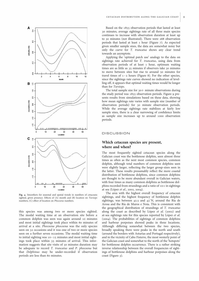
Spatial and temporal trends in numbersof animals seen, given presenceGeneralized additive model results for numbers of cetaceanssighted, given presence, are summarized in Table 5.Numbers of bottlenose dolphins seen (given presence) werehighest in January and September (Figure 4A), and highernumbers tended to be seen further south (Figure 4B).Smaller numbers were seen in the second project year thanthe first. Numbers seen were higher from higher observationpoints and when visibility was higher. Relationships withobservation duration and wind strength, although significant,were non-linear and difficult to interpret: numbers seen werelowest for observation periods of around 40 minutes durationand increased for wind strengths from Beaufort 2 to Beaufort4 (not illustrated). Of all these trends, only those for height,location and observation duration were strong (P , 0.01).

In the case of Delphinus delphis the only significant trendswere for more animals to be seen where field of view area waslarger and in the third and fourth project years compared tothe first. Note that sample size was only around 1/3 of thatfor T. truncatus. In the case of P. phocoena, higher numberswere in the north (Figure 4C). More porpoises were seen inyear 2 than in year 1. More porpoises were seen when visibilitywas higher and there was a weakly significant trend for feweranimals to be seen where field of view area was larger. Notethat sample size was only around 1/7 of that for T. truncatus.

Environmental patterns in cetacean presenceGeneralized additive model results for cetacean presence inrelation to environmental parameters are summarized inTable 6. In the final environmental model for T. truncatuspresence there was a clear tendency for the species to besighted most frequently where the shelf is between 35 and40 km wide and in areas of higher maximum chl-a concen-tration (Figure 5A, B). Effects of observation duration andfield of view area were highly significant, and Tursiops wasseen more frequently from higher observation points andwhen 2 or 3 observers were present rather than one.Sightings were more frequent when visibility was higher(this trend was not significant in the previous analysis ofspatiotemporal trends). The model explained 15.4% ofdeviance.

Sightings of Delphinus delphis occurred most frequentlywhere the continental shelf was narrowest (a linear trend)and more sightings occurred in areas with lower maximumchl-a concentrations (Figure 5C). Positive effects of increasingobservation duration, field of view area and height of theobservation point were evident at low values of these explana-tory variables. The frequency of sightings was lowest aroundwind strength Beaufort 3–4 and was higher at both lowerand higher wind strengths. There was a weak negative effectof having 3 observers rather than one. These trends are con-sistent with those in the spatiotemporal model for Delphinuspresence.

The frequency of porpoise sightings was, similar tocommon dolphin sightings, negatively correlated with conti-nental shelf width (Figure 5D) and maximum chlorophyllconcentration. There were positive effects of longer obser-vation duration (up to around 60 minutes) and presence oftwo or three observers rather than one and a negative relation-ship with both wind strength and height of the observation

Fig. 2. Presence (proportion of observation periods during which cetaceanswere seen) , by calendar month: all cetacean species (All), Tursiops truncatus(Tt), Delphinus delphis (Dd), Phocoena phocoena (Pp), Globicephala melas(Gm) and Grampus griseus (Gg). The highest rates are highlighted in bold.Monthly sample sizes (numbers of observation periods, N) were: 188, 192,205, 186, 190, 183, 221, 206, 260, 241, 194 and 196.

Table 3. Presence (proportion of observation periods during which ceta-ceans were seen) for all cetaceans and the main individual species, byproject year: Tursiops truncatus (Tt), Delphinus delphis (Dd), Phocoenaphocoena (Pp), Globicephala melas (Gm) and Grampus griseus (Gg).The table also indicates the sample size (N). Project years run from

September to August.

Year All Tt Dd Pp Gm Gg N

2003–2004 0.157 0.092 0.041 0.010 0.000 0.003 6762004–2005 0.173 0.102 0.047 0.019 0.006 0.003 6762005–2006 0.169 0.115 0.021 0.020 0.002 0.008 6092006–2007 0.188 0.124 0.038 0.016 0.002 0.000 448

6 graham j. pierce et al.

Fig. 3. Generalized additive model results: smoothing functions for effects of duration of observation, field of view area, time of day and location on presence ofcetaceans. The Y-axis represents the trend (positive or negative) in sightings rate. In the case of location, the X-axis indicates the observation points, numbered insequence from 1 in the far north-east to 53 in the far south-west. Dotted lines are the approximate 95% confidence limits. (A) Effect of observation duration, allspecies combined; (B) effect of field-of-view area, all species; (C) effect of location, all species; (D) effect of location, Tursiops truncatus; (E) effect of time of day,Tursiops truncatus; (F) effect of location, Delphinus delphis; (G) effect of location, Phocoena phocoena.

cetacean distribution along the galician coast 7

point. Porpoises were seen more frequently later in the day.Again these trends are consistent with the previous spatiotem-poral model.

Environmental patterns in numbersof animals seen, given presenceThe numbers of T. truncatus seen, given presence, tended tobe higher when minimum SST was slightly lower than themonthly average and, as evident in the previous spatiotem-poral model of numbers of this species given presence, therewas a clear peak in September (Table 7; Figure 6A, B).There were also positive effects of observation platformheight, and visibility, again as seen for the spatiotemporalmodel of numbers given presence, non-linear effects of obser-vation duration and wind strength.

Numbers of Delphinus were highest later in the year (atrend not evident in the previous spatiotemporal model of

numbers given presence) and where SST was slightly aboveits monthly mean value (Figure 6C). As for the previousspatiotemporal model of numbers given presence, numbersincreased with field of view area (Table 7). No satisfactoryenvironmental model could be fitted to the data on P. pho-coena numbers.

Sampling efficiencyThere were 267 sightings records for which T. truncatus wasthe only species seen and a further six for which this specieswas among two or more species sighted; the former subsetwas used for analysis. The modal waiting time at an obser-vation site before a bottlenose dolphin was seen wasaround 10 minutes and majority of initial sightings of thisspecies took place within 30 minutes of arrival at a site.There were 79 sightings records for which Delphinusdelphis was the only species seen, plus 13 records for which

Table 4. Summary of generalized additive models for spatial and temporal patterns in presence of all cetacean species, Tursiops, Delphinus and Phocoena.For categorical explanatory variables, the effect given for each level is relative to a reference level (e.g. for number of observers, all comparisons are inrelation to observation periods with one observer present). For each model, all significant explanatory variables are listed with their associated probability(P) value, along with the overall % deviance explained by the model and sample size (number of observation periods, N). For categorical and linear expla-natory variables, the direction of the effect is indicated as + or –; for smoothers (s), the degrees of freedom are indicated in parentheses. Data for project

year 5 (i.e. the last two months of the study) were excluded from this analysis to ensure a balanced coverage of the calendar year.

Variables All species Tursiops Delphinus Phocoena

Wind strength s(1.4), P , 0.0001 –, P ¼ 0.0023 s(2.7), P , 0.0001 –, P , 0.00012 observers +, P ¼ 0.0006 +, P ¼ 0.0015 +, P , 0.00013 observers +, P ¼ 0.0021 –, P ¼ 0.0200 +, P , 0.0001.3 observersDuration s(2.8), P , 0.0001 s(2.0), P , 0.0001 s(2.9), P , 0.0001 s(2.3), P , 0.0001Area s(1.5), P , 0.0001 s(1.2), P , 0.0001 s(1.6), P , 0.0001 s(1.2), P , 0.0001Height –, P ¼ 0.0020 s(2.1), P , 0.0001 –, P , 0.0001Project year 2 +, P ¼ 0.0097 +, P ¼ 0.0480 +, P ¼ 0.0010 +, P , 0.0001Project year 3 +, P ¼ 0.0233 +, P ¼ 0.0106 –, P ¼ 0.0040 +, P , 0.0001Project year 4 +, P ¼ 0.0030Time of day s(2.6), P ¼ 0.0003 +, P , 0.0001Location s(8.5), P , 0.0001 s(8.5), P , 0.0001 s(7.1), P , 0.0001 s(6.6), P , 0.0001% deviance explained 16.1% 22.0% 26.8% 30.9%N 2392 2388 2388 2388

Table 5. Summary of generalized additive models for spatial and temporal patterns in numbers of animals seen, given presence, for Tursiops, Delphinusand Phocoena. For categorical explanatory variables, the effect given for each level is relative to a reference level (e.g. for number of observers, all com-parisons are in relation to observation periods with one observer present). For each model, all significant explanatory variables are listed with their associ-ated probability (P) value, along with the overall % deviance explained by the model and sample size (number of observation periods, N). For categoricaland linear explanatory variables, the direction of the effect is indicated as + or –; for smoothers (s), the degrees of freedom are indicated in parentheses.

Variables Tursiops Delphinus Phocoena

Visibility +, P ¼ 0.0192 +, P ¼ 0.0054Wind strength s(2.9), P ¼ 0.0256Duration s(2.9), P ¼ 0.0044Area s(1.1), P , 0.0001 s(2.0), P ¼ 0.0431Height s(1.1), P , 0.001Project year 2 –, P ¼ 0.0202 +, P ¼ 0.0123Project year 3 +, P ¼ 0.0262Project year 4 +, P ¼ 0.0001Month s(2.9), P ¼ 0.0267Location s(3.8), P ¼ 0.0049 s(4.7), P ¼ 0.00002% deviance explained 31.6% 26.1% 73.6%N 256 89 37

8 graham j. pierce et al.

this species was among two or more species sighted.The modal waiting time at an observation site before acommon dolphin was seen was again around 10 minutesand most initial sightings took place within 60 minutes ofarrival at a site. Phocoena phocoena was the only speciesseen on 32 occasions and it was one of two or more speciesseen on a further seven occasions. The modal waiting timeto initial sighting was 10 – 15 minutes and most initial sight-ings took place within 35 minutes of arrival. This infor-mation suggests that site visits of 30 minutes duration maybe adequate to record T. truncatus and P. phocoena butthat Delphinus may be under-recorded if observationperiods are less than 60 minutes.

Based on the 1855 observation periods that lasted at least30 minutes, average sightings rate of all three main speciescontinues to increase with observation duration at least upto 30 minutes (not illustrated). There were 268 observationperiods that lasted at least 1 hour (Figure 7). As expectedgiven smaller sample sizes, the data are somewhat noisy butonly the curve for T. truncatus shows any clear trendtowards an asymptote.

Applying the ‘optimal patch use’ analogy to the data onsightings rate achieved for T. truncatus, using data fromobservation periods of at least 1 hour, optimum waitingtimes are as little as 35 minutes if observers take 30 minutesto move between sites but rise to around 50 minutes fortravel times of 1–2 hours (Figure 8). For the other species,since the sightings rate curves showed no indication of level-ling off, it appears that optimal waiting times would be longerthan for Tursiops.

The total sample size for 30+ minute observations duringthe study period was 1855 observation periods. Figure 9 pre-sents results from simulations based on these data, showinghow mean sightings rate varies with sample size (number ofobservation periods) for 30 minute observation periods.While the average sightings rate stabilizes at fairly lowsample sizes, there is a clear narrowing of confidence limitsas sample size increases up to around 1000 observationperiods.

D I S C U S S I O N

Which cetacean species are present,where and when?The most frequently sighted cetacean species along theGalician coast was the bottlenose dolphin, seen almost threetimes as often as the next most common species, commondolphin, although total numbers of common dolphins seenwere slightly larger, reflecting the larger group-sizes seen inthe latter. These results presumably reflect the more coastaldistribution of bottlenose dolphins, since common dolphinsare thought to be more abundant overall in Galician waters,with four times as many common dolphins as bottlenose dol-phins recorded from strandings and a ratio of 10:1 in sightingsat sea (Lopez et al., 2002, 2004).

The area with the highest overall frequency of cetaceansightings, and the highest frequency of bottlenose dolphinsightings, was between 42.5 and 438N, around the Rıa deArosa and the Rıa de Muros e Noia. This is consistent withthe geographical distribution of strandings of T. truncatusalong the coast as described by Lopez et al. (2002) andat-sea sightings rate for this species reported by Lopez et al.(2004). The probabilities of sightings of common dolphinsand harbour porpoises showed peaks in three locations.Although differing somewhat between the two species,broadly speaking there were peaks in the north and south(around the borders with Asturias and Portugal respectively),and in the vicinity of Cabo Fisterre, the most westerly point ofthe Galician coast and somewhat to the north of the ‘hotspots’for bottlenose dolphin occurrence. There is a rather strikinginverse relationship between the overall frequencies of sight-ings of bottlenose dolphins and harbour porpoises along thecoast (Figure 3).

Fig. 4. Smoothers for seasonal and spatial trends in numbers of cetaceanssighted, given presence. Effects of (A) month and (B) location on Tursiopsnumbers; (C) effect of location on Phocoena numbers.

cetacean distribution along the galician coast 9

The analysis additionally enabled quantification of some ofthe biases inherent in coastal observations, with effects ofobservation duration, field of view area, wind strength, visi-bility and number of observers all being demonstrated. Mostof these trends were in the expected direction and it is

important to note that they can be adequately controlled forin statistical analysis. Some trends were less intuitive. Thushigher observation sites tended to be associated with lowersightings rates for bottlenose dolphins and porpoises buthigher sightings rate for common dolphins and larger

Table 6. Summary of generalized additive models for environmental patterns in presence of Tursiops, Delphinus and Phocoena. For categorical expla-natory variables, the effect given for each level is relative to a reference level (e.g. for number of observers, all comparisons are in relation to observationperiods with one observer present). For each model, all significant explanatory variables are listed with their associated probability (P) value, along withthe overall % deviance explained by the model and sample size (number of observation periods, N). For categorical and linear explanatory variables, the

direction of the effect is indicated as + or –; for smoothers (s), the degrees of freedom are indicated in parentheses.

Variables Tursiops Delphinus Phocoena

Visibility – , P ¼ 0.0004Wind strength s(3.0), P , 0.0001 –, P , 0.00012 observers +, P ¼ 0.0098 +, P , 0.00013 observers +, P , 0.001 –, P ¼ 0.0212 +, P , 0.0001.3 observersDuration s(1.1), P , 0.0001 s(2.6), P , 0.0001 s(2.4); P , 0.0001Area s(1.2), P , 0.0001 s(2.8), P , 0.0001Height –, P ¼ 0.0241 s(2.3), P , 0.0001 –, P ¼ 0.0002MonthStart time +, P , 0.0001Chlorophyll-a (maximum) s(1.7), P ¼ 0.0169 s(1.7), P ¼ 0.0048 –, P , 0.0001Sea surface temperatureShelf width s(2.8), P , 0.0001 –, P , 0.0001 s(2.4), P , 0.0001% deviance explained 15.4% 28.9% 22.9%N 1955 1952 1955

Fig. 5. Smoothers for environmental models of Tursiops, Delphinus and Phocoena presence, showing effects of: (A) shelf width (distance from the coast to the 200m isobath) and (B) maximum chlorophyll-a concentration on Tursiops presence, (C) the effect of maximum chlorophyll-a concentration on Delphinus presenceand (D) shelf width on Phocoena presence.

10 graham j. pierce et al.

group-sizes for bottlenose dolphins. Aside from possibleeffects of observation point height on the ease of seeinganimals, it seems likely that the height of the observationsite is providing information about the type of coastline andthis requires further investigation.

In interpreting the sightings data it is important to keep inmind the behaviour of the animals seen adjacent to the coast.In all three of the most frequently seen species, groups wereseen engaged in directional travel and non-directional move-ments, the latter including foraging boats. In porpoises,around 44% of groups observed undertook only non-directional movements, the figure being closer to 30% forthe two dolphin species. All three species probably spendsome time foraging close to the coast.

Habitat useWhile all single species habitat models explained at least 20%of deviance, it should be borne in mind that some of this‘explained’ variation is accounted for by the effects of variablesrelated to observation effort and efficiency (e.g. wind strengthand observation duration) so the explanatory power of thevariables of interest, while statistically significant, is relativelylow. In addition, the ‘environmental’ (habitat) models weregenerally somewhat weaker than the spatiotemporal models,as would be expected if not all the spatiotemporal variationin presence and numbers (as captured by effects of location,month and year) is related to variation in the suite of environ-mental variables available for modelling (namely continentalshelf width and remotely sensed indices of SST andchlorophyll-a concentration).

The results of the habitat modelling suggested that bottle-nose dolphin sightings are particularly associated with areaswhere the continental shelf is relatively wide and productivity(as indicated by remotely-sensed chlorophyll-a concentration

in surface waters) relatively high. Presumably this is related tothe abundance of their prey. Bottlenose dolphins in Galicia eata wide range of fish species, the most important numericallyand in terms of biomass being blue whiting (Micromesistiuspoutassou) and hake (Merluccius merluccius), which are alsospecies of high commercial value. Blue whiting is probablytaken at the shelf edge while hake can be taken on the shelf(Santos et al., 2007).

Common dolphins were seen most often where the conti-nental shelf is narrowest and productivity lower, consistentwith them normally occupying deeper waters. The most

Fig. 6. Model for environmental trends in numbers of cetaceans sighted, givenpresence. Smoothers for effects of: (A) minimum sea surface temperature (SST)anomaly and (B) month on Tursiops numbers, and (C) effect of minimum SSTanomaly on Delphinus numbers.

Table 7. Summary of generalized additive models for environmental pat-terns in numbers seen, given presence, for Tursiops and Delphinus. Forcategorical explanatory variables, the effect given for each level is relativeto a reference level (e.g. for number of observers, all comparisons are inrelation to observation periods with one observer present). For eachmodel, all significant explanatory variables are listed with their associatedprobability (P) value, along with the overall % deviance explained by themodel and sample size (number of observation periods, N). For categoricaland linear explanatory variables, the direction of the effect is indicated as+ or –; for smoothers (s), the degrees of freedom are indicated in

parentheses.

Variables Tursiops Delphinus

Visibility +, P ¼ 0.0124Wind strength s(2.9), P ¼ 0.0303Duration S(2.9), P ¼ 0.0003Area +, P ¼ 0.0001Month s(2.9), P , 0.0001 +, P , 0.0001Height +, P ¼ 0.0023Start time –, P=0.0172Chlorophyll-a anomaly

(minimum)Sea surface temperature

anomaly (minimum)s(2.7), P ¼ 0.0269 S(2.6), P ¼ 0.0110

Shelf width% deviance explained 29.6% 37.1%N 204 78

cetacean distribution along the galician coast 11

important prey in common dolphin diet in Galician waters areblue whiting and sardine (Sardina pilchardus) (Santos et al.,2004). As is the case for bottlenose dolphins, common dol-phins probably take blue whiting over the shelf break, whilesardine is a more coastal species. Fishermen report commondolphins entering coastal waters to feed on sardine schools(M.B. Santos, personal communication).

Harbour porpoises also tended to be seen where the shelf isnarrower, possibly indicating that they habitually occupydeeper waters. This is consistent with preliminary resultsfrom boat-based surveys, in which the average water depthfor porpoise sightings was 90 m (CEMMA, unpublisheddata). Based on analysis of stomach contents of 32 porpoisesstranded on the Galician coast during 1991–2004, the mostimportant prey of harbour porpoise in Galician waters arescad (Trachurus trachurus), Trisopterus spp. and garfish(Belone belone). Blue whiting is the fourth most importantspecies in the diet (Santos et al., unpublished data). While(as noted above) blue whiting is generally found on the conti-nental slope, the other main prey species of porpoises specieslive in shelf waters.

Even though blue whiting are important in the diets of allthree cetacean species, there are clearly also differences in thespecies of prey eaten and differences in habitat use wouldtherefore not be surprising. Another factor to take into con-sideration is possible avoidance of competition and, in thecase, of porpoises, avoidance attacks by bottlenose dolphins.Although bottlenose dolphin attacks on porpoises do not

appear to be frequent in Galician waters, they have been docu-mented (Lopez & Rodriguez-Folgar, 1995; Alonso et al., 2000).

The sampling programmeTo date the sampling regime has allowed observation durationto vary, mainly in the range 20–60 minutes, and the numberof sites visited monthly was reduced from 53 to 30 from 2007.The present analysis allowed the efficiency of this samplingregime to be evaluated, based on the assumption that maxi-mizing the sightings rate will provide the best informationon species distribution. Clearly other criteria could havebeen used but this seems to be a reasonable starting point.It is evident from the data that sightings per unit effort(not only the absolute number of sightings) increased withobservation duration. However, longer observation periodsobviously impose additional resource requirements: sincefewer sites can be visited in a day, more days of fieldworkare needed to complete the monthly circuit of all sites.Furthermore, estimated sightings rate will not increase indefi-nitely for longer observation periods. The raw data (Figure 7)provide some evidence of approach to an asymptote after 60minutes in the case of bottlenose dolphins. GAM results(see Figure 3A) also suggest that there is a point of inflexionat around 40 minutes in the curve describing the increase inoverall sightings rate for cetaceans in relation to observationduration. By analogy with optimal patch use (e.g. Charnov,1976), once observer travel time between sites is taken intoaccount, to maximize the sightings rate of bottlenose dolphins

Fig. 7. Mean sightings rate versus observation time, based on all observationsof at least 1 hour (N=268).

Fig. 8. ‘Optimal waiting time’. Based on various possible travel times betweenobservation sites, tangents are fitted to the sightings rate–observation timecurve for Tursiops (based on data for 268 observation periods of at least 60minutes duration) to indicate optimum waiting times in order to maximizesightings rate.

Fig. 9. Simulated mean sighting rates (animals/hour) as a function of thenumber of observation periods (50 to 1850), based on data from 1855periods of at least 30 minutes: median and 95% confidence limits based on1000 repeats per sample size/species combination: (A) Tursiops truncatus;(B) Delphinus delphis.

12 graham j. pierce et al.

per hour of observer time, observation periods of 35–50minutes appear be optimal. For the other cetacean species itis inevitable that longer observation periods would beneeded to maximize sightings rates. Thus there is clear justifi-cation for observation periods in excess of 30 minutes.

Confidence limits for sightings rate appear to have stabil-ized after around 1000 observation periods. Almost 2500observation periods were completed during 2003–2007,suggesting that there is scope for reducing the intensity ofsampling. Thus the reduction in the number of sites visitedfrom 53 to 30, made at the end of 2006 due to financial andlogistic constraints, should not have greatly impacted on thevalue of the data collected for monitoring purposes.

The futureThe Galician government is presently formulatingConservation Plans for both bottlenose dolphins andharbour porpoises. Survey data are needed to enable identifi-cation of areas that are consistently used by cetaceans, particu-larly feeding areas and areas frequented by females withcalves. It will also be important to establish the seasonalityof use of coastal waters. Results of the present study providea clear indication that cetaceans are not evenly distributedalong the coast, although the main species are present allyear round.

Obviously, cetaceans range beyond coastal waters, andboat-based surveys are needed to fully document patternsand trends in cetacean distribution and habitat use.Nevertheless, the coastal sightings series has the potential toprovide a relatively inexpensive long-term index of thestatus of local cetacean populations, which could be used tomake inferences about the use of different areas of the coastby cetaceans, especially areas where no data are availablefrom boat-based surveys, and to evaluate the impacts ofthreats such as climate change, overfishing, and pollutionevents.

Another focus for ongoing research will be evaluation ofinteractions with human activities, including fishing andboat traffic in general. While bottlenose dolphins can appar-ently become habituated to heavy boat traffic around ports(e.g. Sini et al., 2005) this does not imply that boat traffichas no effect on the activity patterns and distribution, withmany studies pointing to potentially harmful effects of dis-turbance by boats on bottlenose dolphins (e.g. Nowaceket al., 2001; Hastie et al., 2003; Mattson et al., 2005; Bejderet al., 2006). There is less evidence available on effects of dis-turbance on the other species of cetaceans known to inhabitGalician waters, although changes in activity due to disturb-ance by tourist boats have been detected elsewhere in bothcommon dolphins and Risso’s dolphins (Stockin et al., 2008;Visser et al., in press). The coastal sightings database providesone baseline data set against which to evaluate effects of, forexample, future changes in the distribution and nature oftourism and fishing.

A C K N O W L E D G E M E N T S

The authors wish thank all the volunteers and regional groupswithin CEMMA who contributed to the sightings surveys.The land-based sightings were funded by the Conselleria deMedio Ambiente e Desenvolvimento Sostenible, the Xunta

de Galicia, Fundacion Caixa Catalunhya and the FundacionBiodiversidad. G.J.P. was funded by the European Commissionas part of the ANIMATE project (MEXC-CT-2006-042337).We also thank the referees for helpful suggestions about howto improve the manuscript.

R E F E R E N C E S

Alonso J.M., Lopez A., Gonzalez A.F. and Santos M.B. (2000) Evidenceof violent interactions between bottlenose dolphin (Tursiops trunca-tus) and other cetacean species in NW Spain. European Research onCetaceans 14, 105–106.

Bejder L., Samuels A., Whitehead H., Gales N., Mann J., Connor R.,Heithaus M., Watson-Capps J., Flaherty C. and Krutzen M.(2006) Decline in relative abundance of bottlenose dolphins exposedto long-term disturbance. Conservation Biology 20, 1791–1798.

Cendrero O. (1993) Note on findings of cetaceans off northern Spain.Boletin del Instituto Espanol de Oceanografıa 9, 251–255.

Charnov E.L. (1976) Optimal foraging: the marginal value theorem.Theoretical Population Biology 9, 129–136.

Evans P.G.H. and Hammond P.S. (2004) Monitoring Cetoceans inEuropean waters. Mammol Review 34, 131–156.

Gonzalez A.F., Lopez A., Guerra A. and Barreiro A. (1994) Diets ofmarine mammals stranded on the northwestern Spanish Atlanticcoast with special reference to Cephalopoda. Fisheries Research 21,179–191.

Hastie G.D., Wilson B., Tufft L.H. and Thompson P.M. (2003)Bottlenose dolphins increase breathing synchrony in response toboat traffic. Marine Mammal Science 19, 74–84.

Lahaye V., Bustamante P., Law R.J., Learmonth J.A., Santos M.B., BoonJ.P., Rogan E., Dabin W., Addink M.J., Lopez A., Zuur A.F., PierceG.J. and Caurant F. (2007) Biological and ecological factors related totrace element levels in harbour porpoises (Phocoena phocoena) fromEuropean waters. Marine Environmental Research 64, 247–266.

Lopez A. and Rodriguez Folgar A. (1995) Agresion de arroas (Tursiopstruncatus) a tonina (Phocoena phocoena). Eubalaena 6, 23–27.

Lopez A., Santos M.B., Pierce G.J., Gonzalez A.F., Valeiras X. andGuerra A. (2002) Trends in strandings and by-catch of marinemammals in north-west Spain during the 1990s. Journal of theMarine Biological Association of the United Kingdom 82, 513–521.

Lopez A., Pierce G.J., Santos M.B., Gracia J. and Guerra A. (2003a)Fishery by-catches of marine mammals in Galician waters: Resultsfrom on-board observations and an interview survey of fishermen.Biological Conservation 111, 25–40.

Lopez A., Cedeira J.M., Caldas M., Carril R., Solla P. and Llavona A.(2003b) Monitorizacion de las poblaciones de cetaceos en la plata-forma de Galicia (NW Spain). Thalassas 19, 111–112.

Lopez A., Pierce G.J., Valeiras X., Santos M.B. & Guerra A. (2004).Distribution patterns of small cetaceans in Galician waters. Journal ofthe Marine Biological Association of the United Kingdom 84, 283–294.

Mattson M.C., Thomas J.A. and St Aubin D. (2005) Effects of boatactivity on the behavior of bottlenose dolphins (Tursiops truncatus)in waters surrounding Hilton Head Island, South Carolina. AquaticMammals 31, 133–140.

Murphy S., Herman J., Pierce G.J., Rogan E. and Kitchener A. (2006)Taxonomic status and geographical cranial variation of commondolphins (Delphinus) in the eastern north Atlantic. Marine MammalScience 22, 573–599.

cetacean distribution along the galician coast 13

Nowacek S.M., Wells R.S. and Solow A.R. (2001) Short-term effects ofboat traffic on bottlenose dolphins, Tursiops truncatus, in SarasotaBay, Florida. Marine Mammal Science 17, 673–688.

Pierce G.J., Santos M.B., Murphy S., Learmonth J.A., Zuur A.F., RoganE., Bustamante P., Caurant F., Lahaye V., Ridoux V., Zegers B.N.,Mets A., Addink M., Smeenk C., Jauniaux T., Law R.J., Dabin W.,Lopez A., Alonso Farre J.M., Gonzalez A.F., Guerra A.,Garcıa-Hartmann M., Reid R.J., Moffat C.F., Lockyer C. andBoon J.P. (2008) Bioaccumulation of persistent organic pollutants infemale common dolphins (Delphinus delphis) and harbour porpoises(Phocoena phocoena) from western European seas: geographicaltrends, causal factors and effects on reproduction and mortality.Environmental Pollution 153, 401–415.

Redfern J.V., Ferguson M.C., Becker E.A., Hyrenbach K.D., Good C.,Barlow J., Kaschner K., Baumgartner M.F., Forney K.A., BallanceL.T., Fauchald P., Halpin P., Hamazaki T., Pershing A.J., QianS.S., Read A., Reilly S.B., Torres L. and Werner F. (2006)Techniques for cetacean-habitat modelling. Marine Ecology ProgressSeries 310, 271–295.

Ridoux V., Lafontaine L., Bustamante P., Caurant F., Dabin W.,Delcroix C., Hassani S., Meynier L., da Silva V.P., Simonin S.,Robert M., Spitz J. and Van Canneyt O. (2004) The impact of the‘Erika’ oil spill on pelagic and coastal marine mammals: combiningdemographic, ecological, trace metals and biomarker evidences.Aquatic Living Resources 17, 379–387.

Santos M.B., Pierce G.J., Lopez A., Martınez J.A., Fernandez M.T., IenoE., Mente E., Porteiro C., Carrera P. and Meixide M. (2004)Variability in the diet of common dolphins (Delphinus delphis) inGalician waters 1991–2003 and relationship with prey abundance.International Council for the Exploration of the Sea CM 2004/Q:09.

Santos M.B., Fernandez R., Lopez A., Martınez J.A. and Pierce G.J.(2007) Variability in the diet of bottlenose dolphin, Tursiops truncatus(Montagu), in Galician waters, NW Spain, 1990–2005. Journal of theMarine Biological Association of the United Kingdom 87, 231–242.

Sini M.I., Canning S.J., Stockin K.A. and Pierce G.J. (2005) Bottlenosedolphins around the Aberdeen harbour, north-east Scotland: a study ofhabitat utilization and the potential effects of boat traffic. Journal of theMarine Biological Association of the United Kingdom 85, 1547–1554.

Stockin K.A., Lusseau D., Binedell V., Wiseman N. and Orams M.B.(2008) Tourism affects the behavioural budget of the commondolphin Delphinus sp. in the Hauraki Gulf, New Zealand. MarineEcology Progress Series 355, 287–295.

Torres L.G., Read A.J. and Halpin P. (2008) Fine-scale habitat modelingof a top marine predator: do prey data improve predictive capacity?Ecological Applications 18, 1702–1717.

Valavanis V.D., Pierce G.J., Zuur A.F., Palialexis A., Saveliev A., KataraI. and Wang J. (2008) Modelling of essential fish habitat based onremote sensing, spatial analysis and GIS. Hydrobiologia 612, 5–20.

Varela M., Diaz del Rio G., Alvarez-Ossorio M.T. and Costas E. (1991)Factors controlling phytoplankton size class distribution in the upwel-ling area of the Galician continental shelf northwest Spain. ScientiaMarina 55, 505–518.

Vieites D.R., Nieto-Roman S., Palanca A., Ferrer X. and Vences M.(2004) European Atlantic: the hottest oil spill hotspot worldwide.Naturwissenschaften 91, 535–538.

and

Visser F., Hartman K.L., Rood E.J.J., Hendriks A.J.E., Zult D.B., WolffW.J., Huisman J. and Pierce G.J. (in press) Risso’s dolphin alters dailyresting pattern in response to whale watching at the Azores. MarineMammal Science.

Correspondence should be addressed to:G.J. PierceSchool of Biological SciencesUniversity of AberdeenTillydrone Avenue, Aberdeen AB24 2TZ, UKemail: g.j.pierce@abdn.ac.uk

14 graham j. pierce et al.