Transportation Networks and the Rise of theKnowledge Economy in 19th Century France∗

Georgios Tsiachtsiras†

JOB MARKET PAPERLatest version here

November 8, 2021

Abstract

This paper exploits an episode of French history to study the relationship between the roll-out of railroads and the rise of the knowledge economy. I take advantage of the exogenousvariation in railway access arising from a straight line time variant instrument, to documentthat access to rail network increases the innovation activity at the canton level. I exploretwo underlying mechanisms behind the main results. First, I introduce a mechanism of ac-cess to knowledge to study how patent activity is affected by the reduction of transportationcosts, due to the expansion of rail and canal network, to the cantons where inventors reside.Second, using text analysis techniques, I am able to determine the technology of each patentapplication in the historical database of theNational Institute of Industrial Property of Franceand to explore how connectivity with the global city of Paris is associated with the diffusionof novel technologies. Finally, I introduce a back of the envelope exercise based on canals toshow that in the absence of railroads the invention rate of the French cantons would havebeen, on average, 21.3% lower.

Keywords: innovation, patent data, railroads, access to knowledge

JEL classification: L92, N73, O31, O33, P25, R12

∗I would like to thank from the bottom of my heart, Rosina Moreno and Ernest Miguelez for their guidance and support at all the stagesof this paper. Special thanks to Anastasia Litina and Sergio Petralia for helpful discussions and comments. I am grateful to Steeve Gallizia,Christophe Mimeur, Teresa Sanchís and Nicolas Verdier for sharing with me the historical database of INPI, the railroad data, the GDP dataand the postal offices of France. I would like to express my gratitude to Richard Hornbeck for sharing with me his replication files. I havebenefited from the comments of Thomas Piketty, Sascha O. Becker, Mara Squicciarini, Diogo Britto, Carlo Schwarz, Jan Bakker, FrancescoQuatraro, Stefano Breschi, Denis Cogneau, Laurent Bonnaud, Tommaso Ciarli, Cédric Chambru, Zelda Brutti, Ester Manna, Xavier Fageda,Emilie Bonhoure, Abel Lucena, Mercedes Teruel, Dolores Añon Higon, András Jagadits, Vera Rocha, Alexander Klein, Dirk Martignoni, BjoernBrey, Giuseppe Cappellari, Filippo Tassinari, Eric Melander, Michel Philippe Lioussis, Ivan Hajdukovic, Emanuele Caggiano, Maria TeresaGonzalez and the participants of the DRUID 2021 (Copenhagen Business School), the 15th North American Meeting of the Urban EconomicsAssociation (Arizona University), the PhD - Economics Virtual Seminar, the F4T Seminar Series (Bocconi University), the 6th Summer Schoolon Data & Algorithms for ST&I studies (organized by Aristotle University and KU Leuven, 2021), 11th ifo Dresden Workshop on RegionalEconomics (2021), the EPIP Conference (2021), the Young Economist Symposium 2021 (sponsored by Columbia, NYU, UPenn, Princeton andYale), the XXIII Applied EconomicsMeeting (Universitat de València, 2021), the EconomicHistory Seminar at Paris School of Economics (2021),the PhD in Economics Workshop at University of Barcelona (2020), the Economic Student Seminar at Universitat of Autònoma de Barcelona,VirtualMeeting of the Urban Economics Association (2020), 13th RGSDoctoral Conference in Economics on Regional Disparities and EconomicPolicy in Europe (Technische Universität of Dortmund, 2020), the 5th Geography of Innovation Conference (University of Stavanger, 2020), the7th International PhD Workshop in Economics of Innovation, Complexity and Knowledge (University of Turin, 2020) and the 4th SummerSchool in Economics (University of Ioannina, 2019). Financial support from Agaur (FI-DGR). Any remaining errors are mine.

†Tsiachtsiras: Ph.D. candidate, University of Barcelona School of Economics; Department of Statistics, Econometrics, and Applied Eco-nomics, Barcelona 08034, Spain. email: gtsiachtsiras@ub.edu

1

"There is no country in the world where so small a proportion of the capital investedwithin the last forty years in canals and railroads has been wasted or where travelingis safer, or in which travel and trade are accommodated at more reasonable ratesthan in France" (Moncure Robinson, American Philosophical Society, 1880source: Smith (1990)).

1 Introduction

Productivity growth rely in two elements: new ideas bringing new technologies, and the dif-fusion of these ideas across people and places. Connecting places via transportation networksis essential in order to promote knowledge diffusion across the space, and hence long run eco-nomic growth. Over the last decades, the World Bank dedicated a high proportion of moneyto support infrastructure investments (World Bank, 2007, 2013, 2017).1 Despite an emphasis onreducing transportation costs, we lack empirical evidence on understanding how transporta-tion infrastructure projects could actually create meaningful connections to places that matterfor boosting the innovation performance and to facilitate channels related to the diffusion ofknowledge.

In this paper, I exploit an episode of French history to study the impact of the largest-scale con-struction of French railroads on innovation performance. Over the second half of 19th century,the establishment of railroads transformed the French economy. Railways triggered economicrelations and cultural environments, stimulated commerce and created new economic opportu-nities. The creation of the rail network changed the perception of time (Schwartz et al., 2011).According to Thévenin et al. (2013) a striking example of this transformation is the travel timefrom Paris to Marseille. In 1814, the duration of this trip was four to five days while in 1857, thistrip needed about 13 hours.

Remarkably, the roll-out of the network coincidedwith a rise of innovative activity. Until 1850,the number of patent applications owned by inventors in the historical French patent databasewas 22,978 while from 1850 until 1902 increased to 285,597. Some of the greatest inventions inhistory took place in France during the second half of 19th century. Louis Pasteur in 1865 and1871 developed the modern method for wine and beer pasteurization. Another example is theinvention in 1853 by the French chemist, Charles Frederic Gerhardt, whowas the first to prepareacetylsalicylic acid (aspirin). Finally, the very first patented film camera introduced by Louis LePrince in 1888.

1Based on the reports of 2007, 2013 and 2017 WB committed approximately $105 billion in transport-relatedprojects.

2

I use rich historical data to construct a panel dataset at the canton level for France (2,925 can-tons) over the period 1850-1890.2 I combine a very recent dataset of communes with access torail station over the 19th century (Mimeur et al., 2018) with the historical patent applicationsdatabase of the National Institute of Industrial Property office (INPI from now on) (INPI, 2019)over the time period 1850-1890 to construct a unique dataset.3 The historical patent databaseof INPI is still quite unexplored. Previous papers, have used the INPI database during the firsthalf of 19th century to study the effect of technology transfer from Britain to France (Nuvolariet al., 2020), the influence of the patent system on the economic performance (Galvez-Behar,2019) and the role of women in enterprise and invention in France (Khan, 2016).

Equipped with this dataset, this paper relies on the expansion of the French railroad net-work which provides a unique setting to identify the causal impact of transport infrastructureon innovation outcomes. I use the three different French railway plans over the 19th century toconstruct a time variant straight line instrument. I document that access to a rail station increasesthe innovation activity of a canton. As a robustness analysis to complement the instrumentalvariance approach, I apply an inconsequential units approach in which I rely on the randomlychosen subset of municipalities that received railway access because they lie on the most directroute between the nodal destinations that were used for the creation of the straight line instru-ment. In addition, I exploit the richness of the patent data to create a balance test in which Iregress the distance to rail stations on invention rate of the cantons over the period 1800-1840one decade prior to the actual arrival of railroads. I report no empirical evidence on pre-trendsrelated to the railroads and innovation performance. Also, I provide a conventional difference-in-differences regression model with staggered treatment where I use as independent variablea binary indicator switching to 1 if the canton has access to a rail station. This design takes placefrom 1800 to 1890 allowing me to control for a long period of time, 1800-1840, before the arrivalof railroads in which all the cantons do not have access to a rail station. Finally, I explore crosssection variation for every decade over the period 1850 to 1890 to identify the year that railroadsstarted to have an impact on patenting rate and also to test the validity of the instrument bydecade.

In a second step I explore the mechanism behind the main results. This paper adds to theliterature by using the rationality of "market access" framework, developed by Donaldson andHornbeck (2016), to provide a supply side mechanism related to potential interactions (Akcigitet al., 2018) and knowledge spillovers (Jaffe et al., 1993) among the inventors residing in differentcantons. Instead of using the population in the market access index, the paper uses the numberof inventors. The potential interactions and spillovers among inventors residing in different can-

2I include only the cantons from the mainland of France.3The patent database is available after request.

3

tons could occur by establishing less costly routes, due to infrastructure improvements, withinmainland France. I call this mechanism access to knowledge. A previous attempt in the litera-ture relies on a market access framework (Perlman, 2015) to identify the mechanism that boostsinnovation performance. Other papers in the literature (Agrawal et al., 2017; Andersson et al.,2021; Inoue and Nakajima, 2017; Wong, 2019; Gao and Zheng, 2020; Dong et al., 2020; Sun et al.,2021; Hanley et al., 2021; Komikado et al., 2021; Cui et al., 2020; Huang andWang, 2020) provideevidence on how transportation networks facilitate the diffusion of knowledge but without con-necting directly the knowledge diffusion mechanism to innovation performance. This the firstpaper to create a direct link between a supply side mechanism and the invention rate.

Finally, this paper uses the unique setting of France to introduce as a special case the impor-tance for a given canton 8 to have a less costly connection to a global city such as Paris. Priorliterature argues that Paris can work as a gatekeeper of knowledge which connects the nationalinnovation system to global innovation networks (Miguelez et al., 2019). This is confirmed bythe fact that inventions in Paris are more diverse and spread across the different technologies(Kogler et al., 2018). However, for only a small sample of patent applications, INPI databasecontains information about their technological class. In order to explore this special case, I as-sign technological classes to the remaining patent applications in the historical database of INPI.I assemble a vocabulary which is based on key words from the titles of the patent applicationsfor which I have their technological class and thanks to this vocabulary, I am able to assign tech-nological classes to all patent applications in the INPI database.

This paper directly speaks to the literature about transportation networks and innovation ac-tivity. Closer to my research are the papers of Perlman (2015), Agrawal et al. (2017) and An-dersson et al. (2021). Perlman (2015) establishes a relationship between network access andinnovative activity in the USA over the nineteenth century. Agrawal et al. (2017) find that thestock of highways has a positive effect on patenting in metropolitan statistical areas of the USA.Finally, Andersson et al. (2021) explore the effect of Swedish railroad on patent activity over thetime period 1830-1910. They contend that network access fosters innovation activity. They findsolid evidence that independent inventors start to specialize in specific technologies when theyenter the market. General railroad access facilitates the inventors to develop ideas beyond thelocal economy and to invent in new technological classes.

There is a growing literature exploring the interplay between infrastructure and economicoutcomes from a historical perspective. Railroads in the USA, Sweden, England, Wales andSwitzerland transformed all towns into new places. They manage to lure banks and to increaseurbanization (Atack et al., 2008, 2009; Atack andMargo, 2009; Berger andEnflo, 2017; Büchel andKyburz, 2020; Bogart et al., 2022). They are responsible for the growth and the economic devel-

4

opment of US and Nigeria cities (Nagy, 2016; Okoye et al., 2019). Railroads are meaningful forthe development of the agricultural sector (Donaldson and Hornbeck, 2016; Donaldson, 2018)and have an impact on fertility and human capital (Katz, 2018). Transportation linkage has aadverse effect on health in rural US (Zimran, 2019). Railroads manage to boost manufacturingproductivity in US (Hornbeck and Rotemberg, 2019; Pontarollo and Ricciuti, 2020). Finally, thesteam railway led to the first large-scale separation of workplace and residence (Heblich et al.,2020).

In general, infrastructure networks could affect economy through different channels. The re-allocation of road investments after the division ofGermany creates regional income inequalitiesin terms of GDP per capita (Santamaria, 2020). Highways affect population and employment(Baum-Snow, 2007; Duranton and Turner, 2012). Finally, the adoption of the steamship between1850 and 1900 boosts globalization of trade (Pascali, 2017).

In addition, this paper proposes as a direct policy that may smooth the persistent inequalitiesamong urban and rural areas the targeted investments to infrastructure projects which facili-tate access to big cities. This policy can increase the probability of smaller cities to innovate innew patent classes. Recent papers rise concerns about the correct allocation of infrastructurefunds (Flyvbjerg, 2009) and which are the proper circumstances for these projects to be efficient(Crescenzi et al., 2016). At the same time, complex economic activities concentrate dispropor-tionately in a few large cities, compared to less complex activities (Balland et al., 2020). Largecities are also the places with more interactions between higher-ability participants (Davis andDingel, 2019).

Finally, this paper speaks to an extended literature on the economic history of France aroundthe turn of the 19th and 20th century. Other papers in the literature explore the effect of knowl-edge elites in France or religion on economic development (Squicciarini and Voigtländer, 2015;Squicciarini, 2020). Apart from economic development it was less likely for the more religiouscantons to give birth to scientists (Lecce et al., 2021). Furthermore, regions in the French Em-pire which became better protected from trade from the British for exogenous reasons duringthe Napoleonic Wars increased the capacity in mechanized cotton spinning more than regionswhich remained more exposed to trade (Juhász, 2018). Yet, the major technological break-throughs likemechanized cotton spinning tend to be adopted slowly (Juhász et al., 2020). Otherfactors that affected the economic development of France are the large income shock of the phyl-loxera (Banerjee et al., 2010), emigration intensity (Franck and Michalopoulos, 2017), popu-lation swifts (Talandier et al., 2016) and the early industrialization (Franck and Galor, 2019).Daudin et al. (2019) establishes a relationship between fertility rates and the diffusion of cul-tural and economic information. One previous attempt related to railroads focus on the effect

5

of railroads on population distribution for France, Spain, and Portugal from 1870 to 2000 (Mo-jica and Martí-Henneberg, 2011). Finally, the literature has explored the wealth concentrationin Paris and France (Piketty et al., 2006) and regional inequality in France (Díez-Minguela andSanchis Llopis, 2019).

The rest of the paper is organized as follows: Section 2 contains the historical background,Section 3 presents the data, Section 4 shows the empirical strategy, Section 5 presents the mainresults, Section 6 explores the mechanisms and Section 7 concludes.

2 Historical Background

2.1 Railroads

The first railway line in France established in 1828 from mining companies to connect St. Eti-enne to the Loire River. They used this line to transfer coal. The first line for passengers openedin 1837. It was a short line from Paris to Le Pecq (Dunham, 1941). At that period France wasalready lagged behind comparing to Britain and Belgium. In 1842 Britain had 1,900 miles ofrailways in operation while France only 300 (Lefranc, 1930).

After the success of the first line, the government of France understood the importance of anational railway network. However, the next attempt for a rail line between Paris and Versailleswas unsuccessful. Two different companies created one line each to connect Paris with Versaillesbut they failed financially. The government recognized the problem of the rivalry of local inter-ests (Dunham, 1941). Even though, the government was aware of the importance of a nationalrailroad did not provide funding until 1842 (Ratcliffe, 1976).

According toDunham(1941) the planning of rail networkwas given to�>A ?B34B?>=CB4C2ℎ0DBB44B,an organization of highly trained engineerswhichwas in charge formajor infrastructure projectsin France. The expansion of railroads during the period 1840-1860 took place based on LegrandStar, a design of �>A ?B 34B ?>=CB 4C 2ℎ0DBB44B. According to Legrand plan the purpose of thegovernment was to connect major communes, borders, and coastlines with Paris. In 1865, basedon theMigneret law, the government established direct connections lines among all prefectures.The final expansion of rail network constructed according to Freycinet plan which introducedin 1878 (Thévenin et al., 2013).

The most important railroad expansion occurred from 1860 to 1900 when 45,000 km of raillines established. The final phase was until 1930 and by the end of this phase 56,000 km of rail-

6

road were operational (Thévenin et al., 2013). The introduction of motor vehicles in the end of1930 limited the expansion of railroad network.

2.2 Patent System

Great Britain, France and the United States were the first countries that adopted a legislationon patents in 1791 (MacLeod, 1991; Galvez-Behar, 2019). Prior to the establishment of patentlegislation and more specifically, during the 18th century the name of the patent applicationswere "les privileges" and they were granted by the king and registered by the parliament inParis (MacLeod, 1991). In addition the inventors were receiving remarkable awards for theirinventions. These awards included things like national or local production, pension for a life orexception from the taxes. Finally, a major difference with the English patent system is that theapplication procedure was muchmore severe in case of French patent system (MacLeod, 1991).

In 1791, Boufflers’ bill became the first Patent Act in France. The 1791 law established threedifferent categories for patenting: 1) Patents for invention, 2) Patents for improvement and 3)Patents for importation. The patents were granted from five until fifteen years. The name ofthe inventions changed to "brevets de invention". However, their cost was prohibitive. Apartfrom the initial cost, several taxes were added during the examination process. Patent systemdid not facilitate the spread of patents, because a lot of inventors could not afford the high cost(Galvez-Behar, 2019).

The rise of patenting activity was underpinned by the introduction of a patent law in 1844.This legislation allowed the inventors to export their patents in foreign countries and also changedthe method of payment for the inventors. Now, patentees could spread the payment of the taxover the entire duration of their patent (Galvez-Behar, 2019).

3 Data

3.1 Setting

I start the collection of data by first extracting shapefiles of 19th century France. I make useof the recent constructed shapefiles of Gay (2020) over the period 1870-1940. Over my sampleperiod, France does not experience large changes in the national administrative system exceptfor the departments that become part of Germany. I rely on the shapefile of 1870 to conduct myanalysis. The shapefile of 1870 contains 2,925 cantons for the mainland of France.

7

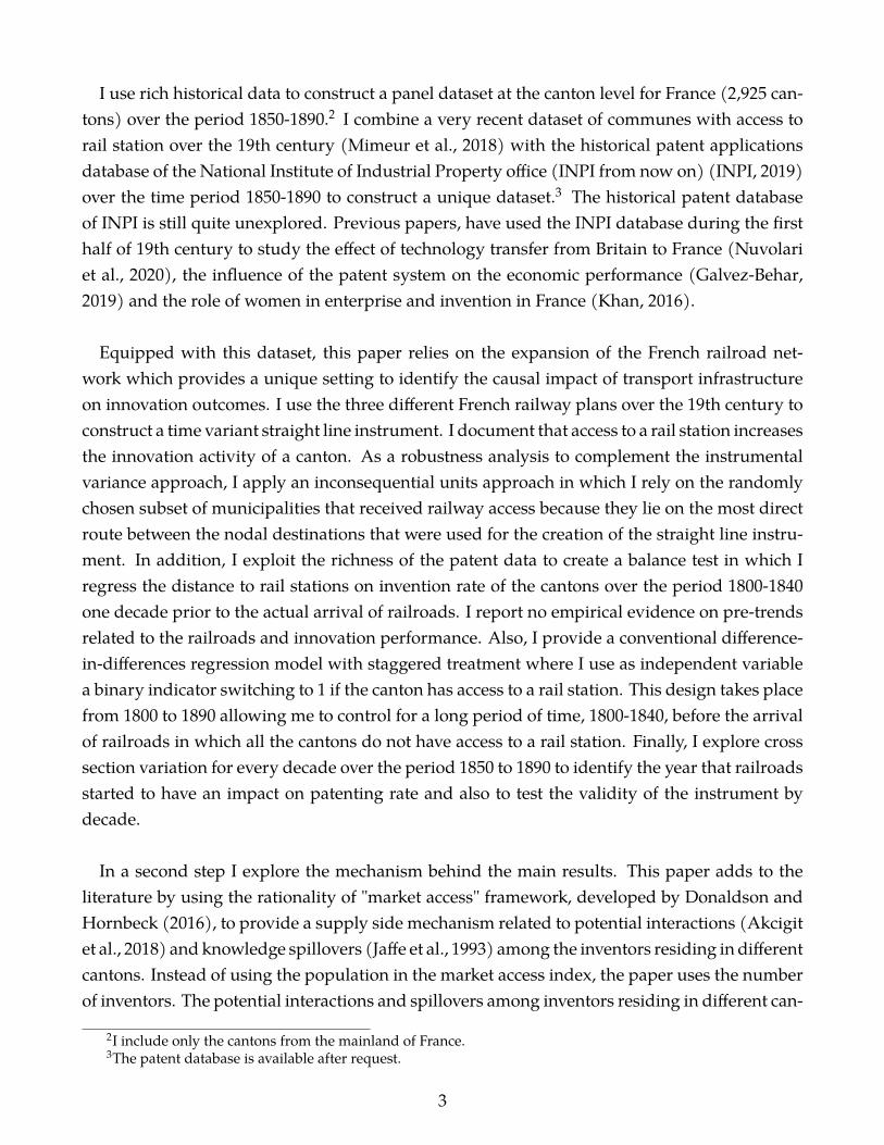
Next, I am able to determine the majority of the city areas in order to use the centroids of thecities. The first data source is Perret et al. (2015) and contains the polygons of the cities, towns,domains and forts during the 18th century. For a given canton 8, I first use the cities within thepolygon then the towns, the domains and the forts. If one canton hasmore than one city, I keep asa reference point the centroid of the largest (in terms of area) city. The same rule applies in caseof a town, domain or fort. I determine the location of 1,961 cities, 69 towns, 112 domains and 3forts which corresponds to 2145 cantons, 73,33% of the sample. I complement my analysis usingthe population raster file of 1840 from HYDE (2020). I use the year 1840 because it is the closestavailable year before the arrival of railroads. Based on the second source of data, I transformin QGIS the raster file to pixels and I choose for the remaining cantons, without a referencepoint, the pixel with the highest population value. Furthermore, I assign a reference point in738 cantons, which corresponds to 25.23% of the sample. For the remaining 42 cantons withouta reference point, I use the centroid of the polygon, 1.44% of the sample. Figure 1 illustrates anexample of the empirical setting. The brown areas are the cantons and the pink areas are thecity polygons. The black dots, within the pink areas, are the city centroids. The white dots arethe rail stations while the blue line is the navigable waterway. Finally, concerning the black dotswithout a pink area, they are the points with the highest population value within the canton. Ibelieve that using these black dots as reference points makes the analysis more realistic.

3.2 Transportation Data

3.2.1 Railroad Data

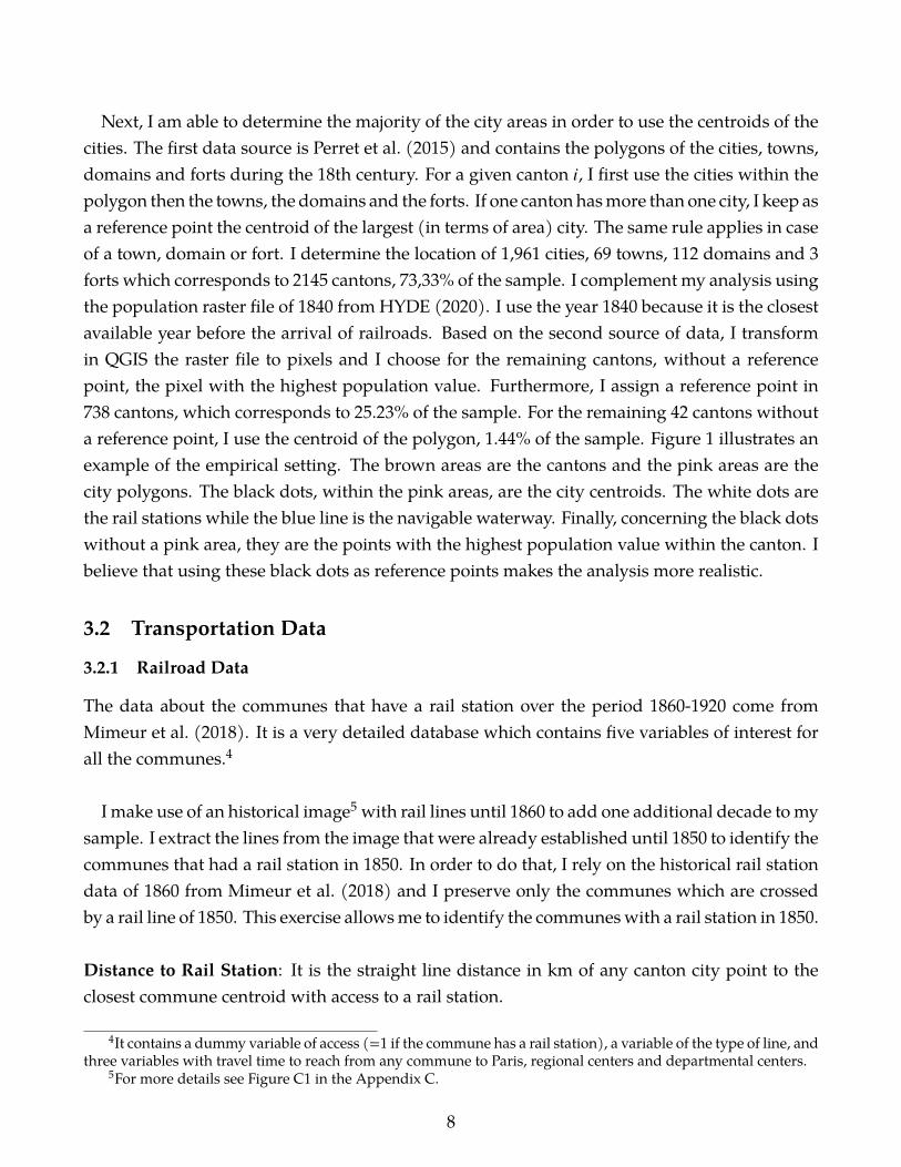
The data about the communes that have a rail station over the period 1860-1920 come fromMimeur et al. (2018). It is a very detailed database which contains five variables of interest forall the communes.4

I make use of an historical image5 with rail lines until 1860 to add one additional decade tomysample. I extract the lines from the image that were already established until 1850 to identify thecommunes that had a rail station in 1850. In order to do that, I rely on the historical rail stationdata of 1860 from Mimeur et al. (2018) and I preserve only the communes which are crossedby a rail line of 1850. This exercise allowsme to identify the communeswith a rail station in 1850.

Distance to Rail Station: It is the straight line distance in km of any canton city point to theclosest commune centroid with access to a rail station.

4It contains a dummy variable of access (=1 if the commune has a rail station), a variable of the type of line, andthree variables with travel time to reach from any commune to Paris, regional centers and departmental centers.

5For more details see Figure C1 in the Appendix C.

8

Figure 1: Setting

Notes: This figure illustrates the research setting of the paper.

Furthermore, I attempt to create the historical rail line network of France. In the absence ofhigh resolution historicalmaps, I use the communeswith rail stations over the period 1850-18906

and modern rail lines of France.7Baum-Snow et al. (2017, 2018) argue that historical infrastruc-ture networks are good predictors and facilitate the construction of a lower cost and more mod-ern infrastructure network. In this paper, I use a modern infrastructure network to re-create anold one. I use a shapefile with the rail lines over the period 2000-2020 (Jeansoulin, 2019) anda shapefile with the lines until 1992 (DIVA-GIS, 2020). Figure 2 presents the results of this ex-ercise. According to the findings a significant development of rail network occurred in Franceover the 19th century.

6For more details see Figure C2 in the Appendix C.7For more details see Figure C3 in the Appendix C.

9

3.2.2 Canal Data and Ports

In addition to the railroads, France developed a canal network. I make use two sources of datain order to identify the canal network of France.

The first source of navigable waterways comes from Ryavec and Henderson (2017) and theirexercise 2 about Cities and Water Transportation in 19th Century France. It is a shapefile de-veloped by Jordi Marti Henneberg (http://europa.udl.cat/projects/inland-waterways/). Thisshapefile includes the canal network of France in 1850. The second source of data is the col-lection of historical maps of University of Chicago (2020). It contains very detailed maps ofnavigable waterways of France over the second half of 19th century.8I digitized these historicalmaps in QGIS. Figure 2 shows the expansion of canals. Next, I construct the indicator of accessto the canal network.

Access to NavigableWaterways: It is a binary indicator which switches to 1 for a canton if thereis a canal within 3 km distance from the city centroid. In the Appendix A, I apply robustnesscheck with different thresholds.

In addition, I make use of a historical map from David Rumsey (2020) collection to identifythe ports of France in 1877.9I complement this data with active ports over the period 1662-1855from García-Herrera et al. (2006). Their database is about the reconstruction of oceanic windfield patterns for this period that precedes the time inwhich anthropogenic influences on climatebecame evident. Nevertheless, they include the variables "voyagefrom" and "voyageto" whichcontain the names of the places where the ship departed from or sailed to. I apply geocoding onStata (Zeigermann, 2018) and I identify 13 active ports10 for France. I use the ports to constructthe instrument.

3.3 Patent Data

The historical database of INPI (National Institute of Industrial Property) contains all the patentapplications (409,324 applications with their additions) covering the period 1791-1902. Thedatabase includes the application number of the patents, the filing year, the name of the ap-plicant(s), the commune, the street and number of the applicant(s), the title of the patents andthe expiration date of the patent applications. Additional details are included in the databaselike if an application is a patent that was imported from abroad, the number of additions of

8For an example of the maps see Figure C4 in the Appendix C.9For more details see Figure C4, Appendix C.10At least one ship departed or sailed to these ports.

10

Figure 2: Expansion of Railroads and Navigable Waterways

(a) 1850 (b) 1860

(c) 1870 (d) 1880

(e) 1890

Notes: This figure shows the expansion of navigable waterways for France over the time period1850-1890. Source: the shapefile of canal network for 1850 comes from Ryavec and Henderson(2017). For the period 1860-1890, it is based on author’s digitization of the historical maps fromUniversity of Chicago (2020). The lines of railroads are constructed by the author based on histor-ical rail stations of Mimeur et al. (2018) and recent shapefiles of rail lines from DIVA-GIS (2020)and Jeansoulin (2019).

11

every patent application and the profession of the applicant.

I restrictmy sample only to applicationswith at least one inventor residing in France. I removeapplications that belong only to firms using key words.11 Next, I exclude 116 applications with-out a filing date. When one application has several improvements, I do not take into account theimprovements, but only the initial design. Finally, I exclude from the sample the patent applica-tions that are importations since it is more likely the inventor to be resident of another countryand only the patent agent to be in France. I end up with 308,926 patent applications over theentire period. Figure 3 presents the evolution of patent applications per capita over the sampleof period of the paper as well the time trend for the average distance to rail stations.

Figure 3: Innovation per Capita and Average Distance to Rail Stations

0.0

00

5.0

01

.00

15

.00

2

Pa

ten

ts p

er

Ca

pita

0.2

.4.6

.81

Dis

tan

ce

to

Ra

il S

tatio

ns

1850 1860 1870 1880 1890Year

Distance to Rail Stations Patents per Capita

Patents per Capita and Average Distance to Stations

Notes: Summary graph showing the time trend of patent applications per capita and averagedistance to rail station. Source: author’s computations based on the patent applications from INPI(2019) database, population from HYDE (2020) and rail stations from Mimeur et al. (2018).

Number of patent applications: I calculate the sum of the patents12 for each decade from 1850

11I exclude all the applications that have the words “COMPAN” or “COMPAGNI” or “SOCIETA” or “SOCIET”or "GESELLSCHAFT" or "SYNDICAT" or "GESELLSCHAF" or "MANUFACTUR" in the applicant name.

12It is the collapse sum command in Stata.

12

until 1890 like in Andersson et al. (2021).Number of patent applications that received an addition: INPI database contains the numberof additions of each patent application. The patent law of 1844 gave the applicants the possi-bility to apply for certificates of addition (Galvez-Behar, 2019). These certificates allowed theapplicants to protect a minor improvement to the initial patent during its term. An addition ofthe initial design has an extra cost of 24 francs (Nuvolari et al., 2020). As a quality measure ofinnovation, I restrict the sample of patents to the ones that received an addition.

Apart from the main database, INPI includes a sample of 38,527 patent applications withtheir technological field. These patents are divided in 20 main classes.13 For only this sampleof patents, I have their main class and also their title. I use the "lsemantica" command in Stata(Schwarz, 2019) to extract key words from the titles of the patent applications. I complementthese keywords with additional words from the names of themain and sub classes of the patentapplications. Then, I keep the unique words among classes to create a vocabulary. Based on thisvocabulary, I manage to assign classes to the rest of patent applications in INPI database. Moretechnical details regarding this method and the vocabulary can be found in the Appendix B.Figure 4 illustrates the time trend for every class. As a result of this analysis, I construct twomore indicators of innovation.

Number of Novel Classes: Number of Novel Classes it is the number of new technology fieldsthat a canton has at least one invention in a given yearStock of Classes: Stock of classes is for every year the number of technological classes that acanton already has at least one invention.

Next, in order to be sure that I do not double count inventors residing in the same canton, Iapply a simple applicants’ disambiguation based on the name surname and their address. Thisexercise allows me to assign a unique identifier to the inventors. I apply fuzzy matching (Raffo,2020) on the name and surname of applicants residing in the same street. Then, I considerthe applicants with a matching score more than 73% to be the same person. I identify 334,504unique applicants from 353,017 patent applications. Even though the disambiguation is simpleand "kills" the mobility of the inventors, since one of the criteria is applicant’s address, it servesits purpose. In the sample every period is a decade and this simple disambiguation allows meto build an indicator of stock of inventors. One additional advantage of this method is that thestock of inventors is not be driven by outliers in the data. (Bahar et al., 2020)14

13The 20 classes are: Agriculture, Alimentation Railways and Trams, Arts textile, Fibers and Yarns, Machines,Marine and Navigation Construction, Public and Private, Mines and Metallurgy, Domestic Economy, Weapons,Road Transport, Instruments of Precision and Electricity, Ceramics, Chemics, Lighting Heating Refrigeration andVentilation, Clothes, Arts, Office Supplies and Education, Medicine and Health, Articles and Various Industries.

14As already explained in Bahar et al. (2020) there could be fluctuations in the stock of inventors if one inventor

13

Figure 4: Applications by classes

05

00

10

00

15

00

Ag

ricu

ltu

re1820 1840 1860 1880 1900

Year

02

00

40

06

00

Alim

en

tatio

n

1820 1840 1860 1880 1900Year

05

00

10

00

15

00

20

00

Ra

ilw

ays a

nd

Tra

ms

1820 1840 1860 1880 1900Year

02

00

40

06

00

80

01

00

0A

rts t

extile

, F

ibe

rs a

nd

Ya

rns

1820 1840 1860 1880 1900Year

01

00

02

00

03

00

04

00

0M

ach

ine

s

1820 1840 1860 1880 1900Year

01

00

20

03

00

40

0M

arin

e a

nd

Na

vig

atio

n

1820 1840 1860 1880 1900Year

05

00

10

00

15

00

20

00

Co

nstr

uctio

n,

Pu

blic a

nd

Priva

te

1820 1840 1860 1880 1900Year

02

00

40

06

00

Min

es a

nd

Me

tallu

rgy

1820 1840 1860 1880 1900Year

02

00

40

06

00

80

0D

om

estic E

co

no

my

1820 1840 1860 1880 1900Year

02

00

40

06

00

80

0R

oa

d T

ran

sp

ort

1820 1840 1860 1880 1900Year

02

00

40

06

00

80

0W

ea

po

ns

1820 1840 1860 1880 1900Year

05

00

10

00

15

00

Instr

um

en

ts o

f P

recis

ion

an

d E

lectr

icity

1820 1840 1860 1880 1900Year

01

00

20

03

00

40

0C

era

mic

s

1820 1840 1860 1880 1900Year

01

00

02

00

03

00

0C

he

mic

s

1820 1840 1860 1880 1900Year

05

00

10

00

15

00

Lig

htin

g,

He

atin

g,

Re

frig

era

tio

n a

nd

Ve

ntila

tio

n

1820 1840 1860 1880 1900Year

05

00

10

00

15

00

20

00

Clo

the

s

1820 1840 1860 1880 1900Year

01

00

02

00

03

00

0A

rts

1820 1840 1860 1880 1900Year

01

00

20

03

00

40

0O

ffic

e S

up

plie

s a

nd

Ed

uca

tio

n

1820 1840 1860 1880 1900Year

01

00

20

03

00

40

05

00

Me

dic

ine

an

d H

ea

lth

1820 1840 1860 1880 1900Year

02

00

40

06

00

Art

icle

s a

nd

Va

rio

us I

nd

ustr

ies

1820 1840 1860 1880 1900Year

Notes: Summary graph presenting the evolution of patent applications by classes. If an appli-cation has several classes, I allocate one application to all of them. The classes are: Agriculture,Alimentation Railways and Trams, Arts textile, Fibers and Yarns, Machines, Marine and Naviga-tion Construction, Public and Private, Mines and Metallurgy, Domestic Economy, Weapons, RoadTransport, Instruments of Precision and Electricity, Ceramics, Chemics, Lighting Heating Refrig-eration and Ventilation, Clothes, Arts, Office Supplies and Education, Medicine and Health, Ar-ticles and Various Industries. Source: author’s computations based on patent applications fromINPI (2019).

3.4 Other Data

I rely on HYDE (2020) database to export (gridded) time series of population and land use. Irely on raster files to form the indicators in QGIS at the canton level. All the indicators havetime variation. I extract data about population (defined as the population counts, in inhabi-tants/gridcell), cropland (defined as the total cropland area, in km2 per grid cell) and grazing(defined as the total land used for grazing, in km2 per grid cell). I use the baseline estimates ofthe database.15

In addition, I construct a binary indicator which switches to one if the canton has a university

residing in a commune has a patent in year C − 1 and C + 1 but not in year C. By taking the average of ten years thesefluctuations are not an issue any more.

15I use the version 3.2 which was released in 04-08-2020.

14

or a grande ecole like in Lecce et al. (2021). I manually collect the locations of the universitiesfrom Ruegg (2004) and check if the universities were abolished during the French Revolution in1793. Next, I extractmanually the addresses of the grand ecole from theConference desGrandesEcoles (www.cge.asso.fr). I geolocalize in STATA the addresses of the universities and grandecole using the command developed by Zeigermann (2018). Finally, I control for the number ofpost offices a canton has, using the database of Verdier and Chalonge (2018), to be in line withthe literature about state capacity and innovation (Acemoglu et al., 2016).

Table 1: Summary Statistics

Variable Mean Std. Dev. Min. Max. N

Innovation VariablesINPI Applications 17.5745 776.0184 0 68635 14625

Probability to Innovate 0.4755 0.4994 0 1 14625Additions 2.8867 107.7245 0 7232 14625

Number of Novel Classes 1.1625 1.9716 0 20 14625Stock of Classes 3.9177 5.1607 0 20 14625

INPI Applications by technological class 1.9523 107.4823 0 25804 292500

Transportation VariablesDistance to Rail Station 41.1569 75.6703 0.0608 594.5292 14625Access to Waterways 0.0003 0.0185 0 1 14625Travel Cost to Paris 7790.6959 7213.0369 0 92328.3125 14625Travel Cost to Lyon 7498.2269 6672.2881 0 87256.3359 14625

Travel Cost to Marseille 9951.6185 6981.023 0 84630.1094 14625Distance to Straight Line (Instrument) 28.6276 39.1383 0 339.3349 14625

Access to Knowledge 0.0002 0.0002 5.64e-06 0.0032 14625Access to Knowledge by technological class 0.0001 0.0000453 1.00e-06 0.0013 292500

Control VariablesPopulation 13244.6819 35836.6914 0 2524117 14625

Average Cropland Area 29.4377 16.1494 0 61.8082 14625Average Grazing Area 18.3853 11.993 0 55.9528 14625

University 0.0116 0.1072 0 1 14625Post Offices 2.1933 1.8605 0 40 14625

Robustness Analysis - VariablesTravel Time to Paris 931.1978 625.1727 0 7817.8740 11700

Distance to a Discrete Station 183.4004 183.5866 0.1922 759.4374 14625Distance to International Collaboration 100.2293 69.7108 0 409.8712 14625Access to Knowledge based on Elevation 0.0002 0.0002 8.80e-07 0.0029 14625

Differences in Differences Model - VariablesINPI Applications 9.3656 550.2264 0 68635 29250

Access to rail within 3km distance 0.1115 0.3148 0 1 29250Access to rail within 5km distance 0.1532 0.3602 0 1 29250Access to rail within 7km distance 0.1817 0.3856 0 1 29250

Population 12090.7981 27842.4077 0 2524117 29250Average Grazing Area 18.302 11.9084 0 55.9528 29250Average Cropland Area 28.6418 16.2708 0 61.9237 29250

Notes: Summary statistics for all the main variables (2,925 cantons, every 10 years is 1 period in the sample, 5 timeperiods in total.). Innovation variables: INPI Applications is the total number of patent applications, Probability toinnovate is a binary indicator which switches to one if the canton has a patent application, Additions is the total numberof patent applications that received an addition, Number of Novel Classes contains the number of novel technologicalclasses that a canton has in a given year and Stock of classes the number of technological classes that a canton alreadyhas. Transportation variables: Distance to Rail Station is the distance (in kilometers) from any city centroid to the closestcommune centroid with access to a rail station, Access to Waterways is defined as a dummy variable which takes thevalue 1 if the centroid of a canton is within 3 kilometers distance from the closest canal, travel cost to Paris, Lyon andMarseille is the computed travel cost based on rail lines and canals of every city centroid to Paris, Lyon andMarseille anddistance to straight line is the instrument (in kilometers). Access to knowledge variables: Access to knowledge is thecomputed access of every canton based on the share of inventors over population and accessibility in rail lines and canalsand market access is the computed market access of every canton based on the number of citizens and accessibility inrail lines and canals. Control variables: population is the total number of inhabitants, cropland is the average croplandarea, grazing is the average land used for grazing, university is a binary variable which switches to 1 if the canton has auniversity and post offices is the number of post offices in a canton. The dimension of the variables INPI Applicationsby technological class and Access to Knowledge by technological class is 2,925 cantons, 20 technological classes every10 years, 5 time periods in total. The time period for the differences in differences model is from 1800 to 1890.

15

4 Empirical Strategy

I start the analysis by estimating the main model through OLS regressions (Correia, 2015). Theestimation equation is:

%0C8C = U0 + V�8BC(C0C8C−1 + W8 + XC + Z-8C + n8C (1)

where, %0C8C is the number of patents in the canton 8, in time period C. The main variable ofinterest is �8BC(C0C8C−1, which contains the distance in km of any canton city centroid to the clos-est commune centroid with a rail station as computed in the previous period.16 I include cantonfixed effects, W8 and year fixed effects, XC . -8C contains all the controls at the canton level such asthe population, the average cropland area, the average grazing area, the number of post officesand the existence of a university.

The variable %0C8C and the population have been transformed using the log transformation17

to reduce the effect of the extreme values in the sample (Squicciarini and Voigtländer, 2015). Asa robustness test, I apply also a Poisson pseudo-maximum likelihood regressions model in theAppendix A without any transformation in the data.

However, I have to take into consideration the potential endogeneity problem due to omittedvariable bias. The placement of the actual network may be endogenous and affected by unob-servable local economic conditions (Andersson et al., 2021). Tomitigate any concerns that couldnaturally arise, I complement the analysis with an instrumental variable approach and severalrobustness tests.

4.1 Endogeneity and Instrumental Variables

Following a similar strategy as in Katz (2018), I propose the use of a time variant instrumentfor the rail network of France. The identification strategy builds on straight lines (Perlman,2015; Katz, 2018; Banerjee et al., 2020) as they represent the Euclidean (least cost) distancebetween two places. In addition, Dunham (1941) mentions about French rail network that"�>A ?B 34B ?>=CB 4C 2ℎ0DBB44B believed in making railroads as straight as possible, no matterwhat important centres of trade or industry theymight by pass on the way". This team of highlytrained engineers was not interested in trade or industry, nor in the problems of economics. The

16A one-lag structure for the effect of railway variable on innovation outcomes is intuitive in this frameworkbecause the railway stations constructed near the end of the calendar year are likely to affect innovation outcomesonly in the following year (Melander, 2020).

17I add 1 in the variables: number of patent applications and population before I apply the log transformation.

16

above theoretical framework justifies the use of straight lines as an instrument in case of France.

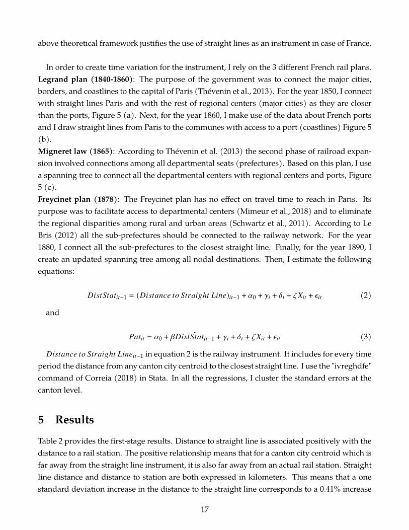
In order to create time variation for the instrument, I rely on the 3 different French rail plans.Legrand plan (1840-1860): The purpose of the government was to connect the major cities,borders, and coastlines to the capital of Paris (Thévenin et al., 2013). For the year 1850, I connectwith straight lines Paris and with the rest of regional centers (major cities) as they are closerthan the ports, Figure 5 (a). Next, for the year 1860, I make use of the data about French portsand I draw straight lines from Paris to the communes with access to a port (coastlines) Figure 5(b).Migneret law (1865): According to Thévenin et al. (2013) the second phase of railroad expan-sion involved connections among all departmental seats (prefectures). Based on this plan, I usea spanning tree to connect all the departmental centers with regional centers and ports, Figure5 (c).Freycinet plan (1878): The Freycinet plan has no effect on travel time to reach in Paris. Itspurpose was to facilitate access to departmental centers (Mimeur et al., 2018) and to eliminatethe regional disparities among rural and urban areas (Schwartz et al., 2011). According to LeBris (2012) all the sub-prefectures should be connected to the railway network. For the year1880, I connect all the sub-prefectures to the closest straight line. Finally, for the year 1890, Icreate an updated spanning tree among all nodal destinations. Then, I estimate the followingequations:

�8BC(C0C8C−1 = (�8BC0=24 C> (CA086ℎC !8=4)8C−1 + U0 + W8 + XC + Z-8C + n8C (2)

and

%0C8C = U0 + V ˆ�8BC(C0C8C−1 + W8 + XC + Z-8C + n8C (3)

�8BC0=24 C> (CA086ℎC !8=48C−1 in equation 2 is the railway instrument. It includes for every timeperiod the distance from any canton city centroid to the closest straight line. I use the "ivreghdfe"command of Correia (2018) in Stata. In all the regressions, I cluster the standard errors at thecanton level.

5 Results

Table 2 provides the first-stage results. Distance to straight line is associated positively with thedistance to a rail station. The positive relationship means that for a canton city centroid which isfar away from the straight line instrument, it is also far away from an actual rail station. Straightline distance and distance to station are both expressed in kilometers. This means that a onestandard deviation increase in the distance to the straight line corresponds to a 0.41% increase

17

Figure 5: Evolution of the Straight Line Instrument

(a) 1850 (b) 1860

(c) 1870

(d) 1880 (e) 1890

Notes: This figure illustrates the expansion of straight line instrument based on the regional centers in 1850, regional centers and ports in 1860,a spanning tree among regional centers, departmental centers and ports in 1870, subprefecture centers in 1880 and a spanning tree among allthe nodal destinations in 1890. Source: author’s computations.

18

in the distance to the actual rail stations. Finally, the instrument is highly significant.

Table 2: First stage: distance to straight line instrument and railway stations

Dep. var. = Distance to Station(1)

Distance to Straight Line 0.413∗∗∗[0.016]

Sample Size 14625Canton FE YesYear FE YesCanton Controls Yes

Notes: First stage regressions. The dependent variable is the distance to the near-est constructed railway station. Distance to straight line is the distance of anycentroid to the closest straight line. Canton controls contain the population, theaccessibility to waterways, the average cropland area, the average land used forgrazing, the existence of a university and the number of post offices. The pop-ulation is transformed using a log transformation. The results are based on theequation 2. Clustered standard errors at the canton level are reported in the paren-thesis.

Moving now to the main results, Table 3 presents the OLS and the IV results. The depen-dent variable in the first three columns is the number of patent applications. Both OLS and IVestimates are highly significant and negative, column 1 and 2 OLS and column 3 the IV. I relyon the IV estimates, column 3, to interpret the results. Since all the variables are standardizedthe interpretation is that for a given canton a one standard deviation decrease in the distanceto a rail station is associated with a 0.049% increase in the number of patent applications. Aone standard deviation increase in the population is associated with approximately 0.22% in-crease in the number of patent applications, column 3. In addition, in line with the literature,the number of post offices has a positive and significant effect meaning that a one standard de-viation increase in the number of post offices in a canton corresponds to a 0.025% increase inthe number of patent applications. Average cropland and grazing land have no significant ef-fect on patenting rate. Finally, access to waterways does not affect innovation activity. In theAppendix, I use alternative indexes of accessibility to canals based on different thresholds. Fi-nally, Kleibergen-PaapWald rk F statistic is high meaning that the instrument performs well. Incolumn 4 and 5, I use as dependent variable a binary indicator which switches to 1 if the cantonhas at least one patent application. Based on the findings of the IV regressions, column 6, a onestandard deviation decrease in the distance to a rail station is associated with a 0.07% increasein the probability of a canton to innovate. Even though population has a strong impact on thenumber of patent applications it appears to have no effect on the probability of a canton to in-novate. A possible explanation is that the population affects innovation performance throughthe theoretical channel of agglomeration and does not boost the innovation performance acrosscantons in contrast with a connection to a network.

19

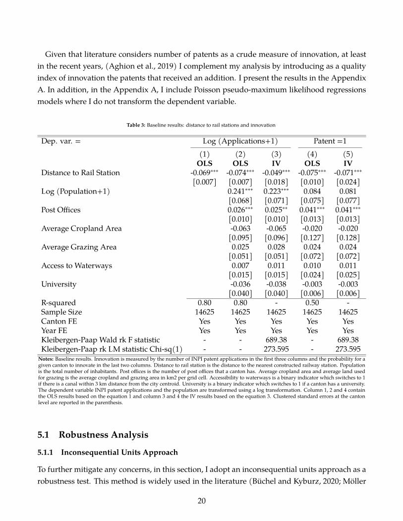
Given that literature considers number of patents as a crude measure of innovation, at leastin the recent years, (Aghion et al., 2019) I complement my analysis by introducing as a qualityindex of innovation the patents that received an addition. I present the results in the AppendixA. In addition, in the Appendix A, I include Poisson pseudo-maximum likelihood regressionsmodels where I do not transform the dependent variable.

Table 3: Baseline results: distance to rail stations and innovation

Dep. var. = Log (Applications+1) Patent =1(1) (2) (3) (4) (5)OLS OLS IV OLS IV

Distance to Rail Station -0.069∗∗∗ -0.074∗∗∗ -0.049∗∗∗ -0.075∗∗∗ -0.071∗∗∗[0.007] [0.007] [0.018] [0.010] [0.024]

Log (Population+1) 0.241∗∗∗ 0.223∗∗∗ 0.084 0.081[0.068] [0.071] [0.075] [0.077]

Post Offices 0.026∗∗∗ 0.025∗∗ 0.041∗∗∗ 0.041∗∗∗[0.010] [0.010] [0.013] [0.013]

Average Cropland Area -0.063 -0.065 -0.020 -0.020[0.095] [0.096] [0.127] [0.128]

Average Grazing Area 0.025 0.028 0.024 0.024[0.051] [0.051] [0.072] [0.072]

Access to Waterways 0.007 0.011 0.010 0.011[0.015] [0.015] [0.024] [0.025]

University -0.036 -0.038 -0.003 -0.003[0.040] [0.040] [0.006] [0.006]

R-squared 0.80 0.80 - 0.50 -Sample Size 14625 14625 14625 14625 14625Canton FE Yes Yes Yes Yes YesYear FE Yes Yes Yes Yes YesKleibergen-Paap Wald rk F statistic - - 689.38 - 689.38Kleibergen-Paap rk LM statistic Chi-sq(1) - - 273.595 - 273.595

Notes: Baseline results. Innovation is measured by the number of INPI patent applications in the first three columns and the probability for agiven canton to innovate in the last two columns. Distance to rail station is the distance to the nearest constructed railway station. Populationis the total number of inhabitants. Post offices is the number of post offices that a canton has. Average cropland area and average land usedfor grazing is the average cropland and grazing area in km2 per grid cell. Accessibility to waterways is a binary indicator which switches to 1if there is a canal within 3 km distance from the city centroid. University is a binary indicator which switches to 1 if a canton has a university.The dependent variable INPI patent applications and the population are transformed using a log transformation. Column 1, 2 and 4 containthe OLS results based on the equation 1 and column 3 and 4 the IV results based on the equation 3. Clustered standard errors at the cantonlevel are reported in the parenthesis.

5.1 Robustness Analysis

5.1.1 Inconsequential Units Approach

To further mitigate any concerns, in this section, I adopt an inconsequential units approach as arobustness test. This method is widely used in the literature (Büchel and Kyburz, 2020; Möller

20

and Zierer, 2018; Faber, 2014). The intuition is that in the early stages of transport infrastructuredevelopments, major destinations are typically connected first. This IV approach relies on therandomly chosen subset of municipalities that received railway access because they lie on themost direct route between these nodal destinations. Even though, I follow the actual rail planswhen I draw the straight lines the selection of the nodal destinations could be endogenous. Tothis end, I re-estimate equation 1 and equation 3, using the inconsequential units approach, toeliminate any concerns.

Based on this approach, I remove from the sample all the focal destinations that were used inthe construction of the instrument. By doing that, I also exclude the capital city of Paris. This iscrucial since it takes into consideration an another type of endogeneity. The only office of INPIwas in Paris and as a result for an inventor it could be easier to use in the application file anaddress of a patent agent in Paris. This could introduce bias in the benchmark analysis, a biasthat is possible not addressed by the instrument.

Moving to the results in Table 4, I re-estimate the equations 1 and 3 after I remove the nodaldestinations. Again, I rely on the IV estimates to interpret the results. The magnitude is nowlower comparing to the benchmark estimates in Table 3 but again significant at 5%. A possibleexplanation for the lower magnitude it could be the exclusion of the big urban centers from thesample.

5.1.2 Balance Test

In this section, I present the results of a balance test exercise. I re-estimate equation 3 but thistime I use as dependent variable the number of patents from 1800 until 1840. The intuition be-hind this empirical exercise is that allows me to explore if there is a pre-trend effect of railroadson innovation performance before the actual sample period.

Table 5 presents the IV results. According to the findings distance to rail station has no effecton innovation performance. This result confirms that the distance to railroads variable is notassociated with pre-trends regarding the patent activity.

5.1.3 Difference-in-Differences Model

Next, I apply as a robustness test a conventional difference-in-differences regressionmodel withstaggered treatment. I collect data about population, cropland and grazing area over the period1800 until 1840 to complement the panel dataset of the benchmark analysis. I create three dif-ferent variables of access to a rail station based on the distance to the closest commune with arail station. The advantage of this method is that allows me to control for pre-trends since the

21

Table 4: Distance to rail stations and innovation - inconsequential units approach

Dep. var. = Log (Applications+1)(1) (2)OLS IV

Distance to Rail Station -0.062∗∗∗ -0.040∗∗[0.007] [0.016]

R-squared 0.64 -Sample Size 13010 13010Canton FE Yes YesYear FE Yes YesCanton Controls Yes YesKleibergen-Paap Wald rk F statistic - 620.68

Notes: I exclude from the sample all the destinationswhich I use to create the instrument. Innovation ismeasured by the number of INPI patentapplications. Distance to rail station is the distance from themost populous point of a canton to the nearest constructed railway station. Cantoncontrols contain the population, the accessibility to waterways, the average cropland area, the average land used for grazing, the existence of auniversity and the number of post offices. The dependent variables and the population are transformed using a log transformation. Column 1contains the OLS results based on the equation 1 and column 2 the IV results based on the equation 3. Clustered standard errors at the cantonlevel are reported in the parenthesis.

arrival of railroads. I am able to do that by using the period 1800 to 1840 in which there is notany canton with access to a rail station. I estimate the following equation:

%0C8C = U0 + V�228C−1 + W8 + XC + Z-8C + n8C (4)

where �228C−1 is the access variable switching to one if a canton has access to a rail station. Iconsider three different variables of access depending on the distance to the closest rail station.It can be 3, 5, or 7 km away. I include canton and year fixed effects and time variant controlslike log of population, grazing area and cropland area. Table 6 summarizes the results. Thesample period now is from 1800 until 1890. I find that access to a rail station has a positive andsignificant effect which confirms the results of the benchmark analysis.

5.1.4 Cross Sectional Analysis by decade

Finally, I apply cross sectional analysis to further explore the interplay between the distance torailroads and innovation performance. I include arrondissement fixed effects and cluster thestandard errors at the department level. I estimate the following equation for each decade:

%0C8 = U0 + V ˆ�8BC(C0C8 + W8 + Z-8 + n8 (5)

22

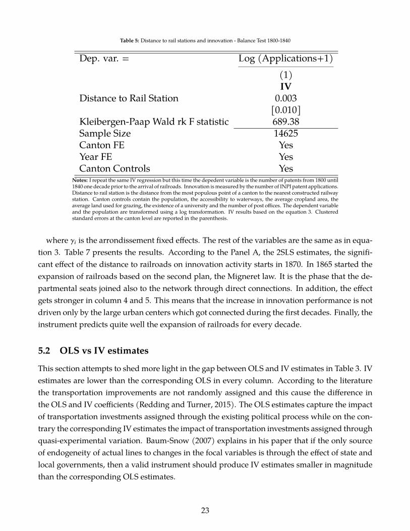
Table 5: Distance to rail stations and innovation - Balance Test 1800-1840

Dep. var. = Log (Applications+1)(1)IV

Distance to Rail Station 0.003[0.010]

Kleibergen-Paap Wald rk F statistic 689.38Sample Size 14625Canton FE YesYear FE YesCanton Controls Yes

Notes: I repeat the same IV regression but this time the depedent variable is the number of patents from 1800 until1840 one decade prior to the arrival of railroads. Innovation ismeasured by the number of INPI patent applications.Distance to rail station is the distance from the most populous point of a canton to the nearest constructed railwaystation. Canton controls contain the population, the accessibility to waterways, the average cropland area, theaverage land used for grazing, the existence of a university and the number of post offices. The dependent variableand the population are transformed using a log transformation. IV results based on the equation 3. Clusteredstandard errors at the canton level are reported in the parenthesis.

where W8 is the arrondissement fixed effects. The rest of the variables are the same as in equa-tion 3. Table 7 presents the results. According to the Panel A, the 2SLS estimates, the signifi-cant effect of the distance to railroads on innovation activity starts in 1870. In 1865 started theexpansion of railroads based on the second plan, the Migneret law. It is the phase that the de-partmental seats joined also to the network through direct connections. In addition, the effectgets stronger in column 4 and 5. This means that the increase in innovation performance is notdriven only by the large urban centers which got connected during the first decades. Finally, theinstrument predicts quite well the expansion of railroads for every decade.

5.2 OLS vs IV estimates

This section attempts to shed more light in the gap between OLS and IV estimates in Table 3. IVestimates are lower than the corresponding OLS in every column. According to the literaturethe transportation improvements are not randomly assigned and this cause the difference inthe OLS and IV coefficients (Redding and Turner, 2015). The OLS estimates capture the impactof transportation investments assigned through the existing political process while on the con-trary the corresponding IV estimates the impact of transportation investments assigned throughquasi-experimental variation. Baum-Snow (2007) explains in his paper that if the only sourceof endogeneity of actual lines to changes in the focal variables is through the effect of state andlocal governments, then a valid instrument should produce IV estimates smaller in magnitudethan the corresponding OLS estimates.

23

Table 6: Distance to rail stations and innovation - Differences in Differences

Dep. var. = Log (Applications+1)(1) (2) (3)

Access to rail 3km distance 0.102∗∗∗[0.008]

Access to rail 5km distance 0.103∗∗∗[0.008]

Access to rail 7km distance 0.088∗∗∗[0.008]

R-squared 0.67 0.67 0.67Sample Size 29250 29250 29250Canton FE Yes Yes YesYear FE Yes Yes YesCanton Controls Yes Yes Yes

Notes: Access to rail is a binary indicator switching to 1 if a canton has access to railroads within a given dis-tance threshold. Innovation is measured by the number of INPI patent applications. Canton controls contain thepopulation, the average cropland area and the average land used for grazing. The dependent variable and thepopulation are transformed using a log transformation. Differences in differences model based on equation 4.Clustered standard errors at the canton level are reported in the parenthesis.

In case of France, indeed, the rail lines that were planned in the borders with Germany wasan act of political interference. The reason was the Franco-Prussian war in 1870. Accordingto Jordan W. Jonathan (2005) "the French government constructed long stretches of strategicrailways in eastern France along the German border that served strategically crucial ends". Theendogenous selection of these places as recipients of rail lines violates the assumption that trans-portation improvements are randomly assigned and introduces bias to the OLS estimates. Table8 explores the effect of distance to a rail station on innovation activity after I remove from thesample areas that could gain access to a rail station for defensive reasons because they are closeto the borders with Germany. The OLS coefficient is being reduced while the IV increases as wemove from column 1 to 3. In column 3, after the exclusion from the sample the cantons that arewithin 35 km distance from the borders, the two coefficients have the same magnitude.

The war ended with the Treaty of Frankfurt on May of 1871. According to this Treaty thedepartments Bas-Rhin, Haut-Rhin, Moselle, one-third of the department of Meurthe, includingthe cities of Château-Salins and Sarrebourg, and the cantons Saales and Schirmeck in the de-partment of Vosges became part of the German Empire. In the Appendix A, I re-estimate theequations 1 and 3 after I exclude the cantons that were affected from the war.

24

Table 7: Distance to rail stations and innovation by decade

Dep. var. = Log (Applications+1)(1) (2) (3) (4) (5)

Decade 1850 1860 1870 1880 1890Panel A - Second Stage IV IV IV IV IVDistance to Rail Station -0.304 -0.539 -2.475∗∗∗ -6.417∗∗∗ -7.014∗∗∗

[0.187] [0.687] [0.547] [1.350] [1.776]Kleibergen-Paap Wald rk F statistic 38.55 14.91 38.05 26.25 22.82Panel B - First Stage OLS OLS OLS OLS OLSDistance to Straight Line 0.207∗∗∗ 0.078∗∗∗ 0.115∗∗∗ 0.087∗∗∗ 0.069∗∗∗

[0.033] [0.020] [0.019] [0.017] [0.015]Sample Size 2924 2924 2924 2924 2924Canton FE Yes Yes Yes Yes YesYear FE Yes Yes Yes Yes YesCanton Controls Yes Yes Yes Yes Yes

Notes: Distance to rail station is the distance from the most populous point of a canton to the nearest constructed railway station. Innovationis measured by the number of INPI patent applications. Canton controls contain the population, the accessibility to waterways, the averagecropland area, the average land used for grazing, the existence of a university and the number of post offices. The dependent variable andthe population are transformed using a log transformation. Panel A contains the IV results based on the equation 5 and panel B the first stageresults. Clustered standard errors at the department level are reported in the parenthesis.

6 Mechanisms

6.1 Access to Knowledge

Dittmar (2011) studies the adoption of printing from cities in 16th century. Printingwas thema-jor technological innovation of 16th century. The author finds that places with ports and cheapwater transportation benefited more from this invention. The adoption of the printing pressrequired face to face interactions and the cities close to water transportation receive higher ben-efits than comparing to the rest of the sample. Network connections could reduce the obstaclesinvolved in knowledge diffusion (Breschi and Lissoni, 2009). Recent literature has shown thatin contrast with physical stock of capital, human capital is not transferred easily and inventorsinteract with each other to combine their skills (Jones, 2009). In the absence of one of the collab-orators, the remaining inventors lose in terms of patent production and earnings (Jaravel et al.,2018). An inventor acquires knowledge through interactions with others who are more knowl-edgeable than him (Akcigit et al., 2018) and this fact fosters innovation activity.

The intuition of the mechanism relies on a recently paper of Akcigit et al. (2018). The authorsshow that inventors built their knowledge and improve their skills by interacting with othersand learning from them. The knowledge of the inventors could work as an input in the produc-tion function (like the R&D) and not just as an output (like a patent). I employ the share ofinventors over population instead of population as a numerator in the traditional market access

25

Table 8: Distance to rail stations and cantons in the borders

Dep. var. = Log (Applications+1)(1) (2) (3)

Panel A OLS OLS OLSDistance to Rail Station -0.069∗∗∗ -0.068∗∗∗ -0.067∗∗∗

[0.007] [0.007] [0.007]R-squared 0.80 0.80 0.80Panel B IV IV IVDistance to Rail Station -0.059∗∗∗ -0.061∗∗∗ -0.065∗∗∗

[0.017] [0.017] [0.017]Kleibergen-Paap Wald rk F statistic 708.68 712.28 716.22Sample Size 14440 14420 14370Canton FE Yes Yes YesYear FE Yes Yes YesCanton Controls Yes Yes YesDistance from the German Borders 25 km 30 km 35 km

Notes: Column 1 does not contain the cantons that are within 25 kilometers from the borders, column 2 30 kilo-meters and column 3 35 kilometers. Innovation is measured by the number of INPI patent applications. Distanceto rail station is the distance from the most populous point of a canton to the nearest constructed railway station.Canton controls contain the population, the accessibility to waterways, the average cropland area, the average landused for grazing, the existence of a university and the number of post offices. The dependent variables and thepopulation are transformed using a log transformation. Panel A contains the OLS results based on the equation 1and panel B the IV results based on the equation 3. Clustered standard errors at the canton level are reported inthe parenthesis.

index of Donaldson and Hornbeck (2016). I call it access to knowledge since the purpose of thisindex is to explore how for a given canton 8 connectivity to other places where inventors resideaffects the invention rate of the canton 8. It is a supply side mechanism which relies on howimportant are the interactions and potential knowledge spillovers among inventors during theinnovation process.

More details about the construction of the costs for the access to knowledge indicator can befound in the Appendix C. Figure 6 shows the accessibility of every canton based on railroadsand canals over the period 1850-1890. The areas which are less accessible are the darker ones.As the network expands the areas become brighter.

In order to disentangle the effect of knowledge spillovers from the market size, I divide thenumber of inventors of every canton with the population. I rely on the inventors’ disambigua-tion as not to double count inventors who live in the same canton. Next, I form the access toknowledge index as:

�224BB C> =>F;43648C =∑ℎ≠8

�=E4=C>ABℎC/%>?ℎC�>BC8ℎC

(6)

26

Figure 6: Transportation Cost and Accessibility of every Canton

(a) 1850 (b) 1860

(c) 1870 (d) 1880

(e) 1890

Notes: This figure shows the reduction in the transportation cost and the accessibility of every canton due to the expansion of railroads andcanals over the time period 1850-1890. Source: author’s computations based on the shapefiles of canal network and railroads.

27

where for a canton 8 access to knowledge is defined as the sum of the share of inventors overpopulation residing in all the other cantons except 8 divided by the cost to reach in these can-tons. To be in line with the rest of the analysis since the access to knowledge indicator containsinventors, it has been transformed using the log transformation.18

6.1.1 Estimation Method and Results

I estimate the following equation:

%0C8C = U0 + V� 8C−1 + W8 + XC + Z-8Cn8C (7)

The independent variable, � 8C , is the index of access to knowledge. Second, I do not controlfor access to waterways of 19th century because I use the canals to compute the travel costs. Therest of the control variables are the population, the average cropland area, the average grazingarea, the number of post offices and the existence of a university.

Table 9 summarizes the results. Column 1 explore the reduce form equation where I controlonly for canton and year fixed effects. A one standard deviation increase in the share of access toknowledge mechanism corresponds to a 0.060% increase in the number of patent applications. Iinclude all the controls in column 2. The coefficient is now slightly higher. In the third column,I control also for market access, constructed in line with Donaldson and Hornbeck (2016) usingthe population of the cantons, in order to rule out alternativemechanisms. Again, the coefficientis positive and significant. Yet, the high increase in the coefficient of the variable could ariseconcerns related to multicollinearity. For this reason, in column 4, I re-estimate equation 7 butthis time I add a third dimension in themodel which is the technological class of the patent data.The updated equation is:

%0C82C = U0 + V� 82C−1 + ^8C + _82 + `C2 + n82C (8)

This allows me to introduce three pairwise fixed effects: canton-year fixed effects, ^8C , canton-technological class fixed effects, _82, and year-technological class fixed effects, `C2. These com-binations of fixed effects deal with all possible variables that do not vary by canton, year andtechnology like market access. Given that, I find again in the Table 9 that access to knowledgehas a positive and significant effect on the number of patent applications, column 4.

18I multiply both access to knowledge indicators with 10000000. These two indexes do not have zeros but ac-cording to Bellemare and Wichman (2020) the elasticities derived from log transformation hold for large enoughaverage values of the variables. Their suggestions for applied econometricians is to use approximate elasticities forvalues of a variable no less than 10.

28

Table 9: Mechanism: access to knowledge and innovation

Dep. var. = Log (Applications+1)(1) (2) (3) (4)OLS OLS OLS OLS

Log Access to Knowledge 0.060∗∗∗ 0.064∗∗∗ 0.988∗∗∗ 0.174∗∗[0.017] [0.017] [0.110] [0.073]

R-squared 0.79 0.79 0.80 0.82Sample Size 14625 14625 14625 292500Canton FE Yes Yes Yes NoYear FE Yes Yes Yes NoCanton Controls No Yes Yes NoLog Population Market Access No No Yes NoCanton x Year FE No No No YesCanton x Technology FE No No No YesYear x Technology FE No No No Yes

Notes: Access to knowledge is the sum of the share of inventors over population residing in all the other cantons except 8 divided by the costto reach in these cantons. Innovation is measured by the number of INPI patent applications. Canton controls contain the population, theaverage cropland area, the average land used for grazing, the existence of a university and the number of post offices. The dependent variable,the index of access to knowledge, the index of market access and the population are transformed using a log transformation. OLS model basedon the equations 7 and 8. Clustered standard errors at the canton level are reported in the parenthesis.

29

6.2 Diffusion of Novel Technologies and Access to a Global City

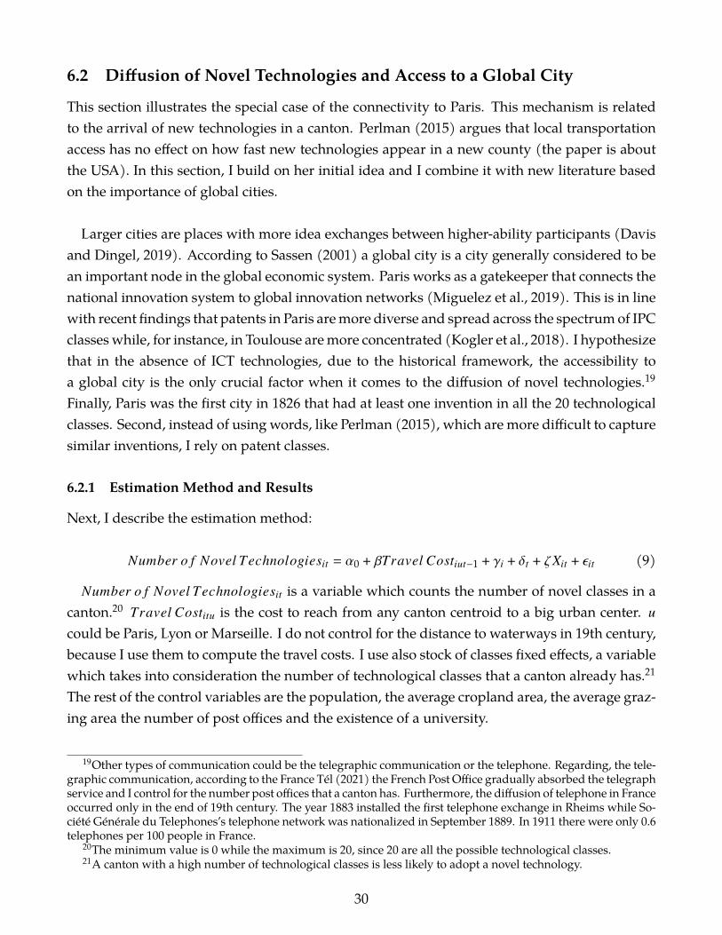
This section illustrates the special case of the connectivity to Paris. This mechanism is relatedto the arrival of new technologies in a canton. Perlman (2015) argues that local transportationaccess has no effect on how fast new technologies appear in a new county (the paper is aboutthe USA). In this section, I build on her initial idea and I combine it with new literature basedon the importance of global cities.

Larger cities are places with more idea exchanges between higher-ability participants (Davisand Dingel, 2019). According to Sassen (2001) a global city is a city generally considered to bean important node in the global economic system. Paris works as a gatekeeper that connects thenational innovation system to global innovation networks (Miguelez et al., 2019). This is in linewith recent findings that patents in Paris aremore diverse and spread across the spectrumof IPCclasseswhile, for instance, in Toulouse aremore concentrated (Kogler et al., 2018). I hypothesizethat in the absence of ICT technologies, due to the historical framework, the accessibility toa global city is the only crucial factor when it comes to the diffusion of novel technologies.19

Finally, Paris was the first city in 1826 that had at least one invention in all the 20 technologicalclasses. Second, instead of using words, like Perlman (2015), which are more difficult to capturesimilar inventions, I rely on patent classes.

6.2.1 Estimation Method and Results

Next, I describe the estimation method:

#D<14A > 5 #>E4; )42ℎ=>;>684B8C = U0 + V)A0E4; �>BC8DC−1 + W8 + XC + Z-8C + n8C (9)

#D<14A > 5 #>E4; )42ℎ=>;>684B8C is a variable which counts the number of novel classes in acanton.20 )A0E4; �>BC8CD is the cost to reach from any canton centroid to a big urban center. Dcould be Paris, Lyon or Marseille. I do not control for the distance to waterways in 19th century,because I use them to compute the travel costs. I use also stock of classes fixed effects, a variablewhich takes into consideration the number of technological classes that a canton already has.21

The rest of the control variables are the population, the average cropland area, the average graz-ing area the number of post offices and the existence of a university.

19Other types of communication could be the telegraphic communication or the telephone. Regarding, the tele-graphic communication, according to the France Tél (2021) the French Post Office gradually absorbed the telegraphservice and I control for the number post offices that a canton has. Furthermore, the diffusion of telephone in Franceoccurred only in the end of 19th century. The year 1883 installed the first telephone exchange in Rheims while So-ciété Générale du Telephones’s telephone network was nationalized in September 1889. In 1911 there were only 0.6telephones per 100 people in France.

20The minimum value is 0 while the maximum is 20, since 20 are all the possible technological classes.21A canton with a high number of technological classes is less likely to adopt a novel technology.

30

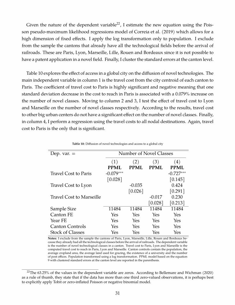
Given the nature of the dependent variable22, I estimate the new equation using the Pois-son pseudo-maximum likelihood regressions model of Correia et al. (2019) which allows for ahigh dimension of fixed effects. I apply the log transformation only to population. I excludefrom the sample the cantons that already have all the technological fields before the arrival ofrailroads. These are Paris, Lyon, Marseille, Lille, Rouen and Bordeaux since it is not possible tohave a patent application in a novel field. Finally, I cluster the standard errors at the canton level.

Table 10 explores the effect of access in a global city on the diffusion of novel technologies. Themain independent variable in column 1 is the travel cost from the city centroid of each canton toParis. The coefficient of travel cost to Paris is highly significant and negative meaning that onestandard deviation decrease in the cost to reach in Paris is associated with a 0.079% increase onthe number of novel classes. Moving to column 2 and 3, I test the effect of travel cost to Lyonand Marseille on the number of novel classes respectively. According to the results, travel costto other big urban centers do not have a significant effect on the number of novel classes. Finally,in column 4, I perform a regression using the travel costs to all nodal destinations. Again, travelcost to Paris is the only that is significant.

Table 10: Diffusion of novel technologies and access to a global city

Dep. var. = Number of Novel Classes(1) (2) (3) (4)

PPML PPML PPML PPMLTravel Cost to Paris -0.079∗∗∗ -0.727∗∗∗

[0.028] [0.145]Travel Cost to Lyon -0.035 0.424

[0.026] [0.291]Travel Cost to Marseille -0.017 0.230

[0.028] [0.213]Sample Size 11484 11484 11484 11484Canton FE Yes Yes Yes YesYear FE Yes Yes Yes YesCanton Controls Yes Yes Yes YesStock of Classes Yes Yes Yes Yes

Notes: I exclude from the sample the cantons of Paris, Lyon, Marseille, Lille, Rouen and Bordeaux be-cause they alreadyhad all the technological classes before the arrival of railroads. The dependent variableis the number of novel technological classes in a canton. Travel cost to Paris, Lyon and Marseille is thecomputed travel cost to reach in Paris, Lyon and Marseille. Canton controls contain the population, theaverage cropland area, the average land used for grazing, the existence of a university and the numberof post offices. Population transformed using a log transformation. PPML model based on the equation9 with clustered standard errors at the canton level are reported in the parenthesis.

22The 63.25% of the values in the dependent variable are zeros. According to Bellemare and Wichman (2020)as a rule of thumb, they state that if the data has more than one third zero-valued observations, it is perhaps bestto explicitly apply Tobit or zero-inflated Poisson or negative binomial model.

31

One possible concern could be that connectivity to Paris is associated with a lower cost forregistration of the patent applications and has nothing to do with the diffusion of novel tech-nologies. Since, the patent office of INPIwas in Paris a faster connection, because of the railroads,could facilitate the registration of the patent applications by the inventors. According to Galvez-Behar (2019) there were patent agents in Paris that could fill in the patent applications on behalfof the inventors. Even after the construction of railroads and the reduction in transportationcosts, it could be much easier for the inventors just to send a letter to the patent agents througha post office and to avoid to face bureaucratic procedures. Given that, controlling for the num-ber of post offices should take into consideration this potential concern. Furthermore, I repeatthe same regressions by excluding the Seine department and the region of Ile de France in theAppendix, Table A4, because for the inventors that were living close to Paris it could be possiblethe same cost to apply through a post office or to go to INPI’s office. The effect of transportationto Paris remains strongly significant.

6.3 Limitations of the Access to Knowledge Approach

The use of freight rates makes comparable the transportation through canals with the trans-portation through railroads. However, according to Donaldson and Hornbeck (2016), there areseveral important limitations that someone has to take into consideration when uses a similarapproach to the market access approach based on freight rates. This paper attempts to addressseveral of these issues.

To begin with, Donaldson and Hornbeck (2016) use Fogel’s average national rates and theserates remain constant over the entire sample period. According to the authors freight rates mayvary with local demand and market power in the transportation sector. In this paper, I take intoconsideration the improvements in the transportation sector and I allow the freight rates to varyover time. As I document in the Appendix C, there is a significant reduction in the freight ratesbetween years. The initial value for canals is 4.1, in 1850, and in the end of the sample period,1890, is 1.8. The decrease of railway cost is even more intense. In 1850 the value of railroads is14.5 and in 1890 is 6.8.

Second, the authors report that there are no congestion effects or economies of scale in trans-porting goods. They do not control for locationswhere trains can turn or switch tracks, so actualrailroad transportation routes may be less direct. Third, they do not take into consideration thespeed of the lines. In order to deal with these issues, at least partially, I make use of an additionalvariable computed in Mimeur et al. (2018). According to the authors, this variable is a discretemeasure which combines two information: the number of axes converging in a station and thequality of the infrastructure. Next, I compute for every canton most populous point the straight

32

line distance to the rail stations that combine the above two characteristics and I re-estimate theequation 6 included this variable.

Table 11: Access to Knowledge index and innovation - distance to discrete stations

Dep. var. = Log (Applications+1)(1) (2)OLS OLS

Log Access to Knowledge 0.056∗∗∗ 0.058∗∗∗[0.017] [0.017]

Distance to a Discrete Station -0.079∗∗∗ -0.085∗∗∗[0.012] [0.012]

R-squared 0.79 0.80Sample Size 14625 14625Canton FE Yes YesYear FE Yes YesCanton Controls No Yes

Notes: Innovation is measured by the number of INPI patent applications. Access to knowledge is thesum of the share of inventors over population residing in all the other cantons except 8 divided by the costto reach in these cantons. Distance to a discrete station controls for the straight line distance in metersfrom the most populous point of a canton to a station that combines information based on the fastestlines and the number of axes converging in. Canton controls contain the population, the average croplandarea, the average land used for grazing, the existence of a university and the number of post offices. Thedependent variables, the index of access to knowledge and the population are transformed using a logtransformation. OLS model based on the equation 7. Clustered standard errors at the canton level arereported in the parenthesis.

Table 11 presents the results. Distance to a discrete station is significant and negativemeaningthat cantons which are close to a discrete station witness an increase in the number of INPI ap-plications. On the other hand, themagnitude of access to knowledge is very close to the baselineestimates reported in Table 9.

Next, I make use of the an additional variable in Mimeur et al. (2018) to confirm the effect ofParis as a global city on the diffusion of novel technologies. This variable contains the time dura-tion of the fastest route for all the communes in France to reach in Paris over the period 1860-1890.It relies on the graph theory definition of shortest path using time rather than length as edgeweight. It combines information based on the fastest lines and the number of axes convergingin a station. However, the variable does not take into account the frequency of train at the timeand the transition from the walking network to the train network is considered instantaneous.Since this study uses the cantons as level of analysis, I first associate every commune centroidwith the closest canton most populous point in order to match the two different level of analysisand then, for every canton 8 I compute the average travel time based on the communes that this

33

canton 8 contains. By definition this measure does not take into consideration the canal network.

Table 12: Diffusion of novel technologies and access to a global city based on travel time

Dep. var. = Number of Novel Classes(1)

PPMLTravel Time to Paris -0.296∗∗∗

[0.063]Sample Size 8702Canton FE YesYear FE YesCanton Controls YesStock of Classes Yes

Notes: I exclude from the sample the cantons of Paris, Lyon, Marseille, Lille, Rouen andBordeaux because they already had all the technological classes before the arrival of rail-roads. The dependent variable is the number of novel technological classes in a canton.Travel time to Paris is the ability to reach in Paris based on the time duration of the fastestroute. Canton controls contain the population, the average cropland area, the averageland used for grazing, the existence of a university and the number of post offices. Popu-lation transformed using a log transformation. PPMLmodel based on the equation 9 withclustered standard errors at the canton level are reported in the parenthesis.

In line with the baseline results in Table 10, I find that accessibility to the city of Paris has astrong effect on the number of novel technologies, Table 12. The difference with Table 10 is thatthe magnitude of the coefficient of travel cost to Paris is much larger. One explanation is thatthis cost is computed only based on the rail lines and not in canals and it could over estimatethe impact of railroads.

Another one limitation is that the network is restricted to transportation linkageswithin France.The computation of transportation cost includes only the cantons of France and does not takeinto consideration the exposure of the cantons to international patent collaborations. I exploitthe richness of the patent database and I am able to track and exclude from the sample all thepatent applications that come as a result of an international collaborations. Then, I computeagain the number of patent applications at the canton level. Furthermore, I include as a con-trol the straight line distance in kilometers from any most populous canton point to the closestcanton point with a patent application based on international collaboration. I control for thestraight line distance because areas that are close to the cantons which benefited from exposureto international patent collaborations could also be benefited. Table 13 provides the results. Ifind that even though straight line distance to a canton with an international collaboration hasa negative effect it is not significant. On the other hand, the variables of interest, distance to railstations and access to knowledge, have a similar effect with the benchmark analysis.

34

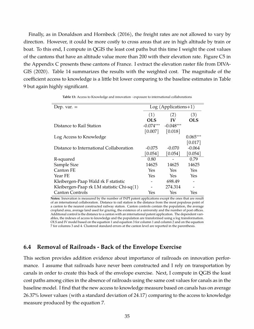
Finally, as in Donaldson and Hornbeck (2016), the freight rates are not allowed to vary bydirection. However, it could be more costly to cross areas that are in high altitude by train orboat. To this end, I compute in QGIS the least cost paths but this time I weight the cost valuesof the cantons that have an altitude value more than 200 with their elevation rate. Figure C5 inthe Appendix C presents these cantons of France. I extract the elevation raster file from DIVA-GIS (2020). Table 14 summarizes the results with the weighted cost. The magnitude of thecoefficient access to knowledge is a little bit lower comparing to the baseline estimates in Table9 but again highly significant.

Table 13: Access to Knowledge and innovation - exposure to international collaborations

Dep. var. = Log (Applications+1)(1) (2) (3)OLS IV OLS

Distance to Rail Station -0.074∗∗∗ -0.048∗∗∗[0.007] [0.018]

Log Access to Knowledge 0.065∗∗∗[0.017]

Distance to International Collaboration -0.075 -0.070 -0.064[0.054] [0.054] [0.054]

R-squared 0.80 - 0.79Sample Size 14625 14625 14625Canton FE Yes Yes YesYear FE Yes Yes YesKleibergen-Paap Wald rk F statistic - 698.49 -Kleibergen-Paap rk LM statistic Chi-sq(1) - 274.314 -Canton Controls Yes Yes Yes

Notes: Innovation is measured by the number of INPI patent applications except the ones that are resultof an international collaboration. Distance to rail station is the distance from the most populous point ofa canton to the nearest constructed railway station. Canton controls contain the population, the averagecropland area, average land used for grazing, the existence of a university and the number of post offices.Additional control is the distance to a cantonwith an international patent application. The dependent vari-ables, the indexes of access to knowledge and the population are transformed using a log transformation.OLS and IVmodel based on the equation 1 and equation 3 for column 1 and column 2 and on the equation7 for columns 3 and 4. Clustered standard errors at the canton level are reported in the parenthesis.

6.4 Removal of Railroads - Back of the Envelope Exercise

This section provides addition evidence about importance of railroads on innovation perfor-mance. I assume that railroads have never been constructed and I rely on transportation bycanals in order to create this back of the envelope exercise. Next, I compute in QGIS the leastcost paths among cities in the absence of railroads using the same cost values for canals as in thebaselinemodel. I find that the new access to knowledgemeasure based on canals has on average26.37% lower values (with a standard deviation of 24.17) comparing to the access to knowledgemeasure produced by the equation 7.

35

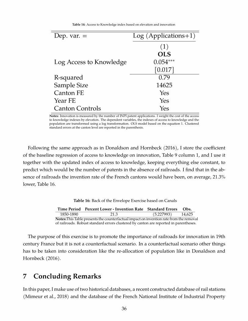
Table 14: Access to Knowledge index based on elevation and innovation

Dep. var. = Log (Applications+1)(1)OLS

Log Access to Knowledge 0.054∗∗∗[0.017]

R-squared 0.79Sample Size 14625Canton FE YesYear FE YesCanton Controls Yes

Notes: Innovation is measured by the number of INPI patent applications. I weight the cost of the accessto knowledge indexes by elevation. The dependent variables, the indexes of access to knowledge and thepopulation are transformed using a log transformation. OLS model based on the equation 1. Clusteredstandard errors at the canton level are reported in the parenthesis.

Following the same approach as in Donaldson and Hornbeck (2016), I store the coefficientof the baseline regression of access to knowledge on innovation, Table 9 column 1, and I use ittogether with the updated index of access to knowledge, keeping everything else constant, topredict which would be the number of patents in the absence of railroads. I find that in the ab-sence of railroads the invention rate of the French cantons would have been, on average, 21.3%lower, Table 16.

Table 16: Back of the Envelope Exercise based on Canals

Time Period Percent Lower - Invention Rate Standard Errors Obs.1850-1890 21.3 (5.227993) 14,625

Notes:This Table presents the counterfactual impact on invention rate from the removalof railroads. Robust standard errors clustered by canton are reported in parentheses.

The purpose of this exercise is to promote the importance of railroads for innovation in 19thcentury France but it is not a counterfactual scenario. In a counterfactual scenario other thingshas to be taken into consideration like the re-allocation of population like in Donaldson andHornbeck (2016).

7 Concluding Remarks

In this paper, Imake use of two historical databases, a recent constructed database of rail stations(Mimeur et al., 2018) and the database of the French National Institute of Industrial Property

36

to study the effect of access to railroads on patent activity. I exploit the enormous expansion ofrailroads in France over the second half of 19th century to document that access to rail networkfosters the patent activity at the canton level. Controlling for navigable waterways and the num-ber of postal offices, I am able to capture the net effect of rail network. Finally, the results are alsoconfirmedby an IV strategy and several robustness tests regarding the validity of the instrument.

I explore access to knowledge as an underlying mechanism behind the results. I compute ac-cessibility measures for the largest cities of the 2,925 French cantons. Findings suggest that fora given canton 8, the reduction of the transportation costs to all the other cantons with high per-centage of inventors has a positive impact on patenting activity of the canton 8. I state, that thiseffect is mainly driven by potential interactions among inventors residing in different cantons.Back of the envelope exercise based on canals provides additional evidence that in the absenceof railroads the invention rate of the French cantons would have been, on average, 21.3% lower.

In the last part of the paper, I use text analysis techniques to determine for the first time thetechnological class of each patent application in the historical database of INPI. Equipped withthis dataset this paper documents that less costly access to the global city of Paris, compared toother large urban centers, is associated with a higher probability for a given canton 8 to innovatein a novel patent class. The intuition behind this effect is that Paris works as a gatekeeper ofknowledge (Miguelez et al., 2019) that connects the national innovation system to global inno-vation networks.

This paper contributes to a growing literature about infrastructure and economic outcomesfrom a historical perspective and more specifically to the papers about railroads and innovationactivity. It also adds to the literature about the industrial era in France. In terms of policy, thepaper shows that general network contributes to the increase of innovation. Yet, in the case ofdiffusion of novel technologies what matters more is connections to global cities. This is crucial,especially in our days with the intense concentration of complex activities in big cities (Ballandet al., 2020).

37

References

Abrams, David, Ufuk Akcigit, and Jillian Grennan, “Patent Value and Citations: Creative De-struction or Strategic Disruption?,” NBER Working Paper 19647, 2018.

Acemoglu, Daron, JacobMoscona, and JamesA.Robinson, “State capacity andAmerican tech-nology: Evidence from the nineteenth century,” American Economic Review, 2016, 106 (5), 61–67.

Aghion, Philippe, Ufuk Akcigit, Antonin Bergeaud, Banque De France, Richard Blundell,and David Hemous, “Innovation and Top Income Inequality,” Review of Economic Studies,2019, 86 (1), 1–45.

Agrawal, Ajay, Alberto Galasso, and Alexander Oettl, “Roads and innovation,” Review of Eco-nomics and Statistics, 2017, 99 (3), 417–434.

Akcigit, Ufuk, Santiago Caicedo Soler, Ernest Miguelez, Stefanie Stantcheva, and ValerioSterzi, “Dancing with the Stars: Innovation Through Interactions,” NBER Working Paper24466, 2018.

Andersson, David, Thor Berger, and Erik Prawitz, “Making a Market: Infrastructure, Integra-tion, and the Rise of Innovation,” The Review of Economics and Statistics, 2021, pp. 1–44.

Atack, Jeremy and Robert Margo, “Agricultural Improvements and Access to Rail Transporta-tion: The American Midwest as a Test Case, 1850-1860,” NBER Working Paper 15520, 2009.

, Fred Bateman, Michael Haines, and Robert Margo, “Did Railroads Induce or Follow Eco-nomic Growth? Urbanization and Population Growth in the American Midwest, 1850-60,”NBER Working Paper 14640, 2009.

, Michael Haines, and Robert Margo, “Railroads and the Rise of the Factory: Evidence forthe United States, 1850-70,” NBER Working Paper 14410, 2008.

Bahar, Dany, Prithwiraj Choudhury, and Hillel Rapoport, “Migrant inventors and the techno-logical advantage of nations,” Research Policy, 2020, p. 103947.

Balland, Pierre Alexandre, Cristian Jara-Figueroa, Sergio G. Petralia, Mathieu P.A. Steijn,David L. Rigby, and César A. Hidalgo, “Complex economic activities concentrate in largecities,” Nature Human Behaviour, 2020, 4 (3), 248–254.

Banerjee, Abhijit, Esther Duflo, and Nancy Qian, “On the Road: Access to Transporta-tion Infrastructure and Economic Growth in China,” Journal of Development Economics, 2020,p. 102442.

38

, , Gilles Postel-Vinay, and Tim Watts, “Long-run health impacts of income shocks: Wineand phylloxera in nineteenth-century France,” Review of Economics and Statistics, 2010, 92 (4),714–728.

Baum-Snow, Nathaniel, “Did Highways Cause Suburbanization?,” Quarterly Journal of Eco-nomics, 2007, 122 (2), 775–805.

, J. Vernon Henderson, Matthew A. Turner, Qinghua Zhang, and Loren Brandt, “Does in-vestment in national highways help or hurt hinterland city growth?,” Journal of Urban Eco-nomics, 2018.

, Loren Brandt, J. Vernon Henderson, Matthew A. Turner, and Qinghua Zhang, “Roads,railroads, and decentralization of Chinese cities,” Review of Economics and Statistics, 2017, 99(3), 435–448.

Bellemare, Marc F. and Casey J. Wichman, “Elasticities and the Inverse Hyperbolic Sine Trans-formation,” Oxford Bulletin of Economics and Statistics, 2020, 82 (1), 50–61.

Berger, Thor andKerstin Enflo, “Locomotives of local growth: The short- and long-term impactof railroads in Sweden,” Journal of Urban Economics, 2017, 98, 124–138.

Bogart, Dan, Xuesheng You, Eduard J. Alvarez-Palau, Max Satchell, and Leigh Shaw-Taylor,“Railways, divergence, and structural change in 19th century England and Wales,” Journal ofUrban Economics, 2022, 128, 103390.

Breschi, Stefano and Francesco Lissoni, “Mobility of skilled workers and co-invention net-works: An anatomy of localized knowledge flows,” Journal of Economic Geography, 2009, 9 (4),439–468.

Büchel, Konstantin and Stephan Kyburz, “Fast track to growth? Railway access, populationgrowth and local displacement in 19th century Switzerland,” Journal of Economic Geography,2020, 20 (1), 155–195.

Correia, Sergio, “Singletons, Cluster-Robust Standard Errors and Fixed Effects: A Bad Mix *,”2015.

, “IVREGHDFE: Stata module for extended instrumental variable regressions with multiplelevels of fixed effects,” Statistical Software Components, 2018.

, Paulo Guimarães, and Thomas Zylkin, “ppmlhdfe: Fast Poisson Estimation with High-Dimensional Fixed Effects,” Papers 1903.01690, arXiv.org, 2019.

39

Crescenzi, Riccardo, Marco Di Cataldo, and Andrés Rodríguez-Pose, “Government Qualityand the Economic Returns of Transport Infrastructure Investment in European Regions,” Jour-nal of Regional Science, 2016, 56 (4), 555–582.

Cui, Jingbo, Tianqi Li, and Zhenxuan Wang, “High-Speed Railway and Collaborative Innova-tion: Evidence from University Patents in China,” SSRN Electronic Journal, 2020.

Daudin, Guillaume, “Domestic trade and market size in late-eighteenth-century France,” Jour-nal of Economic History, 2010, 70 (3), 716–743.

, Raphaël Franck, and Hillel Rapoport, “Can Internal Migration Foster the Convergence inRegional Fertility Rates? Evidence from 19th Century France,” Economic Journal, 2019, 129(620), 1618–1692.

David Rumsey, “David Rumsey Map Collection,” 2020.

Davis, Donald R. and Jonathan I. Dingel, “A spatial knowledge economy†,”American EconomicReview, 2019, 109 (1), 153–170.

Díez-Minguela, Alfonso andM. Teresa Sanchis Llopis, “Regional income inequality in France1860–1954: Methods and findings,” Historical Methods, 2019, 52 (1), 1–14.

Dijkstra, E. W., “A note on two problems in connexion with graphs,” Numerische Mathematik,1959, 1 (1), 269–271.

Dittmar, Jeremiah E., “Information technology and economic change: The impact of the print-ing press,” Quarterly Journal of Economics, 2011, 126 (3), 1133–1172.

DIVA-GIS, “DIVA-GIS | free, simple effective,” 2020.

Donaldson, Dave, “Railroads of the Raj: Estimating the impact of transportation infrastruc-ture,” American Economic Review, 2018, 108 (4-5), 899–934.

and Richard Hornbeck, “Railroads and American Economic Growth: A “Market Access”Approach,” Quarterly Journal of Economics, 2016, 131 (2), 799–858.

Dong, Xiaofang, Siqi Zheng, andMatthew E. Kahn, “The role of transportation speed in facil-itating high skilled teamwork across cities,” Journal of Urban Economics, 2020, 115, 103212.

Dunham, Arthur L., “How the First French RailwaysWere Planned,” Journal of Economic History,1941, 1 (1), 12–25.

Duranton, Gilles and Matthew A. Turner, “Urban Growth and Transportation,” Review of Eco-nomic Studies, 2012, 79 (4), 1407–1440.

40

Faber, Benjamin, “Trade integration, market size, and industrialization: Evidence from China’snational trunk highway system,” Review of Economic Studies, 2014, 81 (3), 1046–1070.

Flyvbjerg, Bent, “Survival of the unfittest: why the worst infrastructure gets built—and whatwe can do about it,” Oxford Review of Economic Policy, 2009, 25 (3), 344–367.

France Tél, “France Tél | Encyclopedia.com,” 2021.

Franck, Raphaël and Oded Galor, “Flowers of evil? Industrialization and long run develop-ment,” Journal of Monetary Economics, 2019.

and Stelios Michalopoulos, “Emigration during the French Revolution: Consequences inthe Short and Longue Durée,” NBER Working Paper 23936, 2017.

Galvez-Behar, Gabriel, “The patent system during the French industrial revolution: Institu-tional change and economic effects,” Economic History Yearbook, 2019, 60 (1), 31–56.

Gao, Yanyan and Jianghuai Zheng, “The impact of high-speed rail on innovation: An empiri-cal test of the companion innovation hypothesis of transportation improvement with China’smanufacturing firms,”World Development, 2020, 127, 104838.

García-Herrera, Ricardo, Gunther P. Können, Dennis A. Wheeler, Maria R. Prieto, Phips D.Jones, and Frits B. Koek, “Ship logbooks help analyze pre-instrumental climate,” Eos, Trans-actions American Geophysical Union, 2006, 87 (18), 173.

Gay, Victor, “Mapping the Third Republic. A Geographic Information System of France(1870–1940).,” SSRN Electronic Journal, 2020.

Hanley, Douglas, Jiancheng Li, and Mingqin Wu, “High-speed railways and collaborative in-novation,” Regional Science and Urban Economics, 2021, p. 103717.

Heblich, Stephan, Stephen J Redding, and Daniel M Sturm, “The Making of the ModernMetropolis: Evidence from London*,”Quarterly Journal of Economics, 2020, 135 (4), 2059–2133.

Hornbeck, Richard andMartin Rotemberg, “Railroads, Reallocation, and the Rise of AmericanManufacturing,” NBER Working Paper 26594, 2019.

Huang, Yue andYebinWang, “Howdoes high-speed railway affect green innovation efficiency?A perspective of innovation factor mobility,” Journal of Cleaner Production, 2020, 265, 121623.

HYDE, “History Database of the Global Environment - the Netherlands Environmental Assess-ment Agency (PBL),” 2020.

Inoue, Hiroyasu and Kentaro Nakajima, “The Impact of the Opening of High-Speed Rail onInnovation,” RIETI Discussion Paper Series 17-E-034, 2017.

41

INPI, “INPI (Institut National De La Propriété Industruelle),” 2019.

Jaffe, A. B., M. Trajtenberg, and R. Henderson, “Geographic Localization of KnowledgeSpillovers as Evidenced by Patent Citations,” Quarterly Journal of Economics, 1993, 108 (3),577–598.

Jaravel, Xavier, Neviana Petkova, and Alex Bell, “Team-specific capital and innovation,” Amer-ican Economic Review, 2018, 108 (4-5), 1034–1073.

Jeansoulin, Robert, “rail data (railway lines, stations) - France Dataverse 2000-2020,” HarvardDataverse, V1, 2019.

Jones, Benjamin F., “The Burden of Knowledge and the “Death of the Renaissance Man”: IsInnovation Getting Harder?,” Review of Economic Studies, 2009, 76 (1), 283–317.

Jordan W. Jonathan, “Reign of the Railroads,” in Rod Paschall, ed., The Quarterly Journal of Mil-itary History, 4 ed., Vol. 17, Primedia Inc, 2005.

Juhász, Réka, “Temporary protection and technology adoption: Evidence from the NapoleonicBlockade,” American Economic Review, 2018, 108 (11), 3339–3376.

, Mara Squicciarini, andNicoVoigtländer, “TechnologyAdoption and Productivity Growth:Evidence from Industrialization in France,” NBER Working Paper 27503, 2020.

Katz, Ori, “Railroads, Economic Development, and the Demographic Transition in the UnitedStates,”MPRA Paper, 2018, (88869).

Khan, B. Zorina, “Invisible Women: Entrepreneurship, Innovation, and Family Firms inNineteenth-Century France,” Journal of Economic History, 2016, 76 (1), 163–195.

Kogler, Dieter Franz, Gaston Heimeriks, and Loet Leydesdorff, “Patent portfolio analysis ofcities: statistics and maps of technological inventiveness,” European Planning Studies, 2018, 26(11), 2256–2278.

Komikado, Hiroshi, So Morikawa, Ayushman Bhatt, and Hironori Kato, “High-speed rail,inter-regional accessibility, and regional innovation: Evidence from Japan,” Technological Fore-casting and Social Change, 2021, 167, 120697.

Le Bris, David, “Les grands travaux du plan freycinet : De la subvention à la dépression ?,”Entreprises et Histoire, 2012, 69 (4), 8–26.

Lecce, Giampaolo, Laura Ogliari, and Mara P. Squicciarini, “Birth and migration of scientists:Does religiosity matter? Evidence from 19th-century France,” Journal of Economic Behavior andOrganization, 2021, 187, 274–289.

42

Lefranc, Georges, “The French Railroads, 1823-1842,” Journal of Business and Economic History,1930, 2, 299–331.

MacLeod, Christine, “The Paradoxes of Patenting: Invention and Its Diffusion in 18th- and 19th-Century Britain, France, and North America,” Technology and Culture, 1991, 32 (4), 885.

McCormick, Michael, Guoping Huang, Giovanni Zambotti, and Jessica Lavash, “RomanRoad Network (version 2008),” Harvard University, Cambridge MA 02138, 2013, DARMC Scho(DARMC, Center for Geographic Analysis,).

Melander, Eric, “Transportation Technology, Individual Mobility and Social Mobilisation,”CAGE Online Working Paper Series, 2020, (471).

Michaels, Guy and Ferdinand Rauch, “Resetting the UrbanNetwork: 117-2012,” Economic Jour-nal, feb 2018, 128 (608), 378–412.

Miguelez, Ernest, Julio Raffo, Christian Chacua, Massimiliano Coda-Zabetta, Deyun Yin,Francesco Lissoni, and Gianluca Tarasconi, “Tied in: the Global Network of Local Innova-tion,” Cahiers du GREThA (2007-2019), 2019.

Mimeur, Christophe, François Queyroi, Arnaud Banos, and Thomas Thévenin, “Revisitingthe structuring effect of transportation infrastructure: An empirical approach with the Frenchrailway network from 1860 to 1910,” Historical Methods, 2018, 51 (2), 65–81.

Mojica, Laia and Jordi Martí-Henneberg, “Railways and population distribution: France,Spain, and Portugal, 1870-2000,” Journal of Interdisciplinary History, 2011, 42 (1), 15–28.

Möller, J. and M. Zierer, “Autobahns and jobs: A regional study using historical instrumentalvariables,” Journal of Urban Economics, 2018, 103, 18–33.

Nagy, David, “City location and economic development,” 2016 Meeting Papers, 2016, (307).

Nicholas, David, The growth of the medieval city : from late antiquity to the early fourteenth century,Longman, 1997.

Nuvolari, Alessandro, Gaspare Tortorici, andMichelangelo Vasta, “British-French technologytransfer from theRevolution to Louis Philippe (1791-1844): evidence frompatent data,”CEPRDiscussion Papers, 2020.

Okoye, Dozie, Roland Pongou, and Tite Yokossi, “New technology, better economy? The het-erogeneous impact of colonial railroads in Nigeria,” Journal of Development Economics, 2019,140, 320–354.

43

Pascali, Luigi, “The wind of change: Maritime technology, trade, and economic development,”American Economic Review, 2017, 107 (9), 2821–2854.

Perlman, Elisabeth Ruth, “Dense Enough To Be Brilliant: Patents, Urbanization, and Trans-portation in Nineteenth Century America,” CEH Discussion Papers, 2015, (036).

Perret, Julien, Maurizio Gribaudi, and Marc Barthelemy, “Roads and cities of 18th centuryFrance,” Scientific Data, 2015, 2 (1), 1–7.

Piketty, Thomas, Gilles Postel-Vinay, and Jean Laurent Rosenthal, “Wealth concentration ina developing economy: Paris and France, 1807-1994,” American Economic Review, 2006, 96 (1),236–256.

Pontarollo, Nicola and Roberto Ricciuti, “Railways and manufacturing productivity in Italyafter unification,” Journal of Regional Science, 2020, p. jors.12484.

Raffo, Julio, “MATCHIT: Stata module to match two datasets based on similar text patterns,”Statistical Software Components, 2020.

Ratcliffe, Barrie, “Railway Imperialism: the example of the Pereires’ Paris-Saint-Germain Com-pany, 1835-1864,” Business History, 1976, 18, 66–84.

Redding, Stephen J. and Matthew A. Turner, “Transportation Costs and the Spatial Organiza-tion of Economic Activity,” in “Handbook of Regional and Urban Economics,” Vol. 5, ElsevierB.V., 2015, pp. 1339–1398.

Ruegg, Walter.,Universities in the nineteenth and early twentieth centuries (1800-1945), CambridgeUniversity Press, 2004.

Ryavec, KE andMHenderson, “Mapping Political Economies over Time, GIS Exercise 2: Citiesand Water Transportation in 19th Century France,” University of California, Merced, 2017.

Santamaria,Marta, “Reshaping Infrastructure : Evidence from the division ofGermany,”CAGEOnline Working Paper Series, 2020, (456).

Sassen, Saskia., The global city : New York, London, Tokyo, Princeton University Press, 2001.

Schwartz, Robert, Ian Gregory, and Thomas Thévenin, “Spatial history: Railways, unevendevelopment, and population change in France and Great Britain, 1850-1914,” Journal of Inter-disciplinary History, 2011, 42 (1), 53–88.

Schwarz, Carlo, “lsemantica: A command for text similarity based on latent semantic analysis,”Stata Journal: Promoting communications on statistics and Stata, 2019, 19 (1), 129–142.

44

Smith, Cecil O., “The Longest Run: Public Engineers and Planning in France,” American Histor-ical Review, 1990, 95 (3), 657–692.

Squicciarini, Mara P., “Devotion and Development: Religiosity, Education, and EconomicProgress in Nineteenth-Century France,” American Economic Review, 2020, 110 (11), 3454–3491.

and Nico Voigtländer, “Human capital and industrialization: Evidence from the age of en-lightenment,” Quarterly Journal of Economics, nov 2015, 130 (4), 1825–1883.

Sun, Daxin, Saixing Zeng, Hanyang Ma, and Jonathan J. Shi, “How Do High-Speed RailwaysSpur Innovationx003F;,” IEEE Transactions on Engineering Management, 2021.

Talandier, Magali, Valérie Jousseaume, and Bernard-Henri Nicot, “Two centuries of economicterritorial dynamics: the case of France,” Regional Studies, Regional Science, 2016, 3 (1), 67–87.

Thévenin, Thomas, Robert Schwartz, and Loïc Sapet, “Mapping the distortions in time andspace: The French railway network 1830-1930,” Historical Methods, 2013, 46 (3), 134–143.

Toutain, J., “Les transports en France de 1830 à 1965,” Cahiers de l’ISEA, 1967, 9 (8), 7–306.

University of Chicago, “University of Chicago Collections,” 2020.

Verdier, Nicolas and Ludovic Chalonge, “The issue of scales in geohistory. Post offices from the18th century to the present day,” Cybergeo : Revue européenne de géographie / European journalof geography, UMR 8504 Géographie-cités, 2018.

Wong, Jason C Y, “Blue-sky Thinking: Connectivity Impacts on Regional Economies and Inno-vation in the United States *,” 2019.

World Bank, “A Decade of Action in Transport : An Evaluation ofWorld Bank Assistance to theTransport Sector, 1995-2005,”Washington, DC: World Bank Publications, 2007.

, “Improving Institutional Capability and Financial Viability to Sustain Transport,” Washing-ton, DC: World Bank Publications, 2013.

, “Mobile Metropolises: Urban Transport Matters,” Washington, DC: World Bank Publications,2017.

Zeigermann, Lars, “OPENCAGEGEO: Stata module for forward and reverse geocoding usingthe OpenCage Geocoder API,” 2018.

Zimran, Ariell, “Transportation and Health in the Antebellum United States 1820-1847,”NBERWorking Paper 24943, 2019.

45

Zobl, Franz Xaver, “Regional economic development under trade liberalisation, technologicalchange and market access: evidence from 19th century France and Belgium,” PhD thesis, TheLondon School of Economics and Political Science (LSE), 2018.

46

Appendix A: Additional Findings

This section provides additional findings that confirm the benchmark analysis. Table A1 sum-marizes the results of the patents that have an addition as a quality index of innovation. Theresults hold for all the three models. Yet, it should be taken into consideration that this is a verycrude measure based only on the additional cost for an inventor to have an addition. 23

Next, I estimate as a robustness test a PPMLmodel in Table A2 to take into account, a possiblelarge number of zeros in the dependent variables. The dependent variables are now the INPIApplications without any transformation. The results are again highly significant at 1% column1 and column 2 and 5% in column 2.

In Table A3, I re-estimate equation 1 and equation 3 after I exclude from the sample the can-ton that became part of Germany in the end of the Franco-Prussian War in 1870. I rely on theshapefile of 1880 from Gay (2020) to identify these cantons. Again the results, both OLS and IVare highly significant.

Road Network of 18th Century

Historical infrastructure networks may be correlate with the construction of modern infrastruc-ture networks (Baum-Snow et al., 2017, 2018). This is true in case of France. According to Smith(1990), the same organization, the �>A ?B 34B ?>=CB 4C 2ℎ0DBB44B, was responsible for the con-struction of the Legrand Star rail plan of 1842 and the royal highways of 1770. They continuedfrom the highway system in the eighteenth century through the waterways and railroads of thenineteenth century to electric power and economic planning in the twentieth. The purpose of therail networkwas to imitate the improved highway system of the eighteenth and early nineteenthcenturies (Schwartz et al., 2011). The road network of 18th century seems as a good potentialinstrument. However, there are two main drawbacks: the absence of the time variation, sincethe road network is static compared to the rail network and possible correlation direct or indi-rect with outcomes of interest (Baum-Snow et al., 2017, 2018). These reasons discourage theuse it as an instrument. In contrast, I incorporate it into the analysis to control for pre-trends ininfrastructure network since the arrival of railroads. I extract data about road network of Franceduring the 18th century from Perret et al. (2015). I use only the main road network. Figure inthe Appendix C presents the old network. Based on this data, I create an indicator of accessibil-ity in the infrastructure network of 18th century.

23It is common in the recent time period the production of defensive patent applications from the firms whichdo not reflect valuable inventions and the way to deal with this issue is the use of patent citations (Abrams et al.,2018). A possible reason could be the high cost of patent applications.

47

Transportation of 18th century: I compute straight line distance of any canton city centroid tothe closest infrastructure network line of 18th century.

Roman Road Network

Recent literature finds an association among Roman roads and modern urban network in caseof France. Michaels and Rauch (2018) explore the resetting of the urban network for Britain andFrance. They find that France’s urban network was largely shaped by its Roman origins. In theironline Appendix, they argue that bishops had crucial roles in the evolution of the town life inFrance after the fall of the Western Roman Empire. According to Nicholas (1997) bishops wereinstrumental in the survival of towns in France after the end of the Roman Empire. I extract datafor the main Roman network fromMcCormick et al. (2013). Figure in the Appendix C presentsthe Roman road network for France. Next, I define accessibility to Roman road network.

Roman Road Network: I compute straight line distance of any canton city centroid to the closestline of Roman road.

Table A4 summarizes the results. In the first three columns, I use different thresholds for thebinary indicator access to navigable waterways. Comparing to the results in Table 3 they aresimilar in magnitude even though the results now are significant at 5%. In column 5, I controlfor the distance to canals, a measure similar to the main independent variable distance to railstations. There is a reduction in the magnitude but the coefficient is still highly significant. Fi-nally, in the last column, I add the additional variables, distance to road network of 18th centuryand distance to Roman road network multiplied with time dummies. The coefficient of the IVestimator is similar to the one in Table 3.

Table A5 presents the results for the diffusion of novel technologies model when I removefrom the sample the department of Seine in column 1 which I use the transportation cost basedon canals and rails and in column 3 which I use the travel time measure based on railroads.In columns 2 and 4, I remove the entire region of Ile de France. The results are highly signif-icant. This robustness test confirms that the results are not driven by inventors who are closeto Paris and are facilitated by the fact that can now travel to INPI’s office faster for bureaucraticprocedures which are not related to the diffusion of novel technologies.

48

Table A1: Distance to rail stations and quality indexes of innovation

Dep. var. = Log (Additions+1) Additions(1) (2) (3)OLS IV PPML

Distance to Rail Station -0.051∗∗∗ -0.032∗ -0.135∗∗[0.007] [0.019] [0.063]

R-squared 0.76 - -Sample Size 14625 14625 7550Canton FE Yes Yes YesYear FE Yes Yes YesCanton Controls Yes Yes YesKleibergen-Paap Wald rk F statistic - 689.38 -

Notes: Innovation is measured by the number of INPI patent applications that have an addition. Distance to rail station is the distance fromthe most populous point of a canton to the nearest constructed railway station. Canton controls contain the population, the accessibility towaterways, the average cropland area, the average land used for grazing, the existence of a university and the number of post offices. Thedependent variables and the population are transformed using a log transformation. Column 1 contains the OLS results based on the equation1 column 2 the IV results based on the equation 3 and column 3 the PPML results. Clustered standard errors at the canton level are reportedin the parenthesis.

49

Table A2: Distance to rail station and innovation - PPML model

Dep. var. = Applications(1)OLS

Distance to Rail Station -0.143∗∗[0.063]

Sample Size 11830Canton FE YesYear FE YesCanton Controls Yes

Notes: Innovation is measured by the number of INPI patent applications. Distance to rail station is the distanceto the nearest constructed railway station. Canton controls contain the population, the accessibility to waterways,the average cropland area, the average land used for grazing, the existence of a university and the number of postoffices. The population is transformed using a log transformation. PPML model. Clustered standard errors at thecanton level are reported in the parenthesis.

Table A3: Distance to rail stations and innovation - German Empire

Dep. var. = Log (Applications+1)(1) (2)OLS IV

Distance to Rail Station -0.061∗∗∗ -0.073∗∗∗[0.007] [0.016]

R-squared 0.81 0.01Sample Size 14145 14145Canton FE Yes YesYear FE Yes YesCanton Controls Yes YesKleibergen-Paap Wald rk F statistic - 732.91

Notes: Innovation is measured by the number of INPI patent applications in the first column. Distance to rail station is the distanceto the nearest constructed railway station. Canton controls contain the population, the accessibility to waterways, the averagecropland area, the average land used for grazing, the existence of a university and the number of post offices. The dependentvariables and the population are transformed using a log transformation. Panel A contains the OLS results based on the equation1 and panel B the IV results based on the equation 3. Clustered standard errors at the canton level are reported in the parenthesis.

50

Table A4: Distance to rail stations and innovation - Other types of Networks

Dep. var. = Log (Applications+1)(1) (2) (3) (4) (5)

Panel A OLS OLS OLS OLS OLSDistance to Rail Station -0.073∗∗∗ -0.073∗∗∗ -0.073∗∗∗ -0.073∗∗∗ -0.075∗∗∗

[0.007] [0.007] [0.007] [0.007] [0.007]R-squared 0.80 0.80 0.80 0.80 0.80Panel B IV IV IV IV IVDistance to Rail Station -0.048∗∗∗ -0.047∗∗ -0.047∗∗ -0.038∗∗ -0.048∗∗

[0.018] [0.018] [0.019] [0.018] [0.019]Kleibergen-Paap Wald rk F statistic 690.35 691.14 692.09 723.22 580.36Sample Size 14625 14625 14625 14625 14625Canton FE Yes Yes Yes Yes YesYear FE Yes Yes Yes Yes YesCanton Controls Yes Yes Yes Yes YesAccess to Waterways 5km 7km 9km No NoDistance to Waterways No No No Yes YesDistance to other Road Networks x Time Dummies No No No No Yes

Notes: In the first column, I include a variable which switches to 1 if a city is within 5 km from a canal, in column 2 if it is within7 km from a canal, in column 3 if it is within 9 km from a canal and in fourth column I control for the distance to navigablewaterways. In the last column, I control for the distance to other road networks like the distance to roman road network and to theroad network of 18th century. I have multiply the distances with time dummies. Innovation is measured by the number of INPIpatent applications. Distance to rail station is the distance to the nearest constructed railway station. Canton controls contain thepopulation, the accessibility towaterways, the average cropland area, the average landused for grazing, the existence of a universityand the number of post offices. The dependent variables and the population are transformed using a log transformation. Panel Acontains the OLS results based on the equation 1 and panel B the IV results based on the equation 3. Clustered standard errors atthe canton level are reported in the parenthesis.

Table A5: Diffusion of novel technologies and access to a global city - Robustness

Dep. var. = Number of Novel Classes(1) (2) (3) (4)

PPML PPML PPML PPMLTravel Cost to Paris -0.080∗∗∗ -0.069∗∗

[0.028] [0.028]Travel Time to Paris -0.296∗∗∗ -0.290∗∗∗

[0.063] [0.064]Sample Size 11472 11174 8702 8478Canton FE Yes Yes Yes YesYear FE Yes Yes Yes YesCanton Controls Yes Yes Yes YesStock of Classes Yes Yes Yes Yes

Notes: I exclude from the sample the cantons of Paris, Lyon, Marseille, Lille, Rouen and Bordeaux be-cause they already had all the technological classes before the arrival of railroads. In addition, I excludefrom the sample the department of Seine in columns 1 and 3 and the whole Region of Ile de France incolumns 2 and 4. The dependent variable is the number of novel technological classes in a canton. Travelcost to Paris is the computed travel cost to reach in Paris. Travel time to Paris is the ability to reach inParis based on the time duration of the fastest route. Canton controls contain the population, the averagecropland area, the average land used for grazing, the existence of a university and the number of postoffices. Population transformed using a log transformation. PPML model based on the equation 9 withclustered standard errors at the canton level are reported in the parenthesis.

51

Appendix B: Assignment of Classes

INPI provides me a sample of 38,527 (out of 308,513) patent applications that already have apatent class. I use these patents to create a vocabulary which helps me to assign classes to therest of patent applications. Even though INPI contains a subclass, I use only the main class. Istart my analysis by splitting the sample of patents based on their main class. The 35,663 patentapplications have a unique class. Using the "lsemantica" command in Stata (Schwarz, 2019),for a given class 8, I keep the words from the title of patent applications that appear at least 3times24 in the sample of patents of the class 8. I exclude from the vocabulary the words withlength less than 2 letters. Finally, I keep in the vocabulary the words that are unique amongclasses. Then, I use this vocabulary to assign classes to the rest of patent applications. Basedon this methodology, I manage to delegate classes in 138,611 patent applications out of 290,761.From these 138,611 patent applications the 100,049 have a unique class. I repeat the same anal-ysis but this time, I expand my initial vocabulary based on the 100,049 patent applications witha unique class. I complement the vocabulary with key words from the titles of the classes andsub classes of the patents.

38527 patentapplications

1st vocabulary100049 patentapplications

2nd vo-cabulary

I repeat the same procedure manually until there are in the sample 28,645 patent applicationswith no class. However, the allocation of patent classes could be bias from the number of wordsin each individual step. For instance, it could be possible agricultutae, to have more key wordsin the 1st vocabulary than weapons because it has a higher number of patent applications inthe initial sample. This bias could be generate more patent applications for agriculture in thesecond step. A second problem regarding this methodology, is that for instance in the secondstep machines has more applications, which leads to more words but if the class machines hadthese words in the first step it may even had more patent applications. To this end, after I sumup the words from all the vocabularies and keep these which are unique among classes, I repeatthe procedure from the beginning using only the final vocabulary. This again leavesmewith the28,645 patent applications with no class. For these patent applications, I apply fuzzy matchingin Stata (Raffo, 2020) between the key words and the titles of the patent applications. I keep thekey word which has the maximum similarity score with the patent title and then I assign a classaccording to this key word25. shows the number of patent applications in the initial and finalsample by main class.

24Only for class 11 I keep the words that appear 2 times because it has a very limited number of patents25If more key words has the same maximum similarity score I assign two classes in the patent application.

52

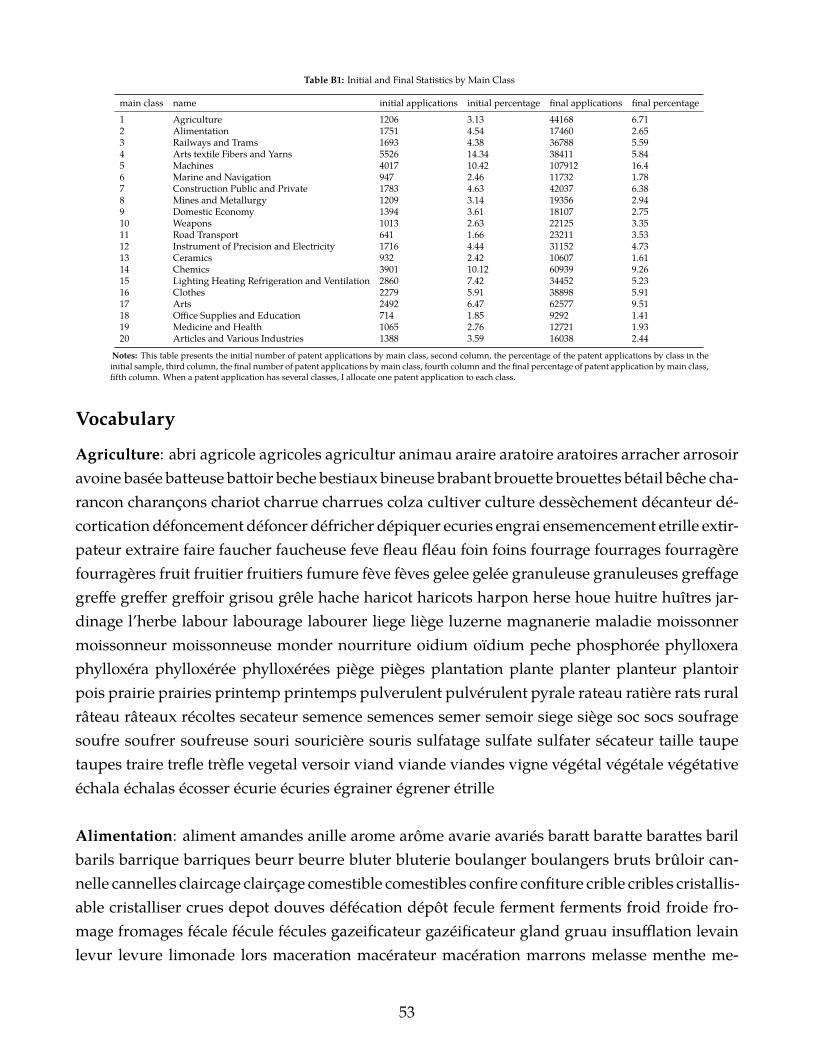
Table B1: Initial and Final Statistics by Main Class

main class name initial applications initial percentage final applications final percentage1 Agriculture 1206 3.13 44168 6.712 Alimentation 1751 4.54 17460 2.653 Railways and Trams 1693 4.38 36788 5.594 Arts textile Fibers and Yarns 5526 14.34 38411 5.845 Machines 4017 10.42 107912 16.46 Marine and Navigation 947 2.46 11732 1.787 Construction Public and Private 1783 4.63 42037 6.388 Mines and Metallurgy 1209 3.14 19356 2.949 Domestic Economy 1394 3.61 18107 2.7510 Weapons 1013 2.63 22125 3.3511 Road Transport 641 1.66 23211 3.5312 Instrument of Precision and Electricity 1716 4.44 31152 4.7313 Ceramics 932 2.42 10607 1.6114 Chemics 3901 10.12 60939 9.2615 Lighting Heating Refrigeration and Ventilation 2860 7.42 34452 5.2316 Clothes 2279 5.91 38898 5.9117 Arts 2492 6.47 62577 9.5118 Office Supplies and Education 714 1.85 9292 1.4119 Medicine and Health 1065 2.76 12721 1.9320 Articles and Various Industries 1388 3.59 16038 2.44

Notes: This table presents the initial number of patent applications by main class, second column, the percentage of the patent applications by class in theinitial sample, third column, the final number of patent applications bymain class, fourth column and the final percentage of patent application bymain class,fifth column. When a patent application has several classes, I allocate one patent application to each class.

Vocabulary

Agriculture: abri agricole agricoles agricultur animau araire aratoire aratoires arracher arrosoiravoine basée batteuse battoir beche bestiaux bineuse brabant brouette brouettes bétail bêche cha-rancon charançons chariot charrue charrues colza cultiver culture dessèchement décanteur dé-cortication défoncement défoncer défricher dépiquer ecuries engrai ensemencement etrille extir-pateur extraire faire faucher faucheuse feve fleau fléau foin foins fourrage fourrages fourragèrefourragères fruit fruitier fruitiers fumure fève fèves gelee gelée granuleuse granuleuses greffagegreffe greffer greffoir grisou grêle hache haricot haricots harpon herse houe huitre huîtres jar-dinage l’herbe labour labourage labourer liege liège luzerne magnanerie maladie moissonnermoissonneur moissonneuse monder nourriture oidium oïdium peche phosphorée phylloxeraphylloxéra phylloxérée phylloxérées piège pièges plantation plante planter planteur plantoirpois prairie prairies printemp printemps pulverulent pulvérulent pyrale rateau ratière rats ruralrâteau râteaux récoltes secateur semence semences semer semoir siege siège soc socs soufragesoufre soufrer soufreuse souri souricière souris sulfatage sulfate sulfater sécateur taille taupetaupes traire trefle trèfle vegetal versoir viand viande viandes vigne végétal végétale végétativeéchala échalas écosser écurie écuries égrainer égrener étrille

Alimentation: aliment amandes anille arome arôme avarie avariés baratt baratte barattes barilbarils barrique barriques beurr beurre bluter bluterie boulanger boulangers bruts brûloir can-nelle cannelles claircage clairçage comestible comestibles confire confiture crible cribles cristallis-able cristalliser crues depot douves défécation dépôt fecule ferment ferments froid froide fro-mage fromages fécale fécule fécules gazeificateur gazéificateur gland gruau insufflation levainlevur levure limonade lors maceration macérateur macération marrons melasse menthe me-

53

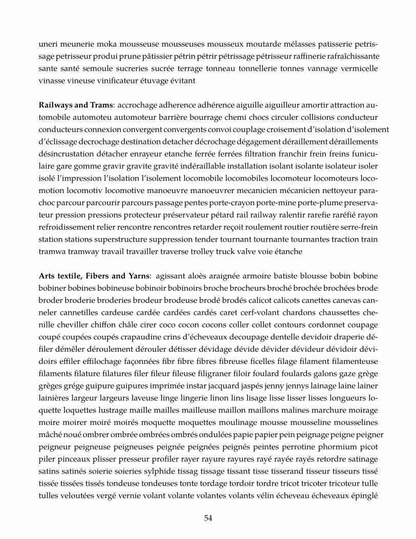
uneri meunerie moka mousseuse mousseuses mousseux moutarde mélasses patisserie petris-sage petrisseur produi prunepâtissier pétrin pétrir pétrissage pétrisseur raffinerie rafraîchissantesante santé semoule sucreries sucrée terrage tonneau tonnellerie tonnes vannage vermicellevinasse vineuse vinificateur étuvage évitant

Railways and Trams: accrochage adherence adhérence aiguille aiguilleur amortir attraction au-tomobile automoteu automoteur barrière bourrage chemi chocs circuler collisions conducteurconducteurs connexion convergent convergents convoi couplage croisement d’isolationd’isolementd’éclissage decrochagedestinationdetacher décrochagedégagement déraillement déraillementsdésincrustation détacher enrayeur etanche ferrée ferrées filtration franchir frein freins funicu-laire gare gomme gravir gravite gravité indéraillable installation isolant isolante isolateur isolerisolé l’impression l’isolation l’isolement locomobile locomobiles locomoteur locomoteurs loco-motion locomotiv locomotive manoeuvre manoeuvrer mecanicien mécanicien nettoyeur para-choc parcour parcourir parcours passage pentes porte-crayonporte-mine porte-plumepreserva-teur pression pressions protecteur préservateur pétard rail railway ralentir rarefie raréfié rayonrefroidissement relier rencontre rencontres retarder reçoit roulement routier routière serre-freinstation stations superstructure suppression tender tournant tournante tournantes traction traintramwa tramway travail travailler traverse trolley truck valve voie étanche

Arts textile, Fibers and Yarns: agissant aloès araignée armoire batiste blousse bobin bobinebobiner bobines bobineuse bobinoir bobinoirs broche brocheurs broché brochée brochées brodebroder broderie broderies brodeur brodeuse brodé brodés calicot calicots canettes canevas can-neler cannetilles cardeuse cardée cardées cardés caret cerf-volant chardons chaussettes che-nille cheviller chiffon châle cirer coco cocon cocons coller collet contours cordonnet coupagecoupé coupées coupés crapaudine crins d’écheveaux decoupage dentelle devidoir draperie dé-filer démêler déroulement dérouler détisser dévidage dévide dévider dévideur dévidoir dévi-doirs effiler effilochage façonnées fibr fibre fibres fibreuse ficelles filage filament filamenteusefilaments filature filatures filer fileur fileuse filigraner filoir foulard foulards galons gaze grègegrèges grége guipure guipures imprimée instar jacquard jaspés jenny jennys lainage laine lainerlainières largeur largeurs laveuse linge lingerie linon lins lisage lisse lisser lisses longueurs lo-quette loquettes lustrage maille mailles mailleuse maillon maillons malines marchure moiragemoire moirer moiré moirés moquette moquettes moulinage mousse mousseline mousselinesmâché noué ombrer ombrée ombrées ombrés ondulées papie papier pein peignage peigne peignerpeigneur peigneuse peigneuses peignée peignées peignés peintes perrotine phormium picotpiler pinceaux plisser presseur profiler rayer rayure rayures rayé rayée rayés retordre satinagesatins satinés soierie soieries sylphide tissag tissage tissant tisse tisserand tisseur tisseurs tissétissée tissées tissés tondeuse tondeuses tonte tordage tordoir tordre tricot tricoter tricoteur tulletulles veloutées vergé vernie volant volante volantes volants vélin écheveau écheveaux épinglé

54

épinglés

Machines: actionne actionner actionné actionnée agencement anse articulation articule articuleearticulée ascenseur balancier bielle bouche bouchon broyeur bâti casse-fil charnière chaudierechaudière chéneaux clape clapet cliquet condensateur couverture d’entraînement d’introductiond’ouverture d’élévateur d’émaillage d’étamage entretien equilibre essieu fardeau feux fluidefreinage gouttière hydraulique l’ouverture lanière levagmachinemachines-outilmanivellemaniv-elles manutention manèges molette monte-charge motocycle moufle mouvant multiplicateurmultitubulair multitubulaire mâchoire mèche noria obtention obturateur obturateurs opaqueopère organe orientant oscillant oscillante ouverture ouvertures ouvrier palan pedale perfora-teur perforer pesanteur physico pivot pneumato pompe porte porte-outil porter porteur pouliepouvant pressoirs primitif produire produit produites progressif progressive précieux puiserpuissance puissances pulverisation pulveriser pulvérisateur pulvérisation pulvériser pédale pé-dalier quadruple rabot rabots raccords rectification reflux refoulante refouler regulateur re-lief reparation roche rogner rondelles rotateur rotule roulant roulante rouli râpe réchauffeurréfrigérant régulateur régulatrice réparation scier scierie scieries scies sieur sieurs siphon siphonssortie soufflante soufflantes soufflerie soufflet soufflets soulever tamiser tamiseur tampon tararetarauder tare tarière teindre tombereau trancher transbordement transportable transports transvasertreuil trieur tubulaire tuyère vanne vannes vapeur varier vasista vendange verticalement virolesvisser vitess vitesse vitesses wagon élévateur élévatoire épuisements équilibre équilibré étau

Marine and Navigation Construction: ailette ancre aviation aviron barque barrage boisseaubouée buee buée canalisée canaux canot ciseaux d’hélice dock embarcation fabriquer fleuve flotflottante flotteur gouverner hélic hélice latéraux marin marine maritime navigable navigationnavire propulseur propulsive sonore sous-mari sous-marin toile torpille trame

Construction Public and Private: alluvion architecture armé assemblage aérienn aérienne bal-ayeuse boulangerie brosse canalisation caniveau citerne classement constructio constructioncourbe cuvier d’aronded’assemblage d’attelage d’echelle d’ecluse d’indicateur d’échelle d’éclusedallage dalle destruction dispositif disposition echelle elastique excavateur façade ferme fer-meture fermé fondation fosse frottement frotter hourdi incassable incendie indicateur interieurl’assemblage latte magasi mecanique mortier mécanique ondule ondulé palier passementeriepavage pelle pincette plafond planche plastique plate poutre poutrelle pratique quai scellementsolaire substitution suspendu suspendus terrain terrassement terrassements terrasses terrassiertoit toits tourbe tranchées treilli triangulaires trottoir trottoirs utilisable viaducs vieux vitragevitre vitrerie vitrine voiri volcanique voûte voûtes échafaud échafaudage échafaudages échellesécluses élastique

55

Mines and Metallurgy: acier aciers affinage affinerie alliage alliages argenter artésiens brasercamphre cannelure ciselés couche couches coudés coulé creuset cuivrage cuivre cémentationcémenté damasquinage décapage element emboutir emboutissage enclumes fonte fontes for-age forge forgeage forger fourche galvanisation guimpier laminage laminoir laminoirs laminélaminés maillechort malléabl malléable martinets metallurgie mine miniere métallurgie métal-lurgiquemétallurgiques pilon platinage plombage proportions puddlage puddler raccord recuitrevêtir réchauffage salants scories sondage soudage soudés souterrains spéciaux sucre treillagetreillages trempe tréfilerie trépan tôles zincage élément étirés

Domestic Economy: affiche affiler affiloir affiloirs alcôves ameublement ameublements baig-noire balcon banquette banquettes bassinoire berceau bibliothèque bouillante cache-entrée ca-dena cadenas cafetiere cafetière cage canapé cane casseroles cisaille coffre coffres coisées com-mode contrevent contrevents corbeille coucher couchette coutellerie cremon croisee croisée cré-mon crémone crémones d’affiche d’appel diffusion divan divans dossier dossiers espagnoletteespagnolettes fauteuil ferrements ferronnerie feuillure fiches fusion galet gonds gorge gorgeshachoir hermétiquement incrochetable incrochetables infusion infusions literie loquets man-teau menage meuble mobilier mousqueton mécaniquement patères paumelle paumelles penepentures persienne pincettes pliant poinconneuse poinçonneuse pène pêne pênes quincaillerierallonges rappel rasoirs repliable rideaux roulette râpes secret serrure serrurerie serrures son-nettes sphériques table tabourets tapisserie tenture théière tournebroche tringle tringles valiseverrou verrous vols vrilles

Weapons: arme artillerie baionnette barreau barreaux baïonnette bouclier calibre canon carneauxcarreaux cible classeur d’alarm d’armure detendeur detente dynamite défensive détendeur dé-tente embrasure emploi engin explosible faible flexible force fusee fusil fusée gaine hammer-les l’art l’artillerie lance masque militaire noyau nuance pistolet piston poignées portatif porta-tiv portative poudrière projectile projectiles rayées recharger revolve revolver revolvers rotativesabre sabres schakos silex tendeur tente tente-abri tir tonnerre troupes épée équipement

Road Transport: appelées bitumineux brancard brancards bridon brisés burette cabriolet cabri-olets calcination capote carrosserie d’arçon diligences dételage ferrement ferrer flèche gourmetteharnachement inversable inversables landau licou longe lubrifiante luxemarcmarchepiedmarecha-lerie messageries mors moyen moyeu muselière oxyde oxydé porte-brancard portière publiquerais renferment roulage selle selles separateur separation sulfuré séparateur séparation trans-port velocipedie voiturette écartement éperon étrier

Instrument of Precision and Electricity: abat-jour accumulateur acoustique aimant anéroïdebascul bascule binocle blutoir communication commutateur compensateur compteur consom-

56

mation curseur d’arpentage d’horloge d’électricit demontage dosage dynamiquedynamodynamo-électrique electricite electrique electro-automatique electro-magnetique electro-moteur electrodeelectrolyse electrolytique enregistrer enregistreur enregistreuse galvanique horloge instrumentl’electrolyse l’électricit l’électrolyse lentille lorgnette lorgnettes lorgnon lunette magnétiquesmagnétismemagnétomanomètremanomètresmathematiquemesuragemesurantmesuremesureurmicroscopemontagemètremètresmédecineméridienmétriquemétriques niveau niveaux nom-bres objectif obscure observation pesage peseur peson pesée piles pince-ne pince-nez plan-imètre polymètre pondérateur precision pyromètre pèse quadrature quantième rapporteur re-cepteur reconnaître remontage remontoir remontées rouage récepteur secondes sonnerie son-neries spectacle stadia surveillance telegraphie telephon tempes terrestres thermique thermo-électrique thermomètre thermomètres tracer transmetteur transmettre triangulaire télégraphetélégraphes télégraphie télégraphique télégraphiques téléphone téléphoni téléphonie téléphoniquevoltaïque échappements électricité électrique électro-automatique électro-chimique électro-magnétiqueélectro-moteur électrode électrolyse électrolyte électrolytique

Ceramics: argile argileuse brique briqueterie carrelage creuse céramiqu céramique faience faïencefaïences glaise goulots incrustés manchon manchons marqueterie plâtr plâtre porcelain porce-laine poterie poteries potier pouzzolane rebord rebords recuire refractaire réfractaire réfractairessoufflage tain tuile verrerie verreries vitrifiées

Chemics: absorbante acétate acétates acétique alambic albumine alcali alcalines alcalins alcalisalcool alcooliques alcools altération aluminate alumine alumineuses aluminium alun ambu-lant ammoniac ammoniaque amorphe amylacée antiseptique appret apprêt apprêter aqueusearomatique asphaltes asphaltiques azote azotique azurer barium baryte baryum bases bichro-mate bioxyde bisulfate bisulfite borate borax borique bouillon brome brute cachou caoutchouccarbonatation carbonate carbonates carburation carburé caustique caustiques celluloid chaleuchaleur chimique chimiquement chlor chlorate chlore chlorhydrate chlorhydrique chlorure chlorurescidre cirage cire colle colorants composition compositions compound conservateur conserva-teurs copal coque corroyer couleur couperose creme cristallisé crème crèmes cuir cuve cyanogènecyanure cyanures cérus céruse d’aluminiumd’ammoniumd’appret d’apprêt d’aprè d’eaud’eauxd’encre d’encrier d’epurationd’ether d’hydrate d’oxydationd’oxyded’épurationd’éther d’évaporatiod’évaporation decantation dentifrice dessécher dissou dissoudre distillation distillatoire distil-latoires distille distiller distillée distillés dorer dorure doseur décantation déchet décreusagedésagrégation désinfectante désulfuration encre encres encrier epuration essence evaporationevaporer explosive extracteur extrait extraite extraits fermentation fermentescible fermentés feu-tre filtr filtrante filtrantes filtre filtrer filtres fluorure foie fondants frigorifique galle gallique gal-vanoplastie garancine gelatine glucose glucoses glycérine gommes gommeuses gommogoudrongoudrons graisseur gras hydrate hydraté hydratée hydrochlorique hydrofuge hydrofuges hypochlo-

57

rite imperméabl imperméable imputrescible inattaquable incolore indicatrice industriel indus-trielle inflammable injecter injecteur injection inodor inodore instantane instantanee instanta-née iode l’alcoo l’aluminate l’aluminium l’amiante l’amidon l’ammoniaqu l’anhydride l’apprêtl’eau l’epuration l’evaporation l’hydrate l’industrie l’oxyde l’ozon l’ozone l’évaporation laqueslessives levûre lichen liquide lubrifiantes lubrifier luisant magnesium magnésie magnésiummanganèsemargariquemaroquinmelangemelangeurmethyleminéraleminérauxmixtionmoruemucilagineuse muriate muriatique mélange mélanger mélangeur mélangé mélangée métallisa-tion méthyle nature naturel naturelle naturels neutralisation neutre neutres nitrate nitreux ni-trique ocres olive oléine oléique onctueux ourdir oxalique oxydant oxygène parfum parfumerieparfumspendant periodique perméables peroxydepheniquephenol phosphate phosphore phéniquephénol plaque potable potasse potassium protoxyde prussiate prussiates précipitation pulpepulpes purifier pyrites périodique pétrol pétrole queue quinine reducteur resine rouille réac-tif réducteur réfrigération résine résines résineux saccharatus saccharification saccharine salinesalins salpêtre sang saponification saponifier saturation savon savonneuse savonneuses savonsschiste siccatif silicate silice siphoïd siphoïde sodium soi sorgho souder soudes soutache ster-iliser strontiane strontium stéarine stéarique stéariques stériliser sucré suif suifs sulfates sulfitesulfonique sulfures sulfureux sulfuriqu sulfurique surtout tableau taches tanin tanner tannerietannin tanné tannés taquet tartre tartrique terreux tinctoriales térébenthine vaporisation vernirvernis volatil volatils végéto émailler évaporation évaporatoires évaporer

Lighting Heating Refrigeration and Ventilation: absorber active activer aeration aggloméra-tion agglomérer aggloméré allumage allume-fe allume-feu allumer allumette allumeur allu-moir amadou appliquee appliquée artificiel artificielle aérage aéro bobèche bougeoir bougeoirsbouilloire brai braise briquet briquets bruler brûlant brûler brûleur bûches calorifèr calorifèrecaloripède candélabre carboniser carbure carbures carcel centra central chandelier chandelierschapeliers charbonnières chaud chaude chauffage chauffages chauffant chaufferette chauffer-ettes cheminée combustible congélateur crémaillère cuisines cuisinière culinaire d’anthracited’extincteur d’extinction d’hydrocarbure d’éclairage d’écran dirigeable eclairage ecran enflam-mer etincelle etui extincteur flambeau flambeaux flammflamme forêts fournaises fumeurs fumifumifuge fumivores galerie galeries gazo gazomètre gazomètres glacière houille hydrocarburehydrocarbures hydrogene hydrogène hydrostatique ignition illuminations incandescence incan-descente inflammables ininflammable intensité intermittente l’incandescence l’éclairage l’étincellelampe lanterne lanternes lenticulaire lignite longues-vue lumineuxphares phosphoriques pignonporte-allumette porte-bougie porte-meche porte-mèche poussier poêle pyro pyrogène pyrogènespyrogénées pyrotechnique rayonnant refrigeration reverbere réchaud réchauds réflecteur réflecteursréflexion réverbère réverbères salles sechoir supérieur séchoir séchoirs thermosiphon thermo-stat ustensile veilleuse veilleuses ventilation volumevues échauffer éclairant éclairer écran écranséteignoir étincelle étui étuves

58

Clothes: anneau ardillon ardillons benzidine bijou blanche bleue botte bottine boutonnièreboutonnières bretelle brodequin brodequins brun brune brunir buanderie buanderies caleçoncaleçons cambre cambrée cambrées canne canne-paraplui caoutchoute caoutchouté casquettechapea chapeau chapellerie chaussette chausson chaussure coiffes coiffure col concentree con-centrée corsages corset coulant coulants coupes cousu cousues couture couturiere couturièrecravache cravat cravate crinoline culotte d’adaptation d’alizarine d’espadrille d’uniforme dou-blure drapé dressage embauchoirs empeigne epingle eventail ferrage fixe-cravat flanelle fleurforme fouet fourrure friser frisure ganse gant gibus gilet griffes guêtre guêtres gélatine habille-ments habit habits hiver invisible jambiere jambière jarretière jarretières jaune jupe jupon lacerlacet latanier lessive lessiver leur ligno manchette manchettes mannequin mannequins man-teaux marquises musette ombrelle osier panier pantalon pantoufle paracrotte paraplui para-pluie parasol parasols perruque plissage plume porte-canne poser propreté rebras repassagesandale semelle semelles socque socques soulier suspensoir tailleur talon teignant teinte toquestoupets tournure tournures tournurière tresses tricoté uniform velocipede verte vetement violetviolette visière visières vélocipède vélocipédiste vêtement épingle

Arts: accord accorder accords accordéon accordéons agrafe album amplificateur anime animéanimée applique archet archets argentés arrondir artistique autographie autographique baguebagues baleine basses battant bijoux boiseries bonde bourrelet bouto bustes cahiers caloriquecarcasse carnet chant charge charger chargeur chemise chevalet chevalets cheveux chromatiquechromatiques chromo cinematographe cinématographe ciselure clairons clarinette clarinettesclavi clavier claviers coloriées compositeur concertinas confection confectionner cor cornet cor-nets couronne couronnes coussin crin culot d’agrandissement d’albumd’amiante d’imaged’imitationd’instrument d’oreille d’ornement d’épreuve daguerréotype dessin dessinateur dessinateursdessiner diamant dièses décors découpés déterminer déterminée développer ecremeuse em-boitement embouti emboîtement emporte-piece emporte-pièce encadrement encrage estampesestampé estampés explosif expressif expressifs expressives faconne feuille feuillets fixateur fleu-rons flûte flûtes flûtinas fonction format graphique gravure gravures gravées guitare harmonieharmonique harmoniques harmonium harpe harpes hautbois image images imitation imprimeimprimé joaillerie jonction l’image l’imitation l’imprimerie l’influence l’ivoire l’ornementationl’outillage lavis lithochromique lithographie lithographier lithographique lithographiquesmatemedaille medaillon miniature monnaie monnaies monétaire mouvoir murale musical musicalemusicaux musique médaille médailles médaillon médaillons métronome nacre nappe notationnote notes négatif négative octaves orchestre orfevrerie orfèvrerie orgue orgues ornement orne-menté ouvrage paillette panoramique papeterie passe-partout peint peintre pelliculaire pel-licule pendule perce perforation perfore perforé perle perles phonographe photographie pho-tographique photographiques photogravure pian pianinos piano pianos pierre pierreries pi-

59

quage pointure poinçons polychrome porte-monnaie portrait portraits pourvu presse-etoupepresse-étoupe production projeter précieuse précisio précision présentant recouvert reproduc-tion rondelle s’appliquant sculpter sculpture sculptures sertissure sons stéréoscop stéréoscopestéréoscopiques tabletterie tabouret taille-douce teint ton tons touche toucher touches tourne-feuillet tourne-page transformable transformant transformer transparents travaux trompette trompettestypes typo typographiques veloutage velouter vignettes violon violons vitraux vitrification zincogra-phie écrémeuse

Office Supplies and Education: affichage albums almanach apprendre biblorhapte brochurecalligraphie calligraphique copie copies copiste correspondance d’enveloppe document ecrireenseignement enseigner enveloppe envelopper facture géographie géographique journal jour-naux lecture lettre leçons manuscrit mettre orthographe paquets porte-journa postale postauxposte prendre public publication quotidien reliure reliures rendre reproduire sciences sphèresphères tendre uranographique écrire écrit écritoire

Medicine and Health: accouchement accouchements affections allaitement analeptique aro-matiques aseptique baignoires balayage baume bibero biberon biberons blessé blessés cabinetscachet cadavre canules cautère cercueil cercueils chalumeau chauffe chauffe-bain chauffe-piedchauffer chirurgical chirurgicaux chirurgie clysoir clysopompe clysopompes crachoir cremationcuisses curage dentaire descente descentes difformités domestique douche douches délétèresdésinfecteur désinfecteurs déviations egout embaumement gymnastique hernie hernies humainhydrotherapie hygiene hygiène immondice jambes latrines lavabo linceulmalademaladesmamelonmatrice mauvaise maux medecine mortuaire médical médicament médicamenteuse médica-ments médicinales médicinaux méphitiques natation nettoyage orthopédique pansement pes-saire pessaires pharmaceutique pharmacie plaies plumeaupoitrine redressement remède salubritesangsue sein stereotypie sterilisateur stérilisateur stéréotypie sulfureuses topique traitement uri-noir urinoirs utérus varices ventouse ventouses vertébrale vidange égout émanations

Articles and Various Industries: banque bebe bidon bidons billard billards bille blouses bou-quet bouquin bourse bourses bruyere bruyère bébé campement canonnière carnets casier cerceaucigare cigarette cigarettes concert coupon course d’échec domino dominos désigné emballageemballer embouchure embouchures empaqueter entonnoir estagnon fermoir fermoirs fragilesfumeur gainerie goulot guidon hochet illustre illustré jeux jouer jouet jouets joueurs loto mar-queur nicotine oeillet ongles oranger panorama panoramas papier patin patins pipe pipes porte-papier poupée poupées serviette serviettes société tabac tabatières theatre théâtre tourniquetvoyage échecs

60

Appendix C: Transportation Network and Least Cost Paths

The key element of the market access framework is the least cost paths among the city points ofthe cantons, the term�>BC8ℎC . This cost term is allowed to vary by year, C. The source of variationrelies on the expansion of railroads and waterways. Therefore, I compute the least cost paths inQGIS for each year based on the following steps:

1. Division France into 0.008> × 0.008> grid26.

2. Assignment of a cost to each grid cell using the same properties as in Zobl (2018), Toutain(1967) and Daudin (2010). The values, that the authors propose, are:

Table C1: French absolute freight rates by transport mode

Period Road Canal Railway1841-1844 25 4.1 14.51845-1854 25 3.8 10.61855-1865 25 3.2 8.71865-1874 25 2.4 7.51885-1894 25 1.8 6.8

Freight absolute rates are measured as centimes per ton and kilometre. The canals have alower value in terms of cost than the railways. However, the reduction over the years is greaterfor the railways than the canals. Next, the roads have a fixed cost over the sample period. Theeffect of roads is then captured by the time fixed effect. I assign a cost of 23127 for walking likein the paper of Donaldson and Hornbeck (2016).

3. Construction of cost raster file.

4. Calculation for each of the 2,925 cantons in the sample, the travel cost to every other canton.This is a minimisation problem based on Dijkstra (1959) algorithm over the least cost surfacewhich selects the optimal route.

Finally, I compare the costs between canton pairs and between two different consecutive years(C and C + 1) and I assign always in year C the lower of the two costs (Perlman, 2015). Thismethodology produces 8,555,625 pairwise least cost terms for every year. These cost terms canbe collected in a cost matrix:

26One grid is approximately 1.2 square kilometers.27The value of Donaldson and Hornbeck (2016) is 23.1. I have multiplied it by 10 in order to be in line with the

other values.

61

62

Figure C1: Rail lines until 1860

(a) initial image

(b) 1850

Notes: Railroads until 1860. Source: https://www.wikiwand.com.

63

Figure C2: Communes with rail stations

(a) 1850 (b) 1860

(c) 1870 (d) 1880

(e) 1890

Notes: This figure shows the expansion of the communeswith rail stations. Source: Mimeur et al. (2018).

64

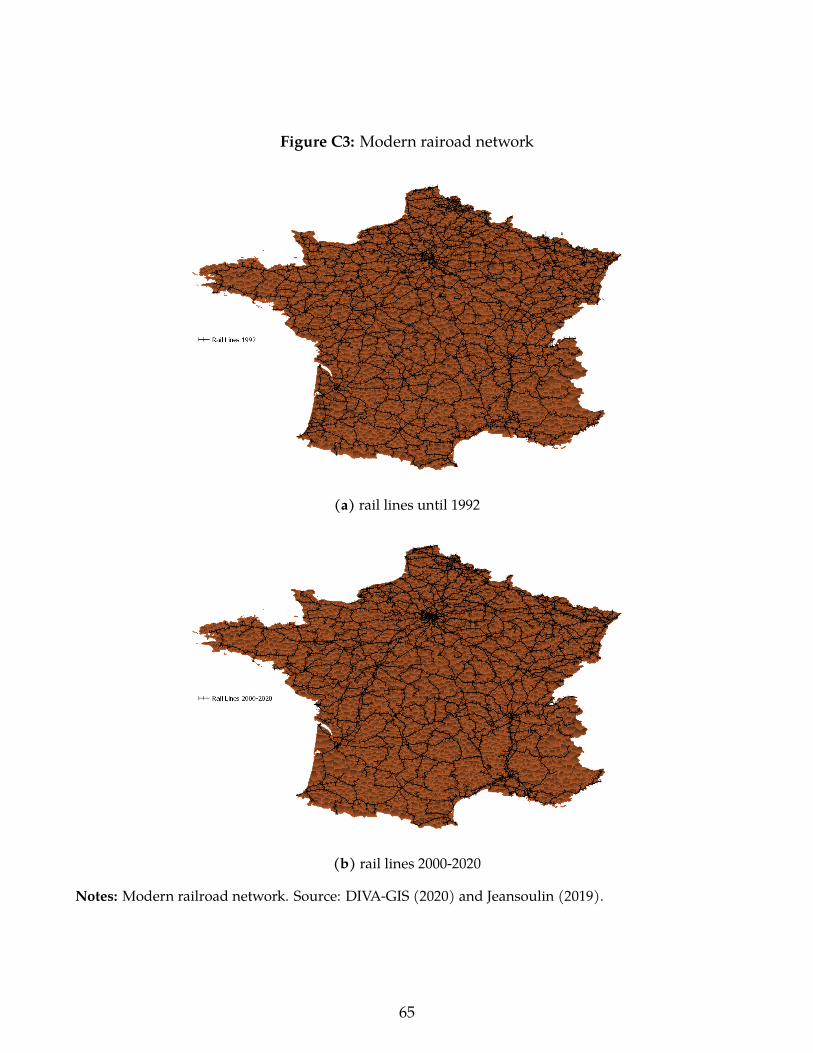
Figure C3: Modern rairoad network

(a) rail lines until 1992

(b) rail lines 2000-2020

Notes: Modern railroad network. Source: DIVA-GIS (2020) and Jeansoulin (2019).

65

Figure C4: canal network and ports

(a) canal network in 1878

(b) Ports in 1877

Notes: The first graph presents the canal network of France in 1878. The second includes the ports in1877. Source: University of Chicago (2020) and David Rumsey (2020).

66

Figure C5: areas with high elevation

Notes: Cantons of France with high elevation. Source: DIVA-GIS (2020).

67