Transfer Optimization in an Interactive Graphic System for Transit Planning

Matthias H. Rapp, W. and J. Rapp Company, Basel, Switzerland Claus D. Gehner, * Department of Civil Engineering, University of Washington,

Seattle

This paper describes a coordinated four-stage interactive graphic process for operational transit planning. Stage 1 deals with route, headway, and vehicle-type optimization; stage 2 attempts to optimize transfer delays; stage 3 designs runs so that the service resulting from the previous stages can be oporetionalized; and stage 4 provides computer assistance in mak­ing manpower assignments. The network optimization procedure of stage 1 has been previously reported on, and the latter two stages aro currently under development. This paper deals principally with the trans· fer optimization tool of stage 2. The operational tool to optimize trans· fer delays involves the automated-iterative modification of terminal de· parture times. An interactive graphic computer approach is used to in· crease the transparency of the tool to the planner. The analysis takes Into account the calculation of expected waiting times for transfers be· tween transit lines with different headways and the interdependence of terminal departure times. Within the interactive graphic optimization process. the user can request computer-generated and com1>uter-drawn charts of transfer movements and delays, time-distance diagrams of in· dividual routes, and computer-produced transfer statistics at individual stops as well as the entire system. The process has been applied to the Basel Transit System in Switzerland, which serves a population of 500 000. In comparison with the existing hand-generated timetable, the optimized timetable reduces the total transfer delays by approximately 20 percent with no increase in operating costs.

Operational transit planning has a short time horizon and for our purposes can be described as shown in Fig­ure 1. The input to tllis planning process is a number of itenia that must, in the short run, be fixed. These items are the demand for b:ansit service in terms of trip origin and destination {O-D), which are stratified perhaps by time of day; a base network {eXl.sting rail right-of-way and arterial streets), terminals, depots, and other iufl'asfructu.res; and the characteristics of available rolling stock.

The planning )?rocess should generally be guided by user objectives (e.g., minimum total travel tbne); it is constrained both by the financial considerations of the operator (e.g., maximum allowable deficit) and by ex-

Publication of this paper sponsored by Task Force on Computer Graphics and Interactive Graphics.

*Mr. Gehner was with W. and J. Rapp Company when this research was performed.

isting labor contracts (e .g., required terminal layovers). The desired output from the operational planning process is the transit routes, the vehicle types serving each route and the headway with which they are served, the time­tables, the runs used to operationally service the routes, and the vehicle and driver assignments.

INTERACTIVE GRAPHIC APPROACH

Past experience has shown that, given the cw·rent state of our analytic tools and of compute1· hudware, it is im­possible to treat the entire operational transit planning process in one step as shown in Figure 1. In the past, the approach has been to treat subareas of the total prob­lem separately, and in most cases disjointedly, and to apply to each subproblem an analytic technique that seemed best suited to it. 'I11e methods that have been used in the past include simulation-modeling techniques to design bus routes; mathematical programming tech­niques (integer progumming); and heul"istic techniques to construct timetables, define runs, and assign vehicle and driver resources. A useful description of some of these past efforts is given by Wren (1) . The following p1·inciples were used as guidelines to approach the prob­lem of operational transit planning.

One of the principal desires was to make the entire process as transparent as possible to the transit planner and to adapt as many as possible of the planner's existing methods and tools. 'nus desire was motivated by the fact that higbly sophisticated, but nontransparent, computer models that employ drastically different methods are only reluctantly accepted within the existing planning and op­erations framework of transit prope1·ties.

It was also decided to build the entire operational planning tool around an environment of minicomputer hardware by using low-cost storage tubes {cathode ray tubes) as shown in Figure 2. Currently, only this type of environment gives the user the quick response time needed, and at a price that is compatible with small and medium-sized transit operators. In the network optimi ­zation stage, a computer with 32~Kwords memory can analyze a transit network with 250 nodes, 950 links, and 60 lines. (This memory is automatically expanded to ac­cow1t for transfer movements to 700 nodes and 2300 links.>

27

28

Third, and most important, all the functions of oper­ational tnnsit pianning had to be coordinated into a uni­fied p1·ocess . The operational planning process that re­sul ted from these considerations is shown. in Figure 3. The problem was segmented into four stages so it could lie tractable ·with minicomputers and existing anBJytic techniques. However, the data flow between stages is explicitly linked to higbligh,t the dependence of one anal­ysis stage on the output of the preceding one and to main­tain the desired coordination of the process as a whole. To increase the transparency of the process to the plan­ner and to facilitate the adaption of existiug operational planning tools, we adopted the interactive graphic person-computer approach . This technique, as demon­sti·ated in past applica:tions, has the added benefit of al­lowing the discovery of mm.1:-oµUmal solutions by use of simple analytic techniques and low-cost computer hard­ware (2_, 1, .1).

Stage 1 (network optimization) has been previously reported on (5) and documented (6). This stage was ap­plied to the problem of coordiuatfog the subu.rban and urban transit routes in the Basel, Switzerland, ar.ea. Op­tilnum s olutions to this problem, deflned by planner ob­jectives and limited by the iterative search process, were efficiently generated (7). This paper describes stage 2 (transfer optimization), which has recently been operationalized. Stages 3 and 4 (run allocation and man­power assignment procedures) a1·e curi·ently undru.· de­velopment and will be reported on later.

Figure 1. Operational transit planning defined by input and output.

INPUT: ( fixed in the short - run)

TRANSIT DEMAND BASE NETWORK (O- D MATRIX)

ROUTES VEHICLE TYPES

HEADWAYS TIME TABLE

OUTPUT

RUNS VEHICLE +DRIVER ASSIGNMENTS

Figure 2. Typical storage terminal for interactive graphic data.

TRANSFER-OPTIMIZATION PROBLEM

Except in the case of a highly sophisticated, fully automated transit technology, e.g., personal rapid tran­sit (PRT), most transit operations will require some transfer movemeuts from one route to another to serve the diverse origin-destinatio11 patterns of t he current urban agglomerations. To minimize the adverse e'ffects (in terms of the competi:tlon between public transit and private automobile), the transit operator must try to (a) i·educe the required number of transfers by adjusting the routing to the given 0-D pattern of transit trips and (b) minimize the transfer delays (i.e., the waiting time at the transfer point) . As shown in Figure 2 and cle­sc_ribed elsewhere (5, 6), the first part of this problem is solved during i;tage 1. Thus, transfe1· optimization can be attained by minimizing transfe1· delays.

The typical operating day of a transit system can be divided into a number of periods that are characterized by the level of demand and thus the headway U1at can be justified. Typically, there will be the morning and eve­ning peak periods during wh'ich demand is high and con­sequently the headways rather short (from less than 1 min to about 6 min) and the off-peak pe1·iods during which headways can range from 15 to 60 min. The min­imization of transfer delays will be treated separately for each of these periods of constant headway. Since, in gene1·al, the waiting time is proportional to the headway, it is primarily in the off-peak periods that transfer op­timization is important.

The transfer situation at a given stop is shown in Figure 4, and the waiting times between stops on the

Figure 3. Cuurdinated, four-stage, operational transit planning process.

STAGE I Demand Base Network Rolling Stock

User Obj ~---1.;.... _ __,/ Operotor Obj ~I time _____l NETWORk ~min, operating cost

min transfer delay~ OPTIM12AI ION ~ f""' Labor Constraints

min overloading ! 1 \layover times

- opttmal " .. Optima I.. '"Oplima l"'

STAGE II Routes

User Obj .

min . transfer

delays

STAGE Ill

Frequencies Vehicle Types

\ 1 TRANSFER OPTI MIZATION

l

/ Operator Obj .

~min , operating cost

~ Lttbor Constra int& layover times

Terminal Offset Time for each Period

= Steady State Time Tab le

1 RUN .L__ Ope• alo• Obj ALLOCATION ,------ mll"\ , operolfng cost

j \ Optimal Times

STAGE IV Run

Allocation

Tables for

entire day

MANPOWER .L__ ASSIGNMENTS ,.-- Labor Con• lra lnt1

l Driver Assignments

Basel Transit System are given in Table 1. As given in Table 1, the 1011gest wait (5.5 min) occurs for transfers from line 36 at stop KU to line 15 at stop TE. This waiting time could be reduced to 0 min by moving line 36 ahead by 5.5 min, t hus reducing the total waiting time (average waiting time x number of transfers) by 38 min. However, the 23 passengers wanting to transfer from KU to STB would miss their connection, and their aver­age waiting time would increase by 5. 5 min. Added com­plications arise from the following:

1. Since a given line will intersect more than one other line, then a change in arrival-departure times at one stop will have repercussions at a number of other transfer points;

2. Since the headways on two intersecting lines need not be the same, then the optimization of the transfer at one point in time will not necessarily yield an overall optimum transfe1· situation, even at one stop· and

3. Since the arrival and dep:u-tw·e times are dil'ectly linked to terminal layover times, and layover times are constrained by labor regulations, then more vehicles will be needed to serve a given route, if the layover times are longer.

Thus, transfer optimization can be attained by an interactive modification of arrival and ctepartu1·e times at stops. This modification is used to reduce the total waiting times t hroughout the system by taking into ac­count the added complications of 1mtltiple-transfer points on a given lille, nonuniform headways between lines, and the interdependence of layover ti.mes and vehicle require­ments.

INTERACTIVE GRAPHIC TRANSFER OPTIMIZATION

Network Optimizatio11

The interactive graphic computer approach to transfer optimization is pa1:t of a coordinated operational transit planning process. As such, the input to tl1e transfer optimization is del'ived directly from the netwo1·k op­timization (stage 1). Thus, the following is a brief over­view of the network-optimization system (NOPTS) . Basic input to NOPTS consists o! a base network (existing streetcar and supway trackage, subset of the street net­work suitable for bus transit, and some pedestrian con­nectors), a transit-frip 0-D matrix, a11d the cJ.iaracter­istics of available rolling stock (capacities and opei-ating costs) . A transit system is then designed interactively by specifying the routings, vehicle types, and [requen­cies of individual lines. A mltltipath stochastic model (81 9) is used to assign the demand to the system of i:Outes. Tbis assignment allows the calculation of some performance parameters of the particular transit system design. By iterating this design-evaluation cycle, the planner can quickly approach an optimum transit network design that is indicated by the choice of design objectives (e.g., minimize operating costs and number of required transfers).

The output from this iterative procedure for network optinlization that is important for the subsequent trans­fer optimization is (a) the selected (optimum) route structure and headways for each line; and (b) at each transfer point, the number of ti·ansfer motions between all applicable pairs of transit lines. The fact that the detailed transfer movements can be retrieved from the trip assignment is an important feature that is obtained by using Dial's algoritlun (8). As previously mentioned, tl'ansfer optimization is conducted separately for each operating period during which headways are constant,

29

and, thus, the route-headway optimization must also be done for each of these operating periods.

Minimization of Transfer Delays

Since the operating period is a portion of the daily opera­tion during whic11 headways remain constant, then a par­ticular transit line is completely described in time and space, during such an operating period, by the following three parameters:

1. The geographic routing (i.e., sequence of stops), 2. The headway (i.e., the time interval between ve­

hicles passing a given stop), and 3. The terminal offset times (i. e ., the time delay, at

both terminals of the line, that beglJls at the start of the operating period and continues until the departure of the first vehicle).

Parameters 1 and 2 result from the net\vork optimization describecl above, and parameter 3 represents the primary design vuiables for the transfer-optimization procedure. The iterative design process is aimed at fi nding a set of terminal offset times that will minimize the aggregate transfer delays systemwide; however, "the p1·ocess is con­strained by the operator's desire to keep the operating costs (i.e., the number of vehicles required) ataminin,um.

This cost constraint is important because it limits the degree of freedom with which terminal offset times can be varied. This phe.nomenon is observed in Figure 5, which shows the time-distance diagrams. The terminal offsets (the design variables in Uie interactive grapluc process) shown 011 the upper diagram have the effect that three vehicles are needed, whereas, in the offsets shown on the lower diagram, one vehicle can be saved without violating the minimum layover time requirements.

In the optimization process, the terminal offsets (de­parture times at any inte1·mediate stop) are repeatedly varied with the objective of reducing the transfer delays systeruwide. The complications of multiple line­crossings, nonuniform headways, and the relation be­t.ween layove1· times and vehicle requirements are auto­matically taken into account. To this effect, the planner can demand the following tasks:

1. Display graphically the internal desire lines of any transfer point;

2. Perform input and interactive editing of terminal phase offsets;

3. Display the current set of terminal offsets, lay­over times 1 and the corresponding number of vehicles needed;

4. Display the transfer statistics (arrival time, de­parture time, number of transferring passengers, wait times) between any pair of lines at any transfer point;

5. Display global statistics (sum of transfer delays, etc.>;

6. Display time-distance diagrams of any transit line; 7. Print timetables (depa1·ture times at all stops on

any line) · and 8. Move departut•e times of lines or groups of lines

forward or backward.

The number of possible transfer movements (i.e., direction-specific pairs of lines at each transfer point) is very high, even in a medium-sized city (1200 to 4000). Therefore, it would be impossible to iind optimal solu­tions \vithout some degree of automation. A heuristic technique was developed that searches all the possible terminal point phase offsets of one line (directional) and selects the one offset that produces, with all crossing or parallel lines, the shortest total of transfer delays. The

30

s arch process ls repeated until the total systemwide delays can no longer be reduced. Of course, the heu­ristic technique is only able to locate local minima, and it is dependent on the starting point (in terms of the set of initial phase offsets) and on the 01·der in which the transit iin~:; a1·~ ti~eated tu the iterative process.

SYSTEM APPLICATION

To demonstrate the potential reduction in transfer de­lays that can be achieved, we applied this system to the existing Basel Transit System shown In Figure 6, which had beeu coded for another project (6). The public tune sci1edules were used to obtain the plrnse offsets at the evening off-peak period from 8:00 p.m. to 12:00 m.n.

Figure 4. Transfer movements at a typical transfer point.

LINE

NUMBER OF TRANSFER MOVEMENTS

HEADWAYS OF LINES N0.15 ANO 36 ~ 8 MIN .

Table 1. Waiting times between example stops.

Fro m Stop

STll STD TE TE KU KU zw Total

Line

15 15 15 15 36 36 36

Terminal

Arrival at BO (min)

5.5 5.5 5.0 5.0 0.0 0.0 1.5

During this period, most lines have a headway of 12 min, and some lines ope1·ate every 15, 24, 30 01· 3G min. A total of 82 vehicles we1·e used. NOPTS was used to as­sign the evening off-peak transit demand to the network, and the number of transfers, the transfer point desire line~ , b:ansfor wait, and the total transfer delay (pas­senger-minutes per hour) were calculated for each stop. The total systemwide transfer delay for 82 vehicles operating on this existing service schedule was 20 544 passenger-min/h. This transfer delay represented the state in which an application of the transfer optimization can be used for improvement.

The heuristic technique was applied, and a minimum in the total transfer delay was achieved. This minimum was 15 600 passenger-min/ h or a reduction of about 25

LINE NO, 36

Departure Avg Wait Total To From BO al BO No. or Wnit Stop Line (min) (min) Transfers (min)

zw 36 6.0 0.5 9 4.5 KU 36 7.5 2.0 18 36.0 zw 36 6.0 1.0 8 8.0 KU 36 7.5 2.5 9 22.5 TE 15 5. 5 5.5 7 38.5 STB 15 5.0 5.0 23 115.0 STB 15 5.0 3.5 10 3S.O

259.5

Figure 5. Relation between terminal offsets and vehicle requirements. Offset Elf. Layover

A I ' ~. Layov•: I

1 L7\l\2 B --lL

A

I B

Terminal Offset A' Min. Layover

© 0 Time

3 vehicles required

2 vehicles required

Figure 6. Line map of Basel Transit System.

Figure 7. Transfer delay times before and after optimization.

--- LRT Lines ------ Bus or Trolley Lines

EXISTING TIME - TABLE

TOTAL DELAY 20 544 pass.min./ hr.

--200 - -- - ------- -- - - ------------------- - ----

"' ~ w

" w > 0

"

----

~ too _: ,...- - -- _,~ ... ·1-lf+- -f·-+ ·-- ~ ----------------· -

"' -z .. a: -.... ... 0 a: w m

" ::> z

---0 5 10

1. I I t I. I I

15 I

20

OPTIMIZED TIME - TABLE

-- TOTAL DELAY 16 667 pass. min./hr. ---

200 - ---------·----------------------­-

"' .... z w

" w > 0

"

------

~ 100 -t--t-H11~-t-l-l-t-· -,

"' -z .. :! ... 0

~ .. " ::> z

-----

0 5

- -------------------------

I ii .. I. I ' 10 15 20

WAIT TIME (MINUTES)

31

32

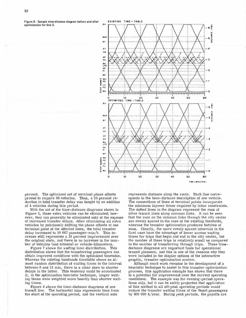
Figure 8. Sample time-distance diagram before and after optimization for line 3.

EXISTING TIME -TABLE BH

BAA

BT

AT

HA

AP

OU

BA LYS

SP Pl

BP

in SEI

~PS Z LU o. PU 0 ~BG

0 10 20 OPTIMIZED TIME-TABLE

30 40 so 60

BH

BAR

BT

AT HA

AP

DU

BA LYS

SP Pl

DP

fl) SEI

~ ?S

~LU o. PU 0 ;; BG

0

percent . The optimized set of terminal phase offsets proved to require 86 vehicles. Thus, a 25 percent re­duction in total transfer delay was bought by an addition of 4 vehicles during this period.

With the aid of the time-distance diagrams shown in Figure 5, these extra vehicles can be eliminated; how­ever, they can generally be eliminated only at the expense of increased transfer delays. After eliminating all extra vehicles by judiciously shifting the phase offsets at one terminal point of the affected H11es, the total transfer delay increased to 16 667 passenger-min/h. This in­crease still represents a 19 percent improvement over the original state, and there is no increase in the num­ber of vehicles (and drivers) or vehicle-kilometers.

Figure 7 shows the waiting time distribution. This distribution shows that the transferring passengers can obtain improved conditions with the optimized timetable. Whereas the existing handmade timetable shows an al­most random distribution of waiting times in the interval between 0 and 12 min, there is a clear skew to shorter delays in the latter. This tendency could be accentuated if, in the optimization heuristic technique, longer wait­ing times were weighted more heavily than shorter wait­ing times.

Figure 8 shows the time-distance diagrams of one transit line. The horizontal axis represents time from the start of the operating period, and the vertical axis

10 20 30 40 50 60

TIME (MINUTES)

represents distance along the route. Each line corre­sponds to the time-distance description of one vehicle. The connections of lines at terminal points incorporate the minimum layover times required by labor constraints. The dotted lines in the diagram represent the runs of other transit lines along common links. It can be seen that the runs on the common links through the city center are evenly spaced in the case of the existing timetable, whereas the transfer optimization produces batches of runs. Clearly, the more evenly spaced intervals in the first case have the advantage of lower access waiting times for trips that begin and end in the city center, but the number of these trips is relatively small as compared to the number of transferring through trips. These time­distance diagrams are important tools for operational transit planners, and this is one of the reasons why they were included in the display options of the interactive graphic, transfer-optimization system.

Although much work remains in the development of a heuristic technique to assist in this transfer-optimization process, this application example has shown that there is a potential for improvement over the current operating conditions. The example was for evening-period opera­tions only, but it can be safely projected that application of this method to all off-peak operating periods would reduce the transfer waiting times of the Basel passengers by 500 000 h/year. During peak periods, the payoffs are

smaller because of reduced headways (6 min on most lines), and it is difficult to maintain the timetables in mixed traffic conditions.

The example also highlighted the trade-offs that must be made between improving the level of service by re­ducing transfer delays and economic considerations, in terms of the number of vehicles needed to mount the service. It is in evaluating these kinds of trade-off pos­sibilities that the interactive graphic implementation of the transfer-optimization system demonstrates its great­est use.

LII'v1ITATIONS OF APPROACH

Implicit in the way the problem of operational transit planning has been ailpt·oached, there are a number of simplifying assumptions. The most important of these assumptions is that both transit travel demand and num­be1· of transfers are fixed. One basic input to this op­erational transit planning process in general, and the network-optimization stage in particular, is the demand for tJ:a11sit trips. It is thus assumed that changes in transit routing a11d level of service will not affect the demand for the short planning horizon of interest. The primary reason for 1uaking this assumption is that data on transit trips are generally more available than those for travel demand in general. It also avoids the neces­sity of modal-split modeling, which includes additional data requirements and uncertainty.

Each alternative design during the network­optimization stage will, in general, result in a dif­ferent netwo1·k loading (as predicted by the multipath assignment algorithm). These loadings are based on ex­pected transfer waiting times. The transfer optimiza­tion, as a separable problem, assumes that ti·ansfer time opti,mization will not significantly affect loading patterns. This decision of problem separation was made primarily on the basis of computational efficiency: Re­computing assignments after every transfer time alter­ation would increase the computing time to the point of making the interactive approach of questionable use.

CONCLUSIONS

In the past, planners have frequently criticized transit operators for a lack of flexibility in adjusting the transit service to the changing demand patterns. Even within transit companies, route and service planners have often found opposition :from the operations departments to ad­justing the routings and levels of service to the user's observed patterns of change. On the other hand, the op­erations departments have critic.ized planners for a lack of understanding of the complexities of frequent route and service changes in ter1ns of the requirements for schedule coordination, run design, and manpower allo­cation. Thus, a formalized coordinated procedw·e is needed that will account for both the planners' objectives a1)d the constraints of operations. It is felt that the co­ordinated, fom·-stage, operational planning tool dis­cussed in this paper is a first step in this direction.

The transfer-optimization procedure, as stage 2 in this operational planning tool, considers in detail the line-to­line transfer movements, the complexities of nonuniform headways among h'ansit lines, and the constraints im­posed by the linkage of labor requil·ements, which relate to minimal layover times and the numbers of vehicles needed and thus the operating cost. If this search tech­nique is applied to this complex problem, then the special skills of schedulers and operations experts can be com­bined with the data-handling powers of the computer. Its application should he·lp transit companies to serve their customers better without increasing their deficits.

33

ACKNOWLEDGMENTS

The computer models described in this paper have been jointly developed by the Transportation Institute of the Federal Institute of Technology, Lausanne, Switzerland, and by the W. and J. Rapp Company, Basel, Switzerland.

REFERENCES

1. A. Wren. Computers in Transport Planning and Operations. Ian Allan, London, 1971.

2. J. B. Schneider. Solving Urban Location Problems. Paper presented at Human Intuition Versus the Com­puter, Regional Sciences Research Institute, Phila­delphia, Series 40, 1969.

3. M. H. Rapp and C. D. Gehner. Criteria for Bus Rapid Transit Systems in Urban Corridors: Some Experiments With an Interactive Graphic Design Sys­tem. HRB, Highway Research Record 455, 19'74, pp . 36-48.

4. J. B. Schneider. Interactive Graphics in Transpor­tation Systems Planning and Design. Battelle-Seattle Research Center, Seattle, 1974.

5. M. H. Rap1l, P. Mattenbe1·ger, S. Piguet, ru1d A. Robert-Granclpierre. Interactive Graphics System .for the Transit Route Optimization. TRB, Trans­portation Research Record 559, 1975, 1?P· 73-78.

6. R. Keller. Netzoptimierwigs-System fur die Netzstruktur der Offentlichen Nahverkehrsmittel in der Region Basel. w. and J. Rapp Co., Basel, Switzerland; and Basler Verkehrs-Betriebe, Regionalplanungsstelle beider Basel, Stadtplanburo Basel-Stadt, Final Rept., June 1975.

7. The Interactive Graphic Network Optimization System (NOPTS): Description and Documentation. Peat, Marwick, Mitchell and Co ., Sept. 1975; Urban Mass Transportation Administration, U.S. Department of Transportation.

8. R. B. Dial. A Multipath Traffic Assignment Model. HRB, Highway Reseru·ch Record 369, 1971, pp. 199-210.

9. M. Trahan. Probabilistic Assignment: An Algorithm. Department of Information, University o'C Montreal, Canada, No. 132, May 1973.