Trajectory Generation Between Two Arbitrary States Based On Hamilton's Principle -A Variable...

May 1, 2012 3:20 WSPC/INSTRUCTION FILE morita20120501tue

International Journal of Humanoid Roboticsc© World Scientific Publishing Company

TRAJECTORY GENERATION BETWEEN TWO ARBITRARY

STATES BASED ON HAMILTON’S PRINCIPLE

-A VARIABLE SUBSTITUTION METHOD –

SUSUMU MORITA∗

Department of Mechanical and Biofunctional Systems, Institute of Industrial Science,

The University of Tokyo,

4-6-1, Komaba, Meguro-ku, Tokyo, 153-8505, Japan

[email protected]

Received 2 October 2011Revised 2 May 2012

Accepted Day Month Year

Motion principles of animals and humans has been a field of interest for over half acentury. As for human motions, the study by modern science started off by a Sovietphysiologist in the 1930’s, followed by many proposals of models and principles to explainhow human beings move.

This paper introduces an alternative motion principle with a motion generationmethod. The subject in discussion is the Hamilton’s principle which yields equation offree motion. The motion generation method is derived based on a novel variable substi-tution to be applied to the Hamilton’s principle which then yields the Euler-Lagrangeequation that can be used for motion trajectory generation between two arbitrary states.A numerical example with measured data is shown, and a mathematical explanation ofthe variable substitution and the qualitative meaning of the trajectory generation method

is given .

Keywords: Natural motion; Reaching Task; Hamilton’s principle.

1. Introduction

Scientific pursuit towards principles of motion regarding to living things, especially

human beings, was started by a Soviet physiologist Nikolai Bernstein in the 1930’s.

More than a few studies were conducted since then. In 1981, Morasso have put

a momentum to make the topic open for physicists and mathematicians.1 Since

this concerns human brain function, neuro scientists also have a deep interest into

this topic as well as researchers in the field of engineering as a key to artificially

realizing a natural looking motion, different from what we can see today in factory

automations. Among the studies in various fields,1–17 there are no publications that

will serve as a overall review, due to the topic being enormously interdisciplinary.

∗1-6-8-206 Kitazawa, Setagaya-ku, Tokyo, 155-0031, JAPAN

1

!"#$%&'()

!"#$%&'('%)*%+*,-!*.+%/.-01#("2)3%/*(").4564575680'9)':%


2 Susumu Morita

The author leaves to a combination of several publications for a survey for an

overview.5, 7, 11–13

Within the wide variety of approaches, there lacks a point of view that is based

purely on mechanics. We focus on mechanics because it stands as a law that is

inevitable to disobey, regardless to whether the subject is animate or inanimate,

with no discrimination of what so ever, thus human beings can not escape from its

influence. Morita and Ohtsuka conducted a research by a deductive approach purely

based on laws of mechanics, in contrast to former studies based on characteristics

of measured data for example, joint torques or neural signals.14 In reference 14 ,

a novel trajectory generation method between two arbitrary states was proposed

towards systems which Lagrangian can be formulated, which is fairly a broad class

of systems. Also, a simulation of a reaching task of a two-link arm was shown in

comparison with the measured data. The two has fairly good resemblance, better

than ones generated by conventional methods. The resemblance is not only about

the kinematic trajectory in the work space, but also in the angular space and joint

torques. Unfortunately, the reason why there was such an accordance was left un-

known, as well as the qualitative meaning the proposed method. The main aim of

this paper is to reveal these unanswered questions.

The contents of this paper is in the following order. Section 2 is a concrete

introduction of the proposed trajectory generation method. Simulation results with

measured data and trajectories by other conventional models are shown in Sec. 3,

followed by a mathematical and qualitative explanation of the proposed method in

Sec. 4. Section 5 concludes in brief.

2. Trajectory generation method

2.1. Equation of free motion and its mathematical inconvenience

when adopted for trajectory generation

Hamilton’s principle δ∫

t1

t0L dt = 0 is the key physical law that lets anyone derive

an equation of free motion, a motion that has no nonconservative force acting

within the system. When one thinks about a case as to control a certain mechanical

system, one must consider the work W of the actuation. This can be dealt with by

δ∫ t1

t0(L+W ) dt = 0.18

In this paper, we focus on what kind of motion can be called natural in sense

of mechanics, a law that governs the motion of any living or non-living things

and allows no exception. We denote clearly that the phenomenon of our interest

is not about nano size particles where the governing law must be that of quantum

mechanics, but scales in sizes where Newtonian mechanics is sufficient.

Thinking straight forward of a motion that is natural in the sense of mechanics,

free motion will be a strong candidate based on a fair guess that there will only

be few objections about calling free motion a natural motion. This is because that

there is no artificial force of any kind acting on the system, only forces from poten-

tial fields. But, our goal is to obtain a natural motion with actuation because the


Trajectory Generation Between Two Arbitrary States Based on Hamilton’s Principle 3

objective is to control.

We now briefly review the variational calculus in the Hamilton’s principle de-

scribed in reference 18. Let a vector that contains m generalized coordinates qibe denoted as q where all qi are independent, t for time, time differentiation as

d/dt = ˙( ) , L(q, q) as Lagrangian, δ( ) for variation or virtual displacement, J [f ]xdenoting a functional of a function f(x) or in other words an action integral, F

as a nonconservative force, and W as its work. In general δW = F T δq holds. Re-

garding this equilibrium, the variation of the action integral taking into account

nonconservative forces can be calculated as

δJ [L+W ]q = δ

∫

t1

t0

(L+W ) dt

=

∫

t1

t0

(δL+ δW )dt

=

∫ t1

t0

(

∂L

∂qδq +

∂L

∂qδq + F T δq

)

dt

=

[

∂L

∂qδq

]t1

t0

+

∫ t1

t0

{

−d

dt

(

∂L

∂q

)

+∂L

∂q+ F T

}

δq dt.

Assuming the virtual displacements δq(t0) = δq(t1) = 0, then the stationary con-

dition of δJ = 0 is

−d

dt

(

∂L

∂q

)

+∂L

∂q+ F T = 0T . (1)

Eq. (1) is an equation of motion when there is a nonconservative force, like for

instance an actuation to a system. Needless to say that putting F ≡ 0 will yield

the equation of motion of a free motion. Thus, δ∫ t1

t0(L+W )dt = 0 implies broader

cases than δ∫

t1

t0L dt = 0, due to the difference of whether nonconservative forces

are taken into consideration or not.

If one desires to obtain a natural motion that connects two arbitrary states, then

it will be met if such a trajectory is obtained by solving equation of free motion. But

in reality, equation of free motion does not have the capacity to yield trajectories

between two arbitrary states. The reason is because of the of the differentiation

order of the equation. m denoting the number of independent generalized coordi-

nates, equation of free motion is generally an m simultaneous 2nd-order Ordinary

Differential Equations (ODEs), so it naturally has 2m integration constants.

Therefore, in solving the ODE to obtain a trajectory, there is only 2m param-

eters which we are allowed to fix. Meanwhile, as an intent to realize a trajectory

generation between two states, it is ideal if we are able to fix at least 4m parameters,

in this case the initial coordinates, initial velocities, terminal coordinates, and ter-

minal velocities. With only 2m integration constants, we can only fix 2m out of the

4m demanded. Thus, the equation of free motion does not have enough integration

constants necessary for trajectory generation between two arbitrary states.


4 Susumu Morita

2.2. Application of the variable substitution to Hamilton’s

principle

In this section, we take Hamilton’s principle as a variational problem and see the

effects of the variable substitution through higher differentiation order.

In this section, we apply a variable substitution through a higher differentiation

order.

Let us assume the existence of a ϕ(t) such that q = ϕ holds. Applying this as

a substitution in the Hamilton’s principle, we obtain a new variational problem

δJ [L]ϕ = δ

∫

t1

t0

L(ϕ,ϕ(3))dt = 0. (2)

In Eq.(2), the variation δJ is to be calculated until δϕ is the only virtual displace-

ments that appears in the integrand. So, the variation will be calculated as

δJ [L]ϕ = δ

∫

t1

t0

L(ϕ,ϕ(3)) dt

=

[

∂L

∂ϕi(3)

δϕ+

{

∂L

∂ϕ−

d

dt

(

∂L

∂ϕ(3)

)}

δϕ

+

{

−d

dt

(

∂L

∂ϕ

)

+d2

dt2

(

∂L

∂ϕ(3)

)}

δϕ

]t1

t0

+

∫ t1

t0

[

d2

dt2

{

−d

dt

(

∂L

∂ϕ(3)

)

+∂L

∂ϕ

}

δϕ

]

dt. (3)

The manipulation of Eq.(3) will be shown in detail in the appendix.

Applying the boundary conditions δϕ(t1) = δϕ(t2) = δϕ(t1) = δϕ(t2) = 0 , we

get

d2

dt2

{

−d

dt

(

∂L

∂ϕ(3)

)

+∂L

∂ϕ

}

= 0T . (4)

Since our interest is on q(t), not on ϕ(t), we use ϕ = q to eliminate ϕ from Eq.(4)

and we obtain

d2

dt2

{

−d

dt

(

∂L

∂q

)

+∂L

∂q

}

= 0T . (5)

Note that Eq.(5) is a 4th-order ODE of q. That is, this new derived ODE has 4m

integration constants, twice the number of the equation of free motion. By this in-

crease, we have a sufficient number of parameters to fix to determine a trajectory

between two arbitrary states, the initial coordinates, initial velocities, terminal co-

ordinates, and terminal velocities. We now have formulated a trajectory generation

problem as a Two-Point Boundary Value Problem (TPBVP) of Eq.(5).

In Eq.(5) d(∂L/∂q)/dt − ∂L/∂q is parenthesized inside d2/dt2( ). Since

d(∂L/∂q)/dt− ∂L/∂q = 0T is the equation of free motion, if q(t) meets the equa-

tion of free motion, then it automatically is a solution to Eq.(5). So trajectory of

free motion is included in the solution class of Eq.(5).



One can simply increase the number of integration constants of their choice by

choosing an adequate differentiation order n. Applying q = ϕ(n)(n ∈ Z) and you

will get

dn

dtn

{

d

dt

(

∂L

∂q

)

−∂L

∂q

}

= 0T

⇔

d

dt

(

∂L

∂q

)

−∂L

∂q= F T ,

F (n) = 0 ,(6)

⇔d

dt

(

∂L

∂q

)

−∂L

∂q=

n−1∑

k=0

aktk.

F in Eq.(6) serves as a generalized force due to how it shows in the equation. The

third equation in Eq.(6) shows F is a polynomial of time.

One may argue that approximating the nonconservative force by a polynomial

of time is, to a certain extent, uninspiring. The author agree if the policy was

given a priori. But this is not the case here. The only added manipulation is the

variable substitution through differentiation and this does not imply such result.

The nonconservative force being a polynomial of time was derived as a solution to

a variational problem. Thus, by an adequate choice of differentiation order n, the

method derives a set of ODEs that has generalized nonconservative force as its state

variables. This could be useful in situations such as actuations are to be 0 at start

and end points. In Sec. 3 we will provide the reader a different impression of the

uninspiring polynomial force by numerical simulations.

3. Accordance between measured data and a simulation by the

proposed method

3.1. Simulation particulars

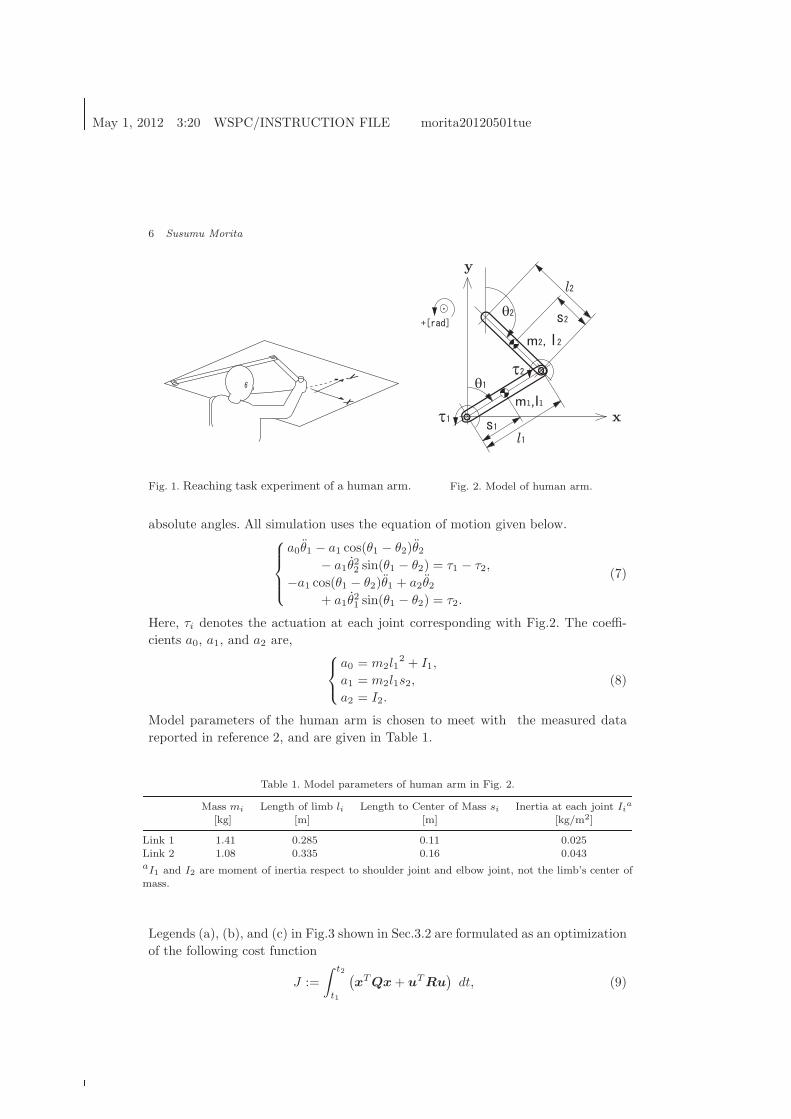
Fig.1 is a simplified picture of an experimental apparatus to measure joint angles and

hand trajectory on a planar table. The subject is asked to perform something called

a reaching task. This experiment is conducted to explore what kind or what in exact

mathematical language may be the principle adopted when a person reaches for a

cup of coffee on a table. The number of angular trajectories that accomplishes this

task is infinite, therefore leaving us with a problem “what criteria is it that chooses

one out of the million, and how?”, a problem named after a Soviet physiologist, “a

Bernstein problem.”

In Sec. 2.2, we introduced a method that generates a trajectory where the non-

conservative force is a polynomial of time. It is fair to say that it is rather a primitive

way to generate actuation. We will share an interesting result that may provide the

reader a different impression against the proposed method.

Motion generation method in comparison is all a kind of an optimization problem

and uses the same 2 link arm model shown in Fig. 2 . Note that θ1 and θ2 are both


6 Susumu Morita

Fig. 1. Reaching task experiment of a human arm. Fig. 2. Model of human arm.

absolute angles. All simulation uses the equation of motion given below.

a0θ1 − a1 cos(θ1 − θ2)θ2− a1θ

22 sin(θ1 − θ2) = τ1 − τ2,

−a1 cos(θ1 − θ2)θ1 + a2θ2+ a1θ

21 sin(θ1 − θ2) = τ2.

(7)

Here, τi denotes the actuation at each joint corresponding with Fig.2. The coeffi-

cients a0, a1, and a2 are,

a0 = m2l12 + I1,

a1 = m2l1s2,

a2 = I2.

(8)

Model parameters of the human arm is chosen to meet with the measured data

reported in reference 2, and are given in Table 1.

Table 1. Model parameters of human arm in Fig. 2.

Mass mi Length of limb li Length to Center of Mass si Inertia at each joint Iia

[kg] [m] [m] [kg/m2]

Link 1 1.41 0.285 0.11 0.025Link 2 1.08 0.335 0.16 0.043aI1 and I2 are moment of inertia respect to shoulder joint and elbow joint, not the limb’s center of

mass.

Legends (a), (b), and (c) in Fig.3 shown in Sec.3.2 are formulated as an optimization

of the following cost function

J :=

∫

t2

t1

(

xTQx+ uTRu)

dt, (9)



where x = [q1, · · · , qm, q1, · · · , qm, τ1, · · · , τm]T , u = [τ1, · · · , τm]T . The parameter

settings for Eq.(9) respect to the legends in Fig.3 is noted below.

(a) Q = I3m×3m, R = Im×m

(b) Q = block-diag[I2m×2m,0m×m], R = 0m×m

(c) Q = 03m×3m, R = Im×m

Here, m denotes the number of independent generalized coordinates, and Ik×k is a

k × k unit matrix.

(a), (b), and (c) are optimizations of a Linear-Quadratic cost function with

different figures for elements of the weight matrices Q and R. (a) and (b) are an

example showing a condition to start a heuristic search, giving engineers some sense

how conventional methods may act, so there is no physical or physiological meaning.

The weight matrix set as (c) will be that of the Minimum Torque-change Model

proposed in reference 2. Legends are commonly used from Fig.3 through Fig.9.

For the proposed method, second line of Eq.(6) for this system was derived

to form a TPBVP of the ODEs. The variable substitution in this example was

chosen as q = ϕ(4). Thus, the state vector in the proposed method is x =

[θ1, θ2, θ1, θ2, F1, F2, F1, F2, F1, F2, F1(3), F2

(3)]T . The first 6 state variables were

fixed at the start and end of the motion. TPBVP was solved by shooting method.

Note that shoulder torque τ1 and elbow torque τ2 in Eq.(7) needs caution in

how they appear. According to Eq.(6) , the generalized forces Fi is F1 = τ1 − τ2and F2 = τ2. Fi does not necessary appear as an control input term. Fi is a result

of the variational calculation after applying the substitution q = ϕ(n). The variable

substitution does not imply any kind of information about how the actual control

inputs will be in real application.

The motion duration was set to 0.52 sec, which was the time that the subjects

were asked to aim for the three reaching tasks shown in Fig.3.2 0.52 sec was the

normal average duration time of the reaching tasks between the two points shown

in Fig.3. The subjects were trained in advanced to the data acquisition till they

were able to meet a small neighborhood of the target point with this duration time.

All numerical calculation adopted 0.001 sec for its time step.

There is an argument that whether the friction and damping being taken

into consideration effects physiological comprehensions. For example, the minimum

torque change model daringly neglects friction and damping, while a motion princi-

ple that will predict different results by considering these factors is proposed.4 There

is also an indication that the optimization becomes more difficult when considering

friction and damping.9 We chose not to consider joint friction and damping.

3.2. Simulation results

In Fig. 3, the whole area shows the table in X-Y coordinates, and [X,Y ] = [0, 0]

is the point where the shoulder joint of a right arm is located. There are three

reaching task motions in the figure. All three has a rather dark thick curve line,


8 Susumu Morita

0

0.1

0.2

0.3

0.4

0.5

-0.4 -0.3 -0.2 -0.1 0 0.1 0.2 0.3 0.4

Y-p

osi

tio

n [

m]

X-position [m]

start

end

start

end

start

end

actual dataa) Q=I,R=I

b) Q=block-diag[I,I,0], R=0c) MTC

proposed method

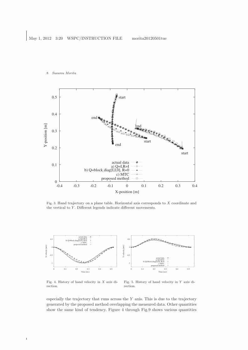
Fig. 3. Hand trajectory on a plane table. Horizontal axis corresponds to X coordinate andthe vertical to Y . Different legends indicate different movements.

-1

-0.5

0

0.5

0 0.1 0.2 0.3 0.4 0.5

X-v

eloci

ty [

m/s

]

Time [sec]



proposed method

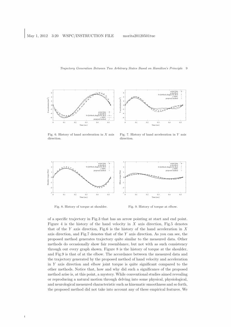
Fig. 4. History of hand velocity in X axis di-rection.

-1

-0.5

0

0.5

0 0.1 0.2 0.3 0.4 0.5

Y-v

eloci

ty [

m/s

]

Time [sec]



proposed method

Fig. 5. History of hand velocity in Y axis di-rection.

especially the trajectory that runs across the Y axis. This is due to the trajectory

generated by the proposed method overlapping the measured data. Other quantities

show the same kind of tendency. Figure 4 through Fig.9 shows various quantities



-6

-4

-2

0

2

4

6

0 0.1 0.2 0.3 0.4 0.5

X-a

ccel

erat

ion [

m/s

2]

Time [sec]



proposed method

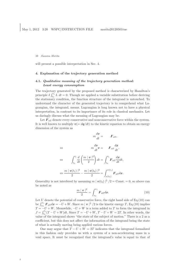
Fig. 6. History of hand acceleration in X axisdirection.

-6

-4

-2

0

2

4

6

0 0.1 0.2 0.3 0.4 0.5

Y-a

ccel

erat

ion [

m/s

2]

Time [sec]



proposed method

Fig. 7. History of hand acceleration in Y axisdirection.

-3

-2

-1

0

1

2

3

0 0.1 0.2 0.3 0.4 0.5

Should

er t

orq

ue

[Nm

]

Time [sec]



proposed method

Fig. 8. History of torque at shoulder.

-3

-2

-1

0

1

2

3

0 0.1 0.2 0.3 0.4 0.5

Elb

ow

torq

ue

[Nm

]

Time [sec]



proposed method

Fig. 9. History of torque at elbow.

of a specific trajectory in Fig.3 that has an arrow pointing at start and end point.

Figure 4 is the history of the hand velocity in X axis direction, Fig.5 denotes

that of the Y axis direction, Fig.6 is the history of the hand acceleration in X

axis direction, and Fig.7 denotes that of the Y axis direction. As you can see, the

proposed method generates trajectory quite similar to the measured data. Other

methods do occasionally show fair resemblance, but not with as such consistency

through out every graph shown. Figure 8 is the history of torque at the shoulder,

and Fig.9 is that of at the elbow. The accordance between the measured data and

the trajectory generated by the proposed method of hand velocity and acceleration

in Y axis direction and elbow joint torque is quite significant compared to the

other methods. Notice that, how and why did such a significance of the proposed

method arise is, at this point, a mystery. While conventional studies aimed revealing

or reproducing a natural motion through delving into some physical, physiological,

and neurological measured characteristic such as kinematic smoothness and so forth,

the proposed method did not take into account any of these empirical features. We


10 Susumu Morita

will present a possible interpretation in Sec. 4.

4. Explanation of the trajectory generation method

4.1. Qualitative meaning of the trajectory generation method:

Least energy consumption

The trajectory generated by the proposed method is characterized by Hamilton’s

principle δ∫ t1

t0L dt = 0. Though we applied a variable substitution before deriving

the stationary condition, the function structure of the integrand is untouched. To

understand the character of the generated trajectory is to comprehend what La-

grangian, the integrand, means. Lagrangian is long known not to have a physical

interpretation, in contrast to its importance of its role in classical mechanics. Let

us daringly discuss what the meaning of Lagrangian may be.

Let F all denote every conservative and nonconservative force within the system.

It is well known to multiply v(= dq/dt) to the kinetic equation to obtain an energy

dimension of the system as

mdv

dt= F all,

⇔ mdv

dtv = F all

dx

dt,

⇔

∫ t1

t0

d

dt

(

m | v |2

2

)

dt =

∫ t1

t0

F all

dx

dtdt,

⇔m | v(t1) |

2

2−

m | v(t0) |2

2=

∫ x(t1)

x(t0)

F alldx.

Generality is not interfered by assuming m | v(t0) |2 /2 = Const. = 0, so above can

be noted as

m | v |2

2=

∫ x1

x0

F alldx. (10)

Let U denote the potential of conservative force, the right hand side of Eq.(10) can

be∫ x1

x0

F alldx = −U +W . Since m | v |2 /2 is the kinetic energy T , Eq.(10) implies

T = −U +W . Meanwhile, −U +W is a term added to T to form the integrand in

J =∫ t1

t0(T −U +W )dt. Since T = −U +W , T −U +W = 2T . In other words, the

value of the integrand shows “the state of the subject of motion.” There is a 2 as a

coefficient, but this does not affect the information of the integrand being the state

of what is actually moving being applied various forces.

One may argue that T − U +W = 2T indicates that the integrand formalized

in this fashion only provides us with a system of a non-accelerating mass in a

void space. It must be recognized that the integrand’s value is equal to that of



2T and not its function structure. It holds information of forces U and W . Hence

δ∫ t1

t0(T − U +W )dt = 0 can yield kinetic equation. Lagrangian L = T − U being

the integrand is the case where there is only conservative force within the system.

In this case, T = −U always holds, thus L = T − U = 2T still holds as well.

Eq.(10) implies that every work applied to the subject of motion is equal to the

kinetic energy of the subject of motion at all times. Since the value of the integrand

T −U +W being equal to 2T = m | v |2, a convex function at all times, Hamilton’s

principle δ∫ t1

t0L+W dt = 0 can be interpreted as a search for a trajectory q(t) of

the least total expensed energy, or more intuitively speaking the total effort to move

the motion subject of issue. This is more suitable to be the least energy consumption

criterion. It maybe that, by calculating Lagrangian from motion captured data of

athletes, the value may show a certain tendency respect to the dominance of his or

her performance.

4.2. Miscellaneous features of the variable substitution method

4.2.1. Conservation law

Hamiltonian is known to be conserved in cases where there is only a conservative

force within the system. Despite a force that is a polynomial of time is nonconser-

vative because there is no corresponding potential, the second equation in Eq.(6)

implies the existence of conserved quantities,

dn−1

dtn−1

{

d

dt

(

∂L

∂q

)

−∂L

∂q

}

. (11)

While equation of free motion is formulated with q, q, and q, Hamiltonian is a

function of q and q. Second equation in Eq.(6) and Eq.(11) shows resemblance as,

the second equation in Eq.(6) is formulated with q(n+1), q(n), · · · , q, while Eq.(11)

is a function of q(n), q(n−1), · · · , q. This is not necessary a result of the variable

substitution, rather a result that can be obtained by adopting a force that is a

polynomial of time.

4.2.2. Variable substitution method as a constraint to an optimization

problem

The proposed method can be formulated as a constraint added to Hamilton’s prin-

ciple. λ = [λ1, · · · , λm]T being Lagrange multipliers, the substitution q = ϕ(n) can

be achieved with,

δJ =

∫ t1

t0

{

L(q, q) + λT(q −ϕ(n))}

dt = 0. (12)

With applying δq(t0) = δλ(t0) = δϕ(t0) = δq(t1) = δλ(t1) = δϕ(t1) = 0, the

stationary condition for Eq.(12) is


12 Susumu Morita

−d

dt

(

∂L

∂q

)

+∂L

∂q+ λ = 0,

λ(n) = 0,

q −ϕ(n) = 0.

(13)

Third equation in Eq.(13) is the variable substitution to be applied to the Hamilton’s

principle. Since ϕ(t) is not our concern, this need not be solved.

5. Conclusion

This paper introduced a trajectory generation method that obeys the exact same

principle of free motion in terms of variational problem, but yields a trajectory that

is not necessarily a free motion. The mathematical and qualitative interpretation

was given, which is an unconventional meaning of the Hamilton’s principle. This

lead to a qualitative meaning of the Lagrangian as a by-product, which has been

left without an interpretation since its birth.

Appendix A.

We will show the details of the variational calculation of Eq.(3). We have been show-

ing equations and formulas by vector operations. Here, we will show the arithmetic

broken down to manipulation of each elements of vectors. δ∫

t1

t0L(ϕ,ϕ(3)) dt will be

calculated as

δ

∫

t1

t0

L(ϕ,ϕ(3)) dt =

∫

t1

t0

{

m∑

i=1

(

∂L

∂ϕi

δϕi

)

+

m∑

i=1

(

∂L

∂ϕi(3)

δϕi(3)

)

}

dt. (A.1)

To turn all the virtual displacements to be only δϕi and nothing else with in the

integrand, we apply partial integration two times to the first term in the integrand

and three times to the second term in the integrand of Eq.(A.1). The calculation

to the first term will be

∫

t1

t0

m∑

i=1

(

∂L

∂ϕi

δϕi

)

dt =

[

m∑

i=1

(

∂L

∂ϕi

δϕi

)]t1

t0

+

∫

t1

t0

m∑

i=1

{

−d

dt

(

∂L

∂ϕi

)

δϕi

}

dt

=

[

m∑

i=1

(

∂L

∂ϕi

δϕi

)

+

m∑

i=1

{

−d

dt

(

∂L

∂ϕi

)

δϕi

}]t1

t0

+

∫

t1

t0

m∑

i=1

{

d2

dt2

(

∂L

∂ϕi

)

δϕi

}

dt. (A.2)



As to the second term, it will turn out to be∫

t1

t0

m∑

i=1

(

∂L

∂ϕi(3)

δϕi(3)

)

dt =

[

m∑

i=1

(

∂L

∂ϕi(3)

δϕi

)

]t1

t0

+

∫

t1

t0

m∑

i=1

{

−d

dt

(

∂L

∂ϕi(3)

)

δϕi

}

dt

=

[

m∑

i=1

(

∂L

∂ϕi(3)

δϕi

)

+m∑

i=1

{

−d

dt

(

∂L

∂ϕi(3)

)

δϕi

}

]t1

t0

+

∫

t1

t0

m∑

i=1

{

d2

dt2

(

∂L

∂ϕi(3)

)

δϕi

}

dt

=

[

m∑

i=1

(

∂L

∂ϕi(3)

δϕi

)

+

m∑

i=1

{

−d

dt

(

∂L

∂ϕi(3)

)

δϕi

}

+

m∑

i=1

{

d2

dt2

(

∂L

∂ϕi(3)

)

δϕi

}

]t1

t0

+

∫

t1

t0

m∑

i=1

{

−d3

dt3

(

∂L

∂ϕi(3)

)

δϕi

}

dt. (A.3)

Applying δϕi(t0) = δϕi(t0) = δϕi(t0) = δϕi(t1) = δϕi(t1) = δϕi(t1) = 0 to

Eq.(A.2) and Eq.(A.3) yields Eq.(3).

References

1. P. Morasso, Spatial control of arm movements, Experimental Brain Research 42(2),223–227 (1981).

2. Y. Uno , M. Kawato and R. Suzuki, Formation and control of optimal trajectory inhuman multijoint arm movement –Minimum torque-change model–, Biological Cyber-netics 61, 89–101 (1989).

3. C. M. Harris and D. M. Wolpert, Signal-dependent noise determines motor planning,Nature 394, 780–784 (1998).

4. E. Nakano, H. Imamizu, R. Osu, Y. Uno, H. Gomi,T. Yoshioka and M. Kawato, Quanti-tative examinations of internal representations for arm trajectory planning : Minimumcommanded torque change model, Journal of Neurophysiology 81, 2140–2155 (1999).

5. M. Kawato, Internal models for motor control and trajectory planning, Current Opinionin Neurobiology, 9, 718–727 (Elsevier Science Ltd., 1999).

6. M. Desmurget and S. Grafton, Forward modeling allows feedback control for fast reach-ing movements, Trends in Cognitive Sciences 4, 11, 423–431 (2000).

7. A. Pouget and L. H. Snyder, Computational approaches to sensorimotor transforma-tions, Nature Neuroscience 3, 1192–1198 (2000).

8. J. Spoelstra, N. Schweighofer, and M. A. Arbib, Cerebellar learning of accurate predic-tive control for fast-reaching movements, Biological Cybernetics, 82, 321–333 (2000).

9. Y. Wada, Y. Kaneko, E. Nakano, R. Osu and M. Kawato, Quantitative examinations formulti joint arm trajectory Planning –Using a robust calculation algorithm of the Min-imum commanded torque change trajectory–, Neural Networks 14(2), 381–393 (2001).

10. J. Izawa, T. Kondo, K. Ito, Biological Robot Arm Motion through ReinforcementLearning IEEE Int. Conf. Robotics and Automation (ICRA) (IEEE Press, Washington,DC, USA, 2002), 3398–3403.

11. S. Schaal, Arm and Hand Movement Control, The Handbook of Brain Theory andNeural Networks, 2nd edn. (MIT Press, Cambridge, 2002), 110–113


14 Susumu Morita

12. T. Flash, N. Hogan, and M. J. E. Richardson, Optimization Principles In MotorControl, The Handbook of Brain Theory and Neural Networks, 2nd edn. (MIT Press,Cambridge, 2002), 827–831

13. Y. Taniai and J. Nishii, Optimality of the minimum endpoint variance model basedon energy consumption, Experimental Brain Research, 167(4), 487–495 (2005).

14. S. Morita and T. Ohtsuka, Natural Motion Trajectory Generation Based on Hamil-ton’s Principle –Transformation of Dynamical Variables–, Transactions of the Societyof Instrument and Control Engineers 42(1), 1–10 (2006), (in Japanese).

15. P. Bays and D. M. Wolpert, Computational principles of sensorimotor control thatminimize certainty ans variability, Journal of Physiology, 578, 387–396 (2007).

16. J. Nishii and Y. Taniai, Evaluation of trajectory planning models for arm reachingmovements based on energy cost, Neural Computation, 21(9), 2634–2657, (2009)

17. D. Caligiore , E. Guglielmelli, A.M. Borghi, D. Parisi, and G. Baldassarre, Learn-ing Model of Reaching Integrating Kinematic and Dynamic Control in a SimulatedArm Robot, IEEE Int. Conf. Development and Learning (ICDL2010) (IEEE Press,Piscataway, NJ, 2011), 211–218.

18. C. Lanczos, The Variational Principles of Mechanics, 4th edn. (Dover, New York,1970), 111–119, 138–140.

Susumu Morita received his M.S. and Ph.D. degrees from the

Osaka University, Japan, in 2002 and 2006, respectively.

From 2006 to 2009, he worked for Mitsubishi Electric Co.

From 2009, he is an Assistant Professor at the Institute of Indus-

trial Science at The University of Tokyo. His research interests

are in motion generation of animals and humans. Main focus

is in the dynamics and principles of various motions and how

it is implemented. This includes control theory, especially op-

timal control, trajectory planning, acquisition and recognitionof inner body and environment informations and how they are utilized. He also

has interests to flocks and swarm behaviors and its principles. He is a mem-

ber of The Society of Instrument and Control Engineers, The Institute of Sys-

tems, Control and Information Engineers, and The Robotics Society of Japan.

Trajectory Generation Between Two Arbitrary States Based On Hamilton's Principle -A Variable...

Documents

Transcript of Trajectory Generation Between Two Arbitrary States Based On Hamilton's Principle -A Variable...