Traffic Analysis for Voice over IP Traffic Analysis for Voice over IP

Traffic Analysis for Voice over IP

Version History

Traffic Analysis for Voice over IP discusses various traffic analysis concepts and features that are applicable to Voice over IP (VoIP). This document presents fundamental traffic theory, several statistical traffic models, application of traffic analysis to VoIP networks, and an end-to-end traffic analysis example.

This document contains the following sections:

• Traffic Analysis Overview, page 1

• Traffic Theory Basics, page 2

• Traffic Model Selection Criteria, page 5

• Traffic Models, page 8

• Applying Traffic Analysis to VoIP Networks, page 14

• End-to-End Traffic Analysis Example, page 18

• Related Documents, page 20

Traffic Analysis OverviewNetworks, whether voice or data, are designed around many different variables. Two of the most important factors that you need to consider in network design are service and cost. Service is essential for maintaining customer satisfaction. Cost is always a factor in maintaining profitability. One way that you can factor in some of the service and cost elements in network design is to optimize circuit utilization.

This document describes the different techniques you can use to engineer and properly size traffic-sensitive voice networks. It discusses several different traffic models and explain how to use traffic probability tables to help you engineer robust and efficient voice networks.

Version Number Date Notes

1 06/25/2001 This document was created.

2 11/01/2001 Incorporated editorial comments.

3 6/20/2007 Corrected per CSCsj34541.

1Traffic Analysis for Voice over IP

Traffic Analysis for Voice over IPTraffic Theory Basics

Traffic Theory BasicsNetwork designers need a way to properly size network capacity, especially as networks grow. Traffic theory enables network designers to make assumptions about their networks based on past experience.

Traffic is defined as either the amount of data or the number of messages over a circuit during a given period of time. Traffic also includes the relationship between call attempts on traffic-sensitive equipment and the speed with which the calls are completed. Traffic analysis enables you to determine the amount of bandwidth you need in your circuits for data and for voice calls. Traffic engineering addresses service issues by enabling you to define a grade of service or blocking factor. A properly engineered network has low blocking and high circuit utilization, which means that service is increased and your costs are reduced.

There are many different factors that you need to take into account when analyzing traffic. The most important factors are described in the following sections:

• Traffic Load Measurement

• Grade of Service

• Traffic Types

• Sampling Methods

Of course, other factors might affect the results of traffic analysis calculations, but these are the main ones. You can make assumptions about the other factors.

Traffic Load MeasurementIn traffic theory, you measure traffic load. Traffic load is the ratio of call arrivals in a specified period of time to the average amount of time taken to service each call during that period. These measurement units are based on Average Hold Time (AHT). AHT is the total time of all calls in a specified period divided by the number of calls in that period, as shown in the following example:

(3976 total call seconds)/(23 calls) = 172.87 sec per call = AHT of 172.87 seconds

The two main measurement units used today to measure traffic load are erlangs and centum call seconds (CCS).

One erlang is 3600 seconds of calls on the same circuit, or enough traffic load to keep one circuit busy for 1 hour. Traffic in erlangs is the product of the number of calls times AHT divided by 3600, as shown in the following example:

(23 calls * 172.87 AHT)/3600 = 1.104 erlangs

One CCS is 100 seconds of calls on the same circuit. Voice switches generally measure the amount of traffic in CCS.

Traffic in CCS is the product of the number of calls times the AHT divided by 100, as shown in the following example:

(23 calls * 172.87 AHT)/100 = 39.76 CCS

Which unit you use depends highly on the equipment you use and what unit of measurement they record in. Many switches use CCS because it is easier to work with increments of 100 rather than 3600. Both units are recognized standards in the field. The following is how the two relate: 1 erlang = 36 CCS.

Although you can take the total call seconds in an hour and divide that amount by 3600 seconds to determine the traffic in erlangs, you can also use averages of various time periods. These averages allow you to use more sample periods and determine the proper traffic.



Busy Hour Traffic

You commonly measure network traffic load during the busiest hour because this period represents the maximum traffic load that your network must support. The result gives you a traffic load measurement commonly referred to as the Busy Hour Traffic (BHT). There are times when you cannot do a thorough sampling or you have only an estimate of how many calls you are handling daily. In such a circumstance, you can usually make assumptions about your environment, such as average number of calls per day and the AHT. In the standard business environment, the busy hour of any given day accounts for approximately 15 to 20 percent of the traffic for that day. In your computations, you generally use 17 percent of the total daily traffic to represent the peak hour traffic. In many business environments, an acceptable AHT is generally assumed to be 180 to 210 seconds. You can use these estimates if you ever need to determine trunking requirements without having more complete data.

Network Capacity Measurements

Among the many ways to measure network capacity are the following:

• Busy Hour Call Attempts (BHCA)

• Busy Hour Call Completions (BHCC)

• Calls per Second (CPS)

All of these measurements are based on the number of calls. Although these measurements do describe network capacity, they are fairly meaningless to traffic analysis because they do not consider the hold time of the call. You need to use these measurements in conjunction with an AHT to derive a BHT that you can use for traffic analysis.

Grade of ServiceGrade of Service (GoS) is defined as the probability that calls will be blocked while attempting to seize circuits. It is written as P.xx blocking factor or blockage, where xx is the percentage of calls that are blocked for a traffic system. For example, traffic facilities requiring P.01 GoS define a 1 percent probability of callers being blocked to the facilities. A GoS of P.00 is rarely requested and will rarely happen because to be 100 percent sure that there is no blocking, you would have to design a network where the caller to circuit ratio is 1:1. Also, most traffic formulas assume that there are an infinite number of callers.

Traffic TypesYou can use the telecommunications equipment that is offering the traffic to record the data described. Unfortunately, most of the samples received are based on the carried traffic on the system and not the offered traffic load.

Carried traffic is the traffic that is actually serviced by telecommunications equipment. Offered traffic is the actual amount of traffic attempts on a system. Note that the difference in the two can cause some inaccuracies in your calculation.

The greater the amount of blockage you have, the greater the difference between carried and offered load. You can use the following formula to calculate offered load from carried load:

Offered load = carried load/(1 – blocking factor)



Unfortunately, this formula does not take into account any retries that might happen when a caller is blocked. You can use the following formula to take the retry rate into account:

Offered load = carried load * Offered Load Adjustment Factors (OAF)OAF = [1.0 – (R * blocking factor)]/(1.0 – blocking factor)

Where R is a percentage of retry probability. For example, R = 0.6 for a 60 percent retry rate.)

Sampling MethodsThe accuracy of your traffic analysis will also depend on the accuracy of your sampling methods. The following parameters will change the represented traffic load:

• Weekdays versus weekends

• Holidays

• Type of traffic (modem versus traditional voice)

• Apparent versus offered load

• Sample period

• Total number of samples taken

• Stability of the sample period

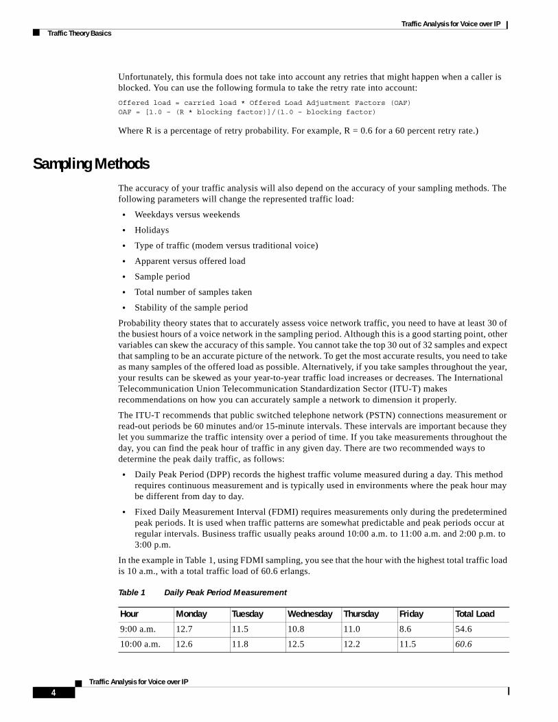
Probability theory states that to accurately assess voice network traffic, you need to have at least 30 of the busiest hours of a voice network in the sampling period. Although this is a good starting point, other variables can skew the accuracy of this sample. You cannot take the top 30 out of 32 samples and expect that sampling to be an accurate picture of the network. To get the most accurate results, you need to take as many samples of the offered load as possible. Alternatively, if you take samples throughout the year, your results can be skewed as your year-to-year traffic load increases or decreases. The International Telecommunication Union Telecommunication Standardization Sector (ITU-T) makes recommendations on how you can accurately sample a network to dimension it properly.

The ITU-T recommends that public switched telephone network (PSTN) connections measurement or read-out periods be 60 minutes and/or 15-minute intervals. These intervals are important because they let you summarize the traffic intensity over a period of time. If you take measurements throughout the day, you can find the peak hour of traffic in any given day. There are two recommended ways to determine the peak daily traffic, as follows:

• Daily Peak Period (DPP) records the highest traffic volume measured during a day. This method requires continuous measurement and is typically used in environments where the peak hour may be different from day to day.

• Fixed Daily Measurement Interval (FDMI) requires measurements only during the predetermined peak periods. It is used when traffic patterns are somewhat predictable and peak periods occur at regular intervals. Business traffic usually peaks around 10:00 a.m. to 11:00 a.m. and 2:00 p.m. to 3:00 p.m.

In the example in Table 1, using FDMI sampling, you see that the hour with the highest total traffic load is 10 a.m., with a total traffic load of 60.6 erlangs.

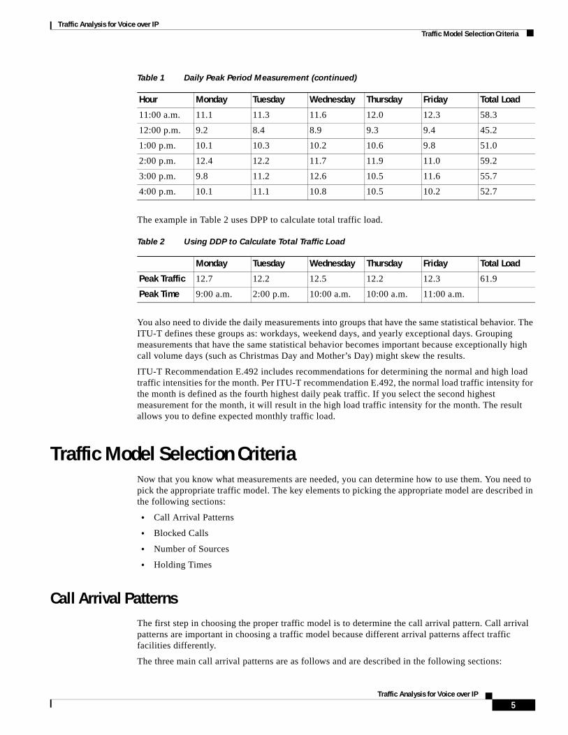
Table 1 Daily Peak Period Measurement

Hour Monday Tuesday Wednesday Thursday Friday Total Load

9:00 a.m. 12.7 11.5 10.8 11.0 8.6 54.6

10:00 a.m. 12.6 11.8 12.5 12.2 11.5 60.6


Traffic Analysis for Voice over IPTraffic Model Selection Criteria

The example in Table 2 uses DPP to calculate total traffic load.

You also need to divide the daily measurements into groups that have the same statistical behavior. The ITU-T defines these groups as: workdays, weekend days, and yearly exceptional days. Grouping measurements that have the same statistical behavior becomes important because exceptionally high call volume days (such as Christmas Day and Mother’s Day) might skew the results.

ITU-T Recommendation E.492 includes recommendations for determining the normal and high load traffic intensities for the month. Per ITU-T recommendation E.492, the normal load traffic intensity for the month is defined as the fourth highest daily peak traffic. If you select the second highest measurement for the month, it will result in the high load traffic intensity for the month. The result allows you to define expected monthly traffic load.

Traffic Model Selection CriteriaNow that you know what measurements are needed, you can determine how to use them. You need to pick the appropriate traffic model. The key elements to picking the appropriate model are described in the following sections:

• Call Arrival Patterns

• Blocked Calls

• Number of Sources

• Holding Times

Call Arrival PatternsThe first step in choosing the proper traffic model is to determine the call arrival pattern. Call arrival patterns are important in choosing a traffic model because different arrival patterns affect traffic facilities differently.

The three main call arrival patterns are as follows and are described in the following sections:

11:00 a.m. 11.1 11.3 11.6 12.0 12.3 58.3

12:00 p.m. 9.2 8.4 8.9 9.3 9.4 45.2

1:00 p.m. 10.1 10.3 10.2 10.6 9.8 51.0

2:00 p.m. 12.4 12.2 11.7 11.9 11.0 59.2

3:00 p.m. 9.8 11.2 12.6 10.5 11.6 55.7

4:00 p.m. 10.1 11.1 10.8 10.5 10.2 52.7

Table 1 Daily Peak Period Measurement (continued)

Hour Monday Tuesday Wednesday Thursday Friday Total Load

Table 2 Using DDP to Calculate Total Traffic Load

Monday Tuesday Wednesday Thursday Friday Total Load

Peak Traffic 12.7 12.2 12.5 12.2 12.3 61.9

Peak Time 9:00 a.m. 2:00 p.m. 10:00 a.m. 10:00 a.m. 11:00 a.m.



• Smooth Call Arrival Pattern

• Peaked Call Arrival Pattern

• Random Call Arrival Pattern

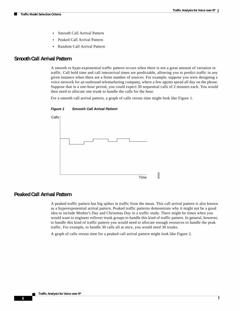
Smooth Call Arrival Pattern

A smooth or hypo-exponential traffic pattern occurs when there is not a great amount of variation in traffic. Call hold time and call interarrival times are predictable, allowing you to predict traffic in any given instance when there are a finite number of sources. For example, suppose you were designing a voice network for an outbound telemarketing company, where a few agents spend all day on the phone. Suppose that in a one-hour period, you could expect 30 sequential calls of 2 minutes each. You would then need to allocate one trunk to handle the calls for the hour.

For a smooth call arrival pattern, a graph of calls versus time might look like Figure 1.

Figure 1 Smooth Call Arrival Pattern

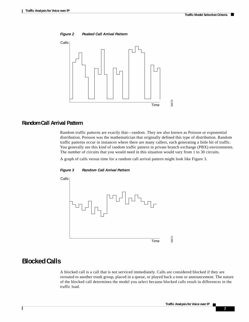
Peaked Call Arrival Pattern

A peaked traffic pattern has big spikes in traffic from the mean. This call arrival pattern is also known as a hyperexponential arrival pattern. Peaked traffic patterns demonstrate why it might not be a good idea to include Mother's Day and Christmas Day in a traffic study. There might be times when you would want to engineer rollover trunk groups to handle this kind of traffic pattern. In general, however, to handle this kind of traffic pattern you would need to allocate enough resources to handle the peak traffic. For example, to handle 30 calls all at once, you would need 30 trunks.

A graph of calls versus time for a peaked call arrival pattern might look like Figure 2.

5656

9

Calls

Time



Figure 2 Peaked Call Arrival Pattern

Random Call Arrival Pattern

Random traffic patterns are exactly that—random. They are also known as Poisson or exponential distribution. Poisson was the mathematician that originally defined this type of distribution. Random traffic patterns occur in instances where there are many callers, each generating a little bit of traffic. You generally see this kind of random traffic pattern in private branch exchange (PBX) environments. The number of circuits that you would need in this situation would vary from 1 to 30 circuits.

A graph of calls versus time for a random call arrival pattern might look like Figure 3.

Figure 3 Random Call Arrival Pattern

Blocked CallsA blocked call is a call that is not serviced immediately. Calls are considered blocked if they are rerouted to another trunk group, placed in a queue, or played back a tone or announcement. The nature of the blocked call determines the model you select because blocked calls result in differences in the traffic load.

5657

0

Calls

Time

� 5657

1

�

Calls

Time


Traffic Analysis for Voice over IPTraffic Models

The main types of blocked calls are as follows:

• Lost Calls Held (LCH)—These blocked calls are lost, never to come back again. Originally LCH was based on the theory that all calls introduced to a traffic system were held for a finite amount of time. All calls include any of the calls that were blocked, which meant the calls were still held until time ran out for the call.

• Lost Calls Cleared (LCC)—These blocked calls are cleared from the system, meaning that when a caller is blocked, the call goes somewhere else (mainly to other traffic-sensitive facilities).

• Lost Calls Delayed (LCD)—These blocked calls remain on the system until facilities are available to service the call. LCD is used mainly in call center environments or with data circuits because the key factors for LCD would be delay in conjunction with traffic load.

• Lost Calls Retried (LCR)—LCR assumes that once a call is blocked, a percentage of the blocked callers retry and all other blocked callers retry until they are serviced. LCR is a derivative of the LCC model and is used in the Extended Erlang B model.

Number of SourcesThe number of sources of calls also has bearing on what traffic model you choose. For example, if there is only one source and one trunk, the probability of blocking the call is zero. As the number of sources increases, the probability of blocking gets higher. The number of sources comes into play when sizing a small PBX or key system, where you can use a smaller number of trunks and still arrive at the designated GoS.

Holding TimesSome traffic models take into account the holding times of the call. Most models do not take holding time into account because call holding times are assumed to be exponential. Generally, calls have short rather than long hold times, meaning that call holding times will have a negative exponential distribution.

Traffic ModelsAfter you have determined the call arrival patterns and determined the blocked calls, number of sources, and holding times of the calls, you are ready to select the traffic model that most closely fits your environment. Although no traffic model can exactly match real life situations, these models assume the average in each situation. There are many different traffic models—the key is to find the model that best suits your environment.

The traffic models that have the widest adoption are Erlang B, Extended Erlang B, and Erlang C. Other commonly adopted traffic models are Engset, Poisson, EART/EARC, and Neal-Wilkerson. A comparison of traffic model features is shown in Table 3.

Table 3 Traffic Model Comparison

Traffic Model Sources Arrival PatternBlocked Call Disposition Holding Times

Poisson Infinite Random Held Exponential

Erlang B Infinite Random Cleared Exponential



The following sections describe various traffic models from which you can choose when you are calculating the number of trunks required for your network configuration. Although the tables for all the traffic models are too large to be included in a document of this size, you can find the information on line or from other sources. You can choose to calculate blocking factor by using any of the following:

• The formulas in this document

• On-line calculators, such as can be found at the following URL:

http://www.erlang.com/calculator/index.htm

• Traffic tables, available on line or in reference books

Erlang BThe Erlang B traffic model is based on the following assumptions:

• An infinite number of sources

• Random traffic arrival pattern

• Blocked calls cleared

• Hold times exponentially distributed

The Erlang B model is used when blocked calls are rerouted, never to come back to the original trunk group. This model assumes a random call arrival pattern. The caller makes only one attempt; if the call is blocked, then the call is rerouted. The Erlang B model is commonly used for first-attempt trunk groups where you need not take into consideration the retry rate because callers are rerouted, or you expect to see very little blockage.

The following formula is used to derive the Erlang B traffic model:

Extended Erlang B Infinite Random Retried Exponential

Erlang C Infinite Random Delayed Exponential

Engset Finite Smooth Cleared Exponential

EART/EARC Infinite Peaked Cleared Exponential

Neal-Wilkerson Infinite Peaked Held Exponential

Crommelin Infinite Random Delayed Constant

Binomial Finite Random Held Exponential

Delay Finite Random Delayed Exponential

Table 3 Traffic Model Comparison (continued)

Traffic Model Sources Arrival PatternBlocked Call Disposition Holding Times

B(c,a) =

ac

c

k=0

c!

Σ ak

k!

6024

6



Where:

• B(c,a) is the probability of blocking the call.

• c is the number of circuits.

• a is the traffic load.

Example 1: Using the Erlang B Traffic Model

Problem

You need to redesign your outbound long distance trunk groups, which are currently experiencing some blocking during the busy hour. The switch reports state that the trunk group is offered 17 erlangs of traffic during the busy hour. You want to have low blockage so you want to design for less than 1 percent blockage.

Solution

If you look at the Erlang B Tables, you see that for 17 erlangs of traffic and a GoS of 0.64 percent, you need 27 circuits to handle this traffic load.

You can also check the blocking factor using the Erlang B equation, given the information provided. Another way you can check the blocking factor is by using the Microsoft Excel Poisson function in the following format:

=(POISSON(<circuits>,<traffic load>,FALSE))/(POISSON(<circuits>,<traffic load>,TRUE))

There is a very handy Erlang B, Extended Erlang B and Erlang C calculator at the following URL: http://www.erlang.com/calculator/index.htm

Extended Erlang B The Extended Erlang B traffic model is based on the following assumptions:



• Blocked calls cleared


The Extended Erlang B model is designed to take into account the calls that are retried at a certain rate. This model assumes a random call arrival pattern, that blocked callers make multiple attempts to complete their calls, and that no overflow is allowed. The Extended Erlang B model is commonly used for standalone trunk groups with a retry probability (for example, a modem pool).

Example 2: Using the Extended Erlang B Traffic Model

Problem

You want to determine how many circuits you need for your dial access server. You know that you receive about 28 erlangs of traffic during the busy hour and that 5 percent blocking during that period is acceptable. You also expect that 50 percent of the users will retry immediately.



Solution

If you look at the Extended Erlang B Tables, you see that for 28 erlangs of traffic with a retry probability of 50 percent and 4.05 percent blockage, you need 35 circuits to handle this traffic load.

Again, there is a very handy Erlang B, Extended Erlang B, and Erlang C calculator at the following URL: http://www.erlang.com/calculator/index.htm

Erlang CThe Erlang C traffic model is based on the following assumptions:



• Blocked calls delayed


The Erlang C model is designed around queuing theory. This model assumes a random call arrival pattern; the caller makes one call and is held in a queue until the call is answered. The Erlang C model is more commonly used for conservative automatic call distributor (ACD) design to determine the number of agents needed. It can also be used for determining bandwidth on data transmission circuits, but it is not the best model to use for that purpose.

In the Erlang C model, you need to know the number of calls or packets in the busy hour, the average call length or packet size, and the expected amount of delay in seconds.

The following formula is used to derive the Erlang C traffic model:

Where:

• C(c,a) is the probability of delaying the call.



Example 3: Using the Erlang C Traffic Model for Voice

Problem

You expect the call center to have approximately 600 calls lasting approximately 3 minutes each, and that each agent has an after-call work time of 20 seconds. You would like the average time in the queue to be approximately 10 seconds.

C(c,a) =

a cc

c–1

k=0

c!(c – a)

Σ a cc

c!(c – a)a +

k

k!

6024

7



Solution

Calculate the amount of expected traffic load. You know that you have approximately 600 calls of 3 minutes duration. To that number you must add 20 seconds because each agent is not answering a call for approximately 20 seconds. The additional 20 seconds is part of the amount of time it takes to service a call, as shown in the following formula:

(600 calls * 200 seconds AHT)/3600 = 33.33 erlangs of traffic

Compute the delay factor by dividing the expected delay time by AHT, as follows:

(10 sec delay)/(200 seconds) = 0.05 delay factor

Example 4: Using the Erlang C Traffic Model for Data

Problem

You are designing your backbone connection between two routers. You know that you will generally see about 600 packets per second (pps) with 200 bytes per packet or 1600 bits per packet. Multiplying 600 pps by 1600 bits per packet gives the amount of needed bandwidth: 960,000 bits per second (bps). You know that you can buy circuits in increments of 64,000 bps, the amount of data necessary to keep the circuit busy for 1 second. How many circuits will you need to keep the delay under 10 ms?

Solution

Calculate the traffic load as follows:

(960,000 bps)/(64,000 bps) = 15 erlangs of traffic load

Calculate the average transmission time. Multiply the number of bytes per packet by 8 to get the number of bits per packet, then divide that by 64,000 bps (circuit speed) to get the average transmission time per packet as follows:

(200 bytes per packet) * (8 bits) = (1600 bits per packet)/(64000 bps)= 0.025 seconds (25 ms) to transmit(Delay factor 10 ms)/(25 ms) = 0.4 delay factor

If you look at the Erlang C Tables, you see that with a traffic load of 15.47 erlangs and a delay factor of 0.4, you need 17 circuits. This calculation is based on the assumption that the circuits are clear of any packet loss.

Again, there is a very handy Erlang B, Extended Erlang B, and Erlang C calculator at the following URL: http://www.erlang.com/calculator/index.htm.

EngsetThe Engset model is based on the following assumptions:

• A finite number of sources

• Smooth traffic arrival pattern

• Blocked calls cleared from the system




The Engset formula is generally used for environments where it is easy to assume that a finite number of sources are using a trunk group. By knowing the number of sources, you can maintain a high grade of service. You would use the Engset formula in applications such as global system for mobile communication (GSM) cells and subscriber loop concentrators. Because the Engset traffic model is covered in many books dedicated to traffic analysis, it is not discussed here.

PoissonThe Poisson model is based on the following assumptions:



• Blocked calls held


In the Poisson model, blocked calls are held until a circuit becomes available. This model assumes a random call arrival pattern; the caller makes only one attempt to place the call and blocked calls are lost. The Poisson model is commonly used for overengineering standalone trunk groups.

The following formula is used to derive the Poisson traffic model:

Where:

• P(c,a) is the probability of blocking the call.

• e is the natural log base.



Example 5: Using the Poisson Traffic Model

Problem

You are creating a new trunk group to be used only by your new office and you need to determine how many lines are needed. You expect the office to make and receive approximately 300 calls per day with an AHT of about 4 minutes (240 seconds). The goal is a P.01 GoS or 1 percent blocking rate. To be conservative, we assume that approximately 20 percent of the calls happen during the busy hour. Calculate the busy hour traffic as follows:

300 calls * 20% = 60 calls during the busy hour(60 calls * 240 AHT)/3600 = 4 erlangs during the busy hour

Solution

If you look at the Poisson Tables, you see that at 4 erlangs of traffic with a blocking rate of 0.81 percent (close enough to 1 percent), you need 10 trunks to handle this traffic load. You can check this number by plugging the variables into the Poisson formula, as follows:

P(c,a) = 1 – e–a

c–1

k=0Σ a

k

k!

6024

8


Traffic Analysis for Voice over IPApplying Traffic Analysis to VoIP Networks

Another easy way to find blocking is by using the Microsoft Excel POISSON function with the following format:

=1 – POISSON(<circuits> – 1,<traffic load>,TRUE)

EART/EARC and Neal-WilkersonThe EART/EARC and Neal-Wilkerson models are used for peaked traffic patterns. Most telephone companies use these models for rollover trunk groups that have peaked arrival patterns. The EART/EARC model treats blocked calls as cleared and the Neal-Wilkerson model treats them as held. Because the EART/EARC and Neal-Wilkerson traffic models are covered in many books dedicated to traffic analysis, they are not discussed here.

Applying Traffic Analysis to VoIP NetworksBecause VoIP traffic uses Real-time Transport Protocol (RTP) to transport voice traffic, you can use the same principles to define the bandwidth on your WAN links.

There are some challenges in defining the bandwidth. The considerations discussed in the following sections will affect the bandwidth of voice networks:

• Voice Codecs

• Samples

• Voice Activity Detection

• RTP Header Compression

• Point-to-Point Versus Point-to-Multipoint

Voice CodecsMany voice codecs are used in IP telephony. These codecs all have different bit rates and complexities to them. Some of the standard voice codecs are G.711, G.729, G.726, G.723.1, and G.728. All Cisco voice-enabled routers and access servers support some or all of these codecs.

Codecs impact bandwidth because they determine the payload size of the packets transferred over the IP leg of a call. In Cisco voice gateways, you can configure the payload size to control bandwidth. By increasing payload size, you reduce the total number of packets sent, thus decreasing the bandwidth needed by reducing the number of headers required for the call.

P(10, 4) = 1 – e = 1 – e (1+ 4 + )+ + +... ≈ 0.00813–4 –4

10–1

k=0Σ 4

k

k!162

646

25624

6024

9



SamplesThe number of samples per packet is another factor in determining the bandwidth of a voice call. The codec defines the size of the sample but the total number of samples placed in a packet affects how many packets are sent per second. So, the number of samples included in a packet affects the overall bandwidth of a call.

For example, a G.711 10-ms sample is 80 bytes per sample. A call with only one sample per packet would yield the following:

80 bytes + 20 bytes IP + 12 UDP + 8 RTP = 120 bytes per packet120 bytes per packet * 100 pps = (12000 * 8 bits)/1000 = 96 kbps per call

The same call using two 10 ms samples per packet would yield the following:

(80 bytes * 2 samples) + 20 bytes IP + 12 UDP + 8 RTP = 200 bytes per packet(200 bytes per packet) * (50 pps) = (10000 * 8 bits)/1000 = 80 kbps per call

Note Layer 2 headers were not included in the preceding calculations.

The results show that there is a 16 kbps difference between the two calls. By changing the number of samples per packet, you definitely can change the amount of bandwidth a call uses, but there is a trade-off. When you increase the number of samples per packet, you also increase the amount of delay on each call. DSP resources, which handle each call, must buffer the samples for a longer period of time. You should keep this in mind when you design a voice network.

Voice Activity DetectionTypical voice conversations can contain up to 35 to 50 percent silence. With traditional, circuit-based voice networks, all voice calls use a fixed bandwidth of 64 kbps regardless of how much of the conversation is speech and how much is silence. With VoIP networks, all conversation and silence is packetized. Voice Activity Detection (VAD) sends RTP packets only when voice is detected. For VoIP bandwidth planning, assume that VAD reduces bandwidth by 35 percent. Although this value might be less than the actual reduction, it provides a conservative estimate that takes into consideration different dialects and language patterns.

The G.729 Annex-B and G.723.1 Annex-A codecs include an integrated VAD function, but otherwise have identical performance to G.729 and G.723.1, respectively.

RTP Header CompressionAll VoIP packets have two components: voice samples and IP/UDP/RTP headers. Although the voice samples are compressed by the digital signal processor (DSP) and vary in size depending on the codec used, the headers are always a constant 40 bytes. When compared to the 20 bytes of voice samples in a default G.729 call, these headers take up a considerable amount of overhead. By using RTP Header Compression (cRTP), which is used on a link by link basis, these headers can be compressed to 2 or 4 bytes. This compression can offer substantial VoIP bandwidth savings. For example, a default G.729 VoIP call consumes 24 kbps without cRTP, but only 12 kbps with cRTP enabled.

Codec type, samples per packet, VAD, and cRTP affect, in one way or another, the bandwidth of a call. In each case, there is a trade-off between voice quality and bandwidth. Table 1-4 shows the bandwidth utilization for various scenarios. VAD efficiency in the graph is assumed to be 50 percent.



Table 4 lists the effects of payload size on the bandwidth requirements of various codecs.

Table 4 Voice Codec Characteristics

Algorithm

VoiceBW(kb/s)

FrameSize(bytes)

CiscoPayload(bytes)

PacketsperSecond

IP/UDP/RTPHeader(bytes)

CRTPHeader(bytes) L2

Layer 2Header(bytes)

TotalBandwidth(kb/s)No VAD

TotalBandwidth(kb/s)With VAD

G.711 64 80 160 50 40 — Ether 14 85.6 42.8

G.711 64 80 160 50 — 2 Ether 14 70.4 35.2

G.711 64 80 160 50 40 — PPP 6 82.4 41.2

G.711 64 80 160 50 — 2 PPP 6 67.2 33.6

G.711 64 80 160 50 40 — FR 4 81.6 40.8

G.711 64 80 160 50 — 2 FR 4 66.4 33.2

G.711 64 80 80 100 40 — Ether 14 107.2 53.6

G.711 64 80 80 100 — 2 Ether 14 76.8 38.4

G.711 64 80 80 100 40 — PPP 6 100.8 50.4

G.711 64 80 80 100 — 2 PPP 6 70.4 35.2

G.711 64 80 80 100 40 — FR 4 99.2 49.6

G.711 64 80 80 100 — 2 FR 4 68.8 34.4

G.729 8 10 20 50 40 — Ether 14 29.6 14.8

G.729 8 10 20 50 — 2 Ether 14 14.4 7.2

G.729 8 10 20 50 40 — PPP 6 26.4 13.2

G.729 8 10 20 50 — 2 PPP 6 11.2 5.6

G.729 8 10 20 50 40 — FR 4 25.6 12.8

G.729 8 10 20 50 — 2 FR 4 10.4 5.2

G.729 8 10 30 33 40 — Ether 14 22.4 11.2

G.729 8 10 30 33 — 2 Ether 14 12.3 6.1

G.729 8 10 30 33 40 — PPP 6 20.3 10.1

G.729 8 10 30 33 — 2 PPP 6 10.1 5.1

G.729 8 10 30 33 40 — FR 4 19.7 9.9

G.729 8 10 30 33 — 2 FR 4 9.6 4.8

G.723.1 6.3 30 30 26 40 — Ether 14 17.6 8.8

G.723.1 6.3 30 30 26 — 2 Ether 14 9.7 4.8

G.723.1 6.3 30 30 26 40 — PPP 6 16.0 8.0

G.723.1 6.3 30 30 26 — 2 PPP 6 8.0 4.0

G.723.1 6.3 30 30 26 40 — FR 4 15.5 7.8

G.723.1 6.3 30 30 26 — 2 FR 4 7.6 3.8

G.723.1 5.3 30 30 22 40 — Ether 14 14.8 7.4

G.723.1 5.3 30 30 22 — 2 Ether 14 8.1 4.1



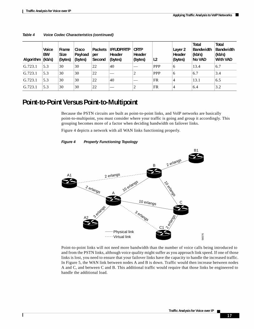
Point-to-Point Versus Point-to-MultipointBecause the PSTN circuits are built as point-to-point links, and VoIP networks are basically point-to-multipoint, you must consider where your traffic is going and group it accordingly. This grouping becomes more of a factor when deciding bandwidth on failover links.

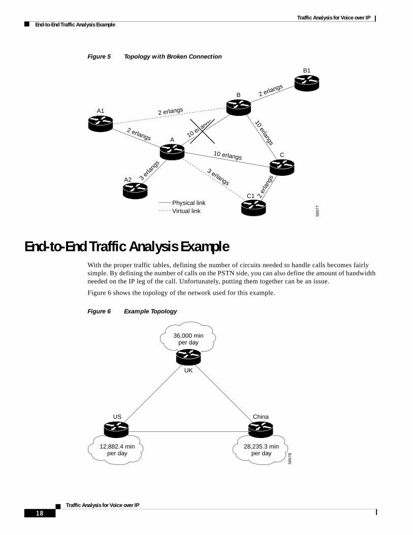
Figure 4 depicts a network with all WAN links functioning properly.

Figure 4 Properly Functioning Topology

Point-to-point links will not need more bandwidth than the number of voice calls being introduced to and from the PSTN links, although voice quality might suffer as you approach link speed. If one of those links is lost, you need to ensure that your failover links have the capacity to handle the increased traffic. In Figure 5, the WAN link between nodes A and B is down. Traffic would then increase between nodes A and C, and between C and B. This additional traffic would require that those links be engineered to handle the additional load.

G.723.1 5.3 30 30 22 40 — PPP 6 13.4 6.7

G.723.1 5.3 30 30 22 — 2 PPP 6 6.7 3.4

G.723.1 5.3 30 30 22 40 — FR 4 13.1 6.5

G.723.1 5.3 30 30 22 — 2 FR 4 6.4 3.2

Table 4 Voice Codec Characteristics (continued)

Algorithm

VoiceBW(kb/s)

FrameSize(bytes)

CiscoPayload(bytes)

PacketsperSecond

IP/UDP/RTPHeader(bytes)

CRTPHeader(bytes) L2

Layer 2Header(bytes)

TotalBandwidth(kb/s)No VAD

TotalBandwidth(kb/s)With VAD

2 erlangs

2 erlangs

2 er

lang

s

2 erlangs

3 er

langs

3 erlangs

10 erlangs

10 erlangs 10 erlangs

5657

6

Physical linkVirtual link

A1

A2

A

C1

C

B

B1


Traffic Analysis for Voice over IPEnd-to-End Traffic Analysis Example

Figure 5 Topology with Broken Connection

End-to-End Traffic Analysis ExampleWith the proper traffic tables, defining the number of circuits needed to handle calls becomes fairly simple. By defining the number of calls on the PSTN side, you can also define the amount of bandwidth needed on the IP leg of the call. Unfortunately, putting them together can be an issue.

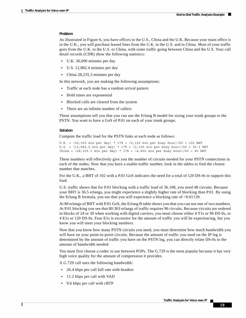
Figure 6 shows the topology of the network used for this example.

Figure 6 Example Topology

2 erlangs

2 erlangs

2 er

lang

s

2 erlangs

3 er

langs

3 erlangs

10 erlangs

10 erlangs 10 erlangs

5657

7

Physical linkVirtual link

A1

A2

A

C1

C

B

B1

5657

8

36,000 minper day

12,882.4 minper day

US China

UK

28,235.3 minper day


Traffic Analysis for Voice over IPEnd-to-End Traffic Analysis Example

Problem

As illustrated in Figure 6, you have offices in the U.S., China and the U.K. Because your main office is in the U.K., you will purchase leased lines from the U.K. to the U.S. and to China. Most of your traffic goes from the U.K. to the U.S. or China, with some traffic going between China and the U.S. Your call detail records (CDR) show the following statistics:

• U.K. 36,000 minutes per day

• U.S. 12,882.4 minutes per day

• China 28,235.3 minutes per day

In this network, you are making the following assumptions:

• Traffic at each node has a random arrival pattern

• Hold times are exponential

• Blocked calls are cleared from the system

• There are an infinite number of callers

These assumptions tell you that you can use the Erlang B model for sizing your trunk groups to the PSTN. You want to have a GoS of P.01 on each of your trunk groups.

Solution

Compute the traffic load for the PSTN links at each node as follows:

U.K. = (36,000 min per day) * 17% = (6,120 min per busy hour)/60 = 102 BHTU.S. = (12,882.4 min per day) * 17% = (2,190 min per busy hour)/60 = 36.5 BHTChina = (28,235.3 min per day) * 17% = (4,800 min per busy hour)/60 = 80 BHT

These numbers will effectively give you the number of circuits needed for your PSTN connections in each of the nodes. Now that you have a usable traffic number, look in the tables to find the closest number that matches.

For the U.K., a BHT of 102 with a P.01 GoS indicates the need for a total of 120 DS-0s to support this load.

U.S. traffic shows that for P.01 blocking with a traffic load of 36.108, you need 48 circuits. Because your BHT is 36.5 erlangs, you might experience a slightly higher rate of blocking than P.01. By using the Erlang B formula, you see that you will experience a blocking rate of ~0.01139.

At 80 erlangs of BHT with P.01 GoS, the Erlang B table shows you that you can use one of two numbers. At P.01 blocking you see that 80.303 erlangs of traffic requires 96 circuits. Because circuits are ordered in blocks of 24 or 30 when working with digital carriers, you must choose either 4 T1s or 96 DS-0s, or 4 E1s or 120 DS-0s. Four E1s is excessive for the amount of traffic you will be experiencing, but you know you will meet your blocking numbers.

Now that you know how many PSTN circuits you need, you must determine how much bandwidth you will have on your point-to-point circuits. Because the amount of traffic you need on the IP leg is determined by the amount of traffic you have on the PSTN leg, you can directly relate DS-0s to the amount of bandwidth needed.

You must first choose a codec to use between POPs. The G.729 is the most popular because it has very high voice quality for the amount of compression it provides.

A G.729 call uses the following bandwidth:

• 26.4 kbps per call full rate with headers

• 11.2 kbps per call with VAD

• 9.6 kbps per call with cRTP


Traffic Analysis for Voice over IPRelated Documents

• 6.3 kbps per call with VAD and cRTP

Therefore, the bandwidth needed on the link between the U.K. and the U.S. is as follows:

• Full Rate: 96 DS0s * 26.4 kbps = 2.534 Mbps

• VAD: 96 DS0s * 11.2 kbps = 1.075 Mbps

• cRTP: 96 DS0s * 17.2 kbps = 1.651 Mbps

• VAD/cRTP: 96 DS0s * 7.3 kbps = 700.8 kbps

The bandwidth needed on the link between the U.K. and China is as follows:

• Full Rate: 72 DS0s * 26.4 kbps = 1.9 Mbps

• VAD: 72 DS0s * 11.2 kbps = 806.4 kbps

• cRTP: 72 DS0s * 17.2 kbps = 1.238 Mbps

• VAD/cRTP: 72 DS0s * 7.3 kbps = 525.6 kbps

As you can see, VAD and cRTP have a substantial impact on the bandwidth needed on the WAN link.

Related DocumentsCisco IOS Voice, Video and Fax Configuration Guide

Voice over IP Fundamentals, Cisco Press, 2000

ITU-T Recommendation E.500, Traffic Intensity Measurement Principles

ITU-T Recommendation E.492, Traffic Reference Period


Traffic Analysis for Voice over IP Traffic Analysis for Voice over IP

Documents

Transcript of Traffic Analysis for Voice over IP Traffic Analysis for Voice over IP