Toxic Exposure Assessment: A Columbia-Harvard (TEACH) Study (The New York City Report)
169
Toxic Exposure Assessment: A Columbia-Harvard (TEACH) Study (The New York City Report) Patrick L. Kinney, Steven N. Chillrud, Sonja Sax, James M. Ross, Dee C. Pederson, Dave Johnson, Maneesha Aggarwal, and John D. Spengler NUMBER 3 2005
-
Upload
independent -
Category
Documents
-
view
2 -
download
0
Transcript of Toxic Exposure Assessment: A Columbia-Harvard (TEACH) Study (The New York City Report)
Toxic Exposure Assessment: A Columbia-Harvard(TEACH) Study (The New York City Report)
Patrick L. Kinney, Steven N. Chillrud, Sonja Sax,James M. Ross, Dee C. Pederson, Dave Johnson,Maneesha Aggarwal, and John D. Spengler
NUMBER 32005

ABOUT THE NUATRC
The Mickey Leland National Urban Air Toxics Research Center (NUATRC or the LelandCenter) was established in 1991 to develop and support research into potential humanhealth effects of exposure to air toxics in urban communities. Authorized under the CleanAir Act Amendments (CAAA) of 1990, the Center released its first Request for Applicationsin 1993. The aim of the Leland Center since its inception has been to build a researchprogram structured to investigate and assess the risks to public health that may beattributed to air toxics. Projects sponsored by the Leland Center are designed to providesound scientific data useful for researchers and for those charged with formulatingenvironmental regulations.
The Leland Center is a public-private partnership, in that it receives support fromgovernment sources and from the private sector. Thus, government funding is leveragedby funds contributed by organizations and businesses, enhancing the effectiveness of thefunding from both of these stakeholder groups. The U.S. Environmental Protection Agency(EPA) has provided the major portion of the Center’s government funding to date, and anumber of corporate sponsors, primarily in the chemical and petrochemical fields, havealso supported the program.
A nine-member Board of Directors oversees the management and activities of the LelandCenter. The Board also appoints the thirteen members of a Scientific Advisory Panel (SAP)who are drawn from the fields of government, academia and industry. These membersrepresent such scientific disciplines as epidemiology, biostatistics, toxicology and medicine.The SAP provides guidance in the formulation of the Center’s research program andconducts peer review of research results of the Center’s completed projects.
The Leland Center is named for the late United States Congressman George Thomas“Mickey” Leland from Texas who sponsored and supported legislation to reduce theproblems of pollution, hunger, and poor housing that unduly affect residents of low-incomeurban communities.
This project has been funded wholly or in part by the United States Environmental Protection Agency under assistance agreement R828678.The contents of this document do not necessarily reflect the views and policies of the Environmental Protection Agency, nor does mention oftrade names or commercial products constitute endorsement or recommendation for use.

Toxic Exposure Assessment: A Columbia-Harvard(TEACH) Study
(The New York City Report)
Patrick L. Kinney1, Steven N. Chillrud2, Sonja Sax3,James M. Ross2, Dee C. Pederson2, Dave Johnson2,
Maneesha Aggarwal1, and John D. Spengler3
1 Mailman School of Public Health at Columbia University2 Lamont Doherty Earth Observatory at Columbia University
3 Harvard School of Public Health
TABLE OF CONTENTS
NUATRC RESEARCH REPORT NO. 3
133334444666788
10101010101111111215151616171718
18181920222324282828
PREFACEEXECUTIVE SUMMARY
STUDY AIMS
FINDINGS
Subject and Home Characteristics
Personal Air Toxic Exposures
Indoor Air Toxic Concentrations
Outdoor Air Toxic Concentrations
LIMITATIONS
INTRODUCTIONBACKGROUND
REPORT ORGANIZATION
STUDY AIMS AND DESCRIPTION
METHODSSTUDY DESIGN
STUDY COMMUNITY
RECRUITMENT
QUESTIONNAIRES
Home Environment Questionnaire
Time-Location-Activity Diary and 48-Hour Exposure Questionnaire
SAMPLING AND ANALYSIS
General Methods of Indoor/Outdoor/Personal and Ambient Sampling
Volatile Organic Compounds
PM2.5, Black Carbon, and Elements
Aldehydes
Air Exchange
DATA PROCESSING AND DATABASE STRUCTURE
Data Processing
Database Structure
DATA ANALYSIS OVERVIEW
QUALITY ASSURANCELIMITS OF DETECTION, OUTLIERS AND ANALYTICAL PROBLEMS, ACCURACY AND PRECISION OF
MEASUREMENTS
Limits of Detection
Outliers and Analytical Problems
Accuracy
Precision
Details of Multi-Element Analysis QA
COMPARISON OF PASSIVE AND ACTIVE VOC SAMPLERS
RESULTS AND DISCUSSIONSUBJECT CHARACTERISTICS
Demographics
NUATRC RESEARCH REPORT NO. 3
TABLE OF CONTENTS (cont.)
2830303031343535
3643474750535559596670737474747575757680808387878797
115123131131149157
Housing Factors
Time-Activity Patterns
AIR MONITORING RESULTS
Introduction
Overview of Ambient Data: Urban and Upwind Fixed Sites and Home Outdoor
Overview of Home Indoor and Personal Data
PERSONAL EXPOSURES TO AIR TOXICS
Descriptive Analyses
Temporal and Spatial Associations Between Personal Exposures and Ambient Concentrations of PM2.5,
Sulfate, and Black Carbon
Tracking the Source of Elevated Personal Exposures to Metals
INDOOR/OUTDOOR AND AIR EXCHANGE RELATIONSHIPS
Descriptive Analyses
The Influence of Air Exchange on Indoor/Outdoor Ratios
Filter Reflectance as a Tracer of the Ambient Contribution to Indoor Fine Particle Concentrations
Results and Discussion
AMBIENT AIR MONITORING DATA
Descriptive Analyses
Urban Influence (Urban versus Upwind Concentrations)
Analysis of Spatial and Temporal Variance Components
Preliminary Source Apportionment of Ambient VOCs
SUMMARY OF KEY FINDINGSSUBJECT AND HOME CHARACTERISTICS
PERSONAL AIR TOXIC EXPOSURES
INDOOR AIR TOXIC CONCENTRATIONS
OUTDOOR AIR TOXIC CONCENTRATIONS
LIMITATIONSREFERENCESACKNOWLEDGMENTSABBREVIATIONSLIST OF FIGURES AND TABLESAPPENDICES
APPENDIX A: QUESTIONNAIRES AND CODEBOOKS
Appendix A1 Student Survey
Appendix A2 Home Environment Questionnaire
Appendix A3 Time-Location-Activity Diary
Appendix A4 48 Hour Questionnaire
APPENDIX B: VARIABLE LISTING AND PRINTOUTS OF PM2.5 DATA SETS
Appendix B1 Reference PM Dataset
Appendix B2 Fixed-site Ambient PM Dataset
Appendix B3 Subject-based PM Dataset
NUATRC RESEARCH REPORT NO. 3
PREFACE
The Clean Air Act Amendments of 1990 established acontrol program for sources of 188 “hazardous airpollutants, or air toxics,” which may pose a risk to publichealth. Also, with the passage of these Amendments,Congress established the Mickey Leland National Urban AirToxics Research Center (NUATRC) to develop and direct anenvironmental health research program that would promotea better understanding of the risks posed to human healthby the presence of these toxic chemicals in urban air.
Established as a public/private research organization, theCenter’s research program is developed with guidance anddirection from scientific experts from academia, industry,and government and seeks to fill the gaps in scientific data.These research results are intended to assist policy makersin reaching sound environmental health decisions. TheNUATRC accomplishes its research mission by sponsoringresearch on human health effects of air toxics in universitiesand research institutions and by publishing researchfindings in its “NUATRC Research Reports,” therebycontributing meaningful and relevant data to the peer-reviewed scientific literature.
The NUATRC realized that the development of strategiesto address air toxics was hampered by the relative paucityof data on both exposures and health effects of the 188HAPs. More data were needed, on both the levels andsources of air toxic exposures, especially in urban areaswhere increasing numbers of persons live. Furthermore, theresults from the total exposure assessment methodologystudies (TEAM studies) published in the early 1990ssuggested that air toxic concentrations from central sitemonitors are not representative of personal exposure, thatexposure to air toxics may depend on time/ activity patternsand time spent indoors, and that indoor air concentrationsmay exceed outdoor due to indoor sources for air toxics. Asa result, the NUATRC developed and published RFA 96-02-B entitled, “Personal Exposures to Air Toxics in UrbanEnvironments” to address the paucity of information onindoor/outdoor concentrations of air toxics and personalexposures and to define the contribution by ambientsources to air toxic exposures.
Dr. Patrick Kinney at the Mailman School of the PublicHealth, Columbia University, was the recipient of the awardin response to this RFA. His study, “The Toxics ExposureAssessment- A Columbia and Harvard Study (TEACH), wasdeveloped to generate data on personal air toxics exposuresof high school students living in the inner cityneighborhoods of New York City (NYC) and Los Angeles(LA) and to characterize levels of and factors influencingpersonal exposures to urban air toxics.
The study provides information on the roles of seasonsand days of the week, different meteorological conditions,and daily activities on exposures to selected volatile organiccompounds (VOC), aldehydes, and metals on particles (<2.5m) present in the environment. Soluble fractions of selectedmetals on particles were also assayed for correlations withsource measurements. Exposure measurements were madein indoor, outdoor, and personal environments. Theinvestigators relate these exposures to the apportionment ofair toxics among area, point, and mobile sources, as well asnon-anthropogenic sources.
This report on the New York portion of TEACH presentsboth descriptive analyses of all the data and more detailedanalyses addressing primary aims of the study. Acompanion report on the LA portion of the TEACH studywill be published soon.
When a NUATRC-funded study is completed, theInvestigators submit a draft final research report. Every draftfinal reports report resulting from NUATRC-fundedresearch undergo undergoes an extensive evaluationprocedure which assesses the strengths and limitations ofthe study, comments on clarity of the presentation, dataquality, appropriateness of study design, data analysis, andinterpretation of the study findings. The objective of thereview process is to ensure that the Investigator’s report iscomplete, accurate, and clear.
The evaluation first involves an external review of thereport by a team of three external reviewers including abiostatistician. The reviewers’ comments are thenconsidered by members of the NUATRC Scientific AdvisoryPanel (SAP), and the comments of the external reviewersand the SAP are provided to the Investigator. In itscommunication with the investigator, the SAP may suggestalternate interpretations for the results and also discuss newinsights that the study may offer to the scientific literature.The investigator has the opportunity to exchange commentswith the SAP and, if necessary, revise the draft report. Inaccordance with the NUATRC policy, the SAP recommendsand the Board of Directors approves the publication of therevised final report. The research presented in the NUATRCResearch Reports represents the work of its investigators.
The NUATRC appreciates hearing comments from itsreaders from industry, academic institutions, governmentagencies, and the public about the usefulness of theinformation contained in these reports, and about otherways that the NUATRC may effectively serve the needs ofthese groups. The NUATRC wishes to express its sincereappreciation to Dr. Kinney and his research team, the SAPand external peer reviewers whose expertise, diligence, andpatience have facilitated the successful completion of thisreport.
1
NUATRC RESEARCH REPORT NO. 3
EXECUTIVE SUMMARY
The Toxics Exposure Assessment: A Columbia HarvardProject (TEACH) study, funded by the National Urban AirToxic Research Center (NUATRC), was designed to collectand analyze data on personal exposures to urban air toxicsamong inner city youths in New York City (NYC) and LosAngeles (LA) and to investigate factors that influence thoseexposures. This is a report on the NYC portion of theTEACH study.
In the U.S., 60% of Hispanics and 50% of AfricanAmericans, compared to 33% of Caucasians, live in areasfailing to meet two or more of the national ambient airquality standards (NAAQS) (Wernette and Nieves 1992;Metzger, et al., 1995). Over 30% of Hispanics and 16% ofAfrican Americans live in areas that do not meet thestandards for PM (Metzger, et al., 1995). The TEACH studyrepresents one important step in addressing the on-goingnational interest in better characterization ofdisproportionately high exposures of a minoritydisadvantaged population to various hazardous airpollutants. The study tested evidence suggesting thatminority and disadvantaged populations aredisproportionately exposed to various toxic pollutants.
Air monitoring was carried out two seasons per city.Simultaneous personal, home indoor, and home outdoordata were collected over six to nine weeks on high schoolstudents from non-smoking homes among a population oflargely inner city black and Hispanic teenagers.Simultaneous monitoring was carried out at upwind andurban ambient fixed sites. Every sampling event involvedintegrated 48-hour sampling for PM2.5, black carbon, up to28 elements of particulate matter (PM), and a suite of 15volatile organic compounds (VOCs) and two aldehydes.The multi-elements, mass, soot, and VOC concentrations,along with critical ancillary information, allow thepartitioning of risk by season, gender, outdoor sources,indoor sources, and mode of transportation, among otherfactors of interest.
For the NYC portion of the study, 46 students participatedin the monitoring, 33 of whom participated in both seasons.These participants ranged in age from 14 to 19, werepredominantly black and/or Hispanic, lived in relativelysmall rental apartments in multi-floor apartment buildings,and lived in neighborhoods with relatively high levels ofself-reported motor vehicle traffic.
STUDY AIMS
The overall objective of the study was to characterizelevels of and factors influencing personal exposures tourban air toxics among high school students living in innercity neighborhoods. The study had five principal aims:
Aim 1: To describe and compare weekday personalexposures to urban air toxics in two representative groupsof 30 high school students (NYC and LA) and analyzeseasonal changes in exposures and activity patterns.
Aim 2: To evaluate the contributions of indoor andoutdoor air toxics concentrations to personal exposures inwinter and summer. In addition, to evaluate the influence oftime-activity patterns and home ventilation rates on theserelationships.
Aim 3: To assess the contributions of a range of sourcecategories to personal, outdoor, and/or indoor exposuresusing data on individual VOCs, aldehydes, and particulatecomponents.
Aim 4: To characterize home indoor and outdoorexposures to the soluble fraction of selected metals and tocorrelate these measurements with simultaneous fixed-siteoutdoor measurements.
Aim 5: To develop and design a methodology for anationwide study addressing personal exposures to urbanair toxic pollutants.
FINDINGS
The study provided extensive descriptive data onexposures to a wide range of air pollutants encountered byyouths living in the urban cores of America's two largestcities. In addition, the design captured information onseveral important sources of variability that may drivepersonal exposures: variability across days, variabilityacross subjects, variability across seasons, and, finally,variability across cities. The design facilitates analyses ofthe relationships among simultaneously collected personal,home indoor and outdoor measurements, and urban fixed-site data and the exploration of factors that may influencethese relationships, such as air exchange rate, indoor andoutdoor sources, and activity patterns.
Subject and Home Characteristics
Time-activity patterns were similar to previous surveys ofurban young people, except that commuting by cars wasuncommon in this population. Subway and bus commutingwere common.
3
Patrick L. Kinney et al
Personal Air Toxic Exposures
For pollutants with significant indoor sources, includingmost of the VOCs, personal exposures showed littlerelationship to outdoor concentrations. For those pollutantslacking significant indoor sources, including most PM-associated elements and a few VOCs, both personal andindoor exposures were associated with outdoor levels.Strong temporal correlations were observed between centralsite ambient data and mean personal exposures for PM2.5,sulfate, and black carbon. In addition, a significant spatialcorrelation was found between home outdoor and personalblack carbon levels, with a stronger correlation in winter.Neither PM2.5 nor sulfate exhibited spatial correlationsbetween outdoor and personal levels. Personal exposureswere significantly higher than home indoor and ambientsamples for several elements, including iron, manganese,and chromium. The iron/manganese andchromium/manganese ratios, as well as strong correlationsamong these elements, suggested steel dust as the source ofthese metals for a large subset of the personal samples.Furthermore, time-activity data suggested the NYC subwaysystem to be a possible source of these elevated personalmetals. The levels and ratios of iron, manganese, andchromium in a single set of duplicate PM2.5 samplesintegrated over eight hours of underground subwayexposure are consistent with the subway system being thepredominant source of these metals to subway-ridingsubjects.
Indoor Air Toxic Concentrations
Indoor VOC levels were generally much higher thanoutdoors, and thus indoor/outdoor (I/O) ratios were above1.0 for most compounds. However, I/O ratios closer to 1.0were observed for a few VOCs, including methyl tertiarybutyl ether (MTBE), benzene, ethylbenzene, toluene, andxylene (BETX). Indoor/outdoor ratios were also lower insummer than in winter, reflecting an increased air exchangeduring summer as compared to winter. The I/O ratios forPM-associated elements were typically close to or below1.0, reflecting the role played by outdoor sources in drivingindoor levels. For a few elements, including cadmium,potassium, and tin in winter and chromium and tin insummer, I/O ratios greater than 1.0 were observed. Foranalytes with I/O ratios appreciably greater than 1.0, thoseratios showed consistent declines at higher air exchangerates.
During the winter season, indoor and personal blackcarbon concentrations can be useful as an alternative tosulfate for tracing PM2.5 of ambient origin. In contrast to
sulfate, black carbon measurements are far more related tolocal urban particle emissions than to regional air masses.Hence, black carbon may be a useful ambient tracer infuture studies addressing the health impacts of traffic-related particulate matter.
Outdoor Air Toxic Concentrations
Ambient concentrations of most VOCs were lower thanlevels measured indoors or as personal samples. Because ofthe relatively low concentrations measured in ambient air,median outdoor concentrations at the urban fixed site werebelow the respective limits of detection for six of 17 VOCs.Better detection results were obtained for the indoor andpersonal samples. With the exception of chromium, allmedian concentrations of ambient PM2.5 and associatedelements exceeded limits of detection.
Analysis of spatial and temporal variations in ambientconcentrations revealed two distinct groups of air toxics:those related to regional air masses (for example sulfur,selenium, arsenic, and formaldehyde) and those related tolocal sources (for example, black carbon, cobalt, lanthanum,nickel, MTBE, other BETX, and VOCs). Concentrationvariations for compounds of the former group were greaterover time than space, whereas the latter group showedgreater variability across locations than across time. A largeurban influence was seen for the BETX VOCs, as well asmany particle components, especially those associated withcombustion of heating oil and diesel fuel. The urban effectwas generally larger in winter than in summer. A statisticalvariance components analysis using a mixed effects modelconfirmed many of these observations.
Patterns of elemental and VOC concentrations across sitesand seasons strongly suggest that outdoor transportationand heating fuel combustion represent the two mostsignificant sources of urban air toxics in NYC. Apreliminary source apportionment analysis of ambient VOCand aldehyde data showed that primary emissions frommotor vehicles were the dominant source category,followed by formation of secondary compounds andspecific point sources.
LIMITATIONS
Several sources of potential bias and/or random errorexist in the measurement design of this study. One relates tothe non-random process used to recruit subjects, whotended to select motivated students and families that mightdiffer from their peers. To address this issue, a largernumber of students (approximately 600 to 700) weresurveyed at each school with respect to basic demographics,
4
Toxic Exposure Assessment: A Columbia-Harvard (TEACH) Study (The New York City Report)
NUATRC RESEARCH REPORT NO. 3
NUATRC RESEARCH REPORT NO. 3
socio-economic status and other characteristics. Findingsfrom this survey were compared to findings regarding studyparticipants. For the most part, the subject populations weresimilar to the survey groups at each school with respect toage, race, and socioeconomic status, although the subjectpopulations had a higher proportion of females than theschool as a whole.
Strictly speaking, the subject-based results of this studycannot be generalized beyond populations of urban highschool students with ethnic and socio-economic status(SES) characteristics similar to those monitored in thesespecific cities. However, it is likely that insight intomechanisms of exposure will be transferable to othersettings and populations. Subject-based measurementswere collected only on weekdays. This may have resultedin a positive bias in exposure levels, since traffic-relatedpollutants are usually greater on weekdays than weekends.
The selection of seasonal periods for sampling alsopresents potential for bias. The seasonal periods wereselected to maximize the contrast between ambientmeteorological conditions and pollutant concentrations.
Thus, it is appropriate to view seasons as fixed effectsselected to maximize contrasts in ambient concentrations.The “winter” sampling period in NYC extended fromFebruary to April. However, during the winter season, theweather was unseasonably warm, and subjects participatingin personal monitoring were not exposed to the sub-freezingtemperatures that are more typical NYC mid-winterconditions. Nevertheless, the data analysis confirms that thetwo NYC sampling seasons did indeed provide contrastingair toxic concentrations, air exchange rates, and time-activity patterns.
Biases may exist in the air pollution measurements.Potential causes include improper calibrations, loss ofanalytes from collection media during or after sampling,contamination of samples during handling, the placementof samplers, or changes in behavior associated with carryingpersonal samplers. Appropriate Quality Control procedureswere established to identify any of these factors should theyoccur.
5
Patrick L. Kinney et al
INTRODUCTION
The Toxics Exposure Assessment: A Columbia HarvardProject (TEACH) study was designed to collect and analyzedata on personal exposures to urban air toxics among innercity youth and to investigate factors which influence thoseexposures. The air monitoring was carried out in two cities,New York (NYC) and Los Angeles (LA), and in two seasonsper city. During each monitoring campaign, simultaneouspersonal, home indoor, and home outdoor data werecollected over six to nine weeks on a group of more than 30high school students from non-smoking homes. In addition,simultaneous monitoring was carried out at upwind andurban ambient fixed sites. Every sampling event involvedintegrated 48-hour sampling for fine particulate matter(PM2.5), black carbon, up to 28 particulate elements, and asuite of 15 volatile organic compounds (VOCs) and twoaldehydes. The fixed-site monitors operated over the entireseason’s sampling campaign, whereas individual subjectswere monitored only once for 48 hours in each season. Mostsubjects were monitored in both seasons. For the NYCportion of the TEACH study, 46 students participated in themonitoring, 33 of whom participated in both seasons.
BACKGROUND
Since the passage of the 1990 Clean Air ActAmendments, issues related to the regulation of air toxics(also referred to as hazardous air pollutants) have gainedincreasing importance. However, the development ofstrategies to address air toxics is hampered by the relativepaucity of data on both exposures and health effects. Moredata are needed on both the levels and determinants of airtoxic exposures, especially in urban areas where increasingnumbers of persons live, both in the U.S. and elsewhere.The study, “Urban Air Toxic Exposures of High SchoolStudents: the TEACH Study,” was developed to generatedata on personal air toxics exposures of urban youth in NYCand LA.
Evidence suggests that there is disproportionately highexposure of minority and disadvantaged populations tovarious toxic pollutants, both nationwide and in NYC. Thisapplies to air pollutants, lead, and certain pesticides (Oldenand Poje 1995; Heritage 1992; Wernette and Nieves 1992;Metzger et al., 1995). In the U.S., 60% of Hispanics and 50%of African Americans, compared to 33% of Caucasians, livein areas failing to meet two or more of the national ambientair quality standards (NAAQS) (Wernette and Nieves 1992;Metzger, et al., 1995). Over 30% of Hispanics and 16% ofAfrican Americans live in areas that do not meet thestandards for PM (Metzger, et al., 1995).
The TEACH study, funded by the National Urban AirToxic Research Center (NUATRC), represents one importantstep in addressing the on-going national interest in bettercharacterization of exposures and risks due to hazardous airpollutants. For our selected population of largely inner cityblack and hispanic teenagers, we have generated importantevidence on factors and contaminants that have thepotential of affecting their health risk from air pollution.The multi-elements, mass, soot, and VOC concentrationsmeasured along with critical ancillary information allowthe partitioning of risk by season, gender, outdoor sources,indoor sources, and mode of transportation, among otherfactors of interest. The value of these data will be partiallyrealized under the current contract. Additional resourceswill be required to fulfill more comprehensive and vitallyimportant objectives of interpreting potential risk to thisunder-studied segment of our population.
REPORT ORGANIZATION
This report on the New York portion of TEACH presentsboth descriptive analyses of all the data and more detailedanalyses addressing primary aims of the study. This firstsection introduces the rationale for studying exposures toair toxics. It provides a brief overview of the design ofTEACH and the aims of the study. Our principle findingsfrom the New York study phase are summarized in“Summary of Key Findings,” followed by a section thatdiscusses some limitations of our study design.
“Methods” describes the study methods in detail,including the questionnaires and the analytical techniquesused for measuring VOCs, particles, soot, elements, and airexchange measurements.
“Results and Discussion” presents the results, dataanalysis, and discussion, starting with data on the studentvolunteers, their demographics, home characteristics, andactivity patterns. We include an analysis of the locationsand activities these teenagers engaged in during thepersonal monitoring. An overview of all air monitoringresults is presented, followed by sections presentingdetailed data and targeted analyses of personal, homeindoor/outdoor, and outdoor sampling.
In “Personal Exposures to Air Toxics,” we begin withdescriptive analysis of selected analytes to illustrate theinfluences of outdoor versus indoor versus personalcontaminants. We analyze the relationships betweenpersonal exposures and ambient concentrations for selectedanalytes. In addition, we describe results of analysesexamining our observation that personal concentrations foriron and several other metals were not correlated witheither indoor or outdoor concentrations. Suspecting that the
6
Toxic Exposure Assessment: A Columbia-Harvard (TEACH) Study (The New York City Report)
NUATRC RESEARCH REPORT NO. 3

NUATRC RESEARCH REPORT NO. 3
mode of commuting might be relevant to these personalexposures, we explored a possible relationship withsubway transit.
In “Indoor/Outdoor and Air Exchange Relationships,” weexamine and analyze the home indoor and outdoor data,along with corresponding data on air exchange rates. Thesection begins with full descriptive analyses of all indoorand air exchange measurements, ratios of indoor-to-outdoorconcentrations, and selected scatter plots of indoor versusoutdoor concentrations. Indoor/outdoor (I/O) ratios are thenanalyzed in relation to air exchange rates (AER), identifyinganalytes for which I/O ratios are significantly influenced byAER. Finally, we carry out an analysis demonstrating theutility of particulate black carbon as a tracer for particles ofambient origin in winter.
In “Ambient Air Monitoring Data,” we present results onthe air toxic concentrations measured at the upwind fixedsite, the urban fixed site, and the individual home outdoorlocations in both winter and summer. As in the other resultssections, “Ambient Air Monitoring Data” begins with a fulltabular presentation of summary statistics, plots showingmedian concentrations and limits of detection, and timeseries plots examining spatial and temporal variations. Wenext analyze the degree of urban influence for each analyte,both as absolute differences between the urban and upwindfixed sites, and as urban-to-upwind ratios. Analytes withsignificant urban-to-upwind differences are noted. Weapply a mixed linear model to apportion the totalmeasurement variance for each analyte into the spatial(between sites) and temporal (between days) components.Analytes with large urban-to-upwind differences and withstronger spatial than temporal variations in ambientconcentrations are identified and interpreted in the contextof local urban sources. Preliminary source apportionmentanalysis is also described.
In “Quality Assurance,” we report the results of ourQA/QC procedures. This section includes an analysis of theorganic vapor monitor (OVM) badge versus thermaldesorption tube (TDT) comparisons for personal VOCmeasurements.
STUDY AIMS AND DESCRIPTION
The TEACH study was designed to facilitate theexamination of a wide range of issues regarding inner cityexposures to air toxics within the available time andbudgetary limits. The study provided extensive descriptivedata on exposures to a wide range of air pollutantsencountered by youth living in the urban cores of America’stwo largest cities. In addition, the design capturedinformation on several important sources of variability that
may drive personal exposures: variability across days,variability across subjects, variability across seasons, and,finally, variability across cities. The design facilitatesanalyses of the relationships among simultaneouslycollected personal, home indoor and outdoormeasurements, and urban fixed-site data and theexploration of factors that may influence theserelationships, such as air exchange rate, indoor and outdoorsources, and activity patterns.
A large data set comprised of 15 VOCs, two aldehydes,particle mass PM2.5, and soot fraction, as well as 28elements, was assembled. Quality assurance wasestablished for all the NYC samples collected. This includesoutdoor, indoor, and personal samples. In addition, homeand personal characteristics, indoor air exchange rates, timeactivity information, and other variables comprise the dataset available for assessing air toxic exposures andsubsequent risk.
The overall objective of the TEACH study was tocharacterize levels of and factors influencing personalexposures to urban air toxics among high school studentsliving in inner city neighborhoods. These populations havebeen under-represented in past studies of personalexposures. To characterize exposure levels, we collectedpersonal concentration data over 48 hours from groups of30 to 40 students in two cities, NYC and LA. To characterizefactors influencing exposures, we collected a variety ofadditional data, including simultaneous home indoor,home outdoor, fixed-site urban, and fixed-site upwindconcentrations, along with air exchange rates, homecharacteristics, and personal activity pattern data. Toprovide a wider range of air exchange rates, activitypatterns, ambient concentrations, and compositions, themeasurements were carried out in two very different citiesand in two seasons per city.
In the original study plan, five specific aims wereproposed. Here we list those five aims and the ways inwhich they have been addressed to date.
Aim 1: To describe and compare weekday personalexposures to urban air toxics in two representative groupsof 30 high school students (NYC and LA) and analyzeseasonal changes in exposures and activity patterns.
The present report provides extensive descriptive data onpersonal exposures to air toxics among students enrolled inthe NYC sub-study. A companion report on the LA data willinclude comparisons between the two cities. Seasonalvariability in exposures was examined by comparing theNYC measurements collected in winter and summer. Activitypattern data were collected and analyzed in both seasons aswell (“Time Activity Patterns”). Representativeness ofsubjects was confirmed by comparing demographic and other
7
Patrick L. Kinney et al
characteristics of study participants with the student body atthe high school under study.
Aim 2: To evaluate the contributions of indoor andoutdoor air toxics concentrations to personal exposures inwinter and summer, and to evaluate the influence of time-activity patterns and home ventilation rates on theserelationships.
This aim represents the main focus of analyses reportedhere. The relationships between personal exposures andoutdoor concentrations are examined for all analytes in“Descriptive Analyses,” with more detailed examinations oftemporal and spatial correlations between personal andoutdoor for PM2.5 black carbon, and sulfate in “Temporaland Spatial Associations Between Personal Exposures andAmbient Concentrations of PM2.5, Sulfate, and BlackCarbon.”
Aim 3: To assess the contributions of a range of sourcecategories to personal, outdoor, and/or indoor exposuresusing data on individual VOCs, aldehydes, and particulatecomponents.
Outdoor source categories of interest include local mobilesources and long-range transport of pollutants from thepredominant upwind location. Indoor source categories ofinterest include indoor combustion appliances, buildingmaterials, and consumer products. Only homes with nosmokers were eligible for the study.
Much of our analysis of the ambient data throughout“Ambient Air Monitoring Data” relates to the issue ofcharacterizing the relative importance of local versusregional pollution sources in driving air toxics exposures inNYC. The analysis of personal versus ambient particle datain “Temporal and Spatial Associations Between PersonalExposures and Ambient Concentrations of PM2.5, Sulfate,and Black Carbon” further examines this issue as it relatesto personal exposures. These observations are augmentedby preliminary source apportionment analyses of theambient data (“Preliminary Source Apportionment ofAmbient VOCs”). Analyses of the strengths of indoor VOCand aldehyde sources will be presented for both NYC andLA in the companion LA TEACH report.
Aim 4: To characterize home indoor and outdoorexposures to the soluble fraction of selected metals and tocorrelate these measurements with simultaneous fixed-siteoutdoor measurements.
No analyses of soluble metals were completed. Fundingconstraints precluded our carrying out the aqueousextraction and analysis of metals on duplicate filters.Substantial numbers of duplicate filters collected indoorsand outdoors at the home locations have been archived forfuture analyses pending the availability of funding.
Aim 5: To develop and design a methodology for a
nationwide study addressing personal exposures to urbanair toxic pollutants.
The successful sampling design pioneered in the TEACHstudy serves as a model for future efforts to characterize airtoxics exposures in other locations.
METHODS
STUDY DESIGN
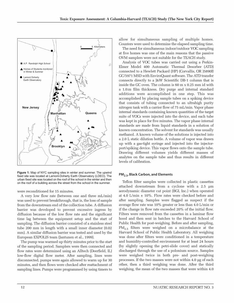
Exposure to air toxics was assessed in a group of 46 highschool students from the A. Philip Randolph Academy, apublic high school located in the West Central Harlemsection of NYC. Each of two field campaigns (winter andsummer, 1999) involved eight weeks of fixed-site ambientmonitoring on a school roof and on a roof at the LamontDoherty Earth Observatory (LDEO) in Palisades, NYC.These two outdoor monitoring locations are referred to asthe urban fixed site and the upwind fixed site. In winter, theurban roof site was located on the seven-story high schoolitself. In summer, the urban roof site was located on a five-story building across the street. Both buildings are situatedon a ridge with one of the highest elevations in Manhattan,so that monitoring results represent area-wide urbanconcentrations. The LDEO roof site was on a three-storybuilding near the Palisades cliffs overlooking the HudsonRiver, 13 miles northwest of Manhattan. Since predominantwinds are from the west, the LDEO rooftop usually reflectsthe upwind air masses. However, on occasion, especiallyduring the summer, sea breezes may cause winds to flow upthe Hudson River valley from NYC towards LDEO.
The fixed-site monitoring covered three consecutive 48-hour periods each week. Concurrent with monitoring of thefirst of these ambient samples each week from Tuesdaythrough Thursday, subject-based monitoring wasconducted. This consisted of collecting personal, homeindoor, and home outdoor samples. Typically, each weekfive subjects were monitored simultaneously. A schematicsummary of the study design is displayed in Table 1. Asshown in Table 2, pollutants monitored at every samplingevent included a suite of 15 VOCs and two aldehydes,PM2.5, black carbon, and a suite of 28 particle-associatedtrace elements. The air exchange rate was monitored in eachhome over a two- to four-day period that always includedthe 48-hour air pollution measurement period.
Quality assurance samples were included in all phases ofmonitoring. Field blanks accompanied all field samples andwere collected regularly throughout each season. Largenumbers of duplicate samples also were collected. Some
NUATRC RESEARCH REPORT NO. 38
The New York City TEACH Study

NUATRC RESEARCH REPORT NO. 3
have been analyzed to determine measurement precision.Others were archived for future analyses. Details areprovided below.
In addition to the main study described above, three sub-studies were completed. In the first study year, two pilotstudies were conducted. The purpose of the first pilot studywas to assess the proposed sampling methodology in asmall group of NYC high school students. Nine studentswere monitored over a two-week period in May of 1998. Adetailed report of the first pilot study was submitted to theNUATRC in October 1998 as part of the Year 1 AnnualProgress Report (Kinney et al., 1998a). Results of the studyreaffirmed the utility of our basic sampling design, whilealso pointing out technical challenges to be addressedbefore the winter NYC measurements began.
The second pilot study was designed to compare twoalternative VOC measurement methods. One method wasbased on active sampling onto TDTs following EPAmethods (EPA Compendium Method 17 for toxic organics);the other method was based on passive sampling onto OVMbadges (Morandi et al., 1998). Side-by-side indoor, outdoor,
9
Patrick L. Kinney, et al
tu-thO
O
Subj i*I,O,P
Subj i*I,O,P
Subj i*I,O,P
Subj i*I,O,P
Subj i*I,O,P
Week 1th-sa
O
O
sa-moO
O
tu-thO
O
Subj i*I,O,P
Subj i*I,O,P
Subj i*I,O,P
Subj i*I,O,P
Subj i*I,O,P
Week 2th-sa
O
O
sa-moO
O
tu-thO
O
Subj i*I,O,P
Subj i*I,O,P
Subj i*I,O,P
Subj i*I,O,P
Subj i*I,O,P
Week 3th-sa
O
O
sa-moO
O
tu-thO
O
Subj i*I,O,P
Subj i*I,O,P
Subj i*I,O,P
Subj i*I,O,P
Subj i*I,O,P
Week 4th-sa
O
O
sa-moO
O
tu-thO
O
Subj i*I,O,P
Subj i*I,O,P
Subj i*I,O,P
Subj i*I,O,P
Subj i*I,O,P
Week 5th-sa
O
O
sa-moO
O
tu-thO
O
Subj i*I,O,P
Subj i*I,O,P
Subj i*I,O,P
Subj i*I,O,P
Subj i*I,O,P
Week 6th-sa
O
O
sa-moO
O
SummerUpwind Fixed-Site
Urban Fixed-Site
Subject-basedMeasurements
tu-thO
O
Subj 1I,O,P
Subj 2I,O,P
Subj 3I,O,P
Subj 4I,O,P
Subj 5I,O,P
Week 1th-sa
O
O
sa-moO
O
tu-thO
O
Subj 6I,O,P
Subj 7I,O,P
Subj 8I,O,P
Subj 9I,O,P
Subj 10I,O,P
Week 2th-sa
O
O
sa-moO
O
tu-thO
O
Subj 11I,O,P
Subj 12I,O,P
Subj 13I,O,P
Subj 14I,O,P
Subj 15I,O,P
Week 3th-sa
O
O
sa-moO
O
tu-thO
O
Subj 16I,O,P
Subj 17I,O,P
Subj 18I,O,P
Subj 19I,O,P
Subj 20I,O,P
Week 4th-sa
O
O
sa-moO
O
tu-thO
O
Subj 21I,O,P
Subj 22I,O,P
Subj 23I,O,P
Subj 24I,O,P
Subj 25I,O,P
Week 5th-sa
O
O
sa-moO
O
tu-thO
O
Subj 26I,O,P
Subj 27I,O,P
Subj 28I,O,P
Subj 29I,O,P
Subj 30I,O,P
Week 6th-sa
O
O
sa-moO
O
WinterUpwind Fixed-Site
Urban Fixed-Site
Subject-basedMeasurements
i* = 1 to 30
Table 1: Idealized sampling design for NYC. Note that the order of subject monitoring in summer was based on convenience. I=indoor; O=outdoor;P=personal.
Particulate MatterComponents
Volatile OrganicCompounds
Aldehydes
Iron TinLanthium TitaniumLead* VanadiumMagnesium Zinc
Benzene*Trace Elements: 1,3-Butadiene*
Carbon Tetrachloride*Aluminum Manganese* Chloroform*Antimony* Nickel* Ethylbenzene*Arsenic* Platinum m,p-Xylene*Beryllium* Potassium o-Xylene*Cadmium * Scandium Methylene Chloride*Calcium Selenium* MTBE*Cesium Silver Styrene*Chromium* Sodium Tetrachloroethylene*Cobalt* Sulfur Toluene*Copper Thallium Trichloroethelene*
2.5PM 1,1,1-Trichloroethane Formaldehyde*Black Carbon 1,4-Dichlorobenzene* Acetaldehyde*
* listed as one of 189 Hazardous Air Pollutants in 1990 Clean Air Act Amendments,sec. 112(b)1
Table 2: Air pollutants monitored in the TEACH study
and personal sampling was carried out over a four-weekperiod in the fall of 1998. A detailed report of the secondpilot study was submitted to the NUATRC in December1998 (Kinney et al., 1998b). Both methods yieldedcomparable results, with some evidence suggesting lowervalues using the OVM method. On the basis of this pilotstudy and the logistical constraints posed by the OVMmethod for indoor and outdoor sampling in our study, wedecided to use the active TDT method in our main study.
The purpose of the third sub-study was to furtherdocument relationships between the active and passiveVOC methods, and it involved side-by-side personalsampling in a subset of subjects enrolled in our main study.Analysis of the results of the personal OVM/TDTcomparison is provided below in “Comparison of Passiveand Active VOC Samplers.”
STUDY COMMUNITY
The study school is located at 135th Street and ConventAvenue in Harlem, a low income neighborhood whoseresidents are mainly African American and Hispanic(Dominican). Students attending the school live primarilyin Northern Manhattan and the South Bronx. Additionalstudents come from the boroughs of Queens and Brooklyn.From an environmental perspective, Harlem is at the centerof the metropolitan New York region that in recent years hasbeen out of compliance with the NAAQS for PM10.Ambient air toxic levels in northern Manhattan and theSouth Bronx result from region-wide emissions, as well asfrom local sources such as diesel bus depots, wasteincinerators, industrial operations, and the network ofcommuter highways, commercial truck routes, and busroutes surrounding and interlacing these communities.
RECRUITMENT
School teachers distributed and collected a brief ‘studentsurvey’ that collected information on demographics,parental education, student commuting patterns, andpersonal and passive smoking exposures for all students.Appendix A1 contains the questionnaire and the codebookused for data entry. The student survey was developed usingquestions that we used previously in other studies. It wasfirst tested in a pilot study that enrolled nine students inproject Year 01. Test results demonstrated that studentscould complete the survey in less than 15 minutes. A total of611 survey forms was collected by teachers and madeavailable to project staff. Findings from the survey were usedto describe the overall characteristics of the student body.
Initial contact with potential study subjects took place inschool with the assistance of science teachers. Study staff
visited classrooms to describe the goals and methods of thestudy and to distribute informational brochures andconsent forms. To be eligible to participate, students had tobe non-smokers and to come from non-smoking families.Participants also had to be available for sampling in bothwinter and summer. Students interested in participating inthe monitoring study were instructed to have the consentforms signed by a parent/guardian and to return the signedconsent forms to the teacher. Consent forms and studentsurveys were collected in batches and forwarded to thestudy staff, who identified non-smoking households.Students meeting the necessary criteria were then contactedby telephone and invited to participate. The protocol wasapproved by the Columbia Health Sciences InstitutionalReview Board and the Harvard Human Subject Committee.
QUESTIONNAIRES
Home Environment Questionnaire
A detailed ‘Home Environment Questionnaire’ wasadministered in person by field staff to either the subject orthe parent/guardian in the home at the time of the initialsampling set-up. Appendix A2 contains the questionnaireand the codebook used for data entry. The questionnairewas adapted from instruments used in our previous studies,but it also included new questions focusing on such airtoxics sources as fresh paint or fumes in gas fueling stations.The questionnaire was pilot-tested in a group of nine highschool students who participated in our NYC pilot study,and later refined as necessary. The questionnaire includedinformation on home heating and cooking methods andhabits, recent renovation work or hobbies that might resultin VOC emissions, and other factors. This was the onlyquestionnaire in the study that was administered by projectstaff rather than being self-administered. While no formaltraining of staff was conducted, the questionnaire wasstraightforward and any problems that were encounteredduring its administration were quickly resolved throughdiscussions among the field staff.
Time-Location-Activity Diary and 48-Hour ExposureQuestionnaire
Each subject filled out a ‘Time-Location-Activity Diary’during the 48-hour personal and home indoor and outdoorsampling period (see Appendix A3). The form of this diarywas adapted directly from forms used in several previouspersonal monitoring studies. The diary recorded thelocations and activities of subjects in 15-minute blocks fromthe beginning to the end of the 48-hour sampling period.
10
Toxic Exposure Assessment: A Columbia-Harvard (TEACH) Study (The New York City Report)
NUATRC RESEARCH REPORT NO. 3
NUATRC RESEARCH REPORT NO. 3
The two categories of locations were “in transit,” whichincluded walk/roller blade/bike, motor cycle, car/taxi, bus,or subway train, and “not in transit,” which included homein/out, work in/out, and other in/out. Within locations, itwas possible to indicate whether there was any cooking orsmoking. To obtain a richer set of location and activityinformation for the 48-hour sampling period, while losingtemporal resolution, “48-Hour Exposure Questionnaires”were filled out by the subjects at the completion of thepersonal sampling period (Appendix A4). Thisquestionnaire, which was largely based on questions usedin EXPOLIS, did not attempt to tie particularlocation/activities to particular times. To date, no analyseshave been performed on data from the 48-Hour ExposureQuestionnaires.
SAMPLING AND ANALYSIS
General Methods of I/O/P and Ambient Sampling
One objective of the TEACH study design was to collectsamples on a population of 30 students during two seasons,winter and summer. During the winter season, we over-sampled since we anticipated the possibility that somewinter students might not be available in the summer. Over-sampling also occurred during the summer season to ensureagainst sample losses. In general, five students weremonitored each sampling week during the same 48-hourperiod, typically from Tuesday afternoon to Thursdayafternoon.
During the same 48-hour period each week, personal,indoor, and three different types of outdoor samples werecollected. For each general group of air toxics (VOCs,aldehydes, PM2.5), the samplers used at each of these fivelocations were identical (active thermal desorption tubes, C-18 aldehyde tubes, and BGI personal cyclones [BGI, Inc.,Waltham, MA], respectively). We decided to use the BGIpersonal cyclone to collect PM2.5 after receiving advicefrom the large European EXPOLIS study that was ongoing atthe time we started. The BGI cyclone has been compared toimpactors, and results show good agreement between thetwo methods (Kenny and Gussman, 1997). The personalsampler was run by a BGI pump with the flow split threeways to collect one PM2.5 filter at 4.0 L/min, one VOC TDTat 1.8 standard cm3/min, and one C18 aldehyde sampler atapproximately 100 standard cm3/min. These personalsamplers were housed in customized daypacks thatstudents carried over their shoulders. Columbia black boxes(redesigned and rebuilt Harvard black boxes) containingthree Medo 7.0 L/min pumps were used to collect samplesinside and outside of each subject’s home. Samples were
collected on Teflon filters. The flow rate of each pump wasmaintained at 4.0 L/min either by a mass flow controller orby a needle valve. The first of these filters was analyzed forPM2.5, reflectance, and total metals. The second filter wasarchived (placed in a petri dish, wrapped in aluminum foil,and stored in a freezer). The third Medo pump had its flowsplit three ways to collect one TDT VOC tube atapproximately 1.8 standard cm3/min, one C18 aldehydesampler at approximately 100 standard cm3/min, and a ventline, or duplicate filter sample, at approximately 4.0 L/min.
Three sequential 48-hour outdoor samplers werecollected each week from a rooftop on or near the A. PhilipRandolph High School and a rooftop at LDEO (Figure 1). Inthe NYC area, predominant winds are from the west. Thus,monitoring data from the LDEO is usually representative ofupwind air masses, while the school roof represents theurban fixed site. Samples from the LDEO rooftop arereferred to as those from the upwind site; those from theschool or adjacent roof are referred to as the urban fixed site.
During each sampling week, a total of three 48-hoursample sets were collected at the urban and upwind fixed-sites. The first of the sample sets was taken at the same timeas the individual indoor and outdoor samples. Twoadditional consecutive 48-hour samples were also takenafter the individual monitoring samples. Thus, rooftopsample sets were typically collected from Tuesdayafternoon to Thursday afternoon, Thursday afternoon toSaturday afternoon, and Saturday afternoon to Mondayafternoon. The objective for obtaining these additionalrooftop samples was two-fold: 1) to place the individualpersonal, indoor, and outdoor sampling in context of thetemporal variability, and 2) to provide additional outdoorsamples for source apportionment purposes.
Volatile Organic Compounds
Samples of VOC were collected on multi-sorbent “AirToxics” tubes (Perkin-Elmer). These are stainless steel tubesapproximately 90 mm long and 6.35 mm in diameter thatcontain 35 mm of Carbopack B (a medium strengthhydrophobic sorbent) and 10 mm of Carboxen 1000 (astrong sorbent, slightly hydrophilic). The mixture of sorbentstrengths allows for collection of VOCs from n-C3 to n-C12,a range that includes the analytes of interest for this study.The tube is designed after the sample style number 2 in theEPA Compendium Method TO-17 (Woolfenden andMcClenny, 1997). The sampling method is also described inthe Compendium Method TO-17. The tubes wereconditioned prior to use by heating at 350° C for two hoursand passing 50 mL/min of pure helium gas. In addition,after analysis and before returning to the field, used tubes
11
Patrick L. Kinney et al
were reconditioned for 15 minutes.A very low flow rate (between one and three mL/min)
was used to prevent breakthrough, that is, the loss of samplefrom the downstream end of the collection tube. A diffusionbarrier was developed to prevent excessive ingress bydiffusion because of the low flow rate and the significanttime lag between the equipment setup and the start ofsampling. The diffusion barrier consisted of a stainless steeltube 200 mm in length with a small inner diameter (0.02mm). A similar diffusion barrier was tested and used by theEuropean EXPOLIS team (Jantunen et al., 1999).
The pump was warmed up thirty minutes prior to the startof the sampling period. Samplers were then connected andflow rates were determined using an Alltech (Deerfield, IL)low-flow digital flow meter. After sampling, lines weredisconnected, pumps were again allowed to warm up for 30minutes, and then flows were checked after reattachment ofsampling lines. Pumps were programmed by using timers to
allow for simultaneous sampling of multiple homes.Counters were used to determine the elapsed sampling time.
The need for simultaneous indoor/outdoor VOC samplingat five homes was one of the main reasons that the passiveOVM samplers were not suitable for the TEACH study.
Analysis of VOC tubes was carried out using a Perkin-Elmer Model 400 Automatic Thermal Desorber (ATD)connected to a Hewlett Packard (HP) (Corvallis, OR )5890IIGC/5971 MSD with EnviroQuant software. The ATD transferconnects directly to a J&W Scientific DB-1 column that isinside the GC oven. The column is 60 m x 0.25 mm id witha 1.0:m film thickness. Dry purge and internal standardadditions were accomplished in one step. This wasaccomplished by placing sample tubes on a spiking devicethat consists of tubing connected to an ultrahigh puritynitrogen tank with a carrier flow of 75 mL/min. Vapor phaseinternal standards containing known quantities of the targetsuite of VOCs were injected into the device, and each tubewas kept in place for five minutes. The vapor phase internalstandards are made from liquid standards in a solution ofknown concentration. The solvent for standards was usuallymethanol. A known volume of the solutions is injected intoa 2.0 L static dilution bottle. A volume of vapor was drawnup with a gas-tight syringe and injected into the injector-port/spiking device. This vapor flows onto the sample tube.Drawing different volumes yields different masses ofanalytes on the sample tube and thus results in differentlevels of calibration.
PM2.5, Black Carbon, and Elements
Teflon filter samples were collected in plastic cassettesattached downstream from a cyclone with a 2.5 µmaerodynamic diameter cut point (BGI, Inc.) when operatedat 4.0 L/min ± 10%. Flow rates were checked before andafter sampling. Samples were flagged as suspect if theaverage flow rate was 10% greater or less than 4.0 L/min orif the change in flow rate exceeded 20% of the initial flow.Filters were removed from the cassettes in a laminar flowhood and then sent in batches to the Harvard School ofPublic Health for post-weighing. Before and after sampling,PM2.5 filters were weighed on a microbalance at theHarvard School of Public Health Laboratory. All weighingwas done after filters were conditioned in a temperatureand humidity-controlled environment for at least 24 hours(by slightly opening the petri-slide cover) and staticallydischarged through the use of a polonium source. Sampleswere weighed twice in both pre- and post-weighingprocesses. If the two masses were not within 4.0 µg of eachother, then a third weighing was done. After the thirdweighing, the mean of the two masses that were within 4.0
12
Toxic Exposure Assessment: A Columbia-Harvard (TEACH) Study (The New York City Report)
NUATRC RESEARCH REPORT NO. 3
New Jersey
A.P. Randolph High School
Homes of Students monitoredin Winter & Summer
Lamont DohertyEarth Observatory
0 5 Kilometers
Brooklyn
Bronx
Manhattan Queens
Figure 1: Map of NYC sampling sites in winter and summer. The upwindfixed site was located at Lamont-Doherty Earth Observatory (LDEO). Theurban fixed site was located on the roof of the school in the winter and thenon the roof of a building across the street from the school in the summer.

NUATRC RESEARCH REPORT NO. 3
µg of each other was used for calculating concentrations. Inevery batch of ten samples, the zero, span, and linearity ofthe balance were checked via a set of class "S" weights.
Black Carbon
After PM2.5 analyses were complete, Teflon filters werereturned to LDEO where they were analyzed for reflectance,a measure of filter blackness. Prior studies havedemonstrated that, in working with outdoor filters,reflectance can be a good proxy for elemental carbonconcentrations (Edwards et al., 1983; Kinney et al., 2000).Elemental carbon has often been used as a tracer of dieselemissions, although it also is emitted by other combustionsources, including such indoor sources as burning candles.We used reflectance measurements of TEACH filters as aproxy for elemental carbon. The term ‘black carbon’ is usedto distinguish our measurements from measurements ofanalytical elemental carbon.
Reflectance measurements are expressed as theabsorption coefficient (a), in reciprocal meters. Thisparameter is calculated using Equation 1:
a = [(A/2V)] x [ln (Ro/R)] [1] Where:
R is the reflectance of sample filter, expressed as a percentage of Ro
Ro is the reflectance of a clean control filter (100.0 by definition)
V is the volume sampled, in cubic metersA is the active filter area, in square meters
Many groups report values of the absorption coefficientafter multiplying by 100,000. We follow this custom here.
Reflectance measurements were made inside a class-100flow bench using an EEL smoke stain reflectometer(Diffusion Systems, Ltd, Model 43D [London, UK]). Themeasurements were made following the standard operatingprocedures of the European ULTRA/EXPOLIS group, whichspecify that measurements of five separate locations are tobe made on each filter. Since this method has the potentialfor the reflectometer head to touch the active filter area, wedesigned and built a new filter holder to prevent contact ofthe measurement device with the active area of the filter.The filter holder is designed to touch only the outer plasticring, holding the filter in a fixed flat geometry. These designmodifications make it possible to measure reflectancewithout significant risk of filter contamination. This isimportant since filters will later undergo multi-elementanalysis. The reflectance measurement is sensitive to thedistance between the reflectometer head and the filter (an
additional 2.5 mm with our filter holder); consequently, tohelp distinguish our measurements from those of others, wereport our reflectance measurements as “modified”absorption coefficients (Abs*).
Multi-element Analysis
Prior to sample digestion for multi-element analysis,filters were stored in their petri dishes. All sample handlingwas done in a class 100 laminar flow bench. We used 18-Mohm (Megaohm-cm) water, and Optima® or trace-metalgrade acids (Optima brand, Fisher Scientific,Loughborough, UK). All plastic ware was acid-leached andtriply rinsed with 18- Mohm water.
Particles on the filters were extracted by microwavedigestion with HNO3 and HF. The microwave programrequired 52 minutes. During the last 20 minutes ofextraction, it was necessary for the samples to be kept attemperatures close to 200° C. Because undigested materialremained on certain filters after the first digest, winter NYCsamples were digested twice. Prior to analysis of thesummer NYC samples, it was observed that the addition ofa small amount of ethanol eliminated the need for a seconddigestion. Consequently, NYC summer filters were digestedone time. To ensure that NYC summer samples werecompletely digested, additional digestions were performedon summer samples. Results indicated that no materialremained. The specific procedures for the two seasons aredescribed below. In both seasons, 15 to 20% of digests ineach batch were procedural blanks (acids only). Fieldblanks were treated as samples. Samples and proceduralblanks from digestion batches were analyzed on the sameday.
Winter New York
The supporting ring was cut from the filter, and the filtertransferred to a 7.0 mL vial. Sixty µl of water and 200 µl ofconcentrated Optima® (Optima brand, Fisher Scientific,Loughborough, UK) HNO3 were added. The vial was sealedand placed in a microwave vessel containing 10 mL of 65%HNO3 outside the vial. The microwave program was run,the vials were taken out, and 100 µl of HNO3 and 40 µl ofHF added. The vials were returned to the microwavevessels with a second 10-mL aliquot of 65% HNO3, and theprogram was run again.
After the digestion, the mass of remaining digest solutionwas determined gravimetrically. Based on the massremaining, the digest was diluted with 5.0 mL of eitherwater, 1% HNO3, or 2% HNO3, to yield an acid strength inthe analysis solution of 5% HNO3. The filter was removed,
13
Patrick L. Kinney et al

transferred to a clean vial, and redigested in the samemanner. Both the first and second digests were analyzed.Before running the winter samples, digestion of test filterssuggested that the particulate matter on the Teflon filtersrequired two extractions to ensure good recoveries of allelements. Effectiveness of the winter two-step digestionprocedure was assessed in two ways. First, by looking atrecoveries of the standard reference material (UrbanParticulate Matter). Recovery of this material was veryacceptable. Second, a "first step recovery" was calculated.This was done by dividing the amount of the first digest bythe sum of the first and second digests. Two digestions weredone for all New York winter samples. "First steprecoveries" were above 90% for most elements but werebelow 90% for the following percentages of NYC wintersamples: 25% (cadmium), 29% (iron), 23% (potassium),31% (lead), and 26% (sulfur). This is consistent with theneed to perform the two-step digestion procedure.
After the analysis of the NYC winter samples, wemodified the digestion procedure by adding a small amountof ethanol to wet the filter prior to digestion. Based ondigests of 24 test filters, this change improved first-steprecoveries markedly. The following percentage of filters hadrecoveries below 90% for these elements: 8% (cadmium),13% (iron), 4% (potassium), 4% (lead), and 0% (sulfur).Because of this substantial improvement, we decided toeliminate the second extraction for New York summersamples. Recoveries of the standard reference material werealso very acceptable in the summer analysis.
Summer New York
The supporting ring was cut from filters. The filter wastransferred to a 7.0 mL Perfluoroalkoxy (i.e. PFA teflon) vial.Twenty µL of ethanol were added to wet the filter, followedby the addition of 60 µL water and 225 µL concentratedOptima® HNO3. After the ethanol and nitric acid reacted,the vial was sealed and placed in a microwave vessel with10 mL of 65% HNO3 (outside the vial). The microwaveprogram was run, the vials were taken out, and 10 µLethanol, 100 µL HNO3, and 40 µL HF were added. The vialswere returned to the microwave vessels containing a second10-mL aliquot of 65% HNO3, and the program was runagain.
After the digestion, the mass of remaining digest wascalculated gravimetrically. Based on the amount remaining,the digest was diluted with 5.0 mL of either water, 1%HNO3, or 2% HNO3 to make the acid strength of theresulting solution as close to 3% as possible. This reducedacid strength used for the summer samples was chosen inan effort to minimize instrument corrosion. Because
standards were diluted to the identical acid strength,sample concentrations were not affected by this minormethod change.
Aliquots of Standard Reference Material (SRM) 1648(Urban Particulate Matter) were weighed out on amicrobalance and digested several times during the courseof the analyses of NYC winter and summer samples. Themass of SRM 1648 digested (between 150 and 500 µg) wassimilar to the total mass of PM2.5 collected onto many of oursample filters. The SRM aliquots were then digested usingthe same quantities of acids and microwave program.
HR-ICP-MS Analysis
Multi-element analysis of diluted digests was conductedwith magnetic sector high-resolution inductively-coupled-plasma mass-spectrometry (HR-ICP-MS). Winter NYCsamples were run on the Element® (Thermo-Finnigan[Bremen, Germany]) at Rutgers University; summer NYCdigests were run on the newly-purchased Axiom® (Thermo-Elemental [England]) at LDEO. Since the analyticaltechnique using both instruments is similar, the procedurewill only be presented once.
Data were collected for all isotopes of interest at theappropriate resolving power (RP) to avoid isobaricinterferences. Beryllium, silver, cadmium, tin, antimony,cesium, lanthanum, thallium, and lead, elements for whichinterferences are not a problem, were run at RP 400.Sodium, magnesium, aluminum, sulfur, calcium,scandium, titanium, vanadium, chromium, iron, cobalt,nickel, copper, and zinc were run at RP of 3000 to 4300, andpotassium, arsenic, and selenium were run at RP 9300.Indium was added to all samples, blanks, and standards asan internal drift corrector and run in all resolving powers.Quantification is done by external and internalstandardization. On each analysis date, several sets ofmulti-element standards were analyzed in both clean acidand sample matrices. We routinely found that indium-corrected elemental sensitivities in either matrix differed byless than 5% of the sample for all elements. The dailyaverage sample-matrix sensitivity was used to quantifysamples, and the sensitivity in clean acid to quantify blanks.Internal standardization is not routinely used for beryllium,sulfur, arsenic, selenium, tin, and platinum. However, spottests have shown that sensitivities of these elements, likethe sensitivities of others, do not differ by more than 5%from sample to clean acid matrix.
Three multi-element standards were used for the externalcalibration. All were prepared at LDEO from primary,single-element standards acquired from Spex® or High-Purity Standards®. They were mixed to approximaterelative elemental abundances in samples. Standard 1
14
Toxic Exposure Assessment: A Columbia-Harvard (TEACH) Study (The New York City Report)
NUATRC RESEARCH REPORT NO. 3
NUATRC RESEARCH REPORT NO. 3
contains aluminum, scandium, titanium, vanadium,chromium, manganese, iron, cobalt, nickel, copper, zinc,silver, cadmium, tin, antimony, cesium, lanthanum,thallium, and lead. Standard 2 contains sodium,magnesium, potassium, and calcium. Standard 3 containsberyllium, arsenic, selenium, and platinum. Tin and sulfurare run as separate single-element standards.
Data from HR-ICP-MS were reduced in a Microsoft Excel®
spreadsheet. Data were drift-corrected using Indium,quantified, converted to a mass, and corrected for blanks.Samples that were below the limit of quantification (LOQ)based on daily procedural blanks were flagged. For the NYCwinter samples, analyte mass of the first and second digestswas combined.
Aldehydes
The method used in this study was introduced by Fungand Grosjean (1981) and has been published as a standardoperating procedure by EPA (EPA, 1999b). This method iscurrently used at photochemical assessment monitoringstation sites across the country. The technique involvesconversion of a carbonyl group to a stable derivative thatcan be measured. The derivative is formed by pumping airthat contains aldehydes through a cartridge packed withsilicagel coated with acidified 2,4-dinitrophenylhydrazine(DNPH). Two types of substrates can be used: silicagel orC18. In this study, DNPH-coated C18 cartridges, purchasedby AtmAA (Chatsworth, CA) were used. Sample flow wassplit to allow sampling of both VOC and aldehydes usingthe same pump. For a sampling time of 48 hours, the flowrate we used was approximately 100 mL/min. The flow waschecked using a mass flow meter (Alltech [Deerfield, OR]).Because of the potential for ozone interference, an upstreamozone scrubber was used in the summer samples. Thescrubber consisted of copper tubing (0.25 in byapproximately 4 in) coated with potassium iodide.
Samplers were sealed and refrigerated before and afteruse. After sampling, the cartridges were sealed, wrapped infoil, and placed in plastic bags with DNPH-coated paper.They were then stored under refrigeration prior to analysis.To minimize sample losses during storage, analyses tookplace within three months of sampling. This method hasbeen extensively tested (Grosjean and Grosjean, 1995).
The DNPH-derivatives (hydrazones) were eluted withacetonitrile and then analyzed using high pressure liquidchromatography (HPLC) (Hewlett Packard 1100 [Corvallis,OR]) with a UV detector (360 nm). The different DNPH-derivatives have different retention times, primarily as afunction of their molecular size. External standards wereused to determine the concentration of the samples based
on the peak area. Laboratory and field blanks were used forquality control purposes, and the concentration ofaldehydes found in blank cartridges were subtracted fromthe sample concentration. The variability of the blank levelswas used to determine the limit of detection.
Air Exchange
Based on recommendations of the NUATRC ScientificAdvisory Panel, air exchange rates (AER) were measuredusing the perfluorocarbon technique (PFT). In contrast tothe originally proposed pulse release SF6 tracer technique,PFT is able to estimate average AER over a longer period oftime (one to several days). The technique is based ondiffusional sources (continual release of tracer gas) anddiffusional samplers (capillary absorption tubes, or CATs).The sources are placed in the subject’s home 24 to 72 hoursprior to placement of CATs to allow equilibrium to developbetween the source release rate and the AER of the home.Most studies that use this technique place only one CAT inthe home and calculate the AER based on the assumptionthat air in the entire home is well mixed. In the TEACHstudy, we used two to three CATs per home to provide amuch richer database. The CATs were typically placed inthe main living area and in the subject’s bedroom.
Following sampling, samples were sent to Harvard foranalysis in the laboratory of Dr. Robert Wecker. Theperfluorinated methylcyclohexane (PMCH) tracercompound collected by the small (0.25" OD x 2.5" L) CAT ismeasured using thermal desorption and a unique multi-dimensional gas chromatograph (GC) with electron capturedetection (ECD) (Agilent Technologies [Corvallis, OR]Model 6890 GC custom design). All operations arecomputer controlled using Chemstation Software(AgilentTechnologies [Corvallis, OR]). A comprehensive qualitycontrol/quality assurance (QA/QC) program is in place toproduce accurate and precise results.
The CAT contains a resin (Ambersorb XE-347, Rohm &Haas Co. [Philadelphia, PA]) that is activated or cleaned byheating to approximately 400 to 450° C in a stream ofultrahigh purity (UHP) nitrogen for 30 minutes. It isimmediately capped at both ends and stored in a plasticresealable bag with charcoal paper as protection against anyairborne contamination. Every cleaned CAT is analyzed andmust test less than 0.3 pl residual PMCH before it can beused in the field. Capillary absorption tubes that fail the testfor re-use are re-cleaned and reanalyzed until they pass. Thefailure rate is less than two percent. Fifteen percent of allcleaned and analyzed CATs are retained as laboratoryblanks. Acceptable CATs are always stored in plastic re-sealable bags with charcoal paper except during sampling
15
Patrick L. Kinney et al
periods. They are shipped to and from field locations incardboard boxes with "bubble-wrap" or equivalentwrapping.
The analytic technique has been thoroughly documented(Dietz et al., 1986). Briefly, adsorbed PMCH (and any otheradsorbate) is thermally desorbed from the resin in a CAT atapproximately 400 to 450° C in a stream of ultrahigh puritynitrogen carrier gas at 30 mL/min. The desorbed materialpasses first through a Nafion column to remove water, thenthrough a nickel-based catalytic column to combust labilecompounds, and finally through a preliminary separationcolumn (6" x 1/8" SS with 0.1% SP-1000 on ChromosorbWAW 100/120 mesh) allowing faster eluting compounds tovent externally. With an automatically timed valve switch,the PMCH and any remaining compounds are deposited onthe front of a Porapak QS column (Sigma Aldrich, St. Louis,MO)before they can be vented. At a predetermined time, thecarrier gas flow is reversed by another valve switch, and thePorapak QS column is heated ballistically to about 175° C.The compounds, including the PMCH, are desorbed fromthe Porapak QS column and passed through a secondcatalytic converter onto a main separation column (18" x1/8" SS with 0.1% SP-1000 on Chromosorb WAW 100/120mesh), then to the detector. Under these conditions, PMCHhas a retention time of 5.8 minutes with a near-Gaussian-shaped peak, nicely separated from other compounds.
For calibration, a stream of ultrahigh purity nitrogencontaining 1.0 pL (pico-liters) PMCH/ mL is prepared bypassing carrier gas at 30 mL/min over a PMCH permeationdevice (300 ng/min) in a constant temperature water bath.From this source, 0 (two "zero"s are prepared), 2, 4, 10, 20,40, 100, and 200 pL PMCH are injected through septa intocleaned capped CATs with gas-tight syringes. They areallowed to stand for at least two hours to ensure completeadsorption of the tracer on the resin. These CATs areanalyzed as above on the GC-ECD to establish a linearstandard curve.
Lab standards (n=9), a laboratory blank, and field blanksare run together with samples. The Chemstation software(Agilent Co. [Corvallis, OR]) performs all instrumentaloperations, acquires the data, and produces a chromatogramand results for each analysis, as well as a final summaryresults table. Thirteen field samples are completed in aboutfive hours, followed by review and revision whennecessary.
DATA PROCESSING AND DATABASE STRUCTURE
Data Processing
Questionnaire and field log data were recorded on paperin the field. Original forms were sent to ColumbiaUniversity, where data were keypunched onto MicrosoftAccess databases under the direction of the data manager.All files were verified by having one data entry technicianread the database printout while another technicianchecked the original questionnaire. Discrepancies werenoted and fixed by the data manager. Microsoft Excel fileswere then created containing the verified questionnaire andfield log data.
Analytical results of air monitoring were put intoMicrosoft Excel files by the individual laboratories doingthe analyses. These data sets typically contained the masscollected per sample, the sample ID, and one or moreanalytical validity flags and/or comments. The analyticaldata sets were sent to the data manager, who merged thesedata sets with the field log data (sampling date, location,duration, flow rate, sampling validity flags, and comments)and calculated air concentrations by dividing masscollected by volume of air sampled. The air concentrationdata sets were then output to Microsoft Excel files.
As noted, validity flags were created in the data sets toindicate problems encountered in the field or laboratory.Two field data flags were created, one to indicate out-of-range flow rates and the other to indicate out-of-rangesample durations. In the case of PM, we flaggedobservations if the mean flow rate deviated by more than10% from the nominal 4.0 L/min or if the sample durationdeviated by more than 25% from the nominal of 2,880minutes. The stricter flow rate criterion reflects theimportance of flow rate in ensuring the 2.5 µm size cut forthe cyclone pre-selector. We were less concerned aboutsamples that ran for too long or too short a time period, aslong as the actual time was known, since this ensured avalid calculation of sample concentration. For VOCs andaldehydes, we used the same duration criterion as for PM,but the flow rate flag identified samples where the changein flow rate from start to finish was more than 30% of themean flow rate. Laboratory flags indicated samples belowdetection limits and any analytical problems.
The air-concentration Microsoft Excel files underwent anindependent validation prior to further processing of datainto working SAS datasets. Validation was conducted bythose staff not responsible for creating the datasets. Hence,different staff validated datasets for different analytes. Toensure consistency, the entire process was overseen by theproject quality assurance officer. Datasets were firstthoroughly examined visually for consistency of structure
16
Toxic Exposure Assessment: A Columbia-Harvard (TEACH) Study (The New York City Report)
NUATRC RESEARCH REPORT NO. 3
NUATRC RESEARCH REPORT NO. 3
and content. Next, a formal data audit was performed inwhich every tenth concentration value reported in thedataset was completely recalculated by hand using theoriginal field logs and laboratory records. When problemswere encountered, more extensive checking was conductedand corrections made. An indicator variable for datavalidity was added to the dataset at this stage. A value ofzero meant that the concentration observation was valid; avalue of one meant that the concentration was invalid.Decisions of invalidity were based on a review of allavailable information for that sample, including commentsrecorded on field and laboratory log sheets and the field andlaboratory data flags. Following validation, two finalMicrosoft Excel files were created for each city-season, onecontaining all PM-related pollutants and the othercontaining all VOC (including aldehyde) pollutants. Thus,for NYC, a total of four such files were created: PM andVOCs for winter and PM and VOCs for summer. TheseMicrosoft Excel files were imported into SAS for dataanalysis, as described below.
The final Microsoft Excel files described above wereimported directly into SAS and saved as SAS datasets forreference purposes. In addition, the data were processedfurther to create SAS and Excel datasets that were optimalfor various kinds of graphical or statistical analyses. Belowwe describe the structure of these various datasets.
Database Structure
The reference SAS datasets combined all the NYC PMdata for both seasons into one file and all NYC VOC data forboth seasons into another file, each containing all of the airquality data and associated sampling parameters. In thesedatasets, each observation (that is, row) corresponds to onesample (that is one filter, one VOC tube, or one aldehydesampler). Variables contained in the dataset include subjectID, sample ID, season, week, sample start date, location ofsample (upwind fixed, urban fixed, home outdoor, homeindoor, personal), whether the sample was a single sampleor duplicate, the minutes sampled, the average flow rateduring the sampling, the mass of each analyte on thesample, the air concentration of the analyte, and validationflags for each analyte. Appendix B1 includes a completevariable listing and a sample printout for the PM referencefiles. While exhaustive and complete, this reference datasetstructure was not optimal for statistical analyses comparingsample types. Therefore, we created two ‘secondgeneration’ SAS datasets from each reference dataset, onecontaining all of the ambient fixed-site data sorted by dateand the other containing all of the subject-relatedmeasurements sorted by date and subject ID.
The ambient dataset contained the fixed-site ambient datain a format in which each observation (that is, row)corresponded to a single date. Variables in this datasetincluded sample IDs for the urban and upwind samples,season, week, sample start date, and concentrations for eachanalyte for each site. Appendix B includes a completevariable listing and a sample printout for the PM ambientfile. This data structure, with data from the two fixed sitesmerged side by side, facilitated analyses comparing theupwind and fixed-site data.
The subject dataset contained the subject’s home indoor,outdoor, and personal data in a format where eachobservation (row) corresponds to a single subject on a givendate (two observations per subject, one in winter, one insummer). Variables include sample ID for the each type ofsample (indoor, outdoor, personal), subject ID, sample startdate, week, and the analyte concentrations for each type ofsample (indoor, outdoor, personal). Appendix B3 includes acomplete variable listing and a sample printout for the PMsubject file. This format, with indoors, outdoors, andpersonal monitoring data for each subject-date aligned sideby side, was convenient for analyses that compare indoor,outdoor, and personal data. Also note that it isstraightforward to merge the subject dataset with theambient dataset (merge by date) in order to compare acrossfixed and subject-based measurements.
DATA ANALYSIS OVERVIEW
Analysis of the NYC TEACH data consisted of bothdescriptive analyses and statistical modeling. Here webriefly describe the methods used for analysis of the TEACHdata. More detailed descriptions of analytical methods areprovided in the individual results sections below. Thougheach of the analytical categories are not mutually exclusive,splitting the analyses in this way provides a convenient wayof organizing the vast amount of information contained here.
Descriptive analyses consisted of tabular presentation ofall data distributions and several graphical displays thatreveal temporal, spatial, or between-variable patterns in thedata. One graphical format that we used extensively is thetime-series plot showing ambient concentrations for theupwind fixed site, the urban fixed site, and one type ofindividual subject-based measurement (home outdoor orpersonal). These were produced for each city-season forselected pollutants and were convenient for examining bothtemporal and spatial variations in outdoor concentrations. Inparticular, they illustrated the influence of the urban area onair toxic levels and the relationships between multiple homemeasurements and the urban fixed-site data over time andspace. Multiple examples are provided in the figures below.
17
Patrick L. Kinney et al

Another graphical format used in descriptive analysiswas the scatter plot displaying the variation of home indoorpollutant as a function of home outdoor pollutant. Theseplots provide a convenient format to examine indoor versusoutdoor relationships.
The following statistical/modeling methods were used.To compare upwind versus urban outdoor concentrations,we used the non-parametric Wilcoxon sign rank test. Toassess the relative magnitude of spatial versus temporalvariability in outdoor air concentrations, we used a mixedeffects model that accounted for serial and spatialcorrelations. To analyze indoor black carbon as a tracer ofambient PM2.5, we used regression analysis. For personaldata, we used elemental concentration ratios to examinelikely sources for the observed elevated metalsconcentrations. We carried out a preliminary cancer riskassessment using standard methods in which personalconcentrations, averaged over the two seasons, werecombined with unit risk factors to determine pollutant-specific risks. These were accumulated to estimate totalrisk.
Prior to analysis, we examined the distributions of allanalytes to determine if each was normal with or withoutlog-transformation. The test for normality was done usingthe SAS univariate procedure, which automatically prints atest statistic for deviations from normality. Results weremixed across analytes, locations, and seasons, with somecases showing normality without log transformation, othersshowing normality following log transformation, and othersnot showing normality in either case. Because no consistentapproach could be taken to data transformation, wegenerally worked in natural units. Logarithms were used insome cases for graphical displays where concentrationsranged over several orders of magnitude.
Unless otherwise noted, all analyses reported hereinclude those sample concentrations which fell belowlimits of detection. While we calculate and report LODs forall analytes, as well as the number and percentage ofsamples falling above the LOD (see Tables 5 and 6), from adata analysis perspective we included all instrumentreadings as reported, even if they fell below the LOD. Wedid not, for example, set all concentrations below LODs toone-half the LOD, as is sometimes done. We justify ourapproach on statistical grounds, in that the best, unbiasedestimate of a concentration is that value reported by theanalytical instrument. In any event, this only affects verylow concentrations, which are of less interest.
QUALITY ASSURANCE
Here we outline the QA/QC procedures used for the datagenerated in the NYC TEACH project with the objective ofoutlining the types of quality assurance procedures thatwere used to generate all the data in this final report.
LIMITS OF DETECTION, OUTLIERS, AND ANALYTICALPROBLEMS, ACCURACY, AND PRECISION OF MEASUREMENTS
Limits of Detection
Approximately 10% of all samples were field blanks andlaboratory blanks. Field blanks were transported andhandled like regular samples, opened and resealed in thefield, and then returned to the laboratory. These blanks wereused to determine background contamination and forcalculation of LODs. Detection limits are calculated in totalmass of analyte measured, and it is this unit that is used forvalidation purposes and to do blank corrections. The LODsare calculated as three times the standard deviation of thefield blank mass. To convert the instrument detection limit(IDL) and LOD from total mass to mass per volume of air,nominal flow rates and sampling times were used: 1.7mL/min for VOCs, 200 mL/min for aldehydes, 4.0 L/min forparticle-associated measurements, and the 48-hr samplingtime.
Limits of detection and IDL values are listed in Table 3 forall target VOCs and for NYC winter and summer. A LODvalue of zero is reported for compounds where nothing wasmeasured on the blanks. Some LODs differed substantiallyacross seasons. For example, 1,4-dichlorobenzene,formaldehyde, and toluene all had substantially lowerLODs in summer. We speculate that in the winter season
18
Toxic Exposure Assessment: A Columbia-Harvard (TEACH) Study (The New York City Report)
NUATRC RESEARCH REPORT NO. 3
Compound1,1,1-Trichloroethane1,3-Butadiene1,4-DichlorobenzeneAcetaldehydeBenzeneCarbon TetrachlorideChloroformEthylbenzeneFormaldehydeMethylene ChlorideMTBEStyreneTetrachloroethyleneTolueneTrichloroethyleneo-Xylenem,p-Xylene
Winter0.130.061.611.541.660.10.120.311.100.250.130.460.171.980.150.370.78
LOD (µg/m3)Summer
0.130.061.610.641.90.10.120.310.341.840.130.460.170.320.150.370.94
Table 3: Limit of detection, by season
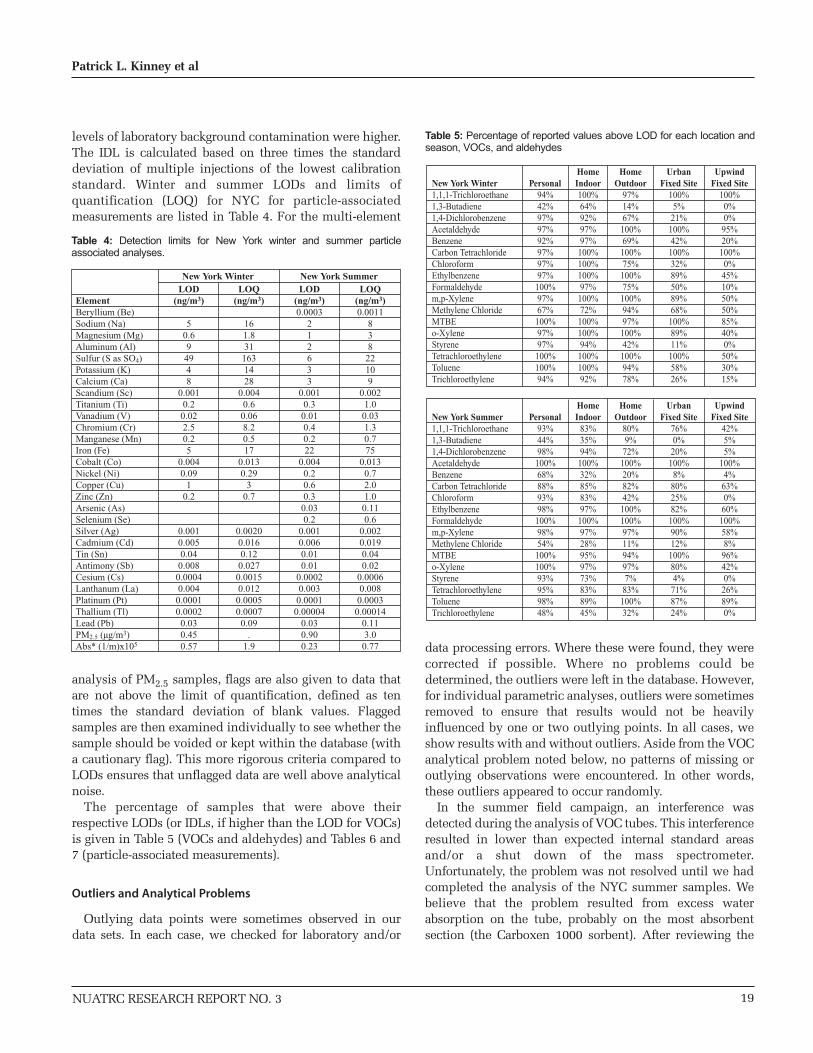
NUATRC RESEARCH REPORT NO. 3
levels of laboratory background contamination were higher.The IDL is calculated based on three times the standarddeviation of multiple injections of the lowest calibrationstandard. Winter and summer LODs and limits ofquantification (LOQ) for NYC for particle-associatedmeasurements are listed in Table 4. For the multi-element
analysis of PM2.5 samples, flags are also given to data thatare not above the limit of quantification, defined as tentimes the standard deviation of blank values. Flaggedsamples are then examined individually to see whether thesample should be voided or kept within the database (witha cautionary flag). This more rigorous criteria compared toLODs ensures that unflagged data are well above analyticalnoise.
The percentage of samples that were above theirrespective LODs (or IDLs, if higher than the LOD for VOCs)is given in Table 5 (VOCs and aldehydes) and Tables 6 and7 (particle-associated measurements).
Outliers and Analytical Problems
Outlying data points were sometimes observed in ourdata sets. In each case, we checked for laboratory and/or
data processing errors. Where these were found, they werecorrected if possible. Where no problems could bedetermined, the outliers were left in the database. However,for individual parametric analyses, outliers were sometimesremoved to ensure that results would not be heavilyinfluenced by one or two outlying points. In all cases, weshow results with and without outliers. Aside from the VOCanalytical problem noted below, no patterns of missing oroutlying observations were encountered. In other words,these outliers appeared to occur randomly.
In the summer field campaign, an interference wasdetected during the analysis of VOC tubes. This interferenceresulted in lower than expected internal standard areasand/or a shut down of the mass spectrometer.Unfortunately, the problem was not resolved until we hadcompleted the analysis of the NYC summer samples. Webelieve that the problem resulted from excess waterabsorption on the tube, probably on the most absorbentsection (the Carboxen 1000 sorbent). After reviewing the
19
Patrick L. Kinney et al
ElementBeryllium (Be)Sodium (Na)Magnesium (Mg)Aluminum (Al)Sulfur (S as SO4)Potassium (K)Calcium (Ca)Scandium (Sc)Titanium (Ti)Vanadium (V)Chromium (Cr)Manganese (Mn)Iron (Fe)Cobalt (Co)Nickel (Ni)Copper (Cu)Zinc (Zn)Arsenic (As)Selenium (Se)Silver (Ag)Cadmium (Cd)Tin (Sn)Antimony (Sb)Cesium (Cs)Lanthanum (La)Platinum (Pt)Thallium (Tl)Lead (Pb)PM2.5 (µg/m3)Abs* (1/m)x105
LOQ(ng/m3)
161.8311631428
0.0040.6
0.068.20.517
0.0130.29
30.7
0.00200.0160.120.0270.00150.0120.00050.00070.09
.1.9
LOD(ng/m3)
50.694948
0.0010.20.022.50.25
0.0040.09
10.2
0.0010.0050.040.008
0.00040.004
0.00010.00020.030.450.57
New York Winter New York SummerLOQ
(ng/m3)0.0011
838
22109
0.0021.0
0.031.30.775
0.0130.72.01.0
0.110.6
0.0020.0190.040.02
0.00060.0080.00030.00014
0.113.0
0.77
LOD(ng/m3)0.0003
212633
0.0010.30.010.40.222
0.0040.20.60.30.030.2
0.0010.0060.010.01
0.00020.0030.00010.00004
0.030.900.23
Table 4: Detection limits for New York winter and summer particleassociated analyses.
New York Winter1,1,1-Trichloroethane1,3-Butadiene1,4-DichlorobenzeneAcetaldehydeBenzeneCarbon TetrachlorideChloroformEthylbenzeneFormaldehydem,p-XyleneMethylene ChlorideMTBEo-XyleneStyreneTetrachloroethyleneTolueneTrichloroethylene
Personal94%42%97%97%92%97%97%97%100%97%67%100%97%97%100%100%94%
HomeIndoor100%64%92%97%97%
100%100%100%97%
100%72%
100%100%94%
100%100%92%
UpwindFixed Site
100%0%0%
95%20%
100%0%
45%10%50%50%85%40%0%
50%30%15%
UrbanFixed Site
100%5%
21%100%42%
100%32%89%50%89%68%
100%89%11%
100%58%26%
HomeOutdoor
97%14%67%
100%69%
100%75%
100%75%
100%94%97%
100%42%
100%94%78%
New York Summer1,1,1-Trichloroethane1,3-Butadiene1,4-DichlorobenzeneAcetaldehydeBenzeneCarbon TetrachlorideChloroformEthylbenzeneFormaldehydem,p-XyleneMethylene ChlorideMTBEo-XyleneStyreneTetrachloroethyleneTolueneTrichloroethylene
Personal93%44%98%100%68%88%93%98%100%98%54%100%100%93%95%98%48%
HomeIndoor
83%35%94%
100%32%85%83%97%
100%97%28%95%97%73%83%89%45%
UpwindFixed Site
42%5%5%
100%4%63%0%
60%100%58%8%
96%42%0%
26%89%0%
UrbanFixed Site
76%0%
20%100%
8%80%25%82%
100%90%12%
100%80%4%
71%87%24%
HomeOutdoor
80%9%
72%100%20%82%42%
100%100%97%11%94%97%7%
83%100%32%
Table 5: Percentage of reported values above LOD for each location andseason, VOCs, and aldehydes

20
Toxic Exposure Assessment: A Columbia-Harvard (TEACH) Study (The New York City Report)
NUATRC RESEARCH REPORT NO. 3
NYC winter data, a few tubes also showed the same patternof interference. This resulted in a moderate loss of data.Data loses included five upwind site data points, two urbansite days, and six outdoor home samples. In the NYCsummer session, ten upwind site days were lost, five urbansite days, nine outdoor homes, seven indoor samples, andeight personal samples were lost. Because the interferenceintroduced uncertainty in calculating concentrations, noneof these samples were included in the analyses presented inthis report.
Accuracy
Accuracy of results was tested by looking at recoveries ofstandard materials, done by different methods for thedifferent analyses. For VOCs, analytical recovery rates weredetermined by spiking tubes with known amounts ofstandards. Liquid standards in solution of a knownconcentration were injected as a known volume into a 2.0 Lstatic dilution bottle. The solvent was generally methanol.Then, a volume of vapor was drawn up with a gas-tightsyringe and injected into the injector port/spiking device,with flow onto the thermal desorption (sampling) tube.Drawing different volumes yielded different masses ofanalytes on the tube. For example:
• 10 uL of analyte solution at 2000 ug/mL into 2 L of airyields 10,000 ng/L
• 1 mL of this vapor contains 10 ng of analyte, 5 mL has50 ng, and so on
Mean analytical recoveries ranged from 73 to 149% forMTBE and benzene, respectively, with a mean recovery of95%. The high benzene recoveries were related tobackground contamination.
In addition, VOC breakthrough was tested by samplingand analysis of sorbent tubes connected in series.Breakthrough of benzene was found in a few samples andwas probably a result of background contamination on thetube. No other compounds exhibited breakthrough.
The primary indication of accuracy for the multi-elementanalyses is based on analysis of SRM 1648 (urbanparticulate matter), which was digested repeatedlythroughout the NYC winter and summer analyses. Figure 2displays the mean percent recovery and standard deviationfor the elements that have certified or recommended values,where recovery is defined as the ratio of the measuredconcentration divided by the published concentration forthe SRM. Mean recoveries for most elements are within10% of the published concentration of the SRM, and meanrecoveries for all elements covered by this SRM are within
New York WinterPM2.5 (µg/m3)Abs (1/m * 105)Silver (Ag)Aluminum (Al)Arsenic (As)Beryllium (Be)Calcium (Ca)Cadmium (Cd)Cobalt (Co)Chromium (Cr)Cesium (Cs)Copper (Cu)Iron (Fe)Potassium (K)Lanthanum (La)Magnesium (Mg)Manganese (Mn)Sodium (Na)Nickel (Ni)Lead (Pb)Platinum (Pt)Antimony (Sb)Scandium (Sc)Selenium (Se)Tin (Sn)Sulfur (S as SO4)Titanium (Ti)Thallium (Tl)Vanadium (V)Zinc (Zn)
Personal100%91%
100%100%
100%100%100%
100%100%100%100%100%100%100%100%100%100%68%
100%
100%100%100%100%100%100%
HomeIndoor100%87%100%100%
100%100%100%
100%97%100%100%100%100%100%100%100%100%100%100%97%
100%100%100%100%100%100%
UpwindFixed Site
100%25%
100%100%
74%100%100%
100%58%
100%100%100%100%100%100%100%100%68%
100%
100%100%100%100%100%100%
UrbanFixed Site
100%90%100%100%
100%100%100%
100%100%100%100%100%100%100%100%100%100%75%100%95%
100%100%100%100%100%100%
HomeOutdoor
100%100%100%100%
100%100%100%
100%100%100%100%100%100%100%100%100%100%86%100%100%
100%100%100%100%100%100%
Table 6: Percentage of reported values above LOD by location for NYwinter particulate-associated measurements
New York WinterPM2.5 (µg/m3)Abs (1/m * 105)Silver (Ag)Aluminum (Al)Arsenic (As)Beryllium (Be)Calcium (Ca)Cadmium (Cd)Cobalt (Co)Chromium (Cr)Cesium (Cs)Copper (Cu)Iron (Fe)Potassium (K)Lanthanum (La)Magnesium (Mg)Manganese (Mn)Sodium (Na)Nickel (Ni)Lead (Pb)Platinum (Pt)Antimony (Sb)Scandium (Sc)Selenium (Se)Tin (Sn)Sulfur (S as SO4)Titanium (Ti)Thallium (Tl)Vanadium (V)Zinc (Zn)
Personal100%98%
100%100%100%100%100%100%100%92%
100%100%98%
100%100%100%100%100%100%100%100%100%100%100%100%100%100%100%100%100%
HomeIndoor100%100%100%100%100%100%100%100%100%69%
100%100%97%
100%100%100%100%100%100%100%100%100%97%95%
100%100%100%100%100%100%
UpwindFixed Site
100%100%100%100%100%100%100%100%100%36%
100%96%88%
100%100%100%100%100%100%100%100%100%100%100%100%100%100%100%100%100%
UrbanFixed Site
100%100%100%100%100%100%100%100%100%40%
100%100%100%100%100%100%100%100%100%100%96%
100%100%92%
100%100%100%100%100%100%
HomeOutdoor
100%100%100%97%100%100%100%100%100%44%100%100%97%
100%100%100%100%97%100%100%100%100%88%100%100%100%100%100%100%
Table 7: Percentage of reported values above LOD by location for NYsummer particulate-associated measurements
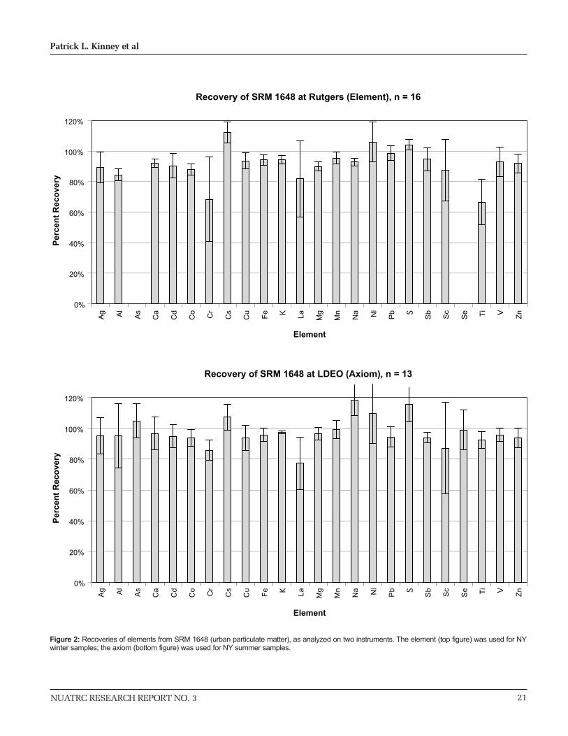
NUATRC RESEARCH REPORT NO. 3 21
Patrick L. Kinney et al
Recovery of SRM 1648 at Rutgers (Element), n = 16
0%
20%
40%
60%
80%
100%
120%
Element
Per
cen
t R
eco
very
Recovery of SRM 1648 at LDEO (Axiom), n = 13
0%
20%
40%
60%
80%
100%
120%
Ag Al
As
Ca
Cd
Co Cr
Cs
Cu
Fe K La Mg
Mn
Na Ni
Pb S
Sb
Sc
Se Ti V Z
n
Ag Al
As
Ca
Cd
Co Cr
Cs
Cu
Fe K La Mg
Mn
Na Ni
Pb S
Sb
Sc
Se Ti V Z
n
Element
Per
cen
t R
eco
very
Figure 2: Recoveries of elements from SRM 1648 (urban particulate matter), as analyzed on two instruments. The element (top figure) was used for NYwinter samples; the axiom (bottom figure) was used for NY summer samples.
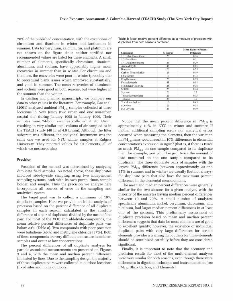
22
Toxic Exposure Assessment: A Columbia-Harvard (TEACH) Study (The New York City Report)
NUATRC RESEARCH REPORT NO. 3
20% of the published concentration, with the exceptions ofchromium and titanium in winter and lanthanum insummer. Data for beryllium, calcium, tin, and platinum arenot shown on the figure since neither certified norrecommended values are listed for these elements. A smallnumber of elements, specifically chromium, titanium,aluminum, and sodium, have appreciably higher meanrecoveries in summer than in winter. For chromium andtitanium, the recoveries were poor in winter (probably dueto procedural blank issues which improved substantially)and good in summer. The mean recoveries of aluminumand sodium were good in both seasons, but were higher inthe summer than the winter.
In existing and planned manuscripts, we compare ourdata to other values in the literature. For example, Gao et al.(2001) analyzed ambient PM2.5 samples collected at threelocations in New Jersey (two urban and one non-urbancoastal site) during January 1998 to January 1999. Theirsamples were 24-hour samples collected at 9.0 L/min,resulting in very similar total volume of air sampled as inthe TEACH study (48 hr at 4.0 L/min). Although the filtersubstrate was different, the analytical instrument was thesame one we used for NYC winter samples at RutgersUniversity. They reported values for 10 elements, all ofwhich we measured also.
Precision
Precision of the method was determined by analyzingduplicate field samples. As noted above, these duplicatesinvolved side-by-side sampling using two independentsampling systems, each with its own pump, timer, sampleholder, and sample. Thus the precision we analyze hereincorporates all sources of error in the sampling andanalytical system.
The target goal was to collect a minimum of 10%duplicate samples. Here we provide an initial analysis ofprecision based on the percent difference of all duplicatesamples in each season, calculated as the absolutedifference of a pair of duplicates divided by the mean of thepair. For most of the VOC and aldehyde compounds, themean relative percent differences of duplicate pairs wasbelow 20% (Table 8). Two compounds with poor precisionwere butadiene (46%) and methylene chloride (37%). Bothof these compounds are very difficult to measure in ambientsamples and occur at low concentrations.
The percent differences of all duplicate analyses forparticle-associated measurements are presented on Figures3 and 4, with the mean and median percent differenceindicated by lines. Due to the sampling design, the majorityof these duplicate pairs were collected at outdoor locations(fixed sites and home outdoors).
Notice that the mean percent difference in PM2.5 isapproximately 10% in NYC in winter and summer. Ifneither additional sampling errors nor analytical errorsoccurred when measuring the elements, then the variationin PM2.5 mass would result in 10% differences in elementalconcentrations expressed in ng/m3 (that is, if there is twiceas much PM2.5 on one sample compared to its duplicatethen, for example, you would expect twice the amount oflead measured on the one sample compared to itsduplicate). The three duplicate pairs of samples with thelargest PM2.5 difference (between approximately 20 and35% in summer and in winter) are usually (but not always)the duplicate pairs that also have the maximum percentdifference in the elemental measurements.
The mean and median percent differences were generallysimilar for the two seasons for a given analyte, with themajority of the analytes having median percent differencesbetween 10 and 20%. A small number of analytes,specifically aluminum, nickel, beryllium, chromium, andplatinum, had larger median percent differences in at leastone of the seasons. This preliminary assessment ofduplicate precision based on mean and median percentdifferences suggests that data for most elements are of goodto excellent quality; however, the existence of individualduplicate pairs with very large differences for certainelements provides a warning that outliers for these elementsshould be scrutinized carefully before they are consideredsignificant.
Finally, it is important to note that the accuracy andprecision results for most of the multi-element analyseswere very similar for both seasons, even though there weredifferences in digestion technique and instrumentation (seePM2.5, Black Carbon, and Elements).
Compound1,1,1-Trichloroethane1,3-Butadiene1,4-DichlorobenzeneAcetaldehydeBenzeneCarbon TetrachlorideChloroformEthylbenzeneFormaldehydeMethylene ChlorideMTBEStyreneTetrachloroethyleneTolueneTrichloroethyleneo-Xylenem,p-Xylene
N (pairs)265
264326261726432526262626162626
Mean Relative PercentDifference
0.160.510.290.050.250.190.330.190.080.360.240.2
0.150.2
0.430.180.19
Table 8: Mean relative percent difference as a measure of precision, withduplicates from both seasons combined

NUATRC RESEARCH REPORT NO. 3
Details of Multi-Element Analysis QA
Fifteen to twenty percent of digests in each digest batchwere procedural blanks (acids only). Field blanks weretreated as samples. Samples and procedural blanks fromdigestion batches were analyzed on the same day.
Aliquots of SRM 1648 (Urban Particulate Matter) similarin magnitude to the samples were weighed and digestedthroughout the course of the analyses.
Data were collected for all isotopes of interest at theappropriate RP to avoid isobaric interferences. Beryllium,silver, cadmium, tin, antimony, cesium, lanthanum,platinum, thallium, and lead, for which interferences werenot a problem, were run at RP 400; sodium, magnesium,aluminum, sulfur, calcium, scandium, titanium, vanadium,chromium, manganese, iron, cobalt, nickel, copper, andzinc were run at RP of 3000 to 4300; and potassium, arsenic,and selenium were run at RP 9300.
Indium was added to all samples, blanks, and standardsas an internal drift corrector and run in all resolving powers.Quantification was done by external and internal
standardization. On each analysis date, several sets ofmulti-element standards were analyzed in both clean acidand sample matrices. We routinely have found that indium-corrected elemental sensitivities in either matrix differed byless than 5% for all elements. The daily average sample-matrix sensitivity was used to quantify samples, and thesensitivity in clean acid was used to quantify blanks.Internal standardization was not routinely used forberyllium, sulfur, arsenic, selenium, tin, and platinum.However, spot tests have shown that sensitivities of theseelements, like the others, do not differ by more than 5%from sample to clean acid matrix.
Three multi-element standards were used for the externalcalibration. All were prepared at LDEO from primary,single-element standards acquired from Spex® or High-Purity Standards®. They were mixed to approximaterelative elemental abundances in samples. Standard 1contains aluminum, scandium, tin, vanadium, chromium,manganese, iron, cobalt, nickel, copper, zinc, silver,cadmium, tin, antimony, cesium, lanthanum, thallium, andlead. Standard 2 contains sodium, magnesium, potassium,
23
Patrick L. Kinney et al
NY winter duplicates, percent difference,elements as ng/m3
0
0.2
0.4
0.6
0.8
1
abs* 101% Ni 190%,112%
Cu 141%Cd 145%
Cs 111%
Pt 134%
Tl 115%, 101%
Mean
Median
PM
2.5
(µg
/m3 )
Ab
s* Be
Na
Mg Al S K C
a
Sc Ti V Cr
Mn Fe
Co Ni
Cu
Zn
Se
As
Ag
Cd
Sn
Sb
Cs
La Pt Tl
Pb
Figure 3: Percent differences of duplicate samples for NY winter samples. Elemental data are expressed as ng/m3. For PM2.5 and Abs*,n =16; for Na, n = 10; for Mg, n = 13; for Al and Sc, n = 8; for all others, n = 15. Outlier duplicates which do not fit on the scale are indicated by arrows andnumeric value. Lines show mean & median.
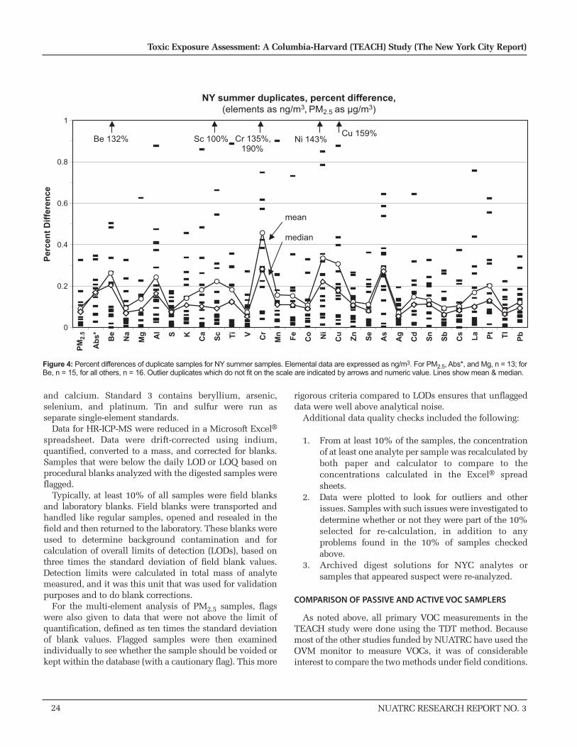
24
Toxic Exposure Assessment: A Columbia-Harvard (TEACH) Study (The New York City Report)
NUATRC RESEARCH REPORT NO. 3
and calcium. Standard 3 contains beryllium, arsenic,selenium, and platinum. Tin and sulfur were run asseparate single-element standards.
Data for HR-ICP-MS were reduced in a Microsoft Excel®
spreadsheet. Data were drift-corrected using indium,quantified, converted to a mass, and corrected for blanks.Samples that were below the daily LOD or LOQ based onprocedural blanks analyzed with the digested samples wereflagged.
Typically, at least 10% of all samples were field blanksand laboratory blanks. Field blanks were transported andhandled like regular samples, opened and resealed in thefield and then returned to the laboratory. These blanks wereused to determine background contamination and forcalculation of overall limits of detection (LODs), based onthree times the standard deviation of field blank values.Detection limits were calculated in total mass of analytemeasured, and it was this unit that was used for validationpurposes and to do blank corrections.
For the multi-element analysis of PM2.5 samples, flagswere also given to data that were not above the limit ofquantification, defined as ten times the standard deviationof blank values. Flagged samples were then examinedindividually to see whether the sample should be voided orkept within the database (with a cautionary flag). This more
rigorous criteria compared to LODs ensures that unflaggeddata were well above analytical noise.
Additional data quality checks included the following:
1. From at least 10% of the samples, the concentrationof at least one analyte per sample was recalculated byboth paper and calculator to compare to theconcentrations calculated in the Excel® spreadsheets.
2. Data were plotted to look for outliers and otherissues. Samples with such issues were investigated todetermine whether or not they were part of the 10%selected for re-calculation, in addition to anyproblems found in the 10% of samples checkedabove.
3. Archived digest solutions for NYC analytes orsamples that appeared suspect were re-analyzed.
COMPARISON OF PASSIVE AND ACTIVE VOC SAMPLERS
As noted above, all primary VOC measurements in theTEACH study were done using the TDT method. Becausemost of the other studies funded by NUATRC have used theOVM monitor to measure VOCs, it was of considerableinterest to compare the two methods under field conditions.
mean
median
Be 132% Sc 100% Cr 135%,190%
Ni 143%Cu 159%
NY summer duplicates, percent difference,(elements as ng/m3, PM2.5 as µg/m3)
Per
cen
t D
iffe
ren
ce
PM
2.5
Ab
s* Be
Na
Mg Al S K C
a
Sc Ti V Cr
Mn Fe
Co Ni
Cu
Zn
Se
As
Ag
Cd
Sn
Sb
Cs
La Pt Tl
Pb
0
0.2
0.4
0.6
0.8
1
Figure 4: Percent differences of duplicate samples for NY summer samples. Elemental data are expressed as ng/m3. For PM2.5, Abs*, and Mg, n = 13; forBe, n = 15, for all others, n = 16. Outlier duplicates which do not fit on the scale are indicated by arrows and numeric value. Lines show mean & median.
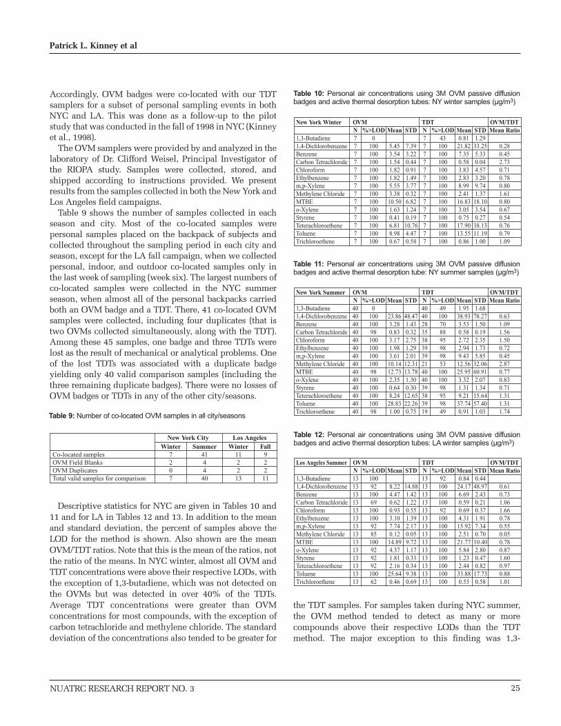
NUATRC RESEARCH REPORT NO. 3
Accordingly, OVM badges were co-located with our TDTsamplers for a subset of personal sampling events in bothNYC and LA. This was done as a follow-up to the pilotstudy that was conducted in the fall of 1998 in NYC (Kinneyet al., 1998).
The OVM samplers were provided by and analyzed in thelaboratory of Dr. Clifford Weisel, Principal Investigator ofthe RIOPA study. Samples were collected, stored, andshipped according to instructions provided. We presentresults from the samples collected in both the New York andLos Angeles field campaigns.
Table 9 shows the number of samples collected in eachseason and city. Most of the co-located samples werepersonal samples placed on the backpack of subjects andcollected throughout the sampling period in each city andseason, except for the LA fall campaign, when we collectedpersonal, indoor, and outdoor co-located samples only inthe last week of sampling (week six). The largest numbers ofco-located samples were collected in the NYC summerseason, when almost all of the personal backpacks carriedboth an OVM badge and a TDT. There, 41 co-located OVMsamples were collected, including four duplicates (that istwo OVMs collected simultaneously, along with the TDT).Among these 45 samples, one badge and three TDTs werelost as the result of mechanical or analytical problems. Oneof the lost TDTs was associated with a duplicate badgeyielding only 40 valid comparison samples (including thethree remaining duplicate badges). There were no losses ofOVM badges or TDTs in any of the other city/seasons.
Descriptive statistics for NYC are given in Tables 10 and11 and for LA in Tables 12 and 13. In addition to the meanand standard deviation, the percent of samples above theLOD for the method is shown. Also shown are the meanOVM/TDT ratios. Note that this is the mean of the ratios, notthe ratio of the means. In NYC winter, almost all OVM andTDT concentrations were above their respective LODs, withthe exception of 1,3-butadiene, which was not detected onthe OVMs but was detected in over 40% of the TDTs.Average TDT concentrations were greater than OVMconcentrations for most compounds, with the exception ofcarbon tetrachloride and methylene chloride. The standarddeviation of the concentrations also tended to be greater for
the TDT samples. For samples taken during NYC summer,the OVM method tended to detect as many or morecompounds above their respective LODs than the TDTmethod. The major exception to this finding was 1,3-
25
Patrick L. Kinney et al
Co-located samplesOVM Field BlanksOVM DuplicatesTotal valid samples for comparison
Summer4144
40
Winter7207
New York City Los AngelesFall
92211
Winter1122
13
Table 9: Number of co-located OVM samples in all city/seasons
New York Winter
1,3-Butadiene1,4-DichlorobenzeneBenzeneCarbon TetrachlorideChloroformEthylbenzenem,p-XyleneMethylene ChlorideMTBEo-XyleneStyreneTeterachloroetheneTolueneTrichloroethene
N77777777777777
%>LOD0
100100100100100100100100100100100100100
Mean
5.453.541.541.821.825.553.38
10.501.630.416.818.980.67
STD
7.393.220.440.911.493.770.326.821.240.1910.764.470.58
OVM/TDTMean Ratio
0.280.452.730.710.780.801.610.800.670.540.760.791.09
OVMN77777777777777
%>LOD43
100100100100100100100100100100100100100
Mean0.8121.827.350.583.832.838.992.4116.833.050.7517.9013.550.86
STD1.2933.255.330.044.573.209.741.3718.103.540.2738.1311.191.00
TDT
Table 10: Personal air concentrations using 3M OVM passive diffusionbadges and active thermal desorption tubes: NY winter samples (µg/m3)
New York Summer
1,3-Butadiene1,4-DichlorobenzeneBenzeneCarbon TetrachlorideChloroformEthylbenzenem,p-XyleneMethylene ChlorideMTBEo-XyleneStyreneTeterachloroetheneTolueneTrichloroethene
N4040404040404040404040404040
%>LOD0
10010098
10010010010098
10010010010098
Mean
23.863.280.833.171.983.61
10.1412.732.350.648.24
28.831.00
STD
48.471.430.322.751.292.0112.3113.781.300.3012.6522.260.75
OVM/TDTMean Ratio
0.631.091.561.500.720.452.870.770.830.711.311.311.74
OVMN4040283538393921404039383919
%>LOD49
100708895989853
10010098959849
Mean1.9538.933.530.582.722.949.4312.5625.953.321.319.2137.740.91
STD1.6878.271.500.192.351.735.8532.0660.912.071.3415.6457.401.03
TDT
Table 11: Personal air concentrations using 3M OVM passive diffusionbadges and active thermal desorption tube: NY summer samples (µg/m3)
Los Angeles Summer
1,3-Butadiene1,4-DichlorobenzeneBenzeneCarbon TetrachlorideChloroformEthylbenzenem,p-XyleneMethylene ChlorideMTBEo-XyleneStyreneTeterachloroetheneTolueneTrichloroethene
N1313131313131313131313131313
%>LOD10092
10069
1001009285
100929292
10062
Mean
8.224.470.620.933.107.740.12
14.894.371.812.16
25.640.46
STD
14.881.421.220.551.392.170.059.721.170.330.349.380.69
OVM/TDTMean Ratio
0.610.731.061.660.780.550.050.780.871.600.970.881.01
OVMN1313131313131313131313131313
%>LOD92
10010010092
100100100100100100100100100
Mean0.8424.176.690.590.694.3115.922.5121.775.841.232.4433.880.53
STD0.4448.972.430.210.371.917.340.7010.402.800.470.8217.730.58
TDT
Table 12: Personal air concentrations using 3M OVM passive diffusionbadges and active thermal desorption tubes: LA winter samples (µg/m3)
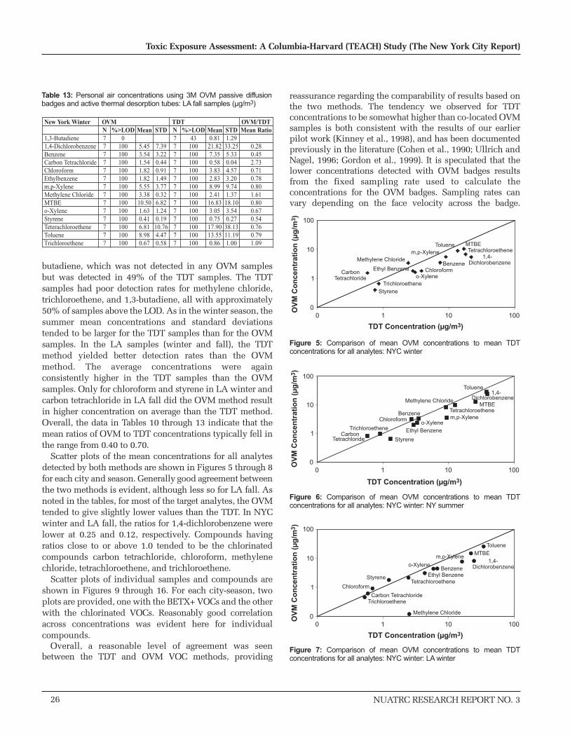
butadiene, which was not detected in any OVM samplesbut was detected in 49% of the TDT samples. The TDTsamples had poor detection rates for methylene chloride,trichloroethene, and 1,3-butadiene, all with approximately50% of samples above the LOD. As in the winter season, thesummer mean concentrations and standard deviationstended to be larger for the TDT samples than for the OVMsamples. In the LA samples (winter and fall), the TDTmethod yielded better detection rates than the OVMmethod. The average concentrations were againconsistently higher in the TDT samples than the OVMsamples. Only for chloroform and styrene in LA winter andcarbon tetrachloride in LA fall did the OVM method resultin higher concentration on average than the TDT method.Overall, the data in Tables 10 through 13 indicate that themean ratios of OVM to TDT concentrations typically fell inthe range from 0.40 to 0.70.
Scatter plots of the mean concentrations for all analytesdetected by both methods are shown in Figures 5 through 8for each city and season. Generally good agreement betweenthe two methods is evident, although less so for LA fall. Asnoted in the tables, for most of the target analytes, the OVMtended to give slightly lower values than the TDT. In NYCwinter and LA fall, the ratios for 1,4-dichlorobenzene werelower at 0.25 and 0.12, respectively. Compounds havingratios close to or above 1.0 tended to be the chlorinatedcompounds carbon tetrachloride, chloroform, methylenechloride, tetrachloroethene, and trichloroethene.
Scatter plots of individual samples and compounds areshown in Figures 9 through 16. For each city-season, twoplots are provided, one with the BETX+ VOCs and the otherwith the chlorinated VOCs. Reasonably good correlationacross concentrations was evident here for individualcompounds.
Overall, a reasonable level of agreement was seenbetween the TDT and OVM VOC methods, providing
reassurance regarding the comparability of results based onthe two methods. The tendency we observed for TDTconcentrations to be somewhat higher than co-located OVMsamples is both consistent with the results of our earlierpilot work (Kinney et al., 1998), and has been documentedpreviously in the literature (Cohen et al., 1990; Ullrich andNagel, 1996; Gordon et al., 1999). It is speculated that thelower concentrations detected with OVM badges resultsfrom the fixed sampling rate used to calculate theconcentrations for the OVM badges. Sampling rates canvary depending on the face velocity across the badge.
26
Toxic Exposure Assessment: A Columbia-Harvard (TEACH) Study (The New York City Report)
NUATRC RESEARCH REPORT NO. 3
New York Winter
1,3-Butadiene1,4-DichlorobenzeneBenzeneCarbon TetrachlorideChloroformEthylbenzenem,p-XyleneMethylene ChlorideMTBEo-XyleneStyreneTeterachloroetheneTolueneTrichloroethene
N77777777777777
%>LOD0
100100100100100100100100100100100100100
Mean
5.453.541.541.821.825.553.3810.501.630.416.818.980.67
STD
7.393.220.440.911.493.770.326.821.240.1910.764.470.58
OVM/TDTMean Ratio
0.280.452.730.710.780.801.610.800.670.540.760.791.09
OVMN77777777777777
%>LOD43100100100100100100100100100100100100100
Mean0.8121.827.350.583.832.838.992.4116.833.050.7517.9013.550.86
STD1.2933.255.330.044.573.209.741.3718.103.540.2738.1311.191.00
TDT
Table 13: Personal air concentrations using 3M OVM passive diffusionbadges and active thermal desorption tubes: LA fall samples (µg/m3)
Ethyl Benzeneo-Xylene
Chloroform
TolueneTetrachloroethene
Benzene1,4-
Dichlorobenzene
MTBE
m,p-XyleneMethylene Chloride
Carbon Tetrachloride
TrichloroetheneStyrene
0
1
10
100
0 1 10 100
OV
M C
on
cen
trat
ion
(µ
g/m
3 )
TDT Concentration (µg/m3)
Figure 5: Comparison of mean OVM concentrations to mean TDTconcentrations for all analytes: NYC winter
0
1
10
100
0 1 10 100
OV
M C
on
cen
trat
ion
(µ
g/m
3 )
TDT Concentration (µg/m3)
ChloroformBenzene
Ethyl Benzeneo-Xylene
Methylene Chloride
1,4-Dichlorobenzene
Toluene
MTBETetrachloroethenem,p-Xylene
TrichloroetheneCarbon
Tetrachloride Styrene
Figure 6: Comparison of mean OVM concentrations to mean TDTconcentrations for all analytes: NYC winter: NY summer
0
1
10
100
0 1 10 100
OV
M C
on
cen
trat
ion
(µ
g/m
3 )
TDT Concentration (µg/m3)
Benzeneo-Xylene
m,p-Xylene1,4-
Dichlorobenzene
MTBE
Toluene
Ethyl BenzeneTetrachloroethene
Styrene
Chloroform
Carbon TetrachlorideTrichloroethene
Methylene Chloride
Figure 7: Comparison of mean OVM concentrations to mean TDTconcentrations for all analytes: NYC winter: LA winter

NUATRC RESEARCH REPORT NO. 3
Changes in temperature and humidity can also affect thesampling efficiency of the OVM badges (Morandi et al.,1998; Chung et al., 1999). The OVM sampling rate for eachcompound is a function of its diffusion coefficient, and thediffusion coefficient is directly proportional to temperature.Thus, higher OVM sampling rates would be expected insummer than in winter, especially for outdoor samples, butpossibly also for personal samples. We did observe atendency for the OVM results to agree better with TDTresults in summer. In addition, some compounds, such asthe chlorinated compounds, have been shown to have poorrecoveries on the OVM badges (Shields et al., 1996;Morandi et al., 1998). Consideration should be given toderiving updated sampling rates for passive collection ofcertain VOCs.
27
Patrick L. Kinney et al
0
1
10
100
0 1 10 100
OV
M C
on
cen
trat
ion
(µ
g/m
3 )
TDT Concentration (µg/m3)
o-Xylene
Tetrachloroethene
Methylene Chloride
Benzene
Ethyl Benzene
Carbon Tetrachloride
Chloroform
Styrenem,p-Xylene MTBE1,4-
Dichlorobenzene
Figure 8: Comparison of mean OVM concentrations to mean TDTconcentrations for all analytes: NYC winter: LA fall
0
1
10
100
0 1 10 100
OV
M C
on
cen
trat
ion
(µ
g/m
3 )
TDT Concentration (µg/m3)
Benzene
Toluene
Ethyl Benzene
m,p-Xylene
o-Xylene
MTBE
1:1 Line
Figure 9: Comparison of OVM and TDT concentrations for the BTEX+compounds: NYC winter
0
1
10
100
0 1 10 100
OV
M C
on
cen
trat
ion
(µ
g/m
3 )
TDT Concentration (µg/m3)
Tetrachloroethene
Carbon Tetrachloride
1,4-Dicholorbenzene
Chloroform
1:1 Line
Figure 10: Comparison of OVM and TDT concentrations for thechlorinated VOCs: NYC winter
0
1
10
100
0 1 10 100
OV
M C
on
cen
trat
ion
(µ
g/m
3 )
TDT Concentration (µg/m3)
Benzene
Toluene
Ethyl Benzene
m,p-Xylene
o-Xylene
MTBE
1:1 Line
Figure 11: Comparison of OVM and TDT concentrations for the BTEX+compounds: NYC summer
0
1
10
100
0 1 10 100
OV
M C
on
cen
trat
ion
(µ
g/m
3 )
TDT Concentration (µg/m3)
Tetrachloroethene
Carbon Tetrachloride
1,4-Dicholorbenzene
Chloroform
1:1 Line
Figure 12: Comparison of OVM and TDT concentrations for thechlorinated VOCs: NYC summer

RESULTS AND DISCUSSION
SUBJECT CHARACTERISTICS
Demographics
A total of 46 self-reported non-smoking and non-ETSexposed students were enrolled in the NYC TEACH project,including 33 who completed both winter and summerphases. Five students in winter and eight students insummer participated in only one season. Subjects rangedfrom 14 to 19 years of age; 31 (67%) were female, and 15were (33%) male. The racial distribution was 43% black,50% Hispanic, and the remaining 7% either Asian or notreported. These and other characteristics were similar to alarger group of 611 students surveyed at the same school(Table 14), showing that the sample group wasrepresentative of the overall student body.
Housing Factors
Figure 1 shows a map of the study area, with symbolsindicating the locations of the school and of subject homes.The majority of the students lived in the boroughs of upperManhattan (63% in winter and 46% in summer) and Bronx(24% in winter and 27% in summer) boroughs of NYC.Only a few lived in Brooklyn (8 and 10% for winter andsummer, respectively) or Queens (5 and 17% for winter andsummer, respectively).
Figure 17 shows the distribution of types of homes in thestudy group. Most students lived in apartment buildings(81%). The large majority of the study population lived inrented homes (81%), leaving only 19% that lived in owner-
28
Toxic Exposure Assessment: A Columbia-Harvard (TEACH) Study (The New York City Report)
NUATRC RESEARCH REPORT NO. 3
0
1
10
100
0 1 10 100
OV
M C
on
cen
trat
ion
(µg
/m3 )
TDT Concentration (µg/m3)
Benzene
Toluene
Ethyl Benzene
m,p-Xylene
o-Xylene
MTBE
1:1 Line
Figure 13: Comparison of OVM and TDT concentrations for the BTEX+compounds: LA winter
0
1
10
100
0 1 10 100
OV
M C
on
cen
trat
ion
(µg
/m3 )
TDT Concentration (µg/m3)
Tetrachloroethene
Carbon Tetrachloride
1,4-Dicholorbenzene
Chloroform
1:1 Line
Figure 14: Comparison of OVM and TDT concentrations for thechlorinated VOCs: LA winter
0
1
10
100
0 1 10 100
OV
M C
on
cen
trat
ion
(µg
/m3 )
TDT Concentration (µg/m3)
Benzene
Toluene
Ethyl Benzene
m,p-Xylene
o-Xylene
MTBE
1:1 Line
Figure 15: Comparison of OVM and TDT concentrations for the BTEX+compounds: LA fall
0
1
10
100
0 1 10 100
OV
M C
on
cen
trat
ion
(µg
/m3 )
TDT Concentration (µg/m3)
Tetrachloroethene
Carbon Tetrachloride
1,4-Dicholorbenzene
Chloroform
1:1 Line
Figure 16: Comparison of OVM and TDT concentrations for thechlorinated VOCs: LA fall

NUATRC RESEARCH REPORT NO. 3
occupied homes. In NYC residential areas, many homes aresituated in five-story apartment buildings, consistent withthe subject data showing 63% of the homes in apartmentbuildings with four to six floors. Twenty-three percent ofsubject homes were in structures of three floors or less. Only6% of homes were in apartment buildings with more thansix floors. This distribution of structures is reflected in thedistribution of floor levels, with most subjects living on thesecond floor, and a fairly even distribution of the remainingsubjects living on first, third, or higher-than-third floorlevels (Figure 18). One apartment was on the 16th floor of a
building, and another was on the 26th floor. The homesranged in size from 450 to 1800 square feet, with a mean of775 square feet.
Information on the average weekday car volume andheavy truck volume was collected in the home environmentquestionnaires. The levels include high (many passing by allthe time), medium (many passing by, but not all the time),light (an occasional vehicle passing by), and never. Figures19 and 20 show the distributions of car traffic volume andheavy truck/bus volume, respectively. More than half of thehomes were reported to be located in a high car volumestreet, and 40% had heavy truck or bus traffic in front of theirhomes.
The home environment questionnaire was also used to
identify sources and sinks of indoor air pollutants. Table 15lists some of the home characteristics that are potentialsources and sinks of indoor air pollutants and the numberand percent of homes in the study with thesecharacteristics. Even though we tried to exclude smokinghomes in the study (as reported by the students in the initialsurvey), smokers were present in two homes (less than tencigarettes per day). This was later identified by examinationof questionnaire data. A few homes had attached garages(19%), and half of these had a door leading to the garagefrom the home. In 65% of the homes, air fresheners werecommonly used. About half the homes had suchrenovations as wall painting in the year before sampling.The most common fuel used for heating the homes was fueloil (63%), and most homes had central heating (72%). Themajority of the homes (91%) used gas for cooking, and fewhomes had a kitchen fan with a vent (14%). This strikinglyhigh percentage of homes using gas without venting will bea major source of NO, NO2, and possibly ultrafine particles,
29
Patrick L. Kinney et al
MaleFemaleNot answeredBlackAmerican IndianWhiteAsianOthersDon’t knowNot answeredYesNoDon’t knowNot answeredDid not graduate fromhigh schoolHigh school graduateTechnical trade schoolSome collegeCollege graduateGraduate ProfessionalDon’t knowNot answeredYesNoNot answeredYesNoNot answeredYesNoDon’t knowNot answeredMinimumMaximumMeanStd. dev.
Survey Pop.n=61142.2%57.8%0.7%
45.9%-
1.3%1.6%
47.6%2.5%1.3%
47.5%46.9%2.1%3.4%
11.5%21.0%3.0%
11.6%16.9%6.2%
29.6%0.3%
44.9%54.3%1.0%
18.7%80.4%1.0%
18.2%77.6%2.6%1.6%12.519.616.11.2
Study Pop.n=4632.6%67.4%
-43.5%
--
2.2%50.0%4.4%
-50.0%43.5%2.5%4.4%
13.0%15.2%6.5%
17.7%19.6%8.7%
19.6%-
65.2%34.8%
-19.6%80.4%
-6.5%
91.3%2.2%
-14.118.716.80.9
New York City
Sex
Race
Of SpanishOrigin
Fathereducationlevel
Have anafter schoolactivityHave a job
Haveasthma
Age
Table 14: Characteristics of study populations and survey populations inNew York City, self reported
14%
5%
12%
5%
2%
63%Apt. Bldg. >6 Floors
Apt. Bldg. 4-6 Floors
Apt. Bldg. 2-3 Floors
2-3 Family Hse
1 Family Hse, Attached
Other
Figure 17: Distribution of housing type (43 completed questions out of totalof 46 subjects from NYC)

depending on the burner and type of cooking performed. Itis important to note that study staff administered the homeenvironment questionnaire in the home, allowing visualverification of many of the answers.
Time-Activity Patterns
The time-activity-location patterns reported by eachstudent during the two-day personal sampling are shown inFigures 21 and 22, which summarize the percentage of timespent in each of six microenvironments for winter andsummer, respectively. Total hours in the time-activity diarywere not constrained to add up to 24 each day. In fact, onaverage, students accounted for 26.8 hours/day in summerand 26.1 hours/day in winter. Thus, to compute percentagesof time spent in specific microenvironments, these numbersare used as denominators. Most of the students’ time wasspent indoors at home (17.1 hours/day in the winter and19.7 hours/day in the summer). In the winter, the studentsspent on average 6.3 hours/day at school. In the summer,this time was spent either at home or in other indoorenvironments. The average time spent in subways or trainswas slightly higher in the winter than in the summer,probably because of commuting to school. The average timespent outdoors was 40% higher (1.4 hours/day) in thesummer than in the winter (1.0 hour/day), and the summerhad a higher standard deviation for outdoor time.
Time-activity patterns for the TEACH participants werecompared with the National Human Activity PatternsSurvey (NHAPS) (Klepeis et al., 2001) for EPA Region 2,which corresponds to New York and New Jersey. TheNHAPS results showed that 16 hours/day were spentindoors in a residence, 2.6 hours/day were spent indoorselsewhere, 1.4 hours/day were spent in a car, and 1.7hours/day were spent outdoors. A comparison betweenNHAPS and TEACH is made in Table 16. The TEACHtime/location patterns were very consistent with NHAPS,except for the amount of time spent in a car. The muchshorter time spent in cars by the TEACH group is notsurprising given the age group and urban location. TheNHAPS time spent in cars (1.4 hours/day) was very similarto the TEACH average time spent in subways andcars/buses/motorcycles (1.4 hours/day in winter, 1.1hours/day in summer).
AIR MONITORING RESULTS
Introduction
Table 17 summarizes data captured for NYC TEACH. TheTEACH study achieved the study design goal of monitoringat least 30 inner city teenagers over two seasons. Over-sampling in NYC winter yielded 33 students completingboth periods. However, problems with pumps, compliance,and laboratory analyses reduced the size of the combineddata set somewhat. The final yield for complete indoor,
30
Toxic Exposure Assessment: A Columbia-Harvard (TEACH) Study (The New York City Report)
NUATRC RESEARCH REPORT NO. 3
19%
21%
24%
36%
1st Floor
2nd Floor
3rd Floor
>3rd Floor
Figure 18: Floor level of subjects’ homes (42 completed questions out oftotal of 46 subjects from NYC)
High
Medium
Light
Missing
55%
24%
16%
5%
Figure 19: Self-reported car traffic in front of each subject’s home
High
Medium
Light
Never
Missing
40%
34%
18%
5% 3%
Figure 20: Self-reported heavy truck/bus traffic in front of each subject’shome
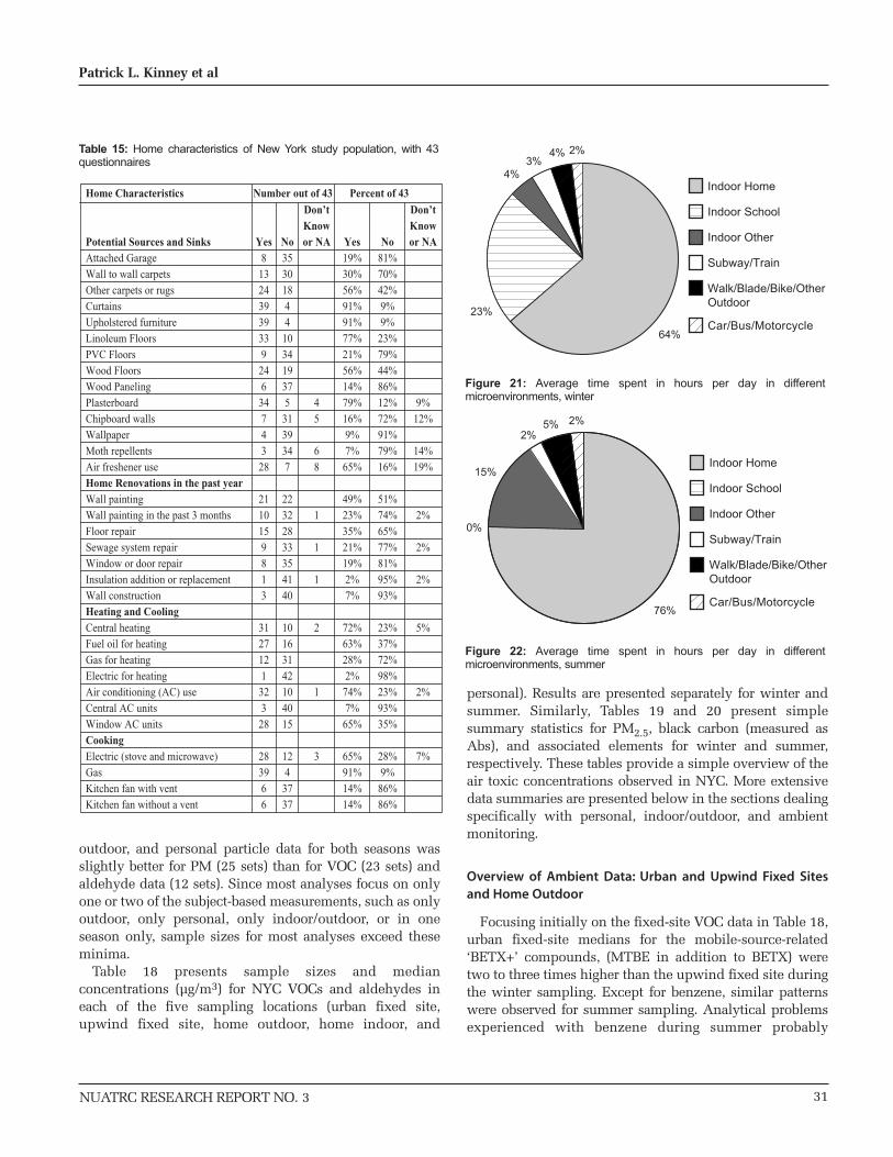
NUATRC RESEARCH REPORT NO. 3
outdoor, and personal particle data for both seasons wasslightly better for PM (25 sets) than for VOC (23 sets) andaldehyde data (12 sets). Since most analyses focus on onlyone or two of the subject-based measurements, such as onlyoutdoor, only personal, only indoor/outdoor, or in oneseason only, sample sizes for most analyses exceed theseminima.
Table 18 presents sample sizes and medianconcentrations (µg/m3) for NYC VOCs and aldehydes ineach of the five sampling locations (urban fixed site,upwind fixed site, home outdoor, home indoor, and
personal). Results are presented separately for winter andsummer. Similarly, Tables 19 and 20 present simplesummary statistics for PM2.5, black carbon (measured asAbs), and associated elements for winter and summer,respectively. These tables provide a simple overview of theair toxic concentrations observed in NYC. More extensivedata summaries are presented below in the sections dealingspecifically with personal, indoor/outdoor, and ambientmonitoring.
Overview of Ambient Data: Urban and Upwind Fixed Sitesand Home Outdoor
Focusing initially on the fixed-site VOC data in Table 18,urban fixed-site medians for the mobile-source-related‘BETX+’ compounds, (MTBE in addition to BETX) weretwo to three times higher than the upwind fixed site duringthe winter sampling. Except for benzene, similar patternswere observed for summer sampling. Analytical problemsexperienced with benzene during summer probably
31
Patrick L. Kinney et al
Don’tKnowor NA
9%12%
14%19%
2%
2%
2%
5%
2%
7%
No81%70%42%9%9%
23%79%44%86%12%72%91%79%16%
51%74%65%77%81%95%93%
23%37%72%98%23%93%35%
28%9%
86%86%
Yes19%30%56%91%91%77%21%56%14%79%16%9%7%
65%
49%23%35%21%19%2%7%
72%63%28%2%
74%7%
65%
65%91%14%14%
Don’tKnowor NA
45
68
1
1
1
2
1
3
No35301844
103419375
3139347
22322833354140
10163142104015
124
3737
Yes8
13243939339
246
34743
28
2110159813
3127121
323
28
283966
Potential Sources and SinksAttached GarageWall to wall carpetsOther carpets or rugsCurtainsUpholstered furnitureLinoleum FloorsPVC FloorsWood FloorsWood PanelingPlasterboardChipboard wallsWallpaperMoth repellentsAir freshener useHome Renovations in the past yearWall paintingWall painting in the past 3 monthsFloor repairSewage system repairWindow or door repairInsulation addition or replacementWall constructionHeating and CoolingCentral heatingFuel oil for heatingGas for heatingElectric for heatingAir conditioning (AC) useCentral AC unitsWindow AC unitsCookingElectric (stove and microwave)GasKitchen fan with ventKitchen fan without a vent
Home Characteristics Percent of 43Number out of 43
Table 15: Home characteristics of New York study population, with 43questionnaires
Indoor Home
Indoor School
Indoor Other
Subway/Train
Walk/Blade/Bike/OtherOutdoor
Car/Bus/Motorcycle64%
23%
4%
4%3%
2%
Figure 21: Average time spent in hours per day in differentmicroenvironments, winter
Indoor Home
Indoor School
Indoor Other
Subway/Train
Walk/Blade/Bike/OtherOutdoor
Car/Bus/Motorcycle76%
0%
15%
2%5% 2%
Figure 22: Average time spent in hours per day in differentmicroenvironments, summer
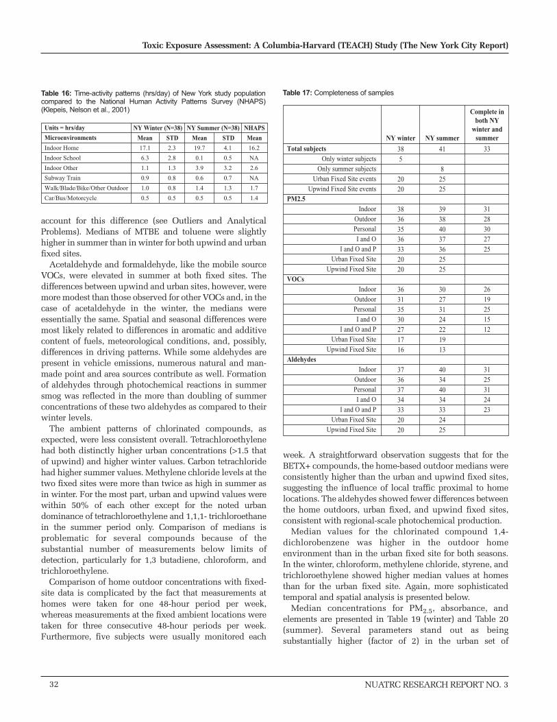
account for this difference (see Outliers and AnalyticalProblems). Medians of MTBE and toluene were slightlyhigher in summer than in winter for both upwind and urbanfixed sites.
Acetaldehyde and formaldehyde, like the mobile sourceVOCs, were elevated in summer at both fixed sites. Thedifferences between upwind and urban sites, however, weremore modest than those observed for other VOCs and, in thecase of acetaldehyde in the winter, the medians wereessentially the same. Spatial and seasonal differences weremost likely related to differences in aromatic and additivecontent of fuels, meteorological conditions, and, possibly,differences in driving patterns. While some aldehydes arepresent in vehicle emissions, numerous natural and man-made point and area sources contribute as well. Formationof aldehydes through photochemical reactions in summersmog was reflected in the more than doubling of summerconcentrations of these two aldehydes as compared to theirwinter levels.
The ambient patterns of chlorinated compounds, asexpected, were less consistent overall. Tetrachloroethylenehad both distinctly higher urban concentrations (>1.5 thatof upwind) and higher winter values. Carbon tetrachloridehad higher summer values. Methylene chloride levels at thetwo fixed sites were more than twice as high in summer asin winter. For the most part, urban and upwind values werewithin 50% of each other except for the noted urbandominance of tetrachloroethylene and 1,1,1- trichloroethanein the summer period only. Comparison of medians isproblematic for several compounds because of thesubstantial number of measurements below limits ofdetection, particularly for 1,3 butadiene, chloroform, andtrichloroethylene.
Comparison of home outdoor concentrations with fixed-site data is complicated by the fact that measurements athomes were taken for one 48-hour period per week,whereas measurements at the fixed ambient locations weretaken for three consecutive 48-hour periods per week.Furthermore, five subjects were usually monitored each
week. A straightforward observation suggests that for theBETX+ compounds, the home-based outdoor medians wereconsistently higher than the urban and upwind fixed sites,suggesting the influence of local traffic proximal to homelocations. The aldehydes showed fewer differences betweenthe home outdoors, urban fixed, and upwind fixed sites,consistent with regional-scale photochemical production.
Median values for the chlorinated compound 1,4-dichlorobenzene was higher in the outdoor homeenvironment than in the urban fixed site for both seasons.In the winter, chloroform, methylene chloride, styrene, andtrichloroethylene showed higher median values at homesthan for the urban fixed site. Again, more sophisticatedtemporal and spatial analysis is presented below.
Median concentrations for PM2.5, absorbance, andelements are presented in Table 19 (winter) and Table 20(summer). Several parameters stand out as beingsubstantially higher (factor of 2) in the urban set of
32
Toxic Exposure Assessment: A Columbia-Harvard (TEACH) Study (The New York City Report)
NUATRC RESEARCH REPORT NO. 3
Table 16: Time-activity patterns (hrs/day) of New York study populationcompared to the National Human Activity Patterns Survey (NHAPS)(Klepeis, Nelson et al., 2001)
Units = hrs/day
Microenvironments
Indoor Home
Indoor School
Indoor Other
Subway Train
Walk/Blade/Bike/Other Outdoor
Car/Bus/Motorcycle
NY Winter (N=38)
Mean STD
NY Summer (N=38)
Mean STD
NHAPS
Mean
17.1
6.3
1.1
0.9
1.0
0.5
2.3
2.8
1.3
0.8
0.8
0.5
19.7
0.1
3.9
0.6
1.4
0.5
4.1
0.5
3.2
0.7
1.3
0.5
16.2
NA
2.6
NA
1.7
1.4
Table 17: Completeness of samples
Complete inboth NY
winter andsummer
33
3128302725
2619251512
3125312423
NY winter
385
2020
38363536332020
36313530271716
37363734332020
NY summer
41
82525
39384037362525
30273124221913
40344034332425
Total subjectsOnly winter subjects
Only summer subjectsUrban Fixed Site events
Upwind Fixed Site eventsPM2.5
IndoorOutdoorPersonalI and O
I and O and PUrban Fixed Site
Upwind Fixed SiteVOCs
IndoorOutdoorPersonalI and O
I and O and PUrban Fixed Site
Upwind Fixed SiteAldehydes
IndoorOutdoorPersonalI and O
I and O and PUrban Fixed Site
Upwind Fixed Site
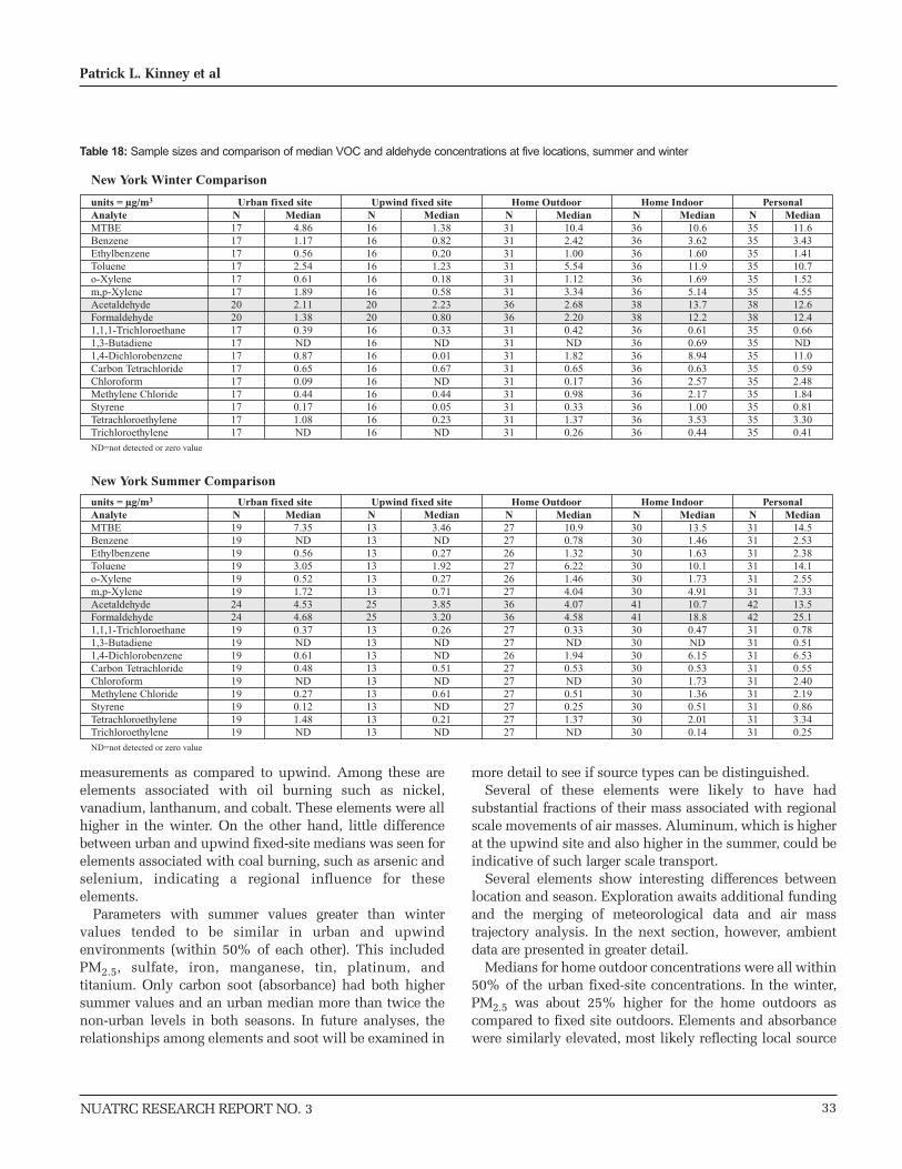
NUATRC RESEARCH REPORT NO. 3
measurements as compared to upwind. Among these areelements associated with oil burning such as nickel,vanadium, lanthanum, and cobalt. These elements were allhigher in the winter. On the other hand, little differencebetween urban and upwind fixed-site medians was seen forelements associated with coal burning, such as arsenic andselenium, indicating a regional influence for theseelements.
Parameters with summer values greater than wintervalues tended to be similar in urban and upwindenvironments (within 50% of each other). This includedPM2.5, sulfate, iron, manganese, tin, platinum, andtitanium. Only carbon soot (absorbance) had both highersummer values and an urban median more than twice thenon-urban levels in both seasons. In future analyses, therelationships among elements and soot will be examined in
more detail to see if source types can be distinguished.Several of these elements were likely to have had
substantial fractions of their mass associated with regionalscale movements of air masses. Aluminum, which is higherat the upwind site and also higher in the summer, could beindicative of such larger scale transport.
Several elements show interesting differences betweenlocation and season. Exploration awaits additional fundingand the merging of meteorological data and air masstrajectory analysis. In the next section, however, ambientdata are presented in greater detail.
Medians for home outdoor concentrations were all within50% of the urban fixed-site concentrations. In the winter,PM2.5 was about 25% higher for the home outdoors ascompared to fixed site outdoors. Elements and absorbancewere similarly elevated, most likely reflecting local source
33
Patrick L. Kinney et al
units = µg/m3
AnalyteMTBEBenzeneEthylbenzeneTolueneo-Xylenem,p-XyleneAcetaldehydeFormaldehyde1,1,1-Trichloroethane1,3-Butadiene1,4-DichlorobenzeneCarbon TetrachlorideChloroformMethylene ChlorideStyreneTetrachloroethyleneTrichloroethylene
ND=not detected or zero value
Median4.861.170.562.540.611.892.111.380.39ND0.870.650.090.440.171.08ND
N1717171717172020171717171717171717
Urban fixed site Upwind fixed site Home Outdoor Home Indoor PersonalMedian
1.380.820.201.230.180.582.230.800.33ND0.010.67ND0.440.050.23ND
N1616161616162020161616161616161616
N3131313131313636313131313131313131
Median10.42.421.005.541.123.342.682.200.42ND1.820.650.170.980.331.370.26
Median10.63.621.6011.91.695.1413.712.20.610.698.940.632.572.171.003.530.44
N3636363636363838363636363636363636
Median11.63.431.4110.71.524.5512.612.40.66ND11.00.592.481.840.813.300.41
N3535353535353838353535353535353535
units = µg/m3
AnalyteMTBEBenzeneEthylbenzeneTolueneo-Xylenem,p-XyleneAcetaldehydeFormaldehyde1,1,1-Trichloroethane1,3-Butadiene1,4-DichlorobenzeneCarbon TetrachlorideChloroformMethylene ChlorideStyreneTetrachloroethyleneTrichloroethylene
ND=not detected or zero value
Median7.35ND0.563.050.521.724.534.680.37ND0.610.48ND0.270.121.48ND
N1919191919192424191919191919191919
Urban fixed site Upwind fixed site Home Outdoor Home Indoor PersonalMedian
3.46ND0.271.920.270.713.853.200.26NDND0.51ND0.61ND0.21ND
N1313131313132525131313131313131313
N2727262726273636272726272727272727
Median10.90.781.326.221.464.044.074.580.33ND1.940.53ND0.510.251.37ND
Median13.51.461.6310.11.734.9110.718.80.47ND6.150.531.731.360.512.010.14
N3030303030304141303030303030303030
Median14.52.532.3814.12.557.3313.525.10.780.516.530.552.402.190.863.340.25
N3131313131314242313131313131313131
New York Winter Comparison
New York Summer Comparison
Table 18: Sample sizes and comparison of median VOC and aldehyde concentrations at five locations, summer and winter

influences. In the next sections, plots will display the rangeof concentrations for selected parameters measured outsidethe homes along with fixed-site data as a time series. Thesedisplays and the statistical analysis using a mixed modelprovide a clearer partitioning of spatial and temporalvariations.
Overview of Home Indoor and Personal Data
For the mobile-source-related VOCs, indoor and personalmedian concentrations were similar in the winter (Table18). In the summer, personal values were 25% to 100%higher than indoor median values. Many previous studieshave shown that indoor levels of benzene, toluene, andxylene can be higher than outdoor levels. A similar patternwas seen with the NYC TEACH data. When compared tothe urban fixed-site data, personal exposures to BETX+compounds were from two to six times higher.
While aldehyde levels were fairly consistent acrossambient locations, personal and indoor median levels wereabout six times higher than ambient levels in the winter andtwo and a half to six times higher in the summer. In thesummer, personal exposures were higher than indoors,suggesting additional sources of exposure. Future analyses
will examine activity diaries to see if time spent in otherindoor places can explain the excess, since it should not becoming from outdoor locations. Focusing on indoor andpersonal data, it is also interesting to note that, althoughformaldehyde and acetaldehyde concentrations weresimilar in winter, formaldehyde levels in summer werealmost twice as high as acetaldehyde, suggesting that ozonereacts with formaldehyde precursors, leading toformaldehyde production.
The VOCs exhibited three distinct patterns. One set ofVOCs, including carbon tetrachloride, trichloroethyleneand 1,1,1-trichloroethane, were clearly of outdoor origin.Median indoor and personal samples were similar toambient levels. Another set of five chlorinated VOCs(chloroform, methylene chloride, styrene,tetrachloroethylene, and 1,4 dichlorobenzene) gave clearevidence of indoor sources. Possible indoor sources of thesecompounds include deodorants, sanitizers, chlorinatedwater, paint strippers, and cleaners, as well as otherunidentified household products. Indoor levels measuredin the summer dropped for all of these compounds,presumably because of higher air exchange rates (seebelow). Finally, 1,3-butadiene was difficult to measure,with many values below the LOD. Only the winter indoor
34
Toxic Exposure Assessment: A Columbia-Harvard (TEACH) Study (The New York City Report)
NUATRC RESEARCH REPORT NO. 3
AnalytePM2.5 (µg/m3)Abs (1/m * 105)Aluminum (Al)Antimony (Sb)Arsenic (As)Beryllium (Be)Cadmium (Cd)Calcium (Ca)Cesium (Cs)Chromium (Cr)Cobalt (Co)Copper (Cu)Iron (Fe)Lanthanum (La)Lead (Pb)Magnesium (Mg)Manganese (Mn)Nickel (Ni)Platinum (Pt)Potassium (K)Scandium (Sc)Selenium (Se)Silver (Ag)Sodium (Na)Sulfur (S)Thallium (Tl)Tin (Sn)Titanium (Ti)Vanadium (V)Zinc (Zn)
Median9.41.2931
0.70
0.10748
0.0082
0.943.9466
0.515.0321
1.2717
0.000434
0.004
0.032119798
0.00700.411.276.1325
N2020202000
2020200
20202020201820202020200
206
201820202020
Urban fixed site Upwind fixed site Home Outdoor Home Indoor PersonalMedian
5.50.3466
0.38
0.08815
0.0045
0.141.3734
0.082.5812
0.803
0.000331
0.02934
5070.00790.221.322.62
6
N20205
1900
1919190
1919191919191919191900
1719191919191919
N3737363600363636036363636363636363636360
3622362736363636
Median12.51.9837
1.23
0.13655
0.0100
1.475.321000.716.5024
2.1728
0.000640
0.006
0.044108807
0.01040.621.947.6727
Median16.81.5638
1.01
0.17465
0.0066
1.225.7174
0.636.6627
1.9619
0.000875
0.006
0.057105724
0.01180.892.236.4428
N3838263800
3838380
38383838383838383838290
3830383838383838
Median15.21.7482
0.99
0.223106
0.0079
1.019.094260.565.7128
5.4724
0.000767
0.088128841
0.01031.114.325.8039
N353583500353535035353535353535353535003527353535353535
New York Winter ComparisonConcentrations (ng/m3) unless otherwise stated
Table 19: Comparison of median and N for New York winter for PM2.5, modified absorbance, and particle-associated elements at five locations
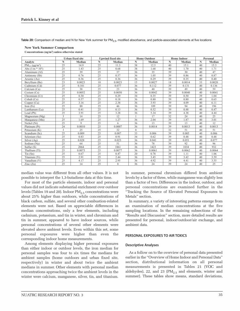
NUATRC RESEARCH REPORT NO. 3
median value was different from all other values. It is notpossible to interpret the 1,3-butadiene data at this time.
For most of the particle elements, indoor and personalvalues did not indicate substantial enrichment over outdoorlevels (Tables 19 and 20). Indoor PM2.5 concentrations wereabout 25% higher than outdoors, while concentrations ofblack carbon, sulfate, and several other combustion-relatedelements were not. Based on appreciable differences inmedian concentrations, only a few elements, includingcadmium, potassium, and tin in winter, and chromium andtin in summer, appeared to have indoor sources, whilepersonal concentrations of several other elements wereelevated above ambient levels. Even within this set, somepersonal exposures were higher than even thecorresponding indoor home measurements.
Among elements displaying higher personal exposuresthan either indoor or outdoor levels, the iron median forpersonal samples was four to six times the medians forambient samples (home outdoors and urban fixed site,respectively) in winter and about twice the ambientmedians in summer. Other elements with personal medianconcentrations approaching twice the ambient levels in thewinter were calcium, manganese, silver, tin, and titanium.
In summer, personal chromium differed from ambientlevels by a factor of three, while manganese was slightly lessthan a factor of two. Differences in the indoor, outdoor, andpersonal concentrations are examined further in the“Tracking the Source of Elevated Personal Exposures toMetals” section.
In summary, a variety of interesting patterns emerge froman examination of median concentrations at the fivesampling locations. In the remaining subsections of the“Results and Discussion” section, more detailed results arepresented for personal, indoor/outdoor/air exchange, andambient data.
PERSONAL EXPOSURES TO AIR TOXICS
Descriptive Analyses
As a follow on to the overview of personal data presentedearlier in the “Overview of Home Indoor and Personal Data”section, distributional information on all personalmeasurements is presented in Tables 21 (VOC andaldehydes), 22, and 23 (PM2.5 and elements, winter andsummer). These tables show means, standard deviations,
35
Patrick L. Kinney et al
AnalytePM2.5 (µg/m3)Abs (1/m * 105)Aluminum (Al)Antimony (Sb)Arsenic (As)Beryllium (Be)Cadmium (Cd)Calcium (Ca)Cesium (Cs)Chromium (Cr)Cobalt (Co)Copper (Cu)Iron (Fe)Lanthanum (La)Lead (Pb)Magnesium (Mg)Manganese (Mn)Nickel (Ni)Platinum (Pt)Potassium (K)Scandium (Sc)Selenium (Se)Silver (Ag)Sodium (Na)Sulfur (S)Thallium (Tl)Tin (Sn)Titanium (Ti)Vanadium (V)Zinc (Zn)
Median14.91.4339
0.760.36
0.00230.101
380.00520.300.573.1680
0.413.9114
1.699
0.001025
0.0090.83
0.02864
20640.00730.672.914.1714
N2525252525232525252525252525253
2525243
25252525252525252525
Urban fixed site Upwind fixed site Home Outdoor Home Indoor PersonalMedian
11.30.6837
0.570.36
0.00230.077
230.00500.290.182.3846
0.133.2812
1.276
0.000732
0.0070.910.023
511861
0.00770.472.442.95
8
N252525252518252525252525252525252525252525252525252525252525
N3838363636153636363436363636361363636033343636363620363636
Median12.51.6835
1.050.29
0.00270.112
400.00420.350.803.931090.525.2417
2.0413
0.0014
0.0060.62
0.04178
14230.00610.783.454.9224
Median15.11.7030
0.860.35
0.00140.131
490.00400.500.804.0994
0.484.3824
1.8713
0.001351
0.0050.480.051
921034
0.00621.113.424.4124
N404039393918393939393939393939323939393239393939393939393939
Median15.31.7147
0.870.40
0.00200.136
590.0041
1.040.656.111960.474.4425
3.0112
0.001351
0.0060.480.077
96932
0.00641.063.593.5525
N404040404033404040394040404040404040404040404040404040404040
New York Summer ComparisonConcentrations (ng/m3) unless otherwise stated
Table 20: Comparison of median and N for New York summer for PM2.5, modified absorbance, and particle-associated elements at five locations
minimum concentrations, 25th percentiles, median, 75thpercentiles, and maximum concentrations for all personalair pollutant measurements. This section begins with anexamination of the overall distribution of median personalconcentrations across all analytes and an examination of therelationship between personal exposures and ambientconcentrations, with special emphasis on distinguishingbetween temporal and spatial ambient influences onpersonal exposures to locally generated fine particles. Thesection continues with an investigation of the likely sourceof the unusually high personal metal concentrationsobserved for some subjects. Finally, we use the NYCTEACH personal air toxic concentrations to perform apreliminary cancer risk assessment.
Personal Exposure Levels and LODs
Figure 23 displays the personal median concentrations ofVOCs and aldehydes for winter (open boxes) and summer(filled diamonds). Analytes are plotted in rank order ofsummer concentrations in µg/m3. The LOD values, definedas three times the standard deviation of field blank samples,are also shown. Except for 1,3-butadiene (winter andsummer) and trichloroethylene (summer), which both hadvery low concentrations, median personal VOCconcentrations ranged from about 0.4 to 20 µg/m3. Theseobservations are quite similar to findings for indoor data(“Indoor/Outdoor and Air Exchange Relationships” sectionbelow). In contrast to the indoor data, where winterconcentrations generally exceeded those measured insummer, personal medians were often higher in summer,especially for the xylenes, ethylbenzene, and formaldehyde.This suggests that personal VOC exposures are driven inpart by activities and/or microenvironments other thanhome indoors. Most personal median concentrations wereabout an order of magnitude greater than the LODs,indicating high measurement sensitivity for mostcompounds. Exceptions to this generalization included 1,3-butadiene and trichloroethylene. Median methylenechloride and benzene concentrations exceeded LODs byabout a factor of two.
Personal exposures to particle-associated air pollutantsranged over more than seven orders of magnitude, and wereall well above LODs with the exceptions of selenium andchromium (Figure 24). As with the ambient and indoor datapresented, the most abundant element measured was sulfur.Sulfur was assumed to occur primarily as sulfate andreported as such. Other abundant elements in order ofmedian concentrations were iron, sodium, calcium,potassium, aluminum, zinc, and magnesium. Though thelog scale compresses vertical differences, a tendency was
seen for winter elemental exposures to exceed those insummer (see also Tables 19 and 20).
Personal Exposures Compared with Outdoor Concentrations
The ratio of personal to home outdoor concentrations(measured for the same 48-hour period) was computed foreach subject for all analytes. Box plots of the individualratios by analyte provide a simple visual tool for identifyinganalytes for which personal exposures and ambientconcentrations were similar, as opposed to those analytesshowing evidence of non-ambient sources. Figure 25displays these ratios for winter and summer for all VOCs,ranked by the median winter ratios. The personal and homeoutdoor ratios of VOCs displayed on the left side of thefigure do not differ greatly. This includes carbontetrachloride, MTBE, the xylenes, and ethyl benzene.Displayed on the right side are those VOCs exhibitinghighly enriched personal exposures as compared to outdoorexposures. This includes chloroform, formaldehyde, 1,4-dichlorobenzene, and acetaldehyde. The overall patternswere similar in winter and summer, although the 75th and95th percentiles tended to be higher in summer, possiblyreflecting unique summer-specific activities and/ormicroenvironments for a subset of subjects.
The box plots of personal/outdoor ratios for PM andassociated elements are displayed in Figure 26. Ascompared to the VOCs, personal/outdoor ratios generallyclustered closer to 1.0, suggesting greater importance ofoutdoor sources in driving personal exposures to particle-associated measurements. Nevertheless, personal exposuresto several elements were typically two to five times higherthan outdoors, especially in winter. Elements includedchromium (measured only in summer), iron, silver,manganese, tin, copper, calcium, cadmium, aluminum,potassium, zinc, and magnesium. This again suggests non-ambient sources or activity patterns that impact personalexposures to certain metals among NYC youth. This issue isexamined further in the “Tracking the Source of ElevatedPersonal Exposures to Metals” section below.
Temporal and Spatial Associations Between PersonalExposures and Ambient Concentrations of PM2.5, Sulfate, andBlack Carbon
As noted, personal exposures and outdoor concentrationsof many particulate matter components did not differgreatly. It is of considerable interest to investigate the natureand extent of agreement between ambient and personalexposures to PM2.5 and elemental components, both overtime and space. Understanding these relationships will
36
Toxic Exposure Assessment: A Columbia-Harvard (TEACH) Study (The New York City Report)
NUATRC RESEARCH REPORT NO. 3
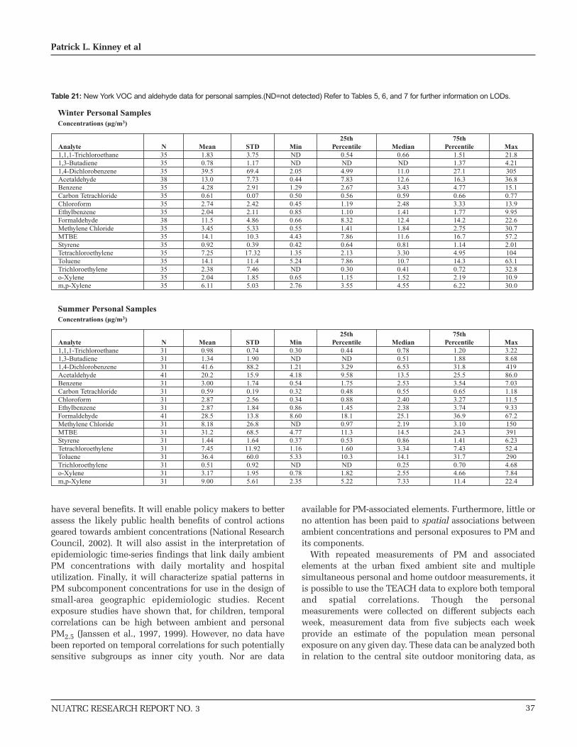
NUATRC RESEARCH REPORT NO. 3
have several benefits. It will enable policy makers to betterassess the likely public health benefits of control actionsgeared towards ambient concentrations (National ResearchCouncil, 2002). It will also assist in the interpretation ofepidemiologic time-series findings that link daily ambientPM concentrations with daily mortality and hospitalutilization. Finally, it will characterize spatial patterns inPM subcomponent concentrations for use in the design ofsmall-area geographic epidemiologic studies. Recentexposure studies have shown that, for children, temporalcorrelations can be high between ambient and personalPM2.5 (Janssen et al., 1997, 1999). However, no data havebeen reported on temporal correlations for such potentiallysensitive subgroups as inner city youth. Nor are data
available for PM-associated elements. Furthermore, little orno attention has been paid to spatial associations betweenambient concentrations and personal exposures to PM andits components.
With repeated measurements of PM and associatedelements at the urban fixed ambient site and multiplesimultaneous personal and home outdoor measurements, itis possible to use the TEACH data to explore both temporaland spatial correlations. Though the personalmeasurements were collected on different subjects eachweek, measurement data from five subjects each weekprovide an estimate of the population mean personalexposure on any given day. These data can be analyzed bothin relation to the central site outdoor monitoring data, as
37
Patrick L. Kinney et al
Table 21: New York VOC and aldehyde data for personal samples.(ND=not detected) Refer to Tables 5, 6, and 7 for further information on LODs.
Analyte1,1,1-Trichloroethane1,3-Butadiene1,4-DichlorobenzeneAcetaldehydeBenzeneCarbon TetrachlorideChloroformEthylbenzeneFormaldehydeMethylene ChlorideMTBEStyreneTetrachloroethyleneTolueneTrichloroethyleneo-Xylenem,p-Xylene
Mean1.830.7839.513.04.280.612.742.0411.53.4514.10.927.2514.12.382.046.11
N3535353835353535383535353535353535
25th 75thMinNDND2.050.441.290.500.450.850.660.554.430.421.355.24ND0.652.76
STD3.751.1769.47.732.910.072.422.114.865.3310.30.39
17.3211.47.461.855.03
Percentile0.54ND4.997.832.670.561.191.108.321.417.860.642.137.860.301.153.55
Median0.66ND11.012.63.430.592.481.4112.41.8411.60.813.3010.70.411.524.55
Max21.84.2130536.815.10.7713.99.9522.630.757.22.0110463.132.810.930.0
Percentile1.511.3727.116.34.770.663.331.7714.22.7516.71.144.9514.30.722.196.22
Analyte1,1,1-Trichloroethane1,3-Butadiene1,4-DichlorobenzeneAcetaldehydeBenzeneCarbon TetrachlorideChloroformEthylbenzeneFormaldehydeMethylene ChlorideMTBEStyreneTetrachloroethyleneTolueneTrichloroethyleneo-Xylenem,p-Xylene
Mean0.981.3441.620.23.000.592.872.8728.58.1831.21.447.4536.40.513.179.00
N3131314131313131413131313131313131
25th 75thMin0.30ND1.214.180.540.320.340.868.60ND4.770.371.165.33ND0.782.35
STD0.741.9088.215.91.740.192.561.8413.826.868.51.64
11.9260.00.921.955.61
Percentile0.44ND3.299.581.750.480.881.4518.10.9711.30.531.6010.3ND1.825.22
Median0.780.516.5313.52.530.552.402.3825.12.1914.50.863.3414.10.252.557.33
Max3.228.6841986.07.031.1811.59.3367.21503916.2352.42904.687.8422.4
Percentile1.201.8831.825.53.540.653.273.7436.93.1024.31.417.4331.70.704.6611.4
Summer Personal SamplesConcentrations (µg/m3)
Winter Personal SamplesConcentrations (µg/m3)
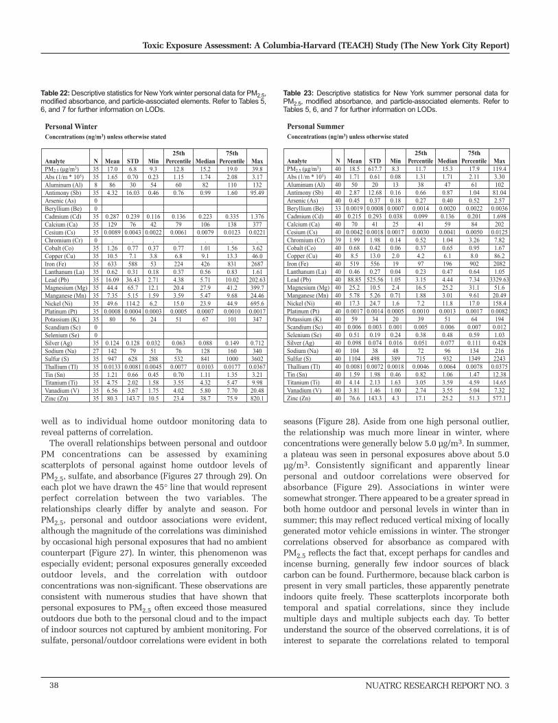
well as to individual home outdoor monitoring data toreveal patterns of correlation.
The overall relationships between personal and outdoorPM concentrations can be assessed by examiningscatterplots of personal against home outdoor levels ofPM2.5, sulfate, and absorbance (Figures 27 through 29). Oneach plot we have drawn the 45° line that would representperfect correlation between the two variables. Therelationships clearly differ by analyte and season. ForPM2.5, personal and outdoor associations were evident,although the magnitude of the correlations was diminishedby occasional high personal exposures that had no ambientcounterpart (Figure 27). In winter, this phenomenon wasespecially evident; personal exposures generally exceededoutdoor levels, and the correlation with outdoorconcentrations was non-significant. These observations areconsistent with numerous studies that have shown thatpersonal exposures to PM2.5 often exceed those measuredoutdoors due both to the personal cloud and to the impactof indoor sources not captured by ambient monitoring. Forsulfate, personal/outdoor correlations were evident in both
seasons (Figure 28). Aside from one high personal outlier,the relationship was much more linear in winter, whereconcentrations were generally below 5.0 µg/m3. In summer,a plateau was seen in personal exposures above about 5.0µg/m3. Consistently significant and apparently linearpersonal and outdoor correlations were observed forabsorbance (Figure 29). Associations in winter weresomewhat stronger. There appeared to be a greater spread inboth home outdoor and personal levels in winter than insummer; this may reflect reduced vertical mixing of locallygenerated motor vehicle emissions in winter. The strongercorrelations observed for absorbance as compared withPM2.5 reflects the fact that, except perhaps for candles andincense burning, generally few indoor sources of blackcarbon can be found. Furthermore, because black carbon ispresent in very small particles, these apparently penetrateindoors quite freely. These scatterplots incorporate bothtemporal and spatial correlations, since they includemultiple days and multiple subjects each day. To betterunderstand the source of the observed correlations, it is ofinterest to separate the correlations related to temporal
38
Toxic Exposure Assessment: A Columbia-Harvard (TEACH) Study (The New York City Report)
NUATRC RESEARCH REPORT NO. 3
AnalytePM2.5 (µg/m3)Abs (1/m * 105)Aluminum (Al)Antimony (Sb)Arsenic (As)Beryllium (Be)Cadmium (Cd)Calcium (Ca)Cesium (Cs)Chromium (Cr)Cobalt (Co)Copper (Cu)Iron (Fe)Lanthanum (La)Lead (Pb)Magnesium (Mg)Manganese (Mn)Nickel (Ni)Platinum (Pt)Potassium (K)Scandium (Sc)Selenium (Se)Silver (Ag)Sodium (Na)Sulfur (S)Thallium (Tl)Tin (Sn)Titanium (Ti)Vanadium (V)Zinc (Zn)
Mean17.01.6586
4.32
0.287129
0.0089.
1.2610.56330.62
16.0944.47.3549.6
0.000880
0.124142947
0.01331.214.756.5680.3
N35358
3500
3535350
3535353535353535353500
3527353535353535
25th 75thMin9.30.2354
0.46
0.11642
0.0022.
0.373.853
0.182.7112.11.596.2
0.000324
0.03251288
0.00450.451.581.7510.5
STD6.8
0.7030
16.03
0.23976
0.0043.
0.777.15880.3136.4365.75.15114.2
0.000456
0.12879628
0.00810.662.023.67143.7
Percentile12.81.1560
0.76
0.13679
0.0061.
0.776.82240.374.3820.43.5915.0
0.000551
0.06376532
0.00770.703.554.0223.4
Median15.21.7482
0.99
0.223106
0.0079.
1.019.14260.565.7127.95.4723.9
0.000767
0.088128841
0.01031.114.325.8038.7
Max39.83.17132
95.49
1.376377
0.0221.
3.6246.026871.61
202.63399.724.46695.60.0017
347
0.712340
36020.0367
3.219.98
20.48820.1
Percentile19.02.081101.60
0.335138
0.0123.
1.5613.38310.83
10.0241.29.6844.9
0.0010101
0.1491601000
0.01771.355.477.7075.9
Personal WinterConcentrations (ng/m3) unless otherwise stated
Table 22: Descriptive statistics for New York winter personal data for PM2.5,modified absorbance, and particle-associated elements. Refer to Tables 5,6, and 7 for further information on LODs.
AnalytePM2.5 (µg/m3)Abs (1/m * 105)Aluminum (Al)Antimony (Sb)Arsenic (As)Beryllium (Be)Cadmium (Cd)Calcium (Ca)Cesium (Cs)Chromium (Cr)Cobalt (Co)Copper (Cu)Iron (Fe)Lanthanum (La)Lead (Pb)Magnesium (Mg)Manganese (Mn)Nickel (Ni)Platinum (Pt)Potassium (K)Scandium (Sc)Selenium (Se)Silver (Ag)Sodium (Na)Sulfur (S)Thallium (Tl)Tin (Sn)Titanium (Ti)Vanadium (V)Zinc (Zn)
Mean18.51.7150
2.870.45
0.00190.215
700.00421.990.688.55190.46
88.8525.25.7817.3
0.001759
0.0060.51
0.098104
11040.00811.594.143.8176.6
N404040404033404040394040404040404040404040404040404040404040
25th 75thMin8.3
0.0813
0.160.18
0.00070.038
250.0017
0.140.062.019
0.041.052.4
0.711.6
0.000520
0.0010.240.016
48389
0.00180.461.631.004.3
STD617.70.6120
12.680.37
0.00080.293
410.00181.980.4213.05560.27
525.5610.55.2624.7
0.001434
0.0030.190.074
38498
0.00721.982.131.46143.3
Percentile11.71.3138
0.660.27
0.00140.099
410.00300.520.374.297
0.233.1516.51.887.2
0.001039
0.0050.380.051
72715
0.00460.823.052.7417.1
Median15.31.7147
0.870.40
0.00200.136
590.00411.040.656.11960.474.4425.23.0111.8
0.001351
0.0060.480.077
96932
0.00641.063.593.5525.2
Max119.43.30102
81.042.57
0.00361.698202
0.01257.821.6786.220821.05
3329.6351.6
20.49158.40.0082
1940.0121.03
0.428216
22430.037512.3814.657.32
577.1
Percentile17.92.1161
1.040.52
0.00220.201
840.0050
3.260.958.09020.647.3431.19.6117.0
0.001764
0.0070.59
0.111134
13490.0078
1.474.595.0451.3
Personal SummerConcentrations (ng/m3) unless otherwise stated
Table 23: Descriptive statistics for New York summer personal data forPM2.5, modified absorbance, and particle-associated elements. Refer toTables 5, 6, and 7 for further information on LODs.

NUATRC RESEARCH REPORT NO. 3
variations from those related to spatial variations. To date,most evaluations of personal and outdoor correlations havefocused on temporal factors, which is relevant tointerpreting time-series epidemiological results. Here weexamine both time and space.
To begin examining temporal associations, the personalexposure data are plotted over time along with the fixed-siteoutdoor data. This is shown in Figures 30 through 32 forPM2.5, sulfate, and absorbance. To varying extents, temporalcorrelations are apparent between the urban fixed-siteconcentrations and levels of personal exposure measuredeach day. The temporal patterns of peaks and troughs inambient concentrations appear to correlate withconcurrently measured personal exposures. Thesecorrelations appear stronger for sulfate and absorbance thanfor PM2.5, and stronger for summer than for winter.
To more clearly isolate and quantify these temporalassociations, weekly mean personal exposures were plottedagainst simultaneous ambient concentrations in ascatterplot format. This is shown for PM2.5, sulfate, andabsorbance in Figures 33 through 35. Table 24 shows resultsfrom a linear regression fit to the these data. For PM2.5temporal correlations were relatively weak in summer andcompletely absent in winter. The lower air exchange rates inwinter may have reduced clearance of indoor-generatedPM. In both seasons, the regression intercepts werestatistically significant; however, only in summer was theslope significant, and the value of the slope was close to 1.0.Temporal correlations for sulfate were much stronger thanthose for PM2.5, reflecting the lack of indoor sources forsulfate. The sulfate intercepts and slopes were significantfor both seasons, with slopes ranging from 0.6 to 0.7. Forabsorbance, moderate temporal correlations were apparentin both seasons and appeared stronger in summer.Intercepts were non-significant, and slopes were very closeto 1.0. Note that both sulfate and black carbon representambient tracers; however, sulfate represents the regionalcomponent, while black carbon reflects more localinfluences. These results show that temporal associations
39
Patrick L. Kinney et al
102
101
100
10-2
10-1
1,3-
But
adie
ne
Tri
chlo
roe
thyl
en
e
1,1
,1-T
rich
loro
eth
an
Sty
ren
e
Car
bon
Tet
rach
lori
de
Met
hyle
ne C
hlor
ide
Ch
loro
form
Ben
zene
Eth
ylbe
nzen
e
o-X
yle
ne
Tet
rach
loro
ethy
lene
m,p
-Xyl
en
e
1,4-
Dic
hlor
oben
zene
To
lue
ne
Ace
tald
ehyd
e
MT
BE
For
mal
dehy
de
Summer Home Indoor Median
Winter Home Indoor Median
LOD (µg/m3)
Med
ian
Co
nce
ntr
atio
n (
µg
/m3 )
Figure 23: Median concentrations of VOC and aldehyde measurementsfor personal samples, for winter and summer. Also shown is the mean limitof detection (LOD).
105
101
102
103
104
100
10-5
10-1
10-2
10-3
10-4
Summer Home Indoor Median
Winter Home Indoor Median
LOD (ng/m3)
Med
ian
Co
nce
ntr
atio
n (
ng
/m3 )
Pt
Be
Cs
Sc Tl
Ag
Cd
As
La Se Cr
Co
Sb
Sn
Abs
*M
n Ti
Cu
Pb V Ni
Mg
Zn Al
Ca K Na
Fe
SO
4P
M2
.5
Figure 24: Median concentrations of particle-associated measurementsfor personal samples, for winter and summer. Also shown is the mean limitof detection (LOD).
Pollutant
PM2.5
Sulfate
Absorbance
Season
Winter
Summer
Winter
Summer
Winter
Summer
R2
0.01
0.47
0.63
0.94
0.52
0.59
Parameter
Intercept
Slope
Intercept
Slope
Intercept
Slope
Intercept
Slope
Intercept
Slope
Intercept
Slope
ParameterEstimate
16.4
0.09
5.77
0.90
0.79
0.69
0.83
0.66
0.10
1.01
0.29
0.96
p-value
<0.0001
0.53
0.003
<0.0001
0.008
<0.0001
<0.0001
<0.0001
0.68
<0.0001
0.15
<0.0001
Table 24: Regression estimates from ordinary linear regressions of meanweekly personal exposures on simultaneous urban fixed-siteconcentrations, quantifying the degree of temporal association betweenpersonal and ambient levels
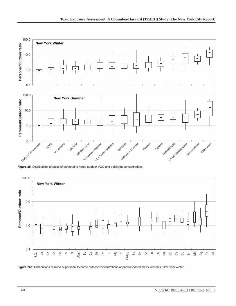
40
Toxic Exposure Assessment: A Columbia-Harvard (TEACH) Study (The New York City Report)
NUATRC RESEARCH REPORT NO. 3
0.1
1.0
10.0
100.0
Per
son
al/O
utd
oo
r ra
tio New York Winter
New York Summer
0.1
1.0
10.0
100.0
Carbo
n Tet
rach
loride
MTBE
m,p
-Xyle
ne
o-Xyle
ne
Ethylb
enze
ne
Tetra
chlor
oeth
ylene
1,1,
1-Tric
hloro
etha
ne
Benze
ne
Met
hylen
e Chlo
ride
Toluen
e
Styren
e
Aceta
ldehy
de
1,4-
Dichlor
oben
zene
Form
aldeh
yde
Chloro
form
Per
son
al/O
utd
oo
r ra
tio
Figure 25: Distributions of ratios of personal to home outdoor VOC and aldehyde concentrations
0.1
1.0
10.0
100.0
New York Winter
Per
son
al/O
utd
oo
r ra
tio
Co Ni
La Be
Fe
Cs
Sb V
Abs
*
Pb
Mn
Sc
Se
Mg
SO
4
NaAl
Pt
Ca
CuTl
ZnTi
Cd
As
Cr
Ag
Sn
PM
2.5 K
Figure 26a: Distributions of ratios of personal to home outdoor concentrations of particle-based measurements, New York winter

NUATRC RESEARCH REPORT NO. 3 41
Patrick L. Kinney et al
0.1
1.0
10.0
100.0
New York Summer
Per
son
al/O
utd
oo
r ra
tio
Co Ni
La Be
Fe
Cs
Sb V
Abs
*
Pb
Mn
Sc
Se
Mg
SO
4
NaAl
Pt
Ca
CuTl
ZnTi
Cd
As
Cr
Ag
Sn
PM
2.5 K
Figure 26b: Distributions of ratios of personal to home outdoor concentrations of particle-based measurements, New York winter
0
5
10
15
20
25
30
35
40
45
0 5 10 15 20 25 30 35 40 45Home Outdoor PM2.5
Per
son
al P
M2.
5
r=0.16n.s.
NY Summer
NY Winter
0
5
10
15
20
25
30
35
40
45
0 5 10 15 20 25 30 35 40 45Home Outdoor PM2.5
Per
son
al P
M2.
5
r=0.41p=0.01
Figure 27: Plot of personal vs. home outdoor PM2.5 concentrations
0
5
10
15
20
0 5 10 15 20
Home Outdoor Sulfate
Per
son
al S
ulf
ate
r=0.44p=0.01
0
5
10
15
20
0 5 10 15 20Home Outdoor Sulfate
NY Winter
NY Summer
Per
son
al S
ulf
ate
r=0.70p<0.0001
Figure 28: Plot of personal vs. home outdoor sulfate concentrations
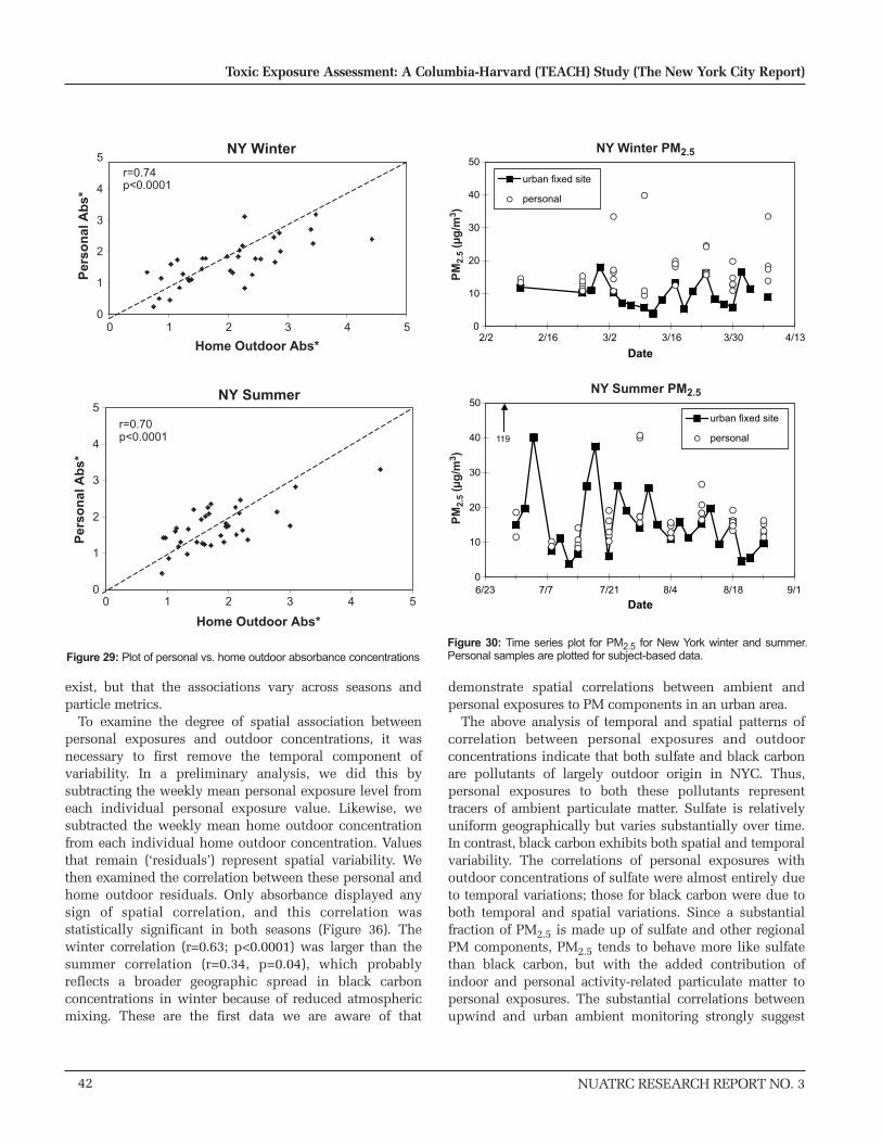
exist, but that the associations vary across seasons andparticle metrics.
To examine the degree of spatial association betweenpersonal exposures and outdoor concentrations, it wasnecessary to first remove the temporal component ofvariability. In a preliminary analysis, we did this bysubtracting the weekly mean personal exposure level fromeach individual personal exposure value. Likewise, wesubtracted the weekly mean home outdoor concentrationfrom each individual home outdoor concentration. Valuesthat remain (‘residuals’) represent spatial variability. Wethen examined the correlation between these personal andhome outdoor residuals. Only absorbance displayed anysign of spatial correlation, and this correlation wasstatistically significant in both seasons (Figure 36). Thewinter correlation (r=0.63; p<0.0001) was larger than thesummer correlation (r=0.34, p=0.04), which probablyreflects a broader geographic spread in black carbonconcentrations in winter because of reduced atmosphericmixing. These are the first data we are aware of that
demonstrate spatial correlations between ambient andpersonal exposures to PM components in an urban area.
The above analysis of temporal and spatial patterns ofcorrelation between personal exposures and outdoorconcentrations indicate that both sulfate and black carbonare pollutants of largely outdoor origin in NYC. Thus,personal exposures to both these pollutants representtracers of ambient particulate matter. Sulfate is relativelyuniform geographically but varies substantially over time.In contrast, black carbon exhibits both spatial and temporalvariability. The correlations of personal exposures withoutdoor concentrations of sulfate were almost entirely dueto temporal variations; those for black carbon were due toboth temporal and spatial variations. Since a substantialfraction of PM2.5 is made up of sulfate and other regionalPM components, PM2.5 tends to behave more like sulfatethan black carbon, but with the added contribution ofindoor and personal activity-related particulate matter topersonal exposures. The substantial correlations betweenupwind and urban ambient monitoring strongly suggest
42
Toxic Exposure Assessment: A Columbia-Harvard (TEACH) Study (The New York City Report)
NUATRC RESEARCH REPORT NO. 3
0
1
2
3
4
5
0 1 2 3 4 5
Home Outdoor Abs*
Per
son
al A
bs*
Home Outdoor Abs*
Per
son
al A
bs*
r=0.74p<0.0001
0
1
2
3
4
5
0 1 2 3 4 5
r=0.70p<0.0001
NY Winter
NY Summer
Figure 29: Plot of personal vs. home outdoor absorbance concentrations
0
10
20
30
40
50
2/2 2/16 3/2 3/16 3/30 4/13
Date
0
10
20
30
40
50
6/23 7/7 7/21 8/4 8/18 9/1
Date
119
PM
2.5
(µg
/m3 )
PM
2.5
(µg
/m3 )
NY Winter PM2.5
NY Summer PM2.5
urban fixed site
personal
urban fixed site
personal
Figure 30: Time series plot for PM2.5 for New York winter and summer.Personal samples are plotted for subject-based data.
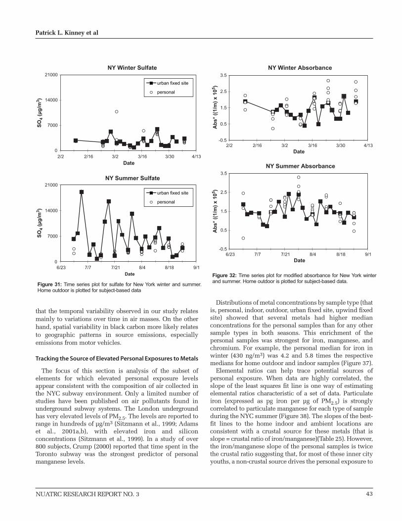
NUATRC RESEARCH REPORT NO. 3
that the temporal variability observed in our study relatesmainly to variations over time in air masses. On the otherhand, spatial variability in black carbon more likely relatesto geographic patterns in source emissions, especiallyemissions from motor vehicles.
Tracking the Source of Elevated Personal Exposures to Metals
The focus of this section is analysis of the subset ofelements for which elevated personal exposure levelsappear consistent with the composition of air collected inthe NYC subway environment. Only a limited number ofstudies have been published on air pollutants found inunderground subway systems. The London undergroundhas very elevated levels of PM2.5. The levels are reported torange in hundreds of µg/m3 (Sitzmann et al., 1999; Adamset al., 2001a,b), with elevated iron and siliconconcentrations (Sitzmann et al., 1999). In a study of over800 subjects, Crump (2000) reported that time spent in theToronto subway was the strongest predictor of personalmanganese levels.
Distributions of metal concentrations by sample type (thatis, personal, indoor, outdoor, urban fixed site, upwind fixedsite) showed that several metals had higher medianconcentrations for the personal samples than for any othersample types in both seasons. This enrichment of thepersonal samples was strongest for iron, manganese, andchromium. For example, the personal median for iron inwinter (430 ng/m3) was 4.2 and 5.8 times the respectivemedians for home outdoor and indoor samples (Figure 37).
Elemental ratios can help trace potential sources ofpersonal exposure. When data are highly correlated, theslope of the least squares fit line is one way of estimatingelemental ratios characteristic of a set of data. Particulateiron (expressed as pg iron per µg of PM2.5) is stronglycorrelated to particulate manganese for each type of sampleduring the NYC summer (Figure 38). The slopes of the best-fit lines to the home indoor and ambient locations areconsistent with a crustal source for these metals (that isslope = crustal ratio of iron/manganese)(Table 25). However,the iron/manganese slope of the personal samples is twicethe crustal ratio suggesting that, for most of these inner cityyouths, a non-crustal source drives the personal exposure to
43
Patrick L. Kinney et al
0
7000
14000
21000
2/2 2/16 3/2 3/16 3/30 4/13
Date
0
7000
14000
21000
6/23 7/7 7/21 8/4 8/18 9/1Date
SO
4 (µ
g/m
3 )S
O4
(µg
/m3 )
NY Winter Sulfate
NY Summer Sulfate
urban fixed site
personal
urban fixed site
personal
Figure 31: Time series plot for sulfate for New York winter and summer.Home outdoor is plotted for subject-based data
NY Winter Absorbance
-0.5
0.5
1.5
2.5
3.5
2/2 2/16 3/2 3/16 3/30 4/13Date
NY Summer Absorbance
-0.5
0.5
1.5
2.5
3.5
6/23 7/7 7/21 8/4 8/18 9/1Date
Ab
s* (
(1/m
) x
105 )
Ab
s* (
(1/m
) x
105 )
Figure 32: Time series plot for modified absorbance for New York winterand summer. Home outdoor is plotted for subject-based data.
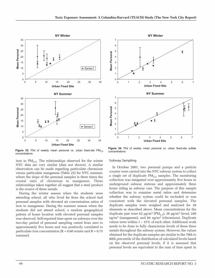
iron in PM2.5. The relationships observed for the winterNYC data are very similar (data not shown). A similarobservation can be made regarding particulate chromiumversus particulate manganese (Table 25) for NYC summer,where the slope of the personal samples is three times thecrustal ratio of chromium to manganese. Theserelationships taken together all suggest that a steel productis the source of these metals.
During the winter season when the students wereattending school, all who lived far from the school hadpersonal samples with elevated air concentration ratios ofiron to manganese. During the summer season when thestudents did not attend school, a random geographicalpattern of home location with elevated personal sampleswas observed. Self-reported time spent on subways over thetwo-day period of personal sampling varied from zero toapproximately five hours and was positively correlated toparticulate iron concentration (R = 0.60 winter and R = 0.75summer).
Subway Sampling
In October 2001, two personal pumps and a particlecounter were carried into the NYC subway system to collecta single set of duplicate PM2.5 samples. The monitoringcollection was integrated over approximately five hours inunderground subway stations and approximately threehours riding in subway cars. The purpose of this samplecollection was to examine metal ratios and determinewhether the subway system could be excluded or wasconsistent with the elevated personal samples. Theduplicate samples were weighed and analyzed for 28elements as described above. Mean concentrations for theduplicate pair were 62 µg/m3 (PM2.5), 26 µg/m3 (iron), 240ng/m3 (manganese), and 84 ng/m3 (chromium). Duplicatevalues were within 1 – 15% of each other. Additional workneeds to be done to fully characterize levels of these threemetals throughout the subway system. However, the valuesobtained for the duplicate samples are similar to the 70th to80th percentile of the distribution of calculated levels basedon the observed personal levels, if it is assumed thatpersonal levels are equivalent to the sum of time spent in
44
Toxic Exposure Assessment: A Columbia-Harvard (TEACH) Study (The New York City Report)
NUATRC RESEARCH REPORT NO. 3
NY Winter
0
5
10
15
20
25
30
35
Urban Fixed Site
Mea
n P
erso
nal
Series1
NY Summer
0
5
10
15
20
25
30
35
0 5 10 15 20 25 30 35
0 5 10 15 20 25 30 35
Urban Fixed Site
Mea
n P
erso
nal
Series1
Figure 33: Plot of weekly mean personal vs. urban fixed-site PM2.5concentrations
NY Winter
0
1
2
3
4
5
6
7
Urban Fixed Site
Mea
n P
erso
nal
NY Summer
0
1
2
3
4
5
6
7
0 1 2 3 4 5 6 7
0 1 2 3 4 5 6 7
Urban Fixed Site
Mea
n P
erso
nal
Figure 34: Plot of weekly mean personal vs. urban fixed-site sulfateconcentrations

NUATRC RESEARCH REPORT NO. 3
subway multiplied by subway concentration and time spentaway from subway multiplied by home indoorconcentration. Real time particle counting suggests thatparticle numbers per volume were significantly higher instations than in the filtered air-conditioned cars. Hence,time spent at stations may be a more powerful predictor ofpersonal exposure than the total time underground. Thisobservation may explain the relatively weak correlationsreported above for self-reported time spent on subways andiron.
The average ratios of iron to manganese and chromium tomanganese for the duplicate subway samples are 107 and0.34, respectively. These are quite similar to the slopes ofthe best-fit line to personal samples for these metals (Table25 and Figures 39 and 40), and are consistent with subwayair potentially being the predominant source of iron,manganese, and chromium in the elevated personalsamples. Iron, manganese, and chromium are all found in
significant concentrations in steel, and these three metalswere the most enriched elements measured in subway airwhen compared to levels found in ambient NYC samples(100 to 200 times median home outdoor levels).
45
Patrick L. Kinney et al
NY Winter
0
3
2
1
Urban Fixed Site
Mea
n P
erso
nal
NY Summer
0
1
2
3
0 1 2 3
0 1 2 3
Urban Fixed Site
Mea
n P
erso
nal
Figure 35: Plot of weekly mean personal vs. urban fixed-site absorbanceconcentrations
Spatial Abs* NY Winter
-2
-1
0
1
2
-2 -1 0 1 2
Home outdoor abs*
Home outdoor abs*
r=0.63
p<0.0001
Spatial Abs* NY Summer
-2
-1
0
1
2
-2 -1 0 1 2
Per
son
al a
bs*
Per
son
al a
bs*
r=0.34
p=0.04
Figure 36: Spatial relationship between home outdoor and personalabsorbance concentrations for New York winter and summer
0
500
1000
1500
2000
Personal HomeIndoor
HomeOutdoor
UrbanFixed-site
UpwindFixed-site
Fe
(ng
/m3 )
25th5th
95th75thMed
Figure 37: Box plot of Fe concentrations for five types of samples collectedduring NY winter

Discussion
The NYC subway system appears to be a very importantmicro-environment that controls personal levels of iron,manganese, and chromium for those subjects who rode thesubway. The NYC subway system is one of the largest in theworld, transporting approximately one billion riders everyyear (Dwyer, 1991). Data presented here are consistent withthe speculation that some portion of the time spent in thesubway system could control personal exposure levels ofiron, manganese, and chromium for those subway riderswho do not have occupational exposures to these metals.This represents a majority of riders.
The air concentrations observed for manganese andchromium in the single set of duplicate PM2.5 samples aremore than three orders of magnitude lower than the OSHAPermissible Exposure Limit (PEL) guideline concentrations,
and the personal exposures observed for subway ridingsubjects are even lower. Adverse health outcomes have notbeen investigated at such low levels and are unknown.However, the data suggest that the subway system probablyprovides an exposure pathway that could be amenable tohealth studies. Although additional work needs to be doneto fully characterize concentrations throughout the NYCsubway system, the values obtained by the single set ofduplicate PM2.5 samples suggest that manganese andchromium levels in the system appear to be enriched aboveurban ambient levels by approximately two orders ofmagnitude. The number of people being exposed isrelatively large (millions per day), and the time span ofexposure is potentially long-term (that is, a lifetime of dailycommuting by subway to school and work). Long-termexposures to manganese and chromium are a potentialconcern. At the extremely high levels of manganese foundin certain occupational settings, adverse health outcomes
are thought to result from cumulative exposures over time(Aschner et al., 1999). Chronic reference concentrationguidelines for ambient manganese (200 ng/m3) andchromium (100 ng/m3) (Wu and Pratt, 2001) are similar tolevels observed in the single set of duplicate subway PM2.5samples (Mn = 240 and Cr = 84 ng/m3). A referenceconcentration guideline for a 10-5 lifetime cancer risk fromchromium exposure is two ng/m3 (Wu and Pratt, 2001),similar to levels observed for personal samples of subwayriding subjects, which ranged from one to five ng/m3.
Although cancer risk estimates may indicate potential
46
Toxic Exposure Assessment: A Columbia-Harvard (TEACH) Study (The New York City Report)
NUATRC RESEARCH REPORT NO. 3
0
50,000
100,000
150,000
200,000
250,000
300,000
350,000
400,000
450,000
0 1000 2000 3000 4000
Mn (pg/µg of PM2.5)
Fe
(pg
/µg
of
PM
2.5)
Personal summer
Personal winter
Subway samples
Linear (personal winter)
Figure 39: The ratio of Fe to Mn observed in the personal samples fromTEACH during both summer and winter field seasons were consistent withthe Fe/Mn ratio measured in a single set of duplicate 8 hr samples collectedin the NYC subway system
0
20,000
40,000
60,000
80,000
100,000
120,000
140,000
160,000
0 400 800 1200 1600
Mn (pg/µg of PM2.5)
Fe
(pg
/µg
of
PM
2.5)
Personal
Upwind fixed site
Urban fixed site
Home outdoor
Indoor
Crustal Fe/Mn
Personal trendline
Personal:y = 104x - 5666
R2 = 0.98
Crustal:Fe/Mn = 55
Figure 38: Concentration of Fe and Mn in the particulate matter are highlycorrelated for all sampling locations monitored but only the personalsamples have a slope (Fe/Mn ratio) which is significantly elevated abovethat of typical crustal material. Similarly, Cr/Mn ratios for personal samples(in summer when data are available) are elevated above crustal values (plotnot shown).
Table 25: Slope and R2 of least squares fit line to data of personal andambient sample locations for NY summer samples. Also shown are averagemetal ratios of crustal material (average shale) and subway grab samples.
Location
Personal
Upwind fixed site
Urban fixed site
Home outdoor
Crustal ratio (1)
Subway ratio
(1) Turekian and Wedepohl 1961
slope = Fe/Mn
104
44
56
68
55
107
R2
0.98
0.81
0.75
0.8
slope = Cr/Mn
0.33
Not well constrained
Not well constrained
Not well constrained
0.11
0.35
R2
0.89
0.01
0.02
0.25

NUATRC RESEARCH REPORT NO. 3
hazards faced by urban-dwelling teenagers and others whoride the subway, many uncertainties are associated with themethods used to estimate cancer risk. The use of data fromanimal studies introduces uncertainty because it requiresspecies-to-species and high-to-low dose extrapolation. Datacollected from occupational studies also have uncertainty,since exposures are at higher levels and involveoccupational cohorts (usually healthy male workers) thatmay not represent the general human population. Forchromium and other transition metals, the oxidation state isimportant to toxicity. Hexavalent chromium is consideredmuch more potent than trivalent chromium (Klein, 1996),although most exposure studies including the present onehave only measured total chromium. Chromium in steelshould be elemental or zero-valent, although one studylooking at fumes generated during welding of steel foundmost of the airborne chromium to be tetravalent chromium(Edeme et al., 1997). It is possible that steel dust generatedin subway environments might also provide a significantamount of tetravalent chromium. Compared to totalchromium, the estimated reference guidelineconcentrations for 10-5 excess cancer risk from tetravalentchromium are lower, ranging from 0.25 ng/m3 (WHO, 2000)to 0.8 ng/m3 (Wu and Pratt, 2001).
The oxidation states of iron and manganese may also beimportant when considering potential health effects.Investigators have been studying the impact of electrondonor reactions of transition metals in lung tissue, withzero-valent and reduced transition metals giving upelectrons and fully oxidized species not having any more
electrons available (Costa and Dreher, 1997; Kadiiska et al.,1997). Currently we only have total iron and manganeseconcentrations and have no data on oxidation states.
INDOOR/OUTDOOR AND AIR EXCHANGE RELATIONSHIPS
Descriptive Analyses
As a follow on to the overview of indoor data presentedearlier in “Overview of Home Indoor and Personal Data,”distributional information on all home indoormeasurements is presented in Tables 26, 27, and 28. Thisincludes information on VOC, aldehydes, and particle-associated pollutants in winter and summer. These tablesshow mean, standard deviation, minimum concentration,25th percentiles, median, 75th percentiles, and maximumconcentrations for all indoor air pollutant measurements. Inthe sections that follow, we examine and analyze therelationships between indoor and outdoor concentrationsfor the various analytes, the influence of air exchange rateson the indoor/outdoor ratios, and an analysis of blackcarbon as an indoor tracer for particles of ambient origin.
Home Indoor Concentrations and LODs
Figure 41 displays the indoor median concentrations ofVOCs and aldehydes for winter (open boxes) and summer(closed diamonds). Analytes are plotted in rank order ofsummer concentrations expressed in µg/m3. The LODvalues are also shown. The LOD is defined as three timesthe standard deviation of field blank samples.
Except for 1,3 butadiene and trichloroethylene, whichhave very low concentrations in summer, indoor medianVOC concentrations ranged from about 0.4 to 20 µg/m3.Winter VOC concentrations generally exceeded summerconcentrations. Most indoor median concentrations wereabout an order of magnitude greater than the LODs.
Concentrations of PM2.5, modified absorbance, and 28associated elements ranged over more than seven orders ofmagnitude and were all well above LODs, except forchromium and selenium (Figure 42). As was found with theambient data presented below, the most abundant elementmeasured was sulfur. Sulfur was assumed to occurprimarily as sulfate and reported as such. The otherabundant elements in order of median concentrations wereiron, sodium, potassium, calcium, aluminum, zinc, andmagnesium. Little evidence for seasonal differences wasapparent, although differences were somewhat compressedhere due to the wide range of concentrations depicted onthe logarithmic scale.
47
Patrick L. Kinney et al
0
200
400
600
800
1,000
1,200
1,400
1,600
0 1000 2000 3000 4000 5000
Mn (pg/µg of PM2.5)
Cr
(pg
/µg
of
PM
2.5)
Personal summer
Subway samples
Figure 40: The ratio of chromium to manganese observed in the personalsamples from TEACH during the summer field season were consistent withthe Cr/Mn ratio measured in a single set of duplicate 8 hr samples collectedin the NYC subway system. Cr values were not available from the winterfield season of the TEACH study.

Indoor/Outdoor Ratios
To assess relationships between indoor and outdoorconcentrations for the full suite of air toxics measured,Figures 43 and 44 display box plots of indoor-to-outdoor(I/O) ratios for particle-associated elements, VOCs, andaldehydes. From bottom to top, the box plots present the5th, 25th, 50th (that is median), 75th, and 95th percentilesof the distribution of individual subject I/O ratios. Winterand summer I/O ratios were plotted together in each figure.Analytes were rank ordered by the median I/O ratio inwinter.
No summer home outdoor data are available forpotassium. This is a result of our methods of detection.
Briefly, the ICP-MS has two detectors, counting (moresensitive, for small signals) and analog (less sensitive, forlarge signals). We began using a new instrument at the sametime we started analyzing the NYC summer filters. Ourinitial assessment was that the potassium signals were largeenough to warrant the analog detector, and we analyzed thehome outdoor samples in this way. When the data werereviewed, it became apparent that this decision wasincorrect. The noise of the analog detector on the newinstrument resulted in uncertainties on the same order asthe sample signal. Thus the data were not usable.Thereafter, we used the counting detector for potassium,and were able to collect useful data for fixed site, indoor,and personal samples.
48
Toxic Exposure Assessment: A Columbia-Harvard (TEACH) Study (The New York City Report)
NUATRC RESEARCH REPORT NO. 3
Analyte1,1,1-Trichloroethane1,3-Butadiene1,4-DichlorobenzeneAcetaldehydeBenzeneCarbon TetrachlorideChloroformEthylbenzeneFormaldehydeMethylene ChlorideMTBEStyreneTetrachloroethyleneTolueneTrichloroethyleneo-Xylenem,p-Xylene
ND=not detected or zero value
Mean4.821.0448.715.65.300.673.403.1612.15.4918.71.116.6815.71.112.989.25
N3636363736363636373636363636363636
25th 75thMin0.31ND0.365.401.670.480.460.545.200.213.840.210.783.04ND0.581.83
STD20.21.3793.09.706.470.142.776.135.0112.328.90.6213.112.83.185.4117.8
Percentile0.44ND3.159.892.540.571.541.098.781.398.420.691.868.930.281.243.75
Median0.610.698.9413.73.620.632.571.6012.22.1710.61.003.5311.90.441.695.14
Max1225.8239053.639.21.2212.834.322.369.01702.9678.369.419.431.3106
Percentile1.301.1135.817.75.510.714.152.0216.23.2517.11.406.1315.80.742.226.81
Analyte1,1,1-Trichloroethane1,3-Butadiene1,4-DichlorobenzeneAcetaldehydeBenzeneCarbon TetrachlorideChloroformEthylbenzeneFormaldehydeMethylene ChlorideMTBEStyreneTetrachloroethyleneTolueneTrichloroethyleneo-Xylenem,p-Xylene
ND=not detected or zero value
Mean1.341.1711115.01.690.532.251.8120.910.023.00.775.2915.20.282.025.71
N3030304130303030413030303030303030
25th 75thMinNDND1.192.93NDND0.530.435.81ND3.230.18NDNDND0.371.11
STD3.062.5748816.71.170.141.820.9811.032.951.50.678.7418.90.511.233.71
Percentile0.39ND2.906.771.130.471.101.3813.80.908.730.421.407.74ND1.474.01
Median0.47ND6.1510.71.460.531.731.6318.81.3613.490.512.0110.10.141.734.91
Max16.512.2268491.86.320.799.225.0851.11762933.1543.293.42.656.4819.7
Percentile0.861.1120.115.32.430.582.922.2724.12.5816.20.804.4814.00.362.376.46
Summer Home Indoor SitesConcentrations (µg/m3)
Winter Home Indoor SitesConcentrations (µg/m3)
Table 26: New York VOC and aldehyde data for home indoor sites (ND= not detected)

NUATRC RESEARCH REPORT NO. 3
Median I/O ratios for most particle-associated elementswere close to or less than 1.0 in both winter and summer,consistent with the hypothesis that, for most elements,ambient air was the driving force for indoor concentrations(Figure 43). However, a subset of analytes exhibited medianI/O ratios slightly greater than 1.0. This included potassium,PM2.5, tin, silver, cadmium, titanium, and zinc in winterand tin, silver, chromium, and arsenic in summer. Note thatarsenic and chromium were analyzed only in summer; thiswas the result of upgrades to the ICP-MS analytical systemand improved procedural blanks. Potassium is a componentof cigarette smoke. Although all subjects had reported thatthey lived in non-smoking homes, it was discovered thatsmoking relatives did live in at least two of the 46 homes. Itis not known what indoor sources may have beenresponsible for the elevated I/O ratios for the otherelements; however, most of these are common metals thatare present in a variety of products.
For elements with lower indoor than outdoorconcentrations (that is those on the left side of Figure 43),I/O ratios were slightly lower in winter than summer,consistent with decreased winter air exchange rates and
diminished penetration of outdoor particles. A weaktendency for this relationship to reverse was seen for thoseelements with evidence of indoor sources (that is, with I/Oratios greater than 1.0). Here I/O ratios were often slightlyhigher in winter than in summer, consistent with increasedtrapping of indoor-generated pollutants in winter whenhome air exchange was lower. The influence of home airexchange rates on I/O relationships is investigated furtherin “The Influences of Air Exchange on I/O Rates” section.
The I/O ratios for VOCs and aldehydes were generallymuch higher than those of the elements, with nearly half theVOCs and aldehydes exhibiting median I/O ratios of 2.0 orgreater (Figure 44). A tendency was seen for I/O ratios to belower in summer than in winter, that is closer to 1.0,reflecting enhanced air exchange and clearance of indoor-generated pollutants. Indoor concentrations of chloroformfar exceeded outdoor levels (I/O ratio > 4) in both seasonsThis was also seen in winter for the two aldehydes and for1,4-dichlorobenzene. These findings are consistent withmore significant and widespread indoor sources for thesecompounds. However, for several VOCs, I/O ratios clusteredclose to 1.0, including such traffic-related compounds as
49
Patrick L. Kinney et al
AnalytePM2.5 (µg/m3)Abs (1/m * 105)Aluminum (Al)Antimony (Sb)Arsenic (As)Beryllium (Be)Cadmium (Cd)Calcium (Ca)Cesium (Cs)Chromium (Cr)Cobalt (Co)Copper (Cu)Iron (Fe)Lanthanum (La)Lead (Pb)Magnesium (Mg)Manganese (Mn)Nickel (Ni)Platinum (Pt)Potassium (K)Scandium (Sc)Selenium (Se)Silver (Ag)Sodium (Na)Sulfur (S)Thallium (Tl)Tin (Sn)Titanium (Ti)Vanadium (V)Zinc (Zn)
Mean20.91.6241
5.29
0.20792
0.0087
1.767.084
0.7222.4030.72.2031.6
0.001084
0.006
0.096153983
0.01491.012.949.49
120.7
N3838263800
3838380
38383838383838383838290
3830383838383838
25th 75thMin6.40.1617
0.42
0.04222
0.0026
0.171.025
0.071.888.60.933.0
0.000218
0.001
0.02120275
0.00410.290.401.458.7
STD16.90.7823
22.82
0.164105
0.0057
3.394.740
0.5670.2517.41.1554.5
0.000866
0.004
0.1131351077
0.00990.532.2220.66370.6
Percentile11.71.0029
0.63
0.09546
0.0044
0.753.851
0.333.5416.81.2214.6
0.000536
0.004
0.04180500
0.00760.591.544.1719.9
Median16.81.5638
1.01
0.17465
0.0066
1.225.774
0.636.6626.61.9619.1
0.000875
0.006
0.057105724
0.01180.892.236.4428.5
Max106.72.98134
140.96
0.877547
0.0305
21.6719.31903.10
382.3080.76.33
348.40.0053
3430.018
0.621675
69640.0450
2.269.89
132.562297.9
Percentile22.72.2947
1.57
0.253101
0.0128
1.597.71140.859.2940.42.7630.0
0.0011101
0.008
0.095165996
0.01821.393.537.6787.6
Home Indoor WinterConcentrations (ng/m3) unless otherwise stated
Table 27: Descriptive statistics for New York winter home indoor data forPM2.5, modified absorbance, and particle-associated elements
AnalytePM2.5 (µg/m3)Abs (1/m * 105)Aluminum (Al)Antimony (Sb)Arsenic (As)Beryllium (Be)Cadmium (Cd)Calcium (Ca)Cesium (Cs)Chromium (Cr)Cobalt (Co)Copper (Cu)Iron (Fe)Lanthanum (La)Lead (Pb)Magnesium (Mg)Manganese (Mn)Nickel (Ni)Platinum (Pt)Potassium (K)Scandium (Sc)Selenium (Se)Silver (Ag)Sodium (Na)Sulfur (S)Thallium (Tl)Tin (Sn)Titanium (Ti)Vanadium (V)Zinc (Zn)
Mean19.01.6639
0.900.40
0.00160.145
540.00440.550.7210.395
0.555.8325.21.8112.6
0.001464
0.0050.52
0.062122
12260.00791.423.464.1786.2
N404039393918393939393939393939323939393239393939393939393939
25th 75thMin5.7
0.395
0.130.13
0.00050.031
210.0017
0.060.061.111
0.030.925.0
0.331.3
0.000518
0.0000.110.011
34405
0.00160.381.120.803.3
STD21.50.6231
0.400.20
0.00070.110
260.00200.290.4830.647
0.534.3812.80.818.4
0.001058
0.0030.280.041
98687
0.00601.921.361.68187.5
Percentile11.81.1624
0.580.27
0.00120.090
380.00300.360.272.955
0.202.7316.41.165.3
0.001038
0.0030.310.041
68671
0.00500.642.512.8811.2
Median15.11.7030
0.860.35
0.00140.131
490.00400.500.804.194
0.484.3823.91.8712.6
0.001351
0.0050.480.051
921034
0.00621.113.424.4124.3
Max145.53.171951.881.06
0.00310.671122
0.01211.351.95
195.11853.14
20.1270.04.2141.9
0.0065306
0.0171.21
0.263590
30400.031912.647.567.72
957.9
Percentile17.92.0645
1.160.52
0.00190.170
610.0052
0.681.077.01280.756.5630.52.4116.2
0.001665
0.0070.67
0.081133
15290.0078
1.434.435.1940.7
Home Indoor SummerConcentrations (ng/m3) unless otherwise stated
Table 28: Descriptive statistics for New York summer home indoor data forPM2.5, modified absorbance, and particle-associated elements

MTBE. In general, the I/O ratios we observed for VOCs wereconsistent with those found in the New Jersey andCalifornia TEAM studies (Hartwell, et al., 1987; Wallace, etal., 1985).
Indoor versus Outdoor Scatter Plots
To examine the strength of relationships between indoorand outdoor concentrations for pollutants that comeprimarily from outdoor sources, winter and summer scatterplots of home indoor versus home outdoor concentrationsare displayed for sulfate (a typical regional ambient particlecomponent) and for black carbon (a typical local outdoorparticle component). This is shown in Figures 45 and 46.For both of these outdoor-driven components, substantialcorrelation between indoor and outdoor concentrations isevident. It is noteworthy that this was both true for apollutant of regional character with strong temporalvariability and a pollutant of local character with strongspatial variability. A similar pattern was seen for MTBE(data not shown).
Figures 47 and 48 display scatter plots of indoor-versus-outdoor concentrations for 1,4-dichlorobenzene andformaldehyde showing contrasting patterns for pollutantswith strong indoor sources. The general absence of anysubstantial influence of ambient concentrations on indoorlevels is very evident.
The Influence of Air Exchange on Indoor/Outdoor Ratios
The AER in a given environment is a key determinant ofthe degree to which both indoor and outdoor emissionsources influence indoor concentrations of air toxics. Todetermine the average AER over a two-day period, the AERwas measured in each home using a perfluorocarbon tracermethod. This measurement always included the 48-hrintegrated air sampling period.
Across all homes in winter, the mean hourly AER was0.99 of the whole air volume of the dwelling, with astandard deviation of 0.69 per hour. In the summer, themean AER was almost twice as high, 1.81 per hour, with astandard deviation of 1.14 per hour. The percentiles of thedistributions of AERs in winter and summer are shown inFigure 49.
Differences in typical I/O ratios by season were noted inthe “Descriptive Analyses” section. Here, we assessed theeffects of AER on I/O ratios both graphically andstatistically using the non-parametric Kruskal-Wallis test,an ANOVA analogue. Three levels of air exchange weredefined: low (<0.5 1/hr); medium (0.5-1.5 1/hr); and high(>1.5 1/hr). We then plotted the median I/O ratios withinthese three categories of AER. Figure 50 shows the medianI/Os binned by AER for the elements in winter and summer.The analytes are ranked from lowest to highest I/O based onwinter ratios. For most of the elements with median I/Osless than 1.0, I/Os increased with increased air exchange
50
Toxic Exposure Assessment: A Columbia-Harvard (TEACH) Study (The New York City Report)
NUATRC RESEARCH REPORT NO. 3
102
101
100
10-2
10-1
1,3
-Bu
tad
ien
e
Tri
chlo
roe
thyl
en
e
1,1
,1-T
rich
loro
eth
an
Sty
ren
e
Ca
rbo
n T
etr
ach
lori
de
Me
thyl
en
e C
hlo
rid
e
Ch
loro
form
Benz
ene
Eth
ylb
en
zen
e
o-X
yle
ne
Te
tra
chlo
roe
thyl
en
e
m,p
-Xyl
en
e
1,4
-Dic
hlo
rob
en
zen
e
To
lue
ne
Ace
tald
ehyd
e
MT
BE
Fo
rma
lde
hyd
e
Summer Home Indoor Median
Winter Home Indoor Median
LOD (µg/m3)
Me
dia
n C
on
ce
ntr
ati
on
(µ
g/m
3)
Figure 41: Median concentrations of VOC and aldehyde measurementsfor home indoor sites, for winter and summer. Also shown is the mean limitof detection (LOD).
105
101
102
103
104
100
10-5
10-1
10-2
10-3
10-4
Summer Home Indoor Median
Winter Home Indoor Median
LOD
Me
dia
n C
on
ce
ntr
ati
on
(n
g/m
3)
Pt
Be
Cs
Sc Tl
Ag
Cd
As
La
Se Cr
Co
Sb
Sn
Abs* Mn Ti
Cu
Pb V Ni
Mg
Zn Al
Ca K Na
Fe
SO
4P
M2
.5
Figure 42: Median concentrations of particle-associated measurements forhome indoor samples, for winter and summer. Also shown is the mean limitof detection (LOD).
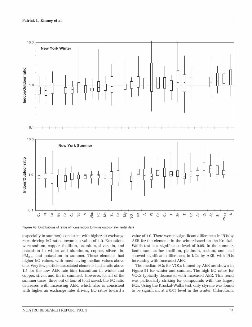
NUATRC RESEARCH REPORT NO. 3
(especially in summer), consistent with higher air exchangerates driving I/O ratios towards a value of 1.0. Exceptionswere sodium, copper, thallium, cadmium, silver, tin, andpotassium in winter and aluminum, copper, silver, tin,PM2.5, and potassium in summer. These elements hadhigher I/O values, with most having median values aboveone. Very few particle-associated elements had a ratio above1.5 for the low AER rate bins (scandium in winter andcopper, silver, and tin in summer). However, for all of thesummer cases (three out of four of total cases), the I/O ratiodecreases with increasing AER, which also is consistentwith higher air exchange rates driving I/O ratios toward a
value of 1.0. There were no significant differences in I/Os byAER for the elements in the winter based on the Kruskal-Wallis test at a significance level of 0.05. In the summer,lanthanum, sulfur, thallium, platinum, cesium, and leadshowed significant differences in I/Os by AER, with I/Osincreasing with increased AER.
The median I/Os for VOCs binned by AER are shown inFigure 51 for winter and summer. The high I/O ratios forVOCs typically decreased with increased AER. This trendwas particularly striking for compounds with the largestI/Os. Using the Kruskal-Wallis test, only styrene was foundto be significant at a 0.05 level in the winter. Chloroform,
51
Patrick L. Kinney et al
0.1
1.0
10.0
0.1
1.0
10.0
Co
Ind
oo
r/O
utd
oo
r ra
tio
Ind
oo
r/O
utd
oo
r ra
tio
Ni
La Be
Fe
Cs
Sb V
Abs Pb
Mn
Sc
Se
Mg
SO
4
Na Al
Pt
Ca
Cu Tl
Zn Ti
Cd
As
Cr
Ag
Sn
PM
2.5 K
New York Summer
New York Winter
Figure 43: Distributions of ratios of home indoor to home outdoor elemental data

tetrachloroethylene, and acetaldehyde were found to besignificant in the summer. It should be noted that, due to thesmall sample size for some of the AER levels, particularlythe low AER level, we might not be able to achievesignificance at the 0.05 level.
In summary, as AER increases, the I/O ratio ofcompounds or substances that come mainly from outdoorsources increases. These substances have I/O ratios below
1.0. This was the typical trend seen for the elements. AsAER increases, the values of I/O decrease for compoundswith indoor sources (I/O ratios above 1.0). This trend wasmore common for the VOCs. Both of these trends areconsistent with increased air exchange rates driving I/Oratios toward a value of 1.0.
52
Toxic Exposure Assessment: A Columbia-Harvard (TEACH) Study (The New York City Report)
NUATRC RESEARCH REPORT NO. 3
Figure 44: Distributions of ratios of home indoor to home outdoor VOC and aldehyde concentrations
0.1
1.0
10.0
100.0
Ind
oo
r/O
utd
oo
r ra
tio
New York Winter
New York Summer
0.1
1.0
10.0
100.0
Carbo
n Tet
rach
loride
MTBE
m,p
-Xyle
ne
o-Xyle
ne
Ethylb
enze
ne
Tetra
chlor
oeth
ylene
1,1,
1-Tric
hloro
etha
ne
Benze
ne
Met
hylen
e Chlo
ride
Toluen
e
Styren
e
Aceta
ldehy
de
1,4-
Dichlor
oben
zene
Form
aldeh
yde
Chloro
form
Ind
oo
r/O
utd
oo
r ra
tio
Ho
me I
nd
oo
r S
ulf
ate
(µ
g/m
3)
Ho
me I
nd
oo
r S
ulf
ate
(µ
g/m
3)
Home Outdoor Sulfate (µg/m3)Home Outdoor Sulfate (µg/m3)
NY Winter
0
2
4
6
0 2 4 6
21
NY Summer
0
5
10
15
20
0 10 20
Figure 45: Sulfate I/O scatterplots, winter (left) and summer (right)
NY Summer
0.0
1.5
3.0
4.5
0.0 1.5 3.0 4.5
NY Winter
0.0
1.5
3.0
4.5
0.0 1.5 3.0 4.5
Home Outdoor Abs* (1/m x 105) Home Outdoor Abs* (1/m x 105)
Ho
me
In
do
or
Ab
s*
(1/m
x 1
05)
Ho
me
In
do
or
Ab
s*
(1/m
x 1
05)
Figure 46: Abs* I/O scatterplots, winter (left) and summer (right)
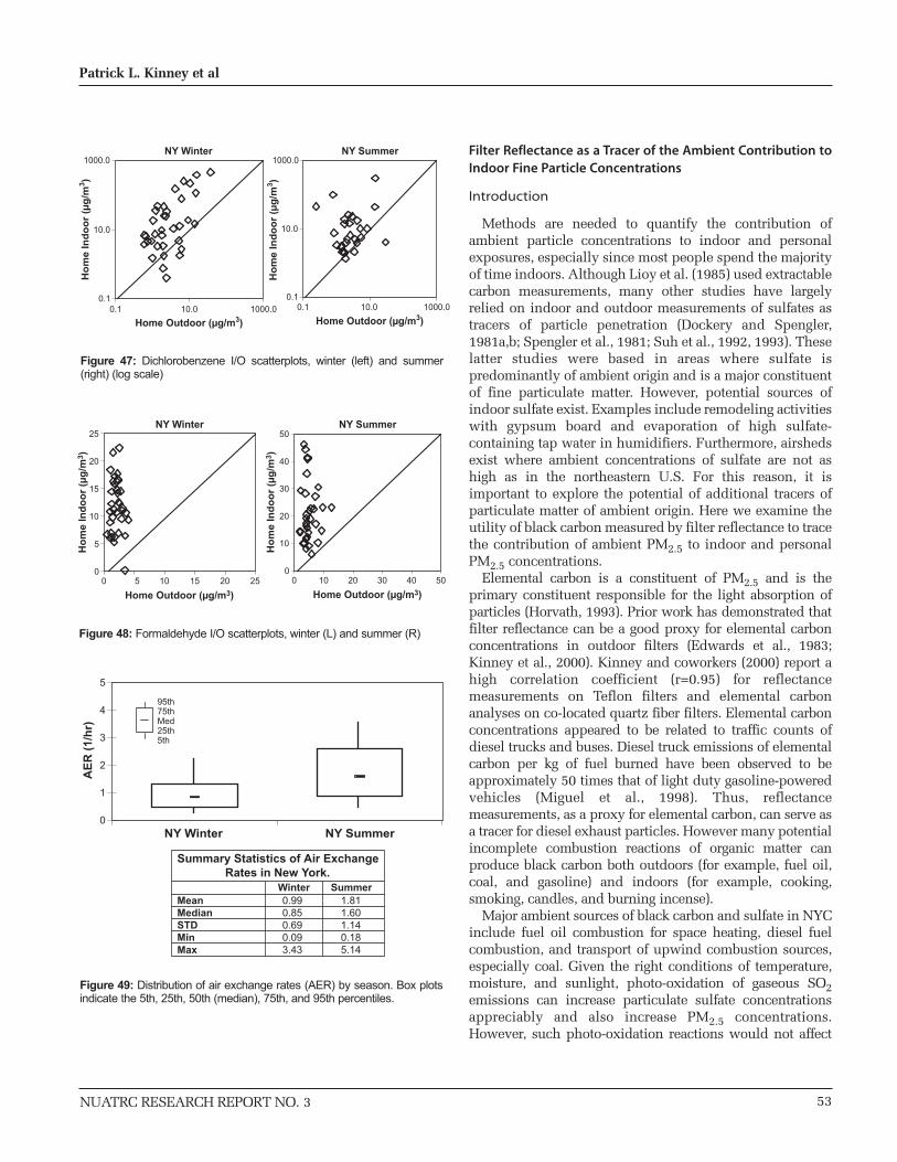
NUATRC RESEARCH REPORT NO. 3
Filter Reflectance as a Tracer of the Ambient Contribution toIndoor Fine Particle Concentrations
Introduction
Methods are needed to quantify the contribution ofambient particle concentrations to indoor and personalexposures, especially since most people spend the majorityof time indoors. Although Lioy et al. (1985) used extractablecarbon measurements, many other studies have largelyrelied on indoor and outdoor measurements of sulfates astracers of particle penetration (Dockery and Spengler,1981a,b; Spengler et al., 1981; Suh et al., 1992, 1993). Theselatter studies were based in areas where sulfate ispredominantly of ambient origin and is a major constituentof fine particulate matter. However, potential sources ofindoor sulfate exist. Examples include remodeling activitieswith gypsum board and evaporation of high sulfate-containing tap water in humidifiers. Furthermore, airshedsexist where ambient concentrations of sulfate are not ashigh as in the northeastern U.S. For this reason, it isimportant to explore the potential of additional tracers ofparticulate matter of ambient origin. Here we examine theutility of black carbon measured by filter reflectance to tracethe contribution of ambient PM2.5 to indoor and personalPM2.5 concentrations.
Elemental carbon is a constituent of PM2.5 and is theprimary constituent responsible for the light absorption ofparticles (Horvath, 1993). Prior work has demonstrated thatfilter reflectance can be a good proxy for elemental carbonconcentrations in outdoor filters (Edwards et al., 1983;Kinney et al., 2000). Kinney and coworkers (2000) report ahigh correlation coefficient (r=0.95) for reflectancemeasurements on Teflon filters and elemental carbonanalyses on co-located quartz fiber filters. Elemental carbonconcentrations appeared to be related to traffic counts ofdiesel trucks and buses. Diesel truck emissions of elementalcarbon per kg of fuel burned have been observed to beapproximately 50 times that of light duty gasoline-poweredvehicles (Miguel et al., 1998). Thus, reflectancemeasurements, as a proxy for elemental carbon, can serve asa tracer for diesel exhaust particles. However many potentialincomplete combustion reactions of organic matter canproduce black carbon both outdoors (for example, fuel oil,coal, and gasoline) and indoors (for example, cooking,smoking, candles, and burning incense).
Major ambient sources of black carbon and sulfate in NYCinclude fuel oil combustion for space heating, diesel fuelcombustion, and transport of upwind combustion sources,especially coal. Given the right conditions of temperature,moisture, and sunlight, photo-oxidation of gaseous SO2emissions can increase particulate sulfate concentrationsappreciably and also increase PM2.5 concentrations.However, such photo-oxidation reactions would not affect
53
Patrick L. Kinney et al
Ho
me
In
do
or
(µg
/m3)
0.1
10.0
1000.0
0.1 10.0 1000.0
Home Outdoor (µg/m3)
0.1
10.0
1000.0
0.1 10.0 1000.0
Ho
me
In
do
or
(µg
/m3)
Home Outdoor (µg/m3)
NY Winter NY Summer
Figure 47: Dichlorobenzene I/O scatterplots, winter (left) and summer(right) (log scale)
NY Summer
0
10
20
30
40
50
0 10 20 30 40 50
Home Outdoor (µg/m3)
NY Winter
0
5
10
15
20
25
0 5 10 15 20 25
Home Outdoor (µg/m3)
Ho
me I
nd
oo
r (µ
g/m
3)
Ho
me I
nd
oo
r (µ
g/m
3)
Figure 48: Formaldehyde I/O scatterplots, winter (L) and summer (R)
0
1
2
3
4
5
NY Winter
AE
R (
1/h
r)
NY Summer
25th5th
95th75th Med
Summary Statistics of Air ExchangeRates in New York.
MeanMedianSTDMinMax
0.99 1.810.85 1.600.69 1.140.09 0.183.43 5.14
Winter Summer
Figure 49: Distribution of air exchange rates (AER) by season. Box plotsindicate the 5th, 25th, 50th (median), 75th, and 95th percentiles.

black carbon concentrations. (Although higher summertimehumidity may play a role in accumulation rates of finerelemental carbon particles into larger ones, it would notaffect total mass of black carbon per volume of air.) Thus itis reasonable to expect that different relationships between
black carbon and PM2.5 exist in winter as opposed tosummer, while it is not obvious whether any seasonal affectshould be seen for the relationship between sulfate andPM2.5.
54
Toxic Exposure Assessment: A Columbia-Harvard (TEACH) Study (The New York City Report)
NUATRC RESEARCH REPORT NO. 3
0.0
0.5
1.0
1.5
2.0
2.5
Analyte
Low (<0.5 1/hr)
Medium (0.5-1.5 1/hr)
High (>1.5 1/hr)
Co Ni
La Be
Fe
Cs
Sb V
Abs Pb
Mn
Sc
Se
Mg S
Na Al
Pt
Ca
Cu Tl
Zn Ti
Cd
As
Cr
Ag
Sn
PM
2.5 K
Ind
oo
r-O
utd
oo
r R
atio
NY Winter
Analyte
0.0
0.5
1.0
1.5
2.0
2.5
3.0
l
Low (<0.5 1/hr)
Medium (0.5-1.5 1/hr)
High (>1.5 1/hr)
Co Ni
La Be
Fe
Cs
Sb V
Abs Pb
Mn
Sc
Se
Mg S
Na Al
Pt
Ca
Cu Tl
Zn Ti
Cd
As
Cr
Ag
Sn
PM
2.5 K
Ind
oo
r-O
utd
oo
r R
atio
NY Summer
Figure 50: Median ratios of indoor-to-outdoor concentrations of particle-associated air pollutants grouped by air exchange rate categories. winter = top;summer = bottom
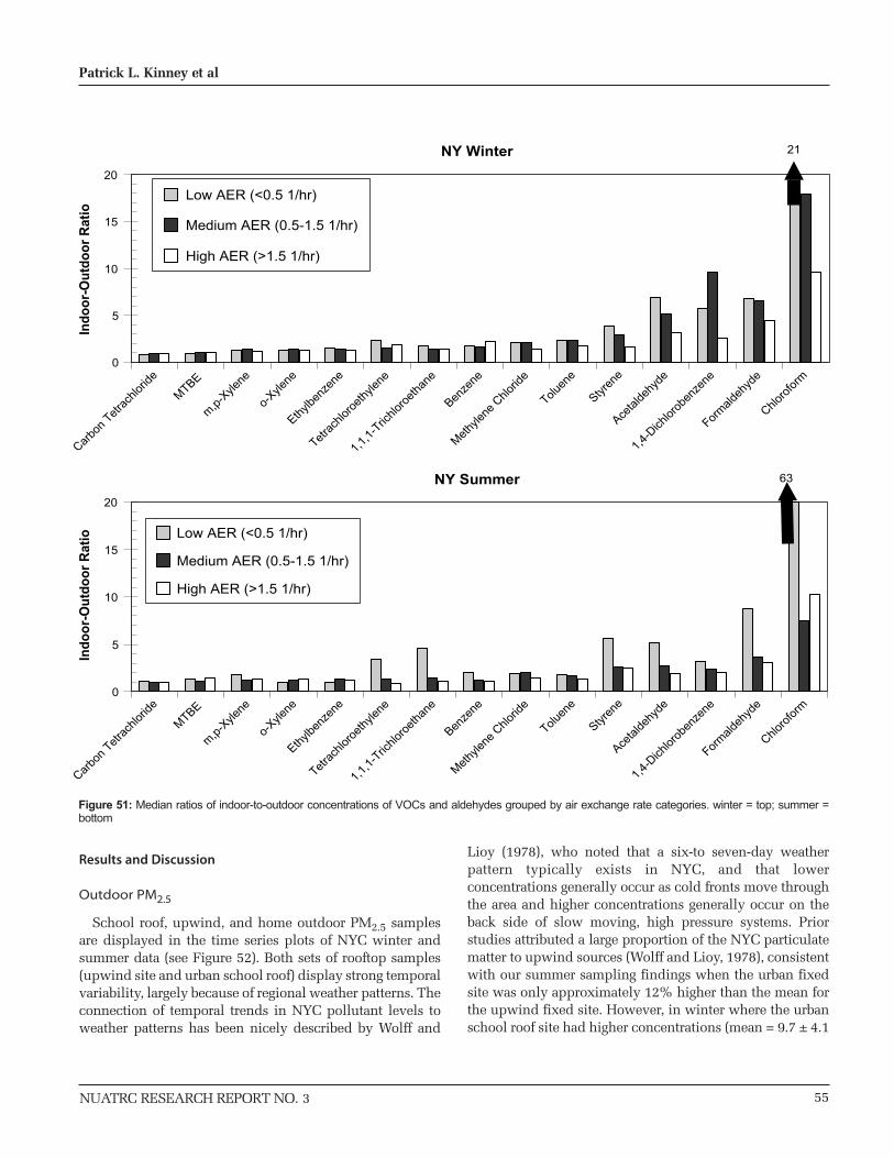
NUATRC RESEARCH REPORT NO. 3
Results and Discussion
Outdoor PM2.5
School roof, upwind, and home outdoor PM2.5 samplesare displayed in the time series plots of NYC winter andsummer data (see Figure 52). Both sets of rooftop samples(upwind site and urban school roof) display strong temporalvariability, largely because of regional weather patterns. Theconnection of temporal trends in NYC pollutant levels toweather patterns has been nicely described by Wolff and
Lioy (1978), who noted that a six-to seven-day weatherpattern typically exists in NYC, and that lowerconcentrations generally occur as cold fronts move throughthe area and higher concentrations generally occur on theback side of slow moving, high pressure systems. Priorstudies attributed a large proportion of the NYC particulatematter to upwind sources (Wolff and Lioy, 1978), consistentwith our summer sampling findings when the urban fixedsite was only approximately 12% higher than the mean forthe upwind fixed site. However, in winter where the urbanschool roof site had higher concentrations (mean = 9.7 ± 4.1
55
Patrick L. Kinney et al
0
5
10
15
20
Ind
oo
r-O
utd
oo
r R
atio
Low AER (<0.5 1/hr)
Medium AER (0.5-1.5 1/hr)
High AER (>1.5 1/hr)
21
NY Summer
NY Winter
0
5
10
15
20
Carbo
n Tet
rach
loride
MTBE
m,p
-Xyle
ne
o-Xyle
ne
Ethylb
enze
ne
Tetra
chlor
oeth
ylene
1,1,
1-Tric
hloro
etha
ne
Benze
ne
Met
hylen
e Chlo
ride
Toluen
e
Styren
e
Aceta
ldehy
de
1,4-
Dichlor
oben
zene
Form
aldeh
yde
Chloro
form
Carbo
n Tet
rach
loride
MTBE
m,p
-Xyle
ne
o-Xyle
ne
Ethylb
enze
ne
Tetra
chlor
oeth
ylene
1,1,
1-Tric
hloro
etha
ne
Benze
ne
Met
hylen
e Chlo
ride
Toluen
e
Styren
e
Aceta
ldehy
de
1,4-
Dichlor
oben
zene
Form
aldeh
yde
Chloro
form
Ind
oo
r-O
utd
oo
r R
atio Low AER (<0.5 1/hr)
Medium AER (0.5-1.5 1/hr)
High AER (>1.5 1/hr)
63
Figure 51: Median ratios of indoor-to-outdoor concentrations of VOCs and aldehydes grouped by air exchange rate categories. winter = top; summer =bottom

mg/m3) than the upwind site (6.3 ± 3.1 mg/m3), resultsindicated the urban contribution to be approximately aslarge as the background. Over the entire 8-week winterperiod, the mean PM2.5 concentration at the urban fixed sitewas approximately 54% higher than the mean for theupwind site. During the summer sampling, PM2.5concentrations were much higher on average than duringthe winter (15.6 and 9.7 µg/m3, respectively).
The time series plots also show the timing of individualhome outdoor measurements over the course of the study(indicated on the plot by open circles). The timing wasidentical to the other subject-based samples. The relevantpoint to draw from these plots is that, during the winter,individual sampling was timed so that the subject-based(personal, home indoor, and home outdoor) monitoringschedule captured the range of temporal variations inoutdoor concentrations identified from the rooftop timeseries. Consequently, the winter data presented here arerepresentative of the full range of winter conditions presentduring the sampling period.
In contrast, during the first six weeks of summermonitoring, the weekly subject-based monitoring happened
to fall on days of the week with the lowest PM2.5concentrations. Only during the last three weeks of summersampling (weeks seven, eight and nine) did the timing of thesubject-based monitoring not coincide with the lowestPM2.5 concentrations. Based on the description of Wolff andLioy (1978), it appears that the subject-based monitoring forthe first six weeks occurred during the passing of cold frontswhen photo-oxidation reactions would be less important. Incontrast, the subject-based monitoring for weeks seven,eight, and nine occurred on days when photo-oxidationreactions may have been more important.
Outdoor Reflectance
Outdoor modified absorbance samples are displayed as atime series plot for the NYC TEACH data in Figure 53. For,winter, temporal variability is observed for modifiedabsorbance in both sets of rooftop samples, with a similartiming to that observed for PM2.5 (see discussion for Figure52). Compared to the PM2.5 time series data, the differencein modified absorbance between the upwind site (mean =0.4 ± 0.4 m-1) and the school roof (mean =1.3 ± 0.5 m-1) wastypically larger, suggesting a relatively larger urban
56
Toxic Exposure Assessment: A Columbia-Harvard (TEACH) Study (The New York City Report)
NUATRC RESEARCH REPORT NO. 3
0
10
20
30
40
50
2/2/99 2/16/99 3/2/99 3/16/99 3/30/99 4/13/99
0
10
20
30
40
50
6/23/99 7/7/99 7/21/99 8/4/99 8/18/99 9/1/99
Date
Date
PM
2.5
(µg
/m3 )
PM
2.5
(µg
/m3 )
NY Summer PM2.5
NY Winter PM2.5
urban fixed siteupwind fixed sitehome outdoor
urban fixed siteupwind fixed sitehome outdoor
Figure 52: Time series plot for PM2.5 for New York winter and summer.Home outdoor is plotted for subject-based data. Unjoined data pointsindicate missing data.
NY Winter Absorbance
-0.5
0.5
1.5
2.5
3.5
4.5
2/2/1999 4/13/19993/30/19993/16/19993/2/19992/16/1999Date
Ab
s*((
1/m
) x
105 )
Ab
s*((
1/m
) x
105 )
NY Summer Absorbance
-0.5
0.5
1.5
2.5
3.5
4.5
6/23/1999 7/7/1999 7/21/1999 8/4/1999 8/18/1999 9/1/1999
Date
urban fixed siteupwind fixed sitehome outdoor
urban fixed siteupwind fixed sitehome outdoor
Figure 53: Time series plot for modified absorbance for New York winterand summer. Home outdoor is plotted for subject-based data.
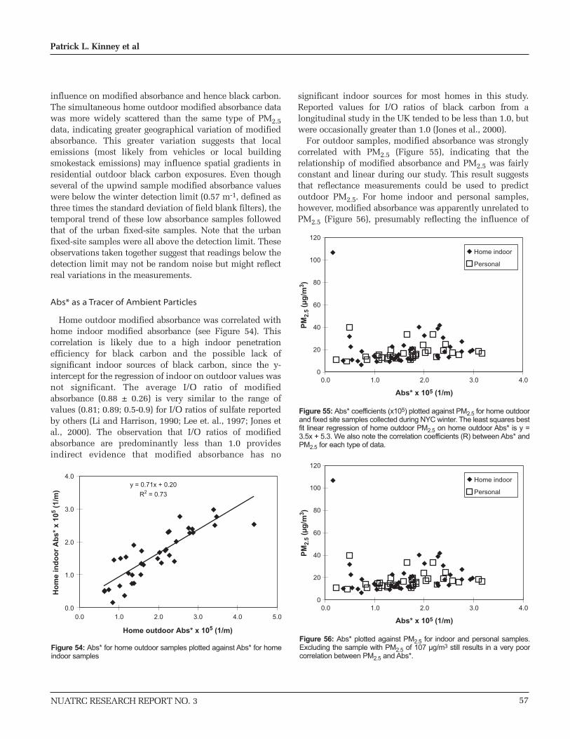
NUATRC RESEARCH REPORT NO. 3
influence on modified absorbance and hence black carbon.The simultaneous home outdoor modified absorbance datawas more widely scattered than the same type of PM2.5data, indicating greater geographical variation of modifiedabsorbance. This greater variation suggests that localemissions (most likely from vehicles or local buildingsmokestack emissions) may influence spatial gradients inresidential outdoor black carbon exposures. Even thoughseveral of the upwind sample modified absorbance valueswere below the winter detection limit (0.57 m-1, defined asthree times the standard deviation of field blank filters), thetemporal trend of these low absorbance samples followedthat of the urban fixed-site samples. Note that the urbanfixed-site samples were all above the detection limit. Theseobservations taken together suggest that readings below thedetection limit may not be random noise but might reflectreal variations in the measurements.
Abs* as a Tracer of Ambient Particles
Home outdoor modified absorbance was correlated withhome indoor modified absorbance (see Figure 54). Thiscorrelation is likely due to a high indoor penetrationefficiency for black carbon and the possible lack ofsignificant indoor sources of black carbon, since the y-intercept for the regression of indoor on outdoor values wasnot significant. The average I/O ratio of modifiedabsorbance (0.88 ± 0.26) is very similar to the range ofvalues (0.81; 0.89; 0.5-0.9) for I/O ratios of sulfate reportedby others (Li and Harrison, 1990; Lee et. al., 1997; Jones etal., 2000). The observation that I/O ratios of modifiedabsorbance are predominantly less than 1.0 providesindirect evidence that modified absorbance has no
significant indoor sources for most homes in this study.Reported values for I/O ratios of black carbon from alongitudinal study in the UK tended to be less than 1.0, butwere occasionally greater than 1.0 (Jones et al., 2000).
For outdoor samples, modified absorbance was stronglycorrelated with PM2.5 (Figure 55), indicating that therelationship of modified absorbance and PM2.5 was fairlyconstant and linear during our study. This result suggeststhat reflectance measurements could be used to predictoutdoor PM2.5. For home indoor and personal samples,however, modified absorbance was apparently unrelated toPM2.5 (Figure 56), presumably reflecting the influence of
57
Patrick L. Kinney et al
y = 0.71x + 0.20
R2 = 0.73
0.0
1.0
2.0
3.0
4.0
0.0 1.0 2.0 3.0 4.0 5.0
Ho
me
ind
oo
r A
bs*
x 1
05 (1
/m)
Home outdoor Abs* x 105 (1/m)
Figure 54: Abs* for home outdoor samples plotted against Abs* for homeindoor samples
0
20
40
60
80
100
120
0.0 1.0 2.0 3.0 4.0
Home indoor
Personal
PM
2.5
(µg
/m3 )
Abs* x 105 (1/m)
Figure 56: Abs* plotted against PM2.5 for indoor and personal samples.Excluding the sample with PM2.5 of 107 µg/m3 still results in a very poorcorrelation between PM2.5 and Abs*.
0
20
40
60
80
100
120
0.0 1.0 2.0 3.0 4.0
Home indoor
Personal
PM
2.5
(µg
/m3 )
Abs* x 105 (1/m)
Figure 55: Abs* coefficients (x105) plotted against PM2.5 for home outdoorand fixed site samples collected during NYC winter. The least squares bestfit linear regression of home outdoor PM2.5 on home outdoor Abs* is y =3.5x + 5.3. We also note the correlation coefficients (R) between Abs* andPM2.5 for each type of data.
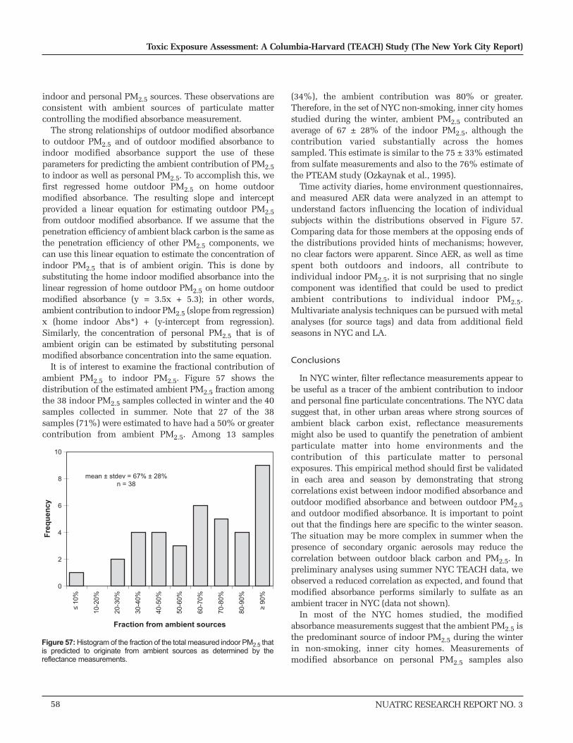
indoor and personal PM2.5 sources. These observations areconsistent with ambient sources of particulate mattercontrolling the modified absorbance measurement.
The strong relationships of outdoor modified absorbanceto outdoor PM2.5 and of outdoor modified absorbance toindoor modified absorbance support the use of theseparameters for predicting the ambient contribution of PM2.5to indoor as well as personal PM2.5. To accomplish this, wefirst regressed home outdoor PM2.5 on home outdoormodified absorbance. The resulting slope and interceptprovided a linear equation for estimating outdoor PM2.5from outdoor modified absorbance. If we assume that thepenetration efficiency of ambient black carbon is the same asthe penetration efficiency of other PM2.5 components, wecan use this linear equation to estimate the concentration ofindoor PM2.5 that is of ambient origin. This is done bysubstituting the home indoor modified absorbance into thelinear regression of home outdoor PM2.5 on home outdoormodified absorbance (y = 3.5x + 5.3); in other words,ambient contribution to indoor PM2.5 (slope from regression)x (home indoor Abs*) + (y-intercept from regression).Similarly, the concentration of personal PM2.5 that is ofambient origin can be estimated by substituting personalmodified absorbance concentration into the same equation.
It is of interest to examine the fractional contribution ofambient PM2.5 to indoor PM2.5. Figure 57 shows thedistribution of the estimated ambient PM2.5 fraction amongthe 38 indoor PM2.5 samples collected in winter and the 40samples collected in summer. Note that 27 of the 38samples (71%) were estimated to have had a 50% or greatercontribution from ambient PM2.5. Among 13 samples
(34%), the ambient contribution was 80% or greater.Therefore, in the set of NYC non-smoking, inner city homesstudied during the winter, ambient PM2.5 contributed anaverage of 67 ± 28% of the indoor PM2.5, although thecontribution varied substantially across the homessampled. This estimate is similar to the 75 ± 33% estimatedfrom sulfate measurements and also to the 76% estimate ofthe PTEAM study (Ozkaynak et al., 1995).
Time activity diaries, home environment questionnaires,and measured AER data were analyzed in an attempt tounderstand factors influencing the location of individualsubjects within the distributions observed in Figure 57.Comparing data for those members at the opposing ends ofthe distributions provided hints of mechanisms; however,no clear factors were apparent. Since AER, as well as timespent both outdoors and indoors, all contribute toindividual indoor PM2.5, it is not surprising that no singlecomponent was identified that could be used to predictambient contributions to individual indoor PM2.5.Multivariate analysis techniques can be pursued with metalanalyses (for source tags) and data from additional fieldseasons in NYC and LA.
Conclusions
In NYC winter, filter reflectance measurements appear tobe useful as a tracer of the ambient contribution to indoorand personal fine particulate concentrations. The NYC datasuggest that, in other urban areas where strong sources ofambient black carbon exist, reflectance measurementsmight also be used to quantify the penetration of ambientparticulate matter into home environments and thecontribution of this particulate matter to personalexposures. This empirical method should first be validatedin each area and season by demonstrating that strongcorrelations exist between indoor modified absorbance andoutdoor modified absorbance and between outdoor PM2.5and outdoor modified absorbance. It is important to pointout that the findings here are specific to the winter season.The situation may be more complex in summer when thepresence of secondary organic aerosols may reduce thecorrelation between outdoor black carbon and PM2.5. Inpreliminary analyses using summer NYC TEACH data, weobserved a reduced correlation as expected, and found thatmodified absorbance performs similarly to sulfate as anambient tracer in NYC (data not shown).
In most of the NYC homes studied, the modifiedabsorbance measurements suggest that the ambient PM2.5 isthe predominant source of indoor PM2.5 during the winterin non-smoking, inner city homes. Measurements ofmodified absorbance on personal PM2.5 samples also
58
Toxic Exposure Assessment: A Columbia-Harvard (TEACH) Study (The New York City Report)
NUATRC RESEARCH REPORT NO. 3
0
2
4
6
8
10
Fraction from ambient sources
Fre
qu
ency
mean ± stdev = 67% ± 28%n = 38
≤ 10
%
10-2
0%
20-3
0%
30-4
0%
40-5
0%
50-6
0%
60-7
0%
70-8
0%
80-9
0%
≥ 90
%
Figure 57: Histogram of the fraction of the total measured indoor PM2.5 thatis predicted to originate from ambient sources as determined by thereflectance measurements.

NUATRC RESEARCH REPORT NO. 3
suggest that the predominant source of personal exposure toPM2.5 originates from ambient sources of PM2.5. For non-ambient sources, the data are consistent with excess indoorPM2.5 being one, but not the only, source of excess personalPM2.5.
AMBIENT AIR MONITORING DATA
The NYC TEACH study operated two fixed-sitemonitoring stations. The urban fixed site was on or near theroof of A. Philip Randolph High School. The upwind fixedsite was located on a roof at the LDEO campus in Palisades,NYC. These sites were operated to evaluate the potential
contributions of both local and regional “synoptic” scalepollution to urban concentrations and to provide a basis forresolving the contribution of temporal variationcomponents to the subject-based measurements.
Descriptive Analyses
As a follow on from the previous overview section, moredetailed distributional information on all the ambientmeasurements is presented in Tables 29 through 38. Thesetables show mean, standard deviations, minimumconcentrations, 25th percentiles, median, 75th percentiles,and maximum concentrations for all ambient air pollutant
59
Patrick L. Kinney et al
Analyte1,1,1-Trichloroethane1,3-Butadiene1,4-DichlorobenzeneAcetaldehydeBenzeneCarbon TetrachlorideChloroformEthylbenzeneFormaldehydeMethylene ChlorideMTBEStyreneTetrachloroethyleneTolueneTrichloroethyleneo-Xylenem,p-Xylene
ND=not detected or zero value
Mean0.370.040.882.201.370.680.080.611.390.515.750.191.243.060.090.742.07
N1717172017171717201717171717171717
25th 75thMin0.26ND0.141.350.100.50ND0.140.44ND1.680.020.490.63ND0.180.46
STD0.070.160.480.600.910.150.070.360.600.413.050.120.622.170.130.451.26
Percentile0.30ND0.491.790.690.58ND0.300.890.243.720.090.791.48ND0.381.00
Median0.39ND0.872.111.170.650.090.561.380.444.860.171.082.54ND0.611.89
Max0.490.671.863.692.921.070.191.322.501.36
11.320.442.437.770.421.644.58
Percentile0.41ND1.152.571.900.770.110.921.930.827.030.251.453.890.191.032.95
Analyte1,1,1-Trichloroethane1,3-Butadiene1,4-DichlorobenzeneAcetaldehydeBenzeneCarbon TetrachlorideChloroformEthylbenzeneFormaldehydeMethylene ChlorideMTBEStyreneTetrachloroethyleneTolueneTrichloroethyleneo-Xylenem,p-Xylene
ND=not detected or zero value
Mean0.50ND0.764.880.270.570.060.825.030.648.170.141.314.000.090.852.46
N1919192419191919241919191919191919
25th 75thMinNDNDND2.24NDNDND0.181.89ND2.71NDNDNDND0.190.60
STD0.93ND0.521.710.630.210.080.582.730.763.860.131.123.100.140.631.80
Percentile0.28ND0.433.54ND0.45ND0.473.05ND5.56ND0.321.90ND0.491.30
Median0.37ND0.614.53ND0.48ND0.564.680.277.350.121.483.05ND0.521.72
Max6.15ND2.129.082.731.020.282.1614.12.9718.90.443.3810.10.362.336.64
Percentile0.41ND1.256.160.120.700.141.096.241.239.070.272.136.380.271.143.20
Summer Urban SiteConcentrations (µg/m3)
Winter Urban SiteConcentrations (µg/m3)
Table 29: New York ambient VOC and aldehyde data for urban fixed-site
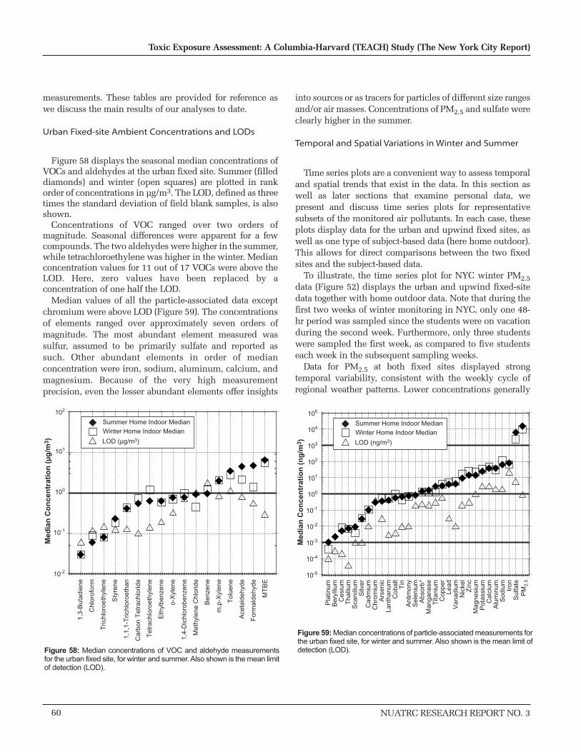
measurements. These tables are provided for reference aswe discuss the main results of our analyses to date.
Urban Fixed-site Ambient Concentrations and LODs
Figure 58 displays the seasonal median concentrations ofVOCs and aldehydes at the urban fixed site. Summer (filleddiamonds) and winter (open squares) are plotted in rankorder of concentrations in µg/m3. The LOD, defined as threetimes the standard deviation of field blank samples, is alsoshown.
Concentrations of VOC ranged over two orders ofmagnitude. Seasonal differences were apparent for a fewcompounds. The two aldehydes were higher in the summer,while tetrachloroethylene was higher in the winter. Medianconcentration values for 11 out of 17 VOCs were above theLOD. Here, zero values have been replaced by aconcentration of one half the LOD.
Median values of all the particle-associated data exceptchromium were above LOD (Figure 59). The concentrationsof elements ranged over approximately seven orders ofmagnitude. The most abundant element measured wassulfur, assumed to be primarily sulfate and reported assuch. Other abundant elements in order of medianconcentration were iron, sodium, aluminum, calcium, andmagnesium. Because of the very high measurementprecision, even the lesser abundant elements offer insights
into sources or as tracers for particles of different size rangesand/or air masses. Concentrations of PM2.5 and sulfate wereclearly higher in the summer.
Temporal and Spatial Variations in Winter and Summer
Time series plots are a convenient way to assess temporaland spatial trends that exist in the data. In this section aswell as later sections that examine personal data, wepresent and discuss time series plots for representativesubsets of the monitored air pollutants. In each case, theseplots display data for the urban and upwind fixed sites, aswell as one type of subject-based data (here home outdoor).This allows for direct comparisons between the two fixedsites and the subject-based data.
To illustrate, the time series plot for NYC winter PM2.5data (Figure 52) displays the urban and upwind fixed-sitedata together with home outdoor data. Note that during thefirst two weeks of winter monitoring in NYC, only one 48-hr period was sampled since the students were on vacationduring the second week. Furthermore, only three studentswere sampled the first week, as compared to five studentseach week in the subsequent sampling weeks.
Data for PM2.5 at both fixed sites displayed strongtemporal variability, consistent with the weekly cycle ofregional weather patterns. Lower concentrations generally
60
Toxic Exposure Assessment: A Columbia-Harvard (TEACH) Study (The New York City Report)
NUATRC RESEARCH REPORT NO. 3
102
101
100
10-2
10-1
1,3-
But
adie
ne
Tri
chlo
roe
thyl
en
e
1,1
,1-T
rich
loro
eth
an
Sty
ren
e
Car
bon
Tet
rach
lori
de
Met
hyle
ne C
hlor
ide
Ch
loro
form
Ben
zene
Eth
ylbe
nzen
e
o-X
yle
ne
Tet
rach
loro
ethy
lene
m,p
-Xyl
en
e
1,4-
Dic
hlor
oben
zene
To
lue
ne
Ace
tald
ehyd
e
MT
BE
For
mal
dehy
de
Summer Home Indoor Median
Winter Home Indoor Median
LOD (µg/m3)
Med
ian
Co
nce
ntr
atio
n (
µg
/m3 )
Figure 58: Median concentrations of VOC and aldehyde measurementsfor the urban fixed site, for winter and summer. Also shown is the mean limitof detection (LOD).
105
101
102
103
104
100
10-5
10-1
10-2
10-3
10-4
Summer Home Indoor Median
Winter Home Indoor Median
LOD (ng/m3)
Med
ian
Co
nce
ntr
atio
n (
ng
/m3 )
Pla
tinum
Ber
ylliu
mC
esiu
mT
halli
umS
cand
ium
Silv
erC
adm
ium
Chr
omiu
mA
rsen
icLa
ntha
num
Cob
alt
Tin
Ant
imon
yS
elen
ium
Abs
orb*
Man
gane
seT
itani
umC
oppe
rLe
adV
anad
ium
Nic
kel
Zin
cM
agne
sium
Pot
assi
umC
alci
umA
lum
inum
Sod
ium
Iro
nS
ulfa
teP
M2
.5
Figure 59: Median concentrations of particle-associated measurements forthe urban fixed site, for winter and summer. Also shown is the mean limit ofdetection (LOD).

NUATRC RESEARCH REPORT NO. 3
occurred as cold fronts moved through the area. Comparedwith the upwind fixed-site PM2.5 concentrations (mean ±standard deviation = 6.3 ± 3.1 µg/m3 in winter), the urbanfixed site had higher concentrations (mean ± standarddeviation = 9.7 ± 3.9 µg/m3), reflecting NYC urban inputsunder winter conditions. During the entire 8-week period,the mean PM2.5 concentration at the urban fixed site wasapproximately 54% higher than the mean for the upwindfixed site.
Another point to be extracted from the time series plot isthat the subject-based samples in NYC winter captured thefull range of temporal variations in outdoor concentrationsidentified from the urban fixed-site time series (that is low,medium, and high concentrations). This is indicated on
Figure 52. In contrast, during the NYC summer field season,the individual sampling events were, by chance, more oftencoincident with the troughs in PM2.5 concentrations.
A visual sense of the relative importance in the urban areaof temporal variability (over time at the urban fixed sites)versus spatial variability (across the home outdoor samplesduring each sampling period) can also be seen in this timeseries plot. For PM2.5, the dominance of temporal overspatial variability is visually evident. This visualcomparison is roughly equivalent to comparing thestandard deviations of the spatial and temporal signals. Toexamine this issue more quantitatively and for all analytes,the spatial variability of an air pollutant was determined. Todo this, the standard deviation of the home outdoor
61
Patrick L. Kinney et al
Analyte1,1,1-Trichloroethane1,3-Butadiene1,4-DichlorobenzeneAcetaldehydeBenzeneCarbon TetrachlorideChloroformEthylbenzeneFormaldehydeMethylene ChlorideMTBEStyreneTetrachloroethyleneTolueneTrichloroethyleneo-Xylenem,p-Xylene
ND=not detected or zero value
Mean0.33ND0.152.270.900.700.020.250.900.401.910.090.311.350.050.240.74
N1616162016161616201616161616161616
25th 75thMin0.22NDND0.77ND0.50ND0.030.30ND0.32NDND0.06ND0.030.05
STD0.08ND0.210.670.620.180.030.190.440.341.510.080.371.170.120.200.63
Percentile0.27NDND1.920.430.60ND0.100.60ND0.620.03ND0.34ND0.100.22
Median0.33ND0.012.230.820.67ND0.200.800.441.380.050.231.23ND0.180.58
Max0.53ND0.713.541.781.270.080.622.081.024.270.261.133.770.460.742.13
Percentile0.38ND0.292.681.480.730.050.351.130.673.510.160.521.930.040.381.11
Analyte1,1,1-Trichloroethane1,3-Butadiene1,4-DichlorobenzeneAcetaldehydeBenzeneCarbon TetrachlorideChloroformEthylbenzeneFormaldehydeMethylene ChlorideMTBEStyreneTetrachloroethyleneTolueneTrichloroethyleneo-Xylenem,p-Xylene
ND=not detected or zero value
Mean0.260.610.344.170.100.43ND0.393.790.493.440.030.201.93ND0.441.16
N1313132513131313251313131313131313
25th 75thMinNDNDND1.86NDNDNDND1.51ND1.40NDNDNDNDND0.16
STD0.231.271.051.600.360.26ND0.252.130.461.770.060.240.71ND0.380.90
PercentileNDNDND3.31ND0.28ND0.262.04ND1.88NDND1.42ND0.220.70
Median0.26NDND3.85ND0.51ND0.273.200.613.46ND0.211.92ND0.270.71
Max0.753.174.267.881.960.89ND0.858.881.9310.00.230.954.09ND1.293.24
Percentile0.43ND0.264.77ND0.60ND0.334.980.813.72ND0.412.29ND0.381.12
Summer Upwind SiteConcentrations (µg/m3)
Winter Upwind SiteConcentrations (µg/m3)
Table 30: New York ambient VOC and aldehyde data for upwind fixed-site

concentrations was calculated after first subtracting fromeach home value the urban fixed-site concentration valuefor the same sampling date. This was done to remove thetemporal component of variability. The temporalcomponent was computed as the standard deviation of theurban fixed-site data across all sampling periods for eachseason. Note that this method would tend to over-estimatethe relative magnitude of the temporal component, becausehomes were measured on only one 48-hour period eachweek, whereas the urban fixed-site data were available forup to three days each week (eight versus 20 days in winterand nine versus 25 days in summer). However, the methodprovides a simple way to compare spatial and temporalvariability. In the case of PM2.5, during the winter season
the spatial standard deviation was 2.75 µg/m3, while thetemporal standard deviation was 3.94 µg/m3, confirmingthe larger role played by temporal variations in PM2.5concentrations over the winter sampling period.
The PM2.5 concentrations were appreciably higher duringthe NYC summer field season than during the winter(difference for urban fixed site = 15.6 ± 9.6 µg/m3; upwindfixed site = 13.9 ± 2.7 µg/m3). Concentrations of PM2.5 werealso relatively similar in the two fixed sites during thesummer (only approximately 12% difference in means).This could be consistent with the influence of large upwindsource regions (Wolff and Lioy, 1978). It is also possible thatLDEO might have been downwind of NYC, since summersea breezes can blow up the Hudson River valley. Future
62
Toxic Exposure Assessment: A Columbia-Harvard (TEACH) Study (The New York City Report)
NUATRC RESEARCH REPORT NO. 3
Analyte1,1,1-Trichloroethane1,3-Butadiene1,4-DichlorobenzeneAcetaldehydeBenzeneCarbon TetrachlorideChloroformEthylbenzeneFormaldehydeMethylene ChlorideMTBEStyreneTetrachloroethyleneTolueneTrichloroethyleneo-Xylenem,p-Xylene
ND=not detected or zero value
Mean0.490.074.242.782.430.670.211.082.111.9110.90.362.235.660.321.253.72
N3131313631313131363131313131313131
25th 75thMin0.31ND0.541.540.210.47ND0.300.530.382.880.120.671.43ND0.371.07
STD0.260.206.560.871.200.110.200.470.853.495.280.201.822.660.250.641.69
Percentile0.35ND1.042.111.530.590.120.651.400.687.160.181.163.340.190.732.21
Median0.42ND1.822.682.420.650.171.002.200.9810.40.331.375.540.261.123.34
Max1.690.7534.15.434.930.971.001.954.0719.123.70.897.7610.21.002.456.83
Percentile0.53ND4.893.153.020.730.231.502.611.4214.30.512.847.930.401.745.16
Analyte1,1,1-Trichloroethane1,3-Butadiene1,4-DichlorobenzeneAcetaldehydeBenzeneCarbon TetrachlorideChloroformEthylbenzeneFormaldehydeMethylene ChlorideMTBEStyreneTetrachloroethyleneTolueneTrichloroethyleneo-Xylenem,p-Xylene
ND=not detected or zero value
Mean0.640.134.094.151.050.460.321.665.280.9912.70.229.196.870.141.804.99
N2727263627272726362727272727272627
25th 75thMinNDND0.221.42NDNDND0.511.90NDNDNDND1.50ND0.42ND
STD1.700.425.591.531.140.230.721.602.271.3713.80.13
32.063.490.221.745.45
Percentile0.21ND1.483.25ND0.430.000.844.060.306.210.160.814.11ND0.902.44
Median0.33ND1.944.070.780.530.001.324.580.5110.90.251.376.22ND1.464.04
Max9.121.9926.510.14.490.843.308.8612.76.6573.00.4616714.30.719.5430.0
Percentile0.44ND3.714.551.720.570.301.926.321.1913.90.292.439.780.381.905.84
Summer Home OutdoorConcentrations (µg/m3)
Winter Home OutdoorConcentrations (µg/m3)
Table 31: New York ambient VOC and aldehyde data for home outdoor sites

NUATRC RESEARCH REPORT NO. 3
investigations will examine this latter possibility in twoways: first by obtaining mean hourly meteorological dataand second by looking at times series data of ambient tracergases measured by other investigators at LDEO. In priorstudies, these other investigators observed large increases inambient fluorocarbon concentrations when winds blewfrom the south-south-west (that is up the Hudson Riverfrom the metropolitan area) as compared to thepredominant wind directions from the northwest tosouthwest (Ho et al., 1998). The time series data of ambienttracer gases exists for our study period.
Although we plan to investigate the latter possibility asoutlined above, the former possibility, namely that thesummertime similarity in PM2.5 concentrations between thetwo fixed sites was due to an increase in upwind regionalsource strength, is supported by an examination of timeseries plots of sulfate and modified absorbance (Figures 52and 60). At first glance, the sulfate time series appear verysimilar to those of PM2.5, with sulfate having the same cycleof temporal variability in each season. However, the relativesummer season increase was much larger for sulfate than forPM2.5. Consistent with this larger increase, concentrations
of summertime sulfate at the two fixed sites were even moresimilar than they were for PM2.5, although the “upwind”fixed site sometimes had greater sulfate concentrations thanthe urban fixed site (for example, weeks three and eight ofthe summer field season). Furthermore, the generally verysmall variation in home outdoor sulfate concentrations onany given week during the summer suggests only a smallamount of geographic variability. All of these observationsare consistent with stronger source emissions from large-scale upwind regions (midwest coal-burning plants duringpeak summer demand), weaker local emissions (lack oflocal combustion of fuel oil and coal as compared to winterheating), and/or with a more stable air mass in the summer.The concept of a stability index has been used by Leadereret al., (1978) and others to show that the strength of urbanparticulate sources is difficult to directly quantify duringNYC winters because of the strong dispersive effects causedby meteorological conditions (relatively large values forwind speed). Mean daily wind speeds during the winterstudy period ranged from 4.2 to 20.5 km per hour.
In contrast, black carbon concentrations (represented bymodified absorbance measurements) were similar duringthe two seasons (Figure 53). Concentrations were almostalways appreciably greater at the urban fixed site than at the“upwind” fixed site, and the relative differences betweenthe fixed sites were somewhat larger in winter thansummer. These observations do not appear to be consistentwith the “upwind fixed site” being downwind of NYC. Theobservations are consistent with large local urban source(s)for black carbon in winter and summer. Temporalvariability was observed for black carbon in both sets ofrooftop samples, with the timing for high and lowconcentrations similar to that observed for PM2.5 andsulfate. However, the magnitude of the temporal variationwas much smaller for black carbon than for PM2.5 andsulfate. The relative differences between the upwind siteand the urban fixed site were typically larger for blackcarbon than PM2.5, suggesting relatively larger urbaninfluence on black carbon than on PM2.5. Relative to theamount of temporal variation, the spatial variation asindicated by the variation in the home outdoor sampleseach week was also greater for black carbon than for PM2.5.The spatial variation in black carbon concentrations wasalso greater than the temporal variation in both seasons. Thestandard deviation of the home outdoor samples aftercorrecting each value for the coincident urban fixed-siteconcentration was 0.85 m-1 in winter and 0.64 m-1 insummer, both larger than the temporal variationrepresented by the standard deviation of the urban fixed site(0.51 m-1 and 0.44 m-1 respectively for winter and summer).This suggests that local emissions of black carbon from
63
Patrick L. Kinney et al
NY Winter Sulfate
0
7000
14000
21000
28000
2/2/199 2/16/199 3/2/199 3/16/199 3/30/199 4/13/1999Date
NY Summer Sulfate
0
7000
14000
21000
28000
6/23/199 7/7/199 7/21/199 8/4/1999 8/18/1999 9/1/1999Date
SO
4 (n
g/m
3 )S
O4
(ng
/m3 )
urban fixed siteupwind fixed sitehome outdoor
urban fixed siteupwind fixed sitehome outdoor
Figure 60: Time series plot for sulfate for New York winter and summer.Home outdoor is plotted for subject-based data.

diesel vehicles, building heating boilers, and other largecombustion sources probably influence spatial gradients inhome outdoor black carbon exposures.
Time series plots of particle-associated HAPs that displayeither predominantly local or predominantly regionalsource influences are displayed in Figure 61 (cobalt in NYCwinter and summer) and Figure 62 (arsenic and seleniumfor NYC summer only), respectively. Cobalt concentrationswere appreciably higher in the winter than the summer atthe urban fixed site and in home outdoor samples. Incontrast, the range in cobalt concentrations at the upwindfixed site was similar during the two seasons. Obviously,the difference in concentrations between the two fixed siteswas much greater in the winter season. In the winter season,the spatial variability in the home outdoor samples(standard deviation = 0.84 ng/m3) was greater than thetemporal variability in the urban fixed site (standarddeviation = 0.36 ng/m3). Similarity of the spatial variability(0.42 ng/m3) to temporal variability (0.31 ng/m3) was greaterin summer, with both temporal and spatial summervariability being less than that observed for the winter
season. Together these observations suggest that urbansources for cobalt are stronger during the winter season.Fuel oils have been identified as an important source ofcobalt. However, it is unclear whether heating oils anddiesel fuel oils used in NYC differ in trace metalcomposition. Hopefully the seasonal increase in heating oiluse in the winter will allow us to investigate whether suchdifferences exist.
Arsenic and selenium concentrations were measuredonly in NYC summer, when they displayed a lack of anysignificant spatial variability both among home outdoormeasurements made on the same day and between the twofixed sites. The lack of spatial variability together withstrong temporal signals is consistent with these elementsbeing controlled by regional rather local urban sources.Similar to findings for summer sulfate concentrations at the“upwind” fixed site, a few of the upwind fixed-site samples(four out of 25) had appreciably greater concentrations thanthose measured on the same dates at the urban fixed site.Electric power generation from coal combustion in theMidwest has been identified as an important upwind
64
Toxic Exposure Assessment: A Columbia-Harvard (TEACH) Study (The New York City Report)
NUATRC RESEARCH REPORT NO. 3
AnalytePM2.5 (µg/m3)Abs (1/m * 105)Aluminum (Al)Antimony (Sb)Arsenic (As)Beryllium (Be)Cadmium (Cd)Calcium (Ca)Cesium (Cs)Chromium (Cr)Cobalt (Co)Copper (Cu)Iron (Fe)Lanthanum (La)Lead (Pb)Magnesium (Mg)Manganese (Mn)Nickel (Ni)Platinum (Pt)Potassium (K)Scandium (Sc)Selenium (Se)Silver (Ag)Sodium (Na)Sulfur (S)Thallium (Tl)Tin (Sn)Titanium (Ti)Vanadium (V)Zinc (Zn)
Mean9.71.3231
1.09
0.15447
0.0088
1.024.570
0.526.1922.92.2218.5
0.000637
0.005
0.045113851
0.00900.681.505.7524.6
N2020202000
2020200
20202020201820202020200
206
201820202020
25th 75thMin3.80.3910
0.27
0.02316
0.0023
0.481.421
0.252.559.60.398.1
0.000015
0.001
0.01271288
0.00020.180.391.3610.1
STD3.9
0.5115
0.98
0.10816
0.0054
0.362.532
0.202.826.8
3.046.9
0.000515
0.003
0.03632431
0.00900.630.952.129.1
Percentile6.50.9620
0.58
0.08035
0.0042
0.812.944
0.373.9317.81.0414.1
0.000228
0.002
0.01979522
0.00340.280.784.2417.8
Median9.4
1.2931
0.70
0.10748
0.0082
0.943.966
0.515.0321.51.2716.9
0.000434
0.004
0.032119798
0.00700.411.276.1324.7
Max17.92.2173
4.34
0.39976
0.0225
1.7111.11321.02
11.5534.2
14.4633.2
0.001771
0.012
0.150150
20030.0365
2.154.039.5548.0
Percentile11.51.7338
1.33
0.21257
0.0108
1.215.781
0.638.4528.81.9923.9
0.000941
0.006
0.0601391010
0.00990.682.026.8229.5
Urban Site WinterConcentrations (ng/m3) unless otherwise stated
Table 32: Descriptive statistics for New York winter urban fixed-site data forPM2.5, modified absorbance, and particle-associated elements. Refer toTables 5, 6, and 7 for information on LODs.
AnalytePM2.5 (µg/m3)Abs (1/m * 105)Aluminum (Al)Antimony (Sb)Arsenic (As)Beryllium (Be)Cadmium (Cd)Calcium (Ca)Cesium (Cs)Chromium (Cr)Cobalt (Co)Copper (Cu)Iron (Fe)Lanthanum (La)Lead (Pb)Magnesium (Mg)Manganese (Mn)Nickel (Ni)Platinum (Pt)Potassium (K)Scandium (Sc)Selenium (Se)Silver (Ag)Sodium (Na)Sulfur (S)Thallium (Tl)Tin (Sn)Titanium (Ti)Vanadium (V)Zinc (Zn)
Mean15.61.4761
0.970.42
0.00330.107
390.00840.440.653.899
0.475.0513.91.9610.6
0.001032
0.0140.92
0.02992
21180.00880.734.604.7014.2
N2525252525232525252525252525253
2525243
25252525252525252525
25th 75thMin3.7
0.7113
0.480.18
0.00070.043
140.0012
0.030.301.346
0.252.3312.90.575.5
0.000018
0.0020.130.012
21270
0.00190.210.941.328.7
STD9.6
0.4496
0.690.19
0.00360.048
210.01100.550.312.456
0.213.660.9
1.154.4
0.000419
0.0170.680.014
751591
0.00670.416.332.823.3
Percentile9.4
1.2322
0.610.27
0.00150.066
260.00370.120.402.366
0.323.0412.91.267.1
0.000818
0.0050.380.018
491054
0.00460.412.122.5811.4
Median14.91.4339
0.760.36
0.00230.101
380.00520.300.573.280
0.413.9114.31.699.3
0.001025
0.0090.830.028
642064
0.00730.672.914.1714.3
Max40.12.424243.891.03
0.01820.248114
0.05162.691.6612.02791.04
18.4914.55.5721.4
0.001754
0.0752.85
0.055258
63400.0348
1.7228.1612.0820.0
Percentile19.61.6950
1.050.53
0.00440.137
430.0076
0.500.814.51160.585.2914.52.2612.9
0.001354
0.0141.33
0.04078
25820.0105
0.893.986.6816.7
Urban Site SummerConcentrations (ng/m3) unless otherwise stated
Table 33: Descriptive statistics for New York summer urban fixed-site datafor PM2.5, modified absorbance, and particle-associated elements. Refer toTables 5, 6, and 7 for information on LODs.

NUATRC RESEARCH REPORT NO. 3
source of sulfate, and selenium and arsenic are importanttrace elements in coal.
It is interesting to note that while particle-associated airpollutants with important regional sources (PM2.5, sulfate,arsenic, and selenium) all showed prominent peaks inconcentrations in the first week of July of the summerseason. These peaks are either much subdued or totallymissing for particle-associated air pollutants dominated bylocal urban sources such as cobalt and black carbon.
Figures 63 through 65 present time series plots for VOCs.Methyl tertiary butyl ether, formaldehyde, andacetaldehyde are highlighted. Concentrations of MTBE atindividual home outdoor locations were quite variable andoften higher than the urban fixed-site measurements,apparently reflecting the influence of different local urbansources on homes throughout the city. The temporalvariability in the urban fixed site was less than or equal tothe spatial variability shown in the home outdoormeasurements. Similar to the time series plots of cobalt andmodified absorbance in NYC summer, MTBE did not
display the prominent concentration peaks in the first weekof July observed for many of the particle-associatedelements with regional sources.
Time series plots for formaldehyde and acetaldehydedisplay many of the characteristics discussed previously forthose particle-associated air pollutants with importantregional sources, namely, relative lack of spatial variabilityof home outdoor measurements, relatively small differencesbetween fixed-site concentrations, and strong temporalvariability including a prominent concentration peak in thefirst week of July. As with sulfate, the formation offormaldehyde and acetaldehyde from precursor pollutantsis enhanced under summer conditions of increasedsunlight, temperature, and humidity, and all had greatlyenhanced ambient concentrations in the summer (Viskari etal., 2000; Zhang et al., 1994).
Although the time series plots for most BETX+compounds are not shown in graphical form, with thepossible exception of benzene the temporal variability of allof the BETX+ compounds was very similar (that is, peak
65
Patrick L. Kinney et al
NY Winter Cobalt
0
1
2
3
4
2/2/1999 2/16/1999 3/2/1999 3/16/1999 3/30/1999 4/13/1999
Date
NY Summer Cobalt
0
1
2
3
4
6/23/1999 7/7/1999 7/21/1999 8/4/1999 8/18/1999 9/1/1999
Date
Co
(n
g/m
3 )C
o (
ng
/m3 )
urban fixed siteupwind fixed sitehome outdoor
urban fixed siteupwind fixed sitehome outdoor
Figure 61: Time series plot for cobalt for New York winter and summer.Home outdoor is plotted for subject-based data. Unjoined data pointsindicated missing data.
NY Summer Arsenic
0
0.4
0.8
1.2
6/23/1999 7/7/1999 7/21/1999 8/4/1999 8/18/1999 9/1/1999
Date
As
(ng
/m3 )
Se
(ng
/m3 )
NY Summer Selenium
0
1
2
3
4
6/23/1999 7/7/1999 7/21/1999 8/4/1999 8/18/1999 9/1/1999
Date
urban fixed siteupwind fixed sitehome outdoor
urban fixed siteupwind fixed sitehome outdoor
Figure 62: Time series plot for arsenic and selenium for New York summer.Home outdoor is plotted for subject-based data.
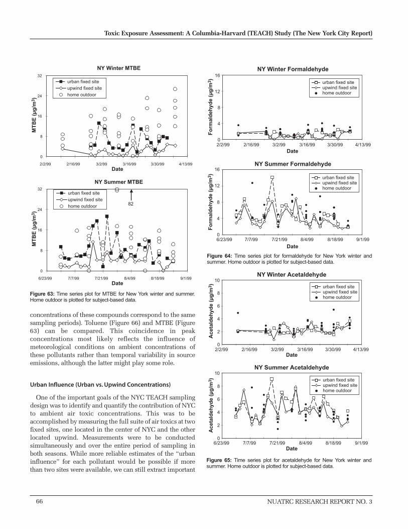
concentrations of these compounds correspond to the samesampling periods). Toluene (Figure 66) and MTBE (Figure63) can be compared. This coincidence in peakconcentrations most likely reflects the influence ofmeteorological conditions on ambient concentrations ofthese pollutants rather than temporal variability in sourceemissions, although the latter might play some role.
Urban Influence (Urban vs. Upwind Concentrations)
One of the important goals of the NYC TEACH samplingdesign was to identify and quantify the contribution of NYCto ambient air toxic concentrations. This was to beaccomplished by measuring the full suite of air toxics at twofixed sites, one located in the center of NYC and the otherlocated upwind. Measurements were to be conductedsimultaneously and over the entire period of sampling inboth seasons. While more reliable estimates of the “urbaninfluence” for each pollutant would be possible if morethan two sites were available, we can still extract important
66
Toxic Exposure Assessment: A Columbia-Harvard (TEACH) Study (The New York City Report)
NUATRC RESEARCH REPORT NO. 3
NY Winter MTBE
0
8
16
24
32
2/2/99 2/16/99 3/2/99 3/16/99 3/30/99 4/13/99Date
MT
BE
(µ
g/m
3 )
urban fixed siteupwind fixed sitehome outdoor
NY Summer MTBE
0
8
16
24
32
6/23/99 7/7/99 7/21/99 8/4/99 8/18/99 9/1/99Date
MT
BE
(µ
g/m
3 )
urban fixed siteupwind fixed sitehome outdoor 82
Figure 63: Time series plot for MTBE for New York winter and summer.Home outdoor is plotted for subject-based data.
NY Winter Formaldehyde
0
4
8
12
16
2/2/99 2/16/99 3/2/99 3/16/99 3/30/99 4/13/99
NY Summer Formaldehyde
0
4
8
12
16
6/23/99 7/7/99 7/21/99 8/4/99 8/18/99 9/1/99
Date
Fo
rmal
deh
yde
(µg
/m3 )
Date
Fo
rmal
deh
yde
(µg
/m3 ) urban fixed site
upwind fixed sitehome outdoor
urban fixed siteupwind fixed sitehome outdoor
Figure 64: Time series plot for formaldehyde for New York winter andsummer. Home outdoor is plotted for subject-based data.
NY Winter Acetaldehyde
0
2
4
6
8
10
2/2/99 2/16/99 3/2/99 3/16/99 3/30/99 4/13/99Date
NY Summer Acetaldehyde
0
2
4
6
8
10
6/23/99 7/7/99 7/21/99 8/4/99 8/18/99 9/1/99Date
Ace
tald
ehyd
e (µ
g/m
3 )A
ceta
ldeh
yde
(µg
/m3 ) urban fixed site
upwind fixed sitehome outdoor
urban fixed siteupwind fixed sitehome outdoor
Figure 65: Time series plot for acetaldehyde for New York winter andsummer. Home outdoor is plotted for subject-based data.
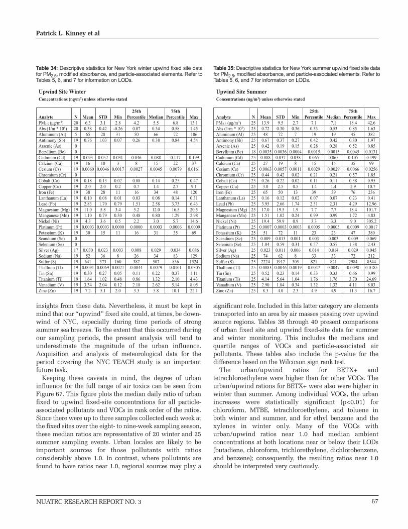
NUATRC RESEARCH REPORT NO. 3
insights from these data. Nevertheless, it must be kept inmind that our “upwind” fixed site could, at times, be down-wind of NYC, especially during time periods of strongsummer sea breezes. To the extent that this occurred duringour sampling periods, the present analysis will tend tounderestimate the magnitude of the urban influence.Acquisition and analysis of meteorological data for theperiod covering the NYC TEACH study is an importantfuture task.
Keeping these caveats in mind, the degree of urbaninfluence for the full range of air toxics can be seen fromFigure 67. This figure plots the median daily ratio of urbanfixed to upwind fixed-site concentrations for all particle-associated pollutants and VOCs in rank order of the ratios.Since there were up to three samples collected each week atthe fixed sites over the eight- to nine-week sampling season,these median ratios are representative of 20 winter and 25summer sampling events. Urban locales are likely to beimportant sources for those pollutants with ratiosconsiderably above 1.0. In contrast, where pollutants arefound to have ratios near 1.0, regional sources may play a
significant role. Included in this latter category are elementstransported into an area by air masses passing over upwindsource regions. Tables 38 through 40 present comparisonsof urban fixed site and upwind fixed-site data for summerand winter monitoring. This includes the medians andquartile ranges of VOCs and particle-associated airpollutants. These tables also include the p-value for thedifference based on the Wilcoxon sign rank test.
The urban/upwind ratios for BETX+ andtetrachloroethylene were higher than for other VOCs. Theurban/upwind rations for BETX+ were also were higher inwinter than summer. Among individual VOCs, the urbanincreases were statistically significant (p<0.01) forchloroform, MTBE, tetrachloroethylene, and toluene inboth winter and summer, and for ethyl benzene and thexylenes in winter only. Many of the VOCs withurban/upwind ratios near 1.0 had median ambientconcentrations at both locations near or below their LODs(butadiene, chloroform, trichlorethylene, dichlorobenzene,and benzene); consequently, the resulting ratios near 1.0should be interpreted very cautiously.
67
Patrick L. Kinney et al
AnalytePM2.5 (µg/m3)Abs (1/m * 105)Aluminum (Al)Antimony (Sb)Arsenic (As)Beryllium (Be)Cadmium (Cd)Calcium (Ca)Cesium (Cs)Chromium (Cr)Cobalt (Co)Copper (Cu)Iron (Fe)Lanthanum (La)Lead (Pb)Magnesium (Mg)Manganese (Mn)Nickel (Ni)Platinum (Pt)Potassium (K)Scandium (Sc)Selenium (Se)Silver (Ag)Sodium (Na)Sulfur (S)Thallium (Tl)Tin (Sn)Titanium (Ti)Vanadium (V)Zinc (Zn)
Mean6.30.3865
0.76
0.09316
0.0060.
0.182.038
0.102.8311.01.104.3
0.000330
0.03052
6410.00910.301.643.347.2
N20205
1900
1919190
1919191919191919191900
1719191919191919
25th 75thMin2.8
-0.2631
0.07
0.0313
0.0017.
0.020.211
0.010.793.40.300.5
0.000011
0.0038
1600.0027
0.050.480.122.0
STD3.1
0.4228
1.03
0.05210
0.0046.
0.132.028
0.081.705.8
0.793.6
0.000315
0.02336373
0.00690.271.022.045.1
Percentile4.20.0750
0.26
0.0468
0.0027.
0.080.716
0.031.515.20.482.2
0.000016
0.00826387
0.00440.110.862.183.3
Median5.5
0.3466
0.38
0.08815
0.0045.
0.141.434
0.082.5812.00.803.0
0.000331
0.02934507
0.00790.221.322.625.8
Max13.11.451064.54
0.19937
0.0161.
0.479.11200.316.4320.52.9814.6
0.000969
0.086129
15240.0305
1.114.438.0522.1
Percentile6.80.5872
0.84
0.11722
0.0079.
0.252.748
0.143.7316.51.295.7
0.000635
0.03483836
0.01010.372.105.1410.1
Upwind Site WinterConcentrations (ng/m3) unless otherwise stated
Table 34: Descriptive statistics for New York winter upwind fixed site datafor PM2.5, modified absorbance, and particle-associated elements. Refer toTables 5, 6, and 7 for information on LODs.
AnalytePM2.5 (µg/m3)Abs (1/m * 105)Aluminum (Al)Antimony (Sb)Arsenic (As)Beryllium (Be)Cadmium (Cd)Calcium (Ca)Cesium (Cs)Chromium (Cr)Cobalt (Co)Copper (Cu)Iron (Fe)Lanthanum (La)Lead (Pb)Magnesium (Mg)Manganese (Mn)Nickel (Ni)Platinum (Pt)Potassium (K)Scandium (Sc)Selenium (Se)Silver (Ag)Sodium (Na)Sulfur (S)Thallium (Tl)Tin (Sn)Titanium (Ti)Vanadium (V)Zinc (Zn)
Mean13.90.7248
0.670.42
0.00350.088
270.00630.440.263.065
0.163.9517.01.5119.4
0.000751
0.0091.04
0.02374
22240.00830.524.142.908.3
N252525252518252525252525252525252525252525252525252525252525
25th 75thMin2.7
0.367
0.270.15
0.00040.038
80.0011
0.020.020.513
0.021.741.9
0.240.9
0.000311
0.0010.310.006
8305
0.00190.141.040.342.3
STD9.5
0.3072
0.370.19
0.00360.037
190.00570.420.222.550
0.122.6619.51.0259.9
0.000372
0.0130.590.011
621912
0.00460.235.641.844.0
Percentile7.1
0.5319
0.420.28
0.00150.065
150.00290.210.111.439
0.072.317.7
0.993.3
0.000523
0.0030.570.014
33821
0.00470.331.761.324.9
Median7.1
0.5319
0.420.28
0.00150.065
150.00290.210.111.439
0.072.317.7
0.993.3
0.000523
0.0030.570.014
33821
0.00470.331.761.324.9
Max42.61.633821.970.85
0.01310.199
990.0256
1.850.9510.72360.41
12.96101.74.83
305.20.0017
3800.0692.43
0.045212
85440.0185
0.9924.698.0316.7
Percentile18.40.8545
0.800.52
0.00450.105
350.0066
0.570.382.976
0.234.2918.41.729.0
0.000947
0.0091.38
0.02972
29840.0098
0.663.704.1111.3
Upwind Site SummerConcentrations (ng/m3) unless otherwise stated
Table 35: Descriptive statistics for New York summer upwind fixed site datafor PM2.5, modified absorbance, and particle-associated elements. Refer toTables 5, 6, and 7 for information on LODs.

For particulate matter and associated elements, the rankordering of median ratios is quite informative. Elementsassociated with regional pollution are at the left side ofFigure 67 (where ratios are near 1.0). In this group are
elements associated with electric power generation throughcoal combustion, including selenium and arsenic. On theright side of the figure are elements having more local urbansources. Included are tracers for heating oil combustion,
68
Toxic Exposure Assessment: A Columbia-Harvard (TEACH) Study (The New York City Report)
NUATRC RESEARCH REPORT NO. 3
AnalytePM2.5 (µg/m3)Abs (1/m * 105)Aluminum (Al)Antimony (Sb)Arsenic (As)Beryllium (Be)Cadmium (Cd)Calcium (Ca)Cesium (Cs)Chromium (Cr)Cobalt (Co)Copper (Cu)Iron (Fe)Lanthanum (La)Lead (Pb)Magnesium (Mg)Manganese (Mn)Nickel (Ni)Platinum (Pt)Potassium (K)Scandium (Sc)Selenium (Se)Silver (Ag)Sodium (Na)Sulfur (S)Thallium (Tl)Tin (Sn)Titanium (Ti)Vanadium (V)Zinc (Zn)
Mean11.91.9440
1.48
0.15765
0.0105
1.596.01070.816.9630.02.3532.3
0.000844
0.006
0.059117840
0.01420.792.457.6835.8
N3737363600
3636360
36363636363636363636360
3622362736363636
25th 75thMin5.50.6315
0.51
0.04029
0.0034
0.422.231
0.202.2112.60.726.6
0.000121
0.002
0.02232276
0.00510.150.922.359.2
STD3.8
0.9117
1.04
0.09231
0.0052
0.783.041
0.493.2714.00.9422.4
0.000817
0.004
0.04370352
0.00940.561.653.1429.0
Percentile8.81.2428
1.02
0.09542
0.0067
1.013.875
0.454.2420.21.6217.5
0.000332
0.004
0.03465518
0.00850.441.525.1319.2
Median12.51.9837
1.23
0.13655
0.0100
1.475.31000.716.5024.32.1728.0
0.000640
0.006
0.044108807
0.01040.621.947.6727.1
Max20.54.4292
6.40
0.402166
0.0254
3.6815.91892.27
14.6269.85.02
103.40.0047
840.017
0.203295
16060.0372
2.3910.0417.08159.6
Percentile13.92.4550
1.49
0.17880
0.0130
2.097.01361.069.3239.42.9836.7
0.001056
0.007
0.0661561035
0.01620.942.948.9939.5
Home Outdoor WinterConcentrations (ng/m3) unless otherwise stated
Table 36: Descriptive statistics for New York winter home outdoor data forPM2.5, modified absorbance, and particle-associated elements. Refer toTables 5, 6, and 7 for information on LODs.
AnalytePM2.5 (µg/m3)Abs (1/m * 105)Aluminum (Al)Antimony (Sb)Arsenic (As)Beryllium (Be)Cadmium (Cd)Calcium (Ca)Cesium (Cs)Chromium (Cr)Cobalt (Co)Copper (Cu)Iron (Fe)Lanthanum (La)Lead (Pb)Magnesium (Mg)Manganese (Mn)Nickel (Ni)Platinum (Pt)Potassium (K)Scandium (Sc)Selenium (Se)Silver (Ag)Sodium (Na)Sulfur (S)Thallium (Tl)Tin (Sn)Titanium (Ti)Vanadium (V)Zinc (Zn)
Mean13.61.7937
1.050.37
0.00320.118
470.00460.460.7812.61140.596.6116.92.0611.7
0.0016
0.0070.58
0.043103
17560.00640.903.544.6234.8
N3838363636153636363436363636361
3636360
33343636363620363636
25th 75thMin6.6
0.912
0.200.17
0.00090.020
30.0015
0.020.020.714
0.030.9616.90.220.1
0.0006
0.0010.020.006
25487
0.00280.320.521.342.4
STD4.5
0.7118
0.450.18
0.00250.055
230.00180.410.4644.056
0.375.08
0.936.3
0.0008
0.0040.340.031
691164
0.00240.481.281.6340.5
Percentile9.8
1.3326
0.680.24
0.00180.076
340.00340.160.412.780
0.293.1116.91.496.0
0.0010
0.0050.280.020
651049
0.00470.482.963.2514.8
Median12.51.6835
1.050.29
0.00270.112
400.00420.350.803.91090.525.2416.92.0412.8
0.0014
0.0060.620.041
781423
0.00610.783.454.9223.5
Max22.74.4886
1.910.78
0.01120.266112
0.00842.151.70
268.02491.31
24.9316.94.9623.1
0.0046
0.0161.26
0.172359
53590.0116
1.866.577.89
196.6
Percentile18.02.1145
1.340.49
0.00350.153
550.0059
0.661.176.81470.928.4716.92.5116.4
0.0019
0.0080.86
0.050106
22620.0077
1.224.505.6135.8
Home Outdoor SummerConcentrations (ng/m3) unless otherwise stated
Table 37: Descriptive statistics for New York summer home outdoor data forPM2.5, modified absorbance, and particle-associated elements. Refer toTables 5, 6, and 7 for information on LODs.
New York Winter
Analyte (µg/m3)1,1,1-Trichloroethane1,3-Butadiene1,4-DichlorobenzeneAcetaldehydeBenzeneCarbon TetrachlorideChloroformEthylbenzeneFormaldehydeMethylene ChlorideMTBEStyreneTetrachloroethyleneTolueneTrichloroethyleneo-Xylenem,p-Xylene
Median0.070.000.15-0.040.52-0.050.030.300.370.073.380.100.941.140.000.401.17
N1818182018181818201818181818181818
Daily Differences Daily RatiosQuartile
range0.110.001.110.980.850.230.070.300.620.373.010.160.891.720.050.411.45
Median1.201.001.190.981.600.941.482.841.481.204.031.816.693.021.003.303.32
p-value0.030.3
0.050.5
0.060.6
0.0050.0050.010.4
0.00020.09
<0.00010.005
0.20.00070.001
Quartilerange0.290.001.430.441.070.291.121.190.751.202.094.437.123.790.472.462.11
New York Summer
Analyte (µg/m3)1,1,1-Trichloroethane1,3-Butadiene1,4-DichlorobenzeneAcetaldehydeBenzeneCarbon TetrachlorideChloroformEthylbenzeneFormaldehydeMethylene ChlorideMTBEStyreneTetrachloroethyleneTolueneTrichloroethyleneo-Xylenem,p-Xylene
Median0.150.00-0.030.480.000.000.000.291.280.023.440.000.681.970.000.880.33
N1818182018181818201818181818181818
Daily Differences Daily RatiosQuartile
range0.360.001.001.370.080.590.080.360.900.544.050.161.395.020.041.010.43
Median1.431.000.971.111.001.001.001.841.401.022.321.008.961.961.002.021.84
p-value0.020.30.7
0.050.70.4
0.0070.060.20.3
0.00060.1
0.0020.0080.010.030.04
Quartilerange5.020.002.180.300.105.331.250.980.370.521.740.68
14.312.160.601.111.07
Table 38: Comparison of urban fixed site to upwind fixed site. Daily differences and daily ratios between the two sites, VOCs and aldehydes.
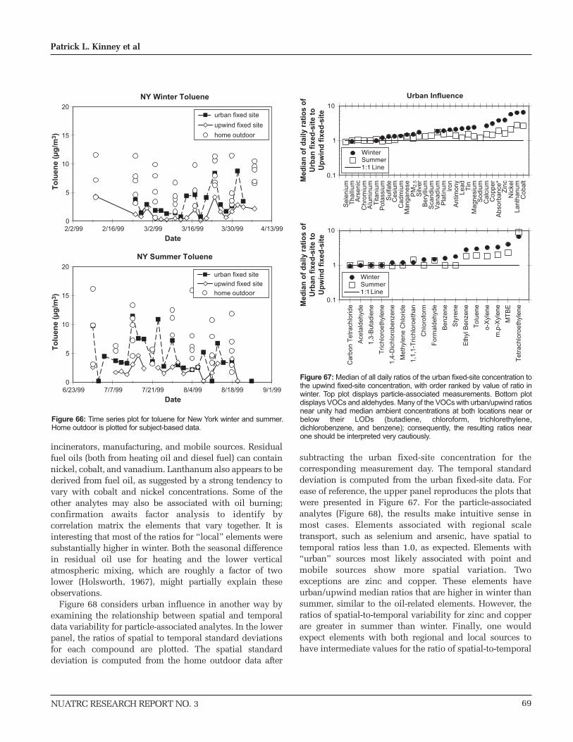
NUATRC RESEARCH REPORT NO. 3
incinerators, manufacturing, and mobile sources. Residualfuel oils (both from heating oil and diesel fuel) can containnickel, cobalt, and vanadium. Lanthanum also appears to bederived from fuel oil, as suggested by a strong tendency tovary with cobalt and nickel concentrations. Some of theother analytes may also be associated with oil burning;confirmation awaits factor analysis to identify bycorrelation matrix the elements that vary together. It isinteresting that most of the ratios for “local” elements weresubstantially higher in winter. Both the seasonal differencein residual oil use for heating and the lower verticalatmospheric mixing, which are roughly a factor of twolower (Holsworth, 1967), might partially explain theseobservations.
Figure 68 considers urban influence in another way byexamining the relationship between spatial and temporaldata variability for particle-associated analytes. In the lowerpanel, the ratios of spatial to temporal standard deviationsfor each compound are plotted. The spatial standarddeviation is computed from the home outdoor data after
subtracting the urban fixed-site concentration for thecorresponding measurement day. The temporal standarddeviation is computed from the urban fixed-site data. Forease of reference, the upper panel reproduces the plots thatwere presented in Figure 67. For the particle-associatedanalytes (Figure 68), the results make intuitive sense inmost cases. Elements associated with regional scaletransport, such as selenium and arsenic, have spatial totemporal ratios less than 1.0, as expected. Elements with“urban” sources most likely associated with point andmobile sources show more spatial variation. Twoexceptions are zinc and copper. These elements haveurban/upwind median ratios that are higher in winter thansummer, similar to the oil-related elements. However, theratios of spatial-to-temporal variability for zinc and copperare greater in summer than winter. Finally, one wouldexpect elements with both regional and local sources tohave intermediate values for the ratio of spatial-to-temporal
69
Patrick L. Kinney et al
NY Winter Toluene
0
5
10
15
20
2/2/99 2/16/99 3/2/99 3/16/99 3/30/99 4/13/99
Date
To
luen
e (µ
g/m
3 )
NY Summer Toluene
0
5
10
15
20
6/23/99 7/7/99 7/21/99 8/4/99 8/18/99 9/1/99
Date
To
luen
e (µ
g/m
3 )
urban fixed site
upwind fixed site
home outdoor
urban fixed site
upwind fixed site
home outdoor
Figure 66: Time series plot for toluene for New York winter and summer.Home outdoor is plotted for subject-based data.
Urban Influence
Med
ian
of
dai
ly r
atio
s o
fU
rban
fix
ed-s
ite
toU
pw
ind
fix
ed-s
ite
0.1
1
10
Med
ian
of
dai
ly r
atio
s o
fU
rban
fix
ed-s
ite
toU
pw
ind
fix
ed-s
ite
0.1
1
10
Sel
eniu
mT
halli
umA
rsen
icC
hrom
ium
Alu
min
umT
itani
umP
otas
sium
Sul
fate
Ces
ium
Cad
miu
mM
anga
nese
PM
2.5
Silv
erB
eryl
lium
Sca
ndiu
mV
anad
ium
Pla
tinum Iron
Ant
imon
yLe
ad Tin
Mag
nesi
umS
odiu
mC
alci
umC
oppe
rA
bsor
banc
e*Z
inc
Nic
kel
Lant
hanu
mC
obal
t
WinterSummer1:1 Line
Car
bon
Tet
rach
lorid
e
Ace
tald
ehyd
e
1,3-
But
adie
ne
Tric
hlor
oeth
ylen
e
1,4-
Dic
hlor
oben
zene
Met
hyle
ne C
hlor
ide
1,1,
1-T
richl
oroe
than
Chl
orof
orm
For
mal
dehy
de
Ben
zene
Sty
rene
Eth
yl B
enze
ne
Tol
uene
o-X
ylen
e
m,p
-Xyl
ene
MT
BE
Tet
rach
loro
ethy
lene
WinterSummer1:1Line
Figure 67: Median of all daily ratios of the urban fixed-site concentration tothe upwind fixed-site concentration, with order ranked by value of ratio inwinter. Top plot displays particle-associated measurements. Bottom plotdisplays VOCs and aldehydes. Many of the VOCs with urban/upwind ratiosnear unity had median ambient concentrations at both locations near orbelow their LODs (butadiene, chloroform, trichlorethylene,dichlorobenzene, and benzene); consequently, the resulting ratios nearone should be interpreted very cautiously.

variability. Sulfate and PM2.5 certainly fall into thiscategory. Because many VOCs and aldehydes had ambientconcentrations near detection limits, this simplifiedapproach provided limited insights into the VOC andaldehyde data.
Analysis of Spatial and Temporal Variance Components
The TEACH study was designed to facilitate analysis oftemporal and spatial variations in concentrations of the airtoxics that were measured. The design included multiplehome measurements in three to five homes over 48-hourperiods during each of the eight to nine weeks, as well asrepeated 48-hr measurements (up to three measurementseach week) at two-fixed-site locations for sampling eachseason. Information on spatial variability was availablefrom the multiple homes that were sampled across the city.However, since different homes were monitored each week,a temporal variance component was present in the homeoutdoor data. This temporal component needed to becontrolled when extracting the spatial variance. The two
fixed sites provided clear temporal variability signals. In thedescriptive analyses presented earlier, spatial and temporalvariability were investigated using simple graphicalpresentations. Here we apply a crossed random effectsmodel to more rigorously analyze spatial and temporalvariance components. This statistical methodology is well-suited to study designs with repeated measurements overboth time and space.
The purpose of the modeling presented here was rathersimple: to estimate the relative magnitude of spatial andtemporal variability in the ambient data measured in theNYC TEACH study, providing quantitative results to backup the qualitative observations discussed above. Becausethe analysis did not involve estimation of regressioncoefficients, issues such as confounding and effectmodification were not of concern.
Apportionment of the spatial and temporal variabilitywas carried out using a crossed random effects model inwhich ambient pollutant concentrations were modeled asdependent variables. Day (each 48-hr period) and subject(each location and site) were random effects in the model.
70
Toxic Exposure Assessment: A Columbia-Harvard (TEACH) Study (The New York City Report)
NUATRC RESEARCH REPORT NO. 3
AnalytePM2.5 (µg/m3)Abs (1/m * 105)Aluminum (Al)Antimony (Sb)Arsenic (As)Beryllium (Be)Cadmium (Cd)Calcium (Ca)Cesium (Cs)Chromium (Cr)Cobalt (Co)Copper (Cu)Iron (Fe)Lanthanum (La)Lead (Pb)Magnesium (Mg)Manganese (Mn)Nickel (Ni)Platinum (Pt)Potassium (K)Scandium (Sc)Selenium (Se)Silver (Ag)Sodium (Na)Sulfur (S)Thallium (Tl)Tin (Sn)Titanium (Ti)Vanadium (V)Zinc (Zn)
Median3.31.03-220.35
0.03628
0.003
0.802.738
0.403.8311.80.5113.1
0.00026
0.01160172
-0.00030.18-0.032.6416.2
N22.74.4886
1.910.78
0.01120.266112
0.00842.151.70268.02491.3124.9316.94.9623.1
0.0046
0.0161.260.172359
53590.01161.866.577.89196.6
Daily Differences Daily RatiosQuartile
range2.10.68
90.44
0.12424
0.003
0.292.424
0.202.386.00.404.3
0.000511
0.02146269
0.00410.210.831.758.6
Median1.523.820.702.12
1.372.681.35
6.663.152.076.392.222.421.505.811.921.21
1.732.651.310.942.300.991.893.96
p-value0.006
<0.00010.030.04
0.07<0.0001
0.05
<0.00010.00040.004
<0.00010.00060.00020.06
<0.00010.20.1
0.20.0090.070.5
0.0080.7
0.003<0.0001
Quartilerange0.379.050.051.18
1.023.240.55
7.023.060.6010.621.472.310.733.022.450.43
1.462.350.400.442.020.510.822.68
New York WinterConcentrations (ng/m3) unless otherwise stated
Table 39: Comparison of urban fixed-site to upwind fixed-site. Dailydifferences and daily ratios between sites, PM2.5, absorbance, andelements.
AnalytePM2.5 (µg/m3)Abs (1/m * 105)Aluminum (Al)Antimony (Sb)Arsenic (As)Beryllium (Be)Cadmium (Cd)Calcium (Ca)Cesium (Cs)Chromium (Cr)Cobalt (Co)Copper (Cu)Iron (Fe)Lanthanum (La)Lead (Pb)Magnesium (Mg)Manganese (Mn)Nickel (Ni)Platinum (Pt)Potassium (K)Scandium (Sc)Selenium (Se)Silver (Ag)Sodium (Na)Sulfur (S)Thallium (Tl)Tin (Sn)Titanium (Ti)Vanadium (V)Zinc (Zn)
Median1.40.63
00.290.02
0.00040.018
130.0000.000.320.834
0.280.823.50.434.1
0.0004-1
0.001-0.170.005
134
-0.00010.230.151.384.8
N2525252525162525252525252525253
2525243
25252525252525252525
Daily Differences Daily RatiosQuartile
range4.5
0.6012
0.220.11
0.00130.045
80.0020.440.241.827
0.161.3213.00.458.6
0.000519
0.0050.490.012
34536
0.00280.300.851.915.1
Median1.171.951.001.411.041.341.191.511.041.012.691.471.642.861.231.321.312.131.500.951.420.901.311.181.000.981.541.101.791.62
p-value0.5
<0.00010.8
0.021
0.90.2
0.0080.70.7
<.00010.06
0.002<.0001
0.090.60.1
0.010.008
0.70.090.40.20.20.90.90.70.4
0.02<.0001
Quartilerange0.451.340.300.550.350.550.620.940.391.663.601.010.654.070.401.740.421.940.930.470.640.490.580.730.460.310.610.300.991.13
New York SummerConcentrations (ng/m3) unless otherwise stated
Table 40: Comparison of urban fixed-site to upwind fixed-site. Dailydifferences and daily ratios between sites, PM2.5, absorbance, andelements.

NUATRC RESEARCH REPORT NO. 3
This analysis was done using Proc Mixed in SAS v.8 (SASInstitute Inc., Cary, NC). A crossed random effects modelwas seen as an efficient way to both model the variancesand allow for covariance across subjects and across time(Coull et al., 2001). We were interested in assessing thespatial variability within the NYC urban environment,while still using the data collected at the upwind site, sincethis adds power to understanding the temporal variability.To do this, we introduced into the model a fixed variable,specifically, an indicator variable for urban sites (the fixedsite and home outdoor measurements) versus upwind site.Data from each season were modeled separately. The modelis shown in Equation 2:
Yij = βo + β1X + αi + bj + eij [2]
Where:
Yij is the pollutant concentration for subject i at time j βo is the intercept β1 is the slope associated with the urban or upwind
indicator X
αi is the random effect for subjects bj is the random effect for time eij is the residual error
For the present purposes, we analyzed the concentrationdata in natural units since log-transformation appeared toovercorrect and greatly reduce spatial variability relative totemporal variability. However, the model was re-run todetermine whether results were influenced by a fewextreme values. Those values in the dataset that weregreater than three times the interquartile range (that is 75th– 25th percentiles) were identified as extreme values.
The results of the spatial and temporal varianceapportionment for particle-associated pollutants aredisplayed graphically in Figure 69 (using all data) andFigure 70 (with extremes removed). The number of extremevalues for each analyte is shown for both seasons in Table41. The elements are ranked in the same order as in the“Urban Influence” section above (regional pollutants to theleft and pollutants with local urban sources to the right).
71
Patrick L. Kinney et al
0.1
1
10S
ele
niu
mT
ha
lliu
mA
rsen
icC
hro
miu
mA
lum
inu
mT
itan
ium
Pot
assi
umS
ulfa
teC
esiu
mC
ad
miu
mM
an
ga
ne
seP
M2
.5S
ilver
Ber
ylliu
mS
can
diu
mV
an
ad
ium
Pla
tinu
mIr
on
An
timo
ny
Le
ad
Tin
Ma
gn
esi
um
Sod
ium
Ca
lciu
mC
op
pe
rA
bso
rba
nce
*Z
inc
Nic
kel
La
nth
an
um
Co
ba
lt
WinterSummer1:1 Line
0
1
2
3
4
5
Se
len
ium
Th
alli
um
Ars
enic
Ch
rom
ium
Alu
min
um
Tita
niu
mP
otas
sium
Su
lfate
Ces
ium
Ca
dm
ium
Ma
ng
an
ese
PM
2.5
Silv
erB
eryl
lium
Sca
nd
ium
Va
na
diu
mP
latin
um
Iro
nA
ntim
on
yL
ea
dT
inM
ag
ne
siu
mS
odiu
mC
alc
ium
Co
pp
er
Ab
sorb
an
ce*
Zin
cN
icke
lL
an
tha
nu
mC
ob
alt
Winter
Summer
Med
ian
of
dai
ly r
atio
s o
fU
rban
fix
ed s
ite
toU
pw
ind
fix
ed s
ite
Sp
atia
l to
Tem
po
ral
vari
abili
ty (
rati
o o
f st
dev
s)
Figure 68: Plot of the ratios of spatial to temporal variability of particle-associated analytes. The spatial variability is calculated as the standarddeviation of the home outdoor data after each home outdoor concentrationis adjusted by removing the urban fixed-site concentration from the outdoorconcentration value. The temporal variability is calculated as the standarddeviation of the urban fixed-site concentrations, including data throughoutthe entire field season. 0.1
1
10
Car
bon
Tet
rach
lori
de
Ace
tald
ehyd
e
1,3
-Bu
tad
ien
e
Tri
chlo
roet
hyle
ne
1,4
-Dic
hlo
rob
en
zen
e
Met
hyle
ne C
hlor
ide
1,1
,1-T
rich
loro
eth
an
Ch
loro
form
For
mal
dehy
de
Be
nze
ne
Sty
rene
Eth
yl B
enze
ne
To
lue
ne
o-X
yle
ne
m,p
-Xyl
ene
MT
BE
Tet
rach
loro
ethy
lene
WinterSummer1:1Line
0
20
40
60
80
100
Car
bon
Tet
rach
lori
de
Ace
tald
ehyd
e
1,3
-Bu
tad
ien
e
Tri
chlo
roet
hyle
ne
1,4
-Dic
hlo
rob
en
zen
e
Met
hyle
ne C
hlor
ide
1,1
,1-T
rich
loro
eth
an
Chl
orof
orm
For
mal
dehy
de
Be
nze
ne
Sty
ren
e
Eth
yl B
enze
ne
To
lue
ne
o-X
yle
ne
m,p
-Xyl
en
e
MT
BE
Tet
rach
loro
ethy
lene
winter
summer
Med
ian
of
dai
ly r
atio
s o
fu
rban
fix
ed s
ite
tou
pw
ind
fix
ed s
ite
Sp
atia
l-to
-tem
po
ral
vari
abili
ty (
rati
o o
f st
dev
s)
Figure 69: Spatial and temporal variance of particle-associated airpollutants including all data, calculated by the mixed model described in thetext.
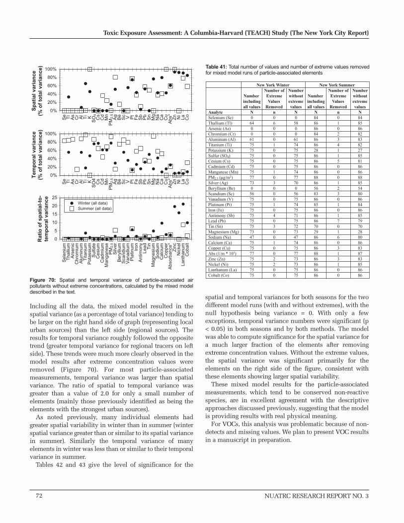
Including all the data, the mixed model resulted in thespatial variance (as a percentage of total variance) tending tobe larger on the right hand side of graph (representing localurban sources) than the left side (regional sources). Theresults for temporal variance roughly followed the oppositetrend (greater temporal variance for regional tracers on leftside). These trends were much more clearly observed in themodel results after extreme concentration values wereremoved (Figure 70). For most particle-associatedmeasurements, temporal variance was larger than spatialvariance. The ratio of spatial to temporal variance wasgreater than a value of 2.0 for only a small number ofelements (mainly those previously identified as being theelements with the strongest urban sources).
As noted previously, many individual elements hadgreater spatial variability in winter than in summer (winterspatial variance greater than or similar to its spatial variancein summer). Similarly the temporal variance of manyelements in winter was less than or similar to their temporalvariance in summer.
Tables 42 and 43 give the level of significance for the
spatial and temporal variances for both seasons for the twodifferent model runs (with and without extremes), with thenull hypothesis being variance = 0. With only a fewexceptions, temporal variance numbers were significant (p< 0.05) in both seasons and by both methods. The modelwas able to compute significance for the spatial variance fora much larger fraction of the elements after removingextreme concentration values. Without the extreme values,the spatial variance was significant primarily for theelements on the right side of the figure, consistent withthese elements showing larger spatial variability.
These mixed model results for the particle-associatedmeasurements, which tend to be conserved non-reactivespecies, are in excellent agreement with the descriptiveapproaches discussed previously, suggesting that the modelis providing results with real physical meaning.
For VOCs, this analysis was problematic because of non-detects and missing values. We plan to present VOC resultsin a manuscript in preparation.
72
Toxic Exposure Assessment: A Columbia-Harvard (TEACH) Study (The New York City Report)
NUATRC RESEARCH REPORT NO. 3
0%
20%
40%
60%
80%
100%
Se Tl
As
Cr
Al
Ti K
SO
4C
sC
dM
nP
M2.
5A
gB
eS
c V Pt
Fe
Sb
Pb
Sn
Mg
Na
Ca
Cu
Abs
*Z
n Ni
La Co
0%
20%
40%
60%
80%
100%S
e Tl
As
Cr
Al
Ti K
SO
4C
sC
dM
nP
M2.
5A
gB
eS
c V Pt
Fe
Sb
Pb
Sn
Mg
Na
Ca
Cu
Abs
*Z
n Ni
La Co
0
5
10
15
20
25
Sel
eniu
mT
halli
umA
rsen
icC
hrom
ium
Alu
min
umT
itani
umP
otas
sium
Sul
fate
Ces
ium
Cad
miu
mM
anga
nese
PM
2.5
Silv
erB
eryl
lium
Sca
ndiu
mV
anad
ium
Pla
tinum Iron
Ant
imon
yL
ea
dT
inM
agne
sium
Sod
ium
Cal
cium
Cop
per
Abs
orba
nce*
Zin
cN
icke
lLa
ntha
num
Cob
alt
Winter (all data)Summer (all data)
Sp
atia
l var
ian
ce(%
of
tota
l var
ian
ce)
Tem
po
ral v
aria
nce
(% o
f to
tal v
aria
nce
)R
atio
of
spat
ial-
to-
tem
po
ral v
aria
nce
Figure 70: Spatial and temporal variance of particle-associated airpollutants without extreme concentrations, calculated by the mixed modeldescribed in the text.
AnalyteSelenium (Se)Thallium (Tl)Arsenic (As)Chromium (Cr)Aluminum (Al)Titanium (Ti)Potassium (K)Sulfur (SO4)Cesium (Cs)Cadmium (Cd)Manganese (Mn)PM2.5 (µg/m3)Silver (Ag)Beryllium (Be)Scandium (Sc)Vanadium (V)Platinum (Pt)Iron (Fe)Antimony (Sb)Lead (Pb)Tin (Sn)Magnesium (Mg)Sodium (Na)Calcium (Ca)Copper (Cu)Abs (1/m * 105)Zinc (Zn)Nickel (Ni)Lanthanum (La)Cobalt (Co)
Number ofExtremeValues
Removedn060001000010300010403001002200
Numberincludingall values
N0
6400
6175757575757577730
56757575757575734775757775757575
New York Winter New York SummerNumberwithoutextremevalues
N05800617475757575747770056757475717572734774757773737575
Number ofExtremeValues
Removedn010234115000123010170160313100
Numberincludingall values
N848686848686288686868688865683868586868670298686868886868686
Numberwithoutextremevalues
N848586828382278581868688855480868486857970288086838783858686
Table 41: Total number of values and number of extreme values removedfor mixed model runs of particle-associated elements

NUATRC RESEARCH REPORT NO. 3
Preliminary Source Apportionment of Ambient VOCs
In an attempt to identify sources and establish groupingsof related VOCs, exploratory factor analysis was carried outon all of the ambient VOC data using SAS version 8.0 (Procfactor with a varimax rotation). These groupings will beused to determine the contributions to VOC concentrationsof different sources. The ambient data for all locations(home outdoor, urban fixed site, and upwind fixed site) andfor both seasons were used for this preliminary survey,since this maximized the number of data points.
Using the Scree test and the percent of variance explainedby each factor, six factors were identified. The VOCsassociated with each are listed in Table 44. Factor 1accounted for 46% of the variance, and was correlated withthe xylenes, ethylbenzene, styrene, and toluene. This factorappears to most likely reflect motor vehicle fuel combustionand evaporative losses. This finding is supported by theliterature. For example, Thijsse et al. (1999) found thattraffic exhaust accounted for 80 to 90% of all VOCsmeasured in the city of Berlin. Similarly, another study
reports that source fingerprints for summer refueling whencompared to roadway emissions show little contribution ofethylbenzene and xylenes to refueling activity (Doskey, etal., 1992), supporting the idea that this factor mainlyassociates with vehicle exhaust. The results from CMBmodeling in Ohio by Mukund et al (1996) showed that
73
Patrick L. Kinney et al
AnalyteSelenium (Se)Thallium (Tl)Arsenic (As)Chromium (Cr)Aluminum (Al)Titanium (Ti)Potassium (K)Sulfur (SO4)Cesium (Cs)Cadmium (Cd)Manganese (Mn)PM2.5 (µg/m3)Silver (Ag)Beryllium (Be)Scandium (Sc)Vanadium (V)Platinum (Pt)Iron (Fe)Antimony (Sb)Lead (Pb)Tin (Sn)Magnesium (Mg)Sodium (Na)Calcium (Ca)Copper (Cu)Abs (1/m * 105)Zinc (Zn)Nickel (Ni)Lanthanum (La)Cobalt (Co)
* NM- not monitored; NA - not available from model output.
p-valueNM
< 0.1 NMNM
0.2< 0.01
NANANA
< 0.1 < 0.01
0.3NMNA
< 0.01NA
< 0.05< 0.05< 0.01< 0.01< 0.01
NA< 0.01
0.3< 0.01< 0.01< 0.01< 0.01
NA
% oftotalNM26%NMNM0%
17%38%0%0%0%
17%15%5%NM0%
51%0%
44%30%53%34%56%0%
59%12%54%70%77%84%82%
p-valueNM0.4NMNM
< 0.05< 0.05< 0.01< 0.01< 0.01< 0.05< 0.01< 0.01< 0.05NM
< 0.05< 0.01
NA< 0.05< 0.05< 0.01< 0.01< 0.01< 0.05< 0.05< 0.05< 0.01< 0.01< 0.01< 0.05< 0.05
% oftotalNM11%NMNM59%42%54%78%76%42%67%78%55%NM62%40%57%26%45%32%59%30%50%18%30%30%21%17%7%10%
p-valueNANANA0.2
< 0.01< 0.01
NA0.12NANA
< 0.1 0.110.12NANANANA
< 0.01< 0.01< 0.050.11NA
< 0.1 < 0.01< 0.01< 0.01< 0.01
0.4< 0.01< 0.01
% oftotal0%2%0%
17%37%31%0%4%6%0%
19%1%
12%0%0%0%
22%48%40%48%24%0%
22%37%46%43%80%1%74%58%
p-value< 0.01< 0.01< 0.01< 0.01< 0.01< 0.01< 0.01< 0.01< 0.01< 0.01< 0.01< 0.01< 0.01
NA< 0.01< 0.01
NA< 0.01< 0.01< 0.05< 0.01
NA< 0.05< 0.01< 0.01< 0.01< 0.05< 0.05< 0.05< 0.01
% oftotal82%85%86%38%51%56%86%87%82%65%65%92%69%74%55%76%44%45%48%25%52%0%
53%45%36%30%10%32%11%31%
New York Winter New York SummerTemporalSpatial TemporalSpatial
Table 43: Significance of spatial and temporal variances from mixed modelresults for NY particle-associated air pollutants without extremes <0.01(very significant), p<0.05 (significant), p< 0.1 (marginally significant), p ≥ 0.1(not significant)
CompoundCarbon TetrachlorideAcetaldehyde1,4-DichlorobenzeneMethylene Chloride1,1,1-TrichloroethaneFormaldehydeBenzeneStyreneEthylbenzeneTolueneo-Xylenem,p-XyleneMTBETetrachloroethylene
New York WinterN10942000000003
New York SummerN00483101302213
Table 44: Number of extreme values for each compound
AnalyteSelenium (Se)Thallium (Tl)Arsenic (As)Chromium (Cr)Aluminum (Al)Titanium (Ti)Potassium (K)Sulfur (SO4)Cesium (Cs)Cadmium (Cd)Manganese (Mn)PM2.5 (µg/m3)Silver (Ag)Beryllium (Be)Scandium (Sc)Vanadium (V)Platinum (Pt)Iron (Fe)Antimony (Sb)Lead (Pb)Tin (Sn)Magnesium (Mg)Sodium (Na)Calcium (Ca)Copper (Cu)Abs (1/m * 105)Zinc (Zn)Nickel (Ni)Lanthanum (La)Cobalt (Co)
* NM- not monitored; NA - not available from model output.
p-valueNM
< 0.05NMNM0.3
< 0.01NA0.5NANANA
< 0.01< 0.01NMNA
< 0.01NA
< 0.050.4
< 0.01NA
< 0.010.11
< 0.01< 0.05< 0.01
NANANANA
% oftotalNM33%NMNM8%
66%46%0%0%0%0%
15%52%NM0%
56%75%44%3%
53%0%
77%43%80%43%61%93%92%91%85%
p-valueNM
< 0.01NMNM
< 0.05< 0.05
NA< 0.01< 0.01< 0.01< 0.01< 0.01< 0.05NM
< 0.05< 0.01
NA< 0.050.12
< 0.01< 0.01< 0.01< 0.05< 0.05< 0.1
< 0.01< 0.01< 0.01< 0.05< 0.05
% oftotalNM56%NMNM55%18%47%76%77%61%61%78%30%NM56%36%13%26%16%32%50%16%42%8%16%25%5%6%4%9%
p-valueNANANANANA
< 0.1NA0.3NA
< 0.05< 0.01
0.2NA
< 0.1NANANA
< 0.010.2
< 0.01< 0.05
NA< 0.01< 0.01
NA< 0.01
NANA
< 0.01< 0.01
% oftotal0%0%0%0%0%1%
100%1%0%36%24%1%81%15%0%0%78%38%10%58%49%0%38%41%100%60%99%0%79%58%
p-value< 0.01< 0.01< 0.010.13
< 0.01< 0.01
NA< 0.01< 0.01< 0.01< 0.01< 0.01< 0.01< 0.01< 0.01< 0.01
NA< 0.01< 0.01< 0.01< 0.01< 0.01< 0.01< 0.01< 0.1
< 0.01< 0.05
0.4< 0.05< 0.01
% oftotal84%84%87%15%88%98%0%
87%65%44%68%94%15%75%85%79%12%58%65%36%34%94%58%52%0%
22%0%1%9%
31%
New York Winter New York SummerTemporalSpatial TemporalSpatial
Table 42: Significance of spatial and temporal variances from mixed modelresults for NY particle-associated air pollutants including all data p<0.01(very significant), p<0.05 (significant), p< 0.1 (marginally significant), p ≥ 0.1(not significant)
vehicle exhaust accounted for over 50% of toluene,ethylbenzene, and xylenes, while industrial solventsaccounted for only 20 to 40%.
Factor 2 was correlated with formaldehyde,acetaldehyde, valeraldehyde, and hexaldehyde, whileFactor 3 was associated with valeraldehyde, hexaldehyde,propionaldehyde, and butyraldehyde. These factorsaccounted for 26 and 9% of the total variance, respectively,and are probably indicative of compounds associated withsecondary formation. Factor 4 was associated with MTBE,benzene, and toluene. This factor accounted for 8% of thevariance, and may be due to stationary gasoline stations oralso evaporative gasoline loss from motor vehicles.Interestingly, benzene and MTBE both did not correlatewith Factor 1 as might be expected. Anderson et al. (2001)found similar results in their analyses of the New JerseyTEAM study, where benzene appeared as a distinct factor.Mukund et al. (1996) found that the gasoline vapor sourcein their model was more consistent with running losses andevaporative emissions from vehicles, rather than servicestations. Factor 5 is associated with methylene chloride and1,1,1-trichloroethane, probably from wastewater treatmentoperations (Mukund et al., 1996) and explained 6% of thevariance. Lastly, Factor 6 is associated with 1,4-dichlorobenzene and tetrachloroethylene and accounted for5% of the variance. This component is probably related todry cleaning, as tetrachloroethylene is a common drycleaning solvent.
Based on the results from this exploratory factor analysis,three different source-related groupings of VOCs wereidentified. The first and most prominent grouping wasrelated to motor vehicle fuel combustion and evaporativeemissions. This grouping included Factors 1 and 4, whichtogether explained 54% of the total variance of the ambientVOCs. The second grouping was for compounds associatedwith secondary formation, which included all thealdehydes in Factors 2 and 3 and which explained another35% of the variance. The last grouping was for compoundsassociated with specific point sources, which includedFactors 5 and 6. Carbon tetrachloride did not relate with anyof the other compounds in these groupings and did notshow up in the factor analysis.
SUMMARY OF KEY FINDINGS
SUBJECT AND HOME CHARACTERISTICS
Air toxics exposure data were collected on 46 inner cityNYC young people ranging in age from 14 to 19. Subjectswere predominantly black and/or Hispanic, lived inrelatively small rental apartments in multi-floor apartment
buildings, and lived in neighborhoods with relatively highlevels of self-reported motor vehicle traffic. Time-activitypatterns were similar to previous surveys of urban youngpeople, except that commuting by cars was uncommon inour population. Time activity patterns were only predictiveof personal exposures in the case of selected metals (such asiron and manganese), which were elevated for subjectscommuting by subway. Subway and bus commuting werecommon.
PERSONAL AIR TOXIC EXPOSURES
Personal exposures reflect the impacts of indoor andoutdoor concentrations, as well as sources that areencountered in unmeasured microenvironments and theimpacts of individual activities (the personal cloud). Forpollutants with significant indoor sources, including mostof the VOCs, personal exposures showed little relationshipto outdoor concentrations. For those pollutants lackingsignificant indoor sources, including most PM-associatedelements and a few VOCs, both personal and indoorexposures were associated with outdoor levels.
Strong temporal correlations were observed betweencentral site ambient data and mean personal exposures forPM2.5, sulfate, and black carbon. In addition, a significantspatial correlation was found between home outdoor andpersonal black carbon levels, with a stronger correlation inwinter. Neither PM2.5 nor sulfate exhibited spatialcorrelations between outdoor and personal levels.
Personal exposures were significantly higher than homeindoor and ambient samples for several elements, includingiron, manganese, and chromium. The iron/manganese andchromium/manganese ratios, as well as strong correlationsamong these elements, suggested steel dust as the source ofthese metals for a large subset of the personal samples.Furthermore, time-activity data suggested the NYC subwaysystem to be a possible source of these elevated personalmetals. The levels and ratios of iron, manganese, andchromium in a single set of duplicate PM2.5 samplesintegrated over eight hours of underground subwayexposure are consistent with the subway system being thepredominant source of these metals to subway-ridingsubjects.
We carried out a preliminary risk assessment for cancerbased on the personal air toxic concentrations measured inNYC TEACH, assuming lifetime exposure at these levels.Unit cancer risks were taken from the U.S. EnvironmentalProtection Agency (EPA) IRIS database. Accumulating risksacross all carcinogenic compounds resulted in risk levels inthe 1/1000 range.
74
Toxic Exposure Assessment: A Columbia-Harvard (TEACH) Study (The New York City Report)
NUATRC RESEARCH REPORT NO. 3
NUATRC RESEARCH REPORT NO. 3
INDOOR AIR TOXIC CONCENTRATIONS
Indoor VOC levels were generally much higher thanoutdoors, and thus indoor/outdoor (I/O) ratios were above1.0 for most compounds. However, I/O ratios closer to 1.0were observed for a few VOCs, including methyl tertiarybutyl ether (MTBE), benzene, ethylbenzene, toluene, andxylene (BETX). Indoor/outdoor ratios were also lower insummer than in winter, reflecting increased air exchangeduring summer (mean of 1.81 air changes per hour) ascompared to winter (mean of 0.99 air changes per hour).The I/O ratios for PM-associated elements were typicallyclose to or below 1.0, reflecting the role played by outdoorsources in driving indoor levels. For a few elements,including cadmium, potassium, and tin in winter andchromium and tin in summer, I/O ratios greater than 1.0were observed. For analytes with I/O ratios appreciablygreater than 1.0, I/O ratios showed consistent declines athigher air exchange rates.
We demonstrated that, during the winter season, indoorand personal black carbon concentrations can be useful asan alternative to sulfate for tracing PM2.5 of ambient origin.In contrast to sulfate, black carbon measurements are farmore related to local urban particle emissions than toregional air masses. Hence, black carbon may be a usefulambient tracer in future studies addressing the healthimpacts of traffic-related particulate matter.
OUTDOOR AIR TOXIC CONCENTRATIONS
As expected, ambient concentrations of most VOCs werelower than levels measured indoors or as personal samples.Because of the relatively low concentrations measured inambient air, median outdoor concentrations at the urbanfixed site were below the respective limits of detection forsix of 17 VOCs. Better detection results were obtained forthe indoor and personal samples. With the exception ofchromium, all median concentrations of ambient PM2.5 andassociated elements exceeded limits of detection (LOD).
Analysis of spatial and temporal variations in ambientconcentrations revealed two distinct groups of air toxics:those related to regional air masses (for example sulfur,selenium, arsenic, and formaldehyde) and those related tolocal sources (for example, black carbon, cobalt, lanthanum,nickel, MTBE, other BETX, and VOCs). Concentrationvariations for compounds of the former group were greaterover time than space, whereas the latter group showedgreater variability across locations than across time. Toidentify air toxics with significant urban influences due tolocal sources in NYC, levels at the urban and upwind fixedsites were compared. A large urban influence was seen for
the BETX VOCs, as well as many NYC particle components,especially those associated with combustion of heating oiland diesel fuel. The urban effect was generally larger inwinter than in summer. A statistical variance componentsanalysis using a mixed effects model confirmed many ofthese observations.
Patterns of elemental and VOC concentrations across sitesand seasons strongly suggest that outdoor transportationand heating fuel combustion represent the two mostsignificant sources of urban air toxics in NYC. Apreliminary source apportionment analysis of ambient VOCand aldehyde data showed that primary emissions frommotor vehicles were the dominant source category,followed by formation of secondary compounds andspecific point sources.
LIMITATIONS
It is important to be aware of several sources of potentialbias and/or random error in the measurement design of theTEACH study. Measurement bias could lead to erroneousconclusions regarding the direction and magnitude ofanalytical contrasts, or they could limit the extent to whichresults could be generalized.
One potential bias in the TEACH study relates to the non-random process used to recruit subjects. Because of theconsiderable demands placed on subjects to successfullycomplete the study, namely a willingness to carry apersonal monitoring backpack for 48-hour periods in twoseasons as well as family support for home-based sampling,a tendency existed to select motivated students andfamilies. Such students might differ from their peers atschool. If those differences were associated with differencesin urban air toxic exposures, then the study findings couldnot be generalized to other students at the school, much lessstudents at other, similar schools. To address this issue, wecollaborated with the schools to survey a larger number ofstudents (approximately 600 to 700) at each school withrespect to basic demographics, socio-economic status, andother characteristics. Findings from this survey werecompared to findings regarding study participants. For themost part, the subject populations were similar to thesurvey groups at each school with respect to age, race, andsocioeconomic status, although the subject populations hada higher proportion of females than the school as a whole.The demographics of our cohort compared to their schoolpopulation at large are presented in the “SubjectCharacteristics” section of this report.
Strictly speaking, the subject-based results of the TEACHstudy cannot be generalized beyond populations of urban
75
Patrick L. Kinney et al

high school students with ethnic and socio-economic status(SES) characteristics similar to those monitored in thesespecific cities. However, while it may not be possible togeneralize exposures based on these measurements alone, itis likely that insight into mechanisms of exposure will betransferable to other settings and populations.
Subject-based measurements were collected only onweekdays. This may have resulted in a positive bias inexposure levels, since traffic-related pollutants are usuallygreater on weekdays than weekends. Given the staff andbudgetary constraints of our study, weekdays were chosenas the more interesting time period to document for allsubject-based monitoring. Future studies may compareweekday and weekend differences in personal exposures toair toxics. While some of our 48-hour fixed-site monitoringdid span weekend days, the timing of start and end times ofthe sampling did not permit clear separation of weekendand weekday data.
The selection of seasonal periods for sampling alsopresents potential for bias. The seasonal periods wereselected to maximize the contrast between ambientmeteorological conditions and pollutant concentrations.Thus, it is appropriate to view seasons as fixed effectsselected to maximize contrasts in ambient concentrations.Our “winter” sampling period in NYC extended fromFebruary to April. However, during the winter season, theweather was unseasonably warm, and subjects participatingin personal monitoring were not exposed to the sub-freezingtemperatures that are more typical NYC mid-winterconditions. Nevertheless, the data analysis presented in“Results and Discussion” confirms that the two NYCsampling seasons did indeed provide contrasting air toxicconcentrations, air exchange rates, and time-activitypatterns.
Biases in the air pollution measurements can result froma number of factors. Potential causes include impropercalibrations, loss of analytes from collection media duringor after sampling, contamination of samples duringhandling, the placement of samplers, or changes in behaviorassociated with carrying personal samplers. Quality controlprocedures were established to identify any of these factorsshould they occur. Procedures in all field and laboratorywork were carefully developed and fully documented. Thisincluded the use of field blanks and spiked samples. Allflow rates were carefully calibrated before and aftersampling. Every effort was made to place home indoor andhome outdoor sampling equipment in a consistent andrepresentative way so that samples captured theenvironment of the whole indoor area. Home indoorsamplers were placed four feet above the ground and at leasttwo feet away from any wall, usually in the main activityroom. Home outdoor samplers were placed two and one-
half feet away from the outer wall of the building. Personalsamplers were housed in Jansport backpacks that were thebrand-type used by the vast majority of the student body inour NYC school for personal belongings and books. While itis possible that students altered their normal activitiesbecause they carried both a book bag and the personalsampler pack, we believe this would in general have onlyminor effects on actual exposures measured. A larger bias inthe personal data would occur if students did not wear thesampling pack for a significant fraction of the samplingperiod. This would tend to make the personal samplersmore reflective of home indoor concentrations than otherlocations. It is clear from our data in both winter andsummer that personal exposures are often different fromindoor or outdoor exposures, somewhat reducing concernabout bias. In the summer NYC monitoring period, weinstituted the use of vibrational data loggers in eachpersonal sampling pack. Subjects were told that they wouldbe rewarded with movie passes only if our equipmentshowed that that pack had been carried. This procedure wasvery successful, and we recommend it in future personalsampling studies.
Random measurement errors occur in all air pollutionsampling. Our goal was to both minimize errors and toestimate their magnitude. Overall sampling precision (thestandard deviation of the measurement error for the entiresampling system) can be derived from duplicate samples(Evans et al., 1984; Kinney and Thurston., 1993). Duplicatesamples are collected using identical but separate samplersplaced side-by-side. Other than collection of personalsamples, which would have involved carrying twobackpacks, we collected extensive duplicate samples in allcomponents of our study. In addition, a small number ofduplicate personal samples were collected by field staff.The QA/QC section reports on issues of accuracy andprecision.
REFERENCES
Adams HS, Nieuwenhuijsen MJ, Colvile RN, McMullenMA, Khandelwal P, 2001. Fine particle (PM2.5) personalexposure levels in transport microenvironments, London,UK. Sci. Total Environment 279: 29-44.
Adams HS, Nieuwenhuijsen MJ, Colvile RN, 2001.Determinants of fine particle (PM2.5) personal exposurelevels in transport microenvironments, London UK.Atmospheric Environments 35: 4557-4566.
76
Toxic Exposure Assessment: A Columbia-Harvard (TEACH) Study (The New York City Report)
NUATRC RESEARCH REPORT NO. 3

NUATRC RESEARCH REPORT NO. 3
Anderson MJ, Miller SL, Milford JB, 2001. Sourceapportionment of exposure to toxic volatile organiccompounds using positive matrix factorization. J. Expo.Anal. Environ. Epidemiol. 11(4): 295-307.
Aschner M, Vrana KE, Zheng, 1999. Manganese uptake anddistribution in the central nervous system (CNS).NeuroToxicology 20: 173-180.
Caldwell, JC, Woodruff, TJ, Morello-Frosch R, Axelrad DA,1998. Use of toxicity data for assessing the environmentalhealth risks of air toxics. Toxicol Ind Health 14(3): 429-54.
Chung CW, Morandi MT, Stock TH, Afshar M, 1999.Evaluation of a passive sampler for volatile organiccompounds at ppb concentrations, varying temperatures,and humidities with 24-h exposures. 2. Samplerperformance. Environmental Science & Technology 33(20):3666-3671.
Cohen MA, Ryan PB, Yanagisawa Y, Hammond SK, 1990.The validation of a passive sampler for indoor and outdoorconcentrations of volatile organic compounds. Journal ofthe Air and Waste Management Association 40(7): 993-997.
Costa DL and Dreher KL, 1997. Bioavailable transitionmetals in particulate matter mediate cardiopulmonaryinjury in healthy and compromised animal models. EnvironHealth Perspect. 105 (Suppl 5): 1053-60.
Coull BA, Hobert JP, Ryan LM, Holmes LB, 2001. Crossedrandom effect models for multiple outcomes in a study ofteratogenesis. Journal of the American StatisticalAssociation 94: 1194-1204.
Crump KS, 2000. Manganese exposures in Toronto duringuse of the gasoline additive, methylcyclopentadienylmanganese tricarbonyl. J. of Exposure Analysis andEnvironmental Epidemiology 10: 227-239.
Dietz RN, Goodrich RW, Cote EA, Wieser RF, 1986. Detaileddescription and performance of passive perfluorocarbontracer system for building ventilation and air exchangemeasurements. Philadelphia, PA, American Society forTesting and Materials: 203-264.
Dockery DW, Spengler JD, 1981. Indoor-outdoor relationshipsof sulfates and particles, Atmos. Environ. 15: 335-343.
Dockery DW, Spengler JD, 1981. Personal exposure torespirable particulates and sulfates, J. Air Poll ControlAssoc. 31: 153-159.
Doskey PV, Porter JA, Scheff PA, 1992. Source fingerprintsfor volatile nonmethane hydrocarbons. Journal of the Air &Waste Management Association 42(11), 1437-1445.
Dwyer J, 1991. Subway Lives – 24 hours in the life of theNew York City subway. Crown Publishers, New York, p 312.
Edemé JL, Shirali P, Mereau M, Sobaszek A, Boulenguez C,Diebold F, Haguenoer JM, 1997. Assessment of biologicalchromium among stainless steel and mild steel workers inrelation to welding processes. Int. Arch. Occup. Environ.Health 70 (4): 237-242.
Edwards JD, Ogren JA, Weiss RE, Charlson RJ, 1983.Particulate air pollutants: a comparison of British "smoke"with optical absorption coefficient and elemental carbonconcentration, Atmos. Environ. 17: 2337-2341.
U.S. EPA, 1999a. Determination of volatile organiccompounds in ambient air using active sampling ontosorbent tubes. Cincinnati, OH, Office of Research andDevelopment, Environmental Protection Agency: 1-53.
U.S. EPA, 1999b. Determination of formaldehyde inambient air using adsorbent cartridge followed by highperformance liquid chromatography (HPLC): activesampling methodology. Cincinnati, OH, Office of Researchand Development, Environmental Protection Agency: 1-56.
Evans JS, Cooper DW, Kinney P, 1984. On the propagationof error in air-pollution measurements. EnvironmentalMonitoring and Assessment 4(2): 139-153.
Fung K, Grosjean D, 1981. Determination of nanogramamounts of carbonyls as 2,4-dinitrophenylhydrazine byhigh-performance liquid chromatography. Aerosol Scienceand Technology 53: 168-171.
Gao Y, Nelson ED, Field MP, Ding Q, Li H, Sherrell RM,Gigliotti C, Van Ry D, Glenn TR, Eisenreich SJ, 2002.Characterization of atmospheric trace elements on PM2.5particulate matter over the New York-New Jersey harborestuary. Atmospheric Environment 36(6): 1077-1086.
Gordon SM, Callahan PJ, Nishioka MG, Brinkman MC,O'Rourke MK, Lebowitz MD, Moschandreas DJ, 1999.
77
Patrick L. Kinney et al
Residential environmental measurements in the NationalHuman Exposure Assessment Survey (NHEXAS) pilotstudy in Arizona: preliminary results for pesticides andVOCs. Journal of Exposure Analysis and EnvironmentalEpidemiology 9(1): 456-470.
Grosjean E, Grosjean D, 1995. Performance of DNPH-coatedC-18 cartridges for sampling C-1-C-9 carbonyls in air.International Journal of Environmental AnalyticalChemistry 61(4): 343-360.
Hardy RJ, Highsmith VR, Costa DL, Krewer JA, 1992. Indoorasbestos concentrations associated with the use of asbestos-contaminated tap water in portable home humidifiers.Environmental Science & Technology 26(4): 680-689.
Hartwell TD, Pellizzari ED, Perritt RL, Whitmore RW, ZelonHS, Sheldon LS, Sparacino CM, Wallace L, 1987. Resultsfrom the total exposure assessment methodology (TEAM)study in selected communities in northern and southernCalifornia. Atmos. Environ. 21(9): 1995-2004.
Heritage J, 1992. Environmental protection - has it been fair?EPA Journal 18(1).
Highsmith VR, Hardy RJ, Costa DL, Germani MS, 1992.Physical and chemical characterization of indoor aerosolsresulting from the use of tap water in portable homehumidifiers. Env Science & Technology 26(4): 673-680.
Highsmith VR, Rodes CE, Hardy RJ, 1988. Indoor particleconcentrations associated with use of tap water in portablehumidifiers. Environmental Science & Technology 22(9):1109-1112.
Ho DT, Schlosser P, Smethie WM, Simpson HJ, 1998.Variability in atmospheric chlorofluorocarbons (CCl3F andCCl2F2) near a large urban area: Implications forgroundwater dating. Environmental Science & Technology32(16): 2377-2382.
Holzworth GC, 1967. Mixing depths, wind speeds and airpollution potential for selected locations in the UnitedStates. J Applied Meteorology 6(6): 1039-1044.
Horvath H, 1993. Atmospheric light absorption – a review,Atmos. Environ., 27(3): 293-317.
Janssen NAH, Hoek G, Harssema H, Brunekreef B, 1997.Childhood exposure to PM10: relation between personal,
classroom, and outdoor concentrations. Occup. Environ.Med. 54: 888-894.
Janssen LHJM, Buringh E, van der Meulen A, van den HoutKD, 1999. A method to estimate the distribution of variousfractions of PM10 in ambient air in the Netherlands. Atmos.Environ. 33: 3325-3334.
Jantunen MJ, Katsouyanni K, Knoppel H., Kunzli N, LebretE, Maroni M, Saarela K, Sram R, Zmirou D, 1999. Airpollution exposure in European cities: the EXPOLIS study:Final report. Kansanterveyslaitoksen julkaisuja B16/1999Kuopio, Finland.
Jones NC, Thornton CA, Mark D, Harrison RM, 2000.Indoor/outdoor relationships of particulate matter indomestic homes with roadside, urban and rural locations.Atmos. Environ. 34: 2603-2612.
Kadiiska MB, Mason RP, Dreher KL, Costa DL, Ghio AJ,1997. In vivo evidence of free radical formation in the ratlung after exposure to an emission source air pollutionparticle. Chem Res Toxicol. 10(10):1104-8.
Kenny LC Gussman A, 1997. Characterization andmodeling of a family of cyclone aerosol preseparators.Journal of Aerosol Science 28(4): 677-688.
Kinney P, Thurston GD, 1993. Field evaluation ofinstrument performance: statistical considerations. Appl.Occup. Environ. Hyg. 8:267-271.
Kinney, PL, Spengler JD, Chillrud S, Ramstrom S, 1998a.Report of pilot results for NYC. A report to the MickeyLeland Urban Air Toxics Research Center.
Kinney PL, Spengler JD, Chillrud S, Ramstrom S, 1998b. Afield comparison of active and passive VOC methods. Areport to the Mickey Leland Urban Air Toxics ResearchCenter.
Kinney PL, Aggarwal M, Northridge ME, Janssen NAH,Shepard P, 2000. Airborne concentrations of PM2.5 anddiesel exhaust particles on Harlem sidewalks: Acommunity-based pilot study. Environ Health Perspect108(3): 213-218.
Kinney PL, Chillrud SN, Ramstrom S, Ross J, Spengler JD,2002. Exposures to multiple air toxics in New York City.Environ. Health Perspect. 110 (suppl 4):539-546.
78
Toxic Exposure Assessment: A Columbia-Harvard (TEACH) Study (The New York City Report)
NUATRC RESEARCH REPORT NO. 3

NUATRC RESEARCH REPORT NO. 3
Klein CB. 1996. Carcinogenicity and genotoxicity ofchromium. In: Chang LW, ed. Toxicology of Metals. CRCPress, New York, pp.205-219.
Klepeis NE, Nelson WC, Ott WR, Robinson JP, Tsang AM,Switzer P, Behar JV, Hern SC, Engelmann WH, 2001. TheNational Human Activity Pattern Survey (NHAPS): aresource for assessing exposure to environmentalpollutants. Journal of Exposure Analysis andEnvironmental Epidemiology 11(3): 231-252.
Leaderer BP, Bernstein DM, Daisey JM, Kleinman MT,Kneip TJ, Knutson EO, Lippmann M, Lioy PJ, Rahn KA,Sinclair D, Tanner RL, Wolff GT, 1978. Summary of New-York-Summer-Aerosol-Study (NYSAS). Journal of the AirPollution Control Association 28(4): 321-327.
Lee HS, Kang BW, Cheong JP, Lee SK, 1997. Relationshipsbetween indoor and outdoor air quality during the summerseason in Korea. Atmos. Environ. 31: 1689-1693.
Li Y, Harrison RM, 1990. Comparison of indoor and outdoorconcentrations of acid gases, ammonia and their associatedsalts. Environ. Tech. 11: 315-326.
Lioy PJ, Wolff GT, 1978. Toxic airborne elements in New-York metropolitan area. Journal of the Air Pollution ControlAssociation 28(5): 510-512.
Lioy PJ, Avdenko M, Harkov R, Atherholt T, Daisey JM, 1985.A pilot I/O study of organic particulate matter and particulatemutagenicity. J Air Poll. Control Assoc. 35, 653-657.
Metzger R, Delgado JL, Herrell R, 1995. Environmental healthand Hispanic children. Env. Health Perspective 103: 25-32.
Miguel AH, Kirchstetter TW, Harley RA, 1998. On-roademissions of particulate polycyclic aromatic hydrocarbonsand black carbon from gasoline and diesel vehicles.Environ. Sci. Tech 32: 450-455.
Morandi MT, Stock TH, 1998. Personal exposures to toxicair pollutants. Houston, TX, Mickey Leland National UrbanAir Toxics Research Center Research Report No. 1, Vol. 2.
Morandi MT, Stock TH, Contant CF, 1988. A comparative-study of respirable particulate microenvironmentalconcentrations and personal exposures. EnvironmentalMonitoring and Assessment 10(2): 105-122.
Morello-Frosch RA, Woodruff TJ, Axelrad DA, Caldwell JC,2000. Air toxics and health risks in California: the publichealth implications of outdoor concentrations. Risk Anal20(2): 273-91.
Mukund R., Kelly TJ, Spicer CW, 1996. Source attribution ofambient air toxic and other VOCs in Columbus, Ohio.Atmospheric Environment 30(20), 3457-3470.
National Research Council, 2002. Estimating the publichealth benefits of proposed air pollution regulations.National Academy Press, Washington, 2002.
Olden K, Poje J, 1995. Environmental justice andenvironmental health. Bulletin of the Society forOccupational and Environmental Health 4: 3-4.
Ozkaynak H, Xue J, Weker R, Butler D, Koutrakis P, SpenglerJD, 1995. The Particle TEAM (PTEAM) study: analysis ofthe data 3:. 2-7. Research Triangle Park, NC, EPA/600/R-95/098.
Pratt GC, Palmer K, Wu CY, Oliaei F, Hollerbach C, FenskeMJ, 2000. An assessment of air toxics in Minnesota. EnvironHealth Perspect 108(9): 815-25.
Shields HC, Fleischer DM, Weschler CJ, 1996. Comparisonsamong VOCs measured in three types of U.S. commercialbuildings with different occupant densities. Indoor Air,International Journal of Indoor Air Quality & Climate 6(1):2-17.
Sitzmann B, Kendall M, Watt J, 1999. Characterization ofairborne particles in London by computer controlledscanning electron microscopy. Sci. Total Environment 241:63-73.
Spengler JD, Dockery DW, Turner WA, Wolfson JM, FerrisBG, 1981. Long-term measurements of respirable sulfatesand particles inside and outside homes. Atmos. Environ.15: 23-30.
Spicer CW, Buxton BE, Holdren MW, Smith DL, Kelly TJ,Rust SW, Pate AD, Sverdrup, GM, Chuang JC, 1996.Variability of hazardous air pollutants in an urban area.Atmospheric Environment 30(20): 3443-3456.
Standard Operating Procedure for determination ofabsorption coefficient using reflectometric method used bythe ULTRA and KTL groups (PSOP ULTRA/KTL-L-1.1)October 16, 1998; Finland.
79
Patrick L. Kinney et al
Suh H, Spengler JD, Koutrakis P, 1992. Personal exposuresto acid aerosols and ammonia. Environ. Sci. Technol. 26:2507-2517.
Suh H, Koutrakis P, Spengler JD, 1993. Validation ofpersonal exposure models for sulfate and aerosol strongacidity. Journal of the Air and Waste Management. Assoc.,43: 845-850.
Tancrede M, Wilson R, Zeise L, Crouch EAC, 1987. Thecarcinogenic risk of some organic vapors indoors: a theoreticalsurvey. Atmospheric Environment 21(10): 2187-2205.
Thijsse,TR, van Oss RF, Lenschow P, 1999. Determination ofsource contributions to ambient volatile organic compoundconcentrations in Berlin. Journal of the Air & WasteManagement Association 49(12): 1394-1404.
Ullrich D, Nagel R, 1996. Comparison of diffusive samplingwith different sampling periods and short term activesampling at low VOC concentrations. Proceedings of the 7thInternational Conference on Indoor Air Quality andClimate, Tokyo, Japan.
Viskari EL, Vartiainen M, Pasanen P, 2000. Seasonal anddiurnal variation in formaldehyde and acetaldehydeconcentrations along a highway in eastern Finland.Atmospheric Environment 34(6): 917-923.
Wallace LA, Pellizzari ED, Hartwell TD, Sparacino CM,Sheldon LS, Zelon H, 1985. Personal exposures, indoor-outdoor relationships, and breath levels of toxic airpollutants measured for 355 persons in New Jersey.Atmospheric Environment 19(10): 1651-1661.
Wernette DR, Nieves LA, 1992. Breathing polluted air:minorities are disproportionately exposed. EPA Journal18(1): 16-17.
Wolff GT, Lioy PJ, 1978. Empirical model for forecastingmaximum daily ozone levels in northeastern United-States.Journal of the Air Pollution Control Association 28(10):1034-1038.
Wolff GT, Lioy PJ, 1978. Transport of suspended particulatematter into the New York metropolitan area. Bulletin of theNew York Academy of Medicine 54(11): 1032-1044.
Woodruff TJ, Axelrad DA, Caldwell J, Morello-Frosch R,Rosenbaum A, 1998. Public health implications of 1990 air
toxics concentrations across the United States. EnvironHealth Perspect 106(5): 245-51.
Woodruff TJ, Caldwell J, Cogliano VJ, Axelrad DA, 2000.Estimating cancer risk from outdoor concentrations ofhazardous air pollutants in 1990. Environ Res 82(3): 194-206.
Woolfenden EA, McClenny WA, 1997. Compendium ofmethods for the determination of toxic organic compoundsin ambient air: Method TO-17. Cincinnati, OH, U.S.Environmental Protection Agency.
World Health Organization, 2000. Air Quality Guidelinesfor Europe, Second Edition. WHO Regional Publications,European Series, No. 91.
Wu CY, Pratt GC, 2001. Analysis of air toxics emissioninventory: inhalation toxicity-based ranking. J. Air. & WasteManage. Assoc. 51: 1129-1141.
Zhang J, He Q, Lioy PJ, 1994. Characteristics of aldehydes:concentrations, sources, and exposures for indoor andoutdoor residential microenvironments. EnvironmentalScience and Technology 28(1): 146-152.
ACKNOWLEDGMENTS
We want to thank the students and staff of A. PhilipRandolph High School who made this project possible.Funds for this research were provided by the MickeyLeland National Urban Air Toxics Center. Additional fundswere provided by the NIEHS Centers for EnvironmentalHealth at Columbia and Harvard.
ABBREVIATIONS
µg MicrogramµL Microliterµm MicrometerAER Air exchange rateBTEX Benzene, toluene, ethyl benzene, xyleneCAT Capillary absorption tubeDNPH Dinitro phenylhydrazineGC Gas chromatographyHPLC High pressure liquid chromatographyI/O Indoor/outdoorIDL Instrument detection limit
80
Toxic Exposure Assessment: A Columbia-Harvard (TEACH) Study (The New York City Report)
NUATRC RESEARCH REPORT NO. 3
NUATRC RESEARCH REPORT NO. 3
Kg KilogramKm KilometerL Liter LA Los AngelesLDEO Lamont Doherty Earth ObservatoryLOD Limit of detectionLOQ Limit of quantificationm3 Cubic metermL MilliliterMohm Megaohm-cmMTBE Methyl tributyl etherNg NanogramNUATRC National Urban Air Toxic Research CenterNYC New York CityOVM 3M Organic Vapor MonitorpL Pico-litersPM Particulate matterPOM Polycyclic organic matterRIOPA Relationships between indoor, outdoor
and personal air RP Resolving powerTDT Thermal Desorption TubeTEACH Toxics Exposure Assessment: A Columbia-
Harvard ProjectUK United KingdomVOC Volatile organic compound
81
Patrick L. Kinney et al

NUATRC RESEARCH REPORT NO. 3 83
LIST OF FIGURES AND TABLES
METHODSTable 1: Idealized sampling design for NYC.
Table 2: Air pollutants monitored in the TEACH study
Figure 1: Map of NYC sampling sites in winter and summer.
QUALITY ASSURANCETable 3: Limit of detection, by season
Table 4: Detection limits for New York winter and summer particle associated analyses.
Table 5: Percentage of reported values above LOD for each location and season, VOCs, and aldehydes
Table 6: Percentage of reported values above LOD by location for NY winter particulate-associated measurements
Table 7: Percentage of reported values above LOD by location for NY summer particulate-associated measurements
Figure 2: Recoveries of elements from SRM 1648 (urban particulate matter), as analyzed on two instruments.
Table 8: Mean relative percent difference as a measure of precision, with duplicates from both seasons combined
Figure 3: Percent differences of duplicate samples for NY winter samples. Elemental data are expressed as ng/m3.
Figure 4: Percent differences of duplicate samples for NY summer samples
Table 9: Number of co-located OVM samples in all city/seasons
Table 10: Personal air concentrations using 3M OVM passive diffusion badges and active thermal desorption tubes: NY winter
samples (µg/m3)
Table 11: Personal air concentrations using 3M OVM passive diffusion badges and active thermal desorption tube: NY summer
samples (µg/m3)
Table 12: Personal air concentrations using 3M OVM passive diffusion badges and active thermal desorption tubes: LA winter
samples (µg/m3)
Table 13: Personal air concentrations using 3M OVM passive diffusion badges and active thermal desorption tubes: LA fall
samples (µg/m3)
Figure 5: Comparison of mean OVM concentrations to mean TDT concentrations for all analytes: NYC winter
Figure 6: Comparison of mean OVM concentrations to mean TDT concentrations for all analytes: NYC winter: NY summer
Figure 7: Comparison of mean OVM concentrations to mean TDT concentrations for all analytes: NYC winter: LA winter
Figure 8: Comparison of mean OVM concentrations to mean TDT concentrations for all analytes: NYC winter: LA fall
Figure 9: Comparison of OVM and TDT concentrations for the BTEX+ compounds: NYC winter
Figure 10: Comparison of OVM and TDT concentrations for the chlorinated VOCs: NYC winter
Figure 11: Comparison of OVM and TDT concentrations for the BTEX+ compounds: NYC summer
Figure 12: Comparison of OVM and TDT concentrations for the chlorinated VOCs: NYC summer
Figure 13: Comparison of OVM and TDT concentrations for the BTEX+ compounds: LA winter
Figure 14: Comparison of OVM and TDT concentrations for the chlorinated VOCs: LA winter
Figure 15: Comparison of OVM and TDT concentrations for the BTEX+ compounds: LA fall
Figure 16: Comparison of OVM and TDT concentrations for the chlorinated VOCs: LA fall
RESULTS AND DISCUSSIONTable 14: Characteristics of study populations and survey populations in New York City, self reported
Figure 17: Distribution of housing type (43 completed questions out of total of 46 subjects from NYC)
Figure 18: Floor level of subjects’ homes (42 completed questions out of total of 46 subjects from NYC)
Figure 19: Self-reported car traffic in front of each subject’s home
Figure 20: Self-reported heavy truck/bus traffic in front of each subject’s home
9
9
12
18
19
19
20
20
21
22
23
24
25
25
25
25
26
26
26
26
27
27
27
27
27
28
28
28
28
29
29
30
30
30
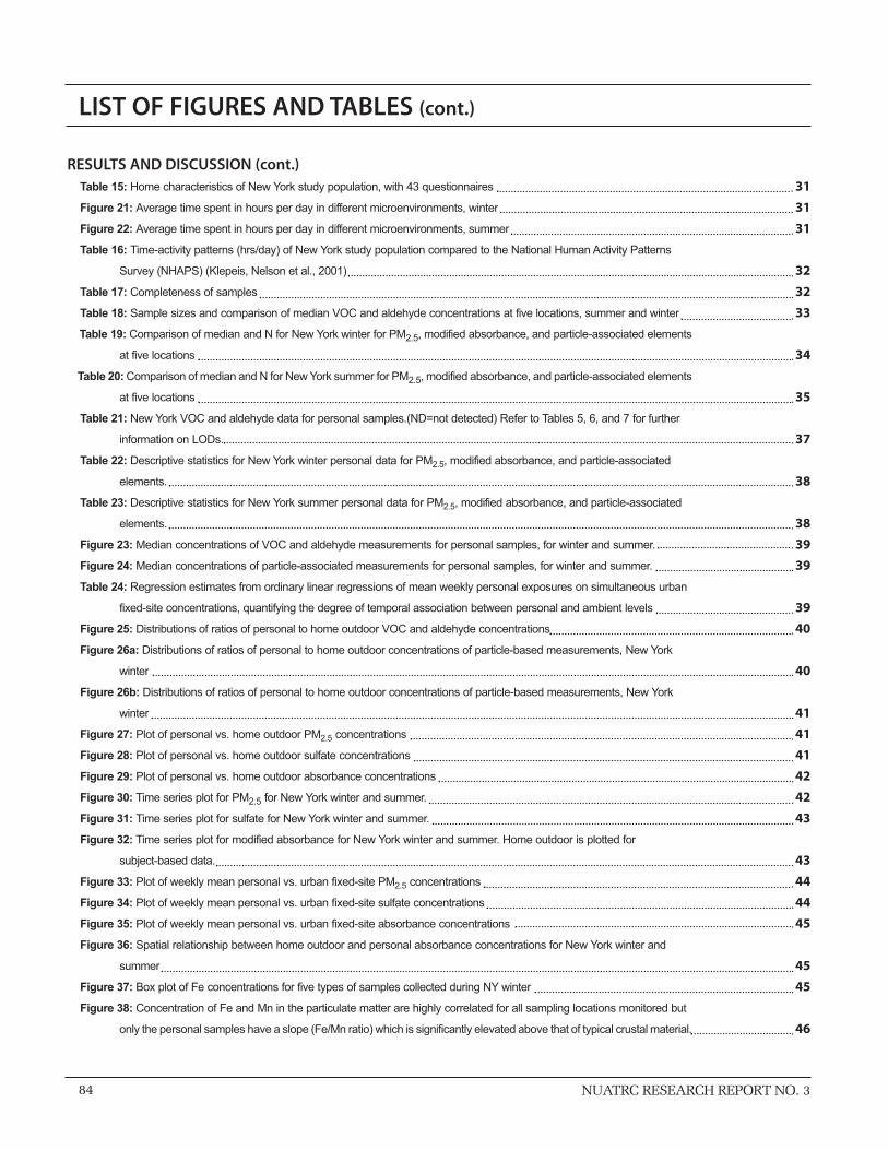
84 NUATRC RESEARCH REPORT NO. 3
LIST OF FIGURES AND TABLES (cont.)
RESULTS AND DISCUSSION (cont.)Table 15: Home characteristics of New York study population, with 43 questionnaires
Figure 21: Average time spent in hours per day in different microenvironments, winter
Figure 22: Average time spent in hours per day in different microenvironments, summer
Table 16: Time-activity patterns (hrs/day) of New York study population compared to the National Human Activity Patterns
Survey (NHAPS) (Klepeis, Nelson et al., 2001)
Table 17: Completeness of samples
Table 18: Sample sizes and comparison of median VOC and aldehyde concentrations at five locations, summer and winter
Table 19: Comparison of median and N for New York winter for PM2.5, modified absorbance, and particle-associated elements
at five locations
Table 20: Comparison of median and N for New York summer for PM2.5, modified absorbance, and particle-associated elements
at five locations
Table 21: New York VOC and aldehyde data for personal samples.(ND=not detected) Refer to Tables 5, 6, and 7 for further
information on LODs.
Table 22: Descriptive statistics for New York winter personal data for PM2.5, modified absorbance, and particle-associated
elements.
Table 23: Descriptive statistics for New York summer personal data for PM2.5, modified absorbance, and particle-associated
elements.
Figure 23: Median concentrations of VOC and aldehyde measurements for personal samples, for winter and summer.
Figure 24: Median concentrations of particle-associated measurements for personal samples, for winter and summer.
Table 24: Regression estimates from ordinary linear regressions of mean weekly personal exposures on simultaneous urban
fixed-site concentrations, quantifying the degree of temporal association between personal and ambient levels
Figure 25: Distributions of ratios of personal to home outdoor VOC and aldehyde concentrations
Figure 26a: Distributions of ratios of personal to home outdoor concentrations of particle-based measurements, New York
winter
Figure 26b: Distributions of ratios of personal to home outdoor concentrations of particle-based measurements, New York
winter
Figure 27: Plot of personal vs. home outdoor PM2.5 concentrations
Figure 28: Plot of personal vs. home outdoor sulfate concentrations
Figure 29: Plot of personal vs. home outdoor absorbance concentrations
Figure 30: Time series plot for PM2.5 for New York winter and summer.
Figure 31: Time series plot for sulfate for New York winter and summer.
Figure 32: Time series plot for modified absorbance for New York winter and summer. Home outdoor is plotted for
subject-based data.
Figure 33: Plot of weekly mean personal vs. urban fixed-site PM2.5 concentrations
Figure 34: Plot of weekly mean personal vs. urban fixed-site sulfate concentrations
Figure 35: Plot of weekly mean personal vs. urban fixed-site absorbance concentrations
Figure 36: Spatial relationship between home outdoor and personal absorbance concentrations for New York winter and
summer
Figure 37: Box plot of Fe concentrations for five types of samples collected during NY winter
Figure 38: Concentration of Fe and Mn in the particulate matter are highly correlated for all sampling locations monitored but
only the personal samples have a slope (Fe/Mn ratio) which is significantly elevated above that of typical crustal material.
31
31
31
32
32
33
34
35
37
38
38
39
39
39
40
40
41
41
41
42
42
43
43
44
44
45
45
45
46

NUATRC RESEARCH REPORT NO. 3 85
LIST OF FIGURES AND TABLES (cont.)
RESULTS AND DISCUSSION (cont.)Table 25: Slope and R2 of least squares fit line to data of personal and ambient sample locations for NY summer samples.
Figure 39: The ratio of Fe to Mn observed in the personal samples from TEACH during both summer and winter field seasons
were consistent with the Fe/Mn ratio measured in a single set of duplicate 8 hr samples collected in the NYC subway
system.
Figure 40: The ratio of chromium to manganese observed in the personal samples from TEACH during the summer field season
were consistent with the Cr/Mn ratio measured in a single set of duplicate 8 hr samples collected in the NYC subway
system.
Table 26: New York VOC and aldehyde data for home indoor sites
Table 27: Descriptive statistics for New York winter home indoor data for PM2.5, modified absorbance, and particle-associated
elements
Table 28: Descriptive statistics for New York summer home indoor data for PM2.5, modified absorbance, and particle-associated
elements
Figure 41: Median concentrations of VOC and aldehyde measurements for home indoor sites, for winter and summer.
Figure 42: Median concentrations of particle-associated measurements for home indoor samples, for winter and summer.
Figure 43: Distributions of ratios of home indoor to home outdoor elemental data
Figure 44: Distributions of ratios of home indoor to home outdoor VOC and aldehyde concentrations
Figure 45: Sulfate I/O scatterplots, winter (left) and summer (right)
Figure 46: Abs* I/O scatterplots, winter (left) and summer (right)
Figure 47: Dichlorobenzene I/O scatterplots, winter (left) and summer (right) (log scale)
Figure 48: Formaldehyde I/O scatterplots, winter (L) and summer (R)
Figure 49: Distribution of air exchange rates (AER) by season.
Figure 50: Median ratios of indoor-to-outdoor concentrations of particle-associated air pollutants grouped by air exchange rate
categories.
Figure 51: Median ratios of indoor-to-outdoor concentrations of VOCs and aldehydes grouped by air exchange rate categories.
Figure 52: Time series plot for PM2.5 for New York winter and summer. Home outdoor is plotted for subject-based data.
Figure 53: Time series plot for modified absorbance for New York winter and summer.
Figure 54: Abs* for home outdoor samples plotted against Abs* for home indoor samples
Figure 55: Abs* coefficients (x105) plotted against PM2.5 for home outdoor and fixed site samples collected during NYC winter.
Figure 56: Abs* plotted against PM2.5 for indoor and personal samples.
Figure 57: Histogram of the fraction of the total measured indoor PM2.5 that is predicted to originate from ambient sources as
determined by the reflectance measurements.
Table 29: New York ambient VOC and aldehyde data for urban fixed-site
Figure 58: Median concentrations of VOC and aldehyde measurements for the urban fixed site, for winter and summer.
Figure 59: Median concentrations of particle-associated measurements for the urban fixed site, for winter and summer.
Table 30: New York ambient VOC and aldehyde data for upwind fixed-site
Table 31: New York ambient VOC and aldehyde data for home outdoor sites
Figure 60: Time series plot for sulfate for New York winter and summer.
Table 32: Descriptive statistics for New York winter urban fixed-site data for PM2.5, modified absorbance, and particle-associated
elements.
Table 33: Descriptive statistics for New York summer urban fixed-site data for PM2.5, modified absorbance, and particle-
associated elements.
46
46
47
48
49
49
50
50
51
52
52
52
53
53
53
54
55
56
56
57
57
57
58
59
60
60
61
62
63
64
64
86 NUATRC RESEARCH REPORT NO. 3
LIST OF FIGURES AND TABLES (cont.)
RESULTS AND DISCUSSION (cont.)Figure 61: Time series plot for cobalt for New York winter and summer. Home outdoor is plotted for subject-based data.
Figure 62: Time series plot for arsenic and selenium for New York summer. Home outdoor is plotted for subject-based data.
Figure 63: Time series plot for MTBE for New York winter and summer
Figure 64: Time series plot for formaldehyde for New York winter and summer.
Figure 65: Time series plot for acetaldehyde for New York winter and summer.
Table 34: Descriptive statistics for New York winter upwind fixed site data for PM2.5, modified absorbance, and particle-
associated elements.
Table 35: Descriptive statistics for New York summer upwind fixed site data for PM2.5, modified absorbance, and particle-
associated elements.
Table 36: Descriptive statistics for New York winter home outdoor data for PM2.5, modified absorbance, and particle-associated
elements.
Table 37: Descriptive statistics for New York summer home outdoor data for PM2.5, modified absorbance, and particle-
associated elements.
Table 38: Comparison of urban fixed site to upwind fixed site. Daily differences and daily ratios between the two sites, VOCs
and aldehydes.
Figure 66: Time series plot for toluene for New York winter and summer.
Figure 67: Median of all daily ratios of the urban fixed-site concentration to the upwind fixed-site concentration, with order ranked
by value of ratio in winter.
Table 39: Comparison of urban fixed-site to upwind fixed-site.
Table 40: Comparison of urban fixed-site to upwind fixed-site.
Figure 68: Plot of the ratios of spatial to temporal variability of particle-associated analytes.
Figure 69: Spatial and temporal variance of particle-associated air pollutants including all data, calculated by the mixed model
described in the text.
Figure 70: Spatial and temporal variance of particle-associated air pollutants without extreme concentrations, calculated by the
mixed model described in the text.
Table 41: Total number of values and number of extreme values removed for mixed model runs of particle-associated elements
Table 42: Significance of spatial and temporal variances from mixed model results for NY particle-associated air pollutants
including all data
Table 43: Significance of spatial and temporal variances from mixed model results for NY particle-associated air pollutants
without extremes
Table 44: Number of extreme values for each compound
65
65
66
66
66
67
67
68
68
68
69
69
70
70
71
71
72
72
73
73
73

NUATRC RESEARCH REPORT NO. 3 87
Patrick L. Kinney et al
APPENDIX A1
Student Survey Questionnaire and Codebook

88
Toxic Exposure Assessment: A Columbia-Harvard (TEACH) Study (The New York City Report)
NUATRC RESEARCH REPORT NO. 3
Toxic Exposures to Air Pollutants- A Columbia Harvard Project
STUDENT SURVEY
The information recorded on this page will be separated from the remainder of this form and kept confidential.
1. TODAY'S DATE ____/ ____/ 99
2. YOUR NAME: ________________________________________________(First Middle Initial Last)
3. HOME ADDRESS: ________________________________________________
________________________________________________
TELEPHONE(Res) (__ ___ _) __ __ __-__ __ __ __
Now please tear off this top sheet. It will be collected separately from the questionnaire that follows.
Appendix A1. Student survey

NUATRC RESEARCH REPORT NO. 3 89
Patrick L. Kinney et al
Appendix A1. (continued)
Instructions:
This is a questionnaire you are asked to fill out. Please answer all questions as accurately as possible. If youdon't know an answer, you should check off 'don't know ' rather than guessing. If you need assistance inanswering a question, please put a check mark against the question. At the end, before you hand in thequestionnaire, ask the teacher / study coordinator who will assist you with the question(s).
All information provided in this questionnaire will be kept strictly confidential and used only for researchpurposes. The top sheet with your name and address will be separated from the questionnaire when you turnit in, and be kept in a locked cabinet at Columbia University. Nobody in the A. Philip Randolph HS will haveaccess to the identifying information on the top sheet. You may leave a question blank if you areuncomfortable answering it.
4. YOUR SEX Male / Female (circle)
5. YOUR DATE OF BIRTH: ___________________________(month, day, year)
6. YOUR GRADE IN SCHOOL: 9 10 11 12 (circle one)
7. DO YOU CONSIDER YOURSELF:
__Black or African-American __American Indian__White __Other (Specify:___________________)__Asian __Don't know
8. ARE YOU OF SPANISH / HISPANIC ORIGIN, SUCH AS DOMINICAN, PUERTO RICAN, CUBAN, ORMEXICAN AMERICAN?
__No__Yes__Don't know
9. DO YOU CURRENTLY SMOKE CIGARETTES ON A REGULAR BASIS? (THAT IS, AT LEAST ONE CIGARETTE PER DAY)
__No__Yes
10. DO YOU CURRENTLY SMOKE CIGARS OR PIPES ON A REGULAR BASIS? (THAT IS, AT LEAST ONCE PER DAY)
__No__Yes

90
Toxic Exposure Assessment: A Columbia-Harvard (TEACH) Study (The New York City Report)
NUATRC RESEARCH REPORT NO. 3
Appendix A1. (continued)
11. DO YOU CURRENTLY SMOKE ANY OTHER PRODUCTS ON A REGULAR BASIS?THAT IS, AT LEAST ONCE PER DAY)
__No__Yes
12. WHAT IS THE HIGHEST LEVEL OF EDUCATION ACHIEVED BY FATHER / MALE GUARDIAN ?
__Did not Graduate from High School__High School Graduate__Technical/Trade School__Some College__College Graduate__Graduate/Professional School__Don't know
13. WHAT IS THE HIGHEST LEVEL OF EDUCATION ACHIEVED BY MOTHER / FEMALE GUARDIAN ?
__Did not Graduate from High School__High School Graduate__Technical/Trade School__Some College__College Graduate__Graduate/Professional School__Don't know
QUESTIONS RELATED TO YOUR HOME
14. HOW WOULD YOU DESCRIBE THE BUILDING WHERE YOU LIVE ?
__Single family house, detached from any other house__Single family house, attached to one or more houses__2-3 Family home__Office/ Apartment building __ An apartment building with 2-3 floors__An apartment building with 4-6 floors__An apartment building with more than 6 floors__Other (please specify) _______________________________________
15. DOES THE AREA WHERE YOU LIVE CONSISTS MAINLY OF : (check all that apply)
__Single family homes__Apartment buildings__Commercial buildings__Industrial buildings
16. WHAT FLOOR IS YOUR HOME ON? _____________(mark 1 for ground floor)

NUATRC RESEARCH REPORT NO. 3 91
Patrick L. Kinney et al
Appendix A1. (continued)
17. HOW OFTEN DO HEAVY TRUCKS AND BUSES PASS ON THE STREET IN FRONT OF YOUR HOME?
__Almost all the time__often /several times per day__rarely / a few times per day__never
18. DO YOU HAVE PLANS TO MOVE IN THE NEXT YEAR?
__No__Yes__Don't know
19. INCLUDING YOURSELF, HOW MANY PEOPLE IN YOUR HOUSEHOLD SMOKE INSIDE YOURHOME?
___________________
20. HOW MUCH IN TOTAL DO THE PEOPLE IN THE PREVIOUS QUESTION SMOKE INSIDE THE HOME?
__Cigarettes per day __Cigars per week __ Pipe tobacco (pipefuls per week)
21. WHEN COMMUTING TO SCHOOL, HOW MUCH TIME (in minutes) DO YOU SPEND ON AVERAGE?(For Going One Way) PLEASE FILL OUT ALL THAT APPLY.
______min. Walking or biking______min. On a motorcycle / scooter / moped______min. In a car / taxi______min. In a bus / tram______min. In a train / metro
22. ASIDE FROM COMMUTING, ON AN AVERAGE DAY ‘IN THE LAST TWO WEEKS’ HOW MUCH TIME(minutes per day) DID YOU SPEND OUTDOORS? _____________minutes / day
23. DO YOU CURRENTLY PARTICIPATE ON A REGULAR BASIS IN ANY AFTER SCHOOL ACTIVITIES?
__No__Yes
IF YES: PLEASE DESCRIBE: ______________________________
HOW MANY HOURS PER WEEK? ___________________________
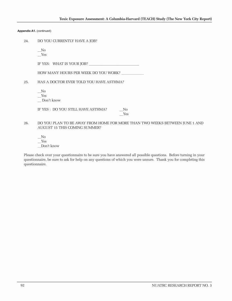
92
Toxic Exposure Assessment: A Columbia-Harvard (TEACH) Study (The New York City Report)
NUATRC RESEARCH REPORT NO. 3
Appendix A1. (continued)
24. DO YOU CURRENTLY HAVE A JOB?
__No__Yes
IF YES: WHAT IS YOUR JOB? _____________________________
HOW MANY HOURS PER WEEK DO YOU WORK? _____________
25. HAS A DOCTOR EVER TOLD YOU HAVE ASTHMA?
__No__Yes__ Don’t know
IF YES : DO YOU STILL HAVE ASTHMA? __No__Yes
26. DO YOU PLAN TO BE AWAY FROM HOME FOR MORE THAN TWO WEEKS BETWEEN JUNE 1 ANDAUGUST 15 THIS COMING SUMMER?
__No__Yes__Don't know
Please check over your questionnaire to be sure you have answered all possible questions. Before turning in yourquestionnaire, be sure to ask for help on any questions of which you were unsure. Thank you for completing thisquestionnaire.

NUATRC RESEARCH REPORT NO. 3 93
Patrick L. Kinney et al
Code book for Student Survey
NA=Not answered
VARIABLE DEFINITION CODES
Sex Sex 1 = Male2 = Female8 = NA
Dob Date of birth
Grade Grade in school
Race Race student considers his/herself 1 = Black/African American2 = White3 = Asian4 = American Indian
5 = Don=t know8 = NA
SpaHisp Are you of Spanish/Hispanic origin 1 = Yes2 = No
3 = Don=t know8 = NA
SmokCig Do you currently smoke cigarettes on aregular basis
1 = Yes2 = No8 = NA
CigarPip Do you currently smoke cigars on aregular basis
1 = Yes2 = No8 = NA
SmokOthr Do you currently smoke any otherproducts on a regular basis
1 = Yes2 = No8 = NA
EduFathr Highest level of education achieved byfather
1 = Did not graduate from highschool2 = High school graduate3 = Technical/Trade school4 = Some college5 = College graduate6 = Graduate/Professional
7 = Don=t know8 = NA
EduMothr Highest level of education achieved bymother
1 = Did not graduate from highschool2 = High school graduate3 = Technical/Trade school4 = Some college5 = College graduate6 = Graduate/Professional
7 = Don=t know8 = NA
Appendix A1. (continued)
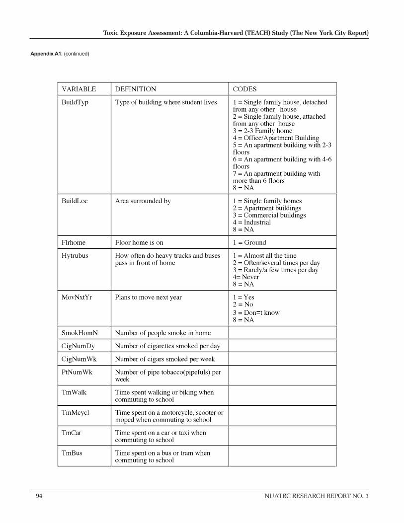
94
Toxic Exposure Assessment: A Columbia-Harvard (TEACH) Study (The New York City Report)
NUATRC RESEARCH REPORT NO. 3
Appendix A1. (continued)
VARIABLE DEFINITION CODES
BuildTyp Type of building where student lives 1 = Single family house, detachedfrom any other house2 = Single family house, attachedfrom any other house3 = 2-3 Family home4 = Office/Apartment Building5 = An apartment building with 2-3floors6 = An apartment building with 4-6floors7 = An apartment building withmore than 6 floors8 = NA
BuildLoc Area surrounded by 1 = Single family homes2 = Apartment buildings3 = Commercial buildings4 = Industrial8 = NA
Flrhome Floor home is on 1 = Ground
Hytrubus How often do heavy trucks and busespass in front of home
1 = Almost all the time2 = Often/several times per day3 = Rarely/a few times per day4= Never8 = NA
MovNxtYr Plans to move next year 1 = Yes2 = No
3 = Don=t know8 = NA
SmokHomN Number of people smoke in home
CigNumDy Number of cigarettes smoked per day
CigNumWk Number of cigars smoked per week
PtNumWk Number of pipe tobacco(pipefuls) perweek
TmWalk Time spent walking or biking whencommuting to school
TmMcycl Time spent on a motorcycle, scooter ormoped when commuting to school
TmCar Time spent on a car or taxi whencommuting to school
TmBus Time spent on a bus or tram whencommuting to school

NUATRC RESEARCH REPORT NO. 3 95
Patrick L. Kinney et al
Appendix A1. (continued)
VARIABLE DEFINITION CODES
TmTrain Time spent in a train or metro whencommuting to school
NumDyOut Number of hours per day spent outsidein the past 2 weeks
TmSptOut Number of hours per day spent outsidein the past 2 weeks
AftSchAc Any after school activities 1 = Yes2 = No8 = NA
KindOfAc Kind of activity
NumHrAc Number of hours spent in activity
Havejob Currently have a job 1 = Yes2 = No8 = NA
KindJob Kind of job
NumHrJob Number of hours spent in job
Asthma Has doctor ever told you have asthma 1 = Yes2 = No
3 = Don=t know8 = NA
NowAsthm Now have asthma 1 = Yes2 = No8 = NA
AwaySpr Plan to be away from home for morethan two weeks in summer
1 = Yes2 = No
3 = Don=t know8 = NA

NUATRC RESEARCH REPORT NO. 3 97
Patrick L. Kinney et al
APPENDIX A2
Home Environment Questionnaire and Codebook

98
Toxic Exposure Assessment: A Columbia-Harvard (TEACH) Study (The New York City Report)
NUATRC RESEARCH REPORT NO. 3
ID : NW_ _ _ _
1
Frm:LHEVer Feb 19, 1999
[Interviewer : This questionnaire should be administered to the parent / guardian of the student participatingin the TEACH project. Circle the correct answer or fill in the appropriate box on the right corner of the
question.
Date of Questionnaire administration __/__/99
1) When was your home built ? 1. After 1980
2. 1960-1979
3. 1940-1959
4. 1920-1939
5. 1900-1919
6. Before 1900
7. Don’t know
HOME ENVIRONMENT QUESTIONNAIRE
Appendix A2. Home environmental questionnaire

NUATRC RESEARCH REPORT NO. 3 99
Patrick L. Kinney et al
ID : NW_ _ _ _
2
2) What year did you move into this house / apartment 1 9
3) What is the volume of car traffic on the street in front of your home during weekdays ?
1. High / many cars passing by all the time
2. Medium / many cars passing by, but not all the time
3. Light / an occasional car passing by,
4. Never / no car passing by
4) What is the volume of heavy truck and / or bus traffic on the street in front of your home on weekdays ?
1. High / many passing by all the time
2. Medium / many passing by, but not all the time
3. Light / an occasional truck/bus passing by
4. Never / no truck or bus passing by
5) Is there a garage attached to this house / apartment ?
1. Yes
2. NO (Go to Q. 10)
6) Where is the attached garage ? 1. Underneath the main living quarters
2. Same level as the main living quarters
3. Other , specify _________________________
7) Is there a doorway leading directly from the garage into the living quarters ?
1. Yes
2. No
8) Are automobiles, vans, trucks orother motor vehicles usually parkedin this attached garage ?
1. Yes
2. No
Appendix A2. (continued)

100
Toxic Exposure Assessment: A Columbia-Harvard (TEACH) Study (The New York City Report)
NUATRC RESEARCH REPORT NO. 3
ID : NW_ _ _ _
3
9) Are any gas powered devices stored in anyroom, basement or attached garage in thishouse. DO include motorcycles, gas-poweredlawnmowers, trimmers blowers, boat engines ?
1.Yes2. No
Yes No
10) Does you home have ? Wall to wall carpet
(Please check all that apply) Other carpets / rugs
Curtains
Upholstered or soft furnishing
Double glazing
Linoleum floor
PVC (plastic) floor
Wood floor
Wood paneling on walls and or ceiling
Plasterboard walls and or ceiling
Chipboard walls
Wall paper (any kind)
Yes No Don’t
11) Has there been any of thefollowing renovations / repair inyour home in the last year ? (Please check all that apply)
Wall painting / new wall paper
Floor repair / polishing /
Water / sewage system repair
Window or door repair / replacement
Insulation repair / replacement
Wall construction / removing
12) Have any of the renovations been 1. Yes
caused by water damage ? 2. No3. Don’t know
Appendix A2. (continued)
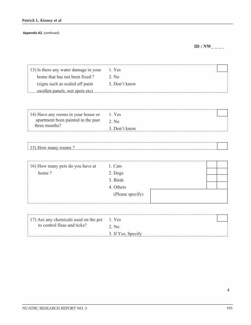
NUATRC RESEARCH REPORT NO. 3 101
Patrick L. Kinney et al
ID : NW_ _ _ _
4
13) Is there any water damage in your 1. Yes
home that has not been fixed ? 2. No
(signs such as scaled off paint 3. Don’t know
swollen panels, wet spots etc)
14) Have any rooms in your house or apartment been painted in the past three months?
1. Yes
2. No
3. Don’t know
15) How many rooms ?
16) How many pets do you have at 1. Cats
home ? 2. Dogs
3. Birds
4. Others
(Please specify)
17) Are any chemicals used on the pet to control fleas and ticks?
1. Yes
2. No
3. If Yes, Specify
Appendix A2. (continued)

102
Toxic Exposure Assessment: A Columbia-Harvard (TEACH) Study (The New York City Report)
NUATRC RESEARCH REPORT NO. 3
ID : NW_ _ _ _
5
18) Including yourself, how many people in your household smoke inside your home ?
19) How much in total do the people Cigarettes per day
in the previous question smoke Cigars per day
inside the home ? Pipe tobacco (pipefuls per week)
20) Is air conditioning / refrigeration used to cool this house?
1. Yes
2. No (go to Q 24)
21) What type of air conditioning units do you use?
1. Central unit / units
2. Window or wall unit / units
3. Portable unit / units
22) During what month do you usually start and stop using air conditioner to cool this house ?
Start month Jan Feb Mar Apr May Jun Jul Aug Sep Oct Nov Dec
Stop month Jan Feb Mar Apr May Jun Jul Aug Sep Oct Nov Dec
23) At what temperature do you usually start using air conditioning to cool this house ?
70-75 F 75-80 F 80-85 F 85-90 F 90-95 F 95- + F
Appendix A2. (continued)
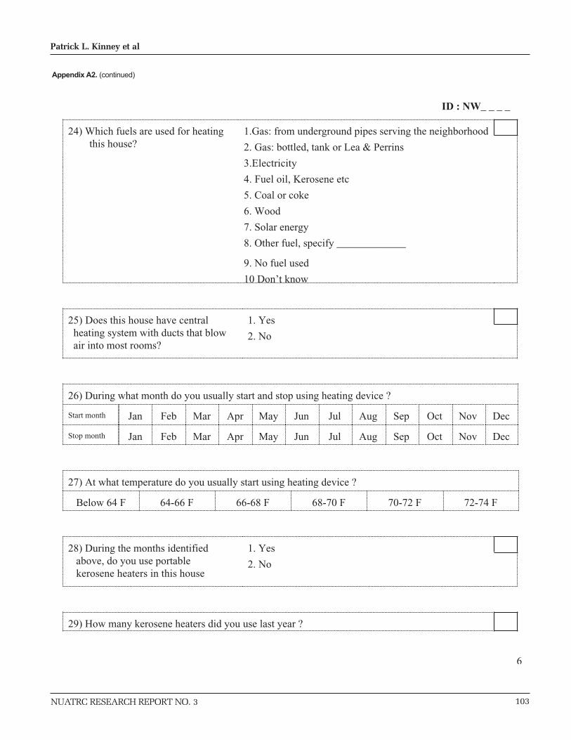
NUATRC RESEARCH REPORT NO. 3 103
Patrick L. Kinney et al
ID : NW_ _ _ _
6
24) Which fuels are used for heating this house?
1.Gas: from underground pipes serving the neighborhood
2. Gas: bottled, tank or Lea & Perrins
3.Electricity
4. Fuel oil, Kerosene etc
5. Coal or coke
6. Wood
7. Solar energy
8. Other fuel, specify _____________
9. No fuel used
10 Don’t know
25) Does this house have central heating system with ducts that blow air into most rooms?
1. Yes
2. No
26) During what month do you usually start and stop using heating device ?
Start month Jan Feb Mar Apr May Jun Jul Aug Sep Oct Nov Dec
Stop month Jan Feb Mar Apr May Jun Jul Aug Sep Oct Nov Dec
27) At what temperature do you usually start using heating device ?
Below 64 F 64-66 F 66-68 F 68-70 F 70-72 F 72-74 F
28) During the months identified above, do you use portable kerosene heaters in this house
1. Yes
2. No
29) How many kerosene heaters did you use last year ?
Appendix A2. (continued)

104
Toxic Exposure Assessment: A Columbia-Harvard (TEACH) Study (The New York City Report)
NUATRC RESEARCH REPORT NO. 3
ID : NW_ _ _ _
7
30) How often do you use kerosene heaters during the heating season?
1. Less than once a month
2. One to three times per month
3. Once or twice a week
4. 3-5 times a week
5. More than 5 time a week
31) During the heating season, is a portable or unvented gas heater used in this house or apartment ?
1. Yes
2. No (go to Q.34)
32) How many gas heaters ?
33) How often is portable or converted gas heater used ?
1. Less than once a month
2. One to three times per month
3. Once or twice a week
4. 3-5 times a week
5. More than 5 time a week
34) During the heating season, is wood-burning or coal burning stove used int this house ?
1. Yes
2. No (go to Q 38)
35) How many wood or coal burning stoves ?
36) How often is wood or coal burning stove used during the heating season ?
1. Less than once a month
2. One to three times per month
Appendix A2. (continued)
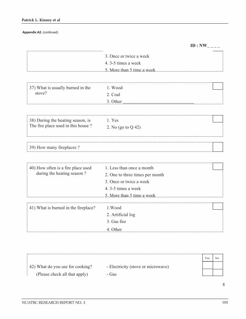
NUATRC RESEARCH REPORT NO. 3 105
Patrick L. Kinney et al
ID : NW_ _ _ _
8
3. Once or twice a week
4. 3-5 times a week
5. More than 5 time a week
37) What is usually burned in the stove?
1. Wood
2. Coal
3. Other _______________________________
38) During the heating season, isThe fire place used in this house ?
1. Yes
2. No (go to Q 42)
39) How many fireplaces ?
40) How often is a fire place used during the heating season ?
1. Less than once a month
2. One to three times per month
3. Once or twice a week
4. 3-5 times a week
5. More than 5 time a week
41) What is burned in the fireplace? 1.Wood
2. Artificial log
3. Gas fire
4. Other
Yes No
42) What do you use for cooking? - Electricity (stove or microwave)
(Please check all that apply) - Gas
Appendix A2. (continued)
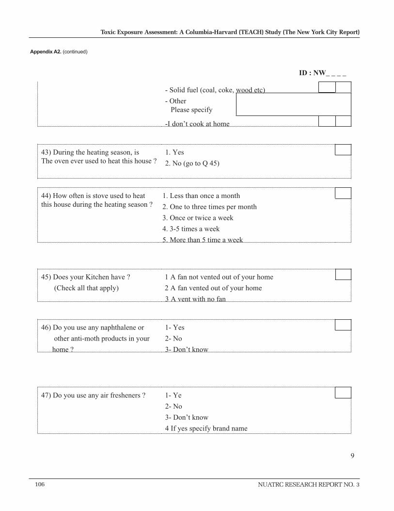
106
Toxic Exposure Assessment: A Columbia-Harvard (TEACH) Study (The New York City Report)
NUATRC RESEARCH REPORT NO. 3
ID : NW_ _ _ _
9
- Solid fuel (coal, coke, wood etc)
- Other Please specify
-I don’t cook at home
43) During the heating season, isThe oven ever used to heat this house ?
1. Yes
2. No (go to Q 45)
44) How often is stove used to heatthis house during the heating season ?
1. Less than once a month
2. One to three times per month
3. Once or twice a week
4. 3-5 times a week
5. More than 5 time a week
45) Does your Kitchen have ? 1 A fan not vented out of your home
(Check all that apply) 2 A fan vented out of your home
3 A vent with no fan
46) Do you use any naphthalene or 1- Yes
other anti-moth products in your 2- No
home ? 3- Don’t know
47) Do you use any air fresheners ? 1- Ye
2- No
3- Don’t know
4 If yes specify brand name
Appendix A2. (continued)

NUATRC RESEARCH REPORT NO. 3 107
Patrick L. Kinney et al
ID : NW_ _ _ _
10
48) Including yourself how many people usually live in this house ?
49) How many people who usually live in this house are 18 years old or younger ?
50) How old are you ?
51) Do you consider yourself ? 1. Black or African-American
2. White
3. Asian
4. American Indian
5. Other (Specify:___________________)
6. Don’t know
52) Are you of Spanish / Hispanicorigin, such as Dominican, PuertoRican, Cuban, or Mexican American ?
1 Yes
2. No
3. Don’t know
53) Is this house or apartment 1. Owned by you or someone in this household with
Mortgage or loan
2. Owned by you or someone in this household
Free and clear (without mortgage)
3. Rented for cash rent
4. Occupied without payment for cash rent
Appendix A2. (continued)

108
Toxic Exposure Assessment: A Columbia-Harvard (TEACH) Study (The New York City Report)
NUATRC RESEARCH REPORT NO. 3
ID : NW_ _ _ _
11
54) What is your relationship to ____ (Give name of student)
1 Mother
2. Father
3. Other, specify ______________________
55) Approximately what is the gross annual income for all family members in this household ?
Hand out the card and give number
D:\Leland\Questionnaire&Logs\Quest\Home envt\home_envt_2.wpd
Appendix A2. (continued)

NUATRC RESEARCH REPORT NO. 3 109
Patrick L. Kinney et al
Appendix A2. (continued)
Code Book for Home Environment Questionnaire
NA: Not answered
VARIABLE DEFINITION CODES
Dt_admin Date of questionnaire administration
Yr_built Year home was built 1 = After 19802 = 1960-19793 = 1940-19594 = 1920-19395 = 1900-19196 = Before 1900
7 = Don=t know8 = Not answered(NA)
Yr_moved Year moved into home 8 = NA
Vol_car Volume of car traffic in front of homeduring weekdays
1 = High/many cars passing by all the time2 = Medium/ many cars passing by, but notall the time3 = Light/an occasional car passing by4 = Never/ no truck or bus passing by8 = NA
Vol_bus Volume of truck and/or bus in front ofhome on weekdays
1 = High/many cars passing by all the time2 = Medium/ many cars passing by, but notall the time3 = Light/an occasional car passing by4 = Never/ no truck or bus passing by8 = NA
Gar_atch Garage attached to home 1 = Yes2 = No8 = NA
Gar_wher Where is attached garage 1 = Underneath the main living quarters2 = Same level as the main living quarters3 = Other8 = NA
Door_gar Doorway leading from the garage into theliving quarters
1 = Yes2 = No8 = NA
Gar_auto Automobiles, vans, trucks parked in attachedgarage
1 = Yes2 = No8 = NA
Gar_gasd Gas powered devices stored in basement orgarage
1 = Yes2 = No
3 = Don=t know8 = NA
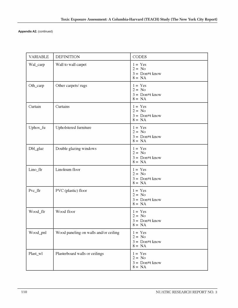
VARIABLE DEFINITION CODES
Wal_carp Wall to wall carpet 1 = Yes2 = No
3 = Don=t know8 = NA
Oth_carp Other carpets/ rugs 1 = Yes2 = No
3 = Don=t know8 = NA
Curtain Curtains 1 = Yes2 = No
3 = Don=t know8 = NA
Uphos_fu Upholstered furniture 1 = Yes2 = No
3 = Don=t know8 = NA
Dbl_glaz Double glazing windows 1 = Yes2 = No
3 = Don=t know8 = NA
Lino_flr Linoleum floor 1 = Yes2 = No
3 = Don=t know8 = NA
Pvc_flr PVC (plastic) floor 1 = Yes2 = No
3 = Don=t know8 = NA
Wood_flr Wood floor 1 = Yes2 = No
3 = Don=t know8 = NA
Wood_pnl Wood paneling on walls and/or ceiling 1 = Yes2 = No
3 = Don=t know8 = NA
Plast_wl Plasterboard walls or ceilings 1 = Yes2 = No
3 = Don=t know8 = NA
110
Toxic Exposure Assessment: A Columbia-Harvard (TEACH) Study (The New York City Report)
NUATRC RESEARCH REPORT NO. 3
Appendix A2. (continued)
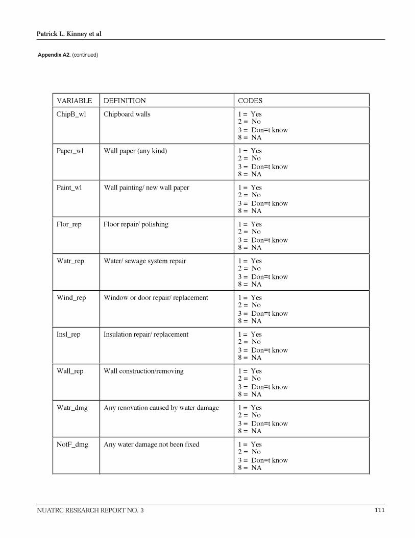
NUATRC RESEARCH REPORT NO. 3 111
Patrick L. Kinney et al
Appendix A2. (continued)
VARIABLE DEFINITION CODES
ChipB_wl Chipboard walls 1 = Yes2 = No
3 = Don=t know8 = NA
Paper_wl Wall paper (any kind) 1 = Yes2 = No
3 = Don=t know8 = NA
Paint_wl Wall painting/ new wall paper 1 = Yes2 = No
3 = Don=t know8 = NA
Flor_rep Floor repair/ polishing 1 = Yes2 = No
3 = Don=t know8 = NA
Watr_rep Water/ sewage system repair 1 = Yes2 = No
3 = Don=t know8 = NA
Wind_rep Window or door repair/ replacement 1 = Yes2 = No
3 = Don=t know8 = NA
Insl_rep Insulation repair/ replacement 1 = Yes2 = No
3 = Don=t know8 = NA
Wall_rep Wall construction/removing 1 = Yes2 = No
3 = Don=t know8 = NA
Watr_dmg Any renovation caused by water damage 1 = Yes2 = No
3 = Don=t know8 = NA
NotF_dmg Any water damage not been fixed 1 = Yes2 = No
3 = Don=t know8 = NA

VARIABLE DEFINITION CODES
RmPnt_3m Any rooms painted in the last 3 months 1 = Yes2 = No
3 = Don=t know8 = NA
No_RmPnt Number of rooms painted
Pet_cat Number of cats
Pet_dog Number of dogs
Pet_bird Number of birds
Pet_othr Any other pet?
Pet_chem Any chemicals used on pets to control fleasand ticks
1 = Yes2 = No3 = If yes, please specify
Smk_pepl Number of people smoke inside home
Cigg_dy Number of cigarettes per day
Cigar_dy Number of cigars per day
Pipe_dy Number of pipe tobacco(pipefuls per week)
Ac_cool Air conditioning used to cool home 1 = Yes2 = No8 = NA
Ac_type Type of air conditioning units 1 = Central unit/units2 = Window or wall unit/units3 = Portable unit/units8 = NA
Ac_start Month start to use air conditioner 0 = NA1 = January2 = February3 = March4 = April5 = May6 = June7 = July8 = August9 = September10 = October11 = November12 = December
112
Toxic Exposure Assessment: A Columbia-Harvard (TEACH) Study (The New York City Report)
NUATRC RESEARCH REPORT NO. 3
Appendix A2. (continued)

NUATRC RESEARCH REPORT NO. 3 113
Patrick L. Kinney et al
Appendix A2. (continued)
VARIABLE DEFINITION CODES
Ac_stop Month stop to use air conditioner 0 = NA1 = January2 = February3 = March4 = April5 = May6 = June7 = July8 = August9 = September10 = October11 = November12 = December
Ac_strtm Temperature at start of use of air conditioner 1 = 70-75 F2 = 75-85 F3 = 80-85 F4 = 85-90 F5 = 90-95 F6 = 95-+F8 = NA
Heat_ful Type of fuels used for heating home 0 = NA1 = Gas: from underneath pipes serving theneighborhood2 = Gas: bottler, tank, or Lea & Perrins3 = Electricity4 = Fuel oil, kerosene etc5 = Coal or coke6 = Wood7 = Solar energy8 = Other fuels, specify9 = No fuel used
10 = Don=t know
Heat_cen Home with central heating system 1 = Yes2 = No8 = NA
Heat_str Month start to use heat 1 = January2 = February3 = March4 = April5 = May6 = June7 = July8 = August9 = September10 = October11 = November12 = December
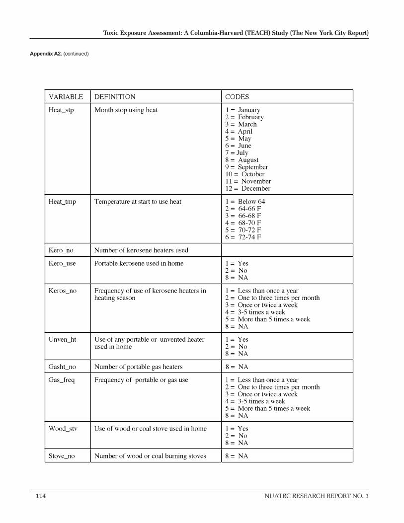
VARIABLE DEFINITION CODES
Heat_stp Month stop using heat 1 = January2 = February3 = March4 = April5 = May6 = June7 = July8 = August9 = September10 = October11 = November12 = December
Heat_tmp Temperature at start to use heat 1 = Below 642 = 64-66 F3 = 66-68 F4 = 68-70 F5 = 70-72 F6 = 72-74 F
Kero_no Number of kerosene heaters used
Kero_use Portable kerosene used in home 1 = Yes2 = No8 = NA
Keros_no Frequency of use of kerosene heaters inheating season
1 = Less than once a year2 = One to three times per month3 = Once or twice a week4 = 3-5 times a week5 = More than 5 times a week8 = NA
Unven_ht Use of any portable or unvented heaterused in home
1 = Yes2 = No8 = NA
Gasht_no Number of portable gas heaters 8 = NA
Gas_freq Frequency of portable or gas use 1 = Less than once a year2 = One to three times per month3 = Once or twice a week4 = 3-5 times a week5 = More than 5 times a week8 = NA
Wood_stv Use of wood or coal stove used in home 1 = Yes2 = No8 = NA
Stove_no Number of wood or coal burning stoves 8 = NA
114
Toxic Exposure Assessment: A Columbia-Harvard (TEACH) Study (The New York City Report)
NUATRC RESEARCH REPORT NO. 3
Appendix A2. (continued)
NUATRC RESEARCH REPORT NO. 3 115
Patrick L. Kinney et al
APPENDIX A3
Time-Location-Activity Diary

116
Toxic Exposure Assessment: A Columbia-Harvard (TEACH) Study (The New York City Report)
NUATRC RESEARCH REPORT NO. 3
Frm:LTADVer February 8,
1999
ID NW _ _ _ _ _________________
Begin:Date: ___ . ___ . ______ (dd, mm, yy) Time: ___. ___. (hh, min.)
End: Date: ___ . ___ . ______ (dd, mm, yy) Time: ___. ___. (hh, min.)
Definitions:
LOCATIONS:
Places you are staying at within a certain period of 15 minutes.
Time-Location-Activity-DiaryExercise Measurements
Appendix A3. Time-location-activity diary

NUATRC RESEARCH REPORT NO. 3 117
Patrick L. Kinney et al
NW _ _ _ _
IN TRANSFER
When you move from one place to another, including going for a walk or making some roundtrip.
Walk/bike: when you walk or bike from one place to another
Motorcycle: when you go on a motorbike from one place to another
Car /Taxi: when you drive or are driven from one place to another inside a private car, ataxi, a van or truck
Bus : when you travel from one place to another using a public bus
Subway/Train: when you travel from one place to another using the subway or a train
NOT IN TRANSFER
When you stay for some time within the same place (including going around within this place)
Home: In(side): all rooms in the house or apartment where you live
Out(side): outdoor locations belonging to your home as garden/ balcony/ yard
Work: In(side): all closed indoor-spaces of work where you are usually working
Out(side): open air locations where you are usually working
Other: In(side): any closed indoor-spaces other than home or work, including shopping,cinema, restaurants, theaters, sport hall, staying at homes of friends etc.
Out(side): all stays in open air which are not a transfer and not outside at home orwork, including staying in a park, at a sport ground, in a garden-café, etc.
ACTIVITIES
If one of the following events happens during a certain period of 15 minutes.
Cooking:
Smoking, self:
Smoking, same room:
when you are inside a kitchen and the stove is on, also if someone
else is cookingwhen you smoke a cigarette, cigar, pipe etc.
when somebody near you, inside a closed space, smokes acigarette, cigar, pipe etc.
Appendix A3. (continued)
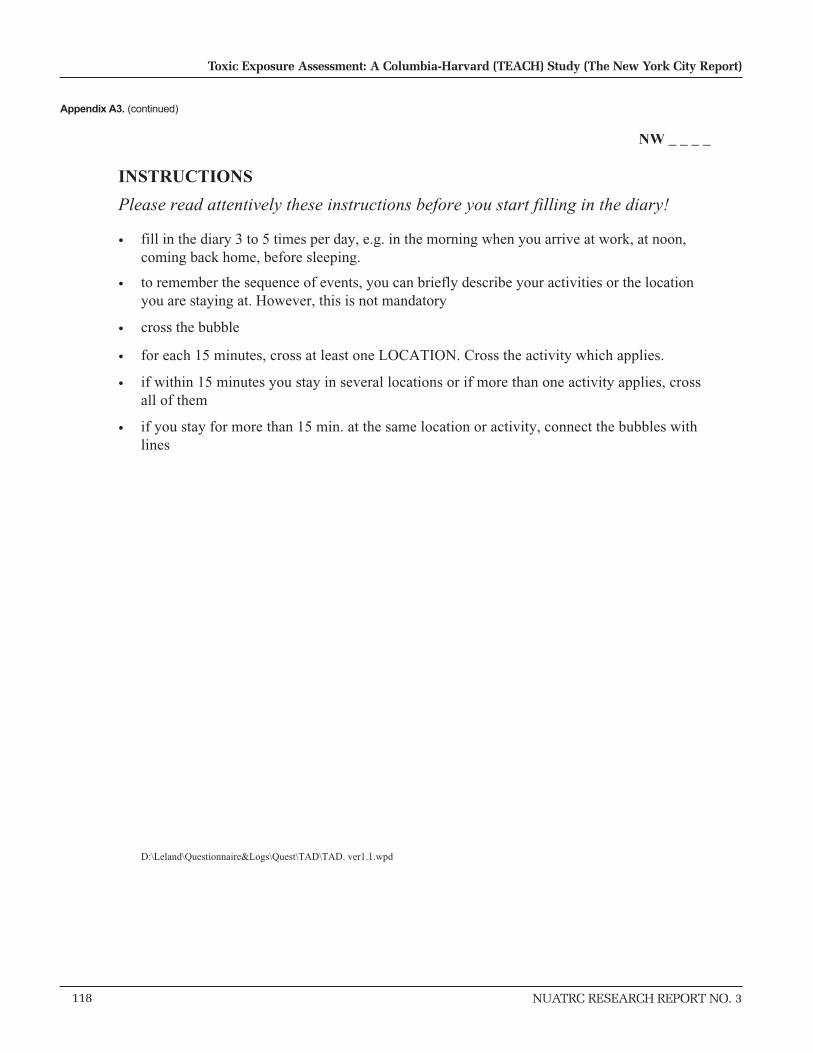
118
Toxic Exposure Assessment: A Columbia-Harvard (TEACH) Study (The New York City Report)
NUATRC RESEARCH REPORT NO. 3
NW _ _ _ _
INSTRUCTIONS
Please read attentively these instructions before you start filling in the diary!
• fill in the diary 3 to 5 times per day, e.g. in the morning when you arrive at work, at noon,coming back home, before sleeping.
• to remember the sequence of events, you can briefly describe your activities or the locationyou are staying at. However, this is not mandatory
• cross the bubble
• for each 15 minutes, cross at least one LOCATION. Cross the activity which applies.
• if within 15 minutes you stay in several locations or if more than one activity applies, crossall of them
• if you stay for more than 15 min. at the same location or activity, connect the bubbles withlines
D:\Leland\Questionnaire&Logs\Quest\TAD\TAD. ver1.1.wpd
Appendix A3. (continued)

NUATRC RESEARCH REPORT NO. 3 119
Patrick L. Kinney et al
ID : NW _ _ _ _
Date______ Location Activities
Time
BrieflyDescribeactivitiy
In Transfer Not In Transfer Cook-ing
Smoking
walkroller-bladebike
motorcycle
cartaxi
bus subwaytrain
home work other self sameroom
in out in out in out
6AM
0 O O O O O O O O O O O O O O
15 O O O O O O O O O O O O O O
30 O O O O O O O O O O O O O O
45 O O O O O O O O O O O O O O
7AM
0 O O O O O O O O O O O O O O
15 O O O O O O O O O O O O O O
30 O O O O O O O O O O O O O O
45 O O O O O O O O O O O O O O
8AM
0 O O O O O O O O O O O O O O
15 O O O O O O O O O O O O O O
30 O O O O O O O O O O O O O O
45 O O O O O O O O O O O O O O
9AM
0 O O O O O O O O O O O O O O
15 O O O O O O O O O O O O O O
30 O O O O O O O O O O O O O O
45 O O O O O O O O O O O O O O
10AM
0 O O O O O O O O O O O O O O
15 O O O O O O O O O O O O O O
30 O O O O O O O O O O O O O O
45 O O O O O O O O O O O O O O
11AM
0 O O O O O O O O O O O O O O
15 O O O O O O O O O O O O O O
30 O O O O O O O O O O O O O O
45 O O O O O O O O O O O O O O
Appendix A3. (continued)

120
Toxic Exposure Assessment: A Columbia-Harvard (TEACH) Study (The New York City Report)
NUATRC RESEARCH REPORT NO. 3
ID : NW _ _ _ _
Time
BrieflyDescribeactivity
In Transfer Not In Transfer Cooking
Smoking
walkroller-bladebike
motorcycle
cartaxi
bus subwaytrain
home work other self sameroom
12 0 O O O O O O O O O O O O O O
15 O O O O O O O O O O O O O O
30 O O O O O O O O O O O O O O
45 O O O O O O O O O O O O O O
1PM
0 O O O O O O O O O O O O O O
15 O O O O O O O O O O O O O O
30 O O O O O O O O O O O O O O
45 O O O O O O O O O O O O O O
2PM
0 O O O O O O O O O O O O O O
15 O O O O O O O O O O O O O O
30 O O O O O O O O O O O O O O
45 O O O O O O O O O O O O O O
3PM
0 O O O O O O O O O O O O O O
15 O O O O O O O O O O O O O O
30 O O O O O O O O O O O O O O
45 O O O O O O O O O O O O O O
4PM
0 O O O O O O O O O O O O O O
15 O O O O O O O O O O O O O O
30 O O O O O O O O O O O O O O
45 O O O O O O O O O O O O O O
5PM
0 O O O O O O O O O O O O O O
15 O O O O O O O O O O O O O O
30 O O O O O O O O O O O O O O
45 O O O O O O O O O O O O O O
Appendix A3. (continued)
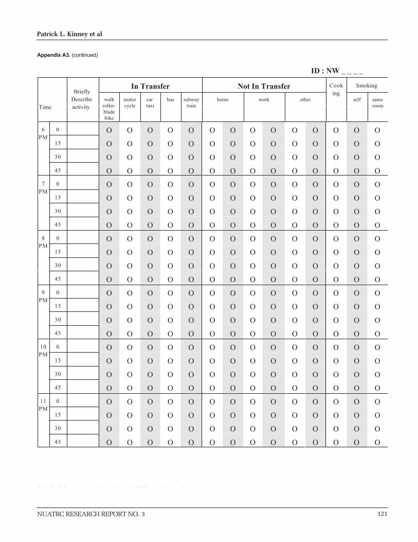
NUATRC RESEARCH REPORT NO. 3 121
Patrick L. Kinney et al
7PM
0 O O O O O O O O O O O O O O
15 O O O O O O O O O O O O O O
30 O O O O O O O O O O O O O O
45 O O O O O O O O O O O O O O
8PM
0 O O O O O O O O O O O O O O
15 O O O O O O O O O O O O O O
30 O O O O O O O O O O O O O O
45 O O O O O O O O O O O O O O
9PM
0 O O O O O O O O O O O O O O
15 O O O O O O O O O O O O O O
30 O O O O O O O O O O O O O O
45 O O O O O O O O O O O O O O
10PM
0 O O O O O O O O O O O O O O
15 O O O O O O O O O O O O O O
30 O O O O O O O O O O O O O O
45 O O O O O O O O O O O O O O
11PM
0 O O O O O O O O O O O O O O
15 O O O O O O O O O O O O O O
30 O O O O O O O O O O O O O O
45 O O O O O O O O O O O O O O
D \L l d\Q i i &L \Q \TAD\Fi TAD d
6PM
0 O O O O O O O O O O O O O O
15 O O O O O O O O O O O O O O
30 O O O O O O O O O O O O O O
45 O O O O O O O O O O O O O O
ID : NW _ _ _ _
Time
BrieflyDescribeactivity
In Transfer Not In Transfer Cooking
Smoking
walkroller-
motorcycle
cartaxi
bus subwaytrain
home work other self sameroom
bladebike
Appendix A3. (continued)

NUATRC RESEARCH REPORT NO. 3 123
Patrick L. Kinney et al
APPENDIX A4
48-Hour Exposure Questionnaire

124
Toxic Exposure Assessment: A Columbia-Harvard (TEACH) Study (The New York City Report)
NUATRC RESEARCH REPORT NO. 3
ID: NW_ _ _ _
1
Frm:L48Ver February
8, 1999
48 HOUR EXPOSURE QUESTIONNAIRETo be completed at the end of the 48 hours of your participation in the study
1. AT HOMEDuring the 48 hours that you carried the air participated in the study
1) For how many hours and minutes were the following devices used?(Please answer 0 if you do not have such a device or it was not used at all):
Hours Minutes
_ A single stove with gas
_A single stove with coal
_A single stove with wood
_A single stove with fuel/ heating oil
_ A fire place
_ A kitchen fan /vent while cooking
_ An air conditioner
Appendix A4. 48-Hour exposure questionnaire

NUATRC RESEARCH REPORT NO. 3 125
Patrick L. Kinney et al
ID: NW_ _ _ _
2
_A humidifier (including any humidifier built
into the heating system or air conditioning
_An electric air cleaner, ionizer of air filter
_An unvented gas fired water heater
_ An electric clothes drier
_ An unvented gas fired clothes drier
_An electric cooking stove
_ A microwave
_ A cooking stove with gas
_ A cooking stove with solid fuel (wood, coke etc)
2) Did you or someone else vacuum clean your home
1- Myself2- Someone else3- Nobody did
3) Were there any cleaning / polishing chemicalsused in your home ? (please give brand names)
4) For how many hours and minutes were the windows
Open ?
2. VARIOUS ACTIVITIESDuring the 48 hours that you participated in the study
Appendix A4. (continued)

126
Toxic Exposure Assessment: A Columbia-Harvard (TEACH) Study (The New York City Report)
NUATRC RESEARCH REPORT NO. 3
ID: NW_ _ _ _
3
1) For how many hours and minutes were you engaged in any of the followingactivities, at home work or elsewhere ?
Hours Minutes
_ Developing / printing photographs
_ Painting / Drawing
_ Using some kind of glue
_ Home workshop/ ‘do it your self”
_ Washing your car
_ Staying at a gas station filling the tank with
Gas ____ or Diesel _____
_ Grilling
_ Staying inside a garage
_ Heavy outdoor work / excercise (e.g. jogging
working in the garden etc.)
_ Heavy indoor work / excercise (e.g., in gym)
_ Staying inside an indoor ice hockey ring
2) For how many hours and minutes did you or someone
else use a photocopy machine or a printer inside thesame room ?
3) Did you use any deodorant, perfume hair spray or after shave ?
1- Yes2- No 3- Don’t remember
Appendix A4. (continued)

NUATRC RESEARCH REPORT NO. 3 127
Patrick L. Kinney et al
ID: NW_ _ _ _
4) Did you use any clothes that have been cleaned by dry cleaning ?
1- Yes2- No 3- Don’t remember
3. ANNOYANCE FROM AIR POLLUTIONDuring the 48 hours that you participated in the study
1) Please mark on the thermometer scale to what degree did you feel annoyed from airpollution at home during the 48 hours
Unbearable annoyane 10
9
8
7
6
5
4
3
2
1
No annoyance at all 0
2) This annoyance consisted mostly of ?
1- Dust2- Exhaust gases3- Chemical
4 - Others (please specify)
4
Appendix A4. (continued)

128
Toxic Exposure Assessment: A Columbia-Harvard (TEACH) Study (The New York City Report)
NUATRC RESEARCH REPORT NO. 3
ID: NW_ _ _ _
5
3) Please mark on the thermometer scale to what degree did you feel annoyed from airpollution at work during the 48 hours that you participated in the study
Unbearable annoyance 10
9
8
7
6
5
4
3
2
1
No annoyance at all 0
4) This annoyance consisted mostly of ?
1 - Dust2 - Exhaust gases3 - Chemical4 - Others (please specify)
Appendix A4. (continued)

NUATRC RESEARCH REPORT NO. 3 129
Patrick L. Kinney et al
ID: NW_ _ _ _
6
5) Please mark on the thermometer scale to what degree did you feel annoyed from airpollution outdoor during the 48 hours
Unbearable annoyance 10
9
8
7
6
5
4
3
2
1
No annoyance at all 0
6) This annoyance consisted mostly of ?
1 - Dust2 - Exhaust gases3 - Chemical4 - Others (please specify)
Appendix A4. (continued)
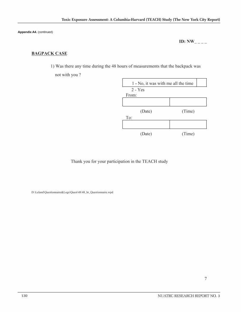
130
Toxic Exposure Assessment: A Columbia-Harvard (TEACH) Study (The New York City Report)
NUATRC RESEARCH REPORT NO. 3
ID: NW_ _ _ _
7
BAGPACK CASE
1) Was there any time during the 48 hours of measurements that the backpack was
not with you ?
1 - No, it was with me all the time
2 - YesFrom:
(Date) (Time)
To:
(Date) (Time)
Thank you for your participation in the TEACH study
D:\Leland\Questionnaire&Logs\Quest\48\48_hr_Questionnaire.wpd
Appendix A4. (continued)

NUATRC RESEARCH REPORT NO. 3 131
Patrick L. Kinney et al
APPENDIX B1
Variable Listing and Sample Printouts of Reference PM Dataset
NYPMELEMABSALL
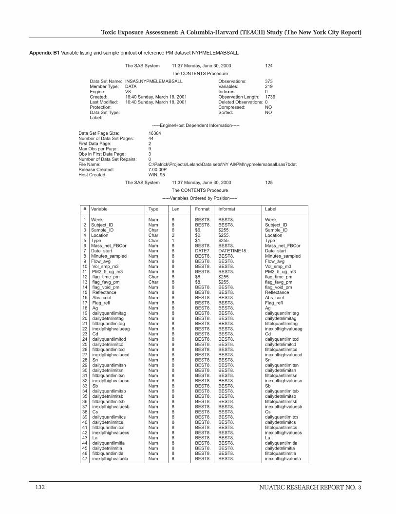
132
Toxic Exposure Assessment: A Columbia-Harvard (TEACH) Study (The New York City Report)
NUATRC RESEARCH REPORT NO. 3
Appendix B1 Variable listing and sample printout of reference PM dataset NYPMELEMABSALL
The SAS System 11:37 Monday, June 30, 2003 124
The CONTENTS Procedure
Data Set Name: INSAS.NYPMELEMABSALL Observations: 373 Member Type: DATA Variables: 219 Engine: V8 Indexes: 0 Created: 16:40 Sunday, March 18, 2001 Observation Length: 1736 Last Modified: 16:40 Sunday, March 18, 2001 Deleted Observations: 0 Protection: Compressed: NO Data Set Type: Sorted: NO Label:
-----Engine/Host Dependent Information-----
Data Set Page Size: 16384Number of Data Set Pages: 44First Data Page: 2Max Obs per Page: 9Obs in First Data Page: 3Number of Data Set Repairs: 0File Name: C:\Patrick\Projects\Leland\Data sets\NY All\PM\nypmelemabsall.sas7bdatRelease Created: 7.00.00PHost Created: WIN_95
The SAS System 11:37 Monday, June 30, 2003 125
The CONTENTS Procedure
-----Variables Ordered by Position-----
# Variable Type Len Format Informat Label 1 Week Num 8 BEST8. BEST8. Week 2 Subject_ID Num 8 BEST8. BEST8. Subject_ID 3 Sample_ID Char 6 $6. $255. Sample_ID 4 Location Char 2 $2. $255. Location 5 Type Char 1 $1. $255. Type 6 Mass_net_FBCor Num 8 BEST8. BEST8. Mass_net_FBCor 7 Date_start Num 8 DATE7. DATETIME18. Date_start 8 Minutes_sampled Num 8 BEST8. BEST8. Minutes_sampled 9 Flow_avg Num 8 BEST8. BEST8. Flow_avg 10 Vol_smp_m3 Num 8 BEST8. BEST8. Vol_smp_m3 11 PM2_5_ug_m3 Num 8 BEST8. BEST8. PM2_5_ug_m3 12 flag_time_pm Char 8 $8. $255. flag_time_pm 13 flag_favg_pm Char 8 $8. $255. flag_favg_pm 14 flag_void_pm Num 8 BEST8. BEST8. flag_void_pm 15 Reflectance Num 8 BEST8. BEST8. Reflectance 16 Abs_coef Num 8 BEST8. BEST8. Abs_coef 17 Flag_refl Num 8 BEST8. BEST8. Flag_refl 18 Ag Num 8 BEST8. BEST8. Ag 19 dailyquantlimitag Num 8 BEST8. BEST8. dailyquantlimitag 20 dailydetnlimitag Num 8 BEST8. BEST8. dailydetnlimitag 21 filtblquantlimitag Num 8 BEST8. BEST8. filtblquantlimitag 22 inexlplhighvalueag Num 8 BEST8. BEST8. inexlplhighvalueag 23 Cd Num 8 BEST8. BEST8. Cd 24 dailyquantlimitcd Num 8 BEST8. BEST8. dailyquantlimitcd 25 dailydetnlimitcd Num 8 BEST8. BEST8. dailydetnlimitcd 26 filtblquantlimitcd Num 8 BEST8. BEST8. filtblquantlimitcd 27 inexlplhighvaluecd Num 8 BEST8. BEST8. inexlplhighvaluecd 28 Sn Num 8 BEST8. BEST8. Sn 29 dailyquantlimitsn Num 8 BEST8. BEST8. dailyquantlimitsn 30 dailydetnlimitsn Num 8 BEST8. BEST8. dailydetnlimitsn 31 filtblquantlimitsn Num 8 BEST8. BEST8. filtblquantlimitsn 32 inexlplhighvaluesn Num 8 BEST8. BEST8. inexlplhighvaluesn 33 Sb Num 8 BEST8. BEST8. Sb 34 dailyquantlimitsb Num 8 BEST8. BEST8. dailyquantlimitsb 35 dailydetnlimitsb Num 8 BEST8. BEST8. dailydetnlimitsb 36 filtblquantlimitsb Num 8 BEST8. BEST8. filtblquantlimitsb 37 inexlplhighvaluesb Num 8 BEST8. BEST8. inexlplhighvaluesb 38 Cs Num 8 BEST8. BEST8. Cs 39 dailyquantlimitcs Num 8 BEST8. BEST8. dailyquantlimitcs 40 dailydetnlimitcs Num 8 BEST8. BEST8. dailydetnlimitcs 41 filtblquantlimitcs Num 8 BEST8. BEST8. filtblquantlimitcs 42 inexlplhighvaluecs Num 8 BEST8. BEST8. inexlplhighvaluecs 43 La Num 8 BEST8. BEST8. La 44 dailyquantlimitla Num 8 BEST8. BEST8. dailyquantlimitla 45 dailydetnlimitla Num 8 BEST8. BEST8. dailydetnlimitla 46 filtblquantlimitla Num 8 BEST8. BEST8. filtblquantlimitla 47 inexlplhighvaluela Num 8 BEST8. BEST8. inexlplhighvaluela

NUATRC RESEARCH REPORT NO. 3 133
Patrick L. Kinney et al
Appendix B1. (continued)
The SAS System 11:37 Monday, June 30, 2003 126
The CONTENTS Procedure
-----Variables Ordered by Position-----
# Variable Type Len Format Informat Label 48 Pt Num 8 BEST8. BEST8. Pt 49 inexlplhighvaluept Num 8 BEST8. BEST8. inexlplhighvaluept 50 Tl Num 8 BEST8. BEST8. Tl 51 dailyquantlimittl Num 8 BEST8. BEST8. dailyquantlimittl 52 dailydetnlimittl Num 8 BEST8. BEST8. dailydetnlimittl 53 filtblquantlimittl Num 8 BEST8. BEST8. filtblquantlimittl 54 inexlplhighvaluetl Num 8 BEST8. BEST8. inexlplhighvaluetl 55 Pb Num 8 BEST8. BEST8. Pb 56 dailyquantlimitpb Num 8 BEST8. BEST8. dailyquantlimitpb 57 dailydetnlimitpb Num 8 BEST8. BEST8. dailydetnlimitpb 58 filtblquantlimitpb Num 8 BEST8. BEST8. filtblquantlimitpb 59 inexlplhighvaluepb Num 8 BEST8. BEST8. inexlplhighvaluepb 60 Na Num 8 BEST8. BEST8. Na 61 dailyquantlimitna Num 8 BEST8. BEST8. dailyquantlimitna 62 dailydetnlimitna Num 8 BEST8. BEST8. dailydetnlimitna 63 filtblquantlimitna Num 8 BEST8. BEST8. filtblquantlimitna 64 inexlplhighvaluena Num 8 BEST8. BEST8. inexlplhighvaluena 65 Mg Num 8 BEST8. BEST8. Mg 66 dailyquantlimitmg Num 8 BEST8. BEST8. dailyquantlimitmg 67 dailydetnlimitmg Num 8 BEST8. BEST8. dailydetnlimitmg 68 filtblquantlimitmg Num 8 BEST8. BEST8. filtblquantlimitmg 69 inexlplhighvaluemg Num 8 BEST8. BEST8. inexlplhighvaluemg 70 Al Num 8 BEST8. BEST8. Al 71 dailyquantlimital Num 8 BEST8. BEST8. dailyquantlimital 72 dailydetnlimital Num 8 BEST8. BEST8. dailydetnlimital 73 filtblquantlimital Num 8 BEST8. BEST8. filtblquantlimital 74 inexlplhighvalueal Num 8 BEST8. BEST8. inexlplhighvalueal 75 S Num 8 BEST8. BEST8. S 76 dailyquantlimits Num 8 BEST8. BEST8. dailyquantlimits 77 dailydetnlimits Num 8 BEST8. BEST8. dailydetnlimits 78 filtblquantlimits Num 8 BEST8. BEST8. filtblquantlimits 79 inexlplhighvalues Num 8 BEST8. BEST8. inexlplhighvalues 80 Ca Num 8 BEST8. BEST8. Ca 81 dailyquantlimitca Num 8 BEST8. BEST8. dailyquantlimitca 82 dailydetnlimitca Num 8 BEST8. BEST8. dailydetnlimitca 83 filtblquantlimitca Num 8 BEST8. BEST8. filtblquantlimitca 84 inexlplhighvalueca Num 8 BEST8. BEST8. inexlplhighvalueca 85 Sc Num 8 BEST8. BEST8. Sc 86 dailyquantlimitsc Num 8 BEST8. BEST8. dailyquantlimitsc 87 dailydetnlimitsc Num 8 BEST8. BEST8. dailydetnlimitsc 88 filtblquantlimitsc Num 8 BEST8. BEST8. filtblquantlimitsc 89 inexlplhighvaluesc Num 8 BEST8. BEST8. inexlplhighvaluesc 90 Ti Num 8 BEST8. BEST8. Ti 91 dailyquantlimitti Num 8 BEST8. BEST8. dailyquantlimitti 92 dailydetnlimitti Num 8 BEST8. BEST8. dailydetnlimitti 93 filtblquantlimitti Num 8 BEST8. BEST8. filtblquantlimitti 94 inexlplhighvalueti Num 8 BEST8. BEST8. inexlplhighvalueti
The SAS System 11:37 Monday, June 30, 2003 127
The CONTENTS Procedure
-----Variables Ordered by Position-----
# Variable Type Len Format Informat Label 95 V Num 8 BEST8. BEST8. V 96 dailyquantlimitv Num 8 BEST8. BEST8. dailyquantlimitv 97 dailydetnlimitv Num 8 BEST8. BEST8. dailydetnlimitv 98 filtblquantlimitv Num 8 BEST8. BEST8. filtblquantlimitv 99 inexlplhighvaluev Num 8 BEST8. BEST8. inexlplhighvaluev 100 Mn Num 8 BEST8. BEST8. Mn 101 dailyquantlimitmn Num 8 BEST8. BEST8. dailyquantlimitmn 102 dailydetnlimitmn Num 8 BEST8. BEST8. dailydetnlimitmn 103 filtblquantlimitmn Num 8 BEST8. BEST8. filtblquantlimitmn 104 inexlplhighvaluemn Num 8 BEST8. BEST8. inexlplhighvaluemn 105 Fe Num 8 BEST8. BEST8. Fe 106 dailyquantlimitfe Num 8 BEST8. BEST8. dailyquantlimitfe 107 dailydetnlimitfe Num 8 BEST8. BEST8. dailydetnlimitfe
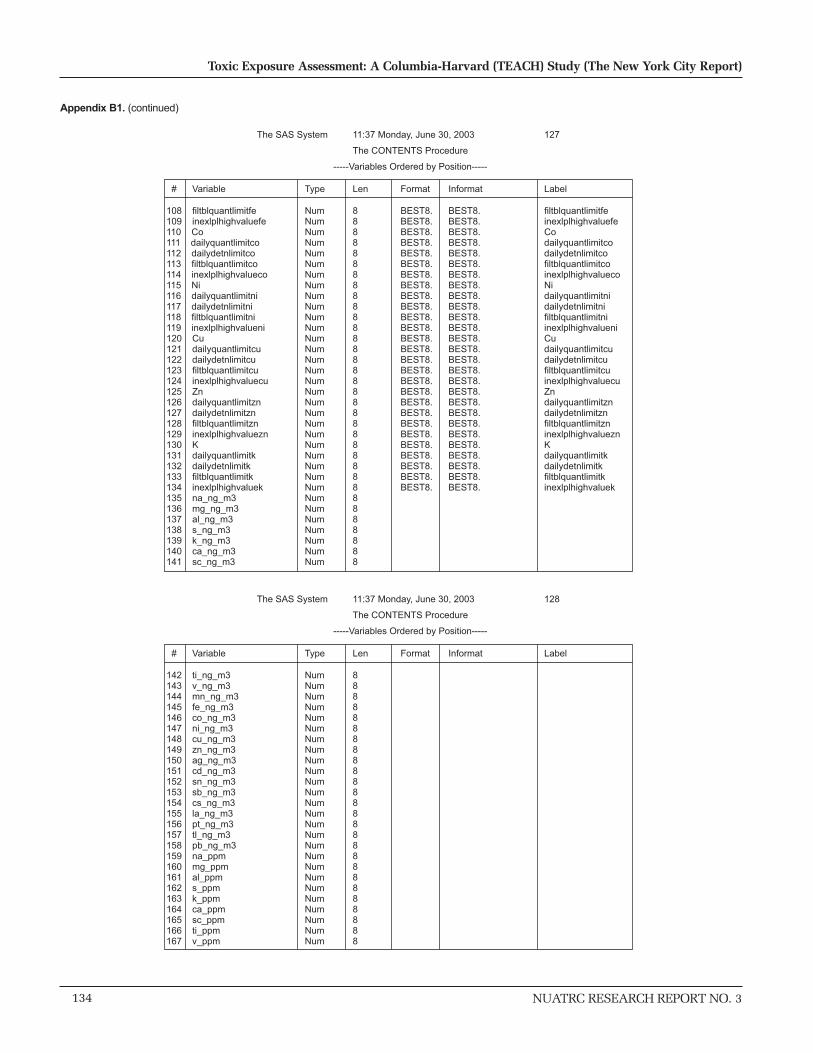
134
Toxic Exposure Assessment: A Columbia-Harvard (TEACH) Study (The New York City Report)
NUATRC RESEARCH REPORT NO. 3
Appendix B1. (continued)
The SAS System 11:37 Monday, June 30, 2003 127
The CONTENTS Procedure
-----Variables Ordered by Position-----
# Variable Type Len Format Informat Label 108 filtblquantlimitfe Num 8 BEST8. BEST8. filtblquantlimitfe 109 inexlplhighvaluefe Num 8 BEST8. BEST8. inexlplhighvaluefe 110 Co Num 8 BEST8. BEST8. Co 111 dailyquantlimitco Num 8 BEST8. BEST8. dailyquantlimitco 112 dailydetnlimitco Num 8 BEST8. BEST8. dailydetnlimitco 113 filtblquantlimitco Num 8 BEST8. BEST8. filtblquantlimitco 114 inexlplhighvalueco Num 8 BEST8. BEST8. inexlplhighvalueco 115 Ni Num 8 BEST8. BEST8. Ni 116 dailyquantlimitni Num 8 BEST8. BEST8. dailyquantlimitni 117 dailydetnlimitni Num 8 BEST8. BEST8. dailydetnlimitni 118 filtblquantlimitni Num 8 BEST8. BEST8. filtblquantlimitni 119 inexlplhighvalueni Num 8 BEST8. BEST8. inexlplhighvalueni 120 Cu Num 8 BEST8. BEST8. Cu 121 dailyquantlimitcu Num 8 BEST8. BEST8. dailyquantlimitcu 122 dailydetnlimitcu Num 8 BEST8. BEST8. dailydetnlimitcu 123 filtblquantlimitcu Num 8 BEST8. BEST8. filtblquantlimitcu 124 inexlplhighvaluecu Num 8 BEST8. BEST8. inexlplhighvaluecu 125 Zn Num 8 BEST8. BEST8. Zn 126 dailyquantlimitzn Num 8 BEST8. BEST8. dailyquantlimitzn 127 dailydetnlimitzn Num 8 BEST8. BEST8. dailydetnlimitzn 128 filtblquantlimitzn Num 8 BEST8. BEST8. filtblquantlimitzn 129 inexlplhighvaluezn Num 8 BEST8. BEST8. inexlplhighvaluezn 130 K Num 8 BEST8. BEST8. K 131 dailyquantlimitk Num 8 BEST8. BEST8. dailyquantlimitk 132 dailydetnlimitk Num 8 BEST8. BEST8. dailydetnlimitk 133 filtblquantlimitk Num 8 BEST8. BEST8. filtblquantlimitk 134 inexlplhighvaluek Num 8 BEST8. BEST8. inexlplhighvaluek 135 na_ng_m3 Num 8 136 mg_ng_m3 Num 8 137 al_ng_m3 Num 8 138 s_ng_m3 Num 8 139 k_ng_m3 Num 8 140 ca_ng_m3 Num 8 141 sc_ng_m3 Num 8
The SAS System 11:37 Monday, June 30, 2003 128
The CONTENTS Procedure
-----Variables Ordered by Position-----
# Variable Type Len Format Informat Label 142 ti_ng_m3 Num 8 143 v_ng_m3 Num 8 144 mn_ng_m3 Num 8 145 fe_ng_m3 Num 8 146 co_ng_m3 Num 8 147 ni_ng_m3 Num 8 148 cu_ng_m3 Num 8 149 zn_ng_m3 Num 8 150 ag_ng_m3 Num 8 151 cd_ng_m3 Num 8 152 sn_ng_m3 Num 8 153 sb_ng_m3 Num 8 154 cs_ng_m3 Num 8 155 la_ng_m3 Num 8 156 pt_ng_m3 Num 8 157 tl_ng_m3 Num 8 158 pb_ng_m3 Num 8 159 na_ppm Num 8 160 mg_ppm Num 8 161 al_ppm Num 8 162 s_ppm Num 8 163 k_ppm Num 8 164 ca_ppm Num 8 165 sc_ppm Num 8 166 ti_ppm Num 8 167 v_ppm Num 8

NUATRC RESEARCH REPORT NO. 3 135
Patrick L. Kinney et al
The SAS System 11:37 Monday, June 30, 2003 128
The CONTENTS Procedure
-----Variables Ordered by Position-----
# Variable Type Len Format Informat Label 168 mn_ppm Num 8 169 fe_ppm Num 8 170 co_ppm Num 8 171 ni_ppm Num 8 172 cu_ppm Num 8 173 zn_ppm Num 8 174 ag_ppm Num 8 175 cd_ppm Num 8 176 sn_ppm Num 8 177 sb_ppm Num 8 178 cs_ppm Num 8 179 la_ppm Num 8 180 pt_ppm Num 8 181 tl_ppm Num 8 182 pb_ppm Num 8 183 i Num 8 184 date_mid Num 8 DATE7. 185 season Char 1 186 Date_time_start Num 8 DATETIME18. DATETIME18. Date_time_start 187 flag_fdif_pm Char 8 $8. $255. flag_fdif_pm 188 flag_fltr_pm Num 8 BEST8. BEST8. flag_fltr_pm
The SAS System 11:37 Monday, June 30, 2003 129
The CONTENTS Procedure
-----Variables Ordered by Position-----
# Variable Type Len Format Informat Label 189 Be Num 8 BEST8. BEST8. Be 190 dailyquantlimitbe Num 8 BEST8. BEST8. dailyquantlimitbe 191 dailydetnlimitbe Num 8 BEST8. BEST8. dailydetnlimitbe 192 filtblquantlimitbe Num 8 BEST8. BEST8. filtblquantlimitbe 193 inexlplhighvaluebe Num 8 BEST8. BEST8. inexlplhighvaluebe 194 Cr Num 8 BEST8. BEST8. Cr 195 dailyquantlimitcr Num 8 BEST8. BEST8. dailyquantlimitcr 196 dailydetnlimitcr Num 8 BEST8. BEST8. dailydetnlimitcr 197 filtblquantlimitcr Num 8 BEST8. BEST8. filtblquantlimitcr 198 inexlplhighvaluecr Num 8 BEST8. BEST8. inexlplhighvaluecr 199 AS Num 8 BEST8. BEST8. AS 200 dailyquantlimitcu1 Num 8 BEST8. BEST8. dailyquantlimitcu1 201 dailydetnlimitcu1 Num 8 BEST8. BEST8. dailydetnlimitcu1 202 filtblquantlimitcu1 Num 8 BEST8. BEST8. filtblquantlimitcu1 203 inexlplhighvaluecu1 Num 8 BEST8. BEST8. inexlplhighvaluecu1 204 Se Num 8 BEST8. BEST8. Se 205 dailyquantlimitse Num 8 BEST8. BEST8. dailyquantlimitse 206 dailydetnlimitse Num 8 BEST8. BEST8. dailydetnlimitse 207 filtblquantlimitse Num 8 BEST8. BEST8. filtblquantlimitse 208 inexlplhighvaluese Num 8 BEST8. BEST8. inexlplhighvaluese 209 dailyquantlimitpt Num 8 BEST8. BEST8. dailyquantlimitpt 210 dailydetnlimitpt Num 8 BEST8. BEST8. dailydetnlimitpt 211 filtblquantlimitpt Num 8 BEST8. BEST8. filtblquantlimitpt 212 be_ng_m3 Num 8 213 cr_ng_m3 Num 8 214 as_ng_m3 Num 8 215 se_ng_m3 Num 8 216 be_ppm Num 8 217 cr_ppm Num 8 218 as_ppm Num 8 219 se_ppm Num 8
Appendix B1. (continued)

136
Toxic Exposure Assessment: A Columbia-Harvard (TEACH) Study (The New York City Report)
NUATRC RESEARCH REPORT NO. 3
Appendix B1. (continued)
The SAS System 11:37 Monday, June 30, 2003 130
Vol_smp_m3
10.69791
0.763
.
11.17034
.
12.339
9.86769
12.059
11.78214
11.93254
11.861
11.90768
Flow_avg
3.9015
3.921
.
4.021
.
4.128
3.405
4.161
3.93
4.109
4.0845
4.071
Minutes_sampled
2742
2745
.
2778
.
2989.2
2898
2898
2998
2904
2904
2925
Mass_net_FBCor
0.1245
0.132
0.022
0.072
0.003
0.1625
0.1395
0.1575
0.16
0.131
0.148
0.153
Subject_ID
1
1
2
2
1040
1040
1040
1040
1040
1049
1049
1049
Date_start
09FEB99
09FEB99
09FEB99
09FEB99
09FEB99
09FEB99
09FEB99
09FEB99
09FEB99
09FEB99
09FEB99
09FEB99
Type
S
D
D
S
D
S
D
S
S
S
D
S
Obs
1
2
3
4
5
6
7
8
9
10
11
12
Week
1
1
1
1
1
1
1
1
1
1
1
1
Location
SR
SR
LR
LR
I
I
O
O
P
I
I
O
Sample_ID
NWP018
NWP021
NWP022
NWP023
NWP002
NWP007
NWP005
NWP006
NWP024
NWP011
NWP016
NWP014
Obs
1
2
3
4
5
6
7
8
9
10
11
12
Obs
1
2
3
4
5
6
7
8
9
10
11
12
Ag
0.764319
0.683529
.
0.325601
.
1.170049
.
0.806090
0.844157
1.229609
1.417276
2.071459
Abs_coef
1.892520
1.691119
.
0.438464
.
2.502772
3.355228
3.428728
2.257406
1.734216
1.995676
2.169578
Reflectance
58.48012
61.73570
.
87.82863
.
44.11765
41.58992
33.43313
49.42197
57.79064
53.40681
50.43062
PM2_5_ug_m3
11.63778
12.26407
1.987644
6.445642
0.25
13.174
14.13705
13.06124
13.57988
10.97839
12.47746
12.84886
dailyquantlimitag
0
0
.
0
.
0
.
0
0
0
0
0
Flag_time_pm
0
0
0
0
0
0
0
0
Flag_fafg_pm
0
0
0
0
1
0
0
0
Flag_void_pm
0
0
1
0
1
0
1
0
0
0
0
0
Flag_refl
0
0
.
0
.
0
0
0
0
0
.
0
Cd
1.630273
1.878515
.
1.311476
.
2.385117
.
1.906616
3.346803
2.137662
2.208866
3.441762
inexlplhighvalueag
0
0
.
0
.
0
.
0
0
0
0
0
dailyquantlimitcd
0
0
.
2
.
0
.
0
0
0
0
0
dailydetnlimitag
0
0
.
0
.
0
.
0
0
0
0
0
filtblquantlimitag
0
0
.
0
.
0
.
0
0
0
0
0

NUATRC RESEARCH REPORT NO. 3 137
Patrick L. Kinney et al
The SAS System 11:37 Monday, June 30, 2003 131
Obs
1
2
3
4
5
6
7
8
9
10
11
12
Cs
0.090647
0.082006
.
0.054386
.
0.083094
.
0.100348
0.090833
0.130969
0.151930
0.167209
inexlplhighvaluesb
0
0
.
0
.
0
.
0
0
0
0
0
dailyquantlimitcs
0
0
.
0
.
0
.
0
0
0
0
0
dailydetnlimitsb
0
0
.
0
.
0
.
0
0
0
0
0
filtblquantlimitsb
0
0
.
0
.
0
.
0
0
0
0
0
Obs
1
2
3
4
5
6
7
8
9
10
11
12
Sb
12.66718
12.80627
.
6.172896
.
12.67248
.
13.44112
21.42598
19.01619
20.80966
29.13956
inexlplhighvaluesn
0
0
.
0
.
0
.
0
0
0
0
0
dailyquantlimitsb
0
0
.
0
.
0
.
0
0
0
0
0
dailydetnlimitsn
0
0
.
0
.
0
.
0
0
0
0
0
filtblquantlimitsn
0
0
.
0
.
0
.
0
0
0
0
0
Obs
1
2
3
4
5
6
7
8
9
10
11
12
Sn
7.719005
7.397842
.
4.147573
.
13.96998
.
5.483997
14.10829
15.42720
16.45227
14.35873
inexlplhighvaluecd
0
0
.
0
.
0
.
0
0
0
0
0
dailyquantlimitsn
0
0
.
0
.
0
.
0
0
0
0
0
dailydetnlimitcd
0
0
.
0
.
0
.
0
0
0
0
0
filtblquantlimitcd
0
0
.
0
.
0
.
0
0
0
0
0
Appendix B1. (continued)
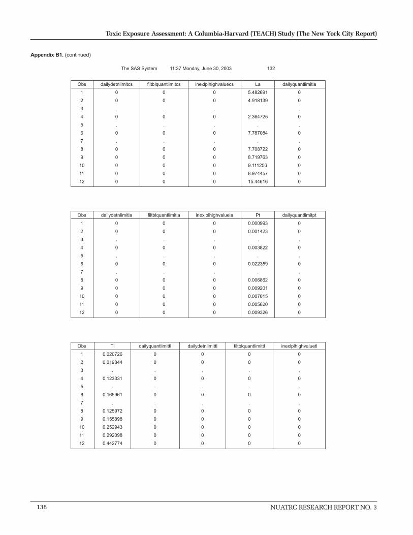
138
Toxic Exposure Assessment: A Columbia-Harvard (TEACH) Study (The New York City Report)
NUATRC RESEARCH REPORT NO. 3
Appendix B1. (continued)
The SAS System 11:37 Monday, June 30, 2003 132
Obs
1
2
3
4
5
6
7
8
9
10
11
12
filtblquantlimittl
0
0
.
0
.
0
.
0
0
0
0
0
dailydetnlimittl
0
0
.
0
.
0
.
0
0
0
0
0
inexlplhighvaluetl
0
0
.
0
.
0
.
0
0
0
0
0
Tl
0.020726
0.019844
.
0.123331
.
0.165961
.
0.125972
0.155898
0.252943
0.292098
0.442774
dailyquantlimittl
0
0
.
0
.
0
.
0
0
0
0
0
Obs
1
2
3
4
5
6
7
8
9
10
11
12
Pt
0.000993
0.001423
.
0.003822
.
0.022359
.
0.006862
0.009201
0.007015
0.005620
0.009326
inexlplhighvaluela
0
0
.
0
.
0
.
0
0
0
0
0
dailyquantlimitpt
0
0
.
0
.
0
.
0
0
0
0
0
dailydetnlimitla
0
0
.
0
.
0
.
0
0
0
0
0
filtblquantlimitla
0
0
.
0
.
0
.
0
0
0
0
0
Obs
1
2
3
4
5
6
7
8
9
10
11
12
La
5.482691
4.918139
.
2.364725
.
7.787084
.
7.708722
8.719763
9.111256
8.974457
15.44616
inexlplhighvaluecs
0
0
.
0
.
0
.
0
0
0
0
0
dailyquantlimitla
0
0
.
0
.
0
.
0
0
0
0
0
dailydetnlimitcs
0
0
.
0
.
0
.
0
0
0
0
0
filtblquantlimitcs
0
0
.
0
.
0
.
0
0
0
0
0

NUATRC RESEARCH REPORT NO. 3 139
Patrick L. Kinney et al
The SAS System 11:37 Monday, June 30, 2003 133
Obs
1
2
3
4
5
6
7
8
9
10
11
12
filtblquantlimitmg
0
0
.
0
.
0
.
0
0
0
0
0
dailydetnlimitmg
0
0
.
0
.
0
.
0
0
0
0
0
inexlplhighvaluemg
0
0
.
0
.
0
.
0
0
0
0
0
Mg
181.5829
155.6447
.
65.50544
.
287.9893
.
161.3791
240.6873
164.8629
174.9260
195.9746
dailyquantlimitmg
0
0
.
0
.
0
.
0
0
0
0
0
Obs
1
2
3
4
5
6
7
8
9
10
11
12
filtblquantlimitna
0
0
.
0
.
0
.
0
0
0
0
0
dailydetnlimitna
0
0
.
0
.
0
.
0
0
0
0
0
inexlplhighvaluena
0
0
.
0
.
0
.
0
0
0
0
0
Na
759.6761
1281.641
.
292.8564
.
1040.945
.
1805.933
1154.401
1764.171
1878.506
2105.879
dailyquantlimitna
0
0
.
0
.
0
.
0
0
0
0
0
Obs
1
2
3
4
5
6
7
8
9
10
11
12
filtblquantlimitpb
0
0
.
0
.
0
.
0
0
0
0
0
dailydetnlimitpb
0
0
.
0
.
0
.
0
0
0
0
0
inexlplhighvaluepb
0
0
.
0
.
0
.
0
0
0
0
0
Pb
87.18618
82.62830
.
47.39559
.
64.57377
.
51.41298
85.89721
70.03320
79.43037
136.9498
dailyquantlimitpb
0
0
.
0
.
0
.
0
0
0
0
0
Appendix B1. (continued)
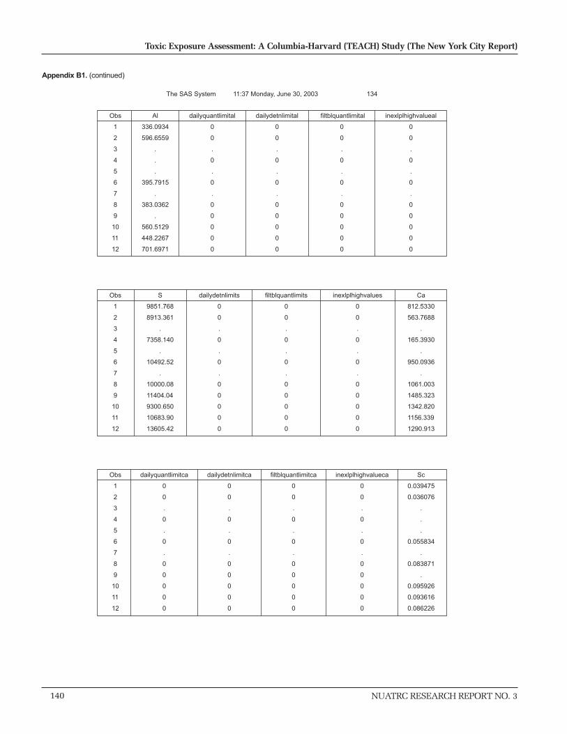
140
Toxic Exposure Assessment: A Columbia-Harvard (TEACH) Study (The New York City Report)
NUATRC RESEARCH REPORT NO. 3
Appendix B1. (continued)
The SAS System 11:37 Monday, June 30, 2003 134
Obs
1
2
3
4
5
6
7
8
9
10
11
12
inexlplhighvalueca
0
0
.
0
.
0
.
0
0
0
0
0
filtblquantlimitca
0
0
.
0
.
0
.
0
0
0
0
0
Sc
0.039475
0.036076
.
.
.
0.055834
.
0.083871
.
0.095926
0.093616
0.086226
dailyquantlimitca
0
0
.
0
.
0
.
0
0
0
0
0
dailydetnlimitca
0
0
.
0
.
0
.
0
0
0
0
0
Obs
1
2
3
4
5
6
7
8
9
10
11
12
inexlplhighvalues
0
0
.
0
.
0
.
0
0
0
0
0
filtblquantlimits
0
0
.
0
.
0
.
0
0
0
0
0
Ca
812.5330
563.7688
.
165.3930
.
950.0936
.
1061.003
1485.323
1342.820
1156.339
1290.913
S
9851.768
8913.361
.
7358.140
.
10492.52
.
10000.08
11404.04
9300.650
10683.90
13605.42
dailydetnlimits
0
0
.
0
.
0
.
0
0
0
0
0
Obs
1
2
3
4
5
6
7
8
9
10
11
12
filtblquantlimital
0
0
.
0
.
0
.
0
0
0
0
0
dailydetnlimital
0
0
.
0
.
0
.
0
0
0
0
0
inexlplhighvalueal
0
0
.
0
.
0
.
0
0
0
0
0
Al
336.0934
596.6559
.
.
.
395.7915
.
383.0362
.
560.5129
448.2267
701.6971
dailyquantlimital
0
0
.
0
.
0
.
0
0
0
0
0
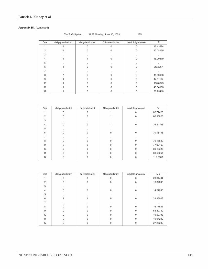
NUATRC RESEARCH REPORT NO. 3 141
Patrick L. Kinney et al
The SAS System 11:37 Monday, June 30, 2003 135
Obs
1
2
3
4
5
6
7
8
9
10
11
12
inexlplhighvaluev
0
0
.
0
.
0
.
0
0
0
0
0
filtblquantlimitv
0
0
.
0
.
0
.
0
0
0
0
0
Mn
20.64404
19.62886
.
14.27958
.
28.35046
.
16.77835
64.30730
19.50793
19.94282
27.26280
dailyquantlimitv
0
0
.
0
.
1
.
0
0
0
0
0
dailydetnlimitv
0
0
.
0
.
1
.
0
0
0
0
0
Obs
1
2
3
4
5
6
7
8
9
10
11
12
inexlplhighvalueti
0
0
.
0
.
0
.
0
0
0
0
0
filtblquantlimitti
1
1
.
1
.
0
.
0
0
0
0
0
V
62.77423
60.36826
.
34.24109
.
70.15188
.
70.18680
77.92469
80.15325
89.53257
115.9083
dailyquantlimitti
0
0
.
0
.
0
.
0
0
0
0
0
dailydetnlimitti
0
0
.
0
.
0
.
0
0
0
0
0
Obs
1
2
3
4
5
6
7
8
9
10
11
12
inexlplhighvaluesc
0
0
.
0
.
0
.
0
0
0
0
0
filtblquantlimitsc
0
0
.
0
.
0
.
0
0
0
0
0
Ti
15.43284
12.08195
.
15.09879
.
20.6057
.
45.56056
47.51112
106.8845
43.64168
56.75418
dailyquantlimitsc
0
0
.
0
.
0
.
2
0
0
0
0
dailydetnlimitsc
0
0
.
1
.
0
.
0
0
0
0
0
Appendix B1. (continued)
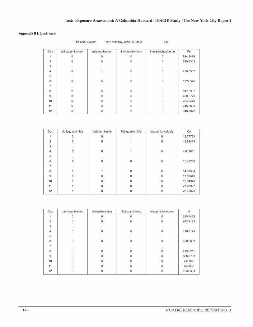
142
Toxic Exposure Assessment: A Columbia-Harvard (TEACH) Study (The New York City Report)
NUATRC RESEARCH REPORT NO. 3
Appendix B1. (continued)
The SAS System 11:37 Monday, June 30, 2003 136
Obs
1
2
3
4
5
6
7
8
9
10
11
12
inexlplhighvalueco
0
0
.
0
.
0
.
0
0
0
0
0
filtblquantlimitco
0
0
.
0
.
0
.
0
0
0
0
0
Ni
245.5468
922.4123
.
120.8192
.
356.6002
.
413.6211
888.6733
741.043
750.638
1231.304
dailyquantlimitco
0
0
.
0
.
0
.
0
0
0
0
0
dailydetnlimitco
0
0
.
0
.
0
.
0
0
0
0
0
Obs
1
2
3
4
5
6
7
8
9
10
11
12
inexlplhighvaluefe
0
0
.
0
.
0
.
0
0
0
0
0
filtblquantlimitfe
1
1
.
1
.
0
.
0
0
0
0
0
Co
13.77704
12.82423
.
4.619811
.
15.40268
.
14.97504
17.99649
18.94970
21.09927
28.57829
dailyquantlimitfe
0
0
.
0
.
0
.
1
0
1
1
1
dailydetnlimitfe
0
0
.
0
.
0
.
1
0
0
0
0
Obs
1
2
3
4
5
6
7
8
9
10
11
12
inexlplhighvaluemn
0
0
.
0
.
0
.
0
0
0
0
0
filtblquantlimitmn
0
0
.
0
.
0
.
0
0
0
0
0
Fe
844.6479
745.6312
.
456.5307
.
1322.526
.
617.5967
4608.779
764.9476
745.6600
940.5072
dailyquantlimitmn
0
0
.
0
.
0
.
2
0
0
0
0
dailydetnlimitmn
0
0
.
1
.
0
.
0
0
0
0
0

NUATRC RESEARCH REPORT NO. 3 143
Patrick L. Kinney et al
The SAS System 11:37 Monday, June 30, 2003 137
Obs
1
2
3
4
5
6
7
8
9
10
11
12
inexlplhighvaluezn
0
0
.
0
.
0
.
0
0
0
0
0
filtblquantlimitzn
0
0
.
0
.
0
.
0
0
0
0
0
K
339.4858
296.5871
.
233.0772
.
727.1749
.
488.2792
834.9739
1383.442
1599.493
933.9928
dailyquantlimitzn
0
0
.
0
.
0
.
0
0
0
0
0
dailydetnlimitzn
0
0
.
0
.
0
.
0
0
0
0
0
Obs
1
2
3
4
5
6
7
8
9
10
11
12
inexlplhighvaluecu
0
0
.
0
.
0
.
0
0
0
0
0
filtblquantlimitcu
0
0
.
1
.
0
.
0
0
0
0
0
Zn
283.0366
288.6072
.
113.3475
.
271.706
.
237.5724
394.1872
237.7109
274.491
326.5941
dailyquantlimitcu
0
0
.
0
.
0
.
0
0
0
0
0
dailydetnlimitcu
0
0
.
0
.
0
.
0
0
0
0
0
Obs
1
2
3
4
5
6
7
8
9
10
11
12
inexlplhighvalueni
0
0
.
0
.
0
.
0
0
0
0
0
filtblquantlimitni
0
0
.
0
.
0
.
0
0
0
0
0
Cu
63.12816
57.88214
.
24.97936
.
89.42488
.
46.8533
115.6161
90.03589
100.2979
96.51579
dailyquantlimitni
0
0
.
0
.
0
.
0
0
0
0
0
dailydetnlimitni
0
0
.
1
.
0
.
0
0
0
0
0
Appendix B1. (continued)
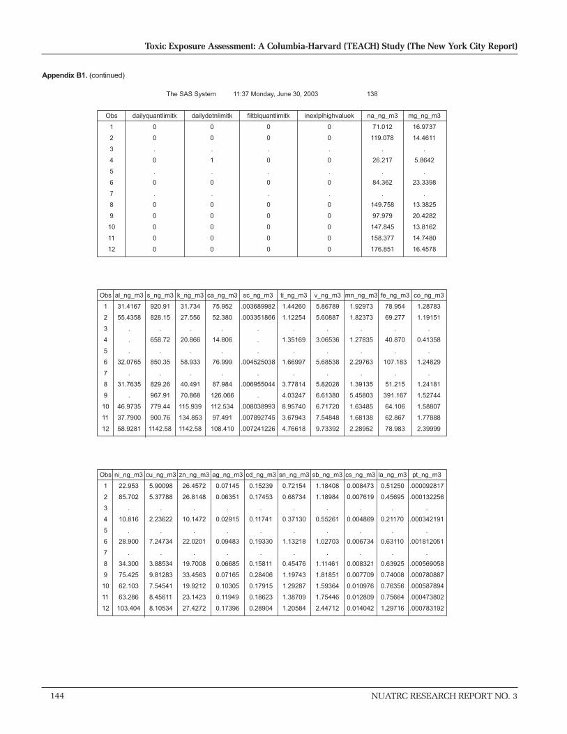
144
Toxic Exposure Assessment: A Columbia-Harvard (TEACH) Study (The New York City Report)
NUATRC RESEARCH REPORT NO. 3
Appendix B1. (continued)
The SAS System 11:37 Monday, June 30, 2003 138
Obs
1
2
3
4
5
6
7
8
9
10
11
12
sc_ng_m3
.003689982
.003351866
.
.
.
.004525038
.
.006955044
.
.008038993
.007892745
.007241226
al_ng_m3
31.4167
55.4358
.
.
.
32.0765
.
31.7635
.
46.9735
37.7900
58.9281
s_ng_m3
920.91
828.15
.
658.72
.
850.35
.
829.26
967.91
779.44
900.76
1142.58
k_ng_m3
31.734
27.556
.
20.866
.
58.933
.
40.491
70.868
115.939
134.853
1142.58
ca_ng_m3
75.952
52.380
.
14.806
.
76.999
.
87.984
126.066
112.534
97.491
108.410
ti_ng_m3
1.44260
1.12254
.
1.35169
.
1.66997
.
3.77814
4.03247
8.95740
3.67943
4.76618
v_ng_m3
5.86789
5.60887
.
3.06536
.
5.68538
.
5.82028
6.61380
6.71720
7.54848
9.73392
mn_ng_m3
1.92973
1.82373
.
1.27835
.
2.29763
.
1.39135
5.45803
1.63485
1.68138
2.28952
fe_ng_m3
78.954
69.277
.
40.870
.
107.183
.
51.215
391.167
64.106
62.867
78.983
co_ng_m3
1.28783
1.19151
.
0.41358
.
1.24829
.
1.24181
1.52744
1.58807
1.77888
2.39999
Obs
1
2
3
4
5
6
7
8
9
10
11
12
cd_ng_m3
0.15239
0.17453
.
0.11741
.
0.19330
.
0.15811
0.28406
0.17915
0.18623
0.28904
ni_ng_m3
22.953
85.702
.
10.816
.
28.900
.
34.300
75.425
62.103
63.286
103.404
cu_ng_m3
5.90098
5.37788
.
2.23622
.
7.24734
.
3.88534
9.81283
7.54541
8.45611
8.10534
zn_ng_m3
26.4572
26.8148
.
10.1472
.
22.0201
.
19.7008
33.4563
19.9212
23.1423
27.4272
ag_ng_m3
0.07145
0.06351
.
0.02915
.
0.09483
.
0.06685
0.07165
0.10305
0.11949
0.17396
sn_ng_m3
0.72154
0.68734
.
0.37130
.
1.13218
.
0.45476
1.19743
1.29287
1.38709
1.20584
sb_ng_m3
1.18408
1.18984
.
0.55261
.
1.02703
.
1.11461
1.81851
1.59364
1.75446
2.44712
cs_ng_m3
0.008473
0.007619
.
0.004869
.
0.006734
.
0.008321
0.007709
0.010976
0.012809
0.014042
la_ng_m3
0.51250
0.45695
.
0.21170
.
0.63110
.
0.63925
0.74008
0.76356
0.75664
1.29716
pt_ng_m3
.000092817
.000132256
.
.000342191
.
.001812051
.
.000569058
.000780887
.000587894
.000473802
.000783192
Obs
1
2
3
4
5
6
7
8
9
10
11
12
inexlplhighvaluek
0
0
.
0
.
0
.
0
0
0
0
0
filtblquantlimitk
0
0
.
0
.
0
.
0
0
0
0
0
mg_ng_m3
16.9737
14.4611
.
5.8642
.
23.3398
.
13.3825
20.4282
13.8162
14.7480
16.4578
na_ng_m3
71.012
119.078
.
26.217
.
84.362
.
149.758
97.979
147.845
158.377
176.851
dailyquantlimitk
0
0
.
0
.
0
.
0
0
0
0
0
dailydetnlimitk
0
0
.
1
.
0
.
0
0
0
0
0
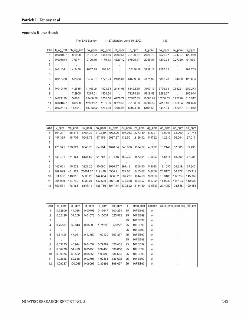
NUATRC RESEARCH REPORT NO. 3 145
Patrick L. Kinney et al
The SAS System 11:37 Monday, June 30, 2003 139
Obs
1
2
3
4
5
6
7
8
9
10
11
12
ni_ppm
1972.26
6987.97
.
1678.04
.
2194.46
.
2626.17
5554.21
5656.82
5071.88
8047.74
v_ppm
504.211
457.335
.
475.571
.
431.704
.
445.631
487.029
611.857
604.950
757.571
mn_ppm
165.816
148.703
.
198.327
.
174.464
.
106.529
401.921
148.915
134.749
178.188
fe_ppm
6784.32
5648.72
.
6340.70
.
8138.62
.
3921.25
28804.87
5839.29
5038.24
6147.11
co_ppm
110.659
97.153
.
64.164
.
94.786
.
95.080
112.478
144.654
142.563
186.786
cu_ppm
507.053
438.501
.
346.936
.
550.307
.
297.481
722.601
687.297
677.688
630.822
zn_ppm
2273.39
2186.42
.
1574.27
.
1672.04
.
1508.40
2463.67
1814.59
1854.67
2134.60
ag_ppm
6.1391
5.1782
.
4.5222
.
7.2003
.
5.1180
5.2760
9.3863
9.5762
13.5389
cd_ppm
13.0946
14.2312
.
18.2149
.
14.6776
.
12.1055
20.9175
16.3180
14.9248
22.4952
sn_ppm
62.000
56.044
.
57.605
.
85.969
.
34.819
88.177
117.765
111.164
93.848
sb_ppm
101.744
97.017
.
85.735
.
77.984
.
85.340
133.912
145.162
140.606
190.455
Obs
1
2
3
4
5
6
7
8
9
10
11
12
pb_ppm
700.291
625.972
.
658.272
.
397.377
.
326.432
536.858
534.605
536.692
895.097
cs_ppm
0.72809
0.62126
.
0.75537
.
0.51135
.
0.63713
0.56770
0.99976
1.02656
1.09287
la_ppm
44.038
37.259
.
32.843
.
47.921
.
48.944
54.499
69.552
60.638
100.955
pt_ppm
0.00798
0.01078
.
0.05309
.
0.13759
.
0.04357
0.05750
0.05355
0.03797
0.06095
tl_ppm
0.16647
0.15034
.
1.71293
.
1.02130
.
0.79982
0.97436
1.93086
1.97364
2.89395
i date_mid season
25 10FEB99 w
25 10FEB99 w
25 10FEB99 w
25 10FEB99 w
25 10FEB99 w
25 10FEB99 w
25 10FEB99 w
25 10FEB99 w
25 10FEB99 w
25 10FEB99 w
25 10FEB99 w
25 10FEB99 w
Date_time_start flag_fdif_pm
.
.
.
.
.
.
.
.
.
.
.
.
Obs
1
2
3
4
5
6
7
8
9
10
11
12
al_ppm
2699.55
4520.12
.
.
.
2435.64
.
2431.98
.
4278.72
3028.56
4586.26
tl_ng_m3
0.001937
0.001844
.
0.011041
.
0.013450
.
0.010446
.
0.021198
0.024627
0.037184
pb_ng_m3
8.1498
7.6771
.
4.2430
.
5.2333
.
4.2635
7.2905
5.8691
6.6968
11.5010
na_ppm
6101.82
9709.40
.
4067.45
.
6405.81
.
11466.24
7215.01
13466.96
12692.61
13763.92
mg_ppm
1458.50
1179.13
.
909.80
.
1772.24
.
1024.63
1504.30
1258.50
1181.93
1280.88
s_ppm
79130.67
67525.47
.
102196.39
.
64569.38
.
63492.55
71275.28
70997.33
72188.53
88924.29
k_ppm
2726.79
2246.87
.
3237.18
.
4474.92
.
3100.19
5218.59
10560.62
10807.39
6104.53
ca_ppm
6526.37
4270.98
.
2297.13
.
5846.73
.
6736.53
9283.27
10250.53
7813.10
8437.34
sc_ppm
0.31707
0.27330
.
.
.
0.34360
.
0.53251
.
0.73226
0.63254
0.56357
ti_ppm
123.959
91.530
.
209.705
.
126.804
.
289.273
296.944
815.912
294.876
370.942
Appendix B1. (continued)
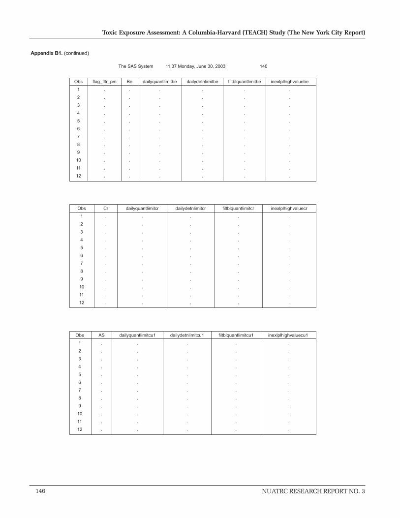
146
Toxic Exposure Assessment: A Columbia-Harvard (TEACH) Study (The New York City Report)
NUATRC RESEARCH REPORT NO. 3
Appendix B1. (continued)
The SAS System 11:37 Monday, June 30, 2003 140
Obs
1
2
3
4
5
6
7
8
9
10
11
12
Cr
.
.
.
.
.
.
.
.
.
.
.
.
dailyquantlimitcr
.
.
.
.
.
.
.
.
.
.
.
.
dailydetnlimitcr
.
.
.
.
.
.
.
.
.
.
.
.
filtblquantlimitcr
.
.
.
.
.
.
.
.
.
.
.
.
inexlplhighvaluecr
.
.
.
.
.
.
.
.
.
.
.
.
Obs
1
2
3
4
5
6
7
8
9
10
11
12
AS
.
.
.
.
.
.
.
.
.
.
.
.
dailyquantlimitcu1
.
.
.
.
.
.
.
.
.
.
.
.
dailydetnlimitcu1
.
.
.
.
.
.
.
.
.
.
.
.
filtblquantlimitcu1
.
.
.
.
.
.
.
.
.
.
.
.
inexlplhighvaluecu1
.
.
.
.
.
.
.
.
.
.
.
.
Obs
1
2
3
4
5
6
7
8
9
10
11
12
flag_fltr_pm
.
.
.
.
.
.
.
.
.
.
.
.
Be
.
.
.
.
.
.
.
.
.
.
.
.
dailyquantlimitbe
.
.
.
.
.
.
.
.
.
.
.
.
dailydetnlimitbe
.
.
.
.
.
.
.
.
.
.
.
.
filtblquantlimitbe
.
.
.
.
.
.
.
.
.
.
.
.
inexlplhighvaluebe
.
.
.
.
.
.
.
.
.
.
.
.
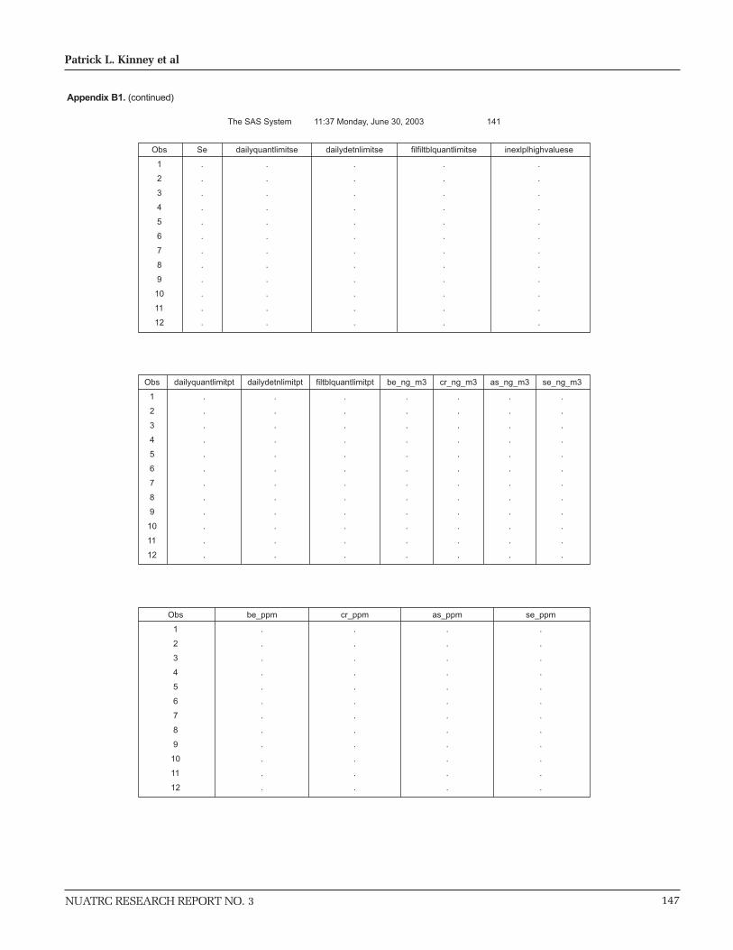
NUATRC RESEARCH REPORT NO. 3 147
Patrick L. Kinney et al
The SAS System 11:37 Monday, June 30, 2003 141
Obs
1
2
3
4
5
6
7
8
9
10
11
12
dailyquantlimitpt
.
.
.
.
.
.
.
.
.
.
.
.
dailydetnlimitpt
.
.
.
.
.
.
.
.
.
.
.
.
filtblquantlimitpt
.
.
.
.
.
.
.
.
.
.
.
.
be_ng_m3
.
.
.
.
.
.
.
.
.
.
.
.
cr_ng_m3
.
.
.
.
.
.
.
.
.
.
.
.
se_ng_m3
.
.
.
.
.
.
.
.
.
.
.
.
as_ng_m3
.
.
.
.
.
.
.
.
.
.
.
.
Obs
1
2
3
4
5
6
7
8
9
10
11
12
be_ppm
.
.
.
.
.
.
.
.
.
.
.
.
cr_ppm
.
.
.
.
.
.
.
.
.
.
.
.
as_ppm
.
.
.
.
.
.
.
.
.
.
.
.
se_ppm
.
.
.
.
.
.
.
.
.
.
.
.
Obs
1
2
3
4
5
6
7
8
9
10
11
12
Se
.
.
.
.
.
.
.
.
.
.
.
.
dailyquantlimitse
.
.
.
.
.
.
.
.
.
.
.
.
dailydetnlimitse
.
.
.
.
.
.
.
.
.
.
.
.
filfiltblquantlimitse
.
.
.
.
.
.
.
.
.
.
.
.
inexlplhighvaluese
.
.
.
.
.
.
.
.
.
.
.
.
Appendix B1. (continued)

NUATRC RESEARCH REPORT NO. 3 149
Patrick L. Kinney et al
APPENDIX B2
Variable Listing and Sample Printout of Fixed-site Ambient PM Dataset
NYWSPMELEMABS_FXSITE
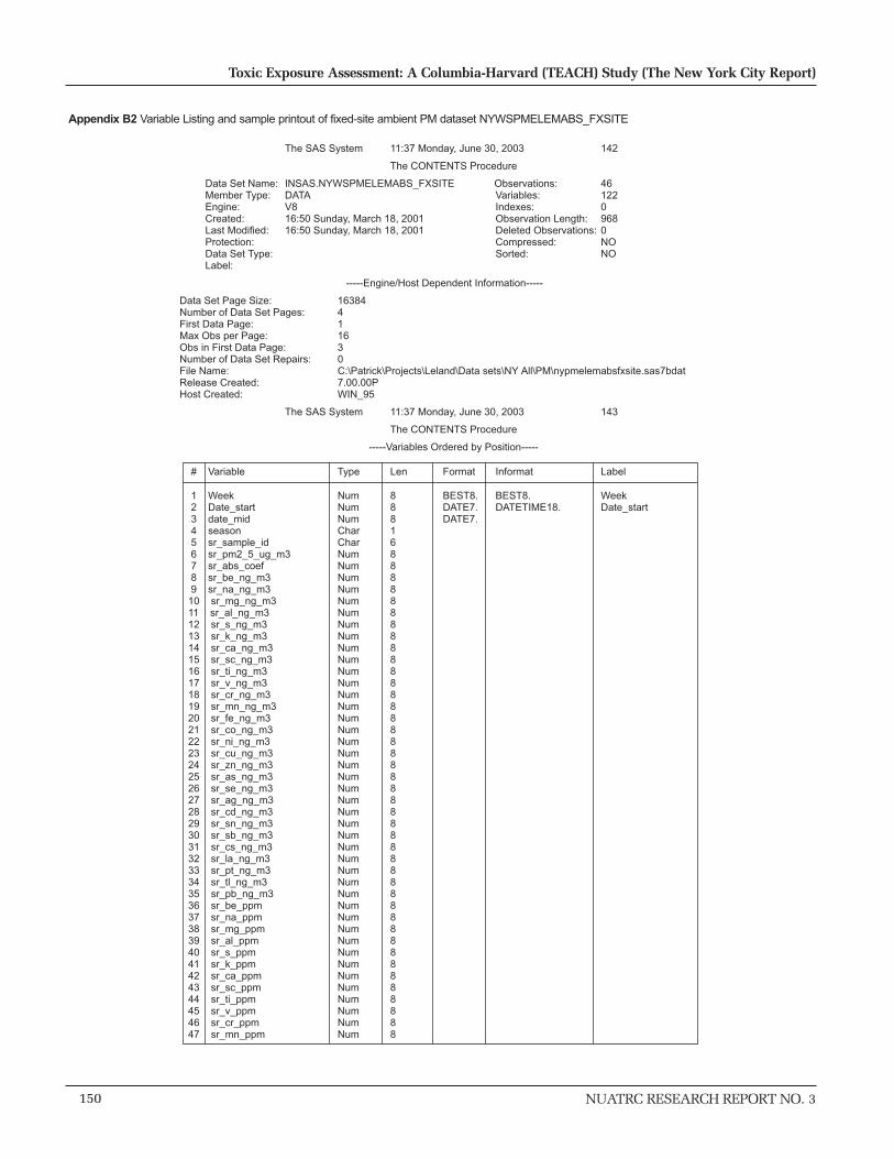
150
Toxic Exposure Assessment: A Columbia-Harvard (TEACH) Study (The New York City Report)
NUATRC RESEARCH REPORT NO. 3
Appendix B2 Variable Listing and sample printout of fixed-site ambient PM dataset NYWSPMELEMABS_FXSITE
The SAS System 11:37 Monday, June 30, 2003 142
The CONTENTS Procedure
Data Set Name: INSAS.NYWSPMELEMABS_FXSITE Observations: 46 Member Type: DATA Variables: 122 Engine: V8 Indexes: 0 Created: 16:50 Sunday, March 18, 2001 Observation Length: 968 Last Modified: 16:50 Sunday, March 18, 2001 Deleted Observations: 0 Protection: Compressed: NO Data Set Type: Sorted: NO Label:
-----Engine/Host Dependent Information-----
Data Set Page Size: 16384Number of Data Set Pages: 4First Data Page: 1Max Obs per Page: 16Obs in First Data Page: 3Number of Data Set Repairs: 0File Name: C:\Patrick\Projects\Leland\Data sets\NY All\PM\nypmelemabsfxsite.sas7bdatRelease Created: 7.00.00PHost Created: WIN_95
The SAS System 11:37 Monday, June 30, 2003 143
The CONTENTS Procedure
-----Variables Ordered by Position-----
# Variable Type Len Format Informat Label 1 Week Num 8 BEST8. BEST8. Week 2 Date_start Num 8 DATE7. DATETIME18. Date_start 3 date_mid Num 8 DATE7. 4 season Char 1 5 sr_sample_id Char 6 6 sr_pm2_5_ug_m3 Num 8 7 sr_abs_coef Num 8 8 sr_be_ng_m3 Num 8 9 sr_na_ng_m3 Num 8 10 sr_mg_ng_m3 Num 8 11 sr_al_ng_m3 Num 8 12 sr_s_ng_m3 Num 8 13 sr_k_ng_m3 Num 8 14 sr_ca_ng_m3 Num 8 15 sr_sc_ng_m3 Num 8 16 sr_ti_ng_m3 Num 8 17 sr_v_ng_m3 Num 8 18 sr_cr_ng_m3 Num 8 19 sr_mn_ng_m3 Num 8 20 sr_fe_ng_m3 Num 8 21 sr_co_ng_m3 Num 8 22 sr_ni_ng_m3 Num 8 23 sr_cu_ng_m3 Num 8 24 sr_zn_ng_m3 Num 8 25 sr_as_ng_m3 Num 8 26 sr_se_ng_m3 Num 8 27 sr_ag_ng_m3 Num 8 28 sr_cd_ng_m3 Num 8 29 sr_sn_ng_m3 Num 8 30 sr_sb_ng_m3 Num 8 31 sr_cs_ng_m3 Num 8 32 sr_la_ng_m3 Num 8 33 sr_pt_ng_m3 Num 8 34 sr_tl_ng_m3 Num 8 35 sr_pb_ng_m3 Num 8 36 sr_be_ppm Num 8 37 sr_na_ppm Num 8 38 sr_mg_ppm Num 8 39 sr_al_ppm Num 8 40 sr_s_ppm Num 8 41 sr_k_ppm Num 8 42 sr_ca_ppm Num 8 43 sr_sc_ppm Num 8 44 sr_ti_ppm Num 8 45 sr_v_ppm Num 8 46 sr_cr_ppm Num 8 47 sr_mn_ppm Num 8

NUATRC RESEARCH REPORT NO. 3 151
Patrick L. Kinney et al
The SAS System 11:37 Monday, June 30, 2003 144
The CONTENTS Procedure
-----Variables Ordered by Position-----
# Variable Type Len Format Informat Label 48 sr_fe_ppm Num 8 49 sr_co_ppm Num 8 50 sr_ni_ppm Num 8 51 sr_cu_ppm Num 8 52 sr_zn_ppm Num 8 53 sr_as_ppm Num 8 54 sr_se_ppm Num 8 55 sr_ag_ppm Num 8 56 sr_cd_ppm Num 8 57 sr_sn_ppm Num 8 58 sr_sb_ppm Num 8 59 sr_cs_ppm Num 8 60 sr_la_ppm Num 8 61 sr_pt_ppm Num 8 62 sr_tl_ppm Num 8 63 sr_pb_ppm Num 8 64 lr_sample_id Char 6 65 lr_pm2_5_ug_m3 Num 8 66 lr_abs_coef Num 8 67 lr_be_ng_m3 Num 8 68 lr_na_ng_m3 Num 8 69 lr_mg_ng_m3 Num 8 70 lr_al_ng_m3 Num 8 71 lr_s_ng_m3 Num 8 72 lr_k_ng_m3 Num 8 73 lr_ca_ng_m3 Num 8 74 lr_sc_ng_m3 Num 8 75 lr_ti_ng_m3 Num 8 76 lr_v_ng_m3 Num 8 77 lr_cr_ng_m3 Num 8 78 lr_mn_ng_m3 Num 8 79 lr_fe_ng_m3 Num 8 80 lr_co_ng_m3 Num 8 81 lr_ni_ng_m3 Num 8 82 lr_cu_ng_m3 Num 8 83 lr_zn_ng_m3 Num 8 84 lr_as_ng_m3 Num 8 85 lr_se_ng_m3 Num 8 86 lr_ag_ng_m3 Num 8 87 lr_cd_ng_m3 Num 8 88 lr_sn_ng_m3 Num 8 89 lr_sb_ng_m3 Num 8 90 lr_cs_ng_m3 Num 8 91 lr_la_ng_m3 Num 8 92 lr_pt_ng_m3 Num 8 93 lr_tl_ng_m3 Num 8 94 lr_pb_ng_m3 Num 8
Appendix B2. (continued)
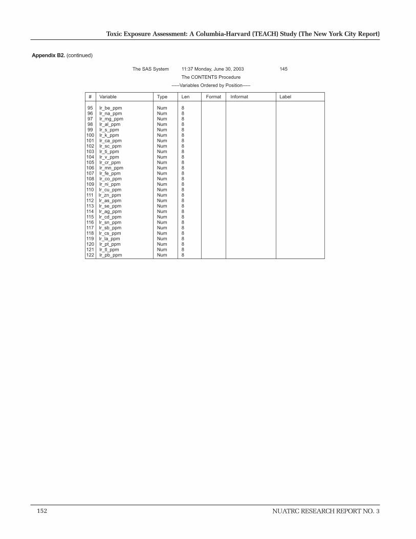
152
Toxic Exposure Assessment: A Columbia-Harvard (TEACH) Study (The New York City Report)
NUATRC RESEARCH REPORT NO. 3
Appendix B2. (continued)
The SAS System 11:37 Monday, June 30, 2003 145
The CONTENTS Procedure
-----Variables Ordered by Position-----
# Variable Type Len Format Informat Label 95 lr_be_ppm Num 8 96 lr_na_ppm Num 8 97 lr_mg_ppm Num 8 98 lr_al_ppm Num 8 99 lr_s_ppm Num 8 100 lr_k_ppm Num 8 101 lr_ca_ppm Num 8 102 lr_sc_ppm Num 8 103 lr_ti_ppm Num 8 104 lr_v_ppm Num 8 105 lr_cr_ppm Num 8 106 lr_mn_ppm Num 8 107 lr_fe_ppm Num 8 108 lr_co_ppm Num 8 109 lr_ni_ppm Num 8 110 lr_cu_ppm Num 8 111 lr_zn_ppm Num 8 112 lr_as_ppm Num 8 113 lr_se_ppm Num 8 114 lr_ag_ppm Num 8 115 lr_cd_ppm Num 8 116 lr_sn_ppm Num 8 117 lr_sb_ppm Num 8 118 lr_cs_ppm Num 8 119 lr_la_ppm Num 8 120 lr_pt_ppm Num 8 121 lr_tl_ppm Num 8 122 lr_pb_ppm Num 8
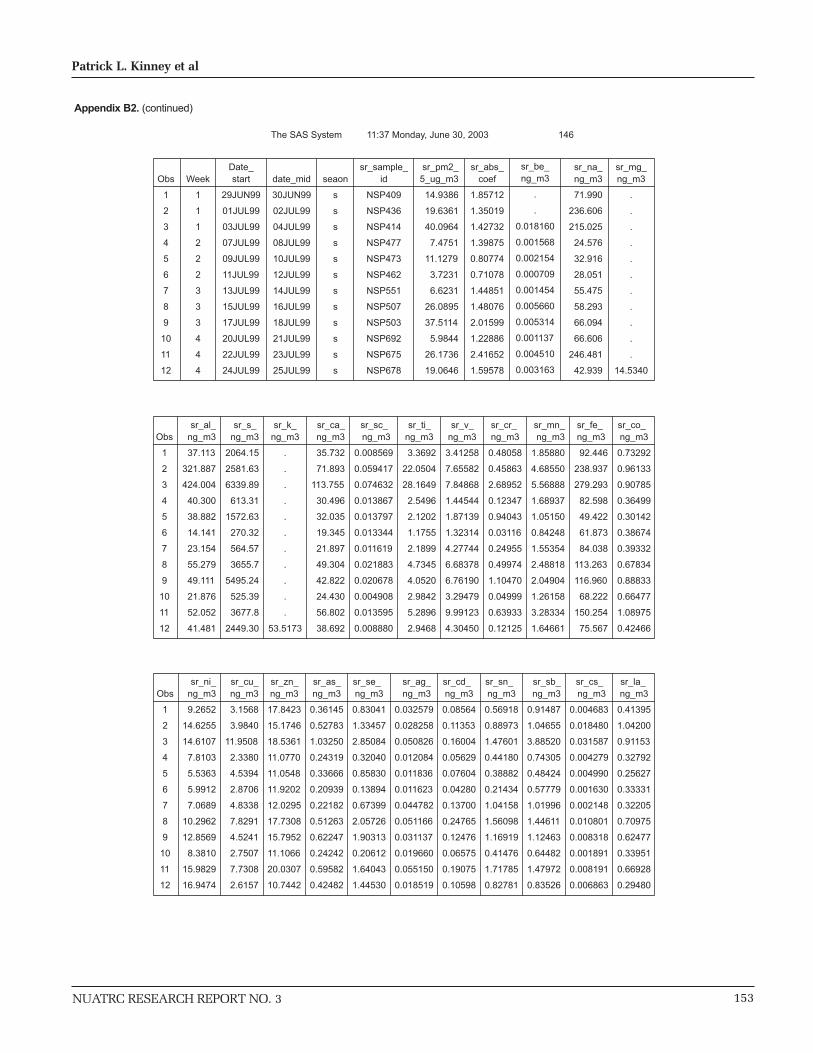
NUATRC RESEARCH REPORT NO. 3 153
Patrick L. Kinney et al
The SAS System 11:37 Monday, June 30, 2003 146
sr_mg_ng_m3
.
.
.
.
.
.
.
.
.
.
.
14.5340
sr_na_ng_m3
71.990
236.606
215.025
24.576
32.916
28.051
55.475
58.293
66.094
66.606
246.481
42.939
sr_be_ng_m3
.
.
0.018160
0.001568
0.002154
0.000709
0.001454
0.005660
0.005314
0.001137
0.004510
0.003163
sr_pm2_5_ug_m3
14.9386
19.6361
40.0964
7.4751
11.1279
3.7231
6.6231
26.0895
37.5114
5.9844
26.1736
19.0646
Date_start
29JUN99
01JUL99
03JUL99
07JUL99
09JUL99
11JUL99
13JUL99
15JUL99
17JUL99
20JUL99
22JUL99
24JUL99
sr_abs_coef
1.85712
1.35019
1.42732
1.39875
0.80774
0.71078
1.44851
1.48076
2.01599
1.22886
2.41652
1.59578
sr_sample_id
NSP409
NSP436
NSP414
NSP477
NSP473
NSP462
NSP551
NSP507
NSP503
NSP692
NSP675
NSP678
Obs
1
2
3
4
5
6
7
8
9
10
11
12
Week
1
1
1
2
2
2
3
3
3
4
4
4
seaon
s
s
s
s
s
s
s
s
s
s
s
s
date_mid
30JUN99
02JUL99
04JUL99
08JUL99
10JUL99
12JUL99
14JUL99
16JUL99
18JUL99
21JUL99
23JUL99
25JUL99
Obs
1
2
3
4
5
6
7
8
9
10
11
12
sr_al_ng_m3
37.113
321.887
424.004
40.300
38.882
14.141
23.154
55.279
49.111
21.876
52.052
41.481
sr_s_ ng_m3
2064.15
2581.63
6339.89
613.31
1572.63
270.32
564.57
3655.7
5495.24
525.39
3677.8
2449.30
sr_ca_ng_m3
35.732
71.893
113.755
30.496
32.035
19.345
21.897
49.304
42.822
24.430
56.802
38.692
sr_sc_ ng_m3
0.008569
0.059417
0.074632
0.013867
0.013797
0.013344
0.011619
0.021883
0.020678
0.004908
0.013595
0.008880
sr_ti_ ng_m3
3.3692
22.0504
28.1649
2.5496
2.1202
1.1755
2.1899
4.7345
4.0520
2.9842
5.2896
2.9468
sr_v_ ng_m3
3.41258
7.65582
7.84868
1.44544
1.87139
1.32314
4.27744
6.68378
6.76190
3.29479
9.99123
4.30450
sr_cr_ ng_m3
0.48058
0.45863
2.68952
0.12347
0.94043
0.03116
0.24955
0.49974
1.10470
0.04999
0.63933
0.12125
sr_mn_ng_m3
1.85880
4.68550
5.56888
1.68937
1.05150
0.84248
1.55354
2.48818
2.04904
1.26158
3.28334
1.64661
sr_fe_ ng_m3
92.446
238.937
279.293
82.598
49.422
61.873
84.038
113.263
116.960
68.222
150.254
75.567
sr_co_ ng_m3
0.73292
0.96133
0.90785
0.36499
0.30142
0.38674
0.39332
0.67834
0.88833
0.66477
1.08975
0.42466
sr_k_ng_m3
.
.
.
.
.
.
.
.
.
.
.
53.5173
Obs
1
2
3
4
5
6
7
8
9
10
11
12
sr_ni_ng_m3
9.2652
14.6255
14.6107
7.8103
5.5363
5.9912
7.0689
10.2962
12.8569
8.3810
15.9829
16.9474
sr_cu_ng_m3
3.1568
3.9840
11.9508
2.3380
4.5394
2.8706
4.8338
7.8291
4.5241
2.7507
7.7308
2.6157
sr_as_ ng_m3
0.36145
0.52783
1.03250
0.24319
0.33666
0.20939
0.22182
0.51263
0.62247
0.24242
0.59582
0.42482
sr_se_ ng_m3
0.83041
1.33457
2.85084
0.32040
0.85830
0.13894
0.67399
2.05726
1.90313
0.20612
1.64043
1.44530
sr_ag_ ng_m3
0.032579
0.028258
0.050826
0.012084
0.011836
0.011623
0.044782
0.051166
0.031137
0.019660
0.055150
0.018519
sr_cd_ ng_m3
0.08564
0.11353
0.16004
0.05629
0.07604
0.04280
0.13700
0.24765
0.12476
0.06575
0.19075
0.10598
sr_sn_ ng_m3
0.56918
0.88973
1.47601
0.44180
0.38882
0.21434
1.04158
1.56098
1.16919
0.41476
1.71785
0.82781
sr_sb_ng_m3
0.91487
1.04655
3.88520
0.74305
0.48424
0.57779
1.01996
1.44611
1.12463
0.64482
1.47972
0.83526
sr_cs_ ng_m3
0.004683
0.018480
0.031587
0.004279
0.004990
0.001630
0.002148
0.010801
0.008318
0.001891
0.008191
0.006863
sr_la_ ng_m3
0.41395
1.04200
0.91153
0.32792
0.25627
0.33331
0.32205
0.70975
0.62477
0.33951
0.66928
0.29480
sr_zn_ ng_m3
17.8423
15.1746
18.5361
11.0770
11.0548
11.9202
12.0295
17.7308
15.7952
11.1066
20.0307
10.7442
Appendix B2. (continued)

154
Toxic Exposure Assessment: A Columbia-Harvard (TEACH) Study (The New York City Report)
NUATRC RESEARCH REPORT NO. 3
Appendix B2. (continued)
The SAS System 11:37 Monday, June 30, 2003 147
sr_ca_ppm
2391.90
3661.26
2837.03
4079.75
2878.79
5195.88
3306.10
1889.82
1141.57
4082.22
2170.20
2029.52
sr_k_ppm
.
.
.
.
.
.
.
.
.
.
.
2807.15
sr_s_ppm
138175.87
131473.76
158115.95
82047.01
141322.97
72606.82
85242.74
140123.71
146495.41
87792.93
140515.58
128473.85
sr_mg_ppm
.
.
.
.
.
.
.
.
.
.
.
762.353
sr_tl_ng_m3
0.005353
0.009908
0.034844
0.003298
0.008259
0.002398
0.003696
0.015841
0.016534
0.002486
0.010551
0.012916
sr_al_ppm
2484.38
16392.61
10574.61
5391.27
3494.11
3798.09
3495.87
2118.81
1309.23
3655.53
1988.71
2175.81
sr_na_ppm
4819.10
12049.54
5362.70
3287.78
2957.93
7534.43
8375.88
2234.34
1761.97
11129.82
9417.17
2252.29
Obs
1
2
3
4
5
6
7
8
9
10
11
12
sr_pt_ng_m3
.001258569
.001395533
.001636824
.000891031
.000493220
.000649936
.001314830
.001734321
.001607166
.000149472
.001573715
.000800692
sr_be_ppm
.
.
0.45291
0.20974
0.19359
0.19055
0.21950
0.21696
0.14165
0.19002
0.17230
0.16591
sr_pb_ng_m3
3.1102
3.9058
18.4875
3.0374
3.2133
2.8183
4.0042
6.0742
4.6961
2.6794
6.8464
3.7235
Obs
1
2
3
4
5
6
7
8
9
10
11
12
sr_sc_ppm
0.57364
3.02591
1.86131
1.85505
1.23981
3.58422
1.75435
0.83876
0.55124
0.82014
0.51943
0.46579
sr_ti_ppm
225.53
1122.95
702.43
341.08
190.53
315.74
330.64
181.47
108.02
498.67
202.10
154.57
sr_cr_ppm
32.1702
23.3564
67.0762
16.5176
84.5109
8.3698
37.6784
19.1548
29.4498
8.3535
24.4265
6.3600
sr_mn_ppm
124.430
238.617
138.887
226.001
94.492
226.284
234.563
95.371
54.625
210.810
125.445
86.370
sr_fe_ppm
6188.44
12168.27
6965.54
11049.74
4441.21
16618.72
12688.54
4341.32
3117.99
11399.88
5740.69
3963.72
sr_co_ppm
49.062
48.957
22.642
48.828
27.086
103.875
59.386
26.000
23.682
111.084
41.635
22.275
sr_ni_ppm
620.22
744.83
364.39
1044.84
497.51
1609.19
1067.30
394.65
342.75
1400.47
610.65
888.95
sr_cu_ppm
211.321
202.891
298.052
312.771
407.924
771.023
729.835
300.087
120.607
459.642
295.366
137.204
sr_zn_ppm
1194.38
772.79
462.29
1481.86
993.43
3201.71
1816.29
679.61
421.08
1855.92
765.30
563.57
sr_as_ppm
24.1961
26.8808
25.7505
32.5329
30.2531
56.2412
33.4923
19.6489
16.5943
40.5092
22.7642
22.2834
sr_v_ppm
228.441
389.885
195.745
193.368
168.170
355.389
645.833
256.186
180.263
550.561
381.729
225.785
Obs
1
2
3
4
5
6
7
8
9
10
11
12
sr_se_ppm
55.589
67.965
71.099
42.862
77.130
37.319
101.764
78.854
50.735
34.443
62.675
75.810
sr_ag_ppm
2.18084
1.43911
1.26758
1.61659
1.06363
3.12193
6.76139
1.96116
0.83006
3.28517
2.10708
0.97138
sr_sn_ppm
38.102
45.311
36.811
59.104
34.941
57.570
157.263
59.832
31.169
69.306
65.633
43.421
sr_sb_ppm
61.242
53.297
96.896
99.403
43.516
155.192
153.999
55.429
29.981
107.750
56.535
43.812
sr_cs_ppm
0.31348
0.94113
0.78776
0.57243
0.44840
0.43784
0.32430
0.41401
0.22174
0.31600
0.31296
0.36000
sr_la_ppm
27.7102
53.0653
22.7335
43.8689
23.0295
89.5261
48.6246
27.2043
16.6554
56.7326
25.5708
15.4632
sr_pt_ppm
0.08425
0.07107
0.04082
0.11920
0.04432
0.17457
0.19852
0.06648
0.04284
0.02498
0.06013
0.04200
sr_tl_ppm
0.35831
0.50458
0.86900
0.44113
0.74222
0.64403
0.55806
0.60719
0.44077
0.41535
0.40311
0.67748
sr_pb_ppm
208.202
198.911
461.075
406.339
288.763
756.983
604.582
232.822
125.192
447.735
261.576
195.310
lr_sample_id
NSP405
NSP429
NSP439
NSP472
NSP470
NSP453
NSP557
NSP491
NSP502
NSP606
NSP674
NSP672
sr_cd_ppm
5.7325
5.7817
3.9913
7.5309
6.8331
11.4962
20.6848
9.4925
3.3259
10.9861
7.2880
5.5589
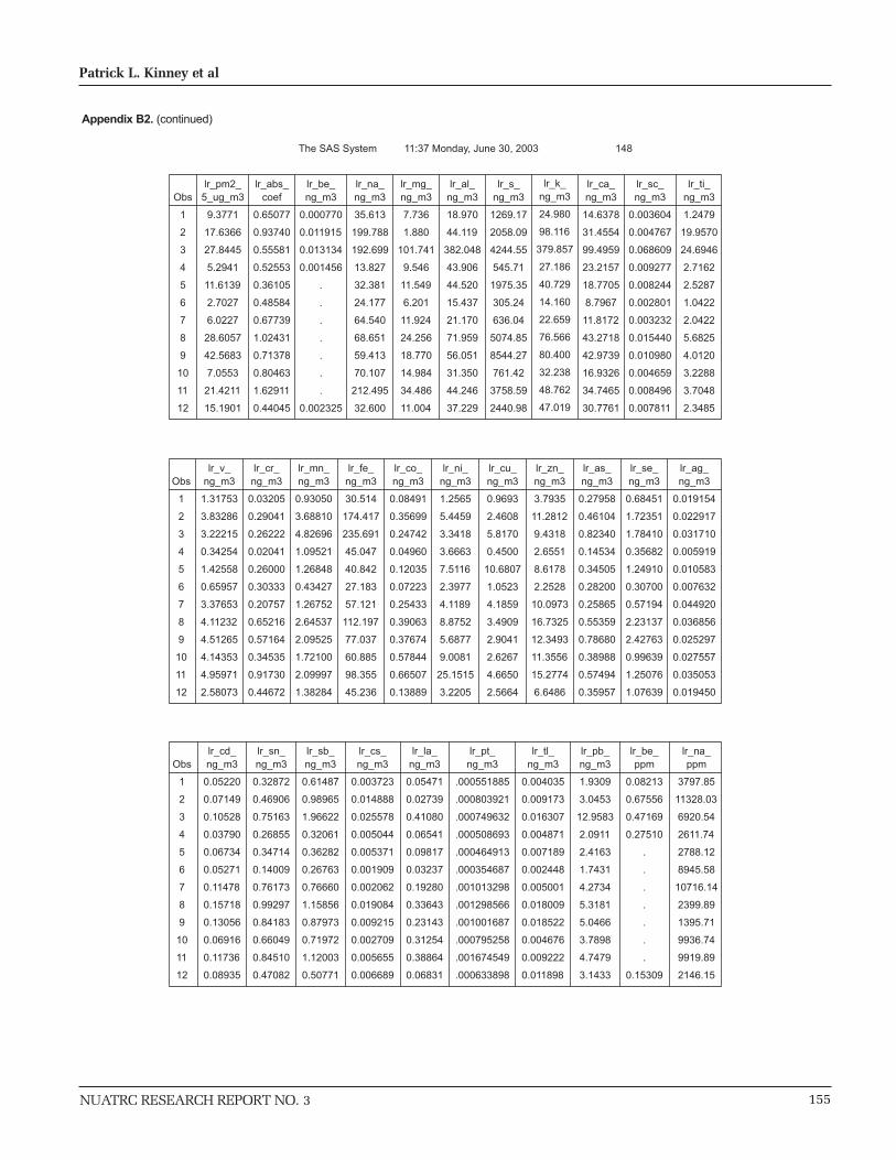
NUATRC RESEARCH REPORT NO. 3 155
Patrick L. Kinney et al
The SAS System 11:37 Monday, June 30, 2003 148
lr_sc_ng_m3
0.003604
0.004767
0.068609
0.009277
0.008244
0.002801
0.003232
0.015440
0.010980
0.004659
0.008496
0.007811
lr_ti_ng_m3
1.2479
19.9570
24.6946
2.7162
2.5287
1.0422
2.0422
5.6825
4.0120
3.2288
3.7048
2.3485
lr_ca_ng_m3
14.6378
31.4554
99.4959
23.2157
18.7705
8.7967
11.8172
43.2718
42.9739
16.9326
34.7465
30.7761
lr_k_ng_m3
24.980
98.116
379.857
27.186
40.729
14.160
22.659
76.566
80.400
32.238
48.762
47.019
lr_al_ng_m3
18.970
44.119
382.048
43.906
44.520
15.437
21.170
71.959
56.051
31.350
44.246
37.229
lr_abs_coef
0.65077
0.93740
0.55581
0.52553
0.36105
0.48584
0.67739
1.02431
0.71378
0.80463
1.62911
0.44045
lr_s_ng_m3
1269.17
2058.09
4244.55
545.71
1975.35
305.24
636.04
5074.85
8544.27
761.42
3758.59
2440.98
lr_mg_ng_m3
7.736
1.880
101.741
9.546
11.549
6.201
11.924
24.256
18.770
14.984
34.486
11.004
Obs
1
2
3
4
5
6
7
8
9
10
11
12
lr_pm2_5_ug_m3
9.3771
17.6366
27.8445
5.2941
11.6139
2.7027
6.0227
28.6057
42.5683
7.0553
21.4211
15.1901
lr_na_ng_m3
35.613
199.788
192.699
13.827
32.381
24.177
64.540
68.651
59.413
70.107
212.495
32.600
lr_be_ng_m3
0.000770
0.011915
0.013134
0.001456
.
.
.
.
.
.
.
0.002325
Obs
1
2
3
4
5
6
7
8
9
10
11
12
lr_v_ng_m3
1.31753
3.83286
3.22215
0.34254
1.42558
0.65957
3.37653
4.11232
4.51265
4.14353
4.95971
2.58073
lr_cr_ng_m3
0.03205
0.29041
0.26222
0.02041
0.26000
0.30333
0.20757
0.65216
0.57164
0.34535
0.91730
0.44672
lr_fe_ng_m3
30.514
174.417
235.691
45.047
40.842
27.183
57.121
112.197
77.037
60.885
98.355
45.236
lr_co_ng_m3
0.08491
0.35699
0.24742
0.04960
0.12035
0.07223
0.25433
0.39063
0.37674
0.57844
0.66507
0.13889
lr_ni_ng_m3
1.2565
5.4459
3.3418
3.6663
7.5116
2.3977
4.1189
8.8752
5.6877
9.0081
25.1515
3.2205
lr_cu_ng_m3
0.9693
2.4608
5.8170
0.4500
10.6807
1.0523
4.1859
3.4909
2.9041
2.6267
4.6650
2.5664
lr_zn_ng_m3
3.7935
11.2812
9.4318
2.6551
8.6178
2.2528
10.0973
16.7325
12.3493
11.3556
15.2774
6.6486
lr_as_ng_m3
0.27958
0.46104
0.82340
0.14534
0.34505
0.28200
0.25865
0.55359
0.78680
0.38988
0.57494
0.35957
lr_se_ng_m3
0.68451
1.72351
1.78410
0.35682
1.24910
0.30700
0.57194
2.23137
2.42763
0.99639
1.25076
1.07639
lr_ag_ng_m3
0.019154
0.022917
0.031710
0.005919
0.010583
0.007632
0.044920
0.036856
0.025297
0.027557
0.035053
0.019450
lr_mn_ng_m3
0.93050
3.68810
4.82696
1.09521
1.26848
0.43427
1.26752
2.64537
2.09525
1.72100
2.09997
1.38284
Obs
1
2
3
4
5
6
7
8
9
10
11
12
lr_cd_ng_m3
0.05220
0.07149
0.10528
0.03790
0.06734
0.05271
0.11478
0.15718
0.13056
0.06916
0.11736
0.08935
lr_sn_ng_m3
0.32872
0.46906
0.75163
0.26855
0.34714
0.14009
0.76173
0.99297
0.84183
0.66049
0.84510
0.47082
lr_cs_ng_m3
0.003723
0.014888
0.025578
0.005044
0.005371
0.001909
0.002062
0.019084
0.009215
0.002709
0.005655
0.006689
lr_la_ng_m3
0.05471
0.02739
0.41080
0.06541
0.09817
0.03237
0.19280
0.33643
0.23143
0.31254
0.38864
0.06831
lr_pt_ng_m3
.000551885
.000803921
.000749632
.000508693
.000464913
.000354687
.001013298
.001298566
.001001687
.000795258
.001674549
.000633898
lr_tl_ng_m3
0.004035
0.009173
0.016307
0.004871
0.007189
0.002448
0.005001
0.018009
0.018522
0.004676
0.009222
0.011898
lr_pb_ng_m3
1.9309
3.0453
12.9583
2.0911
2.4163
1.7431
4.2734
5.3181
5.0466
3.7898
4.7479
3.1433
lr_be_ppm
0.08213
0.67556
0.47169
0.27510
.
.
.
.
.
.
.
0.15309
lr_na_ppm
3797.85
11328.03
6920.54
2611.74
2788.12
8945.58
10716.14
2399.89
1395.71
9936.74
9919.89
2146.15
lr_sb_ng_m3
0.61487
0.98965
1.96622
0.32061
0.36282
0.26763
0.76660
1.15856
0.87973
0.71972
1.12003
0.50771
Appendix B2. (continued)

156
Toxic Exposure Assessment: A Columbia-Harvard (TEACH) Study (The New York City Report)
NUATRC RESEARCH REPORT NO. 3
Appendix B2. (continued)
The SAS System 11:37 Monday, June 30, 2003 149
lr_cr_ppm
3.418
16.467
9.417
3.856
22.387
112.230
34.464
22.798
13.429
48.949
42.822
29.409
lr_mn_ppm
99.231
209.117
173.355
206.874
109.221
160.678
210.456
92.477
49.221
243.930
98.033
91.036
lr_v_ppm
140.505
217.324
115.720
64.703
122.748
244.040
560.635
143.759
106.010
587.290
231.534
169.895
lr_sc_ppm
0.38436
0.27031
2.46401
1.75228
0.70985
1.03637
0.53671
0.53974
0.25795
0.66031
0.39662
0.51423
lr_al_ppm
2022.99
2501.59
13720.78
8293.36
3833.37
5711.68
3515.01
2515.55
1316.73
4443.50
2065.55
2450.86
lr_ti_ppm
133.07
1131.57
886.87
513.07
217.73
385.60
339.09
198.65
94.25
457.64
172.95
154.61
lr_cs_ppm
1561.01
1783.53
3573.27
4385.21
1616.21
3254.77
1962.11
1512.70
1009.53
2399.97
1622.07
2026.07
Obs
1
2
3
4
5
6
7
8
9
10
11
12
lr_mg_ppm
824.95
106.58
3653.91
1803.18
994.38
2294.20
1979.83
847.94
440.95
2123.80
1609.91
724.41
lr_k_ppm
2663.93
5563.23
13642.12
5135.20
3506.93
5239.05
3762.35
2676.61
1888.72
4569.27
2276.38
3095.38
lr_s_ppm
135347.73
116694.19
152438.02
103080.26
170084.64
112938.48
105606.97
177406.64
200718.94
107920.64
175462.27
160695.70
Obs
1
2
3
4
5
6
7
8
9
10
11
12
lr_fe_ppm
3254.09
9889.50
8464.55
8508.90
3516.62
10057.83
9484.35
3922.20
1809.74
8629.60
4591.52
2977.97
lr_cr_ppm
9.0548
20.2415
8.8858
9.3682
10.3622
26.7247
42.2290
13.6556
8.8502
81.9862
31.0476
9.1436
lr_fe_ppm
103.367
139.528
208.910
85.006
919.651
389.360
695.022
122.034
68.222
372.299
217.778
168.949
lr_co_ppm
404.55
639.65
338.73
501.52
742.02
833.53
1676.55
584.94
290.10
1609.51
713.19
437.70
lr_ni_ppm
29.815
26.141
29.571
27.453
29.710
104.340
42.946
19.352
18.483
55.260
26.840
23.672
lr_cu_ppm
72.998
97.723
64.074
67.400
107.552
113.588
94.964
78.004
57.029
141.225
58.389
70.861
lr_zn_ppm
2.04265
1.29939
1.13882
1.11803
0.91119
2.82385
7.45845
1.28841
0.59426
3.90591
1.63639
1.28045
lr_as_ppm
5.5670
4.0538
3.7809
7.1585
5.7982
19.5016
19.0579
5.4948
3.0670
9.8026
5.4787
5.8819
lr_se_ppm
35.056
26.596
26.994
50.726
29.890
51.833
126.476
34.712
19.776
93.616
39.452
30.995
lr_ag_ppm
65.571
56.113
70.614
60.560
31.240
99.021
127.285
40.501
20.666
102.011
52.286
33.424
lr_mn_ppm
134.00
308.79
120.02
692.52
646.78
887.15
683.90
310.26
133.61
1276.78
1174.15
212.01
Obs
1
2
3
4
5
6
7
8
9
10
11
12
lr_cs_ppm
0.39701
0.84414
0.91860
0.95272
0.46248
0.70651
0.34244
0.66714
0.21648
0.38396
0.26397
0.44037
lr_la_ppm
5.8340
1.5533
14.7533
12.3544
8.4531
11.9762
32.0128
11.7609
5.4366
44.2989
18.1428
4.4967
lr_tl_ppm
0.43036
0.52012
0.58564
0.92002
0.61903
0.90567
0.83036
0.62954
0.43512
0.66282
0.43050
0.78327
lr_pb_ppm
205.921
172.671
465.381
394.995
208.052
644.927
709.551
185.910
118.554
537.150
221.648
206.931
lr_pt_ppm
0.05885
0.04558
0.02692
0.09609
0.04003
0.13123
0.16825
0.04540
0.02353
0.11272
0.07817
0.04173

NUATRC RESEARCH REPORT NO. 3 157
Patrick L. Kinney et al
APPENDIX B3
Variable Listing and Sample Printout of Subject-based PM Dataset
NYWSPMELEMABS_SUBJ

158
Toxic Exposure Assessment: A Columbia-Harvard (TEACH) Study (The New York City Report)
NUATRC RESEARCH REPORT NO. 3
The SAS System 11:37 Monday, June 30, 2003 150
The CONTENTS Procedure
Data Set Name: INSAS.NYWSPMELEMABS_SUBJ Observations: 79 Member Type: DATA Variables: 181 Engine: V8 Indexes: 0 Created: 16:54 Sunday, March 18, 2001 Observation Length: 1440 Last Modified: 16:54 Sunday, March 18, 2001 Deleted Observations: 0 Protection: Compressed: NO Data Set Type: Sorted: NO Label:
-----Engine/Host Dependent Information-----
Data Set Page Size: 16384Number of Data Set Pages: 9First Data Page: 2Max Obs per Page: 11Obs in First Data Page: 9Number of Data Set Repairs: 0File Name: C:\Patrick\Projects\Leland\Data sets\NYAll\PM\nypmelemabs_subj.sas7bdatRelease Created: 7.00.00PHost Created: WIN_95
The SAS System 11:37 Monday, June 30, 2003 151
The CONTENTS Procedure
-----Variables Ordered by Position-----
# Variable Type Len Format I nformat Label 1 Week Num 8 BEST8. BEST8. Week 2 Subject_ID Num 8 BEST8. BEST8. Subject_ID 3 date_mid Num 8 DATE7. 4 season Char 1 5 i_sample_id Char 6 6 i_pm2_5_ug_m3 Num 8 7 i_abs_coef Num 8 8 i_be_ng_m3 Num 8 9 i_na_ng_m3 Num 8 10 i_mg_ng_m3 Num 8 11 i_al_ng_m3 Num 8 12 i_s_ng_m3 Num 8 13 i_k_ng_m3 Num 8 14 i_ca_ng_m3 Num 8 15 i_sc_ng_m3 Num 8 16 i_ti_ng_m3 Num 8 17 i_v_ng_m3 Num 8 18 i_cr_ng_m3 Num 8 19 i_mn_ng_m3 Num 8 20 i_fe_ng_m3 Num 8 21 i_co_ng_m3 Num 8 22 i_ni_ng_m3 Num 8 23 i_cu_ng_m3 Num 8 24 i_zn_ng_m3 Num 8 25 i_as_ng_m3 Num 8 26 i_se_ng_m3 Num 8 27 i_ag_ng_m3 Num 8 28 i_cd_ng_m3 Num 8 29 i_sn_ng_m3 Num 8 30 i_sb_ng_m3 Num 8 31 i_cs_ng_m3 Num 8 32 i_la_ng_m3 Num 8 33 i_pt_ng_m3 Num 8 34 i_tl_ng_m3 Num 8 35 i_pb_ng_m3 Num 8 36 i_be_ppm Num 8 37 i_na_ppm Num 8 38 i_mg_ppm Num 8 39 i_al_ppm Num 8 40 i_s_ppm Num 8 41 i_k_ppm Num 8 42 i_ca_ppm Num 8 43 i_sc_ppm Num 8 44 i_ti_ppm Num 8 45 i_v_ppm Num 8 46 i_cr_ppm Num 8 47 i_mn_ppm Num 8
Appendix B3 Variable List and sample printout of subject-based PM dataset NYWSPMELEMABS_SUBJ
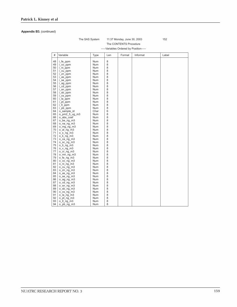
NUATRC RESEARCH REPORT NO. 3 159
Patrick L. Kinney et al
The SAS System 11:37 Monday, June 30, 2003 152
The CONTENTS Procedure
-----Variables Ordered by Position-----
# Variable Type Len Format Informat Label 48 i_fe_ppm Num 8 49 i_co_ppm Num 8 50 i_ni_ppm Num 8 51 i_cu_ppm Num 8 52 i_zn_ppm Num 8 53 i_as_ppm Num 8 54 i_se_ppm Num 8 55 i_ag_ppm Num 8 56 i_cd_ppm Num 8 57 i_sn_ppm Num 8 58 i_sb_ppm Num 8 59 i_cs_ppm Num 8 60 i_la_ppm Num 8 61 i_pt_ppm Num 8 62 i_tl_ppm Num 8 63 i_pb_ppm Num 8 64 o_sample_id Char 6 65 o_pm2_5_ug_m3 Num 8 66 o_abs_coef Num 8 67 o_be_ng_m3 Num 8 68 o_na_ng_m3 Num 8 69 o_mg_ng_m3 Num 8 70 o_al_ng_m3 Num 8 71 o_s_ng_m3 Num 8 72 o_k_ng_m3 Num 8 73 o_ca_ng_m3 Num 8 74 o_sc_ng_m3 Num 8 75 o_ti_ng_m3 Num 8 76 o_v_ng_m3 Num 8 77 o_cr_ng_m3 Num 8 78 o_mn_ng_m3 Num 8 79 o_fe_ng_m3 Num 8 80 o_co_ng_m3 Num 8 81 o_ni_ng_m3 Num 8 82 o_cu_ng_m3 Num 8 83 o_zn_ng_m3 Num 8 84 o_as_ng_m3 Num 8 85 o_se_ng_m3 Num 8 86 o_ag_ng_m3 Num 8 87 o_cd_ng_m3 Num 8 88 o_sn_ng_m3 Num 8 89 o_sb_ng_m3 Num 8 90 o_cs_ng_m3 Num 8 91 o_la_ng_m3 Num 8 92 o_pt_ng_m3 Num 8 93 o_tl_ng_m3 Num 8 94 o_pb_ng_m3 Num 8
Appendix B3. (continued)

160
Toxic Exposure Assessment: A Columbia-Harvard (TEACH) Study (The New York City Report)
NUATRC RESEARCH REPORT NO. 3
The SAS System 11:37 Monday, June 30, 2003 153
The CONTENTS Procedure
-----Variables Ordered by Position-----
# Variable Type Len Format Informat Label 95 o_be_ppm Num 8 96 o_na_ppm Num 8 97 o_mg_ppm Num 8 98 o_al_ppm Num 8 99 o_s_ppm Num 8 100 o_k_ppm Num 8 101 o_ca_ppm Num 8 102 o_sc_ppm Num 8 103 o_ti_ppm Num 8 104 o_v_ppm Num 8 105 o_cr_ppm Num 8 106 o_mn_ppm Num 8 107 o_fe_ppm Num 8 108 o_co_ppm Num 8 109 o_ni_ppm Num 8 110 o_cu_ppm Num 8 111 o_zn_ppm Num 8 112 o_as_ppm Num 8 113 o_se_ppm Num 8 114 o_ag_ppm Num 8 115 o_cd_ppm Num 8 116 o_sn_ppm Num 8 117 o_sb_ppm Num 8 118 o_cs_ppm Num 8 119 o_la_ppm Num 8 120 o_pt_ppm Num 8 121 o_tl_ppm Num 8 122 o_pb_ppm Num 8 123 p_sample_id Char 6 124 p_pm2_5_ug_m3 Num 8 125 p_abs_coef Num 8 126 p_be_ng_m3 Num 8 127 p_na_ng_m3 Num 8 128 p_mg_ng_m3 Num 8 129 p_al_ng_m3 Num 8 130 p_s_ng_m3 Num 8 131 p_k_ng_m3 Num 8 132 p_ca_ng_m3 Num 8 133 p_sc_ng_m3 Num 8 134 p_ti_ng_m3 Num 8 135 p_v_ng_m3 Num 8 136 p_cr_ng_m3 Num 8 137 p_mn_ng_m3 Num 8 138 p_fe_ng_m3 Num 8 139 p_co_ng_m3 Num 8 140 p_ni_ng_m3 Num 8 141 p_cu_ng_m3 Num 8
Appendix B3. (continued)

NUATRC RESEARCH REPORT NO. 3 161
Patrick L. Kinney et al
Appendix B3. (continued)
The SAS System 11:37 Monday, June 30, 2003 154
The CONTENTS Procedure
-----Variables Ordered by Position-----
# Variable Type Len Format Informat Label 142 p_zn_ng_m3 Num 8 143 p_as_ng_m3 Num 8 144 p_se_ng_m3 Num 8 145 p_ag_ng_m3 Num 8 146 p_cd_ng_m3 Num 8 147 p_sn_ng_m3 Num 8 148 p_sb_ng_m3 Num 8 149 p_cs_ng_m3 Num 8 150 p_la_ng_m3 Num 8 151 p_pt_ng_m3 Num 8 152 p_tl_ng_m3 Num 8 153 p_pb_ng_m3 Num 8 154 p_be_ppm Num 8 155 p_na_ppm Num 8 156 p_mg_ppm Num 8 157 p_al_ppm Num 8 158 p_s_ppm Num 8 159 p_k_ppm Num 8 160 p_ca_ppm Num 8 161 p_sc_ppm Num 8 162 p_ti_ppm Num 8 163 p_v_ppm Num 8 164 p_cr_ppm Num 8 165 p_mn_ppm Num 8 166 p_fe_ppm Num 8 167 p_co_ppm Num 8 168 p_ni_ppm Num 8 169 p_cu_ppm Num 8 170 p_zn_ppm Num 8 171 p_as_ppm Num 8 172 p_se_ppm Num 8 173 p_ag_ppm Num 8 174 p_cd_ppm Num 8 175 p_sn_ppm Num 8 176 p_sb_ppm Num 8 177 p_cs_ppm Num 8 178 p_la_ppm Num 8 179 p_pt_ppm Num 8 180 p_tl_ppm Num 8 181 p_pb_ppm Num 8
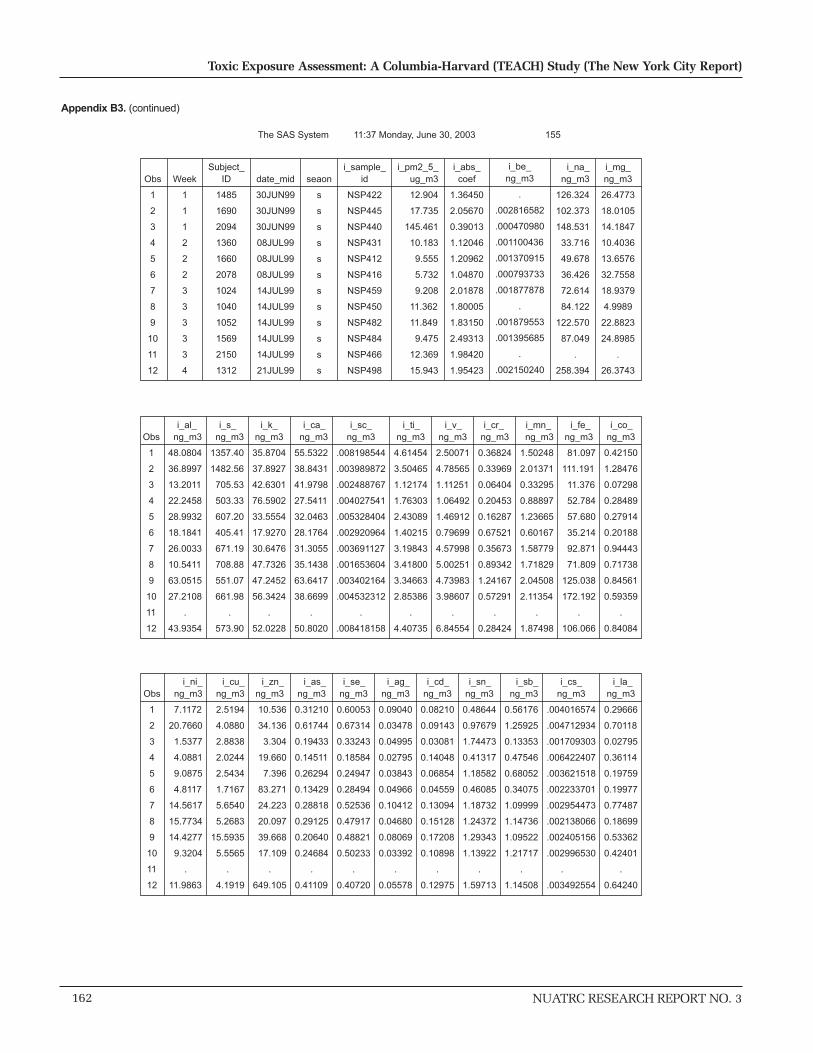
162
Toxic Exposure Assessment: A Columbia-Harvard (TEACH) Study (The New York City Report)
NUATRC RESEARCH REPORT NO. 3
The SAS System 11:37 Monday, June 30, 2003 155
i_mg_ng_m3
26.4773
18.0105
14.1847
10.4036
13.6576
32.7558
18.9379
4.9989
22.8823
24.8985
.
26.3743
i_na_ng_m3
126.324
102.373
148.531
33.716
49.678
36.426
72.614
84.122
122.570
87.049
.
258.394
i_be_ng_m3
.
.002816582
.000470980
.001100436
.001370915
.000793733
.001877878
.
.001879553
.001395685
.
.002150240
i_pm2_5_ug_m3
12.904
17.735
145.461
10.183
9.555
5.732
9.208
11.362
11.849
9.475
12.369
15.943
Subject_ID
1485
1690
2094
1360
1660
2078
1024
1040
1052
1569
2150
1312
i_abs_coef
1.36450
2.05670
0.39013
1.12046
1.20962
1.04870
2.01878
1.80005
1.83150
2.49313
1.98420
1.95423
i_sample_id
NSP422
NSP445
NSP440
NSP431
NSP412
NSP416
NSP459
NSP450
NSP482
NSP484
NSP466
NSP498
Obs
1
2
3
4
5
6
7
8
9
10
11
12
Week
1
1
1
2
2
2
3
3
3
3
3
4
seaon
s
s
s
s
s
s
s
s
s
s
s
s
date_mid
30JUN99
30JUN99
30JUN99
08JUL99
08JUL99
08JUL99
14JUL99
14JUL99
14JUL99
14JUL99
14JUL99
21JUL99
Obs
1
2
3
4
5
6
7
8
9
10
11
12
i_al_ ng_m3
48.0804
36.8997
13.2011
22.2458
28.9932
18.1841
26.0033
10.5411
63.0515
27.2108
.
43.9354
i_s_ ng_m3
1357.40
1482.56
705.53
503.33
607.20
405.41
671.19
708.88
551.07
661.98
.
573.90
i_ca_ ng_m3
55.5322
38.8431
41.9798
27.5411
32.0463
28.1764
31.3055
35.1438
63.6417
38.6699
.
50.8020
i_sc_ng_m3
.008198544
.003989872
.002488767
.004027541
.005328404
.002920964
.003691127
.001653604
.003402164
.004532312
.
.008418158
i_ti_ ng_m3
4.61454
3.50465
1.12174
1.76303
2.43089
1.40215
3.19843
3.41800
3.34663
2.85386
.
4.40735
i_v_ ng_m3
2.50071
4.78565
1.11251
1.06492
1.46912
0.79699
4.57998
5.00251
4.73983
3.98607
.
6.84554
i_cr_ ng_m3
0.36824
0.33969
0.06404
0.20453
0.16287
0.67521
0.35673
0.89342
1.24167
0.57291
.
0.28424
i_mn_ ng_m3
1.50248
2.01371
0.33295
0.88897
1.23665
0.60167
1.58779
1.71829
2.04508
2.11354
.
1.87498
i_fe_ ng_m3
81.097
111.191
11.376
52.784
57.680
35.214
92.871
71.809
125.038
172.192
.
106.066
i_co_ ng_m3
0.42150
1.28476
0.07298
0.28489
0.27914
0.20188
0.94443
0.71738
0.84561
0.59359
.
0.84084
i_k_ng_m3
35.8704
37.8927
42.6301
76.5902
33.5554
17.9270
30.6476
47.7326
47.2452
56.3424
.
52.0228
Obs
1
2
3
4
5
6
7
8
9
10
11
12
i_ni_ng_m3
7.1172
20.7660
1.5377
4.0881
9.0875
4.8117
14.5617
15.7734
14.4277
9.3204
.
11.9863
i_cu_ng_m3
2.5194
4.0880
2.8838
2.0244
2.5434
1.7167
5.6540
5.2683
15.5935
5.5565
.
4.1919
i_as_ ng_m3
0.31210
0.61744
0.19433
0.14511
0.26294
0.13429
0.28818
0.29125
0.20640
0.24684
.
0.41109
i_se_ ng_m3
0.60053
0.67314
0.33243
0.18584
0.24947
0.28494
0.52536
0.47917
0.48821
0.50233
.
0.40720
i_ag_ ng_m3
0.09040
0.03478
0.04995
0.02795
0.03843
0.04966
0.10412
0.04680
0.08069
0.03392
.
0.05578
i_cd_ ng_m3
0.08210
0.09143
0.03081
0.14048
0.06854
0.04559
0.13094
0.15128
0.17208
0.10898
.
0.12975
i_sn_ ng_m3
0.48644
0.97679
1.74473
0.41317
1.18582
0.46085
1.18732
1.24372
1.29343
1.13922
.
1.59713
i_sb_ng_m3
0.56176
1.25925
0.13353
0.47546
0.68052
0.34075
1.09999
1.14736
1.09522
1.21717
.
1.14508
i_cs_ng_m3
.004016574
.004712934
.001709303
.006422407
.003621518
.002233701
.002954473
.002138066
.002405156
.002996530
.
.003492554
i_la_ ng_m3
0.29666
0.70118
0.02795
0.36114
0.19759
0.19977
0.77487
0.18699
0.53362
0.42401
.
0.64240
i_zn_ ng_m3
10.536
34.136
3.304
19.660
7.396
83.271
24.223
20.097
39.668
17.109
.
649.105
Appendix B3. (continued)

NUATRC RESEARCH REPORT NO. 3 163
Patrick L. Kinney et al
Appendix B3. (continued)
The SAS System 11:37 Monday, June 30, 2003 156
i_ca_ppm
4303.33
2190.20
288.60
2704.65
3353.83
4915.91
3399.73
3093.03
5371.19
4081.34
.
3186.49
i_k_ ppm
2779.69
2136.60
293.07
7521.47
3511.77
3127.72
3328.28
4200.98
3987.36
5946.54
.
3263.06
i_s_ppm
105188.19
83595.01
4850.29
49428.66
63547.44
70731.14
72890.48
62389.54
46508.44
69867.54
.
35997.08
i_mg_ ppm
2051.79
1015.53
97.52
1021.68
1429.35
5714.89
2056.63
439.96
1931.20
2627.87
.
1654.29
i_tl_ng_m3
0.003655
0.008443
0.001591
0.007606
0.003348
0.002232
0.007127
0.005533
0.004945
0.004996
.
0.013375
i_al_ppm
3725.87
2080.62
90.75
2184.63
3034.31
3172.56
2823.91
927.73
5321.37
2871.91
.
2755.79
i_na_ppm
9789.13
5772.37
1021.11
3311.10
5199.12
6355.25
7885.78
7403.66
10344.59
9187.42
.
16207.42
Obs
1
2
3
4
5
6
7
8
9
10
11
12
i_pt_ng_m3
.001126154
.001125837
.000480851
.000591083
.001034059
.000579234
.001504595
.001530218
.001555113
.002405884
.
.001003175
i_be_ppm
.
0.15882
0.00324
0.10807
0.14347
0.13848
0.20393
.
0.15863
0.14730
.
0.13487
i_pb_ng_m3
2.33515
6.55335
0.91531
3.90288
2.25383
4.38024
7.07612
5.23893
5.55380
4.69231
.
6.56249
Obs
1
2
3
4
5
6
7
8
9
10
11
12
i_sc_ ppm
0.63533
0.22497
0.01711
0.39552
0.55765
0.50962
0.40085
0.14554
0.28713
0.47835
.
0.52802
i_ti_ ppm
357.593
197.612
7.712
173.137
254.407
244.633
347.344
300.821
282.446
301.204
.
276.445
i_cr_ppm
28.536
19.154
0.440
20.086
17.045
117.804
38.740
78.631
104.793
60.467
.
17.828
i_mn_ ppm
116.431
113.544
2.289
87.301
129.423
104.974
172.432
151.228
172.599
223.069
.
117.605
i_fe_ ppm
6284.42
6269.60
78.21
5183.57
6036.53
6143.80
10085.63
6319.9
10552.85
18173.65
.
6652.86
i_co_ ppm
32.663
72.442
0.502
27.977
29.214
35.222
102.564
63.137
71.367
62.649
.
52.741
i_ni_ ppm
551.53
1170.91
10.57
401.46
951.06
839.49
1581.37
1388.23
1217.66
983.70
.
751.83
i_cu_ ppm
195.24
230.51
19.83
198.80
266.18
299.51
614.02
463.67
1316.05
586.45
.
262.93
i_zn_ ppm
816.43
1924.77
22.72
1930.70
774.05
14528.26
2630.63
1768.76
3347.84
1805.71
.
40714.21
i_v_ ppm
193.786
269.842
7.648
104.580
153.752
139.050
497.379
440.275
400.028
420.702
.
429.377
Obs
1
2
3
4
5
6
7
8
9
10
11
12
i_as_ ppm
24.1853
34.8145
1.3360
14.2502
27.5180
23.4289
31.2959
25.6333
17.4192
26.0527
.
25.7850
i_se_ ppm
46.5366
37.9552
2.2854
18.2505
26.1082
49.7132
57.0528
42.1723
41.2038
53.0174
.
25.5410
i_cd_ ppm
6.3624
5.1554
0.2118
13.7954
7.1728
7.9533
14.2196
13.3139
14.5234
11.5019
.
8.1382
i_sn_ ppm
37.695
55.077
11.995
40.575
124.103
80.404
128.941
109.461
109.162
120.237
.
100.178
i_sb_ ppm
43.532
71.004
0.918
46.692
71.220
59.451
119.457
100.980
92.434
128.463
.
71.823
i_cs_ ppm
0.31125
0.26574
0.01175
0.63071
0.37901
0.38971
0.32085
0.18817
0.20299
0.31626
.
0.21907
i_la_ ppm
22.9886
39.5368
0.1922
35.4651
20.6789
34.8540
84.1497
16.4574
45.0357
44.7512
.
40.2937
i_pt_ppm
0.08727
0.06348
0.00331
0.05805
0.10822
0.10106
0.16340
0.13468
0.13125
0.25392
.
0.06292
i_tl_ ppm
0.28320
0.47607
0.01094
0.74693
0.35035
0.38941
0.77398
0.48694
0.41731
0.52729
.
0.83890
i_ag_ ppm
7.0056
1.9612
0.3434
2.7446
4.0221
8.6638
11.3075
4.1192
6.8100
3.5804
.
3.4985

164
Toxic Exposure Assessment: A Columbia-Harvard (TEACH) Study (The New York City Report)
NUATRC RESEARCH REPORT NO. 3
The SAS System 11:37 Monday, June 30, 2003 157
o_ca_ng_m3
.
31.6217
37.0220
35.1650
47.1297
34.3844
42.3252
33.2524
66.8237
32.9854
.
37.5288
o_k_ng_m3
.
.
.
.
.
.
.
.
.
.
.
.
o_ng_ng_m3
.
2433.68
1522.18
1075.12
1178.19
1023.28
701.39
1138.85
670.99
711.14
.
714.40
o_mg_ng_m3
.
.
.
.
.
.
.
.
.
.
.
.
o_sample_id
NSP420
NSP441
NSP447
NSP433
NSP415
NSP435
NSP480
NSP558
NSP457
NSP485
NSP460
NSP500
o_al_ng_m3
.
16.4971
72.7288
33.5493
41.0691
21.6782
37.6891
36.3005
44.7286
18.6508
.
48.4741
o_be_ng_m3
.
.002084869
.
.001354563
.001766251
.000879695
.
.001729445
.
.
.
.
Obs
1
2
3
4
5
6
7
8
9
10
11
12
i_pb_ppm
180.957
369.516
6.292
383.278
235.876
764.218
768.456
461.083
468.725
495.241
.
411.623
o_abs_coef
1.34957
2.19908
0.96111
1.18627
1.61454
1.36047
1.96546
1.68702
2.31470
2.17746
1.87947
1.66955
o_na_ng_m3
.
79.807
233.459
24.912
53.885
110.140
87.259
82.425
124.571
75.574
.
84.871
o_pm2_5_ug_m3
12.6011
14.1134
11.1564
7.4188
8.6200
6.5717
10.3514
9.3909
11.8396
9.6746
12.5602
9.6132
Obs
1
2
3
4
5
6
7
8
9
10
11
12
o_sc_ ng_m3
.
0.002064
0.014105
0.006267
0.007018
0.003761
0.007067
0.004680
0.008164
0.001427
.
0.012246
o_as_ng_m3
.
0.48719
0.20627
0.22816
0.17087
0.16555
0.20369
0.25721
0.23396
0.18867
.
0.43772
o_ti_ ng_m3
.
3.49885
5.10582
2.61329
3.36337
1.35991
3.56018
3.03936
4.46166
3.02741
.
5.35191
o_cr_ng_m3
.
0.15246
0.13193
0.20372
0.10993
.
0.68629
0.38844
0.98733
0.78299
.
0.62714
o_mn_ng_m3
.
1.92974
1.47873
1.48456
1.61387
0.78907
2.28316
2.03811
2.55430
2.37977
.
2.40587
o_fe_ ng_m3
.
107.704
67.284
88.853
92.425
53.092
158.674
121.307
165.350
202.584
.
145.307
o_co_ng_m3
.
1.25514
0.21214
0.41054
0.40480
0.29305
1.22284
0.76083
1.33157
0.60177
.
1.09334
o_ni_ ng_m3
.
18.7412
5.1665
5.9984
6.3880
4.3307
18.8838
12.5875
22.3761
8.9812
.
16.0801
o_cu_ng_m3
.
4.09977
1.68072
3.58254
2.98407
2.53397
7.17520
6.06152
8.91655
5.29587
.
5.49690
o_zn_ ng_m3
.
29.0986
6.1007
20.8904
9.0381
27.9431
30.6113
21.2552
42.0377
16.2728
.
39.7742
o_v_ ng_m3
.
4.74024
2.72614
1.44430
1.89315
1.34397
6.08451
5.34090
7.66529
3.93846
.
6.48231
Obs
1
2
3
4
5
6
7
8
9
10
11
12
o_pb_ng_m3
.
5.21249
2.01371
5.26959
2.79970
5.31738
8.29259
5.34639
7.61614
4.76902
.
8.65232
o_se_ng_m3
.
0.54136
0.80611
0.09794
0.10050
.
0.67734
0.25732
0.88648
0.65212
.
0.34902
o_cd_ng_m3
.
0.07808
0.05253
0.05422
0.05556
0.07480
0.16116
0.16255
0.19143
0.11902
.
0.12447
o_sn_ng_m3
.
.
0.38297
.
.
.
1.45797
.
1.58314
0.70828
.
0.96774
o_sb_ng_m3
.
1.20688
0.43119
0.65292
0.89156
0.61274
1.33629
1.33293
1.90807
1.14265
.
1.66999
o_cs_ng_m3
.
.003573007
.006924466
.004364841
.005109681
.003759769
.004142871
.003193281
.003811135
.003312747
.
.003600839
o_la_ng_m3
.
0.44446
0.18724
0.34396
0.28447
0.32090
1.02221
0.52502
1.18430
0.32154
.
0.81558
o_pt_ng_m3
.
.001334977
.001238092
.001125201
.001581038
.000744561
.001943959
001968906
.002859378
.002018602
.
.001549676
o_tl_ng_m3
.
.007449981
.004479367
.003334453
.003756399
.002888284
.007813486
.006260169
.006742884
.005229261
.
.004613655
o_ag_ng_m3
.
0.028543
0.019963
0.017571
0.019656
0.012779
0.069623
0.051217
0.058115
0.033194
.
0.038379
Appendix B3. (continued)
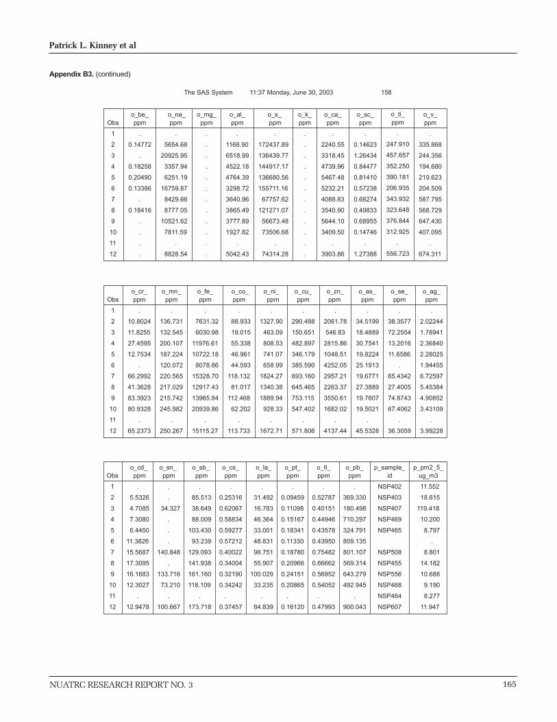
NUATRC RESEARCH REPORT NO. 3 165
Patrick L. Kinney et al
Appendix B3. (continued)
The SAS System 11:37 Monday, June 30, 2003 158
o_v_ppm
.
335.868
244.356
194.680
219.623
204.509
587.795
568.729
647.430
407.095
.
674.311
o_ti_ppm
.
247.910
457.657
352.250
390.181
206.935
343.932
323.648
376.844
312.925
.
556.723
o_ca_ppm
.
2240.55
3318.45
4739.96
5467.48
5232.21
4088.83
3540.90
5644.10
3409.50
.
3903.86
o_na_ ppm
.
5654.68
20925.95
3357.94
6251.19
16759.87
8429.66
8777.05
10521.62
7811.59
.
8828.54
o_sc_ppm
.
0.14623
1.26434
0.84477
0.81410
0.57238
0.68274
0.49833
0.68955
0.14746
.
1.27388
o_s_ ppm
.
172437.89
136439.77
144917.17
136680.56
155711.16
67757.62
121271.07
56673.48
73506.68
.
74314.28
Obs
1
2
3
4
5
6
7
8
9
10
11
12
o_be_ppm
.
0.14772
.
0.18258
0.20490
0.13386
.
0.18416
.
.
.
.
o_al_ppm
.
1168.90
6518.99
4522.18
4764.39
3298.72
3640.96
3865.49
3777.89
1927.82
.
5042.43
o_k_ppm
.
.
.
.
.
.
.
.
.
.
.
.
o_mg_ppm
.
.
.
.
.
.
.
.
.
.
.
.
Obs
1
2
3
4
5
6
7
8
9
10
11
12
o_cr_ppm
.
10.8024
11.8255
27.4595
12.7534
.
66.2992
41.3628
83.3923
80.9328
.
65.2373
o_ag_ppm
.
2.02244
1.78941
2.36840
2.28025
1.94455
6.72597
5.45384
4.90852
3.43109
.
3.99228
o_mn_ppm
.
136.731
132.545
200.107
187.224
120.072
220.565
217.029
215.742
245.982
.
250.267
o_fe_ ppm
.
7631.32
6030.98
11976.61
10722.18
8078.86
15328.70
12917.43
13965.84
20939.86
.
15115.27
o_co_ ppm
.
88.933
19.015
55.338
46.961
44.593
118.132
81.017
112.468
62.202
.
113.733
o_ni_ ppm
.
1327.90
463.09
808.53
741.07
658.99
1824.27
1340.38
1889.94
928.33
.
1672.71
o_cu_ppm
.
290.488
150.651
482.897
346.179
385.590
693.160
645.465
753.115
547.402
.
571.806
o_zn_ppm
.
2061.78
546.83
2815.86
1048.51
4252.05
2957.21
2263.37
3550.61
1682.02
.
4137.44
o_as_ppm
.
34.5199
18.4889
30.7541
19.8224
25.1913
19.6771
27.3889
19.7607
19.5021
.
45.5328
o_se_ppm
.
38.3577
72.2554
13.2016
11.6586
.
65.4342
27.4005
74.8743
67.4062
.
36.3059
Obs
1
2
3
4
5
6
7
8
9
10
11
12
p_pm2_5_ug_m3
11.552
18.615
119.418
10.200
8.797
.
8.801
14.182
10.688
9.190
8.277
11.947
o_cd_ ppm
.
5.5326
4.7085
7.3080
6.4450
11.3826
15.5687
17.3095
16.1683
12.3027
.
12.9478
o_sb_ ppm
.
85.513
38.649
88.009
103.430
93.239
129.093
141.938
161.160
118.109
.
173.718
o_cs_ppm
.
0.25316
0.62067
0.58834
0.59277
0.57212
0.40022
0.34004
0.32190
0.34242
.
0.37457
o_la_ ppm
.
31.492
16.783
46.364
33.001
48.831
98.751
55.907
100.029
33.235
.
84.839
o_pt_ppm
.
0.09459
0.11098
0.15167
0.18341
0.11330
0.18780
0.20966
0.24151
0.20865
.
0.16120
o_tl_ppm
.
0.52787
0.40151
0.44946
0.43578
0.43950
0.75482
0.66662
0.56952
0.54052
.
0.47993
o_pb_ppm
.
369.330
180.498
710.297
324.791
809.135
801.107
569.314
643.279
492.945
.
900.043
p_sample_id
NSP402
NSP403
NSP407
NSP469
NSP465
NSP508
NSP455
NSP556
NSP468
NSP464
NSP607
o_sn_ ppm
.
.
34.327
.
.
.
140.848
.
133.716
73.210
.
100.667
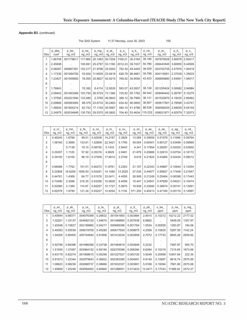
166
Toxic Exposure Assessment: A Columbia-Harvard (TEACH) Study (The New York City Report)
NUATRC RESEARCH REPORT NO. 3
The SAS System 11:37 Monday, June 30, 2003 159
p_sc_ng_m3
.007879528
.006443545
.003702739
.004119581
.006859880
.
.001205424
.009494442
.001532870
.005617561
.006568205
.009021871
p_ti_ng_m3
3.60978
3.60955
2.47976
2.37039
3.54991
.
3.00682
5.26797
4.18435
2.78599
2.94839
4.82579
p_ca_ng_m3
39.190
50.780
36.029
30.798
42.423
.
38.128
90.042
36.131
36.907
86.538
115.232
p_k_ng_m3
30.2184
39.7437
49.4445
98.4681
34.9550
.
43.5937
55.1762
36.7980
46.0800
41.4786
53.4634
p_be_ng_m3
.001179617
.
.000667381
.001084792
.001559992
.
.
.001463369
.002201594
.000983064
.001605214
.002034949
p_v_ng_m3
2.50417
5.44595
1.00419
1.35633
1.94017
.
3.94984
5.10275
2.89463
3.43741
5.04154
7.32073
p_al_ng_m3
50.7204
53.1180
25.5003
23.9418
42.9215
.
12.8530
73.1384
46.9643
30.2483
40.9567
45.0802
Obs
1
2
3
4
5
6
7
8
9
10
11
12
p_abs_coef
1.66708
2.45938
0.08267
1.17330
1.23427
.
1.76843
2.09442
1.37595
2.09868
1.48934
2.24975
p_mg_ng_m3
25.1483
25.2787
21.9796
11.6509
25.8627
.
8.4114
26.5724
2.3765
23.6733
17.1745
29.5370
p_s_ ng_m3
1169.21
2012.23
752.30
628.78
769.52
.
583.07
725.62
389.12
634.42
584.10
704.40
p_na_ ng_m3
117.969
100.691
153.317
53.934
76.055
.
70.392
103.750
133.085
88.379
62.752
135.793
Obs
1
2
3
4
5
6
7
8
9
10
11
12
p_cr_ng_m3
0.46240
1.08160
.
0.29357
0.39100
.
0.66068
5.22808
0.44761
0.73490
0.52060
0.62579
p_ag_ng_m3
0.11066
0.03499
0.05020
0.02704
0.02434
.
0.10640
0.17409
0.06398
0.04021
0.05101
0.05170
p_cd_ng_m3
0.09794
0.09969
0.03850
0.18172
0.06512
.
0.12554
0.21947
0.17443
0.10474
0.13091
0.14997
p_mn_ng_m3
1.6766
2.3685
0.7138
1.1120
1.6100
.
1.7762
16.6209
1.4369
2.3096
2.1380
1.9795
p_fe_ ng_m3
99.01
133.81
19.15
57.92
88.19
.
101.01
1656.93
64.77
216.35
114.97
121.24
p_co_ng_m3
0.42938
1.52909
0.08750
0.35316
0.37459
.
0.80272
0.93281
0.51576
0.53258
0.62257
0.93227
p_ni_ng_m3
14.2187
22.3421
5.1433
4.9929
17.6614
.
11.8761
14.1080
33.0411
10.0828
10.1727
12.9254
p_cu_ng_m3
3.3828
5.1785
2.9443
2.0481
2.3749
.
5.2263
13.2020
4.4050
6.4058
5.0875
5.1130
p_zn_ng_m3
13.085
39.004
4.341
21.879
9.618
.
21.107
27.030
26.908
15.447
19.838
571.250
p_as_ng_m3
0.30659
0.60401
0.17854
0.20889
0.21824
.
0.22343
0.44977
0.21249
0.24541
0.23940
0.40413
p_se_ng_m3
0.51979
0.80127
0.28287
0.32610
0.43465
.
0.49867
0.59927
0.25464
0.47659
0.38974
0.47160
Obs
1
2
3
4
5
6
7
8
9
10
11
12
p_mg_ ppm
2177.02
1357.97
184.06
1142.24
2939.82
.
955.70
1873.68
222.35
2575.95
2075.06
2472.27
p_sn_ng_m3
0.45844
1.02201
1.40548
0.49393
1.04305
.
0.92789
1.51555
0.83179
0.91913
1.08623
1.49858
p_cs_ng_m3
.004076389
.004692120
.002199960
.008019709
.005154840
.
.001686288
.003964152
.001908615
.002975643
.002988737
.004094002
p_la_ng_m3
0.29632
1.04674
0.04217
0.45280
0.91806
.
0.33738
0.58194
0.05256
0.36822
0.38666
0.60864
p_pt_ng_m3
.001541900
.001488660
.000689396
.000617930
.001412034
.
.001464619
.002379398
.001227527
.002383385
.001632337
.001288001
p_tl_ng_m3
0.003864
0.007838
0.001764
0.009675
0.003808
.
0.003846
0.006394
0.003120
0.004901
0.003801
0.013433
p_pb_ng_m3
2.9010
6.8662
1.0534
4.2099
2.7072
.
5.2232
8.6284
3.9249
4.9149
5.5168
13.4471
o_be_ppm
0.10212
.
0.00559
0.10635
0.17733
.
.
0.10319
0.20599
0.10697
0.19394
0.17033
p_na_ ppm
10212.22
5409.09
1283.87
5287.59
8645.26
.
7997.87
7315.65
12451.84
9616.74
7581.80
11366.02
p_sb_ng_m3
0.68371
1.33137
0.15627
0.55036
0.90405
.
0.89396
1.37497
0.82274
1.22344
0.98236
1.25248
Appendix B3. (continued)
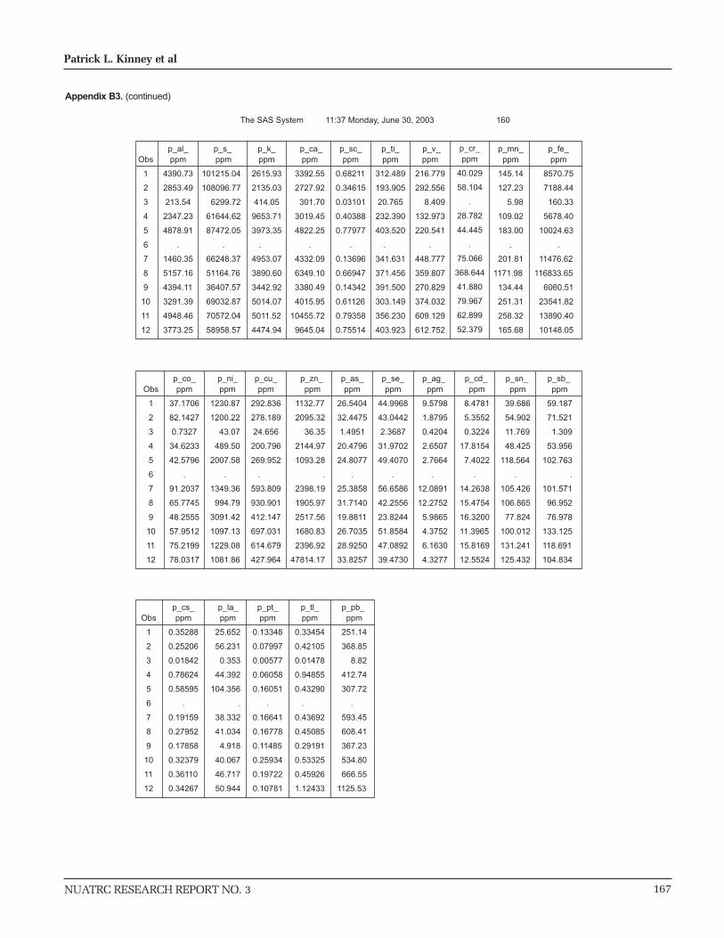
NUATRC RESEARCH REPORT NO. 3 167
Patrick L. Kinney et al
Appendix B3. (continued)
The SAS System 11:37 Monday, June 30, 2003 160
p_mn_ppm
145.14
127.23
5.98
109.02
183.00
.
201.81
1171.98
134.44
251.31
258.32
165.68
p_fe_ ppm
8570.75
7188.44
160.33
5678.40
10024.63
.
11476.62
116833.65
6060.51
23541.82
13890.40
10148.05
p_cr_ppm
40.029
58.104
.
28.782
44.445
.
75.066
368.644
41.880
79.967
62.899
52.379
p_v_ ppm
216.779
292.556
8.409
132.973
220.541
.
448.777
359.807
270.829
374.032
609.129
612.752
p_s_ ppm
101215.04
108096.77
6299.72
61644.62
87472.05
.
66248.37
51164.76
36407.57
69032.87
70572.04
58958.57
p_sc_ppm
0.68211
0.34615
0.03101
0.40388
0.77977
.
0.13696
0.66947
0.14342
0.61126
0.79358
0.75514
Obs
1
2
3
4
5
6
7
8
9
10
11
12
p_al_ppm
4390.73
2853.49
213.54
2347.23
4878.91
.
1460.35
5157.16
4394.11
3291.39
4948.46
3773.25
p_ca_ ppm
3392.55
2727.92
301.70
3019.45
4822.25
.
4332.09
6349.10
3380.49
4015.95
10455.72
9645.04
p_ti_ppm
312.489
193.905
20.765
232.390
403.520
.
341.631
371.456
391.500
303.149
356.230
403.923
p_k_ppm
2615.93
2135.03
414.05
9653.71
3973.35
.
4953.07
3890.60
3442.92
5014.07
5011.52
4474.94
Obs
1
2
3
4
5
6
7
8
9
10
11
12
p_co_ppm
37.1706
82.1427
0.7327
34.6233
42.5796
.
91.2037
65.7745
48.2555
57.9512
75.2199
78.0317
p_sb_ ppm
59.187
71.521
1.309
53.956
102.763
.
101.571
96.952
76.978
133.125
118.691
104.834
p_ni_ ppm
1230.87
1200.22
43.07
489.50
2007.58
.
1349.36
994.79
3091.42
1097.13
1229.08
1081.86
p_cu_ppm
292.836
278.189
24.656
200.796
269.952
.
593.809
930.901
412.147
697.031
614.679
427.964
p_zn_ ppm
1132.77
2095.32
36.35
2144.97
1093.28
.
2398.19
1905.97
2517.56
1680.83
2396.92
47814.17
p_as_ppm
26.5404
32.4475
1.4951
20.4796
24.8077
.
25.3858
31.7140
19.8811
26.7035
28.9250
33.8257
p_se_ppm
44.9968
43.0442
2.3687
31.9702
49.4070
.
56.6586
42.2556
23.8244
51.8584
47.0892
39.4730
p_ag_ ppm
9.5798
1.8795
0.4204
2.6507
2.7664
.
12.0891
12.2752
5.9865
4.3752
6.1630
4.3277
p_cd_ ppm
8.4781
5.3552
0.3224
17.8154
7.4022
.
14.2638
15.4754
16.3200
11.3965
15.8169
12.5524
p_sn_ ppm
39.686
54.902
11.769
48.425
118.564
.
105.426
106.865
77.824
100.012
131.241
125.432
Obs
1
2
3
4
5
6
7
8
9
10
11
12
p_pb_ ppm
251.14
368.85
8.82
412.74
307.72
.
593.45
608.41
367.23
534.80
666.55
1125.53
p_cs_ppm
0.35288
0.25206
0.01842
0.78624
0.58595
.
0.19159
0.27952
0.17858
0.32379
0.36110
0.34267
p_la_ ppm
25.652
56.231
0.353
44.392
104.356
.
38.332
41.034
4.918
40.067
46.717
50.944
p_pt_ppm
0.13348
0.07997
0.00577
0.06058
0.16051
.
0.16641
0.16778
0.11485
0.25934
0.19722
0.10781
p_tl_ppm
0.33454
0.42105
0.01478
0.94855
0.43290
.
0.43692
0.45085
0.29191
0.53325
0.45926
1.12433

NUATRC RESEARCH REPORT NO. 3 169
Patrick L. Kinney et al
Hans P. Blaschek Bernard D. GoldsteinUniversity of Illinois University of Pittsburgh
Josephine Cooper (Chair) Susan F. MooreToyota Motor North America, Inc. Georgia-Pacific Corporation
Wilma Delaney Monica SamuelsDow Chemical Company (Retired) Attorney
Mary Gade Arthur C. VailasSonnenschein Nath & Rosenthal University of Houston
NUATRC STAFF
SCIENTIFIC ADVISORY PANEL
BOARD OF DIRECTORS
Craig Beskid Lata Shirnamé-MoréPresident Research Director
Jack Chang Brenda GehanTechnical Assistant Consulting Staff Scientist
Carolyn WadeFinancial Manager
John C. Bailar III Brian P. LeadererUniversity of Chicago Yale University
Michael Brauer Dennis PaganoUniversity of British Columbia U.S. EPA
James J. Collins (Chair) Dennis J. PaustenbachDow Chemical Company ChemRisk, Inc.
Michael L. Cunningham Bertram PriceNational Institute of Environmental Price Associates, Inc.Health Sciences
Joel SchwartzDavid H. Garabrant Harvard UniversityUniversity of Michigan
Linda SheldonPertti J. (Bert) Hakkinen U.S. EPAEuropean Commission
Gary L. LarsenNational Jewish Medical and Research Center

P.O. Box 20286
Houston, Texas 77225-0286
Tel: 713.500.3450
Fax: 713.500.0345
http://www.sph.uth.tmc.edu/mleland/
Printed on 100% Recycled Paper
Authorized by the Clean Air Act Amendments of 1990 (Title III, Section 301/p)