Biological Conservation 143 (2010) 230–238

Contents lists available at ScienceDirect

Biological Conservation

journal homepage: www.elsevier .com/locate /b iocon

Towards a spatially explicit risk assessment for marine management: Assessingthe vulnerability of fish to aggregate extraction

Vanessa Stelzenmüller *, Jim R. Ellis, Stuart I. RogersCentre for Environment, Fisheries and Aquaculture Science (Cefas), Pakefield Road, Lowestoft NR33 OHT, UK

a r t i c l e i n f o a b s t r a c t

Article history:Received 30 September 2008Received in revised form 14 September2009Accepted 7 October 2009Available online 4 November 2009

Keywords:GISIndicator krigingMarine spatial planningRandom simulationsSensitivity indexVulnerability

0006-3207/$ - see front matter � 2009 Elsevier Ltd. Adoi:10.1016/j.biocon.2009.10.007

* Corresponding author. Tel.: +44 1502 527779; faxE-mail address: vanessa.stelzenmuller@cefas.co.uk

Management of human activities in the marine environment increasingly requires spatially explicit riskassessments that link the occurrence and magnitude of a pressure to information on the sensitivity of theenvironment. We developed a marine spatial risk assessment framework for the UK continental shelfassessing the vulnerability of 11 fish and shellfish species to aggregate extraction. We calculated a sen-sitivity index (SI) using life-history characteristics and modelled species distributions on the UK shelfusing long-term monitoring data and indicator kriging. Merging sensitivity indices and predicted speciesdistributions allowed us to map the sensitivity of the selected fish to aggregate extraction. The robustnessof the sensitivity map was affected primarily by widespread species with a low to medium level of sen-sitivity, while highly sensitive species with more restricted distributions had a limited effect on the over-all sensitivity. The highest sensitivity in the case study occurred in coastal regions, and where nursery andspawning areas of four important commercial species occur. To test the framework, we overlaid the esti-mated sensitivity map with the occurrence of aggregate extraction activity in inshore waters, includingsediment plume estimations, to describe species vulnerability to dredging. We conclude that our spatiallyexplicit risk assessment framework can be applied to other ecosystem components and pressures at dif-ferent spatial scales and it is therefore a promising tool that can support the sustainable development ofmarine spatial plans.

� 2009 Elsevier Ltd. All rights reserved.

1. Introduction

Many human activities have a direct or indirect effect on marineecosystems. To ensure sustainable development in the marineenvironment it is necessary to develop planning tools that movefrom a sectoral to an integrated approach to marine management(Douvere, 2008). A basic requirement for marine spatial plans isa clear understanding of both the spatial and temporal distribu-tions of human pressures and ecosystem components (species,habitats, etc.), and the effects of human pressures on the marineenvironment at meaningful ecological scales (Zacharias and Gregr,2005; Eastwood et al., 2007). Integrated ecosystem-based manage-ment also needs to evaluate cumulative and interactive effects ofmultiple human activities (Evans and Klinger, 2008; Halpernet al., 2008a).

Spatially explicit risk assessments that link information on thesensitivity of the environment to the occurrence of a pressure arefundamental to the implementation of spatial management (Hope,2006). In general, Ecological Risk Assessments (ERAs) comprise theformulation of the problem, followed by analyses and characterisa-tion of risk (Hope, 2006). The ‘problem formulation’ phase consists

ll rights reserved.

: +44 1502 513865.(V. Stelzenmüller).

of the development of assessment endpoints, conceptual modelsand a plan for analyses. The ‘analysis phase’ requires data to deter-mine the occurrence of adverse effects, and the extent to which theecosystem is exposed to the stressor(s). In the last phase, past orfuture risks are estimated and interpreted with the help of bothquantitative and qualitative approaches. Thus the final product isan estimate of the probability or likelihood of adverse ecological ef-fects. Quantitative risk assessments rely on mathematical modelsto predict the response of the ecological receptor to a changingenvironment. In contrast, qualitative approaches use ecosystemattributes combined with ecological receptors and stressors (Astleset al., 2006).

In marine spatial planning, any ERA must address the location-specific characteristics and interactions that define that ecosystem(Woodbury, 2003). There are currently very few examples of spa-tial risk assessments in marine ecosystems, and many risk assess-ments often neglect spatial relationships (Woodbury, 2003; Hope,2006).

Early attempts to assess marine environmental sensitivity wereundertaken for different shore types in relation to the potentialimpacts of oil spills (Gundlach and Hayes, 1978). More recently,biological and life-history traits and information on species intoler-ance have been integrated in sensitivity assessments (Bremneret al., 2006; Hiscock and Tyler-Walters, 2006). Other approaches

V. Stelzenmüller et al. / Biological Conservation 143 (2010) 230–238 231

to assess sensitivity have used species attributes (Williams et al.,1994; Furness and Tasker, 2000) together with spatial informationon species occurrences, for example to gauge the potential impactsof offshore wind farms on seabirds (Garthe and Hüppop, 2004).

Comprehensive spatial information on species distributions isoften based on the predictive modelling of available data. Spatialmodelling is an important component of ecological modellingand is becoming widely used in applied ecology and conservationwhere understanding the spatial distributions is required (Jørgen-sen, 2008). Commonly used spatial modelling techniques to predictspecies occurrences in the marine environment include regressionmodels (Eastwood et al., 2003; Vaz et al., 2008) and geostatisticalmethods (Stelzenmüller et al., 2005). Recent studies have alsocombined regression and Geographical Information System (GIS)techniques (Pittman et al., 2007) or geostatistics and GIS (Stel-zenmüller et al., 2007). In the context of marine conservation orimpact assessment, where predicted species occurrences havebeen required, the geostatistical tool indicator kriging has beenused successfully for less frequently sampled species (Stelzenmül-ler et al., 2004). Indicator kriging was introduced by Journel (1983)as a spatial prediction method that is suitable for highly skeweddata, such as those from fisheries and other field surveys.

Here we developed a spatial risk assessment framework for theUK continental shelf to assess the vulnerability of 11 fish and shell-fish species to aggregate extraction. We calculated a sensitivity in-dex (SI) based on seven factors reflecting species’ potentialvulnerability to aggregate extraction. We used indicator krigingto predict the probability of occurrence for each of the case-studyspecies using a long-term dataset (>10 years) collected from beamtrawl surveys operating within the 60 m depth boundary overextensive parts of the English and Welsh continental shelf. UsingGIS methods we modelled and mapped the average sensitivity(and its uncertainty) to aggregate extraction by combining the cal-culated species sensitivity indices with the probabilities of speciesoccurrence. In the final step of our framework, we compared theoccurrence of planned and licensed aggregate extraction off thesoutheast coast of the UK to the modelled sensitivity in order to de-scribe the vulnerability of the area and highlight the potentialapplications and importance of such an approach. Ultimately, wediscuss how this framework might be used to assess the risk ofmultiple human pressures and serve as a tool for the developmentof sustainable marine spatial plans.

2. Material and methods

2.1. Study area and species included

We limited the study area to within the 60 m depth contour, themaximum depth for aggregate extraction activities (Fig. 1). Our cri-teria to select fish and shellfish species for the analysis were thatthey (i) are likely to be affected by aggregate extraction, (ii) havean appropriate catchability by the survey trawl, and (iii) are ofcommercial and/or conservation interest. We included cod (Gadusmorhua), whiting (Merlangius merlangus), plaice (Pleuronectes plat-essa), sole (Solea solea), turbot (Psetta maxima), spotted ray (Rajamontagui), thornback ray (Raja clavata), edible crab (Cancer pagu-rus), lobster (Homarus gammarus), queen scallop (Aequipectenopercularis) and scallop (Pecten maximus).

2.2. Sensitivity index (SI)

Environmental effects of marine aggregate extraction on theseabed include the removal of sediment and the resident fauna,resulting in changes to the nature and stability of sediments. Otherdirect effects include the exposure of underlying strata, increased

turbidity and redistribution of fine particulate material (Desprez,2000; Newell et al., 2004; Boyd et al., 2005; Robinson et al.,2005; Cooper et al., 2007). There are several potential impacts ofmarine aggregate extraction on commercial fisheries (e.g. loss offishing grounds, increased steaming time, displacement of effort,exposure of boulders that may damage trawl nets, etc.), but the ef-fects on fish are not well described in the literature (Newell et al.,1998; Desprez, 2000). Potential effects include loss of habitat,changes in the availability of prey, and an increased vulnerabilityto predators in turbid waters. The increased turbidity may also af-fect egg and larval stages through elevated exposure to re-sus-pended contaminants. Furthermore, there may be importantimpacts on the suitability of the seabed as a nursery ground(including post-larval habitat) or as a spawning ground, particu-larly for demersal egg-laying teleosts (e.g. herring) and oviparouselasmobranchs which deposit eggs on geological or biological fea-tures on the seabed.

For each of the selected fish and shellfish species we calculateda sensitivity index (SI) reflecting the species sensitivity to aggre-gate extraction based on the approach developed by Furness andTasker (2000) and Garthe and Hüppop (2004). In this context, ‘sen-sitivity’ is the degree to which fish or shellfish species respond to apressure, and ‘vulnerability’ is the probability or likelihood that acomponent will be exposed to a pressure to which it is sensitive(Zacharias and Gregr, 2005).

The sensitivity index sums the scores of seven different factorsderived from species attributes which are most responsive to theimpacts associated with aggregate extraction. We scored each fac-tor on a 5-point scale from 1 (low) to 5 (high). The factors includedare described below.

2.2.1. Geographical distributionIn a GIS we superimposed the locations of survey trawl catch

data (presence/absence; see detailed description of survey data be-low) on a 2 nm by 2 nm grid. For each species we calculated a spa-tial distribution ratio as the number of cells with presence data/total number of grid cells (27,213) and scored 1 for >0.03, 2 for>0.02–0.03, 3 for >0.01–0.02, 4 for >0.005–0.01, and 5 6 0.005, sothat species with patchy or restricted distributions had the highestsensitivity score.

2.2.2. Threat statusWe derived for each species a status of threat from the IUCN

red list published in 2007 (www.iucnredlist.org) and the OSPAR(2007) list of Threatened and/or Declining Species and Habitats.The scores were distributed as follows: 1 = not on a list, 2 = lowerrisk, 3 = vulnerable, 4 = endangered, 5 = critically endangered.

2.2.3. Importance for fisheriesThis factor reflected the economic importance (£) of the species

in commercial fisheries. For each species we multiplied the averageprice per tonne of fish landed in the UK by UK vessels from Januaryto August 2007 (taken from the UK Sea Fisheries Statistics (2007)),by the total weight of fish landed to yield a total value (£/1000).We distinguished five categories and scored as follows:1 = <£2291, 2 = £2292–£5363, 3 = £5364–£10,966, 4 = £10,967–£15,346, and 5 = >£15,347.

2.2.4. Habitat vulnerabilityThe habitat vulnerability factor reflected the proportion of the

habitat vulnerable to aggregate extraction. We distinguished thehabitat categories in terms of distance from shore (estuary, in-shore, inner shelf, outer shelf, slope), and substratum (sand, mud,shelf gravel, and rock), and calculated the species habitat diversity(HD) as the total number of habitat combinations that a species

Fig. 1. Study area, bathymetry, and beam trawl sampling locations included in the analysis.

232 V. Stelzenmüller et al. / Biological Conservation 143 (2010) 230–238

would be associated with. Data were based on expert knowledgeand habitat associations derived from FishBase (Froese and Pauly,2009) and MarLIN (www.marlin.ac.uk). For each species we sum-marised the number of habitats vulnerable to aggregate extraction(VH), and divided VH by HD to derive a percentage of vulnerablehabitats. A high proportion of their habitat being vulnerable indi-cated a higher sensitivity (1 = 6 10%, 2 = 6 20, 3 = 6 30%, 4 = 640%, and 5 = 6 50%).

2.2.5. Ability to switch dietThis was defined using the species’ trophic guild (planktivore,

benthivore (infauna), scavenger, benthivore (epifauna), bentho-piscivore) and the impact of aggregate extraction on its prey (im-pact, benefit, none). We gave a scoring of one for the combinationof bentho-piscivore � none, two for benthivore (epifauna) � none,three for scavenger � benefit, four for benthivore (infauna) �impact, and five for planktivore � impact.

2.2.6. Affinity to seabedThis factor considered both the species habitat (pelagic, bentho-

pelagic, demersal, and epibenthic) and the speed of movement(fast mover, slow mover, and fixed). We scored one for the combi-nations benthopelagic � fast mover and pelagic � slow mover, twofor benthopelagic � slow mover and demersal � fast mover, threefor demersal � slow mover and epibenthic � fast mover, four forepibenthic � slow mover, and five for epibenthic � fixed.

2.2.7. Reproductive strategyThis factor considered three aspects of the reproduction biol-

ogy: position of eggs (laid on the seafloor = + 2, carried by par-ent = + 1, and planktonic = 0), position of post-larval stage(attached to seabed = + 2, associated with seabed = + 1, and plank-tonic = 0), and fecundity (low (<1000 pa) = + 1 and high (>1000pa) = 0). For our case-study species this led to a scoring from 1 to 4.

We then assessed how the sensitivity index would be distrib-uted if each of the seven vulnerability factors had equal probabilityof receiving any of the scores (1–5). We generated all 57 (=78,125)combinations of the scores and calculated the sensitivity index foreach combination. This provided the probability distribution of SIvalues (under the assumption of equal probability of each score),which we summarised and compared with the observed set of SIscores.

2.3. Prediction of species occurrence probabilities

We extracted species catch data sampled between 1990 and2003 within the 60 m depth boundary, during annual beam trawlsurveys. These surveys were carried out in the Irish Sea and BristolChannel, including some stations in the shallower waters of theCeltic Sea; (see Parker-Humphreys, 2004a,b) southern North Seaand eastern English Channel (Parker-Humphreys, 2005) and wes-tern English Channel (see Fig. 1). Surveys were conducted in July/August (eastern Channel) or the third quarter of the year (IrishSea and western English Channel), with some western areas also

V. Stelzenmüller et al. / Biological Conservation 143 (2010) 230–238 233

surveyed during the spring in some years. Annual surveys sampledat fixed stations used a standard 4 m beam trawl, which is de-signed to have high catch efficiency for flatfish and demersal mac-rofauna (Rogers et al., 1998).

We used indicator kriging to predict species occurrence proba-bilities, a non-linear geostatistical method suitable for both abun-dant and less frequent species with highly skewed catch data(Stelzenmüller et al., 2004). Indicator kriging has been widely ac-cepted for application to natural resources and also for analysesof categorical data (Bierkens and Burrough, 1993). We transformedcatch data z(x) (numbers per 30 min�1) into indicator variables i(x,zc) by scoring them 1 if z(x) was more than or equal to a specifiedthreshold, zc, and 0 otherwise (Journel, 1983):

Iðx; zcÞ ¼1 if zðxÞP zc

0 otherwise

�ð1Þ

Goovaerts (1997) recommended the selection of threshold val-ues (zc) according to ecologically relevant information. For eachspecies we used a threshold value of 1 which equals a transforma-tion of catch data to presence and absence data. Subsequently, wecalculated for each species omnidirectional indicator semivario-grams, using all indicator variables and fitted spherical modelswith the help of weighted least squares (Cressie, 1991). We em-ployed cross-validation to evaluate the appropriateness of the indi-cator semivariograms (Isaaks and Srivastava, 1989). A goodrepresentation of the data can be assumed if the cross-validationprocedure yields a mean of the standardised error (Zscore) around0 and a standard deviation (s.d.–Z-score) around 1 (Isaaks and Sri-vastava, 1989). We used indicator kriging on a grid with a cell sizeof ca. 2 km to predict the average probability of catching more thanone individual and its standard error, thus yielding values between0 and 1. To standardize the predictions we stored them in a stan-dard raster format and reclassified raster maps by distributing pre-dicted catch probabilities and associated errors (uncertainty) ingeneral probability of occurrence classes from 1–10 (0–0.1 = 1;up to 0.9–1 = 10). We used ArcView v9.1 (ESRI) with the Geostatis-tical Analyst and Spatial Analyst extensions for the spatial predic-tions and raster calculations.

2.4. Sensitivity maps and risk assessment

Using the species sensitivity indices we constructed a mapreflecting the sensitivity to aggregate extraction. We computedfor each species a sensitivity map (Sspecies) by weighting each cellof the species predicted occurrence map with the species SI. To re-duce the variability of SI values we subsequently standardised the

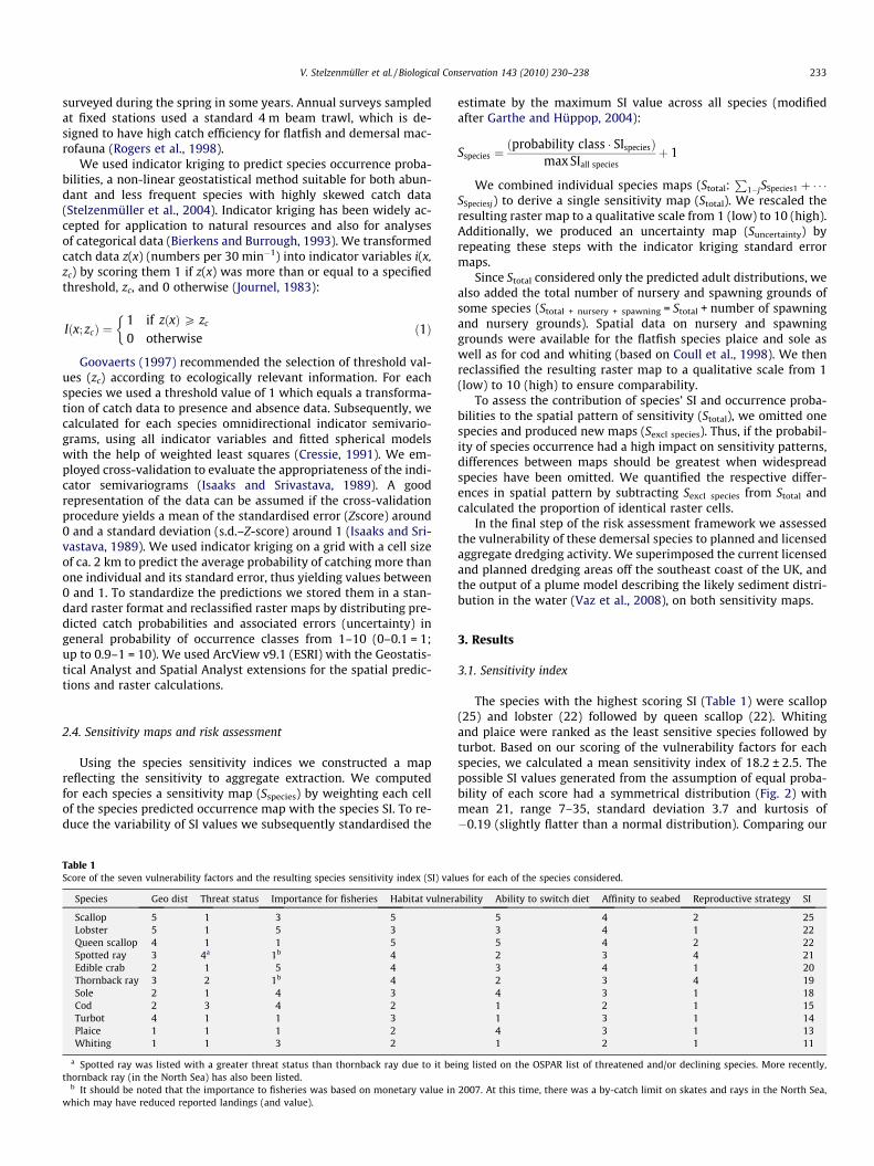
Table 1Score of the seven vulnerability factors and the resulting species sensitivity index (SI) val

Species Geo dist Threat status Importance for fisheries Habitat vulner

Scallop 5 1 3 5Lobster 5 1 5 3Queen scallop 4 1 1 5Spotted ray 3 4a 1b 4Edible crab 2 1 5 4Thornback ray 3 2 1b 4Sole 2 1 4 3Cod 2 3 4 2Turbot 4 1 1 3Plaice 1 1 1 2Whiting 1 1 3 2

a Spotted ray was listed with a greater threat status than thornback ray due to it bethornback ray (in the North Sea) has also been listed.

b It should be noted that the importance to fisheries was based on monetary value inwhich may have reduced reported landings (and value).

estimate by the maximum SI value across all species (modifiedafter Garthe and Hüppop, 2004):

Sspecies ¼ðprobability class � SIspeciesÞ

max SIall speciesþ 1

We combined individual species maps (Stotal:P

1�jSSpecies1 þ � � �SSpeciesj) to derive a single sensitivity map (Stotal). We rescaled theresulting raster map to a qualitative scale from 1 (low) to 10 (high).Additionally, we produced an uncertainty map (Suncertainty) byrepeating these steps with the indicator kriging standard errormaps.

Since Stotal considered only the predicted adult distributions, wealso added the total number of nursery and spawning grounds ofsome species (Stotal + nursery + spawning = Stotal + number of spawningand nursery grounds). Spatial data on nursery and spawninggrounds were available for the flatfish species plaice and sole aswell as for cod and whiting (based on Coull et al., 1998). We thenreclassified the resulting raster map to a qualitative scale from 1(low) to 10 (high) to ensure comparability.

To assess the contribution of species’ SI and occurrence proba-bilities to the spatial pattern of sensitivity (Stotal), we omitted onespecies and produced new maps (Sexcl species). Thus, if the probabil-ity of species occurrence had a high impact on sensitivity patterns,differences between maps should be greatest when widespreadspecies have been omitted. We quantified the respective differ-ences in spatial pattern by subtracting Sexcl species from Stotal andcalculated the proportion of identical raster cells.

In the final step of the risk assessment framework we assessedthe vulnerability of these demersal species to planned and licensedaggregate dredging activity. We superimposed the current licensedand planned dredging areas off the southeast coast of the UK, andthe output of a plume model describing the likely sediment distri-bution in the water (Vaz et al., 2008), on both sensitivity maps.

3. Results

3.1. Sensitivity index

The species with the highest scoring SI (Table 1) were scallop(25) and lobster (22) followed by queen scallop (22). Whitingand plaice were ranked as the least sensitive species followed byturbot. Based on our scoring of the vulnerability factors for eachspecies, we calculated a mean sensitivity index of 18.2 ± 2.5. Thepossible SI values generated from the assumption of equal proba-bility of each score had a symmetrical distribution (Fig. 2) withmean 21, range 7–35, standard deviation 3.7 and kurtosis of�0.19 (slightly flatter than a normal distribution). Comparing our

ues for each of the species considered.

ability Ability to switch diet Affinity to seabed Reproductive strategy SI

5 4 2 253 4 1 225 4 2 222 3 4 213 4 1 202 3 4 194 3 1 181 2 1 151 3 1 144 3 1 131 2 1 11

ing listed on the OSPAR list of threatened and/or declining species. More recently,

2007. At this time, there was a by-catch limit on skates and rays in the North Sea,

Fig. 2. Histogram of the simulated SI values, assuming that each of the sevenvulnerability factors had equal probability of receiving any of the scores (1–5),showing a symmetrical distribution with the eleven SI values computed for theselected species as black circles (see Table 1).

234 V. Stelzenmüller et al. / Biological Conservation 143 (2010) 230–238

estimated SI values to the simulated SI values showed a similarvariance (variance ratio = 1.38, F9, 78124 = 1.38, p-value = 0.36) andmean (t-test, t10 = �2.12, p-value = 0.06). This indicated that thecomputed SI values provide a reasonable amount of discriminationbetween species and, as a group, the species are as sensitive as thetheoretical average.

3.2. Species occurrence probability maps

The parameters of the fitted spherical models and the cross-val-idation results showed a good representation of the data (Table 2).The species distribution maps (Fig. 3) showed a rather homoge-nous distribution of high occurrence probabilities for sole and pla-ice, while probabilities of occurrence were patchier for turbot,edible crab and scallop. We found low probabilities of occurrencein the English Channel for cod and whiting as well as for thornbackray and spotted ray, with higher probabilities of occurrence forthose species in parts of the southern North Sea and Irish Sea.The accuracy of these predictions was confirmed by superimposingpresence/absence data of beam trawl catches onto the predictedoccurrence probability (see Fig. 3 using whiting as an example),and it was also supported by cross-validation results (Table 2).

Table 2Estimated parameters (nugget, partial sill, and range) of spherical models fitted to the avmodels represent the data described by the mean (mean Z-score) and standardised error

Species Model Nugget Partial sil

Sole Spherical 0.082 0.115Plaice Spherical 0.135 0.099Cod Spherical 0.068 0.037Thornback ray Spherical 0.171 0.058Turbot Spherical 0.022 0.000Whiting Spherical 0.151 0.092Edible crab Spherical 0.025 0.023Lobster Spherical 0.001 0.000Queen scallop Spherical 0.030 0.025Scallop Spherical 0.015 0.031Spotted ray Spherical 0.072 0.057

3.3. Sensitivity map

We found highest values of sensitivity with corresponding lowlevels of uncertainty in Cardigan Bay, Liverpool Bay and the south-ern North Sea, and intermediate levels of sensitivity in the BristolChannel and eastern parts of the English Channel (Fig. 4). For partsof the English Channel (e.g. off the Isle of Wight) we predicted alow level of sensitivity to aggregate extraction, but this area hadthe greatest uncertainty.

The assessment of robustness revealed that at the scale of ourstudy area, the pattern of sensitivity was influenced most by wide-spread species such as sole and plaice (Table 3). Results suggestedthat whiting had a greater effect on the overall sensitivity patternthan thornback ray or spotted ray. Hence, the species occurrenceprobabilities had more influence on the sensitivity pattern thenthe species sensitivity indices. Lobster and turbot had least influ-ence on the modelled sensitivity (see Table 3).

3.4. Risk assessment

In the final step of our risk assessment framework we mappedspecies vulnerability by comparing the occurrence of aggregateextraction with the predicted species sensitivity for an examplecase study on the southeast coast of the UK (Fig. 5a). Within thecase study area the mean sensitivity of all cells inside areas, wheredredging occurred, were compared with those outside (Fig. 5a). Wefound a significant difference (t532 = 19.3, p-value� 0.05) betweenthe calculated mean sensitivities inside (7.3) and outside (6.4) thedredging areas, suggesting that areas where dredging occurs aremore vulnerable than elsewhere. This also confirms the observedclear spatial overlap between the areas impacted by dredgingactivities and those areas where demersal fish and shellfish popu-lations were highly sensitive to the effects of dredging activity.

When nursery and spawning grounds were taken into accountto map sensitivity (Stotal + nursery + spawning), we observed in the casestudy area an offshore shift of the highly sensitive areas (Fig. 5b).We also found significant differences (t165 = �5.2, p-value �0.05) between the mean sensitivity inside (7.7) and outside (8.3)the areas impacted by aggregate extraction.

4. Discussion

4.1. Sensitivity mapping

The selected vulnerability factors used to calculate the speciesSI reflect both their sensitivity to the extraction of sediment andtheir ability to recover from the disturbance. Thus the SI summa-rised the degree to which the species respond to such stress, corre-sponding with the general definition of sensitivity (Zacharias and

eraged indicator semivariogram of each species, and the goodness of how the fitted(SD Zscore) of the cross-validation procedure.

l Range (m) Mean Z-score SD Z-score

101,790 �0.007 1.055137,330 �0.001 0.919

42,415 0.004 1.076248,360 �0.004 0.866171,180 �0.003 0.918272,600 0.001 0.889

31,516 �0.002 1.206113,520 0.007 1.230111,340 0.011 1.169116,910 �0.007 1.424121,710 0.005 0.950

Fig. 3. Species occurrence probabilities as reclassified indicator kriging predictions for sole, plaice, thornback ray, spotted ray, lobster, queen scallop, scallop, edible crab, cod,turbot, and whiting. Low occurrence probability is indicated by 1 and high occurrence probability is indicated by 10; bottom right: whiting occurrence probability withsuperimposed beam trawl catch data (1990–2003) as presence/absence data.

V. Stelzenmüller et al. / Biological Conservation 143 (2010) 230–238 235

Gregr, 2005). Although we used semi-quantitative methods, weconsider the overall framework to be quantitative and repeatable,

which is crucial for sensitivity assessments (Zacharias and Gregr,2005; Hiddink et al., 2007).

Fig. 4. Estimated general sensitivity (1 = low; 10 = high) to aggregate extraction based on the sensitivity index of the eleven fish and shellfish species considered (left) and itsassociated uncertainty (right).

Table 3The results of the comparison of the sensitivity map considering all species (Stotal) andthe sensitivity map calculated without the respective species (Sexcl species) as thepercentage of cells showing the same value (Stotal � Sexcl species = 0), the geographicaldistribution (see description in Section 2) as percentage of grid cells with presentdata, and the calculated sensitivity index (SI; see Table 1).

Species excluded fromsensitivity estimation

Identicalcells (%)

Geographicaldistribution (%)

SI

Sole 7 2.6 18Plaice 12.3 3.4 13Scallop 26.7 0.5 25Whiting 26.8 3.3 11Thornback ray 32.7 1.6 19Spotted ray 46.2 1.5 21Cod 47.9 2.4 15Queen scallop 50 0.7 22Edible crab 59.7 2.2 20Turbot 65.9 0.9 14Lobster 66.8 0.4 22

Fig. 5. Light grey polygons indicate current dredging licences and grey polygonsdesignate licence application areas. Results of a plume model are presented ashollow polygons. Species’ vulnerability based on the species sensitivity index andpredicted occurrence probability (A, top left), modelled sensitivity within thepolygons of the plume model within the case study area at the UK east coast (A, topright), species vulnerability based on modelled sensitivity including the presence ofnursery areas and spawning grounds of cod, plaice, sole, and whiting (B, bottomleft), and respective calculated sensitivity within the polygons of the plume model(B, bottom right).

236 V. Stelzenmüller et al. / Biological Conservation 143 (2010) 230–238

We generated all possible combinations of the vulnerabilityscores to compare estimated with simulated values. It is importantto understand the behaviour of the sensitivity index under a simu-lated distribution of scores as this provides insight that aids inter-pretation of the results when the SI is used in other applications.Further work could develop confidence ratings for each vulnerabil-ity score, possibly incorporating the processes generating them,and then estimate a confidence rating for each SI value usingMonte-Carlo simulation (e.g. Rugen and Callahan, 1996).

When indicator kriging is applied in an ecological context, Isa-aks and Srivastava (1989) recommended that meaningful valueswere selected as thresholds to build indicator variables. In thisstudy we selected a threshold value of one (to predict the probabil-ity of catching on average one individual with a beam trawl) as thisreflects a precautionary approach for a risk assessment.

We integrated species of commercial importance and for whichat least parts of the life-history stage are thought to be sampledrelatively well in beam trawl surveys. However, for cod, turbot,edible crab and lobster the occurrence probabilities were probablyunderestimated as the surveys are considered to have a lower levelof catchability for these species. For example, while 0-group codare caught in the Irish Sea beam trawl survey (Parker-Humphreys,2004b), this age class is not well represented in the English Chan-nel survey (possibly because it is earlier in the year), although lownumbers of larger juvenile cod are taken (Parker-Humphreys,2005). In the case of larger species, such as thornback ray and tur-bot, the gear will not sample very large adults effectively, althoughjuvenile thornback ray (Ellis et al., 2005) and intermediate sized

turbot (e.g. Parker-Humphreys, 2004b) are well sampled. Ediblecrab and lobster favour rocky grounds and such habitats are nei-ther sampled comprehensively in beam trawl surveys nor used inaggregate extraction. Despite these differences in catch efficiencywe have confidence in the predicted occurrence probabilities andtherefore in the sensitivity estimations of the case-study speciesas species distribution data were based on an extensive time series,and predicted species occurrences were based on presence/ab-sence data. Hence, this method could be applied to a wide rangeof taxa, although survey data covering other times of the yearand at other sites would be needed to improve the predicted spe-cies occurrence of the less frequently sampled demersal species.

V. Stelzenmüller et al. / Biological Conservation 143 (2010) 230–238 237

As recommended by Woodbury (2003), we used the standarderror of the indicator kriging predictions to map the uncertaintyof the sensitivity estimations. We found low levels of sensitivitybut with corresponding high levels of uncertainty in the EnglishChannel and around the southwest coast (see Fig. 4). The increaseduncertainty in the modelled sensitivity was the result of increasedindicator kriging prediction errors which we found in these areasfor most species. In turn, prediction errors were high, as relativelyfew beam trawl samples have been taken in these areas.

4.2. Spatially explicit risk assessment

Our study aimed to provide a standardised approach for theanalysis phase of a spatial risk assessment. We explored species’vulnerability by assessing the spatial overlap between the mod-elled pattern of sensitivity and areas of dredging activity. The finalstep in our framework does not provide detailed characterisationof risk, such as an estimated probability of ecological effects. How-ever, our modelled sensitivity highlighted an increased level of riskwhere ecological effects due to aggregate dredging are more likelyto occur (see Fig 5). We also showed the importance of the methodused to model sensitivity. The concurrent consideration of overallpopulation distribution as well as spawning and nursery areas rep-resents a precautionary approach, although the delineation of suchimportant habitats are lacking for many fish and shellfish species.It also assumes that such areas are inherently more vulnerable todredging activity.

When interpreting the vulnerability at specific sites, and theimportance of the perceived risk, it should be remembered thatthe scale of the risk framework is a relative one, and only relatesto the species included in the analysis. It is not, therefore, a com-prehensive risk assessment of the pressure on the ecosystem atthe site. More thorough analyses incorporating other ecosystemcomponents, or which include multiple sectors (Ban and Alder,2008; Day et al., 2008) would be necessary before the vulnerabilityassessment could be considered to be comprehensive.

Uncertainty still exists across many components of a riskassessment, including sampling efficiency, model design andparameters used, and species selection. Despite this it should berecognised that management decisions must nevertheless bemade, and are often made in the context of incomplete knowledge(Kerns and Ager, 2007; Halpern et al., 2008a).

4.3. Implications and perspectives for marine management

Our results emphasized the importance of appropriate surveydata for predicting species occurrences, especially for those witha medium to high sensitivity. This is because the patterns of occur-rence for abundant species with medium or high sensitivity hadthe greatest impact on the overall sensitivity map. Consequently,when our approach is applied in marine planning, emphasis shouldbe placed on the use of best quality species distribution data, pref-erably from a standardised source for the region studied.

The spatial scale at which a risk assessment is conducted is acrucial factor in designing a framework. For instance, on a localisedscale (1–10 km) one can expect marginal differences in occurrenceprobability of widespread species to result in marginal effects onthe overall risk or vulnerability assessment. In contrast, differencesin the patterns of occurrence of widespread species are likely to bemore pronounced at regional scales (10–100 km), due to changingenvironmental conditions, and the results of risk assessments maychange significantly. A fully effective, spatially explicit risk assess-ment should therefore balance the scale of the human activity withthe occurrence of the ecological receptor. The consideration ofscale is especially important for integrated ecosystem-based man-agement, such as marine planning, where the scale of management

measures needs to be matched with the scale of the relevant eco-system services (Rosenberg and McLeod, 2005; Halpern et al.,2008a).

Ultimately, for the development of sustainable marine plansmore comprehensive risk assessments are needed which combinethe combined impacts of the various human activities affectingthat environment (see e.g. Hayes and Landis, 2004). The practicalassessment of cumulative impacts of human activities remains asignificant challenge for marine management (Ban and Alder,2008; Halpern et al., 2008a,b), and many cumulative impactassessments fail to analyse multiple impact sources and lack asound quantification of environmental quality (Cooper and Sheate,2002; Dube, 2003).

The task of applying our framework to multiple human activi-ties will be made easier by identifying a small number of genericpressures of activities (e.g. damage, disturbance and contamina-tion) rather than treating each activity separately. An examplefor assessing the vulnerability of ecosystem components (marinefish species) to a single generic pressure (in this case fishing) waspresented by Cheung et al. (2007). More comprehensive attemptsto map cumulative impacts of human activities at a global scale(Halpern et al., 2008b) point the way forward for such riskassessments.

Our framework is an important first step in the development ofa spatially explicit risk assessment and the appraisal of cumulativeeffects of human activities on the marine environment. Despite theincomplete data that are currently available to support compre-hensive marine planning, we suggest that the initial developmentof regional plans should focus on the most spatially extensiveactivities that exert the greatest pressure on the ecosystem, andthe most widespread species which are likely to respond to thosepressures, as well as species/habitats of greatest conservationimportance.

Acknowledgments

This study was funded by the UK Department of Environment,Food and Rural Affairs (contracts AE1148 and A0916). We thankJohn Cotter for helpful comments on the analysis and David Max-well for statistical advice.

References

Astles, K.L., Holloway, M.G., Steffe, A., Green, M., Ganassin, C., Gibbs, P.J., 2006. Anecological method for qualitative risk assessment and its use in themanagement of fisheries in New South Wales, Australia. Fisheries Research82, 290–303.

Ban, N., Alder, J., 2008. How wild is the ocean? Assessing the intensity ofanthropogenic marine activities in British Columbia, Canada. AquaticConservation: Marine and Freshwater Ecosystems 18, 55–85.

Bierkens, M.F.P., Burrough, P.A., 1993. The indicator approach to categorical soildata. Journal of Soil Science 44, 361–368.

Boyd, S.E., Limpenny, D.S., Rees, H.L., Cooper, K.M., 2005. The effects of marine sandand gravel extraction on the macrobenthos at a commercial dredging site(results 6 years post-dredging). ICES Journal of Marine Science 62, 145–162.

Bremner, J., Rogers, S.I., Frid, C.L.J., 2006. Methods for describing ecologicalfunctioning of marine benthic assemblages using biological traits analysis(BTA). Ecological Indicators 6, 609–622.

Cheung, W.W.L., Watson, R., Morato, T., Pitcher, T.J., Pauly, D., 2007. Intrinsicvulnerability in the global fish catch. Marine Ecology Progress Series 333, 1–12.

Cooper, L.M., Sheate, W.R., 2002. Cumulative effects assessment: A review of UKenvironmental impact statements. Environmental Impact Assessment Review22, 415–439.

Cooper, K., Boyd, S., Aldridge, J., Rees, H., 2007. Cumulative impacts of aggregateextraction on seabed macro-invertebrate communities in an area off the eastcoast of the United Kingdom. Journal of Sea Research 57, 288–302.

Coull, K.A., Johnstone, R., Rogers, S.I., 1998. Fisheries Sensitivity Maps in Britishwaters. Published and distributed by UKOOA Ltd., 9 Albyn Terrace, Aberdeen.

Cressie, N.A.C., 1991. Statistics for Spatial Data. John Wiley & Sons, Inc., New York.Day, V., Paxinos, R., Emmett, J., Wright, A., Goecker, M., 2008. The marine planning

framework for South Australia: a new ecosystem-based zoning policy formarine management. Marine Policy 32, 535–543.

238 V. Stelzenmüller et al. / Biological Conservation 143 (2010) 230–238

Desprez, M., 2000. Physical and biological impact of marine aggregate extractionalong the French coast of the Eastern English Channel: Short-and long-termpost-dredging restoration. ICES Journal of Marine Science 57, 1428–1438.

Douvere, F., 2008. The importance of marine spatial planning in advancingecosystem-based sea use management. Marine Policy 32, 762–771.

Dube, M.G., 2003. Cumulative effect assessment in Canada: A regional frameworkfor aquatic ecosystems. Environmental Impact Assessment Review 23, 723–745.

Eastwood, P.D., Meaden, G.J., Carpentier, A., Rogers, S.I., 2003. Estimating limits tothe spatial extent and suitability of sole (Solea solea) nursery grounds in theDover Strait. Journal of Sea Research 50, 151–165.

Eastwood, P.D., Mills, C.M., Aldridge, J.N., Houghton, C.A., Rogers, S.I., 2007. Humanactivities in UK offshore waters: an assessment of direct, physical pressure onthe seabed. ICES Journal of Marine Science 64, 453–463.

Ellis, J.R., Dulvy, N.K., Jennings, S., Parker-Humphreys, M., Rogers, S.I., 2005.Assessing the status of demersal elasmobranchs in UK waters: a review.Journal of the Marine Biological Association of the United Kingdom 85, 1025–1047.

Evans, K.E., Klinger, T., 2008. Obstacles to bottom-up implementation of marineecosystem management. Conservation Biology 22, 1135–1143.

Froese, R., Pauly, D. (Eds.), 2009. FishBase. World Wide Web electronic publication.<www.fishbase.org>.

Furness, R.W., Tasker, M.L., 2000. Seabird-fishery interactions: quantifying thesensitivity of seabirds to reductions in sandeel abundance, and identification ofkey areas for sensitive seabirds in the North Sea. Marine Ecology Progress Series202, 253–264.

Garthe, S., Hüppop, O., 2004. Scaling possible adverse effects of marine wind farmson seabirds: Developing and applying a vulnerability index. Journal of AppliedEcology 41, 724–734.

Goovaerts, P., 1997. Geostatistics for Natural Resources Evaluation. OxfordUniversity Press, New York.

Gundlach, E.R., Hayes, M.O., 1978. Vulnerability of coastal environments to oil spillimpacts. Journal of the Marine Technology Society 12, 18–27.

Halpern, B.S., McLeod, K.L., Rosenberg, A.A., Crowder, L.B., 2008a. Managing forcumulative impacts in ecosystem-based management through ocean zoning.Ocean and Coastal Management 51, 203–211.

Halpern, B.S., Walbridge, S., Selkoe, K.A., Kappel, C.V., Micheli, F., D’Agrosa, C., Bruno,J.F., Casey, K.S., Ebert, C., Fox, H.E., Fujita, R., Heinemann, D., Lenihan, H.S.,Madin, E.M.P., Perry, M.T., Selig, E.R., Spalding, M., Steneck, R., Watson, R.,2008b. A global map of human impact on marine ecosystems. Science 319, 948–952.

Hayes, E.H., Landis, W.G., 2004. Regional ecological risk assessment of a near shoremarine environment: Cherry Point, WA. Human and Ecological Risk Assessment10, 299–325.

Hiddink, J.G., Jennings, S., Kaiser, M.J., 2007. Assessing and predicting the relativeecological impacts of disturbance on habitats with different sensitivities.Journal of Applied Ecology 44, 405–413.

Hiscock, K., Tyler-Walters, H., 2006. Assessing the sensitivity of seabed species andbiotopes – The Marine Life Information Network (MarLIN). Hydrobiologia 555,309–320.

Hope, B.K., 2006. An examination of ecological risk assessment and managementpractices. Environment International 32, 983–995.

Isaaks, E.H., Srivastava, R.M., 1989. An Introduction to Applied Gesostatistics. OxfordUniversity Press, New York.

Jørgensen, S.E., 2008. Overview of the model types available for development ofecological models. Ecological Modelling 215, 3–9.

Journel, A.G., 1983. Nonparametric-estimation of spatial distributions. Journal of theInternational Association for Mathematical Geology 15, 445–468.

Kerns, B.K., Ager, A., 2007. Risk assessment for biodiversity conservation planning inPacific Northwest forests. Forest Ecology and Management 246, 38–44.

Newell, R.C., Seiderer, L.J., Hitchcock, D.R., 1998. The impact of dredging works incoastal waters: a review of the sensitivity to disturbance and subsequentrecovery of biological resources on the sea bed. Oceanography and MarineBiology: An Annual Review 36, 127–178.

Newell, R.C., Seiderer, L.J., Simpson, N.M., Robinson, J.E., 2004. Impacts of marineaggregate dredging on benthic macrofauna off the south coast of the UnitedKingdom. Journal of Coastal Research 20, 115–125.

Parker-Humphreys, M., 2004a. Distribution and relative abundance of demersalfishes from beam trawl surveys in the Bristol Channel (ICES Division VIIf) 1993–2001. In: Science Series Technical Report. CEFAS, Lowestoft, p. 69.

Parker-Humphreys, M., 2004b. Distribution and relative abundance of demersalfishes from beam trawl surveys in the Irish Sea (ICES Division VIIa) 1993–2001.In: Science Series Technical Report. CEFAS, Lowestoft, p. 68.

Parker-Humphreys, M., 2005. Distribution and relative abundance of demersalfishes from beam trawl surveys in the Eastern English Channel (ICES divisionVIId) and the southern North Sea (ICES Division IVc) 1993–2001. In: ScienceSeries Technical Report. CEFAS, Lowestoft, p. 92.

Pittman, S.J., Christensen, J.D., Caldow, C., Menza, C., Monaco, M.E., 2007. Predictivemapping of fish species richness across shallow-water seascapes in theCaribbean. Ecological Modelling 204, 9–21.

Robinson, J.E., Newell, R.C., Seiderer, L.J., Simpson, N.M., 2005. Impacts of aggregatedredging on sediment composition and associated benthic fauna at an offshoredredge site in the southern North Sea. Marine Environmental Research 60, 51–68.

Rogers, S.I., Rijnsdorp, A.D., Damm, U., Vanhee, W., 1998. Demersal fish populationsin the coastal waters of the UK and continental NW Europe from beam trawlsurvey data collected from 1990 to 1995. Journal of Sea Research 37, 79–102.

Rosenberg, A.A., McLeod, K.L., 2005. Implementing ecosystem-based approaches tomanagement for the conservation of ecosystem services. Marine EcologyProgress Series 300, 270–274.

Rugen, P., Callahan, B., 1996. An overview of Monte Carlo, a fifty year perspective.Human and Ecological Risk Assessment 2, 671–680.

Stelzenmüller, V., Maynou, F., Ehrich, S., Zauke, G.P., 2004. Spatial analysis of twaiteshad, Alosa fallax (Lacepède, 1803), in the Southern North Sea: Application ofnon-linear geostatistics as a tool to search for special areas of conservation.International Review of Hydrobiology 89, 337–351.

Stelzenmüller, V., Ehrich, S., Zauke, G.P., 2005. Effects of survey scale and waterdepth on the assessment of spatial distribution patterns of selected fish in thenorthern North Sea showing different levels of aggregation. Marine BiologyResearch 1, 375–387.

Stelzenmüller, V., Maynou, F., Martín, P., 2007. Spatial assessment of benefits of acoastal mediterranean marine protected area. Biological Conservation 136,571–583.

UK Sea Fisheries Statistics, 2007. Published and distributed by Marine and FisheriesAgency, 3-8 Whitehall Place, London SW1A 2HH, <www.mfa.gov.uk/statistics/ukseafish.htm>.

Vaz, S., Martin, C.S., Eastwood, P.D., Ernande, B., Carpentier, A., Meaden, G.J., Coppin,F., 2008. Modelling species distributions using regression quantiles. Journal ofApplied Ecology 45, 204–217.

Williams, J.M., Tasker, M.L., Carter, I.C., Webb, A., 1994. A method assessing seabirdvulnerability to surface pollutants. Ibis 137, 147–152.

Woodbury, P.B., 2003. Dos and don’ts of spatially explicit ecological riskassessments. Environmental Toxicology and Chemistry 22, 977–982.

Zacharias, M.A., Gregr, E.J., 2005. Sensitivity and vulnerability in marineenvironments: An approach to identifying vulnerable marine areas.Conservation Biology 19, 86–97.