ww.sciencedirect.com

i n t e r n a t i o n a l j o u r n a l o f h y d r o g e n en e r g y 3 7 ( 2 0 1 2 ) 5 4 2 1e5 4 3 3

Available online at w

journal homepage: www.elsevier .com/locate/he

A spatially-explicit optimization model for long-termhydrogen pipeline planning

Nils Johnson a,*, Joan Ogden a,b

a Institute of Transportation Studies, One Shields Avenue, University of California, Davis, CA 95616, USAbDepartment of Environmental Science and Policy, One Shields Avenue, University of California, Davis, CA 95616, USA

a r t i c l e i n f o

Article history:

Received 1 June 2011

Received in revised form

16 August 2011

Accepted 19 August 2011

Available online 1 October 2011

Keywords:

Infrastructure modeling

GIS

Pipelines

Network optimization

Hydrogen

* Corresponding author. Tel.: þ1 530 752 159E-mail address: njohnson@ucdavis.edu (N

0360-3199/$ e see front matter Copyright ªdoi:10.1016/j.ijhydene.2011.08.109

a b s t r a c t

One of the major barriers to the deployment of hydrogen as a transportation fuel is the lack

of an infrastructure for supplying the fuel to consumers. Consequently, models are needed

to evaluate the cost and design of various infrastructure deployment strategies. The best

strategy will likely differ between regions based on the spatial distribution of H2 demand

and variations in regional feedstock costs. Although several spatially-explicit infrastruc-

ture models have been developed, none of the published models are capable of optimizing

interconnected regional pipeline networks for linking multiple production facilities and

demand locations. This paper describes the Hydrogen Production and Transmission

(HyPAT) model, which is a network optimization tool for identifying the lowest cost

centralized production and pipeline transmission infrastructure within real geographic

regions. A case study in the southwestern United States demonstrates the capabilities and

outputs of the model.

Copyright ª 2011, Hydrogen Energy Publications, LLC. Published by Elsevier Ltd. All rights

reserved.

1. Introduction delivered at different scales and using various feedstocks,

Hydrogen has been suggested as a future transportation fuel

based on its potential to address many of the energy security

and environmental issues facing the existing petroleum-based

transportation system [1e3]. However, one of the major

barriers to the widespread use of hydrogen vehicles is the lack

of an existing infrastructure for producing and delivering the

fuel to consumers, including production and storage facilities,

distribution networks, and refueling stations [2,4]. The way in

which this infrastructure is deployed will have profound

effects on its cost and ability to meet greenhouse gas (GHG)

targets. For this reason,modelsareneededthatcan identify the

magnitude of required infrastructure and evaluate its cost for

various deployment strategies. These modeling efforts are

complicated by the fact that hydrogen can be produced and

9; fax: þ1 530 752 6572.. Johnson).2011, Hydrogen Energy P

production technologies, and distribution modes, resulting in

a large number of potential supply pathways [4,5].

In order to better understand these pathways, early

modeling efforts focused on quantifying the costs, GHG

emissions, and energy use of hydrogen infrastructure

components [4,6,7] and generic production and delivery

pathways [5,8e14]. These models provide valuable insights

into the tradeoffs between different infrastructure pathways

under static demand conditions. Although models of indi-

vidual pathways do establish static cost estimates for infra-

structure, they do not address the optimal design of

infrastructure for large regionswithmultiple cities or how this

infrastructuremight evolve over time (i.e., transitional issues).

To address these limitations, hydrogen infrastructure

modeling efforts have evolved from simulation models

ublications, LLC. Published by Elsevier Ltd. All rights reserved.

1 A capacitated pipeline network includes capacity constraintsbased on discrete pipeline diameter classes. These capacityconstraints place limits on the quantity of product that can betransported along a pipeline corridor for a specific pipelinediameter.

i n t e rn a t i o n a l j o u r n a l o f h y d r o g e n en e r g y 3 7 ( 2 0 1 2 ) 5 4 2 1e5 4 3 35422

exploring individual pathways and scenarios to optimization

models that attempt to identify the optimal design of systems

given a set of possible production, distribution, and refueling

technologies. Both static and dynamic optimization models of

varying complexity have been developed for hydrogen infra-

structure [15] and many of these models now incorporate

some level of spatial structure, including the “soft-linking” of

geographic information systems (GIS) with infrastructure

models [16e19].

Although spatial structure has been incorporated into

many recent models, it can generally be classified as either:

1) detailed modeling for individual cities or 2) regional

modeling that employs simplified spatial representations. In

the first area, several steady-state models examine methods

for optimizing hydrogen refueling station siting [20e24] and

hydrogen delivery [7] for individual cities. A few studies

have presented case studies of complete infrastructure

pathways in Southern California in which the region is

treated as one large demand node (i.e., like a single city)

[25e27]. Moreover, two studies model infrastructure

deployment in urban Beijing [28,29]. Although these studies

yield insights about infrastructure deployment for indi-

vidual cities, their applicability is limited when considering

an entire region, which requires an infrastructure optimized

to serve multiple cities.

In the second area, several studies employ complex opti-

mization algorithms and scenario-based analyses to model

infrastructure deployment in large regions [17e19,30e42]. In

fact, many regional and national case studies have been

conducted in Asia [28,31,32,39e41], the U.S. [16,19,23,43], and

Europe [14,17,18,30,35,37,38,42,44,45] in recent years.

However, these studies generally use simplified region- or

grid-based spatial representations inwhich the centroid of the

region or grid cell is used to represent the location of potential

production facilities and hydrogen demand [18,30,32,

37,40e42,44]. In some models, there is an allowance for

transport between regions, but the models use Euclidean

distances or highly simplified distribution networks.

Inmany cases, complex optimizationmodels are limited to

simplified technological representations (e.g., fixed plant

capacities and costs) and simple spatial structures (e.g., small

numbers of demand and production nodes) in order to achieve

tractable computing times [17]. As a result, they may be

inappropriate for modeling infrastructure deployment in real

regions in which production facilities of specific sizes are

connected to hundreds of demand nodes. For this reason,

a hydrogen infrastructure deployment model is needed that

can incorporate more spatial and economic detail, including

more demand and production nodes, complex distribution

networks, and greater flexibility in component capacities and

costs.

The incorporation of spatial structure is most important in

modeling two aspects of hydrogen infrastructure: 1) refueling

station siting tomaximize customer access and 2) distribution

networks to minimize H2 transport costs. Spatial models for

refueling station siting have been documented in the litera-

ture [21,23,24] and Johnson et al. (2008) published amodel that

uses a minimum spanning tree algorithm to optimize H2

distribution networks along existing pipeline rights-of-way

[16]. However, this model considers only pipeline length in

the cost optimization. Amodel that considers both length and

diameter and identifies the best way to direct H2 flows along

a capacitated1 pipeline network is needed.

Although this type of model has not been developed for H2

infrastructure, a detailed spatial model for optimizing capaci-

tated CO2 pipeline networks, called SimCCS, has been pub-

lished and provides the inspiration for the model discussed in

this paper [46]. SimCCS is a network optimization model that

identifies the lowest-cost infrastructure for carboncaptureand

storage (CCS) projects in real regions. Given a CO2 reduction

target, the model identifies the best pipeline network for con-

necting CO2 sources with geologic injection sites. Themodel is

able toaggregateCO2flowsbetweenmultiplesourcesandsinks

and can develop interconnected pipeline networks that take

advantage of economies of scale. It has been applied to case

studies in Colorado, Utah, and California [47,48].

This paper describes the Hydrogen Production and Trans-

mission (HyPAT) model, which is a network optimization tool

that incorporates detailed spatial and techno-economic data

to optimize H2 production and pipeline transmission infra-

structure in real geographic regions. This model is part of

a broader hydrogen infrastructure deployment model that

combines optimization tools for infrastructure design with

detailed economic models in order to evaluate spatially

explicit case studies of hydrogen infrastructure deployment

(Fig. 1). The broader hydrogen infrastructure deployment

model, including detailed cost estimates for regional case

studies will be presented in a subsequent paper.

This paper provides a detailed description of the HyPAT

model, including the mathematical formulation and required

spatial and techno-economic inputs. A case study for the

southwestern U.S. is then presented as a demonstration of the

model’s capabilities and outputs. Finally, potential applica-

tions and extensions of the model are discussed.

2. Model description

Given a candidate pipeline network and the locations of H2

demand and potential centralized production facilities, the

HyPAT model identifies the optimal infrastructure design for

producing H2 and connecting production facilities to distri-

bution hubs in demand centers (i.e., cities). In the process, it

develops an interconnected and capacitated regional pipeline

network that can link multiple production facilities and

demand centers. Specifically, it identifies the number, size,

and location of production facilities and the diameter, length,

and location of transmission pipeline corridors. The model is

not designed to optimize intra-city distribution pipelines,

though it could be modified for this purpose.

The model is run for a series of discrete hydrogen fuel cell

vehicle (FCV) market penetration (MP) levels, which define the

locationandmagnitudeofhydrogendemand.Ateach level, the

model optimizes the infrastructure design based on current

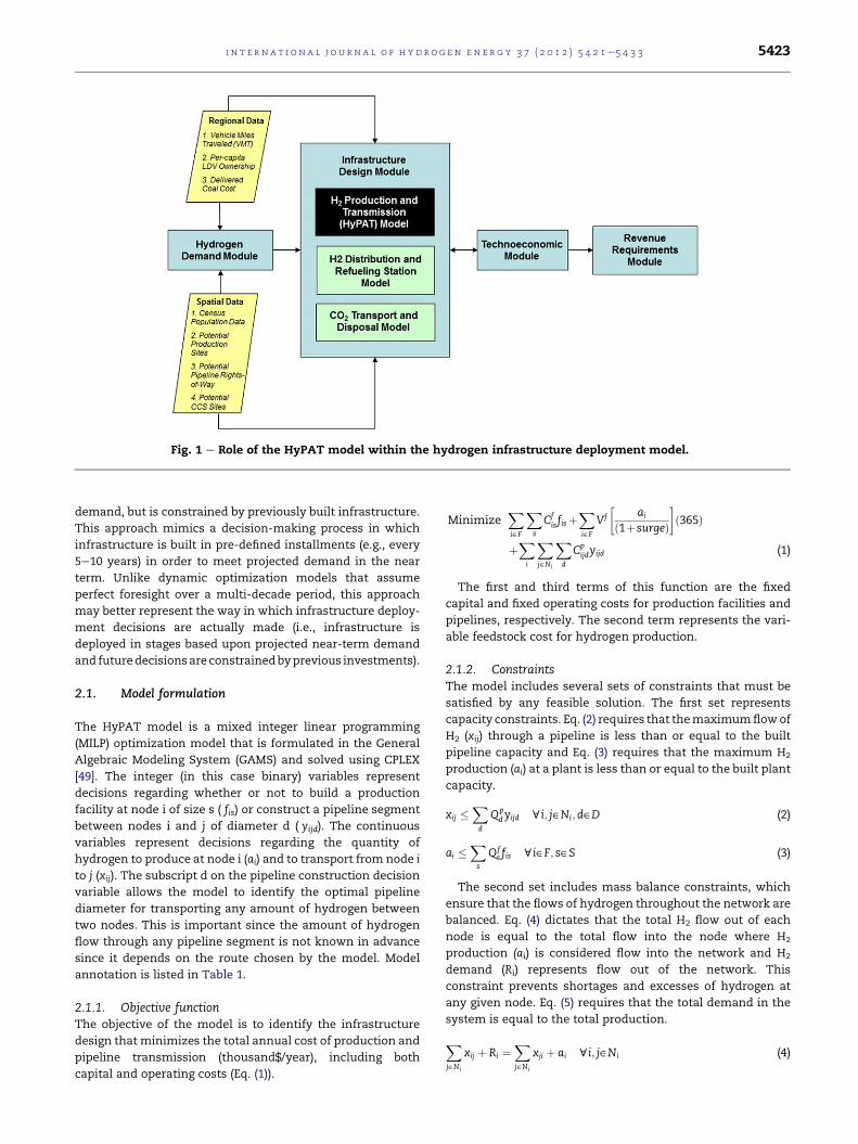
Fig. 1 e Role of the HyPAT model within the hydrogen infrastructure deployment model.

i n t e r n a t i o n a l j o u r n a l o f h y d r o g e n en e r g y 3 7 ( 2 0 1 2 ) 5 4 2 1e5 4 3 3 5423

demand, but is constrained by previously built infrastructure.

This approach mimics a decision-making process in which

infrastructure is built in pre-defined installments (e.g., every

5e10 years) in order to meet projected demand in the near

term. Unlike dynamic optimization models that assume

perfect foresight over a multi-decade period, this approach

may better represent the way in which infrastructure deploy-

ment decisions are actually made (i.e., infrastructure is

deployed in stages based upon projected near-term demand

and futuredecisionsareconstrainedbyprevious investments).

2.1. Model formulation

The HyPAT model is a mixed integer linear programming

(MILP) optimization model that is formulated in the General

Algebraic Modeling System (GAMS) and solved using CPLEX

[49]. The integer (in this case binary) variables represent

decisions regarding whether or not to build a production

facility at node i of size s ( fis) or construct a pipeline segment

between nodes i and j of diameter d ( yijd). The continuous

variables represent decisions regarding the quantity of

hydrogen to produce at node i (ai) and to transport from node i

to j (xij). The subscript d on the pipeline construction decision

variable allows the model to identify the optimal pipeline

diameter for transporting any amount of hydrogen between

two nodes. This is important since the amount of hydrogen

flow through any pipeline segment is not known in advance

since it depends on the route chosen by the model. Model

annotation is listed in Table 1.

2.1.1. Objective functionThe objective of the model is to identify the infrastructure

design that minimizes the total annual cost of production and

pipeline transmission (thousand$/year), including both

capital and operating costs (Eq. (1)).

MinimizeXX

Cfisfisþ

XVf ai

ð1þsurgeÞ ð365Þ

i˛F s i˛F

� �

þXi

Xj˛Ni

Xd

Cpijdyijd (1)

The first and third terms of this function are the fixed

capital and fixed operating costs for production facilities and

pipelines, respectively. The second term represents the vari-

able feedstock cost for hydrogen production.

2.1.2. ConstraintsThe model includes several sets of constraints that must be

satisfied by any feasible solution. The first set represents

capacity constraints. Eq. (2) requires that themaximumflowof

H2 (xij) through a pipeline is less than or equal to the built

pipeline capacity and Eq. (3) requires that the maximum H2

production (ai) at a plant is less than or equal to the built plant

capacity.

xij �Xd

Qpdyijd ci; j˛Ni;d˛D (2)

ai �Xs

Qfs fis ci˛F; s˛S (3)

The second set includes mass balance constraints, which

ensure that the flows of hydrogen throughout the network are

balanced. Eq. (4) dictates that the total H2 flow out of each

node is equal to the total flow into the node where H2

production (ai) is considered flow into the network and H2

demand (Ri) represents flow out of the network. This

constraint prevents shortages and excesses of hydrogen at

any given node. Eq. (5) requires that the total demand in the

system is equal to the total production.

Xj˛Ni

xij þ Ri ¼Xj˛Ni

xji þ ai ci; j˛Ni (4)

Table 1 e Model annotation.

Sets:

N Network nodes

R Demand (city) nodes (subset of N)

F H2 production facility nodes (subset of N)

D Pipeline diameters (8, 12, 16, 20, 24, 30, 36, 42-inch)

S Facility sizes (300, 600, 900, 1200, 1500 tonnes/day)

B Previously built facility sizes (actual built sizes)

Decision variables:

xij Units of hydrogen transported from node i to node

j (tonnes/day)

ai Units of hydrogen produced at node i (tonnes/day)

fis 1, if facility is built at node i with size s; 0, otherwise

yijd 1, if pipeline is constructed from node i to node j with

diameter d; 0, otherwise

Input parameters:

Cf Fixed annual capital and O&M costs for building a

production facility (thousand$/yr)

Cp Fixed annual capital and O&M costs for constructing a

pipeline (thousand$/yr)

Vf Variable feedstock cost for producing hydrogen

(thousand$/tonne)

Qf Useable capacity of a facility (tonnes/day)

Qp Useable capacity of a pipeline (tonnes/day)

Ri Peak demand at node i (tonnes/day)

Lij Length of pipeline segment from node i to node j (km)

Bis Production at previously built facility of size s at

node i (tonnes/day)

Surge Summer surge in demand (10%) [12]

Coal(i) Cost of delivered coal at node i ($/GJ)

s Facility nameplate capacity (tonnes/day)

d Pipeline diameter (inch)

Ccap Overnight capital cost for production facility (million$)

OM Annual operating and maintenance cost for a facility

or pipeline (4% of fixed capital) [58]

CRF Capital recovery factor (10.2% based on discount

rate of 10% and component lifetime of 40 years)

LHVH2 Lower heating value of hydrogen (120 GJ/tonne H2)

efff Plant conversion efficiency

CFf Plant capacity factor

2 Note that the quantity of hydrogen produced may be signifi-cantly less than the nameplate capacity, especially at earlymarket penetration levels when demand is less than theminimum plant size. The quantity of hydrogen produced islimited to this quantity and not the nameplate capacity. Theactual plant size will be exported to the post-optimizationeconomic model so the plant will be sized appropriately in theeconomic analysis.

i n t e rn a t i o n a l j o u r n a l o f h y d r o g e n en e r g y 3 7 ( 2 0 1 2 ) 5 4 2 1e5 4 3 35424

Xi˛F

ai ¼Xi˛R

Ri (5)

The third set contains constraints that define the decision

variables. Non-negativity constraints are placed on the two

continuous decision variables (Eq. (6) and (7)) and binary

constraints are required for the two binary decision variables

(Eq. (8) and (9)).

xij � 0 ci; j˛Ni (6)

ai � 0 ci˛F (7)

yijd˛0;1 ci; j˛Ni;d˛D (8)

fis˛0;1 ci˛F; s˛S (9)

The final set represents constraints that can be considered

optional. These constraints are included in order to improve

the computational efficiency of the model, but can be modi-

fied to represent specific beliefs about the infrastructure

planning process. The listed constraints represent one way to

model the planning process, but we do not assert that they are

necessarily the best way. A future paper will examine how

changes in these constraints impact infrastructure design and

cost. Eq. (10) dictates that only one production facility can be

built at each potential site and Eq. (11) stipulates that, once

built, a plant will continue to produce the same quantity of

hydrogen at all remaining market penetration levels.2 In

essence, these constraints assume that once an investment is

made in a production facility, it will continue to operate and

cannot be expanded. Alternatives to these assumptions are

discussed in Section 4.3.

Eq. (12) dictates that only one pipeline can be built along

any single corridor. This constraint streamlines the network

optimization, but does prevent adjacent pipelines from being

developed. However, there is no constraint that prevents an

existing pipeline from being removed and replaced by a larger

diameter pipeline in the future to meet additional flow

requirements. Ideally, the model would allow adjacent pipe-

lines to be added as flow increases, but allowing adjacent

pipelines would greatly increase the complexity of the model

and would likely result in unreasonable solution times.

Another optionwould be to oversize pipelines for future flows.

However, oversizing pipelineswould require a dynamicmodel

with knowledge of future flows, which again would greatly

increase the complexity of the model.

Psfis � 1 ci˛F; s˛S (10)

ai ¼ Bis ci˛B; s˛S (11)

Pd

yijd � 1 ci; j˛Ni; d˛D (12)

In each model run, the infrastructure built at the previous

market penetration level is provided and constrains the

outcome. Specifically, the location and diameter of pipelines

( yijd), the location and size of plants ( fis), and the actual

production capacity of plants (aii) are passed from the

previousmodel run. Eq. (11) constrains the size and location of

future plants and cost incentives discussed in Section 2.3

encourage the continued use of pre-existing pipelines. The

flow along a pipeline (xij) is not constrained by previous flows,

butmust respect the pipeline capacity constraint. It is possible

for flows to change direction between model runs.

2.2. Spatial inputs

Three spatial inputs are required by this model: 1) the location

and magnitude of hydrogen demand, 2) the location of poten-

tial hydrogen production facilities, and 3) a candidate pipeline

network for connecting supply and demand. These inputs are

developed in a geographic information system (GIS).

i n t e r n a t i o n a l j o u r n a l o f h y d r o g e n en e r g y 3 7 ( 2 0 1 2 ) 5 4 2 1e5 4 3 3 5425

2.2.1. Hydrogen demandThe design of a hydrogen fuel delivery infrastructure depends

on the spatial characteristics of the hydrogen demand. A

hydrogen demand model was developed in ArcGIS and is

described in Johnson et al. (2008) [16]. The model uses U.S.

Census population data [50], estimates of FCV efficiency, and

regional information regarding vehicle miles traveled (VMT)

and per-capita vehicle ownership to quantify the spatial

distribution and magnitude of hydrogen demand at each FCV

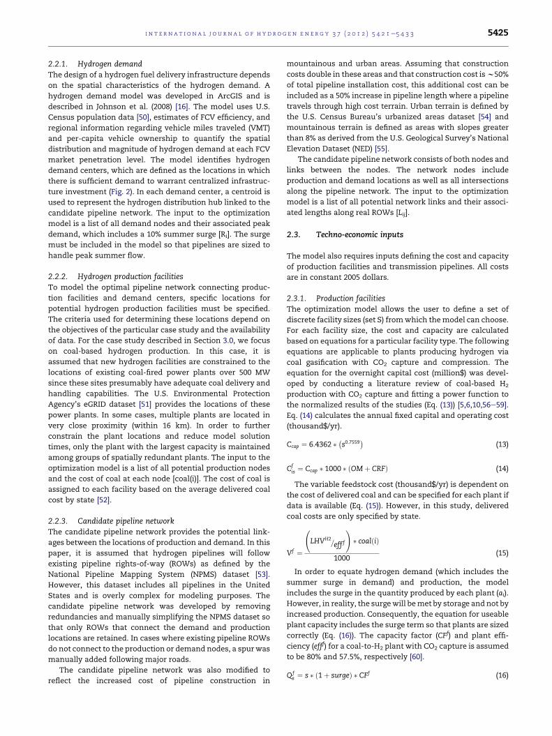
market penetration level. The model identifies hydrogen

demand centers, which are defined as the locations in which

there is sufficient demand to warrant centralized infrastruc-

ture investment (Fig. 2). In each demand center, a centroid is

used to represent the hydrogen distribution hub linked to the

candidate pipeline network. The input to the optimization

model is a list of all demand nodes and their associated peak

demand, which includes a 10% summer surge [Ri]. The surge

must be included in the model so that pipelines are sized to

handle peak summer flow.

2.2.2. Hydrogen production facilitiesTo model the optimal pipeline network connecting produc-

tion facilities and demand centers, specific locations for

potential hydrogen production facilities must be specified.

The criteria used for determining these locations depend on

the objectives of the particular case study and the availability

of data. For the case study described in Section 3.0, we focus

on coal-based hydrogen production. In this case, it is

assumed that new hydrogen facilities are constrained to the

locations of existing coal-fired power plants over 500 MW

since these sites presumably have adequate coal delivery and

handling capabilities. The U.S. Environmental Protection

Agency’s eGRID dataset [51] provides the locations of these

power plants. In some cases, multiple plants are located in

very close proximity (within 16 km). In order to further

constrain the plant locations and reduce model solution

times, only the plant with the largest capacity is maintained

among groups of spatially redundant plants. The input to the

optimization model is a list of all potential production nodes

and the cost of coal at each node [coal(i)]. The cost of coal is

assigned to each facility based on the average delivered coal

cost by state [52].

2.2.3. Candidate pipeline networkThe candidate pipeline network provides the potential link-

ages between the locations of production and demand. In this

paper, it is assumed that hydrogen pipelines will follow

existing pipeline rights-of-way (ROWs) as defined by the

National Pipeline Mapping System (NPMS) dataset [53].

However, this dataset includes all pipelines in the United

States and is overly complex for modeling purposes. The

candidate pipeline network was developed by removing

redundancies and manually simplifying the NPMS dataset so

that only ROWs that connect the demand and production

locations are retained. In cases where existing pipeline ROWs

do not connect to the production or demand nodes, a spurwas

manually added following major roads.

The candidate pipeline network was also modified to

reflect the increased cost of pipeline construction in

mountainous and urban areas. Assuming that construction

costs double in these areas and that construction cost isw50%

of total pipeline installation cost, this additional cost can be

included as a 50% increase in pipeline length where a pipeline

travels through high cost terrain. Urban terrain is defined by

the U.S. Census Bureau’s urbanized areas dataset [54] and

mountainous terrain is defined as areas with slopes greater

than 8% as derived from the U.S. Geological Survey’s National

Elevation Dataset (NED) [55].

The candidate pipeline network consists of both nodes and

links between the nodes. The network nodes include

production and demand locations as well as all intersections

along the pipeline network. The input to the optimization

model is a list of all potential network links and their associ-

ated lengths along real ROWs [Lij].

2.3. Techno-economic inputs

The model also requires inputs defining the cost and capacity

of production facilities and transmission pipelines. All costs

are in constant 2005 dollars.

2.3.1. Production facilitiesThe optimization model allows the user to define a set of

discrete facility sizes (set S) fromwhich themodel can choose.

For each facility size, the cost and capacity are calculated

based on equations for a particular facility type. The following

equations are applicable to plants producing hydrogen via

coal gasification with CO2 capture and compression. The

equation for the overnight capital cost (million$) was devel-

oped by conducting a literature review of coal-based H2

production with CO2 capture and fitting a power function to

the normalized results of the studies (Eq. (13)) [5,6,10,56e59].

Eq. (14) calculates the annual fixed capital and operating cost

(thousand$/yr).

Ccap ¼ 6:4362 � �s0:7559� (13)

Cfis ¼ Ccap � 1000 � ðOMþ CRFÞ (14)

The variable feedstock cost (thousand$/yr) is dependent on

the cost of delivered coal and can be specified for each plant if

data is available (Eq. (15)). However, in this study, delivered

coal costs are only specified by state.

Vf ¼

LHVH2

=eff f

!� coalðiÞ

1000(15)

In order to equate hydrogen demand (which includes the

summer surge in demand) and production, the model

includes the surge in the quantity produced by each plant (ai).

However, in reality, the surgewill bemet by storage and not by

increased production. Consequently, the equation for useable

plant capacity includes the surge term so that plants are sized

correctly (Eq. (16)). The capacity factor (CFf) and plant effi-

ciency (efff) for a coal-to-H2 plant with CO2 capture is assumed

to be 80% and 57.5%, respectively [60].

Qfs ¼ s � ð1þ surgeÞ � CFf (16)

Fig. 2 e Hydrogen demand centers (black polygons) within the southwestern United States at several FCV market

penetration levels.

i n t e rn a t i o n a l j o u r n a l o f h y d r o g e n en e r g y 3 7 ( 2 0 1 2 ) 5 4 2 1e5 4 3 35426

2.3.2. Transmission pipelinesThe optimization model allows the user to input a set of

discrete pipeline diameters (i.e., nominal pipe sizes). For each

diameter, the model calculates the annual capital and oper-

ating cost for each pipeline link based on an equation from the

U.S. Department of Energy’s Hydrogen Analysis (H2A)

spreadsheets (Eq. (17)) [12].

Cpijd ¼

h�Lij � 0:621371 �

�818:64 �

�d2�þ 14288:2 � dþ 284530:3

�þ 431502:5

�� ðOMþ CRFÞ

i1000

(17)

The model also records the location and diameter of built

pipelines ( yijd) and uses this information in subsequentmodel

runs to adjust the costs so that previously built pipelines of

a specific diameter are preferred (i.e., less expensive) in later

construction periods. Specifically, the annual cost reflects only

the operating and maintenance costs and not the annualized

capital for existing pipelines (Eq. (18)). This cost adjustment

provides an incentive to maintain previously built pipelines,

but does not prevent larger pipelines from being built.

Cpijd ¼

h�Lij � 0:621371 �

�818:64 �

�d2�þ 14288:2 � dþ 284530:3

�þ 431502:5

�� ðOMÞ

i1000

(18)

Finally, it is implausible that a pipeline of a particular

diameter would be removed and replaced with a pipeline of

a smaller diameter.3 To address this, the model uses the

variable yijd to identify the diameter classes that are smaller

than any previously built diameter along each pipeline link

and assigns a high cost to these diameter classes (99999). The

useable capacity of each pipeline diameter class (Qpd ) is derived

from H2A assuming a pipeline length of 200 km, a pipeline

capacity factor of 92%, and a pressure drop of 20 atm [12].

3 It is possible that the diameter of a pipeline may need to bedecreased if the minimum capacity of the pipeline is not met insubsequent model runs. However, the model does not includeminimum pipeline capacity.

3. Case study

To illustrate the utility of the HyPAT model, a regional case

study was conducted that includes four states in the south-

western United States (Arizona, New Mexico, Colorado, and

Utah) (Fig. 3). The case study examines optimal infrastructure

design for supplying regional hydrogen demand with

centralized production via coal gasification at five discrete FCV

market penetration levels, corresponding to 5%, 10%, 25%,

50%, and 75% of the onroad light duty vehicle (LDV) fleet.

3.1. Inputs

The spatial inputs to the model include the locations and

magnitudes of hydrogen demand, the potential locations of

production facilities, and a candidate pipeline network. The

spatial distribution of hydrogen demand for several market

penetration levels is illustrated in Fig. 2 and summary statis-

tics for the demand centers are given in Table 2. Fig. 3 shows

the spatial inputs to the optimization model, including the

locations of thirteen potential production facilities, the

candidate pipeline network, and the demand centers at 75%

market penetration.

The techno-economic inputs include the cost and useable

capacity of production facilities and pipelines. Five discrete

facility sizes are modeled in the range of 300e1500 tonnes H2

per day. The costs and capacities of these facilities are listed

in Table 3. Delivered coal costs by state [52] are given in

Table 4.

Fig. 3 e Spatial data inputs within the study region (demand shown at 75% market penetration).

Table 2 e Summary statistics for hydrogen demandwithin the study region.

FCV MarketPenetration(% of LDVs in fleet)

Number of DemandCenters (i.e., cities)

Daily H2

Demand(tonnes/day)

5 14 323.0

10 19 664.4

25 37 1545.8

50 55 2982.9

75 74 4376.2

i n t e r n a t i o n a l j o u r n a l o f h y d r o g e n en e r g y 3 7 ( 2 0 1 2 ) 5 4 2 1e5 4 3 3 5427

For pipelines, sevendiscretepipeline diameters from8 to 36

inches are modeled. The costs and capacities of these diame-

tersaresummarized inTable5.Thepipelinecosts inTable5are

estimated for a 100 km pipeline on flat, rural terrain.4

Table 3 e Costs and useable capacities for productionfacilities.

Facility size(tonnes/day) [s]

Useable facilitycapacity

(tonnes/day) [Qf]

Overnightcapital cost

(Million$) [Ccap]

300 264 479.8

600 528 810.3

900 792 1100.9

3.2. Modeling results

Given the spatial and techno-economic inputs, the optimiza-

tion model is run for each market penetration level in

succession from 5% to 75%. In each successive run, the loca-

tion and diameter of previously built pipelines ( yijd) and the

location and size of previously built production facilities ( fisand ai) are provided to the model. Previously built production

capacity is maintained at existing sites, but cannot be

expanded (i.e., new production capacity must be built at new

sites).

Unlike production facilities, previously built transmission

pipelines are preferred, but can be abandoned or expanded as

4 Note that the pipeline costs in the actual model account formountainous and urban terrain.

necessary. In the optimization tool, a capacity upgrade is

modeled as a replacement of a small diameter pipeline with

a larger diameter pipeline with sufficient capacity to meet the

entire current hydrogen flow. However, in practice, pipeline

planners may decide to either 1) keep the existing small

diameter pipeline and add an adjacent pipeline that can

handle the excess flow or 2) oversize the original pipeline so

that it can meet future flows. This optimization tool cannot

explicitly model scenarios that require knowledge of future

flows because it does not include a dynamic component.

However, these scenarios can be evaluated in a post-

optimization techno-economic model, but would not neces-

sarily match the infrastructure design that a dynamic model

would produce.

Each model run results in an optimized infrastructure

design and represents a stage in building infrastructure to

meet a pre-specified FCV market penetration level. Together,

the five model runs provide a long-term deployment strategy

for production and transmission infrastructure in a specific

geographic region. Specifically, the model identifies the

1200 1056 1368.3

1500 1320 1619.7

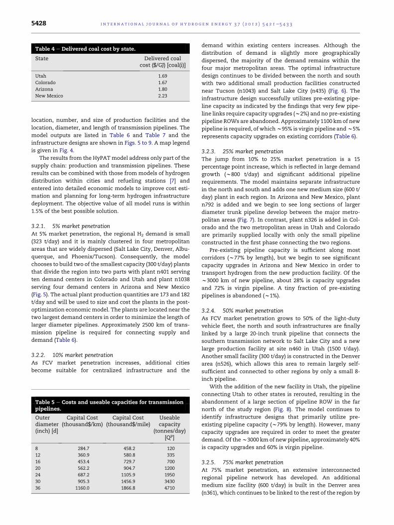
Table 4 e Delivered coal cost by state.

State Delivered coalcost ($/GJ) [coal(i)]

Utah 1.69

Colorado 1.67

Arizona 1.80

New Mexico 2.23

i n t e rn a t i o n a l j o u r n a l o f h y d r o g e n en e r g y 3 7 ( 2 0 1 2 ) 5 4 2 1e5 4 3 35428

location, number, and size of production facilities and the

location, diameter, and length of transmission pipelines. The

model outputs are listed in Table 6 and Table 7 and the

infrastructure designs are shown in Figs. 5 to 9. A map legend

is given in Fig. 4.

The results from the HyPATmodel address only part of the

supply chain: production and transmission pipelines. These

results can be combined with those from models of hydrogen

distribution within cities and refueling stations [7] and

entered into detailed economic models to improve cost esti-

mation and planning for long-term hydrogen infrastructure

deployment. The objective value of all model runs is within

1.5% of the best possible solution.

3.2.1. 5% market penetrationAt 5% market penetration, the regional H2 demand is small

(323 t/day) and it is mainly clustered in four metropolitan

areas that are widely dispersed (Salt Lake City, Denver, Albu-

querque, and Phoenix/Tucson). Consequently, the model

chooses to build two of the smallest capacity (300 t/day) plants

that divide the region into two parts with plant n401 serving

ten demand centers in Colorado and Utah and plant n1038

serving four demand centers in Arizona and New Mexico

(Fig. 5). The actual plant production quantities are 173 and 182

t/day and will be used to size and cost the plants in the post-

optimization economicmodel. The plants are located near the

two largest demand centers in order tominimize the length of

larger diameter pipelines. Approximately 2500 km of trans-

mission pipeline is required for connecting supply and

demand (Table 6).

3.2.2. 10% market penetrationAs FCV market penetration increases, additional cities

become suitable for centralized infrastructure and the

Table 5 e Costs and useable capacities for transmissionpipelines.

Outerdiameter(inch) [d]

Capital Cost(thousand$/km)

Capital Cost(thousand$/mile)

Useablecapacity

(tonnes/day)[Qp]

8 284.7 458.2 120

12 360.9 580.8 335

16 453.4 729.7 700

20 562.2 904.7 1200

24 687.2 1105.9 1950

30 905.3 1456.9 3430

36 1160.0 1866.8 4710

demand within existing centers increases. Although the

distribution of demand is slightly more geographically

dispersed, the majority of the demand remains within the

four major metropolitan areas. The optimal infrastructure

design continues to be divided between the north and south

with two additional small production facilities constructed

near Tucson (n1043) and Salt Lake City (n435) (Fig. 6). The

infrastructure design successfully utilizes pre-existing pipe-

line capacity as indicated by the findings that very few pipe-

line links require capacity upgrades (w2%) and no pre-existing

pipeline ROWs are abandoned. Approximately 1100 kmof new

pipeline is required, of whichw95% is virgin pipeline andw5%

represents capacity upgrades on existing corridors (Table 6).

3.2.3. 25% market penetrationThe jump from 10% to 25% market penetration is a 15

percentage point increase, which is reflected in large demand

growth (w800 t/day) and significant additional pipeline

requirements. The model maintains separate infrastructure

in the north and south and adds one new medium size (600 t/

day) plant in each region. In Arizona and New Mexico, plant

n792 is added and we begin to see long sections of larger

diameter trunk pipeline develop between the major metro-

politan areas (Fig. 7). In contrast, plant n326 is added in Col-

orado and the two metropolitan areas in Utah and Colorado

are primarily supplied locally with only the small pipeline

constructed in the first phase connecting the two regions.

Pre-existing pipeline capacity is sufficient along most

corridors (w77% by length), but we begin to see significant

capacity upgrades in Arizona and New Mexico in order to

transport hydrogen from the new production facility. Of the

w3000 km of new pipeline, about 28% is capacity upgrades

and 72% is virgin pipeline. A tiny fraction of pre-existing

pipelines is abandoned (w1%).

3.2.4. 50% market penetrationAs FCV market penetration grows to 50% of the light-duty

vehicle fleet, the north and south infrastructures are finally

linked by a large 20-inch trunk pipeline that connects the

southern transmission network to Salt Lake City and a new

large production facility at site n460 in Utah (1500 t/day).

Another small facility (300 t/day) is constructed in the Denver

area (n526), which allows this area to remain largely self-

sufficient and connected to other regions by only a small 8-

inch pipeline.

With the addition of the new facility in Utah, the pipeline

connecting Utah to other states is rerouted, resulting in the

abandonment of a large section of pipeline ROW in the far

north of the study region (Fig. 8). The model continues to

identify infrastructure designs that primarily utilize pre-

existing pipeline capacity (w79% by length). However, many

capacity upgrades are required in order to meet the greater

demand. Of thew3000 kmof newpipeline, approximately 40%

is capacity upgrades and 60% is virgin pipeline.

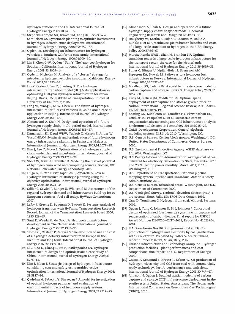
3.2.5. 75% market penetrationAt 75% market penetration, an extensive interconnected

regional pipeline network has developed. An additional

medium size facility (600 t/day) is built in the Denver area

(n361), which continues to be linked to the rest of the region by

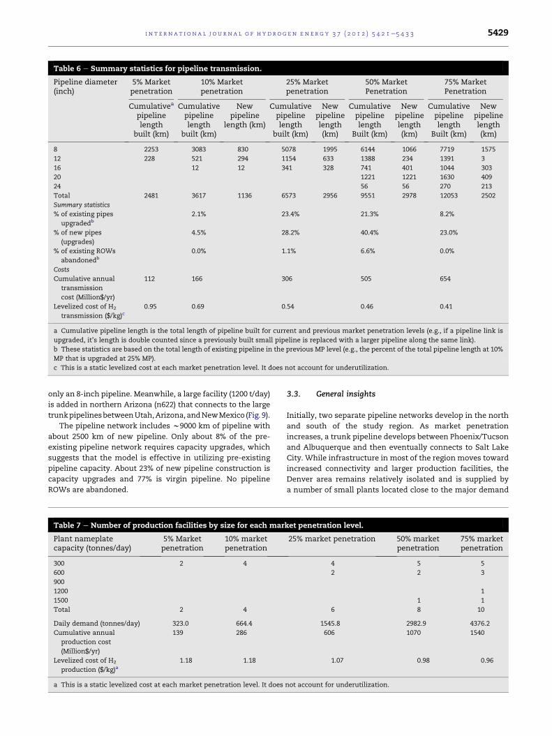
Table 6 e Summary statistics for pipeline transmission.

Pipeline diameter(inch)

5% Marketpenetration

10% Marketpenetration

25% Marketpenetration

50% MarketPenetration

75% MarketPenetration

Cumulativea

pipelinelength

built (km)

Cumulativepipelinelength

built (km)

Newpipeline

length (km)

Cumulativepipelinelength

built (km)

Newpipelinelength(km)

Cumulativepipelinelength

Built (km)

Newpipelinelength(km)

Cumulativepipelinelength

Built (km)

Newpipelinelength(km)

8 2253 3083 830 5078 1995 6144 1066 7719 1575

12 228 521 294 1154 633 1388 234 1391 3

16 12 12 341 328 741 401 1044 303

20 1221 1221 1630 409

24 56 56 270 213

Total 2481 3617 1136 6573 2956 9551 2978 12053 2502

Summary statistics

% of existing pipes

upgradedb

2.1% 23.4% 21.3% 8.2%

% of new pipes

(upgrades)

4.5% 28.2% 40.4% 23.0%

% of existing ROWs

abandonedb

0.0% 1.1% 6.6% 0.0%

Costs

Cumulative annual

transmission

cost (Million$/yr)

112 166 306 505 654

Levelized cost of H2

transmission ($/kg)c0.95 0.69 0.54 0.46 0.41

a Cumulative pipeline length is the total length of pipeline built for current and previous market penetration levels (e.g., if a pipeline link is

upgraded, it’s length is double counted since a previously built small pipeline is replaced with a larger pipeline along the same link).

b These statistics are based on the total length of existing pipeline in the previous MP level (e.g., the percent of the total pipeline length at 10%

MP that is upgraded at 25% MP).

c This is a static levelized cost at each market penetration level. It does not account for underutilization.

i n t e r n a t i o n a l j o u r n a l o f h y d r o g e n en e r g y 3 7 ( 2 0 1 2 ) 5 4 2 1e5 4 3 3 5429

only an 8-inch pipeline. Meanwhile, a large facility (1200 t/day)

is added in northern Arizona (n622) that connects to the large

trunkpipelinesbetweenUtah,Arizona, andNewMexico (Fig. 9).

The pipeline network includes w9000 km of pipeline with

about 2500 km of new pipeline. Only about 8% of the pre-

existing pipeline network requires capacity upgrades, which

suggests that the model is effective in utilizing pre-existing

pipeline capacity. About 23% of new pipeline construction is

capacity upgrades and 77% is virgin pipeline. No pipeline

ROWs are abandoned.

Table 7 e Number of production facilities by size for each mar

Plant nameplatecapacity (tonnes/day)

5% Marketpenetration

10% marketpenetration

300 2 4

600

900

1200

1500

Total 2 4

Daily demand (tonnes/day) 323.0 664.4

Cumulative annual

production cost

(Million$/yr)

139 286

Levelized cost of H2

production ($/kg)a1.18 1.18

a This is a static levelized cost at each market penetration level. It does

3.3. General insights

Initially, two separate pipeline networks develop in the north

and south of the study region. As market penetration

increases, a trunk pipeline develops between Phoenix/Tucson

and Albuquerque and then eventually connects to Salt Lake

City. While infrastructure in most of the region moves toward

increased connectivity and larger production facilities, the

Denver area remains relatively isolated and is supplied by

a number of small plants located close to the major demand

ket penetration level.

25% market penetration 50% marketpenetration

75% marketpenetration

4 5 5

2 2 3

1

1 1

6 8 10

1545.8 2982.9 4376.2

606 1070 1540

1.07 0.98 0.96

not account for underutilization.

Fig. 4 e Map legend.

Fig. 6 e Infrastructure design at 10% market penetration.

i n t e rn a t i o n a l j o u r n a l o f h y d r o g e n en e r g y 3 7 ( 2 0 1 2 ) 5 4 2 1e5 4 3 35430

centers. The cumulative capital investment required for

production and transmission is $7.2 billion and $4.7 billion,

respectively.

The case study demonstrates the ability of the model to

identify the optimal location and number of production

facilities and to develop interconnected and capacitated

pipeline networks that link multiple production facilities and

demand centers. It also demonstrates that the model can

effectively consider pre-existing infrastructure while opti-

mizing design in successive construction phases.

4. Model applications

The case study demonstrates the basic infrastructure plan-

ning capabilities of the HyPATmodel, including the capability

to quantify production and transmission infrastructure

requirements in real geographic regions and to simulate how

Fig. 5 e Infrastructure design at 5% market penetration.

this infrastructure might develop as FCV market penetration

increases. The basic outputs of the model include maps of

optimal infrastructure design and tallies of infrastructure

requirements. However, through post-optimization analysis

of the model outputs, several additional questions regarding

centralized infrastructure deployment can be explored. In

addition, themodel can bemodified to accommodatemultiple

types of centralized production facilities and different

assumptions about facility and pipeline planning.

4.1. How much will centralized infrastructure costduring a hydrogen transition?

The HyPAT model uses cost estimates to optimize infrastruc-

ture design and quantify infrastructure requirements for

Fig. 7 e Infrastructure design at 25% market penetration.

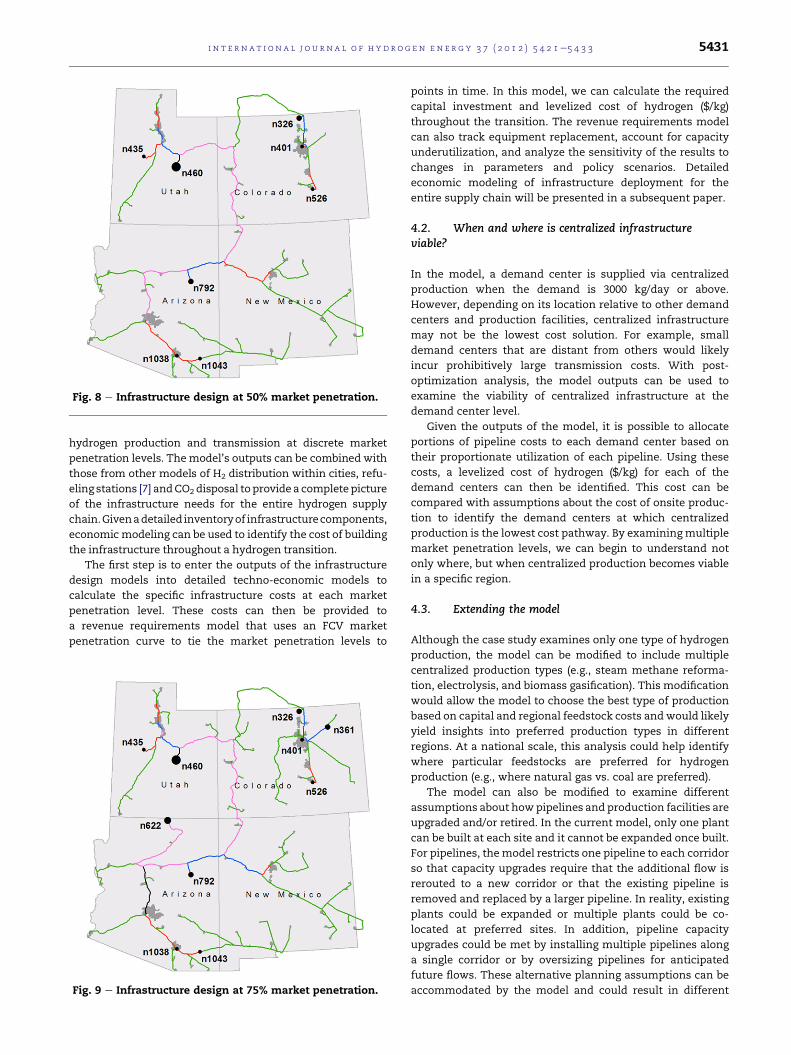
Fig. 8 e Infrastructure design at 50% market penetration.

i n t e r n a t i o n a l j o u r n a l o f h y d r o g e n en e r g y 3 7 ( 2 0 1 2 ) 5 4 2 1e5 4 3 3 5431

hydrogen production and transmission at discrete market

penetration levels. Themodel’s outputs can be combined with

those from other models of H2 distribution within cities, refu-

eling stations [7] andCO2disposal toprovide a complete picture

of the infrastructure needs for the entire hydrogen supply

chain.Givenadetailed inventoryof infrastructurecomponents,

economic modeling can be used to identify the cost of building

the infrastructure throughout a hydrogen transition.

The first step is to enter the outputs of the infrastructure

design models into detailed techno-economic models to

calculate the specific infrastructure costs at each market

penetration level. These costs can then be provided to

a revenue requirements model that uses an FCV market

penetration curve to tie the market penetration levels to

Fig. 9 e Infrastructure design at 75% market penetration.

points in time. In this model, we can calculate the required

capital investment and levelized cost of hydrogen ($/kg)

throughout the transition. The revenue requirements model

can also track equipment replacement, account for capacity

underutilization, and analyze the sensitivity of the results to

changes in parameters and policy scenarios. Detailed

economic modeling of infrastructure deployment for the

entire supply chain will be presented in a subsequent paper.

4.2. When and where is centralized infrastructureviable?

In the model, a demand center is supplied via centralized

production when the demand is 3000 kg/day or above.

However, depending on its location relative to other demand

centers and production facilities, centralized infrastructure

may not be the lowest cost solution. For example, small

demand centers that are distant from others would likely

incur prohibitively large transmission costs. With post-

optimization analysis, the model outputs can be used to

examine the viability of centralized infrastructure at the

demand center level.

Given the outputs of the model, it is possible to allocate

portions of pipeline costs to each demand center based on

their proportionate utilization of each pipeline. Using these

costs, a levelized cost of hydrogen ($/kg) for each of the

demand centers can then be identified. This cost can be

compared with assumptions about the cost of onsite produc-

tion to identify the demand centers at which centralized

production is the lowest cost pathway. By examiningmultiple

market penetration levels, we can begin to understand not

only where, but when centralized production becomes viable

in a specific region.

4.3. Extending the model

Although the case study examines only one type of hydrogen

production, the model can be modified to include multiple

centralized production types (e.g., steam methane reforma-

tion, electrolysis, and biomass gasification). This modification

would allow the model to choose the best type of production

based on capital and regional feedstock costs andwould likely

yield insights into preferred production types in different

regions. At a national scale, this analysis could help identify

where particular feedstocks are preferred for hydrogen

production (e.g., where natural gas vs. coal are preferred).

The model can also be modified to examine different

assumptions about howpipelines and production facilities are

upgraded and/or retired. In the current model, only one plant

can be built at each site and it cannot be expanded once built.

For pipelines, themodel restricts one pipeline to each corridor

so that capacity upgrades require that the additional flow is

rerouted to a new corridor or that the existing pipeline is

removed and replaced by a larger pipeline. In reality, existing

plants could be expanded or multiple plants could be co-

located at preferred sites. In addition, pipeline capacity

upgrades could be met by installing multiple pipelines along

a single corridor or by oversizing pipelines for anticipated

future flows. These alternative planning assumptions can be

accommodated by the model and could result in different

i n t e rn a t i o n a l j o u r n a l o f h y d r o g e n en e r g y 3 7 ( 2 0 1 2 ) 5 4 2 1e5 4 3 35432

infrastructure designs. For example, rather than building

plants in different locations, the model may identify

a preferred location and build multiple plants at a single site.

However, incorporating these changes into the model may

result in prohibitive solution times. A future paper will

examine how changes in planning assumptions impact H2

infrastructure design and cost.

The model can also be modified for CO2 transport and

disposal where the sources are the production facilities and

the sinks are the potential injection sites. A preliminarymodel

has been developed based on SimCCS [46] and applied to

a case study in the southwestern United States [61].

5. Conclusions

To better understand the costs associated with hydrogen

infrastructure deployment, models must be developed that

provide detailed inventories of the infrastructure components

required in real geographic regions. This paper describes the

HyPAT model, which optimizes the design of centralized

production facilities and transmission pipelines at discrete

market penetration levels. Themodel is unique because it can

utilize very detailed spatial data and is capable of developing

interconnected and capacitated pipeline networks that

connect multiple production facilities and demand centers. In

addition, it is designed to consider and build upon previously

built infrastructure in each successive construction stage. The

model provides the location and size of production facilities

and the location, diameter, and length of pipelines at each

market penetration level.

A case study conducted in the southwestern United States

demonstrates the effectiveness of the model in performing

very detailed infrastructure assessments. Additionally, this

study finds that less than one-third of pipelines installed in all

construction phases are abandoned or require capacity

upgrades, which suggests that the model successfully incor-

porates pre-existing infrastructure. The HyPAT model is

a useful infrastructure planning tool and improves upon

existing spatial models of hydrogen production and trans-

mission pipelines. It identifies more spatially detailed inven-

tories of infrastructure components and, thus, may improve

cost estimates for hydrogen infrastructure deployment.

r e f e r e n c e s

[1] McDowall W, Eames M. Forecasts, scenarios, visions,backcasts and roadmaps to the hydrogen economy: a reviewof the hydrogen futures literature. Energy Policy 2006;34:1236e50.

[2] Ball M, Wietschel M. The future of hydrogen - opportunitiesand challenges. International Journal of Hydrogen Energy2009;34:615e27.

[3] Doll C, Wietschel M. Externalities of the transport sector andthe role of hydrogen in a sustainable transport vision. EnergyPolicy 2008;36:4069e78.

[4] Ogden JM. Prospects for building a hydrogen energyinfrastructure. Annual Review of Energy and theEnvironment 1999;24:227e79.

[5] National Research Council (NRC). The hydrogen economy:opportunities, costs, barriers, and R&D needs. Washington,DC: Committee on Alternatives and Strategies for FutureHydrogen Production and Use; 2004.

[6] Kreutz T, Williams R, Consonni S, Chiesa P. Co-production ofhydrogen, electricity and CO2 from coal with commerciallyready technology. Part B: economic analysis. InternationalJournal of Hydrogen Energy 2005;30:769e84.

[7] Yang C, Ogden J. Determining the lowest-cost hydrogendelivery mode. International Journal of Hydrogen Energy2007;32:268e86.

[8] Stephens-Romero S, Samuelsen GS. Demonstration ofa novel assessment methodology for hydrogeninfrastructure deployment. International Journal ofHydrogen Energy 2009;34:628e41.

[9] Thomas CE, Kuhn IF, James BD, Lomax FD, Baum GN.Affordable hydrogen supply pathways for fuel cell vehicles.International Journal of Hydrogen Energy 1998;23:507e16.

[10] U.S. Department of Energy. H2A current Central hydrogenproduction from coal with CO2 sequestration version 2.1.1.Golden, CO: National Renewable Energy Laboratory; 2008.

[11] Simbeck DR, Chang E. Hydrogen supply: cost estimate forhydrogen pathways e scoping analysis. Golden, CO: NationalRenewable Energy Laboratory; 2002.

[12] U.S. Department of Energy. H2A delivery scenario analysismodel Version 2.2. Chicago, IL: Argonne National Laboratory,Center for Transportation Research; 2008.

[13] Moore RB, Raman V. Hydrogen infrastructure for fuel celltransportation. International Journal of Hydrogen Energy1998;23:617e20.

[14] Wietschel M, Hasenauer U, de Groot A. Development ofEuropean hydrogen infrastructure scenarioseCO2 reductionpotential and infrastructure investment. Energy Policy 2006;34:1284e98.

[15] Ogden J. Hydrogen system assessment: recent trends andinsights. In: Stolten D, editor. Hydrogen and fuel cells:fundamentals, technologies and applications. Weinheim:WILEY-VCH Verlag GmbH & Co. KGaA; 2010.

[16] Johnson N, Yang C, Ogden J. A GIS-based assessment of coal-based hydrogen infrastructure deployment in the state ofOhio. International Journal of Hydrogen Energy 2008;33:5287e303.

[17] Strachan N, Balta-Ozkan N, Joffe D, McGeevor K, Hughes N.Soft-linking energy systems and GIS models to investigatespatial hydrogen infrastructure development in a low-carbon UK energy system. International Journal of HydrogenEnergy 2009;34:642e57.

[18] Ball M, Wietschel M, Rentz O. Integration of a hydrogeneconomy into the German energy system: an optimisingmodelling approach. International Journal of HydrogenEnergy 2007;32:1355e68.

[19] Parker N, Fan Y, Ogden J. From waste to hydrogen: anoptimal design of energy production and distributionnetwork. Transportation Research Part E: Logistics andTransportation Review 2010;46:534e45.

[20] Welch C. HyDIVE (Hydrogen dynamic infrastructure andvehicle evolution) model analysis, 2010e2025 scenarioanalysis for hydrogen fuel cell vehicles and infrastructuremeeting. Washington, DC: US Dept. of Energy; 2006.

[21] Nicholas M, Handy S, Sperling D. Hydrogen refuelingnetwork analysis using geographic information systems.Long Beach, CA: National Hydrogen Association; 2004.

[22] Parks K. GIS-Based infrastructure modeling, 2010e2025scenario analysis for hydrogen fuel cell vehicles andinfrastructure meeting. Washington, DC: US Dept. of Energy;2006.

[23] Melaina MW. Initiating hydrogen infrastructures:preliminary analysis of a sufficient number of initial

i n t e r n a t i o n a l j o u r n a l o f h y d r o g e n en e r g y 3 7 ( 2 0 1 2 ) 5 4 2 1e5 4 3 3 5433

hydrogen stations in the US. International Journal ofHydrogen Energy 2003;28:743e55.

[24] Stephens-Romero SD, Brown TM, Kang JE, Recker WW,Samuelsen GS. Systematic planning to optimize investmentsin hydrogen infrastructure deployment. InternationalJournal of Hydrogen Energy 2010;35:4652e67.

[25] Ogden JM. Developing an infrastructure for hydrogenvehicles: a Southern California case study. InternationalJournal of Hydrogen Energy 1999;24:709e30.

[26] Lin Z, Chen C-W, Ogden J, Fan Y. The least-cost hydrogen forSouthern California. International Journal of HydrogenEnergy 2008;33:3009e14.

[27] Ogden J, Nicholas M. Analysis of a "cluster" strategy forintroducing hydrogen vehicles in southern California. EnergyPolicy 2011;39:1923e38.

[28] Lin Z, Ogden J, Fan Y, Sperling D. The hydrogeninfrastructure transition model (HIT) & its application inoptimizing a 50-year hydrogen infrastructure for urbanBeijing. Davis, CA: Institute of Transportation Studies atUniversity of California; 2006.

[29] Feng W, Wang S, Ni W, Chen C. The future of hydrogeninfrastructure for fuel cell vehicles in China and a case ofapplication in Beijing. International Journal of HydrogenEnergy 2004;29:355e67.

[30] Almansoori A, Shah N. Design and operation of a futurehydrogen supply chain: multi-period model. InternationalJournal of Hydrogen Energy 2009;34:7883e97.

[31] Kamarudin SK, Daud WRW, Yaakub Z, Misron Z, Anuar W,Yusuf NNAN. Synthesis and optimization of future hydrogenenergy infrastructure planning in Peninsular Malaysia.International Journal of Hydrogen Energy 2009;34:2077e88.

[32] Kim J, Lee Y, Moon I. Optimization of a hydrogen supplychain under demand uncertainty. International Journal ofHydrogen Energy 2008;33:4715e29.

[33] Short W, Blair N, Heimiller D. Modeling the market potentialof hydrogen from wind and competing sources. Golden, CO:National Renewable Energy Laboratory; 2005.

[34] Hugo A, Rutter P, Pistikopoulos S, Amorelli A, Zoia G.Hydrogen infrastructure strategic planning using multi-objective optimization. International Journal of HydrogenEnergy 2005;30:1523e34.

[35] Stiller C, Seydel P, Bunger U, Wietschel M. Assessment of theregional hydrogen demand and infrastructure build-up for 10European countries, fuel cell today. HyWays Consortium;2007.

[36] Leiby P, Greene D, Bowman D, Tworek E. Systems analysis ofhydrogen transition with HyTrans. Transportation ResearchRecord: Journal of the Transportation Research Board 2006;1983:129e39.

[37] Smit R, Weeda M, de Groot A. Hydrogen infrastructuredevelopment in The Netherlands. International Journal ofHydrogen Energy 2007;32:1387e95.

[38] Tzimas E, Castello P, Peteves S. The evolution of size and costof a hydrogen delivery infrastructure in Europe in themedium and long term. International Journal of HydrogenEnergy 2007;32:1369e80.

[39] Li Z, Gao D, Chang L, Liu P, Pistikopoulos EN. Hydrogeninfrastructure design and optimization: a case study ofChina. International Journal of Hydrogen Energy 2008;33:5275e86.

[40] Kim J, Moon I. Strategic design of hydrogen infrastructureconsidering cost and safety using multiobjectiveoptimization. International Journal of Hydrogen Energy 2008;33:5887e96.

[41] Qadrdan M, Saboohi Y, Shayegan J. A model for investigationof optimal hydrogen pathway, and evaluation ofenvironmental impacts of hydrogen supply system.International Journal of Hydrogen Energy 2008;33:7314e25.

[42] Almansoori A, Shah N. Design and operation of a futurehydrogen supply chain: snapshot model. ChemicalEngineering Research and Design 2006;84:423e38.

[43] Dougherty W, Kartha S, Rajan C, Lazarus M, Bailie A,Runkle B, et al. Greenhouse gas reduction benefits and costsof a large-scale transition to hydrogen in the USA. EnergyPolicy 2009;37:56e67.

[44] Murthy Konda NVSN, Shah N, Brandon NP. Optimaltransition towards a large-scale hydrogen infrastructure forthe transport sector: the case for the Netherlands.International Journal of Hydrogen Energy 2011;36:4619e35.

[45] Stiller C, Bunger U, Møller-Holst S, Svensson AM,Espegren KA, Nowak M. Pathways to a hydrogen fuelinfrastructure in Norway. International Journal of HydrogenEnergy 2010;35:2597e601.

[46] Middleton RS, Bielicki JM. A scalable infrastructure model forcarbon capture and storage: SimCCS. Energy Policy 2009;37:1052e60.

[47] Kuby M, Bielicki JM, Middleton RS. Optimal spatialdeployment of CO2 capture and storage given a price oncarbon. International Regional Science Review; 2011. doi:10.1177/0160017610397191.

[48] Keating GN, Middleton RS, Stauffer PH, Viswanathan HS,Letellier BC, Pasqualini D, et al. Mesoscale carbonsequestration site screening and CCS infrastructure analysis.Environmental Science & Technology 2011;45:215e22.

[49] GAMS Development Corporation. General algebraicmodeling system. 23.3.3 ed; 2010. Washington, DC.

[50] U.S. Census Bureau. Census block groups. Washington, DC:United States Department of Commerce, Census Bureau;2000.

[51] U.S. Environmental Protection Agency. eGRID database ver.1.1; 2007. Washington, DC.

[52] U.S. Energy Information Administration. Average cost of coaldelivered for electricity Generation by State, December 2010and 2009, Electric power monthly, March 2011; 2011.Washington, DC.

[53] U.S. Department of Transportation. National pipelinemapping system. Pipeline and Hazardous Materials SafetyAdministration; 2010.

[54] U.S. Census Bureau. Urbanized areas. Washington, DC: U.S.Department of Commerce; 2000.

[55] U.S. Geological Survey. National elevation dataset (NED) 1arc-second. Sioux Falls, SD: EROS Data Center; 1999.

[56] Gray D, Tomlinson G. Hydrogen from coal. Mitretek Systems;2002.

[57] Ogden J, Yang C, Johnson N, Ni J, Johnson J. Conceptualdesign of optimized fossil energy systems with capture andsequestration of carbon dioxide. Final report for USDOEAward Number DE-FC26e02NT41623, Report No. 41623R04;2004.

[58] IEA Greenhouse Gas R&D Programme (IEA GHG). Co-production of hydrogen and electricity by coal gasificationwith CO2 capture. Prepared by Foster Wheeler Italiana,report number 2007/13, Milan, Italy; 2007.

[59] Parsons Infrastructure and Technology Group Inc.. Hydrogenproduction facilities - plant performances and costcomparisons: final report. to U.S. Department of Energy;2002.

[60] Chiesa P, Consonni S, Kreutz T, Robert W. Co-production ofhydrogen, electricity and CO2 from coal with commerciallyready technology. Part A: performance and emissions.International Journal of Hydrogen Energy 2005;30:747e67.

[61] Johnson N, Ogden J. Detailed spatial modeling of carboncapture and storage (CCS) infrastructure deployment in thesouthwestern United States. Amsterdam, The Netherlands:International Conference on Greenhouse Gas Technologies(GHGT); 2010.