Torsion and geometrostasis in nonlinear sigma models
59
Nuclear Physics B260 (1985) 630-688 © North-Holland Publishing Company TORSION AND GEOMETROSTASIS IN NONLINEAR SIGMA MODELS Eric BRAATEN Department of Physics and Astronomy, Northwestern University, Evanston, IL 60201, USA Thomas L. CURTRIGHT Department of Physics, University of Florida, Gainesville, FL 32611, USA Cosmas K. ZACHOS High Energy Physics Division, Argonne National Laboratory, Argonne, IL 60439, USA Received 15 March 1985 We discuss some general effects produced by adding Wess-Zumino terms to the actions of nonlinear sigma models, an addition which may be made if the underlying field manifold has appropriate homological properties. We emphasize the geometrical aspects of such models, especially the role played by torsion on the field manifold. For general chiral models, we show explicitly that the torsion is simply the structure constant of the underlying Lie group, converted by vielbeine into an antisymmetric rank-three tensor acting on the field manifold. We also investigate in two dimensions the supersymmetric extensions of nonlinear sigma models with torsion, showing how the purely bosonic results carry over completely. We consider in some detail the renormafization effects produced by the Wess-Zumino terms using the background field method. In particular, we demonstrate to two-loop order the existence of geometrostasis, i.e. fixed points in the renormalized geometry of the field manifold due to parallelism. 1. Introduction Nonlinear sigma models defined on field manifolds with nontrivial homology structure may possess additional interactions with break reflection symmetries on the manifold [1]*. Wess and Zumino first stressed the physical importance of such terms within the context of the chiral model of pions [2], for which the terms represent the effects of flavor anomalies. Polyakov and Wiegmann [3], and Witten [4] more recently revived interest in Wess-Zumino interaction terms, pointing out several remarkable quantum effects produced by these interactions in two- dimensional models [5, 6]. Paralleling earlier developments for sigma models without Wess-Zumino terms (see [7], and references therein) a number of authors independently extended the new models to include fermions consistently with supersymmetry [8, 9]. Curtright and Zachos [8] also showed that the renormalization group structure of models * More recent developments for the sigma model appear in [lb-d]. Analogous structures have also been considered in gauge theories: see [le-i]. For phenomenological applications, see [l j]. 630
Transcript of Torsion and geometrostasis in nonlinear sigma models
Nuclear Physics B260 (1985) 630-688 © North-Holland Publishing Company
T O R S I O N A N D G E O M E T R O S T A S I S IN N O N L I N E A R S I G M A M O D E L S
Eric BRAATEN
Department of Physics and Astronomy, Northwestern University, Evanston, IL 60201, USA
Thomas L. CURTRIGHT
Department of Physics, University of Florida, Gainesville, FL 32611, USA
Cosmas K. ZACHOS
High Energy Physics Division, Argonne National Laboratory, Argonne, IL 60439, USA
Received 15 March 1985
We discuss some general effects produced by adding Wess-Zumino terms to the actions of nonlinear sigma models, an addition which may be made if the underlying field manifold has appropriate homological properties. We emphasize the geometrical aspects of such models, especially the role played by torsion on the field manifold. For general chiral models, we show explicitly that the torsion is simply the structure constant of the underlying Lie group, converted by vielbeine into an antisymmetric rank-three tensor acting on the field manifold. We also investigate in two dimensions the supersymmetric extensions of nonlinear sigma models with torsion, showing how the purely bosonic results carry over completely. We consider in some detail the renormafization effects produced by the Wess-Zumino terms using the background field method. In particular, we demonstrate to two-loop order the existence of geometrostasis, i.e. fixed points in the renormalized geometry of the field manifold due to parallelism.
1. Introduction
N o n l i n e a r s igma models defined on field mani fo lds with nontr iv ia l h o m o l o g y
structure may possess addi t iona l in teract ions with break reflect ion symmetr ies on
the man i fo ld [1]*. Wess and Zumino first stressed the physical impor t ance o f such
terms within the context o f the chiral mode l o f pions [2], for which the terms
represent the effects of flavor anomalies . Polyakov and W i e g m a n n [3], and Wit ten
[4] more recent ly revived interest in W e s s - Z u m i n o in teract ion terms, poin t ing out
several r emarkab le q u a n t u m effects p roduced by these interact ions in two-
d imens iona l mode ls [5, 6].
Paral lel ing earl ier deve lopment s for s igma models wi thout W e s s - Z u m i n o terms
(see [7], and references therein) a number o f authors independen t ly ex tended the
new models to include fermions consistent ly with supersymmetry [8, 9]. Curt r ight
and Zachos [8] also showed that the renormal iza t ion group structure o f models
* More recent developments for the sigma model appear in [lb-d]. Analogous structures have also been considered in gauge theories: see [le-i]. For phenomenological applications, see [l j].
630
E. Braaten et a l . / Torsion and geometrostasis 631
with Wess-Zumino terms allowed for an elegant geometrical interpretation by incorporating torsion into the manifold connection and curvature.
In general, for a sigma model without Wess-Zumino terms, the renormalization of the system may be understood as a deformation of the geometry of the field manifold, where the rate of change of the metric with length scale depends on the Riemann curvature of the manifold [10]. For a sigma model with Wess-Zumino interactions, renormalization may again be understood as a similar deformation of the geometry of the field manifold, only in this case the rate of change of the metric depends on the generalized curvature including torsion [8]. For sigma models defined on group manifolds, the torsion is nothing but the structure constant of the underlying Lie group, converted by vielbeine into an antisymmetric rank-three tensor acting on the field space [11]. It is well known that the torsion may cause the generalized curvature to vanish in this case, by a suitable choice of the normalization of the torsion relative to the metric, a phenomenon known in the mathematical literature as "parallelism" (independently discovered by Einstein) [ 11, 12], but so far without cogent physical application.
As a consequence of parallelism there may arise in sigma models a conformally- invariant renormalization group infrared fixed point of geometrical origin due to the vanishing of the generalized curvature of the manifold (geometrostasis). Like other conformally-invariant two-dimensional field theories, sigma models with Wess-Zumino terms are of physical interest in condensed matter physics [13].
Parallelism may also be of physical interest due to a remarkable connection between superstrings and two-dimensional nonlinear sigma models defined on superspace manifolds: it turns out that the covariant form of the superstring action, written on the two-dimensional world sheet swept out by the string, in fact contains a type of Wess-Zumino term [14]. The coefficient of that term has previously been fixed relative to the usual term by a requirement of local supersymmetry [15].
However, by analogy with other supersymmetric sigma models, as discussed above, it is natural to conjecture that the same special value of this relative coefficient is also needed in order to parallelize (or flatten) the supersymmetric group manifold, and may thus be understood as necessary to ensure the radiative stability of the superstring theory. In light of this connection with superstring theory, it is desirable to have a clear overview of supersymmetric sigma models with torsion, especially an overview emphasizing the geometrical underpinnings of renormalization in those models.
In this paper, we provide such an overview. We elaborate on and extend the work in [8]. We explain how the essential results of that paper carry over to arbitrary chiral models, and we show that the fixed points induced by parallelism in the renormalized geometry of the various models persist to two-loop order. Unfortu- nately, a rigorous geometrical demonstration of the fixed point to all orders is not available, but it is quite possible that the essential features for the supersymmetric case are all contained in the two-loop results, as seems to happen for other supersym-
6 3 2 E. Braaten et al. / Torsion and geometrostasis
metric sigma models [7, 16]. However, we provide a heuristic geometrical argument which shows both the bosonic and the supersymmetric sigma models to be locally equivalent to free field theories upon geometrostasis.
We begin in sect. 2 with a discussion of some particular three-dimensional field manifolds in two spacetime dimensions, using a specific choice of coordinates. We generalize these results to arbitrary chiral models in sect. 3 using vielbeine. In sect. 4, we briefly discuss Wess-Zumino terms in higher spacetime dimensions. Then, in sect. 5, we show hdw the previous results for two-dimensional chiral models may be carried over completely to the supersymmetric case. Conclusions and outstanding issues are discussed in sect. 6. Two appendices contain details on the background field method for calculating radiative corrections, and on the general homology structure required of a manifold in order to have Wess-Zumino terms.
2. Basic concepts and simple examples
We first discuss several simple examples of nonlinear sigma models to elucidate the concepts involved and to illustrate the impact of Wess-Zumino terms on quantum behavior. These examples involve the simple three-dimensional field manifolds S 3, $2×S l, and S t ×S t ×S ~. We begin with the S 3 case.
The conventional 0(4) nonlinear sigma model [2] consists of a four-component scalar field, d) i, i = 0 , 1, 2, 3, which is restricted to lie on the unit 3-sphere S 3 by the constraint l=~i=0,._,3(~bi) 2. The action is then given by the standard gradient bilinear, including a scale factor, or coupling, A:
I i / . i I, = (2a2) -I d2x 0~& 0 ~b . (2.1)
Under the rescaling & ~ 2t4~, ~t is identified as the inverse radius of the 3-sphere. A convenient choice of coordinates for S 3 is obtained by resolving the constraint
and determining &o in terms of q~a, a = 1, 2, 3. Of course, there are two solutions for q~o corresponding to the two "hemispheres" of $3: &°---±(1-1&12)~/2, where i q~12_=~a=L2.3 (&,)2. Using either of these solutions for q~0 allows us to re-express the action in terms of the coordinates 6a and the local metric on S 3, g~b[4~]- For either choice of rb °, we have
I 1 = (2a2)-1 ff d2xg,,b[4aJO,qS'~O'ch b , (2.2)
where the metric on the field manifold is given by
g,,b[4a] = 8~b+(1--1qSl2)-l&a~bb (a, b = 1, 2, 3), (2.3)
From this explicit form of the metric, we directly obtain several other geometrical quantities, which will be of use in the following. We list these now for later convenience and to establish some conventions. The determinant and inverse of the
E. Braaten et al. / Torsion and geometrostasis 633
metric are g[~b] = det gab(C~) = (1 --]~b]2) -~ ,
gab[&] -1 ------ gab[~b] = t5 ~b - ~b~& b . (2.4)
The Levi-Civita connection and Riemann curvature are
a 1 ad F bc = ~g {Obgcd q- Ocgbd -- 3dgbc}
= 4 , a g b c [ 6 ] ,
Rabcd ~- gae { ael"edb -- I~JcbI'edf - O dI'ecb --~ GbrecA = g, ,c[ch]gbd[6] -- g~a[b]gbc[6] • (2.5)
The first equalities in (2.5) are general definitions, while the final equalities are
specific to the metric (2.3). Written in the initial form, (2.1), the action for this model is manifestly invariant
under the group 0(4) -~ 0(3) × 0(3) , but writte.n in the form (2.2), the action is only
manifestly invariant under an 0(3) of linearly realized "isospin" transformations. The additional nonlinearly realized "axial" transformations, which leave the action in (2.2) invariant, become apparent upon resolving the constraint and eliminating ~b ° in the linear 0(4) transformation laws for 4~ i, i = 1, 2, 3. Infinitesimally, the resulting transformations have the form
6 b a abc. b,~ c -- = e tp aZ~o~-(1-[rl2)~/2g2a~×~, (2.6)
where t h e / 2 are ~b-independent parameters. Thus the triplet ¢b ~ is to be identified
with the set of Goldstone bosons for the three axial transformations. In geometrical terms, the transformations (2.6) are isometries of the metric.
Isometrics of gab Occur when the Lie derivative of the metric vanishes. A Lie derivative in the ~-direction, ~¢, acting on general covariant and contravariant
vectors, Va and V a, is defined by
~ e V . -= - ( D a ~ b) Vb -- ~bDb Va = - ( G ~ b) Vb -- stbab Va,
~ e V '~ =-- + ( D d ~ " ) V b - ,~bDb V'~ = + ( abS ~'*) V b - ~ % b V " , (2.7)
where the Levi-Civita connections between the terms cancel. Thus for the metric, which is covariantly constant, D,~gbc = 0, we have
~ t g a b = - D , ~ b -- Db~a . (2.8)
Choosing ~: = 6&, as given in (2.6), we find that
Da (rq~)b = _e ,~b~y~o + (O~i~b b _ g2ab×~6 a)/(1 _ 1612)~/2, (2.9)
and hence for both isospin and axial infinitesimal transformations,
J~a4,gab = O. (2.10)
There are no other isometries of the metric for the 0(4) model.
634 E. Braaten et al. / Torsion and geometrostasis
It has long been recognized [10] that the action (2.2) is unchanged under general reparameterizations of the field manifold: ~b a transforms like a contravariant vector under such general coordinate changes, and so the action contains only the invariant line element, gabOt~acg~) b. We utilize this property of the action in our analysis of the renormalization effects in the model, as discussed in detail in appendix A, where we expand the action in terms of fluctuations around a background metric using the geodesics of that metric. Here, however, the meaning of the isospin and axial transformations in (2.6) is clarified by comparing them to infinitesimal general coordinate transformations. General coordinate transformations for covariant and contravariant vectors, namely V~,(qS') = Vb(Cb) ~cbbtOcb 'a and V'~(~ ') = vb(4?) O~b'a/a~b b, have the infinitesimal form
~gc(#) vo -- _(~o#b) vb,
age(C) v ° = +(ob~ :°) v b, (2.11)
where q~'= (b + g and £ = 8~ is the infinitesimal shift in the coordinate. These transformations have an obvious generalization to other tensors. Note in particular that a true scalar on the field manifold is invariant under 6go.
On the other hand, simply shifting the &-coordinates without reorienting the direction of a vector suggests that we define another variation, 8sh, as follows:
6sh(~) vo = +~%bV~,
8sh(~) V ~ = +~%bV'*. (2.12)
That is, a~h acts the same way on arbitrary covariant or contravariant tensors, including scalars on the field manifold. Comparing 8g~, 8sh, and 2#, we find the obvious relation among them:
ago(~:) = ~e + 8~h(~), (2.13)
which is true when acting on tensors of arbitrary rank. The relation in (2.13) is useful in sigma models for determining invariances of
the action. Since the action is a world scalar on the (/,-manifold, it is manifestly invariant under the infinitesimal general coordinate transformations, 8g¢(~:), for any choice of £~. That is, changes in the covariant tensor gab cancel against changes in the contravariant vectors in 0~,4)~0'*~b b, by the definition of 8go. Moreover, 8~u acting on the contravariant vector a~,4~ ~ is always zero for any ~ . That is, 8~h(£)~,,~ ~-= ~bOb(~p.~Da ) = ~bop_(Ob{~ a) = ~bolx(gba ) ~0, and so age(c) and & are identical when acting on 0,q5 ~.
By definition, the variation of the lagrangian density induced by an arbitrary variation of the field, 8q5, is
8{g~b (4))OuCh ~0~'4~ b } ------- {Sshgab(6))0u6~O'th b + g~b ((h) 8g~{Ou(h a O'*tb b }
= {(Sgc- ~'~4,)gab (~)}C~g-~ar)~'( ab q- gab(t~)t~gc{O.&aog-C~ b }
= - {&~g~b (q~)}0~6 ~,)~.6 b, (2.14)
E. B r a a t e n e t al . / T o r s i o n a n d g e o m e t r o s t a s i s 635
where we used (2.13), and in the last step, the invariance of the lagrangian density under general coordinate transformations. . :.: ...:.
Thus, the lagrangian density and the action are invariant when 605 is an isometry of the metric. Of course, the invariance of the lagrangian density is sufficient but not necessary to insure invariance of the action, since the variation of the density itself could also be a total spacetime divergence. The relevance of this additional possibility becomes apparent when the Wess-Zumino interaction density is con- sidered. The action 1l is single-valued for all physically equivalent field configur- ations. Thus a theory based on 11 alone will obviously not discriminate among field configurations related by 0(4) transformations. However, there exists for the two- dimensional 0(4) sigma model another action, /2, which also involves a gradient bilinear, but which is multi-valued [1, 5] in the sense that it changes by integer multiples of a basic unit of action under a general 0(4) transformation. (See appendix B for the underlying mathematics.) By a suitable choice of the normalization for ~, we may arrange for this basic unit of action to be 2~N. We may then take I = I1 + 12 as the total action of the sigma model and it would still not be possible for quantum effects to discriminate among field configurations related by any 0(4) transformations since the functional measure in field space is weighted by exp(iI) and is invariant if I shifts by an integer multiple of 2~-.
The form of 12, and the correct normalization needed to preserve the 0(4) invariance of the quantized two-dimensional sigma model, may be obtained from the well-known form of the instanton densi ty for the 0(4) model in three spacetime dimensions ( i , j , k, l = 0 , 1,2,3):
12 = 27rN(127r2) -I [ d3x 8 t z ~ ' a E ( i k 1 0 5 i o g 0 5 J o u 0 5 k o ; t 0 5 l . (2.15) d
For any integer N, this is properly normalized to contribute an integral multiple of 2 ¢r to the action, given any integer value of the three-dimensional instanton winding number.
Unlike I1, 12 is not invariant under independent spacetime and field reflections: x ~ ~ - x ~, and &~ ~ -&~ ("G-pari ty") . I2 is only invariant if both these reflections are performed simultaneously. Also unlike I~,/2 is real in both Minkowski spacetime and in euclidean spacetime as obtained by the continuation t ~ - i t . We now resolve the constraint and eliminate 050 in the expression for I2. First, we separate the two types of terms involving &o to obtain
e ,~%Oabc{( 1 - 105 12 ) '/20.05 '~O.~b b0~05c -- 3 05 ~ 0. ( 1 - 105 1 2 ) 1/20~05 b 0.05 c}
EOabc E ~ u , ~ . f ( 1 - - d d a b ~ c a d d b c (1_10512)~/2 ~,~ 05 05 )0~05 0~05 oa05 +305 05 0,,05 0~05 0x05 },
where a, b, c, d = 1, 2, 3, and e °abC = e ~bc. But for indices running over three values,
636 E. Braaten et aL/ Torsion and geometrostasis
we have the identity t~e[d8 abc]= O. Therefore
Et*vAt~ge{--t~edE abc q- 3t~aes dbc}~g d ogt~aov~gboxt~ c = O,
and the last two terms in the previous expression cancel. The net result is that the multi-valued action can be written in three dimensions
as
f ~ b I2 =~(2A2) -1 d3 x S,,b~e u~a . 0 ,6 ~ ¢ 0,4, , (2.16) J
where S,b~ =- + NA2E"b~/2rr(1 -[(D]2) 1/2, and where the sign is determined by the sign
of qS°: +, on the upper hemisphere, - on the lower hemisphere. Recalling g-= det gab
in (2.4), this may also be written
Sab c = ±rlg l /28abc (2.17)
on the upper / lower hemisphere with ~---NA2/2rr. In this last form, two crucial properties of S~bc are immediately apparent. First, the Jacobi identity e f[abec]d f= 0
give s
Sf~abSf]d = 0. (2.18)
Also from (2.17), Sab~ is a covariantly constant rank-3 tensor.
DaSbc d ~ OaSbc d -- 3FeatbScd]e = 0 . (2.19)
Consequently, Sabc also has vanishing curl, in which the Levi-Civita terms do not
contribute since Fabc = F~cb. Put differently, S~bc is a closed 3-form, and may thus be represented locally on the field manifold as the curl of a second-rank antisymmetric
t e n s o r , eab:
Sobc = "qO[~ebc] . (2.20)
However, as indicated by the sign change in (2.17) between upper and lower hemispheres, Sabc is not exact and cannot be represented globally on the field manifold as the curl of a single eab. This closure without exactness is a consequence of the homology structure of the field manifold, in particular H3(S 3) = Z , and b~(S 3) = 1 (see appendix B). Of course, as far as Sabc is concerned, its potential eab
is only defined up to a curl, a[a~b]. It is the closure of Sabc which allows a connection to be made between the
three-dimensional instanton winding number and an additional contribution to the two-dimensional action of the sigma model. Suppose the three-dimensional space- time that appears in 12 in (2.16) is given a boundary which is then identified with the two-dimensional spacetime that appears in 11. Applying Gauss 's law with such
E. Braaten et aL / Torsion and geometrostasis 637
boundary conditions reduces 12 to a two-dimensional action [4, 5]:
f f - /zpA a b - c 12=}(212)-17 d3xo[aebc] e c3~6 0 . 6 0 , t 6
2 2 --1 f /zvA a - b =_x(2Z ) 7/ d3xO,{e e~bO~rk 0,4) }
f ,up ~ a b =~(2,~-~)-'n d2xe e~b%q5 0~,q5 , (2.21)
where in the second step, O~e~b = OceabO~qb C. Since eob is only defined up to a curl, it is worth noting that changing e~b by such a term only results in a surface contribution in two dimensions. Thus; if 6eab =.O[a~b:b the corresponding change in the action is
812 = 2(2A2)-IT/ f d2x c3t,~{e~P~bC3p~b}, (2.22)
which vanishes if we assume ~'b attenuates sufficiently rapidly as Ixl--, oo. To determine the potential eab in terms of our specific choice of coordinates, we
make an ansatz
eab = eab~b ¢f (14)12) , (2.23)
whose covariant derivatives are ordinary partials:
Dceab = c3 ceab , (2.24)
and which is in the "Landau gauge"
Daeab = O aeab = O. (2.25)
In order to obtain (2.17) upon taking the curl of our ansatz, the func t ionf must satisfy
• ~ 1
{ l + ~ d } f ( x ) (1 _x),/2 (2.26)
on the upper/lower hemisphere, with If(0)[ = 1. The solution is
±3 f ( x ) = 2 - ~ {arc sin (x '/2) - (x - x2)'/2}. (2.27)
Proceeding as in the case of I~, we next use our explicit form of eab to discuss the 0(4) invariance of L. In the three-dimensional form, (2.15), I2 is manifestly invariant under infinitesimal 0(4) transformations, since these transformations are all linear in the &~, but in the two-dimensional form given in (2.21), I2 is only manifestly invariant under the linearly realized isospin 0(3). The infinitesimal, nonlinearly realized axial transformations, displayed in (2.6), also leave the action ~ invariant,
638 E. Braaten et al. / Torsion and geometrostasis
but cause the lagrangian dens!ty to change by a total divergence as in (2.22) by inducing a "gauge t ransformation" on the potential eab. The corresponding "gauge Parameter ' ' is g i v e n b y , . ' .
~.~xi = s~b~abazaxi¢'c"; --2(II-~ - 14,12)I/~f(I 4,12)} • (2.28)
This may be understood b y noting that, like I1, I2 is also invariant under re- parameterizations of the field manifold if we transform eab(flp) like a covariant rank-two tensor. In fact, under such general coordinate transformations, the lagrangian density in 12 will itself be invariant. Consequently, (2.14) also applies
to the density in 12, so the variation in that density under an arbitrary field variation, &b, also involves the Lie derivative as follows:
Af~e,b ~ --(Oa~C)e~b -- (Ob~ :~) e~ - ~O~e~b. (2.29)
It is straightforward to evaluate the Lie derivatives of e~b along the ~ directions given in (2.6), using (2.26).
,-iP~,,eab = --O[a~'~] i , (2.30)
where ~ax~ is in (2.28). Thus the isovector transformations are isometries of the potential e~b, for which ~e~b = 0, but the Lie derivatives corresponding to the axial
transformations are gauge transformations of e~b, and hence induce a surface term in the variation of the action, as in (2.22). Nevertheless, the action is invariant under both isovector and axial transformations. Although the gauge ambiguity of the 2-form e,b appears upon considering the full set of symmetries of the model, including infinitesimal transformations which change the lagrangian density by a total divergence, it will turn out that the effects of the Wess-Zumino interaction on physical quantities, such as the renormalization group trajectory function, only
appear in the form of "gauge-invariant" quantitites, such as S~b~. We now proceed to study the joint action I1+ I2 in order to appreciate the
significance of the eob term. To that end, let us initially not use specific properties of g a b [ ~ ] and eab[t~], but rather regard them only as some given differentiable, symmetric and antisymmetric covariant tensors on the field manifold, with gob
nonsingular and hence invertible. In this more general field manifold case, the total action is still taken to be
I = (2h2) - ' _[ d2x {g~b[qS]8 ~" +~rle,~b[dp]e""}O,4~%,4) b . (2.31)
The role of the e~b potential now becomes clearer upon deriving the equations of motion for &. These are
G i tx a a b a c a - v c IJ. b 0 = ~1~c3 c~ ~ {6 c3ix + F bctg~) -- S beeix,,O ~b }0 q~ , (2.32)
where the Levi-Civita connection is defined for a general g,b as in the first line of (2.5), and S~b~ =--g~aSdb~ with S,b~ defined for a general eab as in (2.20).
E. Braaten et al. / Torsion and geometrostasis 639
It is seen from the equations of motion, (2.32), that Sabc plays a role similar to that of the Levi-Civita connection in the theory. Hence it is compelling to simply incorporate Sabc into the connection, and thereby identify it with a torsion on the field manifold. Recall that the torsion is in general defined to be just the antisymmetric component of the connection [11]. With this identification of Sabc, it is sensible to refer to eab as the torsion potential , due to (2.20).
Therefore, we define the f u l l connection to be
Fabc ~ Fabc -- S a b c , Fabc ~ gadFdbc, (2.33)
and define corresponding covariant derivatives using this connection. For example, acting on covariant and contravariant vectors,
~ Vb =- oa Vb -- Fcab Vc = D~ Vb + SCab Vc ,
~ a V b ~- O a V b "~ ~:Tbac VC ~ D a V b - Sbac V c . (2.34)
We also define a genera l i zed curvature using the @-derivatives. For example, acting on a covariant vector
[~a, ~b] Vc = ~fl~bVd +2Sa~b~dVc , (2.35)
which displays the standard "translation" term proportional to the torsion tensor. The generalized curvature in (2.35), ~ , is defined by
~ b c d ~- gae{GF¢db - F~bF¢dy - odF~cb + FfdbF¢¢f} ..
= R,,b¢d + D~S~bd -- DdS,,b~ + SyacSfdb -- Sr,,dSqb, (2.36)
Where Rabcd is the conventional Riemann curvature defined in terms of the Levi-Civita connection in (2.5).
We may now exploit the symmetries of the conventional R,,b¢d to isolate various terms involving the torsion in the generalized curvature. Assuming also the antisym- metry of S~b¢, we obtain
~ a b c d ~" ~ [ a b ] [ c d ] ° (2.37)
Making no assumptions about DaShed, we also find
½~ t~bcdl = Dt~Sb~eJ + Ss t~S~d~ ,
3{~t~b¢ld + Yi d[abcl} = -DE.Shed] - DaS~bc,
~ { ~ ~bcd + ~ ¢a,,b} = R~b~d - S¢abS~d + 3 S f l . b S f d a + 2DtaSb~d I • (2.38)
If we now use two specific properties of the torsion which were obtained earlier, namely the Jacobi identity (2.18) and the D-covariant co nstancy (2.19), considerable simplifications occur. The first three identities in (2.38) then vanish, leaving
abcd = ~ cdab ~" R abcd -- S f a b S f c d " (2.39)
640 E. Braaten et al. / Torsion and geometrostasis
Finally, if we use the explicit form for Sabc given in (2.17), and combine it with the specific information on the three-sphere metric given in (2.3) and (2.4), we obtain SyabS~d = ~72(ga~gba--g~dgbc). Comparing with R~bcd for the three-sphere in (2.5) gives
~ob~d = (1 - "q2)Rabcd. (2.40)
This is a remarkable result. It shows that for r I = +1, the generalized curvature vanishes, and in these cases the manifold is said to be "parallelized" [ 12]. This may be visualized in terms of ~-transporting a vector. According to (2.35), for ~ --- ±1, performing a pair of independent infinitesimal ~-transportations of a vector, and comparing the result with that obtained by interchanging the order of the two transportations, will in general reveal the two resulting vectors to be parallel, but displaced from one another due to the translation term (i.e. "parallel at a distance").
The importance of (2.40) for the dynamics of the sigma model is seen in its impact on the renormalization of the model. Under renormalization, the geometry of the manifold evolves [10]. The metric follows a trajectory, as the length scale is changed, in the space of field manifolds. This evolution has been studied in perturbation theory for a variety of models. In perturbation theory, a riemannian metric remains riemannian, and the explicit dependence on length scale can be calculated given the counterterms necessary to remove ultraviolet infinities from the model.
These counterterms are calculated in one- and two-loop perturbation theory in appendix A using the background field method. Here it suffices to observe that the one-loop on-shell UV divergences of the general theory defined by (2.31) are eliminated by adding two counterterms to the action. These counterterms are obtained by simply renormalizing the metric and torsion potentials. The necessary
one-loop corrections are
~ g ~ ) _ 1
2~(2 - d) ~(..b),
2r/ ~(~) 1 3 h 2~ab 2 7 r ( 2 - d ) ~ t = b l ' (2.41)
and involve both symmetric and antisymmetrie components of the generalized Ricci tensor.
~ab =-- ~Cacb = Rob - S c d a S c d b "~ DcScab, (2.42)
where R~b~ Reach = Rba is the usual symmetric Ricci tensor. Also in (2.41), as explained in appendix A, dimensional regularization was used as an ultraviolet cutoff so that ( 2 - d ) is the deviation from two-dimensional spacetime. Thus the ultraviolet divergences in (2.41) emerge as simple poles in the spacetime dimension.
From the counterterms, the scale dependence in the renormalized gab and eat, can be calculated by standard means. For example, if we continue to d dimensions in such a way that the field & is dimensionless, but such that the bare metric and
E. Braaten et al. / Torsion and geometrostasis 641
torsion potential, s~b"(°) and ~#°),b, both have mass dimension ( d - 2), then to one loop we may write for either tensor
f(°) = Md-2 {fab + d~2f(a~) +" " " } , (2.43)
where M is the renormalization group mass scale. Requiring that the bare tensor
be independent of M, i.e. M d f (m/dM = 0, we deduce the scale dependence of the renormalized tensor, f~b, to one loop.
d " l M-d--~f~b = - f~) , (2.44)
where f(~) is the residue of the pole counterterm. Referring back to (2.41), the one-loop scale dependences of the renormalized
metric and torsion potential are therefore given by
d 1 M-~{--~g,~b} :- ~(ab)/2~,
d f 27 ] (2.45)
• These are completely general results following from the action (2.31), assuming only the tensor character of gab and cab, as discussed in appendix A. Such renormalization group evolution equations are a precise statement of our earlier remarks about the
scale dependence of the geometry of the quantized sigma model. Before discussing higher-loop effects, we specialize the results in (2.45) to the
0(4) sigma model. For this case, (2.19) and (2.42)•give ~[ab] = O. The Wess-Zumino term in the action is therefore not renormalized, which is not unexpected considering its topological nature. On the other hand, using the specific results in (2.40) and (2.5), we have ~(ab) = (1 -- ~2)R,b = (1 -- ~72)2gab. Since the renormalization of the metric is therefore proport ional to the metric, we may incorporate all the content of (2.45) into a single statement about the renormalization of the scale factor, A ;
d 1 1 (1 - ~/2). (2.46)
d l n M A 2 7r
Recalling that r/-= NA2/2rr, where N is an integer, this may be rewritten as
_A__0 a2 = -1A4{1 - (A 2N/2~r)2}, (2.47) d l n M rr
which reveals the trivial ultraviolet fixed point at h = 0, and an infrared fixed point
a t A2=2"n'/N. More explicitly, defining z ~ A2N/2~ - and s-~_N -~ In M, we have
dz /ds = - 4 z 2 ( 1 - z 2 ) , (2.48)
642
1.25
E. Braaten et al. / Torsion and geometrostasis
I I
1.00
0 . 7 5
Z
0 . 5 0
0 . 2 5
0.00 -21 O
~s
I
2 0 4 0
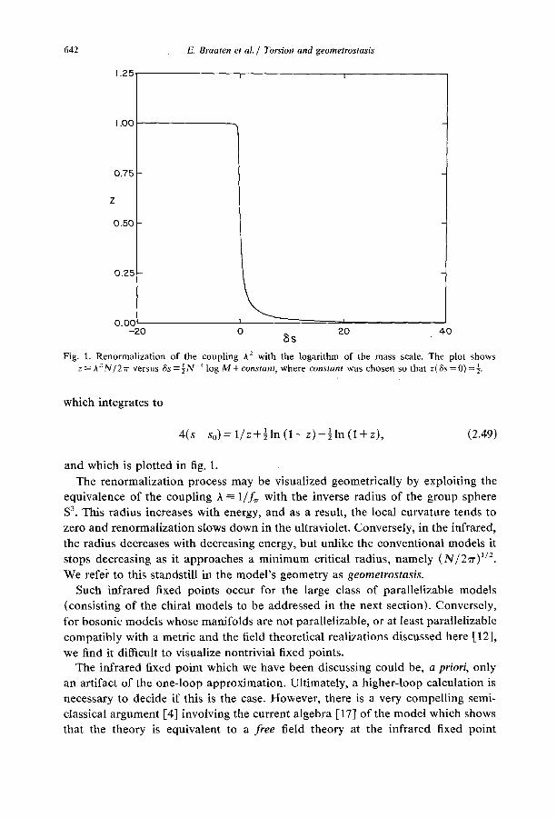
Fig. 1. R e n o r m a l i z a t i o n o f the c o u p l i n g A 2 wi th the l o g a r i t h m o f the m a s s scale . The p lo t s h o w s
z ~ Az N~ 2 ~- versus 6s --- ~ N - t log M + constant, w h e r e constant was c h o s e n so t ha t z(tSs = 0) - ± - - - 2 "
which integrates to
4(s - So) = 1/z +½ In (1 - z) -½ In (1 + z), (2.49)
and which is plotted in fig. 1. The renormalization process may be visualized geometrically by exploiting the
equivalence of the coupling A ~ l / f , with the inverse radius of the group sphere S 3. This radius increases with energy, and as a result, the local curvature tends to zero and renormalization slows down in the ultraviolet. Conversely, in the infrared, the radius decreases with decreasing energy, but unlike the conventional models it stops decreasing as it approaches a minimum critical radius, namely (N/2rr) ~/2. We refer to this standstill in the model 's geometry as geometrostasis.
Such infrared fixed points occur for the large class of parallelizable models (consisting of the chiral models to be addressed in the next section). Conversely, for bosonic models whose manifolds are not parallelizable, or at least parallelizable compatibly with a metric and the field theoretical realizations discussed here [12],
we find it difficult to visualize nontrivial fixed points. The infrared fixed point which we have been discussing could be, a priori, only
an artifact of the one-loop approximation. Ultimately, a higher-loop calculation is necessary to decide if this is the case. However, there is a very compelling semi- classical argument [4] involving the current algebra [17] of the model which shows that the theory is equivalent to a free field theory at the infrared fixed point
E. Braaten et al. / Torsion and geometrostasis 643
A2= 2~-/N. In the geometrical formulation, a related argument may be made as
follows. Consider the "vector potential" which appears in D r in (2.32):
A g b =~ FabcO~4' c --Sabceu~,c)*'4' c. (2.50)
A straightforward calculation of the field strength for this potential gives
O .A~ab -- o~A.ab -t- A , %A~Cb - A acA .C b
= Eix•{-- Sabc ( ~A O~t4' ) c _~_ OcSabd (O~t4' coX4' d ) } __ 3 8.~,Sae[bSecd](O,~4' c ApOp4 , a )
+ {~ ~bca - DcS~bd + DaSabc}O,4" c0~4' d. (2.51)
It follows from (2.18), (2.19) and (2.32) that this field strength vanishes on-shell when the manifold is parallelized. In that case, we have a pure gauge form for At :
A , = u - l ( x ) O i x U ( x ) , (2.52)
where U is a local function of spacetime. Alternatively,
O,U = U A , , OixU -1 = - A ~ U 1, [fx ,] U = P exp d z " A , ( z , (2.53)
which involves the usual path-ordered exponential. Again we stress that U is a local function of x, i.e. path independent, due to the vanishing of the field strength in (2.51) when the 4'-manifold is parallelized and q5 obeys the equations of motion.
Given this local U, the scalar field equations (2.32) are solved by transporting a free field. That is, let
O~4'(x) =- U-l(x)Ou4'o(X). (2.54)
Then, using the second relation in (2.53), the 4'-field equations become
N ' 0 , 4 ' ( x ) = (0" + A T) U-10,4'o
= u-'o'o.4"o(X), (2.55)
which vanishes if and only if 4'0 is a free, massless scalar field. Since the relation in (2.54) is both invertible and solvable for nontrivial q5 and 4'0, we conclude that upon parallelism of the field manifold, there is a local, on-shell equivalence between 4' and a free field 4'0. It is reasonable to expect this equivalence to persist at the full quantum level, and indeed the S-matrix has been argued to be trivial for this model [3], when a2=2~- /N. However, to demonstrate the complete quantum equivalence of the model to a free field theory at the level of Green's functions, or at the level of operators, may be complicated, even when the classical equivalence is so simple.
A consequence of such an equivalence would be the existence of the above infrared fixed point to all orders of perturbation theory. As a check on this
644 E. Braaten et al. / Torsion and geometrostasis
equivalence, we have explicitly verified to two-loops that geometrostasis persists, at the same parallelism induced fixed point. Most of the details are given in appendix A. The main point is that the background field expansion simplifies drastically when the manifold is parallelized, i.e. ~,bca = 0. In that case only two interaction terms survive in the expansion of the action through fourth order in ~ , where ~ is the contravariant vector representing the displacement from the given background field, ~b, along a geodesic of gab[t~]. The background field is assumed to be on-shell, ~,O~b = 0. These O(~ ~) interaction terms are all that are required to calculate the two-loop divergences, and hence determine the renormalization group evolution equations through two-loop order. They are given by
[parallelism] = (2a2) -1 f d2x {2Sabc[4a]~a(~.~)bet*"(~, .~)c /(3÷4)
+ ISeabSecd~b~c (~p.~) a ( ~ ,~)d }. (2.56)
The two-loop ultraviolet divergences of the model are then calculated by Wick- contracting the ~'s in vacuum expectation values of io+~) and (ic3+4))2 to form the
usual " 0 " and "oo" diagrams. The resulting ultraviolet divergence is a scalar on the background field manifold, as follows;
(ii(3+4) +}i2(1(3+4))2) = _~12(2.~ 2)-, f _ d 2x @~S~b~ ~* S ~b~ , (2.57)
the elementary, dimensionally-regularized momentum integral in d where I is dimensions.
i = (27r)_2 I'j ddk(k21 i 1 rn 2)=2--# ( d - 2 i + ' ' ' '
(2.58)
into which we have introduced an infrared regulating mass term to eliminate any ambiguities between UV and IR divergences.
It follows l¥om the explicit form of the density in (2.57) that the model has no
ultraviolet divergences upon parallelism, since in addition to 5? abca = 0, the torsion obeys the Jacobi identity, (2.18), and is covariantly constant, (2.19). Therefore
~,S,,bc ~ (O~,cb d)DaS, bc + 38U-v (c3~,q~ d )Scle[aSebc] (2.59)
also vanishes. Hence the parallelism induced fixed point in the model persists, and geometrostasis prevails to two-loops.
This leads us to again conjecture [8] that the renorrnalization group evolution of the geometry, as in (2.45), is a function solely of the generalized curvature ~tabca,
and perhaps its covariant derivatives, to all orders of perturbation theo ry - just as in the sigma model without a Wess-Zumino term the evolution is a covariant function of the curvature R,,bcd. However, unlike that simpler case, we cannot conclude that the evolution will depend only on ~ab~d on the basis of general
E. Braaten et al. / Torsion and geometrostasis 645
reparameterization invariance alone. In fact, it is somewhat annoying that the usual
background field expansion to fourth order in s c is not manifestly a function of only
~abcd, as shown in appendix A. Evidently, to prove our conjecture, some additional information involving the actual h igh-momentum behavior of the model must be known (such as used to evaluate the "O" and "oo" diagrams above). It is also conceivable that a complete two-loop calculation of the renormalization group evolution equations (a calculation which does not use any special properties of
Sahc) will show the conjecture to be false. We leave this as an open problem for now, and turn to other examples. (See note added in proof.)
As further illustration~ we next discuss the simple models with group manifolds S 2, S 2 × S ~ and S ~ × S ~ × S ~, respectively. As we shall see, none o f these has nontrivial
fixed points because they cannot be parallelized compatibly with a metric. As previously indicated, the above formalism is applicable to a broader variety
of models than mere Wess-Zumino terms. For example, consider the model S 2--- 0 ( 3 ) / 0 ( 2 ) . Since H3(S 2) is trivial, there is no Wess-Zumino term possible. The model 's instanton density in two dimensions (which is nonzero since H2(S 2) = Z)
may be expressed in terms of an antisymmetric tensor eab as in (2.31), except the coefficient of eab is completely arbitrary in this case, unconstrained by the topology.
Explicitly, the torsion potential and its curl in this case are
e~ = e"b g 1/2= e~b(1 --t~bl2) - ,/e
= at .{2e~c4,c(1 -14,12)'/2/1012}, 0t,ebc ~ = 0. (2.60)
Infrared geometrostasis does not occur here since the torsion vanishes identically. For the same reason, it is evident that I2 does not contribute to the renormalization process at all. This is naturally expected, since the integrand in 12 may be written as a total spacetime divergence, given that eab is a curl.
In our next example, $2×S 1, 12 does represent a bonafide Wess-Zumino term, since H3(S 2 ×S 1) ---H2(S 2) × H1(S ~) is nontrivial. The torsion is again proportional to the volume element tensor eabCg ~/2, and is also covariantly constant. However,
the conventional curvature tensor now vanishes if any of its four indices is 1, corresponding to the coordinate of the circle S ~. The nontrivial renormalization group equations (2.45) thus separate into
M~M 9 (g l l /A- ) = -2r/Zg,1/27r for S ~ ,
d ,~ M - ~ ( g o / A ~) = (1-2~72)gJ2~" for S 2 . (2.61)
Now recall how the normalization of the S 3 group volume accounted for the definition of the 12 coefficient r / in (2.15) and (2.16). In the model at hand, the group volume is the product of the volumes of the sphere and the circle, which may be normalized
646 E. Braaten et al. / Torsion and geometrostasis
independently, thus allowing for a second, independent coupling, h~. (For con- venience, we choose ~b ~ to be an angle, so glt is a constant.)
(/~l) 2~-'~ A2/g11, 7] --~ AlAN/(87r) . (2.62)
The renormalization group equations (2.61) then become
d = f o r s t ,
d " )-2= 1-----lh2A~(N/87r)2 forS 2, (2.63) M~---M ( A 27r 7r
where it is evident that the S t and S z decouple when either A 2 or A~ vanish. This
reflects their only being linked through I2 which is suppressed in these limits. To see that these equations exclude nontrivial fixed points of both A 2 and A~, we
rewrite them after absorbing N2/647r 3 into A~, and combine them to obtain
d M ~ - - ~ A ~--- A4A 4 ,
d 2 4[ 1 2 "'~ M - d ~ h = - h ~ G - A h i ) , (2.64)
or alternatively
47rh~ '
which is plotted in fig. 2. (Note in the figure the separatrix C = 0. Trajectories below this line flow to h 2= 0 with increasing energy, and the evolution stops.)
Our final example is the hypertorus S ~ ×S ~ ×S t, for which H3(S ~ ×S ~ ×S ~) is also nontrivial, so that 12 is also a Wess-Zumino term. In analogy to (2.62) for the previous model, the manifold volume normalization changes to accommodate three
2 couplings A,--= A-/ga, (with no sum on a), so that ~ = NA1AzA3/(g'/7"2A). The renor-
malization group equation is
(Aa)- = - NzA ~A ~A ~/(647rSA]), (2.66)
The theory is trivially infrared free, with the couplings evolving in constant ratios, the interaction strength being proport ional to their product:
h~= Ca{ln(Mo/M)} -t/3 , C~C2C3=647rS/3N 2 . (2.67)
3. General scalar field models
We now generalize the discussion of SU(2) × SU(2)/SU(2) in the preceding section to the case of chiral models defined on symmetric spaces, (GL ×GR) /Gv , where G
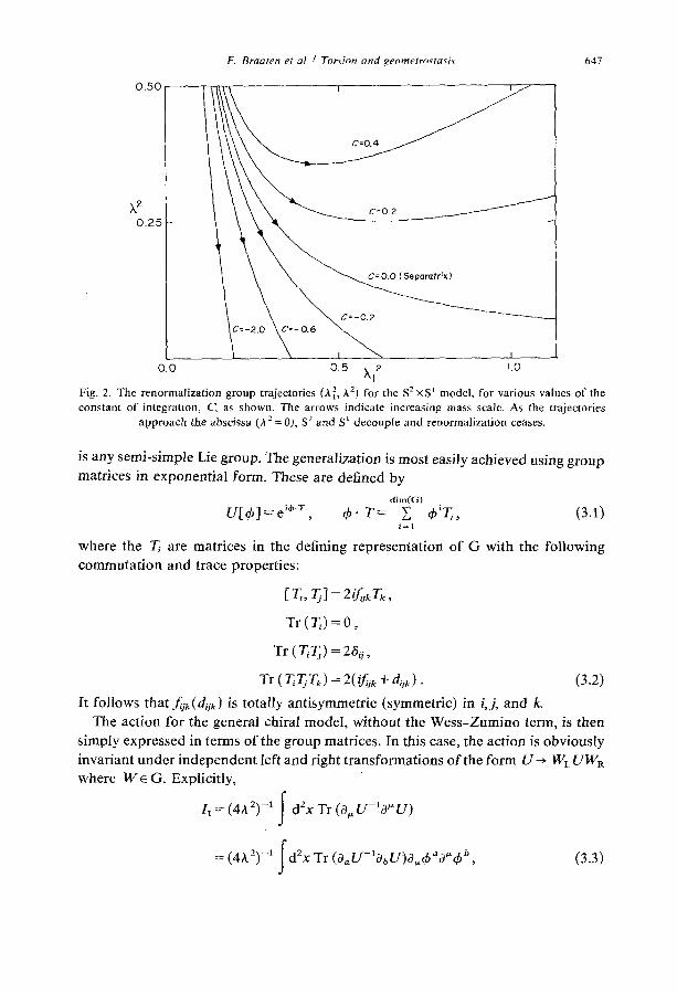
b.'. Flraaten et al. / Tomion and genrnetro~ta~i~ 647 o ol
. 2 5 5 , . 0,0 0.5 Xl 2 1.0
Fig. 2. The renormalization group trajectories (Ai,~ A2) for the SZxs ~ model, for various values of the constant of integration, C, as shown. The arrows indicate increasing mass scale. As the trajectories
approach the abscissa (,~ 2= 0), S 2 and S L decouple and renormalization ceases.
is any semi-simple Lie group. The generalization is most easily achieved using group matrices in exponential form. These are defined by
dim(G) u [ o ] ~- e ~*T 4, T ~ v , , • 4, T~, ( 3 A )
i~l
where the T,. are matrices in the defining representation of G with the following commutation and trace properties:
[ T~, Tj ] = 2 ~jk Tk ,
Tr (T~)=0,
Tr (T~T~) = 26,j,
Tr ( ~TjTk) = 2( ~f~ik + dok) . (3.2)
It follows that fjk(d~ik) is totally antisymmetric (symmetric) in i,j, and k. The action for the general chiral model, without the Wess-Zumino term, is then
simply expressed in terms of the group matrices. In this case, the action is obviously invariant under independent left and right transformations of the form U ~ WL UW~ where W e G. Explicitly,
I~ = (4A2) -~ j d2x Tr ( O . U - ' O ' U )
= (4h2) -~ ~d2x Tr (O~U-lObU)O.4,aO'~b b , (3.3) J
648 E. Braaten et al. / Torsion and geometrostasis
where we have used 0~U[&] = 0~&aGU[&]. The action may now be written in the same form as (2.2) provided that we identify the metric on the &-manifold as
gab[&] = ½ Tr (Oa U-~ObU) . (3.4)
In order to go further and introduce the Wess-Zumino term for the general chiral model, it is convenient (but not necessary) to introduce a vielbein on the field manifold. This is done in a mathematically standard way [11] by constructing elements of the Lie algebra from derivatives of U and U -j with respect to the coordinates &. In general we define the left-invariant ("pure gauge") vielbein
V~J[&] ~--= iU-I[&]O~U[&] = - dt U- ' [&] T~U'[&], (3.5)
the last equality following from either the series expansion or the limit definition of the exponentials. Equivalently, we write
Io' iO, U= UWTj = - dt U I - t T a U t ,
iGU '= - W T j U - ' = dt U - ' L U ' - ' . (3.6)
From these it follows that
GU-~ ObU= VjVbkTjTk
= V~Vbk(~{Tj, Tk}+ if)k,T,), (3.7)
which separately displays the symmetric and antisymmetric components O(a U-~Ob)U and 3[,,U-~Ob] U. The symmetric component appears in the metric, (3.4), and as we shall see, the antisymmetric component appears in the torsion.
Upon multiplying by TJ and tracing (3.5), we project out individual components of the vielbein:
Io Vj[&]=½iTr(TjU-IGU)=-~ dtTr(TjU-'TaU'). (3.8)
Similar traces project out the metric, as in (3.4), and the torsion. These can be expressed in terms of vielbein products and are simply extensions of the usual Cartan metric and structure constants of the group G to the field manifold. For example, tracing (3.7) and comparing with (3.4) gives the expected relation between metric and vielbein:
gab = V a i W ~ i j , (3.9)
which is manifestly symmetric, g~b = gcab)- Similarly, the torsion is given by a totally antisymmetrized product of three
vielbeine [11], and is nothing but the group structure constant expressed in terms of

E. Braaten et al. / Torsion and geometrostasis 649
"world" indices on the field manifold.
=- v'o vd v?
= -½'0 Tr ( U-Io[aUU-IObUU-IOc] U) . (3.10)
The last equality follows from (3.5) and the trace of T~T~Tk given in (3.2). Note, however, that we have introduced into the torsion an arbitrary scale, '0, relative to the metric.
We now use this definition of Sabc to establish those properties which are germane to our purposes, and thereby justify calling Sabc the torsion. First consider the torsion bilinear: SeabScde ~- "0 2 vei Va j Vb k Vc l Vd m Venfijkflhnn = "17 2 Va J Vb k Vc I vdmfijkfllmi since WiVe n = 6 i". Antisymmetrizing this relation over three indices, and using the Jacobi
identity for the structure constants,
f , u k f , lm,= 0, (3.11)
we obtain a similar identity for the torsion:
SeabScde 2V SebcSade 2V SecaSbde ~- 3 Se[ abS c]de
= 3.q 2 Vdvbkv~tVdmfiukfqmi
=0. (3.12)
Next we consider the vielbein field strength, i.e. DtaVbl ~. Using the symmetry of the Levi-Civita connection, Fabe = Facb, as well as (3.8) and (3.6), we have
D[a Vbj i = O[a Vb] i = ½i Tr ( TiO[aU-l Obj U) = ½iV[aJVb] k Tr(TiTjTk).
Hence, by (3.2),
D[a Vb ] i -~ - - f ijk W Vb k. (3.13)
These are the Maurer-Cartan equations (i.e. the group-covariant field strength of a pure gauge field vanishes). The simple structure on the RHS of (3.13) actually allows one to further conclude that the s y m m e t r i z e d covariant derivative of the vielbein vanishes.
This may be established as follows. The Levi-Civita connection is defined to provide D-covariant constancy of gab (the usual metric postulate). Thus
0 ---- Dagbe = (DaVb i) V j + vbi (DaVci) . (3.14)
Symmetrizing on a and b, and subtracting D~g~,b gives
0 = D , gbe + D b g ~ -- D~g,,b
= (DaVb') V~'+ Vb ' (D.V~i )+ (DbV~ ') V~g+ Vai(DoV¢ ~) - V j ( D ¢ V a i) - V a i ( D c V b i)
= 2 V ~ D ~ Vb) ~ + 2 VbiD[a Ve] i + 2 Va~D[b Vc] i .
650 E. Braaten et al. / Torsion and geometrostasis
Using (3.13), the last two terms in this identity cancel. Multiplying the remaining term by V cj leads to the desired conclusion:
D ~ V b / = 0. (3.15)
For convenience, we combine (3.13) and (3.15) into a single expression:
Da Vb ~ = --f~k VJVb k . (3.16)
This result and the Jacobi identity for the structure constants immediately imply that the torsion is covariantly constant, as is the metric. From the definition (3.10) and (3.16), we have
DaShed = ~q fjk Da ( V j V~ Va k)
= -~TVa"VflVckVdm(3fi,ufkm]i)
= 0 . (3.17)
Thus the torsion defined for the general model by (3.10) is covariantly constant on the field manifold, exactly reproducing our results found above using specific coordinates for the 0(4) model (2.19).
As an immediate consequence of (3.17), the torsion is a closed 3-form, i.e. curl-free:
D[ aS bcd ] • O[ aS bcd ] ~- O . (3.18)
Also from (3.17), the torsion is co-closed, i.e. divergenceless, and harmonic on the field manifold:
DaSabc ---- 0, ASabc =- 4DdD[dSab~] + 3 D[aDdSbc]d = O. (3.19)
It is interesting that the closure of S~bc may be seen directly from the definition (3.10) for arbitrary field manifolds and U-matrices, even though S,b~ may not be covariantly constant on such manifolds. This follows from simply noting that
Dr~ Tr ( U-~ObUU-~O~UU ~oa3U) = -3 Tr ( U-IO[aUU-IObUU I(~cUU-I~d]U ) =0
because the cyclic property of the trace forces the complete antisymmetrization of any even number of matrices (e.g. U-aOU) to vanish.
Since S~b~ defined in (3.10) is closed for an arbitrary manifold (in particular for the general chiral model) it may be written locally on the field manifold (e.g. on the upper hemisphere of the 0(4) model) as a curl of a rank-two antisymmetric tensor, Cab , which we again refer to as the torsion potential:
Sabc = ~lO[ aeb~] =- rlc3[~ebc] . (3.20)
As in the 0(4) case, the torsion potential itself is defined only up to a curl Ot,~b ~. An explicit form for e,b in terms of the U-matrices is not difficult to obtain [3]. For convenience, we first introduce some notation. Let
T~(t) = U- t [O]T~U'[6] (3.21)
E. Braaten et al. / Torsion and geometrostasis 651 be a p a r a m e t e r (t) and f ie ld-dependent represen ta t ion matrix. Then the derivatives
of Tb(s) with respect to the fields, for 0 ~ < s ~< 1, are
Io O~Tb(S)=--i dtO(s-t)[T~(t) , Tb(S)1. (3.22)
This m a y be seen f rom the results for derivatives o f powers of U. The latter derivatives fol low f rom either the series or limit definit ions of the exponent ia l . For 0<~ s <~ 1, we have
fo fo O~U'=i d tO(s- t )US- tT~Ut=i dtO(s- t )U'T~(t ) ,
fo ;o O , U - ' = - i d t O ( s - t ) U - ' T ~ U ' - ' = - i d tO(s - t )T~( t )U s. (3.23)
Using To(t), we trace an ordered p roduc t and define
I0'fo f~b=~ ds d t O ( s - t ) Tr{T~(s)Tb(t)}. (3.24)
Several proper t ies of f~b are evident. First, the double integrat ion m a y be reduced to an integrat ion over the single variable (s - t), since the in tegrand is independen t o f ( s + t). Tha t is,
Tr {To(s) Tb(t)} = Tr {T~U'-tTbUt-S}, (3.25)
frO, frO L fO 1 fl--(s--t)/2 ds d t O ( s - t ) F ( s - t ) = d ( s - t ) F ( s - t ) d[(s+t)/2] a(s-t)/2
Io' = d(s - t){1 - (s - t)}F(s - t).
Thus we have
fl f~b = Jo du(1 - u) Tr {T~UUTbU-U}. (3.26)
Secondly, using (3.23) for s = 1 in the express ion for g~b, (3.4), and compar ing with (3.24), (3.25), we see that f(ab~ = ~(fob +J~,o) is s imply the metr ic
fol;0 ' gob =½ ds dt Tr{T~(s)Tb(t)}
Io =~ ds d t (O(s- t )+O(t -s ) )Tr{T~(s)Tb( t )}
=f~ab) • (3.27)
Finally, the an t i symmetr ic part , fc,b~, is the torsion potent ia l for the general chiral
652 E. Braaten et al. / Torsion and geometrostasis
model, up to an overall normalization
~%b = --~f[ob3 - (3.28)
TO see that this is indeed the case, we compute the curl of fEab3 and show that it gives Sab~ as in (3.10). In so doing, we use (3.22), make judicious use of the cyclic properties of the trace, and relabel variables repeatedly.
oEofb~ ? = ds dt O(s - t) Tr {O[~Tb(S ) • T~l(t ) + T~b(S)" O~T~l(t)}
fo' fo ' = - i ds dt d u O ( s - t ) O ( s - u ) Tr{[Tt~(u), Tb(S)]T~](I)}
- i ds dt duO(s- t )O( t -u)Tr{TEb(S)[T~(u) , Tel(t)]} )
= - i ds dt du Tr(T[o(s)Tb(t)T~](u)}
× { 0 ( s - t ) O ( s - u ) + O ( u - t ) O ( u - s ) - O(s- t ) O ( t - u ) - O(u- t )O( t - s ) } . (3.29)
However, recalling
O(s- t )O( s -u ) = O(s- t )O( t - u)+ O ( s - u ) O ( u - t) ,
O(u- t )O(u - s ) = O(u- t ) O ( t - s ) + O ( u - s ) O ( s - t),
(3.29) simplifies to
Io ' OLofb~ = --i ds dt du tr{T~(s)Tb(t)T~](u)}
×{0(s - u)O(u - t)+ O(u - s )O(s - t)}. (3.30)
Finally, using the invariance of Tr { TEa (s) Tb(t) Tcl(u)} under cyclic permutations of a, b and c, we can relabel the variables of integration in (3.30), and replace each of the P-products by (Ix) their cyclic permutations in s, t and u. The result involves the identity
O(s- u)O(u-- t) + 8 (u- t)O(t- s)+ O(t- s)O(s- u)
+ O ( u - s ) O ( s - t ) + O ( s - t ) O ( t - u ) + O ( t - u ) O ( u - s ) = - - l , (3.31)
from which we obtain
Io' Io' o~fbc]=--~l ds dt duTr{T[a(s)Tb(t)Tc~(u)}
~- ½ Tr { U-1ataUU-IObUU-~O~j U}. (3.32)
E. Braaten et al. / Torsion and geometrostasis 653
Comparison with (3.10) verifies the anticipated relation
Sabc 3 = -5~?~[Jbcl • (3.33)
This confirms that the identification in (3.28) indeed gives (3.20). Let us demonstrate parallelism for the general chiral model at ~ = ±1. The proof
is simplified if we express the generalized curvature in terms of the spinor connection of Cartan [11], ~oa °. The relevant expression is
abed = 2 V,,'W{Otctod~ ij + W~ciktodlk~}, (3.34)
where toa U is given in terms of @-derivatives of the vielbein:
O.)a ij ~-~ v b i ~ a V 2
= V b i { D a V 2 + S a b c V j } , (3.35)
using the general definition of ~ in (2.34). The equivalence of (3.34) with our previous expression for 5~,b~d in (2.36) follows upon using (2.5) and the usual relation between metric and vielbein in (3.9). If we now use the definition of S~b~ in terms of vielbeine, (3.10), and the result for D-covariant derivatives of V, ~ on group manifolds, (3.16), the spinor connection becomes
wa 0 = ( rl -- 1)f i jk V~ k . (3.36)
Finally, we insert this relation into the expression for ~,b~d, make use of OE,wb~ ~i=
Drawbj ~j and the Maurer-Cartan equations, (3.13), and utilize the Jacobi identities, (3.11), to obtain our final expression for the generalized curvature for the general chiral model:
~b~a = ( 1 -- ~2) f j ,~fk , , , Va~ Vd V~ k Vd' . (3.37)
ThUS the generalized curvature vanishes, and the field manifold of the general chiral model experiences paraUelism, when ~ = ±1.
The vanishing of 5~ ~b~a when 7/= 1 is evident in (3.36), since w~ ° itself vanishes. The other zero for 5~ abcd could also have been seen at the level of a spinor connection, if we had originally defined the vielbein by interchanging the order of Tj and U in (3.6). This right-invariant vielbein, V, satisfies
i O,,U = f ] ~ T j U . (3.38)
Defining a spinor connection using 17"], as in (3.35), one can show that
O3~ = (1 + ~7)fjk9~ g , (3.39)
with ~b~a given in terms of V and o3 as in (3.34). In this way the vanishing of the generalized curvature at r /= -1 is more readily apparent.
We have proven that all group manifolds can be parallelized by adding the proper amount of torsion to the connection. A converse theorem was also established by
654 E. Braaten et al. / Torsion and geornetrostasis
Cartan and Schouten: with the exception of the seven-sphere (to be discussed in sects. 4 and 6 below), no other manifolds can be so parallelized in a way that leaves the geodesics of the manifold unaltered. We shall not prove this assertion here, although all the relevant concepts are at hand, but rather we refer the reader to the original literature [12].
We may now add to the action a Wess-Zumino term, I2, of the form given in (2.21), with the covariant tensor eab given for the general chiral model by (3.28). The topological nature of the Wess-Zumino term is essentially the same as in the 0 ( 4 ) / 0 ( 3 ) case. We refer the reader to appendix B for a more systematic mathemati- cal discussion of these latter features.
We may also consider the renormalization properties of the general chiral model. All the formalism of this section has been tailored so that the renormalization analysis of the preceding section carries over without change. The one-loop counter- terms and the renormalization group equations are as given in (2.41) and (2.45), respectively, with the corresponding interpretation of an evolving, scale-dependent geometry exactly as before. Once again, upon parallelism, an infrared fixed point is encountered and geometrostasis takes place.
The formalism can be slightly compressed by using the general tensor fab given in (3.24) and (3.26). The general action is then
I (2)t 2) d2x f,,b[ cb ]{ 6 ~ - ~/e }ouch a~b . (3.40) J
The one-loop counterterms are
___~r(1) 1 h2Jt~bl 2r r (2_d)~t~ba '
(3.41)
with the concomitant evolution equations
M d ( 1 ] =
On the basis of this result, it is worth stressing that the antisymmetric part of f~b, i.e. the torsion potential (3.28), is not renormalized for chiral models defined on group manifolds solely because of the covariant constancy of the torsion, (3.17). This is true even when the manifold is not subject to parallelism. The quantization of the coefficient of the Wess-Zumino term (cf. appendix B) suggests that eob remain unrenormalized to all orders of perturbation theory.
E. Braaten et al. / Torsion and geometrostasis 655
The symmetric part o f f~h, i.e. the metric gab, is unrenormalized and therefore encounters a fixed point to one-loop whenever ~<ab) vanishes. In particular, this
happens for general group manifolds upon parallelism, when ~7 = + 1. Once again, we may ask if this is a one-loop artifice. The two arguments of the previous section again suggest not. To reiterate, we first note that the formal arguments surrounding (2.50)-(2.55) are unchanged. Thus the general chiral model appears on-shell to be locally equivalent to a free field theory at r /= ± 1.
Secondly, the explicit two-loop calculation using the background field method described in appendix A again reveals a renormalization group fixed point upon parallelism of the general chiral model. The discussion surrounding (2.56)-(2.59) carries over without modification. It is instructive to consider the above for the cases
where G is one of the classical simple groups, SUnl SOn, or Spn. In particular, one easily verifies for these respective cases that the hermitian matrix M~ =- iU-IO~U is either traceless, or antisymmetric, or that it preserves a skew symmetric metric A ( i . e .A . Ma = - M ~ ~n~- A). These properties of M, are necessary and sufficient to
expand Ma in terms of the Tj as in (3.5), and hence to yield the equalities in (3.7), (3.9) and (3.10). In general, we leave the details as an elementary exercise for the reader. However, for the case of the 3-sphere, S 3~- O(4)/O(3), it is perhaps useful to establish a connection with the results of the previous section since those results require a different parameterization of the group manifold.
Directly evaluating (3.1), (3.4), (3.8) and (3.28) using properties of the SU2 Pauli matrices, %, we obtain the following:
U[~b] --- e *+" = cos (l~l) + itb" a" sin (l&l)/[~b[, (3.43)
g~b[fb] = f b a f b b / l t h l 2 + (3~b _ qS,~t~b/lth/2 ) sin 2 (l~l)/l~[~, (3.44)
g [ 6 ] = sin4 ( I ( f l l ) / l t f l ] 4 , (3.45)
vo~[~X = - 4 , ° 4 , ' / 1 ~ 1 = - (a ~' ~°4,71,~1 ~) sin (21~1) / (21~ ,1) - ~o,~6 ~ s in: (161)/14,1 = , (3.46)
e,b[dp] = 3e~b~6~{214,l--sin (2161)}/[&13 , (3.47)
0[,eb~3 = e~b~ sin 2 (l~b])/lthl 2 = e~b~gg. (3.48)
These expressions reduce to the results of the preceding section, written in terms of the variable ~b', through the reparameterization
~b '~ = q5 ~ sin (I,~l)/14,1, (3.49)
or inversely,
~b" = ~b 'a arc cot [(1 -I~b'12)~/2/[d~'l]/l~b' I . (3.50)
It is a straightforward exercise to verify this change of variables, for example, by checking that the above tensors transform into their counterparts previously given in sect. 2.
656 E. Braaten et al. / Torsion and geometrostasis
4. Higher spacetime dimensions
Wess-Zumino terms exist for nonlinear sigma models in higher than two spacetime dimensions, and their significance from the point of view of classical field theory is well appreciated. However, the role of such interactions in quantum field theory is not understood tully, at least in part due to the nonrenormalizability of the conventional sigma model if the number of spacetime dimensions is greater than two. Low-energy quantum effects arising from Wess-Zumino terms have been studied in the context of effective lagrangians (the original study, in fact), but the ultraviolet importance of such terms remains obscure. The essential reason for this obscurity lies in the large number of spacetime derivatives which appear in the Wess-Zumino density: in d spacetime dimensions the term has d derivatives. In this section, we will first give examples of the Wess-Zumino term in higher dimensions, and then briefly discuss the power counting differences between sigma models in d = 2 and d >/3 dimensions. Most questions regarding the ultraviolet effects of Wess-Zumino terms in higher dimensions will remain unanswered, however.
To follow our previous line of development, we first consider Wess~Zumino terms using an explicit set of coordinates for the O( d + 2 ) model in d dimensional spacetime. The scalar field ~b ~ has d + 2 components subject to the constraint ~=0,....d+t (q 5~)2= i. Hence the field lies on the surface of the (d + 1)-sphere, S a+~. We choose to define upper and lower hemispheres, as for the 0(4) example in sect. 2, by taking 4~°~=±(1-14~12) ~/2, where 14~[z=~a=~.....a,_l(~ba) 2. The Wess- Zumino term in d dimensions then derives from a topological density in d + 1 dimensions, as in the 3 ~ 2 examples considered above. The relevant action in d + 1 dimensions is
Id+l ~ C( d) f dd+lx e~C"~'d+leic"i~+'-qb i~+20~, da i . . . . Oud+~dp id÷' ,
N ( d / 2 ) ! (4.1) C(d)=- 7rd/2( d + 1)!"
Replacing 4) o by +(.1 -I~b12) ~/2 in this expression, and integrating by parts, we obtain the Wess-Zumino action in d dimensions for the upper/ lower hemisphere of the group manifold, exactly as in the O(4), d = 2 case:
ta = C(d) f ddx e~'<"de'c""~+~f(lqbl2)ch"~+~o~,,4)~...o~,4) % (4.2)
where 1 ~< a~ <~ d + 1. The .form function in d dimensions, f ( x ) , satisfies }f(0)l = 1, and on the • hemi-
sphere obeys the first-order inhomogeneous differential equation
{ 2x d } ±1 (4.3) l+d+~-i d--x f ( x ) ( l_x)a /2 .
E. Braaten et al. / Torsion and geometrostasis 657
The solution is
f ( x ) = ±½(d + 1)x -(a+1~/2 d z z ( d - 1 ) / 2 / ( l - - -7) 1/2 , (4.4)
This generalizes the 0(4) result in (2.27). For example, when d = 2n, the integral in (4.4) explicitly evaluates to
±(2n + 1)!! arc sin (x ~/2) f(x) 2 n n ! X (2n+1) /2
, ~ 1 ( 2 n - 1 ) ( 2 n - 3 ) . . . ( 2 n - 2 k + l ) ~ q : ( 2 n + l ) ( 1 - x ) ' / 2 1+ (4.5) 2 n x k :"~ 1 ~ - ' ~ n - ~ 2 ) " " " ( n -- k ) x k J "
The differential equation (4.3) implies the linear homogeneous equation
4x(1 - x ) f ' + 2 ( d + 3 ) ( 1 - x ) f ' - 2 x f ' - ( d + 1) f= 0, (4.6)
which is useful for demonstrating the invariance of the action (4.2) under nonlinear axial transformations as in (2.6).
The geometrical properties following from the above form function are direct extensions of the O(4), 2-dimensional case. Define the d-form
eal- ..... = 8a~'"%bq~ b f ( ]&]2) , (4.7)
in terms of which the d-dimensional Wess-Zumino action is simply
Ia = C ( d ) f dax e ~ l " U d e a . . . . . O ~ ~)a~" " " 0.,,~b ~. (4.8)
Using (4.3) the d-form is directly seen to be co-closed:
Daea~.. .~ = 0~e~<~ .... = 0, (4.9)
where the metric, the Levi-Civita connection appearing in the D-covariant deriva- tive, and the Riemann curvature have exactly the same forms as in (2.3)-(2.5). In addition, the d-form is harmonic:
Ae,,...,~ = (d + 1)D~D~ea . .... j - d(-1)aDE~Dae~2. . .~> = 0, (4.10)
or equivalently, for the (d + 1)-sphere,
D~D,~e~,. . . . . = de~,...,~. (4.11 )
Similarly, on the upper / lower hemisphere the field strength for the d-form is
S~...~d+ , = ~70E,,e~ ~. . . . . . . j = z t z 'qg l /28%"'aa+' , (4.12)
where again g = d e t g , b =(1-1q512) -~. As in the previous cases involving group
658 E. Braaten et al. / Torsion and geometrostasis
manifolds in two spacetime dimensions, the field strength is therefore covariant ly
constant:
DbSa,. ....... -~ O, (4.13)
and hence is also closed, co-closed and harmonic.
The generalization of the symmetric space results in sect. 3 to d (even) spacetime dimensions may be accomplished again through the use of the group matrices U[th] ~-exp(i&. T). These allow the construction of the d-form for general group manifolds:
1 Io eoc .... ~ ( d - l ) ! d t , ' ' ' d t a [ O ( t l - t 2 ) O ( t 2 - t 3 ) ' ' ' O( td_ , - - t d )
+ all permutations of t2,. • •, ta ]
x T r {TEa,(t 0 • • • T,~l(td)} , (4.14)
where Ta(t )=- U - t T a U ~ as in (3.21). In terms of this d-form, the Wess-Zumino action is again given by (4.8), while the corresponding field strength is obtained using properties of To(t ) through a series of steps similar to (3.22)-(3.33). We find
S,h,~2...,~d+ ~ ~-- r13[ol e,2...ae+,]
" I/ Io' I0 = " O ~ dq d t 2 " • • dta+l
×Tr {T~a,(t,) • • • Tad+tl(td+l)}. (4.15)
Alternatively, this may be written as
d ( - - i ) d ~ - - t -1(~ U} (4.16) S . . . . ...a~ = - ~ 7 ~ l r l U OEaiUU-IOo~U . . . U ,~+~l •
with the Wess-Zumino action expressed as the (d + 1)-dimensional integral
I = N f d a + t x ~ : " ~ a + l g 3 ' ~ ' (4.17) - ~ a t . . . a d + l t z l - t - • . . ~ l z a _ ~ l ( ~ a a ÷ l ,
whose proper normalization, N, involves the group volume. Note that the above forms for the field strength would identically vanish for d an odd number due to the cyclic properties of the trace. Also note that in four dimensions, there is no
Wess-Zumino term for SU(2). This last point may be seen by reexpressing Sob..~ in terms of vielbeine, using (3.5).
i d ( - 1 ) a V , ~, '~ IZ ~a~'Tr{T~ ' ' ' T~+,} (4.18) so, . . . . . . . to, v o w - . . -
Specializing this result to d = 4, we evaluate the trace using the properties of the
IF.. Braaten et al. / Torsion and geometrostasis 6 5 9
T~'s given in (3.2). 1 • i j k l m
S abcd e : - ]~l V[a Vt~ V c V d Ve] ~fijndnkpflmp . ( 4 . 1 9 )
Hence, for all groups lacking the symmetric tensor, d~ik , there is no Wess-Zumino action for four spacetime dimensions.
In higher spacetime dimensions, the quantum effects of the Wess-Zumino terms on the geometry of the field manifold are different from what we have previously discussed in two spacetime dimensions. In particular, the Wess-Zumino term does not contribute to the renormalization of the metric gab at the one-loop level. A simple scaling argument (cf. Alvarez-Gaum6, Freedman and Mukhi [7]) can be used to show this.
Consider, for example, the four-dimensional (d =4) case. Upon a conformal rescaiing of the metric, gab"-> A-lgab, Rabcd and eabed have weight -1 , while the l- loop counterterm for gab should have weight 0. (This is exactly the same as in the usual h expansion of the effective action.) Since the contravariant metric has weight +1, the contraction of two covariant indices by gab will raise the conformal weight of a tensor by +1. Thus, in examining candidate tensors which may arise upon renormalization of the metric, we find that only Rah = gCdRcadb is an acceptable candidate. Unlike the situation in two spacetime dimensions, the form potential does not lead to a possible counterterm since gcdeabcd vanishes by symmetry. Longer products of e's and R's, or their derivatives, merely introduce more covariant indices, whose contraction requires more contravariant metrics and thus raises the conformal weight of the tensor above 0. The conclusion is that eabcd cannot contribute to the one-loop metric countertenn and therefore cannot have the same influence as in the two-dimensional case. Similar conclusions hold for all d~>4 spacetime dimensions. On the other hand, the conventional sigma model is not renormalizable in higher-than-two spacetime dimensions, so the failure of the form potential to make the metric finite is perhaps no t a relevant signal.
5. Supersymmetric extensions
The supersymmetric forms of the two-dimensional results in sect. 2 and 3 are easily obtained. Majorana spinor fields 4, ° are added to the model to form supermulti- plets with the scalar fields ~ba. The appropriate generalization of the dynamics, e.g. of the action in (2.31), is obtained essentially by replacing the scalar fields with real, unconstrained superfields @a, which contain ~", q,a and real auxiliaries F a as the coefficients of the usual polynomial in the Majorana Grassman variable 0:
q'° --- ~° + g4,° +_~g0F a . (5.1)
In addition, the supercovariant derivative of the superfield is required:
D @ " = ~b a + ( F a - i y~O~O a)O + ~ffOiyU Ou~b" ,
660 E. Braaten et al. / Torsion and geometrostasis
The following manifestly supersymmetric action then contains the general bosonic action (2.31), with arbitrary metric gab and antisyrnmetric tensor Cab:
f ' f d 2 0 { g [ q ) ] ~ b 2 I s= (2A2) -~ d2x~ --3~?e[CP],b}DCI) ( I + y , . ) D ~ b , (5.3)
where the pseudoscalar matrix is TP = Y°T1- Note that charge conjugation, C = y0, allows the supercovariant derivative terms to be separated into tensors which are symmetric and antisymmetric in a and b, analogous to 6"~8~qSa0~bb and eu%3,4)"O~cb b in the bosonic case. That is, -D-~aDq]~b = +-D-~bDqS° and DcDa'ypD(1 ~b .=-
--D-'~b'ypDfr) a. Expanding the arbitrary functions g,b and e,b as second-order poly- nomials in 0, using (5.1) and (5.2), and performifig the integration over the 0-variable in the usual way, with ~ dO = 0 and ~ d20 O0 = 2, we obtain the action explicitly in terms of component fields:
Is = (2A2) -~ f d2x{g[ (o]ab(OMb"Ou(o b + i~9"y~O.t) b + FOF s)
2 p.v a b + s n e [ d p ] a b ( e O~,c~ O~c b -- i~aTpT~O~q¢ b)
-- Fabc[ f a ~ b @ c + i ~ b ( ' y " O.dp C)@ a ]
+ So~£F~vo4/+ i ~ ( v p v " 0.,b~) 4, °] - ~0~0,g[q~] o~ (~6~4~°q?)
_¼3~?OcOae[~)]ab(tf fct)e~ayp~bb ) 12 . . - a b +~_~n(o e[O]~) 'O ~q.'/.4' }. (5.4)
In writing this expression, we used the definitions of the Levi-Civita connection, (2.5), and the torsion (2.20). We also rearranged some spinor products using the general identity
2~b,(~203) = -1~3((ff2~/tl ) - y/ttft3(lff2")/p.~J,)- ~/tpl~3(l~2~/PlPl) • (5.5)
The auxiliary fields only appear quadratically in (5.4), without spacetime derivatives, and can be replaced through their equations of motion. These are
F ° = ½(F%~ - S~'b~)~b(1 + yp) q f , (5.6)
and so the auxiliary field is nothing but the full connection, as defined in (2.33), contracted with a spinor bilinear. Again, it is evident that due to the charge conjugation properties of the spinor bilinears, this splits into a sum of two terms which involve separately the Levi-Civita connection and the torsion:
2 F a = F ~ b ~ b ( 1 + y e ) t ) C
= Fabclffb~J c - - S a b c l f f b ~ l p t ~ ¢ . (5,7)
Substituting this expression for F ~ back into (5.4), we obtain a form for the action which involves only (b ~ and 0 ~. It is then straightforward to gather the various terms involving F~b~ and S,b~ into ~-covariant derivatives and generalized curvatures, as
E. Braaten et al. / Torsion and geometrostasis 661
defined in (2.36). We find
Is = (2A2) -~ J d2x{g , bO,C~Ou q~ b+ ig,~b~a( Y ~ t ) ) b
i
2 , ~ v a b 1 • - - a IX b +g'rle~be 0~. 4 ) O,.c~ --~rlO~,(le~b~b "YeT ~b )
+~abcdCa(1 + 'yp) OcOb (1 + "yp)Od}, (5.8)
where we have defined the ~-covariant derivative of (#" similarly to that of 04~ ~ in (2.32):
( ~O,~O ) a ~ { Bab O~ + rabcOt~d) c -- Sabceu~,O~'qb c}~o b . (5.9)
Note that the spinor-dependent analogue of the Wess-Zumino term in (5.8) is a total divergence, and may be discarded assuming only that the spinor fields vanish as fxt~co. Also note that the tensor e,b[~b] in (5.8) must be the same function of 4 as in the purely bosonic case, if the supersymmetric model is to have topological properties corresponding to those of its bosonic truncation.
The identification of tO a as a contravariant vector on the field manifold leads to an action which is again invariant under general coordinate changes on that manifold. In that context it is quite natural that the "coupling coefficient" for the quartic spinor interaction is simply the generalized curvature including torsion, and therefore vanishes when the ~b-manifold is parallelized. This vanishing of the quartic spinor interaction was in fact the original evidence which suggested to the authors ofreL [8] that the parallelization of the &manifold was responsible for an infrared renormaliz- ation group fixed-point, both for the supersymmetfic model defined by Is and for the purely bosonic model defined by (2.31).
Before discussing further the renormalization and other quantum mechanical properties of the general supersymmetric model, we consider the specialization of the model to the O(4)-invariant case where the q$-manifold is the three-sphere. For that special case the action reduces to
f 2 o . Is (2A2) -1 . d x{ga~O.¢, o 4, +igo~g,°('y~<D.O) ~ +~,7~ ""eo~0.4'"0~4"
-- iTlg l/2eab~ o , dpa~b'yp "y~ ~tc + ~(1 -- ~2) Rabcd~aO c~b ~ d } , (5.10)
in which we have replaced ~h~d with the equivalent multiple of the ordinary Riemann curvature, (1-~72)R~b~d, and have broken up the ~-dedvative into an explicit torsion and ordinary D-derivative acting on O-
( D,~O ) ~ = O,~O ~ + Fab~(O,~b °)O~. (5.11)
We also used the symmetry properties of R~b~d (cf. (2.38), (2.39)) and the rearrange- ment identity (5.5) to rewrite the quartic spinor interaction.
Now we consider the renormalization properties of the general supersymmetric model, through two-loop order. As shown in appendix A, using the method of
662 E. Braaten et al. / Torsion and geometrosmsis
background fields, the one-loop divergences of the supersymmetric model are identical to those of its bosonic truncation, defined by setting qJ = 0 in (5.8). This result is in fact familiar from the usual supersymmetric sigma model without the Wess-Zumino term (see Alvarez-Gaumr, Freedman and Mukhi [7]). It follows from the well-known absence of an ultraviolet divergence in the self-energy of a minimally coupled vector potential in two dimensions. The only difference between the super- symmetric models with and without Wess-Zumino terms is that the relevant potential contains both vector and axial-vector components, exactly as given by A~ab in (2.50). Since the self-energies of vectors and axial-vectors are both ultraviolet finite in two-dimensions, the divergence structure is unchanged to one loop.
Therefore, the one-loop counterterms to the supersymmetric model are given precisely as in (2.41), as modifications to the metric and torsion potentials, and the renormalization group evolution equations are given precisely as in (2.45). When the torsion is covariantly constant, we have ~abJ = 0. Consequently, the torsion potential is scale invariant. Similarly, under parallelism we also have ~(ab)= 0 and the geometry is completely unchanged by a shift in the mass scale. In short, the one-loop results of the purely bosonic sigma model carry over completely to the general supersymmetric case.
At the two-loop level, the renormalization of the supersymmetric case is discussed in appendix A, wherein it is shown that parallelism persists to two loops, and that the model is free of ultraviolet divergences when ~ = ±1. This is as expected in view of the usual effect of supersymmetry to further soften ultraviolet behavior. In fact, if previous experience with sigma models without Wess-Zumino terms is any guide (see Alvarez-Gaumr, et al. [7], and more recently [16]), we may conjecture that there are no two-loop corrections in the supersymmetric model even when the manifold is not subject to parallelism. A more complete analysis of the supersym- metric model will be reported elsewhere. (See note added in proof.)
However, there is an argument for the general supersymmetric sigma model, completely parallel to that for the bosonic sigma model, which shows the theory to be equivalent to a free field system at the parallelism induced infrared fixed point. (This was previously argued by Rohm [9] for general s u p e r s y m m e t r i c chiral models using vielbeine.) In the supersymmetric case, both 4) and + can be written as D-transported free fields. If the argument can be made rigorous, it would of course imply that the supersymmetric case is indeed ultraviolet finite to all orders of perturbation theory, when ~/= ±1.
To see the details of the argument from a geometric point of view, we again consider the classical equations of motion of the theory. The local variation of the general action (5.8) with respect to qs a gives the spinor equations of motion. Multiplying by A 2, these are
l ( ' y ~,~1)) -t-g{,~ bcd -t- ,~cbad }~bc~b b (1 n t- "/p)~b d
1 a +~{~ bed -- ~cb~d}YPq/q~b (1 + YP)t) d , (5.12)
E. B r a a r e n et al. / Tors ion a n d g e o m e t r o s t a s i s 663
which vanish when the spinors are on-shell. Similarly, (-h2)t imes a variation with respect to ~b ~ gives
- ½ i ~ ( r . o . 4 / ) O ~ { ~ j . - D"S~c. + D ~ S ~ °}
1 . - - b t-t~ d c a a -stg, yp(y 0,~b )0 {D Sb~d- DdS b~}. (5.13)
Again, this vanishes when the scalars are on-shell. Note the presence of the term involving F~b ~, which is not a tensor but which has as coefficient the spinor variation gt~ and hence is absent when 0 is on-shell.
The equations of motion reduce considerably when ~,b~a = 0 = DaSb~a, i.e. in the case of parallelism. In that case, the on-shell fields satisfy
Y ~ , O = 0 = @"0,~b (upon parallelism). (5.14)
Thus, if the potential A , is defined in terms of F and S exactly as in (2.50), its field strength is given exactly as in (2.51), and hence vanishes given parallelism (with 0 = ~abca = DaSbca = S~bcSa~i) and the equations of motion in (5.14). The vanishing of the field strength for A t then allows the construction of a local exponential, as in (2.52) and (2.53), such that A~(x )= U-~(x)O~U(x). Using this exponential, we define local fields ~bo and ~Po by
o,~o(X) ~ U(x)O.4, (x) .
Oo(X) =- U(x)¢ , (x ) . (5.15)
It then follows from (5.14) and a~U= UA u that 6o and qJ0 are free fields. This establishes the local equivalence of the classical supersymmetric sigma model, at the parallelism fixed point, to a free field system. As in the case of the purely bosonic model, it is not unreasonable to conjecture that this equivalence obtains also in the full quantum theory. The direct perturbative calculation exhibiting the parallelism fixed point supports this conjecture.
To close this discussion of the supersymmetric model, we note that the supersym- metric Wess-Zumino term may also be written as a three-dimensional spacetime integral, as in the purely bosonic case. This is apparently due to a one-to-one correspondence between components of scalar superfields in two and three spacetime dimensions: Majorana spinors in three spacetime dimensions have only two real components, just as in two spacetime dimensions (e.g~ see [18]). The three- dimensional expression of the supersymmetric Wess-Zumino action (cf. Rohm [9]) is
d x ~ d20 Sa~c[~](DCrp~yuOu~bD~c), (5.16)
664 IF.. Braaten et al. / Torsion and geometrostasis
where the three-dimensional superfield Oh, and its supercovariant derivatives, have the same form as in (5.1) and (5.2).
6. Discussion
In this paper, we have discussed all two-dimensional sigma models which exhibit renormalization group geometrostasis induced by parallelism of the underlying field manifold.
One may ask whether S 7 is included in the above class, since it is also a paralleliz- able manifold (associated with octonions in the same way that S 3 is associated with quaternions). The answer is no, since there is no two-dimensional Wess-Zumino term for this geometry, i.e. H3(S 7) is trivial. Howe~cer, there is a six-dimensional
• Wess-Zumino term for this geometry, as discussed in sect. 4, since HT(S 7) = Z and b7(S 7) = 1. Remarkably, it is also related to the torsion S, bc on the seven-sphere, since the relevant harmonic (but not exact) seven-form is the torsion bilinear Sabcdefg ~ S[abcOdSefg]. (See, for example, the discussion by Giirsey and Tze [6].)
For sigma models in two spacetime dimensions, as indicated in sect. 2, geometro- stasis is expected to occur at the same coupling as in two loops to all orders of perturbation theory, since the geometry which drives the renormalization process is trivialized at that unique coupling. This appears natural only when the renormaliz- ation group evolution function is to all loops a ~-covar, iant function of the general- ized curvature which vanishes upon parallelism. Thus, the persistence of conformal invariance to all orders in perturbation theory appears as a sensible conjecture, further strengthened by the formal arguments (as described earlier) which identify both the bosonic sigma model, and the supersymmetric sigma model, with free field systems at this particular coupling.
It should also be interesting to express in geometrical language the renormalization of gauge theories with Chern-Simons terms in odd spacetime dimensions [1]. The exact correspondence with sigma models is unclear, but there is a formal analogy (due mainly to Polyakov) between sigma models in two spacetime dimensions and gauge theories in three dimensions when expressed as string functionals (i.e. Wilson loops). This analogy also exists for the supersymmetric case (see [18] and references therein). Given such analogies between gauge theories and nonlinear scalar models in lower spacetime dimensions, it would not be surprising if the renormalization properties of both systems could be subsumed within a more general framework. In this regard, note that the Chern-Simons term for a vector field in three dimensions (see refs. [1b-d]), even in the presence of a nontrivial background spacetime metric, is just eAU~AAF~. (Perhaps we should associate e ~'~ with a torsion on the spacetime manifold.)
Finally, we briefly discuss covariant superstrings [15, 19], which are currently under detailed investigation [20]. These systems may be regarded as sigma models defined on the two-dimensional world sheet [14, 20], whose fibre cosets are either
E. Braaten et al. / Torsion and geometrostasis 665
N = 1 or N = 2 , ten-dimensional supersymmetry mod SO(9, 1), whose projective coordinates are x ~' (/x = 1 . . . . . 10) for translations and 0 A (A = 1 or 2 x32 spinor indices) for one or two Majorana-Weyl supersymmetries. Wess-Zumino terms constructed from closed invariant three-forms on these super-manifolds may be produced. They induce torsion structures analogous to that in the sigma models discussed in sect. 5. The special values of the strength of the Wess-Zumino term relative to the conventional kinetic term, selected in [15] on the basis of classical field considerations, also flatten the relevant superspace manifolds and are therefore expected to yield geometrostatic strings [20].
We have enjoyed several informative discussions with W. Bardeen, P. Green, L. Mezincescu, P. Ramond and St. Shenker. One of us (C.K.Z.) wishes to thank the Particle Theory Group and the Department of Physics at the University of Florida for their hospitality during the completion of this project. This research was suppor- ted in part by the US Department of Energy, contract no. DE-AS-05-81ER40008.
Appendix A
BACKGROUND FIELD EXPANSIONS
The sigma model action is invariant under general coordinate changes to the scalar field manifold. A perturbative analysis of the quantum effects for the sigma model is made more efficient if this general coordinate invariance is manifest. There is a standard method for doing this known as the background field expansion. The basic idea is to first split the field into a classical background, (b, and a quantum fluctuation, ~r, and then change coordinates from those represented by ~- to tangent vectors defined along geodesics of the background field. Since these tangent vectors are contravariant, an expansion of the action in terms of them will involve only tensors. Furthermore, integrating over the quantum fluctuations (i.e. Wick- contracting them) yields an effective action which involves only tensor functions of the background field, 4~, and hence will be invariant with respect to arbitrary reparameterizations of the background field. With this very brief introduction as motivation, we begin with the details of the method. Further systematics and motivation for the technique can be found in [7, 10].
Upon replacing the original field by a classical background field, q~, plus a fluctuating quantum field, ~-, the general scalar field action including the Wess- Zumino term is
I[q5 q- ~] = (2A2) -1 f d2X{gab[ q~ -I- "lr]¢~ ~" q-3rleab[ ~ q- rr]e ~'} X O~[q~ q- ~]ao,,[ ~ q- "It] b
= I(O)+ 1(1)+ 1(2)+ i(3)+ I(4)+.... (A.1)
This action may now be expanded in powers of the quantum fluctuations, as indicated
666 E. Braaten et al. / Torsion and geometrostasis
by the above series of I(~)'s. Rather than expand in powers of ~r, however, we follow the common practice of expanding in terms of normal coordinates, the latter being defined through the use of geodesics on the field manifold.
Geodesics are curves on the field manifold, defined independently at each point in spacetime, which may be represented by variables, p"(x; s), which depend on the arc length in field space, s, as well as on the spacetime position, x. They satisfy the usual geodesic equation
d 2 d d "~s~pa(x; s)+ F"b~[p(x; S)]dss pb(x" s)-~s p (x; s) = 0 , (A.2)
where F is the Levi-Civita connection. An antisymmetric component added to F, i.e. the torsion, would of course not contribute in this equation. In the following, we shall often suppress the dependence on the spacetime coordinate x.
We are interested in geodesics which pass through the background field, 4~, and through the background plus fluctuation, th + ~'. We assume that ~- is small enough so that these geodesics uniquely exist, and we choose the arc-length parameter such that these fields are located at s=O and s = l , i.e. ~b(x)=p(x ; s=O) and ~b(x)+
~r(x) = p(x; s = 1). In addition, we observe that the geodesic equation involves the local tangent
~s"~-dp~(s), ~ s = o ' ~ a , (A.3)
which, when evaluated at s = 0, is a contravariant vector with respect to the back- ground field manifold. Denoting this contravariant vector by ~ , as indicated in (A.3), we expand the action in powers of ~. Thus the nth term in the series in (A.1), I (n), consists of nth-order monomials in ~. Before illustrating some methods which may be used to carry out the expansion in powers of ~, we will give the results to O ( ( ) . As stressed above, since the variable ~ is a contravariant vector, the action will consist only of various th-dependent tensors on the background field manifold, multiplying monomials in ~, with indices contracted to form an overall scalar on the ~b-manifold. In addition, for reasons not completely understood, the tensors on the background field manifold can largely be combined into generalized curvatures, ~abcd, as defined in (2.36), and into ~-covariant derivatives of tensors, as defined in (2.32)-(2.34). So combined, the ~-expansion exhibits a great simplification when the qS-manifold is subject to parallelism. To order ~2, the terms in the expansion of the action in (A.1) are as follows:
= (2A2) -1 f d2X{gab[~p]~ ~" +~r leab[q~]e~}Ojp~O~ga b , (A.4) i(o)
(2A2) -~ [ d2x{--2~"gab[&]~.O"&b}, (A.5) i(1)= d
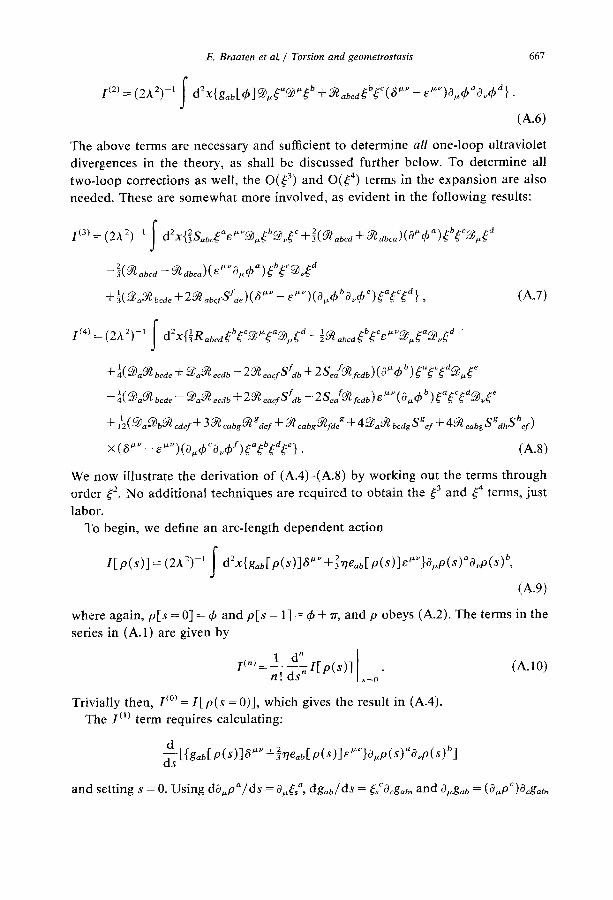
E. Braaten et al. / Torsion and geometrostasis 667
[ ( 2 ) = ( 2 A 2 ) - 1 f 2 o? a ~* b b c **v ~.v a d
J
(A.6)
The above terms are necessary and sufficient to determine all one-loop ultraviolet
divergences in the theory, as shall be discussed further below. To determine all two-loop corrections as well, the O(~ :3) and O(~ :4) terms in the expansion are also needed. These are somewhat more involved, as evident in the following results:
I ~ 2 r 2 c , ~ a p.~,,'~ ~-b&,~ .,-c 2 0 ~/* a b c d i ( 3 ) = ( 2 A 2 ) I a x l S a . b c g e ~ . g ~'~g +5(~abcd+.q labca) (O 4) )'~ ~ ~ . ~
2 0 /xp~ a ' b c d - - X ( O ~ a b c d - - ~ d b c a ) ( e Ot~ff) )~ ~ ~ v ~
_b~(~,~lbed_k2~.g,=befSfe)((~t*,, ~*,, b e a c d - e )(O~& 0~q~ )£ s ~ ~ }, (A.7)
i(4) (2A2)-~f 2 1 b co21.t ao~ d 1, b c p.u a d '
..[_ 1( ~al . ~ bede -k. C~@a,.~ ecdb -- 2 O0~ e a c f S f b -t- 2 Se /O~fcdb) (O~4) b) ~a~c~dc@p " ( e
_7,(~¢~l~,bcct ~aOO~cdb + 2 ~ e a q f S f b _ _ 2 S ~ f c a b ) u" ( O ~ b )~ a ~ c ~ d ~ , ~ e
+ ~ (Do ~b~ ~der + 3 ~ cabs ~ gdef "~- ~ cabs ~fde g ~- 4 @ ~ bcdg S ge¢ "~- 4 .°~ cobs S gdh S her)
x (8 ~" - eU")(a.dpco.~/)Seo~b~dff}. (A.8)
We now illustrate the derivation of (A.4)-(A.8) by working out the terms through order s ~2. No additional techniques are required to obtain the ~3 and ~:4 terms, just
labor. To begin, we define an arc-length dependent action
I[p(s)] = ( 2 1 2 ) - ' ( d 2 X { g a b [ p ( S ) ] S t * ~ + 2 r l e a b [ p ( s ) ] e " ~ } O * * p ( s ) a O ~ p ( S ) b,
(A.9)
where again, p[s = 0] = & and p[s = 1] = 4' + rr, and p obeys (A.2). The terms in the
series in (A.1) are given by
a° [ 1(~) = 1 ds" I[p(s)] . (A.10)
s ~ 0
Trivially then, I(O)= I [p(s = 0)], which gives the result in (A.4). The I °) term requires calculating:
~Ts[{gab[P(X)ja~**, ~ " t* . . . . b +~rleab[p(s)]e }Oup(s) O,p(s) ]
and setting s = 0. Using dOupO/ds = 0~,~ °, dg~b/dS = ~seOcgab, and O,g~b = (O~,P~)O~gab,
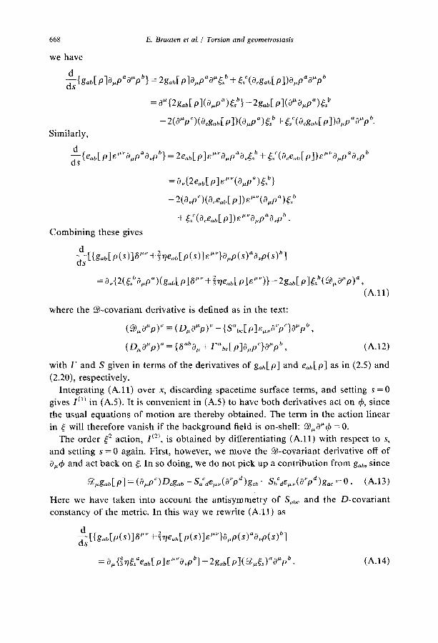
6 6 8 E. Braaten et aL / Torsion and geometrostasis
we have
d {g~b[ P]O~PaO" P b} = 2gab[ p ]O~p"c~" ~ b + ~,~(a~gab[ p])O~paa" p b
= a" {2gob[ p](O,p ~)¢s b} -- 2g~b[ p] (a"a ,po)¢ f -
- 2(O'p~)(o~gab[ p])(O,p~)¢, b + ¢,~(Ocgob[ p])O,p%~'P b. Similarly,
d pie o~p o~p 1=2e~b[p]e O~p O~s ~s (o~e~b[p])e O,p O,p
= O.{2e~b[p]e'*~(O.pa)g b}
- - 2(O.p~)(O~eab[ p])e'*~(O,.p°)g b
+ g~(O~eab[ p]) e'*%.p"O~p b •
Combining these gives
d +~)eob[p(s)]e }O,,p(s) O,p(s) ]
b ~ a p..v 2 =0,,{2(~ O~p )(gab[P]fi +X'rleab[p]e"")}--2gob[P]~b(~.O~P) a, (A.11)
where the ~-covar iant derivative is defined as in the text:
( ~ O ~ p ) ~ =_ ( DuO~ p ) ~ - { Sabc[ p ]e~O~pC}O" pb ,
( D u O" p) a =-- { (5 abO, + Fabc[ p]Oup c}O"p b, (A. 12)
with F and S given in terms of the derivatives of gab[P] and eab[p] as in (2.5) and (2.20), respectively.
Integrating (A.11) over x, discarding spacetime surface terms, and setting s = 0 gives I (1) in (A.5). It is convenient in (A.5) to have both derivatives act on 6, since the usual equations of motion are thereby obtained. The term in the action linear in ~ will therefore vanish if the background field is on-shell: ~,0"4~ = 0.
The order ~2 action, I (2), is obtained by differentiating (A.11) with respect to s, and setting s = 0 again. First, however, we move the ~-covar iant derivative off of 0,4, and act back on ~. In so doing, we do not pick up a contribution from gab, since
~ g a b [ P] ~ (o~pC)Dcgab -- SaCde, v(oVpd)gcb -- SbCde,~,(O"pd)gac = 0 . (A.13)
Here we have taken into account the antisymmetry of Sab~ and the D-covariant constancy of the metric. In this way we rewrite (A.11) as
d "~ ~ p ( s ) ] ~ }o.p(s) pop(s) ] ~-s [ {g .b[p ( s ) ] t~ + 5 " q e ~ b [ "~ a b
- 4 a I ~ ' b a ~ l z b 2 g a b [ P ] ( ~ . ¢ s ) 0 p . =0,{~7~:~ eob[p]e O~p }+ (A.14)
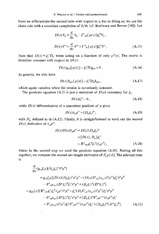
E. Braaten et al. / Torsion and geometrostasis 669
Next we differentiate the second term with respect to s, but in doing so, we use the
chain rule with a covariant completion of d / d s (cf. Boulware and Brown [10]). Let
D(s ) V~ ~ d Va - r ~ b [ p ( s ) ] ~ s b V c ,
D(~) V o = _ d v o o ~ ds + F b~[p(s)](~ V . (A.15)
Note that D ( s ) = - ~ D ~ when acting on a function of only pb(s) . The metric is
therefore constant with respect to D(s) :
D(s)g~b[ p(s)] = ~,~P~g,,b = 0. (A.16)
In general, we also have
D(s)Sabc[ p(s) ] = ~sdDdSabc, (A.17)
which again vanishes when the torsion is covariantly constant. The geodesic equation (A.2) is just a statement of D( s ) constancy for ~s-
O(s)~s a = 0 , (A.18)
while D(s ) differentiation of a spacetime gradient of p gives
D(s)O~p a = (D~sCs) ° , (A.19)
with D~ defined as in (A.12). Finally, it is straightforward to work out the second D(s ) derivative of O~pa:
D ( s ) D ( s ) O . p ~ = D( s ) (D .~s ) ~
= [D(s ) , D.]~s ~
"= Rabcd~sb~sC(O,o.p d ) , (A.20)
where in the second step we used the geodesic equation (A.18). Putting all this together, we compute the second arc-length derivative of I [ p (s)]. The relevant term is
d ~ss{gab[ P ]( ~,~s)aO~ P b}
= gab[ P]{D(s)(D~(~)aO~P b -- (D(s)Saca)e~,,(O~P d )~seoUp b
= gab[ P]{R°cd~'~sdOj.P~OuP b -- "~f(O~Sa¢d)e~(O~pd)~.~O"P b
-- Saedeu,.( D"~s)d~sCOU pb -b ( D.~x)~Sb~deu"(O~.pd)~f
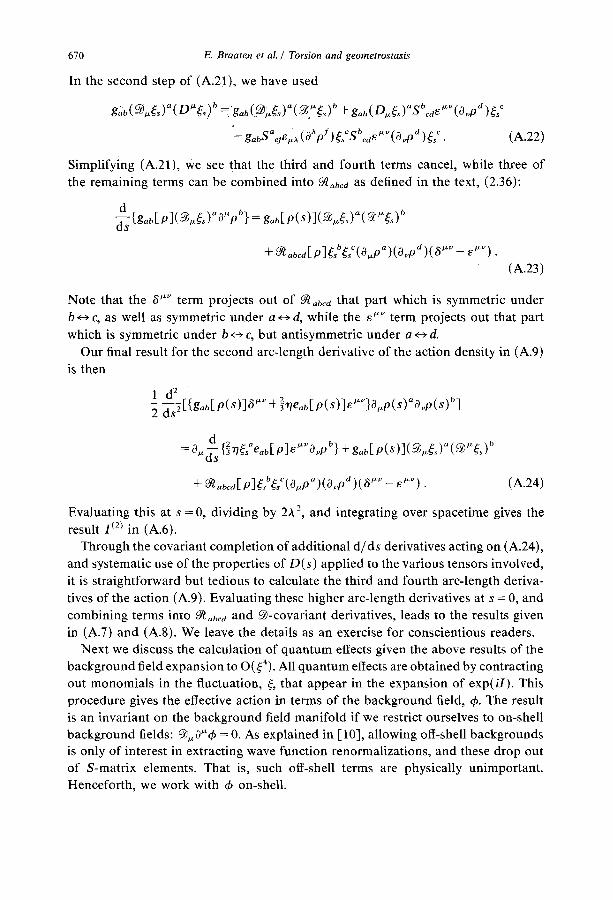
670 E. Braaten et aL / Torsion and geometrostasis
In the second step of (A.2!), we have used
-- gabSaefl~ ~X ( O;~pf ) ~seSbcds~" ( o~p d ) ~s c . (A.22)
Simplifying (A.21), We see that the third and fourth terms cancel, while three of
the remaining terms can be combined into ~abcd a s defined in the text, (2.36):
d G { g a b [ P ]( ~ s ) a ~ P b} = gob[ P( S ) ]( ~ s ) a ( ~,*~,)b
q- ~ abcd[ p ]~sb ~sc ( o ~pa)( c~vpd )( ~ I~*" -- El~') .
(A.23)
Note that the ~ term projects out of ~b~a that part which is symmetric under b ~ c, as well as symmetric under a ~ d, while the e ~'~ term projects out that part which is symmetric under b ~ c, but antisymmetric under a ~ d.
Our final result for the second arc-length derivative of the action density in (A.9) is then
1 d 2 p(s)]3 +~ne~b[p(s)]e }0~p(s) Gp(s) ] ds2[{g~b [ ~ 2 ~ ~ ~ b
2
d 2 o ~ b
+ .~b~d[ P]GbG~(O,P°)(OpP a)(8~ -- e ~ ) . (A.24)
Evaluating this at s = 0, dividing by 2A 2, and integrating over spacetime gives the
result I ¢2) in (A.6). Through the covariant completion of additional d/ds derivatives acting on (A.24),
and systematic use of the properties of D(s) applied to the various tensors involved, it is straightforward but tedious to calculate the third and fourth arc-length deriva- tives of the action (A.9). Evaluating these higher arc-length derivatives at s = 0, and combining terms into ~,~b~d and @-covariant derivatives, leads to the results given in (A.7) and (A.8). We leave the details as an exercise for conscientious readers.
Next we discuss the calculation of quantum effects given the above results of the background field expansion to O(~4). All quantum effects are obtained by contracting out monomials in the fluctuation, ~, that appear in the expansion of exp(iI) . This procedure gives the efiective action in terms of the background field, b. The result is an invariant on the background field manifold if we restrict ourselves to on-shell background fields: @~,3~'b = 0. As explained in [10], allowing off-shell backgrounds is only of interest in extracting wave function renormalizations, and these drop out of S-matrix elements. That is, such off-shell terms are physically unimportant. Henceforth, we work with ¢b on-shell.
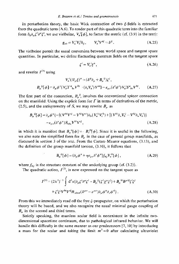
E. Braaten et aL / Torsion and geometrostasis 671
In perturbation theory, the basic Wick contraction of two so-fields is extracted from the quadratic term (A.6). To render part of this quadratic term into the familiar form 6 o a , ~ O ~ i, we use vielbeine, V,~[4,], to factor the metric (cf. (3.9) in the text):
gab : V a i W ~ i j , Va iVaj : 8ij" (A.25)
The vielbeine permit the usual conversion between world space and tangent space quantities. In particular, we define fluctuating quantum fields on the tangent space
and rewrite /(2) using
,~'= V~'~ :~ , (A.26)
W ( ~ . ¢ ) ° = ( a % . + B / ) C j,
B,.°[ 4,] = a.4, ~{ V ~ T % V ~j - ( a~ V~') v ° j } - ~ . . ( a"O ~) Vo'S% V ~ . (A.27)
The first part of the connection, B S , involves the conventional spinor connection on the manifold. Using the explicit form for F in terms of derivatives of the metric, (2.5), and the antisymmetry of S, we may rewrite B. as
B.-'i[4,] --2-:,'°~-'-:~:~'~:~J~ 2 ~ - - - VbJV~')~.( V~V~)+½( V % o W - V%o Vj)}
--e~..( O" 4,'~) S,~b~ Vh~ W j , (A.28)
in which it is manifest that Buq[4,] = - B f [4 , ] . Since it is useful in the following, we also note the simplified form for B u in the case of general group manifolds, as discussed in section 3 of the text. From the Cartan-Maurer equations, (3.13), and the definition of the group manifold torsion, (3.10), it follows that
BS[4,] = (o,~4, ° + n~,..a"4,a}f, uvo~[4, ] , (A.29)
where fkj is the structure constant of the underlying group (cf. (3.2)). The quadratic action, I (2), is now expressed on the tangent space as
f 2 i.tz i ij i tz j I (2) = (2A 2)-, d x{O.~ o ~ - B. (~ ~ ¢ ) + BukiBUk:(~J
+ ~'~U V"' V " ~ ~hcd(6"" -- e~')0~4, ~0.4, d }. (A.30)
From this we immediately read off the free ~'-propagator, on which the perturbation theory will be based, and we also recognize the usual minimal gauge coupling of B~ in the second and third terms.
Strictly speaking, the massless scalar field is nonexistent in the infinite two- dimensional spacetime continuum, due to pathological infrared behavior. We will handle this difficulty in the same manner as our predecessors [7, 10] by introducing a mass for the scalar and taking the limit rn2~0 after calculating ultraviolet
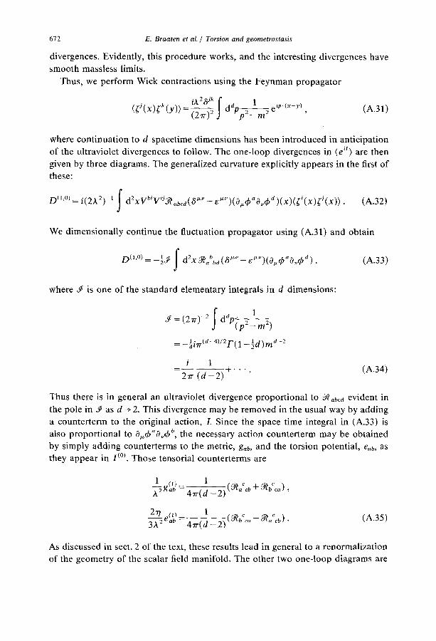
672 E. Braaten et al. / Torsion and geometrostasis
divergences. Evidently, this procedure works, and the interesting divergences have smooth massless limits.
Thus, we perform Wick contractions using the Feynman propagator
ih 2 t~jk (~J(X)~k(y)) = ~ I d d p ~ e ip'(x-y) , (A.31)
where continuation to d spacetime dimensions has been introduced in anticipation of the ultraviolet divergences to follow. The one-loop divergences in (e ~) are then given by three diagrams. The generalized curvature explicitly appears in the first of these:
DO,O~ i(2A2) I f d2xVbivcJ~tabcd(rt~, ~. a d i j = - e )(0.q~ 0.6 )(x)(~ (x)~" (x)) . (A.32) 3
W e dimensionally continue the fluctuation propagator using (A.31) and obtain
= d xYG ba(3 --e ) (0 .6 0~6 ) . (A.33) J
where .~ is one of the standard elementary integrals in d dimensions:
t = (2'n') -2 f a • 1 d p - ( p 2 - m 2 )
=_~izr (a-4) /2F( 1 1 . , d-2 • - - ~ a ) r n
i 1 - - - J r . . . . (A.34)
27r ( d - 2 )
Thus there is in general an ultraviolet divergence proportional to ~ obca evident in the pole in 5 ~ as d -* 2. This divergence may be removed in the usual way by adding a counterterm to the original action, I. Since the space time integral in (A.33) is also proportional to 0~6a0.6 b, the necessary action counterterm may be obtained by simply adding counterterms to the metric, gab, and the torsion potential, eab, as they appear in I (°). Those tensorial counterterms are
1 rl) 1 o~ c ~-7_ ghb -- 47r(d - 2) (~°~cb + °~b co),
3~e~b) = 1 ~ c _~occb) (A.35) 4 r r ( d _ 2 ) ( boo •
As discussed in sect. 2 of the text, these results lead in general to a renormalization of the geometry of the scalar field manifold. The other two one-loop diagrams are
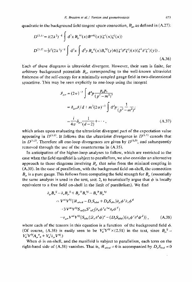
E. Braaten et al. / Torsion and geometrostasis 673
quadratic in the background field tangent space connection, B., as defined in (A.27):
D<I.1) = i(2A2)-' y d2x
= ½i2(2 A 2)-2 _f d2x _f d2y B f f ( x ) B f , ( y ) 4 ( ( f , O , C Q ( x ) ( ; k o ~ , ) ( y ) } . D(I,2)
(1.36)
Each of these diagrams is ultraviolet divergent. However, their sum is finite, for arbitrary background potentials B,, corresponding to the well-known ultraviolet finiteness of the self-energy for a minimally coupled gauge field in two-dimensional spacetime. This may be seen explicitly to one-loop using the integral
o¢~, (277") -2 [ P~P~ d e - = F (p2 __ m2)2
=6~.~5~/d+m2(2rr) -2 dap(p2_m2)2
i 1 = 4--£ au~0--~-2) + ' ' " (1.37)
which arises upon evaluating the ultraviolet divergent part of the expectation value appearing in D °'2). It follows that the ultraviolet divergence in D (k~) cancels that in D (~a). Therefore all one-loop divergences are given by O (l'°), and subsequently removed through the use of the counterterms in (A.35).
In anticipation of the higher-loop analyses to follow, which are restricted to the case when the field manifold is subject to parallelism, we also consider an alternative approach to those diagrams involving B~. that arise from the minimal coupling in (A.30). In the case of parallelism, with the background field on-shell, the connection B, is a pure gauge. This follows from computing the field strength for B, (essentially the same analysis is used in the text, sect. 2, to heuristically argue that qSis locally equivalent to a free field on-shell in the limit of parallelism). We find
O,B, U - O~B S + B 'kB~ kj - B,,ikB kJ
= vaivbJ{~ab~a - D~S.ba + DclSabc}O.~)co~ a
- 3 vaivbJSae[bSeed](Oxt~cs;tPOp~) d)
--e,~VaiVbJ{S~b~(N~O~cb)~--(D~S~bd)(Oa4)~O'~chd)}, (A.38)
where each of the tensors in this equation is a function of the background field &. (Of course, (A.38) is easily seen to be v jvb~×(2 .51) in the text, since B f f = VjVbJAgb + V~'aj, v~J.)
When 4) is on-shell, and the manifold is subject to parallelism, each term on the right-hand side of (A.38) vanishes. That is, ~b~d = 0 is accompanied by D~Sb~d = 0
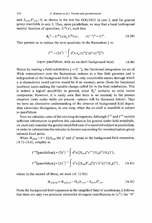
674 E. Braaten et al. / Torsion and geometrostasis
and S~,etbS~cal = 0, as shown in the text for 0 ( 4 ) / 0 ( 3 ) in sect. 2, and for general group manifolds in sect. 3. Thus, upon parallelism, we may find a local (orthogonal matrix) function of spacetime, UO(x), such that
B, fl= Uk~(X)O. UkJ(X), (U- ') U= U s'.
This permits us to reduce the term quadratic in the fluctuation ~ to
(A.39)
f 1(2)= (2A2) - ' J d2x 0,( U°~J)O~'( u'k¢ k)
(upon parallelism, with an on-shell background field). (A.40)
Hence by making a field redefinition ¢--~ U-l¢, the functional integration (or set of Wick contractions) over the fluctuations reduces to a f r ee field gaussian and is independent of the background field qS. The only conceivable means through which a qS-dependence could survive would be if an anomaly arose (from the functional jacobian) upon making the variable change called for in the field redefinition. This is indeed a logical possibility in general, since B,, ° contains an axial vector component. However, it is easily seen that there is no anomaly in the present situation (only scalar fields are present -sp inors will be discussed below). Thus we have an alternative understanding of the absence of background field depen- dent ultraviolet divergences, to one loop, when the on-shell ~b manifold is subject to parallelism.
Next we calculate some of the two-loop divergences. Although i(s) and 1 (4) contain sufficient information to perform this calculation for general scalar field manifolds, we shall only consider the greatly simplified case of a manifold subject to parallelism, in order to substantiate the remarks in the text concerning the renormalization group infrared fixed point.
When ~ abca = 0 = DaSbca, the ¢3 and ¢4 terms in the background field expansion,
(A.7)-(A.8), simplify to
I(3~[parallelism] = ( 2 ~ 2 ) - ' f d2x{2S"b~¢'~e'~(~.¢)b(~"~)~}'
I(4)[parallelism] = (2A2) - ' f d2x{½Sf~bS~a¢b¢~(®'¢)~(N. ¢)a}' (A.41)
where in the second of these, we used (cf. (2.36))
(A.42)
From the background field expansion in the simplified limit of parallelism, it follows that there are only two pertinent ultraviolet divergent contributions to (eit): the "0 "
E. B r a a t e n e t a L / T o r s i o n a n d g e o m e t r o s t a s i s 675
and "oo" diagrams. Those two diagrams correspond respectively to
D(2,,)=ki~(2A~)-~ f d2x f d2y~S~b~(x)Saef(Y)
a tzuO- i b c d OGG e f , x((¢ ~ ~,A: ~,g: )(x)(¢ e ~ ¢ ~,4 )(>)),
i(2A2) -1 f d2x ~Sf~bSY~d(¢b¢~'£~a). (A.43) D(2,2) =
The expectation values in (A.43) may be evaluated by converting to fluctuations on the tangent space, using (A.26), (A.27), and by contracting ~"s using (A.31). Ultravio- let divergences appear in the form of the previous elementary integrals, and a few others, such as
f a P~ 5t~,(k)=(2~') -2 d pip+k)2 m2
= - k ~ 5 , (A.44)
where k~ is an external momentum supplied by the background field. In addition, ultraviolet divergences appear in the form of overlap integrals. For the "0" diagram, the relevant overlap integral is
5t.~to~l(k) = (2w)-4 f dap daq 3
PD, q~]P[oq~] ((p+k)Z_m2)((p+q)2 m2)(qe=m2),
(A.45)
where again k, is an external momentum supplied by the background field. In fact, we actually encounter e"%o~tEu,]Ep~](k) , whose continuation into d-dimensional spacetime requires a prescription for e~L% p~. We shall use eu"e p===- 6~3 "p -8"P8 ~¢, with 6 the d-dimensional Lorentz metric. (It turns out that the final two-loop conclusions are not affected by the choice for this e- product.) Evaluating the resulting double trace of (A.45), we find
1 0 - 7 d ~, 2 (6~8~P-8~6v~)5~[~][p~j(k) ~ k~,k ~ +O(m2)+{finiteas d ~ 2 } . (A.46)
Putting everything together, we finally obtain
1 0 - 7 d I @~S~b~@ S + O ( m - ) + { f i m t e a s d ~ 2 } D(2a)= 36d I2(2A2) d2x u abe 9 • ,
D (2'2) = O(m 2) + {finite as d -+ 2}. (A.47)
These results are quoted and used in sect. 2 of the text (where we took the liberty to set d = 2 in the coefficient (lO-7d)/36d, and to drop the terms which are either ultraviolet finite or vanish as m2~ 0). As stressed in the text, the integrand in (A.47)
676 E. Braaten et al. / Torsion and geometrostasis
vanishes upon parallelism, and hence the model is ultraviolet finite to two-loop order, when the on-shell background field manifold is subject to parallelism. Some remarks about the minimal coupling terms in I (2) may be useful before continuing. First, the two-loop diagrams resulting from such terms alone again give a net contribution which is ultraviolet finite, for an arbitrary background B~. As in the one-loop case considered above, this may be seen by direct inspection of those diagrams. Alterna- tively, when the manifold is on-shell and subject to parallelism, the pure gauge character of B, may be used to dismiss those two-loop diagrams by again making the field redefinition discussed following (A.40). In fact, the pure gauge form for B~, (A.39), is also technically convenient to show that the derivatives acting on Sabc in the integrand of (A.47) are @'s. This follows from again changing variables to U~', which leaves an extra factor of U -~ multiplying S. The ultraviolet divergent terms in the "0" diagram then produce ordinary derivatives which act on U-tS. Applying the chain rule to a(U-~S) yields the factors of @S as given in (A.47).
Our next goal is to consider how spacetime spinors affect the renormalization of the model. To achieve that goal, it is sufficient to view spinor fields ~b as quantum fluctuations o n l y - n o background spinor field will be necessary. Proceeding in a fashion analogous to the scalar field case, we transport spinors along geodesics:
d q, a (x ; s ) + r . . . . b - - x D(s)Oa(x; s) =- bckPl~js ~u b'; S) = 0 , (A.48) ds
where ~fl is the local tangent to the curve, (A.3). Note that here one could add a torsion to F and obtain a nontrivial modification, unlike the original geodesic case, (A.2).
We now introduce an arc-length dependent spinor action patterned after the spinor component of the supersymmetric action, (5.8). Define ~ b ( s ) as in (A.12) and let
[~,[p(s), O(s)] = (2A2) - ' f d 2 x { i g a b [ p ] ¢ a ( s ) ( T ~ t ~ b ( s ) ) b
+½~b~d[p]~a(s)(1 + yp)qf(s)~b(S)(1 + 3Jp)qjd (S)}
- - f ( o) 4-1( ~ ) ~ I ( 2 ) - a - . . .
where the nth term in the series is given by
(A.49)
Note that it is sufficient for two-loop ultraviolet divergence calculations to know the expansion in (A.49) through r(2)
l(o) The first term in the expansion, ~;~ , serves to define the spinor propagator, and contributes to one- and two-loop divergences. Converting to tangent space spinors
ds ~ I~[ p(s), ~(s)] (A.50) s = O
E. Braaten et al. / Torsion and geometrostasis 677
(at s = 0)
X ~ =- Vjq, a , (A.51)
and using the connection B~,, in (A.27), we obtain
( 2A2)-1 f d2x{ixjy~(tVka. +Bfk)X k i(o) 4, =
+ ~,,b~a Va'VbJVCkV"~'(1 + VP)Xk~(1 + Ye)~('} • (A.52)
Consequently, we take the dimensionally continued, tangent spinor propagator to be
i3"28jk f ddp "Y~*P~ +-~. e ip'(x-y) , (A.53) (XJ(x)xk(Y))=-(27r)~ j p2 _ m ~
into which we have also introduced a mass, not because it is necessary in this case, but simply to parallel the above treatment of ~'. After extracting ultraviolet divergen- ces, we always let m2-~0.
The only possible ultraviolet divergent spinor contributions to the one-loop effective action are given by
O(1,3)=~i2(2A2)-2 f d2x f d 2 y i B S k ( x ) i B " l m ( y ) ( ( x J T ~ x k ) ( x ) ( x t T ~ X m ) ( Y ) ) "
(A.54)
Contracting the spinors leads to the integral (with k external momentum)
f ddp Tr [y~,(ya(p + k)a + m)y~(y~p~ + m)] ((p + k) 2 - rnZ)(p 2 - m z)
= T r [1] f dap ( ( p + k) 2 _ m2)(p2 - m2 ) +{finite as d -+ 2},
which is seen to be finite as d-+2 using (A.37) and (A.34). Thus D (1"3~ is ultraviolet finite for arbitrary B,,, and there are no one-loop divergences due to spinor diagrams.
When the background scalar field is on-shell and the ~b-manifold is subject to parallelism, some additional insight into the diagrams arising from the minimal coupling of the spinors to B~, can be gained as before in the scalar field case. Since there is no spinor background to clutter up the &-equations of motion, we still have ~,0~*tb == 0 on-shell, and upon parallelism, we again have a pure gauge form for B~,, as in (A.39). Thus we may write
= (2A 2) I f d2x i( uJk~k)~ltXOix( uJlx l) I(O) +
(upon parallelism, with an on-shell background field). (A.55)
Upon changing variables, X--> U-'X, there would again be no remnant of the background & after integrating over the tangent spinor, except possibly through
678 E. Braaten et al. / Torsion and geometrostasis
anomalies in the jacobian. Unlike the scalar field case, however, here there is an anomaly, so we mus tgo one step further and consider its effects. Fortunately, the anomalous effects can be calculated exactly when the connection is a pure gauge (i.e. the functional determinant called for in evaluating (e w~') can be calculated exactly, cf. Polyakov and Wiegmann [3], Alvarez [6] and Nepomechie [6]). The anomalous dependence on the background field turns out to be ultraviolet finite. In fact, the anomaly vanishes when "O = ±1 by virtue of the self-duality of B~, (A.29).
To carry out an explicit two-loop calculation of spinor effects on ultraviolet divergences, we require ~¢~(1) and ,¢r(2). These are obtained by computing first and second arc-length derivatives of I~,[p(s), ~(s)]. In computing these, we use the chain rule with the covariant completion of d / d s given in (A.15). Employing earlier results, (A.16)-(A.20), we have
D(s) (D~O(s) ) ~ : [D(s), D~]O(s) ~
= Rabcd[ p]~b(s)b~f(O~,pd), (A.56)
where (A.48) was also used. Similarly, using (A.17) and (A.19),
D(s ) ( ~ . O ( s ) ) a = Rabcd [ p]qJ(S)b~(O.p d ) -- S%c[ p] q'(s)be~.( D " ~ ) ~
-- ( DdSabc[ p ]) ~( s )be~u( ovpc)~sd. (A.57)
All the required two-loop information is at hand if we now differentiate this result once more, using the previously given results for D(s) acting on the individual tensors:
(D(s))2(@.th(s)) ~ = ( O ~ R % c a [ p ] ) ~ ( s ) b ~ ( O . p d) + R%~d[ p J O ( s ) b ~ f ( D ~ ) d
-- ( DaS%~[ p J) f~dO( s )be. . ( D~¢~) ~
-- Sabc[ p ]O( s)bRCdef[ p]~sd~se( e~uO*'p f )
- (D~DaSab~[ p])O(s)be~,.(.a"p~)es~d~ e
-- ( DdS%~[p ])tp( s )be,,~( D"¢~)~ d . (A.58)
Incorporating these derivatives (at s = 0) into (A.49) and (A.50), and using the D(s) constancy of ~o and 0"(s) , gives the ingredients for a two-loop calculation of ultraviolet divergences due to spinors on a general &-manifold:
(212)-' f d2x{igob[ C~ ]t~ay~( P ( s ) ~ t ) ( S ) ) b l ' ~ ° i(1)__. ,],
+-~sc~ (De~.b~d[qS]) d~ (1 + Te) ~b~qTb(1 + Te)Oa},
-= ( 2 A 2 ) - ' f d2x{½igab[tb]t~aT" (D(s)2~.O(s))bI~:=o i{2)
+ ~ / J ( D f D ~ . b : ~ [ ~ ] ) O " ( 1 + ye)O{'4;b( 1 + yp)0~} • (A.59)
E. Braaten et aL/ Torsion and geometrostasis 679
For our purposes here, it suffices to consider these terms only when the &manifold is subject to parallelism. In that case, we have ~b~d =0 (cf. (2.36)), as well as D~b~d~ = DaRb~d~ = D~Sb~a = 0 (cf. (2.19)). In addition, we have the Jacobi identity for the torsion, (2.18). Utilizing these simplifications and the definition of @,, we reduce the first and second arc-length derivatives in (A.59) to obtain the following:
f 9 " O~ " a /~v- --b c I~l)[parallelism]=(2A2)-I d-xSabc[dp](u~o.¢) g l(@ "Yv@ ) ,
f 9 1 f a b- --c pL d I~[paral le l ism]=(2A 2) ~ &x~S~b[Cb]S~df[~]¢ ( ~ ¢ ) t ( d ~ y 4' )- (A.60)
It follows from these results for -+t~) and I~, "-) that there is only one possible ultraviolet divergent two-loop spinor diagram upon parallelism: the spinor/scalar " 0 " obtained
- ( D from having two 1~ vertices:
D(2,3)_ l;2/r(ur(1)\ (A.61)
All other conceivable two-loop contributions are easily seen to be ultraviolet finite (the spinor/scalar "oo" diagram vanishes trivially). Again we evaluate the Wick contractions in (A.61) by converting to tangent space fluctuations, ~ and ~(.
The actual evaluation of D ~2̀a~ is immediately simplified by using the parallelism result, ~S~b~ = 0 (cf. (2.59)) before Wick contracting. Integrating by parts in 1t~ ~ttb ,
we then obtain
I(~t)[parallelism] =-2i(2A=) -a ~ d2x Sabc~a~bypy~t(~la.~)c. (A.62) d
We also used e~%,(@vtp)c=-ypy~(@~O) c (although, as in the case of the ee product used earlier, this step can tolerate some modification without changing the eventual conclusions). In the case of parallelism, the diagram of interest then becomes
D(2"3)=2(2A2)-2fd2xfd2ySabc(X)SdefO ')
x ((~alffb'ypy~'~t,t~C)(x)(~dtffeTp3/~q/) (y)). (A.63)
The tangent space contraction procedure now leads to the integral
f Tr [ypy'p~,(y~p~ + m)ypyPqo(y'~q,~ + m)] ddpddq (p2 m2) ( (q_p+k)2 m2)(q2 m 2)
= O(m z) + {finite as d ~ 2}. (A.64)
Therefore, the spinor/scalar "0" diagram is also ultraviolet finite when the manifold is subject to parallelism.
680 E, Braaten et aL / Torsion and geometrostasis
Finally, we note that, as discussed before, the effects of the minimal B, couplings can be most easily taken into account by using the pure gauge form in (A.39). In view of the previously cited anomaly studies, such couplings do not produce any spurious ultraviolet divergences upon parallelism.
In summary for this appendix, we have used the background field expansions to show that two-dimensional sigma models with Wess-Zumino terms have no
on-shell ultraviolet divergences through two-loop order upon parallelism. Our analysis
has included the supersymmetric case as well as the purely bosonic sigma model. As discussed in the text, we expect this ultraviolet finiteness to persist to all higher orders of perturbation theory.
Appendix B
HOMOLOGY THEORY AND WESS-ZUMINO TERMS
A generalized nonlinear sigma model is a field theory in which the field &(x) takes its values on some manifold, M. Both compact and noncompact manifolds are of interest in physics [7]. A Wess-Zumino term is a term in the action whose coefficient must be an integer in order to have a well-defined quantum theory. Such a term is possible only if the manifold M has a nontrivial (d + 1)th homology class, where d is the dimension of spacetime. The dth homology classes of the manifold are also important because they can provide further restrictions on the integer-valued
coefficient of the Wess-Zumino term, and they can introduce arbitrary parameters into the Wess-Zumino term.
In this appendix, we explain the relation between homology and Wess-Zumino terms. We first review the basic concepts of integer homology and DeRham cohomology (a more thorough review may be found in [11]). We then discuss the construction of action terms using ditterential forms, including the special case of Wess-Zumino terms. We show that each of the fundamental forms in the (d + l) th DeRham cohomology class defines an independent Wess-Zumino term. We show that the presence of torsion subgroups in the dth homology class further restricts the integer coefficients of a Wess-Zumino term to be multiples of some integer p. We also show that every torsion-free subgroup of the dth homology class corre- sponds to an arbitrary constant in the definition of the Wess-Zumino term. Finally, we illustrate these points using simple examples, and briefly summarize our results.
We assume that the concept of a manifold is familiar. A subset of a manifold which is itself a manifold is called a submanifold. I f C is a k-dimensional submani- fold, its boundary is denoted by 0C, and is a ( k - 1)-dimensional submanifold. The boundary of a boundary is always zero: 02 = 0. I f the boundary itself is zero, 0C = 0, then C is called a k-cycle. The term "cycle", which we will use frequently, is in fact just a shorthand for "submanifold with no boundary" . Linear combinations of cycles with integer coefficients are also defined to be cycles. In our discussion, we will not
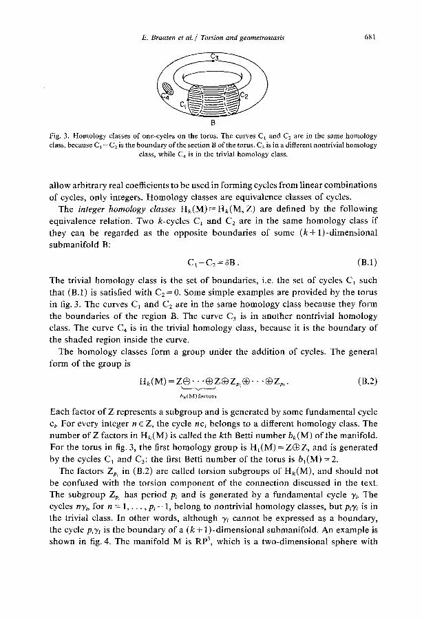
E. Braaten et al. / Torsion and geometrostasis 681
B
Fig. 3. Homology classes of one-cycles on the torus. The curves C1 and C2 are in the same homology class, because C 1 - C 2 is the boundary of the section B of the torus. C 3 is in a different nontrivial homology
class, while C4 is in the trivial homology class.
allow arbitrary real coefficients to be used in forming cycles from linear combinations
of cycles, only integers. Homology classes are equivalence classes of cycles.
The integer homology classes Hk(M)---Hk(M, Z) are defined by the following
equivalence relation. Two k-cycles C~ and C2 are in the same homology class if
they can be regarded as the opposite boundaries of some (k+l ) -d imens iona l
submanifold B:
C~ - C2 = 0B. (B.1)
The trivial homology class is the set of boundaries, i.e. the set of cycles C~ such
that (B.1) is satisfied with C2 = 0. Some simple examples are provided by the torus
in fig. 3. The curves C~ and C2 are in the same homology class because they form
the boundaries of the region B. The curve C3 is in another nontrivial homology class. The curve C4 is in the trivial homology class, because it is the boundary of
the shaded region inside the curve.
The homology classes form a group under the addition of cycles. The general
form of the group is
Hk(M) = Z Q . • -OZ@Zp~@. • .@)Zp,. (B.2)
b k (M) factors
Each factor of Z represents a subgroup and is generated by some fundamental cycle
ci. For every integer n c Z, the cycle nci belongs to a different homology class. The number of Z factors in Hk(M) is called the kth Betti number bg(M) of the manifold.
For the torus in fig. 3, the first homology group is H~(M) = Z ® Z , and is generated
by the cycles C~ and C3: the first Betti number of the torus is b t (M)= 2.
The factors Zp, in (B.2) are called torsion subgroups of Hk(M), and should not be confused with the torsion component of the connection discussed in the text.
The subgroup Zp, has period Pi and is generated by a fundamental cycle yi. The cycles nyi, for n = 1 , . . . , p~ - 1, belong to nontrivial homology classes, but Pi% is in the trivial class. In other words, although ~ cannot be expressed as a boundary,
the cycle Pc% is the boundary of a ( k+ 1)-dimensional submanifold. An example is shown in fig. 4. The manifold M is RP 3, which is a two-dimensional sphere with
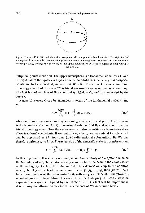
D
E. Braaten et aL / Torsion and geometrostasis 682
Fig, 4. The manifold RP 3, which is the two-sphere with antipodal points identified. The right half of the equator is a one-cycle C which belongs to a nontrivial homology class. However, 2C is in the trivial homology class, because the boundary of the upper hemisphere D is the complete equator which is
equal to 2C.
ant ipodal points identified. The upper hemisphere is a two-dimensional disk D and
the right hal f of the equator is a cycle C in the manifold. Remember ing that ant ipodal
points are to be identified, we see that 0D = 2C. The curve C is in a nontrivial
homology class, but the curve 2C is trivial because it can be written as a boundary .
The first h o m o l o g y class o f this manifold is H 1 ( M ) = Z2, and it is generated by the
curve C.
A general k-cycle C can be expanded in terms of the fundamenta l cycles ci and
yi:
b k ( M ) 1
C = V, nici+ 5 ~ rn,y,+ 0Bo, (B.3) i ~ t i ~ l
where n~ is an integer in Z, and m~ is an integer between 0 and pi - 1. The last term
is the b o u n d a r y o f some ( k + l ) -d imens iona l submanifo ld Bo and is therefore in the
trivial h o m o l o g y class. N o w the cycles rn~% can also be written as boundar ies if we
allow fractional coefficients. I f we multiply rn~7~ by p~, we get a trivial k-cycle which
can be expressed as 0Bi for some ( k + l ) - d i m e n s i o n a l submanifo ld B~. We can
therefore write m~y~ = aBJp~. The expansion of the general k-cycle can then be written
b k ( M ) I
C = ~] n~c~+0B, B = B o + ~ ] Bi/p~. (B.4) i - - I i = 1
In this expression, B is clearly not unique. We can certainly add a cycle to it, since the b o u n d a r y o f a cycle is automatical ly zero. So let us determine the exact extent
o f the ambiguity. Each of the submanifolds B~ is defined only up to the addi t ion
o f a cycle. I f p is the least c o m m o n multiple of {1, Pl,- • •, Pt}, then pB will be a l inear combina t ion o f the submanifolds B~ with integer coefficients. Therefore pB is unambiguous up to addi t ion of a cycle. Thus the ambiguity in B can always be expressed as a cycle multiplied by the fract ion l ip . This fact will be important in
determining the al lowed values for the coefficients o f Wess -Zumino terms.
E. Braaten et aL / Torsion and geometrostasis 683
Before discussing cohomology classes, we recall some terminology and basic facts about differential forms. A k-form g2 is said to be closed if its curl vanishes: dO = 0. Of course, the curl of a curl is automatically zero: d 2= 0. The form £2 is called exact i f / 2 = dA for some ( k - 1 ) - f o r m A. It is important that this equation must hold everywhere on the manifold. The well-known lemma of Poincar6 asserts that, if ~2 is closed, the equation X2 = dA can be solved for A in any coordinate patch of the manifold. However, the resulting f2 is exact only if these local solutions can
be patched together into a global solution. Finally, we recall Stokes' theorem, which relates the integral of an exact form over a submanifold C to an integral over the boundary of C:
fcdo--faco. (B.5)
The DeRham cohomology classes Hk(M, R) are equivalence classes of closed k-forms. Two such forms .O1 and 02 are in the same cohomology class if they differ by the curl of some ( k - 1 ) - f o r m A:
~?I - - ~'~2 = d A . (B.6)
A differential form which belongs to a nontrivial cohomology class must therefore be closed but not exact. The dimension of Hk(M, R) is the Betti number bk(M). DeRham's theorem guarantees that we can find a basis for Hk(M, R) which consists of k-forms o)i, i = 1 . . . . , bk(M), which satisfy
fo wj = a ~, i , j= 1 . . . . , bk(M). (B.7)
where the ci's are the fundamental cycles of Hk(M). We will call the wfsfundamental k-forms. Since ~oj is a closed form, its integral over any boundary is zero by Stokes' theorem. Using the decomposit ion (B.4) for a general k-cycle C, we find that the integral of the fundamental form oJj over any cycle is always an integer:
f ,oj = n j . (B .8 )
I f k = d + 1, each of these bk(M) forms wj is associated with an independent Wess-Zumino term for the nonlinear sigma model in d spacetime dimensions.
The field ~b(x, t) of the nonlinear sigma model maps spacetime R a into the manifold M. By imposing appropriate boundary conditions in space and time, we can make R a topologically equivalent to a manifold with no boundary, such as S d o r s d - l x s 1. The image of spacetime ~b(R d) in the manifold M will then be a
submanifold with no boundary, i.e. a d-cycle. It is then natural to consider action
6 8 4 E. Braaten et al. / Torsion and geometrostasis
terms which are constructed out of a d-form e defined on M. The action term is
f [ ¢ ] = N f ddxe"'"'"dea,...ad[&(X)]O,LCa~(X) "'" " +'~ o.d~ (x)
= N f e,~, ..... [qS] d~b a,-- • d& aa 9 cb(R a )
= N f e. (B.9) J , ( R d )
Because it is constructed out of a differential form, this term depends only on the cycle ~b (R d) in the manifold and not how that region is parameterized by spacetime. This action term is perfectly well defined for any coefficient N. Therefore it is not a Wess-Zumino term.
It is interesting to note that this action term depends only on de and on be(M) real numbers, where bd(M) is the dth Betti number of the manifold. To see this, we apply the general decomposition (B.4) to 6 ( R d) and write the action as
I [ & ] = N ~ n~ e + N de, i = l i B
b a
¢ ( R a ) = E nic,+OB. (B.IO) i = 1
Thus the action depends only on the closed and exact (d + 1)-forms de and on the integrals of e over the ha(M) fundamental cycles ci. These ha(M) numbers do not affect the equations of motion, because a small variation of ~b(x, t) cannot change the homotopy class specified by the integers ni. They are therefore irrelevant in the classical theory. In the quantum theory, they allow us to introduce relative phases into the path integral for configurations which are homologically inequivalent.
We can try to use an expression analogous to (B.10) to define an action using a ( d + l ) - f o r m S which is closed but not exact. Using the same decomposition of &(Ra), we write
b d
I2[(o] = N • n,F[c~]+ NF[OB], i = l
r[oB]= f s, (B.11) B
where F[ci] are arbitrary real numbers. The problem with this expression is that, since S is not exact, the expansion for F[OB] is ambiguous due to the ambiguity in B. Recall that B is well-defined only up to a cycle multiplied by a fraction lip. The ambiguity will be harmless in the quantum theory if we arrange that the ambiguity
E. Braaten et al. / Torsion and geometrostasis 685
in the phase of the path integral is always trivial. This condition is that
exp{iN f~l/p)cS)=l (B.12)
for every (d + 1)-cycle C. To find a solution to (B.12), recall that the fundamental (d + l)-forms w~, j =
1 , . . . , b~+l(M), defined in (B.7) have the property that their integrals over any cycle
C are integer-valued. Thus (B.12) will be satisfied if we choose S = 2¢r% and if N/p is an integer. Each of these choices for S defines a Wess-Zumino term. The number
of independent Wess-Zumino terms is therefore given by the Betti number bd+~(M).
The quantization condition for the coefficients N of a Wess-Zumino term is that
N should be an integer multiple ofp. From (B.11), we see that the ( d + 1)-form S
only determines the Wess-Zumino term for d-cycles in the trivial homology class.
To completely specify the Wess-Zumino term, we must also give its values F[ci] for the fundamental cycles ci. The multiplicity of these arbitrary real numbers is the
Betti number bd(M).
Some good examples are provided by the three-dimensional manifolds S z, S 2 × S 1
and S 1 × S 1 x S ~ in d = 2 spacetime dimensions, which were discussed in sect. 2. For
each of these models, the third homology group is H3(M)--Z. The fundamental
form ~o that we use to construct the Wess-Zumino term is simply the volume element,
normalized so that the manifold has unit volume. The second homology groups are
H2(S 3) =0, H2($2 xS ~) =Z , and H2(S ~ xS ~ ×S ~) = Z • Z O Z . None of these classes
has any torsion subgroups, so the quantization condition for the coefficient of the
Wess-Zumino term is that it be an integer. The Wess-Zumino term for S2xS ~
contains an arbitrary constant which specifies its value for the fundamental 2-cycle.
Similarly, the Wess-Zumino term for S ~ × S ~ x S ~ contains three arbitrary constants.
Let us also consider quantum mechanics on these three manifolds, that is consider the case d = 1. The manifold S 3 admits no Wess-Zumino term, because H 2 ( S 3) -- 0.
The manifold S 2 x S 1, whose second homology group is Z, does have a Wess-Zumino
term. Finally, S 1 x S ~ x S ~ has three independent Wess-Zumino terms, since its second homology group is Z 0 ) Z O Z .
As an example with a torsion subgroup, we will contrast quantum mechanics on R P 3 and S 2. Recall that RP 3 is simply S 2 with antipodal points identified. For both
manifolds, the second homology group is H2(M)= Z. The fundamental form that
we use to construct the Wess-Zumino term is again the volume element, normalized
so that the manifold has unit volume. The first homology group of the two-sphere is HI(S ~) = 0. There are no torsion
subgroups, so the coefficient N of the Wess-Zumino term can be any integer. The manifold M = RP 3 is illustrated in fig. 4. Its first homology group is H~(M)= Z2, so
this group has torsion. Consider the Wess-Zumino term for the curve C in fig. 2.
Since antipodal points are identified, C is a one-cycle. Although it is not a boundary, we can write C = ½0D, where D is the upper hemisphere. The Wess-Zumino term
686 E. Braaten et al. / Torsion and geometrostasis
is then F[C] = ~F[aD]. Now we could equally well write C = ½0(D + M), since OM = 0. Using (B.11), we have two expressions for F[C]:
r[c]---2' s = 2 s = ~ . +M
where in the last step we used the fact that S is 27r times the normalized volume element. In order that this ambiguity be a trivial phase in the path integral, the coeffÉcient N of the Wess-Zumino term must therefore be an even-integer.
We now summarize our results on Wess-Zumino terms for generalized nonlinear sigma models in d spacetime dimensions. Given appropriate boundary conditions on the field ~, spacetime R a is mapped into a d-cycle ~b(R d) in the manifold M. The Wess-Zumino term F[qS(Rd)] depends only on the cycle and not on how it is parameterized by spacetime. It is completely defined by its values for cycles belonging to the trivial dth homology class and by its values for the finite number of cycles which generate the nontrivial torsion-free homology subgroups.
We first discuss the case in which the dth homology group Ha (M) is trivial. Then every d-cycle C can be expressed as a boundary: C = aB. The number of independent Wess-Zumino terms I) is equal to the Betti number bd+~(M). For the cycle C = 0B, F~ is defined by
i
Fj[C] =27r fB %, C=O B, (B.14)
where w i is one of the (d + l)-forms which generate the DeRham cohomology class Ha+~(M, R). They are normalized as in (B.7), so they give 0 or 1 when integrated over any of the fundamental cycles which generate the (d + l)th homology group. Because B in (B.14) is defined only up to the addition of a cycle, F~[C] is only defined modulo 2~-. Its coefficient Nj must therefore be an integer in order to have a well-defined path integral. The complete Wess-Zumino term is then
bd+l r [ c ] = Z N r j [ c ] . (B.15)
j = l
If Hd(M) is not trivial, it can have torsion subgroups and torsion-free subgroups. The torsion-free subgroups are generated by bd(M) fundamental cycles % The Wess-Zumino term F[c~] is not defined by (B.14), because c~ cannot be expressed as a boundary. The numbers F[ci] are therefore be(M) arbitrary constants which must be specified in order to completely define the Wess-Zumino term. The torsion subgroups of Ha(M) are generated by a set of cycles % which have periods pi, so that Piy~ is in the trivial class. The Wess-Zumino term F[%] is defined by (B.14), because y~ can be written as a boundary multiplied by a fraction 1/p~. However, this changes the quantization condition for the integer coefficients /V~ in (B.15). Each Nj must be an integer multiple of p, where p is the least common multiple of all the torsion periods p~.
E. Braaten et al. / Torsion and geometrostasis 687
The relation between Wess-Zumino terms and the (d + 1)th cohomology classes has been described recently by Alvarez [1], without discussing the role of nontrivial dth homology classes.
Note added in proof
Several subsequent developments have taken place which confirm some of the conjectures in the above.
First, the bosonic sigma model has been argued to be ultraviolet finite to all orders upon parallelism through use of the background field expansion [21].
Secondly, again through use of the background field expansion, the Wess-Zumino term for the bosonic model has been argued to remain unrenormalized to all orders, even when the field manifold is not subject to parallelism [22].
Lastly, the renormalization group evolution equations have been explicitly checked to be functions of the generalized curvature to two-loop order, with complete cancellation of all two-loop corrections occurring in the supersymmetric case [23]. Thus (2.45) may well be e x a c t for such supersymmetric models.
Finally, we thank E.A. Ivanov for pointing out that supersymmetric extensions of the Wess-Zumino term were also discussed in the context of super-Liouville theories [24].
References
[ la] J. Wess and B. Zumino, Phys. Lett. 37B (1971) 95 [ lb] A.P. Balachandran, V.P. Nair, and C.G. Trahern, Phys. Rev. D27 (1983) 1369 [lc] E. Witten, Nucl. Phys. B223 (1983) 422 [ld] O. Alvarez, Berkeley preprints UCB-PTH-84/29, and LBL-18658 (November 1984) [le] W. Siegel, Nucl. Phys. B156 (1979) 135 [If] R. Jackiw and S. Templeton, Phys. Rev. D23 (1981) 2291 [lg] J. Schonfeld, Nucl. Phys. B185 (1981) 157 [ lh] S. Deser, R. Jackiw and S. Templeton, Phys. Rev. Lett. 48 (1982) 975 [li] S. Deser, R. Jackiw and S. Templeton, Ann. of Phys. 140 (1982) 372 [lj] G. Kramer, W. Palmer and S. Pinsky, Phys. Rev. D30 (1984) 89
[2] M. Gell-Mann and M. Levy, Nuovo Cim. 16 (1960) 705 [3] A. Polyakov and P. Wiegmann, Phys. Lett. 131B (1983) 121; 141B (1984) 223 [4] E. Witten, Commun. Math. Phys. 92 (1984) 455 [5] S. Novikov, Soy. Math. Dokl. 24 (1981) 222 [6] A. D'Adda, A. Davis and P. DiVecchia, Phys. Lett. 121B (1983) 335;
F. Gursey and C.H. Tze, Phys. Lett. 127B (1983) 191; O. Alvarez, Nucl. Phys. B238 (1984) 6l; R. Nepomechie, Ann. of Phys. 158 (1984) 67; G. Blaattacharya and S. Rajeev, Nucl. Phys. B246 (1984) 157; B. Fridling and A. Jevicki, Phys. Lett. 134B (1984) 70; D. Gepner, Nucl. Phys. B252 (1985) 481;
[7] T.L. Curtright and D.Z. Freedman, Phys. Lett. 90B (1980) 71; L. Alvarez-Gaum6 and D.Zo Freedman, Phys. Lett. 94B (1980) 17; L. Alvarez-Gaum6, D.Z. Freedman and S. Mukhi, Ann. of Phys. 134 (11981) 85; L. Alvarez-Gaum6 and D.Z. Freedman, Commun. Math. Phys. 80 (1981) 443; L. Alvarez-Gaum6, Nucl. Phys. B184 (1981) 180
[8] T.L. Curtright and C.K. Zachos, Phys. Rev. Lett. 53 (1984) 1799
688 E. Braaten et al. / Torsion and geometrostasis
[9] S.J. Gates, C.M. Hull and M. Ro~zek, Nucl. Phys. B248 (1984) 157; P. Howe and G. Sierra, Phys. Lett. 148B (1984) 451; R. Rohm, Princeton preprint (October 1984); T.E. Clark and S.T. Love, Phys. Lett. 138B (1984) 289; P. DiVecchia et al., Nucl. Phys. B253 (1985) 701; D. Nemeschansky and R. Rohm, Nucl. Phys. B299 (1985) 157; G. Atkinson, U. Chattopadhyay and S.J. Gates, Maryland preprint 85-128 (January 1985)
[10] K. Meetz, J. Math. Phys. 10 (1969) 589; J. Honerkamp, Nucl. Phys. B36 (1972) 130; G. Ecker and J. Honerkamp, Nucl. Phys. B35 (1971) 481; D. Friedan, Phys. Rev. Lett. 45 (1980) 1057; PhD thesis, Berkeley preprint LBL-11517, Ann. of Phys., to appear; W. Bardeen, B.W. Lee and R. Schrock, Phys. Rev. D14 (1976) 985; D. Boulware and L. Brown, Ann. of Phys. 138 (1982) 392
[11] T. Eguchi, P. Gilkey and A. Hanson, Phys. Reports 66 (1980) 213; S. Goldberg, Curvature and homology (Dover, New York, 1982)
[12] E. Caftan and J. Schouten, Proc. K. Ned. Akad. Wet. Amsterdam 29 (1926) 803,933; A. Einstein, Sitzungsber. Preuss. Akad. Wiss,, Phys. Math. KI. 1928 217
[13] D. Friedan, Z. Qiu and St. Shenker, Phys. Rev. Lett. 52 (1984) 1575; Phys. Lett. 151B (1985) 37; K.B. Efetov, Adv. in Phys. 32 (1983) 53; S. Hikami, Saclay preprint SPhT/85/012, Suppl. of Progr. Theor. Phys., to be published
[14] M. Henneaux and L. Mezincescu, Phys. Lett. 152B (1985) 340 [15] M. Green and J.H. Schwarz, Phys. Lett. 136B (1984) 367 [16] A.Y. Morozov, A.M. Perelomov and M.A. Shifman, Nucl. Phys. B248 (1984) 274;
C. Hull, MIT preprints Print-85-0292 (January, Februa~ 1985); L. Alvarez-Gaum~ and P. Ginsparg, Harvard preprint HUTP-85/A016
[17] V.G. Knizhnik and A.B. Zamolodchikov, NucL Phys. B247 (1984) 83 [18] T.L. Curtright and C.K. Zachos, in Supergrat~ity, ed. P. Van Nieuwenhuizen and D.Z. Freedman
(North-Holland, Amsterdam, 1979) [19] D. Gross, J. Harvey, E. Martinec and R, Rohm, Phys. Rev. Lett. 54 (1985) 502 [20] T.L. Curtright, L. Mezincescu and C.K. Zachos, Florida preprint UFTP-85-04, Phys. Lett. B, to be
published