Topological solitons in three-band superconductors with broken time reversal symmetry

Julien Garaud, Johan Carlström and Egor BabaevDepartment of Physics, University of Massachusetts Amherst, MA 01003 USA

Department of Theoretical Physics, The Royal Institute of Technology, Stockholm, SE-10691 Sweden(Dated: December 13, 2011)

We show that three-band superconductors with broken time reversal symmetry allow magnetic flux-carryingstable topological solitons. They can be induced by fluctuations or quenching the system through a phasetransition. It can provide an experimental signature of the time reversal symmetry breakdown.

Experiments on iron pnictide superconductors suggest theexistence of more than two relevant superconducting bands[1, 2]. The new physics which can appear in these circum-stances is the possible superconducting states with sponta-neously broken time reversal symmetry (BTRS) as a conse-quence of frustration of competing interband Josephson cou-plings [2] (other scenario for BTRS state was discussed in[3]). BTRS states also attracted much interest earlier in thecontext of unconventional spin-triplet superconducting mod-els. There they have a different origin and are described bytwo-component Ginzburg-Landau models [4]. In those casesthe theory predicts domain walls which pin vortices [4]. It wassuggested that this can result in formation of experimentallyobservable vortex sheets if (i) a domain wall itself is pinnedby sample inhomogeneities, or (ii) if a domain is dynamicallyformed inside a current-driven vortex lattice [4].

Here we show that a BTRS state in a three-band supercon-ductor allows formation of metastable topological solitons.Although it is not by any means required to be near Tc forthese solitons to exist, we use a static three-band Ginzburg-Landau (GL) free energy density model :

F =1

2(∇×A)2 +

∑i=1,2,3

1

2|Dψi|2 + V (ψi)

−∑

i=1,2,3

∑j>i

ηij |ψi||ψj | cos(ϕi − ϕj) (1)

Here, D = ∇ + ieA, and ψi = |ψi|eiϕi are complexfields representing the superconducting components. Wechoose to work here with a minimal effective potential V ≡∑i=1,2,3 αi|ψi|2 + 1

2βi|ψi|4. Although there could be vari-

ous other terms allowed by symmetry in (1) they are not qual-itatively important for the discussion below. For ηij > 0,the Josephson interaction term is minimal for zero phase dif-ference, while ηij < 0 it is minimal for ϕi − ϕj = π.When the signs of ηij coefficients are all positive, [we de-note it as (+ + +)] the ground state has ϕ1 = ϕ2 = ϕ3.Similarly in case (+ − −) one has phase locking patternϕ1 = ϕ2 = ϕ3 + π. However in cases (+ +−) and (−−−)there is a frustration between the phase locking tendencies[i.e. one cannot simultaneously satisfy cos(ϕi − ϕj) = ±1].For example, consider the case αi = −1, βi = 1 andηij = −1. Without loss of generality lets set ϕ1 = 0 thentwo ground states are possible ϕ2 = 2π/3, ϕ3 = −2π/3 orϕ2 = −2π/3, ϕ3 = 2π/3. Thus in these frustrated casesthere is Z2 broken symmetry in the system associated with

complex conjugation of the all ψ fields. The broken Z2 sym-metry implies existence of domain walls solutions, which areschematically shown on Fig. 1. Note that the frustrated phasedifferences can assume values different from 2πn/3 in case ofdiffering effective potentials or Josephson coupling strengths.

Figure 1. (Color online) – Schematic representation of various Z2

domain walls in three-band superconductors with different frustra-tions of phase angles, shown by arrows of different colors. Pink lineschematically shows phase difference between red and green arrow,interpolating between the two inequivalent ground states.

Let us now outline basic properties of the model (1). With-out intercomponent Josephson coupling and αi < 0, its sym-metry is [U(1)]3. Then it allows three kinds of fractional fluxvortices with logarithmically diverging energy [5] character-ized by a phase winding in (i.e. integral over a phase gradi-ent around a vortex) ∆ϕi ≡

∮σ∇ϕi = 2π. Such a vor-

tex carries a fraction of magnetic flux quanta (Φ0), given byΦi = |ψi|2/(|ψ1|2 + |ψ2|2 + |ψ3|2)Φ0. However a bound stateof three such vortices (i = 1, 2, 3) has a finite energy. Thefinite-energy bound state is a “composite" vortex which hasone core singularity where |ψ1| + |ψ2| + |ψ3| = 0. Aroundthis core all three phases have similar winding ∆ϕi = 2π.Thus it is a logarithmically bound state of fractional vorticeswhose flux adds up to one flux quantum Φ0. In case of non-zero Josephson coupling fractional vortices are bound muchstronger since they interact linearly [5].

We show below that the model (1) remarkably has a dif-ferent kind of stable topological excitations distinct from vor-tices. Note that in two-component superconductors Skyrmionand Hopfion topological solitons can be represented as boundstates of two spatially separated fractional vortices [6]. Like-wise we can represent a topological soliton carrying N fluxquanta (i.e. with each phase winding 2πN ) in a three compo-nent superconductor like a stable bound state of spatially sep-arated 3N fractional vortices. Below we will call it “GL(3)

soliton". At first glance, split fractional vortices could not bestable in the model (1) because of the strong linear attractive

arX

iv:1

107.

0995

v3 [

cond

-mat

.sup

r-co

n] 1

2 D

ec 2

011

2

interaction between fractional vortices caused by Josephsoncouplings. However we show that such solutions exist as topo-logically nontrivial local minima in the energy landscape ofthe model (1). These solutions may also be viewed as combi-nations of fractional vortices and closed domain walls.

Domain walls can form dynamically by a quench, but due toits line tension a single Z2 closed domain wall (i.e. a domainwall loop) should rapidly collapse. Because of the field gra-dients, the superfluid density is suppressed on a domain wall.Therefore it can pin vortices. Furthermore at a domain wallone has energetically unfavorable values of cosines of phasedifferences cos(ϕi −ϕj). Thus Josephson terms immediatelyat the domain wall energetically prefer to split integer flux vor-tices into fractional flux vortices since it allows to attain morefavorable phase difference values in between the split frac-tional vortices. (Note that, away from domain walls, Joseph-son terms give in contrast attractive interaction between frac-tional vortices). We find that if the magnetic field penetrationlength is sufficiently large, then there is a length scale at whichrepulsion between the fractionalized vortices pinned by do-main wall counterbalances the domain wall’s tension. It thusresults in a formation of a stable topological soliton made upof 3N fractional vortices. Thus these topological solitons rep-resent a closedZ2 domain wall along which there areN pointsof zeros of each condensate |ψi|. Around each of these zerosthe phase ϕi changes by 2π. The total phase winding aroundthe soliton is

∮∇ϕ1dl =

∮∇ϕ2dl =

∮∇ϕ3dl = 2πN .

Therefore it carries N flux quanta.Since it is a complicated nonlinear problem, no analytical

tools are available and thus a conclusive answer if these soli-tons are stable could only be obtained numerically. We per-formed a numerical study based on energy minimization usinga Non-Linear Conjugate Gradient algorithm showing the exis-tence and stability of the GL(3) solitons. Technical details ofnumerical calculations are discussed in Appendix . The gen-eral tendency which we observed is, that in contrast to most ofthe known topological solitons, they are more stable at highertopological charges. In fact we did not find any stable solitonsfor the lowest topological charge corresponding to enclosedone quanta of magnetic flux (N = 1). The lowest topologi-cal charge solutions we found carry two flux quanta, and thusconsist of six fractional vortices residing on a closed domainwall. The Fig. 2 shows the N = 2 soliton in a supercon-ductor with two passive bands (thus in this respect, similar tothe models which are believed to be relevant for iron pnic-tide) coupled to an active band. Although it consists of sixfractional vortices, one of the bands in this example has largerdensity and thus the magnetic field has two pronounced peaksnear singularities in the main band. This is because the frac-tional vortices in that band carry the largest amount of themagnetic flux Φ3 = |ψ3|2/[|ψ1|2 + |ψ2|2 + |ψ3|2]. So themagnetic field profile of this soliton resembles a vortex pair.We similarly found N = 2 solitons for superconductor withthree passive bands and for three active bands which was notqualitatively different from the one shown on Fig. 2.

We find that solutions with larger number of flux quanta

Figure 2. (Color online) – N = 2 topological solitons for twosimilar passive bands (αi, βi) = (1, 1) with interband couplingη12 = −3. These bands have Josephson coupling η13 = η23 = 1to the third band, which is active (α3, β3) = (−2.5, 1). Thesystem is type-II with e = 0.07 (we use coupling constant e in(1) to parametrize inverse penetration length). The panel A dis-plays the magnetic field B. Panels B and C respectively display(ψ∗

1ψ2−ψ1ψ∗2)/2i and (ψ∗

1ψ3−ψ1ψ∗3)/2i, showing the phase dif-

ference between two condensates. Second line, shows the densitiesof the different condensates |ψ1|2 (D), |ψ2|2 (E), |ψ3|2 (F). Thethird line displays the supercurrent densities associated with eachcondensate |J1| (G), |J2| (H), |J3| (I). Phase differences on pan-els B and C show that there is a closed domain-wall since thereare two areas with different phase-lockings (blue and red) associatedwith two possible ground states. The solution consists of N = 2vortices which are fractionalized : indeed, the panels D, E and Fshow separated highly asymmetric pairs of singularities of differentcondensates. Note the very complicated geometry of supercurrentdensities shown on panels G, H and I.

tend to have ring-like shapes. The Fig. 3 gives an exampleof a solution with N = 8 flux quanta. Note that this ob-ject will have a very distinct magnetic signature which can bedistinguished by scanning SQUID or Hall or magnetic forcemicroscopy. Despite the fact that this object is a bound stateof 24 fractional vortices, the magnetic field has only 8 pro-nounced maxima. They coincide with the position of the 8singularities in the band with the largest density.

The magnetic structure of the soliton always clearly reflectsthe relative densities the bands. When the ground state densi-ties in each band are equal, the magnetic field has a uniformring-like geometry as shown on Fig. 4.

When disparity of the densities in different bands is smallthere is also a family of N quanta solitons which have 2Npronounced maxima in the magnetic field. An example withN = 4 is shown on Fig. 5.

We investigated numerically more than 500 parameter setsin three-component BTRS GL models. For all type-II three-component BTRS GL models we found stableGL(3) solitons,provided the topological charge was large enough. The solu-

3

Figure 3. (Color online) –N = 8 quanta soliton for the same param-eter set as in Fig. 2 except that e = 0.3 and (α3, β3) = (−1.5, 1),giving less disparity in the ground state densities (displayed quanti-ties are the same as in Fig. 2). The cores of vortices in each bandsdo not coincide. Note the complicated structure of currents in eachband.

Figure 4. (Color online) –N = 5 quanta soliton with e = 0.3. Withthree identical passive bands (αi, βi) = (1, 1), with superconductiv-ity induced by repulsion ηij = −3 between the three condensates.Displayed quantities are the same as in Fig. 2.

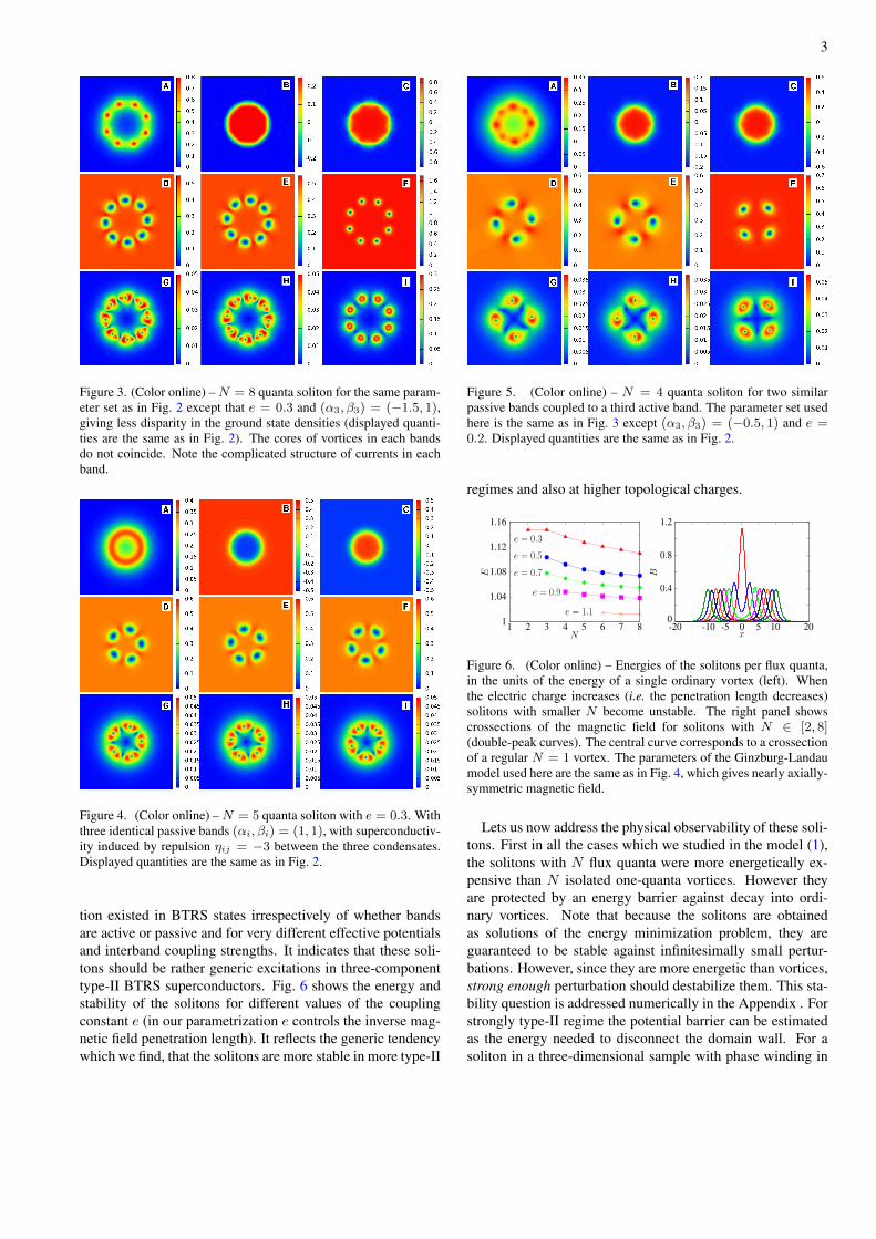
tion existed in BTRS states irrespectively of whether bandsare active or passive and for very different effective potentialsand interband coupling strengths. It indicates that these soli-tons should be rather generic excitations in three-componenttype-II BTRS superconductors. Fig. 6 shows the energy andstability of the solitons for different values of the couplingconstant e (in our parametrization e controls the inverse mag-netic field penetration length). It reflects the generic tendencywhich we find, that the solitons are more stable in more type-II

Figure 5. (Color online) – N = 4 quanta soliton for two similarpassive bands coupled to a third active band. The parameter set usedhere is the same as in Fig. 3 except (α3, β3) = (−0.5, 1) and e =0.2. Displayed quantities are the same as in Fig. 2.

regimes and also at higher topological charges.

1

1.04

1.08

1.12

1.16

1 2 3 4 5 6 7 8

E

N

e = 1.1

e = 0.9

e = 0.7

e = 0.5

e = 0.3

0

0.4

0.8

1.2

-20 -10 -5 0 5 10 20

B

x

Figure 6. (Color online) – Energies of the solitons per flux quanta,in the units of the energy of a single ordinary vortex (left). Whenthe electric charge increases (i.e. the penetration length decreases)solitons with smaller N become unstable. The right panel showscrossections of the magnetic field for solitons with N ∈ [2, 8](double-peak curves). The central curve corresponds to a crossectionof a regular N = 1 vortex. The parameters of the Ginzburg-Landaumodel used here are the same as in Fig. 4, which gives nearly axially-symmetric magnetic field.

Lets us now address the physical observability of these soli-tons. First in all the cases which we studied in the model (1),the solitons with N flux quanta were more energetically ex-pensive than N isolated one-quanta vortices. However theyare protected by an energy barrier against decay into ordi-nary vortices. Note that because the solitons are obtainedas solutions of the energy minimization problem, they areguaranteed to be stable against infinitesimally small pertur-bations. However, since they are more energetic than vortices,strong enough perturbation should destabilize them. This sta-bility question is addressed numerically in the Appendix . Forstrongly type-II regime the potential barrier can be estimatedas the energy needed to disconnect the domain wall. For asoliton in a three-dimensional sample with phase winding in

4

the xy-plane the potential barrier can be estimated as [coher-ence length]2×[sample size in the direction of applied mag-netic field]×[condensation energy density].

Being more expensive than vortices, these objects cannotform as a ground state in low external field [7]. However asdemonstrated in Fig. 6 they are not much more energeticallyexpensive than vortices. In fact the corresponding energy dif-ferences can be just a few percent. Thus they can be excitedby either by (a) thermal fluctuations or (b) by quenching in asample subjected to a magnetic field. To address the scenario(b) of possible formation of these solitons in a post-quenchrelaxation, we have to assess “capture basin" of these solu-tions (i.e. how large is the area in the free energy landscapefrom which an excited system would relax into the local mini-

mum corresponding to a soliton. Although studying real post-quench relaxation dynamics is beyond the scope of this paper,nonetheless we can directly assess the capture basin of thesolutions from the evolution of the system in our relaxationscheme (see also remark [8]). We investigated several hun-dreds regimes and found that solitons typically easily formwhen a system is relaxed from various higher energy states.This indicates that the capture basin of these solutions is typi-cally very large. We find that these defects in fact very easilyform during a rapid expansion of vortex lattice (which shouldoccur when magnetic field is rapidly lowered, or if a systemis quenched through Hc2). A typical example is shown onFig. 7. Animations of these processes are available as a sup-plementary online material [9].

Figure 7. (Color online) – The soliton formation during energy relaxation of an initial state of expanding group of vortices in a circularsystem with open boundary conditions. First line displays the energy density. Second line shows the phase difference between condensates(ψ∗

1ψ2−ψ1ψ∗2)/2i. When domain walls form they separate two inequivalent ground states (blue and red). Third line is the density of the first

condensate |ψ1|2. Initial configuration has a high density of 13 vortices in the center. Repulsive type-II interaction makes all vortices moveaway from each other and escape the sample. In the process of energy minimization domain walls and GL(3) solitons form. Domain wallconnected to boundaries quickly disappear. The final picture shows the resulting long-living state of a well separated N = 4 GL(3) solitonand a vortex. Parameter set used here is the same as in Fig. 4, with e = 0.4.

In conclusion, we have shown that BTRS state of a three-band superconductor can be detected through its magnetic re-sponse. Namely we have demonstrated that in this state thesystem has two kinds of flux carrying topological defects :ordinary vortices and also a different kind of topological soli-tons. These solitons are only slightly more energetically ex-pensive than vortices (in some cases we found the energy dif-ference as small as 10−2Ev where Ev is the energy of a vor-tex). They should form during a post-quench relaxation of aBTRS superconductor in an external field, since they repre-sent local minima with a wide capture basin in the free en-ergy landscape. I.e. a system should relax to these local min-ima from a wide variety of excited states. Then these solitonscan be observed in scanning SQUID, Hall, or magnetic forcemicroscopy measurements. They can provide an experimen-tal signature of possible BTRS states in iron pnictide super-conductors. A tendency for vortex pair formation, yielding

magnetic profile similar to that shown on Fig. 2 was observedin Ba(Fe1−xCox)2As2, [10] as well as vortex clustering inBaFe2−xNixAs2 [11]. These materials have strong pinningwhich can naturally produce disordered vortex states [11], al-though a possibility of “type-1.5" scenario for these vortexinhomogeneities was also voiced in [11]. The vortex pairsobserved in [10] can be discriminated from N = 2 solitons(such as that shown on Fig. 2), by quenching the system andobserving whether or not it forms vortex triangles, squares,pentagons etc corresponding to higher-N solitons.

We thank J.M. Speight for useful communications. Thework is supported by the Swedish Research Council, and bythe Knut and Alice Wallenberg Foundation through the RoyalSwedish Academy of Sciences fellowship and by NSF CA-REER Award No. DMR-0955902.

5

Appendix A : Finite element energy minimization

The GL(3) solitons are local minima of the Ginzburg-Landau energy (1). This means that functional minimizationof (1), from an appropriate initial guess carrying several fluxquanta, should lead to a GL(3) soliton (if it exists as a stablesolution). We consider the two-dimensional problem (1) de-fined on the bounded domain Ω ⊂ R2, supplemented by a‘open’ boundary conditions on ∂Ω.

Strictly speaking, there is a constraint on ∂Ω. This ‘openconstraint’ is a particular Neumann boundary condition, suchthat the normal derivative of the fields on the boundary arezero. These boundary conditions in fact are a very weak con-straint. For this problem one could also apply Robin bound-ary conditions on ∂Ω, so that the fields satisfy linear asymp-totic behavior (exponential localization). However, we chooseto apply the ‘open’ boundary conditions which are less con-straining for the problem in question. ‘Open’ boundary con-ditions also imply that topological defects can easily escapefrom the numerical grid, since it would further minimize theenergy. To prevent this, the numerical grid is chosen to belarge enough so that the attractive interaction with the bound-aries is negligible. The size of the domain is then much largerthan the typical interaction length scales. Thus in this methodone has to use large numerical grids, which is computation-ally demanding. At the same time the advantage is that it isguaranteed that obtained solutions are not boundary pressureartifacts.

The variational problem is defined for numerical compu-tation using a finite element formulation provided by theFreefem++ library [13]. Discretization within finite elementformulation is done via a (homogeneous) triangulation overΩ, based on Delaunay-Voronoi algorithm. Functions are de-composed on a continuous piecewise quadratic basis on eachtriangle. The accuracy of such method is controlled throughthe number of triangles, (we typically used 3 ∼ 6× 104), theorder of expansion of the basis on each triangle (P2 elementsbeing 2nd order polynomial basis on each triangle), and alsothe order of the quadrature formula for the integral on the tri-angles.

Once the problem is mathematically well defined, a numeri-cal optimization algorithm is used to solve the variational non-linear problem (i.e. to find the minima of F). We used herea Nonlinear Conjugate Gradient method. The algorithm is it-erated until relative variation of the norm of the gradient ofthe functional F with respect to all degrees of freedom is lessthan 10−6.

Initial guess

As discussed in the paper, N quanta GL(3) solitons in thethree-component model are more energetically expensive thanN quanta ordinary vortices. They are local minima of the en-ergy functional (1). As a result the initial guess should bewithin the attractive basin of the GL(3) solitons. Otherwise

the configuration converges to ordinary vortices which havethe same total phase winding but cost less energy. We findhowever the attractive basin of the GL(3) soliton solutions tobe generally quite large (i.e. theGL(3) soliton forms quite eas-ily in general). The initial field configuration carrying N fluxquanta is prepared by using an ansatz which imposes phasewindings around spatially separated N vortex cores in eachcondensates :

ψ1 = |ψ1|eiΘ , ψ2 = |ψ2|eiΘ+i∆12 , ψ3 = |ψ3|eiΘ+i∆13 ,

|ψa| = ua

Nv∏i=1

√1

2

(1 + tanh

(4

ξa(Ri(x, y)− ξa)

)),

A =1

eR(sin Θ,− cos Θ) , (2)

where a = 1, 2, 3 and ua is the ground state value of eachsuperfluid density. The parameter ξa gives the core size whileΘ andR are

Θ(x, y) =

Nv∑i=1

Θi(x, y) ,

Θi(x, y) = tan−1

(y − yix− xi

),

R(x, y) =

Nv∑i=1

Ri(x, y) ,

Ri(x, y) =√

(x− xi)2 + (y − yi)2 . (3)

The initial position of a vortex is given by (xi, yi). The func-tions ∆ab ≡ ϕb − ϕa can be used to initiate a domain wall.As an initial guess we generally choose ∆12 = −∆13 ≡ ∆,with ∆ defined as

∆ =π

3(H(r− r0)− 1) , (4)

where H(r − r0) is a Heaviside function. Thus in the ini-tial guess the domain wall has infinitesimal thickness. It takesonly a few steps from this initial guess to relax to a true do-main wall during the simulations. Consequently, it is entirelysufficient to use Heaviside functions for the initial guesses ofdomain walls. Once the initial configuration defined, all de-grees of freedom are relaxed simultaneously, within the ‘open’boundary conditions discussed previously, to obtain highlyaccurate solutions of the Ginzburg-Landau equations. In astrongly type-II system when the initial guess was either (a)vortices placed on a domain wall or (b) closed domain wallsurrounding a densely packed group of vortices, the systemalmost always formed GL(3) solitons. We used also initialguesses (c) without any domain walls (∆ = 0). In that casewe observed GL(3) soliton formation, if in the initial statesvortices were densely packed. This again indicating that theGL(3) solitons in the three component GL model representlocal minima with wide capture basin in the free energy land-scape.

6

Figure 7 in the paper shows stages of the energy minimiza-tion. Corresponding movies are available as the supplemen-tary online material [9]. The main focus of this work is theexistence of stable static solutions, however the numerical re-laxation scheme which we use can give insight into possibleformation dynamics of these objects. That is, the gauge in-variant gradient flow of Ginzburg-Landau free energy can berelated to the dynamics of Time Dependent Ginzburg-Landauequations [8, 14]. Therefore supplementary movies not onlygive information about the size of the capture basin of the lo-cal minima associated with the GL(3) solitons, they also pro-vide some insight into possible real dynamics which can leadto their formation.

Appendix B : Stability of the solutions

The solutions were obtained using an (energy) minimiza-tion algorithm, and not by solving the equations of motion. Asa result, after the convergence (which is carefully controlled),the solution is guaranteed to represent (at least) a local min-imum of the energy functional (1). Because no symmetry-imposing ansatz is used, there are no possible unstable modestruncated by symmetry assumptions. Linear stability analy-sis consists of applying infinitesimally small perturbation tothe fields, and investigating the eigenvalue spectrum of the(linear) perturbation operator, on the background of a givensoliton. When the background solution is (meta) stable all in-finitesimally small perturbations are positive modes and thuscan only increase the energy. However a strong perturba-tion should cause a decay of a soliton to ordinary vorticessince these solitons are protected against decay by a finite en-ergy barrier. Instead of studying different modes, we double-checked the stability numerically by perturbing the solutionby a random noise. The random noise which is applied to alldegrees of freedom, is generated as follows

Re(ψa) = Re(ψa)(0) + PuaµRea (x, y) ,

Im(ψa) = Im(ψa)(0) + PuaµIma (x, y) ,

Ai = A(0)i + Pmax(|A|)µA

i (x, y) . (5)

Here (0) denotes the background solutions, P is a percentagegiving the relative magnitude of the fluctuation with respectto the maximal amplitude of a given field of the backgroundsolution. µRe

a (x, y), µIma (x, y) and µA

i (x, y) are (independent)random functions of the space ∈ [−1 : 1]. As a result allfields initially receive noise whose relative amplitude is P .The system is then again relaxed using the same minimiza-tion scheme as for constructing the solitons. It is found that

if the random noise does not exceed a certain threshold, theconfiguration relaxes back to the soliton solution, as can beseen from Fig. 8. The noise was gradually increased, findingthat indeed, sufficiently strong perturbation drives the solitonover the barrier, in the energy landscape. Thus leading to itsdecay to ordinary vortex solutions as shown on Fig. 9. Theprecise value of the relative amplitude required to destabilizea given soliton, obviously depend on the GL parameters andon the number of flux quanta of the solution.

[1] P.C.W. Chu, et al., Physica C 469, 313 (2009)P. J. Hirschfeld,M. M. Korshunov, and I. I. Mazin, Rep. Prog. Phys. 74, 124508(2011)

[2] T. K. Ng and N. Nagaosa, Europhys. Lett. 87, 17003(2009)V. Stanev and Z. Tesanovic, Phys. Rev. B 81, 134522(2010)X. Hu and Z. Wang, arXiv:1103.0123

[3] W.-C. Lee, S.-C. Zhang, and C. Wu, Phys. Rev. Lett. 102,217002 (2009)C. Platt, R. Thomale, C. Honerkamp, S.-C.Zhang, and W. Hanke, arXiv:1106.5964

[4] M. Sigrist and D. F. Agterberg, Prog. Theo. Phys. 102,965 (1999)Y. Matsunaga, M. Ichioka, and K. Machida,Phys. Rev. Lett. 92, 157001 (2004)Phys. Rev. B 70, 100502(2004)M. Ichioka, Y. Matsunaga, and K. Machida, Phys. Rev.B. 71, 172510 (2005)

[5] J. Smiseth, E. Smørgrav, E. Babaev, and A. Sudbø, Phys. Rev.B 71, 214509 (2005)E. Babaev, Phys. Rev. Lett. 89, 067001(2002)

[6] E. Babaev, Phys. Rev. B 79, 104506 (2009)[7] In principle by adding certain mixed gradient terms, or density-

density interaction which gives energy penalty to the vortexcores where the total density is zero (i.e.

∑i |ψi(r)|2), yields

models where soliton lattice should form instead of vortex lat-tice as a ground state in external field.

[8] We do not study dynamics in this paper. However we note thatbecause Time Dependent Ginzburg-Landau (TDGL) equationscan be seen as the gauge invariant gradient flow of the free en-ergy, our numerical relaxation scheme in fact is indirectly re-lated to the TDGL dynamics of the system, see e.g. Q. Du,Journ. of Math. Phys. 46 095109 (2005).

[9] “http://people.umass.edu/garaud/3CGL-soliton.html,”[10] B. Kalisky, J. R. Kirtley, J. G. Analytis, J.-H. Chu, I. R. Fisher,

and K. A. Moler, Phys. Rev. B 83, 064511 (2011)[11] L. J. Li, T. Nishio, Z. A. Xu, and V. V. Moshchalkov, Phys. Rev.

B 83, 224522 (2011)[12] For this study, we investigated about 600 different configura-

tions, with an average of 100 CPU hours per invested configu-ration. Which required computational resources of a very largesupercomputer.

[13] F. Hecht, O. Pironneau, A. Le Hyaric, and K. Ohtsuka, (2007)Freefem++ (manual). www.freefem.org

[14] Q. Du, Applicable Analysis: An International Journal, Taylor& Francis, 53 1-17 ( 1994)

7

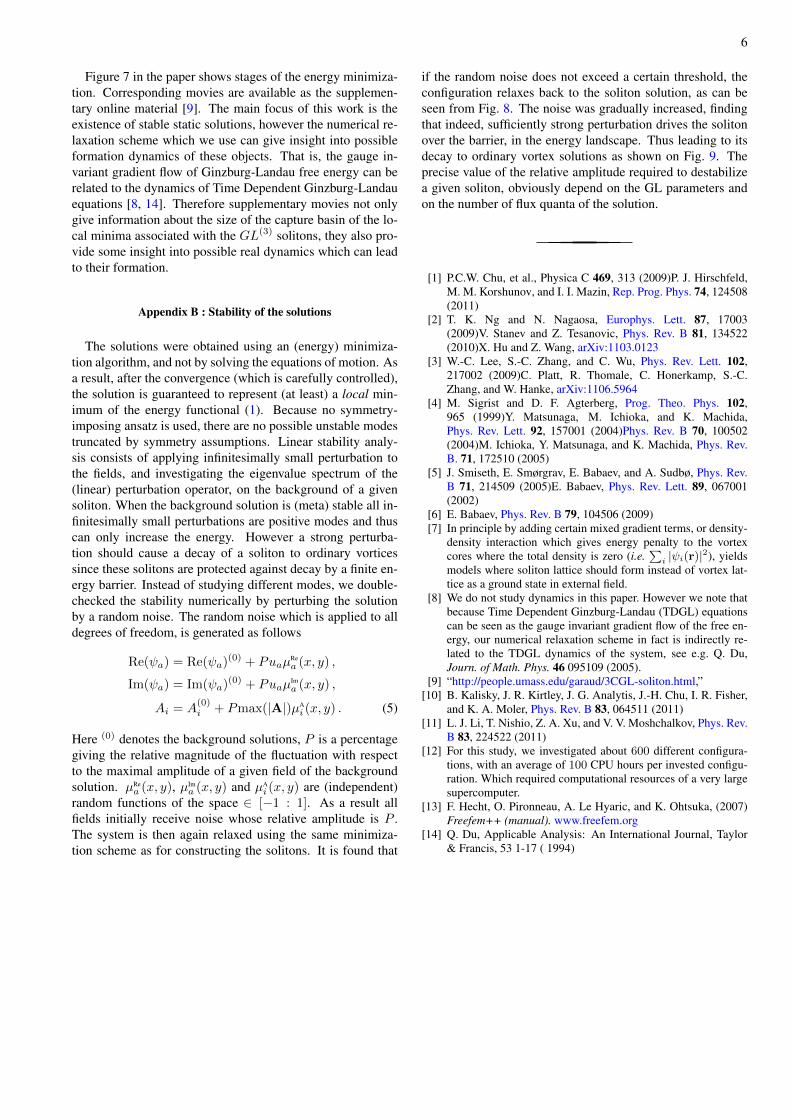
Figure 8. (Color online) – Displayed quantities are the same as in Fig. 7 of the paper, namely the energy density, (ψ∗1ψ2 − ψ1ψ

∗2)/2i and

|ψ1|2. Initial configuration is a charge 8 GL(3) soliton shown in Fig. 3. The snapshots show the state of the system a different stages of theenergy minimization algorithm after the applied perturbation. The initial noise is P = 0.6, which in fact is a very significant perturbationwhere the density fields vary locally up to 60 % of the ground state values, while magnetic field varies up to 60 % of its maximal value. Theconfiguration nevertheless relaxes back to the GL(3) soliton.

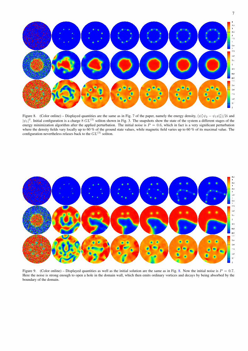
Figure 9. (Color online) – Displayed quantities as well as the initial solution are the same as in Fig. 8. Now the initial noise is P = 0.7.Here the noise is strong enough to open a hole in the domain wall, which then emits ordinary vortices and decays by being absorbed by theboundary of the domain.