Topographic Influence on the Seasonal and Interannual Variation of Water and Energy Balance of...

1 MAY 2001 1989C H E N A N D K U M A R

q 2001 American Meteorological Society

Topographic Influence on the Seasonal and Interannual Variation of Water andEnergy Balance of Basins in North America

JI CHEN AND PRAVEEN KUMAR

Environmental Hydrology and Hydraulic Engineering, Department of Civil and Environmental Engineering,University of Illinois at Urbana–Champaign, Urbana, Illinois

(Manuscript received 24 January 2000, in final form 21 September 2000)

ABSTRACT

A large area basin-scale (LABs) hydrologic model is developed for regional, continental, and global hydrologicstudies. The heterogeneity in the soil-moisture distribution within a basin is parameterized through the statisticalmoments of the probability distribution function of the topographic (wetness) index. The statistical momentsare derived using GTOPO30 (30 arc sec; 1-km resolution) digital elevation model data for North America. Riverbasins and drainage network extracted using this dataset are overlaid on computed topographic indices for thecontinent and statistics are extracted for each basin. A total of 5020 basins with an average size of 3255 squarekilometers, obtained from the United States Geological Survey HYDRO1K data, is used over the continent.

The model predicts runoff generation due to both saturation and infiltration excess mechanisms along withthe baseflow and snowmelt. Simulation studies are performed for 1987 and 1988 using the International SatelliteLand Surface Climatology Project data. Improvement in the terrestrial water balance and streamflow is observeddue to improvements in the surface runoff and baseflow components achieved by incorporating the topographicinfluences. It is found that subsurface redistribution of soil moisture, and anisotropy in hydraulic conductivitiesin the vertical and horizontal directions play an important role in determining the streamflow and its seasonalvariability. These enhancements also impact the surface energy balance. It is shown that the dynamics of severalhydrologic parameters such as basin mean water table depth and saturated fraction play an important role indetermining the total streamflow response and show realistic seasonal and interannual variations. Observedstreamflow of the Mississippi River and its subbasins (Ohio, Arkansas, Missouri, and Upper Mississippi) areused for validation. It is observed that model baseflow has a significant contribution to the streamflow and isimportant in realistically capturing the seasonal and annual cycles.

1. Introduction

During the last two decades significant advances havebeen made in the representation of terrestrial hydrologicprocesses for studying the feedback between the landsurface and atmosphere. These studies were largely fa-cilitated by the improved understanding of the role ofvegetation in determining the transfer of energy andcarbon dioxide fluxes at the land–atmosphere interfacethat lead to the subsequent development of macroscalehydrologic models generally termed as Soil–Vegeta-tion–Atmosphere-Transfer (SVAT) schemes (e.g., Sell-ers et al. 1986; Dickinson et al. 1986; Abramopouloset al. 1988; Famiglietti and Wood 1991; Koster andSuarez 1992a,b; Bonan 1996; Pitman et al. 1991; Yanget al. 1995). Studies using these models have demon-strated the important role of the terrestrial moisture and

Corresponding author address: Dr. Praveen Kumar, EnvironmentalHydrology and Hydraulic Engineering, Dept. of Civil and Environ-mental Engineering, University of Illinois at Urbana–Champaign, Ur-bana, IL 61801.E-mail: [email protected]

heat stores in modulating the climate system. With theincreasing sophistication, resolution and performance ofthe general circulation models (GCMs) it is now pos-sible to study the impact of climatic variability on ter-restrial systems.

Hydrologic models, which provide the link betweenthe physical climate and several terrestrial systems, arenow being adapted for such studies. Important advanceshave been made in the prediction of streamflow (seeAbdulla et al. 1996; Nijssen et al. 1997; Wood et al.1997). However, important limitations exist primarilydue to two reasons. First, the emphasis of the SVATmodel development has been on the exchange of mois-ture and energy fluxes at the land–atmosphere interfaceand not on the subsurface and ground water flow dy-namics that are largely responsible for the seasonal tointerannual streamflow variability. Second, the existingSVAT models are run on rectangular grids that coincidewith that of the GCMs, typically of the order of 200 to400 km on a side. However, the natural unit for therepresentation of hydrologic processes is a basin. In abasin, in the absence of geologic controls, both the sur-face and subsurface flows are controlled by the topog-

1990 VOLUME 14J O U R N A L O F C L I M A T E

raphy with the water leaving the basin through itsmouth. Soil moisture is higher in regions of flow con-vergence such as at the bottom of hill slopes, whereasuphill areas are associated with flow divergence andhigher soil-moisture deficit in the vertical profile. A sig-nificant portion of the total runoff is generated whenrain falls on the saturated regions in the low lying areasnear stream channels. This saturated area expands orcontracts during and between storms. This mechanismcan result in surface runoff production in humid andvegetated areas with shallow water tables, even whereinfiltration capacities of soil surface are high relative tonormal rainfall intensities. The main controls on thesaturated contributing areas are the topographic and hy-drologic characteristics of the hill slopes. The hetero-geneity in the distribution of soil moisture influencesthe evapotranspiration rate and consequently the energybalance. A basin-based representation not only providesa logical way of modeling the vegetation and moistureheterogeneity but also opens the door for the study ofclimate influences on surface hydrology to address is-sues related to water resource management, and eco-logical and environmental issues over seasonal to in-terannual timescales.

Topmodel (Beven and Kirkby 1979), which has un-dergone significant enhancements over the years andincorporates both infiltration and saturation excess run-off generation mechanisms, is often used for modelingthe basin runoff. The basic approach of this model hasbeen adapted into the SVAT schemes (e.g., Famigliettiand Wood 1991) for the representation of soil-moistureheterogeneity using the probability distribution of thetopographic index. However, the streamflow predictionis not emphasized.

In another study, Stieglitz et al. (1997) developed amodel that coupled an SVAT scheme (Pitman et al.1991) with a Topmodel-based basin runoff model (Be-ven and Kirkby 1979). Their essential idea was to treata basin, rather than a rectangular grid, as a column andcouple the Topmodel equations with that of the singlecolumn model. From a hydrologic perspective, a columnmodel has its strength in predicting (i) the partition ofthe incident radiation into various heat components, and(ii) the vertical movement of soil moisture. However, itis weak in predicting the runoff. In contrast, Topmodelcan predict the runoff well but does not model the en-ergy fluxes and the vertical transport of soil moisture.Stieglitz et al. (1997) tested the coupled model in the8.4 km2 W-3 subwatershed of the Sleepers River basinlocated in the glaciated highlands of Vermont and ob-tained very promising results. This development enablesus to account for and validate water balance along withthe energy balance. In addition, it offers the opportunityfor studying the seasonal, interannual, and decadal fluc-tuations of land surface hydrologic parameters such asstreamflow, water table depth, subsurface storage, etc.,in a meaningful way.

Recent availability of digital elevation model (DEM)

data, and basin and stream coverages from the UnitedStates Geological Survey (USGS) for the various con-tinents (Verdin and Verdin 1999) has made it possibleto implement basin-scale models for regional, conti-nental, and global studies. The emphasis of this paperis twofold. First, we describe a basin-scale model, basedon the scheme proposed by Stieglitz et al. (1997), forstudying the hydrologic response over the entire NorthAmerican continent. Several enhancements are made tothe basic scheme. The National Center for AtmosphericResearch (NCAR) Land Surface Model (LSM; Bonan1996) is chosen as the underlying column model for thiswork. It is a well-tested model and already coupled tothe Community Climate Model, Version 3 (CCM3), atNCAR. For application over the North American con-tinent, estimates of topographic indices and basin de-lineation are obtained using USGS GTOPO30 digitalelevation and HYDRO1K data (Verdin and Verdin1999). This latter dataset employs an efficient repre-sentation scheme for the nested basin topology (Pfaf-stetter 1989) that facilitates studies of streamflow re-sponse at several aggregation levels. Model simulationsare performed using the International Satellite Land Sur-face Climatology Project (ISLSCP) dataset for 1987 and1988 (Sellers et al. 1995; Meeson et al. 1995). Themodel is validated using observed streamflow from sev-eral rivers such as the Mississippi, Arkansas, Missouri,Upper Mississippi, and Ohio (EarthInfo 1995).

Second, we explore the role of topographic controlin the hydrologic response at the regional and conti-nental scales. The study demonstrates the improvementin the terrestrial water balance and streamflow throughimprovements in the surface runoff and baseflow com-ponents achieved by incorporating the topographic in-fluences. These enhancements also have an impact onthe surface energy balance. It is shown that several hy-drologic parameters such as water table depth and sat-urated fraction play an important role in determiningthe total streamflow response and show realistic sea-sonal and interannual variations.

This paper is organized as follows. In section 2 wedescribed the model used for the study. The data andthe results from the simulation are described in section3. Summary and conclusions are given in section 4. Theappendixes summarize the technical details.

2. Model description

a. Coupling scheme

Our hydrologic model, called the large area basin-scale (LABs) model (Fig. 1), is based in part on thescheme developed by Stieglitz et al. (1997). Each basinis represented as a single column in order to capture thedynamics of moisture and energy transport. For the ver-tical transfer of heat and moisture fluxes we use theNCAR LSM model (Bonan 1996), which is a one-di-mensional column model that simulates energy, mo-


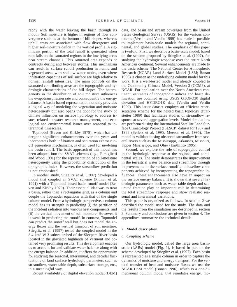
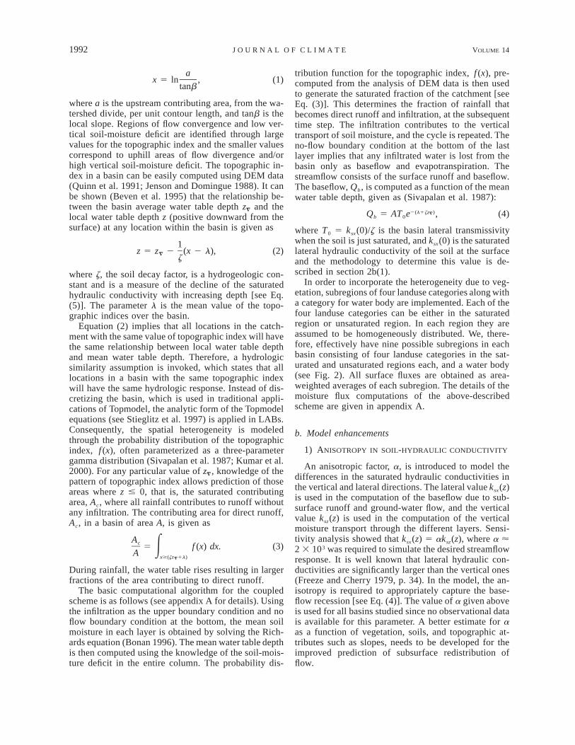
FIG. 1. A basin is modeled as a single column with six soil layers for moisture and heat transport (see section 2 for details).

mentum, water, and CO2 exchanges between the at-mosphere and the land surface. It incorporates subgridvariability by subdividing a grid box into mosaics withdifferent landuse categories. All computations are per-formed independently for each subgrid and the area-weighted fluxes are then computed for the entire grid.The vertical column is divided into six layers. The near-surface layer is 10 cm deep and thickness doubles forsubsequent layers, with the bottom of the last layer at6.3-m depth.

The NCAR LSM model simulates ecosystem dynam-ics, and biophysical, hydrologic, and biogeochemicalprocesses. Ecosystem dynamics includes vegetationphenology (Dorman and Sellers 1989) that simulatesleaf and stem area indices that are updated daily. Thebiogeochemical processes that are simulated by themodel are photosynthesis, plant and microbial respira-tion, and net primary production. Biophysical processesconsist of computation of albedo, radiation fluxesthrough the canopy, and heat and momentum fluxes atthe land–atmosphere interface. The momentum, sensi-ble, and latent heat fluxes are derived by using Monin–

Obukhov similarity theory for the surface layer. Canopyand ground temperatures are computed by consideringtheir energy balance equations. Soil and lake tempera-tures are obtained by using the heat diffusion equation.

The hydrologic processes that are simulated in NCARLSM include interception, throughfall, and stemflow;snow accumulation and melt; infiltration and runoff; andvertical transfer of soil moisture. The soil propertiessuch as soil hydraulic conductivity and soil matrix po-tential are calculated as a function of the soil texture(Clapp and Hornberger 1978). Additional details of thismodel can be found in Bonan (1996). Several enhance-ments are made to the model in our implementation andthey are described in section 2b.

In NCAR LSM the soil-moisture heterogeneity is pa-rameterized through an assumed exponential distribu-tion. In LABs, the spatial heterogeneity of soil moisturewithin the basin is parameterized through the probabilitydistribution of the topographic (wetness) index (Bevenand Kirkby 1979). The topographic index at any locationin the basin is defined as


ax 5 ln , (1)

tanb

where a is the upstream contributing area, from the wa-tershed divide, per unit contour length, and tanb is thelocal slope. Regions of flow convergence and low ver-tical soil-moisture deficit are identified through largevalues for the topographic index and the smaller valuescorrespond to uphill areas of flow divergence and/orhigh vertical soil-moisture deficit. The topographic in-dex in a basin can be easily computed using DEM data(Quinn et al. 1991; Jenson and Domingue 1988). It canbe shown (Beven et al. 1995) that the relationship be-tween the basin average water table depth z= and thelocal water table depth z (positive downward from thesurface) at any location within the basin is given as

1z 5 z 2 (x 2 l), (2)= z

where z, the soil decay factor, is a hydrogeologic con-stant and is a measure of the decline of the saturatedhydraulic conductivity with increasing depth [see Eq.(5)]. The parameter l is the mean value of the topo-graphic indices over the basin.

Equation (2) implies that all locations in the catch-ment with the same value of topographic index will havethe same relationship between local water table depthand mean water table depth. Therefore, a hydrologicsimilarity assumption is invoked, which states that alllocations in a basin with the same topographic indexwill have the same hydrologic response. Instead of dis-cretizing the basin, which is used in traditional appli-cations of Topmodel, the analytic form of the Topmodelequations (see Stieglitz et al. 1997) is applied in LABs.Consequently, the spatial heterogeneity is modeledthrough the probability distribution of the topographicindex, f (x), often parameterized as a three-parametergamma distribution (Sivapalan et al. 1987; Kumar et al.2000). For any particular value of z=, knowledge of thepattern of topographic index allows prediction of thoseareas where z # 0, that is, the saturated contributingarea, Ac, where all rainfall contributes to runoff withoutany infiltration. The contributing area for direct runoff,Ac, in a basin of area A, is given as

Ac 5 f (x) dx. (3)EA x$(zz 1l)=

During rainfall, the water table rises resulting in largerfractions of the area contributing to direct runoff.

The basic computational algorithm for the coupledscheme is as follows (see appendix A for details). Usingthe infiltration as the upper boundary condition and noflow boundary condition at the bottom, the mean soilmoisture in each layer is obtained by solving the Rich-ards equation (Bonan 1996). The mean water table depthis then computed using the knowledge of the soil-mois-ture deficit in the entire column. The probability dis-

tribution function for the topographic index, f (x), pre-computed from the analysis of DEM data is then usedto generate the saturated fraction of the catchment [seeEq. (3)]. This determines the fraction of rainfall thatbecomes direct runoff and infiltration, at the subsequenttime step. The infiltration contributes to the verticaltransport of soil moisture, and the cycle is repeated. Theno-flow boundary condition at the bottom of the lastlayer implies that any infiltrated water is lost from thebasin only as baseflow and evapotranspiration. Thestreamflow consists of the surface runoff and baseflow.The baseflow, Qb, is computed as a function of the meanwater table depth, given as (Sivapalan et al. 1987):

Qb 5 ,2(l1zz )=AT e0 (4)

where T0 5 ksx(0)/z is the basin lateral transmissivitywhen the soil is just saturated, and ksx(0) is the saturatedlateral hydraulic conductivity of the soil at the surfaceand the methodology to determine this value is de-scribed in section 2b(1).

In order to incorporate the heterogeneity due to veg-etation, subregions of four landuse categories along witha category for water body are implemented. Each of thefour landuse categories can be either in the saturatedregion or unsaturated region. In each region they areassumed to be homogeneously distributed. We, there-fore, effectively have nine possible subregions in eachbasin consisting of four landuse categories in the sat-urated and unsaturated regions each, and a water body(see Fig. 2). All surface fluxes are obtained as area-weighted averages of each subregion. The details of themoisture flux computations of the above-describedscheme are given in appendix A.

b. Model enhancements

1) ANISOTROPY IN SOIL-HYDRAULIC CONDUCTIVITY

An anisotropic factor, a, is introduced to model thedifferences in the saturated hydraulic conductivities inthe vertical and lateral directions. The lateral value ksx(z)is used in the computation of the baseflow due to sub-surface runoff and ground-water flow, and the verticalvalue ksz(z) is used in the computation of the verticalmoisture transport through the different layers. Sensi-tivity analysis showed that ksx(z) 5 aksz(z), where a ø2 3 103 was required to simulate the desired streamflowresponse. It is well known that lateral hydraulic con-ductivities are significantly larger than the vertical ones(Freeze and Cherry 1979, p. 34). In the model, the an-isotropy is required to appropriately capture the base-flow recession [see Eq. (4)]. The value of a given aboveis used for all basins studied since no observational datais available for this parameter. A better estimate for aas a function of vegetation, soils, and topographic at-tributes such as slopes, needs to be developed for theimproved prediction of subsurface redistribution offlow.


FIG. 2. The representation of surface heterogeneity for each basin.

FIG. 3. Level 1 Pfafstetter subdivision of North American continent (adapted from Verdin andVerdin 1999).

Further it is assumed that both ksx(z) and ksz(z) havean exponential decay with depth, that is,

ksz(z) 5 k0ze2z(z21). (5)

It is assumed that at a 1-m depth the vertical saturatedhydraulic conductivities reach the compacted value k0z

given in Clapp and Hornberger (1978) under the as-sumption that most roots lie above this level. The lateralconductivity k0x is obtained by scaling k0z with the factora. For each soil layer, the hydraulic conductivity at the

center of the thickness is used. In the Topmodel frame-work z is a calibration parameter (Quinn and Beven1993; Beven et al. 1995). In our model calibration isnot used. Instead a value of z 5 1.8 m21 obtainedthrough sensitivity analysis showed acceptable perfor-mance and this value is used for all basins in NorthAmerica. In theory z can be obtained by the analysisof the streamflow recession curves [Quinn and Beven1993; see Eq. (4)] or through the observed decline ofksz(z) with depth if such data are available. The former


FIG. 4. Level 2 Pfafstetter subdivision of the Mississippi River basin (adapted from Verdin and Verdin 1999). The stars indicate thelocations of stream gauging stations whose data are used for model validation. See Table 3 for quantitative information.

has the advantage of providing a basin-averaged esti-mate that is more appropriate for the proposed modelingframework. These alternatives will be explored in thefuture.

2) COMPUTATION OF WATER TABLE DEPTH

To define the water table depth, that is, the interfacebetween the saturated and the unsaturated soil, Stieglitzet al. (1997) selected a soil-moisture level greater thanor equal to 70% of the field capacity as the definingthreshold, that is,

z (i) for u(i) # 0.7ub 33z 5 u(i) 2 0.7u= 33z (i) 2 Dz(i) for u(i) . 0.7u , b 331 2u 2 0.7usat 33

(6)

where zb(i) and u(i) are the depth of the bottom bound-ary and mean soil water content of soil layer i, respec-tively, and usat and u33 are the saturated soil water contentand field capacity, respectively. However, this meth-

odology results in an abrupt change in the water tabledepth as it crosses layer boundaries. This in turn impactsthe runoff and soil-moisture computations.

In order to resolve this problem, we use a quasi-steady-state condition (e.g., Abramopoulos et al. 1988).After the vertical transport of soil moisture is computedin the soil column using the Richards equation, the soil-moisture deficit, Du 5 Si [usat 2 u(i)] Dz(i), for theentire column is computed. We then assume the verticalmoisture profile is such that there is no vertical flux. Ifz= represents the water table depth from the surface,then this condition gives

c(z) 1 (z= 2 z) 5 C, (7)

that is,

2bu(z)

c 1 (z 2 z) 5 C, (8)sat =[ ]usat

where c is the matrix potential, b is the Brooks–Coreyparameter (Brooks and Corey 1964), and C is a constant.Using the conditions at the capillary fringe it is easily


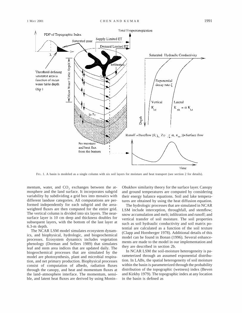
TABLE 1. Average area of North American Pfafstetter units (afterVerdin and Verdin 1999).

Level Average area (km2)

Level 1Level 2Level 3Level 4Level 5

2 209 207232 684

28 71362403255

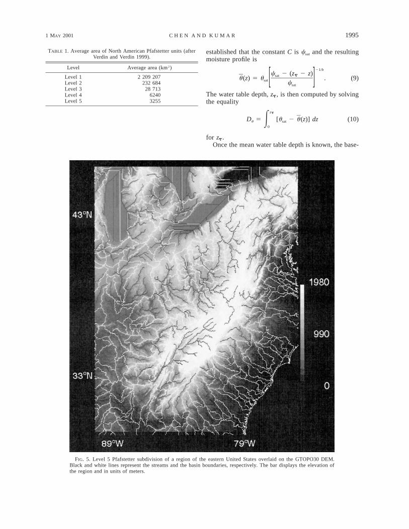
FIG. 5. Level 5 Pfafstetter subdivision of a region of the eastern United States overlaid on the GTOPO30 DEM.Black and white lines represent the streams and the basin boundaries, respectively. The bar displays the elevation ofthe region and in units of meters.

established that the constant C is csat and the resultingmoisture profile is

21/bc 2 (z 2 z)sat =u(z) 5 u . (9)sat [ ]csat

The water table depth, z=, is then computed by solvingthe equality

z=

D 5 [u 2 u(z)] dz (10)u E sat

0

for z=.Once the mean water table depth is known, the base-


TABLE 2. Downscaling equations for obtaining L moments at 90m equivalent (y) using estimates from 1-km DEM data (x) (adaptedfrom Kumar et al. 2000).

MeanL scaleL skewness

y 5 23.29 1 1.16xy 5 0.38 1 0.78xy 5 20.13 1 1.15x

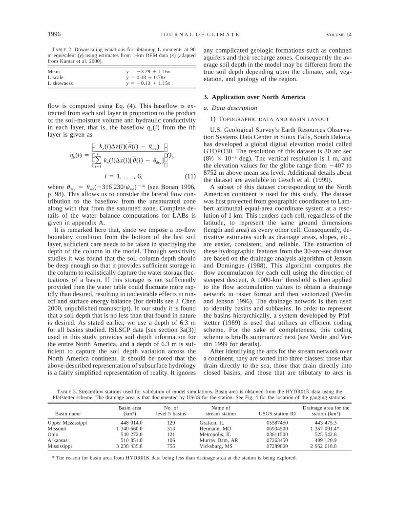
TABLE 3. Streamflow stations used for validation of model simulations. Basin area is obtained from the HYDR01K data using thePfafstetter scheme. The drainage area is that documented by USGS for the station. See Fig. 4 for the location of the gauging stations.

Basin nameBasin area

(km2)No. of

level 5 basinsName of

stream station USGS station IDDrainage area for the

station (km2)

Upper MississippiMissouriOhioArkansasMississippi

448 014.01 340 660.0

549 272.0510 851.0

3 238 435.8

129313121106755

Grafton, ILHermann, MOMetropolis, ILMurray Dam, ARVicksburg, MS

0558745006934500036115000726345007289000

443 475.31 357 091.4*

525 542.8409 120.9

2 952 618.8

* The reason for basin area from HYDR01K data being less than drainage area at the station is being explored.

flow is computed using Eq. (4). This baseflow is ex-tracted from each soil layer in proportion to the productof the soil-moisture volume and hydraulic conductivityin each layer, that is, the baseflow qb(i) from the ithlayer is given as

k (i)Dz(i)(u(i) 2 u )x dry 6q (i) 5 Qb b k (i)Dz(i)[u(i) 2 u ]O x dry i51

i 5 1, . . . , 6, (11)

where udry 5 usat(2316 230/csat)21/b (see Bonan 1996,p. 98). This allows us to consider the lateral flow con-tribution to the baseflow from the unsaturated zonealong with that from the saturated zone. Complete de-tails of the water balance computations for LABs isgiven in appendix A.

It is remarked here that, since we impose a no-flowboundary condition from the bottom of the last soillayer, sufficient care needs to be taken in specifying thedepth of the column in the model. Through sensitivitystudies it was found that the soil column depth shouldbe deep enough so that it provides sufficient storage inthe column to realistically capture the water storage fluc-tuations of a basin. If this storage is not sufficientlyprovided then the water table could fluctuate more rap-idly than desired, resulting in undesirable effects in run-off and surface energy balance (for details see J. Chen2000, unpublished manuscript). In our study it is foundthat a soil depth that is no less than that found in natureis desired. As stated earlier, we use a depth of 6.3 mfor all basins studied. ISLSCP data [see section 3a(3)]used in this study provides soil depth information forthe entire North America, and a depth of 6.3 m is suf-ficient to capture the soil depth variation across theNorth America continent. It should be noted that theabove-described representation of subsurface hydrologyis a fairly simplified representation of reality. It ignores

any complicated geologic formations such as confinedaquifers and their recharge zones. Consequently the av-erage soil depth in the model may be different from thetrue soil depth depending upon the climate, soil, veg-etation, and geology of the region.

3. Application over North America

a. Data description

1) TOPOGRAPHIC DATA AND BASIN LAYOUT

U.S. Geological Survey’s Earth Resources Observa-tion Systems Data Center in Sioux Falls, South Dakota,has developed a global digital elevation model calledGTOPO30. The resolution of this dataset is 30 arc sec(8⅓ 3 1023 deg). The vertical resolution is 1 m, andthe elevation values for the globe range from 2407 to8752 m above mean sea level. Additional details aboutthe dataset are available in Gesch et al. (1999).

A subset of this dataset corresponding to the NorthAmerican continent is used for this study. The datasetwas first projected from geographic coordinates to Lam-bert azimuthal equal-area coordinate system at a reso-lution of 1 km. This renders each cell, regardless of thelatitude, to represent the same ground dimensions(length and area) as every other cell. Consequently, de-rivative estimates such as drainage areas, slopes, etc.,are easier, consistent, and reliable. The extraction ofthese hydrographic features from the 30-arc-sec datasetare based on the drainage analysis algorithm of Jensonand Domingue (1988). This algorithm computes theflow accumulation for each cell using the direction ofsteepest descent. A 1000-km2 threshold is then appliedto the flow accumulation values to obtain a drainagenetwork in raster format and then vectorized (Verdinand Jenson 1996). The drainage network is then usedto identify basins and subbasins. In order to representthe basins hierarchically, a system developed by Pfaf-stetter (1989) is used that utilizes an efficient codingscheme. For the sake of completeness, this codingscheme is briefly summarized next (see Verdin and Ver-din 1999 for details).

After identifying the arcs for the stream network overa continent, they are sorted into three classes: those thatdrain directly to the sea, those that drain directly intoclosed basins, and those that are tributary to arcs in


FIG. 6. Comparison of the biweekly averaged time series of model-simulated specific streamflow, both from LABsand NCAR LSM models, with the observations.

these first two cases. From all arcs draining directly intothe sea, the four with greatest area drained are identifiedand assigned codes 2, 4, 6, and 8 going clockwise aroundthe continent. Basins corresponding to each of these arcsare identified and given the same codes 2, 4, 6, and 8.The largest closed basin is given the code 0. The in-terbasin between basins 2 and 4 is given the code 3,

that between 4 and 6 is given the code 5, and that be-tween 6 and 8 is given the code 7. The area betweenbasins 2 and 8 is divided between interbasins 1 and 9,which is partitioned by choosing a divide that connectsbasin 0 with the coast. The 10 basins resulting from thisscheme, which define the level 1 subdivision, for theNorth America continent are shown in Fig. 3. The four


TABLE 4. Comparison of flow volumes (km3 yr21) of the LABs and NCAR LSM model simulations with observations for the MississippiRiver and four of its tributaries for 1987 and 1988.

1987

Obs LABs LSM

1988

Obs LABs LSM

Upper MississippiMissouriOhioArkansasMississippi

79.986.1

180.063.7

492.2

99.085.5

189.187.4

556.9

140.9151.4292.7149.9926.8

55.749.8

159.546.9

430.1

70.150.1

178.366.5

448.9

119.2120.0282.7131.8826.4

largest river systems for the continent are the Macken-zie, Nelson, St. Lawrence, and Mississippi Rivers.

To obtain the level 2 basins, further subdivision isperformed for each basin and interbasin identified inlevel 1. For each basin, mainstem and tributaries areidentified. Moving upstream from the mouth of the basinto any confluence, the stream draining the larger areais identified as the mainstem and the other as tributary.The tributaries that drain the largest four areas are giventhe level 2 codes 2, 4, 6, and 8 going from the mouthof the basin to upstream. The interbasins are given level2 codes 1, 3, 5, 7, and 9, again going upstream fromthe mouth of the basin. Consequently, interbasin 1 liesbetween the mouth and basin 2, interbasin 3 lies betweenbasin 2 and 4, and so on. Figure 4 shows the level 2subdivision of the Mississippi River basin. The fourlargest basins correspond to the Red, Arkansas, Ohio,and Upper Mississippi Rivers. Each basin code at level2 consists of two digits, one corresponding to level 1and the other to level 2. For coastal interbasins, fourlargest streams flowing to the coast are identified andgiven the codes 2, 4, 6, and 8 traveling clockwise. Theinterbasins and closed basins are defined accordingly.

When the above procedure is carried out recursively,we get smaller and smaller segmentation of the conti-nent. Verdin and Verdin (1999) developed descriptionat five levels of subdivisions. The statistics of areas ofbasins resulting from this scheme is given in Table 1.For this study, level 5 description was chosen with themean basin size of 3255 km2. A total of 5020 basinsare required to cover the continent at this level. Figure5 illustrates a typical layout of basin patterns at level 5for a region in the eastern United States.

The topographic index is computed using the single-flow algorithm (Wolock 1993) that utilizes the flow ac-cumulation and slope at every grid point. The topo-graphic index obtained using the GTOPO30 DEM datacaptures the general spatial distribution over the NorthAmerican continent. Using topographic index obtainedfrom 90-m DEM data for several 18 3 18 latitude–lon-gitude grid boxes it is found that a simple relationshipbetween the statistics obtained at the 1-km and 90-mresolutions can be developed (Kumar et al. 2000). Themean, standard deviation, skewness, L scale, and Lskewness all show approximate linear relationships be-tween the two resolutions making it possible to use themoment estimates from the GTOPO30 data for this

study by applying a simple linear downscaling scheme.The analysis in Kumar et al. (2000) also suggests thatthe use of L moments for downscaling provides a betterestimate than the usual moments. The L-moment ratiodiagram suggests that three-parameter gamma distri-bution provides a reasonable approximation to the prob-ability distribution function of the topographic index.Linearly downscaled L moments of topographic indicesobtained from the GTOPO30 data for each basin at thelevel 5 representation are used to obtain the parametersfor the three-parameter gamma distribution (see Table2 for the downscaling equations). This parameterizationis used for the computation of the water table depth foreach basin in the North American continent.

2) STREAMFLOW OBSERVATIONS

The observed daily streamflow discharges for 1987and 1988 are obtained from the USGS (EarthInfo 1995).Stations near the basin outlet are chosen. Five stationsare selected within the Mississippi River region for val-idation. These stations correspond to the Upper Missis-sippi River at Grafton, Illinois; the Missouri River atHermann, Missouri; the Ohio/Tennessee River at Me-tropolis, Illinois; the Arkansas River at Murray Dam,Arkansas; and the Mississippi River at Vicksburg, Mis-sissippi. These locations are marked on Fig. 4 and thedetails are summarized in Table 3.

All model simulations are performed at the level 5description of the basin and the runoff is then aggregatedto the appropriated level (level 1 for the Mississippi,and level 2 for its tributeries) using the basin codingscheme. This aggregated value is used for validationwith the observations.

3) ISLSCP DATA

Model simulation for the entire North American ba-sins is performed using the ISLSCP Initiative I dataset(Sellers et al. 1995; Meeson et al. 1995). This datasetcontains variables related to vegetation; hydrology andsoils; snow, ice, and oceans; radiation and clouds; andnear-surface meteorology, and covers the period 1987–88. The dataset has been mapped to a common 18 3 18latitude–longitude grid. The temporal frequency formost of parameters in the dataset is monthly. However,a few of the near-surface meteorological parameters are


FIG. 7. Comparison of biweekly averaged specific streamflow with and without anisotropic effect, corresponding toa 5 2000 and a 5 1.0, respectively.

available both as monthly means and 6-h values. Thislatter part of the dataset provides all the parameters/variables to drive the model.

The LABs model is run at a time step of 0.5 h. Thistime step is chosen to facilitate the incorporation of theLABs model in general circulation and regional climate

models for coupled model simulation studies. Therefore,it was necessary to develop temporal interpolationschemes for the shortwave and longwave radiation, aswell as a methodology to model the temporal variabilityof the precipitation. These schemes are described inappendixes B and C, respectively. Other meteorological


FIG. 8. Comparison of the daily averaged latent and sensible heat fluxes, from LABs and NCAR LSM model simulations, over the Mis-sissippi River region for 1987 and 1988.

data are linearly interpolated to the model time step.The forcing for each basin is obtained using an area-weighted average of the parameters from all the 18 318 latitude–longitude grid boxes that it straddles.

Soil texture, soil color, and soil type of each basin inNorth America are obtained by interpolating from NCARLSM’s data file that uses the surface types of Olson etal. (1983), the soil colors of Biosphere–AtmosphereTransfer Scheme (BATS) T42 data (Dickinson et al.1993), and the soil textures of Webb et al. (1993).

b. Results and discussion

Two sets of simulations are performed. The first usesthe LABs model for each of the 5020 level 5 basins. Thesecond treats each basin as a column but only verticalmoisture and heat transfer using only the NCAR LSMmodel components is activated, that is, without the mod-ifications due to the topographic influence as describedin section 2. The second set of the simulation will behereafter referred to as the NCAR LSM simulation. Com-


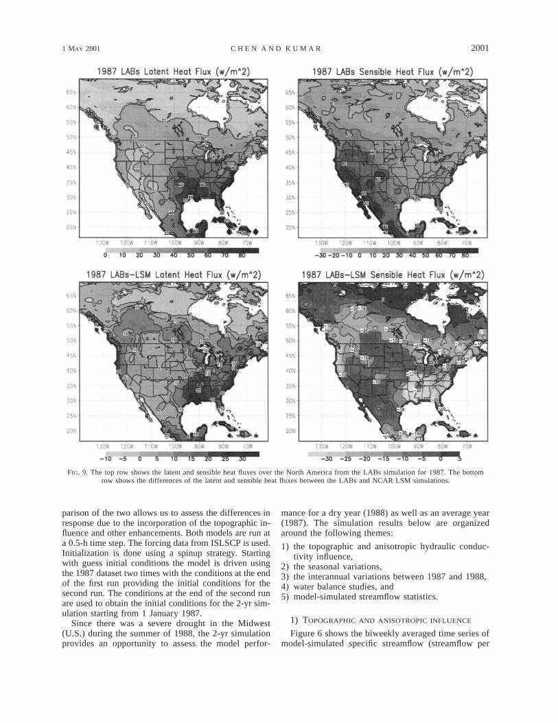
FIG. 9. The top row shows the latent and sensible heat fluxes over the North America from the LABs simulation for 1987. The bottomrow shows the differences of the latent and sensible heat fluxes between the LABs and NCAR LSM simulations.

parison of the two allows us to assess the differences inresponse due to the incorporation of the topographic in-fluence and other enhancements. Both models are run ata 0.5-h time step. The forcing data from ISLSCP is used.Initialization is done using a spinup strategy. Startingwith guess initial conditions the model is driven usingthe 1987 dataset two times with the conditions at the endof the first run providing the initial conditions for thesecond run. The conditions at the end of the second runare used to obtain the initial conditions for the 2-yr sim-ulation starting from 1 January 1987.

Since there was a severe drought in the Midwest(U.S.) during the summer of 1988, the 2-yr simulationprovides an opportunity to assess the model perfor-

mance for a dry year (1988) as well as an average year(1987). The simulation results below are organizedaround the following themes:

1) the topographic and anisotropic hydraulic conduc-tivity influence,

2) the seasonal variations,3) the interannual variations between 1987 and 1988,4) water balance studies, and5) model-simulated streamflow statistics.

1) TOPOGRAPHIC AND ANISOTROPIC INFLUENCE

Figure 6 shows the biweekly averaged time series ofmodel-simulated specific streamflow (streamflow per


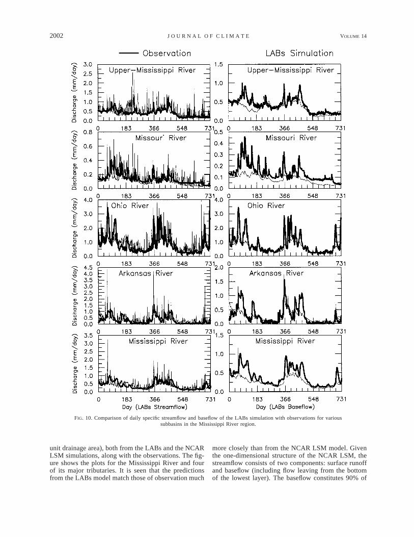
FIG. 10. Comparison of daily specific streamflow and baseflow of the LABs simulation with observations for varioussubbasins in the Mississippi River region.

unit drainage area), both from the LABs and the NCARLSM simulations, along with the observations. The fig-ure shows the plots for the Mississippi River and fourof its major tributaries. It is seen that the predictionsfrom the LABs model match those of observation much

more closely than from the NCAR LSM model. Giventhe one-dimensional structure of the NCAR LSM, thestreamflow consists of two components: surface runoffand baseflow (including flow leaving from the bottomof the lowest layer). The baseflow constitutes 90% of


FIG. 11. Daily averaged saturated fraction and mean water table depth of various subbasins in theMississippi River region.

the runoff generated by the NCAR LSM model and isresponsible for the excessively high total runoff volumesobserved. When the model physics is improved by pa-rameterizing the spatial variability through the Top-model formulation (see section 2a) the generated runoffvolumes are significantly reduced and closer to thoseseen in observations.

We also notice that there is a large range in the specificdischarge between the different basins which the LABsmodel is able to capture. The Missouri River basinshows the lowest specific discharge while the Ohio/Ten-nessee River basin shows the maximum. It is also notedthat the Ohio/Tennessee River basin has a dominant run-off contribution to the Mississippi River and this be-

havior is captured by the LABs model. The simulationsare consistent with the observations in capturing theearly spring high flow conditions. The annual flow vol-umes for each of the rivers studied is given in Table 4.The LABs streamflow volumes are in general a littlelarger than observations. This seems to result from con-sistently higher prediction of low flows (see Fig. 6). Toan extent this could be because aquifer recharge, reg-ulation storage, consumptive use, and ground-waterflow across the basin boundaries (see Zektser and Loai-ciga 1993) are not modeled. However, the exact causeof this discrepancy can be assessed only using stream-flow observations from unregulated streams. This is un-der investigation. From both Fig. 6 and Table 4 it is


FIG. 12. Seasonal variability of specific runoff for 1987 for a region in the eastern United States. The topographic variation of this regionis shown in Fig. 5.

evident that incorporation of the topographic control indescribing the basin flow dynamics improves the modelperformance significantly.

In order to investigate the impact of the anisotropy inthe hydraulic conductivity, the LABs model is run with

a 5 1, with all other conditions including the initialconditions and the spinup strategy, remaining identical.Figure 7 shows the comparison of the two LABs simu-lations along with the observations. It is evident thatdisregarding the anisotropy degrades the model perfor-


FIG. 13. The spatial distribution of the difference between the mean water table depth for Jun of 1987 and 1988.

mance. It is interesting to note that when the anisotropyis ignored, the runoff fluctuates more rapidly. This hap-pens because the lower lateral hydraulic conductivitiesreduce the baseflow, resulting in more storage in the soilcolumn. This in turn raises the water table leading toincreased surface runoff. Therefore, during rainfallevents, there is more surface runoff generated by themodel, and between the rainfall events the baseflow islower. Comparison of a 5 1 case with the NCAR LSMmodel in Fig. 6 also shows that when topographic effectsare neglected the model performance is worse than whenonly anisotropic effects are neglected. This indicates thatthe topographic effects are more important than the an-isotropic effects.

Figure 8 shows the comparison of the average latentand sensible heat fluxes for the entire Mississippi Riverbasin for 1987 and 1988. We see that LABs predictionsfor the latent heat flux are in general larger than thatfrom the NCAR LSM model. During summer this dif-ference can be about 20% of the prediction. This should

be expected since the lower streamflow of the LABsresults in higher soil-moisture storage. The larger latentheat flux seems to be compensated by the sensible heatflux that is lower than that of the NCAR LSM model.These results demonstrate that the improvements in theprediction of runoff have a significant impact on theprediction of the energy balance. Figure 9 shows thespatial distribution of the mean annual latent and sen-sible heat fluxes for 1987. The difference of the meanannual fluxes between the LABs and NCAR LSM mod-el are also plotted. We see that the LABs model pre-diction for latent heat is generally larger in the lowerMississippi/Gulf of Mexico region. This is a region ofconvergence of subsurface moisture and also receiveshigh precipitation. The difference plot for the sensibleheat flux (see Fig. 9) shows that increased latent heatflux is compensated by a reduction in the sensible heatflux in the same region. This characteristic also holdsin the East Coast and northwest region of the UnitedStates.


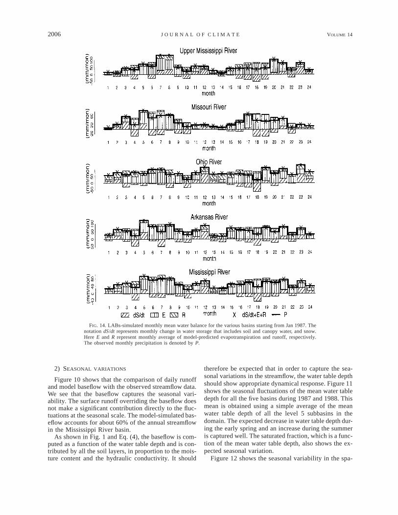
FIG. 14. LABs-simulated monthly mean water balance for the various basins starting from Jan 1987. Thenotation dS/dt represents monthly change in water storage that includes soil and canopy water, and snow.Here E and R represent monthly average of model-predicted evapotranspiration and runoff, respectively.The observed monthly precipitation is denoted by P.

2) SEASONAL VARIATIONS

Figure 10 shows that the comparison of daily runoffand model baseflow with the observed streamflow data.We see that the baseflow captures the seasonal vari-ability. The surface runoff overriding the baseflow doesnot make a significant contribution directly to the fluc-tuations at the seasonal scale. The model-simulated bas-eflow accounts for about 60% of the annual streamflowin the Mississippi River basin.

As shown in Fig. 1 and Eq. (4), the baseflow is com-puted as a function of the water table depth and is con-tributed by all the soil layers, in proportion to the mois-ture content and the hydraulic conductivity. It should

therefore be expected that in order to capture the sea-sonal variations in the streamflow, the water table depthshould show appropriate dynamical response. Figure 11shows the seasonal fluctuations of the mean water tabledepth for all the five basins during 1987 and 1988. Thismean is obtained using a simple average of the meanwater table depth of all the level 5 subbasins in thedomain. The expected decrease in water table depth dur-ing the early spring and an increase during the summeris captured well. The saturated fraction, which is a func-tion of the mean water table depth, also shows the ex-pected seasonal variation.

Figure 12 shows the seasonal variability in the spa-


FIG. 15. Direct surface runoff (represented as layer 0) and baseflow contributions from various soil layers (layers 1–6) tothe total streamflow in the various basins for 1987 and 1988. The mean annual water table depth is indicated as WT.

tial distribution of the runoff over a region in the east-ern United States. As is evident the model adequatelypredicts the winter–spring runoff maximum and thespatial distribution is indicative of the topographic con-trol on the runoff from the Appalachian mountainrange.

3) INTERANNUAL VARIATIONS

In Fig. 7 we see that the model predicted streamflowduring summer of 1988, for all the basins studied, isgenerally lower than that in 1987. Figure 10 shows thatthe baseflow is lower for an extended period of time


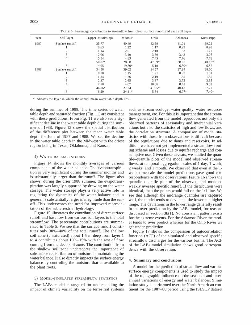
TABLE 5. Percentage contribution to streamflow from direct surface runoff and each soil layer.

Year Soil layer Upper Mississippi Missouri Ohio Arkansas Mississippi

1987 Surface runoff123456

35.770.631.142.065.54

50.82*4.05

40.491.222.013.194.83

28.6819.59*

32.891.172.103.607.45

47.69*5.10

41.010.991.833.437.76

38.676.30*

39.220.981.773.267.78

40.13*6.87

1988 Surface runoff123456

34.580.781.342.377.78

46.86*6.29

39.021.151.762.654.07

27.2424.11*

34.571.212.193.87

10.5641.95*5.64

37.940.971.853.728.41

40.136.97*

38.601.011.853.559.82

37.777.40*

* Indicates the layer in which the annual mean water table depth lies.

during the summer of 1988. The time series of watertable depth and saturated fraction (Fig. 11) are consistentwith these predictions. From Fig. 11 we also see a sig-nificant decline in the water table depth during the sum-mer of 1988. Figure 13 shows the spatial distributionof the difference plot between the mean water tabledepth for June of 1987 and 1988. We see the declinein the water table depth in the Midwest with the driestregion being in Texas, Oklahoma, and Kansas.

4) WATER BALANCE STUDIES

Figure 14 shows the monthly averages of variouscomponents of the water balance. The evapotranspira-tion is very significant during the summer months andis substantially larger than the runoff. The figure alsoshows, during the drier 1988 summer, the evapotrans-piration was largely supported by drawing on the waterstorage. The water storage plays a very active role inregulating the dynamics of the water balance and ingeneral is substantially larger in magnitude than the run-off. This underscores the need for improved represen-tation of the subterrestrial hydrology.

Figure 15 illustrates the contribution of direct surfacerunoff and baseflow from various soil layers to the totalstreamflow. The percentage contributions are summa-rized in Table 5. We see that the surface runoff consti-tutes only 30%–40% of the total runoff. The shallowsoil zone (unsaturated) about 1.5 m deep from layer 1to 4 contributes about 10%–15% with the rest of flowcoming from the deep soil zone. The contribution fromthe shallow soil zone underscores the importance ofsubsurface redistribution of moisture in maintaining thewater balance. It also directly impacts the surface energybalance by controling the moisture that is available tothe plant roots.

5) MODEL-SIMULATED STREAMFLOW STATISTICS

The LABs model is targeted for understanding theimpact of climate variability on the terrestrial systems

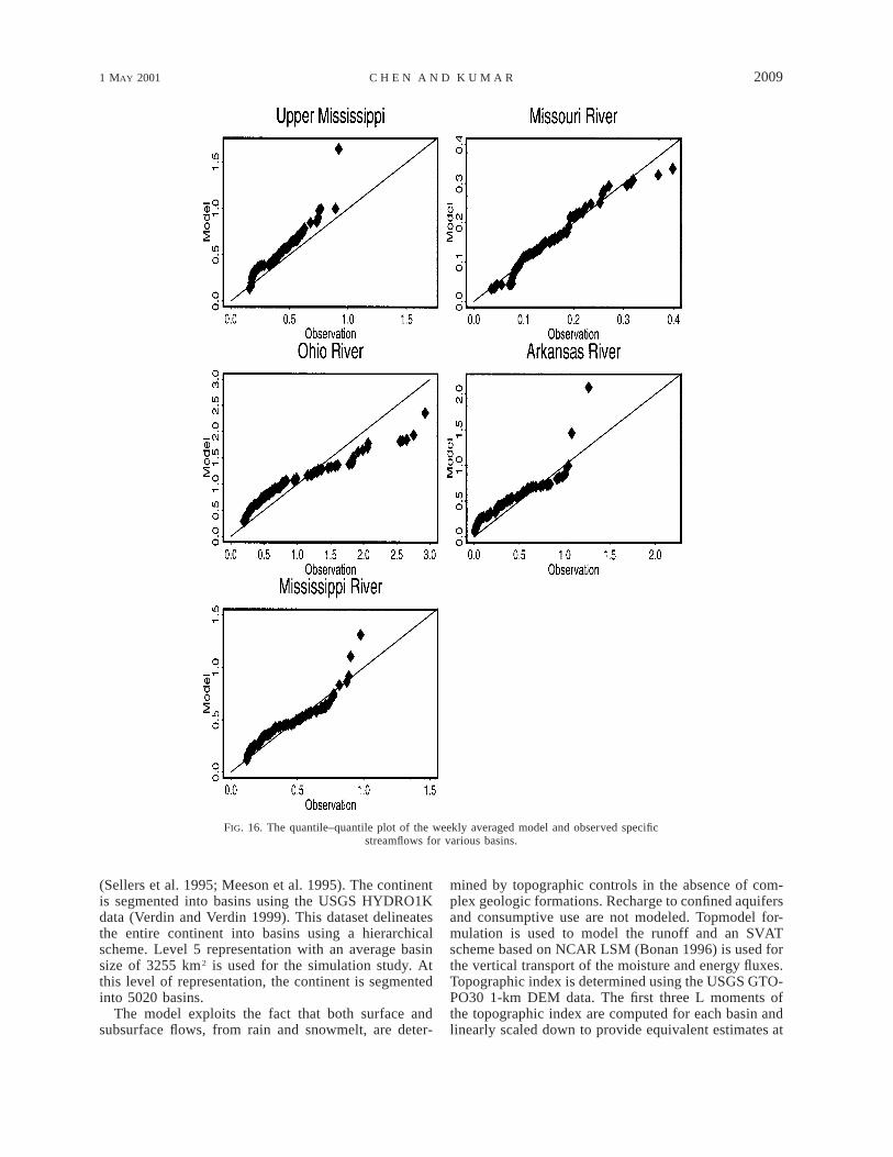
such as stream ecology, water quality, water resourcesmanagement, etc. For this it is important that the stream-flow generated from the model reproduces not only theobserved patterns of seasonality and interannual vari-ations but also the statistics of high and low flows, andthe correlation structure. A comparison of model sta-tistics with those from observations is difficult becauseof the regulations due to dams and reservoirs. In ad-dition, we have not yet implemented a streamflow-rout-ing scheme and losses due to aquifer recharge and con-sumptive use. Given these caveats, we studied the quan-tile–quantile plots of the model and observed stream-flows, at temporal aggregation scales of 1 day, 1 week,2 weeks, and 1 month. We observed that even at the 1-week timescale the model predictions gave good cor-respondence with the observations. Figure 16 shows thequantile–quantile plot of the observed and modeledweekly average specific runoff. If the distribution wereidentical, then the points would fall on the 1:1 line. Wesee that although the midrange quantiles are capturedwell, the model tends to deviate at the lower and higherrange. The deviations in the lower range generally resultin the over prediction by the LABs model, for reasonsdiscussed in section 3b(1). No consistent pattern existsfor the extreme events. For the Arkansas River the mod-el tends to over predict whereas for the Ohio River weget under prediction.

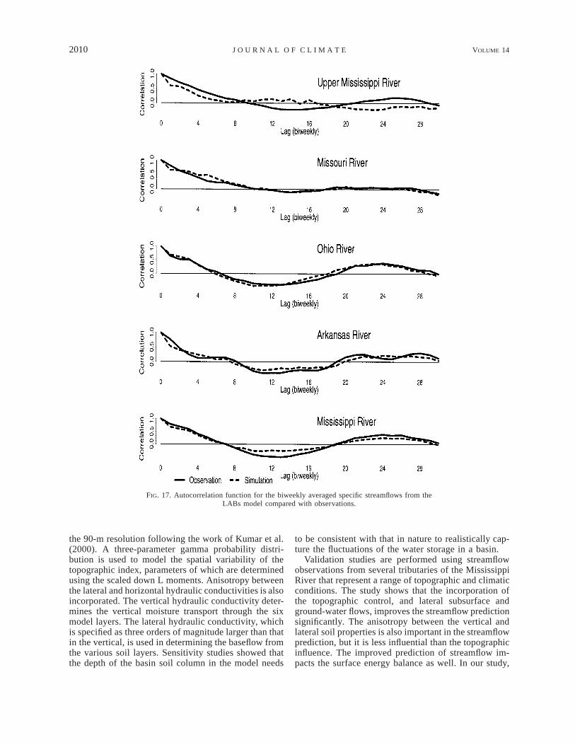
Figure 17 shows the comparison of autocorrelationfunction (ACF) of the simulated and observed specificstreamflow discharges for the various basins. The ACFof the LABs model simulation shows good correspon-dence with the observation.

4. Summary and conclusions

A model for the prediction of streamflow and varioussurface energy components is used to study the impactof the topographic influence on the seasonal and inter-annual variations of energy and water balances. Simu-lation study is performed over the North American con-tinent for the 1987–88 period using the ISLSCP dataset


FIG. 16. The quantile–quantile plot of the weekly averaged model and observed specificstreamflows for various basins.

(Sellers et al. 1995; Meeson et al. 1995). The continentis segmented into basins using the USGS HYDRO1Kdata (Verdin and Verdin 1999). This dataset delineatesthe entire continent into basins using a hierarchicalscheme. Level 5 representation with an average basinsize of 3255 km2 is used for the simulation study. Atthis level of representation, the continent is segmentedinto 5020 basins.

The model exploits the fact that both surface andsubsurface flows, from rain and snowmelt, are deter-

mined by topographic controls in the absence of com-plex geologic formations. Recharge to confined aquifersand consumptive use are not modeled. Topmodel for-mulation is used to model the runoff and an SVATscheme based on NCAR LSM (Bonan 1996) is used forthe vertical transport of the moisture and energy fluxes.Topographic index is determined using the USGS GTO-PO30 1-km DEM data. The first three L moments ofthe topographic index are computed for each basin andlinearly scaled down to provide equivalent estimates at


FIG. 17. Autocorrelation function for the biweekly averaged specific streamflows from theLABs model compared with observations.

the 90-m resolution following the work of Kumar et al.(2000). A three-parameter gamma probability distri-bution is used to model the spatial variability of thetopographic index, parameters of which are determinedusing the scaled down L moments. Anisotropy betweenthe lateral and horizontal hydraulic conductivities is alsoincorporated. The vertical hydraulic conductivity deter-mines the vertical moisture transport through the sixmodel layers. The lateral hydraulic conductivity, whichis specified as three orders of magnitude larger than thatin the vertical, is used in determining the baseflow fromthe various soil layers. Sensitivity studies showed thatthe depth of the basin soil column in the model needs

to be consistent with that in nature to realistically cap-ture the fluctuations of the water storage in a basin.

Validation studies are performed using streamflowobservations from several tributaries of the MississippiRiver that represent a range of topographic and climaticconditions. The study shows that the incorporation ofthe topographic control, and lateral subsurface andground-water flows, improves the streamflow predictionsignificantly. The anisotropy between the vertical andlateral soil properties is also important in the streamflowprediction, but it is less influential than the topographicinfluence. The improved prediction of streamflow im-pacts the surface energy balance as well. In our study,


this resulted in an increase in the latent heat flux duringthe summer and a compensatory decrease in the sensibleheat flux.

The model captures the seasonal and the interannualvariability quite realistically. The seasonal patterns ofstreamflow in all the tributaries of the Mississippi Riverbasin are consistent with the observations. The spatialpatterns capture the topographic influence realistically.The model shows the impact of the 1988 droughtthrough a decrease in streamflow and increased watertable depths. The spatial distribution of the increasedsoil-moisture deficit, as represented by the water tabledepth, shows the impact in the Midwestern UnitedStates. The study also demonstrates that the baseflowpredictions are extremely important for capturing theseasonal and interannual variations of the streamflow.On an average it accounts for 60% of the annual stream-flow in the different basins with 10%–15% contributedby the flow through the shallow soil zone. Comparisonof streamflow statistics through quantile–quantile plotsshowed that in general the model slightly overpredictsthe low flows. The extreme events are not captured. Itis unclear at this time if this is due to model deficiencyor because the streamflow observations have the effectsof reservoir regulations, consumptive use, and aquiferrecharge. This will be investigated further.

One of the motivations for the development of theLABs model is for providing a mechanism for assessingthe impact of the climatic fluctuations on terrestrial hy-drology. This will enable impact assessment on relatedsystems such as ecological and environmental. Asshown in the study, the model is able to predict hydro-logic variables, such as water table depth, that are spa-tially and temporally consistent with what we wouldexpect in a drier climatic condition. The consistencybetween the observed and the model-simulated stream-flow statistics, for a range of quantiles, is also veryencouraging. It leads to the possibility that the modelcan be used for quantitative impact assessment and de-cision making.

All model simulations are performed without cali-bration for the model parameters. Except for two pa-rameters all model parameters are obtained using pub-lished datasets. The two parameters that are specifiedand fixed for all basins are the hydraulic conductivitydecay constant z and the anisotropic factor a. Theirvalues were determined through extensive sensitivityanalysis using the data from the Little Washita basin inOklahoma (Allen and Nancy 1991) obtained throughfield experiments such as Washita’92 (Jackson andSchiebe 1993) and Southern Great Plains 1997 (SGP97).This is a limitation of the current study but no datasetsare available for their estimates directly. The simulationresults presented in this paper provide at least an a pos-teriori justification of their importance and for the choiceof their specific values used in the simulation. In theoryit is possible to obtain z either directly from observationsof hydraulic conductivity decay with depth or an anal-

ysis of baseflow recession curves (Beven et al. 1995).The anisotropic parameter a is even harder to determine.Additional research is required to establish the modelsensitivity to these parameters depending on the specificobjective of the study and ways to determine them ef-ficiently. This issue is currently under investigation.

Acknowledgments. Support for this project has beenprovided by NASA Grant NAG5-3361 and NSF GrantEAR 97-06121. Computational support was also pro-vided by NCSA Grant ATM990003N. Thanks are alsodue to Gordon B. Bonan for making the NCAR LSMmodel available in the public domain.

APPENDIX A

Soil-Moisture Dynamics in LABs

Each basin is divided into eight subregions (j 5 1,. . . , 8; excluding the water body; see Fig. 2) for com-puting infiltration and evaporation. Each basin columnis divided into six layers (i 5 1, . . . , 6) for simulatingsoil-moisture dynamics. The amount of water availablefor infiltration and runoff in the jth subregion denotedas P(j) is dependent on the interception by the vegetationin the subregions and snowmelt characteristics (see Bon-an 1996 for details). The infiltration capacity is assumedto be zero for the saturated subregions, and in the un-saturated subregion it is given as (Entekhabi and Ea-gleson 1989):

5 ksz(0)ns 1 ksz(0)(1 2 n),f*u (A1)

where ksz(0) is the saturated hydraulic conductivity atground surface, n 5 [2(dc/ds)]/[0.5Dz(1)] evaluatedfor s 5 1, c is the soil matrix potential, and Dz(1) isthe thickness of the first layer. The relative saturationin the first layer is given as s 5 [u(1)]/[usat], where u(1)is the average first layer soil moisture in the unsaturatedsubregion of the basin [see also Eq. (A10)]. Note thatthe infiltration capacity is the same for all unsaturatedsubregions, that is, it is dependent on soil texture, whichis specified as a uniform value across the entire basin,and not vegetation type. The infiltration in the jth sub-region is computed as

f * if P( j) . f *u uq ( j) 5 (A2)inf 5P( j) if P( j) # f *.u

The total infiltration for the entire basin is computed as4

q 5 w ( j)q ( j), (A3)OT inf area infj51

where warea(j) is the fractional area of the jth subregion(note j 5 1, . . . , 4 since infiltration occurs in the fourunsaturated subregions only, see Fig. 2).

The latent heat flux for the entire basin is obtainedthrough the sum of the following contributions.

1) Total surface evaporation computed by considering


demand and supply limited rates from the saturatedand unsaturated subregions, respectively, for eachland-use category

8

q 5 w ( j)q ( j), (A4)OTseva area sevaj51

where qseva(j) is the evaporation corresponding tosubregion j.

2) The transpiration is computed based on the similaritytheory for each subregion and is a function of thelanduse category (see Bonan 1996, section 8 for de-tails). This transpiration is assumed to be derivedfrom each of the soil layer in proportion to the rootfraction. The total transpiration from the ith soil layeris given as

8

q (i) 5 w ( j)q ( j)r (i, j), (A5)OT tran area tran rootj51

where qtran(j) is the transpiration from the jth sub-region and root(i, j) is the root fraction in the ithlayer for that subregion (see Bonan 1996, section 1.2for details).

The moisture transport in the soil column is describedby the Richards equation:

]u ] ]u(z) ]c(z)5 k (z) 2 1 . (A6)z 1 2[ ]]t ]z ]z ]u

For each layer the equation is

Du(i)Dz(i)5 2q (i) 1 q (i) 2 e(i), (A7)in outDt

where u(i) is the ith layer soil water content for theentire basin, q in(i) and q out(i) are the averaged quantitiesof input and output water fluxes (positive in the upwarddirection) from layer i over the time period of Dt, e(i)is the averaged evapotranspiration loss, Dz(i) is thethickness of soil layer i, and Dt is the model time step.This equation, with the boundary conditions of qTinf asthe flux of water into the soil and the zero flux of waterat the bottom of the soil column, and with e(1) ø qTseva

1 qTtran(1) for the first layer and e(i) ø qTtran(i) for theother layers, is numerically implemented for a six-layersoil column to calculate soil water (see Bonan 1996,98–101 for details).

In considering the baseflow, qb(i), from each soil lay-er [see Eq. (11)], the soil water obtained from Eq. (A6)is updated by using the following equation:

q (i) 3 Dtbu(i) 5 u(i) 2 . (A8)Dz(i)

The total soil water deficit, Du, through the entire soilcolumn is computed as

6

D 5 [u 2 u(i)]Dz(i). (A9)Ou sati51

The mean water table depth of the basin, z=, is computedby using Eqs. (A9) and (10). This is then used to com-pute the saturated fraction, sf (5Ac/A), of the basin usingEq. (3). The average soil moisture content over the un-saturated subregion for layer i is obtained as

u(i) 2 s uf satu(i) 5 . (A10)

1 2 sf

Although the LABs model structure is one-dimen-sional, the spatial variability is parameterized throughthe probability distribution function of the topographicindex (see Fig. 1). The model predictions for the soilmoisture in each layer are predictions for the mean state,and this mean state determines the water table depth.In the LABs model, the saturated and unsaturated frac-tions in a basin are determined by this mean basin watertable depth as well as topography [see section 2a andEq. (3) for details]. Each of the four landuse categories,which are the same as NCAR LSM’s surface types, canexist in both saturated and unsaturated subregions (seeFig. 2). This results in different runoff and infiltrationrates corresponding to different subregions. This enablesus to model the subregion variabilities in water andenergy fluxes, since evaporation and transpiration areat potential rates over the saturated subregions and atsoil-moisture-controlled rates over the unsaturated ones.These are then aggregated to obtain the basin level en-ergy fluxes. Saturation overland flow occurs in the sat-urated region and infiltration excess overland flow oc-curs in the unsaturated region. The aggregated infiltra-tion is used in the solution of moisture transport throughthe vertical column. Furthermore, the four landuse cat-egories in both unsaturated and saturated regions havethe various properties of vegetation phenology, provid-ing variability in the interception of precipitation andin the radiation processes in the basin.

If necessary, the local water table depth (and con-sequently vertical moisture deficit) at any location canbe recovered using the mean water table depth throughEq. (2). This is not pursued within the scope of thispaper.

APPENDIX B

Radiation Simulation

The ISLSCP data gives four values of averaged short-wave down radiation, Ik (J m22 s21), that correspond toeach 6-h period in one day. In order to drive the modelat subhourly timescale the following algorithm fromBras (1990) is used to simulate the radiation valuesusing the 6-h average.

Clear-sky shortwave radiation, Ic (J m22 s21), is com-puted as

Ic(t) 5 Io(t) exp[2na1(t)m(t)], (B1)

where m(t) is the optical air mass at time t given by thefollowing equation:


m(t) 5 [sina(t) 1 0.15(a(t) 1 3.885)21.253]21,

where a(t) is the zenith angle of the location of interestat time t. We used a turbidity air factor n 5 2, a mo-lecular scattering coefficient a1(t) 5 0.128 2 0.054log10m(t), and an effective radiation intensity at the pointof interest Io(t) 5 Wo sina(t)/r(t)2. Here Wo is the solarconstant (1353 J m22 s21), and r(t) is the ratio of theactual Earth–Sun distance to mean Earth–Sun distancegiven by

2pr(t) 5 1.0 1 0.017 cos (186 2 D(t)) ,[ ]365

where D is the Julian day.Then the total shortwave radiation ro (J m22 day21),

for a day from ISLSCP data is4

r 5 I 3 6.0 3 3600.0. (B2)Oo kk51

The ratio, v, of the daily shortwave radiation, ro, to thesimulated daily data is

v 5 r I (t) dt . (B3)o E c@[ ]1day

Then the equation for the simulated solar radiation, Is(t),can be expressed as

Is(t) 5 vIc(t). (B4)

In order to simulate the longwave radiation, Il(t), weuse the following equation (Bras 1990):

Il(t) 5 WB(t)[0.740 1 0.0049e(t)], (B5)

where e is vapor pressure (mb) and WB is blackbodyemissive power that is equal to the product of theStefan–Boltzmann constant and air temperature.

APPENDIX C

Rainfall Event Simulation

The ISLSCP dataset gives 6-h accumulated rainfallvalues, however, the model is run at a subhourly timestep. Therefore, we need an algorithm to interpolate therainfall data to match the model’s time step. We applya 3-h first-quartile 50% probability rainfall (Huff 1967)to simulate the rainfall process in the model.

Since the 6-h accumulation values do not contain anyinformation about the rainfall duration and its variabil-ity, we assume that all the rainfall events occur for a3-h period from 1030 to 1330 UTC, and each day hasat most one rainfall event. So four 6-h accumulatedrainfall data, p(k) (mm), in one day are combined as adaily value, pt,

4

p 5 p(k), (C1)Otk51

where pt is in millimeters per day.

The rainfall percentage f (g), g 5 1, . . . , 6 for eachof the 30-min interval in the 3-h rainfall duration isobtained using the normalized CDF values given in Huff(1967) from first-quartile 50% probability.

The precipitation rate, I(g), for each 0.5-h interval isobtained as

p 3 f (g)tI(g) 5 g 5 1, . . . , 6, (C2)30 3 60

where I(g) is in millimeters per second.Once the precipitation rate for each time interval is

estimated, the spatial heterogeneity is specified as perthe NCAR LSM scheme (see Bonan 1996, section 8 fordetails).

REFERENCES

Abdulla, F. A., D. P. Lettenmaier, E. F. Wood, and J. A. Smith, 1996:Application of a macroscale hydrological model to estimate thewater balance of the Arkansas-Red River basin. J. Geophys. Res.,101 (D3), 7449–7459.

Abramopoulos, F., C. Rosenzweig, and B. Choudhary, 1988: Im-proved ground hydrology calculations for global climate models(GCMs), soil water movement and evapotranspiration. J. Cli-mate, 1, 921–941.

Allen, P. B., and J. W. Nancy, 1991: Hydrology of the Little WashitaRiver Watershed, OK: Data and analyses. U.S. Dept. of Agri-culture, Agricultural Research Service, Tech. Rep. ARS-90, Du-rant, OK, 74 pp. [Available from National Agricultural WaterQuality Laboratory, Durant, OK 74702.]

Beven, K. J., and M. J. Kirkby, 1979: A physically based variablecontributing area model of basin hydrology. Hydrol. Sci. Bull.,24, 43–69., R. Lamb, P. F. Quinn, R. Romanowicz, and J. Freer, 1995:TOPMODEL. Computer Models of Watershed Hydrology, V. P.Singh, Ed., Water Resources Publication, 627–668.

Bonan, G. B., 1996: A land surface model (LSM version 1.0) forecological, hydrological, and atmospheric studies: Technical De-scription and User’s Guide. NCAR Tech. Note NCAR/TN-4171 STR, Boulder, CO, 150 pp. [Available online at http://www.cgd.ucar.edu/cms/lsm/index.html.]

Bras, R. L., 1990: Hydrology: An Introduction to Hydrologic Science.Addison-Wesley Publishing Company, 643 pp.

Brooks, R. H., and A. T. Corey, 1964: Hydraulic properties in porousmedia. Rep. 3, Colorado State University, Fort Collins, CO, 27pp.

Clapp, R. B., and G. M. Hornberger, 1978: Empirical equations forsome soil hydraulic properties. Water Resour. Res., 14, 601–604.

Dickinson, R. E., A. Henderson-Sellers, P. J. Kennedy, and M. F.Wilson, 1986: Biosphere–Atmosphere Transfer Scheme (BATS)for the NCAR Community Climate Model. National Center forAtmospheric Research, Tech. Note TN-275-STR, Boulder, CO,69 pp., , and , 1993: Biosphere–Atmosphere Transfer Scheme(BATS) version 1e as coupled to the NCAR Community ClimateModel. National Center for Atmospheric Research, Tech. NoteNCAR/TN-387 1 STR, Boulder, CO, 72 pp.

Dorman, J. L., and P. J. Sellers, 1989: A global climatology of albedo,roughness length and stomatal resistance for atmospheric generalcirculation models as represented by the simple biosphere model(SiB). J. Appl. Meteor., 28, 833–855.

EarthInfo, Inc., 1995: CD2. EarthInfo, Inc., CD-ROM, 4 vols; andreference manual, 67 pp. [Available from EarthInfo, Inc., 5541Central Ave., Boulder, CO 80301.]

Entekhabi, D., and P. S. Eagleson, 1989: Land surface hydrology


parameterization for atmospheric general circulation models in-cluding subgrid scale spatial variability. J. Climate, 2, 816–831.

Famiglietti, J. S., and E. F. Wood, 1991: Evapotranspiration and runofffrom large land areas: Land Surface Hydrology for AtmosphericGeneral Circulation Models. Land Surface–Atmosphere Inter-action for Climate Modeling, E. F. Wood, Ed., Kluwer AcademicPublishers, 179–204.

Freeze, R. A., and J. A. Cherry, 1979: Groundwater. Prentice-Hall,Inc., 604 pp.

Gesch, D. B., K. L. Verdin, and S. K. Greenlee, 1999: New landsurface digital elevation model covers the Earth. Eos, Trans.Amer. Geophys. Union, 80, 69–70.

Huff, F. A., 1967: Time distribution of rainfall in heavy storms. WaterResour. Res., 3, 1007–1019.

Jackson, T. J., and F. R. Schiebe, 1993: Hydrology data report Washita’92. National Agricultural Water Quality Lab., U.S. Dept. ofAgriculture, Agricultural Research Service, Rep. NAWQL 93-1,Durant, OK, 161 pp. [Available from National Agricultural Wa-ter Quality Laboratory, Durant, OK 74702.]

Jenson, S., and J. Domingue, 1988: Extracting topographic structurefrom digital elevation data for geographic information systemanalysis. Photogramm. Eng. Remote Sens., 54, 1593–1600.

Koster, R., and M. Suarez, 1992a: Modeling the land-surface bound-ary in climate models as a composite of independent vegetationstands. J. Geophys. Res., 97, 2697–2715., and , 1992b: A comparative analysis of two land-surfaceheterogeneity representations. J. Climate, 5, 1379–1390.

Kumar, P., K. L. Verdin, and S. K. Greenlee, 2000: Basin level sta-tistical properties of topographic index for North America. Adv.Water Resour., 23, 571–578. [Available by anonymous ftp fromcern57.ce.uiuc.edu and cd to pub/praveen/Papers under the filename of LmomentsDem.pdf.]

Messon, B. W., E. F. Corprew, J. M. P. McManus, D. M. Myers, J.W. Closs, K.-J. Sun, D. J. Sunday, and P. J. Sellers, 1995: ISLSCPInitiative I-Global Data Sets for Land–Atmosphere Models,1987–1988. Vols. 1–5, NASA, CD-ROM USApNASApGDAACpISLSCPp001-USApNASApGDAACpISLSCPp005.

Nijssen, B., D. P. Lettenmaier, X. Liang, S. W. Wetzel, and E. F.Wood, 1997: Simulation of runoff from continental-scale riverbasin using a grid-based land surface scheme. Water Resour.Res., 33, 711–724.

Olson, J. S., J. A. Watts, and L. J. Allison, 1983: Carbon in livevegetation of major world ecosystems. Oak Ridge National Lab-oratory, ORNL-5862, Oak Ridge, TN, 164 pp.

Pfafstetter, O., 1989: Classification of hydrographic basins: Codingmethodology. DNOS, translated by J. P. Verdin, 13 pp. [Availabefrom U.S. Geological Survey, EROS Data Center, Sioux Falls,SD 57198.]

Pitman, A. J., Z.-L. Yang, J. G. Gogley, and A. Henderson-Sellers,1991: Description of bare essentials of surface transfer for the

bureau of meteorological research centre AGCM. BMRC, Aus-tralia, BMRC Research Rep. 32, 117 pp.

Quinn, P., and K. Beven, 1993: Spatial and temporal predictions ofsoil moisture dynamics, runoff, variable source areas and evapo-transpiration for Plynlimon, Mid-Wales. Hydrol. Process., 7,425–448., , P. Chevallier, and O. Planchon, 1991: The prediction ofhillslope flow paths for distributed hydrological modeling usingdigital terrain models. Hydrol. Process., 5, 59–79.

Sellers, P. J., Y. Mintz, Y. C. Sud, and A. Dalcher, 1986: A simplebiosphere model (SiB) for use within the general circulationmodels. J. Atmos. Sci., 43, 505–531., and Coauthors, 1995: An overview of the ISLSCP Initiative IGlobal data sets. ISLSCP Initiative I-Global Data Sets for Land–Atmosphere Models, 1987–1988. Vol. 1, NASA, CD-ROM,USApNASApGDAACpISLSCPp001, OVERVIEW.DOC.

Sivapalan, M., K. J. Beven, and E. F. Wood, 1987: On hydrologicsimilarity. 2. A scaled model of storm runoff production. WaterResour. Res., 23, 1289–1299.

Stigelitz, M., D. Rind, J. Famiglietti, and C. Rosenzweig, 1997: Anefficient approach to modeling the topographic control of surfacehydrology for regional global climate modeling. J. Climate, 10,118–137.

Verdin, K. L., and S. Jenson, 1996: Development of continental scaleDEMs and extraction of hydrographic features. Proc. Third Int.Conf./Workshop on Integrating GIS and Environmental Mod-eling, Santa Fe, NM, National Center for Geographic Informa-tion and Analysis, University of California, Santa Barbara, CD-ROM. [Available from NCGIA, Santa Barbara, CA 93106.], and J. P. Verdin, 1999: A topological system for delineationand codification of the Earth’s river basins. J. Hydrol., 218, 1–12.

Webb, R. S., C. E. Rosenzweig, and E. R. Levine, 1993: Specifyingland surface characteristics in general circulation models: Soilprofile data set and derived water-holding capacities. Global Bio-geochem. Cycl., 7, 97–108.

Wolock, D. M., 1993: Simulating the variable-source-area concept ofstreamflow generation with the watershed model Topmodel. U.S.Geological Survey, Water-Resources Investigations Rep. 93-4124, 33 pp. [Available from U.S. Geological Survey, Booksand Open-File Reports, Denver Federal Center, Box 25425, Den-ver, CO 80225.]

Wood, E. F., D. P. Lettenmaier, X. Liang, B. Nijssen, and S. W. Wetzel,1997: Hydrological modeling of continental-scale basins. Annu.Rev. Earth Planet. Sci., 25, 279–300.

Yang, Z.-L., A. J. Pitman, B. McAvaney, and A. Henderson-Sellers,1995: The impact of implementing the bare essentials of surfacetransfer land surface scheme into the BMRC GCM. ClimateDyn., 11, 279–297.

Zektser, I. S., and H. A. Loaiciga, 1993: Groundwater fluxes in theglobal hydrologic cycle: Past, present and future. J. Hydrol.,144, 405–427.

Topographic Influence on the Seasonal and Interannual Variation of Water and Energy Balance of...

Documents

Transcript of Topographic Influence on the Seasonal and Interannual Variation of Water and Energy Balance of...