Toll-Road PPPs - PPIAF
108
Toll-Road PPPs Matt Bull with Anita Mauchan and Lauren Wilson Identifying, Mitigating and Managing Traffic Risk
-
Upload
khangminh22 -
Category
Documents
-
view
2 -
download
0
Transcript of Toll-Road PPPs - PPIAF

›› 1PPIAF | World Bank Group | Toll-Road PPPs: Identifying, Mitigating and Managing Traffic Risk
Toll-Road PPPs
Matt Bull with Anita Mauchan and Lauren Wilson
Identifying, Mitigating and Managing Traffic Risk

2 ‹‹ Toll-Road PPPs: Identifying, Mitigating and Managing Traffic Risk | PPIAF | World Bank Group
”“Prophesy is a good
line of business, but
it is full of risks.
—Mark Twain, Author

›› iPPIAF | World Bank Group | Toll-Road PPPs: Identifying, Mitigating and Managing Traffic Risk
ABOUT THE AUTHORS . . . . . . . . . . . . . . . . . . . . . . . . . . . . . . . . . . . . . . . . . . . . . . . . . . . . . . . . . . . . 1
ABBREVIATIONS AND ACRONYMS . . . . . . . . . . . . . . . . . . . . . . . . . . . . . . . . . . . . . . . . . . . . . . . . . 2
ACKNOWLEDGEMENTS . . . . . . . . . . . . . . . . . . . . . . . . . . . . . . . . . . . . . . . . . . . . . . . . . . . . . . . . . . . 3
PART I: UNDERSTANDING TOLL ROAD PPPS AND TRAFFIC RISK . . . . . . . . . . . . . . . . . . . . . 41. INTRODUCTION TO TRAFFIC RISK . . . . . . . . . . . . . . . . . . . . . . . . . . . . . . . . . . . . . . . . . . . . . . . . . 5
2. DEFINING HIGHWAY PPPS AND THE ROLE OF TRAFFIC RISK . . . . . . . . . . . . . . . . . . . . . . . 9
3. THE IMPORTANCE OF THE TRAFFIC FORECAST . . . . . . . . . . . . . . . . . . . . . . . . . . . . . . . . . . . 13
PART II: IDENTIFYING AND REDUCING TRAFFIC RISK: ERROR, UNCERTAINTY AND BIAS . . . . . . . . . . . . . . . . . . . . . . . . . . . . . . . . . . . . . . . . . . . . . . . . .204. INTRODUCING THE SOURCES OF TRAFFIC RISK . . . . . . . . . . . . . . . . . . . . . . . . . . . . . . . . . . 21
5. ERROR: FORECASTING ‘IN-SCOPE’ TRAFFIC . . . . . . . . . . . . . . . . . . . . . . . . . . . . . . . . . . . . . . . 24
6. UNCERTAINTY: FORECASTING FUTURE TRAFFIC . . . . . . . . . . . . . . . . . . . . . . . . . . . . . . . . . .30
7. BIAS: DELUSION, DISTORTION AND CURSES . . . . . . . . . . . . . . . . . . . . . . . . . . . . . . . . . . . . . .40
PART III: STRUCTURING AND ALLOCATING TRAFFIC RISK . . . . . . . . . . . . . . . . . . . . . . . . . 528. INTRODUCTION: THE STRUCTURING CHALLENGE . . . . . . . . . . . . . . . . . . . . . . . . . . . . . . . . 53
9. SHADOW RISK MODELING: ANALYZING AND QUANTIFYING TRAFFIC RISK . . . . . . .56
10. ALLOCATING TRAFFIC RISK . . . . . . . . . . . . . . . . . . . . . . . . . . . . . . . . . . . . . . . . . . . . . . . . . . . . .64
11. CONCLUSION. . . . . . . . . . . . . . . . . . . . . . . . . . . . . . . . . . . . . . . . . . . . . . . . . . . . . . . . . . . . . . . . . . . 75
ANNEXES . . . . . . . . . . . . . . . . . . . . . . . . . . . . . . . . . . . . . . . . . . . . . . . . . . . . . . . . . . . . . . . . . . . . . . . . 78
ANNEX A: WILLINGNESS TO PAY . . . . . . . . . . . . . . . . . . . . . . . . . . . . . . . . . . . . . . . . . . . . . . . . . . 79
ANNEX B: EXAMPLE SCOPE OF WORK FOR TRAFFIC ADVISOR . . . . . . . . . . . . . . . . . . . . . 81
ANNEX C: SOURCES OF SURVEY ERROR . . . . . . . . . . . . . . . . . . . . . . . . . . . . . . . . . . . . . . . . . . . 83
ANNEX D: SOURCES OF MODELING ERROR . . . . . . . . . . . . . . . . . . . . . . . . . . . . . . . . . . . . . . . . 85
ANNEX E: TYPICAL PPP CONTRACT STRUCTURE . . . . . . . . . . . . . . . . . . . . . . . . . . . . . . . . . . 87
ANNEX F: CASHFLOWS FROM THE DUMMY EXAMPLE OF A SPECULATIVE BIDDER CALL ON TRAFFIC AND REVENUE . . . . . . . . . . . . . . . . . . . . . . . . . . . . . . . . . . . . . . . . .89
ANNEX G: SHADOW BID FINANCIAL MODELING . . . . . . . . . . . . . . . . . . . . . . . . . . . . . . . . . .96
ANNEX H: TRAFFIC RISK INDEX . . . . . . . . . . . . . . . . . . . . . . . . . . . . . . . . . . . . . . . . . . . . . . . . . . .98
Table of Contents

ii ‹‹ Toll-Road PPPs: Identifying, Mitigating and Managing Traffic Risk | PPIAF | World Bank Group
Box 1: Summary of Chapter 1 . . . . . . . . . . . . . . . . . . . . . . . . . . . . . . . . . . . . . . . . . . . . . . . . . . . . . . . . 8
Box 2: Typology for Commercial Models of Toll-Highway PPP Projects . . . . . . . . . . . . . . . . . 10
Box 3: Summary of Chapter 2 . . . . . . . . . . . . . . . . . . . . . . . . . . . . . . . . . . . . . . . . . . . . . . . . . . . . . . . 12
Box 4: Summary of Chapter 3 . . . . . . . . . . . . . . . . . . . . . . . . . . . . . . . . . . . . . . . . . . . . . . . . . . . . . . 18
Box 5: Summary of Chapter 4 . . . . . . . . . . . . . . . . . . . . . . . . . . . . . . . . . . . . . . . . . . . . . . . . . . . . . . 23
Box 6: Summary of Chapter 5 . . . . . . . . . . . . . . . . . . . . . . . . . . . . . . . . . . . . . . . . . . . . . . . . . . . . . . 28
Box 7: Case Study: Hungary's M1-M5 (Failure) . . . . . . . . . . . . . . . . . . . . . . . . . . . . . . . . . . . . . . . 29
Box 8: Summary of Chapter 6 . . . . . . . . . . . . . . . . . . . . . . . . . . . . . . . . . . . . . . . . . . . . . . . . . . . . . . 37
Box 9: Case Study: N4 Maputo-Corridor Toll Highway, South Africa and Mozambique (Success) . . . . . . . . . . . . . . . . . . . . . . . . . . . . . . . . . . . . . . . . . 39
Box 10: Summary Example of a Speculative Bidder Call on Traffic and Revenue . . . . . . . . .43
Box 11: Over-Estimated Travel Forecasts— Real-Life Examples of Error, Uncertainty and Bias . . . . . . . . . . . . . . . . . . . . . . . . . . . . . . . . . 47
Box 12: Summary of Chapter 7 . . . . . . . . . . . . . . . . . . . . . . . . . . . . . . . . . . . . . . . . . . . . . . . . . . . . . .49
Box 13: Case Study—Radial Toll Highways in Madrid, Spain . . . . . . . . . . . . . . . . . . . . . . . . . . .50
Box 14: Summary of Chapter 8 . . . . . . . . . . . . . . . . . . . . . . . . . . . . . . . . . . . . . . . . . . . . . . . . . . . . . 55
Box 15: Summary of Chapter 9 . . . . . . . . . . . . . . . . . . . . . . . . . . . . . . . . . . . . . . . . . . . . . . . . . . . . . . 63
Box 16: Early-Stage Traffic-Risk Management . . . . . . . . . . . . . . . . . . . . . . . . . . . . . . . . . . . . . . . 71
Box 17: Summary of Chapter 10 . . . . . . . . . . . . . . . . . . . . . . . . . . . . . . . . . . . . . . . . . . . . . . . . . . . . . 74
Table of Boxes

›› iiiPPIAF | World Bank Group | Toll-Road PPPs: Identifying, Mitigating and Managing Traffic Risk
Figure 1: Empirical Research on Traffic Risk . . . . . . . . . . . . . . . . . . . . . . . . . . . . . . . . . . . . . . . . . . . 6
Figure 2: The Cause and Effect of Traffic Risk . . . . . . . . . . . . . . . . . . . . . . . . . . . . . . . . . . . . . . . . . 7
Figure 3: Typical Methodological Approach to Toll-Highway Traffic Studies . . . . . . . . . . . . 15
Figure 4: The Building Blocks of Traffic Risk: Breakdown of Theoretical Traffic Forecasts Produced for Toll-Highway Scheme . . . . . . . . . . . . . . . . . . . . . . . . . . . . . . 22
Figure 5: Minimum Measures to Reduce Bias . . . . . . . . . . . . . . . . . . . . . . . . . . . . . . . . . . . . . . . .46
Figure 6: The Structuring Challenge—The Nexus of Risk Transfer, Affordability and Bankability . . . . . . . . . . . . . . . . . . . . . . . . . . . . . . . . . . . . . . . . . . . . . . . . . . . . 53
Figure 7: Structuring Cycle . . . . . . . . . . . . . . . . . . . . . . . . . . . . . . . . . . . . . . . . . . . . . . . . . . . . . . . . . 55
Figure 8: Fictional Traffic Forecast for Low, Base and High Cases . . . . . . . . . . . . . . . . . . . . . . 59
Figure 9: Credit Zones and DSCR/LLCR Boundaries . . . . . . . . . . . . . . . . . . . . . . . . . . . . . . . . . . 62
Figure 10: Structuring Options for Allocating Traffic Risk . . . . . . . . . . . . . . . . . . . . . . . . . . . . .64
Figure 11: Traffic Banding in Shadow-Toll Projects . . . . . . . . . . . . . . . . . . . . . . . . . . . . . . . . . . . .68
Figure 12: Conceptual Diagram of an FTC . . . . . . . . . . . . . . . . . . . . . . . . . . . . . . . . . . . . . . . . . . . . 73
Figure 13: Toll Elasticity of Demand and the Impact on Revenue . . . . . . . . . . . . . . . . . . . . . . .80
Figure 14: Typical PPP Contract Structure . . . . . . . . . . . . . . . . . . . . . . . . . . . . . . . . . . . . . . . . . . . 87
Figure 15: A Typical Structure of a Shadow-Bid Financial Model . . . . . . . . . . . . . . . . . . . . . . .96
Table of Figures

iv ‹‹ Toll-Road PPPs: Identifying, Mitigating and Managing Traffic Risk | PPIAF | World Bank Group
Table 1: Sources of Error in Estimating Diverted Traffic . . . . . . . . . . . . . . . . . . . . . . . . . . . . . . . 27
Table 2: Forecasting-Error Sources and Reduction Measures . . . . . . . . . . . . . . . . . . . . . . . . . 28
Table 3: Uncertainty—Sources and Minimization Measures . . . . . . . . . . . . . . . . . . . . . . . . . . 38
Table 4: Traffic-Risk Index Summary . . . . . . . . . . . . . . . . . . . . . . . . . . . . . . . . . . . . . . . . . . . . . . . . 58
Table 5: Input Assumptions for a Fictional Traffic and Revenue Forecast (Base, Low and High Cases) . . . . . . . . . . . . . . . . . . . . . . . . . . . . . . . . . . . . . . . . . . . . . . . . . . . . . 59
Table 6: Simple Framework for Assessing the Credit Impact of Traffic Risk . . . . . . . . . . . . . 63
Table 7: Considerations for Using an Availability Payment . . . . . . . . . . . . . . . . . . . . . . . . . . . .66
Table 8: Considerations for Using a Blended-Availability Payment . . . . . . . . . . . . . . . . . . . . 67
Table 9: Considerations for Using a Shadow-Toll Structure . . . . . . . . . . . . . . . . . . . . . . . . . . . 69
Table 10: Considerations for Using an MRG/Revenue-Sharing Structure . . . . . . . . . . . . . . .70
Table 11: Considerations for Using a Government-Equity Model Structure . . . . . . . . . . . . . 72
Table 12: Considerations for Using a Full User-Pays Structure . . . . . . . . . . . . . . . . . . . . . . . . . 72
Table 13: Considerations for Using a Flexible-Term Contract Structure . . . . . . . . . . . . . . . . . 74
Table 14: Results of Financial Models Applied to Hypothetical Example . . . . . . . . . . . . . . . .90
Table 15: Revenue, Cash Flows, and IRR Calculations . . . . . . . . . . . . . . . . . . . . . . . . . . . . . . . . . 92
Table of Tables

›› 1PPIAF | World Bank Group | Toll-Road PPPs: Identifying, Mitigating and Managing Traffic Risk
Matt Bull, Senior Infrastructure Finance Specialist, The World Bank (The Global Infrastructure Facility)Matt began his career as a transport economist with the international consultancy firm Steer Davies Gleave, where he worked as a traffic advisor on various transport public-private partnership (PPP) projects for a range of global clients, including governments, sponsors and financiers. He joined PwC’s UK Corporate Finance team in 2007, to provide financial and deal structuring advice on both the “sell side” and “bid side” of a range of big-ticket PPP and private-finance initiative (PFI) transactions. He joined the World Bank’s Public-Private
Infrastructure Advisory Facility (PPIAF) in 2011, serving as its transport-sector specialist until he was appointed acting manager in 2014. He recently joined the newly established Global
Infrastructure Facility (GIF), a major global-funding platform for infrastructure projects housed at the World Bank, within which developed-country governments, major development banks and
leading infrastructure investors collaborate to finance improved infrastructure in emerging and developing economies. Matt holds an MA in transport economics from the University of Leeds’
Institute for Transport Studies.
Lauren Wilson, Operations Analyst, The World Bank (Global Infrastructure Facility)Lauren began her career at PPIAF in 2011 oversaw the facility’s Global Knowledge portfolio. Lauren was also PPIAF’s transport-sector analyst and provided support to the facility’s senior transport specialist on technical assistance activities in the sector. In 2016 Lauren moved to the GIF, where she advises on the preparation of infrastrucutre projects with private finance in the Middle East, North Africa, and Sub-Saharan Africa regions. Lauren holds anMA in economics and international relations from the University of St. Andrews and an MBA from Georgetown University’s McDonough School of Business.
Anita Mauchan, Director, Steer Davies GleaveAnita is a transport planner specializing in demand forecasting for major transport-infrastructure
projects, including roads, bridges, tunnels, railways, ports and tram systems. Over the past 25 years, she has provided demand and revenue advice to governments, bidders, lenders,
concessionaires and international finance Institutions for a range of transport infrastructure projects around the world, with each project requiring different forecasting approaches,
procurement structures and risk assessments. Her experience ranges from project feasibility to procurement, evaluation, project funding and post-construction monitoring and advice.
She is currently a director of the Strategy and Economics team at Steer Davies Gleave, an international transport-planning consultancy firm. She previously worked at CH2M. Anita
has recently advised the PPIAF team supporting the development of PPP projects and national government highway policy in developing countries. Anita holds an MSc in transport planning
from the University of Leeds’ Institue for Transport Studies.
About The Authors

2 ‹‹ Toll-Road PPPs: Identifying, Mitigating and Managing Traffic Risk | PPIAF | World Bank Group
AADT . . . . . . . . . Annual average daily traffic
BCR . . . . . . . . . . . Benefit-cost ratio
BOT . . . . . . . . . . Build operate transfer
CFADS . . . . . . . . Cash flow available for debt service
DBFOM . . . . . . . Design, build, finance, operate and maintain
DBOM . . . . . . . . Design, build, operate and maintain
DSCR . . . . . . . . . Debt-service cover ratio
EIB . . . . . . . . . . . European Investment Bank
EIRR . . . . . . . . . . Economic internal rate of return
F-IRR . . . . . . . . . Financial internal rate of return
FTC . . . . . . . . . . . Flexible-term contract
GDP . . . . . . . . . . . Gross domestic product
IRR . . . . . . . . . . . Internal rate of return
LGTT . . . . . . . . . Loan Guarantee Instrument for Trans-European Transport Network Projects
LLCR . . . . . . . . . . Loan life (or concession life) cover ratio
MRG . . . . . . . . . . Minimum revenue guarantees
NPV . . . . . . . . . . Net present value
PPIAF . . . . . . . . . Public-Private Infrastructure Advisory Facility
PPP . . . . . . . . . . . Public-private partnership
PV . . . . . . . . . . . . Present value
QRA . . . . . . . . . . Quantitative risk assessment
RP . . . . . . . . . . . . Revealed preference
SP . . . . . . . . . . . . Stated preference
SPV . . . . . . . . . . . Special-purpose vehicle
TIFIA . . . . . . . . . Transportation Infrastructure Finance and Innovation Act
Abbreviations and Acronyms

›› 3PPIAF | World Bank Group | Toll-Road PPPs: Identifying, Mitigating and Managing Traffic Risk
Support for this publication was provided by PPIAF and the Global Infrastructure Facility (GIF). PPIAF, a multi-donor trust fund housed in the World Bank Group, provides technical assistance to governments in developing countries. PPIAF’s main goal is to create enabling environments through high-impact partnerships that facilitate private investment in infrastructure. For more information, visit www.ppiaf.org.
The GIF is a global collaborative platform that facilitates preparing and structuring complex PPPs in infrastructure and mobilizing capital from private sector and institutional investors. The GIF supports governments in bringing well-structured and bankable infrastructure projects in the water, energy, transportation, and telecommunications sectors to the market. The GIF is housed in the World Bank Group. To learn more about the GIF, please visit www.globalinfrafacility.org.
Acknowledgements

4 ‹‹ Toll-Road PPPs: Identifying, Mitigating and Managing Traffic Risk | PPIAF | World Bank Group
Understanding Toll-Road PPPs and Traffic Risk
PART I

›› 5PPIAF | World Bank Group | Toll-Road PPPs: Identifying, Mitigating and Managing Traffic Risk
1. Introduction to Traffic Risk»
1 .1 . WHAT IS TRAFFIC RISK, AND WHY DO WE CARE?
Public-private partnerships (PPPs) are often viewed as the ideal solution for governments balancing limited budgets and growing infrastructure demands. The notion of the private sector raising finance to fund construction and improvements to highway infrastructure, to be recovered through future toll payments from road users, can be attractive to cash-strapped governments in both developed and developing countries.
However, as the failure of some high-profile toll-highway PPPs illustrates, implementing such projects is often not as straightforward as many governments envision. One of the most common factors contributing to these failures is traffic volume (and the resulting toll revenues) that turns out to be significantly different from what was originally forecast. This risk of actual traffic being lower (or higher) than forecast, and the inaccuracy of traffic forecasts, is referred to as traffic risk.
Traffic risk has manifested in many projects, leading to numerous financially distressed toll-road assets, which in turn have led to high-profile bankruptcies, renegotiations and government bailouts. More profoundly, due to these failures, private financiers are now significantly more cognitive of traffic (and revenue) risk and have become increasingly more risk averse towards highway PPP projects. Many financiers will now only support projects that provide them with significant shelter from the risk of lower traffic flows or that allocate these risks entirely to the government. In today’s project-finance market, financiers that are overly exposed to the risk will either add significant risk pricing to their financing or choose not to invest in the project at all (i.e., capital flight).
1 Muller, Robert H., “Examining toll road feasibility studies,” Public Works Financing 97 (1996).2 Bain, Robert, and Polakovic, Lidia, “Traffic forecasting risk study update 2005: through ramp-up and beyond,” Standard & Poor’s, London (2005).
1 .2 . JUST HOW BAD IS TRAFFIC RISK?
Empirical evidence on the performance of toll-road traffic and revenue forecasts suggests that inaccuracies are frequently observed. Several empirical studies have concluded that the range of these inaccuracies is often large, and that there may be a tendency towards overestimation. One of the earliest empirical studies on toll-road traffic forecast performance (Muller, 1996)1 compared the revenue forecast and the actual revenue for 14 urban toll-road projects in the United States. The study focused on the performance of the toll roads in their early years of operation and stressed that forecast performance has a high degree of variability during this period. For 10 out of the 14 toll roads, actual revenues on average differed from the original forecast by 20 to 75 percent. Only one of the toll roads studied by Muller had a positive difference, where actual revenue exceeded the forecast amount.
Similar results were obtained by Standard & Poor’s, which conducted a series of traffic-forecasting research exercises on privately financed toll roads around the world from 2002 to 2005. It accumulated more than 100 case studies and compared traffic forecasts with outturn traffic data. The study used the ratio of actual to forecast traffic as the indicator for traffic-forecasting accuracy; a ratio above 1.0 indicates that the forecast underestimated the actual traffic, whereas a ratio below 1.0 indicates overestimation. The blue line in Figure 1 shows the distribution of the actual/forecast traffic ratio of 104 projects.2 The traffic-forecasting performance ratio ranged from 0.14 to 1.51, which represents a considerable range of forecasting inaccuracy. The mean of the ratio was 0.77, which implies that, on average, the forecast overestimated traffic levels by 23 percent.

6 ‹‹ Toll-Road PPPs: Identifying, Mitigating and Managing Traffic Risk | PPIAF | World Bank Group
FIGURE 1: Empirical Research on Traffic Risk
A similar approach was used in the Flyvbjerg, et. al. 2005 study,3 which also analyzed the accuracy of traffic forecasts with large samples. This analysis, however, focused on 183 public (toll-free) roads located in 14 countries. The distribution of the actual/forecast traffic ratio is shown by the orange line in Figure 1. Their main findings were partly consistent with the aforementioned studies, in that they showed very wide error ranges. For half of the projects, the difference between the actual and forecast traffic was more than +/- 20 percent, and for quarter of the projects, the difference was more than +/- 40 percent. However, unlike the Standard & Poor’s research findings, the results of the analysis did not find any clear tendency towards overestimation. In fact, the mean ratio was 1.10, which indicates that forecasts were underestimated, and that the actual traffic was on average 10 percent higher than the forecasted traffic. This may point to the problem of overestimation being more common in privately financed toll roads, rather than public (toll-free) roads (which we will cover in more detail later).
Bain’s 2009 study4 compared the findings of the Standard & Poor’s and Flyvbjerg, et. al. research. It compared the distribution pattern of the two studies, as shown in Figure 1,
3 Flyvbjerg, Bent; Holm, Mette K. Skamris; and Buhl, Søren L., “How (in)accurate are demand forecasts in public works projects?: The case of transportation,” Journal of the American Planning Association 71.2 (2005): 131-146.
4 Bain, Robert, “Error and optimism bias in toll road traffic forecasts,” Transportation 36.5 (2009): 469-482.
and noted that the standard deviation and distribution patterns are similar. Bain also noted that the reason the distribution of the Standard & Poor’s samples leans towards overestimation could be because of optimism bias. Additionally, Bain notes that the similarity in the shape and the standard deviation of the two distribution patterns reflects the prediction error present in both data sets.
However, despite this history of forecasting inaccuracy and high-profile examples of project failure, developing country governments remain eager to develop highway PPPs, and, if possible, to transfer traffic and revenue risk to the private sector as a way of reducing their own financial exposure and long-term liabilities. Yet governments and even the other project parties in a typical PPP transaction often have a limited capacity to understand the nature of traffic and revenue risk, the technicalities of the traffic-forecasting process, the perceptions of the private sector, and the different ways to mitigate the risk and then allocate and manage the remaining risk efficiently between the public and private sectors. This guide seeks to be a timely resource to address these issues as demand for new highway infrastructure continues to grow.

›› 7PPIAF | World Bank Group | Toll-Road PPPs: Identifying, Mitigating and Managing Traffic Risk
1 .3 . PURPOSE, STRUCTURE AND LIMITATIONS OF THIS GUIDE: MAKING SENSE OF TRAFFIC RISK
The guide is primarily intended for technical officials in developing-country governments looking to understand the potential traffic risk in highway PPP projects, how it can affect the viability of projects, and the actions they can take to maximize project success. It may also be useful for private sponsors and commercial lenders (particularly in developing countries) who want to gain a better understanding of the factors that influence traffic risk, in order to make informed decisions regarding structuring bids and financing for highway PPP projects and managing exposure to risk. It also seeks to assist professionals who are advising governments on developing highway PPP programs with appraising the likelihood of success for those programs.
This guide is not, however, intended to be a comprehensive guide to traffic forecasting or to designing and implementing highway PPPs (references on traffic modeling and forecasting are included throughout the guide).5 Nor does the guide intend to negate the need for governments to hire reputable transport-planning consultancies to undertake high-quality traffic studies as part of a robust project-preparation process (to the contrary, as we point out throughout the guide—we want to encourage
5 For example, for a detailed overview of traffic modeling and forecasting, see: Modeling Transport, 4th Edition (Juan de Dios Ortuzar and Luis G. Willumsen, 2011) or Better Traffic and Revenue Forecasting (Luis G. Willumsen, 2015).
6 https://ppp.worldbank.org/public-private-partnership/library/toolkit-public-private-partnerships-roads-and-highways7 For a primer on PPPs, see PPP Reference Guide V2.0 http://wbi.worldbank.org/wbi/Data/wbi/wbicms/files/drupal-acquia/wbi/WBIPPIAFPPPReference-
Guidev11.0.pdf
the hiring of such advisors). Likewise, while managing traffic risk is critical, there are numerous other factors that contribute to the viability of a PPP project but are not addressed here. Finally, PPPs are only one mechanism for implementing highway projects, and this guide does not provide a thorough discussion regarding which projects are most suitable to be implemented as PPPs. The authors encourage readers to consult other resources produced by PPIAF and the World Bank (such as the PPIAF Highway PPP Toolkit)6 as well as the PPP Reference Guide7 for further information on issues related to PPPs.
In structuring the contents of this guide, we have tried to be cognizant of what the authors consider to be the causal process that leads to the occurrence of traffic risk, and how, in turn, the inadequate mitigation and management of the risk increases the risk of project failure and capital flight. Figure 2 illustrates this causal process.
Figure 2 shows that traffic risk is first born out of the very nature of traffic forecasting, which is prone to forecasting error, uncertainty about the future, and biases. These problems are effectively the “inputs” that lead to the omnipresence of traffic risk in road projects. It is the degree to which these inputs are present that dictates the size of the risk and its potential impact on project success or failure.
FIGURE 2: The Cause and Effect of Traffic Risk

8 ‹‹ Toll-Road PPPs: Identifying, Mitigating and Managing Traffic Risk | PPIAF | World Bank Group
Although traffic risk is therefore nearly always present, the good news is that through the actions of project parties, it can be reduced in size (mitigated), and then the residual risk (because it is inevitable that some risk will always remain) can be allocated (or structured) to the party that can most efficiently manage it. Taking this set of actions should reduce the risk of project failure and capital flight from road projects. It is this entire causal process, from how traffic risk arises through to how it can be reduced and then managed/allocated, that pervades the structure of the guide.
More specifically, the guide is structured in three parts:
• Part I: Understanding Toll Road PPPs and Traffic Risk. The first part of the guide sets the context, explaining the different
models of highway PPPs and the role that traffic risk can play in each. It then explains why the traffic forecast is so important and how traffic forecasts are developed.
• Part II: Identifying and Reducing Traffic Risk: Error, Uncertainty and Bias. The central part of the guide explains how traffic risk can grow out of the traffic forecast, through a mixture of forecasting error, uncertainty and bias. This section also outlines actions project parties can take to reduce traffic risk while preparing and procuring highway PPPs.
• Part III: Structuring and Allocating Traffic Risk. The final part of the guide explains how traffic risk can be quantified and then allocated to the party best able to manage the risk.
BOX 1: Summary of Chapter 1
The key points discussed in this chapter include:
• Traffic risk refers to the inaccuracy of traffic forecasts.
• Traffic risk is one of the most common factors contributing to the failure of toll-highway PPPs
• Traffic forecasts are often inaccurate. The range of these inaccuracies is often large, and there may be a tendency towards overestimation.
• The various parties involved in typical PPP transactions often have a limited capacity to adequately understand, mitigate, allocate and manage traffic risk. This guide is designed to address this gap.

›› 9PPIAF | World Bank Group | Toll-Road PPPs: Identifying, Mitigating and Managing Traffic Risk
2. Defining Highway PPPs and the Role of Traffic Risk
»
2 .1 . DEFINING HIGHWAY PPPS AND THE ROLE OF TRAFFIC RISK
Highway networks are critical for economic growth. They facilitate trade, improve urban and rural communities’ ability to access key public services, provide access to employment, and connect producers to markets. Highways are particularly important in developing countries, where more than 70 percent of freight is transported by road.8 Improving highway networks reduces journey times and damage to vehicles from poorly maintained roads, which makes trade cheaper and unlocks opportunities for economic growth. Improved highways also enhance highway safety and reduce fatalities, particularly among the poorest sections of society, where vehicle roadworthiness and safety features and equipment are less readily available.
Despite these widespread and well-understood social and economic benefits, the highway assets in most developing countries are insufficient to meet current or future levels of demand and are often poorly maintained. National highway programs must compete with other heavy infrastructure sectors (e.g., water and electricity) and social services (e.g., health and education) for limited government budget resources. Highway improvements require large upfront investments and large maintenance burdens. Previous underinvestment in the sector, coupled with increasing demand, has resulted in a large investment gap in most highway programs. Facing fiscal constraints, low management capacity and increased infrastructure demands, governments are therefore increasingly turning to PPPs to help bridge this gap.
A PPP can be any one of a variety of partnership structures between the government and the private sector to deliver
8 Freight Transport for Development, http://www.ppiaf.org/freighttoolkit/9 PPP Reference Guide V1.0 http://wbi.worldbank.org/wbi/Data/wbi/wbicms/files/drupal-acquia/wbi/WBIPPIAFPPPReferenceGuidev11.0.pdf
infrastructure and social services. For the purposes of this guide, we will use the same definition as specified in the PPIAF and World Bank’s PPP Reference Guide9:
“A long-term contract between a private party and a government agency, for providing a public asset or service, in which the private party bears significant risk and management responsibility.”
This definition encompasses PPPs that involve the financing and building of entirely new highway assets, through to those that involve the management and maintenance of existing assets that require no private capital investment. It also encompasses different revenue streams, ranging from projects that are funded from government sources (typically called availability or service payments) through to projects funded by user payments (i.e., tolls).
A typology of the main commercial models for highway PPPs is presented in Box 1 (note: this is not intended to be an exhaustive typology). Most forms of PPP can be distinguished across two principal characteristics: the level of investment and involvement of the private sector in the construction of the asset, and the extent to which user payments create a revenue stream for the private sector. It is this latter characteristic of PPP models that is the primary focus of this guide, whereby if the private sector’s income is either partially or fully reliant on toll revenues, then the private sector’s ability to finance the project is heavily dependent on the predictability and reliability of those revenues (and the traffic forecasts that underpin them).

10 ‹‹ Toll-Road PPPs: Identifying, Mitigating and Managing Traffic Risk | PPIAF | World Bank Group
BOX 2: Typology for Commercial Models of Toll-Highway PPP Projects
The following diagram shows the typology for commercial models of toll-highway PPP projects.
• Management contract: In a management contract, the private sector operates and maintains an existing road for the government. The private partner assumes the risks for operating the road over the length of the contract, while the government retains the remaining risks. Management contracts are typically structured to incentivize improved service delivery from the private operator, by making government payments conditional on achieving specific performance targets. There is no private capital invested in the project, because the road is an existing infrastructure asset (or an asset that has recently been publicly financed). The private operator is, however, responsible for providing the working capital (i.e., short-term finance) to fund the operations and maintenance work, before being reimbursed by the government if specified outputs and performance levels are met. Management contracts tend to be shorter in length than other PPP structures, because the private operator does not need to recover any capital investment, and the government will want to retain long-term flexibility over its road-management practices. The private sector does not retain any traffic risk and does not benefit from revenues collected from user tolls.
• Operating concession (or lease): Similar to a management contract, a lease requires the private-sector partner to operate and maintain an existing highway to a required standard. Under the lease model, however, the private sector’s work is partially or fully funded by collecting user tolls over a specified lease period. A lease agreement would typically require an agreed-upon lease payment to be paid by the private partner to the government, either up front or an ongoing basis (i.e., a premium), to ensure the government receives fair value from leasing out a viable economic asset. In this sense, the private-sector partner is exposed to the financial risk of traffic and revenues being lower than expected. Lease models are more common in the rail or urban transit sectors, where there has been traditionally a more established role for the private sector in operating services and collecting user payments to finance these operations. However, such models have been used in many developed countries as a way of monetizing existing toll facilities (e.g., Indiana Toll Road in the United States)—i.e., by leasing the road to the private sector, the government is able to receive a “windfall” up-front payment that can ease budgetary pressure or help fund other projects.

›› 11PPIAF | World Bank Group | Toll-Road PPPs: Identifying, Mitigating and Managing Traffic Risk
• Design, build, operate and maintain (DBOM): The private sector is contracted to design and build a new highway, or rehabilitate an existing one, and operate the asset over an extended period of time. In the DBOM structure, the private partner assumes the construction risks (e.g., delay or budget overruns) along with the operational risks (e.g., highway availability, unforeseen maintenance costs, incident response, etc.). The traffic risk is typically retained by the government, which funds the capital investment costs. The project therefore is fully funded by the government (i.e., “on the government’s balance sheet”) and does not involve any (or perhaps limited, in the form of equity) private-sector capital investment. One of the primary benefits of the DBOM structure is that it achieves whole-of-life cost efficiencies, whereby the same private entity is responsible for the design, construction and long-term operation and maintenance of the road and therefore should be incentivized to reduce costs over the entire lifecycle of the contract. The private partner should therefore be incentivized to design and build a higher-quality asset than it would under a traditional design-build procurement model, reducing the lifetime cost of the asset.
• Build and operate Concession: Similar to the DBOM model, the private-sector partner will be responsible for building, operating and maintaining the highway facility and will not be obliged to finance the asset. However, the private partner will be allowed to benefit from user toll revenues by leasing the asset over a specified period once it is constructed. In return for paying a lease fee upfront or on an ongoing basis, the private partner is granted the right to collect and retain toll revenues over the lease period. The private partner is exposed to the risk that traffic and toll revenues could be much lower than anticipated under this model. On the other hand, unless there is a revenue-sharing mechanism, the public sector could miss out on outturn toll revenues that are higher than forecast. It is important to note that if lease payments are made on an ongoing basis, such a model can often encourage aggressive forecasting through so-called “strategic misrepresentation” (see Chapter 7 for further discussion). Because this model involves little or no private-sector investment, private-sector parties such as contractors can exit a project during the operational phase without suffering significant financial distress, and they will have potentially already been compensated for what may have been a very lucrative construction contract. As a result, such PPP contracts have to be very carefully structured, perhaps with some equity investment or other forms of security (e.g., performance bonds).
• Design, build, finance, operate and maintain (DBFOM): Similar to the DBOM model, the same private partner will construct the asset and operate and maintain it over a specified period, but the key distinguishing feature of the DBFOM structure is that the private partner finances some or all of the upfront capital costs for the project. Structuring highway PPPs as DBFOMs therefore allows governments to leverage private-sector capital for infrastructure investment and might help remove projects from the public-sector balance sheet (depending on the assessment of relevant public accounting systems). This can be useful for governments looking to bring forward the construction of projects, as well as those with large fiscal or capital constraints. Many of the risks—including construction, operational and financing—in this model are allocated to the private sector. Demand (traffic) risks are retained by the government. The private-sector partner is paid in the form of availability payments, which are conditional on achieving specific outputs and performance targets . As with the DBOM model, the DBFOM structure achieves whole-of-life costing efficiencies.
• Full concession / build-operate-transfer (BOT): A toll concession involves the private partner financing some or all of the upfront capital costs for a project, and then, as with the DBFOM model, the same private partner is responsible for operating and maintaining the highway asset over a specified contract period. However, under this model, the private partner (i.e., the concessionaire) is remunerated only through toll payments from the user and therefore is exposed to the risk of usage of the road being lower than expected at any given time. Such a model removes significant ongoing financial liabilities from the government and frees up government resources for other capital expenditure priorities. However, a concession model typically involves conceding the value of an asset to the private sector over a set period, and if demand and revenue are higher than expected, this upside may be mostly lost to the private sector.

12 ‹‹ Toll-Road PPPs: Identifying, Mitigating and Managing Traffic Risk | PPIAF | World Bank Group
In the developing world and in emerging economies experiencing rapid economic and car-ownership growth, there is perhaps a much greater propensity (and indeed pressure) to try to develop the “user-pays” PPP models (the top row of the figure in Box 1). This is because government budgets are typically extremely constrained and face a variety of competing demands (from other spending priorities). Under these fiscal constraints, the raising of private investment against future toll revenues becomes very attractive, whether it be in the form of a lease payment to the government (to offset some or all of the public investment in an existing “brownfield” asset) or a concession/BOT (to offset some or all of the public investment in a new “greenfield” asset). This is hardly surprising, given that the government receives a windfall in either cash or assets, with little exposure to the risk of traffic and revenues being lower than anticipated, because the traffic risk has been transferred.
However, it is this transfer of traffic risk that often proves much more difficult in practice. The scale of the risk can be either underestimated by the project parties—which can result in financial distress, renegotiations, bankruptcy and sometimes government bail-outs—or so negatively perceived by the private sector that it places a significant risk premium on its project pricing, which can be passed on to users (in the form of unaffordable tolls) or to governments (in the form of unaffordable subsidies and large contingent liabilities).
These difficulties are caused by the reliance of project partners on traffic forecasts. These forecasts play a vital role in any such PPP project, but it is here that forecasting error, uncertainty and biases can occur and ultimately lead to project failure. In the next chapter, we explain the role of the traffic forecast and provide a brief overview of the forecasting process.
BOX 3: Summary of Chapter 2
The key points discussed in this chapter include:
• For the purposes of this guide, a PPP is defined as: “A long-term contract between a private party and a government agency, for providing a public asset or service, in which the private party bears significant risk and management responsibility.”
• Common PPP models for highway PPPs include: O&M; lease; DBOM; DBOM and lease; DBFOM; and toll concession.
• There is a relationship between the selected PPP model and the level of traffic risk to which the public and private-sector partners are exposed.

›› 13PPIAF | World Bank Group | Toll-Road PPPs: Identifying, Mitigating and Managing Traffic Risk
3. The Importance of the Traffic Forecast
3 .1 . INTRODUCTION
In recent years, the accuracy of traffic forecasts produced for toll highways, tunnels and bridges has become a major source of debate amongst governments, concessionaires, investors, financial institutions and the media, due to the significant underperformance of some toll highways in countries such as Australia, Spain and the United States. The failure of high-profile projects in the developed world has earned traffic forecasters a bad reputation, and the perceived accuracy of traffic forecasts has suffered greatly as a result.
Nevertheless, traffic forecasts play an essential role in the development of future transport infrastructure. Without them, the economic viability of infrastructure cannot be assessed by governments, infrastructure design cannot be tailored to demand, and the revenue-generating potential of a highway remains unknown. This section explains why traffic forecasts are needed for highway PPP projects; what a traffic study can tell its audience; and how traffic forecasts are produced.
3 .2 . WHY ARE TRAFFIC FORECASTS NEEDED?
Traffic forecasts are required at all stages of highway project development. Initially they will be used to inform the decision to undertake the project, by serving as inputs to the calculation of the project’s financial and economic justification (often captured through a net-present-value (NPV) or economic-internal-rate-of-return (EIRR) calculation). Forecasts are also used to design the highway, ensuring that sufficient road capacity is provided to accommodate future traffic growth whilst maintaining high standards of service, and to assess the environmental and socio-economic impact of
10 Also known as Level 3, investment grade is a rating that indicates that a municipal or corporate bond has a relatively low risk of default.11 Traffic Risk in Start-up Toll Facilities, Standard & Poor’s (September 2002)
the highway. Traffic and (in the case of toll highways) revenue forecasts will also inform the allocation of traffic risk during procurement (or negotiation) of a private partner; determine the likely size of the public subsidy that might be required to make the project financially viable; and ultimately be used by public authorities or lending institutions to secure financing.
Over time, several traffic studies may be commissioned for the same highway. At the pre-feasibility stage, the traffic study assesses the viability of the project. The forecast is then refined during the project-development phase. The final traffic study, after achieving investment-grade10 status, is used for the financial close of a project. Concessionaires may also commission traffic-study updates during the highway operation, to adjust their annual budgets and assess the impact of on-going factors affecting future traffic and toll-revenue projections.
The traffic study at each stage of project development should be scoped appropriately for the task at hand. Typically the level of complexity of the traffic model, the collection of traffic data, the range of forecasts produced, and the number of sensitivity tests all increase as the project progresses along the development cycle towards financial close, until the forecast is considered investment grade.
Due to the subjective nature of many traffic-forecasting assumptions, due-diligence and peer reviews are essential to reduce the likelihood that the traffic forecasts are overly optimistic or overly conservative (see Chapter 7 for further discussion of bias). Empirical evidence has shown that traffic forecasts produced for privately financed toll highways are statistically more accurate than those produced for publicly financed toll-highway projects,11 largely as a result of the due diligence required by the credit committees of lending institutions.

14 ‹‹ Toll-Road PPPs: Identifying, Mitigating and Managing Traffic Risk | PPIAF | World Bank Group
The type of project asset under consideration will influence the methodological approach used to develop the traffic forecast. For example, traffic forecasts for an improvement of an existing rural highway with few alternative competing routes could be estimated using a relatively simple traffic model. However, the construction of a greenfield project in an urban area where many alternative route choices are available would require a more complex model, preceded by an extensive traffic-data collection program. The traffic risk associated with the forecasts produced for these projects will also vary significantly. On-line highway improvement projects generally benefit from an existing, measurable level of demand, while the estimation of traffic for a greenfield project is much less certain and is related to the accuracy of the traffic assigned to the new highway by the traffic model (see Chapter 4).
The level of risk adopted by each party is also a consideration in the definition of a traffic study. For projects where all traffic risk is passed on to the private party (see Chapter 9), it is essential for the success of the project that the private party has based its offer on detailed and realistic traffic forecasts, prepared with adequate sensitivity testing (risk analysis) and due diligence. This requirement is less essential to the public party that is not assuming any traffic risk, although the public party will still typically need to undertake a robust traffic study (including highway capacity, level of subsidy required, and potential toll tariffs) in order to define the project specification. The public party’s traffic study should also be used to evaluate bidders’ forecasts and set appropriate forecast thresholds (see Chapter 7 for additional discussion of this point). Conversely, if the public sector has retained all traffic risk and is committed to pay some kind of revenue support (such as an availability payment or minimum revenue guarantee; see Chapter 10) or is servicing public debt, it is essential that the public-sector forecasts are accurate and have sufficient tolerance to allow the public sector to meet its future financial responsibilities.
3 .3 . WHAT DOES A TRAFFIC STUDY TELL US?
A traffic study is designed to answer all traffic-related questions asked by highway designers, financiers, environmental engineers, sociologists, economists, politicians and the public. To provide these answers, the practitioner must first create an artificial representation of the existing transport situation. The new or improved highway infrastructure is then introduced into the existing transport situation in order to enable the future demand, in terms of traffic volumes, to be predicted.
Put simply, a traffic study for a new (or improved) highway will:
• Identify the existing traffic demand that could use the new highway (in-scope);
• Estimate the proportion of the “in-scope” traffic that will use the new highway (traffic capture); and
• Predict future traffic growth (traffic forecasting).
The main output of a traffic study is a set of traffic forecasts and, in the case of toll highways, revenue forecasts. Numerous forecasting assumptions underlie the production of forecasts, which combine to produce the forecaster’s best estimate (or base case). It is critical that these assumptions are well understood by all affected parties, and that alternative forecast scenarios are prepared to test the financial viability of the highway for a range of future outcomes.
The risk of underestimating or overestimating traffic and revenue forecasts is not generally borne by the traffic forecaster. The onus is therefore on the parties assuming the traffic risk to ensure that they understand and question the forecasting assumptions that underlie the traffic and revenue forecasts used to establish the financial viability of a highway scheme.
3 .4 . HOW ARE TRAFFIC FORECASTS PRODUCED?
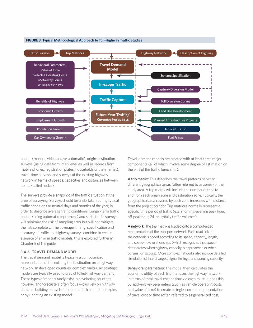
An important first step towards increasing awareness of traffic risk is an understanding of how traffic forecasts for toll highways are developed. A computer-based traffic simulation model sits at the core of a traffic study. A typical simplified methodological approach for a traffic study designed to provide traffic and revenue forecasts for a new greenfield toll highway is provided below, in Figure 3. This simplified example does not take into account transfers from other modes of transport (e.g., public transport), which can be included in more complex forecasting procedures. Its relative simplicity means that it can be used to predict highway traffic in developing countries where pre-existing traffic models are rarely available. In the following sections, we will describe the role each element of this diagram plays in the forecasting process.
3 .4 .1 . TRAFFIC AND HIGHWAY SURVEYSTraffic and highway surveys form the basis of a travel demand model that is built to accurately represent the existing highway traffic situation in a study area. The surveys should provide sufficient data to accurately reflect the existing traffic conditions in terms of traffic volumes, trip patterns, travel times and network characteristics. Typical surveys include traffic
›› 15PPIAF | World Bank Group | Toll-Road PPPs: Identifying, Mitigating and Managing Traffic Risk
counts (manual, video and/or automatic), origin-destination surveys (using data from interviews, as well as records from mobile phones, registration plates, households or the internet), travel-time surveys, and surveys of the existing highway network in terms of speeds, capacities and distances between points (called nodes).
The surveys provide a snapshot of the traffic situation at the time of surveying. Surveys should be undertaken during typical traffic conditions or neutral days and months of the year, in order to describe average traffic conditions. Longer-term traffic counts (using automatic equipment) and serial traffic surveys will minimize the risk of sampling error but will not mitigate the risk completely. The coverage, timing, specification and accuracy of traffic and highway surveys combine to create a source of error in traffic models; this is explored further in Chapter 5 of the guide.
3 .4 .2 . TRAVEL-DEMAND MODEL The travel demand model is typically a computerized representation of the existing traffic situation on a highway network. In developed countries, complex multi-user strategic models are typically used to predict tolled-highway demand. These types of models rarely exist in developing countries, however, and forecasters often focus exclusively on highway demand, building a travel-demand model from first principles or by updating an existing model.
Travel-demand models are created with at least three major components (all of which involve some degree of estimation on the part of the traffic forecaster):
A trip matrix: This describes the travel patterns between different geographical areas (often referred to as zones) of the study area. A trip matrix will include the number of trips to and from each origin zone and destination zone. Typically, the geographical area covered by each zone increases with distance from the project corridor. Trip matrices normally represent a specific time period of traffic (e.g., morning/evening peak hour, off-peak hour, 24-hour/daily traffic volumes).
A network: The trip matrix is loaded onto a computerized representation of the transport network. Each road link in the network is coded according to its speed, capacity, length, and speed-flow relationships (which recognizes that speed deteriorates when highway capacity is approached or when congestion occurs). More complex networks also include detailed simulation of interchanges, signal timings, and queuing capacity.
Behavioral parameters: The model then calculates the economic utility of each trip that uses the highway network, in terms of total travel cost or time via each route. It does this by applying key parameters (such as vehicle operating costs and value of time) to create a single, common representation of travel cost or time (often referred to as generalized cost;
FIGURE 3: Typical Methodological Approach to Toll-Highway Traffic Studies

16 ‹‹ Toll-Road PPPs: Identifying, Mitigating and Managing Traffic Risk | PPIAF | World Bank Group
see Section 3.4.3 below). Traffic is then generally assigned to the least-cost route, through an iterative procedure such as Wardrop’s equilibrium,12 taking into consideration the rest of the traffic on the highway network. Some models employ stochastic equilibrium13 in the choice of least-cost route, based on the assumption that drivers do not always perceive the full cost of their route choice decisions and do not always have perfect knowledge of the highway network.
The travel-demand model is calibrated14 to the existing traffic conditions and validated15 using supplementary traffic-survey data to demonstrate how well it reflects the existing supply and demand for road travel in the study area, and therefore its suitability to be used to predict the demand for new highway infrastructure. The calibration and validation of the model is a resource-intensive process that can take a significant proportion of the study period to complete. Validation criteria are used to demonstrate that the model is “fit for purpose” and adequately represents the existing traffic situation16. Because it would be impossible to observe every trip movement on the highway network, unobserved trips are usually simulated using matrix-estimation techniques contained within the model software.
Once the travel demand model has been satisfactorily validated, the proposed highway specification is introduced into the computer simulation of the highway network. By adding a new toll-free highway, tunnel or bridge to the existing traffic situation, the in-scope traffic or the total market for the new facility can then be established.
3 .4 .3 TRAFFIC CAPTUREThe next step is unique to tolled-highway forecasting—the assessment of drivers’ willingness to pay a toll for the benefits offered by a new highway, when compared to the alternative routes. Unfortunately, this essential step introduces the possibility of additional errors, regarding the future drivers’ decisions to pay for these benefits, and the accuracy of the model to accurately forecast the benefits. This additional forecasting step is generally thought to have the most significant negative impact on the accurate production of traffic and revenue forecasts for toll highways, and may explain why forecasts for such highways have been less reliable than for toll-free highways17.
12 Wardrop’s equilibrium states that no driver can unilaterally reduce his/her travel costs by shifting to another route. It is assumed that drivers have perfect knowledge about travel costs on a network and choose the best route.
13 Stochastic equilibrium is based on the principle that traffic arranges itself on the highway network such that the routes chosen by individual drivers are those with the minimum perceived cost.
14 Calibration seeks to replicate observed traffic data by adjusting the highway network, trip matrices and/or behavioral parameters.15 Validation requires the comparison of the model outputs with an independent set of traffic data, such as traffic counts, origin-destination data and travel-time
surveys, and making logic checks.16 See validation criteria and acceptability guidelines in TAG UNIT M3.1, Highway Assignment Modelling, January 2014, Department for Transport (UK).17 Flyvbjerg, Bent; Holm, Mette K. Skamris; and Buhl, Søren L. “How (in)accurate are demand forecasts in public works projects?: The case of transportation,”
Journal of the American Planning Association 71.2 (2005).
The proposed toll strategy for the highway is a key input into the calculation of traffic capture. The toll strategy (or regulations) encompasses the location of toll-charging points; toll tariffs by vehicle class; toll increases over time; and toll payment mechanisms. In most cases, the awarding authority specifies the toll strategy for the proposed new highway. Bidders may be asked to propose their own toll tariffs and payment mechanisms, depending on the highway authority’s toll policy.
The specification of toll tariffs (in terms of monetary value; differentiation by vehicle class, trip frequency and time of day; and the applicability of sales tax) directly influence the capture of traffic by the new highway. The tariff specification is used in the calculation of the generalized cost of using a new toll highway and subsequently in the allocation (“capture”) of traffic to the highway. If the toll tariffs exceed the perceived benefits offered by the toll highway, drivers will not choose to use the highway, which may result in its underperformance in terms of traffic and revenue outturn. The toll tariff escalation/indexation formula is generally established by the awarding authority, which will formally agree on the escalation with the concessionaire, usually on an annual basis. In most cases, toll tariff escalation is directly linked to the national consumer price index (CPI). Escalation rates may also be linked to economic growth and/or to foreign exchange rates if, for example, the majority of the project debt is lent in hard currency.
Travel-demand models attempt to simulate human behavior with a monetized (or time-based) representation of behavioral parameters that affect route choice, including value of time and motorway bonus (often combined into a willingness-to-pay parameter), and vehicle operating costs. The “generalized” cost (or time) is then calculated for each trip represented in the model. A simplified calculation of the generalized cost of a trip made on a toll highway is provided below:
Generalized Cost = (Travel Time x Value of Time) + (Distance x Vehicle Operating Costs) + Toll Tariff – Motorway Bonus (design, safety, convenience, reliability)

›› 17PPIAF | World Bank Group | Toll-Road PPPs: Identifying, Mitigating and Managing Traffic Risk
The travel time and distance elements of the generalized cost can usually be estimated reasonably accurately, based on the computerized representation of the highway network in the travel-demand model. The vehicle operating costs, if considered influential in the route choice, are typically linked to fuel cost per kilometer for cars and may include operating and staff costs for goods vehicles (again, this is established for all trips in the travel-demand model). The elements of the generalized cost equation that are much more difficult to estimate accurately include the highway users’ value of time and the motorway bonus. Often these two parameters are combined to create a “willingness to pay” parameter that includes the monetization of the time savings, and the value that highway users place on the superior design, safety, comfort, convenience and journey-time reliability offered by the new highway (see ANNEX A: WILLINGNESS TO PAY for more information).
The allocation (or “capture”) of traffic for a toll highway and toll-free alternatives is based on a comparison of the generalized cost for each route option to all trip movements represented in the trip matrices. These generalized cost comparisons can be undertaken within the travel-demand model itself, or externally in a supplementary model (often a spreadsheet model) using a “logit” type approach or a diversion model. The model will generally assign the trip along the route of lowest cost, after a set number of iterations.18 Diversion models (also known as capture models) are used to calculate the tendency to use a toll highway, based on the relative generalized cost or time between the highway and non-tolled alternatives19. The diversion model is adjusted for local conditions, based on the elasticity (sensitivity) of demand for the toll highway, i.e., the rate of allocation of traffic to the highway over a range of generalized cost/time differences between the tolled and toll-free alternatives.
3 .4 .4 . FUTURE-YEAR FORECASTSPredicting the growth of trip movements, in terms of volumes, trip patterns and route choices, is possibly the second-most-difficult element of traffic forecasting, and is a key contributor to traffic risk (see Chapter 6 for a deeper discussion on forecasting uncertainty).
18 Based on algorithms such as Wardrop’s of Stochastic Equilibrium19 Train, Kenneth, “Discrete Choice Methods with Simulation,” University of California, Berkeley, National Economic Research Associates (2002)20 Bain, Robert, “Toll Road Traffic & Revenue Forecasts, An Interpreter’s Guide” (2009)
Future demand for toll highways is derived from forecasting the drivers of traffic growth, such as economic, employment and population growth; car ownership growth; and fuel prices. By analyzing the relationship between these drivers and historic traffic growth, it is often possible to establish a mathematically significant statistical relationship that can be used to forecast future traffic. A statistically significant historical relationship may inform future growth patterns, but it should not necessarily be assumed that the relationship is transferable to long-term forecasting.20 The accuracy of long-term traffic-growth predictions are generally assumed to decline over time, due to increasing uncertainty surrounding the forecasts and the declining ability of historical relationships to inform long-term forecasts.
Forecasts of demand are based on certain parameters that are inherently uncertain. The traffic forecaster should use all the relevant and available data to make intelligent, realistic assumptions about how these variables will change over time. The impact of any planned improvements to the existing highway network (in addition to the project under consideration) and other transport modes should be included in the future-year forecasts.
During the forecasting period, which can cover 20, 30 or 40 or more years, demand for the new highway is likely to be affected by transport infrastructure projects that were not conceived during project procurement. Additionally, the timing of planned transport infrastructure, whether complementing or competing with the new highway, may differ from that assumed in the forecasts and may affect outturn traffic and revenues.
Typically a range of traffic forecasts are produced, based on pessimistic, “best-estimate” and optimistic sets of forecasting assumptions. Sensitivity tests conducted on key drivers of demand, often accompanied by a risk analysis, inform the range of output forecasts and indicate the parameters with the greatest potential to affect the accuracy of the forecasts.
The sections above provide a simplified description of the process of traffic forecasting. As we will see in the next chapter, forecasting errors, uncertainty and bias in this traffic-forecasting exercise affect the accuracy of the predictions, and this is what leads to traffic risk.

18 ‹‹ Toll-Road PPPs: Identifying, Mitigating and Managing Traffic Risk | PPIAF | World Bank Group
BOX 4: Summary of Chapter 3
The key points discussed in this chapter include:
• Traffic forecasts are needed to determine the economic viability of a highway project; inform project design; assess environmental and socio-economic impacts; and, for toll highways, determine revenue forecasts.
• Forecast complexity and associated risks will vary with the type of project. For example, forecasts for greenfield highways are more complex than forecasts for existing road assets.
• All traffic forecasts are based on assumptions, and it is critical for all parties to understand these assumptions and how they may affect the forecasts.
• Driver willingness to pay is determined by a combination of time savings, vehicle operating cost savings, and how drivers value toll-highway features such as superior design, comfort, safety, convenience and reliability.
• Willingness to pay can be difficult to measure. If a comparable toll-free highway exists, forecasters can conduct revealed preference surveys. These are generally more accurate than other data collection methods, because they are based on actual driver behavior. In the absence of a comparable highway, stated preference surveys are used to determine drivers’ willingness to pay a toll.
• The accurate estimate of the initial traffic capture by a new toll highway is considered the most significant risk in traffic forecasting. The second-most-significant risk is considered to be the prediction of future traffic growth.
• A range of forecasts based on pessimistic, “best-estimate” and optimistic forecasting assumptions should be provided, as well as sensitivity tests to indicate the parameters that will have the greatest impact on the accuracy of traffic forecasts.

›› 19PPIAF | World Bank Group | Toll-Road PPPs: Identifying, Mitigating and Managing Traffic Risk

20 ‹‹ Toll-Road PPPs: Identifying, Mitigating and Managing Traffic Risk | PPIAF | World Bank Group
Identifying and Reducing Traffic Risk: Error, Uncertainty and Bias
PART II

›› 21PPIAF | World Bank Group | Toll-Road PPPs: Identifying, Mitigating and Managing Traffic Risk
4. Introducing the Sources of Traffic Risk»
In the previous sections, we explained the concept of traffic risk. Some degree of traffic risk is present in all road projects, because it is inherent in the traffic-forecasting process, which attempts to predict future human behavior. Despite gradual methodological improvements in traffic-forecasting techniques, the process of estimating traffic volumes over the life of a major highway investment (e.g., 30 years) remains a probabilistic rather than deterministic exercise. As a result, actual traffic flows can vary (in some case dramatically) from the original traffic forecasts.
This potential divergence between predicted and actual traffic volumes becomes crucially important if some or all of a project’s costs are to be recovered from users through toll payments. Regardless of whether a project is publicly or privately financed, if the actual toll revenue outturn is lower than forecast, then the ability to recover investment costs and meet operational costs is undermined and can result in unforeseen financial losses, the need for costly renegotiations, and even bankruptcy. This is known as downside risk. Conversely, if the revenue outturn is higher than forecast (i.e., upside risk), it can create financial gains for the financiers. This upside can be viewed positively, but it may also leave the door open to accusations of profiteering at the expense of highway users, regardless of whether the project is publicly or privately financed.
Although traffic risk is present in all projects funded partially or fully by toll revenues, it often assumes greatest importance in projects financed by the private sector. There is strong competition for scarce private capital (particularly since the 2008 global financial crisis), and investors seek assets with the most stable and secure financial returns. If traffic risk is perceived to be too high, with too many potential revenue outcomes, there can be a significant impact on both the cost and availability of private capital for toll-highway projects. Likewise, private investors do not always have the same financial capacity as government entities to absorb losses from
a project and, unlike governments, are unable to adjust fiscal levers (e.g., increase taxation or borrowing) and alter policy (e.g., increase toll tariffs) to compensate for losses. This is not to say that the materialization of traffic risk is not a significant issue for publicly financed projects; it is, and it can create significant financial liabilities for governments that must be managed effectively. However, the perception of this risk can be very different for private investors. Thus if governments wish to attract and sustain private investment in their highway network, the perceived range of future traffic levels and expected revenue forecasts must be narrowed as much as possible to reduce uncertainty around the investment. Only by achieving this will private capital view a toll-highway asset as sufficiently stable, and only then will investment be attracted and sustained at a reasonable cost of capital.
So, how can we reduce and mitigate traffic risk and improve the accuracy of the traffic forecasts? Answering this question requires us to go deeper into the underlying causes of traffic forecasting inaccuracy. To do this, it is helpful to revisit the three main sources of inaccuracy in the traffic forecasting process, which were explained in the introduction:
• Error: The inaccuracies that result from the errors of the forecasting method itself are internal to the forecasting process and are effectively the result of (involuntary) human error that occurs during the development of the traffic study.
• Uncertainty: These are the inaccuracies that are typically out of the control of the traffic forecaster. They represent the changes in the external environment that occur during the project life and were not foreseen at the time the traffic study forecasts were originally developed.
• Bias: This may be voluntary—whereby traffic forecasts are artificially high, in order to facilitate a specific goal of

22 ‹‹ Toll-Road PPPs: Identifying, Mitigating and Managing Traffic Risk | PPIAF | World Bank Group
a project party (e.g., a bidder trying to develop a winning bid for a project, or a government official trying to ensure a project achieves government approval)—or it may be an involuntary natural tendency for planners, managers and policy makers to focus on the specifics of a current project rather than the outcomes of similar projects in the past.
In order to gain a better perspective on these potential inaccuracies residing within a set of traffic forecasts, it is helpful to break down the forecast into its various elements, to see where error, uncertainty and bias are most likely to be prevalent. To help illustrate this, Figure 4 overleaf shows the typical “building blocks” of a project’s traffic profile over time, and which blocks of traffic can be affected by forecasting error, uncertainty and bias.
The scenario presented in Figure 4 shows a simplistic representation of the forecasting elements of a theoretical toll highway. A toll-free version of the highway already existed and had an established set of users that could be observed (existing traffic). A project was then initiated that
widened the road and added additional capacity in the first year, when a toll for all vehicles was introduced. The introduction of the toll resulted in the loss of a proportion of local traffic to secondary highways (diverted traffic). A larger proportion of traffic was attracted from other highways (re-assigned traffic) to take advantage of the greater highway capacity and improved travel times and journey reliability. Over time, traffic is expected to grow along with economic growth that leads to increasing car ownership and mobility, and population growth (traffic growth). An element of development traffic is predicted to build up over the first three years after the highway opens, due to the improved accessibility provided by the highway and new residential/commercial (land-use) developments nearby. Finally, because the capacity improvements reduce travel times and significantly improve journey-time reliability, the highway is expected to induce trips that are not currently being made on the highway network (induced traffic).
As Figure 4 shows, error (as we have defined it) is most common when we try to accurately establish the existing traffic situation and how it will react to the introduction of tolls and
FIGURE 4: The Building Blocks of Traffic Risk: Breakdown of Theoretical Traffic Forecasts Produced for Toll-Highway Scheme

›› 23PPIAF | World Bank Group | Toll-Road PPPs: Identifying, Mitigating and Managing Traffic Risk
improvements (in the form of existing and re-assigned traffic). However, once we start to move beyond this existing potential market and start forecasting additional traffic over time (traffic growth, development traffic and induced traffic), then uncertainty starts to take over the forecast. This is because the forecasting methods for this new (yet to be observed) traffic rely more heavily on statistical methods and predictions about unobserved behavior or exogenous (external) factors that are very hard to predict. The potential for bias can be present across the entirety of the traffic forecast but tends to be concentrated in the upper levels of the traffic blocks, where future uncertainty can facilitate biases, including optimism bias.
The potent combination of error, uncertainty and bias means that traffic risk in toll-road projects will be an “always and everywhere” phenomenon, but does this mean that
toll-highway assets can never be sufficiently stable and attractive for private investors? The answer to this question is categorically “no.” Traffic risk cannot be fully eliminated, but it can be better understood, reduced in size, and managed properly, so that investor confidence can be achieved at a reasonable cost of capital. In the remainder of this section, we provide an overview of each of these drivers of traffic risk and explain the measures that the project parties can take to reduce the traffic risk.
In Part III, we discuss how residual traffic risk can be tested, understood and better categorized, before discussing the ways in which governments can use this understanding to efficiently allocate the risk between the public and private sectors through suitable deal structures.
BOX 5: Summary of Chapter 4
The key points discussed in this chapter include:
• The difference between predicted and actual traffic volumes becomes critical if any project costs are to be recovered from users through toll payments. Downside risk (if actual toll revenue outturn is lower than forecast) can result in unforeseen financial losses, the need for costly renegotiations, and even bankruptcy. Upside risk (if revenue outturn is higher than forecast) can create financial gains for financiers, but may also lead to accusations of profiteering.
• Traffic risk often assumes greatest importance in projects financed by the private sector.
• It is helpful to break down the forecast into its various “building blocks,” to see where error, uncertainty and bias are most likely to occur.
• Error is most common when trying to establish how current traffic will react to the introduction of tolls and improvements (in the form of existing traffic and reassigned traffic). Uncertainty takes over when forecasting additional traffic over time (traffic growth, development traffic and induced traffic).
• Traffic risk cannot be eliminated, but it can be reduced and managed, so that investor confidence can be achieved at a reasonable cost of capital.

24 ‹‹ Toll-Road PPPs: Identifying, Mitigating and Managing Traffic Risk | PPIAF | World Bank Group
5 .1 . INTRODUCTION
Highway usage is dependent on individual route choices and a multitude of underlying growth assumptions. Traffic-forecasting methodologies are consequently imperfect, making forecasting errors inevitable. Traffic-forecasting errors occur when the forecaster is trying to observe, understand and simulate existing and future travel behavior. In this sense, error occurs when the forecaster attempts to establish the existing demand for a road (existing traffic), what traffic might be attracted to it from other routes once it is improved (reassigned traffic), and the traffic that may be diverted to other roads as a result of the introduction of a toll (diverted traffic). The combination of these different types of traffic is what we have defined as “in-scope” traffic—i.e., the traffic that we know has the potential to use the new or improved highway on the day it opens.
As we will see in subsequent chapters, financiers and their advisors will look very closely at these “opening-day” traffic types and rely heavily on them when analyzing the creditworthiness of a project, because they represent the blocks of demand we know the most about. Conversely, traffic that will materialize in the distant future is subject to high levels of uncertainty, “back-ended” in time and valued less by financiers, as we will see in later chapters. Existing and re-assigned traffic is especially important for debt providers who want to be sure that the “opening-day” traffic volumes will produce sufficient revenues to allow sponsors to service their debt. As such, financier due diligence should include an examination of potential sources of error in the estimation of existing and reassigned traffic. This is the market about which the forecaster has the highest level of confidence, and which financiers will be relying on to enable the project to meet its debt obligations. In other words, this is the traffic they feel they can “bank.”
In the following sub-sections, we provide more details about each of these traffic types (existing, reassigned and diverted) and explain where errors can materialize. We also examine the steps that can be taken to reduce the errors to a more acceptable level and minimize the risk of outturn traffic volumes falling substantially above or below forecasted volumes. Because forecasting error can never be completely eliminated, governments will need to consider the inherent trade-off between time and budgetary constraints to minimize the risk. This trade-off is an important consideration and should not be dismissed. As such, we describe the minimum level of traffic study that should be undertaken and provide sample terms of reference for a typical traffic study in ANNEX B: SAMPLE SCOPE OF WORK FOR TRAFFIC ADVISOR.
5 .2 . FORECASTING EXISTING TRAFFIC: DATA-COLLECTION ERRORS
As illustrated in Figure 4, existing traffic often forms the majority of the predicted demand for an upgraded (or brownfield) highway, particularly in the early years of a concession, but existing traffic is also important for greenfield projects, because the forecaster needs to establish demand on the competing network from which demand for the new road will be captured.
Although there is inevitably an element of inaccuracy in any forecast, this type of traffic is generally less prone to forecasting error, because the traffic already exists and can be observed. Errors can, however, still occur, because it is impossible to survey all users of a transport system. As we explained in Chapter 3, for a typical traffic study, the forecasting team will need to observe existing traffic conditions by undertaking a program of traffic surveys. Typical surveys include traffic counts, origin-destination surveys, travel time surveys and surveys of the existing highway network.
5. Error: Forecasting "In-Scope" Traffic»
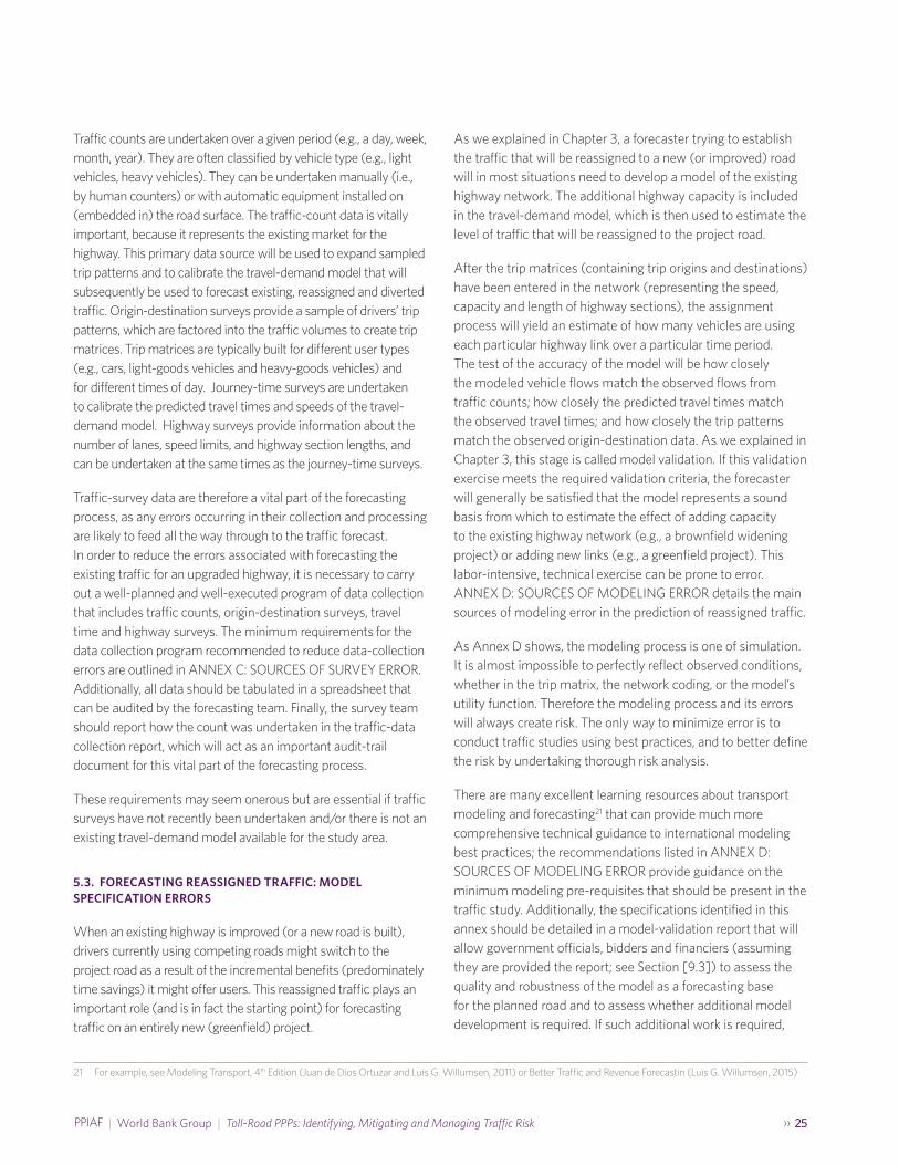
›› 25PPIAF | World Bank Group | Toll-Road PPPs: Identifying, Mitigating and Managing Traffic Risk
Traffic counts are undertaken over a given period (e.g., a day, week, month, year). They are often classified by vehicle type (e.g., light vehicles, heavy vehicles). They can be undertaken manually (i.e., by human counters) or with automatic equipment installed on (embedded in) the road surface. The traffic-count data is vitally important, because it represents the existing market for the highway. This primary data source will be used to expand sampled trip patterns and to calibrate the travel-demand model that will subsequently be used to forecast existing, reassigned and diverted traffic. Origin-destination surveys provide a sample of drivers’ trip patterns, which are factored into the traffic volumes to create trip matrices. Trip matrices are typically built for different user types (e.g., cars, light-goods vehicles and heavy-goods vehicles) and for different times of day. Journey-time surveys are undertaken to calibrate the predicted travel times and speeds of the travel-demand model. Highway surveys provide information about the number of lanes, speed limits, and highway section lengths, and can be undertaken at the same times as the journey-time surveys.
Traffic-survey data are therefore a vital part of the forecasting process, as any errors occurring in their collection and processing are likely to feed all the way through to the traffic forecast. In order to reduce the errors associated with forecasting the existing traffic for an upgraded highway, it is necessary to carry out a well-planned and well-executed program of data collection that includes traffic counts, origin-destination surveys, travel time and highway surveys. The minimum requirements for the data collection program recommended to reduce data-collection errors are outlined in ANNEX C: SOURCES OF SURVEY ERROR. Additionally, all data should be tabulated in a spreadsheet that can be audited by the forecasting team. Finally, the survey team should report how the count was undertaken in the traffic-data collection report, which will act as an important audit-trail document for this vital part of the forecasting process.
These requirements may seem onerous but are essential if traffic surveys have not recently been undertaken and/or there is not an existing travel-demand model available for the study area.
5 .3 . FORECASTING REASSIGNED TRAFFIC: MODEL SPECIFICATION ERRORS
When an existing highway is improved (or a new road is built), drivers currently using competing roads might switch to the project road as a result of the incremental benefits (predominately time savings) it might offer users. This reassigned traffic plays an important role (and is in fact the starting point) for forecasting traffic on an entirely new (greenfield) project.
21 For example, see Modeling Transport, 4th Edition (Juan de Dios Ortuzar and Luis G. Willumsen, 2011) or Better Traffic and Revenue Forecastin (Luis G. Willumsen, 2015)
As we explained in Chapter 3, a forecaster trying to establish the traffic that will be reassigned to a new (or improved) road will in most situations need to develop a model of the existing highway network. The additional highway capacity is included in the travel-demand model, which is then used to estimate the level of traffic that will be reassigned to the project road.
After the trip matrices (containing trip origins and destinations) have been entered in the network (representing the speed, capacity and length of highway sections), the assignment process will yield an estimate of how many vehicles are using each particular highway link over a particular time period. The test of the accuracy of the model will be how closely the modeled vehicle flows match the observed flows from traffic counts; how closely the predicted travel times match the observed travel times; and how closely the trip patterns match the observed origin-destination data. As we explained in Chapter 3, this stage is called model validation. If this validation exercise meets the required validation criteria, the forecaster will generally be satisfied that the model represents a sound basis from which to estimate the effect of adding capacity to the existing highway network (e.g., a brownfield widening project) or adding new links (e.g., a greenfield project). This labor-intensive, technical exercise can be prone to error. ANNEX D: SOURCES OF MODELING ERROR details the main sources of modeling error in the prediction of reassigned traffic.
As Annex D shows, the modeling process is one of simulation. It is almost impossible to perfectly reflect observed conditions, whether in the trip matrix, the network coding, or the model’s utility function. Therefore the modeling process and its errors will always create risk. The only way to minimize error is to conduct traffic studies using best practices, and to better define the risk by undertaking thorough risk analysis.
There are many excellent learning resources about transport modeling and forecasting21 that can provide much more comprehensive technical guidance to international modeling best practices; the recommendations listed in ANNEX D: SOURCES OF MODELING ERROR provide guidance on the minimum modeling pre-requisites that should be present in the traffic study. Additionally, the specifications identified in this annex should be detailed in a model-validation report that will allow government officials, bidders and financiers (assuming they are provided the report; see Section [9.3]) to assess the quality and robustness of the model as a forecasting base for the planned road and to assess whether additional model development is required. If such additional work is required,

26 ‹‹ Toll-Road PPPs: Identifying, Mitigating and Managing Traffic Risk | PPIAF | World Bank Group
this should be recorded in a model-development report (which is ideally included in the bid submissions).
5 .4 . FORECASTING DIVERTED TRAFFIC: ESTIMATION ERROR
If a toll is introduced on an improved (or new) highway, it will have the simultaneous effect of suppressing some of the reassigned and existing traffic. That is because the introduction of the toll reduces the benefits of the new or improved highway, by imposing an additional cost on new or existing users, thereby increasing the generalized cost of travel.
The extent to which this happens depends on the elasticity of demand with respect to tolls (see ANNEX A: WILLINGNESS TO PAY). The level of toll elasticity is crucial, particularly for those parties (public or private) that are financing, or investing in, the project. However, the toll elasticity is unique to each project and cannot be known until the toll is introduced. Like all forecasting elements, it is derived through estimation and therefore is prone to estimation error.
Understanding how error arises in forecasting toll elasticity requires a better understanding of drivers’ willingness to pay tolls. Highway users are prepared to pay tolls to save time, above everything else, but the significance of the saved time and whether it can be used effectively are important factors. In general, the more time saved, the more likely it is that drivers will pay a reasonable toll, and the lower the error associated with forecasting the demand for the highway. Estuarial (or river) crossings provide good examples of projects for which the time and distance savings are likely to be significant, and for which the error surrounding the forecasts therefore tends to be reduced (put another way, demand is more inelastic and responds much less to new tolls and toll changes). However, if the project only offers small individual time savings, these might not provide significant value to the individual driver, lowering the probability of that person using the highway, and increasing the level of error associated with the forecasts.22
Additionally, drivers must be able to use the saved time effectively. Saving 20 minutes on a new section of a trans-continental highway before waiting up to 24 hours to cross a national border may not be considered worthwhile, and therefore the willingness to pay the toll might be lower than would otherwise be anticipated. Logistics managers may not attribute significant benefits to a new highway if the time and distance savings are not sufficiently large to result in significant cost savings.
22 Although the individual time savings may be small, in aggregate across all users, there might be a large net benefit to the improved (or new) highway; this will be reflected in the cost-benefit analysis of the project.
23 Travel-time reliability is sometimes treated separately and is known as the “value of reliability.”
In addition to the level and usefulness of the time and distance savings offered by the project, the willingness to pay will depend on:
• Convenience of use, travel time reliability,23 and highway safety standards;
• Trip purpose and trip frequency;
• Toll tariff level;
• Disposable income;
• Whether the toll cost is being paid by the individual or by a third party;
• Familiarity with the highway network; and
• Biases for or against toll highways.
Although the time and distance savings can be estimated using the travel-demand model (and are therefore prone to the errors already laid out in ANNEX C: SOURCES OF SURVEY ERROR and ANNEX D: SOURCES OF MODELING ERROR), and the toll tariff is typically fixed by either the private or public sector, the traffic forecaster must simulate the combined impact of the above factors into a willingness-to-pay parameter, typically using revealed-preference (RP) or stated-preference (SP) survey methods.
The design of these surveys must capture all of the factors that together determine drivers’ willingness to pay. The SP survey allows respondents to make simple tradeoffs between journey improvements and toll amounts they are prepared to pay for these benefits. The design of the survey is complex, and it can be difficult to achieve meaningful results, particularly if drivers have had little route choice in the past. Operational research methods such as SP are statistical approaches, so there is the potential for estimation error around key parameters. Also, as with any surveying approach, potentially serious sampling errors can occur, because SP surveys tend to have relatively low sample rates due to the time it takes to complete each survey (typically 10 to 30 minutes, depending on the complexity of the design). Low sample rates can make it difficult to capture wide ranges of willingness to pay across different socio-economic groups (e.g., different income levels). This is particularly important for high-frequency road users, such as commuters. It is vitally important to ensure that a large-enough number of high-frequency users are sampled, because these users will suffer the largest income effect of their route choice, and their decisions will be strongly influenced by household incomes and budgets. This

›› 27PPIAF | World Bank Group | Toll-Road PPPs: Identifying, Mitigating and Managing Traffic Risk
can lead to complex route-choice decisions, such as only using the road in one direction and/or on certain days.
Moreover, research methods such as SP also can produce “strategic biases,” whereby respondents’ stated responses about their willingness to pay a toll do not correspond to the choices they will really end up making. On the one hand, they have very little to lose by responding optimistically, given that they will benefit from having the option of using a new or improved road, even if they might not be prepared to pay for it when it opens. Alternatively, respondents may be ideologically opposed to tolls and therefore refuse to trade any level of toll for any level of benefit in order to make a statement in an attempt to influence the policy decision to introduce tolls.
If the willingness to pay is overestimated, toll tariffs could be set too high, resulting in lower-than-expected traffic outturn. If the willingness to pay is underestimated, toll tariffs could be set too low, traffic volumes may be higher than forecast, more revenue could have been generated by the highway, and the level of service of the highway may be jeopardized. Willingness to pay is therefore a critical element in the determination of traffic capture. It can, however, be very difficult to estimate accurately, and it introduces significant error to the forecasting process. The table below summarizes the key errors in estimating willingness to pay and diverted traffic more generally.
To help reduce the potential errors outlined in the table above, willingness to pay should ideally be determined from local behavioral studies, including RP and/or SP surveys, often preceded by focus groups to aid the survey design. Willingness-to-pay parameters should vary by user class in order to represent a range of behavioral responses to the benefits on offer and the toll tariffs to be charged. The impact of lower or higher willingness-to-pay parameters on the traffic and revenue forecasts should be sensitivity tested (see Chapter 9) and communicated to the project parties. If national willingness-to-pay parameters are provided by the state, local variations should be considered by, for example, comparing the national gross domestic product (GDP) per capita with the regional equivalent in order to demonstrate the appropriateness (or otherwise) of employing the national values.
If there is a need to carry out an SP survey, it is essential that it be done with a high-quality market-research company that has the appropriate expertise in using SP methods. The requirements for an SP survey are built into the sample terms of reference in ANNEX B: SAMPLE SCOPE OF WORK FOR TRAFFIC ADVISOR. It is vital that the survey has reasonable sample rates and attempts to avoid response biases. For that reason, it is important to pilot the survey, analyze the results, and make any necessary refinements in the survey design. There are numerous resources that can be consulted regarding the use of SP for valuing the economic benefits and costs of new transport projects.24
TABLE 1: Sources of Error in Estimating Diverted Traffic
Error Source of Error Description Consequence
Estimating the Time and Distance Savings
Travel-demand model The model estimates the level of time and distance savings for the new (or improved) road. As shown in Table 2, a number of errors can occur in the development of the model.
This can lead to an over- or under-estimation of the benefits offered by the toll highway, which in turn can under- or over-predict traffic.
Sample Error
Willingness-to-pay surveys (e.g., RP/SP surveys)
Because of the length of time it takes to complete these complex surveys, it is very difficult to get truly representative samples.
This can lead to an over- or under-estimation of willingness to pay, which in turn can under- or over-predict traffic.
Survey-Design Error These surveys involve combining many decision factors into simple (often binary) choices. Designing an effective survey can be very difficult.
Strategic Biases Respondents can be bullish or dogmatic about the introduction of tolls within the hypothetical setting of a survey, which might not reflect their route-choice behavior in reality.
Unfamiliarity with Toll Highways
Willingness-to-pay surveys (e.g., RP/SP surveys)
Toll highways may not exist in some countries, or drivers may not be used to making route choices.
This can lead to illogical behavioral parameters and lack of traders during the survey.
24 An excellent guide was drafted for the then-named Department for Transport, Local Government and Regions (DTLR) in 2002, which can be found at: https://www.gov.uk/government/uploads/system/uploads/attachment_data/file/191522/Economic_valuation_with_stated_preference_techniques.pdf
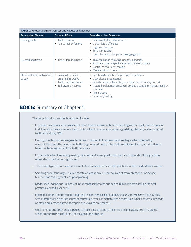
28 ‹‹ Toll-Road PPPs: Identifying, Mitigating and Managing Traffic Risk | PPIAF | World Bank Group
BOX 6: Summary of Chapter 5
The key points discussed in this chapter include:
• Errors are involuntary inaccuracies that result from problems with the forecasting method itself, and are present in all forecasts. Errors introduce inaccuracies when forecasters are assessing existing, diverted, and re-assigned traffic for highway PPPs.
• Existing, diverted, and re-assigned traffic are important to financiers because they are less affected by uncertainties than other sources of traffic (e.g., induced traffic). The creditworthiness of a project will often be based on these elements of the traffic forecasts.
• Errors made when forecasting existing, diverted, and re-assigned traffic can be compounded throughout the remainder of the forecasting process.
• Three main types of error were discussed: data collection error, model specification effort and estimation error.
• Sampling error is the largest source of data collection error. Other sources of data collection error include human error, misjudgment, and poor planning.
• Model specification error is inherent in the modeling process and can be minimized by following the best practices outlined in Annex C
• Estimation error is specific to toll roads and results from failing to understand drivers’ willingness to pay tolls. Small sample size is one key source of estimation error. Estimation error is more likely when a forecast depends on stated preference surveys (compared to revealed preference).
• Governments and other project parties can take several steps to minimize the forecasting error in a project, which are summarized in Table 2 at the end of this chapter
TABLE 2: Forecasting-Error Sources and Reduction Measures
Forecasting Element Source of Error Error-Reduction Measures
Existing traffic • Traffic surveys• Annualization factors
• Extensive traffic-data collection• Up-to-date traffic data• High sample rates• Time-series data• User-class and time-period disaggregation
Re-assigned traffic • Travel-demand model • TDM validation following industry standards• Accurate scheme specification and network coding• Controlled matrix estimation• Model-validation report
Diverted traffic: willingness to pay
• Revealed- or stated-preference surveys
• Traffic-capture model• Toll-diversion curves
• Benchmarking willingness-to-pay parameters• User-class disaggregation• Realistic scheme benefits (time, distance, motorway bonus)• If stated preference is required, employ a specialist market-research
company• Pilot surveys• Sensitivity testing

›› 29PPIAF | World Bank Group | Toll-Road PPPs: Identifying, Mitigating and Managing Traffic Risk
In the early 1990s, the Hungarian government recognized that demand for highway-transport capacity could not be met due to budget constraints. It established the Bureau for Motorway Concessions to find private financing solutions for more than 500 kilometers of highways and bridges. An initial success, the M1-M15 highway achieved financial closure in December 1993. The $366-million project consisted of the design, build, finance, maintenance and operation of 43 kilometers of highway between Gyor (northwest Hungary) and the Austrian Border (M1) and 14 kilometers of motorway linking the M1 to Bratislava (M15). The new highway was estimated to save users 20 minutes’ travel time. Toll collection relied on one main toll plaza and five ramp plazas at three interchanges.
The winning consortium—Transroute (France) and Strabag (Austria)—provided 19 percent equity; the remaining debt was provided by EBRD, insurance companies, and local and international commercial banks. No subsidy was provided by the Hungarian government, and the concessionaire, ELMKA, assumed all of the traffic and revenue risk for the 35-year concession period. A restriction on construction of parallel competing highways was included in the concession/project agreement. Risk-transfer allocation towards the private sector created significant benefits to the Hungarian taxpayer—the construction was completed on time and within budget; its operation and maintenance were effective and of the highest standard; and during the critical economic period following its opening, Hungary benefited from the project without contributing to its financing.
Despite these successes, the project faced immediate challenges upon opening in 1996:
• Willingness to pay tolls: Local (Hungarian) drivers and longer-distance (Western-European) drivers exhibited significantly different willingnesses to pay tolls to save travel time.
• High-toll tariffs: Set by the concessionaire to maximize revenue, the tolls—the highest in Europe at that time—were considered too high by local users, who won a lawsuit against them.
• Low level of traffic: Volumes were only 46 percent of initial estimates. Explanations for the underperformance include the high toll tariffs; the location of a major truck depot on the toll-free highway; traffic surveys undertaken during atypical traffic conditions; and lower-than-expected domestic-car-traffic growth after new Hungarian shopping centers eliminated the need for cross-border travel.
• Revenue shortfall: By 1998, the company faced a revenue shortfall of about 30 percent and could not meet its debt-service obligations.
• Change in toll policy: The Hungarian Ministry of Transport refused to re-negotiate the deal, and the new government elected in 1998 opposed toll highways.
The highway was nationalized in April 1999. The concessionaire’s outstanding debt was transformed into a sovereign debt with more favorable terms and conditions. The ELMKA shareholders lost their equity stakes without compensation. The toll rates were reduced by nearly 50 percent in August 1999; traffic volumes immediately increased by 15 to 20 percent, but revenues decreased by 45 percent annually. International funding sources for new highway projects dried up, and only a fraction of the ambitious motorway program outlined in 1991 was completed. In January 2000, the tolls were replaced by a "vignette" system that allows users to pay to use the toll highways for a certain number of days. The revenues generated by the highway network do not cover the maintenance and operational costs of the state-managed motorways.
This case study demonstrates the impact of forecasting error on the success of a highway project, the implications for future national highway projects, and the importance of the commitment and support of the awarding authority. Willingness to pay tolls, traffic volumes and revenue outturn were overestimated, and a change in the toll policy ultimately resulted in the failure of the highway PPP deal, which is addressed in the next chapter on uncertainty.
Sources: Toolkit for Public – Private Partnerships in roads & Highways, World Bank and PPIAF Version March 2009
BOX 7: Case Study: Hungary's M1-M5 (Failure)

30 ‹‹ Toll-Road PPPs: Identifying, Mitigating and Managing Traffic Risk | PPIAF | World Bank Group
6 .1 . INTRODUCTION
As the forecaster moves away from establishing the demand that might come from existing, reassigned and diverted trips, and starts to forecast how that traffic might grow over time, the potential for inaccuracy increases. This is because the factors that affect the growth (or decline) of traffic over time are fundamentally linked to our imperfect knowledge of the future. However, this traffic can contribute significantly to the overall value of a toll road asset, and is particularly important to long-term investors, such as equity providers and institutional investors (e.g., pension funds).
In this chapter, we will consider the following key sources of uncertainty in the traffic forecast:
• Ramp-up;
• Socio-economic traffic growth;
• Development traffic growth;
• Induced traffic growth; and
• Other sources of uncertainty.
We also consider the ways in which project parties, particularly governments, can take action to minimize forecasting uncertainty. Generally it is more difficult to mitigate long-term uncertainty than forecasting error, because of our very imperfect knowledge of the future. Nevertheless it is important for project parties to use best practices as much as possible, and to create a stable environment within which the project road will operate. Some of this will require difficult policy choices and an inherent reduction in political flexibility for future governments, which will be addressed in this guide.
6 .2 . RAMP-UP
Ramp-up describes the performance of a toll highway in terms of traffic and revenue outturn during the early years of a concession. Traffic levels do not generally reach their true potential for several months or years after the highway opens, as drivers familiarize themselves with the new highway and operational systems become established. The ramp-up period is often critical to the financial viability of the concession. Because it is highly specific to each project, ramp-up is extremely difficult to predict accurately, particularly for greenfield projects. Uncertainty regarding the scale and duration of the ramp-up period therefore introduces further potential inaccuracy into the forecasting process. As we will see, financiers (particularly debt providers / banks) will look very closely at the ramp-up assumptions in the traffic forecast, because the ramping-up of traffic inconveniently occurs when debt balances and obligations are typically at their highest (and therefore when there is the highest probability of financial distress and default). We will describe how financiers address this particular driver of traffic risk in subsequent chapters.
The ramp-up profile of a highway project is extremely difficult to forecast, because it can be affected by a variety of factors, such as a lack of driver awareness, operational problems, and trip frequency of traffic using the highway. One can reasonably expect that the ramp-up period would be much shorter for a brownfield improvement, where drivers have already been using the road, than for a greenfield project, when it may occur during a period of high debt or other financial obligations. In both scenarios, the government and the private-sector partner must actively communicate with drivers and build awareness of the highway opening.
It is recommended that one (or all) of the project parties should take the following steps:
6. Uncertainty: Forecasting Future Traffic »

›› 31PPIAF | World Bank Group | Toll-Road PPPs: Identifying, Mitigating and Managing Traffic Risk
• A benchmarking exercise of the ramp-up profile of similar operational toll-road projects should be undertaken by the traffic forecaster;
• The references found from the benchmarking exercise should be built into a clearly stated set of ramp-up assumptions to be used in the forecast (this will include the length of the ramp-up period, and the level of ramp-up each year—e.g., year one = 80 percent of forecast; year two = 90 percent of forecast; and year three = 100 percent of forecast);
• A marketing campaign should build awareness of the new highway and its benefits; and
• Ramp-up assumptions should be sensitivity tested, given their potential to cause debt distress (see Chapter 10 on sensitivity testing).
6 .3 . SOCIO-ECONOMIC DRIVERS OF TRAFFIC GROWTH
Drivers of future traffic growth include economic, employment, and population growth; car-ownership growth; fuel prices; and land-use development. Forecasting each of these socio-economic factors is in itself a task prone to forecasting error and uncertainty, especially when looking at the long term. We will see in Chapter 9 that extensive sensitivity testing is often required to stress test the lowest and highest potential growth rates that might occur in the most pessimistic and optimistic scenarios, but even then, there is likely to be significant residual uncertainty that creates a risk that must be carefully allocated to the project parties.
As explained in Chapter 3, to estimate the relationship between these socio-economic factors and traffic growth, the forecaster will often develop a traffic-growth model. This model is typically an econometric analysis that regresses historical traffic-growth data against socio-economic data over the same period, to create a statistical relationship that can be used to plug in forecasts of socio-economic variables in order to create traffic-growth forecasts. The forecaster will be able to assess the error and statistical reliability around the traffic-growth model using well-established descriptive statistics and error tests. The model will subsequently output a set of traffic growth rates that can be applied to the travel-demand
25 It is important to note that forecasters will not typically generate a separate travel-demand model (e.g., trip matrix and network) for each year of the forecast, but instead will interpolate between two model years (e.g., 10 years post-opening and 20-years post-opening).
26 Vassallo, José Manuel; de los Angeles, Maria; and Ortega, Alejandro, « What was wrong with the toll highway concessions in the Madrid Metropolitan Area?” (December 2010)
model trip matrix, to create future-year trip matrices (e.g., 10 years post-opening, 20 years post-opening) that will be run against assumed future-year networks to generate future-year forecasts.25
Even with statistically robust traffic-growth models, the overall reliability of the model will of course be dependent on the assumptions made for the forecasts of the socio-economic variables themselves (i.e., the independent variables of the regression). For example, how accurately can we predict population or economic growth over several decades? Moreover, some of the socio-economic variables are themselves related to each other, which also can lead to the unreliability of the traffic-growth model. For example, car ownership is likely to be closely correlated to economic growth, because as incomes rise, car ownership typically increases. If the economic-growth forecast is too high, the car-ownership forecast will also be too high, compounding the inaccuracy in the overall forecast. This problem of “autocorrelation” is common in all econometric models and can be corrected for to an extent, but it is impossible to fully correct any model for this source of inaccuracy. Another major problem is the scarcity of continuous, reliable traffic data over an extended period (i.e., unreliable data on the dependent variable in the regression). Without this, it is difficult to develop a robust traffic-growth model, and doing so may actually introduce more inaccuracy than making a simple long-term assumption about traffic growth (perhaps related to a long-term economic-growth forecast).
Regardless of how the forecaster develops the traffic-growth model, the relationship between economic growth and traffic growth is typically the most important relationship to establish in a traffic forecast. Evidence suggests that toll-highway traffic is more susceptible to economic downturns than toll-free highway traffic.26 This is principally because drivers’ decisions regarding whether or not to use a toll road affects their incomes, so when income and economic activity increases, willingness to pay should also increase; conversely, when income and economic activity decline (such as during an economic recession), there can be a significant decrease in traffic growth, and sometimes a decline in traffic. Evidence shows that this is particularly important for heavy-goods vehicle traffic. Activity in the freight industry is naturally very dependent on the overall output of an economy, and the

32 ‹‹ Toll-Road PPPs: Identifying, Mitigating and Managing Traffic Risk | PPIAF | World Bank Group
industry is very competitive, operating on tight profit margins. The combination of these factors can significantly affect the volume and willingness-to-pay of heavy-goods traffic.
These factors together make the task of forecasting long-term traffic growth prone to uncertainty, which increases as we move the forecast further into the future. This inherent uncertainty around long-term traffic growth typically leads the forecaster to gradually slow down the growth in traffic, to reflect its increasing uncertainty over time.
There are several steps forecasters can take to reduce the potential inaccuracies arising from the uncertainty of forecasting future traffic growth. At a minimum, the forecaster should do the following:
• When possible, use independent forecasts of socio-economic variables (e.g., from international organizations such as the United Nations or World Bank; or consensus forecasts; or the Economist Intelligence Unit), and use localized/regional data that corresponds to the study area. In situations where this is not possible, use data collected by official government statistical agencies or a reputable academic institution.
• Ensure the traffic-growth model has sufficient statistical significance (e.g., R-Squared, values, F-value, P-values, t-values), and the model has sufficient statistical integrity (e.g., autocorrelation is minimized through a Durbin-Watson Test).
• Undertake thorough sensitivity testing using the traffic-growth model. It is recommended, at a minimum, to produce a pessimistic socio-economic traffic-growth forecast (which uses lower forecasts of the various socio-economic variables) and an optimistic traffic-growth forecast (which uses higher forecasts of the various socio-economic variables). As described in later sections, these pessimistic and optimistic forecasts build into an overall set of low and high traffic and revenue forecasts.
Forecasters are also increasingly using back-casting techniques,27 i.e., the application of the travel-demand model to forecast traffic in a year prior to the model base year, to test the accuracy of the model and future traffic-growth assumptions. “Reverse-forecast” traffic growth is used to ensure that the observed historic factors affecting traffic growth (economic, employment, population growth, etc.) in the model for a year prior to the calibration year result in the model replicating the
27 Travel Model Validation and Reasonableness Checking Manual Second Edition, Cambridge Systematics, Inc. (2010)28 http://online.wsj.com/news/articles/SB1000142405270230348250457917789046181258829 Trunk Roads and the Generation of Traffic, SACTRA, UK Department of Transport, December 1994
traffic volumes observed in that year. This of course adds further cost and time into the forecasting process, but can be a useful tool to calibrate the travel-demand and traffic-growth models.
6 .4 . DEVELOPMENT AND INDUCED TRAFFIC GROWTH
Future land-use proposals are investigated as part of the traffic study. If the evidence strongly suggests that additional traffic will be attracted to the new highway, above the level of traffic growth expected to be attributable to socio-economic drivers, newly generated trips may be introduced into the future-year trip matrices of the travel-demand model. These trips are referred to as development traffic. However, caution should be exercised if the land-use proposals are speculative. Traffic forecasts associated with development proposals can result in significant overestimation, as recently demonstrated by the Foley Beach Express Bridge in Alabama, for which the forecasts assumed significant coastal development that failed to materialize. The bridge concessionaire filed for bankruptcy protection in July 2013, after the traffic outturn turned out to be only 23 percent of the forecasted volumes, due to the collapse of real-estate projects along Alabama’s Gulf Coast, the 2010 Gulf oil spill, and toll and gasoline price increases.28
Predicting how a new (or improved) road will affect land-use patterns is an extremely difficult task, especially as we move further into the future. We know that building new (or improved) roads can affect land use, because projects provide greater accessibility and may therefore attract economic activity (e.g., new residential or commercial developments). However, accurate predictions will rely heavily on sound data regarding existing land uses and firm development proposals, which are often not available, especially in developing countries.
Induced traffic refers to trips that were not made (on any part of the highway network) prior to the opening of a new or improved highway. Improved accessibility, time savings, and travel-time reliability may combine to provide the highway user with such significant benefits that new trip opportunities are created and a new trip is induced. The United Kingdom’s Department of Transport commissioned a report by the Standing Advisory Committee on Trunk Road Assessment (SACTRA) in 1994, which stated: “Considering all these sources of evidence, we conclude that induced traffic can and does occur, probably quite extensively, though its size and significance is likely to vary widely in difference circumstances.”29 SACTRA found that

›› 33PPIAF | World Bank Group | Toll-Road PPPs: Identifying, Mitigating and Managing Traffic Risk
induced traffic may build up over time rather than appear at once, and that “travelers must, as a matter of logic, be assumed to respond to reductions in travel time brought about by road improvements by travelling more or further.” In the case of toll highways, the level of induced traffic may be dampened by the requirement to pay a toll to use the highway. Typically, a (small) proportion of induced traffic is included in a forecast, based on an elasticity applied to the generalized cost savings provided by the new highway.
Although the phenomenon of induced traffic has been endorsed by SACTRA, the inclusion of induced traffic is considered one of the most uncertain elements of traffic forecasting. The proportion of induced traffic, if included at all in traffic forecasts, should be small and justified by significant generalized cost savings offered by the new highway.
The accurate prediction of development and induced traffic volumes is generally considered the most difficult part of the traffic-forecasting process. Due to the often-speculative nature of future development and the uncertain ability of the project to induce traffic, the presence and absence and time of appearance of these types of forecasted traffic should be included in the sensitivity-testing exercise (see Chapter 9). The forecasting of development and induced traffic is also hard to separate from the socio-economic traffic growth that was previously discussed. This is because socio-economic traffic growth is forecast by regressing various independent variables against historical traffic growth, which may therefore already incorporate development factors and induced effects, as a result of historical improvements in infrastructure. Thus, it can be very difficult to avoid potential double counting by forecasting this traffic separately.
As a result of this inherent difficulty in forecasting development and induced traffic, the project should be financially feasible without an over-dependence on this traffic. Debt financiers typically will not rely on it, and equity providers often view it as an upside rather than as something that is factored into their expected returns from the project.
However if there is a compelling case to be made for forecasting this traffic separately (e.g., the infrastructure will unlock a major enterprise zone), the following mitigating actions may be required as a minimum:
30 The Furness distribution model is described in detail in many good transport modelling textbooks. For a good overview, please see http://www.transportmod-eller.com/distributionoverview.html
31 The United Kingdom’s guidance on modeling induced/elasticity traffic can be found at: https://www.gov.uk/government/uploads/system/uploads/attach-ment_data/file/427122/webtag-tag-unit-m2-variable-demand-modelling.pdf
• Ensure that the forecasting team has full access to developer master plans. It is prudent for forecasters to only incorporate information contained in existing development plans, rather than speculative, undocumented plans. The forecasting team should also consult real-estate professionals and economists to assess the viability of the development plans.
• Forecasters should use either benchmark trip rates from similar developments within the country or international benchmarks to establish how much additional demand will be generated by the new developments.
• Likewise, forecasters should carefully distribute this new demand within the trip matrix by understanding where these additional trips are going to be originating and ending. It can be perilous and difficult to make accurate assumptions for this, given that it is not possible to observe such trips yet. Moreover, even when an assumption is made, building the trips into the trip matrix must be done carefully, using mathematical approaches such as the Furness Distribution Model,30 and the results must be carefully reviewed.
• When forecasting induced traffic, forecasters should refer to existing technical guidance, describe the methodology to the project parties, and provide an audit trail for this very risky type of traffic. The established methods typically use an elasticity-based approach, which tries to capture the change in travel demand as a result of changes in travel costs (i.e., generalized costs).31 It is worth noting that this is an area of significant academic debate, and there is no internationally accepted approach for how to forecast induced traffic.
For both development and induced traffic, it is important to sense-check the results of the exercise to ensure that this traffic is not representing a large proportion of the overall traffic forecast (e.g., more than 10 percent of the traffic forecast in any given year). If it is representing a significant proportion of the traffic, it goes without saying that the traffic risk for the project is going to be exceptionally high. This in turn means that significant sensitivity testing is required around these types of traffic (see Chapter 9).

34 ‹‹ Toll-Road PPPs: Identifying, Mitigating and Managing Traffic Risk | PPIAF | World Bank Group
6 .5 . ADDITIONAL SOURCES OF UNCERTAINTY
6 .5 .1 . TOLL POLICYThe existence of a robust and relevant national toll policy reduces the uncertainty surrounding key inputs to the traffic and revenue forecasts, such as toll tariffs. However toll policies may not always be in place, and like all government policies, they can be subject to change, for example due to a change of government. The impact of no stated policy, or future changes in policy, on forecast accuracy should not be underestimated (see the M1-M15 Hungary Case Study in Box 4).
The toll policy should reinforce the transparency, predictability and uniformity of highway-toll collection, thereby reducing the error associated with the toll-strategy specification embedded in the forecasts. The policy should be grounded in the government’s objectives for tolling and should define the mandatory toll-collection requirements. These may include: the vehicle classification structure; identification of vehicles exempt from toll payment; the distance between charging points; and if there is a requirement to provide a toll-free alternative route.
The toll policy may be amended over time to address a developing market for PPP highway projects. For example, the government of India’s toll policy, initially launched in 1997, was updated in 2009, in response to deficiencies and anomalies experienced during the implementation of the National Highway Development Project from 2000 onwards.32 However some flexibility in setting toll tariffs may be favorable to optimize traffic and/or revenues, as recommended by Vassallo,33 based on the underperformance of recently completed urban toll roads in Madrid that have rigid contractual toll-pricing policies.
6 .5 .2 . TOLL STRATEGYTraffic and revenue forecasts are based on a clear specification of a new highway’s opening date, capacity, speed limits, location of interchanges, location of tolling points, and toll tariffs to be charged by vehicle categorization, which is known as the toll strategy. In most cases, the government authority that is awarding a project specifies its toll strategy, although bidders may be asked to propose their own toll tariffs. Forecast inaccuracy is likely to increase if the specifications covered by a toll strategy are unclear or change over time.
Examples of toll-strategy amendments that will affect traffic volumes and revenue outturn include:
32 “Review of Toll Policy for National Highways,” The Secretariat for the Committee on Infrastructure, Government of India (May 2009)33 Vassallo, José Manuel; de los Angeles, Maria; and Ortega, Alejandro, « What was wrong with the toll highway concessions in the Madrid Metropolitan Area?”
(December 2010)
• Delay/cancellation of toll-tariff increases, due to political and/or economic pressure;
• Introduction of an alternative payment technology, such as a vignette;
• Toll vehicle reclassification; and
• Relocation/increase/reduction of toll-charging points.
These changes often occur throughout the typical lifecycle of a major highway project and can potentially invalidate the original traffic and revenue forecasts. If the toll strategy is significantly altered, the traffic and revenue forecasts should be updated to reflect these changes.
The toll strategy should be clearly defined in the concession/project agreement and not amended by the awarding authority or concessionaire (if legally able to do so) without an impact assessment being carried out on the traffic and revenue forecasts. The tariffs should be contractually binding, with compensation payable if the toll-indexation procedure is not adhered to.
6 .5 .3 . TOLL EVASION AND PAYMENT ENFORCEMENTTraffic and revenue forecasts for new highways typically assume no fare evasion. Fare-evasion levels cannot be easily predicted or measured but can result in revenue outturn being lower than predicted in the original revenue forecasts. Post-model adjustments may therefore be made to allow for some evasion, both intentional and unintentional. Fare-evasion levels are rarely published and vary significantly, depending on exogenous factors such as toll-enforcement regulations; user familiarity with the toll strategy; accuracy of vehicle-registration records (with addresses of violators); policing of enforcement regulations; staff integrity; local crime levels; and operational system design.
Enforcement regulations and their active enforcement are essential to the financial success of toll highways. The regulations should define a violation, list the procedures to be followed if one occurs, and the penalties incurred. The procedures and penalties should be set so as to provide a sufficient deterrent against future toll evasion. Operational design and live testing should minimize the opportunities for revenue loss through intentional or unintentional toll evasion. The risk associated with toll evasion can be mitigated to some extent by ensuring that the penalties cover the violators’

›› 35PPIAF | World Bank Group | Toll-Road PPPs: Identifying, Mitigating and Managing Traffic Risk
administrative costs and lost revenue. Predicted toll-evasion levels should be benchmarked with examples from similar projects when possible, to minimize inaccuracies.
6 .5 .4 . CURRENCY-EXCHANGE RATESToll escalation formulae are sometimes linked to currency-exchange rates, particularly when the project’s debt has been raised in a hard currency (e.g., U.S. dollars), to minimize the risks of currency fluctuations on the financial viability of the project. However, a driver’s willingness to pay a toll is typically linked to local inflation and economic growth rather than to fluctuations of the exchange rate with the hard currency used to finance the project. The use of currency-exchange rates in toll escalation formulae can introduce significant uncertainty into the traffic forecasts, due to the unpredictability of exchange-rate fluctuations and the impact of above-inflation toll increases on drivers’ willingness to pay a toll.
Conversely, if exchange-rate movements are not built into the toll-indexation formulae, the impact of currency fluctuations will not have a material impact on traffic flows but will create potentially significant fluctuations in revenue, which could affect ability to service project debt in hard currency. This risk materializes most profoundly when governments devalue their currencies partway through a concession or contract period. For example, Mexico’s devaluation of the peso in 1994 had a significant detrimental effect on the ability of concession companies to service U.S.-dollar-denominated bond holders.34
Currency fluctuations are very difficult to predict accurately, but it is vitally important that the project’s forecaster and/or financial advisor assess historical trends in exchange-rate fluctuations against major currencies, in order to gain a thorough understanding of the peaks and troughs of the local currency. If there is a history of sudden and deep devaluations or revaluations of the local currency, it would be apparent that this could have a regular and profound impact on both traffic and revenue. The forecaster should at least understand the likelihood and magnitude of such risk, even though mitigation may not be possible. In Chapters 9 and 10, we discuss how this risk can be quantified (including through sensitivity analysis) and allocated.
6 .5 .5 . FUEL PRICESSudden or prolonged increases and decreases in gasoline and diesel prices can significantly impact vehicle use in developed and developing countries. Changes in fuel prices affect the propensity of drivers to make a trip and also change the
34 http://www.icwa.org/wp-content/uploads/2015/10/WF-16.pdf
generalized cost of that trip. Fuel prices are also affected by the exchange-rate fluctuations described above; the depreciation of a local currency against the U.S. dollar often results in an increase in fuel prices. Drivers with fixed budgets may then be less willing to pay a toll because more of their budget has been spent on fuel. The future-growth profile of fuel prices introduces further uncertainty into the forecasting process. The forecaster can analyze historical trends in fuel prices and/or assess near-term forecasts, but it is very difficult to accurately predict the long-term price volatility of a commodity such as oil. The forecaster therefore often assumes static fuel costs in the generalized cost function throughout the entire forecasting period, given the difficulty of justifying variation in any particular direction. However, the difficulty of predicting future changes in fuel prices can result in long-term inaccuracies in the traffic forecasts, particularly when fuel prices reach very high levels, as they did in 2008 and 2011, or very low levels, such as those experienced in 2015/2016.
Just as with currency-exchange rates, there is little the forecaster can do to better predict fuel prices. Global and local fuel prices continuously fluctuate and can experience significant peaks and troughs. While some sources (e.g., World Bank) may issue short-term global oil-price forecasts, these tend to only extend out one to two years and are often not localized. Fuel prices therefore will naturally result in variations between forecasts and actual outturn traffic volumes. Again, the forecaster can investigate the probability and impact of the risk by reviewing any historical data on fuel prices and road traffic, and build this into the sensitivity analysis.
6 .5 .6 . OPERATIONAL PROBLEMSTraffic and revenue forecasts are based on the assumption that toll-collection technology is 100-percent accurate and 100-percent operational, 100 percent of the time. Unfortunately this is not always the case, and technological problems can result in lost revenue, for reasons including vehicle misclassification and errors in registration-plate matching. The M50 toll highway in Dublin, Ireland, for example, experienced significant operational problems during the introduction of free-flow tolling in 2008.
Operational problems are unforeseen, and it is extremely unlikely that forecasts will take operational failures into consideration. Nevertheless it should be noted that, should operational problems occur, they could affect the accuracy of traffic forecasts.

36 ‹‹ Toll-Road PPPs: Identifying, Mitigating and Managing Traffic Risk | PPIAF | World Bank Group
The risk of operational problems affecting traffic and revenue outturn can be significantly reduced if the government can impose a testing-and-commissioning requirement in the concession/project agreement, specifying that the road is not considered operational (and therefore the concessionaire cannot start receiving toll revenues) until the reliable and safe operation of the facility has been validated through an agreed-upon testing process. This helps incentivize the concessionaire to overcome operational glitches and more serious operating problems.
Over the longer term, many concession agreements also have very specific performance regimes that financially penalize the concessionaire if the road does not operate according to specified standards or if part or all of the road is unavailable (or closed) to traffic beyond an agreed-upon or planned period. This helps incentivize the concessionaire to mitigate operational problems and optimize traffic management. The exact calibration of the performance regime needs to be developed in close coordination with the project’s financial, technical and legal advisors, because an over-zealous regime may reduce bidder appetite or lead to significant risk pricing (or “gold plating”) and reduced value for money.
6 .5 .7 . COMPETING OR COMPLEMENTARY TRANSPORT INFRASTRUCTUREThe introduction or delay of competing or complementary transportation projects can pose a serious risk to the reliability of a traffic forecast and the financial viability of a toll highway. If the new highway’s alignment duplicates that of an existing highway, it is not uncommon for the existing route to be downgraded in terms of speed limits and capacity reductions, in order to enhance highway safety and aesthetics, to further reduce the impact of noise and air pollution on neighboring communities, and to promote the use of the new highway. The uncertainty regarding whether or not complementary or competing measures will actually be constructed, their timing, and their impact on the new highway’s traffic volumes, introduces the potential for significant uncertainty in the traffic forecasts.
If future traffic growth is expected due to the completion of complementary traffic-management schemes, such as traffic calming on a competing route, or improved access roads, their impact (both during construction and after they are completed) on the toll highway should be built into the network coding of the travel-demand model. Strictly speaking, this factor relates to the issues discussed earlier, with respect to forecasting re-assigned traffic and forecasting errors associated with the scheme specification. However, this error would likely present itself as lower or higher traffic growth after the opening of the scheme, hence the decision to address it here. The risk
associated with these works—which may be critical to the financial viability of the highway project—can be mitigated by specifying the measures, their timing, and their sources of financing in the concession agreement. These agreements are sometimes called “landscape clauses” and mitigate the risk of the complementary works not being implemented. The incorporation of landscape clauses reduces flexibility for future governments and can contractually commit governments to these plans. This is not without political challenges, and governments must trade a loss of policy and planning flexibility with the need to minimize risk and make the project more attractive to the private sector and its financiers.
Conversely, the toll highway may face competition from other highway or public-transport schemes during the concession period. This risk can be mitigated in the concession agreement by identifying all planned projects or identifying a corridor within which no other competing transport scheme can be developed, without compensation being paid to the party assuming the traffic risk. Again, the government faces a difficult policy choice, and over a long period may need the flexibility to develop competing projects without such an impact on its budgets. Governments should use market-sounding exercises to try to understand the perception of this long-term risk. One way in which government can share the risk is to offer a moratorium period (e.g., five to 10 years) on the development of competing projects, after which the government is able to develop new projects. This would help to protect financiers (particularly senior debt providers in the early years of a toll-road project) and would allow government to respond in the longer term if corridor (or project-area) travel demand grows significantly and places too much stress on existing transport infrastructure.
6 .5 .8 . WEATHERSeasonal variations in traffic volumes are observed on most highways. Extreme weather events or extended periods of unexpected weather also affect traffic outturn. Unexpected extended periods of good weather can positively affect highways that provide access to coastal or tourist areas. Extreme weather events may not always have a negative impact on traffic volumes. If the new highway remains open while competing routes are flooded, damaged or made impassable due to snow or ice, the highway may benefit from a boost in the number of new customers.
The impact of weather conditions is not typically included in the traffic forecasts. However, if weather and climatic conditions vary considerably across the year and this variation affects traffic levels, it should be taken into account when calculating the annualization of the forecasts. If a project road is

›› 37PPIAF | World Bank Group | Toll-Road PPPs: Identifying, Mitigating and Managing Traffic Risk
located in an area that is particularly prone to these conditions, it may be vitally important to collect continuous traffic data over the course of the year, or over the course of adversely affected periods, so that the seasonality of traffic flow can be fully established.
The growing impact of climate change is accentuating the impact of weather on the variability of traffic flows, and in certain localities, climatic changes need to be understood as well as possible, particularly if one-off weather events such as floods or major wind events (e.g., hurricanes, tornados) become more frequent. Such events could extensively damage a highway and leave it partially or fully unable to accommodate traffic, which could have a major impact on financial viability. In these situations, traffic risk is likely to widen significantly, and the likelihood is that the risk will either need to be shared with (or fully retained by) government, typically through force majeure and so-called supervening-events clauses in concession agreements.35
6 .5 .9 . UNFORESEEN EVENTSEven when all the potential uncertainties listed above are taken into consideration, there will always remain
35 For information about force majeure and supervening events, see https://ppp.worldbank.org/public-private-partnership/sites/ppp.worldbank.org/files/docu-ments/150808_wbg_report_on_recommended_ppp_contractual_provisions.pdf
the possibility that an unforeseen event will positively or negatively affect the traffic and revenue of a toll highway. Examples of such unforeseen events that have negatively affected traffic outturn and contributed to the inaccuracy of forecasts include: global financial crises; terrorist attacks; environmental disasters; extreme changes in human activity; and political coups.
The impact of unforeseen events has historically not been included in traffic and revenue forecasts. However the shock impact of a sudden substantial loss of toll revenue should be tested to assess the robustness of the project’s financial feasibility with respect to unexpected events. If necessary, this could be dealt with using a one-off downside sensitivity test that features a blanket and catastrophic loss in revenue. However such a blanket assumption should be tested separately and not combined with other sensitivity tests, to separate their effects from other sources of uncertainty. Again, some of these unforeseen events will typically be included in a force majeure clause of a concession agreement, to insure the concessionaire against financial hardship.
BOX 8: Summary of Chapter 6
The key points covered in this chapter include the following:
• Demand for toll highways can be influenced by exogenous factors such as a country’s toll policy and strategy, currency-exchange rates, fuel prices, operational problems, competing infrastructure, weather, and unforeseen events. These factors are outside of the concessionaires’ and financiers’ control and can introduce significant uncertainty to traffic forecasts, because forecasters cannot predict the future perfectly. These uncertainties affect the forecasts of socio-economic factors such as GDP and population, which influence traffic-growth assumptions, development traffic, and induced traffic.
• Although forecasters cannot eliminate uncertainty from forecasts, there are several measures that can be taken to reduce uncertainty when predicting traffic demand. The table below presents the various sources of uncertainty identified in this chapter, as well as the measures that can be undertaken to minimize this uncertainty.

38 ‹‹ Toll-Road PPPs: Identifying, Mitigating and Managing Traffic Risk | PPIAF | World Bank Group
TABLE 3: Uncertainty—Sources and Minimization Measures
Forecasting Element Source of Uncertainty Uncertainty Minimization Measures
Project Asset • Asset characteristics (greenfield/ on-line upgrade, etc.)• Sub-optimal design
• Design optimized in terms of traffic and revenue potential
Ramp-Up • No established forecasting techniques• Driver awareness of road availability
• Benchmarking of similar toll roads• Sensitivity analysis of ramp-up assumptions• Marketing campaign to build driver awareness of new road
Socio-Economic Traffic Growth
• Regression Analysis• Elasticities with drivers of demand, incl. economic,
employment and population growth; car-ownership growth; mobility rates; and fuel prices
• Range of traffic-growth scenarios tested for alternative forecasting assumptions
• Independent socio-economic forecasts• Back-casting
Development and Induced Traffic
• Changes to land use• Trip rates of planned developments • Elasticity of demand to reduction of generalized cost
• Consider whether there is a clear-enough distinction between development traffic and socio-economic traffic growth to justify forecasting this type of traffic separately
• Assess impact without development and alternative timing and trip generation; assess impact with and without induced traffic
• Benchmark trip rates from similar developments• Incorporate development and induced trips into trip
matrices using established methods (e.g. Furness model)
Toll Policy • Absence of toll policy• Toll policy vague and out of date
• Robust national toll policy in place that clearly identifies the mandatory requirements of toll collection
• Policy updates when/if required
Toll Strategy • Revised vehicle toll classification, toll-escalation formulae
• Amendments to the range of tolls on offer• Reductions/increases in charging points• Delay/acceleration of toll escalation
• Clearly defined in concession agreement• Contractually binding tariffs and indexation/escalation
with some flexibility• Fixed charging points• Clear, simple, and easily understood tariff structure
Toll Evasion and Payment Enforcement
• Absence of enforcement regulations• Unenforceable and unenforced regulations
• Enforceable and enforced regulations• Penalties to cover administration costs and revenue loss
due to evasion• Operational design to minimize toll evasion• Benchmarking against observed toll evasion on other projects
Currency-Exchange Rates
• Variation (when linked to toll-escalation formulae) • Trend analysis of historical foreign-exchange and inflation data to inform sensitivity testing and ultimately risk-allocation strategy
Fuel Prices • Sudden or gradual price increases that affect the generalized cost of trips
• Fuel-price sensitivity tests based on historic trends in fuel prices and (if available) the associated impact on traffic levels
Operational Problems • Proficiency of toll-collection system • Build contractual requirement for system testing under real traffic conditions
• Potential operational snags could be included in the ramp-up assumptions
• Consider potential performance regime during operational period of concession
Competing/ Complementary Transport Infrastructure
• Delay or cancellation of complementary works• Competing transport modes / new highways not
envisioned during procurement phase
• Identify all planned schemes or corridor within which competing schemes cannot be built without compensation
• Insert landscape clauses defining complementary schemes in the concession agreement
Weather • Extreme weather events• Prolonged periods of exceptional weather
• Risk assessment of extreme-weather events and risk of highway closure should be built into annualization factors
Unforeseen Events • Unknown impact on traffic/revenue outturn • Test the impact of sudden substantial loss of revenue on financial feasibility of project
• Force-majeure clauses in the concession agreement

›› 39PPIAF | World Bank Group | Toll-Road PPPs: Identifying, Mitigating and Managing Traffic Risk
The N4 highway links the economic heartland of South Africa (Gauteng Province) to Maputo port in Mozambique. The rehabilitation and tolling of the 571-kilometer highway is considered a major success and demonstrates the power of political cooperation between neighboring countries and the benefits of PPP deals to the private and public sectors. The highway standard varies from four-lane separated carriageways on the busiest sections to two lanes with widening to accommodate high proportions of truck traffic. Six mainline toll plazas collect revenues from four categories of traffic.
The $660-million project is based on a concession contract to design, build, finance, maintain and operate the entire highway for a period of 30 years, after which time the assets will be transferred back to the governments of South Africa and Mozambique. The concession agreement with Trans African Concessions (TRAC) was signed in May 1997 and financial close was reached in December that year. The concessionaire assumed full traffic risk, and the project was completed without public subsidy.
The project sponsors—France’s Bouygues and its South African subsidiary Basil Read; South African Stocks & Stocks; and the South Africa Infrastructure Fund—provided 20 percent of the total project cost in the form of equity, with the remainder of the financing in the form of commercial debt. The financing difficulties posed by the two−countries risk were overcome by relying primarily on the South African market for revenue generation.
This case study demonstrates the importance of the project asset in determining the traffic risk. An online upgrade of a key strategic axis, with an established traffic flow and limited route choice, located in a country with established toll highways, meant the traffic risk assumed by the private party was relatively low. Tolls were successfully introduced for the first time in Mozambique, based on focus group and stated-preference survey analysis. Thorough due diligence of the traffic and revenue forecasts, on behalf of the project sponsors and lenders, further reduced the inherent traffic risk.
Despite its success, the project has encountered challenges:
• The staged opening of the highway, from 1998 onwards, took place during an economic downturn, and initial traffic outturn
did not meet expectations. (Higher-than-expected traffic growth of seven to eight percent per annum during the economic recovery soon brought the traffic outturn in line with the original forecasts.)
• Local opposition to the introduction of tolls on a previously un-toll highway was resolved after public consultation and the introduction of local discount structures.
• A parallel, competing highway between the towns of Witbank and Middelburg was upgraded to provide a toll-free alternative route for local users.
• Higher-than-expected damage due to over-loading of trucks was addressed via the implementation of an axle-load control system along the highway corridor.
• The depreciation of the Mozambican metical against the South African rand led to substantial toll increases (20 to 23 percent) in 2006, because the project’s debt is financed in rand.
These exogenous factors demonstrate the dynamic nature of a toll highway during its operational phase. Continued proactive management of the challenges faced by the project parties has contributed to the success of the highway. A greatly improved traffic-risk profile, based on established traffic patterns and sound market conditions, provided the ideal opportunity for the concessionaire to re-finance the project in 2005.
Sources: N4 Toll Road, South Africa and Mozambique, Volume 14, http://tcdc2.undp.org/GSSDAcademy/SIE/Docs/Vol15/14Mozambique.pdf
Toolkit for Public – Private Partnerships in roads & Highways, World Bank and PPIAF Version March 2009
Attracting Foreign Direct Investment Into Infrastructure, Why Is It So Difficult? by Frank Sader, Foreign Investment Advisory Service, Occasional Paper 12, 2000 The International Finance Corporation and the World Bank
www.tracn4.co.za
BOX 9: Case Study: N4 Maputo-Corridor Toll Highway, South Africa and Mozambique (Success)

40 ‹‹ Toll-Road PPPs: Identifying, Mitigating and Managing Traffic Risk | PPIAF | World Bank Group
7 .1 . INTRODUCTION
So far we have focused on the traffic-forecasting inaccuracy that can result from our imperfect knowledge of the current and future demand for travel. Forecasting inaccuracy can also be much more conscious and result from in-built biases. Whereas error and uncertainty should (in theory at least) be evenly distributed (i.e., you are just as likely to over-predict traffic as you are to under-predict it), bias can contribute to systematic inaccuracies in traffic forecasts.
In this section, we describe four important sources of bias that, in some cases, can have a systematic effect on the reliability of traffic forecasts and create significant downside traffic risk:
• Delusion: Optimism bias;
• Distortion: Strategic misrepresentation;
• Unintended Overforecasting: The winner’s curse; and
• Unintended Bias: The survivor’s curse.
After examining these sources of bias, we turn to a discussion of the actions governments can take to reduce bias in their PPP projects through the procurement process, and present key considerations and trade-offs for implementing these actions.
7 .2 . DELUSION: OPTIMISM BIAS
Optimism and overconfidence are part of the human condition. Many of us are overconfident about our own abilities and over-
36 Dillard Amanda J.; McCaul Kevin D.; and Klein William M., “Unrealistic Optimism in Smokers: Implications for Smoking Myth Endorsement and Self-Protective Motivation,” Journal of Health Communication: International Perspectives 11 (2006)
37 March, James G., and Shapira, Zur, “Managerial Perspectives on Risk and Risk Taking,” Management Science 33:11 (1987)38 Svenson, Ola, “Are We All Less Risky and More Skillful Than Our Fellow Drivers?” Acta Psychologica 47 (1981)39 Kahneman, Daniel, “New Challenges to the Rationality Assumption,” Journal of Institutional and Theoretical Economics 3:2 (1994)40 For a full list of Bent Flyvbjerg’s work, see http://www.sbs.ox.ac.uk/community/people/bent-flyvbjerg
optimistic about the future, particularly when our reputations, prosperity or well-being are directly affected by our behavior and choices. The field of psychology is littered with examples of this:
• Smokers under-estimate the impact of nicotine on their own health compared to its impact on other smokers;36
• CEOs investing in new projects strongly underestimate the likelihood of their own project’s failure,37 compared to similar projects that are not their own; and
• When people assess their position within a distribution of peers on a skill such as driving, most people assess that they are in the top half (they cannot all be right!).38
Nobel-Prize-winning psychologist and economist Daniel Kahneman of Princeton University has led the theorizing of this phenomenon39 and described project planners and managers as too frequently accepting the “inside view” while not sufficiently considering the “outside view.” What Kahneman means is that there is a common (almost natural) tendency for planners, managers and policymakers to internally focus on the specifics of a project (about which they are optimistic) without sufficiently focusing on the outcomes of similar past projects, where some of the unforeseen challenges and difficulties of such projects have actually materialized. This so-called “planning fallacy” has been subsequently adopted by a number of academics (most notably Bent Flyvbjerg40) to help illustrate the role of optimism bias in inaccuracy (and therefore risk) in the appraisal and forecasting of costs, benefits, traffic and revenues in large infrastructure projects.
7. Bias: Delusion, Distortion and Curses»

›› 41PPIAF | World Bank Group | Toll-Road PPPs: Identifying, Mitigating and Managing Traffic Risk
Traffic and revenue forecasting can be particularly prone to the over-acceptance of the inside view, for the following reasons:
• The pursuit of success: Forecasters want to be associated with successful projects. Success is typically associated with well-used and high-revenue-generating projects. Even with all the best professional intentions, there is likely to be a conscious or sub-conscious propensity for forecasters to want to be associated with successful projects for their own professional credentials. Put another way, forecasters become part of the project and don’t want to be associated with its failure (e.g., it may be difficult for a forecaster to present a lower-than-viable traffic forecast if it means that the project would not be bankable). This is difficult to prove and somewhat subjective, but most likely plays a role.
• Uncertainty and heterogeneity: In addition to playing a role in the development of accurate traffic forecasts, uncertainty can also itself contribute to optimism biases. We know so little about the future (particularly decades off), that it leaves a lot of open ground for optimistic behavior to go unchecked, because there is so little observed data against which to reference the forecasters’ assumptions/inputs. Likewise, every toll-road project is different in nature (projects are heterogeneous), and each one can have very unique characteristics that might make it difficult to find suitable benchmarks.
• Forecasting as an input-led exercise: The forecasting process is a technical and skilled process underpinned by strands of welfare economics. There are almost infinite levels of complexity and perceived accuracy that can be added to a travel-demand modeling exercise. However, these efforts to perfect the forecasting process may sometimes come at the expense of basic benchmarking and sense-checking of forecasts against other projects (i.e., the outside view), especially because the forecasting process is often done on tight schedules. Once again, it is hard to substantiate this over-emphasis on the inputs rather than the outputs of the forecasting process, and it would be wrong to accuse all forecasters of failing to sense-check and benchmark their work, but the potential biases that can arise from the overly technocratic nature of forecasting cannot be ignored.
Optimism bias is undoubtedly a sensitive issue, because it brings into question the skill and objectivity of the forecasting profession and the individuals who prepare the forecasts.
41 Flyvbjerg, Bent, “From Nobel Prize to Project Management: Getting Risks Right,” Project Management Journal, 37:3 (August 2006)42 Review of Traffic Forecasting Performance Toll Roads, Department of Infrastructure and Transport, Australian Government43 Review of Traffic Forecasting Performance Toll Roads, Department of Infrastructure and Transport, Australian Government, June 2011
Governments, sponsors and financiers cannot objectively ignore the possibility of optimism bias and must consider how this driver of traffic risk can be mitigated. We address potential approaches to mitigation later in this chapter.
7 .3 . DISTORTION: STRATEGIC MISREPRESENTATION
Whereas delusion and optimism bias are generally involuntary and psychological (i.e., we have a cognitive predisposition that makes people judge future events in a more positive light than reality would suggest41), a more serious and potentially systematic bias involves forecasters deliberately manipulating traffic and revenue forecasts because of political and organizational pressures. In contrast to optimism bias, here we can assume that the forecaster and the relevant party have little interest in improving the accuracy of the forecast, because doing so is contrary to their incentives. This situation is therefore more nefarious and is often referred to as strategic misrepresentation.
Strategic misrepresentation refers to the planned, systematic distortion or misstatement of fact, with the aim of increasing the likelihood of success of an event, such as gaining approval for funding.42 Economic or political pressures may underlie the use of overly optimistic traffic forecasts, initially by the awarding authority and subsequently by private-sector parties attempting to become the preferred bidder. Strategic misrepresentation can significantly increase the error associated with traffic forecasts and has been cited by the Australian government (amongst others) as an important factor in the underperformance of several highway PPP projects in Australia43.
We will now consider the public- and private-sector sources of strategic misrepresentation separately.
7 .3 .1 . POLITICAL DISTORTIONThe promotion of transportation schemes is often linked to political cycles. Projects may be heavily promoted by local, regional or national administrations, and political success can become strongly linked to the successful delivery or funding of a project. This can lead to the deliberate over-statement of projects’ economic benefits and revenue streams, so as to improve the perception of project value in the eyes of key stakeholders, whether they be decision makers, funders, potential bidders, or just the wider electorate. These pressures are even more accentuated in a constrained funding environment, when

42 ‹‹ Toll-Road PPPs: Identifying, Mitigating and Managing Traffic Risk | PPIAF | World Bank Group
numerous projects are competing for finite resources. This can create a “bidding up” of the stated project value among competing public promoters. Flyvberg and Cowi44 conducted primary research on this issue as it relates to cost-benefit analysis (economic appraisal) of transport projects, and project managers confirmed to them that such bidding up of project benefits (including traffic/patronage revenues) is indeed practiced.
7 .3 .2 . PRIVATE-SECTOR/BIDDER DISTORTIONPrivate-sector bidders want to win the right to develop toll-road projects. This is a somewhat obvious statement, but it is important to be absolutely clear about their objective, because this “will to win” is what almost entirely drives their behavior. In theory, a well-designed and structured PPP project will tend to manage these behaviors, because it will contain a set of contractual and financial mechanisms that ensure that the bidder’s incentives are broadly aligned with those of the other main project parties, reducing the risk of the bidder behaving in ways that can damage others. (ANNEXES E AND F reiterates who the main project parties are in a typical highway PPP, and presents a theoretical PPP deal to explain their primary objectives and how they interact with each other.)
A well-structured PPP project will typically provide a set of mechanisms that should manage the relationships between the project parties outlined in ANNEX F: CASH FLOWS FROM THE HYPOTHETICAL EXAMPLE OF A SPECULATIVE BIDDER CALL ON TRAFFIC AND REVENUE, so that all parties are able to obtain a satisfactory deal. However, structural weaknesses in the design and functioning of a PPP project open up the potential for speculative behavior from bidders, whereby they can gain a competitive advantage by aggressively forecasting traffic and revenue. This speculative behavior may occur without sanction from one of the other affected parties (e.g., government and financiers), who will be negatively affected if the project is not successful.
The most common way in which bidders participate in this gaming behavior is by speculatively inflating traffic and revenue forecasts, which in turn will provide more financial headroom to increase capital costs and extract more financial return upfront (through the construction contract). Before we answer the question of how bidders are able to do this, let us consider why bidders would want to do this. The fictional example in Box 10 below is instructive45 in this respect, but do bear in mind that
44 Flyvbjerg, Bent, and COWI, Procedures for Dealing with Optimism Bias in Transport Planning: Guidance Document,” prepared for The British Department for Transport (2004)
45 The example does have some prerequisite knowledge of the structuring of bid finance for PPP and project finance projects. Many textbooks are available through the following Google search: https://www.google.co.uk/#q=Project+Finance+textbook
46 See section 7.6 for the relative merits of providing bidders with the government traffic study.
this is designed to easily illustrate why bidders might behave in this way, so it contains a number of simplifying assumptions that would unlikely be present in a real-life bidding scenario (e.g., both bidders making the same capital cost estimates). The full example, including a more detailed description of the fictional scenario and the full revenue, cash flow, and IRR calculations of both bidders, is available in ANNEX F: CASH FLOWS FROM THE HYPOTHETICAL EXAMPLE OF A SPECULATIVE BIDDER CALL ON TRAFFIC AND REVENUE.
The example in Box 10 may be fictional and somewhat simplified, but the type of deceptive behavior practiced by the Imperium Consortium is perfectly possible (and even likely) if the circumstances allow it. The bidder has exploited another party’s lack of information and expertise to gain a financial advantage and strengthen its bidding position. In the example, it was the financier that has been exploited, but this could easily later fall on the government if the financier assesses that the special-purpose vehicle (SPV) is in default, and the project might need a government rescue or renegotiation. Essentially, these speculative calls create an over-leveraging in the capital structure of the project (i.e., more debt is added to the structure than the cash flows can realistically sustain). This is turn can make the transfer of revenue risk to the private sector an illusion at the time of financial close, only for the risk to be inherited by government later on, once the traffic risk has materialized.
Speculative calls like the one described in the example become particularly likely when there are weaknesses in capacity and skewed incentives for some of the project parties. These are some of the key factors that can lead bidders to make speculative calls:
• Government (public-sector) traffic study: If the grantor government/procuring authority has not undertaken a traffic study as part of assessing the feasibility and business case of the project, neither the government nor the bidders46 have a reasonable forecasting benchmark with which to assess the reasonableness of bidders’ traffic forecasts. Without doing its own study, the government is going to find it difficult to establish whether aggressive and potentially damaging forecasts are being provided by bidders.
• No evaluation of traffic forecasts: If governments only evaluate bids on price and ignore the reasonableness/

›› 43PPIAF | World Bank Group | Toll-Road PPPs: Identifying, Mitigating and Managing Traffic Risk
BOX 10: Summary Example of a Speculative Bidder Call on Traffic and Revenue
The fully worked-out version of this example, with financial modeling data, is available in ANNEX F: CASH FLOWS FROM THE HYPOTHETICAL EXAMPLE OF A SPECULATIVE BIDDER CALL ON TRAFFIC AND REVENUE.
Synopsis: A fictional country, the Republic of Vectura, has tendered a 25-year toll concession (DBFOM) for a greenfield 40-kilometer Vectura Tollway between two major economic centers. The concessionaire will collect toll revenue from the users, and tolls will be set at $1.00. Bids will be evaluated based on the lowest upfront capital subsidy/grant required from the government; bidders have been asked to undertake their own traffic studies and derive their own traffic and revenue forecasts. The government’s own traffic study provided the following opening-day traffic forecasts: 60,000 vehicles per day (AADT), based on a 50-percent traffic-capture rate, and opening-year toll revenue of $21.9 million.
The tender has attracted two consortia of bidders:
The Imperium Consortium: This is dominated by Imperium Construction Limited (ICL), the biggest construction company in Vectura; the only other partner is the O&M contractor. Third-party financing will be provided through a senior loan from National Vectura Bank, which has a strong corporate relationship with ICL but does not have any project-finance experience. The equity will be solely provided by ICL. Imperium’s bidding strategy is to artificially increase the traffic forecasts beyond what was proposed in the traffic study, in order to gain a competitive advantage. This results in forecasted project revenues that are nearly 30 percent higher ($28.4 million, compared to the $21.9 million forecast by the government). This allows the consortium to bid more aggressively on the size of subsidy required, as well as to increase the estimated construction costs and still achieve its target equity return (i.e., IRR) of 20 percent (see Annex D for more details).
The Verus Consortium: This consortium is equally comprised of Verus Construction Limited (VCL), Orbit Maintenance Limited (OML), and the Vectura Pension Fund (VPF). VCL will act as the lead construction contractor; OML will be the operations and maintenance contractor; and together with VPF, they will share the equity investment equally. A senior loan will be provided by Galaxy Banking Corporation, a leading international project-finance lender in the highway sector. The Versus Consortium bidding strategy is based on the bank and equity partner’s close analysis and due diligence of the traffic forecasts, with the help of an independent traffic advisor. Both institutions will only sign off on the bid if the opening-day traffic and revenue forecasts are reduced. The lower forecasts mean that the consortium has to increase the capital grant/subsidy required for the project if it is to meet its target equity return of 20 percent.
All other inputs to the bid are the same for both bidders. Both consortia have undertaken a financial modeling exercise for their bids, using the government’s traffic forecast as a benchmark against which to assess their own bids; the results are available in ANNEX F: CASH FLOWS FROM THE HYPOTHETICAL EXAMPLE OF A SPECULATIVE BIDDER CALL ON TRAFFIC AND REVENUE.
The following table summarizes the results of the financial models:
(continued on page 44)
Government Forecast Imperium Bid Verus Bid
Debt required $122m $165m (+$43m) $102m (-$20m)
Equity required $52m $71m (+19m) $44m (-$8m)
Value of capital grant (bidding parameter) $26m $15m (-$11m) $ 55m (+$29m)
Total funding required (construction costs) $200m $250m (+$50m) $200m
Forecast equity return (IRR) 20% 20% 20%
Traffic forecast (opening-day AADT) 60,000 78,000 51,000

44 ‹‹ Toll-Road PPPs: Identifying, Mitigating and Managing Traffic Risk | PPIAF | World Bank Group
BOX 10: Summary Example of a Speculative Bidder Call on Traffic and Revenue (cont.)
(continued from page 43)
The Imperium Consortium was selected to build the tollway, because of the significantly lower subsidy required. Opening-day traffic flows turn out to be only 50,000 AADT versus the 78,000 predicted in the bid.
The Imperium Consortium made a speculative play to win the bid, by artificially inflating the traffic and revenue forecasts as a way of reducing their subsidy requirement (i.e., the bidding parameter) but also by front-loading their effective return by increasing ICL’s construction price by $50m (to $250m) because the same parent company is effectively being rewarded through both the construction contract and the equity in the project. So when the traffic and revenue forecasts turned out to be significantly lower upon opening of the tollway, was this speculative call worthwhile, or did the consortium end up losing money as a result of its highly speculative bid?
The answer is yes, it was worthwhile for Versus. Although dividends were significantly reduced due to the lower profitability of the project (resulting from much lower traffic figures), the fact that the Imperium Consortium was able to abstract an additional $50m through its construction company (ICL) meant that its effective IRR was 21 percent, rather than the targeted 20 percent. Thus the Imperium Consortium still made a larger profit, even after actual opening-day traffic flows were 36 percent lower than those forecasted in Imperium’s bid. By contrast, National Vectura Bank (the senior lender) suffered losses, due to the un-performing nature of the loan they provided to the consortium, with the SPV missing several scheduled repayments due to cash shortfalls (caused by the lower traffic and revenue flows).
deliverability of the bidder’s traffic forecasts, there is no sanction for overly aggressive forecasting. As we will discuss later in this chapter, one way of dealing with this is to make the reasonableness of traffic forecasts an explicit evaluation criteria (evaluated by reputable traffic advisors) so as to incentivize realistic forecasting and narrow the variance between bidder forecasts.
• Limited or no due diligence by government (know your bidder): If governments do not understand the structure of a bidding consortium, there is a risk that they will fail to see the over-bearing presence of any one party (most notably a dominant construction contractor) that might significantly skew the bidder’s approach to traffic risk. Moreover, if there is a dominant party, it is important to understand its ability to absorb the risk if the forecasts do not materialize; in particular this requires an understanding of how carefully the financiers have structured their lending so as to protect themselves from the materialization of downside traffic risk. As we will see in Part III of this guide, the role of a financial advisor throughout the bidding process is important in evaluating the structure of the consortium, and in particular the strength of the due diligence undertaken by the financier (remember that, when it comes to traffic risk, assuming the lender is a genuine third party, the interests of the financier and the government should be aligned—i.e., neither wants to be exposed to downside traffic risk, as it is ultimately
these two parties that will suffer the most).
• Weak due diligence and “flighty” commitment from financiers: If banks do not have the capacity or the incentive to fully assess the reasonableness of the bidder’s traffic forecasts, they are exposing themselves and potentially the government to the downside risk of low traffic flows (particularly if the government is committed to a compensation payment to lenders; see ANNEX E: TYPICAL PPP CONTRACT STRUCTURE). Weak lender due diligence and over-zealous commitment can occur, particularly where there are strong corporate relationships between dominant corporate members, or where the lenders have little or no experience with non-recourse financing. As noted earlier, governments need to be aware of this, because they may ultimately be exposed to the traffic risks if the project requires some kind of government rescue or termination payment.
• Enforceability—weak legal and regulatory environment: If bidders perceive that they can forecast aggressively to win a bid, then later renegotiate with government and financiers when forecasts do not materialize, the possibility of speculative calls clearly increases. This can happen particularly in cases where contract enforceability (whether it be the concession/project agreement with the government, or the loan/finance agreements with financiers) and legal systems are weak. Likewise, if the
›› 45PPIAF | World Bank Group | Toll-Road PPPs: Identifying, Mitigating and Managing Traffic Risk
government is perceived to have limited negotiation capacity, this might increase the possibility of this aggressive behavior.
It is important for governments to be aware of the potential for strategic misrepresentation and to try to mitigate it as best as possible by better aligning incentives across the different project parties. The case study on the radial toll highways in Madrid, Spain in Box 13 provides another example of the potential consequences of political and bidder strategic misrepresentation.
7 .4 . UNINTENDED OVER-FORECASTING: THE WINNER’S CURSE
A bidder may deliberately forecast traffic aggressively for financial gain (typically at the expense of other project parties). However, it is also possible that the obverse situation can occur, whereby bidders have insufficient and often-unequal information compared to their competitors and unknowingly (or naively) over-estimate their forecasts.
This situation is often referred to as the winner’s curse and is most likely to occur in the following situations:
• Value uncertainty: If the government does not provide any information from its own traffic study, or does not even undertake a traffic study, there is the potential for greater variance among the bidders’ forecasts. This creates value uncertainty and may particularly hurt bidders that are looking to minimize bid costs and may not adequately invest in doing a high-quality, investment-grade traffic study. In contrast, if government provides the traffic study or key information sources that led to it (e.g., the travel-demand model), this will likely reduce the variance of traffic forecasts among bidders and also reduce the uncertainty around traffic and revenue predictions.
• Low capacity and unequal bidders: If certain bidders are newer to the project’s geographic area, the sector, and PPPs, compared to other bidders, this opens up the possibility for unintended over-forecasting, because they might not be aware of the specific challenges inherent to the project or to the more general technical challenge of developing high-quality, investment-grade forecasts with experienced transport planners and economists.
• Too many bidders: The presence of many bidders for a PPP project could be interpreted as a positive sign, because much economic theory on auctions (such as PPP project bids) suggests that the more bidders, the more competitive pressure, and therefore the better the value obtained by government. However, increasing the number of bidders (particularly with low-capacity bidders; see bullet point above) is in itself likely
to create greater variance around the average traffic forecast, because it adds different perceptions to what is already an uncertain and error-laden task. Thus in this sense, governments need to carefully balance the increase in competitive pressure with the potential to obtain outlying and unrealistic traffic forecasts that could help win the bid but later not materialize and eventually re-impose liabilities on bidders (and the government).
Later in this chapter, we will outline how governments can potentially mitigate against the winner’s curse. In some respects, this is the most counter-intuitive aspect of traffic risk for governments to understand. Governments may rightly question why, when they are transferring traffic risk, they should protect against unintended and intended aggressive forecasting, when this is exactly the risk they are transferring to the private sector. However, history tells us that, if unchecked, there remains a basic “agency problem,” whereby the actions of the bidder still can have a profound effect on the government, because some of the potential future losses may still need to be absorbed by government through renegotiation, compensation or full-scale bail-outs (i.e., re-nationalization).
7 .5 . THE SURVIVOR’S CURSE AND UNBIASED BIASES
Even if we discount the possibility of the types of biases discussed above, frustratingly, bias can still exist due to the sources of error and uncertainty in the forecasting process.
As previously discussed, error and uncertainty should in theory be random and therefore balance out in the forecasting process—i.e., if you make an error in one aspect of the forecast (e.g., induced traffic) that leads to over-forecasting of traffic, it should be equally likely that it will be counteracted by error and uncertainty somewhere else in the process (e.g., development traffic) that reduces the forecast back to its true level. Mathematically, this suggests that the average (or mean) of error and uncertainty in the forecasting process should be zero. This might be true over a large sample of projects, but the reality of forecasting any single project is different. As we described in previous chapters, the sources of error and uncertainty can be of such different magnitudes that within a single project, a forecasting error might be so great that there is unlikely to be a compensating forecasting error in the other direction. For example, if the forecaster does traffic surveys on a coastal toll road during the busiest week in the summer months and then annualizes traffic only on this basis, the magnitude of error is unlikely to be offset by under-estimating, for example, the level of development-related traffic that was attracted to the road. In other words, some forecasting errors are much more serious than others and can lead to a skewed distribution of error and uncertainty.

46 ‹‹ Toll-Road PPPs: Identifying, Mitigating and Managing Traffic Risk | PPIAF | World Bank Group
This situation is where the so-called survivor’s curse can play out. This curse is the notion that if error and uncertainty are positively distributed in the forecasting process (i.e., traffic is over-forecast due to error and uncertainty), this in itself is likely to increase the likelihood that the project will pass government screening, receive government approval, secure private financing, or deliver the winning bid, vis-à-vis other projects that have negatively distributed errors and therefore look less attractive to decision makers and financiers. Higher forecasts inflate the value of the project to all parties (whether intended or not), so there is an almost systematic bias that arises from the error and uncertainty of the forecasting process, which means that projects that survive and go on to become operational will have a higher degree of inaccuracy (on the downside) than those that failed.
The survivor’s curse is hard to avoid, as it is a direct product of the error and uncertainty of the forecasting process, but as we will see, governments can try to reduce this bias by providing a high degree of due diligence all the way through the project cycle (from identification to transaction), to ensure that potential sources of errors and uncertainty are understood and can be minimized.
7.6. MEASURES TO REDUCE BIAS
As previously explained, bias can lead to deliberate and systematic inaccuracies in traffic forecasts. More specifically, because of the different incentives of the project parties, these biases more often than not translate into the over-forecasting of traffic and the subsequent financial losses that occur when these traffic flows do not materialize. The burden of tackling bias often falls most heavily on the government, which can use policy and contractual levers to suppress the incentives for bias. Figure 5 below outlines the minimum measures governments should take during the identification and procurement process to reduce bias in traffic forecasts for highway PPPs.
Each of these actions has benefits and trade-offs, which the public sector must carefully consider when designing the project-preparation and procurement process. We describe the benefits and trade-offs for each of these steps in greater detail below:
1. Public-sector traffic study: The public sector prepares a traffic study with the help of independent advisors. Preparing a traffic study as part of the project-preparation process reduces the survivor’s curse by estimating the economic value of the project and having higher-quality forecasts from the outset. This step also provides government with the benchmark necessary to assess speculative calls and identify bidder distortion when evaluating bids (see below). Optimism bias and political
distortion are reduced by engaging independent advisors to provide an outside view. Trade-offs and considerations: Conducting a traffic study will incur a cost for the government, including for the hiring of the independent advisor. It will also take time to prepare the traffic study, lengthening the project-preparation process.
2. Independent benchmarking—government-side due diligence: An independent body, such as a government PPP unit or a public financier (e.g., a multilateral development bank), reviews the traffic study produced in step one and benchmarks key assumptions (e.g., capture rates, willingness to pay, and traffic density) against similar studies, to determine if there is a positive bias to the forecast. Benchmarking and “reference-class” forecasting can help reduce optimism bias and political distortion by encouraging additional outside views. Basically, government should try to scrutinize the traffic forecast as much as possible before tendering a project or negotiating directly with a prospective private-sector partner. Box 7 below provides an overview of some of the key tell-tale signs in a traffic forecast and can serve as a guide for where a reviewer should look for potential over-forecasting. Trade-offs and considerations: The independent body may need to hire external advisors if it does not have sufficient capacity to assess the traffic study itself. The review will add additional time to project preparation, particularly if revisions are required after the review. Additionally, it may be difficult to identify reliable reference resources, adding additional time and cost to the preparation phase.
FIGURE 5: Minimum Measures to Reduce Bias

›› 47PPIAF | World Bank Group | Toll-Road PPPs: Identifying, Mitigating and Managing Traffic Risk
BOX 11: Over-Estimated Travel Forecasts— Real-Life Examples of Error, Uncertainty and Bias
BACKGROUNDAs seen in Section 7.3 and the example of a speculative play, if the evaluation criteria reward high traffic forecasts without taking into account the realism of those forecasts, bidding teams may be incentivized to submit their highest forecasts in order to increase their chance of winning the bid. Such a procurement strategy can place substantial pressure on the traffic forecaster to produce sufficiently optimistic forecasts.
The following list (not exhaustive) presents some real-life examples of forecasting methodologies and assumptions (many unintentional, but some intentional) that have resulted in traffic-forecast overestimation. It can be used by project partners as a “lessons learned” checklist to indicate the likelihood of traffic forecasts being overestimated by prospective bidders:
FORECASTING ERROR• Old and/or insufficient traffic-survey database• Poor travel-demand model time period and user-class specification • Poor willingness-to-pay survey design• Overestimation of willingness to pay tolls• Inaccurate specification of generalized cost equation • Unsatisfactory travel-demand model validation• Insufficient technical assurance carried out on travel-demand model• Inaccurate project specification• Insensitivity of traffic-capture model to changes in generalized cost• Inadequate modeling of congestion• Inaccurate annualization factors• Under- or over-reliance on historic traffic-growth trends• Overly simplistic/overly complex traffic-growth model specification
UNCERTAINTY• Lack of recognition that annualization factors are likely to change after the tolled facility is constructed• Inclusion of speculative development and induced traffic • Inclusion of complementary transport projects• Forecasts not updated when toll strategy changes prior to opening• Overly ambitious ramp-up profile
BIAS• Optimistic view of future correlation between traffic growth and key drivers (e.g., GDP, population, car ownership)• Optimistic assumptions of traffic management on competing routes• Selection of optimistic socio-economic and planning forecasts• Over-reliance on aspirational growth forecasts and targets• Exclusion of non-traders in SP willingness-to-pay survey analysis• Optimistic growth of willingness to pay in the future• Ignoring negative mode constants against the proposed toll road in the SP survey
Some forecasting errors and assumptions relating to future uncertainties are much more serious than others and can easily lead to forecasts that are overly optimistic. Unintentional and intentional bias compounds this problem. As a rule of thumb, the more of the above factors that are present in a set of traffic forecasts, the greater the likelihood that the forecasts will be overestimated.
As demonstrated, there are many reasons underlying the overestimation of traffic, and both governments and financiers should remain vigilant by: ensuring that bidders are not incentivized to submit high traffic forecasts, conducting realism tests on the traffic forecasts; and ensuring that sufficient downside sensitivity testing is undertaken to increase a project’s likelihood of success.
*Source: Bain, Robert, and Lidia Polakovic. "Traffic forecasting risk study update 2005: through ramp-up and beyond." Standard & Poor’s, London (2005).

48 ‹‹ Toll-Road PPPs: Identifying, Mitigating and Managing Traffic Risk | PPIAF | World Bank Group
3. Sharing the base-year travel-demand model: The base-year travel-demand model from the public-sector study is shared with bidders. The base year represents the year for which the model was validated using existing traffic volumes. This provides a common reference point for bidder forecasts, thereby reducing the winner’s curse. Bidders must still prepare their own future forecasts. Importantly, sharing the government’s model may also save significant bid costs for bidders and help prevent the unnecessary duplication and disruption of each bidder carrying out very extensive data-collection programs. Instead, the bidder will likely be able to undertake a smaller data-collection exercise simply to further validate the model. Trade-offs and considerations: Before sharing the base-year model, the government should ensure it is not liable for the use of the base-year model for future-year forecasting. Requiring bidders to prepare their own forecasts will reduce some of this risk, as bidders will make their own assumptions about key parameters. However, bidders may choose not to use the base-year model for their forecasts, reducing the benefits of this approach. Additionally, forecasts prepared by bidders that are based on the base-year traffic model may still be influenced by optimism bias or misrepresentation/distortion.
4. Financier due diligence and financier commitment: Financiers, particularly those with only limited recourse to the bidding consortium as their borrower (as is typical under a project-financing structure; see Section 7.3.2) should undertake due diligence on the traffic forecasts. To do this, the financier will typically hire an independent forecasting firm (or individual), commonly referred to as a lender’s traffic advisor (LTA). This provides an important second opinion regarding the validity of the forecasts and is often key in reducing the potential strategic misrepresentation of bidders. The LTA will do a thorough review of the methodology and will also be looking for some of the common forecasting tell-tale signs presented in Box 11 on page 47. The LTA will often make a set of recommendations to alter the forecasts, typically taking a more pessimistic position and in turn providing the financier with a forecasting scenario that makes them comfortable (a “debt case”; see Section 9.2). However, a key related question for government is when to ask bidders to demonstrate solid commitment from financiers to lend to the project, and therefore when to require them to have their forecasts scrutinized by an LTA (which of course
comes at a cost). Ideally, governments would like to see final bids accompanied by firm commitment letters (e.g., credit-committee approval) from financiers showing their support for the bid, so that there is less likelihood of significant changes in the forecasts after bids are submitted, stemming from the LTAs’ work. This reduces the risk of bidders being very speculative in their bids in order to win, because they know they won’t be put under significant scrutiny until the subsequent preferred bidder stage, when their forecasts are likely to be reviewed by the LTA. Trade-offs and considerations: If there are multiple bidders, it is unrealistic and potentially unfair to ask bidders to incur the cost of hiring an LTA on behalf of the prospective financiers. In this case, it is probably much more effective for the government to have evaluation criteria that assess the realism of the forecasts (see next point) and instead accepting a much less binding level of commitment from lenders (e.g., management approval) and one that is clearly subject to the review of the LTA.
5. Penalize bidders for excessively high forecasts: The government establishes a forecast threshold above which bidders will be penalized. The level at which the threshold is set is based on the government’s own traffic study and is not disclosed to the bidders, so as to avoid all bidder forecasts tending towards that level. Such a penalty reduces bidders’ incentives to strategically misrepresent or distort traffic forecasts for their own gain, especially if lender due diligence (through the LTA) is only likely to take place during the preferred-bidder stage (see previous point about financier due diligence). This step also narrows the range of forecasts and further reduces the likelihood of winner’s curse. Trade-offs and considerations: Calibrating such a regime is always something of a value judgment rather than an exact science, and governments should work with their financial advisors to make sure that such a regime allows enough room for bidders to demonstrate their own appetite for traffic risk and should only really damage bids
6. Ensure concession agreement is robust: Once the winning bidder has been selected, the government should reduce potential loopholes in the concession agreement. This reduces the incentives for strategic misrepresentation and bidder distortion, by ensuring there is little opportunity for renegotiation. Without this opportunity, bidders may not be able to realize the expected gains from distorting the traffic forecasts.

›› 49PPIAF | World Bank Group | Toll-Road PPPs: Identifying, Mitigating and Managing Traffic Risk
Trade-offs and considerations: This step requires enforcement of contractual provisions by the judicial system, which is not always possible to obtain. Additionally, the government
should be careful to retain some flexibility in the contract, because there may be valid reasons for renegotiation over the lifespan of the project.
BOX 12: Summary of Chapter 7
The key points discussed in this chapter include:
• Bias can contribute to systematic inaccuracies in traffic forecasts, whereas error and uncertainty should be evenly distributed.
• Optimism bias is the natural tendency to be overly optimistic when developing projections for a project. The role of uncertainty and the input-led nature of the forecasting exercise, as well as the pursuit of success, contribute to optimism bias in traffic forecasts.
• Strategic misrepresentation is the planned, systematic distortion or misstatement of fact, with the aim of increasing the likelihood of success for an event, and can occur in both the public and private sectors.
• Public-sector misrepresentation (political misrepresentation) is often motivated by political incentives to obtain approval or funding for a project. Political misrepresentation may be more likely when resources are highly constrained.
• Private-sector misrepresentation (bidder misrepresentation) is motivated by the desire to win a project bid. Bidder misrepresentation can be addressed through a well-structured and thorough tendering process.
• The winner’s curse (when a bidder unknowingly over-forecasts traffic) is most likely to occur in the presence of uncertainty about the project value, low-capacity and unequal bidders, and too many bidders.
• The tendency for projects that benefit from positively skewed errors to be more likely to pass government screening, receive government approval, secure private financing, or deliver the winning bid is known as the survivor’s curse.
• The minimum measures governments should take to reduce bias are: i) preparing a public-sector traffic study; ii) conducting independent benchmarking of key forecasting assumptions; iii) sharing the base-year travel-demand model with bidders; iv) penalizing bidders for excessively high forecasts; and v) ensuring the concession agreement is robust.

50 ‹‹ Toll-Road PPPs: Identifying, Mitigating and Managing Traffic Risk | PPIAF | World Bank Group
Spain has extensive experience with financing highways through PPP deals. In 1998 the national government decided to use the concession approach to design, build, finance, maintain and operate four greenfield radial highways and a new semi-orbital beltway around Madrid. The highways were intended to alleviate congestion problems during peak times, caused by the mix of commuter and regional traffic on the existing toll-free highways. The concessions represented the first large-scale urban tolled-highway program to be implemented in Spain. Traffic and revenue risk was transferred entirely to the private sector, and no public subsidy was payable.
The PPP approach was chosen for the following reasons:
• The government had scarce budgetary resources for urban highways;
• The preliminary traffic estimates suggested that the highways could be self-financing and cross-finance the new semi-orbital M-50 beltway;
• The concessions were intended to represent the first step towards urban-congestion pricing; and
• The new highways were intended to promote new areas of real estate in the Madrid Metropolitan Area.
The three highway concessions (R-2, R-3/R-5, and R-4) were built in four of the six radial corridors leading to Madrid’s city center. However, unlike the toll-free highways, most of these did not provide access to downtown Madrid and ended at various beltways instead (the exception was R-3). After opening in 2003 and 2004, the traffic performance of the highways was extremely disappointing. On average, the highways only attracted 13 percent of the corridor market share (14-percent car market share and nine-percent truck-market share). Market share increased during times of perceived congestion on the toll-free highways, but transfer to the toll highways was difficult due to the distance between the tolled and toll-free highways, access between the highways, and the fact that users were not informed of the best highway option, for example by variable-message signs. Commuters were more likely to use the toll highways in the inbound direction during the morning peak period than during the afternoon peak period, resulting in an imbalance of traffic flows during the day.
The three highway concessions have faced the following major challenges:
• Additional cost of land acquisition (contractor risk): The cost of urban land was significantly underestimated by the government. Land-acquisition costs led to construction-cost over-runs of 15 to 30 percent, and delayed highway opening by 16 to 26 months.
• Traffic outturn was significantly lower than forecast by government and the bidders. During the first five years, average traffic outturn was 40 to 50 percent less than forecast.
Traffic forecasting was difficult because the concessions represented the first large-scale urban toll highways in Spain; the toll-free highway and transit system competes with the concessions; and forecasts were based on the future development of the real-estate market. Nevertheless, the deviation of the traffic outturn and forecasts from the reality demonstrated that the forecasters—for both the government and successful bidders—had not captured the behavior of users, and that the forecasting error was extremely significant. The difference in the forecasts of the government and the successful bidders was not substantial, leading to the accusation of strategic misrepresentation to prove the viability of the projects. The forecasts were particularly optimistic during the two-week ramp-up period. Finally, the financial economic crisis in Spain that started in 2008 had a severe impact on traffic growth.
This case study demonstrates the importance of the project asset in the accurate prediction of traffic and revenue forecasts; the importance of accessibility to the toll highways; and the potential implications of strategic misrepresentation. Overly optimistic government forecasts were used to prove the financial viability of the concessions, but the transfer of the traffic risk left the concessionaire extremely exposed to the substantial forecasting errors and to uncertainties such as the financial economic crisis.
Source: What was wrong with the toll highway concessions in the Madrid Metropolitan Area? José Manuel Vassallo, Maria de los Angeles, Alejandro Ortega, December 2010
BOX 13: Case Study—Radial Toll Highways in Madrid, Spain

›› 51PPIAF | World Bank Group | Toll-Road PPPs: Identifying, Mitigating and Managing Traffic Risk
52 ‹‹ Toll-Road PPPs: Identifying, Mitigating and Managing Traffic Risk | PPIAF | World Bank Group
Structuring and Allocating Traffic Risk
PART III

›› 53PPIAF | World Bank Group | Toll-Road PPPs: Identifying, Mitigating and Managing Traffic Risk
8. Introduction: The Structuring Challenge»
In the previous part of this guide, we focused on identifying the sources of traffic risk and how good project preparation, due diligence, and sound incentive-setting and policymaking can help the project parties (particularly the grantor government) to minimize the risk of inaccurate forecasting and the subsequent financial losses this might incur. However, some risk (and sometimes lots of it) will inevitably remain.
We cannot predict traffic flows decades into the future with perfect accuracy because it is just not possible to identify or act upon all of the potential sources of error, uncertainty and bias in the forecasting process. So there is always residual traffic risk and, except by freak chance, forecasts are always going to be wrong to some degree (too low or even too high). The key question is how to measure this risk (i.e., how wrong can forecasts be?) and how to allocate it amongst the project parties. This is the crucial final part of the puzzle
that is needed to help reduce the potential for project failure, whether it take the form of failure to reach financial close, or costly renegotiations, bankruptcy, public dissatisfaction or government bail-outs.
For many governments setting out to seek private investment in their road networks, the starting position is understandably to try to minimize their financial exposure and liabilities, by transferring as much of the traffic risk to the private sector as possible. However, this decision is rarely without very important trade-offs, most notably the projects’ bankability (i.e., the attractiveness of the project to financiers) and affordability (in terms of tolls and/or subsidy). The task of trying to find an adequate balance between all three of these factors (risk transfer, bankability and affordability) is often referred to as “deal structuring.” The figure below shows the challenge of structuring.
FIGURE 6: The Structuring Challenge—The Nexus of Risk Transfer, Affordability and Bankability

54 ‹‹ Toll-Road PPPs: Identifying, Mitigating and Managing Traffic Risk | PPIAF | World Bank Group
This Venn diagram is a simplistic way of showing how, if the government does not strike the right balance between all three key objectives, there is the potential for a project to fail. Specifically, the diagram shows three key “failure zones”:
• Unbankable: The project has transferred traffic risk and tolls (and/or subsidy) are at an acceptable level for government and users. However, the risk passed to the private sector is too high—there is insufficient return on investment or financial coverage in the project to attract financiers, should traffic and revenues be lower than forecast. Financiers would need to significantly price this risk in their investment terms, which might make the project unaffordable (see below).
• Unacceptable: Tolls (and/or subsidy) are at an affordable level for the users and government, but financiers are only attracted to the project because the level of traffic risk transferred to the private sector is low or is not transferred at all. This might overly expose the government’s finances if the traffic risk materializes and traffic and revenue outturn are much lower than forecast. On that basis, it might be fiscally and politically unacceptable to retain all of the traffic risk.
• Unaffordable: The project has transferred traffic risk and is attractive to private financiers, but only because tolls and/or subsidy have reached a level that makes them unaffordable to the users and government, because financiers needed additional financial coverage in the project.
Avoiding the failure zones and structuring a deal that is acceptable to all project parties47 is therefore an important challenge for the government and its advisors. Such a project would be one that is bankable, that the users and/or taxpayers can afford, and that allocates risk in the most efficient way possible. This is of course harder than it sounds—it typically requires extremely diligent preparation by government, but more fundamentally, it requires the government to effectively proxy the behavior of the private sector, even before the project has been tendered or is under negotiation.
Reputable transaction advisors (including legal, financial, technical and traffic advisors) should be engaged to help structure the deal. Each project, and each set of advisors, will approach structuring differently, and the advisors will focus on all project risks, not just traffic risk. However, when specifically considering how to allocate traffic risk, an iterative process is typically followed during the structuring process, as shown in Figure 7.
47 Such a deal could be described as achieving “value for money,” but the authors have deliberately avoided this terminology, because it relates to a technique that is more broadly applicable to the decision about whether to use PPPs or traditional procurement, and therefore could lead to some confusion.
The 4-stage process shown on page 55 is iterative and will typically work as follows:
• Step 1: Assess Financial Viability—The government will typically build a baseline financial model (a so-called shadow-bid financial model) to provide an initial view of the underlying profitability and financial viability of the project under the base-case traffic forecasts (these are the best estimates of the government’s traffic forecasters). Through well-understood summary metrics, such as IRR and NPV, the shadow-bid financial model yields an initial estimate regarding the level of return on investment. But perhaps most importantly, it shows the level of headroom between the project’s cash flows and debt obligations (often referred to as debt-service coverage, which is a key indicator of a project’s credit strength) under different traffic-forecast scenarios.
• Step 2: Analyze and Quantify Traffic Risk—Working with traffic and financial advisors, the government will then assess the potential range and size of traffic risk (based on the pessimistic and optimistic forecast scenarios referred to in Chapter 3) and analyze the impact of the risk on the financial viability of the project in the shadow-bid financial model.
• Step 3: Allocate Traffic Risk—The government can then use the analysis from Steps 1 and 2 to make an informed decision about how to allocate the risk between the two parties, using a range of potential structures.
• Step 4: Manage Risk—The chosen structure is then re-tested in the shadow-bid financial model to assess whether the structure will be affordable to government and users, and whether the financiers can manage the traffic risk that has been allocated to them (i.e., ensure bankability). If the project is neither bankable nor affordable, it may be necessary to make another iteration through the cycle and adjust the risk allocation or change some of the fundamentals of the project (for example, reducing the number of lanes, length of road, etc.)
In the remaining three chapters, we analyze in more detail the key aspects of this process.

›› 55PPIAF | World Bank Group | Toll-Road PPPs: Identifying, Mitigating and Managing Traffic Risk
FIGURE 7: Structuring Cycle
BOX 14: Summary of Chapter 8
The key points discussed in this chapter include:
• Deal structuring is the process of balancing the bankability, affordability and risk transfer of a project in a way that is acceptable to all parties.
• Projects will fail in the deal-structuring process if they are unbankable, unacceptable or unaffordable.
• A project is unbankable if the investors do not believe there is sufficient financial return (reward) for the level of risk transferred, and/or the financial coverage in the project is too low for financiers.
• A project is unacceptable if the level of risk transfer is too low for the financial return (reward) earned by the private sector, and the government’s finances may be overly exposed to traffic risk.
• A project is unaffordable when the user tolls and/or government subsidy required to provide sufficient financial coverage for financiers is too high.
• The four steps in the structuring process are: i) assessing financial viability; ii) analyzing and quantifying traffic risk; iii) allocating traffic risk; and iv) managing the risk.

56 ‹‹ Toll-Road PPPs: Identifying, Mitigating and Managing Traffic Risk | PPIAF | World Bank Group
The starting point for understanding what options a government has for structuring traffic risk is the underlying financial viability (or profitability) of the project and how this profitability might change if traffic and revenues are significantly lower (or indeed higher) than forecast. We call this process shadow-risk modeling, and it involves two inter-related tasks:
• Preparing a shadow-bid financial model: This establishes the base level of profitability of a project, under the most-likely (or base-case) traffic forecast.
• Traffic-risk analysis: This establishes different traffic and revenue-forecasting scenarios and then applies these to the shadow-bid financial model, to show the impact of the traffic risk on the project finances.
We deal with these two tasks in the following sub-sections.
9 .1 . PREPARING A SHADOW-BID FINANCIAL MODEL
In very general terms, the more profitable the project, the more options the government has to transfer traffic risk to the private sector. The reason for this is that a profitable project is generally more bankable, because it should provide more financial headroom (or coverage) for financiers and still provide a reasonable financial return, should traffic and revenue be much lower than forecasted. In contrast, less-profitable projects may not be able to withstand large traffic-flow variations from the forecast, which makes the transfer of the risk more difficult and the project less bankable from the financiers’ perspective.
Governments therefore need to be able to forecast the
48 Lynch, Penelope, “Financial Modeling for Project Finance,” 2nd Edition
underlying profitability of a project in advance of structuring the traffic risk, so that they avoid transferring too much or even too little risk. They also need to understand what toll the users and/or the government (through subsidy) might have to pay, in order for this risk to be transferred, and whether the transfer of traffic risk will make the project unaffordable. To do this with sufficient accuracy, governments should try to estimate how the private sector values and prices the project, through what is often referred to as a shadow-bid financial model.
This model is therefore a vital and important part of the project due-diligence process and will typically be prepared and presented by financial advisors to the procuring government. There are a number of resources available that can explain financial-modeling approaches for project finance;48 we also provide a more detailed description of the typical structure of a shadow-bid financial model in ANNEX G: SHADOW-BID FINANCIAL MODELING.
9 .2 . TRAFFIC-RISK ANALYSIS
As mentioned previously, the shadow-bid financial model is first set up using the base-case traffic forecast. However, how do we know whether we can trust and rely on the base-case traffic and revenue forecast, and how do we estimate how much the project’s traffic and revenue forecasts could vary from this base case?
The bad news is that traffic forecasting is such a complex process, with so many variables that are all processed in a complex travel-demand model, that there is no easy way to assess the probability of certain traffic and revenue flows being
9. Shadow-Risk Modeling: Analyzing and Quantifying Traffic Risk
»

›› 57PPIAF | World Bank Group | Toll-Road PPPs: Identifying, Mitigating and Managing Traffic Risk
achieved. This makes the type of quantitative risk assessment (QRA) that is commonly used to analyze cost risk in major infrastructure projects much less common and reliable (although not impossible, if done correctly49). Instead, traffic forecasters still tend to rely more on deterministic (rather than probabilistic) methods for assessing the range of potential outcomes around a traffic forecast. In the sub-sections below, we outline two useful methods, often used in combination, for assessing traffic risk:
• Inferring traffic risk (through a traffic-risk index) which is largely qualitative, and
• Sensitivity and scenario testing.
9 .2 .1 . INFERRING TRAFFIC RISK (USING A TRAFFIC-RISK INDEX)Every road project is different, and their forecasts will be exposed to differing levels of error, uncertainty and bias, which will ultimately dictate the potential for inaccuracy in the forecasts (and therefore the level of traffic risk). For this purpose, Standard & Poor’s Traffic Risk Index50 and Moody’s Rating Methodology for Privately Managed Toll Roads51 broadly classify how risky a project is likely to be, based on a range of project criteria. Each criterion is effectively a driver of error, uncertainty and bias in the forecast, and the more pronounced each is, the riskier the project is assessed to be.
Based on these extremely useful methodologies, we have developed a similarly indicative traffic-risk index in the following table, based on the various sources of risk that we described in the previous part of the guide. The traffic-risk index is effectively a multi-criteria analysis that assesses the level of traffic risk in a project across a range of criteria, allocating a score of 0, 5 or 10 for each (representing low risk, medium risk and high risk, respectively). The total risk score is then added across all criteria; the average can then be used as an overall traffic-risk rating. The higher the overall rating, the higher the perceived traffic risk.
This approach is very useful for any party wanting to review a project at a high level, for the purposes of assessing the level of traffic risk and especially for comparing projects to one another. This might be particularly useful for prospective financiers who may be interested in the project but do not yet want to commit to full due diligence and credit analysis, and instead just want a reference point on its perceived riskiness.
49 “Toll Road Traffic & Revenue Forecasts: An Interpreter’s Guide” (Robert Bain, 2009) provides an overview of how methods such as Monte-Carlo analysis can be used in traffic forecasting, and their potential pitfalls.
50 “Traffic Risk in Start-up Toll Facilities,” Standard and Poor’s (September 2002)51 “Rating Methodology, Privately Managed Toll Roads,” Moody’s Investors Service (May 2014)
As we will see, it could also help government decision-makers who need to continue to assess how risky the project is and whether they are allocating this risk most efficiently (see next chapter). However, there are some of the limitations to such an approach:
• Not a substitute for more statistical analysis: The table we present below is a qualitative framework for high-level analysis and therefore assesses risk in a coarse way. As we will show, it is no substitute for a more quantitative assessment of traffic risk and its impact on the credit strength of a project.
• Calibration: As a framework, it needs to be calibrated against more quantitative methods for assessing risk, to ensure that it is not inconsistent. If there is significant deviation, potential weightings could be added to each criterion, to make it better calibrated.
• Subjectivity and independence: There is the potential for subjectivity when analyzing a project against any of the risk factors, so for the sake of credibility, this kind of multi-criteria analysis should always be done by third-party traffic consultants, rather than by the government itself.
Table 4 on page 58 provides an overview of the traffic-risk index and the types of risk factors it includes. The complete traffic-risk index, and the assessment of a sample project, is available in ANNEX H: TRAFFIC-RISK INDEX.
SENSITIVITY AND SCENARIO TESTING
Whereas a traffic-risk index assesses relative risk by analyzing how a project (or a range of projects) performs against a number of key risk factors, sensitivity and scenario testing more accurately tries to quantitatively pinpoint how the traffic and revenue forecast would decrease (downside risk) or increase (upside risk) if these risk factors do in fact materialize. In this sense, sensitivity and scenario testing is a way of producing alternative sets of forecasts, based on different sets of assumptions.
To explain this further, we need to refer again to Chapter 3, in which we described the process of developing a traffic study and a set of traffic forecasts. Here a forecast is developed based on what the forecaster views as the most likely future

58 ‹‹ Toll-Road PPPs: Identifying, Mitigating and Managing Traffic Risk | PPIAF | World Bank Group
scenario. As we have mentioned, this is often referred to as the base-case forecast, which essentially is a traffic and revenue forecast based on a set of reasonable estimates for the forecast inputs (e.g., socio-economic traffic-growth rates, value of time). The forecaster should acknowledge that due to our imperfect knowledge of both existing and future travel behavior, there is potential error, uncertainty and bias around each of the forecast inputs, and each could in fact be lower or higher. The forecaster will typically stress-test the base-case forecast to show the impact on traffic and revenue of changing one (sensitivity testing) or more (scenario testing) of the forecast inputs. This kind of testing provides vital information about how inaccurate the forecast might end up being—in essence, it tells us how bad
(or good) the situation might be if the inputs to the forecasting process turn out to be different than assumed.
The most commonly adopted use of this technique is the development of a low-case forecast (sometimes referred to as a downside or debt case) and a high-case forecast (sometimes referred to as a upside or equity case). These scenarios are basically intended to act as the risk boundaries around the base-case forecasts—i.e., they are intended to be a reasonable representation of how much the forecasts may deviate around the base case. The table and figure below show how the forecast inputs and outputs change for a fictional set of forecasts across the base, low and high scenarios.
TABLE 4: Traffic-Risk Index Summary
Source of Risk Risk Factor Risk Drivers
Error
Asset type Existing trafficReassigned trafficDiverted traffic
Traffic mix Existing trafficReassigned trafficDiverted traffic
Project need / business case Reassigned traffic
Level of user benefit Reassigned trafficDiverted traffic
History of tolling Diverted traffic
Connectivity of project Reassigned traffic
Uncertainty
Macro environment Socio-economic growth
Level of interdependency with new development Development trafficInduced traffic
Level of interdependency with rest of highway network Complementary projects
Foreign-exchange volatility Currency-rate exchange
Stability of tolling environment Tolling policy
Bias
Level of government preparation Optimism biasStrategic misrepresentationWinner’s curseSurvivor’s curse
Financier due diligence Strategic misrepresentation
Strength of legal environment and enforceability of contracts Strategic misrepresentation
Asymmetry of bidder information Winner’s curse

›› 59PPIAF | World Bank Group | Toll-Road PPPs: Identifying, Mitigating and Managing Traffic Risk
TABLE 5: Input Assumptions for a Fictional Traffic and Revenue Forecast (Base, Low and High Cases)
Risk Factor Base-Case Inputs Low-Case Input High-Case Input
In-Scope Traffic As captured in travel-demand model (through data collection, matrix estimation and model calibration)
Traffic volumes reduced by 5% due to potential traffic-survey error
Traffic volumes increased by 5% due to potential traffic-survey error
Traffic Growth 3% p.a. 2% p.a. 5% p.a.
GDP-per-Capita Growth 5% p.a. No growth 7% p.a.
Induced Traffic 5% of forecast traffic 0% of forecast traffic 10% of forecast traffic
Competing Roads Competing/alternative road unaltered during concession period
Competing/alternative road widened during concession period
Competing/alternative road deteriorating, traffic calmed during concession period
Complementary Network All complementary road projects are constructed during concession period
No complementary road projects are constructed during concession period
Additional complementary road project are added during concession period
Toll-Rate Escalation Indexed in line with inflation (e.g., CPI)
Indexed one percentage point below inflation (e.g., CPI minus 1%)
Indexed one percentage point above inflation (e.g., CPI plus 1%)
Ramp-up Year 1: 90% of forecast traffic Year 1: 80% of forecast traffic; Year 2: 90% of forecast traffic
No ramp-up
FIGURE 8: Fictional Traffic Forecast for Low, Base and High Cases
60 ‹‹ Toll-Road PPPs: Identifying, Mitigating and Managing Traffic Risk | PPIAF | World Bank Group
While sensitivity/scenario testing is a vital tool for better understanding the full extent of traffic risk, the choices of which risk factor to test and the range to be tested remain subjective. Moreover, the low and high cases are often anchored to the assumptions of the base case, so if that case has little credibility or has been subject to bias, there is a good chance the low and high cases have too. In such a situation, all project parties have to take as many steps as possible (like those outlined in Chapter 7) to reduce the propensity for bias, and if they feel there is still a high probability of bias, then a more drastic “haircut” (i.e., a percentage reduction) may need to be applied to the forecast.
It is also worth noting that this kind of forecast is still deterministic in nature—i.e., the different assumptions in the low, base and high cases are all point estimates and are not based on specific probabilities. For this purpose, probabilistic risk analysis, typically Monte Carlo simulation, attempts to quantify in probability terms the likelihood of traffic and revenue forecasts being realized. Probabilistic risk analysis assumes each key driver of demand is, in reality, bounded by a range of values, with the likelihood of these values occurring arranged according to a fixed statistical distribution. The technique is considered very useful in demonstrating the traffic risk associated with forecasts, because it provides a range of possible outcomes and a distinct probability of the outcome taking place. For example, the P95 Forecast would be interpreted as the traffic and revenue forecast that would be reached or exceeded 95 times out of 100 (i.e., this would be a more quantitatively defined low case), whereas the P5 Forecast would be interpreted as the traffic and revenue forecast that would be reached or exceeded only five times out of 100 (i.e., this would be a more quantitatively defined high case), and so on.
However, subjectivity still underlies the choice of forecast parameter to test, the range of values tested, and the probability distribution applied to each parameter. Proponents of Monte-Carlo simulation state that it “establishes the actual likelihood of loss (rather than more basic win/lose indicators from a limited set of ‘stress tests’)”.52 The conventional Monte-Carlo risk analysis has been developed further into a process known as quantified-probability analysis,53 which places researched distributions around key forecast drivers. These are input, together with a simplified representation of the travel-demand model, into the Monte-Carlo risk-analysis procedure54. In practice, both deterministic and probabilistic approaches are used to provide a range of potential traffic and revenue outcomes, known
52 Lemp, Jason D., and Kockelman, Kara K., “Understanding and Accommodating Risk and Uncertainty in Toll Road Projects: A Review of the Literature,“ The University of Texas at Austin (January 2009)
53 Tillman, Ray, and Adler, Tom, “Improving T&R Forecasts Using ‘QPA,’” Public Works Financing (February 2012)54 Adler, Thomas; Doherty, Michael; Klodzinski, Jack; and Tillman, Raymond, “Methods for Quantitative Risk Analysis for Travel Demand Model Forecasts” (2013)
as the “envelope of uncertainty,” between an upside (equity) case and downside (debt) case, (as shown in Figure 8).
9 .3 . SHADOW CREDIT ANALYSIS: COMBINING FINANCIAL ANALYSIS AND TRAFFIC ANALYSIS
Sensitivity and scenario testing provide a quantitative estimate of the range of potential traffic and revenue outcomes. However, this kind of testing only considers the likelihood and extent of the risk of inaccurate forecasting; it does not go far in estimating the true impact of the risk. This impact is predominately financial—i.e., revenues are lower, investors are unable to make a return, debt obligations are left un-met, and ultimately government may end up renegotiating or bailing out the project. It is for this reason that financiers of toll roads (particularly commercial banks) will combine (or nest) sensitivity/scenario testing into their credit analysis by running these lower (or higher) forecasts through their financial models. Before tendering or negotiating a project, governments should do the same, by applying their sensitivity/scenario analysis to the revenues in the shadow-bid financial model to estimate the impact of traffic risk on the underlying finances of the project, as this will be a true test of bankability and will inform what options the government might have to transfer the traffic risk. Before we assess how governments can do this analysis, it is important to outline a few fundamentals of project finance and credit analysis.
9 .3 .1 . PROJECT FINANCE AND CREDIT ANALYSIS Credit analysis is the evaluation of the ability of a borrower (in this case a toll-road company/SPV) to honor its financial obligations. In many everyday situations (e.g., corporate lending), credit analysis considers a company’s existing debt obligations (i.e., liabilities) and assets (including cash) that can be secured against the additional borrowed funds being requested (this is sometimes known as lenders taking a floating charge over a company’s assets). In the case of toll roads, the company typically only has one asset that can act as security, and that is the roadway itself—specifically the revenues it generates, and the contractual right of the company to use these revenues. Therefore a typical financing structure for a privately financed toll road (often referred to as project finance) has the following characteristics:
• The lender is fully reliant on a single source of revenue to service its debt (a typical toll road company does not have multiple streams of revenue);

›› 61PPIAF | World Bank Group | Toll-Road PPPs: Identifying, Mitigating and Managing Traffic Risk
• The lender is fully reliant on being able to step in to operate the road and collect that revenue if the borrower goes out of business, or on selling the contractual rights to another party; and
• After exhausting all of these options, the lender is left relying on any compensation that may be due from the government for taking the road back into public ownership.
In this typical structure, the lender is said to have a “fixed charge” over the entire toll-road asset, but only the asset as an “operating whole” has any genuine value—the individual assets that make up the road (e.g., bitumen, road signs, concrete) have little or no saleable value and can’t be relied on to provide adequate security to lenders. It is this unique nature of project finance that makes the analysis of the project’s revenues so important to lenders. In other words, if a project’s revenues are volatile or unpredictable (i.e., traffic risk is high), the lender is potentially heavily exposed, because there are no other assets that it can rely on (or have recourse to). Additionally, the saleable value of the toll-road asset itself is also likely to be wholly correlated to its revenues and thus is potentially compromised. This is why lenders perform very strict credit analysis on the traffic and revenue forecasts.
The specific credit analysis tools used by lenders vary by institution, but lenders are focused mostly on the ability of the borrower’s ability at any given time during the concession to service the debt. To do this, lenders (and rating agencies) will focus on a range of factors, but will often pay particularly close attention to key financial ratios that try to summarize various factors that affect the project company’s ability to service its debt into a single measure. For project finance transactions such as toll roads, two ratios are particularly important and are described below:
• Debt-service cover ratio (DSCR): In any period during which a debt payment is due (principal and interest), this is the available cash flow55 of the project company in that period, divided by the debt payment that is due. For any period, this shows how many times more cash is available than the value of the debt payment itself. For example, if during a given period (e.g., a month), the project company has $2 million of available cash flow and a debt payment of $1 million, the
55 Available cash flow in this respect is often more accurately defined as cash flow available for debt service (CFADS). The exact definition of CFADS can differ from project to project and lender to lender, but typically it follows this formula: CFADS = Net Operating Cash Flow – Changes in Working Capital – Corpora-tion Tax, where Net Operating Cash Flow = Toll Revenues – Operating and Maintenance Costs (note: this might sometimes be referred to as EBITDA—earn-ings before interest tax depreciation and amortization)
56 The PV of CFADS, which is typically calculated using the following formula: Sum of CFADS over Loan Period (1 + Interest Rate) Repayment Period (1 to n)
57 In the case of toll-road projects, one might expect the LLCR to increase over time, given that traffic levels and therefore toll revenues tend to increase over time, and because the debt will be repaid (i.e., amortized) over time.
DSCR is two (2/1 = 2). It is therefore showing the project company’s liquidity cushion against its debt obligations in that same period (i.e., for every $1 of debt, the project company has $2 available to service that debt). Clearly, as the ratio tends towards one (and below), this shows reduced ability to service debts in any given period and is an important indicator of the “credit health” of the project company.
• Loan life (or concession life) cover ratio (LLCR): This ratio shows the ability of the project company to repay its outstanding debt balances based on its future expected cashflows. It does this by dividing the present value (PV) of future available cash flows56 by the outstanding amount of debt owed by the project company. Unlike the DSCR, which is a period-by-period assessment of creditworthiness, the LLCR is forward looking and provides lenders with a measure of the number of times a project’s cash flows over the scheduled life of the loan can repay the outstanding debt balance. For example if the PV of future available cash flows is $9 million, and there is only $3 million of outstanding debt, the LLCR would be three (i.e., the future available cash flows can repay the debt three times over). The LLCR can be assessed at any point and will likely be different throughout the life of a loan.57 As with the DSCR, as the ratio tends towards one (and below), this shows reduced ability to service debts over the remainder of the loan and is an important indicator of the “credit health” of the project company.
Both the DSCR and LLCR are key outputs from the bidder’s financial model. The lender will use the model (or just its cash-flow analysis) to assess whether the DSCR or LLCR are adequate under a range of sensitivity and stress tests (including those for traffic and revenue; see below), and by doing so will likely stipulate in their term sheet (and eventually the loan agreement) that both the DSCR and LLCR must be forecast to be above a certain minimum level for the duration of the loan (and also occasionally above a certain average level). This minimum DSCR and LLCR target will be a binding requirement (or covenant) of the loan, and the financial model will typically be audited (by a third party) to check whether this has been interpreted correctly by the bidder before the loan is executed at financial close (i.e., it is a so-called “conditions precedent” to financial close).

62 ‹‹ Toll-Road PPPs: Identifying, Mitigating and Managing Traffic Risk | PPIAF | World Bank Group
Once the project is operational, the lender will continue to monitor both ratios, based on actual cash flows. If the ratios fall below certain specified levels, the lender may have a contractual right to prevent distributions of cash (e.g., dividends) to shareholders, so that additional cash is prevented from exiting the project company and is effectively ring-fenced to provide additional comfort that the project company has enough headroom to continue servicing debt into the future. This is the so-called lock-up DSCR and LLCR threshold. Lenders will also likely set an even lower threshold, beyond which the project company will officially default on the loan and trigger the subsequent stepping-in of the lenders or the sale or termination of the project. This is the so-called default DSCR and LLCR threshold.
When assessing the impact of traffic risk, it is these ratios that lenders analyze in their due diligence, to gain a better understanding of the potential financial damage that inaccurate forecasting could cause. It is important that governments try to shadow and replicate this process, so that the government has an ex-ante understanding of the bankability and affordability of the project. In the following sub-section, we will try to replicate this kind of analysis through a simplified reference framework that brings together sensitivity/scenario testing of traffic and revenue forecasts with these key ratios. This framework could act as a simplified guide to help project parties (particularly government and bidders) decide how to think about evaluating the extent of risk and subsequently guide them on how they might want to ultimately allocate and manage the risk.
9 .3 .2 . AN EXAMPLE TRAFFIC AND CREDIT RISK ANALYSIS FRAMEWORKThe matrix in Table 6 below provides a simplified framework for categorizing traffic risk, based not only on the probability and extent of inaccurate traffic forecasting (i.e., established by sensitivity/scenario testing), but also the financial (or credit) impact (as measured by key financial metrics and ratios). This is the kind of analysis that might be undertaken by financiers (particularly banks) when they want to establish the impact
and extent of traffic risk (although it is important to note that each lender has their own detailed credit-analysis techniques).
The basic idea of the matrix is to define a simplified credit position of a project (the columns of the matrix) under different traffic-forecasting scenarios (the rows of the matrix) as a way of categorizing the extent and impact of traffic risk. The credit position of the project is defined by one of four “credit zones,” which are bounded by different levels of DSCR and LLCR, as shown in the bullets below and in Figure 9.
• Strong: Target (covenant) cover ratios (DSCR and/or LLCR) are exceeded or met
• Solvent: Target cover ratios (DSCR and/or LLCR) are not met, but equity returns are still permitted (i.e., lock-up not breached)
• Distressed: Lock-up cover ratios (DSCR and/or LLCR) are not being met, but project company is not yet in default
• Default: Default cover ratios (DSCR and/or LLCR) have been breached, and the project company is in default on its debt
The resulting matrix effectively provides a range of different traffic-risk ratings, according to the credit position of the project that results from each of the traffic scenarios. For example, traffic risk is benign if the project remains strong (i.e., cover ratios are above covenant targets), even when the low scenario is run (remember the low case is a combination of pessimistic estimates around the key forecasting variables). Conversely, at the end other end of the scale, traffic risk is absolutely critical if DSCR and LLCR are below default levels, even when the high case is run by the traffic forecaster. Of course a project could achieve more than one risk rating, depending on which traffic scenario is used, but as with most credit analysis tools, it would be the lower rating that prevails.
It is important to stress that this is just a sample framework for establishing the impact of the traffic risk. Exactly how you would
FIGURE 9: Credit Zones and DSCR/LLCR Boundaries

›› 63PPIAF | World Bank Group | Toll-Road PPPs: Identifying, Mitigating and Managing Traffic Risk
define the traffic scenarios, the credit scenarios, and the risk ratings themselves would be primarily decided by the financiers, in close coordination with the traffic forecaster and the bidder. However, the framework does provide a simple approach that might be followed by the government’s traffic and financial advisors when they are preparing and structuring the project, because it is effectively a way of shadowing the credit analysis of the financier and therefore can inform how the traffic risk might be viewed and priced, and whether the transfer of the
risk to the private sector offers value for money vis-à-vis the government retaining the risk or sharing it. If traffic risk is found to be very high using a framework such as this, it is likely that the private sector is not going to have the ability to manage the risk effectively and may either aggressively price the risk or not bid at all. As we will see in the next section, assessing a project against the level of traffic risk on the one hand and the level of profitability on the other hand can help guide the type of approach used to allocate the project’s traffic risk.
BOX 15: Summary of Chapter 9
The key points discussed in this chapter include:
• A project’s underlying financial viability and sensitivity to changes in traffic volume determine the options for structuring traffic risk. The more profitable the project, the more options a government will have to transfer traffic risk to the private sector.
• Governments should use a shadow-bid financial model when structuring a project, to estimate bidder behavior and assess the financial viability of the project.
• Traffic-risk analysis provides an assessment of the reliability of the base-case forecast. Governments should use both qualitative (traffic-risk index) and quantitative (sensitivity and scenario testing) methods of analysis.
• A traffic-risk index qualitatively assesses a project’s relative risk, by analyzing how the project would perform against a number of risk factors.
• Sensitivity and scenario testing quantitatively analyze risk by producing alternative sets of forecasts based on different input assumptions.
• The debt-service cover ratio shows the available cash flow of a project relative to the debt payment for a given period. It is a period-by-period measure of a project’s ability to meet its debt obligations.
• The loan-life cover ratio is a forward-looking measure of a project’s creditworthiness. It is the present value of future cash flows, divided by the outstanding amount of debt owed by a project company. This ratio shows the ability of a project to repay its outstanding debt balances.
• A project’s credit position can be determined by assessing whether the target financial ratios are met over the duration of the project.
• Shadow credit analysis combines the traffic-risk analysis with the analysis of a project’s credit position, to determine the financial implications of traffic risk for a project.
TABLE 6: Simple Framework for Assessing the Credit Impact of Traffic Risk
CREDIT SCENARIO
Strong Solvent Distressed Default
LOW CASE Benign Traffic Risk Low Traffic Risk Medium Risk High Traffic Risk
HIGH CASE Medium Traffic Risk High Traffic Risk Very High Traffic Risk Critical Traffic Risk

64 ‹‹ Toll-Road PPPs: Identifying, Mitigating and Managing Traffic Risk | PPIAF | World Bank Group
The allocation of traffic risk should adhere to the general principle of assigning the risk to the party best positioned to manage it. In nearly all cases, the higher the traffic risk, the less able the private sector is to manage the risk. In other words, the private sector does not have either the policy tools or financial capacity vis-à-vis the government to effectively reduce and absorb the risk. Therefore, if high levels of traffic risk are transferred to the private sector, that can lead to the project being unbankable or unaffordable if the private-sector partner must aggressively price risk (see again the Venn diagram in Figure 6). However, the task of deciding how to allocate traffic risk is not just limited to this one dimension of the size and scale of the risk—it also depends on the financial viability of the project given the best estimates of the base-case traffic forecast. Together, these two factors make up the “risk-and-reward” equation of the project.
The figure below provides an illustrative framework to help explain these options of allocating risk. It essentially shows the typical models available to governments to structure and allocate traffic risk, and plots these models against the level of traffic risk in the project and the reward (financial viability/ profitability) of the project under the base-case forecast.
As can be seen, the framework assesses different structuring models within four quadrants:
• Risk-retention models: Projects that would fall into this quadrant would have high perceived traffic risks, and toll revenues alone (if any) would be unable to provide the private sector (and its financiers) with a sufficient return on investment. This typically requires that traffic risk be retained by the government, and that the revenues of the
10. Allocating Traffic Risk»
LOW
LE
VEL
OF
TRA
FFIC
RIS
K H
IGH
RISK RETENTION RISK SHARING
RISK INJECTION RISK TRANSFER
LOW REWARD (RETURN ON INVESTMENT (IRR)) HIGH
Government Pays Models (Availability
Payment)
Full User Pay Models (Concession)
Flexible Term Concession
Minimum Revenue Guarantees and Revenue Sharing
Blended Availability Payment
Shadow Toll
Government Equity Models
FIGURE 10: Structuring Options for Allocating Traffic Risk

›› 65PPIAF | World Bank Group | Toll-Road PPPs: Identifying, Mitigating and Managing Traffic Risk
project be heavily supported by government subsidy. In other words, these projects are challenging for the private sector, from both funding and risk perspectives.
• Risk-transfer models: These projects are perceived to have a manageable level of traffic risk, and toll revenues are mostly able to provide a sufficient financial return to the private sector (and its financiers). In such projects, it is possible to transfer significant amounts of traffic risk to the private sector.
• Risk-sharing models: These are projects that have sufficient toll revenues to provide a financial return to the private sector in the base case, but could be exposed to high traffic risk (and thus significant variance from the base-case forecast). In such projects, the traffic risk is effectively shared between the private sector and the government.
• Risk-injection models: These are projects for which toll revenues might not be sufficient to provide an adequate return to the private sector, but the traffic risks are perceived to be manageable (particularly vis-à-vis other risks, such as government payment risks; see sub-section on shadow tolls below). Here, some traffic risk is artificially transferred to the private sector, even if the toll revenues are insufficient to provide a return or the road is untolled.
This framework is illustrative in nature and cannot precisely make the case for adopting any of the models, but it does offer guidance regarding what might drive structuring decisions. In reality, the decision regarding which model to adopt is an ex-ante value judgment by the government that should be informed as much as possible by the results of the shadow-bid financial modeling, as outlined in the previous chapter. However, it is also something of a qualitative decision to be made based on the pros and cons of each model and the specific circumstances of the project. For this purpose, the sub-sections below describe each of the models, when they might be used, and their relative pros and cons.
10 .1 . GOVERNMENT-PAYS MODELS: AVAILABILITY PAYMENT
The public sector assumes all traffic risk in the availability-payment model. The private sector uses its working capital to operate and maintain the highway, and is reimbursed by periodic fixed payments from the government. These payments are conditional on the private operator satisfying the standards relating to the road condition and operational performance specified in the contract. If the operator fails to meet the specified performance conditions, the payment will be reduced, according to the terms set out in the contract.
The availability-payment model removes lenders’ exposure to traffic risk, by delinking the private sector’s revenue from the level of traffic. This reduction in risk will likely reduce the overall cost of financing, because the risk premium is reduced or eliminated, and lenders are willing to provide more debt in place of equity.
However this model does introduce new risks, such as government-payment risk, with the private sector depending entirely on the government for its revenue. Thus all parties must be confident that the payment obligation is affordable and there is a strong history of the government honoring such obligations. This can be a significant risk in situations where the government is fiscally constrained. In such situations, private-sector bidders and financiers may still gain comfort from the project road being tolled, even if the availability payment is not in any way linked to the toll revenues, simply because the revenues indicate the presence of cash flow that can financially support the government’s payment obligation. Bidders and financiers may even require that the toll revenues be kept in a third-party account (e.g., an escrow account), as security against the payment obligation, so that this cash flow can be used if the government misses or defaults on its payments. If the availability payment is backed up by toll revenues, one could argue that the private sector is still exposed to some traffic risk (through the “back door”), because any inaccuracy in the traffic and revenue forecasts could reduce the amount of payment security available. Thus even in availability-payment models, it is not always possible for the private sector to completely dismiss traffic risk, because there may be a ”back door” impact of downside traffic risk.
As such, the availability-payment model is typically used in cases where users cannot fund the project fully or at all with toll payments. However, this funding problem should not serve as cover for projects with weak economics (i.e., low benefit-cost ratio (BCR) and EIRR), because in such situations, this type of model only serves to move significant levels of project risk (whether payment or traffic risk) between project parties and, because of the scale, the risk cannot be easily managed by any of the parties. In this case, it is necessary to return to the project’s fundamentals and re-consider the scope and design of the project, to assess whether the project specifications could feature less capacity or be phased into the future.
The table on page 66 provides some guidance regarding when an availability-payment structure may be considered, and what factors need to be carefully considered if such a structure is chosen.

66 ‹‹ Toll-Road PPPs: Identifying, Mitigating and Managing Traffic Risk | PPIAF | World Bank Group
10 .2 . GOVERNMENT-PAYS MODELS: BLENDED-AVAILABILITY PAYMENT
A variation on the availability-payment model is to blend the revenue from the government payment with toll revenues collected by the private sector. Such a model will typically be used in cases where the financial viability of the project is still weak (i.e., toll revenues are insufficient to provide an adequate return to financiers), but where they could still be used to reduce or offset the availability-payment obligation. This type of model may be used if there are affordability constraints and/or associated payment risks involving the government. However, such a model is only going to work if the prevailing traffic risk is not too high, because the private sector is being potentially exposed to both payment risks and traffic risk.
The table on page 67 provides some guidance on situations in which a blended-availability payment structure may be considered, and what factors need to be carefully weighed if such a structure is chosen.
10 .3 . RISK-INJECTION MODELS: SHADOW TOLLS
Shadow tolls refer to situations whereby the private sector is reimbursed not through tolls paid by the users, but by the government (even if “real” tolls are levied on the road). Shadow tolls can be used when the financial viability of the project is generally low, but the traffic risk may still be manageable by the private sector, and the government specifically wants the private sector to take on some of the traffic risk. Here are some examples of when this might be the case:
• Incentives: The government wants to incentivize the private sector to make the road a success from a user- and wider-economic-benefits perspective, even if this cannot be captured in the amount that users pay in tolls (or even when no tolls are levied). For example, the government may want a project road to divert new vehicles away from urban centers, and will measure success on this basis, or the government may want the road to encourage new development and wants to incentivize the private sector to encourage this.
TABLE 7: Considerations for Using an Availability Payment
Consider Using an Availability Payment if: Structuring Considerations
Toll revenues and financial viability are low, for example when:• The project has low in-scope traffic;• There is low willingness to pay amongst users;• Competing routes and modes of transport are available; • User benefits are difficult to monetize;• The proposed project is not well connected to the rest of the
highway network; and/or• The economic appraisal / shadow-bid financial model reveal a
low financial internal rate of return (F-IRR).
Traffic Risk is High, for example when:• It is the first highway PPP in a country;• It is a greenfield project with highly uncertain traffic levels;• There is public resistance to tolling and/or no history of toll
roads in the country;• There is potential for bias in the forecasts; and/or• There is an uncertain macroeconomic environment.
• The availability payment must be affordable, given fiscal constraints, because not only will this lead to budgetary pressures, but it could also increase the perception of payment risks by the private sector, if the obligations are too high.
• The traffic risk may be retained by the government, but that does not mean the risk simply goes away; it just means that it is the government that could potentially suffer losses. This is especially a problem if the availability payment will be funded by toll revenues.
• Availability payments are effectively a direct obligation on the government, and in most accounting treatments of projects, the financing secured by the private sector will be treated as government debt and therefore could be subject to public-debt limits.
In summary, availability payments may often appear to be the most bankable structuring solution vis-à-vis transferring traffic risk, but the affordability and the liabilities of the government must be carefully considered for each project, as it could turn out that the prevailing payment risks are greater than the risks of transferring at least some traffic risk.
Above all, if the economics of the project are weak (low BCR and EIRR), then such a model will only have a marginal impact, and in this case, it is necessary to re-consider the scope and design of the project in order to assess whether a more economically viable project can be specified.

›› 67PPIAF | World Bank Group | Toll-Road PPPs: Identifying, Mitigating and Managing Traffic Risk
• Managing other risks: There are situations where the private sector cannot rely on the “real” toll revenues, because of other risks associated with this cash flow that they are unable to manage. For example, the toll revenues may be collected in a domestic currency, but the project’s debts and costs may be due in a foreign currency, so to avoid a mismatch in revenues and costs (i.e., foreign-exchange risk), a shadow toll is specified in the foreign currency and applied to the prevailing traffic flows to determine the private-sector’s revenues. In this situation, the shadow toll allows the private sector to take traffic risk without having to manage the risk of currency-value fluctuations and the risk of inconvertibility between currencies (both of which are very difficult for the private sector to manage). Likewise, if there are high levels of toll evasion or legal exemptions from tolls, shadow tolls might be a way to apply a blanket set of toll levels on all vehicles, regardless of whether the drivers actually pay or not. In both examples, we are making an important distinction between traffic risk and revenue (or tariff) risk—the shadow toll essentially allows traffic risk to be transferred to the private sector, but leaves the risk of what revenue will be generated from this traffic with the government.
• Stratifying and sharing traffic risk: Shadow-toll structures often (but not always) use a toll-payment formula that is set on a diminishing sliding scale (i.e., highest toll rate paid for the first X-thousand vehicles using the road, a lower rate for the next X-thousand vehicles, and an even lower rate for any vehicles after that). These “traffic bands” allow bidders to adjust the toll rate according to their perceptions of risk—for example, the bidder will likely use the first band to set a shadow toll to ensure sufficient revenue to cover debt obligations, then use higher bands to achieve its equity return; the highest bands will represent bonus (super) returns. The figure on page 68 shows how this banding tends to be structured.
This approach provides bidders with significant flexibility to try to manage risk. For example, if they perceive significant “opening-day” (greenfield) risk, they can adjust the lowest band and corresponding shadow-toll rate to allow for this, so that it provides protection for lenders should the risk materialize; if equity providers do not perceive this risk in the same way, this can be reflected in setting lower tolls or higher bands for the higher traffic levels. The problem with this approach is that bids can be difficult for governments to evaluate, and with this much flexibility, there is the possibility
TABLE 8: Considerations for Using a Blended-Availability Payment
Consider Using a Blended-Availability Payment if: Structuring Considerations
Toll revenues and the financial/economic viability are low, for example when:• The project has low in-scope traffic;• There is low willingness to pay amongst users;• Competing routes and modes of transport are available; • User benefits are small and/or difficult to monetize; • The proposed project is not well connected to the rest of the
highway network; and/or• The economic appraisal / shadow-bid financial model shows
a low F-IRR.
Traffic Risk is lower and more manageable, for example where:• The project has brownfield characteristics that provide it with
a base in-scope market;• The policy environment is stable, and political risks are
minimal;• There is a stronger macroeconomic environment; and/or• The project’s economics are not too heavily reliant on
speculative sources of traffic (e.g., development traffic or induced traffic).
• The availability payment, even if offset by toll revenues, must still be affordable for the government.
• The traffic risk may offset the payment obligation, but if the private sector still perceives traffic risk to be very high, there may still be aggressive risk pricing, and value for money will be questioned.
• Allowing the private sector to retain toll revenues and traffic risk leads to inevitable restriction in the policy environment, particularly around toll policy and development of the surrounding network. The loss of this control must be weighed against the benefit of a lower government payment obligation.
In summary, blended-availability payment structures can work in cases where overall financial viability is low, but traffic risk is more manageable. Allowing the private sector to benefit from the toll revenues can then help reduce the fiscal pressure on the government. Likewise, it shields the government from any downside traffic risk and therefore makes budgeting more straightforward. However, these benefits need to be traded off against the likely increase in risk pricing by the private sector and the loss of policy/regulatory flexibility that inevitably comes with surrendering toll revenues.

68 ‹‹ Toll-Road PPPs: Identifying, Mitigating and Managing Traffic Risk | PPIAF | World Bank Group
of strategic misrepresentation in bids, as was described in Part II of this guide. Therefore the evaluation criteria for shadow-toll projects must be carefully calibrated to prevent both overly aggressive bidding and also overly conservative bidding (using the lowest band). One way to do this is to potentially fix either the shadow-toll rate or the bands, instead of making the bands and the toll rates floating parameters. Unfortunately this will reduce some flexibility to bidders at the expense of greater clarity and ease of evaluation for the government.
The table on page 69 provides some guidance on when a shadow-toll structure may be considered, and what factors need to be carefully weighed if such a structure is chosen.
10 .4 . RISK-SHARING MODELS: MINIMUM-REVENUE GUARANTEES AND REVENUE-SHARING MECHANISMS
As the name suggests, minimum revenue guarantees (MRG) are assurances by the government to the concessionaires that they will receive a minimum (usually fixed) level of revenue for the duration of the contract, regardless of what actual revenues are collected. The MRG mechanism is designed to (at least partially) cover the project’s debt component, so as to reduce lenders’ risk perception and reduce the overall cost of financing.58 Therefore the MRG is typically enough to cover a project’s debt payments, reducing lenders’ exposure to traffic and revenue risk. MRGs are useful in cases where a project
58 “Best Practices in Public-Private Partnerships in Financing in Latin America: The Role of Guarantees,” The World Bank (2012)
has financial viability based on the base-case traffic forecasts, but also has potentially high downside traffic risk that, if it materializes, could cause significant financial losses. Such mechanisms are particularly important for greenfield projects that have significant “opening-day” risks due to potential error and bias in the reassigned-traffic calculations. Therefore MRGs are normally critical during the early years of a project, when the debt obligations are at their highest and traffic levels are typically at their lowest. As the project progresses, the MRG is likely to become less critical, because traffic and revenue is generally expected to grow and move away from the specified minimum level, whilst at the same time, debt obligations generally decrease as the debt is amortized/repaid.
MRGs are one of the most common types of tradeoffs that governments make between risk transfer and bankability in privately financed toll roads, because they know that without some kind of floor on the revenues, it will be difficult for financiers to invest in the project. The biggest challenge for governments then becomes the affordability and budgeting of a contingent liability. As we discussed in the previous chapter, it is vitally important for the government to fully understand its potential liabilities under such an obligation, by running the shadow-bid financial model with low-case traffic and revenue scenarios. In cases where financiers are concerned about the government’s ability to meet this contingent liability, or there are questions about the government’s payment history around
YEAR
Nil-toll tra�c band Upper tra�c band Base-case tra�c band Lower tra�c band
TRA
FFIC
VO
LUM
E
FIGURE 11: Traffic Banding in Shadow-Toll Projects
$0 .00/vehicle
$1 .00/vehicle
$1 .50/vehicle
$2 .00/vehicle

›› 69PPIAF | World Bank Group | Toll-Road PPPs: Identifying, Mitigating and Managing Traffic Risk
such obligations, third-party risk guarantees may be used. These are most typically provided by international financial institutions, such as the World Bank.59
Like shadow tolls, MRGs are essentially an artificial way to stratify risk between lender risk and equity risk, the idea being that these two investor types have very different investment perspectives. Equity investors tend to have higher risk appetites, risk pricing, and investment horizons. Therefore it makes sense not to over-protect them with a mechanism such as an MRG, because it may offer protection without significantly affecting equity pricing or terms, given that these investors are generally seeking long-term, highly priced returns (i.e., the risk and reward equation becomes unbalanced in favor of investors). MRGs may only need to be in place during the project’s debt tenor, which can reduce the government’s contingent liability over the life of the project.
Similar to shadow tolls, MRGs can give bidders flexibility to adjust the required guarantee and the bid parameter (e.g., toll rate or capital subsidy) so that they can optimize their bids (e.g., they could charge a lower toll to users if they knew they could have a higher MRG). However, allowing the MRG to “float” alongside another parameter can be an extremely
59 http://www.worldbank.org/en/programs/guarantees-program60 Macquarie Korea Infrastructure Fund, General Presentation (2013)
difficult proposition to evaluate (e.g., how do you value the MRG versus a toll rate, and combine these into one evaluation criterion, when these factors are largely unrelated in size and do not have a common unit). If both parameters are able to float (this is not recommended), the government should very carefully calibrate this with its transaction advisors. In most cases, it may be more prudent to fix the guarantee level and allow the other bid parameter to float. This would also have the added advantage of the government knowing what its liabilities will be, regardless of who wins the bids.
MRGs can also be part of a broader revenue-sharing mechanism that involves sharing the upside of traffic risk, in addition to providing downside coverage. In such a mechanism, a revenue cap is put into place that allows the government to receive part of the surplus revenues collected by the concessionaire when the traffic turns out to be greater than projected. This arrangement, often called “cap and collar,” ensures a symmetric risk structure between the government and the concessionaire. In South Korean toll roads, for example, the MRG line is typically set in the range of 80 to 90 percent of the revenue forecast that is established in the concession agreement, while the revenue cap is typically set at 110 to 120 percent of the forecast.60
TABLE 9: Considerations for Using a Shadow-Toll Structure
Consider Using a Blended-Availability Payment if: Structuring Considerations
The government wants to incentivize the private sector to make the road a success from a traffic perspective, for example:• To encourage certain types of traffic to use the project road
rather than other unsuitable parts of the network (e.g., long-distance traffic, heavy vehicles), and
• To encouraging development traffic along the road.
But toll revenues and the financial/economic viability might be low, because the above benefits cannot be monetized, if for example:• The project has low in-scope traffic;• There is low willingness to pay amongst users, and potential
public opposition to tolls; and/or• Competing routes and modes of transport are available.
Or the project has some other prevalent risks that will prevent the private sector from taking revenue risk but still allow it to take traffic risk, for example if:• Revenue and cost currency don’t match (i.e., foreign-exchange
risk), and/or• There is oll evasion and exemptions (i.e, toll collection risks).
• The shadow toll, even if offset by toll revenues, must still be affordable to the government, particularly at higher traffic bands if banding is used (this is why the government may want to specify a zero-rate toll at the highest band, to avoid excessive profiteering from the private sector).
• Traffic banding in these structures is a very good way to provide flexibility to bidders regarding how to manage the risk, but this has to be carefully traded off against the difficulty of evaluating bids and the potential for strategic misrepresentation.
In summary, shadow-toll structures work best in cases where financially viable tolling is not possible, but where it is still possible and desirable for the government to transfer traffic risk but retain revenue risk.

70 ‹‹ Toll-Road PPPs: Identifying, Mitigating and Managing Traffic Risk | PPIAF | World Bank Group
In some cases (more likely in franchise/lease-type structures), the revenue-sharing mechanism may be continuous on the downside but without a “floor” provided by an MRG. Such a model is an alternative way of sharing risk if traffic and revenue is below forecast, while ensuring that the risk is always shared proportionally, rather than making the government fully liable if the revenues fall below the level of the MRG. As mentioned, these models would work best in lease/franchise structures for brownfield roads, where there is no significant opening-day risk due to unpredictable levels of reassigned or diverted traffic.
The table below provides some guidance on when an MRG/revenue-sharing structure may be considered, and what factors need to be carefully weighed if such a structure is chosen.
10 .5 . REVENUE-SHARING MODELS: GOVERNMENT-EQUITY MODELS
Governments can also help to share downside revenue risk by co-investing in projects. To do this, a government will normally make a mezzanine (or subordinated) loan to the project. When is the revenue (or net cash flow) is lower than expected, repayment of the mezzanine debt tranche will not start until the senior debt obligations have been met in that period. In
61 http://www.fhwa.dot.gov/ipd/tifia/62 http://www.eib.org/products/blending/project-bonds/
other words, the mezzanine tranche acts as a further cushion against lower-than-anticipated traffic and revenues for the senior lenders (e.g., commercial banks). Moreover, in cases where there is limited financing capacity, liquidity, appetite, or a high cost of capital, this public tranche of financing can often fill an important funding gap. A situation in which this might occur is on in which there is significant payment (or counterparty) risk around an MRG, such as a situation involving a low-credit-rated sovereign government.
Mezzanine structures are not new in road projects and have been used extensively in the United States (through the U.S. Transportation Infrastructure Finance and Innovation Act (TIFIA)61) and in the European Union (through the European Investment Bank (EIB) Project Bond Initiative62). The EIB has taken this concept further and drilled down on opening-day risk and ramp-up risk (which of course occur in the early years of the concession, when traffic levels are lowest and debt obligations are highest) through their Loan Guarantee Instrument for Trans-European Transport Network Projects (LGTT). The LGTT mechanism is described in more detail in Box 12 below. Such instruments can play a genuine leveraging role, particularly in developing countries, where the combination of traffic risks and other country-specific risks can
TABLE 10: Considerations for Using an MRG/Revenue-Sharing Structure
Consider Using an MRG/Revenues Sharing structure if: Structuring Considerations
The project shows strong financial viability based on the base-case traffic and revenue forecasts, for example when:• There is high in-scope traffic;• There is high willingness to pay;• User benefits are easily monetized (e.g., estuarial crossing);
and/or• The macroeconomic environment looks strong.
But risk around the base-case traffic and revenue forecasts is high, as shown in scenario testing (i.e., low case), for example when:• A greenfield project with traffic is fully dependent on
reassigned traffic (i.e., opening-day risk);• There is high variance and low statistical comfort in estimates
of willingness to pay;• There are low sample rates in data collection (e.g., in a dense
urban area), requiring significant matrix estimation; and/or• There is an uncertain policy and macroeconomic environment.
• The MRG represents a contingent liability that will aid bankability but must be stress-tested to assess the government’s overall financial exposure and whether this can be afforded vis-à-vis other fiscal commitments. Likewise, because the MRG is a liability for the government, financiers may perceive a payment risk if the government is already fiscally constrained.
• Careful consideration is needed regarding whether the government allows bidders to set the level of MRG at the same time as other bidding parameters (e.g., toll rate/level of subsidy). Allowing them to do so provides flexibility but could increase the chance for strategic misrepresentation and might make evaluation of bids very difficult. A more prudent approach is to fix the MRG and allow bidders to adjust one bid parameter.
In summary, MRG/revenue-sharing structures may be appropriate in cases where the project is financially viable in the base case, but where there could be a significant risk envelope around those base-case traffic forecasts (particularly opening-day traffic risk for greenfield projects).

›› 71PPIAF | World Bank Group | Toll-Road PPPs: Identifying, Mitigating and Managing Traffic Risk
make it difficult to attract private financiers, and multilateral tools can provide much-needed credit enhancement.
Government equity models are not without challenges and must be structured carefully. Firstly, the concept behind such instruments is to “crowd in” private investment, by reducing some of the risks for lenders. However the government also has to be careful to ensure there is a genuine need and demand for such an instrument, otherwise there is a risk that this will instead “crowd out” private investment. As much as possible, these instruments should be on hand as options for the private sector throughout the bid process, and should only be provided if they can be demonstrated to significantly reduce the cost of capital or clearly meet a funding gap. Secondly, the government is effectively investing its scarce capital in the project and must somehow separate itself from being both an investor and a grantor of the project, because these two roles can have conflicting interests. On that basis, it is worth ensuring that any kind of mezzanine facility is provided through a separate government team, department or institution that has the ability to more independently assess the strength of such an investment on its own merits.
63 Yescombe, E.R., “Principles of Project Finance” (2nd Edition) (2014)
Finally, a government mezzanine facility will be just one lender to the project, and there will therefore be a need to establish the legal machinery around how these different types of financiers will work together to arrange financial close; how voting arrangements will work for amendments and decisions once the loan is operational; and how security is to be shared with the mezzanine facility. These are so-called inter-creditor issues and should in most cases be straightforward to solve, because the mezzanine facility is likely to be subordinate in all aspects, and therefore the senior lenders should have first right or charge over security and have more voting power. However, the process of negotiating inter-creditor agreements will nonetheless require legal advice and time. As an example of the complexity that can be found in a existing facility of this type, TIFIA is subordinated if there is a cash shortfall in any repayment period (i.e., senior lenders will be paid before the TIFIA mezzanine tranche), but if there is a full default by the project company, the TIFIA debt becomes pari-passu (equal) with the senior debt (a so-called “springing lien”)63. In the case of TIFIA, there is a deal history that has allowed precedent agreements to be drafted to allow for this complexity, but these would need to be reworked in other countries. Governments
BOX 16: Early-Stage Traffic-Risk Management
Traffic risks are often high during the initial or “ramp-up” phase of toll-road operations, when projects experience their lowest revenue levels. To reduce these early-stage risks and increase private investment in the transport sector, the European Investment Bank (EIB) developed the Loan Guarantee Instrument for Trans-European Transport Network Projects (LGTT).
The LGTT improves the ability of transport projects to meet their senior debt obligations during the ramp-up phase, by guaranteeing up to 10 percent of senior debt for the first five years of operations (this can be up to 20 percent of debt and a period of seven years in exceptional cases). If a project is unable to service its debt because of low demand during this period, the debt payment will be made from the LGTT facility. Once the guarantee is called, the EIB becomes a junior creditor to the project and will be repaid only after the senior debt obligations have been met.
By providing a senior debt guarantee and taking a subsequent first-loss position, the LGTT facility increases the likelihood that senior debt will be repaid by the project if traffic demand is lower than forecasted. This structure enhances the credit profile of the project and should reduce its financing costs by lowering the risk margins required by senior lenders.
Source: EIB (http://www.eib.org/attachments/press/2008-005-fact_sheet_en.pdf and http://www.eib.org/products/lgtt/index.htm)

72 ‹‹ Toll-Road PPPs: Identifying, Mitigating and Managing Traffic Risk | PPIAF | World Bank Group
and their advisors need to strike a careful balance between improving the bankability / cost of capital and maintaining a manageable level of complexity.
The table above provides some guidance on when a government-equity model structure may be considered and what factors need to be carefully weighed if such a structure is chosen.
10 .6 . RISK-TRANSFER MODELS: FULL USER-PAYS STRUCTURES (CONCESSION/LEASE)
A full transfer of traffic and revenue risk, such as those seen with concessions and lease agreements, will most likely offer greatest value for money when the project has very strong financial viability based on the base-case traffic forecasts, and where lower traffic scenarios have only limited impact on the project’s profitability and can be financially absorbed by the
project’s financiers. Under these circumstances, traffic risk is essentially manageable for the private sector, which should therefore not need to impose higher costs on the user (in the form of excessive tolls). With these characteristics of low risk and high reward, the project should also be bankable and attractive to private financiers. The types of projects most likely to fall into this category are those for which there are few viable alternatives and/or significant user benefits (e.g., estuarial bridges and tunnels) or brownfield projects (e.g., existing tollways) that are being leased in order to raise capital for the government.
Because such projects are profitable by their very nature, the key decision facing government is whether it wants to concede and forego future (or existing) revenues in exchange for an up-front capital windfall. This is a long-standing debate faced by most governments when considering whether to monetize or effectively privatize new or existing assets. Ultimately, it is
TABLE 11: Consider Using a Government Equity Model structure if:
Consider Using a Government Equity Model structure if: Structuring Considerations
There are similar circumstances to those shown in the table on MRG/revenue-sharing models, but where:• There is also a potential funding gap in the project;• An MRG (which is a contingent security) is not sufficient, and
instead there needs to be a physical investment to provide comfort to senior lenders (e.g., there is significant payment risk around a government guarantee); and/or
• An MRG would not sufficiently reduce the cost of capital (because of payment risk), and a cheaper source of risk finance is required.
• Inter-creditor issues must be worked through by government.• Government needs to create some “ethical walls” between its role as
grantor and its role as investor.• Government has to be careful that it is not overly “crowding out”
investment.
In summary, government-equity model structures are most appropriate when an MRG is not appropriate (or insufficient) due to potential payment/counterparty risk and/or there is a funding gap or cost of capital is high.
TABLE 12: Considerations for Using a Full User-Pays Structure
Consider Using a Full User-Pays structure if: Structuring Considerations
Project shows strong financial viability with the base-case traffic and revenue forecasts and can withstand downside traffic and revenue scenarios, for example where:• There is high in-scope traffic (e.g., a brownfield asset);• There is high willingness to pay;• User benefits are easily monetized (e.g., for an estuarial
crossing);• The macroeconomic environment is very strong and unlikely to
deviate significantly;• There is a strong program of data collection and no need for
extensive matrix estimation, and strong statistical significance of willingness to pay estimates or even revealed preference data; and/or
• There is a stable policy and contractual environment
• Governments still have to consider the value for money of foregoing future stable profits in favor of future revenue streams. This should be carefully done with strong technical and financial advice.
• Governments still need to protect against potential biases that might inflate traffic forecasts and valuations of the project (public and/or private).
In summary, full user-pay structures are most appropriate in cases where the project is financially viable in the base case and downside traffic risk is negligible and can be absorbed by the private sector.

›› 73PPIAF | World Bank Group | Toll-Road PPPs: Identifying, Mitigating and Managing Traffic Risk
a question of whether the private sector can match or exceed the government’s valuation of the project. However, to make such a valuation accurately, the government needs to study the project carefully (particularly by undertaking a high-quality traffic forecast). Moreover, the government still needs to be mindful of the risk of strategic misrepresentation and other biases (as described in Part II) that could be prevalent in both the private-sector and government valuations of the project, as this still might lead to project failure through expensive renegotiations or bailouts. If such a failure occurs, it effectively means that risk was not transferred at all (see Hungary M1-M15 case study in Part II).
Table 12 provides some guidance on when a full user-pays structure may be considered and what factors need to be carefully weighed if such a structure is chosen.
10 .7 . RISK-TRANSFER MODELS: FLEXIBLE-TERM CONTRACTS
Traffic risk is allocated to the private sector in the flexible-term contract (FTC) model. However, with this model. the concession period is not fixed; when the cumulative revenue (or cumulative revenue in present value) reaches a predetermined amount, the toll road asset is transferred back to the government. If the traffic volume turned out to be lower than projected, the concession period is extended so that the
concessionaire can collect the predetermined revenue. The FTC mechanism was first used in the United Kingdom, and has since been applied in several countries, including Portugal, Chile and Colombia.
Governments may choose to use FTCs because the model does not require any contingent support if traffic levels are lower than forecast, unlike other options discussed above (e.g., MRGs or shadow tolls). This model is less popular with the private sector, however, because it caps the level of return. If traffic is higher than forecast, the concession length with be reduced and the private sector is not rewarded with a higher return on its investment. Additionally, the model does not entirely protect the concessionaire from revenue risks if traffic levels are lower than forecast. Although the concessionaire will eventually earn a return on the project, it may face liquidity issues in the early years of the contract if traffic levels are insufficient to meet its debt obligations. On that basis, FTC contracts will most likely work best where there is not significant ramp-up or opening-day risk, but where the only constraint on profitability will be the uncertainty around long-term traffic growth (e.g., brownfield projects that are very reliant on development or induced-traffic effects). The table below provides some guidance on when an FTC structure may be considered and what factors need to be carefully weighed if such a structure is chosen.
FIGURE 12: Conceptual Diagram of an FTC

74 ‹‹ Toll-Road PPPs: Identifying, Mitigating and Managing Traffic Risk | PPIAF | World Bank Group
TABLE 13: Considerations for Using a Flexible-Term Contract Structure
Consider Using a Flexible-Term Contract Structure if: Structuring Considerations
There are similar circumstances as shown in the table on MRG/revenue-sharing models, but more specifically focused on projects with potential growth constraints and projects without opening day/ramp-up risks.
• Government still has to consider the value for money of forgoing future stable profits in favor of future revenue streams. This should be carefully done with the help of strong technical and financial advice.
• Governments still need to protect against potential biases that might inflate traffic forecasts and valuations of the project.
In summary, FTC structures are most appropriate in cases where the project is financially viable in the base case and downside traffic risk is largely negligible, except for the uncertainty around long-term traffic growth.
BOX 17: Summary of Chapter 10
The key points discussed in this chapter include:
• Two key factors should be considered when allocating traffic risk in a project: i) the size and scale of the risk, and ii) the project’s financial viability. Together these factors make up the project’s “risk-and-reward” equation.
• Risk-retaining models, such as availability payment and blended availability payment models, should be used for projects that have high traffic risk and low financial viability (low reward). In these models, the government retains all or a significant majority of the risk.
• Risk-sharing models, such as minimum-revenue guarantees, revenue-sharing mechanisms, and government-equity models, are best suited for project that have high financial viability (reward) and high traffic risk. These models allow the project parties to share the risk exposure and, in some cases, the upside/reward.
• Multilateral development bank tools can provide credit-enhancement support to projects and yield benefits for the risk-sharing models.
• Risk-injection models such as shadow tolls can be used in cases where financial viability is low, the traffic risk is manageable, and the government specifically wants the private sector to take on some risk. Shadow tolls can be used to separate traffic risk from other risks that prevent the private sector from relying on toll revenue (e.g., exchange-rate risk, revenue risk from toll evasion).
• Risk-transfer models, such as full user-pay (concession/lease) and flexible-term contracts, are best suited to projects that offer relatively low traffic risk and high reward (financial viability). Governments should undertake careful due diligence to ensure that the traffic risk is manageable (to avoid project bankruptcy or renegotiation) and that the asset is fairly valued (to mitigate excessive profiteering by the private sector).

›› 75PPIAF | World Bank Group | Toll-Road PPPs: Identifying, Mitigating and Managing Traffic Risk
11. Conclusion»
This guide has been developed to provide technical officials in developing country governments, their advisors, and other interested stakeholders, with an understanding of the potential traffic risk in highway PPP projects. This guide sets out the sources of traffic risk, how it affects the viability of projects, and actions that governments can take to maximize project success.
While traffic risk is present in all highway PPPs funded partially or fully by toll revenue, the project parties can take action to reduce this risk and allocate the residual risk to the party that can most efficiently manage it. Taking action to mitigate and allocate risk should reduce the risk of project failure, making projects more sustainable and better positioned to attract private financing.
11 .1 UNDERSTANDING, IDENTIFYING, AND REDUCING TRAFFIC RISK
Traffic risk is present in some degree in all road projects. Traffic forecasting is a probabilistic exercise and, as a result, actual traffic flows can vary considerable from the original traffic forecasts. The potential different between the predicted and actual traffic volumes is critical if the project is funded (partially or entirely) by toll revenues. Potential exposure to traffic risk is a key factor in lenders’ willingness to provide debt financing for road projects undertaken by the private sector.
There are three main sources of inaccuracy in traffic forecasting, which contribute to traffic risk: error, uncertainty, and bias. The causes of these inaccuracies, and measures governments can take to address them, are discussed further below.
ERRORErrors are involuntary inaccuracies that result from problems with the forecasting method itself, and are present in all forecasts. Error is most common when trying to establish
how current traffic will react to the introduction of tolls and improvements (in the form of existing, diverted, and reassigned traffic). The data collection process, model specification and estimating how traffic will respond to tolls are the main sources of error discussed in this guide.
Minimizing error in traffic forecasts is important for two reasons. First, the creditworthiness of a project will often be based on existing, diverted, and reassigned traffic because these types of traffic are less affected by uncertainties than others. Financiers will therefore look closely at this component of the traffic forecast, and the resulting revenues, when assessing projects. Second, errors made when forecasting existing, diverted, and re-assigned traffic can be compounded throughout the remainder of the forecasting process. Reducing error at this stage will increase the accuracy of the forecast for other sources of traffic that will contribute to the project’s revenue.
Governments and other project parties can take several steps to minimize the forecasting error in a project, including: conducting extensive traffic-data collection; using high sample rates and time-series data; disaggregating data by user class and time-period; benchmarking willingness to pay parameters; hiring specialized research companies; and sensitivity testing the data.
UNCERTAINTYUncertainty arises from forecasting additional traffic over time (e.g., traffic growth, development traffic and induced traffic). This “new” traffic cannot be observed and must be forecast using statistical methods and predictions about unobserved behavior or exogenous (external) factors that are very hard to predict. These factors include socio-economic variables such as GDP and population growth, as well as other influences such as fuel prices and weather that are outside the control of forecasters and further contribute to uncertainty in traffic projects.

76 ‹‹ Toll-Road PPPs: Identifying, Mitigating and Managing Traffic Risk | PPIAF | World Bank Group
Although forecasters cannot eliminate uncertainty from forecasts, there are several measures that can be taken to reduce uncertainty when predicting traffic demand. These include: using independent socio-economic forecasts for input assumptions; benchmarking the performance of similar projects already in operation; developing a range of forecasts based on alternate forecasting assumptions; sensitivity testing forecasts; and establishing robust toll policies, regulation and enforcement.
BIAS Bias in traffic forecasting is driven by project parties responding to differing incentives and can be present across the entire forecast. While error and uncertainty should be evenly distributed, bias can contribute to systematic overestimation in traffic forecasts.
This guide examined six types of bias that can produce inaccuracies in traffic forecasts:
• Optimism bias: the natural tendency to be overly optimistic when developing projections for a project. The role of uncertainty and the input-led nature of the forecasting exercise, as well as the pursuit of success, contribute to optimism bias in traffic forecasts.
• Strategic misrepresentation: the planned, systematic distortion or misstatement of fact, with the aim of increasing the likelihood of success for an event.
• Political misrepresentation: overstatement of traffic forecasts by the public sector, often motivated by political incentives to obtain approval or funding for a project.
• Bidder misrepresentation: overstatement of traffic forecasts by the private sector/bidders, often motivated by the desire to win a project bid.
• Winner’s curse: a bidder unknowingly over-forecasts traffic; is most likely to occur in the presence of uncertainty about the project value, low-capacity and unequal bidders, and too many bidders.
• Survivor’s curse: the tendency for projects that benefit from positively skewed errors to be more likely to pass government screening, receive government approval, secure private financing, or deliver the winning bid.
Governments can take several actions throughout the project cycle to identify and reduce the sources of potential bias. These include: i) preparing a public-sector traffic study with independent advisors; ii) conducting independent
benchmarking of key forecasting assumptions; iii) sharing the base-year travel-demand model with bidders; iv) penalizing bidders for excessively high forecasts; and v) ensuring the concession agreement is robust.
11 .2 STRUCTURING AND ALLOCATING TRAFFIC RISK
In addition to taking steps to improve the forecasting process, governments also need to understand and address the residual risk present in all road projects. This is done through the deal structuring process. Deal structuring is the process of balancing the bankability, affordability and risk transfer of a project in a way that is acceptable to all parties. Projects that do not balance these three aspects will not be sustainable in the long-term, as they will be unbankable, unacceptable or unaffordable:
• A project is unbankable if the investors do not believe there is sufficient financial return (reward) for the level of risk transferred, and/or the financial coverage in the project is too low for financiers.
• A project is unacceptable if the level of risk transfer is too low for the financial return (reward) earned by the private sector, and the government’s finances may be overly exposed to traffic risk.
• A project is unaffordable when the user tolls and/or government subsidy required to provide sufficient financial coverage for financiers is too high.
The four steps in the structuring process are: i) assessing financial viability; ii) analyzing and quantifying traffic risk; iii) shadow credit analysis; and iv) allocating and managing the risk.
ASSESSING FINANCIAL VIABILITY A project’s underlying financial viability and sensitivity to changes in traffic volume determine the options for structuring traffic risk. The more profitable the project, the more options a government will have for transferring traffic risk to the private sector.
A project’s financial viability can be assessed by building a baseline financial bid model (or a shadow-bid financial model). This will provide the government with an initial view of the underlying profitability and financial viability of a project, and will provide an initial estimate of the level of return (IRR). These models can also be used to assess the project’s expected cash flows and debt obligations under different traffic-forecast scenarios.

›› 77PPIAF | World Bank Group | Toll-Road PPPs: Identifying, Mitigating and Managing Traffic Risk
ANALYZING AND QUANTIFYING TRAFFIC RISK Traffic-risk analysis provides an assessment of the reliability of the base-case forecast. Governments should use both qualitative (traffic-risk index) and quantitative (sensitivity and scenario testing) methods of analysis. A traffic-risk index qualitatively assesses a project’s relative risk, by analyzing how the project would perform against a number of risk factors. Sensitivity and scenario testing quantitatively analyze risk by producing alternative sets of forecasts based on different input assumptions.
SHADOW CREDIT ANALYSIS Shadow credit analysis combines the traffic-risk analysis with the analysis of a project’s credit position, to determine the financial implications of traffic risk for a project. The target ratios examined in shadow credit analysis are the debt-service cover ratio (DSCR) and the loan-life cover ratio (LLCR). The debt-service cover ratio is a period-by-period measure of a project’s ability to meet its debt obligations. The loan-life cover ratio is a forward-looking measure of a project’s creditworthiness and shows the ability of a project to repay its outstanding debt balances. A project’s credit position can be determined by assessing whether the target financial ratios are met over the duration of the project. A project with a strong credit position will have more flexibility to manage traffic risk, compared to a project with a weaker credit position.
ALLOCATING AND MANAGING TRAFFIC RISK Finally, the residual traffic risk should be allocated to project parties through a risk allocation model that takes account of the two key factors discussed above: the project’s financial viability and the size and scale of the traffic risk. Together these factors make up the project’s “risk-and-reward” equation. There are four main categories of risk allocation models: risk-retaining models; risk-sharing models; risk-injection models; and risk-transfer models. Each of these models is best suited to a different risk-reward balance, as outlined below:
• High traffic risk and low financial viability: risk-retaining models, such as availability payment and blended availability payment models, should be used for high risk, low reward projects. The government retains all or a significant majority of the traffic risk in these structures.
• High traffic risk and high financial viability: risk-sharing models, such as minimum-revenue guarantees, revenue-sharing mechanisms, and government equity models, are best suited for high risk, high reward projects. These models allow the project parties to share the risk exposure and, in some cases, the upside/reward.
• Manageable traffic risk and low financial viability: risk-injection models, such as shadow tolls, can be used in cases where financial viability is low, the traffic risk is manageable, and the government specifically wants the private sector to take on some risk. Shadow tolls can be used to separate traffic risk from other risks that prevent the private sector from relying on toll revenue (e.g., exchange-rate risk, revenue risk from toll evasion).
• Manageable traffic risk and high financial viability: risk-transfer models, such as full user-pay (concession/lease) and flexible-term contracts, are best suited to projects that offer relatively low risk and high reward. Governments should undertake careful due diligence to ensure that the traffic risk is manageable (to avoid project bankruptcy or renegotiation) and that the asset is valued fairly to mitigate excessive profiteering by the private sector.
11 .3 CONCLUSION
Governments can take several measures in the preparation, structuring, and procurement of highway PPPs to mitigate and manage traffic risk. While solutions need to be tailored to each project’s specific characteristics, this guide has provided some key factors for governments to consider in this process. By addressing, mitigating and managing traffic risk, governments can increase the sustainability of their highway PPP projects.

78 ‹‹ Toll-Road PPPs: Identifying, Mitigating and Managing Traffic Risk | PPIAF | World Bank Group
ANNEXES

›› 79PPIAF | World Bank Group | Toll-Road PPPs: Identifying, Mitigating and Managing Traffic Risk
Two alternative survey methods are typically used to define willingness to pay by highway-user group: revealed preference (RP) and stated preference (SP). The results of RP surveys are generally more reliable, because willingness to pay is inferred from observed driver behavior in a similar situation (for example, drivers using an existing toll highway). However, if a comparable highway does not exist, SP techniques can be used to simulate potential route choices among tolled and un-toll highways, requiring highway users to make choices about hypothetical situations in order to elicit estimates of willingness to pay. Prior to conducting SP surveys, focus groups can be used to gain an appreciation of the local issues faced by highway users, to test the SP survey design, and to explore the acceptance of the user-pays approach to financing highway infrastructure.
Despite the availability of survey techniques, willingness to pay can often be difficult to assess if few alternative toll-free route options exist and/or drivers are unfamiliar or unwilling to discuss hypothetical situations. The accurate estimation of willingness to pay is, however, a critical part of the traffic forecasting process, and a poor understanding of local willingness to pay can result in tolls that may be unaffordable and sub-optimal in terms of revenue outturn (see M1-M15 Hungary case study in Annex 1 for one such example).
A final feature of the willingness-to-pay assessment is toll elasticity. The elasticity is essentially a measure of how sensitive demand for the new or improved road is to the imposition of (or increase in) tolls. The toll elasticity can range anywhere between three key marker points:
• Perfectly elastic (symbol = ∞): As soon as a toll is introduced (or increased), all drivers decide to stop choosing that road/routing. This is an extreme and unlikely (perhaps even impossible) scenario.
• Unitary (symbol = 1): A proportional increase in toll (or generalized cost) will lead to an exactly proportional decrease in traffic using the road.
• Perfectly inelastic (symbol = 0): Any introduction or increase in toll has no effect on traffic levels. This is an extreme and unlikely (perhaps even impossible) scenario.
The toll elasticity of demand not only shows how traffic responds to tolls, but also how toll revenues will respond to new or increased tolls. This makes it a crucial aspect of forecasting, because it will show how sensitive the potential cash flows from a new or improved highway project are to toll increases and can point to the optimal toll to set for the road. We can describe the impact of toll increases on toll revenue in three ways:
• Revenue negative / over-tolling (elasticity = 1 < ∞): The proportional increase in travel cost imposed by a toll exceeds the incremental benefits of the new (or improved) road. More traffic is lost than the number of vehicles that stay and pay the toll, resulting in a loss of revenue.
• Revenue neutral / maximizing (elasticity = 1): The proportional increase in travel cost imposed by the toll is exactly equal to the proportional loss in traffic, so there is no impact on revenue. We can say that this is the point of theoretical revenue maximization—i.e., if a higher or lower toll is charged, revenue would be lost.
• Revenue positive / under-tolling (elasticity = 0 < 1): The proportional increase in travel cost imposed by the toll is less than the proportional decrease in traffic resulting from the toll. Under this scenario, the imposition of or increase in the toll will increase revenue.
The possible range of toll elasticity is shown in the figure below, using a standard demand curve, which shows the typical inverse relationship between travel cost and the volume of travel/traffic. The elasticity of demand is adjusted for local conditions, using RP or SP data.
ANNEX A: Willingness to Pay »

80 ‹‹ Toll-Road PPPs: Identifying, Mitigating and Managing Traffic Risk | PPIAF | World Bank Group
Elasticity = 1
FIGURE 13: Toll Elasticity of Demand and the Impact on Revenue

›› 81PPIAF | World Bank Group | Toll-Road PPPs: Identifying, Mitigating and Managing Traffic Risk
GENERAL
The technical proposal should include a write-up (with a concise explanation of) the proposed forecast methodology to be used, the base traffic data required, and the structure and key features of the travel-demand model.
The following tasks are anticipated:
SITE VISIT• Visit proposed toll-road corridor and alternative routes to
get a first-hand impression of the traffic situation, traffic attractors, feeder roads, alternative routes, etc., and draw appropriate conclusions to feed into the forecasting effort.
TRAFFIC SURVEY / DATA COLLECTION• If necessary, undertake traffic surveys (manual/automatic
traffic counts, origin-destination surveys, travel time, highway surveys, and willingness-to-pay surveys) in the study area, to ensure that there are no information gaps.
• Traffic data should be collected at a disaggregated level by vehicle type, trip purpose, and time period.
• The traffic survey / data-collection exercise will be reported in the traffic-data collection report.
BASE-YEAR TRAVEL-DEMAND MODEL • Update or construct a travel-demand model addressing
network coverage/zoning, trip matrices, behavioral parameters, model calibration and validation. The base-year model should be robust, in the sense that it properly reflects base-year vehicle classification and existing current levels of traffic by route, within an acceptable margin of error (model-validation criteria).
TRAFFIC-CAPTURE/DIVERSION MODEL • Justify the generalized cost equation to be used in the traffic-
capture/diversion model.• Specify, justify and benchmark all behavioral parameters
and coefficients to be used in the traffic-capture/diversion model, including the willingness-to-pay parameters, by highway users.
• Demonstrate that behavioral parameters are suitable for use in the locality of the transport corridor.
A description of the structure and inputs of the base-year travel-demand model and traffic-capture/diversion models should be provided in a model-development report. The suitability of using these models for future forecasting should be demonstrated in the model-validation report.
TRAFFIC AND REVENUE FORECAST ASSUMPTIONS• Propose a set of traffic forecast assumptions—such as
socio-economic development indicators (e.g., GDP growth, population growth), willingness to pay, vehicle operating costs—justifying the use of this data and clearly identifying its sources.
• In this context, the advisor shall elaborate on the type and source of macroeconomic forecasts they are intending to deploy, and the criteria that shall be applied in reviewing such forecasts and selecting the corresponding assumptions to be used in the traffic forecast.
• Clearly specify and justify forecasting assumptions related to future development (including speculative development) and induced traffic (if included).
• Clearly specify and justify future transport projects assumed in the travel-demand model.
ANNEX B: Sample Scope of Work for Traffic Advisor »

82 ‹‹ Toll-Road PPPs: Identifying, Mitigating and Managing Traffic Risk | PPIAF | World Bank Group
• Propose tolling scheme and assumptions about tolls (including discounts) in line with the client’s objectives.
• Propose a forecasting assumptions table to be agreed with the client prior to forecasts being prepared.
TRAFFIC AND REVENUE FORECAST• Recommend and use an appropriate number of forecast
years for the concession period to be used for further interpolation.
• Specify and justify the annualization process used to expand the model forecasts to annual values.
• Propose and justify a ramp-up profile to be applied to the traffic and revenue forecasts.
• Derive robust, realistic base-case traffic and revenue forecasts by highway section and toll class for the concession period.
• Include an allowance for toll evasion and the impact of payment enforcement.
• Elaborate on, and carry out, plausibility checks on the traffic and revenue forecasts (any leaps in traffic, ramp up, etc.), including benchmarking the forecast, and provide evidence of a peer review.
• Include an assessment of the impact on future road and public transport developments (as appropriate).
• Run sensitivity tests to identify the parameters that have the strongest impact on forecast results (e.g., GDP, tolls, willingness to pay, removal of complementary projects), rank input parameters according to their importance, and verify such forecast assumptions to confirm the base-case traffic and revenue forecast.
• Discuss the most important forecast assumptions (as identified/confirmed through sensitivity tests) with client and agree on:
» An optimistic set of assumptions to derive a high case, and
» A pessimistic set of assumptions to derive a low case.
• Prepare a traffic-forecast report, including a summary of the traffic-data-collection report, model-development report, model-validation report, and forecast-assumptions table.
SUPPORT DURING DUE DILIGENCE • Provide support to and respond to questions from project
parties’ due-diligence advisors, to the extent required and requested.

›› 83PPIAF | World Bank Group | Toll-Road PPPs: Identifying, Mitigating and Managing Traffic Risk
ANNEX C: Sources of Survey Error »
Survey Type Survey Uses Sources of Error Consequences Minimum Mitigation Recommendations
Traffic Counts
1. Estimate existing traffic flows on existing roads
2. Estimate demand on competing projects to calculate diverted and reassigned traffic
3. Gather data to calibrate and validate the travel-demand model
4. Annualization factors
Insufficient staffing / number of counting locations
Under-estimation or poor model calibration/validation
Locations should be based on potential toll plazas and key intersections. There should be a 3-4-hour pilot count, to ensure sufficient staff for accurate count.
Human (or technical) error (e.g., counter malfunction)
Forecasting team should conduct control counts and audit count data. Automatic counters should be checked regularly.
Atypical traffic flows (e.g., survey takes place when traffic is abnormally high or low)
Traffic count should be done on a neutral week that does not exhibit abnormal traffic flows.
Counting takes place over too short a period to be representative (e.g., just one day)
Traffic counts at key locations should take place for at least 12 hours a day, for at least 7 days. A 24-hour count should be carried out on one weekday and one weekend day.
Classification too simplistic or too complex (i.e., counters makes mistakes in allocating traffic to the right class)
Printed count form that defines vehicle classes should be provided to surveyors. Survey form and counting device should be tested in a pilot count. Future toll classification should be a consideration.
Origin/Destination Surveys
1. Develop trip matrix for travel-demand model
Insufficient interception of vehicles for interview (e.g., police not available (or able) to stop vehicles)
Low sampling and inaccuracy of trip matrix
Locations and times for the surveys should exactly correspond with those of the traffic counts, so the sample rates can be established. The survey location should be safe for intercepting vehicles (which is ideally done by local law enforcement officers); this will ensure safety and better sample rates. A minimum target sample rate of 15 percent should be achieved (dependent on traffic volumes).
Drivers (i.e., respondents) are too vague, or surveyors have not been sufficiently trained in data gathering
Inaccurate distribution of trips in trip matrix
A simple interview form should be drafted that will capture (at a minimum) the respondent’s origin, destination, journey purpose and journey frequency.
Staff should be properly trained on interview form and questions. A pilot survey is essential.
(continued on page 84)
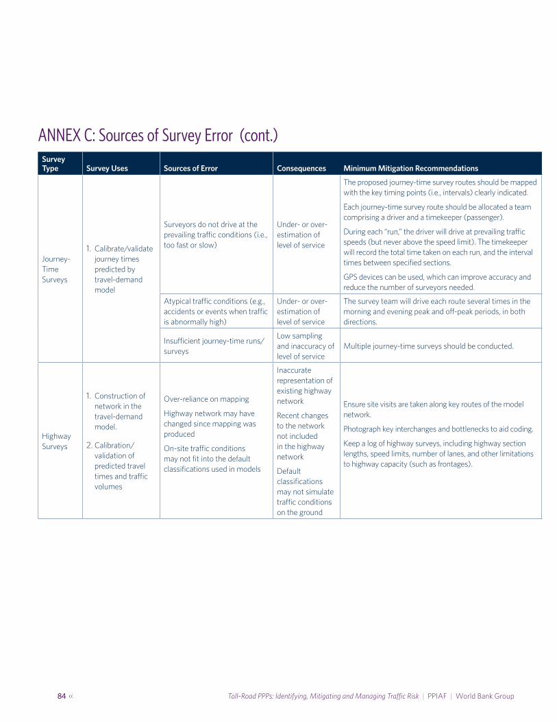
84 ‹‹ Toll-Road PPPs: Identifying, Mitigating and Managing Traffic Risk | PPIAF | World Bank Group
Survey Type Survey Uses Sources of Error Consequences Minimum Mitigation Recommendations
Journey-Time Surveys
1. Calibrate/validate journey times predicted by travel-demand model
Surveyors do not drive at the prevailing traffic conditions (i.e., too fast or slow)
Under- or over-estimation of level of service
The proposed journey-time survey routes should be mapped with the key timing points (i.e., intervals) clearly indicated.
Each journey-time survey route should be allocated a team comprising a driver and a timekeeper (passenger).
During each “run,” the driver will drive at prevailing traffic speeds (but never above the speed limit). The timekeeper will record the total time taken on each run, and the interval times between specified sections.
GPS devices can be used, which can improve accuracy and reduce the number of surveyors needed.
Atypical traffic conditions (e.g., accidents or events when traffic is abnormally high)
Under- or over-estimation of level of service
The survey team will drive each route several times in the morning and evening peak and off-peak periods, in both directions.
Insufficient journey-time runs/surveys
Low sampling and inaccuracy of level of service
Multiple journey-time surveys should be conducted.
Highway Surveys
1. Construction of network in the travel-demand model.
2. Calibration/validation of predicted travel times and traffic volumes
Over-reliance on mapping
Highway network may have changed since mapping was produced
On-site traffic conditions may not fit into the default classifications used in models
Inaccurate representation of existing highway network
Recent changes to the network not included in the highway network
Default classifications may not simulate traffic conditions on the ground
Ensure site visits are taken along key routes of the model network.
Photograph key interchanges and bottlenecks to aid coding.
Keep a log of highway surveys, including highway section lengths, speed limits, number of lanes, and other limitations to highway capacity (such as frontages).
ANNEX C: Sources of Survey Error (cont.)

›› 85PPIAF | World Bank Group | Toll-Road PPPs: Identifying, Mitigating and Managing Traffic Risk
ANNEX D: Sources of Modeling Error »
Error TypeError Sub-Type Source of Error Consequence Minimum Mitigation Recommendations
Trip matrix error
Origin/destination (O/D) survey errors
See ANNEX C: SOURCES OF SURVEY ERROR
Low sampling and inaccuracy of trip matrix leads to under- or over-estimation of travel demand on certain routes and/or trip-length bias.
Trip matrices should be segmented at least by the main vehicle classes (e.g., light vehicles and heavy vehicles) and times of day. Generally, the greater the disaggregation of the trip matrix (e.g., by journey purpose and income), the better the ability to predict the travel demand in the network and the behavioral response of this demand to the project road.
Matrix estimation errors
It is impossible to sample all trip movements in an O/D survey (due to sampling constraints), and this inevitably creates gaps in the matrix that must be filled using an iterative estimation process and observed traffic count data. This is a key part of the model-calibration exercise and is extremely synthetic by nature.
The matrix is filled inaccurately with synthesized trips. This becomes a compounded source of error in the future, when traffic growth rates (see Chapter 4) get applied to these cells in the matrix.
Controlled matrix estimation techniques should be used to simulate the un-observed trip movements. The prior matrix estimation and final trip matrices should be compared to ensure that the matrix-estimation techniques have not introduced a significant bias to the matrices, such as changes to the average trip length and/or in-filling of short trips. Errors associated with the travel-demand model can be minimized by ensuring that it meets strict validation criteria, and arranging for a peer review of the model’s ability to accurately forecast existing traffic volumes, origin-destination patterns and travel times.
Annualization errors
See ANNEX C: SOURCES OF SURVEY ERROR. The matrix may be built (and validated) from traffic count and origin/destination data that may be atypical and does not reflect normal traffic conditions. This can lead to estimation errors when the forecasts from the hourly assigned traffic are factored up to daily or annual traffic flows.
The matrix does not reflect typical hourly or daily flows, because the underlying traffic data is not an accurate reflection of average conditions. This could lead to either over- or under-estimation.
The data-collection program used to populate the model should be carried out in line with the recommendations described in ANNEX C: SOURCES OF SURVEY ERROR.
(continued on page 86)

86 ‹‹ Toll-Road PPPs: Identifying, Mitigating and Managing Traffic Risk | PPIAF | World Bank Group
Error TypeError Sub-Type Source of Error Consequence Minimum Mitigation Recommendations
Network Errors
Journey-time and highway survey errors
See ANNEX C: SOURCES OF SURVEY ERROR
Under- or over-estimation of level of service leads to an inaccurate representation of travel time/cost on certain links, which in turn can lead to an inaccurate assignment of traffic to the network.
The specification and coding of the project road in the travel-demand model network (e.g., project road distances, free-flow speeds, intersections, capacities, etc.) requires close cooperation among the project’s technical advisors/engineers, so that the benefits (i.e., reduction in generalized cost) of the road are not overstated.
Network Coding Errors
It is impossible to capture perfectly accurately the service levels over the full extent of a network (unless the study area is very small) during journey-time surveys. This means that distances, speeds, delays, etc., are often estimated from other sources (such as maps, design manuals, etc.), which may not be reflective of observed conditions.
This can lead to assignment errors, because the relative benefits of making different route choices can be miscalculated—e.g., a new road looks much faster or shorter than a competing road, leading to over-assignment of traffic to the new road.
Behavioral Parameter Errors
Utility-function specification error
Route choice is a complex and individualized process, and it is impossible to reflect perfectly all drivers’ decisions regarding which routes to take on their journey in a single utility function (like the generalized cost function shown in section 3.4.3). These functions are calibrated to reflect the behavior of the average driver, but there may be significant variation in the values and relative importance (i.e., the coefficient) of each parameter, which could significantly affect route choice. Alternatively, the specification used may be missing a key behavioral parameter altogether, such as reliability or variability of journey times.
Route choice can be miscalculated because the utility function does not accurately reflect how drivers behave. This can lead to over- or under-forecasting of a new or improved road link.
Local behavioral parameters should be determined using revealed- or stated-preference techniques undertaken by a reputable company.
Behavioral parameters should—at a minimum—be benchmarked with other traffic studies, as well as being internationally benchmarked, adjusting for the GDP of different countries.
ANNEX D: Sources of Modeling Error (cont.)

›› 87PPIAF | World Bank Group | Toll-Road PPPs: Identifying, Mitigating and Managing Traffic Risk
ANNEX E: Typical PPP Contract Structure »
The procuring authority/government: The government commissions and oversees the long-term contract to develop the project. The government will want to receive a high-quality asset at a minimal cost to the user (e.g., low tolls) and the taxpayer (e.g., low capital or ongoing subsidy).
The bidding consortia and the project company (or SPV): The primary counterparty to the government is typically a consortium of bidding firms. These will typically be led by a cross-representation of the construction contractor, the operating contractor, and the equity investors in the project. Upon successful contract award or at financial close, the bidding consortium is incorporated as a new company (the
SPV), which then becomes contractually responsible for delivering the project. The bidding consortium (and then the SPV) have the overriding (and sometimes competing) objective of winning the bid and maximizing their financial returns from winning the right to deliver the project.
Senior third-party financiers (e.g., debt providers such as banks): Banks and other third-party financial institutions typically provide the bulk of finance (e.g., loans or bonds) to the SPV, to allow it to build the project. These financiers are then repaid with the future cash flows from the project (i.e., toll revenues and/or government subsidy). Third-party financiers want to support the winning bidder but expect a
FIGURE 14: Typical PPP Contract Structure

88 ‹‹ Toll-Road PPPs: Identifying, Mitigating and Managing Traffic Risk | PPIAF | World Bank Group
return that sufficiently covers the risk of default and provides an expected level of profit. In addition to imposing certain debt covenants (e.g., debt-service cover ratios; see Chapter 9) they will also expect co-financing from equity providers (that will absorb initial losses in the event of cash shortfalls or default of the SPV) and a package of financial security (e.g., performance bonds, letters of credit) from the construction contractor (which will partially or fully cover the cost of replacing the contractor if their performance is unsatisfactory or they become insolvent). The financiers will also often expect contractual protection from the government, should default occur by the SPV (or one of the contractors), so that they have the power and time to step in and try to remedy the situation. They may also expect compensation from the government in this situation, given that the government will inherit an asset that they have predominately financed.
The construction contractor: The construction contractor is the sub-contractor responsible for constructing the project. This tends to be a large contractor with a track record and financial standing commensurate with the size of the project. The contractor will want to win the bid and build the project on time and within budget, at a construction price that provides sufficient profit. While wanting to win the right to build the road, the contractor also wants to minimize the exposure of the company’s financial standing (i.e., balance sheet) to the project, should the contractor encounter difficulties in building the project. This is a crucial aspect of PPPs, and project finance
in general—major infrastructure projects (such as toll roads) are often too big for any one construction firm (and its supply chain) to absorb the risks of delay or cost overruns, so they reduce their exposure by participating as a sub-contractor to an SPV (i.e., the financing is non or limited recourse to the contractor) and capping the exposure (i.e., the liabilities) of their company.
The operating and maintenance contractor: The operating and maintenance contractor is the sub-contractor legally responsible for managing the operations and maintenance of the road. Again, this will tend to be a contractor with a track record and financial standing commensurate with the size of the project. The contractor will want to win the bid and operate the road to contractual standards, at a price that provides sufficient profit and minimizes the exposure of the company’s financial standing (i.e., balance sheet) to the project, should the contractor encounter difficulties through the operating period. The contractor could be an entirely separate entity from the constructor, or may share the same parent company.
The equity investors: The SPV is capitalized with shares from one or more equity investors. This capital acts as a buffer for senior financiers, in the event of default or cash shortfalls. Equity can be provided by specialist investors (e.g., private-equity funds) and/or by the construction and operating contractors. Equity investors typically take on the most risk and therefore expect higher financial returns.

›› 89PPIAF | World Bank Group | Toll-Road PPPs: Identifying, Mitigating and Managing Traffic Risk
ANNEX F: Cash Flows from the Hypothetical Example of a Speculative Bidder Call on Traffic and Revenue
»
Synopsis: The fictional Republic of Vectura has tendered a 25-year toll concession for the greenfield, 40-kilometer Vectura Tollway between two major economic centers. The concessionaire will design, build, finance, operate and maintain the highway, and in return will collect toll revenue from the road’s users. The tolls, which are regulated through the concession agreement, will be strictly set at $1.00 and cannot be altered by the concessionaire. The winning bidder will be the one that requires the lowest upfront capital subsidy/grant from the government; there will be no other bidding criteria. The government has undertaken a traffic study of its own but has also asked bidders to undertake their own studies and derive their own traffic and revenue forecasts. The government traffic study was completed by an internationally recognized consultancy firm and provided the following opening-day traffic forecasts: 60,000 vehicles per day annual average daily traffic (AADT), based on a 50-percent traffic capture rate, and a resulting opening-year toll revenue of $21.9 million.
The tender has attracted two consortia of bidders:
The Imperium Consortium: This consortium is dominated by Imperium Construction Limited (ICL), the largest construction company operating in Vectura. The only other consortium partner is Millennium Road Services Limited, which will be the consortium’s O&M contractor. Third-party financing will be provided through a senior loan from National Vectura Bank, which has a strong corporate relationship with ICL but does not have any project-finance experience and has yet to lend to a project of this kind. The equity will be solely provided by ICL; there are no third-party equity investors in the consortium.
The Verus Consortium: This consortium has equal representation between Vectura Construction Limited (VCL), Orbit Maintenance Limited (OML), and the Vectura Pension Fund (VPF). VCL will act as the lead construction contractor; OML as the operations and maintenance contractor; and together with VPF, they will share the equity investment equally. A senior loan will be provided by Galaxy Banking Corporation, a leading international project-finance lender in the highway sector.
All other inputs to the bid (capital costs, operating and maintenance costs, financing costs, debt-to-equity ratio, and target equity rate of return) are the same for both bidders. Both consortia have undertaken a financial modeling exercise for their bids, using the government’s traffic forecast (as a benchmark for their bids), the results of which are captured in the table on the next page.
BIDDING STRATEGIES
Imperium Consortium: Imperium hires its own traffic consultant, who initially derives very similar forecasts to those provided by the government. The Imperium Consortium begins to consider how it might gain a competitive advantage over its competitor before it submits its final bid, given that capital cost and operating maintenance costs are likely to be similar between the two bids. On that basis, it decides speculatively to artificially increase the traffic forecasts beyond what was proposed in the government’s traffic study, which increases the forecasted project revenues by nearly 30 percent ($28.4 million, compared to $21.9 million).

90 ‹‹ Toll-Road PPPs: Identifying, Mitigating and Managing Traffic Risk | PPIAF | World Bank Group
By changing the traffic and revenue forecasts in this way, the financial model would show an equity return of 26 percent. This provides the Imperium Consortium with the headroom to further increase the construction price (i.e., capital costs), from $200 million to $250 million, while maintaining the target equity return at 20 percent and also reducing the value of the capital grant (the bidding parameter). The Imperium Consortium will do this because the financial gain ICL (the sub-contractor) derives from increasing the construction price will outweigh the financial loss in terms of lower dividends/equity returns to ICL (as the sole shareholder), if these higher traffic and revenue flows do not materialize (in essence, the project now appears to be able to support more debt and equity due to artificially high future cash flows).
National Vectura Bank has overlooked these higher (and somewhat unrealistic) traffic and revenue forecasts while doing its due diligence, and it is willing to commit to lending to the project on the basis of these higher forecasts.
Verus Consortium: In contrast, both Galaxy Banking Corporation (the debt financier) and Verus Pension Fund (the third-party equity provider) have both closely scrutinized the government’s traffic forecasts, with the help of an independent traffic advisor. Both institutions have stated that they will only sign off on the consortium’s bid and commit to investing in the project if the opening-day traffic and revenue forecasts
are reduced by 15 percent below the government’s forecasts. These lower traffic and revenue forecasts were entered into the financial model, and it was clear that a higher level of capital grant was required to ensure the target equity return of 20 percent could be met (i.e., the lower traffic and revenue forecasts mean that the project can only support a lower amount of debt and equity).
The table below summarizes the results of the financial models.
CONTRACT AWARD AND FINANCIAL CLOSE
The Republic of Vectura opened the sealed bids (without evaluation) and found that the Imperium Consortium had a lower capital grant requirement of $15 million, versus the $52 million proposed by the Verus Consortium. The contract award was subsequently made to the Imperium Consortium, and financial close was reached with National Vectura Bank shortly afterwards.
OPERATIONS
The Imperium Consortium constructed the Vectura Tollway to the original specification, on time and within their original capital cost estimate of $200 million. However, the opening-day traffic flows turn out to be only 50,000 AADT, versus the
TABLE 14: Results of Financial Models Applied to Hypothetical Example
Government Forecast Imperium Bid Verus Bid
Debt Required $122m $165m (+$43m) $102m (-$20m)
Equity Required $52m $71m (+19m) $44m (-$8m)
Value of Capital Grant (Bidding Parameter)
$26m $15m (-$11m) $ 55m (+$29m)
Total Funding Required (Construction Costs)
$200m $250m (+$50m) $200m
Forecast Equity Return (IRR)
20% 20% 20%
Traffic Forecast (Opening-Day AADT)
60,000 78,000 51,000

›› 91PPIAF | World Bank Group | Toll-Road PPPs: Identifying, Mitigating and Managing Traffic Risk
78,000 AADT predicted in the bid. Thereafter traffic did grow in line with forecast, at five percent per annum.
CONCLUSION: CALCULATING THE VALUE OF THE SPECULATIVE CALL
The Imperium Consortium made a speculative play to artificially inflate the traffic and revenue forecasts as a way of reducing their subsidy requirement (i.e., the bidding parameter), and also front-loaded their return by increasing ICL’s construction price by $50 million, to $250 million. So when the traffic and revenue forecasts turned out to be significantly lower, was this speculative call worthwhile, or did the consortium end up losing money as a result of its highly speculative bid?
The answer is yes, it was worthwhile. Although dividends were significantly reduced due to the lower profitability of the project
(resulting from much lower traffic figures), the fact that the Imperium Consortium was able to abstract an additional $50 million through its construction company (ICL) meant that its actual IRR was 21 percent, rather than the targeted 20 percent. Thus, the Imperium Consortium still made a larger profit, even though actual opening-day traffic flows were 36 percent lower than those forecasted in Imperium’s bid.
In contrast, National Vectura Bank suffered losses due to the un-performing nature of the loan they provided to the Imperium Consortium, with the SPV missing several scheduled repayments due to cash shortfalls (caused by the lower traffic and revenue flows), with key loan ratios (ADSCR and LLC; see Chapter 9) below acceptable levels.
Table 14 on pages 92-95 shows the full revenue, cash flows and IRR calculations of both bidders.

92 ‹‹ Toll-Road PPPs: Identifying, Mitigating and Managing Traffic Risk | PPIAF | World Bank Group
TABLE 15: Revenue, Cash Flows, and IRR Calculations
GOVERNMENT FINANCIAL MODEL (SHADOW-BID MODEL)
2018 2019 2020 2021 2022 2023 2024 2025 2026 2027 2028 2029 2030 2031 2032 2033 2034 2035 2036 2037 2038 2039 2040 2041 2042 2043
Debt Drawdown 61 61 0 0 0 0 0 0 0 0 0 0 0 0 0 0 0 0 0 0 0 0 0 0 0 0
Equity Drawdown 26 26 0 0 0 0 0 0 0 0 0 0 0 0 0 0 0 0 0 0 0 0 0 0 0 0
Revenues 0 0 24 26 28 30 33 35 38 41 45 48 52 57 61 66 72 78 84 91 98 106 115 124 139 0
Construction Cost (100) (100) 0 0 0 0 0 0 0 0 0 0 0 0 0 0 0 0 0 0 0 0 0 0 0 0
O&M Cost 0 0 (3) (3) (3) (4) (4) (4) (4) (4) (4) (4) (4) (5) (5) (5) (5) (5) (5) (6) (6) (6) (6) (6) (6) 0
Taxes 0 0 0 0 0 (2) (3) (4) (5) (6) (7) (8) (10) (11) (12) (13) (14) (16) (17) (19) (21) (23) (25) (27) (29) (1)
Debt Service 0 0 (16) (18) (19) (19) (20) (22) (22) (24) (26) (20) 0 0 0 0 0 0 0 0 0 0 0 0 0 0
Distributions 0 0 0 0 0 (6) (10) (13) (15) (8) (8) (16) (38) (41) (45) (48) (52) (53) (54) (60) (65) (72) (78) (86) (93) (52)
IRR calculation: 20%Minimum annual debt-service cover ratio (ADSCR): 1.30Minimum loan-life cover ratio (LLCR): 1.46
IMPERIUM’S BID MODEL
2018 2019 2020 2021 2022 2023 2024 2025 2026 2027 2028 2029 2030 2031 2032 2033 2034 2035 2036 2037 2038 2039 2040 2041 2042 2043
Debt Drawdown 82 82 0 0 0 0 0 0 0 0 0 0 0 0 0 0 0 0 0 0 0 0 0 0 0 0
Equity Drawdown 35 35 0 0 0 0 0 0 0 0 0 0 0 0 0 0 0 0 0 0 0 0 0 0 0 0
Revenues 0 0 31 34 36 39 43 46 50 54 58 63 68 74 80 86 93 101 109 118 127 138 149 161 174 0
Construction Cost (125) (125) 0 0 0 0 0 0 0 0 0 0 0 0 0 0 0 0 0 0 0 0 0 0 0 0
O&M Cost 0 0 (3) (3) (3) (4) (4) (4) (4) (4) (4) (4) (4) (5) (5) (5) (5) (5) (5) (5) (6) (6) (6) (6) (6) 0
Taxes 0 0 0 0 0 (2) (4) (5) (7) (8) (9) (11) (13) (14) (16) (17) (19) (21) (23) (25) (27) (30) (32) (35) (39) (1)
Debt Service 0 0 (21) (23) (35) (26) (27) (25) (30) (32) (35) (30) 0 0 0 0 0 0 0 0 0 0 0 0 0 0
Distributions 0 0 0 0 0 (7) (13) (17) (21) (10) (10) (18) (51) (55) (59) (64) (69) (70) (72) (78) (86) (94) (103) (112) (123) (73)
IRR calculation: 20%Minimum annual debt-service cover ratio (ADSCR): 1.30Minimum loan-life cover ratio (LLCR): 1.45

›› 93PPIAF | World Bank Group | Toll-Road PPPs: Identifying, Mitigating and Managing Traffic Risk
TABLE 15: Revenue, Cash Flows, and IRR Calculations
GOVERNMENT FINANCIAL MODEL (SHADOW-BID MODEL)
2018 2019 2020 2021 2022 2023 2024 2025 2026 2027 2028 2029 2030 2031 2032 2033 2034 2035 2036 2037 2038 2039 2040 2041 2042 2043
Debt Drawdown 61 61 0 0 0 0 0 0 0 0 0 0 0 0 0 0 0 0 0 0 0 0 0 0 0 0
Equity Drawdown 26 26 0 0 0 0 0 0 0 0 0 0 0 0 0 0 0 0 0 0 0 0 0 0 0 0
Revenues 0 0 24 26 28 30 33 35 38 41 45 48 52 57 61 66 72 78 84 91 98 106 115 124 139 0
Construction Cost (100) (100) 0 0 0 0 0 0 0 0 0 0 0 0 0 0 0 0 0 0 0 0 0 0 0 0
O&M Cost 0 0 (3) (3) (3) (4) (4) (4) (4) (4) (4) (4) (4) (5) (5) (5) (5) (5) (5) (6) (6) (6) (6) (6) (6) 0
Taxes 0 0 0 0 0 (2) (3) (4) (5) (6) (7) (8) (10) (11) (12) (13) (14) (16) (17) (19) (21) (23) (25) (27) (29) (1)
Debt Service 0 0 (16) (18) (19) (19) (20) (22) (22) (24) (26) (20) 0 0 0 0 0 0 0 0 0 0 0 0 0 0
Distributions 0 0 0 0 0 (6) (10) (13) (15) (8) (8) (16) (38) (41) (45) (48) (52) (53) (54) (60) (65) (72) (78) (86) (93) (52)
IRR calculation: 20%Minimum annual debt-service cover ratio (ADSCR): 1.30Minimum loan-life cover ratio (LLCR): 1.46
IMPERIUM’S BID MODEL
2018 2019 2020 2021 2022 2023 2024 2025 2026 2027 2028 2029 2030 2031 2032 2033 2034 2035 2036 2037 2038 2039 2040 2041 2042 2043
Debt Drawdown 82 82 0 0 0 0 0 0 0 0 0 0 0 0 0 0 0 0 0 0 0 0 0 0 0 0
Equity Drawdown 35 35 0 0 0 0 0 0 0 0 0 0 0 0 0 0 0 0 0 0 0 0 0 0 0 0
Revenues 0 0 31 34 36 39 43 46 50 54 58 63 68 74 80 86 93 101 109 118 127 138 149 161 174 0
Construction Cost (125) (125) 0 0 0 0 0 0 0 0 0 0 0 0 0 0 0 0 0 0 0 0 0 0 0 0
O&M Cost 0 0 (3) (3) (3) (4) (4) (4) (4) (4) (4) (4) (4) (5) (5) (5) (5) (5) (5) (5) (6) (6) (6) (6) (6) 0
Taxes 0 0 0 0 0 (2) (4) (5) (7) (8) (9) (11) (13) (14) (16) (17) (19) (21) (23) (25) (27) (30) (32) (35) (39) (1)
Debt Service 0 0 (21) (23) (35) (26) (27) (25) (30) (32) (35) (30) 0 0 0 0 0 0 0 0 0 0 0 0 0 0
Distributions 0 0 0 0 0 (7) (13) (17) (21) (10) (10) (18) (51) (55) (59) (64) (69) (70) (72) (78) (86) (94) (103) (112) (123) (73)
IRR calculation: 20%Minimum annual debt-service cover ratio (ADSCR): 1.30Minimum loan-life cover ratio (LLCR): 1.45
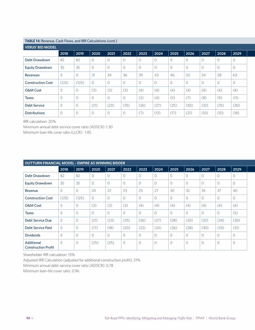
94 ‹‹ Toll-Road PPPs: Identifying, Mitigating and Managing Traffic Risk | PPIAF | World Bank Group
TABLE 14: Revenue, Cash Flows, and IRR Calculations (cont.)
VERUS’ BID MODEL
2018 2019 2020 2021 2022 2023 2024 2025 2026 2027 2028 2029 2030 2031 2032 2033 2034 2035 2036 2037 2038 2039 2040 2041 2042 2043
Debt Drawdown 82 82 0 0 0 0 0 0 0 0 0 0 0 0 0 0 0 0 0 0 0 0 0 0 0 0
Equity Drawdown 35 35 0 0 0 0 0 0 0 0 0 0 0 0 0 0 0 0 0 0 0 0 0 0 0 0
Revenues 0 0 31 34 36 39 43 46 50 54 58 63 68 74 80 86 93 101 109 118 127 138 149 161 174 0
Construction Cost (125) (125) 0 0 0 0 0 0 0 0 0 0 0 0 0 0 0 0 0 0 0 0 0 0 0 0
O&M Cost 0 0 (3) (3) (3) (4) (4) (4) (4) (4) (4) (4) (4) (5) (5) (5) (5) (5) (5) (5) (6) (6) (6) (6) (6) 0
Taxes 0 0 0 0 0 (2) (4) (5) (7) (8) (9) (11) (13) (14) (16) (17) (19) (21) (23) (25) (27) (30) (32) (35) (39) (1)
Debt Service 0 0 (21) (23) (35) (26) (27) (25) (30) (32) (35) (30) 0 0 0 0 0 0 0 0 0 0 0 0 0 0
Distributions 0 0 0 0 0 (7) (13) (17) (21) (10) (10) (18) (51) (55) (59) (64) (69) (70) (72) (78) (86) (94) (103) (112) (123) (73)
IRR calculation: 20%Minimum annual debt-service cover ratio (ADSCR): 1.30Minimum loan-life cover ratio (LLCR): 1.45
OUTTURN FINANCIAL MODEL – EMPIRE AS WINNING BIDDER
2018 2019 2020 2021 2022 2023 2024 2025 2026 2027 2028 2029 2030 2031 2032 2033 2034 2035 2036 2037 2038 2039 2040 2041 2042 2043
Debt Drawdown 82 82 0 0 0 0 0 0 0 0 0 0 0 0 0 0 0 0 0 0 0 0 0 0 0 0
Equity Drawdown 35 35 0 0 0 0 0 0 0 0 0 0 0 0 0 0 0 0 0 0 0 0 0 0 0 0
Revenue 0 0 20 22 23 25 27 30 32 35 37 40 44 47 51 55 60 65 70 76 82 88 96 103 112 0
Construction Cost (125) (125) 0 0 0 0 0 0 0 0 0 0 0 0 0 0 0 0 0 0 0 0 0 0 0 0
O&M Cost 0 0 (3) (3) (3) (4) (4) (4) (4) (4) (4) (4) (4) (5) (5) (5) (5) (5) (5) (5) (6) (6) (6) (6) (6) 0
Taxes 0 0 0 0 0 0 0 0 0 0 0 (5) (7) (8) (9) (10) (11) (12) (13) (15) (16) (18) (20) (22) (24) 0
Debt Service Due 0 0 (21) (23) (25) (26) (27) (28) (30) (32) (34) (30) 0 0 0 0 0 0 0 0 0 0 0 0 0 0
Debt Service Paid 0 0 (17) (18) (20) (22) (24) (26) (28) (30) (33) (31) 0 0 0 0 0 0 0 0 0 0 0 0 0 0
Dividends 0 0 0 0 0 0 0 0 0 0 0 0 0 (27) (37) (41) (44) (43) (42) (46) (51) (57) (62) (68) (75) (73
Additional Construction Profit
0 0 (25) (25) 0 0 0 0 0 0 0 0 0 0 0 0 0 0 0 0 0 0 0 0 0 0
Shareholder IRR calculation: 13%Adjusted IRR Calculation (adjusted for additional construction profit): 21%Minimum annual debt-service cover ratio (ADSCR): 0.78Minimum loan-life cover ratio: 0.96

›› 95PPIAF | World Bank Group | Toll-Road PPPs: Identifying, Mitigating and Managing Traffic Risk
TABLE 14: Revenue, Cash Flows, and IRR Calculations (cont.)
VERUS’ BID MODEL
2018 2019 2020 2021 2022 2023 2024 2025 2026 2027 2028 2029 2030 2031 2032 2033 2034 2035 2036 2037 2038 2039 2040 2041 2042 2043
Debt Drawdown 82 82 0 0 0 0 0 0 0 0 0 0 0 0 0 0 0 0 0 0 0 0 0 0 0 0
Equity Drawdown 35 35 0 0 0 0 0 0 0 0 0 0 0 0 0 0 0 0 0 0 0 0 0 0 0 0
Revenues 0 0 31 34 36 39 43 46 50 54 58 63 68 74 80 86 93 101 109 118 127 138 149 161 174 0
Construction Cost (125) (125) 0 0 0 0 0 0 0 0 0 0 0 0 0 0 0 0 0 0 0 0 0 0 0 0
O&M Cost 0 0 (3) (3) (3) (4) (4) (4) (4) (4) (4) (4) (4) (5) (5) (5) (5) (5) (5) (5) (6) (6) (6) (6) (6) 0
Taxes 0 0 0 0 0 (2) (4) (5) (7) (8) (9) (11) (13) (14) (16) (17) (19) (21) (23) (25) (27) (30) (32) (35) (39) (1)
Debt Service 0 0 (21) (23) (35) (26) (27) (25) (30) (32) (35) (30) 0 0 0 0 0 0 0 0 0 0 0 0 0 0
Distributions 0 0 0 0 0 (7) (13) (17) (21) (10) (10) (18) (51) (55) (59) (64) (69) (70) (72) (78) (86) (94) (103) (112) (123) (73)
IRR calculation: 20%Minimum annual debt-service cover ratio (ADSCR): 1.30Minimum loan-life cover ratio (LLCR): 1.45
OUTTURN FINANCIAL MODEL – EMPIRE AS WINNING BIDDER
2018 2019 2020 2021 2022 2023 2024 2025 2026 2027 2028 2029 2030 2031 2032 2033 2034 2035 2036 2037 2038 2039 2040 2041 2042 2043
Debt Drawdown 82 82 0 0 0 0 0 0 0 0 0 0 0 0 0 0 0 0 0 0 0 0 0 0 0 0
Equity Drawdown 35 35 0 0 0 0 0 0 0 0 0 0 0 0 0 0 0 0 0 0 0 0 0 0 0 0
Revenue 0 0 20 22 23 25 27 30 32 35 37 40 44 47 51 55 60 65 70 76 82 88 96 103 112 0
Construction Cost (125) (125) 0 0 0 0 0 0 0 0 0 0 0 0 0 0 0 0 0 0 0 0 0 0 0 0
O&M Cost 0 0 (3) (3) (3) (4) (4) (4) (4) (4) (4) (4) (4) (5) (5) (5) (5) (5) (5) (5) (6) (6) (6) (6) (6) 0
Taxes 0 0 0 0 0 0 0 0 0 0 0 (5) (7) (8) (9) (10) (11) (12) (13) (15) (16) (18) (20) (22) (24) 0
Debt Service Due 0 0 (21) (23) (25) (26) (27) (28) (30) (32) (34) (30) 0 0 0 0 0 0 0 0 0 0 0 0 0 0
Debt Service Paid 0 0 (17) (18) (20) (22) (24) (26) (28) (30) (33) (31) 0 0 0 0 0 0 0 0 0 0 0 0 0 0
Dividends 0 0 0 0 0 0 0 0 0 0 0 0 0 (27) (37) (41) (44) (43) (42) (46) (51) (57) (62) (68) (75) (73
Additional Construction Profit
0 0 (25) (25) 0 0 0 0 0 0 0 0 0 0 0 0 0 0 0 0 0 0 0 0 0 0
Shareholder IRR calculation: 13%Adjusted IRR Calculation (adjusted for additional construction profit): 21%Minimum annual debt-service cover ratio (ADSCR): 0.78Minimum loan-life cover ratio: 0.96

96 ‹‹ Toll-Road PPPs: Identifying, Mitigating and Managing Traffic Risk | PPIAF | World Bank Group
A shadow-bid financial model will differ from project to project and from advisor to advisor, but in general, a shadow model will
have the type of structure shown below in Figure 15:
ANNEX G: Shadow-Bid Financial Modeling»
FIGURE 15: A Typical Structure of a Shadow-Bid Financial Model

›› 97PPIAF | World Bank Group | Toll-Road PPPs: Identifying, Mitigating and Managing Traffic Risk
As shown on page 96, a shadow-bid financial model typically has four main segments (or portals):
• Model control: This is effectively the bid-price variable that a bidder (who the government is trying to proxy) can adjust up or down in order to price (or value) their bid for the project. For a toll-road project, this will depend on the main financial criteria to be used to evaluate the bids. Typically, the winning financial bid64 will be the one offering the lowest65 toll rate or subsidy66 (whether capital or ongoing subsidy). Thus, the purpose of the financial model is to allow the bidder to calculate the lowest, most-competitive toll or subsidy that will still allow the project to service debt, while earning an acceptable return on equity and keeping the project operating and maintained to an acceptable standard (i.e., paying operating and maintenance costs). This process is typically referred to as model optimization and is the key modeling process that all bidders will typically undertake in order to price their bids as efficiently as possible, whilst ensuring the project still remains financeable. From the perspective of the government, this is the parameter in the shadow-bid financial model that will ultimately help estimate the cost to be imposed on the user (through tolls) and/or the taxpayer (through subsidy), and therefore measures affordability.
• Model inputs: This is where a variety of project information is entered into the model, including project timing, financing assumptions (e.g., cost and terms of debt), macro-economic assumptions (e.g., inflation), estimated capital costs, operating and maintenance costs, and toll revenue forecasts. For the shadow-bid financial model, the government will typically be given this information by its technical and financial advisors. The toll-revenue forecasts will likely be based on the government traffic forecasters’ base case. Model inputs, including revenue forecasts, are typically presented in real prices (according to a specified pricing base year).
• Model calculations: The model calculation sheets convert the inputs into nominal prices and calculate how the project costs are financed through different sources (so-called sources and uses) and how the financed amounts are ultimately serviced/repaid by the project’s cash flows
64 Financial criteria are often considered alongside technical criteria in the evaluation of bids. The relative weighting between financial and technical criteria will depend on the objectives of the granting government and on the specifics of the project. A transaction advisor would typically work with a government to define the overall evaluation criteria.
65 Often this is done on an NPV basis, using a specified discount rate that all bidders must use.66 Financial evaluation criteria that blend toll rates and subsidies (or different types of subsidies) into a single bid variable are possible but are much harder to
evaluate and could lead to the strategic misrepresentation problems discussed in the previous part of this guide.
(typically shown in a funding schedule). These sheets will also include the calculation of tax to be paid by the project company.
• Model outputs: The model outputs use the information from the model calculation sheets to summarize the overall finances of a project, by generating typical summary financial statements (i.e., cash-flow statement, income statement and balance sheet). The model outputs also typically include a summary of key financial ratios. These typically relate to the financial ratios that measure the project’s ability to adequately service the project’s debt (e.g., debt-service coverage ratios, which are explained in more detail later in this section) and the financial return the project offers to its equity investors (i.e., through an IRR calculation). The model outputs will also summarize the level of subsidy (either upfront capital subsidy or ongoing revenue subsidy) and thus show the government’s direct liabilities under the project. The model outputs are typically also summarized on the same sheet as the model control, so that the bidder can easily see how changing the bid parameter will impact the project’s finances and can more easily optimize the model.
The shadow-bid financial model will therefore provide the government with an understanding of the underlying financial viability of the project under the base-case traffic scenario. This is vital information for the government, because it represents a starting point for understanding the attractiveness of the project to private financiers (i.e., bankability) and the affordability of the project to users and government. However, we know from the previous sections of this guide that traffic and revenue forecasts are prone to inaccuracy, and the extent to which the traffic and revenue forecasts could vary from the base case could have a significant impact on the project’s finances and subsequently on both bankability and affordability.

98 ‹‹ Toll-Road PPPs: Identifying, Mitigating and Managing Traffic Risk | PPIAF | World Bank Group
ANNEX H: Traffic Risk Index»
Source of Risk Risk Factor Risk Drivers Low Traffic Risk Medium Traffic Risk High Traffic Risk
Category Score (0= Low Risk; 5 = Medium Risk; 10= High Risk)
Highways that … Highways that: Highways that:
Asset type • Existing traffic• Reassigned traffic• Diverted traffic
… already exist (brownfield) … already exist but require substantial off-line improvements or extensions (e.g., greenfield bypasses)
… are completely new (greenfield) 0
Traffic mix • Existing traffic• Reassigned traffic• Diverted traffic
… are designed to attract peak traffic movements and have a strong assignment of traffic throughout the day and night and for a variety of purposes (including a very high proportion of non-discretionary/frequent trip purposes,—e.g., commuting and business)
… are expected to attract a mix of peak-hour and off-peak-hour trips (i.e., a strong share of non-discretionary/frequent trip purposes,—e.g. commuting and business)
… attract high proportions of discretionary/infrequent trips (e.g., leisure) and very few non-discretionary trips
0
Project need / business case
• Reassigned traffic … address a clear transport need and/or a gap in the highway network,—i.e., add much-needed capacity to the network
… address a transport need and/or gap in the highway network—i.e., add needed capacity to the network
… do not address a specific transport need or gap in the highway network—i.e., sufficient capacity is provided by the existing network
5
Level of user benefits • Reassigned traffic … relieve roads that are congested all day, most severely during peak periods … relieve roads that are congested during peak periods … do not attract traffic from congested highways 5
• Reassigned and diverted traffic
… offer a substantial benefit (usually journey-time savings) to users (e.g., estuarial crossing, tunnel) that can be monetized through willingness to pay
… offer significant benefits (usually journey-time savings) to users, which can be partially monetized through willingness to pay
… offer relatively small benefits to users, which cannot be monetized through willingness to pay
5
History of tolling • Diverted traffic … supplement a well-developed tolled-highway network … are in areas where toll highways are still under development … introduce toll highways to a country/region for the first time 5
Connectivity of project • Reassigned traffic … are efficiently linked to the highway network … are reasonably linked to the highway network … are not well-linked to the existing highway network 5
Macro environment • Socio-economic growth
… have a strong macro-economic environment and for which demographic changes support rapid traffic growth
… have a stable macro-economic environment and for which demographic changes are supporting steady traffic growth
… have a weak macro-economic environment and for which demo-graphic changes lead to stagnated/deterioriating traffic growth
10
Level of interdependency with new development
• Development and induced traffic
… have forecasted traffic growth that is not dependent on additional development and land uses materializing near the project road
… have forecasted traffic growth that is somewhat dependent on additional development and land uses materializing near the project road
… have forecasted traffic growth that is heavily dependent on additional development and land uses materializing near the project road
0
Level of interdependency with rest of highway network
• Complementary crojects
… have forecasted traffic that is not reliant on the timely completion of complementary schemes
… have forecasts that are not substantially dependent on the timely completion of complementary schemes
… are dependent on the timely completion of complementary schemes
0
Foreign-exchange volatility • Currency-exchange rates
… charge tolls that are collected in local currency and are escalated in line with local inflation (i.e., toll setting is not exposed to foreign-exchange fluctuations)
… charge tolls that are collected in a mix of local and foreign currency, with separate escalation (i.e., toll- setting is at least partially protected against foreign-exchange fluctuations)
… collect tolls in the local currency but adjust/escalate them with foreign-exchange fluctuations
10
Stability of tolling environment
• Tolling policy … have a relatively simple, transparent toll strategy, with minimal discount structures
… have a toll policy that is simple but offers discounts (e.g., for local, frequent users)
… have a complex toll strategy 10
Level of government preparation
• Optimism bias• Strategic
misrepresentation• Winner’s curse• Survivor’s curse
… are commissioned by a government that: has completed a high-quality, independent traffic study; had it reviewed by a third party; supplied the base-year travel-demand model to bidders; and will evaluate the realism of bidder forecasts
… are commissioned by a government that: has carried out an independent traffic study that has not been reviewed by a third party; will not supply the base-year travel-demand model to bidders; and will not evaluate the realism of bids
… are commissioned by a government that has not carried out a traffic study and will not evaluate bidders on realism
5
Due diligence undertaken by financiers
• Strategic misrepresentation
… are financed by financiers who have hired independent lender’s traffic advisors (LTAs) to review the bidder forecasts
… are financed by financiers who have carried out their own review of traffic forecasts
… are financed by financiers who have not conducted due diligence on traffic forecasts
0
Strength of legal environment and enforceability of contracts
• Strategic misrepresentation
… feature a legal environment, bidder-security package and concession agreement that ensure that contractual stipulations will be fully enforced and there is little or no room for renegotiation
… feature a legal environment, bidder-security package and concession agreement that make it likely that most contractual stipulations will be enforced while leaving room for renegotiation
… feature a weak legal environment, bidder-security package and concession agreement, and have a high chance of renegotiation
10
Asymmetry of bidder information
• Winner’s curse … have a limited number of bidders, all of equal capacity and with strong experience in the toll-road sector
… have a lmited number of bidders, with variable experience in the toll-road sector
… have many bidders with variable experience in the toll-road sector
5
AVERAGE SCORE (TOTAL SCORE/NUMBER OF CATEGORIES) 75/16 = 4 .7
OVERALL TRAFFIC RISK RATING: >7 < 10>4< 7
<4
High RiskMedium RiskLow Risk
Erro
rUn
certa
inty
Bias

›› 99PPIAF | World Bank Group | Toll-Road PPPs: Identifying, Mitigating and Managing Traffic Risk
Source of Risk Risk Factor Risk Drivers Low Traffic Risk Medium Traffic Risk High Traffic Risk
Category Score (0= Low Risk; 5 = Medium Risk; 10= High Risk)
Highways that … Highways that: Highways that:
Asset type • Existing traffic• Reassigned traffic• Diverted traffic
… already exist (brownfield) … already exist but require substantial off-line improvements or extensions (e.g., greenfield bypasses)
… are completely new (greenfield) 0
Traffic mix • Existing traffic• Reassigned traffic• Diverted traffic
… are designed to attract peak traffic movements and have a strong assignment of traffic throughout the day and night and for a variety of purposes (including a very high proportion of non-discretionary/frequent trip purposes,—e.g., commuting and business)
… are expected to attract a mix of peak-hour and off-peak-hour trips (i.e., a strong share of non-discretionary/frequent trip purposes,—e.g. commuting and business)
… attract high proportions of discretionary/infrequent trips (e.g., leisure) and very few non-discretionary trips
0
Project need / business case
• Reassigned traffic … address a clear transport need and/or a gap in the highway network,—i.e., add much-needed capacity to the network
… address a transport need and/or gap in the highway network—i.e., add needed capacity to the network
… do not address a specific transport need or gap in the highway network—i.e., sufficient capacity is provided by the existing network
5
Level of user benefits • Reassigned traffic … relieve roads that are congested all day, most severely during peak periods … relieve roads that are congested during peak periods … do not attract traffic from congested highways 5
• Reassigned and diverted traffic
… offer a substantial benefit (usually journey-time savings) to users (e.g., estuarial crossing, tunnel) that can be monetized through willingness to pay
… offer significant benefits (usually journey-time savings) to users, which can be partially monetized through willingness to pay
… offer relatively small benefits to users, which cannot be monetized through willingness to pay
5
History of tolling • Diverted traffic … supplement a well-developed tolled-highway network … are in areas where toll highways are still under development … introduce toll highways to a country/region for the first time 5
Connectivity of project • Reassigned traffic … are efficiently linked to the highway network … are reasonably linked to the highway network … are not well-linked to the existing highway network 5
Macro environment • Socio-economic growth
… have a strong macro-economic environment and for which demographic changes support rapid traffic growth
… have a stable macro-economic environment and for which demographic changes are supporting steady traffic growth
… have a weak macro-economic environment and for which demo-graphic changes lead to stagnated/deterioriating traffic growth
10
Level of interdependency with new development
• Development and induced traffic
… have forecasted traffic growth that is not dependent on additional development and land uses materializing near the project road
… have forecasted traffic growth that is somewhat dependent on additional development and land uses materializing near the project road
… have forecasted traffic growth that is heavily dependent on additional development and land uses materializing near the project road
0
Level of interdependency with rest of highway network
• Complementary crojects
… have forecasted traffic that is not reliant on the timely completion of complementary schemes
… have forecasts that are not substantially dependent on the timely completion of complementary schemes
… are dependent on the timely completion of complementary schemes
0
Foreign-exchange volatility • Currency-exchange rates
… charge tolls that are collected in local currency and are escalated in line with local inflation (i.e., toll setting is not exposed to foreign-exchange fluctuations)
… charge tolls that are collected in a mix of local and foreign currency, with separate escalation (i.e., toll- setting is at least partially protected against foreign-exchange fluctuations)
… collect tolls in the local currency but adjust/escalate them with foreign-exchange fluctuations
10
Stability of tolling environment
• Tolling policy … have a relatively simple, transparent toll strategy, with minimal discount structures
… have a toll policy that is simple but offers discounts (e.g., for local, frequent users)
… have a complex toll strategy 10
Level of government preparation
• Optimism bias• Strategic
misrepresentation• Winner’s curse• Survivor’s curse
… are commissioned by a government that: has completed a high-quality, independent traffic study; had it reviewed by a third party; supplied the base-year travel-demand model to bidders; and will evaluate the realism of bidder forecasts
… are commissioned by a government that: has carried out an independent traffic study that has not been reviewed by a third party; will not supply the base-year travel-demand model to bidders; and will not evaluate the realism of bids
… are commissioned by a government that has not carried out a traffic study and will not evaluate bidders on realism
5
Due diligence undertaken by financiers
• Strategic misrepresentation
… are financed by financiers who have hired independent lender’s traffic advisors (LTAs) to review the bidder forecasts
… are financed by financiers who have carried out their own review of traffic forecasts
… are financed by financiers who have not conducted due diligence on traffic forecasts
0
Strength of legal environment and enforceability of contracts
• Strategic misrepresentation
… feature a legal environment, bidder-security package and concession agreement that ensure that contractual stipulations will be fully enforced and there is little or no room for renegotiation
… feature a legal environment, bidder-security package and concession agreement that make it likely that most contractual stipulations will be enforced while leaving room for renegotiation
… feature a weak legal environment, bidder-security package and concession agreement, and have a high chance of renegotiation
10
Asymmetry of bidder information
• Winner’s curse … have a limited number of bidders, all of equal capacity and with strong experience in the toll-road sector
… have a lmited number of bidders, with variable experience in the toll-road sector
… have many bidders with variable experience in the toll-road sector
5
AVERAGE SCORE (TOTAL SCORE/NUMBER OF CATEGORIES) 75/16 = 4 .7
OVERALL TRAFFIC RISK RATING: >7 < 10>4< 7
<4
High RiskMedium RiskLow Risk
The shaded boxes in the table represent the characteristics of an example project. Each characteristic is separately scored in the right-hand column. An average score is calculated to determine the overall risk rating of the project.

100 ‹‹ Toll-Road PPPs: Identifying, Mitigating and Managing Traffic Risk | PPIAF | World Bank Group

›› 3PPIAF | World Bank Group | Toll-Road PPPs: Identifying, Mitigating and Managing Traffic Risk

4 ‹‹ Toll-Road PPPs: Identifying, Mitigating and Managing Traffic Risk | PPIAF | World Bank Group
ENABLING INFRASTRUCTURE INVESTMENT
PPIAF, a multi-donor trust fund housed in the World Bank Group, provides technical assistance to governments in developing countries. PPIAF’s main goal is to create enabling environments through high-impact partnerships
that facilitate private investment in infrastructure.
www.ppiaf.org
@PPIAF_PPP