1This paper is an expanded version of an earlier one titled “The Importance of Employer-to-Employer Flows in the U.S. Labor Market”, Finance and Economics Discussion Series #2001-18, Board of Governors of the Federal Reserve System, April 2001.

Employer-to-Employer Flows in the U.S. Labor Market:The Complete Picture of Gross Worker Flows1

by

Bruce Fallick* and Charles A. Fleischman**

May 2004

JEL code: J63, J64, J21, E24

Keywords: accessions, business cycle, gross flows, job creation, job destruction, job-to-job,on-the-job search, separations, turnover, worker flows

The views expressed in this paper are those of the authors and do not necessarily represent theviews or policies of the Board of Governors of the Federal Reserve System or its staff. Wethank seminar participants at the Board of Governors and the Federal Reserve Bank of Clevelandfor helpful comments. We are especially grateful to staff members at the Bureau of LaborStatistics and the Bureau of the Census for their assistance with the data, and to SiddharthaChowdri, Paul Adler, Maura McCarthy, and Jennifer Gregory for research assistance.

* Federal Reserve Board, Washington, DC 20551. (202)452-3722 bruce.fallick@frb.gov ** Federal Reserve Board, Washington, DC 20551. (202)452-6473 cfleischman@frb.gov

Abstract

Despite the importance of employer-to-employer (EE) flows to our understanding of

labor market and business cycle dynamics, the literature has lacked a comprehensive and

representative measure of the size and character of these flows. To construct the first reliable

measures of EE flows for the United States, this paper exploits the “dependent interviewing”

techniques introduced in the Current Population Survey in 1994. The paper concludes that EE

flows are large: On average 2.6 percent of employed persons change employers each month, a

flow more than twice as large as that from employment to unemployment. Indeed, on-the-job

search appears to be an important element in hiring, as nearly two-fifths of new jobs started

between 1994 and 2003 represented employer changes. EE flows are also markedly procyclical,

although the cyclicality is concentrated around the recession: EE flows did not increase as the

labor market tightened between 1994 and 2000, but they did drop sharply as the labor market

loosened during the period 2001 through 2003. We view the uneven cyclical pattern of EE flows

as a pattern to be incorporated into future models.

1

2Recognizing the empirical importance of quits (see note 3), the search models in Parsons(1973) and Burdett (1978) allowed for on-the-job search in their models.

3Mattila (1974) found that about 60 percent of workers lined up new jobs before leavingtheir old jobs; of course, not all workers moving more-or-less directly from one employer toanother quit their previous job. See section 5 below.

4The potential for large employer-to-employer flows is also a critical premise underlyingthe literature that seeks to explain wage contracts as a way to reduce turnover, including animportant class of efficiency-wage models (for example, Bester 1989), and of models of implicitcontracts whose enforcement depends upon internal reputation (for example, Bull 1987). Ironically, such models often (by assumption) rule out quitting to employment in order toconcentrate on other incentive effects, but employer-to-employer flows are the most natural“punishment” a firm faces for any loss of reputation among its existing work force.

1. Introduction

A large literature on the macroeconomics of the labor market has emphasized the role of

gross flows of both workers and jobs. Much of this literature has used search and matching

models, perhaps best exemplified by Mortensen and Pissarides (1994), to capture the dynamics

of the labor market. Most early examples of this type of model ruled out on-the-job search and

the movement of workers directly from one employer to another – partly for analytical

convenience, and partly because employer-to-employer (EE) flows were difficult to measure in

the aggregate.2 Tobin (1972) criticized the exclusion of on-the-job search from early search

models. He argued that the restriction could be justified only if on-the-job search is substantially

less efficient than searching while unemployed, which he did not believe it to be, at least for

many occupations. Indeed, casual observation, and the occasional estimates of EE flows that

have appeared in the literature, suggest that on-the-job search is important.3 In addition,

ignoring on-the-job search can lead to mismeasurement of the parameters of the matching

function, which are critical in many models of business cycle dynamics and of hysteresis

(Anderson and Burgess 2000, van Ours 1995). Consequently, more recent models of labor

market dynamics include a prominent role for on-the-job search and associated movements from

one employer to another without significant intervening periods of nonemployment (Mortensen

1994, Pissarides 1994, Davis and Haltiwanger 1999, Eriksson and Gottfries 2000, Petrongolo

and Pissarides 2001).4

2

5In contrast, analysts (most prominently, Davis, Haltiwanger, and Schuh 1996) havedevoted considerable effort to measuring flows of jobs between firms. However, as emphasizedby Lane, Stevens and Burgess (1996), job flows and worker flows are not synonymous, eitherconceptually or empirically.

6For example, Mortensen (1994) uses a value of 1.55 percent per quarter.

7Because our data do not begin until 1994, and because as of this writing the recoverydoes not appear to have spread to the labor market, we do not observe the labor market in a

Although most researchers recognize that employer-to-employer flows (henceforth “EE”

flows) in the United States are large, previous estimates of these flows have been derived either

indirectly, at low frequencies, or from data that are not representative of the nation in terms of

industry, age, geography, and so on. In short, despite the importance of EE flows to our

understanding of labor market and business cycle dynamics, until now the literature has lacked a

comprehensive and representative measure of the size and character of these flows.5

In this paper, we provide the first reliable measures of EE flows for the United States, by

exploiting the “dependent interviewing” techniques used in the Current Population Survey (CPS)

since 1994. We find that an average of 2.6 percent of employed persons change employers each

month — a higher fraction than has been sometimes used in calibration exercises.6 Indeed, the

number of persons who change employers from one month to the next is about the same as the

number who move from employment to out of the labor force and more than twice the number

who move from employment to unemployment. Similarly, on-the-job search appears to be an

important element in hiring: Nearly two-fifths of new jobs started between 1994 and 2003

represented employer changes, a much higher proportion than the estimates used in, for example,

Blanchard and Diamond (1989) or Pissarides (1994).

In addition, attempts to reconcile business cycle models with the patterns of gross flows

among labor market states and with the patterns of job creation and job destruction have

concluded that large and highly procyclical EE flows are essential to explaining the observed

dynamics of the labor market (Burgess 1994, Mortensen 1994, Albaek and Sorensen 1998). We

do, indeed, find marked procyclicality, but it is concentrated around the recession. That is, EE

flows did not increase as the labor market tightened between 1994 and 2000, but they did drop

sharply as the labor market loosened in 2001-2003.7 Unfortunately, because business cycle

3

recovery phase and so cannot examine the presumption that EE flows increase sharply duringthat phase of the cycle.

8The papers cited in this section are meant to represent the available sources of data; theyare far from an exhaustive selection of the studies that have attempted to estimate transition ratesof various sorts, retention rates, tenure distributions, and the like.

9For overviews of data sources, see Farber (1999) and Davis and Haltiwanger (1999a). For descriptions of some available sources of data for Europe, see Bender and others(forthcoming), Booth (1999), Burda and Wyplosz (1994), Galizzi and Lang (1998), Gregg andWadsworth (1995), van Ours (1995); Jackman and others (1989); for Canada, see Christofidesand McKenna (1996); for Japan, see Hashimoto and Raisian (1985).

models typically concentrate on the differences between contractions and expansions (which are

generally characterized by net job losses and net job gains, respectively), and have little to say

about how flows should vary as the economy heats up within an expansion, the way in which

this pattern should be interpreted in terms of the theoretical literature is not clear . We view the

uneven cyclical pattern of EE flows as a characteristic to be incorporated into future models.

The paper proceeds as follows: In section 2, we review previous attempts to measure EE

flows, and discuss alternative data sources. In section 3, we describe how we use the redesigned

CPS to measure EE transitions. In section 4, we present a complete picture of gross worker

flows, summarizing the size and demographic variation in EE flows. In section 5, we examine

the relationship between on-the-job search and EE flows. In section 6, we describe the cyclical

behavior of gross flows. Section 7 concludes, and is followed by an appendix describing the

data in greater detail.

2. Previous Estimates and Alternative Sources of Data8

Estimates of the extent and character of EE flows in the United States have been difficult

to come by. Because convenient and representative data have been lamentably scant until

recently, those few studies that have attempted to estimate EE transition rates have been limited

to using unrepresentative data, low-frequency data or data from which only rough inferences can

be drawn.9 In this paper, we use data from the CPS to supply reliable and representative

estimates of EE flows. In this section, we review other possible sources of data on EE flows.

4

10 Blanchard and Diamond assumed that the quit rate in the manufacturing sectorpublished by the Bureau of Labor Statistics (BLS) through 1981 was valid for the entireeconomy, an assumption that has not withstood scrutiny. They drew estimates on the fraction ofquits from Akerlof, Rose, and Yellen (1988), who drew, in turn, from Bancroft and Garfinkle(1963); they also used their own tabulations from the National Longitudinal Survey of MatureMen. See also Matilla (1974), Marston (1976), and Fallick (1996) for estimates of EE flowsfollowing quits.

11Blanchard and Diamond present their EE estimates only graphically, but it appears thattheir preferred estimates appear to average about 12 percent of employment each year. See alsoStewart (1999).

12See, for example, Parsons (1991), Farber (1994), Monks and Pizer (1998), Royalty(1998), Bernhardt and others (1999), and Farber (1999).

Blanchard and Diamond (1989) attempted to estimate EE flows by combining rough

estimates of the quit rate in manufacturing with estimates of the fraction of quits that are

followed by an EE flow.10 However, both components of this calculation came from intermittent

data sources that were not representative of the population. In addition, of course, quits are not

the only source of EE flows.

Blanchard and Diamond (1990) used the annual demographic supplement to the March

CPS to estimate EE flow rates. The March CPS provides information on the number of different

employers (up to three) that a person worked for during the previous year and on the number of

spells of unemployment (up to three) during the previous year. With these data, Blanchard and

Diamond constructed upper- and lower-bound estimates of EE flows, for men only, at the annual

frequency. Unfortunately, this information is not much to go on, and the range between their

upper and lower bounds, as a fraction of employment, is about 10 percentage points.11

Several studies have used the National Longitudinal Survey of Youth (NLSY) or the

National Longitudinal Survey of Young Men (NLSYM) to measure some components of EE

flows.12 These sources are limited to younger workers, at least to date (even in 2000, the oldest

workers in the NLSY were only forty-two, and the oldest persons in the NLSYM were only

thirty-eight when the survey ended). Also, each source is limited to a single cohort, so that at no

time can they provide a representative picture of the working population.

Ruhm (1990) used the Social Security Administration’s Retirement History

Longitundinal Survey to calculate EE transitions for persons who retire from their “career” jobs.

5

These data could be used to calculate more general EE flows, but only for persons over age fifty-

seven.

Numerous researchers have calculated rates at which workers separate from firms, or the

related rates of retention or distributions of tenure, without particular regard to whether those

separations are followed closely by employment with another employer. Ureta (1992) and

Neumark, Polsky and Hansesn (1999), among others, have used the occasional tenure

supplements to the CPS (administered in 1963, 1967, 1969, 1975, 1979, 1983, 1987, 1991, 1996,

and 1998) to look at job stability. Using either constructed synthetic cohorts across surveys, or

the information about different age groups in each cross-sections, these authors estimated

survival rates with an employer. However, these data do not allow one to distinguish between

transitions to another employer and transitions to nonemployment.

Several of the data sources that have been used to calculate survival or separation rates –

including the Panel Study of Income Dynamics (PSID) and administrative records from the

states’ unemployment insurance systems – can be used to estimate EE flows. Each has of these

data sources has own advantages and disadvantages. The PSID provides sufficient information

to calculate EE flows at the annual, if not higher, frequency, and to link these flows to a rich set

of information about the workers involved, including their employment histories. Unfortunately,

the PSID asks the necessary questions only about heads of households and their spouses, which

leaves out large numbers of younger people, among whom EE flows are especially common.

Moreover, estimation of flows at higher than annual frequencies is problematic (Polsky 1999;

Gottschalk and Maloney 1985).

Perhaps the most attractive alternative survey of households for this purpose is the

Survey of Income and Program Participation (SIPP). Each wave of the SIPP covers a four-

month period and provides information on which weeks a person was employed, was

unemployed, or neither, the number of employers (up to three) and beginning and ending dates

for up to two employers. In addition, the survey assigns employer identification numbers to up

to two employers in each wave, and these numbers will remain the same if a person has the same

employer in a subsequent wave. From this information, one can estimate monthly EE rates, and

these flows can be linked to (short) longitudinal information about the workers and to

6

13Of course, as we discuss below, this type of attrition is potentially more severe in theCPS.

14The estimates presented by Anderson and Meyer imply that EE flows amount to about10 percent of employment each quarter.

15 See Golan, Lane, and McEntfarfer (2004). As of this writing, these data cover morethan twenty states and counting.

16We adopt the following dating convention: We refer to a flow from month 1 to month 2as a month 1 flow (for example, a flow from January to February is a January flow). Accordingly, we use monthly CPS data for December 2003 and January 2004 to measure the

information on the reason for the transition (Bansak and Raphael 1998; Gottschalk and Moffitt

1999).

Administrative data from the unemployment insurance systems of various states allow

one to follow workers across employers at the quarterly frequency -- as long as they remain

within the state.13 Several researchers have assembled data for a handful of states (Anderson and

Meyer 1994; Burgess, Lane, and Stevens 2000).14 More recently, the Census Bureau’s

Longitudinal Employer-Household Dynamics program is assembling such data for the nation as

a whole that are not limited to in-state moves.15 Similar, but older, data can be found in the

Longitudinal Employee-Employer Data File, which contains quarterly Social Security earnings

records for a large sample of persons from 1957 to 1972 (Topel and Ward 1992).

3. Employer-to-Employer Changes and Gross Flows in the CPS Data

The magnitude of worker flows across the labor market states of employment,

unemployment, and not-in-the-labor-force swamps the net flows between these states. Marston

(1976), most notably, used this fact about the gross flows to overturn the conventional wisdom

that the U.S. labor market was inflexible, as had been suggested by the size of the net flows and

the long average duration of spells of unemployment. But, as described above, although much is

known about the flows across labor market states, little is known about the movement of workers

from one employer to another. To remedy this deficiency, we use matched data from the basic

monthly CPS covering the period from January 1994 to December 2003 to measure EE flows

and other gross flows among labor market states.16

7

December 2003 flows.

17Respondents who report no change in employer are asked whether their job dutiesremained the same as in the previous month.

With the redesign of the CPS in January 1994, the Census Bureau began using dependent

interviewing techniques. Rather than asking all respondents every question afresh in each month

– which was a substantial burden on respondents as well as an important source of measurement

errors – interviewers now ask some questions that refer back to the answers given in the previous

month. In particular, if a person is reported to be employed in one month and was reported to be

employed in the previous month’s survey as well, the interviewer asks the respondent whether

the person still works for the same employer as reported in the previous month, reading out the

employer’s name from the previous month. If the answer is yes, then the interviewer carries

forward the industry data from the previous month’s survey; if the answer is no, then the

respondent is asked the full series of questions about industry, class, and occupation.17 We

exploit this dependent interviewing in the redesigned CPS to characterize workers employed in

two consecutive months as employer stayers or employer changers and to construct a reliable

estimate of EE flows.

In practice, a price one pays for frequent surveys is the need to rotate the sample to

reduce the burden on respondents. As a result we can construct only a short panel with the

matched CPS data: We can follow each individual for at most four consecutive months. This

limitation does not diminish the usefulness of these data for measuring gross flows in the

aggregate, but it does reduce our ability to control for heterogeneity that may influence

individuals’ transition rates. However, we can link data from the first through fourth interviews

with those from the fifth through eighth interviews in order to partially control for unobserved

individual characteristics, and we can link our matched individuals to their information collected

in the periodic supplements to the CPS, such as the March annual demographic supplements and

the tenure supplements. We will pursue both these avenues in future work.

Although no source of data is superior to all others in all dimensions, we believe that the

redesigned CPS is the best source of data on EE transitions, and that it has several important

advantages over possible alternative sources of data. First, the CPS is representative of the entire

8

18In a related vein, because the CPS data become available within a couple of months ofthe survey, they allow for timely updates of the flows.

19This scheduled changes in December, when both the reference week and the surveyweek are one week earlier.

civilian noninstitutional population in terms of age, geography, industry, and other

demographics. As discussed above, most previous estimates of EE flows in the United States

have been limited by the unrepresentativeness of age or geography of the sample, or they have

referred only to manufacturing. Second, the CPS data are the source of the official measures of

unemployment and labor force participation; thus, our operational definitions of the gross flows

correspond to the familiar concepts of employment, unemployment, and not in the labor force

prevalent in the literature. Similarly, CPS data are the source of the standard estimates of the

flows across these labor market states. Third, the CPS questionnaire goes into considerable

detail, with careful probing, to accurately determine each individual’s labor market status.

Fourth, the size of the sample in the CPS is considerably larger than in other household-based

surveys, which allows for more detailed analyses. Fifth, the CPS survey is administered monthly,

and asks about labor market experience in the previous week. This information should be easier

to recall than information about the previous calendar year (as in the PSID or NLSY) or even

about the previous four months (as in the SIPP).18 Finally, the CPS measures of all types of EE

flows, whether initiated by a quit or a discharge.

Of course, our measure of EE transitions is not perfect. One deficiency that it shares

with almost all attempts to measure transitions is that it may include as a single EE transition an

employer change that involved an intervening period of nonemployment or multiple employers

between survey dates. Respondents are interviewed during the week that includes the 19th of

each month about their labor market activities during the week including the 12th of the month.19

Because of the gap between surveys, some workers who are employed during the reference

periods in two successive months may have experienced some period of nonemployment

between the reference weeks. We have no way of quantifying this effect, so we classify all

workers who report different employers in the two months as employer changers. Of course, the

possibility that an individual changed employers several times between reference weeks – with

9

20In addition, our month-to-month measure of EE flows does not account for workerswho may return to a previous employer after a short temporary separation. Also, we defineemployer-changing with respect to a person’s main job; a person holding multiple jobssimultaneously may be recorded as having changed employers if he separates from his or hermain employer but remains employed at his or her second job.

21For example, Bleakely, Ferris and Fuhrer (1999), Blanchard and Diamond (1990),Poterba and Summers (1986), and Davis and Haltiwanger (1999a).

22These tabulations, and those that follow in the rest of this section, exclude data from theyear 1995, for which we do not have data for all twelve months. (The Census Bureau changedits household identification methodology between June 1995 and August 1995 and preventedmatches during these months for fear that respondents’ confidentiality could be breached.) Because of the strong seasonal component to the EE and other flows, we eliminated the entirecalendar year from our basic sample out of concern that using only some months during a yearmight bias the estimates of gross flows.

We found that rotation groups one and five had higher rates of EE changing and flowsout of employment. Given that this is consistent with the well-documented “rotation group bias”in the CPS, we have decided to feature results that exclude these rotation groups. We discuss therotation group bias more completely in the appendix, where we also report results including thefirst and fifth months groups.

or without intervening periods of nonemployment – makes signing, let alone estimating, the bias

in our estimates of EE rates difficult, but at the monthly frequency of the CPS we do not regard

this problem as serious.20 In quarterly data, such as that drawn from unemployment insurance or

Social Security records, this problem is potentially much more severe: A person employed by

one employer in one quarter and a different employer the following quarter may have

experienced a long period of nonemployment between observations.

Sample attrition is a potentially more serious issue. This problem, as well as other issues

related to matching CPS files, are discussed in the appendix.

4. The Complete Picture of Gross Labor Market Flows

Several researchers have examined gross worker flows between employment (E),

unemployment (U), and not in the labor force (N).21 Table 1 presents our estimates of these

flows as a percentage of the population for the years 1994 and 1996-2003.22 In the table, first-

month labor force status is shown along the vertical axis and second month labor force status is

shown along the horizontal axis. Each box represents a flow from the first month to the second

10

23In addition to allowing one to measure EE transitions, the redesigned CPS goes intogreater detail to establish each individual’s correct labor market status. The increased probinghas produced smaller--and presumably better--estimates of gross flow rates across labor marketstates. Indeed, Bleakley, Ferris, and Fuhrer (1999) provide time series plots of the gross flowrates over the period from January 1976 to March 1999; these plots show a notable drop-offbeginning in 1994 – even as compared with pre-1994 flow rates adjusted using the Abowd-Zellner (1985) factors.

month. The diagonal represents individuals who remain in the same state in both months.

Roughly 2.5 percent of the relevant population – The civilian noninstitutional population aged

16 and over – moved from employment to nonemployment (that is, unemployment plus not in

the labor force) in an average month, and a slightly higher number moved from nonemployment

to employment.23

These figures are large. In 1999, to take just one year, average flows out of employment

amounted to about 5 million workers per month, compared with average net employment growth

of “only” 120,000 per month. However, these numbers understate the full extent of worker

mobility because they exclude information on EE transitions.

Table 1

Gross flows among labor market states, 1994 and 1996-2003

(percent of population, monthly)

State in first monthState in second month

Employed Unemployed NLF

Employed 60.6 0.8 1.7

Unemployed 1.0 1.7 0.8

Not in labor force (NLF) 1.6 0.8 31.0

We extend the standard analysis of gross labor market flows to include EE flows in table

2. If employed in the first month, a worker can be in one of four states in the second month:

employed with the same employer (an employer stayer), employed with a new employer (an

employer changer), unemployed, or not in the labor force. Likewise, if employed in the second

11

month, a worker could have been in one of four states in the first month: employed with the

same employer, employed with a different employer, unemployed, or not in the labor force. To

accommodate the added state, “still employed/new employer,” we added a column to the table.

Adding the EE flows increases the number of separations (the sum of the flows from

employment to nonemployment and from one employer to another) and the number of

accessions (the sum of the flows from nonemployment to employment and from one employer to

another) by more than half.

Table 2

Gross flows among labor market states with EE flows, 1994 and 1996-2003

(percent of population and percent of state in first month, monthly)

State in first month

State in Second Month

Same

Employer

New

EmployerUnemployed NLF

As a percent of population

Employed 59.0 1.6 0.8 1.7

Unemployed -- 1.0 1.7 0.8

NLF -- 1.6 0.8 31.0

As a percent of state in first month

Employed 93.4 2.6 1.3 2.7

Unemployed -- 28.3 48.4 23.3

NLF -- 4.8 2.4 92.8

All in all, 6.6 percent of all employee-employer matches (“jobs”) were dissolved in an

average month, and 6.6 percent of all matches in an average month were new, compared with

average published net employment growth in the CPS of only 0.1 percent per month in these

years. On average, 2.6 percent of employed workers leave one employer for another each month

– about two-fifths of the total number of employer separations. This flow is about the same size

12

24This flow is about four times as large as estimated in Blanchard and Diamond (1989),somewhat smaller than would be consistent with the 10 percent of employment per quarterestimated by Anderson and Meyer (1994), and consistent with the wide range of estimatesprovided by Blanchard and Diamond (1990).

25Overall rates of separation and accession for young men differ little from those foryoung, although young men are more likely to move to make EE or EU transitions and are lesslikely to make EN transitions. Royalty (1998) finds similar differences between the turnoverpatterns of men and women in the NLSY.

as the EN flow and double the EU flow.24 Similarly, about two-fifths of the workers acceding to

a new employers did so straight from a previous employer. Clearly, excluding EE transitions

from an analysis of gross labor market flows misses a large part of the mobility in the US labor

market.

Group Differences in Gross Flows

A well-known feature of the labor market is that the frequency of labor force transitions

varies greatly over the life cycle and across demographic groups. We find that EE flows vary

considerably less than do other flows. As a result, overall turnover differs less across groups

once one accounts for EE movements.

As shown in figure 1, the monthly separation rate (separations as a percent of

employment) falls through about age forty, as workers settle into jobs, and begins to rise as

retirement becomes more common near to age sixty. Similarly, the percentage of employment at

each age that represents new accessions falls sharply through the mid-twenties and begins to rise

as retirements increase. However, the degree of churning – job-shopping and the like – is best

represented by the EE rates shown in the top panel of the figure. Although researchers have

repeatedly demonstrated that the rate of EE movement declines sharply through about age thirty,

less well known is that the EE rate shows little change from about age forty on.25 Thus, the

contribution of workers in the youngest two age groups to the total number of EE transitions is

about twice their share of employment. As shown in table 3, the contributions to EE flows of

workers at or above middle age is fairly stable at about two-thirds, although the relative

contribution to separations and accessions rises with age.

13

Table 3Contributions to monthly employment transitions by age

(percent)

Age Employment Separations(EE+EU+EN)

EE Accessions(EE+UE+NE)

16-19 5.1 15.6 11.1 16.7

20-24 9.4 16.5 17.5 16.9

25-34 23.1 21.3 25.2 21.5

35-44 27.2 19.1 21.9 19.2

45-54 21.8 13.6 15.0 13.8

55-64 10.4 8.6 7.3 7.8

65 and over 3.1 5.3 2.1 4.8

Total 100 100 100 100Note. Flows are abbreviated as follows: EE employer-to-employer; EU employment to unemployment; EN employment to not in the labor force; UE unemployment to employment; NE not in the labor force toemployment. Components may not sum to totals because of rounding.

Moreover, even at younger ages, EE flows decline with age more slowly than do other

forms of separation. Because EE flows vary less with age than do other labor market transitions,

the bulk of the age differences in measures of job stability based on separation rates (for

example, Jaeger and Stevens 1999; Neumark, Polsky and Hansen 1999) stem from departures to

nonemployment rather than employer changes. That is, including EE flows mitigates differences

in turnover rates by age.

In a similar fashion, EE flows reduce the differences in separation and accessions rates

between men and women. Women separate from their employers more often overall (due

largely to higher rates of leaving the labor force) but move from one employer to another a bit

less often than do men. Table 4 summarizes flows for these and other demographic breakdowns.

Nonwhite workers separate from their employers at higher rates than do whites, but the two

groups have similar EE rates. Both total separation rates and EE transition rates fall as education

levels rise, but EE rates fall much more slowly.

14

Table 4Employment transitions by demographic characteristics

(percent of employment, monthly)

Characteristic Separations(EE+EU+EN)

EE Accessions(EE+UE+NE)

Age

16-24 14.6 5.1 15.3

25-54 4.9 2.2 5.0

55 and over 6.9 1.8 6.3

SexFemale 7.0 2.5 7.1

Male 6.3 2.7 6.2

RaceNonwhite 7.7 2.6 7.8

White 6.4 2.6 6.5

Education

< high school 12.0 3.4 12.5

High school 6.6 2.6 6.5

Some college 6.4 2.7 6.5

College 4.6 2.3 4.6

> college 3.9 2.0 3.9Note. Flows are abbreviated as follows: EE employer-to-employer; EU employment to unemployment; EN employment to not in the labor force; UE unemployment to employment; NE not in the labor force toemployment.

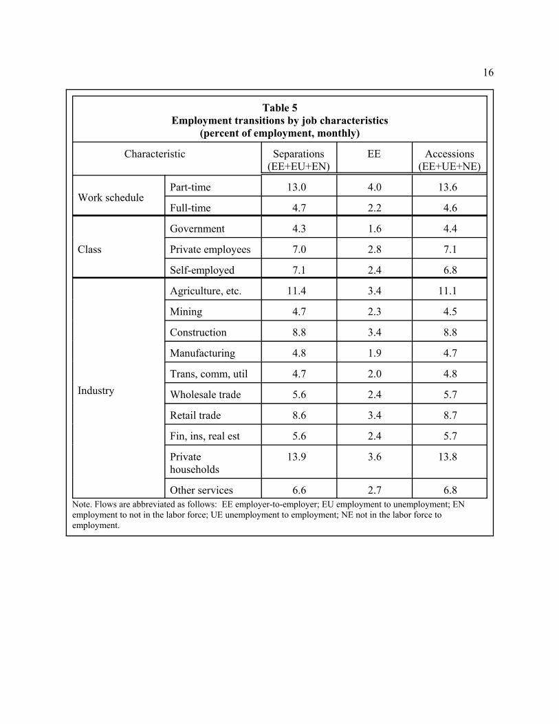
Table 5 summarizes flows for different breakdowns of job characteristics. Full-time

workers (those reporting that they usually worked thirty-five or more hours on their main job)

show greater job stability than do part-time workers, but, as is the case for education, the EE

rates differ considerably less than do the rates of other types of separations. In keeping with

conventional wisdom, government workers are less likely to separate from their employers than

are workers in the private sector; this finding includes lower EE rates. In the private sector, self-

employed workers have similar separation rates and slightly lower EE rates than do those who

15

26For our purposes, we group the incorporated and the unincorporated self-employedtogether. In contrast, the official statistics from the BLS include the incorporated self-employedin private wage and salary workers.

work for someone else.26 Although most of the self-employed workers who report an EE

transition move out of self-employment, a significant number remain self-employed, in which

case the economic meaning of the transition is less clear. Within the private sector, the

industries with particularly high EE rates are agriculture, construction, retail trade, and private

household services.

16

Table 5Employment transitions by job characteristics

(percent of employment, monthly)

Characteristic Separations(EE+EU+EN)

EE Accessions(EE+UE+NE)

Work schedulePart-time 13.0 4.0 13.6

Full-time 4.7 2.2 4.6

Class

Government 4.3 1.6 4.4

Private employees 7.0 2.8 7.1

Self-employed 7.1 2.4 6.8

Industry

Agriculture, etc. 11.4 3.4 11.1

Mining 4.7 2.3 4.5

Construction 8.8 3.4 8.8

Manufacturing 4.8 1.9 4.7

Trans, comm, util 4.7 2.0 4.8

Wholesale trade 5.6 2.4 5.7

Retail trade 8.6 3.4 8.7

Fin, ins, real est 5.6 2.4 5.7

Private households

13.9 3.6 13.8

Other services 6.6 2.7 6.8Note. Flows are abbreviated as follows: EE employer-to-employer; EU employment to unemployment; EN employment to not in the labor force; UE unemployment to employment; NE not in the labor force toemployment.

17

27See, for example, Mattila (1974), Tobin (1972), and Blanchard and Diamond (1989).

28See Meisenheimer and Ilg (2000) for a more complete description of the surveyquestions and for descriptive statistics on the extent of on-the-job search; these authors do notaddress the outcomes of on-the-job search.

29Specifically, the supplement asks, “What are all of the things you have done to findother employment ... ?” Active search includes contacting an employer directly; contacting apublic or private employment agency; contacting friends or relatives; contacting a schoolemployment center; sending out resumes or filling out applications; checking union orprofessional registers; or placing or answering a want advertisement. Passive search includeslooking at advertisements or attending a job training course.

5. On-the-Job Search

Lacking direct measures of EE flows, some researchers have estimated such flows as the

fraction of workers who quit from employment after having already lined up another job.27

However, defining EE flows as resulting only from quits, and especially from quits that follow

on-the-job search, will underestimate the extent of EE flows. We find that only about one-fifth

of EE changers engaged in active on-the-job search in the three months before the move, a

smaller fraction than -- but still not too different from -- the approximately one-third of newly

employed workers who were unemployed (that is, actively searching) in the previous month.

We construct a dataset that includes information on both on-the-job search and labor

market flows by linking our monthly matched CPS data with information on the job-search

behavior of employed workers collected in the contingent worker supplements to the February

1997 and February 1999 CPS.28 For workers employed more than three months, the survey

supplement asks (in mid-February), “Since the beginning of December, have you looked for

other employment?” For workers employed at most three months with their current employer,

the survey asks “Since you started working for [fill: employer’s name from basic CPS], have you

looked for other employment?” The supplement differentiates between active and passive

methods of search, using the same definitions as the basic CPS uses in determining whether an

individual is unemployed.29 The survey also differentiates between those looking for a new job

and those looking for an additional job. By analogy with the CPS definition of unemployment

(excluding those on temporary layoff), we define as on-the-job-searchers as only those workers

actively looking for a new job.

18

30Not all individuals employed in February 1997 and February 1999 had valid responsesto the supplement questions. There are small differences in composition between the full sampleof February-March matches and that restricted to valid supplement responses in February; inparticular, the supplement reports that 2.5 percent of employed workers in February held adifferent job at the March reference period compared with a 2.6 percent EE rate for the broadersample. We calculated the rates in table 7 by multiplying each of the overall flow rates based on

Table 6 reports on the March labor force status of individuals employed in February 1997

and February 1999, differentiated by on-the-job search behavior. Of those employed in February,

4.4 percent had engaged in active on-the-job search. These job-seekers were much more likely

to have changed employers between February and March: The proportion of on-the-job

searchers who reported a new employer in March was 11.3, compared with only 2.1 percent of

nonsearchers. Searchers were also more likely to have become unemployed in March -- when

they presumably continued their search for a new job – than were nonsearchers (5.6 percent vs.

0.9 percent). However, searchers were no less likely than were nonsearchers to leave the labor

force.

Table 6Flow rates for employed workers in February 1997 and February 1999 by on-the-

job search behavior (percent of searchers or nonsearchers, monthly)

Search behavior (Percent of employment)

Employed

Unemployed NLFSame

employerNew

employer

No on-the-job search (95.6%)

95.0 2.1 0.9 2.0

On-the-job search (4.4%)

80.9 11.3 5.6 2.3

Table 7 reports the importance of on-the-job search in overall labor market flows. It is

analogous to table 2, except that in table 7 we divide employed workers into on-the-job searchers

and nonsearchers, we distinguish between unemployed workers who are on temporary layoff and

those who are not, and we report only on the flows between February and March of 1997 and

1999.30 As shown in the table, on-the-job search between the beginning of December and mid-

19

the full February-March matches by the share of the appropriate group that engaged in on-the-job search in the February supplements.

February (or since the job held in February began--whichever period is shorter) was associated

with about 20 percent of all EE changers; thus, 80 percent of the EE changers between February

and March did not engage in any active on-the-job search, at least through the February

reference week.

Table 7Gross worker flows by on-the-job search behavior

(percent of population, monthly)

Search behaviorEmployer

stayer(or employed) New employer Unemployed NLF

Employed 59.2 1.6 0.7 1.4

On-the-job search 2.2 0.3 0.2 0.1

No on-the-job search 57.0 1.3 0.5 1.4

Unemployed (not ontemporary layoff) 0.7 -- 1.4 0.7

Unemployed (ontemporary layoff) 0.3 -- 0.3 0.1

NLF 1.5 -- 0.8 31.3

On its face, the relatively small share of EE flows explained by on-the-job search may

seem odd. However, although EE changers who engaged in on-the-job search were in the

minority, the same was true of workers who were newly employed in March and had reported

that they were actively searching for a job (that is, unemployed) at the time of the February

survey. Only about one-third of the movers from non-employment (excluding those on

temporary layoff) to employment reported themselves as unemployed (that is, actively

searching) in February. Thus, the contribution of on-the-job search in explaining flows from

other employers into new employers, and the contribution of off-the-job search in explaining

flows into new employers from nonemployment, appear to be of similar importance.

20

31In addition, contacts initiated by another employer may not be classified as on-the-jobsearch in our data, and seasonal jobs that had been lined up well in advance of the start datewould not be counted in these data as involving search. Note that these reasons may also applyto the share of the nonemployed who report active search, that is, to the unemployed.

32An alternative conception would define the cyclicality of flows by their correlation withthe growth in activity, that is, with the (detrended) growth in employment or with the change inthe unemployment rate, rather than with their levels. The choice largely reflects differences inthe question of interest. In an algebraic sense, the steady-state level of flows determines thesteady-state level of the unemployment rate, and when not at the steady-state rate of

Moreover, we have reason to believe that our estimate understates the share of EE

changers who had looked for a new job while employed. First, because our measure of on-the-

job search captures search only before the first month of each matched observation, we do not

pick up any job-seeking behavior between the February and March reference weeks. Second,

many EE changes involve geographic moves; because the CPS is an address-based survey, a

person who moves out of an address to be closer to a new job will not be counted as a job

changer in our sample.31

6. The Cyclical Properties of Gross Flows

Until now, the business cycle literature has lacked a reliable and representative measure

of the frequency of EE flows to which models may be calibrated and with which their simulation

results may be compared. In section 3, we provided such a measure of the level of EE flows and

found that level to be higher than the indirect measures typically used in the literature. In this

section, we examine another aspect of EE flows often used in modeling exercises: how EE

flows change with the business cycle.

The literature on worker flows has tended to define the cyclicality of flows by their

correlations with the level of economic activity, as measured by the unemployment rate (e.g.,

Blanchard and Diamond 1990; Mortensen 1994; Merz 1999), the level of employment (e.g.,

Albaek and Sorensen 1998; Cole and Rogerson 1999), or the level of capital utilization (e.g.,

Burda and Wyplosz 1994). Because we use the level of the unemployment rate as a measure of

the cycle, we compare stylized facts about the change in gross flow rates over the business cycle

to changes in the unemployment rate.32

21

unemployment, the level of flows determines the change in the unemployment rate. From theperspective of search and matching models, however, the interesting question is how the level ofworker flows react to the elements of the Beveridge Curve, and thus to the level of theunemployment rate.

33See, for example, Blanchard and Diamond (1990), Burda and Wyplosz (1994),Mortensen (1994), and Merz (1999).

34The hazard rate for leaving unemployment is procyclical, but the countercylicality ofthe size of the pool of unemployed is the dominant factor.

35For example, Pissarides (1994) and Petrongolo and Pissarides (2001).

The literature has established several facts about the behavior of gross flows of workers

across labor market states over the business cycle.33 Several of these empirical regularities are as

follows, where flows are viewed as a percentage of the population, rather than as hazard or

transition rates:

1. The flow into unemployment is countercyclical.

2. The flow out of unemployment is countercyclical.34

3. The cyclicality of the flow into employment is unclear; it combines a

countercyclical flow from unemployment to employment with a procyclical flow

from not in the labor force to employment.

4. The flow out of employment is probably countercyclical in the United States, but

if so only weakly; in Europe it appears to be procyclical.

The literature has concluded that reconciling these flows with the stylized facts about job

creation and job destruction requires that EE flows be large and highly procyclical.

Accordingly, Pissarides (1994), Petrongolo and Pissarides (2001), and others have pursued

model-building strategies that aim to accommodate these two properties.35

Of these two requirements, the first is satisfied: We have shown above that EE flows are,

indeed, large. The question of cyclicality is more difficult because our sample period is short.

But we do have data for a period of strong expansion during which the labor market tightened

22

36The National Bureau of Economic Research dated the peak of the expansion in March2001 and the trough in November 2001.

37 Because not all months in 1995 are represented in our matched data, we regress themonthly flow rates on month and year dummies, and report the coefficients on the year dummieswith the mean of the coefficients on the month dummies added back in. The conclusions herewould not change if instead we drew our annual averages from an X-12 seasonal adjustmentprocedure.

markedly (the years 1994-2000), for the recession year of 2001, and for two years of further

deterioration or stagnation in the labor market (2002 and 2003).36

We begin by showing that over our sample period, during which the annual

unemployment rate decreased a bit more than 2 percentage points (from 6.1 percent to 4.0

percent) and then rose by a similar amount (back up to 6 percent), the flows across labor market

states other than the EE flow have moved in accordance with the stylized facts concerning their

cyclicality; from this result we conclude that our sample period is informative about cyclical

properties and therefore can be used to inform us about the cyclical behavior of EE flows as

well.

Figure 2 shows the pattern of the flows into and out of the labor market states of

unemployment, employment, and not in the labor force in our data during the years 1994-2003.37

(Note that the range of the vertical axis in each panel is the same, although the endpoints

naturally differ).

1. Shown in the top left panel, the flow into unemployment is countercyclical.

2. In the top right panel, the flow out of unemployment is countercyclical.

3. The flow into employment in the middle left panel follows no clear cyclical

pattern, and varies less than do the flows in the top panels. Its components are

shown in the top panels of figure 3: The flow from unemployment to

employment is roughly countercyclical and the flow from not in the labor force to

employment is roughly procyclical.

4. The flow out of employment is at best only weakly countercyclical in the

literature. In our data, this flow declines for the first couple of years of our

sample before increasing as the expansion continued, and then spikes in the

23

recession year of 2001 before falling again. As shown in the middle and bottom

left panels of figure 3, this ambiguous result is a combination of a roughly

countercyclical EU flow and a roughly procyclical EN flow.

Because our data cover only ten years and one recession, we take advantage of an

additional source of business cycle variation to verify the cyclical patterns of the gross flows in

our sample: the substantial differences across states in the degree and timing of labor market

tightening. For example, the declines in published unemployment rates between the beginning

of our sample in 1994 and the last year of general expansion in 2000 ranged from more than 3-

1/2 percentage points in Maine and California to about 1 percentage point in Wisconsin and

Mississippi to essentially zero in Montana and Nebraska; and the change from 2001 to 2003

ranged from increases of 2-1/4 percentage points in Colorado and Connecticut to small declines

in Nevada and Hawaii.

Table 8 reports estimated coefficients from regressions of the state-level flows on the

unemployment rate, with state fixed-effects removed, for the period 1994 to 2000 (that is, only

the years of a tightening labor market), and the period 2001-2003 (that is, only the years of a

loosening labor market). The state-level results generally accord well with the stylized facts,

confirming the impressions from figure 2.

1. The state-level estimates in column 1 indicates that the flow into unemployment

is strongly countercyclical.

2. Similarly, column 2 indicates that the flow out of unemployment is strongly

countercyclical.

3. In column 3, the cyclicality of the flow into employment is not clear.

4. In column 4, the flow out of employment appears to be acyclical, as in the

aggregate data, in the earlier period, but procyclical (as in the literature on

Europe) in the later period. In fact, as shown in table 9, the EN flow is

countercyclical in both periods; the change in the cyclicality of the total flow out

of employment occurs between the two periods appears because the EU flow

loses its procyclicality in the later period.

24

38In addition, Burgess (1993) argues that the procyclicality of accessions and theacyclicality of flows out of unemployment in the United Kingdom imply procyclical EE flows.

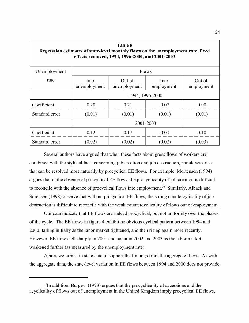
Table 8Regression estimates of state-level monthly flows on the unemployment rate, fixed

effects removed, 1994, 1996-2000, and 2001-2003

Unemployment

rate

Flows

Intounemployment

Out ofunemployment

Intoemployment

Out ofemployment

1994, 1996-2000

Coefficient 0.20 0.21 0.02 0.00

Standard error (0.01) (0.01) (0.01) (0.01)

2001-2003

Coefficient 0.12 0.17 -0.03 -0.10

Standard error (0.02) (0.02) (0.02) (0.03)

Several authors have argued that when these facts about gross flows of workers are

combined with the stylized facts concerning job creation and job destruction, paradoxes arise

that can be resolved most naturally by procyclical EE flows. For example, Mortensen (1994)

argues that in the absence of procyclical EE flows, the procyclicality of job creation is difficult

to reconcile with the absence of procyclical flows into employment.38 Similarly, Albaek and

Sorensen (1998) observe that without procyclical EE flows, the strong countercylicality of job

destruction is difficult to reconcile with the weak countercyclicality of flows out of employment.

Our data indicate that EE flows are indeed procyclical, but not uniformly over the phases

of the cycle. The EE flows in figure 4 exhibit no obvious cyclical pattern between 1994 and

2000, falling initially as the labor market tightened, and then rising again more recently.

However, EE flows fell sharply in 2001 and again in 2002 and 2003 as the labor market

weakened further (as measured by the unemployment rate).

Again, we turned to state data to support the findings from the aggregate flows. As with

the aggregate data, the state-level variation in EE flows between 1994 and 2000 does not provide

25

39As with the aggregate data, the regression results for the other flows at the state levelmatch up well with the stylized facts. The second and third columns of table 9 show thecoefficients from regressions of the EU flow rate and the UE flow rate, respectively. Asexpected, both flows are strongly countercyclical, with a 1 percentage point increase in theunemployment rate raising the EU and UE rates by 0.08 and 0.1 percentage point, respectively. Conversely, as shown in the remaining columns, the EN and NE flow rates are procyclical, andthe NU and UN flow rates are countercyclical. Of course, the same caveats apply here as to ouranalysis of the cyclicality of flows at the aggregate level.

any evidence of procyclicality. Table 9 reports estimated coefficients from regressions of the

state-level flows on the unemployment rate with state fixed-effects removed; these coefficients

are are analogous to those reported in table 8. As shown in the first column, when only these

expansion years are included, a 1 percentage point increase in a state’s unemployment rate is

associated with essentially no change in the EE flow rate (as a percentage of the population), and

the coefficient is not statistically significant.39 However, during the weak labor market years of

2001-2003, the coefficient on the unemployment rate in the EE regression becomes significantly

negative, suggesting that the procyclicality of EE flows is concentrated around recessions.

26

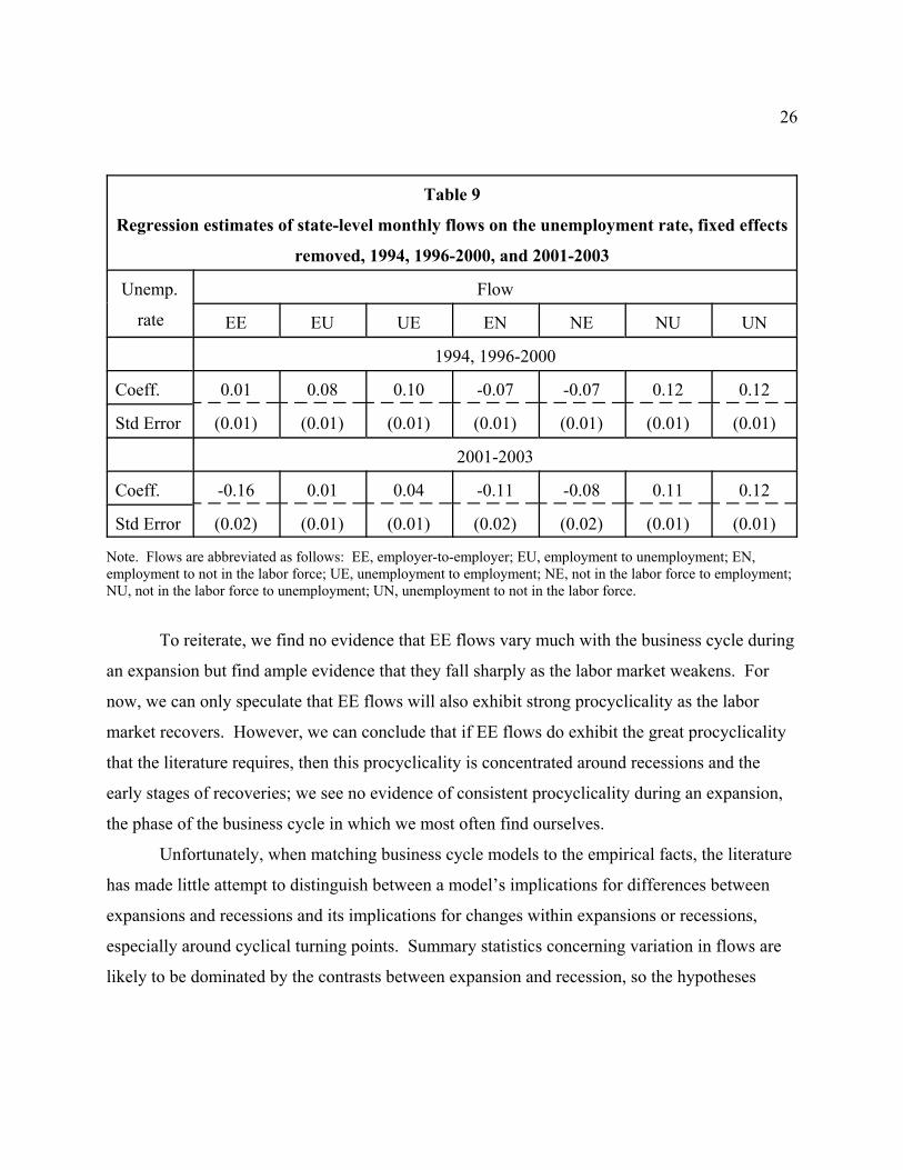
Table 9

Regression estimates of state-level monthly flows on the unemployment rate, fixed effects

removed, 1994, 1996-2000, and 2001-2003

Unemp.

rate

Flow

EE EU UE EN NE NU UN

1994, 1996-2000

Coeff. 0.01 0.08 0.10 -0.07 -0.07 0.12 0.12

Std Error (0.01) (0.01) (0.01) (0.01) (0.01) (0.01) (0.01)

2001-2003

Coeff. -0.16 0.01 0.04 -0.11 -0.08 0.11 0.12

Std Error (0.02) (0.01) (0.01) (0.02) (0.02) (0.01) (0.01)

Note. Flows are abbreviated as follows: EE, employer-to-employer; EU, employment to unemployment; EN, employment to not in the labor force; UE, unemployment to employment; NE, not in the labor force to employment;NU, not in the labor force to unemployment; UN, unemployment to not in the labor force.

To reiterate, we find no evidence that EE flows vary much with the business cycle during

an expansion but find ample evidence that they fall sharply as the labor market weakens. For

now, we can only speculate that EE flows will also exhibit strong procyclicality as the labor

market recovers. However, we can conclude that if EE flows do exhibit the great procyclicality

that the literature requires, then this procyclicality is concentrated around recessions and the

early stages of recoveries; we see no evidence of consistent procyclicality during an expansion,

the phase of the business cycle in which we most often find ourselves.

Unfortunately, when matching business cycle models to the empirical facts, the literature

has made little attempt to distinguish between a model’s implications for differences between

expansions and recessions and its implications for changes within expansions or recessions,

especially around cyclical turning points. Summary statistics concerning variation in flows are

likely to be dominated by the contrasts between expansion and recession, so the hypotheses

27

40Pissarides writes “Intuitively, when economic conditions first improve, many employedworkers enter the market to look for better jobs. There is nothing to slow down this entry, so itfollows immediately after the shock. As the new entrants succeed in finding jobs, andunemployment also falls in response to the better conditions, the number of workers employed inbad jobs and looking for work begins to fall. Thus [the level of EE flows] ‘overshoots’ onimpact its steady-state level.” This conjecture is consistent with the pattern we observe in ourdata.

41Although the data for 2003 fit the general pattern of low employment growth and lowEE flows, that year is a bit unusual (even for this short sample) in that EE flows slowed furthereven as the deterioration of the labor market slowed. But, in the view of many observers, grosshiring failed to pick up in 2003 even as job losses slowed, so the level of gross activity, so tospeak, in the labor market did not pick up in keeping with the improvement in employmentgrowth.

generated by the literature may be more applicable to comparisons between phases of the

business cycle than to comparisons within a phase. Pissarides (1994) is a notable exception.40

The data do bear another interpretation: The unemployment rate in 1994 averaged 6.1

percent -- about the same as the 6.0 percent average over 2003 -- yet the level of EE flows was

much higher in 1994 than in 2003. Perhaps there is a secular downtrend in EE flows that

obscures a procyclical pattern that is consistent throughout the business cycle. Without a longer

time series, we cannot distinguish definitively between these alternative interpretations.

However, the results from the state-level regressions favor the view that the cyclicality of EE

flows is uneven across the business cycle.

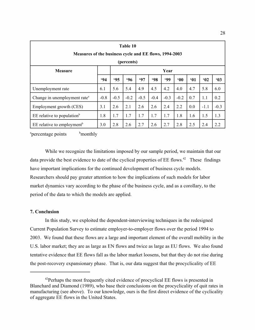
Why is phase of cycle important for EE flows, but not for the other flows across labor

force statuses? Table 10 suggests that unlike other flows, EE flows are related to the change

rather than to the level of employment or labor market tightness. Although the unemployment

rate fell throughout the expansion, the rate of employment growth and the EE flows were

reasonably stable. And although unemployment rates in 2001-2003 did not exceed those in, say,

1994-1996, employment growth rates in the later period were much lower (and changes in the

unemployment rate more positive) and EE flows much lower than in the earlier period.41

Similarly, in the state regressions, the rate of EE flow was much better explained by employment

growth (or the change in the unemployment rate) than by the level of the unemployment rate,

while the opposite was true, overall, for the other flows.

28

42Perhaps the most frequently cited evidence of procyclical EE flows is presented in Blanchard and Diamond (1989), who base their conclusions on the procyclicality of quit rates inmanufacturing (see above). To our knowledge, ours is the first direct evidence of the cyclicalityof aggregate EE flows in the United States.

Table 10

Measures of the business cycle and EE flows, 1994-2003

(percents)

Measure Year

‘94 ‘95 ‘96 ‘97 ‘98 ‘99 ‘00 ‘01 ‘02 ‘03

Unemployment rate 6.1 5.6 5.4 4.9 4.5 4.2 4.0 4.7 5.8 6.0

Change in unemployment ratea -0.8 -0.5 -0.2 -0.5 -0.4 -0.3 -0.2 0.7 1.1 0.2

Employment growth (CES) 3.1 2.6 2.1 2.6 2.6 2.4 2.2 0.0 -1.1 -0.3

EE relative to populationb 1.8 1.7 1.7 1.7 1.7 1.7 1.8 1.6 1.5 1.3

EE relative to employmentb 3.0 2.8 2.6 2.7 2.6 2.7 2.8 2.5 2.4 2.2apercentage points bmonthly

While we recognize the limitations imposed by our sample period, we maintain that our

data provide the best evidence to date of the cyclical properties of EE flows.42 These findings

have important implications for the continued development of business cycle models.

Researchers should pay greater attention to how the implications of such models for labor

market dynamics vary according to the phase of the business cycle, and as a corollary, to the

period of the data to which the models are applied.

7. Conclusion

In this study, we exploited the dependent-interviewing techniques in the redesigned

Current Population Survey to estimate employer-to-employer flows over the period 1994 to

2003. We found that these flows are a large and important element of the overall mobility in the

U.S. labor market; they are as large as EN flows and twice as large as EU flows. We also found

tentative evidence that EE flows fall as the labor market loosens, but that they do not rise during

the post-recovery expansionary phase. That is, our data suggest that the procyclicality of EE

29

flows that is not present in all phases of the business cycle, but only around recessions. Looked

at another way, our data suggest that the size of EE flows seems to be related to the change in,

rather than the level of, employment or the unemployment rate.

These data raise several questions that we intend to pursue in future work (beyond further

study of the cyclical variation in gross flows). One such question is the role of EE flows in the

sectoral reallocation of labor. This role is important for understanding both the way in which

reallocation contributes to equilibrium unemployment and the relationship between reallocation

and the business cycle (Lilien 1982; Fallick 1996). Our preliminary work indicates that about

one-third of structural reallocation, defined as the variance in seasonally adjusted net

employment growth across two-digit industries, is accomplished through EE flows. In addition,

these data should prove useful in studying the determinants of job mobility and the tremendous

seasonality that is characteristic of labor market flows.

30

43Bleakley, Ferris, and Fuhrer (1999) use a similar method. For an exploration ofalternative criteria for matching CPS files, see Madrian and Lefgren (2000).

Appendix: Measuring Gross Flows with CPS Data

Matching Individuals in the CPS

Each month, the CPS collects demographic and labor force data from a sample of

approximately 60,000 households (50,000 between 1996 and 2000) , which yields information

for about 120,000 individuals. Households are interviewed eight times over a sixteen-month

period. They are interviewed for four consecutive months, not interviewed for the next eight

months, and then interviewed again for another four consecutive months. The households are

divided into eight approximately equal-sized groups so that in any month one-eighth of the

households (referred to as a “rotation group”) have been interviewed once, one-eighth have been

interviewed twice, and so on. Thus, by design, about three-fourths of the households

interviewed for the CPS in any one month had been interviewed in the previous month as well,

and one can match the data for most of the persons in these households across the two months;

the remaining one-fourth of the households are either just entering the sample or re-entering after

an eight-month absence.

To match individuals’ records from one month to the next, we use a matching algorithm

similar to that used by the BLS in constructing gross flow figures.43 We match individual

records from one month to the next using the household identification number (ID), augmented

by state of residence and serial suffix whene IDs are not unique, the person’s line number within

the household, and the person’s sex, race, and age. We require exact matches for all of the

variables except age; we accept cases in which age decreased by no more than one year or

increased by no more than two years. In practice, our algorithm completes about 95 percent of

the potential matches.

A seemingly eligible individual may not match from one month to the next for several

reasons. Among them, the household may move residence, the individual may move out of the

household, the members of the household may be unavailable or unwilling to complete the CPS

questionnaire, or a coding error may have occurred. Our estimates of flow rates may be biased

31

44Bleakley, Ferris, and Fuhrer (1999) found that the probability of not matching wascorrelated with household characteristics.

45See Barkume and Horvath (1995) for discussion of attrition bias in computing grossflows with pre-1994 data.

46 See U.S Department of Labor (2000, pp.10-9, 16-8 and following).

to the extent that matching probabilities are correlated with probabilities of leaving or entering

employment.44 We label this type of bias “attrition bias” and discuss its effects on our results

below.45

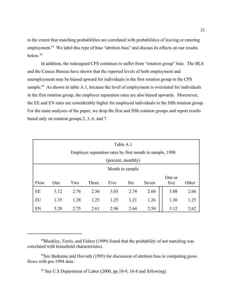
In addition, the redesigned CPS continues to suffer from “rotation group” bias. The BLS

and the Census Bureau have shown that the reported levels of both employment and

unemployment may be biased upward for individuals in the first rotation group in the CPS

sample.46 As shown in table A.1, because the level of employment is overstated for individuals

in the first rotation group, the employer separation rates are also biased upwards. Moreoever,

the EE and EN rates are considerably higher for employed individuals in the fifth rotation group.

For the main analyses of the paper, we drop the first and fifth rotation groups and report results

based only on rotation groups 2, 3, 6, and 7.

Table A.1

Employer separation rates by first month in sample, 1998

(percent, monthly)

Month in sample

Flow One Two Three Five Six SevenOne or

five Other

EE 3.12 2.76 2.56 3.03 2.74 2.60 3.08 2.66

EU 1.35 1.28 1.25 1.25 1.21 1.26 1.30 1.25

EN 3.28 2.75 2.61 2.96 2.64 2.50 3.12 2.62

32

47In table A.2 we report only flow rates out of employment; the effects of attrition bias onthe flows into employment are similar.

Attrition Bias

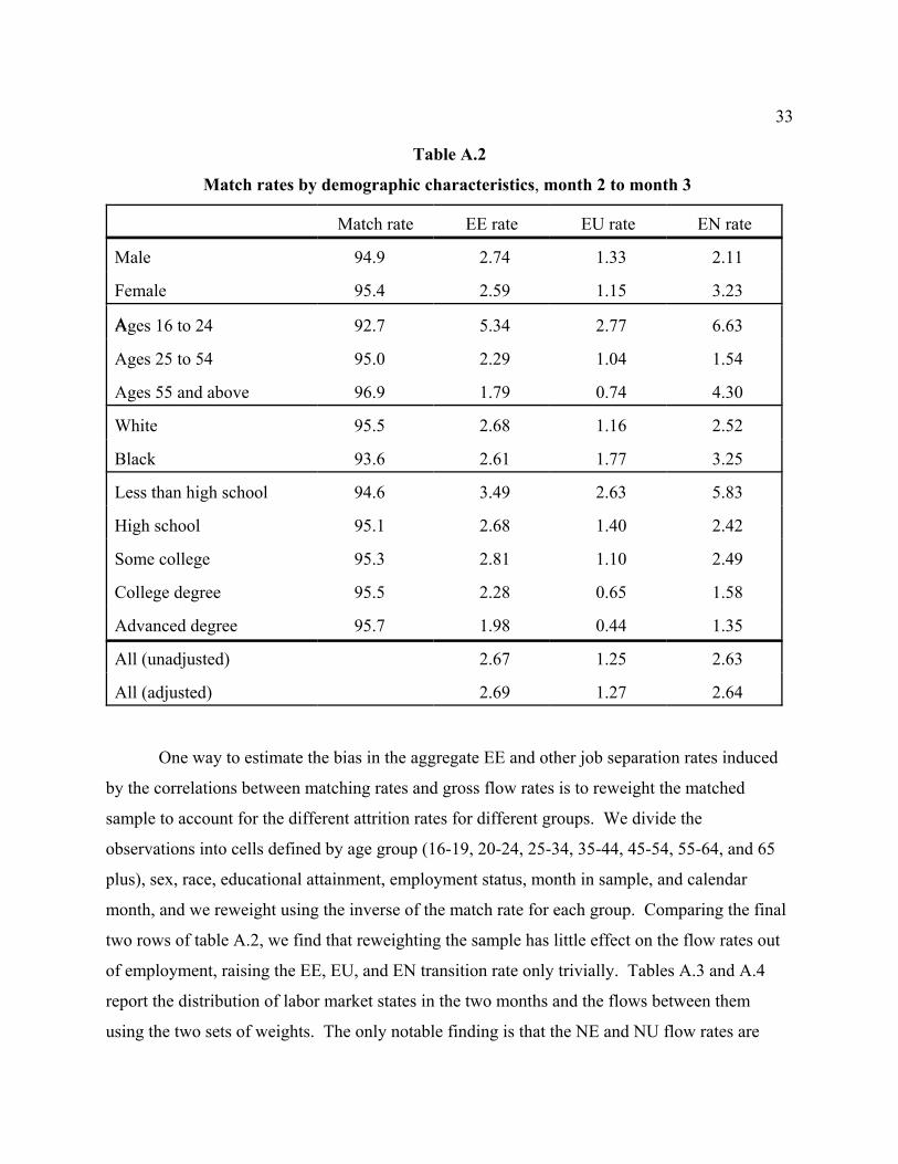
To explore the extent of attrition bias in our estimates of flow rates and the relationship

between the size of the bias and individuals’ characteristics, we expanded our main dataset to

include nonmatches, such as those resulting from noninterviews. The first column of table A.2

reports match rates for various demographic groups for calendar year 1998, and the remaining

columns report EE flow rates, EU flow rates, and EN flow rates.47 As shown in the table, match

rates are lowest for young workers and less educated workers, who also had the highest rates of

EE, EU, and EN transitions. In addition, match rates are lowest for unemployed workers, a

finding that may simply reflect the relatively higher unemployment rates for younger, less

educated workers.

33

Table A.2

Match rates by demographic characteristics, month 2 to month 3

Match rate EE rate EU rate EN rate

Male 94.9 2.74 1.33 2.11

Female 95.4 2.59 1.15 3.23

AAges 16 to 24 92.7 5.34 2.77 6.63

Ages 25 to 54 95.0 2.29 1.04 1.54

Ages 55 and above 96.9 1.79 0.74 4.30

White 95.5 2.68 1.16 2.52

Black 93.6 2.61 1.77 3.25

Less than high school 94.6 3.49 2.63 5.83

High school 95.1 2.68 1.40 2.42

Some college 95.3 2.81 1.10 2.49

College degree 95.5 2.28 0.65 1.58

Advanced degree 95.7 1.98 0.44 1.35

All (unadjusted) 2.67 1.25 2.63

All (adjusted) 2.69 1.27 2.64

One way to estimate the bias in the aggregate EE and other job separation rates induced

by the correlations between matching rates and gross flow rates is to reweight the matched

sample to account for the different attrition rates for different groups. We divide the

observations into cells defined by age group (16-19, 20-24, 25-34, 35-44, 45-54, 55-64, and 65

plus), sex, race, educational attainment, employment status, month in sample, and calendar

month, and we reweight using the inverse of the match rate for each group. Comparing the final

two rows of table A.2, we find that reweighting the sample has little effect on the flow rates out

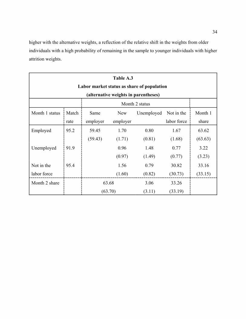
of employment, raising the EE, EU, and EN transition rate only trivially. Tables A.3 and A.4

report the distribution of labor market states in the two months and the flows between them

using the two sets of weights. The only notable finding is that the NE and NU flow rates are

34

higher with the alternative weights, a reflection of the relative shift in the weights from older

individuals with a high probability of remaining in the sample to younger individuals with higher

attrition weights.

Table A.3

Labor market status as share of population

(alternative weights in parentheses)

Month 2 status

Month 1 status Match

rate

Same

employer

New

employer

Unemployed Not in the

labor force

Month 1

share

Employed 95.2 59.45

(59.43)

1.70

(1.71)

0.80

(0.81)

1.67

(1.68)

63.62

(63.63)

Unemployed 91.9 0.96

(0.97)

1.48

(1.49)

0.77

(0.77)

3.22

(3.23)

Not in the

labor force

95.4 1.56

(1.60)

0.79

(0.82)

30.82

(30.73)

33.16

(33.15)

Month 2 share 63.68

(63.70)

3.06

(3.11)

33.26

(33.19)

35

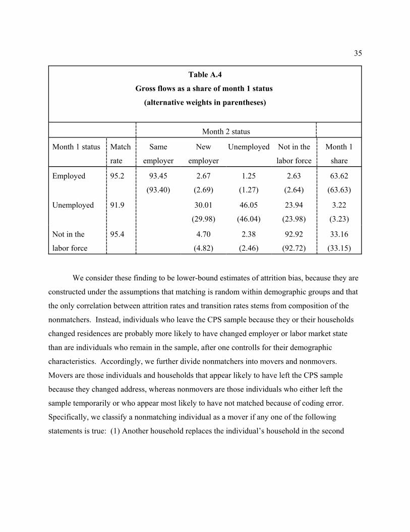
Table A.4

Gross flows as a share of month 1 status

(alternative weights in parentheses)

Month 2 status

Month 1 status Match

rate

Same

employer

New

employer

Unemployed Not in the

labor force

Month 1

share

Employed 95.2 93.45

(93.40)

2.67

(2.69)

1.25

(1.27)

2.63

(2.64)

63.62

(63.63)

Unemployed 91.9 30.01

(29.98)

46.05

(46.04)

23.94

(23.98)

3.22

(3.23)

Not in the

labor force

95.4 4.70

(4.82)

2.38

(2.46)

92.92

(92.72)

33.16

(33.15)

We consider these finding to be lower-bound estimates of attrition bias, because they are

constructed under the assumptions that matching is random within demographic groups and that

the only correlation between attrition rates and transition rates stems from composition of the

nonmatchers. Instead, individuals who leave the CPS sample because they or their households

changed residences are probably more likely to have changed employer or labor market state

than are individuals who remain in the sample, after one controlls for their demographic

characteristics. Accordingly, we further divide nonmatchers into movers and nonmovers.

Movers are those individuals and households that appear likely to have left the CPS sample

because they changed address, whereas nonmovers are those individuals who either left the

sample temporarily or who appear most likely to have not matched because of coding error.

Specifically, we classify a nonmatching individual as a mover if any one of the following

statements is true: (1) Another household replaces the individual’s household in the second

36

48Because we excluded the first and fifth rotation groups from our sample, the secondmonth in our sample is actually the third month in the CPS sample.

month of our sample;48 (2) the individual’s entire household is not interviewed in the second

month and does not match in the third month, or (3) the individual is not interviewed in the

second month and does not match in the third month although other members of the household

remain in the sample. We classify individuals as nonmovers if either of the following conditions

is true: (1) The individual that is absent in the second month has a successful match from the

first to the third month, or (2) the individual appears to have been interviewed in the second

month but for some unknown reason does not match from the first to the second month.

Under this scheme, we classify 48 percent of the nonmatches in 1998 as movers. Of

these movers, 18 percent are in households that were replaced in the second month, 46 percent

are in households that were not interviewed in month 2, and the remaining 36 percent are

individuals who appear to have moved out of households that continued in the CPS sample.

Similarly, we classify about 45 percent of the nonmatches who were employed in month 1 as

movers. If we assume that all employed movers separate from their first-month job, the true job

leaving rate will be about 2-1/4 percentage points higher than the 6.6 percent reported in the

body of the paper. This difference should be considered as an upper bound estimate for the size

of the attrition bias, as many movers likely did not change jobs or leave employment--especially

those who move to a new location within the same labor market area.

37

References

Abowd, John M. and Arnold Zellner, “Estimating Gross Labor-Force Flows,” Journal ofBusiness and Economic Statistics 3(3), June 1985, pp. 254-83.

Akerlof, George A., Andrew K. Rose, and Janet L. Yellen, “Job Switching and Job Satisfactionin the U.S. Labor Market,” Brookings Papers on Economic Activity 2, 1988, p.495-592.

Albaek, K. and B.E. Sorensen, “Worker flows and job flows in Danish manufacturing, 1980-91,”Economic Journal 108(451), November 1998, pp.1750-1771.

Anderson, Patricia M., and Simon M. Burgess, “Empirical Matching Functions: Estimation andInterpretation Using State-Level Data,” Review of Economics and Statistics 82(1), February2000, pp.93-102.

Anderson, Patricia M., and Bruce D. Meyer, “The Extent and Consequences of Job Turnover,”Brookings Papers on Economic Activity: Microeconomics, 1994, pp. 177-236.

Bancroft, Gertrude and Stuart Garfinkle, “Job Mobility in 1961,” US Department of Labor,Special Labor Force Report 35, August 1963.

Bansak, Cynthia, and Steven Raphael, “Have Employment Relationships in the United StatesBecome Less Stable?” University of California, San Diego, Discussion Paper 98-15, June 1998.

Barkume, Anthony J. and Francis W. Horvath, “Using gross flows to explore movements in thelabor force,” Monthly Labor Review 118(4), April 1995, pp.28-35.

Bender, Stefan, Christian Dustmann, David Margolis and Costas Meghir, "WorkerDisplacement in France and Germany," in Peter Kuhn and Randal Eberts (eds.), Losing Work, Moving On: International Comparisons of Worker Displacement, (Kalamazoo, MI: The UpjohnInstitute), forthcoming.

Bernhardt, Annette, Martina Morris, Mark S. Hancock, and Marc A. Scott, “Trends in JobInstability and Wages for Young Adult Men,” Journal of Labor Economics 17(4), Part 2,October 1999, pp.S65-S90.

Bester, H., “Incentive-Compatible Long-Term Contracts and Job Rationing,” Journal of LaborEconomics 7(2), 1989, pp.238-255.

Blanchard, Olivier and Peter Diamond, “The Beveridge Curve,” Brookings Papers on EconomicActivity 1, 1989, p.1-60.

Blanchard, Olivier and Peter Diamond, “The Cyclical Behavior of Gross Flows of U.S.Workers,” Brookings Papers on Economic Activity 2, 1990, p.85-156.

38

Bleakley, Hoyt, Anne E. Ferris, and Jeffrey C. Fuhrer, “New Data on Worker Flows DuringBusiness Cycles,” New England Economic Review, July/August 1999, pp.49-76.

Booth, Alison L., Marco Francesconi, and Carlos Garcia-Serrano, “Job Tenure and Job Mobilityin Britain,” Industrial and Labor Relations Review 53(1), October 1999, pp.43-70.

Bull, C., “The Existence of Self-Enforcing Implicit Contracts,” Quarterly Journal of Economics102(1), 1987, pp.147-159.

Burda, M. and C. Wyplosz, “Gross Worker Flows and Job Flows in Europe,” EuropeanEconomic Review 38(6), June 1994, pp.1287-1315.

Burdett, Kenneth, “A Theory of Employee Job Search and Quit Rates,” American EconomicReview, 68(1), March 1978, pp. 212-220.

Burgess, S.M., “The Flow Into Unemployment in Britain,” Economic Journal 102(413), July1992, pp.888-895.

Burgess, S.M., “Matching Models and Labor-market Flows,” European Economic Review 38(3-4), April 1994, pp.809-816 .

Burgess, Simon M., “A Model of Competition Between Unemployed and Employed JobSearchers: An Application to the Unemployment Outflow Rate in Britain,” Economic Journal103(420), September 1993, pp.1190-1204.

Burgess, Simon, Julia Lane, and David Stevens, “Job Flows, Worker Flows, and Churning,”Journal of Labor Economics 18(3), July 2000, pp. 473-502.

Campbell, Jeffrey R. and Kenneth N. Kuttner, “Macroeconomic Effects of EmploymentReallocation,” Carnegie-Rochester Conference Series on Public Policy, Volume 44, June 1996.pp. 87-116.

Christofides, L.N., and C.J. McKenna, “Unemployment Insurance and Job Duration in Canada,”Journal of Labor Economics 14(2), April 1996, pp.286-312.

Cole, H.L., and R. Rogerson R, “Can the Mortensen-Pissarides matching model match thebusiness-cycle facts?” International Economic Review 40(4), November 1999, pp.933-959.

Davis, Steven J. and John Haltiwanger, "Measuring Gross Worker and Job Flows," in LaborStatistics Measurement Issues, edited by John Haltiwanger, Marilyn Manser and Robert Topel,(Chicago: University of Chicago Press), 1999a, pp. 77-122.

Davis, Steven J., and John Haltiwanger, “On the driving forces behind cyclical movements inemployment and job reallocation,” American Economic Review 89(5), December 1999b, pp.1234-1258.

39

Davis, Steven J., John C. Haltiwanger, and Scott Schuh, Job Creation and Job Destruction,Cambridge, Massachusetts: The MIT Press, 1996.

Dippo, Cathryn, Anne Polivka, Kathleen Creighton, Donna Kostanich, and Jennifer Rothgeb,(1994) "Redesigning A Questionnaire For Computer-Assisted Data Collection: The CurrentPopulation Survey Experience," CPS Research Documentation Report, 1994.

Eriksson, Stefan, and Nils Gottfries, “Ranking of Job Applicants, On-the-Job Search andPersistent Unemployment,” Department of Economics, Uppsala University, Working Paper2000:3, March 2000.

Fallick, Bruce C., "The Hiring of New Labor by Expanding Industries," Labour Economics 3(1),March 1996, pp.25-42.

Farber, Henry S., “The Analysis of Interfirm Worker Mobility,” Journal of Labor Economics12(4), October 1994, pp.554-593.

Farber, Henry S., “Mobility and Stability: the Dynamics of Job Change in Labor Markets,”Handbook of Labor Economics, Volume 3B, edited by Orley Ashenfelter and David Card, 1999,pp. 2439-2480.

Figura, Andrew, "Is Reallocation Related to the Cycle? A Look at Permanent and TemporaryJob Flows", Finance and Economics Discussion Series #2002-16, Federal Reserve Board, March2002.

Foote, Christopher L., “Trend Employment Growth and the Bunching of Job Creation andDestruction,” Quarterly Journal of Economics 113(3), August 1998, pp. 809-34.

Galizzi, M. and K. Lang, “Relative Wages, Wage Growth, and Quit Behavior,” Journal of LaborEconomics 16(2), April 1998, pp.367-391.

Golan, Amos, Julia Lane, and Erika McEntarfer, “The Dynamics of Worker Reallocation: AMarkov Approach”, LEHD Working Paper #2004-01, February 2004.

Gottschalk, Peter and Tim Maloney, “Involuntary Terminations, Unemployment, and JobMatching: A Test of Job Search Theory,” Journal of Labor Economics 3(2), April 1985, pp.109-123.

Gottschalk, Peter, and Robert Moffitt, “Changes in Job Instability and Insecurity Using MonthlySurvey Data,” Journal of Labor Economics 17(4), Part 2, October 1999, pp.S91-S126.

Gregg, Paul and Wadsworth, Jonathan, “A Short History of Labour Turnover, Job Tenure, andJob Security, 1975-93,” Oxford Review of Economic Policy 11(1), April 1995, pp. 73-90.

40

Hamermesh, Daniel S., Wolter H. J. Hassink, and Jan C. van Ours, “New Facts about Factor-Demand Dynamics: Employment, Jobs, and Workers,” National Bureau of Economic Research,Working Paper No. 4625, 1994.

Hashimoto, M. and J. Raisian, “Employment Tenure and Earnings Profiles in Japan and theUnited States,” American Economic Review 75(4), 1985, pp.721-735.

Jackman, R., R. Layard, and C. Pissarides, “On Vacancies, ” Oxford Bulletin of Economics andStatistics 51(4), November 1989, pp.377-94.

Jaeger, David A. and Ann Huff Stevens, “Is Job Stability in the United States Falling? Reconciling Trends in the Current Population Survey and Panel Study of Income Dynamics,”Journal of Labor Economics 17(4), Part 2, October 1999, pp.S1-S28.

Lane, Julia, David Stevens, and Simon Burgess, “Worker and Job Flows,” Economics Letters51(1), April 1996, pp.109-13.

Lilien, David M., "Sectoral Shifts and Cyclical Unemployment," Journal of Political Economy90(4), 1982, pp.777-793.

Madrian, Brigitte C., and Lar John Lefgren, "An Approach to Longitudinally Matching CurrentPopulation Survey Respondents,” Journal of Economic and Social Measurement 26(1), 2000,pp.31-62.

Marston, Stephen T. , "Employment Instability and High Unemployment Rates," BrookingsPapers on Economic Activity 1:1976, pp.169-203.

Mattila, J. Peter, “Job Quitting and Frictional Unemployment,” American Economic Review64(1), March 1974, pp.235-9.

Meisenheimer, Joseph R. II and Randy E. Ilg, “Looking for a ‘Better’ job: Job Search Activity ofthe Employed,” Monthly Labor Review, September 2000, pp. 3-14.

Merz, Monika, “Heterogeneous Job-Matches and the Cyclical Behavior of Labor Turnover,”Journal of Monetary Economics 43(1), February 1999, pp. 91-124.

Millard, Stephen, Andrew Scott, and Marianne Sensier, “Business cycles and the labour marketcan theory fit the facts?” Bank of England working paper, 1999.

Monks, James and Steven D. Pizer, “Trends in Voluntary and Involuntary Job Turnover,”Industrial Relations 37(4), October 1998, pp. 440-59.

Mortensen, D. T., “The Cyclical Behavior of Job and Worker Flows,” Journal of EconomicDynamics and Control 18(6), November 1994, pp.1121-42.

41

Mortensen, D.T., and C.A. Pissarides, “Job Creation and Job Destruction in the Theory ofUnemployment,” Review of Economic Studies 61(3), July 1994, pp.397-415.

Neumark, David, Daniel Polsky, and Daniel Hansen, “Has Job Stability Declined Yet? NewEvidence for the 1990s,” Journal of Labor Economics 17(4), Part 2, October 1999, pp.S29-S64.

Parsons, D. O., “Quit Rates Over Time: A Search and Information Approach,” AmericanEconomic Review, 63(2), June 1973, pp. 390-401.

Parsons, D. O., "The Job Search Behavior of Employed Youth" Review of Economics andStatistics 73(4), 1991, pp.597-604.

Petrongolo, Barbara and Christopher A. Pissarides, “Looking into the Black Box: A Survey ofthe Matching Function,” Journal of Economic Literature 38 (June 2001), pp. 390-431.

Pissarides, C.A., “Search Unemployment with On-the-Job Search,” Review of Economic Studies61(3), July 1994, pp.457-75.

Polsky, Daniel, “Changing Consequences of Job Separation in the United States,” Industrial andLabor Relations Review 52(4), July 1999, pp.565-80.

Poterba, James M. and Lawrence H. Summers, “Reporting Errors and Labor Market Dynamics,”Econometrica 54(6), November 1986, pp. 1319-38.

Royalty, Anne Beeson, “Job-to-Job and Job-to-Nonemployment Turnover by Gender andEducation Level,” Journal of Labor Economics 16(2), April 1998, pp.392-443.

Ruhm, C.J., “Bridge Jobs and Partial Retirement,” Journal of Labor Economics 8(4), 1990,pp.482-501.

Stewart, Jay, “Recent Trends in Job Stability and Job Security,” manuscript, Bureau of LaborStatistics, December 1999.

Tobin, James. “Inflation and Unemployment,” American Economic Review, 62(1), March 1972,pp. 1-18.

Topel, R.H., and M.P. Ward, “Job Mobility and the Careers of Young Men,” Quarterly Journalof Economics 107(2), May 1992, pp.439-79.

Ureta, M., “The Importance of Lifetime Jobs in the United States Economy, Revisited,”American Economic Review 82(1), March 1992, pp.322-35.

U.S Department of Labor, Bureau of Labor Statistics and U.S. Department of Commerce,Economics and Statistics Administration, U.S. Census Bureau, Current Population SurveyTechnical Paper 63: Design and Methodology, 2000.

42

Van Ours, J.C., “An Empirical Note on Employed and Unemployed Job Search,” EconomicsLetters 49(4), October 1995, pp.447-452.

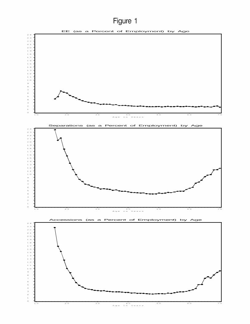
0

1

2

3

4

5

6

7

8

9

1 0

1 1

1 2

1 3

1 4

1 5

1 6

1 7

1 8

1 9

2 0

2 1

2 2

2 3

2 4

A g e i n Y e a r s

1 0 2 0 3 0 4 0 5 0 6 0 7 0

0

1

2

3

4

5

6

7

8

9

1 0

1 1

1 2

1 3

1 4

1 5

1 6

1 7

1 8

1 9

2 0

2 1

2 2

2 3

2 4

A g e i n Y e a r s

1 0 2 0 3 0 4 0 5 0 6 0 7 0

0

1

2

3

4

5

6

7

8

9

1 0

1 1

1 2

1 3

1 4

1 5

1 6

1 7

1 8

1 9

2 0

2 1

2 2

2 3

2 4

A g e i n Y e a r s

1 0 2 0 3 0 4 0 5 0 6 0 7 0

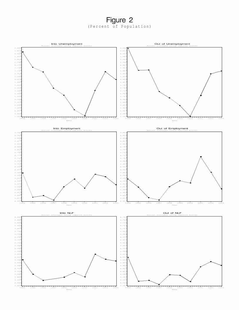
( P e r c e n t o f P o p u l a t i o n )

Annu a l a v e r a g e s u s i n g i m p u t e d m o n t h s

1 . 4 1

1 . 4 3

1 . 4 5

1 . 4 7

1 . 4 9

1 . 5 1

1 . 5 3

1 . 5 5

1 . 5 7

1 . 5 9

1 . 6 1

1 . 6 3

1 . 6 5

1 . 6 7

1 . 6 9

1 . 7 1

1 . 7 3

1 . 7 5

1 . 7 7

1 . 7 9

1 . 8 1

1 . 8 3

1 . 8 5

1 . 8 7

1 . 8 9

Y e a r

1 9 9 4 1 9 9 5 1 9 9 6 1 9 9 7 1 9 9 8 1 9 9 9 2 0 0 0 2 0 0 1 2 0 0 2 2 0 0 3

A n n u a l a v e r a g e s u s i n g i m p u t e d m o n t h s

1 . 5 6

1 . 5 8

1 . 6 0

1 . 6 2

1 . 6 4

1 . 6 6

1 . 6 8

1 . 7 0

1 . 7 2

1 . 7 4

1 . 7 6

1 . 7 8

1 . 8 0

1 . 8 2

1 . 8 4

1 . 8 6

1 . 8 8

1 . 9 0

1 . 9 2

1 . 9 4

1 . 9 6

1 . 9 8

2 . 0 0

2 . 0 2

2 . 0 4

Y e a r

1 9 9 4 1 9 9 5 1 9 9 6 1 9 9 7 1 9 9 8 1 9 9 9 2 0 0 0 2 0 0 1 2 0 0 2 2 0 0 3

A n n u a l a v e r a g e s u s i n g i m p u t e d m o n t h s

2 . 4 5

2 . 4 7

2 . 4 9

2 . 5 1

2 . 5 3

2 . 5 5

2 . 5 7

2 . 5 9

2 . 6 1

2 . 6 3

2 . 6 5

2 . 6 7

2 . 6 9

2 . 7 1

2 . 7 3

2 . 7 5

2 . 7 7

2 . 7 9

2 . 8 1

2 . 8 3

2 . 8 5

2 . 8 7

2 . 8 9

2 . 9 1

2 . 9 3

Y e a r

1 9 9 4 1 9 9 5 1 9 9 6 1 9 9 7 1 9 9 8 1 9 9 9 2 0 0 0 2 0 0 1 2 0 0 2 2 0 0 3

A n n u a l a v e r a g e s u s i n g i m p u t e d m o n t h s

2 . 4 0

2 . 4 2

2 . 4 4

2 . 4 6

2 . 4 8

2 . 5 0

2 . 5 2

2 . 5 4

2 . 5 6

2 . 5 8

2 . 6 0

2 . 6 2

2 . 6 4

2 . 6 6

2 . 6 8

2 . 7 0

2 . 7 2

2 . 7 4

2 . 7 6

2 . 7 8

2 . 8 0

2 . 8 2

2 . 8 4

2 . 8 6

2 . 8 8

Y e a r

1 9 9 4 1 9 9 5 1 9 9 6 1 9 9 7 1 9 9 8 1 9 9 9 2 0 0 0 2 0 0 1 2 0 0 2 2 0 0 3

A n n u a l a v e r a g e s u s i n g i m p u t e d m o n t h s

2 . 4 0

2 . 4 2

2 . 4 4

2 . 4 6

2 . 4 8

2 . 5 0

2 . 5 2

2 . 5 4

2 . 5 6

2 . 5 8

2 . 6 0

2 . 6 2

2 . 6 4

2 . 6 6

2 . 6 8

2 . 7 0

2 . 7 2

2 . 7 4

2 . 7 6

2 . 7 8

2 . 8 0

2 . 8 2

2 . 8 4

2 . 8 6

2 . 8 8

Y e a r

1 9 9 4 1 9 9 5 1 9 9 6 1 9 9 7 1 9 9 8 1 9 9 9 2 0 0 0 2 0 0 1 2 0 0 2 2 0 0 3

A n n u a l a v e r a g e s u s i n g i m p u t e d m o n t h s

2 . 3 0

2 . 3 2

2 . 3 4

2 . 3 6

2 . 3 8

2 . 4 0

2 . 4 2

2 . 4 4

2 . 4 6

2 . 4 8

2 . 5 0

2 . 5 2

2 . 5 4

2 . 5 6

2 . 5 8

2 . 6 0

2 . 6 2

2 . 6 4

2 . 6 6

2 . 6 8

2 . 7 0

2 . 7 2

2 . 7 4

2 . 7 6

2 . 7 8

Y e a r

1 9 9 4 1 9 9 5 1 9 9 6 1 9 9 7 1 9 9 8 1 9 9 9 2 0 0 0 2 0 0 1 2 0 0 2 2 0 0 3

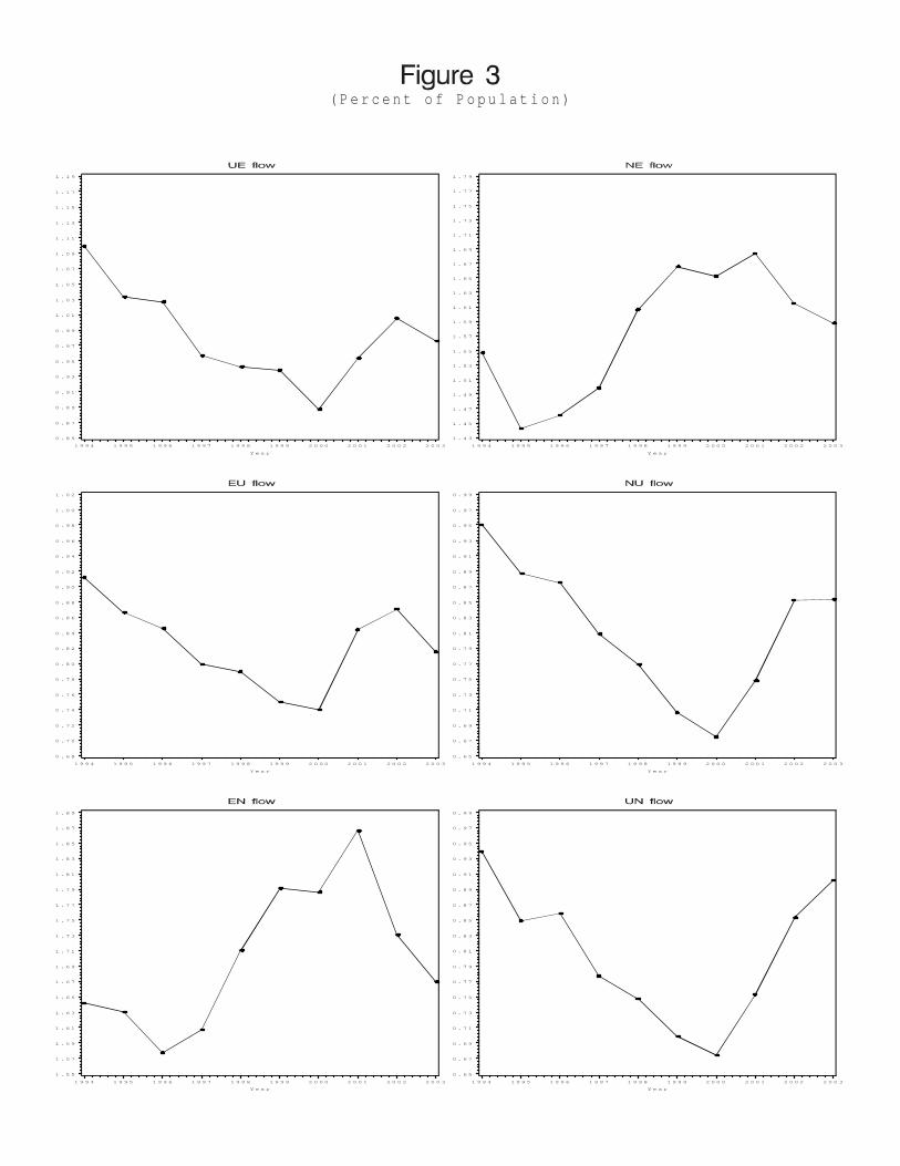
( P e r c e n t o f P o p u l a t i o n )

0.85

0 . 8 7

0 . 8 9

0 . 9 1

0 . 9 3

0 . 9 5

0 . 9 7

0 . 9 9

1 . 0 1

1 . 0 3

1 . 0 5

1 . 0 7

1 . 0 9

1 . 1 1

1 . 1 3

1 . 1 5

1 . 1 7

1 . 1 9

Y e a r

1 9 9 4 1 9 9 5 1 9 9 6 1 9 9 7 1 9 9 8 1 9 9 9 2 0 0 0 2 0 0 1 2 0 0 2 2 0 0 3

1 . 4 3

1 . 4 5

1 . 4 7

1 . 4 9

1 . 5 1

1 . 5 3

1 . 5 5

1 . 5 7

1 . 5 9

1 . 6 1

1 . 6 3

1 . 6 5

1 . 6 7

1 . 6 9

1 . 7 1

1 . 7 3

1 . 7 5

1 . 7 7

1 . 7 9

Y e a r

1 9 9 4 1 9 9 5 1 9 9 6 1 9 9 7 1 9 9 8 1 9 9 9 2 0 0 0 2 0 0 1 2 0 0 2 2 0 0 3

0 . 6 8

0 . 7 0

0 . 7 2

0 . 7 4

0 . 7 6

0 . 7 8

0 . 8 0

0 . 8 2

0 . 8 4

0 . 8 6

0 . 8 8

0 . 9 0

0 . 9 2

0 . 9 4

0 . 9 6

0 . 9 8

1 . 0 0

1 . 0 2

Y e a r

1 9 9 4 1 9 9 5 1 9 9 6 1 9 9 7 1 9 9 8 1 9 9 9 2 0 0 0 2 0 0 1 2 0 0 2 2 0 0 3

0 . 6 5

0 . 6 7

0 . 6 9

0 . 7 1

0 . 7 3

0 . 7 5

0 . 7 7

0 . 7 9

0 . 8 1

0 . 8 3

0 . 8 5

0 . 8 7

0 . 8 9

0 . 9 1

0 . 9 3

0 . 9 5

0 . 9 7

0 . 9 9

Y e a r

1 9 9 4 1 9 9 5 1 9 9 6 1 9 9 7 1 9 9 8 1 9 9 9 2 0 0 0 2 0 0 1 2 0 0 2 2 0 0 3

1 . 5 5

1 . 5 7

1 . 5 9

1 . 6 1

1 . 6 3

1 . 6 5

1 . 6 7

1 . 6 9

1 . 7 1

1 . 7 3

1 . 7 5

1 . 7 7

1 . 7 9

1 . 8 1

1 . 8 3

1 . 8 5

1 . 8 7

1 . 8 9

Y e a r

1 9 9 4 1 9 9 5 1 9 9 6 1 9 9 7 1 9 9 8 1 9 9 9 2 0 0 0 2 0 0 1 2 0 0 2 2 0 0 3

0 . 6 5

0 . 6 7

0 . 6 9

0 . 7 1

0 . 7 3

0 . 7 5

0 . 7 7

0 . 7 9

0 . 8 1

0 . 8 3

0 . 8 5

0 . 8 7

0 . 8 9

0 . 9 1

0 . 9 3

0 . 9 5

0 . 9 7

0 . 9 9

Y e a r

1 9 9 4 1 9 9 5 1 9 9 6 1 9 9 7 1 9 9 8 1 9 9 9 2 0 0 0 2 0 0 1 2 0 0 2 2 0 0 3

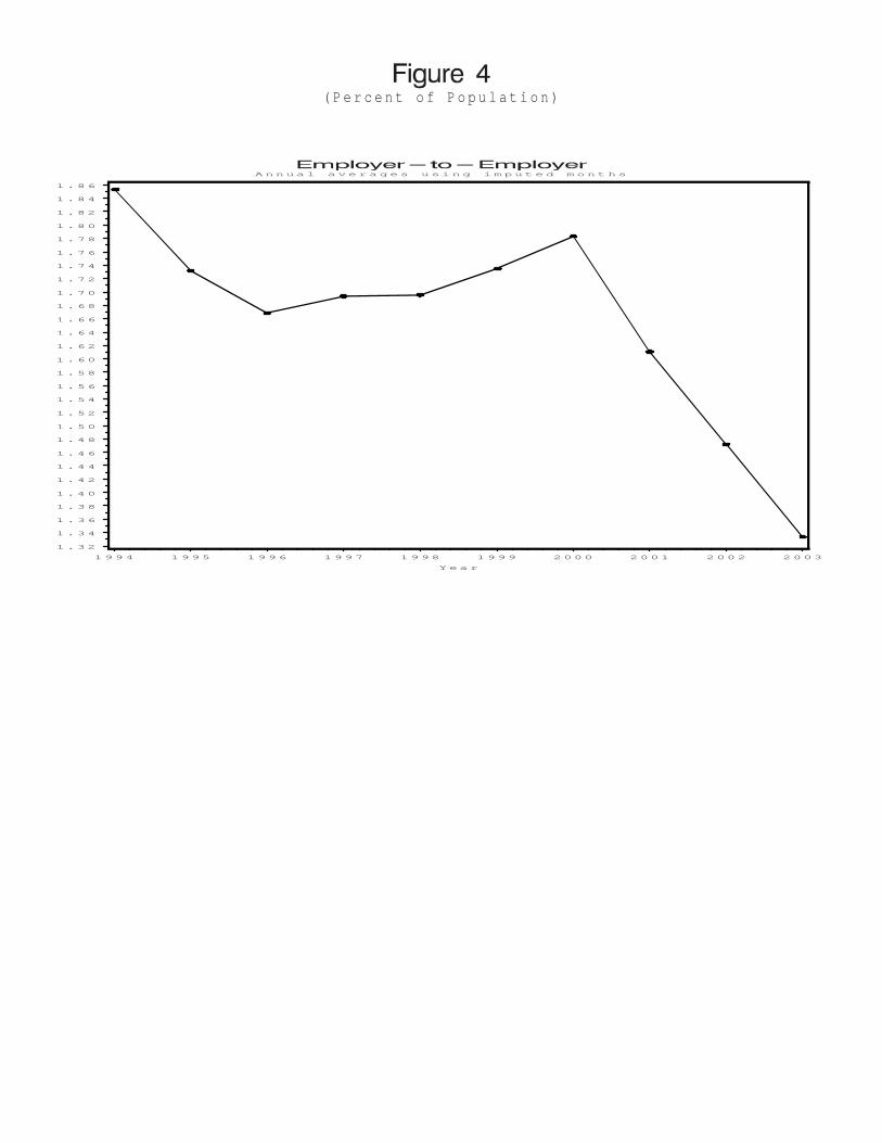
( P e r c e n t o f P o p u l a t i o n )

A n n u a l a v e r a g e s u s i n g i m p u t e d m o n t h s

1 . 3 2

1 . 3 4

1 . 3 6

1 . 3 8

1 . 4 0

1 . 4 2

1 . 4 4

1 . 4 6

1 . 4 8

1 . 5 0

1 . 5 2

1 . 5 4

1 . 5 6

1 . 5 8

1 . 6 0

1 . 6 2

1 . 6 4

1 . 6 6

1 . 6 8

1 . 7 0

1 . 7 2

1 . 7 4

1 . 7 6

1 . 7 8

1 . 8 0

1 . 8 2

1 . 8 4

1 . 8 6

Y e a r

1 9 9 4 1 9 9 5 1 9 9 6 1 9 9 7 1 9 9 8 1 9 9 9 2 0 0 0 2 0 0 1 2 0 0 2 2 0 0 3