To appear in Synthese Probability and Proximity in Surprise
19
Page 1 of 19 To appear in Synthese Probability and Proximity in Surprise Tomoji Shogenji 1 Abstract This paper proposes an analysis of surprise formulated in terms of proximity to the truth, to replace the probabilistic account of surprise. It is common to link surprise to the low (prior) probability of the outcome. The idea seems sensible because an outcome with a low probability is unexpected, and an unexpected outcome often surprises us. However, the link between surprise and low probability is known to break down in some cases. There have been some attempts to modify the probabilistic account to deal with these cases, but they are still faced with problems. The new analysis of surprise I propose turns to accuracy (proximity to the truth) and identifies an unexpected degree of inaccuracy as reason for surprise. The shift from probability to proximity allows us to solve puzzles that strain the probabilistic account of surprise. Keywords Qualitative hypothesis ∙ Quantitative hypothesis ∙ Probabilistic hypothesis ∙ Inaccuracy ∙ Scoring rules ∙ Expected inaccuracy 1. Introduction This paper proposes an analysis of surprise formulated in terms of proximity to the truth, to replace the probabilistic account of surprise. It is common to link surprise to the low (prior) probability of the outcome. 2 The idea seems sensible because an outcome with a low probability is unexpected, and an unexpected outcome often surprises us. However, the link between surprise and low probability is known to break down in some cases. There have been some attempts to modify the probabilistic account to deal with these cases, but as we shall see, they are still faced with problems. The new analysis of surprise I propose turns to accuracy (proximity to the truth) and identifies an unexpected degree of inaccuracy as reason for surprise. The shift from probability to proximity allows us to solve puzzles that strain the probabilistic account of surprise. 1 Philosophy Department, Rhode Island College, Providence, RI, USA 2 See, for example, recent quantitative formulations (McGrew 2003, Schupbach & Sprenger 2011, Crupi & Tentori 2012) of Peirce’s idea that explanation eliminates surprise (Peirce 1931-35, 5: 189). These authors all assume that the degree of surprise is an inverse function of the (prior) probability.
-
Upload
khangminh22 -
Category
Documents
-
view
6 -
download
0
Transcript of To appear in Synthese Probability and Proximity in Surprise
Page 1 of 19
To appear in Synthese
Probability and Proximity in Surprise
Tomoji Shogenji1
Abstract This paper proposes an analysis of surprise formulated in terms of proximity to the
truth, to replace the probabilistic account of surprise. It is common to link surprise to the low
(prior) probability of the outcome. The idea seems sensible because an outcome with a low
probability is unexpected, and an unexpected outcome often surprises us. However, the link
between surprise and low probability is known to break down in some cases. There have been
some attempts to modify the probabilistic account to deal with these cases, but they are still
faced with problems. The new analysis of surprise I propose turns to accuracy (proximity to the
truth) and identifies an unexpected degree of inaccuracy as reason for surprise. The shift from
probability to proximity allows us to solve puzzles that strain the probabilistic account of
surprise.
Keywords Qualitative hypothesis ∙ Quantitative hypothesis ∙ Probabilistic hypothesis ∙
Inaccuracy ∙ Scoring rules ∙ Expected inaccuracy
1. Introduction
This paper proposes an analysis of surprise formulated in terms of proximity to the truth, to
replace the probabilistic account of surprise. It is common to link surprise to the low (prior)
probability of the outcome.2 The idea seems sensible because an outcome with a low probability
is unexpected, and an unexpected outcome often surprises us. However, the link between
surprise and low probability is known to break down in some cases. There have been some
attempts to modify the probabilistic account to deal with these cases, but as we shall see, they are
still faced with problems. The new analysis of surprise I propose turns to accuracy (proximity to
the truth) and identifies an unexpected degree of inaccuracy as reason for surprise. The shift from
probability to proximity allows us to solve puzzles that strain the probabilistic account of
surprise.
1 Philosophy Department, Rhode Island College, Providence, RI, USA 2 See, for example, recent quantitative formulations (McGrew 2003, Schupbach & Sprenger 2011, Crupi & Tentori
2012) of Peirce’s idea that explanation eliminates surprise (Peirce 1931-35, 5: 189). These authors all assume that
the degree of surprise is an inverse function of the (prior) probability.

Page 2 of 19
To clarify the nature of the project, it is not my goal to predict the degree of surprise for
some practical purposes. Surprise is a psychological phenomenon that resists simple
generalization. The same outcome may greatly surprise some individuals under some conditions,
but not others under other conditions to the same degree. It is highly unlikely that a single formal
quantity, such as accuracy, can adequately predict the degree of surprise for different individuals
under different conditions. To complicate the matter further, it is well known that heuristics we
use for quantitative judgments are unreliable in many ways.3 These are legitimate concerns if we
are trying to predict the degree of surprise for some practical purposes, but that is not my goal.
The analysis of surprise I propose aims to make paradigmatic cases of surprise understandable. It
is informed by the way people commonly respond to paradigmatic cases of surprise (or no
surprise), and solves puzzles in some of these cases that defy the probabilistic account. So, I
consider the analysis successful if it solves puzzles in those paradigmatic cases of surprise even
if it cannot account for some differences in people’s reactions.
The paper proceeds as follows. After a critical examination of Horwich’s analysis of
surprise (Section 2), I propose to shift our focus from probability to proximity (Section 3). I will
then describe two formal measures of inaccuracy that allow us to flesh out the idea of proximity
to the truth (Section 4). With the help of these measures, I introduce a new analysis of surprise to
solve puzzling cases (Section 5). I conclude with brief remarks on two ways of seeking the
alethic goals, via probable truth and via proximity to the truth (Section 6).
2. Horwich on Surprise
I begin with Horwich’s analysis of surprise (1982, Ch. 5), which shaped recent discussions of the
subject.4 His analysis consists of three explicit points and a fourth point that is endorsed
implicitly. The first point is that a low prior probability is necessary but not sufficient for some
event to be surprising. The necessity part is straightforward. If an event is not so improbable and
thus is among the expected outcomes, then its occurrence is not surprising. A low prior
probability is therefore necessary for surprise. It is the denial of sufficiency that is interesting and
important. Horwich compares two cases. “Suppose I fish a coin from my pocket and begin
tossing it. I would be astonished if it landed heads 100 times in a row” (p. 101). Let’s call the
surprising sequence in question E. Meanwhile, we are not surprised at an “irregular sequence of
about 50 heads and 50 tails.” Let’s call the unsurprising sequence F. Horwich’s point is that
despite our different reactions to them, E and F are actually equally improbable at p(E) = p(F) =
2-100 because each of them is one of the 2100 equally probable sequences of heads and tails. Since
F is not surprising, a low prior probability is not sufficient for surprise.
3 See Tversky & Kahneman (1974) and the subsequent literature on “heuristics and biases”. See, in particular,
Landy, Silbert & Goldin (2013) on heuristics for estimating large numbers, which is often a factor in paradigmatic
cases of surprise. 4 Authors sympathetic to Horwich’s analysis include Good (1984), White (2000), Olsson (2002) and Manson &
Thrush (2003). See Schlesinger (1991, pp. 99-102) and Harker (2012) for criticisms of Horwich’s analysis.
Page 3 of 19
Horwich then proposes the further condition for surprise, which is his second point, viz.
an event is surprising only if it substantially diminishes the probability of some default
assumption. The relevant default assumption in the case of E and F is that the coin is fair. Let’s
call the assumption C. The surprising sequence E diminishes the probability of C substantially,
while F doesn’t. This is the reason, according to Horwich, for our different reactions to E and F
despite their equally low prior probability. The point is compelling—it is hard to think of cases
where we are surprised at an event, but it does not shake our confidence in the default
assumption.
The question remains, however, as to why some low-probability events shake our
confidence in the default assumption while others don’t. Horwich answers this question in his
third point, viz. an event diminishes the probability of the default assumption substantially “if
there is some initially implausible (but not wildly improbable) view K about the circumstances,
relative to which E would be highly probable” (p. 102). Such K in the case of E is that the coin is
double headed or that it is heavily biased. There is, in other words, a serious alternative
hypothesis to explain E that is inconsistent with the default assumption that the coin is fair. It is
this third point that has received most criticisms, but as it is worded by Horwich, the statement is
actually unproblematic. Horwich makes it clear by a Bayesian analysis that the existence of such
K is sufficient (“if there is […] K”) for substantial reduction in the probability of the default
assumption. Indeed, when we recognize a serious alternative hypothesis for an event that is
improbable by the default assumption, our confidence in the latter diminishes substantially.
The reason for the criticisms is the interpretation that Horwich takes the existence of a
serious alternative hypothesis to be also necessary for surprise.5 This reading is not entirely
unfair to Horwich because he implicitly endorses it when he states that the sequence F is not
surprising because “there is no obvious candidate for the role of K” (p. 102). Unless the existence
of a serious alternative explanation is necessary for surprise, the absence of such a hypothesis
does not account for the absence of surprise. Note also that the phrase “no obvious candidate”
indicates that the alternative hypothesis must be recognized by us. The natural reading of
Horwich’s remark is that the recognition of a serious alternative hypothesis that makes the
improbable (by the default assumption) event probable is necessary for surprise. As his critics
point out, there are counterexamples to this claim.6
There is no need to look far for a counterexample. We only need to modify the coin toss
case slightly, viz. that you already checked the coin before tossing it and the coin was not
double-headed or heavily biased in any conceivable way. So, you cannot think of any serious
alternative hypothesis that would make the outcome E (100 consecutive heads) probable. The
outcome E is still surprising—perhaps more so—despite the absence of any serious hypothesis
that makes E probable. Cases of this kind indicate strongly that it is not necessary for surprise,
5 See Schlesinger (1991, pp. 99-102) and Harker (2012). Baras (2019, p. 1409n) reports (based on his
correspondence with Horwich) that Horwich did not intend the existence of a serious alternative hypothesis to be a
necessary condition for surprise. 6 See, again, Schlesinger (1991, pp. 99-102) and Harker (2012).
Page 4 of 19
and for a loss of confidence in the default assumption, that you recognize a hypothesis that
makes the improbable (by the default assumption) outcome probable.
To summarize, Horwich makes two important and compelling points. First, a low prior
probability is necessary but not sufficient for surprise. Second, a surprising event shakes our
confidence in the default assumption. To combine the two points, we are surprised at an outcome
that is improbable in a way that shakes our confidence in the default assumption. The further
question is what additional condition (beyond the low probability) shakes our confidence in the
default assumption. As for Horwich’s two further points, it is true that we lose confidence in the
default assumption when we recognize a serious alternative hypothesis that makes the
improbable (by the default assumption) outcome probable, but recognizing such a hypothesis is
not necessary for losing confidence in the default assumption. Horwich seems to be putting the
cart before the horse here. We do not lose confidence in the default assumption for the reason
that there is an alternative hypothesis that makes the surprising outcome probable; we seek an
alternative hypothesis for the reason that we lose confidence in the default assumption. A
satisfactory analysis of surprise should identify the additional condition necessary for shaking
our confidence in the default assumption.
3. From Probability to Proximity
Let us take a closer look at the two coin toss sequences E and F. The reason for our different
reactions to them is actually not hard to find, viz. E and F have very different ratios of heads
(hereafter “H-ratios”). We are surprised at E whose H-ratio of 100/100 is extreme, while we are
not surprised at F whose H-ratio is close to even (say 53/100 to make it definite). To put this idea
formally, we can think of different ways of classifying the outcomes of 100 coin tosses. We may
classify them by the exact sequence of heads and tails. Since there are 2100 possible sequences,
the resulting partition XSEQ consists of 2100 members. We can, however, also classify the
outcomes by their H-ratio. Since there are 101 possible H-ratios, we can think of the partition
XH/100 {x0, …, x100}, where the outcome belongs to xi if and only if its H-ratio is i/100. It is
presumably the partition XH/100 that is salient to us when we compare E and F, and thus is
responsible for our different reactions to them.
Some other partition may become salient, depending on the outcome and the
circumstance. For example, the outcome with an unremarkable H-ratio of 53/100 may be
surprising if the sequence consists of 53 consecutive heads and 47 consecutive tails. Such an
outcome prompts us to classify the outcomes differently, e.g. by the number of times the coin
lands on the same side as the previous toss. Given the default assumption that the coin is fair and
each toss is independent of the previous one, we expect the number to be roughly one half of the
times, while the sequence of 53 consecutive heads and 47 consecutive tails (landing on the same
side as the previous toss 98 times out of 99) is extreme. The circumstance may also affect the
partition. For example, if a self-proclaimed clairvoyant declares an exact sequence of 100 coin

Page 5 of 19
tosses in advance, we may partition the outcomes by the number of matches with the predicted
sequence. Sensitivity to the context may complicate the analysis in some cases, but not in
paradigmatic cases of surprise where the partition salient to the subject is reasonably clear.
Once we settle on a salient partition, XH/100 {x0, …, x100} for E and F, there are two
ways to proceed. One is to retain the probabilistic approach, and apply it to the new partition. We
can differentiate E and F probabilistically because x100 (to which E belongs) is extremely
improbable at p(x100) 2-100 whereas x53 (to which F belongs) is not as improbable as x100. The
second way to proceed is to shift our focus to proximity. If the coin is fair, the expected H-ratio
is 50/100, and x50 is at the center of the partition XH/100 {x0, …, x100}. We can then compare E
and F by their proximity to the center, viz. x100 (to which E belongs) is extremely distant from
the center, while x53 (to which F belongs) is close to the center. This may explain our different
reactions to E and F.
So, which approach should we take: probability or proximity? One concern about the
probability approach is that p(x53) 0.067 for F (53 heads out of 100 tosses) is still quite low,
though not as extreme as p(x100) 2-100 for E. Compare it with the case of four consecutive heads
in four coin tosses. If the coin is fair, the probability for that outcome is 2-4 1/16 0.0625,
which is comparable to p(x53) 0.067. However, four consecutive heads in four coin tosses is at
least mildly surprising while F (53 heads out of 100 tosses) is not even mildly surprising.
Some defenders of the probabilistic account may suggest here that we can avoid the
problem of a low probability with no surprise by adopting the range of H-ratios. For example, it
is sensible to expect an outcome falling in the range of “5010 heads” instead of precisely “50
heads”. Since the probability of getting an outcome in this range is high at p(x5010) 0.96, we
are surprised at an outcome like E that falls outside the range.7 Meanwhile, we are not surprised
at F, despite the low probability p(x53) 0.067 for its H-ratio, because this H-ratio is within the
expected range “5010 heads” that is highly probable.
The range proposal has problems, though. First, it is in need of some refinement to
account for the degree of surprise. For example, if the expected range is “5010 heads”, then
both 61 heads and 100 heads are outside the range. This means that both of them are surprising
by the range proposal, but our reactions to these outcomes are very different. 61 heads is only
mildly surprising while 100 heads is extremely surprising. There are some ways of refining the
range proposal to account for the degree of surprise, for example, by considering the maximum
range that excludes the outcome in question. The maximum range that excludes 61 heads is
“5010 heads” while the maximum range that excludes the outcome of 100 heads is “5049
heads”. We may, then, measure the degree of surprise by the probability of exclusion by the
maximum range, i.e. 1 – p(x5010) 0.04 for the outcome of 61 heads while 1 – p(x5049) = p(x0) +
p(x100) = 2-99 for the outcome of 100 heads. This (or something similar) may explain our different
reactions to 61 heads and 100 heads. Note, however, that the refinement reveals that the range
proposal tacitly relies on proximity. The center of the range is x50 because the expected H-ratio is
50/100, and the range expands to 501, 502, …, 5049 in the order of proximity from the
7 See Harker (2012, p. 253) for a proposal along this line.

Page 6 of 19
center. The range proposal cannot allow an arbitrary “range” of H-ratios to exclude a particular
outcome, for example, the subset {x45, x46, x47, x48, x49, x50, x51, x52, x54, x55} to exclude x53 (to
which F belongs).
If we have to use the proximity relation anyways, we might as well use it upfront by
taking the proximity approach. However, the proximity approach has its own problems. First, it
is doubtful that the proximity to the center of the partition is the only determinant of surprise.
The way the probability is distributed over different H-ratios (e.g. the extremely low probability
for 100/100) also seems relevant. Besides, there are some cases of surprise where there is no
proximity relation among the outcomes. Consider, for example, a large-scale raffle (say, of 1,000
tickets) with exactly one winner. You will be surprised if a single ticket you bought turns out to
be the winner. Note, however, there is no quantity in this case on which to define the proximity
relation among the outcomes. There is no “center” of the partition either.8 In cases of this kind,
only the probabilities assigned to the outcomes seem relevant.
So, the role of proximity in surprise is not immediately clear. We need to consider it in
some paradigmatic cases of surprise, but in some others only probabilities seem to matter. An
easy way out is to take different approaches to different cases of surprise. However, a unified
framework is desirable, and there is a way of achieving unification at least at the conceptual
level. The key here is that the probabilities are themselves quantities, which we can evaluate by
proximity to the truth. Suppose you and your friend are guessing the outcome of a raffle
drawing—wondering, in particular, whether the biggest donor to the organization will win. You
assign the probability 0.001 based on the assumption that the raffle is fair, while your friend
assigns 0.9 based on the strong suspicion that the raffle is rigged. Note that the goal in making
these estimates is not the truth per se, because the actual outcome—the donor in question is the
winner or not the winner—has no degree, such as 0.001 or 0.9. Our goal is proximity to the truth.
If the donor is the winner, then your friend’s estimate (probability 0.9) is closer to the truth than
is yours (probability 0.001), but if the donor is not the winner, your estimate is closer to the truth
than is your friend’s.
Some may question the virtue of unification here: It seems no quantitative analysis can
provide a whole picture of surprise anyways because in many paradigmatic cases of surprise the
subject assigns no quantity to the outcome. For example, your friend may only say—without
assigning any probability—that she is quite confident the biggest donor will win, and then
surprised when somebody else wins. Where there is no assignment of quantity, the quantitative
analysis is not applicable. But this is too quick. We do not need a precise quantity in applying a
quantitative analysis. A range of quantity is enough. For example, if we can interpret “quite
confident” as no smaller than 0.8 and no greater than 0.95 in probability, and if any probability
assignment in this range warrants a significant degree of surprise given the outcome, then the
quantitative analysis can make her surprise understandable. Note also that we do not need sharp
boundaries for the range. To put it in technical terms, the probabilities 0.8 and 0.95 need not be
8 The raffle tickets may have numerals on them, but they are assigned only for the purpose of identification. We can
replace them by letters, colors, shapes, etc. that represent no quantities.
Page 7 of 19
the greatest lower bound and the smallest upper bound, respectively. They may only be,
respectively, a lower bound and an upper bound.9 If so, some probability greater than 0.8 may
still be an inappropriate precisification, but it does not matter as long as any reasonable
precisification makes her surprise understandable.
Here is a broader picture. Once we abandon the aspiration for absolute certainty in favor
of probabilistic estimates, hypotheses to evaluate are quantitative because the probabilities are
quantities. This means that given the actual outcome (the truth), we can evaluate any
probabilistic hypothesis by its proximity to the truth. There is still an important distinction
between cases where the probabilities are assigned to quantities (e.g. H-ratios) and cases where
the probabilities are assigned to qualities (e.g. the biggest donor is the winner or not the winner).
However, the distinction only affects the technical way we measure proximity to the truth, while
the core idea of evaluating the hypothesis by proximity to the truth is the same. The next section
describes two “scoring rules” that are designed to measure inaccuracy (distance to the truth) for
the two types of probabilistic hypotheses just mentioned. I will make use of these measures in
the analysis of surprise in Section 5.
4. Measuring Inaccuracy
4.1 Scoring Rules
I want to clarify, first, the conception of proximity to the truth that I do not pursue in this section.
The idea of differentiating false theories by their proximity to the truth has been familiar to
philosophers of science since Popper (1963) under the name “verisimilitude” (or “truthlikeness”
in the recent literature). However, Popper’s approach is not suitable for the present purpose. The
idea of verisimilitude is motivated by Popper’s view that the primary virtue of scientific theory is
informativeness. Since a more informative (more specific) theory has a lower probability of
being true, a high probability is not an indication of a good theory in his view. Instead, a good
theory is one with high truth-content (true logical consequences) and low falsity-content (false
logical consequences). The verisimilitude of a theory is therefore determined by the amounts of
its truth-content and falsity-content. The trouble is that verisimilitude is hard to define formally
in a way that serves the intended purpose.10 Even more troubling—for the purpose of analyzing
surprise—is the problem of epistemic access, i.e. we cannot actually measure the verisimilitude
9 If x is the greatest lower bound, no other quantity is a greatest lower bound; but if x is only a lower bound, any
quantity smaller than x is also a lower bound. 10 Miller (1974) and Tichý (1974) proved, independently, that the original definition by Popper (1963) is defective.
See Oddie (2016) for a review of various attempts to overcome the difficulty, and for different conceptions of
verisimilitude (truthlikeness).
Page 8 of 19
of a theory because for many of its logical consequences we are unable to tell whether they are
true or false.11
Fortunately, it is not necessary to deal with these problems of verisimilitude for the
purpose of analyzing surprise. First, there is no issue of epistemic access since we are only
measuring how close an estimated quantity is to the observed (true) quantity. For example, we
know in the case of E that surprises us that the outcome is 100 heads out of 100 coin tosses. We
can simply measure the distance between this quantity and the prior estimate. There is some
complication when the estimate is not given in the form of a quantity, but in the form of a
probability distribution over the possible outcomes. However, we already have a large literature
on “scoring rules” for measuring the inaccuracy of a probability distribution.12 In what follows I
am going to use the term “accuracy” (and “inaccuracy”) that are standard in the literature on
scoring rules, to distinguish it from the different conception of proximity in the verisimilitude
literature.
A scoring rule measures the inaccuracy of a probability distribution over possible
outcomes when given the actual outcome.13 To put it formally, a scoring rule SR(p, i) is a
function whose inputs are a probability distribution p over the partition X = {x1, …, xn} and one
member i (the actual outcome) of the partition, and whose output is a real number (the degree of
inaccuracy). The partition over which the probability is distributed may be “ranked” or “non-
ranked”. The members of a ranked partition are ordered in a specific way. If the members are
quantities, then the partition is ranked in a natural way, but the members of the ranked partition
need not be quantities. For example, there is a natural order among the members of the partition
XGAME {Win, Draw, Loss} so that the distance between two members varies, depending on their
positions in the order—Loss is more distant from Win than Draw is from Win. This can affect
the degree of inaccuracy. Suppose your distribution p splits the probability equally between Win
and Draw (with no probability for Loss), while your friend’s distribution q splits the probability
equally between Win and Loss (with no probability for Draw). If the outcome turns out to be
Win, p is more accurate (closer to the truth) overall than q is. Although p and q assign the same
probability p(W) q(W) 0.5 to the true outcome, p assigns the remaining probability to Draw
that is closer to Win than is Loss to which q assigns the remaining probability.
In contrast, there is no such difference in distance among the members of a non-ranked
partition. For example, the partition XCOL {Red, Green, Blue} is not ranked (unless you impose
an order for some reason) so that Red is no more distant from Blue than it is from Green, etc. As
11 Note also that adding a known (new) truth to a theory does not necessarily increase its overall verisimilitude if the
theory to which it is added is false (has false logical consequences). Adding a truth to a false theory may increase its
falsity-content more than its truth-content. As a result, we cannot even make a comparative judgment that the
addition of a truth increases the verisimilitude of the theory. 12 See Gneiting and Raftery (2007) for a review of the literature, and Winkler and Jose (2010) for an accessible
overview. 13 I will not discuss a categorical statement (with no assignment of a probability) separately because a categorical
statement can be considered a special case of a probability distribution where the entire probability is assigned to
one member of the partition.

Page 9 of 19
a result, there is no difference in the degree of inaccuracy between p that splits the probability
equally between Red and Green (with no probability for Blue) and q that splits the probability
equally between Red and Blue (with no probability for Green), when the outcome turns out to be
Red. So, we need different scoring rules for a ranked partition and a non-ranked partition. I
describe one rule for each here: The Ranked Probability Score SRRPS(p, i) for the former and the
Brier Score SRB(p, i) for the latter.14
Before going into their mathematical details, it should be noted that all scoring rules—
including SRRPS(p, i) and SRB(p, i)—are formulated so as to satisfy the widely accepted
constraint known as Strict Propriety:
Strict Propriety: A scoring rule SR(p, i) must be strictly proper in the sense that
∑ 𝑝(𝑥𝑖)SR(𝑝, 𝑖)𝑖 < ∑ 𝑝(𝑥𝑖)SR(𝑞, 𝑖)𝑖 for any p q.
To see what this means intuitively, take p to be your own probability distribution over X = {x1,
…, xn}. Since p is your own probability distribution, you use p as “weights” when you calculate
the expected inaccuracy ∑ 𝑝(𝑥𝑖)SR(𝑞, 𝑖)𝑖 of any probability distribution q over the same
partition. When a scoring rule is strictly proper, the p-weighted expected inaccuracy of q is
minimal if and only if q is identical to p.
An often cited reason for making the scoring rule strictly proper is to prevent duplicity. If
the scoring rule is strictly proper, then in announcing a probability distribution q, you can
minimize its expected inaccuracy only by making q identical to your own distribution p. If the
scoring rule is not strictly proper—i.e. if you can minimize the expected inaccuracy by some
probability distribution other than your own—the incentive to make an honest announcement is
lost. We can also see reason for Strict Propriety in retrospective evaluation. Suppose we already
have the correct probability distribution p over X = {x1, …, xn} based on the actual frequency
ratio in the population. We can then use a scoring rule to evaluate the prior probability
distribution q in retrospect by the average inaccuracy ∑ 𝑝(𝑥𝑖)SR(𝑞, 𝑖)𝑖 . Strict Propriety means
that q receives the highest mark (less inaccurate than any other distribution) if and only if q is
identical to p, and that is the way it should be, i.e. the distribution that matches the actual
frequency ratio in the population should receive the highest mark.15
Strict Propriety is a powerful constraint, but it alone does not narrow down the choices to
a single scoring rule for each type of partition. I select here the Ranked Probability Score and the
Brier Score because they are widely known and frequently used in various applications. Those
14 When the members xi in the ranked partition are the values of a continuous variable, we need the Continuous
Ranked Probability Score instead of the Ranked Probability Score, but I restrict discussions to discrete cases here
because an extension to the continuous cases does not change the substance of my analysis. 15 See Roche & Shogenji (2018) for similar reasoning for Strict Propriety. Calling it “an epistemic reason” (p. 594),
they argue that the prior probability distribution p(xi) is the most accurate in retrospect if and only if it is identical to
the posterior (updated) probability distribution p(xi | y) given the new evidence y.
Page 10 of 19
who prefer a different measure may use a scoring rule of their choice.16 The substance of the
analysis below is not affected, as long as the scoring rule is strictly proper.
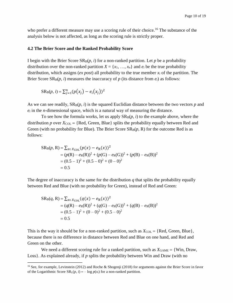
4.2 The Brier Score and the Ranked Probability Score
I begin with the Brier Score SRB(p, i) for a non-ranked partition. Let p be a probability
distribution over the non-ranked partition X = {x1, …, xn} and ei be the true probability
distribution, which assigns (ex post) all probability to the true member xi of the partition. The
Brier Score SRB(p, i) measures the inaccuracy of p (its distance from ei) as follows:
SRB(p, i) ∑ (𝑝(𝑥𝑗) − 𝑒𝑖(𝑥𝑗))2𝑛𝑗=1
As we can see readily, SRB(p, i) is the squared Euclidian distance between the two vectors p and
ei in the n-dimensional space, which is a natural way of measuring the distance.
To see how the formula works, let us apply SRB(p, i) to the example above, where the
distribution p over XCOL {Red, Green, Blue} splits the probability equally between Red and
Green (with no probability for Blue). The Brier Score SRB(p, R) for the outcome Red is as
follows:
SRB(p, R) ∑ (𝑝(𝑥) − 𝑒R(𝑥))2𝑥𝑋COL
(p(R) – eR(R))2 + (p(G) – eR(G))2 + (p(B) – eR(B))2
(0.5 – 1)2 + (0.5 – 0)2 + (0 – 0)2
0.5
The degree of inaccuracy is the same for the distribution q that splits the probability equally
between Red and Blue (with no probability for Green), instead of Red and Green:
SRB(q, R) ∑ (𝑞(𝑥) − 𝑒R(𝑥))2𝑥𝑋COL
(q(R) – eR(R))2 + (q(G) – eR(G))2 + (q(B) – eR(B))2
(0.5 – 1)2 + (0 – 0)2 + (0.5 – 0)2
0.5
This is the way it should be for a non-ranked partition, such as XCOL {Red, Green, Blue},
because there is no difference in distance between Red and Blue on one hand, and Red and
Green on the other.
We need a different scoring rule for a ranked partition, such as XGAME {Win, Draw,
Loss}. As explained already, if p splits the probability between Win and Draw (with no
16 See, for example, Levinstein (2012) and Roche & Shogenji (2018) for arguments against the Brier Score in favor
of the Logarithmic Score SRL(p, i) – log p(xi) for a non-ranked partition.

Page 11 of 19
probability for Loss) while q splits the probability between Win and Loss (with no probability
for Draw) and the outcome is Win, then p is more accurate (closer to the truth) overall than q is,
but the Brier Score does not differentiate p and q. So, we turn to the Ranked Probability Score
SRRPS(p, i) defined as follows:
SRRPS(p, i) ∑ [𝑃(𝑥𝑗) − 𝐸𝑖(𝑥𝑗)]2𝑛𝑗=1
Like the Brier Score, the Ranked Probability Score SRRPS(p, i) measures inaccuracy by the
squared Euclidian distance between two vectors in the n-dimensional space. The difference is
that the two vectors to compare are cumulative distributions, P and Ei, derived respectively from
p and ei:
𝑃(𝑥𝑗) = ∑ 𝑝(𝑥𝑙𝑗𝑙=1 )
𝐸𝑖(𝑥𝑗) = ∑ 𝑒𝑖(𝑥𝑙𝑗𝑙=1 )
In most cases P(xj) increases gradually till it reaches one. Meanwhile, Ei(xj) jumps abruptly from
zero to one at j = i because ei(xj) 1 for j i and ei(xj) 0 for j i.
By applying the Ranked Probability Score to p and q above over the ranked partition
XGAME {Win, Draw, Loss} for the outcome Win, we obtain different degrees of inaccuracy,
SRRPS(p, W) and SRRPS(q, W), as follows:
SRRPS(p, W) ∑ (𝑃(𝑥) − 𝐸W(𝑥))2𝑥𝑋GAME
[P(W) – EW(W)]2 + [P(D) – EW(D)]2 + [P(L) – EW(L)]2
[p(W) – eW(W)]2 + [(p(W) + p(D)) – (eW(W) + eW(D))]2
+ [(p(W) + p(D) + p(L)) – (eW(W) + eW(D) + eW(L))]2
[0.5 – 1]2 + [(0.5 + 0.5) – (1 + 0)]2 + [(0.5 + 0.5 + 0) – (1 + 0 + 0)]2
0.25
SRRPS(q, W) ∑ (𝑄(𝑥) − 𝐸W(𝑥))2𝑥𝑋GAME
[Q(W) – EW(W)]2 + [Q(D) – EW(D)]2 + [Q(L) – EW(L)]2
[q(W) – eW(W)]2 + [(q(W) + q(D)) – (eW(W) + eW(D))]2
+ [(q(W) + q(D) + q(L)) – (eW(W) + eW(D) + eW(L))]2
[0.5 – 1]2 + [(0.5 + 0) – (1 + 0)]2 + [(0.5 + 0 + 0.5) – (1 + 0 + 0)]2
0.5
SRRPS(p, W) 0.25 is smaller than SRRPS(q, W) 0.5, as it should be, because p assigns a greater
probability (than q does) to the closer member Draw and a smaller probability (than q does) to

Page 12 of 19
the more distant member Win, while assigning the same probability (as q does) to the true
member Win.
5. The Inaccuracy Analysis of Surprise
5.1 Non-Ranked Partitions
With two measures of inaccuracy in hand, let us now return to the paradigmatic cases of surprise.
To begin with a non-ranked partition, recall the example of a raffle with 1,000 tickets for a single
winner, where you are surprised to find that you are the winner. This is not a difficult case in
itself. Even the probabilistic account can explain the surprise because the probability for a win is
very low at 0.001. Note, however, that you are not surprised if somebody else (John Doe) is the
winner, though the probability of that outcome is also very low at 0.001. What is the difference?
There is still a sensible account by the probability, viz. when you are a participant, the salient
partition of the outcomes is ego-centric, viz. XEGO {You, Not-You} and John Doe belongs to
the second member of the partition, whose default probability is very high at 0.999. The
difference in probability, 0.001 vs. 0.999, explains the different reactions to the two outcomes.
There is, however, a more serious problem when you are not a participant. You won’t be
surprised when somebody (John Doe) turns out to be the winner because somebody is going to
win anyways, but the probability of anybody (John Doe) being the winner is very low at 0.001.
Why is there no surprise?
Let us now turn to inaccuracy. The appropriate measure is the Brier Score since the
partition XRAF = {x1, …, x1000} is non-ranked. If the winner is xi, then the Brier score SRB(p, i) for
the equiprobable distribution p over XRAF is as follows:
SRB(p, i) ∑ [𝑝(𝑥𝑗) − 𝑒𝑖(𝑥𝑗)]21000𝑗=1
= [0.001 – 1]2 + [0.001 – 0]2 999
= 0.999
The degree of inaccuracy is high, but that is not the important point here. The point to note is that
no matter who wins the raffle, the Brier Score is the same at 0.999 because p is equiprobable
over the partition XRAF = {x1, …, x1000}. In other words, the Brier Score of 0.999 is exactly the
expected degree of inaccuracy.17 This is why you are not surprised.
To put this formally, the expected inaccuracy (the probability-weighted average Brier
Score) of the distribution p over the non-ranked partition XRAF = {x1, …, x1000} is:
17 The point holds regardless of the choice of the scoring rule. Since p is equiprobable over XRAF = {x1, …, x1000}, the
degree of inaccuracy is the same no matter who is the winner, so that the actual inaccuracy is exactly the expected
inaccuracy.

Page 13 of 19
Ep(XRAF) = ∑ [𝑝(𝑥𝑖)SRB(𝑝; 𝑖)]1000𝑖=1
∑ [𝑝(𝑥𝑖) ∑ [𝑝(𝑥𝑗) − 𝑒𝑖(𝑥𝑗)]21000
𝑗=11000𝑖=1 ]
∑ [𝑝(𝑥𝑗) − 𝑒𝑖(𝑥𝑗)]21000𝑗=1
= 0.999.
We are not surprised at any outcome because the actual degree of inaccuracy SRB(p, i) is exactly
the expected degree of inaccuracy Ep(XRAF), regardless of the outcome. A high degree of
inaccuracy as such does not surprise us if that is expected. What surprises us is an unexpected
degree of inaccuracy.
Recall the compelling point in the probabilistic account of surprise that we are surprised
when the outcome is unexpected. The new analysis preserves the connection between surprise
and unexpectedness, but it interprets unexpectedness in terms of inaccuracy instead of a low
probability. The probabilistic account falls short in cases where all possible outcomes are
improbable, because it is expected that we obtain an improbable outcome. The new analysis
proposes that we are surprised at an unexpected (surprising) degree of inaccuracy. To state it
fully, we are surprised at an outcome (surprise is an understandable response to the outcome)
when—and only when—the outcome makes the default probability distribution over the salient
partition inaccurate to an unexpected degree, and the degree of surprise is proportional to the
degree of unexpectedness.
5.2 Ranked Partitions
The same point applies to the ranked partition, such as XH/100 {x0, …, x100} in the coin toss
case, where the appropriate measure of inaccuracy is the Ranked Probability Score SRRPS(p, i).
The degrees of inaccuracy for the outcomes E (100 heads) and F (53 heads) are, respectively,
SRRPS(p, 100) and SRRPS(p, 53) below, where p is the default probability distribution (based on
the assumption that the coin is fair) over XH/100 {x0, …, x100}:
SRRPS(p, 100) ∑ [𝑃(𝑥𝑗) − 𝐸100(𝑥𝑗)]2100𝑗=0
∑ [𝑃(𝑥𝑗) − 0]299𝑗=0 + [P(x100) – 1]2
∑ [𝑃(𝑥𝑗)]2 + [1 − 1]299𝑗=0
∑ [∑ 𝑝(𝑗𝑙=0 𝑥𝑙)]299
𝑗=0
47.18
SRRPS(p, 53) ∑ [𝑃(𝑥𝑗) − 𝐸53(𝑥𝑗)]2100𝑗=0
∑ [𝑃(𝑥𝑗) − 0]252𝑗=0 + ∑ [𝑃(𝑥𝑗) − 1]2100
𝑗=53
∑ [𝑃(𝑥𝑗)]252𝑗=0 + ∑ [𝑃(𝑥𝑗) − 1]2100
𝑗=53
Page 14 of 19
∑ [∑ 𝑝(𝑥𝑙)𝑗𝑙=0 ]252
𝑗=0 + ∑ [∑ 𝑝(𝑥𝑙)𝑗𝑙=0 − 1]2100
𝑗=53
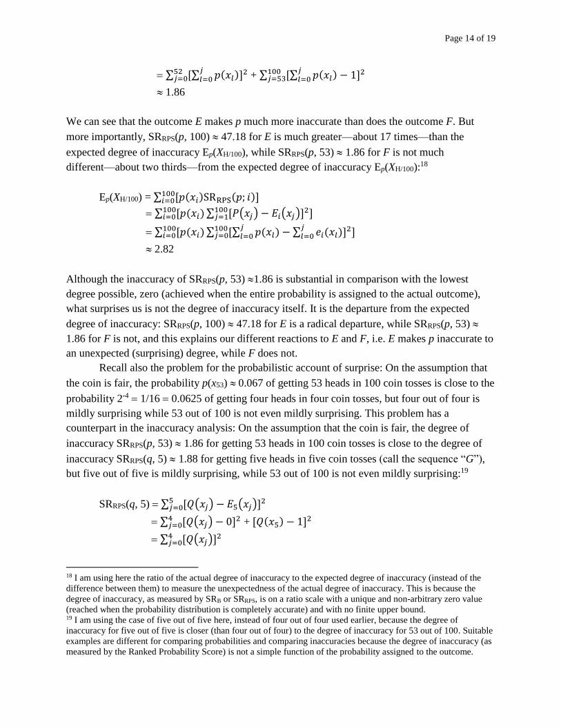
1.86
We can see that the outcome E makes p much more inaccurate than does the outcome F. But
more importantly, SRRPS(p, 100) 47.18 for E is much greater—about 17 times—than the
expected degree of inaccuracy Ep(XH/100), while SRRPS(p, 53) 1.86 for F is not much
different—about two thirds—from the expected degree of inaccuracy Ep(XH/100):18
Ep(XH/100) = ∑ [𝑝(𝑥𝑖)SRRPS(𝑝; 𝑖)]100𝑖=0
∑ [𝑝(𝑥𝑖) ∑ [𝑃(𝑥𝑗) − 𝐸𝑖(𝑥𝑗)]2100𝑗=1
100𝑖=0 ]
∑ [𝑝(𝑥𝑖) ∑ [∑ 𝑝(𝑥𝑙𝑗𝑙=0 ) − ∑ 𝑒𝑖(𝑥𝑙
𝑗𝑙=0 )]2100
𝑗=0100𝑖=0 ]
2.82
Although the inaccuracy of SRRPS(p, 53) 1.86 is substantial in comparison with the lowest
degree possible, zero (achieved when the entire probability is assigned to the actual outcome),
what surprises us is not the degree of inaccuracy itself. It is the departure from the expected
degree of inaccuracy: SRRPS(p, 100) 47.18 for E is a radical departure, while SRRPS(p, 53)
1.86 for F is not, and this explains our different reactions to E and F, i.e. E makes p inaccurate to
an unexpected (surprising) degree, while F does not.
Recall also the problem for the probabilistic account of surprise: On the assumption that
the coin is fair, the probability p(x53) 0.067 of getting 53 heads in 100 coin tosses is close to the
probability 2-4 1/16 0.0625 of getting four heads in four coin tosses, but four out of four is
mildly surprising while 53 out of 100 is not even mildly surprising. This problem has a
counterpart in the inaccuracy analysis: On the assumption that the coin is fair, the degree of
inaccuracy SRRPS(p, 53) 1.86 for getting 53 heads in 100 coin tosses is close to the degree of
inaccuracy SRRPS(q, 5) 1.88 for getting five heads in five coin tosses (call the sequence “G”),
but five out of five is mildly surprising, while 53 out of 100 is not even mildly surprising:19
SRRPS(q, 5) ∑ [𝑄(𝑥𝑗) − 𝐸5(𝑥𝑗)]25𝑗=0
∑ [𝑄(𝑥𝑗) − 0]24𝑗=0 + [𝑄(𝑥5) − 1]2
∑ [𝑄(𝑥𝑗)]24𝑗=0
18 I am using here the ratio of the actual degree of inaccuracy to the expected degree of inaccuracy (instead of the
difference between them) to measure the unexpectedness of the actual degree of inaccuracy. This is because the
degree of inaccuracy, as measured by SRB or SRRPS, is on a ratio scale with a unique and non-arbitrary zero value
(reached when the probability distribution is completely accurate) and with no finite upper bound. 19 I am using the case of five out of five here, instead of four out of four used earlier, because the degree of
inaccuracy for five out of five is closer (than four out of four) to the degree of inaccuracy for 53 out of 100. Suitable
examples are different for comparing probabilities and comparing inaccuracies because the degree of inaccuracy (as
measured by the Ranked Probability Score) is not a simple function of the probability assigned to the outcome.

Page 15 of 19
∑ [∑ 𝑞(𝑗𝑙=0 𝑥𝑙)]24
𝑗=0
1.88
The reason for our different reactions is the expected degree of inaccuracy. In general, as the
number n of coin tosses increases and the size n + 1 of the partition XH/n {x0, …, xn} by H-
ratios becomes larger, the expected inaccuracy of the default probability distribution becomes
greater. As noted above, the degree of inaccuracy SRRPS(p, 53) 1.86 for getting 53 heads in 100
coin tosses (as in F) is close to the expected inaccuracy of p over XH/100 {x0, …, x100}, but the
similar degree of inaccuracy SRRPS(q, 5) 1.88 for getting five heads in 5 coin tosses (as in G) is
noticeably greater—roughly three times—than the expected inaccuracy Eq(XH/5) 0.62 of q over
XH/5 {x0, …, x5}:
Eq(XH/5) = ∑ [𝑞(𝑥𝑖)RPS(𝑞; 𝑖)]5𝑖=0
∑ [𝑞(𝑥𝑖) ∑ [𝑄(𝑥𝑗) − 𝐸𝑖(𝑥𝑗)]25𝑗=0
5𝑖=0 ]
∑ [𝑞(𝑥𝑖) ∑ [∑ 𝑞(𝑥𝑙𝑗𝑙=0 ) − ∑ 𝑒𝑖(𝑥𝑙
𝑗𝑙=0 )]25
𝑗=05𝑖=0 ]
0.62
The noticeable—but not drastic—departure from the expected inaccuracy explains why G is
mildly surprising.
I want to mention one more case of coin tosses to underscore a distinctive feature of the
present analysis. The analysis of surprise by an unexpected degree of inaccuracy draws on an
often underappreciated aspect of a probabilistic estimate, viz. it is normal (expected) that the
actual frequency ratio in the data is different from the best estimate based on the correct
probability distribution. For example, even if the coin is completely fair and thus the probability
of obtaining heads is exactly one half, it is normal that the actual number of heads in 100 coin
tosses is not 50 because of random variation (“noise”). So, we are not surprised at 53 heads out
of 100. The outcome is surprising when—and only when—the degree of inaccuracy is
unexpected. Note here that the degree of inaccuracy can be unexpected in two ways, i.e. it may
be more than expected or it may be less than expected. Indeed, we are surprised when the H-ratio
of a long sequence of coin tosses is exactly even (call such a sequence “H”), e.g. obtaining
exactly 50 heads out of 100 tosses, exactly 5,000 heads out of 10,000 tosses, exactly 500,000
heads out 1,000,000 tosses, etc. Given the default assumption that the coin is fair, why are we
surprised when the H-ratio is exactly even? My analysis provides a sensible answer, viz. these
outcomes make the default probability distribution noticeably more accurate than expected—it
looks too good to be true—and we suspect a possible manipulation of some kind.20 For example,
20 The exact H-ratio of one half (more generally, the exact match between the probability and the observed
frequency ratio) looks particularly suspect for two reasons. First, it makes the degree of accuracy not just better than
expected, but the best possible. The second reason is the possible explanation of the exact match by manipulation.
As Horwich points out (see Section 2 above), the recognition of a possible alternative explanation shakes our

Page 16 of 19
when we obtain 50 heads out of 100 coin tosses, the actual degree of inaccuracy is SRRPS(p; e50)
1.16, which is noticeably less than the expected degree of inaccuracy ∑ [𝑝(𝑥𝑖)SRRPS(𝑝; 𝑖)]100𝑖=0
2.82. The departure from the expected degree of inaccuracy becomes greater as the number of
coin tosses increases and the H-ratio is still exactly even. The case reveals a significant
advantage of the new analysis over the probabilistic account: It is hard to explain in probabilistic
terms why the H-ratio of exactly one half is surprising given that it is the most probable H-ratio
based on the default assumption that the coin is fair.21
Here is a summary of the analyses of the four coin toss cases. The outcome E (100 heads
out of 100) is extremely surprising because the outcome E makes the default probability
distribution p over XH/100 {x0, …, x100} much more inaccurate than expected. In contrast, the
outcome F (53 heads out of 100) is not even mildly surprising because the outcome F makes the
default probability distribution p over XH/100 {x0, …, x100} roughly as inaccurate as expected.
The outcome G (five heads out of five) is mildly surprising because the outcome G makes the
default probability distribution q over XH/5 {x0, …, x5} noticeably more inaccurate than
expected, though not to the same extent as E does for p over XH/100 {x0, …, x100}. Finally, the
outcome H (exactly one half of a very large number of coin tosses are heads) is surprising
because H makes the default probability distribution noticeably more accurate than expected.
The general point is the same as before: We are surprised at an outcome (surprise is an
understandable response) when—and only when—the outcome makes the default probability
distribution over the salient partition inaccurate to an unexpected degree (noticeably higher or
noticeably lower), and the degree of surprise is proportional to the degree of unexpectedness.
6. Conclusion
This paper proposed a new analysis of surprise formulated in terms of inaccuracy, or proximity
to the truth. I want to conclude with brief remarks on the broader context of the proposal. It is
now common in epistemology to aim at the probable truth instead of absolute certainty, but even
this modest goal is often unachievable when it comes to quantitative hypotheses. Where there are
numerous quantities to choose from and in the absence of unusually favorable circumstances, we
do not expect the estimated quantity, such as 50 heads out of 100 coin tosses, to be the true
confidence in the default assumption. When the H-ratio is close to one half, but not exactly one half, the possible
explanation of the departure from the expectation is less obvious. 21 This point is consistent with the fact that the most probable outcome is unsurprising in many cases. It is true that
the most probable member of a non-ranked partition (to set aside the additional complication for a ranked partition)
makes the probability distribution the least inaccurate, and thus makes the degree of inaccuracy less than expected.
Note, however, that the probability distribution plays two roles. It determines the degree of inaccuracy SR(p, i) for
the outcome xi, but it also determines the weights for calculating the expected inaccuracy. Since the most probable
member receives the greatest weight, the expected inaccuracy is pulled closer to its degree of inaccuracy. In order
for the most probable outcome to be surprising, the partition must consist of many members and the outcome in
question must not be so probable as to pull the expected inaccuracy close to its degree of inaccuracy.

Page 17 of 19
outcome or even probably the true outcome. We are content if the false estimate is close to the
truth. Our realistic alethic goal in such cases is proximity to the truth, and not the probable truth.
This is seemingly in contrast to a case where the outcomes are qualitative and not ranked,
so that no distance is defined among the outcomes. We cannot seek proximity to the truth where
there is no distance defined among the outcomes to begin with. However, once we assign
probabilities to qualitative and non-ranked outcomes, as is common, we can again seek
proximity to the truth because probabilities are quantities. This is easy to see when the
probability assigned is an estimate of the frequency ratio, viz. given the actual frequency ratio,
we can measure the inaccuracy of the assigned probability by its proximity to the actual
frequency ratio. Further, even when the probability is assigned to a single qualitative outcome,
we can still measure the inaccuracy of the assigned probability given the actual outcome. If, for
example, different prior probabilities 0.4 and 0.7 are assigned to the true qualitative outcome, the
latter is closer to the truth than is the former. So, we can evaluate the probability assignment in
general by its proximity to the true outcome.22
The analysis of surprise proposed in this paper is guided by the idea of evaluating the
hypothesis by proximity to the truth, and draws specifically on the point that even the correct
probability assignment is expected to be inaccurate with regard to the actual outcome due to
random variation. It is therefore when—and only when—the degree of inaccuracy is noticeably
different from the expectation that we are surprised at the outcome. A high degree of inaccuracy
as such does not surprise us if that is expected, while a low degree of inaccuracy may surprise us
if it is noticeably lower than expected. When some puzzle resists the probabilistic analysis, it is
worthwhile to see the issue from the perspective of proximity to the truth.23
Acknowledgments Precursors of this paper were presented at Chinese Academy of Social Sciences,
Rhode Island College, the University of Turin, and the University of Groningen. I would like to thank the
audiences at these institutions for valuable comments. I would also like to thank Matt Duncan and
William Roche for carefully reading an earlier version and making many suggestions for improvement.
References
Baras, D. (2019) Why do certain states of affairs call out for explanation? A critique of two
Horwichian accounts. Philosophia 47(5), 1405-1419.
22 These are all cases of the ex post evaluation of the hypothesis based on the actual outcome, but we can extend the
idea to ex ante evaluation: We may seek to minimize the estimated inaccuracy of the hypothesis in the ex ante
selection of a probabilistic hypothesis. This is a familiar theme in statistical learning theory (see Burnham &
Anderson 2002 for an overview). 23 There is the proposal of the “accuracy first” approach (Leitgeb & Pettigrew 2010a, 2010b; Pettigrew 2016) to use
accuracy as the ground for the basic principles of the probability calculus, but what I have in mind here is the use of
proximity to the truth in solving some puzzles in epistemology and philosophy of science. See Shogenji (2018) for
an instance of such attempts.
Page 18 of 19
Burnham, K. P., & Anderson, D. R. (2002). Model Selection and Multimodel Inference: A
Practical Information-Theoretic Approach. New York: Springer.
Crupi, V., & Tentori, K. (2012). A second look at the logic of explanatory power (with two novel
representation theorems). Philosophy of Science, 79(3), 365-385.
Gneiting, T., & Raftery, A. E. (2007). Strictly proper scoring rules, prediction, and estimation.
Journal of the American Statistical Association, 102(477), 359-378.
Good, I. J. (1984). A Bayesian approach in the philosophy of inference. British Journal for the
Philosophy of Science, 35(2), 161-173.
Harker, D. (2012). A surprise for Horwich (and some advocates of the fine-tuning argument
(which does not include Horwich (as far as I know))). Philosophical Studies, 161(2), 247-
261.
Horwich, P. (1982). Probability and Evidence. Cambridge: Cambridge University Press.
Landy, D., Silbert, N., & Goldin, A. (2013). Estimating large numbers. Cognitive Science, 37(5),
775-799.
Leitgeb, H., & Pettigrew, R. (2010a). An objective justification of Bayesianism I: Measuring
inaccuracy. Philosophy of Science, 77(2), 201-235.
Leitgeb, H., & Pettigrew, R. (2010b). An objective justification of Bayesianism II: The
consequences of minimizing inaccuracy. Philosophy of Science, 77(2), 236-272.
Levinstain, B. A. (2012). Leitgeb and Pettigrew on accuracy and updating. Philosophy of
Science, 79(3), 413-424.
Manson, N. A., & Thrush, M. J. (2003). Fine-tuning, multiple universes, and the "This Universe"
objection. Pacific Philosophical Quarterly, 84(1), 67-83.
McGrew, T. (2003). Confirmation, heuristics, and explanatory reasoning. The British Journal for
the Philosophy of Science, 54(4), 553-567.
Miller, D. (1974). Popper's qualitative theory of verisimilitude. British Journal for the
Philosophy of Science, 25(2), 166-177.
Oddie, G. (2016). Truthlikeness. Retrieved from Stanford Encyclopedia of Philosophy:
https://plato.stanford.edu/archives/win2016/entries/truthlikeness/
Olsson, E. (2002). Corroborating testimony, probability and surprise. British Journal for the
Philosophy of Science, 53(2), 273–288.
Peirce, C. S. (1931-35). The Collected Papers of Charles Sanders Peirce (Vols. 1-6). (C.
Hartshorne, & P. Weiss, Eds.) Cambridge MA: Harvard University Press.
Pettigrew, R. (2016). Accuracy and the Laws of Credence. Oxford: Oxford University Press.
Popper, K. (1963). Conjectures and Refutations. London: Routledge.
Roche, W., & Shogenji, T. (2018). Information and Inaccuracy. British Journal for the
Philosophy of Science, 69(2), 577-604.
Schlesinger, G. (1991). The Sweep of Probability. Notre Dame: University of Notre Dame Press.
Schupbach, J. N., & Sprenger, J. (2011). The logic of explanatory power. Philosophy of Science,
78(1), 105-127.
Shogenji, T. (2018). Formal Epistemology and Cartesan Skepticism: In Defense of Belief in the
Natural World. Abingdon: Routledge.
Tichý, P. (1974). On Popper's definitions of verisimilitude. The British Journal for the
Philosophy of Science, 25, 155-160.

Page 19 of 19
Tversky, A., & Kahneman, D. (1974). Judgment under uncertainty: heuristics and biases.
Science, 185, 1124-1131.
White, R. (2000). Fine-tuning and multiple universes. Noûs, 34(2), 260–276.
Winkler, R. L., & Jose, V. R. (2010). Scoring Rules. In J. J. Cochran (Ed.), Wiley Encychopedia
of Operations Research and Management Science. Hoboken NJ: John Wiley & Sons.