título - brazil - UNIA

TÍTULOBRAZIL

A POSSIBLE SYMBIOTIC RELATIONSHIP BETWEEN THEEVOLUTION OF CARBON EMISSIONS, ENERGY CONSUMPTION

AND ECONOMIC GROWTH

AUTORAErika Reesink Cerski

Esta edición electrónica ha sido realizada en 2017Tutores PhD. José Enrique García Ramos ; PhD. Ángel Mena Nieto

Instituciones Universidad Internacional de Andalucía ; Universidad de HuelvaCurso Máster Oficial Interuniversitario en Tecnología AmbientalISBN 978-84-7993-765-2 Erika Reesink Cerski De esta edición: Universidad Internacional de Andalucía

Fechadocumento 2016

Universidad Internacional de Andalucía, 2017

Reconocimiento-No comercial-Sin obras derivadas

Usted es libre de: Copiar, distribuir y comunicar públicamente la obra.

Bajo las condiciones siguientes:

Reconocimiento. Debe reconocer los créditos de la obra de la manera. especificadapor el autor o el licenciador (pero no de una manera que sugiera que tiene su apoyo o apoyan el uso que hace de su obra).

No comercial. No puede utilizar esta obra para fines comerciales.

Sin obras derivadas. No se puede alterar, transformar o generar una obra derivada a partir de esta obra.

Al reutilizar o distribuir la obra, tiene que dejar bien claro los términos de la licencia de esta obra.

Alguna de estas condiciones puede no aplicarse si se obtiene el permiso del titular de los derechos de autor.

Nada en esta licencia menoscaba o restringe los derechos morales del autor.


1

THE INTERNATIONAL UNIVERSITY OF ANDALUCIA

THE UNIVERSITY OF HUELVA

BRAZIL: A POSSIBLE SYMBIOTIC RELATIONSHIP BETWEEN THE

EVOLUTION OF CARBON EMISSIONS, ENERGY CONSUMPTION AND

ECONOMIC GROWTH.

MASTER THESIS PRESENTED BY

ERIKA REESINK CERSKI IN THE POSTGRADUATE PROGRAM IN ENVIRONMENTAL TECHNOLOGY

ADVISORS

PhD. JOSÉ ENRIQUE GARCÍA RAMOS PhD. ÁNGEL MENA NIETO

December, 2016.


2

“Scientific evidence for warming of the climate system is unequivocal,

there is 95 percent confidence that humans are the main cause of the

current global warming”.

- Intergovernmental Panel on Climate Change

"La evidencia científica para el calentamiento del sistema climático es

inequívoca, hay 95 por ciento de confianza que los seres humanos son la

principal causa del calentamiento global actual".

- Grupo Intergubernamental de Expertos sobre el Cambio Climático


3

Acknowledgments

I would like to thank my advisors, José Enrique García Ramos and Ángel Mena Nieto,

whose work showed me that concern for environmental affairs, supported by an

“engagement” in literature and technology, should always consider an interaction of

not only environmental, but also social, economic, political and cultural factors in

order to provide alternatives for our times.

I would also like to thank Fundación Carolina for their financial support granted to

Latin America students, which allowed me to have this stunning experience of taking

my Master’s at both the International University of Andalucia (UNIA) and the

University of Huelva (UHU).

Furthermore, I would like to thank the city of Huelva, especially La Rabida, for its warm

and friendly welcome. And for giving me the opportunity to make friends and share

experiences, which I will take with me for the rest of my life.

And last but not least, I would like to thank my loved ones who have supported me

throughout this entire process. I will be forever grateful for their love.


4

ABSTRACT

In December 2015, 195 countries adopted the first-ever legally binding global

climate deal at Paris Climate Conference (COP21), known as Paris Agreement.

Although, the agreement entered into force on November 4th in 2016, it sets out a

global action plan to avoid risky climate change by limiting global warming less than to

2°C in the long term. In the Paris Agreement, Brazil plays a crucial role due to the fact

that it has the ninth largest economy in the world, an important relationship with its

neighbors in South America, a population exceeding 200 million people, and covers

practically the entire Amazon Rainforest. These are some of the reasons that explain

why Brazil has pledged to cut down greenhouse gases (GHG) emissions by 37 per cent

by 2025, and 43 per cent by 2030, compared to 2005 levels.

The development of a country, especially Brazil, requires appropriate and

realistic policies to current and changing demands. In this way, it is fundamental to

achieve not only a secure but also a consistent environmental planning for the energy

sector and GDP growth. Within this context, this study proposes a model of economic

growth, carbon emissions and sustainable development for Brazil.

This work applies to the period 1971-2030, using the methodology proposed by

Robalino-López (2014), based on a GDP formation approach, which includes the effect

of renewable energies. A historical data, from 1971 to 2012, and a forecast period of

18 years have been considered for testing four different economic scenarios. Our

predictions show that the scenario which corresponds to a heavy GDP increase can

have the same value of CO2 emissions as a scenario in which the GDP increases

modestly if appropriate changes in the renewable energy and energy intensity are

promoted. The final conclusion of this work suggests that Brazil goals at the COP21 are

extremely ambitious, and it is likely the Brazilian targets will not be achieved. In any

case, the Brazilian mitigation program for carbon emissions should be continued to

benefit everyone.


5

RESUMEN

En diciembre de 2015, 195 países adoptaron un acuerdo climático universal y

jurídicamente vinculante en Paris, conocido como Acuerdo de París sobre Cambio

Climático y que nació en la Conferencia del Clima de París (COP21), aunque no ha

entrado en vigor hasta el 4 de noviembre de 2016. El acuerdo establece un plan de

acción global para evitar el peligroso Cambio Climático, y limita el calentamiento global

por debajo de 2°C. Brasil tiene un papel crucial en el Acuerdo de París, pues es la

novena economía del mundo, tiene una importante relación con sus países vecinos en

América del Sur, tiene una población actual de 200,4 millones de personas y cubre casi

toda la Amazonía. Estas son algunas de las razones que explican por qué Brasil se ha

comprometido a reducir las emisiones de gases de efecto invernadero en un 37 por

ciento en 2025, y en un 43 por ciento en 2030, en comparación con los niveles de

2005. El desarrollo de un país, especialmente del Brasil, requiere políticas adecuadas y

realistas a las demandas actuales y futuras. De esta manera, es fundamental tener una

planificación segura y consistente, pero también ecológica para el sector energético y

el crecimiento del PIB.

Dentro de este contexto, el presente estudio propone un modelo que englobe

el crecimiento económico, las emisiones de carbono y el desarrollo sostenible de

Brasil. Este trabajo analiza el período 1971-2030, utilizando la metodología propuesta

por Robalino-López (2014), para estudiar el efecto del uso de las energías renovables

sobre la formación del PIB. Un período histórico de 1971 a 2012 y una previsión de 18

años han sido considerados en la prueba de cuatro diferentes escenarios económicos y

energéticos. Nuestras predicciones muestran que el escenario que corresponde a un

fuerte aumento del PIB puede tener el mismo valor de emisiones de CO2 que un

escenario en que el PIB crezca moderadamente si se promueven los cambios

apropiados en el uso de energía renovable y en la intensidad energética. La conclusión

final de este trabajo sugiere que las metas de reducción de carbono presentadas por

Brasil en la COP21 son muy ambiciosas y probablemente no serán alcanzadas. En

cualquier caso, el programa brasileño de mitigación de emisiones de carbono debe

continuar en beneficio de todos.


6

List of Figures

Figure 1. Schematic plot of the relationship between the GDP per capita (pc) and the CO2

emission per capita: (1) linear growth of the emission, (2) stabilization, and (3) reduction of the

CO2 emission as the income increases ........................................................................................ 11

Figure 2. Causal diagram of the model. Continuous lines stand for the relationship between

variables, while dashed ones correspond to control terms(S: productive sectoral structure, M:

energy matrix, U: emission factors). Bold line represents a feedback mechanism.. .................. 25

Figure 3. Domestic electricity supply by source .......................................................................... 31

Figure 4. Domestic electricity supply by sector. ......................................................................... 32

Figure 5. Domestic energy supply in 2014. ................................................................................ 34

Figure 6. Evolution of the domestic energy supply structure. .................................................... 35

Figure 7. GDP official and predicted data. .................................................................................. 49

Figure 8. Fossil energy official and predicted data. .................................................................... 50

Figure 9. Renewable energy official and predicted data. ........................................................... 50

Figure 10.Total energy official and predicted data. .................................................................... 50

Figure 11.CO2 emissions official and predicted data. ................................................................. 51

Figure 12. GDP of Brazil for the period 1971-2011. .................................................................... 53

Figure 13. GDP of Brazil for the period 2010-2030. .................................................................... 53

Figure 14. Total energy consumption of Brazil for the period 1971-2011 .................................. 54

Figure 15. Total energy consumption of Brazil for the period 2010-2030. ................................ 55

Figure 16. Fossil energy consumption of Brazil for the period 1971-2030. ................................ 55

Figure 17. Renewable energy consumption of Brazil for the period 1971-2030. ....................... 56

Figure 18. Energy consumption of Brazilian primary sector for the BS and SC-2 scenarios during

the period 2000-2030.................................................................................................................. 56

Figure 19. Energy consumption of Brazilian primary sector for the SC-3 and SC-4 scenarios

during the period 2000-2030. ..................................................................................................... 57

Figure 20. Energy consumption of Brazilian manufacturing sector for the BS and SC-2 scenarios


Figure 21. Energy consumption of Brazilian manufacturing sector for the SC-3 and SC-4

scenarios during the period 2000-2030. ..................................................................................... 58

Figure 22. Energy consumption of Brazilian energetic sector for the BS and SC-2 scenarios


Figure 23. Energy consumption of Brazilian energetic sector for the SC-3 and SC-4 scenarios


Figure 24. Energy consumption of Brazilian tertiary sector for the BS and SC-2 scenarios during

the period 2000-2030.................................................................................................................. 60

Figure 25. Energy consumption of Brazilian tertiary sector for the SC-3 and SC-4 scenarios


Figure 26. The Brazilian energy consumption by seven types of fuels according to the four

scenarios during the period 2010-2030. The types of energy are: natural gas (E1), liquefied

petroleum gases (E2), motor gasoline (E3), gas/diesel oil (E4), fuel oil (E5), petroleum coke (E6)

and renewable, alternative and nuclear (E7). ........................................................................... 62


7

Figure 27. Brazilian energy consumption of natural gas for the four scenarios for the period

2010-2030. .................................................................................................................................. 62

Figure 28. Brazilian energy consumption of liquefied petroleum gases for the four scenarios for

the period 2010-2030.................................................................................................................. 63

Figure 29. Brazilian energy consumption of motor gasoline for the four scenarios for the period

2010-2030. .................................................................................................................................. 63

Figure 30. Brazilian energy consumption of gas/diesel oil for the four scenarios for the period

2010-2030. .................................................................................................................................. 64

Figure 31. Brazilian energy consumption of fuel oil for the four scenarios for the period 2010-

2030. ............................................................................................................................................ 64

Figure 32. Brazilian energy consumption of petroleum coke for the four scenarios for the

period 2010-2030. ....................................................................................................................... 65

Figure 33. Brazilian consumption of renewable, alternative and nuclear energies for the four

scenarios for the period 2010-2030. ........................................................................................... 66

Figure 34. CO2 emissions of Brazil for the period 1971-2011. .................................................... 67

Figure 35. CO2 emissions of Brazil for the period 2010-2030. .................................................... 67

List of Tables

Table 1. Summary of recent studies that analyzed the GDP growh-energy-CO2 relationship. ... 14

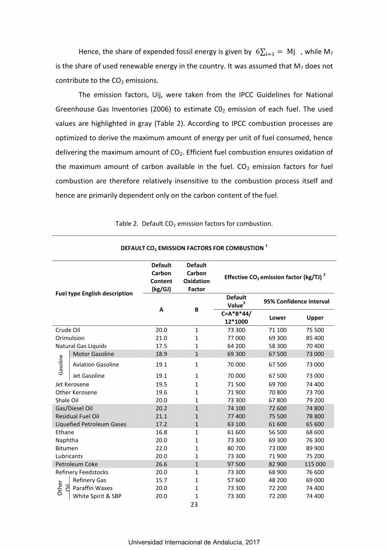
Table 2. Default CO2 emission factors for combustion. ............................................................. 23

Table 3. Brazilian total population from 2000 to 2060. ............................................................. 29

Table 4. Domestic energy supply from 2005 to 2014 ................................................................. 34

Table 5. Brazilian general data. ................................................................................................... 38

Table 6. Brazilian general data. Part II......................................................................................... 39

Table 7. Information about Brazilian agriculture sector. ............................................................ 40

Table 8. Information about Brazilian manufacturing sector. ...................................................... 41

Table 9. Information about Brazilian energetic sector. .............................................................. 42

Table 10. Information about Brazilian tertiary sector. ................................................................ 43

Table 11. Energy by type of fuels in agriculture sector. .............................................................. 44

Table 12. Energy by type of fuels in imanufacturing sector. ....................................................... 45

Table 13. Energy by type of fuels in energetic sector. ................................................................ 46

Table 14. Energy by type of fuels in tertiary sector. ................................................................... 47

Table 15. MAPE values for the main variables of the model. .................................................... 49


8

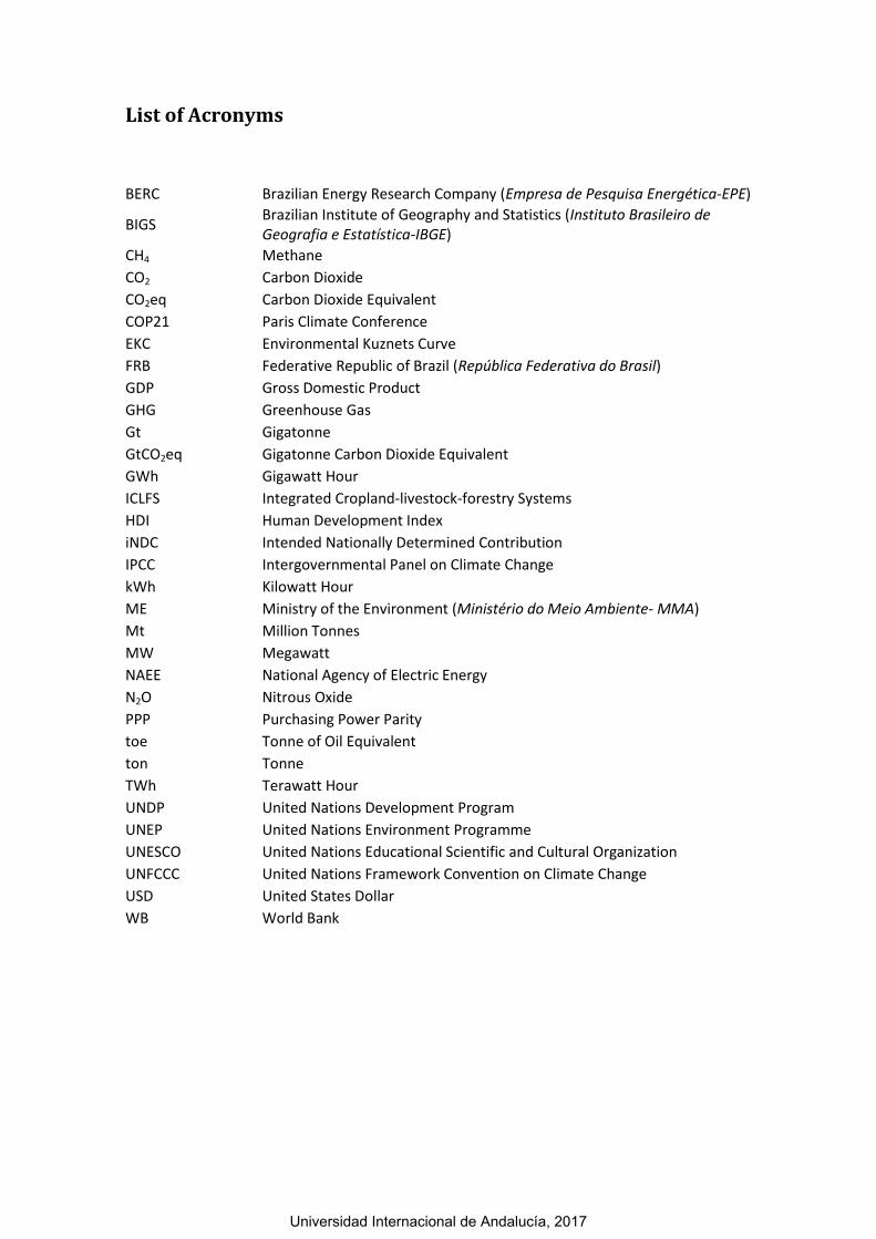
List of Acronyms

BERC Brazilian Energy Research Company (Empresa de Pesquisa Energética-EPE)

BIGS Brazilian Institute of Geography and Statistics (Instituto Brasileiro de Geografia e Estatística-IBGE)

CH4 Methane

CO2 Carbon Dioxide

CO2eq Carbon Dioxide Equivalent

COP21 Paris Climate Conference

EKC Environmental Kuznets Curve

FRB Federative Republic of Brazil (República Federativa do Brasil)

GDP Gross Domestic Product

GHG Greenhouse Gas

Gt Gigatonne

GtCO2eq Gigatonne Carbon Dioxide Equivalent

GWh Gigawatt Hour

ICLFS Integrated Cropland-livestock-forestry Systems

HDI Human Development Index

iNDC Intended Nationally Determined Contribution

IPCC Intergovernmental Panel on Climate Change

kWh Kilowatt Hour

ME Ministry of the Environment (Ministério do Meio Ambiente- MMA)

Mt Million Tonnes

MW Megawatt

NAEE National Agency of Electric Energy

N2O Nitrous Oxide

PPP Purchasing Power Parity

toe Tonne of Oil Equivalent

ton Tonne

TWh Terawatt Hour

UNDP United Nations Development Program

UNEP United Nations Environment Programme

UNESCO United Nations Educational Scientific and Cultural Organization

UNFCCC United Nations Framework Convention on Climate Change

USD United States Dollar

WB World Bank


https://en.wikipedia.org/wiki/Tonne_of_oil_equivalent

9

CONTENTS

1. INTRODUCTION ............................................................................................................................... 10

1.1. The goals of this research ........................................................................................................ 13

2. LITERATURE REVIEW ....................................................................................................................... 14

3. MODEL AND METHODOLOGY ......................................................................................................... 19

3.1 Formulation of the model ......................................................................................................... 19

3.2 Economic submodel .................................................................................................................. 21

3.3 Energy consumption and productive sectoral structure submodel ......................................... 22

3.4 CO2 intensity and energy matrix submodel .............................................................................. 22

3.5 Model equations and causal diagram ....................................................................................... 25

3.6 Model validation and verification ............................................................................................. 26

4. RESULTS AND DISCUSSION .............................................................................................................. 28

4.1 Brazil in numbers ...................................................................................................................... 28

4.1.1 Overview ............................................................................................................................ 28

4.1.2. Economy ........................................................................................................................... 29

4.1.3 Energy analysis .................................................................................................................. 30

4.1.4 Forecasts for 2030 ............................................................................................................. 34

4.1.5. Brazil and the United Nations Framework Convention on Climate Change ..................... 36

4.1.6. Data ....................................................................................................................................... 38

Gross domestic product ............................................................................................................. 38

4.2 Estimates .................................................................................................................................. 49

4.2.1 MAPE ................................................................................................................................. 49

4.2.2 Scenarios ............................................................................................................................ 51

4.2.3 Economic estimates ........................................................................................................... 52

4.2.4 Energy estimates ............................................................................................................... 54

4.2.4.1 Total energy .................................................................................................................... 54

4.2.4.2 Energy by sector ............................................................................................................ 56

4.2.4.3 Energy by type of fuels .................................................................................................. 61

4.2.5 CO2 emissions ................................................................................................................... 66

4.2.4.1 Brazil and the COP21 ..................................................................................................... 68

5. CONCLUSIONS ................................................................................................................................ 69

6. REFERENCES .................................................................................................................................... 72

7. APPENDIX ........................................................................................................................................ 77


10

1. INTRODUCTION

According to Intergovernmental Panel on Climate Change (IPCC, 2014), despite

a growing number of climate change mitigation policies, annual greenhouse gas (GHG)

emissions grew on average by 1.0 gigatonne carbon dioxide equivalent (GtCO2eq)

(2.2%) per year from 2000 to 2010 compared to 0.4 GtCO2eq (1.3%) per year from

1970 to 2000. The highest anthropogenic GHG emissions in human history were from

2000 to 2010, which reached 49 (±4.5) GtCO2eq/yr in 2010. Besides, CO2 emissions

from fossil fuel combustion and industrial processes contributed about 78% of the

total GHG emission increase from 1970 to 2010. In addition, CO2 remained the major

anthropogenic GHG accounting for 76% of the total emissions in 2010, 16% coming

from methane (CH4), 6% from nitrous oxide (N2O), and 2% from fluorinated gases.

Globally, economic and population growth are continued to be the important

drivers in CO2 emissions derived from fossil fuel combustion. The contribution of

population growth between 2000 and 2010 remained similar to the previous three

decades, whereas the contribution of economic growth rose sharply. Anthropogenic

GHG emissions are mainly driven by population size, economic activity, lifestyle,

energy use, land use patterns, technology and climate policy (IPCC, 2014).

Several international organizations have been warning about the need of

stabilizing CO2 and other anthropogenic GHG emissions in order to avoid catastrophic

warming of the climatic system during this century. The adoption of environmentally

sustainable technologies, energy efficiency improvement, energy saving, forest

conservation, reforestation, or water conservation are the most effective ways to

address the climate change issue. As a result of it, 195 countries adopted the first-ever

legally binding global climate deal during the Paris Climate Conference (COP21), in

December 2015. The international agreement sets out a global action plan to avoid

dangerous climate changes by limiting global warming to well below 2°C. The

agreement is due in 2020.


11

Unfortunately, the economic growth, according to the environmental Kuznets

curve (EKC), in a first stage will also increase the CO2 emissions of the country. The EKC

reveals how a technically specified environmental quality measurement changes

according to the income of a country (see Figure 1).

Figure 1. Schematic plot of the relationship between the GDP per capita (pc) and the CO2

emission per capita: (1) linear growth of the emission, (2) stabilization, and (3) reduction of the CO2 emission as the income increases. Source: Robalino-López et al., 2014.

The name EKC or the inverted-U relationship comes from the work of Kuznets

who created an inverted-U relationship between income inequality and economic

development. The logic of EKC hypothesis follows the general intuition. In the first

stage of industrialization process, pollution grows rapidly because priority is given to

increase material output, and the economy is more interested in providing jobs and

income than keeping clean air and water (Dasgupta et al., 2002). The rapid growth due

to the industrialization process inevitably results in greater use of natural resources

and pollutant emission, which in turn put more pressure on the environment.

Countries under this situation, are too poor to afford for abatement, so they disregard

environmental growth consequences. In a later stage of industrialization, as income

rises, the government and people value the environment more, regulatory institutions

become more effective, green energy and energy efficiency are more frequent and

pollution level declines. Thus, EKC hypothesis posits a well-defined relationship


12

between level of economic activity and environmental pressure (defined as the level of

concentration of pollution or flow of emissions, depletion of resources, etc.).

The decomposition of changes in an aggregate environmental impact and of its

driving forces has become popular to unravel the relationship of society and economy

with the environment. The specific application in energy consumption and CO2

emissions is known as Kaya identity (Kaya, 1990 and Kaya et al., 1993). The Kaya

identity is a linking expression of factors that determine the level of human impact on

environment, in the form of CO2 emissions. It states that total emission level can be

expressed as the product of four inputs: population, GDP per capita, energy use per

unit of GDP, carbon emissions per unit of energy consumed. The Kaya identity plays a

core role in the development of future emissions scenarios in the IPCC Special Report

on Emissions Scenarios (IPCC, 2000). The scenarios set out a range of assumed

conditions for future development of each of the four inputs. Population growth

projections are available independently from demographic research; GDP per capita

trends are available from economic statistics and econometrics; similarly for energy

intensity and emission levels. The projected carbon emissions can drive carbon cycle

and climate models to predict future CO2 concentration and climate change.

The identification of these kinds of sources of CO2 emissions and of their

magnitude is essential information for economic planning and decision makers. As

Chien and Hu (2008) and Robalino-López et al. (2013, 2014) had shown the use of

renewable energy improves the CO2 efficient emission in relation to economic growth.

The proposal of the present work is to apply a model that links the GDP

formation and the use of renewable energy. The methodology was created by

Robalino-López et al. (2014) and was firstly applied to Ecuador (2013) and then to

Venezuela (2015); the present work applies the proposed methodology to Brazil.


13

1.1. The goals of this research

The general objective of this research is to estimate the CO2 emissions in Brazil

using and improving the Robalino-López (2014) methodology; the research also aims

to understand the driving forces that guide the emission process, such as economic

growth, energy use, energy structure mix, and fuel use in the productive sectors.

A multi-scenario approach is used to analyze the evolution of energy

consumption and energy-related emissions and its implications in the socio-economic

and environmental development of the study area.

This study could help the development and implementation of proactive

policies to the challenge of sustainable development. The application of scenario

analysis-modelling in the short-to-medium term is intended to develop insights into

plausible future changes with green goals in the driving forces of the national policies.

The specific research objectives are:

To study in details the way that changes in the energy matrix and in

gross domestic product (GDP) will affect CO2 emissions in the country.

To develop a set of integrated qualitative and quantitative baseline

scenarios at both macro and sectorial level to explore plausible

alternative development of income, energy use and CO2 emissions in a

medium term (2030) in Brazil.

To fill the gap in the literature of studies on the relationship between

emissions, energy consumption and income growth in Brazil.

This research is organized as follows: Literature Review; Model and

Methodology; Results and Discussion; and ends with Conclusions.


14

2. LITERATURE REVIEW

In this day and age, sustainable development it is a very popular topic. Many

countries, regardless to their economic situation, have been studying the relationship

between economic growth, energy consumption and CO2 emission. In the literature it

is possible to find many researches about this subject, as shown on Table 3, which

summarizes the set of references, analyzed in detail below. Notice that there are

different lines of research, some study the relationship between GDP and energy

consumption or GDP, energy and CO2 emissions, including the study of the causality

relationships; others study the different aspects of the EKC hypothesis; and finally,

there are also researches that use scenarios to be able to conduct forecast calculations

of CO2 emissions in forthcoming period.

Table 1. Summary of recent studies that analyzed the GDP growh-energy-CO2 relationship.

Author Relationship Region Methodology Period Outcomes

Padilla et al. CO2-GDP Groups of countries

Non-parametric estimations

1971-1999

GDP inequality → CO2 inequality

Kuntsi-Reunanen CO2-energy Selected Latin America

CO2 emission flows 1970-2001

No significant changes

Narayan and Narayan

CO2-GDP 43 developing countries

EKC analysis 1980-2004

35% of the countries show EKC evidences

Jaunky C02-energy-GDP

36 high-income countries

EKC analysis 1980-2005

GDP→CO2 EKC evidence found

Robalino-López et al.

CO2-energy-GDP

Ecuador System dynamics modeling and scenario analysis

1980-2025

Strong connection GDP-C02


CO2-energy-GDP

Ecuador System dynamics modeling and scenario analysis

1980-2025

EKC not fulfilled

Cowan et al. CO2-energy-GDP

BRICS countries Granger causality 1990-2010

Evidences of GDP → CO2

Ibrahim et al. CO2-GDP 69 countries GMM estimators 2000-2008

Mixed evidences

Al-mulali et al. Energy-GDP Latin America Cointegration, Granger causality

1980-2010

Long run relationship between renewable energy and GDP growth


CO2-energy-GDP

Venezuela System dynamics modeling and scenario analysis

1980-2025

GDP→CO2 CO2→ renewable sources EKC not fulfilled


CO2-energy-GDP

10 South America countries

Kaya I dentity 1980-2010

Relationship GDP→ C02

Zambrano-Monserrate et al.

CO2- GDP-energy

Brazil EKC analysis 1971-2011

EKC not fulfilled for short-run, but EKC fulfilled for long run.


15

Padilla et al. (2006) researched the inequality in C02 emissions across group of

countries and the relationship with the income inequality from 1971 to 1999. The

authors concluded that for an overwhelming majority of countries, higher per capita

income should be expected to be followed by higher emissions.

In 2007 Kuntsi-Reunanen studied a comparison of Latin America energy with

CO2 emissions from 1970 to 2001. The author inferred that the increase in CO2

emissions could be attributed partly to economic growth and to population growth.

Also, the structural shifts from a rural, predominantly agricultural economic base, to a

manufacturing one resulted in increasing energy demand. As Winkler et al. (2002)

affirmed the nature of the energy economy will strongly influence emissions per capita

of GDP. Kutsi as well concluded that since the developing countries will continue to

emphasize their manufacturing sectors, CO2 emissions can be expected to increase

unless energy efficiency is increased commensurably. While energy efficiency has

slightly improved in these countries, the improvement is considerably lower than

countries of the Organisation for Economic Co-operation and Development (OECD).

Most developing countries should be expected to increase their emissions to meet

human development needs at least in the next few decades.

Narayan and Narayan (2010) explored the carbon dioxide emissions and

economic growth from 43 developing countries in the period 1980 to 2004. A new

approach was employed. They propose that if the long-run elasticity is lower than the

short run elasticity, then this is also equivalent to lower carbon emissions as economic

growth occurs over time. With this methodology, they found that in 35% of the sample

the CO2 diminished in the long run, which confirms that these countries approach the

sloping down part of the EKC.

Jaunky (2011) attempted to examine the EKC hypothesis for 36 high income

countries over the period 1980–2005. The author applied the methodology proposed

by Narayan and Narayan (2010) and added several panel unit root and co-integration

tests. He detected unidirectional causality, running from GDP to CO2 emissions, in

short-run and long-run. In the long-run, CO2 emissions have fallen as income rises for

various countries.


16

Robalino-López et al. (2013, 2014) presented a model approach of CO2

emissions in Ecuador up to 2020 and also analyzed whether the EKC hypotheses holds

within the period 1980-2025 under four different scenarios. The main goal was studied

in detail the way the changes in the energy matrix and in the GDP would affect the CO2

emissions of the country. In particular, the effect of a reduction of the share of fossil

energy, as well as of an improvement in the efficiency of the fossil energy use. The

results do not supported the fulfillment of the EKC, nevertheless, its showed that it is

possible to control the CO2 emissions even under a scenario of continuous increase of

the GDP, if it is combined with an increase of the use of renewable energy, with an

improvement of the productive sectoral structure and with the use of a more efficient

fossil fuel technology.

Cowan et al., in 2014, studied the nexus of electricity consumption, economic

growth and CO2 emissions in the BRICS countries from 1990 to 2010. The results

suggest that the existence and direction of Granger causality differ among the

different BRICS countries. The main recommendation for these countries in general is

to increase investment in electricity infrastructure. Because, this will expand electricity

production capabilities in order to keep up with supply, while at the same time

improving electricity efficiency. This will result in higher levels of electricity production

and lower levels of CO2 emissions.

However, in terms of Brazil, Cowan et al. (2014) concluded that no evidence of

causality running in any direction between electricity consumption and economic

growth is found, thus supporting the neutrality hypothesis. Similarly, no causality was

found to exist between electricity consumption and CO2 emissions. This result makes

sense as electricity only accounts for a marginal amount of Brazil's total GHG

emissions, the majority coming from land usage. This relatively small contribution

made by the electricity sector may also be a result of increasing levels of infrastructure

and the use of renewable energy sources, particularly hydroelectricity in Brazil. With

respect to the CO2 emissions—economic growth nexus, causality was found to run

from CO2 emissions to economic growth. This result may be due to the rapid and large-

scale deforestation of the Amazon rain forest. This deforestation is being done in order

to increase the area available for agriculture and human settlement. The increased in


17

agriculture and the resulting employment have helped to increase economic growth

but at the expense of raising CO2 levels, not just in Brazil, but globally.

Ibrahim and Law (2014) examined the mitigating effect of social capital on the

EKC for CO2 emissions using a panel data of 69 developed and developing countries.

Adopting generalized method of moments (GMM) estimators, they found evidence

substantiating the presence of EKC. Moreover, the authors suggest that the pollution

costs of economic development tend to be lower in countries with higher social capital

reservoir. In addition to policy focus on investments in environmentally friendly

technology and on the use of renewable energy, investments in social capital can also

mitigate the pollution effects of economic progress.

Al-mulali et al. (2014) investigated the impact of electricity consumption from

renewable and non-renewable sources on economic growth in 18 Latin American

countries between 1980 and 2010. It was found that economic growth, renewable

electricity consumption, non-renewable electricity consumption, gross fixed capital

formation, total labor force and total trade were cointegrated. In addition, the results

revealed that renewable electricity consumption, non-renewable electricity

consumption, gross fixed capital formation, total labor force, and total trade have a

long run positive effect on economic growth in the investigated countries. The most

important conclusion is that electricity consumption from renewable sources is more

effective in increasing the economic growth than the nonrenewable electricity

consumption in the investigated countries.

Robalino-López et al., in 2015, tested the case of Venezuela for the period

1980-2025, through a methodology based on an extension of Kaya identity and on a

GDP formation approach that includes the effect of renewable energies, the same that

will be used in this work. Also the authors experimented the EKC hypothesis under

different economic scenarios. The predictions showed that Venezuela does not fulfill

the EKC hypothesis, however, the country could be on the way to achieve

environmental stabilization in the medium term.

Later Robalino-López et al. (2016) analyzed the convergence process in CO2

emissions per capita from 1980 to 2010 based on the Kaya identity and in its

components, namely, GDP per capita, energy intensity, and CO2 intensity among 10


18

South American countries (Argentina, Bolivia, Brazil, Chile, Colombia, Ecuador, Peru,

Paraguay, Uruguay and Venezuela). They concluded that over these countries Brazil

has the highest GDP in the region reaching 1968 billion USD in 2010, and that Brazilian

industry is the most energy demanding sector of these countries. Furthermore, the

results show that energy intensity in South America is lower (136 kgoe/000 USD in

2010) than world average energy intensity (184 kgoe/000 USD). However, the CO2

intensity (CO2 over energy) in the region has remained relatively constant (2.2 kg

CO2/kgoe) during the analyzed period and always below the world average (2.5 kg

CO2/kgoe). In addition, the use of renewable energy is very heterogeneous in the

region. Indeed, the share of renewable and alternative energy in the total energy use is

(for the year 2010): 6.0% for Argentina, 2.5% for Bolivia, 14.7% for Brazil, 6.1% for

Chile, 11.1% for Colombia, 5.6% for Ecuador, 9.0% for Peru, 98.7% for Paraguay, 18.4%

for Uruguay and 8.8% for Venezuela. Finally, CO2 emission per capita in the region (2.3

tonnes) is much lower than the world average (4.3 tonnes). Venezuela is the country

with the highest CO2 emission per capita (6.2 tonnes), followed by Argentina (3.8

tonnes), Chile (3.0 tonnes), Ecuador (1.9 tonnes), Brazil, Colombia and Uruguay (1.6

tonnes each), Peru (1.2 tonnes), Bolivia (1.1 tonnes) and Paraguay (0.6 tonnes).

Zambrano-Monserrate et al. (2016) investigated the relationship between CO2

emissions, economic growth, energy use and electricity production by hydroelectric

sources in Brazil. They verified the EKC hypothesis using a time-series data for the

period 1971-2011. Empirical results find out that there is a quadratic long run

relationship between CO2 emissions and economic growth, confirming the existence of

an EKC for Brazil in the long run. Furthermore, energy use shows increasing effects on

emissions, while electricity production by hydropower sources has an inverse

relationship with environmental degradation. The short run model does not provide

evidence for the EKC theory. The difference between the results in the long and short

run could be related to the establishment of environmental policies.


19

3. MODEL AND METHODOLOGY

The methodology which was chosen to analyze the relationship between

carbon emissions, energy consumption and sustainable development in Brazil was

proposed by Robalino-López (2014) and will be explained in the next pages.

3.1 Formulation of the model

The authors projected a model which uses a variation of the Kaya identity,

where the amount of CO2 emissions can be studied quantifying the contributions of

five different factors:

Global industrial activity;

Industry activity mix;

Sectoral energy intensity;

Sectoral energy mix;

CO2 emission factors.

The CO2 emissions can be calculated as

𝐶 = ∑ 𝐶𝑖𝑗𝑖𝑗 = 𝑄 ∑𝑄𝑖

𝑄

𝐸𝑖

𝑄𝑖

𝐸𝑖𝑗

𝐸𝑖

𝐶𝑖𝑗

𝐸𝑖𝑗𝑖𝑗 = 𝑄 ∑ 𝑆𝑖. 𝐸𝐼𝑖. 𝑀𝑖𝑗. 𝑈𝑖𝑗𝑖𝑗 (1)

Where:

C - is the total CO2 emissions (in a given year)

Cij - is the CO2 emission arising from fuel type j in the productive sector i

Q - is the total GDP of the country

Qi - is the GDP generated by the productive sector i

Ei - is the energy consumption in the productive sector i

Eij - is the consumption of fuel j in the productive sector i

Si - is the share of sector i to the total GDP (Qi/Q)

EIi - is the energy intensity of sector i (Ei/Qi)


20

Mij - is the energy matrix (Eij/Ei)

Uij - is the CO2 emission factor (Cij/Eij)

i - index runs over the considered industrial sectors

j - index runs over the considered types of energy

It is also of interest to write up how to calculate the total energy in terms of the

GDP,

𝐸 = ∑ 𝐸𝑖𝑗𝑖𝑗 = 𝑄 ∑ 𝑆𝑖. 𝐸𝐼𝑖. 𝑀𝑖𝑗𝑖𝑗 (2)

And the expended energy of every kind of fuel,

𝐸𝑗 = 𝑄 ∑ 𝑆𝑖. 𝐸𝐼𝑖. 𝑀𝑖𝑗𝑖 (3)

The equation 1 is an extension of the Kaya identity because Robalino-López et

al. (2014) disaggregated in type of productive sector and kind of fuel used, while in the

original formulation only aggregated terms are considered: C, Q, and E.

Like Robalino-López et al. (2015) suggests the subsequent data analysis and the

preprocessing of the time series was performed using the Hodrick-Prescott (HP) filter

(1997), which allows isolation of outliers of the time series under study. After that, it is

possible to get the trend component of a time series and to perform more adequate

estimations.

The raw data to perform the model correspond to the official available data

based on Brazil, provided by the Word Bank and the Brazilian Energy Research

Company.

The simulation period extends from 1971 to 2030. The period of 1971-2012

(which corresponds to 31 years) was used to fix the parameters of the model and

2013-2030 (18 years) corresponds to the forecast period, under the assumption of

different scenarios concerning the evolution of the income, the evolution of the energy

mix, and the efficiency of the used technology.

As a convention for this work, the productive sector will be refer as i index and

the type of energy source like j index. It is important to highlight that the index I runs

over four sectors (1) Agriculture sector, (2) Industrial sector, (3) Energy sector and (4)


21

Services, residential and transportation sector. While the index j runs over seven type

of fuels, which are (1) natural gas, (2) liquefied petroleum gases, (3) motor gasoline, (4)

gas/diesel oil, (5) fuel oil, (6) petroleum coke and (7) renewable, alternative and

nuclear energy.

3.2 Economic submodel

This methodology presents a key point the explicit inclusion of the effect of

renewable energy on the GDP, allowing to establish a link between economic

indicators and CO2 emissions. Also this method considers that renewable energy can

increase GDP through substitution of the energy import which has direct and indirect

effects on increasing GDP and trade balance (Chien and Hu, 2008). The expenditure

approach to form the GDP is

𝑄 = 𝐶𝑎 + 𝐼 + 𝐺 + 𝑇𝐵 (4)

Where:

Ca - is the final household consumption expenditure

I - is the gross domestic capital formation

G - is the general government final consumption expenditure

TB - is the trade balance

However, there is a particular concern which it is important to highlight, the

variable G should be removed of the model estimation in order to avoid

multicollinearity. The system of the theoretical GDP formation model is composed of

the equation below

𝑄 = 𝑎1. 𝐼 + 𝑎2. 𝑇𝐵 + 𝑎3. 𝐶𝑎 + 𝑎4. 𝐸𝑖𝑚𝑝 + 𝑎5. 𝑅𝑁 + ∊1 (5)

Where:

𝐸𝑖𝑚𝑝 - is the energy import

RN - is the renewable energy


22

∊ - are residuals

𝑎1…𝑎5 - are the coefficients

The data used to calibrate the model corresponds to the period of 1971-2012

and was extracted from the official dataset of the country. In equation 5 the GDP is

positively influenced by consumption (𝑎3 = +7.882 10- 1), energy import (𝑎4= +1.728

10-2 $2005/koe) and renewable energies (𝑎5 = +6.698 10 $2005/koe), however, capital

formation (𝑎1= -5.309 10-1) and trade balance (𝑎2= -4.253 10-1) had a negatively

influenced.

3.3 Energy consumption and productive sectoral structure submodel

Energy consumption refers to the use of primary energy before transformation

into any other end-use energy, which is equal to the local production of energy plus

imports and stock changes, minus the exports and the amount of fuel supplied to ships

and aircrafts engaged in international transport. Energy intensity is defined as the ratio

of energy consumption and GDP.

3.4 CO2 intensity and energy matrix submodel

CO2 intensity of a given country corresponds to the ratio of CO2 emissions and

the total consumed energy written in terms of mass of oil equivalent.

𝐶𝑂2𝑖𝑛𝑡 =∑𝑖𝑗𝐶𝑖𝑗

∑𝑖𝑗𝐸𝑖𝑗 (6)

The value of the CO2int in a given year depend on the particular energy mix

during that year. Mij gives the energy matrix, but is more convenient to sum over the

different sectors and aggregate the fossil fuel contributions, therefore, it was defined

for each type of fuel (j=1 to 7).

𝑀𝑗 =∑𝑖𝐸𝑖𝑗

∑𝑖𝑗𝐸𝑖𝑗 (7)


23

Hence, the share of expended fossil energy is given by 6∑i=1 = Mj , while M7

is the share of used renewable energy in the country. It was assumed that M7 does not

contribute to the CO2 emissions.

The emission factors, Uij, were taken from the IPCC Guidelines for National

Greenhouse Gas Inventories (2006) to estimate C02 emission of each fuel. The used

values are highlighted in gray (Table 2). According to IPCC combustion processes are

optimized to derive the maximum amount of energy per unit of fuel consumed, hence

delivering the maximum amount of CO2. Efficient fuel combustion ensures oxidation of

the maximum amount of carbon available in the fuel. CO2 emission factors for fuel

combustion are therefore relatively insensitive to the combustion process itself and

hence are primarily dependent only on the carbon content of the fuel.

Table 2. Default CO2 emission factors for combustion.

DEFAULT CO2 EMISSION FACTORS FOR COMBUSTION

1

Fuel type English description

Default Carbon Content (kg/GJ)

Default Carbon

Oxidation Factor

Effective CO2 emission factor (kg/TJ) 2

A B

Default Value

3

95% Confidence Interval

C=A*B*44/ 12*1000

Lower Upper

Crude Oil 20.0 1 73 300 71 100 75 500 Orimulsion 21.0 1 77 000 69 300 85 400 Natural Gas Liquids 17.5 1 64 200 58 300 70 400

Gas

olin

e Motor Gasoline 18.9 1 69 300 67 500 73 000

Aviation Gasoline 19.1 1 70 000 67 500 73 000

Jet Gasoline 19.1 1 70 000 67 500 73 000

Jet Kerosene 19.5 1 71 500 69 700 74 400 Other Kerosene 19.6 1 71 900 70 800 73 700 Shale Oil 20.0 1 73 300 67 800 79 200 Gas/Diesel Oil 20.2 1 74 100 72 600 74 800 Residual Fuel Oil 21.1 1 77 400 75 500 78 800 Liquefied Petroleum Gases 17.2 1 63 100 61 600 65 600 Ethane 16.8 1 61 600 56 500 68 600 Naphtha 20.0 1 73 300 69 300 76 300 Bitumen 22.0 1 80 700 73 000 89 900 Lubricants 20.0 1 73 300 71 900 75 200 Petroleum Coke 26.6 1 97 500 82 900 115 000 Refinery Feedstocks 20.0 1 73 300 68 900 76 600

Oth

er

Oil

Refinery Gas 15.7 1 57 600 48 200 69 000 Paraffin Waxes 20.0 1 73 300 72 200 74 400 White Spirit & SBP 20.0 1 73 300 72 200 74 400


24

Other Petroleum Products 20.0 1 73 300 72 200 74 400 Anthracite 26.8 1 98 300 94 600 101 000 Coking Coal 25.8 1 94 600 87 300 101 000 Other Bituminous Coal 25.8 1 94 600 89 500 99 700 Sub-Bituminous Coal 26.2 1 96 100 92 800 100 000 Lignite 27.6 1 101 000 90 900 115 000 Oil Shale and Tar Sands 29.1 1 107 000 90 200 125 000 Brown Coal Briquettes 26.6 1 97 500 87 300 109 000 Patent Fuel 26.6 1 97 500 87 300 109 000

Co

ke Coke oven coke and

lignite Coke 29.2 1 107 000 95 700 119 000

Gas Coke 29.2 1 107 000 95 700 119 000 Coal Tar 22.0 1 80 700 68 200 95 300

Der

ived

Gas

es

Gas Works Gas 12.1 1 44 400 37 300 54 100 Coke Oven Gas 12.1 1 44 400 37 300 54 100 Blast Furnace Gas

4 70.8 1 260 000 219 000 308 000

Oxygen Steel Furnace Gas

5

49.6 1 182 000 145 000 202 000

Natural Gas 15.3 1 56 100 54 300 58 300 Municipal Wastes (non-biomass fraction)

25.0 1 91 700 73 300 121 000

Industrial Wastes 39.0 1 143 000 110 000 183 000 Waste Oil 20.0 1 73 300 72 200 74 400 Peat 28.9 1 106 000 100 000 108 000

Solid

Bio

fuel

s Wood/Wood Waste 30.5 1 112 000 95 000 132 000 Sulphite lyes (black liquor)

26.0 1 95 300 80 700 110 000

Other Primary Solid Biomass

27.3 1 100 000 84 700 117 000

Charcoal 30.5 1 112 000 95 000 132 000

Liq

uid

Bio

fuel

s

Biogasoline 19.3 1 70 800 59 800 84 300 Biodiesels 19.3 1 70 800 59 800 84 300

Other Liquid Biofuels 21.7 1 79 600 67 100 95 300

Gas

bio

mas

Landfill Gas 14.9 1 54 600 46 200 66 000 Sludge Gas 14.9 1 54 600 46 200 66 000

Other Biogas 14.9 1 54 600 46 200 66 000

Municipal Wastes (biomass fraction)

27.3 1 100 000

84 700 117 000

Notes: 1 The lower and upper limits of the 95 percent confidence intervals, assuming lognormal distributions,

fitted to a dataset, based on national inventory reports, IEA data and available national data. A more detailed description is given in section 1.5 2 TJ = 1000GJ

3 The emission factor values for BFG includes carbon dioxide originally contained in this gas as well as

that formed due to combustion of this gas. 4 The emission factor values for OSF includes carbon dioxide originally contained in this gas as well as

that formed due to combustion of this gas 5 Includes the biomass-derived CO2 emitted from the black liquor combustion unit and the biomass-

derived CO2 emitted from the kraft mill lime kiln.

Source: IPCC Guidelines for National Greenhouse Gas Inventories, 2006.


25

3.5 Model equations and causal diagram

In the equation presents along this chapter it is possible to see how the model

is split in two different parts: energy and productive sectoral submodels, equations (2)

and (3) , and economic submodel, equation 5.

In the first case, the energy and, in particular, the amount of renewable energy,

Ej=7, are calculated. In the second one, the value of GDP is calculated in terms of its

components, one of which is renewable energy. These two parts are coupled throught

the renewable energy terms which generates a feedback mechanism positive in the

case of Brazil.

Figure 2. Causal diagram of the model. Continuous lines stand for the relationship between variables, while dashed ones correspond to control terms(S: productive sectoral structure, M: energy matrix, U: emission factors). Bold line represents a feedback mechanism. Source: Robalino-López et al., 2014.


26

Figure 2 presents the schematic view of the model. Where the feedback

mechanism is highlighted. This way of presenting the model is extremely useful

because it allows us to see the driving forces of CO2 emissions in a hierarchical way,

showing the causality relationship between the different variables. It can be observed

that the CO2 emitted into the atmosphere has several connections with the variables

of the model: economic growth, productive sectoral structure, energy consumption,

and energy matrix.

A more quantitative way of presenting how the different variables are

extrapolated is through the difference equations that should be solved:

𝑄(𝑡) = 𝑎1𝐼(𝑡) + 𝑎2𝑇𝐵(𝑡) + 𝑎3𝐶𝑎(𝑡) + 𝑎4𝐸𝑖𝑚𝑝(𝑡) + 𝑎5𝑅𝑁(𝑡 − 1) (8)

𝐸𝑗(𝑡) = ∑ 𝑆𝑖(𝑡). 𝐸𝐼𝑖 (𝑡). 𝑀𝑖𝑗(𝑡). 𝐺𝐷𝑃(𝑡)𝑖

(9)

𝑅𝑁(𝑡) = 𝐸7(𝑡) (10)

𝑦(𝑡) = 𝑦(𝑡 − 1). (1 + 𝑟𝑦) (11)

Where Si(t), EI(t), Mij (t), I(t), TB(t), Ca (t) and Eimp(t) evolve following Eq. (11)

while the parameters ai have constant values. Note that index j runs over the type of

energy sources, while i on the industrial sectors; j=7 corresponds to renewable and

alternative energy. t=o corresponds to the reference year 2012 and t is given in

number of years since 2012. The value of ry is fixed through the definition of the used

scenario. In the case of the BS scenario one should use a value of ry that depends on

the time. In this case ry roughly corresponds to the yearly average increase over the

period 1971-2012.

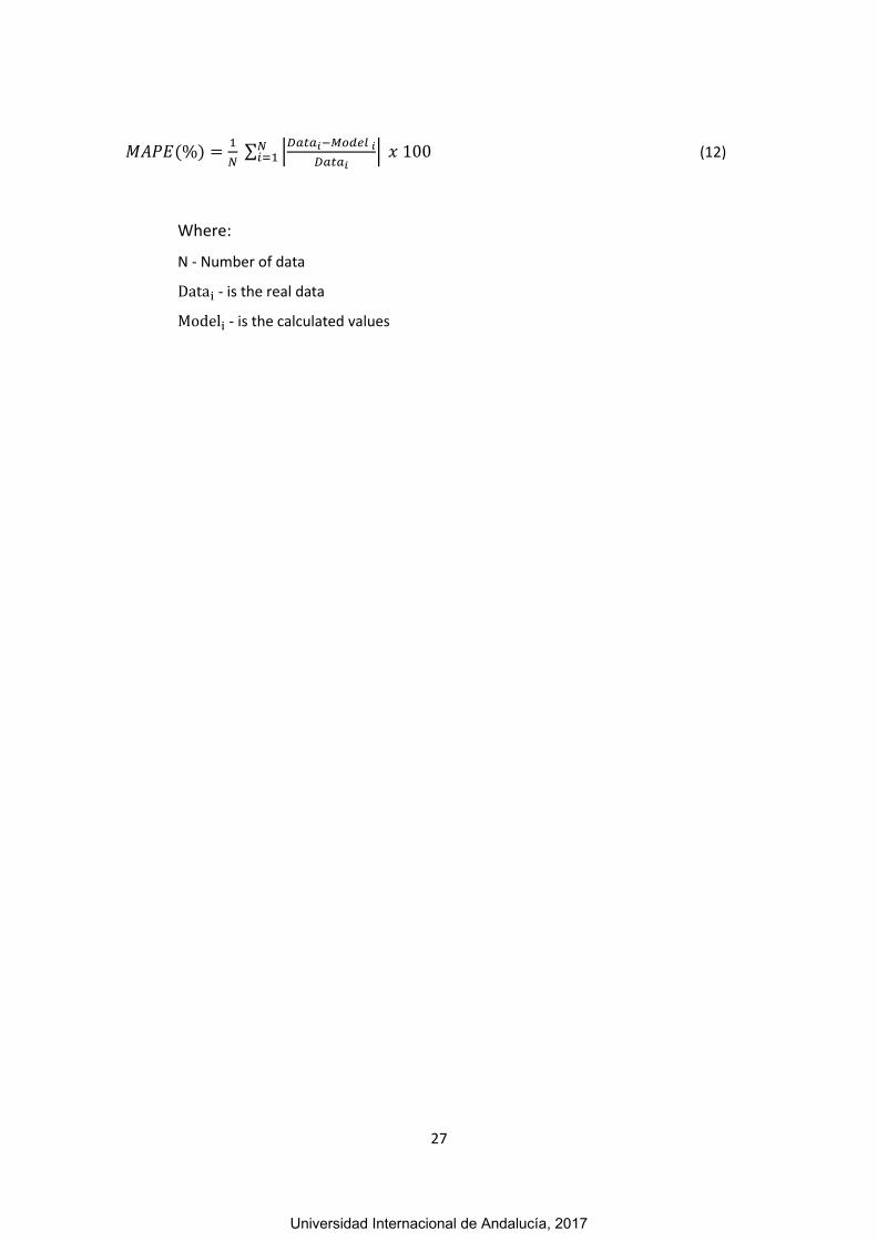
3.6 Model validation and verification

The official dataset from 1971 to 2012 and the output of the model can be

compared to test its robustness and reliability. This analysis can be carried out

calculating the mean absolute percentage error (MAPE), which is defined as equation

12. MAPE is commonly used to evaluate cross-sectional forecasts.


27

𝑀𝐴𝑃𝐸(%) =1

𝑁 ∑ |

𝐷𝑎𝑡𝑎𝑖−𝑀𝑜𝑑𝑒𝑙 𝑖

𝐷𝑎𝑡𝑎𝑖|𝑁

𝑖=1 𝑥 100 (12)

Where:

N - Number of data

Datai - is the real data

Modeli - is the calculated values


28

4. RESULTS AND DISCUSSION

4.1 Brazil in numbers

4.1.1 Overview

Brazil is the fifth largest country in the world in terms of area and population,

occupying approximately half of the entire South America. Brazil extends through

8,515,692 km² divided into 99.3 % of land and 0.7% of water. The coastline stretches

for 7,491 km (Brazilian Institute of Geography and Statistics-BIGS, 2016).

First country to sign the Convention on Biological Diversity, Brazil is the most

biologically diverse nation in the world with six terrestrial biomes and three large

marine ecosystems, and with at least 103,870 animal species and 43,020 plant species

currently known in Brazil. There are two biodiversity hotspots currently acknowledged

in Brazil – the Atlantic Forest and the Cerrado, and 6 biosphere reserves are globally

recognized by the United Nations Educational, Scientific and Cultural Organization

(UNESCO) in the country (ME, 2011). This diversity makes Brazil one of the 17 mega-

diverse countries in the world (United Nations Environment Programme-UNEP, 2002).

Brazil’s Human Development Index (HDI) was 0.755 in 2014 (UN Development

Program, 2015), placing it in 75th position of 188 countries and territories. Between

1980 and 2014, Brazil’s HDI soared from 0.547 to 0.755, an increase of 38.1% which

represents an annual growth of 0.95%.

The Brazilian Institute of Geography and Statistics (BIGS, 2013) provides

population projection, which is a calculated demographic component based on the

2000 Demographic Census and the latest information from records of births and

deaths. The projection starts in 2000 and the time horizon adopted for the projection

of Brazil's population is 2060. The results are shown in Table 3.


29

Table 3. Brazilian total population from 2000 to 2060.

Years Population Years Population Years Population

2000 173,448,346 2020 212,077,375 2040 228,153,204 2001 175,885,229 2021 213,440,458 2041 228,287,681 2002 178,276,128 2022 214,747,509 2042 228,359,924 2003 180,619,108 2023 215,998,724 2043 228,343,224 2004 182,911,487 2024 217,193,093 2044 228,264,820 2005 185,150,806 2025 218,330,014 2045 228,116,279 2006 187,335,137 2026 219,408,552 2046 227,898,165 2007 189,462,755 2027 220,428,030 2047 227,611,124 2008 191,532,439 2028 221,388185 2048 227,256,259 2009 193,543,969 2029 222,288,169 2049 226,834,687 2010 195,497,797 2030 223,126,917 2050 226,347,688 2011 197,397,018 2031 223,904,308 2051 225,796,508 2012 199,242,462 2032 224,626,629 2052 225,182,233 2013 201,032,714 2033 225,291,340 2053 224,506,312 2014 202,768,562 2034 225,896,169 2054 223,770,235 2015 204,450,649 2035 226,438,916 2055 222,975,532 2016 206,081,432 2036 226,917,266 2056 222,123,791 2017 207,660,929 2037 227,329,138 2057 221,216,414 2018 209,186,802 2038 227,673,003 2058 220,254,812 2019 210,659,013 2039 227,947,957 2059 219,240,240

2060 218,173,888

Source: BIGS, 2013.

4.1.2. Economy

According to the World Bank (2016), in 2015 Brazil was the ninth largest

economy in the world, with a GDP 1,774,725 USD (2011 purchasing power parity-PPP).

Moreover, the GDP per capita in 2015 was 8,538 USD (2011 PPP).

In addition, the World Bank (2016) affirms that Brazil's economic and social

progress between 2003 and 2014 took 29 million people away from poverty, as well as

the social inequality dropped significantly. The income level of 40% of the poorest

population rose, at the average of 7.1% (in real terms) between 2003 and 2014,

compared to a 4.4% income growth for the population as a whole. However, the rate

of poverty and inequality reduction has been showing signs of stagnation since 2015.

Besides, Brazil is currently going through a strong recession. The country's

growth rate has decelerated steadily since the beginning of this decade, from an

average annual growth of 4.5% between 2006 and 2010 to 2.1% between 2011 and


30

2014. The GDP contracted by 3.8% in 2015. The realignment of regulated prices

combined with the pass-through of exchange rate depreciation caused an inflation

peak in 2015 (with 12-month accumulated inflation rate of 10.7% in December of

2015), exceeding the upper limit of the target band (6.5%).

The economic crisis - coupled with the ethical-political crisis faced by the

country - has contributed to those numbers. On August 31st, with public opinions

divided, the Resolution N°35 of 2016 was published in the Official Newspaper of the

Union, which established the impeachment of Mrs. Dilma Vana Rousseff, who had

been the democratically elected President of the Brazilian Republic (FRB,2016).

The fiscal adjustment is undermined by budget rigidities and by a difficult

political environment. Less than 15% of expenditures in Brazil are expected to be

discretionary. Most public spending is mandatory (mandated by the Constitution or

other legislation) and increases in line with revenues, nominal GDP growth, or other

pre-established rules. Additionally, a large portion of revenues for education and

health care are earmarked. Attempts to pass legislation to increase revenue collection

in the short term and address issues of a more structural nature - such as pensions -

have so far fallen short of the government's intentions (Word Bank, 2015).

4.1.3 Energy analysis

The information summarized below was obtained from the 2015 Brazilian

Energy Balance report published by the Brazilian Ministry of Mines and elaborated by

the Energy Research Company (BERC, 2015).

Electricity: The electricity generation in the Brazilian public service and self-

producer power plants reached 590.5 TWh in 2014. The public service plants remain as

the main contributors, with 84.1% of total generation, which the main source is

hydropower. The electricity generation from fossil fuels accounted for 26.9% of the

national total in 2014, also the self-producer generation participated with 15.9% of

total production, considering the aggregation of all sources used, reaching 94 TWh. Of

this total, 52.2 TWh are produced and consumed in situ, in other words not injected in


31

the electricity network. Net imports of 33.8 TWh, added to internal generation,

allowed a domestic electricity supply of 624.3 TWh and the final consumption was

531.1 TWh.

Figure 3 illustrates the structure of the domestic supply of electricity in Brazil in

2014. It can be observed that Brazil presents an electricity matrix predominantly

renewable, and the domestic hydraulic generation accounts for 65.2% of the supply.

Adding imports, which are also mainly from renewable sources, it can be stated that

74.6% of electricity in Brazil comes from renewable sources.

Figure 3. Domestic electricity supply by source. Source:BERC, 2015.

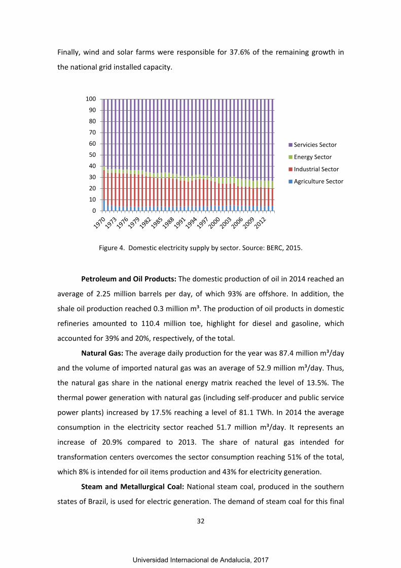
On the consumption side, the residential sector grew by 5.7%. The industrial

sector recorded a decrease of 2.0% in electricity consumption over the previous year

(2013). The other sectors - public, agriculture and livestock, commercial and

transportation - when analyzed collectively showed a positive growth of 7.0% over

2013. The energy sector increased 4.8%. Figure 4 shows the domestic electricity supply

by sector.

In 2014, due to an increase of 7,171 MW, Brazil’ installed electricity generation

capacity reached 133,914 MW, which is the sum of the public service and self-

producer power plants. Out of this total, the increase in hydro power plants accounted

for 44.3%, while thermal power plants accounted for 18.1% of the added capacity.


32

Finally, wind and solar farms were responsible for 37.6% of the remaining growth in

the national grid installed capacity.

Figure 4. Domestic electricity supply by sector. Source: BERC, 2015.

Petroleum and Oil Products: The domestic production of oil in 2014 reached an

average of 2.25 million barrels per day, of which 93% are offshore. In addition, the

shale oil production reached 0.3 million m³. The production of oil products in domestic

refineries amounted to 110.4 million toe, highlight for diesel and gasoline, which

accounted for 39% and 20%, respectively, of the total.

Natural Gas: The average daily production for the year was 87.4 million m³/day

and the volume of imported natural gas was an average of 52.9 million m³/day. Thus,

the natural gas share in the national energy matrix reached the level of 13.5%. The

thermal power generation with natural gas (including self-producer and public service

power plants) increased by 17.5% reaching a level of 81.1 TWh. In 2014 the average

consumption in the electricity sector reached 51.7 million m³/day. It represents an

increase of 20.9% compared to 2013. The share of natural gas intended for

transformation centers overcomes the sector consumption reaching 51% of the total,

which 8% is intended for oil items production and 43% for electricity generation.

Steam and Metallurgical Coal: National steam coal, produced in the southern

states of Brazil, is used for electric generation. The demand of steam coal for this final

0

10

20

30

40

50

60

70

80

90

100

Servicies Sector

Energy Sector

Industrial Sector

Agriculture Sector


33

use increased 9.4% in 2014 when compared to the previous year. In 2014, the steel

industry showed a 7.5% increase in consumption of metallurgical coal due to the

increase of crude steel production via reducing coke in this period (2.1%).

Wind Energy: The production of electricity from wind power reached 12,210

GWh in 2014. This represents an 85.6% increase over the previous year, when it had

reached 6,578 GWh. In 2014, the installed capacity for wind generation in the country

increased by 122%. According to the Power Generation Database from National

Agency of Electric Energy (NAEE), the national wind farm grew 2.686 MW, reaching

4,888 MW by the end of 2014.

Biodiesel: In 2014 the amount of biodiesel produced in Brazil reached

3,419,838 m³, against 2,917,488 m³ in the previous year. Thus, there was an increase

of 17.2% in available biodiesel in the national market. The percentage of biodiesel

compulsorily added to mineral diesel was increased to 6% in July and 7% in November

2014. The main raw material was the soybean oil (69.2%), followed by tallow (17%).

Sugarcane, Sugar and Ethanol: According to the Ministry of Agriculture,

Livestock and Food Supply, the sugar cane production in the calendar year 2014 was

631.8 million tons. This amount was 2.5% lower than in the previous calendar year,

when the milling was 648.1 million tons. In 2014 the national sugar production was

35.4 million tons, 5% lower than the previous year, while the production of ethanol

increased by 3.3%, yielding the amount of 28,526 m³. About 57.1% of this total refers

to hydrous ethanol: 16,296 m³. In comparative terms, the production of this fuel

increased by 4.4% compared to 2013. Regarding the production of anhydrous ethanol,

which is blended with gasoline A to form gasoline C, there was an increase of 1.9%,

totaling 12,230 m³. The Total Recoverable Sugar (ATR) in sugarcane, which is the

amount of sugar available in raw material minus the losses in the manufacturing

process, kept stable and recorded averages of 136.3 and 132.6 ATR/ton of cane for the

2012-2013 and 2013-2014 harvests, respectively.

Table 4 and Figure 5 below demonstrate consolidated data of the evolution of

domestic energy supply for the period 2005-2014.


34

Table 4. Domestic energy supply from 2005 to 2014

Sources (%) 2005 2006 2007 2008 2009 2010 2011 2012 2013 2014

Non-renewable energy 55.9 55.4 54.5 54.4 53.2 55.3 56.5 58.2 59.6 60.6

Petroleum and oil products 38.8 37.9 37.5 36.7 37.9 37.8 38.6 39.3 39.3 39.4

Natural gas 9.4 9.6 9.3 10.3 8.8 10.2 10.2 11.5 12.8 13.5

Coal and coke 6.0 5.7 5.7 5.5 4.6 5.4 5.7 5.4 5.6 5.7

Uranium 1.2 1.6 1.4 1.5 1.4 1.4 1.5 1.5 1.4 1.3

Other none-renewable 1.0 1.0 1.0 0.0 1.0 0.0 0.0 0.0 1.0 1.0

Renewable energy 44.1 44.6 45.5 45.6 46.8 44.7 43.5 41.8 40.4 39.4

Hydraulic 14.9 14.9 14.9 14.1 15.2 14.0 14.7 13.8 12.5 11.5

Firewood and charcoal 13.1 12.7 12.0 11.6 10.1 9.7 9.6 9.1 8.3 8.1

Sugar cane products 13.8 14.6 15.9 17.0 18.1 17.5 15.7 15.4 16.1 15.7

Other renewable source 2.3 2.5 2.7 2.9 3.4 3.5 3.5 3.5 3.6 4.1

Source: BERC, 2015.

Figure 5. Domestic energy supply in 2014. Source: BERC, 2015.

4.1.4 Forecasts for 2030

The Brazilian National Energy Plan 2030 (BERC, 2007) establishes different

economic and energy demand scenarios considering four different GDP trajectories,

the scenarios have been based on different annual GDP growth rates for the period

between 2005 and 2030, as follows: Scenario A 5.1%, B1 scenario 4.1%, B2 scenario

39%

16% 14%

11%

8%

6% 4% 1% 0.6%

Petroleum and oil products Sugar cane products Natural gas

Hydraulic Firewood and charchoal Coal and coke

Other renewables Uranium Other non-renewables


35

3.2% and scenario C 2.2%. The plan, however, prioritizes the scenario B1 and Figure 6

shows the evolution of the domestic energy supply structure.

The evolution of the energy matrix in the period 2005-2030 shows an

expansion in its diversification. Thus, within this period, it is expected a significant

reduction from 13% to 5.5% in the use of wood and charcoal; an increased share of

natural gas from 9.4% to 15.5%; a reduction of oil and derivatives share from 38.7% to

28%; an increase in the share of derived products from sugarcane and other

renewables (ethanol, biodiesel and others) from 16.7% to 27.6%.

Figure 6. Evolution of the domestic energy supply structure Source: MME, 2007.

The demographic scenario considered a population growth of 185,4 million

people in 2005 to 238,5 million inhabitants in 2030. The domestic supply of energy per

capita of 1.19 toe/capita recorded in 2005 evolve to 2.33 toe/capita in 2030. In relation


36

to GDP, this domestic energy supply would imply 5% reduction in energy intensity. The

value expressed in toe/ (US$ 1,000) is 0.275 in 2005 and 0.261 in 2030.

The import of energy focuses on coal for steel, natural gas and electricity, the

latter coming mainly from the Paraguayan side of Itaipu. It can be stated that,

according to the same assumptions, Brazil would find a situation in this period 2005-

2030, which was close to energy self-sufficiency.

4.1.5. Brazil and the United Nations Framework Convention on Climate Change

Despite the fact that Brazil was responsible for only 1.45% of global emissions

in 2013 (Word Bank, 2016), in September 2015, the Brazilian Government

communicated to the Secretariat of the United Nations Framework Convention on

Climate Change (UNFCCC) their intended Nationally Determined Contribution (iNDC) to

the new agreement under the Convention that was adopted at the 21st Conference of

the Parties (COP-21) to the UNFCCC in Paris (FRB, 2015).

In this document, the Brazilian contribution intends to be committed to reduce

greenhouse gas emissions by 37% below 2005 levels (reference point) by 2025. In

addition, Brazil proposed, for reference purpose only, a subsequent indicative

contribution, which was to reduce greenhouse gas emissions by 43% below 2005 levels

by 2030. These goals cover 100% of the territory, the Brazilian economy, and include

CO2, CH4, N2O, perfluorocarbons, hydrofluorocarbons and SF6 emissions.

Brazil hopes to achieve these cuts by implementing measures that are in line

with a transition to a low-carbon economy, mainly:

increasing the share of sustainable biofuels in the Brazilian energy mix

to approximately 18% by 2030, by expanding biofuel consumption, by

increasing ethanol supply, by increasing the share of advanced biofuels

(second generation), and also by increasing the share of biodiesel in the

diesel mix;

in land use change and forestry: by strengthening and enforcing the

implementation of the Forest Code, at federal, state and municipal

levels; also, strengthening policies and measures with a view to achieve,


37

in the Brazilian Amazonia, zero illegal deforestation by 2030 and

compensating for greenhouse gas emissions from legal suppression of

vegetation by 2030; and restoring and reforesting 12 million hectares of

forests by 2030, for multiple purposes; finally, enhancing sustainable

native forest management systems, through georeferencing and

tracking systems applicable to native forest management, with a view to

curbing illegal and unsustainable practices;

in the energy sector: by achieving 45% of renewables in the energy mix

by 2030. Including: the expanding the use of renewable energy sources

other than hydropower in the total energy mix to between 28% and

33% by 2030; the expanding the use of non-fossil fuel energy sources

domestically, increasing the share of renewables (other than

hydropower) in the power supply to at least 23% by 2030, by raising the

share of wind, biomass and solar; and, achieving 10% efficiency gains in

the electricity sector by 2030.

Furthermore, Brazil also intends to:

in the agriculture sector: strengthen the Low Carbon Emission

Agriculture Program as the main strategy for sustainable agriculture

development. This includes: restoring an additional 15 million hectares

of degraded pasturelands by 2030 and enhancing 5 million hectares of

integrated cropland-livestock-forestry systems (ICLFS) by 2030;

in the industry sector: promote new standards of clean technology and

further enhance energy efficiency measures and low carbon

infrastructure;

in the transportation sector: promote efficiency measures and improve

infrastructure for transport and public transportation in urban areas.

Finally, in September 2016, the president Michel Temer ratifies the Paris

Agreement against the climatic changes in Brasilia (UNFCCC, 2016).


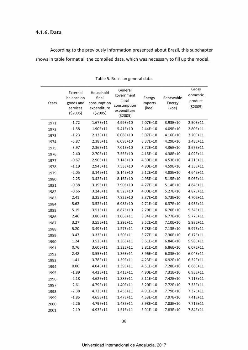
38

4.1.6. Data

According to the previously information presented about Brazil, this subchapter

shows in table format all the compiled data, which was necessary to fill up the model.

Table 5. Brazilian general data.

Years

External balance on goods and

services ($2005)

Household final

consumption expenditure

($2005)

General government

final consumption expenditure

($2005)

Energy imports

(koe)

Renewable Energy (koe)

Gross

domestic

product

($2005)

1971 -1.72 1.67E+11 4.99E+10 2.07E+10 3.93E+10 2.50E+11

1972 -1.58 1.90E+11 5.41E+10 2.44E+10 4.09E+10 2.80E+11

1973 -1.23 2.13E+11 6.08E+10 3.07E+10 4.16E+10 3.20E+11

1974 -5.87 2.38E+11 6.09E+10 3.37E+10 4.29E+10 3.48E+11

1975 -3.97 2.36E+11 7.01E+10 3.72E+10 4.36E+10 3.67E+11

1976 -2.40 2.70E+11 7.55E+10 4.15E+10 4.38E+10 4.02E+11

1977 -0.67 2.90E+11 7.14E+10 4.30E+10 4.53E+10 4.21E+11

1978 -1.19 2.94E+11 7.53E+10 4.80E+10 4.59E+10 4.35E+11

1979 -2.05 3.14E+11 8.14E+10 5.12E+10 4.88E+10 4.64E+11

1980 -2.25 3.42E+11 8.16E+10 4.95E+10 5.15E+10 5.06E+11

1981 -0.38 3.19E+11 7.90E+10 4.27E+10 5.14E+10 4.84E+11

1982 -0.66 3.24E+11 8.52E+10 4.00E+10 5.27E+10 4.87E+11

1983 2.41 3.25E+11 7.82E+10 3.37E+10 5.73E+10 4.70E+11

1984 5.62 3.52E+11 6.98E+10 2.71E+10 6.37E+10 4.95E+11

1985 5.15 3.51E+11 8.87E+10 2.70E+10 6.70E+10 5.34E+11

1986 2.46 3.80E+11 1.06E+11 3.34E+10 6.77E+10 5.77E+11

1987 3.27 3.55E+11 1.29E+11 3.52E+10 7.10E+10 5.98E+11

1988 5.20 3.49E+11 1.27E+11 3.78E+10 7.13E+10 5.97E+11

1989 3.47 3.33E+11 1.50E+11 3.77E+10 7.30E+10 6.17E+11

1990 1.24 3.52E+11 1.36E+11 3.61E+10 6.84E+10 5.98E+11

1991 0.76 3.60E+11 1.32E+11 3.81E+10 6.86E+10 6.07E+11

1992 2.48 3.55E+11 1.36E+11 3.96E+10 6.83E+10 6.04E+11

1993 1.41 3.78E+11 1.39E+11 4.23E+10 6.92E+10 6.32E+11

1994 0.00 4.04E+11 1.39E+11 4.51E+10 7.28E+10 6.66E+11

1995 -1.89 4.42E+11 1.41E+11 4.90E+10 7.31E+10 6.95E+11

1996 -2.18 4.62E+11 1.38E+11 5.11E+10 7.42E+10 7.11E+11

1997 -2.61 4.79E+11 1.40E+11 5.20E+10 7.72E+10 7.35E+11

1998 -2.38 4.72E+11 1.45E+11 4.91E+10 7.79E+10 7.37E+11

1999 -1.85 4.65E+11 1.47E+11 4.53E+10 7.97E+10 7.41E+11

2000 -2.26 4.79E+11 1.48E+11 3.98E+10 7.83E+10 7.71E+11

2001 -2.19 4.93E+11 1.51E+11 3.91E+10 7.83E+10 7.84E+11


https://en.wikipedia.org/wiki/Gross_domestic_product



39

2002 0.84 5.00E+11 1.57E+11 2.84E+10 8.39E+10 8.08E+11

2003 2.22 4.97E+11 1.59E+11 2.07E+10 9.03E+10 8.17E+11

2004 3.41 5.17E+11 1.65E+11 2.76E+10 9.52E+10 8.64E+11

2005 3.40 5.40E+11 1.68E+11 2.06E+10 9.85E+10 8.92E+11

2006 2.71 5.68E+11 1.74E+11 1.65E+10 1.04E+11 9.27E+11

2007 1.36 6.04E+11 1.82E+11 1.90E+10 1.12E+11 9.83E+11

2008 -0.19 6.43E+11 1.85E+11 2.04E+10 1.18E+11 1.03E+12

2009 -0.40 6.72E+11 1.91E+11 9.86E+09 1.17E+11 1.03E+12

2010 -1.04 7.14E+11 1.98E+11 1.93E+10 1.24E+11 1.11E+12

2011 -0.77 7.48E+11 2.03E+11 2.08E+10 1.23E+11 1.15E+12

2012 -1.36 7.74E+11 2.07E+11 2.98E+10 1.22E+11 1.18E+12

Table 6. Brazilian general data. Part II.

Years Etotal (koe) Efossil (koe) CO2 (kg)

1971 69782239000 30462959000 102635663000

1972 74795465000 33940037000 114362729000

1973 81979056000 40410700000 132463041000

1974 87240887000 44327931000 143456707000

1975 91088153000 47466218000 151164741000

1976 95613021000 51771859000 155154437000

1977 98812027000 53479117000 162961480000

1978 105143010000 59270804000 176925416000

1979 111795554000 62993257000 188322452000

1980 113851143000 62391966000 187090340000

1981 109221017000 57785378000 171806284000

1982 111048266000 58356502000 172176651000

1983 113818111000 56514565000 166632147000

1984 121142064000 57424648000 168806678000

1985 129353459000 62365653000 181248809000

1986 135404315000 67713126000 198883412000

1987 140665921000 69633442000 207530198000

1988 142563758000 71252283000 209363698000

1989 145436473000 72475374000 214024455000

1990 140206947000 71808152000 208886988000

1991 142858191000 74221609000 219330604000

1992 144347671000 76048684000 220705729000

1993 147959977000 78809772000 230738641000

1994 155760142000 82967033000 242154012000

1995 161094731000 87971017000 258347484000

1996 169663097000 95465071000 284782887000

1997 178276103000 101049006000 300547320000

1998 182552948000 104676788000 312289054000

1999 186690738000 106952649000 320173104000


40

2000 187441584000 109151103000 327983814000

2001 190711767000 112423995000 337433673000

2002 195758711000 111883929000 332266870000

2003 198976524000 108723416000 321621569000

2004 210041760000 114889113000 337826042000

2005 215331854000 116822529000 347308904000

2006 222817428000 119035502000 347668270000

2007 235459748000 123994607000 363212683000

2008 248579623000 130676967000 387675240000

2009 240453393000 123396972000 367147374000

2010 265862911000 142197735000 419754156000

2011 270026935000 147344496000 439412943000

2012 281724649000 159305890000 470029000000

Table 7. Information about Brazilian agriculture sector.

Years E1

(toe) QiS1

($2005) EIS1 (koe/$2005)

1971 5317393 12747328362 0.417137857

1972 5338469 13266383781 0.40240576

1973 5441909 13277561656 0.409857561

1974 5376379 13560571269 0.396471439

1975 5348720 14467230432 0.369712806

1976 5426899 14757370032 0.367741584

1977 5500892 16493196402 0.333524938

1978 5372788 15785603000 0.340360003

1979 5565328 16529093581 0.336698939

1980 5752243 18092857362 0.317928926

1981 5724525 19505610406 0.293480959

1982 5772134 19414489329 0.297310631

1983 5906319 19229663086 0.307146235

1984 5736611 19710901245 0.291037471

1985 6058588 21618403812 0.280251384

1986 5949630 19976787839 0.297827183

1987 6386838 22982759541 0.277896917

1988 6461362 23165919194 0.278916719

1989 6532165 23853738504 0.273842387

1990 6026929 23265949662 0.25904505

1991 6147780 23696849617 0.259434477

1992 6073669 24985314289 0.243089563

1993 6432895 25231832312 0.254951562

1994 6652211 27109399276 0.245383944

1995 7050618 28664417688 0.245971078

1996 7287707 29527880535 0.246807648


41

1997 7528143 29773497162 0.252847133

1998 7308493 30881986380 0.236658778

1999 7536184 32967958777 0.228591154

2000 7322063 33765662219 0.216849368

2001 7728679 35958389316 0.214933961

2002 7809259 38477327408 0.202957417

2003 8149978 40723243107 0.200130868

2004 8274035 41659945213 0.198608879

2005 8357612 38958191676 0.214527723

2006 8550542 40817363327 0.20948295

2007 9054700 42167678540 0.214730806

2008 9908631 44514949276 0.22259109

2009 9551669 42877973582 0.222764005

2010 10026747 45772592734 0.219055697

2011 9998667 48351978361 0.206789203

2012 10361298 47208027453 0.219481702

Table 8. Information about Brazilian manufacturing sector.

Years E2

(toe) QiS2

($2005) EIS2

(koe /$2005)

1971 18294772 71700000000 0.255173942

1972 19949620 82100000000 0.243001041

1973 22332696 95540000000 0.233758892

1974 23966850 103400000000 0.231704499

1975 25140543 107500000000 0.233912068

1976 27933382 120300000000 0.232161297

1977 30623874 121900000000 0.251213633

1978 31985725 126600000000 0.252564194

1979 34151271 134800000000 0.253306144

1980 36237490 147200000000 0.246247695

1981 33067304 131800000000 0.250796009

1982 33840772 129900000000 0.260470777

1983 34738063 120100000000 0.289178805

1984 37749169 125400000000 0.301143515

1985 39702697 134000000000 0.296207019

1986 42166445 150000000000 0.281175377

1987 44469317 153600000000 0.289485024

1988 45454856 148300000000 0.306487431

1989 45341751 151700000000 0.298820683

1990 42233981 138900000000 0.303952896

1991 43182926 139800000000 0.308876689

1992 44116935 132000000000 0.334255495

1993 46138230 144900000000 0.318369933


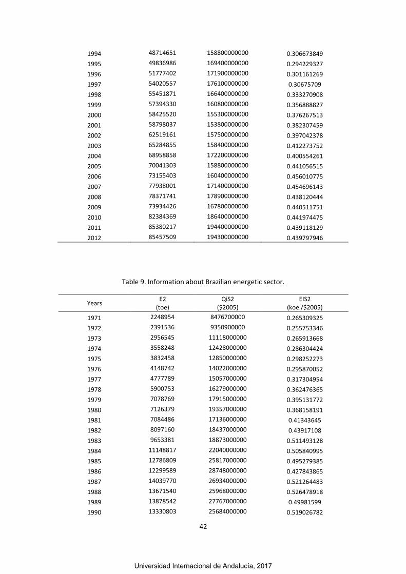
42

1994 48714651 158800000000 0.306673849

1995 49836986 169400000000 0.294229327

1996 51777402 171900000000 0.301161269

1997 54020557 176100000000 0.30675709

1998 55451871 166400000000 0.333270908

1999 57394330 160800000000 0.356888827

2000 58425520 155300000000 0.376267513

2001 58798037 153800000000 0.382307459

2002 62519161 157500000000 0.397042378

2003 65284855 158400000000 0.412273752

2004 68958858 172200000000 0.400554261

2005 70041303 158800000000 0.441056515

2006 73155403 160400000000 0.456010775

2007 77938001 171400000000 0.454696143

2008 78371741 178900000000 0.438120444

2009 73934426 167800000000 0.440511751

2010 82384369 186400000000 0.441974475

2011 85380217 194400000000 0.439118129

2012 85457509 194300000000 0.439797946

Table 9. Information about Brazilian energetic sector.

Years E2

(toe) QiS2

($2005) EIS2

(koe /$2005)

1971 2248954 8476700000 0.265309325

1972 2391536 9350900000 0.255753346

1973 2956545 11118000000 0.265913668

1974 3558248 12428000000 0.286304424

1975 3832458 12850000000 0.298252273

1976 4148742 14022000000 0.295870052

1977 4777789 15057000000 0.317304954

1978 5900753 16279000000 0.362476365

1979 7078769 17915000000 0.395131772

1980 7126379 19357000000 0.368158191

1981 7084486 17136000000 0.41343645

1982 8097160 18437000000 0.43917108

1983 9653381 18873000000 0.511493128

1984 11148817 22040000000 0.505840995

1985 12786809 25817000000 0.495279385

1986 12299589 28748000000 0.427843865

1987 14039770 26934000000 0.521264483

1988 13671540 25968000000 0.526478918

1989 13878542 27767000000 0.49981599

1990 13330803 25684000000 0.519026782


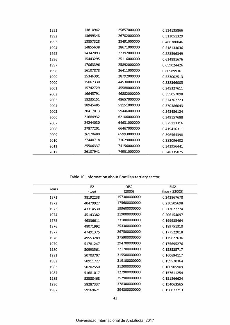
43

1991 13810942 25857000000 0.534135866

1992 13699348 26702000000 0.513051329

1993 13857328 28491000000 0.486380046

1994 14855638 28671000000 0.518133036

1995 14342093 27392000000 0.523596349

1996 15443295 25116000000 0.614881676

1997 17063396 25892000000 0.659024426

1998 16107878 26411000000 0.609899361

1999 15346391 28792000000 0.533002513

2000 15067330 44530000000 0.338366005

2001 15742729 45588000000 0.345327611

2002 16645791 46882000000 0.355057098

2003 18235151 48657000000 0.374767723

2004 18945485 51151000000 0.370386043

2005 20417013 59446000000 0.343456124

2006 21684932 62106000000 0.349157688

2007 24244030 64631000000 0.375113316

2008 27877201 66467000000 0.419416311

2009 26170480 65993000000 0.396564398

2010 27440718 71629000000 0.383096402

2011 25506337 74156000000 0.343956441

2012 26107941 74951000000 0.348335075

Table 10. Information about Brazilian tertiary sector.

Years E2

(toe) QiS2

(2005) EIS2

(koe / $2005)

1971 38192238 157300000000 0.242867678

1972 40479927 175600000000 0.230505698

1973 43314530 199600000000 0.217027774

1974 45143382 219000000000 0.206154097

1975 46336611 231800000000 0.199935464

1976 48071992 253300000000 0.189751318

1977 47491375 267500000000 0.177522018

1978 49553289 275900000000 0.179622636

1979 51781247 294700000000 0.175695276

1980 50993561 321700000000 0.158535717

1981 50703707 315500000000 0.160694117

1982 50911727 319100000000 0.159570364

1983 50202550 312000000000 0.160905909

1984 51681017 327900000000 0.157611254

1985 53588468 352900000000 0.151866624

1986 58287337 378300000000 0.154063565

1987 59169621 394300000000 0.150077213


44

1988 60098346 399700000000 0.150344842

1989 62043994 413400000000 0.150079664

1990 61448787 409700000000 0.149973753

1991 63538728 417300000000 0.152259497

1992 63933204 420200000000 0.152163931

1993 65077987 433400000000 0.1501708

1994 67884840 451100000000 0.150491418

1995 72385412 469700000000 0.154115583

1996 76821906 483900000000 0.158757251

1997 79751378 502800000000 0.158608825

1998 82736622 513400000000 0.161156963

1999 82824877 517900000000 0.159909155

2000 82103480 537400000000 0.152775902

2001 81195599 548400000000 0.148053516

2002 84303846 564900000000 0.149243988

2003 83196304 569200000000 0.146171058

2004 87952728 599000000000 0.146833539

2005 90412680 634400000000 0.14251177

2006 91197620 663600000000 0.137429742

2007 98393767 705000000000 0.13956089

2008 106391617 743400000000 0.143105335

2009 107945393 755300000000 0.142917061

2010 115681669 805900000000 0.1435425

2011 118872472 836200000000 0.14216534

2012 124143966 858700000000 0.144569048

Table 11. Energy by type of fuels in agriculture sector.

Years ktoe

E11 E12 E13 E14 E15 E16 E17

1971 0 0 0.00 531.54 23.01 0 4762.84

1972 0 0 0.00 711.58 46.02 0 4580.87

1973 0 0 0.00 936.20 73.64 0 4432.08

1974 0 0 0.00 1035.64 85.60 0 4255.13

1975 0 0 0.00 1150.53 91.13 0 4107.07

1976 0 0 0.82 1329.71 104.32 0 3992.06

1977 0 0 0.82 1511.46 106.20 0 3882.42

1978 0 0 1.64 1534.61 115.59 0 3720.95

1979 0 0 1.64 1886.11 120.29 0 3557.29

1980 0 0 1.63 2217.86 115.52 0 3417.23

1981 0 0 1.65 2155.23 100.37 0 3467.27

1982 0 0 0.83 2257.23 67.21 0 3446.87

1983 0 0 0.00 2443.99 25.63 0 3436.69

1984 0 0 0.83 2571.79 25.63 0 3138.36


45

1985 0 0 0.84 3005.97 23.93 0 3027.85

1986 0 0 0.82 2975.75 25.15 0 2947.92

1987 0 0 0.83 3230.57 34.53 0 3120.92

1988 0 0.62 0.00 3383.78 35.88 0 3041.09

1989 0 0.62 0.00 3588.39 28.70 0 2914.46

1990 0 0.62 0.00 3246.26 26.25 0 2753.80

1991 0 0.62 0.00 3376.52 21.39 0 2749.25

1992 0 1.23 0.83 3461.85 32.09 0 2577.66

1993 0 0.62 0.83 3825.80 34.99 0 2570.65

1994 0 0.62 0.00 4013.87 63.18 0 2574.54

1995 0 1.23 0 4275.07 94.29 0 2680.02

1996 0 1.23 0 4479.68 82.63 0 2724.16

1997 0 3.70 0 4659.05 79.71 0 2785.69

1998 0 7.97 0 4475.08 45.35 0 2780.10

1999 0 13.49 0 4617.46 87.27 0 2817.97

2000 0 15.90 0 4452.01 106.45 0 2747.70

2001 0 21.37 0 4855.39 143.85 0 2708.07

2002 0 19.55 0 4772.54 106.45 0 2910.71

2003 0 17.72 0 4825.12 83.43 0 3223.71

2004 0 20.16 0 4766.61 70.97 0 3416.30

2005 0 22.91 0.11 4734.22 63.87 0 3536.50

2006 0 19.00 0 4799.30 66.17 0 3666.07

2007 0 19.28 0 5098.85 61.00 0 3875.57

2008 0 22.28 0 5685.25 68.09 0 4133.01

2009 0 22.96 0 5514.69 68.09 0 3945.93

2010 0 8.09 0 5772.22 78.85 0 4167.58

2011 0 12.06 0.02 5662.47 16.52 0 4307.60

2012 0 11.35 0.01 5889.07 21.14 0 4439.73

Table 12. Energy by type of fuels in imanufacturing sector.

Years ktoe

E21 E22 E23 E24 E25 E26 E27

1970 2.64 288.03 27.86 292.35 5015.61 1237.02 10072.12

1971 10.56 305.47 45.07 297.49 6003.27 1235.35 10397.57

1972 19.35 326.26 114.43 288.92 6526.09 1347.09 11327.47

1973 20.23 363.07 121.96 295.78 8005.28 1388.90 12137.48

1974 143.38 383.39 130.97 296.63 8683.66 1432.56 12896.25

1975 152.18 467.54 135.11 312.07 9112.59 1743.05 13218.01

1976 160.98 527.41 121.43 350.64 10636.53 2166.60 13969.79

1977 274.45 670.49 158.56 354.93 11090.45 2963.05 15111.94

1978 258.62 716.78 175.33 365.22 11921.22 3293.60 15254.96

1979 273.57 856.07 179.16 348.93 12314.99 4065.41 16113.14

1980 319.31 952.49 146.67 323.08 12093.91 4412.00 17990.02


46

1981 335.15 952.58 155.80 382.77 8979.53 3958.99 18302.49

1982 363.29 1030.63 140.65 260.42 8198.55 4614.14 19233.08

1983 394.96 1298.83 93.44 223.51 6083.10 5151.25 21492.97

1984 404.64 1448.29 82.14 199.51 4940.58 6294.79 24379.22

1985 540.10 1556.08 69.46 187.38 4932.40 6990.58 25426.68

1986 703.72 1642.57 70.13 202.18 5359.53 7232.06 26956.25

1987 951.78 2067.50 64.37 204.31 6081.27 7826.71 27273.37

1988 1005.52 2032.96 70.64 209.69 6145.32 8501.85 27488.87

1989 1023.50 1913.80 62.66 231.88 6460.26 8013.82 27635.83

1990 1288.31 1560.76 49.11 241.50 6298.00 6867.21 25929.08

1991 1357.37 1668.62 47.45 226.38 6332.03 8080.66 25470.42

1992 1523.55 1684.38 33.30 242.92 6809.30 7748.16 26075.31

1993 1639.66 1697.91 25.81 278.62 6930.82 8276.96 27288.45

1994 1704.76 1785.03 30.80 336.96 6715.02 8828.70 29313.39

1995 1989.76 1911.37 24.14 334.34 7283.68 9245.91 29047.78

1996 2405.84 1975.05 18.31 305.61 8258.66 9550.32 29263.61

1997 2659.61 2062.05 26.64 356.98 8629.01 9915.51 30370.75

1998 2649.50 2010.04 20.66 362.08 8322.36 10296.90 31790.34

1999 2952.10 2047.10 12.32 353.01 7136.88 11408.31 33484.61

2000 3725.68 2249.46 13.97 365.90 6253.64 13225.27 32591.61

2001 4285.45 2028.79 10.68 324.94 5398.21 13340.83 33409.14

2002 5399.77 1806.60 10.93 412.98 5104.76 13734.76 36049.37

2003 5668.08 1943.23 9.29 447.74 4298.24 13841.65 39076.62

2004 6434.56 1997.88 7.64 490.14 3855.18 13974.79 42198.66

2005 6954.01 2070.76 6.39 455.02 3773.91 13707.28 43073.92

2006 7303.23 2091.78 3.95 445.50 3324.85 13658.36 46327.73

2007 7859.79 2253.13 2.75 482.79 3418.88 15217.33 48703.33

2008 8026.90 2393.03 1.48 500.14 3412.12 15025.47 49012.60

2009 7083.34 2363.32 1.64 482.80 3309.42 13516.07 47177.84

2010 8645.48 2507.23 1.22 464.99 2835.71 16695.18 51234.56

2011 9317.37 2725.78 1.25 610.37 2660.82 18307.82 51756.80

2012 9175.36 2755.59 1.03 653.05 2395.67 17918.88 52557.92

Table 13. Energy by type of fuels in energetic sector.

Years ktoe

E31 E32 E33 E34 E35 E36 E37

1970 65.09 85.97 0.00 90.02 1075.10 191.15 306.95

1971 81.81 88.11 0.00 90.02 1170.83 477.40 340.78

1972 87.96 90.26 0.00 100.31 1338.35 438.02 336.63

1973 86.21 103.16 2.46 156.03 1656.84 537.92 413.94

1974 120.51 99.29 4.10 168.04 1851.05 887.14 428.12

1975 131.07 122.93 5.74 185.18 2045.27 874.69 467.58

1976 128.43 158.61 8.19 197.18 2263.95 908.76 483.62


47

1977 140.74 162.90 9.01 202.33 2398.34 896.31 968.14

1978 137.23 174.08 12.29 210.04 2528.97 1140.05 1698.09

1979 141.62 166.77 16.39 280.34 2694.37 1223.91 2555.35

1980 165.37 165.91 15.48 305.08 2693.95 1138.08 2642.49

1981 173.29 157.56 16.54 296.56 2247.96 1189.19 3003.39

1982 343.94 178.67 12.44 376.35 2087.32 1206.82 3891.63

1983 430.15 223.65 10.77 427.18 1810.31 1426.06 5325.26

1984 604.32 299.23 37.16 367.65 1988.32 1509.69 6342.46

1985 859.42 377.37 7.53 421.62 1977.55 1349.00 7794.33

1986 986.09 376.42 8.16 453.36 2085.39 1405.42 6984.75

1987 977.29 367.98 6.60 433.07 2218.26 1598.34 8438.23

1988 934.25 380.09 4.11 517.70 2211.66 1657.39 7966.34

1989 928.98 383.36 4.95 465.50 2128.55 1800.48 8166.72

1990 901.72 361.76 7.49 506.63 2128.82 1583.95 7840.44

1991 798.65 399.41 7.49 523.28 1558.22 1803.65 8720.24

1992 850.65 419.61 18.31 579.88 1636.68 1871.26 8322.95

1993 1029.53 432.32 15.82 435.34 1957.74 1939.39 8047.19

1994 984.95 402.01 11.24 379.62 2271.71 2053.82 8752.29

1995 978.37 373.68 32.26 282.10 2289.21 1960.51 8425.95

1996 1223.28 384.19 14.85 290.81 2116.18 2506.41 8907.58

1997 1343.08 379.28 6.34 331.73 2302.82 2753.98 9946.17

1998 1400.40 367.43 7.98 375.01 2275.96 2760.43 8920.67

1999 1681.06 324.05 8.76 395.86 1964.03 2748.72 8223.92

2000 2207.36 384.49 7.93 410.99 1892.11 3102.29 7062.16

2001 2481.60 359.09 8.76 424.20 1660.99 3420.60 7387.49

2002 2727.92 342.66 8.76 247.62 1736.75 3525.39 8056.69

2003 2930.65 351.83 4.11 350.22 1868.13 3538.14 9192.07

2004 3176.65 378.98 2.47 362.94 1568.92 4060.50 9395.03

2005 3521.27 371.21 1.40 368.76 1698.08 4399.97 10056.32

2006 3760.58 385.48 0.82 314.03 1773.48 4385.52 11065.02

2007 4054.72 422.63 1.34 373.41 1820.76 4564.07 13007.10

2008 5352.18 174.07 1.32 400.76 1481.94 4610.41 15856.51

2009 5164.41 228.35 1.64 386.49 1336.09 4526.93 14526.57

2010 4503.18 217.84 0.61 1168.01 1002.30 4492.12 16056.66

2011 5366.18 237.52 0.56 1311.75 719.29 4349.31 13521.73

2012 5931.30 224.85 0.71 1573.55 540.59 4052.25 13784.69

Table 14. Energy by type of fuels in tertiary sector.

Years ktoe

E41 E42 E43 E44 E45 E46 E47

1970 0 1422.11 8544.68 4617.54 497.97 16.16 21510.77

1971 0 1528.06 9276.18 5048.77 542.15 16.16 21780.91

1972 0 1679.56 10358.56 5726.91 629.60 10.78 22074.53


48

1973 0 1839.34 12117.68 6751.41 779.63 1.96 21824.51

1974 0 1948.80 12597.73 7524.71 1329.15 7.84 21735.15

1975 0 2009.31 12903.55 8433.47 1439.61 9.80 21540.88

1976 0 2197.96 13123.71 9786.33 1574.15 12.73 21377.12

1977 0 2276.19 12121.18 10473.04 1196.35 15.67 21408.94

1978 0 2506.08 12359.24 11560.98 1449.15 19.10 21658.73

1979 0 2766.51 12529.11 12283.71 1662.49 18.61 22520.82

1980 0 2959.96 10820.75 12854.70 1306.73 21.55 23029.86

1981 0 3195.40 10627.25 12614.11 1708.22 20.08 22538.64

1982 0 3607.62 10241.94 13024.26 1743.60 19.59 22274.71

1983 0 3754.54 9042.95 12494.40 1627.10 24.49 23259.09

1984 0 3731.97 8098.24 12987.86 1550.74 23.51 25288.69

1985 0 4067.88 8090.88 13469.16 1885.66 12.73 26062.15

1986 0 4346.13 8996.41 15388.13 1533.09 6.86 28016.73

1987 1.76 4604.64 8128.30 15882.16 1494.18 6.37 29052.21

1988 2.75 4971.38 7938.21 16214.13 1558.15 7.35 29406.37

1989 4.51 5270.77 8754.84 16926.95 988.22 6.86 30091.84

1990 8.80 5463.28 9531.98 16949.70 1108.15 8.95 28377.93

1991 10.56 5569.88 10242.88 17577.43 1029.42 2.55 29106.02

1992 7.92 5818.04 10062.19 17874.33 1090.15 0 29080.58

1993 51.02 5843.49 10572.31 18337.54 1348.25 0 28925.37

1994 82.69 5889.96 11410.09 19075.01 1473.65 18.33 29935.11

1995 120.51 6170.55 13563.85 20293.10 1461.98 16.59 30758.83

1996 138.10 6440.05 15599.88 21102.84 1589.33 17.46 31934.25

1997 193.52 6535.41 17113.35 22221.67 1288.96 0 32398.46

1998 255.10 6654.52 18008.46 23328.84 1343.00 0 33146.70

1999 259.50 6915.82 16796.44 23717.91 1345.48 0 33789.74

2000 451.26 6991.99 16479.20 24275.90 1236.15 20.94 32648.05

2001 784.65 7022.73 16319.50 25014.23 1253.41 20.94 30780.15

2002 1217.92 6809.76 15620.18 26311.07 1279.31 0 33065.61

2003 1583.12 6372.73 15369.84 25392.77 944.62 0 33533.23

2004 1834.80 6571.92 15965.33 27259.04 976.26 0 35345.37

2005 2184.17 6463.01 16207.96 27084.04 981.86 0 37491.64

2006 2557.46 6427.66 16889.88 27558.00 897.62 0 36867.00

2007 2804.24 6620.19 16969.85 28936.08 1131.72 0 41931.70

2008 2616.19 6760.10 17404.97 30497.91 1246.70 0 47865.74

2009 2339.81 6622.99 17556.33 29837.61 1194.82 0 50393.84

2010 2283.65 6976.18 20770.06 32512.56 993.49 0 52145.73

2011 2247.32 7136.90 24465.69 34162.39 1008.36 0 49851.80

2012 2241.69 7087.20 28278.15 36171.15 966.02 0 49399.76


49

4.2 Estimates

4.2.1 MAPE

MAPE values for the main variables of the model are show in the Table 15, and

Figures 7, 8, 9, 10 and 11. The main difference between official data and the predicted

one due to the application of Hodrick-Prescott filter (1997).

Table 15. MAPE values for the main variables of the model.

Variable MAPE (%)

GDP 2.4% Efossil 6.8% RN 2.8%

Etotal 2.4% CO2 4.4%

Figure 7. GDP official and predicted data.


50

Figure 8. Fossil energy official and predicted data.

Figure 9. Renewable energy official and predicted data.

Figure 10.Total energy official and predicted data.


51

Figure 11.CO2 emissions official and predicted data.

4.2.2 Scenarios

In this research we calculate the value of CO2 emissions in the medium term. As

it was said before, CO2 emissions depend on several variables, therefore we have

defined four scenarios concerning the growth of GDP, the evolution of the energy

matrix, of the productive sectoral structure, and the improvement of energy efficiency

for the period 2013-2030.

1. Baseline scenario (BS): GDP, energy matrix and productive sectoral structure

will evolve through the smooth trend of the period 1971-2012, extrapolated to 2013-

2030 using the geometric growth rate method.

2. Doubling of the GDP (SC-2 scenario): GDP in 2030 will be more than double

that of 2012. To generate this scenario a constant annual growth of the GDP formation

components (I, TB, C, Eimp) of 4.1% per year between 2012 and 2030 is assumed. This

value was extracted of the Brazilian national plan on energy (2007). Also, it was

assumed a structural change in the productive sectorial, that will be implemented

through a stabilization of the primary sector, a reduction of 4.5% on the industrial and

energetic sector and an increase on the service sector of 9%. The rest of the variables

will evolve as in the BS scenario.


52

3. Doubling of the GDP and changed the energetic matrix (SC-3 scenario): The

doubling of the GDP and the change of the productive sectoral structure as in the SC-2

scenario are considered, however, the consumption of renewable and nuclear fuel will

increase 9% while the natural gas growth 2%. At the same time the consumption of oil

and its derivatives will decrease 10% in the whole period.

4. 3. Doubling of the GDP, changed the energetic matrix and improved the

efficiency of energy use (SC-4 scenario): The doubling of the GDP, the change of the

productive sectoral structure and the reordering of fuel use are the same as in the SC-3

scenario. Moreover an improvement in the efficiency of energy use is implemented

with a reduction in the sectoral energy intensity of 5% in the whole period.

4.2.3 Economic estimates

The estimate values of GDP for the pre-established scenarios are presented in

Figure 12, Figure 13 and Appendix 1. The first projection refers to 2013 and for the BS

scenario corresponds nearly to 1,2 trillion short scale 2005$*. For the year 2030, the

BS scenario reaches 2,5 trillion short scale 2005$, which corresponds to more than

double that of 2013.

As Figure 13 shows the estimated GDP for the SC-2 scenario is around 3,6

trillion short-scale (2005$) in 2030 (44% higher than for BS scenario) and its average

growth rate is 6.5% while in BS scenario it is 4.4%. Furthermore, for SC-3 and SC-4 the

results are 3,4 trillion short scale USD 2005 (36% higher than for BS scenario) and 2,9

trillion short scale 2005$ (16% higher than for BS scenario), with an average growth

rate of 6.0% and 5.2%, respectively.

*Trillion short scale means 1012

2005$


53

Figure 12. GDP of Brazil for the period 1971-2011.

Figure 13. GDP of Brazil for the period 2010-2030.

Note that the difference in the values found between SC-2, SC-3 and SC-4

scenarios are due to the feedback mechanism between GDP and renewable energy.

Besides, it is important to highlight that these values do not intend to be a meticulous

projection of the GDP, but rather the repercussion of the considered scenarios.


54

4.2.4 Energy estimates

4.2.4.1 Total energy

Figure 14, Figure 15 and Appendix 2 illustrate the progress of the total energy

consumption. In 2013 the projections demonstrated 277130556 toe; 279586116 toe;

279586116 toe; and 278778771 toe for BS scenario, SC-2, SC-3 and SC-4, respectively.

However, for 2030, the numbers are superior, being 550593722 toe; 829104077 toe;

774498261 toe; and, 629445279 toe for the same order above.

Further, in 2030 the total energy consumption of the SC-2 corresponds to

50.6% higher than the BS scenario. Likewise, the SC-3 is 40.6% higher than BS scenario.

These two last scenarios show the growth of the energy consumption due to the

increase of GDP and to the changes of the productive sectoral structure. Lastly, SC-4

generates a consumption of only 14.3% higher than the BS scenario. It distinctly

reveals the benefits of the reduction of energy intensity.

Figure 14. Total energy consumption of Brazil for the period 1971-2011.


55

Figure 15. Total energy consumption of Brazil for the period 2010-2030.

The previsions of the consumption of fossil energy (Figure 16 and Appendix 3)

in 2030 in the BS scenario is 306448946 toe, while in SC-2 is 444402429 toe (45%

higher than the BS scenario), in SC-3 is 371067222 toe (21% higher than the BS

scenario) and in SC-4 is 305332983 toe (0.66% lower than the BS scenario). Moreover,

the estimations of the consumption of renewable energy are elucidated in Figure 17

and Appendix 4. As we can see, in 2030 the results correspond nearly to 290212188

toe, 443429030 toe, 405460499 toe and 325638742 toe in the BS, SC-2, SC-3 and SC-4

scenarios, representing increases about of 53%, 40% and 12% compared to the BS

scenario, respectively.

Figure 16. Fossil energy consumption of Brazil for the period 1971-2030.


56

Figure 17. Renewable energy consumption of Brazil for the period 1971-2030.

4.2.4.2 Energy by sector

The change in the behavioral pattern of energy consumption in the primary

sector can be seen in Figure 18 and 19, the first makes reference to BS scenario and

SC-2, while the second refers to the SC-3 and SC-4.

Figure 18. Energy consumption of Brazilian primary sector for the BS and SC-2 scenarios during the period 2000-2030.


57

Figure 19. Energy consumption of Brazilian primary sector for the SC-3 and SC-4 scenarios during the period 2000-2030.

In the BS scenario and SC-2, for the next years the fuel oil tends to have an

insignificant consumption, while gas/diesel oil will decline 10% and renewable,

alternative and nuclear energy will rise 12% (Appendix 5). For the same period, in

2030, the SC-3 and SC-4 shows the same disappearance of fuel oil in the agricultural

sector, but the reduction in gas/diesel oil will be 5% and the accretion in the

renewable, alternative and nuclear energy will be 7% (Appendix 6).

In the manufacturing sector, the BS scenario and SC-2 result in a nearly rise

from 6 to 16% of natural gas and from 58 to 63% of renewable, alternative and nuclear

energy. At the same time, the liquefied petroleum gases, gas/diesel oil, fuel oil and

petroleum coke practically keep the same values (Figure 20 and Appendix 7).

The SC-3 and SC-4 scenarios, show that the liquefied petroleum gases,

gas/diesel oil and petroleum coke maintained the same proportions, which are

approximately 3%, 0.6% and 20%, respectively. Whereas, the natural gas increase to

11% and the renewable, alternative and nuclear energy to 63%. In addition, the

consumption of fuel oil decreases from 10.8% to 2.2% (Figure 21 and Appendix 8).


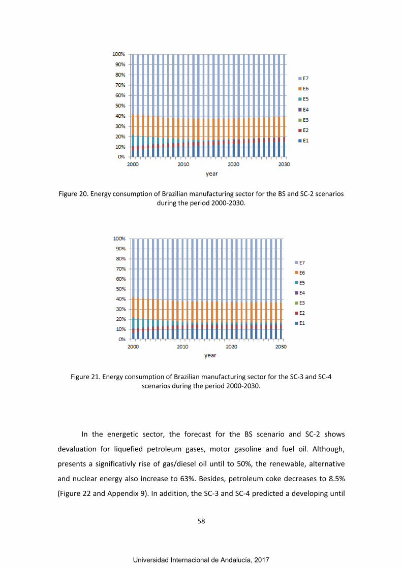
58

Figure 20. Energy consumption of Brazilian manufacturing sector for the BS and SC-2 scenarios during the period 2000-2030.

Figure 21. Energy consumption of Brazilian manufacturing sector for the SC-3 and SC-4 scenarios during the period 2000-2030.

In the energetic sector, the forecast for the BS scenario and SC-2 shows

devaluation for liquefied petroleum gases, motor gasoline and fuel oil. Although,

presents a significativly rise of gas/diesel oil until to 50%, the renewable, alternative

and nuclear energy also increase to 63%. Besides, petroleum coke decreases to 8.5%

(Figure 22 and Appendix 9). In addition, the SC-3 and SC-4 predicted a developing until


59

21% of natural gas, up 4.5% of gas/diesel oil and up 56% of renewable, alternative and

nuclear energy (Figure 23 and Appendix 10).

Figure 22. Energy consumption of Brazilian energetic sector for the BS and SC-2 scenarios during the period 2000-2030.

Figure 23. Energy consumption of Brazilian energetic sector for the SC-3 and SC-4 scenarios during the period 2000-2030.


60

Finally, the tertiary sector presents a reduction on liquefied petroleum gases

from 8.2 to 2.7%, and gas/diesel oil from 29.5 to 24.3%. At the same time, the increase

on natural gas is only 1%, the motor gasoline growth up to 26% and the renewable,

alternative and nuclear energy up to 44.7%, as it is possible to see in Figure 24 and

Appendix 11.

Figure 24. Energy consumption of Brazilian tertiary sector for the BS and SC-2 scenarios during the period 2000-2030.

Furthermore, SC-3 and SC-4 show an add to 2.2% of natural gas and to 44% of

renewable, alternative and nuclear energy. However, the decline of liquefied

petroleum gases is only 5.5% and the consumption of motor gasoline and gas/oil diesel

are almost the same (Figure 25 and Appendix 12).


61

Figure 25. Energy consumption of Brazilian tertiary sector for the SC-3 and SC-4 scenarios during the period 2000-2030.

4.2.4.3 Energy by type of fuels

The energy consumption in accordance with seven types of fuels for each

scenario is present on the Figure 26.

Such as Figure 27 and Appendix 13 illustrate, the natural gas in 2010 represents

7.1% of all energy consumption, later in 2030 for BS scenario and SC-2 it reaches

10.2%, however SC-3 and SC-4 remain the same value (7%). Posteriorly, Figure 28 and

Appendix 14 show that in 2010, the liquefied petroleum gases was 4.2% of all energy

consumption, 30 years later the forecast shows 2.5% for BS scenario and SC-2 while it

shows 4% for SC-3 and SC-4.


62

Figure 26. The Brazilian energy consumption by seven types of fuels according to the four scenarios during the period 2010-2030. The types of energy are: natural gas (E1), liquefied petroleum gases (E2), motor gasoline (E3), gas/diesel oil (E4), fuel oil (E5), petroleum coke (E6) and renewable, alternative and nuclear (E7).

Figure 27. Brazilian energy consumption of natural gas for the four scenarios for the period 2010-2030.


63

Figure 28. Brazilian energy consumption of liquefied petroleum gases for the four scenarios for the period 2010-2030.

The motor gasoline was 10.3% of all energy consumption in 2010, this number

go up to 14.2%, 13.2%, 9.9% and 10.4% for the BS scenario, SC-2, SC-3 and SC-4,

respectively (Figure 29 Appendix 15).

Figure 29. Brazilian energy consumption of motor gasoline for the four scenarios for the period 2010-2030.


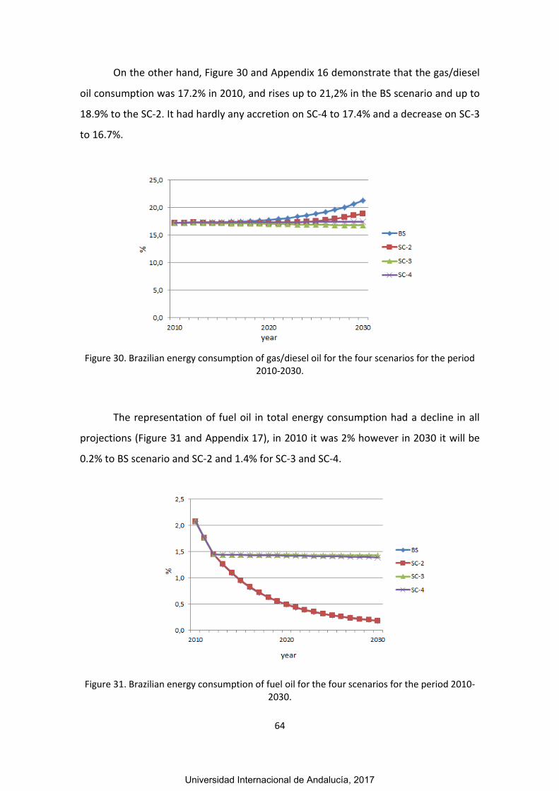
64

On the other hand, Figure 30 and Appendix 16 demonstrate that the gas/diesel

oil consumption was 17.2% in 2010, and rises up to 21,2% in the BS scenario and up to

18.9% to the SC-2. It had hardly any accretion on SC-4 to 17.4% and a decrease on SC-3

to 16.7%.

Figure 30. Brazilian energy consumption of gas/diesel oil for the four scenarios for the period 2010-2030.

The representation of fuel oil in total energy consumption had a decline in all

projections (Figure 31 and Appendix 17), in 2010 it was 2% however in 2030 it will be

0.2% to BS scenario and SC-2 and 1.4% for SC-3 and SC-4.

Figure 31. Brazilian energy consumption of fuel oil for the four scenarios for the period 2010-2030.


65

In 2010, the petroleum coke was nearly to 9% of all energy consumption, in

2030 the prevision results in a decrease for all scenarios, being 7.3% for BS scenario,

8.5% to SC-2, 8.8% to SC-3 and finally 8.2% to SC-4 (Figure 32 and Appendix 18).

Figure 32. Brazilian energy consumption of petroleum coke for the four scenarios for the period 2010-2030.

Figure 33 and Appendix 19 show that in 2010 the renewable energy accounted

for 51% of all energy consumption of Brazil, the forecast reveals a similar increase in all

scenarios, achieving 52.7% for BS scenario, 53.5% for SC-2, 52.3% for SC-3 and 51.7%

for SC-4.


66

Figure 33. Brazilian consumption of renewable, alternative and nuclear energies for the four scenarios for the period 2010-2030.

4.2.5 CO2 emissions

Figure 34 and Figure 35 show CO2 emissions as a function of time for the period

1971-2030 under the four considered scenarios.

In 2030 the highest emission coincides to the SC-2 scenario (1357 million

tonnes), follow by SC-3 (1154 million tonnes), posteriorly comes the SC-4 (945 million

tonnes) which resulted in a similar value to BS scenario (927 million tonnes) (Appendix

20).

The SC-3 and SC-4 scenarios imply on the continuous growth of the GDP and

also added mitigation measures, like reduction of the fossil energy contribution to the

energy matrix and changes in the productive sectoral structure. With the reduction of

fossil energy, down to 10% in SC-3, without modifying the energy intensity, one

reaches a decrease of 203 million tonnes, while implementing energy efficiency

measures in the productive sectoral structure (SC-4) emissions are reduced down to

412 million tonnes.


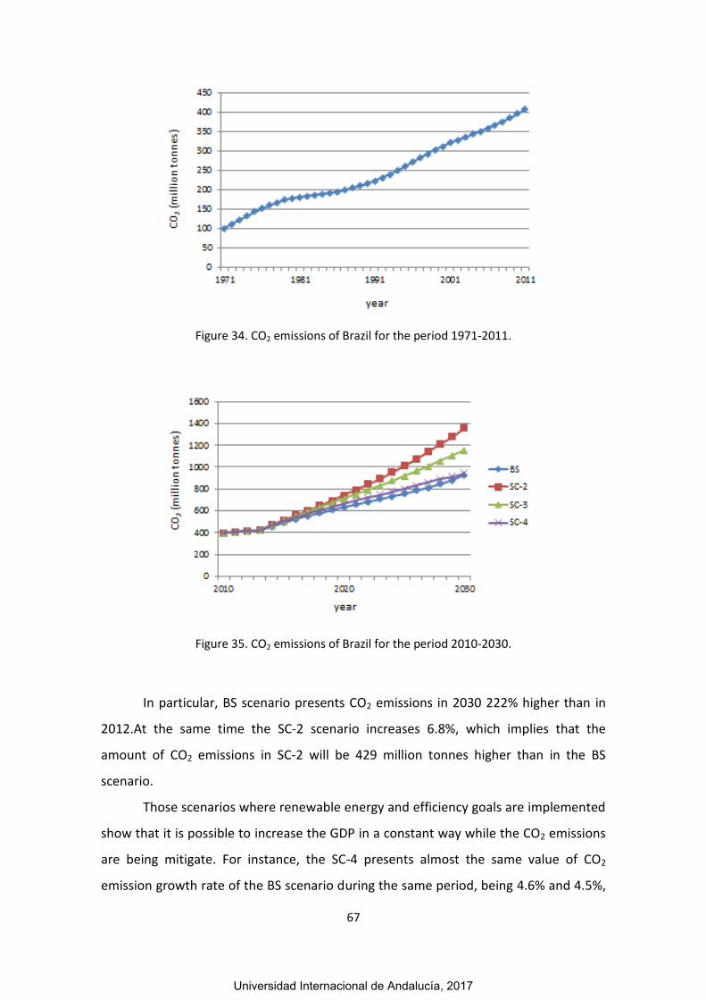
67

Figure 34. CO2 emissions of Brazil for the period 1971-2011.

Figure 35. CO2 emissions of Brazil for the period 2010-2030.

In particular, BS scenario presents CO2 emissions in 2030 222% higher than in

2012.At the same time the SC-2 scenario increases 6.8%, which implies that the

amount of CO2 emissions in SC-2 will be 429 million tonnes higher than in the BS

scenario.

Those scenarios where renewable energy and efficiency goals are implemented

show that it is possible to increase the GDP in a constant way while the CO2 emissions

are being mitigate. For instance, the SC-4 presents almost the same value of CO2

emission growth rate of the BS scenario during the same period, being 4.6% and 4.5%,


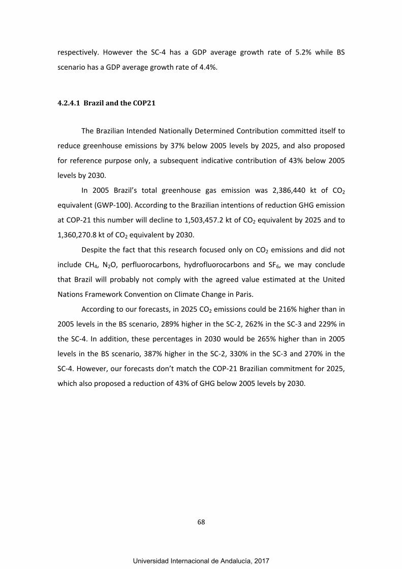
68

respectively. However the SC-4 has a GDP average growth rate of 5.2% while BS

scenario has a GDP average growth rate of 4.4%.

4.2.4.1 Brazil and the COP21

The Brazilian Intended Nationally Determined Contribution committed itself to

reduce greenhouse emissions by 37% below 2005 levels by 2025, and also proposed

for reference purpose only, a subsequent indicative contribution of 43% below 2005

levels by 2030.

In 2005 Brazil’s total greenhouse gas emission was 2,386,440 kt of CO2

equivalent (GWP-100). According to the Brazilian intentions of reduction GHG emission

at COP-21 this number will decline to 1,503,457.2 kt of CO2 equivalent by 2025 and to

1,360,270.8 kt of CO2 equivalent by 2030.

Despite the fact that this research focused only on CO2 emissions and did not

include CH4, N2O, perfluorocarbons, hydrofluorocarbons and SF6, we may conclude

that Brazil will probably not comply with the agreed value estimated at the United

Nations Framework Convention on Climate Change in Paris.

According to our forecasts, in 2025 CO2 emissions could be 216% higher than in

2005 levels in the BS scenario, 289% higher in the SC-2, 262% in the SC-3 and 229% in

the SC-4. In addition, these percentages in 2030 would be 265% higher than in 2005

levels in the BS scenario, 387% higher in the SC-2, 330% in the SC-3 and 270% in the

SC-4. However, our forecasts don’t match the COP-21 Brazilian commitment for 2025,

which also proposed a reduction of 43% of GHG below 2005 levels by 2030.


69

5. CONCLUSIONS

This research discusses the GDP, energy consumption and CO2 emissions of

Brazil in a medium term from 2013 to 2030 based on a model introduced by Robalino-

López et al. (2014 , 2015). This model analyzes the direct influence of renewable

energies on the GDP, creating a feedback mechanism between income and CO2

emissions.

The official data set (1971-2012) was used to parameterize the model, whereas

in the period 2013-2030, an estimation of different variables, including the CO2

emissions, was carried out. Beyond that, for a more complete analysis, four different

scenarios were proposed. They represent the development of GDP, energy matrix and

productive sectorial structure, which were previously defined.

First, a BS scenario (baseline scenario) has been established, based on the

model variables that were parameterized according to the observed tendency during

the period 1971-2012. In this scenario, the CO2 emission in 2030 was 222% higher than

in 2012.

Suchlike, the second scenario, called SC-2, was characterized not only by the

doubling of GDP during the 2013-2030 period, but also by a change in the productive

sector. This change would be caused by a stabilization of the primary sector, a

reduction of 4.5% in the industrial and energetic sector and an increase in service

sector of 9%. As a result, the emissions in 2030 were 325% higher than in 2012.

In the third scenario, SC-3, it was assumed the increase in GDP, the change in

the productive sector and an imposing increase of 2% in natural gas consumption and

9% in renewable, alternative and nuclear energy consumption. At the same time, a

decrease of 10% in fossil energy consumption was also taken into consideration. In this

case, the CO2 emissions in 2030 were 276% higher than in 2012. Finally, the fourth

one, SC-4, had the same variables as SC-3 but complement with a 5% reduction in the

sectorial energy intensity. This scenario in 2030 is 226 % higher than in 2012.


70

It is important to highlight that the BS scenario corresponds to a modest GDP

increase, whereas in the three other scenarios the GDP increases heavily. The SC-2 was

the scenario with the highest CO2 emission value, precisely the very one for which no

mitigation measures were taken.

In addition, the SC-3 and SC-4 indicate that it is possible to maintain the CO2

emissions while the GDP is growing. However, this can only happen by promoting the

renewable energy (as in the SC-3 scenario) and reducing the energy intensity (likewise

in the SC-4 scenario). So, the promotion of renewable energy and improvement of the

energy intensity are effective in attenuating CO2 emissions.

It is worth noting that the main outcome of this research is the estimation of

CO2 emissions of Brazil in the medium term, until 2030. That’s why it’s so important to

compare these results with the Brazil’s commitment in Paris Agreement.

Brazil defined a reduction of greenhouse emissions to 37% below 2005 levels by

2025. According to our CO2 emission forecast, the BS scenario corresponds to CO2

emissions 216% higher than in 2005 levels in the BS scenario, 289% higher in the SC-2,

262% in the SC-3 and 229% in the SC-4.

Moreover, if we consider the Brazilian proposal for 2030, which is the reduction

of 43% below 2005 levels, the values reached by CO2 emissions are 265% higher than

in 2005 levels in the BS scenario, 387% higher in the SC-2, 330% in the SC-3 and 270%

in the SC-4. We can infer that Brazil’s goals at the United Nations Framework

Convention on Climate Change in Paris are very ambitious, and unlikely be achieved.

Nevertheless, the mitigation program for carbon emissions must be

maintained. Among all shares assumed by Brazil, we emphasize the increase of 18% in

the share of sustainable biofuels in the Brazilian energy mix to by 2030; the

strengthening policies and measures achieve zero illegal deforestation in Brazilian

Amazonia Rainforest by 2030; the achievement of 45% of renewables in the energy

mix by 2030 and 10% of efficiency gains in the electricity sector by 2030.


71

This study has demonstrated the potential of a model applied to measure CO2

emissions in a short term of Brazil, many opportunities for extending this work remain,

such as:

Create a bigger sectoral disaggregation. This means, study more than

the four sectors approached in this research, which were: agriculture

sector, industrial sector, energy sector and services, residential and

transportation sector.

Apply and extend the current methodology to other countries in order

to compare the CO2 emission results with those obtained in this work. It

would be also useful to use the methodology to get results for other

countries under development, as Russia, India, China and South Africa.

Those results can be, then, compared with the results obtained for the

Brazilian analysis.

Perform a sensitivity analysis to check which variables have the most

important impact on the proposed model. This analysis shall give an

idea about the variables that should be prioritized by stakeholders in

order to reduce the CO2 emissions in the future.

Monitors the CO2 emissions in the country and calibrates the model

based on the real data registered in the future. Also be aware of the

policies proposed by Brazil at COP21 and consider them in order to

improve the proposed model.

Suggest political plans by determining which measures would imply in

an increase of GDP and a reduction of CO2 emissions. For instance, how

Brazilian government should develop public transportation in order to

be profit and reduce CO2 emissions levels. Discuss economic and

political plans with entrepreneurs and the Brazilian government; the

objective is to find out a more sustainable way of increasing the GDP

without compromising in terms of CO2 emissions.


72

6. REFERENCES

Al-mulali U, Fereidouni HG, Lee JYM. Electricity consumption from renewable

and non-renewable sources and economic growth: evidence from Latin American

countries. Renewable and Sustainable Energy Reviews 2014;30:290–8.

Brazilian Energy Research Company (BERC). Brazilian Energy Balance 2015 (Year

2014). Ministry of Mines and Energy. Rio de Janeiro: BERC, 2015.

Brazilian Energy Research Company (BERC). Brazilian National Energy Plan

2030. Rio de Janeiro: EPE 2007.408p. ISBN: 978-85-60025-02-2

Brazilian Institute of Geography and Statistics (BIGS), 2013. Research

Department of Population and Social Indicators. Projection of population by age and

sex for Brazil, Major Regions and Federation Units in 2013.

http://www.ibge.gov.br/home/estatistica/populacao/projecao_da_populacao/2013.sh

tm May, 2016.

Brazilian Institute of Geography and Statistics (BIGS). Brazilian territorial area.

http://www.ibge.gov.br/home/geociencias/areaterritorial/ historico.shtm. May, 2016.

Chien T. Hu JL. Renewable energy: an efficient mechanism to improve GDP.

Energy Policy 2008:36:3045-52.

Cowan WN, ChangT, Inglesi-LotzR, GuptaR. The nexus of electricity

consumption, economic growth and CO2 emissions in the BRICS countries. Energy

Policy 2014;66:359–68.


http://www.ibge.gov.br/home/estatistica/populacao/projecao_da_populacao/2013

http://www.ibge.gov.br/home/geociencias/areaterritorial/%20historico

73

Dasgupta S., Laplante B., Wang H., and Wheeler D. Confronting the

Environmental Kuznets Curve. Journal of Economic Perspectives 16 (1), 147–168, 2002.

Federative Republic of Brazil (FRB). Federal Senate. Legislative Information

Secretariat. Resolution Nº35 of 2016 provides for penalties in the impeachment

proceedings against the President of the Republic, Dilma Vana Rousseff, and other

measures. August, 2016.

Federative Republic of Brazil (FRC). Intended Nationally Determined

Contribution Towards Achieving the Objective of the United Nations Framework

Convention On Climate Change. December, 2015.

Hodrick R., Prescott E. Postwar U.S. business cycles: an empirical investigation. J

Money, Credit Bank 1997; 29 (February (1)): 1-16.

Ibrahim MH, Law SH. Social capital and CO2 emission–output relations: a panel

analysis. Renewable and Sustainable Energy Reviews 2014; 29:528–34.

Intergovernmental Panel on Climate Change (IPCC). IPCC Mitigation of Climate

Change 2014. Contribution of Working Group III to the Fifth Assessment Report of the

Intergovernmental Panel on Climate Change [Edenhofer, O., R. Pichs-Madruga, Y.

Sokona, E. Farahani, S. Kadner, K. Seyboth, A. Adler, I. Baum, S. Brunner, P. Eickemeier,

B. Kriemann, J. Savolainen, S. Schlömer, C. von Stechow, T. Zwickel and J.C. Minx

(eds.)]. Cambridge University Press, Cambridge, United Kingdom and New York, NY,

USA.

Intergovernmental Panel on Climate Change (IPCC). IPCC guidelines for national

greenhouse gas inventories, Prepared by the National Greenhouse Gas Inventories

Programme. Technical Report. IPCC- Intergovernmental Panel on Climate Change;

2006.


74

Intergovernmental Panel on Climate Change (IPCC). IPCC Special Reports.

Emissions Scenarios. Cambridge University Press, The Edinburgh Building Shaftesbury

Road, Cambridge CB2 2RU England, 2000.

Jaunky VC. The CO2 emissions-income nexus: evidence from rich countries.

Energy Policy 2011; 39:1228–40.

Kaya. Y. Impact of Carbon Dioxide Emission Control on GNP Growth:

Interpretation of Proposed Scenarios. Paper presented to the IPCC Energy and Industry

Subgroup, Response Strategies Working Group, Paris, (mimeo), 1990.

Kaya Y. and Yokobori K. Environment, Energy, and Economy: strategies for

sustainability. Conference on Global Environment, Energy, and Economic Development

(1993 : Tokyo, Japan)., 1993.

Kuntsi-Reunanen E .A comparison of Latin American energy-related CO2

emissions from 1970 to 2001.Energy Policy 2007;35:586–96.

Ministry of the Environment (ME). Forth National Report to the Convention on

Biological Diversity. Brasília, ME, 2011. 248 p. ISBN 978-85-7738-150-0.

Narayan PK, Narayan S. Carbon dioxide emissions and economic growth: panel

data evidence from developing countries. Energy Policy 2010; 38:661–6.

Padilla E, Serrano A. Inequality in CO2 emissions across countries and its

relationship within come inequality: a distributive approach. Energy Policy 2006;

34:1762–72.

Robalino-López A, Carbon emissions, energy consumption and sustainable

development in Ecuador (1980-2025): System dynamics modelling, decomposition

analysis and the environmental Kuznets curve. Access to PhD dissertantion:


75

http://columbus.uhu.es/search*spi/X?(tesis%20universidad% 20huelva)&searchscope

=1&Da=&Db=&SORT=D. Huelva, 2014.

Robalino-López A, García-Ramos JE, Golpe AA , Mena-Nieto A. CO2 emissions

convergence among 10 South American countries. A study of Kaya components (1980-

2010). Carbon Management 2016.

Robalino-López A, García-Ramos JE, Golpe AA , Mena-Nieto A. System dynamics

modelling and the Environmental Kuznets Curve in Ecuador (1980–2025). Energy Policy

2013; 67:923–31.

Robalino-López A, Mena-Nieto A, García-Ramos JE, Golpe AA. Studying the

relationship between economic growth,CO2, emissions and the environmental Kuznets

curve in Venezuela (1980-2025). Renewable and Sustainable Energy Reviews 2015; 41:

602-14.

Robalino-López A, Mena-Nieto A, García-Ramos JE. System dynamics modeling

for green energy consumption and CO2 emissions: a case study of Ecuador Energy

Sustainable Development 2014; 20:11–20.

United Nations Development Program (UNDP). 2015 Human Development

Report. United Nations Development Programme, ISBN: 978-92-1-126398-5, 2015.

United Nations Environment Programme (UNEP). Convention on Biological

Diversity. Cancun Declaration of Like-Mided Megadiversity Countries. March, 2002.

United Nations Framework Convetion on Climate Change (UNFCCC). Report of

the Conference of the Parties on its twenty-first session, held in Paris from 30

November to 13 December 2015. Addendum Part two: Action taken by the Conference

of the Parties at its twenty-first session. January, 2016.


http://columbus.uhu.es/search*spi/X?(tesis%20universidad%25

76

World Bank (WB). Data, statistics and National referents-Brazil.

http://www.world bank.org/pt/country/brazil, May 2016.

Zambrano-Monserrate M.A, Valverde-Bajana I., Aguilar-Bohorquez J., Mendoza-

Jimenez M.J. Relationship between economic growth and environmental degradation:

is there evidence of an environmental Kuznets Curve for Brazil? International Journal

of Energy Economics and Policy 2016; 6:208-16.


http://www.world/

77

7. APPENDIX

Appendix 1. GDP values. From 1971 to 2012 corresponds to official dataset and from 2013 to

2030 corresponds to predictions.

Year GDP ($2005)

BS Scenario SC-2 SC-3 SC-4

1971 268292950571 268292950571 268292950571 268292950571

1972 293609799387 293609799387 293609799387 293609799387

1973 318745465697 318745465697 318745465697 318745465697

1974 343385946002 343385946002 343385946002 343385946002

1975 367224921145 367224921145 367224921145 367224921145

1976 390006259509 390006259509 390006259509 390006259509

1977 411467114267 411467114267 411467114267 411467114267

1978 431468980995 431468980995 431468980995 431468980995

1979 449968466128 449968466128 449968466128 449968466128

1980 466953316290 466953316290 466953316290 466953316290

1981 482551474443 482551474443 482551474443 482551474443

1982 497283968389 497283968389 497283968389 497283968389

1983 511686511181 511686511181 511686511181 511686511181

1984 526190261193 526190261193 526190261193 526190261193

1985 540811797684 540811797684 540811797684 540811797684

1986 555255853302 555255853302 555255853302 555255853302

1987 569162423719 569162423719 569162423719 569162423719

1988 582389172071 582389172071 582389172071 582389172071

1989 595080070261 595080070261 595080070261 595080070261

1990 607526993468 607526993468 607526993468 607526993468

1991 620238654170 620238654170 620238654170 620238654170

1992 633624790909 633624790909 633624790909 633624790909

1993 647959408688 647959408688 647959408688 647959408688

1994 663218591598 663218591598 663218591598 663218591598

1995 679218855644 679218855644 679218855644 679218855644

1996 695801701916 695801701916 695801701916 695801701916

1997 712967642946 712967642946 712967642946 712967642946

1998 730863824248 730863824248 730863824248 730863824248

1999 74985356990 74985356990 74985356990 74985356990

2000 770362275762 770362275762 770362275762 770362275762

2001 792722085958 792722085958 792722085958 792722085958

2002 817271352880 817271352880 817271352880 817271352880

2003 844258854052 844258854052 844258854052 844258854052


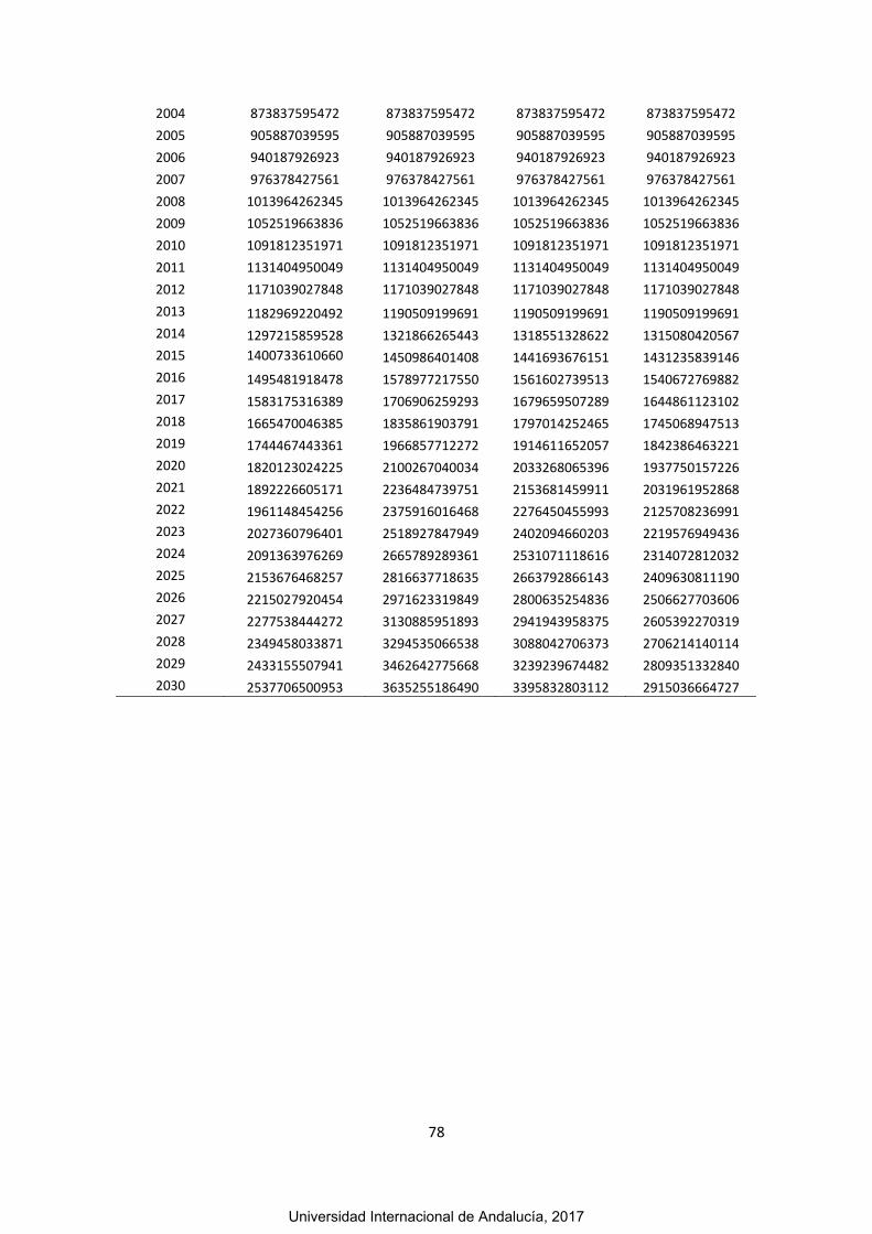
78

2004 873837595472 873837595472 873837595472 873837595472

2005 905887039595 905887039595 905887039595 905887039595

2006 940187926923 940187926923 940187926923 940187926923

2007 976378427561 976378427561 976378427561 976378427561

2008 1013964262345 1013964262345 1013964262345 1013964262345

2009 1052519663836 1052519663836 1052519663836 1052519663836

2010 1091812351971 1091812351971 1091812351971 1091812351971

2011 1131404950049 1131404950049 1131404950049 1131404950049

2012 1171039027848 1171039027848 1171039027848 1171039027848

2013 1182969220492 1190509199691 1190509199691 1190509199691

2014 1297215859528 1321866265443 1318551328622 1315080420567

2015 1400733610660 1450986401408 1441693676151 1431235839146

2016 1495481918478 1578977217550 1561602739513 1540672769882

2017 1583175316389 1706906259293 1679659507289 1644861123102

2018 1665470046385 1835861903791 1797014252465 1745068947513

2019 1744467443361 1966857712272 1914611652057 1842386463221

2020 1820123024225 2100267040034 2033268065396 1937750157226

2021 1892226605171 2236484739751 2153681459911 2031961952868

2022 1961148454256 2375916016468 2276450455993 2125708236991

2023 2027360796401 2518927847949 2402094660203 2219576949436

2024 2091363976269 2665789289361 2531071118616 2314072812032

2025 2153676468257 2816637718635 2663792866143 2409630811190

2026 2215027920454 2971623319849 2800635254836 2506627703606

2027 2277538444272 3130885951893 2941943958375 2605392270319

2028 2349458033871 3294535066538 3088042706373 2706214140114

2029 2433155507941 3462642775668 3239239674482 2809351332840

2030 2537706500953 3635255186490 3395832803112 2915036664727


79

Appendix 2. Total energy values. From 1971 to 2012 corresponds to official dataset and from

2013 to 2030 corresponds to predictions.

Year Total Energy (toe)


1971 71873660 71873660 71873660 71873660

1972 77144748 77144748 77144748 77144748

1973 82150776 82150776 82150776 82150776

1974 86875635 86875635 86875635 86875635

1975 91319144 91319144 91319144 91319144

1976 95498246 95498246 95498246 95498246

1977 99436658 99436658 99436658 99436658

1978 103163593 103163593 103163593 103163593

1979 106697324 106697324 106697324 106697324

1980 110068211 110068211 110068211 110068211

1981 113353692 113353692 113353692 113353692

1982 116670191 116670191 116670191 116670191

1983 120086093 120086093 120086093 120086093

1984 123603048 123603048 123603048 123603048

1985 127154334 127154334 127154334 127154334

1986 130645577 130645577 130645577 130645577

1987 134002054 134002054 134002054 134002054

1988 137200533 137200533 137200533 137200533

1989 140287006 140287006 140287006 140287006

1990 143363630 143363630 143363630 143363630

1991 146587524 146587524 146587524 146587524

1992 150087211 150087211 150087211 150087211

1993 153955841 153955841 153955841 153955841

1994 158233916 158233916 158233916 158233916

1995 162898485 162898485 162898485 162898485

1996 167888200 167888200 167888200 167888200

1997 173100450 173100450 173100450 173100450

1998 178425183 178425183 178425183 178425183

1999 183796182 183796182 183796182 183796182

2000 189204614 189204614 189204614 189204614

2001 194716118 194716118 194716118 194716118

2002 200438007 200438007 200438007 200438007

2003 206476391 206476391 206476391 206476391

2004 212910808 212910808 212910808 212910808

2005 219755198 219755198 219755198 219755198

2006 227004980 227004980 227004980 227004980

2007 234621361 234621361 234621361 234621361

2008 242524337 242524337 242524337 242524337

2009 250633841 250633841 250633841 250633841

2010 258922162 258922162 258922162 258922162

2011 267249494 267249494 267249494 267249494


80

2012 275535500 275535500 275535500 275535500

2013 277130556 279586116 279586116 278778771

2014 302594573 309872213 309095124 306478855

2015 325356491 339543142 337368566 331956602

2016 345884178 368852803 364794084 355633909

2017 364584109 398044454 391690608 377872666

2018 381844159 427360314 418317181 398981962

2019 398190459 457056868 444915969 419224528

2020 413615911 487215446 471673167 438823555

2021 428077040 517921826 498746365 457967755

2022 441665859 549265428 526270931 476816402

2023 454499232 581328184 554364956 495503809

2024 466701956 614172370 583134591 514143262

2025 478393681 647824423 612670229 532830524

2026 489740012 682314194 643053638 551646723

2027 501210877 717669766 674359994 570660933

2028 514610698 753912553 706659396 589932364

2029 530427537 791055350 740017969 609512223

2030 550593722 829104077 774498262 629445279


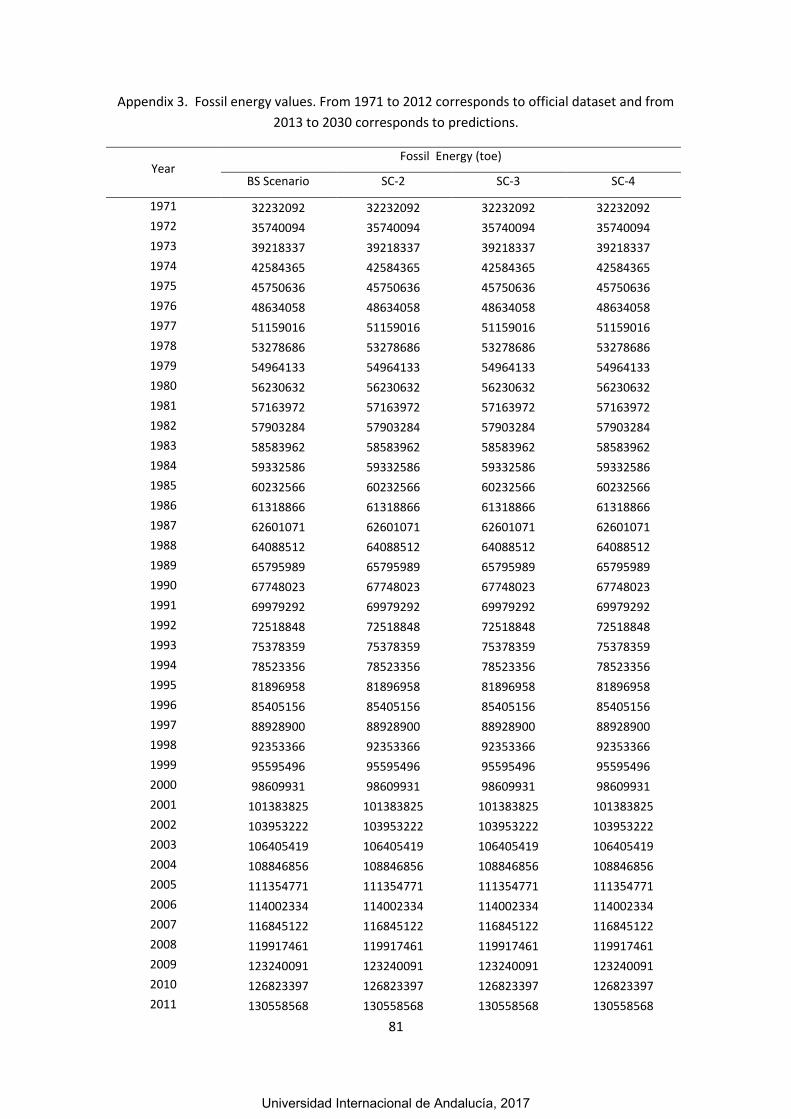
81

Appendix 3. Fossil energy values. From 1971 to 2012 corresponds to official dataset and from


Year Fossil Energy (toe)


1971 32232092 32232092 32232092 32232092

1972 35740094 35740094 35740094 35740094

1973 39218337 39218337 39218337 39218337

1974 42584365 42584365 42584365 42584365

1975 45750636 45750636 45750636 45750636

1976 48634058 48634058 48634058 48634058

1977 51159016 51159016 51159016 51159016

1978 53278686 53278686 53278686 53278686

1979 54964133 54964133 54964133 54964133

1980 56230632 56230632 56230632 56230632

1981 57163972 57163972 57163972 57163972

1982 57903284 57903284 57903284 57903284

1983 58583962 58583962 58583962 58583962

1984 59332586 59332586 59332586 59332586

1985 60232566 60232566 60232566 60232566

1986 61318866 61318866 61318866 61318866

1987 62601071 62601071 62601071 62601071

1988 64088512 64088512 64088512 64088512

1989 65795989 65795989 65795989 65795989

1990 67748023 67748023 67748023 67748023

1991 69979292 69979292 69979292 69979292

1992 72518848 72518848 72518848 72518848

1993 75378359 75378359 75378359 75378359

1994 78523356 78523356 78523356 78523356

1995 81896958 81896958 81896958 81896958

1996 85405156 85405156 85405156 85405156

1997 88928900 88928900 88928900 88928900

1998 92353366 92353366 92353366 92353366

1999 95595496 95595496 95595496 95595496

2000 98609931 98609931 98609931 98609931

2001 101383825 101383825 101383825 101383825

2002 103953222 103953222 103953222 103953222

2003 106405419 106405419 106405419 106405419

2004 108846856 108846856 108846856 108846856

2005 111354771 111354771 111354771 111354771

2006 114002334 114002334 114002334 114002334

2007 116845122 116845122 116845122 116845122

2008 119917461 119917461 119917461 119917461

2009 123240091 123240091 123240091 123240091

2010 126823397 126823397 126823397 126823397

2011 130558568 130558568 130558568 130558568


82

2012 134322904 134322904 134322904 134322904

2013 134986833 136021416 136137177 135848020

2014 147471239 150662594 150360890 149305150

2015 158824807 165165938 163962638 161672586

2016 169271696 179659549 177128385 173156757

2017 179005021 194265899 190010248 183934646

2018 188229654 209129403 202731523 194157373

2019 197244747 224436570 215418043 203953015

2020 206053087 240247581 228157725 213430537

2021 214643198 256630733 241025034 222681993

2022 223080269 273668972 254084308 231785012

2023 231451796 291455395 267392242 240804988

2024 239853520 310081315 281000449 249797005

2025 248378515 329618587 294950757 258807615

2026 257154343 350153545 309281108 267876204

2027 266482676 371785500 324026455 277036257

2028 277406041 394623687 339219326 286316433

2029 290315882 418785957 354890154 295741476

2030 306448946 444402429 371067222 305332983


83

Appendix 4. Renewable energy values. From 1971 to 2012 corresponds to official dataset and

from 2013 to 2030 corresponds to predictions.

Year Renewable Energy (toe)


1971 38431711 38431711 38431711 38431711

1972 39668459 39668459 39668459 39668459

1973 40914082 40914082 40914082 40914082

1974 42189326 42189326 42189326 42189326

1975 43521479 43521479 43521479 43521479

1976 44945067 44945067 44945067 44945067

1977 46495617 46495617 46495617 46495617

1978 48197620 48197620 48197620 48197620

1979 50063939 50063939 50063939 50063939

1980 52084183 52084183 52084183 52084183

1981 54235345 54235345 54235345 54235345

1982 56488166 56488166 56488166 56488166

1983 58785393 58785393 58785393 58785393

1984 61031807 61031807 61031807 61031807

1985 63117370 63117370 63117370 63117370

1986 64958902 64958902 64958902 64958902

1987 66511926 66511926 66511926 66511926

1988 67759288 67759288 67759288 67759288

1989 68729041 68729041 68729041 68729041

1990 69484758 69484758 69484758 69484758

1991 70132334 70132334 70132334 70132334

1992 70766804 70766804 70766804 70766804

1993 71468244 71468244 71468244 71468244

1994 72292055 72292055 72292055 72292055

1995 73270454 73270454 73270454 73270454

1996 74440671 74440671 74440671 74440671

1997 75838468 75838468 75838468 75838468

1998 77497181 77497181 77497181 77497181

1999 79464031 79464031 79464031 79464031

2000 81790031 81790031 81790031 81790031

2001 84528931 84528931 84528931 84528931

2002 87699490 87699490 87699490 87699490

2003 91258051 91258051 91258051 91258051

2004 95122714 95122714 95122714 95122714

2005 99201526 99201526 99201526 99201526

2006 103402836 103402836 103402836 103402836

2007 107628070 107628070 107628070 107628070

2008 111782443 111782443 111782443 111782443

2009 115809544 115809544 115809544 115809544

2010 119714162 119714162 119714162 119714162

2011 123513554 123513554 123513554 123513554


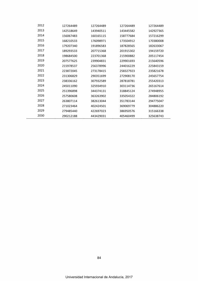
84

2012 127264489 127264489 127264489 127264489

2013 142518649 143940511 143445582 142927365

2014 156067483 160165115 158777684 157216299

2015 168210533 176098971 173504912 170380008

2016 179207340 191896583 187828565 182633067

2017 189293533 207715368 201915302 194159720

2018 198684500 223701368 215900882 205117454

2019 207577625 239904831 229901693 215640596

2020 215978537 256378996 244016229 225843159

2021 223872045 273178415 258327923 235821678

2022 231306829 290351699 272908170 245657754

2023 238336162 307932589 287818781 255420313

2024 245011090 325934910 303114736 265167614

2025 251396898 344374131 318845124 274948955

2026 257580608 363263902 335054322 284806192

2027 263807114 382613044 351783144 294775047

2028 271023464 402424501 369069779 304886220

2029 279485440 422697023 386950576 315166338

2030 290212188 443429031 405460499 325638743


85

Appendix 5. Values of energy consumption of Brazilian primary sector for the BS and SC-2

scenarios.

Years E1 E2 E3 E4 E5 E6 E7

2000 0 0.0017 0 0.6086 0.0118 0 0.3781

2001 0 0.0019 0 0.6053 0.0119 0 0.3811

2002 0 0.0021 0 0.6009 0.0117 0 0.3856

2003 0 0.0022 0 0.5957 0.0112 0 0.3911

2004 0 0.0022 0 0.5903 0.0106 0 0.3970

2005 0 0.0022 0 0.5852 0.0098 0 0.4029

2006 0 0.0021 0 0.5806 0.0090 0 0.4083

2007 0 0.0020 0 0.5767 0.0081 0 0.4131

2008 0 0.0019 0 0.5734 0.0072 0 0.4173

2009 0 0.0017 0 0.5706 0.0062 0 0.4212

2010 0 0.0016 0 0.5680 0.0052 0 0.4249

2011 0 0.0014 0 0.5655 0.0042 0 0.4286

2012 0 0.0012 0 0.5631 0.0031 0 0.4322

2013 0 0.0011 0 0.5601 0.0026 0 0.4359

2014 0 0.0009 0 0.5572 0.0021 0 0.4395

2015 0 0.0008 0 0.5542 0.0017 0 0.4430

2016 0 0.0007 0 0.5512 0.0013 0 0.4465

2017 0 0.0006 0 0.5481 0.0010 0 0.4499

2018 0 0.0006 0 0.5448 0.0008 0 0.4533

2019 0 0.0005 0 0.5416 0.0007 0 0.4566

2020 0 0.0004 0 0.5382 0.0005 0 0.4598

2021 0 0.0004 0 0.5348 0.0004 0 0.4630

2022 0 0.0003 0 0.5313 0.0003 0 0.4662

2023 0 0.0003 0 0.5278 0.0003 0 0.4693

2024 0 0.0003 0 0.5242 0.0002 0 0.4724

2025 0 0.0002 0 0.5206 0.0002 0 0.4754

2026 0 0.0002 0 0.5169 0.0001 0 0.4783

2027 0 0.0002 0 0.5131 0.0001 0 0.4812

2028 0 0.0002 0 0.5093 0 0 0.4841

2029 0 0.0001 0 0.5055 0 0 0.4869

2030 0 0.0001 0 0.5016 0 0 0.4896


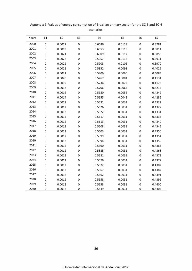
86

Appendix 6. Values of energy consumption of Brazilian primary sector for the SC-3 and SC-4

scenarios.


2000 0 0.0017 0 0.6086 0.0118 0 0.3781

2001 0 0.0019 0 0.6053 0.0119 0 0.3811

2002 0 0.0021 0 0.6009 0.0117 0 0.3856

2003 0 0.0022 0 0.5957 0.0112 0 0.3911

2004 0 0.0022 0 0.5903 0.0106 0 0.3970

2005 0 0.0022 0 0.5852 0.0098 0 0.4029

2006 0 0.0021 0 0.5806 0.0090 0 0.4083

2007 0 0.0020 0 0.5767 0.0081 0 0.4131

2008 0 0.0019 0 0.5734 0.0072 0 0.4173

2009 0 0.0017 0 0.5706 0.0062 0 0.4212

2010 0 0.0016 0 0.5680 0.0052 0 0.4249

2011 0 0.0014 0 0.5655 0.0042 0 0.4286

2012 0 0.0012 0 0.5631 0.0031 0 0.4322

2013 0 0.0012 0 0.5626 0.0031 0 0.4327

2014 0 0.0012 0 0.5622 0.0031 0 0.4331

2015 0 0.0012 0 0.5617 0.0031 0 0.4336

2016 0 0.0012 0 0.5613 0.0031 0 0.4340

2017 0 0.0012 0 0.5608 0.0031 0 0.4345

2018 0 0.0012 0 0.5603 0.0031 0 0.4350

2019 0 0.0012 0 0.5599 0.0031 0 0.4354

2020 0 0.0012 0 0.5594 0.0031 0 0.4359

2021 0 0.0012 0 0.5590 0.0031 0 0.4363

2022 0 0.0012 0 0.5585 0.0031 0 0.4368

2023 0 0.0012 0 0.5581 0.0031 0 0.4373

2024 0 0.0012 0 0.5576 0.0031 0 0.4377

2025 0 0.0012 0 0.5572 0.0031 0 0.4382

2026 0 0.0012 0 0.5567 0.0031 0 0.4387

2027 0 0.0012 0 0.5562 0.0031 0 0.4391

2028 0 0.0012 0 0.5558 0.0031 0 0.4396

2029 0 0.0012 0 0.5553 0.0031 0 0.4400

2030 0 0.0012 0 0.5549 0.0031 0 0.4405


87

Appendix 7. Values of energy consumption of Brazilian manufacturing sector for the BS and SC-

2 scenarios.


2000 0.0665 0.0344 0 0.0064 0.1086 0.2028 0.5816

2001 0.0721 0.0335 0 0.0065 0.0991 0.2043 0.5850

2002 0.0775 0.0326 0 0.0065 0.0893 0.2049 0.5896

2003 0.0827 0.0319 0 0.0065 0.0798 0.2046 0.5949

2004 0.0874 0.0313 0 0.0065 0.0709 0.2037 0.6006

2005 0.0917 0.0308 0 0.0064 0.0628 0.2026 0.6060

2006 0.0953 0.0305 0 0.0065 0.0555 0.2015 0.6109

2007 0.0985 0.0304 0 0.0065 0.0489 0.2007 0.6150

2008 0.1013 0.0304 0 0.0066 0.0430 0.2004 0.6183

2009 0.1039 0.0304 0 0.0067 0.0376 0.2006 0.6207

2010 0.1063 0.0306 0 0.0068 0.0324 0.2012 0.6226

2011 0.1087 0.0307 0 0.0069 0.0273 0.2021 0.6240

2012 0.1110 0.0309 0 0.0071 0.0223 0.2031 0.6253

2013 0.1136 0.0310 0 0.0072 0.0191 0.2034 0.6270

2014 0.1162 0.0311 0 0.0073 0.0162 0.2039 0.6285

2015 0.1188 0.0312 0 0.0074 0.0137 0.2045 0.6297

2016 0.1213 0.0313 0 0.0076 0.0115 0.2051 0.6307

2017 0.1240 0.0314 0 0.0077 0.0097 0.2056 0.6318

2018 0.1267 0.0315 0 0.0078 0.0082 0.2059 0.6327

2019 0.1294 0.0316 0 0.0079 0.0069 0.2063 0.6335

2020 0.1321 0.0317 0 0.0081 0.0058 0.2067 0.6342

2021 0.1349 0.0318 0 0.0082 0.0049 0.2071 0.6348

2022 0.1378 0.0318 0 0.0083 0.0041 0.2074 0.6354

2023 0.1406 0.0319 0 0.0085 0.0035 0.2076 0.6358

2024 0.1435 0.0320 0 0.0086 0.0029 0.2079 0.6361

2025 0.1465 0.0320 0 0.0088 0.0025 0.2081 0.6363

2026 0.1494 0.0321 0 0.0089 0.0021 0.2082 0.6364

2027 0.1525 0.0321 0 0.0090 0.0018 0.2084 0.6365

2028 0.1555 0.0322 0 0.0092 0.0015 0.2085 0.6364

2029 0.1586 0.0322 0 0.0093 0.0012 0.2086 0.6363

2030 0.1618 0.0323 0 0.0095 0.0011 0.2087 0.6361


88

Appendix 8. Values of energy consumption of Brazilian manufacturing sector for the SC-3 and

SC-4 scenarios.


2000 0.0665 0.0344 0 0.0064 0.1086 0.2028 0.5816

2001 0.0721 0.0335 0 0.0065 0.0991 0.2043 0.5850

2002 0.0775 0.0326 0 0.0065 0.0893 0.2049 0.5896

2003 0.0827 0.0319 0 0.0065 0.0798 0.2046 0.5949

2004 0.0874 0.0313 0 0.0065 0.0709 0.2037 0.6006

2005 0.0917 0.0308 0 0.0064 0.0628 0.2026 0.6060

2006 0.0953 0.0305 0 0.0065 0.0555 0.2015 0.6109

2007 0.0985 0.0304 0 0.0065 0.0489 0.2007 0.6150

2008 0.1013 0.0304 0 0.0066 0.0430 0.2004 0.6183

2009 0.1039 0.0304 0 0.0067 0.0376 0.2006 0.6207

2010 0.1063 0.0306 0 0.0068 0.0324 0.2012 0.6226

2011 0.1087 0.0307 0 0.0069 0.0273 0.2021 0.6240

2012 0.1110 0.0309 0 0.0071 0.0223 0.2031 0.6253

2013 0.1109 0.0309 0 0.0070 0.0223 0.2029 0.6260

2014 0.1108 0.0309 0 0.0070 0.0223 0.2028 0.6266

2015 0.1107 0.0308 0 0.0070 0.0223 0.2026 0.6273

2016 0.1107 0.0308 0 0.0070 0.0223 0.2024 0.6280

2017 0.1106 0.0308 0 0.0070 0.0222 0.2023 0.6286

2018 0.1105 0.0308 0 0.0070 0.0222 0.2021 0.6293

2019 0.1104 0.0307 0 0.0070 0.0222 0.2019 0.6300

2020 0.1103 0.0307 0 0.0070 0.0222 0.2018 0.6306

2021 0.1102 0.0307 0 0.0070 0.0222 0.2016 0.6313

2022 0.1101 0.0307 0 0.0070 0.0222 0.2014 0.6320

2023 0.1100 0.0306 0 0.0070 0.0221 0.2013 0.6326

2024 0.1099 0.0306 0 0.0070 0.0221 0.2011 0.6333

2025 0.1098 0.0306 0 0.0070 0.0221 0.2009 0.6340

2026 0.1098 0.0306 0 0.0070 0.0221 0.2008 0.6346

2027 0.1097 0.0305 0 0.0070 0.0221 0.2006 0.6353

2028 0.1096 0.0305 0 0.0070 0.0220 0.2005 0.6360

2029 0.1095 0.0305 0 0.0070 0.0220 0.2003 0.6366

2030 0.1094 0.0305 0 0.0069 0.0220 0.2001 0.6373


89

Appendix 9. Values of energy consumption of Brazilian energetic sector for the BS and SC-2

scenarios.


2000 0.1260 0.0227 0.0006 0.0201 0.1187 0.1895 0.5227

2001 0.1359 0.0218 0.0006 0.0193 0.1129 0.1945 0.5152

2002 0.1451 0.0208 0.0005 0.0187 0.1066 0.1979 0.5107

2003 0.1535 0.0196 0.0004 0.0184 0.0996 0.1996 0.5090

2004 0.1610 0.0184 0.0003 0.0186 0.0922 0.1995 0.5099

2005 0.1680 0.0170 0.0002 0.0194 0.0844 0.1978 0.5130

2006 0.1744 0.0156 0.0002 0.0209 0.0762 0.1945 0.5178

2007 0.1806 0.0141 0.0001 0.0233 0.0677 0.1901 0.5238

2008 0.1867 0.0126 0 0.0265 0.0588 0.1849 0.5300

2009 0.1929 0.0111 0 0.0307 0.0498 0.1792 0.5359

2010 0.1992 0.0097 0 0.0355 0.0406 0.1734 0.5413

2011 0.2059 0.0083 0 0.0407 0.0313 0.1675 0.5460

2012 0.2127 0.0069 0 0.0461 0.0220 0.1614 0.5505

2013 0.2196 0.0060 0 0.0528 0.0176 0.1562 0.5558

2014 0.2268 0.0052 0 0.0605 0.0138 0.1509 0.5608

2015 0.2341 0.0044 0 0.0693 0.0107 0.1457 0.5656

2016 0.2416 0.0038 0 0.0791 0.0082 0.1407 0.5702

2017 0.2494 0.0033 0 0.0903 0.0063 0.1358 0.5749

2018 0.2573 0.0028 0 0.1033 0.0049 0.1311 0.5796

2019 0.2654 0.0024 0 0.1181 0.0038 0.1265 0.5842

2020 0.2738 0.0021 0 0.1349 0.0029 0.1221 0.5886

2021 0.2824 0.0018 0 0.1541 0.0022 0.1178 0.5931

2022 0.2912 0.0015 0 0.1760 0.0017 0.1136 0.5975

2023 0.3002 0.0013 0 0.2010 0.0013 0.1095 0.6018

2024 0.3094 0.0011 0 0.2296 0.0010 0.1056 0.6061

2025 0.3189 0.0010 0 0.2621 0.0008 0.1018 0.6103

2026 0.3287 0.0008 0 0.2992 0.0006 0.0982 0.6144

2027 0.3386 0.0007 0 0.3414 0.0005 0.0946 0.6185

2028 0.3489 0.0006 0 0.3897 0.0004 0.0912 0.6225

2029 0.3594 0.0005 0 0.4446 0.0003 0.0879 0.6265

2030 0.3701 0.0004 0 0.5072 0.0002 0.0847 0.6304


90

Appendix 10. Values of energy consumption of Brazilian energetic sector for the SC-3 and SC-4

scenarios.


2000 0.1260 0.0227 0.0006 0.0201 0.1187 0.1895 0.5227

2001 0.1359 0.0218 0.0006 0.0193 0.1129 0.1945 0.5152

2002 0.1451 0.0208 0.0005 0.0187 0.1066 0.1979 0.5107

2003 0.1535 0.0196 0.0004 0.0184 0.0996 0.1996 0.5090

2004 0.1610 0.0184 0.0003 0.0186 0.0922 0.1995 0.5099

2005 0.1680 0.0170 0.0002 0.0194 0.0844 0.1978 0.5130

2006 0.1744 0.0156 0.0002 0.0209 0.0762 0.1945 0.5178

2007 0.1806 0.0141 0.0001 0.0233 0.0677 0.1901 0.5238

2008 0.1867 0.0126 0 0.0265 0.0588 0.1849 0.5300

2009 0.1929 0.0111 0 0.0307 0.0498 0.1792 0.5359

2010 0.1992 0.0097 0 0.0355 0.0406 0.1734 0.5413

2011 0.2059 0.0083 0 0.0407 0.0313 0.1675 0.5460

2012 0.2127 0.0069 0 0.0461 0.0220 0.1614 0.5505

2013 0.2125 0.0069 0 0.0460 0.0220 0.1613 0.5511

2014 0.2123 0.0069 0 0.0460 0.0220 0.1612 0.5517

2015 0.2122 0.0069 0 0.0459 0.0220 0.1611 0.5523

2016 0.2120 0.0069 0 0.0459 0.0220 0.1609 0.5529

2017 0.2118 0.0069 0 0.0459 0.0220 0.1608 0.5535

2018 0.2117 0.0069 0 0.0458 0.0219 0.1607 0.5541

2019 0.2115 0.0069 0 0.0458 0.0219 0.1605 0.5546

2020 0.2113 0.0069 0 0.0458 0.0219 0.1604 0.5552

2021 0.2111 0.0069 0 0.0457 0.0219 0.1603 0.5558

2022 0.2110 0.0069 0 0.0457 0.0219 0.1601 0.5564

2023 0.2108 0.0069 0 0.0456 0.0218 0.1600 0.5570

2024 0.2106 0.0069 0 0.0456 0.0218 0.1599 0.5576

2025 0.2104 0.0069 0 0.0456 0.0218 0.1598 0.5582

2026 0.2103 0.0068 0 0.0455 0.0218 0.1596 0.5588

2027 0.2101 0.0068 0 0.0455 0.0218 0.1595 0.5593

2028 0.2099 0.0068 0 0.0455 0.0218 0.1594 0.5599

2029 0.2098 0.0068 0 0.0454 0.0217 0.1592 0.5605

2030 0.2096 0.0068 0 0.0454 0.0217 0.1591 0.5611


91

Appendix 11. Values of energy consumption of Brazilian tertiary sector for the BS and SC-2

scenarios.


2000 0.0096 0.0822 0.1941 0.2951 0.0150 0 0.4040

2001 0.0118 0.0807 0.1930 0.2972 0.0144 0 0.4030

2002 0.0141 0.0789 0.1911 0.2987 0.0137 0 0.4035

2003 0.0164 0.0770 0.1889 0.2993 0.0130 0 0.4054

2004 0.0184 0.0748 0.1868 0.2992 0.0124 0 0.4084

2005 0.0201 0.0726 0.1850 0.2983 0.0118 0 0.4122

2006 0.0214 0.0702 0.1839 0.2968 0.0113 0 0.4163

2007 0.0223 0.0679 0.1837 0.2948 0.0108 0 0.4205

2008 0.0227 0.0655 0.1845 0.2927 0.0103 0 0.4243

2009 0.0228 0.0632 0.1865 0.2905 0.0098 0 0.4273

2010 0.0227 0.0609 0.1895 0.2884 0.0093 0 0.4292

2011 0.0225 0.0586 0.1933 0.2865 0.0087 0 0.4304

2012 0.0222 0.0564 0.1974 0.2846 0.0082 0 0.4313

2013 0.0222 0.0543 0.2002 0.2824 0.0077 0 0.4332

2014 0.0221 0.0522 0.2034 0.2803 0.0073 0 0.4348

2015 0.0219 0.0503 0.2069 0.2781 0.0068 0 0.4360

2016 0.0217 0.0483 0.2104 0.2760 0.0064 0 0.4372

2017 0.0216 0.0465 0.2139 0.2738 0.0060 0 0.4383

2018 0.0214 0.0447 0.2172 0.2715 0.0057 0 0.4395

2019 0.0213 0.0430 0.2207 0.2692 0.0054 0 0.4405

2020 0.0211 0.0413 0.2242 0.2669 0.0050 0 0.4414

2021 0.0209 0.0397 0.2277 0.2646 0.0047 0 0.4423

2022 0.0208 0.0382 0.2312 0.2623 0.0044 0 0.4431

2023 0.0206 0.0367 0.2347 0.2599 0.0042 0 0.4439

2024 0.0204 0.0352 0.2383 0.2576 0.0039 0 0.4446

2025 0.0203 0.0338 0.2419 0.2552 0.0037 0 0.4452

2026 0.0201 0.0325 0.2454 0.2528 0.0035 0 0.4457

2027 0.0199 0.0312 0.2490 0.2503 0.0033 0 0.4462

2028 0.0198 0.0299 0.2527 0.2479 0.0031 0 0.4467

2029 0.0196 0.0288 0.2563 0.2455 0.0029 0 0.4470

2030 0.0194 0.0276 0.2600 0.2430 0.0027 0 0.4473


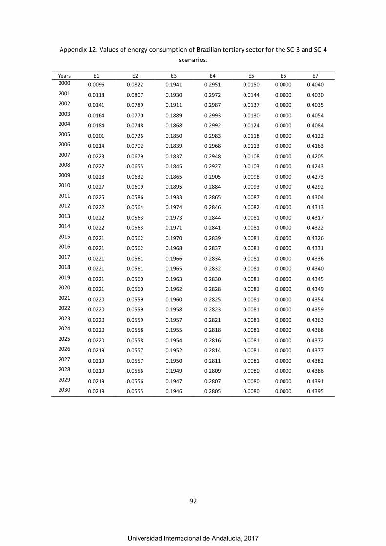
92

Appendix 12. Values of energy consumption of Brazilian tertiary sector for the SC-3 and SC-4

scenarios.


2000 0.0096 0.0822 0.1941 0.2951 0.0150 0.0000 0.4040

2001 0.0118 0.0807 0.1930 0.2972 0.0144 0.0000 0.4030

2002 0.0141 0.0789 0.1911 0.2987 0.0137 0.0000 0.4035

2003 0.0164 0.0770 0.1889 0.2993 0.0130 0.0000 0.4054

2004 0.0184 0.0748 0.1868 0.2992 0.0124 0.0000 0.4084

2005 0.0201 0.0726 0.1850 0.2983 0.0118 0.0000 0.4122

2006 0.0214 0.0702 0.1839 0.2968 0.0113 0.0000 0.4163

2007 0.0223 0.0679 0.1837 0.2948 0.0108 0.0000 0.4205

2008 0.0227 0.0655 0.1845 0.2927 0.0103 0.0000 0.4243

2009 0.0228 0.0632 0.1865 0.2905 0.0098 0.0000 0.4273

2010 0.0227 0.0609 0.1895 0.2884 0.0093 0.0000 0.4292

2011 0.0225 0.0586 0.1933 0.2865 0.0087 0.0000 0.4304

2012 0.0222 0.0564 0.1974 0.2846 0.0082 0.0000 0.4313

2013 0.0222 0.0563 0.1973 0.2844 0.0081 0.0000 0.4317

2014 0.0222 0.0563 0.1971 0.2841 0.0081 0.0000 0.4322

2015 0.0221 0.0562 0.1970 0.2839 0.0081 0.0000 0.4326

2016 0.0221 0.0562 0.1968 0.2837 0.0081 0.0000 0.4331

2017 0.0221 0.0561 0.1966 0.2834 0.0081 0.0000 0.4336

2018 0.0221 0.0561 0.1965 0.2832 0.0081 0.0000 0.4340

2019 0.0221 0.0560 0.1963 0.2830 0.0081 0.0000 0.4345

2020 0.0221 0.0560 0.1962 0.2828 0.0081 0.0000 0.4349

2021 0.0220 0.0559 0.1960 0.2825 0.0081 0.0000 0.4354

2022 0.0220 0.0559 0.1958 0.2823 0.0081 0.0000 0.4359

2023 0.0220 0.0559 0.1957 0.2821 0.0081 0.0000 0.4363

2024 0.0220 0.0558 0.1955 0.2818 0.0081 0.0000 0.4368

2025 0.0220 0.0558 0.1954 0.2816 0.0081 0.0000 0.4372

2026 0.0219 0.0557 0.1952 0.2814 0.0081 0.0000 0.4377

2027 0.0219 0.0557 0.1950 0.2811 0.0081 0.0000 0.4382

2028 0.0219 0.0556 0.1949 0.2809 0.0080 0.0000 0.4386

2029 0.0219 0.0556 0.1947 0.2807 0.0080 0.0000 0.4391

2030 0.0219 0.0555 0.1946 0.2805 0.0080 0.0000 0.4395


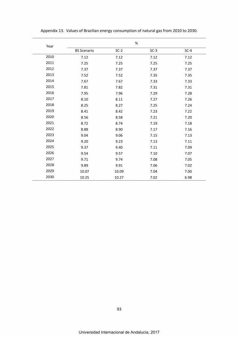
93

Appendix 13. Values of Brazilian energy consumption of natural gas from 2010 to 2030.

Year %


2010 7.12 7.12 7.12 7.12

2011 7.25 7.25 7.25 7.25

2012 7.37 7.37 7.37 7.37

2013 7.52 7.52 7.35 7.35

2014 7.67 7.67 7.33 7.33

2015 7.81 7.82 7.31 7.31

2016 7.95 7.96 7.29 7.28

2017 8.10 8.11 7.27 7.26

2018 8.25 8.27 7.25 7.24

2019 8.41 8.42 7.23 7.22

2020 8.56 8.58 7.21 7.20

2021 8.72 8.74 7.19 7.18

2022 8.88 8.90 7.17 7.16

2023 9.04 9.06 7.15 7.13

2024 9.20 9.23 7.13 7.11

2025 9.37 9.40 7.11 7.09

2026 9.54 9.57 7.10 7.07

2027 9.71 9.74 7.08 7.05

2028 9.89 9.91 7.06 7.02

2029 10.07 10.09 7.04 7.00

2030 10.25 10.27 7.02 6.98


94

Appendix 14. Values of Brazilian energy consumption of liquefied petroleum gases from 2010

to 2030.

Year %


2010 4.18 4.18 4.18 4.18

2011 4.07 4.07 4.07 4.07

2012 3.96 3.96 3.96 3.96

2013 3.85 3.85 3.96 3.96

2014 3.75 3.75 3.96 3.97

2015 3.65 3.66 3.97 3.97

2016 3.56 3.56 3.97 3.98

2017 3.46 3.48 3.98 3.98

2018 3.38 3.39 3.98 3.99

2019 3.29 3.31 3.98 3.99

2020 3.20 3.23 3.98 4.00

2021 3.12 3.16 3.99 4.00

2022 3.04 3.08 3.99 4.01

2023 2.97 3.02 3.99 4.01

2024 2.89 2.95 4.00 4.02

2025 2.82 2.88 4.00 4.02

2026 2.75 2.82 4.00 4.03

2027 2.68 2.76 4.00 4.03

2028 2.61 2.71 4.01 4.03

2029 2.55 2.65 4.01 4.04

2030 2.48 2.60 4.01 4.04


95

Appendix 15. Values of Brazilian energy consumption of motor gasoline from 2010 to 2030.

Year %


2010 9.29 9.29 9.29 9.29

2011 9.54 9.54 9.54 9.54

2012 9.80 9.80 9.80 9.80

2013 9.99 9.95 9.80 9.84

2014 10.21 10.12 9.81 9.87

2015 10.44 10.31 9.82 9.90

2016 10.68 10.50 9.82 9.94

2017 10.91 10.69 9.83 9.97

2018 11.14 10.87 9.83 10.01

2019 11.38 11.06 9.84 10.04

2020 11.62 11.25 9.85 10.07

2021 11.87 11.44 9.85 10.11

2022 12.12 11.63 9.86 10.14

2023 12.36 11.83 9.86 10.17

2024 12.62 12.02 9.86 10.21

2025 12.87 12.22 9.87 10.24

2026 13.13 12.41 9.87 10.27

2027 13.39 12.61 9.87 10.30

2028 13.66 12.81 9.88 10.34

2029 13.92 13.00 9.88 10.37

2030 14.19 13.20 9.88 10.40


96

Appendix 16. Values of Brazilian energy consumption of gas/diesel oil from 2010 to 2030.

Year %


2010 17.22 17.22 17.22 17.22

2011 17.24 17.24 17.24 17.24

2012 17.27 17.27 17.27 17.27

2013 17.28 17.21 17.23 17.28

2014 17.31 17.16 17.20 17.28

2015 17.35 17.12 17.18 17.29

2016 17.41 17.10 17.15 17.30

2017 17.47 17.08 17.12 17.30

2018 17.55 17.07 17.09 17.31

2019 17.65 17.08 17.06 17.32

2020 17.78 17.11 17.03 17.33

2021 17.92 17.15 17.01 17.34

2022 18.10 17.21 16.98 17.35

2023 18.31 17.30 16.95 17.36

2024 18.56 17.41 16.92 17.37

2025 18.85 17.55 16.89 17.38

2026 19.20 17.73 16.86 17.39

2027 19.60 17.95 16.83 17.40

2028 20.08 18.21 16.81 17.41

2029 20.63 18.52 16.78 17.43

2030 21.27 18.88 16.75 17.44


97

Appendix 17. Values of Brazilian energy consumption of fuel oil from 2010 to 2030.

Year %


2010 2.08 2.08 2.08 2.08

2011 1.76 1.76 1.76 1.76

2012 1.45 1.45 1.45 1.45

2013 1.25 1.26 1.44 1.44

2014 1.09 1.09 1.44 1.44

2015 0.94 0.95 1.44 1.44

2016 0.81 0.82 1.44 1.43

2017 0.71 0.72 1.44 1.43

2018 0.62 0.63 1.44 1.43

2019 0.55 0.56 1.44 1.42

2020 0.49 0.49 1.44 1.42

2021 0.43 0.44 1.44 1.42

2022 0.39 0.39 1.43 1.42

2023 0.35 0.35 1.43 1.41

2024 0.31 0.32 1.43 1.41

2025 0.28 0.29 1.43 1.41

2026 0.26 0.26 1.43 1.40

2027 0.24 0.23 1.43 1.40

2028 0.22 0.21 1.43 1.40

2029 0.20 0.19 1.43 1.39

2030 0.18 0.18 1.43 1.39


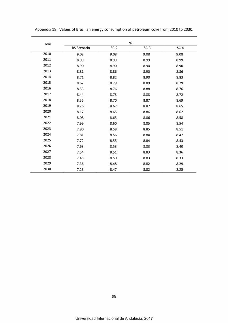
98

Appendix 18. Values of Brazilian energy consumption of petroleum coke from 2010 to 2030.

Year %


2010 9.08 9.08 9.08 9.08

2011 8.99 8.99 8.99 8.99

2012 8.90 8.90 8.90 8.90

2013 8.81 8.86 8.90 8.86

2014 8.71 8.82 8.90 8.83

2015 8.62 8.79 8.89 8.79

2016 8.53 8.76 8.88 8.76

2017 8.44 8.73 8.88 8.72

2018 8.35 8.70 8.87 8.69

2019 8.26 8.67 8.87 8.65

2020 8.17 8.65 8.86 8.62

2021 8.08 8.63 8.86 8.58

2022 7.99 8.60 8.85 8.54

2023 7.90 8.58 8.85 8.51

2024 7.81 8.56 8.84 8.47

2025 7.72 8.55 8.84 8.43

2026 7.63 8.53 8.83 8.40

2027 7.54 8.51 8.83 8.36

2028 7.45 8.50 8.83 8.33

2029 7.36 8.48 8.82 8.29

2030 7.28 8.47 8.82 8.25


99

Appendix 19. Values of Brazilian consumption of renewable, alternative and nuclear energy

from 2010 to 2030.

Year %


2010 51.02 51.02 51.02 51.02

2011 51.15 51.15 51.15 51.15

2012 51.25 51.25 51.25 51.25

2013 51.43 51.48 51.31 51.27

2014 51.58 51.69 51.37 51.30

2015 51.70 51.86 51.43 51.33

2016 51.81 52.03 51.49 51.35

2017 51.92 52.18 51.55 51.38

2018 52.03 52.34 51.61 51.41

2019 52.13 52.49 51.67 51.44

2020 52.22 52.62 51.73 51.47

2021 52.30 52.75 51.80 51.49

2022 52.37 52.86 51.86 51.52

2023 52.44 52.97 51.92 51.55

2024 52.50 53.07 51.98 51.57

2025 52.55 53.16 52.04 51.60

2026 52.60 53.24 52.10 51.63

2027 52.63 53.31 52.17 51.66

2028 52.67 53.38 52.23 51.68

2029 52.69 53.43 52.29 51.71

2030 52.71 53.48 52.35 51.73


100

Appendix 20. CO2 emissios values. From 1971 to 2012 corresponds to official dataset and from


Year CO2 (kg)


1971 99506720602 99506720602 99506720602 99506720602 1972 110600634670 110600634670 110600634670 110600634670 1973 121654516122 121654516122 121654516122 121654516122 1974 132418863435 132418863435 132418863435 132418863435 1975 142622630207 142622630207 142622630207 142622630207 1976 152002953774 152002953774 152002953774 152002953774 1977 160312587371 160312587371 160312587371 160312587371 1978 167382562658 167382562658 167382562658 167382562658 1979 173097885639 173097885639 173097885639 173097885639 1980 177485461507 177485461507 177485461507 177485461507 1981 180799938992 180799938992 180799938992 180799938992 1982 183472248904 183472248904 183472248904 183472248904 1983 185917241973 185917241973 185917241973 185917241973 1984 188518417300 188518417300 188518417300 188518417300 1985 191524797521 191524797521 191524797521 191524797521 1986 195044885829 195044885829 195044885829 195044885829 1987 199116376857 199116376857 199116376857 199116376857 1988 203775649698 203775649698 203775649698 203775649698 1989 209083629225 209083629225 209083629225 209083629225 1990 215144247181 215144247181 215144247181 215144247181 1991 222099542311 222099542311 222099542311 222099542311 1992 230020720417 230020720417 230020720417 230020720417 1993 238921739206 238921739206 238921739206 238921739206 1994 248736208558 248736208558 248736208558 248736208558 1995 259286086663 259286086663 259286086663 259286086663 1996 270277784924 270277784924 270277784924 270277784924 1997 281335602205 281335602205 281335602205 281335602205 1998 292084285650 292084285650 292084285650 292084285650 1999 302237714722 302237714722 302237714722 302237714722 2000 311619094337 311619094337 311619094337 311619094337 2001 320158684782 320158684782 320158684782 320158684782 2002 327957197012 327957197012 327957197012 327957197012 2003 335291036612 335291036612 335291036612 335291036612 2004 342507666154 342507666154 342507666154 342507666154 2005 349868355777 349868355777 349868355777 349868355777 2006 357620323999 357620323999 357620323999 357620323999 2007 365953153994 365953153994 365953153994 365953153994 2008 374982637132 374982637132 374982637132 374982637132 2009 384783948142 384783948142 384783948142 384783948142 2010 395383935204 395383935204 395383935204 395383935204 2011 406425082982 406425082982 406425082982 406425082982


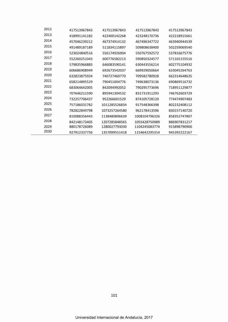
101

2012 417513967843 417513967843 417513967843 417513967843 2013 418991141182 422400142268 423248170736 422218915661 2014 457046239212 467374914132 467496347722 463940944539 2015 491489187189 511834115897 509808638400 502259069540 2016 523024840516 556174926904 550767592572 537816675776 2017 552260251043 600776582213 590850324577 571165155516 2018 579835966883 646083590141 630443556214 602775104932 2019 606686908949 692673542037 669929050664 633045264763 2020 632823875934 740727460770 709582780928 662314648635 2021 658214895529 790451004776 749638073136 690869516732 2022 683064642005 842094992052 790295773696 718951129877 2023 707646211590 895941304532 831731911293 746762603729 2024 732257706437 952266601529 874105728120 774474907483 2025 757186031782 1011285526834 917548366398 802232408112 2026 782822849798 1073257264580 962178413596 830157140720 2027 810088356443 1138480896639 1008104796326 858352747807 2028 842148173405 1207285848565 1055428750989 886907831217 2029 880178726089 1280027793030 1104245083774 915898790900 2030 927912337756 1357099551418 1154642295314 945392222167


título - brazil - UNIA

Documents

Transcript of título - brazil - UNIA