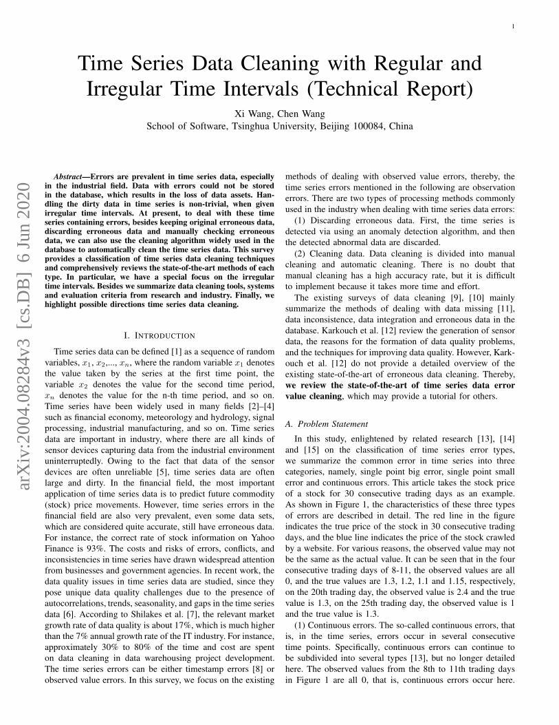
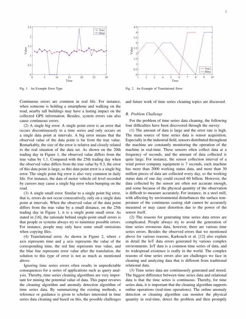
arX

iv:2

004.

0828

4v3

[cs

.DB

] 6

Jun

202

01

Time Series Data Cleaning with Regular andIrregular Time Intervals (Technical Report)

Xi Wang, Chen Wang

School of Software, Tsinghua University, Beijing 100084, China

Abstract—Errors are prevalent in time series data, especiallyin the industrial field. Data with errors could not be storedin the database, which results in the loss of data assets. Han-dling the dirty data in time series is non-trivial, when givenirregular time intervals. At present, to deal with these timeseries containing errors, besides keeping original erroneous data,discarding erroneous data and manually checking erroneousdata, we can also use the cleaning algorithm widely used in thedatabase to automatically clean the time series data. This surveyprovides a classification of time series data cleaning techniquesand comprehensively reviews the state-of-the-art methods of eachtype. In particular, we have a special focus on the irregulartime intervals. Besides we summarize data cleaning tools, systemsand evaluation criteria from research and industry. Finally, wehighlight possible directions time series data cleaning.

I. INTRODUCTION

Time series data can be defined [1] as a sequence of random

variables, x1, x2,..., xn, where the random variable x1 denotes

the value taken by the series at the first time point, the

variable x2 denotes the value for the second time period,

xn denotes the value for the n-th time period, and so on.

Time series have been widely used in many fields [2]–[4]

such as financial economy, meteorology and hydrology, signal

processing, industrial manufacturing, and so on. Time series

data are important in industry, where there are all kinds of

sensor devices capturing data from the industrial environment

uninterruptedly. Owing to the fact that data of the sensor

devices are often unreliable [5], time series data are often

large and dirty. In the financial field, the most important

application of time series data is to predict future commodity

(stock) price movements. However, time series errors in the

financial field are also very prevalent, even some data sets,

which are considered quite accurate, still have erroneous data.

For instance, the correct rate of stock information on Yahoo

Finance is 93%. The costs and risks of errors, conflicts, and

inconsistencies in time series have drawn widespread attention

from businesses and government agencies. In recent work, the

data quality issues in time series data are studied, since they

pose unique data quality challenges due to the presence of

autocorrelations, trends, seasonality, and gaps in the time series

data [6]. According to Shilakes et al. [7], the relevant market

growth rate of data quality is about 17%, which is much higher

than the 7% annual growth rate of the IT industry. For instance,

approximately 30% to 80% of the time and cost are spent

on data cleaning in data warehousing project development.

The time series errors can be either timestamp errors [8] or

observed value errors. In this survey, we focus on the existing

methods of dealing with observed value errors, thereby, the

time series errors mentioned in the following are observation

errors. There are two types of processing methods commonly

used in the industry when dealing with time series data errors:

(1) Discarding erroneous data. First, the time series is

detected via using an anomaly detection algorithm, and then

the detected abnormal data are discarded.

(2) Cleaning data. Data cleaning is divided into manual

cleaning and automatic cleaning. There is no doubt that

manual cleaning has a high accuracy rate, but it is difficult

to implement because it takes more time and effort.

The existing surveys of data cleaning [9], [10] mainly

summarize the methods of dealing with data missing [11],

data inconsistence, data integration and erroneous data in the

database. Karkouch et al. [12] review the generation of sensor

data, the reasons for the formation of data quality problems,

and the techniques for improving data quality. However, Kark-

ouch et al. [12] do not provide a detailed overview of the

existing state-of-the-art of erroneous data cleaning. Thereby,

we review the state-of-the-art of time series data error

value cleaning, which may provide a tutorial for others.

A. Problem Statement

In this study, enlightened by related research [13], [14]

and [15] on the classification of time series error types,

we summarize the common error in time series into three

categories, namely, single point big error, single point small

error and continuous errors. This article takes the stock price

of a stock for 30 consecutive trading days as an example.

As shown in Figure 1, the characteristics of these three types

of errors are described in detail. The red line in the figure

indicates the true price of the stock in 30 consecutive trading

days, and the blue line indicates the price of the stock crawled

by a website. For various reasons, the observed value may not

be the same as the actual value. It can be seen that in the four

consecutive trading days of 8-11, the observed values are all

0, and the true values are 1.3, 1.2, 1.1 and 1.15, respectively,

on the 20th trading day, the observed value is 2.4 and the true

value is 1.3, on the 25th trading day, the observed value is 1

and the true value is 1.3.

(1) Continuous errors. The so-called continuous errors, that

is, in the time series, errors occur in several consecutive

time points. Specifically, continuous errors can continue to

be subdivided into several types [13], but no longer detailed

here. The observed values from the 8th to 11th trading days

in Figure 1 are all 0, that is, continuous errors occur here.

2

0 5 10 15 20 25 30Time

0

0.5

1

1.5

2

2.5V

alue

TrueDirty

Fig. 1. An Example Error Type

Continuous errors are common in real life. For instance,

when someone is holding a smartphone and walking on the

road, nearby tall buildings may have a lasting impact on the

collected GPS information. Besides, system errors can also

cause continuous errors.

(2) A single big error. A single point error is an error that

occurs discontinuously in a time series and only occurs on

a single data point at intervals. A big error means that the

observed value of the data point is far from the true value.

Remarkably, the size of the error is relative and closely related

to the real situation of the data set. As shown on the 20th

trading day in Figure 1, the observed value differs from the

true value by 1.1. Compared with the 25th trading day when

the observed value differs from the true value by 0.3, the error

of this data point is large, so this data point error is a single big

error. The single point big error is also very common in daily

life. For instance, the data of motor vehicle oil level recorded

by cursors may cause a single big error when bumping on the

road.

(3) A single small error. Similar to a single point big error,

that is, errors do not occur consecutively, only on a single data

point at intervals. When the observed value of the data point

differs from the true value by a small distance, on the 25th

trading day in Figure 1, it is a single point small error. As

stated in [16], the rationale behind single-point small errors is

that people or systems always try to minimize possible errors.

For instance, people may only have some small omissions

when copying files.

(4) Translational error. As shown in Figure 2, where x

axis represents time and y axis represents the value of the

corresponding time, the red line represents true value, and

the blue line represents error value after the translation, the

solution to this type of error is not as much as mentioned

above.

Ignoring time series errors often results in unpredictable

consequences for a series of applications such as query anal-

ysis. Thereby, time series cleaning algorithms are very impor-

tant for mining the potential value of data. This paper reviews

the cleaning algorithm and anomaly detection algorithm of

time series data. By summarizing the existing methods, a

reference or guidance is given to scholars interested in time

series data cleaning and based on this, the possible challenges

1 2 3 4 5 6 7 8 9 10Time

0

0.5

1

1.5

2

2.5

3

3.5

4

4.5

Val

ue

TrueDirty

Fig. 2. An Example of Translational Error

and future work of time series cleaning topics are discussed.

B. Problem Challenge

For the problem of time series data cleaning, the following

four difficulties have been discovered through the survey:

(1) The amount of data is large and the error rate is high.

The main source of time series data is sensor acquisition.

Especially in the industrial field, sensors distributed throughout

the machine are constantly monitoring the operation of the

machine in real-time. These sensors often collect data at a

frequency of seconds, and the amount of data collected is

quite large. For instance, the sensor collection interval of a

wind power company equipment is 7 seconds, each machine

has more than 2000 working status data, and more than 30

million pieces of data are collected every day, so the working

status data of one day could exceed 60 billion. However, the

data collected by the sensor are often not accurate enough,

and some because of the physical quantity of the observation

is difficult to measure accurately. For instance, in a steel mill,

with affecting by environmental disturbances the surface tem-

perature of the continuous casting slab cannot be accurately

measured or may cause distortion due to the power of the

sensor itself.

(2) The reasons for generating time series data errors are

complicated. People always try to avoid the generation of

time series erroneous data, however, there are various time

series errors. Besides the observed errors that we mentioned

above for various reasons, Karkouch et al. [12] also explain

in detail the IoT data errors generated by various complex

environments. IoT data is a common time series of data, and

its widespread existence is really in the world. The complex

reasons of time series errors also are challenges we face in

cleaning and analyzing data that is different from traditional

relational data.

(3) Time series data are continuously generated and stored.

The biggest difference between time series data and relational

data is that the time series is continuous. Thereby, for time

series data, it is important that the cleaning algorithm supports

online operations (real-time operations). The online anomaly

detection or cleaning algorithm can monitor the physical

quantity in real-time, detect the problem and then promptly

3

alarm or perform a reasonable cleaning. Thereby, the time

series cleaning algorithm is not only required to support

online calculation or streaming calculation but also has good

throughput.

(4) Minimum modification principle [17]–[19]. Time series

data often contain many errors. Most of the widely used

time series cleaning methods utilize the principle of smooth

filtering. Such methods may change the original data too

much, and result in the loss of the information contained in

the original data. Data cleaning needs to avoid changing the

original correct data. It should be based on the principle of

minimum modification, that is, the smaller the change, the

better.

C. Organization

Different algorithms tackle these challenges in differ-

ent ways, which usually include smoothing-based methods,

constraint-based methods, and statistical-based methods as

shown in Table I. Besides some time series anomaly detection

algorithms can also be effectively used to clean data. The

remainder of this paper is organized as follows. The aforesaid

four types of algorithms are discussed from Section II to V,

respectively. In Section VI we introduce existing time series

cleaning tools, systems, and evaluation criteria. Finally, we

summarize this paper in Section VII and discuss possible

future directions.

II. SMOOTHING BASED CLEANING ALGORITHM

Smoothing techniques are often used to eliminate data noise,

especially numerical data noise. Low-pass filtering, which

filters out the lower frequency of the data set, is a simple

algorithm. The characteristic of this type of technology is

that the time overhead is small, but because the original data

may be modified much, which makes the data distorted and

leads to the uncertainty of the analysis results, there are not

many applications used in time series cleaning. The research

of smoothing technology mainly focuses on algorithms such

as Moving Average (MA) [20], Autoregressive (AR) [4], [21],

[22] and Kalman filter model [25]–[27]. Thereby, this chapter

mainly introduce these three technologies and their extensions.

A. Moving average

The moving average (MA) series algorithm [20] is widely

used in time series for smoothing and time series prediction.

A simple moving average (SMA) algorithm: Calculate the

average of the most recently observed N time series values,

which is used to predict the value at time t. A simple definition

as shown in equation (1).

xt =1

2n+ 1

n∑

i=−n

xi+t (1)

In equation (1), xt is the predicted value of xt, xt represents

the true value at time t, 2 ∗ n+ 1 is the window size(count).

For a time series x(t)=9.8, 8.5, 5.4, 5.6, 5.9, 9.2, 7.4, for

TABLE ITHE OVERVIEW OF METHODS

Type MethodSmoothing based(Section II)

Moving Average [20]AutoRegressive [4], [21], [22]Autoregressive Moving Average Model[13], [23], [24]Kalman Filter [25]–[32]Interpolation [33], [34]State-space Model [26], [35], [36]Trajectory Simplification [37], [38]

Constraint based(Section III)

Order Dependencies [39]–[42]Denial Constraints [43]Sequential Dependencies [44]Speed Constraints [45]Variance Constraints [46]Similarity Rule Constraints [47]Learning Individual Models [48]Temporal Dependence [49], [50]

Statistics based(Section IV)

Maximum Likelihood [51]–[55]Bayesian Model [56], [57]Markov Model [58]–[60]Hidden Markov Model [61]–[64]SMURF [65]–[67]Spatio-Temporal Probabilistic Model[68]Expectation-Maximization [69]Relationship-dependent Network [70]–[72]

Anomaly detection(Section V)

Density-Based Spatial Clustering of Ap-plications with Noise [73], [74]Local Outlier Factor [73]Abnormal Sequence Detection [75]–[78]Window-based Anomaly Detection [79]Generative Adversarial Networks [80]–[82]Long Short-Term Memory [83]–[85]Speed-based cleaning algorithm [86]

simplicity, we use SMA with n = 3 and k = 4, then calculate

according to equation (2).

xt =(xt−n + xt−2...+ xt+n)

(2n+ 1)= 7.4 (2)

To eliminate errors or noises, the data x(t) can be con-

sidered as a certain time window of sliding window, then

continuously calculate the local average over a given interval

2n + 1 to filter out the noise (erroneous data) and get a

smoother measurement.

In the weighted moving average (WMA) algorithm, data

points at different relative positions in the window have

different weights. Generally defined as:

xt =

n∑

i=−n

ωixi+t (3)

In equation (3), ωi represents the weight of the influence

of the i position data point on the t position data point, other

definitions follow the example above. A simple strategy is

that the farther away from the two data points, the smaller the

mutual influence. For instance, a natural idea is the reciprocal

of the distance between two data points as the weight of their

mutual influence. Similarly, the weight of each data point in

4

the exponential weighted moving average (EWMA) algorithm

[32] decreases exponentially with increasing distance, which

is mainly used for unsteady time series [87], [88].

Aiming at the need for the rapid response of sensor data

cleaning, Zhuang et al. [31] propose an intelligent weighted

moving average algorithm, which calculates weighted moving

averages via collected confidence data from sensors. Zhang

et al. [89] propose a method based on multi-threshold control

and approximate positive transform to clean the probe vehicle

data, and fill the lost data with the weighted average method

and exponential smoothing method. Qu et al. [90] first use

cluster-based methods for anomaly detection and then use

exponentially weighted averaging for data repair, which is used

to clean power data in a distributed environment.

B. Autoregressive

The Autoregressive (AR) Model is a process that uses itself

as a regression variable and uses the linear combination of the

previous k random variables to describe the linear regression

model of the random variable at the time t. The definition of

AR model [21], [91] as shown in equation (4).

xt =

k∑

i=1

ωixt−i + ǫt + a (4)

In equation (4), xt is the predicted value of xt, xt represents

the true value at time t, k is the order, µ is mean value of the

process, ǫt is white noise, ωi is the parameter of the model,

a is a constant.

Park et al. [92] use labeled data y to propose an autore-

gressive with exogenous input (ARX) model based on the AR

model:

yt = xt +k∑

i=1

ωi(yt−i − xt−i) + ǫt (5)

In equation (5), yt is the possible repair of xt, and others

are the same to the aforesaid AR model. Alengrin et al.

[24] propose Autoregressive moving average (ARMA) model),

which is composed of the AR model and MA model. Besides

that, the Gaussian Autoregressive Moving Average model is

defined as shown in equation (6) [13].

Φ(B)Zt = θ0 + θ(B)xt (6)

In equation (6), Φ(B) = 1 − Φ1B − ... − ΦpBp and

θ(B) = 1− θ1B− ...− θqBq are polynomial in B of degrees

p and q, respectively, θ0 is a constant, B is the backshift

operator such that BZt = Zt−1, and xt is a sequence of

independent Gaussian variates with mean µ=0 and variance

σ2x. Box et al. [93] propose a more complex Autoregressive

Integrated Moving Average (ARIMA) model based on the

ARMA model, which is not described in detail here. Akouemo

et al. [94] propose a method combining ARX and Artificial

Neural Network (ANN) model for cleaning time series, which

performs a hypothesis test to detect anomalies the extrema

of the residuals, and repairs anomalous data points by using

the ARX and ANN models. Dilling et al. [23] clean high-

frequency velocity profile data with ARMA model and Chen

et al. [95] use the ARIMA model to clean wind power data.

C. Kalman filter model

Kalman [25] proposes the Kalman filter theory, which

can deal with time-varying systems, non-stationary signals,

and multi-dimensional signals. Kalman filter creatively in-

corporates errors (predictive and measurement errors) into

the calculation, the errors exist independently and are not

affected by measured data. The Kalman model involves proba-

bility, random variable, Gaussian Distribution, and State-space

Model, etc. Consider that the Kalman model involves too

much content, no specific description is given here, and only

a simple definition is given. First, we introduce a system of

discrete control processes which can be described by a Linear

Stochastic Difference equation as shown in equation (7).

xt = mxt−1 + nvt + pt (7)

Also, the measured values of the system are expressed as

shown in equation (8).

yt = rxt−1 + qt (8)

In equation (7) and (8), xt is the system state value at

time t, and vt is the control variable value for the system at

time t. m and n are system parameters, and for multi-model

systems, they are matrices, yt is the measured value at time t,

r is the parameter of the measurement system, and for multi-

measurement systems, r is a matrix, p(k) and q(k) represent

the noises of the process and measurement, respectively, and

they are assumed to be white Gaussian Noise.

The extended Kalman filter is the most widely used es-

timation for a recursive nonlinear system because it simply

linearizes the nonlinear system models. However, the extended

Kalman filter has two drawbacks: linearization can produce

unstable filters and it is hard to implement the derivation of

the Jacobian matrices. Thereby, Ma et al. [96] present a new

method of predicting the Mackey-Glass equation based on the

unscented Kalman filter to solve these problems. In the field

of signal processing, there are many works [28]–[30] based on

Kalman filtering, but these techniques have not been widely

used in the field of time series cleaning. Gardner et al. [32]

propose a new model, which is based on the Kernel Kalman

Filter, to perform various nonlinear time series processing.

Zhuang et al. [31] use the Kalman filter model to predict sensor

data and smoothed it with WMA.

D. Trajectory Simplification

The main purpose of trajectory simplification is to reduce

the original trajectory from N trajectory data points to M

trajectory data points, M < N . And retain important location

or topological features. The compression algorithm needs

to ensure that the sequence of M points has a minimum

compression error (M -ǫ problem), Such as MRPA [37], Error-

Search [38]. The input of the Error-Search algorithm is the

target compression ratio λ, Original track T . Returns the

compression that satisfies the given compression ratio λ with

the smallest DAD error. The main steps of the Error-Search

algorithm are as follows: (1) According to the original trajec-

tory T , Build search space ǫ, create a search ǫ space based

on the opposite direction in a more efficient way Trace T . (2)

5

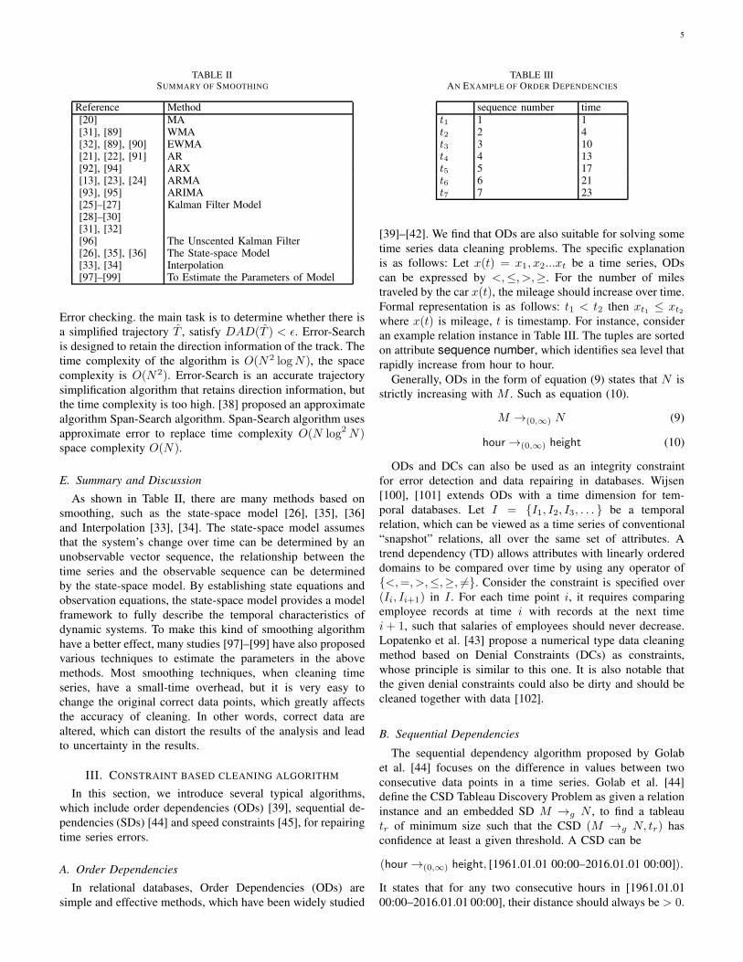
TABLE IISUMMARY OF SMOOTHING

Reference Method[20] MA[31], [89] WMA[32], [89], [90] EWMA[21], [22], [91] AR[92], [94] ARX[13], [23], [24] ARMA[93], [95] ARIMA[25]–[27][28]–[30][31], [32]

Kalman Filter Model

[96] The Unscented Kalman Filter[26], [35], [36] The State-space Model[33], [34] Interpolation[97]–[99] To Estimate the Parameters of Model

Error checking. the main task is to determine whether there is

a simplified trajectory T , satisfy DAD(T ) < ǫ. Error-Search

is designed to retain the direction information of the track. The

time complexity of the algorithm is O(N2 logN), the space

complexity is O(N2). Error-Search is an accurate trajectory

simplification algorithm that retains direction information, but

the time complexity is too high. [38] proposed an approximate

algorithm Span-Search algorithm. Span-Search algorithm uses

approximate error to replace time complexity O(N log2 N)space complexity O(N).

E. Summary and Discussion

As shown in Table II, there are many methods based on

smoothing, such as the state-space model [26], [35], [36]

and Interpolation [33], [34]. The state-space model assumes

that the system’s change over time can be determined by an

unobservable vector sequence, the relationship between the

time series and the observable sequence can be determined

by the state-space model. By establishing state equations and

observation equations, the state-space model provides a model

framework to fully describe the temporal characteristics of

dynamic systems. To make this kind of smoothing algorithm

have a better effect, many studies [97]–[99] have also proposed

various techniques to estimate the parameters in the above

methods. Most smoothing techniques, when cleaning time

series, have a small-time overhead, but it is very easy to

change the original correct data points, which greatly affects

the accuracy of cleaning. In other words, correct data are

altered, which can distort the results of the analysis and lead

to uncertainty in the results.

III. CONSTRAINT BASED CLEANING ALGORITHM

In this section, we introduce several typical algorithms,

which include order dependencies (ODs) [39], sequential de-

pendencies (SDs) [44] and speed constraints [45], for repairing

time series errors.

A. Order Dependencies

In relational databases, Order Dependencies (ODs) are

simple and effective methods, which have been widely studied

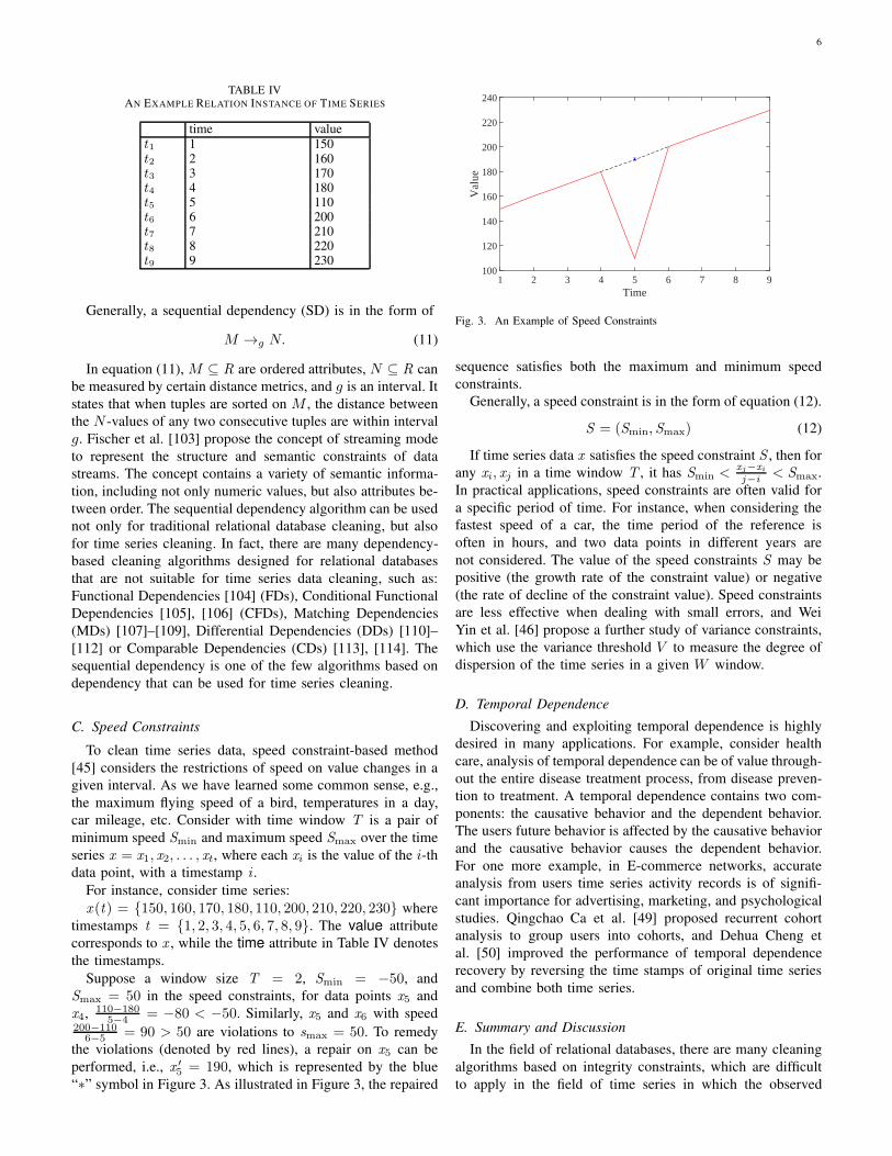
TABLE IIIAN EXAMPLE OF ORDER DEPENDENCIES

sequence number timet1 1 1t2 2 4t3 3 10t4 4 13t5 5 17t6 6 21t7 7 23

[39]–[42]. We find that ODs are also suitable for solving some

time series data cleaning problems. The specific explanation

is as follows: Let x(t) = x1, x2...xt be a time series, ODs

can be expressed by <,≤, >,≥. For the number of miles

traveled by the car x(t), the mileage should increase over time.

Formal representation is as follows: t1 < t2 then xt1 ≤ xt2

where x(t) is mileage, t is timestamp. For instance, consider

an example relation instance in Table III. The tuples are sorted

on attribute sequence number, which identifies sea level that

rapidly increase from hour to hour.

Generally, ODs in the form of equation (9) states that N is

strictly increasing with M . Such as equation (10).

M →(0,∞) N (9)

hour →(0,∞) height (10)

ODs and DCs can also be used as an integrity constraint

for error detection and data repairing in databases. Wijsen

[100], [101] extends ODs with a time dimension for tem-

poral databases. Let I = {I1, I2, I3, . . . } be a temporal

relation, which can be viewed as a time series of conventional

“snapshot” relations, all over the same set of attributes. A

trend dependency (TD) allows attributes with linearly ordered

domains to be compared over time by using any operator of

{<,=, >,≤,≥, 6=}. Consider the constraint is specified over

(Ii, Ii+1) in I . For each time point i, it requires comparing

employee records at time i with records at the next time

i + 1, such that salaries of employees should never decrease.

Lopatenko et al. [43] propose a numerical type data cleaning

method based on Denial Constraints (DCs) as constraints,

whose principle is similar to this one. It is also notable that

the given denial constraints could also be dirty and should be

cleaned together with data [102].

B. Sequential Dependencies

The sequential dependency algorithm proposed by Golab

et al. [44] focuses on the difference in values between two

consecutive data points in a time series. Golab et al. [44]

define the CSD Tableau Discovery Problem as given a relation

instance and an embedded SD M →g N , to find a tableau

tr of minimum size such that the CSD (M →g N, tr) has

confidence at least a given threshold. A CSD can be

(hour →(0,∞) height, [1961.01.01 00:00–2016.01.01 00:00]).

It states that for any two consecutive hours in [1961.01.01

00:00–2016.01.01 00:00], their distance should always be > 0.

6

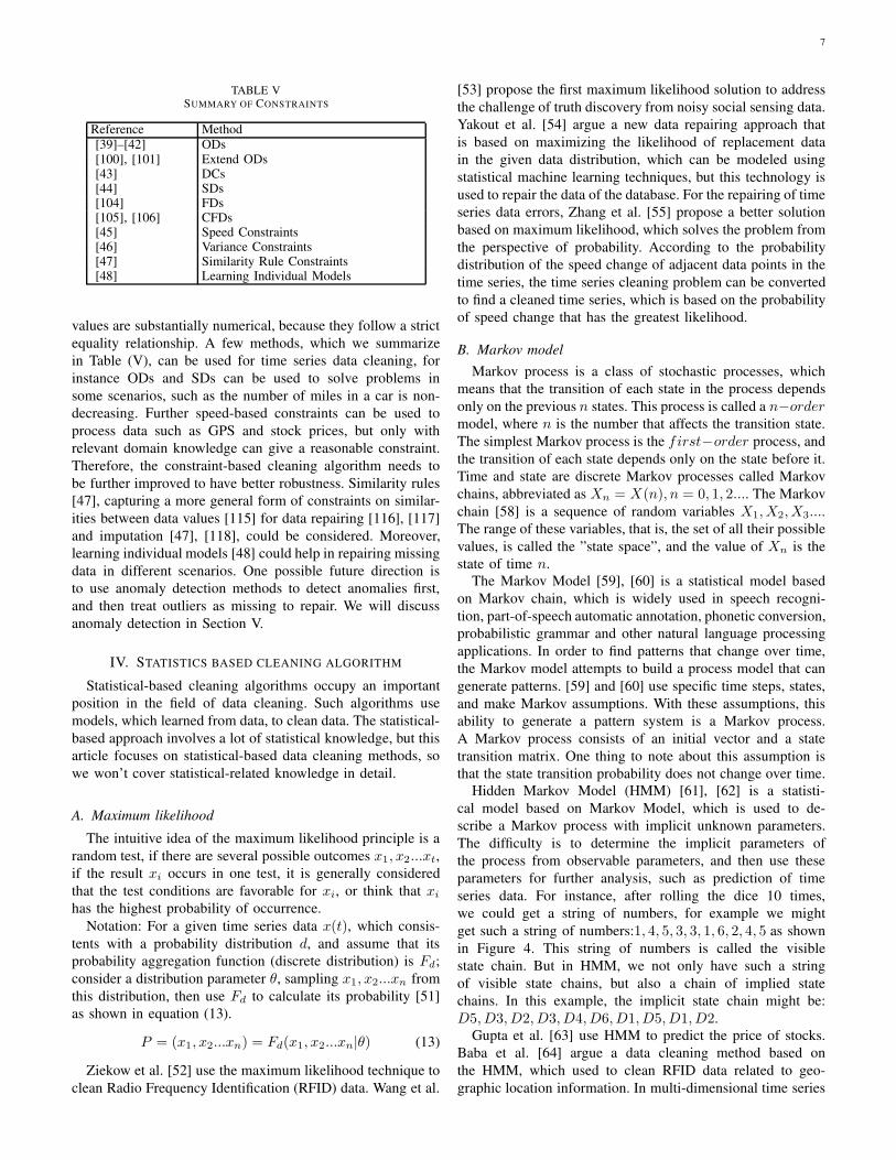
TABLE IVAN EXAMPLE RELATION INSTANCE OF TIME SERIES

time valuet1 1 150t2 2 160t3 3 170t4 4 180t5 5 110t6 6 200t7 7 210t8 8 220t9 9 230

Generally, a sequential dependency (SD) is in the form of

M →g N. (11)

In equation (11), M ⊆ R are ordered attributes, N ⊆ R can

be measured by certain distance metrics, and g is an interval. It

states that when tuples are sorted on M , the distance between

the N -values of any two consecutive tuples are within interval

g. Fischer et al. [103] propose the concept of streaming mode

to represent the structure and semantic constraints of data

streams. The concept contains a variety of semantic informa-

tion, including not only numeric values, but also attributes be-

tween order. The sequential dependency algorithm can be used

not only for traditional relational database cleaning, but also

for time series cleaning. In fact, there are many dependency-

based cleaning algorithms designed for relational databases

that are not suitable for time series data cleaning, such as:

Functional Dependencies [104] (FDs), Conditional Functional

Dependencies [105], [106] (CFDs), Matching Dependencies

(MDs) [107]–[109], Differential Dependencies (DDs) [110]–

[112] or Comparable Dependencies (CDs) [113], [114]. The

sequential dependency is one of the few algorithms based on

dependency that can be used for time series cleaning.

C. Speed Constraints

To clean time series data, speed constraint-based method

[45] considers the restrictions of speed on value changes in a

given interval. As we have learned some common sense, e.g.,

the maximum flying speed of a bird, temperatures in a day,

car mileage, etc. Consider with time window T is a pair of

minimum speed Smin and maximum speed Smax over the time

series x = x1, x2, . . . , xt, where each xi is the value of the i-th

data point, with a timestamp i .

For instance, consider time series:

x (t) = {150, 160, 170, 180, 110, 200, 210, 220, 230} where

timestamps t = {1, 2, 3, 4, 5, 6, 7, 8, 9}. The value attribute

corresponds to x , while the time attribute in Table IV denotes

the timestamps.

Suppose a window size T = 2, Smin = −50, and

Smax = 50 in the speed constraints, for data points x5 and

x4, 110−1805−4 = −80 < −50. Similarly, x5 and x6 with speed

200−1106−5 = 90 > 50 are violations to smax = 50. To remedy

the violations (denoted by red lines), a repair on x5 can be

performed, i.e., x ′

5 = 190, which is represented by the blue

“∗” symbol in Figure 3. As illustrated in Figure 3, the repaired

1 2 3 4 5 6 7 8 9Time

100

120

140

160

180

200

220

240

Val

ue

Fig. 3. An Example of Speed Constraints

sequence satisfies both the maximum and minimum speed

constraints.

Generally, a speed constraint is in the form of equation (12).

S = (Smin, Smax) (12)

If time series data x satisfies the speed constraint S , then for

any xi, xj in a time window T , it has Smin <xj−xi

j−i< Smax.

In practical applications, speed constraints are often valid for

a specific period of time. For instance, when considering the

fastest speed of a car, the time period of the reference is

often in hours, and two data points in different years are

not considered. The value of the speed constraints S may be

positive (the growth rate of the constraint value) or negative

(the rate of decline of the constraint value). Speed constraints

are less effective when dealing with small errors, and Wei

Yin et al. [46] propose a further study of variance constraints,

which use the variance threshold V to measure the degree of

dispersion of the time series in a given W window.

D. Temporal Dependence

Discovering and exploiting temporal dependence is highly

desired in many applications. For example, consider health

care, analysis of temporal dependence can be of value through-

out the entire disease treatment process, from disease preven-

tion to treatment. A temporal dependence contains two com-

ponents: the causative behavior and the dependent behavior.

The users future behavior is affected by the causative behavior

and the causative behavior causes the dependent behavior.

For one more example, in E-commerce networks, accurate

analysis from users time series activity records is of signifi-

cant importance for advertising, marketing, and psychological

studies. Qingchao Ca et al. [49] proposed recurrent cohort

analysis to group users into cohorts, and Dehua Cheng et

al. [50] improved the performance of temporal dependence

recovery by reversing the time stamps of original time series

and combine both time series.

E. Summary and Discussion

In the field of relational databases, there are many cleaning

algorithms based on integrity constraints, which are difficult

to apply in the field of time series in which the observed

7

TABLE VSUMMARY OF CONSTRAINTS

Reference Method[39]–[42] ODs[100], [101] Extend ODs[43] DCs[44] SDs[104] FDs[105], [106] CFDs[45] Speed Constraints[46] Variance Constraints[47] Similarity Rule Constraints[48] Learning Individual Models

values are substantially numerical, because they follow a strict

equality relationship. A few methods, which we summarize

in Table (V), can be used for time series data cleaning, for

instance ODs and SDs can be used to solve problems in

some scenarios, such as the number of miles in a car is non-

decreasing. Further speed-based constraints can be used to

process data such as GPS and stock prices, but only with

relevant domain knowledge can give a reasonable constraint.

Therefore, the constraint-based cleaning algorithm needs to

be further improved to have better robustness. Similarity rules

[47], capturing a more general form of constraints on similar-

ities between data values [115] for data repairing [116], [117]

and imputation [47], [118], could be considered. Moreover,

learning individual models [48] could help in repairing missing

data in different scenarios. One possible future direction is

to use anomaly detection methods to detect anomalies first,

and then treat outliers as missing to repair. We will discuss

anomaly detection in Section V.

IV. STATISTICS BASED CLEANING ALGORITHM

Statistical-based cleaning algorithms occupy an important

position in the field of data cleaning. Such algorithms use

models, which learned from data, to clean data. The statistical-

based approach involves a lot of statistical knowledge, but this

article focuses on statistical-based data cleaning methods, so

we won’t cover statistical-related knowledge in detail.

A. Maximum likelihood

The intuitive idea of the maximum likelihood principle is a

random test, if there are several possible outcomes x1, x2...xt,

if the result xi occurs in one test, it is generally considered

that the test conditions are favorable for xi, or think that xi

has the highest probability of occurrence.

Notation: For a given time series data x(t), which consis-

tents with a probability distribution d, and assume that its

probability aggregation function (discrete distribution) is Fd;

consider a distribution parameter θ, sampling x1, x2...xn from

this distribution, then use Fd to calculate its probability [51]

as shown in equation (13).

P = (x1, x2...xn) = Fd(x1, x2...xn|θ) (13)

Ziekow et al. [52] use the maximum likelihood technique to

clean Radio Frequency Identification (RFID) data. Wang et al.

[53] propose the first maximum likelihood solution to address

the challenge of truth discovery from noisy social sensing data.

Yakout et al. [54] argue a new data repairing approach that

is based on maximizing the likelihood of replacement data

in the given data distribution, which can be modeled using

statistical machine learning techniques, but this technology is

used to repair the data of the database. For the repairing of time

series data errors, Zhang et al. [55] propose a better solution

based on maximum likelihood, which solves the problem from

the perspective of probability. According to the probability

distribution of the speed change of adjacent data points in the

time series, the time series cleaning problem can be converted

to find a cleaned time series, which is based on the probability

of speed change that has the greatest likelihood.

B. Markov model

Markov process is a class of stochastic processes, which

means that the transition of each state in the process depends

only on the previous n states. This process is called a n−order

model, where n is the number that affects the transition state.

The simplest Markov process is the first−order process, and

the transition of each state depends only on the state before it.

Time and state are discrete Markov processes called Markov

chains, abbreviated as Xn = X(n), n = 0, 1, 2.... The Markov

chain [58] is a sequence of random variables X1, X2, X3....

The range of these variables, that is, the set of all their possible

values, is called the ”state space”, and the value of Xn is the

state of time n.The Markov Model [59], [60] is a statistical model based

on Markov chain, which is widely used in speech recogni-

tion, part-of-speech automatic annotation, phonetic conversion,

probabilistic grammar and other natural language processing

applications. In order to find patterns that change over time,

the Markov model attempts to build a process model that can

generate patterns. [59] and [60] use specific time steps, states,

and make Markov assumptions. With these assumptions, this

ability to generate a pattern system is a Markov process.

A Markov process consists of an initial vector and a state

transition matrix. One thing to note about this assumption is

that the state transition probability does not change over time.Hidden Markov Model (HMM) [61], [62] is a statisti-

cal model based on Markov Model, which is used to de-

scribe a Markov process with implicit unknown parameters.

The difficulty is to determine the implicit parameters of

the process from observable parameters, and then use these

parameters for further analysis, such as prediction of time

series data. For instance, after rolling the dice 10 times,

we could get a string of numbers, for example we might

get such a string of numbers:1, 4, 5, 3, 3, 1, 6, 2, 4, 5 as shown

in Figure 4. This string of numbers is called the visible

state chain. But in HMM, we not only have such a string

of visible state chains, but also a chain of implied state

chains. In this example, the implicit state chain might be:

D5, D3, D2, D3, D4, D6, D1, D5, D1, D2.Gupta et al. [63] use HMM to predict the price of stocks.

Baba et al. [64] argue a data cleaning method based on

the HMM, which used to clean RFID data related to geo-

graphic location information. In multi-dimensional time series

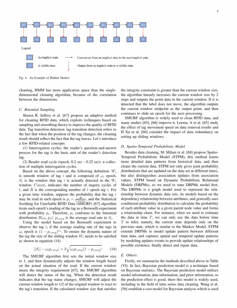
8

Fig. 4. An Example of Hidden Markov

cleaning, HMM has more application space than the single-

dimensional cleaning algorithm, because of the correlation

between the dimensions.

C. Binomial Sampling

Shawn R. Jeffery et al. [67] propose an adaptive method

for cleaning RFID data, which exploits techniques based on

sampling and smoothing theory to improve the quality of RFID

data. Tag transition detection: tag transition detection refers to

the fact that when the position of the tag changes, the cleaning

result should reflect the fact that the tag leaves. Let’s introduce

a few RFID-related concepts.

(1) Interrogation cycles: the reader’s question-and-answer

process for the tag is the basic unit of the reader’s detection

tag.

(2) Reader read cycle (epoch, 0.2 sec - 0.25 sec): a collec-

tion of multiple interrogation cycles.Based on the above concept, the following definition: Wi

is smooth window of tag i and is composed of ωi epoch,

Si is the window that tag i is actually detected in the Wi

window, Countt indicates the number of inquiry cycles of

t, and R is the corresponding number of t epoch tag i. For

a given time window, suppose the probability that the tag i

may be read in each epoch is pi =R

Countt, and the Statistical

Soothing for Unreliable RFID Data (SMURF) [67] algorithm

treats each epoch’s reading of the tag as a Bernoulli experiment

with probability pi. Therefore, pi conforms to the binomial

distribution B(ωi, pi). pi,avg is the average read rate in Si.Using the model based on the Bernoulli experiment to

observe the tag i, if the average reading rate of the tags in

ωi epoch is (1 − pi,avg)ωi . To ensure the dynamic nature of

the tag the size of the sliding window Wi needs to be satisfied

as shown in equation (14).

||Si| − ωipi,avg| > 2√ωipi,avg(1− pi,avg) (14)

The SMURF algorithm first sets the initial window size

to 1, and then dynamically adjusts the window length based

on the actual situation of the read. If the current window

meets the integrity requirement [67], the SMURF algorithm

will detect the status of the tag. When the detection result

indicates that the tag status changes, SMURF will adjust the

current window length to 1/2 of the original window to react to

the tag’s transition. If the calculated window size that satisfies

the integrity constraint is greater than the current window size,

the algorithm linearly increases the current window size by 2

steps and outputs the point data in the current window. If it is

detected that the label does not move, the algorithm outputs

the current window midpoint as the output point, and then

continues to slide an epoch for the next processing.SMURF algorithm is widely used to clean RFID data, and

many studies [65], [66] improve it. Leema, A et al. [65] study

the effect of tag movement speed on data removal results and

H Xu et al. [66] consider the impact of data redundancy on

setting up sliding windows.

D. Spatio-Temporal Probabilistic Model

Besides data cleaning, M. Milani et al. [68] propose Spatio-

Temporal Probabilistic Model (STPM), this method learns

more detailed data patterns from historical data, and then

cleans the current data. STPM not only gives joint probability

distributions that are updated on the data set at different times,

but also distinguishes association updates from association

values. STPM based on Dynamic Probabilistic Relational

Models (DRPMs), so we need to state DRPMs model first.

The DRPMs is a graph model used to represent the rela-

tionship between dynamic data sets, its models based on the

dependency relationship between attributes, and generally uses

conditional probability distribution to calculate the probability

of each attribute value in a given parent node value and forms

a relationship chain. For instance, when we need to estimate

the data at time T , we can only use the data before time

T to infer, namely, the current state depends only on the

previous state, which is similar to the Markov Model. STPM

extends DRPMs to model update pattern between different

time data, and captures spatial and temporal update patterns

by modeling updates events to provide update relationships of

possible existence, finally detect and repair data.

E. Others

Firstly, we summarize the methods described above in Table

(VI). In fact, Bayesian prediction model is a technique based

on Bayesian statistics. The Bayesian prediction model utilizes

model information, data information, and prior information, so

the prediction effect is good, there this model is widely used,

including in the field of time series data cleaning. Wang et al.

[56] establish a cost model for Bayesian analysis which is used

9

TABLE VISUMMARY OF STATISTICS

Reference Method[51]–[53], [78][54], [55]

Maximum Likelihood

[58]–[60] Markov Model[61]–[63][64]

HMM

[65]–[67] SMURF[68] STPM[56], [57] Bayesian[70]–[72] RDN[120] GMM[69] EM

to analyze errors in the data. Bergman et al. [70] consider the

user’s participation and use the user’s feedback on the query

results to clean the data. Mayfield et al. [72] propose a more

complex relationship-dependent network (RDN [71]) model to

model the probability relationships between attributes. The dif-

ference between RDN and traditional relational dependencies

(such as Bayesian networks [57]) is that RDNs can contain

ring structures. The method iteratively cleans the data set

and observes the change in the probability distribution of the

data set before and after each wash. When the probability

distribution of the data set converges, the cleaning process is

aborted. Zhou et al. [119] argue a technique for accelerating

the learning of Gaussian models via using GPU. The article

believes that in the case of excessive data, it is not necessary to

use all the data to learn the model. Also, the author provides

a method of automatic tuning. In order to clean and repair

fuel level data, Tian et al. [120] propose a modified Gaussian

mixture model (GMM) based on the synchronous iteration

method, which uses the particle swarm optimization algorithm

and the steepest descent algorithm to optimize the parameters

of GMM and uses linear interpolation-based algorithm to

correct data errors. Shumway et al. [69] use the EM [121]

algorithm combined with the spatial state model [27], [35] to

predict and smooth the time series.

V. TIME SERIES ANOMALY DETECTION

Gupta et al. [14] investigate the anomaly detection methods

for time series data: for a given time series data, there may

be two types of outliers, namely single-point anomalies and

subsequence anomalies (continuous anomalies). In this sec-

tion, we first discuss the detection methods of abnormal points

and abnormal sequences, next introduce the application of

Density-Based Spatial Clustering of Applications with Noise

(DBSCAN) algorithm in data cleaning, and then review the

abnormal detection methods related to machine learning.

A. Abnormal point detection

For single-point anomalies, the most common idea is to use

predictive models for detection. That is, the predicted value

of the established model and the observed value for each

data point is compared, and if the difference between the two

values is greater than a certain threshold, the observed value

is considered to be an abnormal value. Specifically, Basu et

Fig. 5. An Example Abnormal Point Detection

al. [122] select all data points with timestamps t− k to t+ k

with the timestamp t as the center point, and the median of

these data points is considered to be the predicted value of

data points with timestamp t value. Hill et al. [21] first cluster

the data points and take the average of the clusters as the

predicted value of the point. The AR model and the ARX

model are widely used for anomaly detection in various fields,

such as economics, social surveys [3], [4], and so on. The ARX

model takes advantage of manually labeled information, so it

is more accurate than the AR model when cleaning data. The

ARIMA model [123] represents a type of time series model

consisting of AR and MA mentioned above, which can be used

for data cleaning of non-stationary time series. Kontaki et al.

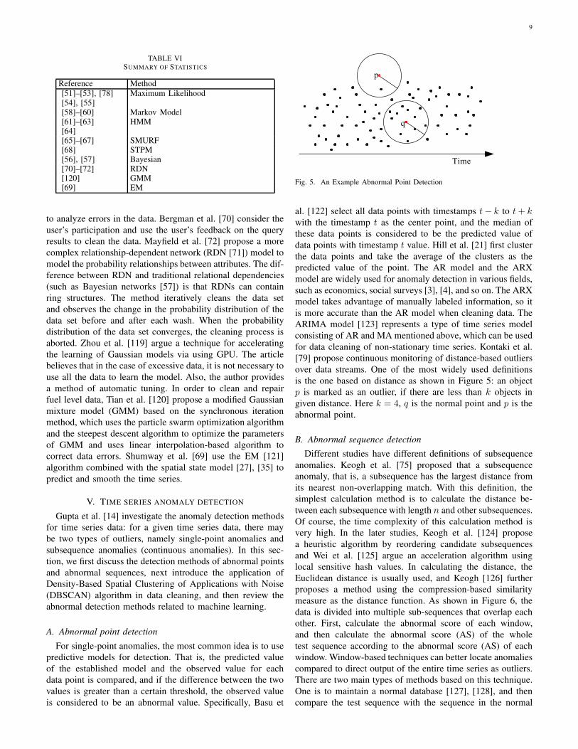
[79] propose continuous monitoring of distance-based outliers

over data streams. One of the most widely used definitions

is the one based on distance as shown in Figure 5: an object

p is marked as an outlier, if there are less than k objects in

given distance. Here k = 4, q is the normal point and p is the

abnormal point.

B. Abnormal sequence detection

Different studies have different definitions of subsequence

anomalies. Keogh et al. [75] proposed that a subsequence

anomaly, that is, a subsequence has the largest distance from

its nearest non-overlapping match. With this definition, the

simplest calculation method is to calculate the distance be-

tween each subsequence with length n and other subsequences.

Of course, the time complexity of this calculation method is

very high. In the later studies, Keogh et al. [124] propose

a heuristic algorithm by reordering candidate subsequences

and Wei et al. [125] argue an acceleration algorithm using

local sensitive hash values. In calculating the distance, the

Euclidean distance is usually used, and Keogh [126] further

proposes a method using the compression-based similarity

measure as the distance function. As shown in Figure 6, the

data is divided into multiple sub-sequences that overlap each

other. First, calculate the abnormal score of each window,

and then calculate the abnormal score (AS) of the whole

test sequence according to the abnormal score (AS) of each

window. Window-based techniques can better locate anomalies

compared to direct output of the entire time series as outliers.

There are two main types of methods based on this technique.

One is to maintain a normal database [127], [128], and then

compare the test sequence with the sequence in the normal

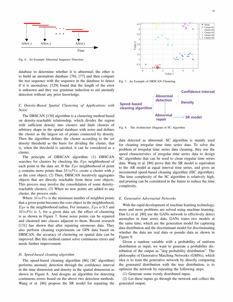
10

Fig. 6. An Example Abnormal Sequence Detection

database to determine whether it is abnormal; the other is

to build an anomalous database [76], [77] and then compare

the test sequence with the sequence in the database to detect

if it is anomalous. [129] found that the length of the error

is unknown and they use grammar induction to aid anomaly

detection without any prior knowledge.

C. Density-Based Spatial Clustering of Applications with

Noise

The DBSCAN [130] algorithm is a clustering method based

on density-reachable relationship, which divides the region

with sufficient density into clusters and finds clusters of

arbitrary shape in the spatial database with noise and defines

the cluster as the largest set of points connected by density.

Then the algorithm defines the cluster according to the set

density threshold as the basis for dividing the cluster, that

is, when the threshold is satisfied, it can be considered as a

cluster.

The principle of DBSCAN algorithm: (1) DBSCAN

searches for clusters by checking the Eps neighborhood of

each point in the data set. If the Eps neighborhood of point

p contains more points than MinPts, create a cluster with p

as the core object; (2) Then, DBSCAN iteratively aggregates

objects that are directly reachable from these core objects.

This process may involve the consolidation of some density-

reachable clusters; (3) When no new points are added to any

cluster, the process ends.

Where MinPts is the minimum number of neighbor points

that a given point becomes the core object in the neighborhood,

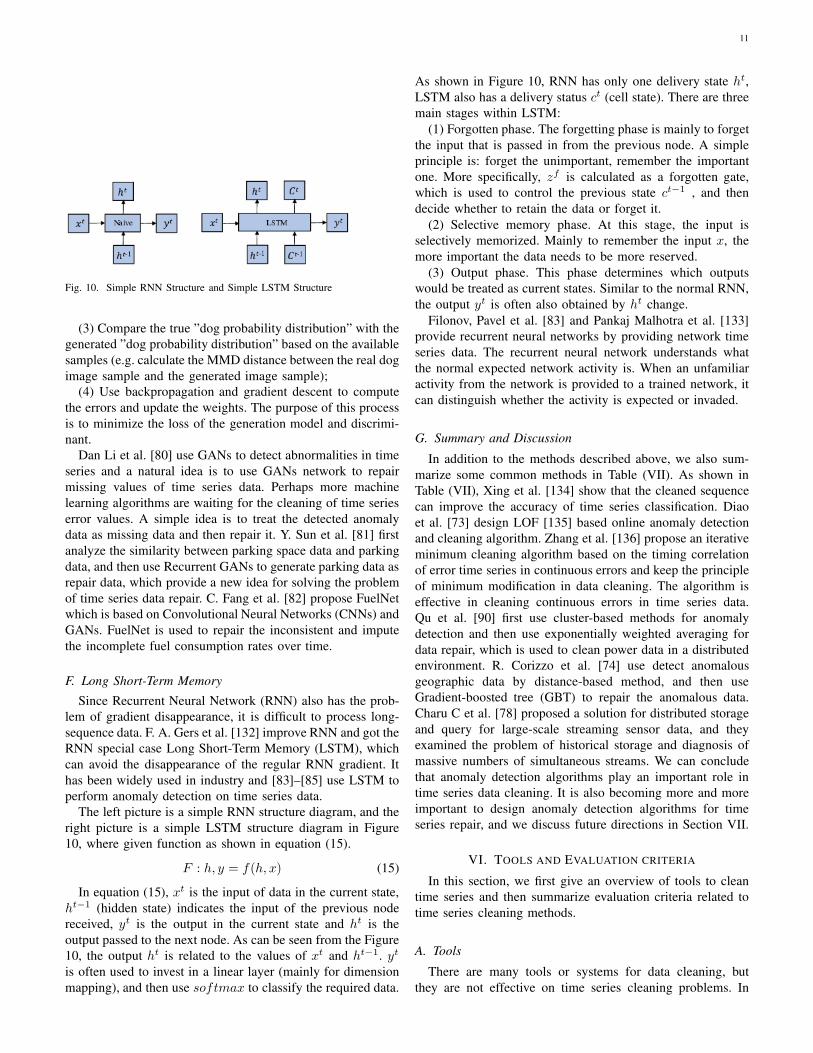
Eps is the neighborhood radius. For instance, Eps is 0.5 and

MinPts is 3, for a given data set, the effect of clustering

is as shown in Figure 7. Some noise points can be repaired

and clustered into classes adjacent to them. Recent research

[131] has shown that after repairing erroneous data. They

also perform cleaning experiments on GPS data based on

DBSCAN, the accuracy of clustering on spatial data can be

improved. But this method cannot solve continuous errors and

needs further improvement.

D. Speed-based cleaning algorithm

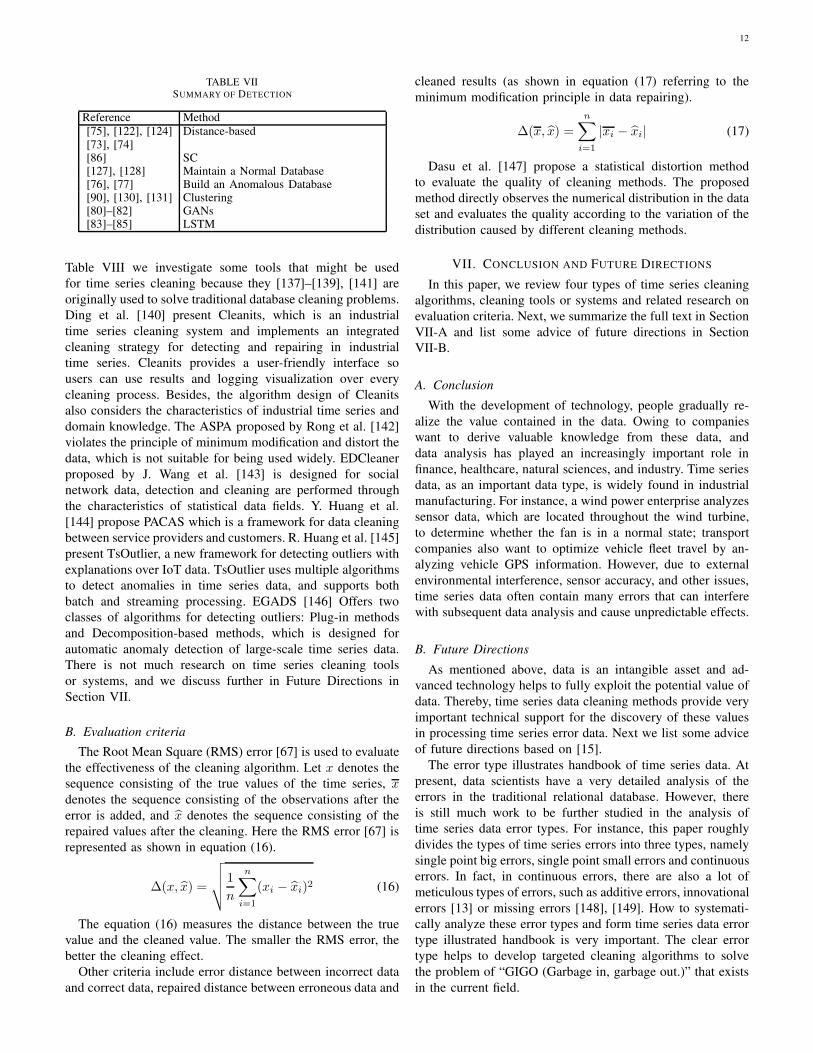
The speed-based cleaning algorithm [86] (SC algorithm)

performs anomaly detection through the confidence interval

in the time dimension and density in the spatial dimension as

shown in Figure 8. And designs an algorithm for detecting

continuous errors based on the above two detection methods.

Wang et al. [86] propose the SR model for repairing the

0 1 2 3 4 5Value 1

0.5

1

1.5

2

2.5

3

3.5

4

4.5

Val

ue 2

NoiseCluster #1Cluster #2Cluster #3Cluster #4Cluster #5

Fig. 7. An Example of DBSCAN Clustering

Fig. 8. The Architecture Diagram of SC Algorithm

data detected as abnormal. SC algorithm is mainly used

for cleaning irregular time time series data. To solve the

problem of irregular time series data cleaning, they use the

speed characteristics of irregular time series data to design

SC algorithms that can be used to clean rregular time series

data. Wang et al. [86] prove that the SR model is equivalent

to the AR model at equal interval time series, and gives an

incremental speed-based cleaning algorithm (ISC algorithm).

The time complexity of the SC algorithm is relatively high,

and pruning can be considered in the future to reduce the time

complexity.

E. Generative Adversarial Networks

With the rapid development of machine learning technology,

more and more problems are solved using machine learning.

Dan Li et al. [80] use the GANs network to effectively detect

anomalies in time series data. GANs trains two models at

the same time, which are the generation model for capturing

data distribution and the discriminant model for discriminating

whether the data are real data or pseudo data as shown in

Figure 9.

Given a random variable with a probability of uniform

distribution as input, we want to generate a probability dis-

tribution of the output as ”dog probability distribution”. The

philosophy of Generative Matching Networks (GMNs), which

idea is to train the generative network by directly comparing

the generated distribution with the true distribution, is to

optimize the network by repeating the following steps:

(1) Generate some evenly distributed input;

(2) Let these inputs go through the network and collect the

generated output;

11

Fig. 9. A Simple Flow Chart of Generative Adversarial Networks

Fig. 10. Simple RNN Structure and Simple LSTM Structure

(3) Compare the true ”dog probability distribution” with the

generated ”dog probability distribution” based on the available

samples (e.g. calculate the MMD distance between the real dog

image sample and the generated image sample);(4) Use backpropagation and gradient descent to compute

the errors and update the weights. The purpose of this process

is to minimize the loss of the generation model and discrimi-

nant.

Dan Li et al. [80] use GANs to detect abnormalities in time

series and a natural idea is to use GANs network to repair

missing values of time series data. Perhaps more machine

learning algorithms are waiting for the cleaning of time series

error values. A simple idea is to treat the detected anomaly

data as missing data and then repair it. Y. Sun et al. [81] first

analyze the similarity between parking space data and parking

data, and then use Recurrent GANs to generate parking data as

repair data, which provide a new idea for solving the problem

of time series data repair. C. Fang et al. [82] propose FuelNet

which is based on Convolutional Neural Networks (CNNs) and

GANs. FuelNet is used to repair the inconsistent and impute

the incomplete fuel consumption rates over time.

F. Long Short-Term Memory

Since Recurrent Neural Network (RNN) also has the prob-

lem of gradient disappearance, it is difficult to process long-

sequence data. F. A. Gers et al. [132] improve RNN and got the

RNN special case Long Short-Term Memory (LSTM), which

can avoid the disappearance of the regular RNN gradient. It

has been widely used in industry and [83]–[85] use LSTM to

perform anomaly detection on time series data.

The left picture is a simple RNN structure diagram, and the

right picture is a simple LSTM structure diagram in Figure

10, where given function as shown in equation (15).

F : h, y = f(h, x) (15)

In equation (15), xt is the input of data in the current state,

ht−1 (hidden state) indicates the input of the previous node

received, yt is the output in the current state and ht is the

output passed to the next node. As can be seen from the Figure

10, the output ht is related to the values of xt and ht−1. yt

is often used to invest in a linear layer (mainly for dimension

mapping), and then use softmax to classify the required data.

As shown in Figure 10, RNN has only one delivery state ht,

LSTM also has a delivery status ct (cell state). There are three

main stages within LSTM:

(1) Forgotten phase. The forgetting phase is mainly to forget

the input that is passed in from the previous node. A simple

principle is: forget the unimportant, remember the important

one. More specifically, zf is calculated as a forgotten gate,

which is used to control the previous state ct−1 , and then

decide whether to retain the data or forget it.

(2) Selective memory phase. At this stage, the input is

selectively memorized. Mainly to remember the input x, the

more important the data needs to be more reserved.

(3) Output phase. This phase determines which outputs

would be treated as current states. Similar to the normal RNN,

the output yt is often also obtained by ht change.

Filonov, Pavel et al. [83] and Pankaj Malhotra et al. [133]

provide recurrent neural networks by providing network time

series data. The recurrent neural network understands what

the normal expected network activity is. When an unfamiliar

activity from the network is provided to a trained network, it

can distinguish whether the activity is expected or invaded.

G. Summary and Discussion

In addition to the methods described above, we also sum-

marize some common methods in Table (VII). As shown in

Table (VII), Xing et al. [134] show that the cleaned sequence

can improve the accuracy of time series classification. Diao

et al. [73] design LOF [135] based online anomaly detection

and cleaning algorithm. Zhang et al. [136] propose an iterative

minimum cleaning algorithm based on the timing correlation

of error time series in continuous errors and keep the principle

of minimum modification in data cleaning. The algorithm is

effective in cleaning continuous errors in time series data.

Qu et al. [90] first use cluster-based methods for anomaly

detection and then use exponentially weighted averaging for

data repair, which is used to clean power data in a distributed

environment. R. Corizzo et al. [74] use detect anomalous

geographic data by distance-based method, and then use

Gradient-boosted tree (GBT) to repair the anomalous data.

Charu C et al. [78] proposed a solution for distributed storage

and query for large-scale streaming sensor data, and they

examined the problem of historical storage and diagnosis of

massive numbers of simultaneous streams. We can conclude

that anomaly detection algorithms play an important role in

time series data cleaning. It is also becoming more and more

important to design anomaly detection algorithms for time

series repair, and we discuss future directions in Section VII.

VI. TOOLS AND EVALUATION CRITERIA

In this section, we first give an overview of tools to clean

time series and then summarize evaluation criteria related to

time series cleaning methods.

A. Tools

There are many tools or systems for data cleaning, but

they are not effective on time series cleaning problems. In

12

TABLE VIISUMMARY OF DETECTION

Reference Method[75], [122], [124][73], [74]

Distance-based

[86] SC[127], [128] Maintain a Normal Database[76], [77] Build an Anomalous Database[90], [130], [131] Clustering[80]–[82] GANs[83]–[85] LSTM

Table VIII we investigate some tools that might be used

for time series cleaning because they [137]–[139], [141] are

originally used to solve traditional database cleaning problems.

Ding et al. [140] present Cleanits, which is an industrial

time series cleaning system and implements an integrated

cleaning strategy for detecting and repairing in industrial

time series. Cleanits provides a user-friendly interface so

users can use results and logging visualization over every

cleaning process. Besides, the algorithm design of Cleanits

also considers the characteristics of industrial time series and

domain knowledge. The ASPA proposed by Rong et al. [142]

violates the principle of minimum modification and distort the

data, which is not suitable for being used widely. EDCleaner

proposed by J. Wang et al. [143] is designed for social

network data, detection and cleaning are performed through

the characteristics of statistical data fields. Y. Huang et al.

[144] propose PACAS which is a framework for data cleaning

between service providers and customers. R. Huang et al. [145]

present TsOutlier, a new framework for detecting outliers with

explanations over IoT data. TsOutlier uses multiple algorithms

to detect anomalies in time series data, and supports both

batch and streaming processing. EGADS [146] Offers two

classes of algorithms for detecting outliers: Plug-in methods

and Decomposition-based methods, which is designed for

automatic anomaly detection of large-scale time series data.

There is not much research on time series cleaning tools

or systems, and we discuss further in Future Directions in

Section VII.

B. Evaluation criteria

The Root Mean Square (RMS) error [67] is used to evaluate

the effectiveness of the cleaning algorithm. Let x denotes the

sequence consisting of the true values of the time series, x

denotes the sequence consisting of the observations after the

error is added, and x denotes the sequence consisting of the

repaired values after the cleaning. Here the RMS error [67] is

represented as shown in equation (16).

∆(x, x) =

√√√√ 1

n

n∑

i=1

(xi − xi)2 (16)

The equation (16) measures the distance between the true

value and the cleaned value. The smaller the RMS error, the

better the cleaning effect.

Other criteria include error distance between incorrect data

and correct data, repaired distance between erroneous data and

cleaned results (as shown in equation (17) referring to the

minimum modification principle in data repairing).

∆(x, x) =

n∑

i=1

|xi − xi| (17)

Dasu et al. [147] propose a statistical distortion method

to evaluate the quality of cleaning methods. The proposed

method directly observes the numerical distribution in the data

set and evaluates the quality according to the variation of the

distribution caused by different cleaning methods.

VII. CONCLUSION AND FUTURE DIRECTIONS

In this paper, we review four types of time series cleaning

algorithms, cleaning tools or systems and related research on

evaluation criteria. Next, we summarize the full text in Section

VII-A and list some advice of future directions in Section

VII-B.

A. Conclusion

With the development of technology, people gradually re-

alize the value contained in the data. Owing to companies

want to derive valuable knowledge from these data, and

data analysis has played an increasingly important role in

finance, healthcare, natural sciences, and industry. Time series

data, as an important data type, is widely found in industrial

manufacturing. For instance, a wind power enterprise analyzes

sensor data, which are located throughout the wind turbine,

to determine whether the fan is in a normal state; transport

companies also want to optimize vehicle fleet travel by an-

alyzing vehicle GPS information. However, due to external

environmental interference, sensor accuracy, and other issues,

time series data often contain many errors that can interfere

with subsequent data analysis and cause unpredictable effects.

B. Future Directions

As mentioned above, data is an intangible asset and ad-

vanced technology helps to fully exploit the potential value of

data. Thereby, time series data cleaning methods provide very

important technical support for the discovery of these values

in processing time series error data. Next we list some advice

of future directions based on [15].

The error type illustrates handbook of time series data. At

present, data scientists have a very detailed analysis of the

errors in the traditional relational database. However, there

is still much work to be further studied in the analysis of

time series data error types. For instance, this paper roughly

divides the types of time series errors into three types, namely

single point big errors, single point small errors and continuous

errors. In fact, in continuous errors, there are also a lot of

meticulous types of errors, such as additive errors, innovational

errors [13] or missing errors [148], [149]. How to systemati-

cally analyze these error types and form time series data error

type illustrated handbook is very important. The clear error

type helps to develop targeted cleaning algorithms to solve

the problem of “GIGO (Garbage in, garbage out.)” that exists

in the current field.

13

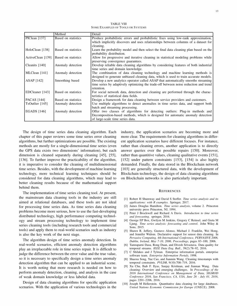
TABLE VIIISOME EXAMPLES OF TOOLS OR SYSTEMS

Method DetailPIClean [137] Based on statistics Produce probabilistic errors and probabilistic fixes using low-rank approximation,

which implicitly discovers and uses relationships between columns of a dataset forcleaning.

HoloClean [138] Based on statistics Learn the probability model and then select the final data cleaning plan based on theprobability distribution.

ActiveClean [139] Based on statistics Allow for progressive and iterative cleaning in statistical modeling problems whilepreserving convergence guarantees.

Cleanits [140] Anomaly detection Develop reliable data cleaning algorithms by considering features of both industrialtime series and domain knowledge.

MLClean [141] Anomaly detection The combination of data cleaning technology and machine learning methods isdesigned to generate unbiased cleaning data, which is used to train accurate models.

ASAP [142] Smoothing based Develop a new analytics operator called ASAP that automatically smooths streamingtime series by adaptively optimizing the trade-off between noise reduction and trendretention.

EDCleaner [143] Based on statistics For social network data, detection and cleaning are performed through the charac-teristics of statistical data fields.

PACAS [144] Based on statistics Design a framework for data cleaning between service providers and customers.TsOutlier [145] Anomaly detection Use multiple algorithms to detect anomalies in time series data, and support both

batch and streaming processing.EGADS [146] Anomaly detection Offer two classes of algorithms for detecting outliers: Plug-in methods and

Decomposition-based methods, which is designed for automatic anomaly detectionof large-scale time series data.

The design of time series data cleaning algorithm. Each

chapter of this paper reviews some time series error cleaning

algorithms, but further optimizations are possible. The existing

methods are mostly for a single-dimensional time series (even

the GPS data exists two dimensions’ information), but each

dimension is cleaned separately during cleaning [45], [55],

[136]. To further improve the practicability of the algorithm,

it is imperative to consider the cleaning of multidimensional

time series. Besides, with the development of machine learning

technology, more technical learning techniques should be

considered for data cleaning algorithms, which may lead to

better cleaning results because of the mathematical support

behind them.

The implementation of time series cleaning tool. At present,

the mainstream data cleaning tools in the industry are still

aimed at relational databases, and these tools are not ideal

for processing time series data. As time series data cleaning

problems become more serious, how to use the fast-developing

distributed technology, high performance computing technol-

ogy and stream processing technology to implement time

series cleaning tools (including research tools and commercial

tools) and apply them to real-world scenarios such as industry

is also the key work of the next stage.

The algorithm design of time series anomaly detection. In

real-world scenarios, efficient anomaly detection algorithms

play an irreplaceable role in time series repair. It is difficult to

judge the difference between the error value and the true value,

so it is necessary to specifically design a time series anomaly

detection algorithm that can be applied to an industrial scene.

It is worth noting that more research is needed on how to

perform anomaly detection, cleaning, and analysis in the case

of weak domain knowledge or less labeled data.

Design of data cleaning algorithms for specific application

scenarios. With the application of various technologies in the

industry, the application scenarios are becoming more and

more clear. The requirements for cleaning algorithms in differ-

ent application scenarios have different focuses. For instance,

rather than cleaning errors, another application is to directly

answer queries over the possible repairs [150]. Moreover,

rather than quantitive values, cleaning qualitative events [151],

[152] under pattern constraints [153], [154] is also highly

demanded. Finally, the data stored in the Blockchain network

[103] are generally structured data, with the development of

Blockchain technology, the design of data cleaning algorithms

on Blockchain networks is also particularly important.

REFERENCES

[1] Robert H Shumway and David S Stoffer. Time series analysis and its

applications: with R examples. Springer, 2017.[2] James Douglas Hamilton. Time series analysis, volume 2. Princeton

university press Princeton, NJ, 1994.

[3] Peter J Brockwell and Richard A Davis. Introduction to time series

and forecasting. springer, 2016.

[4] George EP Box, Gwilym M Jenkins, Gregory C Reinsel, and Greta MLjung. Time series analysis: forecasting and control. John Wiley &Sons, 2015.

[5] Shawn R. Jeffery, Gustavo Alonso, Michael J. Franklin, Wei Hong,and Jennifer Widom. Declarative support for sensor data cleaning. InPervasive Computing, 4th International Conference, PERVASIVE 2006,

Dublin, Ireland, May 7-10, 2006, Proceedings, pages 83–100, 2006.

[6] Tamraparni Dasu, Rong Duan, and Divesh Srivastava. Data quality fortemporal streams. IEEE Data Eng. Bull., 39(2):78–92, 2016.

[7] C Shilakes and J Tylman. Enterprise information portals. enterprisesoftware team. Enterprise Information Portals, 1998.

[8] Shaoxu Song, Yue Cao, and Jianmin Wang. Cleaning timestamps withtemporal constraints. PVLDB, 9(10):708–719, 2016.

[9] Xu Chu, Ihab F. Ilyas, Sanjay Krishnan, and Jiannan Wang. Datacleaning: Overview and emerging challenges. In Proceedings of the

2016 International Conference on Management of Data, SIGMODConference 2016, San Francisco, CA, USA, June 26 - July 01, 2016,pages 2201–2206, 2016.

[10] Joseph M Hellerstein. Quantitative data cleaning for large databases.United Nations Economic Commission for Europe (UNECE), 2008.

14

[11] Mourad Khayati, Alberto Lerner, Zakhar Tymchenko, and PhilippeCudre-Mauroux. Mind the gap: An experimental evaluation of impu-tation of missing values techniques in time series. PVLDB, 13(5):768–782, 2020.

[12] Aimad Karkouch, Hajar Mousannif, Hassan Al Moatassime, andThomas Noel. Data quality in internet of things: A state-of-the-artsurvey. J. Network and Computer Applications, 73:57–81, 2016.

[13] Ruey S Tsay. Outliers, level shifts, and variance changes in time series.Journal of forecasting, 7(1):1–20, 1988.

[14] Manish Gupta, Jing Gao, Charu C. Aggarwal, and Jiawei Han. Outlierdetection for temporal data: A survey. IEEE Trans. Knowl. Data Eng.,26(9):2250–2267, 2014.

[15] Aoqian Zhang. Research on Time Series Data Cleaning. PhD thesis,Tsinghua University, 2018.

[16] Philip Bohannon, Michael Flaster, Wenfei Fan, and Rajeev Rastogi.A cost-based model and effective heuristic for repairing constraints byvalue modification. In Proceedings of the ACM SIGMOD InternationalConference on Management of Data, Baltimore, Maryland, USA, June

14-16, 2005, pages 143–154, 2005.[17] Foto N. Afrati and Phokion G. Kolaitis. Repair checking in inconsistent

databases: algorithms and complexity. In Database Theory - ICDT

2009, 12th International Conference, St. Petersburg, Russia, March23-25, 2009, Proceedings, pages 31–41, 2009.

[18] Jan Chomicki and Jerzy Marcinkowski. Minimal-change integritymaintenance using tuple deletions. Inf. Comput., 197(1-2):90–121,2005.

[19] Ronald Fagin, Benny Kimelfeld, and Phokion G. Kolaitis. Dichotomiesin the complexity of preferred repairs. In Proceedings of the 34th

ACM Symposium on Principles of Database Systems, PODS 2015,

Melbourne, Victoria, Australia, May 31 - June 4, 2015, pages 3–15,2015.

[20] David R. Brillinger. Time series - data analysis and theory, volume 36of Classics in applied mathematics. SIAM, 2001.

[21] David J. Hill and Barbara S. Minsker. Anomaly detection in streamingenvironmental sensor data: A data-driven modeling approach. Environ-

mental Modelling and Software, 25(9):1014–1022, 2010.[22] Kenji Yamanishi and Jun’ichi Takeuchi. A unifying framework for

detecting outliers and change points from non-stationary time seriesdata. In Proceedings of the Eighth ACM SIGKDD International

Conference on Knowledge Discovery and Data Mining, July 23-26,

2002, Edmonton, Alberta, Canada, pages 676–681, 2002.[23] S Dilling and BJ MacVicar. Cleaning high-frequency velocity profile

data with autoregressive moving average (arma) models. Flow Mea-

surement and Instrumentation, 54:68–81, 2017.[24] Gerard Alengrin and Gerard Favier. New stochastic realization al-

gorithms for identification of ARMA models. In IEEE InternationalConference on Acoustics, Speech, and Signal Processing, ICASSP ’78,

Tulsa, Oklahoma, USA, April 10-12, 1978, pages 208–213, 1978.[25] Rudolph Emil Kalman. A new approach to linear filtering and

prediction problems. Journal of basic Engineering, 82(1):35–45, 1960.[26] Martyna Marczak, Tommaso Proietti, and Stefano Grassi. A data-

cleaning augmented kalman filter for robust estimation of state spacemodels. Econometrics and Statistics, 5:107–123, 2018.

[27] G Wayne Morrison and David H Pike. Kalman filtering applied tostatistical forecasting. Management Science, 23(7):768–774, 1977.

[28] Robert Grover Brown, Patrick YC Hwang, et al. Introduction to random

signals and applied Kalman filtering, volume 3. Wiley New York, 1992.[29] Garry A. Einicke and Langford B. White. Robust extended kalman

filtering. IEEE Trans. Signal Processing, 47(9):2596–2599, 1999.[30] Zenton Goh, Kah-Chye Tan, and B. T. G. Tan. Kalman-filtering speech

enhancement method based on a voiced-unvoiced speech model. IEEE

Trans. Speech and Audio Processing, 7(5):510–524, 1999.[31] Yongzhen Zhuang, Lei Chen, Xiaoyang Sean Wang, and Jie Lian. A

weighted moving average-based approach for cleaning sensor data. In27th IEEE International Conference on Distributed Computing Systems

(ICDCS 2007), June 25-29, 2007, Toronto, Ontario, Canada, page 38,2007.

[32] Everette S Gardner Jr. Exponential smoothing: The state of the art—part ii. International journal of forecasting, 22(4):637–666, 2006.

[33] Eamonn J. Keogh, Selina Chu, David M. Hart, and Michael J. Pazzani.An online algorithm for segmenting time series. In Proceedings of the

2001 IEEE International Conference on Data Mining, 29 November -2 December 2001, San Jose, California, USA, pages 289–296, 2001.

[34] Shu Xu, Bo Lu, Michael Baldea, Thomas F Edgar, Willy Wojsznis,Terrence Blevins, and Mark Nixon. Data cleaning in the processindustries. Reviews in Chemical Engineering, 31(5):453–490, 2015.

[35] Richard H Jones. Exponential smoothing for multivariate time series.Journal of the Royal Statistical Society: Series B (Methodological),28(1):241–251, 1966.

[36] JWC Van Lint, SP Hoogendoorn, and Henk J van Zuylen. Accuratefreeway travel time prediction with state-space neural networks undermissing data. Transportation Research Part C: Emerging Technologies,13(5-6):347–369, 2005.

[37] Minjie Chen, Mantao Xu, and Pasi Franti. A fast $o(n)$ multiresolutionpolygonal approximation algorithm for GPS trajectory simplification.IEEE Trans. Image Processing, 21(5):2770–2785, 2012.

[38] Cheng Long, Raymond Chi-Wing Wong, and H. V. Jagadish. Trajectorysimplification: On minimizing the direction-based error. PVLDB,8(1):49–60, 2014.

[39] Jirun Dong and Richard Hull. Applying approximate order dependencyto reduce indexing space. In Proceedings of the 1982 ACM SIGMOD

International Conference on Management of Data, Orlando, Florida,

June 2-4, 1982., pages 119–127, 1982.[40] Seymour Ginsburg and Richard Hull. Order dependency in the

relational model. Theor. Comput. Sci., 26:149–195, 1983.[41] Seymour Ginsburg and Richard Hull. Sort sets in the relational model.

In Proceedings of the Second ACM SIGACT-SIGMOD Symposium on

Principles of Database Systems, March 21-23, 1983, Colony Square

Hotel, Atlanta, Georgia, USA, pages 332–339, 1983.[42] Seymour Ginsburg and Richard Hull. Sort sets in the relational model.

J. ACM, 33(3):465–488, 1986.[43] Andrei Lopatenko and Loreto Bravo. Efficient approximation algo-

rithms for repairing inconsistent databases. In Proceedings of the23rd International Conference on Data Engineering, ICDE 2007, The

Marmara Hotel, Istanbul, Turkey, April 15-20, 2007, pages 216–225,2007.

[44] Lukasz Golab, Howard J. Karloff, Flip Korn, Avishek Saha, and DiveshSrivastava. Sequential dependencies. PVLDB, 2(1):574–585, 2009.

[45] Shaoxu Song, Aoqian Zhang, Jianmin Wang, and Philip S. Yu.SCREEN: stream data cleaning under speed constraints. In Proceedingsof the 2015 ACM SIGMOD International Conference on Management

of Data, Melbourne, Victoria, Australia, May 31 - June 4, 2015, pages827–841, 2015.

[46] Wei Yin, Tianbai Yue, Hongzhi Wang, Yanhao Huang, and Yaping Li.Time series cleaning under variance constraints. In Database Systems

for Advanced Applications - DASFAA 2018 International Workshops:

BDMS, BDQM, GDMA, and SeCoP, Gold Coast, QLD, Australia, May21-24, 2018, Proceedings, pages 108–113, 2018.

[47] Shaoxu Song, Yu Sun, Aoqian Zhang, Lei Chen, and Jianmin Wang.Enriching data imputation under similarity rule constraints. IEEE

Trans. Knowl. Data Eng., 32(2):275–287, 2020.[48] Aoqian Zhang, Shaoxu Song, Yu Sun, and Jianmin Wang. Learning

individual models for imputation. In 35th IEEE International Con-

ference on Data Engineering, ICDE 2019, Macao, China, April 8-11,

2019, pages 160–171, 2019.[49] Qingchao Cai, Zhongle Xie, Gang Chen, H. V. Jagadish, Beng Chin

Ooi, and Meihui Zhang. Effective temporal dependence discovery intime series data. PVLDB, 11(8):893–905, 2018.

[50] Dehua Cheng, Mohammad Taha Bahadori, and Yan Liu. FBLG: asimple and effective approach for temporal dependence discovery fromtime series data. In The 20th ACM SIGKDD International Conference

on Knowledge Discovery and Data Mining, KDD ’14, New York, NY,USA - August 24 - 27, 2014, pages 382–391, 2014.

[51] Yoram Bresler and Albert Macovski. Exact maximum likelihoodparameter estimation of superimposed exponential signals in noise.IEEE Trans. Acoustics, Speech, and Signal Processing, 34(5):1081–1089, 1986.

[52] Tomasz Gogacz and Szymon Torunczyk. Entropy bounds for con-junctive queries with functional dependencies. In 20th InternationalConference on Database Theory, ICDT 2017, March 21-24, 2017,

Venice, Italy, pages 15:1–15:17, 2017.[53] Dong Wang, Lance M. Kaplan, and Tarek F. Abdelzaher. Maximum

likelihood analysis of conflicting observations in social sensing. TOSN,10(2):30:1–30:27, 2014.

[54] Mohamed Yakout, Laure Berti-Equille, and Ahmed K. Elmagarmid.Don’t be scared: use scalable automatic repairing with maximal likeli-hood and bounded changes. In Proceedings of the ACM SIGMOD

International Conference on Management of Data, SIGMOD 2013,

New York, NY, USA, June 22-27, 2013, pages 553–564, 2013.[55] Aoqian Zhang, Shaoxu Song, and Jianmin Wang. Sequential data clean-

ing: A statistical approach. In Proceedings of the 2016 International

Conference on Management of Data, SIGMOD Conference 2016, San

Francisco, CA, USA, June 26 - July 01, 2016, pages 909–924, 2016.

15

[56] Xiaolan Wang, Xin Luna Dong, and Alexandra Meliou. Data x-ray: A diagnostic tool for data errors. In Proceedings of the 2015ACM SIGMOD International Conference on Management of Data,

Melbourne, Victoria, Australia, May 31 - June 4, 2015, pages 1231–1245, 2015.

[57] Lise Getoor, Nir Friedman, Daphne Koller, and Benjamin Taskar.Learning probabilistic models of relational structure. In Proceedings of

the Eighteenth International Conference on Machine Learning (ICML

2001), Williams College, Williamstown, MA, USA, June 28 - July 1,2001, pages 170–177, 2001.

[58] AM Dukhovny. Markov chains with quasitoeplitz transition matrix:Applications. International Journal of Stochastic Analysis, 3(2):141–152, 1900.

[59] Jun Cai. A markov model of switching-regime arch. Journal of

Business & Economic Statistics, 12(3):309–316, 1994.[60] Qinqing Zhang and Saleem A. Kassam. Finite-state markov model for

rayleigh fading channels. IEEE Trans. Communications, 47(11):1688–1692, 1999.

[61] Md. Rafiul Hassan, Baikunth Nath, and Michael Kirley. A fusion modelof hmm, ANN and GA for stock market forecasting. Expert Syst. Appl.,33(1):171–180, 2007.

[62] Ming Dong, Dong Yang, Yan Kuang, David He, Serap Erdal, andDonna Kenski. Pm2.5 concentration prediction using hidden semi-markov model-based times series data mining. Expert Syst. Appl.,36(5):9046–9055, 2009.

[63] Aditya Gupta and Bhuwan Dhingra. Stock market prediction usinghidden markov models. In 2012 Students Conference on Engineeringand Systems, pages 1–4. IEEE, 2012.

[64] Asif Iqbal Baba, Manfred Jaeger, Hua Lu, Torben Bach Pedersen,Wei-Shinn Ku, and Xike Xie. Learning-based cleansing for indoorRFID data. In Proceedings of the 2016 International Conference onManagement of Data, SIGMOD Conference 2016, San Francisco, CA,

USA, June 26 - July 01, 2016, pages 925–936, 2016.[65] A Anny Leema and M Hemalatha. An effective and adaptive data

cleaning technique for colossal rfid data sets in healthcare. WSEAS

transactions on Information Science and Applications, 8(6):243–252,2011.

[66] He Xu, Jie Ding, Peng Li, Daniele Sgandurra, and Ruchuan Wang. Animproved SMURF scheme for cleaning RFID data. IJGUC, 9(2):170–178, 2018.

[67] Shawn R. Jeffery, Minos N. Garofalakis, and Michael J. Franklin.Adaptive cleaning for RFID data streams. In Proceedings of the 32nd

International Conference on Very Large Data Bases, Seoul, Korea,

September 12-15, 2006, pages 163–174, 2006.[68] Mostafa Milani, Zheng Zheng, and Fei Chiang. Currentclean: Spatio-

temporal cleaning of stale data. In 35th IEEE International Conference

on Data Engineering, ICDE 2019, Macao, China, April 8-11, 2019,pages 172–183, 2019.

[69] Robert H Shumway and David S Stoffer. An approach to time seriessmoothing and forecasting using the em algorithm. Journal of time

series analysis, 3(4):253–264, 1982.[70] Moria Bergman, Tova Milo, Slava Novgorodov, and Wang Chiew Tan.

Query-oriented data cleaning with oracles. In Proceedings of the 2015

ACM SIGMOD International Conference on Management of Data,

Melbourne, Victoria, Australia, May 31 - June 4, 2015, pages 1199–1214, 2015.

[71] Jennifer Neville and David D. Jensen. Relational dependency networks.J. Mach. Learn. Res., 8:653–692, 2007.

[72] Chris Mayfield, Jennifer Neville, and Sunil Prabhakar. ERACER:a database approach for statistical inference and data cleaning. InProceedings of the ACM SIGMOD International Conference on Man-

agement of Data, SIGMOD 2010, Indianapolis, Indiana, USA, June

6-10, 2010, pages 75–86, 2010.[73] Yinglong Diao, Ke-yan Liu, Xiaoli Meng, Xueshun Ye, and Kaiyuan

He. A big data online cleaning algorithm based on dynamic outlierdetection. In 2015 International Conference on Cyber-Enabled Dis-tributed Computing and Knowledge Discovery, CyberC 2015, Xi’an,

China, September 17-19, 2015, pages 230–234, 2015.[74] Roberto Corizzo, Michelangelo Ceci, and Nathalie Japkowicz.

Anomaly detection and repair for accurate predictions in geo-distributed big data. Big Data Res., 16:18–35, 2019.

[75] Eamonn J. Keogh, Jessica Lin, Sang-Hee Lee, and Helga Van Herle.Finding the most unusual time series subsequence: algorithms andapplications. Knowl. Inf. Syst., 11(1):1–27, 2007.

[76] Fabio A. Gonzalez and Dipankar Dasgupta. Anomaly detection usingreal-valued negative selection. Genetic Programming and Evolvable

Machines, 4(4):383–403, 2003.

[77] Dipankar Dasgupta and Nivedita Sumi Majumdar. Anomaly detectionin multidimensional data using negative selection algorithm. In Pro-ceedings of the 2002 Congress on Evolutionary Computation. CEC’02

(Cat. No. 02TH8600), volume 2, pages 1039–1044. IEEE, 2002.

[78] Charu C. Aggarwal and Philip S. Yu. On historical diagnosis of sensorstreams. In 31st IEEE International Conference on Data Engineering,ICDE 2015, Seoul, South Korea, April 13-17, 2015, pages 185–194,2015.

[79] Maria Kontaki, Anastasios Gounaris, Apostolos N. Papadopoulos,Kostas Tsichlas, and Yannis Manolopoulos. Continuous monitoringof distance-based outliers over data streams. In Proceedings of the

27th International Conference on Data Engineering, ICDE 2011, April11-16, 2011, Hannover, Germany, pages 135–146, 2011.

[80] Dan Li, Dacheng Chen, Baihong Jin, Lei Shi, Jonathan Goh, andSee-Kiong Ng. MAD-GAN: multivariate anomaly detection for timeseries data with generative adversarial networks. In Artificial NeuralNetworks and Machine Learning - ICANN 2019: Text and Time Series

- 28th International Conference on Artificial Neural Networks, Munich,

Germany, September 17-19, 2019, Proceedings, Part IV, pages 703–716, 2019.

[81] Yuqiang Sun, Lei Peng, Huiyun Li, and Min Sun. Exploration onspatiotemporal data repairing of parking lots based on recurrent gans.In 21st International Conference on Intelligent Transportation Systems,ITSC 2018, Maui, HI, USA, November 4-7, 2018, pages 467–472, 2018.

[82] Chenguang Fang, Shaoxu Song, Zhiwei Chen, and Acan Gui. Fine-grained fuel consumption prediction. In Proceedings of the 28th ACMInternational Conference on Information and Knowledge Management,

CIKM 2019, Beijing, China, November 3-7, 2019, pages 2783–2791,2019.

[83] Pavel Filonov, Andrey Lavrentyev, and Artem Vorontsov. Multivariateindustrial time series with cyber-attack simulation: Fault detectionusing an lstm-based predictive data model. CoRR, abs/1612.06676,2016.

[84] Pankaj Malhotra, Vishnu TV, Anusha Ramakrishnan, Gaurangi Anand,Lovekesh Vig, Puneet Agarwal, and Gautam Shroff. Multi-sensor prog-nostics using an unsupervised health index based on LSTM encoder-decoder. CoRR, abs/1608.06154, 2016.

[85] Pankaj Malhotra, Lovekesh Vig, Gautam Shroff, and Puneet Agarwal.Long short term memory networks for anomaly detection in time series,2015.

[86] Xi Wang. Research on irregular time series data cleaning based onspeed. Master’s thesis, Tsinghua University, 2020.

[87] Robert Goodell Brown. Smoothing, forecasting and prediction ofdiscrete time series. Courier Corporation, 2004.

[88] Charles C Holt. Forecasting seasonals and trends by exponentiallyweighted moving averages. International journal of forecasting,20(1):5–10, 2004.

[89] Zhaosheng Zhang, Diange Yang, Tao Zhang, Qiaochu He, and Xi-aomin Lian. A study on the method for cleaning and repairing theprobe vehicle data. IEEE Trans. Intelligent Transportation Systems,14(1):419–427, 2013.

[90] Z Qu, Y Wang, Chong Wang, Nan Qu, and Jia Yan. A datacleaning model for electric power big data based on spark framework.International Journal of Database Theory and Application, 9(3):137–150, 2016.

[91] Maksims Volkovs, Fei Chiang, Jaroslaw Szlichta, and Renee J. Miller.Continuous data cleaning. In IEEE 30th International Conference on

Data Engineering, Chicago, ICDE 2014, IL, USA, March 31 - April 4,

2014, pages 244–255, 2014.[92] Gyuhae Park, Amanda C Rutherford, Hoon Sohn, and Charles R Farrar.

An outlier analysis framework for impedance-based structural healthmonitoring. Journal of Sound and Vibration, 286(1-2):229–250, 2005.

[93] George EP Box and David A Pierce. Distribution of residual autocorre-lations in autoregressive-integrated moving average time series models.Journal of the American statistical Association, 65(332):1509–1526,1970.

[94] Hermine N Akouemo and Richard J Povinelli. Data improving in timeseries using arx and ann models. IEEE Transactions on Power Systems,32(5):3352–3359, 2017.

[95] Peiyuan Chen, Troels Pedersen, Birgitte Bak-Jensen, and Zhe Chen.Arima-based time series model of stochastic wind power generation.IEEE transactions on power systems, 25(2):667–676, 2009.

[96] Jie Ma and Jian-fu Teng. Predict chaotic time-series using unscentedkalman filter. In Proceedings of 2004 International Conference on Ma-

chine Learning and Cybernetics (IEEE Cat. No. 04EX826), volume 2,pages 687–690. IEEE, 2004.

16

[97] Ih Chang, George C Tiao, and Chung Chen. Estimation of time seriesparameters in the presence of outliers. Technometrics, 30(2):193–204,1988.

[98] Ananthram Swami and Jerry M. Mendel. ARMA parameter estimationusing only output cumulants. IEEE Trans. Acoustics, Speech, and

Signal Processing, 38(7):1257–1265, 1990.[99] Gregory L Plett. Extended kalman filtering for battery management

systems of lipb-based hev battery packs: Part 3. state and parameterestimation. Journal of Power sources, 134(2):277–292, 2004.

[100] Jef Wijsen. Reasoning about qualitative trends in databases. Inf. Syst.,23(7):463–487, 1998.

[101] Jef Wijsen. Trends in databases: Reasoning and mining. IEEE Trans.

Knowl. Data Eng., 13(3):426–438, 2001.[102] Shaoxu Song, Han Zhu, and Jianmin Wang. Constraint-variance

tolerant data repairing. In Proceedings of the 2016 International

Conference on Management of Data, SIGMOD Conference 2016, San

Francisco, CA, USA, June 26 - July 01, 2016, pages 877–892, 2016.[103] Roberto Casado-Vara, Fernando de la Prieta, Javier Prieto, and Juan M.

Corchado. Blockchain framework for iot data quality via edge com-puting. In Proceedings of the 1st Workshop on Blockchain-enabled

Networked Sensor Systems, BlockSys@SenSys 2018, Shenzhen, China,

November 4, 2018, pages 19–24, 2018.[104] Catriel Beeri, Martin Dowd, Ronald Fagin, and Richard Statman.

On the structure of armstrong relations for functional dependencies.Journal of the ACM (JACM), 31(1):30–46, 1984.

[105] Wenfei Fan, Floris Geerts, Xibei Jia, and Anastasios Kementsietsidis.Conditional functional dependencies for capturing data inconsistencies.ACM Transactions on Database Systems (TODS), 33(2):6, 2008.

[106] Wenfei Fan, Floris Geerts, Jianzhong Li, and Ming Xiong. Discoveringconditional functional dependencies. IEEE Trans. Knowl. Data Eng.,23(5):683–698, 2011.

[107] Shaoxu Song and Lei Chen. Discovering matching dependencies.In Proceedings of the 18th ACM Conference on Information andKnowledge Management, CIKM 2009, Hong Kong, China, November

2-6, 2009, pages 1421–1424, 2009.[108] Shaoxu Song and Lei Chen. Efficient discovery of similarity constraints

for matching dependencies. Data Knowl. Eng., 87:146–166, 2013.[109] Yihan Wang, Shaoxu Song, Lei Chen, Jeffrey Xu Yu, and Hong Cheng.

Discovering conditional matching rules. TKDD, 11(4):46:1–46:38,2017.

[110] Shaoxu Song and Lei Chen. Differential dependencies: Reasoning anddiscovery. ACM Trans. Database Syst., 36(3):16:1–16:41, 2011.

[111] Shaoxu Song, Lei Chen, and Hong Cheng. Parameter-free determina-tion of distance thresholds for metric distance constraints. In IEEE

28th International Conference on Data Engineering (ICDE 2012),

Washington, DC, USA (Arlington, Virginia), 1-5 April, 2012, pages846–857, 2012.

[112] Shaoxu Song, Lei Chen, and Hong Cheng. Efficient determination ofdistance thresholds for differential dependencies. IEEE Trans. Knowl.

Data Eng., 26(9):2179–2192, 2014.[113] Shaoxu Song, Lei Chen, and Philip S. Yu. On data dependencies in

dataspaces. In Proceedings of the 27th International Conference onData Engineering, ICDE 2011, April 11-16, 2011, Hannover, Germany,pages 470–481, 2011.

[114] Shaoxu Song, Lei Chen, and Philip S. Yu. Comparable dependenciesover heterogeneous data. VLDB J., 22(2):253–274, 2013.

[115] Shaoxu Song, Han Zhu, and Lei Chen. Probabilistic correlation-basedsimilarity measure on text records. Inf. Sci., 289:8–24, 2014.

[116] Shaoxu Song, Hong Cheng, Jeffrey Xu Yu, and Lei Chen. Repairingvertex labels under neighborhood constraints. PVLDB, 7(11):987–998,2014.

[117] Shaoxu Song, Boge Liu, Hong Cheng, Jeffrey Xu Yu, and Lei Chen.Graph repairing under neighborhood constraints. VLDB J., 26(5):611–635, 2017.

[118] Shaoxu Song, Aoqian Zhang, Lei Chen, and Jianmin Wang. En-riching data imputation with extensive similarity neighbors. PVLDB,8(11):1286–1297, 2015.

[119] Jingbo Zhou and Anthony K. H. Tung. Smiler: A semi-lazy timeseries prediction system for sensors. In Proceedings of the 2015

ACM SIGMOD International Conference on Management of Data,

Melbourne, Victoria, Australia, May 31 - June 4, 2015, pages 1871–1886, 2015.

[120] Daxin Tian, Yukai Zhu, Xuting Duan, Junjie Hu, Zhengguo Sheng,Min Chen, Jian Wang, and Yunpeng Wang. An effective fuel-leveldata cleaning and repairing method for vehicle monitor platform. IEEE

Trans. Industrial Informatics, 15(1):410–422, 2019.

[121] Arthur P Dempster, Nan M Laird, and Donald B Rubin. Maximumlikelihood from incomplete data via the em algorithm. Journal of theRoyal Statistical Society: Series B (Methodological), 39(1):1–22, 1977.

[122] Sabyasachi Basu and Martin Meckesheimer. Automatic outlier detec-tion for time series: an application to sensor data. Knowl. Inf. Syst.,11(2):137–154, 2007.

[123] Guoqiang Peter Zhang. Time series forecasting using a hybrid ARIMAand neural network model. Neurocomputing, 50:159–175, 2003.

[124] Eamonn J. Keogh, Jessica Lin, and Ada Wai-Chee Fu. HOT SAX:efficiently finding the most unusual time series subsequence. InProceedings of the 5th IEEE International Conference on Data Mining

(ICDM 2005), 27-30 November 2005, Houston, Texas, USA, pages 226–233, 2005.

[125] Li Wei, Eamonn J. Keogh, and Xiaopeng Xi. Saxually explicit images:Finding unusual shapes. In Proceedings of the 6th IEEE International

Conference on Data Mining (ICDM 2006), 18-22 December 2006,

Hong Kong, China, pages 711–720, 2006.[126] Eamonn J. Keogh, Stefano Lonardi, and Chotirat (Ann) Ratanama-

hatana. Towards parameter-free data mining. In Proceedings of

the Tenth ACM SIGKDD International Conference on KnowledgeDiscovery and Data Mining, Seattle, Washington, USA, August 22-25,

2004, pages 206–215, 2004.[127] Anup K. Ghosh, Aaron Schwartzbard, and Michael Schatz. Learning

program behavior profiles for intrusion detection. In Proceedings ofthe Workshop on Intrusion Detection and Network Monitoring, Santa

Clara, CA, USA, April 9-12, 1999, pages 51–62, 1999.[128] D. Endler. Intrusion detection applying machine learning to solaris

audit data. In 14th Annual Computer Security Applications Conference

(ACSAC 1998), 7-11 December 1998, Scottsdale, AZ, USA, pages 268–279, 1998.

[129] Pavel Senin, Jessica Lin, Xing Wang, Tim Oates, Sunil Gandhi,Arnold P. Boedihardjo, Crystal Chen, and Susan Frankenstein. Timeseries anomaly discovery with grammar-based compression. In Pro-

ceedings of the 18th International Conference on Extending DatabaseTechnology, EDBT 2015, Brussels, Belgium, March 23-27, 2015, pages481–492, 2015.

[130] Martin Ester, Hans-Peter Kriegel, Jorg Sander, and Xiaowei Xu.A density-based algorithm for discovering clusters in large spatialdatabases with noise. In Proceedings of the Second International

Conference on Knowledge Discovery and Data Mining (KDD-96),

Portland, Oregon, USA, pages 226–231, 1996.[131] Shaoxu Song, Chunping Li, and Xiaoquan Zhang. Turn waste into

wealth: On simultaneous clustering and cleaning over dirty data.In Proceedings of the 21th ACM SIGKDD International Conference

on Knowledge Discovery and Data Mining, Sydney, NSW, Australia,August 10-13, 2015, pages 1115–1124, 2015.

[132] Felix A. Gers, Jurgen Schmidhuber, and Fred A. Cummins. Learningto forget: Continual prediction with LSTM. Neural Computation,12(10):2451–2471, 2000.

[133] Pankaj Malhotra, Anusha Ramakrishnan, Gaurangi Anand, LovekeshVig, Puneet Agarwal, and Gautam Shroff. Lstm-based encoder-decoderfor multi-sensor anomaly detection. CoRR, abs/1607.00148, 2016.

[134] Zhengzheng Xing, Jian Pei, and Philip S. Yu. Early classification ontime series. Knowl. Inf. Syst., 31(1):105–127, 2012.

[135] Markus M. Breunig, Hans-Peter Kriegel, Raymond T. Ng, and JorgSander. LOF: identifying density-based local outliers. In Proceedingsof the 2000 ACM SIGMOD International Conference on Management

of Data, May 16-18, 2000, Dallas, Texas, USA., pages 93–104, 2000.[136] Aoqian Zhang, Shaoxu Song, Jianmin Wang, and Philip S. Yu. Time

series data cleaning: From anomaly detection to anomaly repairing.PVLDB, 10(10):1046–1057, 2017.

[137] Zhuoran Yu and Xu Chu. Piclean: A probabilistic and interactive datacleaning system. In Proceedings of the 2019 International Conferenceon Management of Data, SIGMOD Conference 2019, Amsterdam, The

Netherlands, June 30 - July 5, 2019., pages 2021–2024, 2019.[138] Theodoros Rekatsinas, Xu Chu, Ihab F. Ilyas, and Christopher Re.

Holoclean: Holistic data repairs with probabilistic inference. PVLDB,10(11):1190–1201, 2017.

[139] Sanjay Krishnan, Jiannan Wang, Eugene Wu, Michael J. Franklin, andKen Goldberg. Activeclean: Interactive data cleaning for statisticalmodeling. PVLDB, 9(12):948–959, 2016.

[140] Xiaoou Ding, Hongzhi Wang, Jiaxuan Su, Zijue Li, Jianzhong Li, andHong Gao. Cleanits: A data cleaning system for industrial time series.PVLDB, 12(12):1786–1789, 2019.

[141] Ki Hyun Tae, Yuji Roh, Young Hun Oh, Hyunsu Kim, and Steven Eui-jong Whang. Data cleaning for accurate, fair, and robust models: A bigdata - AI integration approach. In Proceedings of the 3rd International

17

Workshop on Data Management for End-to-End Machine Learning,

DEEM@SIGMOD 2019, Amsterdam, The Netherlands, June 30, 2019,pages 5:1–5:4, 2019.

[142] Kexin Rong and Peter Bailis. ASAP: prioritizing attention via timeseries smoothing. PVLDB, 10(11):1358–1369, 2017.

[143] Jinlin Wang, Hongli Zhang, Binxing Fang, Xing Wang, Gongzhu Yin,and Ximiao Yu. Edcleaner: Data cleaning for entity information insocial network. In 2019 IEEE International Conference on Commu-

nications, ICC 2019, Shanghai, China, May 20-24, 2019, pages 1–7,2019.

[144] Yu Huang, Mostafa Milani, and Fei Chiang. PACAS: privacy-aware,data cleaning-as-a-service. In IEEE International Conference on Big

Data, Big Data 2018, Seattle, WA, USA, December 10-13, 2018, pages1023–1030, 2018.

[145] Ruihong Huang, Zhiwei Chen, Zhicheng Liu, Shaoxu Song, andJianmin Wang. Tsoutlier: Explaining outliers with uniform profilesover iot data. In 2019 IEEE International Conference on Big Data (BigData), Los Angeles, CA, USA, December 9-12, 2019, pages 2024–2027,2019.

[146] Nikolay Laptev, Saeed Amizadeh, and Ian Flint. Generic and scalableframework for automated time-series anomaly detection. In Proceed-

ings of the 21th ACM SIGKDD International Conference on Knowledge

Discovery and Data Mining, Sydney, NSW, Australia, August 10-13,

2015, pages 1939–1947, 2015.[147] Tamraparni Dasu and Ji Meng Loh. Statistical distortion: Consequences

of data cleaning. PVLDB, 5(11):1674–1683, 2012.[148] Jianmin Wang, Shaoxu Song, Xiaochen Zhu, and Xuemin Lin. Efficient

recovery of missing events. PVLDB, 6(10):841–852, 2013.[149] Jianmin Wang, Shaoxu Song, Xiaochen Zhu, Xuemin Lin, and Jiaguang

Sun. Efficient recovery of missing events. IEEE Trans. Knowl. Data

Eng., 28(11):2943–2957, 2016.[150] Xiang Lian, Lei Chen, and Shaoxu Song. Consistent query answers

in inconsistent probabilistic databases. In Proceedings of the ACM

SIGMOD International Conference on Management of Data, SIGMOD2010, Indianapolis, Indiana, USA, June 6-10, 2010, pages 303–314,2010.

[151] Xiaochen Zhu, Shaoxu Song, Xiang Lian, Jianmin Wang, and Lei Zou.Matching heterogeneous event data. In International Conference onManagement of Data, SIGMOD 2014, Snowbird, UT, USA, June 22-

27, 2014, pages 1211–1222. ACM, 2014.[152] Yu Gao, Shaoxu Song, Xiaochen Zhu, Jianmin Wang, Xiang Lian, and

Lei Zou. Matching heterogeneous event data. IEEE Trans. Knowl.

Data Eng., 30(11):2157–2170, 2018.[153] Xiaochen Zhu, Shaoxu Song, Jianmin Wang, Philip S. Yu, and Jiaguang

Sun. Matching heterogeneous events with patterns. In IEEE 30thInternational Conference on Data Engineering, Chicago, ICDE 2014,

IL, USA, March 31 - April 4, 2014, pages 376–387, 2014.[154] Shaoxu Song, Yu Gao, Chaokun Wang, Xiaochen Zhu, Jianmin Wang,

and Philip S. Yu. Matching heterogeneous events with patterns. IEEETrans. Knowl. Data Eng., 29(8):1695–1708, 2017.