Time of events in quantum theory - E-Periodica
24
Time of events in quantum theory Autor(en): Blanchard, Ph. / Jadczyk, A. Objekttyp: Article Zeitschrift: Helvetica Physica Acta Band (Jahr): 69 (1996) Heft 5-6 Persistenter Link: http://doi.org/10.5169/seals-116970 PDF erstellt am: 21.07.2022 Nutzungsbedingungen Die ETH-Bibliothek ist Anbieterin der digitalisierten Zeitschriften. Sie besitzt keine Urheberrechte an den Inhalten der Zeitschriften. Die Rechte liegen in der Regel bei den Herausgebern. Die auf der Plattform e-periodica veröffentlichten Dokumente stehen für nicht-kommerzielle Zwecke in Lehre und Forschung sowie für die private Nutzung frei zur Verfügung. Einzelne Dateien oder Ausdrucke aus diesem Angebot können zusammen mit diesen Nutzungsbedingungen und den korrekten Herkunftsbezeichnungen weitergegeben werden. Das Veröffentlichen von Bildern in Print- und Online-Publikationen ist nur mit vorheriger Genehmigung der Rechteinhaber erlaubt. Die systematische Speicherung von Teilen des elektronischen Angebots auf anderen Servern bedarf ebenfalls des schriftlichen Einverständnisses der Rechteinhaber. Haftungsausschluss Alle Angaben erfolgen ohne Gewähr für Vollständigkeit oder Richtigkeit. Es wird keine Haftung übernommen für Schäden durch die Verwendung von Informationen aus diesem Online-Angebot oder durch das Fehlen von Informationen. Dies gilt auch für Inhalte Dritter, die über dieses Angebot zugänglich sind. Ein Dienst der ETH-Bibliothek ETH Zürich, Rämistrasse 101, 8092 Zürich, Schweiz, www.library.ethz.ch http://www.e-periodica.ch
-
Upload
khangminh22 -
Category
Documents
-
view
6 -
download
0
Transcript of Time of events in quantum theory - E-Periodica

Time of events in quantum theory
Autor(en): Blanchard, Ph. / Jadczyk, A.
Objekttyp: Article
Zeitschrift: Helvetica Physica Acta
Band (Jahr): 69 (1996)
Heft 5-6
Persistenter Link: http://doi.org/10.5169/seals-116970
PDF erstellt am: 21.07.2022
NutzungsbedingungenDie ETH-Bibliothek ist Anbieterin der digitalisierten Zeitschriften. Sie besitzt keine Urheberrechte anden Inhalten der Zeitschriften. Die Rechte liegen in der Regel bei den Herausgebern.Die auf der Plattform e-periodica veröffentlichten Dokumente stehen für nicht-kommerzielle Zwecke inLehre und Forschung sowie für die private Nutzung frei zur Verfügung. Einzelne Dateien oderAusdrucke aus diesem Angebot können zusammen mit diesen Nutzungsbedingungen und denkorrekten Herkunftsbezeichnungen weitergegeben werden.Das Veröffentlichen von Bildern in Print- und Online-Publikationen ist nur mit vorheriger Genehmigungder Rechteinhaber erlaubt. Die systematische Speicherung von Teilen des elektronischen Angebotsauf anderen Servern bedarf ebenfalls des schriftlichen Einverständnisses der Rechteinhaber.
HaftungsausschlussAlle Angaben erfolgen ohne Gewähr für Vollständigkeit oder Richtigkeit. Es wird keine Haftungübernommen für Schäden durch die Verwendung von Informationen aus diesem Online-Angebot oderdurch das Fehlen von Informationen. Dies gilt auch für Inhalte Dritter, die über dieses Angebotzugänglich sind.
Ein Dienst der ETH-BibliothekETH Zürich, Rämistrasse 101, 8092 Zürich, Schweiz, www.library.ethz.ch
http://www.e-periodica.ch
Helv Phys Acta 0018-0238/96/060613-23$l .50+0.20/0Vol. 69 (1996) (c) Birkhäuser Verlag, Basel
Time of Events in Quantum Theory1
By Ph. Blanchard^ and A. Jadczyk»3
b Faculty of Physics and BiBoS, University of BielefeldUniversitätstr. 25, D-33615 Bielefeld' Institute of Theoretical Physics, University of WroclawPL Maxa Borna 9, PL-50 204 Wroclaw
(21.V.1996)
Abstract. We enhance elementary quantum mechanics with three simple postulates that enable
us to define time observable. We discuss shortly justification of the new postulates and illustratethe concept with the detailed analysis of a delta function counter.
Zeit ist nur dadurch, daß etwas
geschieht und nur dort wo etwas
geschieht.(E.Bloch)
1 Introduction
Time plays a peculiar role in Quantum Mechanics. It differs from other physical quantitieslike position or momentum. When discussing position a dialogue may look like this: 4
1This paper is dedicated to Klaus Hepp and to Walter Hunziker on the occasion of their sixtiethanniversary
2e-mail: [email protected]: [email protected] use the method chosen by Galileo in his great book "Dialogues Concerning Two New Sciences"[1].
Galileo is often refered to as the founder of modern physics. The most far-reaching of his achievementswas his counsel's speech for mathematical rationalism against Aristotle's logico-verbal approach, and hisinsistence for combining mathematical analysis with experimentation.
614 Blanchard and Jadczyk
SP: What is the position?SG: Position of what?SP: Of the particle.SG: When?SP: At t=tl.SG: The answer depends on how you are going to measure this position. Are you sure you
have detectors put everywhere that interact with the particle only during the time interval
(t-dt,t+dt) and not before?
When talking about time we will have something like this:
SP: What is time?SG: Time of what?SP: Time of a particle.SG: Time of your particle doing what?SP: Time of my particle leaving the box where it was trapped. Or time at which my
particle enters the box.SG: Well, it depends on the box and it depends on the method you want to apply to
ascertain that the event has happened.SP: Why can't we simply put clocks everywhere, as it is common in discussions of special
relativity? And let these clocks note the time at which the particle passes them?SG: Putting clocks disturbs the system. The more clocks you put - the more you disturb.
If you put them everywhere - you force wave packet reductions a'la GRW. If you increasetheir time resolution more and more - you increase the frequency of reductions. When theclocks have infinite resolutions - then the particle stops moving - this is the Quantum Zenoeffect [2],
SP: I do not believe these wave packet reductions. Zeh published a convincing paperwhose title tells its content: "There are no quantum jumps nor there are particles" [3], andBallentine [4, 5], proved that the projection postulate is wrong.
SG I remember these papers. They had provocative titles...SV. First of all Ballentine did not claim that the projection postulate is wrong. He said
that if incorrectly applied - then it leads to incorrect results. And indeed he showed howincorrect application of the projection postulate to the particle tracks in a cloud chamberleads to inconsistency. What he said is this: "According to the projection postulate, a
position measurement shou'd "co"apse" the state to a position eigenstate, which is spherically
symmetric and would spread in all directions, and so there would be no tendency tosubsequently ionize only atoms that lie in the direction of the incident momentum. Anapproximate position measurement would similarly yield a spherically symmetric wave packet,so the explanation fails." This is exactly what he said. And this is correct. This shows howcareful one has to be with the projection postulate. If the projection postulate is understoodas operating with an operator on a state vector: ip —> Ä^/||fi^||, then the argument does
not apply. Thus a correct application would be to multiply the moving Gaussian of the
In the dialog SG=Sagredo, SV=Salviati, SP=Simplicio

Blanchard and Jadczyk 615
particle, something like:
ip(x,t) exp(ip(x — a(t))exp(—(x — a(t))2/a(t))
which is spherically symmetric, but only up to the phase, by a static Gaussian modelling adetector localized around a:
f(x) exp(-a(x - a)2)
The result is again a moving Gaussian. And in fact, such a projection postulate is not a
postulate at all. It can be derived from the simplest possible Liouville equation.SP: Has this "correct", as you claim, cloud chamber model been published? Have its
predictions been experimentally verified?SV: A general theory of coupling between quantum system and a classical one is now
rather well understood [6], The cloud chamber model has been published quite recently, youcan take a look at [7, 8], Belavkin and Melsheimer [9] tried to derive somewhat similar resultfrom a pure unitary evolution, but I am not able to say what assumptions they used, whatapproximations they made and what exactly are their results.
SP: Hasn't the problem been solved long ago in the classical paper by Mott [10]?SV Mott did not even attempt to derive the timing of the tracks. In the cloud chamber
model of Refs. [7, 8], that I understand rather well, because I participated in its construction,it is interesting that the detectors - even if they do not "click" - influence the continuousevolution of the wave packet between reductions. They leave a kind of a "shadow". Thisis another case of a "interaction-free" experiment discussed by Dicke [11, 12], and then byElitzur and Vaidman [13] in their "bomb-test" allegory, and also by Kwiat, Weinfurter,Herzog and Zeilinger [14], The shadowing effect predicted by EEQT 5
may be testedexperimentally. I believe it will find many applications in the future, and I hope these will be notonly the military ones! Yet we must now not digress upon this particular topic since youare waiting to hear what I think about the problem of time in quantum theory. We alreadyknow that "time" must be "time of something". Time of something that happens. Timeof some event.6 But in quantum theory events are not simply space-time events as it is inrelativity. Quantum theory is specific in the sense that there are no events unless there is
something external to the quantum system that "causes" these events. And this somethingexternal must not be just another quantum system. If it is just another quantum system -then nothing happens, only the state vector continuously evolves in parameter time.
SP But is it not so that there are no sharp events? Nothing is sharp, nothing reallysudden. All is continuous. All is approximate.
SG How nothing is sharp, do we not register "clicks" when detecting particles?SP I do not know what clicks are you talking aboutSG How you don't know? Ask the experimentalist.SP I am an experimentalist!SV The problem you are discussing is not an easy one to answer. I pondered on it many
times, but did not arrive at a clear conclusion. Nevertheless something can be said with
5Salviatti refers here to " Event Enhanced Quantum Theory" of reference [6] - paper apparently well knowto the participants of the dialog.
6Heisenberg proposed the word "event" to replace the word "measurement", the latter word carrying a
suggestion of human involvement.

616 Blanchard and Jadczyk
certainty. First of all you both agree that in physics we always have to deal with idealizations.
For instance one can argue that there are no real numbers, that the only, so to say,
experimental numbers are the natural numbers. Or at most rational numbers. But realnumbers proved to be useful and today we are open to both possibilities: of a completelydiscrete world, and of a continuous one. Perhaps there is also a third possibility: of a fuzzyworld. Similarly there are different options for modeling the events. One can rightly arguethat they are never sharp. But do they happen or not? Do we need counting them? Dowe need a theory that describes these counts? We do. So, what to do? We have no otherchoice but to try different mathematical models and to see which of them better fit theexperiment, better fit the rest of our knowledge, better explain what makes Nature tick. Inthe cloud chamber model that we were talking about just a while ago the events are unsharpin space but they are sharp in time. And the model works quite well. However, if youtry to work out a relativistic cloud chamber model, then you see that the events must bealso smeared out in the coordinate time.7 Nevertheless they can still be sharp in a different"time", called "proper time" after Fock and Schwinger. If time allows I will tell you moreabout this relativistic theory, but now let us agree that in a nonrelativistic theory sharplocalization of events in time does not contradict any known principles. We will rememberat the same time that we are dealing here with yet another idealization that is good as longas it works for us. And we must not hesitate to abandon it the moment it starts to lead us
astray. The principal idea of EEQT is the same as that expressed in a recent paper by Haag[17]. Let me quote only this: "... we come almost unavoidably to an evolutionary picture ofphysics. There is an evolving pattern of events with causal links connecting them. At anystage the 'past' consists of the part which has been realized, the 'future' is open and allows
possibilities of new events ..."SG Let me interrupt you. Perhaps we should remember what Bohr was telling us. Bohr
insisted that the apparatus has to be described in terms of classical physics; this point ofview is a common-place for experimental physicists. Indeed any experimental articleobserves this rule. This principle of Bohr is not in any way a contradiction but simply the
recognition of the fact that any physical theory is always the expression of an approximationand an idealization. Physics is always a little bit false. Epistemology must also play role inthe labs. Physics is a system of analogies and metaphors. But these metaphors are helpingus to understand how Nature does what it does.
SP I agree with this. So what is your proposal? How to describe time of events in a
nonrelativistic quantum theory? Does one first have to learn EEQT - your "Event Enhanced
Quantum Theory" that you are so proud of? I know many theoretical physicists dislike yourexplicit introduction of a classical system. They prefer to keep everything classical in thebackground. Never put it into the equations.SV Here we have a particularly lucky situation. For this particular purpose of discussingtime of events it is not necessary to learn EEQT. It is possible to describe time observationwith simple rules. This is normal in standard quantum mechanics. You are told the rules,and you are told that they work. So you believe them and you are happy that you weretold them. In EEQT Schrödinger's evolution and reduction of the wave function appearas special cases of a single law of motion which governs all systems equally. EEQT is one
7Cf. an illuminating discussion of this point in [15, 16].

Blanchard and Jadczyk 617
of the few approaches that allow you to derive quantum mechanical postulates and to see
that these postulates reflect only part of the truth. Here, when discussing time of events
we do not need the full predictive power of EEQT. This is so because after an event has
been registered the experiment is over. We are not interested here in what happens to oursystem after that. Therefore we need not to speak about jumps and wave packet reductions.It is only if you want to derive the postulates for time measurements, only then you willhave to look at EEQT. But instead of deriving the rules, it is even better to see if theygive experimentally valid predictions. We know too many cases where good formulas wereproduced by doubtful methods and bad formulas with seemingly good ones. Using the righttool makes the job easier.
SP I become impatient to see your postulates, and to see if I can accept them as reasonable
even before any experimental testing. Only if I see that they are reasonable, only thenI will have any motivation to see whether they really be derived from EEQT, or perhaps insome other way.
2 Time of Events
We start our discussion on quite a general and somewhat abstract level. Only later on,in examples, we will specialize both: our system and the monitoring device. We consider
quantum system described using a Hilbert space H.8 To answer the question "time ofwhat?", we must select a property of the system that we are going to monitor. It must giveonly "yes-no", or one-zero answers. We denote this binary variable with the letter a. In ourcase, starting at t — 0, when the monitoring begins, we will get continuously a 0 readingon the scale, until at a certain time, say t tït the reading will change into "yes". Our aimis to get the statistics of these "first hitting times", and to find out its dependence of theinitial state of the system and on its dynamics.Speaking of the "time of events" one can also think that "events" are transitions which occur;sometimes the system is changing its state randomly - and these changes are registered.There are two kinds of probabilities in Quantum Mechanics the transition probabilities andother probabilities - those that tell us when the transitions occur. It is this second kind ofprobabilities that we will discuss now.
2.1 First Postulate - the Coupling
Our first postulate reads: the coupling to a "yes-no" monitoring device is described by an
operator A > 0 in the Hilbert space %. In general A may explicitly depend on time buthere, for simplicity, we will assume that this is not the case. That means: to any realexperimental device there corresponds a A. In practice it may be difficult to produce the Athat describes exactly a given device. As it is difficult to find the Hamiltonian that takes
8More generally we would need two Hilbert spaces: Hn0present discussion we need not be pedantic, so we will assume them to be identified.

618 Blanchard and Jadczyk
into account exactly all the forces that act in a system. Nevertheless we believe that anexact Hamiltonian exists, even if it is hard to find or impractical to apply. Similarly ourpostulate states that an exact A exists, although it may be hard to find or impractical toapply. Then we use an approximate one, a model one.
It should be noticed that we do not assume that A is an orthogonal projection. Thisreflects the fact that our device - although giving definite "yes-no" answers, gives themacting upon possibly fuzzy criteria. In the limit when the criteria become sharp one should
think of A as A —> XE, where A is a coupling constant of physical dimension <_1 and E a
projection operator. In the general case it is usua"y convenient to write A AAU, where A0is dimensionless.
It is also important to notice that the property that is being monitored by the device need
not be an elementary one. Using the concepts of quantum logic (cf. [18, 19]) the propertyneed not be atomic - it can be a composite property. In such a case, when thinking aboutphysical implementation of the procedure determining whether the property holds or no,there are two extreme cases. Roughly speaking the situation here is similar to that occurringin discussion of superpositions of state preparation procedures. Some procedures lead to a
coherent superpositions, some other lead to mixtures. Similarly with composite detectors:
one possibility is that we have a distributed array of detectors that can act independentlyof each other, and our event consists on activating one of them. Another possibility is thatwe have a coherent distributed detector like a solid state lattice that acts as one detector.In the first case (called incoherent) A will be of the form
A £>*&,,a
while in the second coherent case:
a a
where ga are operators associated to individual constituents of the detector's array. Morecan be said about this important topic, but we will not need to analyze it in more detailsfor the present purpose.
2.2 Second Postulate - the Probability
We assume that, apart of the monitoring device, our system evolves under time evolutiondescribed by the Schrödinger equation with a self-adjoint Hamiltonian H0 Hq. We denoteby K0(t) exp(-iHot) the corresponding unitary propagator. Again, for simplicity, we willassume that Ho does not depend explicitly on time.
Our second postulate reads: assuming that the monitoring started at time t 0, whenthe system was described by a Hilbert space vector ipo, \\ipo\\ 1, and when the monitoringdevice was recording the logical value "no", the probability P(t) that the change no —t yes

Blanchard and Jadczyk 619
will happen before time t is given by the formula:
P(t) 1 - \\K(t)iP0\\\ (2.1)
where
K(t) exp(-iH0t - y). (2.2)
Remark: The factor | in the formula above is put here for consistency with the notationused in our previous papers.
It follows from the formula (2.1) that the probability that the counter will be triggeredout in the time interval (t,t+dt), provided it was not triggered yet, is p(t)dt, where p(t) is
given by
p(t) ±P(t) =< K(t)iPo, AK(t)iPo > (2.3)at
We remark that /0°° p(t)dt P(oo) is the probability that the detector will notice the particleat all. In general this number representing the total efficiency of the detector (for a giveninitial state) will be smaller than 1.
2.3 Third Postulate - the Shadowing Effect
As noticed above in general we expect P(oo) < 1. That means that if the experiment is
repeated many times, then there will be particles that were not registered while close tothe counter; they moved away, and they will never be registered in the future. The naturalquestion then arises: is the very presence of the counter reflected in the dynamics of theparticles that pass the detector without being observed? Or we can put it as a "quantumespionage" question: can a particle detect a detector without being detected? Andif so - which are the precise equations that tell us how?.
To answer this question it is not enough to use the two postulates above. One needs tomake use of the Event Engine of EEQT once more.
Our third postulate reads: prior to any event, and independently of whether any eventwill happen or not, the state of the system is described by the vector V>t undergoing thenon-linear evolution given by:
*-ra- (2-4)
where
rpt K(t)iP0. (2.5)
It is not too difficult to think of an experiment that will test this prediction.Fig. 1 shows four shots from time evolution of a gaussian wavepacket monitored by a gaussiandetector placed at the center of the plane. The efficiency of the detector is in this case ca.
P(oo) ~ 0.55. There is almost no reflection. The shadow of the detector that is seen on thefourth shot can be easily interpreted in terms of ensemble interpretation: once we count only

620 Blanchard and Jadczyk
those particles that were not registered by the detector, then it is clear that there is nothingor almost nothing behind the detector. However a careful observer will notice that there is
a local maximum exactly behind the counter. This is a quantum effect, that of "interferenceof alternatives". It has consequences for the rate of future events for an individual particle.
2.4 Justification of the postulates
The above postulates are more or less "natural". They are in agreement with the existingideas of non-unitary9 evolution. So, for instance, in [20] the authors considered the ionizationmodel. They wrote: 'According to the usual procedure the ionization probability P(t) shouldbe given by P(t) 1 - |*|2'.Even if our postulates are natural, it is worthwhile to notice that EEQT allows us to interpretthem, to understand them and to derive them, in terms of classical Markov processes. First ofall let us see that the above formula for P(t) can be understood in terms of an inhomogeneousPoisson decision process as follows.10 Assume the evolution starts with some quantum stateipo, of norm one, as above. Define the positive function \(t) as
A(*) (&,A&), (2.6)
where Then P(t) above happens to be nothing but the first-jump probability of theinhomogeneous Poisson process with intensity X(t). It is instructive to see that this is indeedthe case. To this end let us divide the interval (0, t) into n subintervals of length Ai t/n.Denote tk (k — l)At, k 1,..., n. The inhomogeneous Poisson process of intensity X(t)consists then of taking independent decisions 'jump-or-not-jump' in each time subinterval.The probability for jumping in the k-th. subinterval is assumed to be pk X(tk_i)At (thatis why A is called the intensity of the process). Thus the probability Pnot(t) of not jumpingup to time t is
Pnot(t) lim TJ (1 - Pk) exp(- f X(s)ds). (2.7)
Let us show that 1 — Pnot(t) can be identified with P(t) given by Eq. (2.7). To this endnotice that
jt(l-P(t)) -<ipt,Aipt>=-X(t)\\ipt\\2
-X(t)(l - P(t)).
Thus 1 — P(t), given by Eq. (2.1) satisfies the same differential equation as Pnot(t) givenby Eq. (2.7). Because 1 - P(0) P„ot(0) 1, it follows that 1 - P(t) Pnot(t), and so
P(t) 1 — Pnot(t) indeed is the first jump probability of the inhomogeneous Poisson processwith intensity X(t).
This observation is useful but rather trivial. It can not yet stand for a justification ofthe formula (2.1) - this for the simple reason that the jump process above, based upon a
9Known in the literature also under the name of "non-hermitian"10A mathematical theory of a counter that leads to an inhomogeneous Poisson process, starting from
formal postulates that are different than ours was given almost fifty years ago by Res Jost [21]

Blanchard and Jadczyk 621
continuous observation of the variable a and registering the time instant of its jump, is nota Markovian process. It would become Markovian if we know X(t), but to know X(t) wemust know ipt. This leads us to consider pairs xt — (ipt,at), where ipt is the Hilbert spacevector describing quantum state, and at is the yes-no state of the counter. Then rpt evolves
deterministically according to the formula (2.4), the intensity function X(f) is computed onthe spot, and the Poisson decision process described above is responsible for the jump ofvalue of a - in our case it corresponds to a "click" of the counter. The time of the click is a
random variable 7\, well defined ant computable by the above prescription.This prescription sheds some light onto the meaning of the quantum state vector ip. We
see that ip codes in itself information that is being used by a decision mechanism workingin an entirely classical way - the only randomness we need is that of a biased (by X(t))classical roulette. Until we ask why the bias is determined by this particular functional ofthe quantum state, until then we do not have to invoke more esoteric concepts of quantumprobability - whatever they mean. But, in fact, it is possible to understand somewhat more,still in pure classical terms. We will not need this extra knowledge in the rest of this paper,but we think it is worthwhile to sketch here at least the idea.In the reasoning above we were interested only in what governs the time of the first jump,when the counter clicks. But in reality nothing ends with this click. A photon, for instance,when detected, is transformed into another form of energy. So, if we want to continue ourprocess in time, after 7\, we must feed it with an extra information: how is the quantumstate transformed as the result of the jump. So, in general, we have a classical variable athat can take finitely many, denumerably many, a continuum, or more, possible values, and
to each ordered pair (a —> ß) there corresponds an operator gaß. The transition (a —> ß) is
called an event, and to each event there corresponds a transformation of the quantum stateip —» .??" In the case of a counter there is only one ß. In general, when there are several
/3-s, we need to tell not only when to jump, but also where to jump. One obtains in this
way a piecewise deterministic Markov process on pure states of the total system: (quantumobject, classical monitoring device). It can be then shown [6, 22] that this process, includingthe jump rate formula (2.6) follows uniquely from the simplest possible Liouville equationthat couples the two systems.
3 The Time of Arrival
As the most natural application of the above concept of "time of event" we consider thenotion of "time of arrival" of a particle to a certain state. There are several methodsavailable for computing the "time of arrival" distribution given our postulates. We shalltake the approach that seems to us to be the simplest one. One by one we shall specializeour assumptions about A.

622 Blanchard and Jadczyk
3.1 One elementary detector
Let K(t) be given by Eq. (2.2), and let11
K0(t) exp(-iHot). (3.1)
Then K(t) satisfies the Schrödinger equation
K -iH0K(t) - ^K(t). (3.2)
This differential equation, together with initial data K(0) /, is easily seen to be
equivalent to the following integral equation:
K(t) K0(t) -\f Ko(t - s)AK(s)ds. (3.3)I Jo
By taking the Laplace transform and by the convolution theorem we get the Laplacetransformed equation:
k=k0- l-KoAK. (3.4)
Let us consider the case of a maximally sharp measurement. In this case we would takeA \a >< a\, where \a > is some Hilbert space vector. It is not assumed to be normalized; infact its norm stands for the strength of the coupling (notice that < a\a > must have physicaldimension t'1). Taking look at the formula (2.3) we see that now p(t) \ < a\ipt > \2 and
so we need to know < a\K(t)ip0 > rather than the full propagator K(t). Multiplying Eq.(3.4) from the left by < a\ and from the right by \ip0 > we obtain:
- 2 < a\Ko\iPo >< a\ip >= -=— (3.5)'
2A<a\K0\a>V '
where ip is the Laplace transform of t —> ip(f) :
iP(z) / e~tziP(t)dt K(z)ip0, Mz) > 0. (3.6)./o
3.2 Composite detector
We consider now the simplest case of a composite detector. It will be an incoherent composition
of two simple ones. Thus we will take:
A |oi >< a,| + \a2 >< a2\. (3.7)
nFrom this time on the subscript o may refer to either the initial state, as in ipo or to free evolution, as
in Ho, or to initial state evolving under free evolution. In case of confusion the actual meaning should bederived from the context.

Blanchard and Jadczyk 623
Remark Notice that if < a\\a2 >= 0, then coherent and incoherent compositions areindistinguishable, as in this case, with <?,¦ |a,- >< o,-|, we have that J2ig*9i — (Z)i5i)*(Si5r«)tFor pit) we have now the formula:
p(t) Y\ <«.#*> I2, (3-8)
and to compute the complex amplitudes < ai\ipt > we will use the Laplace transform methodas in the case of one detector. To this end one applies < a;| from the left and \ip0 > fromthe right to Eq. (3.4) and solves the resulting system of two linear equations to obtain:
(3.9)< ai|V > | ((2 + (22)) < ajlV-o > -(12) < a2\ip0 > 1
< a2$ > A ((2 + (11)) < aSo > -(21) < ai|^o > J
where we used the notation(ij)=<at\Ko\a3>, (3.10)
IÄ» >= k0\iPo >, (3.11)
and where A stands for
A 4 + 2((11) + (22)) + ((11)(22) - (12)(21)). (3.12)
The probability density p(t) is then given by
p(t) Y\Ut)\\ (3-13)1
where <j?i is the inverse Fourier transform
1 f°°Ut) ^j_j,tyUiy)dy (3.14)
of(piiiy) — lim < a;\ip(x A iy) > ¦ (3.15)
By the Parseval formula we have that P(oo) is given by:
1 r°°p(^) ^YJ_JUiy)\2dy. (3.16)
3.3 Example: Dirac's S counter for ultra-relativistic particle
Let us now specialize the model by assuming that we consider a particle in R1 and that theHilbert space vector \a > approaches the improper position eigenvector t/k5(x — a) localized

624 Blanchard and Jadczyk
at the point a. This corresponds to a point-like detector of strength k placed at a.12 We see
from the equation (2.3) that p(t) is in this case given by:
P(t) W)\\ (3.17)
where the complex amplitude (p(t) of the particle arriving at a is:
4>(t)=<a\ip(t)>, (3.18)
or, from Eq. (3.5)
^- 2y/* -Ma) (3.19)2 + K,k0(a,a)
pM TTT^/l rfa^o(*)l2 (3.21)
where t/)0 stands for the Laplace transform of Ko(t)ipo-Let us now consider the simplest explicitly solvable example - that of an ultra-relativisticparticle on a line. For H0 we take H0 —icj^, then the propagator Ko is given by
K0(x,x';t) 5(x' — x + ct), and its Laplace transform reads ko(x,x';z) ±e(x~x }*lc.
In particular k0(a,a;z) ì and from Eq. (3.19) we see that the amplitude for arriving atthe point a is given by the "almost evident" formula:
4>(t) const(n) x ip(a - ct), (3.20)
where const(A) t/k/(1 A ^). It follows that probability that the particle will be registeredis equal to
k/c(ITI)2
which has a maximum P(oo) 1/2 for « 2c if the support of ip0 is left to the counterposition a. We notice that in this example the shape of the arrival time probabilitydistribution p(t) does not depend on the value of the coupling constant - only the effectiveness ofthe detector depends on it. For a counter corresponding to a superposition J2i \/kI&(x — a;)we obtain for P(oo) exactly the same expression as for one counter but with k replaced withl^i Ki-
3.4 Example: Dirac's S counter for Schrödinger's particle
We consider now another example corresponding to a free Schrödinger's particle on a line.We will study response of a Dirac's delta counter \a >= y/rï6(x — a), placed at x a, to aGaussian wave packet whose initial shape at t 0 is given by:
Mx) (ärFvEexp ("(y)2 +2lk{x -Xo)) ¦ (3-22)
12The case of Hermitian singular de/ia-function perturbation was discussed by many authors - see [23, 24,25, 26, 27, 28, 29] and references therein

Blanchard and Jadczyk 625
In the following it will be convenient to use dimensionless variables for measuring space,time and the strength of the coupling:
e v r w' a -r (3-23)
We denote
io xo/2ri, (a a/2n, v 2r]k (3.24)
In these new variables we have:
V>o(0= (l)1/4e-K-fo)2+2.'v(f-«o) (3.25)
Ko(i',i;r)= (47)1/2exp(ll^) (3.26)
ko((',i\z)= (i«)-2exp(-2v/=îilf-^l) (3.27)
We can compute now explicitly ip(z) of Eq. (3.6):
Ma; z) ^r^izy^e-*-2™* [w(u+) + w(u_)] (3.28)
where
u± i\J-iz ± (v — id), d io-£a, (3.29)
and the amplitude <f> of Eq. (3.19), when rendered dimensionless,13 reads
cP(z) (2^/V/V^ WKHW(»-)(3.30)
2VÌ2T -f a
with the function w(z) defined by
w(w) e_u erfc(—iu) (3.31)
(see Ref. [30], Ch. 7.1.1 - 7.1.2). We have also used the formula
/;«™^i^P(^) .*(£) (,32)
valid for U(a) > 0 (see [30], Ch. 7.4.2).To compute p(t) from Eqs. (3.13,3.14) the correct boundary values of the complex squareroot (with the cut on the negative real half-axis) must be taken. Thus for z x + iy, x 0+we should take
l/S-fyL yll (3.33)1 yf^y y<0
Vzrz fVy y>l {3M)1 -*v-y 2/<o
13We should have \(j>(t)\2dt \(j>(r)\2dr

626 Blanchard and Jadczyk
The time of arrival probability curves of the counter for several values of the couplingconstant are shown in Fig.2. The incoming wave packet starts at t 0, x — —4, withvelocity v 4. It is seen from the plot that the average time at which the counter, placedat x 0, is triggered is about one time unit, independently of the value of the couplingconstant. This numerical example shows that our model of a counter serves can be used formeasurements of time of arrival. It is to be noticed that the shape of the response curve is
almost insensitive to the value of the coupling constant. Fig.3 shows the curves of Fig.2, butrescaled in such a way that the probability P(oo) 1. The only effect of the increase of thecoupling constant in the interval 0.01 — 100 is a slight shift of the response time to the left- which is intuitively clear. Notice that the shape of the curve in time corresponds well tothe shape of the initial wave packet in space.For a given velocity of the packet there is an optima* value of the coupling constant. In ourdimensionless units it is aopt x 2v. Figure 4 shows this asymptotically linear dependence.At the optimal coupling the total response probability P(oo) approaches the value 0.5, - thesame as in the ultra-relativistic case.
By numerical calculations we have found that the maximal value of P(oo) that can beobtained for a single Dirac's delta counter and Schrödinger's particle is slightly higher than0.7, that corresponds to the value a 1.3 of the coupling constant. The dependence ofP(oo) on the coupling constant for a static wave packet (that is v 0) centered exactly overthe detector is shown in Fig.5. Fig.6 shows the dependence of P(oo) on both variables: vand a.
The value 0.7 for the maximal response probability P(oo) of a detector may appear to be
rather strange. It is however connected with the point-like structure of the detector in oursimple model. For a composite detector, for instance already for a two-point detector, thisrestriction does not apply and P(oo) arbitrarily close to 1.0 can be obtained. Our methodapplies as well to detectors continuously distributed in space. In this case the efficiency ofthe detector (for a given initial wavepacket) will depend on the shape of the function A(x).The absorptive complex potentials studied in [31, 32] are natural candidates for providingmaximal efficiency as measured by P(oo) defined at the end of Sec. 2.2.
4 Concluding Remarks
Our approach to the quantum mechanical measurement problem was originally shaped to a
large extent by the important paper by Klaus Hepp [33]. He wrote there, in the concludingsection: 'The solution of the problem of measurement is closely connected with the yetunknown correct description of irreversibility in quantum mechanics...'Our approach does notpretend to give an ultimate solution. But it attempts to show that this "correct description"is, perhaps, not too far away.In the present paper we have only been able to scratch the surface of some of the newmathematical techniques and physical ideas that are enhancing quantum theory in the frameworkof EEQT, that free the quantum theory from the limitations of the standard formulation.For a long time it was considered that quantum theory is only about averages. Its numerical

Blanchard and Jadczyk 627
predictions were supposed to come only from expectation values of linear operators. On
the other hand in his 1973 paper [34] Wigner wrote: 'It seems unlikely, therefore, that the
superposition principle applies in full force to beings with consciousness. If it does not, orif the linearity of the equations of motion should be invalid for systems in which life plays a
significant role, the determinants of such systems may play the role which proponents of thehidden variable theories attribute to such variables. All proofs of the unreasonable natureof hidden variable theories are based on the linearity of the equations ...'. Weinberg [35]
attempted to revive and to implement Wigner's idea of non-linear quantum mechanics. He
proposed a nonlinear framework and also methods of testing for linearity. Warnings againstpotential dangers of nonlinearity are well known, they were summarized in a recent paper byGisin and Rigo [36]. The scheme of EEQT avoids these pitfalls and presents a consistent and
coherent theory. It introduces necessary nonlinearity in the algorithm for generating samplehistories of individual systems, but preserves linearity on the ensemble level. It is not onlyabout averages but also about individual events (cf. the event generating PDP algorithm ofref. [6]). Thus it explains more, it predicts more and it opens a new gateway leading beyondtoday's framework and towards new applications of Quantum Theory. These new applications
may involve the problems of consciousness. But in our opinion (supported in the allquoted papers on EEQT, and also in the present one) quantum theory does not need neitherconsciousness nor human observers - at least not more than any other probabilistic theory.On the other hand, to understand mind and consciousness we may need Event Enhanced
Quantum Theory. And more.In the abstract to the present paper we stated that we "enhance elementary quantummechanics with three simple postulates". In fact the PDP algorithm replaces the standardmeasurement postulates and enables us to derive them in a refined form. This is because
EEQT defines precisely what measurement and experiment is - without any involvement ofconsciousness or of human observers. It is only for the purpose of the present paper - tointroduce time observable into elementary quantum mechanics as simply as possible - thatwe have chosen to present our three postulates as postulates rather than theorems. Thetime observable that we introduced and investigated in the present paper is just one (butimportant) trace of this nonlinearity.14 Time of arrival, time of detector response, is an
"observable", is a random variable whose probability distribution function can be computedaccording to the prescription that we gave in the previous section. But its probabilitydistribution is not a bilinear functional of the state and as a result "time of arrival" can notbe represented by a linear operator, be it Hermitian or not. Nevertheless our "time" ofarrival is a "safe" nonlinear observable. Its safety follows from the fact that what we called
"postulates" in the present paper are in fact "theorems" of the general scheme EEQT. AndEEQT is the minimal extension of quantum mechanics that accounts for events: no extraunnecessary hidden variables, and linear Liouville equation for ensembles.Our definition of time of arrival bears some similarity to the one proposed long ago by Allcock[40]. Although we disagree in several important points with the premises and conclusionsof this paper, nevertheless the detailed analysis of some aspects of the problem given byAllcock was prompting us to formulate and to solve it using the new perspective and the
14This is why our time observable does not contradict the well known objections by Pauli [37]. Cf. alsothe discussion in a recent book by Bush, Grabowski and Lahti [38]). For the same reason it does not fallinto the family analysed axiomaticaUy by Kijowsk; [39].

628 Blanchard and Jadczyk
new tools that EEQT endowed us with. Our approach to the problem of time of arrival goesin a similar direction as the one discussed in an (already quoted) interesting recent paperby Muga and co-workers [32]. We share many of his views. The difference being that whatthe authors of [32] call "operational model" we promote to the role of a fundamental newpostulate of quantum theory. We justify it and point out that it is a theorem of a morefundamental theory - EEQT. Moreover we take the non-unitary evolution before the detectionevent seriously and point out that the new theory is experimentally falsifiable.Once the time of arrival observable has been defined, it is rather straightforward to applyit. In particular our time observable solves Mielnik's "waiting screen problem" [41]. But notonly that; with our precise definition at hand, one can approach again the old puzzle oftime-energy uncertainty relation in the spirit of Wigner's analysis [42] (cf. also [43, 44]. One
can also approach afresh the other old problem: that of decay times (see [45] and references
therein) and of tunneling times ([46, 47, 48] and references therein). This last problem needs
however more than just one detector. We need to analyse the joint distribution probabilityfor two separated detector. We must also know how to describe the unavoidable disturbanceof the wave function when the first detector is being triggered. For this the simple postulatesof this paper do not suffice. But the answer is in fact quite easy if using the event generatingalgorithm of EEQT.More investigations needs also our "shadowing effect" of section 2.3. Every "real" detectoracts not only as an information exchange channel, but also as an energy-momentumexchange channel. Every real detector has not only its "information temperature" describedby our coupling constant X (cf. Sec. 2.1), but also ordinary temperature. Experimentsto test the effect must take care in separating these different contributions to the overallphenomenon. This is not easy. But the theory is falsifiable in the laboratory and criticalexperiments might be feasible within the next couple of years.In the introductory chapter the problem of extension of the present framework to therelativistic case has been shortly mentioned. Work in this direction is well advanced and wehope to be able to report its result soon. But this will not be end of the story. At the veryleast we have much to learn about the nature and the mechanism of the coupling betweenQ and C.15
AcknowledgementsOne of us (A.J) acknowledges with thanks support of A. von Humboldt Foundation. Healso thanks Larry Horwitz for encouragement, Rick Leavens for his interest and pointingout the relevance of Muga's group papers and to Gonzalo Muga for critical comments. We
are indebted to Walter Schneider for his interest, critical reading of the manuscript and forsupplying us with relevant informations. We thank Rudolph Haag for sending us the firstdraft of [17],
15More comments in this direction can be found in [6] and also under WWW address of the QuantumFuture Project: http://www.ift.uni.wroc. pi/ajad/qf.htm
Blanchard and Jadczyk 629
References
[1] Galileo Galilei, "Dialogues Concerning Two New Sciences, Dover Pubi., New York 1954
[2] Blanchard, Ph. and Jadczyk, A.: 'Strongly coupled quantum and classical systems andZeno's effect', Phys. Lett. A 183 (1993) 272-276, and references therein
[3] Zeh, H.D.: 'There are no quantum jumps nor there are particles', Phys. Lett. A 172(1993) 189-192
[4] Ballentine, L.E.: 'Limitation of the Projection Postulate', Found. Phys 11 (1990) 1329-1343
[5] Ballentine, L.E.: 'Failure of Some Theories of State Reduction', Phys. Rev. A 43 (1991)9-12
[6] Blanchard, Ph., and A. Jadczyk.: 'Event-Enhanced-Quantum Theory and PiecewiseDeterministic Dynamics', Ann. der Physik 4 (1995) 583-599, hep-th 9409189; see alsothe short version: 'Event and Piecewise Deterministic Dynamics in Event-EnhancedQuantum Theory' Phys.Lett. A 203 (1995) 260-266
[7] Jadczyk, A.: 'Particle Tracks, Events and Quantum Theory', Progr. Theor. Phys. 93(1995) 631-646, hep-th/9407157
[8] Jadczyk, A.: 'On Quantum Jumps, Events and Spontaneous Localization Models',Found. Phys. 25 (1995) 743-762, hep-th/9408020
[9] Belavkin, V.P., Melsheimer, 0.: 'A Hamiltonian Approach to Quantum Collapse, StateDiffusion and Spontaneous Localization', in Quantum Communications and Measurement,
Ed. V.P. Belavkin et al, Plenum Press, New York 1995
[10] Mott, N.F.: 'The Wave Mechanics of a-Ray Tracks', Proc. Roy. Soc. A 125(1929)79-884
[11] Dicke, R.H.: 'Interaction-free quantum measurements: A paradox? ', Am. J. Phys 49(1981) 925-930
[12] Dicke, R.H.: 'On Observing the Absence of an Atom', in Between Quantum and Chaos,Ed. Zurek, W. et al., Princeton University Press, Princeton 1988, pp. 400-407
[13] Elitzur, A., Vaidman, L.: 'Quantum Mechanical Interaction-Free Measurements',Found. Phys 23 (1993) 987-997
[14] Kwiat, P., Weinfurter, H., Herzog, T, Zeilinger, A.: 'Interaction-Free Measurement',Phys. Rev. Lett. 74 (1995) 4763-4766
[15] Unruh, W.G.: 'Particles and Fields'in Quantum Mechanics in Curved Space-Time, Ed.Audretsch et al, NATO ASI Series B 230, Plenum Press, New York, 1990
630 Blanchard and Jadczyk
[16] Bialynicki-Birula, L: 'Is Time Sharp or Diffused', in Physical Origins of Time Asym¬
metry Ed. Halliwell, J.J. et al., Cambridge University Press 1994
[17] Haag, R.: 'An evolutionary picture for Quantum Physics', to appear, 1996
[18] Jauch, J.M.: Foundations of Quantum Mechanics, Addison-Wesley, Reading, Ma. 1968
[19] Piron, C: Foundations of Quantum Physics, W.A. Benjamin, London 1976
[20] Dattoli, G., Torre, A., Mignani, R.: 'Non-Hermitian evolution of two-level quantumsystems', Phys. Rev. A 42 (1990) 1467-1475
[21] Jost, R.: 'Bemerkungen zur mathematischen Theorie der Zähler ', Helv. Phys. Acta 20
(1947) 173-182
[22] Jadczyk, A., Kondrat, G., and Olkiewicz, R.: 'On uniqueness of the jump process inquantum measurement theory', Preprint BiBoS 711/12/95, quant-ph/9512002
[23] Bauch, D.: 'The Path Integral for a Particle Moving in a rS-Function Potential', NuovoCim. 85 B (1985) 118-123
[24] Gaveau, B., and Schulman, L.S.: 'Explicit time dependent Schrödinger propagators', J.
Phys. A 19 (1986) 1833-1846
[25] Blinder, S.M.: 'Green's function and propagator for the one-dimensional A-functionpotential', Phys. Rev. A 37 (1987) 973-976
[26] Lavande, S.V. and Bhagwat, K.V.: 'Feynman propagator for the ^-function potential',Phys. Lett. A 131 (1988) 8-10
[27] Albeverio, S., Gesztesy, F., H0egh-Krohn, R., Holden, H. Solvable Models in QuantumMechanics, Springer, New York 1988,
[28] Manoukian, E.B.: 'Explicit derivation for a Dirac 5 potential'J. Phys. A 22 (1989)67-70
[29] Grosche, O: 'Path integrals for potential problems with J-function perturbation', J.
Phys A 23 (1990) 5205-5234
[30] Abramowitz, M., Stegun, I.: Handbook of Mathematical Functions, Dover, New York1972
[31] Brouard, S., Macias, D. and Muga, J.G.: 'Perfect absorbers for stationary and
wavepacket scattering', J. Phys. A 27 (1994) L439-L445
[32] Muga, J.G., Brouard, S., and Macias, D.: 'Time of Arrival in Quantum Mechanics',Ann. Phys. 240 (1995) 351-366
[33] Hepp, K.: 'Quantum Theory of Measurement and Macroscopic Observables', Helv.
Phys. Acta 45 (1972) 237-248

Blanchard and Jadczyk 631
[34] Wigner, E.P.: 'Epistemological Perspective on Quantum Theory', in ContemporaryResearch in the Foundations and Philosophy of Quantum Theory Hooker (ed.), ReideiPubi. Comp., Dordrecht 1973
Weinberg, S.: 'Testing Quantum Mechanics', Ann. Phys. 194 (1989) 336-386
Gisin, N., Rigo, M.: 'Relevant and irrelevant nonlinear Schrödinger equations', J. Phys.A 28 (1995) 7375-7390
Pauli, W.: 'Die allgemeinem Prinzipien der Wellenmechanik', in Handbuch der Physik,Band V Teil 1, Flügge, S. Ed., Springer, Berlin 1958, p. 60
Bush, P., Grabowski, M., and Lahti, P.J.: Operational Quantum Physics, Springer,Berlin 1995
Kijowski, J.: 'On the time operator in quantum mechanics and the Heisenberg uncertainty
relation for energy and time', Rep. Math. Phys. 6 (1974) 361-386
Allcock, G.R.: 'The Time Arrival in Quantum Mechanics: I. Formal Considerations',Ann. Phys. 53 (1969) 252-285
Mielnik, B.: 'The Screen Problem', Found. Phys. 24 (1994) 1113-1129
Wigner, E.P.: 'On the Time-Energy Uncertainty Relation', in Aspects of QuantumTheory, Ed. Salam, E., and Wigner, E.P. Cambridge University Press, Cambridge1972
Recami, E.: 'A Time Operator and the Time-Energy Uncertainty Relation', in The
Uncertainty Principle and Foundations of Quantum Mechanics, Ed. Price, W.C. et al.,Wiley, London 1977
Pfeifer, P., and Fröhlich, J.: 'Generalized Time-Energy Uncertainty Relations andBounds on Life Times Resonances', Preprint ETH-TH/94-31
Eisenberg, E., and Horwitz, L.P.: 'Time, Irreversibility and Unstable Systems in Quantum
Physics', Adv. Chem. Phys., to appear
Olkhowsky, V.S., and Recami, E.: 'Recent Developments in the Time Analysis ofTunelling Processes', Phys. Rep. 214 (1992) 339-356
Landauer, R.: 'Barrier interaction time in tunneling', Rev. Mod. Phys. 66 (1994) 217—
228
Leavens, C.R.: 'The "tunneling time problem": fundamental incompatibility of theBöhm trajectory approach with the projector and conventional probability currentapproaches', Phys. Lett. A 197 (1995) 88-94

632 Blanchard and Jadczyk
¦1¦HII III i IH¦ Ili ili '
li 111 ill H
Il IMI >
'1! !!iiiStiii!bI ji'
¦IlitiliMIHI fla'i i 9 IIISBiil > «i i
'< jiì !ifl'i1 ili U1
il IJiiWKlillis li -^ BhTìSbSms
i1 jj
illili Ili IflJyEfi 11 iti Imi
1 Uhi 1HillIli lllillilllipuli il il!
Iil il Ir9
Itilii^^^HK||||; II!E ili li
liHI) 1 III IH HIli iliil II IHIUIillil
111!
Ili il¦i ¦HI 1li ili
38 1II Ha liifflll llk'itîfflHliIliiFflKfev^œil1¦luti I 1 1HI! pi«li 1 H
1 m |j|
1
lili¦¦allllìwll ilSilBIMili 1ili¦3|j j|gi iliHIPlil HB |||
Ü™11iliEffii ili11! Il 1ü 1 IHft iliil ili ili il
Hin li 11il 1 IIIlilil!11il li!li il i!¦¦8 Pi' lai ffiIl iliH il il |IHHHttOi il! ìsSI kJb^hH
Figure 1: Four shots from the time evolution of a gaussian wavepacket monitored by a
gaussian detector placed at the center of the plane. The efficiency of the detector is in thiscase ca. P(oo) ~ 0.55.

Blanchard and Jadczyk 633
Probability density p(t)
1.0-^ alpha=4.0
^- alpha«16.0
^- alpha=2 0
-
05l^alpha=1.0
V%- alpha=0.01
000
\NSr-" a^ha= 100.0
0 0.5 1.0 1.5 2.0 2.5 3.
Figure 2: Probability density of time of arrival for a Dirac's delta counter placed at x 0,
coupling constant alpha. The incoming wave packet starts at t 0, x —4, with velocityv 4
Rescaled probability density p(t)
1.500
o.ooo00 10 20
Figure 3: Rescaled probability densities of Fig.l

634 Blanchard and Jadczyk
Optimal coupling constant
8 0
7.0
60
" 5.0
£ 40
30
20
0000 10 2.0 3.0
wave packet velocity v
Figure 4: Optimal coupling constant as a function of velocity of the incoming wave packet.The dependence pretty soon saturates to a linear one. At the saturation value P(oo) x 0.5.
Static wave packet over the counter
08
0 7
06
0 5
04
0.3
0.2
000.0 1.0 2.0 3.0 4.0 5.0 6.0 7.0 8.0 9.0 10.0
coupling constant alpha
Figure 5: P(oo) as a function of a for a static wave packet centered over the counter. Themaximum, of P(oo) 0.725448 is reached for a 1.3216.
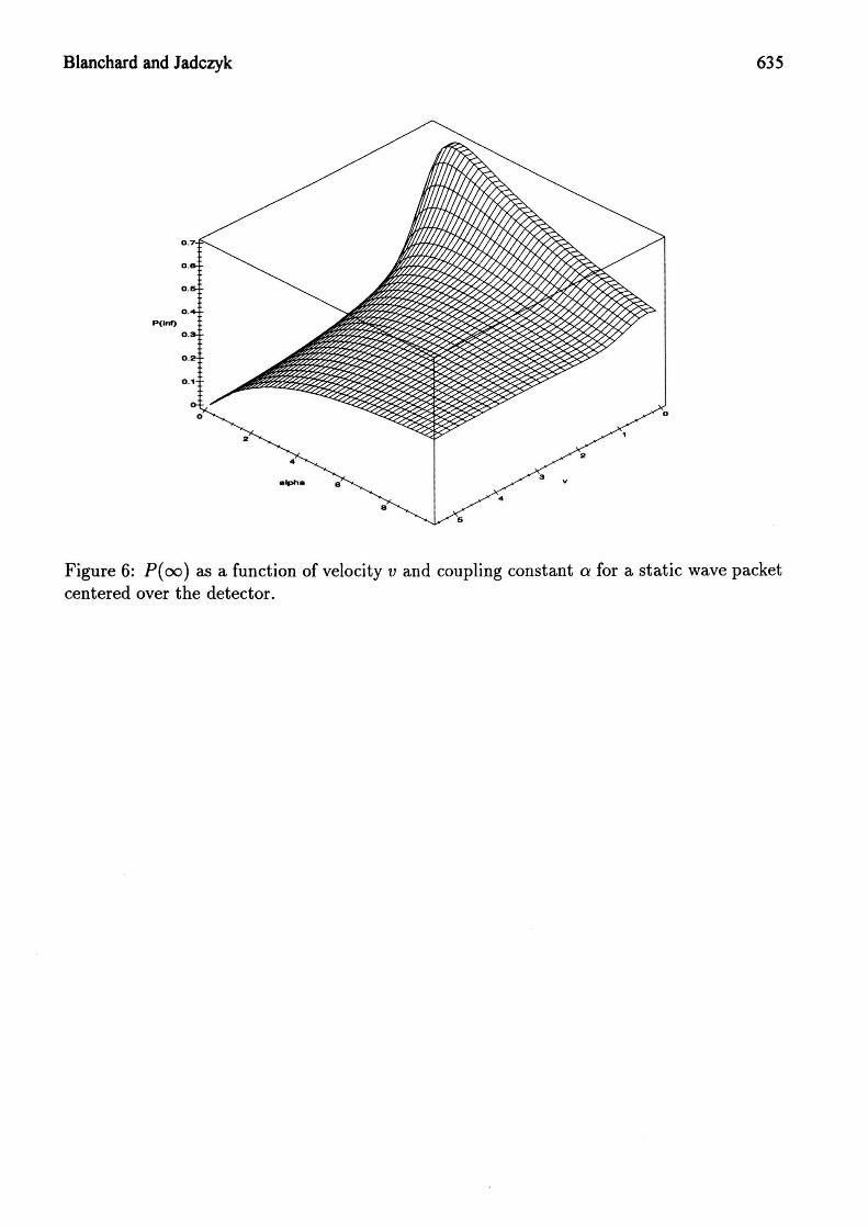
Blanchard and Jadczyk 635
Figure 6: P(oo) as a function of velocity v and coupling constant a for a static wave packetcentered over the detector.