Tidal Effect on Chemical Spill in San Diego Bay

Peter C. Chu1), Kleanthis Kyriakidis1), Steven D. Haeger2), and Mathew Ward3)

1) Naval Postgraduate School, Monterey, CA 93943, USA 2) Naval Oceanographic Office, Stennis Space Center, MS 39529, USA 3) Applied Science Associates, Inc., Narrangansett, RI 02882, USA

Abstract A coupled hydrodynamic-chemical spill model is used to investigate the

chemical spill in the San Diego Bay. The hydrodynamic model shows that the San Diego Bay is tidally dominated. Two different patterns of chemical spill were found with pollutants (methanol, benzene, liquefied ammonia, etc.) released at 0.5 m depth in the northern bay (32o43’N, 117o13.05’ W) and in the southern bay (32o39’N, 117o07.92’ W). For the north-bay release, the chemical pollutants spreading in the whole basin with a fast speed of spill in the northern part (12 hours) and a slow speed of spill in the southern part (20 days) with very small concentration. For the south-bay release, the chemical pollutants are kept in the southern part. Very few pollutants reach 32o41’N parallel (the boundary between the north and south bays).

Keywords: San Diego Bay, Water Pollution, Water Quality Management, Chemical Fate Model, Tidal Basin, Chemical Spill, Hydrodynamic model

1 Introduction

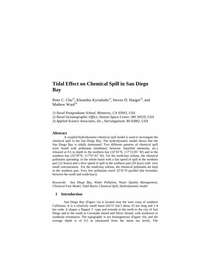
San Diego Bay (Figure 1a) is located near the west coast of southern California. It is a relatively small basin (43-57 km2) about 25 km long and 1-4 km wide. It shapes a flipped Γ -type and extends to the north to the city of San Diego and to the south to Coronado Island and Silver Strand, with northwest to southeast orientation. The topography is not homogeneous (Figure 1b), and the average depth is of 6.5 m (measured from the mean sea level). The

northern/outer part of the bay is narrower (1-2 km wide) and deeper (reaching depth of 15 m) and the southern/inner part is wider (2-4 km wide) and shallower (depth less than 5 m). Near the mouth of the bay, the north-south channel is about 1.2 km wide, bounded by Point Loma to the west and Zuniga jetty to the east with depths between 7 and 15 m (Chadwick and Largier 1999a). The western side of the channel is shallower than the east side.

The shoreline landscape of San Diego Bay is spotted with highly polluting shipbuilding and ship repair facilities. Ship operations including recreational boating and Navy operations are other sources of pollution in the San Diego Bay. These toxins threaten public health and environment. Investigation of chemical dispersion of floating chemicals such as methanol, benzene and ammonia is very important for the water quality control.

(a) (b)

Figure 1. San Diego Bay: (a) geographical locations, and (b) bathymetry.

2 Tidal Basin

San Diego Bay is a tidal basin connected to the ocean by an inlet with

an artificial jetty (Zuniga) built to control beach erosion. The Zuniga jetty extends almost one mile offshore Zuniga Point and most of it is not clearly visible at high water. Obviously, the bay has been intensively engineered to accommodate shipping activities. Ninety percent of all available marsh lands and fifty percent of all available inter-tidal lands have been reclaimed and dredging activities within the bay have been equally extensive (Peeling 1975; Wang et al. 1998). Kelp forests extend approximately 2 km south of Point Loma (Figure 1a) and along its western side. They are quite thick and they create seasonal dumping of currents to about one-third their values outside (Jackson and Winant 1983).

Currents in San Diego Bay are predominately produced by tides (Wang et al. 1998). This tidal exchange between the ocean and the bay is a result of a phenomenon called “tidal pumping” (Fischer et al. 1979). The “pumping” of water is due to the flow difference between the ebb and the flood flows. Being located at mid-latitude, tides and currents within the San Diego Bay are dominated by a mixed diurnal-semidiurnal component (Peeling 1975). The tidal range from mean lower-level water (MLLW) to mean higher-high water (MHHW) is 1.7 m with extreme tidal ranges close to 3 m (Chadwick and Largier 1999a). Typical tidal current speeds range between 0.3-0.5 m/s near the inlet and 0.1-0.2 m/s in the southern region of the bay. The phase propagation suggests

that the tides behave almost as standing waves with typical lags between the mouth and the back portion of the bay of 10 min and a slight increase in tidal amplitude in the inner bay compared to the outer bay. The overall tidal prism for the bay is 5.5×107 m3 and the tidal excursion is larger than the mouth with a value of 4.4 km (Chadwick and Largier 1999b).

3 Water Quality Monitoring

In 1960, an earthquake with a Richter scale of 9 in Chile caused the

biggest sudden rise in sea level ever recorded in the San Diego area of 1.07 m at the Scripps pier. There is a natural protection due to the 160 km wide continental shelf of San Diego. There is a fault off San Diego Bay, but it is inactive. These are the reasons why from the 15 locally generated tsunamis in California since 1812, only two have occurred in Southern California, and only one in San Diego, dating back to 1862.

There is widespread toxicity in San Diego Bay sediments attributable to copper, zinc, mercury, polycyclic aromatic hydrocarbons, polychlorinated biphenyls (PCBs) and chlordane. No single chemical or chemical group has a dominant role in contributing to the identified toxicity. Contributions of trace metals from vessel activities have long been suspected as a potentially large source to San Diego Bay. Actually, Shelter Island Yacht Basin, a semi-enclosed boat harbor, has been added to the State's list of impaired water bodies. These contributions arise from specially formulated paints, impregnated with biocides, and applied to boat hulls to retard the growth of fouling organisms such as barnacles.

4 Hydrodynamic Model

The numerical hydrodynamic model implemented for San Diego Bay is a boundary fitted tidal and residual circulation model known as the Water Quality Management and Analysis Package (WQMAP) (Muin and Spaulding 1996; 1997) developed at the Applied Science Associates Inc.. WQMAP consists of three basic components: a boundary-fitted coordinate grid creation module, a three-dimensional hydrodynamics model, and a water quality or pollutant transport model. These models are executed on a boundary fitted grid system. They can also be operated on any orthogonal curvilinear grid or a rectangular grid, which are special cases of the boundary fitted grid. The model is configured to run in a vertically averaged (barotropic) mode or as a fully three-dimensional (baroclinic) mode. Several assumptions are made in the model formulation, including the hydrostatic (shallow water) approximation, the Boussinesq approximation, and incompressibility. In this study, the 2D version is used. WQMAP for San Diego Bay covers an area of 43 km2. The computational mesh has 150×200 (30,000) grid nodes with an average horizontal resolution of 40 m. Model bathymetry is determined from depth sounding data provided by NOAA and supplemented by data from published navigation charts. Recently Navy conducted bathymetry surveys show that the water depths in regions near

the bay entrance are significantly deeper than the water depths shown on the NOAA navigation chart (Wang et al. 1998). The most up-to-date bathymetry data are used in the model. Surface elevation and velocity are set to zero, and temperature and salinity are assigned as the characteristic values for San Diego Bay (16oC, 34 ppt) at all grid points. The model is allowed to “spin up” from quiescent initial condition for one day before any model results are used for analysis. A six-minute time step is chosen for time step. At this time step the CFL condition is satisfied. Temporally varying sea surface elevation (or tidal harmonic constituents) along the open boundary (entrance of San Diego Bay) is taken as the model forcing function. Such data are available at the NOAA Center for Operational Oceanographic Products and Services website. The elevation data with six-minute interval are archived from time 0000 on 22 June 1993 to 2354 on 27 August 1993 for San Diego Bay entrance, in accordance with NOAA San Diego Station number 9410170, located at (32o42’48”N, 117o10’24”W). High correlation (>90%) between prediction and observation exists in phase and amplitude. For nb1, the u speed between the data and the model has a correlation coefficient of 91.87% and can be verified. The observational u-velocity ranges between -51.8 and 44.5 cm/s and the modeled u-velocity changes between -46.9 and 40.8 cm/s. The difference between the observational and modeled mean u-velocity is 0.49 cm/s (Figure 2). (a) (b)

U for nb1

-60

-50

-40

-30

-20

-10

0

10

20

30

40

50

7/10/1993 0:00 7/15/1993 0:00 7/20/1993 0:00 7/25/1993 0:00

Time (date)

U (c

m/s

)

V for nb1

-50

-40

-30

-20

-10

0

10

20

30

40

50

7/10/1993 0:00 7/15/1993 0:00 7/20/1993 0:00 7/25/1993 0:00

Time (date)

V (c

m/s

)

(c) (d)

U for nb2

-50

-40

-30

-20

-10

0

10

20

30

40

50

7/10/1993 0:00 7/15/1993 0:00 7/20/1993 0:00 7/25/1993 0:00

Time (date)

U (c

m/s

)

V for nb2

-50

-40

-30

-20

-10

0

10

20

30

40

50

7/10/1993 0:00 7/15/1993 0:00 7/20/1993 0:00 7/25/1993 0:00Time (date)

V (c

m/s

)

Figure 2. Model (dark curve) and (ADCP) data (light curve) comparison for station-nb1 (upper panels) and nb2 (lower panels): (a) u-component, and (b) v-component.

Overall, the model results are reasonably good, especially taking into account that the comparison between data and model is not at exactly the same position and the proximity of the ADCPs to the shore. If finer grid and more accurate bathymetry are used, the model results may be further improved.

5 Chemical Spill Model

A chemical spill model (CHEMMAP, developed at the Applied Science Associates Inc.) is used to predict the trajectory and fate of floating, sinking, evaporating, soluble and insoluble chemicals and product mixtures. It estimates the distribution of chemical elements (as mass and concentrations) on the surface, in the water column and in the sediments. The model is initialized for the spilled mass at the location and depth of the release. The state and solubility are the primary determining factors for the initialization algorithm. If the chemical is highly soluble in water and is either a pure chemical (e.g., the benzene scenario) or dissolved in water (e.g., the methanol scenario), the chemical mass is initialized in the water column in the dissolved state and in a user-defined initial volume. For insoluble or semi-soluble gases released underwater (e.g., the naphthalene gas scenario), the spilled mass is initialized in the water column at the release depth in a user-defined plume volume, as bubbles. The median particle size is characterized by a user-defined diameter (McCay and Isaji 2002). The model simulates adsorption onto suspended sediment, resulting in sedimentation of material. The Stokes Law is used to compute the vertical velocity of pure chemical particles or suspended sediment with adsorbed chemical. If rise or settling velocity overcomes turbulent mixing, the particles are assumed to float or settle to the bottom. Settled particles may later re-suspend (assumed to occur above 20 cm/s current speed). Wind-driven current (drift) in the surface water layer (down to 5m) is calculated within the fates model, based on hourly wind speed and direction data. Surface wind drift of oil has been observed in the field to be 1-6% of wind speed in the direction of 0-30 degrees to the right (in the northern hemisphere) of the down-wind direction (Youssef and Spaulding 1993). The user may also specify the wind drift speed and angle (McCay and Isaji 2002).

6 Chemical Spill Patterns The coupled hydrodynamical-chemical model (WQMAP-CHEMMAP) is used to investigate the chemical spill patterns for floating, sinking, gaseous chemicals. Since the WQMAP is integrated for the period from 0000 on 22 June 1993 to 2354 on 27 August 1993 for San Diego Bay, the following scenarios were suggested: A small boat drops one barrel of chemical (e.g., methanol) in less than 12 minutes on midnight July 4, 1993 (Independence Day) at (1) northern San Diego Bay (32o43’N, 117o13.05’ W) (Point 2 in Figure 1a), and (2) southern San Diego Bay (32o39’N, 117o07.92’ W) (Point 4 in Figure 1a). The release depth is 1 m and the initial plum thickness is 0.5 m. Two distinct

spill patterns are found for all the chemicals. Here, spill of methanol is presented for illustration. 6.1. Pollutants Released at North San Diego Bay

The chemical spill pattern is described as follows. In 3 hours, the methanol is in San Diego port (Figure 3a) and in 10 hours it is spread all over the North San Diego Bay. However, the south part of the Bay is contaminated much later. After two days, there are no pollutant particles south of 32o40’N (Figure 3b). After 3 days the northern part is heavily impacted but after 9 days, there are still no pollutant particles south of 32o39’N. The methanol reaches the south end of the Bay only after 20 days (Figure 3c), but its concentration in the water column can be neglected. Figure 4 shows the swept area after 2 days and 32 days. In such a case, it can be concluded that there is plenty of time to take protective measures for the southern part of the Bay where the results of such an incident would be minimal.

(a) (b) (c)

Figure 3. Dissolved concentration in San Diego after (a) 3 hours, (b) 2 days, and (c) 20 days after methanol dropped in North San Diego Bay. (a) (b)

Figure 4. Swept area after (a) 2 days and (b) 32 days for methanol dropped in North San Diego Bay.

Furthermore, after five entire days, one third of the methanol is still in the water column (Figure 5). Note that it takes almost 12 days for the

concentration in the water column to reach 10% and 15 days for the decayed methanol to reach a level of 80%. Moreover, the end-state is the contamination not only of the San Diego Bay but also a considerable part of the sea outside the Bay. The scenario is repeated by increasing the amount of methanol, but nothing changes fundamentally. The mass balance curves and the area contaminated remain the same.

Figure 5. Mass balance for methanol dropped in North San Diego Bay. 6.2. Pollutants Released at South San Diego Bay

The chemical spill pattern is described as follows. In 13 hours, the methanol reaches the central San Diego Bay (Figure 6a). But, very few pollutants reach 32o41’N parallel. Figure 6b shows the swept area after 32 days. It is crucial for protective measures to highlight this fact because a chemical attack in the South San Diego Bay will have minimal effects, or at least much less considerable than an attack (or accident) in the north part of the bay. Figure 7 shows a similar but different result as regards the mass balance curves. Thus, the decayed methanol reaches 80% in only nine days, mainly due to the inert nature of methanol in combination to the shallow bathymetry of the southern part of the Bay. It is important to single out that in the first case (methanol spill over in the north), the dissolved concentration disappears after only 15 days, but in the second case (south), it needs 29 days. It is noted that the ecological catastrophe that can be caused with a relatively big amount of methanol spill over is very considerable, especially if the spill over is in the north. It can also be harmful to humans.

Figure 6. Methanol spill in San Diego Bay with release in the southern bay: (a) dissolved concentration after 13 hours; (b) swept area after 32 days.

Figure 7. Mass balance for methanol dropped in South San Diego Bay. 7 Conclusions

This study shows the vulnerability of a semi-enclosed tidal basin in a possible chemical attack or accident, with the aforementioned particular results for San Diego Bay. In order to summarize these results, it should be repeated that in a case of a chemical attack or accident, first the sensitive eco-system would be severely damaged, no matter the nature of the event and the location. If the chemical were a sinker, the results would be more catastrophic than if it were a floater. Since the water exchange with the Pacific Ocean occurs only through a narrow entrance, the water would be contaminated for long time.

Two regimes of the chemical dispersion were found in this thesis. The first was the case of an attack/accident in the North San Diego Bay. In that case the entire Bay would be contaminated. In 3 hours the chemical would reach San Diego port and city, in 12 hours the entire northern part of the Bay would be

affected and in 2-5 days the south part of the bay would be contaminated as well. The rest of the Bay would be reached much later. The second regime was an attack/accident in the South San Diego Bay. In such case, the incident would have minimal effects on the city and the shores of Coronado Island (located in the north part of the bay) and none outside the Bay. On the other hand, when the spill occurs in the southern part of the Bay, a larger percentage of the chemical remains in the water column and for longer period of time, which makes it more “effective”, which in a case of a chemical attack means lethal.

For the aforementioned reasons, the propagation model shows that the northern part of the Bay is more likely to be a target because it would affect the city, and it would reach, even slightly, the South San Diego Bay and would spread outside the Bay as well. In general, results concerning San Diego Bay can also be applied to studies in other semi-closed, barotropic, no-wind driven circulation basins.

As regards recommendations for future research, it should be mentioned that the use of more accurate bathymetry and of a finer grid would give better results in a similar case. Moreover, the use of more recent ADCP measurements, during a longer period of time would further improve the results and verify the overall conclusions. It would be helpful if the ADCPs used in the future were located in a bigger distance from the shore.

A more detailed comparison of 3D vs. 2D model is encouraged, as well as its application for drift and for instantaneous current prediction. Last but not least, as regards chemical propagation, a classified research with data unavailable to foreigners about real chemical threats (e.g. anthrax) should be conducted.

Acknowledgments

This work was funded by the Naval Oceanographic Office, the Office of Naval Research, and the Naval Postgraduate School.

References

Chadwick, D. B., and Largier, J. L. (1999a). “Tidal Exchange at the Bay-Ocean Boundary.” J. Geophys. Res., 104 (C12), 29901-29924. Chadwick, D. B., and Largier, J. L. (1999b). “The Influence of Tidal Range on the Exchange Between San Diego Bay and the Ocean.” J. Geophys. Res., 104 (C12), 29 885-29 899. Chu, P.C., Lu S. H., and Chen, Y. C. (2001). “Evaluation of the Princeton Ocean Model using the South China Sea Monsoon Experiment (SCSMEX) Data.” J. Atmos. Oceanic Technol., 18, 1521-1539. Defant, A (1961). Physical Oceanography, New York, Pergamon Press. Delvigne, G. A. L., and Sweeney, C. E. (1988). “Natural Dispersion of Oil.” Oil Chem. Pollut., 4, 281-310. DiToro, D. M., Zarba, C. S., Hansen, D. J., Berry, W. J., Swartz, R. C., Cowan, C. E., Pavlou, S. P., Allen, H. E., Thomas, N. A., Paquin, P. R. (1991). “Annual Review: Technical Basis for Establishing Sediment Quality Criteria for

Nonionic Organic Chemicals Using Equilibrium Partitioning.” Environ. Toxicol. Chem., 10, 1541-1583. Fagherazzi, S., Wiberg, P. L., and Howard, A. D. (2003). “Tidal Flow in a Small Basin.” J. Geophys. Res., 108 (C3), 16-1 to 16-10. Fay, J. A. (1971). “Physical Processes in the Spread of Oil on a Water Surface.” Proc. Joint Conference on Prevention and Control of Oil Spills, Washington, D.C., USA, 463-467. Fischer, H. B., List, E. J., Koh, R. C. Y., Imberger, J., and Brooks, N. H. (1979). “Mixing in Inland and Coastal Waters.” Academic Press, pp. 483. French, D., Reed, M., Jayko, K., Feng, S., Rines, H., Pavignano, S., Isaji, T., Puckett, S., Keller, A., French III, F. W., Gifford, D., McCue, J., Brown, G., MacDonald, E., Quirk, J., Natzke, S., Bishop, R., Welsh, M., Phillips, M., Ingram, B.S. (1996). “The CERCLA Type A Natural Resource Damage Assessment Model for Coastal and Marine Environments (NRDAM/CME).” Technical Documentation, Vol. I -VI, Final Report, the Office of Environmental Policy and Compliance, U.S. Dept. of the Interior, Washington, D.C., Contract No. 14-0001-91-C-11. Gambill, W. R., (1959). “How to calculate liquid viscosity without experimental data.” Chem. Eng., 66, 151-152. Jackson, J. A., and Winant, C. D. (1983). “Effect of a Kelp Forrest on Coastal Currents.” Cont. Shelf Res., 2 (1), 75-80. Lyman, C. J., Reehl, W. F., Rosenblatt, D. H. (1982). “Handbook of Chemical Property Estimation Methods.” McGraw-Hill, New York. McCay, D. P. F., Whittier, N., Ward, M., and Santos, C. (2006). “Spill harzard evaluation for chemicals shipped in bank using modeling.” Environ. Model. Software, Journal of Marine Systems, 21 (2), 156-169. Muin, M., and Spaulding, M. L. (1996). “Two-Dimensional Boundary Fitted Circulation Model in Spherical Coordinates.” J. Hydraul. Eng., 122 (9), 512-520. Muin, M., and Spaulding, M. L. (1997). “Three-Dimensional Boundary Fitted Circulation Model.” J. Hydraul. Eng., 123 (1), 2-12. Peeling, T. J. (1975). “A Proximate Biological Survey of San Diego Bay, California.” Naval Undersea RD Center, San Diego, California, Technical Report No. TP389. Pritchard, D. W. (1952). “Estuarine Hydrography.” Academic Press, pp. 342. Spaulding, M. L., Mendelsohn, D. L., and Swanson, C. J. (1999). “WQMAP: An Integrated Three-Dimensional Hydrodynamic and Water Quality Model System for Estuarine and Coastal Applications.” Marine Technol. Soc. J., 33 (3), 38-54. Wang, P. F., Cheng, R. T., Richter, K., Gross, E. S., Sutton, D., and Gartner, J. W. (1998). “Modeling Tidal Hydrodynamics of San Diego Bay, California.” J. Amer. Water Res. Assoc., 34 (5), 1123-1140. Youssef, M. and Spaulding, M. L. (1993). “Drift Current Under the Action of Wind and Waves.” Proc. 16th Arctic and Marine Oil Spill Program Technical Seminar, Calgary, Alberta, Canada, pp. 587-615.