Three Eyes on Malawi Poverty - White Rose eTheses Online
431
Three Eyes on Malawi Poverty: A Comparison of Quantitative and Subjective Wellbeing Assessments Maxton Grant Tsoka PhD The University of York Social Policy and Social Work October 2011
-
Upload
khangminh22 -
Category
Documents
-
view
3 -
download
0
Transcript of Three Eyes on Malawi Poverty - White Rose eTheses Online

Three Eyes on Malawi Poverty:
A Comparison of Quantitative and Subjective Wellbeing
Assessments
Maxton Grant Tsoka
PhD
The University of York
Social Policy and Social Work
October 2011

Three eyes on Malawi Poverty Page 2
Abstract
This dissertation aims at improving the official measurement of wellbeing in Malawi by
proposing the incorporation of popular understanding of wellbeing. The objective is to
reduce targeting errors that come due to differences in the understanding of wellbeing
and poverty between those that identify the poor (villagers) and those who evaluate the
quality of the targeting (experts).
The dissertation compares the official measure of household wellbeing (consumption
expenditure) against subjective measures of wellbeing (self and peers assessments) that
are applied on the same households at the same time. Four comparisons are made;
household rankings, poverty rates, households determined as poor, and characteristics of
poor households. The comparisons determine similarities and differences and, where
different, whether the characteristics unique to subjective assessments can be
incorporated in the official wellbeing assessment.
The dissertation finds that the three assessments are not similar, although there are some
overlaps. The ranking of the households based on consumption expenditure is
significantly different from that based on peers-assessment. Likewise, poverty rates for
three assessments are different. While some households identified as poor are the same,
these are less than discordant households. In terms of characteristics, some are common
in all the three assessments while some features associated with subjective assessments
are absent in the official wellbeing assessment system.
An assessment of the absent features shows that it is possible to improve the official
assessment without radical changes. Modifications can be made in data collection and
analysis, and wellbeing profiling. In particular, qualitative aspects of wellbeing like type
and frequency of meals, food security, quality and quantity of clothing would improve
the relevance of the operational definition of poverty. Likewise, wellbeing profiling that
includes subjective wellbeing assessment is likely to resonate with what is on the ground.

Three eyes on Malawi Poverty Page 3
List of Contents
Abstract ........................................................................................................... 2
Acknowledgements .......................................................................................... 11
Author‟s declaration ......................................................................................... 14
Chapter 1: Introduction .................................................................................... 15
1.1 Study rationale ................................................................................ 15
1.2 Wellbeing measurement and identification of the poor .................... 21
1.3 Justifying Malawi as a case study .................................................... 24
1.4 The research problem and questions ............................................... 26
1.5 Analytical framework ..................................................................... 27
1.6 Outline of the thesis ....................................................................... 30
Chapter 2: Measuring wellbeing and identifying the poor ................................... 31
2.1 Introduction.................................................................................... 31
2.2 Theories of Poverty ......................................................................... 31
2.3 Poverty concepts as sources of poverty measures ............................ 38
2.4 Measuring wellbeing and poverty: challenges and solutions ............. 44
2.5 Issues on wellbeing and poverty measures ....................................... 55
2.5.1 Mismatches between concepts and measures................................ 55
2.5.2 Comparison of quantitative measures .......................................... 57
2.5.3 Unit of analysis – gender dimension of poverty ............................ 61
2.6 Operational definition of poverty: drawing a poverty line .............. 63
2.7 Identifying the poor ....................................................................... 64
2.8 Poverty analysis in developing countries ......................................... 66
2.9 Factoring in of voices of non-experts in poverty research ................ 67
2.9.1 Household voices: self assessment of wellbeing ............................ 67
2.9.2 Community voices: wellbeing analysis and ranking ...................... 75
2.10 Lessons from the literature review .................................................... 91
Chapter 3: Methodology ................................................................................. 93
3.1 Introduction................................................................................... 93
3.2 The study domain: research questions ............................................. 93
3.3 Value/normative standpoint of the study ........................................ 93
3.4 Study‟s methodological framework ................................................. 94
3.5 Research objects and approach ....................................................... 97
3.6 Data collection tasks, data sources, and expected outputs ................ 98
3.6.1 Secondary data sources for wellbeing characteristics ..................... 99
3.6.2 Data collection methods and tools ............................................. 101
3.6.3 Primary data collection .............................................................. 102
3.7 Constructing the wellbeing measure and poverty line ..................... 105
3.7.1 Food consumption aggregate ..................................................... 105
3.7.2 Non-food expenditure aggregate ................................................ 107
3.7.3 Use value of durable goods ........................................................ 108
3.7.4 Wellbeing measure: per capita consumption expenditure ............ 108
3.7.5 Adjusting the poverty line .......................................................... 109
3.8 Ethical considerations .................................................................... 109
3.9 Study‟s challenges ........................................................................... 110
Chapter 4: Country background and poverty studies .........................................112
4.1 Introduction................................................................................... 112
4.2 Country background and poverty commentaries ............................. 112
4.2.1 Country background .................................................................. 112

Three eyes on Malawi Poverty Page 4
4.2.2 Why Malawi is poor .................................................................. 114
4.3 Official poverty status from poverty profiles ................................... 116
4.3.1 Determining the poverty line ......................................................... 117
4.3.2 Poverty prevalence .................................................................... 118
4.4 Self-rated poverty from the subjective assessment studies ................ 122
4.4.1 Self-assessed poverty under CPS5 ................................................ 122
4.4.2 Self-assessed poverty under MOPS .............................................. 128
4.4.3 Self rating from the 2004/5 dataset ............................................ 133
4.5 Comparisons of objective and subjective assessments ...................... 135
Chapter 5: Wellbeing status from three perspectives ......................................... 137
5.1 Introduction.................................................................................. 137
5.2 Profiles of the three visited villages ................................................ 137
5.3 Poverty status in the three villages ................................................. 147
5.3.1 Consumption poverty and distribution ....................................... 147
5.3.2 Self-assessed wellbeing status in the three villages ........................ 149
5.3.3 Peer assessed wellbeing and poverty status ................................. 156
5.4 Comments on household placement .............................................. 158
5.5 Households identified as poor in the three sites .............................. 163
5.6 Comparisons of poverty rates and the identified poor .................... 163
5.6.1 Comparison of households ranking ............................................. 164
5.6.2 Comparing the lists of poor households ...................................... 165
5.6.3 Characteristics of the different groups of poor households ........... 168
5.7 Policy implications on the measures ............................................... 172
Chapter 6: Official version of wellbeing and poverty ........................................ 173
6.1 Introduction.................................................................................. 173
6.2 Wellbeing and poverty features from 2000 and 2007 profiles ........ 173
6.2.1 Poverty correlates ...................................................................... 173
6.2.2 Wellbeing determinants ............................................................. 174
6.2.3 Way forward for the official wellbeing characteristics .................. 177
6.3 Community level poverty correlates and wellbeing determinants .... 177
6.3.1 Model for poverty correlates in the three villages ....................... 177
6.3.3 Model for wellbeing determinants in the three villages................ 180
6.3.4 Comparison of the national and village level characteristics ......... 186
6.4 Concluding remarks ...................................................................... 187
Chapter 7: Community characterisation of wellbeing ........................................ 189
7.1 Introduction.................................................................................. 189
7.2 Characteristics of wellbeing and poverty from qualitative studies .... 189
7.2.1 Definition of poverty ................................................................. 189
7.2.2 Causes of poverty in rural households in Malawi ........................ 191
7.2.3 Characteristics of wellbeing categories ........................................ 194
7.3 Identifying popular wellbeing features ........................................... 201
7.3.1 Wellbeing categories and their characteristics .............................. 201
7.3.2 Important characteristics for various wellbeing categories ........... 203
7.3.3 Different shades of the prominent wellbeing characteristics.......... 210
7.3.4 Popular wellbeing features ........................................................ 220
7.4 Characterising wellbeing in the three villages ................................. 230
7.4.1 Ngochera wellbeing characteristics .............................................. 231
7.4.2 Chikhwaza wellbeing characteristics ........................................... 234
7.4.3 Dzilekwa wellbeing characteristics ............................................. 238
7.4.4 A comparison of the national and village level pictures .............. 242
Three eyes on Malawi Poverty Page 5
7.5 Summarised national qualitative picture of wellbeing .................... 242
Chapter 8: Characteristics of wellbeing from households .................................. 245
8.1 Introduction................................................................................. 245
8.2 Subjective wellbeing under IHS2 ................................................... 245
8.3 Characteristics of self-assessed wellbeing status in the three villages 247
8.3.1 Reasons for household wellbeing grouping ................................ 247
8.4 Correlates and determinants of subjective poverty ........................ 252
8.4.1 Self-assessed poverty correlates .................................................. 252
Chapter 9: Conclusions, recommendations and implications ............................. 260
9.1 Introduction: putting the three eyes together ................................ 260
9.2 Comparing poverty correlates at national and local levels .............. 261
9.3 Comparing the three assessments at village level ........................... 266
9.4 Interrogation of the official definition of poverty .......................... 270
9.4.1 The official wellbeing analysis system .......................................... 271
9.4.2 Wellbeing characteristics: official versus local concepts ............... 276
9.4.3 Prominent features: official versus peer assessment ..................... 285
9.5 Summary of the findings, recommendations and implications ........ 288
9.5.1 Households identified as poor ................................................... 288
9.5.2 Wellbeing characteristics ............................................................ 289
9.5.3 Appropriateness of the official wellbeing analysis system ............ 289
9.5.4 Proposed changes to the official wellbeing analysis system ......... 290
9.5.5 Implications of the study ........................................................... 293
9.6 Contribution to knowledge .......................................................... 294
Appendices .................................................................................................. 297
Appendix 1: Data collection tools ................................................................... 297
A1.1 Modifications made to IHS2 for the survey of the three villages ..... 297
A1.2 FGD Interview Guide for wellbeing and pairwise ranking .............. 299
Appendix 2: Data analysis notes from the 2007 analysis .................................. 302
A2.1 Note on Construction of consumption expenditure Aggregate ....... 302
Introduction ......................................................................................... 302
Consumption expenditure aggregate ..................................................... 302
Food consumption aggregate ................................................................ 303
Non-food consumer durable goods and services .................................... 304
Consumer durable goods ...................................................................... 304
Poverty line .......................................................................................... 305
A2.2 A note on housing and imputed rent ............................................ 308
Summary .............................................................................................. 308
Introduction ......................................................................................... 308
Data Available ...................................................................................... 309
Results of the regression models ............................................................. 312
Predictions ............................................................................................. 315
Conclusion ............................................................................................ 316
A2.3 Factors used to convert amount from various units to grams .......... 318
Appendix 2d: Cut off points for amounts, costs, values and numbers ....... 331
Appendix 3: Malawi country background and commentaries on poverty .......... 337
Appendix 3a: Country background ........................................................ 337
Political and economic history ............................................................... 337
Geography ........................................................................................... 338
Social system, culture and religion ......................................................... 339
Public and land administration .............................................................. 340

Three eyes on Malawi Poverty Page 6
Development financing and planning and the role of donors ................. 342
National economy ................................................................................ 344
Population and the household economy ................................................ 345
Appendix 3b: Poverty status and persistence in Malawi .......................... 347
A3b.1 Is Malawi and an island in poverty? .............................................. 347
A3b.2 Has Malawi changed its social economic status over time? ............. 348
A3b.3 Why poverty persisted in Malawi ................................................. 350
A3b.3.1 Poor start: blame poverty on colonialism ............................. 350
A3b.3.2 Poverty amidst hope: years after independence .................... 354
A3b.3.3 Fated to be poor: the role of nature and bad luck ................ 364
Appendix 4: Hypothetical targeting performance in the three villages ............... 382
Appendix 5: Wellbeing determinants in the 1996 analysis ................................ 385
Appendix 6: A poverty profile of the three villages ......................................... 387
Appendix 6a: Characterising households based on their poverty status .... 387
A6a.1 Demographic factors ................................................................. 387
A6a.2 Education status ........................................................................ 388
A6a.3 Morbidity status........................................................................ 389
A6a.4 Housing quality and ownership of assets .................................... 390
A6a.5 Agricultural inputs and credit ..................................................... 392
A6a.6 Ownership of non-farm enterprises ........................................... 393
A6a.7 Resources devoted to food consumption and sources of income 394
A6.8 Implication of the characterisation ............................................. 395
Appendix 6b: Adaptation of 2000 and 2007 determinants models ......... 398
A6b.1 The 2000 analysis model .......................................................... 398
A6b.2 The 2007 analysis model .......................................................... 400
A6b.3 Results of the analyses ................................................................ 401
A6b.5 Specifying a village level model ................................................. 404
Appendix 7: Self assessed wellbeing characteristics from CPS5 and MOPS .......... 407
A7.1 Wellbeing characteristics from mobility factors .............................. 407
A7.1.1 Economic wellbeing ............................................................. 409
A7.1.2 Power and rights .................................................................. 410
A7.1.3 Happiness ............................................................................ 411
A7.2 A comparison of factors from CPS5 and MOPS ............................... 411
Glossary ........................................................................................................ 415
References ..................................................................................................... 417

Three eyes on Malawi Poverty Page 7
List of Tables
Table 2.1: Poverty concepts, definitions and measures .................................................... 45
Table 2.2: Categories of poverty measures ...................................................................... 46
Table 2.3: Wellbeing dimensions and indicators .............................................................. 50
Table 2.4: Child wellbeing dimensions and indicators ...................................................... 51
Table 2.5: Domains of life used in Mexico ...................................................................... 52
Table 2.6: Different types of income .............................................................................. 57
Table 2.7: PRA Principles ................................................................................................ 77
Table 2.8: PRA Methods and techniques ........................................................................ 79
Table 3.1: Study‟s tasks in response to research questions ................................................ 99
Table 4.1: Key socio-economic indicators ........................................................................ 115
Table 4.2 Poverty line in US$ equivalent ........................................................................ 118
Table 4.3: Poverty incidence reported in the four analyses ............................................. 119
Table 4.4: Rural and urban poverty incidence in Malawi ............................................... 120
Table 4.5: Regional poverty incidence and population shares ........................................ 120
Table 4.6: Poverty measures by region ........................................................................... 121
Table 4.7: District poverty rates, 1998 and 2005 ........................................................... 122
Table 4.8: Respondents rating of household circumstances in percent ............................ 127
Table 4.9: Self-assessed household positions on 10-step ladder in 1995 and 2005 .......... 128
Table 4.10: Proportion of households in percent by mobility status and dimension ....... 130
Table 4.11: Proportion of households in wellbeing categories in percent, 1995-2005 ...... 131
Table 4.12: Proportion of households in percent by type of adequacy and dimension ... 134
Table 4.13: Proportion of households with adequacy of consumption in percent ........... 134
Table 5.1 Household size by village ................................................................................ 141
Table 5.2: Proportion of females by village ................................................................... 142
Table 5.3 Household composition by village ................................................................. 142
Table 5.4: Proportion of children in household by village ............................................. 143
Table 5.5: Education and health status of household members by village ....................... 143
Table 5.6: Characteristics of household heads by village ................................................ 144
Table 5.7: Household enterprises and time allocation by village .................................... 144
Table 5.8: Housing and assets by village ........................................................................ 145
Table 5.9 Housing and assets by village ......................................................................... 146
Table 5.10: Summary measures for closeness to national average ................................... 147
Table 5.11: Consumption expenditure poverty rates by site ........................................... 148
Table 5.12: Distribution of consumption expenditure in the three villages ...................... 148
Table 5.13: Poverty rates by type of poverty line .......................................................... 155
Table 5.14: Number and proportion of households on each step ................................... 157
Table 5.15: FGD and CE rankings correlation using Spearman's rho ................................ 164
Table 5.16: FGD and Self assigned steps correlation using Spearman's rho ...................... 164
Table 5.17: Poverty incidence by measure and village .................................................... 165
Table 5.18: Poor households by method of identification and village ............................. 166
Table 5.19: Per capita consumption in British Pound by group of poor .......................... 169
Table 5.20: Per capita consumption in British Pound by group of poor by village ......... 169
Table 5.21a: Household characteristics by poverty group ............................................... 170
Table 5.21b: Comparison of household characteristics by poverty group ........................ 171
Table 6.1: Poverty correlates in 2000 and 2007 analyses ............................................... 174
Table 6.2: Wellbeing determinants in the 2000 and 2007 analyses ................................ 176
Table 6.3a: Descriptive statistics for the scalar profiling variables ................................... 178
Table 6.3b: Descriptive statistics for non-scalar profiling variables .................................. 179
Table 6.4: Poverty correlates for the three villages ........................................................ 180
Table 6.6: Descriptive statistics and correlation coefficients the villages model ................ 181
Table 6.7: Wellbeing determinants in the three villages – scale variables ........................ 182
Table 6.8: Wellbeing determinants in the three villages – dummy variables ................... 182

Three eyes on Malawi Poverty Page 8
Table 6.9: Wellbeing determinants by village ................................................................ 183
Table 6.10: Wellbeing determinants in the three villages – effect of measurement .......... 184
Table 6.11: Wellbeing determinants in the three villages ................................................ 185
Table 6.12: Common poverty correlates and wellbeing determinants ............................ 186
Table 7.1: Aspects of rural poverty definition in Malawi ................................................ 190
Table 7.2: Attributes of poverty in Malawi ..................................................................... 191
Table 7.3: Number of groups mentioning the causes of poverty ..................................... 192
Table 7.4: Characteristics of rich households in rural Malawi ......................................... 195
Table 7.5: Characteristics of households in between in rural Malawi .............................. 197
Table 7.6: Characteristics of poorest households in rural Malawi ................................... 199
Table 7.7: Number of wellbeing categories by site and type of group ............................ 202
Table 7.8: Number of groups using dimension to characterise the richest ....................... 204
Table 7.9: Number of groups using dimension to characterise the moderately rich ........ 205
Table 7.10: Number of groups using dimension to characterise the moderately poor ..... 206
Table 7.11: Number of groups using dimension to characterise the poorest .................... 207
Table 7.12: Number of groups using the important dimension by category .................... 208
Table 7.13 Shades of livestock ownership for the richest category ................................... 211
Table 7.14: Shades of livestock ownership for the moderately rich category ................... 211
Table 7.15: Shades of livestock ownership for the moderately poor ............................... 212
Table 7.16: Shades of food for the richest category ........................................................ 213
Table 7.17: Shades of food for the moderately rich category ......................................... 213
Table 7.18: Shades of food for the moderately poor category ....................................... 214
Table 7.19: Shades of food for the poorest category ...................................................... 214
Table 7.20: Shades of housing for richest category ......................................................... 215
Table 7.21: Shades of housing for the moderately rich category ..................................... 216
Table 7.22: Shades of clothing for the richest category .................................................. 217
Table 7.23: Shades of children education for the moderately rich category .................... 218
Table 7.24: Shades of work status for the moderately poor category ............................. 219
Table 7.25: Shades of asset ownership for the richest category ...................................... 220
Table 7.26: Variations of popular features across wellbeing categories ........................... 222
Table 7.27: Varying numbers of livestock by category and site ...................................... 223
Table 7.28: Varying shades of clothing across categories and sites .................................. 226
Table 7.29: Varying shades of where and how people sleep by category and site .......... 228
Table 7.30: Characteristics of wellbeing categories in Ngochera ..................................... 231
Table 7.31: Wellbeing dimensions from household ranking in Ngochera ........................ 232
Table 7.32: Number of times dimension is used to describe category in Ngochera ......... 233
Table 7.33: Characteristics of wellbeing categories in Chikhwaza ................................... 235
Table 7.34: Wellbeing dimensions by category in Chikhwaza ........................................ 237
Table 7.35: Characteristics of wellbeing categories in Dzilekwa ...................................... 239
Table 7.36: Wellbeing dimensions by category in Dzilekwa ........................................... 240
Table 7.37: Wellbeing characteristics and features: usability and way forward ............... 243
Table 8.1: Self-assessed poverty correlates from IHS2 data ............................................. 246
Table 8.2: Self-assessed wellbeing determinants from IHS Data ...................................... 246
Table 8.3: Positive reasons for wellbeing group assignment ........................................... 248
Table 8.4: Negative reasons for wellbeing group assignment ......................................... 248
Table 8.5: Mapping of factors from original reasons ...................................................... 250
Table 8.6: Share of wellbeing factors in total number of reasons ................................... 251
Table 8.7: Most prevalent reasons for wellbeing group assignment ................................ 251
Table 8.8: Self-assessed poverty correlates in the three villages ...................................... 253
Table 8.9: Descriptive statistics of variables for the determinants model ......................... 254
Table 8.10: Self-assessed wellbeing determinants in the three villages ............................. 255
Table 9.1: Comparison of poverty correlates at national level ........................................ 262
Table 9.2: Comparison of wellbeing determinants at national level ............................... 263
Table 9.3 Comparison of correlates and determinants at community level ..................... 264
Three eyes on Malawi Poverty Page 9
Table 9.4: Comparison of wellbeing determinants by village ......................................... 265
Table 9.5: Top wellbeing factors for peers and self assessment in the 3 villages .............. 266
Table 9.6: Wellbeing factors featuring in only assessment type in the 3 villages ............. 267
Table 9.7: Comparison of wellbeing features under the three assessments ...................... 269
Table 9.8: Wellbeing factors common in all the three types of assessments .................... 279
Table 9.9: Wellbeing factors common in the official and one other assessments ............. 281
Table 9.10: Wellbeing factors in self and peers assessment only ...................................... 282
Table 9.11: Prominent wellbeing features under official and peer assessment .................. 286
Table A2.1: Estimated Lifetime for consumer durables in IHS1 and IHS2 ......................... 305
Table A2.2: Calorie Requirements ................................................................................. 306
Table A2.3: MK Cost per 1000 Calories by Decile .......................................................... 306
Table A2.4: Ranking of the quality of building materials and facilities ............................. 311
Table A2.5: Housing ad a share of total consumption .................................................... 312
Table A2.6: Household characteristics ............................................................................ 313
Table A2.7: Results of the regression models ................................................................. 314
Table A2.8: Correlation coefficients of the predicted and estimated values .................... 316
Table A2.9: Conversion factors from other units to grams by food item ........................ 319
Table A2.10: Maximum food consumption by item ....................................................... 331
Table A2.11: Cut off values and number of durable goods ............................................. 334
Table A2.12: Cut off cost and values for household expenditure items ........................... 335
Table A3.1: Key socio-economic indicators for Malawi and its neighbours ..................... 347
Table A3.2: Trends in key socio-economic in Malawi .................................................... 349
Table A3.3: Estate number, area and average size .......................................................... 357
Table A3.4: Malawi net resource transfers ..................................................................... 370
Table A3.5: Major World bank SAP initiatives since 1988 .............................................. 372
Table A3.6: Income and consumption distribution, 1968-2005 ...................................... 379
Table A4.1: Calculating inclusion and exclusions error rates ........................................... 382
Table A4.2: Targeting errors by identification method and village ................................. 383
Table A6.1: Comparison of demographic factors between the poor and nonpoor ......... 387
Table A6.2: Highest class attended by poverty status ..................................................... 389
Table A6.3: Housing quality and ownership of land, livestock and durable assets .......... 392
Table A6.4: Inputs and crops grown .............................................................................. 393
Table A6.5: Income from various sources ...................................................................... 395
Table A6.6: Descriptive statistics for modified 2000 model variables ............................. 400
Table A6.7: Descriptive statistics for modified 2007 model variables ............................. 401
Table A6.8: Results of bivariate analysis of the modified models .................................... 402
Table A6.9: Wellbeing determinants in the three villages by model ............................... 403
Table A6.10: Wellbeing determinants in the three villages using hybrid model ............... 405
Table A6.11: Descriptive statistics for significant variables for new model ....................... 406
Table A7.1: Mobility factors from the CPS5 ................................................................... 407
Table A7.2: Major mobility factors under economic wellbeing ...................................... 409
Table A7.3: Major mobility factors under power and rights ............................................ 410
Table A7.4: Factors associated with changes in happiness ................................................ 411
Table A7.5: Factors associated with upward wellbeing mobility by survey ..................... 412
Table A7.6: Factors associated with downward wellbeing mobility by survey ............... 413

Three eyes on Malawi Poverty Page 10
List of figures
Figure 1.1: Analytical framework for the identified poor .................................................. 29
Figure 2.1: Wellbeing measurement framework ............................................................... 42
Figure 3.1: People‟s participation in poverty discourse and programmes .......................... 96
Figure 3.2: Wellbeing and Poverty Analysis Process ......................................................... 97
Figure 4.1: Sectoral shares in GDP, 2002-09 .................................................................... 114
Figure 4.2: Regional poor population share to total population share ........................... 120
Figure 4.3: Consumption adequacy in various wellbeing dimensions ............................. 123
Figure 4.4: Respondents perceptions on various aspects of life ....................................... 124
Figure 4.5: Perceptions on agency: actions, changing things and protect interest ............ 125
Figure 4.6: Proportion of household categories in some wellbeing dimensions .............. 126
Figure 4.7: Proportion of household in wellbeing categories in percent, 1995-2005 ...... 129
Figure 4.8: Household economic status mobility status between 1995 and 2005 ............ 131
Figure 4.9: Household mobility status by type of movement, 1995 and 2005 ............... 132
Figure 4.10: Comparison of CPS5 and MOPS poorest and richest categories .................. 133
Figure 4.11: Objective and subjective poverty rates ........................................................ 136
Figure 5.1: Distribution of per capita consumption by village ......................................... 148
Figure 5.2: Overall life satisfaction: share of respondents by type of satisfaction ............ 149
Figure 5.3: Perceptions on life satisfaction in the three villages ....................................... 150
Figure 5.4: Proportion of households by type of economic changes over a year ............. 151
Figure 5.5: Proportion by type of change in economic wellbeing by village .................... 152
Figure 5.6: Proportion of households in wellbeing groups in percent by village ............. 153
Figure 5.7: Proportion of households in percent by step in the three villages ................. 154
Figure 5.8: Proportion of residents in percent by step by village .................................... 155
Figure 5.9: Proportion of households in percent on each step for the three villages ....... 157
Figure 5.10: Proportion of households in percent on each step by village ...................... 158
Figure 5.11: Poverty rates using different poverty lines ................................................... 162
Figure 5.12: Proportion of poor households by type of assessment in percent ................ 168
Figure A3.1: External debt/GDP in percent ...................................................................... 344
Figure A3.2: Sectoral distribution of GDP, 2002-2009 ................................................... 345
Figure A3.3: Producer price – border price ratio, 1970-1985 ........................................... 355
Figure A3.4: Remittances compared to net foreign capital in million US Dollars ............ 358
Figure A3.5: Number of migrant and estate workers, 1964-1989 .................................... 358
Figure A3.6: Ratio of wages in agriculture and non-agriculture sectors ........................... 359
Figure A3.7: Share of agriculture employment in total formal employment in percent ... 361
Figure A3.8: GDP growth, 1970-2009 ........................................................................... 366
Figure A3.9: Terms of trade, 1970-1986 ......................................................................... 368
Figure A3.10: Trends in rail and road transport of external trade, 1978-1985 ................. 369
Figure A3.11: Manufacturing sector share in GDP ........................................................... 372
Figure A3.12: Trends in maize and rice producer prices .................................................. 373
Figure A3.13: Trends in tobacco and groundnuts producer prices ................................... 374
Figure A3.14: Trends in sectoral shares of smallholder and estate agriculture .................. 374
Figure A3.15: GDP and agriculture sector growth, 1970-1986 & 1995-2009 ................... 375
Figure A3.16: Functional classification of public expenditure, 1964-1984 ........................ 376
Figure A3.17: Inflation, 1971-2009 ................................................................................. 377
Figure A6.1: Proportion of children in school ................................................................. 389
Figure A6.2: Health status of poor and nonpoor households ......................................... 390
Figure A6.3: Inputs cost and loan value by poverty status ............................................. 392

Three eyes on Malawi Poverty Page 11
Acknowledgements
I would like to thank many individuals and organisations that contributed towards this
work. I take the risk of mentioning some and hope that those not mentioned feel
proud that their absence is good for saving trees.
I am thankful to Malawi Government‟s Department of Human Resources Management
and Development for nominating me for the Commonwealth Scholarship that
supported my study. I am grateful to my supervisor, Dr John Hudson, who guided and
supported both academically and socially. In the same vein, I would like to register my
appreciation for the comments and guidance I got from Dr Stephen Kühner (a member
of my Thesis Advisory Panel) and from Professor Jonathan Bradshaw (a member of the
upgrade panel). In the same vein, I appreciate the comments I received from Dr Henry
Chingaipe and Mr James Milner, then Malawi PhD students at the University of York,
during a presentation I made in preparation for an SPA conference. I also acknowledge
the comments I received from Mr Robert Chonzi on draft chapters on poverty in
Malawi and community perceptions on poverty.
In the course of the analysis of the primary data, I also got support from Dr Kathleen
Beegle of World Bank and Dr Todd Benson of IFPRI, who led the 2000 and 2007
analysis respectively. Their hand was invaluable without of which the quality of the
work would have been very different. I would also like to thank the National Statistical
Office in the name of Mr Shelton Kanyanda for providing the IHS2 data set and related
material, including the IHS3 questionnaire and Mr John Kapalamula for providing
population statistics for the sampled area. In the same vein, I would like to thank the
World Bank for providing the cleaned dataset for the Moving out of Poverty Study for
Malawi (through Dr Deepa Narayan) and also Dr Candace Miller of Boston University
for providing data obtained as part of the evaluation of Mchinji Cash Transfer Pilot
Project in Malawi. Without these data, the study would have been incomplete.
The fieldwork would have been impossible if it was not for the financial support I got
from the Centre for Social Research and the Faculty of Social Science of the University of
Malawi after the College‟s Research and Publication Committee indicated that it had no
funds. Thus the „abnormal‟ decision made by Professor Ephraim Chirwa as Dean proved
catalytic and is greatly appreciated. Likewise, I am indebted to Professor Paul Kishindo,
the Director of the Centre, who agreed to part fund the study.
I would like to acknowledge the support I got from the field team and the visited
villages. In particular, the work of Mr James Mwera is much appreciated. His assistance

Three eyes on Malawi Poverty Page 12
in the training of field staff, supervising data collection, note taking and tape recording
group discussions, managing the pairwise ranking of households, transcribing of the
taped discussions, and translating the transcripts was superb. I am also thankful to Mr
McDonald Chitekwe who also assisted in supervising data collection and Mr Shadreck
Saidi, Mr Owen Tsoka and Miss Charity Tsoka who administered the household
questionnaire with dedication. I would also like to give special thanks to Miss Charity
Tsoka, who doubled as a driver during the field work. Her sacrifice enabled the limited
resources available for data collection to go further.
The fieldwork was also made easy by the willingness of the village heads, group
discussants and community members to participate. I am therefore particularly indebted
to the village heads of Ngochera, Chikhwaza, and Dzilekwa and the group discussants
Mr Nyerere, Ms Idess Robert, Mr Shaibu Bamusi, Mr Macheso, Mrs Asima Chimwala,
Ms Esinati James, Mrs. Chrissie Mapila, Mr. Gift Banda, and Mr Saidi Yusuf from
Ngochera village; Mr Patrick Piyo, Mr James Kumbukani, Mrs Mverazina, Mrs Sabola,
Mrs Mandala, Mrs Kantondo, Mrs. Lipenga, Mr. Mike Munlo, Mr. James Abraham, and
Mr. Dennis Sasamba from Chikhwaza Village; and Mr Pearson Joseph, Ms Lisy Fanuel,
Mrs Zigly Malunga, Mrs Idesi James, Mr Lafukeni John, Mrs. Elicy Mlumbe, Mrs Brenda
Nkhoma, Mr W. Kapalamula, and Mr. Steven Mateyu from Dzilekwa Village.
I am grateful for the administrative support I got during my study. From the University
of York, I recognise the department support from Professor Ian Shaw and Ms Samantha
McDermott. From the Commonwealth Scholarship Secretariat and British Council, I
would like to appreciate the support I received from Mr James Ransom (and later Peter
Vlahos) and Ms Vanessa Marshall (later Ms Laura Carr), respectively. I am equally
grateful for the support I received from my employer the University of Malawi. In this
vein, I am grateful that Chancellor College provided a guest house and that the Centre
for Social Research provided an office during my fieldwork visit.
Lastly, but not least, I would like to appreciate the sacrifice my family made. My wife
was forced to work and take on shifts even when not feeling very well, just to ensure
that there is some food on the table. The support I received from Mr Mpunga while I
was away with my study was invaluable. He reduced my extended family and project
management thereby giving me a lot of peace of mind to concentrate on this study. I
pray the good Lord to bless him greatly.
While appreciating the many hands that have made this work possible, I take full
responsibility for any errors, omissions and otherwise.
Three eyes on Malawi Poverty Page 13
Dedication
I dedicate this to my mother, mai a Lidess, who inculcated in me the benefits of
education despite being uneducated herself and the ideals of hard work. Her
efforts as a single mom in ensuring that I had what I needed for my primary
school laid a foundation for whatever followed thereafter.

Three eyes on Malawi Poverty Page 14
Author‟s declaration
I declare that this dissertation is my own work and is being presented to the
University of York for the first time.
Signed: .................................................................................
Date: ......................................................................................

Three eyes on Malawi Poverty Page 15
Chapter 1: Introduction
1.1 Study rationale
This study has been inspired by challenges facing well-meaning project implementers
when they use community members to identify poor people in their community to
benefit from social transfers like cash, free or subsidised food or inputs. One of the
challenges is that some of the people who are selected as beneficiaries are said to be
non-poor and some who are not benefiting are said to be poor. Even after factoring in
biases, some mismatches still linger on. The question is why? Is there any other source
for these identification or targeting errors? If wrong targeting is common place, why
target at all? There are reasons why targeting is common in Malawi.
Malawi is a poor country. With over half of the population defined as living „in absolute
poverty, unable to reach a subsistence level of income‟(GoM & WorldBank, 2007a, p.
213), any effective programme using universal targeting would cost a fortune. Malawi
public resources are, as expected, limited and its budget tight. Further, external donors
support a substantial amount of the government budget; contributing between a third
and almost three-fifths of public expenditure in the period 1994 and 2004 (Barnett, et
al., 2006, p. 7). Thus, the implementation of the budget and especially the efficiency of
resource use are of interest to both local taxpayers as well as those in donor countries.
Chinsinga (2005) provides motivations for targeting at three levels. At the national
level, limited public resources forces government to cut back on expenditures and
targeting the limited resources becomes paramount. At the programme level, designers
want the limited resources to reach those in dire need at the least possible cost as this
maximises benefits from the amount spent. At the outcome level, targeting achieves the
highest possible „return‟ by delivering to the neediest or the most deserving. He states
that delivering to the relatively well off and excluding poorest reduces „returns to
investment‟. To maximise the return to investment, several choices need to be made.
The first is the type of budget instrument to use, the second is the type of programme to
run, third is the geographical area the programme is to be implemented and lastly the
target group (Smith, 2001).
With the high poverty rates, the tight budgets in Malawi mean limited resources
available for meeting the range of needs of the people. Botolo (2008) reports that
public expenditure directed to social protection in the 2002/3 - 2004/5 period peaked

Three eyes on Malawi Poverty Page 16
at 7% of the total budget in 2003/4. In another case, tight budgets (and donor pressure)
forced Government of Malawi (GoM) to replace a popular universal free inputs
programme with a targeted one (GoM & WorldBank, 2007a, p. 225).
Donor pressure is potent because the bulk of social protection programmes are donor-
funded. For example, in the period 2003-2006, local resources covered only 3% of
social protection activities (WorldBank, 2007, p. 35). Pressure from taxpayers in donor
countries also means pressure to evaluate the programmes to determine their
effectiveness and efficiency. It is common to find programmes with revealed high
targeting errors modified as was the case with the free inputs programme which was
scaled down and finally abandoned (Levy, et al., 2000; Levy and Barahona, 2001; Levy
and Barahona, 2002).
Even in programmes where there is no donor support and pressure, Malawi
Government has ever abandoned them due to poor targeting, among other reasons. A
case in point is a popular micro enterprise credit revolving fund programme which was
scrapped because of massive inclusion of undeserving and default-prone politicians
(GoM, 2003). Thus, development partners have ever abandoned programmes due to
problems of targeting, among other reasons. In theory and practice, targeting errors are
critical policy informers. Financiers, programme designers, and implementers use them as
barometers of resource use efficiency.
Since targeting efficiency is a critical input in policy and programme development, it
follows that reporting the correct targeting errors is crucial. It also follows that to get
correct targeting errors the evaluation methodology has to be correct. Thus the method
used to check whether beneficiaries meet the criteria and non-beneficiaries do not meet
the criteria is just as important. In other words, faulty evaluation methodology is likely
to lead to faulty policy and programme decisions.
Evaluators and commentators seem to conclude that correct targeting is rare in Malawi.
For example, the Malawi Social Support Policy states that few social transfers reach the
intended targets (GoM, 2009) and a review of benefit incidence of social transfers in
households found high targeting errors and that one of the major programmes, the
Targeted Inputs Programme, excluded over half of those it intended to reach while four
in ten of its actual beneficiaries were in fact ineligible (GoM & WorldBank, 2007a). This
echoed what Levy and colleagues (2002) in earlier evaluations found. Evaluation of the
inputs subsidy programme also found high targeting errors (Doward, et al., 2008). A
review of evaluations of small scale projects also found varying degrees of targeting

Three eyes on Malawi Poverty Page 17
errors (World Bank, 2007). An evaluation of a cash transfer pilot project also found
high targeting errors (Miller, et al., 2009). This gives the impression that targeting of
social transfers in Malawi faces some challenges.
A number of reasons are given for these targeting errors in Malawi. One of the most
commonly cited reasons is lack of household level database (Levy, et al., 2000;
Chinsinga, 2005; GoM, 2006; GoM, 2006a; Doward, et al., 2008) due to the absence
of a household or individual registration system, a system that would have been
amenable to modification to include some basic „poverty‟ variables for household
targeting purposes. Another related point is that the nationally representative household
socio-economic data that is frequently collected is valid only at the district level (Levy, et
al., 2000; Chinsinga, 2005). Others argue that even if that data were available at
household level, they would not be useful for poverty targeting because they mainly
focus on monetary dimension of wellbeing when households seldom interact with the
cash economy (Levy, et al., 2000). The implicit point is that an operational definition of
poverty that is based on monetary dimensions may not match community poverty
criteria such that when communities identify the poor among them, their selection can
be inaccurate, in the „eyes‟ of the monetary measure and vice versa.
The other reason given for wrong targeting is that there are no simple poverty proxies
for identifying the poor (Levy and Barahona, 2001) when the poor are a large and
undifferentiated group (Smith, 2001). As a result project implementers are „forced‟ to use
poverty proxies that fail to narrowly target the neediest. Related to this reason is that
sometimes these imprecise proxies are imposed on a community group to use for
identifying the poor on behalf of implementers. In some cases, the community group is
given the freedom to design its own criteria as long as the poorest are identified. The
assumption here is a community group has superior knowledge of the households in the
community compared to an outsider. However, the use of community groups do not
get rid of targeting errors even when the community is given a free hand to develop
own criteria (Levy, et al., 2000; Chinsinga, 2005).
However, evaluators have found that the use of well managed community groups
produce „acceptable‟ targeting errors (Chinsinga, 2005; Milner and Tsoka, 2005; Miller
et al., 2008). Apart from identifying beneficiaries, the community agents are able to
refine the selection criteria to ensure that the right recipients are selected (Chinsinga,
2005; Milner and Tsoka, 2005). Chinsinga et al. (2001) found that community groups,
in the presence of facilitators, are able to develop targeting criteria and identify the
poorest of the poor. Non-Governmental Organisations (NGOs) who use community
Three eyes on Malawi Poverty Page 18
groups state that most of the misidentification is deliberate based on the fact that the
community agents expertly developed the criteria and demonstrated that they can
identify the poor (Milner and Tsoka, 2005).
At the same time, the community agents are prone to „tuck‟ in undeserving recipients,
especially when a possibility of „getting away with it‟ exists. Miller and colleagues
(2008) found that community groups include households that were otherwise not the
poorest because they „realised‟ that no one, including the traditional leaders, checked
the quality of their work. Again, elite capture and favouritism, at times, discount the
information advantage associated with community based targeting (Chinsinga, et al.,
2001; Levy and Barahona, 2001; GoM & WorldBank, 2007a).
There have been recommendations on how to deal with the high targeting errors
associated with community based targeting (Levy and Barahona, 2001; Chinsinga, 2005;
WorldBank, 2007; WorldBank, 2007a; Miller, et al., 2008). For example, Chinsinga
(2005) and Miller and colleagues (2008) recommend effective community oversight of
the selection process while Levy and Barahona (2001) discourage the use of community
based targeting unless there are sufficient resources for its monitoring. The stocktake
report on social protection in Malawi (World Bank, 2007) recommends a top-down
approach; community groups should be given rules, guidelines and proxy indicators to
use for targeting. In contrast, Chinsinga (2005) advocates for a hands-free approach
where the community group is given the freedom to determine its targeting criteria
instead of the top-down „credibly analysed proxy indicators‟ or guidelines developed
from monetary-based profile of the ultra poor.
NGOs have already found ways of reducing the impact of elite capture and favouritism
associated with community based targeting by using the community or independent
assessors to validate the list of identified potential beneficiaries (Milner and Tsoka,
2005). In practice, NGOs provide poverty proxy indicators to a community group
democratically elected by the community to refine into criteria which it uses to identify
beneficiaries which are then validated by either the entire community or independent
assessors (Milner and Tsoka, 2005). Large scale programmes generally fail to
independently validate the selected households because of resource limitations. Instead,
broad proxy indicators are used and this is why Government programmes have
generally higher targeting errors than those run by NGOs (WorldBank, 2007). Indeed,
the use of unrefined or broad poverty proxies have been found to be one of the sources
of targeting errors (Levy and Barahona, 2001; Doward, et al., 2008; Miller, et al.,
2008).

Three eyes on Malawi Poverty Page 19
When broad top-down poverty proxy indicators are given, community groups are
forced to deal with them depending on the type and size of the transfer. They can either
refine them to identify the right recipients, or use them to the best of their knowledge,
or take advantage of them to include themselves or their favourites. According to Levy
and Barahona (2001), the type of the transfer sometimes determines how well the
community refines the proxy indicators; pure welfare transfer (e.g. food for the starving)
attracts refinement of the proxy indicators while cash or free or subsidised inputs attract
no refinement to enable those identifying to take advantage of the „loopholes‟. Thus
intentional targeting errors (taking advantage of the criteria) are common when a
transfer is addressing a covariate shock or a common livelihood constraint. This is not
surprising because in rural areas there are very small differences between the poor and
non-poor or the ultra-poor and moderately poor or the so-called local elites and the
poor (Levy and Barahona, 2001; Levy and Barahona, 2002; Chinsinga, 2005; Doward,
et al., 2008). This is confirmed by the Gini coefficient of 0.34 for rural as opposed to
0.48 for urban areas (GoM & WorldBank, 2007a).
According to Levi and Barahona (2001) inputs programmes in Malawi are emotive
because two-thirds of farmers cannot afford commercial inputs. Indeed, evaluative
community visits found that communities resisted targeting because, according to them,
everyone needed inputs (Chinsinga, et al., 2001; Van Donge, et al., 2001). Miller and
colleagues (2008) also found that non-recipients „waited their turn‟ for the second
round of targeting of the cash transfer programme because they felt they deserved to be
beneficiaries as well. They also found that community groups, by using the proxy
indicators, included „border line‟ households that satisfied the broad poverty indicators
but not the consumption criterion used to evaluate targeting efficiency.
Targeting errors have also been found in projects that use self-selection. In Malawi, self-
selection is mostly used in public works programmes. Beneficiary assessments of such
programmes found that non-poor individuals participate (Zgovu, et al., 1998; Mvula, et
al., 2000; Chirwa, et al., 2002). The review of benefit incidence of public works
programmes found that households that could have participated in public works did not
and that about a third of those that participated were non-poor (GoM & WorldBank,
2007b). The evaluations generally used the official wellbeing measure to determine
whether the targeting is efficient. That assumes that the understanding of wellbeing held
(or criteria used) by those who target is similar to that held or used by evaluators.
Otherwise, it is possible for the identifier and evaluator to classify differently. This is
clear when the processes of targeting and evaluation are compared.

Three eyes on Malawi Poverty Page 20
How do evaluators determine targeting errors? Evaluators use the operational definition
of poverty used by the designers when determining targeting efficiency. This is done to
be fair to programme designers. For example, if a programme‟s target group is the ultra
poor, an evaluator will use the designers‟ definition of ultra poverty. It is rare, if at all,
for evaluators to use the community‟s understanding of the target group or criteria in
evaluating the targeting efficiency even when it is known that the community refined
the criteria to make it implementable. A review of anti-poverty interventions between
2003 and 2006 found that most of the interventions had broad target groups or
poverty proxy indicators (WorldBank, 2007).
Examples of broad target groups include „poorest households‟, „ultra poor‟, „chronically
ill‟, „food-insecure‟, „households with no valuable assets‟, „resource poor‟, and „rural
poor without labour‟ (World Bank, 2007). All of the programmes that had these
indicators used community based targeting. In the case of, say poorest or ultra poor
households, an evaluator uses the official ultra poverty line to check whether the
recipients are ultra poor at the time of their selection. Yet, it is likely that the community
agents that identified the recipients used their perceptions of the poorest or ultra poor
households. If the two differ then it is likely that the evaluation would find that the
community did not do a good job. This is worse when the target group is vague like
„rural poor with no labour‟.
This means that an evaluator, by using the programme‟s definition and not the
community‟s criteria, can find „wrongly‟ targeted recipients due to the differences in the
criteria used to select and evaluate. Once a different measure from that used by the
community is used to determine the targeting efficiency, it is not easy to pinpoint the
sources of targeting errors, if any. Sources of targeting errors in such a case can include
deliberate wrong targeting as well as differences in the understanding of the criteria.
Targeting errors that are due to differences in the understanding of the target group or
criteria (termed superficial) are a creation of improper evaluation and need not be
included in the determination of targeting efficiency. The contention in this study is that
such errors are a product of imprecise conceptualisation, definition and measurement.
It is possible that superficial errors are among targeting errors reported in a number of
evaluations. All the three evaluations of the free inputs programme realised that
evaluating the targeting efficiency using the monetary definitions of poverty was
inappropriate for households in Malawi (Levy, et al., 2000; Levy and Barahona, 2001;
Levy and Barahona, 2002). Instead the evaluations used a livelihood assets-based
approach. This does not entirely deal with possible differences unless the assets-based

Three eyes on Malawi Poverty Page 21
methodology is empirically found to be similar to the one used by community groups.
So far there is no evidence that such is the case.
The other reviews and evaluations used the consumption-based measure to determine
targeting efficiency (Dorward, et al, 2008; Miller, et al, 2008; GoM & World Bank,
2007). Miller and colleagues (2008) also followed up each of the handed-down proxy
indicators in the criteria to determine the targeting efficiency based on each and found
that each had targeting errors. However, no evaluation has been based on what
community groups understood the criteria to mean. While such an approach would
imply using different criteria for each community, it has the advantage that what is
purported to have been used for selection is what is used for evaluating the selection.
Targeting errors that would come from such an evaluation would be more correct than
otherwise. Whether the criteria would match what the programme designer had in mind
is irrelevant if it is assumed that the community knows better.
Chinsinga (2005) reports that local people modified selection criteria apparently based
on notions of need, equity, and entitlement. He found that while officials considered
the targeting a failure, communities found it acceptable. In fact, a study covering
communities in catchment areas of NGO‟s social transfer projects found that
implementers permitted community institutions to modify the criteria; and that both
implementers and households preferred the use of community based targeting than any
other targeting methodology (Milner and Tsoka, 2005).
Thus for evaluation of targeting efficiency to be fair, the question should be whether the
evaluator has the same understanding of wellbeing as the community agents
(community group or household representative). With same understanding what
remain are „genuine‟ targeting errors. In other words, superficial errors would be high if
the differences in the understanding is big. The reported high targeting errors in Malawi
can be due to high intentional or superficial errors or indeed both. Suggestions have
already been made on how the intentional errors can be minimised. What are missing
are suggestions on how to minimise the superficial targeting errors. From the discussion
above, the suggestions should focus on the understanding and measurement of
wellbeing and poverty.
1.2 Wellbeing measurement and identification of the poor
The concepts of wellbeing and poverty are complex. Their definitions are battlegrounds
of different schools of thoughts as very well summarised by Pete Alcock (2006) and
Ruth Lister (2004). Measurement of poverty, in particular, is embroidered in
Three eyes on Malawi Poverty Page 22
contentions and differences. As the following quotes indicate, these differences are said
to be due to an absence of an agreed concept or definition of poverty.
“There is no credible theory that explains the phenomenon of poverty. … there is
no uniform definition of poverty or agreement on its most precise form or
measurement.” (Samad, 1996, p.34)
“The weak theoretical foundation of poverty research makes it difficult for most
researchers to identify and use a coherent framework in poverty studies.”(Oyen,
et al., 1996, p.5)
“Poverty continues to be a term widely applied … but with enormous scope for
disagreement about what it means and how it is best applied.”(Nolan and
Whelan, 1996, p.10)
[There is] “…growing consensus that there is no single definition of poverty
capable of serving all purposes … [because] Poverty … is multi-faceted and
complex human condition.”(Wilson, 1996, p.21)
At the same time, this does not deter others to advocate for developing a definition of
poverty believing that differences should not derail a noble cause (Townsend, 1993)
because “poverty is a condition that is unacceptable” (Nolan and Whelan, 1996, p. 10)
and something should be done about poverty (Alcock, 2006).What is clear from
literature is that poverty is defined, measured and dealt within an uncertain conceptual
environment to the extent that some operational definitions of poverty are not in synch
with reality, especially considering that they are derived from politically constructed
poverty lines (Lister, 2004). Inevitably, as constructs, they miss some who are genuinely
poor and include some non-poor as poor (Nolan and Whelan, 1996). The multiplicity
of concepts and measurement approaches makes poverty analysis academically
„hazardous‟ and practically draining. For example on the concepts, a decision has to be
made as to whether to measure subsistence or basic needs or relative poverty. On
measures, there are choices to be made too regarding whether to use a direct measure of
wellbeing (e.g. consumption or expenditure) or indirect (income or assets or resources in
general); whether the measure is objective (quantitative determination of indicators) or
subjective (based on unsubstantiated opinions); and whether the measure is one
dimensional (income/expenditure/consumption) or multidimensional (composite indices,
wealth ranking, self-rating).

Three eyes on Malawi Poverty Page 23
Ideally, the choice of a measure should be based on an understanding of well-being or
poverty but this is not always the case (Ringen, 2006). With so many „legitimate‟
options to choose from coupled with the absence of credible theories of poverty
(Ringen, 2006), cherry picking of the measure as well as the poverty line is
commonplace. On the issue of the poverty line, Gordon (2000) reports that it can
either be scientific (i.e. based on the minimum consumption required to sustain life) or
moral (i.e. based on the consumption necessary to lead a socially acceptable life). Apart
from very few (Doyal and Gough, 1991), most of poverty lines follow the moral route
because as Townsend (1979) argues, a human being is a physical as well as social
animal.
Whatever the case, both the scientific and moral routes have their challenges. Deciding
the amount and types of goods to achieve the scientific poverty line is difficult because
the required intake of calories to achieve the minimum required quantities can come
from an array of goods and services. Likewise, the fact that the moral poverty line
accepts any good or service considered socially acceptable and that there is no set
definition of what is socially acceptable, it is therefore too fluid. The number of goods in
the needs basket is not predetermined and there is nothing to stop wants being referred
to as needs (Piachaud, 1987).
Poverty lines, apart from being political constructs, are political (Lister, 2004). Since the
level or choice of the poverty line determines the level of poverty, governments take
keen interest on how it is conceptualised, operationalised and reported. In countries
where the government is not directly involved in poverty analysis, they can refute
results they are not happy with using prevalent academic disagreements. In countries
where officials are directly involved, the governments can influence the choice of the
wellbeing measure and poverty line. In most developing countries, poverty analyses are
mostly donor funded. In such cases, the choice of the wellbeing measures and poverty
lines is jointly done by the national government and the donors (Wilson, 1996).
It is assumed that the choice of the measure and poverty line in the cases where donors
get involved is strategic because the blame for „unfavourable‟ poverty statistics is
generally shared among governments, NGOs and development partners (Chirwa,
2008). In fact, where poverty rates are high, some governments pass or extend the
„blame‟ to development partners while in others use them to request for increased levels
of development aid (Oyen, 1996).
Three eyes on Malawi Poverty Page 24
There are some measures that involve people especially at the measurement stage
(Lister, 2004). For example, in consensual poverty measurement, respondents are
requested to decide on goods and services they consider necessary for a minimum
standard of living. However, experts decide the final composition of the minimum or
typical needs basket. The absence of effective involvement of people in the choice of the
wellbeing measure and poverty line results into operational definitions that inadequately
reflect realities on the ground (Chambers, 1997) and wrong categorisation of some
people as poor or non-poor (Van Praag and Ferrer-i-Carbonell, 2008).
There have been calls for increased involvement of people in the conceptualisation of
poverty and refinement of operational definitions of poverty. Chambers (2007) is one
scholar who strongly advocates for the transfer of responsibility of defining and
measuring poverty to the experts in poverty, the poor themselves. Others argue for the
creation of space for „the voices of the people in poverty to be heard more clearly than
hitherto‟ (Lister and Beresford, 2000, p.284); especially at the stage of the
conceptualisation (Oyen 1996) in order to bring out subjective dimensions of poverty
(Baulch, 1996) and fine-tune policy formulation and programming (Robb, 2002). So far
these calls have not been heeded fully insofar as interrogating the official experts‟
poverty with that of practical experts at household and community levels.
The study‟s quest is to answer the call using Malawi as a case study. In Malawi official
eyes dominate poverty analysis leaving those of households largely ignored though
known and those of communities relegated to identifying beneficiaries. The study
compares how the three pairs of eyes view poverty and determines the feasibility of
introducing spectacles contoured by people‟s voices to the officials.
1.3 Justifying Malawi as a case study
Malawi is an ideal country for this kind of work for a number of reasons. The first
reason is that Malawi has been and is still a poor country. Poverty worsened since 1964
when the country got its independence from Britain. According to commentators on
early Malawi economy, the rural development policies adopted after independence
created poverty among smallholder farmers (Kydd & Christiansen, 1982; Sahn &
Arulpragasam, 1991a). The conditions of the poor were only bearable by subsidies and
price control policies (World Bank, 2007). The introduction of structural adjustment
programmes (SAPs) in the 1980s hit the poor hardest as the country dismantled price
controls without freeing produce and labour markets (Lele, 1990).

Three eyes on Malawi Poverty Page 25
Even when the produce and labour markets were freed more than ten years later, the
damage had already been done such that wellbeing status has not changed since early
1990s. For example, Malawi‟s human development index was 17th poorest in 1992
(UNDP, 1994) as well as in 2010 (UNDP, 2010) and in terms of purchasing parity
income per capita, Malawi was 20th poorest with US$800 in 1991 and 3
rd poorest with
US$911 in 2008 (UNDP, 2010). The no-improvement picture is confirmed by the latest
poverty analysis which shows that poverty incidence did not change between 1998 and
2005 (GoM & World Bank, 2007a).
The second reason is that Malawi has designed, implemented and evaluated a number
of anti-poverty programmes in the recent past. Apart from a number of poverty
reducing development programmes, Malawi introduced a number of prominent anti-
poverty programmes in support of local enterprises and smallholder farmers since 1994
(GoM, 2006; NEC, 2002). These were complemented by small-scale programmes
implemented by NGOs and „sprinkled‟ around the country (World Bank, 2007). Most
of these have been evaluated and their results provide a sense of the quality of their
targeting.
The third is that most of the social protection initiatives used community based
targeting, most of which have been evaluated (Levy, et al., 2000; Levy and Barahona,
2001; Levy and Barahona, 2002; Doward, et al., 2008; Miller, et al., 2008) and
reviewed (Smith, 2001; World Bank, 2007). Most of the evaluations used quantitative
wellbeing assessment to determine the targeting errors. Their results are instructive as to
the targeting performance of community based targeting. Apart from informing the
design of the primary data collection, some of the evaluations give some reasons why it
is possible for the official measure of wellbeing to be out of synch with local
understanding of wellbeing.
The fourth reason is that there have been a number of quantitative and subjective
wellbeing assessments. In particular, the assessments offer glimpses of what quantitative
and subjective assessments of wellbeing and poverty entail. An analysis of these offers a
chance to compare „the three eyes‟ as how they characterise and measure wellbeing and
poverty.
Thus secondary data available in Malawi on wellbeing and poverty offers an
opportunity to interrogate the official wellbeing and poverty perspective with that from
people at community level. With supplementary data from few communities, Malawi
offers a chance to check whether the official measure used to evaluate targeting

Three eyes on Malawi Poverty Page 26
efficiency matches the implicit measure used by local people to judge wellbeing status of
households in their communities and why it is possible for the measures to classify the
same household differently.
1.4 The research problem and questions
High prevalence of poverty and limited resources in Malawi leads to widespread use of
community based targeting. Evaluations have shown high targeting errors on the basis of
which some social protection projects have been scaled down or scrapped altogether.
However, it is possible that some of the errors have less to do with the quality of
targeting but more with the evaluation criteria. In particular, some of the errors could
be a reflection of conceptual differences between officials and people at local level
regarding who is poor.
It is therefore imperative that any errors that are due to conceptual differences be
reduced or removed in order to present policy makers and programme designers with
genuine targeting errors. This can be done by either requiring the use of one criteria for
selecting beneficiaries and evaluating the selection or modifying the official wellbeing
and poverty version using people‟s understanding of the two concepts. In both cases it is
important to have good knowledge of the community‟s understanding of wellbeing and
poverty. The advantage of the latter is that if the official version is corrected by
grassroots version, the official poverty definition and proxy indicators would resonate
with people‟s understanding.
The first solution has the problem that if the „criteria‟ is the official poverty definition or
proxy indicators, it is possible that the community may not understand them and this
will lead to discordant identification between identifiers and evaluators. Regarding the
use of poverty proxies, Miller and colleagues (2008) report that people found proxy
indicators handed down to them unusable. If they are community-based, it is also
imperative that the evaluators understand them. Even if they understand, it implies that
evaluators may have to use different standards if the project covered communities with
different criteria. This would also make comparisons difficult. Milner and Tsoka (2005)
found that even though some communities were allowed to modify the proxy
indicators, evaluators did not use the modified proxy indicators in assessing the
community group‟s targeting performance. Thus the use of an official version which has
incorporated people‟s voices is a better option since it can be used across communities.
However, that solution would make sense if it is established that there are differences in
perspectives between experts and communities. What is established in Malawi is that

Three eyes on Malawi Poverty Page 27
the process of developing a wellbeing measure and an operational definition of poverty
did not include community voices (GoM & World Bank, 2007a; GoM, 2000; World
Bank, 1996; World Bank, 1990). The non-involvement of people in the process may not
necessarily mean that their concepts are not factored in. In fact, by the time of the first
major poverty analysis in 2000, Malawi had produced a landmark report on poverty
covering both quantitative and subjective perspectives of wellbeing (GoM & UN, 1993)
which was specifically consulted to inform the analysis (GoM, 2000). Further, by the
second poverty analysis in 2007, more subjective assessments of wellbeing and poverty
had been completed (GoM, 2002; Khaila, et al., 1999) which were referenced as well
(GoM & World Bank, 2007a). Thus until the official wellbeing measure and the
operational definition of poverty are checked against those at community level, it is
premature to conclude that the official (quantitative) version is different from the
subjective versions of wellbeing.
The policy objective of the research is to reduce superficial targeting errors by making
the wellbeing measure and operational definition of poverty relevant to community
based targeting in Malawi through systematic incorporation of people‟s conceptions of
wellbeing and poverty in official wellbeing and poverty analysis system1. Following from
this policy objective are three research objectives which are meant to first find out
whether indeed the official version of wellbeing and poverty needs to be modified. The
research objectives are:
i. To determine whether household wellbeing rankings, in a given community,
generated by official measure and peers assessment are the same;
ii. To determine whether the list of households identified as poor, in a given
community, using the official poverty definition, self-rating and peer assessment
are the same; and
iii. To determine whether the implicit wellbeing features/proxy indicators in the
official measure are similar to those implicit in self and peers assessment.
1.5 Analytical framework
The study uses participatory poverty research whereby people‟s views are factored in
the official process of analysing poverty. There are four inter-related tasks envisaged
and these include: (i) Reviewing official and community level wellbeing and poverty
1 System here covers the design of data collection tools, construction of the wellbeing measure,
construction of the poverty line (operational definition of poverty), wellbeing/poverty correlates and
determinants analyses and wellbeing/poverty profiling.
Three eyes on Malawi Poverty Page 28
concepts and definitions to get respective implicit factors used to characterise wellbeing
and poverty; (ii) Comparing the factors in order to highlight similarities and differences
which may explain similarities and differences in the way experts and local people assess
wellbeing and poverty; (iii) Comparing household wellbeing rankings based on
consumption expenditure, the official measure, and community group assessment; and
(iv) Comparing households that have been identified as poor by „the three eyes‟;
consumption expenditure, peers assessment, and self assessment in order to simulate
targeting errors, if any.
The study uses both qualitative and quantitative methods. Qualitative methods are
employed to get the views of community groups. Quantitative methods are used to get
household-level data including self-assessment. Further, quantitative data analysis is used
to calculate the wellbeing measure and poverty rates as well as determine
wellbeing/poverty determinants and correlates. Qualitative methods are specially used
to facilitate the characterisation of well-being, ranking of households and analysis of
wellbeing/poverty features. Document and secondary data analysis of nationally
representative quantitative and qualitative studies are used to get features associated
with wellbeing and poverty.
Primary data collection is conducted in three randomly selected villages in the Southern
part of Malawi2. The sampling of the villages is based on the 2008 population and
housing census. At each site, both qualitative and quantitative data collection methods
are used. The data so collected are used to construct wellbeing measure for three
different methods of analysing wellbeing and poverty on which basis the households in
each village are ranked from the worst off to best off, poor households identified, and
wellbeing/poverty characteristics determined. A comparison of the household rankings
responds to the first research objective and a comparison of the lists of poor people
from the three measures deals with the second research objective. Figure 1.1 facilitates
the analysis of the identified poor by the three assessments.
2 Due to financial constraints, a one-hundred kilometre radius from Zomba, a town in the South of the
country, is also imposed. This implies that only two regions of the country were covered. The South is
the poorest region in Malawi.

Three eyes on Malawi Poverty Page 29
Figure 1.1: Analytical framework for the identified poor
The size (proportion) of ABC determines whether the three methods of identifying the
poor are similar or not. Likewise, the sizes of the intercepts (AB, BC and AC) determine
the closeness of the respective pairs. If the three types of assessment are divergent, the
sizes of A B C (representing households identified as poor by one measure) are relatively
large. It is the size of A B and C that determines whether the official wellbeing analysis
system needs some modification.
A combination of statistical data analysis and content analysis is used to identify
wellbeing factors that are common in all the measures (ABC), common to pairs (AB, BC,
and AC) and unique to each measure (A, B and C). If any modification is warranted by
the number of households uniquely identified by a measure, the unique features from
self and peer-assessments are analysed for possible inclusion in the official wellbeing and
poverty analysis system.
Quantitative Assessment
Self Assessment
Peer assessment
ABC
AB
AC
BC
B
AB
CB

Three eyes on Malawi Poverty Page 30
1.6 Outline of the thesis
The thesis is presented in nine chapters. The first four chapters lay the background and
the second four present findings that assist in responding to the research questions. The
final chapter takes the findings and puts them together to respond to the research
questions and based on the responses moves on to suggest ways of modifying the
Malawi wellbeing and poverty analysis system.
This chapter has presented the research problem and how the problem can be broken
into various components that can easily be dealt with by this rather small study.
Chapter 2 reviews literature on measurement of poverty and identification of the poor.
It covers both quantitative measurement of poverty and subjective assessment of
wellbeing by households themselves and community groups. It particularly focuses on
wellbeing analysis and pairwise ranking used by community groups to assess household
wellbeing. The chapter 2 provides a basis for the methodology adopted by the study
presented in Chapter 3. Just like Chapter 2, Chapter 4 lays a foundation for the findings
presented in Chapters 5 to 8. It presents the Malawi country background, commentaries
on poverty and results of previous poverty studies.
Chapter 5 is the first of the four chapters on findings. It responses to the research
questions whether or not the three types of assessment under study are the same. It
presents the poverty rates and the households identified as poor for each type of
assessment before comparing them. Chapter 6 presents household characteristics
associated with the official version of wellbeing and poverty while Chapters 7 and 8 do
the same from the perspectives of community groups and households, respectively.
Chapter 9 summarily deals with the research problem. The chapter compares the
characteristics obtained from Chapters 6 to 8 to check for convergences and divergences.
Then concentrating on the divergences especially from the community groups, the
chapter proposes what needs to be done to the data collection and analysis regime and
the profiling of household wellbeing and poverty. In essence, this final chapter provides
the tools for broadening the official vision based on the households and community
visions.

Three eyes on Malawi Poverty Page 31
Chapter 2: Measuring wellbeing and identifying the poor
2.1 Introduction
The objective of this chapter is to show the existence of diversity, fluidity, and
complexity of wellbeing measurement and the identification of the poor. Its focus is on
the opening up of poverty analysis to local people to improve the measurement and
identification at community level. As a platform for these, the chapter looks at theories,
concepts, and measures associated with poverty analysis. The chapter‟s emphasis is on
how wellbeing and poverty are measured in developing countries so as to situate the
research problem and design.
2.2 Theories of Poverty
There is some variety in poverty measurement. Apart from advancements made in this
field, the variety is also reflective of divergence of thinking. Absence of a general theory
of poverty creates a „free for all‟ state of affairs. Many poverty researchers recognise the
absence of a theory of poverty but the recognition is rarely followed up by the
development of one, giving an excuse that „poverty is hardly germane to any
behavioural economic analysis” (Sohata, 1990, p. 3). However, a theory is needful for
poverty measurement. As David Gordon puts it, “for a measurement of poverty to be
„scientific‟, the theory it is based upon must also be „scientific‟. The theory must not only
be logically internally consistent but also fulfil a number of strict criteria” (2000a, p. 43).
Townsend (1979) argues that the formulation of a theory of poverty precedes the
formulation of policy or programme, which in turn are preceded by conceptualisation,
definition, and measurement. Tony Novak states that most “existing studies of poverty
make the mistake of beginning where they should end up. Instead of beginning with an
understanding of the nature and causes of poverty, from which adequate and
appropriate measurements can be drawn, they begin by trying to quantify poverty”
and this results in arbitrary, partial, inadequate understanding, and definition of poverty
(Novak, 1995, p. 59). Gordon (1972, p. 3) cites lack of a coherent theory or theories of
poverty and lack of analytical definition of poverty as the causes of the divergencies and
confusions in poverty studies.
The point is not the absence of theories of poverty but the existence of theories that are
described either as unscientific or internally inconsistent or logically inconsistent or

Three eyes on Malawi Poverty Page 32
incoherent (Gordon, 1972; Townsend, 1993). Indeed each theory of poverty that has
been put forward has its strengths and weaknesses. Some are but indirect theories of
poverty since they focus on income as a measure of economic wellbeing. In any case, it
is only when all the theories are seen together that a picture of poverty comes out.
Some of the theories are discussed below.
Character deficiency theory of poverty
In this theory, deficient personal characteristics like idleness, improvidence causes
poverty because they prevent an individual from utilising their resources for the benefit
of uplifting their wellbeing. Under this theory poverty reduction is achieved by the
introduction of discipline and change of attitudes (Townsend, 1993). This theory
assumes no structural rigidities that may make a good-attitude and disciplined individual
fail to transform labour power to functionings for wellbeing improvement. Townsend
(1993) considers this theory „„wholly misplaced or, at the most, as a very small factor in
the multiple causation of poverty” (p. 97). This implicit theory of poverty was an
incomplete explanation of poverty even then because lack of land or property, for
example, was structural and character alone could not explain the state of poverty.
Minority group theory of poverty
This is a Townsend (1979) label given to early Booth-Rowntree poverty studies because
of the minimalist isolation of poverty as a condition of a subset of the working class. It is
minimalist because hitherto the term poverty described “the condition of a working
class, of a propertyless proletariat … a state of one who, in order to obtain a mere
subsistence, is forced to have recourse to labour” (Novak, 1995, p. 64). This theory
corresponds with the concept of subsistence poverty (Rowntree, 2000). Thus poverty
analyses in the spirit of Booth and Rowntree curve groups like the underclass, core poor
and primary poor out of the poor. This theory focuses on identification and
characterisation of groups prone to poverty. It fits the prevalent practice in developing
countries where poverty analysis inevitably means poverty profiling. Just like the
character deficiency theory, this is an implicit theory. It is a label more than a theory.
Theory of the sub-culture of poverty
In this theory, the poorest section of the society forms a distinctive self-perpetuating sub-
society as an adaptation (Lewis, 1965) and reaction to their marginal position in a class-
stratified, highly individualised capitalistic society (Townsend, 1979). Homes and
communities act as conveyor belts for poverty-enhancing characteristics as they raise

Three eyes on Malawi Poverty Page 33
children to accept poverty as fate (Harrington, 1962). As a result, the poor do not work
to get out of poverty even when opportunities are available (Lewis, 1968). In this
theory, behaviour and attitudes make poverty inevitable and the culture of poverty is a
way of accepting poverty; facilitated by resignation and fatalism (Holman, 1978).
The theory characterises the poor as socially excluded by own choice, unorganised,
morally corrupt, and unmotivated (Holman, 1978). The poor do not participate in
normal wellbeing enhancing activities available in the society and are not integrated in
society‟s institutions. Further, the poor are not organised apart from relying on their
extended family and community‟s cohesiveness. Under this theory, the morals of poor
people are said to be different from the rest of the society. For example, they abandon
family, initiate sex early, and practice free unions. Holman (1978) include helplessness,
dependence, inferiority, resignation and fatalism, and failure to control impulses
(evidenced by inability to defer gratification and plan for the future) as characteristics of
the poor. Little motivation for change, advancement, and work underline the poor‟s
resignation and fatalism. The theory posits that the poor are poor because they do not
want to move out of poverty; they choose not to participate in work, mismanage their
resources and families, and do not prepare their children to escape poverty.
Just like the character deficiency theory, this theory blames the poor for their poverty
(Townsend, 1993). Thus even when presented with income-guaranteeing job
opportunities the poor are said not take them since their culture “intervenes in the
response to opportunities, sometimes making it impossible … to develop the behaviour
and value patterns needed” (Gans, 1970, p. 150). According to Gans (1970) this is not
true in reality because fatalism or resignation comes when the poor structurally fail to
realise their preferred or own-conceived alternatives. He argues that “if the culture of
poverty is defined as those cultural elements which keep people poor, it would be
necessary to include also the persisting cultural patterns among the affluent that combine
to keep their fellow citizens poor” and concludes that poverty exists due to “an
economic system that is dedicated to the maintenance and increase of wealth among the
already affluent” (Gans, 1970, p. 156). In other words, culture alone cannot explain the
existence of poverty.
Cycle of deprivation theory
This is a 1970s British version of the culture of poverty theory. It is credited to Sir Keith
Joseph, who stressed the importance of child-rearing practices in the first five years for
shaping personality in later life. This was an explanation for the persistence of

Three eyes on Malawi Poverty Page 34
deprivation despite improved living standards in the UK. Unlike the culture of poverty,
the theory takes deficient family morals and conventions as intrinsic conveyor belts of
poverty-enriching characteristics in children which manifest in their adulthood
(Hawthorn & Carter, 1977) . In this theory, deprivation and poverty pass from one
generation to another through inadequate family practices.
Unlike the culture of poverty where socialisation enforces poverty, the cycle of poverty
blames the absence of the right socialisation (Hawthorn & Carter, 1977). The theory
states that there are aspects in culture that assist people to keep out of poverty and that
failure to inculcate those aspects in children perpetuates poverty (Holman, 1978).
Deprived children grow up to become parents with deficient child-rearing practices who
end up raising socially deprived children themselves. This creates a cycle of deprivation
and, over time, the culture of the poor ends up different from that of the rest of the
society.
The poor in this theory are characterised by insecurity, sexual disturbance, inability to
form close relationships, absence of a strong ego, inability to postpone satisfactions,
marked narcissism, aggressiveness, a tendency to flee from unpleasant experiences, and a
rebellious attitude towards authority (Holman, 1978). The deprived have improper
attitudes towards work and ambition and therefore fail to succeed in occupations,
marriages, and relationships.
There are similarities between the culture of poverty and cultural deprivation theories.
One of them is that the poor are qualitatively and distinctly different from the rest of
society and the other is that the family socialisation transmits poverty from generation
to generation. The criticism raised against the culture of poverty theory also applies
here. While accepting that socialisation plays a role in motivating children and shaping
their personality, it is also true that not all children in poor families end up poor and
that not all children in non-poor families end up rich. Some intervening factors can
affect the final destination of socially deprived or well socialised children. Just like the
culture of poverty theory, the cycle of deprivation is a partial theory of poverty.
Structural theories of poverty
Three theories look at low income as the major cause of poverty. Consequently, they
explain poverty via income determination. The first, orthodox economic theory of
poverty, assumes perfect and competitive markets, including the labour market. The
second theory, dual labour market, assumes a differentiated labour market. The third

Three eyes on Malawi Poverty Page 35
theory, radical economic theory, assumes highly differentiated labour markets with fluid
wage determination.
The orthodox economic theory of poverty and underemployment links income to
marginal productivity after assuming labour market equilibrium and harmony, perfect
competition, homogeneity of labour and perfect identity of wage and marginal product.
In this theory, poverty is a result of distribution of labour earnings, which is dependent
on interaction between demand and supply of labour (Gordon, 1972). According to
Townsend (1979), to get out of poverty an individual has to improve her/his marginal
productivity through, among others, education, training and mobility.
The down side of the theory is that the assumptions it is based on are flimsy because
perfect markets do not exist in the real world. Secondly, even if the assumptions were
firm, low income is a distant cause of poverty. Thus it is more a theory of income
determination than poverty because it cannot explain poverty in economies where
wages are a non-existent source of income for the majority of the population (Gordon,
1972). As such it is a partial explanation of poverty, if at all.
According to the dual labour market theory, the poor get their wages from unstructured
labour markets (termed secondary) whose wages and working conditions are inferior to
primary labour markets, characterised by stable and decent pay and job structures. In
this theory, there is very little inter-sectoral mobility between the two labour markets.
The labour market in which one starts in is where one ends. Race, sex, and education
are the major determinants of where one starts from, making some doomed to life of
poverty (Gordon, 1972).
According to Townsend (1979), this theory is an improvement over the orthodox
theory because it recognises the existence of labour market segmentation, inter-sectoral
labour immobility and the role of non-market factors in wage determination. However,
Gordon (1972) takes issue with the „iron curtain‟ between primary and secondary labour
markets because in practice it is difficult to separate labour markets based on job
stability. Further, the theory suffers from the same problem identified under the
orthodox theory; it is an income determination and not poverty theory.
The radical economic theory of income determination and distribution also explains
poverty as a low-income phenomenon. In this theory, the power and productivity of
labour vis-à-vis capital determines the level of wages and, by implication, poverty. Thus,
poverty is an outcome of class struggle between workers and capitalists. In particular,
social division of labour and their contracts in a capitalist economic system create

Three eyes on Malawi Poverty Page 36
worker classes whose respective wages depend on their respective productivity
(Gordon, 1972). The radical economic theory combines the orthodox theory (by
considering demand for and supply of labour) and class conflict theory (Gordon, 1972).
This theory recognises intra-sectoral labour differentiation. Townsend (1979) argues that
the differentiation enables employers to create worker classes and hierarchies and, using
this „divide and rule‟ system, determine income distribution among the classes. Crucially,
the dual labour and radical economic theories recognise the non-existence of perfect
competition implied by the presence of trade unions as well as employers‟ associations,
and government institutions in the labour market (Townsend, 1979). According to
Gordon (1972), poverty changes with the rate of labour exploitation by capitalists.
Putting this differently, Townsend (1979) argues that what determines the level of
poverty is the relative power of the institutions in negotiating the share of the final
product.
These three structural theories are but economic theories of wage determination. Two
assumptions link the theory to poverty. The first assumption is that low income causes
poverty since low income implies low purchasing power of goods and services. The
second is that wage income is the major, if not the only, source of income. Novak
(1995), in support of the structural view, states that power relationships (e.g. class, race
and gender) provide the only and better context to understand poverty. He concludes
that it “is this relationship that lies at the heart of the nature and experience of poverty,
and an understanding of this relationship as the cause of poverty must be the starting
point of any attempt to define and measure it” (Novak, 1995, p. 63). The link between
income and poverty is arguably weak (Sen, 1999). This view, and the theories it
supports, focuses too much on opulence concept in its understanding of poverty. It
would have been better if resources, which are broad enough to cover more than
income and wealth, replaced income and wealth. In particular, the theories do not
explain the link between income and human needs.
Lessons from the theories
There is no specific theory of poverty. What has been presented are just characterisation
of poverty. They help breakdown the mystic poverty into easily „seen‟ parts. For
example, the character deficiency theories blame poverty on genetics, psychological
state of mind, and culture (Holman, 1978). According to these theories, genetic
deficiency/disorder leads to low intelligence and, therefore, failure to advance
wellbeing. Poor attitudes, attributes, and psychological states of mind (manifested as
Three eyes on Malawi Poverty Page 37
laziness, lack of industry and efficiency, sloth and sinfulness or absence of marketable
skills) limit an individual‟s capacity to take advantage of free markets to sale own
produced goods and labour services. Inappropriate cultural upbringing leads to dislike of
work, and willingness to survive out of charity or state instead of working. Thus,
individual genetics, psychological state of mind, and cultural upbringing determine how
the economic person reacts to opportunities offered in the markets.
The structural theories, on the other hand, highlight the structural obstacles an individual
meets in pursuing their goals, regardless of individual characteristics. They stress that a
high IQ, strong „economic nose to sniff‟ opportunities, strong and positive mind, or
competitive upbringing are not guarantees of success in capitalist-controlled markets.
The point being that the behaviourists ignore the need to analyse the structures
(economic system, culture, and customs) that are vital in the process of transforming
one‟s resources and using one‟s capabilities (e.g. labour) into functionings to achieve
one‟s wellbeing. Townsend (1993) particularly calls for the inclusion of an analysis of the
role of international, national and community level institutions in poverty production or
reduction. At international level, he proposes analysing the roles of the IMF, World
Bank, UN, EU, and multinational corporations. At national level, he proposes focusing
on laws, regulations, and codes and employers‟ terms and conditions of employment;
and at community level, customs and conventions.
Robert Pinker (1999) bemoans the polarisation because poverty “itself is a dynamic
rather than a static phenomenon and the poor themselves are subject to complex
processes of upward and downward social mobility” (p.1). He recommends recognising
the “the diversity of values that motivate people and the many structural and cultural
variables that shape their lives” (Pinker, 1999, p. 2). Sohata (1990) proposes including
sectoral, policy and life cycle dimensions in a theory of poverty. He states that a theory
of poverty should factor in location (rural/urban), sector of operation (formal/informal),
and accessibility. He proposes that the policy dimension should cover macro as well
micro policies like the budget (taxes and expenditures), institutions (social assistance
systems), parastatals, controls, laws, regulations, public investment, incentive schemes,
and public research (Sohata, 1990). Sohata‟s policy dimension is, in effect, a breakdown
of the institutional analysis of poverty as proposed by Townsend (1993). Sohata‟s life
cycle dimension includes fertility, infancy, childhood, adolescence, marriage, working
life and old age, each of which brings with it specific needs.
Waxman (1977) brings behaviourists and structuralists together by arguing that poverty
is a stigma from which the poor develop some behaviour to cope with as such the

Three eyes on Malawi Poverty Page 38
culture of poverty is relational; it has both internal and external sources. According to
Waxman (1977), the culture is not solely internal, as the behaviourists argue, and is not
solely external, as the structuralists argue. Therefore, poverty analysis should take the
middle ground; combine the best of the structuralists and behaviourists.
The bottom line is that there is a need for a theory of poverty that addresses bottlenecks
affecting availability of resources, and development of capabilities, and expansion of
opportunities so that individuals pursue their desired styles of life. Such a theory is likely
to combine the individual characteristics and the structures that the individual works
under. In other words, such a theory has to address the conditions that lead to the
failure to satisfy minimum or basic human needs (Gregor, 2007). So far, such a theory
does not exist. However, there are lessons like (i) theories seen together shed some
useful light on poverty; (ii) the absence of a general theory of poverty does not stop
poverty research; and (iii) concepts breakdown the complex poverty in manageable bits
and as such no concept is useless just as none explains poverty comprehensively. It is on
the basis of concepts rather than theories that poverty research has flourished.
2.3 Poverty concepts as sources of poverty measures
In the absence of a theory of poverty, concepts provide a platform for deriving poverty
definitions and measures because a poverty concept provides a framework for
understanding its related definition and, by extension, measure (Lister, 2004). By
operating at a general level, concepts comprise meanings or understandings as well as
discourses and images of poverty. A poverty definition breaks down a general meaning
or understanding into a precise characterisation of poverty or being poor while a
poverty measure operationalises the definition by providing ways of counting those in
poverty and the extent or severity of their poverty (Lister, 2004). The move from
concept to measures necessarily means narrowing down the focus, from a framework of
poverty to a state of poverty to people in poverty.
This is in line with the recommendation that poverty measures must stem from theory
and understanding of poverty (Novak, 1995) because a poverty measure is a translation
of a poverty definition (Hagenaars, 1986). Poverty definition has two parts; analytical
and operational. The analytical definition describes the state of poverty or being poor
while the operational definition, which naturally follows from the analytical definition,
provides a measureable characterisation of the poor (Novak, 1995). Poverty
measurement then completes the poverty analysis process by finding details about the
characterised poor, in terms of numbers and extent of their poverty. Townsend (1979)
Three eyes on Malawi Poverty Page 39
states that different definitions of poverty lead to different methodologies of
measurement.
Over time there have been a variety of poverty concepts that have been used or
advocated for use. In fact since the inception of formal poverty analysis, there have
been advances in the conceptualisation of poverty facilitated by general social, political
and economic development in Europe and America. Starting from subsistence poverty,
poverty has been conceptualised as failure to meet basic needs, failure to achieve a style
of life lived by the average and capability failure to function as an active member of the
community one is in. With constant changes in culture, life styles and social structures,
there have been continuous changes in the measured basket of basic needs, styles of
living, and society requirements of its members. Each of these concepts has its
challenges. In some cases the challenges come from the concept itself while in others it is
how it is defined or measured. Some of these are discussed below.
The subsistence concept of poverty only considers physical needs of a human. Apart
from food, it also covers rent, bare minimum clothing, and heating. Subsistence poverty
neglects the fact that people, unlike animals, have social needs in their various roles as
citizens or parents or wives or husbands or neighbours, or friends. It is also sidesteps the
fact that people are both consumers and producers. These roles, mediated by customs,
values, and availability of needs satisfiers, determine the type and amount of physical
needs required by a human being to function. Experts are employed to determine what
is required for subsistence living.
The basic needs concept of poverty goes beyond physical efficiency by covering social
needs as well. Basic needs covers at least food, shelter, clothing, basic furniture, and
equipment but cover essential services notably health, water and sanitation, public
transport, education, and cultural facilities and in some cases human autonomy and
dignity. The coverage of basic needs is dependent on the researcher‟s objective but no
scientific method exists that limits what can be included. The theory of human needs
(Doyal and Gough, 1991) helps narrow the list but not all researchers may agree with
the reasoning.
The relative poverty concept focuses the poor segments of the population on
distribution of income or consumption. It does not dwell on what the income covers or
what is consumed. No budget standard is used. A poverty line is imposed based on the
position of the mean of the measure used. By ignoring what is actually consumed or
what the income can purchase, it is more of an inequality than poverty concept.

Three eyes on Malawi Poverty Page 40
The relative deprivation concept is based on the premise that as people become poor,
they forgo consumption of goods and services that their peers consume as standard. This
concept is an improvement of the relative and basic needs concepts in that the goods
and services considered „standard‟ are defined and that the definition is done by the
people themselves. No goods and services are fixed over time since “during any period
of a few years in history new commodities are made up differently, social roles are
merged, replaced and extended; customs decline or grow or new ones become
established; and the division between paid and unpaid work, as well as the scope and
nature of that work, changes dramatically” (Townsend, 1970, p. 34).
The capability concept has been advanced by Amartya Sen in several publications (1982;
1991). The concept is an alternative to income-based poverty measurement in that it
argues that it is not the resources that an individual or household has but how those
resources are converted to wellbeing outcomes. The concept allows for the multi-
dimensionality of poverty and relativity of poverty by space. Despite its many
attractions the concept does not have credible operational definition and measures.
However, some measures in the form of composite indices have been devised. Kakwani
and Silber (2008a; 2008b) have jointly and individually advanced such measures.
The Oxford Poverty and Human Development Initiative (OPHI) is a specific research
programme focusing on measurement of multi-dimensional poverty. Apart from
developing measures for „missing dimensions‟ of poverty namely employment quality,
empowerment, physical safety, the ability to go about without shame, and
psychological and subjective wellbeing (Alkire, 2007), OPHI has developed a
Multidimensional Poverty Index (MPI) as an international measure of acute poverty
(Alkire and Santos, 2010). The MPI has three dimensions (and ten indicators) namely
education (years of schooling and school attendance), health (nutrition and child
mortality) and living standard (cooking fuel, sanitation, water, electricity, floor, and
assets).
The discussion of the multidimensional poverty logically leads to a discussion of
wellbeing. The expansion of poverty beyond resources under the capability approach
inevitably puts multidimensional poverty on the same plane as wellbeing. In fact,
poverty defined as illbeing neatly falls within the wellbeing plane. Many scholars have
therefore moved from measuring poverty to measuring wellbeing (Bradshaw and Finch,
2003; Bradshaw et al., 2006; Fattore et al., 2006; Hanafin et al., 2006; Bradshaw and
Richardson, 2008). Analysis of the research on wellbeing shows that they are similar to
those measuring multi-dimensional poverty, insofar as they both use composite indices.

Three eyes on Malawi Poverty Page 41
Other scholars working in the wellbeing research programme coordinated by the
University of Bath are focusing their work on coming with various measures for
wellbeing in developing countries (WeD, 2011). Scholars in the programme argue that
poverty should be located in wellbeing discourse because wellbeing is wide enough to
accommodate multidimensional poverty (Gough, et al., 2007, p. 4) and that poverty
and suffering being variants of wellbeing, fit the capability approach (Gough, et al.,
2007, p. 10). Echoing this, White and Ellison (2007) argue that “wellbeing offers
rounded, positive focus which includes not only material resources and social
relationships, but also the psychological states and subjective perceptions of people
themselves” (pp. 58-9). The study of wellbeing goes beyond poverty because it is
concerned with “the essential conditions for human flourishing” (White & Ellison, 2007,
p. 159).
However, just like quality of life, wellbeing is not an agreed concept. Gough and
colleagues (2007) report that in applied social science, wellbeing is a novel category
whose meaning is yet to emerge (p. 5) and whose nature is yet to be agreed (p. 4).
Gasper (2007), also states that wellbeing is still a complex term even when it is restricted
to material wellbeing because even material wellbeing can embrace economic opulence,
„objective‟ needs and a variety of psychological (subjective) states. As such, there is no
consensus on the tools for measuring it. Further, in many cases the tools are still „under
development‟. Just like capability approach, measurement tools for wellbeing prove
more difficult to develop than the concept itself. To move forward, wellbeing as a
research subject “requires both a better explanatory theory of need satisfactions and a
more sophisticated measurement and communicative device than the human
development index” (Gough et al., 2007, p. 34).
McGregor (2007) proposes a conceptual framework (Figure 2.1) that incorporates the
livelihoods framework discussed by White and Ellison (2007), theory of human needs
satisfaction and subjective wellbeing. In this framework, the social human being is at the
centre relating with others at different levels of the structure in pursuit of own wellbeing
goals.

Three eyes on Malawi Poverty Page 42
Figure 2.1: Wellbeing measurement framework
Source: McGregor, 2007, p. 337
The framework also shows the intertwining of wellbeing processes and outcomes, the
iteration of processes and outcomes over time. Given goals (a combination of needs and
desirables), available resources are deployed and, depending on how the goals are
achieved, new goals are reformulated and available resources at that point in time
deployed to meet the goals. The process continues through time, mediated by the
relevant social structures at international, national, community and household levels
(McGregor, 2007).
The methodology developed to deal with this framework has three parts covering
structures, processes and outcomes. There are two data collection parts under outcomes;
(i) questionnaire covering resources and needs and (ii) qualitative methods covering
quality of life. The questionnaire is used to collect data on individual demographics and
distribution of resources (material, human, social, cultural, and natural) and basic needs
Relationships
with others
Wellbeing
processes, which
produce wellbeing
outcomes
Social structure o International
o Nation states
o Community
o Household
Relationships with
others
Wellbeing processes involving the interplay over
time of goals formulated, resources deployed, goals and
needs met, and the degree of
satisfaction in their
achievement
The social
human being
Wellbeing
outcomes
o Resources
commanded or
lost
o Needs met or
denied
o Quality of life
achieved
TIME

Three eyes on Malawi Poverty Page 43
covering health, education, food and housing, and income and expenditure. It is also
used to collect individual level data on levels of needs satisfaction. The income sub-
component aims at mapping how household resources are transformed to meet needs
or achieve goals, over a period of one year. The expenditure sub-component is used to
collect individual level data on how needs are met or goals achieved. The methodology
has two alternative routes it uses to factor in seasonal effects in income and expenditure;
either to administer the income and expenditure questionnaire thrice a year or use a
monthly household diary.
The quality of life component uses a three-phased approach. The first phase involves
discussing with communities about goals and resources they consider important with the
aim of establishing a community-specific workable definition of quality of life. The
second phase involves gathering data related to the community‟s operational definition
of quality of life. The third phase involves assessing the validity, consistency and
reliability of various measures by relating community level data to household data. This
third phase is important in that it checks the relationships between subjective data and
questionnaire-collected quantitative and qualitative data.
The structures study includes community profiling (documenting salient demographic,
social and physical characteristics of the community from secondary data, key informant
interviews and participatory methods) and an institutional analysis of national and
international structures of power, exchange and information that have a direct link to
community level outcomes and processes. The institutional study also covers how
community level actors mediate between the households and the outside (government,
business and civil society organisations and institutions).
The processes study provides insights into relationships between wellbeing outcomes
and structures using qualitative engagement with a purposively selected subsample of
different individuals and households. This processes study is meant to determine the
types of processes that households regard as most important in formulating their
wellbeing goals and strategies. The study covers country and community specific themes,
diary work and repeated interviews over an extended period.
A short hand of the methodology shows eight wellbeing domains (i.e. economic
resources, local environment, agency and participation, social connections, family
relationship, competence and self-worth, physical and mental health and values and
meanings) influencing individual and household enabling environment, objective

Three eyes on Malawi Poverty Page 44
wellbeing, reflections on the objective wellbeing and subjective wellbeing (WeD, 2011).
The methodology uses a variety of research methods to ensure a wide inclusion of
relevant wellbeing issues. In this methodology, subjective wellbeing is considered as
important as objective wellbeing just as social, cultural and political resources are treated
the same as economic resources. Its disadvantage is its complexity and the related
resource requirements both in terms of time and money.
2.4 Measuring wellbeing and poverty: challenges and solutions
The concepts discussed above yield a variety of definitions and measures. However,
some, like the capability concept, have no clear measure. Table 2.1 presents those that
have been gleaned from available literature. This list may not be exhaustive but it paints
the required picture; i.e. poverty is measured variously.
Each wellbeing measure can be classified in terms of how it measures the concept. A
measure can be classified as direct or indirect depending on whether or not it
directly/indirectly reflect the status of wellbeing under that concept. The measures can
also be classified on the basis of whether they provide an absolute or relative level of
the status. Another way of looking at a measure is whether it is objectively or
subjectively determined. Again, a measure can be classified in terms of whether it is one
dimensional or multi-dimensional. For example, income as a measure of wellbeing is
indirect, absolute, objective and one-dimensional. Table 2.2 presents some of the
classification and examples together with some brief explanations to illustrate the point.
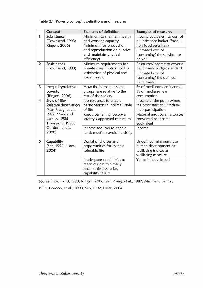
Three eyes on Malawi Poverty Page 45
Table 2.1: Poverty concepts, definitions and measures
Concept Elements of definition Examples of measures
1 Subsistence
(Townsend, 1993;
Ringen, 2006)
Minimum to maintain health
and working capacity
(minimum for production
and reproduction or survive
and maintain physical
efficiency)
Income equivalent to cost of
a subsistence basket (food +
non-food essentials)
Estimated cost of
„consuming‟ the subsistence
basket
2 Basic needs
(Townsend, 1993)
Minimum requirements for
private consumption for the
satisfaction of physical and
social needs.
Resources/income to cover a
basic needs budget standard
Estimated cost of
„consuming‟ the defined
basic needs
3 Inequality/relative
poverty
(Ringen, 2006)
How the bottom income
groups fare relative to the
rest of the society
% of median/mean income
% of median/mean
consumption
4 Style of life/
Relative deprivation
(Van Praag, et al.,
1982; Mack and
Lansley, 1985;
Townsend, 1993;
Gordon, et al.,
2000)
No resources to enable
participation in „normal‟ style
of life
Income at the point where
the poor start to withdraw
their participation
Resources falling „below a
society‟s approved minimum‟
Material and social resources
converted to income
equivalent
Income too low to enable
„ends meet‟ or avoid hardship
Income
5 Capability
(Sen, 1992; Lister,
2004)
Denial of choices and
opportunities for living a
tolerable life
Undefined minimum; use
human development or
wellbeing indices as
wellbeing measure
Inadequate capabilities to
reach certain minimally
acceptable levels; i.e.
capability failure
Yet to be developed
Source: Townsend, 1993; Ringen, 2006; van Praag, et al., 1982; Mack and Lansley,
1985; Gordon, et al., 2000; Sen, 1992; Lister, 2004

Three eyes on Malawi Poverty Page 46
Table 2.2: Categories of poverty measures
Category of
measure
Description Examples
1 Direct measure Measurement of poverty
outcomes like living
conditions or style of life
Consumption, expenditure,
subjective assessment, HDI
Indirect measure Measurement of poverty
determinants
Income or resources
2 Absolute Measurement based on set
standard
Calorific-intake based; basic
needs-based, $1/day
Relative Measurement based on a
standard that is dependent
on a situation
Percentage of median/ mean;
deprivation index
3 Objective Measurement based on
some quantitative
determination of indicators
of say need or deprivation
Nutrition-based measures;
Human-needs-based measures;
Deprivation-index-based
Subjective Assessment of wellbeing
based on views of
households
Minimum income poverty
Income evaluation poverty
4 Uni-dimensional Measurement of poverty
on one indicator or
dimension
Income/consumption/expenditure
Multi-
dimensional
Measurement covering
more than one dimension
of poverty
Composite indices like HDI,
wellbeing indices, child wellbeing
indices
Source: Alcock, 2006; Lister, 2004
The many wellbeing and poverty measures also reflect developments in poverty
research. Arguably, poverty is largely a product of capitalist development and poverty
research is a by-product of modern development. For example, the pioneers of modern
poverty analysis, Booth and Rowntree, concentrated on workers who had been „pulled
to industrial sites‟ and depended on wages as the only source of livelihood (Novak,
1995). Poverty analysis has traditionally concentrated in more developed and
industrialised countries and its use in developing countries arguably followed the largely
failed structural adjustment programmes designed and financed by the World since early
1980s (Oyen, et al., 1996).
The concern of pioneering poverty measurements was the physical efficiency of workers.
They focussed on measuring absolute poverty in terms of what is needed to sustain life;
mainly food, shelter, heating and warm clothing (Lister, 2004; Alcock, 2006). Perhaps
not surprising most of poverty analysis in developing countries follows the absolute
poverty tradition (Alcock, 2006). Absolute poverty utilises a basket of goods to
determine a minimum level of consumption (expenditure) under which the poor fall. In

Three eyes on Malawi Poverty Page 47
practice, experts determine a weekly budget standard of food and essential items for
survival (subsistence concept) or food and non-food items socially determined as
acceptable for living a normal life (basic needs concept).
The measurement of poverty in absolute terms survived but evolved over time. Starting
from a basket meant for physical efficiency, a basic needs basket replaced it. The basic
needs basket itself increased in size with affluence and open-mindedness. Alcock (2006)
shows that over time and guided by culture, non-essential items like tea, radio,
newspaper, presents to children, holidays, swimming, trips to cinema, and other leisure
activities have progressively been included in the basic needs basket and since 1990s
participation, freedom, and choice have variously been added in the basket, courtesy of
the capability approach.
In some studies, the basic needs items are derived from observed expenditure (Alcock,
2006). This is more so for the non-food component of the basket where science cannot
determine them. The use of income continues as a poverty measure, where poverty is
lack of income (resources) to acquire the minimum basket of goods and services.
Consumption as a measure gained currency with the realisation that in some
circumstances, income is a less comprehensive and an indirect measure of economic
status (Alcock, 2006).
Poverty analysis in developed countries rarely use subsistence poverty measures
following the realisation that the rapidly declining subsistence-based poverty rates were
blind to the fact that even physical needs are socially constructed and therefore just
statistical artefacts (Ringen, 2006)3. This led to the reformulation of the „rediscovered‟
relative poverty evident in earlier poverty discourses as far back as Adam Smith (Novak,
1995; Lister, 2004; Alcock, 2006).
Relative poverty uses a poverty line imposed as some proportion of the mean or
median income/consumption. Relative poverty studies use different proportions but
common ones are 50% or 60% of either the mean or median. There is no science
behind the choice of the percentage or the benchmark statistic. However, the median is
the preferred benchmark because it is not sensitive to outliers on the wellbeing measure.
Further, the use of the observed mean or median implicitly takes into account changes in
affluence and other style of life variables. However, there is no conceptual link between
relative poverty and need just as there is no way of determining extent of poverty
(Townsend, 1993).
3 Ringen (2006) reports that by early 1960s, the subsistence poverty rate in the UK was 2%.
Three eyes on Malawi Poverty Page 48
Relative deprivation came to maintain the concept of relativity while addressing some
of the problems associated with relative poverty like the setting of the arbitrary poverty
line and the absence of a link to need (Mack and Lansley, 1985; Townsend, 1993).
Relative deprivation sets out to determine an objective poverty line; a point on a
ranked income scale where deprivation increases faster than the fall in income
(Townsend, 1993). In Townsend‟s methodology, a combination of public opinion and
expert manipulation, transforms a 60-indicator list of goods and services into twelve
deprivation indicators used to derive two lines for the deprived and the non-deprived
that intersect at a point considered as the poverty line. Mack and Lansley improve
Townsend‟s methodology by reducing expert opinion in determining the deprivation
indicators. This is accomplished by requesting respondents to indicate whether the
absence of a needful item is due to choice or lack of resources. If a needful item is missed
by at least 50% of the respondents then it is included in the deprivation index.
Relative deprivation studies have shown that it is possible to determine an „objective‟
poverty line based on the relationship between a deprivation index and income
(Townsend, 1979; Mack and Lansley, 1985; Desai, 1986; Townsend, 1993). Each found
a point where the relationship between income and deprivation indices behaved
differently, a point below which participation in customary activities and enjoyment of
the benefits of being a member of a society is or nearly impossible. From that point, an
individual or household is severely deprived to the point of withdrawing from society‟s
style of life. In other words, at some point in the income distribution, low incomes force
the poor to withdraw from being an active member of a society. Mack and Lansley
(1985) pointed out that Townsend‟s methodology arbitrarily trimmed the list of
indicators from 60 to 12. Yet their methodology also arbitrary chose 50% as the cut off
point between need and desirable. Although the 50% is easy to defend, it too is
arbitrary because it does not have any scientific link to need or wellbeing or poverty.
The Leyden consensual poverty (van Praag, et al., 1982) is a version of relative
deprivation. In this methodology, public opinion sets the minimum income required to
escape poverty or hardship or „make ends meet‟. Poverty incidence comes from
analysing the public views regarding required minimum income in line with
corresponding household socio-economic characteristics. This method completely leaves
the deciding of the income level necessary to avoid poverty in the hands of the public.
Although sophisticated quantitative analysis is employed to determine the poverty line,
the fact that public opinion sets the poverty line, the Leyden consensual poverty is also
termed as subjective poverty. This underlines the point that how the poverty line is set

Three eyes on Malawi Poverty Page 49
determines whether a poverty measure is subjective or objective. An analysis of the
British Poverty and Social Exclusion Survey which combined the Leyden and Mack and
Lansley methodologies4, found no divergence between subjective and objective poverty
(Gordon, et al., 2000, p. 56).
The capability approach expertly expounded by Sen (1982) has remained a potential
answer for multidimensional poverty measurement. The approach comes from
dissatisfaction with income as a measure of wellbeing and poverty. This approach has
been expounded more at the theoretical than empirical level. According to Nolan and
Whelan (1996, p. 5), the capability approach is yet to be tested empirically. There are
advances made though. The crude human development index developed and used by
the UNDP is one of the few measures that are inspired by capability approach. Kakwani
and Silber (2007; 2008) include potential tools for measuring multi-dimensional poverty
as well as operationalising the capability approach.
There have been a few studies on multidimensional poverty or wellbeing. Stewart
(2002) found that wellbeing studies conducted in Europe used material well-being,
health, education and literacy, productive participation, social participation, housing,
exposure to crime, political participation, and leisure pursuits as dimensions of
wellbeing. Table 2.3 presents dimensions and indicators that have been used successfully
in a number of studies.
4 The only difference was that instead of using three necessities for the multiply deprived, the analysis
used two. In other words, it relaxed the deprivation criterion making it easier for a household to be
defined as poor.

Three eyes on Malawi Poverty Page 50
Table 2.3: Wellbeing dimensions and indicators
Dimension Indicators Other possible
indicators
Material Average equalised household
income
Poverty rate measured against a
national poverty line
Poverty rate measured against a
region-specific poverty line
Decile ratio
Measure of housing quality
Distribution of
income
Poverty incidence
and persistence
Poverty gap
Participation in
productive life
Unemployment rate
Long-term unemployment rate
Share of working age adults „not in
employment‟
Jobless households
Education Share of adult population with
ISCED 3 qualifications or below
Share of 17 year olds in full-time
education
Early school leavers
Health Infant mortality rate
Standardised mortality rate
Self-assessed health measure
Life expectancy
Social participation Club membership
Social contract with friends,
relatives and neighbours
Source: Stewart (2002)
Bradshaw and colleagues (2006) analysed wellbeing of children in 25 European
countries using eight dimensions (material situation, housing, health, subjective well-
being, education, children‟s relationships, civic participation, and risk and safety)
covering 23 domains and 51 indicators (Table 2.4).

Three eyes on Malawi Poverty Page 51
Table 2.4 Child wellbeing dimensions and indicators
Cluster Domain Indicators
Material
situation
Relative child income
poverty
At risk poverty rate
Relative poverty gap
Child deprivation Children reporting low family affluence (%)
Children reporting < 6 educational possessions
(%)
Children reporting < 10 books in the home (%)
Children living in
workless families
Children aged 0-17 living in jobless households
as a share of the total population of children 0-
17
Child health Health at birth Infant mortality rate; Low birth weight
Immunisation Measles immunisation coverage; DPT3
immunisation coverage; and Polio3
immunisation coverage
Health behaviour Young people who brush their teeth > 1 a day
Young people who eat a fruit everyday
Young people who eat breakfast every school
day
Mean # days when young people are physically
active for one hour or more of the
previous/typical week
Young people who are overweight by BMI
Education Education attainment Reading literacy attainment; Mathematics
literacy attainment; and Science literacy
attainment
Education
participation
Children aged 0-2 in registered childcare most
recent yr
Proportion of 15-19 year olds in education (%)
Youth labour market
outcomes from
education
Proportion of the youth population aged 15-19
not in education and not employed (%)
Proportion of pupils aged 15 yrs aspiring to low
skilled work
Housing and
environment
Overcrowding Rooms per person in households with children
Quality of the local
environment
Proportion of h/holds with children that think it
is unsafe or very unsafe to walk around in their
area at night (%)
Proportion of h/holds with children < 15
scoring six or more on a scale of physical
environment problems (%)
Housing problems Proportion of h/holds with children < 15
reporting at least two housing problems (%)
Children‟s
relationships
Family structure Proportion of children living in single parent
families
Proportion of children living in step families
Relationships with
parents
Family meals around a table several times a
week
Just talking with parents several times a week
Relationships with
peers
Young people finding their peers kind and
helpful

Three eyes on Malawi Poverty Page 52
Table 2.4 Child wellbeing dimensions and indicators (contd.)
Cluster Domain Indicators
Children‟s
subjective
well-being
Self-defined health Young people (11-15) rating their health as fair
or poor
Personal well-being % above the middle of the life satisfaction scale
% feeling like an outsider or left out of things
% feeling awkward and out of place
% feeling lonely
Well-being at school % feeling pressured by schoolwork
% liking school a lot
Risk and
safety
Child mortality Accidental and non-accidental deaths under 19
years per 100000 most recent data
Risky behaviour Cigarette smoking; Drunkenness; Cannabis;
Inhalants; Teenage pregnancy rate; 15-year olds
who have had sexual intercourse; and Young
people who used condoms during their last
sexual intercourse
Experience of
violence
Young people involved in physical fighting in
previous 12 months; and Young people who
were bullied at least once in previous 12 months
Civic
participation
Participation in civic
activities
Young people‟s participation in two or more
civic activities
Political interest Young people reporting political interest above
median score
Source: Bradshaw et al. (2006, pp. 141-168)
In Mexico, Rojas (2007) reports of a study that avoided imposing wellbeing dimensions
and indicators by using factor analysis. The analysis yielded seven domains of quality of
life. These are presented in Table 2.5.
Table 2.5: Domains of life used in Mexico
Domain Satisfaction with aspects of life
Health Current health; and availability and quality of medical services
Economic Housing; living conditions; income‟s purchasing power; and financial
solvency
Job Job‟s activity; job‟s responsibility; working shifts; and hierarchical
working relations
Family Spouse or stable partner; children; and rest of the family
Friendship Friends; and availability of time to spend with friends
Person Availability of time to pursue personal hobbies and interests; recreation
activities; and personal growth and educational level
Community Community services (rubbish collection; public transport; road
conditions; public lights; neighbourhood safety); and trust in local
authorities and neighbours
Source: Rojas (2007, p. 267)
Three eyes on Malawi Poverty Page 53
Moller (2007) used seven dimensions (income, social security, access to jobs, material
living conditions, housing, infrastructure services covering water and sanitation,
electricity and education) to measure wellbeing in South Africa. She recommends the use
of multiple measures instead of composite indices in poverty profiling if the objective it
to inform policy. This is because “a profile of quality indicators would clearly pinpoint
areas that fell short of citizen‟s expectations of the good life, and needed urgent
remedial action on the part of policy makers” (Moller, 2007, p. 246).
The OPHI‟s Multidimensional Poverty Index has already been adopted by UNDP‟s
Human Development Report and covers 104 developing countries (UNDP, 2011)5. The
index is reported alongside the Human Development Index and Gender Inequality
Index and seems to replace the Human Poverty Index in the latest report. As for the
multidimensional poverty index, it has been demonstrated that it is different from the
human development index and the human poverty index based on how it ranks
countries significantly different from any of the two indices (Alkire & Foster, 2007).
Batana (2008) also reports of the use of a WeD-inspired multidimensional poverty
measure in fourteen Sub-Saharan African countries based on existing data. This measure
covers four domains namely assets, health, education and empowerment (Alkire &
Foster, 2007). On the other hand, the WeD methodology was implemented in four
countries namely Bangladesh, Ethiopia, Peru and Thailand (Copestake, et al., 2009). The
WeD Peru team used factor analysis to indentify and analyse wellbeing components to
“minimise reliance on the ideas (and values) of outsiders in selection and classification of
items” (Copestake, et al., 2009, p. 24). The methodology is also being implemented in
Zambia and India (WeD, 2011). The WeD research work has a number of breakthroughs
that are of use to this study. The first is that it is possible to develop national-level
assessment scales from a smaller set of local level items as long as the items are shared
across the country (Copestake, et al., 2009). The second is that it is possible to identify
components of wellbeing using factor analysis without imposing an expert conceptual
framework.
The implication of the first breakthrough is that subjective wellbeing data from non-
questionnaire tools can still be used across the country if the local specificity is sacrificed,
albeit that it is best-suited for local analysis. This is important because it gives some
credence to the use of SSI and FGD reports to get dimensions or household features that
5 The number of countries covered by the index continues to grow as countries with relevant data are
added. By December 2011, the number of countries had reached one hundred and nine (OPHI, 2011).

Three eyes on Malawi Poverty Page 54
are applicable across the country. The second breakthrough has two implications. The
first is that it gives strength to the position taken in this study that it is not necessary to
impose a conceptual framework when analysing data from field reports. The second
implication is that the thesis has some basis for using factor analysis on data obtained
from in-depth interviews and focus group discussions reports.
It is also noted that the subjective wellbeing assessment in WeD use open-ended SSI as
opposed to questionnaire-based assessment as recommended by Dolan and others
(2008). In the WeD methodology, instead of an integrated household questionnaire
with a module covering the subjective wellbeing assessment, a multistage data collection
strategy is employed to get different types of data that complement each other. Each
methodology has advantages and disadvantages and which methodology to adopt
depends on the objective of the study. Suffice to say that the goal of the WeD research
programme is to “develop a conceptual and methodological framework for
understanding the social and cultural construction of wellbeing in developing countries”
(Copestake, et al., 2009, p. 3). Further, the WeD methodology is specific to developing
countries where social and cultural factors are fundamental in shaping subjective
assessments of wellbeing.
Whether the OPHI‟s multidimensional poverty index is better than the WeD‟s measure is
an empirical question. These two measures share two domains (health and
education/schooling). The OPHI index includes a domain on standard of living with six
indicators. This is absent in the WeD measure and the WeD measure has assets and
empowerment which are absent in the OPHI measure. On the other hand, these are
just two of the many measures of wellbeing. With proliferation of multidimensional
poverty measures6, it is only the objective of the study that assists in narrowing down
the choice.
The absence of subjective wellbeing in national poverty or wellbeing profiling has been
picked up as in issue in recent years (Dolan, et al., 2008). Indeed, there has been some
urgency to include subjective wellbeing following the Report by the Commission on the
Measurement of Economic Performance and Social Progress (Stiglitz, et al., 2009). In
the UK, steps are being made to ensure that subjective and objective wellbeing are
treated equally in the official statistics (Beaumont, 2011). Of course, work on subjective
wellbeing has been done in the UK for some time (Dolan, et al., 2008). What is missing
6 Batana (2008) discusses these measures in the introduction

Three eyes on Malawi Poverty Page 55
is the systematically and consistent collection of subjective wellbeing data at the official
level. This is what Dolan et al (2008) and Stiglitz et al (2009) recommended and what
the Office of the National Statistics (Waldron, 2010; Beaumont, 2011) plans to do. This
will put subjective wellbeing and objective wellbeing on equal footing in data
collection, analysis and presentation. It is likely that once the UK government develops
the system other countries, including Malawi, will learn and adapt the system for their
own use.
2.5 Issues on wellbeing and poverty measures
2.5.1 Mismatches between concepts and measures
Given that a measure is a translation of the concept through the analytical definition, it
is imperative that a measure matches the concept since a measure has no life on its own.
However, mismatches are a common place and this has been a concern for some
researchers. Ringen (2006) reports that some studies mismatch poverty concepts and
measures, making their results misleading, if not invalid. Nolan and Whelan (1996) note
that some poverty measures are inadequate to „translate‟ the underlying poverty
concept to the extent that they fail to correctly identify the „poor‟ in line with the
concept. Rein (1970, p. 47) gives an example of a programme whose goal is to improve
wellbeing yet its evaluation uses subsistence poverty measure to check whether it
achieved its goal.
Some of the mismatches are historical. In centuries before the industrial revolution, the
concept of poverty was for the propertyless people who worked for other households
to earn a living (Novak, 1995). In those days, all workers were classified as poor and the
proportion of workers to the total population was the poverty incidence. Following the
industrial revolution, the subsistence concept of poverty replaced the structural view of
poverty as a group of the workers were now considered to be affected. From then on
failure to meet subsistence levels of existence without begging and getting assistance
defined poverty (Alcock, 2006). Measuring poverty meant estimating the level of
income that enables the consumption of goods and services that keep soul and body
together because the poor were uprooted from subsistence type of living.
With trade unions and marked development, the subsistence concept gave way to basic
needs concept where the interest was to cover both subsistence and basic goods and
services. To be poor under this concept means consumption of food that is less than the
recommended minimum and consuming non-food goods and services is below the
minimum acceptable. This concept also focused on workers in industry and still used
Three eyes on Malawi Poverty Page 56
income as a measure because the worker only relied on income to acquire such goods
and services. This means that anyone whose income earned was below the cost of the
minimum food and non-food baskets the individual was classified as poor.
Use of income as a measure dominated even in all the concepts except the capability
concept. The reasoning was the same. The poverty of interest was of workers who
solely depend on wages for all their livelihoods. However, there is some mismatch
when the consumption is measured by income earned. By using income to measure
consumption it is assumed that income is used to purchase what is considered as basic or
standard first before any other type of expenditure. This assumption may not always be
true. Using expenditure would be an improvement over income because expenditure is
a very strong indicator of intention. However, even then expenditure does not always
translate to consumption. Thus an improvement over expenditure would be to measure
the consumption itself because it is more direct than income. Others argue that even
consumption is not wellbeing because the same consumption does not yield the same
wellbeing. This is where the capability concept was hatched (Sen, 1982; 1991).
There are also others who argue for more open mindedness because not all poverty is
amenable to measurement. According to Lister (2004) measureable poverty is no better
than (or superior to) other forms of poverty that cannot be measured easily and
measuring poverty using a single measure is but a „technical artefact‟ because poverty is
multisectoral as well as multidimensional. She contends that if concepts of poverty
embrace „how people talk about and visualise poverty‟ (Lister, 2004, p. 4) then it
follows that conceptualisation of poverty should benefit from the involvement of the
people who feel and talk about poverty.
The relative deprivation and consensual poverty concepts seem to get this idea because
behind these concepts is an understanding that people themselves are better placed to
define poverty than experts. For example, Mack and Lansley state that „need has no
meaning outside the perceptions of people‟ (1985, p. 41). The involvement of people
under the relative deprivation and consensual poverty concepts is only at the measuring
stage and not conceptualising or defining. It must be said that the Breadline Britain
methodology as practised by Gordon and colleagues (2000) of conducting FGDs across
the country to first determine the list of goods and services considered necessary for an
acceptable style of life is one big step towards involving households in defining poverty.
However, there is still need to involve the people even at those earlier stages so that
their involvement at the measuring stage makes sense to them.

Three eyes on Malawi Poverty Page 57
2.5.2 Comparison of quantitative measures
The commonest measures of wellbeing and poverty have been income, expenditure,
and consumption. The application of the measures varies from study to study. In theory,
measure is a derivative of a concept or theory. In practice, what drives the choice of a
measure is pragmatism in the face of limited financial resources vis-à-vis required data
and time. In developed countries, income is easier to collect than expenditure and
consumption. In developing countries, none of the three measures is readily available.
Data for the measures are collected through household surveys. Since one survey can be
used to collect data for all the three measures, it is possible to use any of them. Probably
the question is on the quality or appropriateness of each of the measures in the context
of developing countries.
Income measure
The basic coverage of income as measure is wages and salaries. In general, income
covers resources like money, financial and capital assets. Broad definitions also include
employment benefits, social security benefits, and private income in kind (Table 2.6). To
compute the measure, all non-cash income is valued and converted into cash income
equivalent. Other estimations replace the holdings of stocks and shares, and value of
property, land, and buildings with net additions to wealth in the reference period; i.e.
flow instead of stock.
Table 2.6: Different types of income
Dimension of income Examples
1 Current cash Wages and salaries, income from assets, dividends and
interests, social security benefits and pensions
2 Capital assets Cash and deposits in financial institutions, holdings of
stocks and shares, value of property in businesses, land
and buildings including household possessions and
facilities, and education qualifications, especially beyond
primary
3 Employment benefits Income in kind like housing, cars and travel, education,
meals and entertainment
4 Social services benefits Value of public service benefits in kind – health,
education and housing
5 Private income in-kind Gifts of food and clothing, produce from land and
gardens, help with outings, holidays and education
Source: Townsend (1970)
According to Townsend (1970), income has been defined variously in studies. Others use
gross income while others net out taxes; others further net out housing costs while
others gross them in. The question that needs to be answered in the choice of the

Three eyes on Malawi Poverty Page 58
measure is which of these income best approximate wellbeing status or which would
impact on wellbeing status most. Those who net out taxes and housing costs focus on
finding a measure of available resource for „commanding‟ a standard of living. Those
who use gross-of-housing-costs income consider the type of housing to be an integral
part of standard of living and that the level of housing costs (rent/mortgages) reflects
more the quality of the housing than the type of financing. This effectively takes
mortgage or rent as use value of the housing.
Collecting income is complicated in developing countries because of diversity of sources
as well as intervals of receipt of the income (Townsend, 1970). On diversity, he
mentions that one source of income can have multiple intervals of different amounts;
one household can have different sources each with multiple periods of receipt and
amounts. The result is that income earners have recall challenges and depending on the
chosen recall period in the questionnaire the quality of the data would be affected if it is
inappropriate for most of the respondents. To minimise the impact of these problems,
studies use multiple report periods for various sources of income depending on
commonly known frequency of receipt (Townsend, 1970). For example, the past seven
days can be used for micro-enterprise income, the past one month for wages and salaries
and the past twelve months for crop sales which are then annualised to normalise them.
Expenditure measure
Some poverty studies use the expenditure approach (Ravallion, 1994). It is one of the
direct measures of economic welfare because it measures outcomes. In this method, all
expenditures an individual or a household does are added up to come with a
distribution of expenditure. It assumes that all purchases are for the individual‟s or
household‟s use and good. The effect of tastes (and brand loyalty) is assumed away. At
the least, the measure covers all cash expenditures on goods and services for current
period consumption. The measure excludes expenditure on investment and durable
goods because their consumption goes beyond the year they are purchased. It is the
annual use value of all investment and durable goods which are included in the
measure. In its broad usage, expenditure includes estimated value of non-cash
acquisition of goods and services. This includes valuation of in-kind gifts.
In developed countries, the frequency and volume of purchases make the method
impractical. Although it is theoretically better than income, it is rarely used. Even in
developing countries where the frequency of purchases is relatively low, low

Three eyes on Malawi Poverty Page 59
monetarisation of household economies implies that expenditure covers wellbeing
rather inadequately.
Consumption measure
The consumption measure pools non-cash and cash household economies together in
that it benefits from expenditures as well as own production (Ravallion, 1994). In
practice, the consumption measure replaces expenditure on durable goods with their use
value of all durable services and also nets out expenditures on investment items (medical
care and education) and cash donations. At the end of the valuation, a cash equivalent
of consumption is established. Equivalent scales are used to normalise consumption
across households of different demographic characteristics. According to Meyer and
Sullivan (2003), consumption is the closet measure of wellbeing because it reflects
current living standards but is blind to quality or sustainability of sources of the
consumed goods
Comparison of the three measures
Income is supported as a measure by many. Baudot (2000) and Gordon and colleagues
(2000) argue that income defined to include other resources is a vehicle for the
satisfaction of material needs (Gordon, et al., 2000, p. 18); and lack of control over
resources is inseparably linked to poverty (Baudot, 2000, p. 25). This echoes what
Townsend (1970) stated earlier on that income is a sufficient measure of economic
position when “all receipts which increase an individual‟s command over the use of
society‟s scarce resources – net accretion of economic power between two points in
time” are included (p. 24). Others do not agree with this.
For example, Meyer and Sullivan (2003) argue that it is likely that „all receipts‟
highlighted by Townsend (Table 2.6) exclude in-kind transfers and illegal sources, which
may be important for poor households. In fact, Meyer and Sullivan (2003) and Sen
(1982) contend that consumption is a better measure of poverty than income because it
is a direct measure. Ringen (2006, p. 160) gives five reasons why income is not a good
proxy of consumption and by extension wellbeing or poverty. First, income is useful
only in markets where income has some „power‟ to command goods and services.
Second, „the same income does not buy everyone the same consumption‟. Third, the
market is not the same for all because education, knowledge, and information influence
how income interacts with the market. Fourth, when estimated from surveys, income is
an inaccurate measure of economic resources since it excludes wealth. Fifth, and echoing

Three eyes on Malawi Poverty Page 60
Nolan and Whelan (1996), low income is not the sole determinant of current
consumption although low consumption is strongly influenced by low income.
Fields (1980) supports the argument that consumption is better than income. He gives a
number of reasons. The first is that it directly measures the flow of utility-producing
inputs. The second is that it approximates permanent economic position better than
current income since income only measures the potential to acquire those inputs. This is
why low income does not always imply low consumption as pointed out by Nolan and
Whelan (1996). Since consumption manifests actual and not potential flow, income is
only a proxy measure of poverty because it only approximates consumption. The third
reason is that price differences of the same item drive a wedge between distributions of
income and consumption. This wedge makes consumption a better measure of poverty
than income because consumption already factors in price decisions. Conversion of
income into a measure requires making assumptions on the prices of goods and services
to ascertain how much an income „can‟ command.
There are other reasons in support of consumption. One of them is that consumption is
smoother than both income and expenditure (Meyer and Sullivan, 2003; Ringen,
2006). Unlike income, consumption is smooth also because it captures the effect of
access to credit and previous acquisition of assets (Meyer and Sullivan, 2003). Further,
household income distribution is more unequal than household consumption
distribution (Novak, 1995). Sen (1982) argues that income is second best to
consumption because it measures wellbeing indirectly. However, consumption does not
have universal approval either.
Townsend (1970) argues that collecting and estimating consumption data from the poor
is almost impossible. On the other hand, Meyer and Sullivan (2003) report that income
is relatively difficult to collect among the poor, even in developed countries. Wilson
(1996) and Chambers (1997) argue that income collected through household surveys is
normally incomplete; it does not cover all resources. Meyers and Sullivan (2003) state
that income is always lower than consumption and singles out self-employment
earnings, private transfers, and public transfers as the most under-reported as
respondents attempt to hide their income. In general, there is little bias in the collection
of consumption data although measurement errors exist. On income and expenditure,
Townsend (1970) states that income is generally understated compared to expenditure.
Thus conceptually consumption is a better measure of poverty than expenditure and
income and expenditure is better than income. Practically, though, income is a preferred

Three eyes on Malawi Poverty Page 61
measure in developed countries while consumption supported by expenditure carries
the day in developing countries where all are measured with errors (Meyer and Sullivan,
2003). Gordon and colleagues (2000) also support the use of more direct measures.
Fields (1980) recommends the use of both income and consumption as measures
wherever possible.
Given this scenario, Chambers (1997) argues that both income and consumption
measures, if determined from questionnaires surveys are researchers‟ social and personal
constructs because of the „reductionism‟ implicit in pre-coding responses to questions. He
argues that by pre-coding the responses varied and dynamic needs experienced by the
poor are replaced by researcher-standardised needs implicit in the codes. He instead
recommends wealth ranking although he is quick to point out that wealth ranking is not
always accurate if done incorrectly.
2.5.3 Unit of analysis – gender dimension of poverty
Most of poverty research in general uses household as a unit of analysis. This is also true
for Malawi where consumption expenditure is used a measure of household wellbeing
(GoM & World Bank, 2007; GoM, 2000). The use a household as a unit of analysis
assumes that consumption is equal amongst household members and that expenditure
on each household member is equal. This is hardly the case even in Malawi (GoM &
UN, 1993). Even on the basis of human needs, men and women, boys and girls, adults
and children, pregnant/lactating women and other women have different needs. While
sophisticated adult equivalent scales can deal with these human needs differences, they
fail to deal with other intra-household differences in general (Lister, 2004).
Given that poverty is a function of structures and processes in terms of its creation and
perpetuation (Lister, 2004), there is bound to be unequal distribution of poverty
amongst women and men because social, economic and political structures confronting
women are different from those confronting men and the processes that create poverty
are not gender blind (Ruspini, 2001). In particular, there are differences among men,
women, parents, children, adults and the elderly emanating from differences in interests,
power relations, division of labour, access to resources (e.g. food and clothing), space,
warmth, light, and responsibilities say in ensuring the provision of basic necessities and
needs of children (Ruspini, 2001; Pentazis & Ruspini, 2006). These differences mean that
women and men, for example, could have different causes of poverty and therefore
experience poverty differently (Pentazis and Ruspini, 2006). This implies that women,
men, boys and girls in the same poor household, can experience poverty rather
differently (Ruspini, 2001). On the other hand, even in a non-poor household, it is

Three eyes on Malawi Poverty Page 62
possible to have a poor woman or girl because, as Ruspini (2001, p. 106) puts it, “a
poor person may be a member of a rich family and that the burden of poverty falls
mainly on women.”
Indeed most research has found that women are at a disadvantage because they
generate less income than men, spend less of their income on themselves than men and
more of their resources to ensure availability of basic necessities and child care; and
consume less than other household members; (Chant, 2010; Pentazis & Ruspini, 2006).
There is therefore a strong basis for a gendered analysis of poverty.
However, gendered analysis of poverty has implications on data collection as well as
unit of analysis. Regarding unit of analysis, gendered poverty analysis requires analysis
of data at individual, instead of household, level. Collecting data at an individual level
allows not only gendered analysis but also other types as well. With individual level
data, it is easier to group individuals by demographic characteristics like age, sex,
education level and marital status. Such fine analysis is likely to lead to better policy
formulation and programme design than otherwise. Thus one of the conditions for fine
analysis is level of data aggregation. As Pentazis & Ruspini (2006) state, most of the data
collected even in developed countries is mostly at household level. Further, Ruspini
(2001) states that meaningful gendered analysis of poverty requires individual data on
structures and processes that create and perpetuate poverty or enable people to escape
from it.
This requirement is what has slowed down gendered analysis of poverty, even in
developed countries (Pentazis & Ruspini, 2006). No wonder the household is still the
used unit of analysis even for subjective wellbeing (Stiglitz, et al., 2009) with sex of the
household head as the only possible channel for gendered analysis of poverty (Pentazis
& Ruspini, 2001). Unfortunately, the use of women-headed households as a proxy for
gendered analysis is misleading because of the diversity of such households (Chant,
1997).
On the other hand, Pantazis & Ruspini (2006) have demonstrated that once data at an
individual level is available, gendered analysis of poverty is possible. This leaves the
level of data aggregation as the main decider of the unit of analysis. The lesson from
this discussion is that as long as women and men are different in Malawi, the individual
should be used as the unit of poverty analysis. Again, since gendered poverty analysis is
crucial for meaningful poverty reduction, data collection systems should be changed to
allow for collection at individual level.

Three eyes on Malawi Poverty Page 63
2.6 Operational definition of poverty: drawing a poverty line
Whatever measure is adopted, there is need to set a standard that identifies two groups
in the sample; the poor and the non-poor. Quantitative measures like income,
expenditure and consumption require three separate steps to identify the two groups;
i.e. estimating the wellbeing status of each subject (household/individual), determining a
point on that measure that separates the poor from non-poor, and determining the
number or proportion of the poor out of the population. A poverty line is the point on
the measure where the two groups are separated and it is therefore an operational
definition of poverty.
There are many ways of determining the poverty line and in theory they should be
inspired by the poverty concept is in use. Some poverty lines are imposed, for instance
the US$1 per day per person or the 60% of the median of the measure while others use
minimum wages, and minimum benefits levels (Viet-Wilson, 1998). Some poverty lines
represent estimated cost of expert-drawn budget standards (basket of goods and
services) or family budget units drawn from actual consumption or expenditure levels
(Viet-Wilson, 1998). Items in the basket are dependent on the poverty concept adopted.
Market prices are the preferred source of costs although computed prices are used in
cases where the market does not supply the goods and services.
The family budget units methodology was developed to get around the problem of
using expert-drawn baskets of needs (Bradshaw, et al., 1987; Bradshaw, 1993). In this
methodology, need is assumed to be implicit in the actual expenditure or consumption
pattern. The role of experts in this methodology is to establish a range of family budget
units for different family types based on actual expenditure patterns, calculate
consumption needs of different family types, and establish weekly budgets for each
family type based on actual expenditure patterns.
Under consensual poverty approach, there are two ways of drawing a poverty line,
depending on the type of question asked. The minimum income question asks the
respondent to estimate how much income a hypothetical family of certain demographic
characteristics in their community would need to achieve a certain living standard. In
this method, the poverty line is an average of the estimated incomes normalised by
demographic characteristics. The income evaluation question requires respondents to
indicate goods and services they regarded as necessities for some living standards. Those
mentioned by the majority of the respondents make it into the basket of necessities. A

Three eyes on Malawi Poverty Page 64
costing of the goods and services yields the poverty line in this consensual standard of
living approach. The valuation of the basket is similar to that done for the budget
standard.
Other than the consensual income poverty line and physical efficiency subsistence
basket, poverty lines are arbitrary. They reflect more the value judgements of
researchers than the condition of poverty. The arbitrariness comes in when drawing the
basket of goods and services. This makes the poverty „found‟ not as objective as it is
supposed to be, especially when the objective is to influence policy. Uncomfortable with
this „subjectivity‟ some researchers set out to and derived a „value-free‟ poverty line out
of deprivation indices (Townsend, 1979; Mack and Lansley, 1985; Desai, 1986). There
have been questions on the „objectivity‟ of derived poverty line from this methodology
(Piachaud, 1987) and even Mack and Lansley (1985) who also derived a „poverty line‟
from deprivation indices, admit that as long as socially perceived necessities „construct‟ a
poverty line, that line is but subjective.
Thus there is no science available to help decide which method is most suited on what
condition. Martin Rein (1970) likens the search for a value-free poverty line as the
search for the philosopher‟s stone. Novak (1995) considers unrealistic the idea that a
poverty line can „objectively‟ separate the poor from non-poor because there is little
qualitative difference between those around the poverty line since the experience of
poverty is a continuum. Poverty lines are therefore political constructs (Lister, 2004) and
therefore subjective. This makes poverty be „in the eyes of the beholder‟ (Orshansky,
1965) because the amount of poverty found is dependent on its definition and measure
(Ringen, 2006).
Consequently, most disagreements centre on the choice of goods included in the basket.
The scientific concept of poverty clearly favours the limiting of the basket only to goods
and services that would ensure survival and autonomy. The moral concept of poverty
favours the use of a basket that caters for both physical and social needs. Granted that
these are opposed views, an acceptable poverty line is but a dream. Apparently, what is
important in poverty analysis is to make one‟s position clear (Bevan, 2007).
2.7 Identifying the poor
Most quantitative poverty analyses present measures at individual level. This facilitates
statistical manipulation. However, there is no national database of the poor despite
many studies. One of the reasons is that the basis of measures is sample surveys and not
census. Even if the census is the basis of the results, changing circumstances make poverty

Three eyes on Malawi Poverty Page 65
dynamic. The poor of yesterday may not be the poor of tomorrow and the rich of
yesterday can as well be the poor of tomorrow. This means that identifying the poor
requires fresh analysis of circumstances. Whether the analysis of the conditions is on
household or individual level depends on the objective of the identification.
In theory, the operational definition of poverty provides a criterion for identifying the
poor. If consumption of less than 3,000 calories per day per person defines the poor,
then counting the amount of calories consumed by each individual leads to the
identification of the poor. If being in a female headed household is defined as being
poor, the poverty rate is the total number of members in female headed households
relatively to total household population. In each of the examples, a register is required
to identify the poor - of calorie consumption by households/individuals need to exist
and population of households by sex of household head and the corresponding
household population. In practice such registers do not exist. This means that the
identification of the poor requires a census of all households or individuals in order to
determine who meets the criteria.
Unless it is a small scale project, conducting a census is expensive and wasteful if the idea
is to establish a database for identifying the poor because results of today may not be
the same tomorrow since household and individual circumstances may change rapidly
making the „shelf life‟ of such data very short indeed. In practice, it is very rare to
identify the poor just for „record purposes‟. It is also rare to identify the poor,
individually and physically, in the entire population. Further, Malawi‟s population and
housing censuses collect too rudimental data to use for the identification of the poor
unless the operational definition of the poor is as crude as demographic groups like
„members of female-headed households‟ or „double orphans‟. Identification of the poor,
in the real world, is associated with social transfers. The operational definition of
poverty in such cases is generally dependent on the objective of the intervention. Once
the definition is chosen, the poor are identified.
In developing countries, poverty profiles are mostly used to identify proxy indicators or
categories for identifying the poor. Once the poverty line is established and the poor
identified, the characteristics of the poor and non-poor are used to determine poverty
correlates. The poverty correlates are used as proxy indicators. Project implementers
use these to identify beneficiaries of social transfers (Conning and Kevane, 2002; Coady
and Skoufias, 2004; Galasso and Ravallion, 2005). By implication, the poverty
correlates reflect what the questionnaire covered and by extension the poverty concepts

Three eyes on Malawi Poverty Page 66
and definitions included in the questionnaire. This is one of the areas this study is
exploring.
2.8 Poverty analysis in developing countries
Apparently, poverty research is a shadow of capitalism-driven poverty as evidenced by
its late arrival in developing world. Poverty discourses and poverty research in
developing countries are „imported‟ by international agencies most notably the World
Bank, IMF, EU, and UN Agencies (Townsend, 1993). Starting in the 1990s, the EU and
World Bank, among others, also embarked on face-saving poverty assessments in
developing countries (Townsend, 1993). A review of poverty research in developing
countries found that researchers used no theoretical frameworks or simply borrowed
theoretical or conceptual frameworks uncritically and that most of them were externally
financed, possibly explaining the absence of home-grown poverty discourses (Oyen, et
al., 1996).
The advances in poverty analysis in developed countries are yet to filter to developing
countries. For example, poverty analysis in developing countries rarely employs
methodologies like relative poverty, relative deprivation, and consensual poverty. There
are reasons for this. Apparently, the level of development justifies the use of some
measures. Prevalence of hunger, poor shelter, overcrowding housing, poor clothing, ill
health, illiteracy, and even totalitarian regimes justifies the use of absolute poverty
measures (Rein, 1970). One other reason is that there is little monetarisation of
consumption and production activities. Low monetarisation of household economies
make any measure dependent on the level of income less effective because of the
required estimation of income from a variety of resources.
International organisations only use the crude absolute poverty measurement US$1 or
US$2 a day per person poverty lines to compare developing countries (Townsend,
1993). For country poverty reports, the absolute poverty measures dominate. The
commonest status measure is consumption expenditure computed from a socio-
economic survey (Ravallion, 1994). A poverty line is determined based on a food and
non-food basket. In this methodology, WHO recommendations on calories per day per
person are used for food component while observed expenditure at the mean/median
economic measure determines the non-food component thereby replacing expert
determination of the non-food component. Of late, subjective assessment of wellbeing
has been included in integrated household survey questionnaires. Although they are not
a permanent feature of poverty profiles, at least in Malawi, the inclusion of this aspect

Three eyes on Malawi Poverty Page 67
shows a move towards including the voices of the people in poverty research in
developing countries.
2.9 Factoring in of voices of non-experts in poverty research
Since Townsend (1979) and Mack and Lansley (1985) works on relative deprivation,
there have been efforts to involve households in poverty research. The Leyden
consensual poverty work added yet another angle to the household‟s role in
determining the poverty line and by implication poverty rate (van Praag, et al., 1982).
The participatory poverty assessments, which use rapid rural appraisal or participatory
rural appraisal approaches, bring in communities into the poverty research arena. While
the relative deprivation, Leyden consensual poverty and subjective assessment of
wellbeing are done in the context of a household questionnaire, the poverty assessments
are not. The rest of the chapter is then devoted to discussing the subjective assessment
of wellbeing and the participatory rural appraisal approach as vehicles used to bring in
the voices of the non-experts into poverty research.
2.9.1 Household voices: self assessment of wellbeing
The Leyden approach also introduced evaluation of wellbeing status by directly
requesting respondents to indicate the level of income required either for a hypothetical
4-member family (or their own family) required to avoid living sub-optimally described
various as „to make ends meet‟ or „to get along‟ or „to live a decent life‟ or „to avoid
feeling poor‟ (Lokshin, et al., 2004; Mangahas, 1995; van Praag, et al., 1982). In some
cases, respondents are requested to estimate level of income associated with various
statuses of living like „very bad‟, „bad‟, „insufficient‟, „sufficient‟, „good‟ and „ very good‟
(Bosch, 2001).
More progressive approaches request respondents to directly evaluate their wellbeing
status (Moller, 2007; Ravallion and Lokshin, 2002; Van Praag, et al., 2003) represented
by „overall life satisfaction‟ or „rights or power‟ or „economic wellbeing‟ (Bosch, 2001,
Narayan and Petesch, 2005). Thus there has been some progression of people‟s
involvement in poverty analysis; from merely providing their income, consumption, and
expenditure to indicating necessities and evaluating their own style of life.
In general, economists and poverty analysts prefer to estimate cardinal utility from data
on income or expenditure or consumption questions to ordinal utility estimated through
attitudinal questions (Sen, 1982; Van Praag, 1991). Critics are not sure whether
respondents have the same understanding of the terms used when giving their
perceptions. For example, Van Praag (1991) reports that sceptics are not sure whether

Three eyes on Malawi Poverty Page 68
respondents have the same understanding of the verbal labels like „very satisfied‟,
„satisfied‟, „neither satisfied nor unsatisfied‟, „unsatisfied‟ and „very unsatisfied‟.
Mangahas (1995) argues that terms like „to live a decent life‟, „live decently‟, „make ends
meet‟, and „to get along‟ used in the minimum income question (MIQ) are too vague to
draw similar interpretations. Bosch (2001) also questions the uniformity of
understanding of terms like „in your circumstances‟ in some of the MIQs.
Lokshin and colleagues (2004) also argue that the concept of income is not uniformly
understood in developing countries where a large proportion of consumption is non-
monetary. In fact, Lokshin and colleagues report that subjective poverty lines derived
from the MIQ „do not seem to generate sensible poverty profiles‟ just as they „show
weak correspondence to both objective and [other] subjective poverty measures‟ (2004,
p. 560). Actually Ringen (2006) rejects any measure that is based on feeling because “to
be poor depends on how you live and not how you feel” (p. 146). In this line, Sen
(1999) argues that a person‟s “well being is concerned with a person‟s achievement:
how „well‟ is his or her „being‟ … an assessment of the particular achievements of the
person – the kind of „being‟ he or she succeeds in having” (pp. 3, 33).
Others point to non-random biases in perceptions from the very poor and very rich.
The very poor are said to have deformed preferences. For example, Gregor (2007)
questions the truthfulness of the ratings of the poor arguing that deprivation mentally
conditions the poor to adapt and that society shapes an individual‟s perceptions (p.
335). Further, Bradshaw and Finch (2003, p. 517) and Ringen (2006, p. 145) argue that
limited knowledge of a better life elsewhere creates a false consciousness resulting in a
situation where the poor feel non-poor. In Sen‟s words, “a thoroughly deprived, non-
grumbling and resigned person with low expectations of life leading a very reduced life
can rate him/herself as non-poor” (1999, p.55). The very rich are also said to have
blurred vision of life lived by the poor. Bosch (2001) argues that the rich have limited
knowledge of life experienced by the poor to the extent that when requested to
estimate the minimum income needed to escape poverty, their average is generally
much higher than others.
According to Kapteyn (1994) economists trust the indirect method of estimating
wellbeing through people‟s revealed preference. They consider it objective because it is
verifiable as opposed to the direct method of soliciting people‟s view which is generally
unobservable. In particular, Gordon (2000) finds issue with the absence of „ground
truthing‟ in subjective methods because „the elucidation of opinion takes precedence
over the elucidation of behaviour‟ (p. 61). According to him, the perception of need,

Three eyes on Malawi Poverty Page 69
just as it is important, should be complemented by documentation of behaviour when
in need because it is when in need that genuine prioritisation is undertaken. Indeed as
Mack and Lansley (1985) found out, some households identified as poor (based on their
feelings of enforced lack of necessities) afforded, at the same time, to purchase goods
and services judged as non-essential by the society at large. This is an example of
feelings not matched by behaviour and therefore a cause of concern.
Multiplicity of influences on people‟s perceptions gives some critics some reason to
discount the usefulness of subjective wellbeing measures. Elster (1989) states that
rankings over life are generally incomplete and unreliable but argues that this is not
necessarily due to irrationality because, as he puts it, „irrationality is neither marginal nor
omnipresent‟ (p. 28). Kalugina and Najman (2003) state that the disadvantage of
subjective methods is that each answer can be influenced by a combination of different
factors (attitudes, anticipations, social norms and rules, group references, current
income, permanent income, among many others). They single out the influence of a
reference group as the best deformer of perceptions as evidenced by people who feel
poorer than their objective standard of living just because their reference group is
objectively richer than them.
The issues of language and understanding of questions elucidating the perceptions have
been dealt with or solutions found. For example, Van Praag (1991) conducted a study to
determine whether people have the same understanding of verbal labels used in income
or life satisfaction questions. The study found that verbal labels are understood similarly
by respondents. The conclusion was that it is legitimate to include attitudinal variables in
welfare models. Mangahas (1995) proposes using direct instead of vague terms in the
minimum income question like „how much would your family need each month for
home expenses in order not to feel poor anymore‟ instead of a hypothetical 4-member
family „getting along‟ or „making ends meet‟. A similar approach is used by Ravallion
and Lokshin (2002) in a study elucidating perceptions on the levels of economic
wellbeing. They explicitly use the words „poor‟, „rich‟ or „nonpoor‟ and requires the
respondent to use own household as a reference. This keeps the perceptions of the
respondents focused on what is being measured.
Kapteyn (1994) conducted a study to check whether feeling poor is the same as being
poor. Kapteyn had the implicit hypothesis that subjective poverty is similar to objective
poverty given the same sample. The study found that subjective poverty profile was
different from objective poverty profile of the same population. Although he attributed
this to possible model misspecification he concluded that the direct method (based on

Three eyes on Malawi Poverty Page 70
feelings) and the indirect method (based on observed expenditure, income or
consumption) do not measure the same poverty and are therefore not the same.
While there is a great temptation to compare, recognising that subjective poverty is
different from objective poverty helps put the comparison in perspective. For example,
even when the subjective poverty rate is similar to objective poverty rate, it does not
mean that they measure the same poverty and this may be evidenced by differences in
the households identified as poor. In general, it is rare to have same poverty rates
because objective poverty generally covers defined dimensions unlike subjective
wellbeing whose dimensions are dependent on the assessor‟s understanding. As Gordon
(2000) notes, subjective poverty rates are generally higher than objective poverty rates
and they are prone to change depending on changes in tastes and prices. Expecting the
two to be the same and blaming any differences on poor value judgements is somewhat
flawed.
Further, it is ironic that value judgements under subjective poverty measurement are
frowned upon when objective poverty measurement is plagued by value judgements
too. To begin with, the poverty line basic-needs basket requires value judgement which
is dependent on social circumstances making the separating line between luxury and
needs blurred over time (Pradham and Ravallion, 2000, p. 462). The question then is
why is it that the value judgements made by experts on people‟s wellbeing are more
acceptable than those made by people on their own welfare status?
Mangahas (1995) states that poverty as a normative concept needs norms for its
measurement. The question is what and whose norms should be used. He argues that
the objective poverty measurement is top down because it uses norms imposed by some
institution on behalf of society with little or no regard to what the society feels. On the
other hand, the bottom-up approaches use the norms given by people themselves „who
are the object of poverty measurement‟ (Mangahas 1995, p. 40). Until the norms used
by the top down and bottom up measures are the same, objective and subjective
poverty are bound to be measuring different „strains‟ of poverty (Mangahas 1995). In
fact, Mangahas (1995) takes the two approaches as two snapshots of the same subject
from different angles thereby acting as complements of each other only that the bottom
up approach picture is rather cheaper and faster „to develop‟ than the top down one as
echoed by Chambers (1997).
Apart from the different values attached to expert and people‟s value judgements, there
is the question of different values attached to „mistakes‟ made by the same person in

Three eyes on Malawi Poverty Page 71
objective and subjective poverty. It is noted that objective poverty is better than
subjective poverty because the former is based on „facts‟ about standard of living and
the latter on unobservable „feelings‟ about the standard of living. However, the bottom
line is that trusting objective poverty is trusting, for example, the accuracy a
respondent‟s recall of how much income was generated or expenditure made on all
goods and services or consumption done by all members in the household over say a
day, week, month, or year prior to the interview.
Mistrusting subjective poverty is mistrusting what the same respondent feels about the
adequacy of the same income, expenditure or consumption (as measures of wellbeing).
In other words, those who trust objective poverty sweep respondents‟ recall problems,
lies and gestimates under some statistical carpet while blowing out of proportion the
same respondents‟ biases in their perceptions. One wonders whether it is the
respondents who are rational fools (Sen, 1982) or the objective poverty analysts who
like to fool themselves (Chambers, 1997). It makes sense to accept that there is no
poverty measurement that is value free after all (Alcock, 2006; Mangahas, 1995).
Currently, there is no science that helps a researcher choose between the top down
(expert) and bottom up (people‟s) norms; it is a matter of choice. While preferring the
„scientific‟ measurement of poverty and deprivation, Gordon (2000) recommends using
subjective method in situations where there is limited time and resources. Gordon
(2000) takes subjective poverty measurement as peripheral and only useful in providing
some insights. He, just like Kalugina and Najman (2003), values the fact that the
poverty line in subjective poverty measurement is not defined by experts but the
society. There are others who consider subjective poverty research to offer more than a
palatable poverty line.
Beresford and Croft (1995) recommend increased involvement of people in poverty
research. According to them, if the objective of poverty research is to advance the
interest of the people it is important that they be involved because “it is only with their
involvement that poverty discussion is likely to accurately identify, reflect and advance
their needs, concerns and interests‟ (Beresford and Croft, 1995, p. 91). They do not
propose replacing experts in poverty analysis with experts in poverty, as ably proposed
by Chambers (1997), but rather the involvement of both because there is a possibility
that stigma may limit participation and low expectations and standards may result in
deformed outcomes and that experts may be divorced from the reality of the poor.
More importantly, Beresford and Croft (1995) believe that the involvement of both

Three eyes on Malawi Poverty Page 72
experts has the potential of reducing mismatches between objective and lived poverty
and number of unrealistic programme designs.
The study takes its inspiration from the recommendation that involving people who live
in poverty or live with the poor enriches the poverty discourse. While accepting that
people can be irrational, the study takes the conclusion that „irrationality is neither
marginal nor omnipresent‟ and the proposition that it is better to err on the assumption
that people are rational (Elster, 1989, p. 28). Given that the objective poverty is based
on the responses of the same person who does the self assessment, the study takes
subjective assessment to be as good or bad as „objective‟ assessment.
Self assessment in practice
For self assessment to be used in poverty research, some fundamental assumptions have
to be made. One of the assumptions is that individuals are able to evaluate their
satisfaction and that assessments are comparable across respondents (van Praag, et al.,
1982 and van Praag, 1991). Related to this assumption is the assumption that verbal
labels used in evaluation questions have the same emotional meaning to respondents
and therefore understood similarly (van Praag and Wirnaar (1997). As van Praag and
colleagues (2003) put it, the implication of these assumptions is that individuals who
give the same response „enjoy similar satisfaction levels‟ (p. 30). These assumptions
were found to hold (van Praag, et al. 2003).
There are also a number of formulations self-assessment can take. The simplest is the
minimum income formulation which simply asks for an income level using a number of
verbal labels which are coded for analysis purposes. As reviewed by Ravallion and
Lokshin (2002), self-rated wellbeing studies have ever used 3-point (Philippines), 5-point
(South Africa), 7-point (Europe), and 10-point (Russia) scales. According to Ravallion
and Lokshin (2002), the type of scale does not matter as long as respondents understand
what each point on the scale means.
The use of self assessment also assumes that the approach is valid. A number of
validation studies were conducted and found that self-rating as a measure of wellbeing
or poverty is reliable, valid, and convergent valid when correlated with other methods
of measurement (Ravallion and Lokshin, 2002). Likewise, Mangahas (1995) who
analysed independently conducted studies at the same time on the same population in
Philippines found that self assessment was valid. According to Mangahas (1995),
subjective poverty lines are sensitive to prices, norms and household size. Thus self-rated

Three eyes on Malawi Poverty Page 73
poverty is volatile because median poverty lines differ as long as there are differences
and changes in norms and prices between areas and over time.
In self assessment, drawing of the poverty line depends on whether question asked for a
minimum income (MIQ) or income evaluation (IEQ). For the MIQ, some studies use a
median poverty line while others use regression analysis to compute it (Lokshin, et al.,
2006). Pradham and Ravallion (2000), on the other hand, advise against using
subjective poverty lines for poor countries because it is difficult to get sensible answers
from the MIQ or IEQ since income as a concept is not well-defined. Further, Mangahas
(1995) argues against constructing a societal poverty line out of the individual poverty
lines because the latter “constitute an entire distribution of poverty lines” that cannot be
substituted by a single line common to all (p. 41). On the other hand, using individual
poverty lines implies that some households of similar household structure in the same
area can be classified differently. According to Pradham and Ravallion (2000) that is
unacceptable because it violates one of the assumptions that households on the same
level (step on the ladder or income) have the same status.
Despite these methodological debates, research has continued with each researcher
justifying positions taken. Just like with objective poverty analysis, once a poverty line is
determined two groups of people emerge and with it poverty profiling. There have
been a range of models that have been used to come up with self assessed poverty
correlates and determinants. Ravallion & Lokshin (2002) used probit models by
assuming that the dependent ordinal variable has nominally distributed random errors.
On the other hand, Kalugina & Najman (2003) used logit models since they do not
require any normality of the error terms.
As part of validity checking or otherwise, some studies compared the poverty rates and
profiles obtained from self and objective assessments. Studies using the style of life
approach find that necessities change and poverty lines fluctuate over time (Gordon, et
al., 2000; Gordon, 2000; Mack and Lansley, 1985). They also show that those who are
income poor have low expectations which influence their perceptions of necessities
(Townsend, 1979; Mack and Lansley, 1985; and Gordon, 2000). Some studies have also
found that, over time, people automatically modify their basic-needs basket.
On self assessment and objective poverty rates and profiles, Moller (2007) found that
self-rated quality of life matched external observations and Groot and colleagues (2007)
and Groot and Brink (2004) found that self-rating poverty correlated with objective
poverty when the respective data are collected concurrently. Kalugina and Najman

Three eyes on Malawi Poverty Page 74
(2003) also reported similar poverty rates for self-rated and objectively assessed
poverty. In general though, it is found that subjective methods produce higher poverty
rates than objective ones (Gordon, 2000, Ravallion and Lokshin, 2002; Mangahas,
1995; and Lokshin, et al., 2006).
According to Mangahas (1995), the differences could reflect mismatches between
subjective and objective poverty among the very poor and very rich. He alleges that the
former underrate and the latter overrate themselves vis-à-vis the observed status.
Ravallion and Lokshin (2002) also found that 60% of those who felt poor were not
necessarily income poor. Possibly more critical is that the difference in poverty rates
does not explain the mismatches because Kalugina and Najman (2003) who found
similar poverty rates still found mismatches.
Lokshin and colleagues (2006) blame the mismatches on fundamental differences
between self and objective assessments especially considering that self assessment
implicitly incorporates factors such as anticipated future shocks, perception of income
security, perception of household lifecycle needs, and relativity of household welfare.
Whether this is true is an empirical question. One has to compare the wellbeing or
poverty dimensions or domains or indicators that are implicitly used in both
assessments.
Ravallion and Lokshin (2002) undertook a subjective poverty determinants analysis
using regression analysis model with a host of individual and household characteristics.
They found that despite the long list of determinants the model had very weak
explanatory power. They concluded that subjective poverty is difficult to explain even
with a rich data set. In summary, these studies provide a number of important clues for
this study which include the following:
Use of verbal labels in poverty models: Just like responses to income, expenditure and
consumption or any other measure of wellbeing, responses to subjective questions if
coded correctly are useful wellbeing proxies (van Praag, et al., 2003, p. 45).
Poverty line on the ten-step ladder: There are many ways of deriving the subjective
poverty line. The method used has to be justified by the researcher because there is no
hard and fast rule (Ravallion and Lokshin 2002; Lokshin, et al., 2006).

Three eyes on Malawi Poverty Page 75
Sources of differences between subjective and objective poverty: It is likely that the
mismatches between subjective and objective poverty come from fundamental
differences on how they „measure‟ wellbeing and operationalise poverty (Ravallion and
Lokshin, 2002). Such differences are what this study would like to follow up.
Incompleteness of income as a measure: Income is not a good proxy measure of
wellbeing and judging by the magnitude of the unexplained variation it is just one of the
many dimensions of wellbeing (Ravallion and Lokshin, 2002).
Self-rated and income poverty are no substitutes: Subjective and objective measures of
poverty are correlated but not perfectly enough to act as substitutes and, more
importantly, the usefulness of a measure is not dependent on its high correlation with
the objective measure but its usefulness in explaining poverty (Mangahas, 1995).
Use of self-rated wellbeing assessment: Subjective poverty approach can be used to
assess policy interventions and evaluate tradeoffs between monetary and non-monetary
wellbeing at household level (Lokshin, et al., 2006), validate objective poverty (Lokshin
and colleagues, 2006), „design better poverty alleviation policies and channel limited …
resources‟ (Van Praag and Wirnaar, 1997, p. 578). This latter conclusion runs counter to
another conclusion which states that it is impractical to target anti-poverty initiatives
using subjective poverty analysis because it identifies more people than objective
poverty analysis (Lokshin, et al., 2006).
There are also a number of conclusions that are drawn from these studies. The first is
that self assessment can legitimately be used to measure household wellbeing and be
compared with other methods. The second is that objective poverty cannot be a
substitute of self-assessment because it is too narrow just as self-assessment cannot be a
substitute of objective poverty because they have different areas of focus. If anything,
they are complements. The third is that just like in objective poverty analysis, researchers
standpoint dominate the choice of the poverty line. What is important is to make the
standpoint upfront. The fourth is that choice of model to use for poverty correlates or
determinants under self assessment depends on the assumptions made regarding the
characteristics of the dependent variable.
2.9.2 Community voices: wellbeing analysis and ranking
The use of a questionnaire to collect voices of the people is restricted by its rigid
questions, codes and absence of probing (Lister, 2004 and Chambers, 1997). Advocates
of community participation argue for the creation of space for „the voices of the people
in poverty to be heard more clearly than hitherto‟ (Lister and Beresford, 2000, p.284).

Three eyes on Malawi Poverty Page 76
Robert Chambers (2007) calls for the transfer of responsibility of defining poverty from
poverty experts to experts in poverty. Beresford and Croft (1995) argue that the
exclusion of local voices in wellbeing and poverty conceptualisation and analysis is
„unfair‟ considering that almost everyone else (academics, researchers, policy makers,
and civil society organisations) are invariably involved. According to them, it has been
difficult to involve local people because such requires a major culture shift – a culture of
who is better placed to conceptualise issues; decide on what goes into the poverty
debates; and who is „listenable‟, knowledgeable, unbiased and free. As Chambers
(1994a) puts it, the problem is with the professionals:
„For the beliefs, behavior and attitudes of most outsiders have been similar
all over the world. [They] … have believed that their knowledge was
superior and that the knowledge of farmers and other local people was
inferior; and that they could appraise and analyze but poor people could
not.‟ (p. 963)
Beresford and Croft (1995) also report that experts have a number of excuses for the
exclusion which they tame as lame because the main reason is that they deliberately fail
to create the right type of political space for everyone to get involved. Their contention
is that it is better to involve both experts and non-experts because each would bring
their expertise and biases to the discussions. Robert Chambers (1994b) considers the
excuses as culture shift failure because involving the poor requires a change in rules of
engagement between experts and local people. Some of the changes experts may be
uncomfortable with like changing from „learning after‟ to „learning during data
collection‟; from leading to listening; from being rigid to being flexible; from being
formal to being relaxed and not rushing.
Participatory rural appraisal (PRA) is one approach that opens the space for local people
to articulate their understanding of wellbeing and poverty, including characterising,
categorising households in groups, and sorting households into those groups with little
or no help from experts7. According to Chambers (1994a), PRA is an approach for
learning from, with and by people at community level that has developed to deal with
questionnaire inadequacies like failure to give room for open discussion with the people
whose wellbeing is being measured, and being time consuming, costly and user-
7 Most of works on PRA after 1994 (in their various forms) owe their inspiration from three World
Development articles published in 1994 which were authored by Robert Chambers. The articles
summarised works related to Rapid Rural Appraisal and Participatory Rural Appraisal (PRA). No attempt
is made here to summarise the articles or others that came after. This section only picks those elements
that are relevant to this study.

Three eyes on Malawi Poverty Page 77
unfriendly. As an approach that challenges the dominance of survey questionnaires in
data collection at local level for local level use, PRA uses principles that are in line with
the need to give space to local people for them to take part in the debate on poverty
definition and measurement. These principles work on the understanding that local
people have capacities to undertake activities that may seem complicated as long as they
are given the right type of atmosphere. While local people have a capacity to map,
model, observe, quantify, estimate, compare, rank, score and diagram they need a
relaxed and trusting facilitation to show it (Chambers, 1997). Table 2.7 presents some
of the principles and their description.
Table 2.7: PRA Principles
Principle Description
Participation Maximum input from local people and minimum input
from researcher.
This principle requires facilitators to set aside their own
biases and instead take time to listen to a free flowing
discussion
Teamwork Maximum input from each local team member through
informal interaction and brainstorming
Limited facilitators‟ role (politely probe or „slow down‟ a
dominant speaker or „rev up‟ a silent member or change
topic)
Flexibility Freedom to employ tools that are appropriate
Flexibility to change tools when need arises
Facilitator takes personal responsibility of the process (no
rule book but best judgement)
Optimal ignorance Collect only required data (save time and money)
Measure only to appropriate accuracy
Allow researcher to explore, improvise, iterate & cross
check
Triangulation At least three tools to collect the same information for cross
checking or progressive learning
Maximum diversity Learn from exceptions, oddities, dissenters and outliers
Give space to contradictions, anomalies, and differences
i.e. Negative case analysis or maximum learning from
diversity and richness of information
Self-critical awareness Turn facilitator errors into opportunity for learning
Continuous and critical examination of own behaviour to
spot errors
Fall forward - embrace error, face it positively and correct it
Source: Chambers (1994a) Chambers (1994b), Chambers (1994c), Adebo, S. (2000),
Luigi Cavestro. L. (2003); World Bank (1996b)
Chambers (1997) believes that PRA can replace survey questionnaire at local or project
level except time-series and national sample surveys and specifically rules out one-off
questionnaire surveys on account that they are costly for nothing and a discredit to

Three eyes on Malawi Poverty Page 78
social sciences. Indeed, over time PRA has been used for various purposes. Exploratory
PRA has been used to understand a phenomenon in order to fine tune a survey design
(Mukherjee, 1993; Chambers, 1994a). In some cases PRA is used to collect data for a
baseline as well as monitoring changes (Chambers, 1994c). Mukherjee (1993) and Robert
Chambers (1994c) also report that PRA is used to evaluate the impact of projects at local
level.
Topical PRA is used to understand a specific topic or issue from the perspective of local
people. Deductive PRA comes into play when tackling sensitive topics like hunger and
theft or prostituting for food in times of food insecurity as the openness of PRA allows
the facilitator to skate around while nibbling into the topic by discussing related issues
(Chambers, 1994a; Mukherjee, 1993). The openness of PRA allows the facilitator to
steer away from any area a group or discussant is unwilling to discuss.
PRA is also a best companion of projects as it is used in problem and solution
identification, project planning and implementation (Mukherjee, 1993) including
selecting or deselecting beneficiaries (Chambers, 1994c). In general, PRA is used as a
research and training tool (Mukherjee, 1993; Chambers, 1997). As a research tool, it is
used to learn about local people‟s perceptions, experiences and capabilities; to evaluate
the impact of past and current policies or programmes; to collect data and gather
information; to estimate trends and ascertain conditions; and validate or cross-check
data collected from other sources (Mukherjee, 1993; Chambers, 1994c). Thus PRA is
employed in the appraisal, analysis and research of social, cultural and economic
conditions of local people (Chambers, 1994a). PRA, in the form of participatory
poverty assessments, is used to monitor impacts of programmes (Chambers, 1994a).
With this array of uses, PRA is used variously by governments, international and local
NGOs, donor agencies, and universities (Van Campenhout, 2006; Chambers, 1994b).
According to Chambers (1994a; 1994c), PRA is used as a research tool and topic for
training in universities. Judging by works on PRA, this approach is popular in
developing countries as there are relatively very few cases where PRA has been applied
in the West (Chambers, 1997). But why is PRA most popular in poor countries? The
popularity of PRA in poor countries is a reflection of the inadequacies of survey
questionnaires. In developed countries data quality is relatively high due to high
monetarisation of household economies. Unlike in developed countries, household
economies are complex because of multiple and difficult-to-trace sources of incomethat
determine consumption levels. Moreover, there are a multitude of small scale sources of
cash income that are sparsely distributed among households and vary by area and

Three eyes on Malawi Poverty Page 79
season. This is why survey questionnaires are not very good at tracking these. For
example, van Campenhout (2006) argues that PRA has become popular because
questionnaire-based analysis fails to identify local level development obstacles and
acceptable solutions. The fact that PRA is cheap to conduct boosts the popularity even
more (Chambers, 1997).
PRA is also popular because, unlike a questionnaire, its techniques are not a drain to the
interviewee or interviewer or data analyst leading to accurate and reliable data, which
leads to meaningful reports (Chambers, 1994a). As Mukherjee (1991) puts it, survey
questionnaires are by design incapable of taking advantage of indigenous technical
knowledge. Above all, according to Chambers (1994b), the purest form of PRA is better
than the purest form of questionnaire because the former is empowering; it gives space
to locals to present their knowledge and reality, reconstruct their world, and, in the
process, learn enough to develop an action plan. Table 2.5 lists some of the most
commonly used PRA methods and tools under each method.
Table 2.5: PRA Methods and techniques
Method Specific tool
Semi-structured
interviews
Guide for in-depth interviews with individuals (specialist or
key informant) or groups (casual, specialist or focus,
deliberately structured, community or neighbourhood)
Ranking and scoring Matrix scoring; matrix ranking; pair-wise ranking; wellbeing
analysis; wealth ranking; and proportional piling
Diagramming, mapping
and modelling
Transect walks; mapping (resources, social, farm); Venn
diagramming; Seasonal calendars; Institutional diagramming;
trend and change analysis (time lines, trend lines, activity
profiles); analytical diagramming (pie and bar charts, and
flow diagrams)
Problem analysis
(matrices)
Problem identification; problem specification; and casual
chaining; prioritisation
Case studies Portraits; profiles; case studies; and life stories
Source: Chambers (1994a); Chambers (1994b); Adebo (2000); Cavestro (2003)
Notwithstanding, PRA is not as popular as survey questionnaires among academics.
When academics use PRA it is mainly to complement orthodox methods or to check
whether it is valid or reliable (Chambers, 1997). According to Campbell (2001), not
many academics use PRA in basic research or conduct basic research on PRA as little
effort is expended to legitimise or denounce it as an academic method of inquiry. To
begin with mainstream economists consider qualitative research, under which PRA falls,
as too soft for policy formulation which requires rigor, a characteristic of quantitative
techniques (White, 2002; Chambers, 1997). The dominance of economists in policy
Three eyes on Malawi Poverty Page 80
formulation at country and international levels implies the dominance of quantitative
methods over qualitative methods including PRA as a research tool and research area
(Chambers, 1997). The result of this is that there are few academic works on PRA
(Campbell, 2001).
The disquiet among some academics about PRA, does not take away the popularity of
PRA among practitioners. Further, the increased use of PRA, even in universities,
regardless of its rough edges implies a need for smoothing the edges (Chambers, 2006).
Given that survey questionnaires have genuine shortfalls and that PRA is arguably „one
of the best players on the bench‟, the way forward is to deal with genuine issues
surrounding PRA in order to make it a „super-sub‟ or indeed a „first choice player for
some games‟.
Possibly reflecting the dearth of academic literature on PRA, only one work by
Campbell (2001) stand out as an objective critique of PRA as a method of inquiry.
Apart from Campbell, Robert Chambers in his various contributions on RRA and PRA
also highlight some of the issues that determine usability of PRA although written from
an advocate point of view. These issues are summarised below.
Limited academic rigor in PRA works: Even within qualitative research, there are
questions as to whether PRA meets set standards. For example, Campbell (2001) found
that the bulk of works using PRA fail to follow conventions of qualitative research like
giving a detailed account of the research methods and procedures used. Without such,
he argues, it is not possible to assess the validity and reliability of the collected data and
information (Campbell, 2001).
The pivotal role of facilitation in PRA: The success of PRA heavily depends on quality of
facilitation (Chambers, 1997; Campbell, 2001) as facilitator skill and behaviour are
crucial for achieving validity and reliability given PRA‟s openness. Further, objective
learning requires the facilitator to set the arena and let the „indigenous knowledge
theatre group‟ act because correct facilitator behaviour and attitudes are more important
than correct methods (Chambers, 1994a; 1994b). In particular, it is “showing humility,
respect, patience and interest in what people have to say and show; wandering around
and not rushing; paying attention, listening, watching and not interrupting … [that]
sustain and strengthen the participatory process of which they are a part‟ (Chambers,
1997, p. 134). As Campbell (2001) observes not many facilitators of PRA have these
skills and it is no wonder that Chambers (1997) considers training of facilitators pivotal
for PRA sustainability.

Three eyes on Malawi Poverty Page 81
Documenting both the process and output: Since the value of PRA is in meaningful
participation of local people, documenting the participation process covering selection
of participants (why, how and who in terms of number, socio-economic background,
and competence vis-à-vis techniques to be used and area of inquiry); techniques used (in
terms of objectives, easiness of use by participants, the quality of output); group
interaction and individual member actions; facilitator behaviour; and problems
(Campbell, 2001). This includes recording the sessions (video or audio), taking note of
non-verbal actions, movements, activities, problems areas, and outputs and transcribing
the recordings. Since PRA stresses iteration and triangulation, the report should also
discuss whether the process included any iteration or whether a technique was used to
cross-check or obtain discrete types of data. This documentation, apart from informing
the analysis, helps track whether the methodology was in accordance with standards for
qualitative research.
Representativeness of indigenous knowledge and experience: PRA is meant to reverse
roles; researcher learning from local people and local people learning from themselves
(Chambers, 1994a). The researcher aims at getting individual and common but
undocumented knowledge locked in each member of a community. To optimise the
acquisition of the knowledge, the researcher needs to deal with a critical number of
people who between them have most of the knowledge and experience on the research
topic. Campbell (2001) argues that the complex local knowledge on any topic may not
be grasped in a week or day‟s visit. Pottier and Orone (1995) argue that some PRA
techniques like group interviews, which are consciously considered a public arena, are
not suitable for sensitive topics. They give examples from their food insecurity coping
study where group interviews did not bring out stealing or sex or marriage for food
despite these being major coping strategies. Campbell (2001) recommends spending
more time in a community to accommodate the application of various methods and
techniques and as many people as possible to enable triangulation and cover more
people . This problem is true for any discussion of a sensitive topic and any group
discussion.
Matching participants and techniques: The validity and reliability of PRA data also
hinges on competence and knowledge of participants in terms area of focus and
technique used (Campbell, 2001; Chambers, 1997). Since not all community members
are competent in all areas of research and techniques (Campbell, 2001), facilitators
should take time to search for local experts (Chambers, 1997). In particular, Campbell
(2001) is not in favour of using the same group of participants for a number of

Three eyes on Malawi Poverty Page 82
techniques because some may be uncomfortable with some techniques, which may lead
to getting less than the maximum possible out of the community. According to
Campbell (2001) this extends to communities; some may be uncomfortable with some
„complex‟ techniques like diagramming, mapping and matrix ranking.
PRA data does not speak for itself: Contrary to popular thinking, PRA data and
information does not speak for themselves. To get meaning out of PRA, there is need to
analyse the outputs against the process account and conceptual framework relevant to
the topic (Campbell, 2001). This re-enforces the need to document the process and
outputs accurately.
The centrality of triangulation in PRA: Triangulation is important in PRA for validity and
reliability of the results (Campbell, 2001). Methodological triangulation whereby PRA is
compared with other methods is important because it legitimises PRA as a method.
While some results of some PRA techniques have been collaborated and cross-checked
with other methods (Chambers, 1994a), no basic research on the feasibility of the
comparisons has been done making the triangulation precarious (Campbell, 2001). The
absence of basic research (on the complementarity of the techniques) is also true for
data triangulation (Campbell, 2001). Even if complementarity is established, most recent
PRAs spend too little time in the field to cover at least three techniques (Campbell,
2001). Almost non-existent is investigator triangulation whereby different facilitators
apply the same techniques (Campbell (2001). It is therefore not possible to determine
whether PRA is valid.
Need for basic research on PRA: This issue has been emphasised by Campbell (2001).
Noting the thin basic research on PRA, he calls for basic research on comparability of
PRA and other methods including survey methods; suitability of combining PRA
techniques for triangulation; strength and limitations of adding visualisation, ranking,
scoring techniques on group interviews; and compatibility of various PRA techniques
with other techniques (PRA, qualitative and quantitative). Campbell (2001) notes that
most of the basic research has been wellbeing analysis/wealth ranking used either done
individually or under group interviews.
Categorising and ranking households
Wellbeing analysis and wealth ranking, as noted above, fall under ranking and scoring
methods. The terms wellbeing and wealth are different. Although the practice of
wellbeing analysis and wealth ranking is the same, their difference lies with the criteria
for ranking. Wealth is narrow and is more concerned with tangibles (material) while

Three eyes on Malawi Poverty Page 83
wellbeing includes intangibles. As Chambers (1997) puts it “Unlike wealth, well-being is
open to the whole range of human experience, social, mental and spiritual as well as
material … [may include] living standards, access to basic services, security and freedom
from fear, health, good relations with others, friendship, love, peace of mind, choice,
creativity, fulfilment and fun” (p.10). With this array of dimensions it is no wonder that
Chambers (1997) states that people, individually or as a group, can define wellbeing in
their own way.
Perhaps more relevant to the study is the point that extreme poverty and ill-being go
together while wealth does not necessarily lead to improved wellbeing unlike reducing
poverty which usually leads to reduced ill-being (Chambers, 1997). This implies that
poverty is more akin to wellbeing than wealth. However, for the purposes of this
discussion, wealth ranking and wellbeing analysis are used interchangeably. In both
cases, poverty has the same meaning because the two are the same in practice.
Wellbeing analysis is a technique whereby households in a defined community are
stratified in wellbeing groups based on well-defined criteria (Van Campenhout, 2006;
Feulefack and Zeller, 2005; Adams, et al., 1997; Chambers, 1997). The ranking can be
done by individuals (Chambers, 1994b) or a group and in the cases where several
individuals are used to rank the same households separately the individual rankings are
reconciled amongst them to come up with one final community ranking (Chambers,
1994a). The wellbeing groups and criteria are mostly defined by the community or the
ranking group. In some cases, the number of groups and criteria are given by outsiders
but this is becoming increasingly rare. Typical wellbeing analysis is undertaken by a
selected group of community members who decide the number of wellbeing categories
and criteria for each of category.
Wellbeing analysis is used for a variety of reasons. The first is to provide insights on local
definitions and characterisation of wellbeing (Feulefack, et al., 2006; Bergen, et al.,
1998; Adams, et al., 1997; Chambers, 1997). The second is to identify poorest
households in a community for anti-poverty project participation (Feulefack, et al.,
2006; Bergen, et al., 1998; Adams, et al., 1997; Chambers, 1997). Wealth ranking is also
used to track wellbeing changes for project monitoring and evaluation (Bergen, et al.,
1998; Adam, et al., 1997; Chambers, 1997). The similarities of the uses of wellbeing
analysis with those of questionnaires force a comparison of the two data collection
techniques.

Three eyes on Malawi Poverty Page 84
Jeffries and colleagues (n.d.) argue that wellbeing analysis came into being because
analysts were interested to go beyond statistical abstracts. More importantly, wellbeing
analysis is considered better than the use of questionnaires because it is personal,
incorporates intangibles, flexible; and reduces the risk of biases and misreporting
(Feulefack, et al., 2006; Adam, et al., 1997; Bergen, et al., 1998). Wellbeing analysis is
considered quicker, and less costly and skills-intensive, and more detailed and intuitive
than survey questionnaire-based wellbeing analysis, which requires data entry, data
analysis and weighting (Bergen, et al., 1998; Chambers, 1997). Thus wellbeing analysis
has the advantage of combining both qualitative and quantitative assessments by
different people with different perspectives over different time periods (Scoones, 1995).
Use of a group of informants in wellbeing analysis has the advantage of getting a spread
of knowledge which can cover a number of topics; real time gap filling, correcting, and
cross-checking (Chambers, 1994b). At a practical level, wellbeing analysis is easy to
replicate at community level because it is easy to teach the technique to community
based organisations or practitioners and also reduce the cost of identifying project
beneficiaries (Adam, et al., 1997; Bergen, et al., 1998). Again, wellbeing analysis takes
the burden of determining the criteria for identifying the poor from academics or
project implementers since these are easily developed in the process (Adams, et al.,
1997).
There are, nonetheless, issues wellbeing analysis has to contend with to maintain its
advantages over survey questionnaires. One of the key issues is that the people
undertaking the ranking should, amongst themselves, know the households to be ranked
very well. Wellbeing analysis needs the right mix of people bearing in mind that men
are less open than women to talk about others and that people know more about
people of their wellbeing status than about those in other groups (Bergen, et al., 1998).
If the group does not have a good mix of knowledge, it may categorise some
households incorrectly or fail altogether (van Campenhout, 2001; Jeffries, et al., n.d.).
This is why recruitment of participants in wellbeing analysis is crucial. As recommended
earlier, the facilitator should invest time in that process. The need to have good
knowledge of all households in the community brings in another issue. Wellbeing
analysis is best-suited for remote and closed communities in traditional societies that
have high social cohesion (Bergen, et al., 1998). Thus wellbeing analysis cannot produce
good results if used in urban settings. One other issue is that the higher the number of
households to be ranked, the poor the quality of ranking. Thus, apart from the
knowledge, the size of the community is also important such that if the number of

Three eyes on Malawi Poverty Page 85
households in a community is more than one hundred, the recommendation is to split it
into sections (Bergen, et al., 1998; Chambers, 1997).
The quality of facilitation is another issue. Wellbeing analysis requires quick rapport
establishment and a very good explanation of the objective of the study (Bergen, et al.,
1998) because if results of the ranking are perceived to benefit the identified poor,
misreporting and general untruthfulness may creep in to position own households or
those of family and close friends for the benefits (Jeffries, et al., n.d.). Since wellbeing
analysis is frequently used to identify the poorest for some project participation,
wellbeing analysis has an inherent bias problem that needs to be reduced with good
facilitation. A related issue is that some group members may not want their household
or those of their family or friends to be ranked (Chambers, 1997; Chambers, 1994b;
Jeffries, et al., n.d.) and this can be dealt with by good facilitation. Good facilitation is
also required for dealing with the issue of dominant group members who overrule
others; a common feature in group interviews (Chambers, 1997; Chambers, 1994b;
Chambers, 1994c).
Even when wellbeing analysis is done well, there are still some issues. One of the issues is
that wellbeing analysis cannot identify and quantify differences in specific dimensions of
household wealth because the implicit weights attached to various elements of the
criteria used for the ranking are not known (Adams, et al., 1997). The other is that
wellbeing analysis is not amenable to cross-regional comparisons because local level
characterisation and categorisation of wellbeing and categorisation are area specific
(Adams, et al., 1997). This also applies to a community whose population is split to
have manageable households for ranking. If different groups rank the same households
using different characterisation and criteria, their rankings would not be comparable.
In summary, wellbeing analysis is scientific and comparable where those responsible for
ranking have common knowledge and use commonly held and well understood criteria;
and where the wellbeing dimension used is of intense interest to the community and the
results of the ranking are not used to advantage or disadvantage anyone (Chambers,
1997; Chambers, 1994b). Does this not open wellbeing analysis to criticism considering
that some of the conditions are too stringent? Indeed, it is reported that the majority of
academics, policy makers and programme designers perceive wellbeing analysis as less
scientific, therefore suitable for comparisons across studies such that as early as mid-
nineties, wellbeing analysis needed scientific credibility to answer the critics (Bergen, et
al., 1998; Adams, et al., 1997). In an effort to deal with the perceived scientific cloud

Three eyes on Malawi Poverty Page 86
over wellbeing analysis particularly its validity, reliability and accuracy, a number of
studies were undertaken.
According to Chambers (1994b), validity has to do with closeness to reality while
reliability is concerned with constancy of findings. Thus validity of a technique is
checked by comparing its results against another technique whose results are closest to
reality; i.e. standard measure. Reliability is checked by repeating the technique and
checking the consistency of the results. Chambers (1994b) argues that a technique can
have high reliability and low validity if it has systematic bias. On the basis of principles
of optimal ignorance and appropriate imprecision and the fact that validity and
reliability are not absolute values, Chambers (1994b) posits that high validity and
reliability can be traded off with cost-effectiveness, utility and timeliness. This implies
that it is not in the spirit of PRA to always insist on validity and reliability.
Wellbeing analysis: validity and reliability checks
Bergen and colleagues (1998) report of one study that found wellbeing analysis to be
valid and three studies that found it unreliable and this led them to conclude that
wellbeing analysis can only be used to complement or supplement survey-based socio-
economic ranking. The unreliability emanated from knowledge differences among
group members (including between men and women), facilitator bias and skills, and
rigidity in the ranking criteria. They observed that reliability of wellbeing analysis was
heavily influenced by the design of the study, particularly facilitator training, choice of
criteria and participant selection.
Adam and colleagues (1997) give three types of validity; content, empirical and
construct validity. Content validity covers face validity, which is subjective assessment of
the accuracy of the measure, and sampling validity or theoretical construct, which is
concerned with whether the sample population is adequately measured by the
instrument. Empirical validity or predictive validity assesses whether the measure
outcome and standard measure outcome are related using computed correlation or
validity coefficient. Construct validity has two parts; external validity (whether there is a
link between the instrument and the theoretical basis for the research) and
generalisability (whether the instrument‟s results are applicable to a larger population).
In terms of wellbeing analysis, construct validity implies establishing whether household
characteristics (collected using household survey) of one category (determined by
wellbeing analysis) significantly differ from those of another category. Adam and
colleagues (1997) found that wellbeing analysis is construct valid; empirically valid,

Three eyes on Malawi Poverty Page 87
generalizable and externally valid. It is judged construct valid based on differences
amongst wellbeing categories across health, demographic, and socio-economic measures
of household wellbeing and externally valid on the basis of comparisons with similar
studies. They, nonetheless, failed to establish content validity because this particular
wellbeing analysis used a pre-determined criteria and the technique does not provide
details of how the criteria were used in ranking households (Adam, et al., 1997).
Most validity tests of wellbeing analysis are concerned with empirical validity using
survey questionnaire-based household income or consumption as a standard measure.
This is also true of accuracy tests. For example, Van Campenhout (2006) found that
wellbeing analysis is a valid method such that it can even replace survey-based
questionnaires. Chambers (1994b) reports of a study in India that found that wellbeing
analysis is more accurate than the questionnaire method; whereas the survey method
was 67% accurate the wellbeing analysis was 97% accurate. Scoones (1995) also found
that wellbeing analysis is more accurate than the survey method. In terms of validity,
Scoones (1995) found that wellbeing analysis is valid when its results are compared with
those from a household survey of the same households. This was evidenced by high
correlation between most of the indicators in wellbeing analysis and household survey
data indicators. Scoones (1995) also found that some wellbeing analysis indicators were
insignificantly correlated to household data and attributed these differences to
inconsistent application of the implicit weightings and variables used in wellbeing
analysis across the households.
Feulefack and colleagues (2005; 2006) tested the accuracy of wellbeing analysis.
Feulefack with Zeller (2005) found that wellbeing analysis had predicting accuracy of
between 70% and 79% for the entire sample and 60% for the very poor. They also
found that the higher the number of households ranked the lower the predictive
accuracy and attributed the differences between the wellbeing analysis and the survey-
based rankings to the differences between the dimensions implicit in each of the
measures (Feulefack and Zeller, 2005). Feulefack and colleagues (2006) found that
wellbeing analysis is more accurate when used on the well off than the poorest.
However, the level of accuracy changes if tests are conducted by dimension. They
conclude that accuracy of wellbeing analysis depends on wellbeing group and the
dimensions under consideration
Campbell (2001) reports of a 20-year study that found divergence between wellbeing
statuses measured by consumption-expenditure and wellbeing analysis and this was
explained by differences in the wellbeing dimensions in the two measures. Thus while

Three eyes on Malawi Poverty Page 88
there could be overlaps between the two, it is possible that the overall impact of the
factors could be different; the qualitative measure showed improved wellbeing while the
quantitative measure showed the opposite (Campbell, 2001). He further reports of a
study that compared the extent variables from wellbeing analysis and survey converged
or diverged. The study found that 12% were completely different and 88% of the
variables were similar but revealing details differently; 42% were similar with the focus
group wellbeing analysis revealing more details, 17% were similar with the survey
providing more details, and 28% were similar with the same details (Campbell, 2001).
It showed that validity tests fail to highlight similarities and differences between the two
measures because of the need to use one as a standard. The study showed that
wellbeing analysis is more than valid; it is better at revealing more factors than the
survey method.
The use of survey questionnaire-based measures to validate wellbeing analysis, implicitly
assumes that the former is the standard measure of wellbeing. Adam and colleagues
(1997) argue that the questionnaire is not a gold standard because wellbeing analysis,
apart from covering more wellbeing dimensions, is capable of successfully covering those
dimensions covered by survey questionnaires. While that sounds reasonable, it does not
take away the fact that those dimensions covered by survey questionnaires are taken as
a standard for measuring the validity of wellbeing analysis. Then what about the extra
dimensions the wellbeing analysis uses to rank the households? What about the possible
differences in the weights attached to dimensions even when they are the same?
Using survey method standard to check the validity of qualitative research methods is
therefore difficult to understand. After all, advocates of PRA like Chambers (1997) and
Jeffries and colleagues (n.d.) show that the questionnaire method is inferior in many
respects when identifying the poor. Moreover, too much emphasis on quantitative data
analysis of wellbeing analysis outputs is counter to the ideals of qualitative research
(Jeffries, et al., n.d.). It is therefore paradoxical, if not hypocritical, for Chambers
(1994b; 1997) to propose the use of household survey data results to check the validity
of wellbeing analysis results. The only way wellbeing analysis‟s validity can be checked
against a survey-based measure is when the criteria for analysis is exactly the same as the
measure of poverty in the survey method.
Another area of interest for the study is complete ranking of households in a community
using PRA tools. This is important because survey data provides an opportunity to rank
households from the highest to the lowest on a number of criteria like income, food
consumption, expenditure or any factor that is collected. Wealth ranking only

Three eyes on Malawi Poverty Page 89
categorises households in wellbeing groups. There are no published studies that present
a complete ranking of households on some criteria. Few if any have ranked even the
poorest in some order. One of the reasons is that to rank households well is time
consuming. The closest PRA technique that can assist in the ranking of households is
pairwise ranking.
Pairwise ranking
Pairwise ranking is a technique that is used to systematically compare items to come up
with an ordered list. In this technique, each item is compared with every other item
(Heyden, 2010). Pairwise ranking requires some criteria for the comparison. As Russell
(1997) states, pairwise ranking is used to prioritise, or rank lists of problems or projects
or commodities prepared by a community. For each pair under comparison, the idea is
to get the item considered first on the basis of the chosen criterion. In cases where more
information is required, the question „why‟ can be added to give the pairwise rank some
colour (Mearns and Bayartsogt, 1994). Apart from giving a rank of the items, this gives a
list of reasons that can be turned into criteria for scoring the items under a matrix or
preference ranking (Mearns and Bayartsogt, 1994).
Pairwise ranking can be done by an individual or a group. In most cases, pairwise
ranking is done in a group discussion (Mulhall and Taylor, 1998; Chambers, 1997)
facilitated by a semi-structured interview guide which has the advantage of bringing out
important issues since participants take charge and feel relaxed (Kersten, 1996). The
ranking is computed by adding the number of times an item is picked over the other
(Mulhall and Taylor, 1998). The topmost has the highest number while the bottommost
has the lowest number of times it became first.
Just like in many PRA techniques the choice of participants is crucial to get the best out
of pairwise ranking. Pottier and Orone (1995) used the gatekeeper to recruit equal
number of men and women to participate in a group interview based on a criteria
agreed with the facilitators. They report that the discussion went on well but realised
later on that some socio-groups were not „represented‟ in the group. Whether that is a
problem depends on the topic because what is important is whether the group was the
best representation of the community in terms of common knowledge (Chambers,
1997). They also found that the group discussion did not discuss some issues that were
considered sensitive. This problem is true for any discussion of a sensitive topic and any
group discussion. It is rarely reported as a problem in pairwise ranking, if at all.

Three eyes on Malawi Poverty Page 90
Probably the main issue against pairwise ranking is its failure to yield systematic reasons
for the ranking. Granted that each comparison may give reasons why an item is
considered to be „better‟ than the other, pairwise ranking does not have the mechanism
of synthesising these reasons (Saville, et al. (2000). In fact, pure pairwise ranking does
not require the reasons to be given explicitly. It is preference ranking that goes beyond
just ranking the items. Preference ranking ranks the items by a criterion and the item
with the most scores is ranked first. The absence of weights for each criterion makes the
preference ranking only better than pairwise ranking but not ideal (Fielding, et al., 1998;
Maxwell and Bart, 1995).
Considering that pairwise ranking compares an item against all items in pairs, it would
be tiresome and less interesting for an individual or group to do pairwise ranking of fifty
to one hundred households. A combination of wellbeing analysis and pairwise ranking
can assist to get around such a problem. In this scenario, pairwise ranking can be applied
to households within a wellbeing category. With say five categories, a 50-household
community would have an average of ten households per category. That is manageable
for pairwise ranking. The Moving Out Poverty Study (Narayan and Petesch, 2005)
developed a methodology that made pairwise ranking manageable.
Using a focus group discussion, semi-structured interview techniques and wellbeing
analysis, a community group superimposed wellbeing categories on a ten-step ladder
and then placed each household in the community on a step. This approach meant that
the community was sub-divided in at most ten wellbeing sub-groups8. No further
ranking of the households was recommended in that study. However, it is clear that
pairwise ranking of households on each step would produce a complete ranking of
households. This study takes this extra step to produce a complete ranking of
households in order to compare it with the ranking from the objective wellbeing
measure. This completes the needs of the study because self assessment and wellbeing
analysis provides the wellbeing characteristics which are compared with those from
objective poverty and the pairwise ranking provides an ordered list of households that is
compared with an ordered list of the same households using the objective wellbeing
measure.
8 At most ten because community groups were free to place households in less than ten steps.

Three eyes on Malawi Poverty Page 91
2.10 Lessons from the literature review
This chapter aimed at reviewing theories, concepts, definitions and measures of poverty
as a basis for the study design. A number of lessons on these issues have been learnt
which have a fundamental impact on the methodology of the study including analysis of
the data as highlighted below.
Theory on poverty: There is no poverty theory and what are presented as theories are
but just characterisations of various aspects of poverty. The main lesson is that these
seen together show various aspects of poverty. These aspects play a crucial role when
analysing the characterisation of wellbeing and poverty by households and community
members.
Concepts of poverty: There has been a progression of concepts of poverty ever since
poverty analysis started in earnest at the turn of the twentieth century. From the
simplistic subsistence poverty to capability failure, there has been increasing light thrown
on poverty. That said, each of the concepts has its place empirically and limitations such
that no one concept deals with poverty wholly. The lesson is that the choice of a
concept should be accompanied by a justification and highlight of its limitations.
Measures of wellbeing status: The common measures (income, expenditure and
consumption) as well as multidimensional measures (composite indices) have merits and
demerits. The one dimensional measures are easy to collect and analyse but limited in
their coverage while the multidimensional ones are best suited but require advanced
technical skills. Subjective measures (self and peer assessment) are holistic but considered
technically weak. There are three lessons. The first is that there is no measure that covers
wellbeing satisfactorily and use of multiple measures may reveal more of poverty. The
second lesson is that it is not how good a measure is but its relevance to the poverty
concept. The third is that choice of measures is also influenced by the competence and
standpoint of the researcher.
Operational definition of poverty: Poverty analysis hinges on the choice of a poverty
threshold yet there is no „clean‟ way of determining it. Some of the advances in poverty
research have sprung from trying to improve the objectivity of the poverty lines to the
extent that one constructed based on views of the population is viewed as more realistic
than that based on expert opinion. The lesson is that involving the people whose
wellbeing is being assessed constitutes advancement in poverty research.
Role of non-experts in conceptualisation process: The use of relative deprivation,
consensual poverty and subjective assessment of poverty in poverty research underlines

Three eyes on Malawi Poverty Page 92
the increased involvement of households in poverty measurement. PRA has provided
even a bigger space for individuals and groups of people to get more engaged in
wellbeing and poverty analysis. However, their involvement at the conceptualisation
stage is almost non-existent, at least in Malawi. Such absence begs a number of
questions: Do wellbeing dimensions, domains and indicators in poverty profiles in
Malawi reflect what people consider as important? Do the voices of local people
„recorded‟ in various forums in Malawi support them?
Inspiration for methodology: Two things are needed if voices are to be used in
wellbeing analysis in Malawi. The first is to check whether there are any differences
between the official wellbeing measure and the subjective assessments. The second is
whether the differences are reconcilable to the extent that the official wellbeing analysis
system can be modified to reflect what is on the ground. This requires using the same
communities and households to assess their wellbeing and poverty status using official
measure, self assessment and peers assessment.
Three eyes on Malawi Poverty Page 93
Chapter 3: Methodology
3.1 Introduction
The chapter presents the research questions, methods that are employed to answer the
questions. It details the methodological framework, data collection tools, data sources
and analytical framework. Apart from a detailed discussion of how the secondary data is
used the chapter also describes how the complementary primary data collection was
conducted and its data processed to come up with the required output to deal with the
research problem. The chapter also presents how the secondary and primary data are
used to respond to the research question.
3.2 The study domain: research questions
This study is interested to assess the relevance of a consumption-based measure in
identifying the poor generally. Consumption-expenditure is the official wellbeing
measure in Malawi. It is on its basis that poverty profiles are developed. To check the
relevance of the official measure, the study compares the dimensions of poverty implicit
in the measure and those of the public in Malawi. Three specific research questions
follow from this quest.
(a) Do official and people‟s wellbeing and poverty measures identify the same or
different people?
(b) Do official and people‟s dimensions of wellbeing and poverty in Malawi
converge or diverge?
(c) Can the official and people‟s wellbeing or poverty dimensions be reconciled to
improve the measurement of poverty and identification of the poor in Malawi?
3.3 Value/normative standpoint of the study
One critical standpoint adopted in the study is that poverty is located within the
concept of poverty such that if wellbeing is a continuum, poverty would be located at
the poor side of the continuum (Gough, et al., 2007). Thus given any measure of
wellbeing one adopts, it is possible to identify those that are in poverty using the same
measure by isolating those that are „endowed‟ with relatively less of what is measured.
This standpoint enables the research to term consumption expenditure as a measure of
wellbeing just as it assumes that self and peer assessments use implicit measures of
wellbeing.

Three eyes on Malawi Poverty Page 94
Another key standpoint is summarised well by the Voices of the poor report which
states that that “There are 2.8 billion poverty experts, the poor themselves. Yet the
development discourse about poverty has been dominated by the perspectives and
expertise of those who are not poor – professionals, politicians and agency officials”
(Narayan, et al., 2000, p, 2). The research is premised on the belief that villagers are
expert enough to be meaningfully engaged in conceptualising wellbeing and poverty
and devising ways of measuring them as advocated by Narayan and colleagues (2000)
as well as Lister and Beresford (2000), Robb (2000), Chambers (2007) and Van Praag
and Ferrer-i-Carbonell (2007).
Another standpoint, but related to the above, is that there are reconcilable differences in
perspectives on wellbeing and poverty between the community (where the poor are)
and the official world (where designs, funding and evaluations of anti-poverty
programmes come from). The reconciliation is premised on the understanding that if the
official version is for the population then it should reflect the concepts of the population
and not those of experts. This standpoint provides the justification for the evaluation
and modification of the official version of wellbeing and poverty using the population‟s
inputs.
In summary, the study starts from the standpoint that local people‟s conceptualisation is
critical for coming up with realistic operational definition of poverty for identifying the
poor. This involves interrogating the policy-dominant neo-classical economics approach
by a populist participatory approach. The study subjects the household-level
income/consumption wellbeing and poverty to community scrutiny. This standpoint
ascribes to the notion of the centrality of people in the poverty research (Bevan, 2007).
By giving „power to the people‟, the study accepts the views of the people regardless of
whether they are structuralist, post-structuralist, or welfarist, or any standpoint. In some
ways, the study‟s approach fits the normative theory of democratic liberalism (Bevan,
2007).
3.4 Study‟s methodological framework
The study aims at injecting the official wellbeing and poverty discourse with concepts,
domains or indicators from local people. According to Lister (2004) a poverty concept
provides a framework for understanding its related definition and, by extension,
measure. By operating at a general level, concepts comprise meanings or understandings
as well as discourses and images of poverty. A poverty definition breaks down a general
meaning or understanding into a precise characterisation of poverty or being poor while
a poverty measure operationalises the definition by providing ways of counting those in

Three eyes on Malawi Poverty Page 95
poverty and the extent or severity of their poverty (Lister, 2004). The move from
concept to measures necessarily means narrowing down the focus, from a framework of
poverty to a state of poverty to people in poverty.
In the context of the research problem, the point is to trace the potential and actual role
of people in the process of conceptualising and defining poverty which drives the
design, implementation and evaluation of projects and programmes. Using Figure 3.1 to
illustrate the point, people should play a role in conceptualising wellbeing and poverty.
For example, people should define wellbeing and characterise its various categories. This
is also true when breaking down the concepts into measureable indicators and coming
up with the operational definition of poverty. In this case, people should be come up
with the definitions and indicators of poverty. Beresford and Croft (1995) also argue
that people should be involved in programmes meant to benefit their community. This
is true for selection of beneficiaries, and programme implementation and evaluation.
The extent of people‟s involvement in these stages is dependent on the type of
programme. However, for programmes where community based targeting is used
people‟s involvement in the design, implementation and evaluation is necessary.
Of all these stages it is the development of the wellbeing measure and the choice of the
operational definition that are critical because poverty profiles, targeting criteria,
programme designs, beneficiary identification and programme evaluation are based on
these. The study is therefore focussing on these two stages because of their impact on
the other stages. The research problem is that people are mostly involved at the stage of
selecting beneficiaries but rarely, if at all, at any other stage. This is what creates the
mismatches at the stage of evaluation.

Three eyes on Malawi Poverty Page 96
Figure 3.1: People‟s participation in poverty discourse and programmes
OFFICIAL WORLD
(GOVERNEMNT, DONORS, NGOs)
Source: Adapted from Lister (2004) and Lister and Beresford (2000)
Concepts, definitions and measures are not static. These change based on changes in the
economic, social, cultural and political circumstances of the concerned population.
These changes can be filtered back into the main process through research and studies
that are meant to interface the official process and the people. For example,
participatory wellbeing and poverty research may expose deficiencies in concepts,
definitions and measures that are in use which can then be addressed by factoring in the
research results. This is also true for qualitative wellbeing and poverty studies. In fact,
given that concepts, definitions and measures are never static, it is incumbent upon
officials to purposively undertake the research and studies at the community level to
enrich the discourse. Figure 3.2 summarises the process.
COMMUNITY
Selection of
beneficiaries (Assessment of
wellbeing)
Programme
Implementation (Transfer of
benefits)
Programme
Evaluation (Assessment of
wellbeing)
Well-being and poverty
conceptualisation Development
of wellbeing
and poverty
measures
Programme
design
Choice of
operational
definition of
poverty

Three eyes on Malawi Poverty Page 97
Figure 3.2: Wellbeing and Poverty Analysis Process
Source: Adapted from Lister, 2004, p. 6 Figure 0.1
The study uses results from participatory poverty research and qualitative studies to
interrogate the concepts, definitions and measures current in use by government and
development partners in Malawi for the identification of the poor.
3.5 Research objects and approach
This is an evaluative study. As such it has to use what is in use to be comparable. This is
why the household is used as the unit of analysis. This does not mean that the gender
dimension is not recognised in Malawi. Rather it is a symptom of a data collection
system that uses the household as the level of aggregation. In fact, the gender dimension
of poverty was established as early as early 1990s (GoM & UN, 1993). In cases where
the sex of the household was used as a proxy for gendered analysis of poverty, women-
headed households have been found to be more disadvantaged than men-headed ones
(Mukherjee & Benson, 2003; GoM & World Bank, 2007a). Malawi Government also
recognises that a gendered analysis of poverty is necessary if resources towards the
reduction are to be directed well (GoM, 2006).
The study has two types of poverties to follow; consumption poverty and subjective
poverty. The measurement of the consumption poverty comes from an integrated
household survey questionnaire covering consumption of food, expenditure on non-
Concepts of poverty (Meanings and understandings)
(Discourses and images)
Definitions (Distinguishers of states)
Measurement (Operationalisation of
definitions)
Pa
rtic
ipa
tory
pov
erty
res
earc
h
Qu
ali
tati
ve
pov
erty
stu
die
s

Three eyes on Malawi Poverty Page 98
food items, and use value of durable goods. For the purposes of conducting correlates
and determinants analyses, the questionnaire also covers household production, income
covering all possible resources as proposed by Townsend (1970) and Ravallion (1994)
over and above demographic characteristics, education and health status and labour use.
The questionnaire is an adapted version of the Second Malawi Integrated Household
Survey 2004/05 questionnaire (NSO, 2004), whose data was used for the latest Malawi
poverty analysis.
The measurement of subjective wellbeing comes from household heads and community
groups. Household heads, in a questionnaire scenario, are requested to assess their
households‟ status on a number of areas including using a ten-step wellbeing ladder of
life running from 1 to 10; step 1 being the worst and 10 the best. The head also states
whether the household is poor or non-poor. After the rating, the household head gives
reasons for the rating. So far no study has done this. This is a modification of the
methodology used by the Moving out poverty study (MOPS) as proposed by Narayan
and Petesch (2005). The reasons given provide a glimpse of factors considered
important for household wellbeing. These are the factors that are taken as dimensions,
domains or indicators coming from households.
The subjective wellbeing of households also comes from a group of community
members working under a facilitated group discussion using wellbeing analysis and
pairwise ranking. In line with the Narayan and Petesch (2005) methodology, the group
first provides wellbeing characteristics for wellbeing categories. It then superimposes the
wellbeing categories on a ten-step wellbeing ladder similar to the one used in the
questionnaire. For poverty analysis, the group decides the poverty line on the ten-step
ladder (i.e. the step below which the poor are). The group then places each household
in the community on an appropriate step on the ladder and provides the reasons for the
placement. This is a modification to the MOPS methodology meant to bring out
wellbeing and poverty dimensions, domains or indicators. After step placement, the
group ranks households from the poorest to the richest on each of the ten steps. This
gives a complete ranking of households from the poorest (poorest on step 1) to richest
(richest on step 10).
3.6 Data collection tasks, data sources, and expected outputs
The study employs a five-task approach to answer the research questions. The first task
involves mapping wellbeing and poverty dimensions implicit in the official wellbeing
measure and community wellbeing categorisation and characterisation. The second is the
ranking of households from poorest to the richest using the official measure and peers

Three eyes on Malawi Poverty Page 99
assessment. The third identifies a set of poor households. The fourth compares the
characteristics, rankings and sets of the poor. The fifth determines aspects of the official
wellbeing analysis system that needs to be modified based on the differences found
during the comparisons. Table 3.1 presents some details for each stage including sources
of data and expected outputs.
Table 3.1: Study‟s tasks in response to research questions
Task Source of data Output
1. Mapping
dimensions
(a) Poverty analysis – Secondary data
(IHS1 & IHS2 data)
(b) Secondary data analysis (33 KII
and FGD reports and CSP5 and
MOPS)
(b) Primary data analysis (3 site FGD
reports)
(a) Poverty correlates and
poverty determinants
(b) National level wellbeing
features
(c) Community level wellbeing
features
2. Ranking
households
(a) Primary data analysis (3 site FGD
reports)
(b) Primary data analysis (statistical
analysis of 164 households in 3 sites)
(a) Ordered list of households
by peer assessment
(b) Ordered list of households
by level of consumption
expenditure
3. Identifying
the poor
(a) Primary data analysis (3 site FGD
reports)
(b) Statistical analysis of primary data
(164 households in 3 sites)
(d) Statistical analysis of primary
subjective assessment data (164
households in 3 sites)
(a) List of the poor by peer
assessment
(b) List of the poor by self
assessment
(c) list of the poor by
consumption expenditure
measure
4. Comparing
dimensions,
features, the
rankings and
poor
(a) Outputs in Tasks 1-3 (a) Similarities/differences of
measures judged by
characterisations, rankings,
poverty rates and the identified
poor
(b) Community features that are
absent and weak in the official
wellbeing analysis system
5. Factoring in
critical
dimensions of
poverty
(a) Outputs of task 4 (a) Proposals for modifying the
official wellbeing analysis
system
IHS1=First Malawi Integrated Household Survey 1997/98; IHS2=Second Malawi Integrated
Household Survey 2004/05; KII=Key Informant Interview; FGD=Focus Group Discussions;
CPS5=Complementary Panel Survey Fifth Round; MOPS=Moving Out of Poverty Study
3.6.1 Secondary data sources for wellbeing characteristics
A number of studies that used wellbeing analysis provide a glimpse of the
characterisation of wellbeing and poverty as well as categorisation of wellbeing. For
wellbeing characteristics associated with the official wellbeing and poverty, the main
sources are the poverty profiles produced in 2000 and 2007 based on the 1997/98 and

Three eyes on Malawi Poverty Page 100
2004/05 integrated household surveys, respectively (GoM, 2000; GoM & World Bank,
2007a). For ease of reference the 2004/05 integrated household survey is termed IHS2
in this study. Likewise the profiles are referred to as 2000 analysis and 2007 analysis.
General wellbeing characteristics from community groups are obtained from a number
of reports. These include: „A study to develop research policy and operational definition
of poverty in Malawi‟ (Machinjili, et al., 1998); „Qualitative Impact Monitoring (QIM)
of the Poverty Alleviation Policies and Programmes in Malawi‟; „Consultations with the
Poor‟ (Khaila, et al., 1999)9; and „Sources of risks and vulnerability for Malawian
Households and communities‟ (Kadzandira, 2002). Popular (national level) wellbeing
characteristics come from field reports from nationally representative study conducted in
2005 titled „Moving out poverty study‟10 (CSR, 2005c). This is the only study with field
reports.
The Machinjili study was conducted in 1998. One of the objectives of the study was to
define poverty from three perspectives; local Malawian, policy makers and practitioners.
It used wellbeing analysis under group discussions in twenty communities in both rural
and urban areas from 9 districts in all regions. QIM was conducted in 2000. It combined
participatory poverty assessment and policy impact monitoring covering eighteen sites in
all regions. The Voices of the Poor study (Khaila, et al. 1999) covered ten sites in ten
districts in all the tree regions and used wellbeing analysis to come up with the wellbeing
characteristics. The Kadzandira study was conducted in 2001 covering nineteen sites
across the country. It used wellbeing analysis as well. The moving out study (MOPS)
covered fifteen sites spread across the country and yielded thirty-three reports from key
informant interviews and group discussions both of which characterised wellbeing
categories. The reports are used to get the national level wellbeing characteristics from
peers-assessment.
For self assessment, there is no nationally representative survey that provides
unrestricted household voices on wellbeing characterisation11. The IHS2 included a
subjective assessment of wellbeing module which was used to determine correlates and
determinants of self assessed poverty (Devereux, et al., 2006; GoM & World Bank,
2007b). To fill the gap, the primary data collection includes a question that specially
9 This was part of a World Bank global study on poverty led by Dr Deepa Narayan mostly referred to as
Voices of the Poor meant to inform the 2000 World Development Report (Narayan, et al, 2000). 10
This was also part of a World Bank global study also led by Dr Narayan generally referred to as
Moving out Poverty study (Narayan and Petesch, 2005). 11
Household voices are generally collected using pre-coded responses under the subjective assessment of
wellbeing module. The small studies conducted by CSR also closed questionnaires and focused on
mobility rather than status. They are therefore not reviewed for self assessment. Only the IHS2 data is
included.

Three eyes on Malawi Poverty Page 101
requests the households to give reasons for their status. The reasons are analysed to get
the wellbeing characteristics but this is only at village level therefore limited.
3.6.2 Data collection methods and tools
The study uses three methods of data collection namely document review, questionnaire
and PRA. Document review is used to collect and analyse wellbeing characteristics from
summary reports and field reports. The questionnaire is used to collect data for a
number of tasks. The first is the construction of the wellbeing measure for each
household. The second is the determination of wellbeing/poverty correlates. The third is
the conduct of regression analyses to come up with wellbeing/poverty determinants.
The fourth is the analysis of subjective wellbeing assessment to come up with self-rated
poverty rates, correlates and determinants. Under the PRA, two tools are used in the
context of group discussions; wellbeing analysis which is used to bring out household
wellbeing characteristics and sort households into various categories and pairwise
ranking which is used to rank households in each category.
The questionnaire, a word by word copy of the IHS2 questionnaire (NSO, 2004),
covered household demography, education of all household members, status of all
household members, time use and employment, housing characteristics including
household utilities, consumption of food, consumption of non-food items, ownership of
durable assets, livestock and household enterprises, crop production and sales, non-
farming sources of income, gifts, credit, social safety nets and subjective assessment12.
Modules that were not important for the study were excluded and these included
Module F „Security & Safety‟, Module AB „Recent shocks to household welfare‟, Module
AC „Deaths in household‟ and Module AD „Child Anthropometry‟. The subjective
assessment module was modified to replace the 7-step ladder by a 10-step ladder in line
with the MOPS methodology. Further, a question was added to get reasons for a
household‟s category placement (rich, poor, in-between).
The group discussions used a guide modified from the MOPS. The guide has four areas;
discussion of wellbeing/poverty concepts and definitions, identification and
characterisation of wellbeing categories and superimposition of wellbeing categories and
poverty line on a ten-step ladder, placement of households on the ten-step ladder and
justification for the placement, and ranking of households by step and its justification.
The discussion guide is in Appendix 1. Although placement of households in categories
12
As already discussed all modules and questions that pertain to poverty analysis were maintained. The
subjective assessment module was substantially re-worked. A copy of the PDF format questionnaire is
available from NSO and its website www.nso.malawi.net as of September 30, 2011.

Three eyes on Malawi Poverty Page 102
or on steps is assumed to use the group‟s own defined category characteristics, the
household level characteristics were requested to produce household level characteristics
which can then be compared with poverty correlates and features from the objective
and self assessments. More features are obtained during pairwise ranking.
3.6.3 Primary data collection
The secondary data is used to respond to only one of the research objectives. They
provide national level wellbeing and poverty characteristics for each of the three
measurement methods. Primary data is therefore needed to respond to the rest. In
particular, primary data is needed for comparison of all the three types of assessments
wellbeing applied to the same households at the same time. What is required as a
minimum is a community where all the three assessments are applied and outputs like
rankings, poverty rates, lists of the poor from the same set of households produced and
compared. However, to strengthen the results the study visited three communities as
case studies.
Sampling of the three villages
The use of a community group to undertake wellbeing and pairwise ranking requires a
choice of a community with a well-defined boundary and known households falling
under it and a group of people in that community who know the wellbeing status of all
households in the community. A village in Malawi meets these conditions. A village is
the smallest administrative unit headed by a hereditary traditional leader. Village sizes
vary since family ties and geographical features are the basis for village formation. To
put the size of a village in perspective, a typical primary sampling area or enumeration
area (EA) comprises a number of villages. On average an EA has 300 households.
Villages in an EA are available in the Malawi housing and population census reports.
Due to limited resources and time, the three villages were randomly selected from a
population of villages within a radius of one hundred kilometres from Zomba, the base
of the author. This radius covered 8 districts (out of 26 in the country) in the South of
the country. Since there was no reason to give a higher chance to large villages, the
villages were selected using simple random sampling. The three villages sampled were
Ngochera in Zomba district, Chikhwaza in Thyolo district and Dzilekwa in Ntcheu
district. In all these villages the household population was in excess of seventy-five.
With the help of the traditional leaders of the villages, the villages were subdivided into
sub-villages. The study was then conducted in the main sub-village. Profiles of the three
villages are presented later.
Three eyes on Malawi Poverty Page 103
Selection of group discussants
In accordance with recommendation by experts (Chambers, 1997; Bryman, 2008), a
total of ten village members were recruited for the FGD at each site. The study used a
mixed-sex group. The experience during the MOPS showed that wellbeing and ranking
of households were neutral enough topics for mixing the sexes (Tsoka, et al., 2006). In
fact, the differences in perspectives between men and women make them
complementary and good for the study. The only conditions imposed on their
recruitment were that each should have almost complete knowledge of the households
in the village and be willing to donate at least six hours to the group discussions13. Since
outsiders would not know who would meet these conditions, the village head was
requested to recruit an equal number of men and women.
Management of the primary data collection at each site
Data collection fieldwork in the three sites commenced on 19th July, 2010 and was
completed on 6th August, 2010. Three research assistants were used to administer the
household questionnaire. Filled-in questionnaires were checked in the field and in cases
where responses were not clear, research assistants were asked to re-visit the household.
This was possible because the team worked in a site for six days. All households in each
selected village were visited. A total of one hundred and sixty-four households were
visited in the three villages; forty-nine in Ngochera, fifty-nine in Chikhwaza and fifty-six
in Dzilekwa.
The group discussion was preceded by households listing. The household listing
provided the group discussion with name of the household heads and household size to
remind the group of the household when placing and ranking it. The discussions were
tape recorded after obtaining permission from discussants. Two outsiders took part in
the FGD; one facilitated while the other took notes and taped the discussions. The
author was assisted by a note taker who also played a major role during pairwise
ranking as that process required tracking every household on every step. The note taker
participated in the 2005 study when a similar methodology was applied.
Data collection quality control
The study used five strategies to minimise measurement errors that may also lead to
mismatches between the consumption-expenditure measure and wellbeing analysis. The
13
The study provided refreshments (mid-morning and mid-afternoon) and lunch and token amount of
money (roughly £1.50) at the end of the discussions. No one was told of this token money before hand.

Three eyes on Malawi Poverty Page 104
first strategy was an intensive training regime of the research assistants. The training took
five days, including a field trial. The second was close supervision and further training
during the field work. Where there were common data collection problems, group
discussions were used. Otherwise a one-on-one system was used to deal with consistent
enumerator-specific problems. The third strategy which is related to household pairwise
ranking was to limit the number of households to less 75. The fourth strategy was the
use of consistent and clear introduction of the study to the community, discussants and
questionnaire respondents. In particular, the group discussants were informed that the
exercise was not a precursor of any welfare benefits since similar exercise lead to social
transfer projects. This was meant to reduce the propensity to strategically misreport a
household status14. The fifth strategy was good facilitation of the group discussion
whereby every member was given a chance to speak. The note taker, as a seasoned
facilitator, also acted as good referee in difficult circumstances. This helped both the
facilitator (author) and the group discussants.
Data entry and cleaning
Data entry commenced thereafter and was completed in September 2010. Data
cleaning was undertaken in September 2010 but finalised during the preliminary data
analysis in October 2010. Basic methods of data cleaning were used; frequencies and
sorting were used to check for outliers/underliers while cross tabulations were used to
check inconsistencies. Data entry errors were corrected by referring to the original
questionnaires. Data collection errors were corrected by checking consistencies with
other related questions. Data with unresolved data collection errors were deleted.
Data entry was done using either Microsoft Excel or SPSS. Data from questionnaires
were entered in SPSS. Where necessary, data in Microsoft Excel were transferred into
SPSS for merging and later analysis. Electronic copies of IHS2 were provided by Malawi‟s
National Statistical Office. Permission was obtained from the World Bank to use the
MOPS dataset. Regarding the group discussions, all were taped, transcribed and
translated into English.
Wellbeing characteristics from secondary sources were entered in MS Excel then coded
before being transferred into SPSS. Open ended responses in the subjective assessment
module and the household category and ranking justifications given during group
discussions were coded similarly. This means a similar coding system was used for all
data on wellbeing characteristics to ensure comparability. The coding did not use any
14
This did not always work, as will be seen later.

Three eyes on Malawi Poverty Page 105
framework to avoid squeezing the data into a „box‟ they do not belong (Chambers,
1997).
3.7 Constructing the wellbeing measure and poverty line
To ensure that the aggregate is comparable to that constructed for the 2007 poverty
analysis, the methodology used then is used in the analysis of the primary data with
necessary adjustments. That methodology is documented in Box 1.1 and Annex 1B of
the Malawi Poverty and Vulnerability Assessment (Malawi Government and World
Bank, 2007a and 2007b, respectively). Further, to ensure that all adjustments made are
in line with the procedure used in the 2007 poverty analysis, the steps taken as
documented in data analysis syntax file was obtained15 are used with necessary
modifications. The aggregate has three components namely food, non-food and use
value of durable goods. Use value of housing was not included in 2007 analysis and is
not in this analysis as well.
3.7.1 Food consumption aggregate
The value of food consumption is a sum of food consumption from own production,
gifts and purchases. Two key procedures are applied to the cleaned food consumption
data set. The first is converting all quantities into grams and the second is annualising the
quantities. The study used the same conversion factors used in the 2007 analysis16. The
unit adjustments are required because the questionnaire used different units for the same
item, a technique meant to minimise data conversion during data collection. No attempt
is made to correct seemingly „wrong‟ conversion factors to ensure that the procedure
adopted is the same as used in 2007 poverty analysis.
The methodology also requires making adjustments for outliers and underliers for
quantities consumed and prices paid to take care of data collection errors. Each item has
its cut off points for outliers and underliers17. Again, to get value of food consumed from
own production and gifts there is need to use unit prices. Since respondents are not
requested to estimate these, the unit prices are derived from purchases of the same item.
To ensure that the unit prices generated from purchased food are credible several checks
and adjustments are made. The first check is whether the quantity consumed is an
outlier. Using the quantity cut off points, outlier quantities are replaced by median
quantities. The second is whether the amount paid for the quantity purchased is an
15
A copy of the manual was obtained from World Bank‟s Dr. Kathleen Beegle who led the analysis.
Copies of the syntax files and notes for the construction of the aggregates are in Appendix 2. 16
Given that their food consumption covered over hundred items and each item has a maximum of twenty
possible units, the list of conversion factors is long. The list is not included. 17
These are placed in Appendix 2.

Three eyes on Malawi Poverty Page 106
outlier. Unlike quantities, however, there are no given cut off points for the amount of
money paid. Instead, each item‟s upper and lower limits are determined using the
following formula:
Upper limit = mean + limiter; and Lower limit = mean - limiter
Where:
mean = mean of the log of the amount spent
limiter = 2.5 x standard deviation of log of amount spent.
This means that any value that falls outside the lower and upper limits is considered an
outlier and it replaced by the median. The third check is on purchased items with given
quantities but no amount of money paid for it (i.e. a respondent remembered the
amount bought but not how much was paid for it). Subject to an outlier check of the
quantity purchased, a median unit price for the item is used. This also goes for cases
where amount of money paid for the purchase is given without its quantity. In such a
case, the median quantity replaces the blank. The fourth is when an item consumed
from own production or gifts was never purchased by any household from the three
villages. In this case, IHS2 unit prices, adjusted for inflation, are used. The inflation-
adjusted IHS2 unit prices are also used when there are less than seven purchases of an
item in the entire sample18. The median quantities or value or unit prices used are first
those from relevant village. If the village does not have at least seven purchases, then
the median for the three villages is used and when purchases of the item from the three
villages is less than seven then the IHS2 median is used.
Before valuation of food consumption from own production and gifts is done, the
quantities are also checked for outliers using the same procedure used to check quantity
consumed from purchases. Outliers are replaced with medians from the site or from the
three sites or IHS2 depending on the number of cases of consumption of the item. All in
all, there were few adjustments made on quantities just as there were very few
adjustments on the amount paid for the purchases.
After all the adjustments on quantities is done the sum of the amount of food consumed
from own production and gifts in grams is calculated. This sum is valued using the
median unit prices of each item computed from purchases. A total value of food
consumption is calculated by adding this value to the value of purchases. Since all food
consumption used a-seven day recall period, this total value is multiplied by fifty-two to
18
The 2007 analysis adopted seven purchases as the minimum for calculating a median. Though seven is
too high for the study‟s small sample, this rule is still used to ensure comparability of the measure.

Three eyes on Malawi Poverty Page 107
obtain an annual food consumption aggregate for each household. This completes the
construction of the food component of the consumption expenditure aggregate.
3.7.2 Non-food expenditure aggregate
The non-food expenditure aggregate is constructed from various modules and items.
These have different recall periods. The items include education and health expenses,
cost of utilities, household and personal expenses, clothing and footwear, glassware,
furniture and entertainment, purchase of skin and mouth care products, household
utensils, cleaning products and decorations, and other household expenses.
The education expenses cover tuition fees, school books and other material, school
uniform and clothing, boarding fees, contribution for school building or maintenance,
fees for parent associations and other education related expenditures individually. The
health expenses include three categories. The first is curative health services covering
purchase of prescribed drugs and payment of tests, consultation and inpatient fees. The
second is the cost of preventative health care services including prenatal visits and
checkups as well as purchase of over the counter non-prescription drugs. The third is
cost of hospitalisation and admission either at a health facility or traditional or faith
healer. The cost of utilities covers the cost of firewood, electricity, telephone, mobile
phones, and water.
A host of household item purchases under three modules (based on recall period) are
included. In fact, almost all the items listed in these modules19 are included with the
exception of donations, mortgage and repairs and maintenance to dwelling unit,
building materials, losses due to theft, fines and legal fees, lobola, marriage ceremony
costs and funeral costs. Just like in the case of food consumption, the first step is to deal
with outliers. Using the 2007 analysis cut off points but adjusted for inflation, outliers
are replaced by medians using the same method where priority is given to the median
from the village then the three villages combined and then inflation adjusted IHS2. The
final stage is annualising the expenditures. Each recall has its own multiplier; 52 for a
one-week recall, 13 for a four-week recall, 12 for one-month or 30-day recall, and 4 for
three-month recall. Once the expenditures are annualised, they are added to compute
the total non-food expenditure for each household.
19
The modules include J for weekly and monthly expenditure (24 items), K for three months expenditures
(39 items) and L for annual expenditures (17 items).

Three eyes on Malawi Poverty Page 108
3.7.3 Use value of durable goods
The objective is to construct annual value for the use of durable consumer goods in the
household. The annual use-value is a quotient of the current value and remaining
lifetime of each durable asset. To calculate remaining lifetime, there is need for have an
expected life time of each asset. The 2007 analysis methodology provides expected life
time for each durable asset. Given that the questionnaire collects data on current age of
each asset, then the remaining life time is the difference between the expected life time
and the current age. Before the collected current value and age are used, they are
checked for outliers and underliers. Those found to be outliers or underliers are replaced
by computed median values or inflation-adjusted IHS2 median values, depending on the
respective number of cases in the villages visited.
3.7.4 Wellbeing measure: per capita consumption expenditure
The first step towards constructing a comparable welfare indicator among the household
is to normalise the total household consumption expenditure on the basis of household
composition. Differences in ages and numbers of members imply that household needs
are different such that the same total household consumption may be adequate or
inadequate. One of the ways to normalise the consumption is to use the household
size20
. A superior method is to consider the varying needs according to age, sex and
activity status of members. Both the 2000 and 2007 analyses used the 1985 WHO scales
for medium activity in East Africa (GoM 2000, GoM & World Bank, 2007a).
Although both analyses recognised the superiority of the adult equivalents over
household size, they decided against using them. The reasons given were that using
household size ensured simplicity, comparability and consistency. Another justification
was that adult equivalence only makes sense when used on food consumption but not
non-food expenditure. Although the latter problem can be solved by using the adult
equivalent scales for the food component and household size for the non-food
component, the study has used household size to standardise the household
consumption expenditure to ensure that the method used mimics that of 2007 analysis.
Thus the household wellbeing measure per capita consumption expenditure which is the
sum of food and non-food consumption divided by household size.
20
This assumes that each member of the household regardless of age and other features has the same
needs.

Three eyes on Malawi Poverty Page 109
3.7.5 Adjusting the poverty line
This study does not construct a poverty line for the three villages. It instead uses the
2007 poverty line and adjusts it for price changes since then. The food component of
the poverty line in the 2007 analysis was a consumption estimate of 2,400 calories,
computed from the WHO recommendation. It used the median unit price of food
consumption for households in 5th and 6
th deciles. The non-food component was
computed from expenditure of households around the food poverty line. All prices
were converted to March 2004, the first month of the twelve-month data collection
exercise (GoM & World Bank, 2007a). To bring that poverty line to this study‟s period
(July/August 2010), the 2004 prices-poverty line is adjusted by finding a multiplying it
with the change in consumer price index (CPI) between March 2004 and July 2010.
Since all the three villages are in rural areas, the rural CPI is used. The 2004 annual CPI
was 172.021 and the July 2010 is 261.6 (NSO, 2010). This gives a conversion factor of
1.520930233. On the basis of this, the poverty line in 2004 prices of MK16,165 per
capita per annum and the ultra poverty line of MK10,029 per capita per annum (GoM
& World Bank, 2007a) are adjusted to MK24,586 and MK15,253 per capita per annum,
respectively. These using July 2010 exchange rates translate to £107 (or $163) and £66
(or $101) per capita per annum, respectively (RBM, 2010).
3.8 Ethical considerations
This study has a direct link with Malawi Government policy and practice on poverty
analysis. The strength of the funding proposal which was approved by the
Commonwealth Scholarship Committee (the funder of my PhD programme) was this
direct policy link, especially the implications on poverty reduction programming in
Malawi. The implication is that to be relevant and comparable, the study uses research
protocols used in Malawi for poverty studies as opposed to those normally adopted in
UK for such studies. However, the ethical guidelines established by the Government of
Malawi and University of Malawi were approved by the Department of Social Policy &
Social Work at the University of York‟s Graduate School before fieldwork commenced.
(The researcher has been nominated by the Government of Malawi and seconded from
the University of Malawi to complete this study. The University of Malawi also financed
the primary data collection including the research assistants).
What is required for a socio-economic survey in Malawi is permission from traditional
leaders of the sampled villages (after a thorough introduction of the study) and verbal
consent from the households or individual participating as questionnaire respondents or
21
The dataset does not have monthly price indices for 2004

Three eyes on Malawi Poverty Page 110
focus group discussants. Verbal, as opposed to signed, consent is used in Malawi
because of high illiteracy levels. In the case of the study‟s focus group discussion, the
traditional leader was requested to select ten participants who were willing to spend
some time. Given that it was known that the exercise would take time, the traditional
leader was informed of the time requirement. For both the questionnaire and focus
group discussants, participants were given the option to opt out after explaining the
objective of the study. Further, it was made clear that they were free to quit even after
the start of the interview or discussion.
In general, only health-related research requires government level approval in Malawi.
No such official approval is required for socio-economic studies, as long as the
traditional leader and the people are willing to participate, so this permission was not
sought in this instance.
3.9 Study‟s challenges
The main challenges of the study are concerned with a number of uncharted territories it
has gone into. One such area is the use of pairwise ranking by step of the „ladder‟ to
produce a complete ranking of households in a community. This puts faith in the order
on the steps. Further, it would have been better if this faith was tested with pairwise
ranking of households at the top of one step and bottom of the following to check
continuity of the ranking at the ends. For example, it would have been ideal if it was
shown that the „richest‟ on step 1 is the poorest on step 2 and that the poorest on Step 8
is indeed the richest on Step 7. This was the plan which could not be implemented in
the field due to time constraint and fatigue. It was apparent having spent almost half
day proposing pairwise ranking for eight more pairs (top of Step 1 and bottom of Step 2
to top of Step 9 and bottom of Step 10) was out of question. Thus the study still keeps
faith that placement of households on the steps was reasonable.
Another area is the comparison of poverty correlates and wellbeing determinants with
wellbeing features obtained from wellbeing and pairwise ranking. The challenge has to
do with the fact that household characteristics are derivatives of questionnaire data.
Likewise, variables for determinants models are constructed from the household
characteristics hence related to the questionnaire data. On the other hand, household
features from wellbeing analysis come unrestricted by codes or questioning. This is like a
fight of handcuffed and free fighters; it is unfair. On the other hand, this perceived
„unfairness‟ may force one to unconsciously „handcuff‟ the free data for a fair „fight‟.
This leads to loss of the original meanings given by the people. To avoid leaching the
community data of its richness, the study resisted using any analytical framework that

Three eyes on Malawi Poverty Page 111
would impose shape to the data. It is hoped that the attempt to make the data from
peers and self assessments comparable with the correlates and determinants did not
unduly distort the meaning of the reasons/factors given by the households or
community groups.
Another challenge was that the study works on the equality of voices. The study has
taken the position that the household and community should be „heard‟ as well as
experts are heard on issues regarding their wellbeing and poverty. However, during
fieldwork it becomes clear that the study does not have enough tools to deal with
„unreasonable‟ voices. While experts have developed ways of dealing with „out of line‟
data, qualitative data collection methods like PRA does not believe in using the „hedge‟
approach where the data is trimmed to size. They instead trust in good facilitation to
deal with such „out of line‟ voices. However, it does not have „an answer‟ for wholesale
out of line voices. The implication is that there is some unfairness because PRA allows in
„outliers‟ while quantitative data analysis trims them in. To deal with this challenge the
study arbitrarily adopted standards like only considering those that pass the half-way
mark or having a frequency of 5% as important. These levels are challengeable but they
should be understood as an attempt to introduce some „fairness‟ in the comparison.
Another challenge has been the treatment of the three villages. In quantitative analysis,
these three villages are mostly taken as one unit. However, these are almost always
treated separately when looking at the qualitative data. This switch from „communal‟ to
individual treatment can be confusing. Quantitative data analysis works better with large
numbers and working with the three as one unit yields better quantitative results than
individual village analysis. Separating the villages in qualitative data analysis does not
pose any problem and yields clear patterns. It is hoped that switches are clear enough
for the reader to understand the objective in each case.
As an evaluation of the current government practice, the study used the most recent
methodology which was recently used in the government‟s poverty analysis.
Unfortunately that analysis was done four years earlier and the next one is due in 2012.
The implication is that some observations made in this study on that methodology may
have already been incorporated. Further, although the study may find that the current
system needs to be overhauled and replaced, the proposals have largely been on
improvements of the current system because there has been no time to undertake
sophisticated work like factor or principal component analyses needful for the use of
indices. Thus even with the knowledge that a better system can be proposed, the
absence of supporting analyses forces such recommendations to future work.

Three eyes on Malawi Poverty Page 112
Chapter 4: Country background and poverty studies
4.1 Introduction
This chapter reviews some poverty studies that were undertaken in Malawi. These are
meant to provide a background for the analysis of the data collected from the three
villages. It reviews the poverty profiles so far done and some qualitative studies that
were undertaken in 2005, just after the large scale 2004/05 integrated household survey
was under conducted. The studies cover objective and self assessment. The chapter also
cover some wellbeing characterisation from some of the qualitative studies which
covered both self and peers assessments.
4.2 Country background and poverty commentaries
There are a number of factors that have been used to understand the status and
persistence of poverty in Malawi. Some point at some of the characteristics of the
country. Others at what has been done to the country in terms of policies, programmes
and projects. A detailed presentation of these is in Appendix 3. This section presents a
summary of the factors from that presentation. The objective is lay a background that
can be used to understand the findings that are later presented.
4.2.1 Country background
Malawi is located in the East African Rift Valley and is locked away from the Indian
Ocean by Mozambique and Tanzania. Zambia covers most of its Western side. Malawi,
with a 2,881 km border and area of 119,140 km2 of which 20% is water, is small (GoM,
1986). With a population 13.1 million in 2008 and density of 139 per km2, Malawi is
densely populated by African standards (NSO, 2008; UNDP, 2010).
Malawi became independent in 1964 after being a British protectorate since 1892, a
republic in 1966 (GoM, 1986), a constitutional one-party dictatorship in 1971, and a
multiparty democracy in 1993 (Chijere Chirwa, 1998). From 1971 to 1993 the dictator
President was a cold war buddy of the West because Malawi was a capitalist island
among socialist neighbours. With the collapse of communism Malawi was forced to
adopt multipartyism in 1993 following aid freeze and a little of internal pressure. With
multiparty elections in 1994 the change was complete (Chijere Chirwa, 1998).
On the economic front, Malawi adopted managed liberalism at independence which
was changed somewhat with the introduction of structural adjustment in the early 1980s
following serious economic crisis induced by the two oil shocks of the 1970s. On the

Three eyes on Malawi Poverty Page 113
social front, the government did not have any social policy and expenditure on social
services was the lowest (Tsoka, 2008). To support the poor, the government opted for
an economic policy in the form of price control and inputs subsidies but these were
systematically erased over the course of SAPs such that by 1994, there was no official
protection of the poor (World Bank, 2008). The Poverty Alleviation Programme
launched in 1994 included some safety nets for the poor but were few and small (Smith,
2002).
Malawi has two major religions namely Christianity and Islam (NSO, 2005). On the
other hand, traditional culture dominates lives and practices. With very low urbanisation
rate, high illiteracy, and slow development changes in culture are very slow and religion
is the most potent driver of change of Malawi culture.
Malawi has three strands of public administration namely central government, local
government and traditional authority. Of these, the Central Government is the strongest
and the local government almost non-existent given that since 1994 councillors only
existed between 2000 and 2004.
Malawi has survived on aid since independence. From independence to 1970, British
Government fully funded the Malawi Government recurrent budget up to 1970.
However, it refused to fund the development programme because it was assessed to be
non-viability. In the 1970s, the World Bank funded some projects while South Africa and
international commercial banks funded most of what was considered by the British as
unviable (Gulhati, 1989). Following exogenous shocks of the 1970s, Malawi was faced
by economic crisis which forced it to adopt structural adjustment programmes since
1981. From then on, management of development financing was in the hands of the
World Bank (WB) and International Monetary Fund (IMF) with IMF becoming a donor
leader such that if there is no IMF programme, other like-minded donors suspended
their aid with the result that it has been forced to reform in line with policy dictates of
donors (Chirwa, 2008).
The Malawi economy is dominated by the agriculture sector. Most of the agricultural
land is devoted to smallholder maize production mainly for subsistence. Tobacco is by
far the largest cash crop in the country and is the single-largest export commodity and
foreign exchange earner. The manufacturing sector is small and has been diminishing.
The share of the distribution sector has increased over time to fill the gap created by
liberalisation-induced de-industrialisation. The government also plays a major role in the

Three eyes on Malawi Poverty Page 114
economy through its own services and those of its parastatals. Figure 4.1 presents
average sectoral shares for the period.
Figure 4.1: Sectoral shares in GDP, 2002-09
Source: Author‟s computation from Annual Economic Report (MEPD, 2010)
4.2.2 Why Malawi is poor
Malawi is and has been poor. This is evident in various descriptions of the country over
time. In 1989, Gulhati (1989) described Malawi as a low-income small country with a
rapidly growing, underdeveloped, and short-life population engaged in traditional
technology agriculture. Chilowa (1998) described it as a very poor country dominated
by the agriculture sector with a narrow economic base and rapid population growth.
Mukherjee and Benson (2003) described it as an agriculture-dependent food insecure
poor country whose population is faced with unmet consumption needs, declining life
expectancy and dwindling employment opportunities. In 2007, Malawi was described
as a poor and vulnerable country with little arable land, high population density, and a
young and rapidly growing population and its economy as very fragile and unstable due
to its dependence on agriculture which is itself dependent on weather (GoM & World
Bank, 2007a).
The descriptions are supported by data as well (see Table 4.1).
Agriculture33%
Distribution14%
Manufacturing8%
Construction4%
Trans-commu7%
Govt-social12%
Fin-professional12%
Utilities-others10%

Three eyes on Malawi Poverty Page 115
Table 4.1: Key socio-economic indicators
Indicator 1970-79 1987 1998 2007
Population (millions) 1/ 5.5 8.0 9.9 13.1
Population density (persons per sq km) 1/ 59 85 105 139
Urbanisation rate (% population in urban areas) 1/ 7.7 8.1 11.0 11.8
Life expectancy 42 48 39.5 52.4
Total fertility rate (births per woman) 2/ 7.6 7.4 6.5 6.0
Maternal mortality rate (per 100,000 live births) 2/
620 620 984
Under-5 mortality rate (per 1,000 live births) 2/ 330 262 213 133
Infant mortality rate (per 1,000 live births) 2/ 189 167 125 76
People living with HIV/AIDS (% of 15-49 year olds) 14.9 11.8
Children under weight for age (% aged under 5) 3/ 25.9 24 30 19
Adult literacy rate (% aged 15 and above) 30 42 58.2 71.8
Adult literacy rate (male) 42 52 73.2 79.2
Adult literacy rate (female) 18 31 44.1 64.6
Combined gross enrolment ratio in education (%) 75 61.9
Male 79 62.1
Female 70 61.7
GNP Per capita (1995 US$ for 1975, 1987, 1998) 157 160 166 256
GDP per capita PPP (US$) 476 523 761
Poverty incidence (%) 4/ 76.6 54.1 52.4
Gini Index (income/consumption expenditure) 5/ 44.8 59.9 39 39
1/ The 2007 figures are for 2008; 2/ The 2007 are for 2004;3/ The 1970-79 figure is for 1981
(after harvest); 4/ The 1987 figure is a population weighted average of urban and rural
poverty; 5/ The 1970-79 figure is for 1968/69
Source: UNDP (various); GoM & World Bank (2007); NSO (2008); NSO (1998); Macro
& NSO (2004); World Bank (1996a); and Pryor (1989)
The persistence of poverty has been blamed on colonialism, poor policy and
programme design, the MCP dictatorship, and structural adjustment, bad luck and
nature. The colonial government is blamed for adopting policies that favoured settlers
over the natives (Pryor, 1989; Kydd & Christiansen, 1982). The independent
government is blamed for adopting policies that favoured capitalists including
agriculture estate owners at the expense of workers and smallholder farmers (Gulhati,
1989); Pryor, 1989; Kydd and Christiansen, 1982). The MCP dictatorship is blamed for
suppressing entrepreurship (Chingaipe Ng‟oma, 2010). Natural factors that are blamed
include erratic weather patterns, absence of sea ports, and lack of minerals. Bad luck in
the form of exogenous factors like declining terms of trade and independence and civil
wars in Mozambique have been blamed for increasing the import bill. Structural
adjustment gets the most of the blame because its stabilisation phase (1980s) paid no
attention to the impact of the policies on the poor and doing too little too late when

Three eyes on Malawi Poverty Page 116
the negative impact was realised (Chirwa, 2008; Ellis, et al., 2006; Sen & Chikunda,
2002; Orr & Mwale, 2001; Chilowa, 1998; Sahn & Arulpragasam, 1991a).
Of course, there are positives related to colonialism, government policies and SAPs. For
example, colonialism is credited for opening the country to trade and development
including agricultural development (Kydd and Christiansen, 1982). According to Gulhati
(1989) SAPs saved the economy from total collapse (Gulhati, 1989) and when it turned
to sectoral policies, it specifically dealt with policies that specifically disadvantaged the
poor (Chirwa, 2008; Tsoka, 2008). Governments especially after 1994 have strived to
develop policies and programmes that target the poor like the liberalisation of tobacco
growing and market, free and subsidised inputs programmes, business loans to small
enterprises, and free primary education (Tsoka, 2008). What is of interest to the study
is whether these are picked up either in the poverty profiles (next section) or the people
themselves in describing their wellbeing.
4.3 Official poverty status from poverty profiles
Malawi has had four poverty profiling whose results were presented in World Bank
(1990), World Bank (1996a), GoM (2000) and GoM and World Bank (2007a and
2007b). In this chapter, these are respectively referred to as the 1990 analysis, 1996
analysis, 2000 analysis and 2007 analysis. The 1990 analysis was conducted by the
World Bank and was based on an agriculture survey conducted in 1984/85 from which
income data on rural smallholders was determined. The 1996 analysis was also
conducted by the World Bank. It was based on two unrelated datasets; a nationally
representative 1990/91 Household Expenditure and Small-Scale Economic Activities
(HESSEA) survey and a nationally representative 1992/93 National Sample Survey of
Agriculture (NSSA). HESSEA provided household consumption and expenditure data
nationwide while NSSA provided household income data for rural smallholders only.
The 2000 analysis was conducted by Malawi Government with technical assistance from
International Food Policy and Research Institute (IFPRI) paid for by the World Bank.
Unlike the first two analyses, this was based on a household survey specifically designed
for poverty analysis in the tradition of the World Bank consumption expenditure
method (Ravallion, 1994). The same approach was adopted for the 2007 analysis,
which was conducted jointly by the Malawi Government and World Bank. The 2007
analysis also includes self-rated poverty.
Due to differences in methodologies for collecting and analysing the data, the results are
not always comparable. The differences in the data collection methods also means that

Three eyes on Malawi Poverty Page 117
even the use of international poverty lines like US$1 or US$2 per person per day or
US$40 per person per annum are not entirely safe. However, there is some
comparability between the 2000 and 2007 analyses in some aspects because the 2007
analysis made an effort to re-compute the 2000 poverty rates using the 2007
methodology.
4.3.1 Determining the poverty line
The 1990 analysis used an arbitrary absolute poverty line of US$40 per annum per
person which was converted to Malawi Kwacha, the local currency, and equalised by
household size. The 1996 analysis used absolute and relative poverty lines. Absolute
poverty lines included the equivalised US$40 per person per annum, food poverty line
(cost of 200 kilogramme of maize per person per annum) and basic needs poverty line
(food poverty line plus clothing and housing costs). The relative poverty lines were 40th
percentile and 20th percentile. The 200 kilogrammes of maize were assumed to yield
annual equivalent calorie requirements for an adult using WHO equivalent scales for
Sub-Saharan Africa.
The 2000 analysis used consumption-based basic needs poverty line, which is a cost of
acquiring a set of daily basic food and non-food individual requirements in Malawi
Kwacha. The poverty line, just like the 1995 basic needs line, had food and non-food
components only. The 2000 analysis refined the basic needs poverty line; it included
total value of food consumption; total expenditure on non-food durable goods;
estimated use-value of durable goods like vehicles, furniture, appliances; and actual or
imputed rental value of housing for the household. These were adjusted to daily
consumption or expenditure and then equivalised to yield per capita consumption-
expenditure. The food component was the cost of per capita expert-recommended daily
calorie requirement. It used 1987 WHO Eastern, Central, and Southern Africa scales
factoring in age, sex, and moderate activity for adults, all children under the age of 12
months as lactating and no woman as being in the last semester of her pregnancy
(Benson, et al., 2004).
Based on the food consumption patterns revealed by the data set, this yielded an
estimated mean recommended per capita requirement of 2,198 calories for Malawi
(Benson, et al., 2004). The non-food component was determined on the basis of non-
food expenditure pattern of households on and around the objectively determined food
poverty line. According to Benson and colleagues (2004), this meant considering
households whose total consumption was within 20 percent of the food poverty line
(10% below and 10% above) but using a weighting scheme that overvalues

Three eyes on Malawi Poverty Page 118
consumption of those near and undervalues those far from the poverty line such that,
for example, those within 1% get a weight of 10 and those within 9% and 10% get a
weight of 1.
The 2007 analysis followed a similar procedure only that it used median instead of
mean calorie requirement. This resulted in a median of 2,400 calories per day per
person (GoM & World Bank, 2007), which is higher than the 2,198 calories. The 200
calories difference, in a poor country like Malawi, could be significant in terms poverty
rates. Table 4.2 presents US$ poverty lines used in the four analyses
Table 4.2 Poverty line in US$ equivalent
Type of poverty line 1985 1993 1998 2005
20th Percentile n.a. 13 74 106
Ultra/calorie needs n.a. 23 90 113
40th Percentile n.a. 27 108 141
Basic needs n.a. 35 150 182
MK/US$ 1.7 4.3 25.4 88.6
Note: the 1998 and 2005 20% and 40% per capita equivalent were read from Figures2 (GoM
2000) and Figure 1.5 (GoM & World Bank, 2007a); n.a. = Not available
Source: World Bank (1990), World Bank (1996a), GoM (2000), GoM & World Bank
(2007a)
It is advisable not to compare the levels of the poverty lines even when they are
presented in US$ because of the differences in the actual baskets. As already indicated,
the food poverty line used different calorific values and the non-food component is
dependent of the household expenditures around the food poverty line. Thus that
component is not fixed and changes with every survey. Another issue is that for the 12-
month surveys used in 1997/8 and 2004/5, the prices used to value the per capita non-
cash consumption matters. For example, the 2000 analysis used prices as at the end of
the survey while the 2007 analysis used prices as at the start of the survey. In an
economy where inflation is high, it matters from which side of the 12-month survey the
prices are taken.
4.3.2 Poverty prevalence
Poverty prevalence was determined by superimposing the poverty line on the relevant
wellbeing measure. In the 1990 analysis, the equivalent of US$40 in Malawi Kwacha
was superimposed on the household‟s total reported household income, taking into
consideration household composition and regional prices. In the 1995 analysis, poverty
incidence was determined on the basis of both expenditure (HESSEA) and income
(NSSA) data. The expenditure measure from the HESSEA was computed from the cash
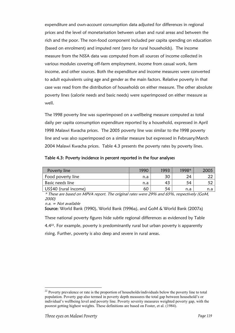
Three eyes on Malawi Poverty Page 119
expenditure and own-account consumption data adjusted for differences in regional
prices and the level of monetarisation between urban and rural areas and between the
rich and the poor. The non-food component included per capita spending on education
(based on enrolment) and imputed rent (zero for rural households). The income
measure from the NSSA data was computed from all sources of income collected in
various modules covering off-farm employment, income from casual work, farm
income, and other sources. Both the expenditure and income measures were converted
to adult equivalents using age and gender as the main factors. Relative poverty in that
case was read from the distribution of households on either measure. The other absolute
poverty lines (calorie needs and basic needs) were superimposed on either measure as
well.
The 1998 poverty line was superimposed on a wellbeing measure computed as total
daily per capita consumption expenditure reported by a household, expressed in April
1998 Malawi Kwacha prices. The 2005 poverty line was similar to the 1998 poverty
line and was also superimposed on a similar measure but expressed in February/March
2004 Malawi Kwacha prices. Table 4.3 presents the poverty rates by poverty lines.
Table 4.3: Poverty incidence in percent reported in the four analyses
Poverty line 1990 1993 1998* 2005
Food poverty line n.a 30 24 22
Basic needs line n.a 43 54 52
US$40 (rural income) 60 54 n.a n.a
* These are based on MPVA report. The original rates were 29% and 65%, respectively (GoM,
2000)
n.a. = Not available
Source: World Bank (1990), World Bank (1996a), and GoM & World Bank (2007a)
These national poverty figures hide subtle regional differences as evidenced by Table
4.422
. For example, poverty is predominantly rural but urban poverty is apparently
rising. Further, poverty is also deep and severe in rural areas.
22
Poverty prevalence or rate is the proportion of households/individuals below the poverty line to total
population. Poverty gap also termed in poverty depth measures the total gap between household‟s or
individual‟s wellbeing level and poverty line. Poverty severity measures weighted poverty gap, with the
poorest getting highest weights. These definitions are based on Foster, et al. (1984).

Three eyes on Malawi Poverty Page 120
Table 4.4: Rural and urban poverty incidence in Malawi
Year Prevalence (%) Poverty gap (%) Poverty severity (%)
Urban Rural Urban Rural Urban Rural
1985 9 60 n.a n.a n.a n.a
1993 20 42 7 17 4 10
1998 19 58 5 20 2 9
2005 25 56 7 19 3 9
Source: World Bank (1990), World Bank (1996a), GoM (2000), GoM & World Bank
(2007a)
Other estimates of urban poverty in 1980s put the incidence at 65%, which is much
higher than the World Bank estimate of 9% (GoM & UN, 1993). At least between 1998
and 2005, urban poverty appears to have increased although its depth and severity, it
has not changed as much. In terms of regions, poverty is highest in Southern Region;
making it a disproportional host of the poor (Table 4.5) and Figure 4.2.
Table 4.5: Regional poverty incidence and population shares in percent
Year Population share Poverty rate Poor people's share
South Centre North South Centre North South Centre North
1993 51 39 10 n.a. n.a. n.a. 66 27 7
1998 47 42 11 68 48 56 62 57 62
2005 40 38 10 64 47 56 50 34 11
n.a. = Not available. Regional poverty rates would have been determined by superimposing the
40% poverty line on the regional income measure. This was not done.
Source: World Bank (1996a), GoM (2000); GoM & World Bank (2007a)
Figure 4.2: Regional poor population share to total population share (%)
Source: World Bank (1996a), GoM (2000), and GoM & World Bank (2007a)
0.0
20.0
40.0
60.0
80.0
100.0
120.0
140.0
South Centre North Urban
1993
1998
2005

Three eyes on Malawi Poverty Page 121
Only in 2005 did the share of the poor in the North surpass the share of the regional
population share. Central Region has always contributed to the population of the poor
below its total population share. Likewise, urban areas are underrepresented in the
population of the poor based on the 2005 statistics23
. See Table 4.6.
Table 4.6: Poverty measures by region
Region 1998 2005
Incidence Gap Severity Incidence Gap Severity
Urban areas 18.5 4.8 1.8 25.4 7.1 2.8
Rural areas 58.1 20.2 9.2 55.9 19.2 8.6
Northern Region 56.3 19.5 8.9 56.3 19.6 8.8
Central Region 47.6 14.4 6.0 46.7 14.1 5.9
Southern Region 68.4 25.7 12.3 64.4 23.8 11.2
MALAWI 54.1 18.6 8.5 52.4 17.8 8.0
Source: GoM & World Bank (2007a)
According to the 2007 analysis (GoM & World Bank, 2007), there are pockets of
poverty all over the country but poverty is deepest in the tips of the country (i.e.
Nsanje, the Southernmost, and Chitipa, the Northernmost) and severest in the Southern
Region. Although there were some differences between the 1998 and 2005 data sets in
quality and the 2000 and 2007 methods of analysis, Southern region emerges as the
poorest of three. The poorest district in both analyses was from the Southern Region,
although it was not the same district. Of the poorest five districts in the 2007 analysis,
four are from the Southern region and out of the five richest districts, only one is from
the Southern Region. Again, based on the 2007 analysis, ten of the eleven districts in
the Southern Region had poverty rates above the national average as opposed to three
out of nine districts in the Central Region. Poverty in cities is generally low. See Table
4.7 which is based on the two latest poverty analyses24
.
This is also true for the 1995 analysis. In the 1995 analysis, major cities had lowest
prevalence of poverty, except for Lilongwe city (World Bank, 1996). Since then the
status of the cities has been fluid; Lilongwe was richest in 1998 but second richest in
2005. The 1996, 2000 and 2007 analyses starting from 1995 shows that poverty is
generally rising in urban areas.
23
Note that in the 2007 analysis, urban areas were considered separately while in the 2000 analysis the
various urban areas were within the regional totals. 24
The district results, unlike the regional results, are not directly comparable. The focus is on the
proportion of districts above or below the national average as calculated in that analysis rather than
whether district poverty has changed or not.

Three eyes on Malawi Poverty Page 122
Table 4.7: District poverty rates, 1998 and 2005
Region/district 1998 2005 Region/district 1998 2005
Northern Rural 62.5 56.3 Southern Rural 68.1 64.4
Chitipa 71.3 67.2 Chiradzulu 74.0 63.5
Karonga 42.1 54.9 Mangochi 69.8 60.7
Rumphi 65.8 61.6 Machinga 63.5 73.7
Nkhata Bay 47.7 63.0 Phalombe 83.9 61.9
Mzimba 67.5 50.6 Mulanje 67.2 68.6
Central Rural 62.8 46.7 Thyolo 76.8 64.9
Nkhotakota 65.3 48.0 Zomba Rural 71.9 70.0
Ntchisi 76.3 47.3 Blantyre Rural 65.3 46.5
Dowa 53.6 36.6 Mwanza 71.4 55.6
Kasungu 48.9 44.9 Chikwawa 54.8 65.8
Mchinji 68.0 59.6 Nsanje 51.3 76.0
Lilongwe Rural 65.6 37.5 Mzuzu City 70.9 34.0
Salima 60.8 57.3 Lilongwe City 37.9 24.6
Dedza 73.3 54.6 Zomba City 78.0 28.7
Ntcheu 84.0 51.6 Blantyre City 60.5 23.6
Source: GoM (2000) and NSO, 2010
4.4 Self-rated poverty from the subjective assessment studies
The bases of this section are three surveys all of which included a subjective wellbeing
module in household living standards questionnaires all of which were conducted in
2005. As described in Chapter 3, one of the 2005 surveys, IHS2 was conducted jointly
designed and analysed by Malawi Government and World Bank officials the officials
(GoM & World Bank, 2007a and 2007b). Apart from the officials, the dataset including
the subjective assessment wellbeing module was analysed by Devereux and colleagues
(2006). Again, the two small nationally representative surveys (CPS5) and MOPS were
conducted by the Centre for Social Research but the data was not analysed as part of
poverty analysis25
. The presentation starts with two small studies.
4.4.1 Self-assessed poverty under CPS5
The subjective module in CPS5 included perception questions on life satisfaction,
adequacy of food consumption, housing, clothing, health care, child education, and
total income. It also covered perceptions on economic situation and circumstances
compared to a year, three years and ten years earlier. The respondents were requested
to give reasons for the given household status. Further, the questionnaire used a ten-
step ladder for the respondent to position the household in terms of economic
wellbeing, rights, and ability to change circumstances.
25
These two studies have already been introduced in Chapter 3 Section 6.

Three eyes on Malawi Poverty Page 123
Consumption adequacy question
The consumption adequacy question covered six dimensions of wellbeing namely food,
housing, clothing, health care, schooling and income. Judging from the proportion of
households that had less than adequate in terms of their household needs, income is the
most binding dimension followed by clothing and health care. Of all the six dimensions,
adequacy rates (a sum of „just enough‟ and „more than enough‟) are highest in housing
(64%) followed by schooling (58%) and food consumption (51%). Income and
clothing have the least proportion of households with „at least adequate income‟ (30%)
and „clothing‟ (33%), respectively. See Figure 4.3.
Figure 4.3: Consumption adequacy in various wellbeing dimensions
(% of respondents)
Source: Author‟s computations from CPS5 dataset
Taking those that indicate having less than adequate as being poor in that wellbeing
dimension and averaging across the six dimensions, the poverty rate is 53%. Using this
crude method, the subjective perceptions in the six dimensions approximate the poverty
rate in the same year of 52% (GoM & World Bank, 2007a). This is also matched by the
evaluation of current household status if 'struggling' and 'unable to meet needs' are
combined to represent the poor status; the poverty rate is 56 percent26
. As concluded
earlier on, having similar poverty rates does not mean similarities of dimensions these
different questions are dealing with.
26
The codes for the question are „struggling‟, „unable to meet needs‟, „doing just okay‟ and „doing well‟.
70 68
49 53
3642
27 30
41
46
55
56
3 210
19
1
0%
10%
20%
30%
40%
50%
60%
70%
80%
90%
100%
Income Clothing Food cons Health care Housing Schooling
Less than adequate Just adequate More than adequate

Three eyes on Malawi Poverty Page 124
Life evaluation statements
The CPS5 had five life evaluation statements that required the respondent to indicate
the strength of agreement or disagreement. These are (i) „I am satisfied with my life‟,
(ii) „so far I have gotten the important things I want in life‟, (iii) „If I could live my life
over, I would change almost nothing‟, (iv) „In most ways my life is close to my ideal‟
and (v) „the conditions of my life are excellent‟ . The options were „strongly disagree‟,
disagree‟, neither agree nor agree‟, „agree‟ and „strongly agree‟. Figure 4.4 presents the
findings after the five options are collapsed into three categories „disagree‟ for „strongly
disagree‟ and „disagree‟ and „agree‟ for „strongly agree‟ and „agree‟. Note that the
proportion of households that are neutral is generally small compared to the others.
Figure 4.4: Respondents perceptions on various aspects of life in percent
Source: Author‟s computations from CPS5 dataset
What is noteworthy is that the perceptions display some consistencies. For example, the
proportion that disagreed that their life was satisfactory (55%) is close to the average
obtained from the six wellbeing dimensions (53%) seen above. The findings could imply
that the majority of people do not have what they would like to have and given a
chance to turn back the clock and capability they would change almost everything. In
other words, although some people are satisfied with their current life, that life is not
excellent and ideal since it lacks some elements they feel are important.
Considering that the majority implicitly said that given a chance to live their life over
they could change some things, it may be worthwhile to check their perceptions on their
agency (i.e. power to change things). CPS5 had three statements on people‟s agency.
55
82
69 6974
43
1727 25 24
0%
10%
20%
30%
40%
50%
60%
70%
80%
90%
100%
Life satisfaction Important things Change nothing Ideal life Excellent life
Disagree Neither Agree

Three eyes on Malawi Poverty Page 125
These are „my life is determined by my own actions‟, „I have the power to make
important decisions that change the course of my life‟, and „I am usually able to protect
my personal interests‟. Figure 4.5 gives the picture.
Figure 4.5: Proportion of respondents holding the perceptions on agency in percent
Source: Author‟s computations from CPS5 dataset
Judging from the high proportion of households who agree with the statements on
responsibility of actions, power to change course of life and ability to protect personal
interests, people in Malawi are not particularly fatalistic (64%, 71% and 71%,
respectively). This reduces the probability of blaming either government, god or
somebody else for their condition. Indeed only a small proportion attributed their state
affairs to god (2% of those who had improved status) or bad luck (0.2% of those
whose status declined).
Ladder of life ratings
Three ten-step ladders were presented to respondents to rate their households in terms
of economic status, power and rights and agency dimensions. On economic wellbeing
the question was: 'imagine that at the bottom, on the first step, stand the poorest and
worst off, and the highest step, the tenth, stand the richest and best off. On which step
of this ladder are you located today?' On power and rights the question was 'And now
imagine, please, another 10-step ladder, where at the bottom, on the first step, stand
people who are completely powerless and without rights, and the highest step, the
tenth, stand those who have a lot of power and rights. On which step of this ladder are
you today?' The third, on power to change things, the question was 'Now imagine,
32 26 23
53 6
6471 71
0%
10%
20%
30%
40%
50%
60%
70%
80%
90%
100%
Own actions Power to change Protect interests
Disagree Neither Agree

Three eyes on Malawi Poverty Page 126
please, another 10-step ladder, where at the bottom, on the first step, stand people who
are completely powerless to change the course of their lives, and the highest step, the
tenth, stand those who have the power to change the course of their lives. On which
step of this ladder are you today?'
To facilitate discussions, three arbitrary wellbeing groups are imposed. The first (poor)
covers steps 1 to 3, the second (in-betweeners) covers steps 4 to 7, and the third (richest)
covers the rest. Further, borrowing from Devereux, et al. (2006), a poverty line is
imposed on step 4 thereby labelling all households in the first group „poor‟. Figure 4.6
presents the proportion of the three groups in the three dimensions of wellbeing. Note
that the economic poverty rate of 53% is very comparable to the objective poverty rate
of 52%.
Figure 4.6: Proportion of respondents in various categories in percent by dimension
Source: Author‟s computations from CPS5 dataset
Again, the low agency poverty rate (26%) mirrors the findings on the perceptions on
agency reported above. In particular it is the same as that reported for power to change
the course of one‟s life. In any case, just like when six dimensions of wellbeing were
examined using a five point scale, economic wellbeing is the most constrained of all
dimensions amongst households in Malawi. The group of the richest dramatically
increase from only 3% under economic wellbeing to 16% in power and rights and 21%
in agency. Apparently, the Malawi bill of rights introduced in 1995 liberated many but
may not have translated into access to economic resources.
53
3326
43
5153
316 21
0%
10%
20%
30%
40%
50%
60%
70%
80%
90%
100%
Economic wellbeing Power and rights Agency
Poor In-betweeners Richest

Three eyes on Malawi Poverty Page 127
Changes in household economic situation and circumstances
CPS5 has two different types of questions that compare the current with previous
economic status. The first compares the current household circumstances with
circumstances three, five and ten years ago and has seven possible read-out responses:
„rich‟, comfortable‟, „manage to get by‟, „never quite enough‟, „poor‟ and „destitute‟.
The second question enables the respondent to consider all wellbeing dimensions they
find important and reads: „comparing the current overall economic situation of your
household with that one year ago, would you say it is much better now, a little better
now, the same, a little worse now, or much worse now?‟.
Responses to the first question show that over the ten year period between 1995 and
2005, the rich did not grow richer as the poor grew poorer because both grew poorer.
For example, 2% of the population were very rich in 1995 but by 2000 this group had
vanished as poverty measured by the sum of those that were „destitute‟, „poor‟ and
„never quite enough‟ increased from 46% to 51% by 2002. Apparently, the gainers
have been those who simply 'managed to get by' whose proportion increased from
24% to 28% to 33% over the ten year period. See Table 4.8.
Table 4.8: Respondents rating of household circumstances in percent
Rating
3 years ago
(2002)
5 years ago
(2000)
10 years ago
(1995)
n=480 n=476 n=460
Very rich 0 0.2 1.7
Rich 2.7 4.0 5.7
Comfortable 13.3 16.8 23.0
Managed to get by 33.3 28.4 23.9
Never quite enough 25.8 27.1 25.9
Poor 21.3 19.5 15.4
Destitute 3.5 4.0 4.3
Source: Author‟s computations from CPS5 dataset
The growth in the „middle class‟ is supported by the findings from the question on
overall economic situation. If three groups are constructed from the responses i.e. those
who did better (much better now and a little better now), those whose situation did not
change (same) and those who did worse (much worse now and a little worse now), the
proportions are 22%, 41% and 37%, respectively. Taken together, these findings also
show that inequality has improved between 1995 and 2005. The findings also show that
economic poverty can co-exist with food adequacy and that income poverty does not
imply food poverty.

Three eyes on Malawi Poverty Page 128
4.4.2 Self-assessed poverty under MOPS
The MOPS also used ten-step ladders for respondents to rate their households‟ economic
wellbeing status, power and rights, and happiness. The question for the economic
wellbeing was: “Here is a picture of a 10-step ladder. Imagine that at the bottom, on the
first step, stand the poorest and worst off people, and on the highest step, the tenth,
stand the richest and best off. On which step of this ladder are you located today? And
on which step were you located 10 years?‟ The question for the power and rights
dimension was similar only that on the first step „stand people who are completely
powerless and without rights‟, and the highest „stand those who have a lot of power
and rights‟. For the happiness dimension step 1 is for the sad and step 10 is for happiest.
General changes between 1995 and 2005
In line with the assumptions made for CPS5, the poorest are on steps 1 up to 3, the
richest are on steps 8 to 10 with the rest as in-between, again to facilitate discussions.
Table 4.9 presents the proportions for the three wellbeing dimensions for 1995 and
2005 for each step.
Table 4.9: Self-assessed household positions on 10-step ladder in 1995 and 2005
(% of households)
Ladder step Economic wellbeing Power and rights Happiness
1995 2005 1995 2005 1995 2005
n=139 n=139 n=132 n=139 n=137 n=138
Step 1 18.0 20.1 12.9 10.1 11.7 12.3
Step 2 18.7 13.7 15.9 7.9 11.7 13.0
Step 3 18.0 12.9 13.6 10.8 13.9 12.3
Step 4 10.8 12.9 12.1 18.0 10.2 8.7
Step 5 16.5 15.1 12.1 13.7 19.0 11.6
Step 6 5.0 7.9 9.8 12.2 10.9 8.0
Step 7 5.8 9.4 9.8 7.9 7.3 8.7
Step 8 5.0 4.3 6.1 7.2 7.3 12.3
Step 9 0.7 2.2 2.3 7.9 2.2 3.6
Step 10 1.4 1.4 5.3 4.3 5.8 9.4
Source: Author‟s computations from MOPS dataset
Just like in the case of CPS5, poverty is more prevalent in the economic wellbeing
dimension and the situation improved over the ten year period. The proportion of the
poor economic wellbeing and power-rights respectively declined over the ten-year
period from 55% to 47% and from 42% to 29%. On the other hand, the proportion
of the saddest marginally increased as the proportion of the happiest significantly
increased.

Three eyes on Malawi Poverty Page 129
Of the three dimensions, the economic wellbeing and power-rights seem to have similar
patterns. They both saw the proportions of the non-poor groups increase between 1995
and 2005. On the other hand, the happiness dimension registered declines in the
proportion of the in-betweeners and increase in the proportion of the richest in the
same period (Figure 4.7). This implies that there are other factors that influence
happiness over and above economic wellbeing, power and rights.
Figure 4.7: Proportion of households in wellbeing categories in percent, 1995-2005
Source: Author‟s computations from MOPS dataset
Mobility status
The data on the three ladders can also be analysed in terms of simple mobility status;
those that moved at least one step up or down or none at all since 1995. The economic
wellbeing ladder can also be analysed in terms of poverty mobility status, assuming step
4 to be the poverty line. It can also be analysed in terms of wellbeing category mobility
status among the three groups (poorest, in-betweeners and richest) as defined under
CPS5 and used above. Table 4.10 presents the household mobility status in the three
wellbeing domains on the basis of at least one step movement.
5547
42
2937 38
3845
44
52
47
37
7 814
1915
25
0%
10%
20%
30%
40%
50%
60%
70%
80%
90%
100%
1995 2005 1995 2005 1995 2005
Economic wellbeing Power and rights Happiness
Richest
In-betweener
Poorest

Three eyes on Malawi Poverty Page 130
Table 4.10: Proportion of households in percent by mobility status and dimension
Type of move Economic wellbeing Rights Happiness
n=139 n=132 n=137
Upward movement 48.9 44.7 46.0
No change 14.4 29.5 16.1
Downward movement 36.7 25.8 38.0
Source: Author‟s computations from MOPS dataset
In all domains, there were more households that improved their status than those
whose status declined or remained the same. In general, there is more change than
stability and that instability is most prevalent in economic wellbeing and least in power
and rights. It is noted that the movements in economic wellbeing are mirrored by those
in the happiness dimension.
It is, therefore, tempting to link economic wellbeing and happiness seeing their
similarities. Indeed a correlation analysis of household mobility from 1995 to 2005
shows strong relationship between economic wellbeing and happiness. The two have a
Pearson Correlation coefficient of 0.642 which is significant at 1% level. As expected,
the mobility becomes reduced when the three groups are used because movements
within a group are not considered. Using the economic wellbeing dimension, 27% of
households moved up (from poorest to either in-betweeners or richest and from in-
betweeners to richest) and 19% moved down (from richest to in-betweeners or poorest
and from in-betweeners to poorest). The largest movement was from poorest to in-
betweeners (22%) followed by in-betweeners to poorest (14%). Only two households
managed to move from being among the poorest in 1995 to being among the richest in
2005. On the other hand, only one household had the misfortune of becoming one of
the poorest in 2005 from being one of the richest in 1995.
The general picture is that maintenance of one‟s economic wellbeing group was more
prevalent than change as evidenced by the fact that 55% of the households did not
change their group over the period. This is represented by the diagonal in the mobility
matrix presented in Table 4.11 (i.e. 32% poorest, 20% in-betweeners and 3% richest).
The implication of this is that most of the movements presented in Table 4.9 were small
step movements.

Three eyes on Malawi Poverty Page 131
Table 4.11: Proportion of households in wellbeing categories in percent 1995-2005
Group Poorest In-betweeners Richest 2005
Poorest 31.7 21.6 1.4 54.7
In-betweeners 14.1 20.2 3.7 38.0
Richest 0.7 3.7 2.9 7.3
1995 46.5 45.5 8.0 100
Source: Author‟s computations from MOPS dataset
When the households are divided between poor and nonpoor with step 4 as the
poverty line, the mobility is further constrained. Only 23% poor households crossed
the poverty line and 15% nonpoor households moved into poverty (Figure 4.8). This
implies that 37% of the households changed their economic status while 32% remained
poor and 30% remained nonpoor between 1995 and 2005.
Figure 4.8: Household economic status mobility status between 1995 and 2005
Source: Author‟s computations from MOPS dataset
The trend is what is expected as the households are aggregated. With ten groups (each
step representing a group) very few households maintained their positions. With three
groups and two groups, the mobility was highly checked because most of the moves
were very small. In fact, if only 3-step movements are considered to be meaningful27
,
only 17% of households would qualify to have improved their status and 13% lost out
over the period. As Figure 4.9 shows, more households moved up than down.
27
Although the three is an arbitrary number it is chosen because with three steps, a household can change
welfare groups especially if it is in the poorest or richest groups.
Poor-Rich23%
Rich-Poor15%
Poor-Poor32%
Rich-Rich30%

Three eyes on Malawi Poverty Page 132
Figure 4.9: Household mobility status by type of movement, 1995 and 2005
(% of households)
Source: Author‟s computations from MOPS dataset
When the ratings under the CPS5 and MOPS are compared it can be concluded that by
and large people‟s perceptions are consistent and differences between the two studies
can be explained by differences in questionnaire design28
. For example, both studies
were conducted in the same year and households and by the same institute, researcher
(the author) and field manager and research assistants. This fixes most of the factor that
can introduce differences.
For simplicity, the comparisons are based on the proportions of the top and bottom
three steps on the ladder of economic wellbeing (poorest and richest). Figure 4.10
presents the proportions of households in the bottom and top 3 steps on economic
wellbeing and power and rights ladders for the two surveys.
28
Both studies were conducted in the same year and households and by the same institute, researcher (the
author) and field manager and research assistants. This fixes most of the factor that can introduce
differences.
2327
49
1519
37
62
55
14
0
10
20
30
40
50
60
70
Poverty Group Step
Upward movers Downward movers No movers
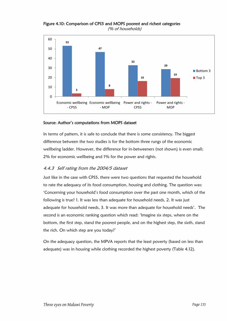
Three eyes on Malawi Poverty Page 133
Figure 4.10: Comparison of CPS5 and MOPS poorest and richest categories
(% of households)
Source: Author‟s computations from MOPS dataset
In terms of pattern, it is safe to conclude that there is some consistency. The biggest
difference between the two studies is for the bottom three rungs of the economic
wellbeing ladder. However, the difference for in-betweeners (not shown) is even small;
2% for economic wellbeing and 1% for the power and rights.
4.4.3 Self rating from the 2004/5 dataset
Just like in the case with CPS5, there were two questions that requested the household
to rate the adequacy of its food consumption, housing and clothing. The question was:
„Concerning your household‟s food consumption over the past one month, which of the
following is true? 1. It was less than adequate for household needs, 2. It was just
adequate for household needs, 3. It was more than adequate for household needs‟. The
second is an economic ranking question which read: „Imagine six steps, where on the
bottom, the first step, stand the poorest people, and on the highest step, the sixth, stand
the rich. On which step are you today?‟
On the adequacy question, the MPVA reports that the least poverty (based on less than
adequate) was in housing while clothing recorded the highest poverty (Table 4.12).
53
47
33
29
3
8
1619
0
10
20
30
40
50
60
Economic wellbeing - CPS5
Economic wellbeing - MOP
Power and rights -CPS5
Power and rights -MOP
Bottom 3
Top 3

Three eyes on Malawi Poverty Page 134
Table 4.12: Proportion of households in percent by type of adequacy and dimension
Domain Less than adequate Just adequate More than
adequate
Food 57.2 36.5 6.1
Housing 55.4 40.0 5.6
Clothing 72.6 25.6 1.8
Health 60.9 35.9 3.11
Source: GoM and World Bank (2007b) Table A3.1
This varied by region. Using those reporting less than adequate consumption or
expenditure, the least poverty was recorded on food consumption in Rural North and
the highest was recorded on expenditure on clothing in Rural Centre (Table 4.13). In
general, households in Rural North have the least self-assessed poverty based on the
four domains. Rural Centre households in general feel the most poor. This is because
they feel most poor in all domains except in food consumption.
Table 4.13: Proportion of households with adequate consumption in percent
Region Food Housing Clothing Health
Urban 48.3 44.1 54.5 51.8
Rural North 35.1 36.1 52.1 43.0
Rural Centre 59.2 60.3 84.2 65.6
Rural South 63.9 58.8 71.8 63.7
Source: GoM and World Bank (2007b) Table A3.2
On the economic ranking question, the MPVA found that step 2 (1.8) was the average
for the population, implying on average people rated themselves as mostly poor. The
ranking varied by region with urban households having the highest average rank of 2.3
followed by Rural North (1.9) then Rural Centre (1.7) and finally Rural South (1.6).
Unlike the consumption/expenditure adequacy where Rural Centre was the poorest,
Rural South is the poorest on economic wellbeing analysis. Using regression analysis to
determine the poverty line from the MIQ following the Leyden methodology (van
Praag, et al., 1982), MPVA found a subjective poverty rate of 80% (GoM & World
Bank, 2007b).
MPVA did not impose a poverty line on the six-step ladder to directly determine the
subjective poverty from the ladder. On the other hand, Devereux, et al. (2006) created
a poverty status dummy variable with code 1 standing for the poor for households that
rated themselves to be on steps 1 and 2 and 0 for the non-poor on steps 3 to 6. This
implies step 3 was designated as the poverty line „after examining the data and

Three eyes on Malawi Poverty Page 135
frequencies of households falling into each category‟29
. The data was categorised into
four regions, namely Urban, Rural North, Rural Centre, and Rural South. The respective
self-assessed poverty rates were 65%, 79%, 84% and 91%. The poverty rates show
that self-assessed poverty incidence increases as from the North to South and from urban
to rural areas.
4.5 Comparisons of objective and subjective assessments
The Malawi Poverty and Vulnerability Assessment (GoM & World Bank, 2007b) found
that the objective and subjective poverty lines are consistent with each other. They also
found that that per capita consumption is a strong predictor of subjective poverty.
When household per capita consumption and the ladder step were compared, they
found that they are strongly correlated (GoM & World Bank, 2007b). The conclusion
was that self-rated poverty and objective poverty are related. On poverty rates, The
Malawi Poverty and Vulnerability Assessment (GoM and World Bank, 2007b) used
regression analysis to determine the poverty line from the MIQ following the Leyden
methodology (van Praag, et al., 1982) and found a subjective poverty rate of 80%
which is higher than 52% for the consumption-expenditure poverty. Devereux and
colleagues (2006) found that subjective poverty is higher than objective poverty by at
least 30% (Figure 4.11).
29
This is still arbitrary because the six steps have no categories. The poverty line is set by the experts.
Possibly, the best was to state that the step was arbitrary but useful for some analysis or state „we are
convinced that step 3 is the best poverty line‟.

Three eyes on Malawi Poverty Page 136
Figure 4.11: Objective and subjective poverty rates by region
Source: Devereux, et al. (2006) Figure 20
Thus both studies on IHS2 found that subjective poverty rate is higher than objective
poverty rate. This confirms the finding other studies elsewhere that subjective poverty
rate is generally higher than objective poverty rate. Whether this is also true in the three
villages is examined next.
21
48
38
55
65
7984
91
0
10
20
30
40
50
60
70
80
90
100
Urban Rural North Rural Centre Rural South
Objective Subjective

Three eyes on Malawi Poverty Page 137
Chapter 5: Wellbeing status from three perspectives
5.1 Introduction
This chapter is dedicated to responding to the research question whether the official
measure of wellbeing and poverty is the same as peer assessment and self-rating in terms
of poverty rates and the households each identifies. This is done by presenting and
comparing findings from the three perspectives of experts, community and households
using countrywide data and that from the three sampled villages. The chapter starts
with profiling the three villages. It then presents the poverty rates by type of wellbeing
assessment. Comparisons of the rates and the people each assessment found in the three
are made before concluding the chapter with the responses to the research questions.
5.2 Profiles of the three visited villages
Before going into poverty analysis, this section sketches the characteristics of the three
villages in the sample. The qualitative information was gathered during the field visits
through observation and the focus group discussions. The profiles start with
presentations of basic facts about each village. This is followed by a presentation of the
basic socio-economic data from the questionnaires administered in the villages. The idea
is to give an idea of what the villages are like in order to appreciate the findings that
follow.
Ngochera Village
Ngochela village is under Area Chief Mlumbe in Zomba district. The village lies at the
foot of the western side of Zomba plateau and situated between Chinseu and Chingale
trading centres. Each of these trading centres has its market day, giving the village (and
many others in the area) two main trading days in a week. Just like many villages in
Chingale area, land is not a binding constraint.
The area, and by extension Ngochera village, is relatively closed. The nearest main road
is approximately thirty kilometres away. It is served by some dirty roads, one down the
mountain from Zomba district headquarters and another parallel the mountain range
joining the Zomba-Lilongwe Road close to Machinga district headquarters. Just like the
mountain road, the parallel road is almost impassable during the rainy season because
the many streams from the mountain cross and cut or flood it. Bicycle taxis thrive in the
area and operating a bicycle taxi is one of income earning opportunities. As an isolated
area, manufactured goods are relatively expensive and produce relatively cheap as the
Three eyes on Malawi Poverty Page 138
law of demand and supply force farmers to reduce their asking prices to attract buyers
into the area.
The village is one of the closest to the closed Changalume cement quarry, now an army
barracks. Before the quarry was closed the livelihood of the village depended on the
quarry. After the closure of the quarry, the most enterprising in the village have turned
to natural resource exploitation in the form of charcoal making, firewood collection,
bamboo collection and basket making for sale at the barracks or Zomba district
headquarters. Subsistence farming is one of the few constants. Those with some capital
venture into vending.
There is limited presence of government in the area in general and village in particular.
A school exists nearby but in another village. Likewise, a health centre operates within a
walking distance. The most common safety net programme operating in the village in
the past three years has been a Government inputs subsidy. An NGO, World Vision
International, has successfully run irrigation projects in the area but this village has never
benefited. There is no organisation offering credit to village members and indeed
running any activity in the village.
Chikhwaza Village
This village falls under area chief Chimaliro of Thyolo district. It is roughly 20 kilometres
from the district headquarters. Blantyre, the commercial capital of the country, is
roughly 30 kilometres away. The village is located on sub-prime land in the fringes of
tea estates. Household landholding sizes are very small. Farming without fertilizers is
virtually useless because the soil is overused. One of the key features in the village is that
its people are enterprising since almost everything in the village, including firewood, has
to be purchased.
The village is accessible. It is about five kilometres from the main road and it is fed by a
gravel road that is generally passable even during rainy season. A dirty road leading to
the centre of the village (where the village head is located) is not passable during the
rainy season because of the quality of the road and terrain. Two major produce
markets within ten kilometres of the village are available to the village. Many take
advantage of these as sellers or buyers or traders while more enterprising ones go as far
as Blantyre city.
The village has no school but the nearest school is located in the next village and pupils
easily walk there even during the rainy season. There are no clinics in the village.

Three eyes on Malawi Poverty Page 139
However, the closest clinic is less than 8 kilometres. More present in the village than
anything else are buildings of Christian denominations. In this village of possibly 300
households, there are over ten denominational church buildings. Some of the buildings
are used as pre-school and adult education classes. The village has at least one borehole
working.
Being close to estates, a few members of the village are estate workers and their pay is
more poverty alleviating than reducing. Close to the village is a dairy farm which
purchases milk from smallholder farmers and also breeds milk cows for sale. A number
of village members participate in the dairy business. The village also boasts of a number
of grocery shops run by village members. Some households with land in the dambo
area have taken on winter cropping to grow vegetables and green maize for sale.
These as well as dairy farmers are considered the well-to-do of the village.
The houses are mostly built with bricks and roofed with iron sheets, mainly out of
necessity and not riches. The village does not have trees (mostly used for house building)
and grass suitable for house thatching. Most of building materials, including poles and
grass have to be bought. Since grass and poles are not permanent, any time a household
gets some money, building a semi permanent or permanent house becomes a priority
since such structures save money in the long run.
Although there are no national or international organisations operating in the village,
there are a number of CBOs including those dealing in credit extension, managing pre
schools and adult education classes and caring for the elderly and orphans. The presence
of these organisations, though small scale, combined with the proximity to the road,
major produce markets and the city puts Chikhwaza at a relative advantage compared
to Ngochera; they enable Chikhwaza adopt intensive agriculture to maximise land use
to take advantage of available markets. On the other hand, lack of markets and access
to markets make the relative abundant land enjoyed by Ngochera of no major
consequence.
Dzilekwa Village
This village is under area chief Mpando of Ntcheu District. It is five kilometres away
from the district headquarters (slightly less using foot paths). The village lies along a
permanent gravel road that leads to a main source of Irish potatoes in the country. The
road also acts as a boundary between Malawi and Mozambique. Thus Dzilekwa is a
border village. Some relatives of residents of Dzilekwa are Mozambican (i.e. across the

Three eyes on Malawi Poverty Page 140
road) and many members of the Dzilekwa village cross into Mozambique to farm and
collect firewood.
Farming is the main occupation of the village. Apart from maize and beans, Irish potato
is the major poverty reducing crop. Other crops, though not as lucrative include
cabbage, tomato, onions and carrots. Progressive farmers grow these crops thrice a
year. Some rent land on the Mozambican side where irrigatable land is relatively
abundant. A major trading centre at the edge of village on the main road connecting
the South and Centre of the country provide opportunities for produce trading, casual
work (ganyu) and trading in general. Produce marketing is done on Tuesday and attracts
farmers, buyers, and traders from Malawi as well as Mozambique. The farming in the
village owes its viability to this market and that at the district headquarters.
Transporting of produce especially Irish potatoes, cabbages, tomato, carrots and onions
to the market also provides some business opportunities for village members around the
market including Dzilekwa. Transporting the produce from farm gates to the market
provides some income generating opportunities for head, bicycle and ox-cart
transporters, apart from those with trucks. More importantly, the market is the major
„wholesale‟ market for Irish potatoes, tomatoes, cabbages, onions and carrots. The
processing of the goods provides casual work village members who bulk and load the
produce for onward transport. The process also provides business for empty bag and
basket makers and sellers. According to some informants of Dzilekwa village, the market
acts as a mine for the village. The majority of young men in the village offer themselves
as packers and loaders. Enterprising women are mostly engaged in produce trading; they
buy on the market day from farmers and sell at a profit at the roadside vendor market
close by operational twenty four hours.
Dzilekwa Village members also have the opportunity to trade at the district
headquarters whose market days are Wednesday and Saturday. As a market at a district
headquarters, Ntcheu Market offers more variety but less quantity than the produce
market at the edge of the village. Thus Dzilekwa Village members have the advantage
of trading two busy markets and sourcing of their needs at both markets with minimum
cost. Dzilekwa also boasts of a market in the village, easy access to energy sources, and
grass and trees for house construction. Very few houses have roofs with corrugated iron
sheets. This is even true for households considered relatively well off. Most of residents
enjoy drinking beer and excessive drinking especially at the trading centre is said to be
common especially for young and middle aged men who spend most of their time at
the market. The market offers a combination of income generation, beer drinking and

Three eyes on Malawi Poverty Page 141
prostitutes. On the basis of the focus group discussions, it is very common to make and
misuse money at the market before the rest of family benefits.
Of all the villages visited, Dzilekwa is the easiest to access. It also has the most income
earning opportunities, although employment is not necessarily one of the opportunities.
Irish potato farmers and traders can make a lot of money. Again, those with strength to
work as loaders can also make money. Chances of generating sizeable income by many
people are slim in Chikhwaza and almost non-existent in Ngochera. Dairy farming and
winter cropping is open to a few in Chikhwaza and their returns are not as high.
Natural resource exploitation in Ngochera has limits as its returns are very low.
A comparison of the villages based on data collected
The three villages are „measured‟ based on a national rural average obtained from the
integrated household survey conducted in 2004/5. The idea is to check whether the
villages visited are way out of the ordinary. Such information helps put the findings in
perspective. Although the three villages are compared, the focus is on the position of
each village against the national picture.
Table 5.1 presents the average household sizes in the three villages. Ngochera
household size is the farthest from the national rural average of 4.6 persons. Chikhwaza
is the closest. Nonetheless Ngochera is not atypical of villages in rural Southern Region
where the regional average is 4.2 persons. It is in fact Chikhwaza that is not a typical
Southern Region village. The Central Region average, under which Dzilekwa Village
falls, is 4.5 persons. In general, Chikhwaza Village has households resembling the
national picture.
Table 5.1 Household size by village
Indicator Ngochera Chikhwaza Dzilekwa IHS Rural
Number of households 49 59 56 9,840
Population 202 271 238 49,192
Household size 4.1 4.6 4.3 4.6
Source: Calculations from primary data and IHS2 data set
Females generally outnumber men in the population. The 2008 census report that 52%
of the population comprise women (NSO, 2008). Similar findings are reported in the
IHS2. According to Table 5.2 and on this characteristic, Dzilekwa village is atypical as it
has more male than female residents. It is Chikhwaza that is closest to the national
average. On proportion of unmarried women in the village, Ngochera is closest to the

Three eyes on Malawi Poverty Page 142
national average. In terms of proportion of female heads, no village is typical. All the
three villages have more female heads than the average but Chikhwaza has the closest
proportion.
Table 5.2: Proportion of females by village
Indicator Ngochera Chikhwaza Dzilekwa IHS Rural
Proportion of females 50.5 52.2 48.7 51.7
Proportion of unmarried women 34.7 35.8 35.6 32.7
Proportion female heads 38.0 27.1 34.5 24.0
Source: Calculations from primary data and IHS2 data set
Table 5.3 presents some characteristics on household composition. Considering the
population of the single heads or heads with their spouses, Chikhwaza is the closest to
the national average although the others are not too far off. In terms of the proportion
of children whose parent is the head, Dzilekwa is the closest to the average with
Chikhwaza as the furthest. Dzilekwa is again the closest on average age of the village
population with Ngochera as the furthest.
Table 5.3 Household composition by village
Indicator Ngochera Chikhwaza Dzilekwa IHS Rural
% of heads & spouses in hh 39.2 37.3 38.6 36.9
% of head's children in hh 43.6 54.2 50.4 48.1
Average age (years) 28.3 20.8 22.1 21.6
% of the aged in hh 7.4 3.3 5.1 4.0
% of children in hh 54.9 54.7 51.9 52.9
Dependency ratio 1.7 1.4 1.3 1.3
Source: Calculations from primary data and IHS2 data set
The proportion of the population 65 years or older is closest to the national average in
Chikhwaza although Dzilekwa is not too far off. It is Ngochera that still has highest
proportion of senior citizens. Dzilekwa village has the proportion of children to the
total population that is closest to the national average. However, Chikhwaza and
Ngochera are not very off from the average either. It is Ngochera‟s dependency ratio
that shows that the village is laden with dependents unlike Dzilekwa, whose ratio is
similar to that of the national average.
The proportion of children living with both parents in the three villages is way above
the national average. The closest is Ngochera Village, though. Chikhwaza Village has
twice as many children living with both parents as the national average. This

Three eyes on Malawi Poverty Page 143
characteristic is apparently more area dependent and therefore more notable for its
diversity. That said all the three villages are in matrilineal societies as such being a
maternal orphan is generally worse than a paternal one because fathers are less attached
to children. In fact in all the villages there are more paternal than maternal orphans.
Double orphanage is, nonetheless, severest in Dzilekwa Village. Table 5.4 presents the
details on children characteristics.
Table 5.4: Proportion of children in household by village
Indicator Ngochera Chikhwaza Dzilekwa IHS Rural
Living with both parents (%) 56.8 73.5 61.0 36.8
Maternal orphans (%) 4.5 4.1 8.9 3.0
Paternal orphans (%) 9.0 6.8 16.3 7.4
Double orphans (%) 3.6 2.7 6.5 2.6
Source: Calculations from primary data and IHS2 data set
Table 5.5 presents a number of characteristics on religion, education and health. In
terms of religion, Chikhwaza Village which hosts more than ten Christian denominations
has 96% of its population Christian as opposed to the national average of 83%. It is
Dzilekwa that has the closet to the national average.
Table 5.5: Education and health status of household members by village
Indicator Ngochera Chikhwaza Dzilekwa IHS Rural
Christianity rate (%) 63.9 95.7 84.7 82.8
% of illiterate adults 48.0 39.1 39.5 40.8
% of no-school adults 17.3 9.6 8.9 30.6
% no-interest drop outs 17.8 19.0 33.3 20.2
% of out of school children 51.1 63.2 60.0 56.1
Morbidity rate (%) 21.3 17.0 21.8 29.1
% suffering from malaria 31.1 21.1 19.6 26.5
Source: Calculations from primary data and IHS2 data set
As for adult literacy, Chikhwaza and Dzilekwa are the closest. The national average for
the proportion of adults that never attended school is so much higher than those in the
three villages although Ngochera is closest. While lack of money for fees or uniform top
the list of reasons why some household members dropped out of school, lack of interest
also plays a major part. Of the three villages, Chikhwaza is closest to the national
average in this respect. On the proportion of children in the school-going age (6-13
years) who are out of school, Dzilekwa has the closest proportion of school-going age
children who are out of school. Using the proportion of household members who were

Three eyes on Malawi Poverty Page 144
ill or injured in the two-weeks preceding the visit, all the villages report low incidence of
illness and injury compared to the national average. However, Dzilekwa is marginally
the closest. In terms of malaria incidence, Dzilekwa Village has the closest proportion of
household members that suffered from malaria although the rest are not too far off.
Table 5.6 presents the characteristics of household heads are thought to determine the
welfare outcome of the household.
Table 5.6: Characteristics of household heads by village
Indicator Ngochera Chikhwaza Dzilekwa IHS Rural
Average age (years) 49.1 42.0 41.5 43.2
Those 65 years or older (%) 22.0 11.9 14.5 13.0
Unmarried heads (%) 35.4 29.3 32.7 26.6
In polygamy (%) 6.3 6.9 10.9 10.5
Never attended school (%) 22.0 11.9 12.5 29.4
Illiterate heads (%) 44.0 23.7 23.2 37.6
Source: Calculations from primary data and IHS2 data set
The first is age. On average, Ngochera heads of households are much older than those
of the other two villages. It has by far the highest proportion of household heads that
are older than 64 years. Chikhwaza is nonetheless closest to the national average age
although Dzilekwa is also close. Regarding marital status, the proportion of unmarried
heads in Chikhwaza village is the closest to the national average. On the other hand,
although the incidence of polygamy is lower than average in Ngochera and Chikhwaza,
it is Dzilekwa Village that has a proportion closest to the national average.
Engagement in IGA activities is season dependent, just like self-employment. The best
method to capture the seasonality is to use a year round rolling survey. This is what the
IHS2 did. It is not surprising that the national averages clearly differ from those
obtained from the three sites as depicted in Table 5.7.
Table 5.7: Household enterprises and time allocation by village
Indicator Ngochera Chikhwaza Dzilekwa IHS Rural
Has an enterprise (%) 71.4 55.9 66.1 33.4
Adults in self-employment (%) 21.1 15.8 26.3 3.8
Worked on some IGA (%) 50.9 46.0 49.3 64.8
Spent time in enterprise (%) 15 13.3 13.9 8.1
Time spent in enterprise (hours) 2.3 1.7 5.2 1.8
Source: Calculations from primary data and IHS2 data set

Three eyes on Malawi Poverty Page 145
For example, the proportion of those that ever worked on an IGA over the preceding
week was high at national level relative to those calculated for the three villages.
Likewise the time spent on the IGAs at the national level was relatively low compared
to those for the three sites. However, when it comes to the average hours spent on the
household enterprise, it is only in Dzilekwa where the average is very different from the
national average with Chikhwaza reporting average hours closest to that of the national
average. Table 5.8 presents a number of characteristics on housing and ownership of
assets. In terms of the average age of the dwelling units, the national average is above
every village average.
Note that the village averages are closer to each other than any of them is to the
national average. The proportion of dwelling units whose walls are made of burnt
bricks in Dzilekwa village is closest to the national average. As a testimony of its
proximity to natural resources, the proportion of dwelling units with burnt bricks is
more than 20% higher in Ngochera. The reverse is true for the type of roof. While
Ngochera and Dzilekwa are close to the national average for the proportion of
households with iron sheets, Chikhwaza which has no grass around has by far the
highest proportion of dwelling units with iron sheets.
Table 5.8: Housing and assets by village
Indicator Ngochera Chikhwaza Dzilekwa IHS Rural
Age of dwelling units (years) 7.6 6.8 6.9 13.6
Houses with burnt bricks (%) 57.1 32.2 26.8 29.3
Roofs with iron sheets (%) 16.3 69.5 19.6 18.2
Houses with cement floor (%) 8.2 25.4 12.5 13.6
HHs with cellular phone (%) 34.7 42.4 42.9 1.0
HHs using borehole (%) 0.0 81.4 90.9 49.9
HHs with no toilet (%) 30.6 18.6 14.3 18.2
Source: Calculations from primary data and IHS2 data set
While Chikhwaza village has the best floors, Dzilekwa is closest to the national average.
One of the developments since 2005 when IHS2 was conducted is the increase in
mobile phone use. It is almost meaningless to compare the national average with the
proportions in the three villages. Nevertheless Ngochera seems to have lagged behind
the other two villages and is therefore closest to the (2005) national average. In terms
of access to potable water, Chikhwaza and Dzilekwa are well off and way above the
national average. At the time of the visit, the Ngochera had a borehole that was not
working. As for having no toilets, Ngochera is the worst but Chikhwaza is closest to the

Three eyes on Malawi Poverty Page 146
national average. Ownership of assets in Malawi is generally low as depicted in Table
5.9.
Table 5.9 Housing and assets by village
Indicator Ngochera Chikhwaza Dzilekwa IHS Rural
Persons per one bed 8.8 8.7 11.3 18.5
Households per radio 1.7 1.5 2.2 1.8
Households per bicycle 4.9 2.4 2.4 2.6
Chickens per household 5.3 5.0 6.5 4.6
Source: Calculations from primary data and IHS2 data set
For example, there are 18 persons per beds in Malawi just as they are 2 households per
radio and 3 households per bicycle. Although all the three villages have similar
ownership patterns of beds, radios and bicycles, Dzilekwa is closest to the national
average on beds, Ngochera on radio ownership and both Chikhwaza and Dzilekwa on
bicycles. In terms of livestock, the national average for number of chickens per
household is lower than any village but the closest to the national average is Chikhwaza.
Overall comparison
One of the objectives of the profiling was to show that the villages are typical as
evidenced. In some instances a village is closest to the national average on one feature
and but furthest in another. Overall, Chikhwaza is the closest site to the national
average (Table 5.10) 30
. However, the difference between the sites is minimal when
only socio-economic indicators are considered. Using number of times a site is closest to
the national average, Chikhwaza and Dzilekwa are similar on socio-economic indicators.
Using the dispersion measure, Chikhwaza is still the closest but Ngochera is closer to the
national average than Dzilekwa.
30
Three measures are used. The first measure is constructed by assigning a 1 for the site that is closest to
the national average and zero for the other two. The second assigns a 3 for the one closest and 1 for the
furthest with 2 for the middle site. The third measures dispersion between the national average and the
site. It is constructed by calculating the proportion of the site level to the national average in percentage
terms.

Three eyes on Malawi Poverty Page 147
Table 5.10: Summary measures for closeness to national average
Indicator Ngochera Chikhwaza Dzilekwa
All indicators
Number of times site is closest 10 18 13
Total score (3=closest, 2=middle, 1=furthest) 75 90 83
Proportion of the average (% IHS rural =100) 127 114 134
Demographic Indicators
Number of times site is closest 2 9 5
Total score (3=closest, 2=middle, 1=furthest) 25 38 33
Proportion of the average (% IHS rural =100) 124 107 136
Socio-economic indicators
Number of times site is closest 8 9 9
Total score (3=closest, 2=middle, 1=furthest) 50 52 50
Proportion of the average (% IHS rural =100) 130 120 132
Source: Calculations from Tables in the chapter
5.3 Poverty status in the three villages
So far, there has been no study that used three wellbeing assessment methods at the
same time. The primary data collection was designed to address that shortfall. What is
presented in this section, are findings from the primary data collection in the three
sampled villages. These are meant to squarely respond to the research question. This is
done by presenting and, later, comparing poverty status for each village for each
assessment starting with consumption expenditure, self-assessment and peer assessment.
This subsection only presents the statistics. Comparison is done later.
5.3.1 Consumption poverty and distribution
On the basis of the per capita consumption expenditure measure, 31% of the
households in the three villages are poor. The overall ultra poverty rate is 12%
implying that 19% of the households are moderately poor31. There are differences
among the three villages. Ngochera is the poorest village while Dzilekwa is the richest.
This is true even for ultra poverty. As Table 5.11 depicts, Chikhwaza is twice as poor as
Dzilekwa and Ngochera almost three times as poor as Dzilekwa village.
31
Ultra poor households are those whose total consumption expenditure is below the food poverty line.
The moderately poor households are those whose total consumption is between the food and overall
poverty line.

Three eyes on Malawi Poverty Page 148
Table 5.11: Consumption expenditure poverty rates by site
Poverty rates (%) Ngochera Chikhwaza Dzilekwa All sites
Poor 46.9 32.2 16.1 31.1
Ultra poor 20.4 10.2 7.1 12.2
Moderately poor 26.5 22.0 9.0 18.9
Non poor 53.1 67.8 83.9 68.9
Source: Author‟s computations from primary data
Overall, the poorest 20% consume between 8% and 7% of the „cake‟. Considering
only the richest and poorest quintiles, Dzilekwa has the worst and Chikhwaza the best
distribution of consumption. See Table 5.12. In fact, using Lorenz Curves as presented in
Figure 5.1, it is clear that Dzilekwa is the worst in terms of inequality because its curve is
the furthest away from the perfect distribution line on almost every point of the
distribution.
Table 5.12: Household distribution by level of consumption expenditure in percent
Group Ngochera Chikhwaza Dzilekwa All sites
Share of the top 20% 42 41 44 44
Share of bottom 50% 28 26 26 26
Share of bottom 20% 8 7 7 7
Source: Author‟s computations from primary data
Figure 5.1: Cumulative distribution of household pc consumption by village
Source: Author‟s computation of primary data
0
10
20
30
40
50
60
70
80
90
100
0 20 40 60 80 100 120
Ngochera Chikhwaza Dzilekwa Perfect
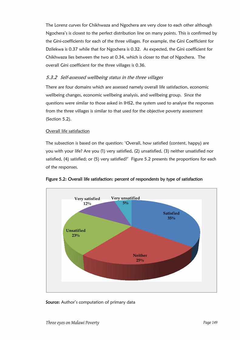
Three eyes on Malawi Poverty Page 149
The Lorenz curves for Chikhwaza and Ngochera are very close to each other although
Ngochera‟s is closest to the perfect distribution line on many points. This is confirmed by
the Gini-coefficients for each of the three villages. For example, the Gini Coefficient for
Dzilekwa is 0.37 while that for Ngochera is 0.32. As expected, the Gini coefficient for
Chikhwaza lies between the two at 0.34, which is closer to that of Ngochera. The
overall Gini coefficient for the three villages is 0.36.
5.3.2 Self-assessed wellbeing status in the three villages
There are four domains which are assessed namely overall life satisfaction, economic
wellbeing changes, economic wellbeing analysis, and wellbeing group. Since the
questions were similar to those asked in IHS2, the system used to analyse the responses
from the three villages is similar to that used for the objective poverty assessment
(Section 5.2).
Overall life satisfaction
The subsection is based on the question: „Overall, how satisfied (content, happy) are
you with your life? Are you (1) very satisfied, (2) unsatisfied, (3) neither unsatisfied nor
satisfied, (4) satisfied; or (5) very satisfied?‟ Figure 5.2 presents the proportions for each
of the responses.
Figure 5.2: Overall life satisfaction: percent of respondents by type of satisfaction
Source: Author‟s computation of primary data
Satisfied35%
Neither25%
Unsatified23%
Very satisfied12%
Very unsatified5%

Three eyes on Malawi Poverty Page 150
Combining the positives as „satisfied‟ and the negatives „unsatisfied‟, 47% were satisfied
while 28% were unsatisfied with their life and a quarter were neutral. There are
differences among the three villages, though (See Figure 5.3).
Figure 5.3: Perceptions on life satisfaction in the three villages
(% of households)
Source: Author‟s computation from primary data
While life satisfaction is highest in Dzilekwa where the poverty is least, in Ngochera
residents perceive their life in more positive light than Chikhwaza residents yet
Ngochera is poorer than Chikhwaza.
Changes in economic wellbeing over a year
The question was „In terms of your household economic wellbeing, are you better off,
the same as, or worse off than the same time a year ago? The responses run from much
better (1) to much worse (5) with no change (3) in the middle. Overall, the highest
proportion of households fell under „no change‟ but the rest of the categories were
almost mirror images of each other as depicted in Figure 5.4.

Three eyes on Malawi Poverty Page 151
Figure 5.4: Proportion of households in percent by type of change over a year
Source: Author‟s computation from primary data
Indeed when positives and negatives are put together, the proportions are almost the
same; better off (32%), no change (35%), and worse off (33%). The picture is
somewhat different for each of the three villages. In Ngochera, perceptions on changes
in economic wellbeing are more varied than in the other two villages; only in Ngochera
Village is the proportion of those that became worse off more than those that became
better off. In fact, the perceptions in Chikhwaza and Dzilekwa villages „agree‟ in
direction and magnitude. See Figure 5.5
Comparing the perceptions on life satisfaction and changes in economic wellbeing
between Ngochera and Chikhwaza gives the impression that life satisfaction is derived
possibly from a variety of sources, one of which (but not the most important) could be
economic wellbeing. Chikhwaza residents whose economic wellbeing improved more
than those in Ngochera gave lower life satisfaction rates than those in Ngochera. The
differences between the two wellbeing dimensions in the three villages show how
complex perceptions on wellbeing are.
Much better7%
Better25%
No change35%
Worse off26%
Much worse7%
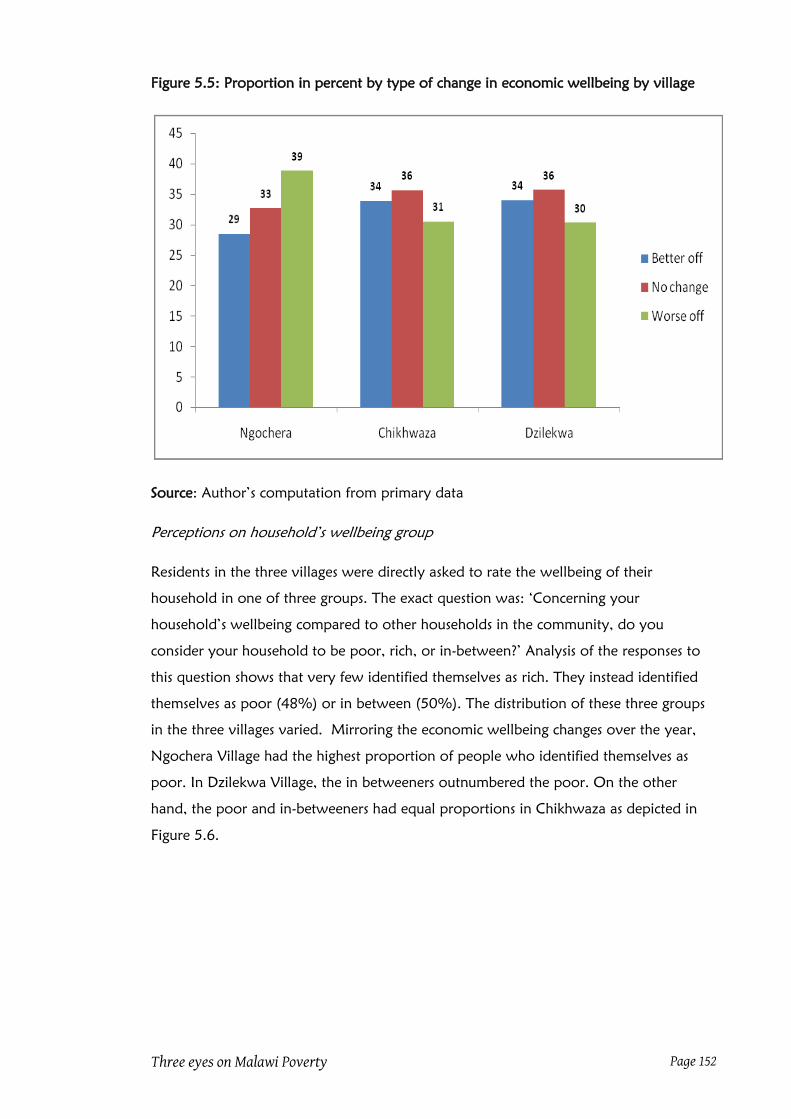
Three eyes on Malawi Poverty Page 152
Figure 5.5: Proportion in percent by type of change in economic wellbeing by village
Source: Author‟s computation from primary data
Perceptions on household‟s wellbeing group
Residents in the three villages were directly asked to rate the wellbeing of their
household in one of three groups. The exact question was: „Concerning your
household‟s wellbeing compared to other households in the community, do you
consider your household to be poor, rich, or in-between?‟ Analysis of the responses to
this question shows that very few identified themselves as rich. They instead identified
themselves as poor (48%) or in between (50%). The distribution of these three groups
in the three villages varied. Mirroring the economic wellbeing changes over the year,
Ngochera Village had the highest proportion of people who identified themselves as
poor. In Dzilekwa Village, the in betweeners outnumbered the poor. On the other
hand, the poor and in-betweeners had equal proportions in Chikhwaza as depicted in
Figure 5.6.

Three eyes on Malawi Poverty Page 153
Figure 5.6: Proportion of households in wellbeing groups in percent by village
Source: Author‟s computation of primary data
Apparently, the issue of stigma does not come into play as evidenced by the high
proportion of respondents that rated their households as poor. In fact based on the
wellbeing analysis conducted in the three villages, it is not „normal‟ to identify one‟s
household as rich even if it is32
.
Poverty status based on a ten-step wellbeing ladder
Household respondents were asked two questions; one that set the poverty line (the
step under which households are perceived to be poor) and another that positioned the
household on the ladder. The questions, based on a shown picture of a ten-step ladder,
were: „Concerning households in this community, which step is the top most poor
households take up? On which step is your household now?‟ By responding to this
question, the respondent not only drew a poverty line but also classified itself as either
poor or non-poor. Most of the residents rated themselves among the low level step;
seven placed own household on step 8, three on step 9 and only one step 10. There was
a very big „drop‟ between step 6 and step 7 as depicted in Figure 5.7. The bottom 3
steps host 40% of the residents while the top three host only 7% of the households.
32
During the FGD, group members were first asked to rate themselves before other group members
commented on their rating. In general, very few overrated themselves. Members who were known to be
rich by the community‟s standards rated themselves low and „waited‟ for their colleagues to „push‟ them
up. They rarely complained of being „overrated‟ by their peers.

Three eyes on Malawi Poverty Page 154
Figure 5.7: Proportion of households in percent by step in the three villages
Source: Author‟s computation from primary data
There is some variation among the three villages. For example, there are no households
on step 10 in Ngochera and none on steps 9 and 10 in Chikhwaza. In fact, residents in
Chikhwaza are „packed‟ between steps 2 and 5 (71%) unlike Ngochera where the
majority placed themselves in the first four steps (68%). Dzilekwa residents are spread
but step 5 was the most popular. However, the residents are concentrated between
steps 3 and 6 (70%). See Figure 5.8.
Given the distribution of the households on each step, to compute a poverty rate there
is need for poverty line. There are three ways of „drawing‟ the poverty line. The first
way is to impose a step, say step 4, as was the case with CPS5 and MOPS data in section
5.2. The second way is to compute a village median out of the poverty lines given by
each respondent in the village. The third way is to use a poverty line given by the
household itself. Table 5.13 presents poverty rates by each type of poverty line33
.
33
It is noted that the imposed and median poverty lines for Ngochera and Chikhwaza villages are all at
step 4. Only Dzilekwa Village has a median poverty line at step 3.
10
1515
1718
12
6
4
21
0
2
4
6
8
10
12
14
16
18
20
Step 1 Step 2 Step 3 Step 4 Step 5 Step 6 Step 7 Step 8 Step 9 Step 10
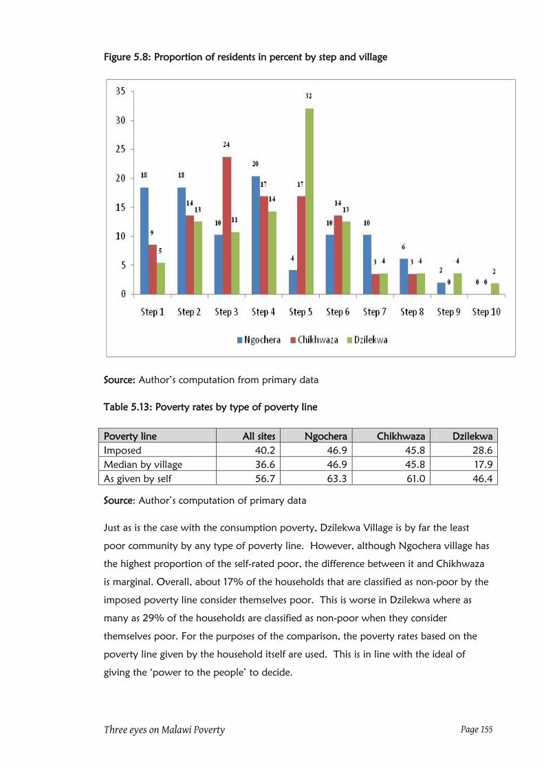
Three eyes on Malawi Poverty Page 155
Figure 5.8: Proportion of residents in percent by step and village
Source: Author‟s computation from primary data
Table 5.13: Poverty rates by type of poverty line
Poverty line All sites Ngochera Chikhwaza Dzilekwa
Imposed 40.2 46.9 45.8 28.6
Median by village 36.6 46.9 45.8 17.9
As given by self 56.7 63.3 61.0 46.4
Source: Author‟s computation of primary data
Just as is the case with the consumption poverty, Dzilekwa Village is by far the least
poor community by any type of poverty line. However, although Ngochera village has
the highest proportion of the self-rated poor, the difference between it and Chikhwaza
is marginal. Overall, about 17% of the households that are classified as non-poor by the
imposed poverty line consider themselves poor. This is worse in Dzilekwa where as
many as 29% of the households are classified as non-poor when they consider
themselves poor. For the purposes of the comparison, the poverty rates based on the
poverty line given by the household itself are used. This is in line with the ideal of
giving the „power to the people‟ to decide.

Three eyes on Malawi Poverty Page 156
5.3.3 Peer assessed wellbeing and poverty status
Peer assessment of poverty included defining wellbeing categories, superimposing the
categories on a ten-step ladder, deciding the poverty line (step) on the ladder and
placing housing on the steps of the ladder. The placing of households meant that
proportions of households in each category or those that were poor could be
determined. Likewise, the actual households that are poor were implicitly identified.
Wellbeing categories and poverty line
In Ngochera village two categories were identified; the poorest and the poor. The
group insisted that there were no rich households in the community. The poorest
category covered steps 1 to 4 and the poor steps 5 to 10. The poverty line in Ngochera
was placed on Step 5 implying that all households in the poorest category were defined
as poor. In Chikhwaza, the group identified four wellbeing categories. These were
superimposed on the ladder with the „poor‟ category covering steps 1 to 4, the
„moderately poor‟ covering steps 5 and 6, the „moderately rich‟ covering steps 7and 8
and the „richest‟ covering steps 9 and 10. The group made step 6 as the poverty line.
This meant that some of the moderately poor households (at step 5) were defined as
poor. The group in Dzilekwa decided on three wellbeing categories with the „poorest‟
covering steps 1 and 2, the „poor‟ covering steps 3 to 5, the „rich‟ covering the rest of
the steps. Just like in Chikhwaza, the poverty line was placed on step 6 thereby defining
the poorest and poor as poor. These definitions had profound link to the placement of
households on the ladder steps.
Placement of households on the ladder steps
Overall, households are concentrated in the first steps. The most popular step is 5, which
„received‟ 24% of the households in the three villages. Step 2 and 3 were almost the
same with 14% of households each. As Figure 5.9 shows, few households made it the
top three steps. This marks some differences among the three villages. Table 5.14
presents the distribution of households on the ten step ladder.

Three eyes on Malawi Poverty Page 157
Figure 5.9: Proportion of households in percent on the steps for the three villages
Source: Author‟s summary of FGD Transcripts
Table 5.14: Number and proportion of households on each step
Step Ngochera Chikhwaza Dzilekwa All
# % # % # % # %
Step 1 8 14.8 2 3.2 5 8.6 15 8.6
Step 2 4 7.4 17 27.4 3 5.2 24 13.8
Step 3 4 7.4 14 22.6 7 12.1 25 14.4
Step 4 5 9.3 13 21 4 6.9 22 12.6
Step 5 13 24.1 11 17.7 17 29.3 41 23.6
Step 6 8 14.8 0 0 9 15.5 17 9.8
Step 7 4 7.4 2 3.2 6 10.3 12 6.9
Step 8 2 3.7 2 3.2 1 1.7 5 2.9
Step 9 3 5.6 1 1.6 1 1.7 5 2.9
Step 10 3 5.6 0 0 5 8.6 8 4.6
Total 54 100 62 100 58 100 174 100
Source: Author‟s summary of FGD Transcripts
In Ngochera, step 5 was the mode while in Chikhwaza it was step 2 and Dzilekwa was
step 5. Apparently, the group in Ngochera spread the households over the steps while
the group in Chikhwaza spread the households in the first five steps while Dzilekwa
spread them up to step 7. See Figure 5.10
8.6
13.8 14.412.6
23.6
9.8
6.9
2.9 2.9 4.6
0.0
5.0
10.0
15.0
20.0
25.0
Step 1 Step 2 Step 3 Step 4 Step 5 Step 6 Step 7 Step 8 Step 9 Step 10

Three eyes on Malawi Poverty Page 158
Figure 5.10: Proportion of households in percent on the steps by village
Source: Author‟s summary of FGD Transcripts
5.4 Comments on household placement
The exercise of placing households on the steps revealed that local people have the
capacity to independently differentiate households‟ wellbeing status using implicit
weights. The placement also highlighted some features that were frequently used as tie
breakers during pairwise ranking. The exercise also exposed the limitations of PRA
where „power is given to the people‟. A number of examples from Ngochera illustrate
the point of weighting. This is followed by a discussion of pitfalls of PRA in Chikhwaza
and Dzilekwa.
A „rich‟ old woman was initially placed on step 8 based on the quality of her house.
After some short discussion (not even heated) she was placed on step to 3. The reason
given for the radical change was that the basis for the original placement was
outweighed by her other living conditions because the house was built by her son who
had since died together with the support the woman was getting from him. On the
other hand, a „doing well‟ young family was not placed at a step that would qualified it
as well off in line with its current income and consumption levels because it did not
have a good house. Considering that a good house was discounted in the case of the old
woman, such a judgement meant that the group viewed the two households differently.
The group used different weights for the households. For the old woman, failure to
-5
0
5
10
15
20
25
30
35
Step 1 Step 2 Step 3 Step 4 Step 5 Step 6 Step 7 Step 8 Step 9 Step 10
Ngochera Chikhwaza Dzilekwa

Three eyes on Malawi Poverty Page 159
consume basic goods was considered worse than enjoying a good house while failure to
construct a good house discounted the high consumption in the young family.
Another example concerns a physically challenged „rich‟ beggar whose household was
ranked among the poorest on Step 1 although the household had features far superior
features for the poorest category (i.e. steps 1-4) as defined by the group itself. The group
insisted that the household should be on Step 1 and could not even be 'promoted' to
step 2 because according to the group physically challenged people are, by definition,
amongst the poorest of the poor and that the livelihood strategy used (begging) was
demeaning. Thus affording to „do well‟ (i.e. buy clothes for wife, send children to
school, buy a radio, and buy food) was not good enough to place the household
among the well off. They seemed to imply that such a move would „glorify‟ begging
and discount the disadvantages people with disabilities face.
A similar case involved a very old and immobile woman who was placed on level 2. At
that step, she was assessed to be the richest because she gets external support and has a
goat, a feature absent in any of the households from step 1 to 4. However, the group
did not „promote‟ her household to any step higher despite her high consumption level
because she was very old and immobile. It was like: „what is the point of eating well if
you cannot move about‟?
These examples, apart from showing that people use some value system, they also give
a glimpse of why local level judgement of poverty can differ with one-dimensional
official version of poverty. To local people and in some circumstances, quality of life is
more important than „quantity‟ of life. Consumption-expenditure cannot pick that. For
example, a questionnaire cannot pick the fact that loss of dignity implicit in begging
outweighs consumption of donated goods. Likewise, it cannot pick that loss of mobility
cannot be compensated by the „sound of bleating goats‟ or a very good meal.
The placement of households also revealed the value of a „man in the home‟. In
Ngochera a man is useful in farming and exploitation of natural resources like charcoal
making and selling by bicycle. In Dzilekwa, a man is useful in farming and/or ganyu34
during off-season. According to the Dzilekwa group a man that „fears a hoe‟ is no good
34
This local term ‘ganyu’ is extensively used in field reports and consequently the next three chapters.
Ganyu is the hire of labour or offer of labour services for a specific task. Its payment is based on a
completed task. The task can take minutes, hours, half day, whole day or days or weeks. Ganyu is popular
for its flexibility in form of payment (cash or in-kind like food, clothes or any agreed commodity) and
payment-as- you complete system. One goes for ganyu if there is a need for instant cash or food. An
employer goes for ganyu for quick completion of a task. Ganyu is the dominant source of quick cash.
Ganyu is generally more rewarding than wage employment. Its downside is that its frequency is
unpredictable.

Three eyes on Malawi Poverty Page 160
for household wellbeing. The group dubbed households headed by such men as
„women-run households‟, especially if the wife takes on farming seriously and trading
during the off-season. In the main, the presence or absence of a husband in the
household was used to break ties during pairwise ranking.
The placement also revealed the role of a wife too. If households with husband and
wife tied, the group used the characteristics of the husbands to break the tie first. In cases
that did not produce a „winner‟ the group used the wives‟ characteristics. In some cases
even the woman‟s characteristics were good enough such that a female headed
household was not always placed below a male-headed household. There were a
number of cases where female-headed household were ranked higher than male-headed
households based on the criteria set by the group.
In Chikhwaza, placement of households was marred by mismatches between household
features and criteria set up by the group itself. What was remarkable, though, was the
reluctance to „promote‟ or „relegate‟ households that were obviously „out of place‟. The
possibility that some households may have been „wrongly‟ assessed brings to the fore
the limitations of the use of group interviews for wellbeing assessment. Given that the
group was „unwilling‟ to deal with mismatches it could acknowledge itself (or at least
some members did) gives the impression that the group was wrongly motivated.
Perhaps more serious is the question of usability of the data. Since the group „ensured‟
that most households are placed in the poor category, the village has a very high
poverty rate. This is made worse by the mismatches between wellbeing status and the
set wellbeing category features.
These two have implications on the study. If the poverty rate from this village is not
truthful comparing it with the others from the other sites is unfair because the
comparison assumes truthfulness from donors of the data. Wholesale untruthfulness in a
group discussion renders the data less useful. The mismatch between criteria and
household features also violates the assumption that placement of households is based
on the criteria laid by the group. The mismatch means that the household features
cannot be taken as correlates or determinants and therefore not proper to compare
them with others from other assessments. This is taken as a limitation of the
comparisons for this site.
In Dzilekwa placement of households was also unorthodox. There was one household
each on steps 8 and 9 but five on step10. Can this be explained? Although wellbeing
analysis is not a science, one is tempted to speculate why in this seemingly „rich‟ village

Three eyes on Malawi Poverty Page 161
the moderately „rich‟ are scarce. There are two possible related explanations for this.
The first is the criteria used to determine the rich. The second is composition of the
group discussants.
Judging from the reasons given for the placement of the households, it is possible that
the group did not approve of certain livelihoods strategies like ganyu at the local market
and by implication abandonment of farming. According to the group, money made
through ganyu at the market does not translate into any tangible household investment
but drunkenness. This is a confirmation of the finding in Chapter 6 where involvement
in ganyu was a negative determinant of wellbeing. The group rarely placed a household
dependent on ganyu on steps for the moderately rich or the rich.
Another possible explanation is the membership of the group. The group mostly
comprised farmers because traders were away and could not afford to join the
discussions that were to last over six hours. Further, one of the discussants was assessed
to be the „richest‟ man in the village through intensive farming. In his frequent
contributions he emphasised features related to own production of maize, hardworking
in cash cropping and amount of maize stocks. Thus the group was apparently biased
towards agricultural livelihoods against non-farm income generating activities.
The implication was that some well off small scale traders, middlemen, and ganyu
workers could not be placed among the moderately rich or the rich as long they did not
have maize stocks. Likewise by emphasising intensive farming and large scale trading as
gateways to joining the „club of the richest‟, the few that qualified were placed on Step
10 leaving very few on steps 8 and 9. It is probable that if the emphasis on farming and
maize stocks was relaxed, some households on steps 5, 6 and 7 could have been placed
on higher steps and that some households on Steps 9and 10 could have been on lower
steps. This, it must be said, is speculation.
What is noted is that the quality of the exercise was relatively high because there were
very few „out of place‟ households during the pairwise ranking. Out of the fifty-eight
households only one household, on step 9, was promoted to step 10. To prove that the
promotion was genuine, the promoted household ended up being third amongst the
richest five. Another sign is that the placement of households was generally good there
were many households that tied and difficulty to break. Thus data from Dzilekwa is
therefore useable because the criteria were seriously used to place households unlike in
Chikhwaza. The discussion above is simply questioning the basis of the criteria especially
since such would make some poor households be classified as non-poor and some non-

Three eyes on Malawi Poverty Page 162
poor households as poor. The net of this is not known. It is assumed its net effect on
the poverty rate is minimal.
Poverty rates in the three villages
Based on the poverty lines defined by each village group and the placement of the
households on the steps, poverty incidence in Ngochera is 39% because 21 out of the 54
households were placed on steps 1 through 4. In Chikhwaza the poverty rate is 92%
since only 5 households were placed above the poverty line. In Dzilekwa 36 out of 58
households were ranked below the poverty line giving a poverty rate of 62%.
It is noted that if the Ngochera poverty line (Step 5) was imposed on Chikhwaza and
Dzilekwa their poverty rates would come down to 74% and 33%, respectively. On the
other hand if the poverty line applicable in Chikhwaza and Dzilekwa were imposed on
Ngochera the poverty rate in Ngochera would rise to 63%. This implies that if a
uniform poverty line was used for all the three villages, Dzilekwa would have the least
and Chikhwaza highest poverty prevalence. However, Ngochera and Dzilekwa would
have rates that were close to each other. Figure 5.11 clearly shows how Chikhwaza
ratings are atypical with three different poverty lines.
Figure 5.11: Poverty rates in percent using different steps as poverty lines
Source: Author‟s summary of the site FGD transcripts
29.6
38.9
63.0
53.2
74.2
91.9
25.9
32.8
62.1
0.0
10.0
20.0
30.0
40.0
50.0
60.0
70.0
80.0
90.0
100.0
Step 4 Step 5 Step 6
Ngochera
Chikhwaza
Dzilekwa

Three eyes on Malawi Poverty Page 163
5.5 Households identified as poor in the three sites
The list of households listed here are only those that were interviewed. Some
households that were considered during peers assessment were not interviewed for a
number of reasons. One of the reasons is that what passed as a household during listing
may not have passed during questionnaire administration because the household
definition was applied strictly. Unfortunately the peer assessment was based on the
listed households. This meant that in Ngochera the number of households dropped
from 54 to 49 and Chikhwaza from 62 to 59 and in Dzilekwa from 58 to 56 giving a
total of 164 households. This affects the poverty rates already presented but does not
change the status of any household.
The three different types of assessments found different number of households in
Ngochera. The consumption-expenditure found that 23 households were poor. At the
same time, 26 households were self-assessed as poor while peers assessed 21 households
to be poor. In Chikhwaza the consumption expenditure measure found that 19
households out of the 59 households were poor. When the same respondents assessed
their households, 30 felt that their households were poor. Peers assessed almost every
household as poor as 52 of the 59 households were classified as poor. In Dzilekwa, the
official measure found only 9 households out of the 56 households but self-assessment
found 17 of them to be poor while peers assessed 34 households to be poor.
An analysis of the lists of the poor identified by each type of assessment shows that in
Ngochera as many as 40 out of the 49 households were ever identified as poor,
representing 82 percent. In Chikhwaza, 56 of the 59 households (95%) were identified
as poor by at least one type of assessment. In Dzilekwa, it was three-quarters of the
households that were ever identified as poor (i.e. 42 of the 56 households). The study
is interested to check whether or not the bulk of the households identified as poor are
the same for the three assessments. In other words, do the assessments converge or
diverge and if so to what extent? These comparisons are taken on in the next section
5.6 Comparisons of poverty rates and the identified poor
This section is devoted to respond to the research question on whether the three
assessments are the same in terms of their poverty rates and the households they identify
as poor. This question is dealt squarely by the findings in the three villages. All the three
villages are used in the comparisons the results for Chikhwaza are taken with some pinch
of salt because of the exaggerated poverty rate as discussed before.

Three eyes on Malawi Poverty Page 164
5.6.1 Comparison of households ranking
Before comparing the different lists of poor households by wellbeing measure, this
subsection makes two comparisons. The first compares two sets of ranked households;
one based on per capita consumption expenditure and the other on subjective
assessment of each household guided by wellbeing analysis and pairwise ranking. The
second comparison is between two sets of step assignments given to each household by
peers and self. For test of significance of differences, if at all, the comparisons are done
using correlation analysis in each of the villages.
Regarding household‟s wellbeing position as assessed by peers and using consumption
expenditure, the results of the correlation analysis shows that there is no relation in all
the three villages separately or combined (Table 5.15).
Table 5.15: FGD and CE rankings correlation using Spearman's rho
Ngochera Chikhwaza Dzilekwa All sites
Coefficient 0.19 0.16 -0.09 0.08
Significance level 0.205 0.242 0.498 0.300
Cases 48 58 56 162
Source: Author‟s analysis of data from primary data sets and FGD transcripts
However, when the steps assigned by peers and self are compared, there is very close
relationship, except in Chikhwaza Village (Table 5.16).
Table 5.16: FGD and Self assigned steps correlation using Spearman's rho
Ngochera Chikhwaza Dzilekwa All sites
Coefficient 0.44 -0.067 0.61 0.33
Significance level 0.001 0.613 0.000 0.000
Cases 49 59 56 164
Source: Author‟s analysis of data from primary data sets and FGD transcripts
It is noted that the comparison in Table 5.15 is between the official and community
versions of poverty while Table 5.16 is between two local level assessments. The
mismatch in Chikhwaza Village is an echo of the finding that the peer assessment was
deliberately biased. The message from these two tables is that the official measure of
wellbeing does not always match those at local levels. This gives an indication that those
identified as poor by the official measure could be different from those identified by the
local level assessments. This is checked next.
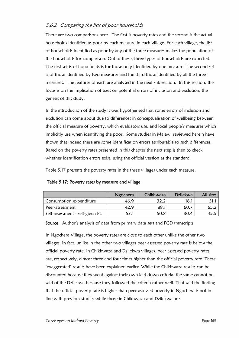
Three eyes on Malawi Poverty Page 165
5.6.2 Comparing the lists of poor households
There are two comparisons here. The first is poverty rates and the second is the actual
households identified as poor by each measure in each village. For each village, the list
of households identified as poor by any of the three measures makes the population of
the households for comparison. Out of these, three types of households are expected.
The first set is of households is for those only identified by one measure. The second set
is of those identified by two measures and the third those identified by all the three
measures. The features of each are analysed in the next sub-section. In this section, the
focus is on the implication of sizes on potential errors of inclusion and exclusion, the
genesis of this study.
In the introduction of the study it was hypothesised that some errors of inclusion and
exclusion can come about due to differences in conceptualisation of wellbeing between
the official measure of poverty, which evaluators use, and local people‟s measures which
implicitly use when identifying the poor. Some studies in Malawi reviewed herein have
shown that indeed there are some identification errors attributable to such differences.
Based on the poverty rates presented in this chapter the next step is then to check
whether identification errors exist, using the official version as the standard.
Table 5.17 presents the poverty rates in the three villages under each measure.
Table 5.17: Poverty rates by measure and village
Ngochera Chikhwaza Dzilekwa All sites
Consumption expenditure 46.9 32.2 16.1 31.1
Peer-assessment 42.9 88.1 60.7 65.2
Self-assessment - self-given PL 53.1 50.8 30.4 45.5
Source: Author‟s analysis of data from primary data sets and FGD transcripts
In Ngochera Village, the poverty rates are close to each other unlike the other two
villages. In fact, unlike in the other two villages peer assessed poverty rate is below the
official poverty rate. In Chikhwaza and Dzilekwa villages, peer assessed poverty rates
are, respectively, almost three and four times higher than the official poverty rate. These
„exaggerated‟ results have been explained earlier. While the Chikhwaza results can be
discounted because they went against their own laid down criteria, the same cannot be
said of the Dzilekwa because they followed the criteria rather well. That said the finding
that the official poverty rate is higher than peer assessed poverty in Ngochera is not in
line with previous studies while those in Chikhwaza and Dzilekwa are.

Three eyes on Malawi Poverty Page 166
On the surface, these findings and in the context of errors of inclusion and exclusion,
one can conclude that in Ngochera there are more households that have been identified
as non-poor when in fact they are poor by the official standard than those that have
been wrongly identified as poor when otherwise non-poor. Similarly one can expect the
opposite for Chikhwaza and Dzilekwa because they have poverty rates that are way
above the standard measure. However, there is more to errors of inclusion and
exclusion than the difference between the poverty rates. For example, it is not always
true that measures with similar poverty rates identify the same households. Likewise, it is
not always true that those with different poverty rates identify very different
households. For the first case, two measures with similar poverty rates can identify
mutually exclusive sets of households. Likewise, those with different rates could have a
set of households that are common in both assessments. There are 138 households out
of the 164 households that are identified as poor. Some of these are identified by
consumption expenditure (CE) measure only, self-assessment (SA) only, peer-assessment
(PA) only; and others by a combination of these. Table 5.18 presents the results of an
analysis of those households.
Table 5.18: Poor households by method of identification and village
Type Ngochera Chikhwaza Dzilekwa All sites
N % N % N % N %
Poor by CE only 7 17.5 1 1.8 3 7.1 11 8.0
Poor by SR only 7 17.5 3 5.4 4 9.5 14 10.1
Poor by PA only 3 7.5 18 32.1 19 45.2 40 29.0
Poor by CE and SA 6 15.0 2 3.6 1 2.4 9 6.5
Poor by CE and PA 4 10.0 7 12.5 3 7.1 14 10.1
Poor by SA and PA 7 17.5 16 28.6 10 23.8 33 23.9
Poor by all 6 15.0 9 16.1 2 4.8 17 12.3
Total poor 40 100 56 100 42 100 138 100
Source: Author‟s analysis of survey data and FGD transcripts
In terms of the research question of whether the three wellbeing assessment methods are
the same, the table clearly shows that the assessments are different in all the three
villages. Even in Ngochera where the poverty rates were similar, there are minimal
overlaps. The implication is that the local wellbeing assessments identify different
households as poor from those the official one does. This does not mean that self rating
and peer assessment are similar either. They also identify different households as poor.
The magnitude of differences also varies by village.

Three eyes on Malawi Poverty Page 167
The Ngochera data shows that convergences are as prevalent as divergences.
Households identified as poor by all the assessments (15%) are as many as those
identified by only one assessment or jointly by two measures only (17% or 15%). Thus
despite the poverty rates being close to each other each agreement and disagreements
almost matched. The small proportion of households identified only by peer assessment
(7%) reflects the low peers-assessed poverty rate. Thus in Ngochera, it is difficult to
conclude that self and peer assessment are closer to each other than each is to the official
measure. What is safe to conclude is that the three measures are different based on the
different households each identifies.
As expected the picture is somewhat different in Chikhwaza village. Peer assessment
identified more households as poor when no other measure considered them as thus. In
fact, peer assessment identified so many households as poor when the households
themselves considered themselves non-poor. The least measure to identify households
as poor when no other measure did was the official measure. In terms of agreement of
measures in Chikhwaza, the least is between the official measure and self-rating (4%)
and the highest is between peer assessment and self rating (29%). The proportion of
households jointly identified as poor by all is 16%, which is close to that witnessed in
Ngochera. The high peer-assessed poverty rate ensured high joint identification with the
official measure (12%) as well. If the community group that identified 88% of the
population as poor is given the benefit of the doubt, Chikhwaza shows that local level
assessments are more similar than dissimilar and that local people‟s assessment is
different from that of experts.
This conclusion is echoed in Dzilekwa where the agreement between self and peer
assessment (24%) is almost twelve times that between the official measure and either
self rating (2%) and more than three times that between the official and peer assessment
(7%). However, Dzilekwa is more prominent for a combination of divergences and
convergences than Ngochera. For example, 62% were identified as poor by only one
assessment, leaving 38% as those which were jointly identified as poor. In fact,
Dzilekwa has the least proportion of households identified as poor by all the three
assessments (5%). A similar conclusion is therefore reached that the three types of
assessing wellbeing and poverty are different in Dzilekwa.
In the hope that the low peers-assessed poverty rate in Ngochera compensates for the
high peers-assessed poverty rate, the one hundred and thirty-eight households identified
as poor are put together to check once again whether the three assessments have similar
traits. Only 12% of the households were identified as poor by all the three assessments.

Three eyes on Malawi Poverty Page 168
Those identified by only one assessment (a sign of divergence of assessments) were as
many as those jointly identified by at least two assessments (an indicator of
convergence); 47% and 51%, respectively. The highest proportion of households
(29%) fell under sole identification of peers-assessment. This was followed by joint
identification by self and peers assessments (24%). Figure 5.12 presents the proportions
of households identified as poor by various assessments.
Figure 5.12: Proportion of poor households by type of assessment in percent
Source: Author‟s computation from primary data
This confirms the conclusions reached above. The first conclusion is that the three types
of wellbeing and poverty assessments are neither the same nor mutually exclusive.
Apparently their cores are different while other aspects are the same. The second
conclusion is that self- and peers assessments are closer to each other than each is to the
official standard. Whether this is reflected in the features implicit in each of these
assessments is the subject of the next chapter.
5.6.3 Characteristics of the different groups of poor households
As a precursor for the next chapter and in the spirit of Bradshaw and Finch (2003)35
, this
subsection closely looks at the seven sub-groups of the poor. Given that the end result of
the exercise is to make the official measure incorporate community level wellbeing
features in order to reduce the prevalent divergences, learning from the overlaps would
35
In their article, they recommend that making a comparison of characteristics of those jointly identified
as poor by all the measures with those identified as poor by two measures or only one.
12.3
6.5
10.1
23.9
8.010.1
29.0
0.0
5.0
10.0
15.0
20.0
25.0
30.0
35.0
All CE and Self CE and Peers self and peers
CE only Self only Peers only

Three eyes on Malawi Poverty Page 169
assist in the exercise36
. The most important overlap is where all the three measures agree
that a household is poor. According to Table 5.19, households identified as poor by all
the assessments are not necessarily the poorest in terms of per capita consumption
expenditure, whether the mean or median is used.
Table 5.19: Per capita consumption in British Pound by group of the poor
Type of sub-group Mean Median Cases
CE only 60.2 64.6 11
PA only 209.3 151.0 40
SA only 184.1 143.3 14
CE & PA 55.3 54.9 14
CE & SA 52.6 60.9 9
PA & SA 159.6 124.9 33
All poor 59.7 61.2 17
Nonpoor 155.1 162.5 26
ALL HHs 141.3 111.4 164
MK300=£1
Source: Author‟s analysis of survey data and FGD transcripts
The main lesson from the table is that peers assessment, and to some extent self-
assessment, are insensitive to current consumption evidenced by the high per capita
consumption of households assessed as poor by these on their own or jointly. This is an
important finding because it shows fundamental differences between the official and
local assessments. This finding still holds even when the households are analysed by
village (Table 5.20).
Table 5.20: Per capita consumption in British Pound by group of the poor by village
Ngochera Chikhwaza Dzilekwa
Mean Median Cases Mean Median Cases Mean Median Cases
CE only 58.5 64.6 7 58.7 58.7 1 64.7 66.0 3
PA only 233.5 223.4 3 196.2 163.0 18 217.8 141.3 19
SA only 137.2 130.2 7 158.0 146.5 3 285.6 250.3 4
CE & PA 63.2 61.1 4 57.0 57.8 7 40.7 42.8 3
CE & SA 45.0 40.7 6 65.1 65.1 2 73.1 73.1 1
PA & SA 106.3 102.9 7 203.7 194.0 16 126.3 112.8 10
All poor 57.3 58.1 6 61.5 61.2 9 58.8 58.8 2
Total poor 151.4 119.2 9 142.3 159.0 3 160.1 167.3 14
ALL HHs 102.9 86.6 49 149.7 125.5 59 166.0 123.5 56
MK300=£1
Source: Author‟s analysis of survey data and FGD transcripts
36
It is recognised that divergences between the measures cannot be eliminated because they are
fundamentally different and have inherit biases that cannot be dealt with tinkering of the wellbeing
measure.

Three eyes on Malawi Poverty Page 170
The small differences are in the group which has the highest and lowest averages. Using
median as the basis for the comparisons, the lowest was recorded for the group of the
poor jointly identified by official and self assessments while the highest was recorded for
those only identified as poor by peers. The same is true for Ngochera. In Chikhwaza it
was the group of households identified by the official measure that had the lowest
median while the group jointly identified by self and peers assessments had the highest
median. Dzilekwa has yet a different scenario. The highest is recorded for those assessed
as poor by themselves only while the lowest for those jointly assessed by the official
measure and peers. In all the three villages, the official measure is associated with
lowest median. Clearly, those households jointly identified as poor by all the measures
are not necessarily consumption poor in any of the villages or in all the three villages
combined regardless of whether the mean or median is used (shaded cells in the table).
To check whether there are other features apart from per capita consumption, the
variables that were used for the poverty correlates analysis are also used37
. Some of the
variables showed no discernible differences among the seven groups and they are,
therefore, dropped. The variables found significant by poverty group are presented in
Tables 5.21a and 5.21b. To make sense of the table, lowest and highest median for each
characteristic are highlighted. Where there is more than one case, no shading is done.
Table 5.21a: Household characteristics by poverty group
Scale variables
CE
only
PA
only
SA
only
CE-
PA CE-SA PA-SA All
Nonpoo
r
HH size 6.0 4.5 3.0 5.0 5.0 4.0 5.0 4.0
Depend. ratio 1.5 1.5 1.0 2.0 1.5 1.0 2.0 1.3
Age HHH 34.0 35.5 40.0 36.5 39.0 38.0 42.0 43.0
IGA hours 12 11 7 8 6 6 6 10
Inputs cost (£) * 3.33 25.08 11.00 4.08 2.00 7.67 3.33 14.42
Non-agric Y (£) * 34.00 82.00 197.33 6.58 40.00 40.00 20.00 124.00
Labour Y (£) * 0.00 0.00 1.67 0.08 0.00 4.33 16.67 0.00
# durables 2 6 1 3 1 2 1 6
# children 3 3 1 3 3 1 3 2
% in school 0 25 100 0 0 0 25 0
Land owned (ha) 1.00 0.61 0.51 0.91 0.50 0.61 0.51 0.91
# crops 3 4.5 5 3 4 4.5 5 5
* MK300/£1
Source: Author‟s analysis of survey data and FGD transcripts
37
The ideal method is to use factor analysis. Unfortunately the small number of cases for most of the sub-
groups makes such an exercise futile. Most of the characteristics selected are scale variables which are
amenable to calculations of mean and median. There are a few dummy and nominal variables.

Three eyes on Malawi Poverty Page 171
Table 5.21b: Comparison of household characteristics by poverty group
Nominal variable
CE
only
PA
only
SA
only CE-PA CE-SA PA-SA All
Non
poor
HHH sex (M=1/F=0) 0.73 0.72 0.71 0.57 0.67 0.67 0.71 0.62
HHH married (1/0) 0.82 0.75 0.71 0.57 0.67 0.64 0.65 0.62
Employed (1/0) 0.27 0.10 0.07 0.21 0.11 0.09 0.18 0.08
Enterprise (1/0) 0.64 0.63 0.57 0.43 0.67 0.67 0.47 0.69
Gave gifts (1/0) 0.91 0.80 0.93 0.79 1.00 0.88 0.71 0.92
Fertilizer (1/0) 0.82 0.97 0.71 0.79 0.56 0.76 0.59 0.92
Coupon (1/0) 0.91 0.72 0.86 0.71 0.56 0.64 0.65 0.81
Livestock (1/0) 0.82 0.80 0.57 0.50 0.44 0.67 0.59 0.73
HHH illiterate (1/0) 0.73 0.83 0.71 0.71 0.56 0.64 0.65 0.69
HHH class (1-21) 4.55 6.20 4.36 5.50 3.56 5.03 5.65 5.19
Adult class (1-23) 5.18 6.78 5.43 5.71 6.89 6.18 4.24 7.88
Source: Author‟s analysis of survey data and FGD transcripts
These tables show that households that are jointly identified as poor are unique only in
five characteristics namely age of the household head, source of income, extending of
gifts to others, application of fertilizer and education status of adults in the household.
These households are just as good and bad as the other sub-groups of the poor. On age,
the finding implies that households headed by old people are likely to be assessed as
poor by households themselves and peers in the community groups, apart from having
very low consumption levels. Likewise, the finding on the source of income implies that
those that rely mostly on ganyu are likely to be identified as poor by all the assessments.
It also makes sense that those jointly identified as poor have the least proportion of
households that give out gifts to other households and apply fertilizer, and with
educated adults.
In general, however, this group of the poor is not necessarily the poorest. Depending on
a characteristic, it is as poor as the poorest group. For example, just like at least one
other group, it has the highest dependency ratio, lowest number of hours spent on IGAs,
and least number of durable goods. On some characteristics, the group is among those
in the middle. Finally, poor households (regardless of the measure used to identify
them) do not have features that are markedly different from the non-poor. The
implication of this is that these household features do not necessarily help to distinguish
the poor from the nonpoor, especially when community assessment is used.
Three eyes on Malawi Poverty Page 172
5.7 Policy implications on the measures
So far it has been established that the three wellbeing assessment methods are neither
the same nor mutually exclusive. It has also been established, based on the proportion
of households jointly identified as poor, that peer assessment and self-rating are more
related to each other than each is to the official measure.
The findings in the three villages also show that there should be no illusion that
qualitative methods or quantitative methods are better than the other. Village groups, if
not properly motivated or if wrongly oriented, can turn wellbeing analysis upside
down. That is possible even with a well motivated and resourced facilitation team.
There is no guarantee that every time a method of learning or data collection is
implemented in a certain community the process and results will be as expected.
Further, the high levels of discordance between the official and local level assessments of
wellbeing may also imply that there are fundamental differences in poverty
conceptualisation between official and locals. In this case, if the official version was used
to check the „truthfulness‟ of the other methods of assessment the verdict would be that
self and peers assessment are not good at identifying the poor38
. More importantly,
given the value standpoint that the official version ought to reflect local
conceptualisation of poverty, it is important that a comparison of wellbeing
characteristics between the official version and local concepts of poverty be done. This
is the subject of the next chapter.
38
Appendix 4 provides the exact levels of errors of inclusion and exclusion in the three villages.

Three eyes on Malawi Poverty Page 173
Chapter 6: Official version of wellbeing and poverty
6.1 Introduction
The previous chapter has shown that the three methods of assessing the wellbeing status
of households are different in many ways. This chapter and two others that are to
follow intend to find out the characteristics that are implicitly or explicitly used when
assessing the household wellbeing or poverty status or those that are associated with
wellbeing and poverty. This chapter brings out those characteristics associated with the
official measure, which are in the form of correlates and determinants. The main source
of the correlates and determinants are the 2000 and 2007 analyses. The correlates and
determinants from the three villages are meant just to check whether the villages are
atypical or not.
6.2 Wellbeing and poverty features from 2000 and 2007 profiles
The 2000 and 2007 analyses used purpose-designed integrated household surveys
covering income and expenditure, demographics, health, education and livelihoods
strategies. They were complemented by community questionnaires that collected
instrumental variables like access to markets, roads, health facilities, financial institutions,
and safety nets, among others. The 2004/5 questionnaire also included modules like
Security and Safety, Social Safety Nets, Credit, Subjective Assessment of Well-being, and
Recent Shocks to the Household. These extra modules were meant to provide data for
vulnerability and subjective wellbeing assessments.
6.2.1 Poverty correlates
Table 6.1 presents poverty correlates or proxies or predictors gleaned from the 2000
and 2007 analyses. There are twelve factors that are common in both analyses and
there are some factors that were only reported in one analysis. For example, the 2000
analysis had eleven and the 2007 analysis had six unique factors. Some of the differences
can be explained more by differences in the correlation models than changes in the
characteristics of the poor. Some of the mismatches are due to differences in the factors
used in the correlation models. For the purposes of the study, any factor that was ever
found to be a correlate under either model is taken as an important factor. Thus Table
6.1 provides the poverty correlates that form part of the characteristics of wellbeing and
poverty from official wellbeing and poverty analysis.
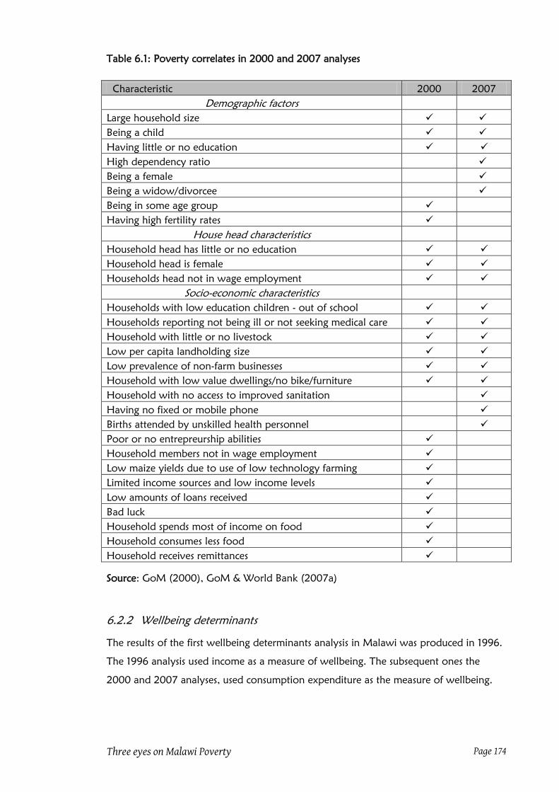
Three eyes on Malawi Poverty Page 174
Table 6.1: Poverty correlates in 2000 and 2007 analyses
Characteristic 2000 2007
Demographic factors
Large household size
Being a child
Having little or no education
High dependency ratio
Being a female
Being a widow/divorcee
Being in some age group
Having high fertility rates
House head characteristics
Household head has little or no education
Household head is female
Households head not in wage employment
Socio-economic characteristics
Households with low education children - out of school
Households reporting not being ill or not seeking medical care
Household with little or no livestock
Low per capita landholding size
Low prevalence of non-farm businesses
Household with low value dwellings/no bike/furniture
Household with no access to improved sanitation
Having no fixed or mobile phone
Births attended by unskilled health personnel
Poor or no entrepreurship abilities
Household members not in wage employment
Low maize yields due to use of low technology farming
Limited income sources and low income levels
Low amounts of loans received
Bad luck
Household spends most of income on food
Household consumes less food
Household receives remittances
Source: GoM (2000), GoM & World Bank (2007a)
6.2.2 Wellbeing determinants
The results of the first wellbeing determinants analysis in Malawi was produced in 1996.
The 1996 analysis used income as a measure of wellbeing. The subsequent ones the
2000 and 2007 analyses, used consumption expenditure as the measure of wellbeing.

Three eyes on Malawi Poverty Page 175
As already stated earlier, wellbeing determinants analyses use regression models39
.
However, the models used do not determine causality but test the relationships posited
by economic theory. It is when a relationship is confirmed that a factor is deemed as a
determinant (Mukherjee & Benson, 2003; GoM & World Bank, 2007a). In this sub-
section only the consumption expenditure determinants analysis are presented. Results
of the 1996 analysis are given in Appendix 5. Two poverty determinants analyses were
conducted on the 1997/8 data. The first used bivariate analysis (GoM, 2000a). The
second used multivariate analysis (Mukherje and Benson, 2003). To facilitate
comparison, the multivariate analysis results are used because 2007 analysis used the
same.
It is noted that the two analyses treated the samples and some factors differently. The
2007 used regional dummies instead of splitting the national sample as did the 2000
analysis, which had four separate regional samples. Since the three villages are mostly in
the South, the discussion uses the results of that region‟s model estimation. As for
variables, the 2000 analysis used age, education level of household head, age of
household head, age of children, and size of household as corrected while the 2007
analysis categorised them into groups or made dummies out of them based on their
theorised differentiated impact on household consumption expenditure.
Table 6.2 presents the variables that were at least significant at 5% level from the two
analyses. The non-linear effect of household size is only one demographic determinant
that is common in both analyses. However, age of household split or otherwise show
that it has some effect on wellbeing. The 2007 analysis shows that household wellbeing
declines with age of its head. It also shows that being a child is associated with being
poor. For non-demographic factors, only wage income and production of tobacco are
common determinants. Related to the wage income, education and employment have
strong influence on wellbeing. Further, it is apparent that it is not the size of rain-fed
land owned but land under cultivation. In other words, landholding size is not a binding
constraint but resource-dependent cultivation because land constraint can be overcome
by land renting. It is irrigatable land ownership that is important.
39
These are referred to wellbeing determinants instead of poverty determinants because the dependent
variable is not poverty status (as is the case with correlates) but the wellbeing measure (per capita
consumption)

Three eyes on Malawi Poverty Page 176
Table 6.2: Wellbeing determinants in the 2000 and 2007 analyses
Factors SR Rural Rural
(Regressors) 2000 2007
Size of the household squared + ** + **
Size of the household - **
Number of adult males - *
Female household head - **
Widowed household head + **
26-35 years household head + **
36-45 years household head + **
56-65 years household head - *
66 + years household head - **
Age of household head - **
Number of 0-9 year children - **
Number of 0-4 year children - **
Number of 5-10 year children - **
Number of 10-17 year children - **
Household has wage/salary income + ** + **
Household grew tobacco last season + ** + **
Head completed some primary education + *
Head completed primary education + **
Head completed post-primary education + **
Household owns any dambo plot + **
Household has a non-farm enterprise + **
Area of rain fed plots (logarithm) + **
Whether clinic in community + **
Whether EA at BOMA or trading centre + **
Takes >30-45 minutes to nearest BOMA - **
ADMARC in community - **
Tarmac road in community +**
Takes >45-60 minutes to nearest BOMA - *
Members in tertiary industry +**
Maximum education level by any adult + **
Cultivated land (per capita) + **
Value of livestock (log per capita) + **
Whether PWP in TA + **
Mean time to community facility (hrs) - **
Members in primary industry +*
Significant levels: ** 1% level; * 5% level
Source: Mukherjee and Benson (2003); GoM & World Bank (2007a)
A confounding finding in the 2007 analysis was that having the government marketing
agency (ADMARC) was associated with reduced consumption expenditure. A similar
finding is reported by Sharma, et al. (2002). However, access to other socio-economic
facilities like the trading centre, district headquarters or being near an all-weather road
have the expected impact on wellbeing.

Three eyes on Malawi Poverty Page 177
6.2.3 Way forward for the official wellbeing characteristics
Tables 6.1 and 6.2 provide the characteristics that are associated with consumption
expenditure the official measure of wellbeing and poverty regardless of they are
correlates or determinants or whether they are unique to one analysis. Peers and self
assessments of wellbeing and poverty are holistic since they incorporate causes, effects
and manifests. In recognition that poverty correlates and determinants for self-assessed
poverty and wellbeing, respectively, come from the same model and dataset (Chapter
8), they are taken forward to Chapter 9 for comparison as they are.
6.3 Community level poverty correlates and wellbeing determinants
The correlates and determinants in Tables 6.1 and 6.2 are at national level. Whether
these obtain at local level is what this section is interested to determine. Once
community level correlates and determinants are found, they are compared with the
national ones to check whether there is some relationship between them. Without a
strong relationship, the study‟s goal of modifying the official wellbeing analysis system
using community level findings is not justifiable. To produce comparable community
level poverty correlates and wellbeing determinants, the study adapts the models used
for the 2000 and 2007 analysis.
6.3.1 Model for poverty correlates in the three villages
Tables 6.3a and 6.3b present the list of the factors and descriptive statistics. It is noted
that in some „system missing‟ cases, zeroes were used instead. For example, where no
member of the household was ill or injured, the number of days lost due to illness/injury
is zero although the data has system missing because the question was not asked. It is
also noted that percent replaces mean for the dummy variables because the mean
effectively runs between 0 and 1 which is then conveniently converted to percent and
easy to explain or understand. For the ordinal variables, the reference code is used in
describing the variable. For example, for the type of house where there are three codes
(for modern, mixed and traditional), the modern house is taken as the reference and is
therefore used in describing the variable. Just like the dummy variables, the mean is
converted to percent.

Three eyes on Malawi Poverty Page 178
Table 6.3a: Descriptive statistics for the scalar profiling variables
Scale variables N Min Max Mean S D
Household size 164 1 10 4.3 1.8
Adult equivalent 164 1 8 3.8 1.5
Members less than 15 years old 164 0 7 2.3 1.6
Members 65 years or older 164 0 2 0.2 0.5
Members between 15 to 64 years old 164 0 5 1.8 0.8
Dependency ratio 151 0 5 1.4 0.9
Age of household head 164 15 100 44.1 18.3
Proportion of school going age children in school 120 0 100 31.7 39.7
Average years in school for all adults 164 0 12 5.3 3.0
Highest class attended by head 163 0 12 5.3 3.7
Highest class attended by any adult member 164 0 12 6.3 3.7
Proportion of members reporting being ill (%) 164 0 100 22.3 27.4
Days lost by adults due to illness/care of the ill 164 2 80 4.4 10.2
Average hours adults spent on IGAs 164 0 65 11.5 11.6
Total land owned by household 164 0 11 0.9 1.0
Total dimba land owned by household 164 0 2 0.1 0.2
Inputs cost (MK'000) 164 0 251 11.6 26.6
Tropical livestock units 164 0 1 0.1 0.2
Agriculture income (MK'000) 164 0 325 6 28.4
Non-agriculture income (MK'000) 164 0 932 60.5 122.7
Annual income from work (MK'000) 164 0 624 32.4 96.6
Share of food in total consumption 164 3.7 94 57.6 16.1
Share of ganyu income in work-related income 75 0 100 68.4 45.52
Number of different crops 161 1 14 4.6 2.0
Number of different types of livestock 164 0 4 1 0.9
Number of durable assets in the household 164 0 23 4.4 4.5
Source: Author‟s computation from primary dataset

Three eyes on Malawi Poverty Page 179
Table 6.3b: Descriptive statistics for non-scalar profiling variables
Dummy/nominal variables N Min Max Percent S D
% headed by females 164 0 1 32.3 0.47
% of heads who are illiterate 164 0 1 29.3 0.46
% wage income heads 164 0 1 11.6 0.32
% with a member in wage employ 164 0 1 13.4 0.37
% with non-farm enterprise 164 0 1 61.0 0.49
% that gave no gifts to others 164 0 1 14.6 0.36
% of households with a bike 164 0 1 26.7 0.44
% whose member has a cell phone 164 0 1 40.2 0.49
% with no toilet 164 0 1 20.7 0.41
% that did not apply fertilizer 164 0 1 18.9 0.39
Ordinal variables N Min Max Percent S D
% employed by non-formal employer 19 1 3 73.7 0.34
% of households without coupon 164 1 3 28.7 0.49
% of head with no spouse 164 1 6 32.3 1.69
% of heads with post-primary qualification 163 1 5 12.2 0.87
% of households with modern house 164 1 3 4.9 0.54
Source: Author‟s computation from primary dataset
The analysis uses a two-tail test because such avoids imposing the type of relationship
between the dependent and independent variable40
. For cardinal factors, Pearson
correlation statistics are used while Kendal tau B statistics are used for factors with
ordinal values. Pearson Chi-Squared statistics are used for nominal variables, including
dummy variables. In all cases, a difference is considered significant if it falls outside the
95% confidence interval. The correlation analysis uses the poverty status (poor or
nonpoor) as the dependent variable, which takes the value 1 if the household is poor
and 0 if nonpoor.
Table 6.4 presents factors that are strongly associated with household poverty status.
Some of these factors can be hypothesised to determine the household wellbeing level
while others are mere effects of the level. For example, having too many dependents
reduces labour supply without reducing consumption requirements. By this token, the
demographic factors can be considered as determinants of household welfare status.
However, having a bicycle or cell phone can be a sign of high income in the household.
In turn, household income is highly associated with household consumption. Therefore
ownership of assets cannot be considered as a determinant of household consumption
40
Ordinarily poverty profiling starts with simple comparisons of the descriptive statistics for the poor and
non-poor. That simple analysis is done in Appendix 6a.

Three eyes on Malawi Poverty Page 180
poverty because ownership of bicycle is not independent of income which is strongly
related to consumption.
Table 6.4: Poverty correlates for the three villages
Factor Sig level Group
Household size 1% Demographic
Dependency ratio 1% Demographic
Number of dependent children 1% Demographic
Household applied fertilizer 1% Agriculture
Amount of money spent on inputs 1% Agriculture
Food consumption share 1% Economic
Durable assets diversity 1% Economic
Household has cell phone member 1% Economic
Household has a bicycle 1% Economic
Highest class by all adults (mean) 5% Education
Amount of credit assessed 5% Enterprises
Income from agriculture 5% Agriculture
Livestock diversity 5% Agriculture
Highest class by adult 5% Education
Time spent on IGAs (hours) 5% Enterprises
Source: Author‟s computation from primary dataset
Just like in the case of the national level correlates, these will be compared with poverty
correlates for self-assessed poverty. This is also true for the wellbeing determinants that
are found in the next sub-section.
6.3.3 Model for wellbeing determinants in the three villages
For comparison purposes, this analysis uses the conceptual frameworks used in the 2000
and 2007 analyses (Mukherjee & Benson, 2003, p. 340; GoM & World Bank, 2007b, p.
49).
The model takes the form
ln cj = βxj + ηj
Where
cj is total annual per capita consumption expenditure of household j in Malawi
Kwacha,
xj is a set of explanatory variables (factors)for household j, and
ηj is a random error term.

Three eyes on Malawi Poverty Page 181
To be in line with the 2000 and 2007 analysis, the model that is used is an adaptation
of models used in those analyses. In particular, the models used by Mukherjee and
Benson (2003, p.344) and GoM & World Bank (2007b, p. 196) are rationalised. The
process of modification is presented in Appendix 6b. What is presented here is the final
model. Table 6.6 presents the descriptive statistics and partial correlation coefficients.
Table 6.6: Descriptive statistics and correlation coefficients the villages model
Model variables (n=164) Min Max Mean S.D. Coefficient T-statistic
Log per capita consumption 9 12 10.7 0.7
Household size ** 1 10 4.3 1.8 -0.214 0.006
HH size squared (/100) * 0 1 0.2 0.2 -0.172 0.028
Under-5 children 0 3 0.7 0.8 -0.026 0.744
5-10 year old children ** 0 3 0.9 1.0 -0.228 0.003
11-14 year old children 0 3 0.5 0.7 -0.138 0.077
Highest class by any adult * 0 12 6.3 3.7 0.187 0.017
Members in agriculture 0 6 1.2 1.1 0.063 0.423
Members in enterprise 0 6 0.7 0.8 0.011 0.888
Members engaged in ganyu * 0 3 0.4 0.6 -0.184 0.018
Members in employment 0 1 0.1 0.3 -0.141 0.072
Household has wage income * 0 2 0.2 0.4 -0.179 0.022
Harvest (tonnes/ha) ** 0 21 2.0 3.1 0.238 0.002
HH owns dimba land ** 0 1 0.3 0.5 0.268 0.001
Value of livestock (log) ** 5 13 9.0 1.7 0.297 0.002
Loans accessed (MK '000) ** 0 60 2.51 8.42 0.21 0.006
Inputs costs (MK '000) ** 0 251 11.6 26.6 0.24 0.002
Loans accessed (log) 6 11 8.8 1.2 0.300 0.090
Inputs costs (log) ** 5 12 8.2 1.6 0.465 0.000
Ngochera village ** 0 1 0.3 0.5 -0.349 0.000
Chikhwaza village ** 0 1 0.4 0.5 0.242 0.002
Dzilekwa village 0 1 0.3 0.5 0.092 0.244
Household accessed credit ** 0 1 0.2 0.4 0.306 0.000
Applied fertilizer last season ** 0 1 0.8 0.4 0.283 0.000
** Significant at 1%; * significant at 5%
Source: Author‟s computation from primary data
In the table, access to inputs and application of fertilizer are measured in three different
ways. The amounts are either in thousands of the local currency or logarithm of the
amount. They are also turned into dummies with the code „1‟ if they accessed credit or
applied fertilizer. These three are not used in the same but alternative models. The first
to be used are the logarithm versions. To ensure that only the most suitable factors are
used in the model, the stepwise linear regression analysis is adopted. Table 6.7 presents
a summary of the findings.

Three eyes on Malawi Poverty Page 182
Table 6.7: Wellbeing determinants in the three villages – scale variables
Explanatory variables B S. E. Beta t-statistic Sig.
(Constant) 9.787 0.793 12.344 0
Household size -0.165 0.059 -0.466 -2.768 0.012
Amount spent on inputs (log) 0.247 0.085 0.444 2.89 0.009
Children from 11 to 14 old -0.397 0.178 -0.375 -2.236 0.038
R2 = 0.573; Adjusted R2=0.505; S.E. = 0.416
Source: Author‟s computation from primary dataset
This model has an explanatory power of 50% with only three explanatory variables. As
indicated, dummy variables can replace the scale variables for loans and inputs cost.
When the model is re-estimated using the dummy variables in place of the scale versions
(Table 6.8), the number of determinants increases from 3 to 7 at the cost of the
explanatory power of the model (i.e. from 50% to 43%). For the purposes of the
study, the reduction of the explanatory power is not a problem. What is important is
the addition of factors.
Table 6.8: Wellbeing determinants in the three villages – dummy variables
Explanatory variables B S. E. Beta t-statistic Sig.
(Constant) 10.823 0.294 36.855 0.000
Ngochera village -0.488 0.119 -0.350 -4.105 0.000
Household size -0.144 0.03 -0.414 -4.751 0.000
Value of livestock (log) 0.069 0.03 0.182 2.277 0.025
Members engaged in ganyu -0.223 0.083 -0.202 -2.667 0.009
Household owns dimba land 0.278 0.115 0.205 2.410 0.018
Household accessed credit 0.252 0.125 0.159 2.019 0.046
Children less than 5 years old 0.132 0.066 0.164 1.995 0.049
R2=0.465; Adjusted R2=0.428; S.E. of estimate=0.492
Source: Author‟s computation from primary dataset
This model has yielded new factors in place of some in Table 6.7. For example, under-
five children replace the 11-14 year olds and „amount of money spent on inputs‟ is
replaced by „household has access to credit‟. Only the household size survives. Further,
the use of dummies brings out the fixed effects of Ngochera Village as the single-most
important factor in the model, explaining almost half of the variation. Applying the
same model to the specific village data reveals some village differences. Table 6.9 lists
the factors that are found to be significant contributors of per capita consumption
expenditure by village. The table only presents the coefficients to show the direction
and strength of relationship.

Three eyes on Malawi Poverty Page 183
Table 6.9: Wellbeing determinants by village
Explanatory variables Coefficients
Village --> Ngochera Chikhwaza Dzilekwa
Constant 10.96 11.32 10.92
Household size -0.15 -1.23
Household size squared 2.23
Children from 5 to 10 years old -0.46
Children from 11 to 14 old -0.46
Members in wage employment -0.44
Members engaged in ganyu -0.29
Household accessed credit 0.50
Harvest in tonnes per hectare 0.05
R2 0.193 0.487 0.475
Adjusted R2 0.168 0.429 0.402
S.E. estimate 0.507 0.425 0.475
Source: Author‟s computation from primary dataset
The table shows that only one factor explains the variation in per capita consumption in
Ngochera. This is because most of the variation in per capita consumption is explained
by the village fixed effects (Table 6.8). On the other hand, other factors are prominent
in Chikhwaza and Dzilekwa. In fact, they explain per capita consumption variations
much better (43% in Chikhwaza and 40% in Dzilekwa) although the specific factors are
totally different. Ngochera and Dzilekwa share one factor, household size. The issue of
ganyu in Dzilekwa is picked up in group discussions in Chapter 7, where ganyu is
associated with poverty, vindicating the findings here.
It is clear that the determinants are dependent on the type of model and the scale of
measurement. Given that the study is interested to get as many legitimate determinants
as possible, different measures of the factors „livestock ownership‟, „access to credit‟ and
„access to inputs‟ are used41. Four models are estimated using stepwise regression
analyses. The first (Model 1) uses the amounts for the three variables in thousand. The
second (Model 2) uses the natural logarithm of the original amounts for the three
variables. The third (Model 3) uses two dummies for credit and fertilizer with value of
livestock in thousands. The fourth (Model 4) uses the two dummies with logged value
of livestock. The results of these four regressions are presented in Table 6.10.
41
Note that differences between scaled and not scaled amounts are only in the size of the coefficients and
not the model results in terms of factors and explanatory power. The scaled values are generally used
because they give higher coefficients. However, when using logarithm, the original values are used since
logarithm are used basically to scale down large values.

Three eyes on Malawi Poverty Page 184
Table 6.10: Wellbeing determinants in the three villages – effect of measurement
Explanatory variables MK‟000 Log Dummies for credit & inputs
All three All three Livestock(‟000) Livestock (log)
Model 1 Model 2 Model 3 Model 4
Constant 11.195 9.787 10.653 10.823
Ngochera village -0.376 -0.27 -0.488
Household size -0.118 -0.165 -0.144
Children less than 5 years old 0.132
Children from 5 to 10 years old -0.19
Children from 11 to 14 old -0.397
Value of livestock 0.002 0.001 0.069
Members engaged in ganyu -0.136 -0.217 -0.223
Household owns dimba land 0.298 0.278
Amount spent on inputs 0.247
Amount of loans accessed 0.011
Household accessed credit 0.373 0.252
Applied fertilizer last season 0.311
R2 0.319 0.573 0.331 0.465
Adjusted R2 0.293 0.505 0.306 0.428
S.E. of estimate 0.562 0.416 0.557 0.492
Source: Author‟s computation from primary dataset
Each one of the four models has unique results. The use of scale variables (Models 1 and
3) produces the least explanatory power but twice the number of factors compared to
the models with logged variables while the use of dummies allows many factors to
„claim some stake‟ in per capita consumption although the factors differ depending on
the measure of the value the livestock. Possibly comforting is the finding that not every
model yields complete new factors. For example, out of the six factors from Model 1,
only one „amount of loans accessed‟ is unique.
The use of dummy variables generally yields a variety of factors that are not necessarily
unique. For example, the combination of the dummies and logged value of livestock
yields the highest number of factors (7) but only one of them (number of under-five
children) is unique. When the dummies are combined with scaled value of livestock, the
number of factors is six out of which two are unique („number of children in the age
group 5-10 years‟ and „household applied fertilizer‟). None of the other two models has
these three factors.
What these models demonstrate is that it is not the use of either dummies or natural
logarithm that increases the number of explanatory factors. Further, it is not the
number of explanatory variables that increase the explanatory power of the model.

Three eyes on Malawi Poverty Page 185
Finally, regardless of the scale of the measurement, some variables are consistent
contributors of per capita consumption. At the top are household size, being in
Ngochera village, number of household members engaged in ganyu and value of
livestock. Apparently, numbers of children in various age groups are important in
different specifications in different ways. Amount of money spent on inputs, amount of
loans accessed and application of fertilizer are also important but in specific model
specifications.
Just was the case with the national level determinants, all factors that have been found
to be a determinant is any of the models are taken forward for comparison. Table 6.11
puts them together
Table 6.11: Wellbeing determinants in the three villages
Factor All sites Ngochera Chikhwaza Dzilekwa
Ngochera Village √
Household size √ √ √
Household size squared √ √
Number of under-five children √
Number in 5-10 year age group √ √
Number in 11-14 year age group √ √
Number involved in ganyu √ √
Number in wage employment √
Household has a dimba plot √ √
Value of livestock √
Amount of money spent on inputs √
Household accessed credit √ √
Amount of loans accessed √
Yield of all crops (tonnes/hectare) √
Household applied fertilizer √
Source: Tables 6.7 to 6.10
A summary of the table is that there are thirteen factors that impact per capita
consumption in three villages combined six of which are not important at individual
village level. On the other hand, there are two factors that are only important at village
level. Wage employment is important for Chikhwaza village. This is expected because
this is the only village with the highest wage employment. The crops yield is important
in Dzilekwa, the most agriculturally-driven of the three. The only factor that is
important in all the three villages is household size or its quadratic form implying that
apart from household size, all village level contributors are unique to the village.

Three eyes on Malawi Poverty Page 186
6.3.4 Comparison of the national and village level characteristics
The numbers of national level correlates and determinants are expected to be more than
community level ones because (i) the sample sizes are different (12,000 and 164); (ii) the
study covered three out of thousands of villages; and (iii) the villages are confined to a
radius of 100 kilometres, mostly in the poorest region42
. What of interest to the study is,
given these differences, there are some convergences. Given that poverty correlates are
used as identifiers for the poor, any matching of factors implies there are factors that can
be used as identifiers. Indeed according to Tables 6.12 and 6.13, there are nine correlates
and eight determinants that are common.
Table 6.12: Common poverty correlates and wellbeing determinants
Characteristics National Local
Poverty correlates
Access to telephone/mobile phone √ √
Amount of credit assessed √ √
Food consumption share √ √
Household applied fertilizer/low use of technology √ √
Household has a bicycle √ √
Livestock: ownership and/or value √ √
Number of dependent children √ √
Number of dependent members/dependency ratio √ √
Number of household members/fertility rate √ √
Wellbeing determinants
Household size √ √
Household size squared √ √
Number of 0-4 year old children √ √
Number of 5 to 10 years old children √ √
Number of 10-17/11-14 year old children √ √
Household has wage/salary income √ √
Household owns dimba land √ √
Value of livestock (log) √ √
Source: Tables 6.2 and 6.11
There are, of course, other correlates and determinants that are unique at each level. For
example, income from agriculture is only important at local level while remittances are
only at national level. Likewise, education level of adults is only significant at local but
not national level. As for wellbeing determinants, there are also some unique factors
worth mentioning. For example, age, sex and education level of household head are
important only at the national level. While wage employment is positively important at
42
In fact, Dzilekwa is in Ntcheu in the Central Region. Its poverty rate at 52% was the lowest among the
three districts which had 70% for Zomba for Ngochera and 65% for Thyolo for Chikhwaza.

Three eyes on Malawi Poverty Page 187
national level, ganyu employment is negatively so at local level. The point is that using
national level factors that are not important at local level as identifiers is likely to lead to
identification errors. These issues are picked up in the concluding remarks.
6.4 Concluding remarks
This chapter has presented poverty correlates and wellbeing determinants based on
previous poverty profiles and data collected from the three villages. The methodology
used to come up with the correlates and determinants in the three villages was the same
as that used in previous two poverty analyses in Malawi. Very minor and necessary
modifications were made. Such modifications do not make the methodology adopted in
any way different. The lessons and conclusions presented herein are based on this
methodological comparability.
1. What obtains at the national level does not always apply at local level. In other
words, a clear picture at national level may not always be understood at local
level. As such the national picture may be good for national level policy and
programme development but may not be appropriate for local level application.
The uniqueness of the three villages (combined and individually) from the
national picture has been demonstrated.
2. What applies in one village does not always apply in another even when they
are close to each other. For example, the absence and presence of robust
markets make Ngochera a different village from Dzilekwa. Likewise, the
availability of diverse income generating activities in Chikhwaza village
compensates for the low landholdings.
3. It is easier to pinpoint what produces poverty in some villages than in others.
For example, an average household in Ngochera can be poor just because it is
located there. A similar household in Chikhwaza and Dzilekwa is likely to take
advantage of poverty reducing opportunities to move out of poverty. That is
almost impossible in Ngochera apart from reducing number of children.
4. Just as national level factors cannot be „transferred‟ down, local level factors
cannot be „scaled up‟. Further, the uniqueness of villages implies that local level
characteristics cannot be applied across villages either. This calls for localisation
instead of centralisation of poverty studies. In other words, having more local
level poverty studies is better than having one good national level study.

Three eyes on Malawi Poverty Page 188
5. If a situation dictates that national level proxy indicators be used, careful analysis
of national and local level data can yield some common proxies as demonstrated
in this study. Where such a study is not possible, it is imperative that each
national level proxy indicator be examined by local experts to determine
whether it is applicable.
All in all, the chapter has managed to identify factors that have some association with
the official version of wellbeing and poverty. Although the list of factors does not, on
its own, respond to a particular research question, it provides a comparator required to
deal with the research question: „Do conceptualisation of poverty by official, self and
peers converge or diverge in a given community in Malawi?‟ The question is ultimately
dealt with in Chapter 9 by comparing the characteristics found in this chapter with those
that are gleaned from community groups (Chapter 7) and households themselves
(Chapter 8).

Three eyes on Malawi Poverty Page 189
Chapter 7: Community characterisation of wellbeing
7.1 Introduction
The objective of this is chapter is to identify popular features and dimensions of
wellbeing from a countrywide qualitative study and in the three sites that were visited
during the primary data collection. The features and dimensions of wellbeing are used to
interrogate the official operational definition of poverty in Chapter 9. The main source
of wellbeing features for interrogating the official wellbeing analysis system come from
the MOPS already discussed in Chapter 3. As explained in the methodology chapter, a
fresh analysis of the 33 field reports was done by the author to come up with the
common features that are used across the country.
The first part of this chapter presents findings of other qualitative studies. This is
followed by findings from the MOPS. The final part presents findings from the three
villages. The ultimate output of the chapter is a list of prominent wellbeing features that
can apply across the country and wellbeing categories. Since the research problem
centres on the use of community groups in targeting the poor, these features are taken
as serious candidates for incorporation in the official wellbeing analysis system.
7.2 Characteristics of wellbeing and poverty from qualitative studies
This section presents the findings from studies that were designed to be nationally
representative in the sense of covering areas that had to be seen to be diverse in terms
of culture and livelihood strategies. The idea is to provide a national picture while
highlighting area specific differences. A number of studies that used wellbeing analysis
provide a glimpse of the characterisation of wellbeing and poverty as well as
categorisation of wellbeing. Some defined as well as characterised wellbeing and
poverty. Others concentrated on characterising wellbeing and poverty.
7.2.1 Definition of poverty
According to Machinjili and colleagues (1998), poverty was said to describe “a situation
of low income, denial of the right to participate in social development and human
capital formation; and lack of access to productive assets” (p. 57). Aspects of the Malawi
rural poverty definition are many but the commonest are food insecurity, poor clothing,
low or no cash income, and poor housing (NEC, 2002). Although most of the aspects
are at household level, there are others that operate at community level. As Table 7.1

Three eyes on Malawi Poverty Page 190
shows, it is the lack of basic necessities that are frequently mentioned in the definition of
poverty.
Table 7.1: Aspects of rural poverty definition in Malawi
Aspect Men FGD Women FGD All
n=13 n=13 n=26
Food shortage 12 12 24
Poor clothing 11 13 24
No money 7 8 15
Poor quality house 8 5 13
No potable water 4 2 6
No livestock 2 2 4
Inaccessibility 3 1 4
No fertilizer/inputs 1 2 3
No health facilities 1 2 3
No drugs in health facilities 1 1 2
Land shortage 0 1 1
Unemployed 1 0 1
Source: NEC (2002) Table 2.1
Lack of access to community-level basic social services like potable water, health services
and drugs and public transport or passable roads are rarely highlighted as attributes of
poverty in rural Malawi. Judging priority by the number of groups mentioning an
attribute, access to socio-economic infrastructure is not among the top. This is
confirmed by the attributes of poverty presented in Table 7.2 as lack of basic necessities
of life is the most frequently mentioned attribute. Non household attributes were rarely
mentioned. For example, only the study by Machinjili and colleagues (1998) did
infrastructure come up. It is noted that not all attributes were mentioned in the three
studies. In fact only lack of food, shelter, clothing and money were mentioned in the
three studies. Some attributes were unique to a study while others were mentioned in
two of the three studies reviewed here. This is significant because each of the studies
had at least 15 group discussions. If an attribute does not appear in at least one it may
imply that it is not very important. Most of these attributes re-appear when discussing
characteristics of households in various wellbeing groups. In fact the NEC (2002) study
uses the same attributes as criteria for categorising households.

Three eyes on Malawi Poverty Page 191
Table 7.2: Attributes of poverty in Malawi
Attribute Machinjili Khaila NEC Sites *
Lack of sufficient food √ √ √ 18
Poor/inadequate shelter √ √ √ 15
Inadequate clothing/beddings √ √ √ 13
Few or no livestock √ 9
Dependency on casual work √ √ 7
Inadequate Income/money √ √ √ 6
No assets/poor living conditions √ √ 5
Lack of employment opportunities √ √ 4
Poor health √ √ 4
Inputs unavailability √ √ 3
Dependency on begging √ √ 2
Credit unavailability √ √ 1
Insecurity √
Lack of adequate infrastructure √
Lack of entrepreneurship spirit √
Transport unavailability √
Inadequate farmland √
Mat instead of timber coffin √
* Only the NEC report gave the number of sites mentioning the attribute
Source: Machinjili, et al. (1998); Khaila (1999); NEC (2002) Table 2.3
7.2.2 Causes of poverty in rural households in Malawi
It is instructive to present what people consider to be causes of their poverty in their
communities before discussing the characteristics of households in various wellbeing
categories. Causes of poverty are the equivalent of poverty determinants. The impact
monitoring study (NEC, 2002) discussed causes of poverty in the sites they visited. The
study on sources of risks (Kadzandira, 2002) also discussed conditions that trap people
in poverty.
An analysis of the causes of poverty shows that no one factor dominated. In fact no
factor was mentioned in more than half of the group discussions. The top five causes of
poverty are laziness, lack of employment opportunities, poor health, failure to apply
farm inputs and lack of credit facilities for farm inputs or start-up capital for businesses
(Table 7.3).

Three eyes on Malawi Poverty Page 192
Table 7.3: Number of groups mentioning the cause of poverty
Cause Men FGD Women FGD All
n=13 n=13 n=26
Laziness 6 6 12
Unemployment 6 6 12
Poor health 5 7 12
Failure to apply farm inputs 5 6 11
Lack of credit facilities 5 6 11
Erratic weather pattern 4 3 7
No money for essentials/business 3 4 7
Inadequate or no farmland 4 2 6
Low produce prices 4 2 6
Over population 3 2 5
Theft 3 2 5
Soil degradation 1 4 5
Illiteracy 2 2 4
Inaccessible markets 2 2 4
Crops destroyed by animals 2 2 4
Reliance on casual work/ganyu 2 1 3
Large families 1 1 2
Orphanhood 1 1 2
Lack of food 1 1 2
Deforestation 1 1 2
Low agricultural productivity 1 1 2
Lack of extension services 1 1 2
Source: NEC (2002) Table 2.2
It is noted that there are no significant differences between the sex groups, especially on
the major causes of poverty. What are noteworthy are the differences on poor health,
inadequate land, low produce prices and soil degradation. The factors are not
independent of each other and this is what makes no one factor be the most prominent
factor. This inter-linkage of factors demands careful and 'respectful' analysis. A similar
pattern emerges when the poverty-producing conditions obtained by Kadzandira (2002)
from 19 sites are analysed. According to Kadzandira (2002) people link food insecurity
to adverse weather conditions (droughts and floods), declining soil fertility, declining
landholdings and high incidence of illness and death. The discussants said food
insecurity pushes and keeps people in poverty because in times of food insecurity
households abandon their farms and resort to work elsewhere either for food or cash to
buy food. This creates a vicious cycle because by abandoning their farms, they harvest
little which leads to subsequent food insecurity. This was mentioned in all the 19 sites
visited.
Three eyes on Malawi Poverty Page 193
Another condition that was reported to push people into poverty or keep them in
poverty is constant rise of prices of inputs and basic necessities. By referring to various
years in the past when there were price spikes, Kadzandira (2002) concluded that SAP-
inspired exchange rate and inputs subsidy policies were to blame. What the people
reported, however, was that commodity price increases constantly squeezed the
purchasing power of the little they made and that inputs price increases led to a decline
in agricultural productivity due to reduced use of inputs especially fertilizer and hybrid
maize seed. People stated that this was exacerbated by wages and produce prices that
did not keep pace with inflation. According to Kadzandira (2002), the low produce
prices were a result of yet another structural adjustment policy that reduced the role of a
state run produce trader and allowed private traders to take its place. This low produce
price was mentioned as a condition that pushes and keeps people in poverty in 8 sites.
The groups concluded that a combination of ever rising commodity and inputs prices on
one hand and stagnant or declining income results in increasing poverty.
Frequent diseases and deaths as a condition that pushes and keeps people in poverty
were also mentioned in all the 19 sites (Kadzandira, 2002). The point the people made
was that morbidity affects food production through lost days by those ill and taking care
of the ill. The severity of HIV and AIDS related illnesses were also blamed for asset and
livestock depletion. Deaths, especially those related to AIDS, were said to be
devastating since they rob families of „breadwinners‟ and therefore plunge otherwise
„safe‟ households into immediate poverty. Worse still, funerals require the bereaved
families to feed those who attend the service with „good‟ food, which invariably means
meat. This further means either losing more money to buy the food or slaughtering
some livestock both of which are poverty producing for the remaining household
members. Related to the funeral ceremony, people mentioned that culture demands
that no work be carried out during the days of the mourning which means suspension of
income generating activities.
With „kid-glove‟ handling of criminals that came with the bill of rights in mid-1990s,
crime and insecurity increased to the extent that loss of property, livestock and crops
were common place. This affected the livelihoods strategies in rural areas where wealth
was previously stored in livestock and productive assets. The increased insecurity meant
that a household by saving in livestock or groceries shops would be reduced to a poor
household overnight. With increasing crime, the people said, the incentive to invest was
reduced and many income generating activities were limited to more safe but less
lucrative ventures. Apart from pushing households into poverty, crime and insecurity

Three eyes on Malawi Poverty Page 194
ensured that households that could otherwise have moved out by setting up businesses
remained poor. This condition was mentioned in 10 of the 19 sites.
The causes of poverty or poverty-producing conditions gleaned from the two
nationwide studies provide a good background for the analysis of reasons given during
the pairwise ranking of households and, to some extent, during wellbeing ranking under
which households are categorised into wellbeing groups. In the meantime, the criteria
used to categorise households in the three studies are presented next.
7.2.3 Characteristics of wellbeing categories
Wellbeing analysis gives participants an opportunity to decide the number of wellbeing
categories the households in the community should have. The number of categories
varies by group. Khaila and colleagues (1999) report of four wellbeing categories in all
FGDs, except one that defined three. FGDs in the impact monitoring study (NEC, 2002)
defined three wellbeing categories, except one FGD that defined only two. On the
other hand, Kadzandira (2002) reports of wellbeing categories that ranged from two to
five.
After the categories are decided, the participants are asked to give characteristics
associated with households in each43
. While Khaila and colleagues (1999) presented
characteristics for the four wellbeing categories and the unique three categories, NEC
(2002) and Kadzandira (2002) used three categories. For the purposes of combining
the results of the three studies, three groups are used. The top and bottom categories are
left intact. All categories in between are collapsed into one category termed „middle‟.
As observed in all the three studies, one characteristic can be a criterion for two different
categories in different areas. It is therefore proper that some discussion is presented for
the key characteristics.
Table 7.4 presents the characteristics of rich households arranged in descending order of
number of groups mentioning the characteristic in the policy impact study (NEC, 2002).
Discounting possible differences in frequency of mention, it can be concluded that there
is considerable agreement amongst the studies. For example, there is agreement on
access to basic household necessities like food, housing, and clothing just as there is on
access to money and inputs and ownership of livestock, land, and assets (productive,
durable and vehicles).
43
It is noted that in wellbeing ranking these characteristics are not weighted. However, people implicitly
use the weights when they categorise or „pairwisely‟ rank the households.

Three eyes on Malawi Poverty Page 195
Table 7.4: Characteristics of rich households in rural Malawi
Characteristic NEC Khaila Kadzandira
Food secure √ √ √
Good quality house √ √ √
Decent clothing √ √ √
Have livestock √ √ √
Have one or more bicycles √ √
Have stable IGA √ √
Enough money √ √ √
Uses inputs (seeds/fertilizer) √ √ √
Have motorised vehicle(s) √ √ √
Can employ or hire labour √ √
Have access to credit √ √
Have productive assets √ √ √
Household members are healthy √ √ √
Have plenty of farmland √ √ √
Have household durables √ √ √
Have charms √
Children continue with education √
Have town working children √
Have peace of mind √
Source: NEC (2002) Table 2.2; Khaila (1999) Table 4; Kadzandira (2002) Table 2
However, these characteristics have different shades, depending on area and emphasis of
a study44
. For example, food security is measured in terms of food availability
throughout the year (NEC, 2002; Khaila, et al., 1999), the size and fullness of a maize
granary (Khaila, et al., 1999) and eating thrice a day (Khaila, et al., 1999; Kadzandira,
2002). A good quality house has to look good and have burnt bricked wall, cemented
floor (NEC, 2002; Khaila, et al., 1999), and should have a roof with iron sheets (NEC,
2002; Khaila, et al., 1999; Kadzandira, 2002). While Kadzandira did not breakdown
what „decent clothing‟ meant, Khaila and colleagues (1999) and NEC (2002) broke it
down to cover „enough‟, or „several that were also good quality‟. Khaila and colleagues
(1999) added that children in rich households have change of clothes.
On ownership of livestock, the number and type is important. NEC (2002) gives
numbers and types but stress that the numbers and types are dependent on location. For
example, it states that in one site, four or five goats was a criterion for categorising the
44
Raw data on how different each group discussion broke down the characteristic is difficult to establish.
It is not clear whether the difference shades represent true differences or lack of detail in summarising or
indeed poor facilitation. However, in some cases the reports give an idea that they note the differences in
the shades. A deeper analysis of the differences is attempted later as field reports are used instead of
expert summaries of the reports.

Three eyes on Malawi Poverty Page 196
rich while in another it had to be five to ten cattle to be categorised in the rich category
and four to five goats to be in the middle category (NEC, 2002, p. 16). In the other
studies, it is generally lots of high value livestock like cattle or goats or pigs or sheep that
are considered as a criterion for the rich category (Khaila; et al., 1999; Kadzandira,
2002). This implies that chickens on their own, no matter how many, are not
considered as a characteristic of the rich.
There is also variety in the characterisation of the rich in terms of ownership of durable
assets. Just like the case of livestock, NEC (2002) found that in one site owning a bicycle
was a criterion for the rich while in another it was for the middle group. Ownership of
radio and beds were mentioned in all studies (NEC, 2002; Khaila, et al., 1999;
Kadzandira, 2002) while beddings and furniture in general were mentioned in two
studies (NEC, 2002 and Kadzandira, 2002). Some assets were mentioned only in one
study and these include metallic plates; mosquito nets; cassette players (Khaila, et al.,
1999) and mattresses and pillows (Kadzandira, 2002). Differences are also observed on
ownership of productive assets. While all studies mentioned oxcarts as one of the
characteristics of the rich, maize mills were mentioned in two studies (Khaila, et al., 1999
and Kadzandira, 2002). Some only feature in one study: motorised boats, fish nets and
ploughs (Khaila, et al., 1999); merchandise shops or hawkers (Kadzandira, 2002).
There is little variety given on the kinds of activities rich households undertake to
generate income. The only examples given in the reports include selling fish for those
with boats (Khaila, et al., 1999) and produce trading (Kadzandira, 2002). The
implication is that some of the known businesses and activities are the preserve of the
not-so-rich households, as will be seen later. What is true in all the studies is that the
rich households have „enough‟ money. This is variably described as finding money
without struggling (Khaila, et al., 1999) or producing a lot of cash crops like Irish
potatoes or tobacco (Khaila, et al., 1999 and Kadzandira, 2002), or affording not to
work for anyone (Khaila, et al., 1999); and ability to purchase laundry and bath soap,
cooking oil, meat frequently, and perfumes or lotions (Khaila, et al., 1999 and
Kadzandira, 2002).
All studies agree that the rich can afford to buy farm inputs like fertilizer and seeds and,
according to Khaila and colleagues (1999), can afford to employ or hire labour to work
in their gardens or fishing boats or as domestic servants. The absence of education and
employment status among the characteristics of the rich is noteworthy. It is also
noteworthy that the rich are said to keep their children in school and also have children
working in urban areas. This has the connotation that while education status of parents
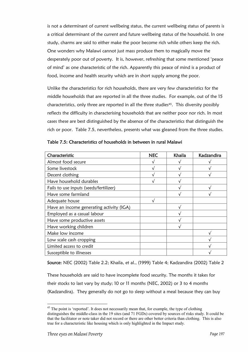
Three eyes on Malawi Poverty Page 197
is not a determinant of current wellbeing status, the current wellbeing status of parents is
a critical determinant of the current and future wellbeing status of the household. In one
study, charms are said to either make the poor become rich while others keep the rich.
One wonders why Malawi cannot just mass produce them to magically move the
desperately poor out of poverty. It is, however, refreshing that some mentioned „peace
of mind‟ as one characteristic of the rich. Apparently this peace of mind is a product of
food, income and health security which are in short supply among the poor.
Unlike the characteristics for rich households, there are very few characteristics for the
middle households that are reported in all the three studies. For example, out of the 15
characteristics, only three are reported in all the three studies45
. This diversity possibly
reflects the difficulty in characterising households that are neither poor nor rich. In most
cases these are best distinguished by the absence of the characteristics that distinguish the
rich or poor. Table 7.5, nevertheless, presents what was gleaned from the three studies.
Table 7.5: Characteristics of households in between in rural Malawi
Characteristic NEC Khaila Kadzandira
Almost food secure √ √ √
Some livestock √ √ √
Decent clothing √ √ √
Have household durables √ √
Fails to use inputs (seeds/fertilizer) √ √
Have some farmland √ √
Adequate house √
Have an income generating activity (IGA) √
Employed as a casual labour √
Have some productive assets √
Have working children √
Make low income √
Low scale cash cropping √
Limited access to credit √
Susceptible to illnesses √
Source: NEC (2002) Table 2.2; Khaila, et al., (1999) Table 4; Kadzandira (2002) Table 2
These households are said to have incomplete food security. The months it takes for
their stocks to last vary by study; 10 or 11 months (NEC, 2002) or 3 to 4 months
(Kadzandira). They generally do not go to sleep without a meal because they can buy
45
The point is „reported‟. It does not necessarily mean that, for example, the type of clothing
distinguishes the middle-class in the 19 sites (and 71 FGDs) covered by sources of risks study. It could be
that the facilitator or note taker did not record or there are other better criteria than clothing. This is also
true for a characteristic like housing which is only highlighted in the Impact study.

Three eyes on Malawi Poverty Page 198
food when food runs out (Khaila, et al., 1999). According to Kadzandira (2002), they
are said to have two or three meals a day. On ownership of livestock, they are said to
own few (NEC, 2002) mainly goats or chickens (Khaila, et al., 1999) if not chickens only
(Kadzandira, 2002).
There is also some variety on the quality of clothing. In some sites, those in the middle
categories were said to have no enough clothes while in others they were said to have
enough clothes (Khaila, et al., 1999). Kadzandira (2002), on the other hand, reports that
some sites mentioned that these households are known to buy clothes once or twice a
year. There is no mention of the quality of the „enough clothes‟ or the clothes they buy
once or twice a year. As for ownership of durable assets, the middle category
households own radios, bicycles, metallic plates (Khaila, et al., 2002) and some chairs
but no sofa sets (Kadzandira, 2002). Just like in the case of the rich, these households do
not have land as a constraint because they can cultivate between 1 and 2 acres (Khaila,
et al., 1999) or if they need more land to cultivate they can rent (NEC, 2002).
Unlike the rich who can afford to purchase and use inputs and employ others, these
households are said to fail to purchase inputs and spend at least 6 months offering
themselves as casual labourers (Khaila, et al., 1999). Some are said to be involved in
small-scale fishing while others distil a local sprit called kachasu or operate a myriad of
micro enterprises just to earn money to purchase basics (Khaila, et al., 1999). These
sources of income are said to yield incomes that are too low with the result that they fail
to make purchases or payments that require a lump sum like secondary school fees or a
bag of maize or fertilizer (Khaila, et al., 1999). Some of the consequences are that their
children drop out of secondary school or they buy maize and fertilizer in smaller
quantities which are more expensive or sell their produce too early just to get the much
needed cash for their essentials (Khaila, et al., 1999).
The characteristics for the poorest category are presented in Table 7.6. There is more
agreement on most characteristics among the three studies. Of the 16 characteristics, nine
are reported in all the three studies and six in two of the studies leaving only one
characteristic (i.e. laziness) reported in one study. Perhaps behind the similarities are
differences in shades. For instance, the food insecurity criterion is variously described by
the amount of food stocks as well as quality and frequency of meals. On stocks, poor
households have stocks that last few months (NEC, 2002) or 1 to 2 months to be exact
(Kadzandira, 2002). Since their stocks last early, poor households are said to be pre-
occupied with securing food supply at the expense of other basics (Khaila, et al., 1999).

Three eyes on Malawi Poverty Page 199
Table 7.6: Characteristics of poorest households in rural Malawi
Characteristic NEC Khaila* Kadzandira
Lack of sufficient food √ √ √
Poor/inadequate shelter √ √ √
Inadequate clothing/beddings √ √ √
Dependency on casual work √ √ √
Inadequate Income/money √ √ √
No assets/poor living conditions √ √ √
Poor health √ √ √
Inputs unavailability √ √ √
Dependency on begging √ √ √
Few or no livestock √ √
Lack of employment opportunities √ √
Credit unavailability √ √
Small farmland √ √
Labour constrained - no support √ √
Children out of school √ √
Lazy √
* Combines 'Have nots' (3 sites); 'The poorest' (3 sites); 'Strugglers' (one site) and 'The
stunted' (one site)
Source: NEC (2002) Table 2.2; Khaila, et al., (1999) Table 4; Kadzandira (2002) Table 2
Again, this „food hunting‟ forces the food insecure to abandon their farms. This reduced
attention to own farm when combined with no fertilizer application and small farmland
results in poor harvests. The frequency of food consumption in poor households is said
to be erratic such that they may stay days without food or eat once a day (Khaila, et al.,
1999; Kadzandira, 2002). This may force some children to eat in their friends homes or
indeed beg for food (Kadzandira, 2002). In hard times poor households are said to be
forced to use bran flour or even a mixture of sawdust and maize/bran flour instead of
pure maize flour (Khaila, et al., 1999; Kadzandira, 2002). Khaila and colleagues (1999)
also report that during the hungry period when even bran is not available, poor
households survive on vegetables-only meals.
The food insecurity in poor households is compounded by inadequate income. Most of
the poor are not employed or engaged in any IGAs (NEC 2002; Kadzandira, 2002). The
poor household‟s main source of income, casual work, is undertaken at the cost of
future food insecurity as they are forced to abandon their farms to work for money
elsewhere (Kadzandira, 2002; Khaila, et al., 1999). Further, this source, just like selling
firewood or fishing with small nets, line and hook or growing sweet potatoes for sell
yield very low incomes (Khaila, et al., 1999). It is also reported that poor households
that are labour-constrained rely on alms to survive (Khaila, et al., 1999). In general,

Three eyes on Malawi Poverty Page 200
poor households generate income that is said to be so low that they can‟t afford
cooking oil let alone meat or fresh fish (Khaila, et al., 1999; Kadzandira, 2002). This
makes vegetables their main relish with cheap small dried fish sporadically breaking the
monotony (Kadzandira, 2002). The low income is compounded by lack of access to
credit facilities as they are excluded on account that they are not credit worthy (NEC,
2002; Kadzandira, 2002).
The poor‟s housing situation is also precarious. In some cases, the poor are said to have
no house of their own (NEC, 2002) while in others their house is said to be grass
thatched (NEC, 2002 and Khaila, et al., 1999) which leaks when it rains (NEC, 2002).
Yet in others, the roof of the poor‟s house is said to have half-fallen in or blown out
(Khaila, et al., 1999; Kadzandira, 2002) and the wall is said to be made of mud (NEC,
2002) which is half-fallen (Khaila, et al., 1999; Kadzandira, 2002). Some houses of the
poor are said to have no windows at all (Kadzandira, et al., 2002). The poor are also
said to sleep rough even in their own houses. Some poor are reported to sleep on mats
because they have no beds (Kadzandira, 2002; NEC, 2002) while others do not even
have a mat (Khaila, et al., 1999). Further, the poor do not have blankets or beddings
(NEC, 2002; Khaila, et al., 1999; Kadzandira, 2002) and to compensate for this they
sleep by the fire for warmth (Khaila, et al., 1999).
The houses of the poor are said to be empty too. It is reported that the poor own very
few utensils (Kadzandira, 2002) most of which are made of plastic (Khaila, et al., 1999).
Otherwise, the poor are reported to have no furniture (Kadzandira, 2002). They are
said to have no durable assets including bicycles, oxcart and radio (NEC, 2002). The
poor lack basic household items including hoes, chairs, plates, plate drying rack, latrine,
kitchen and bathroom (Khaila, et al., 1999). They also do not have adequate clothes as
a result their dressing is poor (NEC, 2002; Kadzandira, 2002) and some children of the
poor are reported to have no clothes (Khaila, et al., 1999). In terms of numbers, some
sites reported that the poor have very few clothes or one change clothing or only one
which they put on until it is tattered (NEC, 2002; Khaila, et al., 1999). Poor households
are reported to rely on clothes handouts (Khaila, et al., 1999). Kadzandira (2002) also
reports that the poor do not have shoes.
The poor are also said to have poor health. This is mostly in terms of the appearance of
their bodies and hair as well as susceptibility to illness. For example, Khaila and
colleagues (1999) report that the poor are said to have unhealthy or stunted or thin
bodies that do not 'shine' even after a bath. In fact the poor are said to rarely take a
bath because they cannot afford to buy soap (Kadzandira, 2002). On account of the

Three eyes on Malawi Poverty Page 201
unhealthy bodies, the poor are said to be susceptible to diseases (Kadzandira, 2002;
Khaila, et al., 1999) and are also inactive (Khaila, et al., 1999). Further, the hair of the
poor is said to be pale (Khaila, et al., 1999) and their children are said to be
malnourished (Kadzandira, 2002).
7.3 Identifying popular wellbeing features
The three studies reviewed in the previous section have yielded wellbeing characteristics
from across the country. Since the point of the study is to find local level dimensions of
wellbeing that are likely sidelined in the official version of wellbeing poverty, the focus
is on characteristics that are common in most of the areas visited. The section answers
questions like „is goats ownership a countrywide characteristic of the „middle‟ class?‟ or
„Are children from most rich households in (good) school or well educated across the
country?‟ or „is poor clothing a common characteristic of the poor across the country?‟
To answer such questions more detailed data than reviewed is required. The 33 MOPS
field reports (CSR, 2005c) provide such data. The reports provide features of wellbeing
categories as well as detailed characteristics of households in those categories.
7.3.1 Wellbeing categories and their characteristics
Each village group defined the number of wellbeing categories prevalent in the village.
The categories ranged from three to six, one group had six and another had five
categories. Otherwise, 18 groups identified four and 13 groups identified three
categories. Table 7.7 provides the details by site. Three steps are taken to analyse the
category characteristics. The first involves establishing the „importance‟ of a characteristic
based on the number of times it is mentioned within a category. In this simple analysis,
absence of mention implies less importance attached to the criterion by the group. It is
understood that this is simplistic but in the absence of purpose-built survey this is the
best that can be done. Moreover, the spontaneous mention of a characteristic gives an
impression that it is important to the one that mentioned it46
.
46
Weights can be „scientifically‟ established by including a comprehensive list of criterion for, say the
four common wellbeing groups, and asking a representative sample to check factors deemed important in
the spirit of Townsend (1979) and Mack and Lansley (1985). The proportions for each factor can be used
as weights.

Three eyes on Malawi Poverty Page 202
Table 7.7: Number of wellbeing categories by site and type of group
FGD name and type Richest Rich Moderate Moderate Poor Poorest Categories
Rich Poor
Phaso Women LOL 1 1 1 1 1 1 6
Nkanile Mixed LOL 1 1 1 1 1 5
Sosola Mixed CM 1 1 1 1 4
Sosola Men LOL 1 1 1 1 4
Zidyana Mixed CM 1 1 1 1 4
Zidyana Women LOL 1 1 1 1 4
Zidyana Men LOL 1 1 1 1 4
Fombe mixed LOL 1 1 1 1 4
Nkanile Mixed CM 1 1 1 1 4
Kasimu Mixed CM 1 1 1 1 4
Kawiliza Mixed LOL 1 1 1 1 4
Kumwanje Mixed CM 1 1 1 1 4
Kuchilimba Mixed CM 1 1 1 1 4
Malonda Women LOL 1 1 1 1 4
Mchoka Mixed CM 1 1 1 1 4
Mchoka Men LOL 1 1 1 1 4
Phaso Men LOL 1 1 1 1 4
Mwachilolo Mixed LOL 1 1 1 1 4
Siwinda Mixed LOL 1 1 1 1 4
Yokoniya Mixed CM 1 1 1 1 4
Fombe mixed CM 1 1 1 3
Kasimu Mixed LOL 1 1 1 3
Kawiliza Mixed CM 1 1 1 3
Kuchilimba Mixed LOL 1 1 1 3
Mchoka Women LOL 1 1 1 3
Tsoyo-Undi Mixed LOL 1 1 1 3
Siwinda Mixed CM 1 1 1 3
Yokoniya Mixed LOL 1 1 1 3
Sosola Women LOL 1 1 1 3
Kumwanje Mixed LOL 1 1 1 3
Malonda Men LOL 1 1 1 3
Mwachilolo Mixed CM 1 1 1 3
Tsoyo-Undi Mixed CM 1 1 1 3
Total/average 33 1 28 25 2 33 3.7
Note: LOL = FGD on ladder of life; CM = Key informant interview on community mobility
Source: Author‟s summary of MOPS field reports
The second step involves highlighting how different levels of the same characteristic are
used to describe households in the same category or how the same level of a
characteristic can be used to describe households of different categories in different sites.
The third step focuses on identifying characteristics that are consistent within and across

Three eyes on Malawi Poverty Page 203
categories and sites. Given that there is „no science‟ behind the number of wellbeing
categories, this third step is meant to determine whether a characteristic consistently
changes over the wellbeing continuum. This third step is necessary to identify
characteristics that can be said to be national in nature. Those characteristics that pass
the third „test‟ are the ones that are later used to interrogate the official operational
definition of poverty in Chapter 9.
7.3.2 Important characteristics for various wellbeing categories
The field reports show that groups find it easier to characterise the richest and poorest
categories than those in between. Categories in between are variants of the extremes
and they rarely have unique characteristics. Considering that the majority of the 33
groups defined four categories, the analysis in this sub-section uses four categories47
as
well. For convenience, these are termed „the richest‟, „the moderately rich‟, „the
moderately poor‟, and „the poorest‟48
. Further, for a characteristic to be considered
important it must be mentioned by at least half of the groups (i.e. at least 17 groups).
However, there is some discussion of less popular but unique characteristics.
Important characteristics for the richest category
There are ten characteristics that meet the criterion and these are ownership of livestock,
amount of maize stocks, type of house used, ability to hire labour, type and number of
changes of clothes, support of child education, quality of food consumed, number of
meals taken per day, ownership of durable assets, and ability to purchase fertilizer. See
Table 7.8.
Access to labour refers to casual labour (ganyu) because use of salaried labour is rare in
rural areas. In line with the findings in Chapter 5, education and health status are both
not important features for the richest. This is also true of access to credit. Hidden within
most of the characteristics is access to cash. Although availability of cash was mentioned
by only 8 groups, cash underwrites most of the popular characteristics like food quality,
quantity and diversity. In a rural setting, having milk tea breakfast is a feat because such
requires the availability of tea itself, then sugar, milk and some bread/bun/scones all of
which require cash. For lunch and supper, money for vegetable oil, salt, soda for
vegetables and maize milling is frequently required just as it also needed to purchase
47
This collapses the six and five categories into four to simplify analysis. The rich in Phaso become part
of the richest. Likewise the poor in Phaso and Nkanile become part of the poorest. 48
The original (local language) labels for the categories describe them well. The labels given here are for
convenience because no group described any category in terms of „richest‟ or „moderately rich‟. The
common literal translations for the top category include „those who eat well‟ and „those who do well‟,

Three eyes on Malawi Poverty Page 204
meat/fish/pulses that are consumed daily by the richest. Likewise, cash for
soap/detergents and lotion is required for baths and washing clothes. This is why some
groups summarised the richest category as one in which money is not a problem.
Table 7.8: Number of groups using the dimension to characterise the richest
Dimension # Dimension # Dimension #
Livestock ownership 33 Productive assets 13 Footwear quality 5
Food stocks 30 Farmland size 12 Access to land 5
House structure 30 Child clothing 10 Access to basics 4
Access to labour 28 Body condition 10 Health status 4
Clothing 27
Access to shock
absorbers 10 Dimba ownership 4
Child education 24 Relationship 9 House amenities 4
Food quality 24 Crops for sale 8 Child quality of life 3
Food consumption 23 Access to cash 8 Child food 3
Durable assets 21 Employment status 7
Crops for
food/sale 3
Access to inputs 18 Life style 7 Access to credit 2
Access to nutrition 16 Number of children 6 Crops in dimba 2
Bedroom conditions 15 Child body condition 6 Personal traits 1
Quality of life 14 Home care 5 Utensils 1
IGA 14 Child behaviour 5 External support 1
Source: Author‟s summary of MOPS Field Reports
In general, a household that affords even lumpy outlays like hire of labour or rent of
land or purchase of inputs or child education (especially secondary school) is expected
to have access to cash or shock absorbers (livestock/crop sales, savings, and remittances)
on regular basis. The limited mention of access to cash may imply the groups used cash
manifests to describe the rich because of limited knowledge of how much money a
household has. By labelling a household as a tea-drinking, for example, challenges the
listener to imagine what it takes to have a cup of tea. Likewise, affording meat/fish
everyday tells a story of how much money a household has. Thus the absence of access
to cash for the richest may be due to discussants‟ concentration on what money does
when available.
Important characteristics for the moderately rich
The characteristics for the moderately rich are similar to those for the richest only that
fewer groups mentioned them. Using the 50% rule, the commonest criteria for this
wellbeing category include livestock ownership, amount of food stocks, type of house
and type of education a household affords the children. See Table 7.9.

Three eyes on Malawi Poverty Page 205
Table 7.9: Number of groups using dimension to describe the moderately rich
Dimension # Dimension # Dimension #
Livestock ownership 26 Productive assets 6 Relationship 2
Food stocks 22 Quality of life 5 Footwear quality 2
House structure 20 Income generating activity 5 Dimbaland ownership 2
Child education 19 Child clothing 5 Access to credit 2
Food consumption 15 Body condition/appearance 5 Crops in dimba 2
Clothing 14 Access to nutrition 4 Personal traits 1
Access to labour 12 Access to shock absorbers 4 Child behaviour 1
Durable assets 12 Home care 4 Child quality of life 1
Food quality 10 Life style 3 Child food 1
Access to inputs 9 Access to basics 3 Access to ganyu income 1
Employment status 7 Access to cash 3 Access to land 1
Crops for sale 7 Household utensils 3 Crops for food/sale 1
Bedroom conditions 6 Farmland size 2 House amenities 1
Number of children 6 Health status 2
Source: Author‟s summary of MOPS Field Reports
Important characteristics of the moderately poor
There are also four characteristics that are mentioned by at least 50% of the groups in
describing the moderately poor. These are offer of labour services, amount of maize
stocks, type of livestock owned and type of house. In this category, child education and
type and number or changes of clothing are not mentioned by the majority. It is the
offer of labour services that is mostly used. See Table 7.10.
The prominence of non-farm income generation in this category is noteworthy.
Apparently, this category depends more on resources generated outside the farm. Thus
the moderately poor are identified by their struggle to „make ends meet‟ through the
operation of micro enterprises, exploitation of natural resources for sale and
involvement in ganyu.
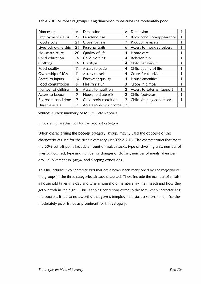
Three eyes on Malawi Poverty Page 206
Table 7.10: Number of groups using dimension to describe the moderately poor
Dimension # Dimension # Dimension #
Employment status 22 Farmland size 7 Body condition/appearance 1
Food stocks 21 Crops for sale 7 Productive assets 1
Livestock ownership 21 Personal traits 6 Access to shock absorbers 1
House structure 20 Quality of life 4 Home care 1
Child education 16 Child clothing 4 Relationship 1
Clothing 16 Life style 4 Child behaviour 1
Food quality 11 Access to basics 4 Child quality of life 1
Ownership of IGA 11 Access to cash 4 Crops for food/sale 1
Access to inputs 10 Footwear quality 4 House amenities 1
Food consumption 9 Health status 3 Crops in dimba 1
Number of children 8 Access to nutrition 2 Access to external support 1
Access to labour 7 Household utensils 2 Child footwear 1
Bedroom conditions 7 Child body condition 2 Child sleeping conditions 1
Durable assets 7 Access to ganyu income 2
Source: Author summary of MOPS Field Reports
Important characteristics for the poorest category
When characterising the poorest category, groups mostly used the opposite of the
characteristics used for the richest category (see Table 7.11). The characteristics that meet
the 50% cut off point include amount of maize stocks, type of dwelling unit, number of
livestock owned, type and number or changes of clothes, number of meals taken per
day, involvement in ganyu, and sleeping conditions.
This list includes two characteristics that have never been mentioned by the majority of
the groups in the three categories already discussed. These include the number of meals
a household takes in a day and where household members lay their heads and how they
get warmth in the night. Thus sleeping conditions come to the fore when characterising
the poorest. It is also noteworthy that ganyu (employment status) so prominent for the
moderately poor is not as prominent for this category.

Three eyes on Malawi Poverty Page 207
Table 7.11: Number of groups using the dimension to describe the poorest
Dimension # Dimension # Dimension #
Food stocks 27 Access to basics 10 Child quality of life 4
House structure 26 Food quality 9 Child food 4
Livestock ownership 21 Child clothing 9 Access to safety nets 4
Clothing 21 Personal traits 9 Access to shock absorbers 3
Food consumption 21 Household utensils 7 Access to ganyu income 3
Child education 20 Access to cash 6 Durable assets 2
Employment status 17 Labour capacity 6 Access to nutrition 2
Bedroom conditions 17 Crops for sale 5 Productive assets 2
Access to inputs 13 Health status 5 Ownership of IGA 1
Number of children 13 Child behaviour 5 Relationship 1
Life style 13 Access to credit 5 Dimbaland ownership 1
Farmland size 11 Home care 4 Crops for food/sale 1
Body condition/
appearance 11
Child body condition/
appearance 4
Availability of external
support 1
Quality of life 10
Source: Author summary of MOPS Field Reports
Prominent characteristics across all categories
Given that wellbeing status is a continuum (McGregor, 2007) it follows that a good
wellbeing measure would also apply across the continuum. Since wellbeing categorising
is an attempt to „chop‟ the continuum into manageable bits, a good characteristic would
show different magnitudes at different sections of the continuum. Table 7.12, which is a
summary of Tables 7.8 to 7.11, shows that some characteristics apply across the
continuum while others are category specific. The table also includes some
characteristics that are not prominent but are related to the prominent measures.
The commonest criteria for categorising households include livestock ownership, amount
of own produced maize in stock, type of dwelling unit, type of clothing and capability
to educate children. Others that come close include number of meals taken per day and
access to inputs. It is, however, noted that the emphasis for both of these criteria, is
reduced for the „moderates‟. There are a number of characteristics that are more
popular for richest and poorest categories and less popular for the moderately rich and
poor. For example, sleeping conditions is one characteristic that is used to mainly
characterise the richest (i.e. the presence of beds, blankets, mattresses and linen) and the
poorest (i.e. absence of mats or blankets). This is also true for type of clothes and
farmland size.

Three eyes on Malawi Poverty Page 208
Table 7.12: Number of groups using the important dimension by category
Dimension Richest Moderate Rich Moderate Poor Poorest
Ownership of assets
Livestock ownership 33 26 21 21
Durable assets 21 12 7 2
Productive assets 13 6 1 2
Household utensils 1 3 2 7
Access to shock absorbers 10 4 1 3
Food availability and consumption
Food stocks 30 22 21 27
Food quality 24 10 11 9
Food consumption 23 15 9 21
House structure 30 20 20 26
Cash-dependent characteristics
Access to labour 28 12 7 0
Access to inputs 18 9 10 13
Access to nutrition 16 4 2 2
Access to basics 4 3 4 10
Clothing and beddings
Type of clothing 27 14 16 21
Child clothing 10 5 4 9
sleeping conditions 15 6 7 17
Others
Child education 24 19 16 20
Employment status 7 7 22 17
Source: Tables 7.9 to 7.12
There are other characteristics not listed in the table that are mostly used to characterise
the extremes. Examples include quality of life („lacking nothing‟, „happy‟, „free‟, „having
peace of mind‟, „being worry-free‟ as unique for richest and „being in constant worries
and unhappy‟, „having no peace of mind‟, „lacking everything' and „looking miserable‟ as
unique features for the poorest) and behaviour or conduct of household members. The
poorest are variably described as lazy or liars or thieves or argumentative or beggars or
gamblers or poor managers of own resources or not creditworthy or drunks or cannabis
abusers. On the other hand, the richest are said to be prudent managers of resources or
good planners but proud, boastful and not courteous if not sarcastic.
There are also some characteristics mainly used for one side of the spectrum. For
example, the hire of labour and type of meals a household takes (consumption of meat
and fish and the use of cooking oil in the preparation of food), ownership of durable
and productive assets, and access to shock absorbers and land are almost exclusively
used to describe the richest category. The drop in number of groups using food quality

Three eyes on Malawi Poverty Page 209
from 24 to 9 groups signify that the poorest are described alternatively rather than
whether they only eat nsima49 with vegetables. Likewise, ownership of assets (durable
and productive) is used to describe the rich but lack of these is not used to describe the
poor or poorest.
Another characteristic that is mainly used to describe the poor is offer of labour services
for casual work. The moderately poor are more described as being heavily involved in
ganyu than the poorest. One of the possible reasons is that group discussants use labour-
constraint as a criterion for the poorest, implying that some of the poorest lack labour
by definition. Another characteristic mostly used for the poorest category is number of
children. The few groups that used number of children to describe the rich or
moderately rich, praised them for practising family planning. When used for the poor
category households, groups „blamed‟ them for ignoring family planning. Absence of
utensils is also used mainly to describe the poorest households yet the presence of
utensils is rarely used to describe any other category.
Thus group discussants use unique (as opposed to common) characteristics that easily
distinguish a category. This is consistent with what experts do when selecting indicators.
The group discussants consistently selected characteristics that showed differences. For
example, the rich are easily recognised by presence of assets while the poor are
described by the absence of the „must have‟ utensils. Again, sale of livestock or surplus
food crops to meet cash flow problems is mostly used to describe the rich while
involvement in ganyu at the expense of future consumption is used to describe the poor.
For example, it is not the absence of durable assets in the poor man‟s home or the
absence of a fallback position for the poor that is used to identify them but failure to
have the basics (plate, pot, salt, soap, mat, shirt/blouse, short/skirt and blanket) or
absence of able-bodied members or laziness or misuse of resources.
There are three points here. The first point is that there are characteristics that are
common in more than two categories. Such characteristics are potential candidates for
incorporation in the operational definition of poverty, if they are not already
incorporated. They however need to pass a popularity test; they must apply across the
country. This then implies that for all characteristics that were ever mentioned by at least
half of the groups are potential candidates for the popularity test. The second point is
that there are some characteristics that are used mostly for one side of the spectrum
49
Nsima is a product of maize flour and water stirred to taste over a fire. It is the main dish which MUST
be accompanied by a side dish (relish). Nsima is food because it goes with any type of relish. A rich
household takes nsima with a number of relish dishes, preferably protein-based and vegetables. This is
what is commonly referred to as diet diversity.

Three eyes on Malawi Poverty Page 210
because they are best for that side. Again, if these are popular across the country they
are better used as dummy variables. The third point is that each potential candidate
ought to have different levels or qualities that are different at various sections of the
wellbeing spectrum. This type of analysis is the subject of the next subsection.
7.3.3 Different shades of the prominent wellbeing characteristics
This sub-section analyses the prominent characteristics to determine their varying
attributes, termed features in this discussion, across categories. To do so, „measureable‟
features mentioned by discussants are checked for consistency across sites but within a
category. To facilitate the consistency check across sites, the fifteen sites are placed in
four regions namely South, East, Centre and North.
Livestock ownership
As Tables 7.13 to 7.15 shows, ownership of livestock diminishes with poverty. This is in
terms of number of sites using livestock as a characteristic and the types of livestock
owned. While the richest own a variety of livestock, the commonest types of livestock
for this category are cattle, goats and chickens. For the moderately rich, the commonest
livestock are goats and chickens while chickens are the commonest for the moderately
poor. The poorest are mostly known for having no livestock. It is noted that although
pigs are found in all the regions, they are most prevalent in the Centre50
. These tables
also show that ownership of sets of livestock is mostly used to characterise categories. It
is common to have cattle, goats and chickens mentioned together as a characteristic for
the richest. This is true for goats and chickens for the moderately rich, and chickens for
the moderately poor and no livestock for the poorest.
50
The assumption made in this analysis is that by not being mentioned, the attribute is considered less
important for characterising the category. The absence of an attribute in the characteristics of the
category does not necessarily mean its absence in the households in the category or indeed in the
community. Importance is determined by mention. The openness of the discussion is assumed to be good
enough for any important attribute to be remembered.
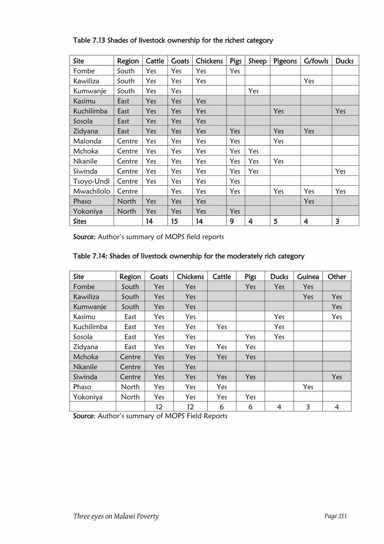
Three eyes on Malawi Poverty Page 211
Table 7.13 Shades of livestock ownership for the richest category
Site Region Cattle Goats Chickens Pigs Sheep Pigeons G/fowls Ducks
Fombe South Yes Yes Yes Yes
Kawiliza South Yes Yes Yes
Yes
Kumwanje South Yes Yes
Yes
Kasimu East Yes Yes Yes
Kuchilimba East Yes Yes Yes
Yes
Yes
Sosola East Yes Yes Yes
Zidyana East Yes Yes Yes Yes
Yes Yes
Malonda Centre Yes Yes Yes Yes
Yes
Mchoka Centre Yes Yes Yes Yes Yes
Nkanile Centre Yes Yes Yes Yes Yes Yes
Siwinda Centre Yes Yes Yes Yes Yes
Yes
Tsoyo-Undi Centre Yes Yes Yes Yes
Mwachilolo Centre
Yes Yes Yes
Yes Yes Yes
Phaso North Yes Yes Yes
Yes
Yokoniya North Yes Yes Yes Yes
Sites 14 15 14 9 4 5 4 3
Source: Author‟s summary of MOPS field reports
Table 7.14: Shades of livestock ownership for the moderately rich category
Site Region Goats Chickens Cattle Pigs Ducks Guinea Other
Fombe South Yes Yes
Yes Yes Yes
Kawiliza South Yes Yes
Yes Yes
Kumwanje South Yes Yes
Yes
Kasimu East Yes Yes
Yes
Yes
Kuchilimba East Yes Yes Yes
Yes
Sosola East Yes Yes
Yes Yes
Zidyana East Yes Yes Yes Yes
Mchoka Centre Yes Yes Yes Yes
Nkanile Centre Yes Yes
Siwinda Centre Yes Yes Yes Yes
Yes
Phaso North Yes Yes Yes
Yes
Yokoniya North Yes Yes Yes Yes
12 12 6 6 4 3 4
Source: Author‟s summary of MOPS Field Reports

Three eyes on Malawi Poverty Page 212
Table 7.15: Shades of livestock ownership for the moderately poor
Site Region Chicken Goats Pigs ducks Cattle
Fombe South Yes
Yes Yes
Kawiliza South Yes
Sosola East Yes Yes
Zidyana East Yes Yes
Malonda Centre Yes Yes Yes
Mchoka Centre Yes Yes
Mwachilolo Centre Yes
Nkanile Centre Yes Yes
Siwinda Centre Yes
Tsoyo-Undi Centre Yes Yes Yes
Phaso North Yes
Yes
Yokoniya North Yes
12 6 3 1 1
Source: Author‟s summary of MOPS Field Reports
Food security and consumption
Food attributes used to characterise categories vary. For the richest, the popular
attributes are having (i) maize stocks that last harvest to harvest; (ii) every lunch and
supper with protein-rich relish; (iii) breakfast tea; (iv)at least three meals in a day. For
the moderately rich features that are common across the country are inadequate maize
stocks and two meals a day. For the moderately poor category moderately poor
households are characterised by having maize stocks that last less than 12 months,
averaging five and half months. The poorest category is mostly known for having no
stocks of maize and only one meal in a day. There are variations by site and region.
However, Tables 7.16 to 7.19 show that food security and consumption is popularly
used across the country in varying ways. In some sites some moderately rich have annual
stocks and take three meals a day.
The food security feature is strengthened when used in conjunction with strategies
households use to fill the maize stock gap. Reading through the reports, the rich have
surplus maize stocks which they use to sell or pay labour, the well off moderately rich
sometimes have a surplus but they also buy stocks by selling livestock or durable goods.
The moderately poor sell their labour services to bridge the gap but also attend to their
land. The poorest with labour work the entire year to get or purchase maize and the
labour-constrained survive on handouts.

Three eyes on Malawi Poverty Page 213
Table 7.16: Shades of food for the richest category
Site Region Enough Surplus Three B/fast Protein Vegetable Snacks
stocks maize meals tea relish oil
Fombe South Yes
Yes Yes
Yes
Kawiliza South Yes
Yes Yes Yes Yes Yes
Kumwanje South Yes Yes Yes Yes Yes
Zidyana East Yes Yes Yes Yes Yes
Kasimu East Yes Yes Yes Yes Yes Yes Yes
Kuchilimba East
Yes Yes Yes Yes
Sosola East Yes Yes
Yes Yes
Mwachilolo Centre Yes
Yes Yes
Tsoyo-Undi Centre Yes
Yes Yes Yes
Malonda Centre Yes Yes Yes Yes Yes
Siwinda Centre
Yes Yes
Yes
Mchoka Centre Yes Yes Yes
Yes
Nkanile Centre Yes Yes Yes Yes Yes
Phaso North Yes
Yes Yes Yes
Yokoniya North Yes Yes Yes Yes Yes Yes Yes
13 8 12 14 13 5 5
Source: Author‟s summary of MOPS Field Reports
Table 7.17: Shades of food for the moderately rich category
Site Region 12 months < 12 m 2 meals Good food Tea Porridge
Fombe South
Yes Yes Yes
Kawiliza South
Yes Yes Yes
Kumwanje South
Yes Yes
Kasimu East Yes Yes Yes
Yes
Kuchilimba East
Yes Yes
Sosola East Yes Yes Yes
Zidyana East Yes Yes
Yes Yes
Mchoka Centre Yes Yes
Yes
Mwachilolo Centre Yes
Nkanile Centre
Yes Yes
Siwinda Centre Yes Yes Yes Yes
Phaso North Yes
Yes
Yokoniya North
Yes Yes Yes Yes
7 11 9 5 2 3
Source: Author‟s summary of MOPS Field Reports

Three eyes on Malawi Poverty Page 214
Table 7.18: Shades of food for the moderately poor category
Site Region Stocks in < 12 Two One No Porridge
months months meals meal diversity
Fombe South
Yes
Kawiliza South 4 Yes Yes Yes Yes
Kumwanje South 0 Yes
Kasimu East 3 Yes Yes Yes
Kuchilimba East 0 Yes Yes
Sosola East 12 Yes
Zidyana East 5 Yes
Malonda Centre 6 Yes Yes
Mchoka Centre 12 Yes Yes
Mwachilolo Centre 3 Yes Yes
Nkanile Centre 5 Yes Yes
Siwinda Centre 4 Yes
Tsoyo-Undi Centre 5 Yes Yes Yes Yes
Phaso North 12 Yes
5.5 10 4 4 5 3
Source: Author‟s summary of MOPS Field Reports
Table 7.19: Shades of food for the poorest category
Site Region Number day meal Eat Stock Eat Before Diet
of meals skip meat months bran harvest diversity
Fombe South 1 Yes rare 0
No
Kawiliza South 1 Yes
0 Yes Yes
Kasimu East 1 Yes
0 Yes Yes No
Kuchilimba East 1
0
Sosola East 1
0/3 Yes
Zidyana East 1
0/3 Yes Yes
Malonda Centre 2
rare 0/1
Yes No
Mchoka Centre 2/1 Yes rare 0/2
Yes No
Mwachilolo Centre 1
0
Yes
Nkanile Centre 1 Yes
0/1 Yes
Siwinda Centre 1 Yes
0
Tsoyo-Undi Centre 1
rare 0
Yes No
Phaso North 1 Yes
0
No
Yokoniya North 1 Yes
0
Source: Author‟s summary of MOPS Field Reports

Three eyes on Malawi Poverty Page 215
Quality of housing
There is some variety on this dimension across the country and categories. Except in
one district (two sites), having corrugated iron roof is the commonest feature for the
richest category. The moderately rich category has a mixed bag of features and there is
no one feature commonly used to characterise the group. For the moderately poor
households, a grass thatched house is commonest. The feature that is common for the
poorest category is dilapidation51 in terms of the condition of either walls or roof and
desolation in terms of the surrounding. In fact, it appears the richer the household the
more the care given to the dwelling unit and surroundings. However, the picture
presented is stylised because, as evidenced in Tables 7.20 and 7.21, there is so much
variety. In some cases, one feature is used to characterise more than one category, even
at the same site and group discussion.
Table 7.20: Shades of housing for richest category
Site Region Iron Brick Cement Glass Grass Home Amenities
roof wall floor window thatch care
Fombe South Yes Yes Yes
Kawiliza South Yes Yes
Kumwanje South Yes
Kasimu East Yes
Yes Yes Yes Yes
Kuchilimba East Yes
Yes Yes Yes
Sosola East Yes Yes Yes Yes Yes
Yes
Zidyana East Yes
Yes Yes
Yes
Malonda Centre Yes
Yes Yes
Mchoka Centre Yes Yes Yes Yes
Yes
Nkanile Centre Yes Yes Yes Yes Yes Yes
Siwinda Centre Yes
Yes
Mwachilolo Centre
Yes
Yes Yes
Tsoyo-Undi Centre
Yes
Yes
Phaso North Yes
Yes Yes Yes
Yes
Yokoniya North Yes Yes Yes Yes
Yes
13 8 9 10 6 5 5
Source: Author‟s summary of MOPS Field Reports
51
Some of factors were fallen wall or roof (one side), sooty interiors due to in-house fire, rugged walls,
untidy surrounding, overcrowding, and not well-maintained roofs to the extent that some have grass
growing on their roofs.

Three eyes on Malawi Poverty Page 216
Table 7.21: Shades of housing for the moderately rich category
Site Region Grass Iron Cement Burnt Other Mud Glass
roof roof floor bricks wall floor window
Fombe South Yes Yes Yes Yes
Kawiliza South Yes Yes
Kumwanje South
Yes
Kuchilimba East Yes
Sosola East Yes Yes
Yes Yes Yes
Zidyana East
Yes
Malonda Centre Yes
Yes Yes
Mchoka Centre Yes
Yes Yes Yes
Nkanile Centre Yes
Yes
Yes
Siwinda Centre
Yes
Phaso North Yes Yes
Yes
Yes
Yokoniya North Yes
Yes Yes
9 7 3 5 2 4 2
Source: Author‟s summary of MOPS Field Reports
Clothing and footwear
This dimension is used to characterise the richest and poorest categories only. The richest
are characterised as having quality clothes variously put as having „decent‟, „nice-looking‟
and „wearing expensive‟ clothes. The most common feature for the poorest is that their
clothes are torn or dirty because they are rarely changed and washed (with detergents),
respectively. In general, the poorest have poor quality clothes in terms price, quality and
appearance. They also have no or few changes of clothes. On the other hand, the
richest have expensive clothing (a translation of „zodula‟). Expensive takes a number of
meanings including pricey, high quality (a translation of zapamwamba) or rare (zosowa
meaning not common in the area or 'out of this world'). It is noted that the feature that
the richest have clothes that are 'clean' (meaning they are washed) and 'tidy' (meaning
they are iron pressed) is only prevalent in the East and Centre and having changes of
good clothes (on daily basis, i.e. 'they can change their clothes everyday') is sparsely
popular. Table 7.22 gives the features used for the richest category.

Three eyes on Malawi Poverty Page 217
Table 7.22: Shades of clothing for the richest category
Site Region High Good Have Suits New Good
quality care changes
shoes
Fombe South Yes
Yes Yes
Kawiliza South Yes Yes Yes
Kumwanje South Yes
Kasimu East Yes Yes
Kuchilimba East Yes Yes
Sosola East Yes Yes Yes
Yes
Zidyana East Yes
Yes
Malonda Centre Yes Yes Yes
Yes
Mchoka Centre Yes Yes
Yes Yes
Mwachilolo Centre Yes Yes
Tsoyo-Undi Centre
Yes Yes
Yes
Nkanile Centre Yes Yes
Siwinda Centre Yes
Yes
Phaso North Yes
Yes
Yes
Yokoniya North Yes
Yes
14 9 6 3 3 4
Source: Author‟s summary of MOPS Field Reports
Child education
This dimension is used for all categories except the moderately poor. The richest are
described by their ability to support children‟s education up to or beyond secondary
school. The commonly mentioned features include fees for secondary school or money
for private or boarding fees in public secondary schools. As Table 7.23 shows, child
education as a dimension is not popularly used to characterise the moderately rich given
that only 11 out of the 15 used it. However, the feature that is common is that children
attend school and complete primary school (PS) but not secondary school (SS). For the
poorest, the most popular feature under child education is that children of the poor
drop out of primary school. The drop out for the poorest category is associated with
lack of food and presentable clothing (washed and not torn). For the moderately rich,
the drop out is due to failure to pay school fees and other school expenses and those
who complete do so through the sale of their livestock.

Three eyes on Malawi Poverty Page 218
Table 7.23: Shades of children education for the moderately rich category
Site Region Attend Drop out Complete PS Complete SS Dropout SS
Fombe South Yes
Yes Yes Yes
Kawiliza South Yes
Yes Yes Yes
Kasimu East Yes Yes Yes
Yes
Kuchilimba East Yes Yes
Sosola East Yes
Yes Yes Yes
Zidyana East Yes Yes Yes Yes Yes
Mchoka Centre Yes
Yes Yes
Nkanile Centre Yes
Siwinda Centre Yes Yes Yes Yes Yes
Phaso North Yes
Yokoniya North Yes
Yes
Yes
11 4 8 6 7
Source: Author‟s summary of MOPS Field Reports
Hire and offer of labour services
Only households in the richest category are said to use paid labour. Any household that
can consistently hire 'hands' to work for them is considered rich. In general, the richest
households do not do hard jobs, especially farm work. They instead hire other people
to do such jobs for them. Given that the richest have „surplus‟ money or food, they are
best known as local safety nets as the poor rely on them when in need. Some of the
richest households are said to „create‟ work just to help out the needy seeking help from
them. On the other hand, the poor (moderately poor and poorest) are best known for
offering their labour services in ganyu activities. Since the poorest category also include
labour-constrained households, offer of labour services is mostly used to characterise the
moderately poor. In fact, apart from sites in Mangochi (Kuchilimba and Kasimu), where
fishing is the main livelihood strategy, all sites used offer of labour services to describe
the moderately poor (Table 7.24).
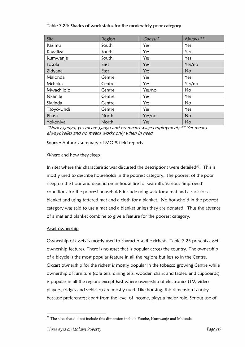
Three eyes on Malawi Poverty Page 219
Table 7.24: Shades of work status for the moderately poor category
Site Region Ganyu * Always **
Kasimu South Yes Yes
Kawiliza South Yes Yes
Kumwanje South Yes Yes
Sosola East Yes Yes/no
Zidyana East Yes No
Malonda Centre Yes Yes
Mchoka Centre Yes Yes/no
Mwachilolo Centre Yes/no No
Nkanile Centre Yes Yes
Siwinda Centre Yes No
Tsoyo-Undi Centre Yes Yes
Phaso North Yes/no No
Yokoniya North Yes No
*Under ganyu, yes means ganyu and no means wage employment; ** Yes means
always/relies and no means works only when in need
Source: Author‟s summary of MOPS field reports
Where and how they sleep
In sites where this characteristic was discussed the descriptions were detailed52
. This is
mostly used to describe households in the poorest category. The poorest of the poor
sleep on the floor and depend on in-house fire for warmth. Various „improved‟
conditions for the poorest households include using sack for a mat and a sack for a
blanket and using tattered mat and a cloth for a blanket. No household in the poorest
category was said to use a mat and a blanket unless they are donated. Thus the absence
of a mat and blanket combine to give a feature for the poorest category.
Asset ownership
Ownership of assets is mostly used to characterise the richest. Table 7.25 presents asset
ownership features. There is no asset that is popular across the country. The ownership
of a bicycle is the most popular feature in all the regions but less so in the Centre.
Oxcart ownership for the richest is mostly popular in the tobacco growing Centre while
ownership of furniture (sofa sets, dining sets, wooden chairs and tables, and cupboards)
is popular in all the regions except East where ownership of electronics (TV, video
players, fridges and vehicles) are mostly used. Like housing, this dimension is noisy
because preferences; apart from the level of income, plays a major role. Serious use of
52
The sites that did not include this dimension include Fombe, Kumwanje and Malonda.

Three eyes on Malawi Poverty Page 220
this dimension requires a study meant to determine whether the noise is manageable
statistically and, if manageable, establish district level weights for the popular assets.
Table 7.25: Shades of asset ownership for the richest category
Site Region Bike Oxcart Furniture Electro Radio Vehicles Produc.*
Fombe South Yes Yes
Yes
Kawiliza South Yes
Yes
Yes
Kumwanje South
Yes
Kasimu East Yes
Yes
Sosola East Yes Yes
Yes Yes Yes
Zidyana East Yes Yes
Yes
Yes
Kuchilimba East
Yes Yes Yes Yes Yes
Mwachilolo Centre Yes Yes Yes
Yes
Tsoyo-Undi Centre Yes
Yes
Mchoka Centre
Yes Yes
Nkanile Centre
Yes Yes Yes
Yes
Siwinda Centre
Yes
Phaso North Yes
Yes Yes
Yes
Yokoniya North Yes Yes Yes
Yes
Yes
9 8 8 5 3 5 7
* Productive assets include tobacco baling jacks, ploughs, tangerine trees, bicycle taxis,
motorised boats and fishing nets, each of which is site specific
Source: Author‟s summary of MOPS Field Reports
Access to fertilizer
This is another dimension that is not only unique to the richest category but is also not
popular across the country. For example, out of the 15 sites 11 sites spread across the
regions used access to fertilizer to characterise the richest. However, fertilizer is most
popular in the Centre evidenced by its use in all the five sites each with unprompted
estimates of number of bags the richest purchase in a season.
So far, the analysis has established features within characteristics that have the potential
of being used across categories and regions. The next step is to determine whether such
features would, in some form, apply in other categories. As stated earlier unless a feature
is capable of „changing colours‟ over the wellbeing continuum it cannot be taken as a
good identifier.
7.3.4 Popular wellbeing features
Moving forward from the previous subsection, the features that can easily characterise
households in the top most wellbeing category across the country include (i) the
ownership of at least cattle and goats and chickens; (ii) the availability of maize stocks

Three eyes on Malawi Poverty Page 221
that go as far as the next harvest; (iii) consumption of protein-rich relish every lunch and
supper; (iv) taking tea breakfast; (v) hire of labour; (vi) ability to support child
education; and (vii) purchase of fertilizer. Other important but less popular features
include (viii) ownership of a house with corrugated iron sheet roof; (ix) ownership of
good quality clothes; and (x) ownership of bicycles.
Under the category for the moderately rich the most popular features are (a) ownership
of both goats and chickens, (b) the inadequacy of maize stocks combined with ability to
cover the food gap, and (c) consumption of two meals a day. There are two features
that are popular for the moderately poor. These are (i) working for other households
and (ii) having maize stocks that run out before the next harvest. These are related in
that households are forced to work for relatively well off households in order to bridge
the food gap. For the poorest category, the features that are popular include (i) having
maize stocks that last three months at the most, (ii) having one meal in a day, (iii)
absence of meat-based meal for a long time, (iv) owning no livestock, (v) having
primary school going age children out of school, and (vi) having no mat and blankets.
Some of these have caveats but when used in combination with others, they are good
features.
The question is, are these features consistent across categories? This then requires some
sort of consistency check. To do so each important feature, regardless of the category it
is popular under, is checked for some consistent variation across the four wellbeing
categories53
. Table 7.26 lists the features in a form that is easy to compare across the
categories. For most of these features, it is difficult to see their different shades. To
make it clear, a discussion of the ambiguous features is required. This is done in the next
paragraphs.
53
What is applied here is a mild form of consistency check recognising that the data was not collected for
a rigorous consistency check.

Three eyes on Malawi Poverty Page 222
Table 7.26: Variations of popular features across wellbeing categories
Feature Richest Moderate
rich
Moderate
poor
Poorest
Ownership of chickens Majority Majority Some None
Ownership of goats Majority Majority Some None
Ownership of cattle Majority Some None None
Taking breakfast tea Majority Few None None
Months of maize stocks >=12 <=12 <=6 0
Number of meals per day 3 2 <=2 <=1
Protein every meal and day All Some Few None
Corrugated iron roof Majority Some Few None
Hire of labour All Few None None
Working for others None Few Majority Some
Type of clothes* New HQ used PQ used None
Type of 'sleeper' Bed/mattress Mattress Mat Sack
Type of beddings HQ blankets Blankets Blankets Fabric
Level of child education Secondary Primary < full PS None
Purchase of fertilizer Majority Some Few None
Ownership of bicycles Majority Some Few None
* HQ used=high quality used clothes; PQ used=poor quality used clothes
Source: Summary of the sub-section (shades of wellbeing dimensions)
Livestock ownership
Three types of livestock (cattle, goats and chickens) are found to be popular features
across the country. As to how categories differ is best dealt with numbers owned. Table
7.27 presents the numbers. Judging from the table, the numbers of goats and chickens
decline as wellbeing status declines, at least within a site. Across sites, Zidyana appear to
be an exception because the numbers of livestock owned by the moderately rich and
poor are what in other sites are used for the „richer categories‟. For example, owning 3
to 10 goats is used for the moderately poor in Zidyana but the moderate rich in Nkanile,
Kawiliza and Kasimu.
Considering that this picture is based on unprompted responses, it is likely that more
consistent collection of number of cattle, goats and chickens would yield better
indicators of wellbeing status of households.
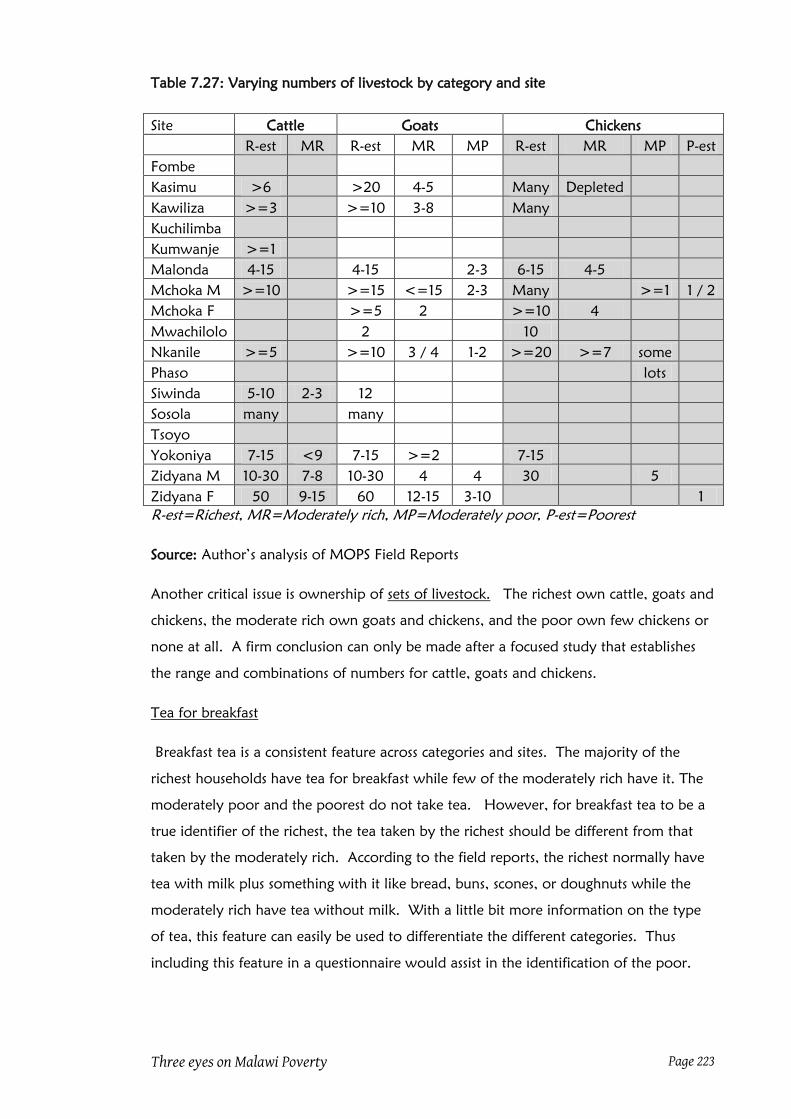
Three eyes on Malawi Poverty Page 223
Table 7.27: Varying numbers of livestock by category and site
Site Cattle Goats Chickens
R-est MR R-est MR MP R-est MR MP P-est
Fombe
Kasimu >6
>20 4-5
Many Depleted
Kawiliza >=3
>=10 3-8
Many
Kuchilimba
Kumwanje >=1
Malonda 4-15
4-15
2-3 6-15 4-5
Mchoka M >=10
>=15 <=15 2-3 Many
>=1 1 / 2
Mchoka F
>=5 2
>=10 4
Mwachilolo
2
10
Nkanile >=5
>=10 3 / 4 1-2 >=20 >=7 some
Phaso
lots
Siwinda 5-10 2-3 12
Sosola many
many
Tsoyo
Yokoniya 7-15 <9 7-15 >=2
7-15
Zidyana M 10-30 7-8 10-30 4 4 30
5
Zidyana F 50 9-15 60 12-15 3-10
1
R-est=Richest, MR=Moderately rich, MP=Moderately poor, P-est=Poorest
Source: Author‟s analysis of MOPS Field Reports
Another critical issue is ownership of sets of livestock. The richest own cattle, goats and
chickens, the moderate rich own goats and chickens, and the poor own few chickens or
none at all. A firm conclusion can only be made after a focused study that establishes
the range and combinations of numbers for cattle, goats and chickens.
Tea for breakfast
Breakfast tea is a consistent feature across categories and sites. The majority of the
richest households have tea for breakfast while few of the moderately rich have it. The
moderately poor and the poorest do not take tea. However, for breakfast tea to be a
true identifier of the richest, the tea taken by the richest should be different from that
taken by the moderately rich. According to the field reports, the richest normally have
tea with milk plus something with it like bread, buns, scones, or doughnuts while the
moderately rich have tea without milk. With a little bit more information on the type
of tea, this feature can easily be used to differentiate the different categories. Thus
including this feature in a questionnaire would assist in the identification of the poor.

Three eyes on Malawi Poverty Page 224
Months of maize stocks
According to the majority of the reports, the richest households have at least 12 months
of stocks. They are also more likely to sell than buy maize. The stocks for the
moderately rich barely make it from harvest to harvest and more often than not the
households are forced to purchase maize to bridge the gap. Sale of livestock is the
common way of generating income to buy the maize. The moderately poor are
generally short of maize stocks to the extent that most of their time is spent working on
ganyu to bridge the gap. The poorest have maize stocks that last at most three months
after harvest. The consistency of this feature, in terms of decreasing number of months
of stocks over a year as the wellbeing status worsens, makes it a good candidate for
inclusion. This feature is made even better when combined with strategies employed to
deal with the surplus or deficit. Consistently, the richest sell or use surplus maize to pay
for labour. The moderately rich sell livestock to bridge the gap and the moderately poor
sell their labour to bridge the gap but for a few months while the poorest almost spend
the entire year selling labour to access food. However, the coping strategies need to be
collected to argument the maize stocks feature.
Number and types of meals per day
This is yet another feature that is easy to use, especially if it is combined with other
features like the type of relish and maize stocks available. The richest take three meals a
day. Their breakfast is heavy and the main meals (lunch and supper) are described as
good because they comprise at least two types of „side plates‟ (meat and vegetables).
The moderately rich take two meals with occasional meat or fish. The amount of relish
for the moderately rich is less than that of the richest. As one group put it, the richest
can afford to throw away leftovers. Again, according to the reports, some households
in the moderately poor category take two meals a day with vegetables as the
predominant „one-out‟ relish. Very few of the moderately poor afford to have
meat/fish. Compared to the moderately poor, who can afford some „modern‟
vegetables (mustard, Chinese cabbage, and rape), the poorest are forced to have one
meal of nsima (the staple) accompanied by own-grown or wild „leaves‟. Thus number
of meals combined with type of meals can be used to characterise households at
different wellbeing levels.
Ownership of a house with corrugated iron sheets
The majority of the richest in almost all sites have houses with iron sheets compared to
only some and few for the moderately rich and moderately poor, respectively. Given

Three eyes on Malawi Poverty Page 225
that some households in the three categories have houses with iron sheets and some
with grass thatch, it would be difficult to use iron sheets or grass thatch as indicators of
wellbeing status. Unless used in combination with other house-specific features like the
condition of the entire house, type of windows, walls and floor, these iron sheets are
not useful. An index that respects weights obtained from people themselves is a possible
way forward. The housing index that is currently used needs to be modified to account
for district or regional differences in subjective valuation of various housing
characteristics.
Demand for and supply of labour
There is a clear message that the rich demand and the poor supply labour services.
According to field reports analysed, households in the richest category only hire labour
while moderately rich households hire and offer labour services irregularly. The
moderately rich hire if they have surplus maize or agriculture income but offer labour
services when cash-strapped. The differences between the moderately poor and the
poorest, in terms of supply of labour services, are not clear from the reports. However,
in many cases the poorest are said to fail to work their farm because they are busy
selling their labour to get their needs (cash, maize, meat, old clothes, and blankets). This
is true for the poorest with labour. For the labour-constrained poorest, there is no
option of selling labour services.
Clothing
Table 7.28 is an attempt to piece together a story from various voices (key informants
and focus groups) from each site that used clothing to characterise categories. The
clothing description covered source of clothes (shop or flea market), quality (decent/nice
and their negatives), condition of the clothes (clean and tidy/dirty and torn), and
number of changes.

Three eyes on Malawi Poverty Page 226
Table 7.28: Varying shades of clothing across categories and sites
Site Richest Moderate rich Moderate
poor
Poorest
Fombe nice few changes no change
expensive suits one cloth
new and expensive new and used
Kasimu expensive used but clean PQ used PQ used and torn
Kawiliza expensive cheap given
daily change no change
pressed clean dirty
very nice/decent not nice/decent
Kuchilimba expensive cheap torn and dirty given and dirty
daily change no change or none
Kumwanje expensive not nice
Malonda daily change some change no change
pressed dirty
new and expensive HQ used given
nice and clean clean rarely stained
Mchoka shop new decent PQ used given
good quality torn
clean one/two changes
nice shoes plastic shoes no shoes
Mwachilolo dress very well some change one change
pressed clean
Nkanile expensive/suits used PQ used
daily change one change
pressed not pressed
Phaso nice/suits No suits some clothes not decent
nice shoes HQ used shoes slip-ons
Siwinda expensive/HP used used PQ used
nice/suits torn
Sosola decent/fashionable dirty
daily change some change just enough none/one change
nice shoes plastic shoes
Tsoyo-Undi daily change no change
shoes no shoes torn
pressed clean/nice faded/dirty
Yokoniya very well very well one change no change
daily change few changes torn
Zidyana expensive nice used torn or none
daily change few changes no change
PQ=poor quality; HQ=High quality
Source: Author‟s summary of MOPS Field Reports

Three eyes on Malawi Poverty Page 227
The gaps in the table signify the absence of the dimension or feature in the discussions.
Decent clothes cover clothes that are described as pressed and of good quality. Pressed
clothes, in turn, cover clean or washed clothes since pressing comes after washing. In
general, „no clothes‟ stand for no „effective‟ clothes (top less and dirty and torn
skirts/shorts for children and dirty and torn clothes for adults).
The table shows that some features are not always consistent across sites as they apply
to more than one category. For example, in Siwinda some of the richest households are
said to purchase high quality used (HQ used) clothing. This is a characteristic of the
moderately rich in Malonda. Again, in Mchoka some of the poorest households have
one or two changes of clothes yet in Fombe and Yokoniya this is a feature of the
moderately rich. In general, though, there are clear patterns.
One of the patterns is that the richest are well dressed and the poorest are the worst
dressed and there is some retrogression in the quality of clothes worn as wellbeing status
declines. For example, the richest buy expensive clothes (including suits) from shops and
the moderately rich and poor buy varying qualities of used clothing while the poorest
rely on being given or working for clothes. Another pattern is that the richest can afford
to change every day (especially women) and the moderately rich can change twice or
thrice in a week. On the other hand the moderately poor have one or two changes of
clothes and the poorest have none. A third pattern is that the richest have clothes that
are washed and pressed while the poorest have dirty and torn clothes with the
categories between having variations of these extremes.
Footwear was rarely mentioned but there is some retrogression from the richest (new
nice shoes from shops), moderately rich (used shoes), moderately poor (plastic shoes)
and the poorest (no shoes). However, there is need for a purposive study that looks at
the various features surrounding clothes to get a clear picture.
Where and how people in various categories sleep
This dimension is mostly used for the poorest category. Further, three sites did not use it
at all making it difficult to get a national story. However, based on those that used it,
the use of blankets is rare among households in the poorest category while the use of
beds, mattresses, linen and blankets defines the richest households. Table 7.29 presents
features that were gleaned from the 12 sites that used this dimension.
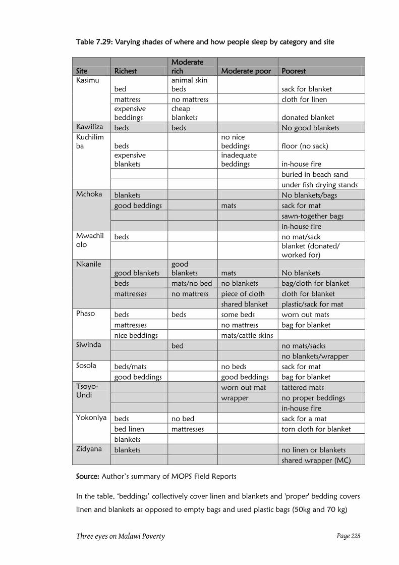
Three eyes on Malawi Poverty Page 228
Table 7.29: Varying shades of where and how people sleep by category and site
Site Richest
Moderate
rich Moderate poor Poorest
Kasimu
bed
animal skin
beds sack for blanket
mattress no mattress cloth for linen
expensive
beddings
cheap
blankets donated blanket
Kawiliza beds beds No good blankets
Kuchilim
ba beds
no nice
beddings floor (no sack)
expensive
blankets
inadequate
beddings in-house fire
buried in beach sand
under fish drying stands
Mchoka blankets No blankets/bags
good beddings mats sack for mat
sawn-together bags
in-house fire
Mwachil
olo
beds no mat/sack
blanket (donated/
worked for)
Nkanile
good blankets
good
blankets mats No blankets
beds mats/no bed no blankets bag/cloth for blanket
mattresses no mattress piece of cloth cloth for blanket
shared blanket plastic/sack for mat
Phaso beds beds some beds worn out mats
mattresses no mattress bag for blanket
nice beddings mats/cattle skins
Siwinda bed no mats/sacks
no blankets/wrapper
Sosola beds/mats no beds sack for mat
good beddings good beddings bag for blanket
Tsoyo-
Undi
worn out mat tattered mats
wrapper no proper beddings
in-house fire
Yokoniya beds no bed sack for a mat
bed linen mattresses torn cloth for blanket
blankets
Zidyana blankets no linen or blankets
shared wrapper (MC)
Source: Author‟s summary of MOPS Field Reports
In the table, „beddings‟ collectively cover linen and blankets and 'proper' bedding covers
linen and blankets as opposed to empty bags and used plastic bags (50kg and 70 kg)
Three eyes on Malawi Poverty Page 229
and pieces of cotton cloths. The bags are either opened up to make them bigger or left
intact. In some cases, they are sawn together to make larger mats for adults‟ use or a
group of children. „Blankets‟ are ideally made from fabric-based bags. In some cases,
even large shopping plastic carrier bags are used as mats. Two types of pieces of cloths
are used as linen and blankets; patterned cloth worn around by women (termed
wrappers in the reports and locally referred to as chitenje) and one-coloured cotton
cloths (commonly used as a wrapper by older women and locally called chilundu).
These cloths are better than the fabric bag „blanket‟ but of the two the latter is warmer.
It is also noted that in some homes fire is used to warm the room instead.
The table shows that some of the rich in some sites use mats (Sosola) and some of the
moderately poor use beds (Phaso). In general, the poorest go without basic beddings
like mats and blankets while the richest have beds, mattress and expensive blankets.
However, the available evidence does not show any clear pattern. This then calls for a
study that would provide some weights for the various aspects of the dimension. This
can be done in the spirit of Breadline Britain methodology (Gordon, et al., 2000),
which requests community groups and household respondents to identify important
features, and indicate absence or presence of the feature and for those absent indicate
whether the absence is by choice or due to lack of resources.
Level of child education
In general, there is some progression from the poorest to the richest in terms of the
average level of child education. This moves from rare school enrolment (poorest) to
completion of primary school to enrolment but rare completion of primary school
(moderately poor) to completion of primary school but rare completion of secondary
school (moderately rich) to completion of secondary school and beyond (richest). Since
some children from the moderately rich complete secondary school, the question is:
how then can secondary school completion distinguish the two categories? According to
the groups, moderately rich households support their children through asset or maize
stocks depletion. They are forced to sell livestock to the last animal or sell non-surplus
maize just to ensure that their children complete secondary school. This implies that
completion of secondary school can be used only with the support of financing
mechanism of the education.

Three eyes on Malawi Poverty Page 230
Purchase of fertilizer
The majority of the richest purchase fertilizer without depleting their assets and some of
the moderately rich purchase some fertilizer using proceeds from the sale of livestock
and modest maize surplus. While very few of the moderate poor purchase one or two
bags of fertilizer by working for other households, the poorest do not buy fertilizer.
This feature can best be used in combination with other features like source of money
for the purchase and number of bags of fertilizer purchased although the latter is crop
and area specific.
Ownership of bicycles
Ownership of bicycle alone is not a good indicator of wellbeing status because some
moderately poor households own bicycles while some moderately rich and richest
households do not. This is true even within a site. It is apparent that ownership of a
bicycle is dependent on a number of factors including preference, terrain of an area and
distance to socio-economic infrastructure like maize mills, markets, and health facilities.
What then?
This chapter has identified characteristics that are important in characterising various
wellbeing categories, especially the richest and poorest. It has also shown that there are
differences by site, region and category. These differences are important in
understanding that a national picture runs into the risk of being a mirage. That said the
sub-section has taken the risk of establishing national features that can be used to
interrogate the national official wellbeing assessment system. Before concluding the
chapter attempts to show once again the national picture can be useful in some cases
and not in others by comparing the national picture with the three village pictures
„painted‟ during the group discussions.
7.4 Characterising wellbeing in the three villages
The objective of the section is to determine whether village pictures painted are the two
rankings is the same or different from the national picture. The analysis starts with
looking at the headline characteristics from a general discussion of wellbeing. It then
moves on to bringing out key characteristics from reasons given for household step
placement and ranking. By definition, households placed on the same level can have
similar features. By using pairwise ranking, the group is „forced‟ to look for features that
make the households on the same step different. Thus pairwise ranking bring out more
or finer features.

Three eyes on Malawi Poverty Page 231
7.4.1 Ngochera wellbeing characteristics
Table 7.30 presents the categories that were identified and their characteristics.
Table 7.30: Characteristics of wellbeing categories in Ngochera
Rich Poor Poorest
Food secure More income than the poorest Go to bed hungry frequently
Eat daily No maize granary Skip meals
Good „sleeping place' House not well 'taken care of' Mangoes only
Have a blanket Do not support to survive Physically challenged
Have clothes No house Aged - can't work
Have livestock House with no amenities No external support
Have good clothes Have some maize Too many children
Have a bicycle Eat less frequently Orphans without support
Have a radio Mostly out working Orphans with old grandparents
Have cash for needs No start-up capital Have nothing/no blanket
Diligent in work Run low-profit enterprises Clothes are given
Diligent in IGAs Women take on hard IGAs Built-for house
Children in school Poor house
Source: Author‟s primary data collection – Ngochera FGD Transcript
A total of 283 features were given by the Ngochera group. Table 7.31 presents the
number of times a feature was mentioned as well as its share in the total number of
features. There is prominence of features that describe the struggles households go
through to make a living. The main ones are natural resource exploitation like charcoal
making and selling, firewood collection and selling, and bamboo collection and selling
(43%); casual jobs (19%); skill-based activities like basket making and making grass or
bamboo fences and poultry houses (16%); and operating microenterprises (16%). Only
two households were rated on the basis of receiving regular income while one was rated
on the basis of 'income' from alms.

Three eyes on Malawi Poverty Page 232
Table 7.31: Wellbeing dimensions from household ranking in Ngochera
Dimension Count Percent
Income generating activities (all types) 76 26.9
Labour capacity (old age, disability, ill-health) 38 13.4
Demographic factors (children, family size, marital status) 37 13.1
Food availability and quality 25 8.8
Access to external support (within and outside area) 21 7.4
Ownership of all physical assets 20 7.1
Ownership of livestock 20 7.1
Work ethics (laziness, drunkenness, diligence) 20 7.1
Housing structure 11 3.9
Quality of life 10 3.5
Clothing 3 1.1
Child education 2 0.7
Total 283 100
Source: Author‟s summary of Ngochera FGD Chichewa Transcript
Various capacities available to households to engage in income generating activities (i.e.
being young, strong and in good health) were frequently used. Other capacity-related
features included the absence of a man in a household, ill health and old age.
Households with strong members but poor were said to be lazy while those that applied
themselves in whatever they were doing were described as hard working. Thus work
ethics is important in this village. In particular, hard working earns one a high position
on the ladder of life. For example, 15 of the 20 cases that used the work ethic dimension
mentioned working diligently as a feature that made some households achieve.
Food availability and consumption, the most popular dimension at the national level,
was only fourth and represented less than 10% of the features given. Indeed, features
like number of meals per day, the use of cooking oil and consumption of meat and tea
were not mentioned at all. This is also true of livestock and asset ownership. Based on
the national picture, Ngochera village is poor. Maybe this validates the group‟s decision
to have no category for the rich in the village. This is further confirmed by the
livelihoods strategies adopted in the village.
Superimposing the Ngochera features over the national picture shows that the intensive
use of ganyu and natural resource exploitation fits the moderately poor category.
Further, in the national picture, the moderately poor were the main operators of low-
capital low profit enterprises. In Ngochera, operating such enterprises put a household
just above the poorest category, i.e. steps 5 to 6. Again, in Ngochera Village, there are
very few households that are taken as the 'source of livelihood for the poor'. In fact,

Three eyes on Malawi Poverty Page 233
only one household was said to be such. To further show the difference between
Ngochera and the national picture, the dimensions are broken down by steps. Steps 1 to
4 are, as described by the village group, the poorest. The poor which run from step 5 to
10 are subdivided into two equal sections; steps 5 to 7 labelled „poor‟ and steps 8 to 10
„rich‟54
. Table 7.32, which breaks down the income generating activities and presents
the number of features by each group of steps labelled poorest, poor and rich.
Table 7.32: Number of times dimension is used to describe category in Ngochera
Dimension Poorest Poor Rich Total
Labour capacity 30 8 0 38
Demographics 17 20 0 37
IGA - NR exploitation 11 20 2 33
External support 12 8 1 21
Ownership of assets 1 6 13 20
Livestock 1 8 11 20
Work ethics 6 10 4 20
Food availability 4 7 6 17
IGA – ganyu 7 8 0 15
IGA - Skills jobs 0 10 3 13
Cash for food/needs 3 9 0 12
IGA – enterprises 2 6 4 12
Housing 5 1 5 11
Quality of life 4 0 2 6
Clothing 2 1 0 3
Child education 1 1 0 2
Employed/honoraria 0 1 1 2
IGA – beg 1 0 0 1
Total 107 124 52 283
IGA=Income Generating Activities
NR=natural resources
Source: Author‟s summary of Ngochera FGD Chichewa Transcript
Households in the poorest category were mostly described using their physical and
numerical capacity to fend for their households, the number of children they take care,
their involvement in the common livelihood strategy in the area (firewood
collection/charcoal making and selling), and by the extent of external support they get.
Households just above the poverty line (step 5 to 7) share two dimensions with the
poorest, i.e. demographics (number of children) and natural resource exploitation.
Other than these, they were also described using their diligence and use of their skills to
54
It is noted that „rich‟ in this case is just a label because the village group emphasised that none of the
households qualifies to be rich.

Three eyes on Malawi Poverty Page 234
generate income. Only two dimensions stand out for the rich; asset and livestock
ownership mainly goats and chickens.
Given that the top four dimensions for the national picture are food stocks, quality of
housing, livestock ownership and clothing, the poorest in Ngochera are described very
differently. The only one that is common in the top four is livestock ownership but even
then the sets of livestock are different. Although Ngochera is not an average village it
still has most of the critical national features. Ngochera Village has unique feature,
though.
The national picture rarely portrays the importance of a man in a household in Malawi.
In Ngochera, the „cry for a man‟ is common perhaps because of types of livelihood
sources like charcoal making, fence making and even farm-based casual work. The group
agreed that charcoal making is a „man‟s job‟ and that women involvement in charcoal
making was a sign of desperation and lack of viable alternatives. The group also stated
that women engagement in farm-based casual work was stressful. This could be a
reason why a hardworking husband is „prized‟ highly.
The importance of a husband comes up in other versions too. In describing a divorced
or separated or widowed female head, the group used the term „has no husband‟. This
was to underline the perceived importance of the man‟s labour input. Likewise,
households with polygamous husbands were perceived in negative light. In many cases it
is the absence of the labour input that is of more of concern than the absence of the
man‟s „kisses or hugs‟. The importance of a male is also clear in the external support
dimension. Out of the 21 cases under external support, husband was explicitly
mentioned six times, son twice and father once. On the other hand, no mother or wife
was explicitly mentioned and daughter to mother was mentioned once.
The short of it is that Ngochera village is poor by the national standard established
earlier. However, it is not seriously out of place because it has some features that are
reflected at the national level.
7.4.2 Chikhwaza wellbeing characteristics
The group identified and characterised four wellbeing categories. Table 7.33 presents
the categories and characteristics.

Three eyes on Malawi Poverty Page 235
Table 7.33: Characteristics of wellbeing categories in Chikhwaza
The richest The moderately rich
Have houses with electricity Do not lack soap
Own vehicles Do not lack food
Lack nothing Lack nothing
Eat anything they want Do not ask for help
Run 'large scale' businesses Have a cash generator
Use hired labour Have adequate clothes
Go to private hospitals Have dairy cattle
Send child to good schools Have large farmland
The poorest The moderately poor
Have inadequate farmland Take meals irregularly
Can't afford fertilizer Eat meat/fish irregularly
Have many children Have inadequate food stocks
Have no beds or mats Have no tea breakfast
Have no linen and blankets Can't afford fertilizer
Have no decent clothes Generate very little income
Have no or poor houses Have poor quality houses
Have no external support Have no livestock
Care for orphans Are socially excluded
Have no capacity to work* Are estate wage employees
Have poorly educated children
* These include the aged, chronically ill, and disabled
Source: Author‟s summary of Chikhwaza FGD Transcript
Some of characteristics are similar to the national pictures. Some are unique and these
are the ones that are of interest. Starting with the richest category, the group did not
use food stocks as a characteristic. One of the possible reasons is that the village has
limited land and growing enough maize to last the entire year is too rare to be used as
an indicator. In fact farmland size is not used to describe the richest but the moderately
rich, which is different from the national picture. As such using food self-sufficiency to
characterise the rich would not make sense. In Chikhwaza, the richest are more
associated with large scale businesses and vehicles than farming.
Another feature that is missing is livestock ownership among the richest. Instead, it is the
moderately rich that are associated with cattle. Even then, it is dairy cows bought for
income generation and not store of wealth as is often the case. Ownership of pigs is
also associated with the moderately rich. Just like cattle ownership, the pigs are for
income generation. To prove the point, the numbers of livestock are so small. The
absence of goats also confirms that the livestock ownership pattern in the village is
mainly for income generation.

Three eyes on Malawi Poverty Page 236
In this village, child education is used to describe the richest and moderately poor. The
richest are said to send their children to good and expensive schools. On the other hand,
some children of the moderately poor are said to be out of school while others enrol
and drop out before completing primary school and a few go to secondary school but
fail to complete. This is not very different from the national picture.
Contrary to expectation, only the moderately poor in the village are described as
socially excluded; due to their clothing they are discouraged to attend community
meetings. Likewise, due to their 'low voice', they are excluded from pro-poor
programmes including free or subsidised inputs. It is not clear why social exclusion is
not used to describe the poorest, which are likely to be worst affected.
One other feature worthy discussing is participation in low wage employment. The
moderately rich and richest are not described in terms of their offer of labour services.
Wage employment is associated with the moderately poor. Likewise, engagement in
casual work (ganyu) is not mentioned, even for the poorest. One of the reasons is that
labour intensive farming is not prevalent in the village. Persistence of poverty among the
employed moderately poor is blamed on very low wages. The poverty associated with
wage matches the national picture.
A total of 322 features were used to describe the households that were placed and
ranked. To aid analysis, the features are placed into manageable wellbeing dimensions.
As an explanation, labour employment covers ganyu workers (4 cases), brick layers (3)
and tinsmith (1). Further, under food availability and quality, there are only four cases of
food quality (3 cases of consumption of small dried fish and 1 case of tea for breakfast).
Table 7.34 presents the breakdown of the features by wellbeing categories.

Three eyes on Malawi Poverty Page 237
Table 7.34: Wellbeing dimensions by category in Chikhwaza
(% share in all features)
Dimension Poor Moderate poor Moderate rich Total
Type and condition of house 16.2 17.3 11.4 15.8
Ownership of assets 6.8 21.2 37.1 12.4
Food availability and quality 11.1 13.5 11.4 11.5
IGA – enterprises 8.1 7.7 17.1 9.0
Capacity to work 1/ 11.1 3.8 0.0 8.7
IGA – farming 8.5 9.6 5.7 8.4
IGA - labour employment 9.4 5.8 2.9 8.1
Access to cash for needs 2/ 7.2 9.6 0.0 6.8
Demographics 3/ 7.2 7.7 2.9 6.8
External support 6.0 0.0 0.0 4.3
Livestock ownership 4.3 3.8 5.7 4.3
Quality of life 4.3 0.0 5.7 3.7
Total number of features (n) 235 52 35 322
1/ includes features on age, health status, and work ethics of household members
2/ Includes features focusing on purchase of food, necessities and support of or failure to support
child education
3/ covers features like 'many children', caring for orphans, divorced, no husband, polygamous
husband
Source: Author‟s summary of Chikhwaza site FGD Transcript
The top three most popular dimensions used to describe the poorest are (i) type and
condition of the house, (ii) amount of food stocks available and quality of meals and
(iii) capacity to work. Two of these (housing and food) were also popular for the
moderately poor (households on step 5) but ownership of assets (i.e. lack of assets) is
the most popular for the moderately poor. For the moderately rich category, the top
three popular dimensions include (i) ownership of assets, (ii) operation of
microenterprises and (iii) housing and food jointly.
What is of note in Chikhwaza is that almost all wellbeing categories have households
that progress or cope or survive by getting involved in some non-farm income
generating activities. Apparently, the poorest undertake low-capital activities like selling
firewood while the relative well off set up merchandise shops in the village with
vegetable and produce trading in between. The scale of the agricultural produce trading
is judged by how far the trading market is. Those who manage to go to the city
(Blantyre over 30 kilometres away) and beyond are considered to be more prosperous
than those who concentrate on local markets. Another feature of note is that no
household among the moderately rich is said to be labour-constrained. In fact, the
poorest are dodged by capacity problems than any other category. This is possibly by
definition since the community designated the lowest step for labour-constrained
households.

Three eyes on Malawi Poverty Page 238
Wage employment is almost exclusively used to characterise the moderately poor. This
is in line with the national picture which paints wage employment as a sign of poverty
because the more a household is well off the less likely it is to be described by wage
employment. Indeed wage employment does not lift the worker out of poverty.
According to the group, wages are so low that they „vanish‟ into debt repayment once
received giving the impression that wage employment is more for securing „lines of
credit‟ than moving out of poverty.
Another unique feature is that capacity to work amongst the poorest go hand in hand
with access to external support. Labour constrained households were differentiated
based on actual or potential access to external support. In fact access to external
support was an exclusive dimension used to describe the poorest.
Just like in the case of Ngochera, the role of a husband seems to come up as well
although not as strongly. In describing very poor households, the group used features
like divorced, widowed, no husband and polygamous husband. The polygamous
husband is rated negatively because of his minimal contribution to the household. The
number of children was also used as an indicator of wellbeing status. Apparently having
five or more children is blamed for poverty because the little a household produces
feeds too many mouths.
On the basis of the household clustering in this village and absence of a dimension
specific to the richest, poverty is more equally distributed. Further, when the Chikhwaza
picture is compared with the national one, there are three important dimensions that
are missing: (i) type and quantity of clothing; (ii) child education and (iii) food
consumption in terms number of meals taken in a day. The absence could be a sign that
these are not meaningful indicators.
7.4.3 Dzilekwa wellbeing characteristics
The village group identified three wellbeing groups namely poorest, poor and rich
(termed literally the worst sufferers, sufferers and the doing well, respectively). The
characterisation of the categories is not very different from those obtained from the
national studies. For example, food stocks, livestock ownership, housing and quality of
the home, involvement or capacity to get involved in income generating activities, and
the role of external support in the household livelihoods were used to describe the
categories. See Table 7.35.

Three eyes on Malawi Poverty Page 239
Table 7.35: Characteristics of wellbeing categories in Dzilekwa
The poorest The Rich
Have no mats and beddings Have adequate food stocks
Have uncared for home Eat adequate food and fruits
Have few months maize stocks Have a good house
Some are lazy ('they abhor the hoe') Have leak-proof roof (grass or iron sheet)
Have no kitchen Have a house with windows
Have a leaking house Have a well cared for home
Have inadequate external support Have a smoothed floor house
Do not apply fertilizer Have access to potable water
Buy or beg for food Dress well (good clothes)
Poor or no breakfast Use good mats and beddings
Use empty bags as mats Have adequate utensils 1/
Have difficulties generating cash Have livestock (goats and chickens)
Fail to cover secondary school costs Eat quality food 2/
The poor Parents and children well mannered
Have maize lasting over six months Are hardworking farmers
Some receive some support Meet all necessary needs (lack nothing)
Some sell subsidised fertilizer Can afford to receive overnight visitors
meet some of the needs Children go up to secondary school
Have some access to cash
Fail to cover secondary school costs
1/ Includes pots, plates, tins, bath basins, bamboo basket, bamboo winnower, mortar, pestle
2/The group specifically mentioned vegetables eaten together with mice, or beans, or eggs
Source: Author‟s summary of Dzilekwa FGD Transcript
The descriptions of the features, on the other hand, are not as elaborate as those from
the national studies. For example, on food stocks very little emphasis is placed on
number of months the stocks last. Further, details about number of meals taken per day
and type of relish consumed by categories were hardly mentioned. Dzilekwa also has
some features which are different from the national ones. For example, some of the
poorest households are said to have breakfast of porridge but without sugar. This is
different and confirms earlier findings that the site is above average. Dzilekwa is also
different in that, unlike the national picture, children in the poorest category complete
primary school. A good house in Dzilekwa does not necessarily have burnt brick walls
or corrugated iron sheets roofs or cement floors. For some, having a grass thatch is a
choice. This is similar to some sites reviewed.

Three eyes on Malawi Poverty Page 240
The wellbeing and pairwise ranking came up with 268 features. Table 7.3655
summarises these in dimensions similar to those used previously.
Table 7.36: Wellbeing dimensions by category in Dzilekwa
(% share in all features)
Dimension Wellbeing category
Poorest Poor Rich Total
IGA – trading 2.5 16.4 24.5 17.2
IGA – Farming 0 14.2 19.1 13.8
Social behaviour 1/ 2.5 20.9 3.2 11.9
Food availability 12.5 12.7 6.4 10.4
Capacity to work 37.5 3.7 2.1 8.2
Demographics 2/ 5.0 11.2 5.3 8.2
Housing 5.0 4.5 6.4 5.2
Food production 0 2.2 10.6 4.9
Livestock ownership 0 3.7 8.5 4.9
IGA – ganyu 0 6.0 4.3 4.5
External support 12.5 3.0 2.1 4.1
Access to cash for needs 22.5 0 1.1 3.7
Assets ownership 0 1.5 5.3 2.6
Hire of labour 0 0 1.1 0.4
Total number of features 40 134 94 268
Number of households 8 28 22 58
1/ includes laziness, misuse of resources for beer, concentration on ganyu as the expense of farm
and home work, excessive drinking, 'womanising', and children who do not help parents or steal
from parents; 2/ Demographics include 'no husband (9); polygamous husband (3), family size (4),
new family or recently returned (5), widower (1)
Source: Author‟s summary of Dzilekwa FGD Transcript
In Dzilekwa, the two main dimensions used to characterise the poorest category include
capacity to work (determined by age and health status) and inability to access cash for
households needs. These two are related since failure to work leaves a household with
no cash for needs. The limited access to cash then leads to the reliance on external
support such that if support is not available the households fall further into poverty.
That is why external support is one of the popular dimensions used to describe poorest
households. One other dimension that is used to describe the poorest households is
amount of maize stocks.
The characterisation of the poor category was dominated by social behaviour, a short
hand for personal habits and attitude towards work of household head (and/or spouse
if married). The type of husband in terms of involvement in farming, trading and casual
55
The shaded cells in the table represent dimensions that have a proportion of at least 10% of the features
in the category.

Three eyes on Malawi Poverty Page 241
work and management of generated income are major features in this dimension.
Another popular dimension is involvement in trading activities, especially of women (or
wives). Trading was followed by Irish potato production. Although this dimension was
dominated by reference to farming men, the group also stressed woman's participation
in farming activities. The expectation is that a good husband leads and a good wife
follows the lead. In cases where this happens the group was quick to acknowledge and
accord „high‟ marks accordingly. Perhaps underlining all the dimensions discussed, the
marital status of the household head was also popularly used to describe households in
this category. This dimension termed „demographics‟ is dominated by absence of a
husband or presence of an absent husband56
.
For the rich category, the most common dimension used was high-capital trading like
the buying and selling of Irish potatoes in bulk and running of well-stocked shops at the
market. This was followed by multi-season Irish potato and vegetable production. This
type of farming almost always was reserved for rich households. One other important
dimension for the rich category includes maize production. Livestock ownership, which
is popular at the national level, was not used frequently to describe the rich.
One other unique feature of Dzilekwa is that households are, by far, described by their
livelihood strategies and not what they do or do not own, wear or eat. Apparently, the
group mentally used the following sequence of questions when placing and ranking
households: Does the household produce own food and how much? Does it cultivate
Irish potatoes for sell? Does it trade on regular basis at the market? What is the scale of
the farming or trading? For men, do they spend most of their time at the local market
instead of their farm? Mental responses to these determined the category a household
was placed.
The presence of the market also brings in unique labour market dynamics. Unlike the
rich in other rural areas, the richest in Dzilekwa are 'forced' to work their farms
themselves. This is why hardworking as a trait of the farmers is emphasised. One of the
reasons is that the village seems to have no desperately poor people that offer their
labour services as farm hands. Instead, the poor offer their labour services at the local
market where cash generation is relatively easy. Ironically, farmers frown at and label
those who offer their labour services at the market as either lazy or unproductive or
drunks. The absence of surplus labour in the village also affects single women who trade
at the market. These women who could otherwise use hired labour to work their maize
farms are also left with no choice but to concentrate on their trading activities. Such
56
This refers to polygamous or non-remitting away husbands.

Three eyes on Malawi Poverty Page 242
choices, according to the discussants, showed that such women were „lazy' since they
prioritised trading over their farms. This labelling of frequent local market „workers‟ is
probably because the local market is seen to upset local labour market conditions against
farmers.
7.4.4 A comparison of the national and village level pictures
Just like in the case of the quantitative pictures, each village is unique. Of the three
villages, Dzilekwa is closest to the national picture. This is different from the conclusion
made based on average household characteristics presented in Chapter 4. In that
analysis, it was Chikhwaza that was closest to the national picture. However, it has been
confirmed that Ngochera is the poorest among the three villages and Dzilekwa is the
richest even using the characterisation in this chapter. In general, all the villages have
features that reflect the national picture. This then leads to two conclusions. The first is
that modifying the quantitative picture based on national quantitative picture can
improve the relationship between the quantitative measure and the local qualitative
measure of wellbeing. The second is that the difference between the national and local
qualitative picture means that even the modified quantitative methodology would not
be perfect. As such its application at the local level would still be need to be done
cautiously.
7.5 Summarised national qualitative picture of wellbeing
The main output of this chapter is a set of wellbeing features considered important for
the determining wellbeing status of a household. Table 7.37 presents the popular
characteristics and features as well as their potential usability. Coming up with these
involved identifying popular dimensions used to characterise wellbeing categories then
breaking them down into „measurable‟ features and finally checking their consistency
across the country and categories. While some features were found to be consistent
enough to be used across all the wellbeing categories some were found to be either too
broad or narrow for use without either a study to verify their consistency or other
features to complement them.

Three eyes on Malawi Poverty Page 243
Table 7.37: Wellbeing characteristics and features: usability and way forward
Characteristic/feature Usability Way forward
Livestock ownership
Ownership of cattle
Richest - with goats and
chickens
Study to establish
numbers
Ownership of goats
Moderately rich - with
chickens
Study to establish
numbers
Ownership of chickens Moderately poor
Study to establish
numbers
Food security &
consumption
Months of maize stocks
Use with coping with food
insecurity module
Modify sources of food
module
Number of meals per day Use with type of meal
Collect at least yesterday
meals
Taking breakfast tea
Use with modified
consumption module
Modify consumption
module
Protein relish every meal Use with number of meals
Collect at least yesterday
meals
Housing
Corrugated iron sheet roof
Use as part of a housing
index
Study to establish
weights
Labour services
Demand for labour services Use as a dummy
Supply of labour services Combine with other features
Modify labour supply
module
Clothing and beddings
Type of clothes
Not useable without
modifications
Study to establish
weights
Type of 'sleeper'
Not useable without
modifications
Study to establish
weights
Type of beddings
Not useable without
modifications
Study to establish
weights
Child education support
Level of child education
Useable but needs some
caution
Use sources of education
money
Access to inputs
Purchase of fertilizer
Useable but needs some
support
Use sources of inputs
money
Asset ownership
Ownership of bicycle Not useable on its own
Study to establish
weights
Source: Sub-section 7.3.4
The sub-section that discussed these provided pointers on how these can be dealt with if
they are to be used to modify the official wellbeing assessment system. These pointers
are picked up in Chapter 9 when the official wellbeing assessment system is
systematically analysed for possible gaps that can be filled using qualitative information.

Three eyes on Malawi Poverty Page 244
As indicated in the same, some of the feature would need further study for them to be
incorporated. Apart from these features, the modification would also benefit from the
perspective of the households themselves. Chapter 8 is meant to come up with features
gleaned from self assessment.

Three eyes on Malawi Poverty Page 245
Chapter 8: Characteristics of wellbeing from households
8.1 Introduction
The year 2005 witnesses three studies that introduced self assessment as one way of
understanding wellbeing and poverty in households in Malawi. The CPS5 and MOPS,
which have already been introduced, also had extensive modules on subjective
assessment of wellbeing. Due to some differences in the design of these two, the results
from the two studies are not presented in this chapter. However, Appendix 7 presents
the findings from those two studies. This chapter is based on two surveys; IHS2 and the
survey conducted in the three villages as part of the primary data collection for this
study. The chapter analyses the responses in the subjective assessment of wellbeing
modules of the questionnaires used in those surveys. The focus is on responses that
qualitatively described the household‟s wellbeing status. The first part of the chapter
presents the poverty correlates and wellbeing determinants for the self-assessed poverty
from the IHS2 (Devereux, et al., 2006 and GoM & World Bank, 2007). The second part
presents the results of subjective poverty correlates and wellbeing determinants for the
three villages.
8.2 Subjective wellbeing under IHS2
The subjective wellbeing module of the IHS2 included the three questions namely (i) the
consumption adequacy questions (CAQ) covering food consumption, housing, clothing
and health care; (ii) subjective economic wellbeing (SEW) rating questions that compare
current with previous and future; and (iii) the minimum income question (MIQ). The
adequacy question have three ordinal responses 1 to 3 for „less than adequate for
household needs‟, „just adequate for household needs‟ and „more than adequate for
household needs‟. The life satisfaction question uses a 5-point scale for „very
unsatisfied‟, „unsatisfied‟, „neither unsatisfied nor satisfied‟, „satisfied‟ and „very satisfied‟.
The household economic wellbeing rating runs from 1 „much better‟ to 5 „much worse‟
with 3 in the middle for „no change‟ and „better‟ (2) and „worse off‟ (4) on the other
end.
As explained already the IHS2 module was analysed by Devereux and colleagues and
Malawi Government and World Bank officials. Both conducted some statistical analysis
to establish some relationship between self-assessed poverty (as defined by the analysts)
and some selected household characteristics available in the dataset. Table 8.1 presents
the self-assessed poverty correlates as found by Devereux and others.

Three eyes on Malawi Poverty Page 246
Table 8.1: Self-assessed poverty correlates from IHS2 data
Factor Factor
Household size In a matrilineal system
Female-headed household In a minority language group
Household head is divorced Has permanent housing
Household head is unmarried Has semi-permanent housing
Household head is widowed Number of ganyu days last year
Head is in a polygamous union Household's assets index
Household head has JC Household's landholding size
Household head has MSC Tropical livestock units
Head a university education Experienced death in the family
At least one disabled member
JC=Junior Certificate; MSC=Malawi School Certificate
Source: Devereux, et al. 2006
Eight of these nineteen correlates concern the households head (sex, marital status and
education) and other than few social factors, most are economic. The poverty
determinants analyses used a number of formulations taking advantage of responses
from the CAQ, SEW and MIQ57
58
. Table 8.2 presents factors found to influence the
evaluation of consumption adequacy (CAQ), wellbeing (SEW) and minimum income for
making ends meet (MIQ).
Table 8.2: Self-assessed wellbeing determinants from IHS Data
Independent variables ↓ Dependent variables CAQ SEW MIQ
Log real per capita consumption √ √ √
Household size √ √ √
Household size squared √ √ √
Share of children in total population X X √
Share of elderly X X √
Female household head X √ √
Age of household head X X √
Completed pre-school √ √ √
Completed junior primary √ √ √
Completed senior primary √ √ √
Completed senior secondary √ √ √
Completed junior secondary X √ √
Household owns an enterprise √ √ X
* significant at 5% (MIQ) the rest at 1%
57
Ordered probit regression analysis was used to come up with predictors of feelings of consumption
adequacy and economic wellbeing (GoM and World Bank, 2007b). OLS was used to analyse the poverty
status dummy created from the MIQ 58
Malawi Poverty and Vulnerability Analysis (GoM & World Bank, 2007b) used regression analysis to
determine the poverty line from the MIQ following the Leyden methodology (Van Praag, et al., 1982)
Three eyes on Malawi Poverty Page 247
Source: Tables A3.6 of Annex 2D (GoM & World Bank, 2007b)
The results show that the level of consumption is related to feelings about wellbeing as
evidenced by its significance under the three types of subjective wellbeing assessment.
Other than that the table shows that self wellbeing assessment is negatively influenced
by a large household size composed mainly of dependents. The table also shows the
role education status of the household plays in self wellbeing assessment. The difference
between Devereux and colleagues and the officials is that the officials‟ list does not bring
out economic factors.
8.3 Characteristics of self-assessed wellbeing status in the three villages
After assigning their household a group, the respondents gave at most three reasons why
they assessed their households thus. These reasons are discussed at three levels; in their
original form, simple categorisation. The sub-section also presents findings from
subjective poverty correlates and determinants analysis.
8.3.1 Reasons for household wellbeing grouping
There were 394 reasons given and 63% can be classified as negative and the rest
positive. The first discussion does not necessarily attach the reasons to their respective
wellbeing group or any steps on the ladder of life. As is seen later few reasons have
monopoly of a group or step because the open-ended nature of the question implies
that one reason can be given by households on different steps or in different categories.
Positive reasons
Just like in CPS5 and MOPS, availability of food is the most important factor when
assessing household wellbeing status. Another factor is diversification of income sources
(including operating some enterprises or engaging in some IGAs). These are supported
by hard working spirit and child-parents remittances. Some respondents mentioned
outcome indicators like 'household meets all or most needs' and 'household has
adequate money to cover household needs'. As Table 8.3 shows, factors on ownership
of assets like land (4%), livestock (3%), durables (1%) and ownership of a good house
(3%) are not used frequently as reasons for wellbeing status.

Three eyes on Malawi Poverty Page 248
Table 8.3: Positive reasons for wellbeing group assignment
Positive factors (n=147) Per cent
Household has adequate food 22.4
Household operates an enterprise 13.6
Household meets all or most needs 12.2
Member(s) work hard in farm or business 8.8
The household gets support from children 8.2
Household has adequate money for needs 6.1
member(s) engage in non-farm IGAs 5.4
Source: Author‟s summary from village FGD transcripts
Negative reasons
Mirroring the positive side, the top most reason is food insecurity or inadequate
harvests. Other reasons are more like causes of the poor harvests and these include high
prices or inaccessibility of inputs. Struggling to generate income is given as an indicator
of their wellbeing group while poorly performing enterprises is given as the cause of
their being where they are. Some gave the poor state of their house as a sign of their
chosen wellbeing group. See Table 8.4.
Table 8.4: Negative reasons for wellbeing group assignment
Negative factors (n=247) Percent
Food insecure, inadequate harvest 11.3
No/inadequate farm inputs, high prices 8.9
Struggles to generate income 6.5
Poor housing quality 5.3
Too small/non-performing business 4.9
Too old to work as expected 4.5
Source: Author‟s summary from village FGD transcripts
There are other less frequently mentioned reasons, some of which could be related to
the prominent factors discussed above. For example, owning inadequate farmland
(4%) and no irrigatable land (3%) could be related to harvests and struggles households
go through to generate income. This is true of reasons related to labour supply (too ill
to farm - 1%, having no husband to work with (1%), and, for the married, having a
spouse who is in poor health (3%) or in polygamy (1%) or who drinks alcohol
excessively (1%)). It is also true of reasons related to labour demand (being unemployed
(4%), rare or no labour demand (2%) and relying on casual work (1%)). There are less
frequently mentioned reasons that may be related to performance of enterprises. These

Three eyes on Malawi Poverty Page 249
include inadequate money to prosper (3%), lack of business start up capital (2%), and
generation of income that is adequate to support consumption only (2%).
The advantage of using open-ended questions is that they yield diverse responses. The
risk is that some factors can be discarded on the basis of low frequency. To avoid that it
may be better to group reasons that are related. While this runs the risk of losing the
original flavour and injecting too much expert opinion, it may be useful to be open on
how the responses are grouped. For the purposes of this study the reasons are grouped
along the lines presented in Table 8.5. With this rationalisation, the most prominent
factors include having inadequate income, being food secure, meeting basic needs, being
food insecure, having an enterprise or some income generating activity, having limited
labour, having no or limited access to inputs, and lack of gainful employment. These
eight factors take up 58% of all the responses as opposed to 38% before rationalisation.
Table 8.6 presents all the frequencies of all the factors.
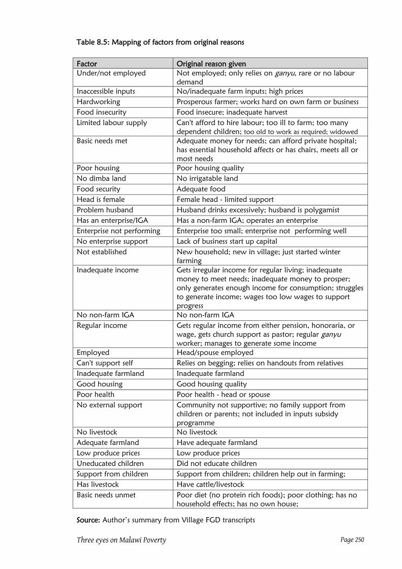
Three eyes on Malawi Poverty Page 250
Table 8.5: Mapping of factors from original reasons
Factor Original reason given
Under/not employed Not employed; only relies on ganyu, rare or no labour
demand
Inaccessible inputs No/inadequate farm inputs; high prices
Hardworking Prosperous farmer; works hard on own farm or business
Food insecurity Food insecure; inadequate harvest
Limited labour supply Can't afford to hire labour; too ill to farm; too many
dependent children; too old to work as required; widowed
Basic needs met Adequate money for needs; can afford private hospital;
has essential household affects or has chairs, meets all or
most needs
Poor housing Poor housing quality
No dimba land No irrigatable land
Food security Adequate food
Head is female Female head - limited support
Problem husband Husband drinks excessively; husband is polygamist
Has an enterprise/IGA Has a non-farm IGA; operates an enterprise
Enterprise not performing Enterprise too small; enterprise not performing well
No enterprise support Lack of business start up capital
Not established New household; new in village; just started winter
farming
Inadequate income Gets irregular income for regular living; inadequate
money to meet needs; inadequate money to prosper;
only generates enough income for consumption; struggles
to generate income; wages too low wages to support
progress
No non-farm IGA No non-farm IGA
Regular income Gets regular income from either pension, honoraria, or
wage, gets church support as pastor; regular ganyu
worker; manages to generate some income
Employed Head/spouse employed
Can't support self Relies on begging; relies on handouts from relatives
Inadequate farmland Inadequate farmland
Good housing Good housing quality
Poor health Poor health - head or spouse
No external support Community not supportive; no family support from
children or parents; not included in inputs subsidy
programme
No livestock No livestock
Adequate farmland Have adequate farmland
Low produce prices Low produce prices
Uneducated children Did not educate children
Support from children Support from children; children help out in farming;
Has livestock Have cattle/livestock
Basic needs unmet Poor diet (no protein rich foods); poor clothing; has no
household effects; has no own house;
Source: Author‟s summary from Village FGD transcripts

Three eyes on Malawi Poverty Page 251
Table 8.6: Share of wellbeing factors in total number of reasons (%)
Factor
Percent
(n=391) Factor
Percent
(n=391)
Inadequate income 11.2 Inadequate farmland 2.5
Food secure 8.4 Head is female 2.3
Basic needs met 7.6 No irrigatable land 2.0
Food insecure 7.1 Poor health 1.8
Has an enterprise/IGA 7.1 No livestock 1.8
Limited labour supply 6.1 No support for business 1.5
Inaccessible inputs 5.6 Adequate farmland 1.5
Under/not employed 4.6 Problem husband 1.3
Hardworking 3.8 Good house 1.3
Poor housing 3.3 Has livestock 1.3
Support from children 3.3 New 1.0
Unmet basic needs 3.3 Relies on alms/handouts 0.5
Non-performing enterprise 3.0 Low produce prices 0.5
Regular income 3.0 Failed to educate children 0.3
No external support 3.0 Total 100
Source: Author‟s calculations based on primary data
Reasons by wellbeing group
To understand the reasons further, the wellbeing group they are meant to justify is
superimposed. The results are presented in Table 8.7. The results show that there is no
major factor that is common in all the wellbeing groups considering that the groups are
mutually exclusive59
.
Table 8.7: Most prevalent reasons for wellbeing group assignment
Poor Group (n=176) % Middle group (n=206) % Rich group (n=9) %
Inadequate income 15.3 Has enterprise/IGA 13.1 Basic needs met 44.4
Food insecure 14.8 Food secure 12.6 Food secure 22.2
Limited labour supply 10.8 Basic needs met 11.2 Hardworking 11.1
Under/not employed 8.0 Inadequate income 8.3 Regular income 11.1
Inaccessible inputs 6.8 Hardworking 6.8 Support from children 11.1
No external support 5.7 Regular income 5.3
Unmet basic needs 4.5 Support from children 5.3
Inaccessible inputs 4.9
Source: Author‟s calculations based on primary data
59
This is true for the most prevalent factors (i.e. whose share is at least 5%) only. There are some factors
that are found in all only that there frequencies are low. For example, food security and basic needs
security are found in all the groups only that very few in the poor group are food and basic needs secure;
3% and 1% respectively.

Three eyes on Malawi Poverty Page 252
However, there are factors that are common between pairs like poor and in-between
and in-between and the rich. Of the two pairs, there are more common factors
between the rich and in-between groups than between the poor and in-between groups.
Inadequate income and inaccessible inputs are common factors between the poor and
in-between groups60
while food security, basic needs security, hardworking, regular
income, and support from children are common factors between the rich and in-
between groups. The bottom line though is that the in-between group has the potential
of accommodating both poor and rich households. As such some positive factors can
cater for the in-between and rich groups. Likewise, some negative factors can apply to
households that are in-between and poor wellbeing groups.
Despite these commonalities, there are factors that are mostly prevalent in one group61.
For example, factors that are prevalent mainly among the poor are limited labour
supply, underemployment or unemployment, lack of external support and unmet basic
needs. On the other hand, there is only one factor for the „middle class‟; ownership of a
non-farm enterprise or income generating activity62
. There is no factor that is particular
to the rich. It is however curious that ownership of an enterprise is not necessarily
mentioned as a factor by the rich. This does not necessarily mean that they do not have
enterprises. It may simply mean that the rich do not single them out as a defining factor.
8.4 Correlates and determinants of subjective poverty
8.4.1 Self-assessed poverty correlates
The correlation analysis in this chapter uses the household characteristics (variables) from
the objective poverty analysis used in Chapter 6. This list is supplemented by three self-
rated wellbeing variables (self-rated welfare group, level of life satisfaction, and self-
rated economic wellbeing change). Table 8.8 presents the correlates of self-rated
poverty using the median poverty line.
60
There are many other factors that are common between the two but are not popularly used. 61
Again, this analysis focuses only on the most frequently used factors. Exclusivity especially between
the poor and middle groups is not guaranteed. 62
Again, this analysis focuses only on the most frequently used factors. Exclusivity especially between
the poor and middle groups is not guaranteed. Even the factor „household has a non-farm enterprise is not
exclusive to the middle group. This reason was also mentioned by one poor household.

Three eyes on Malawi Poverty Page 253
Table 8.8: Self-assessed poverty correlates in the three villages
Factor All sites Ngochera Chikhwaza Dzilekwa
Maize output per cultivated land ** ** **
Level of consumption expenditure (log) ** *
Livestock diversity ** **
Household owns dimba land *
Head aged 65 years and above *
Children from 5 to 10 years old **
Amount spent on agricultural inputs (log) ** **
Highest class by any adult **
Household head is widowed *
Dzilekwa village **
Level of life satisfaction **
Self-assessed wellbeing group ** ** ** **
** =significant at 1% level; * = significant at 5% level
Source: Author‟s analysis of primary data
One clear message from the table is that what is important at combined level is not
always important at village level and what is important at one village may not be
important at another. For example, three factors only appear at the combined level
and two „global‟ factors appear in one village only. Out of the eight factors that are
important at the combined level, only one is common to all the three villages, one to
two villages and two to one village only. On the other hand, there are four factors that
are only important at village level; Dzilekwa has two factors unique to itself and
Ngochera has one unique factor. Chikhwaza shares one unique factor with Dzilekwa.
This shows that there are differences even among the villages. For example, out of the
twelve factors found to be important correlates of self-rated poverty only one factor is
common to all the three villages; the household wellbeing group. This further confirms
that the value judgements made by the respondents are generally consistent. There are
two factors that are common to either two of the villages; amount of maize produced
per given cultivated land (Ngochera and Chikhwaza) and amount of money spent on
inputs (Chikhwaza and Dzilekwa). Number of under-five children is a unique factor for
Ngochera village while education level of adults and household head widowhood are
unique factors for Dzilekwa Village. Looking at the factors associated with each village‟s
self-rated wellbeing status, Chikhwaza village has factors that are more related to
objective poverty. It is the only village whose self-rated poverty status is strongly
associated with most factors directly related to the objective poverty measure. These
include maize output, consumption expenditure, livestock ownership, and amount of

Three eyes on Malawi Poverty Page 254
money spent on inputs. The absence of asset ownership factors is worth noting because
it is sometimes thought that subjective wellbeing assessment is biased towards asset
ownership.
8.4.2 Determinants of perceptions on wellbeing status
In line with the lessons from previous studies, logit models are used to determine factors
that influence the perceptions on wellbeing status as measured by the step a household
is said to be63
. Since Logit models are more amenable to nominal and ordinal variables,
most of the variables used in objective poverty determinants analysis are converted to
either dummy or ordinal variables. Some are combined to make one variable. Table 8.9
presents the descriptive statistics for the variables used in the model while Table 8.10
presents the estimation results.
Table 8.9: Descriptive statistics of variables for the determinants model
Variable (n=164) Mean SD
Step (1=poor, …, 10=rich) 4.1 2.05
Group (1=Poor, 2=in-between; 3=Rich) 1.6 0.55
Life (1=very unsatisfied, 2=unsatisfied, 3=neither, 4=satisfied, 5=very satisfied) 3.3 1.08
HHSize (1=1-2 ; 2=3-4 ; 3=5-7; 4=8 or more members) 2.3 0.80
Under5 0.7 0.80
Headsex (0=Head is male; 1=Head is female) 0.3 0.47
Younghead (0=Head is at least 45 years old; 1=Head is at most 44 years) 0.6 0.48
Widowed (0=Head is not widowed; 1=Head is widowed) 0.2 0.37
HHHWage (0=Head is unemployed; 1=Head is employed) 0.1 0.32
Educlevel (1=head no educ.; 2=Some prim; 3=Full prim; 4=Post prim) 2.6 0.99
Morbidity (0=no member ever ill; 2=A member ever ill) 0.6 0.50
Employer (0=None; 1=Formal; 2=Non-formal) 0.2 0.58
Credit (0=No credit; 1=Had credit) 0.2 0.40
Fertilizer (0=Did not apply; 1=Applied) 0.8 0.39
Coupon (0=Did not use coupon; 1=used a coupon) 0.7 0.49
Inputs (0=Did not spend on inputs; 1=Spent on inputs) 0.9 0.30
Enterprise (0=Has not enterprise; 1=Has an enterprise) 0.6 0.49
Landcat (1=landholding size < 0.5 ha; 2= 0.5 - 1 ha; 3= > 1 ha) 2.0 0.85
Dimbaland (0=No irrigatable land; 1= has irrigatable land) 0.3 0.46
PovCE (0=non-poor by CE; 1=Poor by CE) 0.3 0.46
Livestock (0=No livestock; 1=Has livestock) 0.7 0.47
Village (1=Ngochera; 2=Chikhwaza; 3=Dzilekwa) 2.0 0.80
Source: Author‟s computation from primary data
63
The ordered probit model is not used because it is not possible to guarantee that the dependent variable
(step on the ten-step ladder) is normally distributed. If anything, the negative log-log model could be the
closest because if the finding that households generally understate their wellbeing status is taken as
commonplace.

Three eyes on Malawi Poverty Page 255
Table 8.10: Self-assessed wellbeing determinants in the three villages
Factor Coefficients
All sites Ngochera Chikhwaza Dzilekwa
Household in poor group -5.5** 4.855 -9.7**
Household middle group -2.33* 9.4** -6.8**
Rich group (Reference)
Very unsatisfied with life -2.04* -6.9** -13.0** -2.808
Unsatisfied with life -1.005 -1.039 -20.8** -1.349
Neither with life -1.204 -2.665 -18.0** -3.55*
Satisfied with life -1.043 -4.9** -18.0** -2.35
Very satisfied with life (reference)
No under-five child -3.05* -6.14* -2.28 -7.08*
One under5 child -2.583 0.059 -2.94* -6.69*
Two under5 children -2.07 -7.29*
Three under5 children (reference)
Head of household is male -0.84* -3.4**
Household did not apply fertilizer -1.19*
Land holding is less than 0.5 ha -0.801 -0.73
Landholding is 0.5 to 0.99 ha -1.4** -3.82*
Landholding is 1 ha or more (reference)
Household has no irrigatable land -7.9**
Head of household is not widowed -4.06*
Head is not in employed -11.2**
One member household 6.08*
Two-member household 8.0**
Three-member household 9.1**
Four-member household (reference)
Head has no education -5.95*
Head has some primary -1.365
Head some full primary 1.016
Head has post primary
None employed 4.0**
Non-formal employment 7.6**
Formal employment (reference)
Household is not objectively poor 2.4**
*=Significant at 5% level; **=Significant at 1% level
Source: Author‟s analysis of primary data
Results of the estimation of the model show that while most of the determinants of
wellbeing status at the combined level (all sites) are applicable at local level, some
villages have unique determinants. In Ngochera Village, for example, the assigned
household welfare group does not determine the assignment of the household step
(welfare status). Instead, it is whether or not the household has irrigatable land and
whether the head is widowed or employed. In Chikhwaza the story is different. Sex of

Three eyes on Malawi Poverty Page 256
the household, whether fertilizer was applied and landholding size do not have a
bearing on the household welfare. Instead it is household size, education and
employment status that do. A complete different picture emerges from Dzilekwa
because it has no unique determinants. The results also show that the villages themselves
have less common than unique factors. For example, there are only two factors that are
common in all the three villages; number of under-five children and perceptions on life
satisfaction. Application of fertilizer, which influenced the welfare rating at the
combined level, does not at village level.
The role of a „man in the house‟ is picked up in Ngochera village where sex,
widowhood, and employment of the household head64
influence the assessment of
wellbeing. The prominence of household size in Chikhwaza is most probably related to
the size of their small landholdings while the importance of education and employment
is to do with the village‟s proximity to employment centres (nearby estates and Blantyre
City which is 30 kilometres away). The bottom line is that most of these findings make
some sense and are in line with most of those already presented. In other words, these
subjective poverty determinants are not very different from the objective poverty
determinants. It can therefore be concluded that some factors that predict consumption
poverty can also predict subjective poverty and that some factors are better predictors
in some circumstances than others.
8.5 Key findings, conclusions and implications
Most of the factors found to be associated with self-assessed wellbeing status and
poverty are similar to those found for objective poverty. That said, some of the factors
that have some implication on the official wellbeing assessment system are discussed
below.
Agricultural production
In all the studies, production of food crops is mentioned as one of the most important
wellbeing defining factor. For those that had a ten-year perspective their responses focus
on whether food security improved or not. For those providing a snapshot, the focus is
on the perception on food security for the material year. Apart from the level, other
64
This is based on the gender bias in single household heads and employment. In general, 92% of the
single heads were female and 68% of those employed heads were men. In Ngochera Village, 89% of
single household heads are women and 61% of employed heads are men. As can be deduced and recalled,
Ngochera is not the worst affected in terms of female headship or unemployment of female heads. This is
most probably related to the type of livelihoods options available to Ngochera women. In Ngochera,
natural resources exploitation (e.g. felling trees for firewood extraction and charcoal making) is
predominant and such favours men.

Three eyes on Malawi Poverty Page 257
aspects of agricultural production mentioned include diversity of agricultural production
(number of crops grown and types of livestock owned) as well as intensification (new
and improved varieties and methods of cultivation/management).
Most of the elements of agricultural production dimension are taken care of in the
current official wellbeing assessment system. What are not specifically asked are the new
methods of cultivation and the period the methods have been used, and any external
support the household gets or got. Such questions would assist in assessing the link
between agricultural development and external support. For policy purposes, it is
needful to go beyond acknowledging that diversity is important by matching different
types of diversifications to different levels of outcomes. This is therefore an area that
needs to be looked into in the design of the data collection tools.
Quality and quantity of labour
Availability of labour and its capacity to generate income dominates reasons given for
the household‟s economic wellbeing status. In particular, the commonly mentioned
factors include number of dependents and availability of productive labour
(hardworking/employed spouses, working children, ganyu workers, and healthy
household members). Thus availability of household capabilities and assets in food
production and income generation either through wage employment or running
household enterprises or engagement in specific IGAs play a critical role in shaping
perceptions on economic wellbeing.
Most of these aspects are collected in the current questionnaire. What is missed is the
exact labour contribution by members in the household production process. Reasons
like „the wife/husband is hard working or lazy or is alcoholic‟ show that households
place some value on labour quality. Likewise, reasons like „the father of the children
abandoned the family‟ or „do not have a husband‟ seem to imply the importance of
quantity of labour. That said it is also curious that while some women heading
households blame their low wellbeing on the absence of a man in the house while other
women of marital status have high economic wellbeing status which is mainly attributed
to working hard and other reasons instead of previous presence of a man. It is clear that
households consider labour composition of the household crucial in assessing wellbeing
or poverty status of their households. What is, therefore, needed is a data collection
tool that takes care of different aspects of household labour.

Three eyes on Malawi Poverty Page 258
Household operating environment
Household respondents, in giving reasons for their wellbeing status rarely mention the
role of external environment. Ironically, there are many aspects of household living
conditions are dependent on the institutional climate. For example, price levels facing a
household determine the purchasing power of generated income regardless of its source.
Generally, a flourishing national economy boosts demand just as availability of technical
advice and business credit affect household supply of goods and services. In the same
vein, availability of institutions like family, CBOs, NGOs and government impacts
household‟s ability to live productively. Could it be that households do not mention
institutions because the role of institutions is remote and therefore not felt? Or is that
the role of institutions can only be inferred from other reasons given by households?
The current poverty analysis only makes inferences. What is required is a direct
approach to the analysis of the role of institutions. A specially designed study is required
to give households a platform to tell their institutional story; the type of institutional
support they got/lost or indeed the type they need and when.
The role of the macro economy in facilitating or hindering the progress of individual
households is rarely discussed in poverty analysis. What are discussed are aspects of the
macro economy at area or national level evidenced by the use a community
questionnaire to supplement the household questionnaire. What is needed is a discussion
of macroeconomic conditions facing households. For example, there is need to have
questions linking households to critical macro economic trends like major changes in
commodity or produce prices; introduction or cessation of smallholder farmer credit; or
changes in labour or produce demand. Until the local translation of the macro
economy is specifically related to the household economy the impact of the macro
economy will continue to be confined to statistical inference.
Perceptions in poverty analysis
Although the main data collection tool used for poverty analysis includes subjective
wellbeing module with almost all known aspects, the data from this module is not
included in the main poverty profile. The absence of the voices in the profile further
alienates the profile from the people it is supposed to profile. It is important to know
whether what people spend their income on are needs just as it is important to check
whether the consumption poor rate themselves as poor or unhappy or unsatisfied with
life. Further, the current poverty analysis sidelines perceptions on wellbeing. None of

Three eyes on Malawi Poverty Page 259
the surveys in Malawi has used the Breadline Britain methodology where respondents
are involved in deciding basic goods.
Poverty correlates and determinants from self-rated wellbeing status
Most of the self-rated poverty correlates and determinants found are the same as those
found for objective poverty. This does not prove that the two are the same. If anything,
this is expected since both use the same or similar independent variables. However, the
variables are biased towards objective poverty since the questionnaire from which the
variables are derived is specifically designed for consumption poverty. What self-assessed
poverty determinants analysis requires is a data collection tool that incorporates
hypothesised factors associated with it. If one data set is to be used for poverty
determinants analysis of both objective and self-assessed poverty then such a dataset
should be derived from a data collection system that incorporates hypothesised factors
associated with both. This is where factors identified in this chapter come in. The
identified factors are therefore used to develop a data collection system that is sensitive
to the needs of self-rated poverty analysis
Characteristics of self-assessed wellbeing and poverty for comparisons
This chapter was meant to bring out characteristics that are associated with wellbeing
and poverty based on self-assessment for possible comparison with those obtain from
objective poverty and peer assessed wellbeing and poverty. Unlike peer assessment,
there has been no nationally representative qualitative study from where „pure‟
characteristics of self-assessed wellbeing or poverty could be gleaned. The quantitative
treatment of subjective assessment module of IHS2 does not give the same level of
analysis required of qualitative data. After all, the questionnaire use pre-coded
responses.
This is why the primary data collection incorporated an open ended question on the
wellbeing status in order to capture as much variety and „colour‟ as possible. However,
despite the interesting results from that data, the results cannot be used as representative
of the country. They are however useful for local level comparison of characteristics
from the three types of wellbeing assessments.

Three eyes on Malawi Poverty Page 260
Chapter 9: Conclusions, recommendations and implications
9.1 Introduction: putting the three eyes together
This chapter provide answers to the three research questions. The first question is
whether or not the three types of household wellbeing assessments identify the same
households as poor. The second is whether or not features used to characterise
wellbeing or poverty differ if the assessment is done by a representative of the
household being assessed or peers or experts using consumption expenditure. The third
is whether the method used by the experts can be modified to reflect the features used
by locals in order to reduce the divergence in understanding between the experts and
the locals? This last question is relevant only when results of self and peers assessments
are different from those of experts.
In Chapter 3 (methodology), five tasks are proposed to deal with these three questions.
Task 1 was to determine prominent wellbeing features using statistical analysis and
wellbeing analysis and pairwise ranking. Task 2 was to separately rank households in the
three sampled villages from the richest to the poorest based on consumption
expenditure and focus group developed local criteria. Task 3 was to identify the
households that are poor in each of the three villages based on poverty lines imposed by
experts, households‟ representatives and community members. Task 4 was to make
three comparisons namely the national level wellbeing features (output of Task 1); the
households rankings from consumption expenditure and pairwise ranking (output of
Task 2), and households assessed as poor from the consumption expenditure, self and
peers assessments (output of Task 3). This fourth task gives an idea on whether or not
the three assessments are similar in terms of poverty analysis. Task 5 is to discuss what
can be done to the official version of poverty in case the comparisons reveal differences
between expert and local level understanding of poverty.
Chapter 5 has dealt with the first research question and Task 2. To recap, it has been
established that the three types of wellbeing assessments are neither the same nor
completely different; they are not substitutes but complements. The evidence of this is
that they rank wellbeing status of some households differently. The convergences and
divergences in the households identified as poor gave justification for further analysis of
characteristics each assessment uses to assess household wellbeing in Chapters 6 through
8 which individually covers official, peers and self assessments, respectively. The
characteristics from the official assessment have taken the form of wellbeing correlates

Three eyes on Malawi Poverty Page 261
and determinants at national and community level. The characteristics from peers
assessment has taken the form of reasons given for household wellbeing category
placement and ranking. Characteristics from self assessment have taken the form of
reasons for ranking a household in a particular wellbeing group.
The findings in these three chapters provide the inputs to deal with the remaining two
research questions. They also offer some chance to compare national and local level
perspectives on wellbeing correlates, determinants and characteristics. In particular, the
chapter makes three comparisons. The first is on poverty correlates between the official
and self assessments at national (using IHS2 data) and local level (using data from the
three villages). The second comparison is on wellbeing determinants at national and
local level as a group of villages as well as individually. The third comparison is on
wellbeing characteristics between peers and self assessments using data from the three
villages combined. The task of interrogating the official wellbeing assessment system uses
the findings from the analysis of the qualitative studies.
9.2 Comparing poverty correlates at national and local levels
The independent analysis by Devereux and colleagues (2006) and joint analysis by
officials from Government and World Bank (GoM & World Bank, 2007b) provide two
sets of results from the same IHS2 dataset. Devereux and colleagues found 21 poverty
correlates when they used consumption expenditure as a measure of wellbeing and 19
when they used self assessed wellbeing status. Of these, 13 matched, implying that the
„objective‟ poverty had 8 correlates that were unique while the other had 6. See Table
9.1.
Their conclusion was that monetary poverty analysis is an inadequate representative of
household poverty and that determinants of monetary and subjective poverty are likely
to be different due to the fact that subjective poverty includes feelings of relative
deprivation, vulnerability, social exclusion and lack of access to basic needs.
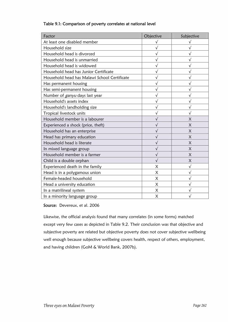
Three eyes on Malawi Poverty Page 262
Table 9.1: Comparison of poverty correlates at national level
Factor Objective Subjective
At least one disabled member √ √
Household size √ √
Household head is divorced √ √
Household head is unmarried √ √
Household head is widowed √ √
Household head has Junior Certificate √ √
Household head has Malawi School Certificate √ √
Has permanent housing √ √
Has semi-permanent housing √ √
Number of ganyu days last year √ √
Household's assets index √ √
Household's landholding size √ √
Tropical livestock units √ √
Household member is a labourer √ X
Experienced a shock (price, theft) √ X
Household has an enterprise √ X
Head has primary education √ X
Household head is literate √ X
In mixed language group √ X
Household member is a farmer √ X
Child is a double orphan √ X
Experienced death in the family X √
Head is in a polygamous union X √
Female-headed household X √
Head a university education X √
In a matrilineal system X √
In a minority language group X √
Source: Devereux, et al. 2006
Likewise, the official analysis found that many correlates (in some forms) matched
except very few cases as depicted in Table 9.2. Their conclusion was that objective and
subjective poverty are related but objective poverty does not cover subjective wellbeing
well enough because subjective wellbeing covers health, respect of others, employment,
and having children (GoM & World Bank, 2007b).

Three eyes on Malawi Poverty Page 263
Table 9.2: Comparison of wellbeing determinants at national level
Household characteristics Objective Subjective
Household size √ √
Household size squared √ √
Share*/number of 0-4 & 5-10 yr children √ √
Female household head √ √
Age of h-head/age groups (26-35/36-45/65+) √ √
Household owns an enterprise √ √
Completed junior primary √ √
Completed senior primary √ √
Completed senior secondary/post-prim √ √
Completed junior secondary/Post-prim √ √
Household head is widowed √ X
Household has wage income √ X
Household owns dimba plot √ X
Household grew tobacco last season √ X
Total rain fed land area (log) √ X
Completed pre-school X √
Share of elderly X √
* significant at 5% (MIQ) the rest at 1%
Source: Tables A3.6 of Annex 2D and Annex 2E (GoM & World Bank, 2007b)
The mismatches between objective poverty correlates and wellbeing determinants
become very obvious when the comparison is done at the local level. Table 9.3 presents
poverty correlates and determinants for the three villages combined. There is only one
correlate that is common between the official and self assessments. In fact self assessment
has only four correlates while the official boasts of sixteen correlates.
As for the wellbeing determinants, there were two that were common to both
assessments. Both found that the number of children in the household affect the
wellbeing status. Application of fertilizer also influenced the level of consumption as
well as self assessed wellbeing status. These two determinants are not surprising.
Possibly what is surprising is that access to credit, which is a determinant of consumption
expenditure, is not for self-assessed wellbeing and that landholding size is not a
determinant of consumption expenditure when it is for self assessed wellbeing status.

Three eyes on Malawi Poverty Page 264
Table 9.3 Comparison of correlates and determinants at community level
Feature Poverty correlates Wellbeing determinants
Official Self Official Self
Location: Ngochera √
Location: Dzilekwa
√
Household size √
√
Dependency ratio √
Number of dependent children √
√ √
Years in school for adults (mean) √
Highest class by adult member √
Whether applied fertilizer √
√ √
Amount spent on inputs √
√
Share of food in total consumption √
Number of durable assets √
Whether a member has cell phone √
Whether household has a bicycle √
Hours adults spend on enterprise √
Access to credit (incl. amt) √
√
Income from agriculture √
Maize output per cultivated land
√
Livestock ownership (types/values)) √ √ √
Number involved in ganyu
√
Household has a irrigatable land
√ √
Landholding size is 0.5 and 0.9 ha
√
Source: Tables 6.11, 6.12, 8.8 and 8.10
Things get worse when the determinants models are applied at each village individually.
As Table 9.4 shows, there is not even one case of matching. Determinants of
consumption expenditure are completely different from the one for self assessed
wellbeing status. In fact, in Dzilekwa there are no determinants of consumption
expenditure.

Three eyes on Malawi Poverty Page 265
Table 9.4: Comparison of wellbeing determinants by village
Village --> Ngochera Chikhwaza Dzilekwa
Characteristic Official Self Official Self Official Self
Household size √ √
Household size squared √
Children from 5 to 10 years old √
Children from 11 to 14 old √
Members in wage employment √
No under-five child √ √
Head is not in employed √
Head of household is male √
Head of household is not widowed √
Household has no irrigatable land √
Landholding is 0.5 to 0.99 ha √
None employed √
Non-formal employment √
One member household √
Three-member household √
Two-member household √
Head has no education √
One under5 child √ √
Household accessed credit √
Harvest in tonnes per hectare √
Members engaged in Ganyu √
Two under5 children √
Source: Tables 6.12 and 8.10
It is clear that monetary and subjective assessments of wellbeing are different. The
difference gets clear the lower the level. Although, some of the difference could be due
to number of cases for applying the models, the difference reflects differences in
coverage as suggested by the officials that analysed the IHS2 (GoM & World Bank,
2007b). The differences also reveal the limitation of using variables derived from a
survey specifically designed to provide data for objective poverty for self assessed
wellbeing. To come up with meaningful profiles for self assessed wellbeing, there is need
to collect data that is in line with self assessed wellbeing. Open-ended discussions on
wellbeing status and its causes would assist in refining the subjective assessment of
wellbeing module currently in use. A first step towards this was done by opening the
discussion, results of which have been presented in chapter 8 and compared with those
from community groups next.

Three eyes on Malawi Poverty Page 266
9.3 Comparing the three assessments at village level
The comparison between peers and self assessments is made easy because the coding
system used to analyse the responses was the same. There are sixty-five different reasons
that were given by both assessments (53 for peers and 52 for self assessments). To
highlight the similarities and differences between the two assessments this long list of
reasons is broken down in several ways. In terms of convergence and divergence, forty
reasons appear in both assessments. That is 75% for peers assessment and 76% for self-
assessment. Without considering the relative weights for each reason, the conclusion is
that the two assessments are generally in agreement. The reasons with at least 5% on
either assessment are listed Table 9.5.
Table 9.5: Top wellbeing factors for peers and self assessment in the 3 villages
(% of total responses)
Factor Peers Self
n=537 n=394
1 Has a non-farm enterprise 12.1 7.1
2 Has adequate food 6.9 8.4
3 Is a hard worker 7.1 3.3
4 Has inadequate food 3.2 7.1
5 Meets all/most needs 1.5 7.1
6 Too old to work as required 4.5 2.8
7 Owns some livestock 5.8 1.3
8 Is a ganyu worker 5.0 2.0
9 Has diligent farmer(s) 5.8 0.5
10 Has a good house 4.7 1.3
11 Uses no or inadequate fertilizer 0.2 5.6
Source: Author‟s computation of primary data
When factors with at least 3% difference in weight (shaded) are considered a certain
pattern emerges. While households themselves thought they were doing well in terms
of meeting basic needs, other community members did not use that „fact‟. Similarly,
while households used their failure to apply fertilizer to justify their wellbeing position,
the community group did not use that factor as much. To some extent, this goes for
food stocks as well. On the other hand, while the community groups valued the
hardworking spirit (hard, diligent and ganyu worker) the households themselves did not
see it as much. This is also true for ownership of enterprises, livestock and good house.
A similar picture emerges when factors that appear only under one assessment are
considered. For example, community groups used ownership of durable and productive
assets in assessing household wellbeing status but no household used such. This is true
for orphan care and laziness (opposite of working hard or diligence). On the other

Three eyes on Malawi Poverty Page 267
hand, ownership of irrigatable land and lack of money and employment opportunities
were used by households when assessing their wellbeing status but these were not used
by the community groups. Table 9.6 presents reasons that were mentioned in only one
assessment.
Table 9.6: Wellbeing factors featuring in only assessment type in the 3 villages
(% of total responses)
Peers assessment n=537 Self assessment n=394
Owns some durable asset 3.5 Has no irrigatable land 2.0
Takes care of orphans 1.5 Has no money to prosper 2.0
Has lazy member(s) 1.3 No/rare job openings 1.5
Has some productive assets 0.9 Generates money for basics only 1.5
Has a small household 0.7 Excluded in subsidy programme 0.8
Has no supportive husband 0.7 Has poor quality clothes 0.8
Acts as a source of help 0.6 Low produce prices 0.5
Has beddings - beds/blankets 0.4 Has no educated children 0.3
Has a husband in town 0.4 Community is not supportive 0.3
Is physically challenged 0.4 Can't hire labour 0.3
Eats no protein foods 0.2 Has household utensils 0.3
Is promiscuous 0.2 Gets too low wages 0.3
Is old but still strong 0.2
Source: Author‟s computation of primary data
These differences in valuation show differences in weighting between community
members and households themselves. These differences in weighting could be a
reflection of inadequate knowledge or difference in perceptions of what matters for
wellbeing at community and household levels. Assuming the latter is true it does not
mean that the community or household perception is superior. None is superior or
inferior but each matters because community perceptions matters just as households do
Comparison of all the three requires some rationalisation of some of the factors. Those
that have been modified are discussed before the comparison in done. The location
factor is dropped since most of the factors are household based. Likewise household size
and number of dependent children are considered to be related to „too many children‟
or „taking care of orphans‟ prevalent in subjective assessments. Dependency ratio, part
of which covers members over sixty-four years old, is taken to be related to „too old to
make a living‟ mentioned in both self-rating and peer assessment. Similarly, share of
food to total consumption is taken to be related to „adequate food stocks‟ or
„inadequate food stocks‟ both of which are popular in wellbeing assessments.

Three eyes on Malawi Poverty Page 268
There are other factors that are in different forms but can be rationalised. For example,
amount of hours spent by adults in a household enterprise is related to „whether a
household operates an enterprise‟, number of household members engaged in casual
work is related to „household head or spouse get engaged in casual work‟, and the
factors: number of durable assets, whether a household member has a mobile phone
and whether the household owns a bicycle are jointly linked to „ownership of durable
assets‟ under peer assessment. Finally, durable assets as presented in survey questionnaire
include some utensils such combining utensils and durable assets would benefit the
analysis.
Others under self rating and peer assessment also need some rationalisation. For
example, whether a household lives in a poor quality house (as given by self and peer
assessment) or a good quality house (peer assessment only) it is that these are not
unique features but the opposite of each other. As already stated, the factor „good
quality house‟ is more prominently used by peers than household representatives.
Factors „presence of external support‟ (mentioned in self rating) and „absence of external
support‟ (mentioned under peer assessment) are not two unique factors but just „sides of
the same coin‟. It is only that household representatives emphasise one side while peers
notice the other more.
Table 9.7 presents prominent factors associated with each of the three assessments
following the rationalisations. The table shows that there are four factors that are
common in all the three assessments. There are two factors that are common between
the official and peers assessments and two between the official and self assessments.
Once again proving that peers and self assessments are more related to each other than
each to official assessments, there are four factors that are common between them. It is
noted that consumption and self-rating shared the more measurable features or those
that are best known by the households (inputs use and income levels and sources) while
peer assessment shares with consumption expenditures features that are conspicuous
(livestock and durable assets).

Three eyes on Malawi Poverty Page 269
Table 9.7: Comparison of wellbeing features under the three assessments
Household wellbeing feature Official Self Peers
1 Has adequate/inadequate food stocks √ √ √
2 Operates an enterprise (including size/time spent) √ √ √
3 Head too old (implied in dependency ratio) √ √ √
4 Members are involved in ganyu (also number) √ √ √
5 Applied no/inadequate farm inputs (incl. amount) √ √ §
6 Income source and type (meets needs) √ √ §
7 Owns (no) livestock (types and values) √ § √
8 Owns some durable assets/utensils √ § √
9 Lives in a poor/good quality house § √ √
10 Gets (no) external support (children and others) § √ √
11 Head or spouse is a regular ganyu worker § √ √
12 Member(s) work hard in farm or business x √ √
13 Large household size/too many children √ § §
14 Number of dependent children/too many children √ § §
15 Household has (no) irrigatable farmland √ § x
16 Access to credit (amount or start up capital) √ § §
17 Education level of adult members (highest class) √ x x
18 Has money that meet/meets all or most needs § √ §
19 Struggles to generate income x √ §
20 Head has no husband § § √
21 Head or spouse is in poor health § § √
22 Husband is polygamist § § √
23 Head and/or spouse is/are diligent farmer(s) x § √
√ means it is a significant feature; § means that it is present but not as prominent
feature; and x means it is absent as a feature
Source: Author‟s analysis of Tables 9.3 to 9.6 and primary data
Further, considering only factors that are important or significant (marked with „√‟)
there are eight important features under the official assessment that are shared with at
least one other assessment. Self and peers assessments have both ten factors that are
shared with at least one other assessment. This implies that both peer and self
assessments are generally broader because they include dimensions not taken care of by
the official assessment.
This is confirmed when the features that are present in local level assessments but absent
in official assessment are analysed. For example, the official assessment misses „hard
working members‟, „households that struggle to generate cash income‟ and „households
with diligent farmers‟. One of the possible reasons for this, as Chambers (1997) put it, is
that survey questionnaires shy away from difficult-to-measure wellbeing indicators. As
long as it is difficult to operationalise subjective assessment of wellbeing in a

Three eyes on Malawi Poverty Page 270
questionnaire, any measure based on such data is likely to miss out some aspects of
wellbeing that are considered important at community level.
Another look at the features shows that areas covered by the survey questionnaire were
also covered in some form by the subjective wellbeing module and wealth and pairwise
ranking. For example, there is only one important feature under the official measure
(education level of adults) that did not come up during self or peer assessments in all the
three villages. This is understood because in rural economies where formal employment
is almost non-existent, education level is of no consequence (GoM & World Bank,
2007a). On the other hand, only ownership of irrigatable land did not come up under
peer assessment possibly because the group reasoned that those without such farmland
can lent it if they have money. The implication is that despite using different „views‟, a
carefully designed survey questionnaire can cover some aspects of important features
that are found to be important by self and peer assessments. It is noted that this is only
indicative since the villages visited are not representative of the country. What is needed
are national level factors – factors gleaned from qualitative studies that were nationally
representative, which is the subject of the next section.
9.4 Interrogation of the official definition of poverty
So far it has been established that the three methods of assessing household wellbeing
and poverty are neither the same nor completely different. It has also been established
that although they share some dimensions, each emphasises different characteristics and
in some cases each uses completely different characteristics. In line with the research
problem, the findings imply that the official wellbeing measure barely include qualitative
aspects of wellbeing commonly associated with self and peers assessments. Using the
three villages as case studies, it has been shown that the use of either peers or self
assessment to identify the poor would lead to targeting errors if the evaluation is done
using the official measure. It has also shown that some of the targeting errors would
possibly emanate from conceptual and weighting differences.
This leaves one research question unanswered. The question is whether the official
version of wellbeing and poverty can be modified based on the findings from qualitative
studies nationally and the three villages. To answer this question, there is a need to
review the official wellbeing analysis system first to identify entry points in the system
for modifications.
Three eyes on Malawi Poverty Page 271
9.4.1 The official wellbeing analysis system
In Malawi, the official wellbeing analysis system comprise the administration of two
survey questionnaires (household and community) countrywide over twelve months,
the analysis of the survey data to construct the consumption expenditure aggregate and
the poverty line, the analysis of the data to construct poverty measures like poverty
incidence, severity and depth, and the determination of household and community
characteristics that are associated with wellbeing and poverty. The characteristics are in
the form of poverty correlates (used as poverty proxy indicators) and wellbeing
determinants (meant to infer causes of poverty). An internal evaluation of some parts of
the system is done before the system is exposed to the external „elements‟ gathered from
peers and self assessments.
The consumption expenditure aggregate
As seen in Chapter 5, the consumption expenditure aggregate has three parts; food
consumption, household expenditure on non-food goods and services, non-consumer
durables and use value of durable goods. Food consumption component covers food
consumed from own production, purchases and gifts. Almost all kinds of food
consumed are included. Further, the list is prompted implying that the respondent is
reminded in case the item could slip through. In responding, the interviewee gives the
unit used and quantity consumed. Valuation of food consumed from own production
and gifts is done using prices used in the purchase of the same. To complete food
consumption amount of money spent on water is added.
The non-food, non-durable component covers expenditure or purchases of goods and
services; spending on heat and lighting, private and public transport, personal and
household hygiene and care, payment for services; clothing and footwear, household
utensils, and entertainment materials and equipment; ad hoc payments and costs; and
education expenses. Use value of durable goods covers 17 out of the 36 durable goods
collected. Traditionally housing mortgage payments, repairs, maintenance and
decorations are excluded from the non-food expenditure because the consumption
expenditure aggregate uses housing use value instead.
There are a few cases the consumption expenditure has the potential to come up a
wellbeing status that may not match that of self or peers assessment. As reported in
Chapter 3, in collecting food consumption the interviewee gives the actual unit the food
was eaten or made from. The advantage of this approach is that both the respondent
and interviewer are not asked to estimate. This improves the accuracy of the amounts of

Three eyes on Malawi Poverty Page 272
data collected. To standardise the units, experts come up with conversion factors. This is
where there is some potential of introducing measurement errors. A casual look at the
conversion factors (from various units to grams) shows that some of them are
inconsistent or questionable. This is clear in the case of maize flour, the main ingredient
used to cook „nsima‟, the main food item in Malawi.
The first example of a unit used for maize flour is „heap‟. A heap of maize flour
converts to 4581 grams yet a large pail (between 8 to 10 litres) of maize flour converts
to 2036 grams and a basketful converts to 4841 grams. The question is: what type of
flour heap is this? Other „strange‟ conversion units for maize flour include „piece‟,
„basket shelled‟ and „basket unshelled‟. A „piece‟ of maize flour converts to 580 grams,
which is close to the value assigned for a no. 12 plate (595 g). This begs the question:
what is this „piece‟ in terms of maize flour? Again, what is „shelled‟ or „unshelled‟ basket?
Are these mistakes considering that they have the same conversion factors? Another
curious unit is „oxcart‟ of maize flour. Given that the consumption in question is for a
week the use of an oxcart for a unit seems out of place. Even if it were used (may be for
a very large household) its conversion factor of 32270 grams is even lower than that of
a 50-kg bag of maize flour (46658 g). Normally an oxcart is capable of packing at least
five such bags. Is it that the unit is wrong for a week or that the factor is wrong or both?
Similar mismatches between a unit and its conversation factor are observed on basin and
tin. A basin has a factor of 4308 grams, which is almost twice that of a large pail (2036
grams) yet a standard basin is rarely larger than a large pail. At the same time a tin has
33 grams as its conversion factor yet the smallest tin imaginable cannot be a quarter of a
cup (whose conversion factor is 160 g). A more practical question is: why sell maize
flour in such a small unit, even if it existed? It would have been better if these dubious
units were just on paper. However, all these units are present in the IHS2 dataset and
for a good measure that even have cases of „litres‟ of maize flour. The point being made
here is that analysts use these to construct the food consumption aggregate and if they
are wrong the aggregate is bound to be wrong.
Whether these significantly affect the level of maize flour consumption is not clear. What
is clear, though, is that they do not inspire confidence in the aggregate. It is not
advisable to continue using dubious units and conversion factors. Since consumption-
expenditure is the standard wellbeing measure used to evaluate other wellbeing
assessment methods, its construction should meet high standards. It is therefore
recommended that experts review all units and factors for all food items to satisfy
themselves of their appropriateness and accuracy. In the interim, units and conversion

Three eyes on Malawi Poverty Page 273
factors for maize and maize flour, the major food consumption item, should be
rationalised. For those units found to be inappropriate, they should be blocked out
during data collection and entry. For factors that are out of line, they should be revised
based on other credible conversion factors in the same food category.
Another area that can bring differences in assessment is on use value of durable goods.
As indicated, not all durable goods in a household are included in this aggregate. Some
are, understandably, left out because they are productive assets (e.g. boats, nets, ox-
carts, and ploughs) whose use may translate into food or income. However, the list of
durable goods considered (17) are generally not „traditional‟ except one (mortar/pestle
for food processing). While noting that there are some „modern‟ durable goods that are
excluded also, exclusion of some durable goods associated with rural households like
(hoe, panga, hoe, axe, sickle, wheel barrow, and drum) is difficult to justify unless it has
been proven that these are valueless to their wellbeing. To settle the matter, there is
need for a study to first establish which durable goods are considered valuable for
wellbeing status in rural areas and separately in urban areas and for those found useful,
establish the relevant information for the computation of the use value (expected life
time and range of retail prices). Until then, the use value of durable goods may be
divorced from the thinking local people and therefore can be a source of differences
between the assessments.
Another area is the removal of the user-value of housing in the aggregate. The
justification for the removal was that there is no effective housing market in Malawi to
get market prices for the valuation. Considering that the non-food non-durable
component excludes housing costs (building materials, repairs, maintaining, and
decoration) on the understanding that the user-value covers these, the removal
effectively blocks housing out of the consumption expenditure aggregate. The solution is
to re-introduce housing costs in the non-food non-durable component. Excluding
housing from the wellbeing measure is a potential source of assessment mismatch
because quality of the dwelling unit features as a prominent wellbeing characteristic at
local level.
Addressing these would affect wellbeing levels as measured by consumption
expenditure. Given a poverty line such changes would affect the poverty status of some
households. In other words, changes in the measure affect the poverty status of some
households. This is also true of changes in the poverty line itself. This means that the
appropriateness of the poverty line needs to be addressed as well before comparing
wellbeing features from the official and local level assessments.

Three eyes on Malawi Poverty Page 274
The official poverty line
The construction of the official poverty line is based on the basic needs concept (GoM &
World Bank, 2007b). Just like the wellbeing measure, the basic needs poverty line has
food and non-food components. The food component is based on what is actually
consumed while the non-food component is based on expenditure. Food being one of
the components of basic needs (Doyal & Gough, 1991), the food component of the
poverty line defines ultra poverty (GoM, 2000).
As discussed in Chapter 5, the food poverty line uses a WHO-based median minimum
daily calorie requirement for a medium activity population valued at median cost of
food consumed by the 5th and 6
th decile households (GoM & World Bank, 2007). Two
discussion points come out of this: (i) the assumption that Malawi is a medium activity
country and (ii) value used to cost the calorific value. The question is whether Malawi is
a medium activity country given that the hoe is still the main agricultural implement for
tilling the land. Perhaps more pertinent is the point that the 2007 wellbeing analysis
used 1985 recommendations (GoM & World Bank, 2007b) instead of 2004
recommendations (FAO/WHO/UNU, 2004). According to the 2004 recommendations,
it is possible to assign values for each individual instead of assigning activity status for an
entire population. Clearly the new system resonates with the finding that households
differ in activity level and therefore energy requirements. Until when the new
recommendations are used, it is not clear whether the food poverty line is the right one.
As for the use of median cost of food consumption for the 5th and 6
th decile, it is not
clear whether it is appropriate to use it to value the 2400 calories per day per person
ultra poverty line. So far it has been established that at a village level, what and how
much a household eats determines its wellbeing status. This implies that consumption
patterns reflect wellbeing statuses. If 2400 calories per day separates the ultra poor from
the rest, it should therefore be the median cost of food consumed by the poor that
should be used. That may not be true for the 5th and 6
th deciles. A more realistic
proposition would be to use the median for the bottom 50%.
In effect using the median value from the bottom 50% may result in poverty line that is
lower than the current one on the assumption that the poor purchase cheap calories
(GoM & World Bank, 2007b). However, given that the resultant minimum calorific
value from using the 2004 WHO recommendation may result in a minimum more than
2400 calories (what with child labour, agricultural activities, and constant casual work
among the poor) the overall impact could go either way. The advantage would be that

Three eyes on Malawi Poverty Page 275
such a poverty line would be reflecting the thinking of differentiated needs by activity
and growth needs.
It is also noted that the Malawi poverty line is NOT based on basic needs. It is based on
food consumption at the median. No expert is involved in defining the foods that make
up the minimum calories. The calories can come from different sources as long as it is
what the average household consumes. This is also true of the non-food component.
No expert draws a list of non-food basic needs. Instead revealed preference of the
average households (i.e. households along the food poverty line, plus minus 5%) is
taken as the standard. . This procedure is meant to avoid the subjectivity associated with
expert choice of basic needs. The assumption on both cases (food and non-food
components) is that food consumed and goods purchased by the ultra poor are basic.
Of course, this is not always true. It is needful that some analysis be done to check
whether indeed most of the goods and services around the poverty line are basic needs.
But what are considered basic items in a Malawian household?
So far there has been no study to establish what basic needs in Malawi are. One solution
is to conduct a comprehensive Breadline Britain type of study (Gordon, et al., 2000)
where community group discussants, at the first instance, come up with a list goods and
services that are considered essential for normal style of living in their community and
households are requested to indicate, from the list compiled from the FGDs, those they
consider necessary for their household. Apart from being relevant, the resultant list
would help in establishing whether what is consumed at the median matches the „ideal‟
minimum basket. The list would also be used to check local level definitions of poverty.
The implication is that a self-rating poverty line would then be used to check against the
consumption expenditure poverty line and peer assessed poverty line. So far, self-rating
does not have a standard.
Other possible sources of differences
The consumption expenditure measure combines actual (food consumption) and
potential consumption (expenditure). This approach excludes current use of goods and
services acquired previously (clothes, shoes, blankets and linen) and, by extension, future
use of goods and services, acquired in the current period. Residual use of goods and
services purchased previous and current years is assumed to be zero. While this is alright
given the limitations of quantitative analysis of wellbeing where flow and stock cannot
be mixed, peers and self assessments have no such boundaries because the assessors
consider all these. This is also true for the separation of income and consumption

Three eyes on Malawi Poverty Page 276
analysis. The use of consumption as a measure automatically excludes the use of income.
Yet local people consider income, consumption and many other wellbeing aspects in
their analysis.
For example, apart from the „calories‟ consumed, local people also consider the source
of the calorie. Some sources of food, no matter how rich they are in calories, may be
considered unattractive for some wellbeing categories. Likewise, spending a lot on some
items may be seen as a sign of poverty. This is also true for some sources of income as
some sources are considered more respectable than others regardless of the level of
income. The implication is that the level of wellbeing implied in the consumption
expenditure (or income level) may not always agree with the assessment of local
people. In particular, the use of one dimension of wellbeing (consumption or income or
expenditure) does not match the process used by local wellbeing assessors.
Finally, consumption expenditure is a flow and not stock concept. In the flow concept,
it is not the amount of maize a household has in store that matters but how much is
consumed regardless of source. At local level, both are considered as part of wellbeing.
Thus, unless the assessments use the same principles, there are bound to be differences
among the three measures. Apparently, self and peer assessments are more holistic in
their approach than the official measure. They consider various sides of wellbeing:
income as well as consumption; flow as well as stock; actual as well as potential; and
quantitative as well as qualitative.
But is the current official wellbeing analysis system completely out of touch with self and
peers assessments? Do wellbeing category characteristics obtained from wellbeing
analysis completely alien to consumption expenditure measure? Do factors considered
important by households not assessed by the questionnaire used to assess the household
wellbeing status? These are the remaining questions worthy checking against the official
wellbeing analysis system.
9.4.2 Wellbeing characteristics: official versus local concepts
To get the features or characteristics that are covered in the official system, there is need
to revisit the questionnaires in order to check what they cover. It is what they cover that
dictates what household characteristics are likely to come out of the official system since
both poverty correlates and wellbeing determinants analyses are based on variables
from the questionnaires.
The household questionnaire covers household demographics, education and health
status, time use and employment, and security and safety of all household members. It

Three eyes on Malawi Poverty Page 277
also covers child anthropometry. At household level it covers housing structure, housing
amenities, and housing costs; consumption of food (from different sources) over three
days and a week; non-food consumption over a week, month, three months and a year
depending on assumed frequency of expenditure; and durable assets. The consumption
expenditure aggregate is constructed from various parts of these modules.
For instrumental variables (aspects hypothesised to have some effect or be related to
household wellbeing as measured by consumption expenditure), the questionnaire
collects data on agriculture production inputs (land, technical advice, purchased seed
and fertilizer), harvests, sales, consumption and stocks by crops cultivated. It also covers
production and sale of tobacco, dimba crops, livestock and trees. It also covers
operation of household enterprises and access to savings interest, pension, property
rental, remittances as sources of income outside agriculture; and access to commercial
credit and social programmes (for free or worked for food, social employment,
subsidised credit, and free or worked for or subsidised inputs). Other instrumental
variables are constructed from modules on recent shocks (natural, economic and social)
and deaths in the household.
Other than these modules which are used to indirectly assess wellbeing, the subjective
assessment of wellbeing module directly assesses the household wellbeing status in a
number of areas. These include an assessment of the adequacy of consumption (food,
housing, clothing and health care), sufficiency of current income and economic
wellbeing, minimum income and life satisfaction. Targeting only the household head,
the questionnaire has questions on number of changes of clothes, and what the head
sleeps on and under.
The household questionnaire is supplemented by a community questionnaire. The
community questionnaire includes a direct observation section on children and adults
clothing and footwear, whether windows have glass and surroundings are swept, and
type of building material used for the walls and roofs. Other sections covered include
community-level basic physical and demographic characteristics (language, ethnic make-
up and inheritance system); access to basic services (all-weather roads, clinics, schools,
commodity and produce markets, financial services, and representation); economic
activities include public works programmes; agriculture activities (adoption of new crop
varieties, access to technical advice and credit facilities, and prevalence of farmer clubs
and cooperatives); and prices and changes over a five year period on a myriad of areas
including major wellbeing-affecting events.

Three eyes on Malawi Poverty Page 278
These two questionnaires provide a long list of areas covered and provide an
opportunity to construct just as long a list of variables used in the correlates and
determinants analyses. To deal with the question whether the wellbeing features given
by community groups have some „relations‟ in the official wellbeing analysis, there is
need to first check the local features against factors that have ever been found to have
significant association with wellbeing. For management purposes, the local features are
divided into three categories; those that are present in all measures (official, self and
peers assessments), those under either self rating or peer assessment and official system,
and those only under peer assessment65
.
Common wellbeing features
It is noted that even the case where a feature is common under all the three assessments,
it does not mean that they are used the same way. It could be that what is common is
the dimension but not necessarily their measurement or use in analysis. Thus if the
objective is to modify the official system to reflect the local concepts, then it is
important to analyse the official system in order to check how the feature fits in that
system in terms of how it is collected or incorporated in the measure or used in the
analyses. Table 9.8 presents 16 factors that are common. Six of these (shaded in the
table) are either measured differently or excluded from analyses. These are the ones that
are discussed individually.
65
There is no feature that is unique to self-rating.

Three eyes on Malawi Poverty Page 279
Table 9.8: Wellbeing factors common in all the three types of assessments
Factor Official Self Peers
1 Access and level of cash income √ √ √
2 Access/ownership to and size of land √ √ √
3 Age of head/aged without support √ √ √
4 Education of adult member/head √ √ √
5 Engagement in ganyu √ √ √
6 Health status of members √ √ √
7 Household has an enterprise √ √ √
8 Household shock (price, theft, death) √ √ √
9 Marital status of household √ √ √
10 Number of members/Household size √ √ √
11 Number/share of dependent children √ √ √
12 Ownership and type of durable assets √ √ √
13 Ownership of non-farm IGAs √ √ √
14 Ownership or value of livestock √ √ √
15 Quality of housing structure √ √ √
16 Wage employment and income √ √ √
Source: Chapters 6, 7 and 8
The official system for wellbeing analysis includes health status of household members in
terms of morbidity and expenditure on health care. In the analysis, the factor „whether a
household has a member that was ill or injured‟ is used as a dummy variable in the
correlation analysis. What is missing is the impact of illness/injury on wellbeing status,
especially the number of lost days by adults (the ill/injured or carer) in the poverty
determinants analysis. Considering that local people consider illness/injury holistically,
this extra analysis may bring the official treatment of this factor closer to that of local
people.
The data collected covers ownership of an enterprise and a dummy variable is used in
correlation analysis. However, no analysis is done to relate various aspects of the
enterprise (type, size and profitability) to household type. Community reports give the
impression that enterprise size, type and profitability are related to wellbeing status. It is
the extra analysis that can ground truth the impression. Ownership and type of durable
assets are collected but partially used. As discussed above a study on usefulness of
various durable goods is required. A Mack and Lansley (1985) type of study would
establish such a list.
The questionnaire and analysis cover ownership and value of livestock. While the
questionnaire is used to collect ownership and numbers of all types of livestock and
income from livestock, the analysis uses various variable constructs from this to relate

Three eyes on Malawi Poverty Page 280
livestock ownership to wellbeing status. One area that can be added in the analysis is a
categorisation of types of livestock owned. Since local people use ownership of sets of
livestock in assessing household wellbeing status, there is need to include a variable that
incorporates this. For example, the analysis can have a categorical variable with values 3
for a set of cattle, goats, and chicken (and others); 2 for goats and chickens (and others);
1 for chickens only; and 0 for no livestock. This would resonate with the local reasoning.
Quality of housing structure is collected and used in analysis. However, it is completely
missing in the wellbeing measure. As already proposed above, the housing costs should
be introduced to compensate for the removal of the housing use value. Apart from that,
there is need to engage local people to give shape to the „quality of housing‟ factor.
From community reports, a „quality house‟ may mean different things in different areas.
Therefore, there is need for a study to establish relevant importance of various building
materials by area and type of household. The study proposed under the durable goods
can incorporate this aspect. Related to housing is tidiness or cleanliness of the home and
its surrounding. This qualitative aspect is only collected at community level. Since
community groups attach important to this, the direct observation as done under
community questionnaire should be done at household level. In other words, the
observation should be transferred from the community to the household questionnaire
Ownership of non-farm IGAs is related to activities that mostly rely on individual skills
or capability like handcrafts making, shoe repairing, brick-laying, and also grass/bamboo
fence building, traditional kraal/house building, maintaining or thatching. Currently,
what each member does over a particular period is covered by the questionnaire.
Various variables are also constructed from the module on time use and labour. What is
not specifically dealt with is the possession of the skills or capabilities by household
members. The questionnaires should specifically collect each member‟s skills and how
they have been used over a specific period in the material year. The reason is that both
the possession and use of skills and capabilities are used by peers to assess wellbeing
status.
Wellbeing features under official and either measures
Table 9.9 lists factors that are at least present under official assessment.

Three eyes on Malawi Poverty Page 281
Table 9.9: Wellbeing factors common in the official and one other assessments
Factor Official Self Peers
1 Households has a disabled head/member √ √ X
2 Location/language group/inheritance system √ √ X
3 Sex of household head √ √ X
4 Access to external support √ X √
5 Access to inputs √ X √
6 Access to social economic services √ X √
7 Availability of amenities √ X √
8 Education status of children √ X √
9 Household owns a dimba plot √ X √
10 Production of cash crops √ X √
11 Type and amount of food consumed √ X √
Source: Chapters 6, 7 and 8
The list shows that the official wellbeing analysis system provides some space for the
subjectively determined features. The issue is whether the space is sufficient for the local
features to manifest freely. This then requires an analysis of each of the listed factor. The
first is the presence of an adult member with physical disability. This factor is not
comprehensively dealt with because the questionnaire does not deal with the extent of
the physical disability vis-à-vis ability to make a living. Thus each household member
should be assessed in terms of disability and level of independence. This, if done in
conjunction with the skills assessment and employment of skills and capabilities, would
make a clear link between disability and wellbeing status. What a questionnaire cannot
do is deal with the local people‟s thinking that disability, regardless of ability, negatively
affects wellbeing.
The factor that a household grows cash crops is collected but not analysed
comprehensively to include the number of cash crops. Production of tobacco is found to
be associated with high wellbeing status by both assessments. However, in non-tobacco
growing areas it is the number of crops that acts as an indicator of wellbeing. One way
of dealing with this is to supplement the value with a categorical variable on number of
cash crops grown weighted by either size of cultivated land or value of the sales.
The type and amount of food consumed is a factor that can be inferred from the data
collected on food consumption. While the food consumption aggregate takes care of the
amount, the analysis does not deal with the type of food consumed. This is an area of
possible difference because local people use both amount and type to assess wellbeing
status of a household. Thus the type of food consumed has to be related to local

Three eyes on Malawi Poverty Page 282
concepts regarding the type of foods eaten at various points of food/income security
continuum (i.e. when desperate or just coping or in abundance). Since the data on type
of food consumed is not collected together with the circumstances, a dedicated module
on food security would include questions that would provide the context. The same
module would collect information on the type of food that is considered „normal‟ in the
community for the three meals and other times.
Wellbeing features not prominent under the official system
There are twenty-six factors under self rating or peer assessments. Only eight of them are
common to both self-rating and peer assessment while the rest are only mentioned in
peer assessments. These are presented in Table 9.10.
Table 9.10: Wellbeing factors in self and peers assessment only
Factor Official Self Peers
1 Adoption of new varieties/production methods X √ √
2 Amount of food (maize) stocks X √ √
3 Attitude to work/hardworking X √ √
4 Household access to hired labour X √ √
5 Household has working children (in/out) X √ √
6 Institutional analysis - opportunity space X √ √
7 Number/share of dependent adults X √ √
8 Types of crops produced X √ √
9 Access to credit facilities X X √
10 Access to household basics X X √
11 Access to productive assets X X √
12 Accessibility of community X X √
13 Behaviour/attitude to life X X √
14 Body and skin appearance X X √
15 Cleanliness of home and surrounding X X √
16 Frequency of food consumption X X √
17 Household has peace of mind X X √
18 Household members beg X X √
19 Luck/charms X X √
20 Natural factors (weather/soil quality) X X √
21 Ownership and type of household utensils X X √
22 Personal/property security X X √
23 Quality of clothing and footwear X X √
24 Quality of life X X √
25 Quality of sleeping place/beddings X X √
26 Widowhood/orphanhood X X √
Source: Chapters 6, 7 and 8

Three eyes on Malawi Poverty Page 283
It is noted that the absence of these under „official‟ does not mean that they are not
collected or analysed. Some are collected but not analysed while others are collected,
analysed and found statistically insignificant. Factors that are well covered include
accessibility of the community, access to credit facilities, access to basics like salt, soap,
and soda; involvement is casual work; access to hired labour; and personal and property
security.
The official system also covers expenditure on clothing, footwear and linen. However,
the questionnaire does not collect their stocks and quality. While the questionnaire
collects number of changes of clothes and the type of beddings (sleep on and under) for
the head, even this data is not analysed. Since local assessments also use quality and
adequacy (stocks) for children and all adults (and not only the head) in assessing
wellbeing, the questionnaire should also cover number of changes of clothes/beddings
for each member and their quality (age/conditions) to match the local concepts.
Just like in the case of cash crops discussed above, the number and types of crops grown
are not used in the official analyses yet local people use crop diversification as an
indicator of wellbeing status. Since the data is collected, the analysis can use these as
unweighted or weighted by production quantities/value of output or cultivated area.
Related to crops grown are natural factors. While weather is dealt with, soil fertility is
not. However, local people consider soil fertility as an important determinant of
wellbeing especially when viewed against inputs accessibility. A dummy indicating
whether crops like maize are grown without fertilizer on given plots could deal with the
missing factor.
Crop harvests in the questionnaire covers amount of food stocks. However, the
relationship between stocks and wellbeing is not dealt with. On the other hand, local
people also consider food stocks when assessing household wellbeing. To incorporate
stocks, the analysis can convert stocks into per capita months of food supply or per
capita food supply per annum. Alternatively, the proposed food security module can
directly request the respondent to estimate food supply months from own stocks.
Quality of life and attitude towards life (agency) are covered in various degrees under
subjective wellbeing module. However, the data in this module are not mainstreamed
in the poverty profiling that follows. This makes subjective wellbeing assessment
secondary to the official assessment which uses consumption expenditure as the
measure. For the purposes of policy making, subjective assessment of wellbeing is

Three eyes on Malawi Poverty Page 284
equally important because people‟s assessments are likely to influence their responses to
the opportunity structure in general or policy initiatives in particular.
Data on orphanhood and widowhood are collected. The analysis extensively deals with
orphanhood but scantly with widowhood. A household headed by a widow is covered
by female headed household. However, what a widow goes through in wellbeing terms
may be different from what a divorcee goes through. Further, the immediate and
sometimes permanent impacts on wellbeing of orphanhood and widowhood are
stressed in peer assessment. To deal with this, the module on recent shocks or death in
the household should specifically trace changes in wellbeing due to loss of spouse or
parents over a five year period.
Body and skin appearance is often used in peer assessment. This is possibly in place of
„use or non-use of bathing soap and lotion‟ because people just see the manifests of use
or non-use. Direct observation by the interviewer can deal with this feature directly. It
can, however, be dealt with indirectly by including questions on use or non-use of
bathing soap and lotion. The downside of the observation method is that data quality
would depend on the representativeness of the observed household members. Use and
type of soap and lotions used would give an idea of the quality of skin and body care.
For a good measure, the two methods can be used simultaneously.
The community questionnaire collects data on cleanliness/tidiness of the home and its
surrounding through direct observation. However, this does not satisfy people‟s
thinking. Local people seem to relate low priority given to quality of living environment
to poverty. To get household level data on this, the direct observation should be
transferred from the community to household questionnaire. This can be done under
the housing module.
There are factors that are rather difficult to collect. These include the behaviour of
household members or attitude to life including belief in luck or bad luck. These factors
are best dealt with third persons because it is difficult to get honest responses from
household respondents. Few would be honest enough to say that they are not hard
working or fatalistic. The use of charms for household prosperity is another difficult-to-
collect factor due to negative publicity on charms. While many are free to discuss the
issue generally, few would do so specifically. Therefore, these factors are best collected
under the confines of peer assessment or other participatory methods.
The adoption of new varieties of crops and production methods are factors that are
considered important for wellbeing improvement. Yet these are not directly dealt with

Three eyes on Malawi Poverty Page 285
in the household questionnaire. The questionnaire covers crops grown but not newly
adopted crops. As for production methods, the questionnaire is silent. However, these
two can easily be incorporated by finding our whether the household adopted or
abandoned new crops or methods of production with reasons, say in the past three or
five years. It is likely this question would bring out institutional issues at household level
as well. In particular, the role of technical advisors, credit or markets for the household‟s
wellbeing can come out here. Most of these institutional issues are covered under the
community questionnaire. However, what is required is an institutional analysis of
households‟ opportunities and constraints.
A household institutional analysis is an area that has been neglected in wellbeing analysis
in Malawi. Local people, in assessing wellbeing of households rarely mention the role of
institutions in improving their opportunity structure. This could be a reflection of the
long absence or non-existence of institutions at local level. It could also imply that they
don‟t need governmental and non-governmental organisation, in the form of technical
advice and microcredit. It is therefore important to ascertain this by getting an actual
account of how the presence/absence of institutional support makes a difference to the
household.
9.4.3 Prominent features: official versus peer assessment
The comparisons and discussions done in the previous sub-section provide a
comprehensive list of areas that need to be dealt with if the current official wellbeing
analysis system is to respond to local voices. However, not every local feature is
important. In particular, not every local feature is prominent across the country all the
time. To be fair, the comparison should be between official wellbeing correlates and
determinants and prominent local features that are determined in studies conducted
around the same time. These are presented in Table 9.11 for the comparison.
Clearly there are more mismatches than matches in this list. For example, out of the 30
features only 4 are common to both while 17 factors that are significant under official
assessment are absent in peer assessments and 9 prominent features under peer
assessment are either insignificant or absent in official assessments. As has been argued
before, even when the official and peer assessments have a similar factor it does not
mean it is the same in measurement. The implication is that each prominent feature
under peer assessment needs to be analysed. Those that were already dealt with in the
previous subsection are not discussed here.

Three eyes on Malawi Poverty Page 286
Table 9.11: Prominent wellbeing features under official and peer assessment
Factor Official Peers
1 Education status of children √ √
2 Household head/member get wage income √ √
3 Type/number/value of livestock √ √
4 Ownership of durable goods (phone/bike) √ √
5 Access to amenities (sanitation) √ X
6 Access to SE services (clinic, markets, etc) √ X
7 Accessibility of community (location) √ X
8 Age of household head √ X
9 Education level of head or adults √ X
10 Health status of household member √ X
11 Household landholding size √ X
12 Household size √ X
13 Marital status of household head √ X
14 Maternity services open to mothers √ X
15 Number of children/Dependency ratio √ X
16 Ownership of non-farm enterprises √ X
17 Production of cash crops (tobacco) √ X
18 Sex of household head (female) √ X
19 Whether a household owns a dimba plot √ X
20 Whether member is a child (dummy) √ X
21 Whether member is a woman (dummy) √ X
22 Access to inputs/purchase of fertilizer X √
23 Access to paid labour X √
24 Amount and frequency of food consumed X √
25 Amount and quality of beddings/linen X √
26 Amount and quality of child clothing X √
27 Amount and quality of clothing X √
28 Amount of food stocks X √
29 Quality of food consumed X √
30 Quality of house structure X √
Source: Chapters 6 and 7
Education status of children: peer assessment covers three angles; (i) the level/class
children achieve (ii) parental support in terms of type/quality of school, food (before
and after school) and school supplies (uniform and fees) and (iii) source of finance for
school expenses. The official system covers the first angle fully, education expenses only
out of the second and does not cover the third angle at all. For education status to
reflect wellbeing status of the household while factoring in child‟s agency and capability,
all the angles should be fully incorporated in the official wellbeing analysis system. This
can be done in the education module by including questions on availability of food

Three eyes on Malawi Poverty Page 287
before and after school, type of school and source of money for the last major
education expense (school fees, uniform or supplies).
Employment status of household head/adult members: This is taken care of in the
official system. In peer assessment, wage employment is viewed positively but is
consigned to poor households. In official assessment, wage employment is also positive
but not necessarily consigned to the poor. This is possibly because the wage
employment covers both rural and urban households while the peer assessment is based
on rural households by design.
Livestock ownership – type, number and value: This is as discussed above.
Ownership of durable assets: Two assets are found to be important in official wellbeing
analyses (mobile phone and bicycle). Peer assessments mostly mention bicycles.
However, to ensure that the official system recognise assets normally used and owned,
the bias against traditional assets implicit in the calculation of user-value of durables
should be revisited as proposed above.
Access to inputs (fertilizer): This feature is collected and analysed although it is not
statistically significant whether used as a dummy (whether a household applied fertilizer)
or scalar variable (inputs costs). Thus this factor is well taken care.
Access to paid labour: This is another factor that is well covered by the official system
though it is statistically not significant.
Food stocks and consumption: This is already discussed above.
Quality of clothing, shoes, beddings and linen: This is discussed above.
Quality of housing structure: This has already been discussed above.
This analysis shows that the current system does not need to be overhauled to deal with
key local people‟s concepts of wellbeing. If these aspects are incorporated in data
collection and analysis, the resultant wellbeing measure and poverty proxies would be
closer to local wellbeing conceptualisation. That implies that if the official wellbeing
measure or poverty proxies are used to evaluate the efficiency of community-based
targeting, it would lead to reduced levels of „superficial‟ targeting errors. This has been
the overall objective of the study.

Three eyes on Malawi Poverty Page 288
9.5 Summary of the findings, recommendations and implications
The study concerned itself with showing a mismatch between the official version of
wellbeing and those of people whose wellbeing is being measured. The literature review
showed that the way wellbeing is conceptualised and measured, there is a possibility
that even in Malawi what the officials consider as poverty may not necessarily be what
people on the ground conceive as poverty. By extension, the reviewed literature
showed that households that are locally assessed as poor are evaluated as non-poor by
the official measure and those locally assessed as non-poor are poor. The review also
checked and confirmed that some differences in assessments emanate from differences in
the features implicit in the methods used to measure household wellbeing.
The study then moved to check whether the mismatches can be proven to exist in
Malawi. To do that the study adopted a methodology that required replicating the
processes officials and local people use to assess household wellbeing and identify poor
people. This led to the (i) construction of consumption expenditure aggregates in the
three randomly selected villages, representing the official version of wellbeing, and (ii)
determination wellbeing status of each household using self and peer assessments,
representing local versions of wellbeing. Application of official, self-declared and peer-
chosen poverty lines assisted to categorise the households into poor and non-poor
households.
The resultants lists of poor people for each measure (official, self and peer assessments)
in each village provided inputs for the comparisons. An analysis of wellbeing
characteristics under each measure in the three villages provided a glimpse of possible
differences at national level. However, analysis of data from nationally representative
studies provided comprehensive lists of wellbeing features from the official and local
perspectives that were compared. The aim of the latter comparison was to determine
areas in the official wellbeing analysis system that can be modified for the sake of
making the official version of wellbeing sensitive to local concepts. So far the three
research questions have been answered. A summary of the answers are presented
hereafter.
9.5.1 Households identified as poor
Regarding the question whether the consumption-expenditure, self-rating and peer
assessment identify the same households as poor, the answer is: „not necessarily‟. Using
the rankings of households based on the consumption measure and a combination of
wealth and pairwise ranking for the peer assessment, the two measures do not match.

Three eyes on Malawi Poverty Page 289
Using poverty rates, each of the measures identified different numbers of households as
poor. Comparing the lists of the poor households shows that very few households were
common in the three measures. In fact, there were more households that were uniquely
identified by a measure. Further, those households jointly identified as poor by all
measures are not very different those from either identified by two assessments or only
one, in terms of per capita consumption levels and other socio-economic characteristics.
To cap it, identification errors in all the three villages are very high confirming that each
of the measure is unique. The conclusion is that taking one type of assessment as a
measure of the other is not practical.
9.5.2 Wellbeing characteristics
Based on the wellbeing characteristics from the three villages, there are more common
than unique features for the three measures. The features also show that peers and self
assessments have more convergence between them than each with the official measure.
This points to the possibility that conceptualisation of wellbeing at household and
community level is closer than that of officials with each. Overall, the analysis of features
in the three villages does not show major differences among the three measures. Of
course, three villages out of thousands can hardly be representative but the few
differences may point to possible differences at national level.
A cursory analysis of national level factors shows that a good number of factors are
common to all the three methods. In terms of policy implications, this means the
common factors can act as the core proxy indicators for wellbeing or poverty. The
advantage is that most of these are in the current official wellbeing analysis system.
Adding a few modifications would make them even better. A much more strict analysis
shows that only four features (out of 30) are common to official and peer assessments.
This change shows the problem of scalability of local level features. This fundamentally
reveals that, at national level, there are relatively few universality acceptable features
from qualitative studies. The differences confirm the thinking that consumption-
expenditure barely measures the wellbeing the way local people do. Indeed analysis of
each local feature shows that the official wellbeing analysis system does not include
some aspects of wellbeing that are considered in local wellbeing assessment.
9.5.3 Appropriateness of the official wellbeing analysis system
Overall, the official wellbeing analysis system takes care of local concepts of wellbeing
to an extent. It has been found that the questionnaires used to collect data for wellbeing
analysis best covers consumption expenditure aspects, by design. It has also been found

Three eyes on Malawi Poverty Page 290
that some features from self-rating and peer assessment are covered in the
questionnaires. It has also been found that in some cases data is collected by not
analysed appropriately or at all.
There are some features that are not covered in the household questionnaire like stock
of durable goods, utensils, clothing, blankets and linen. Institutional analysis is also
absent. The questionnaire does not include some qualitative aspects like household
member behaviour and attitudes towards life because these are difficult to collect. The
analysis misses availability of food, types of livestock owned by household types, impact
of widowhood, and assessment of quality of life and subjective wellbeing.
The local aspects that are not very well covered by the official wellbeing system are the
likely contributors of the divergences between the official and local measures of
wellbeing and poverty. The study has therefore proposed areas that need to be looked
into in order to bring the official version of poverty closer to people without necessarily
changing its fundamental tenets.
9.5.4 Proposed changes to the official wellbeing analysis system
The study has made sets of proposals for change on a number of aspects of the official
wellbeing analysis system in order to make the wellbeing measure and operational
definition of poverty sensitive to people‟s characterisation of wellbeing and poverty.
These proposals are premised on the belief that a country‟s definition and measurement
of wellbeing and poverty should be based on what people in that country take them to
be. This is even imperative when the people, as is the case in Malawi, are asked to
identify the poor among themselves; a situation that requires the officials and people to
have same understanding of who is poor or otherwise.
The proposed changes are on the data collection system, construction of wellbeing
measure, determination of the poverty line, analysis of the data for wellbeing proxy
indicators, and profiling of wellbeing and poverty. These are recapped below.
Construction of the consumption expenditure aggregate
1. Review units used for food consumed, received and purchased to remove
possible data „noise‟ that may come with the use of inappropriate units
2. Review conversion factors to remove inconsistencies and thereby improve the
accuracy of the amounts of food consumed, received and purchased

Three eyes on Malawi Poverty Page 291
3. Review the list of durable assets used in the calculation of their use value under
the non-food consumption aggregate to ensure that all relevant durable assets
from both rural and urban households are included
4. Include housing costs in the non-food consumption aggregate in lieu of housing
use-value that is rightly abandoned in Malawi
Determination of the poverty line
1. Revise the method used to determine the minimum calorific value by using the
2004 instead of the 1985 expert recommendations which favours the use of
individual instead of country level activity levels to determine food
requirements.
2. Revise the method used to determine the cost for valuing the minimum calories
by using the median cost for the bottom five deciles instead of the 5th and 6
th
deciles
3. Introduce a „true‟ basic needs poverty line by conducting a study that determines
a consensual set of goods and services considered basic for living in Malawi using
the Breadline Britain Methodology.
Potential poverty proxy indicators that have to be included and tested
1. Per capita stock of clothes, footwear, blankets and linen
2. Quality of clothes, footwear, blankets and linen
3. Quality of housing and surroundings
4. Number of lost days by adults due to illness/injury
5. Size of an enterprise (based on either capital requirements or turnover or profits)
6. Per capita months of maize supply or per capita maize stocks per annum
7. Types of livestock owned in recognition of the differences in ownership of sets
of livestock by wellbeing groups
8. Household member skills and capabilities
9. Number of crops (cash crops separately) weighted by either area under
cultivation or value of their harvests or sales (cash crops)
10. Types of food consumed by meal and number of meals taken per day
11. Self-assessed soil fertility
12. Various kinds of institutional support
Profiling of wellbeing and poverty

Three eyes on Malawi Poverty Page 292
1. Include subjective assessment of wellbeing as part of the Malawi poverty profile
since the household questionnaire has a fully fledged module on this.
2. Where possible, the profile should include community groups‟ assessment of
wellbeing of communities and, if possible, households.
Use of proxy indicators for identifying the poor
1. If there is need to narrow down the list of wellbeing/poverty indicators, priority
should be given to the four that were found to be common to all the three
assessments. If more are required the 16 factors found under the non-binding
analysis should be considered second.
2. The difference between prominent factors at national level and community level
(three villages) imply that the use of national level wellbeing/poverty proxy
indicators needs to be done with caution. The best is to first ground truth each
because different communities may value them differently despite being
common. This is an issue of weighting.
Data collection
1. Introduce a direct observation module in the household questionnaire to include
subjective assessment of the condition of the main dwelling unit, and cleanliness
of household members‟ bodies and clothes as well as the surroundings
2. Introduce a module on clothing, footwear and beddings to get more details on
stocks and conditions for each household member in the household; and also
frequency of wash/baths, type of detergents preferred and used, and type of
soap and lotion preferred and used
3. Introduce a food consumption and security module to collect data on typical
foods eaten by meal, actual food eaten by meal, amount of food stocks and
sources of food when stocks run out
4. Modify the time use and labour module to include skills and capabilities of each
household member and their recent use
5. Modify the education module to include type of school, type of food given
before, in-school and after school, and the source of finance for various
education expenses
6. Modify the agriculture production modules to include assessment of soil fertility
7. Introduce an institutional analysis module in the household questionnaire to get
views on the potential and actual impact of institutions on the wellbeing of the
household

Three eyes on Malawi Poverty Page 293
Special study
1. A Breadline Britain type of study (Gordon, et al., 2000) to establish goods and
services considered basic for living a decent life, normal meals in a day, type of
foods for each meal, typical durable goods in a household, and typical type of
houses including type of materials for the roof, walls, windows, and floor.
9.5.5 Implications of the study
One of the study‟s viewpoints is that all the three types of wellbeing assessment are
equal. The study started off with the view that what a household respondent (mostly
head or spouse) says to an enumerator administrating a questionnaire is as good as what
the respondent says when subjectively (directly) evaluating the household‟s wellbeing
status. This thinking is also extended to a group of individuals representing the
community. This study has shown that each of the types has inherent challenges
regardless of the quality of enumerators and facilitators. In particular, it has been shown
that the construction of the wellbeing measure in Malawi leaves some room for
improvement. It has also shown that peers assessment can easily go wrong if the group
or some of the members choose to distort facts. Thus there is no method that is better
than the other as that is dependent on many factors some of which are outside the
control of the researcher.
The study avoided focussing on the differences amongst the three sampled villages to
ensure that the objectives of the study are achieved. However, it has come clear that
wellbeing and poverty trajectories of households, regardless of differences in local
definitions and characterisation of wellbeing or poverty, are dictated by location. The
study has shown village differences are too important to ignore in poverty analysis. By
implication, any design of local level poverty reduction or alleviation initiative should
bear this in mind.
The study is based on the hypothesis that some targeting errors associated with projects
that use community based targeting and self-selection are superficial. Indeed, the
analysis of the primary data supports this hypothesis. Although not pursued in detail,
the data has also shown that some of the errors could indeed be due to deliberate
misclassification of households even when the criteria are clear or developed by the
identifiers themselves. Since no analysis was done on these deliberate errors, all that can
be said at this juncture is that dealing with the superficial errors is but one side of the
story. The assumed information advantage at community level can be misused if there

Three eyes on Malawi Poverty Page 294
are no mechanisms to verify whether or not the superior knowledge is indeed used
during the identification. Thus community based targeting requires some monitoring.
The goal of the study was to improve the measurement of wellbeing for the benefit of
community based targeting. Judging from the areas that have been found to be missing
in the current system of wellbeing analysis, it is not easy to have them all incorporated.
While others can easily be incorporated, there are many more that require further work.
This study has highlighted all such areas. However, the study does not provide concrete
statistics on how much improvement each change or all changes can bring to the
measurement of wellbeing and poverty. It also does not discuss the practicality of
bringing the required changes, including the financial implications.
Such gray areas are the study‟s areas for further study. Chief among them is a study on
consensual poverty and role of institutions in determining wellbeing status of
households. The consensual poverty analysis would not only supplement the subjective
wellbeing assessment well but also improve the definition of the needs basket in
Malawi. The institutional analysis study would provide material for civic education on
demand for and supply of appropriate and relevant support.
9.6 Contribution to knowledge
This study has made a modest contribution to the understanding of wellbeing
measurement in a rural setting. It has managed to modify techniques used elsewhere and
apply them to Malawi and three rural villages. In particular the study has the following
contributions.
Application of overlapping dimensions adapted from Bradshaw and Finch (2003)
Factors associated with consumption-expenditure measure are compared with those
from self-rating and peer assessment to determine those that overlap as best candidates
for developing proxy indicators.
Comparative analysis of the three methods
There has been no study that has compared the three methods on the same households
at the same time. Reviewed studies have compared consumption/income measure with
either self-rating or peer assessment. The comparison of consumption/income measure
with self-rating traditionally uses one questionnaire to collect the consumption/income
and subjective assessment of wellbeing (called self assessment or rating in this study). The
comparison between consumption/income and community assessment (called peer-
assessment) requires an administration of a questionnaire on households that were

Three eyes on Malawi Poverty Page 295
assessed by the community. In this study, the two approaches were pooled together
with an added question in the module on subjective wellbeing assessment to get reasons
for the assessment. This approach provides „objective‟ correlates and determinants for
the consumption-expenditure measure and self-rating and „subjective‟ wellbeing features
for self-rating and peer assessment.
Bringing local-specific features to the national level
Statistical analysis makes it easy to identify factors that are associated with wellbeing or
poverty from a purpose-built survey questionnaire. The same is not true for factors from
group discussions using wellbeing analysis and pairwise ranking. This study, using
content analysis of country representative group discussions, gleaned factors that are not
only consistent for a wellbeing category but also consistent across space. That process
brought the FGD-specific features to national level where they were compared with the
national level poverty correlates and determinants. Although no „science‟ was used to
come up with the national level features from focus group discussions, the process was
sound enough for comfortable comparison.
Use of three independent populations
The comparisons so far reviewed use one sample (either nationally representative
sample or one community). This study was done on three randomly selected
communities to ensure that findings are not subject to a community‟s peculiarity. The
three sites offer a chance to check whether the research questions can have the same
answer in all the three sites. It has been a bonus that the three communities are different
on a number of important aspects, especially livelihoods strategies.
Use of census instead of sampling
This study, unlike previous studies, opted to conduct a village census instead of a sample
to ensure that all the three methods of identifying the poor were applied to the same
households. With this method, there is no question of representativeness of the
households visited since the unit for community-based targeting is a village.
Complete ranking of households
Consumption expenditure measure enables the complete ranking of households from
poorest to richest. Traditional wealth analysis goes as far as determining proportions of
different wellbeing categories in a community. That cannot be used to rank households
from poorest to richest. Pairwise ranking is traditionally used to rank problems or

Three eyes on Malawi Poverty Page 296
projects. This study, borrowed the use of a ten-step ladder, to further breakdown
households into ten categories and borrowed pairwise ranking to sort households on
each ladder step. Thus by combining wellbeing analysis (placing households in categories
and later ten steps) and pairwise ranking (sorting by step), households were ranked from
poorest (the lowest household on step 1) to the richest (the highest placed household on
the highest community-designated step). This ranking was then compared with the
consumption-expenditure ranking using statistical methods to check their correlation.
This has never been done before.
Thus apart from answering the research questions, this thesis has made some
contributions to knowledge, especially for Malawi wellbeing assessment.

Three eyes on Malawi Poverty Page 297
Appendices
Appendix 1: Data collection tools
A1.1 Modifications made to IHS2 for the survey of the three villages
A PDF format of the IHS2 household questionnaire is available on demand from the
National Statistical Office. It is also available online at www.nso.malawi.net at least by
30th September, 2011. The modifications made on IHS2 were meant to concentrate on
parts that are relevant for the construction of the consumption-expenditure aggregate
and variables for the poverty correlates and wellbeing determinants models. These are
outlined in the table below.
Module Label Changes made
A-1 Household identification No change
A-2 Survey staff details Maintained only A12, A13 and A14
B Household roster Deleted B08-B11because household head provided
info
C Education Deleted C04-07. Did not differentiate languages
Deleted C21-C29. Did not want schooling details
D Health Deleted D02-D03because household head provided
info
Deleted D06 – did not need to know who diagnosed
illness
Deleted D21-38 – did not need details beyond
morbidity
E Time use and Labour No change
F Security and Safety Deleted – not directly important
G Housing No change
H Food consumption past 3
days
No change
I Food consumption past 1
week
No change
J Non-food expenditures
past 1 week & 1 month
No change
K Non-food expenditures
past 3 months
No change
L Non-food expenditures
past 12 months
No change
M Durable goods No change
N Agriculture - General Deleted N02 – not applicable
Deleted N08-N30 – did not need the details
O Agriculture – Rain fed
cultivation
Deleted O04 – did not need decision maker
Deleted O10 – did not need details on land market
P Agriculture – Rain fed
crop sales
No change
Q Agriculture – Tobacco Deleted P02-P08 – details on tobacco growing

Three eyes on Malawi Poverty Page 298
unnecessary
R Agriculture – Dry season
(Dimba) cultivation
Deleted R01 – not applicable
Deleted R03-R4 – because ownership not prevalent
Deleted R09-R12 - did not need details on land
market
S Agriculture – Dry season
(Dimba) crop sales
No change
T Agriculture – Tree crop
production & sales
No change
U Agriculture – Livestock &
livestock sales
No change
V Household enterprises No change
W Other income No change
X Gifts given and received No change
Y Social safety nets No change
Z Credit No change
AA Subjective Assessment of
well-being
Modified AA01 – from food consumption adequacy
to wellbeing category (poor or rich or in between)
Replaced AA02 with a question that request
respondent to justify the selected category in AA01
Deleted adequacy questions (AA03-AA04) because
there would not be used
Modified AA05 – replaced 6-step ladder with a 10-
step ladder; requested for a poverty step; retained
AA05
Deleted AA06-AA07 – no need to compare with
neighbours and friends
AB Recent Shocks to
household welfare
Deleted – not needed
AC Deaths in household Deleted – not needed
AD Child Anthropometry Deleted – not needed

Three eyes on Malawi Poverty Page 299
A1.2 FGD Interview Guide for wellbeing and pairwise ranking
Introduction
Our meeting will take most of the day today. We appreciate very much your being with
us. We had indicated to the chief that the meeting would take some time and that only
those who feel can stand that should be requested to come. However, this is not a
prison. In case, you feel that you are unable to be with us the whole day, don‟t feel
pressed to just stay on, you are free to go.
In our discussions, we will be discussing wellbeing, poverty, and how these affect
households. We will be mentioning names of households and placing them on position.
Others may find discussing their households while they are here uncomfortable. If you
feel that you don‟t have to be here while we are discussing your household, you will be
excused for that time.
We know we will take some time discussing this. We plan to have a break, then lunch
together and then another break in the afternoon. We have asked some people to help
us with the cooking instead of asking the discussants here to do it. When food is ready
we will be informed.
The discussion forms part of a study on how to match community understanding of
wellbeing and poverty with those of officials in Government, NGOs and donors who
sometimes help the poor in communities. It has not been commissioned by
Government. However, it is being conducted by a member of the University of Malawi
who works with Government, NGOs and donors on promoting pro-poor initiatives. It
is hoped that the results of this study will influence how these stakeholders take the
views of people on the ground regarding their experience in poverty.
Our discussion is divided into several parts. We will start with categorising the
households in this village into welfare groups from the poorest to the richest and giving
characteristics of each group. Following the characterisation, we will introduce a ten-
step ladder on which we will superimpose the welfare groups. Once we agree, we will
place households in this village on the ten steps of ladder. We will be asked to give
reasons why we think a household should be placed on a particular step. After
households are placed on the steps, we will sort the households on each step from
poorest to the richest on that ladder. By doing that we would have sorting the
households from the poorest to the richest.

Three eyes on Malawi Poverty Page 300
Part I: Welfare groups in the community and their categorisation
o We know in every society that there are differences in well being among people.
We are visiting three communities in this study to learn about these differences.
We especially hope to learn from you how these differences are used when
identifying the poor in the village for transfers like cash transfers, free inputs,
subsidies.
o Tell me about people at the bottom and the top of your community. How
would you describe the people living at the bottom – the poorest and worst-off?
How can you tell that a person is in this category? How do they live? How
would you describe people living at the top – the richest and best off? How do
they live?
o Let‟s move on. What about people who are just above the category of people
who are at the bottom? How would you describe people in this category?
o Now, let‟s move up from that category. [Keep inquiring about additional
categories until the best off is reached. For each of the categories identified:]
How would people living in this category be described?
o Let us now recap. We have identified [X] categories of people who live in this
village. Is this so? We will need the characteristics of these [X] categories as we
discuss individual households. Can we move to the second part?
Part II: Introducing a ten-step ladder of life and superimposing welfare categories
o Imagine again a ten step wellbeing ladder on which the first step stands the
poorest households you know. Those could be in the village or elsewhere.
Consider the [X] categories we have just defined. Which steps does the poorest
category occupy?
o Which steps does the richest category occupy?
o What about the group(s) in the middle?
Part III: Placing a community poverty line
Now we have [X] categories placed on a ten-step ladder of life. Sometimes, it may be
required just to have two groups; one poor and the other non-poor. On which step
would you say is the step where the first group of the non-poor are found?
Part IV: Placing households on the wellbeing ladder steps
Call out the name of each household on the list. Ask the focus group what step the
household is at today and why.

Three eyes on Malawi Poverty Page 301
[To reduce the potential for recording errors or miscommunication, please record each
response in a matrix that the entire focus group can see and verify. The facilitator should
remind the discussants the characteristics of the welfare categories superimposed on the
ladder of life, especially at the beginning and occasionally during the sorting exercise.
This is a very important step. Facilitator should ensure that detailed notes are taken and
that the recorder is picking the voices]
Part V: Ranking households by step on the ladder
We have now managed to place the households on the ten steps of the ladder. What
we need to do next is to sort households on each step. We can start from any step. To
make it easier let us start from the top most step in the community.
Call names of households on step according to the record and then perform pair wise
wealth ranking to rank households from poorest to richest on each step until all steps
with households are dealt with.
[Although emphasis is not on distinguishing features between households in this pair
wise ranking, take down all distinguishing factors given by the group]
Concluding Note
[Summarise the work of the day: Groups, key characteristics and poverty rate]
[Open for comments and questions]
[Thank the members of the FGD for their participation]

Three eyes on Malawi Poverty Page 302
Appendix 2: Data analysis notes from the 2007 analysis
This appendix reproduces Annex 1B found in the Appendices of the Malawi Poverty and
Vulnerability Assessment (GoM & World Bank, 2007b). It also reproduces the notes
from the team (Ms Beegle) on construction of the housing use value. These are modified
to reflect only the relevant parts that have been used in the current analysis.
A2.1 Note on Construction of consumption expenditure Aggregate
Introduction
The Malawi 2004-2005 Integrated Household Survey (IHS2) was a comprehensive
socio-economic survey of the living standards of households in Malawi. The National
Statistics Office administered the IHS2 household questionnaire to 11,280 households
from March 2004-April 2005. The survey was designed so that information gathered
could be used for, among other things, an assessment of the incidence of poverty in the
population at the district level and above.
Poverty is that condition in which basic needs of a household (or individual) are not
met. Clearly it is a multidimensional concept. Nevertheless, for purposes of identifying
the poor using international standards, a monetary measure is developed as a welfare
indicator for each household. Using this monetary measure, households can be ranked
from richest to poorest. By developing a poverty line (a monetary threshold, below
which a household is labelled as poor), households can be further described as poor or
non-poor. For more nuanced classification, multiple poverty lines can be developed,
for example, to identify the ultra poor.
This note describes the construction of this welfare indicator, referred to as the
consumption expenditure aggregate, and the development of poverty lines which can
be applied to the welfare indicator to label households as poor. The following sections
describe how the aggregate was constructed.
Consumption expenditure aggregate
Broadly speaking, the consumption expenditures fall into four categories: (1) food;
(2)non-food, non-consumer durables; (3) consumer durable goods; and (4) actual or
self-estimated rental cost of housing. In the following sections there is more information
on the calculation of these components of the consumption expenditures. Some general
issues to note are.

Three eyes on Malawi Poverty Page 303
Outlier values: Outliers are identified based on a combination of graphical review and
standard deviations from means for each subcomponent. Generally, outlier values are
replaced by median values based on households in the enumeration area (or by median
values at the district/national level if less than 7 observations at the lower level). Lists of
cut off points used to establish outliers are in Appendix 2d.
Annualization: Recall periods for expenditure subcomponents vary, ranging from past 7
days to 12 months. For uniformity all values are annualized.
Real values: Since the data were collected in the three villages were collected within a
month and within a radius of 200 km, there is no need to adjust prices to take into
account spatial and temporal price differences. In some cases where IHS2 cost or value
data is used, they are brought to 2010 using the growth in the rural CPI between March
2004 and July 2010.
Food consumption aggregate
Food consumption is reported at the household level in Sections H and I of the IHS2
questionnaire. Section H has food consumption over the last 3 days for a limited
number of products which were self-produced (not purchased). Section I has food
consumed over the last 7 days for a much larger range of products. Section H, by
definition, is a subset of Section I.
For computing food consumption only Section I is included. Section I collects
information on 80 different food categories. In addition interviewers could include
“other” products consumed that were not specified in the list. Products reported under
“other” were also included and given a value in the expenditure aggregate.
Section I has information on food consumption from three different sources: (1)
purchased food; (2) consumption from own-production; and (3) food received as gifts
or free from some other sources. In addition, drinking water expenditures from Section
G are later added to the beverage sub-aggregate.
Unit prices and conversion of units to grams: For purchased food, both quantity and
expenditure in Malawi Kwacha (MK) were collected. For consumption of food from
own-production and food from gifts, only quantities are recorded. In order to compute
the MK value for own-production and food from gifts, a unit price for each purchased
product was calculated. These unit prices were then multiplied by the quantities
reported from own-production and food from gifts. In general, the unit prices are
computed as the median product price over all households in that geographical area at

Three eyes on Malawi Poverty Page 304
that time of the year. If less than seven households in that area and time purchased a
particular product, a larger geographical area was used. The use of a minimum seven
households to calculate the unit-price guards against high volatility in unit prices over
different households.
In the questionnaire, quantities can be reported in 20 different units of measurement. In
order to calculate the unit prices and to multiply the quantities with the unit prices, the
different units of measurements were all converted into grams. Appendix 2c gives a full
list of the conversion factors.
Non-food consumer durable goods and services
Expenditure on non-food, non-consumer durable goods and services are collected in
several sections of the IHS2 household questionnaire. Relevant sections of the
questionnaire include sections J, K, L, and G (utilities). The recall period varies across
items, depending on the general frequency of purchase. More frequently purchased
items have shorter recall periods, while less frequent purchases have long recall periods.
The recall periods are last 7 days, last month, last 3 months, and last 12 months. All
values are annualized. Education expenditures were reported either by type of
expenditure, for example, tuition, books, uniforms, etc., or as an overall total. The total
expenditure for education was calculated as the sum of all the sub-categories if they
were reported, or as the overall total, whichever is greatest.
Consumer durable goods
Section M of the IHS2 questionnaire collects information on household ownership of 36
durable consumer goods. Seventeen of the items were deemed consumer durables and
are included in the consumption expenditure aggregate. The other durable consumer
goods are predominately related to income generation or enable higher consumption
and, as such, are considered production durables. Therefore, these were excluded. Of
course, there are some goods for which it is not clear how to classify them. The
assignments used were based on best practices as well as the assignments used in the
IHS1 analysis.
As durable consumer goods last for several years, and because it is clearly not the
purchase itself of durables that is the relevant component of welfare, they require special
treatment when calculating total expenditure. It is the use of a durable good that
contributes to welfare, but since the use is rarely observed directly the yearly use value is
estimated in the following way:

Three eyes on Malawi Poverty Page 305
1) Assuming that each product is uniformly distributed, expected lifetime for each
product is calculated as twice the mean age of each product.
2) Remaining lifetime is calculated as current age minus expected lifetime. If current
age of product exceeds expected lifetime, remaining lifetime is replaced by two years.
The two years were arbitrarily chosen, however other expenditure aggregates have used
this value in the past. The yearly use value of each product is then calculated as current
value divided by remaining lifetime.
Table A2.1 shows the estimated lifetime used for IHS2 computation of user-values. It
also shows the values used in IHS1 (1997/98) analysis for the subset of durables included
in IHS1 with number of observations in parenthesis.
Table A2.1: Estimated Lifetime for Consumer Durables in IHS1 and IHS2
Section M
Expected Lifetime (years) IHS2
Item Code Item IHS2 (2004 ) IHS1 (1998)
501 Mortar/pestle/pounding mill 14.5 (5641) 16.3 (1457)
502 Bed 15.0 (3625) 17.0 (2498)
503 Table 13.8 (4030) 16.0 (2488)
504 Chair 12.3 (5060) 13.8 (3202)
505 Fan 7.8 (262)
506 Air conditioner 8.8 (28) 8.1 (153)*
507 Radio (wireless) 6.8 (6184) 4.1 (1199)
508 Tape or CD player, HiFi 8.4 (1851)
509 Television & VCR 6.9 (439) 7.5 (131)
510 Sewing machine 22.6 (326)
511 Kerosene/paraffin stove 10.4 (241)
512 Electric or gas stove, hot plate 7.6 (287) 4.8 (858)
513 Refrigerator 10.1 (227) 9.6 (238)
514 Washing machine 10.7 (19) 19.7 (14)
515 Bicycle 12.2 (4082) 9.7 (2156)
516 Motorcycle/scooter 14.0 (41) 13.3 (41)
517 Car/motor vehicle 12.9 (136) 8.1 (124)
Note: Numbers of observations are in parentheses. Some of the item labels were
slightly different across the two surveys. For example, fan and air conditioner were
combined into one category in IHS1
Poverty line
The total poverty line has two principal components; a food component and a non-
food component. The food poverty line is the amount of expenditures below which a
person is unable to purchase enough food to meet caloric requirements, based on a set
basket of food. It is also known as the ultra poor poverty line.
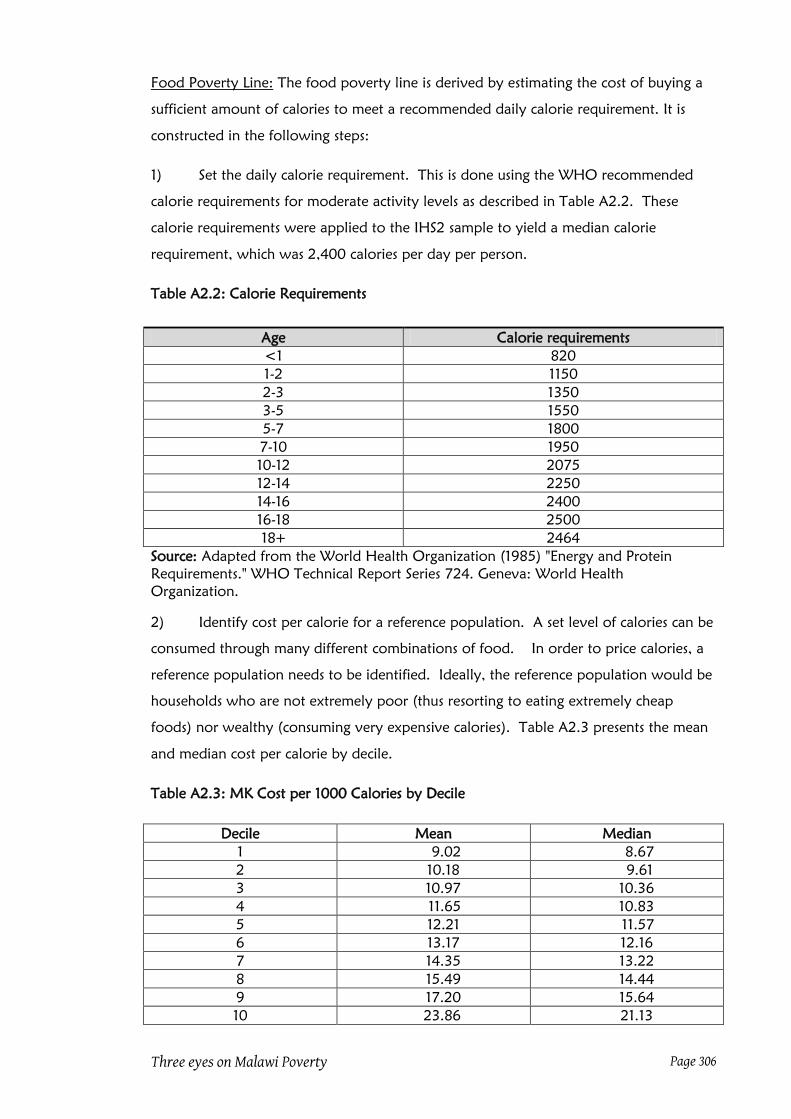
Three eyes on Malawi Poverty Page 306
Food Poverty Line: The food poverty line is derived by estimating the cost of buying a
sufficient amount of calories to meet a recommended daily calorie requirement. It is
constructed in the following steps:
1) Set the daily calorie requirement. This is done using the WHO recommended
calorie requirements for moderate activity levels as described in Table A2.2. These
calorie requirements were applied to the IHS2 sample to yield a median calorie
requirement, which was 2,400 calories per day per person.
Table A2.2: Calorie Requirements
Source: Adapted from the World Health Organization (1985) "Energy and Protein
Requirements." WHO Technical Report Series 724. Geneva: World Health
Organization.
2) Identify cost per calorie for a reference population. A set level of calories can be
consumed through many different combinations of food. In order to price calories, a
reference population needs to be identified. Ideally, the reference population would be
households who are not extremely poor (thus resorting to eating extremely cheap
foods) nor wealthy (consuming very expensive calories). Table A2.3 presents the mean
and median cost per calorie by decile.
Table A2.3: MK Cost per 1000 Calories by Decile
Decile Mean Median
1 9.02 8.67
2 10.18 9.61
3 10.97 10.36
4 11.65 10.83
5 12.21 11.57
6 13.17 12.16
7 14.35 13.22
8 15.49 14.44
9 17.20 15.64
10 23.86 21.13
Age Calorie requirements
<1 820
1-2 1150
2-3 1350
3-5 1550
5-7 1800
7-10 1950
10-12 2075
12-14 2250
14-16 2400
16-18 2500
18+ 2464

Three eyes on Malawi Poverty Page 307
The reference population was chosen to be the population in the 5th and 6th deciles of
the consumption aggregate distribution. In fact, these are households that are close
to/near the poverty line itself (as seen by the poverty rate which is described below. The
cost per calorie applied is 11.48 MK per 1000 calories.
3) Calculate the food poverty line. The food poverty line is calculated as the price
per calorie multiplied (0.01148 MK) by the recommended per capita daily calorie
requirement (2,400). The food poverty line is 10,029 MK per person per year, or 27.5
MK per person per day
The food poverty line is also the Ultra Poverty Line. The ultra poor are those
households whose total per capita expenditure levels are below the food poverty line.
Non-Food Poverty Line: Identifying basic needs non-food expenditures is more difficult
as there is no concept like calories which can be applied. The non-food component of
the total poverty line is based on the non-food consumption of those households whose
food consumption is close to the food poverty line. The non-food component is
calculated as the weighted average of non-food expenditure for those close to the food
poverty line. The average expenditure is kernel weighted so that that those that are very
close to the food poverty line are given most weight and those further away are given
less weight. Households with food expenditure per capita that was five percent below
or above the food poverty line was included in the kernel weighted average. The non-
food component of that total poverty line is 6,136 MK per person per year, or 16.8 MK
per person per day.
Poverty Line: The total poverty line is simply the sum of the food and non-food poverty
lines described above. The poverty line is 16,165MK per person per year, or 44.3 MK
per person per day. Once the poverty line is established, all households can be
categorized as poor or non-poor depending on whether their per capita expenditure
(their welfare indicator adjusted for household size) is below or above the poverty line.
The poverty headcount, then, can be computed, indicating the proportion of individuals
living in poverty. The poverty rate for the population of Malawi is 52.4%. This is the
proportion of the population whose household per capita consumption is below
16,165MK per year.
Three eyes on Malawi Poverty Page 308
A2.2 A note on housing and imputed rent
Summary
In most developing countries including Malawi, a small proportion of households
explicitly pay for their dwelling with rent. The thin rental markets make it difficult to
assess a value of owner-occupied dwellings. There are three ways to consider housing
valuation for home-owners in the consumption aggregate: use self-reported estimated
rents, use imputed rents based on sample of renters, or exclude from the consumption
aggregate.
It should be noted that there is no consistency on whether and how housing valuation
should be included in a consumption aggregate measure among countries in the region.
The approaches that have been used by countries close to Malawi have been diverse.
For example, Ethiopia, Kenya and Tanzania have excluded housing valuation;
Mozambique have included actual rents and self-reported estimates; while Uganda and
Zambia have included actual rental values estimated from regression models of actual
renters.
The key findings from the analyses undertaken in this note are:
The lack of reliability of the estimated rental values suggests that the values
should not be used for housing valuation or to extrapolate rental values for
households with missing rental values.
The small number of households renting in rural areas, combined with the
notable differences in the dwelling characteristics of rented and owned
houses in rural areas, suggests that the sample of renting households is too
small to impute rental values for owned dwellings from actual rental values.
Given the above conclusions, excluding housing valuation from the
consumption aggregate should be given serious consideration.
Introduction
Consumption aggregates are designed to estimate the total value of goods and services
consumed by members of the household. For many items, this is fairly straightforward,

Three eyes on Malawi Poverty Page 309
for example, valuing the amount of food consumed in the past one week. For other
areas, where the item “consumed” is a durable good or owner-occupied housing, this
valuation is much more complicated. This note pertains to the issue of valuing the
“consumption” of housing in Malawi. In the case of Malawi, where the vast majority of
housing is owner-occupied, this issue becomes much more complicated. In areas where
rental markets are thin (or non-existent, as in some rural areas), there is doubt as to
whether the concept of renting (and hence estimated rental values) is understood by
households. Most households in Malawi are either owners of their dwelling or
otherwise do not pay rent. Overall, 91 percent of households in Malawi pay nothing
for their dwelling. In rural areas, this figure is 97 percent.
This note evaluates the options with respect to valuing housing consumption for
Malawi. The options available are:
1. Include the valuation of housing in the consumption aggregate, by one of the
following methods:
a. Use actual rent and self-reported estimated rent for dwelling owners.
For missing values of estimated rent (108 households), use regression
estimates to predict estimated rent.
b. Use actual rent and imputed rental values for owner-occupied dwellings.
The imputed values would be predicted based on regressions of actual
rent values reported by renters.
2. Exclude the valuation of housing consumption from the consumption aggregate
In order to assess these options, this note evaluates several features of the data. It
reviews the data available, including the housing characteristics of the renters and home-
owners in rural and urban areas. It then reviews the correlates of rental values (actual
and estimated). As an extension, the exercise tests whether the estimated rental values
provided by non-renters were close to the predicted values based on actual rents paid
by households living in houses of similar characteristics and in the same location. Based
on the results from this analysis, a set of key findings are highlighted in the conclusions.
Data Available
In IHS2, information on housing was collected Module G: Housing. The main parts that
were used for this exercise were questions on estimated rental value (G03) and actual
rent paid (G04). Other variables that were also used included housing characteristics. In

Three eyes on Malawi Poverty Page 310
addition, using the information on district and tradition authority, two dummy
variables, regional and rural or urban, were also created. The next section gives a brief
description of the main variables used in the regression models.
G03 Estimated rent values: For households who reside in owner-occupied dwellings (or
those residing in free housing that is not technically owned by the household)66
, the
household head was asked to estimate the value of rent for that dwelling.
G04 Actual rent paid: For households that paid rent, the household head provided
information on the actual rent values they were paying.
Overall, 9 percent of households were paying rent for their housing (this corresponds to
1,068 households, unweighted).67
There is a large difference between the prevalence of
renting across urban and rural areas. Fifty percent of urban households were renting
(720 out of 1,403 households, unweighted) compared to 3.3 percent of rural
households (348 out of 9,667 households, unweighted).
Descriptive Statistics
Before moving to multivariate analysis, we first present descriptive statistics on housing
characteristics for renters and non-renters. The variables included the following: roofing
material (G07), type of roofing material (G09), floor material (G10), number of rooms
occupied (G11), access to electricity (G20), main source of drinking water (G35) and
type of toilet facility (G36). Since urban and rural differences are expected to be very
salient, households are divided into four categories: urban and rural by renter and non-
renter status.
The descriptive statistics show that there were significant differences between dwellings
in urban and rural areas, and between rented and owned dwellings. Most of the houses
in urban areas, both rented and owned, were constructed with better quality materials
such as permanent materials, iron sheets, and smooth cement floors as compared to
dwellings in rural areas. However, even so, there was also marked differences within the
urban setting between those that were rented and those that were owned. Most of the
rented dwellings in urban areas were of relatively better quality than the owned
dwellings. The descriptive statistics also highlighted that in rural areas, the characteristics
of rented houses were significantly different from owned houses. Renters in rural areas
66
We use the term “owner-occupied” to refer to households that are not renting their dwelling. The
majority of these households are, in fact, owner-occupied but not all are. In the IHS2 sample of non-
renting households, 89 % were owners (or in the process of purchasing), 3.8 % live in employer provided
housing, 7 % live in free, authorized housing, and 0.2 % are in free, unauthorized housing. 67
All statistics are weighted using the preliminary household weights.

Three eyes on Malawi Poverty Page 311
reside in dwellings of higher quality relative to home owners, as do their urban
counterparts.
The differences in the characteristics of rented and owned dwellings may complicate the
ability to impute rental values for owners from the sample of renters. This is because
there may not be a sufficient number of comparable rented houses from which to
estimate a model of rental values. This will be particularly problematic for rural areas.
For example, in rural areas, there is a sample of 348 households who rent. Only about
one-third of these dwellings are constructed of smoothed mud. However, the majority
of owned dwellings in rural areas are constructed of smoothed mud. Thus, there are
only approximately 100 rural renting households nationwide with which to estimate
rental values for the sample of approximately 9300 rural home-owning households.
To understand the magnitude of the differences between characteristics of houses in
different locations, houses were ranked according to the quality and facilities. A
summary of the ranking of the 4 regions for each of the dwelling characteristics is
presented in Table A2.4 below. Each housing characteristic is ranked from 1 to 4 with 1
indicated the area with the highest level in terms of quality of that characteristics, and 4
the lowest/poorest.
Table A2.4: Ranking of the Quality of Building Materials and Facilities
Variable Urban Rural
Rented Owned Rented Owned
Type of construction material 2 3 1 4
Roofing material 1 3 2 4
Floor material 1 3 2 4
Access to electricity 1 2 3 4
Source of drinking water 1 2 3 4
Type of toilet facility 2 1 3 4
Note: 1indicates the best/highest score/quality and 4 is the lowest/poorest score/quality for each
indicator among the four types of the households (urban renter, urban owner, rural renter, and
rural owner). See Appendix 1 for the underlying statistics for each of these indicators of housing
quality
The results of the ranking supports earlier findings that rented urban houses were better
than urban owned, rural rented and rural owned houses. The rented urban houses
scored higher than the rest in roofing material, floor and access to facilities such as
electricity and water. The underlying statistics in Table A2.4 suggest minimum
differences between urban owned and rural rented houses. The rural rented houses were
better than the rest of the houses in the type of construction material while urban

Three eyes on Malawi Poverty Page 312
owned had superior toilet facilities. On the other hand, rural owned houses ranked the
worst in all the categories.
Using housing valuation based on actual rent for renters and self-reported estimated rent
for dwelling owners, we can evaluate the share in total consumption and correlation of
housing to total consumption. Housing valuation as a share of total household
consumption ranges from 11% to 6% (Table A2.5). Interestingly, the relationship is
somewhat U-shaped, implying larger shares of housing in total consumption for the
richest and poorest households, relative to households in the middle of the distribution.
Housing valuation is highly correlated with total consumption. The correlation
coefficient between total consumption and housing valuation is 0.73. For most of the 4
groups (urban/rural, renters/non-renters), the correlations are similar: renting rural
households 0.68, non-renting rural households 0.68, and renting urban households
0.64. For urban non-renters, the correlation is much higher, 0.88
Table A2.5: Housing as a Share of Total Consumption
Note: Housing valuation is based on actual rent for renters and self-reported estimated rent for
dwelling owners. Total Consumption aggregate is based on preliminary version
Results of the regression models
In order to evaluate the self-reported estimated rental value of owner-occupied
dwellings, this section imputes rental value using regression analysis. In the following
section, the imputed rent values from the regressions will then be compared with the
estimated rent values reported by households that do not pay rent.
Six regression models were estimated. Three were estimated on logged estimated rent
paid by households in owner-occupied dwellings (all and by urban/rural). Three were
estimated on logged actual rent values reported by renting households (all and by
urban/rural). Table A2.6 presents the descriptive statistics of the variables for the six
models.
Consumption Decile Housing as a share of total consumption
1 11.1%
2 9.1%
3 8.1%
4 8.2%
5 7.2%
6 6.2%
7 6.0%
8 6.6%
9 5.9%
10 7.8%

Three eyes on Malawi Poverty Page 313
Table A2.6: Housing Characteristics
Housing Characteristics Urban Rural
All Rented Owned All Rented Owned
G07. (Type of Construction Material
(%)
1. Permanent 42.6 47.1 37.9 12.1 53.3 10.6
2. Semi-Permanent 37.9 44.0 31.5 16.0 21.6 15.8
3. Traditional 19.5 8.9 30.6 71.9 25.2 73.6
G09. Roofing Material (%)
1. Grass/Plastic Sheeting 23.6 12.0 35.8 81.5 32.9 83.2
2. Iron sheets/clay tiles/concrete 76.4 88.0 65.2 18.5 67.1 16.8
G10. Floor Material (%)
1. Smoothed Mud /Sand 35.2 23.2 47.7 86.7 39.0 88.4
2. Wood/tile 2.4 1.8 3.1 0.0 0.0 0.0
3. Smooth Cement 62.8 75.0 49.2 13.3 61.0 11.6
G11. Number of Separate Rooms
Occupied (Mean)
2.5 2.1 2.8 2.5 2.3 2.5
G20. Has Access to Electricity (%) 33.0 36.8 29.0 2.0 15.4 1.5
G30. Main Source of Drinking Water
(%)
1. Piped in house 12.6 11.9 13.4 0.8 2.7 0.7
2. Piped outside/communal pipe 64.4 79.5 48.6 11.9 31.8 11.2
3. Pump/protected spring 10.9 4.7 17.3 51.5 52.5 51.5
4. Unprotected water source 12.1 3.9 20.7 35.8 13.0 36.6
G36. Type of Toilet Facility (%)
1. Flush toilet 14.0 12.4 15.7 1.2 6.0 1.1
2. Pit Latrine 83.0 87.2 78.7 79.8 91.4 79.4
3. None 3.0 0.5 5.6 19.0 2.6 19.5
Number of Observations 1,403 709 694 9.667 348 9.319
Note: Statistics are weighted using preliminary household weights. Total sample in IHS2 consists
of 11,280 households. This table contains 11,070 households: 108 households missing actual or
estimated rent and 101 households missing one or more of the dwelling characteristics in this
table
The logged dependent variables were regressed on the various house and geographic
characteristics noted above (type of structure, type of roofing material, type of floor
material, number of rooms occupied, access to electricity, main source of drinking water,
type of toilet facility). Region dummy variables were also included. The results of the
models are Table A2.7.

Three eyes on Malawi Poverty Page 314
Table A2.7: Results of the Regression Models
Estimated Rent Actual Rent
Model --> 1 2 3 4 5 6
Characteristic All Urban Rural All Urban Rural
Semi-permanent -0.18 -0.372 -0.121 -0.12 -0.095 -0.194
(4.56)** (4.45)** (2.71)** (2.62)** (1.97)* -1.7
Traditional -0.385 -0.339 -0.341 -0.208 -0.165 -0.336
(8.44)** (2.46)* (6.76)** (2.28)* -1.35 (2.04)*
Iron sheets/tiles 0.382 0.351 0.404 0.169 0.27 0.05
(11.33)** (3.04)** (11.33)** (2.40)* (2.83)** -0.44
Wood/tiles 1.287 0.947 0.19 0.046 -0.003
(7.35)** (4.71)** -0.42 -0.27 -0.02
Smooth Cement 0.225 0.061 0.261 0.285 0.277 0.237
(6.08)** -0.72 (6.37)** (5.64)** (5.02)** (2.17)*
# of separate rooms 0.198 0.323 0.191 0.203 0.216 0.187
(31.39)** (13.65)** (29.16)** (11.82)** (10.23)** (6.02)**
Electricity 0.876 0.777 0.87 0.723 0.685 0.841
(14.97)** (8.71)** (11.18)** (15.43)** (13.95)** (7.46)**
Piped water - outside -0.54 -0.585 -0.293 -0.18 0.113 -0.596
(5.69)** (3.53)** (2.47)* -1.56 -0.89 (2.09)*
Pump/protected spring -0.552 -0.832 -0.297 -0.208 0.094 -0.659
(5.73)** (4.45)** (2.51)* -1.62 -0.61 (2.26)*
Unprotected source -0.593 -0.754 -0.344 -0.199 0.062 -0.643
(6.13)** (4.07)** (2.89)** -1.44 -0.39 (2.10)*
Latrine 0.121 -0.116 0.244 -0.361 -0.715 0.185
-1.51 -0.74 (2.60)** (3.34)** (5.71)** -0.92
No toilet -0.031 -0.303 0.091 -0.455 -0.64 -0.048
-0.38 -1.53 -0.95 (2.37)* (2.12)* -0.16
Northern region -0.269 -0.003 -0.289 -0.019 0.178 -0.306
(10.15)** -0.03 (10.54)** -0.27 (2.20)* (2.49)*
Central region 0.141 -0.149 0.155 -0.012 -0.021 -0.054
(8.45)** (2.12)* (8.98)** -0.32 -0.46 -0.73
Rural Residence -0.258 -0.372
(7.17)** (7.89)**
N 10,013 694 9,319 1,057 709 348
R-squared 0.41 0.72 0.32 0.65 0.68 0.5
Notes: Absolute value of t-statistics in parentheses. Regressions are weighted using preliminary household
weights. * indicates significance at 5% level; ** significance at 1% level. Omitted categories are: permanent
construction material, grass/plastic sheeting roofing material, smoothed mud/sand floor material, piped
water in house, and flush toilet
The first three models estimated regression equations using estimated rent for all
households that reported estimated rent, as well as estimated rent for urban and rural
rent only respectively. Comparing the models for the urban and rural samples (Table
2.7), the results from urban-only model were able to explain about 72 percent of the
variation in rental prices based on the household characteristics. On the other hand, the
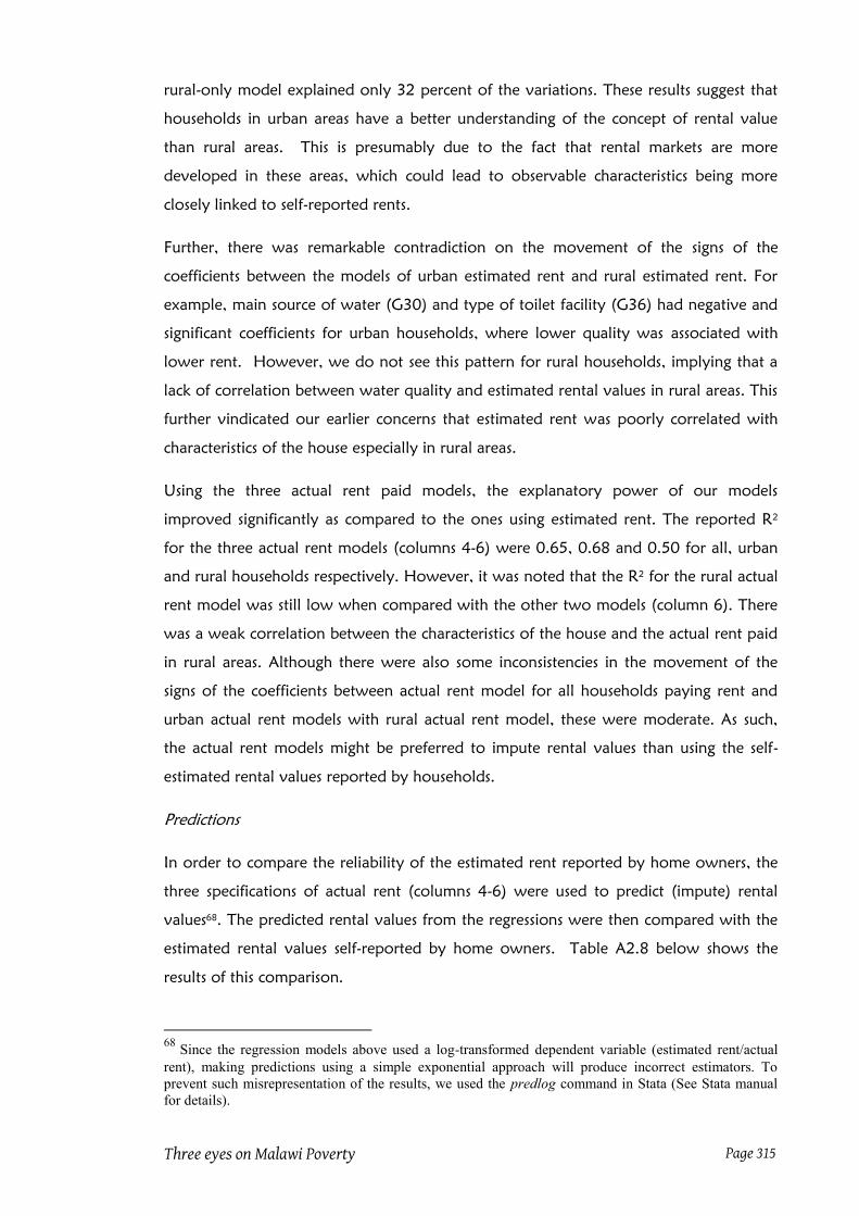
Three eyes on Malawi Poverty Page 315
rural-only model explained only 32 percent of the variations. These results suggest that
households in urban areas have a better understanding of the concept of rental value
than rural areas. This is presumably due to the fact that rental markets are more
developed in these areas, which could lead to observable characteristics being more
closely linked to self-reported rents.
Further, there was remarkable contradiction on the movement of the signs of the
coefficients between the models of urban estimated rent and rural estimated rent. For
example, main source of water (G30) and type of toilet facility (G36) had negative and
significant coefficients for urban households, where lower quality was associated with
lower rent. However, we do not see this pattern for rural households, implying that a
lack of correlation between water quality and estimated rental values in rural areas. This
further vindicated our earlier concerns that estimated rent was poorly correlated with
characteristics of the house especially in rural areas.
Using the three actual rent paid models, the explanatory power of our models
improved significantly as compared to the ones using estimated rent. The reported R2
for the three actual rent models (columns 4-6) were 0.65, 0.68 and 0.50 for all, urban
and rural households respectively. However, it was noted that the R2 for the rural actual
rent model was still low when compared with the other two models (column 6). There
was a weak correlation between the characteristics of the house and the actual rent paid
in rural areas. Although there were also some inconsistencies in the movement of the
signs of the coefficients between actual rent model for all households paying rent and
urban actual rent models with rural actual rent model, these were moderate. As such,
the actual rent models might be preferred to impute rental values than using the self-
estimated rental values reported by households.
Predictions
In order to compare the reliability of the estimated rent reported by home owners, the
three specifications of actual rent (columns 4-6) were used to predict (impute) rental
values68
. The predicted rental values from the regressions were then compared with the
estimated rental values self-reported by home owners. Table A2.8 below shows the
results of this comparison.
68
Since the regression models above used a log-transformed dependent variable (estimated rent/actual
rent), making predictions using a simple exponential approach will produce incorrect estimators. To
prevent such misrepresentation of the results, we used the predlog command in Stata (See Stata manual
for details).
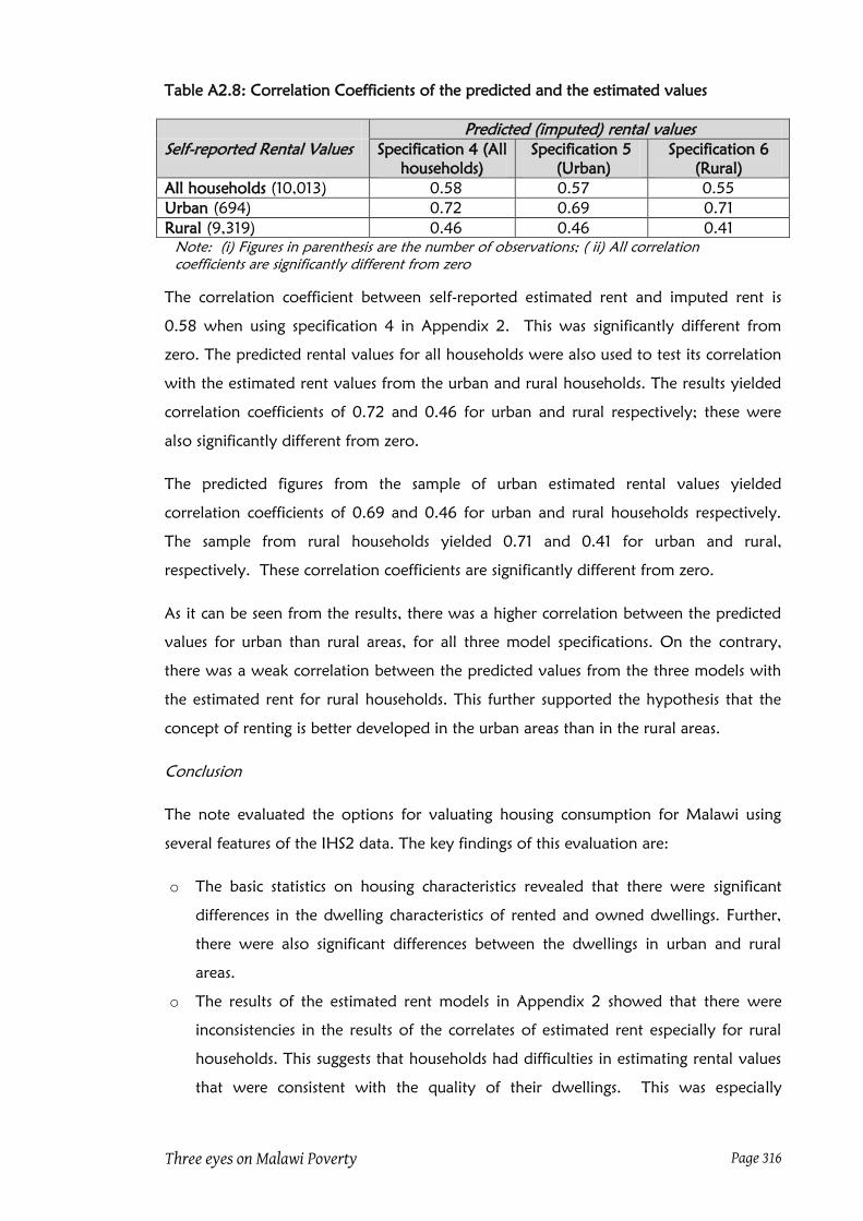
Three eyes on Malawi Poverty Page 316
Table A2.8: Correlation Coefficients of the predicted and the estimated values
Predicted (imputed) rental values
Self-reported Rental Values Specification 4 (All
households)
Specification 5
(Urban)
Specification 6
(Rural)
All households (10,013) 0.58 0.57 0.55
Urban (694) 0.72 0.69 0.71
Rural (9,319) 0.46 0.46 0.41
Note: (i) Figures in parenthesis are the number of observations; ( ii) All correlation
coefficients are significantly different from zero
The correlation coefficient between self-reported estimated rent and imputed rent is
0.58 when using specification 4 in Appendix 2. This was significantly different from
zero. The predicted rental values for all households were also used to test its correlation
with the estimated rent values from the urban and rural households. The results yielded
correlation coefficients of 0.72 and 0.46 for urban and rural respectively; these were
also significantly different from zero.
The predicted figures from the sample of urban estimated rental values yielded
correlation coefficients of 0.69 and 0.46 for urban and rural households respectively.
The sample from rural households yielded 0.71 and 0.41 for urban and rural,
respectively. These correlation coefficients are significantly different from zero.
As it can be seen from the results, there was a higher correlation between the predicted
values for urban than rural areas, for all three model specifications. On the contrary,
there was a weak correlation between the predicted values from the three models with
the estimated rent for rural households. This further supported the hypothesis that the
concept of renting is better developed in the urban areas than in the rural areas.
Conclusion
The note evaluated the options for valuating housing consumption for Malawi using
several features of the IHS2 data. The key findings of this evaluation are:
o The basic statistics on housing characteristics revealed that there were significant
differences in the dwelling characteristics of rented and owned dwellings. Further,
there were also significant differences between the dwellings in urban and rural
areas.
o The results of the estimated rent models in Appendix 2 showed that there were
inconsistencies in the results of the correlates of estimated rent especially for rural
households. This suggests that households had difficulties in estimating rental values
that were consistent with the quality of their dwellings. This was especially

Three eyes on Malawi Poverty Page 317
apparent for rural households. Therefore, it can be concluded that the estimated
rental values reported by households especially in the rural areas are unreliable.
The lack of reliability of the estimated rental values suggests that the values
should not be used for housing valuation or to extrapolate rental values for
households with missing rental values.
o A second option for including housing consumption in the consumption aggregate is
to use the actual rental values reported to predict the rental values for owner-
occupied dwellings. Out of the total 11,280 households interviewed, only 1,068
households are renting but most of these are urban households. The number of
households paying rent is much lower for rural areas (348 renting households).
The small number of households renting in rural areas, combined with the
notable differences in the dwelling characteristics of rented and owned
houses in rural areas, suggests that the sample of renting households is too
small to impute rental values for owned dwellings from actual rental values.

Three eyes on Malawi Poverty Page 318
A2.3 Factors used to convert amount from various units to grams
Table A2.9 presents conversion factors used to convert amounts in various units into
grams.

Three eyes on Malawi Poverty Page 319
Table A2.9: Conversion factors from other units to grams by food item
Unit Description Grams Unit Description Grams
101 Maize - whole grain flour 104 Maize grain
1 kg 1000 1 kg 1000
2 50kg bag 46658 3 90kg bag 90000
4 pail small 1014.3 4 pail small 1312.5
5 pail large 2036.25 6 no. 10 plate 194
6 no. 10 plate 150 7 no. 12 plate 770
7 no. 12 plate 595 9 piece 271
9 piece 580 12 basket shelled 6263.1
12 basket shelled 4840.5 16 cup 207
13 basket unshelled 4840.5 18 gram 1
14 ox-cart 32270 22 basin/pot 3580
16 cup 160 105 Maize – green
17 tin 33 1 kg 1000
18 gram 1 2 50kg bag 47595
22 basin/pot 4308 4 pail small 1312.5
23 sachet/tube/packet 595 5 pail large 1515.6
102 Maize - refined grain flour 7 no. 12 plate 770
1 kg 1000 8 bunch 269
2 50kg bag 46658 9 piece 185
4 pail small 1014.3 10 heap 269
5 pail large 2036.25 12 basket shelled 6263.1
6 no. 10 plate 150 13 basket unshelled 3616.05
7 no. 12 plate 595 106 Rice
9 piece 580 1 kg 1000
10 heap 4580 2 50kg bag 50000
12 basket shelled 4840.5 4 pail small 1014.3
16 cup 150 5 pail large 2036.25
17 tin 23.1 6 no. 10 plate 120
18 gram 1 7 no. 12 plate 495
22 basin/pot 4308 9 piece 271
103 Maize bran flour 16 cup 200
1 kg 1000 18 gram 1
4 pail small 1014.3 22 basin/pot 356
5 pail large 2036.25 23 sachet/tube/packet 500
6 no. 10 plate 150 107 Finger millet
7 no. 12 plate 595 1 kg 1000
12 basket shelled 4840.5 5 pail large 2634
17 tin 39 6 no. 10 plate 80
18 gram 1 7 no. 12 plate 320
22 basin/pot 4308 12 basket shelled 6281.85
16 cup 200
18 gram 1
22 basin/pot 442
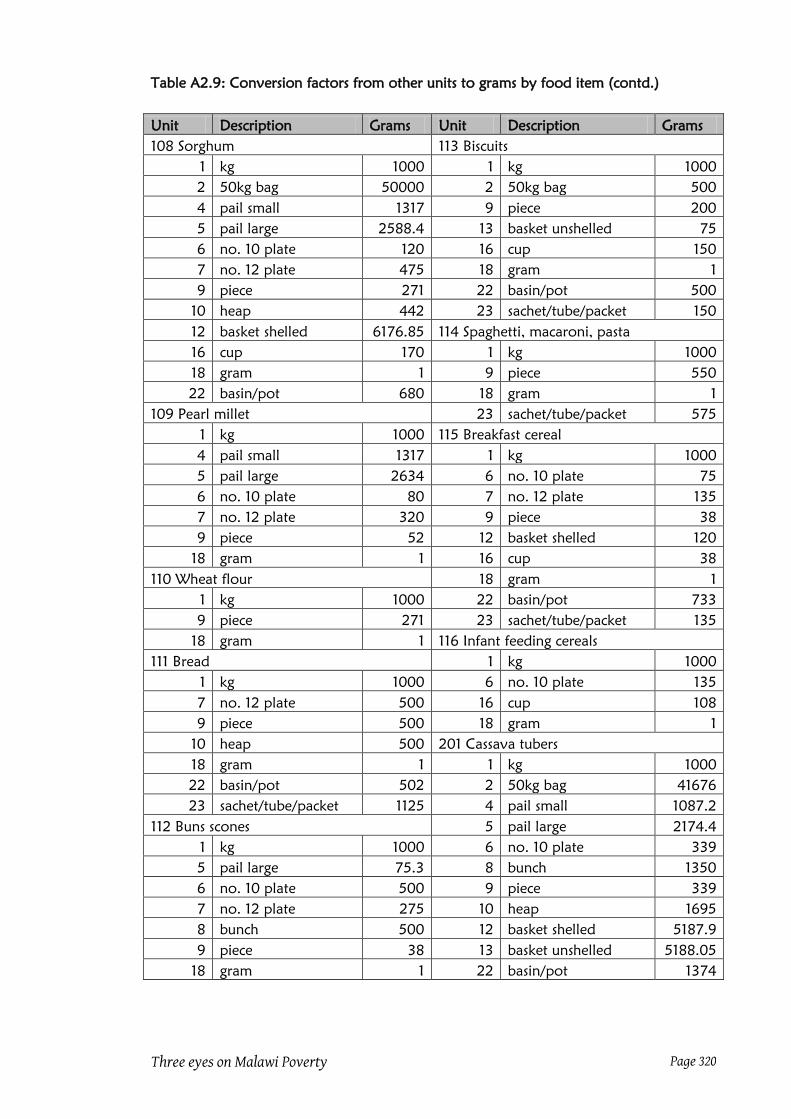
Three eyes on Malawi Poverty Page 320
Table A2.9: Conversion factors from other units to grams by food item (contd.)
Unit Description Grams Unit Description Grams
108 Sorghum 113 Biscuits
1 kg 1000 1 kg 1000
2 50kg bag 50000 2 50kg bag 500
4 pail small 1317 9 piece 200
5 pail large 2588.4 13 basket unshelled 75
6 no. 10 plate 120 16 cup 150
7 no. 12 plate 475 18 gram 1
9 piece 271 22 basin/pot 500
10 heap 442 23 sachet/tube/packet 150
12 basket shelled 6176.85 114 Spaghetti, macaroni, pasta
16 cup 170 1 kg 1000
18 gram 1 9 piece 550
22 basin/pot 680 18 gram 1
109 Pearl millet 23 sachet/tube/packet 575
1 kg 1000 115 Breakfast cereal
4 pail small 1317 1 kg 1000
5 pail large 2634 6 no. 10 plate 75
6 no. 10 plate 80 7 no. 12 plate 135
7 no. 12 plate 320 9 piece 38
9 piece 52 12 basket shelled 120
18 gram 1 16 cup 38
110 Wheat flour 18 gram 1
1 kg 1000 22 basin/pot 733
9 piece 271 23 sachet/tube/packet 135
18 gram 1 116 Infant feeding cereals
111 Bread 1 kg 1000
1 kg 1000 6 no. 10 plate 135
7 no. 12 plate 500 16 cup 108
9 piece 500 18 gram 1
10 heap 500 201 Cassava tubers
18 gram 1 1 kg 1000
22 basin/pot 502 2 50kg bag 41676
23 sachet/tube/packet 1125 4 pail small 1087.2
112 Buns scones 5 pail large 2174.4
1 kg 1000 6 no. 10 plate 339
5 pail large 75.3 8 bunch 1350
6 no. 10 plate 500 9 piece 339
7 no. 12 plate 275 10 heap 1695
8 bunch 500 12 basket shelled 5187.9
9 piece 38 13 basket unshelled 5188.05
18 gram 1 22 basin/pot 1374

Three eyes on Malawi Poverty Page 321
Table A2.9: Conversion factors from other units to grams by food item (contd.)
Unit Description Grams Unit Description Grams
202 Cassava flour 205 Irish potato
1 kg 1000 1 kg 1000
2 50kg bag 50000 4 pail small 945
4 pail small 1014.3 5 pail large 1590.75
5 pail large 2036.25 6 no. 10 plate 400
6 no. 10 plate 150 7 no. 12 plate 587
7 no. 12 plate 595 8 bunch 1350
9 piece 4580 9 piece 174
10 heap 4580 10 heap 1045
12 basket shelled 4840.5 12 basket shelled 4509.45
16 cup 220 13 basket unshelled 4509.45
17 tin 33 17 tin 621.6
18 gram 1 18 gram 1
22 basin/pot 4580 22 basin/pot 326
203 White sweet potato 23 sachet/tube/packet 518
1 kg 1000 206 Potato crisps
2 50kg bag 36225 1 kg 1000
4 pail small 945 4 pail small 67.5
5 pail large 1890 6 no. 10 plate 25
6 no. 10 plate 339 9 piece 25
7 no. 12 plate 442 10 heap 25
8 bunch 1350 12 basket shelled 67.5
9 piece 174 16 cup 25
10 heap 1045 18 gram 1
12 basket shelled 4509.45 23 sachet/tube/packet 18
13 basket unshelled 4509.45 207 Plantain, cooking banana
14 ox-cart 45100 1 kg 1000
17 tin 2652 4 pail small 930
22 basin/pot 850 8 bunch 6700
23 sachet/tube/packet 455 9 piece 135
204 Orange sweet potato 10 heap 6700
1 kg 1000 23 sachet/tube/packet 455
2 50kg bag 36225 208 Cocoyam
4 pail small 945 1 kg 1000
5 pail large 1890 2 50kg bag 36225
9 piece 174 4 pail small 930
10 heap 1045 5 pail large 5250
12 basket shelled 4509.45 8 bunch 400
13 basket unshelled 4509.45 9 piece 100
10 heap 400
12 basket shelled 6750
18 gram 1
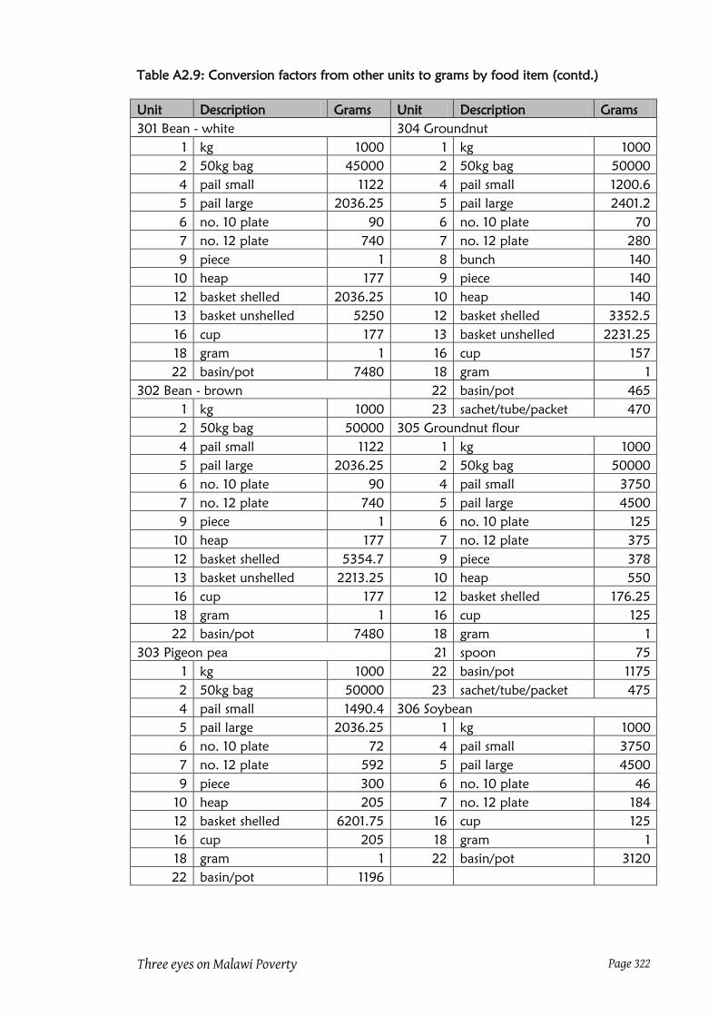
Three eyes on Malawi Poverty Page 322
Table A2.9: Conversion factors from other units to grams by food item (contd.)
Unit Description Grams Unit Description Grams
301 Bean - white 304 Groundnut
1 kg 1000 1 kg 1000
2 50kg bag 45000 2 50kg bag 50000
4 pail small 1122 4 pail small 1200.6
5 pail large 2036.25 5 pail large 2401.2
6 no. 10 plate 90 6 no. 10 plate 70
7 no. 12 plate 740 7 no. 12 plate 280
9 piece 1 8 bunch 140
10 heap 177 9 piece 140
12 basket shelled 2036.25 10 heap 140
13 basket unshelled 5250 12 basket shelled 3352.5
16 cup 177 13 basket unshelled 2231.25
18 gram 1 16 cup 157
22 basin/pot 7480 18 gram 1
302 Bean - brown 22 basin/pot 465
1 kg 1000 23 sachet/tube/packet 470
2 50kg bag 50000 305 Groundnut flour
4 pail small 1122 1 kg 1000
5 pail large 2036.25 2 50kg bag 50000
6 no. 10 plate 90 4 pail small 3750
7 no. 12 plate 740 5 pail large 4500
9 piece 1 6 no. 10 plate 125
10 heap 177 7 no. 12 plate 375
12 basket shelled 5354.7 9 piece 378
13 basket unshelled 2213.25 10 heap 550
16 cup 177 12 basket shelled 176.25
18 gram 1 16 cup 125
22 basin/pot 7480 18 gram 1
303 Pigeon pea 21 spoon 75
1 kg 1000 22 basin/pot 1175
2 50kg bag 50000 23 sachet/tube/packet 475
4 pail small 1490.4 306 Soybean
5 pail large 2036.25 1 kg 1000
6 no. 10 plate 72 4 pail small 3750
7 no. 12 plate 592 5 pail large 4500
9 piece 300 6 no. 10 plate 46
10 heap 205 7 no. 12 plate 184
12 basket shelled 6201.75 16 cup 125
16 cup 205 18 gram 1
18 gram 1 22 basin/pot 3120
22 basin/pot 1196

Three eyes on Malawi Poverty Page 323
Table A2.9: Conversion factors from other units to grams by food item (contd.)
Unit Description Grams Unit Description Grams
307 Ground bean 403 Tanaposi
1 kg 1000 1 kg 1000
6 no. 10 plate 90 4 pail small 9
7 no. 12 plate 740 5 pail large 15
9 piece 300 6 no. 10 plate 80
10 heap 177 7 no. 12 plate 85
12 basket shelled 5354.7 8 bunch 60
16 cup 177 9 piece 15
18 gram 1 10 heap 60
22 basin/pot 7480 12 basket shelled 183
308 Cowpea 13 basket unshelled 97.5
1 kg 1000 18 gram 1
6 no. 10 plate 74 22 basin/pot 612
7 no. 12 plate 296 404 Pumpkin leaves
8 bunch 140 1 kg 1000
10 heap 166 2 50kg bag 3500
16 cup 166 4 pail small 96
18 gram 1 5 pail large 212.25
20 other 6 no. 10 plate 67
22 basin/pot 1138 7 no. 12 plate 83
401 Onion 8 bunch 155
1 kg 1000 9 piece 8
2 50kg bag 50000 10 heap 155
4 no. 12 plate 150 12 basket shelled 94.95
6 no. 10 plate 50 13 basket unshelled 96.75
8 bunch 50 18 gram 1
9 piece 13 22 basin/pot 178
10 heap 50 405 Chinese cabbage
18 gram 1 1 kg 1000
402 Cabbage 4 pail small 51
1 kg 1000 5 pail large 15
6 no. 10 plate 1030 6 no. 10 plate 80
8 bunch 1030 7 no. 12 plate 85
9 piece 1030 8 bunch 140
10 heap 1030 9 piece 23
18 gram 1 10 heap 140
18 gram 1
23 sachet/tube/packet 235

Three eyes on Malawi Poverty Page 324
Table A2.9: Conversion factors from other units to grams by food item (contd.)
Unit Description Grams Unit Description Grams
406 Other cultivated vegetables 408 Tomato
1 kg 1000 1 kg 1000
4 pail small 141.15 3 90kg bag 12000
5 pail large 15 4 pail small 35.25
6 no. 10 plate 206 5 pail large 45
7 no. 12 plate 578 6 no. 10 plate 235
8 bunch 155 7 no. 12 plate 300
9 piece 8 8 bunch 235
10 heap 155 9 piece 45
12 basket shelled 120 10 heap 235
13 basket unshelled 97.5 12 basket shelled 120
18 gram 1 13 basket unshelled 1800
22 basin/pot 258 15 litre 947
407 Gathered wild leaves 16 cup 235
1 kg 1000 17 tin 35.25
2 50kg bag 5038 18 gram 1
4 pail small 64.35 19 millilitre 0.947
6 no. 10 plate 96 22 basin/pot 1248
7 no. 12 plate 192 23 sachet/tube/packet 235
8 bunch 155 411 Okra
9 piece 8 1 kg 1000
10 heap 155 2 50kg bag 5038
12 basket shelled 120 4 pail small 9
13 basket unshelled 97.5 5 pail large 15
18 gram 1 6 no. 10 plate 180
22 basin/pot 354 7 no. 12 plate 720
23 sachet/tube/packet 192 8 bunch 240
409 Cucumber 9 piece 30
1 kg 1000 10 heap 240
4 pail small 90 12 basket shelled 222
5 pail large 97.5 18 gram 1
8 bunch 600 22 basin/pot 838
9 piece 200 23 sachet/tube/packet 74
10 heap 600
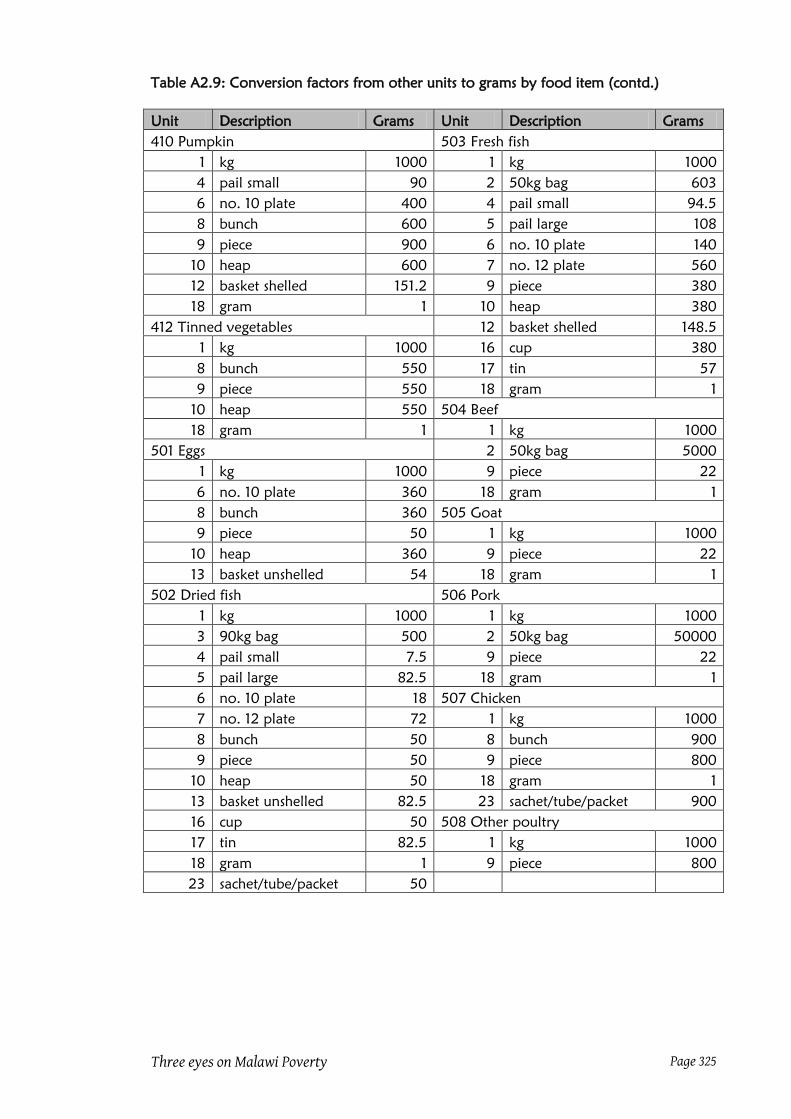
Three eyes on Malawi Poverty Page 325
Table A2.9: Conversion factors from other units to grams by food item (contd.)
Unit Description Grams Unit Description Grams
410 Pumpkin 503 Fresh fish
1 kg 1000 1 kg 1000
4 pail small 90 2 50kg bag 603
6 no. 10 plate 400 4 pail small 94.5
8 bunch 600 5 pail large 108
9 piece 900 6 no. 10 plate 140
10 heap 600 7 no. 12 plate 560
12 basket shelled 151.2 9 piece 380
18 gram 1 10 heap 380
412 Tinned vegetables 12 basket shelled 148.5
1 kg 1000 16 cup 380
8 bunch 550 17 tin 57
9 piece 550 18 gram 1
10 heap 550 504 Beef
18 gram 1 1 kg 1000
501 Eggs 2 50kg bag 5000
1 kg 1000 9 piece 22
6 no. 10 plate 360 18 gram 1
8 bunch 360 505 Goat
9 piece 50 1 kg 1000
10 heap 360 9 piece 22
13 basket unshelled 54 18 gram 1
502 Dried fish 506 Pork
1 kg 1000 1 kg 1000
3 90kg bag 500 2 50kg bag 50000
4 pail small 7.5 9 piece 22
5 pail large 82.5 18 gram 1
6 no. 10 plate 18 507 Chicken
7 no. 12 plate 72 1 kg 1000
8 bunch 50 8 bunch 900
9 piece 50 9 piece 800
10 heap 50 18 gram 1
13 basket unshelled 82.5 23 sachet/tube/packet 900
16 cup 50 508 Other poultry
17 tin 82.5 1 kg 1000
18 gram 1 9 piece 800
23 sachet/tube/packet 50

Three eyes on Malawi Poverty Page 326
Table A2.9: Conversion factors from other units to grams by food item (contd.)
Unit Description Grams Unit Description Grams
509 Small animal 602 Banana
1 kg 1000 1 kg 1000
7 no. 12 plate 45 6 no. 10 plate 500
9 piece 35 7 no. 12 plate 600
510 Termites/other insects 8 bunch 600
1 kg 1000 9 piece 50
4 pail small 15 10 heap 600
6 no. 10 plate 18 14 Ox-cart 12000
7 no. 12 plate 72 15 litre 50
9 piece 22 21 spoon 50
10 heap 50 22 basin/pot 655
16 cup 50 23 sachet/tube/packet 1038
17 tin 5.25 603 Citrus
18 gram 1 1 kg 1000
22 basin/pot 100 4 pail small 3750
511 Tinned meat or fish 5 pail large 4500
1 kg 1000 6 no. 10 plate 500
9 piece 350 9 piece 159
17 tin 52.5 13 basket unshelled 4500
18 gram 1 17 tin 82.5
601 Mango 18 gram 1
1 kg 1000
2 50kg bag 50000
4 pail small 3750 606 Guava
5 pail large 2851.2 1 kg 1000
6 no. 10 plate 500 4 pail small 3750
8 bunch 500 5 pail large 4500
9 piece 50 7 no. 12 plate 600
10 heap 500 9 piece 68
12 basket shelled 3300.45 10 heap 640
13 basket unshelled 4500 12 basket shelled 4500
17 tin 82.5 13 basket unshelled 4500
21 spoon 50 17 tin 82.5
604 Pineapple 18 gram 1
1 kg 1000 22 basin/pot 864
9 piece 472 607 Avocado
605 Pawpaw 1 kg 1000
1 kg 1000 6 no. 10 plate 500
9 piece 1170 9 piece 525
18 gram 1 10 heap 1050
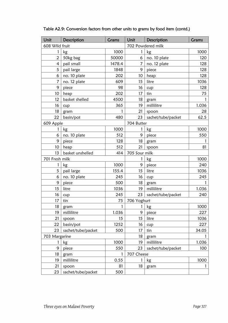
Three eyes on Malawi Poverty Page 327
Table A2.9: Conversion factors from other units to grams by food item (contd.)
Unit Description Grams Unit Description Grams
608 Wild fruit 702 Powdered milk
1 kg 1000 1 kg 1000
2 50kg bag 50000 6 no. 10 plate 120
4 pail small 1478.4 7 no. 12 plate 128
5 pail large 1848 9 piece 128
6 no. 10 plate 202 10 heap 128
7 no. 12 plate 609 15 litre 1036
9 piece 98 16 cup 128
10 heap 202 17 tin 75
12 basket shelled 4500 18 gram 1
16 cup 365 19 millilitre 1.036
18 gram 1 21 spoon 28
22 basin/pot 480 23 sachet/tube/packet 62.5
609 Apple 704 Butter
1 kg 1000 1 kg 1000
6 no. 10 plate 512 9 piece 550
9 piece 128 18 gram 1
10 heap 512 21 spoon 81
13 basket unshelled 414 705 Sour milk
701 Fresh milk 1 kg 1000
1 kg 1000 9 piece 240
5 pail large 155.4 15 litre 1036
6 no. 10 plate 245 16 cup 245
9 piece 500 18 gram 1
15 litre 1036 19 millilitre 1.036
16 cup 245 23 sachet/tube/packet 240
17 tin 75 706 Yoghurt
18 gram 1 1 kg 1000
19 millilitre 1.036 9 piece 227
21 spoon 15 15 litre 1036
22 basin/pot 1252 16 cup 227
23 sachet/tube/packet 500 17 tin 34.05
703 Margarine 18 gram 1
1 kg 1000 19 millilitre 1.036
9 piece 550 23 sachet/tube/packet 100
18 gram 1 707 Cheese
19 millilitre 0.55 1 kg 1000
21 spoon 81 18 gram 1
23 sachet/tube/packet 500

Three eyes on Malawi Poverty Page 328
Table A2.9: Conversion factors from other units to grams by food item (contd.)
Unit Description Grams Unit Description Grams
708 Infant feeding formula 803 Cooking oil
1 kg 1000 1 kg 1000
9 piece 400 2 50kg bag 50000
15 litre 541 6 no. 10 plate 224
17 tin 60 8 bunch 224
18 gram 1 9 piece 40
19 millilitre 0.541 10 heap 456
15 litre 947
801 Sugar 16 cup 224
1 kg 1000 17 tin 75
2 50kg bag 50000 18 gram 1
3 90kg bag 82000 19 millilitre 0.947
4 pail small 160.8 21 spoon 198
5 pail large 282.3 22 basin/pot 6629
6 no. 10 plate 81 23 sachet/tube/packet 456
7 no. 12 plate 324 810 Salt
9 piece 970 1 kg 1000
10 heap 970 2 50kg bag 50000
16 cup 220 4 pail small 177.3
18 gram 1 5 pail large 192.3
19 millilitre 0.947 6 no. 10 plate 120
21 spoon 208 7 no. 12 plate 175
23 sachet/tube/packet 970 8 bunch 166
802 Sugar cane 9 piece 85
1 kg 1000 10 heap 45
2 50kg bag 50000 12 basket shelled 4840.5
3 90kg bag 82000 13 basket unshelled 4840.5
4 pail small 4500 15 litre 947
5 pail large 5250 16 cup 166
9 piece 375 17 tin 75
12 basket shelled 5250 18 gram 1
18 gram 1 19 millilitre 0.974
19 millilitre 0.947 21 spoon 204
813 Tomato sauce 22 basin/pot 204
1 kg 1000 23 sachet/tube/packet 500
9 piece 947 820 Maize boiled/fried
15 litre 947 1 kg 1000
18 gram 1 9 piece 217
19 millilitre 0.947 10 heap 654
21 spoon 35

Three eyes on Malawi Poverty Page 329
Table A2.9: Conversion factors from other units to grams by food item (contd.)
Unit Description Grams Unit Description Grams
811 Spices 814 Hot sauce
1 kg 1000 1 kg 1000
6 no. 10 plate 75 9 piece 108
9 piece 10 18 gram 1
10 heap 75 19 millilitre 0.947
18 gram 1 21 spoon 15
19 millilitre 0.425 821 Chips vendor
20 Tea spoon 46 1 kg 1000
21 Table spoon 92 5 pail large 54.9
22 basin/pot 237 6 no. 10 plate 89
23 sachet/tube/packet 125 7 no. 12 plate 366
812 Yeast/baking powder/soda 8 bunch 246
1 kg 1000 9 piece 7
2 50kg bag 5000 10 heap 246
6 no. 10 plate 6 12 basket shelled 83.25
9 piece 6 16 cup 166
10 heap 250 18 gram 1
15 litre 250 21 spoon 166
16 cup 250 22 basin/pot 338
18 gram 1 23 sachet/tube/packet 166
19 millilitre 0.25
21 spoon 192 822 Cassava - boiled (vendor)
22 basin/pot 250 1 kg 1000
23 sachet/tube/packet 250 6 no. 10 plate 267
9 piece 267
815 Jam, jelly, honey 10 heap 267
1 kg 1000 823 Eggs boiled vendor
9 piece 224 1 kg 1000
15 litre 947 2 50kg bag 5000
16 cup 224 9 piece 50
18 gram 1 824 Chicken vendor
19 millilitre 0.524 1 kg 1000
816 Sweets, candy, chocolates 9 piece 39
1 kg 1000 10 heap 39
5 pail large 150 18 gram 1
6 no. 10 plate 580 825 Meat vendor
9 piece 12 1 kg 1000
10 heap 580 6 no. 10 plate 39
18 gram 1 9 piece 39
23 sachet/tube/packet 25 18 gram 1

Three eyes on Malawi Poverty Page 330
Table A2.9: Conversion factors from other units to grams by food item (contd.)
Unit Description Grams Unit Description Grams
826 Fish vendor 901 Tea
1 kg 1000 1 kg 1000
5 pail large 93.45 5 pail large 840
6 no. 10 plate 335 6 no. 10 plate 240
8 bunch 337 7 no. 12 plate 458
9 piece 39 8 bunch 375
10 heap 337 9 piece 10
827 Doughnuts/fritters 10 heap 375
1 kg 1000 15 litre 1120
5 pail large 82.5 16 cup 375
9 piece 42 17 tin 22.5
10 heap 550 18 gram 1
828 Samosa (vendor) 19 millilitre 0.947
1 kg 1000 21 spoon 42
9 piece 45 22 basin/pot 7840
18 gram 1 23 sachet/tube/packet 250
829 Meat at restaurant 902 Coffee
1 kg 1000 1 kg 1000
6 no. 10 plate 950 6 no. 10 plate 240
7 no. 12 plate 1325 15 litre 125
8 bunch 375 16 cup 375
9 piece 950 18 gram 1
10 heap 950 21 spoon 12
12 basket shelled 5.85 22 basin/pot 875
15 litre 39 903 Squash
16 cup 375 1 kg 1000
17 tin 56.25 9 piece 1048
18 gram 1 15 litre 1048
19 millilitre 0.947 18 gram 1
21 spoon 1 19 millilitre 1.048
22 basin/pot 1325 904 Fruit juice
905 Freezes 1 kg 1000
1 kg 1000 9 piece 210
9 piece 42 15 litre 1048
10 heap 42 18 gram 1
15 litre 947 19 millilitre 1.048
18 gram 1 22 basin/pot 7336
19 millilitre 0.947 911 Wine or commercial liquor
21 spoon 21 1 kg 1000
22 basin/pot 947 15 litre 1000
23 sachet/tube/packet 42 19 millilitre 1

Three eyes on Malawi Poverty Page 331
Table A2.9: Conversion factors from other units to grams by food item (contd.)
Unit Description Grams Unit Description Grams
906 Soft drinks 909 Local sweet beer (thobwa)
1 kg 1000 1 kg 1000
4 pail small 47.1 4 pail small 1211.25
9 piece 314 5 pail large 1436.25
15 litre 1048 7 no. 12 plate 947
16 cup 314 9 piece 237
17 tin 49.5 14 ox-cart 860
18 gram 1 15 litre 947
19 millilitre 1.048 16 cup 237
22 basin/pot 7336 17 tin 129
23 sachet/tube/packet 278 18 gram 1
907 Commercial traditional beer 19 millilitre 1
1 kg 1000 22 basin/pot 3605
9 piece 1015 910 Traditional beer (masese)
15 litre 1000 1 kg 1000
16 cup 1015 4 pail small 1500
19 millilitre 1 5 pail large 35.55
908 Bottled/canned beer 7 no. 12 plate
1 kg 1000 9 piece 237
5 pail large 45 15 litre 1000
9 piece 300 16 cup 237
15 litre 1000 17 tin 78
16 cup 300 18 gram 1
17 tin 49.5 19 millilitre 1
19 millilitre 1 22 basin/pot 2345
912 Local spirit (kachasu)
1 kg 1000
9 piece 237
911 Wine or commercial liquor 15 litre 1000
1 kg 1000 16 cup 237
15 litre 1000 18 gram 1
19 millilitre 1 19 millilitre 1
Appendix 2d: Cut off points for amounts, costs, values and numbers
The tables in this appendix present the cut off points used in the analysis as used in the
2007 analysis

Three eyes on Malawi Poverty Page 332
Table A2.10: Maximum food consumption by item
Food tem code and name Grams Food tem code and name Grams
101 Maize flour - whole grain 35,000 401 Onion 1,000
102 Maize flour - refined 35,000 402 Cabbage 10,000
103 Maize bran flour 20,000 403 Tanaposi 5,000
104 Maize grain 20,000 404 Pumpkin leaves 15,000
105 Maize – green 35,000 405 Chinese cabbage 5,000
106 Rice 20,000 406 Other cultiv veggies 10,000
107 Finger millet 20,000 407 Gathered wild leaves 5,000
108 Sorghum 20,000 408 Tomato 5,000
111 Bread 20,000 409 Cucumber 5,000
112 Buns scones 5,000 410 Pumpkin 10,000
113 Biscuits 5,000 411 Okra 5,000
114 Spaghetti, macaroni, pasta 10,000 412 Tinned vegetables 5,000
115 Breakfast cereal 10,000 501 Eggs 5,000
116 Infant feeding cereals 10,000 502 Dried fish 5,000
201 Cassava tubers 20,000 503 Fresh fish 20,000
202 Cassava flour 20,000 504 Beef 10,000
203 White sweet potato 20,000 505 Goat 10,000
204 Orange sweet potato 20,000 506 Pork 5,000
205 Irish potato 20,000 507 Chicken 10,000
206 Potato crisps 1,000 508 Other poultry 20,000
207 Plantain, cooking banana 20,000 509 Small animal 5,000
208 Cocoyam 20,000 510 Termites/other insects 1,000
301 Bean - white 20,000 511 Tinned meat or fish 5,000
302 Bean - brown 20,000 601 Mango 10,000
303 Pigeon pea 20,000 602 Banana 5,000
304 Groundnut 20,000 603 Citrus 10,000
305 Groundnut flour 5,000 604 Pineapple 5,000
306 Soya bean 20,000 605 Pawpaw 10,000
307 Ground bean 20,000 606 Guava 10,000
607 Avocado 10,000
608 Wild fruit 5,000
609 Apple 5,000

Three eyes on Malawi Poverty Page 333
Table A2.10: Maximum food consumption by item (continued)
Item code and name Grams Item code and name Grams
701 Fresh milk 10000 823 Eggs boiled vendor
1,000
702 Powdered milk 5000 824 Chicken vendor
5,000
703 Margarine 5000 825 Meat vendor
5,000
704 Butter 5000 826 Fish vendor
5,000
705 Sour milk 5000 827 Doughnuts/fritters
5,000
706 Yoghurt 5000 828 Samosa (vendor)
5,000
707 Cheese 5000 829 Meat at restaurant
10,000
708 Infant feeding formula 5000 901 Tea
1,000
801 Sugar 10000 902 Coffee
1,000
802 Sugar cane 30000 903 Squash
5,000
803 Cooking oil 10000 904 Fruit juice
5,000
810 Salt 5000 905 Freezes
5,000
811 Spices 1000 906 Soft drinks
5,000
812 Yeast/baking
powder/soda 5000
907 Commercial traditional
beer
20,000
813 Tomato sauce 1000 908 Bottled/canned beer
20,000
814 Hot sauce 1000 909 Local sweet beer (thobwa)
20,000
815 Jam, jelly, honey 1000 910 Traditional beer (masese)
10,000
816 Sweets, candy, chocolates 1000 911 Wine or commercial liquor
5,000
820 Maize boiled/fried 5000 912 Local spirit (kachasu)
5,000
821 Chips vendor 5000
822 Cassava - boiled
(vendor) 10000

Three eyes on Malawi Poverty Page 334
Table A2.11: Cut off values and number of durable goods
Item Estimated value Number of items
Item ID Value (MK) ID #
Mortar/pestle M05-501 1,000 M05-501 7
Bed M05-502 20,000 M03-502 10
Table M05-503 10,000 M03-503 10
Chair M05-504 10,000 M03-504 10
Fan M05-505 8,000
Air conditioner M05-506 10,000
Radio (wireless) M05-507 8,000 M03-507 5
Tape or CD player; HiFi M05-508 35,000 M03-508 5
Television & VCR M05-509 40,000
Sewing machine M05-510 20,000
Kerosene/paraffin stove M05-511 3,000
Electric or gas stove; hot plate M05-512 50,000 M03-512 5
Refrigerator M05-513 50,000
Washing machine M05-514 50,000
Bicycle M05-515 20,000 M03-515 10
Motorcycle/scooter M05-516 150,000
Car M05-517 500,000 M03-517 4

Three eyes on Malawi Poverty Page 335
Table A2.12: Cut off cost and values for household expenditure items
Item Cost MK Item Cost MK
Weekly expenditure 3-month expenditure
Firewood 1,000 Infant clothing 25,000
Charcoal 600 Baby nappies 1,500
Paraffin/kerosene 400 Boy's trousers 2,000
Tobacco 200 Boy's shirts 2,500
Matches 100 Boy's jackets 1,000
Public transport 4,000 Boy's undergarments 2,200
4-week/monthly Boy's other clothing 5,000
Curative health services 2,000 Men's trousers 3,000
Preventive health care 1,500 Men's shirts 5,000
Common drug expenses 1,500 Men's jackets 5,000
Milling fees 1,000 Men's undergarments 1,000
Bar soap 1,000 Men's other clothing 3,000
Powdered soap 1,000 Girl's blouse/shirt 3,000
Toothbrush/toothpaste 500 Girl's dress/skirt 2,500
Toilet paper 1,000 Girl's undergarments 1,000
Skin care items 750 Girl's other clothing 4,000
Other body care items 1,000 Lady's blouse/shirt 3,000
Household cleaning agents 1,000 Chitenje cloth 2,000
Light bulbs 300 Lady's dress/skirt 4,100
Postage 200 Lady's undergarments 1,020
Petrol/diesel 25,000 Lady's other clothing 6,000
Vehicle service 30,000 Boy's shoes 3,000
Bicycle service 2,500 Men's shoes 4,500
Servant wages 10,000 Girl's shoes 2,000
Item repairs 2,000 Lady's shoes 2,000

Three eyes on Malawi Poverty Page 336
Table A2.12: Cut off cost and values for household expenditure items (contd.)
Item Cost MK Item Cost MK
3-month expenditure
12-month expenses
Cloth, sewing items 3,200 Tuition fees 30,000
Cloth services 4,000 School books/stationery 10,000
Bowls, glassware, plates,… 2,000 School fund 2,000
Cooking utensils 2,500 School PTA fund 2,500
Cleaning utensils 450 Carpets, rugs, drapes, curtains 12,000
Torch/flashlight 250 Linen - towels, sheets, … 8,000
Umbrella 600 Mat - sleeping/drying 1,500
Paraffin lamp 800 Mosquito net 1,000
Stationery items 1,000 Mattress 10,000
Ordinary books 3,500 Sports/music/hobby equipment 8,000
Music/video cassette/CD 5,000 Film/film processing, … 4,000
Tickets for sports 2,000 Council rates 9,000
Household decorations 7,000 Insurance 80,000
Rest house or hotel expenses 3,000 Electricity costs 100,000
Informal health care expenses 5,000
Three eyes on Malawi Poverty Page 337
Appendix 3: Malawi country background and commentaries
on poverty
Appendix 3a: Country background69
Political and economic history
Malawi was Nyasaland before it became independent in 1964. Nyasaland as country
was a creation of the Great Britain. Before then the area was ever under the Maravi
Kingdom in the 15th Century, Ngonde Kingdom in the 17
th Century and
Chikulamayembe Kingdom in the 18th Century. Over time, various Bantu tribes settled
in various parts of the area. The rampart slave trade witnessed by explorer David
Livingstone and entrepreneur Cecil Rhodes forced Britain to declare Nyasaland a
protectorate in 1892 after annexing it in 1891. Colonial government managed Nyasaland
until the country joined the Federation of Rhodesia and Nyasaland in 1951. World
changes, and a little bit of internal pressure, brought down the federation, replaced by
self government in 1961, independence in 1964 and republic status under the British
Commonwealth in 1966. During its time, colonialism introduced and formalised the
market economy. It brought cash crop agriculture, some manufacturing and organised
commerce. It also brought organised public administration that required the population
to enter the market economy to pay for it. In summary, colonialism brought economic
and social development through public administration and the market.
The Malawi Government that took over from the colonial government did not change
things as much. It continued most of the social and economic policies inherited from the
colonial government. Within years of independence, Malawi became one-party state
government by a parliamentary majority and a constitutional one-party dictatorship
from 1971 to 1993. During this period, the President had absolute powers; no dissenting
views were allowed and terror ruled. On the economic front, the government
employed managed liberalism. The government worked to make the central
government and few individuals rich. It did not have instruments that directly
encouraged individual local businesses. According to Chingaipe Ng‟oma (2010), politics
ensured that even the African businesses the government openly supported failed to
benefit. In the end it was only the president and his close associates who prospered. In
fact, government practices of detaining successful businessmen who supported the
opposition, forfeiture of property of those suspected to be „unsympathetic‟ to the
69
There are three main sources for the country background and these are GoM, 1987; GoM & UN, 1993;
Tsoka, 2008.

Three eyes on Malawi Poverty Page 338
regime, and forced party donations extracted from businesses bottled up
entrepreneurship. Worse still, the government did not have any social policy. To
support the poor, the government opted for an economic policy in the form of price
control and inputs subsidies. However, even these vanished as the country was forced
to adopt liberal economic management in the 1980s following serious economic crises.
Politically, Malawi was a favoured country because it was an island among socialist
neighbours. The collapse of communism changed the geo-politics that propped the
dictatorial regime and with aid freeze in early 1990s and a little of internal pressure,
multipartyism was introduced in 1993 followed by multiparty elections and government
in 1994. At the same time, Malawi adopted a new constitution that provided for respect
of human rights, separation of powers among the executive, legislature and judiciary
and accountability like Human Rights Commission, Anti-Corruption Bureau and the
Ombudsman
This brought some changes, both good and bad for poverty reduction. On one hand,
the freedoms unleashed entrepreneurial spirits bottled up under the dictatorial regime.
On the other hand, crime and insecurity followed the collapse of the village vigilant
groups associated with the old regime and the introduction of the respect of rights of a
suspect. Ownership of livestock, property and businesses especially in rural areas
received a very big knock and immediately negated the benefits of the freedom. In the
early years, dissatisfaction with the liberal approach to crime sometimes led to instant
mob justice, where suspects were burnt alive.
The change in political system did not change the economic policy which firmly
remained in the hands of donors. There were some social policy changes, though. For
the first time since independence, poverty was officially recognised as a problem and in
1995 the new government launched the Poverty Alleviation Programme. The hallmark
of the programme was free primary education, credit to small businesses and free inputs,
community projects, and public works. Although the credit schemes were plagued by
politics, it was clear that poverty was on the lips of the politicians and getting a service.
Geography
Malawi is located in the southern part of the East African Rift Valley. It is locked away
from the Indian Ocean in the East by Mozambique and Tanzania. Zambia covers most
of its Western side. The country is small (119,140 m2) with a border totalling 2,881
kilometres. Lake Malawi contains, by far, the largest body of that water and with a
length of 580 km, is Malawi‟s prominent feature. The country has sub-tropical climate

Three eyes on Malawi Poverty Page 339
with a rainy season from November to May and dry season from June to October. It
has an immensely varied topography and therefore agro-economic zones as it rises from
37 to 3,002 metres above sea level. There are very few mineral deposits in the country.
Most of them are not in large enough quantities for mining.
The location of the country makes it an unattractive investment destination because it is
cut off from the sea. Its lack of minerals provides limited options for development and
sustainable growth. The varied topography (and presence of a variety of agro-economic
zones) is a clear signal for agriculture development. There is also potential for irrigation
given that 20% of the country‟s surface is water.
Social system, culture and religion
Malawi's society is characterised by both patrilineal and matrilineal systems; the latter
being the commonest. There is no dominant tribal grouping and ethnicity is not a major
problem although regionalism crops up as a talking point. Extended families are
prominent although the nuclear family is slowly creeping in as the chief production unit
and main source of social support. Modernisation and economic pressure is diminishing
the prominence of the extended family although the impact of HIV/AIDS is demanding
its intensive and extensive use. Traditional beliefs, customs, ceremonies, and other social
and cultural factors, under the guidance of traditional leaders, have a powerful influence
on community life especially in matters of social relationships, decision-making patterns,
inheritance rights, acceptability of new ideas and practices (education, health, family
planning, sanitation, agriculture, borrowing and debt repayment). Culture in Malawi
has changed over time as the country came in touch with external actors. Currently, the
Malawi culture is a product of traditional beliefs and customs, development (brought by
colonialism and independence), and foreign religions.
Malawi has two major religions namely Christianity and Islam but it is labelled a
Christian country because the majority profess to be Christians. In fact, until the election
of the Moslem Bakili Muluzi as state president in 1994, Islam was obscure. The ten years
of Muluzi enabled Islam to flourish in the public arena with mushrooming of mosques in
non-traditional areas and Moslems being appointed to some important public positions.
In general, there have been no religious tensions whether at area or national levels.
Cases of infightings are very rare. The culture of tolerance which has seen co-existence of
different tribes and races has enabled the co-existence of religions to the extent that
zealots and militants are almost non-existent. It should be pointed out that religions,

Three eyes on Malawi Poverty Page 340
just like traditional beliefs and customs, are good at designating gender roles. The
position of women in the Malawi society is a legacy of these two.
Nature gives women a head start in Malawi; they outnumber men in the population.
However, they have multiple roles. From young age females are home makers, home
nurses, food processors, child carers, and farmers. With about two in five births attended
by non-professionals women of experience are birth attendants. In the social arena, they
are behind-the-scenes king makers and main actors in major ceremonies like initiation,
weddings, and funerals. Female traditional leaders are also common in matrilineal
societies. Overall, women in Malawi weave the fabric of the society. However, women
are generally disadvantaged in almost all spheres. Even in matrilineal societies, they still
play second fiddle to uncles and brothers. In general, most of the roles women play are
not rewarding financially, if at all.
The interplay of culture, religion and social development are continuously and
dynamically shaping the Malawi culture. However, the slow development in general
and urbanisation in particular leaves tradition and religion as still the major culture
shaping instruments in Malawi. Malawians are considered hardworking, especially when
rewards are right. They are also considered as peaceful, docile and welcoming. They are
eager to lend a hand to a stranger at no cost, although this is changing as some token
payment may be expected. Working on voluntary basis in the name of development
was „normal‟ under the dictatorship. This still persists although some token „incentive‟ is
now expected. Economic pressure and NGOs‟ practice of „paying for people‟s time‟ and
participation‟ are eroding some of this culture. All in all, Malawi is not yet a capitalist
society but marks of capitalism are evident.
Public and land administration
Malawi has three strands of public administration namely central government, local
government and traditional authority. Local government is organised along a single-tier
system of councillors in either urban or district councils. The traditional system is a
crucial communication link between the population and the other strands of public
administration. The system has a hierarchy of leaders from village head to group village
head, then area chief and paramount chief. Central government supervises the
traditional system and pays graded honoraria to the traditional leaders in the hierarchy.
Appointment is hereditary but starting from area chief level, the appointment is subject
to presidential approval.

Three eyes on Malawi Poverty Page 341
The judicial matters in the country are handled by formal and informal structures. The
High Court and Supreme Court of Appeal with their derivatives like the Industrial
Relations Court and Commercial Courts comprise the formal structures. Traditional
courts from village to area chief level form the informal structures. The informal
structures are given limited jurisdiction over civil cases, including family and customary
land matters. Of the three organs of the state, the executive is the most dominant. Apart
from controlling the purse, the president as the head of the executive appoints judges as
well as heads and commissioners of the accountability bodies.
Multiparty local government councils only existed between 2000 and 2004. Before
1994 one-party councils existed but had no decision making powers since the Life
President then had absolute powers. The one-party councils were dissolved in 1994 but
no elections were held until 2000, a year after the second multiparty elections in 1999.
In 2005, local government councils were dissolved and no elections have been held
since. Instead, district councils are run as central government entities.
There are four land ownership avenues; leasehold, freehold, public, and customary.
Land is administered by central government at the formal level and informally by
traditional leaders in traditional areas. The state president is the trustee of all land.
Historically most of the land was customary and the traditional leaders were the trustee
and administrator. They defended it in wars and allocated it to their subjects. With the
advent of the state (colonial and independent governments), the head of state
(King/queen and President) assumed the trusteeship and left the traditional leaders as
nominal administrators. Under this arrangement, the state has the power to convert
customary land to any type of ownership with little resistance and compensation, as
long as the state has a reason. In areas where land is still available, traditional leaders
still allocate land to families. On the other hand, customary land owners do not hold
any title. However, customary law protects the land from being re-allocated to non-
family members. This means that customary land once allocated to a family remains in
that family. It can be sub-divided and passed on to family members.
Overall, the performance of public administration institutions is influenced by the
political system in place. During the one-party dictatorship, the party and government
were one. The government could not rescue a citizen from the jaws of the party. This
meant that the public administration produced a society that respected the rule of law
and zipped its mouth. Undoing this has proved difficult even under the liberal politics
because the central government is still dominant and the local governments are not
functional. The domineering central government has apparently reduced a population

Three eyes on Malawi Poverty Page 342
that looks up to government for almost anything. At the same time, people hardly take
public officials to account even if what is expected is not provided. In fact, provision of
public services is taken as a privilege and not a right and civil servants are still taken as
knights and citizens as pawns. Demonstrations, petitions, and any form of local
organisation for a public administration cause are rare even in urban areas. As for
politicians and political parties, people leave them alone until the day of elections.
There is no recall provided in the laws.
Development financing and planning and the role of donors
Financing of development in Malawi has evolved over time. After independence, in the
first years up to 1970, the British Government fully paid the Malawi Government
recurrent budget. However, the British Government nominally participated in the
financing of the development budget in the 1970s because Malawi Government opted
for a development agenda that was evaluated as unviable by British experts. The World
Bank funded some projects in agriculture, education, health, roads and power but not
the high-profile „unviable‟ projects. To fund them, Malawi Government turned to non-
concessional financing, mainly from South African Government. After the economy was
knocked off-balance by a series of shocks starting in Mid-1970s, Malawi Government
contracted commercial debt in the hope that the crisis would soon pass (Gulhati, 1989).
More exogenous shocks made Malawi unable to repay its debt as the economy went
further deep into recession. To survive the crisis Malawi sought balance of payment
assistance from the IMF in 1979 and by 1981 went full swing into structural adjustment.
Up until this time, Malawi Government was in full control of policy direction. The role
of donors in policy development and direction was very limited.
From then on, management of development financing was in the hands of the World
Bank (WB) and International Monetary Fund (IMF), which co-financed the programmes
in the form of soft loans and credits. The first phase of structural adjustment
programmes (SAPs), which run up to 1986, focussed on stabilising the economy. The
second phase focused on dealing with sectoral constraints. Starting with the second
phase, other multilateral as well as bilateral donors joined the two in co-financing
programmes. This external financing was came with conditionalities, some bad for the
poor. Further, IMF became a donor team leader such that if there is no IMF
programme, other like-minded donors withheld their aid. The results of the two have
been that Malawi Government has been forced to reform in line with policy dictates of
donors and if it fails donor financing dries up leaving projects and activities in limbo.

Three eyes on Malawi Poverty Page 343
Suspending of aid in the „carrot and stick‟ approach implies uncertainty in development
financing. This means that Malawi, as a donor dependent country, cannot have
concrete and long-term development programmes. This is why most programmes
adopt a three-year rolling system. In some instances, aid suspension has forced
Government to borrow money from the Central Bank or the domestic money market in
order to finance ongoing activities. A recent example is the suspension of an IMF
programme in 2001 that stayed in force up until 2004. During that period, Malawi‟s
domestic debt more than doubled between 2002 and 2005 as donor aid remained
frozen (Botolo, 2008).
This situation has not changed much over time because Malawi is still dependent on
donor funding. As Khaila and colleagues put it,
“While agriculture is indeed the backbone of Malawi‟s economy, it has to be
mentioned that the Malawi‟s economy is really dependent on the largesse of the
donor agencies and nations.” (Khaila, et al., 1999, p. 18)
SAPs and their financing did not necessarily reduce the debt burden but composition.
The introduction of SAPs meant that Malawi Government was more dependent on
what was termed concessional than commercial financing. As Figure A3.1 shows,
Malawi has always been debt-laden, at least since 1994.

Three eyes on Malawi Poverty Page 344
Figure A3.1: External debt/GDP in percent
Source: World Bank (2000); MEPD (2005)
National economy
The Malawi economy is dominated by the dualist agriculture sector. Smallholder
farming is undertaken on customary land. Estate agriculture is undertaken on leasehold
land. Most of the agricultural land is devoted to smallholder maize production for own
consumption. Other common food crops grown include cassava, bananas, rice and
groundnuts. Tobacco is by far the largest cash crop in the country. It is the single-largest
export and foreign exchange earner. Tea is another important cash crop and comes
second in export earnings. Other cash crops include cotton (exclusively grown by
smallholders), coffee and sugar. Limited employment opportunities in the formal sector
force the active labour force to take on farming as their occupation. The smallholder
farming is done by hand-held hoes. Ownership of drought animals is very low. There
have been no improvements in the technology used possibly because farming is a
default occupation.
The manufacturing sector is small and mainly for import substitution and basic agro-
processing. Export earnings rarely cover imports. The absence of production of
manufactured exports limits the scope for increasing the role of the manufacturing sector
in the economy. The role of the distribution sector in the economy has increased over
time as imports filled the gap created by liberalisation-induced de-industrialisation.
Government services have always played a dominant role in the economy. See Figure
A3.2.
0
50
100
150
200
250
1992 1994 1996 1998 2000 2002 2004 2006

Three eyes on Malawi Poverty Page 345
Figure A3.2: Sectoral distribution of GDP, 2002-2009
Source: Annual Economic Reports, MEPD (various)
Population and the household economy
The household population in 2008 was estimated to be 3.0 million containing 13.1
million individuals and therefore averaging 4.4 members per household. The population
grew by 3.0 per annum between 1998 and 2008. The population density at 139 persons
per km2 is high, even by African standards. The population is concentrated in the
Southern (45%) and Central (42%) regions with 185 and 154 per km2, respectively. The
population density in the Northern Region was 63 persons per km2. However, in terms
household size, the Southern Region had the least (4.2 persons) compared to 4.5 and
4.9 for the Central and Northern Regions, respectively. The population is rural-based
(88%) and young (52%).
Labour force participation is estimated at 93% when own farm employment is
considered. Otherwise only 12% of the labour force is estimated to be formally
employed and 6% are self employed in the non-agriculture informal sector. Most of
those employed in the formal sector are male given that women represent over two-
thirds of full-time farmers. In fact, in terms of agriculture work women undertake 70%
of it. Even when employed, women are generally paid less than men (63% of men in
Agriculture33%
Distribution14%
Manufacturing8%
Construction4%
Trans-commu7%
Govt-social12%
Fin-professional12%
Utilities-others10%

Three eyes on Malawi Poverty Page 346
terms of median wage). This is true even when it‟s the same type of work and same
number of hours (38% in production activities and 69% as labourers).
Apart from being overworked and under rewarded, women are under-resourced.
According to MPVA (GoM & World Bank, 2007a), even in small-scale agriculture and
enterprises in which they are over-represented, women are less likely to get loans and
advisory services. Further, about 70% of female-headed households have average
landholding size of less than a hectare compared to 50% for men. In fact, nearly twice
as many female heads of households, as male counterparts, have landholdings below
half of a hectare. Women are twice likely to be illiterate than men. Consequently,
women and their household members are overrepresented in poverty. For example,
whereas 23% of households are headed by women 58% of the members in female-
headed households are poor.

Three eyes on Malawi Poverty Page 347
Appendix 3b: Poverty status and persistence in Malawi
A3b.1 Is Malawi and an island in poverty?
Table A3.1 presents key socio-economic characteristics for Malawi and its immediate
neighbours.
Table A3.1: Key socio-economic indicators for Malawi and its neighbours
Indicator Malawi Zambia Mozambique Tanzania
Human poverty rank (out of 134) 90 110 127 93
HDI Rank (out of 182 countries) 160 164 172 151
GDP per capita rank (out of 182) 174 152 169 157
GDP per capita (PPP $) 761 1358 802 1208
GDP per capita ($) 256 953 364 400
Population (million) 13 12 22 41
Population density (persons km2) 139 16 25 41
Population rate (%) 52 68 54 36
Population living on < $1.25 a day
(%) 74 64 75 88
Gini index 39 51 47 35
Life expectancy at birth (years) 52 44 48 55
Survival to age 40 (% of cohort) 32.6 42.9 40.6 28.2
Adult literacy rate (% > 14 years) 72 71 44 72
Combined gross enrolment ratio (%) 62 63 55 57
Source: UNDP (various), GoM & World Bank (2007a), NSO (2008)
Based on these indicators, Malawi is poor even by regional standards. In terms of
human development, Malawi is the least developed among its neighbours. In terms of
income, the country is the poorest by far. Malawi is not the least only on very few
indicators like life expectancy, combined gross enrolment, population living below
US$1.25 a day. Malawi is the most densely populated country by far. While it ranks the
least among the four countries on the human development index, it ranks highest on the
human poverty index.
Overall, Malawi is the poorest in the region, even when other countries like Zimbabwe,
Lesotho, Swaziland, Namibia, Botswana, and South Africa are added. This is why some
Malawians migrated to neighbouring countries, especially Zambia, Zimbabwe and South
Africa. Although the flow to Zambia and Zimbabwe has reversed due to economic
problems in those countries as well, Malawians still attempt to migrate to South Africa
and Botswana.

Three eyes on Malawi Poverty Page 348
A3b.2 Has Malawi changed its social economic status over time?
The characterisation of Malawi as a country has not changed much over time. In 1989,
Gulhati described Malawi as a low-income small country with a rapidly growing,
underdeveloped, and short-life population engaged in traditional technology agriculture
(Gulhati, 1989). In 1990 the Malawian economy was said to be fragile and narrow and
its population characterised by rapid growth, widespread poverty, high mortality rates,
and low human capital status (Frischtak, 1990). This seemed to be echoed in 1995 when
the economy was described as overwhelmingly agricultural, and the population as
having low health and education indicators in terms of life expectancy and child
mortality, and literacy and enrolment, respectively (World Bank, 1996). Chilowa (1998)
as if copying from a script from the 1980s, described Malawi as a very poor country
dominated by the agriculture sector with a narrow economic base and rapid population
growth. Thus, for four decades (1960s to 1990s) Malawi remained a poor agricultural
country. Did the characterisation change in the new millennium?
Smith (2001) characterised Malawi as a rural-based country in the early stages of the
transition out of subsistence agriculture, evidenced by low monetarisation of the
economy, with a very poor population and unequally distributed income. Mukherjee
and Benson (2003) described Malawi as an agriculture-dependent food insecure poor
country whose population is faced with unmet consumption needs, declining life
expectancy and dwindling employment opportunities. In 2007, Malawi was described
as a poor and vulnerable country with little arable land, high population density, and a
young and rapidly growing population and its economy as very fragile and unstable due
to its dependence on agriculture which is itself dependent on weather (GoM & World
Bank, 2007a). The characterisation of Malawi has not changed over time. Is this a
reflection of limited vocabulary or there is evidence in support of the unchanging
characterisation? Table A3.2 presents some indicators from the 1970s to as late as 2008.

Three eyes on Malawi Poverty Page 349
Table A3.2: Trends in key socio-economic indicators in Malawi
Indicator 1970-79 1987 1998 2007
Population (millions) 1 5.5 8.0 9.9 13.1
Population density (persons per sq km) 1 59 85 105 139
Urbanisation rate (% population in urban areas) 1 7.7 8.1 11.0 11.8
Life expectancy 42 48 39.5 52.4
Total fertility rate (births per woman) 2 7.6 7.4 6.5 6.0
Maternal mortality rate (per 100,000 live births) 2 620 620 984
Under-5 mortality rate (per 1,000 live births) 2 330 262 213 133
Infant mortality rate (per 1,000 live births) 2 189 167 125 76
People living with HIV/AIDS (% of 15-49 year olds) 14.9 11.8
Children under weight for age (% aged under 5) 3 25.9 24 30 19
Adult literacy rate (% aged 15 and above) 30 42 58.2 71.8
Adult literacy rate (male) 42 52 73.2 79.2
Adult literacy rate (female) 18 31 44.1 64.6
GNP Per capita (1995 US$ for 1975, 1987, 1998) 157 160 166 256
GDP per capita PPP (US$) 476 523 761
Poverty incidence (%)4 76.6 54.1 52.4
Gini Index (income/consumption expenditure) 5 44.8 59.9 39 39
1 The 2007 figures are for 2008;
2 The 2007 are for 2004;
3 The 1970-79 figure is for 1981 (after
harvest); 4 The 1987 figure is a population weighted average of urban and rural poverty;
5 The
1970-79 figure is for 1968/69
Source: UNDP (various), GoM & World Bank (2007), NSO (2008), NSO (1998), Macro
and NSO (2004), World Bank (1996a), and Pryor (1989), UNICEF, 2010
The indicators echo the general characterisation given over time. They support the
conclusion that Malawi was poor and is still poor on almost all fronts although there
have been improvements in some indicators. They show that Malawi has a rapidly
increasing population. The population pressure on land resources is also made worse by
lack of diversification from low productivity agriculture. This has resulted in very low
GNP per capita and skewed income distribution.
There are some improvements though. Total fertility and illiteracy rates declined and the
increase in female literacy has been remarkable. Child malnutrition and mortality have
declined over time although they are still relatively high. Likewise, there have been
some improvements in education albeit not sufficient because of very low status at base.
Still over a quarter are illiterate and at least a quarter of the country's children are not in
school. Malawi is struggling to reduce the runaway maternal mortality rate, which ever
reached 1120 per 100,000 live births in early 2000s.

Three eyes on Malawi Poverty Page 350
Apparently, life expectancy has tended to fluctuate with trends in major diseases and
advances in medical science vis-à-vis those diseases. For example, the advent of
HIV/AIDS in late 1980s reversed the positive trend established between 1977 and 1987
following the success in child immunisation. The downward trend has been contained (if
only for a time) by the provision of free life prolonging drugs to HIV-infected people.
The possibility of a reversal is still there because the HIV infection rate, though declining,
is still high and the ART programme‟s effectiveness is dependent on patients‟ attitudes
and its sustainability. The programme is donor-funded as such sustainability is
questionable.
It is clear that poverty in its various forms has persisted. Poverty survived the colonial
and federal governments. Poverty flourished under the one-party with no official
recognition. Poverty in Malawi has worsened under the hard core structural adjustment.
Poverty has just been restrained under the so-called structural adjustment with a human
face. The liberal politics has failed to reduce poverty, either. If anything it has, at times,
simply alleviated its effects. The question is why has poverty persisted despite sometimes
open declaration of war against it by all stakeholders?
A3b.3 Why poverty persisted in Malawi
This issue of persistence of poverty is best seen using experts‟ lenses over time. In most
cases, these agree and in others they disagree but a picture emerges. The categorisation
of the answers has benefited from hindsight. In some cases, space economics has taken
pre-eminence over comprehensiveness. What has been found is that the poverty can be
blamed on nature, colonialism, poor policy and programme design, the MCP
dictatorship, and structural adjustment. In presenting the reasons under these broad
topics, the emphasis is on negatives. There is limited effort put on balancing the
negatives and positives because if poverty persisted it implies that the negatives
outweighed the positives. It is recognised, though, that without the positives the poverty
situation could have been worse. For example, without colonialism, structural
adjustment and possibly independence, the country may have been worse off. Of
course, the opposite could also be true. This is why it has been elected not to go for the
counterfactual in this presentation.
A3b.3.1 Poor start: blame poverty on colonialism
Colonialism has variously been blamed for the poor start Malawi had at independence.
It is argued that had it been that the colonial government prioritised the development of
the economy and population Malawi would have had a good footing. Probably

Three eyes on Malawi Poverty Page 351
expecting the colonial government to develop the country is expecting too much but
some commentators has picked on this. Can colonialism be blamed for the creation and
propagation of poverty in Malawi?
Negative side of colonialism
One of the factors cited is that the country did not receive high volume of European
investments compared to neighbouring countries like Northern and Southern Rhodesia
(Pryor 1989). The speculation is that that the country was of no economic value because
of its lack of exploitable mineral resources. The result is that very few settlers chose
Malawi as a colonial destination. The small size of the settler population and modern
sector meant limited development of socio-economic infrastructure since those were
meant to follow the settlers. This colonial neglect meant underdevelopment and
poverty (Pryor, 1989).
Another factor is that implemented policies were dictated by the few settlers and
detrimental to the welfare of the majority natives (Pryor, 1989; Kydd & Christiansen
1982). In agriculture, for example, the colonial government facilitated the transfer of
land from subsistence to estate agriculture (Kydd & Christiansen, 1982) such that by
independence, 13% of the land was held by the few settlers that were in Malawi (Pryor,
1989). Another example is that to provide cheap labour to the estates, the colonial
government forced people to seek wage employment in estates by imposing hut tax
(Kydd & Christiansen, 1982). In the Southern Region where the settlers had grabbed
most of the prime land, the colonial government facilitated a quasi-feudal arrangement
whereby the use of a plot of estate land was exchanged for supply of labour in the
estate (Kydd & Christiansen, 1982; Pryor, 1989). Further, the colonial government
facilitated a visiting tenant system under which a household grew cash crops on an
estate land on condition that it would sell the crop to the estate at a price determined
by the estate (Kydd & Christiansen, 1982). These policies ensured that the tenants
remained poor and dependent upon the estates for their livelihoods.
Although the colonial government is credited with the introduction of cash cropping,
settler politics ensured that the local farmer remained poor. Firstly, smallholders were
not allowed to grow lucrative cash crops like burley and flue-cured tobacco and tea and
the few crops they could grow they were restricted to sell them to marketing boards
whose prices ensured that estates workers benefited (Pryor, 1989). Worse still, the
colonial government adopted a minimum wages policy which ensured that estates and
capitalists got cheap labour (Pryor, 1989). Another negative is that the colonial

Three eyes on Malawi Poverty Page 352
government emphasised primary education at the expense of secondary and tertiary
education thereby ensuring a docile and unorganised labour force (Pryor, 1989). In the
end neither own farm production nor employment guaranteed movement out of
poverty.
Policies in the financial sector did not even give the natives a chance to get business
finance. According to Pryor (1989), the colonial government facilitated a liberal
economic environment for settler capitalists but implemented stunting market regulation
to the extent that factor markets (labour, capital and land) for the locals were virtually
non-existent. In the end, ownership of production activities in the modern sector (i.e.
production for exports, transport, and communication) were firmly in foreign hands
(Pryor, 1989). For example, 56% of total manufacturing gross output in 1960 was from
foreign owned enterprises and the recorded 38% contribution from locals comprised
production of handcrafts (Pryor, 1989). Again, at independence, all banks were foreign-
owned (Pryor, 1989).
The lack of interest in the economic development by the British Government after
independence in Malawi is also cited as a factor explaining the difficult the country had
in dealing with poverty (Pryor, 1989). Given the colonial neglect which resulted in a
largely a rural economy (96% of population in 1966) and differences in living standards
and income between foreigners and locals, it was expected that the British Government
would „save‟ its face by investing in the country so as to increase the size of the market,
even for its products (Pryor, 1989).
Overall, this engineered low economic status is believed to be the root cause of the
persistent poverty; too much was left undone and the likelihood of sustainable poverty
reduction has been diminishing with the advent of new and tougher challenges. Pryor
(1989) talks of colonial neglect earning the country the titles of imperial slum and
Ireland of Central Africa and reports of derogatory characterisation like a country with
an empty economy and a handful of educated people. While it may be true that the
independent government inherited an empty government, it may not be true that
colonial government left nothing.
Positive side of the colonial era
The introduction of the market economy to a people that had little contact with the
outside world is considered as positive although others can argue against it. The
introduction of the cash economy started with the introduction of payment of a hut tax
in cash which forced men to seek wage employment out of which the hut tax was paid

Three eyes on Malawi Poverty Page 353
(Kydd & Christiansen, 1982). In the agriculture sector, the cash economy came in earnest
with smallholder farmers selling their surplus food to the growing estate agriculture
(Kydd & Christiansen, 1982). With time, the colonial government introduced cash
cropping in the smallholder sector and in time, smallholder production of cash crops
outstripped that of estates (Kydd & Christiansen, 1982; Pryor, 1989). From an economy
that was effectively subsistence, the proportion of the monetary GDP to total GDP
stood at 47% by independence (Pryor 1989). By rooting the economy in the market
economy, the colonial government arguably provided a platform for development and
possibly poverty reduction.
The colonial government gets credit for emphasising agriculture when it was clear that
the majority of the people would benefit from agricultural development more than any
other sector. The emphasis came especially after the Second World War (Pryor, 1989).
The colonial government put in place two medium-term development plans which were
implemented and increased smallholder production. The investments in the sector
started after the Second World War and peaked in the period 1953-1959 when the
Federation of Rhodesia and Nyasaland was in operation (Pryor, 1989). The downside is
that at independence the agriculture sector, including the subsistence sector, contributed
90% of GDP (Pryor 1989). With the rural sector involved in one or another in the
production of food and cash crops, the colonial government had raised the awareness
of the potential benefits of agriculture, which the independent government could have
exploited positively.
Just like the emphasis of agriculture is considered positive, the colonial government‟s
migration policy is considered in the same light. The colonial government responded to
economic opportunities offered by external migration, namely remittances and
employment of the underemployed. The colonial government followed this policy
despite pressure from estate owners (for cheap labour) and missionaries (for family
stability) (Pryor, 1989). While emigration was a sign of poverty in Malawi vis-à-vis its
neighbours(Pryor, 1989), it is difficult to argue that it robbed the economy of the
requisite labour for its development since external migrant made up of only 14% of the
labour force in 1960 and when the modern sector employed only 3% in 1965 (Gulhati,
1989). It is fair to conclude that, on the balance, the emigration policy was a positive
rather than negative poverty reducing factor (Pryor, 1989; Kydd & Christiansen, 1982).
One other positive factor is that the country was not plundered, discounting the forcible
free transfer of land from locals to foreigners and considering that the colonial

Three eyes on Malawi Poverty Page 354
government turned some freehold land over to locals for settlement and at
independence there were very few landless households (Pryor 1989).
Considering both the negative and positive factors and the absence of the
counterfactual, it is not justifiable to continue to blame colonialism for the persistent
poverty. While it is true that the colonial government had policies that propagated
poverty in the agriculture sector, it is also true that it laid a foundation for an
agriculture-led development. The independent government had the chance to right the
wrong without jeopardising the overall poverty reduction goal. Apparently, the
independent government carried forward the wrong colonial policies with devastating
effects.
A3b.3.2 Poverty amidst hope: years after independence
The independence campaign in the early 1960s had one strong message: Malawi was an
imperial slum which had to be turned into a Denmark of Africa (Pryor, 1989). The
targets were poverty in the form of hunger, poor clothing, and poor housing as well as
disease and ignorance (GoM, 1971)70
. The message gave hope to many Malawians and
earned the independence movement a landslide victory. Some decades after
independence, it was observed that poverty persisted despite some rapid growth of the
economy (Kydd & Christiansen, 1982). In fact as early as 1975, experts spotted tell-tell
signs that the welfare of the poor was likely getting worse evidenced by increasing
inequity in the distribution of gains from growth and lack of growth in the smallholder
sector on the back of lack of government‟s and donor‟s attention to distribution effects
of the adopted policies and strategies (Kydd & Christiansen, 1982).
The economic success story of an economy growing at an average of 6% per annum
against a population growth of 3% per annum between 1964 and 1979 (Sen &
Chikunda, 2002, Gulhati 1989) is marred by stories of declining smallholder farmer
productivity and declining living standards of the majority (Pryor, 1989) due to
government policies and practices that worked against smallholder agriculture but
supported estate agriculture (Kydd & Christiansen, 1982). In some cases, the
independent government carried on regressive colonial policies and practices and in
others complemented them with meaner ones. For example, it carried forward the
colonial policies that restricted smallholder farmers from selling their produce at price
they wanted and to whosoever was willing to buy it. Malawi government also
continued the tenancy system and the supplementary minimum wage policy. It also
70
GoM (1971), Statement of Development Policies, 1971-1980, Zomba: Economic Planning Division

Three eyes on Malawi Poverty Page 355
carried forward the policy of restricting smallholders from growing burley tobacco and
this also went hand in hand with the continuation of the transfer of land from
smallholder agriculture to estate agriculture, this time at a faster rate than did the
colonial government. This implies that the Malawi Government maintained the law
that restricted the production of crops like burley tobacco, tea, flue-cured tobacco and
coffee on customary land. This was a good recipe for continued poverty.
Implicit taxing of smallholder farmers
According to Kydd and Christiansen (1982), Malawi government consolidated
smallholder crop marketing boards into one (called Farmers Marketing Board) and
required smallholders to sell their produce to that marketing board only. By 1971, the
name of the board changed to Agricultural Development and Marketing Board
(ADMARC) and its mandate expanded to cover both crop marketing and agricultural
development. Contrary to the official policy that cautioned ADMARC against taxing
smallholders (Gulhati, 1989), over time ADMARC paid lower than export parity prices
to farmers and used the surplus generated to finance estate agriculture (Kydd &
Christiansen, 1982; Pryor, 1989). Figure A3.3 presents the trends in the ratio between
producer prices of the three cash crops and their border prices.

Three eyes on Malawi Poverty Page 356
Figure A3.3: Producer price – Border Price Ratio, 1970-1985
Source: Gulhati (1989)
It is clear that smallholder cash crop producers were paid far below the border prices.
Cotton and groundnuts producers were much better than tobacco producers in terms of
the implicit tax paid. Tobacco producers were persistently paid far below the border
price (averaging 19% for the period 1970 and 1985) than cotton (85%) and groundnuts
(64%). It is noted that ADMARC used the objective of cross-subsidy to justify this
implicit tax (Pryor, 1989). Unfortunately, the subsidy did not benefit the rural poor
because their participation in the cash economy was very minimal. According to Kydd
and Christiansen (1982), the surplus food crops purchased by ADMARC and later sold at
subsidised prices served the estate agriculture workers and urban dwellers more than
food deficit smallholders.
Low return for smallholder crops and good land for estates
Gulhati (1989) argues that there is no technical reason why smallholders were not
permitted to grow lucrative burley tobacco. According to him, all they needed was
what estates farmers got: credit and technical advice (Gulhati, 1989). Just as settlers
wanted this lucrative crop to be exclusive to them, politicians wanted this crop to
remain a crop only they and few capitalists could grow (Kydd & Christiansen, 1989).
This is why Government supported the transfer of land from smallholder to estate
agriculture by enacting a law in 1965 that required traditional leaders to transfer „idle‟
land for estate agriculture (Gulhati, 1989).
0
50
100
150
200
250
300
350
400
1968 1970 1972 1974 1976 1978 1980 1982 1984 1986
Tobacco Cotton Groundnuts

Three eyes on Malawi Poverty Page 357
The president encouraged politicians as well as senior civil servants to take up burley
tobacco production (Gulhati, 1989; Pryor, 1989). This political influence backed by the
1965 Land Act eased the transfer of good customary land (Kydd & Christiansen, 1982).
Land availability in the smallholder declined by 26% as opposed to a more than ten-
fold increase in land leased by estate agriculture between 1964 and 1985 (Gulhati, 1989).
Likewise, number of estates increased from 229 in 1970 to 14,355, albeit with declining
estate sizes (See Table A3.3).
Table A3.3: Estates number, area and average size
70 79 80 81 82 83 84 85 86 87 88 89
Estates („000) 0.2 1.1 1.3 2.1 3.8 4.8 5.3 5.7 6.2 8.1 12
14.
4
Area („000 ha) 79
25
6
27
3
32
0
38
6
43
5
46
0
49
2
51
8
58
8
69
6 759
Average size
(ha)
34
5
23
2
20
7 153 101 91 87 87 83 73 58 53
Source: Mkandawire, 1999 Table 1
Nowhere to go: migration, minimum wages, and tenancy system
After a flourishing start for migration and peaking at 25% of the labour force in 1972
(Kydd & Christiansen, 1982), formal migration was stopped in 1974, restarted in 1977
but at a limited rate (Gulhati, 1989). Formal migration was finally stopped in 1989
(Chijere-Chirwa, 1996). This was in disregard to the positive impact remittances had on
the economy. For example, at the peak of formal migration, remittances surpassed net
foreign capital (Figure A3.4). In other words remittances, apart from the household
effects, assisted in balancing the foreign payments the country was facing in its infancy.

Three eyes on Malawi Poverty Page 358
Figure A3.4: Remittances compared to net foreign capital in million US$
Source: Data for graph from Gulhati (1989)
The unemployed were forced to seek wage employment in estates. Others took their
families and joined a growing population of tenant farmers in estates, courtesy of a
colonial system that survived a ban just before independence. According to Gulhati
(1989), settler estate owners prevented the enactment of a bill that would have
abolished the tenancy system on estates but the independent government carried it
forward. According to Mkandawire (1999), tenants are the main labour force in burley
tobacco estates. However, estates also benefited through estate wage employment
judging from Figure A3.5 below.
Figure A3.5: Number of migrant and estate workers („000), 1964-1989
Source: Data for graph from Chijere-Chirwa (1996)
0
10
20
30
40
50
60
70
1966 1967 1968 1969 1970 1971 1972 1973 1974 1975 1976 1977
Remittances Net foreign capital
-50
0
50
100
150
200
250
1960 1965 1970 1975 1980 1985 1990 1995
Migrant workers Estate workers

Three eyes on Malawi Poverty Page 359
Mkandawire (1999) reports that malnutrition was rampant among tenants as they
generally lived in abject poverty. GoM & UN (1993) reports that tenant farmers hardly
get enough returns to redeem themselves out of the system and return home.
Unfortunately, wage earners in estates could not escape poverty either. According to
Gulhati (1989) Malawi Government maintained the minimum wage policy to ensure
capitalists had cheap labour. Although the average wage in the agriculture sector was
above the minimum wage, they have always been way below all other sectors (Pryor,
1989). See Figure A3.6.
Figure A3.6: Ratio of agriculture wages to non-agriculture wages in percent
Source: Data for graph from Gulhati (1989)
It is no wonder that the situation analysis of poverty in early 1990s identified estate
workers and tenants as poverty groups (GoM & UN, 1993). Yet the bulk of those
employed were in this sector. This followed new policies and orientation adopted by
Malawi Government. It adopted a labour-intensive development strategy. This was
complemented by an incomes policy and the already discussed minimum wages policy.
In agriculture, Malawi Government fervently employed development strategy that
created dualism between estate and smallholder agriculture in the sector supported by
production, marketing and pricing policies. The dualism was enhanced by introduction
of a powerful corporation and the investment strategies of ADMARC. These and their
effects are discussed in turn.
The labour-intensive development strategy
Government strategy was to prioritise sectors that were labour intensive and keep them
competitive (Gulhati, 1989). This meant prioritising agriculture and keeping the price of
0.0
5.0
10.0
15.0
20.0
25.0
30.0
35.0
1966 1968 1970 1972 1974 1976 1978 1980 1982 1984 1986

Three eyes on Malawi Poverty Page 360
labour low. In essence this meant rural as opposed to urban development and limited
employment opportunities in urban areas (Pryor, 1989). Some of the strategies used
included the minimum wages policy, suppression of trade unionism and an incomes
policy that required any employer to get an approval from government if it meant to
increase salaries of its workers by more than 5% (Pryor, 1989; Gulhati, 1989). The
minimum and incomes policies were meant to stem rural-urban migration. This was to
be achieved by keeping urban and rural income gaps constant and, by keeping public
sector wages lower than private sector wages government to avoid creaming scarce
skilled labour away from the private sector (Gulhati, 1989). The strategy was also meant
to constrain cost-push inflation (Gulhati, 1989).
This seemed to work in terms of creating employment opportunities and limiting rural-
urban migration. Further, it managed to woo marginal smallholders away from
smallholder farming into wage employment in estate agriculture, estate associated
enterprises and import substitution industries (Kydd & Christiansen, 1982). This resulted
in an increase of the modern sector share of the labour force from 8% in 1968 to 14%
in the 1980, with the estate agriculture share rising from 35% to 50% (Gulhati, 1989).
Kydd and Christiansen (1982) states that the share of agriculture sector employment to
total employment rose from 44% to at least 51% in the same period. On the other
hand, urbanisation rate between 1965 and 1980 rose from 5% to 10% (Gulhati, 1989).
However, the share of the manufacturing sector between 1967 and 1984 did not change
much; from 11% to 12% and its output grew by 5% (Pryor, 1989). According to
Mkandawire (1999), the share of the agriculture sector wage employment to total wage
employment rose from 33% in 1968 to 54% in 1995 although the stabilisation period
may have put a halt to the rapid growth as depicted in Figure A3.7.

Three eyes on Malawi Poverty Page 361
Figure A3.7: Share of agriculture employment in total formal employment in percent
Source: Data for graph from Mkandawire (1999, Table 5)
The strategy was not negative per se. It was its implementation that made the living
conditions of workers poor. The main problem was that there were infrequent and
relatively low adjustments. Minimum wages and salaries remained unchanged between
1974 and 1979 (Gulhati, 1989). The results were that in real terms minimum wages for
low income Blantyre dwellers declined by 31% between 1974 and 1980 and modern
sector wages fell by 28% between 1968 and 1978 with estate workers bearing the blunt
of the decline (Gulhati, 1989). Chilowa (1998) reports that estate wage earners were
considered the least food secure because they were effectively paid less than minimum
wages. On the other hand, overall real wages and salaries in the public sector did not
fall because, apart from the 1974 6% adjustment and the 1978 32% adjustment, the
annual merit increases of 4% were maintained throughout the 1970s (Gulhati, 1989).
Smallholder agriculture development strategy
Government concentrated most of its energy on developing estate agriculture (Sahn &
Frausum, 1994; Kydd & Christiansen, 1982). Smallholders were left to the „experiments‟
of the World Bank, initially four integrated projects and later on national rural
development programme (Kinsey, 1984; Kydd & Christiansen, 1982). Kinsey (1984)
doubt if Malawi Government and World Bank genuinely cared about equity in these
projects. Lele (1990) states that even the designers of the successor NRDP did not factor
in strategies that would meet the needs of the risk-averse farmers. For example, the
financial and technical packages in the projects and programme were mostly directed to
non-poor smallholder farmers (Sofranko & Fliegel, 1989). Thus smallholder
development strategies failed because they could not provide inputs and appropriate
agricultural equipment to the majority of the farmers (Gulhati, 1989; Pryor, 1989;
0
10
20
30
40
50
60
1965 1970 1975 1980 1985 1990 1995 2000

Three eyes on Malawi Poverty Page 362
Kinsey, 1984). Even the few targeted non-poor smallholders only accessed short-term
credit tied to inappropriate technical packages, making medium term credit effectively
non-existent (Gulhati, 1989). Adoption of new technology, though increasing, was low
(Sofranko & Fliegel, 1989).
Although the share of smallholder agricultural output in GDP increased overtime
(Sofranko & Fliegel, 1989), productivity hardly rose (Kinsey 1984; Gulhati 1989)).
Further, the increase in production was from a small section of the smallholder farmers
(Sofranko & Fliegel, 1990; Gulhati, 1989; Kinsey, 1984; Kydd & Christiansen, 1982)). In
terms of equity, only the top 2.5% of the population experienced an increase in their
aggregate share of the income in the period 1968-77 (Kinsey 1984). Pryor (1989) argues
that Malawi Government performed no better than the colonial government judging
from pre and post independence growth in smallholder crop production.
Whence the implicit tax revenue? The irony of ADMARC as a friend of farmers
The ADMARC advertises itself as a „friend of farmers‟. Indeed the design of ADMARC
was to promote smallholder crop production (Gulhati, 1989). Unfortunately, ADMARC
vied away from this objective by imposing an implicit tax on smallholders (Pryor, 1989)
and not investing the „tax revenue‟ in smallholder friendly financial and technical
services (Pryor, 1989). Instead, it invested in its „enemy‟, the estate agriculture known for
„stealing‟ smallholder agriculture land and labour (Kinsey, 1984). Gulhati (1989) reports
that between 1972 and 1981, the development of estates took up 76% of ADMARC‟s
investments and loans. In fact by 1981, ADMARC owned tobacco estates covering
12,350 hectares and had lent out a lot of its money (MK50million) to Press Holding, the
largest single investor in estate agriculture (Gulhati, 1989).
The emergence of Press Holdings as a private sector player
Press Holding was wholly owned and established by the dictator president in 1969 as an
investment holding company (Gulhati, 1989). By the end of the 1970s, it covered
tobacco production, trade, transport and manufacturing and its turnover was a third of
GDP and its work force 10% of modern sector employment (Gulhati, 1989). The fact
that this was the president‟s meant that any policies related to land, estate agriculture,
wages and incomes had a special place in his personal development. As such, policy
makers understood the advantages of rapidly transferring land to his company, and
keeping wages low. On the financial market, this meant that commercial banks had to
provide special treatment to estates financing. This further crowded out the smallholder

Three eyes on Malawi Poverty Page 363
sub-sector in terms of land, labour and capital availability. It is ironic that ADMARC
used profits from smallholder crop marketing to prop this conglomerate.
Anything left for the poor? Price controls of essential products
Poverty persisted in the 1960s and 1970s because Government policies and strategies
worked against the smallholder. If there was any consolation then it was the price
controls on essential commodities. According to Kaferankhande and Ndhlovu (2006),
there were ten goods whose prices were controlled and fertilizer was among them. This
was meant to keep inflation in check. According to Chingaipe-Ng‟oma (2010) price
controls were enforced by party zealots at community level. By the end of the 1970s,
the price controls weakened the financial positions of those manufacturers mostly
producing pro-poor products. This constrained supply and resulted in either queues or
non-existence of the products as producers switched to non-essential commodities
(Gulhati, 1989). It has to be said that had it not been for this policy, the declining real
wage incomes in the 1970s would have resulted in worse living conditions.
On the other hand, this policy can be viewed as an inefficient cover up for the regressive
policies adopted in agriculture and a clear deterrent to the development of the
manufacturing sector which was facing a squeezed local market, limited human capital
and expensive transport cost for its raw materials. It could have been better if farmers
and workers got what they deserved so as to expand the local market for manufactures
rather than constraining prices of labour, farm produce, and manufactures. As will be
seen later, liberalisation under the structural adjustment programme further disseminated
the manufacturing sector.
The impact of Malawi Government policies and strategies on the poor
There were no poverty studies in the 1970s and 1980s. As such it is not easy to
determine whether poverty increased or not. However, using income as a measure of
poverty, some gauging of direction of the effect can be done. On smallholder farming
returns, Kinsey (1984) reports that both rich and poor smallholder farmers faced
declining returns; the cash cropping farmers faced increasing input prices with static
producer prices while subsistence farmers faced declining and uncertain returns vis-à-vis
modern sector wages. Pryor (1989) calculates that returns in the smallholder subsector
grew by less than 1% and its aggregate employment increased by 2% compared to 3%
growth in labour force between 1978 and 1987. The returns were particularly affected
by the implicit taxes ADMARC exacted from farmers, the lack of opportunities to grow
lucrative crops, non-availability of inputs and extension services, diminishing

Three eyes on Malawi Poverty Page 364
landholding sizes, and slightly higher wages in the modern sector (Kydd & Christiansen,
1982; Pryor 1989). The declining returns led to further weakening the smallholder sector
because strong labour moved away from smallholder subsector leaving women, children
and the weak. Further, those that remained in smallholder farming moved away from
cash cropping and concentrated on low-yielding but low-risk local maize production for
food security (Kydd & Christiansen, 1982; Pryor 1989).
On wage income, the results are likely to be ambiguous. The increase in modern sector
employment may have more than compensated for the declining returns. According to
Gulhati (1989), growth in modern employment was faster than the labour force
between 1971 and 1980. This coupled with the fact that modern sector wages were
higher than minimum wages, the development may not have directly led to the creation
of poverty (Pryor 1989). However, this ignores that inflation for the low-income
population outpaced growth in nominal wages by 6% (Kydd & Christiansen, 1982).
On diminishing landholdings, Pryor (1989) observed that despite the massive state
transfer of land from customary to leasehold status, landlessness and land renting in
rural Malawi was uncommon. However, that does not negate the fact that families,
especially in the Southern Region where land is scarce, are forced to subdivide the
landholding and, when sub-division is no longer possible, abandon agriculture
altogether.
Overall, personal benefit to the political elite took priority in policy making and strategy
development. The welfare costs were systematically devalued as Government chose to
support estate agriculture at the expense of smallholder farmers. According to Sahn and
Frausum (1994), this created three poverty groups out of smallholder farmers;
subsistence farmers who stayed on the land, estate wage earners and estate tenant
farmers.
A3b.3.3 Fated to be poor: the role of nature and bad luck
Commentators also blame nature and bad weather for the persistent poverty in Malawi.
The weather pattern, absence of seashore and minerals, land size, and endemic diseases
are often used as default scapegoats. Others blame bad luck in terms of droughts and
floods, insecurity in neighboring countries, and volatile terms of trade. In some cases
culture is blamed for the high population growth and HIV prevalence rate as well as low
women status which are considered causes of poverty. Culture is also blamed for the
risk-averseness prevalent among potential investors. Most of these have a bearing on the

Three eyes on Malawi Poverty Page 365
size and structure of the economy and are sometimes associated with Malawi poverty.
These factors are briefly discussed below.
Land holding size
The discussion on the transfer of land from customary to leasehold title was predicated
on the premise that such a policy reduces landholding sizes to levels that are not viable
even for subsistence farming without massive investments in technology. The land factor
has consistently been mentioned as a cause of poverty (Gulhati, 1989; Sofranko and
Fliegel, 1989; GoM & UN, 1993 and Chirwa, 2004). By looking at the diminishing
landholding sizes and relating poverty levels with landholdings sizes, many conclude
that people are poor because of the meagre landholding sizes. For example, Sofranko
and Fliegel (1989) argue that the average landholding size even in 1980/81were too
small for meeting basic subsistence needs. Chirwa (2004) argues that households in areas
with no spare land should be facilitated to relocate to areas with spare land. However,
poverty determinants studies rarely find landholding size as a factor (Mukherje &
Benson, 2003, Chirwa, 2004, GoM & World Bank, 2007).
Erratic weather pattern
Another nature-related factor is the rainfall pattern which allows only one growing
season and is very erratic. The point the commentators (Ellis, et al., 2002; Pryor, 1989;
Devereux, et al., 2006) make is that one season on the very small landholding sizes is
not adequate for annual household food security and cash generation. Further, the
erratic rainfall makes things worse in years when the rainfall pattern is less than normal.
In such years, the population is plunged from general poverty to food poverty. The
impact of this factor even at national level is enormous. Malawi‟s economic
performance is closely linked to the weather pattern. The poor weather of 1991, 1994
and 2001 is clear in Figure A3.8.

Three eyes on Malawi Poverty Page 366
Figure A3.8: GDP Growth 1970-2009
Source: Author‟s calculations from various editions of MEPD‟s Economic Report
However, this weather can be mitigated somehow. Strategies like weather-based
insurance (GoM & World Bank, 2007) and irrigation (GoM 2006)71 can be adopted.
Again, there are certain aspects of nature that are positives and can be exploited to the
benefit of the poor. Pryor (1989) lists mild temperature, fairly rich soils, relative
abundance of rain, and varied topography with varied rainfall pattern which permit the
cultivation of a variety of crops.
Absence of high value minerals and sea shore
Perhaps one key natural factor highlighted by many, including Pryor (1989) and Gulhati
(1989), is that Malawi, unlike all its neighbours, has no viable mineral resources as
evidenced by almost non-existent mining industry and mineral exports. It is expected
that resources from the minerals could have lifted some out of poverty. Another
physical disability mentioned as holding the country back is lack of a sea shore for
external trade (Pryor, 1989; Gulhati, 1989). With a minimum 1,500km distances to a
seaport (Ellis, et al., 2002), overland transport costs are said to consume unsustainable
levels of the country‟s foreign exchange and therefore limit the capacity of the country
to deal with poverty. Further, the bottleneck makes Malawi an unattractive investment
destination.
71
GoM (2006) Malawi Growth and Development Strategy: From Poverty to prosperity 2006-2011.
Lilongwe: Ministry of Economic Planning and Development.
-15.0
-10.0
-5.0
0.0
5.0
10.0
15.0
20.0
1965 1970 1975 1980 1985 1990 1995 2000 2005 2010 2015

Three eyes on Malawi Poverty Page 367
The curse of living in a valley
Malawi is said to have high morbidity rates due to endemic diseases like malaria,
diarrhoea, acute respiratory infections and cholera (Pryor, 1989; Devereux, et al., 2006).
Malaria, diarrhoea and cholera are endemic especially during the rainy season, the very
time where labour demand is at its highest for the majority of the population. Attending
to the suffering or sufferers reduces agricultural labour productivity and therefore leads
to poverty (GoM & UN, 1993).
People‟s attitudes towards family size and HIV infection
The population growth since 1966 averages 3 percent per annum (NSO, 2008). Use of
contraceptives for limiting number of children is very low (17% - Macro and NSO,
2004) and yet the rapid population growth has been identified as one of the causes of
poverty (GoM & UN, 1993) or „driver of Malawi‟s persistent poverty‟ (GoM & World
Bank, 2007a, p. 21). Rapid population growth has also led to diminishing family
landholding sizes (Pryor, 1989; Gulhati, 1989). This rapid population growth seems to
come from people‟s preferences of large family sizes. For example, 29% of women with
five or more living children wanted to have another child while 49% of men had the
same desire and even the ideal numbers of children, 4.1 for women and 4.0 for men,
are high (Macro and NSO, 2004).
The attitude against the use of contraceptives is also apparent in HIV prevention. HIV
transmission in Malawi is mostly through heterosexual sex. However, despite almost
universal knowledge of HIV and AIDS and how it transmitted (Macro and NSO, 2004),
condom use prevalence is only 15% (GoM & World Bank, 2007a). The dare-devil
attitudes are apparent in the finding that only 42.5% of men who paid for sex in the
past year used a condom in the last paid episode (GoM & World Bank, 2007a).
Prevalence of poorly resourced female-headed households
Devereux and colleagues (2006) argue that female-headed households are prone to
poverty because of the reduced labour availability (Devereux, et al. 2006) as well as the
limited cultural and economic power available to them. Female households are said to
have significantly less landholding sizes (GoM & World Bank, 2007a; Sofranko and
Fliegel, 1989), less contact time with agricultural extension services (Kinsey, 1984; Kydd
& Christiansen, 1982), and less loan episodes and amounts (Devereux, et al. 2006, GoM
& UN 1993). Devereux and colleagues (2006) found that women are paid only two
thirds of men‟s rate when they work on ganyu. The disadvantage starts while young;

Three eyes on Malawi Poverty Page 368
girls are more likely to be absent and drop out from school (Devereux, et al., 2006).
When they grow up and become heads of households, they are more likely to have a
fraction of the value of assets in male-headed households and their households are more
likely to depend on transfers for survival than male-headed households (Devereux, et
al., 2006).
With more women than men in smallholder farming and 44% of women being illiterate
(Devereux, et al., 2006), it is no wonder that Malawi is confronted with low agricultural
labour productivity as a cause of poverty (GoM & UN, 1993; Chirwa, 2003). In fact,
poverty analysis in Malawi shows that poverty incidence in female-headed households is
higher than in households headed by their counterparts (GoM & World Bank, 2007a;
GoM, 2000). In general, female-headedness is associated with the „production‟ and
sustenance of poverty for its household members.
Bad luck
Others have observed that the country would have developed faster or reduced poverty
more if the country was not plagued by ill-timed „bad‟ luck like the two oil shocks in the
1970s when the economy was booming, the declining primary commodity terms of
trade, the disruption of the rail routes to the sea and influx of refugees in the 1970s and
1980s from wars in Mozambique (Gulhati, 1989). The terms of trade deteriorated such
that by 1986, they were 70% of what they were in 1970. See Figure A3.9.
Figure A3.9: Terms of trade, 1970-1986
Source: Data for Graph from Gulhati (1989)
0
20
40
60
80
100
120
1968 1970 1972 1974 1976 1978 1980 1982 1984 1986 1988
(1970=100)

Three eyes on Malawi Poverty Page 369
The disruption in the rail routes to the sea resulted in a complete switch from using short
and cheap routes to overland, long and expensive routes. Whereby almost all external
trade was routed through Mozambique in 1978, in 1985 this had reversed as depicted in
Figure A3.10.
Figure A3.10: Trends in rail and road transport of external trade, 1978-1985
Source: Data for graph from Gulhati (1989)
Of course, there were incidences of good luck as well. The boom in burley tobacco
production owes its existence to trade embargo imposed on Southern Rhodesia to force
it to allow democracy in the country. Likewise, Malawi benefited from the collapse of
the communism through the introduction of liberal politics as opposed to the one-party
one man dictatorial regime. These had very profound impact on the economy. The
estate agriculture absorbed a good proportion of the otherwise underemployed labour
force. Likewise, human rights and multiparty politics in Malawi brought in a lot of NGO
activities that brought with them poverty reduction safety nets as well some
employment for the educated.
A3b.3.4 Suffering at the hands of the doctor: SAPs and the poor
A synopsis of SAPs in Malawi
Structural adjustment in Malawi started in earnest in October 1979 with an IMF standby
agreement and were initially supported primarily by IMF credits and World Bank loans
(Gulhati, 1989). However, other donors were still funding projects and some of them,
with some nagging from the World Bank started co-financing SAPs. According to Chirwa
(2008), the adjustment period run from 1981 to 1995 because since then the policy
0.0
20.0
40.0
60.0
80.0
100.0
120.0
1977 1978 1979 1980 1981 1982 1983 1984 1985 1986
Rail (Mozambique ports) Road (SA Ports)

Three eyes on Malawi Poverty Page 370
reforms being implemented simply revisit the reforms implemented earlier. Early SAP
effort (1981-1986) was meant to bring about stability in the economy by correcting
prices and tightening fiscal and monetary policies. IMF supported the programme with
two extra standby agreements in 1982 and 1983 while the World Bank extended three
adjustment loans in 1981, 1983 and 1985. Apart from the World Bank and IMF, Malawi
was supported by bilateral donors judging from the net transfers. See Table A3.4
Table A3.4: Malawi net resource transfers (US$ million)
Source 1980 1981 1882 1983 1984 1985 1986
World Bank 19 44 42 19 67 24 72
IMF 34 24 -6 18 8 -6 -24
Bilateral ODA 99 113 91 77 77 76 90
Bilateral Other 23 0 -5 1 -7 -5 -10
Commercial Banks 0 2 1 1 2 2 -42
Supplier's credit 10 -1 -5 -5 -3 -4 -3
Total all sources 212 193 124 123 58 97 83
Source: Gulhati (1989) Table 7
The stabilisation of the economy included the gradual removal of inputs subsidies,
restructuring of ADMARC to reduce fiscal support, and the removal of price controls to
stimulate domestic production (Kaferankhande and Ndhlovu, 2006; Chirwa, 2008). The
removal of fertilizer subsidy was planned to start in 1984 and was meant to complete in
1990 but due to exogenous factors like rapid rise in world prices of fertilizer and
transport costs for external trade the programme, it was completed in 1994 (Sahn &
Arulpragasam, 1991a; Orr & Mwale, 2001; Sen & Chikunda, 2002). The restructuring of
ADMARC commenced and completed in this period such that by 1987 its quasi-
monopsony power was legally removed (Sen & Chinkunda, 2002). The restructuring of
ADMARC included the opening of the market to the private sector and withdrawal
from unprofitable markets in a bid to reduce its losses and therefore reliance on
government subsidy (Sahn & Arulpragasam, 1991a; Chilowa, 1998; Sen & Chinkunda,
2002).
SAP efforts since the 1987 focussed on removing sectoral bottlenecks starting with
industry (1989), then agriculture (1990), labour and capital markets (1992) and public
sector management, including parastatal reform (1994) with economic stabilisation as an
ever-present undercurrent (Sen & Chikunda, 2002; Chirwa, 2008). Probably in response
to the 1980s „adjustment without human face‟ (Jolly, 1991), World Bank and other
donors started to think about the poor. In Malawi, World Bank and DFID piloted a
project in early 1990s that targeted financial assistance to the poor called „Social

Three eyes on Malawi Poverty Page 371
Dimensions of Adjustment‟ (Chirwa, 2008) from which the 1995 Malawi Social Action
Fund was born (Chirwa, 2008). Indeed, since 1995 safety nets have supplemented
policy reforms (Ellis, et al. 2006; Chirwa, 2008). Most donors, including the World
Bank, funded these safety nets through NGOs, quasi-government agencies and, for the
large ones, government itself (Chirwa, 2008; Sen & Chinkunda, 2002; World Bank
2007; GoM & World Bank 2007a). The free and subsidised inputs programmes are
some of the safety nets initiatives prevalent in Malawi.
Public sector reform went beyond the parastatal reform by including restructuring of
utilities (power, water, and housing) and public enterprise monopolies like rail and
water transport, and communications. Performance pay and management by contract
were also introduced in the civil service and the public sector in general. Since the turn
of the century and following the Jubilee 2000 debt cancellation campaign, structural
adjustment programmes took the form of a conditionality of the second Highly
Indebted Poor Countries Initiative under the term „Poverty Reduction Strategies Paper‟
(Booth, 2001). Malawi was one of the first countries to take advantage of the initiative
by producing a PRS (Chirwa 2008; Ellis, et al. 2006). Table A3.5 chronicles the major
SAP initiatives since 1988. Needless to mention that World Bank was also financing
other non-SAP projects and the SAP project funding was only 28% of total World Bank
project cost in the period 1981-2009. Further, these exclude IMF credits in the same
period. For example, there were sixteen loan disbursements between 1988 and 2008
amounting to a total of 214 million SDR. Thus structural adjustment programmes
brought in substantial inflows and in some cases had conditionalities that were meant to
benefit the poor.

Three eyes on Malawi Poverty Page 372
Table A3.5: Major World Bank SAP initiatives since 1988
Project Year Target sector or area
Industrial and Trade Policy Adjustment
Programme 1988 Industry and trade
Agriculture Sectoral Adjustment Programme 1990 Agriculture
Financial Sector and Enterprise Development
Programme 1991 Capital market
Entrepreneurship Development and Drought
Recovery Programme 1992 Labour and informal sector
Institutional Development Programme 1994 Civil service reform
Railways Restructuring Project 1995 Parastatal sector reform
Fiscal Restructuring and Deregulation
Programme 1996 Public sector reform
Privatization and Utility Reform Programme 2000 Parastatal sector reform
Financial Management, Transparency and
Accountability Programme 2003 Public sector reform
Fiscal Management and Accelerating Growth
Programme 2004
Stabilisation - budget
support
Malawi Poverty Reduction Support Programme 2007
Stabilisation - budget
support
Malawi Social Action Fund Programme 1996 Safety nets
Source: World Bank, 2010
The jury is out on the impact of SAPs on the poor because SAPs had both positive and
negative effects. On the positive side, SAPs were responsible for the reversal of most of
the policies that worked against the smallholder and worker. SAPs first focussed on
reviving growth using the private sector. To do this, product and producer prices were
used as signals for stimulating growth in the manufacturing and agriculture sectors,
respectively.
To encourage domestic production of goods demanded in the local economy, SAP
chose to target price controls. Price controls were gradually lifted over the adjustment
and by end of the 1980s, pricing of almost all locally-produced goods were de-
controlled. At the same time, local industry protection was gradually lifted to make the
local industry competitive, much to the advantage of consumers. The manufacturing
sector revived but its growth was constrained by cheap imports. The share of
manufacturing to total GDP in the 1980s (12.7%) was not very different from that
achieved in the 1970s (12.4%). A special programme for the manufacturing sector was
implemented starting in 1988. The programmed revived the sector such that its share in
the national economy averaged to 13.2% in the 1990s. However, complete
liberalisation of imports and foreign exchange market in 1994 flooded the country with
cheap imports such that in the new millennium the manufacturing is just a skeleton of its

Three eyes on Malawi Poverty Page 373
former self. Its sectoral share declined and averaged at 8% in the 2000s. Since mid
1990s, Malawi was a vendors‟ paradise. Figure A3.11shows the trend much better.
Figure A3.11: Manufacturing sector share in GDP (%)
Source: Data for from various editions of MEPD‟s Economic Report
In the 1980s, frequent adjustments of producer prices and the exchange rate of the local
currency were implemented to stimulate smallholder and estate agriculture, respectively.
By mid 1990s, both producer price adjustments and the exchange rate were liberalised,
again in the hope of stimulating production. According to Ndaferankhande and
Ndhlovu (2006), there were six devaluations between 1983 and 1994, when the Malawi
Kwacha was finally floated. Between 1981 and 1989, producer prices were adjusted in
1982 (except rice) and 1984 and 1988 and 1989. In the 1980s, the producer prices were
too slow compared to the rise in inputs and product prices as depicted in Figure A3.12
for maize and rice and Figure A3.13 for tobacco and groundnuts (Sahn & Arulpragasam,
1991a, Sen & Chinkunda, 2002).
Figure A3.12: Trends in maize and rice producer prices in MK constant prices
0
5
10
15
20
1965 1970 1975 1980 1985 1990 1995 2000 2005 2010 2015
0
2
4
6
8
10
12
14
16
18
1974 1976 1978 1980 1982 1984 1986 1988 1990
Maize Rice

Three eyes on Malawi Poverty Page 374
Source: Sahn and Arulpragasam (1991)
Figure A3.13: Trends in tobacco and groundnuts producer prices in MK constant prices
Source: Sahn and Arulpragasam (1991)
Since 1990s, it has been smallholder agriculture that has driven the growth in the
economy. The result of the shifts is that the share of smallholder agriculture steadily
declined in the 1980s but rebounded in the 1990s. On the other hand, the estate sub-
sector progressively lost its steam in the 1980s as depicted in Figure A3.14.
Figure A3.14: Trends in sectoral shares of smallholder and estate agriculture
Source: Sen and Chinkunda (2002)
0
10
20
30
40
50
60
1974 1976 1978 1980 1982 1984 1986 1988 1990
Tobacco Groundnuts
0
5
10
15
20
25
30
35
1975 1980 1985 1990 1995 2000 2005
Smallholder agriculture Estate agriculture

Three eyes on Malawi Poverty Page 375
It is noted that the slow adjustment of prices in the 1980s has very little to do with SAP
just as the rapid growth in smallholder agriculture since the second half of the 1990s
cannot wholly be attributed to liberalisation of burley tobacco production. In fact,
maize production supported by non-SAP initiatives like free and subsidised inputs
programmes explain the bulk of the growth (Sen & Chinkunda, 2002). This is confirmed
by the rapid fall of the market-oriented estate agriculture despite the continuation of
SAPs.
In Malawi, economic growth is driven by agricultural growth. While credit goes to SAP
for economic recovery especially in the 1980s and early 1990s, economic growth in the
1990s and 2000s was more determined by weather and subsidised inputs than the SAP
reforms. Specifically, the yo-yo pattern in the period 1991-1996 and deeps in 2001 and
2005 reflect poor weather conditions (Figure A3.15). It can, however, be argued that
SAP provided the platform for enterprising farmers and entrepreneurs to prosper by
liberalising the produce pricing and marketing, burley tobacco production and
marketing and trade in general.
Figure A3.15: GDP and agriculture sector growth 1970-1986 & 1995-2009
Source: Author‟s computations from various editions of MEPD‟s Economic Report
SAPs are not necessarily poverty and distribution neutral. They have some negatives as
well. One of the features of the stabilisation programme (1981-1986) was public
expenditure contraction (including removal of input subsidies). As already seen, SAPs
also came with liberalisation of markets particularly product and produce markets,
labour, capital and foreign exchange markets. Malawi was forced to liberalise all these
markets. Some of these had negative consequences. According to Jolly (1991), SAPs
-15.0
-10.0
-5.0
0.0
5.0
10.0
15.0
20.0
25.0
30.0
35.0
1965 1970 1975 1980 1985 1990 1995 2000 2005 2010 2015
Agriculture growth GDP Growth

Three eyes on Malawi Poverty Page 376
worldwide achievements in the 1980s had no human face. This is particularly true for
Malawi. For example, public expenditure contraction was mainly borne by the social
sectors. The squeeze of the social sectors in the 1980s followed yet a decade of neglect.
The picture is clear in Figure A3.16.
Figure A3.16: Functional classification of public expenditure 1964-1984
Source: Author‟s computation from various editions of MEPD‟s Economic Report
While social sectors suffered under SAPs, some public expenditure items were ring-
fenced under statutory expenditures. As will be seen later, the low priority given to
social services was only reversed in the 1990s. Donors used SAP conditionality to force
Government to increase spending on education and health. The net effect of the
liberalisation of all the markets, including labour in the 1990s, has not been done
systematically in Malawi. However, some preliminary analysis can be done based on the
behaviour of prices. Inflation covering the period 1971 to 2009 is presented in Figure
A3.17.
0.0
5.0
10.0
15.0
20.0
25.0
30.0
35.0
40.0
45.0
1964-1970 1971-1978 1979-1984
General services Social services Economic services Statutory services

Three eyes on Malawi Poverty Page 377
Figure A3.17: Inflation 1971-2009
Source: Author‟s computation from NSO‟s Monthly Statistical Bulletin (NSO various)
The normal impact of inflation is erosion on income or consumption if there is no
matched increased in those aggregates. Most of the inflation in the 1980s can be
explained via the liberalisation policies implemented. Unfortunately as already seen,
smallholders did not contribute to the growth of output in the 1980s. This implies that
they bore the blunt of the17% average inflation in the period. SAPs explain some of the
inflation in the 1990s but not all of it. For example, the 1995 spike followed a 1994
massive depreciation after the local currency was floated. The value of the Malawi
Kwacha fell from 4.4 to over 17 per dollar within 12 months and this is also true for the
1998 spike which also followed fiscal-deficit induced fall in the value from MK16 to
MK31 (Ndaferankhande & Ndlovu, 2006).
Other than the SAP reforms, weather induced supply shocks and fiscal indiscipline were
major accelerators of inflation in the 1990s (Ndaferankhande & Ndlovu, 2006; Sen&
Chinkunda, 2004). Determining the net impact of the increased burley tobacco
production, flourishing informal and cross-border trade and transport businesses on one
hand and the erosion of incomes and consumption expenditure due to the floatation of
the Kwacha and liberalisation of all prices is yet to be done. All that can be said is that
on the balance, the negatives balanced the positives such that consumption poverty and
inequality remained the same between 1998 and 2005 (GoM & World Bank, 2007a).
Another issue raised has been the impact of the removal of inputs subsidy on
smallholder production. Chilowa (1998) blames the slow growth in smallholder
production in the 1980s and early 1990s on the rising prices of fertilizer following the
0
10
20
30
40
50
60
70
80
90
1965 1970 1975 1980 1985 1990 1995 2000 2005 2010 2015

Three eyes on Malawi Poverty Page 378
removal of the subsidy and devaluations. However, the rapid rise in the fertilizer prices
was more due to exogenous factors like rising world fertilizer prices and the switch of
transport routes from rail routes to overland routes as already discussed above (Sahn &
Arulpragasam, 1991a). Paradoxically, purchases of fertilizer in the 1980s increased. That
would imply that the rising prices did not unduly affect smallholder farmers‟ use of
fertilizer. However, according to Sahn and Arulpragasam (1991), this rise is mainly
explained by increased purchases by the non-poor (smallholder farmers with large
landholding sizes and, illegally, estate owners) as supply constraints were removed by a
fertilizer supply project funded by the WB-funded project outside the SAP. It may, in
fact, mean that smallholders reduced their intake of fertilizer until free and subsidised
inputs were re-introduced by Government as safety net programmes in the 1990s.
As already mentioned, SAPs led to de-industrialisation. Apart from market flooding,
parastatal sector reform under SAP also contributed to the de-industrialisation.
Nyirenda (2005) reports that over 42 state owned companies were privatised resulting
in at least 10000 job losses. Had it not been for the growth of the informal sector, the
welfare effects of SAPs on employment would have been worse (Nyirenda, 2005).
Currently, there is no tangible estimate of the proportion of the labour force engaged in
the informal sector but it is substantial judged by small scale shopping outlets in urban as
well as rural areas.
The impact of SAPs on income distribution is difficult to call. The period 1971-1980 is
marked by increased income inequality (Kydd & Christiansen, 1982). Whether or not
SAPs worsened the situation with its increase in producer prices and decontrol of
consumer prices is not known. However, Gulhati (1989) thinks the design of NRDP may
have propagated income inequality since it still targeted the no-poor. Again, it is noted
that SAPs forced ADMARC to adjust producer prices more than it did in the 1970s but
the adjustments lagged behind inflation. This means that even in the 1980s, smallholder
farmers that dared sell their crops to ADMARC lost out. The gainers were most likely
purchasers of subsidised ADMARC food crops. According to Table A3.6, income
distribution, measured by the Gini index, worsened in the stabilisation period and
continued to decline since 1991 judging by the consumption expenditure distribution,
especially for second and third quintiles.

Three eyes on Malawi Poverty Page 379
Table A3.6: Income and consumption distribution 1968-2005
Population
Share
Cumulative income share Cumulative consumption share
1968/9 1984/85 1991/92 1990/91 1997/98 2004/05
20 8.2 3.3 3 4 5 5
40 18.8 9.5 9 10 16 18
60 30.9 19.1 22 20 31 32
80 44.6 34.3 46 38 53 53
90 53.8 47.6 65 48 69 69
95 61.1 58 80 62 75 77
100 100 100 100 100 100 100
Gini index 45 60 62 57 39 39
Notes: Figures from 1990/91 on were read from Lorenz curves and could differ slightly from
those used in construction
Source: Pryor (1989) Table I-5 and I-6 for 1968/69 and 1984/85; World Bank (1995) for
1990/91 and 1991/92; GoM (2000) for 1997/98; and GoM & World Bank (2007) for
2004/05
There have been some shifts among the quintiles over time also. In the period 1968 and
1985 the bottom four quintiles lost out to the richest but in the period 1985-1992 the 3rd
and 4th quintiles gained at the expense of the richest. These are possibly the small estate
owners and large smallholders who took advantage of the price incentives in that
period. In the 1998-2005 period, there were no major shifts, only that the richest 5%
lost out a little bit of consumption expenditure and no particular group benefited from
this „unduly'. It is not surprising that both the Gini Index and poverty rate remained the
same between 1998 and 2005.
Restructuring of ADMARC and market access
ADMARC restructuring had had both negative and positive effects (Sen & Chinkunda,
2002). The introduction of private traders benefited farmers located in more developed
areas. Orr and Mwale (2001), who conducted a qualitative study in relatively
developed areas, found that the majority of households indicated that their economic
wellbeing improved over a ten-year period due high income from crop sales (Orr &
Mwale, 2001). On the negative side, those in remote areas suffered because without
ADMARC‟s pan-territorial prices, farmers paid for transport and storage costs incurred
by private traders through reduced producer prices and increased consumer prices
(Chilowa, 1998). In some cases, private traders did not even move in (Chirwa, 2008).
Further, input marketing has not taken off as expected (Sen & Chinkunda, 2002). Lack
of effective demand and high transport costs have constrained the development of the

Three eyes on Malawi Poverty Page 380
private sector involvement in inputs marketing. Once again, farmers in remote areas that
depended on ADMARC inputs marketing have lost out and their welfare negatively
affected. In effect the market reforms introduced market segregation. Sen and
Chinkunda (2002), however concludes that on the whole, market reforms have been
beneficial to smallholder farmers.
Burley tobacco production and food security
Chilowa (1998) also blames SAP for increased food insecurity among households in areas
where burley tobacco production is common. He argues that just like the decontrol of
producer pricing, decontrol of tobacco production by smallholders has benefitted those
with resources to grow it. Chirwa (2004) report that smallholder burley tobacco
production overtime outstripped that of estates and peaked at 70% percent of total
production. The effect has been that incomes of burley tobacco smallholder farmers
increased (Sen & Chikunda, 2002). Chilowa (1998) however argues that the high
incomes fooled some farmers with smallholdings to switch away from maize to burley
tobacco production in the hope that they would use the income from burley tobacco
production to purchase maize on the market. He argues that due to resource constraints
and sometimes poor weather, such farmers ended up with no income from tobacco and
therefore no food. While there is no evidence for this, it is noted that most of the
reforms in the agriculture benefited farmers that were into cash cropping; leaving
female-headed and near landless households „stuck in poverty‟ (Sen & Chinkunda,
2002).
A3b.3.5 Who is to blame? Concluding remarks
Blaming the doctor is rather too harsh just as blaming colonialism is but dogmatic.
Colonialism get credit for bringing the country into a family of countries and putting it
in a position where it could take off. Malawi Government had a chance to reduce the
impact of colonialism. Likewise, SAPs get credit for bringing the economy back from
oblivion. SAPs also get credit for forcing Malawi Government to dismantle poverty-
producing policies and practices although in some cases it was too late to benefit the
poor. There is no hard evidence that SAPs were responsible for generating poverty just
as there is no hard evidence that SAPs reduced poverty. Malawi Government had some
chance to improve the living conditions of the population. Self-enrichment has always
blinded leaders to the plight of the poor.
In a situation where, on one hand, policy makers blame donors for ADMARC market
closures, company closures, job losses, inflation, stagnant producer prices, and

Three eyes on Malawi Poverty Page 381
unreachable input prices and, on the other, get credit when things improve SAPs are
bound to bear a bad name while policy makers and politicians end up being knighted.
The truth is that the doctor administered bitter „medicine‟ and the patient is recovering
but with considerable pain. On the whole, it may be bad luck, bad policies, and bad
politics that brought the patient to the doctor. It may take good luck, good policies and
good politics to bring the patient out of the doctors‟ clinic for good. Some countries
have managed to do that.

Three eyes on Malawi Poverty Page 382
Appendix 4: Hypothetical targeting performance in the
three villages
An evaluation of targeting performance requires comparing the households identified as
poor by a certain assessment against households determined as poor based on the
official standard. In this case, the standard is the consumption expenditure. Thus the
quality of identification performances of self and peers assessments in the three villages
can be evaluated. In evaluating targeting performance two errors are calculated;
exclusion and inclusion. The error of exclusion also referred to as under coverage is
refers to consumption poor households that are not identified as poor by either the peer
assessment or self-rating. The error of inclusions, also termed leakage, refers to
households that consumption nonpoor but are identified as poor by either of the local
criteria. According to Coady, et al. (2004), the two errors can be presented as in Table
A4.1.
Table A4.1: Calculating inclusion and exclusion error rates
Wellbeing status of households*
Poor Nonpoor Total
Excluded** A B AB
Included*** C D CD
Total AC BD ABCD
* Using consumption expenditure as the standard measure of wellbeing
** Those identified as nonpoor by local criteria (peer assessment or self-rating)
*** Those identified as poor by local criteria (peer assessment or self-rating)
Source: Coady, et al. (2004) Table 2.1
The exclusion error rate is therefore calculated as the proportion of the number of
households determined as consumption poor but excluded as potential beneficiaries to
the total number of consumption poor households (i.e. A/AC). On the other hand,
inclusion rate is calculated as the proportion of households that are determined as not
consumption poor but identified as poor to the total number of households included as
potential beneficiaries (i.e. D/CD). Based on the above formulae and with the rates
expressed as a percent, Table 5.23 presents the exclusion and inclusion errors for all the
three villages on the assumption that peer assessment and self assessment were used to
identify the poor and consumption expenditure was used to evaluate the identification.

Three eyes on Malawi Poverty Page 383
Table A4.2: Targeting errors by identification method and village
Ngochera Chikhwaza Dzilekwa
Peer assessment
Exclusion error 56.5 15.8 44.4
Inclusion error 50.0 65.4 85.3
Self rating
Exclusion error 47.8 42.1 66.7
Inclusion error 53.8 63.3 82.4
Source: Author‟s analysis of survey data and FGD transcripts
Of the three villages, Dzilekwa displays the worst scenario possibly because it has the
lowest consumption poverty and high poverty rates in the other two measures. Just like
in the case of poverty rates, Ngochera has smallest differences between inclusion and
exclusion errors for both peer assessment and self assessment. It also has the highest
under coverage (reflected by the exclusion error for peer assessment) possibly because its
peer assessed poverty rate was lower than that of consumption expenditure. On the
other hand, Chikhwaza has a low under coverage of 16%, reflecting its unusually high
peer assessed poverty. It is noteworthy that even with almost every household assessed
as poor, out of the seven households that were considered nonpoor by the Chikhwaza
group some were in fact consumption poor.
Despite the village differences, what is clear is that the errors very high targeting errors in
all the three villages72
. This underlines the discord between the official and local
wellbeing measures and confirms that they are not the same and do not identify the
same households as poor. As such using one measure to check the quality of the other is
futile73
. It fact, when a target number of households is imposed, say poorest 20% in
each village74
, the results confirm that is unfair to use one measure to check the other.
To show this, the rankings created by the group discussion following the wellbeing and
pairwise rankings are compared with the consumption expenditure rankings for each
village. In Ngochera, a 20% cut off implies selecting the poorest 10 households. Out of
the ten households none is in the poorest 20% judged by the consumption expenditure
72
For example, the targets for the Malawi Cash Transfer Pilot Project were a maximum of 10% and 20%
for inclusion and exclusion errors, respectively but its evaluation of community based targeting found
inclusion errors ranging from 16% to 43% and exclusion errors ranging from 37% to 68% (Miller, et al.,
2008). Coady, et al., (2004) in their review of various social protection projects across the world found
similar ranges of targeting errors for community assessment. 73
It is understood that the study did not stimulate a project beneficiary identification scenario. In fact, the
introduction of the study questionnaire and focus group discussions stressed that the exercise had no
benefits attached to it in the form of a project. It was nonetheless ensured that the exercise followed the
protocol generally used to identify project beneficiaries. 74
The Malawi Cash Transfer Programme uses 10% as a cut off point (Miller, et al, 2009). With
household populations of less than 100, 10% would be too small for robust analysis.

Three eyes on Malawi Poverty Page 384
measure. In Chikhwaza, out of the 12 that would be in the poorest 20% only four are
consumption poor. In Dzilekwa, only three of the 11 are consumption poor. This
implies that a project evaluator using consumption expenditure as a standard would
summarily condemn the Ngochera Village group as incompetent and Chikhwaza and
Dzilekwa groups as mainly biased. But is the consumption expenditure a gold standard?

Three eyes on Malawi Poverty Page 385
Appendix 5: Wellbeing determinants in the 1996 analysis
Coming up with determinants of poverty goes beyond correlation analysis. It requires
some theory or conceptual framework to build a poverty explaining model since the
point is to establish some causal link. Regression analysis is used to establish factors that
have an impact on the poverty measure as a group. Again, the type of the poverty
measure also matters because the modelling requires an understanding of the link
between the measure and the instrumental variables. The implication is that poverty
determinants of income poverty could differ from those of consumption poverty. In
other words, same household factors can have different causal effect on poverty
depending on the measure of poverty chosen unless the different poverty measures are
perfectly or highly correlated.
The 1990 analysis did not go as far as producing the poverty determinants. However,
the situation analysis of poverty (GoM & UN, 1993) hypothesised that poverty was
caused by four interlinked factors with two cross-cutting factors „urging‟ them on. The
four included low agricultural production, low non-farm income, low education levels,
and poor health. The cross-cutting issues were rapid population growth and weak
institutional structures. The conceptual framework presented in the situation analysis
has been used in subsequent poverty determinants analyses. Poverty determinants
analyses presented here point out that the models do not determine causality but test
the relationships posited by economic theory. Once the relationship is confirmed then
the factors are considered as causal (Mukherje & Benson, 2003, GoM & World Bank,
2007).
The 1996 analysis highlights five factors as determinants of rural income poverty namely
„size of cultivated land‟; „sex of household head‟; „age of household head‟; „household
size and dependency ratio‟; and „education level of household head‟. There were spatial
factors as well. The analysis found out that a minimum of 0.54 hectare was needed for
an average household to generate enough income to move it out of poverty and that
the average income of female-headed households were 79% of identical male-headed
households. The hypothesis being that female-headed households have limited income
generating opportunities. On age of household head and household size, the finding
was that household income poverty increases with age of the household head and
household size. On education of the household head, the finding was that low levels of
education have neutral impact on poverty while higher levels have positive impact to

Three eyes on Malawi Poverty Page 386
the extent that a household whose head had secondary or tertiary education had
incomes 10% higher than those without education.
Female headedness is also a producer of poverty. Likewise, more poverty is produced
with increasing age. This gives an indication that age is a non-linear determinant of
poverty, especially when seen together with household composition. Further, large
household size causes poverty. There are access factors too which affect the level of
consumption expenditure and by extension poverty. For example, being in Karonga,
Kasungu and Salima Agricultural Development Divisions significantly boosted household
income.

Three eyes on Malawi Poverty Page 387
Appendix 6: A poverty profile of the three villages
Appendix 6a: Characterising households based on their poverty status
The characterisation of 51 poor households and 113 non-poor households takes the form
of comparing the means (where the factor is represented by a scale variable) or
proportions (where the factor is represented by a nominal or ordinal variable). At this
level, there is no disaggregation by village suffice to mention that 45% of the poor are
in Ngochera, 37% in Chikhwaza and 18% in Dzilekwa. Further, at this level of analysis
there is no attempt to check whether the differences are statistically significant. That
level of analysis is undertaken later. The presentation is done by groups of factors.
A6a.1 Demographic factors
Previous profiles found that poor households have, on average, larger household sizes
than nonpoor households (GoM, 2000; GoM & World Bank, 2007). This characteristic
is also true in the three villages visited. Just like in the previous profiles (GoM, 2000;
GoM & World Bank, 2007a), poor households have more dependent children than the
nonpoor. This is also confirmed by the dependency ratio. According to the 2000 and
2007 analyses, poor households have, on average, more dependents per „worker‟ than
nonpoor households (GoM, 2000; GoM & World Bank, 2007a). As Table 6.5 shows,
this is also true in the three villages visited.
Table A6.1: Comparison of demographic factors between the poor and non-poor
Factor Poor Non-poor
N Mean N Mean
Household size 51 5.0 113 4.0
Members less than 15 years old 51 3.0 113 2.0
Members 65 years or older 51 0.2 113 0.2
Members between 15 to 64 years old 51 1.8 113 1.8
Dependency ratio 47 1.8 104 1.2
Age of household head 51 43.8 113 44.3
Proportion headed by females (%) 51 33.3 113 31.9
Source: Author‟s computation from primary dataset
There is no major difference between the poor and nonpoor in terms of average age of
the household head. Previous studies found that the poor were generally headed by
older people (GoM, 2000; GoM & World Bank, 2007a). In the three sites, the average

Three eyes on Malawi Poverty Page 388
age of the head in both groups is 44 years. Again, unlike previous studies (GoM, 2000;
GoM & World Bank, 2007a), female headed households are not disproportionately
represented among poor households because make up 32% of the household
population and 33% of the households in poverty.
A6a.2 Education status
The association between education and welfare status in rural Malawi can be described
as difficult or remote mainly because of the general low education status. For example,
28% of heads never attended school and only 17% have post-primary education (GoM,
2005). Yet a household headed by a primary school „graduate‟ is likely to „cross‟ the
poverty line (GoM, 2000) and indeed a third of the richest 40% are illiterate (GoM,
2005). However, what is clear from both 2000 and 2007 analyses is that post-
secondary education is almost always associated with high welfare status (GoM, 2000;
GoM & World Bank, 2007a). In general, education of the household head is a major
welfare determinant (GoM, 2000) and illiteracy is associated with poor households
(GoM & World Bank, 2007a). In the three villages, 33% of the heads of poor
households are illiterate compared to 27% of the nonpoor.
Using the highest class attended as a measure, poor households are generally at a
disadvantage. For example, 18% of household heads in poor households have no
education compared to 13% of nonpoor households and, respectively, 47% had
completed some primary compared to 55%. However, completing at least primary
school is „no cure‟ for poverty because 33% of poor households are headed by those
who completed at least primary school compared to 31% among the nonpoor. Unlike
the 1998 profile, it is when education status of all adults in the household is considered
that the education disadvantage in poor households is seen clearly (Table A6.2).

Three eyes on Malawi Poverty Page 389
Table A6.2: Highest class attended by poverty status
Level Nonpoor Poor
Household head
None 13.3 17.6
Some primary 54.8 47.0
At least full primary 31.0 35.2
Any adult
None 6.2 15.7
Some primary 46.9 51.0
At least full primary 46.9 33.3
All adults (mean)
None 6.2 15.7
Some primary 62.1 66.8
At least full primary 32.0 17.7
Source: Author‟s computation from primary dataset
Unfortunately, the education disadvantage in poor households is „passed on‟ to children.
At national level, more children in poor households are out of school than those in non-
poor households (GoM & World Bank, 2007) as depicted in Figure 5.3 below. Further,
on the basis of the highest classes attended the average years spent in school by adults in
poor households (4 years) is two classes lower than that for nonpoor households. This is
a new characteristic and therefore does not have a comparator.
Figure A6.1: Proportion of children in school in percent
Source: Author‟s computation from primary dataset
A6a.3 Morbidity status
The paradox found on morbidity in previous studies in Malawi is also found in the three
sites. Nonpoor households report are more likely to report being ill than the poor. In
this particular case, 42% of nonpoor household members were ever ill or injured as
opposed to 38% in poor households. The 2000 analysis called this finding „counter-
71.5
64.6
68.9
60
62
64
66
68
70
72
Nonpoor Poor All

Three eyes on Malawi Poverty Page 390
intuitive‟ (GoM, 2000) while the 2007 analysis qualified it as „interesting‟ (GoM &
World Bank 2007). The explanation given is that the poor report feeling „ill‟ only when
serious as compared to the nonpoor who feel „out of sorts‟ easily (GoM, 2000). This
explanation is apparently supported when the number of lost days by adults due to the
reported illness or injury is analysed. Using lost days to gauge the intensity of the illness
or injury, it is found that poor households lose four more hours than nonpoor
households in times of illness or injury. This may mean that the poor report more
serious illnesses that require withdraw from normal activities than the nonpoor. See
Figure A6.2.
Figure A6.2: Health status of poor and nonpoor households
Source: Author‟s computation from primary dataset
A6a.4 Housing quality and ownership of assets
The 2007 analysis, using a housing quality index75
, found that poor households had a
larger share of poor quality dwelling units and smaller share of good quality dwelling
units. Since this study was conducted mainly in rural areas, an ordinal variable
considering only the quality of building materials was constructed. Just like in the 2007
analysis there are three types – traditional (mud walls, mud floor and grass thatched
roof), modern (burnt bricks for wall, cement for the floor, and iron for the roof) and
mixed (various combinations of traditional and modern materials)76
. Although the bulk
of the dwelling units are built using traditional material, 6% of the nonpoor households
75
The index takes into consideration housing tenure, construction material, outer walls, roofing materials,
flooring materials, number of rooms, presence of electricity, presence of drinking water, type of toilet
facilities and method of garbage disposal. 76
Availability (and not quality) of toilet is considered separately. The quality is discounted because
almost all with toilets have the traditional pit latrine.
42
14
38
18
0
5
10
15
20
25
30
35
40
45
Morbidity (%) Lost days
Non poor Poor

Three eyes on Malawi Poverty Page 391
have dwelling units built using modern material compared to 2% of the poor
households. Among the nonpoor households, 83% have a toilet as compared to 71%
among the poor households.
Ownership of land, livestock and durable assets do always mirror the income picture.
The 2000 analysis reports that poor households have significantly low per capita
landholding ownership (GoM, 2000) and the 2007 analysis reports that per capita
landholding in poor households was half of the nonpoor households (GoM & World
Bank, 2007a). However, the difference between the poor and nonpoor is marginal in
the three villages (0.2 ha vs. 0.3, respectively).
On livestock ownership, the 2000 analysis found that there are no differences between
the poor and nonpoor, except in cattle ownership while the 2007 analysis found that
the non-poor have more livestock than the poor (GoM & World Bank, 2007a). Using
the same measurement as the 2007 analysis77
, there is no difference found between the
nonpoor and the poor (0.1 for both groups). This reflects the general low ownership of
livestock in these parts of the country78
. Even using the livestock diversity variable
(number of different types of livestock), the difference between the poor and nonpoor
(0.7 as opposed to 1.1 animals) is not pronounced.
In terms of durable assets diversity, poor households are also slightly disadvantaged;
they own five as compared to seven types for the non poor. Differences become
apparent on the ownership of some durable goods. For example, almost half of all
nonpoor households have a member who owns a mobile phone as opposed to only a
fifth in poor households. It is nonetheless noted that even the 20% ownership is a feat
because just five years prior (2005), virtually all poor households had no member with a
mobile phone (GoM & World Bank, 2007a). As for bicycle ownership, the 2007
analysis reports that nonpoor households own more bicycles than poor households
(GoM & World Bank, 2007a). Findings from the three villages support this because one
in three nonpoor households has a bicycle as compared to one in eight in poor
households. Table A6.3 summarises the statistics.
77
The 2005 profile used the concept of Tropical Livestock Units (TLU). TLU enables the standardisation
of measurement of different livestock by using conversion factors that reflect the relative value of
different species. The conversion factors are oxen=1.0; cattle=0.7; goats and sheep=0.10; pigs=0.2;
poultry=0.01; rabbits=0.01; turkey=0.10‟ (GoM & World Bank, 2007a, pp. 38-39) 78
The TLU index for the South, where this study was conducted, was less than 0.4 and that is for both
poor and non-poor households (GoM & World Bank, 2007a, p. 39).

Three eyes on Malawi Poverty Page 392
Table A6.3: Housing quality and ownership of land, livestock and durable assets
Factor Poor Non-poor
N Mean N Mean
Proportion of households with modern house (%) 51 2 113 6.2
Proportion with no toilet (%) 51 29.4 113 16.8
Total land owned by household 51 0.9 113 0.9
Total dimba land owned by household 51 0.0 113 0.1
Number of different types of livestock 51 0.7 113 1.1
Tropical livestock units 51 0.1 113 0.1
Number of durable assets in the household 51 2.5 113 5.3
Proportion of households with a bicycle (%) 51 11.8 113 33.6
Proportion whose member has a cell phone (%) 51 19.6 113 49.6
Source: Author‟s computation from primary dataset
The use of inputs like fertilizer and improved seeds is considered vital for household
food security and income generation. Level of income from agriculture can therefore be
linked to level of inputs use, especially fertilizer. For example, while 69% of poor
households applied fertilizer, 87% of the non-poor households did. This is in line with
findings presented in the 2007 analysis (GOM, 2000).
A6a.5 Agricultural inputs and credit
Although there is no difference between the two groups in terms receipt of coupon for
subsidised inputs (71% in both groups)79
, it is likely the non-poor purchased some
commercial inputs to supplement the subsidised ones. For instance, nonpoor households
spent four times as much as did poor households on inputs. Again, only 6% of poor
households obtained loans compared to 27% for the nonpoor. Worse still, the mean
value of loans accessed by poor households was a third of those obtained by nonpoor
households. See Figure A6.3.
79
Note that among the poor, 71% reported receiving and purchasing inputs while 69% actually applied
fertilizer. The difference could be that some were only able to purchase seeds with their coupons and not
fertilizer or they have sold the fertilizer instead of applying it on their plots.

Three eyes on Malawi Poverty Page 393
Figure A6.3: Inputs cost and loan value (MK‟000) by poverty status
Source: Author‟s computation from primary dataset
This is slightly worse than reported in the 1998 profile where the nonpoor accessed
twice as much as the poor (GoM, 2000).
Regarding crop production diversity, there is little difference between the poor and non-
poor. On average poor households plant 4 different crops as compared to 5 for non-
poor households. However, the difference between the two groups is in the output per
cultivated area. While poor households produce a tonne per hectare, non-poor
households produce almost two and half times that. See Table A6.4.
Table A6.4: Inputs and crops grown
Factor Poor Non-poor
N Mean N Mean
Inputs cost (MK'000) 51 3.3 113 15.4
Proportion that did not apply fertilizer (%) 51 31.4 113 13.3
Proportion of households without coupon (%) 51 29.4 113 28.3
Number of different crops 49 4.0 112 4.8
Crops output per cultivated area 51 1.0 113 2.43
Source: Author‟s computation from primary dataset
A6a.6 Ownership of non-farm enterprises
Non-farm enterprises of different types and sizes provide an opportunity for households
to generate some cash income to finance household activities. Type as well as scale of
operation reflects the welfare status of the household running the business. For
example, some households use them as poverty alleviation (survival) strategies (GOM &
World Bank, 2007a). Just like in the two profiles, ownership of household enterprises is
16
13
4 3
0
2
4
6
8
10
12
14
16
18
Inputs cost Loan value
Nonpoor Poor

Three eyes on Malawi Poverty Page 394
higher in non poor households than poor households (67% compared to 53%). In the
2000 analysis, ownership rates were 25% and 20%, respectively and, according to the
2007 analysis, 63% of all household business enterprises were owned by nonpoor
households. Clearly enterprise ownership in the three villages is much higher than was
the case in 1998 and 2005.
The 2000 analysis states that entrepreneurial abilities more associated with welfare status
than education in rural areas, (GoM, 2000). However, it does provide any evidence.
The 2007 analysis, despite collecting time allocation towards various income generating
activities, did not use that information to check whether nonpoor households devote
more time to business enterprises than poor households. Instead it uses the information
to show the differences in time allocation between women and men (GoM & World
Bank, 2007a). This study uses number of hours adult household members spend on
family business as a proxy for scale or importance of the enterprise to the household80
.
Using the average number of hours devoted to an enterprise, the study found that
nonpoor households devote 13 hours a week running non-farm enterprises, four hours
more than poor households.
A6a.7 Resources devoted to food consumption and sources of income
It is argued that the poor dedicate most of their resources to food consumption (Benson,
et al. 2004) implying that the share of food consumption is higher in poor than
nonpoor households. However, this argument is not supported in the three villages
because the share of food consumption is lower in poor households than in nonpoor
households (51% compared to 60%). This may imply that although the households are
categorised as different on the basis of consumption poverty, most of them are
struggling to reach a decent level of food consumption in quantity as well as quality.
This is further supported by the proportion of households that rely on ganyu; type of
work generally associated with the poor (World Bank, 1996; GoM & UN, 1993). In the
three villages, the share of ganyu income in total labour income among the nonpoor
was 88% compared to 84% for the poor households.
As expected, the consumption poor are also income poor. In the 2000 analysis, the
share of cash income in total income81 was 37% and 59% for poor and nonpoor
households, respectively (GoM, 2000). Considering all sources of cash in the form of
80
It is duly acknowledged that time allocation depends on a number of factors inter alia type of business,
distance to the operational base and household composition. Collecting firewood and selling, making
charcoal and selling are time consuming activities with low return to time allocated. Likewise, a family
business may be left to children to run because of no adults in the household. Likewise, an adult may be
forced to run a micro enterprise instead of a child because the household has no children. 81
Total income includes value of home production consumed.

Three eyes on Malawi Poverty Page 395
labour income (ganyu and employment), agriculture income (crops, livestock and fruits)
and non-agriculture income (enterprises, remittances and others), nonpoor households
have three times more income than poor households in the three villages. Poor
households are worse even in agriculture and labour income. See Table A6.5.
Table A6.5: Income from various sources
Factor Poor Non-poor
N Mean N Mean
Share of food in total consumption 51 51.3 113 60.5
Agriculture income (MK'000) 51 1.1 113 8.2
Non-agriculture income (MK'000) 51 26.0 113 76.1
Annual income from work (MK'000) 51 11.7 113 41.7
Share of ganyu income in work-related income 26 54.8 49 75.6
Proportion with wage income heads 51 17.6 113 8.8
Proportion with wage employment members 51 21.6 113 9.7
Source: Author‟s computation from primary dataset
This could be a reflection of their labour constraints as manifested in the high
dependency ratio. Again, those from poor households who are in wage employment
seem to get a „raw deal‟ judging from the share of ganyu income in total work-related
income. The share of wage income is much lower in poor than in nonpoor households
yet the proportion of households whose heads are in wage employment is almost twice
as high as those in non-poor households.
A6.8 Implication of the characterisation
The characterisation of poor and nonpoor households shows that most of factors are
potential poverty correlates of poverty. Those factors that were earlier found to
distinguish the poor from nonpoor have also been found to do the same in the three
villages. Further, those that have been modified or added are found to be credible
factors in terms of distinguishing the two groups of households. This provides some
confidence that these can be used in the correlation analysis. Obviously some have
strong relationship with poverty status than others.
Factors that stand out include household size, dependency ratio, household human
capital stock, child school enrolment, days lost by adults due to household illness or
injury, ownership of bicycles/cell phones/non-farm enterprises, money spent on inputs
and level of income from all sources. What is of interest for the research problem is
whether these differences are significant because it is only then that these factors can be
used as good poverty proxy indicators.
Three eyes on Malawi Poverty Page 396
A discussion of the factors found significant as poverty correlates in the three villages
Out of the long list of demographic factors, only three factors are significant. These
include dependency ratio, household size and number of children below the age of 15
years. These last two factors mean that a household with a large number of child
dependents (as opposed to the aged) it is more likely to be poor. Unlike the 2000 and
2007 analyses, age or sex or marital status of the household head are not associated
with a household‟s welfare status. In terms of education factors, only two factors
namely „highest class by any adult in the household‟ and 'average highest class for
members of the household aged 15 years or older' are significant poverty correlates.
This implies that the higher the education level of all adults in a household the less likely
the household is to be consumption poor. However, the relationship is not as strong as
that of the demographic factors.
No health factor is associated with welfare status. This is in line with earlier profiles.
Even anthropometry-measured nutrition status defies conventional wisdom (GoM &
World Bank, 2007a). Even the new factor „total number of days lost by all adults in the
household due to their or household's members illness or injury‟ is not a significant
associate of poverty. To confirm the similarity, the statistic on the morbidity rate is
negative which implies that the nonpoor are more likely to report being sick than the
poor. The positive sign on „number of days lost‟ confirms that lost days and poverty go
hand in hand although the association is not strong.
In the three villages, running a household enterprise and being in wage employment per
se are not strongly associated with welfare status. It is the „number of hours spent in an
enterprise‟ and the „value of loan accessed‟ that are. Further, it is the „application of
fertilizer‟ and not „receipt of an inputs subsidy‟ that is more associated with welfare
status. With the indiscriminate allocation of subsidy coupons between the poor and
nonpoor, it is the total cost of inputs that distinguishes the poor from nonpoor. This
gives only four of the nine economic factors that have been found to be significant.
Other economic factors that are significant include share of food in total consumption
and share of agriculture income in total income. Thus having non-agriculture income
does not necessarily households escape poverty. This is also true of ganyu and business
income sources. This underlines the important of agriculture income in rural Malawi.
Apparently, the need to access non-food essentials force households to divert resources
from food to non-food consumption. This could be in the form of selling food crops in
order to purchase the essential non-food items.

Three eyes on Malawi Poverty Page 397
Contrary to popular expectation but in line with other findings, land is not critically
associated with welfare status. Further, quality of dwelling units does not reveal the
welfare status of a household. It is the ownership of a mobile phone and bicycle that is
strongly associated with poverty status. As for livestock, it is the livestock diversity
rather than the standardised number of livestock (tropical livestock units) that
distinguishes the poor from nonpoor.
The factor on giving gifts is not associated with welfare status in the three villages. There
are possible explanations. The first is that giving out is a cultural practice to the extent
that people do son even when they can ill afford. The second is that poverty status
measured by consumption is not good enough to take into account all resources that
determine giving out. The two explanations are not mutually exclusive.
Apparently, where a household is located amongst the three villages has a bearing on its
poverty status. A household in Ngochera is likely to be poor and a household in
Dzilekwa is likely to be non-poor82
. Chikhwaza is a neutral village with few fixed
effects, if at all.
82
The Pearson Chi-squared statistics for Ngochera and Dzilekwa of 8.2 and 9.0 respectively, are
statistically significant at 1% level.

Three eyes on Malawi Poverty Page 398
Appendix 6b: Adaptation of 2000 and 2007 determinants models
The poverty correlates analysis checks the association between one characteristic and
poverty status at a time (Mukherjee & Benson, 2003). It ignores the fact that some
factors work together or against each other in influencing the welfare status of a
household. As such correlates cannot be used to infer causality. What is needed to infer
causality is either a theory or conceptual framework. Given that the welfare measure is
consumption expenditure, what is needed is to find and test a theory of consumption of
goods and services in a rural setting. Chapter 2 shows that so far there is no suitable
theory that can be operationalised to determine factors that influence consumption.
Instead, just like in many countries, poverty determinants analyses in Malawi use
conceptual frameworks83
.
To come up with the model that is used for the data from the three villages, there is
need to get inspiration from the models that have been used before for similar data.
Similar data were collected in 1997/98 and 2004/05 and these were analysed in 2000
and 2007. What follows is a process used to come up with the 2010 model for the
three villages‟ data.
A6b.1 The 2000 analysis model
The 2000 analysis mostly used scale variables. Only regions had dummy variables. The
model used disaggregated sex variable (male/female) to test the hypothesis that women
are disadvantaged. It also emphasised agriculture-related variables. Below is a quick
rundown of the model and the changes that have been made to line them up with the
data collected from the three villages
Demographic factors: There were eight demographic variables constructed; age of
household head (1), sex of household head (1), household size squared (1) and age of
household member (5 age groups). Sex and age of household head has been retained.
Likewise, the quadratic form of household size is also retained. However, the household
size itself is introduced. Out of „age of household member' came number of children
between 0 and 9 years and 10 and 17 years, number of adults in the prime (18-59 years)
by sex and finally number of the elderly (60 years and older). Due to the small sample
size in this study and the need to line up the ages with dependency ratio, only four
groups are considered (0-4, 5-10, 11-14 and 65 years or older). The numbers of adults by
83
According to Mukherjee and Benson (2003), the model is not used to come up with determinants of
poverty but infer causality by using what various theories state about the relationship of various factors
with consumption of various goods and services. In this case, the variables used in the model are those
that theory suggests would affect the welfare measure, the per capita consumption expenditure.

Three eyes on Malawi Poverty Page 399
sex as variables are dropped. However, to deal with the effect of sex envisaged in
variables modified and dropped, the proportion of females in the household population
is included.
Education variables: Instead of disaggregating the number of members by sex who
qualified for education certificates, aggregated variables are used because of the small
sample size. The maximum education level attained by any adult is maintained.
However, the age range is modified to line it up with labour age; i.e. 15 years and
above instead of 20 to 59 years.
Economic variables: There are three variables for number of members engaged in
primary, secondary and tertiary industries. Since most of the household members are in
rural areas, the three variables are replaced by number of members engaged in
agriculture or business or ganyu or wage employment in the past seven days. Number of
household members with formal employment income is retained while the variable
whether the household grew tobacco is dropped because none did. The variable EA
maize yield is replaced by „maize output per cultivated area‟84
no such data exists. The
variable „number of crops cultivated by household excluding maize and tobacco‟ is
replaced by „number of all crops cultivated‟ because there is no tobacco or many cash
crops. Maize is used as both cash and food crop and excluding it does not take care of
households that may have opted to grow hybrid maize primarily for sale.
Area and regional dummies: Being a community-level study, only village dummies are
included in the model to measure location fixed effects.
The final model: Table A6.6 list the descriptive statistics of the variables that are used in
the model, which is a modification of the 2000 model.
84
This is not maize yield because the area under cultivation is for all crops. Since maize is the main crop
in almost all households and that many other crops are intercropped with it, this is considered satisfactory.

Three eyes on Malawi Poverty Page 400
Table A6.6: Descriptive statistics for modified 2000 model variables
Variables N Min Max Mean S. D.
Log Per capita consumption 164 9 12 10.68 0.67
Age of household head 164 15 100 44.02 18.15
Sex of household head 164 0 1 0.68 0.47
Proportion of females in household 164 0 1 0.54 0.23
Children less than 5 years old 164 0 3 0.68 0.8
Children from 5 to 10 years old 164 0 3 0.93 0.96
Children from 11 to 14 old 164 0 3 0.45 0.68
Members aged 65 years or older 164 0 2 0.22 0.51
Household size squared 164 1 100 22.01 17.45
Highest class by any adult (> 14 years) 164 0 12 6.26 3.65
Members with JC 164 0 2 0.12 0.34
Members with MSC plus 164 0 2 0.1 0.37
Members in agriculture in past 7 days 164 0 6 1.15 1.13
Members in business in past 7 days 164 0 6 0.66 0.85
Members in ganyu past 7 days 164 0 3 0.39 0.59
Members in employment past 7 days 164 0 1 0.11 0.31
Members with wage income past year 164 0 2 0.15 0.37
Maize output per total land cultivated 161 0 12 1.64 2.4
Value of livestock (log) 108 -2 7 2.13 1.71
Different crops cultivated 161 1 14 4.57 2.05
Log land cultivated land (ha) 164 -2 2 -0.41 0.75
Source: Author‟s computation from primary dataset
A6b.2 The 2007 analysis model
The model used mostly dummy variables. Unlike the 2000 model, it disaggregated
characteristics of the household head and not sex. The model introduced ownership of
dimba land (wetland used for winter cropping) and ownership of non-farm enterprise.
It also modified the 2000 education variables. The specifics are discussed below.
Demographic factors: The model subdivided the age of the household head into five
dummy variables for various age groups. Given that there are only 164 household heads
in this study, the number of age groups is reduced to three and aligned to the
dependency ratio years. The model used three age-group variables for number of
children. While the 0-4 and 5-10 years age groups are maintained, the 11 to 17 years age
group is modified to cover go up to 14 years only to line it up with others. The model
used a scaled down (by 100) „household size squared‟ introduced in the 2000 model to
capture possible non-linear effects of the number of household members (GoM 2001).

Three eyes on Malawi Poverty Page 401
Education: Instead of education of all household members, the model uses dummies for
whether a household head attended primary but did not complete or completed
primary but did not proceed to secondary school or the head had secondary school
education.
Economic factors: Only two variables are dropped; one on the whether the household
cultivated tobacco and the household used rain fed plots. The former is dropped
because no one grew tobacco and the latter because all 164 households except three
used rain fed plots to grow crops.
Area dummies: Village dummies replace all location dummies.
The final model: Table A6.7 presents the variables and related descriptive statistics.
Table A6.7: Descriptive statistics for modified 2007 model variables
Variable N Min Max Mean S. D.
Per capita consumption (log) – Dependent variable 164 9 12 10.68 0.67
Sex of household head 164 0 1 0.32 0.47
Household head is aged up to 44 years 164 0 1 0.63 0.48
Household head is aged between 45 and 64 years 164 0 1 0.21 0.41
Household head is aged 65 years old and above 164 0 1 0.16 0.37
Household head has some primary education 164 0 1 0.52 0.50
Household head has primary education 164 0 1 0.15 0.36
Household head has post primary education 164 0 1 0.18 0.39
Household head is widowed 164 0 1 0.16 0.37
Household size 164 1 10 4.34 1.80
Household size squared /100 164 0 1 0.22 0.17
Number of children less than 5 years old 164 0 3 0.68 0.80
Number of children from 5 to 10 years old 164 0 3 0.93 0.96
Number of children from 11 to 14 years old 164 0 3 0.45 0.68
Household has a member with wage income 164 0 2 0.15 0.37
Household has a non-farming enterprise 164 0 1 0.61 0.49
Household owns dimba land 164 0 1 0.30 0.46
Amount of rain-fed land in hectare (log) 164 -2 2 -0.41 0.75
Ngochera village 164 0 1 0.30 0.46
Chikhwaza village 164 0 1 0.36 0.48
Dzilekwa village 164 0 1 0.34 0.48
Source: Author‟s computation from primary dataset
A6b.3 Results of the analyses
Table A6.8 presents the significant variables and their coefficients. The coefficient is
included to show the type of relationship. On the basis of these partial correlations, the
important demographic factors include household size and its derivative and children

Three eyes on Malawi Poverty Page 402
between 5 and 10 years. The negative sign implies that per capita consumption
decreases with increased household size or number of children in the age group 5 to 10
years. In education, only the highest class by any adult in the household is strongly
related to the level of per capita consumption. Education level, sex and age of
household head do not strongly affect per capita consumption even on one on one
basis. The negative and significant relationship between getting involved in ganyu or
wage employment may be taken as an indication that in rural Malawi ganyu and wage
employment are more poverty producers than survival strategies.
Table A6.8: Results of bivariate analysis of the modified models
Dep. variable: Per capita consumption (log) Coefficient 2000 model 2007 model
Household size ** -0.214 √
Household size squared * -0.172 √ √
Number of children from 5 to 10 years old ** -0.228 √ √
Highest class by any adult (> 14 years) * 0.187 √
Number of members in ganyu in past 7 days * -0.184 √
Number of members with wage income * -0.179 √
Household has a member with wage income -0.179 √
Maize output per total land cultivated ** 0.232 √
Household owns dimba land ** 0.268 √
Ngochera village ** -0.349 √ √
Chikhwaza village ** 0.242 √ √
* = significant at 5% level and ** = significant at 1% level
Source: Author‟s computation from primary dataset
The limitation of rain fed agriculture apparently makes ownership of wetland a booster
of per capita consumption as household with dimba land supplement their crop
production using these pieces of land. Of the three village dummies, two have strong
relationship with per capita consumption. What is perhaps more intriguing is that they
have opposite effects. Being in Ngochera Village implies low per capita consumption
while being in Chikhwaza Village has a positive effect on the level of per capita
consumption. Note that Chikhwaza was a neutral village under the poverty correlates
analysis. Ngochera continues to show that it is disadvantaged regardless of the model
used.
These results cannot be taken as final because there are possible interactions between
and among the dependent variables in both models. Using stepwise multivariate linear
regression, these interactions are taken care of such that only those with „clean and
strong‟ relationship with per capita consumption are retained thereby coming up with

Three eyes on Malawi Poverty Page 403
only significant determinants of poverty85
. This means that variables even shown to
have strong bilateral relationship with the per capita consumption can be weaned out if
they correlate with other variables in the model. Likewise, variables with insignificant
bilateral relationship can become significant contributors when working with other
factors in the system. Table A6.9 presents the variables that were found significant at
least at 5% level after conducting the stepwise multivariate regression analysis. Five
variables are found to be strong determinants of per capita consumption using the 2000
model as compared to three for the 2007 model.
Table A6.9: Wellbeing determinants in the three villages by model
Variable 2000 model 2007 model
Coefficient Std Error Coefficient Std Error
Ngochera village -0.643 0.113 -0.411 0.107
Members in ganyu in past 7 days -0.243 0.088
Household size -0.118 0.027
Household size squared -0.012 0.003
Value of livestock (log) 0.078 0.031
Children less than 5 years old 0.14 0.069
Household owns some dimba land 0.391 0.112
R2 Adj. R
2 R
2 Adj. R
2
Explanatory power of the model 0.39 0.36 0.24 0.22
* = significant at 5% level and ** = significant at 1% level
Source: Author‟s computation from primary dataset
As can be seen, some variables that were not significant under the bivariate analysis are
found to be significant under the multivariate analysis. These include value of livestock
and number of under-five children. In the same vein, factors like number of children in
the age group 5-10 years, highest class by any adult member, wage income and
employment, and crops yield have disappeared. The Chikhwaza effect also wilted.
Given that the size of the coefficient indicates the strength of its predictive power, being
in Ngochera village is the strongest determinant of per capita consumption in both
models. Comparing the two models, the 1998 model has more explanatory factors and
explanatory power than the 2005 model (36% compared to 22%). It is when these
models are applied to a village that the differences between the villages and factors
become apparent86
.
85
The stepwise methodology reduces the impact of Multicolinearity where the supposedly explanatory
variables explain each other (as opposed of being independent of each other) instead of just explaining the
dependent variable. By using stepwise regression analysis all independent variables that are related with
each are grouped only the one with the strongest relationship with the dependent variable is included in
the model. 86
It is recognised that applying the models on village data reduces the sample size and therefore the
explanatory power of the model. The results of the analysis are cautiously interpreted.

Three eyes on Malawi Poverty Page 404
In Ngochera Village, only household size is the only predictor of per capita consumption
using for both models. The 2000 model has only the non-linear effects of household
size while the other has the household size at the only factor. Household size squared
explained 18% while household size explained 17% of the per capita consumption. This
is because Ngochera as a location explains most of the variation in the per capita
consumption overall.
In Chikhwaza there are a good number of factors. Using the 2000 model, significant
factors include „number of children in the age group 5-10 years‟, „number of children in
the age group 11-14 years‟, „household size squared‟ and „number of household members
in wage employment in the past seven days‟. The 2007 model yielded only two factors
in Chikhwaza namely „number of children in the age group 5 to 10 years‟ and
„household owns dimba land‟. Again the explanatory power of the 2000 model was
much higher; 43% compared to 16% for the 2007 model. Using the 2000 model for
Dzilekwa Village, only „number of household members involved in ganyu‟ is significant.
That factor explains 13% of the per capita consumption. The 2007 model yielded no
factor at all in Dzilekwa Village.
A6b.5 Specifying a village level model
It is apparent that the 1998 model is a better model for the villages visited in terms of
explanatory factors and explanatory power. However, it is also clear that both models
have unique features that need to be exploited to improve the model specification for
the three villages. A logical starting point is to combine the two models and
rationalising variables measuring the same factor. The results of the bivariate correlation
analysis provide a basis for choosing one over another. First, all factors that have
significant relationship are considered. The next step is to include the family of factors
related to any of the significant factor just in case the stepwise regression considers any
of the factors as more important than the one that was significant on bilateral basis.
Thus instead of only the age group 0-4 years, all age groups for children are included.
Likewise, all variables in the family related to number of household members in wage
employment (i.e. in agriculture, business and ganyu) are included. The dummy for
Dzilekwa Village is also included to complete the picture.
This gives a list with two variables that are similar: number of household members with
wage income and whether a household has wage income. With only one household
having two workers in wage employment, these variables are exactly the same if the
dummy variable assigns 1 to a household with such a worker – which is the case. In this

Three eyes on Malawi Poverty Page 405
case the dummy is retained because it is easier to interpret than the number of workers.
Finally all variables found to be determinants of per capita consumption have to be
included. So far all of them have been included except the value of livestock. Since the
quadratic factor representing household size is not the same in the 1998 and 2005
models, the scaled down version as used in the 2007 is retained. The results of the
regression for this group of variables are presented in Table A6.1087
.
Table A6.10: Wellbeing determinants in the three villages using hybrid model
Model B S Error Beta t-statistic Sig. level
(Constant) 11.40 0.15 77.65 1%
Ngochera village -0.54 0.11 -0.39 -4.80 1%
Household size -0.16 0.03 -0.45 -5.16 1%
Value of livestock (log) 0.08 0.03 0.20 2.51 5%
Household owns dimba land 0.29 0.12 0.21 2.45 5%
Number of members engaged in Ganyu -0.21 0.08 -0.19 -2.45 5%
Number of under-five children 0.14 0.07 0.18 2.18 5%
R2=0.45 and adjusted R
2=0.42
Source: Author‟s computation from primary data
They show that the number of factors has increased and the explanatory power of the
model has increased. According to these results, being in Ngochera is a surest way of
having low per capita consumption. Another depressor of per capita consumption is the
household size; per capita consumption declines with increasing number of household
members. Strangely, having under-five children is associated with high per capita
consumption. It is difficult to explain this finding other than speculating that under-five
children are generally prioritised over older children when it comes to consumption
because they are considered vulnerability.
The fact that the model explains less than half of the variation in per capita consumption
implies that there may be other factors that are not included in the model. While it is
possible that data for some of them were are not generally collected, it is possible that
there are some that can be included that may explain per capita consumption even
better. To check on that possibility, some modifications are made to the model
specification. The changes are discussed below.
The first modification is the variable used as a proxy for maize yield. Instead of
considering only maize, all crops are considered to ensure that all crops grown on the
cultivated land are taken into consideration. Two factors: „access to credit‟ and „access
to inputs‟ are introduced to check the effect of inputs and credit accessibility (GoM &
87
Note that stepwise regression analysis is still used because the variables are coming from different
models with different orientations. Each variable has to be tested for multicolinearity.

Three eyes on Malawi Poverty Page 406
UN, 1993). Two variables are constructed for each one of the two factors; dummies for
whether „household accessed loans‟ and „household applied fertilizer‟ and scale variables
for „amount of credit accessed‟ and „amount of money spent on inputs‟ (scaled down by
1000 and natural log), which are used alternatively in various estimations. Table A6.11
presents the descriptive statistics as well as bivariate correlation coefficients for the
significant wellbeing correlates. It is noted that the modified „crop yield‟ variable and
the added variables are all important correlates of per capita consumption on one-on-
one basis.
Table A6.11: Descriptive statistics for significant variables for new model
Model variables N Min Max Mean S.D. Coef. t-stat
Log per capita consumption 164 9 12 10.7 0.668
Household size ** 164 1 10 4.3 1.797 -0.214 0.006
Household size squared (/100) * 164 0 1 0.2 0.175 -0.172 0.028
Children from 5 to 10 years old ** 164 0 3 0.9 0.956 -0.228 0.003
Highest class by any adult * 164 0 12 6.7 3.652 0.187 0.017
Members engaged in Ganyu * 164 0 3 0.4 0.591 -0.184 0.018
Household has wage income * 164 0 2 0.2 0.371 -0.179 0.022
Harvest in tonnes per hectare ** 164 0 21 2 3.129 0.238 0.002
Household owns dimba land ** 164 0 1 0.3 0.459 0.268 0.001
Value of livestock (log) ** 108 5 13 9 1.713 0.297 0.002
Amount spent on inputs (log) ** 148 5 12 8.2 1.631 0.465 0
Ngochera village ** 164 0 1 0.3 0.459 -0.349 0
Chikhwaza village ** 164 0 1 0.4 0.481 0.242 0.002
Household accessed credit ** 164 0 1 0.2 0.402 0.306 0
Applied fertilizer last season ** 164 0 1 0.8 0.393 0.283 0
** Correlation is significant at the 1% level (2-tailed); * significant at the 5% level (2-tailed)
Source: Author‟s computation from primary dataset

Three eyes on Malawi Poverty Page 407
Appendix 7: Self assessed wellbeing characteristics from CPS5
and MOPS
A7.1 Wellbeing characteristics from mobility factors
In CPS5, one of the two small qualitative studies conducted in 2005, household
respondents were asked to give at most three reasons why their household
circumstances have changed compared to ten years earlier. Table A7.1 presents the
mobility factors for both upward and downward movers88
.
Table A7.1: Mobility factors from the CPS5
Upward mobility n=288 Downward mobility n=466
Harvests have been good 23.3 Harvests have been poor 37.8
Wife works hard 11.1 Wife died 9.0
Worked hard 9.7 Have less livestock 5.6
Started growing new crops 6.9 Managed my crops poorly 5.4
IGA has been profitable 6.9 IGA did not do well 4.9
Set up a new business or trade 6.6
Live in a nicer house 5.9
Times are better 5.6 Times have been bad 13.7
Source: Author‟s computation from CPS5 Dataset (CSR, 2005a)
Agricultural-related factors dominate both lists. It is noted that factors like good or bad
harvests as outcome factors are dependent on other factors including weather pattern,
availability of labour and land, and access to and use of inputs. In turn, access to inputs
is dependent on economic conditions like prices and availability. This is also true for
factors like „started growing new crops‟ because it depends on availability of seeds,
fertilizer and market for the new crops, among others. This means that there are some
unmentioned factors behind some of these factors.
Other than agricultural-related factors, absence or presence or performance of income
generating activities (IGAs) play a vital role in influencing the economic status of
households. For example, the economic status of those that had resources to set up
enterprises or run profitable enterprises improved and those whose enterprises did not
perform well saw their economic wellbeing decline over the period. It is noted that the
operating environment of the enterprise, apart from the human capability, is crucial to
88
The list only includes factors whose share in the total is at least 5 percent. They represent 76% of all
responses for both upward and downward mobility.

Three eyes on Malawi Poverty Page 408
the extent that some prosper while others wilt depending on conditions facing the
enterprise.
Another factor with close relationship to the operating environment faced by the
household in general is the factor „times has been good‟ or „times have been bad‟.
These factors can easily cover conditions of human capability (level of entrepreneurial
skills, strength, physical assets like equipment and start up and operating capital) or
economic environment or social or political environment or indeed a combination of
these. Since no follow up questions were asked, it is difficult to know what was behind
some of these responses.
Some respondents may not have mentioned factors like working hard and diversifying
into new crops together with factors like increased harvest. However, it is noted that
increased harvest might have come from the respondent „working hard‟ or „wife worked
hard‟, or „started growing new crops‟. By implication, a drop in crop production might
have resulted from household members not working as hard or death of a hard working
wife or a wife that drinks too much. Indeed, the importance of a wife is evident; as
many as 11% of the households that prospered over the ten year period attributed the
progress to their hard working wives. On the other hand, those that 'lost ground'
attributed the loss to their wives‟ death (9%), illness (3%), excessive beer drinking and
laziness (2%)
The point of this is that while some factors can be analysed on their own, most of them
interact with other factors. This then requires a holistic approach to analysing mobility
factors. A questionnaire, with pre-coded responses as was the case in CPS5, is not the
best method because it does not allow for probing and tangential questioning.
Nevertheless, these factors give a pointer as to which factors are important for self-
assessed poverty.
A similar module was included in the Moving Out Poverty Study (MOPS) questionnaire.
The MOPS was designed to bring out factors that determine household mobility on a
number of aspects including economic wellbeing, power and rights, and happiness.
Respondents were given the chance to give a maximum of three reasons for their
household‟s mobility status over the period 1995-2005. Unlike in the CPS5, even those
whose status did not change were requested to provide reasons. However, MOPS did
not for adding new factors over and above the pre-coded responses. Further, a
comparison of the pre-coded responses in CPS5 and MOPS shows some differences in
orientation reflecting conceptual differences between the IFPRI (CPS5) and World Bank

Three eyes on Malawi Poverty Page 409
(MOPS) designers. This sub-section discusses the reasons for changes in economic
wellbeing, power and rights and happiness. Only those factors that contributed at least
5% to total responses are presented in the tables.
A7.1.1 Economic wellbeing
From those households that reported upward movement on the ladder of life, a total of
140 responses on reasons for the change were given. Likewise, 114 responses were given
by those that reported downward movement in their economic wellbeing. Table A7.2
presents the factors.
Table A7.2: Major mobility factors under economic wellbeing
Factors for positive change n=140 Factors for negative change n=114
Increased crop production 15.0
Vulnerability to market price
fluctuations 20.2
New /multiple sources of
income 14.3 Low Agric. yield/bad harvest 15.8
New Business/Better business 13.6
Ill health/accident/high health
expenses 10.5
Crop diversification 12.1 Inflation/Increase in price of basics 7.0
Hard work 7.9 Natural disaster (drought/flood) 7.0
Death of an earning member 7.0
Better health 5.0 Job loss/Unemployment 5.3
Source: Author‟s computation from MOPS dataset (CSR, 2005b)
Just like under the CPS5, crop production is a key factor for both upward and
downward mobility. The bad harvest is most probably related to natural disasters,
which appear as a separate factor for downward mobility. Diversifying crop production
and sources of income including into non-farm enterprises also feature as important
factors for upward mobility. These are underwritten by hard work and good health.
Perhaps reflecting the increased role of the market in improving the economic wellbeing
of many households, market price fluctuations and inflation are among the top factors
that dragged down economic wellbeing status. Just like in the case of upward mobility,
ill-health or high health spending and death of income earner worked against many
households over the period. Another factor that negatively affected economic wellbeing
of some households was job losses.
Major factors mentioned for those few households that indicated no change (not
presented in a table) include poor access to inputs and markets (17%), failure to obtain
credit (11%), limited or inconsistent employment opportunities (11%), unemployment
(8%), ill-health (8%), death of an income earner (6%) and lack of government social

Three eyes on Malawi Poverty Page 410
support (6%). There were other reasons which could not be matched by the codes
given. In all, these „unspecified‟ reasons combined to contribute 25% of the 36
responses for no movement. This shows that the pre-coded reasons were unsuitable for
this category of households.
A7.1.2 Power and rights
Apparently, the pre-coded responses for power and rights were also out of line. The
proportion for unspecified reasons (others) topped the list of upward and downward
mobility factors (13%) for upward mobility and (17%) for downward mobility. Table
A7.3 gives the other factors.
Table A7.3: Major mobility factors under power and rights
Factors for improved status n=107 Factors for declined status n=52
Conducive government services 12.1 Health problems/accident 15.4
Increased respect within community 11.2 Economy got worse 11.5
Marriage 11.2 Poor government services/support 11.5
Operating new/better business 8.4 Job loss/Unemployment 7.7
Becoming a member of CBO 8.4 Loss of respect within community 7.7
Becoming a leader of a CBO 8.4 Death of earning member 7.7
Economy improved 7.5 Lost a business 5.8
Getting a new or better job 4.7
Acquired productive tool/good/asset 4.7
Source: Author‟s computation from MOPS data set (CSR, 2005b)
These factors show that institutions (government, the community and family) and the
position of a household in the economic sphere are considered vital for power and
rights. For example, running a business, getting a job and acquiring a productive asset
were mentioned to have contributed to improved power status for some households.
Institutional failure feature highly on the negative side. For example, poor government
services or support, variously manifested as poor access to government services, worse
national government, less government assistance and unfair judicial or legal system,
contributed just as bad as worsening macroeconomic environment manifested as
worsening national economy and loss of a job or business as manifests. Of all the
reasons, however, power and rights are said to be greatly eroded by poor health.
The role of marriage is clear on both sides as getting married is a prominent power/right
change and death of a husband curbs a household‟s power/rights. The prominence of
economic factors in determining changes in power and rights gives the impression that

Three eyes on Malawi Poverty Page 411
Malawi is still at the stage where economic power and access rights to productive assets
are the key constraints to improved wellbeing.
A7.1.3 Happiness
Perhaps as expected, economic factors especially income feature highly as determinants
of happiness; increased household income is the topmost reason for increased happiness
while declined household income tops the negative side (Table A7.4).
Table A7.4: Factors associated with changes in happiness
Factors for increased happiness n=105 Factors for reduced happiness n=85
More household income 24.8 Less household income 32.9
More rights/representation 11.4 Health problems 17.6
Home (improved/move to new) 9.5 Unspecified 12.9
Marriage/Having children 9.5 Problems in the community 7.1
Unspecified 9.5 Worse National Govt 5.9
New business 8.6
Social relationships 6.7
Better health 6.7
Source: MOPS dataset (CSR, 2005b)
Other than income, running an enterprise is another economic reason that increased
happiness over the period. One other factor that features on both sides is health status.
Again, unspecified factors took a good portion of the responses; 10% on the positive
side and 13% on the negative side. This again is a sign that there are other important
factors that are related to happiness that were not considered when designing the
questionnaire. In general, socio-political factors contribute more to happiness than
economic factors.
A7.2 A comparison of factors from CPS5 and MOPS
A comparison of CPS5 and MOPS shows that, by and large, people‟s perceptions are
consistent and differences between the two studies can be explained by differences in
questionnaire design89
. It is noted that due to differences in the breakdown of reasons
in the pre-coded responses, there are more factors from the MOPS than the CPS5. It is
noted that it is rather difficult to meaningful match the factors and eventually order
them in some categories due to apparent conceptual differences in the pre-coded
89
Both studies were conducted in the same year and households and by the same institute, researcher (the
author) and field manager and research assistants. This fixes most of the factor that can introduce
differences.

Three eyes on Malawi Poverty Page 412
reasons. Nevertheless, there are few factors that can be matched without losing match of
their original flavour. These are discussed below.
„Harvests have been good‟ is assumed to be the same as „increased crop production‟.
The factor „worked hard‟ from CPS5 is assumed to be the same factor as „hard work‟
from MOPS. Again, all factors related to non-farm enterprises are combined under
„operated productive non-farm enterprise‟. Another factor 'times are better' is assumed
to cover 'improved national economy', 'increase in community prosperity', 'better
national government', „better local government', and „improved security‟90
. Likewise,
factors „adopted new methods of farming‟ and „managed crops and livestock well‟ are
combined under 'Improved crop/livestock management'. Employment related factors
like 'steady job/increase in wages', and 'got a job/better job/more work opportunities‟
are combined under the factor 'better labour use/returns'.
Given this rationalisation and taking on only those contributing at least 5%, Table A7.5
presents the factors reported to have attributed to the improvement of household
economic wellbeing.
Table A7.5: Factors contributing to upward wellbeing mobility by survey
Reasons given as important for upward mobility CPS( n=288) MOP (n=140)
Harvests have been good/increases crop production 23.3 15.0
Productive non-farm enterprise 16.3 13.6
Adopted new or multiple sources of income 14.3
Crop diversification/started growing new crops 6.9 12.1
Wife works hard/drinks less 11.5
Worked hard/ hard work 9.7 7.9
Accumulated assets (livestock and others) 7.6
Improved crop/livestock management 7.3
Better labour use/returns 6.4
Moved to live in nicer home 5.9
Improved national conditions/times have better 5.6 3.6
Better health 5.0
Source: CPS5 (CSR, 2005a) and MOPS datasets (CSR, 2005b)
In both surveys, economic wellbeing was said to have improved due to increased crop
production; operating or opening new non-farm enterprises; working hard; adoption of
crop diversification; and improved operating environment. There are other factors that
are present and prominent in only one study. For example, the role of a hard working
90
This assumption has taken a leap of faith. For someone who was not involved in the design of the
questionnaire, especially the pre-coded responses, it is difficult to unpack a factor like „times have been
good‟. This assumption is meant to make sense of the factor. However, the assumption could be wrong.

Three eyes on Malawi Poverty Page 413
wife who drinks less was only recorded in the CPS5 and was a third most important
factor. The factor adopted „new or multiple sources of income‟ was the second most
important factor in MOP but does not appear in CPS5. Likewise factors like asset
accumulation and improved crop and livestock management only appear in CPS5. It is
noted that MOPS has factors on employment (new jobs, government jobs, increased
wages, and more work opportunities) that do not appear in CPS5.
Before analysing factors for downward economic wellbeing mobility, rationalisation of
some factors is undertaken. The factor „harvests have been poor‟ is matched with „low
agricultural yield or bad harvest‟ and modified as 'declining crop production'. The factor
„times has been bad' from CPS5 is assumed to cover MOPS factors 'high inflation or
increase in prices of basic necessities', 'inconsistent work opportunities', 'the economy got
worse', 'rising insecurity', 'worse national government' and 'discrimination'. They are
then reconstituted under 'deteriorating operating environment'.
All factors related to poor management or performance of non-farm enterprises are
matched and grouped under the factor „non-performing enterprise‟. The factors
„reduced number of livestock‟ and „poor crop management‟ or „failure to benefit from
crop diversification‟ are put under the factor 'poor crop/livestock management'.
Likewise, all factors related to wife‟s death, illness, alcohol abuse and laziness are
grouped under 'declining wife capability'. CPS5 factors on ill and migrant children are
matched with MOPS's „problematic children‟ and „too many dependents‟ and grouped
under 'adverse child characteristics'. The factor „health problems/accident/high health
expenses‟ is replaced by 'declining household human capability' for convenience. This is
also true of the factor „job loss or unemployment‟ that is combined with 'inconsistent
work opportunities‟. These come under 'lack of employment opportunities'. Table A7.6
presents the proportion of the responses for CPS5 and MOPS.
It is noted that there are fewer similarities than differences between downward mobility
factors under CPS5 and MOPS; only four factors are common. These include declining
crop production, deteriorating operating environment, non-performing or poor
management of enterprises and adverse child characteristics manifested in their illness,
death, migration, young age and lack of cooperation. Even then their importance is
different; the four in CPS5 represent 62% of all responses but only 36% of MOPS
responses.

Three eyes on Malawi Poverty Page 414
Table A7.6: Factors contributing to downward wellbeing mobility by survey
Factors for downward mobility CPS5 (n=466) MOPS (n=114)
Declining crop production 37.8 15.8
Volatile product prices 20.2
Declining wife capability 14.4
Deteriorating operating environment 13.7 14.9
Poor crop/livestock management 12.4
Declining household human capability 10.5
Lack of employment opportunities 7.9
Death of an earning member 7.0
Natural disasters 7.0
Non-performing enterprises 5.8 2.6
Adverse child characteristics 5.2 2.6
100 100
Source: CPS5 (CSR, 2005a) and MOPS datasets (CSR, 2005b)
There are unique but prominent factors for each study. These vulnerability to market
price fluctuations and health related factors, unemployment, death of an income earner
and natural disasters under MOPS; and the quality of wife in terms of death, illness,
alcohol abuse and laziness took and poor crop and livestock management under CPS5.
The differences coming from similar studies in the same areas, period and households
reflect some fundamental differences in the design of the questionnaire especially the
pre-coded responses. As Chamber (1997) argues, research assistants approximate
response based on the codes given. They rarely use the code 'other, specify' because it
may imply they did not understand the response or just don't want to waste time
writing the response instead of simply writing or „circling‟ the code that is closest to the
response. Again, few and broad codes attract errors of assignment by research assistants.
This is why it is recommended to use open-ended discussions on such questions is
considered despite the time requirements in post-survey coding or content analysis it is
yields clear results91.
91
Instead of open ended questions to household respondents, focus group discussions (FGDs) and key
informants discussions were held in 15 sites whose reports provided the inputs for chapter 7.

Three eyes on Malawi Poverty Page 415
Glossary
Abbreviations
ADB African Development Bank
ADMARC Agricultural Development and Marketing Corporation
ART Antiretroviral Therapy for HIV/AIDS patients
CAQ Consumption Adequacy Question
CBO Community Based Organisation
CE Consumption Expenditure
CM Community mobility
CPI Consumer Price Index
CPS5 First round of the IHS1 Complementary Panel Survey conducted
in 2005
CSR Centre for Social Research of the University of Malawi
DHSS Department of Health and Social Security (UK)
EA Enumeration Area (primary sampling unit in Malawi)
EU European Union
GDP Gross Domestic Product
FGD Focus Group Discussion
FHH Female Headed Household
GoM Government of Malawi
HDI Human Development Index
HESSEA Household Expenditure and Small-Scale Economic Activities
HH Household
HHH Head of household
IEQ Income Evaluation Question
IFPRI International Food Policy Research Institute
IGA Income Generating Activity
IHS1 First Integrated Household Survey conducted in 1997/98
IHS2 Second Integrated Household Survey conducted in 2004/05
IMF International Monetary Fund
JC Junior Certificate
KII Key Informant Interview
LOL Ladder of life
MCP Malawi Congress Party
MEPD Ministry of Economic Planning Development
MHH Male headed household
MIQ Minimum Income Question
MK Malawi Kwacha – Malawi‟s local currency
MOPS Moving Out of Poverty Study conducted in 2005
MPRS Malawi Poverty Reduction Strategy
MPRSP Malawi Poverty Reduction Strategy Paper
MPVA Malawi Poverty and Vulnerability Assessment
MSC Malawi School Certificate
NEC National Economic Council (formerly Department of Economic
Planning and Development and later Ministry of Economic
Planning and Development)
NGO Non-Government Organisation
NRDP National Rural Development Programme

Three eyes on Malawi Poverty Page 416
NSSA National Sample Survey of Agriculture
NSO National Statistical Office (central statistics bureau elsewhere)
OPHI Oxford Poverty and Human Development Initiative
PA Peers assessment
PL Poverty line
PRA Participatory Rural Appraisal
PWP Public Works Programme
QIM Qualitative Impact Monitoring
SA Self Assessment
SAP Structural Adjustment Programme
SDR Special Drawing Rights (IMF currency)
SEW Subjective Economic Wellbeing
SSRC Social Science Research Council (UK)
SR Southern Region (of Malawi)
TA Traditional Authority (traditional chief or area of the chief‟s
jurisdiction)
TV Television
UK United Kingdom
UN United Nations
UNDP United Nations Development Programme
UNU United Nations University
VCR Video Cassette Recorder
WeD Wellbeing in Developing Countries Research Programme
WHO World Health Organisation
Local terms
BOMA District headquarters originally British Overseas Military
Administration
Ganyu Temporary piece work with flexible work and payment system
Lobola Bride price paid by gloom for bride
Chitenje Patterned cloth generally used to wrap around a woman from
wait down
Chilundu Cloth (mainly one colour) used to wrap around a woman‟s body
mostly from upper body to feet

Three eyes on Malawi Poverty Page 417
References
Abel-Smith, B. & Bagley, C. (1970). The Problem of Establishing Equivalent Standards of
Living for Families of Different Composition in Townsend, P. (Ed.), The Concept
of Poverty. London: Heinemann Educational Books.
Adams, A. M., Evans, T. G., Mohammed, R. & Farnsworth, J. (1997). Socioeconomic
Stratification by Wealth Ranking: Is it Valid, World Development, 25, 1165-1172.
ADB (2005) Malawi Multi-sector Country Gender Profile, Agriculture and Rural
Development, Abidjan: Africa Development Bank.
Alcock, P. (2006). Understanding Poverty, New York: Palgrave Macmillan.
Alkire, S., (2007). The Missing Dimensions of Poverty data: An Introduction,
OPHI Working Paper No. 00 Oxford: Queen Elizabeth House, accessed
from www.ophi.org.uk on 30/12/11
Alkire, S. & Foster, J. (2007). Counting and Multidimensional Poverty Measurement,
OPHI Working Paper No. 7, Oxford: Queen Elizabeth House
Alkire, S., & Santos, M., (2010). Acute Multidimensional Poverty: A new Index
for Developing Countries, OPHI Working Paper No. 38, Oxford: Queen
Elizabeth House, accessed from www.ophi.org.uk on 30/12/11
Atkinson, A. B. (1990). Comparing Poverty Rates Internationally: Lessons from Recent
Studies in OECD Countries, London: Suntory-Toyota International Centre for
Economics and Related Disciplines.
Batana, Y. (2008). Multidimensional Measurement of Poverty in Sub-Saharan Africa,
OPHI Working Paper No. 13, Oxford: Queen Elizabeth House, accessed
from www.ophi.org.uk on 30/12/11
Beaumont, J., (2011), Measuring National Well-Being – Discussion Paper on Domains
and Measures, London: Office for National Statistics accessed from
http://www.ons.gov.uk/ons/publications/index.html on 30/12/11
Barnett, C., Kadzamira, E., Van Der Meer, E., Paalman, M. & Risner, C. (2006).
Evaluation of DFID Country Programmes Country Study: Malawi 2000 – 2005,
Evaluation Report 661. London: DFID.
Baudot, J. (2000). The international build up: poverty and the spirit of the time in
Gordon, D. & Townsend, P. (Eds.) Breadline Europe: The Measurement of
Poverty, Bristol: The Policy Press.
Baulch, B. (1996). Neglected Trade-offs in Poverty Measurement, IDS Bulletin, 27, 36-
42.
Bebbington, A., Hinojosa-Valencia, L., Munoz, D. & Lizarazu, R. (2007). Livelihoods and
Resource Accessing in the Andes: Desencuentros in Theory and Practice in
Gough, I. & McGregor, J. A. (Eds.), Wellbeing in Developing Countries: From
Theory to Research, Cambridge: Cambridge University Press.
Benson, T., Machinjili, C. & Kachikopa, L. (2004). Poverty in Malawi, 1998,
Development Bank of Southern Africa, 21.

Three eyes on Malawi Poverty Page 418
Beresford, P. & Croft, S. (1995). It‟s Our Problem Too! Challenging the Exclusion of
Poor People from Poverty Discourse, Critical Social Policy, 15, 75-95.
Bergeron, G., Morris, S. S. & Banegas, J. M. M. (1998). How Reliable are Group
Informant Ratings? A Test of Food Security Ratings in Honduras, World
Development, 26, 1893-1902.
Betti, G., Cheli, B. & Verma, V. (2008). The Fuzzy Set Approach to Multidimensional
Poverty: the Case of Italy in the 1990s in Kakwani, N. & Silber, J. (Eds.)
Quantitative Approaches to Multidimensional Poverty Measurement, New York:
Palgrave Macmillan.
Bevan, P. (2007). Researching Wellbeing across the Disciplines: Some Key Intellectual
Problems and Way Forward in Gough, I. & McGregor, J. A. (Eds.) Wellbeing in
Developing Countries: From Theory to Research, Cambridge: Cambridge
University Press.
Booth, D. (2003). Fighting Poverty in Africa: Are PRSPs Making a Difference? London:
Overseas Development Institute.
Bosch, K. (2001). Identifying the Poor Using Subjective and Consensual Measures,
Hampshire: Ashgate Publishing Limited.
Botolo, B. (2008). Poverty Reduction Strategies in Malawi: Process, Implementation and
Sustainability in OSSREA (Ed.), Assessment of Poverty Reduction Strategies in
Sub-Saharan Africa: The Case of Malawi, Addis Ababa: OSSREA.
Bradshaw, J. (Ed.) (1993). Household Budgets and Living Standards, York: Joseph
Rowntree Foundation.
Bradshaw, J. & Finch, N. (2003). Overlaps in Dimensions of Poverty, Journal of Social
Policy, 32, 513-525.
Bradshaw, J., Hoelschier, P. & Richardson, D. (2006). An Index of Child Well-being in
the European Union. Social Indicators Research, 80, 133-177.
Bradshaw, J., Mitchell, D. & Morgan, J. (1987). Evaluating Adequacy: the Potential of
Budgets Standards. Journal of Social Policy, 16.
Bradshaw, J. & Richardson, D. (2008). Does Child Income Poverty Measure Child Well-
Being Internationally. Social Policy & Society, 7, 521-536.
Bryman, A. (2008). Social Research Methods, New York: Oxford University Press.
Buhrmann, B., Rainwater, L., Schmaus, G. & Smeeding, T. (1990). Equivalence Scales,
Well-Being, Inequality, And Poverty: Sensitivity Estimates Across Ten Countries
Using The Luxembourg Income Study (LIS) Database in Smeeding, T., O'Higgins,
M. & Rainwater, L. (Eds.) Poverty, Inequality, and Income Distribution in
Comparative Perspective: The Luxembourg income study (LIS), New York:
Harvester Wheatsheaf.
Campbell, J. R. (2001). Participatory rural appraisal as qualitative research:
Distinguishing methodological issues from participatory claims, Human
Organization, Winter.
Chambers, R. (2007). Participation, Pluralism and Perceptions of Poverty in Kakwani, N.
& Silber, J. (Eds.) The Many Dimensions of Poverty. New York: Palgrave
Macmillan for UNDP.

Three eyes on Malawi Poverty Page 419
Chambers, R. (1997). Whose Reality Counts? Putting the First Last, London: ITDG.
Chambers, R. (1994). Origins and practice of participatory rural appraisal. World
Development, 22, 953-969.
Chambers, R. (1994). Participatory Rural Appraisal (PRA): Analysis of experience. World
Development, 22, 1253-1268.
Chambers, R. (1994). Participatory Rural Appraisal (PRA): Challenges, Potentials and
Paradigm. World Development, 22, 1437-1454.
Chant, S., (Ed). (2010). The International Handbook of Gender and Poverty,
Chelternham: Edward Elgar
Chant, S., (1997). Women-Headed Households: Diversity and Dynamics in the
Developing World, Hampsire: Macmillan Press Ltd
Chijere-Chirwa, W. (1996). The Malawi Government and South African Labour
Recruiters, 1974-92, The Journal of Modern African Studies, 34, 623-642.
Chijere-Chirwa, W. (1998). 'We Want Change': Transition or Transformation. Bwalo.
Chilowa, W. (1991). Structural adjustment and poverty: The case of Malawi. Bergen:
Chr. Michelsen Institute.
Chilowa, W. (1998). The impact of Agricultural Liberalisation on Food Security in
Malawi, Food Policy, 23 (6), 553-569.
Chingaipe Ng'oma. (2010). Business and the State in Malawi: the Politics of Institutional
Formation, Maintenance and Change, PhD, York: University of York.
Chinsinga, B. (2005). The Clash of Voices: Community-based Targeting of Safety-net
Interventions in Malawi, Social Policy and Administration, 39, 284-301.
Chinsinga, B., Dzimadzi, C., Chaweza, R., Kambewa, P., Kapondamgaga, P. &
Mgemezulu, O. (2001). TIP 2000-01 Evaluation Module 4: Consulting the Poor
on Safety Nets, Lilongwe: DFID.
Chirwa, E. (2005). Providing Income Security through Public Works and Paid
Employment in Bloom, G. (Ed.) Poverty Reduction During Democratic
Transition: The Malawi Social Action Fund 1996-2001, Sussex: IDS.
Chirwa, E. (2007). Sources of technical efficiency among smallholder maize farmers in
Southern Malawi, Nairobi: African Economic Research Council.
Chirwa, E. (2008). Poverty Reduction Strategies in Malawi: Processes, Implementation
and Sustainability in OSSREA (Ed.) Assessment of Poverty Reduction Strategies in
Sub-Saharan Africa: The Case of Malawi. Addis Ababa: Organisation for Social
Science Research in East Africa.
Chirwa, E., Zgovu, E. & Mvula, P. (2002). Participation and Impact of Poverty-oriented
Public Works Projects in Rural Malawi, Development Policy Review, 20, 159-
176.
Clarke, R. (2006). Measuring Wealth Across Seven Thai Communities. Bath: University
of Bath.
Coady, D., Grosh, M. & Hoddinott, J. (2004). Targeting of Transfers in Developing
Countries: Review of Lessons and Experiences, Washington, DC: World Bank.

Three eyes on Malawi Poverty Page 420
Coady, D. & Skoufias, E. (2004). On the Targeting and Redistributive Efficiencies of
Alternative Transfer Instruments, Review of Income and Wealth, 50, 11-27.
Commission, M. L. (2006). The Character of the Legislature under the Constitution of
the Republic of Malawi, 1994, Lilongwe: Malawi Law Commission.
Conning, J. & Kevane, M. (2002). Community-Based Targeting Mechanisms for Social
Safety Nets: A Critical Review, World Development, 30, 375-394.
Copestake, J. & Camfield, L. (2009). Measuring Subjective Wellbeing in Bangladesh,
Ethiopia, Peru and Thailand using a personal life goal satisfaction approach,
WeD Working Paper 09/45, Bath: University of Bath accessed from
http://www.welldev.org.uk/wed-new/workingpapers/index.html on 30/12/11
Cross, S. & Kutengule, M. (2001). Decentralisation and Rural Livelihoods in Malawi,
Norwich: University of East Anglia.
CSR (2005a). Moving out of Poverty Study Dataset, Zomba: Centre for Social Research.
CSR (2005b). Moving out of poverty field reports, Zomba: Centre for Social Research.
CSR (2005c). Complementary Panel Survey: Fifth Round, Zomba: Centre for Social
Research.
De Aula, H. (1872). New Theory of Poverty, London: Williams and Norgate.
Desai, M. (1986). Drawing the Line: On Defining the Poverty Threshold in Golding, P.
(Ed.) Excluding the Poor, London: Child Poverty Action Group.
Desai, M. & Shah, A. (1988). An Econometric Approach to the Measurement of Poverty,
Oxford Economic Papers, 40, 505-522.
Devereux, S., Baulch, B., Phiri, A. & Sabates-Wheeler, R. (2006). Vulnerability to
Chronic Poverty and Malnutrition, Lilongwe: DfID Malawi
Dolan, P., Peasgood, T. & White, M., (2008). Do We Really Know What Makes Us
Happy? A Review of the Economic Literature on the Factors Associated with
Subjective Wellbeing, Journal of Economic Psychology, 29 (2008) pp. 94-122
Doward, A., Chirwa, E., Kelly, V., Jayne, T., Slater, R. & Boughton, D. (2008).
Evaluation of the 2006/7 Agricultural Input Subsidy Programme, Malawi: Final
Report, London: School of Oriental and African Studies.
Doyal, L. & Gough, I. (1991). A Theory of Human Need, Basingstoke, Macmillan.
Ellis, F., Kutengule, M. & Nyasulu, A. (2003). Livelihoods and rural poverty reduction in
Malawi, World Development, 31, 1495-1510.
Elster, J. (1989). Solomonic Judgements: Studies in limitations of rationality, Cambridge:
Maison des Sciences de l‟Homme and Cambridge University Press.
Fattore, T., Mason, J. & Watson, E. (2006). Children's Conceptualisation(s) of their
Well-Being, Social Indicators Research, 80, 5-29.
Feulefack , J. & Zeller, M. (2005). How accurate is Participatory Wealth Ranking (PWR)
in Targeting the Poor? A Case of Study from Bangladesh, Stuttgart-Hohenheim:
Conference on International Agricultural Research for Development.
Feulefack , J., Zeller, M. & Schwarze, S. (2006). Accuracy Analysis of Participatory

Three eyes on Malawi Poverty Page 421
Wealth Ranking (PWR) in Socio-economic Poverty Comparisons, Goettingen:
University of Goettingen.
Fielding, W., Riley, J. & Oyejola, B. (1998). Ranks are statistics: some advice for their
interpretation. PLA Notes 1998, 35–39.
Fields, G. (1980). Poverty, Inequality, and Development, Cambridge, Cambridge
University Press.
Flaherty, J., Veit-Wilson, J. & Dornan, P. (2004). Poverty : the facts London, Child
Poverty Action Group.
Foster, J., Greer, J. & Thorbecke, E. (1984). A Class of Decomposable Poverty Measures,
Economica, 52, 761-766.
Foster, P. G. (1994). Culture, Nationalism, and the Invention of Tradition in Malawi.
The Journal of Modern African Studies, 32, 477-497.
Frischtak, C. (1990). Adjustment and Constrained Response: Malawi at the Threshold of
Sustained Growth, Washington, DC: World Bank.
Galasso, E. & Ravallion, M. (2005). Decentralised Targeting of an Anti-poverty Program,
Journal of Public Economics, 89, 705-727.
Gans, H. J. (1970). Poverty and Culture: Some Basic Questions about Methods of
Studying Styles of the Poor in Townsend, P. (Ed.), The Concept of Poverty.
London: Heinemann Educational Books Ltd.
Gasper, D. (2007). Conceptualising human needs and wellbeing in Gough, I. &
McGregor, J. A. (Eds.) Wellbeing in Developing Countries. Cambridge:
Cambridge University Press.
George, L. K. & Bearon, L. B. (1980). Quality of life in older persons: meaning and
measurement, New York: Human Sciences Press.
Glennerster, H. (2000). US Poverty Studies and Poverty Measurement: The Past
Twenty-Five Years, New York: CASE.
GoM (2009). Malawi Social Support Policy, Lilongwe: Ministry of Economic Planning
and Development of Malawi Government.
GoM (2006). Malawi Growth and Development Strategy 2006-2011, Lilongwe: Ministry
of Economic Planning and Development of Malawi Government.
GoM (2002). Malawi Poverty Reduction Strategy Paper, Lilongwe: Ministry of Finance.
GoM (2000). Profile of Poverty in Malawi, 1998: Poverty Analysis of the Malawi
Integrated Household Survey, 1997-98, Lilongwe: National Economic Council.
GoM (1994). The Constitution of the Republic of Malawi, Lilongwe: Ministry of Justice.
GoM (1993). Situation Analysis of Poverty in Malawi, Lilongwe: Government of Malawi
and United Nations in Malawi.
GoM (1986). Statement of Development Policies 1987-1996, Lilongwe: Department of
Economic Planning and Development, Office of the President and Cabinet.
GoM (1971). Statement of Development Policies, 1971-1980, Zomba: Economic Planning
Division.

Three eyes on Malawi Poverty Page 422
GoM & World Bank (2007a). Malawi Poverty and Vulnerability Assessment: Investing in
Our Future (Full Report), Report No. 36546-MW, Washington, DC: World Bank
Poverty Reduction and Economic Management.
GoM & World Bank (2007b). Malawi Poverty and Vulnerability Assessment: Investing
in Our Future (Appendices), Washington, DC: World Bank.
GoM & World Bank (2007c). Malawi Poverty and Vulnerability Assessment: Investing in
Our Future (Synthesis Report), Washington DC: World Bank Poverty Reduction
and Economic Management.
Gordon, D. (2002). The International Measurement of Poverty and Anti-Poverty
Policies in Townsend, P. & Gordon, D. (Eds.), World Poverty: New Policies to
Defeat an Old Enemy Bristol: The Policy Press.
Gordon, D. (2000a). The Scientific Measurement of Poverty: Recent Theoretical
Advances in Bradshaw, J. & Sainsbury, R. (Eds.), Researching Poverty,
Hampshire: Ashgate for Joseph Rowntree Foundation.
Gordon, D. (2000b). Measuring Absolute and Overall poverty in Gordon, D. &
Townsend, P. (Eds.) Breadline Europe: the Measurement of Poverty. Bristol: The
Policy Press.
Gordon, D. (1972). Theories of Poverty and Underemployment: Orthodox, Radical,
and Dual Labor Market Perspectives, Lexington: Lexington Books.
Gordon, D., Adelman, A., Ashworth, K., Bradshaw, J., Levitas, R., Middleton, S.,
Pantazis, C., Payne, S., Townsend, P. & Williams, J. (2000). Poverty and Social
Exclusion in Britain, York: Joseph Rowntree Foundation.
Gordon, D., Pantazis, C. & Townsend, P. (2000). Absolute and Overall Poverty: a
European History and Proposal for Measurement in Gordon, D. & Townsend, P.
(Eds.), Breadline Europe: the Measurement of Poverty, Bristol: The Policy Press.
Gordon, D. & Spicker, P. (Eds.) (1999). The International Glossary of Poverty, London:
CROP Publications.
Gough, I., McGregor, J. & Camfield, L. (2007). Theorising Wellbeing in International
Development in Gough, I. & McGregor, J. A. (Eds.), Wellbeing in Developing
Countries: From Theory to Research. Cambridge: Cambridge University Press.
Green, C. & Baden, S. (1994). Women in Development in Malawi, Sussex: IDS BRIDGE.
Gregor, J. A. (2007). Researching Wellbeing: From Concepts to Methodology in Gough,
I. & McGregor, J. A. (Eds.) Wellbeing in Developing Countries: From Theory to
Research. Cambridge: Cambridge University Press.
Groot, W. & Brink, H. M. (2004). A Direct Method for Estimating the Compensating
Income Variation for Severe Headache and Migraine, Social Science & Medicine,
58, 305-314.
Groot, W., Brink, H. M. & Van Praag, B. (2007). The Compensating Income Variation
of Social Capital, Copenhagen: CESinfo WP 1889.
Gulhati, R. (1989). Malawi: Promising Reforms, Bad luck, Washington DC: World Bank.
Hagenaars, A. J. (1986). The Perception of Poverty, Amsterdam, Elsevier Science
Publishers.

Three eyes on Malawi Poverty Page 423
Hanafin, S., Brooks, A., Carroll, E., Fitzgerald, E., Gabhainn, S. & Sixsmith, J. (2006).
Achieving Consensus in Developing a National Set of Child Well-Being
Indicators, Social Indicators Research, 80, 79-104.
Harrington, M. (1962). The Other America, Harmondsworth: Penguin Books
Hawthorn, G & Carter, H., 1977. The Concept of Deprivation: A Report to the
Transmitted Deprivation Working Party of the DHSS/SSRC, London: DHSS
Hoeven, R. (1991). Adjustment with a Human Face: Still Overtaken by Events? World
Development, 19, 1835-1845.
Holman, R. (1978). Poverty: Explanations of Social Deprivation. , London: Martin
Robertson.
Honderich, T. (Ed.) (2005). The Oxford Companion to Philosophy, Oxford: Oxford
University Press.
Hughes, B. (1990). Quality of life in Peace, S. M. (Ed.), Researching Social Gerontology.
London: Sage.
Jeffries, D., Warburton, H., Oppong-Nkrumah, K. & Fredua-Antoh, F. (n.d.).Wealth
Ranking Study of Villages in Peri-urban Areas of Kumasi
Jolly, R. (1991). Adjustment with a Human Face: A UNICEF Record and Perspective on
the 1980s. World Development, 19, 1807-1821.
Jomo, F. (2011). World Bank Holds Back $40 Million in Malawi, Washington DC:
Bloomberg
Jordan, B. (2008). Welfare and Well-being: Social Value in Public Policy, Bristol: The
Policy Press.
Kadzandira, J. (2002). Sources of Household Risk and Vulnerability in Malawi, Zomba:
Centre for Social Research
Kaferankhande, M. & Ndhlovu, T. (2006). Inflationary experiences in Malawi: An
investigation of the underlying determinants (1980.1-2002.4), AERC Research
Report, Nairobi: African Economic Research Council.
Kakwani, N. & Silber, J. (Eds.) 2007. The Many Dimensions of Poverty, New York:
Palgrave Macmillan for UNDP.
Kakwani, N. & Silber, J. (Eds.) (2008). Quantitative Approaches to Multidimensional
Poverty Measurement, New York: Palgrave Macmillan for UNDP.
Kalugina, E. & Najman, B. (2003). Labour and Poverty in Russia Self-rated Perceptions
and Monetary Evaluations, Ekonomitsheskii J, 7, 20-49.
Kapteyn, A. (1994). The Measurement of Household Cost Functions: Revealed
Preference Versus Subjective Measures Journal of Population Economics, 7, 333-
350.
Kebede, B. (2009). Community Wealth Ranking and Household Surveys: An Integrative
Approach. Journal of Development Studies, 45, 1731-1746.
Kersten, S. (1996). Matrix ranking: a means to discussion, PLA Notes, 1996, 21–25.
Khaila, S., Mvula, P. & Kadzandira, J. (1999). Consultations with the Poor: Malawi

Three eyes on Malawi Poverty Page 424
Country Synthesis Report, Zomba: Centre for Social Research.
Kinsey, B. (1984). Integrated Rural Development, agricultural growth and equity in
Malawi: Refining development strategies and tactics for the 1980s, Agricultural
Administration, 15, 45-63.
Kydd, J. & Christiansen, R. (1982). Structural Change in Malawi since Independence:
Consequences of a Development Strategy based on Large-Scale Agriculture.
World Development, 10, 355-375.
Layard, R., (2010). Measuring Subjective Well-Being, Science, 327 (2010), pp. 534-535
Lele, U. (1990). Structural Adjustment, Agricultural Development and the Poor: Some
Lessons from the Malawian Experience. World Development, 18, 1207-1219.
Levy, S. & Barahona, C. (2002). 2001-02 Targeted Inputs Programme (TIP): Main
Report of the Evaluation Programme, Reading: Calibre Consultants and
Statistical Services Centre.
Levy, S. & Barahona, C. (2001). 2000-01 Targeted Inputs Programme (TIP): Main
Report of the Monitoring and Evaluation Programme, Reading: Calibre
Consultants and Statistical Services Centre.
Levy, S., Barahona, C. & Wilson, I. (2000). 1999-2000 Starter Pack Evaluation
Programme: Main Report, Reading: Statistical Services Centre.
Lewis, O. (1968). La Vida, London: Panther Books
Lewis, O. (1965). The Children of Sanchez, Harmondsworth: Penguin Books
Lister, R. (2004). Poverty, Cambridge: Polity.
Lister, R. & Heresford, P. (2000). Where Are 'the Poor' in the Future of Poverty
Research in Bradshaw, J. & Sainsbury, R. (Eds.) Researching Poverty, Hants:
Ashgate Publishing Company.
Lokshin, M., Umapathi, N. & Paternostro, S. (2004). Robustness of Subjective Welfare
Analysis in a Poor Developing Country: Madagascar 2001, World Bank Policy
Research, Working Paper
Maasoumi, E. & Lugo, M. (2008). The Information Basis of Multivariate Poverty
Assessments in Kakwani, N. & Silber, J. (Eds.), Quantitative Approaches to
Multidimensional Measurement, New York: Palgrave Macmillan.
Machinjili, C., Mataya, C. & Tsoka, M. (2003). A Study to Develop an Operational
Definition for Malawi and PMS Research Strategy, Lilongwe: National Economic
Council.
Mack, J. & Lansley, S. (1985). Poor Britain, London: George Allen and Unwin.
Mangahas, M. (1995). Self-rated Poverty in the Philippines, International Journal of
Public Opinion Research, 7, 40-55.
Maxwell, S. & Bart, C. (1995). Beyond ranking: exploring relative preferences in P/RRA,
PLA Notes, 1995, 28–35.
Mayer, S. & Jencks, C. (1988). Living Conditions Among the Poor in Four Rich
Countries. Journal of Human Resources, 24, 88-114.

Three eyes on Malawi Poverty Page 425
McGregor, J. A. (2007). Researching Wellbeing: From Concepts to Methodology in
Gough, I. & McCregor, J. A. (Eds.) Wellbeing in Developing Countries: From
Theory to Research. Cambridge: Cambridge University Press.
Mearns, R. & Bayartsogt, D. (1994). Institution ranking and social mapping in rural
Mongolia RRA Notes, 1994.
MEPD (1980-2010). Economic Report: Budget Document No. 4. Lilongwe: Ministry of
Economic Planning and Development.
Meyer, B. & Sullivan, J. (2003). Measuring the Well-being of the Poor Using Income and
Consumption Cambridge, Cambridge, National Bureau of Economic Research.
Miller, C., Tsoka, M. & Reichert, K. (2008). Targeting Report: External evaluation of the
Mchinji Social Cash Transfer Pilot, Boston: Center for International Health and
Development.
Milner, J. & Tsoka, M. (2005). Targeting the Poorest of the Poor for Insecticide Treated
Nets, Zomba: Centre for Social Research.
Mkandawire, T. (1999). Agriculture, employment and poverty in Malawi, Harare: ILO
Southern Africa Multidisciplinary Advisory Team (ILO/SAMAT).
Moller, V. (2007). Researching Quality of Life in a Developing Country: Lessons from
the South African Case in Gough, I. & McGregor, J. A. (Eds.), Wellbeing in
Developing Countries: From Theory to Research. Cambridge: Cambridge
University Press.
Muffels, R. (ed.) (1993). Deprivation Standard and Style of Living Indices, Aldershot:
Avebury.
Mukherjee, S. & Benson, T. (2003). The Determinants of Poverty in Malawi, 1998,
World Development, 31, 339-358.
Mvula, P., Zgovu, E., Chirwa, E. & Kadzamira, E. (2000). Malawi Social Action Fund:
Third Beneficiary Assessment of the Public Works Programme, Lilongwe: MASAF.
Narayan, D. (ed.) (2005). Conceptual framework and Methodological Challenges,
Washington, DC: The World Bank.
Narayan, D. (2005). Introduction in Narayan, D. (Ed.) Measuring empowerment: Cross-
disciplinary perspectives Washington, DC: World Bank.
Narayan, D., Chambers, R., Shah, M. & Petesch, P. (2000). Voices of the poor crying
out for change, Washington, DC: World Bank.
Narayan, D. & Petesch, P. (2005). Moving out of Poverty: Understanding Freedom,
Democracy and Growth from the Bottom-Up: Methodology Guide,
Washington, DC: The World Bank: PREM.
Ndaferankhande, M. & Ndhlovu, T. (2006). Inflationary experiences in Malawi: an
investigation of the underlying determinants (1980.1-2002.4), Nairobi: African
Economic Research Consortium.
NEC (2002). Qualitative Impact Monitoring (QIM) of the Poverty Alleviation Policies
and Programmes in Malawi, Lilongwe: National Economic Council: Government
of Malawi.
Three eyes on Malawi Poverty Page 426
NEC (2001). The Determinants of Poverty in Malawi, 1998, Lilongwe: National
Economic Council
NEC (1998). Qualitative Impact Monitoring (QIM) of Poverty in Malawi, Lilongwe:
National Economic Council.
Nolan, B. & Whelan, C. (1996). Resources, Deprivation and Poverty, Oxford, Oxford
University Press.
Novak, M. (1996). Concepts of Poverty in Oyen, E., Miller, S. M. & Samad, S. A. (Eds.)
Poverty: A Global Review: Handbook on International Poverty Research. Oslo:
Scandinavian University Press.
Novak, T. (1995). Rethinking poverty, Critical Social Policy, 15, 58-74.
NSO (2011). Poverty Rates by District, accessed from
http://www.nso.malawi.net/index.php?option=com_content&view=artic
le&id=80%3Aihs-200405-poverty-rates&catid=3%3Areports&Itemid=1
on 04/04/11
NSO (2010). Consumer Price Indices Rural, accessed from
http://www.nso.malawi.net/index.php?option=com_content&view=artic
le&id=69%3Aconsumer-price-index-rural&catid=3&Itemid=37 on
09/04/10
NSO (2008). Malawi Housing and Population Census 2008, Zomba: National Statistical
Office.
NSO (2004). Second Integrated Household Survey 2004, Zomba: National Statistical
Office.
NSO (1998). Malawi Housing and Population Census 1998, Zomba: National Statistical
Office.
NSO & Macro. 2004. Malawi Demographic and Health Survey 2004, Washington DC:
Macro International.
Nyirenda, G. (2005). Country Report for Malawi, Turin ILO Conference paper:
Lilongwe: Malawi Congress of Trade Union
OPHI (2011). New Multidimensional Poverty Index analysis launched ~ 7 December
2011, accessed from http://www.ophi.org.uk/ on 30 December, 2011
OPHI (2008). Missing Dimensions of Poverty Data: Information on the Indicators and
Survey Modules, Oxford: Queen Elizabeth House, University of Oxford.
Orr, A & Mwale, B. (2001) Adapting to adjustment: Smallholder livelihoods strategies in
Southern Malawi, World Development, 29, 1325-1343.
Orshansky, M. (1965). Counting the Poor: Another Look at the Poverty Profile. Social
Security Bulletin 28.
Oyen, E. (1996). Poverty Research Rethought in Oyen, E., Miller, S. M. & Samad, S. A.
(Eds.) Poverty: A Global Review: Handbook on International Poverty Research.
Oslo: Scandinavian University Press.
Oyen, E., Miller, S. M. & Samad, S. A. (eds.) (1996). Poverty: A Global Review:
Handbook on International Poverty Research, Oslo: Scandinavian University

Three eyes on Malawi Poverty Page 427
Press.
Pentazis, C. & Ruspini, E. (2006). Gender, Poverty and Social Exclusion in Pentazis, C,
Gordon, D., & Levitas, R., (Eds). Poverty and Social Exclusion in Britain, Bristol:
the Policy Press.
Piachaud, D. (1981). Peter Townsend and the Holy Grail, New Society, 10 September,
419-21.
Piachaud, D. (1987). Problems in the Definition and Measurement of Poverty, Journal of
Social Policy, 16, 147-164.
Pinker, R. (1999). Do poverty definitions matter? in Gordon, D. & Spicker, P. (Eds.) The
International Glossary on Poverty, New York: Zed Books and Crop.
Pottier, J. & Orone, P. (1995). Consensus or cover-up? the limitations of group meetings,
PLA Notes, 1995, 38–42.
Pryor, F. (1988). Income Distribution and Economic Development in Malawi: Some
historical Statistics, Washington DC: World Bank.
Ramos, X. (2008). Using Efficiency Analysis to measure individual well-being with an
illustration for Catalonia in Kakwani, N. & Silber, J. (Eds.) Quantitative
Approaches to Multidimensional Poverty Measurement. New York: Palgrave
Macmillan.
Ravallion, M. (1994). Poverty Comparisons, CHUR: Harwood Academic Publishers
(Switzerland).
Ravallion, M. & Lokshin, M. 2002. Self-rated Economic Welfare in Russia. European
Economic Review, 46, 1453-1473.
RBM (2011. Monthly Average Exchange Rates accessed from
http://www.rbm.mw/stats_financial.aspx on 4 April, 2011.
Rein, M. (1970). Problems in the Definition and Measurement of Poverty in Townsend,
P. (Ed.) The Concept of Poverty London: Heinemann Educational Books.
Ringen, S. (2006). The Possibility of Politics: A Study in the Political Economy of the
Welfare State, New Brunswick: Transaction publishers.
Robb, C. (2002). Can the poor influence policy: participatory poverty assessments in the
developing world, Washington, DC: World Bank.
Rojas, M. (2007). The Complexity of Wellbeing: A Life-satisfaction Conception and a
Domains-of-life Approach in Gough, I. & McGregor, J. A. (Eds.), Wellbeing in
Developing Countries: From Theory to Research. Cambridge: Cambridge
University Press.
Room, G. (ed.) (1995). Beyond the Threshold: the Measurement and Analysis of Social
Exclusion, Bristol: The Policy Press.
Rowntree, B. (2000). Poverty: A Study of Town Life, Special Centennial Edition, Bristol:
Policy
Ruspini, E., (2001). The Study of Women‟s Deprivation: How to Reveal the Gender
Dimension of Poverty, International Journal of Social Research, 4 (2) 101-118
Russell (1997). Pair wise ranking made easy. PLA Notes, 1997, 25–26.

Three eyes on Malawi Poverty Page 428
Sahn, D. & Arulpragasam, J. (1991a). Land Tenure, Dualism, and Poverty in Malawi in
Lipton M. (Ed.) Including the Poor. Baltimore: Johns Hopkins University Press.
Sahn, D. & Arulpragasam, J. (1991b). The Stagnation of Smallholder Agriculture in
Malawi: A Decade of Structural Adjustment Period. Food Policy, 16, 219-234.
Sahn, D. & Frausum, Y. (1994). Economic Growth, income distribution and agricultural
Policy in Malawi. Journal of African economies, 3, 412-439.
Samad, S. A. (1996). The Present Situation in Poverty Research in Oyen, E., Miller, S. M.
& Samad, S. A. (Eds.) Poverty: A Global Review: Handbook on International
Poverty Research. Oslo: Scandinavian University Press.
Saville, N., Upadhaya, S. & Acharya, N. (2000). Participatory Rural Appraisal
Investigations on Beekeeping in Remote Himalayan Villages of West Nepal,
Paper for the International Aid Session, 7th IBRA Conference on Tropical bees:
management and diversity & 5th Asian Apicultural Association Conference,
Chang Mai: Thailand
Scoones, I. (1995). Investigating Difference: Applications of wealth ranking and
household survey approaches among farming households in Southern
Zimbabwe. Development and Change, 26, 67-88.
Sen, A. 1999. Commodities and Capabilities, New Delhi: Oxford University Press.
Sen, A. 1992. Inequality Reexamined, New York: Oxford University Press.
Sen, A. (1982). Choice, Welfare and Measurement, Oxford: Blackwell.
Sen, K. & Chikunda, A. (2002). Economic reforms and rural livelihoods in Malawi,
Norwich: University of East Anglia.
Sharma, M., Tsoka, M. & Pyongyang, E. (2002). Analysis of Poverty Dynamics in
Malawi with an Assessment of the Impact of ADMARC on Household Welfare,
Washington DC: International Food Policy Research Institute.
Skoufias, E., Davis, B. & Vega, S. (2001). Targeting the poor in Mexico: An evaluation of
the selection of households into PROGRESSA, World Development, 29, 1769-
1784.
Smith, W. J. (2001). Spending on Safety Nets for the Poor: How Much, for How Many?
The Case of Malawi, Washington DC: World Bank.
Sofranko, A. & Fliegel, F. (1989). Malawi‟s Agricultural Development: A success story?
Agricultural economics, 3, 99-113.
Sohata, G. S. (1990). Poverty Theory and Policy: a Study of Panama, Baltimore: Johns
Hopkins University Press.
Spicker, P. (Ed.) (1999). Do Poverty Definitions Matter? London: CROP.
Spicker, P. (2004). Developing Indicators: Issues in the Use of Quantitative Data about
Poverty. Policy and Politics, 32, 431-440.
Stewart, K. (2002). Measuring Well-being and Exclusion in Europe‟s Regions, London:
STICERD Case paper 53.
Stiglitz, J., Sen, A., & Fitoussi, J., (2009). Report by the Commission on the
Measurement of Economic Performance and Social Progress, accessed from

Three eyes on Malawi Poverty Page 429
www.stiglitz-sen-fitoussi.fr on 30/12/11
Subbarao, K. (1997). Safety Net Programs and Poverty Reduction: Lessons from cross-
country experience Washington, DC: World Bank.
Thorbecke, E. (2007). Multi-dimensional Poverty: Conceptual and measurement issues
in Kakwani, N. & Silber, J. (Eds.) The Many Dimensions of Poverty. New York:
Pelgrave Macmillan.
Townsend, P. (1993). The International Analysis of Poverty, London: Harvester
Wheatsheaf.
Townsend, P. (1979). Poverty in the United Kingdom, Harmondsworth: Penguin.
Townsend, P. (ed.) (1970). The Concept of Poverty, London: Heinemann Education
Books.
Townsend, P. (1970). Measures and Explanations of Poverty in High Income and Low
Income Countries: The problems of Operationalising the Concepts of
Development, Class and Poverty in Townsend, P. (Ed.) The Concept of Poverty.
London: Heinemann Educational Books.
Tsoka, M. (2008). Can the Malawi PRSP Reduce Poverty This Time Around? In OSSREA
(Ed.) Assessment of Poverty Reduction Strategies in Sub-Saharan Africa: The Case
of Malawi. Addis Ababa: Organisation for Social Science Research in East Africa.
Tsoka, M. (2002). Literature Review on Malawi's Social Policy, Zomba: Centre for Social
Research.
Tsoka, M. & Chinsinga, B. (2009). Malawi Round 4 Afrobarometer Survey: Summary of
Results, Zomba: Centre for Social Research.
Tsoka, M., Kadzandira, J. & Sharma, M. (2006). Moving out of Poverty: Malawi
National Synthesis Report, Zomba: Centre for Social Research.
Tsoka, M. & Mvula, P. (2003). Migration and Poverty in Malawi, Zomba: Centre for
Social Research.
UNDP (2011). Human Development Report 2011, New York: UNDP.
UNDP (2010). Human Development Report 2010, New York: UNDP.
UNDP (2007). Human Development Report 2007/2008, New York: Oxford University
Press.
UNDP (1994). Human Development Report 1994, New York: United Nations
Development Program.
UNICEF. 2010. Malawi Country Profile, accessed from
http://www.unicef.org/infobycountry on 20/03/10
Van Campenhout, B. (2006). Locally Adapted Poverty Indicators Derived from
Participatory Wealth Ranking: A Case of Four Villages in Rural Tanzania, Journal
of African Studies, 16, 406-438.
Van Donge, J. K., Chivwaile, M., Kasapila, W., Kapondamgaga, P., Mgemezulu, O.,
Sangore, N. & Thawani, E. (2001). A qualitative study of markets and livelihood
security in rural Malawi: Module 2 Part 2 of the TIP Evaluation, Lilongwe: DFID.

Three eyes on Malawi Poverty Page 430
Van Praag, B. (1991). Ordinal and Cardinal Utility: An integration of the two dimensions
of the welfare concept. Journal of Econometrics, 50, 69-89.
Van Praag, B. & Ferrer-I-Carbonell, A. (2008). A Multidimensional Approach to
Subjective Poverty in Kakwani, N. & Silber, J. (Eds.) Quantitative Approaches to
Poverty Measurement. New York: Palgrave Macmillan.
Van Praag, B., Frijters, P. & Ferrer-I-Carbonell, A. (2003). The anatomy of subjective
well-being. Journal of Economic Behavior & Organization, 51, 29–49.
Van Praag, B., Hagenaars, B. & Van Weeren, J. (1982). Poverty in Europe. The Review
of Income and Wealth, 28, 345-359.
Van Praag, B. M. S. & Warnaar, M. F. (1997). Chapter 6 The cost of children and the use
of demographic variables in consumer demand in Mark, R. R. & Oded, S. (Eds.)
Handbook of Population and Family Economics. Elsevier.
Viet-Wilson, J. (1998). Setting Adequacy Standards: How Governments Define Minimum
incomes, Bristol: The Policy Press.
Waldon, S., (2010). Measuring Subjective Wellbeing in the UK, London: Office for
National Statistics
Waxman, C. I. (1977). The Stigma of Poverty: A Critique of Poverty Theories and
Policies, New York: Pergamon Press.
WeD (2011). Wellbeing and Poverty Pathway: An Integrated Model for Assessing
Wellbeing, Briefing No. 1, Bath: University of Bath accessed from
http://www.wellbeingpathways.org/images/stories/pdfs/briefing_papers/b
riefingpaper1.pdf
Whelan, B. & Whelan, C. (1995). In What sense is Poverty Multidimensional? In Room,
G. (Ed.) Beyond Threshold: The Measurement and Analysis of Social Exclusion.
Bristol: The policy Press.
White, H. (2002) . Combining quantitative and qualitative Approaches in poverty
analysis. World Development, 30, 511–522.
White, S. & Ellison, M. (2007). Wellbeing, Livelihoods and Resources in Social Practice
in Gough, I. & McGregor, J. A. (Eds.) Wellbeing in Developing Countries: From
Theory to Research. Cambridge: Cambridge University Press.
Wilson, F. (1996). Drawing Together Some Regional Perspectives on Poverty in Oyen,
E., Miller, S. M. & Samad, S. A. (Eds.) Poverty: A Global Review: Handbook on
International Poverty Research. Oslo: Scandinavian University Press.
World Bank (2010). Projects and Operations: Malawi, accessed from
http://www.worldbank.org/projects/search?lang=en&searchTerm=&coun
tryshortname_exact=Malawi&src= on 14/04/10
World Bank (2007). Malawi Social Protection Status Report, Washington, DC: World
Bank Sustainable Development Network.
World Bank (2000). Attacking Poverty: World Development Report 2000/01. New
York: Oxford University Press for the World Bank.
World Bank (1996a). Malawi Human Resources and Poverty: Profile and Priorities for
Action. Washington, DC: World Bank Southern Africa Department.

Three eyes on Malawi Poverty Page 431
World Bank (1996b). The World Bank Participation Sourcebook, Washington, DC:
World Bank accessed from www.ctu.edu.vn/institutes/mdi/ntth/VN/PRA/PRA-
Worldbank.htm on 4 April, 2011
World Bank (1990). Malawi: Growth through Poverty Reduction, Washington, DC:
World Bank Southern Africa Department.
Zgovu, E., Mvula, P., Kunkwenzu, E. & Potani, M. (1998). A Review and Evaluation of
the MASAF Safety Net Programme: Final Report, Lilongwe: Malawi Social Action
Fund (MASAF).