Three-Dimensional Multimodal Brain Warping using the Demons Algorithm and Adaptive Intensity...

58 IEEE TRANSACTIONS ON MEDICAL IMAGING, VOL. 20, NO. 1, JANUARY 2001

Three-Dimensional Multimodal Brain WarpingUsing the Demons Algorithm and Adaptive Intensity

CorrectionsAlexandre Guimond*, Alexis Roche, Nicholas Ayache, and Jean Meunier

Abstract—This paper presents an original method for three-di-mensional elastic registration of multimodal images. We propose tomake use of a scheme that iterates between correcting for intensitydifferences between images and performing standard monomodalregistration. The core of our contribution resides in providing amethod that finds the transformation that maps the intensities ofone image to those of another. It makes the assumption that thereare at most two functional dependencies between the intensities ofstructures present in the images to register, and relies on robust es-timation techniques to evaluate these functions. We provide resultsshowing successful registration between several imaging modali-ties involving segmentations, T1 magnetic resonance (MR), T2 MR,proton density (PD) MR and computed tomography (CT). We alsoargue that our intensity modeling may be more appropriate thanmutual information (MI) in the context of evaluating high-dimen-sional deformations, as it puts more constraints on the parametersto be estimated and, thus, permits a better search of the parameterspace.

Index Terms—Elastic registration, intensity correction, medicalimaging, multimodality, robust estimation.

I. INTRODUCTION

OVER the last decade, automatic registration techniquesof medical images of the head have been developed fol-

lowing two main trends: 1) registration of multimodal imagesusing low degree transformations (rigid or affine); 2) registra-tion of monomodal images using high-dimensional volumetricmaps (elastic or fluid deformations). The first category mainlyaddresses the fusion of complementary information obtainedfrom different imaging modalities. The second category’s pre-dominant purpose is the evaluation of either the anatomical evo-lution process present in a particular subject or of anatomicalvariations between different subjects.

Manuscript received November 2, 1999; revised October 20, 2000. The workof A. Guimond was supported in part by Le Fonds FCAR. The Associate Ed-itor responsible for coordinating the review of this paper and recommending itspublication was R. Leahy.Asterisk indicates corresponding author.

*A. Guimond is with the Projet Epidaure, INRIA, 2004 Route des LuciolesBP 93, 06902 Sophia Antipolis, France. He is also with the Département d’In-formatique et recherche opérationnelle, Université de Montréal, CP 6128 succCentre-Ville, Montréal QC H3C 3J7, Canada. He can currently be reached atBrigham and Women’s Hospital, Center for Neurological Imaging, 221 Long-wood Avenue, Boston, MA 02115, USA (e-mail: [email protected]).

A. Roche and N. Ayache are with the Projet Epidaure, INRIA, 2004 Routedes Lucioles BP 93, 06902 Sophia Antipolis, France.

J. Meunier is with the Département d’Informatique et recherche opéra-tionnelle, Université de Montréal, CP 6128 succ Centre-Ville, Montréal QCH3C 3J7, Canada.

Publisher Item Identifier S 0278-0062(01)00797-2.

These two trends have evolved separately mainly becausethe combined problem of identifying complex intensity corre-spondences along with a high-dimensional geometrical trans-formation defines a search space arduous to traverse. Recently,three groups have imposed different constraints on the searchspace, enabling them to develop automatic multimodal non-affine registration techniques. All three methods make use ofblock matching techniques to evaluate local translations. Two ofthem use mutual information (MI) [1], [2] as a similarity mea-sure and the other employs the correlation ratio [3].

The major difficulty in using MI as a similarity measure forregistration is to compute the conditional probabilities of oneimage’s intensities with respect to those of the other. To do so,Maintz et al. [4] proposed to use conditional probabilities afterrigid matching of the images as an estimate of the real condi-tional probabilities after local transformations. Hence, the prob-abilities are evaluated only once before fluid registration. How-ever, Gaenset al. [5] argued that the assumption that probabili-ties computed after affine registration are good approximationsof the same probabilities after fluid matching is unsuitable. Theyalso proposed a method in which local displacements are foundso that the global MI increases at each iteration, permitting in-cremental changes of the probabilities during registration. Theirmethod necessitates the computation of conditional probabili-ties over the whole image for every voxel displacement. To alle-viate themselves from such computations owing to the fact thatMI requires many samples to estimate probabilities, Lauet al.[6] have chosen a different similarity measure. Due to the ro-bustness of the correlation ratio with regards to sparse data [3],they employed it to assess the similarity of neighboring blocks.Hence no global computation is required when moving subre-gions of the image.

Our method distinguishes itself by looking at the problemfrom a different angle. In the last years, our group has hadsome success with monomodal image registration using thedemons method [7], [8] an optical flow variant when dealingwith monomodal volumetric images. If we were able to modelthe imaging processes that created the images to register, andassuming these processes are invertible, one could transformone of the images so that they are both represented in thesame modality. Then we could use our monomodal registrationalgorithm to register them. We have, thus, developed a com-pletely automatic method to transform the different structuresintensities in one image so that they match the intensities ofthe corresponding structures in another image, and this withoutresorting to any segmentation method.

0278–0062/01$10.00 © 2001 IEEE

GUIMOND et al.: THREE-DIMENSIONAL MULTIMODAL BRAIN WARPING 59

The rational behind our formulation is that there is a func-tional relationship between the intensity of a majority of struc-tures when imaged with different modalities. This assumption ispartly justified by the fact that the Woods criterion [9] as well asthe correlation ratio [3] which evaluate a functional dependencebetween the images to match, have been used with success inthe past, and sometimes lead to better results than MI [10], [11],which assumes a more general constraint.

The idea of estimating an intensity transformation during reg-istration is not new in itself. For example, Feldmaret al. [12] aswell as Barber [13] have both published methods in which inten-sity corrections are proposed. These methods restrict themselvesto estimating linear intensity transformations in a monomodalregistration context. Fristonet al. [14] also proposed a methodto estimate spatial and intensity functions to put positron emis-sion tomography (PET) and magnetic resonance (MR) imagesinto register using a standard least squares solution. Their mod-eling of the problem is similar to ours but their solution requiressegmentation of the images and is not robust to outliers. We pro-pose here a registration model based on one or two high-degreepolynomials found using a robust regression technique to enablethe registration of raw images from different modalities.

The remaining sections of this paper are organized in the fol-lowing manner. First, we detail our multimodal elastic registra-tion method. We then describe what kind of images were usedto test our method and how they were acquired. Next, resultsobtained by registering different images obtained from severalmodalities are presented and discussed, and future tracks aresuggested.

II. M ETHOD

Our registration algorithm is iterative and each iteration con-sists of two parts. The first one transforms the intensities ofanatomical structures of a source imageso that they matchthe intensities of the corresponding structures of a target image

. The second part regards the registration of(after intensitytransformation) with using our elastic registration algorithm.

In the following, we first describe the three-dimensional(3-D) geometrical transformation model and then the intensitytransformation model. We believe this ordering is more con-venient since it is easier to see what result must provide theintensity transformation once the geometrical transformationprocedure is clarified. However, we wish to make clear to thereader thateach iterationof our registration method proceedsfirst by estimating the intensity transformation and then thegeometrical transformation.

A. Modeling the Geometrical Transformation

Many algorithms have been developed that deform one brainso its shape matches that of another [15]. The procedure usedin the following work was influenced by a variety of methods,

primarily the demons algorithm [7], [8]. It finds the displace-ment for each voxel of so it matches the correspondinganatomical location in . The solution is found using the itera-tive scheme shown in (1) at the bottom of the page, whereis a Gaussian filter with a variance of , denotes the con-volution, denotes the composition, is the gradient operatorand the transformation is related to the displacement by

.Briefly, (1) finds voxel displacements in the gradient direc-

tion . These displacements are proportional tothe intensity difference between and and arenormalized for numerical stability. Convolution with a Gaussiankernel is performed to model a smoothly varying displace-ment field. As is common with registration methods, we alsomake use of multilevel techniques to accelerate convergence.Details about the number of levels and iterations as well as filterimplementation issues are addressed in Section IV.

For details on how we obtained (1) and information on therelevance of the resulting transformation, see [16] and [17].

B. Modeling the Intensity Transformation

Prior to each iteration of the geometrical transformation anintensity correction is performed on so that the intensity ofits structures matches those in, a requirement for the use of(1). The intensity correction process starts by defining the setof intensity couples from corresponding voxels ofand of thecurrent resampled source image , which will be designatedby in this section for simplicity. Hence, the setis defined as

(2)

where is the number of voxels in the images. andcorrespond to the intensity value of theth voxel of and

, respectively, when adopting the customary convention ofconsidering images as one-dimensional arrays. From there, weshow how to perform intensity correction if we can assume thata single intensity value in has either 1) exactly one corre-sponding intensity value in (monofunctional dependence) or2) at least one and at most two corresponding intensity valuesin (bifunctional dependence).

1) Monofunctional Dependence Assumption:Our goal is tomodel the transformation that characterizes the mapping fromvoxel intensities in to those in , knowing that some elementsof are erroneous, i.e., that would not be present inif and

were perfectly matched. If we can assume a monofunctionaldependence of the intensities ofwith regards to the those of

as well as additive stationary Gaussian white noiseon theintensity values of , then we can adopt the model

(3)

where is an unknown function to be estimated. This is exactlythe model employed by Rocheet al.[10], [11] which leads to the

(1)


correlation ratio as the measure to be maximized for registration.In that approach, for a given transformation, the authors seek thefunction that best describesin terms of . They show that in amaximum likelihood context, the intensity functionthat bestapproximates is a least squares (LS) fit of in terms of .

The major difference between our respective problems is thatwe seek a high-dimensional geometrical transformation. As op-posed to affine registration where the transformation is governedby the majority of good matches, the elastic registration modelof (1) finds displacements using mainly local information (i.e.,gradients, local averages, etc.). Hence, we cannot expect gooddisplacements in one structure to correct for bad ones in an-other; we have to make certain each voxel is moved properlyduring each iteration. For this, since the geometrical transfor-mation is found using intensity similarity, the most precise in-tensity transformation is required. Consequently, instead of per-forming a standard least squares regression, we have opted fora robust linear regression estimator which will remove outlyingelements of during the estimation of the intensity transfor-mation. To estimate we use the least trimmed squares (LTS)method followed by a binary reweighted least squares (RLS) es-timation [18]. The combination of these two methods providesa very robust regression technique with outlier detection, whileensuring that a maximum of pertinent points are used for thefinal estimation.

a) LTS Computation:For our particular problem, we willconstrain ourselves to the estimation of a polynomial functionfrom the elements in . We can then relate the intensity corre-spondences with a set of equations of the form

(4)

where needs to be estimated andis the degreeof the polynomial function. A regression estimator will providea which can be used to predict the value of

from

(5)

as well as the residual errors

(6)

A popular method to obtain is to minimize the sum ofsquared residual errors

(7)

which leads to the standard LS solution. It is found by solvinga linear system using the singular value decomposition (SVD)method. See [11] for a more detailed study. This method isknown to be very sensitive to outliers and, thus, is expected toprovide a poor estimate of the monofunctional mapping fromto . The LTS method solves this problem by minimizing thesame sum on a subset of all residual errors, thus rejecting largeones corresponding to outliers

(8)

where is the th smallest value of the set. This corresponds to a standard LS on the

values that best approximates the function we are looking for.Essentially, represents the percentage of “good” pointsin and must be at least , which is thebreakdown value of the LTS method [19], i.e., the minimumpercentage of points required for a proper estimate. A lesservalue would allow to estimate parameters that model a minorityof points which could then all be outliers.will vary accordingto the modalities registered. The values used for our result andthe corresponding modalities are discussed in Section IV.

We have not developed a procedure to findautomatically,but have found reasonablead hocestimates that provide satis-factory results. A more in depth analysis of the influence ofon our results and its relation with different modalities is be-yond the scope of this article, but we have found from visualinspection that a variation of by 5% does not influence theregistration result in a significant way.

Our method for LTS minimization is a simple iterative tech-nique. First, we randomly pickpoints from . We then iteratebetween calculatingusing the standard LS technique on the se-lected points and choosing theclosest points from . Recently,Rousseeuw and Van Driessen [19] proved that this method re-duces the error on at each iteration. Hence, we carry thisprocess until stops decreasing, usually requiring lessthan five iterations. This provides adequate results for our pur-poses. Note that this finds a local minimum, although not guar-antying the global minimum. Since we assume a good globalregistration previous to the estimation process, that might notmake a large difference. Still, in the same paper, the authors alsoproposed a new efficient algorithm to find a good approximatesolution of the LTS minimization. This strategy will be lookedinto in future implementations.

b) RLS Computation:Once is obtained using LTS, wecan compute the standard errorof our points with respect toour estimate. Of course, this value will also be an estimate cor-responding to

(9)

where is the normalized Gaussian distributionand is the th quantile

of . In (9), is a normalization factor introduced becauseis not a consistent estimator of since we

only choose the smallest .Using this average deviation of the points from the estimates,

we then perform an RLS regression by finding a newthatminimizes the sum of squared residual for all points withinof the previous estimate,

whereifotherwise.

(10)


This optimizes the number of points used to computeby con-sidering all the points that relate well to the LTS estimate, notonly the best .

2) Bifunctional Dependence Assumption:Functional de-pendence as expressed in (3) implicitly assumes that twostructures having similar intensity ranges inshould also havesimilar intensity ranges in . With some combinations of im-ages, this is a crude approximation. For example, ventricles andbones generally give similar response values in a T1 weightedimage while they appear with very distinct values in a CT scan.Conversely, white and gray matter are well contrasted in a T1image while they correspond to similar intensities in a CT.

To circumvent this difficulty, we have developed a strategythat enables the mapping of an intensity value into not onlyone, but two possible intensity values in. This method is anatural extension of the previous section. Instead of computinga single function that maps the intensities ofto those of , twofunctions are estimated and the mapping becomes a weightedsum of these two functions.

We start with the assumption that if a point has an intensityin , the corresponding point in has an intensity that is

normally distributed around two possible values depending on, and . In statistical terms, this means that given,is drawn from a mixture of Gaussian distribution

(11)

where and are mixing proportions thatdepend on the intensity in the source image, andrepresentsthe variance of the noise in the target image. Consistently withthe functional case, we will restrict ourselves to polynomial in-tensity functions, i.e., ,and .

An intuitive way to interpret this modeling is to state that forany voxel, there is a binary “selector” variable thatwould tell us, if it was observed, which of the two functionsor actually serves to mapto . Without knowledge of , thebest intensity correction to apply to(in the minimum variancesense) is a weighted sum of the two functions

(12)

in which the weights correspond to the probability that the pointbe mapped according to either the first or the second function.Applying Bayes’ law, we find that

(13)

and thus, using the fact that and, the weights are determined by

(14)

In order to compute the intensity correction (12), we nowneed to identify the parameters of our model, i.e., the polyno-mial coefficients of and , as well as the mixing proportions

and and the variance . For this, we employ anadhocstrategy that proceeds as follows.

First, is estimated using the method described in Sec-tion II-B. The points not used to compute, in a numberbetween zero and , are used to estimatestill using the same method. Note that if this number is less than

, being the polynomial degree, monofunctional depen-dence is assumed and we fall back to the method described inthe previous section.

This provides a natural estimation of the “selector” variablefor each voxel: the points that were used to build are likelyto correspond to , while the points used to build arelikely to correspond to 2. Finally, the points that are rejectedwhile estimating are considered as bad intensity matches. Anatural estimator for the variance is then

(15)

where and are the variances found, respectively, forand during the RLS regression (see Section II-B). Similarly,the mixing proportions are computed according to

(16)

in which is the number of voxels having an intensityand used to build the function . Notice that in the case

where (i.e., no voxel corresponding tothe intensity has been taken into account in the computationof or ), then we arbitrarily set the mixing proportions to

.The intensity correction of can now be performed by rein-

jecting the estimated parameters in (14) and (12).

C. Combining the Intensity and Geometrical Transformations

As stated previously, the use of (1) in Section II-A to modelgeometrical transformations makes the assumption that the in-tensities of structures in matches those in . When dealingwith images obtained from different modalities, this require-ment is not met. To solve this problem, we presented in Sec-tion II-B a method to rectify intensity differences between cor-responding structures in and using an underlying mono-functional or bifunctional model. The result of this intensity cor-rection on for the th iteration will be denoted by with

. In the monofunctional case, [see(3)] and in the bifunctional case [see(12)]. Considering this and (1), the geometrical transformationis found using (17), shown at the bottom of the next page.

The reader might wonder why we restricted our technique toestimating at most two functions. In theory, our technique canwell accommodate for more than two. The problem encounteredregards finding proper values for, i.e., the number of pointsused for the LTS computation of each function. As mentionedpreviously, needs to be at least for the first poly-nomial. The number of points available to compute the secondfunction are then at most and may well be less due


to the RLS regression. This means that at best, less than 25% ofall points would be available to compute a third function, 12.5%for a fourth function, and so on. We expect that the intensitycorrespondences reflected by these third and fourth functionswould not be of real value, especially during the first iterationsof the registration process, where the number of outliers inisat its highest.

D. Mutual Information

Another approach we tested to compute incremental displace-ments was inspired by the works of Violaet al. [1] and Maesetal. [2]. In these approaches, the rigid/affine registration betweentwo images is formulated as a maximization of their MI. Thischoice is motivated by the fact that MI models the similarity be-tween the images while resorting to assumptions that are muchmore general than functional dependence. Consequently, andcontrary to the approach that was presented in Section II-B, theydo not attempt to apply an intensity correction to one image sothat it matches the other. Instead, they model the intensity de-pendence in a purely statistical fashion. Violaet al. [1] do thismodeling using Parzen windowing, which enables them to dif-ferentiate the MI criterion with respect to the geometrical trans-formation.

As shown by Rocheet al. [16] and Guimondet al. [17],our incremental displacements closely relate with a gradient de-scent on the sum of squared difference (SSD) criterion. Usingthis analogy, we implemented an alternative matching strategywhere the incremental displacements given by (1) are replacedwith the following formula:

(18)

in which is a positive constant and is the gradientof the MI criterion with respect to theth displacement vector,whose mathematical expression is found in [1]. This updatingcorresponds to a first-order gradient descent on the MI crite-rion, of course up to the Gaussian filtering which is used as aregularization constraint.

Nonrigid registration results using mutual information as pre-sented here are shown in Section IV-C.

III. D ATA

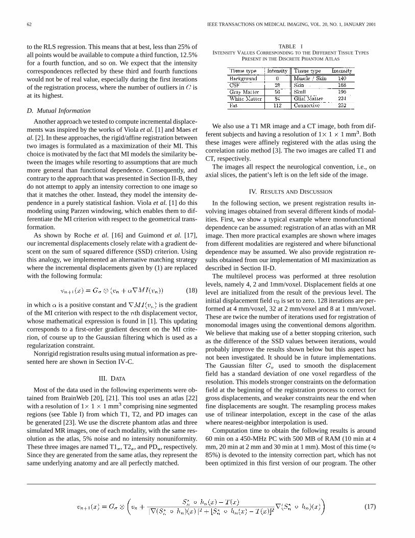
Most of the data used in the following experiments were ob-tained from BrainWeb [20], [21]. This tool uses an atlas [22]with a resolution of 1 1 1 mm comprising nine segmentedregions (see Table I) from which T1, T2, and PD images canbe generated [23]. We use the discrete phantom atlas and threesimulated MR images, one of each modality, with the same res-olution as the atlas, 5% noise and no intensity nonuniformity.These three images are named T1, T2 , and PD, respectively.Since they are generated from the same atlas, they represent thesame underlying anatomy and are all perfectly matched.

TABLE IINTENSITY VALUES CORRESPONDING TO THEDIFFERENTTISSUETYPES

PRESENT IN THEDISCRETEPHANTOM ATLAS

We also use a T1 MR image and a CT image, both from dif-ferent subjects and having a resolution of 11 1 mm . Boththese images were affinely registered with the atlas using thecorrelation ratio method [3]. The two images are called T1 andCT, respectively.

The images all respect the neurological convention, i.e., onaxial slices, the patient’s left is on the left side of the image.

IV. RESULTS AND DISCUSSION

In the following section, we present registration results in-volving images obtained from several different kinds of modal-ities. First, we show a typical example where monofunctionaldependence can be assumed: registration of an atlas with an MRimage. Then more practical examples are shown where imagesfrom different modalities are registered and where bifunctionaldependence may be assumed. We also provide registration re-sults obtained from our implementation of MI maximization asdescribed in Section II-D.

The multilevel process was performed at three resolutionlevels, namely 4, 2 and 1mm/voxel. Displacement fields at onelevel are initialized from the result of the previous level. Theinitial displacement field is set to zero. 128 iterations are per-formed at 4 mm/voxel, 32 at 2 mm/voxel and 8 at 1 mm/voxel.These are twice the number of iterations used for registration ofmonomodal images using the conventional demons algorithm.We believe that making use of a better stopping criterion, suchas the difference of the SSD values between iterations, wouldprobably improve the results shown below but this aspect hasnot been investigated. It should be in future implementations.The Gaussian filter used to smooth the displacementfield has a standard deviation of one voxel regardless of theresolution. This models stronger constraints on the deformationfield at the beginning of the registration process to correct forgross displacements, and weaker constraints near the end whenfine displacements are sought. The resampling process makesuse of trilinear interpolation, except in the case of the atlaswhere nearest-neighbor interpolation is used.

Computation time to obtain the following results is around60 min on a 450-MHz PC with 500 MB of RAM (10 min at 4mm, 20 min at 2 mm and 30 min at 1 mm). Most of this time (85%) is devoted to the intensity correction part, which has notbeen optimized in this first version of our program. The other

(17)


(a) (b) (c) (d)

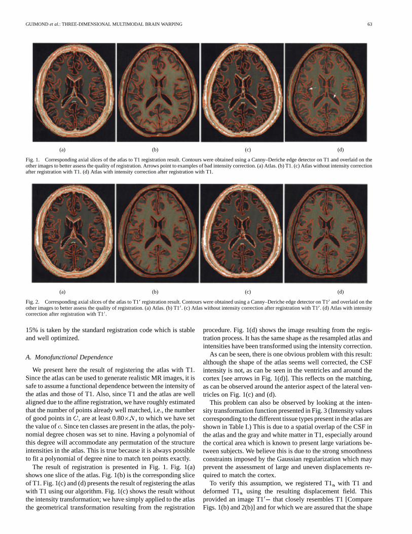
Fig. 1. Corresponding axial slices of the atlas to T1 registration result. Contours were obtained using a Canny–Deriche edge detector on T1 and overlaid on theother images to better assess the quality of registration. Arrows point to examples of bad intensity correction. (a) Atlas. (b) T1. (c) Atlas without intensity correctionafter registration with T1. (d) Atlas with intensity correction after registration with T1.

(a) (b) (c) (d)

Fig. 2. Corresponding axial slices of the atlas to T1registration result. Contours were obtained using a Canny–Deriche edge detector on T1and overlaid on theother images to better assess the quality of registration. (a) Atlas. (b) T1. (c) Atlas without intensity correction after registration with T1. (d) Atlas with intensitycorrection after registration with T1.

15% is taken by the standard registration code which is stableand well optimized.

A. Monofunctional Dependence

We present here the result of registering the atlas with T1.Since the atlas can be used to generate realistic MR images, it issafe to assume a functional dependence between the intensity ofthe atlas and those of T1. Also, since T1 and the atlas are wellaligned due to the affine registration, we have roughly estimatedthat the number of points already well matched, i.e., the numberof good points in , are at least 0.80 , to which we have setthe value of . Since ten classes are present in the atlas, the poly-nomial degree chosen was set to nine. Having a polynomial ofthis degree will accommodate any permutation of the structureintensities in the atlas. This is true because it is always possibleto fit a polynomial of degree nine to match ten points exactly.

The result of registration is presented in Fig. 1. Fig. 1(a)shows one slice of the atlas. Fig. 1(b) is the corresponding sliceof T1. Fig. 1(c) and (d) presents the result of registering the atlaswith T1 using our algorithm. Fig. 1(c) shows the result withoutthe intensity transformation; we have simply applied to the atlasthe geometrical transformation resulting from the registration

procedure. Fig. 1(d) shows the image resulting from the regis-tration process. It has the same shape as the resampled atlas andintensities have been transformed using the intensity correction.

As can be seen, there is one obvious problem with this result:although the shape of the atlas seems well corrected, the CSFintensity is not, as can be seen in the ventricles and around thecortex [see arrows in Fig. 1(d)]. This reflects on the matching,as can be observed around the anterior aspect of the lateral ven-tricles on Fig. 1(c) and (d).

This problem can also be observed by looking at the inten-sity transformation function presented in Fig. 3 (Intensity valuescorresponding to the different tissue types present in the atlas areshown in Table I.) This is due to a spatial overlap of the CSF inthe atlas and the gray and white matter in T1, especially aroundthe cortical area which is known to present large variations be-tween subjects. We believe this is due to the strong smoothnessconstraints imposed by the Gaussian regularization which mayprevent the assessment of large and uneven displacements re-quired to match the cortex.

To verify this assumption, we registered T1with T1 anddeformed T1 using the resulting displacement field. Thisprovided an image T1 that closely resembles T1 [CompareFigs. 1(b) and 2(b)] and for which we are assured that the shape


Fig. 3. Intensity transformation found by registering the atlas with T1 andassuming monofunctional dependence. The functionf is overlaid on the jointhistogram of the two images after registration. The joint histogram valueshave been compressed logarithmically and normalized as is depicted in thecolor scale. The tissue types corresponding to the different atlas intensities arepresented in Table I.

Fig. 4. Intensity transformation found by registering the atlas with T1andassuming monofunctional dependence. The functionf is overlaid on the jointhistogram of the two images after registration. The joint histogram valueshave been compressed logarithmically and normalized as is depicted in thecolor scale. The tissue types corresponding to the different atlas intensities arepresented in Table I.

variation from the atlas can be assessed by our algorithm. Wethen registered the atlas with T1. This result is presented inFig. 2. As can be observed, the CSF intensity value is nowwell corrected. By looking at the intensity transformationshown in Fig. 4, we also notice that each atlas structure hascorresponding intensity ranges in T1 that are less extendedthan those of Fig. 3, reflecting a better match between theimages. This finding puts forth that the displacement fieldregularization has to be able to accommodate the large unevendisplacement of the cortex. To cope with large displacements,Gaussian filtering may probably be replaced with anotherregularization strategy such as that based on a fluid model [24]or on a nonquadratic potential energy [25].

Another difference between Figs. 3 and 4 is the difference inthe intensity mapping of the glial matter (Intensity 224 in the

atlas). This structure forms a small envelope around the ventri-cles and is represented by so few points that they are consid-ered as outliers. This could be corrected by considering morepoints during the intensity transformation. In fact,should beincreased at each iteration to reflect that, during registration,gradually aligns with and more points in can be consideredas well matched.

B. Bifunctional Dependence

When registering images from different modalities, mono-functional dependence may not necessarily be assumed. Here,we applied the method described in Section II-B where twopolynomial functions of degree 12 are estimated. This numberwas set arbitrarily to a relatively high value to enable importantintensity transformations.

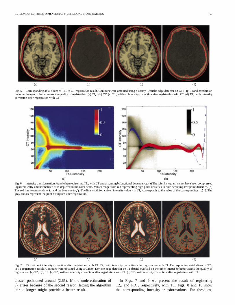
Fig. 5 presents the result of registering T1with CT. Usingthese last two modalities, most intensities of T1should bemapped to gray and only the skull, representing a small por-tion of the image data, should be mapped to white. After affineregistration almost all voxels are well matched, i.e., the numberof good points in is large. Hence, in this particular case, wehave chosen a high value forset to 0.90 .

As we can see in Fig. 5, the skull, shown in black in the MRimage and in white in the CT scan, is well registered and theintensity transformation adequate. Fig. 6(a) presents the jointhistogram of the two images after registration. This histogramis color-coded and ranges from red representing high point den-sities to blue depicting low point densities. Fig. 6(b) presents thefunctions and found during the registration process. Thered line corresponds to and the blue one to . The line widthfor a given intensity is proportional to the value of the corre-sponding . The gray values represent the joint histogramafter registration.

As can be observed in Fig. 6(b), the polynomials found fitwell with the high density clusters of the joint histogram. Still,some points need to be addressed.

We can observe that due to the restricted polynomial degree,, (shown in red) oscillates around the CT gray value instead of

fitting a straight line. This is reflected in the intensity correctedimage, shown in Fig. 5(d), where the underlying anatomy canstill be observed by small intensity variations inside the skull.This artifact has insubstantial consequences during the registra-tion process since the difference between most of the voxels of

and is zero, resulting in null displacements. The displace-ments driving the deformation will be those of the skull and theskin contours, and will be propagated in the rest of the imagewith the Gaussian filtering of the displacement field.

We also notice that (shown in blue), which is mainlyresponsible for the mapping of the skull, does not properlymodel the cluster it represents for intensities smaller than five.The mapping for these intensities is slightly underestimated.This may have two causes. First, as in the previous case, itmight be due to the restricted polynomial degree. Second, wecan notice that some of the background values in T1thathave an intensity close to zero are mapped to gray valuesin the CT which correspond to soft tissues. This means thatsome of the background in T1is matched with the skin inthe CT. This has the effect of “pulling” closer to the small


(a) (b) (c) (d)

Fig. 5. Corresponding axial slices of T1to CT registration result. Contours were obtained using a Canny–Deriche edge detector on CT (Fig. 1) and overlaid onthe other images to better assess the quality of registration. (a) T1. (b) CT. (c) T1 without intensity correction after registration with CT. (d) T1with intensitycorrection after registration with CT

(a) (b)

Fig. 6. Intensity transformation found when registering T1with CT and assuming bifunctional dependence. (a) The joint histogram values have been compressedlogarithmically and normalized as is depicted in the color scale. Values range from red representing high point densities to blue depicting low pointdensities. (b)The red line corresponds tof and the blue one tof . The line width for a given intensity values in T1 corresponds to the value of the corresponding� (s). Thegray values represent the joint histogram after registration.

(a) (b) (c) (d)

Fig. 7. T2 without intensity correction after registration with T1. T2with intensity correction after registration with T1. Corresponding axial slices of T2to T1 registration result. Contours were obtained using a Canny–Deriche edge detector on T1 (b)and overlaid on the other images to better assess the quality ofregistration. (a) T2. (b) T1. (c) T2 without intensity correction after registration with T1. (d) T2with intensity correction after registration with T1.

cluster positioned around (2,65). If the underestimation ofarises because of the second reason, letting the algorithm

iterate longer might provide a better result.

In Figs. 7 and 9 we present the result of registeringT2 and PD, respectively, with T1. Figs. 8 and 10 showthe corresponding intensity transformations. For these ex-


(a) (b)

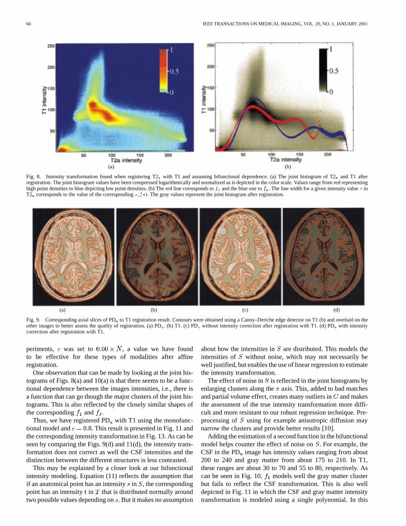
Fig. 8. Intensity transformation found when registering T2with T1 and assuming bifunctional dependence. (a) The joint histogram of T2and T1 afterregistration. The joint histogram values have been compressed logarithmically and normalized as is depicted in the color scale. Values range from red representinghigh point densities to blue depicting low point densities. (b) The red line corresponds tof and the blue one tof . The line width for a given intensity values inT2 corresponds to the value of the corresponding� (s). The gray values represent the joint histogram after registration.

(a) (b) (c) (d)

Fig. 9. Corresponding axial slices of PDto T1 registration result. Contours were obtained using a Canny–Deriche edge detector on T1 (b) and overlaid on theother images to better assess the quality of registration. (a) PD. (b) T1. (c) PD without intensity correction after registration with T1. (d) PDwith intensitycorrection after registration with T1.

periments, was set to , a value we have foundto be effective for these types of modalities after affineregistration.

One observation that can be made by looking at the joint his-tograms of Figs. 8(a) and 10(a) is that there seems to be a func-tional dependence between the images intensities, i.e., there isa function that can go though the major clusters of the joint his-tograms. This is also reflected by the closely similar shapes ofthe corresponding and .

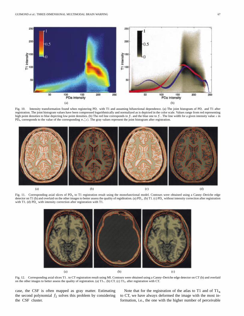
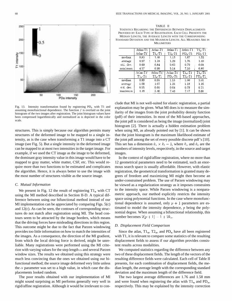
Thus, we have registered PDwith T1 using the monofunc-tional model and 0.8. This result is presented in Fig. 11 andthe corresponding intensity transformation in Fig. 13. As can beseen by comparing the Figs. 9(d) and 11(d), the intensity trans-formation does not correct as well the CSF intensities and thedistinction between the different structures is less contrasted.

This may be explained by a closer look at our bifunctionalintensity modeling. Equation (11) reflects the assumption thatif an anatomical point has an intensityin , the correspondingpoint has an intensityin that is distributed normally aroundtwo possible values depending on. But it makes no assumption

about how the intensities in are distributed. This models theintensities of without noise, which may not necessarily bewell justified, but enables the use of linear regression to estimatethe intensity transformation.

The effect of noise in is reflected in the joint histograms byenlarging clusters along theaxis. This, added to bad matchesand partial volume effect, creates many outliers inand makesthe assessment of the true intensity transformation more diffi-cult and more resistant to our robust regression technique. Pre-processing of using for example anisotropic diffusion maynarrow the clusters and provide better results [10].

Adding the estimation of a second function in the bifunctionalmodel helps counter the effect of noise on. For example, theCSF in the PD image has intensity values ranging from about200 to 240 and gray matter from about 175 to 210. In T1,these ranges are about 30 to 70 and 55 to 80, respectively. Ascan be seen in Fig. 10, models well the gray matter clusterbut fails to reflect the CSF transformation. This is also welldepicted in Fig. 11 in which the CSF and gray matter intensitytransformation is modeled using a single polynomial. In this


(a) (b)

Fig. 10. Intensity transformation found when registering PDwith T1 and assuming bifunctional dependence. (a) The joint histogram of PDand T1 afterregistration. The joint histogram values have been compressed logarithmically and normalized as is depicted in the color scale. Values range from red representinghigh point densities to blue depicting low point densities. (b) The red line corresponds tof and the blue one tof . The line width for a given intensity values inPD corresponds to the value of the corresponding� (s). The gray values represent the joint histogram after registration.

(a) (b) (c) (d)

Fig. 11. Corresponding axial slices of PDto T1 registration result using the monofunctional model. Contours were obtained using a Canny–Deriche edgedetector on T1 (b) and overlaid on the other images to better assess the quality of regidtration. (a) PD. (b) T1. (c) PD without intensity correction after registrationwith T1. (d) PD with intensity correction after registration with T1.

(a) (b) (c)

Fig. 12. Corresponding axial slices T1to CT registration result using MI. Contours were obtained using a Canny–Deriche edge detector on CT (b) and overlaidon the other images to better assess the quality of registration. (a) T1. (b) CT. (c) T1 after registration with CT.

case, the CSF is often mapped as gray matter. Estimatingthe second polynomial solves this problem by consideringthe CSF cluster.

Note that for the registration of the atlas to T1 and of T1to CT, we have always deformed the image with the most in-formation, i.e., the one with the higher number of perceivable


Fig. 13. Intensity transformation found by registering PDwith T1 andassuming monofunctional dependence. The functionf is overlaid on the jointhistogram of the two images after registration. The joint histogram values havebeen compressed logarithmically and normalized as is depicted in the colorscale.

structures. This is simply because our algorithm permits manystructures of the deformed image to be mapped to a single in-tensity, as is the case when transforming a T1 image into a CTimage (see Fig. 5). But a single intensity in the deformed imagecan be mapped to at most two intensities in the target image. Forexample, if we used the CT image as the image to be deformed,the dominant gray intensity value in this image would have to bemapped to gray matter, white matter, CSF, etc. This would re-quire more than two functions to be estimated and complicatesthe algorithm. Hence, it is always better to use the image withthe most number of structures visible as the source image.

C. Mutual Information

We present in Fig. 12 the result of registering T1with CTusing the MI method described in Section II-D. A typical dif-ference between using our bifunctional method instead of ourMI implementation can be appreciated by comparing Figs. 5(c)and 12(c). As can be seen, the contours of corresponding struc-tures do not match after registration using MI. The head con-tours seem to be attracted by the image borders, which meansthat the driving forces have misleading directions in this region.This outcome might be due to the fact that Parzen windowingprovides too little information on how to match the intensities ofthe images. As a consequence, the direction of the MI gradient,from which the local driving force is derived, might be unre-liable. Many registrations were performed using the MI crite-rion with varying values for the step lengthand several Parzenwindow sizes. The results we obtained using this strategy weremuch less convincing than the ones we obtained using our bi-functional method; the source image deformed very little unlessthe parameter was set to a high value, in which case the dis-placements looked random.

The poor results obtained with our implementation of MImight sound surprising as MI performs generally very well inrigid/affine registration. Although it would be irrelevant to con-

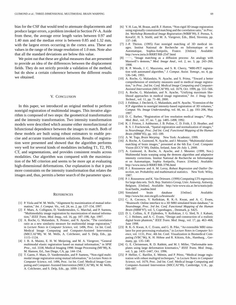
TABLE IISTATISTICS REGARDING THE DIFFERENCESBETWEEN DISPLACEMENTS

PROVIDED BY EACH TYPE OFREGISTRATION. EACH CELL PRESENTS THE

MEDIAN LENGTH, THE AVERAGE LENGTH WITH THE CORRESPONDING

STANDARD DEVIATION AND THE MAXIMUM LENGTH. ALL MEASURESARE IN

MILLIMETERS

clude that MI is not well-suited for elastic registration, a partialexplanation may be given. What MI does is to measure the sim-ilarity of the images from the joint probability density function(pdf) of their intensities. In most of the MI-based approaches,the joint pdf is considered as being the image (normalized) jointhistogram [2]. There is actually a hidden estimation problemwhen using MI, as already pointed out by [1]. It can be shownthat the joint histogram is the maximum likelihood estimate ofthe joint pdf among the set of every possible discrete pdf’s [10].This set has a dimension , where and are thenumbers of intensity levels, respectively, in the source and targetimages.

In the context of rigid/affine registration, where no more than12 geometrical parameters need to be estimated, such an enor-mous search space is usually affordable. However, with elasticregistration, the geometrical transformation is granted many de-grees of freedom and maximizing MI might then become anunder-constrained problem. The use of Parzen windowing maybe viewed as a regularization strategy as it imposes constraintsto the intensity space. While Parzen windowing is a nonpara-metric approach, our method explicitly restricts the intensityspace using polynomial functions. In the case where monofunc-tional dependence is assumed, only parameters are es-timated to model the intensity dependence,being the poly-nomial degree. When assuming a bifunctional relationship, thisnumber becomes .

D. Displacement Field Comparison

Since the atlas, T1, T2 , and PD have all been registeredwith T1, it is relevant to compare some statistics of the resultingdisplacement fields to assess if our algorithm provides consis-tent results across modalities.

We computed statistics regarding the difference between anytwo of these displacement fields. The length of the vectors of theresulting difference fields were calculated. Each cell of Table IIpresents, for each combination of displacement fields, the me-dian length, the average length with the corresponding standarddeviation and the maximum length of the difference field.

The two largest average differences are 1.76 and 1.58 mmand were found when registering the atlas with T1and PD,respectively. This may be explained by the intensity correction


bias for the CSF that would tend to attenuate displacements andproduce larger errors, a problem invoked in Section IV-A. Asidefrom these, the average error length varies between 0.97 and1.40 mm and the median error is between 0.85 and 1.32 mm,with the largest errors occurring in the cortex area. These arevalues in the range of the image resolution of 1.0 mm. Note alsothat all the standard deviations are below this value.

We point out that these are global measures that are presentedto provide an idea of the differences between the displacementfields. They do not strictly provide a validation of the method,but do show a certain coherence between the different resultswe obtained.

V. CONCLUSION

In this paper, we introduced an original method to performnonrigid registration of multimodal images. This iterative algo-rithm is composed of two steps: the geometrical transformationand the intensity transformation. Two intensity transformationmodels were described which assume either monofunctional orbifunctional dependence between the images to match. Both ofthese models are built using robust estimators to enable pre-cise and accurate transformation solutions. Results of registra-tion were presented and showed that the algorithm performsvery well for several kinds of modalities including T1, T2, PD,CT, and segmentations, and provides consistent results acrossmodalities. Our algorithm was compared with the maximiza-tion of the MI criterion and seems to be more apt at evaluatinghigh-dimensional deformations. Our explanation is that it putsmore constraints on the intensity transformation that relates theimages and, thus, permits a better search of the parameter space.

REFERENCES

[1] P. Viola and W. M. Wells, “Alignment by maximization of mutual infor-mation,” Int. J. Comput. Vis., vol. 24, no. 2, pp. 137–154, 1997.

[2] F. Maes, A. Collignon, D. Vandermeulen, G. Marchal, and P. Suetens,“Multimodality image registration by maximization of mutual informa-tion,” IEEE Trans. Med. Imag., vol. 16, pp. 187–198, Apr. 1997.

[3] A. Roche, G. Malandain, X. Pennec, and N. Ayache, “The correlationratio as a new similarity measure for multimodal image registration,”in Lecture Notes in Computer Science, vol. 1496, Proc. 1st Int. Conf.Medical Image Computing and Computer-Assisted Intervention(MICCAI’98), W. M. Wells, A. Colchester, and S. Delp, Eds., pp.1115–1124.

[4] J. B. A. Maintz, E. H. W. Meijering, and M. A. Viergever, “Generalmultimodal elastic registration based on mutual information,” inSPIEProc., vol. 3338, Medical Imaging 1998: Image Processing (MI’98), K.M. Hanson, Ed., San Diego, CA, pp. 144–154.

[5] T. Gaens, F. Maes, D. Vandermeulen, and P. Suetens, “Non-rigid multi-modal image registration using mutual information,” inLecture Notes inComputer Science, vol. 1496, Proc. 1st Int. Conf. Medical Image Com-puting and Computer-Assisted Intervention (MICCAI’98), W. M. Wells,A. Colchester, and S. Delp, Eds., pp. 1099–1106.

[6] Y. H. Lau, M. Braun, and B. F. Hutton, “Non-rigid 3D image registrationusing regionally constrained matching and the correlation ratio,” inProc.Int. Workshop Biomedical Image Registration (WBIR’99), F. Pernus, S.Kovacic, H. S. Stiehl, and M. A. Viergever, Eds., Bled, Slovenia, pp.137–148.

[7] J.-P. Thirion. (1995) Fast nonrigid matching of 3D medical im-ages. Institut National de Recherche en Informatique et enAutomatique, Sophia-Antipolis, France. [Online]. Available:http://www.inria.fr/RRRT/RR-2547.html

[8] , “Image matching as a diffusion process: An analogy withMaxwell’s demons,”Med. Image Anal., vol. 2, no. 3, pp. 243–260,1998.

[9] R. P. Woods, J. C. Mazziotta, and S. R. Cherry, “MRI-PET registra-tion with automated algorithm,”J. Comput. Assist. Tomogr., no. 4, pp.536–546, 1993.

[10] A. Roche, G. Malandain, N. Ayache, and S. Prima, “Toward a bettercomprehension of similarity measures used in medical image registra-tion,” in Proc. 2nd Int. Conf. Medical Image Computing and Computer-Assisted Intervention (MICCAI’99), vol. 1679, Oct. 1999, pp. 555–566.

[11] A. Roche, G. Malandain, and N. Ayache, “Unifying maximum like-lihood approaches in medical image registration,”Int. J. Imag. Syst.Technol., vol. 11, pp. 71–80, 2000.

[12] J. Feldmar, J. Declerck, G. Malandain, and N. Ayache, “Extension of theICP algorithm to nonrigid intensity-based registration of 3D volumes,”Comput. Vis. Image Understanding, vol. 66, no. 2, pp. 193–206, May1997.

[13] D. C. Barber, “Registration of low resolution medical images,”Phys.Med. Biol., vol. 37, no. 7, pp. 1485–1498, 1992.

[14] K. J. Friston, J. Ashburner, J. B. Poline, C. D. Frith, J. D. Heather, andR. S. J. Frackowiak, “Spatial registration and normalization of images,”in NeuroImage, Proc. 2nd Int. Conf. Functional Mapping of the HumanBrain (HBM’95), pp. 165–189.

[15] A. W. Toga,Brain Warping. New York: Academic, 1999.[16] A. Roche, A. Guimond, N. Ayache, and J. Meunier, “Multimodal elastic

matching of brain images,” presented at the 6th Eur. Conf. ComputerVision (ECCV’00), Dublin, Ireland, June 26–July 1, 2000.

[17] A. Guimond, A. Roche, A. Ayache, and J. Meunier. (1999, Nov.)Multimodal brain warping using the demons algorithm and adaptativeintensity corrections. Institut National de Recherche en Informatiqueet en Automatique, Sophia Antipolis, France. [Online]. Available:http://www.inria.fr/RRRT/RR-3796.html

[18] P. J. Rousseeuw and A. M. Leroy,Robust Regression and Outlier De-tection, ser. Probability and mathematical statistics. New York: Wiley,1987.

[19] P. J. Rousseeuw and K. Van Driessen. (1999) Computing LTS regressionfor large data sets. Tech. Rep. Statistics Group, Univ. Antwerp, Antwerp,Belgium. [Online]. Available: http://win-www.uia.ac.be/u/statis/pub-licat/fastlts_readme.html

[20] Simulated brain database [Online]. Available:http://www.bic.mni.mcgill.ca/brainweb/

[21] C. A. Cocosco, V. Kollokian, R. K.-S. Kwan, and A. C. Evans,“Brainweb: Online interface to a 3D MRI simulated brain database,” inNeuroImage, Proc. 3rd Int. Conf. Functional Mapping of the HumanBrain (HBM’97), vol. 5, Copenhagen, , Denmark, p. S425.

[22] D. L. Collins, A. P. Zijdenbos, V. Kollokian, J. G. Sled, N. J. Kabani,C. J. Holmes, and A. C. Evans, “Design and construction of a realisticdigital brain phantom,”IEEE Trans. Med. Imag., vol. 17, pp. 463–468,June 1998.

[23] R. K.-S. Kwan, A. C. Evans, and G. B. Pike, “An extensible MRI simu-lator for post-processing evaluation,” inLecture Notes in Computer Sci-ence, vol. 1131, Proc. 4th Int. Conf. Visualization in Biomedical Com-puting (VBC’96), K. H. Höhne and R. Kikinis, Eds., Hamburg, , Ger-many, pp. 135–140.

[24] G. E. Christensen, R. D. Rabbitt, and M. I. Miller, “Deformable tem-plates using large deformation kinematics,”IEEE Trans. Med. Imag.,vol. 5, pp. 1435–1447, Oct. 1996.

[25] P. Hellier, C. Barillot, E. Mémin, and P. Pérez, “Medical image regis-tration with robust multigrid techniques,” inLecture Notes in ComputerScience, vol. 1679, Proc. 2nd Int. Conf. Medical Image Computing andComputer-Assisted Intervention (MICCAI’99), Cambridge, U.K., pp.680–687.

Three-Dimensional Multimodal Brain Warping using the Demons Algorithm and Adaptive Intensity...

Documents

Transcript of Three-Dimensional Multimodal Brain Warping using the Demons Algorithm and Adaptive Intensity...