Three-dimensional collapse and steady flow in thick-walled flexible tubes

ARTICLE IN PRESS

0889-9746/$ - se

doi:10.1016/j.jfl

�CorrespondE-mail addr

Journal of Fluids and Structures 20 (2005) 817–835

www.elsevier.com/locate/jfs

Three-dimensional collapse and steady flowin thick-walled flexible tubes

A. Marzoa, X.Y. Luob,�, C.D. Bertramc

aDepartment of Mechanical Engineering, University of Sheffield, Sheffield, UKbDepartment of Mathematics, University of Glasgow, Glasgow, UK

cGraduate School of Biomedical Engineering, University of New South Wales, Sydney, Australia

Received 8 March 2004; accepted 10 March 2005

Abstract

Three-dimensional collapse of and steady flow through finite-length elastic tubes are studied numerically. The

Navier-Stokes equations coupled with large, nonlinear deformation of the elastic wall are solved by using the finite-

element software, FIDAP. Three-dimensional solid elements are used for the elastic wall, allowing us to specify any wall

thickness required. Plane-strain results for the cross-sectional shape of thinner-walled tubes are validated by

comparison with published numerical data. Three-dimensional results for flow through finite-thickness tubes are in

excellent agreement with published numerical results based on thin-shell elements, and are used to show the effects of

varying wall thickness. Finally, the computational predictions are compared with experimental pressure–area

relationships for thick-walled tubes. The simulations confirm a previously neglected experimental finding, that the

Young wavespeed can be lower between buckling and osculation for thick tubes than for thinner ones.

r 2005 Elsevier Ltd. All rights reserved.

Keywords: Collapsible tube flow; Finite element methods; Buckling; Wavespeed

1. Introduction

Many physiological conduits transport viscous fluids within our body. Because of their high flexibility, these conduits

may collapse nonaxisymmetrically under particular conditions of external and internal fluid pressure. When this

phenomenon occurs, the buckled vessels become very flexible and small changes in transmural pressure Ptm (internal

minus external pressure) may induce large displacements. This strong interaction between fluid and structure gives rise

to a number of interesting phenomena, including flow-rate limitation, pressure-drop limitation and a tendency to self-

excited oscillation.

In the cardiovascular system, veins above the level of the heart and outside the skull collapse due to hydrostatic

reduction of blood pressure. This assumes particular importance in subjects with long necks, especially giraffes (Brook

and Pedley, 2002). Flow-induced collapse of cardiovascular vessels is believed to play an important role in the supply of

blood to many internal organs (Guyton and Adkins, 1954; Rodbard, 1966). Moreover, dynamic flow-induced collapse

of blood vessels downstream of atherosclerotic stenoses may cause plaque rupture, which can lead to the occlusion of

e front matter r 2005 Elsevier Ltd. All rights reserved.

uidstructs.2005.03.008

ing author. Tel.: +44141 330 4746; fax: +44141 330 4111.

ess: [email protected] (X.Y. Luo).

www.elsevier.com/locate/jfs

ARTICLE IN PRESSA. Marzo et al. / Journal of Fluids and Structures 20 (2005) 817–835818

the vessel lumen distally, with potentially lethal consequences in the case of the carotid artery (Binns and Ku, 1989; Ku,

1997). In the large airways, flow-induced oscillations are believed to give rise to a number of different noises with

important diagnostic value. Controlled self-excited oscillations also play a fundamental role in speech production

(Berke et al., 1991). During micturition, the urethra behaves like a collapsible tube, and accordingly can exhibit flow-

limitation effects (Griffiths, 1971).

Given its importance and complexity, the topic of flow through collapsible tubes has been studied for over 30 years.

However, the full understanding of this physical phenomenon still represents an unsolved challenge. Kamm and Pedley

(1989) reviewed the subject briefly; a more comprehensive review of the biological examples and the theoretical and

computational developments is given by Heil and Jensen (2003), while Bertram (2003) has reviewed the experimental

side of the subject, and applications in medicine and technology. Experimental investigations on a Starling resistor

prototype of the system have revealed a rich dynamic behaviour, with various types of self-excited oscillations (Bertram

et al., 1991; Bertram and Elliott, 2003). To reveal the mechanisms of such oscillations, much work has been carried out,

but most is limited to 1-D or 2-D models (Pedley, 1992; Luo and Pedley, 1995, 1996, 1998, 2000; Cai and Luo, 2003;

Jensen and Heil, 2003).

One-dimensional models adopt a large number of ad hoc assumptions that limit any systematic improvement. Two-

dimensional models of a collapsible channel are based on a more rational approach, and in principle could be realized in

a laboratory. However, only a 3-D study can provide the full picture of a collapsible tube, which exhibits strongly 3-D

behaviour. Owing to the extensive computational resources required and the high nonlinearity of the system, to date

there is only limited published work on 3-D thin-walled tubes. Hazel and Heil (2003) investigated the steady flow

through thin-walled elastic tubes for a finite Reynolds number. In their finite-element approach, they solved the steady

3-D Navier–Stokes equations simultaneously with the equations of geometrical nonlinear, Kirchhoff–Love thin-shell

theory. One of the assumptions underlying thin-shell theory is that the wall thickness of the tube is some 20 or more

times smaller than its radius. Considering that much experimental work is on thick-walled tubes (Bertram, 1987;

Bertram and Castles, 1999), it is important that 3-D numerical simulations are not restricted to thin-shell theory.

In this paper, we present 3-D numerical simulations for a finite-Reynolds-number steady flow in thick-walled tubes,

using the finite-element software FIDAP (2002) (Fluent Inc.).

2. Methods

We model the steady flow at Reynolds number Re of a viscous fluid through a thick-walled deformable tube of

undeformed radius R, wall thickness h, and length L. The tube wall material has Poisson’s ratio n and Young’s modulus

E. The fluid is assumed to be incompressible, with density r, and Newtonian, with viscosity m. The computational

geometry is shown in Fig. 1.

The problem was formulated in Cartesian coordinates (x, y, z), with z chosen to be the direction of the tube axis, while

x and y are the transverse coordinates. The origin is fixed at the centre of the collapsible-tube inlet. In order to apply the

boundary conditions at inlet and outlet of the computational domain properly, and to mimic the experimental set-up,

rigid tubes were added upstream and downstream of the deformable extension. The lengths of the upstream and

downstream rigid extension are Lup and Ldown, respectively. The pressure acting on the external walls of the deformable

tube is pext.

Fig. 1. The geometry of the collapsible tube.

ARTICLE IN PRESSA. Marzo et al. / Journal of Fluids and Structures 20 (2005) 817–835 819

2.1. Fluid–solid coupling

The fluid/structure-interaction (FSI) algorithm treats the equations that solve the structural problem, the remeshing

problem and the fluid problem by a staggered approach; that is to say, the algorithm solves the equations in

sequence. The overall computational procedure adopted to solve FSI problems that involve large displacement is

depicted in Fig. 2.

Firstly, the equations governing the fluid are solved for fluid velocity and pressure fields. Subsequently the traction,

i.e. pressure and viscous stress, is calculated at the interface between fluid and structure. The traction is then applied to

the structure together with the other boundary conditions, and the structural equations are solved for the displacement

of the structure. At this point the position of the wetted surface is updated. Finally, the equations that describe the mesh

displacement are solved by imposing the displacement of the wetted surface as boundary condition. This cycle is

repeated until convergence is achieved.

2.2. Equations governing the fluid

The Navier–Stokes equations are used for the fluid

rui;juj ¼ sij;j , (1)

uj;j ¼ 0, (2)

where i, j ¼ 1, 2, 3, ui is velocity, r is density, and sij is the stress tensor. The stress tensor can be written as

sij ¼ �pdij þ tij , (3)

where p is the pressure, tij is the deviatoric stress tensor, and dij is the Kronecker delta. For viscous, incompressible

fluids the constitutive relation has the form

tij ¼ 2msij , (4)

where m is the viscosity of the fluid and sij is the strain rate tensor defined as

sij ¼1

2ðui;j þ uj;iÞ. (5)

No-slip boundary conditions are fixed on the tube walls

u1 ¼ u2 ¼ u3 ¼ 0.

A fully developed Poiseuille parabolic velocity profile is used for the inlet,

u1 ¼ u2 ¼ 0; u3 ¼ 2U 1�1

R2x2 þ y2� ��

at z ¼ �Lup,

Fig. 2. Strategy of the computational procedure in FIDAP.


where U represents the velocity averaged across the undeformed cross-sectional area. A parallel, axially traction-free

outflow is fixed at the outlet

u1 ¼ u2 ¼ 0; �p þ 2qu3

qz¼ 0 at z ¼ L þ Ldown.

2.3. Equations governing the structure

We assume that the strain of the wall is small, and this allows us to treat the structure as an elastic and linear medium.

The overall structural behaviour is described by the momentum Eq. (6), the equilibrium Eq. (7) and the constitutive

Eqs. (8) and (9)

sij;j ¼ 0, (6)

sijnj ¼sti, (7)

sij ¼ Dijkl�kl , (8)

�kl ¼1

2ðdk;l þ dl;kÞ, (9)

where sij is the Cauchy stress tensor, sti is the externally applied surface traction vector, nj is the outward pointing

normal vector, Dijkl is the material (Lagrangian) elasticity tensor, and �kl is the infinitesimal strain tensor. The wall

deformation is thus governed by the principle of virtual displacementsZSO

sjiddi;j dO ¼

ZSO

rwf iddi dOþ

ZSG

Stiddi dG; (10)

where rw represents the material density, ddi is the virtual displacement vector, f i is an externally applied body force

vector, Sti is the externally applied surface traction vector, SO is the domain occupied by the moving elastic structure,

and SG is the boundary of the structure. This formulation is nonlinear because, at any iteration, the current domain,SO,is unknown. Thus, at each iteration, the solution is calculated using an incremental Lagrangian formulation. At each

stage, the stresses and strain are measured with respect to the most recent available configuration (updated Lagrangian

approach).

We assume that the deformable part of the tube is clamped at both ends

dx ¼ dy ¼ dz ¼ 0 at z ¼ 0; L.

2.4. Remeshing equations

The remeshing problem is solved by considering the mesh as a pseudo-elastic medium, the deformation of which is

based on the boundary conditions resulting from the displacement solution of the structural problem. In fact, the

elasticity-based remeshing algorithm is similar to that employed to solve the structural problem. However, in the

remeshing algorithm, only displacement boundary conditions are allowed (boundary conditions involving stresses or

forces proportional to the displacement have no meaning in the mesh context).

2.5. Numerical implementation

We discretize the structural domain with 3-D solid elements. All six possible stresses (three normal and three shear

components) are taken into account. Shell theory in general (there are several formulations of thin-shell theory) does

not take account of normal stress in the wall thickness direction. This is reasonable if the thickness is small in

comparison with other dimensions. In many of Bertram’s experiments, in order to avoid the well-known problem of the

collapsible part being sucked into the downstream rigid tube, the wall thickness is relatively large. Using a 3-D solid

element enables us to compare our numerical results with Bertram’s experimental data. However, this is done at the cost

of demanding much greater computational resources, and of a propensity to ill-conditioning and locking behaviour

when used for ‘thinner-walled’ tubes.

Due to the extensive computation required and also since in experiments elastic tubes of substantial length usually

collapse into a mode-2 buckling, here we only consider one quarter of the whole domain. The computational domain is


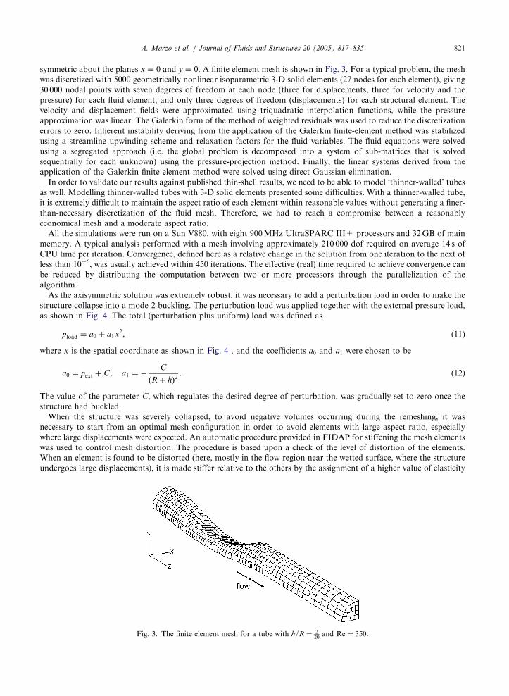
symmetric about the planes x ¼ 0 and y ¼ 0. A finite element mesh is shown in Fig. 3. For a typical problem, the mesh

was discretized with 5000 geometrically nonlinear isoparametric 3-D solid elements (27 nodes for each element), giving

30 000 nodal points with seven degrees of freedom at each node (three for displacements, three for velocity and the

pressure) for each fluid element, and only three degrees of freedom (displacements) for each structural element. The

velocity and displacement fields were approximated using triquadratic interpolation functions, while the pressure

approximation was linear. The Galerkin form of the method of weighted residuals was used to reduce the discretization

errors to zero. Inherent instability deriving from the application of the Galerkin finite-element method was stabilized

using a streamline upwinding scheme and relaxation factors for the fluid variables. The fluid equations were solved

using a segregated approach (i.e. the global problem is decomposed into a system of sub-matrices that is solved

sequentially for each unknown) using the pressure-projection method. Finally, the linear systems derived from the

application of the Galerkin finite element method were solved using direct Gaussian elimination.

In order to validate our results against published thin-shell results, we need to be able to model ‘thinner-walled’ tubes

as well. Modelling thinner-walled tubes with 3-D solid elements presented some difficulties. With a thinner-walled tube,

it is extremely difficult to maintain the aspect ratio of each element within reasonable values without generating a finer-

than-necessary discretization of the fluid mesh. Therefore, we had to reach a compromise between a reasonably

economical mesh and a moderate aspect ratio.

All the simulations were run on a Sun V880, with eight 900MHz UltraSPARC III+ processors and 32GB of main

memory. A typical analysis performed with a mesh involving approximately 210 000 dof required on average 14 s of

CPU time per iteration. Convergence, defined here as a relative change in the solution from one iteration to the next of

less than 10�6, was usually achieved within 450 iterations. The effective (real) time required to achieve convergence can

be reduced by distributing the computation between two or more processors through the parallelization of the

algorithm.

As the axisymmetric solution was extremely robust, it was necessary to add a perturbation load in order to make the

structure collapse into a mode-2 buckling. The perturbation load was applied together with the external pressure load,

as shown in Fig. 4. The total (perturbation plus uniform) load was defined as

pload ¼ a0 þ a1x2, (11)

where x is the spatial coordinate as shown in Fig. 4 , and the coefficients a0 and a1 were chosen to be

a0 ¼ pext þ C; a1 ¼ �C

R þ hð Þ2. (12)

The value of the parameter C, which regulates the desired degree of perturbation, was gradually set to zero once the

structure had buckled.

When the structure was severely collapsed, to avoid negative volumes occurring during the remeshing, it was

necessary to start from an optimal mesh configuration in order to avoid elements with large aspect ratio, especially

where large displacements were expected. An automatic procedure provided in FIDAP for stiffening the mesh elements

was used to control mesh distortion. The procedure is based upon a check of the level of distortion of the elements.

When an element is found to be distorted (here, mostly in the flow region near the wetted surface, where the structure

undergoes large displacements), it is made stiffer relative to the others by the assignment of a higher value of elasticity

Fig. 3. The finite element mesh for a tube with h=R ¼ 220

and Re ¼ 350.

ARTICLE IN PRESS

Fig. 4. The perturbation load applied on the external surface of the tube.

Fig. 5. 4-noded quadrilateral element.

A. Marzo et al. / Journal of Fluids and Structures 20 (2005) 817–835822

modulus for the mesh, thus preventing further deformation that can lead to the breakdown of the mesh. (What is

changed here is a fictitious Young’s modulus used to treat the fluid mesh as a pseudo-elastic material. The procedure

controls only the deformation of fluid elements, and does not affect the actual structural displacement and flow fields.)

The method for computing the distortion depends on the element type. For simplicity, we here consider the case of a 4-

noded quadrilateral element. The same procedure is easily extended to other element types.

The 4-noded quadrilateral element, as shown in Fig. 5 , is divided into four overlapping triangles: D1 ¼ Df1;2;4g,

D2 ¼ Df1;2;3g, D3 ¼ Df2;3;4g, and D4 ¼ Df1;3;4g. The code employs a scalar distortion parameter to indicate element quality.

First, the aspect ratio of each triangle is measured. The aspect ratio is defined as

FD ¼RD

rD,

where RD is the radius of the triangle’s circumcircle and rD that of its incircle. The distortion parameter, Fel , is then

defined by the norm

Fel ¼ max FDl

� �.

where l ¼ 1, 2, 3, 4. A control parameter then measures the change in Fel through the iterative process by

F̄el ¼Fk

el

F0el

,

where k is the iteration count and 0 represents the initial mesh. The pseudo-elastic Young’s modulus of each fluid mesh

element is finally calculated by

Eel ¼ E0ðF̄elÞn,


where E0 and n are inputs of the problem (typical values used in this work were 1 Pa and 2.5 for initial Young’s

modulus and power coefficient, respectively), and F̄el is calculated by the code. Further details can be found in Bar-

Yoseph et al. (2001).

Mesh-independence testing was done by repeating selected analyses using finer discretizations; see Appendix A.

3. Results

3.1. Plane-strain buckling analysis of a tube cross-section

The structural capabilities of the code were first tested by performing the computational analysis of a cylindrical

unsupported tube subjected to a uniform external pressure. We considered a thinner–walled tube of Young’s modulus

E ¼ 105 Pa, Poisson’s ratio n ¼ 0.4, undeformed internal radius R ¼ 5mm, wall thickness h ¼ 0.1mm and infinite

length. The total load applied incrementally to the structure was pext ¼ 0.5 Pa.

The numerical problem was simplified by reducing it to a plane-strain analysis. The computational domain was

discretized with 900 geometrically nonlinear quadrilateral 9-noded elements, giving 3819 nodes with 2 dof at each node

(the two components of displacement). The mesh and the imposed boundary conditions are shown in Fig. 6.

The total pressure load was applied incrementally in 10 000 steps. To avoid solving a contact problem, the simulation

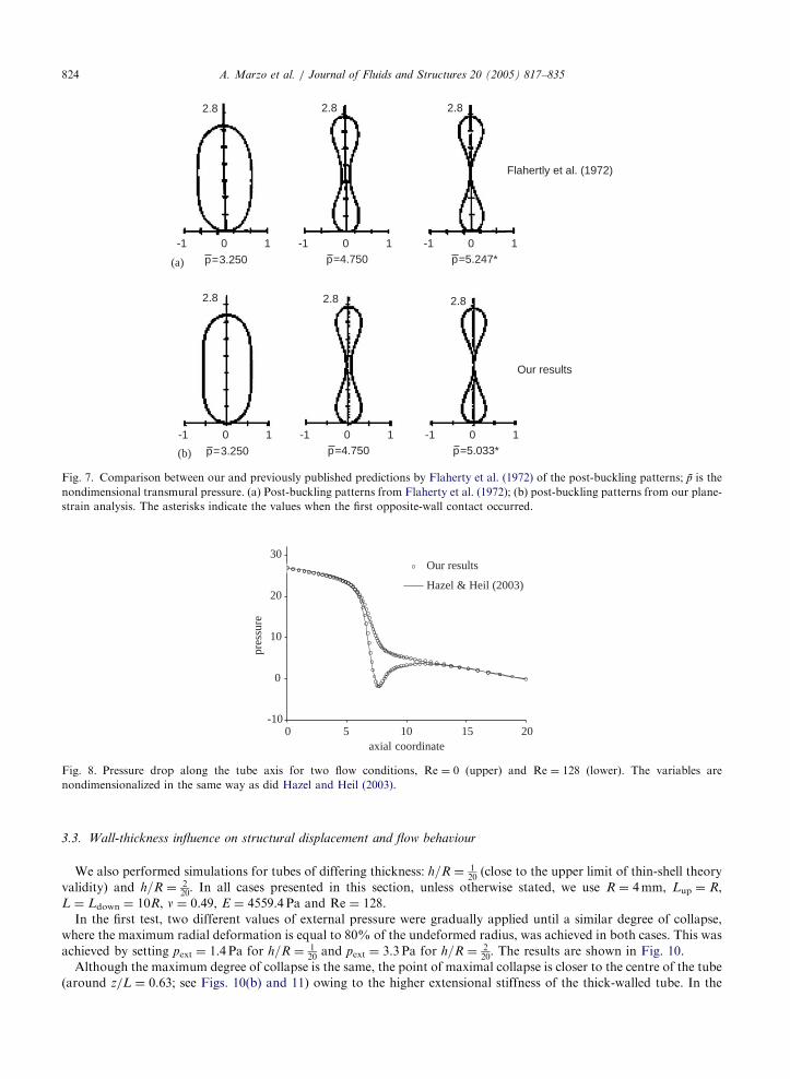
was stopped a few steps before the osculation of the opposite walls of the tube. The computational results are compared

to the numerical results by Flaherty et al. (1972), as shown in Fig. 7 . For convenience, we use below the

nondimensional transmural pressure defined as p̄ ¼ pext=Pk, where Pk ¼ Eh3=½12ð1� n2ÞR3 . First opposite-wall

contact occurred in our simulation at p̄ ¼ 5:033, which is slightly lower than the value obtained by Flaherty et al.

(1972). There is in general very good agreement with the cross-sectional area after tube buckling.

3.2. 3-D analysis of fluid flow through a thinner-walled collapsible tube

In their recent study, Hazel and Heil (2003) used thin-shell theory and the finite-element method to simulate finite-

Reynolds-number flows in collapsible tubes. For validation purposes it is useful to compare our computation for

thinner-walled tubes with their results. To study the effect of fluid inertia on the tube deformation, Hazel and Heil

(2003) obtained numerical predictions for two different flow conditions: Re ¼ 0 and 128.

Here, we follow Hazel and Heil and use R ¼ 4mm, Lup ¼ R, L ¼ Ldown ¼ 10R, n ¼ 0:49, and h=R ¼ 120. In order to

make a meaningful comparison between the two flow conditions, Re ¼ 0 and 128, we set E ¼ 0.0045594 Pa,

pext ¼ 1.19 10�6 Pa for Re ¼ 0, and E ¼ 4559.4 Pa, pext ¼ 1.4 Pa for Re ¼ 128, to achieve the same nondimensional

parameters used by Hazel and Heil (2003). These choices lead to the same degree of collapse (maximum displacement in

y-direction) for the two Re values.

The comparison between our results and those of Hazel and Heil (2003) is shown in Fig. 8. The axial coordinates are

scaled to the radius and the pressure is scaled to the bending stiffness. Excellent agreement is achieved for both flow

conditions.

The displacements for the two flow conditions are shown in Fig. 9.

Fig. 6. The finite-element mesh for the tube cross-section and the boundary conditions specified for the plane-strain analysis.

ARTICLE IN PRESS

2.8 2.8 2.8

2.82.82.8

-1 0 1

p=3.250

-1 0 1p=4.750

-1 0 1p=5.247*

-1 0 1

p=3.250

-1 0 1p=4.750

-1 0 1p=5.033*

Our results

Flahertly et al. (1972)

(a)

(b)

Fig. 7. Comparison between our and previously published predictions by Flaherty et al. (1972) of the post-buckling patterns; p̄ is the

nondimensional transmural pressure. (a) Post-buckling patterns from Flaherty et al. (1972); (b) post-buckling patterns from our plane-

strain analysis. The asterisks indicate the values when the first opposite-wall contact occurred.

-10

0

10

20

30

0 5 10 15 20axial coordinate

pres

sure

Our results

Hazel & Heil (2003)

Fig. 8. Pressure drop along the tube axis for two flow conditions, Re ¼ 0 (upper) and Re ¼ 128 (lower). The variables are

nondimensionalized in the same way as did Hazel and Heil (2003).


3.3. Wall-thickness influence on structural displacement and flow behaviour

We also performed simulations for tubes of differing thickness: h=R ¼ 120(close to the upper limit of thin-shell theory

validity) and h=R ¼ 220. In all cases presented in this section, unless otherwise stated, we use R ¼ 4mm, Lup ¼ R,

L ¼ Ldown ¼ 10R, n ¼ 0.49, E ¼ 4559.4 Pa and Re ¼ 128.

In the first test, two different values of external pressure were gradually applied until a similar degree of collapse,

where the maximum radial deformation is equal to 80% of the undeformed radius, was achieved in both cases. This was

achieved by setting pext ¼ 1.4 Pa for h=R ¼ 120

and pext ¼ 3.3 Pa for h=R ¼ 220. The results are shown in Fig. 10.

Although the maximum degree of collapse is the same, the point of maximal collapse is closer to the centre of the tube

(around z/L ¼ 0.63; see Figs. 10(b) and 11) owing to the higher extensional stiffness of the thick-walled tube. In the

ARTICLE IN PRESS

Fig. 9. The displacement solution for Re ¼ 0 (upper) and Re ¼ 128 (lower).

Fig. 10. Tube configurations for (a) pext ¼ 1.4 Pa with h=R ¼ 120

and (b) pext ¼ 3.3 Pa with h=R ¼ 220. The degree of collapse for both

cases is 80%.

00 0.5

0.5

1

1.5

1z/L

y/R

Thinner tube (h /R=1/20)Thick tube (h/R=2/20)

Fig. 11. Displacements of the edge given by the intersection of the symmetry plane x ¼ 0 with the wetted surface for the thick-walled

and thinner-walled tubes.

A. Marzo et al. / Journal of Fluids and Structures 20 (2005) 817–835 825

thinner-walled case (Figs. 10(a) and 11), the point of greatest collapse occurs further downstream (around z/L ¼ 0.74),

and a small secondary buckling pattern develops at the downstream end. The thick-walled tube does not exhibit this

behaviour under these conditions.

ARTICLE IN PRESS

Fig. 12. Axial-velocity contours are plotted for (a) the thinner-walled, and (b) the thick-walled tube at Re ¼ 128. Fow separation is

observed in the thinner-walled tube flow.


The high degree of collapse strongly influences the fluid flow pattern. Fig. 12 depicts axial velocity contours along the

symmetry planes of the computational domain and in the transverse cross-section at the collapsible-tube inlet for the

two cases under study. Both the location of the greatest collapse and the deformed wall shape have a direct effect on

the flow patterns. In the case of the thicker wall, the increase in axial velocity starts further upstream. However, because

the displacement gradient along the z-axis in the thick-walled tube is smaller compared with the thinner-walled tube, the

flow change is less severe: there is no flow separation downstream, unlike the thinner-walled tube, and the maximum

axial velocity is slightly smaller. In both cases, in the most collapsed section of the tube, the smaller cross-sectional area

is associated with higher-speed fluid flow, which splits into two jets. These jets are formed by the concurrent effect of

increased viscous retardation due to the boundary layers of the inwardly buckled walls.

We next applied the same external pressure, pext ¼ 1.4 Pa, to both the differing-thickness tubes. The tube parameters

were otherwise unchanged. In the case of the thick-walled tube, the external pressure was then insufficient to make the

tube collapse, and the flow pattern therefore retained its Poiseuille profile.

Bertram and Godbole (1997) measured the fluid flow at Re ¼ 705 in a rigid deformed tube resembling the collapsed

state of an elastic tube conveying a flow. They used laser Doppler anemometry to measure the axial velocity component

and one transverse velocity component at several axial locations upstream and downstream of the constriction. For a

relatively high degree of collapse (close to the point of opposite-wall contact), it was observed that the flow splits into

two jets that impinge on the vertical sidewalls of the tube (parallel to the x ¼ 0 symmetry plane in the coordinates used

here) and spread vertically into a crescent shape. With further diffusion of momentum, the flow downstream then

became annular in cross-section, with forward flow near the wall surrounding a central region of low flow, before the

velocity profile reverted to parabolic. For a flow with lower Re, somewhat equivalent phenomena were numerically

predicted by Hazel and Heil (2003).

In order to study the influence of the wall thickness on the development of the two jets, two new cases are here

considered. The geometries used here are the same as those used previously for the thinner-walled and thick-walled

tubes. We set Re ¼ 350, E ¼ 3MPa, n ¼ 0.3 to improve convergence and to remain close to the nondimensional

parameters used by Hazel and Heil (2003). A degree of collapse of 86.4% was imposed on the two tubes by applying

pext ¼ 520 Pa for h=R ¼ 120and pext ¼ 1550Pa for h=R ¼ 2

20. Fig. 13 shows the results of these computations. The point

of maximum collapse is z/L ¼ 0.595 and 0.655 for the thick-walled and thinner-walled tube, respectively. The

development of the flow in the streamwise direction is similar in the two cases, and largely agrees with what was

observed by Bertram and Godbole (1997) and predicted by Hazel and Heil (2003). At the point of greatest collapse, the

fluid flow spreads out along the x-axis while the peak of maximum axial velocity moves from the tube axis and develops

into a line extending towards the sidewalls. Two parallel jets are then formed and axial flow subsequently develops into

a rounded H-shape, with a large area of slow reversed flow near the opposite ends of the minor axis of the cross-section

(y-axis). A strip of positive axial velocity divides the reversed flow areas along the x-axis and unites the two jets at

locations between dt ¼ 4R and 8R, where dt measures distance along the z-axis downstream from the point of the

maximum collapse (tube throat). However, the different displacements of the two geometries produce two slightly

different developments of the two jets. In the thinner-walled-tube case the two jets impinge more on the vertical

sidewalls, and the distance between them, as they develop in parallel along the tube axis, is more pronounced than in the

thicker tube. A difference is also noticeable in the thickness of the strip of positive velocities which divides the two zones

ARTICLE IN PRESS

Fig. 14. Projection of velocity vectors on three cross-sections of (left) the thinner-walled and (right) the thick-walled tube. Cross-

sections are located at dt ¼ 4R, 6R, 8R downstream of the respective points of maximum collapse. As locations relative to the tube

itself, these are z/L ¼ 0.995, 1.195 and 1.395 for the thick-walled tube and z/L ¼ 1.055, 1.255 and 1.455 for the thinner-walled tube.

Fig. 13. 3-D vector plots of axial velocity for (left) the thinner-walled and (right) the thick-walled tube 0, 2R, 4R, 6R, 8R, 10R, and 12R

downstream of the respective points of maximum collapse. Re ¼ 350.

A. Marzo et al. / Journal of Fluids and Structures 20 (2005) 817–835 827

of reversed flow. This extends more along the minor axis of the cross-section in the thick-walled tube than in the thinner

one (most noticeable at dt ¼ 4R; 6R).

Fig. 14 shows details of the secondary flows that develop streamwise for the two geometries. The vectors displayed

are the projection of the velocity vectors on the respective cross-sections. In the thinner-walled tube, four eddies are

formed in each quadrant of the tube cross-section. Their centre of rotation moves from the tube walls towards the tube

ARTICLE IN PRESS

Fig. 15. Particle paths (streamlines) on one quadrant of the computational domain for (bottom left) the thinner-walled and (top right)

the thick-walled tubes at Re ¼ 350. The initial location from which each forward flow streamline develops is given in Cartesian

coordinate (x, y, z) as: (�0.001, 0.001, 0), (�0.0025, 0.001, 0), (�0.001, 0.0025, 0), (�0.0025, 0.0025, 0). For both cases a reversal flow

streamline passing through the same point (0, 0.002, 0.04) inside the reversal zone is also shown in yellow. The actual size of the reversal

zone for both flows is indicated by the light-shadowed area.


axis as z increases. Contrary to that, the displaced geometry of the thick-walled tube does not confer such a pattern to

the fluid flow. The flow direction along the symmetry planes is always directed towards the centre of the cross-section.

Figs. 15 and 16 show details of the reversed flow which develops downstream of the constriction for the two

geometries considered. In the thinner-walled tube case, the flow reversal zone extends from z=L ¼ 0:803 to 1.3. In the

thick-walled tube case, the area occupied by reversed flow is longer, extending from z=L ¼ 0:745 to 1.338. We note from

Fig. 16 that the reversed flow has four initial maxima in the thinner-walled tube, but only two in the thick-walled one.

This is obviously linked to the four-eddy secondary flow for the thinner-walled tube (Fig. 14), absent in the thick-walled

tube flow.

3.4. Comparison with experiments on thick-walled tubes

In this section, results are compared with experimental data on the pressure–area relation for two thick-walled

collapsible tubes reported by Bertram (1987). Bertram measured a ‘thinner-walled’ tube, with a wall-thickness-to-inside-

radius ratio ðh=RiÞ of 0.38, and a ‘thick-walled’ tube with a thickness ratio of 0.50. Both of these are actually much

thicker than is typically regarded as the limit of validity for a thin shell ðh=Rio0:05Þ, emphasizing the importance of

using a computational method able to cope with arbitrarily thick walls. In the experimental rig, a silicone-rubber tube

was mounted and axially loaded between coaxial pipes forming part of a pressure chamber. Pressure within the tube

was maintained constant by connecting the conduit to a source of constant head of aqueous fluid (a solution of water,

sodium nitrite and anti-corrosive additives). External pressure in the chamber was varied by admitting compressed air.

The internal cross-sectional area of the tube halfway along was measured by an electrical impedance method.

In the numerical investigation, the physical problem was again approximated by considering a quarter of the tube.

Applying a constant pressure on the inner wall of the tube approximated the influence of the fluid on the structural

behaviour. In order to stabilize the convergence behaviour of the numerical approach it was necessary to tune the load-

step increment carefully.

Bertram (1987) recorded a slightly hysteretic pressure–area curve for his material; however, we assumed here that our

material was perfectly elastic. Following the reported experimental conditions, the parameters of the ‘thinner-walled’

Fig. 16. Contour plots of axial velocity on seven cross-sections from the most collapsed location of the thinner-walled h=R ¼ 120

� �and

the thick-walled tube h=R ¼ 220

� �at Re ¼ 350. The reversed flow contours are plotted between u3=U ¼ �0:319 and zero with an equal

spacing of 0.0532 (red contours). The forward flow contours are plotted between u3=U ¼ 0:1 and 3.794 with an equal spacing of 0.616

(black contours). Reversed flow first appears at dt ¼ 1:475R for the thinner-walled tube, and 1.5R for the thick-walled one.

ARTICLE IN PRESS

5

00

-5

-10

-15

p

0.5 1

A /Ao

c

c

bb

a

a

Our results

Experimental (Bertram, 1987)

Fig. 17. The computed dimensionless pressure–area relation compared with experimental data of Bertram (1987) for the ‘thinner-

walled’ tube case. The experimental data follow a hysteresis loop, with more external pressure needed to bring about collapse and less

to cause recovery.

5

00

-5

-10

-15

p

0.5 1

c

c

b b

a

a

Our results

A /Ao

Experimental (Bertram, 1987)

Fig. 18. The computed dimensionless pressure–area relation compared with experimental data of Bertram (1987) for the thick-walled

tube case.


tube were chosen to be Ri ¼ 6.35mm, h ¼ 2.4mm, L ¼ 230mm, E ¼ 3.8MPa, n ¼ 0.423, and of the ‘thick-walled’ tube,

Ri ¼ 6.35mm, h ¼ 3.2mm, L ¼ 230mm, E ¼ 4.0MPa and n ¼ 0.423. An axial strain of 0.7% was applied in the axial

direction by imposing a pre-stretch condition of 1.61mm beyond the undeformed length of the thinner-walled tube. The

axial strain of the thick-walled tube was 0.5% and was applied by imposing a pre-stretch condition of 1.15mm beyond

its undeformed length. Each computational result, represented by a point in the pressure-area relation, was computed

starting from a previous converged analysis. The transmural pressure difference was varied in the range p̄ ¼ �4:34 to

5.64 for the thinner-walled tube, and p̄ ¼ �3:65 to 2.23 for the thick-walled tube, respectively. This range excluded

pressure values which would bring the tube walls into contact (beyond point c on the curves). The pressures were

normalized by the same values of Pk as those used by Bertram.1 The computed pressure–area data for the two tubes are

compared with the experimental data in Figs. 17 and 18. The corresponding tube configurations at points a, b and c are

1The comparison of the two experimental tubes in terms of normalised pressure was omitted by Bertram (1987) at the behest of a

referee, but was published by Bertram (1995). As described by Bertram and Elliott (2003), slightly revised values of Pk (11.3 and

26.8 kPa) are now preferred, and are used here.


also shown on the right of the figures. There is reasonable agreement between the computed pressure–area curves and

the experimental curves. In both cases, we were able to perform our computation only until point c, after which,

numerical results were very difficult to obtain using the current approach. For the ‘thinner-walled’ tube, the point c

represents an almost contacted configuration. However, for the thick-walled tube, the two opposite walls were still a

significant distance away from contact. This is in part because we used pressure as the control parameter. The slope

of the predicted pressure–area relation in Fig. 18 is small by point c, so p̄ is very ineffective as a determinant of the

operating point. In both cases, once the tube buckles and the tube becomes highly compliant and sensitive

to the pressure change, the numerical simulation predicts more negative transmural pressure than was observed

in the experiments. This discrepancy, which increases as the tube becomes more collapsed, will be discussed further in

Section 4.

4. Discussion

The numerical results for the buckling tube cross-section, computed as the first test of the numerical model, were in

good agreement with both the analytically predicted buckling load and the tube shapes predicted numerically by

Flaherty et al. (1972).

We then proceeded to model the realistic three-dimensional collapsible tube with ends clamped to rigid tubes. The

results for thinner-walled tubes were compared with Hazel and Heil’s published results (2003), and excellent agreement

was found. Hazel and Heil (2003) adopted a displacement-control technique in obtaining the buckling solutions of the

collapsible tube, whereby the degree of collapse was specified by prescribing the radial displacement of a control point

on the tube wall. As displacement control is not an option in FIDAP, pressure control was used here instead. This

caused us considerable numerical difficulties, because achieving convergence to a buckled state is extremely hard with

pressure as a control parameter, as the sudden tube buckling is highly sensitive to small pressure fluctuations. To

overcome this, the computation had to be carefully monitored through many intermediate stages. At each stage, an

intermediate solution at lower Re and pext was sought, then the load parameters and Re were increased, and the

simulation was restarted from the previous solution. Such a process was repeated until we smoothly approached

the final pext and Re. It was especially tricky to achieve converged solutions when the load increments were large, or the

Reynolds number was higher. In the end, using the pressure-control technique, we have successfully obtained results for

both Stokes flow and finite-Re flows which agree almost identically with results by Hazel and Heil (2003).

The influence of wall thickness on the overall behaviour of the system was then studied. Two comparative situations

were analysed. One compared the different tubes at the same degree of collapse (by imposing different external

pressure); the other compared them when the same external pressure was applied. Finally, we also found the evolution

of the twin jets emanating from the collapsed tube into a rounded H-shaped jet, as computed by Hazel and Heil (2003)

for Re ¼ 350, using both the thinner and thick-walled tubes. Interesting qualitative differences in secondary flow

development between these two tubes were observed. The jet evolution did not reach the stage of becoming a single

annulus, as observed by Bertram and Godbole (1997) for Re ¼ 705 in a rigid tube deformed to include a zone of

collapse.

Not surprisingly, the wall thickness affects the wall deformation significantly, as well as the fluid flow within.

However, the aim of the present study is not to establish the well-known fact that a different wall thickness changes the

system behaviour, but to develop a new model which is suitable for thick-walled tubes. This is important, since it is

thick-walled tubes that have been extensively used in experiments, especially those by Bertram and his colleagues

(Bertram, 1987; Bertram et al., 1991; Bertram and Castles, 1999).

Finally, the numerical predictions for two thick-walled tubes clamped on rigid tubes were compared with the

experimental data measured by Bertram (1987). The application of the pre-stretch condition needed to emulate the

experimental state introduced extra convergence problems, since the computations became even more sensitive to small

pressure changes during the pressure-control manoeuvre. As a result, the pressure increments during the intermediate

stages had to be much smaller than those used without the pre-stretch. The computed pressure–area curves for the

thick-walled tubes are lower than the experimentally measured ones, i.e. the computed tube resists collapse more, and in

Fig. 17 the computed compliance (inversely given by the slope of the pressure–area relation) is less during the collapse

phase between buckling and osculation. Several concurrent reasons may explain these discrepancies. Firstly, there exists

a geometrical difference between the physical problem and the computational approximation. In the experiment, the

collapsible tubes were clamped at both ends over rigid tubes of slightly bigger radius than the nominal collapsible-tube

radius. This was neglected in the computational domain, but is not thought to be of great import. Secondly, the

experiments were performed on silicone-rubber tubing which was found to exhibit subtle signs of aging, whereas we


assumed perfectly elastic behaviour equivalent to subjecting brand-new tubing to compression. The aging in the

experiments would have tended to make the real tube easier to collapse. Finally, Bertram (1987) noted that the preferred

shape of unstressed tube samples was slightly oval; this again is ignored in the computed model, where the starting

cross-sectional area is circular. Thus our model will be stiffer than the real tube; we think that this is the dominant

experimental factor explaining the discrepancy in the level of transmural pressure at which the tube moves from

buckling to osculation. Ribreau et al. (1994) have shown that oval tubes are distinctly less stiff in collapse than truly

circular ones. Both of the computed tubes buckled at close to the theoretical p̄ value for a thinner-walled tube of �3,

despite their very considerable thickness (�3.10 for h=Ri ¼ 0:38, �3.22 for h=Ri ¼ 0:50). The reason why the computed

compliance below buckling in Fig. 17 is substantially lower than that observed is unclear; however, in this context we

note that Bertram and Raymond (1991) found the incremental compliance on this limb of the pressure–area relation to

be much less than the compliance measured from the overall slope. What is of considerable interest, however, is the

finding that the computed thick-walled tube ðh=Ri ¼ 0:50Þ was more compliant than the computed thinner one ðh=Ri ¼

0:38Þ after buckling. This accords with the relative behaviour of the two measured tubes, where the slope dptm=dA

during the transit from buckling to opposite-wall contact was less in the thick than the thinner tube, whether ptm was

normalized or not. The importance of this lies in the fact that the pressure wavespeed c calculated from the Young

equation (c ¼ ðA=rÞðdP=dAÞ1=2) depends on Aðdptm=dAÞ; it thus seems that the thick tube has a lower wavespeed at

corresponding areas between buckling and osculation than the thinner one. This was shown in Fig. 9 of Bertram (1987),

and noted in the text, but the unexpected result was not discussed further. Now, however, the numerical results provide

confirmation of this finding, which runs contrary to the increase of wavespeed with wall thickness in distended tubes.

00.1 0.2 0.3 0.4 0.5 0.6 0.7 0.8 0.9 1.0 1.1

5

10

15

20

25

30

A (dimensionless)

0.1 0.2 0.3 0.4 0.5 0.6 0.7 0.8 0.9 1

A (dimensionless)

wav

espe

ed (

m/s

)

0

5

10

15

20

25

wav

espe

ed (

m/s

)

Thinner tube (h = 2.4 mm)Thick tube (h = 3.2 mm)

Thinner tube (h = 2.4 mm)Thick tube (h = 3.2 mm)

(a)

(b)

Fig. 19. (a) Wavespeed calculated by the Young equation from the pressure-area relations of the two thick-walled tubes measured by

Bertram (1987); (b) same as (a), but using numerical results.


The variation of wavespeed with area for the two observed tubes is shown in Fig. 19(a). Only during collapse was this

found; during recovery, the thick tube, but not the thinner one, displayed much less compliance. Experimentally, the

minimum wavespeed reached (just before osculation) was about 0.66m/s in the thick tube and 1.28m/s in the thinner

one. The corresponding numerical findings are shown in Fig. 19(b). The minimum calculated numerical values were

1.75 and 1.64m/s, respectively, but these are minima dictated by how far along the collapse curve for each tube it was

possible to go numerically, rather than by the relative compliance. Fig. 19(b) shows that over most of the low-

wavespeed range, the numerical wavespeed was lower at corresponding area for the thicker tube than for the thinner

one. (The difference is not as great as might be expected from inspection of the pressure–area curves in Figs. 17 and 18,

where normalization of the transmural pressure by Pk compresses the thick-walled relation vertically rather more.)

It is thought that the inverse dependence of wavespeed on wall thickness may relate to proximity in parameter space

to the start of a cusp catastrophe [see Bertram et al. (1991)]—what Heil and Pedley (1996) term a snap-through in the

specific context of buckling. Given the known connection between minimum wavespeed and choking flow-rate in 1-D

theory, and the experimentally observed association between choking conditions and oscillation (Brower and Scholten,

1975), this finding may have significance in explaining the relative prevalence of oscillation in tubes of varying wall

thickness. [Theory does not necessarily support a connection between choking and oscillation for the relatively short

tube of a Starling resistor, since in the latter the instability of the system is believed to be the main cause of

oscillations—Luo and Pedley (1996).] All in all, remarkable qualitative and reasonably good quantitative agreement is

obtained between the present simulations and Bertram’s published findings on the no-flow properties of thick-walled

collapsible tubes.

5. Conclusions

In this study, we have simulated 3-D flow in collapsible tubes using a finite-element approach and the pressure-

control technique. The numerical approach was systematically and carefully validated. The effects of wall thickness

beyond the thin-shell limitation were studied, and quantitative comparison was made with the thinner-walled model of

Flaherty (1972) and thick-walled tube experiments by Bertram (1987), for no flow. We have confirmed the previous

findings by Hazel and Heil (2003) for thinner-walled tubing, and showed the existence of significant differences if a

thick-walled tube is used. Keeping the same maximal extent of collapse (by imposing a much higher external pressure),

as a result of the different pattern of deformation, there are differences in the flow pattern, including disappearance of

the ‘four-eddy’ secondary flow. We have also confirmed the counter-intuitive compliance behaviour of buckled thick-

walled tubes that was observed by Bertram (1987). Most importantly, this work has set up the foundation for further

quantitative comparison with Bertram’s unsteady flow experiments. Finally, we have showed that by using FIDAP, it is

possible to perform the complicated tasks of fluid–structure interactions. This will enable other researchers in the field

to use FIDAP as an effective tool to explore new phenomena of fluid–structure interactions. Further studies on

unsteady flow simulation are now under way which may lead to new insights into the physical mechanisms of the rich

variety of observed self-excited oscillations.

Acknowledgements

We wish to give special thanks to Nilesh Gandhi, support engineer of Fluent India Pvt. Ltd., and the University of

Sheffield for providing a Ph.D. studentship for A.M. We also wish to thank D.A.M.T.P. of the University of

Cambridge for the award of the David Crighton Fellowship to A.M., and Professor T.J. Pedley, FRS, for many useful

conversations. The experiments of Bertram (1987) were funded in part by a grant from the predecessor body to the

Australian Research Council.

Appendix A

To assess the suitability of the meshes used in this work we repeated some selected analyses using different grids. In

addition, we validated our results for flow in thinner-walled tube against those by Hazel and Heil (2003), obtaining

excellent agreement for the two flow conditions examined. A mesh independence study for the problem described in

Section 3.4 was also carried out. For the thinner-walled tube, the computational domain was discretized by using 2000

finite elements and 20 000 nodal points. An even finer mesh was then considered, which discretised the same

ARTICLE IN PRESS

1.5

0.5

1

00 5 10 15 20 25 30 4035

z /R

x/R

1.5

0.5

1

0

x/R

0 5 10 15 20 25 30 4035z /R

20000 nodal points30000 nodal points

20000 nodal points30000 nodal points

XZ

Y

XZ

Y

(a)

(b)

Fig. 20. Mesh-independence study based on the displacement of two edges of the computational domain.


computational domain with 3000 finite elements and 30 000 nodal points. The same value of pressure, p̄ ¼ 4:08, wasapplied on the external surface of the elastic tube using the two different grids. The results were compared on the

basis of the displacement of two different edges along the tube walls, as indicated by the arrows on the right-hand side

of Fig. 20.

Fig. 20 shows that the two different grids predict almost identical collapsed deformation along the tube. The

maximum relative error in calculating the displacement between the two analyses is less than 0.5%.

References

Bar-Yoseph, P.Z., Mereu, S., Chippada, S., Kalro, V.J., 2001. Automatic monitoring of element shape quality in 2-D and 3-D

computational mesh dynamics. Computational Mechanics 27, 378–395.

Berke, G.S., Green, D.C., Smith, M.E., Arnstein, D.P., Honrubia, V., Natividad, M., Conrad, W.A., 1991. Experimental evidence in

the invivo canine for the collapsible tube model of phonation. Journal of the Acoustical Society of America 89, 1358–1363.

Bertram, C.D., 1987. The effects of wall thickness, axial strain and end proximity on the pressure-area relation of collapsible tubes.

Journal of Biomechanics 20, 863–876.

Bertram, C.D., 1995. The dynamics of collapsible tubes. In: Ellington, C.P., Pedley, T.J. (Eds.), Biological Fluid Dynamics. Company

of Biologists Ltd., Cambridge, UK, pp. 253–264.

Bertram, C.D., 2003. Experimental studies of collapsible tubes. In: Carpenter, P.W., Pedley, T.J. (Eds.), Flow past Highly Compliant

Boundaries and in Collapsible Tubes. Kluwer Academic Publishers, Dordrecht, The Netherlands, pp. 51–65.

Bertram, C.D., Castles, R.J., 1999. Flow limitation in uniform thick-walled collapsible tubes. Journal of Fluids and Structures 13,

399–418.

Bertram, C.D., Elliott, N.S.J., 2003. Flow-rate limitation in a uniform thin-walled collapsible tube, with comparison to a uniform

thick-walled tube and a tube of tapering thickness. Journal of Fluids and Structures 17 (4), 541–559.

Bertram, C.D., Godbole, S.A., 1997. LDA measurements of velocities in a simulated collapsed tube. ASME Journal of Biomechanical

Engineering 119, 357–363.

Bertram, C.D., Raymond, C.J., 1991. Measurements of wave speed and compliance in a collapsible tube during self-excited

oscillations: a test of the choking hypothesis. Medical and Biological Engineering and Computing 29, 493–500.

Bertram, C.D., Raymond, C.J., Pedley, T.J., 1991. Application of dynamical system concepts to the analysis of self-excited oscillations

of a collapsible tube conveying a flow. Journal of Fluids and Structures 5, 391–426.

Binns, R.L., Ku, D.N., 1989. Effect of stenosis on wall motion—a possible mechanism of stroke and transient ischemic attack.

Arteriosclerosis 9, 842–847.

Brook, B.S., Pedley, T.J., 2002. A model for time-dependent flow in (giraffe jugular) veins: uniform tube properties. Journal of

Biomechanics 35, 95–107.

Brower, R.W., Scholten, C., 1975. Experimental evidence on the mechanism for the instability of flow in collapsible vessels. Medical

and Biological Engineering 13, 839–845.


Cai, Z.X., Luo, X.Y., 2003. A fluid-beam model for flow in collapsible channel. Journal of Fluids and Structures 17 (1), 123–144.

FIDAP, 2002. FIDAP 8.7.0 Theory and User’s Manual, Fluent, Inc.

Flaherty, J.E., Keller, J.B., Rubinow, S.I., 1972. Post buckling behavior of elastic tubes and rings with opposite sides in contact. SIAM

Journal of Applied Mathematics 23, 446–455.

Griffiths, D.J., 1971. Hydrodynamics of male micturition—I: theory of steady flow through elastic-walled tubes. Medical and

Biological Engineering 9, 581–588.

Guyton, A.C., Adkins, L.H., 1954. Quantitative aspects of the collapse factor in relation to venous return. American Journal of

Physiology 177, 523–527.

Hazel, A.L., Heil, M., 2003. Steady finite-Reynolds-number flows in three-dimensional collapsible tubes. Journal of Fluid Mechanics

486, 79–103.

Heil, M., Jensen, O.E., 2003. Flows in deformable tubes and channels: theoretical models and biological applications. In: Carpenter,

P.W., Pedley, T.J. (Eds.), Flow past Highly Compliant Boundaries and in Collapsible Tubes. Kluwer Academic Publishers,

Dordrecht, The Netherlands, pp. 15–50.

Heil, M., Pedley, T.J., 1996. Large post-buckling deformations of cylindrical shells conveying viscous flow. Journal of Fluids and

Structures 10, 565–599.

Jensen, O.E., Heil, M., 2003. High-frequency self-excited oscillations in a collapsible-channel flow. Journal of Fluid Mechanics 481,

235–268.

Kamm, R.D., Pedley, T.J., 1989. Flow in collapsible tubes: a brief review. ASME Journal of Biomechanical Engineering 111, 177–179.

Ku, D.N., 1997. Blood flow in arteries. Annual Review of Fluid Mechanics 29, 399–434.

Luo, X.Y., Pedley, T.J., 1995. Numerical simulation of steady flow in a 2-D collapsible channel. Journal of Fluids and Structures 9,

149–197.

Luo, X.Y., Pedley, T.J., 1996. A numerical simulation of unsteady flow in a two-dimensional collapsible channel. Journal of Fluid

Mechanics 314, 191–225.

Luo, X.Y., Pedley, T.J., 1998. The effects of wall inertia on flow in a two-dimensional collapsible channel. Journal of Fluid Mechanics

363, 253–280.

Luo, X.Y., Pedley, T.J., 2000. Multiple solutions and flow limitation in collapsible channel flows. Journal of Fluid Mechanics 420,

301–324.

Pedley, T.J., 1992. Longitudinal tension variation in collapsible channels: a new mechanism for the breakdown of steady flow. ASME

Journal of Biomechanical Engineering 114, 60–67.

Ribreau, C., Naili, S., Langlet, A., 1994. Head losses in smooth pipes obtained from collapsed tubes. Journal of Fluids and Structures

8, 183–200.

Rodbard, S., 1966. A hydrodynamics mechanism for autoregulation of flow. Cardiologia 48, 532–535.

Three-dimensional collapse and steady flow in thick-walled flexible tubes

Documents

Transcript of Three-dimensional collapse and steady flow in thick-walled flexible tubes