This report was funded by the Bonneville Power Administration(BPA), U.S. Department of Energy, as part of BPA’s program toprotect, mitigate, and enhance fish and wildlife affected by thedevelopment and operation of hydroelectric facilities on theColumbia River and its tributaries. The views in this report are theauthor’s and do not necessarily represent the views of BPA.

For additional copies of this report, write to:

Bonneville Power AdministrationPublic Information Office - ALP-22P.O. Box 3621Portland, OR 97208

Please include title, author, and DOE/BP number from back cover in the request.

ASSESSMENT OF THE FLOW-SURVIVAL RELATIONSHIPOBTAINED BY SIMS AND OSSIANDER (1981) FOR SNAKERIVER SPRING/SUMMER CHINOOK SALMON SMOLTS

FINAL REPORT

Prepared by:Cleveland R. Steward

under subcontract to

S.P. Cramer and Associate& Inc.

Prepared for:

U.S. Department of EnergyBonneville Power Administration

Division of Fish and WildlifeP.O. Box 3621

Portland, OR 97208-362 1

Project Number 93-013Contract Number DE-AM79-93BP99654

Task Order Number DE-PiT79-93BFQO121

APRIL 1994

EXECUTIVE SUMMARY

This report critiques the methods, assumptions, and data which underpin the relationshipbetween chinook smolt survival and river flow within the Snake and Columbia Rivers, asreported by Sims and Ossiander (198 1). Those authors obtained the linear relationship logY = 2.488 + 0.395 log X, where Y is per-project survival, expressed as a percentage, andX is Snake River flow in thousands of cubic feet per second. Seven data pairs were usedto derive the relationship; the pairs represented single season flow and survival values forthe years 1973 through 1979. In each of these years, experiments were conducted todetermine the percentage of chinook surviving between the forebay of the first damencountered on the Snake River (Little Goose Dam in 1973-1974 and Lower Granite Damthereafter) and either The Dalles Dam (1973- 1975) or John Day Dam (1976- 1979) on theColumbia River. Sims and Ossiander (198 1) calculated per-project survival - thedependent variable - as the nth root of the overall survival value, where n is the number ofdams in place at the time. The independent variable was the mean daily flow at Ice HarborDam over the two week period centered on the date on which 50% of the annual smeltmigration had passed that dam.

The basic experimental protocol used in smelt survival studies was to brand and releaseactively migrating chinook and steelhead at upstream locations (either trap sites orforebays of dams) and then to monitor the number of marked fish passing one or moredams downstream. Several “treatment” groups of chinook salmon were distinctivelymarked and released over the course of the outmigration. For each treatment group,survival was calculated as the fraction recovered at the downstream dam, adjusted for thecollection (i.e., sampling) efficiency at that dam. Sampling efficiency was estimated byreleasing marked groups of control fish immediately upstream of the dam and determiningthe fraction recovered. If sampling efficiency is designated e, and the fraction of treatmentfish recovered is c, survival ($) is calculated as

This formula was applied to mark-recovery data obtained for individual treatment-controlgroups and to data summed across all treatment and control groups.

Sampling efficiency at the dams varied with the sampling method used, with the biologicalcharacteristics of the chinook smolts and, in particular, with the relative amounts of waterdiverted through the powerhouse and over the spillway. In 1973-1975, a “flow-efficiency”curve was used to predict sampling efficiency at Ice Harbor Dam as a function of flow.Use of the curve was discontinued in 1975 after additional turbines were installed at thedam. In subsequent years, and at all other sampling locations, sampling efficiency wasestimated by periodically releasing control fish above the recovery sites.

Although the original intent was to estimate survival for individual groups of chinooksalmon, recovery rates were often too low or variable to enable group survival estimates.Even in years when sufficient data were collected, sample means and variances were notreported. Raymond (1979) calculated an “average” annual survival for 1973- 1975 byweighting group survival rates by the proportion of the unmarked fish present so that, forexample, survival measured at the peak of the outmigration was weighted more heavilythan survival measured at other times.

There is no evidence that proportional weighting was used in later years. Single seasonsurvival estimates were obtained by combining mark-recovery data across groups. Theseestimates may not have been representative of the run-at-large since there was noindication that experimental releases corresponded in frequency and timing to that of theunmarked population.

Overall survival in 1973-1976 was calculated as the product of survival rates determinedj independently for reaches above and below Ice Harbor Dam. Although sampling

continued at Ice Harbor Dam in subsequent years, no experimental releases were madefrom that dam after 1976 that would have enabled lower river survival estimates.Raymond and Sims (1980) indicated that overall survival for 1977- 1979 was estimated byadjusting the observed recovery rate of treatment fish released into the forebay of LowerGranite Dam by their expected recovery rate at John Day Dam, as determined frommeasures of sampling efficiency. This appears to contradict earlier reports which impliedthat survival was calculated from the ratio of smelt population sizes at upper and lowerdams, taking into account the number of fish collected and transported at Lower Graniteand Little Goose Dams (Sims et al. 1976, 1977, 1978). For example, Sims et al. (1978)provided the formula

where Nupper and Newer are the estimates of the total number of smolts passing LowerGranite and John Day (or The Dalles) dams, respectively, and T is the number of smoltstransported at intervening dams. Application of this formula to smelt abundance andtransportation data found in Sims et al. (1976, 1977, 1978) and Raymond and Sims (1980)yielded survival estimates that agree precisely with those reported in the same documents.

After examining the original mark-recovery data files, it was determined that experimentalreleases necessary to estimate survival from Ice Harbor to either John Day or The Dalleswere not made in 1977-1979. Therefore, the smolt population size at John Day could notbe calculated by multiplying the lower river survival rate by the total number of smoltsestimated to have passed Ice Harbor. However, it is also clear that the population size atJohn Day could not be directly ascertained since an unknown number of smelts from theupper Columbia River were mixed into the population. Population sizes at John Day mayhave been indexed to those estimated for Lower Granite, provided that the number ofmarked fish transported were known.

ii

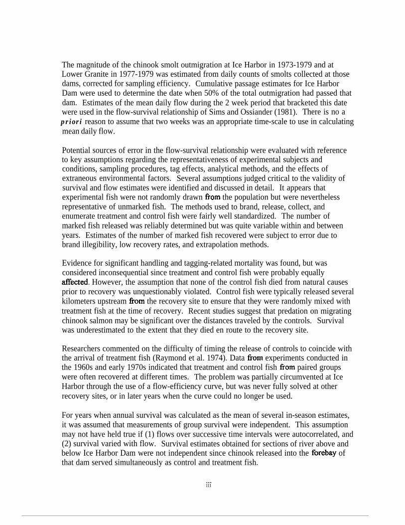
The magnitude of the chinook smolt outmigration at Ice Harbor in 1973-1979 and atLower Granite in 1977-1979 was estimated from daily counts of smolts collected at thosedams, corrected for sampling efficiency. Cumulative passage estimates for Ice HarborDam were used to determine the date when 50% of the total outmigration had passed thatdam. Estimates of the mean daily flow during the 2 week period that bracketed this datewere used in the flow-survival relationship of Sims and Ossiander (1981). There is no apriori reason to assume that two weeks was an appropriate time-scale to use in calculatingmean daily flow.

Potential sources of error in the flow-survival relationship were evaluated with referenceto key assumptions regarding the representativeness of experimental subjects andconditions, sampling procedures, tag effects, analytical methods, and the effects ofextraneous environmental factors. Several assumptions judged critical to the validity ofsurvival and flow estimates were identified and discussed in detail. It appears thatexperimental fish were not randomly drawn from the population but were neverthelessrepresentative of unmarked fish. The methods used to brand, release, collect, andenumerate treatment and control fish were fairly well standardized. The number ofmarked fish released was reliably determined but was quite variable within and betweenyears. Estimates of the number of marked fish recovered were subject to error due tobrand illegibility, low recovery rates, and extrapolation methods.

Evidence for significant handling and tagging-related mortality was found, but wasconsidered inconsequential since treatment and control fish were probably equallyaffected. However, the assumption that none of the control fish died from natural causesprior to recovery was unquestionably violated. Control fish were typically released severalkilometers upstream from the recovery site to ensure that they were randomly mixed withtreatment fish at the time of recovery. Recent studies suggest that predation on migratingchinook salmon may be significant over the distances traveled by the controls. Survivalwas underestimated to the extent that they died en route to the recovery site.

Researchers commented on the difficulty of timing the release of controls to coincide withthe arrival of treatment fish (Raymond et al. 1974). Data from experiments conducted inthe 1960s and early 1970s indicated that treatment and control fish from paired groupswere often recovered at different times. The problem was partially circumvented at IceHarbor through the use of a flow-efficiency curve, but was never fully solved at otherrecovery sites, or in later years when the curve could no longer be used.

For years when annual survival was calculated as the mean of several in-season estimates,it was assumed that measurements of group survival were independent. This assumptionmay not have held true if (1) flows over successive time intervals were autocorrelated, and(2) survival varied with flow. Survival estimates obtained for sections of river above andbelow Ice Harbor Dam were not independent since chinook released into the forebay ofthat dam served simultaneously as control and treatment fish.

. . .111

As the independent variable in the flow-survival relationship, flow was indexed to the dateof median passage of the entire smelt outmigration. Survival, however, was measuredfrom sequential releases of treatment fish -- the number, timing, and size of which werenot necessarily proportional to changes in the relative abundance of unmarked chinook inthe river. So that annual survival estimates would be representative of the unmarkedpopulation, an “average” survival was determined by weighting individual treatment groupsurvival estimates by the proportion of the total migration present. This computation mayhave introduced additional sources of error associated with sampling and estimatingpopulation size. For example, smelt abundance and time of peak migration may have beeninaccurately estimated on more than one occasion due to late startup or prematuretermination of sampling at dams.

Spurious correlations may have been introduced into the regression analysis by theinclusion of survival values that had been computed from the same set of data as flowestimates. In 1973, 1974, and 1975, a flow-efficiency curve was used to predict samplingefficiency at Ice Harbor Dam. The resulting survival estimates, which were themselves afinction of flow, were then regressed against flows that prevailed at the time that samplingefficiency was estimated.

Why were seasonal averages of survival and flow used in the regression analysis ratherthan individual treatment group survival and in-season flow estimates? From thestandpoint of sample size and model validity, it would have made more sense to regressgroup survival rates against flows that occurred at the time of recovery. The reasonappears to be that accurate measurements of survival of individual treatment groups wereoften hampered by small sample sizes and/or low recovery rates. The most dramaticexample of this was 1977, when 5 marked groups of 28 to 15,987 chinook were releasedfrom Lower Granite Dam; of the total of 38,262 fish released, only 19 (0.06%) weresubsequently recovered at Ice Harbor Dam (there is no record of recoveries at John Dayor The Dalles dams). Paradoxically, recovery rates determined for forebay-released fishwere frequently lower than those determined for chinook released further upstream. Myanalysis of unpublished mark-recovery data from 1966, 1967, 1968; and 1972 revealedthat survival, calculated as the ratio of treatment and control group recovery rates,exceeded 100% on 8 out of 22 occasions for fish traveling from the lower Salmon Riverto Ice Harbor Dam. Group survival was not significantly correlated with flow. Similarresults were obtained when the Ice Harbor flow-efficiency curve was used instead ofcontrol group recovery rates to estimate sampling efficiency.

Annual survival estimates used in the flow-survival relationship (Sims and Ossiander 1981)were compared with those reported in earlier documents. Several discrepancies werefound:

1. Sims and Ossiander (198 1) specified a survival value of 5% for the 1973 outmigration.Raymond et al (1974) indicated that this value was the estimated survival to The Dalles

iv

Dam of chinook released in the Salmon River. They reported 17% survival for chinookreleased at Little Goose Dam and subsequently recovered at The Dalles Dam.

2. Survival values reported by Raymond (1979) were lower than those used by Sims andOssiander (1981) for 1974 (34% vs. 40%) and 1975 (23% vs. 25%).

3. Survival values reported by Sims et al. (1977, 1978) and Raymond and Sims (1980)were higher than those used by Sims and Ossiander (1981) in 1976 (30% vs. 24%), 1977(3.3% vs. 2%), 1978 (44% vs. 37%), and 1979 (30% vs. 24%).

4. Although the 1975 survival value (25%) used by Sims and Ossiander (1981) wasconsistent with earlier reports, it represents a composite of survival estimates madeseparately for Rapid River Hatchery chinook (17%) and “native and other hatchery”chinook (38%).

Whereas survival was determined for chinook smelts migrating through segments of the. Snake and Columbia Rivers, the flow used in the flow-survival relationship was measuredat Ice Harbor Dam. Flow at Ice Harbor Dam may be a valid predictor of survival in theSnake River, but it is less appropriate for the Columbia River due to regional differencesin hydrological conditions and water management. More to the point, separate flow-survival relationships should have been derived for the Snake and Columbia Rivers sinceflows, smolt population characteristics, and various mortality factors may have variedbetween reaches within the same years.

Evidence suggests that a disproportionate percentage of chinook smolts died at the firstdam encountered on the Snake River, presumably due to the culling of unfit fish.Consequently, survival rates were generally lower in the Snake River than in the ColumbiaRiver. It should also be noted that the total and relative number of Snake and ColumbiaRiver projects upon which survival estimates were based changed over the 1973-1979period. If survival differed between projects or depended in some way on the totalnumber of projects, then the flow-survival relation may have been influenced by changes inthe configuration and number of projects.

Sims and Ossiander (1981) incorrectly specified the total number of projects in 4 (possibly5) of the 7 years for which overall survival was calculated. They indicated a total of 6projects in 1974 when only 5 were present. The Dalles Dam was included in estimates ofproject totals for 1976-1979 when, in fact, survival had only been empirically determinedfor chinook migrating to John Day Dam. Recalculated per-project survival rates for theseyears averaged 3%-6% lower than those used in the flow-survival relationship.

In their derivation of a flow-survival model, Sims and Ossiander (1981) assumed that thebasic relationship between independent and dependent variables did not change over theyears that data were collected. One must make a similar assumption when using themodel to predict survival for times or conditions other than those under which the data

V

were collected. Several developments occurred both during and after the period of datacollection which cast doubt on the validity of these assumptions. In particular,

1. The number of turbine units installed at Snake River Dams increased from 9 in 1973 to24 in 1979; the relative amounts of water spilled and run through turbines has changedover time;

2. Average fish guidance efficiency increased from 0.12 in 1973 to 0.29 in 1979;

3. Mortalities attributed to lethal concentrations of dissolved nitrogen were significant inhigh flow years (e.g., 1974) prior to the installation of spill deflectors in 1976;

4. Variable amounts of debris accumulated in the forebays of mainstem dams dependingon runoff conditions and efforts to effect its removal. Debris removal produced tangiblebenefits in terms of survivability of chinook migrants; and

5. Descaling and delayed mortality due to natural causes and sampling was extensive.

Annual per-project survival rates were negatively correlated with percent descaling anddelayed mortality measured in transportation experiments during 1973 - 1979. Correlationanalysis revealed that percent descaling and delayed mortality accounted for 86% and49%, respectively, of the observed variation in percent survival. This compares to 76% ofthe variation explained by flow in the original flow-survival regression model. All threeexplanatory variables were strongly correlated. My attempt to include flow, percentdescaling, and delayed mortality in a multiple regression model resulted in the inclusion ofdescaling rate alone as an independent variable; the addition of flow or delayed mortalitydid not significantly improve the predictive capability of the model.

There is concern over the potential effects that hatchery chinook may have had on wildfish survival, on survival estimates, and ultimately on the flow-survival relationship. Thetotal number of hatchery-origin chinook passing the first dam on the Snake River between1973 and 1979 ranged from 1.2 to 2.3 million fish. Hatchery chinook comprised between53% and 75% of the total chinook smelt population passing the upper dam.

Hatchery chinook traveled more slowly, died at higher rates, and may have been more (orless) vulnerable to capture than were their wild counterparts. Survival estimates weretherefore dependent on changes in the relative abundance and fitness of hatchery and wildfish over distance and through time.

Survival was estimated separately for hatchery and wild chinook up until 1975. Estimatesof chinook survival from the Salmon River to the upper Snake River dam for the 1966-1972 period were for wild chinook smelts only. Estimates for the 1973-1979 period werecombined estimates, even though separate estimates were obtained for hatchery and wildchinook in 1973-1975. When measured, survival rates for hatchery chinook were

vi

consistently lower than those observed for wild smolts, especially in the upper river.Higher mortality of hatchery fish may have been due to activation of bacterial kidneydisease.

Hatchery fish may have lowered the survival of wild chinook smolts by competing forscarce resources, by attracting and supporting larger predator populations, by alteringbehaviors and activity levels, and by transmitting disease. However, there is no directevidence that significant negative interactions actually occurred.

Impoundment of the Snake and Columbia rivers was accompanied by changes in theaquatic community. Predator species, both native and non-native, became more abundantand may have contributed to lower survival among chinook migrants over time.

From my assessment of the methods and data used by Sims and Ossiander (1981), Irecommend that the flow-survival relationship not be generalized to existing populationsand passage conditions. Fisheries managers, the public, and the fish themselves would bebetter served by data collected under present conditions using current technological andanalytical techniques. At the same time, however, positive steps should be taken toincrease inriver smolt survival rates to levels that permit the recovery and maintenance ofupriver salmonid populations.

vii

ACKNOWLEDGMENTS

This report was funded by the Bonneville Power Administration (BPA), U.S. Departmentof Energy, as part of BPA’s program to protect, mitigate, and enhance fish and wildlifeaffected by the development and operation of hydroelectric facilities on the ColumbiaRiver and its tributaries. I am grateful to Laura Hamilton and Tim Fisher of BPA for theirassistance in compiling portions of the historical database. Reviewers Michelle DeHart, AlGiorgi, Charlie Petroslq, and John Stevenson provided comments which were useful inrevising an earlier draft of the report. The direction and forebearance provided by DebbieWatkins, BPA project leader, was much appreciated.

. . .vlll

CONTENTS

EXECUTIVE SUMMARY . . . . . . . . . . . . . . . . . . . . . . . . . . . . . . .

ACKNOWLEDGMENTS . . . . . . . . . . . . . . . . . . . . . . . . . . . . . . .

1 .O INTRODUCTION. . . . . . . . . . . . . . . . . . . . . . . . . . . . . . . . .

2.0 SOURCES OF INFORMATION . . . . . . . . . . . . . . . . . . . . . . . . .

3 .O THE HISTORICAL DATABASE AND GENERAL ANALYTIC AL. APPROACH

3.1. Smolt Survival . . . . . . . . . . . . . . . . . . . . . . . . . . . . . . . .

3.2. Smolt Abundance . . . . . . . . . . . . . . . . . . . . . . . . . . . . . . .

3.3. Transportation . . . . . . . . . . . . . . . . . . . . . . . . . . . . . . . . .

3.4. Timing of Peak Migration . . . . . . . . . . . . . . . . . . . . . . . . . . .

3.5. Flow Estimates . . . . . . . . . . . . . . . . . . . . . . . . . . . . . . . .

4.0 POTENTIALSOURCESOFERROR. . . . . . . . . . . . . . . . . . . . . . .

4.1. Sampling and Statistical Assumptions . . . . . . . . . . . . . . . . . . . . .

4.2. Analytical Methods . . . . . . . . . . . . . . . . . . . . . . . . . . . .

4.2.1 Sample Sizes. . . . . . . . . . . . . . . . . . . . . . . . . . . .

4.2.2 RecoveryData . . . . . . . . . . . . . . . . . . . . . . . . . . .

4.2.3 Sampling Efficiency . . . . . . . . . . . . . . . . . . . . . . . . . .

4.2.4 In-season Survival Estimates . . . . . . . . . . . . . . . . . . . . .

4.2.5 Annual Survival Estimates . . . . . . . . . . . . . . . . . . . . . . .

4.2.6 Per-Project Survival Estimates . . . . . . . . . . . . . . . . . . . . .

4.2.7 Timing OfPeakMigration . . . . . . . . . . . . . . . . . . . . . . .

4.3. Additional Sources Of Variation . . . . . . . . . . . . . . . . . . . . . . .

4.3.1 Timing and Magnitude of Migration . . . . . . . . . . . . . . . . . .

4.3.2 Changes in the Hydro-System and Environment . . . . . . . . . . . .

4.3.2.1 Power Generation Capacity and Bypass Changes. . . . . . . .

ix

. . .111

. . .Vlll

1

6

7

9

16

17

18

20

20

23

38

38

40

41

46

52

57

60

60

61

62

62

4.3 2.2 Spill and Problems with Gas Supersaturation . . . . . . . . . . 65

4.3.2.3 DebrisRemoval . . . . . . . . . . . . . . . . . . . . . . . . 65

4.3.3 Scale Loss and Delayed Mortality. . . . . . . . . . . . . . . . . . . . 66

4.3.4. Biological Interactions . . . . . . . . . . . . . . . . . . . . . . . . . 69

4.3.4.1 Hatchery Fish . . . . . . . . . . . . . . . . . . . . . . . . . 69

4.3.4.2 Changes in the Biological Community . . . . . . . . . . . . . 73

5.0 SUMMARY AND CONCLUSIONS. . . . . . . . . . . . . . . . . . . . . . . 73

6.0 LITEFXlVRE!CITED. . . . . . . . . . . . . . . . . . . . . . . . . . . . . . . . 76

X

FIGURES

Figure 1.

Figure 2.

Figure 3.

Figure 4.

Figure 5.

Figure 6.

Figure 7.

Figure 8.

Figure 9.

Figure 10.

Major dams on the lower mainstem Snake and Columbia Rivers.

Flow-survival relationship derived by Sims and Ossiander (198 1; Figure6) for yearling chinook salmon, 1973-1979.

Chinook smolt flow-efficiency curve developed for Ice Harbor Dam(Source: Raymond 1979, Figure 2).

Dates of peak passage of chinook salmon migrants at upper dam(high bar), Ice Harbor Dam (mid bar), and lower dam (low bar). Upperdam passage dates are labeled. (Source: Sims and Ossiander [1981],Table 3).

Relationship between flow and survival obtained by Sims et al. (1983)using data from 1973-1979, 1980, and 1982.

Variations of Ice Harbor flow-efficiency curve for chinook salmonsmolts: Figures A and B display data from 1964, 1965, 1967-69;Figures C and D display data from the same years plus 1972. Figures A‘and C are drawn from data in unpublished tables compiled by Raymond;Figure B is a reproduction of Figure Al from Raymond et al. (1975);Figure D is a reproduction of an unpublished graph from NMFS files.

Proportion of fish released into the Salmon River in 1966, 1967, 1968and 1972 subsequently recovered at Ice Harbor Dam, expressed as afunction of flow.

cSurvival to Ice Harbor Dam of fish released into the Salmon River,determined by Method 1 (see text for details), plotted against river flowassociated with (A) the 50% recovery date (B) the 50% recovery date _+7 days, and (C) the 10% to 90% recovery dates.

Survival to Ice Harbor Dam of. fish released into the Salmon River,determined by Method 2 (see text for details), plotted against river flowassociated with (A) the 50% recovery date (B) the 50% recovery date f7 days, and (C) the 10% to 90% recovery dates.

Per-project survival as a function of Snake River flow, delayed mortality,and percent descaling. Data and sources are identified in Tables 4, 6,and 14.

2

4

4

21

37

45

48

49

50

71

xi

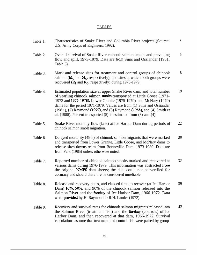
Table 1.

Table 2.

Table 3.

Table 4.

Table 5.

Table 6.

Table 7.

Table 8.

Table 9.

TABLES

Characteristics of Snake River and Columbia River projects (Source:U.S. Army Corps of Engineers, 1992).

Overall survival of Snake River chinook salmon smolts and prevailingflow and spill, 1973-1979. Data are from Sims and Ossiander (1981,Table 5).

Mark and release sites for treatment and control groups of chinooksalmon (Mt and M& respectively), and sites at which both groups wererecovered (Rt and Rc respectively) during 1973-1979.

Estimated population size at upper Snake River dam, and total numberof yearling chinook salmon smelts transported at Little Goose (1971-1973 and 1976-1978), Lower Granite (1975-1979), and McNary (1979)dams for the period 1971-1979. Values are from (1) Sims and Ossiander(198 l), (2) Raymond (1979), and (3) Raymond (1988), and (4) Smith etal. (1980). Percent transported (5) is estimated from (3) and (4).

Snake River monthly flow (kcfs) at Ice Harbor Dam during periods ofchinook salmon smolt migration.

Delayed mortality (48 h) of chinook salmon migrants that were markedand transported from Lower Granite, Little Goose, and McNary dams torelease sites downstream from Bonneville Dam, 1973-1980. Data arefrom Park (1985) unless otherwise noted.

Reported number of chinook salmon smolts marked and recovered atvarious dams during 1976-1979. This information was abstracted fromthe original NMFS data sheets; the data could not be verified foraccuracy and should therefore be considered unreliable.

Release and recovery dates, and elapsed time to recover (at Ice HarborDam) lo%, 50%, and 90% of the chinook salmon released into theSalmon River and the forebay of Ice Harbor Dam, 1966-1972. Datawere .provided by H. Raymond to R.H. Lander (1972).

Recovery and survival rates for chinook salmon migrants released intothe Salmon River (treatment fish) and the forebay (controls) of IceHarbor Dam, and then recovered at that dam, 1966-1972. Survivalcalculations assume that treatment and control fish were paired by group

xii

3

5

8

19

22

30

32

39

42

Table 10.

Table 11.

Table 12.

Table 13.

Table 14.

Table 15.

Table 16.

within years. Data were provided by H. Raymond to R.H. Lander(1972).

Annual survival values (%) for yearling chinook migrants, as reported byvarious authors for the period 1973-1979. Reach 1 = Little Goose Dam(1973-1974) or Lower Granite Dam (1975-1979) to Ice Harbor Dam;Reach 2 = Ice Harbor Dam to The Dalles Dam (1973-1975) or John DayDam (1976- 1979); Reach 3 = overall survival from upper to lower dam.

Number of Snake and Columbia River projects used by Sims andOssiander (1981) to calculate “per project” survival, compared to thenumber of projects ascertained from original literature sources.

Number of turbine units at hydroelectric dams on the Snake River, 1968-1979.

Adjusted fish guiding efficiencies, spring chinook, 1970-l 980.

Percentage of descaled (>lO%) spring chinook salmon migrants sampledfrom the marking facility at Lower Granite, Little Goose, and McNarydams, 1972-1980. Data are from Park (1985) unless otherwise noted.

Bivariate correlation coefficients and significance levels (in parentheses)for selected variables relating to chinook salmon smolt migrations, 1973-1979. Values are based on a sample size (n) of 7 except for correlationsinvolving the descaled variable, in which case n = 6 (no data for 1974).Flow values were transformed to their logarithms; all other values areuntransformed.

Numbers of juvenile chinook salmon released from Rapid River Hatcheryand survival estimates, 1966-1975. S 1 = survival from hatchery to upperdam; S2 = survival from upper to lower dam; S3 = survival fromhatchery to lower dam. These data were compiled by H.L. Raymond,but were not published.

53

58

63

64

67

68

71

. . .XIII

1 .O INTRODUCTION

“The past is not what it used to be.”- Michael Bruton

Alternative Life-History Styles of Fishes

There has been much debate recently among fisheries professionals over the data andfunctional relationships used by Sims and Ossiander (1981) to describe the effects of flow inthe Snake River on the survival and travel time of chinook salmon and steelhead smolts. Therelationships were based on mark and recovery experiments conducted at various Snake andColumbia River sites between 1964 and 1979 (Figure 1) to evaluate the effects of dams andflow regulation on the migratory characteristics of chinook salmon and steelhead trout smolts.The reliability of this information is crucial because it forms the logical basis for many of theflow management options being considered today to protect upriver populations of chinooksalmon and steelhead trout (Salmon River Recovery Team 1993).

Mainstem habitats in the Snake and Columbia rivers in the 1970s differed in many importantrespects from those that existed historically. New hydroelectric dams were being built andoperated that not only impeded migration, they created lake-like environments through whichsmolts and adults were forced to pass (Table 1). By the mid-70s, mainstem survival haddeclined to less than half that observed during the previous decade (Raymond 1979). Most ofthe decline was attributed to increased turbine mortality at the dams, increased predation, lethalconcentrations of dissolved gases that prevailed in high flow years, and increased residualism inlow flow years.

Mainstem habitats continued to change in response to further hydrosystem developments, notall of which may be viewed as detrimental. Examples include improvements in fish bypass andtransportation systems, installation of spillway deflectors, efforts to control predatorpopulations, and an increased ability and commitment on the part of hydropower managers to“shape” mainstem flows and spill to facilitate migration. Although the survival of wild chinooksalmon smolts has not been reliably measured in recent years, it has probably increased fromlevels observed in the 1970s. Nonetheless, further increases in smolt survival are needed ifupriver stocks are to regain their former abundance.

In this paper I evaluate the primary data, assumptions, and calculations that underlie the flow-survival relationship derived by Sims and Ossiander (198 1) for chinook salmon smolts (Figure2). Those authors used least squares regression analysis to fit a straight line to seven pairs ofdata corresponding to flow and survival estimates for the years 1973 through 1979 (Table 2).The line is described by the equation log Y = 2.488 + 0.395 log X, where Y is the averagesurvival per dam and X is the mean daily flow at Ice Harbor Dam during the period of peakmigration.

)) Priest Rapids Dam Little Goose Dam

The Dalles Dam

Lower Monumental

l Sampling Sites

Figure 1. Major dams and smolt sampling sites on the lower Snake and Columbia Rivers.

w

Table 1. Characteristics of projects through which Snake River chinook salmon smolts must migrate en route to the ocean(Source: U.S. Army Corps of Engineers, 1992).

Reservoir Reservoir Elevation ReservoirProject First Year Dam Location Reservoir Name Capacity Normal Operating I-w@

of Operation (River Mile) (acre feet) Range (msl) ON

Lower Granite Dam 1975 107.5 Lower Granite Lake 49,000 733-738 43.9

Little Goose Dam 1970 70.3 Lake Bryan 49,000 633638 37.2

Lower Monumental 1969 41.6 537-540 28.7Lake Herbert G. West 20,000

Ice Harbor Dam 1962 9.7 Lake Sacajawea 25,000 437-440 31.9

McNary Dam 1953 292 Lake Wallula 185,000 335-340 61.6

John Day Dam 1968 215.6 Lake Umatilla 500,000 265-268 (7/l-10/1) 76.4260-265 (11/l-6/1)

The Dalles Dam 1957 191.5 Lake Celilo 53,000 155-160 24

Bonneville Dam 1937 146.1 Lake Bonneville 100,000 71.5-76.5 45

4.75 - /

/

/C H I N O O K

3.75 - Y = 2.488 + 0.395X

/r = 0.87

- - 95% conf idenceinterval

3 . 5 0 . I I I I I I I I3 . 5 4 . 0 4 . 5 5.0 5.5

Log average flow at Ice Harbor Dam (cfs!27 days of peal: migration

Figure 2. Flow-survival relationship derived by Sims and Ossiander(198 1, Figure 6) for yearling chinook salmon, 1973- 1979.

Figure 3. Chinook smolt flow-efficiency curve developed forIce Harbor Dam (Source: Raymond 1979, Figure 2).

4

Table 2. Overall survival of Snake River chinook salmon smelts and prevailing flow andspill, 1973-1979. Data are from Sims and Ossiander (1981, Table 5).

Year ’ Survival to The Survival per Flow at Ice Mean spillDalles Dam (%) project (%) Harbor Dam WW

(kcfs)’

1973 5 55 71 8.6

1974 40 86 158 102.8

1975 25 79 140 102.8

1976 24 79 110 67.0

1977 2 52 40 2.0

1978 37 85 106 34.7

1979 24 79 85 8.3

5

A major objective was to determine how survival and flow were estimated for each of the years1973 through 1979. Techniques used to sample chinook migrants and to estimate survival andflow are evaluated in Section 3.0. Calculations of survival and flow required reference tochinook smolt timing and abundance, so I have also reviewed the methods used to estimatethese parameters.

The validity of the flow-survival data and the regression model by which they are expressedrests on several key assumptions concerned with sampling and statistical procedures. Theseassumptions and evidence for and against their having been met are discussed in Section 4.1.Several numerical discrepancies were noted in flow and survival values reported by Sims andOssiander (198 1) and those found in other documents and unpublished records. Thediscrepancies and their potential causes are discussed in Section 4.2.

Year-to-year variability in natural and anthropogenic factors affecting the migratoryenvironment and their potential effects on survival and flow estimates are discussed in Section4.3. Changes in the hydrographic regime, hydrosystem structure, the biological community,and the chinook population itself may have altered the basic relationship between flow andsurvival. I have attempted to show that the survival of outmigrating chinook salmon may havebeen influenced by factors which were to some extent independent of flow, such as physicalinjury and interactions with hatchery fish. By pointing out alternative explanations for the Simsand Ossiander (198 1) flow-survival relationship and by highlighting some of the limitations ofthe data upon which it was based, it is hoped that an appropriate conclusion is reached.Namely, that decision makers today would be better served by data collected under existingconditions using current technological and analytical techniques.

2.0 SOURCES OF INFORMATION

As a first step, I assembled and reviewed published and unpublished material retrieved fromNational Marine Fisheries Service (NMFS) archives. Sims and Ossiander (198 1) refer toRaymond et al. (1975) and Raymond (1979) as sources of information on the data andmethods which were used to calculate survival. Raymond and his colleagues initiated studiesof chinook and steelhead smolt survival, timing, travel time and relative magnitude of the runsin 1964. Carl Sims became principle investigator on the smolt survival studies in 1975. Bothhe and Frank Ossiander, a statistician at NMFS, remained involved until Al Giorgi assumedcontrol of the smolt survival studies in 1985.

Although not specifically mentioned in Sims and Ossiander (198 l), data collected in the late1970s under the direction of another NMFS researcher -- Don Park -- also figured in survivalestimation. Park headed the agency’s smolt transportation studies -- a long-term (and stillongoing) investigation of the feasibility of collecting chinook and steelhead smolts at SnakeRiver dams and transporting them by barge and truck to release sites in the lower ColumbiaRiver below Bonneville Dam.

6

Raymond left copious handwritten notes and calculations of smelt survival and abundance onfile when he retired from NMFS. This material was carefully reviewed and referenced againstsimilar information compiled in published reports. I was unable to locate supplemental notesor calculations that may have been left on file at NMFS by Sims, Ossiander, or Park. Most ofthe information discussed with reference to these individuals was obtained either frompublished reports or from a partial record of release and recovery data. Original data sheetsfrom the late 1970’s were located at NMFS. With the assistance of Laura Hamiltonl, Ireanalyzed mark/recapture and transportation data from 1978 and 1979 in an attempt tovalidate run timing and survival estimates for those years. We were unsuccesstil for severalreasons, as discussed below, so made no further effort to reproduce survival estimates fromdata recorded for earlier years,

3.0 THE HISTORICAL DATABASE AND GENERAL ANALYTICAL APPROACH

Under the direction of Howard Raymond, researchers from the Bureau of CommercialFisheries (now NMFS) began monitoring chinook and steelhead smelts in 1964 in the SalmonRiver and at Ice Harbor Dam (Table 3). At the time, only Bonneville, The Dalles, McNary,and Ice Harbor dams existed on the lower Columbia and Snake Rivers (Figure 1). NMFS’smelt monitoring program was expanded to include The Dalles Dam and McNary Dam in1966, and John Day Dam following its construction in 1968. Sampling for smelts at LittleGoose Dam on the Snake River began upon completion of the dam in 1970. Lower GraniteDam was built in 1975, and thereafter became the uppermost hydroelectric project to bemonitored for smolts.

At each monitoring site, smelts were collected, enumerated, and examined for marks more-or-less continuously during the outmigration season. Subsamples of fish were marked withthermal brands and released into the river to continue their downstream journey. Up to thirtyindividual groups of fish could be distinctively marked each year by changing the brandorientation and/or location every 3 to 7 days (Raymond 1979). Smolt monitoring based onrecoveries of externally marked fish continued until the development of the passive integratedtransponder (PIT) tag in the mid-1980s (Prentice et al. 1990). Smolts are now implanted withPIT tags and passively monitored as they pass through specially designed detection facilities atLower Granite, Little Goose, Lower Monumental, and McNary Dams.

Before the advent of PIT tags, NMFS biologists relied on external mark-recapture datacollected at various monitoring sites to quantify, for both chinook salmon and steelhead, (1)the rate of travel between release and recovery sites under a variety of flow conditions, (2) theproportion of fish surviving between these points, and (3) the abundance and timing of smoltsmigrating past various Snake and Columbia River dams. NMFS researchers attempted toobtain separate estimates for sequentially released groups of uniquely marked fish, but were

1 A graduate student at the University of Washington at the time.

7

Table 3. Mark and release sites for treatment and control groups of chinook salmon &itand Mc, respectively), and sites at which both groups were recovered (Rt andRc, respectively) during 1973- 1979.

FirsI Year 1973 1974 1975 1976 1977 1978 1979ofopemtioll

Rapid River Hatchery

Riggins Smelt Trap

Whitebird Smolt Trap

Lower Granite Dam

Little Goose Dam

Lower Monumental Dam

Ice Harbor Dam

McNary Dam

John Day Dam

The Dalles Dam

Bonneville Dam

1966

1964

1964

1975

1970

1969

1962

1953

1968

1957

1937

Mt

unsuccessful. Virtually all estimates of timing, travel time, survival, and run size were reportedas seasonal averages.

3.1 Smolt Survival

Survival of yearling chinook between the uppermost dam on the Snake River and The Dallesor John Day Dam on the Columbia River was determined for each of the years 1966-1979,with the exception of 197 1, when there was no sampling at either of the lower dams. Theflow-survival relationship derived by Sims and Ossiander (198 1) was based on data from theyears 1973-1979. The authors did not explain why they excluded years prior to 1973 fl-omtheir analysis.

As originally conceived, the calculation of survival was relatively straightforward; it was thefraction of marked fish released from an upstream site that were subsequently recovered at adownstream site, adjusted for the sampling (collection) efficiency of the downstream site. IfMj fish are marked and released at an upstream site, where the subscript i denotes a pairedtreatment-control group (i = 1, 2, . . ., n) released within a season, and Rj fish are subsequentlyrecovered at a downstream site, then ci = R#%fi is the fraction of treatment fish in group irecovered

Sampling or collection efficiency, ei, at the downstream site can be estimated as the fraction ofcontrol fish released immediately upstream of the site that are subsequently recaptured, ei =

. r{mi, where mi is the number of fish in treatment-control group i released, and ri is the numberof control fish eventually recovered.

The percentage, gj, of treatment fish in group i that survive to the downstream site is estimatedas:

$3 x 100ei

Eq. 1

Paulik and Robson (1969) provide equations for deriving confidence limits. For ii to be avalid estimate of the survival of treatment fish in group i, the following assumptions must holdtrue:

1. treatment and control fish are randomly mixed,2. the probability of recovery is the same for all fish,3. the probability of mortality due to handling and marking is the same for all fish, and4. control fish suffer no additional mortality prior to recapture.

Since most treatment fish arrived at downstream dams over time periods of variable flow and,hence, sampling efficiency, an average sampling efficiency was calculated based onproportional recoveries at different flows. To use Raymond’s (1979, p. 5 11) example, if30%

9

of the treatment fish in a particular group were recovered at an efficiency of 8%, 50% at 4%,and 20% at 2%, then the average sampling efficiency for that group was 8%(0.3) + 4%(0.5) +2%(0.2 )= 4.8%. If the percentage of treatment fish recovered over the same time interval was2.6%, 4 would be 2.6 / 4.8 = 54%.

In most years, brand recoveries were enumerated in subsamples from the sampled (dipnettedgatewells or bypass) population and expanded to estimate fi and mj. Thus, it was assumed thatsubsampled fish were representative of (randomly selected from) the unsampled population,and that the proportion of fish subsampled was accurately determined.

If n paired groups of treatment and control fish are sequentially released, then average survivalcan be calculated:

nc ii

3 -i=l x 1 0 0 Eq. 2n

Sample variance for the n independent estimates:

n 2

C(s-4)3 = i-l

n - lEq. 2a

For S to be representative of the population at large, it must be assumed that either survivaldoes not vary over time (i.e., each group is a true replicate), or marked fish are exposed to thesame kind and degree of mortality, with the exception of marking and handling effects, as areunmarked fish. Clearly, the former assumption is untenable under a variable flow regime. - Theassumption of equal probability of mortality would only be achieved through frequent andrandom sampling.

Raymond (1979) elected to weight treatment-control group survival estimates by theproportion of the total annual migration (indexed to the release site2) represented by eachgroup to determine average annual survival. If the proportion of the total migration at time ofrelease is denoted pi, then

2 To be representative, individual 3i ‘s should be weighted by the proportion of the run passing the release siteat the time test fish were released. As Raymond (1979, p 5 11) noted, however, the number of smelts passingLower Granite and Little Goose Dams was not empirically measured; it was estimated as the product of 4 andthe number of fish passing Ice Harbor Darn.

10

Eq. 3

Thus, if Zi ‘s of 50%, 30%, 25%, 50%, and 30% were obtained for five treatment groups overthe course of a season, and lo%, 20%, 40%, 20%, and 10% of the total run was represented,respectively, .by each of the groups, then the average annual survival was (50%)(0.1) +(30%)(0.2) + (25%)(0.4) + (50%)(0.2) + (30%)(0.1) = 34%. This example is taken from page5 12 of Raymond (1979). All of the previously stated assumptions apply.

The number of smolts passing Ice Harbor Dam during a sampling interval was determined bydipnetting gatewells (nine in all) at the dam, and then dividing by the sampling efficiencydetermined for that time interval.

Sampling efficiency was observed to decline predictably with increasing flow at all dams forboth chinook salmon and steelhead trout, especially after water began to be spilled. Thedesirability of developing a mathematical relationship from multiple observations in order to beable to predict sampling efficiency as a function of river flow at a recovery site was recognizedas early as 1967 (Raymond et al. 1974). If a flow-efficiency curve specific to a recovery sitecould be developed, it was reasoned, it would be unnecessary to continually release control fishabove the site to estimate its sampling efficiency at different flows. Moreover, estimates of Swould be more precise since the s^ i(s were based on sampling efficiencies determined forcomparatively short time intervals (and constant flows) at the time of recovery. One potentialdrawback to using a flow-efficiency curve is that it requires the assumption that the relationbetween sampling efficiency and flow does not change (because of changes in the environment,the fish, or both) after the development of the flow-efficiency curve.

Data were collected in 1964-69 and 1972 for the purpose of establishing flow-efficiency curvesfor The Dalles and Ice Harbor dams. A chinook salmon flow-efficiency curve was neverproduced for The Dalles Dam. The curve developed for Ice Harbor Dam (Figure 3)underwent considerable refinement after 1972 (without benefit of new data) before emerging infinal form in Raymond (1979). More is said later of the versatility Raymond displayed indeveloping and applying the Ice Harbor flow-efficiency curve to estimate chinook smoltsurvival and abundance.

Summary data (total number of fish marked and recovered) relating to sampling efficiencies atlower river dams, and to recoveries at Little Goose Dam, were reported for 1973 and 1974(Raymond et al. 1974 - Table 6; 1975 - Appendices), but not for later years. According toRaymond (1979, p. 5 lo), sampling efficiencies were not determined at Little Goose or LowerGranite dams during 1973-1975 because of potential conflict with ongoing fish transportationexperiments. Sampling efficiency was determined for Lower Granite Dam from 1976- 1979 byreleasing smolts in the forebay of the dam and determining the proportion recovered in thefingerling collection system at the dam. Sampling efficiency was used in conjunction withcounts of fish collected in the fingerling collection system to estimate the total number ofsmolts passing Lower Granite Dam. As will be shown later, the ratio of population sizes at

11

John Day and Lower Granite dams was used to estimate survival in the Snake River andColumbia River during 1976- 1979.

Sampling efficiency data from 1973- 1975 specific to individual treatment and control fishreleases during could not be located in NMFS reports or files. Summary data for 1973 and1974 were reported by Raymond et al. (1974 - Table 6; 1975 - Appendices). I discusselsewhere mark-recovery data for 1976-1979 that was found in NMFS files (see Section 4.23SamnlinP Efficiencv).

The Ice Harbor flow-efficiency curve (Figure 3) was used by Raymond (1979) to estimatepopulation size and pi at that dam during sampling intervals of relatively constant flow during1973-1975. With the installation of three additional turbine units at Ice Harbor Dam in thesummer of 1975, the relation between flow and sampling efficiency at the dam changed. As aconsequence, the flow-efficiency curve was not used to estimate survival following the 1975season. Sampling efficiency was measured directly from recovery rates of fish released in theforebay of Ice Harbor Dam during 1976-1979.

Raymond et al. (1975) used the chinook flow-efficiency curve developed for Ice Harbor Damto predict sampling efficiency at that dam in 1974 for sampling intervals ranging from 2 to 20days. Sampling intervals corresponded to periods of comparatively stable flow during thechinook outmigration. Claiming that too few chinook were marked and recovered in 1974 toestimate survival for individual treatment-control groups, Raymond et al. (1975; see theirAppendix Table A2) devised two other approaches to estimating S : one to estimate survivalto Ice Harbor Dam, the other to estimate survival in the lower river.3 To accomplish theformer, Raymond et al. (1975) first calculated an average recovery rate, F, for treatment fishby combining mark-recovery data across all groups:

He then estimated an average seasonal efficiency:

e = &q,)bl

Eq. 4

Eq. 5

3 Raymond et al. (1975 Report, App A2) noted that “There were not enough fish recovered on a weekly basisin 1974 to provide estimates of week to week differences in survival. Therefore, in 1974, weekly releases werecombined for the entire outmigration to provide a seasonal survival estimate through each stretch of river. ”

12

where sampling efficiency, e, , is determined for each flow intervalj using the chinook flow-efficiency curve and q, is the proportion of the total number of marks recovered in the sametime interval. Note that the average sampling efficiency was weighted by fraction of marksrecovered and not by the proportion of the total run passing the dam, as claimed by Raymond(1979). The reader should consult Appendix Table A2 in Raymond et al. (1975) for samplecalculations of Z .

Survival, S, from Little Goose Dam to Ice Harbor Dam was calculated as:

Implicit to Eq. 6 is the assumption that the number of marks recovered in any time interval isproportional to the total number of fish present in the same time interval. For S to berepresentative, recoveries of treatment fish over the outmigration period should correspond infrequency and timing to that of the unmarked population.

Equation 6, where Z is determined by Eq. 5, could not be used to estimate survival below IceHarbor Dam in 1974 (or in later years) because flow-efficiency curves were never completedfor downstream dams. To complicate matters further, Raymond et al. (1975; Appendix A2)concluded that “insufficient numbers were recovered from forebay releases at The Dalles Damfor accurate measure of our sampling efficiency there in 1974.” An average samplingefficiency, (E)), was therefore calculated by summing across control groups.

Eq. 7

Because the number of recoveries in 1974 precluded estimates of group survival, Raymond etal. (1975) calculated the average survival of chinook migrating from Ice Harbor to’The DallesDam by combining treatment and control fish recoveries over the entire season:

Eq. 8

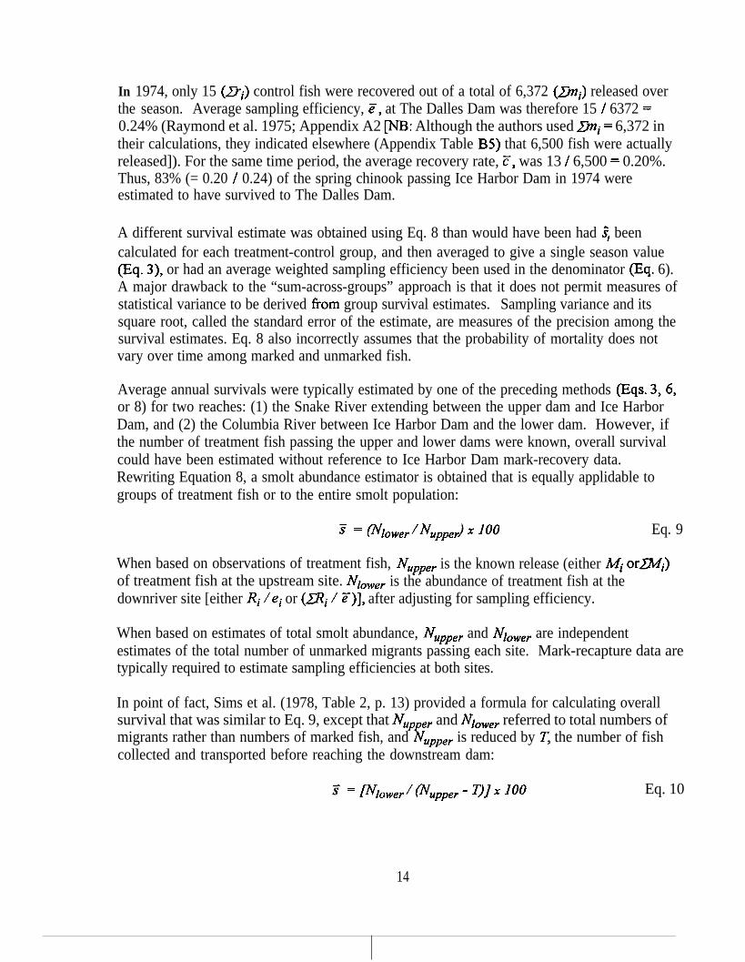
In 1974, only 15 (LPi) control fish were recovered out of a total of 6,372 (mi) released overthe season. Average sampling efficiency, Z, at The Dalles Dam was therefore 15 / 6372 =0.24% (Raymond et al. 1975; Appendix A2 p: Although the authors used mi = 6,372 intheir calculations, they indicated elsewhere (Appendix Table BS) that 6,500 fish were actuallyreleased]). For the same time period, the average recovery rate, C, was 13 / 6,500 = 0.20%.Thus, 83% (= 0.20 / 0.24) of the spring chinook passing Ice Harbor Dam in 1974 wereestimated to have survived to The Dalles Dam.

A different survival estimate was obtained using Eq. 8 than would have been had ij beencalculated for each treatment-control group, and then averaged to give a single season value(Eq. 3), or had an average weighted sampling efficiency been used in the denominator (Eq. 6).A major drawback to the “sum-across-groups” approach is that it does not permit measures ofstatistical variance to be derived from group survival estimates. Sampling variance and itssquare root, called the standard error of the estimate, are measures of the precision among thesurvival estimates. Eq. 8 also incorrectly assumes that the probability of mortality does notvary over time among marked and unmarked fish.

Average annual survivals were typically estimated by one of the preceding methods (Eqs. 3,6,or 8) for two reaches: (1) the Snake River extending between the upper dam and Ice HarborDam, and (2) the Columbia River between Ice Harbor Dam and the lower dam. However, ifthe number of treatment fish passing the upper and lower dams were known, overall survivalcould have been estimated without reference to Ice Harbor Dam mark-recovery data.Rewriting Equation 8, a smolt abundance estimator is obtained that is equally applidable togroups of treatment fish or to the entire smolt population:

Eq. 9

When based on observations of treatment fish, NUPPer is the known release (either Mi ormJof treatment fish at the upstream site. Nlower is the abundance of treatment fish at thedownriver site [either Ri /ei or (JXi / Z)], after adjusting for sampling efficiency.

When based on estimates of total smolt abundance, NUPPer and NloWer are independentestimates of the total number of unmarked migrants passing each site. Mark-recapture data aretypically required to estimate sampling efficiencies at both sites.

In point of fact, Sims et al. (1978, Table 2, p. 13) provided a formula for calculating overallsurvival that was similar to Eq. 9, except that NUPPer and Nlower referred to total numbers ofmigrants rather than numbers of marked fish, and NUPPer is reduced by T, the number of fishcollected and transported before reaching the downstream dam:

Eq. 10

14

qqp?, and %nvt?r are estimates of total smolt abundance at the two dams, application of Eq.10 requires only that the total number of fish removed from the population be known, and doesnot require knowledge of the number of markedfsh transported. However, Eq. 10 can beused to estimate 5 for individual groups of marked fish if the numbers of those fish that weretransported can be estimated. This was actually done in later years (Sims et al. 1983,Appendix Table 12).

Application of Eq. 10 to smelt abundance data found in Sims et al. (Tables 3 & 4 - 1976; Table2 - 1977; Table 2 - 1978) and Raymond and Sims (Table 6 - 1980) yields survival estimatesthat agree precisely with those reported in the same documents. This would appear to explainthe footnote to Table 4 in Sims et al. (1977, p. 12), which refers to “800,000 chinook salmon. . . transported below Bonneville Dam subtracted from total smolts passing Lower Granite Damfor calculations of survival.”

There is additional evidence to suggest that Eq. 10 might have been used to calculate survivalduring 1976-1979, at least for the section of river between Lower Granite and Ice HarborDams. Sims and Ossiander (1981, p. 5) reported that population estimates at Lower GraniteDam during 1976- 1979 were independently estimated by applying efficiency releases tosamples fi-om the fingerling collection system. With independent estimates of N at LowerGranite and Ice Harbor dams, a ratio-based estimate of survival is possible.

The question is unresolved as to whether survival from Lower Granite to Ice Harbor Dam (or,less likely, from Lower Granite to John Day Dam) in the late 1970’s was determined from ratioestimates (Eq. 10) of total smolt abundance or numbers of marked fish. I believe that survivalwas estimated Corn a comparison of marked fish recoveries that had been adjusted to reflectcollection efficiencies and losses due to transportation. Raymond and Sims (1980) appear toconfirm this view, as evidenced by their statement: “survival is estimated by comparing theactual recovery rate of marked fish released at a given dam with the expected recovery rate atthat dam as determined Corn measures of sampling efficiency.” As pointed out above, toestimate survival Corn the ratio of number of marked fish passing upper and lower dams, oneneeds to know the number of marked fish collected and transported at intervening dams. Howthis number was actually determined is unknown.

There is strong evidence to suggest that Eq. 10 was used to calculate survival Corn LowerGranite to Ice Harbor Dam and from Ice Harbor to John Day Dam in 1976. Eq. 10 was alsoused to estimate survival from Lower Granite to John Day Dam in 1977-1979. It was not usedto estimate survival in the Snake River in years prior to 1976 since, as Raymond (1979, p. 5 11)remarked, the “magnitude of populations at Lower Granite and Little Goose dams wasdetermined Corn the percentage of fish marked at Lower Granite or Little Goose dams thatsurvived to Ice Harbor Dam and applying that proportion to the numbers of fish estimated atIce Harbor Dam.” To use his example: “If 2 million chinook salmon were estimated at IceHarbor Dam and survival was 50% between Little Goose and Ice Harbor dams, then 4 millionfish must have passed Little Goose Dam.” If survival from Ice Harbor to The Dalles or JohnDay dams remained at 50%, then 1 million fish must have passed the lower dam. In other

15

words, survival was estimated first, and then applied to the smolt abundance determined for IceHarbor Dam to estimate populations at other dams.

Sims et al. (1982) did not estimate survival from Lower Granite to John Day dam in 1981because sampling efficiencies and the number of marked fish transported at McNary Dam werenot measured. Although smolt monitoring was conducted at McNary Dam in the followingyear, researchers confronted a similar problem when Little Goose Dam sampling wasdiscontinued. However, by making certain assumptions about survival between Lower Graniteand Little Goose Dam, and collection efficiency at Little Goose Dam, Sims et al. (1983,Appendix 12) were able to estimate the survival of individually marked groups of chinook in1982. Group survival (C?i ) was estimated by:

1. dividing observed recovery rates at Lower Granite and John Day dams by prevailingsampling efficiencies to estimate the total number of marked fish in each group that arrivedat the two dams,

2. estimating NUpper - the number of fish in a group that passed Lower Granite Dam - bysubtracting the estimated number of marked fish that were collected and transported fromthe dam,

3. estimating Nlower - the number of fish in a group that would have arrived at John DayDam had none been transported at intervening dams - by subtracting the estimatednumber of marked fish, that were collected and transported from Little Goose and McNarydams, and then

4. calculating ii = (lvloWer /Nupper) 3~ 100 (Eq. 10).

An average survival, S, was calculated as the mean of the four group survival estimates.

3.2 Smolt Abundance

Mention is made briefly here of the method used to calculate instantaneous and cumulativenumbers of chinook migrants passing Ice Harbor Dam and Lower Granite Dam. Populationestimates for Ice Harbor Dam, in particular, were important since the flow associated with thedate of median passage at that dam was the independent variable in the flow-survivalrelationship of Sims and Ossiander (198 1). Lower Granite Dam is considered becauseempirical estimates of smolt abundance obtained there in 1976-1979 may have been used insurvival calculations. Population sizes at The Dalles and John Day dams were indexed to IceHarbor Dam estimates in 1973-1978, and to the Lower Granite Dam estimate in 1979, and SO

are of little interest. Little Goose populations in 1973 and 1974 were similarly indexed to IceHarbor Dam.

16

Details on the methods used to sample smelts and estimate their abundance at Ice Harbor Damprior to 1976 are provided by Bentley and Raymond (1968), Raymond et al. (1975), andRaymond (1979). Raymond’s unpublished notes yielded valuable information. The magnitudeof the chinook smelt population in years 1964 through 1975, excluding 1969, was determinedby summing for a year time-specific gatewell catches divided by the prevailing samplingefficiency. To estimate the total number of smolts passing the dam over a given time interval,the number of fish collected in each gatewell was divided by the sampling efficiency for thattime interval. It was occasionally necessary to expand catches to unsampled gatewells andtime periods (mainly weekend days; Raymond, unpublished notes). A flow-efficiency cmvesimilar to the one portrayed in Figure 3 was used to estimate sampling efficiency over shorttime intervals of comparatively stable flow. Flow-efficiency curves were not applied after 1975due to an increase in the number of turbines operating at the Ice Harbor Dam.

It is assumed that direct measures of sampling efficiency were used to expand chinook smeltcounts in later years, but few details could be gleaned from Sims et al. (1976, 1977, 1978) orRaymond and Sims (1980). The authors tabulated weekly smolt catches at Ice Harbor Damand other sampling locations; they also indicated the week in which 50% of the total samplehad been collected. But the dates indicated were based on the unexpanded counts and did nottake sampling efficiency into account. I was unable to locate sampling efficiency data (i.e.,control group mark-recovery data) specific to Ice Harbor Dam for 1977-1979. Without thisinformation, it remains unclear exactly how population sizes and, more importantly, dates ofmedian passage were estimated.

Sims and Ossiander (198 1) and Sims et al. (198 1, p. 2) clearly indicated that populationestimates for Lower Granite Dam in 1976-1979 were obtained by dividing the number of fishcollected from the fingerling collection system by the efficiency of collection, as empiricallydetermined from releases of control fish into the forebay above the dam. However, thiscontradicts information provided by Sims et al. (1976, 1977) and Raymond and Sims (1980),who stated that smolt numbers at Lower Granite Dam were estimated by first determining thefraction of marked fish surviving from that dam to Ice Harbor Dam and, after adjusting fortransportation losses, multiplying that fraction by the Ice Harbor population estimate. The factthat sampling efficiency may not have been estimated and survival to Ice Harbor Dam wentreported’ after 1976 begs the question of how the median date of passage (and, hence, meanflow) at the dam was actually determined for later years.

3.3 Transnortation

Beginning in 1968, an attempt was made to improve the survival of chinook and steelheadsmolts by collecting them at strategic locations in the Columbia basin during their downstreammigration, and then transporting them downstream of Bonneville Dam for release. Smoltswere collected and transported from 1973 to 1979, except 1974, from Lower Granite Damand/or Little Goose Dam (Table 4). Sims and Ossiander (198 1, Table 1, p. 7) indicated thatchinook salmon smolts were not transported in 1973, but Park and Ebel(l975) and Raymond(1979) provided data which suggested otherwise. The number of chinook smelts transported

17

from the two Snake River dams increased from 247,000 fish in 1973 to 2.1 million in 1979(Smith et al. 1980). Mass transportation at McNary Dam began in 1979 with thetransportation of 0.3 million yearling chinook salmon.

Although the total number of fish collected and transported from Snake River dams wasroutinely estimated, the lack of published estimates of the number or percentage of treatmenffish transported suggests that no special effort was made in this regard. Clearly, marked fish,once collected, were not returned to the river. In most years, therefore, an unknown fractionof the treatment fish were “lost” to transportation before they arrived at Ice Harbor Dam. If nocompensatory adjustments were made to account for these losses, survival estimates based onmark recoveries would be biased downwards. The effect would be especially notable in low-survival years such as 1977 when a high percentage (70%) of the run-at-large was transported(Table 4).

I found no mention in NMFS reports of specific computational steps taken to account fortransportation of marked fish.4 The record clearly shows that removal effects were notconsidered in the calculation of transportation benefits (Park 1985), so it seems unlikely thatNMFS researchers attempted to do so when calculating survival. Interestingly, Sims et al.(1984, p. 10) declined to estimate survival for 1983 migrants because they “did not sample atLittle Goose Dam and have no way of determining how many marks were collected andtransported.” Raymond and Sims (1980, p. 17) claimed that survival estimates for 1979migrants were adjusted for fish transported from McNary Dam, but did not explain how theyestimated the number of marked fish transported or how the corrections were made. Withoutevidence to the contrary, I conclude that transportation data on marked fish were not collectedin any of the years 1973-1979, but that survival was estimated nonetheless. Fromconsideration of the information at hand, I question the validity of the methods used byRaymond, Sims, et aZia to estimate smolt survival as well as the accuracy of the resultingestimates.

3.4 Tin&P of Peak Migration

By Raymond’s (1979, p. 5 10) definition, the peak of the chinook smolt migration at aparticular dam coincided with the date when the cumulative daily total of yearling chinooksalmon collected at the dam reached 50%. The numbers of fish collected were related toprevailing sampling efficiency to determine when 50% of the outmigration has passed. Thepeak migration date is relevant to the present discussion because each flow datum in the flow-survival curve of Sims and Ossiander (198 1) was calculated as the mean daily river dischargeat Ice Harbor Dam over a fifteen day period that centered on the date of peak migration ofsmolts past that dam in a given year.

4 However, unpublished notes by Raymond imply that survival estimates were adjusted for transportation in1973 and 1975 (and possibly other years). I found no information on how this was actually done, so cannotverify the results.

18

Table 4. Estimated population size at upper Snake River dam, and total number ofyearling chinook salmon smolts transported at Little Goose (197 1-1973and 1976-1978), Lower Granite (1975-1979), and McNary (1979) damsfor the period 1971-1979. Values are Corn (1) Sims and Ossiander (1981),(2) Raymond (1979), and (3) Raymond (1988), and (4) Smith et al. (1980).Percent transported (5) is estimated from (3) and (4).

YSU

Number PercentPopulation Size Transported Transported(x L~,~O) 6 ww WI

(1) (2) (3) (4) (5)

1971

1972

1973

1974

1975

1976

1977

1978

1979

5.0

3.5

4.0

5.1

2.0

3.18

4.27

4.0 3.4

5.0 3.9

5.0 4.0

3.5 3.0

4.0 3.9

- 4.3

1.8

2.7

3.6

109 3.2

360 9.2

247 6.2

0 0

414 10.6

751 17.5

1365 75.8

1623 60.1

2409 ’ 66.9

l Includes 300,000 spring chinook transported from McNary Dam in 1979.

Dates of peak migration past Ice Harbor Dam for the years of interest ranged from 28 April in1975 to 26 May in the following year (Figure 4). The average number of days separating thedates of peak migration at the upper dam and Ice Harbor Dam during 1973- 1979 was 7.5 days,compared to 11 days difference between peak migration dates determined for Ice Harbor Damand the lower dam. Thus, chinook smelts spent 1.5 times as long in the lower reach as in theupper reach.

In most years, approximately 40% to 60% of the total run passed Ice Harbor Dam during thefifteen day window used in mean daily flow calculations. The frequency distribution of fishpassing Ice Harbor Dam, as reflected by weekly smelt counts at that dam, was typicallyskewed to the right [see Appendix Tables in Sims et al. (1976, 1977, 1978) and Raymond andSims (198O)J.

3.5 Flow Estimates

Each data pair used by Sims and Ossiander (198 1) to construct the flow-survival relationship(Figure 2) consisted of a single season “per-project” survival and the mean daily flow thatoccurred at Ice Harbor Dam during the peak of migration. Whereas survival was determinedfor both Snake and Columbia River segments, mean daily flow estimates were based solely onmeasurements of Snake River discharge. Mean daily flow was determined for the fifteen dayperiod centered on the date of peak migration. Flows varied considerably over the period ofinterest, including record high and low flows in 1974 and 1977, respectively (Table 5).

Chinook salmon typically migrate as smelts during the ascending limb of the Snake Riverhydrograph, with the peak of migration occurring approximately one month prior to peakrunoff. Although higher flows occurring near the end of the outmigration period might beexpected to result in a frequency distribution that is somewhat skewed to the left, plots ofweekly smelt count data at Ice Harbor Dam typically indicate a pronounced tail in the last fewweeks of the season.

4.0 POTENTIAL SOURCES OF ERROR

NMFS researchers faced formidable logistical problems in devising and carrying out a smeltsampling program on the Snake and Columbia rivers. The relationship between smolt survivaland flow that is the subject of this paper was the product of a remarkable effort on the part ofmany individuals. However, acceptance of the relationship should be contingent on the validityof several assumptions regarding the representativeness of the fish and experimentalconditions, sampling protocols, tagging effects, methods of analysis, and the effects ofextraneous variables. If the more important of these assumptions were not met, inferencesconcerning the effect of flow on smolt survival may be incorrect. In the next section, I identifykey assumptions and discuss the likelihood that they were met.

20

30-Jun

15Jun

3 1 -May

3e 16-Mayn

01-May

16-Apr

17A4ay

T

01-Apr -I-1973 1974 1975 1976 1977 1978 1979

@l-May

IE-

Year

Figure 4. Dates of peak passage of chinook salmon migrants at upper dam (high bar), IceHarbor Dam (mid bar), and lower dam (low bar). Upper dam passage dates arelabeled. (Source: Sims and Ossiander [1981], Table 3).

21

Table 5. Snake River monthly flow (kcfs) at Ice Harbor Dam during periods of chinooksalmon smelt migration.

April May

YCU MCin Rmze Mean bize

1964 65 53-77 120 75-197

1965 115 51-222 152 126-211

1966 63 34-81 77 44-113

1967 44 36-53 108 37-202

1968 47 34-80 75 38-l 10

1969 120 101-153 140 84-179

1970 47 35-60 118 46-196

1971 112 82-139 188 129-243

1972 99 67-129 143 85-199

1973 33 214-43 60 35-89

1974 131 111-163 131 82-176

1975 75 44-109 121 79-179

1976 111 71-153 153 95-191

1977 30 9-53 40 12-60

1978 78 59-124 100 79-122

1979 57 28-75 100 78-143

22

I then consider the validity of methods used to compute recovery rates, sampling efficiency,and other parameters required for survival and flow estimation. The reliability of the flow-survival curve depends upon the appropriateness of methods used to reduce and analyze thedata.

The final section is concerned with environmental factors that may have acted independently orin concert with flow to effect changes in survival over the period of interest. Particularattention is given to the effects of transportation, hatchery fish, and modifications to dams.

4.1 Sampling and Statistical Assumptions

This section describes assumptions that were relevant to the estimation of survival, flow, andtheir statistical relation to one another. Some of the more important experimental assumptionswere explicitly acknowledged and evaluated (Raymond 1979); others, as will be shown wentuntested. I begin by listing key assumptions. Survival estimates determined from recoveryrates of treatment and control fish are essentially paired release-recapture estimates, so most ofthe assumptions listed by Burnham et al. (1987, pp. 5 l-52) are apropos. Drawing on Raymond(1979), Ricker (1975), Bumham et al. (1987), and Dauble et al. (1993), the fifteenassumptions judged most critical to the validity of survival estimates are:

1. Treatment and control fish are randomly &awnjkom the same population andpossessbiological characteristics that are similar to unmarked s-molts,

2. Numbers of marks (ui and mi) and recoveries (Ri and ri, are exactly known or can bemeasured with negligible error,

3. Bran& remain 1egibIe and are accurately read,

4.. The probability of survival and recovery of individuaIfish is unaffected by the presence orfate of otherfish,

5. AIrfish within an experimental replicate have the same probability of survival andrecovery,

6. Probability of mortality due to handling, marking, and transporting to the release site isthe same for treatment and ControIfish and is known,

7. Controllfish su$Ger no additional mortality prior to recovery (or alternativery, the numberof controIj?sh that die is known),

8. Treatment, control, and unmarked&h are complete& mixed and, where coincident, havethe same probabilig of survival and recovery,

23

9. 2%e number of treatment&h collected and transported downriver is either negligible or isexactly known,

IO. If replicate observations (s^ i 5) are averaged to estimate mean survival (Z), the data mustbe statistically independent over replicates,

I I. For S to accurately reflect a seasonal average, sampling effort must be proportional tothe relative abundance of unmarkedjish in the river over time.

The validity of flow estimates and the relationship between smolt survival and flow requiresthree additional assumptions:

I2. The flow metric used was appropriate and was reliably measured,

13. Statistical analyses of the flow-survival data are based on the correct models,

14. The basic relationship between survival andflow did not change during 1973-1979.

Finally, for the flow-survival relationship to be applicable today, it must be assumed that:

15. Conditions that existed in 1973-1979 are representative of conditions to which thejlow-survivaI model is to be applied.

Assumption I. Random and Representative Samples

Results may have been biased and/or estimates of error variance inflated if samples were notrandomly drawn for marking or recovery purposes, or if treatment or control fish possessedcharacteristics that were atypical of the population-at-large. This particular assumption isdifficult to evaluate since it requires comparison of the biological characteristics andprobabilities of capture of marked and unmarked fish. Due to the practical constraints ofsampling a large river, random samples could not be obtained, so the possibility cannot beruled out that fish collected at the dams may not have been representative of the unsampledpopulation. Captured fish may have been more (or less) susceptible to mortality than were fishwhich eluded capture.

Treatment fish were drawn from samples collected at an upper dam and controls werecollected at a downstream site. Migratory characteristics of smelt populations are expected tochange as weaker fish are culled and smoltification progresses (Giorgi et al. 1988). As long asthese changes are consistent across treatment, control, and unmarked groups of fish,experimental subjects may be considered representative of the population-at-large. There is noreason to believe that this assumption did not hold true.

24

Assumptions of random sampling and representativeness should not be confused withAssumption 8 below, which requires complete mixing of treatment, control, and unmarked fishat time of recovery.

Assumption 2. Enumeration of kfi, Ri, mi, and ri

Several issues are germane to the assumption of reliable mark-recovery data. One concernspossible variability in sampling and reporting methods, and is discussed here. A second issue -brand legibility - is addressed under Assumption 3. A final issue concerns “corrections” madeto the data to account for transportation, variations or gaps in sampling effort, etc., and thepotential effects of these adjustments on sampling efficiency and survival estimates. Thesubject of data corrections is covered in later sections of this report (see Section 4.2 AnalvticalMethods).

One would presume that NMFS researchers used standardized methods for marking, releasing,collecting, and enumerating fish since failure to do so would threaten the validity of theexperiments. It is assumed that these methods were equally efficient during all years, and thaterrors in estimating marks and recoveries were negligible. However, there is considerableevidence that procedures used to collect and examine fish varied between years and, as ‘aconsequence, may have affected survival statistics. At Ice Harbor Dam, migrants were dip-netted from gatewell units until 1970, when the U.S. Army Corps of Engineers drilled orificesin each gatewell to permit passage via the ice and trash sluiceway. As Raymond (1979, p. 508)pointed out, it was necessary to assume that “numbers ofjuveniles collected in the sluice trapfrom 1970 to 1975 were comparable to those taken by dip-netting gatewells in 1964 to 1969.”Raymond claimed that there was no difference in the two methods but does not provide data.It is implausible that dipnetting of several (3 to 9) large gatewells (the dipnets measured 18.5long x 11.5 wide x 6.0 fi deep) sampled smolts as effectively as a trap located in the ice andtrash sluiceway of the dam. The gatewells were not dipnetted every day of the week, and insome years only three gatewells were sampled, so although adjustments were made to,extrapolate the data to other times and units, sampling efficiency probably declined.5 On theother hand, there is some question whether all fish that enter a gatewell actually exit via anorifice, and not through the turbine units. If this occurred to any significant degree, thendipnetting may have recovered a greater proportion of fish arriving at the dam than did passivetrapping. Regardless of the direction of change, if changes in sampling efficiency did in factoccur, then the flow-efficiency curve which had been developed in part from 1960’s data wasincorrectly used to estimate survival in 1973-1975.

As a general rule, the precision of survival estimates is positively related to the fraction ofmarks recovered (mi/Mi and ri/Ri). The extremely low recovery rates recorded for treatment

5 Bentley and Raymond (1968, p 126) stated: ” The proportion of the population sampled each year was basedon catches in unit two, which was available for continuous sampling during all three years except for one weekin 1964...All three units were fished continuously only in 1966.”

25

and control chinook salmon in 1973-1979 (see Section 4.2.1 Samnle Sizes) cast considerabledoubt on the accuracy of associated survival estimates. It should also be noted that when themeasurement of a variable such as survival is not perfectly reliable, there is a tendency forextreme scores to regress or move toward the mean (Kirk 1982). The concern here is thatempirical estimates of low and high recovery rates may be higher and lower, respectively, thantheir true values.

Further evaluation of potential biases that may have been introduced by sampling variability isprecluded by the lack of information on the methods used to collect smolts and examine themfor marks after 1975.

Assumption 3. Brand losses

In keeping with Assumption 2, this assumption deals with the specific case of brand retention.Raymond’s unpublished notes revealed that a variety of brands (both hot and cold), fin clips,and tattoos were tried in the 1960’s. The marks were not all equally effective due to illegibility,fin regeneration, and tag-induced mortality, so by 1973 all fish released in survival andtransportation experiments were marked with a cold brand (Sims et al. 1978, Raymond andSims 1980, Park 1985). Raymond (unpublished notes, ca. 1964) reported that cold brandsremained legible for up to 45 days, easily exceeding the length of time required by chinooksmolts to migrate from the upper dam to The Dalles dam in 1973-1979 (Sims and Ossiander1981). However, Sims et al. (1981, p. 2) specifically cited problems with “brand recognition”as a factor preventing direct measurement of collection efficiencies at Lower Granite Dam in1980.

Any unaccounted for losses of tags due to brand illegibility, errors in reading, etc. wouldreduce the number of marked fish recovered and, therefore, cause a downward bias in survivalestimates. Brand recognition is influenced by the method of marking, the symbols to mark thefish, the length of time the brand remains legible, and the conditions under which the brand isread (Wydoski and Emery 1983). It is unlikely that a control fish could be branded, released,and subsequently recovered either before the brand had time to develop into a telltale colorlessscar or after growth and healing had rendered the mark illegible. Brand loss would probablyhave been more common among treatment fish since they spent a longer time in the riverbefore recovery. However, it would be presumptive to conclude that brand loss amongtreatment fish significantly affected survival estimates.

Neither Raymond (1979) nor Sims and Ossiander (1981) mentioned adjustments to releasedata to account for tag “loss.” However, Park (1985) claimed that numerical adjustments weremade in transportation experiments, so it is possible that corrected numbers were used insurvival studies as well. I do not believe so.

Raymond and Sims (1980) indicated that up to 75 hatchery smolts (identified by adipose clips)were collected daily to provide “information relative to survival from the various upstreamhatcheries,” but gave no further details. Hatchery fish were marked with coded wire tags prior

26

to release. Coded wire tag recovery data are typically used to calculate smolt-to-adult survivalrates. Sims et al. (198 1, p. 2), however, noted that estimates of smolt survival, timing, etc.were obtained by expanding coded wire tag samples to the total ad-clips collected each day ata particular site. Results were variable for hatchery chinook smolts recovered at LowerGranite Dam due, in part, to low recovery rates; it was estimated that only 1 out of every 26tagged chinook passing the dam was sampled.

Assumptions 4 and 5. Equal and independent probabilities of survival and recovery

Of the Assumptions considered, 4 and 5 are two of the more critical and difficult to satisfy.These assumptions state that each fish within a treatment or control group has, on average, thesame probability of dying or being captured, and that this probability is not conditioned by thepresence of other fish. There are very few data by which to evaluate these assumptions.

Unequal probabilities of survival may have been caused by local, short-term variations in smoltdensities, especially those caused by transportation, by the presence of hatchery fish, and bydifferences in migratory behavior, especially in routes taken in passing dams. The removal oflarge numbers of smolts at transportation collection facilities in the 1970’s caused smoltdensities to vary rapidly over short distances. Changes in local densities alter the frequencyand intensity of interactions among migrating chinook salmon. Local spatial distributions mayalso be affected if aggregative or dispersal tendencies are density-dependent. It has beensuggested, for example, that solitary Atlantic salmon smolts are attracted to schools of activelymigrating smolts and will conform their behaviors to those of the school (Hansen and Jonsson1985). Although the consequences of varying densities and rates of encounter among chinooksmolts are not well-understood, energy expenditures, feeding rates, social interactions, risk ofpredation, and other factors affecting individual survival might be expected to change.

Hatchery fish comprised 50% to 75% of the total number of smolts passing the first dam theyencountered on the Snake River in 1973-1979 (Raymond 1988). Based on more recent data, itseems reasonable to suspect that hatchery and wild chinook smolts differed in terms ofsurvivability or catchability (Muir et al. 1990, Achord et al. 1992; see general review bySteward and Bjornn 1990). Differences in smoltification and disease status among hatcheryand wild chinook salmon may also have affected the relative probabilities of survival andrecovery at dams (Giorgi et al. 1988, Elliott and Pascho 1991, 1992).

Past studies do not provide conclusive evidence that hatchery-reared chinook salmon affect thesurvival of individual wild chinook smolts, or vice versa (Steward and Bjornn 1990).However, mean survival, when estimated for a mixed population, would appear to depend ondifferences in the relative abundance and rates of recovery and survival of hatchery and wildsmolts. The ratio of hatchery to wild fish probably changed between Lower Granite and IceHarbor dams, even though no additional hatchery fish were released between the two dams, forthe simple reason that wild fish survived at significantly higher rates than hatchery fish at theoutset of their migration (they also traveled more rapidly; see below) (Raymond 1979). Anydecrease in the ratio of hatchery to wild fish in the run-at-large would have resulted in

27

correspondingly fewer hatchery fish in control groups than in treatment groups. Changes inthe composition of experimental groups may have introduced bias into survival estimates andincreased the variance associated with those estimates.

Hoffman and Skalski (1993) concluded that a single-release, multiple-recapture approach toestimating survival is robust to violations of the assumption of homogeneous survivalprobabilities. Their simulation studies indicated that differential mortality in the variouspassage routes through hydroelectric dams does not bias survival estimates unless there ismortality in the bypass route below the point of detection. It is unclear whether the survivalestimation methods employed by Raymond, Sims, et al. exhibited similar properties.

Assumption 6. Mortality related to handling, eic.

In this category can be placed experimental fish whose death prior to recovery can be directlyor indirectly attributed to marking. Effects of this sort will generally be hard to detect. For thepurpose of estimating survival, it is not necessary that mortality due to handling, marking, andtransporting to the release site be negligible or even of consistent magnitude; it is onlynecessary that the number of treatment and control fish that die from these causes can beestimated. Mortalities can be subtracted from the original numbers of fish marked and releasedin each experimental group. However, there is no record of measurements or computationaladjustments being made by NMFS researchers to account for tagging and handling mortalityincurred during 1973-1979 survival experiments. .

Raymond (unpublished notes, ca. 1966) referred to limitations in body size when applying athermal brand to salmonid smolts. He noted that in 1964 “only larger fish (>90 mm) could bemarked; the smaller fish (10% or so of the run) may have survived at different rates or havebeen collected at different efficiencies.” A similar sampling bias may have prevailed in lateryears. If larger smolts were more likely than smaller smolts to receive marks, and if probabilityof survival was positively correlated with fish size, then the survival of marked fish may havebeen higher than that of the unmarked population.

Raymond (1979) raised the issue of sampling-related mortality but suggested that differenceswere “minimal between sites and between years” during 1964-1975. In support of this claim,Raymond (1979) pointed to the positive relationship between sampling efficiency and flow andthe positive correlation between juvenile survival and subsequent adult returns. Aside from thefact that these observations do not prove the point, I found ample circumstantial evidence tosuggest that sampling-related mortality was a recurrent problem and that it varied across sitesand over time.

For example, after 1975 treatment fish were transported by truck to the head of Lower Granitereservoir for release. During 1973-l 974, however, treatment fish were introduced directly intothe tailrace of Little Goose Dam via a flexible hose (Gene Matthews, NMFS, personalcommunication). Mortalities associated with the two methods of release - transport vs. directrelease - very likely were different.

28

Park (1985) summarized results of 48 h delayed mortality tests conducted with juvenilechinook salmon and steelhead under the transportation program during 1975-1980 (Table 6).Delayed mortality of smolts was measured after transportation by truck to release sitesdownstream of Bonneville Dam. Highest mortalities occurred in 1977, when approximately30% of the transported fish died. The data provided by Park (1985), while not pertaining tofish used in survival experiments, nevertheless give some indication of the variability andmagnitude of losses that may have occurred between projects and years. With improvedpassage conditions and handling techniques, mortality of chinook salmon smolts due to theeffects of collection and marking at Snake River dams has declined in recent years to 0.5-l .2%(Matthews et al. 1988).

In 1979, delayed mortality was determined for both transported and non-transported chinooksalmon migrants at Lower Granite Dam (Smith et al. 1980) and McNary Dam (Park et al.1980, p. 4). Mortality of branded controls (non-transported) at Lower Granite Dam averaged5 .O%, compared to 3.1% for fish that were branded and transported by barge. At McNaryDam, delayed mortality averaged 5.7% for controls, compared to 7.2% and 20.4% for fishtransported by barge and truck, respectively. Although the results were not subjected tostatistical analysis, it seems reasonable that similar levels of handling and marking mortalityprevailed among fish used in survival experiments in 1979. Delayed mortalities may actuallyhave been higher among treatment and control fish since, unlike the transportation controls,they were trucked to release sites after marking.

In later years, NMFS researchers adjusted mark releases to account for marking and reservoirmortality, which they assumed to range from 10% to 20% among experimental groups of fishat Lower Granite and McNary dams (Sims et al. 1982, App. Table Fl, Sims et al. 1984, p. 8).These values were based on delayed mortality data for non-transported spring chinookobtained by Park et al. (1981, 1983).

Assumption 7. In-river mortality of controlfish

Another critical assumption of the methods used by NMFS researchers to estimate survival isthat none of the control fish released in the forebay of a recovery dam died before they arrivedback at the dam. This assumption may have been violated since control releases were typicallymade several miles upstream of recovery dams to ensure interspersion, and recoveries ofcontrols were often prolonged over several days. For example, “forebay” releases were madeat various times approximately 33 miles upstream from Lower Granite Dam, 13 miles aboveLittle Goose Dam, and 8 and 13 miles above Ice Harbor Darn. Recent studies have suggestedthat predation on migrating chinook salmon may be significant over reaches of comparablelength within Columbia River reservoirs (Vigg et al. 1991).

Downstream migrations of marked fish were presumably slowed until the fish recovered fromthe stress of handling, etc. High stress levels and significant migrational delays may havepredisposed experimental fish to increased mortality. The time it took to recover 50% of the

29

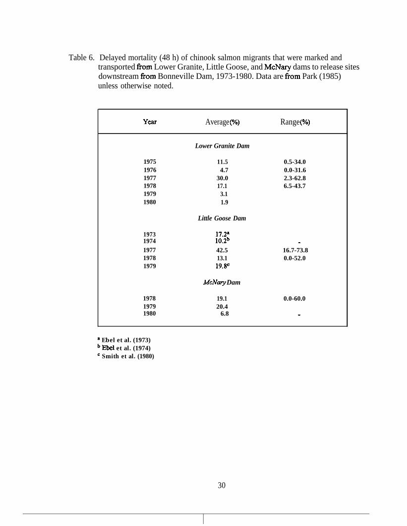
Table 6. Delayed mortality (48 h) of chinook salmon migrants that were marked andtransported Corn Lower Granite, Little Goose, and McNary dams to release sitesdownstream from Bonneville Dam, 1973-1980. Data are from Park (1985)unless otherwise noted.

YC3I Average (%) Range (%)

Lower Granite Dam

197519761977197819791980

11.54.7

30.017.1

3.11.9

Little Goose Dam

0.5-34.00.0-31.62.3-62.86.5-43.7

19731974197719781979

17.2a10.2b42.513.119.8c

McNary Dam

-16.7-73.80.0-52.0

1978 19.1 0.0-60.01979 20.41980 6.8 w

a Ebel et al. (1973)b E%el et al. (1974)c Smith et al. (1980)

30

total number of fish recovered from each of 21 groups released into the forebay of Ice HarborDam during 1966-1972 ranged from less than 1 day to over 13 days (mean 6.4 days; Table 7).Survival estimates will be inflated to the extent that control releases failed to survive up to thetime that they passed the dams.

Assumption 8. Random mixing

This assumption states that treatment and control fish within an experimental group arerandomly mixed with each other and with the unmarked population. Also, marked fish sufferthe same mortality and are as vulnerable to recovery as the unmarked.

Dauble et al. (1993) underscored the importance of random mixing (i.e., complete overlap atthe time of recovery) of treatment and control fish to assure equal sampling probabilities. Thisassumption is more likely to be violated if control and treatment fish are released at differenttimes, at distant locations, or under different environmental conditions. If treatment andcontrol fish arrive at the recovery site at different times, survival estimates can still be obtainedas long as sampling efficiencies did not change over the period of recovery. The assumption ofrandom mixing becomes less tenable as sample sizes (either marks or recoveries) decrease.

Raymond et al. (1974) remarked on the difficulty of timing a forebay release to coincide withthe arrival of upstream releases so that both groups were recovered at identical efficiencies:“When seasonal flows vary, it is often difficult to match recoveries of various marked fishreleases.” Given that flow regimes in most years were unstable, random mixing was probablythe exception rather than the rule.

The hypothesis of random mixing of marked and unmarked fish was “tested” in 1972 byreleasing marked fish on both sides of the river above trap and dam sampling sites (Raymond etal. 1975, Raymond 1979). According to Raymond (1979), “the assumption is satisfied ifrecovery rates from both release points are comparable.” In fact, no significant difference inrecovery rates was found (see his Table l), but this misses the point. Unmarked fish were notinvolved in the comparison so the conclusion that they were randomly interspersed withmarked fish was unwarranted.

Raymond et al. (1975) and Raymond (1979) also reasoned that the assumption of randommixing held true if the ratio of marked-to-unmarked fish collected in gatewells was similar toratios obtained in samples collected with fyke nets, beach seines, and purse seines. Theyindicated that the catch composition of all samples was similar, but neglected to provide dataand statistical analyses to support their claim.

As Dauble et al. (1993) pointed out, efforts to release control fish far enough upstream so thatrandom mixing is ensured may reduce the likelihood that all control fish will survive until theyarrive back at the dam. The potentially conflicting logistical demands imposed by variousassumptions are a primary reason that Dauble et al. (1993) chose not to endorse survivalestimation methods based on sampling efficiencies.

31

Table 7. Release and recovery dates, and elapsed time to recover (at Ice Harbor Dam)1 O%, 50%, and 90% of the chinook salmon released into the Salmon River andthe forebay of Ice Harbor Dam, 1966- 1972. Data were provided by H.Raymond to R.H. Lander (1972).

YEU Replicate MhUlRelease

Date

M&UlRecovery

Date

Number of Days tolo%, 50%, and 90%

Cumulative Recovery

Fish Released into Forebay of Ice Harbor Dam

1966 1 April 7 April 14 4:7: 162 April 8 April 15 -1:7: 113 April 22 April 30 3:8:144 April 23 April 27 1:4: 13

1967 1 April 13 April 26 5 : 13 : 192 April 20 April 27 4:7:123 April 27 May3 1:6:124 May3 May11 5 : 8 : 205 May 10 May 23 6 : 13 15:6 May 17 May 24 2:7:9

1968 1 April 10 April 15 1 : 15 14:2 April 17 April 24 1:7:193 April 24 April 30 2~61224 May 1 May7 2:6: 195 May8 May 14 1:6: 136 May 15 May 20 1:5:8

1972 1 April 11 April 11 -1 : 0 : 172 April 20 April 26 4:6: 183 April 26 MaYI 2:5:164 May 3 May 9 0:6:155 May 10 May 13 1:3: 7

32

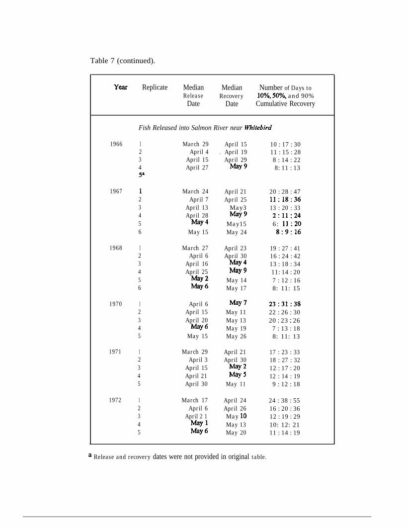
Table 7 (continued).

Ye2l.r Replicate MedianRelease

Date

MedianRecovery

Date

Number of Days toIO%, 50%, and 90%

Cumulative Recovery

Fish Released into Salmon River near whitebird

1966 1 March 29 April 15 10 : 17 : 302 April 4 . April 19 11 : 15 : 283 April 15 April 29 8 : 14 : 224 April 27 my9 8: 11 : 135a

1967 1 March 24 April 21 20 : 28 : 472 April 7 April 25 11:18:363 April 13 May3 13 : 20 : 334 April 28 MY9 2:11:245 MY4 May15 6: 11:206 May 15 May 24 8:9:16

1968 1 March 27 April 23 19 : 27 : 412 April 6 April 30 16 : 24 : 423 April 16 May4 13 : 18 : 344 April 25 MY9 11: 14 : 205 May2 May 14 7 : 12 : 166 mY6 May 17 8: 11: 15

1970 1 April 6 MY7 23:31:382 April 15 May 11 22 : 26 : 303 April 20 May 13 20 : 23 : 264 May6 May 19 7 : 13 : 185 May 15 May 26 8: 11: 13

1971 1 March 29 April 21 17 : 23 : 332 April 3 April 30 18 : 27 : 323 April 15 May2 12 : 17 : 204 April 21 May5 12 : 14 : 195 April 30 May 11 9 : 12 : 18

1972 1 March 17 April 24 24 : 38 : 552 April 6 April 26 16 : 20 : 363 April 2 1 May 10 12 : 19 : 294 MY1 May 13 10: 12: 215 May6 May 20 11 : 14 : 19

a Release and recovery dates were not provided in original table.

Assumption 9. Transportation losses are known

Prior to 1980, significant numbers of yearling chinook salmon were collected and transportedfrom Ice Harbor Dam in 1968-1970, Little Goose Dam in 1971-1973 and 1976- 1978, LowerGranite Dam during 19751979, and McNary Dam in 1979 (Table 5). With the exception of1974, when no fish were transported, the number of fish transported steadily increased from109,000 fish in 1971 to over 2.4 million fish in 1979. The percentage of fish transportedranged from 0% in 1974 to 76% in 1977 (Park 1985).

In 1977, approximately 750,000 to 800,000 chinook salmon smolts were collected at LittleGoose and Lower Granite dams and transported downstream by truck (Smith et al. 1980, Simset al. 1977, p. 10). In a footnote to their Table 4, Sims et al. (1977, p. 12) noted thattransported smolts were “subtracted from total smolts passing Lower Granite Dam forcalculations of survival.” Raymond and Sims (1980, p. 17) indicated that survival estimates for1979 were adjusted for fish transported from McNary Dam, but do not explain how theyarrived at that number. Aside from these two references, I found no further discussion ofcomputational adjustments made. to account for losses to transportation. If adjustments werein fact made, the question remains as to whether calculations of survival were based onestimates of the number of markedfish transported, in which case mark-recovery data could beused, or were based simply on the total number offish transported, which would imply thatpopulation size ratios were used to estimate survival.

Assumption IO. Statistical independence

Here, it is assumed that replicate observations were independent, so that, for example, theywere unaffected by the order in which they were obtained. However, departures fromindependence would be expected a priori because (1) flows over successive time intervals areautocorrelated, and (2) survival varied with flow.

In the spring of each of the years 1973-1979, several treatment and control groups, eachbearing unique brands, were experimentally released into the Snake and Columbia rivers. Whywere they not treated as independent samples? The reason, I believe, is that the fraction ofmarked fish recovered from individual groups and the timing of their recovery was too variablefor them to serve as replicate observations (see earlier discussion). When survival rate iscalculated from recovery of only a few marked fish, it must be used with caution (Ricker1975).

Estimates of survival between the upper dam and Ice Harbor, and between Ice Harbor and thelower dam were not independent and should therefore not be multiplied together to estimatesurvival between upper and lower dams. Fish released and subsequently recovered at of IceHarbor Dam were used to estimate the sampling efficiency of that dam as a prelude tocalculating survival between the upper dam and Ice Harbor Dam. Rates of recovery of thesame fish at downriver dams were used to calculate survival from Ice Harbor Dam to the lowerdam. Survival estimates for Snake River and Columbia River reaches were thus not

33

independently derived. It should also be noted that the number of marked fish intercepted atthe dam immediately downstream of their release were probably not subtracted from the totalnumber of fish marked prior to computing recovery rates dowmiver dams. Using an exampletaken from Raymond’s unpublished notes, 86,43 1 fish were marked and released into theforebay of Ice Harbor Dam in 1968. Of these fish, 7,238 were subsequently recovered at IceHarbor Dam, and 1,390 were recovered at The Dalles. In calculating the proportion recoveredat The Dalles, Raymond neglected to subtract 7,238 from 86,43 1 to account for the reductionin size of the marked population. By not doing so, he underestimated recovery rates by0.15%. Survival estimates would have been underestimated by a greater amount.

Assumption I I. Proportional sampling effort

If an average survival is to be estimated from replicate observations, the frequency and timingof individual estimates should be indexed to the relative abundance of unmarked fish in theriver at the same time. There are two important reasons why this assumption should hold true:

1. “Flow” in the flow-survival relationship was based upon the date of peak passage of theentire run, and not simply on the timing of experimental fish.

2. Smolt survival is not constant over the outmigration period, but varies with time-dependentvariables such as river flow and water temperature.

Raymond (1979) estimated average annual survival in 1973-1975 by weighting individualgroup survival estimates by the proportion of the total migration passing the release site. It isnot clear whether Sims followed Raymond’s example, even though in all years daily estimatesof the number of smelts passing the upper dam were required to determine the date of peakpassage.

Indexing interval-specific survival estimates to smolt population sizes presumes that samplingof marked and unmarked fish at the release site spanned the entire outmigration period. On atleast two occasions, estimates of total smelt abundance and time of peak migration (which issensitive to population estimates) may have been inaccurate due to late startup or prematuretermination of sampling at dams. In 1975, smolt monitoring at The Dalles Dam was conductedfrom 1 May to 3 1 May. Outmigration from the Salmon River (Riggins) peaked on 7 May.Travel time from the Salmon River trap to The Dalles Dam averaged 21 days (the same as in1974), putting the peak of the outmigration there at approximately 28 May (Sims et al. 1976).It is improbable that the latter half of the smelt outmigration would have passed The DallesDam before sampling there was terminated.6

6 Survival estimates for the lower river in 1975 may have been based, at least in part, on data collected at JohnDay Dam, where sampling began on 11 May and continued until 28 December.

34

An unusually late startup date at Lower Granite Dam in 1977 - 29 April (Sims et al. (1978, p.3) - may have resulted in a significant portion of that year’s smolt run being missed, therebyinvalidating the “average” survival estimate obtained for that year. If substantial numbers offish migrated past Lower Granite Dam before smelt monitoring began, then the peak passagemean flow in 1977 was probably lower than the 40 kcfs calculated by Sims and Ossiander(198 1). Dates of peak passage of chinook smolts were earlier in the preceding and followingyears - 2 1 April in 1976 and 29 April in 1978 (Sims and Ossiander 198 1, Table 3). In 1973and 1979, however, later dates of peak passage (14 and 17 May) were recorded. Smolt trapdata indicate that migration from the Salmon River was later than usual in 1977, and since riverflows were exceptionally low that year, a 9 May peak migration date is not altogetherunreasonable. The only way to reliably determine whether sampling at Lower Granite Dam in1977 might have missed the first part of that year’s run is to examine trends in the daily smoltcount data for the dam. These data, unfortunately, could not be found.

Assumption 12. Flow measurements

For each of the survival-flow data pairs used in the least squares regression analysis conductedby Sims and Ossiander (1981), “flow” was determined as the mean daily flow past Ice Harborover a two week period, centered on the date that 50% of the entire smolt outmigration hadpassed the dam. If the date of peak passage was incorrectly determined, then the’mean flowfor that year would be in error.

There is a question as to whether flows averaged over the two week peak migration periodwere representative of the conditions under which smolts actually migrated. Although it makessense to weight flows according to the number of fish present, there is no apriori reason toassume that two weeks is an appropriate time-scale on which to base flows. It is much moreplausible that migrating smelts respond to trends and changes in flow on smaller time-scales(Smith et al. 1993).

Flow was calculated at Ice Harbor Dam on the Snake, yet overall survival was determined forboth Snake and Columbia River segments. If flows in the Snake and Columbia River arestrongly correlated, then discharge at Ice Harbor Dam may be satisfactory as an independentvariable. However, I see little point in using flow measured at a single dam in an analysispurporting to relate flow and survival in both the Snake River and the Columbia River. Flowsat Ice Harbor Dam may be a valid predictor of survival in the Snake River, but they are lessappropriate for the Columbia River. This is particularly true for years such as 1977, whenspecial releases of water (“Operation Fish-Flow”) resulted in higher flows in the ColumbiaRiver, but not in the Snake River (Sims et al. 1978, p. 7). Raymond and Sims (1980) notedthat similar levels of spill were provided at Columbia River mainstem dams in 1977, 1978, and1979, but that survival was much lower in 1977 than in 1978-79.

The bottom line is this: separate flow-survival relationships should have been derived for theSnake and Columbia rivers since flows, smolt population characteristics, and various mortalityfactors may have varied between reaches within the same years.

35

I made no special attempt to assess the reliability of the stage-discharge relationship used toestimate flow at Ice Harbor Dam during 1973-1979. I recalculated mean daily flow valuesassociated with dates of peak outmigration (+ 7 days) for the years of interest and found thatthey corresponded closely with those used by Sims and Ossiander (1981). However, therewere minor inconsistencies in reporting of mean flow values in the various Nh4FS reports. Forexample, Sims et al. (1977, p. 7) indicated that the mean daily flow at peak migration in 1975was 160 kcfs, whereas Sims and Ossiander (198 1) reported 140 kcfs (this appears to be thecorrect value). The reason for this discrepancy is not known.

Assumption 13. Statistical models

One of the problems with applying correlation-regression analysis to the flow-survival databaseis that survival estimates, as Raymond (1979) calculated them, are themselves a function offlow-based sampling efficiencies. If we have a set of flows, yi , . .., y,,, measured at the sametime that survivals are measured as s^ i = ci / ej, where ei = f(l/yJ, and then look at the relationofy to s, we would expect to find a strong, positive correlation between the two parameters.Spurious relations - that is, relations that may have little to do with the true flow-survivalrelationship - may be introduced because flow and survival estimates are computed from thesame set of data. This is an important limitation of the use of flow-efficiency curves in survivalestimation.

I did not attempt to fit a different curve to the Sims and Ossiander (198 1) flow-survival data,but note that Sims et al. (1983) replaced the original log-linear model with one based on aninverted polynomial iunCtion to describe the relation between flow and survival using datafrom 1973-1979, plus 1980 and 1982 (Figure 5). There is no compelling biological basis forbelieving that the relation between survival and flow is linear rather than curvilinear. To thenaked eye, the 1980 and 1982 data would not appear to have much effect on the shape of thecurve since they are tightly clustered with several other data points. Differences in the modelsselected by Sims and Ossiander (198 1) and Sims et al. (1983) reveal doubt in the mind of theauthors as to the true relationship between flow and survival, especially at higher flows.

One final point is that virtually all regression models require assumptions of homoscedasticity(i.e., common variance) and normality of mean survival values for any given flow. Theseassumptions are given ample treatment in basic statistics texts, and so will not be discussedfurther here. Sample sizes used to construct the flow-survival relationship were too small todetermine whether or not these assumptions were satisfied.

Assumptions 14 and 15. Representativeness of experimental conditions

By this assumption it is meant that the relation between survival and flow did not vary betweenyears while the data were being collected, and that the relation remains a valid predictor fortimes (e.g., years) or conditions other than those under which the data were collected. Itshould be stressed that the flow-survival regression is strictly valid only for flows falling within

36

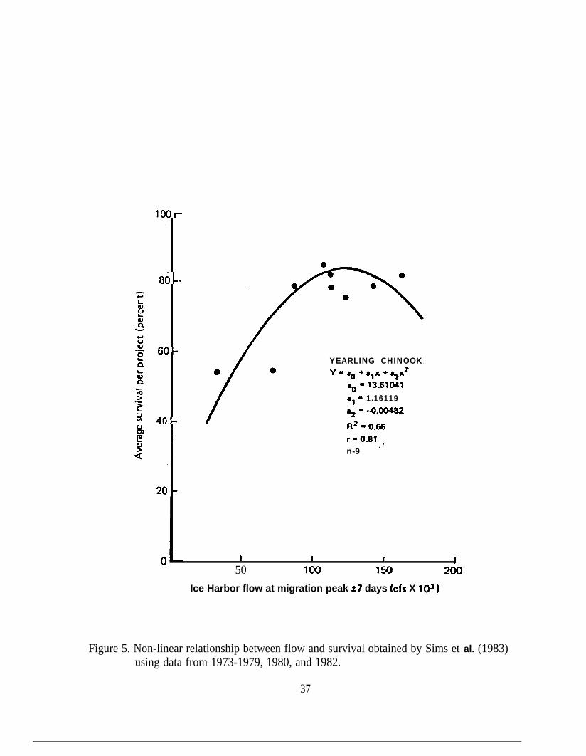
loo-

O-

3-

I-

YEARLING CHINOOK

a, - 1.16119~-0.0041#R2-066r-oar .n-9 ’

I I 1 I50 100 150

Ice Harbor flow at migration peak i7 days (cfs X 1CP)

Figure 5. Non-linear relationship between flow and survival obtained by Sims et al. (1983)using data from 1973-1979, 1980, and 1982.

37

the range of observed values, i.e., 40 to 160 kcfs. One should extrapolate with caution outsidethese limits.

Application of the flow-survival relationship requires the assumption that the dependencyrelation between flow and survival has not changed because of changes in the environment, thefish, or both. As discussed in later sections, several developments occurred both before andafter 1979 that may prevent extrapolation of the flow-survival relationship to contemporarysettings.

4.2 Analvtical Methods

To the extent that information was available, the primary mark-recovery data, the numericaland statistical methods used to analyze them, and the results of the analyses are discussed indetail in this section.

4.2.1 Sample sizes

Although many of the assumptions discussed above are theoretically independent of samplesize, those relating to random and representative sampling of the smelt population are not.Both the number of groups and the number of fish marked and recovered per group haveimportant effects on the precision of annual survival estimates and, ultimately, on the kinds ofstatistical analyses and inferences that can be derived from those estimates.

Information on the number of experimental groups and the number of fish marked andrecovered within each group was not routinely included in NMFS reports. However, datasheets which tabulated marks and recoveries for 1976-1979 were located in NMFS archivedfiles. These data sheets were used to reconstruct the information provided in Table 8. Someof the data sought from this period were missing and therefore could not be summarized; theabsence of such data merely indicates that we were unable to locate it, and is not meant to givethe impression that it was not collected. To the best of my knowledge, the data used tocalculate the statistics presented in Table 8 were accurate and complete. With thesequalifications in mind, we make the following observations:

1. The total number of fish marked and released was variable across dams and years.

2. The number of replicate groups marked and released each year was variable across damsand years.

3. The number of fish marked per group was variable within and across years; the number of .fish per group was inversely related to the total number of groups released. Thus, moreexperimental fish were released at Lower Granite Dam but they were divided among fewerreplicate groups than at downriver dams.

38

Table 8. Reported nutiber of chinook salmon smelts marked and recovered at variousdams during 19761979. This information was abstracted from the originalNMFS data sheets; the data could not be verified for accuracy and shouldtherefore be considered unreliable.

Number of FishRelease Site Recovered Percent Recovery

YtXU Recovery Site Raw Total Range Mean

1976 Lower Granite Dam: 3 markedgroups numbering 56 to 18,312fish (total: 28,688)Ice Harbor Dam 0 - 240 248 0.0% - 1.1% 0.9%McNary Dam 0 - 286 312 0.0% - 1.6% 1.1%John Day Dam I- 8 0 121 0.0% - 1.1% 0.9%

1976 Ice Harbor Dam: 8 markedgroups numbering 291 to 2,033fish (total: 14,800)Ice Harbor Darn o- 91 203 0.0% - 2.4% 1.4%McNary Dam 1 - 129 239 0.1% - 3.0% 1.6%John Day Dam l- 31 62 0.2% - 1.1% 0.4%

1976 John Day Dam: 8 markedgroups numbering 212 to 1,319Jsh (total: 5,940)John Day Dam l- 13 40 0.1% - 1.4% 0.7%

1977 Lower Granite Dam: 5 markedgroups numbering 28 to 15,987jIsh (total: 38,262)Ice Harbor Dam o- 11 19 0.0% - 3.6% 0.06%

1978 Lower Granite Dam: 4 marked groups numbering 2,144 to 15,232fish (total: 46,094)Ice Harbor Dam a 3 - 63 127 0.1% - 0.4% 0.4%John Day Dam 0- 69 191 0.0% - 0.5% 0.4%The Dalles Dam 0- 27 40 0.0% - 0.1% * 0.1%

1978 John Day Dam: 30 marked groups numbering 26 to 636jish (total: 7,281)John Day Dam 0- 16 113 0.0% - 7.7% 1.6%The Dalles Dam o- 3 15 0.0% - 1.8% 0.2%

1979 Lower Granite Dam: 4 marked groups numbering 5,772 to 19,760jish (total: 50,629)Ice Harbor Dam 27 - 154 357 0.0% - 2.7% 0.7%McNary Dam 78 - 788 1367 1.1% - 4.0% 2.7%John Day Dam 12 - 117 161 0.0% - 0.6% 0.3%The Dalles Dam 0- 27 40 0.01% - 0.1% 0.1%

1979 John Day Dam: 20 markedgroups numbering 92 to 425fish (total: 4,536)

John Day Dam 92 - 425 32 0.0% - 4.2% 0.7%The Dalles Dam o- 3 8 0.0% - 1.2% 0.2%

a Recovery data for one of the release groups (brand LAPUS) could not be found and so were excludedfrom range and mean calculations.

39

4. The proportion of fish recovered from each marked group was extremely variable andgenerally low.

Raymond’s notes indicated that he deleted from the database data for experimental groupswhich he considered unreliable. In 1972, for example, the last group of fish released into theforebay at Ice Harbor Dam (actually 2 groups released simultaneously on both sides of theriver) was recovered at a much lower rate (0.34% and 0.45%) than were the preceding 5groups (range 2.46 - 5.75). Raymond did not use the last group in survival calculations forthat year.

4.2.2 Recover-v Data

NMFS studies were designed to measure within-season survival over a range of environmentalconditions. Survival was estimated .by subsampling the chinook smolt population rather thanby marking and resampling the entire population and computing the parameter exactly. Ifmultiple subsamples (i.e., individual release groups) were taken, then it should have beenpossible to analyze survival data by individual release groups to get empirical varianceestimates. Sampling variance among s^ i ‘s would give some indication of within-seasonvariability and precision of the annual survival estimates.

Estimates of sampling variance or standard error normally accompany point estimates of aparameter. Why NMFS researchers chose not to report variance estimates is unclear, sinceindividual s^ i !s were computed and averaged in early survival studies. In some years, thenumber of fish recovered might have been too variable to reliably calculate s^ i. With regard tosampling variability, Sims et al. (1984, p. 24) remarked that in 1982 and 1983, “the variancearound our survival estimates was too great to permit adequate definition of between-yearflow/survival relationships. We will make no further efforts in this area until the precision ofour existing collection efficiency curves are (sic) substantially upgraded.”

Another reason that Raymond, Sims, et alia may have opted to forego estimates of groupsurvival was the extremely small fraction of marked fish recovered in some years, especiallyfrom upstream releases. Raymond and Sims noted (on p. 10 of their 1975 proposal) thatduring “the high runoff of 1974, efficiency [at The Dalles Dam] dropped below 0.5% andrecoveries from Little Goose Dam were insufficient to assess survival from there to the JohnDay-Dalles area with any degree of statistical confidence.” Data provided by Raymond et al.(1975; Appendix AZ) indicated recovery rates of 0.2% for treatment and control fish at TheDalles Dam in 1974.

As low as these rates may seem, recovery rates were an entire order of magnitude lower in1977. Sims et al. (1978; p. 17) cite data from an experiment to measure differences in survivalof fish released in fiontroll and backroll areas at Little Goose Dam: out of a total of 75,751chinook salmon smolts marked and released at the dam, only 14 (0.02%) were recovered laterat The Dalles. The authors concluded that “recoveries at downstream dams were too low to

40

measure statistical differences between fkontroll and backroll releases.” Sims et al. (1978)chose to apply “past collection efficiencies” to estimate population sizes at the upper dam(Lower Granite) in 1977 due to extremely low recoveries of control fish.

Problems associated with low recovery rates were not limited to the 1973-1979 period.Raymond (unpublished notes) provided examples from earlier years, and Smith et al. (1993;see their Table 27) provided examples from the 1980s which point to widespread problems.The long-term record also contains numerous examples in which a higher proportion oftreatment fish than control fish were recovered, with the result that survival estimates exceeded100% (Raymond, unpublished data; Sims et al. 1982, p. 22). Compare, for example, the totalproportion of treatment fish (Salmon River release) and control fish (forebay release)recovered at Ice Harbor Dam in 1966, 1967, 1968, 1972 (Table 9). In all years except 1972,recovery rates were higher for treatment fish. Control fish either died en route to the dam orwere less susceptible to recapture than were treatment fish. This unexpected result obviouslymakes survival estimation based on data summation impossible.

There appears to have been sampling problems in other years as well. Noting that LittleGoose Dam forebay recoveries in 1971 were approximately 40% less than those calculated forfish released into the Salmon River near Riggins, Idaho, Raymond opined, “the fish must havebeen under stress.” In 1974, recoveries at Ice Harbor Dam of Lower Granite Dam releaseswere less than 60% of those recorded for fish released into the Salmon River near Riggins,Idaho (Raymond, unpublished notes). Fish released in the forebay of Ice Harbor Dam in thesame year were recovered at McNary Dam in higher proportions than were fish released in theIce Harbor tailrace.

Sims et al. (1982, p. 22) provided examples from later years in which within-year flow-survivalestimates exceeded 100%. Referring to their Table 2, survival rates of 120% and 102% wereestimated for two of the four experimental groups of fish that traversed the Columbia Riverbetween Ice Harbor and John Day dams.

Since estimates of survival for individual release groups were on occasion unreliable, annualsurvival was often computed by summing the total number of treatment fish marked over theseason, dividing this by the total number of treatment fish recovered at the downstream dam,and then dividing again by the average sampling efficiency of that dam. Sampling efficiencyitself was determined by summation of marks and recoveries over the entire season. Samplingvariance could not be determined by this technique since all mark and recovery data had beencombined to obtain a single season survival estimate.

4.2.3 Samulinn Efficiency

Sampling efficiencies at Columbia River dams were observed to vary as a function of flow.The amount of water spilled, in particular, was important since it affected the movement anddistribution of smolts, and fish passing over the spillway were not sampled. Efficiencies werequite variable. At Ice Harbor dam, for example, as recovery rates as high as 17% were

41

R

Table 9. Recovery and survival rates for chinook salmon migrants released into the Salmon River (treatment fish) andthe forebay (controls) of Ice Harbor Dam, and then recovered at that dam. Survival calculations assume thattreatment and control fish were paired by group within years. Data were provided by H. Raymond toRH. Lander (1972).

Year Group

Treatment Fish Control FishNumber Number Percent Number Number PercentReleased Recovered Recovered Released Recovered Recovered

Percentsurvival

1966 1 4798 329 6.9 2143 117 5.5 125.62 5582 338 6.1 1771 105 5.9 102.13 3929 96 2.4 3341 119 3.6 68.64 4379 95 2.2 2980 56 1.9 115.45 1033 18 1.7

Total 19721 876 19.3 10235 397 16.8 114.5

1967 1 1501 89 5.9 2107 150 7.1 83.32 6690 547 8.2 5100 433 8.5 96.33 7430 618 8.3 7236 616 8.5 97.7,4 2365 119 5.0 4594 192 4.2 120.45 5255 153 2.9 4594 192 4.2 69.76 896 11 1.2 2124 26 1.2 100.3

Total 22636 1448 25.7 23648 1459 26.6 96.5

1968 1 3358 363 10.8 7843 1334 17.0 63.62 647 1 944 14.6 17499 2180 12.5 117.13 2952 374 12.7 15711 1292 8.2 154.14 2120 119 5.6 15711 1292 8.2 68.35 2129 113 5.3 21964 1159 5.3 100.66 2078 63 3.0 11371 542 4.8 63.6

Total 15750 1613 41.2 82256 6465 38.9 105.8

1972 1 17780 226 1.3 4097 231 5.6 22.52 16682 234 1.4 4097 231 5.6 24.93 9725 86 0.9 5023 172 3.4 25.84 28865 123 0.4 5543 121 2.2 19.55 7615 19 0.2 5543 121 2.2 11.4

Total 80667 688 4.2 24303 876 19.1 22.2

recorded for control releases at low flows (1968 tests), when little water (and few fish) werepassed over the spillway, and as low as 1% at high flows, when increasing amounts of waterwere spilled over the face of the dam (Table 9). At other projects - John Day Dam, forexample - sampling efficiencies of less than 1% were commonplace (Table 8).

A flow-efficiency curve was developed for Ice Harbor Dam by Raymond and applied in 1973-1975 to estimate smolt survival and run size. At Ice Harbor during 19751979, and at JohnDay and The Dalles dams during 1973-1979, sampling efficiency was determined fromrecovery rates of control fish released immediately upstream of the dams at more-or-less thesame time that treatment fish were in transit.

Sampling efficiency data for 1973- 1979 were not routinely reported. Sims et al. (1976, 1977,1978) and Sims and Ossiander (1981) declined to provide data. Raymond et al. (1974, 1975)tabulated the total number of chinook and steelhead released in forebays of Little Goose andIce Harbor dams and subsequently recovered at downstream dams in 1973 and 1974.Efficiencies were not provided for individual control groups, nor were they specifically relatedto river flows or treatment groups.

Raymond (1979, p. 509) noted that a flow-efficiency curve was not developed for The Dalles,even though his unpublished and published writings clearly indicated his intent to do so. ThatRaymond (1979) neither explained his failed attempt, nor discussed the problems this mighthave posed was rather odd considering his touting of the Ice Harbor Dam efficiency curve as“a major breakthrough.” The Ice Harbor curve, the reader is informed, permitted estimates inyears “when fish were too stressed from gas bubble disease to be marked and released forefficiency measurements.” These same constraints presumably prevailed at other dams in yearsof high levels of dissolved atmospheric gases (1969-1972 and 1974). Another advantage of aflow-efficiency curve, says Raymond (1979), was that it permits greater temporal resolution -“daily if necessary” - of the number of smolts passing a dam. These benefits were not realizedat The Dalles Dam or, following 1975, at Ice Harbor Dam.

Even though a relation between sampling efficiency and river flow was not established for TheDalles Dam, Raymond (1979) claimed that “recoveries of upstream releases have beensufficient to provide meaningful estimates of survival” at the dam in years of low and averageflow. Efficiencies at The Dalles under these conditions ranged between 2 and 6%,considerably lower than those calculated under similar flow conditions at Ice Harbor. In highflow years, efficiency was less than 1% which, Raymond (1979) remarked, “greatly reducesconfidence in estimates of survival. ”

Raymond et al. (1975) refer the reader to Raymond, Bentley, and Ossiander (1975) forcomputational details on efficiency curves for chinook and steelhead. The reference as citedwas never published and a draft could not be located. The only published information relatingto the derivation of sampling efficiencies is found in Raymond et al. (1974, 1975) andRaymond (1979). The information provided in these documents lacks detail and is somewhatcontradictory. For example, the graph of chinook sampling efficiency versus flow for IceHarbor, first published in Raymond (1975), underwent considerable refinement without benefit

43

of new data before emerging in final form in Raymond (1979). Figure 6 plots the same flow-efficiency curve as it appears in two published and one unpublished documents.

Raymond’s notes and published writings did not describe how the flow parameter used in theflow-efficiency regression was calculated. Each group of control fish was typically releasedover a period of several days; they were recovered over an even greater time interval. Noeffoit was made to calculate a weighted mean flow to account for flow fluctuations whichmight have occurred while fish in a group were in transit.

Far more problematic than curve fitting techniques are computational errors that may haveoccurred in Raymond’s treatment of the sampling efficiency data. The errors relate tonumerical expansions of numbers based on the number of gatewells sampled and the number ofdays when sampling was not conducted. To give some idea of the complexity of the problem,consider the following statement made by Raymond (unpublished notes, letter to “Bob”):

“What I need is average % catch by gatewell with respect to flow and turnover orexit rate in general when a gatewell has not been fished daily. I have catch andmark release records so we can later adjust the measured to an expected efficiencybased on fishing effort.”

The Ice Harbor flow-efficiency curve was based on the proportion of marks recovered in Unit2 gatewells (3 in all) that were expanded to the remaining units of the dam. Twenty sevenindependent observations of flow and sampling efficiency were made during 1964 - 1969 (withthe exception of 1966), and 1972. Actual recoveries were expanded on the basis of theproportion of fish collected from Unit 2 gatewells compared to Unit 1 and 3 gatewells in 1966,when all three units were sampled concurrently. The proportion collected from Unit 2averaged 40%, but the original (unpublished) data reveal that Unit 2 catches comprisedanywhere from 15 to 70% of the total recoveries of forebay-released fish (the cause for thisvariability is unknown). Raymond’s notes suggested that individual gatewells displayeddifferent sampling efficiencies. Bentley and Raymond (1968, p. 126) recovered 1.5% ofpreviously marked control fish from gatewells A, B, and C of Unit 2 at Ice Harbor Dam in1966. Another 2.5% fish were recovered from Units 1 and 3 gatewells, with the totalproportion caught varying between 2% and 6% during high and low flows, respectively. Inany event, Raymond used a factor of 2.5 to expand his Unit 2 recovery proportions to thoseused in his efficiency curve.

If recoveries of marked fish at Ice Harbor Dam in subsequent years were based on samplestaken from Unit 2 alone, then expanded sampling efficiency estimates would have beenunnecessary. However, in an effort to provide an alternate route through the dam, the U.S.Army Corps of Engineers drilled orifices in all gatewells in 1970. From then on, smolt countswere based on sluice trap catches of fish from all gatewells. A “whole dam” samplingefficiency was therefore needed.

The accuracy of the Ice Harbor Dam flow-efficiency curve is difficult to assess but what fewdata exist suggest that sampling efficiency may have been overestimated. From data and

44

R

Figure 6. Variations of Ice Harbor flow-efficiency curve for chinook salmon smolts: Figures A and B display data from 1964, 1965,1967-69; Figures C and D display data from the same years plus 1972. Figures A and C are drawn from data in unpublishedtables compiled by Raymond; Figure B is a reproduction of Figure Al from Raymond et al. (1975); Figure D is a reproductionof an unpublished graph from Nh4FS files.

calculations performed by Raymond et al. (1975, see his Appendix A2 and Appendix TableB2), for example, it can be seen that the 2.4% “average” sampling efficiency at Ice HarborDam in 1974 was conspicuously higher than efficiencies reported that year for McNary andThe Dalles dams (1.3% and 0.2%, respectively). The observed sampling efficiency, based oncontrol fish recoveries, was 0.9%, or 58 fish recovered out of 6,500 marked and released. Theobserved efficiency was considerably less than that predicted by the flow-efficiency curve. Itwas also less than the proportion of Little Goose-released fish recovered at Ice Harbor Dam(1.12 %). Had 0.9% been used instead of 2.4% as an average efficiency value, a survival rateof greater than 100% would have resulted.

Curiously, in 1973 the sampling efficiency observed at Ice Harbor Dam was also 0.9% (102control fish recovered out of 12,000 released), even though flows were much lower in 1973than in 1974 (Table 5). Sampling efficiency would be expected to be higher at lower flows.

Based on the foregoing assessment I conclude that the Ice Harbor Dam flow-efficiency curvedoes not provide adequate estimates of reach survival because of inaccuracies in the methodsused in its computation.

4.2.4 In-season Survival Estimates

Given reliable mark-recovery data, a logical approach to establishing a flow-survivalrelationship would be to use survival (SI J and mean daily flows calculated for individualexperimental groups. The major advantages of this approach are obvious: one obtains a largersample size and a relation based on short-interval estimates rather than seasonal averages ofsurvival and flow. Unfortunately, the number of fish recovered from individual groups wasoften too low or variable to be of much use in this regard. I was unable to assemble a reliableset of data from the 1973-1979 period that would enable a comparison of flow and survival forindividually released groups.

However, a dataset from the 1966-1972 period was located. In 1972, Raymond provideddetailed mark and recovery data to the statistician R.H. Lander for his review and comment.The data, which are reproduced in Table 9, pertained to the number and timing of chinooksalmon released in individually marked groups in the lower Salmon River, and subsequentlyrecovered at Ice Harbor Dam in 1966-1972, except 1969, when funding shortfalls curtailedfield studies. Recovery rates were reported for 3 1 treatment groups and 21 control groups (nodata were provided for control groups that may have been released in 1970 and 1971). Ianalyzed these data to see if a correlation exists between survival values calculated forindividual groups and flows that prevailed at the time that the groups were recovered. Twoapproaches were taken to estimating survival.

Method I. Survival was estimated as the ratio of treatment and control group recovery rates,where each treatment group was paired with the control group from the same year having themost similar median date of recovery. This was the approach originally envisioned byRaymond. Dividing the recovery rate of the treatment group by the recovery rate of its

46

matching control group provided an estimate of survival. Because no data were available forcontrol groups that might have been released in 1970 and 1971, survival was determined byMethod 1 for a total of 21 treatment groups from 1966, 1967, 1968, and 1972.

Method 2. There were three steps to calculating survival by the second method:

1. For each treatment group, a mean daily flow was estimated for (a) the median recoverydate, (b) the fifteen day period centered on the median recovery date (i.e., + 7 days), and (c)the period beginning and ending on the dates when 10% and 90% of the fish in the group hadbeen recovered.

2. Sampling efficiency associated with each flow statistic was determined using Raymond’s(1979) flow-efficiency curve (Figure 3); note that forebay-released (i.e., control) fish and nottreatment fish were used to construct the flow-efficiency curve, and

3. Treatment group survival was estimated by dividing the proportion recovered by samplingefficiency.

Survival values obtained by Methods 1 and 2 were then regressed against flow statisticsassociated with the 50% recovery date, the 50% recovery date + 7 days, and the 10% to 90%recovery dates (see Step 1 of Method 2). The strength of association between flow andsurvival variables was not noticeably improved by scalar transformation of the data.

The proportion of treatment ‘fish recovered at Ice Harbor Dam that had been released in theSalmon River in 1966, 1967, 1968 and 1972 (Figure 7) shows the same pattern that Raymond(1979) observed for forebay-released fish (Figure 3). At low flows, such as occurred in theearly part of the 1968 outmigration, double-digit recovery rates were recorded. A parabolicdecline in the proportion of fish recovered was observed at higher flows.

When the proportion of fish recovered from each treatment group is adjusted by its controlgroup recovery rate, a survival estimate results. Survival rates determined in this fashion wereregressed against mean daily flow (Figure 8). Regardless of the flow statistic used, thecorrelation between flow and survival is weak. This is particularly true when 1972 data areexcluded from the analysis (recall that Lower Monumental and Little Goose dams were built in1969 and 1970, so the comparatively low survival rates from 1972 reflect the effects of thosedams). The resulting straight-line regression equations and correlation coefficients evidence adownward trend in survival with increasing flow, but the correlation between the two variableswas not found to be significant. Another obvious point to be considered is that survival ratesfrequently exceeded 100% - an unrealistic outcome that signals potential violations ofunderlying methodological assumptions.

Survival rates determined by Method 2 also exceeded 100% for several treatment groups(Figure 9). Since a flow-efficiency relationship was used to estimate survival, data from 1970and 1971 were retained in the correlation analysis. Survival rates did not appear to varypredictably with flow when the independent variable was the l-day mean flow associated with

47

A.20.0 -

8 15.0 - I1 I

j -10.0 -

.E$ m8 n

E 5.0-= *

m

0 50 100 150 200 250Flow (kcfs)

B.20.0

g 15.0 - I

%

jj 10.0 - -=0” *.-E2 5.0- - Gma

I I .I I

0.0 -I-‘c I==-: I. I

0 50 100 150 200 250Flow (kcfs)

20.0f----l

100 150Flow (kcfs)

Figure 7. Proportion of fish released into the Salmon River in 1966, 1967, 1968 and 1972subsequently recovered at Ice Harbor Dam, expressed as a finction of flow.

48

A.175.0 -%

150.0 A- -1

125.0 -A .A

‘;;‘@ 100.0 - AA A7.*5:

A-2 75.0 AA AA A A 1912

50.0 -

25.0 -

0.00 50 100 150 200 250

Flow (kcfs)

B.

1 I125.0

.C

2 7 5 . 0i

A

2 AA AA *A 1972

0 50 100 150 200 250Flow (kcfs)

C.175.0 ,

150.01

AI”“,“;‘opo.p”“I

25.0 A

0.0

E 100.0a.aE 7 5 . 0

R

50.0

L I125.0 -

4 A-2AA lr A

A

AA A AA A

b!1972

1

0 50 loo 150 200 250Flow (kcfs)

Figure 8. Survival to Ice Harbdr Dam of fish released into the Salmon River, determinedby Method 1 (see text for details), plotted against river flow associated with (A)the 50% recovery date (B) the 50% recovery date + 7 days, and (C) the 10% to90% recovery dates.

49

125.0

25.0

50 100Flow (kcfs)

B.

200 250

0 50 100 150 200 250Flow (kcfs)

125.0

*. 1-1

0 50 100 150 200 250Flow (kcfs)

Figure 9. Survival to Ice Harbor Dam of fish released into the Salmon River, determinedby Method 2 (see text for details), plotted against river flow associated with (A)the 50% recovery date (B) the 50% recovery date f 7 days, and (C) the 10% fo90% recovery dates.

50

the median date of recovery. When plotted against the other flow statistics, however, survivaldecreased with increasing flows. The slopes of both regression lines were significantlydifferent from zero (p < O.OS), indicating that flow was a useful predictor of survival under theconditions that prevailed at the time. That the relation between the two variables was anegative one was unexpected, since a positive flow-survival relationship was obtained by Simsand Ossiander (198 1) using annual average survival estimates.

51

4.2.5 Annual Survival Estimates

In this section I compare annual survival estimates gleaned from Sims and Ossiander (198 1)and other published sources and highlight major discrepancies in reported values on a year-by-year basis (Table 10). I have tried to identify underlying causes for the discrepancies wherepractical, but emphasize that my analysis was constrained by incomplete information. One onlyneeds to peruse Raymond’s handwritten notes to appreciate the flexibility of his treatment ofmark-recovery data from the 1960’s and 1970’s. I found numerous instances where Raymondhad changed numbers, deleted data, and applied different analytical approaches to the samedata. I do not suggest, however, that scientific objectivity was sacrificed in the process. Tosome extent, exploratory analysis and consideration of alternative treatments of the data areacceptable and necessary actions.

It should be noted that inconsistencies in reported values were not limited to chinook salmonsurvival estimates, but extended to other parameters as well. Compare (see Table 4 above),for example, estimates of annual smolt population size found in Sims and Ossiander (198 1;Table l), Raymond (1979; Table 8) and Raymond (1988; Table 2). They differ by as much as1.1 million smolts for any given year. Population estimates found in Raymond’s earlier works(e.g., Raymond et al. 1975, Table 5) tended to be larger, but not consistently so, than valuesfound in his 1988 paper.

1973

Major discrepancies were noted in survival values reported for the 1973 outmigration (Table10). Sims and Ossiander (198 l), Raymond (1979), and Raymond et al. (1975) give 5% as thesurvival rate of chinook salmon between Little Goose Dam to The Dalles Dam. However,mark-recovery data and survival estimates provided by Raymond et al. (1974; see his Tables 6,10, and 11) clearly indicate that this value (5%) was the estimated survival to the Dalles Damof fish released in the Salmon River near Whitebird, Idaho. For the stretch of river betweenLittle Goose and The Dalles dams, Raymond et al. (1974) pegged annual survival at 17%.Raymond et al. (1974) noted (p. 9) that “sampling problems precluded survival estimates at IceHarbor in 1973,” and therefore declined to estimate survival in the Snake River and ColumbiaRiver sub-reaches (note, however, that reach estimates were provided in a later publication(Raymond 1979; his Table 11).

Raymond et al. (1975) reported a 50% loss of yearling chinook at Little Goose Dam in 1973.If treatment-control recovery data from Table 6 of Raymond et al. (1974) are used to calculatesurvival to Ice Harbor Dam from Little Goose Dam, survival was 29% if Little Goose forebaycontrols are used in the calculation, or 55% if Little Goose tailrace controls are used.Approximately 9% of fish released in the forebay of Ice Harbor Dam survived to The DallesDam.

52

Table 10. Annual survival values (%) for yearling chinook migrants, as reported by various authors for the period 1973-1979. Reach ‘1 = Little Goose Dam (1973-1974) or Lower Granite Dam (1975-1979) to Ice Harbor Dam; Reach2 = Ice Harbor Dam to The Dalles Dam (1973-1975) or John Day Dam (1976-1979); Reach 3 = overall survivalfrom upper to lower dam.

1973 1974 1975 1976 1977 1978 1979Source 1 2 3 1 2 3 1 2’ 3 1 2 3 1 2 3 1 2 3 1 2 3

Raymond et al. ( 1974)Raymond et al. ( 1975)Sims et al. (1976)

Sims et al. (1977)

Sims et al. (1978)Raymond and Sims ( 1980)Raymond ( 1979)Sims and Ossiander (1981)

- 17 - - - - - - - _ _ _ -_ - 5 47 82 40 - - - - - - - -- _ - _ - 40 36 69 25 - - - - -- - - - _ - [24 69 17j1 - - - - -- m e _ - - [50 69 3812 - - - - -- - - - m _ _ - 25 63 48 30 - -I - - - - - _ _ - [63 48 301’ - -- - - - e _ _ _ - [63 48 3012 - -- w 5 - - - _ - 25 - - 30 - -- - - - - - - _ _ _ _ _ __

12 42 5 50 71 34 36 69 23 - - - - -- _ 5 - - 40 - - 25 - - 24 - -

- -

- _

_ -

- m

‘- _

- _

- -

- _

3 -- w- m2 -

1 Survival estimates are for Rapid River Hatchery chinook salmon.

2 Survival estimates are for “native and other hatchery” chinook salmon.

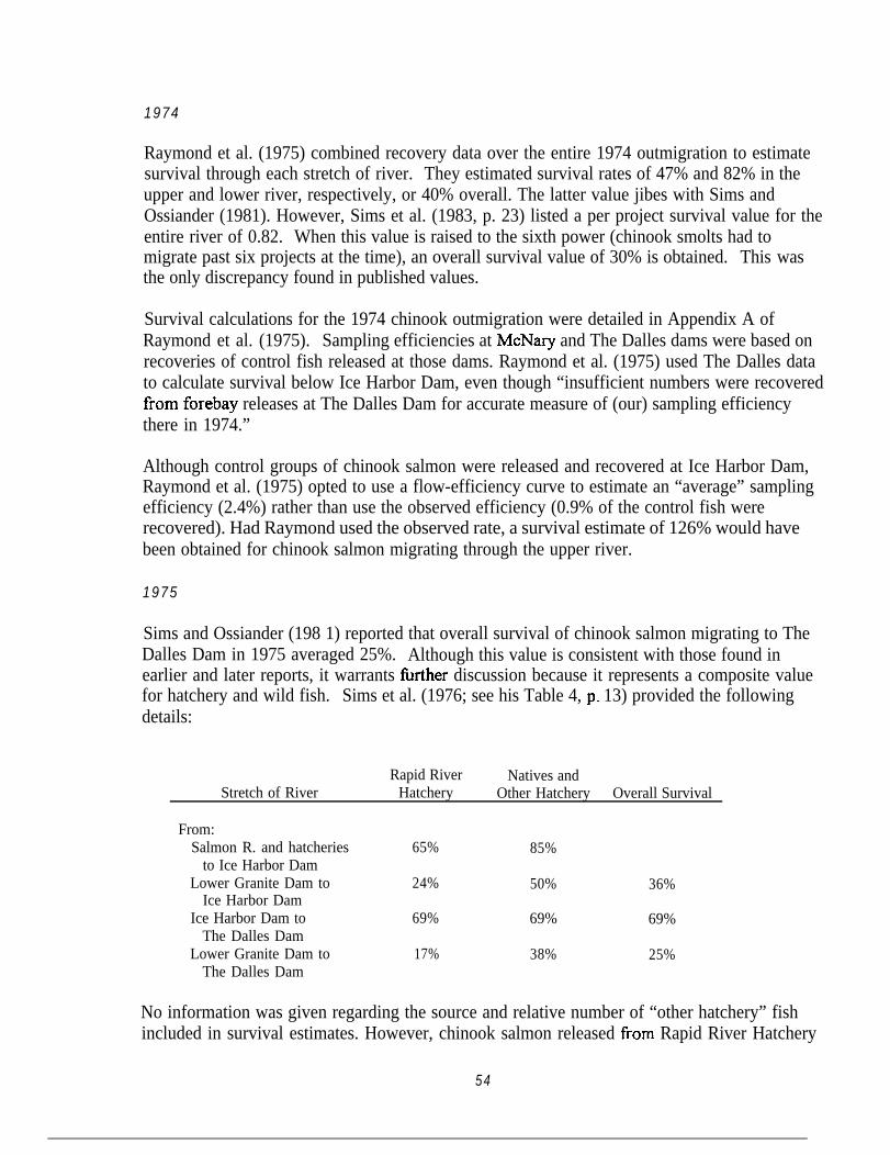
1974

Raymond et al. (1975) combined recovery data over the entire 1974 outmigration to estimatesurvival through each stretch of river. They estimated survival rates of 47% and 82% in theupper and lower river, respectively, or 40% overall. The latter value jibes with Sims andOssiander (1981). However, Sims et al. (1983, p. 23) listed a per project survival value for theentire river of 0.82. When this value is raised to the sixth power (chinook smolts had tomigrate past six projects at the time), an overall survival value of 30% is obtained. This wasthe only discrepancy found in published values.

Survival calculations for the 1974 chinook outmigration were detailed in Appendix A ofRaymond et al. (1975). Sampling efficiencies at McNary and The Dalles dams were based onrecoveries of control fish released at those dams. Raymond et al. (1975) used The Dalles datato calculate survival below Ice Harbor Dam, even though “insufficient numbers were recoveredCorn forebay releases at The Dalles Dam for accurate measure of (our) sampling efficiencythere in 1974.”

Although control groups of chinook salmon were released and recovered at Ice Harbor Dam,Raymond et al. (1975) opted to use a flow-efficiency curve to estimate an “average” samplingefficiency (2.4%) rather than use the observed efficiency (0.9% of the control fish wererecovered). Had Raymond used the observed rate, a survival estimate of 126% would havebeen obtained for chinook salmon migrating through the upper river.

1975

Sims and Ossiander (198 1) reported that overall survival of chinook salmon migrating to TheDalles Dam in 1975 averaged 25%. Although this value is consistent with those found inearlier and later reports, it warrants fin-ther discussion because it represents a composite valuefor hatchery and wild fish. Sims et al. (1976; see his Table 4, p. 13) provided the followingdetails:

Stretch of RiverRapid River Natives and

Hatchery Other Hatchery Overall Survival

From:Salmon R. and hatcheries

to Ice Harbor DamLower Granite Dam to

Ice Harbor DamIce Harbor Dam to

The Dalles DamLower Granite Dam to

The Dalles Dam

65% 85%

24% 50% 36%

69% 69% 69%

17% 38% 25%

No information was given regarding the source and relative number of “other hatchery” fishincluded in survival estimates. However, chinook salmon released from Rapid River Hatchery

54

obviously fared poorly in the upper ‘reaches of the river. Sims et al. (1976, p. 12) ascribed thehigher mortality rate to the culling of weaker hatchery fish at dams. If Rapid River fish areexcluded, overall survival would increase from 36% to 50% in the Snake River, and 25% to3 8% overall.

One might argue that survival estimates (and a flow-survival relationship) should be solelybased on wild fish, especially if the quality and relative abundance of hatchery fish in theoutmigration varied from year-to-year. Raymond (unpublished notes), in fact, made aconcerted effort to exclude hatchery fish from his calculations in earlier years. Arguments forincluding hatchery fish are based on the fact that then, as now, hatchery fish were numericallydominant in the outmigration. It also happened that in most years survival rates were notestimated separately for hatchery and wild fish. I will return to the subject of hatchery fish in alater section.

1976

In contrast to 1975, survival rates reported for hatchery and wild fish did not differ in 1976.Sims et al. (1977) provided the following data (see their Table 2):

Millions of Fish

SourcePassing Passing Passing

Lower Granite Number Number Ice Harbor John DayDam TranSpOrted Remaining Dam DaItl

Rapid River HatcheryNative and Other

Hatchery

3.36 0.55 2.81 ,1.77 0.85

1.74 0.25 1.49 0.93 0.45

Total 5.10 0.80 4.30 2.70 1.30

Using these data, survival can be estimated for Rapid River and Native/Other Hatchery groupsof salmon as follows:

Stretch of RiverRapid River Natives and

Hatchery Other Hatchery Overall Survival

From:Lower Granite Dam to

Ice Harbor DamIce Harbor Dam to

The DaIIes DamLower Granite Dam to

The Dalles Dam

1.7712.81 = 63% 0.9311.49 = 63% 2.7014.30 = 63%

0.8511.77 = 48% 0.4510.93 = 48% 1.3012.70 = 48%

0.8512.81 = 30% 0.4511.49 = 30% 1.3014.30 = 30%

55

It would be incorrect to conclude from this evidence that hatchery and wild fish survived at thesame rates during their downstream passage in 1976. A more likely explanation is that survivalwas calculated for the entire outmigration without regard to fish origin. Estimates of thenumber of hatchery and wild fish passing various dams and being transported at Lower Graniteand Little Goose dams reflect the assumption that hatchery fish made up a constant proportionof the outmigration.

1977

1977 was conspicuous for the extremely low survival of chinook and steelhead migrating thatyear. Sims et al. (1978, pp. 12-13) reported 3.3% (20,000 out of 600,000 migrants) survivalfrom Lower Granite to The Dalles Dam; Sims and Ossiander (1981) use 2% as the 1977survival value. In spite of this discrepancy, there is little question that survival was abysmallylow that year; both the exceptionally low spring runoff and the poor adult return (1977 remainsthe lowest adult return on record) lend credence to this view. However, it seems reasonable toquestion the accuracy of the 2-3% survival value given that (1) as many as 70% of thetreatment fish were transported, yet no computational adjustment was made to account forthese losses (see Section 3.3 Transportation), and, (2) “all survival estimates (we)re based onvery small numbers of mark recaptures” (Sims et al. 1978, p. 5). The 1977 mark-recovery datacertainly appear to bear this statement out (Table 10 above); only 0.06% - 19 out of 38,262 -of the fish released at Lower Granite Dam were recovered at Ice Harbor Dam. As no mark-recovery data could be found for other dams, survival could not be estimated, and furtherspeculation regarding the accuracy of the 1977 survival estimates is inappropriate.

1978

Raymond and Sims (1980, their Table 6) summarized chinook smolt survival data for 1978 and1979. For 1978, they reported 69% survival between Lower Granite and Ice Harbor dams,64% for Ice Harbor to John Day dams, and 44% survival overall. Sims and Ossiander (1981)gave 37% as the survival rate between Lower Granite Dam and John Day Dam. Noexplanation was given for the disparity in the two estimates. All subsequent reports of 1978survival are consistent with the value given in Sims and Ossiander (1981).

The 1978 mark-recovery database retrieved from NMFS files indicated that approximately0.4% of the fish (19 1 out of 46,094) released at Lower Granite Dam were recovered at JohnDay Dam (Table 12). Fish released into the forebay of John Day Dam were recovered at a rateof 1.6% (113 out of 7,281 released). If these two values are taken to be accurate, 1978survival would have been closer to 27%. This estimate should not be used since the accuracyand completeness of the data could not be verified.

1979

Again, survival values reported by Raymond and Sims (1980) and Sims and Ossiander (198 1)do not agree (Table 10). Whereas Raymond and Sims (1980) reported 30% survival for 1979,

56

Sims and Ossiander (198 I) used a value of 24% in their flow-survival analysis. No explanationwas given for the difference in reported values. Survival could not reliably be determined fromthe mark-recapture data obtained from NMFS files.

4.2.6 Per-Proiect Survival Estimates

Sims and Ossiander (198 1) calculated “per project” survival rates for chinook salmonmigrating from the upper dam on the Snake River to either John Day Dam or The Dalles Damon the Columbia River as a function of flow at Ice Harbor Dam. Per-project survival wascalculated as b, = Ulid, where d was the total number of projects, which included theuppermost Snake River dam, since treatment fish were released in the forebay of that dam, butdid not include the lowermost Columbia River dam, where treatment fish were enumerated.Although Sims and Ossiander (198 1) do not list the number of projects used in theircalculations, a number can be calculated from the SIP,, and B values they provided in theirTable 5. There are several discrepancies between the number of projects determined fromthese values and the number of projects calculated from known release and recovery sites(Table 11).

A “project”, as used by Sims and Ossiander (198 l), consisted of a dam and the reach of riverextending to the next dam downstream. This definition, however, was not consistently applied.To cite one example, fish that served as controls in 1977 were released at the head of theLower Granite reservoir near Clarkston, WA (River Mile 742); there were no near-damforebay releases (Park et al. 1979, Appendix Table 1, p. 5). In 1978, however, all of theLower Granite Dam releases were made just upstream (PM 696) of the dam. Thus, controlfish had to swim through 6 reservoirs in 1977, but only 5 reservoirs in 1978 (survival wasestimated to John Day Dam). Nevertheless, Sims and Ossiander (1981) used 6 projects toestimate per-project survival for both years.

According to Sims and Ossiander (198 l), Little Goose Dam was the upper dam and TheDalles Dam the lower dam used to calculate per-project survival for both 1973 and 1974.From their Table 5, however, the number of projects used to estimate per-project survival forthese years was 5 and 6, respectively. The number should have been 5 for both years. Thiswas the number of projects used by Sims and Ossiander (1981) to calculate per-project traveltime estimates for both years. Based on an overall survival of 40%, the 1974 per-projectsurvival rate was 83%, and not 86% as indicated.

In 1975, experimental fish were released in the forebays of Lower Granite Dam, Ice HarborDam, and The Dalles Dam (Sims et al. 1976). As Sims and Ossiander (1981) correctlyindicated, 6 projects were passed from Lower Granite to The Dalles Dam.

Controlled releases of smolts into The Dalles Dam forebay to estimate sampling efficiencywere discontinued in 1976. Although smolt monitoring continued at The Dalles Dam, survivalthrough the lower Columbia River between 1976 and 1979 was

57

Table 11. Number of Snake and Columbia River projects used by Sims and Ossiander(1981) to calculate “per project” survival, compared to the number of projectsascertained from original literature sources.

Number of Projects

YGiI Upper Dam Lower DamSnake Columbia Sims and Os-River River Total siander (1981)

1973 Little Goose Dam The Dalles Dam 3 2 5 5

1975 Lower Granite Dam JohnDay Dam 4 2 6 6

1976 ” ” ” 49 1) ” 4 1 5 6

1978 ” ” ” II II I, 4 1 5 6

1979 ” ” ” I‘ ” 0 4 1 5 6

1 Sampling was conducted in 1977 at both John Day and The Dalles dams. Overallsurvival was determined for the reach extending from Lower Granite to “John Day-The Dalles Dams” (Sims et al. 1978).

58

estimated from samples collected at John Day Dam (Sims et al. 1977, 1978; Raymond andSims 1980). The heading (“Survival to The Dalles Dam”) of the second column in Table 5 ofSims and Ossiander (1981) is therefore incorrectly labeled. From 1976-1979, survival wasestimated for chinook salmon that passed 4 dams - Lower Granite, Little Goose, LowerMonumental, and Ice Harbor - on the Snake River, but only 1 dam - McNary - on theColumbia River. Thus, the number of projects upon which per-project survival was estimatedshould have been 5, and not 6, as indicated by Sims and Ossiander (198 1). Per-project survivalrates for 1976-1979 ranged 3%-6% lower than those indicated in Table 5 of Sims andOssiander (198 1).

The relative number of Snake River and Columbia River projects upon which overall survivalestimates were based ranged from 32 in 1973 to 4:2 in 1975 to 4:l from 1976 onwards (Table11). If survival differed among projects or was in some way dependent on the number ofprojects present, then the flow-survival relation reported by Sims and Ossiander (198 1) mayhave been influenced by changes in the composition and relative number of Snake River andColumbia River projects over the 1973-1979 period.

Historically, fingerling chinook migrant survival rates were lower in the Snake River than in theColumbia River. From 1969 to 1975, survival from the upper Snake River dam to Ice HarborDam averaged 36%. Over the same time period, approximately 58% of the fish passing IceHarbor Dam survived to The Dalles (Raymond 1979). This difference may have been due to“first dam” effects, by which disproportionately high mortalities were sustained by chinookpopulations at the uppermost dam, relative to other dams downstream. In 1968, according toRaymond’s notes, “most (60-75%) of the total mortality occurred at Ice Harbor Dam” (theuppermost dam at the time). Raymond (1979) noted that passage through Little Goose Damresulted in 50% survival in 1973, compared to an average survival of 57-58% at the remainingdams. Variability in per-project survival may have been due to unusually stressful conditions atthe upper dams, such as those caused by large accumulations of debris through whichmigrating smolts were forced to pass (see Section 4.3.2.3 Debris Removal). Raymond (1979,p. 524) suggested that weaker fish were being culled out by stress at the first few darns, andthat mortality due to predation decreased in the downstream direction (“the largest populationsof migrants at upper dams would draw predator fish and birds to these areas”). Raymond andSims (1980, p. 18) noted that in 1979 “the major problem was at Lower Granite Dam wherechinook salmon mortality was measured at 27%.” [i.e., survival = 73%] If this mortality isexcluded, survival from the tailrace of Lower Granite Dam to John Day Dam is much higher(41% rather than 30% (value from Raymond and Sims 1980) or 33% rather than 24% (valuefrom Sims and Ossiander 1981). This equates to a per-dam survival of 86% (vs. 82%) or 83%(vs. 79%).

Because Raymond, Sims, et alia included hatchery fish in their survival estimates, survivalprobably increased with distance downstream as large numbers of hatchery fish succumbedearly on to the rigors of migration. Data are presented below to support the claim thathatchery chinook salmon smolts survived at much lower rates in upper reaches of the SnakeRiver.

59

Projects on the Columbia River may have been less hazardous in general than those the SnakeRiver if a greater fraction of water was spilled at lower river dams, and if the risk of injury ordeath decreased as spill increased. Raymond (1979) attributed differences in reach survivals toprevailing levels of dissolved atmospheric gas; conditions during the early 1970’s were muchworse in the Snake River than in the Columbia River. However, survival was also lower in theSnake River during low flow years such as 1973 and 1977, when gas supersaturation was not aproblem, and during years after fliplips (spillway deflectors) had been installed at dams toreduce dissolved gas supersaturation in the river.

4.2.7 Timing Of Peak Migration

Recall that population estimates for Ice Harbor Dam were determined from the samplednumber of unmarked smolts weighted by prevailing sampling efficiencies. Because samplingefficiency varied with flow, and flow fluctuated over time, estimates of the timing of peakmigration were influenced by the accuracy of sampling efficiency estimates. Timing was alsoaffected by (1) the proportion of hatchery fish in the population, since releases of hatchery fishdid not always coincide with the date of peak migration of wild migrants, and (2) the dates onwhich smelt monitoring at Ice Harbor Dam began and ended, since truncation of either tail ofthe frequency distribution might skew the estimated date of peak migration.

The survival values in the flow-survival relationship were single season estimates based onrecoveries of marked chinook salmon which, more often than not, did not correspond infrequency or timing to the passage of unmarked smolts. It was inappropriate to index thesurvival of experimental fish to the date of peak migration of the unmarked population. Itwould have been better to index survival to the dates of passage of marked fish and, hence, tothe flow conditions under which survival was estimated.

4.3 Additional Sources Of Variation

The 1970’s were characterized by natural and human-caused variations in environmentalconditions unlike any seen previously on the Snake and Columbia River. Year-to-yearvariability and cumulative changes in factors affecting the migratory environment may havealtered the basic relationship between flow and survival. They may also have affected theaccuracy and precision of survival estimates, especially if measurement error was correlatedwith environmental variability.

Raymond (1979) provided a good overview of major climatalogical, hydrological, and otherfactors which may have affected chinook smolt survival in the years 1966 to 1975. Hesuggested that the major causes of mortality during this period were passage through turbinesat the dams, predation, migrational delays, and prolonged exposure to lethal concentrations ofdissolved gases. The effects of these factors on chinook salmon survival varied considerablybetween years, and since they tended to covary with each other and with flow, it was difficultto assess their relative importance on survival for any given year.

60

Flows varied considerably over the period of interest, including record high and low flows in1974 and 1977, respectively (Table 5). Higher flows were spilled at Snake River dams duringthe smolt outmigrations in 1974-76 and 1978 (Sims and Ossiander 198 1). Survival was highduring these years but was less variable than in non-spill years.7 Survival increased with floweven when no spill occurred (i.e., all water was run through the powerhouses); from this itmight be inferred that turbine and/or reservoir passage survival may also have increased withincreases in flow.

In the following sections I review some of the natural and anthropogenic factors that may haveaffected survival or its measurement among marked groups of chinook salmon smolts duringthe 1973-1979 period. I focus on the natural variability in the timing of outmigration and thephysical condition of smolts at the outset of migration, structural and operational changes inthe hydrosystem, and biological interactions between hatchery chinook, wild chinook, andresident fish. The relative importance of sources of mortality other than flow is indicatedwhenever available information permitted an assessment.

4.3.1 Timing and Magnitude of Migration

The physiological, morphological, and behavioral changes in juvenile salmon that convey theability to migrate downstream are synchronized by environmental factors, includingphotoperiod, streamflow, water temperature, and perhaps lunar periodicity (Groot 1981; Muiret al. 1992). Annual variability in environmental cues, along with population-specificdifferences in endogenous rhythms and migratory fitness, may offer partial explanation for thelarge interannual variation in chinook smolt survival observed in the 1970’s.

Dates of peak migration past Ice Harbor Dam in 1973- 1979 ranged from 28 April in 1975 to26 May in the following year.

Raymond (1979 and unpublished notes) gives the impression that he considered watertemperature a greater influence on migration timing than stream discharge. He commented onmigrational delays occasioned by unseasonably cold weather; e.g., “The outmigration of nativechinook smolts was delayed by cold spring weather in 1975. Significant numbers of smoltsnever did show at the Riggins trap on the Salmon River. Those that did were delayed untilwarm weather began about May 5.”

All else being equal, delays in the start of migration may have worked to the advantage ofchinook migrants. Several authors have noted that chinook salmon migrating later in thespring tend to travel faster than early spring migrants (Muir et al. 1992; Smith et al. 1993);travel rate appears to be related to stage of smoltification (Beeman et al. 1991). On the other

7 Sims and Ossiander (198 1) indicated that up to 8 kcfs per dam was spilled during “non-spill”years. This needs to be checked out further.

61

hand, smelts that get a late jump on migration may have fewer lipid reserves to see themthrough their journey. Overwinter conditions are important in this regard: if chinook salmonsmolts began their migrations in a debilitated state following a particularly severe winter, lowerthan normal survival would be expected.

4.3.2 Changes in the Hydro-System and Mainstem Environment

4.3.2.1 Power Generation Capacig and Bypass Changes

Smolt survival during the 1973-1979 period was no doubt influenced by the increase in thetotal number of turbine units installed or operating at dams on the mainstem Columbia andSnake Rivers. The total number of units installed at Snake River dams increased from 9 in1973 to 24 in 1979 (Table 12) (Park 1980, 1993). The number of installed units that wereactually operated also varied between years. Reduced power loading at Lower Granite andLower Monumental dam during the 1975 outmigration was one of factors responsible for thehigh survival of chinook salmon and steelhead that year .8 Noting that only one turbine unitwas operating at Lower Granite Dam, and that most of the river flow passed over the spillway,Sims et al. (1976, p. 1) concluded that “fingerling mortality under these conditions would notbe representative of the mortality that would normally be occurring when all turbines were online. “

Other system modifications that affected chinook smolt survival in the 1970’s included theinstallation of traveling screens to divert migrating smolts away from turbines and into bypassand collection systems at dams (Park 1980). Installation and testing of screens began in 1971.Lower Granite Dam was the first dam on the Columbia River to have tilly screened operatingturbines (Matthews 1977). Not only were the number of diversion screens increased, but theywere made more efficient so that fewer injuries and mortalities resulted. Average fish guidanceefficiency of mainstem dams increased from 0.12 in 1970 to 0.32 by 1980 (McConnaha 1990)(Table 13).

At least one other change in bypass conditions occurred - this one unexpected -,to undermineconfidence in the flow-survival relationship. In 1975, higher than normal mortalities occurredat Ice Harbor Dam (Sims et al. 1976, p. 17). Stoplogs, normally emplaced in the lower sluiceat the dam to create a plunge pool to cushion the fall of migrants passing from the upper to thelower sluice, were either washed out or inadvertently removed between 1974 and 1975.Without a plunge pool, fewer than 50% of the fingerlings passing down the sluice in 1975 werebelieved to have survived (Sims et al. 1976, p. 18). Since dam-related mortality would havebeen much lower had the stoplogs been installed, the overall survival value (25%) used for thatyear as input in the flow-survival regression analysis was probably too low.

* Raymond (unpublished notes) indicated that in 1975 only one turbine unit was operated atLower Granite Dam as well.

62

Table 12. Number of turbine units at hydroelectric dams on the Snake River, 1968-1979.1

Cumulative number of turbine units in place

DZUTl 1968 1969 1970 1971 1972 1973 1974 1975 1976 1977 1978 1979

Lower Granite Dam 0 0 0 0 0 0 0 3 3 3 6 6

Little Goose Dam 0 0 0 3 3 3 3 3 3 3 6 6

Lower Monumental Dam 0 0 3 3 3 3 3 3 3 3 3 6

Ice Harbor Dam 3 3 3 3 3 3 3 6 6 6 6 6

m 3 3 6 9 9 9 9 15 15 15 21 24

1 Data source: Bell et al. (1976), Park (1993)

Table 13. Adjusted fish guiding efficiencies, spring chinook, 1970-1980.1

Dam 1970 1972 1973 1974 1975 1976 1977 1978 1979 1980

Lower Granite Dam - 0.69 0.69 0.69 0.69 0.69 0.69

Little Goose Dam 0.00 0.00 0.00 0.00 0.46 0.46 0.69 0.69 0.69 0.69

Lower Monumental Dam 0.03 0.03 0.03 0.03 0.03 0.03 0.03 0.03 0.03 0.03

Ice Harbor Dam 0.40 0.40 0.40 0.40 0.40 0.40 0.40 0.40 0.40 0.40

McNary Dam 0.00 0.00 0.00 0.00 0.00 0.00 0.00 0.05 0.11 0.32

John Day Dam 0.00 0.00 0.00 0.00 0.00 0.00 0.00 0.00 0.00 0.00

The Dalles Dam 0.40 0.40 0.40 0.40 0.40 0.40 0.40 0.40 0.40 0.40

Bonneville Dam 0.00 0.00 0.00 0.00 0.00 0.00 0.00 0.00 0.00 0.00

Average 0.12 0.12 0.12 0.12 0.25 0.25 0.28 0.28 0.29 0.32

1 Data source: McConnaha (1990)

4.3.2.2 SpiIl and Problems with Gas Supersaturation

As new turbine units were installed and water and hydropower managers gained greatercontrol over river flows, less spilling occurred at mainstem Columbia River Dams, except inyears of above average runoff. Spill, through its effects on the movement and distribution ofsmolts, directly affected survival. During periods of spill, at least a portion of the smoltpopulation are able to pass over the spillway and avoid the dam’s turbines. Changes in therelationship between river flow and the proportion of water spilled during the 1970’s may havealtered the basic relation between survival and flow. Levels of spill that approach those of theearly 1970’s are uncommon today.

Sims and Ossiander (1981) identified spill as a key factor affecting chinook survival, notingthat: “The relationship between survival and spill has a much faster rate of change than therelationship between survival and flow. A proportionate increase in spill at low magnitudeswill yield a greater increase in survival than the same proportionate increase in flow...Amoderate increase in spill, for spill in the lower range of value, will yield substantialimprovements in survival.” The authors observed that spill, like flow, was strongly correlatedwith survival during the period of interest.

Spill was actually deleterious to migrating smolts in high flow years prior to 1977. Migrationconditions during years when large quantities of water were being spilled were notable for highconcentrations of dissolved gases. Prolonged exposure of migrants to supersaturated nitrogengas (greater than 130%) was implicated as a major cause of smolt losses, ranging from zero inthe low flow year of 1973 to 80% in high flow years such as 197 1 (Ebel and Raymond 1976).Nearly two-thirds of the 66% loss of chinook salmon in 1974 was caused by nitrogensupersaturation (Ebel et al. 1975, p. 24). The authors concluded that survival would have beenmuch higher, on the order of 70-80%, had spill deflectors been in place. Mortalities attributableto gas bubble disease began to decline with the installation of fliplips at Little Goose andMcNary Dams in 1976 (Ebel and Raymond 1976).

Petrosky (1991) suggested “backing out” mortality attributable to gas supersaturation ifestimates could be obtained. Unfortunately, no data are available which would permitmodification of annual survival estimates.

4.3.2.3 Debris Removal

During 1981, the U.S. Army Corps of Engineers undertook a major effort to remove debristhat accumulated in the forebay of Lower Granite and other dams (Park 1993, p. 7). Problemsassociated with debris buildup were prevalent throughout the 1970’s, in particular at upperdams during high flow years. Although effective debris control was not initiated at the upperSnake River dams until 1981, earlier attempts to remove debris produced tangible benefits interms of survivability of chinook migrants and transported fish. Debris removal and controlefforts reduced descaling and injury in collection systems. In 1979, for example, the average

65

percent descaling before and after debris was removed from trash racks was 12 and 6%,respectively (Smith et al. 1980, p. 6).

4.3.3 Scale Loss and DelayedMortality

One commonly used index of mainstem passage conditions and their effects on migratingchinook salmon smelts is the percentage of fish observed with significant (>lO%) scale loss;data collected in the 1970’s as part of the transportation studies were summarized by Park(1985). Descaling rates measured during this period were variable between dams and years,ranging from 4.0 to 23% (Table 14). The percentage of chinook migrants that were descaledor injured declined over time. In 1972, over 50% of the chinook sampled from McNary Damgatewells were descaled (Raymond, unpublished data). By 1978-80, the percentage ofdescaled fish had dropped to lo-20%. The progressive decline in descaling was attributed todebris removal, decreasing amounts of spill, and improved bypass conditions at the dams (Park1985).

Descaling rates varied both within a season and between years at a given dam; they also variedamong chinook smolts recovered at different dams in the same year. In 1972, for example, theannual average descaling rate was 16.6% at Little Goose Dam (Park 1985, p. 2-14) and over50% Ice Harbor Dam (Raymond, unpublished notes). In both 1978 and 1979, annualdescaling rates were 2 to 13% higher at Little Goose Dam than at Lower Granite Dam. Thisevidence suggests that, in terms of descaling, the effects of dams on the fitness andcomposition of the smolt population may have been accumulative and detrimental.9

Evidence was provided in Section 4.1 (Sampling and Statistical AssumDtions) of significantsampling-related mortality in most years (Table 6). Delayed mortality was determined fromtests conducted with chinook salmon and steelhead controls under the transportation program,1975- 1980. The values reflect handling effects, but if handling procedures were similar fromone year to the next, then the values also give some indication of the interannual variability insmolt condition and bypass conditions at the dams.

To see whether any of the variation in the per-project survival rates reported by Sims andOssiander (198 1) could be explained by delayed mortality and percent descaling, simple andmultiple regression analyses were performed for the years for which data were available(Tables 7 and 8). These are very crude analyses because of the small sample sizes andassumptions involved, but they nevertheless give insight into mechanisms responsible forobserved rates of survival. Bivariate correlation coefficients were calculated for the followingvariables: per-project survival, Snake River flow (log-transformed), percent delayed mortality,and percent descaling rates (Table 15). The number of yearling chinook that died in 48hdelayed mortality tests and the percentage of migrants exhibiting a significant loss of scales

g It also suggests that treatment fish captured and released at upper dams on the Snake River may haveexperienced different, possibly less, handling and tagging stress-related mortalities than did control fishreleased at John Day and The Dalles dams. If this occurred, the resulting survival estimates would be in error.

66

Table 14. Percentage of descaled (> 10%) spring chinook salmon migrants sampled fromthe marking facility it Lower Granite, Little Goose, and McNary dams, 1972-1980. Data are from Park (1985) unless otherwise noted.

YGlr Mean (%) Range (%)

1975 13.01976 7.01977 27.0’1978 7.01979 5.31980 4.0

1972 16.6b1973 19.6b1977 23.91978 20.01979 8.1c

197819791980

Lower Granite Dam

Little Goose Dam

McNaty Dam

10.0

20.0

-4.0-13.014.0-33.0

1.0-12.01.0-11.0

6.0-49.26.0-44.0

a Ebel et al. (1977)

b Park et al. (1980)

c Smith et al. (1980)

67

Table 15. Bivariate correlation coefficients and significance levels (in parentheses) forselected variables relating to chinook salmon smolt migrations, 1973-1979.Values are based on a sample size (n) of 7 except for correlations involving thedescaled variable, in which case n = 6 (no data for 1974). Flow values weretransformed to their logarithms; all other values are untransformed.

Survival (%)Logarithm of DelayedFlow (kcfs) Mortality (%) Descaled (%)

survival (%) 1.00(0.00)

Logarithm of 0.87 1.00Flow (kcfs) (0.01) (0.00)

Delayed Mortality (%) -0.70 -0.69 1.00(0.08) (0.08) (0.00)

Descaled (%)

68

were negatively correlated with per-project survival rates (Figure 10). The percentage ofdescaled smolts was more highly correlated with survival than was Snake River flow, evenwith one less data point (i.e., 1974) used in the regression analysis. Interpretation of theseresults is complicated by the strong covariation among flow, delayed mortality, and descalingrate. An attempt to include all three variables into a multiple regression model using a liberalF-to-enter criterion (0.1) resulted in the inclusion of only descaling rate as an independentvariable; the addition of flow or delayed mortality did not significantly improve the predictivecapability of the model.

4.3.4 Biological Interactions

4.3.4.1 Hatchery Fish

A major uncertainty surrounding the flow-survival relationship is the effect that hatchery fishmay have had on survival estimates. The number of chinook salmon released from hatcheriesabove Snake River dams increased steadily once Rapid River Hatchery began production in1966. Hatchery steelhead releases also increased. The total number of hatchery-originchinook passing the first dam on the Snake River between 1973 and 1979 ranged from 1.2 to2.3 million fish. Hatchery chinook smolts comprised anywhere from 53% (in 1973) to 75% (in1978) of the total smelt population passing the upper dam.

Concern over potential effects of hatchery chinook on the flow-survival relation are justified onseveral grounds. Hatchery chinook traveled more slowly, died at higher rates, and may havebeen more (or less) vulnerable to capture than were their wild counterparts. Overall survivalestimates were therefore dependent on changes in the relative abundance and fitness ofhatchery and wild fish over distance and through time. Raymond and Sims were acutely awareof the potential for problems of this type. Raymond went so far as to estimate survivalseparately for hatchery and wild chinook up until 1975. His estimates of survival from theSalmon River to the upper Snake River dam for the 1966-1972 period were for wild chinooksmolts only (Lander 1972; Raymond, unpublished notes).

Raymond (unpublished notes) compiled release data along with estimates of the number ofchinook smelts passing the first and last dam they encountered on the Snake and Columbiarivers (Table 16). He also estimated the survival of hatchery chinook from Rapid RiverHatchery to the first dam, and from there to The Dalles Dam. These values can be comparedto survival rates reported for wild chinook in Table 10 (1966-1968: Salmon River to IceHarbor Dam) and for wild and hatchery fish combined (1973-1975: upper to lower dam) inTable 11 of Raymond (1979). In all years except 1973, survival was lower among hatcheryfish (the rate of adult return of hatchery fish was also consistently lower than that of wild fishover the same period [Raymond 19881). The greatest disparity was observed in 1966-1968when survival to the first dam from the Salmon River averaged 16% for hatchery fish,compared to 89% for wild fish over the same distance. Recent studies suggest that survivalrates for hatchery chinook remain well-below those for wild chinook, presumably due to ahigher incidence of bacterial kidney disease among hatchery fish (causative agent:Renibacterium saimoninarum) (Achord et al. 1991, Matthews 1992).

69

40 I

0 40 80 120 160 200Snake River Flow (kcfs)

40 I

0 5 10 Delay: MO&l 25 30 35(%)

0 5 10 I5 20 2s 30Dwxling Ratz (%)

Figure 10. Per-project survival as a fi.mction of Snake River flow, delayed mortality, andpercent descaling. Data and sources are identified in Tables 4, 6, and 14.

70

Table 16. Numbers of juvenile chinook salmon released from Rapid River Hatchery andsurvival estimates, 1966-1975. S1 = survival from hatchery to upper dam; S2 =survival from upper to lower dam; S3 = survival from hatchery to lower dam.These data were compiled by H.L. Raymond, but were not published.

Number of Chinook Smolts(thousands)

YCZUHatchery Passing Passing sulvival

releases upper dam upper w St s2 s3

1966 580 75

1967 450 60

1968 1470 340

1969 960 300

1970 3400 1500

1971 3000 1300

1972 2800 1400

1973 2900 1450

1974 2700 1200

1975 3400 2200

45

36

204

175

400

112

75

270

340

13%

13%

21%

31%

44%

45%

50%

50%

44%

65%

60%

60%

58%

27%

8%

8%

13%

18%

12%

4% 8%

2-3% 5%

10% 23%

11% 13%

71

Interestingly, survival of hatchery fish Corn Rapid River to the upper Snake River damincreased from 13 to 65% between 1966 and 1975. Raymond claimed that increased survivalduring this period resulted from an improvement in hatchery operations and the production ofhigher quality hatchery smolts. One such improvement was the switch from raceway to pond-rearing at Rapid River Hatchery in the late 1960s. The survival of pond-reared fish wassignificantly higher than that of raceway-reared fish (Raymond, unpublished data). Diseasecontrol may also have improved over time (Ebel et al. 1973).r” It is unknown whether thequality of hatchery fish continued to improve during the 1975-1979 period.

Hatchery fish may have lowered the survival of co-migrating wild chinook smelts. While littleis known of hatchery and wild fish interactions, hatchery chinook and steelhead smolts couldconceivably affect the survival of wild smolts through competition for scarce resources, byattracting and supporting larger predator populations, by altering behaviors and activity levels,and by transmitting disease. The outcome of these kinds of interactions depends on therelative abundance of hatchery and wild fish and the degree to which they overlap in time andspace. Density-dependent mortality may have been an important if somewhat unknown factoraffecting hatchery and wild chinook survival. With the exception of 1977, the total number ofchinook and steelhead smelts migrating down the Snake River in the 1970s exceeded thenumber estimated to have migrated in 1964-1969 (Raymond 1988).

Survival rates used in the flow-survival relationship were combined estimates, even thoughseparate estimates were obtained for hatchery and wild chinook in 1973-1975. The magnitudeof the combined estimates depended on changes in the composition of the smolt populationand changes in the relative fitness of hatchery and wild fish over time. In 1975, for example,an estimated 17% of the hatchery fish survived from Lower Granite Dam to The Dalles Dam,compared to 38% of the wild chinook. An “average” smolt survival value of 25% wasreported by Raymond (1979) and used in the flow-survival regression analysis. Sims et al.(1976, p 12) attributed the lower survival observed in 1975 to the dominance of hatchery fishin the outmigration.

Raymond (unpublished data) determined that hatchery fish took 23 days to travel fromWhitebird to Ice Harbor in 1974 compared to 14-15 days for wild fish. Sims et al. (1983) alsoobserved that hatchery chinook traveled much more slowly than did “river run” chinooksmelts. Their conclusion: “Based on this finding, we question the validity of using releases ofmarked hatchery fish to estimate survival and behavior of river run fish.”

lo A letter from E. Parrish, superintendent of Rapid River Hatchery, to H. Raymond in 1970 stated that theyear “started on a rather sour note... Kidney disease took a heavy toll of the (chinook) smolts that were beingheld here for transplanting...We had on hand 1,857,927 fish, and either lost them to the disease, or killed andburied to prevent the disease from spreading.” In contrast, Raymond noted in 197 1 that the Rapid River releasein 1970 included “two million fish released with kidney disease that were to have been buried.” The finaldisposition of the diseased fish remains unclear.

72

4.3.4.2 Changes In The Rioiogicai Community

With the physical and limnological changes that attended the impoundment of the Snake andColumbia rivers came changes in the aquatic community. The abundance of certain nativespecies of fishes declined as free-flowing stretches of river were inundated and transformedinto slow water habitats. Other organisms, non-native species in particular, became moreabundant with the result that biomass and production increased over historical levels (Li et al.1987). Predation mortality on chinook smelts probably increased as populations of squaw-fish(Ptychocheilus oregonensis), walleye (Stizostedion vitreum), smallmouth bass (Micropterusdolomieu), and channel catfish (7ctaZuruspunctatus) grew. Recent studies estimated that 14%of the juvenile salmon that migrated through John Day reservoir were consumed by thesepredators (Rieman et al. 1991). A high level of predation by squawfish, in particular, iscommon throughout the mainstem Snake and Columbia rivers, enough so that a large-scaleprogram to reduce the abundance of this species was initiated by Bonneville PowerAdministration in 1990 (Shively et al. 1991). From this evidence it may be inferred thatsurvival of yearling chinook in 1973- 1979 probably varied with fluctuations in predatorpopulations. However, the extent to which smolt survival may have been affected by increasedrates of predation and other changes in the biological community is unknown.

5.0 SUMMARY AND CONCLUSIONS

Few would contest the statement that chinook salmon smolts are more likely to survive ajourney of several hundred kilometers if they cover the distance in less time, or that theirsurvival and rate of travel will be positively related to flow. However, the exact relationshipbetween flow, rate of travel, and survival can only be determined through careful observationover a broad range of flows. Virtually all scientists who have tried to estimate smolt survivalhave encountered formidable experimental problems. The flow-travel time and flow-survivalrelationships obtained by Sims and Ossiander (1981) and the survival studies upon which theyare based represent the best efforts made to date in this regard. The general relationshipsdepicted may appear intuitive, but are they valid?

This report has provided a critical analysis that attempts to answer the question “How valid isthe flow-survival relationship?” Validity is assessed with respect to experimental design,sampling and analytical methods, and interpretability and applicability of the results. Theprimary assumptions underpinning the relationship are discussed along with potential causes ofand explanations for discrepancies in reported flow and survival estimates. The major points tobe made in this regard are:

l There were significant year-to-year differences in the number and operation of projects,locations of release, and sampling activities;

l Recoveries of marked fish were variable and low - too low in most cases to permitcalculation of mean survival and variance from individual group estimates;

73

l An unknown fraction of control fish died prior to recovery, possibly causing negative andpositive biases, respectively, in sampling efficiencies and survivals;

l Control fish were often recovered at lower rates, at different times, and under differentconditions than were treatment fish;

l Reductions in the number of treatment fish due to transportation were not directlyincorporated into survival calculations;

l Survival estimates were determined for treatment fish released on schedules that did notnecessarily correspond to the timing or relative abundance of the run-at-large. The flowmetric used in the flow-survival relationship was improperly indexed to the date of peakpassage (+ 7 days) of the unmarked population at Ice Harbor Dam.

l A flow-efficiency curve was used to calculate a weighted mean annual survival to IceHarbor Dam for the years 1973- 1975. Spurious correlations exist in the flow-survivalrelationship since the flow-efficiency curve and the flow variable used in the relationshipwere computed from the same set of data;

l Changes in the hydrosystem, logistical constraints, and unanticipated results forcedinvestigators to sum mark-recovery data across replicates after 1975; this approach toestimating “average” annual survival rates resulted in the loss of information (e.g., within-season variability in survival) and lower accuracy;

l Since multiple treatment-control releases were made in all years, within-season estimates ofprecision (standard error) of the observed survival rates were possible; however, onlysingle-season survival estimates were routinely reported;

l A disproportionate share of chinook smolts died at the first dam encountered on the SnakeRiver. Survival was estimated for a section of river that comprised variable and unbalancednumbers of Snake River and Columbia River dams. The flow-survival relation may havebeen influenced by changes in the configuration and number of projects; and

l Separate flow-survival relationships should have been derived for the Snake and ColumbiaRivers since runoff conditions, hydrosystem operations, smolt population characteristics,and various sources of mortality may have varied between reaches within the same years;

l Survival values used in the flow-survival relationship did not agree in many instances withvalues reported elsewhere.

Evidence was provided to demonstrate that chinook smolt survival in 1973-1979 may havevaried in response to factors other than flow. Survival and flow were strongly correlated withpost-sampling (i.e., delayed) mortality and descaling rates measured in transportation studiesbeing conducted at the same time. Factors affecting mainstem passage, including factors

74

responsible for the observed variability in delayed mortality and descaling, varied annually andmay have exerted a strong influence on the migratory behavior and survival of chinook salmonsmolts.

Sampling conditions were too variable, the methods employed to collect and analyze the datawere too unreliable, and the statistical model used to describe the relationship was toosimplistic to justify its use as a predictive tool. Concerns over the validity of the data and themathematical model under which they are subsumed must be addressed before any thought isgiven to applying them. My assessment led me to conclude that the flow-survival relationshipshould not be generalized to existing populations and settings. Further analysis of thehistorical dataset to extract additional information is unwarranted. New field studies andanalytical approaches are needed to clarify the relation between survival and flow within thecontext of current management needs.

Although I question the validity and usefulness of the Sims and Ossiander (1981) flow-survivalrelationship, I have made no attempt to define the “true” flow-survival relationship based onmy interpretation of the data. To do so would require that I superimpose my own assumptionson data of questionable quality, and would in all certainty provoke further controversy.Nevertheless, my own opinion is that, ceterisparibus, a positive relationship exists betweenriver flow and smolt survival, and that it can be satisfactorily .quantified by applying improvedstatistical methodologies to mass marking and recovery data. It is up to today’s researchersand managers to commit the resources necessary to identify the causes, magnitude, andlocations of smolt mortality under present conditions. At the same time, positive steps shouldbe taken to increase in-river smolt survival to levels that permit the recovery and maintenanceof upriver salmonid populations. Shaping flows to better approximate the conditions underwhich these populations evolved would be an appropriate first step.

75

6.0 LITERATURE CITED

Achord, S., G.M. Matthews, O.W. Johnson, and D.M. Marsh. 1992. Use of PIT tags tomonitor the smolt migrations of spring and summer chinook salmon stocks in the SnakeRiver basin. 1989-199 1. Pages l-13 in Bolinger, C. and J. Congleton, editors. Passageand survival of juvenile chinook salmon migrating from the Snake River basin.Proceedings of a technical workshop held at the University of Idaho, February 26-28,1992.

Beeman, J., D. Rondorf J. Faler, P. Haner, S. Sauter, and D. Venditti. 1991. Assessment ofsmolt condition for travel time analysis. U.S. Fish and Wildlife Service 1990 AnnualReport to Bonneville Power Administration (Contract DE-AI79-87-BP35245).

Bentley, W.W., and H.L. Raymond. 1968. Collection ofjuvenile salmonids from turbineintake gatewells of major dams in the Columbia River system. Transactions of theAmerican Fisheries Society 97: 124- 126.

Bentley, W.W., and H.L. Raymond. 1976. Delayed migrations of yearling chinook salmonsince completion of Lower Monumental and Little Goose dams on the Snake River.Transactions of the American Fisheries Society 105: 422-424.

Berggren, T.J., and M.J. Filardo. 1993. An analysis of variables influencing the migration ofjuvenile salmonids in the Columbia River basin. North American Journal of FisheriesManagement 13 : 48-63.

Bruton, M.H. 1990. Alternative Life History Styles of Fishes. Kluwer Academic Publishers.Dordrecht, Netherlands.

Burnham, K.P., D.R. Anderson, G.C. White, C. Brownie, and K.H. Pollock. 1987. Designand analysis methods for fish survival experiments based on release-recapture.American Fisheries Society Monograph 5.

Dauble, D. D., J.R. Skalski, and A.E. Giorgi. 1993. Evaluation and application of statisticalmethods for estimating smolt survival. Report to Bonneville Power Administration(Contract DE-AI79-90-BP626 11).

Ebel, E.J., D.L. Park and R.C. Johnsen. 1973. Effects of transportation on survival andhoming of Snake River chinook salmon and steelhead trout. U.S. Fish and WildlifeService. Fisheries Bulletin 7 1: 549-563.

Ebel, E.J., R.F. Krcma, D.L. Park., H.L. Raymond, E. Slatick, E.M.. Dawley, and G.A. Swan.1974. Evaluation of fish protective facilities at Little Goose Dam and review of other

76

studies relating to protection of juvenile salmonids in the Columbia and Snake Rivers,1974. National Marine Fisheries Service, Seattle, Washington.

Ebel, E. J., H.L. Raymond, G.E. Monan, W.E. Farr, and G.K. Tononaka. 1975. Effect ofatmospheric gas supersaturation caused by dams on salrnon and steelhead trout of theSnake and Columbia rivers. National Marine Fisheries Service, Seattle, Washington.

Ebel, E.J., and H.L. Raymond. 1976. Effect of atmospheric gas saturation on salmon andsteelhead trout of the Snake and Columbia rivers. United States National MarineFisheries Service Marine Fisheries Review 38: 1-14.

Elliott, D.G., and R.J. Pascho. 199 1. Juvenile fish transportation: Impact of bacterial kidneydisease on survival of spring/summer chinook salmon stocks. U.S. Fish and WildlifeService, Seattle, Annual Report 1989 to the U.S. Army Corps of Engineers, WallaWalla, Washington (Contract E86880047).

Elliott, D.G., and R.J. Pascho. 1992. Juvenile fish transportation: Impact of bacterial kidneydisease on survival of spring/summer chinook salmon stocks, 1990. U.S. Fish andWildlife Service, Seattle, Annual Report 1989 to the U.S. Army Corps of Engineers,Walla Walla, Washington (Contract E86890043).

Giorgi, A.E., G.A. Swan W.S. Zaugg, T.C. Coley, and T.Y. Barila. 1988. Susceptibility ofchinook salmon smolts to bypass systems at hydroelectric dams. North AmericanJournal of Fisheries Management 8: 25-29.

Groot, C. 1981. Modification of a theme -. a perspective on migration behaviro of Pacificsalmon. Pp. 1-21 in E.L. Brannon and E.O. Salo, editors. Salmon And TroutMigratory Behavior Symposium. University of Washington, Seattle.

Hansen, L.P., and B. Jonsson. 1985. Downstream migration of hatchery-reared smolts ofAtlantic salmon (SaZmo salar L.) in the River Imsa, Norway. Aquaculture 45: 237-248.

HofZnan, A., and J.R. Skalski. 1993. Evaluation of release-recapture models for Snake riversurvival studies. Appendix A in Dauble, D. D., J. Skalski, and A.E. Giorgi. 1993.Evaluation and application of statistical methods for estimating smolt survival. Reportto Bonneville Power Administration (Contract DE-AI79-90-BP62611).

Kindley, R. 199 1. The flow/survival/time travel relationship: review and analysis ofsupporting information and rationale for flows for juvenile spring and summer chinookmigrations. Report to Pacific Northwest Utilities Conference Committee, Portland,Oregon.

Kirk, R.E. 1982. Experimental Design: Procedures for the Behavioral Sciences.Brooks/Cole Publishing Company, Monterey, California.

77

Lander, R.H. 1972. Review of pre- and post-impoundment estimates for survival andabundance of Snake River chinook salmon. Report to the National Marine FisheriesService, Seattle, Washington.

Li, H.W., C.B. S&reck, C.E. Bond, and E. Rextad. 1987. Factors influencing changes in fishassemblages of Pacific Northwest streams. Pages 193-202 in W.J. Matthews and D.C.Hein, editors. Community and Evolutionary Ecology of North American StreamFishes. University of Oklahoma Press, Norman.

Matthews, G.M., G.A. Swan, and J.R. Smith. 1977. Improved bypass and collection systemfor protection of juvenile salmon and steelhead trout at Lower Granite Darn. MarineFisheries Review 47: 28-34.

Matthews, G.M., D.L. Park, J.R. Harmon, and T.E. Ruehle. 1988. Evaluation oftransportation of juvenile salmonids and related research on the Columbia and SnakeRivers, 1987. National Marine Fisheries Service Research Report to the U.S. ArmyCorps of Engineers (Contract DAW68-84-H0034).

Matthews, G.M., S. Achord, J.R. Harmon, O.W. Johnson, D.M. Marsh, B.P. Sandford, N.N.Paasch, K.W. McIntyre, and K.L. Thomas. 1992. Evaluation of transportation ofjuvenile salmonids and related research on the Columbia and Snake Rivers, 1990.National Marine Fisheries Service Research Report to the U.S. Army Corps ofEngineers (Contract DAW68-84-H0034).

McConnaha, C. 1990. Analytical Methods Work Group: Flow/survival relationship.Memorandum to the Monitoring and Evaluation Group of the Northwest PowerPlanning Council.

Muir, W. D., C.S. McCutcheon, A.E. Giorgi, W.S. Zaugg, W.W. Dickhoff, and B.R.Beckman. 1988. Behavior and physiology studies in relation to yearling chinookguidance at Lower Granite and Little Goose Dams, 1987. National Marine FisheriesService Research Report to the U.S. Army Corps of Engineers (Contract DAW68-84-HO034).

Muir, W.D., A.E. Giorgi, W.S. Zaugg, W.R. Hirtzel, and B.R. Beckman. 1990. Anassessment of the relationship between smelt development and fish guiding efficiency atLower Granite Dam. National Marine Fisheries Service Research Report to the U.S.Army Corps of Engineers (Contract DAW68-84-H0034).

Muir, W.D., W.S. Zaugg, C.S. McCutcheon, and J.G. Williams. 1992. Biologicalmanipulation of migration rate: The use of advanced photoperiod to acceleratesmoltification in yearling chinook salmon, 1990. National Marine Fisheries ServiceReport to Bonneville Power Administration (Contract DE-AI79-87-BP35245).

78