THESIS

GAP ANALYSIS OF INDIA’S WESTERN GHATS PROTECTED AREA NETWORK:

INSIGHTS FROM NEW AND UNDERSTUDIED ENDEMIC SPECIES’ DISTRIBUTIONS

Submitted by

Oliver Miltenberger

Graduate Degree Program in Ecology

In partial fulfillment of the requirements

For the Degree of Master of Science

Colorado State University

Fort Collins, Colorado

Summer 2018

Master’s Committee:

Advisor: Stephen Leisz

Paul Evangelista

Liba Pejchar

Copyright by Oliver Miltenberger 2018

All Rights Reserved

ii

ABSTRACT

GAP ANALYSIS OF INDIA’S WESTERN GHATS PROTECTED AREA NETWORK:

INSIGHTS FROM NEW AND UNDERSTUDIED ENDEMIC SPECIES’ DISTRIBUTIONS

Protected areas are a crucial tool to meet conservation goals of the 21st century, especially in

biodiverse regions threatened by land use change. This study makes use of nine years of field data

collected on over 300 understudied plants and amphibians endemic to the UNESCO-recognized

biodiversity hotspot of the Western Ghats of India to produce a gap analysis of its protected area network.

The gap analysis updates previous analyses to reassess network coverage and to improve biodiversity

distribution estimates. Software for Assisted Habitat Modeling (SAHM) queries possible species

distribution models (SDMs) and predictor variables for thirty-five of these species sub-grouped by range

strategies. This generates parsimonious sets of predictor variables as well as performance assessments of

SDMs, which then populate batch-run distribution Maximum Entropy models (Maxent). These

distributions are overlain in various ensembles to produce clade and biodiversity specific insights about

high and low-occurrences areas for these species. Hotspot assessments of the region are generated using

ensembled distributions and are compared to the current protected area (PA) network to identify gaps in

coverage for high-occurrences of these species’ distributions. Most high species co-occurrences for both

amphibian and plant distributions are covered by the PA network with the exception of three regions for

amphibians and six regions for plants, two of which overlap between clades. Previous studies largely or

exclusively used secondary-data for their assessments while the majority of species in this study have

never been modeled or included in gap analyses. This study’s assessment adds new ecological

information to individual species and novel contributions to conservation planning in a threatened

biodiversity hotspot. This study recommends inclusion of the seven identified high-occurrences areas in

iii

future conservation efforts for the Western Ghats and prioritization of the two areas identified as gaps in

protection for both clades.

iv

TABLE OF CONTENTS

ABSTRACT .................................................................................................................................................. ii

Introduction ................................................................................................................................................... 1

Methods ....................................................................................................................................................... 7

Study Area ...................................................................................................................................... 7

Field Data ........................................................................................................................................ 7

Environmental and Spatial Predictors ............................................................................................. 8

Species Distribution Models ........................................................................................................... 9

Ensembling and Spatial Analysis .................................................................................................. 12

Results ......................................................................................................................................................... 14

Discussion ................................................................................................................................................... 17

Limitations and Future Study ......................................................................................................... 20

Conclusions Recommendations ................................................................................................................. 23

Tables and Figures ..................................................................................................................................... 24

References .................................................................................................................................................. 38

Appendix .................................................................................................................................................... 49

1

Introduction

The conservation of nature, its diversity, and its service to human well-being is one of the most important

goals of this century (IUCN 2017, UNEP 2016, Braat and de Groot 2012). Protected area (PA)

demarcation is among the most frequently used tools for achieving these goals. Effective PAs have been

shown to stop or reverse biodiversity and habitat loss, improve access to and consistency of ecosystem

services, and improve human socio-economic conditions (Costanza et al. 1997, Butchart et al. 2010,

Ferraro et al. 2011, Geldman et al. 2013). However, in many cases, standardized and systematic

monitoring to evaluate the impact and effectiveness of PAs in achieving their stated goals is lacking

(Bottrill et al. 2013). Case studies document PAs as achieving successes as well as being ineffective or

detrimental for conservation and livelihood goals (Christie 2004, Ostrom et al. 2009, 2011). Among many

possibilities, the cause of neutral or negative impacts is commonly attributed to lack of policy

enforcement (e.g. paper parks: Bruner et al. 2001, Gibson et al. 2005) or the failure of PA designs to

adequately protect core habitats and adapt to changing ecological needs of vulnerable species (Brandon

and Kent 1992, Butchart et al. 2015).

Protected area establishment is most effective in conserving biodiversity when it targets areas with

vulnerable species, defined as those of IUCN threatened-status or worse or as endemic species with

restricted ranges (Das et al. 2006; Brooks et al. 2002, 2006). Biodiversity hotspot is a term that describes

areas of high biological diversity and occurrence of vulnerable species (Mace and Lande 1991). Globally,

thirty-six regions are defined as biodiversity hotspots, yet each site measures and qualifies its biodiversity

using disparate or incomparable types of data and monitoring methods (Myers et al. 2000). Therefore

biodiversity hotspots are sometimes critiqued as a metric for setting conservation priorities and should be

considered as one of many possible pathways for identifying conservation policy and practice (Myers et

al. 2003, Marchese et al. 2015). Despite these contentions, given limited information and resources, this

study and others suggest that biodiversity hotspots are reasonable means of guiding conservation action

2

(Mittermeier et al. 2011). In nearly all cases, protecting these hotspots relies on in situ conservation

interventions that prioritize areas with the highest occurrences of endemism, threatened species, species-

richness, and/or intact ranges of multi-species habitat (Possingham and Wilson 2005). However, due to

limitations in primary data, monitoring, variation in policies and enforcement, and/or suboptimal analytic

methods, many hotspots are known only through very coarse estimations of the distributions of the

biodiversity that qualifies them as hotspots (Zachos and Habel 2011, Marchese et al. 2015).

Historically, PA creation has often been based on heavily studied, large bodied or charismatic species or

geophysical uniquenesses (Isaac et al. 2004, Joppa and Pfaff 2009). Including evidence-based

distributions of understudied and vulnerable species in prioritization contributes to the goal-setting and

goal-achieving processes in biodiversity conservation (Kullberg et al. 2015). Gap analysis is both an

established scientific methodology and a practitioners’ tool that assesses the current state of PA design

and integrates important data into PA evaluations, policy, and management (Rodriguez et al. 2004). A gap

analysis uses species distributions to identify geographic areas, or gaps, in a PA network that should be

targeted for protection (Scott et al. 1993). This type of analysis has been widely used to expand and

redirect management of PAs domestically and internationally (Jennings 2000, Vimal et al. 2011).

Selecting which species distributions are used in the gap analysis is determined both by which species are

relevant to PA conservation goals and the availability of data to estimate those distributions (Angelstam

2004, USGS Gap Analysis Program report 2013). As new data become available and species are

discovered, change status of vulnerability, or are identified as important to PA goals, gap analyses must

be updated to adequately reflect those changes.

The species selected to conduct a gap analysis dictate the types and degree of inferences able to be made

about its results (Jennings 2000). Some groups of species can serve as ecological and conservation

indicators (Dufrene and Legendre 1997). Including indicator species in a gap analysis allows results to be

extrapolated to produce broader inferences about biodiversity richness and distribution or ecosystem

function in the study area (Carignan and Villard 2002). For example, some literature suggests endemic

3

plant distributions and richness correlate with overall diversity of vertebrate endemism (Kier et al. 2009).

Endemic amphibian population status and distributions can also be indicators of wider trends in

environmental disturbance and function (Stuart et al. 2004, Lewandowski et al. 2010). However, the

diversity and conservation status of endemics plants and, in particular, endemic amphibians are shown to

be in steep decline globally and yet they are comparatively understudied (Gibbons et al. 2000, Orme et al.

2005, Urbina-Cardona 2008). Despite and because they are understudied, further research on these clades

represents a particularly fruitful opportunity to add to information about their conservation status and

infer ecological conditions of their habitat. Their inclusion in a gap analysis would also serve the purpose

of targeting vulnerable species for protection while still providing the deeper ecological insights into the

health and function of the analyzed PA (Sarkar et al. 2006, Saura and Pascual-Hortal 2007).

Though including all species of conservation concern in a gap analysis is ideal, it is nearly impossible to

account for all relevant, present, and transient diversity and its level of vulnerability on a landscape scale,

even if limited to specific geographies or clades of species (Scott et al. 1993). However, accurately

predicting and adding representative and ecologically demonstrative species’ distributions to gap analyses

begins to improve the capacity of conservation efforts to prioritize and effectively target areas in need of

additional protections (Rodrigues et al. 2003). Species distribution models (SDMs) are one method for

estimating those species occurrences over space and time (Elith and Leathwick 2009). SDMs use a

combination of spatial and environmental predictor variables in conjunction with field data recording

presences and/or absences of species to produce an estimation of habitat suitability across a defined study

area (Guisan and Zimmermann 2000). Though there are many different SDMs and recognizing that it is

necessary to discuss caveats and qualifications related to whichever SDM used, they are persistently

shown to be useful tools in ecologic research and a valuable methodology for identifying and guiding the

delineation of priority areas for species conservation (Guisan et al. 2006). Accurate and well-tested SDMs

of representative species produce insightful and important data for conducting and interpreting gap

analyses (Hernandez et al. 2006).

4

Gap analyses use multiple SDMs overlain as a single map to create heat-maps representative of the

number of species occurrences per modeled spatial unit. Heat-maps and areas of high species co-

occurrence (hotspots) identified therein are sometimes conflated with statistical hotspot maps. Hotspot

maps represent statistically calculated high and low occurrences of a variable across space, such as

species co-occurrence, and in ecologic sciences are often used as a representation for biodiversity richness

(Myer et al. 2000, 2012). Presence of high biodiversity richness commonly serves as a metric for

assessing conservation goals, often in the form of total species per area (alpha diversity) or as a

percentage of distribution covered per unit area (beta and gamma diversity) (Kremen et al. 2008).

Prioritization analysis builds on gap analysis models by calculating replaceability of areas given an

established set of conservation goals, such as a goal to preserve 60% of habitat for 60% of total species

occurring within PA boundaries. Replaceability, or the reciprocal, irreplaceability, is a measure of

environmental redundancy with respect to groups of species’ distributions that occur within a defined

ecosystem (Rüble 1935, Brooks et al. 2006, Carawrdine et al. 2007). This method is useful for identifying

areas that are critical, beneficial, or neutral to meeting conservation goals, and allows policy and practice

to act in accordance with, or at least with awareness, of those trade-offs. Identify high co-occurrence areas

of irreplaceable species as well as where those areas are located in relation to PA network coverage is

crucial to assessing and managing current and future conservation in PAs (Prendergast et al. 1993, Myers

et al. 2000).

The sub-continent of India, particularly its Western Ghats region, represents a unique opportunity for

conservation planners to benefit from a gap analysis. The region faces many potential challenges to

conservation such as rapid land use changes, a hyper-diverse geography, an understudied PA network,

and a richness of biodiversity that continues to be discovered through newly documented species and

genetic testing (UNESCO World Heritage Report 2012, Vijayakumar et al. 2014). The Western Ghats is a

well-recognized biodiversity hotspot with nearly 3200 species of known vulnerable and endemic species

distributed over a landscape of dynamically shifting land uses and biomes (Indian Wildlife Institute

5

Annual Report 2016, Table 1). Formal protections within the region have origins in the Government of

India’s Wildlife Protection Act (WPA) of 1972. The WPA provided an extensive legal framework for the

conservation of vulnerable species and the authority to create PAs in India. In response to the WPA, the

Western Ghats escarpment saw a proliferation of PA creation in an effort to preserve its high biodiversity

and density of endemic and endangered species. However, studies have shown that the placement of

many of those PAs was heavily influenced by convenience of location rather than evidence-based study,

and in the process displaced thousands of people leading to additional unintentional land use and land

cover changes (Gunawardene et al. 2007, Ormsby et al. 2011). In 2006 The Scheduled Tribes and Other

Traditional Forest Dwellers Act (known as the Forest Rights Act) overrode the WPA’s restricted-use

mandate by allowing certain tribal ethnicities and subsistence land-users to occupy PAs and harvest

natural resources therein spurning further land use changes. In 2012 UNESCO declared the region a

World Heritage site referencing its extensive biological, physical, and cultural properties (UNESCO

2012). Though UNESCO’s 2012 World Heritage Report advises that the current and potential future

influences of land use change could negatively affect the integrity of the Western Ghats, their ecologic

effects have been notably understudied in peer-reviewed literature (Sekar 2016). However, some studies

have already suggested the reverse diaspora of the Forest Rights Act have had negative influences on

conservation outcomes within PAs and thereby emphasize the importance of reassessing the PA networks

in India and the Western Ghats (Pawar, et al. 2007, Gerlach, et al. 2013, Satish et al. 2014).

Recognizing the Western Ghats are an internationally important area rich in biodiversity, a gap analysis

was conducted in 2006 (Das et al. 2006). However, this analysis retrieved or created its species

distribution estimations only for species that had available secondary data. Thus its focus was primarily

on mammalian and avifauna species and vegetation cover types. As noted by the authors, the estimations

used to identify hotspots and gaps in PA network coverage were generated using widely varying

methodologies and SDMs which may have biased the normalization of input data. In order to standardize

the analysis, the authors’ species estimations were retrofit to a resolution of 180km² grids cells and thus

6

its results have been subject to scrutiny of scale and precision. In the years since this analysis, continued

conservation work and scientific studies have found that there are potential weaknesses and limitations in

both the conservation planning for the Western Ghats region and in the knowledge related to earlier

conservation efforts and gap analyses. The objectives of this study aim to address these developments and

produce a primary data-driven, refined set of estimations for species’ distributions relevant to the Western

Ghats’ conservation goals.

The objective of the study is to produce new insights and recommendations relating to geographic

protection for the species of conservation concern in this study endemic to the Western Ghats. This effort

relies on estimating their distributions and high-occurrence hotspots in context of the current PA network.

It achieves this goal through accomplishing the following:

• Create and assess SDMs for 69 frog and 306 plant species endemic to the Western Ghats.

• Identify areas with high co-occurrence of these species.

• Spatially assess the overlap of these areas with the existing PA network and identify gaps in

protection.

The hypothesis of this study is that the PA network does not adequately cover the distributions of

vulnerable amphibians and plants in the Western Ghats. This analysis builds on previous studies to assess

the relationship between the geographic coverage of vulnerable species and the PA network of the

Western Ghats. Key additions of this gap analysis include the use of nine years of primary data on

vulnerable indicator species, a spatial resolution of 1km², and a rigorously developed and

methodologically consistent set of SDMs.

7

Methods

Study Area

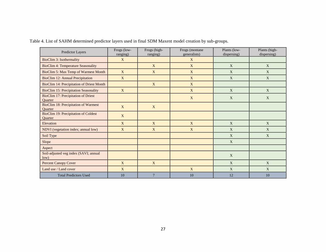
The Western Ghats is approximately 175,000km² stretching 1,600km north-to-south and 300km east-to-

west along the western escarpment of India’s Deccan Plateau (UNESCO 2012, Figure 1). It contains

extensive variations in physical geography with elevation ranging from sea level to 2,695 meters above

sea level and averaging 1,200 meters. Its average annual temperatures are between 18 and 25 degrees

Celsius, and the average annual precipitation ranges from 80cm in the northeastern reaches to over 800cm

in the southwestern peninsular cloud forests (Gunawardene et al. 2007, Ramachandra et al. 2012). The

region encompasses a diverse array of natural features including seven watersheds, one of the world’s

richest arrays of biodiversity estimated to contain hundreds to thousands of undocumented species

(Bebber et al. 2007, Subramanian et al. 2015), and an array of biomes spanning montane grasslands,

temperate forests and drylands, and evergreen subtropical and cloud forest ecosystems (CEPF Western

Ghats Hotspot Assessment 2016, Indian Wildlife Institute Annual Report 2016). Its PA network contains

thirty-nine PAs representing all six levels of IUCN management types and covering approximately 11%

of the Western Ghats range (Figure 1). The study area used in SDM predictions is generated using the

perimeter of the PA network with a half-degree buffer in order to fully encompass the Western Ghats

extent and potential species ranges (Figure 1).

Field Data

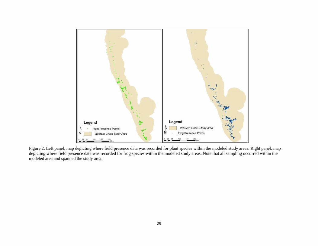
Field data for this study consists of over 8,100 presence point locations of 69 frog and 306 plant species

collected over nine years (2008 – 2017) and fourteen field seasons. The field work was done at the early

onset of the monsoon (early June) or the waning weeks of the monsoon (late September) in order to

maximize likelihood of successful field observations. Surveys were conducted by the biogeographical and

ecology laboratory of the Centre for Ecological Research of Bangalore, India. Sampling surveys span all

fourteen major massifs of the Western Ghats and represent its major biomes and the range of their

8

associated environmental conditions. Data collection methodology utilized randomized convenience plot

surveys of 20 to 100 square meters and totaled over 250 sites for frogs and 350 for plants (Figure 2).

Presence-only point data were collected ranging from 6 to 207 data points per species (Appendix 1, 2).

Upon collection, species were taxonomically identified to the sub-species level and biogeographically

assessed for genetic relations (Vijaykumar et al. 2014; Page et al. 2016). In two cases of few presence

points for allopatric sub-species, data is combined and modeled as a single SDM then manually separated

into individual sub-species SDMs via GIS and expert understanding (Appendix 3). These allopatric

species are known to have only recently sub-speciated and would otherwise have been modeled as a

single species (Vijayakumar et al. 2014). This study would not otherwise include those allopatric species

with such low presence point data.

All frog and plant species are sub-grouped by range strategies (Appendix 1, 2); three sub-groups within

frogs (narrow or widely ranging and montane generalists) and two sub-groups within plants (widely or

narrowly dispersing). Sub-grouping species enables a more tailored selection of predictors that reflect the

unique ecologic profiles of the studied species. Criteria for how species are sub-grouped consists of life-

cycle strategies, meta-data collected during field sampling such as elevation and latitudinal bands, and

known biogeographical speciation patterns (Vijaykumar et al. 2016, Page and Shanker 2018).

Environmental and Spatial Predictors

Twenty-nine geospatial layers are either retrieved as prefabricated predictors or are created from remotely

sensed imager for use as covariates in SDMs (Appendix 4). The Indian National Geographic data base,

known as Bhuvan, provides preprocessed and mosaicked Landsat 8 imagery, a percent canopy cover

layer, and forest fraction cover layer (ISRO 2018). The United Nations’ Food and Agricultural

Organization provides a soil type layer and a nearest-surface-water layer. The raw Landsat 8 imagery

represents time periods from 2015 through 2017. Each Landsat 8 scene is from the late inter-monsoonal

months in order to avoid excessive cloud cover. This time period is also typically associated with the

driest time of year which, after processing, produces conservative estimations of environmental indexes

9

for the study area. Thus, imagery of this time period is purposefully selected since, according to

background literature, reaching the threshold amount of moisture and vegetative growth is the greatest

limiting factor for many of the modeled species (Fu et al. 2008, Baldwin et al. 2009). The raw imagery

and forest fraction layer is used to run an unsupervised classification of the land cover in the study area.

This process emulates Bhuvan’s methodology and was field validated by the Indian Institute Geospatial

Lab (Rao et al. 2006). Defined land cover classes include three variants of forest cover (dry, wet, mixed),

grassy fields, urban, rocky/barren, water surface, built-up and mixed, agricultural, and scrubland. Raw

imagery is also used to derive a Normalized Difference Vegetation Index (NDVI) and Soil Adjusted

Vegetation Index (SAVI) (Heute 1988). ASTER satellite imagery is used to create a digital elevation

model (DEM) and subsequently derived slope and aspect predictor layers (Fischer et al. 2008). All

nineteen BioClimatic II variables retrieved from the WorldClim database are also used as potential

predictors. All predictor variable layers are clipped to the study area extent and standardized to a 1km²

grid-cell resolution.

Species Distribution Models

Sub-sets of each of the sub-grouped clades are semi-randomly selected to represent a gradient of species

with high and low numbers of presence points. These sub-sets, containing five to twelve species, are first

modeled in Software for Assisted Habitat Modeling (SAHM). All species modeled in SAHM are subject

to a covariate correlation assessment for all predictors and generates distribution estimations and a range

of statistical outputs for five SDM algorithms. Results of this SAHM query are tabulated to track which

predictors are most commonly selected within species subgroups and which SDM algorithms produce the

highest model performance metrics (Table 2, 3). The resultant sets of parsimonious predictors are used to

populate Maximum Entropy model (Maxent) SDMs for all species in this study (Table 4).

Maxent is only one of the SDM models run in the SAHM package. Others included and tested are

Boosted Regression Trees (BRT), Random Forest (RF), Multivariate Adaptive Regression Splines

(MARS), and Generalized Linear Model (GLM). BRT and RF are tree-based machine-learning

10

algorithms that allow for multi-dimensional field data to be used. They use statistical modeling fitting for

each data point in order to identify dominant, dynamic patterns across large data sets and large study areas

(Johnson et al. 2012). The ‘boosted’ aspect of a BRT differentiates it from a RF in that it uses an iterative

approach in its model fitting (Elith et al. 2008). The GLM model is among the first to permit presence and

absence data in its estimations and allows for modeling of nonlinear geographic data in SDMs, but has

been critiqued as over-fitting the data because of its tendency to throw-out predictors (McCullagh and

Nelder 1989, Buckland and Elston 1993). MARS like GLM permits presence-absence, but goes a step

further by splining regression between response variables and predictor data (Friedman 1991, Leathwick

et al. 2006). MARS’s noted strong suit is its ability to handle presence points collected in heterogeneous

spatiality and resolution (Moisen and Frescino 2002). Maxent utilizes a maximum entropy Bayesian

algorithm and input data-use features to predict niche-likelihood of a species rather than explicit habitat

suitability (Phillips et al. 2004, Merow et al. 2007; Halvorsen et al. 2015). Maxent is designed to compute

potential species distributions based on the premise of imperfect data and predictors and is well known for

its predictive accuracy given limited presence points and heterogeneous study areas (Warren and Seifert

2011). Common criticisms of Maxent include that the model assumes all predictors carry equal weight

and that its algorithm constrains data via limiting variance in test-trains (Fitzpatrick et al. 2013, Merow et

al. 2013). Maxent is reported to be a powerful tool in its simplicity and though sometimes criticized for

being an overly simple algorithm and blindly relied on by researchers, it is often found to be a useful tool

for modeling small or disparate data sets to produce scientifically sound species distribution predictions

(Warren and Seifert 2011, Elith et al. 2011, Philips et al. 2017).

All five SDM models are run on the predefined sub-sets of species to produce a range of statistical

outputs with which model performances are compared. In cases of low presence points for species, some

models, particularly BRT and RF, are not able to compute distribution estimations because their

algorithms require more input data. SAHM produces evaluations of sensitivity and specificity of predictor

variables, percentage of modeled area correctly classified (PCC), a true-skill statistic measuring the ratio

11

between Cohen’s kappa and PCC, as well as an receiver operation curve (ROC) plot area-under curve

(AUC) value. AUC is a commonly relied upon metric that estimates the ability of a model to correctly

predict its input data given a piece-wise test-split of input data (Wisz et al. 2008, West et al. 2016). These

evaluation metrics are compared to elicit comparative strength of performances across SDM model

algorithm per species. Models’ performance is recorded to show the frequency of a model being high-

performing or not within all sub-groups (Appendix 5, 6, 7). Throughout the initial SAHM query, Maxent

is most frequently shown to be highest performing model and thus is chosen as the primary SDM model

for this study. Using a single SDM, Maxent for instance, helps to maintain consistency of projections and

data usage throughout distribution estimations. Within this initial inquiry into model performances,

SAHM also allows for intra-computational selection of predictor variables by means of a covariate

correlation matrix. The number of predictors selected is limited to a ratio of 1:3 and 1:12 predictors to

number of presence points per species in order to prevent over fitting data to predictors (Austin 2007,

Table 4). Predictors are prioritized in the following way: (1) which predictors explain the most deviance

in model output, (2) which predictors correlate to other variables, and (3) which predictors are

ecologically relevant to the species. No predictors are selected with 70% or higher correlation to another

variable, regardless of percent deviance explained. Individual species results from SAHM’s predictor and

model selection inquiry are tabularized and used to populate batch-run Maxent models of the sub-grouped

species.

Default Maxent parameterizations are used for all species except in cases of species with fewer than 20

presence points in which case data is jackknifed in order to avoid spatial autocorrelations by resampling

data without removing data during the test-split training. In these cases the maximum number of iterations

is increased from 500 to 1000 in order to permit type II errors (false-negative of species occurrence) to

emerge rather than preserve the model’s computational resources (Halvorsen et al. 2016). Pseudo-

absences are created using randomized spatial sampling and allowed to permutate between 500 and 3000

(an average of approximately 1000 are used) depending on the number of species presence points and

12

their spatial distribution. The threshold rule to produce a binary map of species presence is set to a

‘sensitivity equal to specificity’ which selects a threshold of likelihood-presence based on when type I

and type II errors are balanced. This rule is commonly used within SDM literature and found to produce

defensible estimations of distributions for both wide ranging and narrow ranging species (Freeman and

Moisen 2008, Escalante et al. 2013). The SDMs produce both a gradient likelihood map and binary map

for each species.

Ensembling and Spatial Analysis

Species’ binary maps are ensembled with a cell statistic tool by sub-groupings, then by clades, then

collectively across all species in the study. This yields five additive maps for each of the following sub

groups: narrowly-ranging frogs, widely-ranging frogs, montane generalist frogs, narrowly-dispersing

plants, and widely-dispersing plants (Figures 3, 4). Three maps of the following ensembled species

groups are also created: all modeled frogs, all modeled plants, and all modeled species of frogs and plants

combined (Figures 5, 6). Each cell of 1km by 1km area within each of these eight maps is thus

represented by a single whole integer indicating the number of species predicted to occur in the grid cell.

These eight ensemble maps represent heatmaps of species distributions and are used to conduct an

overlay analysis (Flather et al. 1997). Each map is assessed for high species co-occurrence by querying

the study area for cells containing and surrounded by cells containing at least one-third of all possible

species within each ensemble map. This process is conducted twice. First, it includes the entire study area

and distribution data within the PA network and then a second time after removing distribution data that

falls within the boundaries of the PA network (Figures 7, 8). This process reveals the high co-occurrence

areas both within and outside of the PA network as well as individually either within or outside of

protected areas (Figure 8). High co-occurrence points within the PA network are noted as being potential

gaps in coverage. These potential gaps are then evaluated and described for ground assessment by their

predictor layer metrics and classified by the land use in order to draw inference about their ecologic

setting. Statistically-optimized hotspot analyses are then conducted on the all-frog and all-plant species

13

ensemble distribution maps (PA network data included) in order to identify statistically significant areas

of high or low occurrences of species. Results are overlain with heatmap-identified high co-occurrence

areas in order to compare results and assess the presence of corroborative hotspot existence (Figure 9).

14

Results

For the majority of species, Maxent is the most consistently high-performing SDM model in SAHM

(Table 2, 3). Though some more algorithmically complex models performed better in species with a

higher number of presence points, Maxent is comparable to or out-performed the other models when

analyzing species with fewer presence points. Specific cases of other models out-performing Maxent

included results for some of the plant and frog species such as Raorchestes akroparallagii and

Cinnamomum keralaense, which had both an unusually high number of presence points and were widely

sampled throughout the study area. However, their presence points also tended to be clustered which

gives advantage to the independent machine-learning algorithms in BRT and RF. In nearly all cases

MARS and GLMs performed comparably to or less robustly than Maxent (Appendix 6). Overall, the

initial SAHM inquiries appear highly effective in selecting predictors per species’ subgroups and indicate

the effectiveness of Maxent to conduct large-scale estimations on multivariate species and species data.

Results of the frog species models consistently used the following BioClim variables in the final selection

for sub-groups: Isothermality (Bio 3), Temperature Seasonality (Bio 4), Maximum Temperature of

Warmest Month (Bio 5), Annual Precipitation (Bio 12), Precipitation of Driest Month (Bio 14), and

Precipitation Seasonality (Bio 15). NDVI, elevation, land cover and canopy cover are also commonly

used across all frog species (Table 2). However, not all variables were used in all sub-groups. For

instance, low-ranging frog species sub-group models use the Bioclim variables Precipitation of Coldest

Quarter (Bio 19) and Mean Temperature of Coldest Quarter (Bio 11) rather than Temperature Seasonality

(Bio 4) and Precipitation of Driest Month (Bio 14). Likewise high-ranging and montane generalist frog

species used the SAVI and canopy cover variables where low-ranging species did not necessarily. AUCs

across all frog models averaged 0.823 and tended to show higher AUCs for species with higher numbers

of presence points (Appendix 6). The high occurrence areas identified fell largely within the previously

established PAs (Figure 7). However, three areas of high co-occurrence of frogs are located outside of the

15

network near the Munnar and Peermade hillstations and the Ooty Valley (Figure 8). The Ooty Valley is

the largest geographically and highest (35 species) co-occurrence area of frogs. No high occurrence areas

of frog are shown north of the state of Vasco di Gama (Latitude 15.39).

Within the plants’ model results, the BioClim variables of Temperature Seasonality (Bio 4), Max

Temperature of Warmest Month (Bio 5), Annual Precipitation (Bio 12), Precipitation Seasonality (Bio

15), and Precipitation of Driest Quarter (Bio 17) are consistently selected for model inclusion. Other

variables including the annual minimum NDVI, elevation, canopy cover, soil type, and land cover layers

are also included. Compared to widely-dispersing plants, deviance in distribution estimations of the

narrowly-dispersing plants are more explained by the canopy cover variable and less so by the slope and

aspect variables (Table 3). SAVI and the proximity to water variable are not generally included in

SAHM’s model queries nor do they show significant contributions to explained deviance in model results.

The ensembled heatmaps of the plant species show more areas of high occurrence outside of PAs than the

ensemble heatmaps of the frog species do. However, both have high co-occurrence points identified

within and outside of the PA network. Unlike model results for the sub-grouped frog species, the widely

and narrowly-dispersing plants show less distinctive ensembled ranges, likely due to the higher number of

species included in the narrow versus the wide dispersing species that are modeled (212 narrow vs. 94

wide-ranging species). The average plant model AUCs are 0.791, slightly lower than that of frogs

(Appendix 7). The valleys just south of the Periyar National Park and the Kollam district, Kottamala hill

station region, and the Bandipur forest areas are identified as areas of high co-occurrence of plant species

outside of the PA network. The Munnar hill station region and Peermade escarpment are identified as

high species co-occurrence across both frog and plant clades (Figure 9).

Hotspot analysis shows that all heatmap-identified high co-occurrence areas, for both frogs and plant

species, occur entirely within statistically-identified hotspots (Figure 9). The core hotspot identified for

plants covers all high co-occurrence locations. However, unlike frog results, it is predicted to extend

further northward along the western escarpment of the Western Ghats beyond where high species co-

16

occurrence points are identified. The identified frog hotspots appear to be geographically narrower than

those of plants and are more circumscribed to the identified high species co-occurrences locations. In the

ensemble maps of both clades, hotspots and high co-occurrence areas heavily favor the southern portion

of the Western Ghats study area. The hotspot for plants covers nearly all established PAs within the

network whereas the hotspot for frogs does not extend to PAs north and northeast of the Ooty Valley

(Figure 9).

17

Discussion

The value and importance of a gap analysis is to help ensure PA networks are effective in covering areas

of value to the conservation of rare and endangered species. Results of this study provide that value to the

Western Ghats stakeholders and support its stated hypothesis that there are gaps in PA coverage of the

modeled species’ distributions. It identifies areas of high co-occurrence of vulnerable and understudied

frog and plant species outside of the PA network and finds both corroborating evidence for and

conclusions different from previous gap analysis for the region. It also reveals large-scale geographic and

ecologic patterns for the location of these high co-occurrence areas and directs attention to possible

drivers of low and high species presence. This information is essential to ensuring future PA creation and

other conservation interventions will target areas relevant to their biodiversity conservation directives.

Results from achieving the goals and objectives of this study appear to be broadly consistent with

previous literature while also offering novel insights into conservation status of the modeled clades, the

dynamics of gap analyses, and a current assessment of the state of the Western Ghats’ PA network.

Results from the initial SAHM assessments of individual species provide insight into overall habitat

preferences for the modeled species. Annual precipitation, maximum temperature, and minimum

vegetation index are shown to be the most explanative in predicting distribution of frog and plant species.

This result aligns with literature on tropical species SDMs that show such species are better predicted by

environmental rather than biophysical variables (Bisrat et al. 2002). Elevation and percentage canopy

cover are also highly explanatory for estimations of the clades modeled in this study, which intuitively

makes sense from the perspective that changes in these variables correlate to the ecological shifts that

influence community make-up and thus species presence (Woodford and Williams 1987). These predictor

results unite the hotspots results, leading to the conclusion that the species modeled in this study favor the

tropical evergreen forests of the south rather than the more deciduous and xeric regions in the north. This

perhaps suggests that endemism in the region is correspondent to or somehow supported by the narrow

18

range of tropical environmental extremes in the southern peninsula. Across most species, the land cover

predictor layer is included in the final distribution models, yet it has a lower importance in explaining

deviance in the models. This suggests either that land cover is a somewhat plastic indicator of species’

habitat suitability (i.e. multiple land covers can be suitable if other environmental conditions are met) or

that the land cover layer variable is only a superficial or coarse indicator of distribution. The former

possibility corroborates the ecological precept that habitat continuity and human-altered landscapes

influence distribution of most species (Elith and Leathwick 2009, Betts et al. 2014), but is also subject to

species adaptation and niche spread to other cover types. With respect to the second possibility, that land

cover is unimportant, some literature suggests that this notion is more likely a modeling caveat such as

having an insufficiently sophisticated land use/land cover layer or having sampling bias in field data

(Dormann et al. 2007, Randin et al. 2009, Fourcade et al. 2014).

Modeled distribution estimations appear to perform well statistically and demonstrate accuracy in the

context of literature and expert appraisals. Across all frog and plant SDMs, species diversity is

concentrated in the southern half of the Western Ghats and even more so in the southernmost quarter.

This is in alignment with previous studies estimating diversity distributions for the study area as reported

in Sudhakar et al. 2015 and Vattakaven et al. 2016. The plant models tend to show wider distributions

generally, a larger hotspot, and more identified co-occurrence areas than the frog models. This possibly

indicates that the plants naturally occupy wider ranges or could simply be an artifact that there are more

plant species modeled than frog species. Ecologically, this makes intuitive sense from the perspective of

plant versus frog habitat needs. For added validation, individual frog and plant SDMs were assessed and

deemed accurate by independent experts who have field, genetic, and research experience with the

species’ ecology and IUCN statuses (SP Vijayakumar, KS Shankar, NV Page). With support of their

appraisal, this study places added confidence in its SDM predictions and its assessments of high co-

occurrence areas and hotspots.

19

Results from the overlay analysis indicate that there are high co-occurrence areas outside of the PA

network in both frog and plant clades. However, plant species show a slightly larger number and

geographic range of high co-occurrence points. All high co-occurrence points across all of the studied

species groupings are found to be within a statistically identified hotspot area in the Western Ghats,

suggesting consistency in SDM performance and consensus across data and analyses (Vattakaven et al.

2016). The identified areas of high co-occurrence and hotspots are largely covered by the current PA

network. This suggests that the past PA network was well designed even though the network was

established based on data from larger bodied fauna. However, the regions of high co-occurrence identified

outside of the PA network in this study should lead to the consideration of the expansion of this network.

The identified areas represent gaps in protection for both individually vulnerable species and regional

biodiversity, the protection of which is a conservation goal in the Western Ghats’ PA network (UNESCO

2012). By identifying these areas as valuable to conservation goals and, in particular, identifying salient

characteristics related to the ecology of these species, land uses within distributions, and the logistics of

gazzetting these areas, this study begins to address how such gaps may be protected in the future

(Rodrigues et al. 2004).

Two gaps, the Munnar and Peermade regions, are identified as hotspots and high co-occurrence areas for

both frogs and plants and are known coffee and tea production regions. Three other identified areas of

high co-occurrence of species are also noted as coffee and tea regions, one unique to frog distributions in

the Ooty Valley and two unique to plants, one in the southern Kollam district and the northern most

identified gap in protection, the Brahmagiri Valley (Figure 9). It is a notable and curious finding that such

a high proportion of gaps in the PA network correlate to tea and coffee growing land uses. This leads to

new questions about the relationship between the modeled species and managed plantation areas and

moreover, about proper conservation management to protect these high co-occurrence areas. The pattern

perhaps suggests there are other factors, such as unofficial management, ecologic symbiosis between

crops and species, or cultural precepts which enable these species to occur and be conserved in high

20

diversity in these areas. Regardless of speculation, these correlations warrant further research into the

possible conservation benefits for certain types of biodiversity that may be found in traditionally managed

coffee and tea plantations.

Results of this study’s gap analysis show both concurrence and some divergence to the gaps in protection

identified in the previous Das et al. 2006 gap analysis. For instance, Das et al. 2006 and this study identify

the Badipur Forests as a gap in the PA network coverage for their respective species. However, the Das et

al. study further identified three more gaps in close proximity to the Badipur Forests which this study did

not identify. This suggest that these three areas plus the Badipur Forests together, considered as a larger

unit, is highly important to preserving overall biodiversity richness in the region and should be further

investigated. Moreover, corroborating some of the previous results from the gap analysis done by Das et

al. (2006), this study identifies four of the same areas outside of formal protection. However, this analysis

also finds high species diversity in areas not identified by the previous gap analysis (Das et al. 2006,

Figure 10). The three areas identified in this study that are not found in the Das et al. study include two

locations that are high co-occurrence areas for both frogs and plants. This suggests that depending upon

which species or characteristics of clades are included, e.g. endemism or vulnerability, different results

will be derived from a gap analysis. This study thereby encourages the need for a thoughtful, perhaps

methodological process for selecting which species are relevant and representative to include in gap

analyses to adequately address a PA network’s conservation goals. Finally, the Das et al. study also

identifies gaps in protection which have since been integrated into the current PA network and thus are

not gaps in protection in this study. Therefore this study optimistically presents an example of how gap

analysis and their resultant recommendations for protection are useful and impactful to their audience.

Limitations and Future Study

Incomplete information relevant to conservation goals and lack of sufficient or precise data for vulnerable

species both limits the capacity to accurately estimate species distributions and limits the ability of gap

21

analyses to direct and prioritize protection of biodiversity. It is therefore important to acknowledge and

address the caveats of this study in order to understand how results can be interpreted and suggest future

improvements. Sampling bias in the collection of data for an SDM is known to be detrimental to accurate

SDM estimations of distributions (Stockwell and Paterson 2002). Though there is no indication of bias in

data of this study, more can be done to bolster its input components. Additional modeled species, more

presence data and inclusion of absence points could serve to increase the accuracy with which species and

co-occurrence distributions are estimated. Additionally, this study utilized only one SDM, Maxent, in the

final analysis largely due to its high performance in the SAHM subgrouping queries. Though use of a

single SDM subjects results to persistent weakness of the algorithm, it also facilitates standardization of

analysis and data-use between species distribution predictions. This study’s SDMs are thereby subject to

the same caveats and idiosyncrasies in their results and avoid unwieldy comparisons of variable SDMs’

limitations and assumptions. There is however literature and some SAHM results within this study that

indicate some species’ distributions could be better estimated with other SDM model algorithms. Results

from sub-groups indicate that there are predictor-specific differences in SDMs between species with

differing distribution strategies, and thus it is likely that some species are modeled without their ideal set

of predictors; this caveat is true all SDMs created within this study and beyond. Future studies may

benefit from testing other and more refined variables or further inquiry into predictor-data matching and

use of alternative SDMs or SDM ensembling methods to predict distributions. Batch-modeling SDMs

may also contribute to weaknesses in model performance leading to inclusion of non-ecologically

supported variables. Such models over-use easily obtained climatic or geophysical variables which would

consequently yield less refined or even inaccurate SDMs (Elith et al. 2011). More complex or difficult to

obtain ecological variables may out-perform or improve model performance and therefore should be used.

One of the ways to address these limitations is through field validation of the SDM predictions. Field

validation would serve to resolve questions related to type I and II errors in the model predictions,

increase the data available for computing SDMs, and compare on-the-ground realities of a species’

environment with the set of predictor variables used to explain its distribution. Unfortunately, it was

22

beyond the scope of this study to carry out field validation. Future research should integrate field

assessments to determine the degree to which endemic plant and frog species are indicators of

environmental disturbance and overall endemic richness (Werner et al. 2007). This process also offers

opportunity to further investigate the ecology of the species leading to better selected or new spatial and

predictor variable. Furthermore, field assessments could account for predictions wherein habitat

suitability is shown to be high but does not necessarily represent the true number of species occurring.

For example, tea and coffee plantations show high habitat suitability but perhaps species are actually not

occurring here in the numbers suggested by SDMs. Deriving and including other variables that address

spatial management of land cover and land use (e.g. agriculture, permaculture, traditional harvest, etc.),

land ownership and land access right (e.g. land tenure), economic valuations of ecosystem services, etc.

could also be used to populate and conduct a prioritization analysis. This would results in more holistic

recommendations for which areas should first be obtained for inclusion in the PA network. A

prioritization analysis such as this could build on this study’s findings by assessing the pragmatic

conservation barriers to increasing protection for the identified gaps in the PA network (Margules and

Pressey 2000). Integrating projections or time-series of variables to elicit predictive model results would

also be a prudent follow-up analysis in order to assess the sustainability and adaptability of these PAs in

the face of further land use change and climate change.

23

Conclusions and Recommendations

This study’s results improve targeting and capacity of applied conservation efforts, increase scientific

understanding of the Western Ghats’ ecology, and create a platform to study novel permutations in an

established methodology. Multiple gaps in protection for vulnerable species in the Western Ghats’ PA

network are identified and insights drawn about their location and environmental characteristics. These

gaps as well as the individual and combined species’ distributions which enabled their identification, will

guide managers and policy makers in creation and design of future PAs. This will help to accommodate

newly identified ranges of species and prioritize areas in order to efficiently achieve stated conservation

goals regarding biodiversity. Furthermore, the individual species SDMs produced in this study and

insights gleaned from their production will support new and reassessed status’ for dozen of species in the

IUCN species list. These new assessments and results from this study will help to target future research

and surveys of the region’s ecology and conservation efforts. Continued comparison of this study to

previous and future gap analyses will generate new insights about assessing and prioritizing areas through

spatial analysis both within the Western Ghats and in the larger body of scientific knowledge. Results of

this study provide products to an array of stakeholders that can be used to further conservation goals

locally and worldwide. This study provides a wealth of new information and a rich baseline for future

research and immediate conservation action.

24

Tables and Figures

Table 1. Description of Western Ghats Hotspot qualifying characteristics, Indian Wildlife Institute 2016 Annual Report.

Characteristic of Western Ghats Area (km²)

Hotspot Original Extent (km²) 189,611

Hotspot Vegetation Remaining

(km²) 43,611

Endemic Plant Species 3,049

Endemic Threatened Birds 10

Endemic Threatened Mammals 14

Endemic Threatened Amphibians 87

Extinct Species† 20

Human Population Density

(people/km²) 261

Area Protected (km²) 26,130

Area Protected (km²) in Categories

I-IV* 21,259

25

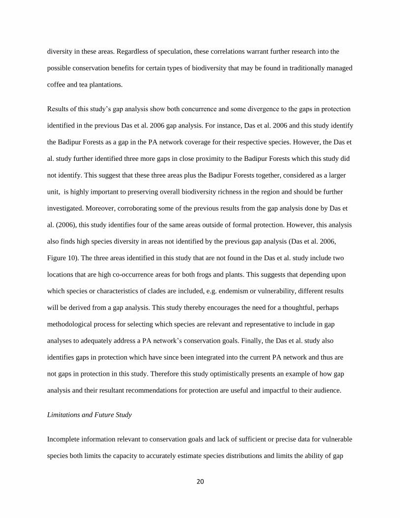
Table 2. Sub-set of SAHM modeled frog species with results depicting selected covariates and highest performing model.

Frog Species N Covariates Selected Best Performing

Models

Pseudophilautus

amboli 38

Mean of diurnal

temp range

Max temp –

warmest month

Landuse/land

cover

Precip.

Seasonality

NDVI

(minnimum

annual)

Canopy cover GLM, RF

Pseudophilautus

kani 42

Annual temp

range

Precip.

Seasonality

Precip. warmest

quarter Elevation

NDVI

(minnimum

annual)

RF, MAXENT

Pseudophilautus

wynaadensis 105 Temp seasonality

Max temp –

warmest month

Precip.

Seasonality

Precip. warmest

quarter

NDVI

(minnimum

annual)

Elevation MAXENT, RF

Raorchestes

akroparallagii 14 Temp seasonality

Max temp –

warmest month Annual Precip.

Precip.

Seasonality

NDVI

(minnimum

annual)

RF, BRT

Raorchestes anili 85 Temp seasonality Max temp –

warmest month Annual Precip.

Precip.

Seasonality

NDVI

(minnimum

annual)

Canopy cover RF, BRT

Raorchestes

beddomii 78 Temp seasonality

Max temp –

warmest month Annual Precip.

Precip. coldest

driest quarter

NDVI

(minnimum

annual)

Elevation RF, MAXENT

Raorchestes

bobingeri 40

Max temp –

warmest month Annual Precip.

NDVI

(minnimum

annual)

Canopy cover MAXENT,

(MARS)

Raorchestes griet 92 Isothermality Max temp –

warmest month

Precip.

Seasonality

Precip. coldest

driest quarter

Landuse/land

cover

NDVI

(minnimum

annual)

MAXENT, GLM*

Raorchestes

bobingeri 29

Max temp –

warmest month

Precip. coldest

driest quarter

Precip. warmest

quarter

Precip. coldest

quarter

NDVI

(minnimum

annual)

MAXENT, (GLM)

Raorchestes

jayarami 6 Isothermality Temp seasonality

Mean temp.

coldest month

Precip.

Seasonality

Precip. coldest

driest quarter

Precip. coldest

quarter MAXENT

Raorchestes

travancoricus 44

Max temp –

warmest month

Min temp.

coldest month

Precip. wettest

month

Precip. coldest

driest quarter

Landuse/land

cover MAXENT (GLM)

Raorchestes

dubois 19

Annual temp

range

Precip. wettest

month

Precip.

Seasonality

NDVI

(minnimum

annual)

Elevation MAXENT, MARS

Raorchestes

resplendens* 6

Max temp –

warmest month

Precip.

Seasonality

Precip. warmest

quarter

Precip. coldest

quarter Elevation MAXENT

Raorchestes

primarumfii 13

Precip. driest

month

NDVI

(minnimum

annual)

Elevation MAXENT

Raorchestes

sushili 31

Precip.

Seasonality

Precip. warmest

quarter

NDVI

(minnimum

annual)

Elevation MAXENT

26

Table 3. Sub-set of SAHM modeled plant species with results depicting selected covariates and highest performing model.

Plant Species N Predictors Selected

Best

Performing

Models

Aglaia barberi 34 Max temp – warmest

month Annual Precip. Landuse/land cover Canopy cover

NDVI (minnimum

annual) RF, MARS

Drypetes

confertiflora 20

NDVI (minnimum

annual) Canopy cover Elevation

MAXENT,

MARS

Cinnamomum

malabatrum 30 Temp seasonality Annual Precip.

NDVI (minnimum

annual) Elevation MAXENT

Diospyros ghatensis 28 Mean of diurnal temp

range

Max temp – warmest

month

NDVI (minnimum

annual) Canopy cover

MAXENT,

GLM

Diospyros oocarpa 19 Isothermality Annual temp range Annual Precip. NDVI (minnimum

annual) MAXENT

Eugenia

macrosepala 23 Temp seasonality

NDVI (minnimum

annual) Canopy cover

GLM,

MAXENT

Ficus nervosa 53 Max temp – warmest

month Annual Precip. Precip. Seasonality Landuse/land cover

NDVI (minnimum

annual)

BRT, RF,

MARS

Ixora elongata 24 Temp seasonality Annual Precip. Precip. wettest month Elevation MAXENT

Microtropis

wallichiana 27 Annual Precip. Landuse/land cover

NDVI (minnimum

annual) Elevation GLM, MARS

Psychotria nigra 87 Max temp – warmest

month Annual temp range Precip. Seasonality Landuse/land cover Canopy cover

NDVI

(minnimum

annual)

Elevation BRT, RF

Atuna indica 9 Temp seasonality NDVI (minnimum

annual) MAXENT

Epiprinus

mallotiformis 17

Max temp – warmest

month Canopy cover Elevation

MAXENT,

GLM

Gordonia obtusa 14 Landuse/land cover NDVI (minnimum

annual) E MAXENT

Humboldtia

brunonis 21 Temp seasonality Precip. warmest quarter

MAXENT,

GLM

Olea dioica 46 Isothermality Annual Precip. Precip. coldest driest

quarter

NDVI (minnimum

annual) Canopy cover Elevation MARS, BRT

Memecylon

pseudogracile 13

Max temp – warmest

month Elevation MAXENT

Syzygium munronii 27 Max temp – warmest

month Annual Precip.

NDVI (minnimum

annual)

MAXENT,

GLM

Thottea shivarajanii 11 Precip. Seasonality Precip. coldest quarter MAXENT

Vateria indica 47 Annual temp range Precip. Seasonality Precip. warmest

quarter

NDVI (minnimum

annual) Canopy cover

Landuse/land

cover RF, BRT

Walsura trifolia 18 Mean of diurnal temp

range

NDVI (minnimum

annual) Elevation MAXENT

27

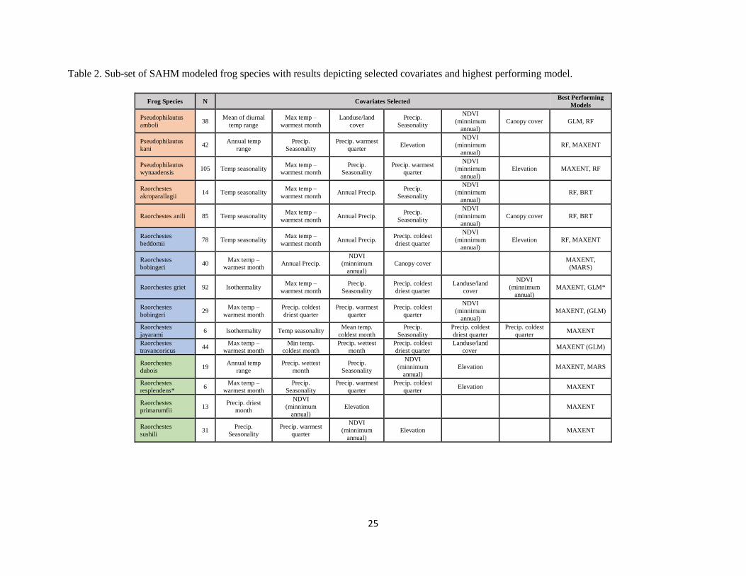
Table 4. List of SAHM determined predictor layers used in final SDM Maxent model creation by sub-groups.

Predictor Layers Frogs (low-

ranging)

Frogs (high-

ranging)

Frogs (montane

generalists)

Plants (low-

dispersing)

Plants (high-

dispersing)

BioClim 3: Isothermality X X

BioClim 4: Temperature Seasonality X X X X

BioClim 5: Max Temp of Warmest Month X X X X X

BioClim 12: Annual Precipitation X X X X

BioClim 14: Precipitation of Driest Month X X

BioClim 15: Precipitation Seasonality X X X X

BioClim 17: Precipitation of Driest

Quarter X X X

BioClim 18: Precipitation of Warmest

Quarter X X

BioClim 19: Precipitation of Coldest

Quarter X

Elevation X X X X X

NDVI (vegetation index; annual low) X X X X X

Soil Type X X

Slope X

Aspect

Soil-adjusted veg index (SAVI; annual

low) X

Percent Canopy Cover X X X X

Land use / Land cover X X X X

Total Predictors Used 10 7 10 12 10

28

Figure 1. Map of India depicting the modeled study area for all SDMs and the Western Ghats protected area network.

29

Figure 2. Left panel: map depicting where field presence data was recorded for plant species within the modeled study areas. Right panel: map

depicting where field presence data was recorded for frog species within the modeled study areas. Note that all sampling occurred within the

modeled area and spanned the study area.

30

Figure 3. Ensembled maps of frog species by sub-groupings of the whole study area. Combined distributions of all narrow-ranging species (panel

A), montane generalist frog species (panel B), wide-ranging frog species (panel C). Note the larger area of high-occurrence in panel C and density

of species in the southern portion of the study area.

31

Figure 4. (panel A) Combined distributions for all narrowly-dispersing plant species. (panel B) Combined distributions for all widely-dispersing

plant species. Note the similar shape of high-occurrence along the Ghats’s spine, yet the widely-dispersing plants is somewhat narrower than the

narrow-dispersing plants, likely an artifact of the higher number of modeled species.

32

Figure 5. Left panel: Ensembled map of all modeled frog species with a high co-occurrence of thirty-five species of sixty-nine possible. Right

panel: Ensembled map of all modeled plant species with a high co-occurrence of two-hundred twenty-four species of three hundred-six possible.

33

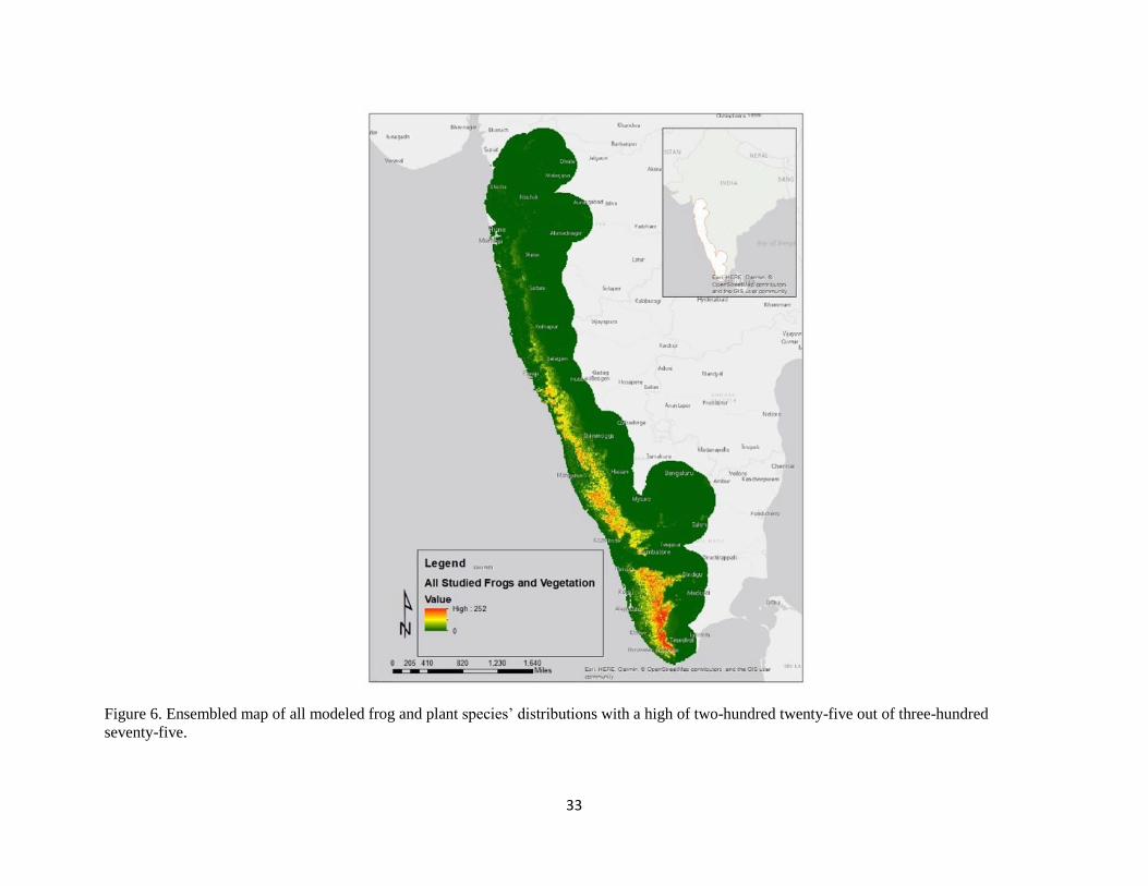
Figure 6. Ensembled map of all modeled frog and plant species’ distributions with a high of two-hundred twenty-five out of three-hundred

seventy-five.

34

Figure 7. Ensembled maps depicting species co-occurrences within and outside of the protected area network. Green to red indicate low to high

species co-occurrence within the network. Light to dark blue represents low to high species co-occurrence outside of the network.

35

Figure 8. Heatmap with frog and plant species ensembled and the protected area network overlain. Green and blue circles indicate high species co-

occurrence of plants and frogs respectively, identified outside of the protected area network.

36

Figure 9. (Panel A) Statistical hotspot analysis of all plants with heatmap identified high species co-occurrence locations. (Panel B) Hotspot

analysis of all modeled frogs with locations of heatmap identified high species co-occurrence areas. Note the hotspot extent’s coverage of the

protected area network as well as the heatmap identified high species co-occurrence areas.

37

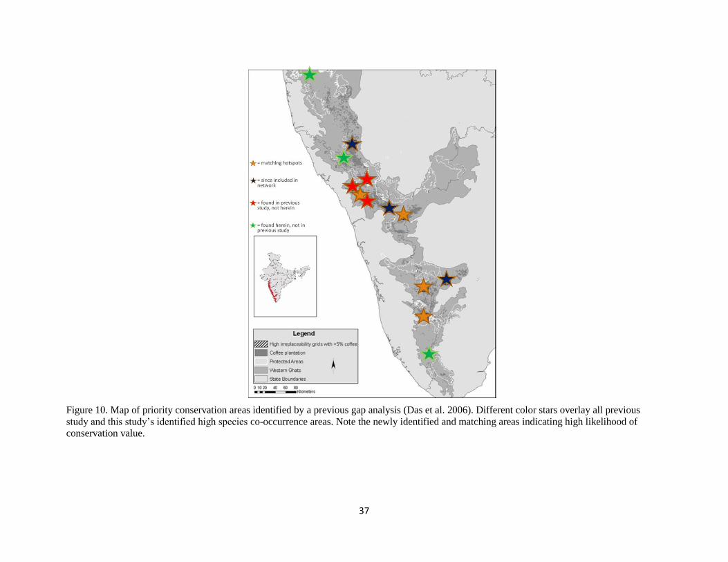
Figure 10. Map of priority conservation areas identified by a previous gap analysis (Das et al. 2006). Different color stars overlay all previous

study and this study’s identified high species co-occurrence areas. Note the newly identified and matching areas indicating high likelihood of

conservation value.

38

References

Anderson, R. P., Lew, D., & Peterson, A. T. (2003). Evaluating predictive models of species’

distributions: criteria for selecting optimal models. Ecological Modelling, 162(3), 211–232.

https://doi.org/10.1016/S0304-3800(02)00349-6

Austin, M. (2007). Species distribution models and ecological theory: A critical assessment and some

possible new approaches. Ecological Modelling, 200(1–2), 1–19.

https://doi.org/10.1016/j.ecolmodel.2006.07.005

Baldwin, R. F., Calhoun, A. J. K., & deMaynadier, P. G. (2009). Conservation Planning for Amphibian

Species with Complex Habitat Requirements: A Case Study Using Movements and Habitat Selection of

the Wood Frog Rana Sylvatica. http://dx.doi.org/10.1670/0022-

1511(2006)40[442:CPFASW]2.0.CO;2. https://doi.org/10.1670/0022-

1511(2006)40[442:CPFASW]2.0.CO;2

Ban, N. C., Mills, M., Tam, J., Hicks, C. C., Klain, S., Stoeckl, N., … Chan, K. M. A. (2013). A social-

ecological approach to conservation planning: Embedding social considerations. Frontiers in Ecology and

the Environment, 11(4), 194–202. https://doi.org/10.1890/110205

Ban, N. C., Mills, M., Tam, J., Hicks, C. C., Klain, S., Stoeckl, N., … Chan, K. M. A. (2013, May). A

social-ecological approach to conservation planning: Embedding social considerations. Frontiers in

Ecology and the Environment. Ecological Society of America. https://doi.org/10.1890/110205

Barker, N. K. S., Slattery, S. M., Darveau, M., & Cumming, S. G. (2014). Modeling distribution and

abundance of multiple species: Different pooling strategies produce similar results. Ecosphere, 5(12),

art158. https://doi.org/10.1890/ES14-00256.1

Barnes, M. D., Craigie, I. D., Harrison, L. B., Geldmann, J., Collen, B., Whitmee, S., … Woodley, S.

(2016). Wildlife population trends in protected areas predicted by national socio-economic metrics and

body size. Nature Communications, 7, 12747. https://doi.org/10.1038/ncomms12747

Birand, A., Vose, A., & Gavrilets, S. (2012). Patterns of Species Ranges, Speciation, and Extinction. The

American Naturalist, 179(1). https://doi.org/10.1086/663202

Bonn, A., Rodrigues, A. S. L., & Gaston, K. J. (2002). Threatened and endemic species: Are they good

indicators of patterns of biodiversity on a national scale? Ecology Letters, 5(6), 733–741.

https://doi.org/10.1046/j.1461-0248.2002.00376.x

Bottrill, M. C., Walsh, J. C., Watson, J. E. M., Joseph, L. N., Ortega-Argueta, A., & Possingham, H. P.

(2011). Does recovery planning improve the status of threatened species? Biological Conservation,

144(5), 1595–1601. https://doi.org/10.1016/j.biocon.2011.02.008

Brandon, K., & Kent, R. (1992). Parks in Peril: People, Politics, and Protected Areas. (Steven Sanderson,

Ed.). Island Press.

Brooks, T. M., Mittermeier, R. A., Da Fonseca, G. A. B., Gerlach, J., Hoffmann, M., Lamoreux, J. F., …

Rodrigues, A. S. L. (2006). Global Biodiversity Conservation Priorities. Source: Science, New Series,

313(5783), 58–61. Retrieved from http://www.jstor.org/stable/3846588

Brooks, T. M., Mittermeier, R. A., Mittermeier, C. G., da Fonseca, G. A. B., Rylands, A. B., Konstant, W.

R., … Hilton-Taylor, C. (2002). Habitat Loss and Extinction in the Hotspots of Biodiversity.

Conservation Biology, 16(4), 909–923. https://doi.org/10.1046/j.1523-1739.2002.00530.x

39

Bruner, A. G., Gullison, R. E., Rice, R. E., & da Fonseca, G. A. (2001). Effectiveness of parks in

protecting tropical biodiversity. Science (New York, N.Y.), 291(5501), 125–

128. https://doi.org/10.1126/science.291.5501.125

Buckland, S. T., & Elston, D. A. (1993). Empirical Models for the Spatial Distribution of Wildlife. The

Journal of Applied Ecology, 30(3), 478. https://doi.org/10.2307/2404188

Bucklin, D. N., Basille, M., Benscoter, A. M., Brandt, L. A., Mazzotti, F. J., Romañach, S. S., …

Watling, J. I. (2015). Comparing species distribution models constructed with different subsets of

environmental predictors. Diversity and Distributions, 21(1), 23–35. https://doi.org/10.1111/ddi.12247

Butchart, S. H. M., Clarke, M., Smith, R. J., Sykes, R. E., Scharlemann, J. P. W., Harfoot, M., …

Burgess, N. D. (2015). Shortfalls and Solutions for Meeting National and Global Conservation Area

Targets. Conservation Letters, 8(5), 329–337. https://doi.org/10.1111/conl.12158

Butchart, S. H. M., Walpole, M., Collen, B., van Strien, A., Scharlemann, J. P. W., Almond, R. E. A., …

Watson, R. (2010). Global Biodiversity: Indicators of Recent Declines. Science, 328(5982), 1164–

1168. https://doi.org/10.1126/science.1187512

Carignan, V., & Villard, M.-A. (2002). Selecting Indicator Species to Monitor Ecological Integrity: A

Review. Environmental Monitoring and Assessment, 78(1), 45–

61. https://doi.org/10.1023/A:1016136723584

Carpenter, S. R., Mooney, H. A., Agard, J., Capistrano, D., DeFries, R. S., Diaz, S., … Whyte, A. (2009).

Science for managing ecosystem services: Beyond the Millennium Ecosystem Assessment. Proceedings

of the National Academy of Sciences, 106(5), 1305–1312. https://doi.org/10.1073/pnas.0808772106

Ceballos, G., & Brown, J. H. (1995). Global Patterns of Mammalian Diversity, Endemism , and

Endangerment. Conservation Biology, 9(3), 559–568. https://doi.org/10.1046/j.1523-

1739.1995.09030559.x

Chape, S., Harrison, J., Spalding, M., & Lysenko, I. (2005). Measuring the extent and effectiveness of

protected areas as an indicator for meeting global biodiversity targets. Philosophical Transactions of the

Royal Society of London. Series B, Biological Sciences, 360(1454), 443–55.

https://doi.org/10.1098/rstb.2004.1592

Christie, P. (2004). Marine Protected Areas as Biological Successes and Social Failures in Southeast

Asia. American Fisheries Society Symposium, 42, 155–164. Retrieved

from http://citeseerx.ist.psu.edu/viewdoc/download?doi=10.1.1.712.7345&rep=rep1&type=pdf

Collen, B., Pettorelli, N., Baillie, J. E. M., & Durant, S. M. (2013). Biodiversity Monitoring and

Conservation: Bridging the Gaps Between Global Commitment and Local Action. Biodiversity

Monitoring and Conservation: Bridging the Gap between Global Commitment and Local Action, 1–16.

https://doi.org/10.1002/9781118490747.ch1

Corlett, R. T. (2007). The Impact of Hunting on the Mammalian Fauna of Tropical Asian Forests.

Biotropica, 39(3), 292–303. https://doi.org/10.1111/j.1744-7429.2007.00271.x

Costanza, R., d’Arge, R., de Groot, R., Farber, S., Grasso, M., Hannon, B., … van den Belt, M. (1997).

The value of the world’s ecosystem services and natural capital. Nature, 387(6630), 253–

260. https://doi.org/10.1038/387253a0

Coyne, J. A., & Orr, H. A. (2004). Speciation. Sinauer Associates.

Critical Ecosystem Partnership Fund (CEPF). (2014). Western Ghats and Sri Lanka. Retrieved from

http://www.cepf.net/resources/hotspots/Asia-Pacific/Pages/Western-Ghats-and-Sri-Lanka.aspx

40

Crooks, K. R. (2002). Relative Sensitivites of Mammalian Carnivores to Habitat Fragmentation.

Conservation Biology, 16(2), 488–502. https://doi.org/10.1046/j.1523-1739.2002.00386.x

Cumming, G. S., Allen, C. R., Ban, N. C., Biggs, D., Biggs, H. C., Cumming, D. H. M., … Schoon, M.

(2014). UNDERSTANDING PROTECTED AREA RESILIENCE: A MULTI-SCALE, SOCIAL-

ECOLOGICAL APPROACH. Ecological Applications, 25(2), 140915094202006.

https://doi.org/10.1890/13-2113.1

Cumming, G. S., Allen, C. R., Ban, N. C., Biggs, D., Biggs, H. C., Cumming, D. H. M., … Schoon, M.

(2015). Understanding protected area resilience: a multi-scale, social-ecological approach. Ecological

Applications, 25(2), 299–319. https://doi.org/10.1890/13-2113.1

Das, A., Krishnaswamy, J., Bawa, K. S., Kiran, M. C., Srinivas, V., Kumar, N. S., & Karanth, K. U.

(2006). Prioritisation of conservation areas in the Western,

3. https://doi.org/10.1016/j.biocon.2006.05.023

Davidar, P., Sahoo, S., Mammen, P. C., Acharya, P., Puyravaud, J. P., Arjunan, M., … Roessingh, K.

(2010). Assessing the extent and causes of forest degradation in India: Where do we stand? Biological

Conservation, 143(12), 2937–2944. https://doi.org/10.1016/j.biocon.2010.04.032

de Groot, R. (2006). Function-analysis and valuation as a tool to assess land use conflicts in planning for

sustainable, multi-functional landscapes. Landscape and Urban Planning, 75(3), 175–186.

https://doi.org/10.1016/j.landurbplan.2005.02.016

De Groot, R. S., Alkemade, R., Braat, L., Hein, L., & Willemen, L. (2009). Challenges in integrating the

concept of ecosystem services and values in landscape planning, management and decision making.

Ecological Complexity, 7, 260–272. https://doi.org/10.1016/j.ecocom.2009.10.006

De Groot, R. S., Wilson, M. A., & Boumans, R. M. J. (2002). A typology for the classification,

description and valuation of ecosystem functions, goods and services. Ecological Economics, 41, 393–

408. Retrieved from www.elsevier.com/locate/ecolecon

Dempsey, C. (2014). What is the Difference Between a Heat Map and a Hot Spot Map? ~ GIS Lounge.

Retrieved from https://www.gislounge.com/difference-heat-map-hot-spot-map/

Dudley, N., Phillips, A., Amend, T., Brown, J., & Stolton, S. (2016). Evidence for Biodiversity

Conservation in Protected Landscapes. Land, 5(4), 38. https://doi.org/10.3390/land5040038

Dudley, N., Stolton, S., & Shadie, P. (2008). IUCN Best Practice Guidance on Recognising Protected

Areas and Assigning Management, Categories and Governance Types Guidelines for Applying Protected

Area Management Categories. Best Practice Protected Area Guidelines Series No. 21. Retrieved from

https://cmsdata.iucn.org/downloads/iucn_assignment_1.pdf

Dufrêne, M., & Legendre, P. (1997). SPECIES ASSEMBLAGES AND INDICATOR SPECIES:THE

NEED FOR A FLEXIBLE ASYMMETRICAL APPROACH. Ecological Monographs, 67(3), 345–

366. https://doi.org/10.1890/0012-9615(1997)067[0345:SAAIST]2.0.CO;2

Edgar, G. J., Stuart-Smith, R. D., Willis, T. J., Kininmonth, S., Baker, S. C., Banks, S., … Thomson, R. J.

(2014). Global conservation outcomes depend on marine protected areas with five key features. Nature,

506(7487), 216–220. https://doi.org/10.1038/nature13022

Elith, J., & Leathwick, J. R. (2009). Species Distribution Models: Ecological Explanation and Prediction

Across Space and Time. Annual Review of Ecology, Evolution, and Systematics, 40(1), 677–

697. https://doi.org/10.1146/annurev.ecolsys.110308.120159

41

Elith, J., Phillips, S. J., Hastie, T., Dudík, M., Chee, Y. E., & Yates, C. J. (2011). A statistical explanation

of MaxEnt for ecologists. Diversity and Distributions, 17(1), 43–57. https://doi.org/10.1111/j.1472-

4642.2010.00725.x

Ervin, J. (2003). Protected area assessments in perspective. Bioscience, 53(9), 819–822.

https://doi.org/10.1641/0006-3568(2003)053[0819:PAAIP]2.0.CO;2

Escalante, T., Rodríguez-Tapia, G., Linaje, M., Illoldi-Rangel, P., & González-López, R. (2013).

Identification of areas of endemism from species distribution models: threshold selection and Nearctic

mammals. TIP, 16(1), 5–17. https://doi.org/10.1016/S1405-888X(13)72073-4

F. Dormann, C., M. McPherson, J., B. Araújo, M., Bivand, R., Bolliger, J., Carl, G., … Wilson, R.

(2007). Methods to account for spatial autocorrelation in the analysis of species distributional data: a

review. Ecography, 30(5), 609–628. https://doi.org/10.1111/j.2007.0906-7590.05171.x

Ferraro, P. J., Hanauer, M. M., & Sims, K. R. E. (2011). Conditions associated with protected area

success in conservation and poverty reduction. Proceedings of the National Academy of Sciences of the

United States of America, 108(34), 13913–13918. https://doi.org/10.1073/pnas.1011529108

Fitzpatrick, M. C., Gotelli, N. J., & Ellison, A. M. (2013). MaxEnt versus MaxLike: Empirical

comparisons with ant species distributions. Ecosphere, 4(5). https://doi.org/10.1890/ES13-00066.1

Flather, C. H., Wilson, K. R., Dean, D. J., & McComb, W. C. (1997). IDENTIFYING GAPS IN

CONSERVATION NETWORKS: OF INDICATORS AND UNCERTAINTY IN GEOGRAPHIC‐BASED ANALYSES. Ecological Applications, 7(2), 531–542. https://doi.org/10.1890/1051-

0761(1997)007[0531:IGICNO]2.0.CO;2

Foley, J. A. (2005). Global Consequences of Land Use. Science, 309(5734), 570–574.

https://doi.org/10.1126/science.1111772

Folke, C. (2006). Resilience: The emergence of a perspective for social–ecological systems analyses.

Global Environmental Change, 16(3), 253–267. https://doi.org/10.1016/j.gloenvcha.2006.04.002

Foody, G. M. (2002). Status of land cover classification accuracy assessment. Remote Sensing of

Environment, 80(1), 185–201. https://doi.org/10.1016/S0034-4257(01)00295-4

Fourcade, Y., Engler, J. O., Rödder, D., & Secondi, J. (2014). Mapping Species Distributions with

MAXENT Using a Geographically Biased Sample of Presence Data: A Performance Assessment of

Methods for Correcting Sampling Bias. PLoS ONE, 9(5),

e97122. https://doi.org/10.1371/journal.pone.0097122

Freeman, E. A., & Moisen, G. G. (2008). A comparison of the performance of threshold criteria for

binary classification in terms of predicted prevalence and

kappa. https://doi.org/10.1016/j.ecolmodel.2008.05.015

Fu, C., Hua, X., Li, J., Chang, Z., Pu, Z., & Chen, J. (2006). Elevational patterns of frog species richness

and endemic richness in the Hengduan Mountains, China: geometric constraints, area and climate effects.

Ecography, 29(6), 919–927. https://doi.org/10.1111/j.2006.0906-7590.04802.x

Gaston, K. J. (2000). Global patterns in biodiversity. Nature, 405(6783), 220–227.

https://doi.org/10.1038/35012228

Geldmann, J., Barnes, M., Coad, L., Craigie, I. D., Hockings, M., & Burgess, N. D. (2013). Effectiveness

of terrestrial protected areas in reducing habitat loss and population declines. Biological Conservation,

161, 230–238. https://doi.org/10.1016/j.biocon.2013.02.018

42

Gerlach, P., Hubbard, M., Norment Jennifer Swenson, E., & Karanth, K. (2013). Land Use Land Cover in

the Western Ghats, India Effects of Human Modification and Use on Protected Areas.

GIBBONS, J. W., DAVID E. SCOTT, & T R AVIS J. RYAN , KURT A. B U H L M A N N , T R

ACEY D. TUBERV I L L E , BRIAN S. MET TS, JUDITH L. GREENE, TONY MILLS, YALE

LEIDEN, SEAN POPPY, A. C. T. W. (2000). The Global Decline of Reptiles, Deja Vu Amphibeans.

BioScience, 50(653). Retrieved from

https://www.biologicaldiversity.org/campaigns/southern_and_midwestern_freshwater_turtles/pdfs/Gibbo

ns-et-al-2000.pdf

Gibson, C. C., Williams, J. T., & Ostrom, E. (2005). Local Enforcement and Better Forests. World

Development, 33(2), 273–284. https://doi.org/10.1016/J.WORLDDEV.2004.07.013

Gilchrist, G. W. (1995). Specialists and Generalists in Changing Environments. I. Fitness Landscapes of

Thermal Sensitivity. The American Naturalist, 146(2), 252–270. https://doi.org/10.1086/285797

Gould, R. K., Klain, S. C., Ardoin, N. M., Satterfield, T., Woodside, U., Hannahs, N., … Chan, K. M.

(2015). A protocol for eliciting nonmaterial values through a cultural ecosystem services frame.

Conservation Biology, 29(2), 575–586. https://doi.org/10.1111/cobi.12407

Guisan, A., & Zimmermann, N. E. (2000). Predictive habitat distribution models in ecology. Ecological

Modelling, 135(2–3), 147–186. https://doi.org/10.1016/S0304-3800(00)00354-9

Guisan, A., Tingley, R., Baumgartner, J. B., Naujokaitis-Lewis, I., Sutcliffe, P. R., Tulloch, A. I. T., …

Buckley, Y. M. (2013). Predicting species distributions for conservation decisions. Ecology Letters,

16(12), 1424–1435. https://doi.org/10.1111/ele.12189

Gunawardene, N. R., Daniels, a E. D., Gunatilleke, I. a U. N., Gunatilleke, C. V. S., Karunakaran, P. V,

Nayak, K. G., … Vasanthy, G. (2007). SPECIAL SECTION : ASIAN BIODIVERSITY CRISES A brief

overview of the Western Ghats – Sri Lanka biodiversity hotspot. Current, 93(10), 1–6.

Gupta, S., Gupta, S., Aithal, B. H., & V, R. T. (n.d.). LAKE 2014: Conference on Conservation and

Sustainable Management of Wetland Ecosystems in Western Ghats LAND USE DYNAMICS IN

CENTRAL AND SOUTHERN WESTERN GHATS. Retrieved from http://ces.iisc.ernet.in/energy

Halvorsen, R., Mazzoni, S., Bryn, A., & Bakkestuen, V. (2015). Opportunities for improved distribution

modelling practice via a strict maximum likelihood interpretation of MaxEnt. Ecography, 38(2), 172–183.

https://doi.org/10.1111/ecog.00565

Halvorsen, R., Mazzoni, S., Dirksen, J. W., Næsset, E., Gobakken, T., & Ohlson, M. (2016). How

important are choice of model selection method and spatial autocorrelation of presence data for

distribution modelling by MaxEnt? Ecological Modelling, 328, 108–118.

https://doi.org/10.1016/j.ecolmodel.2016.02.021

Hernandez, P. A., Graham, C. H., Master, L. L., & Albert, D. L. (2006). The effect of sample size and

species characteristics on performance of different species distribution modeling methods. Ecography,

29(5), 773–785. https://doi.org/10.1111/j.0906-7590.2006.04700.x

Hockings, M. (2003). Systems for Assessing the Effectiveness of Management in Protected Areas.

BioScience, 53(9), 823–832. https://doi.org/10.1641/0006-3568(2003)053

Huang, C., Wylie, B., Yang, L., Homer, C., & Zylstra, G. (n.d.). DERIVATION OF A TASSELED CAP

TRANSFORMATION BASED ON LANDSAT 7 AT-SATELLITE REFLECTANCE. Retrieved from

https://landcover.usgs.gov/pdf/tasseled.pdf

43

Huete, A. R. (1988) A Soil-Adjusted Vegetation Index (SAVI). Remote Sensing of Environment, vol.

25:295-309

Indian Space Research Organization (ISRO). (2018). ISRO’s Geoportal | Gateway to Indian Earth

Observation | 2D Viewer. Retrieved April 3, 2018,

from http://bhuvan.nrsc.gov.in/map/bhuvan/bhuvan2d.php

Isaac, N. J. B., Mallet, J., & Mace, G. M. (2004). Taxonomic inflation: its influence on macroecology and

conservation. Trends in Ecology & Evolution, 19(9), 464–

469. https://doi.org/10.1016/J.TREE.2004.06.004

Jacobs, M. H., Vaske, J. J., & Sijtsma, M. T. J. (2014). Predictive potential of wildlife value orientations

for acceptability of management interventions. Journal for Nature Conservation, 22(4), 377–383.

https://doi.org/10.1016/j.jnc.2014.03.005

Jennings, M. D. (2000). Gap analysis: Concepts, methods, and recent results. Landscape Ecology, 15(1),

5–20. https://doi.org/10.1023/A:1008184408300

Jiménez-Valverde, A., & Lobo, J. M. (2007). Threshold criteria for conversion of probability of species

presence to either-or presence-absence. Acta Oecologica, 31(3), 361–369.

https://doi.org/10.1016/j.actao.2007.02.001

Johnson, R. A., Chawla, N. V, & Hellmann, J. J. (2012). Species Distribution Modeling and Prediction: A

Class Imbalance Problem. Conference on Intelligent Data Understanding. Retrieved

from https://www3.nd.edu/~dial/publications/johnson2012species.pdf

Joppa, L. N., & Pfaff, A. (2009). High and Far: Biases in the Location of Protected Areas. PLoS ONE,

4(12), e8273. https://doi.org/10.1371/journal.pone.0008273

Kier, G., Kreft, H., Lee, T. M., Jetz, W., Ibisch, P. L., Nowicki, C., … Barthlott, W. (2009). A global

assessment of endemism and species richness across island and mainland regions. Proceedings of the

National Academy of Sciences, 106(23), 9322–9327. https://doi.org/10.1073/pnas.0810306106

Kremen, C., Cameron, A., Moilanen, A., Phillips, S. J., Thomas, C. D., Beentje, H., … Zjhra, M. L.

(2008). Aligning Conservation Priorities Across Taxa in Madagascar with High-Resolution Planning

Tools. Science, 320(5873), 222–226. https://doi.org/10.1126/science.1155193

Kullberg, P., Toivonen, T., Montesino Pouzols, F., Lehtomäki, J., Di Minin, E., & Moilanen, A. (2015).

Complementarity and Area-Efficiency in the Prioritization of the Global Protected Area Network. PloS

One, 10(12), e0145231. https://doi.org/10.1371/journal.pone.0145231

Lausche, B., & Burhenne, F. (2010). Guidelines for Protected Areas Legislation Part III, Chapter 2:

Special issues for marine protected areas Part III, Chapter 2: Special iss. IUCN Environmental Policy and

Law, 81, chap. 2. Retrieved from https://mote.org/media/uploads/files/P3_Ch_2.pdf

Leathwick, J. R., Elith, J., & Hastie, T. (2006). Comparative performance of generalized additive models

and multivariate adaptive regression splines for statistical modelling of species

distributions. https://doi.org/10.1016/j.ecolmodel.2006.05.022

Lehtomäki, J., & Moilanen, A. (2013). Methods and workflow for spatial conservation prioritization

using Zonation. Environmental Modelling & Software, 47, 128–137.

https://doi.org/10.1016/j.envsoft.2013.05.001

Leroux, S. J., Krawchuk, M. A., Schmiegelow, F., Cumming, S. G., Lisgo, K., Anderson, L. G., &

Petkova, M. (2010). Global protected areas and IUCN designations: Do the categories match the

conditions? Biological Conservation, 143(3), 609–616. https://doi.org/10.1016/j.biocon.2009.11.018

44

Lewandowski, A. S., Noss, R. F., & Parsons, D. R. (2010). The effectiveness of surrogate taxa for the

representation of biodiversity. Conservation Biology, 24(5), 1367–1377. https://doi.org/10.1111/j.1523-

1739.2010.01513.x

Liu, C., Newell, G., & White, M. (2016). On the selection of thresholds for predicting species occurrence

with presence-only data. Ecology and Evolution, 6(1), 337–348. https://doi.org/10.1002/ece3.1878

Marchese, C. (2015). Biodiversity hotspots: A shortcut for a more complicated concept. Global Ecology

and Conservation, 3, 297–309. https://doi.org/10.1016/J.GECCO.2014.12.008

Marchese, C. (2015). Biodiversity hotspots: A shortcut for a more complicated concept. Global Ecology

and Conservation, 3, 297–309. https://doi.org/10.1016/J.GECCO.2014.12.008

Margules, C. R., & Pressey, R. L. (2000). Systematic conservation planning. Nature, 405(6783), 243–

253. https://doi.org/10.1038/35012251

Mellin, C., Delean, S., Caley, J., Edgar, G., Meekan, M., Pitcher, R., … Bradshaw, C. (2011).

Effectiveness of Biological Surrogates for Predicting Patterns of Marine Biodiversity: A Global Meta-

Analysis. PLoS ONE, 6(6), e20141. https://doi.org/10.1371/journal.pone.0020141

Merow, C., Smith, M. J., & Silander, J. A. (2013). A practical guide to MaxEnt for modeling species’

distributions: What it does, and why inputs and settings matter. Ecography, 36(10), 1058–1069.

https://doi.org/10.1111/j.1600-0587.2013.07872.x

Mittermeier, R. A., Mittermeier, C. G., Brooks, T. M., Pilgrim, J. D., Konstant, W. R., da Fonseca, G. A.

B., & Kormos, C. (2003). Wilderness and biodiversity conservation. Proceedings of the National

Academy of Sciences, 100(18), 10309–10313. https://doi.org/10.1073/pnas.1732458100

Mittermeier, R. A., Turner, W. R., Larsen, F. W., Brooks, T. M., & Gascon, C. (2011). Global

Biodiversity Conservation: The Critical Role of Hotspots. In Biodiversity Hotspots (pp. 3–22). Berlin,

Heidelberg: Springer Berlin Heidelberg. https://doi.org/10.1007/978-3-642-20992-5_1

Morisette, J. T., Jarnevich, C. S., Holcombe, T. R., Talbert, C. B., Ignizio, D., Talbert, M. K., … Young,

N. E. (2013). VisTrails SAHM: visualization and workflow management for species habitat modeling.

Ecography, 36(2), 129–135. https://doi.org/10.1111/j.1600-0587.2012.07815.x

Myers, N., Mittermeier, R. A., Mittermeier, C. G., da Fonseca, G. A. B., & Kent, J. (2000). Biodiversity

hotspots for conservation priorities. Nature, 403(6772), 853–858. https://doi.org/10.1038/35002501

Naidoo, R., & Ricketts, T. H. (2006). Mapping the Economic Costs and Benefits of Conservation. PLoS

Biology, 4(11), e360. https://doi.org/10.1371/journal.pbio.0040360

Nameer, P. O., Molur, S., & Walker, S. (2001). Mammals of Western Ghats : a Simplistic Overview.

Zoos Print Journal, 16(November), 629–639. https://doi.org/10.11609/JoTT.ZPJ.16.11.629-39

National Wildlife Federation. (2007). Species At Risk. Retrieved

from http://macd.org/me/resource material/wildlife/keystone, umbrella, and indicator species.pdf

Orme, C. D. L., Davies, R. G., Burgess, M., Eigenbrod, F., Pickup, N., Olson, V. A., … Owens, I. P. F.

(2005). Global hotspots of species richness are not congruent with endemism or threat. Nature,

436(7053), 1016–1019. https://doi.org/10.1038/nature03850

Ormsby, A. A. (2011). The Impacts of Global and National Policy on the Management and Conservation

of Sacred Groves of India. Human Ecology, 39(6), 783–793. https://doi.org/10.1007/s10745-011-9441-8

45

ORMSBY, A. A., & BHAGWAT, S. A. (2010). Sacred forests of India: a strong tradition of community-

based natural resource management. Environmental Conservation, 37(3), 320–326.

https://doi.org/10.1017/S0376892910000561

Pacala, S. W., Canham, C. D., Saponara, J., Silander, J. A., Kobe, R. K., & Ribbens, E. (1996). Forest

Models Defined by Field Measurements: Estimation, Error Analysis and Dynamics. Ecological

Monographs, 66(1), 1–43. https://doi.org/10.2307/2963479

Page, N. (2017). Photographic Assessment of Endemic Woody Plants of the Western Ghats. Bangalore.

Retrieved from https://www.rufford.org/files/Endemic Woody Plants.pdf

Page, N., & Shanker, K. (2018). Environment and dispersal influence changes in species composition at

different scales in woody plants of the Western Ghats, India. Journal of Vegetation Science , 29, 74–83.

Pawar, S., Koo, M. S., Kelley, C., Ahmed, M. F., Chaudhuri, S., & Sarkar, S. (2007). Conservation

assessment and prioritization of areas in Northeast India: Priorities for amphibians and reptiles. Biological

Conservation, 136(3), 346–361. https://doi.org/10.1016/j.biocon.2006.12.012

Phillips, S. (2008). A Brief Tutorial on Maxent. AT&T Research, 1–38. https://doi.org/10.4016/33172.01

Phillips, S. J., Anderson, R. P., & Schapire, R. E. (2006). Maximum entropy modeling of species

geographic distributions. Ecological Modelling, 190(3–4), 231–259.

https://doi.org/10.1016/J.ECOLMODEL.2005.03.026

Phillips, S. J., Anderson, R. P., Dudík, M., Schapire, R. E., & Blair, M. E. (2017). Opening the black box:

an open-source release of Maxent. Ecography, 40(7), 887–893. https://doi.org/10.1111/ecog.03049

Phillips, S. J., Dudik, M., & Schapire, R. E. (2004). Maxent software for species distribution modeling.

Proceedings of the Twenty-First International Conference on Machine Learning, 655–662.

https://doi.org/10.1016/j.ecolmodel.2005.03.026

Phillips, S. J., Dudik, M., & Schapire, R. E. (2004). Maxent software for species distribution modeling.

Proceedings of the Twenty-First International Conference on Machine Learning, 655–

662. https://doi.org/10.1016/j.ecolmodel.2005.03.026

Platt, R. V., Ogra, M. V., Badola, R., & Hussain, S. A. (2016). Conservation-induced resettlement as a

driver of land cover change in India: An object-based trend analysis. Applied Geography, 69, 75–86.

https://doi.org/10.1016/j.apgeog.2016.02.006

Possingham, H. P., & Wilson, K. A. (2005). Biodiversity: Turning up the heat on hotspots. Nature,

436(7053), 919–920. https://doi.org/10.1038/436919a

Prendergast, J. R., Quinn, R. M., & Lawton, J. H. (1999). The Gaps between Theory and Practice in

Selecting Nature Reserves. Conservation Biology, 13(3), 484–492. https://doi.org/10.1046/j.1523-

1739.1999.97428.x

Prendergast, J. R., Quinn, R. M., Lawton, J. H., Eversham, B. C., & Gibbons, D. W. (1993). Rare species,

the coincidence of diversity hotspots and conservation strategies. Nature, 365(6444), 335–

337. https://doi.org/10.1038/365335a0

Ramachandra, T., Chandra-Subash, M., Joshi, N., & Dudani, S. (2012). Exploring Biodiversity and

Ecology of Central Western Ghats. Retrieved

from http://wgbis.ces.iisc.ernet.in/biodiversity/pubs/ETR/ETR39/overview.htm

46

Ramachandran, R. M., Roy, P. S., Chakravarthi, V., Sanjay, J., & Joshi, P. K. (2018). Long-term land use

and land cover changes (1920–2015) in Eastern Ghats, India: Pattern of dynamics and challenges in plant

species conservation. Ecological Indicators, 85, 21–36. https://doi.org/10.1016/J.ECOLIND.2017.10.012

Ramachandran, R. M., Roy, P. S., Chakravarthi, V., Sanjay, J., & Joshi, P. K. (2018). Long-term land use

and land cover changes (1920–2015) in Western Ghats, India: Pattern of dynamics and challenges in plant

species conservation. Ecological Indicators, 85, 21–36. https://doi.org/10.1016/J.ECOLIND.2017.10.012

Randin, C. F., Jaccard, H., Vittoz, P., Yoccoz, N. G., & Guisan, A. (2009). Land use improves spatial

predictions of mountain plant abundance but not presence-absence. Journal of Vegetation Science, 20(6),

996–1008. https://doi.org/10.1111/j.1654-1103.2009.01098.x

Rao, V. C., Suresh, S. V., Swarna, A. R., Latha, J., Satyanarayana, S. P., & Sekhar, S. N. (2006). National

Land Use and Land Cover Mapping Using Multi-Temporal AWiFS Data National Remote Sensing

Agency. Retrieved from http://bhuvan.nrsc.gov.in/gis/thematic/tools/document/LULC250/0405.pdf

Revadekar, J. V., Tiwari, Y. K., & Kumar, K. R. (2012). Impact of climate variability on NDVI over the

Indian region during 1981–2010. International Journal of Remote Sensing, 33(22), 7132–7150.

https://doi.org/10.1080/01431161.2012.697642

Rodrigues, A. S. L., Akçakaya, H. R., Andelman, S. J., Bakarr, M. I., Boitani, L., Brooks, T. M., … Yan,

X. (2004). Global Gap Analysis: Priority Regions for Expanding the Global Protected-Area Network.

BioScience, 54(12), 1092–1100. https://doi.org/10.1641/0006-3568(2004)054[1092:ggaprf]2.0.co;2

Rodrigues, A. S. L., Andelman, S. J., Bakarr, M. I., Boitani, L., Brooks, T. M., Cowling, R. M., … Yan,

X. (2004). Effectiveness of the global protected area network in representing species diversity. Nature,

428(6983), 640–643. https://doi.org/10.1038/nature02422

Salafsky, N. (2011). Integrating development with conservation: A means to a conservation end, or a

mean end to conservation? Biological Conservation, 144(3), 973–978.

https://doi.org/10.1016/j.biocon.2010.06.003

Salafsky, N., & Wollenberg, E. (2000). Linking livelihoods and conservation: A conceptual framework

and scale for assessing the integration of human needs and biodiversity. World Development, 28(8),

1421–1438. https://doi.org/10.1016/S0305-750X(00)00031-0

Sarkar, S., & Montoya, M. (2011). Beyond parks and reserves: The ethics and politics of conservation

with a case study from PerÃo. Biological Conservation, 144, 979–988.

https://doi.org/10.1016/j.biocon.2010.03.008

Sarkar, S., Pressey, R. L., Faith, D. P., Margules, C. R., Fuller, T., Stoms, D. M., … Andelman, S. (2006).

Biodiversity Conservation Planning Tools: Present Status and Challenges for the Future. Annual Review

of Environment and Resources, 31(1), 123–159.

https://doi.org/10.1146/annurev.energy.31.042606.085844

Satish, K. V., & Reddy, C. S. (2016). Long Term Monitoring of Forest Fires in Silent Valley National

Park, Western Ghats, India Using Remote Sensing Data. Journal of the Indian Society of Remote Sensing,

44(2), 207–215. https://doi.org/10.1007/s12524-015-0491-z

Satish, K. V., Saranya, K. R. L., Reddy, C. S., Krishna, P. H., Jha, C. S., & Rao, P. V. V. P. (2014).

Geospatial assessment and monitoring of historical forest cover changes (1920–2012) in Nilgiri

Biosphere Reserve, Western Ghats, India. Environmental Monitoring and Assessment, 186(12), 8125–

8140. https://doi.org/10.1007/s10661-014-3991-3

47

Saura, S., & Pascual-Hortal, L. (2007). A new habitat availability index to integrate connectivity in

landscape conservation planning: Comparison with existing indices and application to a case study.

Landscape and Urban Planning, 83(2–3), 91–103. https://doi.org/10.1016/j.landurbplan.2007.03.005

Scott, J., Davis, F., Csuti, B., Noss, R., Butterfield, B., Groves, T., … Edwards, T. (1993). Wildlife

monographs : a publication of the Wildlife Society., (123), 1–41. Retrieved from

http://apps.webofknowledge.com.ezproxy2.library.colostate.edu/full_record.do?product=WOS&search_

mode=GeneralSearch&qid=6&SID=6DrSf4QnCDv2FOafUNs&page=1&doc=5

Shahabuddin, G., & Rao, M. (2010). Do community-conserved areas effectively conserve biological

diversity? Global insights and the Indian context. Biological Conservation, 143(12), 2926–2936.

https://doi.org/10.1016/j.biocon.2010.04.040

Shanker, K., Vijayakumar, S. P., & Ganeshaiah, K. N. (2017). Unpacking the species conundrum:

philosophy, practice and a way forward. Journal of Genetics, 96(3), 413–430.

https://doi.org/10.1007/s12041-017-0800-0

Soil Survey Staff, Natural Resources Conservation Service, United States Department of Agriculture.

Web Soil Survey. Available online at https://websoilsurvey.nrcs.usda.gov/. Accessed [month/day/year].

Stockwell, D. R. ., & Peterson, A. T. (2002). Effects of sample size on accuracy of species distribution

models. Ecological Modelling, 148(1), 1–13. https://doi.org/10.1016/S0304-3800(01)00388-X

Stuart, S. N., Chanson, J., Cox, N., Young, B., Rodrigues, A., Fischman, D., & Waller, R. (2004). Status

and Trends of Amphibian Declines and Extinctions Worldwide. Science, 306(5702), 1783–1786.

https://doi.org/10.1126/science.1103538

Thomas, C. D., Cameron, A., Green, R. E., Bakkenes, M., Beaumont, L. J., Collingham, Y. C., …

Williams, S. E. (2004). Extinction risk from climate change. Nature, 427(6970), 145–148.

https://doi.org/10.1038/nature02121

U.S. Fish and Wildlife Service. (2015). Surrogate and Keystone Species. Retrieved April 11, 2017, from

https://www.fws.gov/mountain-prairie/science/surrogateSpecies.php

U.S. Geological Survey, G. A. P. (2013). U.S. Geological Survey Gap Analysis Program Species

Distribution Models. https://doi.org/10.5066/F7V122T2

UNEP-WCMC and IUCN (year), Protected Planet: [insert name of component database; The World

Database on Protected Areas (WDPA)/The Global Database on Protected Areas Management

Effectiveness (GD-PAME)] [On-line], [insert month/year of the version downloaded], Cambridge,

UK: UNEP-WCMC andIUCN. Available at: www.protectedplanet.net.

Urbina-Cardona, J. N. (2008). Conservation of Neotropical Herpetofauna: Research Trends and

Challenges. Tropical Conservation Science, 1(4), 359–375. https://doi.org/10.1177/194008290800100405

van Proosdij, A. S. J., Sosef, M. S. M., Wieringa, J. J., & Raes, N. (2016). Minimum required number of

specimen records to develop accurate species distribution models. Ecography, 39(6), 542–552.

https://doi.org/10.1111/ecog.01509

Vattakaven T, George R, Balasubramanian D, Réjou-Méchain M, Muthusankar G, Ramesh B, Prabhakar

R (2016) India Biodiversity Portal: An integrated, interactive and participatory biodiversity informatics

platform. Biodiversity Data Journal 4: e10279.

VIJAYAKUMAR, S. P., DINESH, K. P., PRABHU, M. V., & SHANKER, K. (2014). Lineage

delimitation and description of nine new species of bush frogs (Anura: Raorchestes, Rhacophoridae) from

the Western Ghats Escarpment. Zootaxa, 3893(4), 451. https://doi.org/10.11646/zootaxa.3893.4.1

48

Vijayakumar, S. P., Menezes, R. C., Jayarajan, A., & Shanker, K. (2016). Glaciations, gradients, and

geography: multiple drivers of diversification of bush frogs in the Western Ghats Escarpment.

Proceedings. Biological Sciences, 283(1836), 20161011. https://doi.org/10.1098/rspb.2016.1011

Vimal, R., Rodrigues, A. S. L., Mathevet, R., & Thompson, J. D. (2011). The sensitivity of gap analysis

to conservation targets. Biodiversity and Conservation, 20(3), 531–543. https://doi.org/10.1007/s10531-

010-9963-1

Wallace, K. J. (2007). Classification of ecosystem services: Problems and solutions. Biological

Conservation, 139(3), 235–246. https://doi.org/10.1016/j.biocon.2007.07.015

Warren, D. L., & Seifert, S. N. (2011). Ecological niche modeling in Maxent: the importance of model

complexity and the performance of model selection criteria. Ecological Applications, 21(2), 335–

342. https://doi.org/10.1890/10-1171.1

Werner, E. E., Skelly, D. K., Relyea, R. A., & Yurewicz, K. L. (2007). Amphibian species richness across

environmental gradients. Oikos, 116(10), 1697–1712. https://doi.org/10.1111/j.0030-1299.2007.15935.x

West, A. M., Evangelista, P. H., Jarnevich, C. S., Young, N. E., Stohlgren, T. J., Talbert, C., …

Anderson, R. (2016). Integrating Remote Sensing with Species Distribution Models; Mapping Tamarisk

Invasions Using the Software for Assisted Habitat Modeling (SAHM) Video Link. J. Vis. Exp,

379154578(11610). https://doi.org/10.3791/54578

West, P., Igoe, J., & Brockington, D. (2006). Parks and Peoples: The Social Impact of Protected Areas.

Annual Review of Anthropology, 35(1), 251–277.

https://doi.org/10.1146/annurev.anthro.35.081705.123308

Whittaker, R. J., Araújo, M. B., Jepson, P., Ladle, R. J., Watson, J. E. M., & Willis, K. J. (2005).

Conservation Biogeography: assessment and prospect. Diversity and Distributions, 11(1), 3–23.

https://doi.org/10.1111/j.1366-9516.2005.00143.x

Wilshusen, P. R., Brechin, S. R., Fortwangler, C. L., & West, P. C. (2002). Reinventing a Square Wheel:

Critique of a Resurgent "Protection Paradigm" in International Biodiversity Conservation.

Society & Natural Resources, 15(1), 17–40. https://doi.org/10.1080/089419202317174002

Wisz, M. S., Hijmans, R. J., Li, J., Peterson, A. T., Graham, C. H., & Guisan, A. (2008). Effects of

sample size on the performance of species distribution models. Diversity and Distributions, 14(5), 763–

773. https://doi.org/10.1111/j.1472-4642.2008.00482.x

With, K. A., & Crist, T. O. (1995). Critical Thresholds in Species’ Responses to Landscape Structure.

Ecology, 76(8), 2446–2459. https://doi.org/10.2307/2265819

Wittemyer, G., Elsen, P., Bean, W. T., Burton, A. C. O., & Brashares, J. S. (2008). Accelerated Human

Population Growth at Protected Area Edges. Science, 321(5885). Retrieved from

http://science.sciencemag.org/content/321/5885/123

World Commission on Environment and Development. (1987). Our common future. Oxford University

Press.

Zachos, F., & Habel, J. C. (2011). Biodiversity Hotspots: Distribution and Protection of Conservation

Priority Areas (1st ed.). Heidelberg, Germany: Springer Publishing.

49

Appendix

Appendix 1. Table of sub-grouped frog species with number of presence points.

Narrow Ranging Species Presence Points (N) Wide Ranging Species Presence Points (N) Montane-generalist Species Presence Points (N)

Pseudophilautus amboli 38 Raorchestes anili 85 Raorchestes bobingeri 6

Pseudophilautus kani 42 Raorchestes archeos 7 Raorchestes aureus 12

Pseudophilautus wynaadensis 193 Raorchestes archeos(sis) 12 Raorchestes chotta 6

Raorchestes agasthyaensis 24 Raorchestes autochrynchos 8 Raorchestes chromoasynchysi 15

Raorchestes akroparallagii 6 Raorchestes beddomii 85 Raorchestes chromokudre 15

Raorchestes blandus 21 Raorchestes bell thigh 7 Raorchestes chromomuthi 3

Raorchestes charius 19 Raorchestes blandus(sis) 4 Raorchestes chromomuthi (sis) 18

Raorchestes coonoor 18 Raorchestes bombayensis 12 Raorchestes dubois 119

Raorchestes coonoor (sis) 70 Raorchestes chalazodes 19 Raorchestes kadalarensis 29

Raorchestes emeralidi 7 Raorchestes chalazodes (sis) 8 Raorchestes kaikatti 6

Raorchestes flaviocularis 10 Raorchestes chlorosomma 12 Raorchestes kaikatti (sis) 7

Raorchestes graminirupes 34 Raorchestes crustai 15 Raorchestes malampandaram 6

Raorchestes hassanensis 14 Raorchestes echinatus 6 Raorchestes manohari 13

Raorchestes luteolus 42 Raorchestes ghatei 92 Raorchestes nerostagona 58

Raorchestes manohari 13 Raorchestes glandulosus 37 Raorchestes primar 7

Raorchestes marki 65 Raorchestes greit 14 Raorchestes primar (sis) 17

Raorchestes munnarensis 43 Raorchestes griet (sis) 6 Raorchestes primarumfii 24

Raorchestes ochlandrae 21 Raorchestes jayarami 68 Raorchestes sushili 19

Raorchestes ponmudi 77 Raorchestes johnceei 18

Raorchestes pothigai 7 Raorchestes travancoricus 44

Raorchestes primar 13

Raorchestes primarumfii 13

Raorchestes ravii 16

Raorchestes resplendes 72

Raorchestes signatus 8

Raorchestes theuerkaufi 47

Raorchestes tinniens 14

Raorchestes tuberohumerus 72

Raorchestes uthamani 8

Endemic Frog Species Supgroups

50

Appendix 2. Table of sub-grouped plant species with number of presence points.

Endemic Vegetation Species Subgroups

Narrow-dispersing Sepceis Presence Points (N) Widely-dispersing Species Presence Points (N)

Actinodaphne angustifolia 24 Aglaia austroindica 7

Actinodaphne bourdillonii 25 Aglaia barberi 34

Actinodaphne campanulata 8 Aglaia bourdillonii 9

Actinodaphne hookerii 7 Cinnamomum keralaense 6

Actinodaphne lawsonii 8 Cinnamomum macrocarpum 6

Actinodaphne malabarica 26 Cinnamomum malabatrum 30

Actinodaphne salicina 9 Cinnamomum sulphuratum 7

Agasthamalaia pauciflora 18 Diospyros angustifolia 12

Glycosmis arborea 6 Diospyros assimilis 21

Aglaia lawii 15 Diospyros barberi 6

Aglaia malabarica 36 Diospyros bourdillonii 21

Aglaia perviridis 9 Diospyros candolleana 70

Aglaia simplicifolia 15 Diospyros foliolosa 8

Aidia densiflora 6 Diospyros ghatensis 28

Anacolosa densiflora 7 Diospyros hirsuta 6

Apollonias arnottii 6 Diospyros humilis 11

Aporusa bourdillonii 21 Diospyros neilgherrensis 6

Ardisia missionis 10 Diospyros nilagirica 8

Ardisia pauciflora 7 Diospyros oocarpa 19

Ardisia rhomboidea 14 Diospyros paniculata 51

Ardisia stonei 61 Diospyros pruriens 6

Arenga wightii 33 Diospyros pyrocarpoides 6

Artocarpus hirsutus 9 Diospyros saldanhae 41

Atalantia wightii 9 Diospyros sylvatica 55

Atuna indica 57 Dipterocarpus bourdilloni 8

Atuna travancorica 8 Dipterocarpus indicus 56

Baccaurea courtallensis 15 Drypetes confertiflora 20

Beilschmiedia dalzelii 8 Drypetes elata 53

Beilschmiedia wightii 12 Drypetes gardnerii 6

Bentickia condapanna 8 Drypetes malabarica 10

Blachia denudata 10 Drypetes oblongifolia 25

Blachia umbellata 20 Drypetes wightii 13

Blepharistemma serratum 7 Dysoxylum beddomei 6

Calophyllum apetalum 18 Dysoxylum binectariferum 18

Calophyllum austroindicum 8 Dysoxylum malabaricum 57

Calophyllum polyanthum 10 Eugenia argentia 6

Canthium travancoricum 8 Eugenia floccosa 6

Capparis rheedii 33 Eugenia galibidu 9

Casearia rubescens 7 Eugenia macrosepala 23

Casearia wynadensis 9 Eugenia rottleriana 6

Chionanthus courtallensis 21 Eugenia singampattiana 6

Chionanthus linocieroides 22 Eugenia thwaitesii 26

Chionanthus mala-elengi 9 Ficus beddomei 10

Chrysophyllum roxburghii 9 Ficus nervosa 53

Cleistanthus malabaricus 41 Flacourtia montana 83

Cleistanthus travancorensis 13 Garcinia gummi-gutta 49

Croton malabaricus 28 Garcinia indica 30

Cryptocarya anamalayana 10 Garcinia pictorius 7

Cryptocarya beddomei 103 Garcinia rubro-echinata 6

Cryptocarya neilgherrensis 48 Garcinia talbotii 49

Cryptocarya wightiana 16 Glochidion ellipticum 66

Cullenia exarillata 6 Glochidion malabaricum 7

Cyathocalyx zeylanicus 6 Gluta travancorica 14

Cynometra bourdillonii 6 Ixora brachiata 94

Cynometra travancorica 21 Ixora elongata 24

Daphniphyllum neilgherrense 16 Ixora lanceolaria 6

Dendrocnide sinuata 23 Microtropis latifolia 7

51

Dillenia bracteata 14 Microtropis stocksii 7

Dimorphocalyx beddomei 8 Microtropis wallichiana 27

Dimorphocalyx lawianus 7 Psychotria anamallayana 9

Ehretia canarensis 6 Psychotria dalzellii 27

Elaeocarpus munronii 17 Psychotria flavida 9

Elaeocarpus venustus 9 Psychotria nigra 87

Epiprinus mallotiformis 9 Psychotria truncata 13

Erythroxylum moonii 6 Pterospermum reticulatum 20

Erythroxylum obtusifolium 6 Pterospermum rubiginosum 6

Euonymus angulatus 25 Saprosma corymbosum 6

Euonymus dichotomus 9 Saprosma indica 16

Euonymus indicus 8 Schefflera capitata 9

Euonymus paniculatus 27 Schefflera racemosa 7

Exoecaria oppositifolia 20 Schefflera rostrata 9

Glycosmis macrocarpa 9 Semecarpus auriculata 15

Glyptopetalum grandiflorum 23 Semecarpus travancorica 6

Gomphandra coriacea 16 Sercandra chloranthoides 17

Goniothalamus cardiopetalus 7 Spondias indica 7

Goniothalamus rhynchantherus 6 Syzygium benthamianum 6

Goniothalamus wightii 7 Syzygium calophyllifolium 7

Goniothalamus wynaadensis 14 Syzygium codyensis 6

Gordonia obtusa 8 Syzygium densiflorum 11

Gymnacranthera farquhariana 6 Syzygium gardneri 116

Helicia nilagirica 24 Syzygium hemisphericum 48

Heritiera papilio 74 Syzygium laetum 94

Holigarna arnottiana 9 Syzygium lanceolatum 8

Holigarna beddomei 7 Syzygium liniare 8

Holigarna ferruginea 82 Syzygium mundagam 25

Holigarna grahamii 39 Syzygium munronii 27

Holigarna nigra 17 Syzygium palghatense 9

Homalium zeylanicum 14 Syzygium phillyraeoides 11

Hopea canarensis 6 Syzygium rubicundum 9

Hopea erosa 6 Syzygium stocksii 9

Hopea glabra 36 Syzygium tamilnadensis 9

Hopea parviflora 43 Syzygium travancoricum 8

Hopea ponga 9 Syzygium zeylanicum 9

Hopea racophloea 9 Total N: 2050

Hopea utilis 21 Humboldtia brunonis 6 Humboldtia decurrens 9 Humboldtia vahliana 10 Hunteria zeylanica 22 Hydnocarpus alpina 9 Hydnocarpus macrocarpa 80 Hydnocarpus pentandra 37 Isonandra lanceolata 7 Isonandra perrottetiana 19 Kingiodendron pinnatum 145 Knema attenuata 12 Lasianthus jackianus 19 Lepisanthes deficiens 8 Leptonychia caudata 6 Ligustrum perrottetii 15 Litsea bourdillonii 62 Litsea floribunda 6 Litsea ghatica 8 Litsea keralana 61 Litsea laevigata 7 Litsea ligustrina 33 Litsea mysorensis 43 Litsea oleoides 19 Litsea stocksii 6 Litsea travancorica 7

52

Litsea UM 6 Litsea venulosa 7 Litsea wightiana 19 Lophopetalum wightianum 9 Macaranga indica 37 Macaranga peltata 6 Madhuca bourdillonii 6 Madhuca neriifolia 12 Mallotus aureo-punctatus 11 Mallotus beddomei 9 Mallotus distans 6 Mallotus rhamnifolius 11 Mallotus stenanthus 10 Mammea suriga 54 Mangifera indica 49 Mastixia arborea 13 Maytenus rothiana 52 Meiogyne pannosa 44 Meiogyne ramarowii 26 Melicope lunu-ankenda 7 Memecylon gracile 24 Memecylon heyneanum 10 Memecylon malabaricum 13 Memecylon pseudogracile 10 Memecylon randeriana 34 Memecylon talbotianum 6 Memecylon terminale 27 Memecylon umbellatum 23 Memecylon wightii 9 Meteoromyrtus wynaadensis 6 Michelia nilagirica 7 Miliusa gokhalaei 7 Miliusa nilagirica 27 Miliusa sp 9 Miliusa wightiana 7 Miliusa wynadica 7 Mitragyna tubulosa 9 Mitrephora grandiflora 7 Myristica dactyloides 9 Myristica fatua 8 Myristica malabarica 128 Nageia wallichiana 9 Nathopodytes nimmoniana 51 Neolitsea fischeri 8 Nothopegia aureo-fulva 22 Nothopegia beddomei 7 Nothopegia heyneana 6 Nothopegia racemosa 89 Nothopegia travancorica 9 Octotropis travancorica 43 Olea dioica 26 Ormosia travancorica 7 Orophea erythrocarpa 64 Orophea shivarajanii 10 Orophea thomsoni 9 Orophea zeylanica 7 Otonephelium stipulaceum 18 Palaquium bourdillonii 9 Palaquium ellipticum 50 Paracroton pendulus 6 Persea macrantha 108 Phaeanthus malabaricus 48 Pinanga dicksonii 103

53

Pittosporum dasycaulon 14 Poeciloneuron indicum 20 Polyalthia coffeoides 7 Polyalthia fragrans 37 Polyalthia shendurunii 21 Popowia beddomeana 68 Prismatomeris tetrandra 7 Pterygota alata 7 Reinwardtiodendron anamalaiense 6 Sageraea grandiflora 19 Stereospermum colais 82 Symplocos macrocarpa 18 Symplocos rosea 10 Tabernaemontana gamblei 9 Tabernaemontana heyneana 13 Tarenna nilagirica 9

Terminalia travancorensis 37 Thottea dinghoui 6 Thottea shivarajanii 10 Thottea siliquosa 7 Tricalysia apiocarpa 11 Tricalysia sphaerocarpa 6 Turpinia malabarica 7 Vateria indica 16 Vepris bilocularis 17 Vernonia travancorica 47 Walsura trifolia 47 Xanthophyllum arnottianum 8 Xylopia parvifolia 46

Total N: 4446

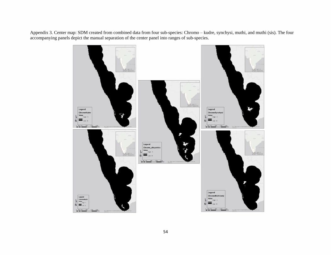
54

Appendix 3. Center map: SDM created from combined data from four sub-species: Chromo – kudre, synchysi, muthi, and muthi (sis). The four

accompanying panels depict the manual separation of the center panel into ranges of sub-species.

55

Appendix 4. List of predictor variables used in SAHM inquiries. Note that not all predictors are used in final model creation – see table 4.

Predictor Layers Source Date Captured/Calculated Notes

BioCl im 1: Annual Mean Temperature WorldClim Monthly (September 2017) Retreived

BioCl im 2: Mean Diurnal Range WorldClim Monthly (September 2017) Retreived

BioCl im 3: Isothermal i ty WorldClim Monthly (September 2017) Retreived

BioCl im 4: Temperature Seasonal i ty WorldClim Monthly (September 2017) Retreived

BioCl im 5: Max Temp of Warmest Month WorldClim Monthly (September 2017) Retreived

BioCl im 6: Min Temp of Coldest Month WorldClim Monthly (September 2017) Retreived

BioCl im 7: Temperature Annual Range WorldClim Monthly (September 2017) Retreived

BioCl im 8: Mean Temperature of Wettest Quarter WorldClim Monthly (September 2017) Retreived

BioCl im 9: Mean Temp of Driest Quarter WorldClim Monthly (September 2017) Retreived

BioCl im 10: Mean Temp of Warmest Quarter WorldClim Monthly (September 2017) Retreived

BioCl im 11: Mean Temp of Coldest Quarter WorldClim Monthly (September 2017) Retreived

BioCl im 12: Annual Precipi tation WorldClim Monthly (September 2017) Retreived

BioCl im 13: Precipi tation of Wettest Month WorldClim Monthly (September 2017) Retreived

BioCl im 14: Precipi tation of Driest Month WorldClim Monthly (September 2017) Retreived

BioCl im 15: Precipi tation Seasonal i ty WorldClim Monthly (September 2017) Retreived

BioCl im 16: Precipi tation of Wettest Quarter WorldClim Monthly (September 2017) Retreived

BioCl im 17: Precipi tation of Driest Quarter WorldClim Monthly (September 2017) Retreived

BioCl im 18: Precipi tation of Warmest Quarter WorldClim Monthly (September 2017) Retreived

BioCl im 19: Precipi tation of Coldest Quarter WorldClim Monthly (September 2017) Retreived

Elevation ASTER imagery April 2017 Remotely Sensed

NDVI (vegetation index; annual low) Landsat 8 (NASA, USGS) May 2017 Remotely Sensed

Soi l -adjusted veg index (SAVI; annual low) Landsat 8 (NASA, USGS) May 2017 Remotely Sensed

Soi l Type UN Food and Agricultural Organization N/A Retreived

Nearness to Surface Water UN Food and Agricultural Organization N/A Retreived

Slope DEM (ASTER) April 2017 Remotely Sensed

Aspect DEM (ASTER) April 2017 Remotely Sensed

Percent Canopy Cover Bhuvan (ISRO) January -May 2017 Retreived

Percent Canopy Cover Bhuvan (ISRO) January -May 2017 Retreived

Land use / Land cover Bhuvan, Landsat 8 (ISRO, NASA, USGS) March 2016 - May 2017 Raw imagery retrieved, classification analysis

56

Appendix 5. Top panels: SAHM outputs depicting a gradient (left) and binary (right) distribution estimation of a wide-ranging species. Lower

panels: SAHM outputs depicting a gradient (left) and binary (right) distribution estimation of a low-ranging species.

57

Appendix 6. Statistical model outputs from initial SAHM runs of a sub-set of frog species. Red-filled boxes are wide-ranging, blue-filled boxes are

narrow-ranging, and green-filled boxes are montane generalist species.

Frog Species N Percent Correctly Classified AUC True-Skill Statistic Cohen's Kappa Best Performing Model Reported

Pseudophilautus amboli 38 0.876 0.901 0.762 0.876 GLM

Pseudophilautus kani 42 0.711 0.834 0.787 0.923 MAXENT

Pseudophilautus wynaadensis 105 0.746 0.829 0.823 0.534 RF

Raorchestes akroparallagii 14 0.651 0.952 0.454 0.786 MAXENT

Raorchestes anili 85 0.164 0.777 0.830 0.565 BRT

Raorchestes beddomii 78 0.502 0.778 0.543 0.572 RF

Raorchestes bobingeri 40 0.569 0.678 0.615 0.121 MAXENT

Raorchestes griet 92 0.666 0.792 0.326 0.205 MARS

Raorchestes bobingeri 29 0.274 0.777 0.293 0.495 MAXENT

Raorchestes jayarami 6 0.271 0.705 0.600 0.300 MAXENT

Raorchestes travancoricus 44 0.809 0.848 0.100 0.373 MAXENT

Raorchestes dubois 19 1.062 0.857 0.824 0.368 MAXENT

Raorchestes resplendens* 6 1.083 0.910 -0.017 0.807 MAXENT

Raorchestes primarumfii 13 0.256 0.863 0.415 0.488 MAXENT

Raorchestes sushili 31 0.740 0.774 0.651 0.393 MAXENT

58

Appendix 7. Statistical model outputs from initial SAHM runs of a sub-set of plant species. Yellow-filled boxes are wide-ranging and green-filled

boxes are narrow-ranging species.

Plant Species N Percent Correctly Classified AUC True-Skill Statistic Cohen's Kappa Best Performing Model Reported

Aglaia barberi 34 0.669 0.816 0.585 0.379 MARS

Drypetes confertiflora 20 0.609 0.848 0.276 0.906 MAXENT

Cinnamomum malabatrum 30 0.764 0.855 0.729 0.563 MAXENT

Diospyros ghatensis 28 0.831 0.793 0.479 0.818 GLM

Diospyros oocarpa 19 0.769 0.780 0.212 0.958 MAXENT

Eugenia macrosepala 23 0.500 0.906 0.654 0.720 GLM

Ficus nervosa 53 0.684 0.693 0.792 0.698 BRT

Ixora elongata 24 0.604 0.963 0.305 0.382 MAXENT

Microtropis wallichiana 27 0.692 0.575 0.600 0.636 MARS

Psychotria nigra 87 0.708 0.718 -0.061 0.873 RF

Atuna indica 9 0.581 0.856 0.730 0.436 MAXENT

Epiprinus mallotiformis 17 0.548 0.637 0.556 0.523 MAXENT

Gordonia obtusa 14 0.812 0.726 0.274 0.624 MAXENT

Humboldtia brunonis 21 0.576 0.967 0.922 0.504 MAXENT

Olea dioica 46 0.771 0.779 0.339 0.458 MARS, BRT

Memecylon pseudogracile 13 0.791 0.820 0.253 0.363 MAXENT

Syzygium munronii 27 0.831 0.897 0.242 0.457 MAXENT, GLM

Thottea shivarajanii 11 0.824 0.835 0.570 0.418 MAXENT

Vateria indica 47 0.638 0.838 -0.394 0.554 RF

Walsura trifolia 18 0.565 0.775 0.298 0.459 MAXENT