Thermodynamic Properties of Gases and

Gas Mixtures at Low Temperatures

and High Pressures

by

David Robert Roe, M.A.

May 19 72

A thesis submitted for the degree of

Doctor of Philosophy of the University of London

and for the Diploma of Imperial College.

Department of Chemical Engineering and Chemical Technology, Imperial College, London, S.W.7.

ABSTRACT

An apparatus of the "Burnett"-type has been constructed

for the measurement of accurate compressibility factors of

gases at pressures up to 100 bar. Results have been obtained

in the temperature range 155 - 291 K for methane, nitrogen,

two methane/nitrogen mixtures, one methane/nitrogen/ethane

mixture and two natural gases.

A method of data treatment using non-linear least-

squares analysis has been developed which included an

investigation of the effect of experimental errors on the

derived virial coefficients by means of data simulated on

the computer.

The compressibility factors for methane agree within

.05% with those of Douslin et al. (43) above 0 °C and within

0.2% of those of Vennix et al. (52) below 0 °C. The results

for nitrogen are in good agreement with those of Crain et al.

(34) and Canfield et al. (67). There are no previously

published results for the methane/nitrogen system at low

temperatures.

Second virial coefficients of methane, nitrogen, argon

and ethane were used to determine parameters of the Lennard-

Jones (n-6) and Kihara intermolecular potential models and,

for methane, of the potential of Barker et al. (125). The

latter and the Lennard-Jones (18-6) potential gave good

agreement with the coefficient of the long-range dispersion

interaction and the experimental third virial coefficients

when the triple-dipole non-additive contribution was included.

None of the combining rules tested were found to be

adequate for all of the systems: CH4/N2, CH4/Ar, CH4/C2H6.

and N2/Ar. A geometric mean correction factor,

1 k12 (= 1 - (612 - (611'622)2)) of 0.03 was necessary for

CH4/N2.

The results for the multicomponent mixtures, including

data on natural gases taken from the literature, were

compared with the predictions of the extended corresponding-

states principle as due to Leland et al. (158). Agreement

was excellent, within experimental error, above °C and

fairly good below 0 °C.

2

3

CONTENTS

PAGE

ABSTRACT • 1 TABLE OF CONTENTS 3 ACKNOWLEDGEMENTS 6

CHAPTER

1. INTRODUCTION 7 1.1 The Equation of State 7

(a) The virial equation of state 9

1.2 Compressibility factors of natural gas 11

1.3 Other thermodynamic properties 13

1.4 The Burnett method of measurement of 14 compressibility factor (a) The non-isothermal Burnett Method 18

2. DESCRIPTION OF APPARATUS AND EXPERIMENTAL 20 PROCEDURE

2.1 Introduction 20

2.2 The Low Temperature System 22 (a) The Pressure Vessel 22 (b) The Radiation Shield 24 (c) The Inlet Tubes 26 (d) The Outer Brass Jacket and Supports -28 (e) The Cryostat 30 (f) Low Temperature System Cables 30

2.3 Temperature Measurement 31

2.4 Temperature Control System 34 (a) Temperature Control of the Pressure 34

Vessel (b) Temperature Control of the Radiation

Shield

2.5 The Ice-Bath Vessel -42,

2.6 Pressure Measurement 45 (a) The Oil Piston-Gauge '45

(i) The acceleration due to gravity -48 (ii) Determination of the mass of - 48

counterbalancing weights (iii) Buoyancy and other corrections 51

to the load on the piston (iv) Hydraulic head of oil 54

(b) The Differential Pressure Cell 55 (c) The Gas-Operated Piston Gauge 58 (d) Atmospheric Pressure Measurement 61 (e) The Precision Pressure Gauge (P.P.G.) 62

(i) Modifications to the P.P.G. 65 (ii) The effect of pressure on the 67

P.P.G. null position (iii) Calibration of P.P.G. sensitivity 73

(f) Errors in Pressure Measurement 75

4

PAGE

2.7 Pressure and Density Gradients due to -17 Gravity

2.8 Calibration of Volumes 80

2.9 Pressure distortion of the vessels '82

2.10 Preparation of Gas Mixtures and Gas '84 Analyses

2.11 Experimental Procedure 86

3. TREATMENT OF EXPERIMENTAL DATA

`190

3.1 Introduction 90 3.2 Analytical Methods of Data Reduction 92

(a) Non-Linear Least-Squares Procedure: 96 Method A

(b) Treatment of experimental data for 100 the non-isothermal Burnett apparatus

(c) Description of computer program 103

3.3 Determination of accurate virial 105, coefficients from the least-squares analysis of PVT data

3.4 Simulation of Burnett Data 108 (a) The model virial series 112 (b) Comparison of Method A and Method B 113 (c) Isotherms of low curvature 115 (d) Isotherms of high curvature 122 (e) Weighting factors 126 (f) Comparison with experimental results 126 (g) The magnitude of the apparatus constant 128

4. EXPERIMENTAL DATA 131

4.1 Experimental results of this investigation '131

4.2 Experimental virial coefficients of this 132 investigation

4.3 Total Error Analysis 133 (a) The Equation of State at 0 °C 133 (b) Other Systematic Errors 135 ( c) Adsorption 136

4.4 Experimental Data of Other Workers 190 (a) Experimental Methods 190 (b) Extraction of Virial Coefficients 190

from PVT Data (c) Methane 193 (d) Nitrogen 201 (e) Methane/Nitrogen Mixtures 206

4.5 Comparison with other workers -209 (a) Methane 210

(b) Nitrogen 216

(c) Methane/Nitrogen 217

4.6 Comparison of Compressibility Factors '218 (a) Methane 218

(b) Nitrogen .222

5

PAGE

4.7 , Experimental Results for other gases and' 225, binary mixtures .._ (a) Argon 225. (b) Ethane 226 (c) Methane/Argon 226 (d) Nitrogen/Argon 226 (e) Methane/Ethane 227 (f) Propane 227 (g) n-Butane 227

5. INTERMOLECULAR POTENTIALS

231

5.1 Introduction 231 (a) The form of the intermolecular '231

potential (b) The intermolecular potential and '233

the virial expansion (c) Inverse Laplace Transform of B(T) -237

5.2 Pair Potential Models 238 (a) The Lennard-Jones (n-6) potential 240 (b) The Kihara spherical-core potential 241 (c) Calculation of potential parameters 241

5.3 Multiparameter Pair Potentials 253 (a) The reduced Barker-Fisher-Watts 255

potential

5.4 Anisotropic Potential of the Nitrogen 261 Molecule

5.5 Third Virial Coefficients 263 (a) Third virial coefficients for simple 267

potential functions (b) Third virial coefficients for the 268

reduced BFW potential (c) Results of comparisons 269 (d) Conclusions 273

5.6 Second Virial Coefficients of Mixtures ' 274

5.7 Third Virial Coefficients of Mixtures 287

6. THE PREDICTION OF ACCURATE COMPRESSIBILITY 293 FACTORS OF MULTICOMPONENT GAS MIXTURES

6.1 Introduction 293

6.2 The Principle of Corresponding States 293

6.3 (a) The Extended Corresponding States 300 Principle

(b) The equation of state for methane 303 (c) Computer program 303 (d) Test of predictive method 304

6.4 Review of Published Experimental Compressibility Factors of Natural 309 Gases

6.5 Conclusions 317

REFERENCES 320

ACKNOWLEDGEMENTS

My sincere thanks are due to the following:

Dr. G. Saville, for his helpful supervision and

invaluable guidance throughout this project.

The Gas Council, London Research Station, for enabling

me to carry out this research and for financial support.

The members of the Departmental, Electronics, and

Glass workshops for their skilful assistance.

Dr. A. Harlow for the sound design of parts of the

apparatus; and to Dr. C.A. Pollard for his helpful advice

during its construction.

Mr. R.E. Clifford and staff of The Gas Council,

Watson House, for providing the gas mixtures; and to

Mr. B. Juren and Dr. Angela Gunning for information on

dew-points.

My parents, for their support, and my wife for her

constant encouragement.

6

7

CHAPTER ONE

INTRODUCTION

1.1 The Equation of State

The equation of state of a perfect gas at pressure P,

temperature T and molar volume V is,

PV = RT (1.1-1)

where R is the gas constant.

Real gases depart from perfect-gas behaviour because of

the finite size of the molecules and the forces between them.

The compressibility factor, Z, of a real gas is defined

by

PV RT (1.1-2)

It is a function of temperature and pressure (or

density) and is a convenient measure of the non-ideality

of a gas because it is non-dimensional. As the pressure

tends to zero and the gas becomes more ideal, Z approaches

the value 1.0.

The variation of Z with reduced temperature and pressure

is of the qualitative form shown in figure 1.1. This graph

has been plotted in reduced form, where reduced temperature

and pressure are here defined by,

TR T ,R P = Tc Pc

(1.1-3)

where TC is the critical temperature and Pc is the critical

pressure, as it is found that most simple gases roughly

follow the same curves (the principle of corresponding states).

2 3 4 5 7 8

1.2

1.1

TR=2.6 i•

0.9

0•G - 1

05--W I

- z 0

O

tX CRITICAL POINT 1 I 1 I 1_ 1

REDUCED PRESSURE, PR

FIG 1.1. GENERALIZED COMPRESSIBILITY FACTORS (FOR PARAFFIN HYDROCARBONS OR NATURAL GAS)

9

Many equations of state, both theoretical and empirical,

have been proposed to express quantitatively the variation

of the compressibility factor with pressure and temperature,

but no one simple equation has yet been completely successful

over the whole range. In this work most of the interest is

in the low pressure region of figure 1.1 where the virial

equation of state is appropriate.

(a) The virial equation of state

The virial equation of state is an expansion of Z as

an infinite series in powers of density:

Z = 1 Bp + Cp2 + Dp3

(1.1-4)

An equation of this type, but in truncated form, was

first suggested as an empirical representation of PVT data.

The significance of the virial series is not in its usefulness

in this respect, as the series appears to diverge at high

densities (1) where other equations requiring fewer terms are

preferable, but in the fact that it has sound theoretical

foundations.

It can be shown that each of the virial coefficients,

B, C, D, etc., is related to the intermolecular forces in a

direct manner (2). Statistical-mechanical calculation

shows that the second virial coefficient, B, is'a function

of the interaction between pairs of molecules, as described

in Chapter 5, the third virial coefficient, C, is a function

of the interaction between three molecules, and so on.

The coefficients are independent of density and are functions

of temperature of the general form shown in figures 1.2 and 1.3.

10

The second virial coefficient is one of the few

macroscopic properties of a system which has a sound

theoretical relationship with the intermolecular forces

between a pair of molecules and which can provide quantitative

information on these forces. However, very accurate

experimental data are necessary.

For mixtures it can be shown by the methods of statistical

mechanics (2), as described briefly in Chapter 5, that the

second virial coefficient is given by,

BM1X . = x. 1J B..

J i=1 j=1

(1.1-5)

where xi is the mole-fraction of the i th. component.

B is the second virial coefficient of the i th. pure

component.

Bij (i j) is the interactional second virial coefficient

which is directly related to the interaction between molecule

i and molecule j.

Similarly,

n n n

Croix = xi x. xk ij C 3 k i=1 j=1 k=1

(1.1-6)

where Cijk is related to the interaction between the three

molecules of type i, type j and type k.

Thus by measurement of the compressibility factors and

hence second and third virial coefficients of mixtures, it is

possible to obtain information on the intermolecular forces

between unlike molecules. In a multicomponent mixture the

11

interactions consist of interactions between pairs of

molecules plus interactions between clusters of three

molecules, and so on. However, the interactions between

clusters of more than two molecules can largely (but not

wholly) be described as the sum of interactions between

pairs (pairwise additivity). For this reason it is

necessary to have experimental data on the binary mixtures

of the components of a multi-component mixture of practical

importance, such as a natural gas, before its compressibility

factor can be predicted with high accuracy.

1.2 Compressibility factors of natural gas

In the metering of large quantities of gas in pipelines

the compressibility factor (or density) is required to

obtain the measured flow-rate in units of mass per second.

A small error in the pre-supposed value of Z at a certain

temperature and pressure could lead to errors of millions

of cu. ft. in the quantity of gas transmitted. The problem

is more acute for natural gases, the compressibility factor

of which varies considerably with temperature and pressure

in the range of interest, than for town gas, the compressibility

factor of which is fortuitously close to 1.0 because of the

high hydrogen content.

Ideally, it is desirable for Z to be measured or

predicted as a function of composition, temperature and

pressure to as high an accuracy as possible, or at least to

an accuracy greater than that inherent in the actual

metering.

Knowledge of the volumetric behaviour of natural gas

12

and its components is also important in the design and

operation of compressors and gas-treatment plants, particularly

in relation to the liquefaction of natural gas, when

information on Z at low-temperatures is required.

The work reported here was initiated as the first part

of a long-term project to measure accurately the com-

pressibility factors of the constituents of natural gas,

their binary mixtures, then ternary mixtures, leading up

to multicomponent mixtures. Data of this type are sparse,

particularly at low temperatures.

The gases studied in this investigation were methane

(the major component of natural gas), nitrogen and their

binary mixtures at temperatures from 155.9 K to 291.4 K at

pressures up to 100 bar; this covers, approximately, the

lighter shaded region of figure 1.1. Nitrogen is an

important component in natural gas not only because it is

inert to combustion but also because it is more ideal than

methane and the higher hydrocarbons. The mole-fractions

of the hydrocarbons tend to decrease in a regular manner

along an homologous series and the compressibility factor

of a natural gas consisting solely of hydrocarbons can

usually be correlated with the average molecular weight or

the specific gravity. The presence of only a small

percentage of nitrogen upsets this correlation.

As there was an immediate requirement for a predictive

method capable of high accuracy, measurements were also

obtained for three multi-component mixtures: a mixture of

methane, nitrogen and ethane, and two natural gases. The

results could then be compared with those of various predictions.

This is done in Chapter 6.

1.3 Other thermodynamic properties

An equation of state based on accurate PVT measurements

is important not only in interpolation of the data and

prediction of the compressibility factor (or density) but

also, of course, in connection with the calculation of other

thermodynamic properties. The changes in thermodynamic

properties of a gas over ranges of temperature and pressure

are simply related to the equation of state. For example,

we have for a reversible infinitesimal change in enthalpy

of a fluid of constant composition,

dH = TdS + VdP

3H = T (L2) 61D T 6P T

From the Maxwell relation,

aS aV) (7) = - (— 3T (1.3-3)

we have

3H (—) = aP T

(1.3-4)

Therefore, from an equation of state of the form

V = f(T,P) (1.3-5)

the partial derivative (ff) can be calculated. T

For a change in enthalpy with both temperature and pressure,

am dH = dT + ( H) dP aT (1.3-6)

CP dT + (V - ) dP

P (1.3-7)

where C is the specific heat at constant pressure.

13

14

. . the enthalpy H of a gas at temperature T1 and pressure P1

is:-

T1 P1_

H = Ho C dT ir (V - T(a ) )dP (1.3-8) a

0 0

where Ho is an integration constant and is usually set to an

arbitrary value at some chosen standard state, (P0, To), such

as at 1 atm., 0 °C. The integration with respect to

temperature is usually performed first, C taking the value

at P0, and then the integration with respect to pressure

is performed at temperature T1. Thus from a knowledge of

Cp at pressure Po and from 414)p and V, i.e. the equation

of state, H - Ho may be calculated.

Similarly, TI

S - So

To

dT T I

Po

(g) dP (1.3-9)

High precision is required in the equation of state and

hence in the PVT measurements, as accuracy is always lost

on differentation of an equation of state. For the gas

phase thermodynamic properties derived in this manner tend

to be of higher accuracy than those from direct calorimetric

measurements (3). Entropy changes cannot, of course, be

measured directly by experiment.

1.4 The Burnett Method of measurement of compressibility

factor

Burnett (4) proposed a method of measurement of the gas

15

compressibility factor that did not require accurate

measurement of the volume, mass or absolute temperature of

the gas under study. Other methods are described briefly

in section 4.4(a); they either involve the determination

of the pressure of a fixed volume of gas as a function of

temperature (isochoric measurements), or the determination

of the pressure as a function of volume at constant

temperature (isothermal measurements).

With reference to figure 1.4, a Burnett apparatus

consists basically of a volume VA, at constant temperature

TA, connected by means of an expansion valve, E, to a second

volume VB at constant temperature TB. When TA is equal to

TB it is known as an 'isothermal' apparatus. At the start

of an experiment VA is charged with gas and the initial

pressure Po is measured. The gas is then expanded through

the valve E into the previously evacuated volume VB and,

after establishment of temperature equilibrium, the new

pressure P1 is measured. Volume V is then vented and

evacuated, another expansion of gas from VA into VB is

carried out, and the pressure P2 measured. Expansions are

continued until the minimum measurable pressure is attained;

the sequence of pressures, Po P1 Pj Pn constitute the

basic data of a Burnett 'run'.

The number of moles of gas, no, in VA prior to the first

expansion is given by

P o A no = RTZ 0

(1.4-1)

where Z0 is the compressibility factor at pressure Po.

116

FIG.1-2. SECOND VIRIAL COEFFICIENT FIG.13. THIRD VIRIAL COEFFICIENT

TO PRESSURE MEASUREMENT

VACUUM

EXPANSION VALVE

A

FIG 1.4. THE BURNETT APPARATUS'.

1 A • B • no = RTZ1 (1.4-2)

After the first expansion,

17

P HenCel p V + VB) Zo

Z N. Zo A

(1.4-3)

where N is known as the 'cell constant' or 'apparatus constant'.

Similarly, after the second expansion

1 1 N. Z (1.4-4) 2 2

and after the jth. expansion,

P1-1 N

-1 -1 3-1 P. - • Z.

J 3

From equations (1.4-3) and (1.4-4),

P2' 0

and similarly,

Pi.Ni = (z°

(1.4-5)

(1.4-6)

(1.4-7)

It can be seen that to obtain the compressibility

factors from the experimental pressures, N and (Po /Zo ) must

be determined; this is accomplished, directly or indirectly,

from either a graphical or analytical method of data

treatment. These procedures are described in Chapter 3.

The Burnett method requires good temperature control

and precise pressure measurements. As no accurate

measurements of volume, mass of gas, or absolute temperature

are necessary, the method is particularly suited to the

determination of precise values of Z at low density and

hence accurate second and third virial coefficients,

particularly at low temperature, where other methods may

lack the necessary precision at low pressures, and at very

high temperatures where the accurate measurement of absolute

temperature is difficult. However, as compressibility

factors are not determined directly in a Burnett apparatus,

their accuracy may be effected not only be experimental

errors in measurement but also by such factors as the degree

of curvature of the isotherm, the magnitude of N and hence

the number of expansions in a run, and the method of data

treatment employed: these factors are considered in detail

in Chapter 3.

(a) The non-isothermal Burnett Method

In the 'isothermal' Burnett apparatus both volumes are

maintained at the same temperature. At low temperatures

the problem of temperature control with the conventional

stirred-fluid bath can be difficult. It is much easier to

ensure close temperature control and eliminate temperature

gradients for each vessel separately. For these reasons

a 'non-isothermal' Burnett apparatus may be employed, as in

this investigation, in which, with reference to figure 1.4,

volume VB is at a temperature TB which is easily maintained

constant, such as 0 °C. Volume VA is maintained at the

temperature TA for which experimental compressibility factors

are required. The expression equating moles of gas before

and after the jth. expansion is then,

18

P3. .V -1 A P.j • VA

TA.(ZA)j + TB"(ZB)j

(1.4-8)

19

T .(Z ). A A 3-1

The disadvantages of the 'non-isothermal' Burnett

method are threefold. Firstly, the equation of state of

the gas at temperature TB must be known either from published

results or by performing an experiment with TA = TB;

however, it is fortunate that errors in the values of ZB

lead to much smaller errors in the experimental values of

ZA, as described in section 4.3. Secondly, some of the

interconnecting tubing, valves, etc. constitute "dead-space

volume" which is maintained at temperatures intermediate

between TA and TB, and part of which must necessarily

contain a temperature gradient. The interior volume of

this dead-space must be known and corrections for the gas

inside included in the calculation of ZA. Thirdly, the

whole data treatment is rendered slightly more complex.

Apart from the major advantage of easier temperature

control, the non-isothermal Burnett method has the advantage

that the expansion valve can usually be maintained at normal

temperatures; many leakage problems occur with valves at

extremes of low or high temperatures. Absolute leak-

tightness of the valve is essential to the accuracy of the

method. Another advantage is that if the gas under in-

vestigation adsorbs on the walls of the vessel at low

temperature then the effect of adsorption on the results is

much smaller when VB is at a higher temperature where

adsorption is insignificant (5). The problem of adsorption

is discussed further in section 4.3(c).

CHAPTER TWO

DESCRIPTION OF APPARATUS AND EXPERIMENTAL PROCEDURE

2.1 Introduction

A general scheme of the 'non-isothermal' Burnett

20

apparatus is shown in figure 2.1. The first vessel,

A, wasat the experimental emperature in the low-temperature

system, described in detail in section 2.2. The second

vessel, B, was situated in an ice-bath at 0 °C.

Both vessels were double-walled and pressure compen-

sated, i.e. the same pressure existed both inside and out-

side of the inner vessel; this served to reduce the

distortion due to pressure of the inner volume and enabled

this distortion to be calculated with accuracy, as described

in Section 2.9. The gas under study was confined within

the inner volumes and the pressure difference between this

gas and that in the outer volumes, which were directly

connected to the pressure measurement system, was nulled by

means of a Precision Pressure Gauge (Texas Instruments).

Pressures between 25 bar and 110 bar were measured by

means of an oil piston-gauge (or pressure balance). The

oil was separated from the pressure-compensating gas by a

differential-pressure cell (Ruska). Pressures below about

25 bar were measured by means of a gas piston-gauge.

The whole apparatus was situated in an enclosure, the

temperature of which was controlled at a few degrees C above

ambient room temperature by means of a toluene regulator with

a proportionating head in conjunction with two 1000 watt

heating elements; the air was circulated by two 10" fans and

r

0 >

gas piston-gauge

FIGURE 2.1

pressure intensifier

xI

oil piston -gauge

< (g)

vacuum

null indicator

'CD differential pressure cell

0>

expansion valve

----1 inner

radiation I shield

i

I -c..1 outer r"- volume

4- volume

L

r -

0

vacuum

'precision pressure

--I gauge

• •

1 L _

ice-bath vessel

\`'.1'\(‘_:` `‘' .' \s,' ''''-

\.:

\ \ \ :\,•

'

''''' N

.. \ ‘ \

- • ' ' - le•.

A • .,

',

. „ N \‘,

:' • „.„,...„\-\\,,,,k ,

I- I - - - - - low-temperature system

THE BUR NETT APPARATUS

the temperature inside the enclosure was constant to

0.1 °C. Thus the piston-gauges, the dead-space volume

and the electronic equipment were all maintained at a

constant temperature.

2.2 The Low Temperature System

The low temperature system is shown in figure 2.2.

The cylindrical stainless-steel pressure vessel is suspended

within a copper radiation shield which is itself suspended

within an evacuated outer jacket, the whole being situated

in a Dewar containing refrigerant. Platinum resistance

thermometers in the pressure vessel were used in conjunction

with an automatic controller to govern the supply to heaters

around the outside of the vessel, thus maintaining its

temperature at a constant value. The temperature of the

radiation shield was controlled by means of a differential

thermocouple at about 1 °C. below that of the pressure vessel,

which thereby was provided with a constant-temperature environ-

ment.

The system was thus designed such that the heat loss from

the pressure vessel was small and radiative, giving close

temperature control and small temperature gradients within the

vessel.

(a) The Pressure Vessel

The pressure vessel was of EN58J stainless-steel. It

consisted of an inner volume, with walls of .125" thickness,

containing the gas under study, and an outer volume, with

walls of 1" thickness, containing gas at the same pressure.

22

SUPPORT TUBES (ST/ST).

INLET TUBE HEATERS.

LEAD-OUT CABLES-t.

BRASS COLLAR

COPPER RING

NYLON SUPPORTING THREADS. SWAGELOK COUPLINGS. MEASURING THERMOMETER WELL.

CONTROL THERMOMETER WELL.

RADIATION SHIEL D (COPPER). RADIATION SHIELD HEATERS. INNER VOLUME.

PRESSURE VESSEL ST./ST. PRESSURE VESSEL HEATERS.

OUTER VOLUME.

REFRIGERATED-t. OUTER JACKET (BRASS)

INLET TUBES.

23

FIG: 2.2' LOW-TEMPERATURE SYSTEM

24

The interior surfaces of the vessel were polished

to reduce adsorption and it was assembled using electron-

beam welding (by courtesy of Vickers Ltd.) to prevent

damage to the polished surfaces. The vessel‘ was provided

with a central well, which housed the platinum resistance

1" thermometer used for temperature measurement, and ten -6.

diameter vertical holes drilled in the outer wall to house

the controlling platinum resistance thermometers.

A copper/constantan thermocouple was soldered to the

pressure vessel at its mid-point and heaters of 32 s.w.g.

cotton-covered manganin wire were non-inductively wound

along the length of the outer wall. The heaters were

electrically insulated from the pressure vessel by a layer

of nylon% stocking material that was stretched over the

vessel and then painted with Formvar (a solution of poly-

vinyl formal in chloroform), which also served as an adhesive.

The thermocouple and heater circuitry is described in section

2.4.

(b) The Radiation Shield

The copper radiation shield consisted of a 0.125" thick

cylindrical side section to which were screwed top and bottom

end plates. To the outside of each section were soldered

the required thermocouple wires, as described in section 2.4.

The pressure vessel was suspended from hooks screwed

into the top of the radiation shield by means of several

strands of strong nylon thread (dental floss), which acted

as both thermal and electrical insulant. The radiation shield

was similarly suspended from the top of the outer brass jacket.

25

The side section had two spiral grooves along its

length, in which were embedded two cables consisting of

all the electrical leads to the radiation shield and

pressure vessel. One cable carried the heater leads and

the other carried all thermocouple and thermometer leads;

both also contained spare leads in order to avoid re-wiring

of the radiation shield heaters in the event of breakage

or shorting in the cables. Along the length of the side

section were non-inductively wound 32 s.w.g. manganin

wire heaters, insulated from the radiation shield by formvar-

painted nylon [stocking that also held in place the embedded

cables. The top and bottom sections each consisted of two

copper discs between which was sandwiched a heater of

manganin wire wound on a circular sheet of mica.

Heater and thermocouple leads from the top and side

sections were passed down over the outside of the side

heaters, from which they were insulated by nylon tape,

and together with those from the bottom section they were

soldered at point A to the appropriate leads in the embedded

cables. Leads from the pressure vessel heaters, thermo-

couples and platinum resistance thermometers were sheathed

in P.V.C. sleeving, passed through the bottom plate of the

radiation shield and similarly connected to the cable leads.

The hole in the bottom plate was provided with a cover to

prevent heat loss by direct radiation from the pressure

vessel to the refrigerated outer jacket. All the soldered

junctions at point A were covered with nylon tape and fixed

at about 1 cm. from the bottom of the radiation shield so

that they would be at about the same temperature.

The leads at the top of the embedded cables were

soldered at point B to the appropriate leads in the

cables coming out of the low temperature system. The

purpose of the spiral grooves was to ensure that the ends

of the embedded cables at point A were reduced to the

temperature of the radiation shield, thus eliminating

heat transfer by conduction down the cables to the thermo-

couple junctions and platinum resistance thermometers.

The inside of the radiation shield was covered with

bright aluminium foil to reduce the heat loss by radiation

from the pressure vessel. Eight holes of 0.125" diameter

in the side of the radiation shield, drilled at an angle

to avoid the transmission of direct radiation, assisted the

quick evacuation of the interior.

(c) The Inlet Tubes

The two inlet tubes to the inner and outer volumes of

the pressure vessel were of 0.063" o.d., 0.043" i.d. stainless-

steel tubing. The tubing chosen was thin-walled, to reduce

the heat transfer by conduction to the pressure vessel, and

of small diameter in order to reduce the quantity of gas

contained within.

Before assembling ,the low-temperature system, eleven

copper/constantan thermocouples were attached to the tubes

at the positions shown in Figure 2.3. The thermocouple

junctions were insulated from the tubes by a thin sheet of

paper coated with formvar and then covered with a further

layer of insulating paper. A heater of 32 s.w.g. manganin

26

ADAPTOR

BRASS SUPPORTING PLATE.

.•111 1.0 •••••••••

Gomm earpookseiro 411=1.1•1•M ill•momm•

INLET TUBE HEATERS.

REFRIGERANT LEVEL.

TOP OF OUTER

e." I

5:: 1

24

cm

(8

x3cm

)

JACKET. L 441.11•111••• •••11•=•••• ••••••••• Iblm•

RADIATION SHIELD

V

PRESSURE VESSEL.

E U

FIG.2.3 INLET-TUBE THERMOCOUPLE POSITIONS.

27

wire was then non-inductively wound over the tubes

between thermocouples 2-and 10.

The tubing leaving the pressure vessel was coiled

to allow for thermal expansion and contraction and then

connected by means of "Swagelok" couplings to the inlet

tubes. These passed through a hole in the top plate of

the radiation shield, from which they were separated by

a teflon sleeve. The inlet tubes passed out to the

atmosphere at the top of the central support tube through

a brass adaptor, the seal being made by means of a soft-

soldered joint.

The heater and thermocoqle wires were soldered at

point B to the appropriate wires in the lead-out cables.

The E.M.F. of each thermocouple was measured by a

digital volt-meter ("Solartron") having a resolution of

about 3 microvolts. The cold junctions were encapsulated

in protecting glass tubes situated in distilled water / ice,

and the terminals of the thermocouples connected into the

D.V.M. through a mercury-bath switch.

(d) The Outer Brass Jacket and Supports

The cylindrical brass jacket surrounding the radiation

shield was supported by means of four stainless-steel tubes,

which were thin-walled to reduce heat transfer to the

refrigerant from outside the cryostat. To the bottom of

each support tube had been hard-soldered a brass collar,

which allowed the tube to be soft-soldered readily into the

top` of the outer jacket. The tubes were joined in a similar

28

manner to a 0.25" thick brass supporting plate which was

bolted to the framework of the apparatus.

The lead-out cables were sheathed in P.V.C. sleeving

and wound several times around a copper ring.soldered to

the underside of the top of the jacket. This served to

cool the cables down,thus reducing their disturbing

effect on the temperature control of the radiation shield.

The central support tube contained the inlet-tubO r . the

second support tube contained the lead-out cables from all

of the heaters and ,a third contained the lead-out cables from

all of the thermometers and thermocouples. The fourth

tube led directly to the vacuum system and contained no

cables because of the possible breakdown of electrical

insulation that would result from condensation of mercury

from the diffusion pump.

The cables passed through a black-waxed B29 brass

cone/glass socket joint at the top of the support tubes.

Each group of twelve wires were led out to the atmosphere

through black-waXed B29 cone: socket seals. The seal was

formed by baring the wires, embedding them into the black

wax of the socket and inserting the waxed cone stopper.

The wires were soldered onto 16 s.w.g. pins, of the same

metal, mounted in a perspex disc on each stopper cone.

The inside of the brass outer jacket was covered with

bright aluminium foil to reduce heat loss by radiation from

the radiation shield. The last stage of the assembly of the

low temperature system was the soldering of the brass jacket

to its lid. A low melting-point (115 °C) tin/indium solder

29

was used to avoid melting the soldered connections on the

radiation shield and the other soldered joints on the

outer jacket, and also to avoid damage to the inner electrical

insulation.

(e) The Cryostat

The brass jacket was immersed in a refrigerating fluid

contained in a large silvered Dewar flask. For temperatures

of the pressure vessel below 200 K the refrigerating fldid

was liquid nitrogen, the level of which was maintained to

within 2 cm. by an automatic level controller.

After several experiments at low temperature a small

leak appeared in the evacuated brass jacket at the point

where one of the support tubes was soldered into the jacket

lid. This leak, which was present only when the jacket was

immersed in liquid nitrogen, was temporarily cured by repeated

application of rubber-based sealant solution. When the

temperature of the pressure vessel was above 200 K a slurry

of solid CO2/methanol was used as refrigerant. Although

this is less convenient to use than liquid nitrogen, it avoided

the problem of leakage.

(f) Low Temperature System Cables

All of the thermocouples were formed by joining 40 s.w.g.

copper wire and 36 s.w.g. constantan wire using thermoelectric

free solder. Wires of the same sizes were used for all the

thermocouple leads from the low-temperature system to the

measuring instruments.

30

31

The lead-out cables passed through the support tubes

in contact with the refrigerant fluid. As variations in the

refrigerant level led to changes in lead resistance, the

thermometer and heater leads were of manganin wire, which has

a much lower thermal coefficient of resistivity than does

dopper. The heater leads were of 32 s.w.g. manganin wire,

whereas the platinum resistance thermometer leads, which

had to have a low resistance, were of 28 s.w.g. manganin wire.

This was the largest diameter that could be manipulated easily

during the wiring of the system.

In the embedded cables there were no changing temperature

gradients and so 32 s.w.g.copper wire was used for both heater

and thermometer leads.

From the pin-blocks at the top of the support tubes

there were no restrictions on the size of leads and so 18 s.w.g.

copper wire was used for the heater leads and for the control

platinum resistance thermometer leads. The measuring platinum

resistance thermometer leads were of coaxial cable with a 18 s.w.g.

copper core and a copper sheath which served to reduce the

pick-up of electrical noise by the core.

2.3 Temperature Measurement

The temperature of the pressure vessel was measured by

means of a platinum resistance thermometer (Tinsley type 5187 L)

No. 193958). It was of the type having a helium-filled outer

platinum sheath and both resistance and potential leads, with

a nominal ice-point resistance of 25 ohnts.f,

The thermometer was calibrated at the National

Physical Laboratory with respect to the International

Practical Temperature Scale of 1948. The temperature

was given by the Callendar van Dusen equation,

t = R- R

o p/ t 3 4. 0 — 1 / p 7) ( — ) / t n/ t

aRo 700 100 100 100

(2.3.1)

where t = temperature in degrees C (IPTS 1948)

Rt = resistance at t oC

Ro

= resistance at 0 °C.

With a measuring current of 1mA the constants of the

equation were calibrated as,

Ro

= 24.8370 ohm

a = 0.00392617

0 = 0 for T > 0 °C

13 • 0.1096 for T < 0 °C

• 1.4936.

The differences between the IPTS 48 scale and the

IPTS 68 scale (in effect the true thermodynamic temperature

scale) are given by Hust (6). These differences in the

range 150 - 325 K were fitted to a polynomial in temperature

and the resultant equation used to change the measured values

to the IPTS 68 scale.

The maximum difference between the two scales in this

range is .04 K.

The thermometer resistance was measured by means of an

A.C. Precision Double Bridge (Automatic Systems Laboratories

Ltd., model H8). The ratio arms of the bridge were balanced

by means of a 'quadrature' control and an 'in-phase' control

32

consisting of eight decade switches, which displayed

the value of the ratio,

r = (2.3-2)

where Rt = resistance of thermometer

Rs = resistance of a standard resistor.

The standard resistor was of nominal 50 ohm

resistance (Tinsley type 1659, No. 175884), with both

resistance and potential leads. Its resistance at a

temperature of is °C was given by

R8 8

= 50.0008 + (t - 20).10-5 ohms. (2.3-3)

The bridge was set such that the voltage across the

thermometer was about Rt mV, giving a current of 1 mA.

Connections to the bridge were made by means of low-

noise plugs with gold-plated pins, to which the leads

were carefully soldered, using thermoelectric-free solder.

The bridge was equipped with a changeover switch

which could change the positions of the ratio arms, thus

giving a check on the- accuracy of the balance position.

Differences between the 'normal' and 'check' positions were

usually equivalent to about .001 °C. The bridge sensitivity

was equivalent to .0005 °C. The overall accuracy of the

absolute temperature measurement was estimated as ± .005 K.

33

Rt

Rt Rs

2.4 Temperature Control System

(a) Temperature Control of the Pressure Vessel

The principle of the temperature control system was

that a series of platinum resistance thermometers in the

wall of the pressure vessel comprised one arm of a Wheatstone

bridge circuit, the unbalance signal from which formed the

input to an electronic control unit. The output from the

control unit supplied power to the heaters around the

pressure vessel.

The ten controlling thermometers (De Gaussa type P5),

each of nominal 100 ohm resistance at 0 °C, were housed in

ten equally spaced vertical wells in the outer wall of the

pressure vessel. They were provided with silver extension

leads which enabled them to be connected in series, giving

a total nominal 1000 ohm resistance at 0 °C and a temperature

coefficient of resistance of about 4 ohm / °C. Compensating

leads of the same type of wire ran alongside the leads between

the thermometers and the bridge.

The bridge circuit is shown in figure 2.4. The ratio

arms, R1 and R2, were set to 1000 Ohms, a value which was

close to that of the thermometer, R4, in order to give

optimum control. The variable resistance, R3, consisted

of four decade boxes, which totalled 10,000 ohms in increments

of 1 ohm, in series with a 10 x 0.1 ohm wire-wound resistance.

Thus the value of R3 could be pre-set to the nearest 0.1 ohm,

corresponding to 0.025 °C. At the control point,

R4 . L‹.2 R3

(2.4-1)

34

=1000.n.

compensating leads

platinum resistance thermometers

_, (lox loon. in series)

heaters

1' 2 3T 4 5' 6

4

FIG. 2.4 TEMPERATURE CONTROL CIRCUIT : PRESSURE VESSEL

null detector

(amplifier)

c.a.t. controller

heater circuit power amplifier

36

The output sensitivity of the bridge was calculated

as follows:

When the bridge was

resistance of the thermometers

• • Voltage across R4

Voltage across R3

• • Output voltage

just off balance, then the

changed to R4 + SR4 V(R4 + 6R4)

(2.4-2)

(2.4-3)

(2.4-4)

(2.4-5)

+ SR4 (1000

V R3 =

* R4 + SR4)

V R4

(1000+R3)

V(R +6R ) 4

(1000+R4)

V R 4

(1000+R4 +6R4 )

1000.V.dR

(1000+R4)

2 (1000+R41

The battery voltage was chosen as 6 volts, giving a

bridge output of 6 microvolts for a change in temperature of

0.001 °C at 0 °C (R4 = 1000 ohms, dit4 = 0.004 ohms). The

bridge output increased at lower temperatures of the pressure

vessel, e.g. 8.7 microvolts/0.001 °C at 190 K. (R4 = 670 ohms).

The output voltage from the bridge formed the input

to an electronic D.C. Null Detector (Leeds and Northrup,

model 9834-2). This instrument was a high-gain, low-noise

operational amplifier, giving an output voltage of from-0.5 to

+ 0.5 volts, displayed on a front-panel meter. The maximum

drift rate was about 0.1 microvolts per hour, corresponding to

an 'apparent temperature change of about 0.001 °C during an

experiment.

The output from the Null-Detector provided the input

to a Current-Adjusting-Type Control Unit (Leeds and Northrup,

Series 60), which gave from 0 to 5 mA output. This instrument

had 3-action control: proportional, integral and rate control.

The proportional control functioned in rapid response to

the error signal by providing a restoring signal in

proportion. The integral control provided an extra

restoring signal to maintain the control point at the

correct set position at which the error signal was zero.

Rate control supplied a further restoring signal in proportion

to the rate of change of temperature.

The output from the control unit was amplified by a

Power Supply-Amplifier (Hewlett-Packard, model 6823 A).

This provided a maximum power of 10 watts at 20 volts d.c.

and 0.5 amp. It could also be used as a direct manually-

controlled power supply; this was important when rapid

heating of the pressure vessel was necessary.

Ideally, the pressure vessel heaters should cover as

large a surface area of the pressure vessel as possible and

should have the optimum total resistance of 40 ohm consistent

with the Power Supply/Amplifier rating. It was possible to

meet these conditions using six sections of 32 s.w.g. manganin

wire heaters, each of 240 ohms, connected in parallel to give

a total resistance of 40 ohm. Alternate sections were connected

in parallel inside the radiation shield and these two 80 ohm

units were then joined outside the low temperature system.

Thus in the event of failure in one of these 80 ohm heaters,

the other could be used without recourse to rewiring of the

pressure vessel.

On assembly of the control system, much attention was

paid to the removal of noise and feed-back interference caused

by ground-loops in the Null-Detector. circuit. Even so, it

37

38

was not possible to use the Null-Detector at itsfull

sensitivity because of unstable oscillations of the null

detector output. At the setting used a change in

control temperature of 0.001 °C resulted in a meter

deflection of 2 mm. of scale. After adjustment of the

control unit settings to give optimum control, it was

found that it was possible to maintain the temperature of

the controlling thermometers such that the meter reading

of the null detector was constant to within 1 mm.,

corresponding to6;000520C. However, the temperature as

measured by the central measuring platinum resistance

thermometer exhibited slow oscillations of ± 0.001 °C.

The slightly worse control at the centre of the pressure

vessel was thought to be due to the time-lag involved in

heat transfer across the outer wall and the layer of pressure-

compensating gas.

On establishment of equilibrium after an expansion the

control temperature was usually less than the value before

the expansion. These increments were about 0.003 oC for

an expansion from 100 bar and decreased in magnitude with

the pre-expansion pressure. The overall change during an

experiment was about 0.005 °C to 0.01 °C. This phenomenon

was thought to be due to the effect of the layer of compensating

gas on the small temperature gradient across the pressure vessel.

(b) Temperature Control of the Radiation Shield

The control system is shown in figure 2.5.

Copper /constantan differential thermocouples were

used to monitor the differences in temperature between

the pressure vessel and the side of the radiation shield,

AB; between the top and the side, CD; and between the

bottom and side, EF. Electrical connection between the

three sections of the radiation shield was made by means

of the copper of the shield itself.

The thermocouple AB was connected in series with a

microvolt source. This source consisted of the voltage

taken across a variable number of small resistances in

series with a 1 megohm resistor and a mercury-cadmium cell.

The combined E.M.F. of the source and thermocouple provided

the input to a Null Detector and C.A.T. Control Unit (Leeds

and Northrup),of the same type that were used in the control

system of the pressure vessel. Thus when the E.M.F. of the

differential thermocouple was equal and opposed to that of the

microvolt source, the radiation shield temperature was at its

control point. The source could be pre-set at a value from

5 to 100 microvolts; corresponding to a temperature of the

radiation shield of from .15 to 3.0 oc below that of the

pressure vessel. This was set for each experiment to as small

a value as possible consistent with good temperature control

of the pressure vessel.

The output of the control unit was amplified by a Power

Supply/Amplifier (Hewlett Packard, model 6824A), having a

maximum output of 50 watt at 1 amp, which supplied the radiation

shield and inlet tube heaters. The heater circuit is also

shown in figure 2.5. The side section of the radiation shield

39

Con

Cu Cu

P E U

9aa

INLET TUBE

4511 AMA

R. S. TOP

—N\AAMAP---

M IC ROVOLTS SOURCE

oF

vE

POWER

AMPLIFIER Con

Con

Con

1 Ms).

C. A • T. CONTROLLER

NULL DETECTOR AMPLIFIER

RADIATION SHIELD

--IMAANW" 150.0-

THERMOCOUPLE POSITIONS

Cu = COPPER Con=CONSTANTAN

--MMAW- --MAAWAA--

R. S. SIDES 45.0.

IAMANV, R. S. BOTTOM

HEATER CIRCUITS

FIG. 2.5 RADIATION SHIELD : TEMPERATURE CONTROL

possessed four heaters of 32 s.w.g. manganin wire, each

of 600 ohms, connected in parallel to give a combined

resistance of 150 ohm. The top and bottom sections

each possessed one heater of 45 ohms. The values of

these heaters were approximately proportional to the mass

of copper that they were required to heat.

The E.M.F.'s across thermocouples CD and EF were

indicated by means of a sensitive 10 ohm suspension

galvanometer (Tinsley, SR4). By manual adjustment of

the three rheostats, Rs, RT and RB in series with the

radiation shield heaters, all three sections could be

maintained at the same temperature. In practice it

was found that after the initial setting of these rheostats,

little further adjustment was required owing to the good

thermal contact between the three sections of the shield

and the high thermal conductivity of the copper.

Rheostat RI controlled the current supplied to the

inlet tube heater, which was of 90 ohms resistance. The

supply to this heater could be cut off by means of the

switch, S, to prevent over-heating at the top of the inlet

tubes if rapid warm-up of the radiation shield were required

before an experiment.

In practice, the temperature of the radiation shield

was controlled to within 0.1 °C, corresponding to ± 3

microvolts in the output of the differential thermocouple.

It was found that with solid CO2/methanol as refrigerant,

then at 295 K the required heating level of the radiation

shield was nearly 1 amp and temperature control was difficult.

41

42

2.5 The Ice-Bath Vessel

A diagram of the ice-bath vessel is shown in figure

2.6. As in the case of the low temperature pressure

vessel, the ice-bath vessel was double-walled and pressure

compensated, enabling the variation with pressure of the

volume to be calculated with accuracy. Another feature

of the design was the provision of four interchangeable

inner vessels of different lengths, giving four possible

ice-bath volumes of 514.9 cc ) 385-7 cc,28I.3 cc , and 176-2 cc (at 20°C).

The accuracy of the results is effected by the particular

volume used in an experiment, as described in section 3.4(g).

The vessels were machined from EN58J stainless-steel

and the interior surfaces polished to reduce adsorption.

They were assembled by means of precision argon-arc welding.

The inlet tube to each inner vessel was of .063" o.d., .043"

i.d. stainless-steel tubing. An 'O'-ring in a groove at

the top of the pressure compensating jacket formed the seal

between the outer volume and the atmosphere. The inner

vessel was held in place by means of the end-cap of the 3 T!

pressure compensating jacket and eight '-whit. stainless-

steel bolts which screwed through the end-cap and located on

the top of the inner vessel end-plug. The tension in these

bolts was adjusted to give a leak-tight seal at the 'O'-ring.

The bolts also passed through a steel ring which was connected 3"

by means of four ri diameter steel rods to the framework of

the apparatus and thus served to support the whole vessel.

The vessel was situated in a large Dewar flask containing

a mixture of distilled water and finely crushed ice. Good

SUPPORT ROD

WATER LEVEL

AMC() CONNECTOR.

RESISTANCE THERMOMETER.

INNER VOLUME.

VESSEL ST./ST.

OUTER VOLUME.

DE WAR FLASK.

WATER/ICE. .

43

SUPPORT RING.

STIRRER MOTOR.

STIRRER BLADES.

STIRRER/PUMP.

FIG. 2.6 ICE- BATH VESSEL

44

circulation of water in the bath was provided by asix-

bladed stirrer inside a plastic tube with holes positioned

as shown in figure 2.6 such that a vigorous pumping action

resulted.

A platinum resistance thermometer inserted in the

bath indicated whether there was sufficient circulation

of waterAln the bath. As a preliminary check on the

temperature stability of the gas in the inner vessel, it

was filled to about 80 bars with nitrogen and the pressure

monitored by the oil piston-gauge. It was found that, as

long as there was sufficient ice in the bath and the stirring

rate was reasonably high, the fluctuations in temperature

were less than .002 °C during a pressure measurement. Both

of the independent vacuum systems comprised an oil rotary pump,

a water-cooled mercury diffusion pump and a liquid nitrogen

trap. One system maintained the vacuum in the outer jacket

of the low temperature system, and the other was used to

evacuate the ice-bath vessel prior to an expansion and to

evacuate the apparatus at the end of an experiment.

The vacuum in the pumping line was measured by means of

an Ionization Gauge. Because of the small-bore inlet tubing

of the ice-bath vessel, the pressure inside the vessel during

its evacuation was greater than that measured by the Ionization

Gauge. Therefore a few tests were carried out to determine

the time of evacuation necessary.

The ice-bath vessel, containing nitrogen at 1 atmosphere

pressure, was directly connected to the pressure poktP of the

Precision Pressure Gauge, the reference side being under vacuum.

It was found that an evacuation time of 40 minutes was required

to reduce the residual pressure to less than 5.10-5 bar, the

minimum value that could be detected by the To

be certain of complete evacuation, this time was increased

to 60 minutes in the course of experiments.

2.6 Pressure Measurement

(a) The Oil Piston-Gauge

Pressures from about 25 - 110 bar were measured by

means of an oil piston-gauge (Budenberg), having a piston/

cylinder unit, No. K231, of .125 in2 nominal piston area.

Its characteristics are described in detail by Bett (7),

who calibrated it against a standard mercury column.

The applied pressure on the piston, i.e. the excess

of internal fluid pressure over atmospheric pressure, was

given by the quotient of the total downward force on the

piston, F, and its 'effective area', A. Prior to the

present study the piston/cylinder unit was submitted to the

National Physical Laboratory for calibration of the effective

area against a primary standard piston-gauge. With reference

to figure 2.7, showing the piston/cylinder unit, the reference

level chosen by the N.P.L. for specification of the applied

load was that of the lower end of the piston at the mid-point

of its range of movement, level C. During calibration the

piston was balanced at its midway position and rotated freely

at 35-40 revs/min, in both directions. The oil used as

pressure transmitting fluid, both by the N.P.L. and in the

present study, was a mixture of Shell 'Diala-B' and Shell

'Talpa-30' in the ratio 3:2.

45

(

piston-gauge

ti

balance wqights

pump

piston/ cylinder

unit

reservoir

\V

gas

cl.p.c.

FIGURE 2.7 46

C

PISTON/CYLINDER UNIT

FIGURE 2.8

intensifier PRESSURE MEASUREMENT (OIL SYSTEM)

The effective piston area, A , at a pressure of P

bars, was given by

A = Ao (1 + bP) (2.6-1)

At 20 °C the calibrated values of Ao and b were,

Ao = 0.806424 ± 0.000013 cm2

b = 4.0 . 10277 bar-1.

The N.P.L. value of Ao differed from that found by Bett,

0.806392 cm2, but agreement was reasonably good considering

the possible effects of ageing on the piston area and that

in the earlier calibration a different pressure standard and

a different fluid, paraffin oil, were used.

The effective area at a temperature t°C was,

A = A (1 + 2a (t-20)) (2.6-2)

= 11 :5 10-6 PC-1 . (2.6-3) A load was applied to the piston by means of counter-

balancing disc weights supported on a stainless-steel weight

carrier, as shown in figure 2.8. The carrier rested on a

ball-bearing in the top of the piston-cap. If the total

mass of the counterbalancing weights, carrier, ball-bearing,

piston and cap is M, then the total downward force, F, on

the piston at level C is,

F = Mg - fa - fo + fs (2.6-4)

g = acceleration due to gravity.

fa = upward force due to buoyancy in air of all the

weights, etc., above level B.

fo = upward force due to buoyancy of that part of the piston

submerged in oil.

fs = downward force due to surface tension at the oil

meniscus at the top of the piston.

47

48

(i) The Acceleration due to Gravity

The absolute value of the acceleration due to gravity,

g, was recently determined at the National Physical Laboratory

(8). = 9'81182 m.sec72 (2.6-5)

The value at the Department of Geophysics, Imperial College,

+ was determined (1971) as equal to 9.81202 m.sec-2 - .00006 m.sec-2

by using a comparative gravimeter. This was the value assumed

for use in this investigation.

(ii) Determination of the Mass of Counterbalancing Weights

The piston-gauge counterbalancing weights were weighed

in air on a 10 Kg. balance (Stanton Instruments), against

rhodium-plated brass analytical weights which had been

standardised at the N.P.L. in 1951. These analytical

weights were checked, prior to the weighings of the piston-

gauge weights, by comparison with a primary standard of mass.

This standard was a chromium-plated brass integral weight

which had been used on only three occasions since its

calibration. It was therefore assumed to have the mass

given in the calibration, which was 6653.759 gm., to the

nearest 0.001 gm.

With the standard integral weight on one scaleloen)

the mass of analytical weights required for balance on the

other pan were found to the nearest .002 gm. by the method

of oscillations using a previously determined value of the

balance sensitivity. The balancing was repeated with the

integral weight moved to the other scale 'pan and the geo-

metric mean of the two readings taken to compensate for

inequality in the lengths of the balance arms. The total

mass of analytical weights was found to differ from that

of the integral weight by less than 0.004_gm. Analytical

weights used in this check were then balanced against

others of the same total nominal mass. It was determined

that the mass of no analytical weight differed from its

nominal value by more than 0.003 gm. and so no corrections

to these values were necessary.

Each of the piston-gauge disc weights, the carrier,

ball and piston were then weighed in air against the

analytical weights by the same method of double weighing,

to the nearest 0.005 gm.

The true mass of the object being weighed was given

by the mass of the balancing analytical weights corrected

for the effect of buoyancy in air,

m m (1 + e (— — —)) B d dB

MB = Mass of balancing brass analytical weights.

d = Density of object being weighed.

dB = Density of brass analytical weights.

P = Density of air.

(2.6-6)

The densities of the relevant materials were,

Cast Iron 7.10 gm.cm 3

Steel 7.83 "

Stainless steel 7.90

Brass 8.40

The value for the oil-blacked cast iron disc weights

was that determined by Bett (7). The density of air was

taken from tables of ambient air density given in Kaye and

Laby (9).

49

50

TABLE 2.1

Masses of Piston-Gauge Disc Weights, Carrier and Piston

Weight No.

Mass ,

December 1971 July 1969 December 1970

18 6668.37 6668.37 6668.39

19 6669.25 6669.25 6669.27

20 6669.38 6669.38 6669.40

21 6669.45 6669.46 6669.48

22 6670.27 6670.27 6670.27 23 6669.93 6669.93 6669.94 24 6668.77 6668.79 6668.80 25 6669.26 6669.26 6669.27

115 6469.91 6469.91 6469.94

116 6516.99 6516.98 6517.00

117 6425.84 6425.84 6425.82

60 2666.45 2666.46 2666.48 61 2666.40 2666.42 2666.43

62 2666.45 2666.46 2666.47

64 1333.01 1333.03 1333.04

65 1333.03 1333.05 1333.06

66 666.18 666.19 666.20 67 666.49 666.51 666.52

69 (steel) 266.709 266.707 266.708 71 ( TT ) 266.731 266.735 266.741 141 ( ft ) 266.499 266.503 266.506 72 ( It ) 133.333 133.335 133.344 73 ( " 133.192 133.198 133.196

Piston Unit (steel) 45.273 Carrier (s.steel) 1130.879 1130.880 1130.881 Ball (s.steel) 2.039 2.039 2.037

Each object was reweighed on the same day and the

results were reproducible to within 0.005 gm. The

maximum buoyancy correction amounted to 0.17 gm. for the

largest weights and the error in this correction was

estimated as less than 0.005 gm. Hence the mass of each

weight was taken as having a maximum error of ± 0 gm. ,

for the largest weights, and ± 04,005 gm. for the smaller

weights. Table 2.1 shows the values obtained on three

separate occasions during the present study. It can be

seen that most of the cast-iron disc weights exhibited a

small increase in mass over this period, possibly due to

an increase in adsorption of water vapour or to the effects

of slight corrosion.

A set of stainless steel analytical weights, ranging

from 0.01 gm. to 100 gm., was used to supplement the set of

disc weights. The true mass of each of these weights was

found to be within 0.002 gm. of its nominal value.

(iii) Buoyancy and Other Corrections to the Load on the Piston

The upward force, fa, due to air buoyancy is given by

fa = g. mwe/dw (2.6-7)

where dw is the density of a weight of mass m and e is the

density of air. Air buoyancy corrections had to be made

to all weights above point B (figure 2.7). The mass of

piston and cap above level B was calculated from the

dimensions of the piston and its total mass.

The tables of ambient air density (9) in the ranges

of 25 - 32 °C. and 730 - 780 mmHg atmospheric pressure

51

52

were represented for computational purposes by the following

equation,

e (1.180 - 0.0045 (t - 27) + 0.0016 (h - 767)).10-3

(2.6-8)

is the air density, in g.cm-3.

t is temperature, C.

h is atmospheric pressure, mmHg.

The error resulting from use of this equation was estimated

as less than .5%. The maximum error in the value of the

density of the disc weights was estimated as 1.5%, giving

a total maximum error in the buoyancy correction of 2%.

This corresponded to an error in pressure of 3 parts in 106.

The upward force, fo, due to oil buoyancy was,

fo = g. V C eo (2.6-9)

where VBC is the volume of the piston between B and C, and

co is the density of the oil.

However/the N.P.L. calibration included the additional

pressure at C, caused by the hydraulic head of oil between

B and C, with the oil buoyancy correction to the total load,

i.e. fo = g.VBCeo g. eo.x.A

(2.6-10)

= geo (A.17 + VCD) - geo.xA

(2.6-11)

= geo (VCD A(x Y)) (2.6-12)

x - y = 0.992 cm. VCD ' = 0.947 cm3

(2.6-13)

VCD is the volume of that part of the piston between D and C,

calculated from its dimensions.

At 20 °C, fo = 0.013 N, from equation (2.6-12);

this value agrees well with the figure given by the

N.P.L. of 0.014 N. The major error in the calculation

of fo from equation (2.6-12) arose from the uncertainty

in VCD '' estimated as - 0.015 cm3 leading to a maximum

error in fo of about 0.0013 N. This corresponded to an

error in pressure of 1.5.10-4 bar.

The effect of surface tension was calculated by the

N.P.L. as,

fs = 0.0096 N

(2.6-14)

The oil-system is shown in figure 2.8. The

hydraulic pump (Blackhawk) was employed for quick pre-

ssurization of the oil and the oil-injection pump provided

fine changes in pressure. All valves were Autoclave 2-way

needle valves with 4" o.d., .07" i.d. stainless-steel inter-

connecting tubing.

Before the first pressure measurement, the base of the

piston-gauge was levelled. During each measurement the

carrier was rotated freely at about 40 revs. min-1 in such

a way that there was no eccentricity in rotation. Oil

leaking past the piston was periodically removed with paper

tissue to maintain the correct shape of the meniscus. It

was found that the gauge was capable of high sensitivity,

its resolution being better than 5.10-5 bar, The short-

term reproducibility on measurement of a constant pressure

was better than 10-4 bar, the direction of rotation of the

piston being immaterial. Just after each measurement, the

temperature of the piston was measured with a mercyry-in-glass

thermometer. This was felt to give a truer indication of

the piston temperature than a thermometer permanently set into

53

the base of the gauge.

(iv) Hydraulic Head of Oil

With reference to figure 2.8, the pressure of the oil

at the diaphragm of the Differential Pressure Cell was

greater than that at level C by SP, where

8P = ep • h. (2.6-15)

eP is the density of oil at pressure 13 bars.

The distance h+y was measured with an accurate cathe-

tometer; the mean of several readings gave

h+x = 34.597 cm. (2.6-16)

Hence, h = (34.597 - 3.716) cm.

h = 30.881 cm.

The major errors in this figure were due to the

uncertainty in the exact diaphragm position, which was

given by a mark on the outside of the D.P.C., and to

deviations from the true mid-point floating position.

The maximum error in h was estimated as 0.05 cm, or 0.15%.

The oil density was determined by means of a 25 ml.

glass density bottle at temperatures from 25 °C to 32 °C.

At each temperature the bottle was first filled with mercury

to determine its volume and then with oil; the bottle was

maintained in a water bath inside the temperature-controlled

enclosure to ensure a steady, known temperature. The

estimated maximum error in each of the measured values of

the oil density given below is 0.0005 g cc-1 (Table 2.2)

The density of the oil increased with pressure. A

value for the compressibility,g, was calculated on the basis

of measured values for mineral oils of similar constitution

54

to the mixture used (10).

PP = Po (1 4. (3 P) p = io-5 bar-1

This leads to a total maximum possible error in ep

of 0.0015 g.ce 1 at 100 bar, or 0.2%. Combined with

the errors in h, the maximum possible error in SP was

about 0.35% at 100 bar, i.e. 0.35% of 0.028 bar.

1.1= 0.0001 bar

(b) The Differential Pressure Cell

The differential pressure cell (Ruska), or D.P.C.,

served both to isolate the gas from the oil of the high-

pressure piston-gauge and to accurately null the pressure

difference between the two media.

It consisted of two stainless-steel pressure chambers

separated by a thin, circular stainless-steel diaphragm.

Attached to the upper surface of the diaphragm was the movable

core of a differential transformer. A pressure difference

between the two chambers caused a deflection of the diaphragm

and thereby a change in the inductance of the transformer.

The resultant signal was amplified and displayed on a Null

Indicator adjacent to the pressure cell. The instrument

had a maximum sensitivity of 0.0003 bar pressure difference

for full scale deflection.

With reference to figure 2.9, each chamber opening had

been threaded to take a 3/8", 24 +.p.i. double male fitting

(Ruska). One half of each fitting was machined to 4" o.d. so

that it could be connected to the 4" o.d. pressure tubing

by means of standard "Ermeto" couplings.

55

(2.6-17)

TO GAS

T OIL LEVEL—P-INDICATOR

DIAPHRAGM

END PLUG ERMETO FITTING.

I 7.1.1--END PLUG

ERMETO FITTING TRANSDUCER .,./••••••••

VENT // TEMPORARY—LINE.

TO OIL

LUBRICATING OIL. PISTON/CYLINDER-4. UNIT.

orAFAMir 1111r4 AVArAnt

MARKER PISTON

-4----FILLER PLUG.

Jo

FIG. 2.9 DIFFERENTIAL PRESSURE CELL (RUSKA)

FROM GAS SUPPLY.

FIG. 2.10 . GAS PISTION GAUGE (BUDENBERG)

Before the introduction of oil into the lower chamber

a temporary line of pressure tubing and a valve, E, were

inserted so that the two chambers might be connected

directly and the shift with pressure of the D.P.C. null

position investigated.

This null-shift was estimated from the calibration

curve supplied by Ruska as being proportional to pressure

below 110 bar and as having the value

4P/P = 2.10-6 (2.6-17)

After nulling the indicator with both chambers open to

atmospherdi on filling the cell with dry nitrogen at 100 bar

a null shift of almost full scale deflection on maximum

sensitivity was observed, corresponding to a AP of 3.10-4

bar. This shift was very small and the difference between

it and the value predicted by the calibration was negligible;

throughout this work the Ruska calibration was used, therefore,

to estimate the null-shift with pressure.

After this preliminary check on the null-shift, the

lower chamber was filled with the oil mixture,which had

previously been filtered to prevent the introduction of

metallic particles that might puncture the diaphragm. Before

a pressure measurement, valves B and C were opened and the side-

tube, T, raised or lowered until the oil meniscus was level with

the position of the diaphragm. The null indicator was

then set on the null position at maximum sensitivity. The

lower chamber was then alternately pressurised to 130 bar and

then depressurised until a stable null was achieved. After

each depressurization several minutes were allowed to elapse

to give a steady cell temperature. During each pressure

57

measurement care was taken to ensure that the pressure in

the upper chamber never greatly exceeded that in the lower

chamber as this could have lead to a permanent shift in

null-position. After a measurement the null-position at 1

atmosphere was redetermined; usually a shift corresponding

to a LP of up to 10-4 bar was noted. Whenever the change

represented a AP of greater than 10-4 bar, the pressure

measurement was immediately repeated.

Throughout this study no deterioration in performance

of the D.P.C. was apparent and the only servicing necessary

involved the replacement of a faulty capacitor in the null-

indicator.

(c) The Gas-Operated Piston Gauge

The lowest pressure that could be measured accurately

with the oil piston-gauge was about 10 bar owing to an

increase in friction between piston and cylinder at low

pressure. The instrument used at lower pressures was a

gasoperated, oil-lubricatedpiston-gauge (Budenberg) with

a working range of about 2-28 bar and a nominal piston area

of 0.125 in2. A diagram is shown in figure 2.10.

The nylon tubing connecting the various sections of the

gauge was replaced by copper tubing with brass 'Simplifix'

couplings to eliminate leaks. Mineral oil, grade S.A.E.

10 (Castro3), was used to lubricate the piston/cylinder unit.

The masses of the counterbalancing piston-gauge weights

were determined on the 10 Kg. balance, using the same

procedure as that described in section 2.6(a). The values

obtained are shown in Table 2.3. Weights Nos. 1-10 were of

oil-blackened steel, density 7.8 g.cc-1 1 and weights Nos. 11 and

12 were of stainless-steel, density 7.90 g.cc-1.

58

TABLE 2.2

59

Density of 3:2 Mixture of Shell "Diala B"

and "Talpa 30" Oil

Temp.

20.0 (N.P.L.)

25.1

26.6

27.5

28.6

29.8

32.0

Density q/cc at 1 atmos.

0.8840

0.8792

0.8779

0.8772

0.8765

0.8757

0.8744

TABLE 2.3

Masses of Gas-Operated Piston-Gauge Weights

Mass, g.

Weight No. July 1969 • -

December 1970

1

2

3

4

(steel) TT

11

tr

5671.06

5671.08

5671.00

2835.54

5671.08

5671.09

5671.02

2835.56 5 11 2835.56 2835.59 6 I/ 2268.22 2268.24 7 11 1133.99 1134.01 8 1134.04 1134.06 9 ft 567.220 567.220 10 11 283.494 283.496

11 (stainless steel) 113.465 113.469 12 113.453 113.455

60

The oil piston-gauge was used to calibrate the gas

piston-gauge in the range from 7 to 28 bar (100 - 400 lb.in-2).

The pressure of nitrogen in the ice-bath vessel was monitored

by both gauges. It was found that the gas piston-gauge was

sensitive to pressure changes as low as 10-4 bar, providing

that the carrier was rotated at about 30 - 50 revs. min-1 ,

the direction of rotation being immaterial. Reproducibility

to 2.10-4 bar was attained as long as the vertical floating

position of the piston was constant, owing to the large effect

of the buoyancy in oil of the submerged section of the piston.

A marker of adhesive tape was attached to the outside of the

piston/cylinder unit and the under surface of the rotating

carrier was always aligned with the top of the marker. In use,

the gas pressure caused oil to leak slowly past the piston

and the reservoir level to fall, decreasing the buoyancy effect.

It was necessary to replenish the oil before each measurement,

topping up to the level of the filler plug, and to clear

excess oil from the well at the top of the cylinder/piston

unit.

The total mass in grammes, m, of the counterbalancing

weights, excluding the carrier and piston, were recorded at

intervals of 25 lb. in-2 from 100 to 450 lb.in-2. It was

found that the variation of the pressure, P, with m was very

linear between 150 - 375 lb.in-2,

p = a + Xm bar (2.6-18)

a and X were determined by a least-squares curve fit,

a = 0.68848 bar, standard deviation = 2.10-5 bar.

= 0.00121606 bar.g-1 , standard deviation ; 4.10-8.

Below 150 lb.in-2 the apparent pressure measured

by the oil piston-gauge was systematically higher than

the true pressure because of the high friction between

piston and cylinder.

In normal use of the gas-operated gauge, the pressure

as given by (2.6-18) was corrected for the differences

between the air density, e and piston temperature, t,

and the values at the time of the calibration, 0.00111g:g.cc-1

and 27.5 0C respectively.

P = a (1 - (f -0.00118) + m X (1 - (e - 0.00118)')

ec CW

(1 + 2.3.10-5 (t - 27.5)) (2.6-19)

ec is the average density of the carrier and piston = 4 g.cc-1 . is the density of the weights = 7.8 g.cc-1.

The gas-operated piston gauge was not used to measure

pressures below about 2.5 bar as at these low pressures the

frictional force on the piston increased and the calibration,

i.e. (2.6-18), was probably invalid.

(d) Atmospheric Pressure Measurement

The atmospheric pressure was measured by means of a

standard Fortin barometer of 13 mm. bore.

The pressure is given by

P = geth + AP (2.6-20)

g = acceleration due to gravity at barometer.

61

Ct = density of mercury at barometer temperature, t oC.

h = corrected height of mercury column at t °C.

AP = small correction for the difference in levels between

the barometer and the piston gauges.

62

As a check that the barometer was sound, it was

compared with a similar, but new, barometer in a nearby

laboratory. Their heights as measured with a metre

cathetometer agreed to within 0.2 mm; this was taken as

the maximum possible "intrinsic error" of the barometer.

The measured height of the mercury column was corrected

for capillary depression, according to values given by Gould

and Vickers (11), and for the scale expansion. The reading

was multiplied by (1 + at), where a is the linear thermal

expansion coefficient of brass.

a = 1.84.10-5. oC-1

(2.6-21)

The density of mercury at 1 atmosphere was obtained from

tables given by Bigg (12). Errors in atmospheric pressure

measurement are discussed in Section 6(f) of this chapter.

(e) The Precision Pressure Gauge (P.P.G.)

This instrument was a Model 145 Precision Pressure

Gauge (Texas Instruments) with a Type 4 stainless-steel

capsule having a quartz spiral Bourdon tube, rated at a

maximum differential pressure of 8.5 bar (125 lb.in-2) at

total pressures up to 136 bar (2000 lb.in 2). This type of

nulling device was chosen mainly because of the very low

change in volume with pressure exhibited by the quartz

spiral (less than 1 part in 1010 up to the maximum pressure).

A Texas Instruments low-pressure capsule had also been found

to have high sensitivity and null stability (13).

A diagram of the capsule and a scheme of the associated

optical system are shown in figure 2.11. A light beam from::

the source passed through the sapphire window of the capsule

and was reflected from the mirror attached to the quartz

QUARTZ BOURDON TUBE. SAPPHIRE

WINDOW.

LIGHT SOURCE DRIVE

SHAFT.

REFERENCE PORT.

THERMOMETER.

PRESSURE PORT.

CAPSULES/S)

TORSION SPRING.

MAIN PHOTOCELLS

MIRROR

TURNTABLE

\--WORM GEAR.

SPUR GEAR

BEVEL GEARS.

6

FIG. 2.11 PRECISION PRESSURE GAUGE (TEXAS INSTRUMENTS)

spiral. The image was focussed onto two silicon photo-

cells. When the image was divided equally between the

two cells, the output from each cell was equal and opposed

and no net current flowed through the associated ammeter

circuit. A pressure difference across the spiral caused

the mirror to deflect and the reflected light beam to

move from its central position, giliing rise to a deflection

on the meter: the sensitivity was of the order of 1 mm.

of scale deflection for 10-4 bar pressure differential.

The optical system, including photocells, was mounted

on a worm-gear turntable that rotated about a central

vertical axis. When the pressure and reference ports were

directly connected the P.P.G. could be nulled by rotation

of the turntable until there was no meter deflection.

A digital counter was operated through a system of

gearing from the turntable rotation, giving a reading of

300.000 for the full-scale 100 ° rotation. When the

operational mode of the P.P.G. was changed from 'METER'

to 'SERVO', the output from the photo-cells actuated an

electric motor which automatically drove the turntable around

the capsule until the reflected light-beam was at the centre

of the photo-cells. The digital counter reading, when

multiplied by an appropriate calibration factor, indicated

the pressure difference across the gauge. Supplementary

photo-cells provided the restoring signal for the servo-system

when the light-beam moved off the central photo-cells.

The capsule was maintained in anenvironment at a

constant temperature of 45 °C.

64

(i) Modifications to the P.P.G.

The original pressure port of the capsule was

modified in order to reduce the dead-space volume above

the quartz spiral. With reference to figure 2,12, .125"

o.d., .030" i.d. stainless-steel tubing was hard-soldered

through the centre of the brass filler which was then

machined to fit the lower part of the pressure port. An

'0'-ring, .063' diameter, seating in a groove in the filler,

formed the seal between the wall of the port and the filler.

The whole unit was held in place by the original fitting,

as shown. This modified fitting reduced the volume of the

port from about 2cm3 to less than 0.1cm3.

The second modification required the incorporation of

an automatic device to protect the quartz spiral in the

event of an excessive pressure differential across the gauge

( > 8.5 bar). A general scheme of the automatic safeguard

is shown in figure 2.13. The lines to the two ports of the

P.P.G. were connected by a pneumatically-operated two-way

needle valve (Autoclave). The supply of nitrogen (at 4

bar) to the valve chamber was controlled by means of a 24 volt

d.c., 3-way solenoid valve (ASCO). When the solenoid was

energised, the pneumatic valve was in the closed position.

An electronic switching device was designed and

constructed by the Electronics Workshop. It amplified

the output from the four most central photocells and, through

an electronic gate, operated a bi-stable switch when the

output from each of the photocells fell to a very small

value, i.e. when there was essentially no light beam on

any of the photocells. The switch cut off the 24 volts

d.c. supply to the solenoid, thus causing the pneumatic

65

CAPSULE

El MAIN PHOTOCELLS

AUTOMATIC TRIGGER DEVICE

ORIGINAL FITTING

1 // 8 O.D. TUBE (S/S) THICK WALLE

BRASS FILLER

QUARTZ

FIG 2.12 PPG. MODIFICATION TO ENTRANCE PORT

SOLENOID VALVE

tl N

PRESSURE SIDE

GAS OPERATED VALVE

REFERENCE SIDE

NITROGEN SUPPLY

24volts

66

FIG•213 RAG, AUTOMATIC SAFEGUARD

67

valve to open, connecting the pressure and reference

ports of the gauge.

It was found that when pressure was slowly applied

to the reference port the switching mechanism operated

satisfactorily at a pressure differential of about 4 bars.

This corresponded to the point where the light beam was

cut off by the steel capsule at the edge of the sapphire

window. When pressure was applied to the pressure port,

however, it was found necessary to reduce the size of the

window with black photographic paper in order to obtain a

sufficiently low triggering point, 7 bar.

At first the electronic switch was occasionally

triggered by spurious external electrical noise. This

problem was solved by supplying both the P.P.G. and the

electronic switching device from a different mains fuse

box to that which supplied the rest of the laboratory.

(ii) The Effect of Pressure on the P.P.G. Null Position

After initial testing of the P.P.G. and adjustment

of the light source to give a sharp, rectangular image on

the photocells, the pressure and reference ports were connected

and evacu&ted. It was found that the null position, 000.000,

was stable to within .002 divisions, corresponding to about

2.10-4 bar, over a period of one week.

However, on filling both sides of the capsule to about

100 bar, it was observed that the null position had changed

to about 999.050, corresponding to an apparent pressure different-

ial of 0.1 bar. The magnitude of this null-shift was not

expected, neither from the published specifications of the P.P.G.

nor from the known behaviour of a low-pressure glass capsule (13).

It was established that,

P P.G. 'NULL-SHIFT

20 40 Pressure, bar

69

1) The shift was very nearly proportional to the total

pressure.

2) At constant pressure, the shift was constant within

.001 divisions over 24 hours: it was a real change in null

position and not a hysteris effect.

3) The magnitude of the shift depended on the particular

gas in the capsule, being larger for methane than for nitrogen.

The null-shifts for each of the gases studied were

measured at intervals of about 3 bar up to 100 bar using

the piston-gauges to measure the pressure. These calibrations

are shown in Figure 2.14. Each was found to be reproducible to

about .003 divisions, or 3.10-4 bar, at 100 bar. At the

beginning of a new series of runs with a particular gas, the

calibration was repeated.

The null-shifts for each gas were fitted to a polynomial

in pressure, usually a quadratic, which was used in the main

data treatment computer program to calculate the true null

position, to the nearest .001 divisions, from the true experi-

mental pressure. Before a pressure measurement the approximate

null position was estimated, to the nearest .005 divisions,

from the appropriate calibration curve and the approximate

pressure as shown on a standard Bourdon gauge. The pressure

difference between this set null position and the true null

position was calculated using the gauge sensitivity as

determined in section 2.6(e)(iii).

The characteristics of the null-shift with pressure

suggested that this phenomenon was due to the variation with

pressure of the refractive index of the gas in the reference

side of the capsule. With reference to figure 2.15, consider

0 5 10 15 20 GAUGE READING, divisions

30 25

iI

c •110

-° •109

z

cc •106

LI- •107

w

106 cc

•105

FIGURE 2.15. REFRACTIVE INDEX EFFECT

F

SAPPHIRE WINDOW

FIGURE 2.16. PP.G. SENSITIVITY

X CALIBRATION

therelative positions of the mirror, sapphire window and

light source. When both the spiral and its surroundings

are under vacuum, the light path is ABCDCBA. If Aa is the

refractive index of the air outside the capsule then,

ya sin io = sin i (2.6-22)

When there is the same pressure p in both sides of

the gauge, it is assumed that the mirror remains at the

same position (i.e. there are no strain effects on the spiral),

and the light path is now A'B'CDCB'A'; if y is the refractive

index of the gas in the capsule at pressure Pr

sin i = p sin i (2.6-23)

sin iP = A

P sin i (2.6-24)

Now as the dimensions of the gauge are such that AB » BD

and AA'› BB'

sin ip - sin io AB (2.6-25)

' • • AA' = AB sin io ( ,gyp - 1) (2.6-26)

The null-shift, ARp, is proportional to the angular deflection

of the light beam from A, i.e. la'

AR = (A - 1)

(2.6-27)

where is a constant dppending solely on the dimensions of

the gauge.

The refractive index of a gas at pressure p is given,

to a good approximation, by the Lorenz-Lorentz equation,

2

PP- I . V = 11, (2.6-28) Pp2 + 2

where 1p is a constant, its value depending on the gas, and V

is the molar volume,

V = RTZ (2.6-29)

For the gases under consideration and up to 100 bar, pp - 1

is small and

71

100 atmospheres, Z = 1.01,

(6,11 ) .0297 p N2 1.01 =

At

• • (2.6-34)

2 Pp 1 . 2 • 5 = (pp - 1) . - v = 1.; + 2

(2.6-30)

72

3V/ (P - 1) . Z = x (2.6-31) 2RT

AR (2.6-32)

The variations of null-shift with pressure shown

in figure 2.14 are certainly of a form consistent with

equation (2.6-32). An approximate quantitative test

can be performed: for example, when the gauge contains

nitrogen at 1 atmosphere (at 45 °C).

p p - 1 = .000297 and Z = 1

• • from (2.6-31)5

XN = .000297 2

(2.6-33)

For methane (at 1 atmosphere,p p - 1 = .000443,

Z .998, at 100 atmospheres Z = 0.90) the corresponding

null shift at 100 atmospheres is ,

(AR ) = .0492 (2.6-35) P CH4

. . (ARpCH4 1.64 (2.6=-36)

(ARpN2

It can be seen from figure 2.14 that at 100 atmospheres

(101.3 bar) the appropriate ratio is actually equal to 1.75.

This agreement is good considering the approximations inherent

in the development of equation (2.6-32), and tends to show

that the cause of the null-shift is indeed that suggested.

Further evidence comes from the relative sizes of the null

73

shifts for the mixtures, which are consistent with the

preceding treatment.

It can be seen that the magnitudes of these null-

shifts were due to a design-fault in this capsule; at

the null position the mirror was inclifted at an angle to

the flat sapphire window giving rise to a large angle of

incidence at the window. This null-shift effect has been

considered here in detail because it was one of the largest

sources of error in pressure measurement..

(iii) Calibration of the P.P.G. Sensitivity

As the P.P.G. was to be used as a means of absolute

pressure measurement during the calibration of the dead-space

volumes (secton 2.8), it was calibrated against the gas

piston-gauge in the range from 10 to 25 lb.in-2 (.68 to 1.7 bar)

at intervals of 1 lb.in-2 (0.69 bar). The P.P.G. was nulled

before each measurement with both ports open to the atmosphere;

the reference port was left open to the atmosphere throughout

each measurement.

Figure 2.16 shows the variation with gauge reading of

the gauge sensitivity, i.e. pressure/gauge-reading. It can

be seen that there was a definite periodic variation in

sensitivity, the maxima recurring at intervals of 3.000 in the

P.P.G. reading which corresponded to 1 of turntable rotation

or one turn of the wornIgear. It was therefore thought to be

due to eccentricity in the worm gear.

The gauge sensitivity at very low pressure differentials

(less than .001 bar) was also required to correct for the

difference between the set null position during a measurement

and the true null position. This sensitivity was determined

both for methane and for nitrogen by using the piston gauges

74

to measure small pressure changes about the null-position

while the system was pressurized and under temperature

control. It was found that the gauge sensitivity at the

null position was equal to 0.105 bar/division with a

standard deviation of .005 bar/division. This value

agrees within experimental error with the extrapolation of

figure 2.16 to zero reading.

It can be shown by a treatment similar to that describing

the null-shift variation that the gauge sensitivity about the

null position also depends on the refractive index of the gas

in the pressure port; it also depends on the exact angular

position of the turntable, owing to the worm gear eccentricity.

As the maximum difference encountered between the 'set' and

the 'true' null positions was only .010 divisions these

effects on the pressure correction were negligible.

However, if the P.P.G. were to 'be used not as a nulling

device, as in this study, but for the measurement of absolute

pressure differences at high pressure then close attention

would have to be paid to the aforementioned effects on gauge

sensitivity and null position before high sensitivity could

be attained.

It is believed that the ideal differential-pressure null

indicator for use in a Burnett apparatus of this type, where

the indicator can be maintained at room temperature, would be

a Texas Instruments P.P.G. designed such that the mirror was

parallel to the sapphire window at the null position, thus

reducing the null shift effect, and having a more sensitive

spiral. Use of a more sensitive spiral would not only

increase the gauge sensitivity but would also decrease the

refractive-index effects: the pressure shift would be smaller

for the same angular deflection.

(f) Errors in Pressure Measurement

There were three basic types of experimental error

inherent in each series of pressure measurements which

constitute a run,

Type 1: Systematic errors proportional to the pressure.

Type 2: Systematic efrors independent of pressure.

Type 3: Random errors.

As the accuracy of the derived compressibility

factors depends essentially on the accuracy of pressure

ratios as opposed to that of absolute pressures, Type 1

errors are much less important than Type 2 and Type 3 errors

of similar magnitude. Detailed investigation of the

dependence of the derived results on the errors in pressure

is given in Chapter 3.

Type 1 errors arise from the uncertainty in the

calibrated effective area of the piston of the oil piston-

gauge (2 parts in 105 max.) and of the gas piston-gauge

(4 parts in 105 max.); others arise from uncertainties in

the value of the acceleration due to gravity, in the buoyancy

corrections, in the masses of the weights and in the null-

shift calibration of the P.P.G., totalling in all about 2

parts in 105 max. Thus Type 1 errors have a total maximum

of about 6 parts in 105, although the probable errors are

much less than this.

The more important Type 2 and Type 3 errors will be

discussed in more detail, as an estimate of their magnitude

is necessary, or at least helpful, in the data treatment.

Random errors introduced by the piston-gauges were

caused mainly by fluctuations in the control temperature, but

these were small (-.5 parts in 106 maximum). For the gas

75

76

piston-gauge there were the further random, Type 3,

errors caused by uncertainties in the correct floating

position of the piston (± 2.10-4 bar max.). Others

were caused by uncertainties in nulling the D.P.C. and by

the D.P.C. null-shift (- 3.10-4 bar max.); uncertainties

in barometric reading (± 3.10-4 bar max.); and errors in

the P.P.G. null-shift calibrations (- 2 part in 105).

Thus the total random errors were estimated as having

a maximum of about ± 3.10-3 bar at 100 bar, decreasing to

± 8.10-4 bar at low pressure. The probable random errors

were estimated as about ± 2.10-4 to 8.10-4 bar.

Systematic errors in pressure, Type 2, are difficult

to estimate. The intrinsic error in the scale of the

barometer gives rise to a maximum Type 2 error of 0.2 mm.

(3.10-4 bar). Incorrect initial null-setting and zero-drift

of the P.P.G. cause Type 2 errors, estimated as having a

value of about 2.10-4 bar. Errors in the correction for

the hydraulic head of oil gives rise to a small Type 2 error.

An unknown systematic error must also arise from the extrapolation

of the gas piston-gauge calibration to low pressure; it is

probably only significant et pressures below about 3 bar.

Total Type 2 errors in pressure measurement were therefore

estimated as about 5.10-4 bar. These systamtic errors which

are not proportional to pressure are probably the most

important: as will be shown in Chapter 3, their magnitude

is not readily apparent from the actual experimental data.

2.7 Pressure and Density Gradients due to Gravity

The gravitational pressure difference between two

points separated by a small vertical distance, Sx, in a

column of gas at temperature T is,

SP = g.d.Sx (2.7-1)

5P = P.M. (2.7-2)

Figure 2.17 shows the various heads of gas that were

present in the apparatus. For computational purposes the

reference level was taken to be that of the topmost thermo-

couple in the inlet-tubes.

A preliminary calculation shows the expected order of

magnitude of these gravitational efects.

e.g. For methane at 218.8 K, 96.9 bar, Zc---• 0.46, M = 16,

we have from (2.7-2),

SP Sx 2.10-4 bar cm -1 (2.7-3)

This value is certainly large enough to warrant

correction of the measured pressure for gravitational

effects. However it is sufficiently small that, to a

very good approximation, P and Z in equation (2.7-2) could

be regarded as constant,

i.e. AP = 5211 x RT.Z (2.7-4)

Equation (2.7-4) was used to calculate the pressure

gradients for all of the heights shown in figure 2.17 except

along h2, h5 and h7, where there were temperature gradients.

Assuming a linear temperature gradient between one

point (T1, Z1) and another (T2, Z2) separated by a distance

h, then at height x above T1,

77

V3 V4 EXPANSION

V7 ' VALVE

V8

h.

V2 h2 V5

WATER LEVEL

h6

L

LOW TEMPERATURE .jSYSTEM -J

ICE-BATH VESSEL.

FIG. 217

APPARATUS VOLUMES AND PRESSURE-HEADS

T = T1 + x/h (T2 - T1) (2.7-5)

Z = ZI + x/h (Z2 - Z1) (2.7-6)

,n = sal Ox R • • Or-

(Tl + x/h (T2 - T1))(Z1 + (Z2 - Z1))

(2.7-7)

79

P+ AP

cc,sP = 211_1 P R

dx

P (T1 + x/h (T2 - T1 ))(Z + X/h(Z2 -Z1 ))

(TZ )

In (1 + P + API AP gMh 2 In 1T Z

1 +P ' R 1 2

(2.7-8)

(2.7-9)

(T1Z2 - Z1T2)

Equation (2.7-9) was used to calculated the pressure

gradient along h5 and h7, and between each pair of thermo-

couples down the inlet-klibes:.-)

It is to be noted that corrections for gravitational

effects were not applied to the P.P.G. null as there was

the same pressure gradient down both the teference and pressure

sides and hence the null position was unaffected.

It was believed that errors introduced by the use of

equation (2.7-9) were negligible as the total corrections

were small and all temperature gradients were nearly linear.

When IT1 - T2I < 1 °C, equation (2.7-4) was used.

2.8 Calibration.oflYolumes

For the purpose of calculating the quantity of gas

in the inner volumes of the two vessels and their inter-

connecting tubing, they were considered as divided into

eight sections as shown in figure 2.17.

The volume of the pressure vessel, V1, included the

inlet tubing up to the top of the radiation shield. The

volume of the ice-bath vessel, V6, included-the tubing

up to the level of water in the ice-bath.

As the ratio V1/V6 was determined with accuracy in

the treatment of the Burnett data, both V1 and V6 were

estimated from the measured dimensions of the vessels and

the values used as first approximations in the computer

program,

V1 = 360.9 cc at 0 °C (2.8-1)

V6 = 281.1 cc at 0 oC

(2.8-2)

All the other sections constituted dead-space volume.

The vessels were connected in such a way as to minimise

as far as possible the length of the interconnecting,

small-bore tubing. The Aminco-type fittings into the

valVes required coned and threaded o.d. tubing.

Short lengths of o.d., 0.070" i.d. stainless-steel

tube were employed containing lengths of 0.063" o.d. steel

rod to reduce their internal volume and that of the valves.

Apart from the 0.063" o.d. inlet tubes, all other tubing

consisted of 1" o.d., 0.027" i.d. stainless-steel tube.

'Swagelok' couplings were used throughout, containing

steel rod to reduce their internal volume where necessary.

80

The volume per unit length of the inlet tubes was

determined from the weight of mercury required to fill a

measured length,

Volume/cm = 0.00870 cc. (2.8-3)

The volumes of the other dead-spaces were calibrated

gas volumetrically using a small gas burette in conjunction

with the P.P.G. as a pressure measuring instrument. First

of all the gas burette, which had been calibrated previously

by filling with mercury, was connected directly into the

pressure port of the P.P.G. After nulling the P.P.G. with

both sides open to the atmosphere the pneumatic safety

valve was closed, and the air expanded from the P.P.G. into

the burette. The pressures before and after the expansion

were obtained by using the P.P.G. readings in conjunction

with the appropriate gauge sensitity shown in figure 2.16.

Hence the internal volume, V8, of the P.P.G. could be

calculated.

The other deadspace volumes were calibrated in a

similar manner, the gas burette being connected into the

tubing at point X.

The final results were,

V3 = 1.972 cc (metering-valve fully open)

V4 = 0.882 cc (with expansion valve shut)

V5 = 0-;026 cc

V7 = 0.107 cc

V8 = 0.592 cc

The estimated maximum errors were

81

For V3, ± 0.015 cc

For V4 + V5, ± 0.015 cc

For V7 + V8, - 0.008 cc.

2.9 Pressure distortion of the vessels

It can be shown (14) that the pressure distortion

of an infinitely-long thick..-walled cylinder, in which

the walls are not constrained by the ends in a radial

direction, is given by,

by _ 2 1

2 1 (1".1 (3(1-20 r? + 2 (1 + v) r2) - E(r.0 - r.1)

- (5 - 4v) ro2 P0)

where 6V = increase in volume

V = volume at zero pressure

r.1 = internal radius

ro = external radius

P = internal pressure

Po - external pressure

(2.9-1)

= Poisson's ratio.

E = Young's modulus of elasticity

For a real cylindrical pressure vessel of finite

length, equation (2.9-1) is an approximation, as there

are end-effects; the walls tend to 'bulge' outwards

when the internal pressure is greater than the external

pressure and the ends are constrained.

When Pi = Po, equation (2.9-1) reduces to

82

—3(1-2i)) Pl = — k P. 1 (2.9-2)

83

where k is the bulk compressibility of the material

of the vessel. Equation (2.9-2) is exact and

independent of the shape of the pressure vessel;

thus the pressure compensation of both vessels of the

apparatus not only reduces the pressure distortion but

also enables it to be calculated with accuracy.

Only about 1% of the surface area of each inner vessel,

where it was supported, was not pressure compensated.

For EN58J stainless-steel (15),

E = 1454 kbar at 20 °C

P = 0.255 at 20 °C

= - 0.762.6.,66p (p in bar) (2.9-3)

The effect of temperature on this distortion is small.

For the inlet-tubes and interconnecting tubing in

the other dead-spaces, the external pressure is effectively

zero, and equation (2.9-1)

6V ( 1

reduces to

2 r2 ) + 2(1+v) P. (2.9-4) V ) (3(1-20r. E(r2-r.2)

1

For the inlet-tubes, SV = 1,51 . 10- P (2.9-5) V

For the narrow-bore .0625"

SV _

o.d.

3g

tubing,

10-6 ? (2.9-6) V

Equation (2.9-6) was used to calculate the pressure

distortion of all other dead-spaces, which included the

interiors of valves, 'Swagelok' couplings, etc.; the

errors in this approximation are negligible compared with

the uncertainty in the dead-space compressibility factors.

84

2.10 Preparation of Gas Mixtures and Gas Analyses

The methane used was Matheson ultra-high-purity (99.99%).

The analysis provided by the suppliers is shown in Table 2.4.

An analysis performed on a mass spectrometer (MAT Varian,

GD150) confirmed that the total impurities were not tore

than 100 p.p.m. Nitrogen was supplied by Air Products

(99.999%); the quoted maximum limits of impurities are

shown in Table 2.4. Mass spectrometric analysis showed

that the impurities totalled less than 20 p.p.m. Both

methane and nitrogen were used without further purification.

The three synthetic gas mixtures, A, B, and C were

prepared by the Gas Quality Division of the Gas Council at

Watson House. The constituent gases were mixed at about

2 atmospheres pressure in a 500 m3 balloon for 24 hours

before being compressed into cylinders. This technique

avoided the problem of incomplete mixing that accompanies

the mixing of gases at high pressures. The mass spectrometric

analyses, together with the estimated limits of error7 are

presented in Table 2.4.

The composition of Mixture C agrees well with the

results of an analysis by gas chromatography (Watson House);

the mass-spectrometric analysis was used in all subsequent

calculations.

Of the two natural gases studied, Mixture 1 was a

Phillips North Sea gas collected at a pressure of 76 bar

(1100 lb.in-2), and Mixture 2 was a sample of natural gas

originating from the No. 4 feeder main and compressed by

Air Products Ltd. to full cylinder pressure. For complex

hydrocarbon mixtures, analysis by mass-spectrometry is

inaccurate and so both natural gases were analysed by gas-

TABLE 2.4 Analyses of Gases

Methane

(Matheson) Mol.%

Nitrogen (Air Products)

Mol.%

Mixture A (Mass Spec.)

Mol.%

Mixture B

(Mass Spec.)

Mol.%

Mixture C

(Mass Spec.)

Mol.%

Natural Gas 1

(Gas Chrom.)

Vol.%

Natural Gas 2

(Gas Chrom.) Vol.%

Methane >99.99 48.4 ± .1 71.9 ± .1 76.8 ± .1 92.35 ± .5 93.09 ± .5

Nitrogen .0016 >99.995 51.6 28.1 15.6 ± .1 2.3 ± .05 2.4 + - .05

Oxygen <.0005 <.0005 0.4 0.24

Ethane .0038 7.2 ± .1 3.7 + - .05 3.1 + - .05

Propane <.0005 0.90 - + .04 + 0.63 - .04

i-Butane 0.18 0.13

n-Butane 0.24 0.14

Pentanes 0.13 0.08

Hexanes 0.06 0.04

Heptanes 0.01 0.02

Octanes 0.01 0.01

Nonanes + 0.01 0.01

Benzene 0.01 0.03

Helium 0.06 0.04

Carbon Dioxide <.001 <.0001 0.04 0.04

Others <.0003 <.01 <.01 <.01 <.01

chromatography in the Analytical Research Group at the

Gas Council's London Research Station. The results

of the analyses, together with estimated maximum

limits of error, are shown in Table 2.4.

2.11 Experimental Procedure

On the day preceding the start of a series of

expansions the following operations were carried out

(1) The ice bath was prepared in order to ensure that

the ice bath vessel was at the temperature of the bath

at the start of the experiment the following day.

(2) both vessels, the interconnecting tubing and

the P.P.G. were fully evacuated.

(3) The outer jacket was surrounded by refrigerant and

the temperature of the pressure vessel controlled at a few oC below the required experimental temperature. Then on

subsequehtj.y filling the pressure vessel with gas the

temperature would rise to about the required value.

(4) The toluene regulator was adjusted to ensure that

the cabinet temperature was controlled at a few deg. C

above that of the surroundings.

At the start of the run the ice bath was re-made

with freshly crushed ice and distilled water, and the

refrigerant around the outer jacket was replaced. The

vacuums in the outer jacket and the vessels were checked.

With the safety valve connecting 'pressure' and 'reference'

ports open, the P.P.G. was nulled at 000,000 and the null

position tested for stability. The whole system was then

flushed through twice with the gas under investigation and

re-evacuated. Both expansion valves were then shut and

86

87

while the evacuation of the ice bath vessel was continued,

both volumes of the pressure vessel were slowly filled

with gas to the desired pressure. Meanwhile the null-

shift with pressure of the P.P.G. was either fully

calibrated or measured at one or two pressures as a

check on the previous calibration.

After filling, the temperature of the pressure

vessel was adjusted until it was close to the required

control temperature. When rapid cooling was necessary

a small quantity of helium, as a heat-transfer medium,

was admitted to the outer jacket for a short period.

As it usually led to a large temperature drop along the

inlet tubes, this method of cooling was not used when the

pressure vessel held a gas mixture at low temperature in

order to avoid any condensation of liquid in the tubes and

hence separation of the mixture. As the required experimental

temperature was approached the controllers were set to

'automatic' and the system allowed to come to equilibrium.

When a steady temperature was attained, the null position

of the P.P.G. was recorded and this value subsequently

used as the null-position for the first pressure measurement.

The safety-valve was then closed, isolating the volume of

gas under study.

Before the first pressure measurement the oil piston-

gauge carrier was loaded with sufficient weights to balance

the piston at a pressure just above the first experimental

pressure. The D.P.C. was then nulled (as described in

section 2.6(b)) and its lower chamber and the piston-gauge

pressurized with oil, using the hand-pump, until the piston

was floating. The upper chamber of the D.P.C. was flushed

through with the gas under study to remove air and

then filled to the first experimental pressure. The

valve connecting it to the P.P.G. and the outer volume

of the pressure vessel was then opened. By means of

small adjustments to the compensating gas pressure and

the weights on the piston-gauge, the piston was made

to float at the correct height, with the D.P.C. at null

at full sensitivity and the P.P.G. at the correct null

position.

The following were then recorded: the A.C. bridge

reading and the temperature of the standard resistor;

the barometer height and temperature; the temperatures

of the cabinet and piston as measured with mercury-in-

glass thermometers; the E.M.F.'s of the inlet-tube

thermocouples; the weights on the piston-gagge carrier.

Measurements were repeated at intervals of about

fifteen minutes until full temperature equilibrium was

attained and the pressure was constant.

Before an expansion, the ice-bath vessel was isolated

from the vacuum system. Both fine metering valves were

closed right down and both expansion valves opened. The

fine-metering valves were slowly opened soAhat gas flowed

into the two volumes of the ice-bath vessel and the P.P.G.

reading stayed close tothe null position.

During an expansion the temperature of the pressure

vessel fell owing to the Joule effect. Therefore during

and after an expansion the supply to the pressure vessel

heaters was increased manually to bring the temperature

back to the control point. Temperature equilibrium was

regained after a length of time varying from 1 to 21/2 hours,

88

depending on the particular gas under study, its

temperature and pressure. When a gas mixture at

a low temperature was expanded, the pressure vessel

was heated before an expansion to prevent possible

cooling below the dew point and hence condensation of

liquid.

When the A.C. bridge reading was steady once

again, the new pressure was measured. The expansion

valve was left about 1/2 turn open until just before the

measurement, when it was closed very slowly to prevent

disproportionation of gas between the two vessels.

After the new pressure measurement, the inner

volume of the ice bath vessel was vented and then evacuated

for about one hour. Expansions were continued until a

pressure of 2.5 bar or less was attained. Pressures

below 25 bar were measured, by means of the gas-operated

piston-gauge (as described in Section 2.6(c)), which was

vented between measurements to prevent undue loss of its

lubricating oil.

Each experiment extended over a period of from 2 to

3 days. During this time the ice bath was re-made at

1/2 day intervals and the refrigerating CO2/methanol

mixture was replaced at intervals of about 1 day.

After the last pressure measurement the safety-valve

was opened and the P.P.G. null position measured; this

enabled the shift in P.P.G. null throughout the run to be

evaluated.

89

90

CHAPTER THREE

TREATMENT OF EXPERIMENTAL DATA

3.1 Introduction

In order to simplify the description of methods of

data treatment the case will first be considered of an

'isothermal' Burnett apparatus in which both vessels are

at the same temperature, T, and in which it is assumed that

the cell volumes are independent of pressure. The treat-

ment for a 'non-isothermal' Burnett apparatus will be

deferred until section 3.2(b).

Reiterating the two basic equations pertaining to the

isothermal

P. =

=

Burnett

N .

apparatus,

ZZ-1. 3

as given in section 1.4,

(3.1-1)

(3.1-2)

P.

Pi

.

(72) 0

where N = VA

VB , the apparatus constant

(Po/Zo is the run constant.

There are essentially two types of methods of data

reduction to obtain Zo Zn from the pressure sequence

Po P n' • the graphical and the analytical methods.

In the original graphical method proposed by Burnett (4),

N is obtained from an extrapolation of a plot of Pj_i/Pj

against P. As Z -> 1 as P -' 0, it may be seen from (3.1-1)

that P.J-1J

/P. N at zero pressure.

91

AsecondgraphicalplotofPj0 is then extrapolated

to zero pressure to give (Po/Zo)' as may be seen from (3.1-2).

By back substitution in (3.1-2) Z may be found.

As N appears to the jth.power in (3.1-2) small errors

in N accumulate and lead to large errors in the compressibility

factors. Unless the gas under study is near-ideal the

first extrapolation does not give the required precision

in N. An improvement due to Canfield (16) involves the

adjustment of N, within the error of the first extrapolation,

to give final values of Z. such that Z.

limiting behaviour at low density, i.e.

with pj at low density.

An alternative is to obtain N from a calibration run

with helium, which is very nearly ideal at normal temperatures

and for which Pj-1

/P is essentially linear with pressure,

enabling the extrapolation to be performed with accuracy.

However, apart from the inconvenience of a separate

calibration run, there is the possibility of real changes

in N between runs, particularly if the apparatus is subjected

to temperature cycling (13).

Before describing the analytical method of data

reduction it must be mentioned why these methods have in

general surpassed the graphical method. The main reason

is that the graphical method requires very precise measure-

ments at low pressure .e. in the region where the second

graphical plot is nearly linear. In a Burnett run the

most precise values of Pi-1

/P occur usually in the mid-

range of the data: these points are hardly utilized at all

in the second graphical plot. With an analytical method

has the correct

(Z.J-1J

)/p. is linear

it is not necessary to have any low pressure points to

obtain a result. Another disadvantage is that it is

impossible to treat runs at the same temperature simultan-

eously with the graphical method. In fact the only major

advantage of the graphical method is that no equation of

state need be assumed, unlike all analytical methods.

3.2 Analytical Methods of Data Reduction

In a non-graphical method of data reduction it must

be assumed that the data can be adequately represented by

an equation of state,

Zj = Z(pj, a1, a2 ak ... am)

or Z. = Z( al' a2 am)

(3.2-1)

The m parameters of the equation of state together

with N and sometimes Po/Zo are then determined by means of

a non-linear regression analysis that is usually based on

the principle of least-squares.

The principle requires that the sum of the weighted

squares of the residuals, called the objective function, S,

shall be a minimum with respect to the M least squares

parameters,

S = R 2 (3.2-1)

j=1

where w, is a weighting factor equal to the reciproc441 of

the expected variance in the jth. residual, and n is the

number of data points.

Each residual is the difference between an observed

92

93

dependent vaiiabde,Y3 ., and its adjusted value, Y.'.

R. = Y.J - (3.2-3)

Theadjustedvalues,Y.] ', are related to the least-

squares parameters, ak, by the equations of condition,

F.(Y , X. a1, a2 3 7 3 9 1, ak ... am) = 0

(3.2-4)

where Xj represents one or more independent variables.

This is the general formulation of the least-squares problem

as described by Deming (17). It requires that experimental

errors occur only in the observed dependent variables, Y. J'

and that these errors are randomly distributed.

The particular objective function and equations of

condition for application to Burnett data are partly a matter

of choice. Weir et al (18), Hall and Canfield (19), and

Barieau and Dalton (20) took as their objective function,

n

S = Zw. up. p.t) 2 J J

j =1

(3.2-5)

The adjusted pressures are related by the equations

of condition, from (3.1-2),

1 P.10 Z = (. 2) Z. o (3.2-6)

and Z. 3

P.' 3

RTp. = Z(pi', a1, a2 ak ... am) (3.2-7)

P,' is determined by an iterative solution of equations

(3.2-6) and (3.2-7). The M least-squares parameters are

am, N, and P o o /Z . Thisformulation of the

Z. S = (PP-1 - N. L1)2

i=1 J J (3.2-8)

94

objective function is termed here 'Method B'.

Method B is based on the assumption that errors occur

only in the observed pressures and that they are random.

However, there are normally present systematic errors in the

observed pressures and errors in other variables, such as

the temperature and the corrections to N for the effect of

pressure. In the 'non-isothermal' Burnett apparatus errors

in other variables are also introduced. Because of the

presence of these additional errors, mostly non-random,

other forms of the objective function were considered that

might offer practical advantages over (3.2-5). One that

was suggested from the form of equation (3.1-1) is

where it is emphasised that the pressures, Pj7 are the

experimental values and not adjusted ones. The equation

of condition is the equation of state,

P. Z. = Z(p.,... ak ... am) R pi a1 (3.2-9)

The least-squares parameters are al ak ... am,

and N. This formulation of the objective function is

termed 'Method A'.

An objective function of this type has been criticized

by Barieau and Dalton (21) on the grounds that it involves

the sum of squares of a function of pressure rather than a

true pressure residual, and because it introduces correlation

between the residuals. These objections are based on the

erroneous assumption that all systematic errors are absent.

Pj-1 j . P +1 Z, J - j+1

P.2 Z.2 (3.2-10)

95

Method A has two possible advantages. Firstly, as it

involves the ratio of experimental pressure, P /P any

systematic error proportional to the pressure will tend to

cancel out. Secondly, a saving in computational time

results through the elimination of the need for the iterative

solution of (3.2-6) to find adjusted pressures. This is

especially so in the case of the 'non-isothermal' Burnett

apparatus.

Method A was compared with Method B (see section 3.4(b))

and, for the reasons given in that section, Method A was

preferred and was adopted for use in the treatment of the

experimental data of this work. The non-linear least-

squares procedure is described in section 3.2(a) and the

extension of the method to the non-isothermal Burnett

apparatus and the resultant computer program are described

in sections 3.2(b) and 3.2(c).:

It can be seen that, by eliminating N between the

expressions for successive expansions, equation (3.1-1),

J

This suggests a further form of the objective function,

n-1

S wi

j=1- (Pi-1 .

Pj+1 Zj . Z-1 j+1)2 2 P. Z.2

(3.2-11)

N is now eliminated as a least-squares parameter at

the expense of one data point. A few preliminary tests

using this objective function showed that if offered no

advantages over Method A; the results were very similar.

96

All analytical methods of data treatment suffer from

one disadvantage; no matter what form of objective function

or least-squares procedure is employed, a form of the equation

of state must be assumed. Ideally the equation must be

capable of representing the experimental compressibility

factors with an accuracy greater than that inherent in the

basic pressure measurements. At low or moderate pressures

the equation chosen is usually the Leiden expansion,

Z = 1 + alp + a2p2 + akpk + ampm

(3.2-12)

The coefficients of this truncated polynomial are not

identical to the corresponding virial coefficients, B, C, etc.

which are coefficients in an infinite series. The value of

m that gives the 'best-fit', in a least-squares sense, to

the data does not necessarily provide the best estimates of

the second and third virial coefficients. Also, a least-

squares fit to all the data points in a Burnett run will

not necessarily provide the best estimates of all the

compressibility factors. The problems of obtaining accurate

estimates of the second and third virial coefficients and

the compressibility factors will be discussed in detail in

sections 3.3 and 3.4.

(a) The non-linear least-squares procedure for Method A.

First trial values are assigned to the least-squares

parameters al 0 • • am, which are the coefficients in the

model equation of state,

2 Pi /RTpi = Zj = 1 + alpj + a2Pj ... akp. + a p n j mj

(3.2-13)

97

Equation (3.2-13) was solved by an iterative procedure.

The Mth. least-squares parameter (M = m+1) was taken as VA,

the value of VB being calculated from the measured dimensions

of the vessel. This is equivalent to taking (VA + VB)/VA,

or N, as the Mth. parameter.

The objective function, S, is given by

S = J

yw R.2 J

(3.2-14)

j=1

In the general formulation of Method A the residuals

are functions of the observed dependent and independent

variables and the least-squares parameters,

R. = f(Y., X. 7 a1 a2 ... am)

For the isothermal Burnett apparatus,

P. Rj

- N . Z.

(3.2-15)

(3.2-16)

R. For—nenon_isotherraalaurnett apparatus.is more

complex, as described in section 3.2(b).

S is to be minimized with respect to each of the

parameters,

aS = 0 for k = 1, 2 ... M. (3.2-17)

. from (3.2-14)

j =1

a R. CO j (---1) . R..= 0 for k = 1, 2 ... M (3.2-18) aak

This set of M equations are known as the normal

equations and are non-linear in the parameters: they must

98

be linearized before a solution can be obtained.

Assuming that approximate values of ak' exist such

that

ak ' = ak for k = 1 M (3.2-19)

Rj may be expanded as a Taylor series about its value

when S is a minimum,

R,(a1 ' a2' R.(a 1,

aR, aR. + Aam . aam

+ aa2

(3.2-20)

This procedure is known as the Gauss-Newton method of

linearization. Terms higher than the second are neglected.

It follows from equation (3.2-18),

n n n R. R. R. R. R. aR. Aa (-1)(----1) + Aa2 :v.( 3)( 3) + Aa W. (-3)( 1)

1 2: wj aak bal. j aak aa2 "" M J aa aalc j=1 i=1 j=1

E wj(aak) Rj' (a1', a2

i=1

for k = 1, 2 • • ••

(3.2-21)

These are the linearized normal equations. The

residuals, R.', are evaluated from the first trial values of

the parameters, ak'. The derivatives are calculated

and used as approximations to (-1) in the equations. (At aR.

aak

(.1111 ) aak

the convergence point, i.e. when Aak = 0, this approximation

is exact).

In matrix notation, equations (3.2-21) are

X Da = Y (3.2-22) 1.1=1

where X is a M by M matrix and Y and Aa are column matrices.

99

The solution to (3.2-22) is

Aa = X-1 Y (3.2-23)

where X-1 is the inverse of the symmetrical matrix X.

After solution of equation (3.2-23) the new approximation

to ak is given by,

ak = ak'

(3.2-24)

These new values of ak are used in the recalculation of

R.' and the solution of the normal equations, the iterations

being continued until all the Aak have converged to very

small values.

The variances and covariances of the parameters are

given, approximately, by

2 _2 - a . xko.„ (3.2-25)

where xk,1 is the element of the kth. row and ith.column

of the inverse matrix, 2S71, and a2 is the variance of the

data, an estimate of which is

11)j . R.2

(3.2-26)

j=1.

-

Thus the variance of the kth. parameter is

wj . R.2 . xk,k j=1-

(3.2-27)

n - M

It has been shown by Barieau and Dalton (20) that

equation (3.2-27) is only an approximation to ak2, albeit

100

a very good approximation except for models with a high

degree of non-linearity in the parameters. However, even

the rigorously derived expression for ak2 given by these

authors is only exact in the absence of any systematic

error in the data. The presence of systematic error can

lead to misleadingly small values of °k2' as will be shown

in section 3.4.

(b) Treatment of experimental data for the non-isothermal

Burnett apparatus.

The formulation of the objective function for Method A,

as described by equations (3.2-8) and (3.2-9), is further

complicated in the case of a real non-isothermal apparatus

by the following,

(i) Volume VB is at temperature T° (0°C) with compressibility

factors Z,.

(ii) The gas in the dead-space volumes must be included.

(iii) The volumes of the vessels vary with pressure.

(iv) The pressures are not identical in each part of the

apparatus because of gravitational effects; in particular

the pressure in VB' 3 P.' will be slightly different from that

in VA, Pj.

For the purpose of calculating the quantity of gas in

the apparatus, it was considered as divided into eight

sections of volumes V1 to V8, as shown in figure 2.17,

containing n2 to n8 moles. (V1E VA and V6 E.- VB in previous

notation).

Equating no. of moles before and after the jth.

expansion,

101

P V1.. J -1 -1 RT. Z. + (n2 + n3 + n7 + n ). 8 j-1

J-1 J-1

P. V1. P.0 V6. J 3 RT. Z. + RT° Z3

+ (n2 + n3 + n4 + n5 + n7 + n8 (3.2-28)

On re-arrangement, the jth. residual is obtained,

P. . T . P° J R. • j / . Vl 3 i . . V6j . T. ,

P. (

T. . Z. . V1.-1 + P. Z. . V1. To J-I J J-1

R . T. . Z.

V1. -1 J-1 . J-1

+ n3 + n7 + n8) j_1

+ n3 + n4 + n5 + n7 + n8)j)

(3.2-29)

P. where Z. = — a.—I-- = 1 + + RT.p. 1p j a213 * -amP j (3.2-30)

J J

and similarly for Zcj), Z3j, etc.

No 'adjusted pressures' are employed in Method A, and

n2 - n8 are calculated before the iterative least-squares

procedure commences and remain unchanged throughout the

program.

In volumes V3, V4 and V8 the temperature was constant

and the no. of moles were given by, for example,

P. V3. J J

n3 = RT3. Z3. J J

( 3 .2-3 1)

In volumes V5 and V7, which were both very small, there

was a temperature gradient that was assumed linear and

'effective' temperatures, T5 and T7, were calculated for use

in the equation corresponding to (3.2-31).

In the inlet-tubing, volume V2, there existed a

temperature gradient for which a special calculation was

necessary. The E.M.F.s of the inlet tube thermocouples

were first converted to temperatures by means of a poly-

nomial fitted to the relevant calibration curve. Consider

two adjacent thermocouples, Tk and Tk+1' separated by a

distance 1.. The no. of moles of gas in a narrow section

of tubing, thickness 5x, at a distance x from thermocouple

Tk is given by

Pk RTx Zx

. A . 5x 5n - (3.2-32)

where A is the cross-sectional area of the tubing

Zx is the compressibility factor at temperature Tx.

Assuming a linear temperature gradient and a linear

gradient in compressibility factor between thermocouples,

102

nk fdn f R(Tk

k . A . dx + x/1„(Tk - Tk+1 ))(Zk + x/t(Zk - k+1))

0

(3.2-33)

Integrating,

nk = Pk . A . L . T Zkl_i_

) (3.2-34) R(Tk Zk - Z In (T

k

k Tk+1 k+1 . Zk

The equivalent expression for the pressure gradient between

Tk and Tk+1 is, from (2.7-9),

Pk g M T . Z Tk k+1 APk In (Tk Zk+1 - Zk Tk+1) Tk+1 . Zk (3.2-35)

(c) Description of computer program.

The computer program was written in the Fortran IV

language for use on the University of London CDC 6600

computer (or the Imperial College 6400 computer).

Before the start of the actual least-squares procedure

in the main program, the following subroutines were called

1) TEMTEM. From the platinum resistance thermometer

readings the temperatures, T1, were calculated from a

solution of the Callendar-van-Dusen equation by means of

a Newton-Raphson iteration. These values were then con-

verted to the IPTS 68 scale as described in section 2.3.

2) PROIL. The experimental pressures were calculated as

described in section 2.6. Allowance was made for the

pressure-heads of gas between the D.P.C. (or the gas piston-

gauge) and the reference level, as described in section 2.7,

and for the pressure head between this level and the ice-bath.

3) VIRCO. For the gas under study and a given temperature,

the appropriate polynomial coefficients a1 ... am were

calculated for use in computation of the compressibility

factors, (Z2), - (Z8) for the dead spaces and ice-bath

vessel, and for use as first trial values of the least-squares

parameters at temperature T (see section 4.3(a)).

4) ZEST. The compressibility factor at temperature T and

pressure P is calculated by solution of

Z = RT = 1+a1p+ a2p2 = .... am pm (3.2-36) p

The iterative solution of this equation is obtained by a

modification of the "Regula Falsi" method (22), which was

found to converge more quickly to the right solution at

103

104

high density than a Newton-Raphson iteration.

5) MSSTUB. This subroutine has two functions: it

calculates the no. of moles of gas, n2, in the inlet-tubes

by means of equation (3.2-34), and simultaneously it

calculates the pressure gradient down the tubes by means

of equation .(3.2-35). Each value of Zk was calculated by

first calling VIRCO for temperature Tk and then calling

ZEST for temperature Tk and pressure Pk.

The non-linear least-squares procedure, as described

in section 3.2(a) was then commenced, the parameters being

the polynomial coefficients a1, a2 ak am and the

volume of the pressure-vessel at zero pressure, V1. In

subroutine PRAT the least-squares residuals were calculated,

first determining the change in volume with pressure of V1

and V6. For the first call of PRAT only, the weighting

factors were calculated according to equations (3.4-8) -

(3.4-10), setting 10-5 and e = 7.10-5 bar. The

derivatives aRj/Pj, etc., were determined analytically.

In setting up the normal equations in the main program,

the partial derivatives ayaak, etc., were determined

numerically by changing each value of ak by 1% in turn and

recalling ZEST and then PRAT. The normal equations were

solved by means of subroutine MATRIX, which solves a set of

simultaneous linear equations by means of Gauss-Jordan double-

pivotal elimination. Subroutines ZEST and PRAT were

recalled, using the new values of a1 ... am and V1, and the

iteration continued until Aa1 < 10-5 cm3 mole-1 and

Aa2 < 10-3 cm6 mole-2. Usually less than ten iterations

were required; if the above convergence criteria were not

satisfied after fifty iterations then convergence was

assumed only if Aal < 10-3 and L1 a2 < 10-1

The whole least-squares procedure was contained within

two repeat loops (DO loops). In the first the value of

m was varied from m = 2 to m = 4, 5 or 6, and in the second

the initial pressure considered in the fit, Pr, was varied,

e.g. from Po to P4 when m = 2.

The total computing-time per run was about four. seconds.

3.3 Determination of Accurate Virial Coefficients from the

Least-Squares Analysis of Conventional PVT Data.

The compressibility factor of a gas is given by an

infinite series expansion in powers of density, the virial

series,

Z = 1 + alp + a2p2 + akpk + (3.3-1)

The series is convergent except in the vicinity of the

critical point, in the liquid state, and at very high

densities. The coefficient ak is the k + 1 th. virial

coefficient.

If one considers a set of experimental PVT measurements

consisting of n data points (Z', p), then a least-squares

curve fit to these points can be carried out, giving the

n points (Z111 1 1 p). The least-squares residuals are,

R- = (Z - Z'). (3.3-2)

and Z is the truncated polynomial,

Zm' = 1 + a1 'p + a2' p2 + ak ... a fp

(3.3-3)

105

106

• The problem is to relate the coefficients of this

`truncated series to the corresponding virial coefficients.

It is a problem that has been considered by Michels, de Graaff

and ten Seldam (23), Hall and Canfield (19) and Van Doren (24).

In all of these treatments, in order to simplify the

statistical analysis it is normally assumed that the

experimental values of Z are subject to random errors but

that the values of the density, p, are known exactly.

Another polynomial can be considered, that of a

least-squares curve fit to the hypothetical error-free

points (Z, p),

Zm = 1 + alp + a2p2 + akpk + amp

(3.3-4)

The mean square error involved in using ak'to represent

the true virial coefficient, uk, can be shown to be (24),

<(ak v 2> = <(akt - ak)› + (3.3-5)

The first term on the right of equation (3.3-5) is the

variance of the kth. polynomial coefficient, ak2, and can

be estimated from the experimental data, as shown in

section 3.2(a), equation (3.2-27),

i.e. ak2 = /w • R.2 . xk,k (3.3-6)

j=1

n - m

where Rj in this case is given by equation (3.3-2).

The second term on the right-hand side of equation

(3.3-5) is termed the bias in ak, and is introduced through

the truncation of the infinite virial series.

107

Hall and Canfield present a criterion for estimation

of the value of m that gives the "best-fit" to the data,

2 i.e. when (Zm' - Z)j is a minimum with respect to m.

This criterion is)subject to several simplifying assumptions,

2 m . w. (Zm - Zw). = minimum (3.3-6)

n - m

This enables m to be chosen such that the least-squares

values, Zm ' provide the best-fit to the true compressibility

factors, Z. Hall and Canfield also present a criterion for

the 'best-fit' to the virial coefficients, i.e. when

equation (3.3-5) is a minimum with respect to m. This

criterion is also subject to several assumptions: it

contains, for instance, an expression involving the unknown

true virial coefficients, ak, which must be approximated by

the series coefficients, ak', from the 'best-fit' to the

data. However, Van Doren (24) questions the validity of

the Hall and Canfield criterion for the 'best-fit' to the

virial coefficients. The statistical analysis presented

by Van Doren shows that, from the experimental data alone,

no estimate is possible of the second term on the right-

hand side of equation (3.3-5), the bias in ak. Therefore

no reliable estimate can be made of the errors involved

in approximating the virial coefficients, ak, by the least-

squares coefficients, ak'.

In view of this disagreement and the over-simplifications

108

inherent in the statistical analysis of this problem,

especially with regard to the neglect of systematic error

in the data, it was deemed necessary to adopt a more

empirical approach to the problem. An investigation of the

results from non-linear least-squares fitting of simulated

Burnett data was therefore instigated.

3.4 Simulation of Burnett Data

In a second computer program a model virial series

was used to generate the 'exact' pressures and compressibility

factors of a hypothetical Burnett run. Various error

distributions, both random and systematic, could be super-

imposed on the exact data to give simulated experimental

pressures, which were then submitted to the non-linear

least-squares treatment of either Method A or Method B.

Simulated runs were investigated for both methane and

nitrogen, choosing the volumes and temperatures of the

'apparatus' such that the results of the program could be

compared with those of the actual experimental runs.

The objectives of the program were

1) To compare Method A and Method B, and to choose a

method of data treatment that was capable of high accuracy.

2) To examine the effect of various factors on the

closeness of the derived virial coefficients and compressibility

factors to those of the exact model. These factors are,

i) The errors superimposed on the simulated data.

ii) The degree, m, of the truncated virial series used in

the least-squares fit and the maximum pressure, Pr,

considered in that fit.

109

iii) The temperature and maximum density of the run,

particularly in relation to the critical point.

iv) The distribution of weighting factors.

v) The magnitude of the apparatus constant, which determines

the number of expansions in each run.

In the simulated apparatus no dead-space volumes were

assumed and the volumes of the vessels, VA and VB, were

independent of pressure.

Thus, for Method A, the objective function is,

VA VB

S = wi (P. J-1

P.

( TZ. + 757

J

VA

)2

( 3 . 4-1)

j=r J TZ.

J-1

where

P. Z. = = 1 + a p. 2

RTpj 3 + a2 pj " akpj . ampjm (3.4-2)

For Method B the objective function is,

S = Wj P., -- P.)2

(3.4-3) j=r

wheretheadjustedpressuresP.'are found such that

p.' VA = (3.4-4) 3 A

TZt J-1

Pi' and Z

J = 1 + alpj' + a (p!)2 RTp.' 2 3

ak ( pj)k ... a (pOrn m

(3.4-5)

VA VB

1777) TZ! J-1

110

Exact values of VA, VB, T, To (273.15K), the initial

pressure Po' and the coefficients a1 . . am and a1 ... am°

are the parameters required to generate the values of

P,Z and Zj for j = o n that constitute the simulated

exact data. The last pressure, Pn' was such that Pn 2 bar.

Then, using these exact pressures, the non-linear

least-squares analysis was applied to all the data using

first m = 2 (B and C only), then m = 3, etc. This was

repeated without considering the first pressure, i.e. in

the range P1 - Pn (r = 1), then in the range P2 - Pn Cr= 2),

etc. The maximum value of m used in a particular range was

such that the least-squares degrees of freedom were never

less than one,

i.e. (n - r) - (m + 1) > 1

(3.4-6)

These same curve-fits were then repeated after various

error distributions had been superimposed on the exact

pressures. For a random error distribution,

P. (experimental) = P. (exact) + e +3 3 P. (3.4-7)

where ej and gj were independent of pressure and randomly

distributed about a zero mean with standard deviations Cr

and 6r respectively. These were chosen to cover the range

of random errors expected in the actual experimental

measurements:

er = 0, .00015 and .00035 bar

-5 = 0, 10-5 and 2.10-5

Theexpectedvarianceinp.is given by

2 2vr 2 2 a

P = er + 0 P. . 3 (3.4-8)

The weighting factor for each residual, assigned on the

prior assumption of the form of the error distribution, is

given by the reciprocal of its expected variance,

w. =1/a R.

2 (3.4-9)

For Method A:

aR. 6R.

aR 2 = (__1)2 op. 2 ( J )2 a 2

aP. + 777-- P. (3.4-10)

J -1 J-1

For Method B:

aR. a 2 . ( 3)2 a 2 2 R. ap. P. a P. (3.4-11)

The partial derivatives in (3.4-10) were determined by

straightforward partial differentiation.

Systematic errors could also be assigned,

P (experimental) = P (exact) + es + Xs P. (3.4-12) -

where es = 0, .00035 or .0007 bar

and 6s = 0, 2.10-5 or 4.10-5

Before describing the results of this program, mention

should be made of an investigation by Levelt Sengers (25)

into the least-squares analysis of PVT data. It was

difficult to utilize the general results of Levelt Sengers,

however, because only conventional PVT data were considered,

not Burnett data. It was shown that a m = 2 fit to a

111

112

certain number of measurements gave higher accuracy than

a fit with larger m to the same number of measurements

spread over a wider pressure range. In a Burnett experiment,

increasing the range gives more measurements which might be

expected to compensate to an unknown extent for the necessity

of using a higher value of Furthermore, Levelt Sengers

did not consider systematic errors: these are difficult to

include in a statistical treatment and are best included in

the specific set of simulated data under study and their

effect investigated empirically.

(a) The model virial series.

It has been claimed by van Doren (24) that because the

true virial coefficients are unknown, no information can be

obtained from tests using simulated data obtained with an

approximation to the virial series as the 'exact' model.

This is true if there is no available prior information on

any of the virial coefficients, but as only order of

magnitude values are all that are really required in this

application excellent approximations to B and C can be

taken from the literature. Estimates of the magnitudes of

higher virial coefficients may usually be obtained either

from experimental PVT data or from theoretical calculations

such as those based on the Lennard-Jones (12-6) intermolecular

potential (26).

If all theoretical virial coefficients are used in the

model large discrepancies could arise between the com-

pressibility factors so calculated and the experimental values:

a simulated Burnett run might have a different number of

expansions than the corresponding experimental run. For

the model series used here, experimental estimates of B,

C, and D were obtained from the literature. With reference

to figures 3.1 and 3.2, it can be seen that the experimental

values of the fourth virial coefficient from different

sources are in reasonable order of magnitude agreement with

the theoretical values. For nitrogen, the four-coefficient

equation of Wood et al (27) was employed in one set of

tests on simulated data, and in another set the same series

was extended to a6 (seven virial coefficients).

The last coefficient, a6, was such that it contributed

.0001 to Z at the maximum density encountered.

For methane the higher coefficients were such that the

ratio of successive coefficients was constant along the

series and equal to the ratio of the earlier theoretical

coefficients; this ensured a realistic convergence rate

to the series and gave the required large increase in

absolute magnitude of the higher coefficients at low

temperatures. Coefficients up to a8 (the ninth virial

coefficient) were used; the last contributed .0001 to Z

at the maximum density encountered.

In retrospect, perhaps an empirical equation of state

would be simpler to use as the model provided, of course,

that it could be reduced to virial form and that it gave

realistic estimates of the lower virial coefficients.

(b) Comparison of Method A and Method B.

It was found that Method A and Method B both gave

virtually identical sets of least-squares coefficients,

0 0 a

0 0 •

0 •

150 200 250 T, K 300 350 400

FIG. 3.1

FIG. 3.2

114

XIN

+8

-2 150 400 350 200

4 4

10-4

D (cc/mol)

+2

250 -r, K 300

METHANE : FOURTH VIRIAL COEFFT.

Lennard-Jones(12-6)(26) Douslin (32)

0 Cryorog + Obert (28) 0 This work, exptl.

(Table 4.1) • ® 0

x •

x

O X • ° a

• •

I

+4

NITROGEN = FOURTH VIRIAL COEFFT. +6

A A 0

+2 101D

(cc/mop- 0

X

0 X 0_ — —

0 x

a Lennard Jon es(12-6) (26 ) x Wood et al. (27) 0 Cryorog + Obert (28 ) ° This work ,exptl.

(Table 4.2) i I I r I

-2

4

x

115

a1 am.and compressibility factors Zo Zn when

simulated Burnett runs were treated. For a given con-

vergence criterion, such as Aa1 < 10-5 cm-3 mole-1,

Method B required about twice as many iterations. Also,

because of its slower convergence and the extra iterative

computation inherent in the calculation of the adjusted

pressures Method B required about ten times more computing

time than Method A. It was therefore felt that Method A,

as described in section 3.2(a) and (b) should be adopted

for further use both in this program and for treatment of

the actual experimental data. Subsequently, all results

given are from the use of Method A.

(c) Isotherms of Low Curvature,

The nitrogen runs cover the range from 155.9 to

291.4K (TR = 1.24 to 2.31) at densities up to a maximum

of .007 mole cm-3 (pR = 0.63) and pressures up to 103 bar.

All of these isotherms, except possibly the one at 155.9K,

are of low curvature (on a Z - p plot) in a region where

the virial series converges relatively quickly and the

general results from simulated data are similar. As an

example, the results for the simulated 218.9K isotherm

are presented in Table 3.1; the maximum pressure is 97 bar,

with a corresponding Zo of .903759, and a four-coefficient

model virial series was used to generate the simulated data.

The results are characterized by the average absolute

deviation in compressibility factor,

n

1171 (n 1 - r) lz.(calc.) yexact)

(3.4-13)

j =r

TABLE 3.1 116 Simulated Data: Nitrogen 218.9K. Po = 96.7 bar

No errors y = 0 e= o

m = 4 Po P1

m . 3 Po P 2 1 P Po

m= 2 P1 2 P3 P4

AB <10-3<10-3 .119 .034 .010 -.354 -.079 -.014 -.001 +.001

0- <10-46.10-4 .025 .007 .002 .078 .019 .004 6.10-4 <10 4

IAZI10-4 <.01 <.01 .4 .08 .02 2.0 .3 .04 <.01 <.01

Random errors yr = 10-5 Er = 0.00015

m = 4 m . 3 m , 2 Po P1 Po p1 P2 Po P1 p2 p3 p4

AB .075 .416 .107 .042-.332 -.339 -.081 -.028 +.189 .10C 0-B .194 .431 .067 .147 .311 .077 .047 .088 .179 .585

1E21.10 .32 1.0 .75 .15 .86 1.9 .48 .10 .57 .40

Systematic errors ys = 2.10-5 6= 0

m = 4 m = 3 m . 2 Po P 1 P P2 o P1 Po

p1 P2 P3 P4

AB .001 <10-3 .120 .034 .010 -.356 -.080 -.014 -.001 <10-3

aB <10-4<10-4 .025 .007 .002 .078 .019 .004 5.10_ <10-4

11\1.164 <.01 <.01 .4 .08 .02 2.0 .3 .04 <.01 <.01

Systematic errors ys = 2.10-5 Es = .00015

m = 4 m , 3 m = 2 Po P Po PI P2 Po p1 P2 2 P3 3 P4

AB .122 .228 .212 .143 .207 -.465 -.079 .046 .134 .274 Cr B .033 .058 .018 .022 .048 .091 .031 .025 .038 .066 lake .7 .9 1.0 .7 1.0 3.2 .4 .3 .6 .8 Systematic errors y = 2.10-5 Es = .0004

m = 4 m . 3 m . 2 Po 1 P o p1 P2 Po P1 P2 P3 P4 AB .225 .461 .264 .229 .391 -.516 -.067 .101 .262 .541 (TB

la0-4 1.11.3

.062 .111

1.9

.017 .046 .094

1.4 1.3 1.6

.094

3.8

.039 .042

.2 ' .6

.074

1.1

.131

1.6

and by the deviation in the second virial coefficient,

AB = B(calc.) - B(exact) = a1' a1 (3.4-14)

and the calculated standard deviation of B, 613(.0.0.

Because of the well-known high correlation between

least-squares parameters, it was found that AB, AC and

im were closely inter-linked: whenever AB was negative,

AC was positive. A curve-fit that gave a good estimate of

B also gave good estimates of C and the compressibility

factors; therefore, to simplify the following discussion

it will be confined largely to the variation in AB.

When there were no errors in the pressures ( lc= 0, e = 0)

the agreement between the least-squares parameters and the

exact values was perfect for m = 4, i.e. when the number of

coefficients in the fitting polynomial was equal to the

number in the model. This was to be expected if the least-

squares method was used correctly. For m = 3 and m = 2

agreement was excellent over the lower pressure ranges but

became systematically worse as Pr increased. When m was

obviously too small, e.g. m = 2 in the range Po - Pn' AB was

much greater than the calculated value of aB because of the

large 'bias', (a1 - a1)2, appearing in equation (3.3-5), that

was unaccounted for in the calculation of aB.

When random errors only were superimposed on the

pressures the values of AB and 1171 increased as the

range Pr - Pn became too narrow and -the number of measurements

decreased. When the six-coefficient model was used to

generate the simulated data the results were virtually the

117

118

same except that the m = 4 fit in the Po - Pn range was

slightly worse. With m = 5 and m = 6 the fits were poor

in the presence of even very small errors.

For example, in figure 3.3 is shown the variation in

AB with Pr' • the random error distribution is characterized

by Zir = 10-5, er = .00015 bar. The 'error-bars' represent

the values of aB. For each value of m there is a particular

pressure range, Pr - Pn, for which AB is a minimum, e.g.

for m = 2 the optimum Pr is P2. This optimum range does

not necessarily correspond to the minimum aB. Only in

smaller ranges for each m, where the fitting model is a good

approximation to the exact model, does the value of aB

represent a true standard deviation and it approximates the

value of AB

As the random errors decrease the relative shapes of

these curves remain much the same but the minima are shifted

slightly to smaller values of Pr and, of course, are at

much smaller values of AB . For quite a wide spread of

random errors the optimum Pr - Pn ranges remain the same.

When a systematic error proportional to the pressure

was superimposed on the data (Table 3.1, ?i = 10-5, e = 0),

the results were virtually identical to those for the exact

pressures. This is because the objective function involves

the ratio of experimental pressures, Pi-1/Pi , and this

systematic error cancels out. As there are errors of this

type in the actual experimental pressures, owing primarily

to the uncertainty in the piston-area of the piston-gauge,

this is an important feature of the method.

No such cancellation occurred when a systematic error, es ,

I t 1

I

I I I I II

FIGURE 3.3 TREATMENT OF SIMULATED DATA : ABSOLUTE ERROR IN B

Nitrogen , 218-9K random errors in pressure

T

m=3 w ii

70 80 90 100 ►

2 10 30 40 50 60 First Pressure in curve-fit , Pr , bar

1

I I I I I I I I I I I I

I I

I I

I TI

I

I I

..r. i t II I I 1 - I rfl = 2 1 , 1

I 1

t, i T 11 1 I I 1 I I I

i I

I 1 I :

I I I II

1 t 1

.5

.3 16.B

cc/mote •2

.1

120

independent of pressure, was superimposed on the exact data.

In figure 3.4 is shown the variation in AB , with the

systematic error distribution characterised by Ss = 2.10-5,

es = .00015 bar. It can be seen that the general results

are similar to those for random errors. However, the

standard deviations, aB, now underestimate AB no matter

what the pressure range. The presence of systematic errors

is indicated in these results by relatively large changes in

B and Z from curve-fit to curve-fit; a random error dis-

tribution which would produce the same small standard deviations

would lead to good estimates of B and C which were changed

little from curve-fit to curve-fit, provided, of course, that

m was not too small for the range considered.

Thus it can be seen that for this simulated run the

best overall estimates of B and of C, are given by the m = 2

fit in the P2 - Pn range. This fit also gives the best

estimates of the compressibility factors Z2 .... Zn. The

best estimate of Z1 is given by either the m = 3 fit in the

P1 - Pn range, or by the m = 4 fit in the Po - Pn range, the

latter giving also the best estimate of Zo. When the

systematic error is larger, e.g. es = .0004 bar (Table 3.1),

the best m = 3 and m = 4 fits (P1 - Pn and Po - Pn respectively)

give very similar values of B and of the compressibility

factors but these are subject to relatively large errors,

i.e. AB = .23 cm3 mole-1, IaZI = .00013. The m = 2 fit

in the P2 - Pn range is definitely superior in this instance.

This is because the more the parameters in the fitting equation,

which is constrained to pass through Z = 1.0 at zero pressure,

the more flexible is the curve-fit, enabling it to 'follow'

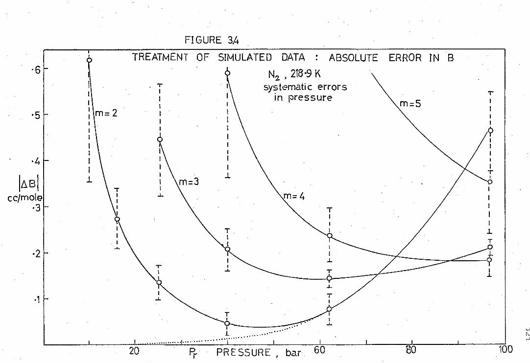
FIGURE 3.4

ccjrnole •3

N2 , 218-9 K systematic errors

in pressure

Pr PRESSURE , bar 60

TREATMENT OF SIMULATED DATA : ABSOLUTE ERROR IN B

L ... ........1 ..• • ...• • ......... .....

20 80 100

122

the systematic deviation at low pressure: in the simulated

data Z does not tend to 1.0 at zero pressure because of the

systematic error. This would give the wrong limiting

behaviour at low pressure and hence the wrong estimate of B.

Similar behaviour was found for the other simulated

runs. For each Z. there was a particular number of fitting

coefficients, m, and pressure range Pr - Pn which provided

the best estimate of Z.. In general a m = 2 fit was best

for the estimation of B and C, especially in the presence of

relatively large systematic errors that are independent of

pressure. Another reason for the choice of a m = 2 fit is

that the uncertainties in the magnitudes of the model virial

coefficients increase along the series and hence the

uncertainties in the results from this program increase

with the value of m. The general conclusion can be drawn

that if the 'true' B were unknown, it would be dangerous

to assume that the value of aB represented a realistic

estimate of AB because of the possible presence of systematic

errors, especially when a large value of m is used.

(d) Isotherms of High Curvature

The results for those simulated isotherms of methane

above 234 K (TR > 1.21 and plIR ‹ .7) were basically similar to

those for nitrogen, with the same conclusions being

applicable. As the temperature approaches the critical

temperature 190.5 K, the isotherms extend to higher

densities (p = 1.14), where the virial series is more slowly

convergent, and exhibit greater curvature on a Z - p plot.

The optimum Pr Pn range for the m = 2 fit is shifted

123

to smaller values of Pr as the temperature decreases. In

figure 3.5 are shown the resultant values of IEBI for the

simulated 248.5 K, 218.9 K, and 181.9 K Burnett runs, with a

random error distribution characterised by yr = 10-5 = .00015

bar. The overall increase in IABI at low temperatures is

apparent. For the low temperature runs, unless the random

errors were very small, the optimum range was such that the

systematic difference between the fitting polynomial and the

model virial series contributed significantly to IABI.

For the 218.9 K, 204.6 K, and 192.6 K simulated runs it

was found that m ?_ 5 was necessary to obtain a good estimate

of Zo and Z1. These fits produced relatively poor estimates

of B and C, however, (e.g. AB = 0.5 cm3 mole-1) and of the

lower compressibility factors. For these runs it is not

usually possible to treat all of the data with one value of

m and obtain good estimates of B and C and all of the

compressibility factors. This conclusion pertains to most

Burnett runs at low reduced temperature which extend to

high pressure, and has not always been realised by previous

experimentalists (for example (83), (29)). It is a con-

sequence of the wide spacing of high pressure Burnett

measurements in a highly-curved region of the isotherm

where the virial series is slowly convergent, or possibly

even divergent.

When the reduced densities, p = pipc, corresponding

to the maximum pressure of each optimum range, Pr, are

plotted against reduced temperature TR the results are as

shown in figure 3.6. It can be seen that for TR > 0.9 the

optimum densities are only slowly changing functions of

METHANE SIMULATED DATA

ABSOLUTE DEVIATION IN B T m= 2 CURVE FITS

random errors on pressure

1

218.9 K

O263.1K O 248.5K

0218.9K

0181.9 K

24 8.5 K V 167.7K

B1

-3 cc/mote

.2

167.7K

63.1 K

FIGURE 3.5

20 40 60 80 First Pressure in Curve-fit ; Pr , bar .

100

FIGURE 3.6

0.5 1.0 1.5 2.5

.4 eR

.2

SIMULATED DATA MAX. REDUCED DENSITY OF OPTIMUM CURVE-FITS

126

temperature. This offers a convenient means of interpolating

the results of this program to other temperatures in this

region and of extrapolation of the results to methane/

nitrogen mixtures.

(e) Weighting Factors

Several simulated runs were retreated using weighting

factors that were inconsistent with the known applied error

distribution. It was found that for a given set of simulated

'experimental' pressures, the results of curve-fitting were

very similar when weighting factors were calculated according

to equations (3.4-8) - (3.4-10) with y = 10-5 and e = 0.0

to .0004 bar. Only when the higher pressures were weighted

much too highly (e.g. ' = 0, e = .0004 bar) were the results

significantly worse than those in which correct weighting

factors were employed.

(f) Comparison with the experimental data

In Chapter 4, Tables 4.1 - 4.7, the results are presented

of the treatment of the experimental data from this

investigation; the lay-out of the Tables is explained in

section 4.1. By comparing the results from the various

curve-fits with those from the simulated data, the optimum

curve-fits were selected. In nearly all runs the results

showed a pattern that was reproduced by the simulated runs,

and in enabling the optimum B, C and compressibility factors

to be determined the use of simulated data proved invaluable.

For some of the experimental runs at the higher reduced

temperatures the maximum density was less than the optimum

for m = 4; for these runs only m = 2 and m = 3 curve-fits

127

need be considered. This is probably also true for those

runs well below the critical temperature, such as the 167.7 K

(run 35) and 155.9 K (run 36) isotherms for methane, where

the saturation vapour pressure limited the maximum density

and hence the number of expansions.

Some of the runs at TR > 1.3 show the absence of any

substantial random or systematic errors, such as run 13

(nitrogen 218.9 K) and run 19 (methane 263.1 K). In these

runs excellent agreement is shown between the optimum curve-

fits and those in pressure ranges narrower than the optimum

ranges. Many other runs show clearly the increase in the

standard deviations as the range Pr - Pn is narrowed, owing

to random experimental errors, e.g. run 14 (nitrogen 218.9 K)

and run 24 (methane 234.1 K).

Other runs show the presence of systematic errors. An

example is run 30 (nitrogen 192.6 K). For the m = 2 fits

as the range is decreased below the optimum (P2 - P8), the

change in B (A(1)) is large compared with the standard

deviation and is much larger than that due to isotherm

curvature.

It has been suggested (23) that a simple method of

determining the correct value of m for a given pressure

range would be to increase m until the residuals were dis-

tributed in a random manner. Further increase in m would

result in larger parameter standard deviations. However, it

is very difficult to disentangle the two separate effects on

the residuals of systematic experimental error on the one hand

and an insufficient value of m on the other. Furthermore,

if the pressure-range were large this procedure, although

128

leading possibly to the correct m for that range, would not

necessarily provide the best estimates of B and C.

In a recent publication, Waxman, Hastings and Chen (30)

compared various rigorously defined methods of non-linear

analysis (not including Method A), testing them on experimental

argon data. As these authors realised, the results were

model dependent, and a comparison of this sort does not give

any real information on the accuracy of the methods as the

'right' answer was unknown: simulated data must be used.

The investigation of simulated data presented here goes some

way towards answering some of the questions posed by Waxman

et al.

(g) The Magnitude of the Apparatus Constant

This program was developed mainly for the study of the

specific set of simulated data relevant to the experimental

data, i.e. methane, nitrogen and their mixtures in a non-

isothermal Burnett apparatus with a particular fixed

apparatus constant, (VA + VB)/VA. The program has also

been modified easily into a more general form, in which it

can be used to study a range of gases in any Burnett apparatus,

'isothermal' or 'non-isothermal', with a variable apparatus

constant, over a wide range of temperature and pressure.

In this form it is more suitable for design applications,

particularly with regard to the selection of the magnitude of

the apparatus constant and pressure range for a set of

proposed experiments.

Weir (31) has shown that fora low-pressure (< 1 atmosphere)

non-isothermal Burnett apparatus, the error expected in B

depends on the magnitude of the non-isothermal apparatus

constant,

N' = VA + VB (3.4-15)

V

For a fixed initial pressure, aB exhibits a minimum as N'

varies. This behaviour can be explained qualitatively:

when N' is too large, there are insufficient points on the

isotherm and aB2 increases because of the (n - m)-1 term in

the equation for aB2 (equation (3.2-27)); when N' is too

small, Pj/Pi _/--*1 and Zi/Zi _1--*1, and obviously in the

limit when N' = 1, i.e. VB = 0, no information is gained.

The best value of N' changes according to the temperature

TA and the maximum pressure, Po.

For these reasons the expansion vessel of the present

apparatus was supplied with four interchangeable inner

volumes, of sizes selected on the basis of the calculations

of Weir. However, the analysis in the case of a high-

pressure Burnett apparatus is further complicated by the

necessity of including the higher virial coefficients and

by the fact that the maximum pressure for a fixed value of m

varies with temperature.

Several simulated runs for methane were therefore

investigated in order to determine the variation of the

experimental results with N'. The value of AB for the

optimum curve fit passed through a shallow minimum at

N' = 1.6 when T >210 K. As long as 1.4 < N' < 1.7 the

results were satisfactory; this is in agreement with the

calculations of Weir. Below TC the value of N' required to

129

give maximum accuracy decreased: more expansions were

required because the first pressure of each run was limited

by the saturation vapour pressure.

The volumes used for all the experimental runs were,

360 cc

VB =or; 280 cc.

These gave the following values of N':

273 K : N' = 1.78

210 K N' = 1.6

155.9 K : 1.4

These values are such that N' was the best from the

choice available except perhaps at 291.4 K and below 170 K

for methane, where N' was just too large. A smaller

expansion volume leading to more measurements would have

provided marginally improved accuracy for these few runs.

On purely practical grounds the size of the expansion vessel

was not changed, as it would probably have led to a new set

of leakage problems that would have to be overcome.

130

131

CHAPTER FOUR

EXPERIMENTAL DATA

4.1 Experimental results of this investigation

Compressibility factors and second and third virial

coefficients of methane, nitrogen, two methane/nitrogen

mixtures and three multi-component mixtures have been

measured at temperatures from 291.4 K to 155.9 K. The

results are presented in Tables 4.1 to 4.7. Compositions

of the mixtures have already been given in Table 2.4.

On the bottom half of each page are shown the results

for several of the least-squares curve fits; at the top

of each column is the number of coefficients used in the

density polynomial series, m, and the pressure range included

in the fit, Pr - Pn. Each coefficient A(K) is given

together with its standard deviation, SD, in units of (cc/mole)k.

Thus A(1) refers to the least-squares estimate of the second

virial coefficient, B, and A(2) refers to the third virial

coefficient, C. V(A) refers to the estimate of the volume

of the pressure vessel, which was the (m+1) th. least-squares

parameter.

At the top of the page the overall optimum compressibility

factors are given, selected by comparing the results with

the results of treatment of the simulated data as described

in Chapter 3. The densities shown were obtained from the

experimental compressibility factors by using the experimental

absolute temperature, T,

P = RTZ (4.1-1)

where R = 83.147 bar.cc.mole.K.

132

The compressibility factors are, to the first order of

accuracy, independent of the value assumed for R and T.

The estimated maximum errors include those due to

experimental errors in pressure, both random and systematic,

and the uncertainties introduced by the truncation of the

virial series. These are necessarily larger than is super-

ficially apparent from the standard deviations in the optimum

curve-fit, for the reasons given in Chapter 3.

In addition, the total errors in the results must also

take into account the effect of various systematic uncertain-

ties introduced by the use of a 'non-isothermal' Burnett

apparatus, which are discussed in section 4.3.

4.2 Experimental virial coefficients of this investigation

The experimental second and third virial coefficients

of methane, nitrogen and the two methane/nitrogen mixtures

are reproduced in Tables 4.8 and 4.9 together with the errors

given in Tables 4.1 - 4.4. The total limits of error must

also include those systematic errors discussed in section 4.3.

The interactional second virial coefficient of a binary

mixture, B12, is given by

B mix x1 2B11 + 2x1x2B12 + x

22 (4.2-1)

where B mix is the second virial coefficient of the mixture

with mole fraction x1 of methane and x2 of nitrogen. In

Table 4.9 are shown the values of B12 calculated from (4.2-1)

for each mixture, with their associated errors, using the

pure component second virial coefficients of Table 4.8. It

can be seen that there are no systematic differences between

the two sets of values; the mean was adopted for use later

in this study, in Chapter 5.

The interactional third virial coefficients C112 and 112

C221 are similarly given by

C = 3C mix x1 111 + 3x12 x2C112 + 3

22 x1C221 + x23 C222 (4.2-2)

From the results for the two mixtures at each temperature

the two equations of the above form were solved to obtain

estimates of C112 (methane-methane-nitrogen) and C221

(nitrogen-nitrogen-methane). These are shown in Table 4.9

together with their associated errors.

4.3 Total Error Analysis

(a) The Equation of State at 0

The largest systematic errors present are usually caused

by the uncertainties in the equation of state assumed for

the gas in the ice-bath.

For each gas studied a four-coefficient polynomial

in density was assumed,

P/RTp = Z0 . (1 + alp + a(11 p2 a3p3 aoe4) (4.3-1)

a1 is the second virial coefficient at 0 0

o a2 is the third virial coefficient at 0 °C, etc.

The values used are given in Table 4.10. For methane

they are the coefficients of Douslin et al (32) (see section

4.4(c)), which reproduce Z0 to within 0.0001 up to 100 bar.

The error in 30 is estimated as -.1 cm3 .mole-1 and in C° as

± 75 cm6.mole-2. For nitrogen, the coefficients are those

133

-134

obtained byre-treating graphically the data of Michels

et al (33) (see section 4.4(d)). They reproduce both the

Michels compressibility factors and those of Crain and

Sonntag (34) to within .0002 up to 100 bar. The error in

B° is estimated as ± .2 cm3.mole-1 and in C as ± 150 cm6.mole-2.

For methane/nitrogen mixtures the second and third

virial coefficients at 0 °C were obtained from an interpolation •

of the results of this investigation. Each set of mixture

raw data was re-treated two or three times, each time re-

adjusting the 0 °C equation of state, until the virial

coefficients at 0 °C were consistent with the interpolated

values. B° is estimated as accurate to 0.4 cm3.mole-1,

about half of which is due to the errors in interpolation,

and C° is estimated as accurate to ± 200 cm3.mole-1. In

retrospect, additional accuracy could have been gained by

carrying out runs at, or close to, 0 °C. The higher

coefficients were chosen such that Z° at the higher pressures

agreed well with the values interpolated from the results at

other temperatures. A double interpolation in both

temperature and pressure was necessary. Z° at 96 bars was

estimated as accurate to ± .0007.

For the multicomponent mixtures runs were carried out

either at or very near to 0 °C and any interpolation necessary

was small. Z° at 100 bar was estimated as accurate to

± .001.

To determine the effect of errors in the 0 °C equation

of state on the experimental results, several runs were

re-processed (methane and nitrogen at 291.4, 248.5, 218.9,

181.9 and 155.9 K). Both Be and C° were subjected in turn

135

to a 1% increment, resulting in small changes in the

experimental B(T) and C(T) values. In Table 4.11 are

presented the resultant derivatives, 613(T)/613°, 6C(T)/b13°,

613(T)/aC° and 6C(T)/6C°. These values were very similar

for both methane and nitrogen. Also shown are the maximum

uncertainties, 5B(T) and 5C(T), in B(T) and C(T) arising

from the estimated maximum errors in 130 and C° for methane,

nitrogen and both binary mixtures.

The derivatives aZ(T,P)/613o and 6Z(T,P)/6C°, shown in

figure 4.1, were found to be virtually independent of

temperature and were smooth functions of pressure. If

different, more accurate values of 130 and C° become accepted

figure 4.1 may be used to apply the necessary small corrections

to Z(T,P); it is emphasized that both curves of figure 4.1

must be used in conjunction with one another. Any small

changeinZ°(P.)leads to a small change in all Z(T) values,

but it was found that the quantity 5Z(T,P.1 )/5Z°(Pi) was

approximately constant for each isotherm, the values ranging

from 0.15 to about 0.3. For example, an uncertainty in

Z° at 0 °C, 100 bars of .0005 leads to an error in Z(T) at

100 bars of between .00008 and .00015. In Table 4.12 are

listed the maximum errors in Z for each run arising from the

estimated uncertainties in Z°.

(b) Other Systematic Errors

Errors in other variables which are independent of

pressure, such as the volumes and temperatures of the dead-

spaces, will tend to have an effect on the experimental

second virial coefficients. Those errors which increase with

pressure, however, such as those in the dead-space

compressibility factors, tend to have a small effect on

B(T) but can lead to relatively larger errors in the high-

pressure compressibility factors. The equations for use

in calculating Z in the inlet-tubes and other dead-spaces

were found by fitting four-coefficient polynomials in

density to the data of Tables 4.1 - 4.7. The errors in

these equations were found to have an insignificant effect

on the results.

Only two errors could lead to a maximum error in B(T)

of more than .005 cm3.mole-1 or to a maximum error in

Z(T,P) of more than .00005; firstly, uncertainties in V3,

the largest section of the dead-space volume; secondly,

uncertainties in T6, the ice-bath vessel temperature. The

maximum value of 3B(T)/W3 is 0.7: therefore the estimated

uncertainty in V3 of .015 cc leads to an error in B(T) of

.01 cc/mole. The maximum value of 613(T)/6126 is 0.25:

therefore the estimated uncertainty in T6 of .02 K leads to

an error in B(T) of less than .01 cc/mole. These are both

negligible.

(c) Adsorption

It is known that adsorption of gas on the walls of the

containing vessel can be a serious problem in Burnett

measurements at temperatures below the critical temperature.

In the design of the vessel, an effort was made to ensure

that the interior surfaces were clean and highly polished in

order to reduce the possibility of adsorption.

There are two reasons for the belief that the effect of

136

137

adsorption was insignificant in this investigation.

Firstly, the results of the curve-fitting to each low-

temperature run, particularly the magnitudes of the standard

deviations, were consistent with the errors expected in

experimental pressure. Serious adsorption could be expected

to result in much larger standard deviations and also much

larger apparent curvature on the isotherms. Secondly, the

effect of adsorption would tend to manifest itself as a

change in the expected value of V1, the volume of the low-

temperature pressure vessel (35). In figure 4.2 these

volumes are plotted against temperature. There are no

systematic differences between the values obtained for

different gases: they all deviate from a smooth, nearly

linear function of temperature by less than .1 cm3 (.03%).

The differences at low temperature are within the expected

errors inherent in the curve-fitting procedure. In

treatment of simulated data it was found that if the

derived least-squares value of V1 was in error by 0.1 cm3

then it was usually accompanied by errors in B of about 0.2

to 0.3 cm3.mole-1 in C of about 100 - 150 cm6.mole-2 and

in Z(T,P0) of from .0002 to .0003.

As already mentioned in Chapter 1, the design of the

'non-isothermal' apparatus is such that errors due to

adsorption are less than in the standard 'isothermal'

apparatus. In the latter it can be shown that as the gas

adsorbs in both VA and VB at low temperature the errors due

to adsorption are accumulative (35).

TABLE 4.1 EXPERIMENTAL DATA FOR METHANE

RUN 23 291.41 K

M=3 130•..P6

M=2 ) P1 -P6

M=3

M=4 P1.-P6

361.140

361.134 .017

-45.755 .45.816

.094 .179

2679.4

2773.1

68.5 156.2 -4.0 .164 -9.6 .164 1.4 .164 5.1 .104

10.6 .106 5.3 .106

M=3 PO -P6

361,186 .024

45.471 .079

2464.2 . 33.8 .58 .104 .40 .104

.83645

.89671 .8966G

.93955 .9394. 4

.96577 .96565

.98092 .98083

.98945 .98946

.99419 .99416

.'83633

.89659

.93943

.96564

.98082 698939 .99416

138

PRESSURE

PRESSURE LBoiS(1.IN. BAR

1448.752 99.8880 837.073 57.7141 476.307 32.8402 266.916 18.4032 148.105 10.2115 81.698 5.6329 44.917 3.0969

Z = PV/RT (OPTIMUM)

.8364

.89670

.93954

.96576

.98091

.98945

.99419

DENSITY LEAST-SQUARES MOLE/DC.10 FIT

4.9284 2.6563 1.4426 0.78647 0.42966 0.23496 0.12857.

OPTIMUM COEFFICIENTS

By CC/MOLE = -45.50 Cp CC/MOLE1 = 2489 V(A), CC = 361.18

ESTIMATED ERRORS (MAX.) .15 100 .05

2 .0002

OPTIMUM FIT

M=2 P1 -P6

RESULTS OF NONLINEAR LEAST-SQUARES ANALYSIS

M=2

M=2 PO •P6

V(A) 361.158 361.182 SD .016 .015

A(1) -"45.579 -45.500 SD .024 .040

A(2) 2512.4 2489.3 SD 3.9 11.1

A(3) SD

A(4) - SD

Z(0) .83638 Z(1) .89665 .89670 Z(2) .93947 .93954 Z(3) .96571 .96576 Z(4) .98088 .98091 Z(5) .98943 .98945 Z(6) .99418 .99419

M=2 P2 •../36

361.148 .010

-45.674 .043

2574.0 -20.2

.93946

.96567

.98085

.98941

.99417

139 TABLE 4.1

EXPERIMENTAL DATA FOR METHANE

RUN 19 263.08 K

PRESSURE PRESSURE iBe/SQ,IN. BAR

.Z = PV/RT (OPTIMUM)

DENSITY LEAST-SQUARES MOLE/CC.103 FIT

1448.325 99.8586 .74800 6.1029 M=4 f PO .•P6 928.850 64.0420 .82871 3.5328 M=3 P1 -P6 576.275 39.7328 .89286 2.03437

346.771 23.9090 .93565 1,16819 204&455 14.0967 .96218 0,66978 M=2 P2-P6 119.055 8.2086 .4,97803 0.38370 68.818 4.7448 098732 0.21970

OPTIMUM COEFFICIENTS

B, CC/MOLE = -58.34 C, CC/MOLE1= 2788 V(A), CC = 360.74

ESTIMATED ERRORS (MAX.) .07

50 .04

Z .0001

OPTIMUM FIT

M=2 P2-P6

RESULTS OF NONLINEAR LEAST-SQUARES ANALYSIS

V(A) SD

A(1) SD

A (2) SD

A(3) SD

A(4) SD

Z(0) Z(1) Z(2) Z(3) Z(4) Z (5) Z (6)

M= 2 PO ••P6

360.719 .010

-58.390 .011

2800.8 1.5

.74796

.82867

.89280

.93561

.96215

.97801

.98731

M=2 P1-P6

360.737 .005

-58.350 .010

2791.6 2.1

.82870

.89285

.93565

.96217

.97802

.98732

M=2 P2-P6

360.740 .0U9

-58.339 .026

2787.8 8.9

.89286 .

.93565

.96218 .97803 .98732

M=3 PO . )6

360.743 .008

.019 2777.6

6.4 .22 .104 .06.104

.74801

.82872

.89286

.93566

.96218.

.97803

.98732

M=3 P1 . 36

360.739 .014

.58.339 .051

2785.9 27.7

.09 .104

.43 .104

.82871

.89285

.93565

.96218

.97803

.98732

M=4 PO-P6

360.737 .022

58.349 .091

2794.4 59.6

-0.2 .104

1.5 .104

0.3 .10 6 1.2 ele

-.74800 $82870 ,89285 4,93565 .96217 07802

..98732

OPTIMUM COEFFICIENTS ESTIMATED ERRORS (MAX.) .10 ..

75 ,04

Z .0001

B, CC/MOLE = -66.48 C, CC/MOLE1 = 3015 V(A), CC = 360.46

OPTIMUM FIT

M=2 P2-P7

140 TABLE 4.1

EXPERIMENTAL DATA FOR METHANE

RUN 20 248.54 K

PRESSURE PRESSURE LB. /SQ. IN. BAR

Z = PV/RT (OPTIMUM)

DENSITY LEAST-SQUARES MOLE/CC.103 FIT

1439.944 99.2807 .68035 990.015 68.2592 .77032 652.848 45.0123 .84934 412.765 28.4592 .90591 253.367 17.4690 .94282 152.638 10.5240 .96578 90.915 6.2683 .97971 53.783 3.7082 .98803

7.0612 4.2879 2.5645 1.5202 0,89660 0,52731 0,30962 0.18162

M=4 p - POP7 M=3 P1-P7

RESULTS OF NONLINEAR LEAST-SQUARES ANALYSIS

M=2 P1-P7

M=2 M=2 P3-P7

M=3 PO-P7

M=3 M=4 PO ••.P7

V(A) 360,473 360.463 360.452 360.456 360.458 360.460 SD .006 .005 .005 .004 .005 .008 A(1) ••••66.448 -66.479 -66.525 -66.510 -•.66.504 •.-66.505 SD .008 .011 .018 .007 .017 .027 A(2) 3005.9 3015.2 3036.4 3035.2- 3032.4 3632.2 SD 1.6 3.3 8.1 2.1 7.8 15.3 A(3)

SD

.104 -0.35 .104 .02 .it .10 .104

-0.3 .104

.3 .104 A(4) -0. 0 .106

SD .2 .106

Z(0) .68035 .68035 Z(1) .77035 .77032 .77032 .77032 Z(2) .84936 .84934 .84933 .84933 .84933 Z(3) .90593 .90591 .90588 .90589 .90590 .90539 Z(4) .94284 :94282 .94279 .94280 .94281 .94231 Z(5) .96580 .96578 .96576 .96577 .96577 .96577 Z(6) .97971 .97971 .97969 .97970 .97970 .97970 Z(7) .98803 098803 .98802 .98802 .98802 .9881.12

141 TABLE. AA

EXPERIMENTAL DATA FOR METHANE

RUN 24 234.05 K

PRESSURE PRESSURE LB./S(1.IN. BAR

Z = PV/RT (OPTIMUM)

DENSITY LEAST-SQUARES • MOLE/CC.1e FIT

1144.975 78.9432 .65574 6.1862 M=4 i PO-P7 832.275 57.3834 .75334 3.9142 M=3 t P1-P7 571.661 39.4146 .83539 2.4245 374.357 25.8110 .89475 1.4824 237.212 16.3552 .93441 0.89945 M=2 t 147.166 10.1467 .95974 0.54328 90.115 6.2132 .97551 0.32730 54.739 3.7741 .98519 0.19686

OPTIMUM COEFFICIENTS ESTIMATED ERRORS

OPTIMUM FIT (MAX.)

B, CC/MOLE = -75.89 .15 Ct CC/MOLE2 = 3299 .100 V(A), CC = 360.20 .05

Z .0001

M=2 P2-P7

RESULTS OF NONLINEAR LEAST-SQUARES ANALYSIS

M=2 P1•..137

M=2 P2-P7

M=2 P3-P7

M=3 PO ..•P7

M=3 P1..•137

M=4

V(A) 360.230 360.202 360.224 360.192 360.193 360.195 SO .018 .020 .032 .019 0030 .043

A(1) -75.811 -.75.894 -75.799 .75.951 -75.949 -75.941 SD .029 .049 .120 .041 0098 .161

A(2) 3272.0 3298.5 3254.2 3343.1 3341.8 3336.2 .SO

A(3) 5.9 1409 54.4 13.7

-0.99 .104 48.0

.•1.0 .104 98.7

-0.8 .104 SD .12 .104 *7 .104 2.2 .104

A(4) 410' Sp 1.7 6106

Z(0) .65574 .65574 Z(1) .75341 .75333 .75334 .75334 Z(2) .83544 .83539 .83536 .83536 .83537 Z(3) .89482 .89475 .89479 .89472 .89473 .89473 Z44) .93445 .93441 .93446 .93438 .93438 .93439 Z(5) .95978 *95974 .95978 .95972 .95972 .95972 Z(6) .97554 .97551 .97554 .97550 .9755C 0 97550 Z(7) .98520 .98519 .98520 .98518 .98518 .98518

OPTIMUM COEFFICIENTS

B, CC/MOLE = -87.16 C, CC/MOLE1= 3551 V(A), CC = 360.03

ESTIMATED ERRORS (MAX.) .30 200 .08

Z .0005

OPTIMUM FIT

TABLE 4.1 142

EXPERIMENTAL DATA FOR METHANE

RUN 21 218.87 K •

PRESSURE PRESSURE

Z = PV/RT

DENSITY LEAST-SQUARES LB. /SQ.IN. BAR

(OPTIMUM) - MOLE/CC.103 FIT

1406.197 96.9539 .4610 1139.705 78.5799 .5220 930.215 64.1361 .4_201 717.510 49.4706 .7226 517.933 35.7102 .8096 354.220 24.4226 .8746 233.244 16.0816 .9195 149.806 10.3287 ..9492 94.705 6.5297 .96818 59.27 8 4.0871 .98022

11.555 8.271 5.6837 .3.7622 2.4238 1.5344 0.96103 0.59797 0.37060 0.22912

M=6 PO-P9 M=5 , P1-P9 M=4 , P2139 M=3 P3-P9

RESULTS OF NONLINEAR LEAST-SQUARES ANALYSIS

M=2 P3 ...P9

M=2 134P9

M=2 P5-P9

M=3 P2 ..•P9

M=3 P3-P9

M=3 P4-P9

V(A) 359.974 360.029 360.063 359.976 360.060 360.077 SD .021 .011 .009 .031 .010 6016

A(1) "87.315 -87.161 -87.027 -87.321 "87'0014 "86.927 SD .033 .026 .029 .066 .031 .072

A(2) 3600.6 3551.2 3490.4 3607.8 3446.2 3381.8 SD 7.1 7.8 12.9 23.1 15.6 51.2

A(3) .104 2.2 .104 3.6 .104 SD .21 .104 0.2 .104 1.1 *104

Z(0) Z(1) Z(2) .61989 Z(3) .72242 .72242 .72258 Z(4) .80950 .80960 080950 .80966 .80970 Z(5) .87448 .87462 .87469 .87448 .87468 .87472 _Z(6) .91940 .91951 .91959 .91940 .91958 .91962 Z (7) .94907 .94915 . .94921 .94907 .94921 .94924 Z(8) .96813 .96818 .96823 .96813 .96823 .96825 Z(9) .98018 .98022 .98024 .98018 .98024 .98026

TABLE 4,1 143

RUN 21

218.87 K (CONTINUED)

RESULTS OF NONLINEAR LEAST-SQUARES ANALYSIS

H=4 P1-P9

M= 4 P2-P9

M=4 P3 ••P9

M=5 P1-P9

M=5 P2 •••1D9

M=6 PO -P9

V(A) 360.046 360.086 360.079 360.093 360.075 360.104 SD 30 2 .023 .017 .030 .038

A(1) -87.034 -86.867 -86.905 .36.821 .86.933 -86.770 SO .043 .045 - .120 .072 .171 *201

A(2) 3422.8 3311.9 3347.6 . 3263.7 3379.9 3224.7 SD 19.3 28.5 106.3 53.8 171.8 226.9

A(3) 4.2 .104 6.9 .104 5.6 .104 9.1 .104 3.8 .104 la. .104 SO .3 .104 .7 .104 347 .104 1.7 *104 7.5 4104 7. .104

A(4) -3.4 .106 :106 -4.1..iG6 -9.9 .106 *3 .10 -11:6.106 SD .2 .106 e6 .106 4.4 .106 .2 *106 15 *106 3.5 6106

A(5) 3.1 .108 -4. .108 4.3 .108 SD 1.3 .10 -10. 108 3.9 .108

A(6) - - -5 .10m SD 10 .10m

Z(0) .46106 Z(1) .52198 .52205 .52207 Z(2) .62J01 .62008 .62009 .62006 .62011

-Z(3) .72255 .72263 .72262 • .72265 . 4.72261 .72267 2(4) .80964 .80972 .80971, .80974 480970 480976 Z(5) .87465 .87474 .87472 .87475 .87472 .87478 Z(6) .91955 .91964 .91963 .91966 .91962 .91968

. 2(7) .94919 .94926 .94924 .94927 .94924 .94929 2(8) .96822 .96827 .96826 .96828 .96825 .96829 Z(9) .98024 .98027 .98026 .98628 .98028 .98029

DENSITY LEAST-SQUARES MOLE/CC.103 FIT

10.801 8.2937 6.0890 4.2772 2.8985 1.9151 1.2444 0.80012 0.51097 0.32496 0.20611

3 M=5 P0• 310

M=4 9 P2'4)1.0

M=3 ,

M=2 , P5-P10

.53756 .64396 .64400 .64414 074266 .74277 .74272 .74285 .74290 .82239 .82256 .82263 .82245 .82264 .82270 .88124 .88138 .88146 .88129 .88148 .88154 .92222 .92232 .92239 .92226 .92241 092246 .94974 .94981 .94986 .94977 .94987 .94992 .96779 .96784 .96787 .96781 .96789 .96792 .97947 .97950 .97953 .97949 .97954 .97956

Z(0) Z(1) Z(2) 2(3) Z(4) Z(5) Z(6) Z(7) Z(8) Z(9) Z(0)

TABLE 4.1 144

. EXPERIMENTAL DATA

RUN 22 204.60 K

PRESSURE PRESSURE LB./SQ.IN. BAR

FOR METHANE

Z = PV/RT (OPTIMUM)

993.587 68,5054 .3728 904.313 62.3502 .4419 807,900 55.7027 .5377 679.785 46.8695 .6441 531.259 36.6290 .7429 388.711 26.8007 .8226 270.648 18.6605 .8815 182.093 12.5549 .9224 119.751 8.2566 .9499 77.601 5.3504 .9679 49.813 3.4345 .9795

OPTIMUM COEFFICIENTS

8 ) CC/MOLE = -100.14 C, CC/MOLES' = 3928 V(A), CC = 359.72

ESTIMATED ERRORS (MAX.) - .25 150 .07

Z. .0005

OPTIMUM FIT

M=2 P5-P10

RESULTS OF NONLINEAR LEAST-SQUARES ANALYSIS

M=2 P3-P10

M=2 P4 P.1.0

M=2 P5-P10

M=3 P2-P10

M=3 P3 'P10

M=3 Ple•Pi0

V(A) 359.624 359.687 359.723 359.649 359.729 359.756 SD .031 .024 .031 .035 .027 .040

-A(1) -100.41 -100.26 -100.14 -100.34 -100.09 99.97 SD .04 .05 .09 .06 .07 .15

A(2)- 4018 3975 3928 399J 3866 3790 SD 8 12 33 20 31 95

A(3) 032 .104 1.9 0104 3.3 .104 SD .15 .11l4" .4 .104 1.6 •ii4

145

RUN 22

TABLE 4.1

204.60 K (CONTINUED)

RESULTS OF NON LINEAR LEAST-SQUARES ANALYSIS

M=4 M=4 M=5 M=5 P1-P10 P2-P10 P0-.1310 f1'.4310

V(A) 359.814 359.761 359.751 359.787 SD .029 .033 .045 .067

A(1) -99.73 -99.93 -99.99 -99.78 SD .06 .11 .17 .34

A(2) 3618 37 40 3800 3605 SD 26 64 118 316

A(3) 8.3 .104 5.7 .104 3.2 *104 11 .10+ SD *4 *104 1.4 *JO+ .3 .104 12 .10+

A(4) -5.8 .106 3.9 .106 0.6 .106 -13 .106 SD .2 .106 1.1 .106 4.4 .106 23 .106

A(5) 2.9 .108 6 .108 SD 1.9 .108 15 .108

Z(0) .37277 Z(1) .44198 .44191 .44195 Z(2) .53780 .53773 .53771 .53776 Z(3) .64429 .64420 *64418 *64424 Z(4) .74300 .74291 .74289 .74296 Z(5). - .82283 .82271 .82269 .82276 Z(6) .88167 .88155 .88153 .88161 Z(7) .92258 .92248 .92245 .92253 Z(8) .95000 .94993 .94991 .94997 Z(9) .96798 .96793 .96791 *96796 Z(0) .97960 .97956 .97955 .97959

1_46 TABLE 4.1

EXPERIMENTAL DATA FOR METHANE

RUN 33 192.64 K

PRESSURE PRESSURE

Z = PV/RT

DENSITY LEAST-SQUARES . LBe/SQ,INe BAR

(OPTIMUM) MOLE/CC*103 FIT

662.282 45,6627 *4909 590.581 40.7192 ..5976 487.367 33.6028 .7000 374.587 25.8269 .67864 272.320 18,7758 .8529 190.233 13.1161 .9009 129.316 8.9160 .9343 86.320 5.9515 .9568 56.936 3.9256 .9718 37.257 2.5688 .9817

568064 4.2539 2.9967 2.0502 1.3743 069089 0.59580 0.38833 0.25219 0.16337

M=5 P0..439 M=4 , P1-P9 M=3 , P2-P9

M=2 , P3-P9

OPTIMUM COEFFICIENTS

B, CC/MOLE = ••112683 C, CCIMOLE1 = 4227 V(A), CC = 359.43

ESTIMATED. ERRORS (MAX.) - .25 150 .07

Z .0003

OPTIMUM FIT

M=2 P3-P9

RESULTS OF NONLINEAR LEAST-SQUARES ANALYSIS

V(A) SD

A(i) - SO A(2)

SD

M=2 P2 •1:'9

359.371 .026

113.03 .07 4305

18

M=2 P3-P9

359.433 .034

-112.83 .09 4227 33

M=2 P4-•P9

359.430 .053

112.85 .20 4235 101

M=3 P1-P9

359.473 .035

-112.60 .09 4034

39

M=3 P2 ••P9

359.464 .052

-112.64 .19 4059

114

M=3 P3-P9

359,416 .049

-112.92 .30 4306 236

A(3) 4.7 .104 4.2 .104 -1.9 4104 SO -04 sie 1.9 .104 5.0 .10*

Z(0) Z(1) .59763 Z(2) .69987 = .70006 .70004 Z(3) .78633 .78644 .78652 .78650 .78641 Z(4) .85276 .85292 .85291 .85300 .85298 .85288 Z(5) .90081 .90094 .90093 .90103 .90102 .90090 Z(6) .93418. .93428 .93427 .93436 .93434 .93424 Z(7) .95675 .95682 .95682 .95689 .95688 .95680 Z(8) .97177 .97181 .97181 .97186 .97185 .97180 Z(9) .98165 .98168 .98168 .98171 .98171 .98167

147 TABLE 4.1

RUN 33 192.64 K (CONTINUED)

RESULTS OF NON-LINEAR LEAST-SQUARES ANALYSIS

M=4 P1-P9

M=5

V(A) 359.453 359.438 SD .065 .082

A(1) -112.70 -112.82 SD .24 .38

A(2) 4117 4258 SD 162 321

A(3) 2.2 .104 -5.3 .104 SD .4.1 .104 11. .104

A(4) 2.5 .106 20.9 0106 SD 3.9 .106 14.4 .106

A(5) .109 SD 5. .108

Z(0) .49094 Z(i) .59760 - .59758 Z(2) .70002 .70000 Z(3) .78648 .78645 Z (4) .85296 .85292 Z(5) .90099 .90095 Z(6) .93432 .93429 Z(7) .95686 .95683 Z(8) .97184 .97182 Z (9) .98170 .98168

PRESSURE PRESSURE LBe/SQ.IN, BAR

Z = PV/RT

DENSITY LEAST- SQUARES (OPTIMUM) MOLE/CC.103 FIT

443.593 30.5847 .6518 358.884 24.7442 .7445 272.983 18.8215 .8187 198.338 13.6749 .8746 139.513 9,6192 .9146 95.982 6.6177 .9426 65.054 4,4853 .9616 43.653 3.0098 .9745

M=4 M=3

PO-P7 p Pi-P7

3.1033 2,1981 1.5203 1.0341 0.69551 0,46432 0.30846 0,20425

- 148 TABLE 4,1

EXPERIMENTAL DATA FOR METHANE

RUN 34 181:66 K

OPTIMUM COEFFICIENTS ESTIMATED ERRORS (MAX.)

By CC/MOLE = -125.71 .30 C, CC/MOLE 4256 200 V(A), CC = 359.39 .07

Z .0003

OPTIMUM FIT

M=2 P2-P7

RESULTS OF NONLINEAR LEAST-SQUARES ANALYSIS

V(A) SD

A(1) SD

A(2) SD

M=2 P1-P7

359.314 .032

-125.98 .08

4390 26

- M=2 P2-P7

359.386 .014

-125.71 .05

-. 4256 21

M=2 P3-P7

359.419 .014

-125.54 .07

-4149 40

M=3 PO-P7

359.426 .012

-125.43 .04

3959 20

M=3 P1-P7

359.437 .016

.•125.38 .07

3912 53

M=4 -P0• )7

359.442 - .028

..125034 .14

-3867 137

A(3) 9.6 .iO4 10.7 .104 13.2 .104 SD .3 .104 1.2 .104 5.3 .104

A (4) -4.8 .106 SD 7.3 .106

Z(0) .65174 .65176 Z(1) .74421 .74442 *74445 .74445 Z(2) .81858 .81872 .81881 .81883 .82884 Z(3) .87440 .87456 .87463 .87464 .87467 .87468 Z(4) .91449 .91463 .91470 .91471 .92474 .91475 Z(5) .94244 .94255 .94261 .94263 .94264 .94265 Z(6) .96155 .96163 .96167 .96169 .96170 .96171 Z (7) .97445 .97450 .97453 .97455 .97456 .97456

149 TABLE 4.1

EXPERIMENTAL DATA FOR. METHANE

RUN 35 167.67 K

PRESSURE PRESSURE

Z = PV/RT

DENSITY LEAST-SQUARES LB. /SQ.IN. BAR

(OPTIMUM)

MOLE/CC.103 FIT .

298.822 20.6031 .7151 237.158 16.3515 .7922 179.424 12.3709 4851.9 131.116 9.0401 .8962 93.504 6.4469 .9280 65.555 4.5199 .9505 45.425 3.1319 .9662

2.0667 1.4805 1.0417. 0,7236 0,4983 0.341i2 0,23250

M=3 , PO-P6

M=2 , P1-P6

OPTIMUM COEFFICIENTS

B, CC/MOLE = 146.54

CC/MOLE1 = 4187 V(A), CC = 359.24

ESTIMATED ERRORS (MAX.) . 40 300 .10

Z .0004

OPTIMUM FIT

M=2 P1-P6

RESULTS OF NONLINEAR LEAST-SQUARES ANALYSIS

M=2 PO-P6

M=2 M=3 M=0 M=0 M=0 POP6 PO-P6 PO-P6 P0-.416

V(A) 359.19 359.24 359.23 SD .06 .08 .16 •

A(i) .1464,71 1.46.54 -146.51 SD' .13 .25 .69

A(2) 4272 4187 4105 SD 51 123 551

A(3) 3.9 .104 SD 12.-:•104

Z(0) .71501 .71509 Z(1) .79213 .79222 .79221 Z(2) .85180 .85190 .85189 Z(3) .89607 .89615 .89615 Z(4) .92795 .92802 .92802 Z(5) .95045 .95050 .95051 Z(6) .96611 .96615 896616

PRESSURE PRESSURE BAR

= PV/RT (OPTIMUM)

186.515 12.8598 .7965 143.608 9.9014 .8525 107.127 7.3862 .8945 78.125 5.3865 -.9253 56.064 3.8655 .9475 39.783 2.7430 -.9633

_DENSITY LEAST-SQUARES MOLE/CC.103 FIT

1.2456 0.8961 0.63703 0,44911 0.31475 0,21968

M=3 PO -.P5

M=2 P1-P5

TABLE 4.1 EXPERIMENTAL DATA FOR. .. METHANE

RUN. 36 155.89 K

150

OPTIMUM COEFFICIENTS

ESTIMATED ERRORS

OPTIMUM FIT (MAX*)

B, CC/MOLE = C, CC/MOLE1 = V(A), CC =

-167.93 3718

359.06

_..60 600 600 .15

Z. .0007

RESULTS OF NONLINEAR LEAST-SQUARES ANALYSIS

M=2 P0..4)5

M=2 Pi-P5

M=3 M=0 PO -P5 P0•41 5

V(A) 359.14 359.06 359.03 SO .06 .08 .21

Ati) -167,52 -167.93 -168.31 SD .21 .39 1.41

A(2) 3422 3718 4358 SD 117 276 1669

A(3) -33 *104 SD 59 0104

Z(0) .79670 .79647 Z(1) .85267 .85251 .85244 Z(2) .89469 .89453 *89446 Z(3) .92547 .92533 .92526 Z(4) .94762 .94751 .94744 Z (5) .96337 .96329 .96323

M=0 M=0 PO-P5 PD-P5

1507.290 103.9241 1.0010 815.486 56.2258 .9935 445.801 30.7369 .9945 244.215 16.8380 .9964 133.807 9.2257 .9979 73.304 5.0541 .9988

4.2844 M=3 P0•-.P5 2.3357 1.2756 0.69744 M=2 Pi-P5 0.38157

- 0.20884

TABLE 4.2 EXPERIMENTAL DATA FOR NITROGEN

RUN 6

291.42 K

-PRESSURE PRESSURE - LB./SO.1Mo BAR

-Z PV/RT (OPTIMUM)

DENSITY LEAST-SQUARES MOLE/CC•102 FIT

151

OPTIPUM COEFFICIENTS ESTIMATED ERRORS OPTIMUM FIT (MAX.)

132 CC/MOLE = -6.20 .30 Cy CC/MOLE = 1458 150 V(A), CC = 361.23 .08

Z .0004

M=2 T1-P5

RESULTS OF NONLINEAR LEAST-SQUARES ANALYSIS

M=2 M=2

M=3 M=U -

M=0 M=0 PO-P5 P1-P5

PO-P5 --P0135

PC-P5

V(A) 361.112 361.232 361.268 SD .059 .015 .010

A(1) ..•6,582 ^6.200 - -5.987 SD .112 .047 .038

A (2) 1572.1 1457.6 1298.1 SD 18.4 13.3 17.1.

A(3) 3.6 .104 SO 2.3 .104

Z(0) 1.00067 1.00106 Z(1) .99320 .99347 .99356 Z(2) .99416 .99446 .99455 Z(3) .99617 .99638 :99647 Z(4) .99772 .99785 .99791 Z(5) .99869 .99877 499881 -

3.5865 2.0062 1,1225. 0.62826 0.35166 0.19686

M=3 , PO-P5

M=2 Pi-P5

OPTIMUM FIT

TABLE 4.2 -EXPERIMENTAL DATA FOR NITROGEN

- RUN 9-- 276.94- K

PRESSURE LB. /SQ.IN.

PRESSURE BAR

PV/RT --(OPTIMUM)

118J.937 81.4228 .9859 661.445 4566E50 -.9872 371.665 25.6254 o9'91,4 208.715 14.39iJ4 .9947 117.081 8.0724 .9969 65.629 4.5249 49982

OPTIMUM COEFFICIENTS - ESTIMATED ERRORS (MAX.)

B, CC/MOLE = -9.38 .25 - C I CC/MOLE = 1496 150

- V(A), CC = 360.91 .07 Z .0003

RESULTS OF NONLINEAR LEAST-SQUARES ANALYSIS

M=2 M=2 M=3 M=0 M=0 M=0 PO-P5 P1-P5 PO-P5 PU-P5 PO P5 PO-P5

V(A) 360,869 360.912 360.934 SO .037 $050 .079

A(1) -9.545 -9.378 -9.247 SC .083 .167 .327

A(2) 1553.5 1495.9 1394.7 SD 15.6 54.5 169.4

A(3) 2.5 ei04

SO 2.6 .10

Z(0)-- .98575 .98592 Z(1) .98710 .98721 .98726 Z(2) .99124 .99136 .99141 Z (3) .99462 .99470 .99475 Z (4) .99684 .99689 .99692 Z(5) .99818 .99821 099823

152

DENSITY LEASTSOUARES MOLE/CC.10

3 FIT

M=2 Pi •...P5

M=3 2 P0 ..•13 6

OPTIMUM COEFFICIENTS

Bi CC/MOLE = -12.95 C, -- CC/MOLE = 1586 V(A), GC = 360.59

ESTIMATED ERRORS (MAX.) .25 .D6 -

Z

OPTIMUM FIT

M=2 P1-P6

M=2 - M=2 P1-P6 P2•4'6"

360.588 360.558 -.007

-12.954 -13.093

4035 :4030

1585.6 1644,2

8.6 ' 12.0

.97625

.98339

.98950

.99367

.99627

.99783

.98332

.98942

.99361

.99623

.99781

TABLE 4.2 EXPERIMENTAL DATA FOR NITROGEN

153

- RUN 17 263.08 K

PRESSURE LB. /SO. IN.

PRESSURE ----BAR

1497.925 1302784 86J,625 59.3381 496.915 3442611

.286,383 19.7454 164,645 11.3519

--- 944481 - - 6.5142 54.152 3.7336

Z = PV/RT (OPTIMUM)

.9751

.9763 -.9834 .9895 .9937 499627 - .99783

DENSITY LEAST-SQUARES MOLE/CC.103 FIT

4.8418 2.7787 1.5927 019122 0052232 0.29892 0.17106

RESULTS OF NON-LINEAR LEAST-SQUARES ANALYSIS

7,1=

V(A) SD

A(1) SD

A(2) SD

A(3) SD

A(4)-

Z(0) - Z(1) Z(2) Z(3) Z(4) Z(5) Z(6) -

M=3

- - 360 • 614

.033 12.803

- 41d8 148004

43,1 2.1 • 104 . 5 6104

.97514

.97631 -498345 .98957 .99371 .99631 .99785

M=3 P1-P6

360.546 .L'08

•••13,186 .039

1738.6 25.3

-3,0 .104 *5 .I.04

-.97614 .98329 .98939 .99358 .99621 .99780

130.4)6 P -P6 360.532

.007 •.13.304

.039 1886.9

3045 -11 .104

1 6104 13 4106 1 .10

.97492

.97610

.98325

.98936

.99355

.99619

.99779

4.0706 2.4005 1.4119 0482909 0.48636 0.28514 0.16712

OPTIMUM FIT

M=2

M=3 P0-416

M=2 P1-P6

TABLE 4.2 EXPERIMENTAL DATA FOR - .NITROGEN

RUN - 10

248,54 g

- PRESSURE PRESSURE LBoiSQ,IN. BAR

- Z - = PV/RT - (0PTIMUM)

--DENSITY LEAST-SQUARES -MOLE/00.103 FIT -,„

1169,198 80.6134 •9583 697.018 48.0577 .9688 414.461 ' 28.5761 69794- 245,298 16.9127 49871 144.635 9.9722 .99217

-.85,065 5.8650 .99532 49,949 3,4439 .99722

OPTIMUM COEFFICIENTS ESTIMATED ERRORS (MAX.)

131 CC/MOLE = -16.86 .20 Cy CC/MOLE = 1608 V(A), CC 360.38 .05

Z .0002

- -RESULTS CF NONLINEAR LEAST-SQUARES ANALYSIS

M=2 M=2 P1-P6 P2-P6

M=3 PO-P6

- V(A) 360.379 360.400 360.400 SD .coe .021 .004

A(1) -16.879 -16.778 -16.756 SD .024 .062 .014

A(2) 1608.3 1560.9 1517.8 - SD 6.8 20.1 6.2

A(3) 2.0 .104 SO .104

41(4) SD

M=4 PO -P6

360.409 .005

-16.698 .029

1464.8 - 25.3 3.9 .104 .9 'le

-2.2 .106 1.1 6 .1.0

M=3 P1 -P6

360.407 .003

-16.711 .013

1484.d 9.7

2.8 .104 .2 ele

M=0 P0.-P6

Z(0) Z(1) .96875 Z(2) .97937, Z(3) .98711 Z(4) .99217 Z(5) .99532 Z(6) .99722

.97942

.98716 .99221 .99534 .99724

.95830

.96880 *97943 .98716 .99221 .99535 .99724

.96882

.97944

.98718

.99223

.99536

.99725

.95832

.96882

.97945 *98719 .99223 .99536 .99725

155

TABLE 4.2 - EXPERIMENTAL DATA FOR NITROGEN

RUN 11- 248.54 K

--:-PRESSURE PRESSURE - LB./SO.1N, BAR

Z =- PV/RT (OPTIMUM)

DENSITY LEAST-SQUARES MOLE/CC,103 FIT

1457.613 100.4989 .9566 5.0836 M=3 , 867.175 59.7896 .9637 3.0021 516.530 35.6135 .9751 1.7674 306.289 21.-1179 .9841 1.0384 180.852 12.4693 .99025 0.60933 M=2 , 106.461 7.3402 .99414 -0.35729 62.544 4.3123 .99651 11.20941 36.700 2.5304 .99794 0.12270

OPTIMUM COEFFICIENTS ESTIMATED ERRORS OPTIMUM FIT -(MAX.)

B, CC/MOLE = -17.00 .20 M=2 -Cy CC/MOLE = 1637 -100 P1-P7 V(A), CC = 360.32 .05

Z .0003

RESULTS OF NON-LINEAR LEAST-SQUARES ANALYSIS

M=2 - M=2 M=3 - M=3 - M=4 M=0

-P1P7 - P2-P7 - P0-. )7 - P1-P7 PO-P7 PO-P7

-11(A) 360.322 360.299 360.349 -360.293 360.283 --- SD .U14 .014 .030 .021 .032

- -16.998 - -.*17.100. -16.837 --17.154 -17.242 - - SO a33 .053 .094 .102 .174 HA (2) 1636.8 - 1677.8 1530.6 - 1735.3 1847.3 -

SD 7.8 20.1 - 36.1 61.8 130.5 - A(3) 2.0 .104 .104 .104 '77 7

SD -.4 - .104 1.1 .104 3.8 .104 - A(4) 9.0 .10

SD - 3.7 .1.06

Z(0) .95661 ..95644 Z(i) - .96372 .96379 .96365 .96362

Z(2) .97507 .97502 .97514 .97500 -O97498 Z(3) .9841i .98405 .98419 .98404 .984U1 Z(4) .99C25 .99620 .99031 099619 .99016

.99414 .99410 .99418 .99409 : .99407 - Z(6)- -.99651 -.99649 .99654 .99648 .99647 Z(7) .9979k .99793 .99796 .99792 .99791

OPTIMUM COEFFICIENTS

CC/MOLE = -21.57 Cy CC/MOLE =

1685

V(A), CC

360.13

ESTIMATED ERRORS (MAX.) .25 150 .06

Z .0003

OPTIMUM FIT

M=2 - Pi •.-P6

TABLE 4.2 - EXPERIMENTAL DATA FOR NITROGEN

RUN 12

234.05 K

PRESSURE - 1.04/SQ,IN.

PRESSURE BAR

-2- = PURI- (OPTIMUM)

-DENSITY LEAST-SQUARES MOLE/CC.103 FIT

156

1198.314 82.6209 .9373 740.589 51.0618 49534 455,210 31.3788 968.8 277,610 19.1405' .9801 168.348 11.6072 .9876

-101,688 - 7.0112 .99239 61.265 4.2241 .99538

4,5294

1.6644. 1.0036 0,60394 0,36305 0.21807

M=3 (3013.6

M=2 P1 .•.P6

RESULTS OF NONLINEAR LEAST-SQUARES

M=2 - M=2 M=3 M=3 - P1P6 F2-P6 P0-•P6 P1-•P6

ANALYSIS

M=4 M=0 PO ••P6 P()-P6

V(A) 360.131 360.167 360.1- 64 363.175 360.172 - SD .023 - .030 - .030 .053 *OH A(1) -21.573 -21.425 -21,407 -21,352 -21.364

. SD .057 .110 .094 .244 .464 A(2) 1685.2 1626.2 1581.0 1545.5 15464,8

SD 14.0 41.7 38.1 150,6 354.7 A(3) 2.0 .104 2.7 .104 3. .104

Sc 45 .104 2.9 itle 11 8104 A(4).. 1 .106

SO 11 *166

Z(0) .93732- .93734 Z(i) .95339 .95348 .95350 .95350 Z(2) .96876 .96885 .96884 .96887 .96886 Z(3) ,980i).5 .98014 .98013 .98016 .98015 Z(4) .98759 .98765 .98765 .98767 .98767 Z(5) .99239 .99244 .99244 .99245 .99245 Z (6) .99538 .99541 .99541 .99542 .99542

1402.587 96.7050 .9022 904.710 62.3776 - .92338 579.825 39.9776 .94630 367.468 25.3361 *96433 230,686 15.9053 .97702 143.832 9.9169 - .98546 89.267 6.1548 .99089 55.239 3,8086 .99433 34,119 2,3524 .99649

5.8896 3.7119 2.3213 1,4437 0.89451 0,55295 0,34130 0.21047 0012971 _)

M=4 PO-P8 M=3 , P1.•4)8

M=2 , P2 .43 8

TABLE 4.2 EXPERIMENTAL DATA FOR. NITROGEN

157

-PRESSURE PRESSURE. LB./SQ.IN-. BAR

Z = PV/RT - (OPTIMUM)

DENSITY - LEAST-SQUARES MOLE/CO.103 FIT

OPTIMUM COEFFICIENTS ESTIMATED ERRORS (MAX.)

BY CC/MOLE = -27.30 .10 C, CC/MOLE = 1794 50 7 V(A), CC = 359.88 .03

Z .0001

GPTIMUM FIT

M=2

RESULTS CF NON-LINEAR LEAST-SQUARES

.M=3 P1-P8

ANALYSIS

. M=2 - P1P8

. M=2 -- P2•4)8

M=2 -

- V(A) 359.882 359.881 359.889 . SD .005 - ,007 *009

A(1) -27.294 ....27O298 -27.260 SD .0.09 .019 .038

A(2) 1792.4 1793.6 1775.3 SD 1.8 5.5 17.1

A(3) SD .

A(4) SD

Z(0) Z(1) .92338 Z(2) - ,94630. . .94630 Z(3) *96433 *96433 *96435 /(4) . .97702 497702 497704

-Z(5) 98546 .98545 .98547 Z(6) .99089 -.99089 o99090 Z(7) .99433 699433 *99434 Z(8) .99649 .99649 .99649

.92338

.94630 .94633

.96433 .96436

- 897702 .97705 - .98546 .98549

-.99089 .99092

.99433 .99435

*99649 .99650

359.882 - 4009 .

••27,294 .034

1792.1 16.6

.00 ,104

.24 4104

- M=3 P2-P8

359,895 .012

27.210 .064

1726.6 47,2

1.5 .104 1.1 .104

M=4 PO-P8

359.871 .016

-27.379 .070

1876.9 43.3

-3.3 .104 1.0 *104 4.2 .106

* 8 .10

.90221

.92335

.94627

.96431

.97699 * 98543 .99087 .99432 .99648

RUN 13

158

TABLE 4.2 EXPERIMENTAL DATA FOR NITROGEN

-RUN 14 - . 218.88'

PRESSURE - LB./SQ.IN•

PRESSURE BAR

Z = PV/RT - (OPTIMUM)

DENSITY - LEAST-SQUARES - .3

MOLE/CC610 FIT

1147.732 7961334 .9107 - 467737 M=4 , PO-P7 739.234 - 50.9684 69343 2.9972 M=3:1 P1-P7 471.346 32.4982 .95525 1.8693.

- 2976324 2064998 .97074 - 1.1604 186.008 1268248 .98131 0.71811 M=2 P2-P7 115.705 -'769776 .98824 0.44357 71.701 469436 .99266 0.27365 44.327 3.0562 699544 0616870_,

OPTIMUM COEFFICIENTS ESTIMATED ERRORS (MAX.)

OPTIMUM FIT

132 CC/MOLE = -27.32 .15 M=2 Ci CC/MOLE = 1816 75 P2 •..P7 1,1(A), CC = -359,87'

Z .0002

RESULTS OF NONLINEAR LEAST-SQUARES ANALYSIS

M= 2 M=2 M=2- M=3 M=3 Pi-P7 PU-P7 P1-P7

M=4 P0-P7

V(A) 359,896 359.874 - 359.855 359.916 359.863 359.850 SD

A(1) .019

.-276234 .024

•..276321 6041

27.426 6034

276124 .035

27.392 .050

.•.276 0j0 38 SD *042 .081 •199 .100 .151 .250

A(2) 1777.5 1810.0 1868.1 1706.5 1872.7 1991.1 SD 9.8 28.3 105.1 39.24 88.3 183.2

A(3) 1.3 .104 '...1•7 6104 .104 SD 0.5 *104 1.6 6104 5.3 •1u4

A(4) 8.2 6101' SD 5.2 6106

Z(0) `69/085 691169 Z(1) •93434 693439 .93426 693423 Z(2) .95530 .95525 .95535 .95523 .95519 Z(3) .97079 .97074- .97069 .97085 697071 .97068 Z(4) •98136 .98131 698127 .98141 •98129 .98126 Z(5) .98827 .98824 6. 98820 .98831 .98822 .98819 Z(6) .99268 .99266 .99263 •99271 .99264 .99262 Z(7) .99546 699544 -699543 .99547 699543 699542

OPTIMUM COEFFICIENTS ESTIMATED (MAX.)

ERRORS OPTIMUM FIT

B, CC/MOLE = •••33047 .15 C, CC/MOLE = 1874 75 V(A), CC = 359.69 .04

Z .0002

M=2 P2 ..P6

TABLE - 4.2 -EXPERIMENTAL.DATA FOR NITROGEN

RUN 15 -204461 K

159

- , PRESSURE LB0/SQ0IN0

PRESSURE BAR

Z - = PV/2T (OPTIMUM)

DENSITY LEAST- SQUARES MOLE/CC.103 FIT

11430456 78.8386 .8758 7690595 53.0617 .9071 510.754 35.2153 .93510

- 334.052 2300321 .95638 2150985 14.8916 .97136 138.513 905501 .98147 88.339 6.0907 .98812

5.2911 - 3.4384 2.2136. 164156 0098115 0057196 0036232

M=4 , Pa-P6 M=3 P1-P6

V(A) -SO

A(1) SD

A(2) SO

RESULTS OF NONLINEAR LEAST-SQUARES ANALYSIS -

M=2 M=2 M=3 K=3 M=4 1=0 P1-P6 P24) 6 PO ..•P6 P1-P6 PO-P6 P0•46

359.676 359.685 359.737 359.685 359.662

.011 . .018 *030 .033 051

-33.493 -33.465 -33.275 -33.463 -33. 573

.020 0045 .071 .108 .192

188200 1873.7 1774.3 1865.7 1957.1

4.1 -1302 23.7 51.2 114.8 A(3) 1.6 .104 6.2 01e -2.9 .104

SD .2 4104 0.7 0101 2. a .10 A(4)- 3.8 .106

SD 2.3 0106

Z(0) .87602 .87584 Z(1) .90708 090723 .90711 .90705 Z(2) .93508 093510 093522 .93517j .93565 Z(3) .95636 .95638 95650 095638 .95633 Z(4) .97135 .97136 *97147 097136 097132 Z(5) 098146 .98147 .98155 .98147 .98143 Z(6) .98811 .98812 - 098818 .98812 .98869

160

TABLE 4.2 EXPERIMENTAL DATA FOR NITROGEN

-6.8211

M=4 *

4.4633

M=3 f P1-P8 2.8890 1.8544 1.1835

0.75236 T M=2 0.47709

- 0.30205 0.19103_„,

359.638 .020

-33.575 *044

1898.1 10.7

359.663 .041

-33.507 .093

1891.6 31.7

359.710 .032

-33.300 - .067

1770.2 - 19.0

1.75 .134 -.15 .104

RUN 16 - 204.61 K

PRESSURE PRESSURE LB./SQ.IN. BAR

1448.508 99.8711 978.034 67.4331 654.996 45.1664 432.062 29.7896 281.187 19.3872 181.147 12.4896 115.883 7.9898 73.786 5.0873 46.837 3.2293

Z = PV/RT (OPTIMUM)

.8606

.88807

.91884,

.94427

.96292

.97581

.98441

.99003

.99366

DENSITY LEAST-SQUARES MOLE/CC.103 FIT

OPTIMUM COEFFICIENTS ESTIMATED ERRORS (MAX.)

OPTIMUM FIT

By GI CC/HOLE

-V(A), CC

= -33.57 .15 1898 75

359.64 .04 Z .00012

RESULTS OF NON-LINEAR LEAST-SQUARES ANALYSIS

M=2 P1 -P8

M=2 P2-P8

M=2 P3-P8 PO-P8

M=3 P1•-P8

-M=4 • PO-P8

359.655 *U24

33.504 .672

1859..8 29.4

.63 .104

-.35 *164

359.644 .038

-'33.573 *134

-1919.4 69.6

-143 .104 1.4 .104

-2-.1 .106 .106

7*-86064 .88804 .91886 .94428 .96294 .97582 .98442 .99003 .99366

V(A) - 359.620 SD - .016

A(1) -33.626 SO .026

A(2) - 1911.5 SD 4.2

A(3) SD -

A(4) SD

-774. 86079

.88799 ---*88820

-491880 .91884 .91900

.94421 .94427 494433 * 34446

.96286 .96292 .96299 - .96311

.97578 .97581 .97586 .97596

.98439 .98441 -:-.98444 .98452

.99002 4.99003 .99005 .99010

.99365 .99366 .99367 ..99370

Z(0) Z(1) •

- Z(2) "Z(3) -Z(4) -Z(5) Z(6) Z(7) Z(8)

-.88807 .91888 .9443/ -.96297 .97585 - *98444 .99005 .99367

161

EXPERIMENTAL DATA

RUN 30.._ - - 192.64 K:

TABLE 4.2 FOR NITROGEN

:PRESSURE PRESSURE Z-= PV/RT- DENSITY -EAST-SQUARES 3 1 LB0/SQ,IN. BAR (OPTIMUM) MOLE/CC•iD FIT

1185.288 81.7228 *8329 6.1259 M=4 , P0-.138 833.040 57.4361 ,8718 4.1179 M=3 $ P1- 21 8 575.880 39,7056 69.066 2.7343 390.774 26.9429 .9352 1.7986 261.105 18,6025 ,9562 1.1754 172,479 11,892C .9709 0,76466 M=2 P2 113.026 7.7928 .98086 C*49601 73,671 5.0794 .98750 0,32113 47.846 3.2989 - .99187 L:420765

OPTIMUM COEFFICIENTS ESTIMATED ERRORS T. (MAX.)

OPTIMUM FIT

B, CC/MOLE = -39.57 .20 -- M=2 CI CC/MOLE = 1981 100 V(A), CC = 359.49 .05

Z .0003,

V(A) SD

A(1) SD

A (2) SD

RESULTS OF NONLINEAR (EAST-SQUARES ANALYSIS

M=2 K=2 M=2 M=3 - M=3 P1-P8 P2-.138 P3-P8 PU-P8

359.456 359.487 - 359.531 359,517 359:n35 -

.021 *021 .1119 ,U17

-39.661 •.39.573 -.39,407 39.446 -39.462

.033 - 4048 - .061 .038 .076 2005.0 - 1981.1 1917.1 1908.9 1.91641 1916.

5.9 - 12.2 22.0 11.7 A (3) 1.3 '104 1.2 .104

SD ,1 ,104 .4 ,1C4 A (4)

SD

Z(0) .83286 - Z(1) .87067 .87081 -487080 Z(2) .90654 .90661 .90688 .90667 Z(3) .93515 .93523 .93533 .93530 .93529 Z(4) 895615 .95622 .95634 .95630 .95629 Z(5) -.97084 .97090 .97099 .97096 - .97095 /(6) .98082 .98586 .98093 .98091 - ',98690

- Z(7) .98747 •98750 498754 .98753 .98753 .Z(8) '99185: .99187 99190 .99189 .99189

M=4

359.519 .033

-39.436 .120

1902.6 6649

1.4 .10 16'5 .104

.1)41. .106 1,1 .106

.83286 87081 .90668 .93532 •95630 .97096 .98091 *98753 .99189

359.344 .022

-45. 866 .071

2065.3 32.3

0.7 .104 .4 0104

359.357 .031

..•45.796 .138

2017.8 8706

1.6 s i04 1.7 .104

TA3LE 4.Z EXPERIMENTAL DATA FOR NITROGEN

RUN 28 --.71814.86 K -

1.62

PRESSURE - LD./SQ.IN.

PRESSURE BAR

- Z -=- PV/RT -DENSITY LEAST-SQUARES (OPTIMUM) MOLE/CC.1e FIT

728.383 518.513 361.371 247.581 /674480 112.282 74.811 49.638 32.841

50.2202 - 35.7503

24.9157 17.0701 11.5474 7.7415 5.1580 3,4224 2.2643

.8532

. 8932

.92489

. 94836

.96501

.97653 -

.98436

.98962

.99313

3.8928 - 2.6470

1.7815. 1.1904 0.79135 '.52427 0.34653 0.22870 0.15078

M=3 P0-.P8

M=2 P2-P8

OPTIMUM COEFFICIENTS

B, CC/MOLE = •••45.85 C, CC/MOLE = - 2072' V(A), CC = 359.35

ESTIMATED ERRORS - (MAX.)

.15 100 .

- .04 Z .0002

OPTIMUM FIT

- M=2 P2-P8

RESULTS OF NON-LINEAR LEAST-SQUARES ANALYSIS -

M=2 M=2 - • -•1=2 M=3 M=3

M=4

P1 •••138 P2-P8 P3-P8 PO-PS P1-P8 PO ..•P8

.85315

. 89319 .89322

.92488 .92491 .94834 .94837 . 96500 .96503 . 97652 .97655 . 98435 .98437 . 98962 .98963 .99313 .99314

V(A) SD

A(i) : SD

A(2) SD

A(3) - -SD

A(4) SD

Z(0) Z(1) Z(2) Z(3) Z(4.) Z (5) Z(6) Z(7) Z(8)

359.332 359.350 35'9.344 .016 - 4020 - .032

-45.925 -45.850 -45.879

.038 .067 .147

2101.5 2072.2 2088.3

10.2 25.0 76.6

.89316

.92485 .92489

.94831 .94836 .94835

.96497 .96501 .96500

.97650 .97653 .97652

.98434 .98436 .98435

. 98961 .98962 .98962

.99312 .99313 .99313

- 359.357 • .044

.231 1995.4

189.7 3 .104 6 .10 *le

7 0106

. 85318

. 89322

. 92491

. 84837

.96503

. 97655 698438 . 98963 . 99314

Z = PV/RT

DENSITY' LEAST-SQUARES (OPTIMUM)

MOLE/OC.10 FIT

.6592 7.1368

.7189 5.3794 3.9770

.83056 2.8913

.77795

.87413 2.0739

.90840 1.4723

.93432 1.0372

.95342 - 0.72662 496721 0653705 .97704 0.35284 .98399 0.24504

M=4- I PO -P10

M=3 9 P2-P10

OPTIMUM COEFFICIENTS

B, CC/MOLE = -65.96 Cy CC/MOLE = 2540 V(A), CC = 358.95

- ESTIMATED ERRORS (MAX.) *20 100 05 60003

OPTIMUM FIT

M=2 FI.FP10

-

687413 690840 .93432 .95342 .96721 .97704 .98399

-4-90831 493423 .95333 .96714 .97700 .98395

358,894 . 6028 •.666081

.044 2575.4

1260 ...Doi. *10

• 1 .104 *65908 .71882 O77782 683041 .87400 .90828 493423 .95334 096715 .97700 .98396

358.939 .020

-65.958 .042

2529.7 14,4

.35 6104

.14 6104

671891 .77790 .83052 667412 0 912,833 693431 695341 .96721 697704 .98399

358,945 358.903

- .020 6024

..435.958 --66,121

.052 $082

254062 2614.2

17.0 35.1

TABLE 4.2 - EXPERIMENTAL DATA FOR NITROGEN

=RUN 29 155.90 K -

PRESSURE PRESSURE LB. /SQ. IN. BAR

884.558 60.9881 727.119 50,1331 581,659 40.1040 451,467 31.1276 340.820 23.4988 251.430 17,3355. 182.180 1265609 133.239 8,9747 92.200 6.3570 64.811 4.4685 45.330 3.1254

163

-- RESULTS OF NON-LINEAR LEASTSQUARES ANALYSIS

M=2 M=2 - M=2 ---M=2

M=3

---M=3 P2-•P10 . 133P10. P4P10 P5-4'10

P0•..P10

P1-.P1D

358.917 -3586946 SD .017 4014

••66,025 SD - .024 .028

2558.1 2539.1 SD 4.6 6.9

- A(3) - SD

-Z(0) Z(1) Z(2) .77786 Z(3) .83047 .83052 Z(4) 487406 :687414 Z(5) .90833 .90840 -Z(6) .93427 -093433 Z(7) .95337 .95342 Z(8) .96718 .96721 Z (9) .97702 697704 Z(0) *98397 .98399

RUN 29

TABLE - 4.2

155.90 K (CONTINUED)

RESULTS OF NONLINEAR LEAST-SQUARES

M=3 M=3 M=4 M=4

ANALYSIS

M=5 -7-P2.P10 P3P10 -- - PO-Pip P1•••P1b -

V(A) 358.963 358.930 358.966 358.965 358.953 SD .024 .030 .026 .036 .048

- - A(1) -65.881 -66.019 -.65.853 -65.913 SD .066 .109 .068 .123 .186

A(2) 2493.1 2576.2 2465.8 2470.4 2509.1 SO 28.8 61.7 31.i 71.3 128.9

A(3) .84 .10 -.6 *104 1.8 .104 1.7 *101 1• SD .36 .1C4 1.0 .104 .5 .104 1.6 .104 3.9 0104

A(4) -1.2 8106 .106 .7 .16(' SD .3 .106 1.3 .10e 5.4 .10.6

A(5) .1U SO o3 .10/

Z(0) .65921 .65919 Z(1) .71896 .71896 .71894 Z(2) .77795 .77796 .77795 .77793

-•Z(3) .83056 .83049 .83057 .83057 .83054 Z(4) .87417 .87410 .87418 .87417 .87415 Z(5) *90844 .90836 .90845 .90844 .90842 Z (6) .93436 .93429 *93437 .93437 .93434

-Z(7) .95345 .95339 .95346 *95346 .95343 Z(8) .96724 .96719 .96725 .96724 .96723 Z(9) .97707 *97703 .97707 .97707 .97706 Z(D) .98401 .98398 .98401 .98401 .98400

164

165

TABLE 4.3 EXPERIMENTAL DATA FOR MIX. A (CH4-48.4 N2-51.6 MOLE %)

1398.179 96.4011 .9395 775.037 53.4369 .9556 429.775 29.6320 .9750 237.333 16.3635 .98560 130.613 9.0055 .99191 71.723 4.9451 -.99551 39.336 2.7122 .99752

4.2346 M=3 P0-•P6 2O3008 - 1.2544 0.68523 M=2 P1..•136 0.37472 0.20502 0.11221

7-RUN 25 - 291.40 K

PRESSURE - - PRESSURE- LB./SO.IN BAR

Z = PV/RT "(OPTIMUM)

DENSITY LEAST- SQUARES MOLE/CC,;13-' FIT

OPTIMUM COEFFICIENTS

By CC/MOLE = :•22.28 Cy CC/MOLE =

1853 V(A), CC =

361..15

ESTIMATED ERRORS OPTIMUM FIT (MAX.) .25

M=2 150. P1 ••'P6 .06 ,

Z .0003

RESULTS OF NON--INEAR'LEASTSQUARES

- M=2 - M=2 M=3 M=3 Pi-P6 P2-P6 PO-P6 P1-P6

ANALYSIS -

M=4 - M=0 PO-P6 PC-F6

V(A) 361.152 361.132 361.170 361.132 361.130 SD - .025 .C41 -- .039 -- .062 .091

A(1) -22.279 .22.400 -22.145 -22.417 -22.451 SD -.079 .213 .152 .394 .694

A(2) 1852.7 1918.2 1737.4 1968.1) 2045.2 SD

A(3) 24.2 111.0 7248,

2.9 .10 320.5

-2 .8 .10 678.3t

-8.7 .16-7 SD 1.0 .104 7.7 810 2.5 .101

A(4) 14 .106

SD -31 406

Z(0) - -493955 - .93945 Z(1) .95855 .95859 .95850 495849 Z(2) .97497 .97491 .97501 .97492 .97491 Z(3) .98560 .98555 .93565 .98555 .98555 Z(4) .99191 .99188 .99195 .99187 .99187 Z(5) .99551 .99549 .99553 o99549 .99548 Z(6) .99752 .99751 -.99754 499751 .99751

RUN 26 248.53 . 1(

PRESSURE PRESSURE LB./S(LIN. BAR

1396-.714 96,300i 869.023 59.9170 553.229 36,7648 322.080 22.2066 192.312 13.2594 113.967 708.578 67.232 4.6355 39.550 2.7269

Z = PV/RT DENSITY LEASTSQUARES (OPTIMUM) MOLE/CO.10 FIT

.8630 - 5040E1

.9930 3.2109

.93733 1.8981

.96126 1.1179

.97660 0,65704

.98604 -.0.38564 '.99174 0.22619 .99513 0,13261

M=3 PO-P7

M=2 P2-P7

TABLE 4,3 - EXPERIMENTAL DATA. FOR MIX.A(CH4-48.4 1 N2-51.6 MOLE %)

166

OPTIMUM COEFFICIENTS ESTIMATED ERRORS OPTIMUM FIT (MAX.)

B, CC/MOLE = 37000 .20 M=2 C, CC/MOLE = 2097 100: P2-P7 V(A), CC = 360.55 .05

Z 00002

V(A) -- SD A(1)

RESULTS OF NONLINEAR LEAST-SQUARES ANALYSIS

M=2 - ' M=2 - M=3 M=3 M=4 M=0 P1-P7 PO -P7 PO -P7

360.514- 360.548 360,554 360.565 360.570

,e23 .026 ot)23 .034 0046

-7r374138 37.00J ••36. 884 -36.850 SD .050 - ..091 .063 .148 .227

- J1(2) 2149.9 2096.9 2032.9 1997.1 1963.7 SD 11.4 32.6 23.4 86.0 163.2

A(3) '7- 200 .104 2.6 $164 3.9 .104 SD 03 .ie 1.5 .104 4.5 .104

-1.7 010 SD 4.3 .104

2(0) -.86295 .86298 Z(1) .93291 --,93301 .90303 .90304 Z(2) -.93725 .93733 .93734 .93737 .93738 Z (3) .96117 .96126 .96127 .96130 .96131 Z(4) .97652 ,97660 .97661 .97664 .97665 Z(5) .9860,3 .98604 .98606 .98608 4:98608 Z(6)- .99171 .99174 .99175 .99176 .99177 Z(7) m99511 .99513 -- - .99514 .99514 099515

360.009 - .024

-51.605 .683

2381,3 32.3

.91775

.94705

.96650

.97902

.98695

.99191

359.983 .028

-51.717 .059

2414.9 17.5

1,03 .10A

.15 .164

M=3 131•-•P8

359.961 *HZ

-51.799 .116.

2453.6 50.3

Ge5 $16 0,6 $104

M=4 PO-P8

359.961 .051

-51.838 ,184

2467.5 101.5

-0.1 *104 2.1 ,104 0,8 .10e 1.5 .106

.76425

.82162

.87534

.91765 4194693 496640 .97895 .98690 .99188

1=2 M=3 P3-P8 Pi:-P8

.76430

.82167 .82162

.87589 .87584

.91773 .91764

.94698 .94693

.96643 09664U

.97898 .97895

.98692 .98690

.99189 .99188

TABLE 4,3 EXPERIMENTAL PATA FOR MIX,A (CH4-48.4 7 N2-51.6 MOLE%)

167

RUN 27 218.86 K

- PRESSURE7 PRESSURE

LB./SQ.IN. BAR

1359.582 93.7399 942.690 64.9962 637.958 43.9857 419.630 28.9325 269.903 18.6092 170.896 11,7829 107.100 7.3843 66.679 4.5974 41.341 2.8504

Z = PV/RT - (OPTIMUM)

.7643

.8216 .0875- 81 .91761 .94689

- .96637 .97893 .98689 .99187

- DENSITY LEAST-SQUARES MOLE/CC.16

3 FIT

6.7400 4.3471 2.7598 1.7327 1,0800

- 0.67002 0,41452 0.25599 0.15792

M=4 , PO-P8 M=3 P1-P8

OPTIMUM COEFFICIENTS

B, CC/MOLE = -51.86

- C t CC/MOLE = 2486 V(A), CC = 359.95

ESTIMATED ERRORS (MAX,) .20 100

Z 405- 60003

OPTIMUM FIT

M=2 F2-P8

RESULTS OF NONLINEAR LEAST-SQUARES ANALYSIS

M=2 131.••P8

M=2 P2-P8

V(A) 359.935 359.947 SD .021 .029

A(1) -51.893 -51.858 SD .032 .066

A(2) 2495.5 2485,7 SD 5.8 17.4

A (3). SO

A(4) SD

Z(0) Z(1) .82157 Z(2) .87579 .87581 Z(3) .91758 .91761 Z(4) .94687 .94689 Z(5) .96635 .96637 Z(6) .97892 .97893 Z(7) .98688 .98689 Z(8) .99187 - .99187

1.65 TABLE 4.3

EXPERIMENTAL DATA FOR MIX.AP448.4, N2-51.6 MOLE)

RUN 31 192.64 K

- PRESSURE PRESSURE LBs/SQ.IN$ BAR

Z = PV/RT (OPTIMUM)

DENSITY LEAST-SQUARES MOLE/CO.103 FIT

981.677 67.6843 .6811 6..2042 M=4 i P0P9 754.823 52.0433 .7545 4.3062 M=3 P1-P9 557.830 38.4610 .8215 2.9229 396.793 27.3579 .87539 1.9511 273.777 18.8763 .91537 1.2874 184,757 12.7386 .94354 0184287 122.792 8.4662 .96277 0.54900 M=2 , P3-P9 80.773 5.5691 .97564 0.35637 52.775 3.6387 .98414 0.23J83 34.327 2.3667 .98971 0.14930

OPTIMUM COEFFICIENTS

B. CC/MOLE = -69.37 C, CC/MOLE = 2819 V(A), CC = 359.55

ESTIMATED ERRORS (MAX.) .30 200 .07

Z .0004

OPTIMUM FIT

M=2 P3

RESULTS OF NON-LINEAR LEAST-SQUARES

M=2 M=2 M=2 M=3 P2-P9 P4•-P9

ANALYSIS

M=3 P2-P9

M=4 PC-P9

V(A) 359.481.359.551 359.519 359.519 359.581 359.547 SO 6032 .625 .1 34 .038 .041 .a45

-A(1) -69.621 -69,366 •••69.524 •-.69.460 •-69.161 -69.31.5 SD .068 .073.147 .109 .166 .155

A(2) 2916.9 2819.3 2903.7 2823.0 2630.2 2711.4 SD

A(3) 17.5 26.274.0 47.3 1.6 .1o4 99.9

5.1 •10-4 87.4

4,9 .1.04 SD .6 .104 1.8 *10 1.8 .104

A(4) -3.3 slab SD 1.3 .1 76'

, - - Z(0) .68106 Z(i) .75451 .75456 Z(2) .82141 .82149 .82163 482155 Z(3) .87525 . .87539 .87534 .87546 48754a Z(4) .91518 .91537 -.91530 .91523 .91544 .91535 Z(5) .94338 .94354 .94346 .94347 094361 .94353 Z(6) .96265 .96277 .96270 .96272 .96283 .96277 Z(7) .97556 .97564 .97559 .97561 .97569 .97564 Z(8) .98408 .98414 .98411 .98412 .98418 .98415 Z(9) .98967 .98971 .98968 .93969 .98973 .98971

Z = PV/RT - (OPTIMUM)

.6239

.7019

.7759

.83838

.88681 - .92232 .94744

- .96476 .97653 *98443

6.4444 -- 4.6479

3•267 2.2512 1.5284 1.0270 0.68528 0145512 0.30129 0819905

M=4 $ PU-.P9 M=3 P1-'P9

DENSITY LEAST-SQUARES MOLE/CC.103 FIT

359.301 .035

••.78,895 .122

31546D 53.1

.88679

.92230

.94741

.96475

.97651

.98442

359.299 .031

-78.867 .076

311.1.0 30.6A

1.21 •10.' .34 .104

359.341 .036

.78.694 .125

3011.6 67.2

2.8 .104 1.0 .104

359.327 .037

.78.737 .113

3018,8 6j.0

3.7 .104 - 1.2 4104

....2•3 .106 .8 .1116

4,62390 .70191 .77600 .83842 .88684 .92236 .94747 696480 .97655 .98445

.70186

.77594 .77603

.83836 .83844

.88677 .88687

.92230 .92239

.94742 .94750

.96475 .96481

.97652 .97657

.98442 .98446

TABLE 4.3 - EXPERIMENTAL DATA - -FOR MIX,A (CH4-48.41 N2-51.6 MOLE %)

169

- RUN 32 181487 K

PRESSURE PRESSURE LB./SO.IN• BAR

881.856 60.8018 715.467 49,3297 556.061 38.3391 413,925 28.5391 297.256 20.4951 207,745 14.3236 142.394 9.8177 96,297 6.6395 64.527 4.4490 42.975 2.9630

OPTIMUM COEFFICIENTS

B, CC/MOLE = -78.85 Cy CC/MOLE = 3136 V(A), CC = 359.31

ESTIMATED ERRORS (MAX.) .20 100 .05

Z - 10003

OPTIMUM FIT

M=2 F3 ...P9

RESULTS OF NON....LINEAR LEASTSQUARES ANALYSIS

M=2 M=2 M=2 M= 3 M=3 M=4 P2 .•.P9 P3 ..•P9 P4 ••139 P1 ••P9 P2-P9 PO ••P9

V(A) 359.258 359,311 - SD *028 .023

A(1) - 79.016 ••78.854 SD ,348 .057

A(2) 3190.5 3135.5 'SD 11.4 18.2

A (3) SO

A(4) SD

Z(0) Z (1) Z(2) .77586 Z(3) .83827 .83838 Z(4) .88667 .88681 Z(5) .92221 .92232 Z(6) .94734 .94744 Z(7) ,96470 •96476 Z (8) .97648 .97653 Z(9) ,9844J .98443

3.-1407 2.3214 1.6834 1.2046 0,8533 0.60012 0.41988 0029272 0.20357

M=3 , P0'418

M=2 ,

J OPTIMUM FIT

M=2 P2 -P8

M-2 -•M=3

M=3

M=4 P3-•P80 PO-P8

P1-P8

PO •..P8

358.940 0070

-108.106 .281

3733.7 150.6

.87518

.91046

.93646

.95526

.96867

.97815

359.003 .057

-107.739 .182

3423.2 101.2

6,7 *104 1.6 .104

359.034 .082

-137.585 *345 '

3306.7 245.0

9.2 .104 5.0 .1.04

359.039 .142

-107.517 .660

3209.0 61900

15 .104 23 .104 -10 *106 30 .106

.69753

.76935

.82874 '487540 .91069 .93667 .95544 .96881 .97825

.69746

.76927 .76934

.82866 .82872

.87531 .87538 *91061 .91067 .93659 *93665 .95537 .95542 .98676 .96880 .97821 .97824

TABLE 4.3 - EXPERIMENTAL DATA FOR MIX.AP4-.48.4$ N251,6 MOLE O

RUN 37 -155.88 K

170

PRESSURE -- PRESSURE LB./SQ.IN. BAR

411.793 28.3921

335.550 ' 23.1354

262.220 18.0794

198,196 13.6651

146,058 10,0704

105.653 7.2845

75,405 5.1990

53.306 3.6753

37.432 2.5809

OPTIMUM COEFFICIENTS

B, CC/MOLE = -107.91 C, CC/MOLE = 3624 • V(A), CC = 358,98

Z = PV/RT (OPTIMUM)

.6975

.7693 48286 .8753 .9106 .9366 .9553 .9687 .9782

ESTIMATED ERRORS (MAX.) .40 250 .08

Z .0003

DENSITY LEAST-SQUARES MOLE/CC*10 FIT

RESULTS OF NONLINEAR LEAST-SQUARES ANALYSIS

=M=2 P1-438

11=2 P2-P8

V(A) 358.906 358.982 SD .048 .047

A(1) -108.187 •107.912 SD .105 .141

A(2) 3745.3 3624.3 SD 34.5 58.7

A(3) - SD

A(4) SD

Z(0) Z(1): .76908 Z (2) .82846 .82861 Z(3) .87509 .87527 Z(4) i91rI4d .91056 - Z (5) .93642 .93655 Z(6) .95523 .95533 Z (7) .96865 .96872 Z(8) .97813 .97818

M=3 PO-P6

171

TABLE 4,4 EXPERIMENTAL DATA FOR MIX,B(CH471.91 N2-28.1 MOLE%)

RUN 40

291.40 K

- PRESSURE LB. ISO, IN.

1394,088 785.078 439.521 244.026 134.703 74.091 40,669

PRESSURE: BAR

96,1190 54.1292 30.3039 16.8250 9.2875 5.1084 2.8041

Z .-PviRT-(QPTImum)

*9000- *9353 .9618 .9782 .9378 899326 .99629

DENSITY LEAST-SQUARES MOLE/CC.103 FIT

- 4,4081 2.3885 1.3005 0.7099 0.38805 0.21227 0.11617

OPTIMUM COEFFICIENTS

B, CC/VOLE = -32.19 C, CC/MOLE =

2135

V(A), CC = 361.13

ESTIMATED ERRORS (MAX.) .25

7150 .07

z .0003

OPTIMUM FIT

M=2 P1-P6

RESULTS OF NON-LINEAR LEAST-SQUARES ANALYSIS

M=2 M=2 M=2

M=3 - M=0

M=0 PO-P6 P1-P6

PO •..P6

PIHP6

P0-P6

- V(A) SD

A(1) SD

A(2) SD

A(3) SD

Z(0) Z(1) Z(2) Z(3) Z(4) Z(5) Z(6)

-361,092 361,133 361.038

- .024 -:*018 •041

32.339 -32.168 .-32*443

.043 -.055- .123

2183.1 2135,3- 2270,8

7.5 - 16.5 . 53.9

.89986

-.93521

.93530

.96163 .96175 .96165 - •97814 *97823

- $97811

.98778 .98783 .98775

.99323 .99326 .99322

.99627 .99629 .99626

361,140

-•••32.126 -.115

2061.0 53.8

1.36 *154 *71 .1d4

.89998 -.93532 .96177 .97825 .96785 .99327 .99630

360.609 .835

-49.323 - .137 2409,5 75.4

1.1 ,104 1.2 '4,104

.86355

.91259

.94616

.96754

.98867

.98856

360.603 0051 -

49.365 .246

2447,0 166,44

-0.3 e1U 4.3 .104 1.8 .10' 3.7 *166

.80282

.86353

.91257

.94614

.96753

.98065

.98855

TABLE 4.4 EXPERIMENTAL DATA FOR MIX, B il4••71. • 9 N2-28.1 MOLE 70

RUN 38 - - 248.54 K-.-

rPRESSURE PRESSURE LB. /SQ.IN. BAR

Z - = PV/RT (OPTIMUM)

- DENSITY .4LEASTSOUARES MOLE/OC,10 FIT

172

1332.360 91.8630 .8028' 856,556 59.0575 -.8635 536.614 36.9983 091.28 328.207 22,6291 .94615 197,427 13.6121 .96753 117,520 8.1027 .98066 69.505 4.7922 .98856

5.5369 3.3093. 1.9618 . 1.1573 0,68080 0.39982 0,23458

M=4 PO-P6 - M=3 3 Pi-P6

OPTIMUM COEFFICIENTS

ESTIMATED ERRORS

OPTIMUM FIT (MAX.)

B1 CC/MOLE = -49.36 .20 C, CC/MOLE = 2446 100 V(A), CC = 360.61 105

Z .0002

RESULTS OF NONLINEAR LEAST-SQUARES

M=2 P2-P6

ANALYSIS

M=2

M=3

M=3

M=4

M=0 P1-P6. P2-P6

PO ••P6

PI-P6

PO .P6

PO-P6

V(A) 360.582 360,605 360.626 - SD .015 .021 .021

A(1) 49.439 -49.359 -49.252 SD .031 .0.64 6054

A(2) 2474.7 2446.0 2369,1 SD 608 - 21.8 - 19,4

A(3) 1.73 .104.

SD .20 0104. A(4)

SD

Z(0) .80287 Z(1) .86349 .86359 Z(2) .91253 .91258 .91263 Z(3) 094609 094615 .94620 Z(4) . .96749 .96753. .96757 Z(5) .98063 .98066 .98069 Z(6) .98854 .98856 .98858

173

TABLE 4.4 EXPERIMENTAL DATA FOR MIX.B(CH4r.71.9, N2-28.1 MOLE%)

RUN 39 218.86 K

PRESSURE LB. ISO. IN.

PRESSURE . BAR

Z = PV/RT (OPTIMUM)

DENSITY LEAST-SQUARES MOLE/OG.1e FIT

1296.867 89 -.4159 .6675 7.361 M=4 PO -P8 953.523 65.7431 .7451 4.8485 M=3 P1-PB 675.457 46,5711 .08201 3.1204 458.653 31.6230 .8796 1.9756 331,191 20,7664 .92197 1.2377 193.250 - 13.3241 .95041 - 0.77;j39 M=2 P3-P8 122.113 8.4194 .96886 0.47753 76,421 5.2690 *98060 0.29527 47.538 3.2776 .98796 - 0.18231

OPTIMUM COEFFICIENTS

By CC/MOLE = -66.55 C, CC/MOLE = 2839. V(A), CC = 360,06

ESTIMATED ERRORS (MAX.) .25 150 .06

Z .0004

OPTIMUM FIT

M=2 P3-P8

V(A) SD

A(1) SD

A(2) SD

RESULTS OF NONLINEAR LEAST-SQUARES

M=2 M=2 M=2 M=3 Pi-P8 P2-P8 PO-P8

359.955 360.010 - 360.063 359.975

.037 .038 - .049 .048

-66.881 -66,744 - •••66.554 -66. 831

.048 - .076 0149 .086

2945.4 2910.0 2839.3 2927.9

8.1 - 18,4 - 51.2 . 24.0

ANALYSIS

M=3 Pi-P8

360.045 .046

.•.660599 .124

2828.2 4906

M=4 PO-F8

360.071 .056

.•.66,472 .177

2736.7 89.9

A(3). 0.17 s1l-.14 1.33 .164 3.8 .104 - SO .26 .1.04 .55 .104 1.7 .104

A(4) -2.3 .106 SD 1.1 0106

- Z(0) :- 466735 066752 Z(1) .74492 .74496 .74510 .74515 2(2) .81995 .82005 82000 .82013 .82U18 Z(3) .87933 .87948 .87959 .87938 .87956 .87962

=7-7 Z(4) .92171 .92184 .92197 .92175 .92192 .92199 Z(5) .95821 ',95030 .95041 .95024 .95038 .95043 Z(6) .96873 .96879 .96886 .96875 .96884 .96889 Z(7) .98051 .98U54 .98060 .98052 .9-8058 .98061 Z(8) -.98790 .98793 .98796 .98791 .98795 .98797

TABLE 444 -EXPERIMENTAL DATA FOR MIX,B (CH4*71.9, N2-28.1 MOLE %)

RUN 41 192.65

806.233 55.5878 .6166 . 650.516 44,8515 - .7064 496.451 34.2291 ,7869, 360.621 24.8639 .8512 252.213 17.3895 .89888 171,695 11.8380 .93251 114.752 7.9119 .95549 75.755 - 5.2231 .97087, 49.609 3,4204 .98103

M=4 M=3

5.628 3..9638 2.7156 1.8236 0.12577 0.79252 0.51695 0.33586 0.21766

PO-P8 , Pi-P8

OPTIMUM COEFFICIENTS ESTIMATED ERRORS (MAX.)

6, CC/MOLE = -87,89 .25 C, CC/MOLE = 3453 -150 V(A), CC = 359.49 .06

OPTIMUM FIT

- M=2 P3-P8

PRESSURE LBs/SO.IN.

PRESSURE EAR

Z = PV/RT (OPTIMUM)

- DENSITY LEAST-SQUARES - MOLE/CO.10 FIT

Z .0004

M=2 P2-P8

41=2 - P3-P8

- M=3 - P1-P8

V(A) 359.457 359.488 359.508 SD .20 .024 -- .025

A(1) *88oCO3 *87.894 -87.778 SC .041 .071 .072

. A(2) 3496,3 3452.5 3349.2 - SD 11.5 27.1 33.7 A(3) .

SD A(4)

SD

Z(0) Z(1) .70641 Z(2) .78678 .78688 Z(3) .85113 .85120 .85124 Z(4) .89881 .89888 .89893 Z(5) .93245 .93251 .93255 Z(6) .95544 .95549 .95552 Z(7) .97084 .97C87 .97090 Z(8) .98101 .98103 .98105.

.78686

.85122

.89891

.93253

.95551

.97089

.98105

.61662

.70645 .70637

.78693 .78684

.85129 .85120

.89898 .89888

.93261 .93251

.95557 .95549

.97093 .97087

.98108 , .98104

RESULTS OF NON-LINEAR LEAST-SQUARES ANALYSIS

M=3 M=4 - M=4 P3-P8 PO-P8 P1*P8

359.499 359.531 359.489

.040 .040 .057 -87.819 -87.651 -87.877

.160 - .138 .269

3376.4 3238.2 3431.9

101.5 83.8 218.8 2112 •1g4 6.4 *104 0.1 .104

1.9 0104 1.9 .104 6.9 .104 .g

4.1 $10 2.9 0104

1.5 6106 7.6 .106

PRESSURE - PRESSURE LB./SpoIN. BAR

641.575 528.897 411.588 205.094 217.945

- 151.620 103.554 69.868 46.733

44.2351 36.4662 28.3780 21.0355 15.0268 10.4538 7.1398 -4.8166 2,2221

-.78470 .84766 7.89470 .92838 -.95183 .96784 .97863

.84778

.89484

.92850

.95192-496790 .97868

TABLE 4.4 EXPERIMENTAL DATA FOR MIX.B (CH4..-71.9, N2-28.1 MOLE%)

- RUN• 43 -1 81.86 K

175

Z = PV/RT - (OPTIMUM) -

.6155

.7059

.7849

.8478

.8948

.9285 49519 .96790 .97868

DENSITY LEASTSQUARES MOLE/CC.103 FIT

4.752 M=4 P0•4)8

3.4166 M=3 - 1 - P1..-P8 2.3913 1.6410 1.1106 0.7446

- 0.49607 0.32913 0.21775

OPTIMUM COEFFICIENTS

B t CC/MOLE = -98.73 C, CC/MOLE = 3636 V(A), CC = 359.38

ESTIMATED ERRORS (MAX.) .30 200 .08

Z .0004H

OPTIMUM FIT

M=2 P3-P8

RESULTS OF NONLINEAR LEAST-SQUARES ANALYSIS

M=2 M=2 M=2 M=3 - M=3 M=4 Pi..‘-P8 P2138 P3-4)8 PO-P8 P1-P8 PO-P8

V(A) 359.212 359.319 359.278 359.355 -359.403 359.431 '.7 = SD oe70 .068 .098 .068 .094 .135

A(1) -.99.241 -98.947 -98.725 ....98.741 -98.562 •-98.412

SD .109 .152 .309 .152 .293 .519 A(2) 3831.2 3733.5 3636.0 3562.6 3461.5 3327.9

-.SD 26.3 47.7 129.5 60.6 154.2 359.4 A(3)-- .1u4 4.0 5.6 ei0 10.2 .10

SO 6.2 oiiii - 2.2 .10 9.4 .184 A(4). ..•5.5 ..166

SD 8.7 *if,' . . , ... -.............,,_ -_-,.:..

Z(0) Z(1) Z(2). Z(3) Z(4) Z (5) 1(6) Z(7) Z(8)

.70553

.78451

.84739 -.89446 .92820 .951M .96775 .97857

-.61542

.70579 .70588

.78478 .78487

.84772 .84783

.89478 .89489

.92846 .92855

.95190 - .95197

.96789 .96794

.97867 .97870

.61554

.70593 478492 .84789 .89495 .92861 .95202 .96798 .97873

A.477 1.060

. 0.7523 0.5298 0.3710 0.2588

V(A) 358.93 SD .11

A(1) -133.62 SO .34

. -A(2) 3947 SD 160

A(3) SD

Z(0) (1)

Z(2) Z(3) Z(4) Z(5)

. 8112

.8628

.9017 .9303 .9510 .9657-

TABLE 4.4 EXPERIMENTAL DATA FOR MIX.B(64-71.9 N2-28.1 MOLE%)

RUN 42

155.89 K

176

- PRESSURE LB. /SQ. IN.

225,273 171.928 127.537 92.653 66.325 46.981

PRESSURE BAR

15.532e 11.8540

8.7934 6.3882 4.5729

- 3,2393

--Z = PV/RT (OPTIMUM)

.8112 48628

.9303 .9510 .9657

DENSITY - LEASTSOUARES - MOLE/CO.ie. FIT

OPTIMUM COEFFICIENTS

B, CC/MOLE = -133.6 C, CC/MOLE =

3950 V(A), CC = . 358693

-. ESTIMATED -ERRORS (MAX.) 480 700 .15

Z .0038

OPTIMUM FIT

M=2 -PO-P5

RESULTS OF NON-LINEAR LEAST-SQUARES ANALYSIS

11=2 M=2 . M=3 M=0 M=0 -- M=0 P0-435 P1-P5 PO-P5 PO-P5 PO-P5 P0-•• P5

359.03 .18

-133.14 .72

3652 431

.8630

.9019

.9305

.9511

.9658

359.06 .44

-132.84 2.52 3164 2510

24 .104 75 .104

.8115

.8631 .9020 .9306 .9512 .9658

171'

TABLE 4.5 _-EXPERIMENTAL DATA FOR MIXTURE: G (CH41N2/C2M6).

N 4

1441.41 ±88 26.13

52 7, 53 30 8.37 177, 54 :.J.G.J.• 28 57.47

5, 510 _ 3,1046

1.7450 0 • 9853 0.55.51

.L • 9 837 -11, 3127 • 9908 0,17E15

-----

ESTIMATED ERRORS OPTIMUM FIT

PRESSURE_ -_"PRESSURE Z = PV/RT± DENSITY LEAST.- SOLAR E S LE. /SO. I BAR (OPTIMUM) MOLE/C C• 10- FIT

99.382 60.4i. 821 36.372 21. 261 - 12.241

0113

"3, 962

0

=2_ s

OPTIMUM COEFFICIENTS

*7945 8630

.9161 *9506 ,9715

(.M A X • )

=0

M=0

N=0 Pa -P6

PO-P6

PO-P6

PO-F6

•

PO-PG.

360.871 • 086

52.750 • 212

2773.4 -156,5

0.56 • 104 A . 53 - .04

_ -.7,79448 .

t CC/ VOLE = I CC/VOLE = . V(A), V(A) CC =

•-52•90 2826.

360 , 85

.50 300 .10

M=2 ,_..==_

F1-P6 - -

V (A)

ti(1) SO

A (2) SO

11(3)

(P Z(1) Z (2) Z(3) Z(4) Z(5) Z(6)

Pi-P6

360. 848 052

-52.901 *101

2825.9

.86310 *91612 • 95n62 9 7 151 • 98373 • 99077

*136314 91625 e 95070. _ • 9 7 1 5 6 .98375 .99078

__-_-,.* 0007

t.RESULTS NONLINE AR LEAST--SQUARES; ANALYSIS

RUN 4 248.55

T ABLE 4.6 PERIMENTAL. DATA FOR MIXTURE: C (CH4/N2/C2H6)

1394. 07 96.118_ 65.264:

.7008 7852

6.6367 4:0219 946.58_

61 8. 87 42.670 8593 2.4028 9. 22 _38 26.836 • 9122 1.4235

238,17 16.421 9467 0 .8393 3, 23 7. 9 6 8 o'4926

85. 24 5.877 .9811. 0.28986 3 -•'475 p..17.004

M=4 PO ...P7

M=2 F2-P7

RESULTS OF NON-LINEAR LEAST-SQUARES ANALYSIS

11=2 132-PTL.

360.422

66.113 .062

3137.4 20.8

V=3 Ri7p

360.438 .057

.7.66,068 .035

-3 063 • 46.9

M=4 V=0 R=0 R=0 PO-P7 PO-P7 Pi;-P7 PU•47

(A) -Z360 • 391 .071 SD

vrA (1 ) SO

T_•660159. .131

-A (2 ) - 3154.1 SD 88. 2

.A (3) -

SO

1.0 4104

,- 2.6 0106'

0 • 104 A 4) `_-_

SO 2. 2 .106

2(0) .70082 7 (1) - .78520 78526 2 (2)

- • 85926 .8. 5923 .85931 .91224 .g1220 • 91229 Z(3)

2 (4 • 94672 .94668 . 94676 (5) *96813 - .96810 • 96816

Z(6) .98110 • 98109 • 98112 Z (7 ) .98885 .98885 .98886

178

PRESSURE LB. /SO. IN.

PRESSURE BAR (OPTIMUM) MOLE/M.03 FIT

DENSITY LEAST SQUARES

8 , _CC/ ROLE C, CD/MOLE V(A)

-66.11 3137

60..42

ESTI MATED ERRORS (MAX.)

150 07

.0005

OPTIMUM FIT ._

M=2 P2-P7

:____OPTIMUM.COEFFICIENTS

:179_

1.57 *104 • 66 .104

••••42in4 427 a le

TABLE 4.5 EXPERIMENTAL DATA FOR MIXTURE C (CH4/N2/C2H6)

_ DENSITY LEAST SQUARES MOLE/CC. 101 FIT

RUN 48 218.86.K

_PRESSURE LE• ISO. IN.

PRESSURE-ii RAR

PV/RT (OPTIMUM)

73.211 .5721 --7.033 M=4 FO-P8 1061. 83 838.87 ___ 5 7 • 838 _ .6696 748 M=3 625.80 43.147 .7646 3.1016

.439. 88 30.329 .8411 9817 295,32 20.362 .8964 1.2484 19 2 • i 2 13.246 _69339 .7795 M=2 g P2-P8 -- 122.45 8.443 • 9534 0. 4841

7 7 • 1 4 5.312 '974/ ___ 0.2997 4.8.08 3.315 • 9839 0 .1852

OPTIMUN COEFFICIENTS ESTIMATED ERRORS (MAX.)

0RTIMUM .FIT

CC/ MOLE = -87.71 .30 M=2 C , CC/MOLE . 3806 150 V (A) g CC 360.00 • 08

.8005

RESULTS CF. :..NON-L INEAR LEASTSQUARES._ -ANALYSIS

V(A) SC

(I.) SD

A(2) SCr'

A13/ -s S0

A(4)

Z(0) _ Z (1) Z (2) Z (3) Z(4) Z (5)

__Z (6) Z (7) Z(8)

57200

*66955 .66964

076445 _ .76466 .84096 .84114 • 84/20 .84093 .84122

.89648 .__._..-89626 _ .89654

.93395 .93381 .93403 __ _•95842 .95834 .95849

.97404 • .97399 • 97409 _ _._98388 . .98385 *98392

M=4 P0- P 8

360.076 • 072

-87.355 • 220

3565.1 115. 8

5.7 .104 2.2 .104

-3.9 .106 1.4 • 106

.57214 .66984

• 76474 .84130

_ • 89663 • 93411 * 95856 • 97414 * 98395

__M=2 M-2 P2-P8

359.934 359.999 • 044 .044

••87•860 -87.705 _4053 .083

3846.9 3805.6

.66959

.76447 .76458

M= 3 P1-P8

M=2_M= P3 PO-P8

.360. 007 359,920 360.004 -- • 055 .071 .056 .87•754 -87.923 8.74, 545

• 157 • 121 .144 3869.1 3879.4 3711.3

- 35. 8 59.6

• 89630 .89644

.93384 .93395

.95836 .95843

.97401 .971+05

*98385 .98389

80

TABLE 4.6 XPERIMENTAL DATA FOR NATURAL GAS_ NO.1.

RUN 4 291.39 K •

-- PRE SSURE PRESSURE BAR

Z`PV/RT (OPTIMUM)

DENSITY 3 LEAST.•SOUA RES MOLE/OC.1 FIT LB. /SO. IN.

_1016.04 586.14 331.58 185.03 102.42 56.43

70 • 053 40.4/3 22.862 12.757 ----

7.061. • 891 --

.8595 89163 .9523 .9733 .9852 .9918_

3.364 11.8295.: 0.9909

5410 0.29584

,0•16192

M

M=2- 7 P1-.P5

1313-P5

OPTIMUM COEFFICIENTS

CC/ MOLE = -50.76 C I CC/ MOLE = 2613 V(A) I CC _,-L_.361 • 66

300 .10 • 0007

-._OPTIMUM FIT

M=2 F i-P5

RESULTS CF NON-LINEAR LEAST-SQUARES ANALYSIS

M=2 PO-P5

M=2 _ M=3 m=0 m=0 . _ .POP5

N=0

ESTIMATED ERRORS ( M A X )

361.557_, 361.656 361.689

.054 .033 .043

.-51.168 •-50.759 50.521

.115 • 119 .189 2775.3- _-

26•2_ • 5

4564 112.0 • 5 .104

1.0 .1o4 Z ( 0 )

:Z (1..) Z ( 2 ) • 95201

(3) *97313 Z .98510

(5) _. _ `.99179--

.85924 • 85955 •9 / 603 - .91625 .91633

• 95227 ___ • 95234 .97330 .97338 .98521 .98527

• • 99185 ; 99188

RUN r..,4 273,76 K

-CPTIMUM _

=2 F1-P

- ESTIMATED ERRORS (MAX.)

450 _300

.0007

::`OPTIMUM COEFFICIENTS

-BII.CC/ MOLE =- ;•'59405 CI CC/ MOLE = 2844 VIA) CC .

TABLE 4.6 XPE RIME NTAL DATA OR NATURAL GAS NO.-1:_

-PRESSURE : PRESSURE BAR

- V./ RT = (OPTIMUM) LELISO4 IN,

987.11 48236 - 601476 1414421 - .-8913 354. 9324.471 49359 205454 14. 172 117.61 8.109 __.9789... _ 66484. - 608 -9880

DENSITY ---- LEAST-SQUARES a MOLE/CO I FI T

RESULTS OF NON.LINEAR_LEAST-._SQUARES_ANALYSIS_

M= 2

-:,.-.361.4'87

M=2 M=3 M=0. M=0 M=0 . _ =P1-P5 _P0-#R5 PO-P5 : PO-P5

P0•45

VIA ) 61. 4573 361.604 SD 4045 .102 .076

A C1 Yu- -__: 594354:. _7.59•051 --r - 584861 SD *083 4211 _4.129

I_A (2) : 951.8 7 2 -='=284345 2680i-6 SD 4548 3747 6747

SC A(3) . - -

#1 .104.

0.8 104

482340 .89111 489129

Z (0) 482365 _ Z (1) _,- --.89136- .

2 ( 2 ) 49357C .93592 .93599 Z ( 3 ) 096285 _496301 • 96308 Z(4) 497879 .97889 497594

===== (5)_ .:49879E _.98802 -

34E30 2.4.0416 141487 0464650,36:39 042049

-

ESTIMATED . ERRORS (MAX.)

650 300 • 10

-.0007 —

M=0 0

- M=0 P0.46

m= _A•!--= a .-- P1 F2 .•.P6

11=3 — M.= PO •...P6 PO—P6

_

-

-182 TABLE 4,7

EXPERIMENTAL DATA _FOR NATURAL GAS. N0.2

RUN 49 -- 294,12 K

—RESULTS OF NON••LINEAR -LEAST—SQUARES ANALYSIS

1/ (A) 3 61 • 516 3E16468 361 • 528 -6020 • 062 .035 _SC_--

A (1) 494 ••48,739 _ 8, 417 SO 6052 -4,268 - ,113--

A(2) .... 2660,7_ 2779.9 2598.9 SO 14.3 78•8 48,

A (3)

1.36 6104

.56 *104 -SO

Z (0) - — 682320 Z (1 ) 688138 4,88835 Z(2) *93495 .93484-7 • 93497 Z(3) .96332 *96320 .96335 Z(4) 697964 97. 956 • 97967

Z(5) • 98879 •.98874 • 9888i Z (6) 9938E. • 99383 -6 99387

PRESSURE PRESSURE 0.AR --

101,977

"LE. /SO, IN,

1479.04 85 1.• 84 -.58,732 48 3, 53 33,338 27 Os 16 149639 10,300 _8 2.11 661. ___5. 44. 97 3.101

Z PV/RT (OPTIMUM)

• 8232 8884

*9350 *9633 _ O9796_

9888_ • 9939

DENSITY LEAST-SQUARES -MOLE/CC. 103 . _FIT__

. 5..06:._ 2,7033 1, 4580

-0, 7906 O. 42F.9_ Oa 2341 0,1276

3 F0-P6

M=2 F1••13 6

OPTIMUM COEFFICIENTS

92 CC/ VOLE ••••"48 • 49 C, CC/MOLE - 2661 1/ (A) CC 361.52

CFTItIUM FIT

M=2 P1-.!:>6

• - ^

TABLE 447 EXPERIMENTAL DATA FOR NATURAL OAS J10.2.--

RUN 50 273.16 K -

PRESSURE LB. ISO. IN.

PV/RT (OPTIMUM-)._

• DENSITY LEAST-SQUARES. _MOLE/CO.103 FIT

14680.3 912.48 55 it 30 324.18 18 7, 26_ L107003 60.81 34, 43

PRESSURE DAR_

101.224 62.913 38.011 22.351 12011 7.380. 4.193

-24 374

.7686 8407

..9027 _._.9428 4.9670 .9812 .9893 ..9940

5.860 3.295 -- 1.8539

0438 04 5879 .3312_ 0.1866 .0.1052

OPTIMUM COEFFICIENTS OPTIMUM FIT

6,.CC/MOLE = C, CC/MOLE =

- V(A) I _CC =

57.75- 2852

". 361.38

ESTIMATED ERRORS (MAX..)

500 4 15 .0010

RESULTS NON-LINEAR LEAST7SQUARES ANALYSIS

M=2 M=2 P1!..P

JA) ,.361..384 :7. '..-- 361•493, .___ 361 . 427 SD 60 49 .692 .050 --:- -

A(1 )57 J49:I :-5.7.282 57.546 - SD .104 .341 .137

_A(2) :_ ::2851se.-. 2663.1' ,..2732.8 i 0

SD-_ 24..4 _ 132.4 50.6

A..97 .104 SD - .50 .ie..._

-- --

_T(0) .76059

__:_7-±Z(1) ,--.84068 Z(2) .90274 ._-__ .90298 .90284 -._ 'Z:(3) _.9.4283 .94313 :_.9.4294 .

Z(4)- .96704 .96725 .96712

,1Z (5) .98119 i .981.33-:±____:_L4.98124 -.,.

Z(6) .98932 .98941 .98936

.- 7..-± Z (7) .99396.- ----:e 99401 • 99398=

TABLE 4.8

Experimental Virial Coefficients

Temperature,

Methane

K. B, cm3.mole-1 C, cm6.mole-2

291.41 -45.50 ± .15 2489 ± 100

263.08 -58.34 ± .07 2788 ± 50

248.54 -66.48 ± .10 3015 ± 75

234.05 -75.89 ± .15 3299 ± 100 218.87 -87.16 ± .30 3551 ± 200

204.60 -100.14 ± .25 3928 ± 150 192.64 -112.83 ± .25 4227 ± 150

181.86 -125.71 ± .30 4256 ± 200

167.67 -146.54 ± .40 4187 ± 300

155.89 -167.93 ± .60 3718 ± ,600

Temperature, K.

Nitrogen

B, cm3.mole-1 cm6.mole-2

291.42 -6.20 ± .30 1458 150 276.94 -9.38 ± .25 1496 150 263.08 -12.95 ± .25 1586 150 248.54 (run 10) -16.88 ± .20 1608 100 248.54 (run 11) -17.00 ± .20 1637 100 234.05 -21.57 ± .25 1685 150 218.88 (run 13) -27.30 ± .10 1794 50 218.88 (run 14) -27.32 "1" .15 1810 75 204.61 (run 15) -33.47 ± .15 1874 75 204.61 (run 16) -33.57 ± .15 1898 75 192.64 -39.57 ± .20 1981 100 181.86 -45.85 - + .15 2072 75 155.90 -65.96 ± .20 2540 100

184

Temperature,

B cm3.mole-1 12' K Mix A Mix B

291.40 -20.0 ± .4 -20.2 ± .4 248.53 -33.8 ± .5 -33.8 ± .4 218.86 -48.4 ± .5 -47.8 ± .6 192.64 -64.9 ± .7 -65.4 ± .7 181.87 -74.5 ± .8 -74.5 ± .8 155.88 -102.1 ± 1.0 -102.9 ± 1.7

Temperature, 6 l -2

C112, cm .mole KC221, 291.40 2080 ± 500 248.53 2230 ± 300 218.86 2430 ± 500 192.64 3320 ± 600 181.87 3520 ± 600 155.88 4540 ± 1000

185 TABLE 4.9

Experimental Virial Coefficients Mole fractions

Methane/Nitrogen : Mixture A CH4: .4840 N2: .5160

C„cm6.mole 2

1853 ± 150

2097 ± 100

2486 ± 100 2819 ± 200

3136 ± 100

3624 ± 200

Temperature, K B, an3.mole-1

291.40 -22.28 ± .25

248.53 -37.00 ± .20

218.86 -51.86 ± .20

192.64 -69.37 ± .30

181.87 -78.85 ± .20

155.88 -107.91 ± .30

Methane/Nitrogen : Mixture B

Temperature, K B, cm3.mole-1

291.40 -32.19 ± .25

248.54 -49.36 ± .20 218.86 -66.55 ± .25

192.65 -87.89 ± .25 181.86 -98.73 ± .30

155.89 -133.6 ± .80

Mole fractions CH4: .7190 N2: .2810

C, cm6.mole-2

2135 ± 150 2446 ± 100

2839 ± 150

3453 ± 150

3636 ± 2• 00 3950 ± 600

Methane/Nitrogen. Interactional Virial Coefficients

(subscript 1 refers to methane, subscript 2 refers to nitrogen)

Mean

-20.1 ± .4 -33.8 ± .4 -48.1 ± .6

-65.2 ± .7 -74.5 ± .8

-102.3 ± 1.0

6 -2 r cm .mole

1590 ± 5• 00 1880 ± 300

2480 ± 5• 00 2300 ± 6• 00 2850 ± 600

3130 ± 8• 00

TABLE 4.10

Coefficients in 0 °C Equation of State

Z 1 + a1 p + a2p2 + a3 p3 + a4p4

a1 a2 a3 a4

Methane -53.35 2620.0 7000

Nitrogen -10.25 1500.0 6000

Mixture A -27.87 1920.0 16000 -400,000

Mixture B -38.70 2250.0 5000 -100,000

Mixture C -52.85 2824.0 5600

Natural Gas 1 -59.28 2850.0 20000

Natural Gas 2 -57.55 2734 20000

186

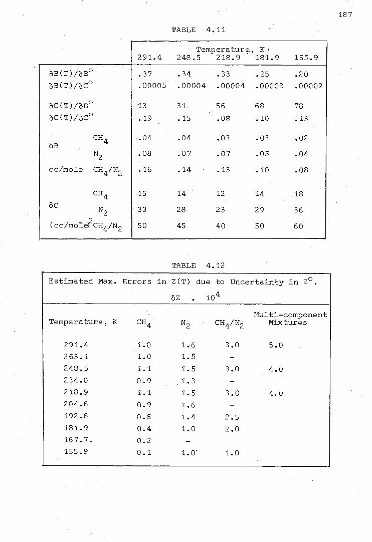
TABLE 4.11

Temperatures K , 291.4 248.5 218.9 181.9 155.9

12,(T)/313° .37 .34 .33 .25 .20 2,B(T)/C° .00005 .00004 .00004 .00003 .00002

3C(T)/313° 13 31 56 68 78 3C(T)/3C° .19 .15 .08 .10 .13

CH4 .04 .04 .03 .03 .02 5B

N2 .08 .07 .07 .05 .04

cc/mole CH4/N2 .16 .14 .13 .10 .08

CH4 15 14 12 14 18 5c N2 33 28 23 29 36

(cc/mold)2CH4/N2 50 45 40 50 60

TABLE 4.12

Estimated Max. Errors in Z(T) due to Uncertainty in Z0.

5Z . 104

Temperature, K CH4 N2 CH4 /N2 Multi-component

Mixtures

291.4 1.0 1.6 3.0 5.0 263.1 1.0 1.5 248.5 1.1 1.5 3.0 4.0 234.0 0.9 1.3 - 218.9 1.1 1.5 3.0 4.0 204.6 0.9 1.6 - 192.6 0.6 1.4 2.5 181.9 0.4 1.0 2.0 167.7. 0.2 -- 155.9 0.1 1.0' 1.0

187

20 30 40 50 60 PRESSURE, bar

FIG. 4.1. EFFECT OF ERRORS IN 273.15K VIRIAL COEFFICIENTS ON EXPERIMENTAL COMPRESSIBILITY FACTORS.

70 80 90 100

2.

2.0 DD CO N

n 0-)

1.5 O 171

0.5

/ ••

1"

,,, ,

11

11,, 1.L

l iL ', i

r ,

.s H. ., 1i

1

I, •, i.„ 1

, • ,

1 i

.-.., 11

',4,1

•

i

it

:Tr I ,

1 1

I ,

l' , 1-.,t' i,',

..„...-..,..;

; • I

.

• " :

; ,

:

-L-

1 I 1 , 1

'4 1 ,

1

I 1 1

Ilt.

'" I

-r:, ,--;174-i--,, .

' i

; 1'

I

li 1 ; 11

t• I 4i-i:il-

;_ ii

.f ,,

I II

II: :' -T-- ,i- i

+1"- 4-• --4

.

T 7 1 ;,

1

I 1 i I

! Id. .,... I

Fr 14 . 14.

,

Il : l'

i I.1 PI

1 1 . 4 i

4

ILI

, '11 1.4 1

I .1

-41.-1-

i i. l.

; 1--,-;-

I

TI ;

1 1.,,

;

.1,441,, /, I.

I-1

: 1 it

.

:111

,

'

1 1

Tit: ' ' 1 ;

• 4_,

t

- I

' • IL,

It I

. , , .-t.;

1_ I r, 1 ;

, i ITIV:;

ii.,1; i 1

lin I I II;

1:i 4 ilrITTI r.'

t 1 1

Ttl ''

I.":

? t f 1 i (Ili ,-t-TI •t, ' il ' 1 .

• rr

i i

, III '

44_

•

;

., . i i I ilLIICI

_ I

1

;

., t 1 I

1 t

,- , I

:

i 4 1

1

,... tLit ....4.-- 1; ;

-1 / 1 -.1

SI : I 1 ____ ___;_Z It

,,, ;;;1

I . ;

VI Il• .

I I i ;

—7-71, • " I

',i 1

,

•

;; „ .

•I; 47P+ It t t

1 1 14 It :1;

1,!•ii

;I.': , t'14.4"4,-,11-

. 11 '

1 ,

-

II l • , t

; ; ; - 11 t

",' •":; -...:_-' il '

11 I.; ' :4,1- ( III t , r

-11 14 ; , i '1 :

• ; ....it,: t t • , ,_,1

1 ; ' ' C I ..,-+-: ; Ill il .r-

I; CI it- 1 1 ; '

, 11 11,1

Tit i• f:

T11, 1 rtt-t-t-1.-1--1111--,-1,,--

1, 1

'-, I

1,-t ;

1 :----r- 1 ',

+/1 1' .1.,

, 1; , ., • I . 1 I t 4 I '

tin'1

1; I I 1 1 li I 1 1 rt ;

; -t-tc/i 'LI , I; 1 ti 1

I t'll fl '

IT ti IT:- t - 1

; i ..,... !i

••

1. v.. , 11 i•

I

1 • II

'

I 1 1

•--11- 1

,

'• 1.j

/ 1 ,

i_L1.

141.; 1;11-11—rTil

"; '1

'

.•r ;

' 1 1

1 ii '; 1 ' 11 ' • 1 1....,_i

it •

,

1 , ,, 4.

;,;:' 1

i __,

; I t II ,

'4-- ;1 • ,

, , i 1, t•'- •

.;-•-•trl;

.,--:- --/

, I -it,- t

t i .-1;---,• 11 , , ..-...:--tt, '1: , .

t

1 ; ' " 1

t

11 .:,-, I'• .

II. - '-'

1 i

, .-.

1

ti , '

ry : „ , ,

:1

l

i — • , „ 1111; , ,-,-,

1 4 .

I 11 it t t i

1

.

, t

I ,

1 . 1 t-III

1 '

1 1 ; 1 Jr; -II ii

` I / r

. , iii

'

,;' .1l.i

'

.--i- 1

, i t ;: • • -It't• - :":1•••

, I -.-4-,-;--1

ii. , ';-1

1 , i ,- • 1111 •

,

r I; , r ';" IT) '•• t ' It 1 ; 1 f 12 i ,. *1 '1:

r;1-'--;-"r-r -- t ' Till

ft -t -I 1 .1 i ; 1, / ,-,--- , . 1, ,,

t, , i • •, , --i-t-i tt, ;ti .

1.

11: 1 -, 1 i1 1 1

1 V ; I 1.,,.. I

I 11

4.-1 . 1 1; , 1

-r-r-'-. ♦ 1

ta 41 ; tl :ill 711"--

i; 1 t; 1 :

Ili 11 • -L'-•-• ; II 1 : 1 ii-1 Tr t ; ;

-, I I 1 '1 f i ri ,: ' ' • , ...,-!--'rr f-•,-

1 :

' r

,

,I, Itrit;

i t. -

,

1 1

t 1 t; r t ,.

t;,. It -7111- *1 . ,.

- ;4 . ft 1-

t -h'

; t --) --

I ,- ,i 1 I 1

44 _,... 1 , . - i •• I- ,-'- 1-1-r-- , 1 i

, I t • ' i ill!

, / 1 1; ki 11 1 44 ii T IT TI 1, I

1 1 t I i iii., li-

itt --.t.T-7 • „ ,• . -,.. , - :ill 1 i 11° I, 1

1---,1 .,.. -7.-1-1711- • , t • ; t ; 1.1 C: ; ;;; III ;:t ,H,

1 ---,T, 1 ,i, ' 11 i • Hi]

441- ' I 4. I ' r; .,.. 1 ,

4 , l';

;.. ';:' 1 ; I;

I 1 ; t .

1

.

• I;

:.

I . , I

I

II 1 : 1

/

I I I /

.1 r I

1,

1 t. tr .1.

•1 “:

.

4+ 41 .11 1

I t

I ;

tr;" ;; ; •

. : 1,

.t.1 r .r I

;

1

• 1 1

!

;II I,

• :

I II

H

I

1 •

I ;

t 1 I ;

1

-;-.4-;

il.

.

1 ..,-li--l-'

:

•; ;.. , • ••

. ;

1 ; tt ,

rt - r-• 1 t1; 4 f11, -444, . . I ' , -.--ri, 11 , I . 44 .1.. 4rt 4

4 I i

,•;-1- T -t— .

... ,-,. t iJ1-

_ ''.

irii ' it?

I ....,1

"1" , 1 ,I 1,

1 i . ...

,I, tl I

1, i 4 trtt

t 11 t it

in !i[

tr. ' ;It iTII

iv t[ , il

I , ,

li, il ' 4

I r 4 t

i t 1.1 ; ; 111111, ' :4 1,

-I t :II I:'

I i W..: ' : ir,': j-11 1 Jr:, "Ii: t ' , II , , L.': r h t: " ,11

, 1 ,-1 * Ft.

4:14-u-:

, . :1- ,, .• i 1, r , t i

--t-- , 1 1 I'

. ' -4-.-

.: 1

•

1 1 I

, 11:! ;;I:

,; 1 I !II ' 1 II ,

1 • 1 11

,

II 1 I,• • • , I

H-,- " +. ; •

ill

' ,1

1 I

1 i

tt

, 1 11

,1,, 1, 1 „I T44, .4._,, 1.

ii .:111 li t 444

;

. ,

"

.

1;

, l ., 1 1" 1. I

; ' 4444;

ITI.1

I t 11

IIItt !!! . I, il

I ;

III

' 1. ;;;.

, 1. • i

i •

1 1 1 r;;; 1 ".' i I I i 1 t , 1 •1 1 I ,

, t i _.,

"I• . 1 ,_ I ; , I

i ; ' • I 1 1

r1, i' ',', HU', ; i i

,,, !'

4----44-,- . t, ! o 'l ':

,. , .,,,-?II i::',

lij

.. .; :,,,i , , ' I , i'r

f , !LI

`,, ;!•, , i , 1

t 1.1- .. "1, ti I Tr:,1 4• 4'; 1 iffi i',''''', , H / t ;,•,' 1...! 1 ,.!:

6.0

5.0 (-)11>

N

4.O

O 7,71 3

3.0

2.0

1.0

A 0 CP

VOLUME OF PRESSURE VESSEL (from least-squares fit)

V

/0

•0 /

O CH4 • Nz • Mix. A ✓ Mix. B

150 175 200Temp. 225 , K 250 .275

FIGURE 4.2

361.0

360.5

vi, cm3

360.0

359.5

3590

189

o'

I A

0 A

At /a)

9'

0

190

4.4 Experimental Data of Other Workers

(a) Experimental Methods

There are a variety of available experimental methods

for determination of PVT data and virial coefficients of

gases. They have recently been reviewed in detail by

Mason and Spurling (1). The methods fall into four basic

categories,

1) The constant-volume, normal-volume apparatus. The

pressure is measured of a gas confined by mercury in a fixed

volume at constant temperature. The quantity of gas in the

apparatus is determined by an expansion into a known volume

at N.T.P.; the mass of the gas is calculated from the normal

volume, which, if not known with sufficient accuracy, must

be measured independently. Alternatively, the gas may be

confined by a diaphragm differential-pressure cell, enabling

low temperature measurements to be made.

2) The free-compression apparatus. A weighed sample

of gas is confined by mercury in a volume which can be

varied by withdrawing or injecting mercury.

3) The Burnett-type of apparatus and similar expansion

methods.

4) Comparative methods. These are usually confined

to low-pressure measurements of the second virial coefficient.

The volumetric behaviour of the gas under study is compared

with that of a reference gas, usually helium, for which the

second virial coefficient is known accurately.

(b) Extraction of Virial Coefficients from PVT Data

191

From the

Z -

virial equation

B Cp + Dp2

- 1 ) Lt = (Z

of state,

+

equation (1.3),

(4.4-1

(4.4-2)

(4.4-3)

P

• . . B

and C

p-K)

= Lt a — 1) ( p p -4o

For the published data given in terms of experimental

compressibility factors and densities, (Z - 1)/p was plotted

against density, p, and B obtained from the intercept at

zero density and C from the limiting slope at zero density.

When the data was given in terms of pressure and density,

it was first converted into compressibility factors only if

the temperature was measured with sufficient accuracy.

Older published compressibility factors were corrected, if

necessary, using the correct thermodynamic temperature

(IPTS '68 scale) and value of the gas constant, R. These

corrections were usually small.

Many of the results from apparatuses of category (1)

are given in amagat units of density, which is defined as

the volume of a given mass of gas at N.T.P. divided by the

actual volume at the experimental temperature and pressure.

These densities may be converted to units of mole.cm-3 if

the normal volume is known accurately from independent

measurements, as is the case with methane, nitrogen and argon.

When the temperature was measured with sufficient accuracy,

as in most of the work of Michels et al, e.g. (36, 37), the

data was converted into compressibility factors and treated

192

graphically to obtain virial coefficients.

The precision with which second and third virial

coefficients may be obtained by this graphical extrapolation

depends on the precision of the measurements, the lowest

density to which they extend, and the curvature of the

graphical plot. The absolute accuracy is very difficult

to assess as it depends also on the absolute accuracy of

the original data which is often not estimated by the

original experimentalists.

This method is preferred to that of curve-fitting in

this instance because any systematic error at low density is

shown up as a departure from linearity of the plot, and

because it offers a convenient comparison of different

data on the same isotherm. It is easier also to find and

discard 'rogue' points. When the virial coefficients

obtained by re-analysing the data did not differ significantly

from those obtained by the experimentalists themselves,

the latter values were used.

In dealing with the calculation of virial coefficients

from experimental data, Mason and Spurling (1) argue that the

accurate determination of virial coefficients requires

measurements down to at least 1 or 2 atm pressure. They cite

as an example the results of Michels et al (38) for carbon

dioxide where the values of B differ by as much as 3 am3.mole-1

from those obtained by Butcher and Dadson (39), whose

measurements extend down to 2 atmospheres. However, the

(Z - 1)/p plots for Michels data are linear at low density

and extrapolate with precision to zero density. A difference

of 3 cm3.mole-1 cannot be attributed to the error in

193.

extrapolation of Michels' data and must be due to systematic

errors in one, or both sets of measurements.

The literature contains many examples of different sets

of 'high pressure' measurements (> 10 atmospheres) which

show good agreement at the same temperature on (Z - 1)/p

plots, e.g. methane above 0 °C (section 4.4(c)), and for

which (Z - 1)/p is linear at low density. In these cases

confidence can be placed in the value of B obtained by

extrapolation as it is unlikely that two or more sets of

data would exhibit identical systematic errors over a large

range, particularly when obtained on different types of

apparatus.

At the present 'state of the art' in PVT measurements

it appears that, at least for the gases considered here,

estimates of B from recent precise 'high-pressure' measurements

in general tend to be more accurate than those from low-

pressure' measurements (below 2 atmospheres). For the

latter type of measurements the non-ideality of the gas

(i.e. the deviation of Z from 1) is very small and a much

higher relative accuracy is required from the pressure

measurement, usually with a precision mercury manometer. It

is only at low reduced temperatures (T < Tc), where the

isotherm curvature is high and the maximum pressure is

limited by the saturation line, that 'low-pressure'

measurements appear more reliable.

(c) Methane

Since the review by Tester (40) in 1961 there appears

to be no satisfactory complete review of the PVT data of

methane, so it will be treated here in some detail.

194

(i) Michels and Nederbragt (41)

Using a constant-volume, normal-volume type of apparatus

measurements were obtained from 273 to 423 K at pressures

from 20 to 380 atmospheres. The results are believed

accurate to within 0.1%.

(ii) Schamp, Mason, Richardson and Altman (42)

These workers used an apparatus of the same type as

that used by Michels and Nederbragt and the results covered

the same temperature range at pressures up to 230 atmospheres.

Their results differed by a small amount (about 0.1%) which

they attributed to a small quantity of ethane impurity in

the methane used by Michels. The second and third virial

coefficients, derived by graphical treatment of the data,

are given in Table 4.13.

(iii) Douslin, Harrison, Moore and McCulloch (43)

Using an apparatus of the free-compression type,

isochoric measurements were obtained from 273 to 623 K and

densities from 0.75 to 12.5 mole.litre-1 (15 to 400

atmospheres). The results are of high precision and are

universally regarded as of high accuracy. The compressibility

factors differ by less than .0003 from those of Schamp at

densities up to 5 mole.litre 1 which is excellent agreement.

Second and third virial coefficients were obtained by

Douslin using a method of graphical extrapolation; these

values are given in Table 4.13. The small differences

between these values and those of Schamp are mainly due to

the difference in the method of extraction of the virial

coefficients, as retreatment of the data of Douslin by the

TABLE 4.13

Methane: Experimental Virial Coefficients of Other Workers (In units of cc/mole).

(ii) Schamp (42)* (iii) Douslin (43).

T,K B C T,K

273.15 -53.37 2635 273;15-53.35 2620

298.15 -42.90 2430 298.15-42.82 2370

323.15 -34.38 2280 303.15-40.91 2320

348.15 -27.32 2170 323.15-34.23 2150

373.15 -21.35 2060. 348.15-27.06 1975

398.15 -16.02 1900 373.15-21.00 1834

423.15 -11.55 1810 398.15-15.87 172 7

423.15-11.40 1640

(iv) Deffet (44)* 448.15 -7.56 1585

T,K B C 473.15 -4.16 1514

323.78 -34.30 2250 498.15 -1.16 1465 374.49 -21.35 2080 523.15 +1.49 1420 425.03 -11.30 1800 548.15 +3.89 1385

573.15 +5.98 1360

(v) Olds (45)*

598.15 +7.88 1345

623.15 +9.66 1330

195

T,K

294.26 -44.90 2520

310.93 -38.93 2500

327.59 -33.80 2400

344.26 -28.95 2290 360.93 -24.40 2100 377.59 -20.57 2070 427.59 -8.00 1750 477.59 -3.75 1700 510.93 0.0 1650

(viii) Mueller (49)*

T,K

199.83 -104.6 3920 227.60 -79.6 3250

255.38 -62.3 2750

283.16 -48.6 2490

(vii) Kvalnes (48)*

T,K

203.15 -99.7 3700 223.15 -82.5 3320

248.15 -66.4 3000

273.15 -53.7 2660

(xi) Thomaes (53)

T,K

108.5 -363.0

125.2 -268.5

149.1 -187.8

186.4 -126.2

223.6 -82.7

249.3 -68.5

Re-treated data m large scatter on isotherm

(xii)

T,K

Brewer (54)

B

TABLE 4.13 (continued)

(xiii) Byrne (55)

T,K 123.15 -264.3 110.8 3 -330.1 148.15 -185.9 112.43 -319.9 173.15 -138.7 114.45 -307.8

198.15 -106.5 116.79 -295.5 223.15 -83.6 121.25 -274.5

128.84 -244.3 136.75 -218.9 148.28 -187.7 162.29 -158.4 178.41 -132.2 202.49 -103.4 221.10 -85.8 243.80 -70.3 273.17 -53.7

196

197

method of 4.4(b) leads to values in even closer agreement.

(iv) Deffet, Liliane and Fick (44)

Using an apparatus of the free-compression type, results

were obtained at three temperatures, 328.8 K, 374.5 K and

425.0 K at pressures from 10 to 253 bars. Plots of

(Z - 1)/p vs. p were smooth and B and C could be obtained

with precision; these values are shown in Table 4.13.

They are in close agreement with those of Douslin and

Schamp.

(v) Olds, Reamer, Sage and Lacey (45)

Measurements were obtained on a free-compression type

of apparatus at temperatures from 294 to 511 K and at

pressures from 13 to 670 bars. The results are of lower

accuracy than those of Douslin et al and were pre-smoothed

prior to publication. The second and third virial

coefficients obtained by graphical retreatment are shown in

Table 4.13.

(vi) Keyes and Burks (46), Freeth and Verschoyle (47)

These early measurements above 0 °C have been super-

seded by the later, more accurate and extensive data already

mentioned, and therefore were not considered here.

(vii) Kyalnes and Gaddy (48)

These early low-temperature measurements (203 to 473 K)

at pressures from 20 to 1000 atmospheres were obtained on an

early form of constant-volume, normal-volume apparatus.

An accuracy no better than 0.1 to 0.2% is expected. Above

273 K the (Z - 1)/p plots showed considerably more scatter

than those of Douslin and the higher temperature isotherms

198

were rejected in favour of Douslin's. Below 273 K the data

appear to show less scatter and the virial coefficients

given in Table 4.13 were obtained by graphical retreatment.

The lowest pressure on each isotherm is quite high and the

points are not closely spaced, leading to an estimated error

in B of about ± 1 cm3.mole-1 caused by the extrapolation

alone.

(viii) Mueller, Leland and Kobayashi (49)

These workers obtained results at six temperatures

from 144 to 283 K at pressures up to 500 bar using a Burnett

apparatus. The experimental compressibility factors had

been derived from the actual Burnett measurements by a

graphical method of data treatment and then interpolated to

evenly-spaced values of pressure. Plots of (Z - 1)/p vs p

show considerable scatter on two isotherms (227.6 and 255.4 K)

and for the two lowest temperatures insufficient points (3

or 4) are given to enable virial coefficients to be extracted.

The derived values of B and C for the other isotherms are

given in Table 4.13.

(ix) Hoover, Nagata, Leland and Kobayashi (50)

A Burnett apparatus capable of very high precision

was used in this work and second and third virial coefficients

were obtained at 131.9 K and 191.1 - 273.2 K. The maximum

pressure was 40 atmospheres. However, the compressibility

factors from Hoover (51) show considerable scatter on a

Z vs. P plot (e.g. as much as .2 to .5% at 240 K), which is

completely incompatible with the high precision claimed for

the virial coefficients. In view of this serious, unexplained

199

discrepancy these data were rejected as a source of virial

coefficients.

(x) Vennix, Leland and Kobayashi (52)

A constant-volume apparatus was used, the cell being

charged with a known mass of methane from a weighed cylinder.

The volume of the cell was determined by a procedure

involving Burnett expansions of helium into a cylinder of

known internal volume. Isochoric measurements were obtained

between .0025 and .225 mole.cm-3 at temperatures from 130 to

273 K and at pressures up to 690 bars. The data which

were estimated as accurate to 0.05%, were also presented as

interpolated to even values of temperature. There are too

few low density points to enable the virial coefficients to

be extracted. At 0 0C the data are in excellent agreement

with those of Douslin and of Schamp.

(xi) Thomaes and van Steenwinkel (53)

These authors measured the second virial coefficient at

low pressure (below 1 atmosphere) and low temperatures

(108 to 249 K). The volumetric expansion was compared with

that of hydrogen. The values obtained are shown in Table 4.13;

no corrections were applied for the effect of higher virial

coefficients, which could be significant at the lowest

temperature.

(xii) Brewer (54)

The second virial coefficients between 123 and 223 K

were determined in a low-pressure apparatus by measurement

of the pressure difference between two constant, equal volumes

200

of methane and helium. The second virial coefficient at

0 °C was taken as - 53.75 cm3.mole-1 and corrections were

applied for the effect of the third virial coefficient. The

results are given in Table 4.13; they are estimated as

accurate to .5%.

(xiii) Byrne, Jones and Staveley (55)

The apparatus used was similar in principle to that

of Brewer, the pressure difference between methane and helium

being measured with a precision differential manometer.

The second virial coefficient was measured at temperatures

from 111 to 273 K. The value of 42.96 cm3.mole-1 was

assumed for the second virial coefficient at 25 °C. Small

corrections to the results were applied for the effect of

adsorption, but none for the third virial coefficient. The

results are given in Table 4.13.

(xiv) McMath and Edmister (56), Lee and Edmister (57)

Measurements were obtained by Lee at 298, 323 and 348 K

with a Burnett apparatus. McMath obtained isochoric

measurements at 264.3, 277.6 and 288.7 K in a constant-

volume apparatus, the density of the gas being taken from

the isotherm of Lee at 298 K. Unfortunately the methane

used was only of 99% purity and the results were not of

sufficient accuracy to justify their inclusion here.

(xv) Pavlovich and Timrot (58)

These results covered a wide range of temperature

(103 to 333 K), but were found by Douslin et al (iii) to be

of very low accuracy and were therefore discarded.

(xvi) Robertson and Babb (59)

Very high-pressure measurements (up to 10 k bar) were

determined from 273 to 473 K.

(xvii) Jansoone, Gielen, Boelpaep and Verbeke (60)

Measurements were obtained in the immediate vicinity

of the critical point, giving accurate estimates of the

critical constants:

Tc 190.50 K

pc = 0.010148 mole.cm-3

(d) Nitrogen,

Recent reviews of the PVT data on nitrogen have been

published by Vasserman and Rabinovich (61), Wood et al (27),

and Coleman and Stewart (62). All of the available data

are not considered here, but only those results not rejected

by these reviewers.

(i) Holborn and Otto (63)

This early work used a constant-volume, normal-volume

apparatus to obtain measurements at temperatures from 143

to 673 K and at pressures from 20 to 100 atmospheres. The

second and third virial coefficients given in Table 4.14 are

those obtained by Saville (64) from a curve-fit to the data

after applying necessary corrections to the original figures.

B is estimated as accurate to ± 1 cm3.mole-1.

(ii) Onnes and van Ui.k (65)

These early measurements were obtained at Leiden with

a glass capillary free-compression apparatus at temperatures

201

TABLE 4.14

Nitrogen: Experimental Virial Coefficients of Other Workers (in units of cm3.mole-1)

(ii) Onnes (65)

C T,K B C

(i)

T,K

Holborn (63)'

B

143.15 -79.38 2814 m126.83 -102.2 3482

173.15 -52.73 2313 128.69 -99.5 3488

223.15 -26.28 1784 131.62 -94.5 3232

273.15 -10.31 1546 141.88 -81.16 2992

323.15 -0.83 1450 151.96 -69.63 2586 373.15 +6.05 1425 170.90 -52.38 2022 423.15 +11.58 1174. m192.05 -39.48 1929 473.15 +15.53 1068 222.89 -24.8 1360 573.15 +20.44 1068 249.53 -16.8 1552 673.15 +23.77 1085 273.15 -8.96 868

N293.15 -5.69 1228 (iii) Michels (33),(66)*

T,K g C (iv) Canfield (67)*

273.15

298.48

322.92

347.91

372.88

398.22

423.04

-10.25 -4.78

-0.52

+3.00

+6.31

+9.20

+11.90

1500

1405

1400

1385

1260

1185

1040

T,K

133.15

143.14

158.15

183.15

223.13

273.15

-92.27

-79.51

-64.08

-45.17

-25.35

-10.0 6

3305

2975

2596

2162

1741

1441

(v) Crain (34) (vi) Saurel (68)*

T,K B C T,K 143.16 -79.45 2889 423.15 +11.25 1320 163.16 -59.42 2392 473.15 +15.05 1265 203.16 -33.85 1837 573.15 +20.30 1200 273.15 -10.26 1517 673.15 +23.80 1140

773.15 +26.10 1120 873.15 +28.00 1040 973.15 +29.25 1050 1073.15 +30.10 1040

202

* Re-treated data Large scatter on isotherm

203

TABLE 4.14 (continued)

(vii) Friedman (70) (ix) Witonsky (72)

T,K B T,K B

80 -251 448.15 +14.28

90 -200.5 523.15 +18.34

100 -162.1 598.15 +20.83

110 -131.8 673.15 +23.40

120 -114.6 748.15 +24.75

125.2 -106.9

150 -71.2 (x) Pfefferle (73)

175 -49.4 T,K B C 200 -34.33 303.16 -4.17 1485 250 -16.19

273.15 -9.50

300 -3.54

(viii) Pool (71)

T,K

90 -201

204

from 124 to 293 K and at pressures from 30 to 50 atmospheres.

The second and third virial coefficients as determined by

Saville (64) are shown in Table 4.14. Although of lower

accuracy than those of Holborn and Otto, the results are

useful at low temperature, where there is a scarcity of

experimental third virial coefficients.

(iii) Michels, Wouters and de Boer (33), Otto, Michels and

Wouters (66)

With a constant-volume, normal-volume apparatus

measurements believed accurate to .05% were obtained at

temperatures from 273 to 423 K and at pressures from 20 to

410 atmospheres. Second and third virial coefficients

obtained by graphical treatment of the data are shown in

Table 4.14. B is estimated as accurate to ± .5 cm3.mole-1

(iv) Canfield, Leland and Kobayashi (67)

Canfield used a Burnett apparatus in conjunction with

the graphical method of data reduction to obtain compressibility

factors at temperatures from 133 to 273 K and pressures up

to 500 atmospheres. There are apparently systematic errors

at low pressure and the virial coefficients obtained by

Wood et al (27) from a graphical treatment of the data are

preferred. These are shown in Table 4.14.

(v) Crain and Sonntag (34)

These authors also used a Burnett apparatus, obtaining

results at four temperatures from 143 to 273 K and pressures

up to 500 atmospheres. The data are in excellent agreement

with those of. Canfield, within .05% except at very high

205

pressure. The virial coefficients given in (34) are shown

in Table 4.14.

(vi) Saurel (68)

These results obtained with a modified free-compression

type of apparatus are important as. they extend to high

temperatures (423 to 1073 K); the pressure range is from

10 to 900 atmospheres. The plots of (Z 1)/p vs p are quite

smooth, enabling B and C to be extracted with high precision;

these values are shown in Table. 4.14.

(vii) Friedman (69)

These results were, obtained with a constant-volume

gas thermometer, and extend to very low temperatures (from

80 to 300 K) and pressures up to 200 atmospheres. The data

have, unaccountably, not been published in the standard

scientific literature but the experimental virial coefficients

have been published elsewhere (70): the values of B are

shown in Table 4.14. The overall precision in Z has been

estimated as ± 0.1%, but this is still not sufficiently

precise to enable meaningful third virial coefficients to

be obtained at very low temperatures.

(viii) Pool, Saville, Herrington, Shields and Staveley (71)

One second virial coefficient, at 90 K, was obtained by

expansion from a calibrated piezometer into a series of

calibrated bulbs at 25 °C. The accuracy was estimated as

± 2 cm3.mole-1.

(ix) Witonsky and Miller (72)

The results of these high-temperature Burnett measurements

206

(448 to 748 K) were given in terms of the 'pressure' virial

coefficient, B',

where Z = 1 + B'P + otIroe

These values were converted to volume virial coefficients by

means of the approximate relation, B = B'.RT. The results

are given in Table 4.14.

(x) Pfefferle, Goff and Miller (73)

The same Burnett method was used as in (ix) but results

were obtained at only one temperature, 303 K. The values of

,B and C are shown in Table 4.14.

(xi) Hall and Canfield (74)

A low-temperature Burnett apparatus was used to study

the helium/nitrogen system. Only two isotherms were

determined for pure nitrogen, at 113 and 103 K, where the

maximum pressure was very low (16 bar and 9 bar respectively),

and the problems with the data treatment are large: these

results were not used.

(e) Methane/Nitrogen Mixtures

(i) Keyes and Burks (75)

These early measurements (1928) were obtained with a

free-compression type of apparatus at temperatures from 273

to 373 K and at pressures from 30 to 240 bars. Two compositions

were studied; the data were re-treated graphically to obtain

the second and third virial coefficients shown in Table 4.15.

The (Z - 1)/p plots were quite smooth, indicating a reasonable

degree of precision. Values of B12 were obtained for each

mixture using the pure component virial coefficients of

Douslin et al (32) (Table 4.13) and of Michels et al (33)

207

(Table 4.14). It can be seen that there are systematic

differences between the values for different mixtures. The

mean of the two values was used for purposes of data

comparison.

Estimates of C112 and C221 were obtained from the

experimental third virial coefficients, by solving the

equations,

x13 C111 + 3x1

2x2 C112 3x1x22 C221 + x23 C222

where x1is the mole fraction of methane and x2 the mole

fraction of nitrogen.

These values, shown in Table 4.15, are unlikely to be

more accurate than ± 500 cm6.mole-2 because of the systematic

differences between the mixtures.

(ii) Brewer (54)

By measurement of the pressure change on mixing at

constant volume, the quantity E was obtained,

where E = B12 - 2(B11 B22)

Only one measurement, at 0 °C, appears to have been carried

out; B12 was re-calculated using the pure component virial

coefficients of Douslin et al and of Crain and Sonntag. The

result, believed accurate to about 1 cm3.mole-1, is given in

Table 4.15.

(iii) Krichevskii and Levchenko (76)

The minimum pressure measured in this work was 100

atmospheres and so virial coefficients cannot be extracted.

Plots of (Z - 1)/p vs p for a few isotherms showed large

scatter and the data were discarded.

TABLE 4.15

Methane/Nitrogen: Virial Coefficients of Other Workers

(in units of Cm3.mole-1)

(i) Keyes

(1) X = CH4

T,K B

(75)*

0.4332

C

(2)

T,K

X = CH4

B

0.80531

C

273.15 -25.55 199 5 273.15 -42.35 2295

323.15 -12.15 1710 323.15 -25.28 1990

373.15 -3.05 1670 373.15 -13.57 1835

T,K B12(1) B12(2) C112 C221

273.15 -24.9 -23.4 1890 2170

323.15 -11.2 -9.4 1780 1690

373.15 -2.19 -0.6 1780 1710

(ii) Brewer (54)*

T,K B12

273.15 -25.54

208

* Re-treated data.

209

(iv) Bloomer, Eakin, Ellington and Gami (77)

Results on mixtures at low temperatures and high

pressure have been obtained but unfortunately the actual

data remain unpublished. Tables of compressibility factors

are presented which are the result of a fit of the Benedict-

Webb-Rubin equation of state to the data. These tables

represent the data to within 0.5%, but these authors presented

no estimate of the accuracy of the original measurements.

(v) Blake, Bretton and Dodge (78)

Measurements were obtained at one temperature only

(299.5 K) and at high pressures (300 to 5000 atmospheres),

for two mixtures in a modified constant-volume type of

apparatus. The results were pre-smoothed and presented at

fixed intervals of pressure.

4.5 Comparison with other workers

A detailed comparison of the second virial coefficients

can be made by presenting graphically the differences

between the experimental values and those calculated from an

arbitrary smooth function of temperature. That chosen was

the function

Bref (T) a1 + a + a3/T3 + a (4.5-1)

This equation was fitted to the experimental virial

coefficients using the general non-linear least-squares

procedure. The resultant coefficients are presented in

Chapter 5, Table 5.2.

The deviations' Bexp (T) - Bref (T), are shown in

210

figure .4.3 for methane and figure 4.5 for nitrogen. The

third virial coefficients are compared with the previously

published results in figure 4.4 for methane and figure 4.6

for nitrogen. The interactional virial coefficients are

compared directly: B12 in figure 4.7 and C112, C221 in

figure 4.8.

(a) Methane

It can be seen that the second'virial coefficients of

this work at the higher temperatures of our range are in

excellent agreement, within experimental error, with those of

Douslin and of Schamp. (The results of Michels are very

close to these latter sets of values and for the sake of

clarity are not shown.) At lower temperatures our results

are in good agreement with the low-pressure results of Brewer,

within experimental error, but some 1 to 3 cm3.mole-1 less

negative than those of Byrne. The results of Mueller are in

reasonable agreement with our values considering the scatter

inherent in some isotherms, but the results of Kvalnes are

some 1 to 1.5 cm3.mole-1 less negative. The results of

Thomaes show considerable scatter.

For the intermolecular potential study of chapter 5,

the following second virial coefficients given in Table 4.13

were not used:-

(i) Michels (41), and Deffet (44), because they are duplicated

by the results of Douslin (32) and Schamp (42), with which

they are in close agreement.

(ii) Thomaes and van Steenwinkel (53).

(iii) Kvalnes and Gaddy (48).

(iv) Mueller (49) (at 283 K).

(v) Olds (45).

FIGURE 4.3

+1 B-Bref(T) cc/mote

0

9 7 6 4 3 2 1

110 120 130 150 170 T) K 200 250 300 400 500 700 METHANE : SECOND VIRIAL COEFFICIENT

0 This work

X Dousli n(32)

Sc hamp(42)

Brewer (54)

A Byrne (55)

7 Deffet (44)

o Olds (45)

Kvalnes1/48),

V Mueiter (4 a

0

0 In

-0.4> — — 0

A

En

V

A

v

0 tt 91 Clot 0 o

o

X 0

FIGURE 4.4

4 000

3000

C ccirriote51

2000

METHANE : THIRD VIRIAL COEFFICIENT

0

000

Ea 0

o This work

X Doustin (32)

• Schamp (42)

• Deffet (44)

• Olds (45)

E0 Kvalnes (48)

Muer ter(49)

1000

100 200 300 Temp. , K 400 500

600

O This work Crain(34)

A Cant ield (67) Michels(33)

W Friedman(70) APfefferle(73)

Wi ton sky(72) VSauret (68) ® Hot born(63)

Onnes(65) 0

7

00 E

+1

B Brei(T) cc/mole

0 MEM. •••••••=0 •M•••••••

100 110 130 150 T, K 200 250 f .

400 1000

7 x a v xe

7 0 is A8

cx X v V ® _ea_ x

,60 aolo 4' ----° — 0—

0 0

0 V

NITROGEN : SECOND VIRIAL COEFFICIENT

V

FIGURE 4.5

11 10

8

7 1/T, 6 K`.103 5

3 2 1

V X •

X

400

450

500

550

• x

FIGURE 4.6

NITROGEN : THIRD VIRIAL COEFFICIENTS . CD This work

O Crain (34)

A Canfield (67)

x Michels (33)

Saure1 (68)

Holborn (63)

o Onnes (65)

ID Pfefferle (73)

3500

3000

2500 C

(moctc4

2000

-to 8

es

0

CU • X X

1500

1000 100 150 200 250 300 350 Temp. ,K

I

2'15 FIG. 4.,7

300 250 150

200 Temp., K

300 150 200 Temp.,K 250

2000 0 0

FIG.4.8 .0

4000

Ciij 2

(cci)te) m

3000

CH4/N2

INTERACTIONAL THIRD. VIRIAL COEFFICIENTS

CcH 0 This Ej Keyes 4' 4" 'work ' (75)

CcH4,t,‘,N, :e 13 Eti .

0

—60

B12 ccn

mote, —80

216

Each of the remaining experimental B values was assigned

a weighting factor, w, for use in the curve-fitting of chapter 5,

where w = 1 a2

(4.5-2)

a is the probable error in the experimental value, estimated

by consideration of both the quoted experimental errors and

the deviation from a smooth curve through the data. For

methane the data sets were weighted in the following order,

those at the beginning being most highly weighted:- Douslin;

Schamp; this work; Brewer; Mueller; Byrne.

The third virial coefficients of this work (figure 4.4)

are also in excellent agreement with those of Douslin and of

Schamp at the upper end of our temperature range. Below 0 0C

there are no other measurements of equivalent accuracy, but

there is fair agreement with the results of Mueller and of

Kvalnes, which show greater scatter.

(b) Nitrogen

It can be seen from figure 4.5 that the second virial

coefficients of this work are in good agreement (within 0.2 to

0.3 cm3.mole-1) with those of Crain, of Canfield, and of

Michels. The results of Holborn, of Onnes, and of Friedman

all show greater scatter but the differences are probably

within their experimental error. The high temperature results

of Saurel are in good agreement with those of Holborn but show

a small difference of 0.6 cm3 .mole-1 from the result of

Michels at 423 K. The results of Witonsky are also in

reasonable agreement with those of Saurel, but show a little

more scatter.

On the whole there are no serious discrepancies between

217

the results of different experimentalists and in the inter-

mediate temperature range good agreement exists between our

results and those of Crain and of Canfield. For the inter-

molecular potential study the following values of Table 4.14

were not used,

(i) Onnes and van Urk (65) (B only).

(ii) Holborn and Otto (63) (below 300 K).

(iii) Hall and Canfield (74).

The remaining sets of data were weighted for use in

curve-fitting in the following order of decreasing importance:

Crain, Michels and this work; Canfield; Saurel; Witonsky;

Pfefferle; Holborn; Friedman; Pool.

Our third virial coefficients, figure 4.6, also agree

within experimental error with the results of Crain and of

Canfield, and, at the upper end of our temperature range, with

the results of Michels. It can be seen that accurate

measurements are still needed at lower temperatures, around

the maximum of the third virial coefficient.

(c) Methane/Nitrogen

Our values of B12, figure 4.7, show scatter of less than

1 cm3.mole-1 about a smooth curve through the data, which is

within the estimated maximum limits of experimental error.

The one point of Brewer at 273 K is in good agreement. If

our results are extrapolated to higher temperatures, the

curve lies some 2 cm3 .mole-1 below the results of Keyes and

Burks, which is within the estimated experimental error of

these early measurements.

The scatter shown about a smooth curve through our

interactional third virial coefficients, figure 4.8, is also

within experimental error.

218

4.6 Comparison of Compressibility Factors

As many of the experimental isotherms extended beyond

the region where only second and third virial coefficients

were important, it is necessary to compare the higher-pressure

compressibility factors with the results of other workers.

The results for the mixtures will be discussed in chapter 6.

(a) Methane

To facilitate the comparison of compressibility factor

data an equation of state was employed; the differences

between the calculated and experimental values may then be

readily interpolated between temperatures and pressures (or

densities). The equation of state used was that of Vennix

and Kobayashi (79), as described in more detail in section 6.

In figure 4.9 Z(experimental) - Z(calculated) is plotted

against density for the 218.9 K, 204.6 K and 192.6 K isotherms

of Table 4.1, and for the experimental isotherms in this

temperature range of Vennix (52), of Mueller (49), and of

Kvalnes (48).

For the 218.9 K and 204.6 K isotherms our results are

in good agreement with those of Vennix, the largest discrepancy

being about + .001 (.2%) at a density of about .008 mole.cm-3

on the 204.6 K isotherm. The data of Mueller show fairly

large scatter but apart from one or two points they lie

within .5% of our values. The compressibility factors of

Kvalnes and Gaddy, however, show a systematic deviation which

increases with density, reaching a maximum of .026 (7%) at

-3 203.1 K and .0107 mole.cm .

0 0 0

A A

A A 4 0

9 10 11

FIGURE 4.9

+.006

+.004

+.002 Z(exp)

-Vcalc)

0'0

-•002

-.004

-006

METHANE : Z LoOer temps.)

V

V V

Vennix (52) This work

4191.0 K e192.6 K

195.0 K o204.6 K

205.0 K 0218.9 K

0220.0 K Mueller (49) Kvalnes(48) 0199.8

V203.2 K a 227.6 v223.2 K e

V 0

0 ---10-ao v70 04, o o - eca 0 e e e 9;1 A

o 0

I 1 2 4 5 6 7 8 DENSITY , kmot /m3

I

OMEN =IMP NW IMO 1=0 IMMO

V a

e

+ o S

0 x • 0

X A

V

A

+ 0

0

X 4- 0

A

8 2 3 DENSITY , kmol im3

5

FIGURE 4.10

+ .002

4- • 0015

0.0

-•0005

+ •001 Z(exID)

-Z(calc)

+•0005

METHANE Z (higher temps)

a.

work 0 234.0 o 248.5

.0 263.1 291.4

Doustin(43) x 273.15 K +298.2 K

Vennix(52) t 235.0 K A. 250-0 K A 273.15 K

Mueller (49) ID 255.4

Kva[nes (48) 248.2

A

1 1 1

At lower temperatures the only measurements of Vennix

that fall within the density range of our results are at a

density of .00255 mole.cm-3. At 192.6 K our value of Z at

this density, after interpolation, is greater by about .0008

(.1%) than that of Vennix. The corresponding difference at

181.9 K is about .0013 (.2%). It appears that at our

maximum density, .0058 mole.cm-3, on the 192.6 K isotherm the

value of Z is larger still than that value interpolated from

Vennix, the difference being about .005 (1%).

In figure 4.10 Z(experimental) - Z(calculated) is plotted

for our higher temperature isotherms at 234.0 K, 248.5 K,

263.1 K and 291.4 K, and for the experimental isotherms in

this range of Douslin (43), of Mueller (49), of Kvalnes (48),

and of Vennix (52). It appears that our values of Z at

the higher densities on the 291.4 K and 263.1 K isotherms are

within .0003 (.04%) of the results of Douslin, after inter-

polation; this is within the limits of experimental error.

There is again fairly good agreement with the low-density

measurements of Vennix, and the systematic deviation from

the data of Kvalnes is apparent. The results of Mueller

exhibit fairly large scatter.

It is to be noted that the deviation of the data from

the Vennix-Kobayashi equation of state passes through a

maximum at a density of about .002 cm3.mole-1. This

deviation shows a maximum of .0008 at about 260-280 K then

passes through zero with decreasing temperature and rises to

-.0017 at 192.6 K. This behaviour arises because the equation

of state was fitted below 0 °C to the data of Vennix (52),

which does not really extend to sufficiently low densities.

221

222

In developing an improved equation of state for methane it

should be constrained to give the correct B and C, or,

preferably, it should be fitted to low density data, such as

that presented in Table 4.1.

(b) Nitrogen

For the corresponding comparisons in the case of nitrogen,

the thirteen constant equation of state of Wood et al (27) was

employed. This equation had been fitted at low temperatures

to the data of Canfield (67).

In figure 4.11 are plotted values of Z(experimental)

- Z(calculated) for the lower temperature isotherms of Table 4.2:

204.6 K, 192.6 K, 181.9 K and 155.9 K, which are compared with

the results of Crain and Sonntag at 203.2 K, 163.2 K, and

143.2 K, and with those of Canfield at 183.2 K, 158.2 K and

143.2 K.

Agreement at 204.6 K with the results of Crain and Sonntag,

after interpolation, is fairly good: within .0004 (.05%).

At 181.9 K our results are within .0004 (.05%) of those of

Canfield, after interpolation. The 183.15 K isotherm of

Canfield shows a small systematic deviation at low density,

as does the 158.15 K isotherm. Our results are in good

agreement at 155.9 K with those of Crain and Sonntag,

although the interpolation is not easy, and within about

.0003 (.04%) with those of Canfield. It can be seen that

the results of Canfield and of Crain and Sonntag on the

143.15 isotherm are in excellent agreement.

In Figure 4.12 the equivalent comparisons are shown for

the higher temperature isotherms of this work: 218.9 K,

234.0 K, 248.5 K, 263.1 K, 276.9 K and 291.4 K; with the

223.2 K and 273.2 K isotherms of Canfield; the 273.2 K and

This work O 155.9 K o 181-9 K 9 192.6 K O 204.6 K

Crain (34) A 143.2 K A 163.2 K A 203'2 K

Canfietd(67) El 14 3.2 K ta 158.2 K in 183.2 K

GO a

a 0 A

0

FIGURE 4.11

NITROGEN : Z (lower temps.)

a a a 0 0 A Ao da A

-43g16118: 1 Go ri 03 0

03 0 0 03 m [ll

0$ o.

o g9

0 m 9

m A 0 I I I 2 3

DENSITY 4 5 6 7 8

kmol 1m3

4. • 003

+ .002

+ • 001 (ex p.)

—H(calc)

0.0

— • 001

—• 002

This work 0218.9 K 0263.1 K 0234.0 K 0276.9 K 0248.5 K 9291.4 K

Michels(33) Canfield(67) x273.2 K 223.2 K +298.5 K 273.2 K

Crain(34) A 273.2 K

O O

x

FIGURE 4.12

+.001

+.0005 Z(exp)

—z(catc)

0.0

—.0005

— 001

— .0015

DD

apt? 0A yo. SI 4. M9 (DX0 W1̀ o A + tD 0 0 X

0 u a)

NITROGEN : Z (higher temps.)

a• 2 3

DENSITY , kmole/m3

A

0

225

298.5 K isotherms of Michels et al; and the 273.2 K isotherm

of Canfield.

It is immediately apparent that the 273.2 K isotherm of

Canfield differs by up to .001 in Z (.1%) from the other results

at this temperature. Otherwise the agreement of our results,

after interpolation, with other workers is good. Similarly,

the results of Canfield at 223.2 K are up to .0008 (.1%) more

positive than the values interpolated from our 218.9 K and

234.0 K isotherms. On the whole, however, the agreement is

very good between these sets of low-density nitrogen

compressibility factor data.

4.7 Experimental Results for Other Gases and Binary Mixtures

Apart from methane, nitrogen and the methane/nitrogen

system the gases considered in the intermolecular potential

study, chapter 5, were argon, ethane and the methane/argon,

nitrogen/argon and methane/ethane systems. In addition,

propane and n-butane were included in the test of virial

coefficient correlations, chapter 6.

In collating the data much use was made of the compilations

of Dymond and Smith (80) and of Mason and Spurling (1). The

sources of the more accurate second and third virial coefficients

are listed here, but only those values obtained by retreating

the data are given in the Tables. Otherwise, the values

used were as given in the original references.

(a) Argon

(i) Michels, Levelt and De Graaf (81), Michels, Wijker and

Wijker (82): re-treated graphically (Table 4.16).

(ii) Crain and Sonntag (34).

(iii) Provine and Canfield (83); re-treated graphically

(Table 4.16).

(iv) Whalley and Schneider (84) re-analysed by Saville (64)

(Table 4.16).

(v) Holborn and Otto (85); re-analysed by Saville (64)

(Table 4.16).

(vi) Byrne, Jones and Staveley (55).

(vii) Weir, Wynn-Jones', Rowlinson and Saville (18).

(viii) Fender and Halsey (86).

(ix) Pool, Saville, Herrington, Shields and Staveley (71).

(b) Ethane

(i) Michels, van Straaten and. Dawson (87); re-treated

graphically (Table 4.17).

(ii) Reamer, Olds, Sage and Lacey (88); re-treated

graphically.

(iii) Hoover, Nagata, Leland and Kobayashi (50).

(c) Methane/Argon

(i) Byrne, Jones and Staveley (55).

(ii) Thomaes and van Steenwinkel (89).

(d) Nitrogen/Argon

(i) Crain and Sonntag (34).

(ii) Brewer and Vaughn (90). B12 was re-calculated using

more accurate values of B11 and B22 (Table 4.18).

(iii) Zandbergen and Beenakker (91). B12 was re-calculated

using more accurate values of B11 and B22 (Table 4.18).

(iv) Knobler, Beenakker and Knapp (92). One point at 90 K,

which was not utilized here because of the uncertainties in

B for nitrogen and argon at this temperature.

226

(e) Methane/Ethane

(i) Michels and Nederbragt (93); re-treated graphically

(Table 4.19).

(ii) Dantzler, Knobler and Windsor (94). B12 was re-

calculated using more accurate values of B11 and B22.

(iii) Hoover, Nagata, Leland and Kobayashi (50).

(f) Propane

(i) Cherney, Marchman and York (95); •re-treated graphically

(Table 4.20).

(ii) Beattie, Kay and Kaminsky (96); re-treated graphically

(Table 4.20).

(iii) McGlashan and Potter (97).

(iv) Kapallo, Lund and Schafer (98).

(g) n-Butane

(i) Connally (99). Presented in Table 4.21.

(ii) Beattie, Simard and Su (100); re-treated graphically

(Table 4.21).

(iii) Jones and Kay (101).

(iv) Bottomley and Spurling (102).

227

TABLE 4.16

LE 22a: Experimental Virial Coefficients (Retreated)

(in units of cm3.mole-1)

(i) Michels (81), (82)

T,K B C

(iv)

T,K

Whalley (84)

B C

128.15 -115.3 2000 273.16 -21.88 1298

133.15 -107.8 2275 323.16 -11.04 1096

138.15 -100.8 2370 373.16 -4.34 1078

143.15 -94.4 2410 423.16 +1.01 1014

150.65 -85.6 2290 473.16 +5.28 912

163.15 -73.20 2060 573.16 +10.77 818

173.15 -65.10 1950 673.16 +15.74 -

188.15 -54.70 1690 773.16 +17.76

203.15 -46.25 1580 873.16 +19.48 -

223.15 -37.26 1440

248.15 -28.4 1320

273.15 -21.35 1200 (v) Holborn (85)

298.15 -15.68 1100

323.15 -11.16 1080 T,K B C

348.15 -7.20 1000 173.15 -65.28 2000

373.15 -3.96 984 223.15 -37.31 1463

398.15 -1.14 950 273.15 -21.23 1195

423.15 +1.32 920 323.15 -10.66 1003 373.15 -4.06 1046 423.15 +1.53 872

(iii) Provine (83) 473.15 +4.98 966 573.15 +11.34 -

T,K B C 673.15 +15.58 - 143.15 -94.0 2335 158.15 -77.9 2180

m183.15 -56.6 1560

228.

Large scatter on isotherm

229

Ethane:

TABLE 4.17

Experimental Virial Coefficients (Re-treated)

(in units of cm3.mole-1)

(i) Michels (87) (ii) Reamer (88)

T,K B C T,K B C

273.15 -221.6 10,700 310.94 -164.4 7,500

298.15 -185.5 10,680 344.27 -134.4 8,200

322.76 -156.6 9,750 N377.60 -110.0 7,400

347.66 -132.9 ' 8,600 410.94 -90.0 6,700

372.53 -113.8 7,800 444.27 -73.3 6,150

397.85 -97.6 7,030 477.60 -59.0 5,450

422.71 -83.65 6,400 N510.94 -47.0 4,800

TABLE 4.18

Nitrogen/Argon: Experimental Virial Coefficients (Re-treated)

(ii) Brewer

T,K

(90)

B12 B12

(iii)

T,K

Zandbergen (91)

148.15 -81.7 170.5

173.15 -59.3 231.7

198.15 -43.4 292.6

223.15 -32.2 248.15 -23.4

273.15 -16.3 (iv) Knobler (92)

298.15 -10.82

323.15 -6.19 T,K B12

90 -216

Large scatter on isotherm

230

TABLE 4.19

Methane/Ethane : Experimental Virial Coefficients (Re-treated) (in units of am3 .mole-1_ )

(ii) Dantzler (94) (i) Michels (93)

T,K B12 C112 C221 B12 T,K

273.15 -112.9 4500 9400 298.15 -93.4

298.50 -92.1 4500 7000 323.15 -78.6

322.99 -77.4 4000 6500 348.15 -67.0

373.15 -55.5

TABLE 4.20

12Ec222.122: Experimental Virial Coefficients (Re-treated) (in units of cm3.mole-1)

(i)

T,K

Cherney (95)

B C

(ii)

T,K

Beattie (96)

323.15 -328 20,250 398.15 -209.3 18,400 373.15 -239.8 19,200 423.15 -181.2 16,150

398.15 -207.5 17,500 448.15 -158.6 14,400 473.15 -138.2 13,300 498.15 -120.6 12,000

n-Butane : Experimental

TABLE 4.21

Virial Coefficients (Re-treated)

(i) Connally (99)** (ii) Beattie (100)

T,K B C T,K 344.26 -517.0 25,000 423.16 -326.6 37,250 360.93 -464.7 40,000 448.16 -284.5 32,750 377.59 -418.6 40,000 473.16 -250.5 29,500 394.26 -381.3 39,500 498.16 -221.0 26,500 406.85 -356.1 39,000 523.16 -196.5 24,900 410.93 -348.6 38,500 548.16 -174.0 22,500 444.26 -289.8 34,000 573.16 -154.5 21,350

** Not re-treated

CHAPTER FIVE

INTERMOLECULAR POTENTIALS

5.1 Introduction

(a) The form of the intermolecular potential

The potential energy of interaction, U(r), between two

spherical non-polar molecules is a function of the inter-

molecular separation, r, having the general form shown in smati silurvf

figure 5.1. At large r the 1:11,n,g range repulsive forces

predominate. The latter are essentially due to the overlap

of the electron clouds. The maximum energy of attraction

is e, the potential well-depth.

The most important long-range attraction between non-

polar molecules is caused by the dispersion (or London)

forces, which may be described (1) as originating from the

mutual interaction of instantaneous induced dipoles and

multipoles. The potential energy due to dispersion forces

is a series in inverse powers of r,

U (dispersion) -=` _ C6 _ C8 6 r • r8

At large r, as U(r) tends to zero, the leading term

in (5.1-1) predominates. In general, calculations of the

short-range forces, which are highly complex, do not lead

to any equivalent simple functional dependence on r, although

an exponential dependence is a fair approximation.

There are several means of obtaining information on the

shape or size of the potential curve, or at least part of the

curve (103), one of the most useful methods being through

231

FIGURE 5.1

232.

u(r)

INTERMOLECULAR POTENTIAL (QUALI TATI VE)

experimental second virial coefficients. There follows

a brief outline of the statistical-mechanical derivation

of the dependence of B(T) on U(r).

(b) The Intermolecular potential and the virial expansion

The partition function for the grand canonical

ensemble is

E eµT ZN (5.1-2) NCO

where SN is the partition function for a canonical ensemble

of N molecules with chemical potential p.

-E; = E e A i=0

(5.1-3)

where Ei is the energy of the ith. quantum state of the

system.

As E = 0 when N = 0

AN E e kT ZN (5.1-3) N1

Equation (5.1-3) is a power series expansion in ep/kT.

Now as the pressure of the system is related to E

through the equation,

PV = kT Ins then,

PV - In { + Eeli=6- ZN kT N?.1 JJ

(5.1-4)

233

234

The right-hand side of (5.1-4) may be expanded as an

infinite series in ep/kT . It may be shown that this can be

converted to a series in powers of density by use of the

relationship,

No p = N = kT ainE V V \a )T,v

(5.1-5)

where No is Avegadro's number.

By equating coefficients of the resultant series with

those of the virial series,

P = NkTp 1 + Bp + Cp2 + (5.1-6)

we have

B( T) = ( 2 Z.2 _ Z2 2 No

(5.1-7)

C(T) = —V2(

Z Z

I2 Z3 3

16 Z22 212

52 )No (5.1-8) t 1 Z2 1 1

These equations are valid for quantum-mechanical systems

and require no assumptions other than that Boltzmann

statistics are applicable and that the expansion of I

in powers of density exists, i.e. that the virial series is

convergent.

In the classical limit the canonical ensemble partition

function for a monatomic gas of N atoms is,

ZN A3N QN

(5.1-9)

where (27rmkT .11- h / 2 (5.1-10)

235

where QN is the configurational integral,

QN e jr ir _u(r 5)4T dr , drN N! (5.1-11)

where U is the molecular potential energy of the N molecules.

Assuming that the potential between molecules is

independent of the angular orientation,

Qi = f dr = V (5.1-12)

Q2 = e U(r12) dr, dr,

(5.1-13)

From equations (5.1-9), (5.1-12) and (5.1-13), on

substitution into (5.1-7), we have

B(T) No / U (r12)/kT

k e d r, ch-2 2V

V

(5.1-14)

On changing variables from r1 and r2 to r1 and r12, integration

over r12 leads to

9(1) =

00 —u(0/

271-NI( — e kT r dr

0 (5.1-15)

where r is the intermolecular separation.

Thus the second virial coefficient is directly related

to U(r) and information on the potential is often obtained

from experimental measurements of B over a range of temperatures,

as considered in the following section.

The equivalent expression to (5.1-14) for the third

236

virial coefficient is not so useful as a means of obtaining

information on U(r), for two reasons. Firstly, experimental

third virial coefficients are much less accurate, and

secondly an assumption must be made concerning the contribution

to 'gr.1 rN) of non-additive forces. The total potential

is given by,

u(rt .... rN, = EE u(qj) u(r.. , tik , rii() +.... —1-16)

i.e. it is the sum of two-body terms (pairwise-additive)

plus three-body, four-body ... N-body terms (pairwise non-

additive). The second term in (5.1-16) is the contribution

from three-body forces and must be included in Q3 and hence

in C(T). The third virial coefficient is considered further

in section 5.5.

Equation (5.1-14) was derived for the classical-

mechanical second virial coefficient, Pdl, and corrections

must be applied for quantum effects. At normal temperatures

these corrections are given by a power series expansion in

Planck's constant, h(2)

B(T) = Bd(T) ,,h2)13P) + \m2 /

(5.1-17)

where m = molecular mass

B1 = first quantum correction

second quantum correction. BIT =

There is also a small correction for non-classical

statistics that is negligible in the intermediate temperature

range. The first quantum correction may be shown (2) to be,

27r No g 0

34e B(0) = f Ar3(0) e (34/ chp

f e—u(rhT (du(r))2 r2 dr

24 r2k2T3 dr (5.1-18)

237

0

(c) Inverse Laplace Transform of B(T)

If the potential curve is considered as divided at the

minimum into left and right branches, U(rL) and U(rR)

respectively, then a new variable Ara may be defined as

Ar3 = r3 3 - r L R

= r3

for -e <U<0

0< U< 00

Then by defining

U + e

and taking 4r as the independent variable it may be shown (104)

from equation (5.1-14) that

00

(5.1-19)

where p = 1 kT

This is aLaplace transform for which there exists an

inversion. By inversion,

3 -118(p) e-Pe Ar3(1P) = 271- No I—l ( ) (5.1-20)

Thus no matter how accurate the data, U(r) cannot be

obtained as an explicit function of r from second virial

coefficients. Equation (5.1-20) shows that the width of

the potential bowl can be obtained only as a function of the

4. e (-a\61 [(7--

cr a -a) 1/4 r-a)

12 u( r ) = (5.2-2)

238

well-depth,e . At present, the use of the inverse Laplace

transform is limited by the lack of independent estimates

of the well-depth, E ; when an independent estimate is available,

as for argon (see section 5.3), the method should give

information on the shape of the potential bowl (105). It

would be necessary first to determine the effect of

experimental errors in B on the result of the inverse Laplace

transform.

5.2 Pair Potential Models

The usual procedure for obtaining information on the

potential energy curve from second virial coefficients is

to assume a model for the form of the potential. The model

has two or more adjustable parameters which are determined

from a comparison between the calculated and experimental

second virial coefficients. The usefulness of the model as

an approximation to the true pair potential may then be

tested by considering its performance in the prediction of

other thermodynathic and transport properties of the substance.

Ideally, the model should be compatible with known theories

of intermolecular forces.

In this work, two three-parameter potential models were

considered; firstly, the Lennard-Jones (n-6),

- 6/n (0(1- 6/n)

u(r) = (1 - 6/n) [09n--(05] (5.2-1)

where the parameters are e , and n.

Secondly, the Kihara spherical-core potential (106),

The Kihara potential includes in the model a hard core

of the molecule, radius a, inside which U(r) is infinite.

By defining y = a/a , (5.2-2) can be written,

239

4 e[(1-Y 12 U(r) = r/o. _ y

6] (5.2-3)

where the parameters are now e and y.

Both the Lennard-Jones (n-6) and the Kihara potential

contain the leading r-6 term in (5r.:1-1), but only the

Kihara possesses the higher terms in r-8, etc., as well as

spurious terms in r-7, r-9, etc.

It is usual for a fixed value to be chosen for the

repulsive exponent, n, in (5.2-1). When n = 12, (5.2-1)

becomes the familiar two-parameter Lennard-Jones (12-6)

potential (107)

am an= 4e [(7) (5.2-4)

When n

obtained,

U(r)

= 18,

3/ 3 2

2

the Lennard-Jones

18 2..\6 t r)

o: ) (

(18-6) potential is

(5.2-5)

Many other two and three-parameter potential functions

have been proposed (2), differing essentially in the

manner of representation of the form of the repulsive

potential energy. It has been demonstrated by Hanley and

Klein (108) that, among those three-parameter potentials

that they studied, if the third parameter was fixed, e.g.

n = 18 in the L-J(n-6) potential, then another three-

parameter potential could be found, e.g. Kihara spherical-

240

core with Y = 0.1, that fitted the data in the same manner.

Because of the equivalence of three-parameter potential

models in this respect, further examples were not considered

here.

(a) The Lennard-Jones (n-6) potential

The classical second virial coefficient has been

calculated by analytical integration after first expanding

the exponential term in (5-,-2-1) as an infinite series (109).

The result is an infinite series in 1/T, involving gamma

functions, that is rapidly converging except at very low

temperatures,

ad(T) En-6)j+ 3] 2

N -0) (n-6) 3 ° k6/ ' n.j!

l=0

[(n-6) j 3]

(n-6)T) 6 (6j - 3 (5.2-6)

* where T = kT/e

The same technique has been used by De Boer and Michels

(110) to obtain the first and second quantum corrections.

The corresponding expressions are given in full by Pollard (13).

Calculation of B for the (12-6) and (18-6) potentials

is simplified by use of the equality

fa)

a1 Da +1)

(5.2-7)

This mathematical convenience is one of the reasons

for the choice of n = 12 in the first applications of this

potential by Lennard-Jones. It has long been realised that

a higher value of n is necessary to provide a good fit to

241

experimental second virial coefficients at low temperatures

(86), and this fact has led to the use of the (18-6)

potential (111) and the three-parameter (n-6) potential

(108).

(b) The Kihara Spherical-Core Potential

The Kihara spherical-core potential is a special case

of the general Kihara potential (106) for a convex core

with superimposed

for the series

given by Pollard

Bcl(T) for

given by

RCP) =

where

Fs (T*) =

L-J

expansion

(13)).

the spherical

-a N cr3 ( 3

3 • 21 (

(12-6) potential. (The

for this general potential

core potential,

x3 1 2

expression

is

(5.2-3) is

FP*) (5.2-8)

( 5.2-9 )

— { (-4( ) 1— 'Y 3' 21(i

zy2 F3(e) I

EV 6j -

F2,(T41 +

6i+s

12 Z./ j! Cam -413.-

rly • 12 J=0

The corresponding first and second quantum corrections

have been calculated by Weir (112).

(c) Calculation of Potential Parameters

The second virial coefficients for the L-J (n-6)

and Kihara spherical-core potentials were calculated as

described in sections 5.2(a) and 5.2(b), to an accuracy of

0.01 cc/mole at each temperature. The general non-linear

least-squares procedure (section 3.2(a)) was used to determine

the parameters (3- to .00001 nm, and e/k to 0.01 K. For the

242

L-J (n-6) potential the third parameter was n and for the

Kihara potential it was V. All derivatives, e.g. 613(T)/0-

and aB(T)/3( 6/k) were determined numerically. The objective

function that was minimized in the least-squares procedure.

was

Ew B(eXp•), Kcalc.)1)

(5.2-10) i = I

The experimental second virial coefficients with their

associated weighting factors were those given in Chapter 4.

The second quantum correction for the Lennard-Jones

(12-6) potential was found to be less than .07 cc/mole for

methane at 110 K. This is negligible compared with the

experimental error and so the second quantum corrections

were not included for the other potentials. However, first

quantum corrections were included as they are by no means

negligible, e.g. for methane at 110.8 K, the total correction

to B is 7.41 cc/mole for L-J (18-6) potential and at 273.2 K

it is 0.75 cc/mole.

The parameters obtained for the Lennard-Jones (12-6),

(18-6) and (n-6) potentials and for the Kihara potential are

given in Table 5.1 for argon, methane, nitrogen and ethane.

Column 4 gives the root mean square deviation,

RMS = 11544 (5.2-11)

It was shown by Hanley and Klein (108) that the second

virial coefficient is insensitive to the form of the

potential function in the range,

2. < T 6 < 10 (5.2-12)

TABLE 5.1

Pair-Potential Parameters

Lennard-Jones Lennard-Jones

Lennard-Jones

Kihara

(12-6) (18-6)

(n-6)

Argon

e/k,K

118.6 160.3

166.4

160.8

y or n

19.1 .153

a,nm

.3458

.3264

.3240 '

.3259

Methane

C ,nm e/k,K y or n

Lennard-Jones (12-6) .3820. 148.6

Lennard-Jones (18-6) .3640 199.6 Lennard-Jones (n-6) .3561 228.0 22.9 Kihara .3614 209.2 .177

Nitrogen

a 1 nm e/k,K y or n

Lennard-Jones (12-6) .3742 95.3 Lennard-Jones (18-6) .3571 127.8 Lennard-Jones (n-6) .3449 159.9 27.9 Kihara .3528 139.4 .197

Ethane

c ,nm e/k,K y or n

Lennard-Jones (12-6) .4911 202.4 Lennard-Jones (18-6) .4605 277.1 Lennard-Jones (n-6) .4375 347.1 26.6 Kihara .4427 319.8 .211

243

where T kT

12-6 612-6

(5.2-13)

244

They recommend using experimental second virial

coefficients that fall only outside this range. However,

Ahlert et al (113) found that by using methane data only in

the range

0.8 <

(5.2-14)

it was possible to obtain more than one minimum in the

objective function, (5.2-10). A necessary condition for

uniqueness in the potential parameters was the use of

experimental data that covered a broad temperature range.

This was confirmed by Lin and Robinson (114) in a systematic

study of the effect of the temperature range and number of

data points on the uncertainties in the derived parameters.

In general it is best to use experimental B values down to

the lowest available temperature, and when the minimum value

of T 12-6 is from 0.5 to 1.0, it is preferable to use data up

to about T 12_6 = 10.0 to obtain minimum uncertainty in the

parameters. All of the available data used in the present

study falls within this wide temperature range. It is

stressed that the preceding discussions refer to parameter

uncertainty with respect to the particular potential model,

and not with respect to the Elk and 0 of the true pair

potential.

To show the performances of the pair potentials in

fitting the experimental data, the differences B Bref(T)

for each gas are shown in figures 5.2 - 5.5, where the base

line refers to the equation

Bref(T) = as + a,/T 7T

4_ ail 3 + a4/T 4

7

(5.2-15)

245

The coefficients were obtained by fitting this equation

to experimental data; they are given in Table 5.2. Use

of this type of plot enables the differences between the

calculated and experimental second virial coefficients to

be conveniently presented.

It is immediately apparent that the L-J (12-6) potential

is a poor approximation, especially at low temperatures,

for all the gases studied. There is little difference

between the results for the flexible three-parameter

L-J (n-6) and Kihara potentials, both of which give a good

fit to the experimental data. The two-parameter L-J (18-6)

potential does very well, but tends to give less negative

values of B at low temperatures. On the basis of the

goodness of fit to the experimental second virial coefficients,

Only the L-J (12-6) potential must be rejected as an

approximation to the true pair potential.

In Table 5.3 the parameters obtained in this work are

compared with those of other investigators, omitting the

L-J (12-6) potential parameters. All of these values were

obtained via second virial coefficients only. Others have

often been derived from a joint fit to both second virial

coefficient and viscosity data but these are not included

here as many of these investigations used high-temperature

viscosity data now known to be erroneous (115).

It can be seen from Table 5.3 that there is in general

good agreement between the different sets of parameters for

a given potential, the small differences reflecting the

different sets of data used. There are one or two exceptions,

notably the results of Tee et al. (116) for the Kihara

VT

FIGURE 5.2

3 11T 6 1,(4.103 5 4

80

+10-

90 100 110 130 150 T, K 200 250 400 1000 ARGON \ SECOND VIRIAL

\ COEFFICIENT

Potentials 49 Crain (34)

L-J (12-6) michels (36,37)

L-J (18-0 CO Provi ne (83)

— L-J (n-6) Weir(18) n=19.1 A Byrne(55) •

Kihara 0 Whalley (84)

••••._••••• BFW 0 Holborn(85)

Pool (71)

V Fender (86)

4 4 - B V. -

Bref(T) • A \ }2 - cc/ ... .

(motes • • • '' •••• ids'' ••-- A O '''''

O

. 0 El

t I 12 11 10

0

•:(

FIGURE 5.3 11 ,1i0 15&. 11k T:K 2b0 2§0 360 460 5b0 760

METHANE : SECOND VIRIAL COEFFICIENT

0\ +2

13 - BreF(T) cc/mole

0

• • 00000000000000 00000

.••••" o ••••

• •

• / A

A

Experimental 0 This work x Douslin et al (32)

Schamp et al (42) • Brewer (54) • Byrne et al(55)

..••• ••••.m.

A

Calculated

Potentials Lennard Jones potentials Kihara .----• (12-6)

--- • -Reduced (18-6)

BFW (n-6) n=22.9

4 9 6 1/T , 5 K"'.103 4

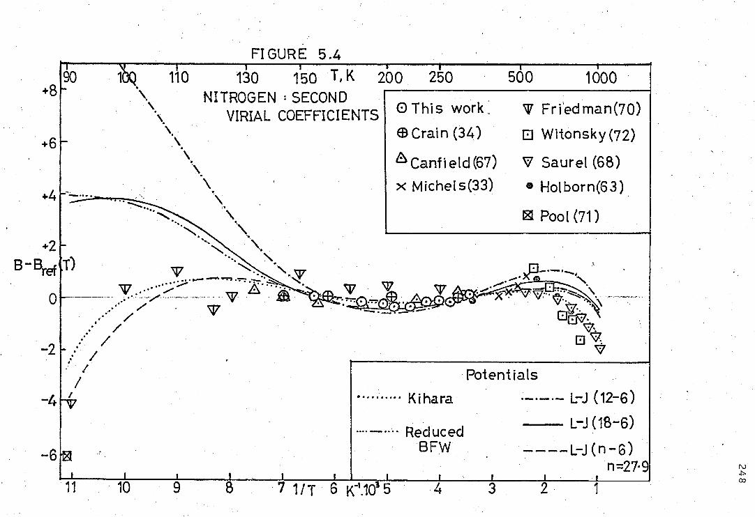
NITROGEN SECOND VIRIAL COEFFICIENTS

FIGURE 5.4 110 130 150 T, K 200 250 500 1000

0 This work Fri'edman(70) ED Crain (34) 0 Witonsky (72)

Canfield (67) 7 Saurel (68) x Michels(33) ® Holborn(63)

El Pool (71)

7

V Potentials

Kihara •-•---•- L-J (12-6)

Reduced L-J (18-6) BFW ----L-J (n-6)

n=27.9 8 7 11 T 4

FIGURE 5.5 1

210 250 300 11 1K 400 500 ETHANE : SECOND VIRIAL COEFFICIENT

• •

.N

•

- X 0 /

O Reamer(88)

X Michels(87) .6, Hoover (50)

Potentials

LJ(12-6) LJ (16-6) ----LJ (n=6)

n=26.6

•••••••• Kihara +2 A

B-Bref(T) 0

4 1/T lc' .103 3

250

TABLE 5.2

Coefficients of Equation fitted to Experimental Second

Virial Coefficients

B = Al + A2/T + A3/T3 + A4/T

Al A2

•

A3 A4

Methane 51.40118 -25.1267 -0.298517 -0.0107310

Nitrogen 45.04587 -13.8035 -0.115836 -0.0047443

Argon 37.8635 -15.0738 -0.0911234 0.00170569

Ethane 72.8718 -50.2603 -3.87578 0.445202

Propane 98.9303 -86.7161 -6.17915 0.266462

n-Butane 240.617 -225.079 4.89262 -3.15465

251

TABLE 5.3

Comparison of Pair-Potential Parameters

ARGON L-J 18-6 L-J n-6 Kihara

6/k)K Vow 6/k,K cr,,,,,i n e/kiK 'Cr, ' ' This work 160.3 .3264 166.4 .3240 19.1 160.8 .3259 .153

(144.4 .3332 0.1)

Hanley and Klein (108) 161.2 147.5 16 140.8 0.1

Dymond, Rigby and Smith(111) 160.3 .3277

Lin and Robinson (114) 161.7 .3259 .155

Tee, Gotoh & Stewart (116) 146.5 .3317

Rossi and Danon (117) 140.4 .3101 .089

Barker, Fock & Smith (118) 142.9 .3363 .1

Sherwood and Prausnitz (119) 147.2 .3314 .125

Calvin and Reed (120) 169.8 .3225 20.0

Weir et al. (18) 163.7 .315 .164

METHANE

This work 199.6 .3640 228.1 .3561 22.9 209.2 .3614 .177 Ahlert, Biguria & Gaston (121) 218.0 .3568 21.0 Sherwood & Prausnitz (119) 204.3 .3620 Tee, Gotoh & Stewart (116) 227.1 .3565 Hoover (50) 207.5 .3633

NITROGEN

This work 127.8 .3571 159.9 .3449 27.9 139.4 .3528 .197 Calvin and

Reed (120) 133.4 .3532 19.3 Sherwood and Prausnitz (119) 139.2 .3526 Tee, Gotoh & Stewart (116) 96.3 .3694 0.0

25 2

TABLE 5.3 (continued)

ETHANE L-J 18-6 L-J n-6 Kihara

6/k , K ac, mi 6/k , K cr ruiA n Elk cr,;,.., r This work 227.1 .4605 347.1 .4375 27.9 319.8 .4427 .211

Hoover (50) 352.0 .4116

Tee, Gotoh & Stewart (116) 496.7 .3504

253

potential parameters of nitrogen and methane, and the results

of Hanley and Klein (108) for the L-J (n-6) potential

parameters of argon. With the three-parameter potentials

a wider spread of values of 6/k and C are obtained because

of the greater flexibility introduced into the model by the

extra parameter. It is noticeable that the sets of Kihara

potential parameters for argon are of two types; one with

0.1, one with y•-•-•.: 0.15. Setting y = 0.1 and repeating

the least-squares fit, varying the other two parameters,

gives a very similar result to that shown in figure 5.2.

If the low-temperature argon data of Weir et al (18) and

Byrne et al (55) are not included then a much lower value

of €/k results (about 150 K for the L-J (18-6) potential).

The larger differences in the case of ethane are

mainly due to the lack of accurate low-temperature virial

coefficients.

5.3 Multiparameter Pair Potentials

There have been several attempts to determine the true

pair potential of a gas by use of multi-parameter potential

models or non-analytic forms of the potential. Nearly all

of this work has been confined to argon, and the most

successful of the recent investigations appear to be those

of Barker and co-workers (122- 125).

Barker and Pompe (122) chose the following form for the

potential,

, L Eczi+08 .,..L.6) 2

0-9E -

i=) i=0

U(R) =. E

(5.3-1) where r = R/Rm R = molecular separation

L = 3

Rm= value of R at minimum of U(R)

254

5 was taken as very small and was included to prevent

a spurious maximum in U(R) at small separations. The

values of C6, C8 and C10 were found from the theoretical

values of the dispersion energy coefficients. High energy

molecular beam measurements, which give information on the

potential at small values of R, and second virial coefficient

data were then used to obtain the remaining parameters.

Several sets of parameters were obtained, and one chosen

on the basis of a comparison between experimental and

calculated static lattice energy and zero-point energy of

the crystal at 0 °K. These calculations required an

assumption about the significance of non-pairwise additive

forces (three-body and n-body forces), which is discussed

in section 5.3 in the section on third virial coefficients.

The potential of Barker and Pompe was later modified

by Barker and Bobetic (123) to also give excellent agreement

with the experimental specific heat and thermal expansion

of crystalline argon below 12 °K. The same potential was

found to predict closely the transport properties of gaseous

argon (124), i.e. viscosity, thermal conductivity, self-

diffusion coefficients and thermal-diffusion. To obtain

good agreement between calculated and experimental thermo-

dynamic properties of liquid argon, Barker, Fisher and Watts

(125) derived a new potential which is a linear combination

of the Barker-Pompe and Barker-Bobetic potentials. This

third potential (BFW) also agreed with the spectroscopic data

on the Art molecule (127), which gives information on the

magnitude of the well-depth,E and it also gave unchanged

or sometimes improved agreement with the properties of the

gaseous and solid states.

255

(a) The Reduced Barker-Fisher-Watts Potential

Argon, methane and nitrogen are known to obey fairly

closely the principle of corresponding states (3), which is

discussed in more detail in Chapter 6. To conform to the

principle of corresponding states the pair potential of each

substance must be of the form,

U«(R) = fa Uo(R/g2) (5.3-2)

where Uo(R) is the pair potential of a reference substance

(in this case taken to be argon), and f and ga are the

scale factors for substance m,

f Ea Cr& a (5.3-3)

60 oro

The second virial coefficient is then given by

B«(T) = 9« .BO(.0a) (5.3-4)

The applicability of the BFW potential to methane and

nitrogen was investigated through the assumption of the

principle of corresponding states, i.e. that (5.3-4) is

valid.

The Barker-Pompe (BP) and Barker-Bobetic (BB) potentials

for argon are both of the form given in (5.3-1), with

constants given in Table 5.4. The BFW potential is,

(---"UBFW ‘4 75 UBB • 25 UBp (5.3L5)

The resultant parameters are,

6/k = 142.095 K 0

Rm = 3.7612 A

Ro = 3.3605

(5.3-6)

TABLE 5.4

The Barker-Fisher-Watts Potential for Argon

Constants of Equation

Barker-Pompe

(5.3-1)

Barker-Bobetic

€/k, K 147.70 140.235

Rm' nm .37560 .37630

Ro' nm .33410 .33666

Ao 0.2349 0.29214

Al -4.7735 -4.41458

A2 -10.2194 -7.70182

A3 -5.2905 -31.9293

A4 0.0 -136.026

A5 0.0 -151.0

C6 1.0698 1.11976

C8 0.1642 0.171551

C10 0.0132 0.013748

a 12.5 12.5

5 0.01 0.01

T,K

TABLE 5.5

Second Virial Coefficient for the BFW Potential

B,cc.mole-1 T,K B cc.mole-1

75.0 -317.3 223.15 -38.31

84.03 -255.4 248.15 -29.24

89.57 -22t.7 273.15 -22.11

97.69 -193.2 323.15 -11.68

102.79 -176.08 373.15 -4.47

113.97 -145.95 423.15 +0.79

128.15 -117.86 473.15 +4.77

143.15 -95.98 573.15 +10.33

163.15 -74.77 673.15 +13.97

183.15 -59.24 773.15 +16.50 203.15 -47.52 873.15 +18.32

1073.15 +20.72

2 56

257

Unfortunately, the calculated virial coefficients for

none of these three potentials have been presented in a

usable form. Therefore the second virial coefficient of

argon for the BFW potential, with first quantum correction,

was calculated by direct numerical integration of

equations (5.1-15)and(5.1-18). A standard computer program

employing Simpson's Rule integration was used. The range 0

of integration for each temperature was from 0.01 A to

30.01 A, giving the classical second virial coefficient to

an accuracy of about 0.03 cc/mole from 163.15 K to 1273.15 K,

and to an accuracy decreasing at lower temperatures to about

0.2 cc/mole at 75 K. A much smaller range of integration, 0

usually up to 8 A, was sufficient for the first quantum

correction. The values-so obtained are presented in Table 5.5,

the reduced temperature and second virial coefficient referring

to,

kT ciNt T = e u - zr4 7r NR (5.3-7)

In figure 5.2 the deviations from the experimental

second virial coefficients are presented. The fit is, on

the whole, reasonable, but the calculated values tend to be

too negative above 140 K as compared with the majority of the

data.

The second virial coefficients of argon for the BFW

potential were then fitted to a polynomial in 1/T,

Bo + at a3 a4 ac TS T4 (5.3-8)

which was taken as the reference equation for use in (5.3-4),

This equation can safely be extrapolated to slightly higher

temperatures but not to lower temperatures.

The experimental second virial coefficients of methane

and nitrogen were then fitted by the equation,

B(T) = e . B0 (i/f) (5.3-9)

The resultant parameters, g3 and f, are given in

Table 5.6, together with the coefficients of equation (5.3-8).

The deviations between the calculated and experimental

virial coefficients are shown in figures 5.3 and 5.4. The

agreement is good except perhaps at low temperatures for

methane. Part of this discrepancy is due to the larger

quantum corrections for methane; the quantum corrections

should not really be included in this corresponding states

treatment. However, this introduces only a small error.

Most of the discrepancy is due to the fact that the BFW

potential gives values that are more negative in the mid-

temperature range than the experimental values of argon,but

reasonable values at low temperature. When the equation

in its reduced form (5.3-9) is fitted to methane data, it

gives a good fit to the data of Douslin et al (32) in the

mid-temperature range, and hence values of B that are too

positive at low temperature. The actual experimental

virial coefficients of methane and argon show, in fact,

much better agreement with the principle of corresponding

states than is apparent from figure 5.3.

To fully test the applicability of the reduced BFW

potential, (5.3-9) to methane and nitrogen, it would be

necessary to compare experimental and calculated values of

258

Methane Nitrogen Argon

g3 1,4060 1.3266 1

f 1.2226 .7836 1

6/k, K 173.7 111.3 142.1

a, nm .3765 .3693 .33605

Polarizability,X .00260 .00176 .00163 (nm)3

Parameters of ref-erence equation

a1 31.84649

a2 -1.000638.103

a3 -1.48933 .106

a4 6.76968 .107

a5 -3.55104 .109

259

TABLE 5.6

Parameters of Reduced Barker-Fisher-Watts Potential

TABLE 5.7

Dispersion Energy Coefficients

Calculated, (Dalgarno)

11 , 10-79.J.m6

Argon Methane

143

Nitrogen

70

reduced BFW 61.3* 148 84

L-J (12-6) 112.0 255.0 144.5

L-J (18-6) 69.5 166.5 95.0

L-J (n-6) 65.8 139.9 72.1

* Calculated, Leonard (126)

2"60

a range of thermodynamic properties as considered by

Barker et al. for argon. Here the comparison is confined

to the third virial coefficients, presented in section 5.5(b),

and the dispersion energy coefficients.

The dispersion energy coefficient, i.e. the coefficient

of r-6 in the long-range part of the potential, may be

calculated by the methods of quantum- mechanics, and recent

estimates are believed accurate to within a few per cent.

In Table 5.7 the calculations of Dalgarno (128) are compared

with those for the reduced Barker-Fisher-Watts potential, the

L-J (12-6), L-J (18-6) and L-J (n-6) potentials.

The dispersion energy coefficient for argon from the

BFW potential was set equal to the calculated value of

Leonard (126),

i.e . E . C6 61.3 . 0-60 erg.cm6 (5.3-10)

Therefore the coefficient for methane or nitrogen is

given by

= fa ga6 60 . 61-3.10 erg.cm6 (5.3-11)

The coefficient for the (n-6) potential becomes,

from (5.2-1)

= (6/n)(1 6

.cr

(I - 4) (5.3-12)

It can be seen, from Table 5.7, that the (L-J) 12-6

potential gives values that are much too high, and the (18-6)

potential gives values that are much nearer the theoretical

values, and in the case of argon the agreement is good.

21

The reduced BFW potential is superior in this respect, giving

very good agreement, especially for methane.

Recent new measurements of low-energy molecular beam

scattering in the Ar/Ar system (129) and a re-analysis of

the vacuum-u-V absorption spectra of Ar2 (130) have both

shown that the pair potential of argon appears to be close

to that of Barker, Fisher and Watts in both shape and size,

e.g. within 0.5% of the value of E/k.

However, all of these potentials give values of the

second virial coefficients that tend to be more positive

than the experimental values at low temperature (e.g.

7-10 cm3.mole-1 at 100 K): this discrepancy is yet to be

explained. It is a possibility that part represents

experimental error on the virial coefficients, (18) (55);

for methane the results of Byrne et al. (55) appear to be

more negative at low temperatures than those of this work

and of Brewer (54) (see section 4.5(a)).

5.4 Anisotropic Potential of the Nitrogen Molecule

It has been shown (131) that for a molecule which is

non-spherical or anisotropic the intermolecular potential

is the sum of an angle-independent term and several terms

which depend not only on the separation between the

molecules but also on their relative orientation. For a

molecule such as nitrogen which possesses zero dipole moment

262

but a significant quadrupole moment, Q, the intermolecular

potential is given by,

U = U(spherical) + U(anisotropic) + U(q-q) (5.4-1)

+ U(q-lui) + U(shape)

where U(spherical) is the centrally-symmetric potential.

U(anisotropic) is the effect of anisotropy on the long-

range dispersion forces.

U(q-q) is the quadrupole-quadrupole interaction.

U(q-µi) is the quadrupole-induced dipole interaction.

U(shape) is the effect of anisotropy on the short-

range exchange forces.

To the first order, the second virial coefficient is given by

B = B(spherical) + B(anisotropic) + B(q-q) (5.4-2)

+ B(q-pi) + B(shape)

The largest of the extra terms is usually due to U(q-q),

which is proportional to Q4 and r-5. The above terms have

been calculated (132) and applied to the determination of Q

from second virial coefficients by Orcutt (133). Unfortunately,

the L-J (12-6) potential was assumed for U(spherical) and this

gives a poor representation of B(spherical) for the isotropic

argon molecule. The potential parameters were determined

from viscosity data, which are less sensitive to anisotropic

effects, and from the differencebetween B(experimental) and

B(spherical) IQ' was estimated to be 1.90.10-26 esu.

A much better estimate of Q is obtained from experimental

measurements which do not require an assumed form for the

263

central potential, such as induced birefringence measurements,

which give 1Q1 = 1.52.10-26 esu (134). This is much

closer to the results of quantum mechanical calculations,

which give 1Q1 = 1.36.10-26 esu (135).

Adjusting the results of Orcutt for these new values of

Q has the effect of reducing considerably the total con-

tributions to B of the anisotropic terms, which are very

sensitive to the magnitude of Q. For instance,

AB

T = 123.5 K T = 274.5 K

Q = 1.90 -12.1 cm3.mole-1 -2.7 cm3.mole-1

Q = 1.52 - 6.0 cm3.mole-1 -1.4 cm3.mole-1

Q = 1.36 - 4.4 cm3 .mole-1 -1.0 cm3.mole-1

These values are still specific to the L-J (12-6)

potential but are probably of similar magnitude for the

other potentials. The contributionsto B are still quite

significant but the uncertainties in the calculations and

in the magnitude of Q are such that little accuracy is

gained in the estimation of the potential parameters of

nitrogen if these contributions to B are first subtracted.

5.5 Third Virial Coefficients

The potential energy of interaction between three

molecules (the three-body potential) may be written as the

sum of pairwise additive terms plus a non-additivity

correction,

U(r12 r23 r31) = U(r12) + U(r23) + U(r31) + Au(r12, r23 r31)

(5.5-1)

where r12, r23 and r31 are the lengths of the sides of the

triangle bounded by the three molecules.

The total third virial coefficient can be shown by the

methods of statistical mechanics (2) to be the sum of a

pairwise additive and a pairwise non-additive part,

C = Cadd AC (5.5-2)

where,for spherically symmetric potentials,

Cadd = - 8 7r2 Nglfp 4 4 12 '23 '13 r r r 12 23 13 12 G 23 (5.5-3)

AC = _ 8 7r2 1\1,,fffi e-AU123/ki 3

( U12+ U23+ U.13 VICT

r12 r23 r13 dri2 dr23 dri3 (5.5-4)

where f12 = e-u(r12)/kT-1, etc.,

and the integration extends over all values of r12, r13 r23 7

which form the sides of a triangle.

Comparisons of theoretical calculations of the third

virial coefficient with experimental values have often been

inconclusive because of the uncertainty surrounding the

nature of the non-additive contribution. At long-range

intermolecular separations the major contribution to non-

additivity arises from the Axilrod-Teller (136) triple-

dipole, dispersion interaction, which for spherically

symmetric potentials is,

264

Lu123 = vi (.3c001 cos02 cos03 4-

r r)3 12 23 2

(5.5-5)

where 01' 02 and 03 are the interior angles of the triangle

265

bounded by r12, r13 and r23, and v123 is a non-additive

dispersion coefficient, given to a good approximation for

a pure gas by

123 3

— 4 a L' (5.5-6)

where a = polarizability

µ = dispersion energy coefficient of the pair potential.

Sherwood and Prausnitz (137) showed that the non-

additive contributions to C due to this interaction are by no

means negligible, amounting to almost half of the total

third virial coefficient in the vicinity of its maximum.

At small intermolecular separations there is non-

additivity due to short-range, three-body exchange forces (or

triple-overlap interactions). These are difficult to

calculate exactly, but calculations have been made by Sherwood,

De Rocco and Mason (138), and by Graben, Present and McCulloch

(139) based on the approximate theory of Jansen (140).

They concluded that the contributions from three-body exchange

forces tend to cancel the contributions from the triple-

dipole dispersion forces. However, the theory of Jansen is

now believed to greatly over-estimate the magnitude of the

three-body exchange forces, a conclusion arrived at by

Barker and Pompe (123).

As described in section 5.3, Barker and Pompe obtained

a range of two-body potential functions, of the form given

by (5.3-1), which were all equally successful in fitting

the data for argon on properties dependent on pair-

interactions only. The calculated third virial coefficients

for all of these potentials agreed within 10% of the

266

experimental values, which was estimated as just outside the

experimental error, when the triple-dipole non-additive

contribution was included. It was concluded that the effect

of other non-additive interactions on the third virial

coefficient must be small, especially as they would be

expected to be sensitive to the exact form of the pair

potential. On the assumption that all non-additive forces

other than the three-body dispersion forces could be

neglected, Barker et al. obtained excellent agreement between

experimental and calculated values of a wide range of

thermodynamic properties of gaseous, liquid and solid argon

(see section 5.3). This was support for the validity of

the aforementioned assumption.

Dymond and Alder (141) have attempted to calculate the

magnitude of the three-body non-additive forces by direct

subtraction of Cadd from the experimental third virial

coefficients, where the former was calculated for their

numerically tabulated pair potential of argon (142). To

obtain the experimental values of C, they 'reanalysed' the

PVT data of Michels et al (81, 82) by using theoretical

values of second, fourth and fifth virial coefficients and

calculating C by difference. This method is highly subject

to error, however, as a small difference between the

calculated and experimental value of B will lead to a large

error in C. Their values lie some 100 - 200 cc3/mole

below those given in Chapter 4. Even so, it appears that,

except perhaps at very small intermolecular separations, the

three-body exchange forces may be neglected. Therefore for

the purposes of calculation of the third virial coefficient

= (2/37Noal

Cadd —( 2.11)

cn . (T*) Cadd

no

n=0

(5.5-7)

267

for the potentials considered here, no corrections for

non-additivity were included other than those for the

triple-dipole dispersion interaction.

(a) Third Virial Coefficients for Simple Potential Functions

If the neglect of three-body non-additive interactions

other than that given by (5.5-5) is accepted as a valid

assumption then by a comparison of theoretical and

experimental third virial coefficients further information

may be obtained on the approximation of a simple pair

potential function to the true pair potential. This is

important for gases such as methane and nitrogen, for which

there have been no systematic attempts to determine a true

pair potential as there have been for argon.

The models considered here are the Lennard--Jones and the

Kihara spherical core potentials. For the L-J (12-6) potential

the third cluster integral (5.5-3) has been evaluated by

expansion as a series in (T*) 2 (143, 144),

where T* = kT 6

For the calculations of this thesis the more recent

results of Stogryn (145) have been employed, where the series

expansion method was used for evaluation of both C*add and LC*,

where

co - (n + 3/2.)

v*E en (e) 2 n=0

a r3

(5.5-8)

(5.5-9)

268

c (n=1 ... 27) and c'(n=1 ... 22) are presented in

(145). The results are believed accurate to 0.1% at T* = 0.5

and to higher accuracy at higher temperatures.

Similar calculations have been carried out by Stogryn (146)

for the L-J (18-6) potential, the series expansionsbeing,

00

add =

(2n3+ 1)

"-add

(5.5-10) n.10

- (4n+ 5) AC* = v*E en • (-09 -6- ( 5 . 5-11)

n

o

and c' for n=1 to 20 are presented in (146) and

the results are believed accurate to about 0.3% at T* = 0.5.

Unfortunately as yet no calculations have been performed

for the three-parameter L-J (n-6) potential.

Values of C*add and AC*/p* for the Kihara spherical core

potential have been tabulated by Sherwood and Prausnitz (119)

at discrete values of a* from a* = 0 to 0.85. All calculations

were performed by numerical integration.

First quantum corrections to C have been calculated for

the L-J (12-6) potential only (147). Values for methane

turn out to be 110 cm6/mole at 150 K and 16 cm6/mole at 200 K.

These are within the present limits of experimental error and

so quantum corrections were neglected throughout.

(b) Third Virial Coefficients for the Reduced BFW Potential

The principle of corresponding states requires that

and

•

C (T)add

AC(T)

DC (T)

96 Co (11f)add (5.5-12)

= V*g6.6,C0(M) (5.5-13)

= 5:k 93 ) o (5.5-14)

269

where Cadd(T) and ACo(T) refer to the additive and non-, o

additive contributions to the third virial coefficient of

argon for the Barker-Fisher-Watts potential. These were

read to the nearest 50 cm6 mole-2 from figure 7 of (122).

_•- (c) Results of Comparisons

Third virial coefficients calculated according to the

methods described in 5.5(a) and (b) are compared with the

selected experimental values of Chapter 4, for methane

(figure 5.6), nitrogen (figure 5.7) and argon (figure 5.8).

The potential parameters used were those obtained by a fit to the

second virial coefficients, as listed in Table 5.1. Values

of the polarizability, a, were taken from (148) and are given

in Table 5.6. For the reduced BFW potential, the values of

g3 and f are those determined in section 5.3(a)'and given in

Table 5.6.

It is apparent from figures 5.6 - 5.8 that the L-J (12-6)

potential, which provides an inadequate fit to second virial

coefficients, gives third virial coefficients that are too

high for all gases when the triple-dipole non-additive

term is included.

The L-J (18-6) potential gives third virial coefficients

for argon which are close to those of the Barker-Fisher-

Watts potential, and are from 100 to 300 cm6.mole-2 smaller

than the experimental values. For methane and nitrogen the

results for the reduced BFW potential and the L-J (18-6)

potential are also close and in good agreement with experiment.

The Kihara potential generally gives values of C that

are higher than those of the L-J (18-6) and BFW potentials,

500 600

FIGURE 5.6

Calculated : Potentials L-.J (16-6 ) (total)

— L-J(16-6)(pairwise additiA — Reduced BFW (total)

•—•— L-J (12-6) (total)

METHANE : THIRD VIRIAL COEFFICIENT

1000 I I I I

100 200 300 T, °K 400

•

5000

4000

3000- C

(cc/mole)4

2000 -

•••••

WM. • •••• • •••••• •

• • • Om. • 4•••• • ••••••1•1

Experimental

0 This work x Douslin et al (32) 0 Schamp et al (42) E Mueller et al (49)

FIGURE 5.7

NITROGEN : THIRD VIRIAL COEFFICIENT

•I=M. ,11•0 •••• ••••

•••••••••••••••

•••••••••41.1MOWW...0

Calculated: Potentials L-J (18-6) (total )

L-J (18-6) (pairwise additive)

Reduced BFW (totat)

L-J (12- 6) (total )

Experimental O This work • Crain (34 ) &Canfield (67 ) x Michels(33 ) • Saurel (68 ) ® Holborn (63 )

• Onnes (65) •

03 Pfefferle (73 )

2

' 3000

C cc/ mole mole)

2000

• •••••• • ••••••

• ••••• • ••••• • ••••• • •••••••• ••••• •••••

• •••••• • own.. • ••••••• ••••• •••••• • •••••• • ,•••

5- r• ••••• 0 •••• 1••••

x 1000 I

100 200 300 400 Temp. S00 K 600 700 900 800 1000

FIGURE 5.8

3000

2500 C

(ccimole

2000

ARGON = THIRD VIRIAL COEFFICIENT.

Calculated Potentials Experimental L-J (18-6) (total) Crain (34 )

•••11MB =NM •••• L-J(18-6) X Michels(36,37) (pairwise additive) Provine(83)

• • • • •••••• • • • • 1•••I

• *lama • a/. • ,•••••

Barker, Fisher,Watts (125), ® Holborn (85 )

L-J (12-6) (total) 0 Whalley (84 )

1500

1000 deo ••••••

\.)t N N. x ❑

•••• •• •••• • ••••• • 4.... • ....a • •••••

*

x 55 cl

•

• •••• • • •••• • •,••

••••• • •••• ••••

••••••• MM. num. ...gm

••••• ••••••m, •••• •••=m, I•••• •••••••• • ••••••• •••••• ••••••

100 200 300 Temp., K 400 500 600 500

273

although in good agreement with experiment for argon and

nitrogen, but not for methane. There is some difficulty

in calculation of LC* for a potential such as the Kihara that

instead of a r-6 term has a (r-a)-6 term, as mentioned by

Sherwood and Prausnitz (119).

(d) Conclusions

It has been shown that the Barker-Fisher-Watts potential

(125), which is probably close to the true pair potential of

argon, can be applied, in a reduced form, to the successful

calculation of third virial coefficients of methane and

nitrogen. It must be assumed, as with argon, that non-

additive contributions other than those due to triple-dipole

dispersion forces are small. This reduced BFW potential

also gives good agreement with the theoretical value of the

dispersion energy (r-6) coefficient. It would be interesting

to investigate further the applicability of this potential

by comparison of calculated and experimental values of all the

thermodynamic and transport properties of methane and nitrogen

that were considered by Barker et al. for argon. This task

will not be attempted here.

It has also been shown that a simple analytical form of

the pair potential, viz the Lennard-Jones (18-6) potential,

is capable of giving good agreement with both second and third

virial coefficients of argon, methane and nitrogen. It has

been shown elsewhere to give a good fit to the experimental

second virial coefficients of krypton and xenon (13). The

dispersion energy coefficients are also in reasonable agreement

with the theoretical values. Thus it is possible that the

L-J (18-6) potential offers a convenient approximation to the

274

true pair potential for simple spherically-symmetric

molecules, at least in the range of intermediate inter-

molecular separation. This is important because by the

use of a pair potential of simple analytical form the

calculation of other thermodynamic and transport properties

of the fluid is simplified. Although they give a slightly

better fit to second virial coefficients, the three-

parameter L-J (n-6) and Kihara potentials would offer no

advantages over the L7J (18-6) potential in this application.

5.6 Second Virial Coefficients of Mixtures

The interactional second virial coefficient, B12, is

given by, 00

B12(.0 = 2r (1 - e u (r12Vkl. rs d r,, ( 5.6-1) 0

where U(r12) is the intermolecular potential energy of

interaction between a molecule of type 1 and a molecule of

type 2 separated by a distance r12. B12 can be calculated

for the potential models of section 5.2, requiring values for

the interaction parameters E12, C12 and n12 (or y12). (For

the L-J (18-6) potential n12 is, of course, equal to 18).

These parameters were obtained for the L-J (18-6),

L-J (n-6) and Kihara potentials by a non-linear least-

squares fit to the, experimental values of B12 for the mixtures

methane/nitrogen, methane/argon, argon/nitrogen and methane/

ethane.

The final parameters are shown in Table 5.8 (columns 1

and 2). The experimental data for these mixtures have been

presented in Chapter 4. The L-J (12-6) potential was not

275

considered because of its inability to fit the second virial

coefficients of the pure gases.

For a given potential energy function, the values of

12 and E12 required to predict B12 are usually estimated from

the known like-interaction parameters by means of "combining-

rules", the simplest of which is 7

Rule 1 :

triz. = 1/2 (CI

1 • 4 E12. = (Ell a

—22/

(5.6-2) is the Lorentz rule of additive diameters,

which is exact for hard spheres, and (5.6-3) is the

geometric mean rule of Berthelot.

Many alternatives to the geometric mean rule have been

proposed,

Rule 2 :

among which two of the more successful are,

Ell = 2E11E2.2i( E + E22) ( 5 . 6-4 )

3 / \a. Rule 3 : 612. = (Ell 67.2.)

0, k) (5.6-5) cr2.2.] [

Ii+ To.

where I is the ionization potential.

Rule 2, the harmonic-mean rule, was found to be the most

successful by Lin and Robinson (149) in the application of the

Dymond-Alder potential (142) to rare gas pairs not containing

helium. For krypton and xenon Pollard (13) found that none

of the rules tested was particularly successful, but that

rules 2 and 3 were preferable. Rule 3 is based on the

London formula for dispersion forces, and Rule 2 is loosely

based on the Kirkwood-Mtller formula for the same forces.

276

Recently it has been shown by Good and Hope (150) that

the form of the L-J (n-6) potential function suggests, on

theoretical grounds, that the Lorentz rule of additive

diameters should be replaced by a geometric mean rule,

criz = (irit cr22 (5.6-6)

On this assumption, Calvin and Reed (120) found the

following rules successful in predicting B12 of seven mixtures,

including methane/ethane and nitrogen/argon, using the

rules and least-squares fitting using

the (n-6) potential, n12 was set at the value given by

(5.6-8). For the Kihara potential, assumption of the

Lorentz rule of additive diameters requires that

Yiz =

(5.6-9) +622.

For all tests and least-squares fitting, y12 was set

equal to the value given by (5.6-9).

In Table 5.8 are shown the values of 612 and E12 from

the full least-squares curve-fitting (columns ,1 and 2), and

in column 3 the values of n12 or Y12 given by equations (5.6-8)

or (5.6-9). In column 4 the value of 612 given by the rule

of additive diameters, (5.6-2), is shown. With 612 fixed at

this value, further least-squares fits to the data were

carried out, and the resultant parameter e12 is shown in

column 5. This value of 12 was then used to determine the

L-J (n-6) potential.

Rule 4 : Ell =

n 12 =

For tests of all

E2.2)4 En

4 C ntt n22 )

(5.6-7)

(5.6-8)

277

TABLE 5.8

Potential Parameters for Binary Systems

Methane/Nitrogen

. a'12 el2A

(Full least- squares fit)

n12

(or yi)

X12 6124 (A.M. rule + least-squares

fit)

k12

L-J (18-6) .3655 152.5 .3605 155.0 .030

L-J (n-6) .3537 183.7 25.2 .3505 185.6 .028

Kihara .3600 164.2 .187 .3571 165.8 .029

Methane/Argon

L-J (18-6) .3414 181.3 .3457 178.7 .001

L-J. (n-6) .3294 202.9 20.9 .3397 193.7 .006

Kihara .3350 189.7' .166 .3436 182.5 .005

Argon/Nitrogen

L-J (18-6) .3436 143.2 .3418 144.2 -.007

L-J (n-6) .3353 164.7 23.1 .3343 165.2 -.012

Kihara .3403 150.6 .176 .3394 151.0 -.009

.0.

Methane/Ethane

L-J (18-6) .4012 243.5 .4123 234.7 .002

L-J (11-6) .3841 297.0 25.2 .3947 286.2 -.017

Kihara .3897 270.9 .196 .4020 259.7 -.004 I

278

geometric-mean correction factor, k12, where

(I - km) (E11 Ezz)1/2

(5.6-10)

The values of k12 are shown in column 6.

In Table 5.9, the values of E12 given by Rules 1 - 3 are

presented, and, in column 4, the value of E12 from the

least-squares fit (from column 5 of Table 5.8). It is

apparent that for methane/nitrogen and nitrogen/argon T12 given by (5.6-6) is similar to that given by (5.6-2), and

Rule 4 is identical to Rule 1. For methane/argon and

methane/ethane they are only slightly different.

Because most of the mixture data covers only a limited

temperature range, the potential parameters obtained from

the least-squares fit are not determined accurately, particularly

for the more flexible three-parameter potentials. A more

realistic test of the combining rules than a comparison of

the values given in Tables 5.8 and 5.9 is the direct

comparison of the calculated and experimental values of B12.

Any rule must be regarded as acceptable if B12 can be

predicted within experimental error. These comparisons 12-

are shown in Figures -

Figure 5.9 : Methane/Nitrogen.

The results for each rule are virtually independent

of the potential model; those for the L-J (18-6) potential

are shown. Rule 2 is good, but Rules 1 (and 4) and Rule 3

both. give B12 values that are too negative.

Figure 5.10: Nitrogen/Argon.

The results for all rules are very similar. Those for

279

TABLE 5.9

Combining Rules

elq, 0.12 given by arithmetic mean rule)

Rule 1 Rule 2 , Rule 3 .Least -squares value

Methane/Nitrogen

L-J (18-6) 159.7 155.8 158.9 155.0

L-J (n-6) 191.0 188.0 190.1 185.6

Kihara 170.8 167.3 170.1 165.8

Methane/Argon

L-J (18-6) 178.9 177.8 176.5 178.7

L-J (n-6) 194.8 192.4 192.6 193.7

Kihara 183.4 181.8 181.1 182.5

Argon/Nitrogen

L-J (18-6) 143.1 142.2 142.2 144.2

L-J (n-6) 163.1 163.1 162.6 165.2

Kihara 149.7 149.4 148.9 151.0

Methane/Ethane

L-J (18-6) 235.1 231.8 - 234.7

L-J (n-6) 281.4 275.3 - 286.2

Kihara 258.7 252.9 - 259.7

-100

Combining Rules - Rule 1 L-J(18-6)

300 150 200 Temp, K 250

METHANE /NITROGEN INTERACTIONAL SECOND

VIRIAL COEFFICIENTS

0 This work

Brewer(54)

.6, Keyes (75)

I

-20

-40

Biz cc/m

-60

-80

--- --Rule 2 —•—.— Rule 3

FIGURE 5.9

280

ARGON/NITROGEN INTERACTIONAL SECOND

VIRIAL COEFFICIENT

Brewer (90 )

LS Crain (34)

Combining Rules

Rule 1 L-.1(18-6)

Rule 2,3

FIGURE 5.10

281

-20

- 40

Biz cc/mole

-60

—80

-100

150 200 Temp. ,K 250

300

300 100 150 Temp, K 200 250

282

FIGURE 5.11

METHANE I ARGON INTERACTIONAL SECOND VIRIAL COEFFICIENT

o Byrne (55) 6 Thomaes(89 )

Combining Rules

Rule 1 , L-J(n-6)

•_•--• Rule 3 , L-J(18-6)

-20'

-40

-60

-80

-100

-120 B12

cc/mot -140

-160

-180

-200

-220

-240

-180

Rule 1

Rule 2

-2

350 250 Temp, K 300

METHANE/ ETHANE INTERACTIONAL SECOND

VIRIAL COEFFICIENT

O Michels (93 )

O Dantzter(94 )

.6 Hoover (50)

-140

-160 Combining Rules

- 40

- 60

- 80

-100 B12

cc/mole

-120

FIGURE 5.12

283

284

Rule 1 and Rules 2 and 3 for the L-J (18-6) potential are

shown. The results for the other potentials lie between

these two curves. In general, rules 1 and 2 are satisfactory

and rule 3 only slightly less so.

Figure 5.11: Methane/Argon.

The results are shown of Rule 1 for the Kihara potential

and Rule 3 for the L-J (18-6). All the other results lie

between these extremes, Rules 1 and 2 being satisfactory but

Rule 3 giving too positive values of B12.

Figure 5.12: Methane/Ethane.

Again, the results for a particular rule tend to be

independent of the potential. Those of Rules 1 and 2 for the

L-J (18-6) potential are shown. Rule 1 is the most

satisfactory and Rule 2 gives values that are slightly too

positive. Rules 3 and 4 are generally worse. Conclusions

are difficult for this system because of the low experimental

acccuracy at low temperatures.

For the systems studied here, Rule 2, the harmonic mean

rule is overall the most satisfactory, and Rule 1, the

geometric mean rule,almost as good except for the methane/

nitrogen system. For these relatively simple systems it is

unnecessary to introduce more complex rules such as Rule 3,

which involves ionization potentials.

The deviations from Rule 1, the geometric mean rule, are

conveniently characterized by the correction factor k12. Lt

can be seen from Table 5.8 that the value of k12 for a

particular mixture is independent of the potential model.

It is estimated that the experimental error in B12 sets a

285

maximum error in k12 of about .005.

Estimates of k12 have been obtained for a wide range

of mixtures by Chueh and Prausnitz (151) from a correlation

of gas mixture PVT data with the Redlich-Kwong equation of

state. In this case, k12 is defined from the critical

temperatures,

- k m) (T T c1. c )1/1 (5.6-11)

These values are in excellent agreement with ours for

methane-nitrogen (see Table 5.10) but are up to .02

larger for the other systems; the differences are still

fairly small, however. The negative values of k12 that

we obtain have no real physical significance but are simply

the result of fixing 0-12 to that given by the rule of

additive diameters, which is known to be only an approximation

for real molecules. A correlation of k12 for many mixtures

has recently been published (152).

The excess free energy and the excess volume of mixing

for liquid mixtures are very sensitive to the value of k12

assumed in a theory of liquid mixtures. A value of k12 can

be found that gives agreement between the theoretical and the

experimental excess property, and a comparison with the k12

from second virial coefficients is a severe test of the

theory of mixing in the liquid state. In Table 5.9 are

shown the results from two of the more successful recent

theories: the 'van-der-Waals one-fluid' model (153) and the

'van-der-Waals two-fluid'model (154). The relatively close

agreement is an indication of the usefulness of these models

in the prediction of the thermodynamic properties of natural

TABLE 5.10

Geometric-mean correction factors

This work (L-J(18-6))

Chueh and Prausnitz (151)

"Van-der-Waals one-fluid model" (153)

"Van-der-Waals two-fluid model" (154)

Methane/Nitrogen Methane/Argon Nitrogen/Argon Methane/Ethane

.030 .002 -.007 .002

.03 .02 .00 .01

.033 .002

.014 .021 .003

287

gas mixtures (see section 6.3).

For systems such as those studied here, where the

molecules do not differ greatly in size, k12 is relatively

small. Systems with large size differences, such as

CH4/C4F10, however, require values of k12 of about'0.1, and

there is evidence that this failure of the geometric mean

rule is mainly due to differences in size and not effects of

asymmetry or of different ionization potentials (152-).

When considering the prediction of the PVT properties

of mixtures, or of other thermodynamic properties of mixtures

the results are sensitive to the values of k12 assumed for

each binary interaction. At present it is difficult to

pre-determine k12 with sufficient accuracy unless there

exists accurate data on the binary mixture.

5.7 Third Virial Coefficients of Mixtures

The third virial coefficient of a mixture of N

components is given as a function of the mole fractions

x1, x2 ... by

.0 = EE:E: xi xi x (5.7_1) J k

where Cijk is given by (5.5-2), (5.5-3) and (5.5-4).

Calculations of Cijk for realistic intermolecular

potentials are limited. Stogryn (145) has presented

exact results for the Lennard-Jones (12-6) potential plus

corrections for the non-additive triple-dipole term. These

results were compared with those of the approximations of

Rowlinson, Sumner and Sutton (144) and of Orentlicher and

Prausnitz((155).. These approximations simplify the evaluation

of the integrals in the calculation by expressingCijk as a

288

function of the reduced third virial coefficient of one pure

component and the intermolecular potential parameters. The

approximation of Rowlinson et al is,

Ciik (T) = (2/3 7 N0 Ciir . C*( 10

where C*(Ts) = Ciii (T)/(2/3 ir N. cri 3)Z

Ti k = k I/€.0

3 and Eijk =Eij EikEik

The approximation of Orentlicher and Prausnitz is,.

C-k = (2/3 "0 )2 (IV • cl(Tii: ) • cjIt CIO (5.7-6)

where C*(T) is defined as in (5.7-3),Crijk is defined as in

. (5.7-5), and T*ij = kT/Eij (5.7-7)

Stogryn concluded that neither approximation could be

trusted to give accurate results in the vicinity of the

maximum of Cijk unless the potential parameters of molecules

1, j and k were not too different. At higher temperatures

both approximations are usually satisfactory, but that of

Rowlinson et al. is overall slightly superior.

Because of the failure of the L-J (12-6) potential to

provide a good fit to the second virial coefficients or to

predict the third virial coefficient of pure components,

comparison with experiment for mixtures will not be given.

In a later paper Stogryn (146) has presented results for the

L-J (18-6) potential based on the approximation of Rowlinson

= k T/ei

3 Crijk = C u. k

(5.7-2)

(5.7-3)

(5.7-4)

(5.7-5)

289

et al. ((5.7-2) to (5.7-5)) and a similar approximation for the

non-additive triple-dipole contribution. These are given

by expansions in powers of T*, (5.5-10) and (5.5-11),

where for mixtures,

* - T,;( = ki/6uk C k - C 1/(2/3 'IT No oil k (5.7-8)

and P4' 23/1 • Viik -.6V02.1c/(31/4 (fAU /AP fkik)4 (5.7-9)

where µ.j are the long-range dispersion energy coefficients,

i.e. 3/2. 6

= 3,2 (5.7-10)

and Vijk is a given function of µ..ij, a., etc.

C112 and C221 were calculated for methane/nitrogen

and argon/nitrogen, and compared with the selected

experimental data (see Chapter 4) in Figures 5.13 and 5.14.

The potential parameters were those given by,

cruz 0:22) (5.7-11)

E.12. = (1 — kiz).(11 Ezzr (5.7-12)

These are the values given in columns 4 and 5 of

Table 5.8.

For methane/nitrogen the agreement is within the limits

of experimental error, and for nitrogen/argon the agreement

is fair, the calculated values being too low as in the case

of pure argon and nitrogen. However, in view of the

probable large experimental errors in C112 and 0221, the

approximation of Rowlinson et al. (144) in conjunction with

the L-J (18-6) potential is successful in predicting the

third virial coefficients of these two systems.

This is further demonstration of the usefulness of

the Lennard-Jones (18-6) potential as a model for. the pair

potential.

290

4000—

FIGURE 5.13 METHANE/NITROGEN (1 = CH4 , 2= 1\12.

0 C112 This work ® C 221

INTERACTIONAL THIRD VIRIAL COEFFICIENT

EB Czzi C112 } Keyes (75 )

//

\\eal C 11 3000-1 • 2 Lennard Jones'(18-6) potential

• ED

022I (total)

(rcncoie)

2000

1000 150 200 Temp, K 250

D

••••••• 41M. amp. in.m.• 11••••• .11111.

300 350 400

►

►

•

e)2 • •

FIGURE 5.14

NI TROGEN/ARGON INTERACTIONAL THIRD VIRIAL COEFFICIENTS

3500

3000

(1=N2 , 2=Ar )

(3 C112 c221} Crain (34 )

2500

Ciij (cc/mo

2000

1500

1000

Cim C221

Lennard-Jones(18-6) potential (total)

250 I

300 100 150 Temp , K 200

293

CHAPTER SIX

THE PREDICTION OF ACCURATE COMPRESSIBILITY

FACTORS OF MULTICOMPONENT GAS MIXTURES

6.1 Introduction

There have been numerous methods proposed in the

literature for calculation of the compressibility factor of

a multi-component mixture such as a natural gas. A

division into two types is possible:

1) Methods which employ the principle of corresponding

states combined with the concept of "pseudo-critical"

constants for a mixture. These form the basis of the

majority of compressibility factor charts in use today and

tabulations such as the American Gas Association's comprehensive

correlation (156). The principle of corresponding states

has been modified and extended by, among others, Pitzer and

Curl (157) and Leland and his co-workers(158).

2) Methods which employ an empirical equation of state with

a different set of constants for each component of the

mixture. The best-known equations are those of Benedict,

Webb and Rubin (159) and of Redlich and Kwong (160). These

have since been modified and improved, in one way or another,

and there are many recent examples of their use.

6.2 The Principle of Corresponding States

The application of the principle of corresponding states

to the pair potentials of argon, methane and nitrogen has

been considered in section 5.3(a). A substance, a, is said

to be conformal with a reference substance, 0, if the pair

potential of substance a is given by

294

U(r) = fa .0 (r/ga )

(6.2-1)

where Uo(r) is the pair potential of the reference substance

and fa and are 'energy' and 'distance' scaling-factors

respectively.

All two-parameter pair potentials, such as the Lennard-

Jones (18-6) are of the type given by equation (6.2-1).

It follows, through a statistical-mechanical derivation

(3), that the equation of state of substance a, assuming

pairwise additivity, is

.. 3

P.gm fa

0m(PI V,T) = 0 V3 7 11;

ga

0 (6.2-2)

where 00(P,V,T) = 0 (6.2-3)

is the equation of state of the reference.

The factors a ga3 , and fa are identical to the 3 '

ga

ratios of the critical constants, Pmc

Pc

and Tac

Tc 7

0 c V 0

respectively, on the above assumptions.

Equation (6.2-2) may be written,

V T V

Vc Tca o Pc ' Vc

a a o

or Za = Z ( o c ' Vc T a

i.e. = Zo (TR- , a VR .)

0 (6.2-4) •

(6.2-5)

(6.2-6)

where T , VR are the reduced temperature and volume

295

respectively. Equations (6.2-4) to (6.2-6) are the

standard expressions of the principle of corresponding

states.

However, this two-parameter form of the principle of

corresponding states is not obeyed exactly by the majority

of substances owing to molecular dissimilarities in shape,

size, polarity, etc., and because of non-pairwise additivity.

Departures from (6.2-6) have often been considered by

including a third parameter, ,

Zm = Z (T

R VR )

(6.2-7)

The third parameter may be, among others, the

compressibility factor at the critical point, Zc, or

Pitzer's acentric factor, w (157), which is defined as

w = - log (P110 - 1.0 (6.2-8)

where PR is the reduced vapour pressure at TR = 0.7.

Substances which have the same three-parameter pair potential,

such as the L-J (n-6) or Kihara spherical core potential,

conform to (6.2-7).

Of the methods available for prediction of the

compressibility factor or a multi-component mixture, the

simplest is that based on the virial equation of state (161).

It has the advantage that the mixing rules are exact for

each of the virial coefficients. The principle of

corresponding states has often been utilized in the correlation

of experimental values of the second and third virial

coefficients. The most successful of those correlations

tested in this investigation were found to be those of

296

Pitzer and Curl (162),

C C BP = BZ = (0.1445 + 0.073w) (6.2-9) RTC VC

(0.33 - 0.46w) (

0.1385 + 0.5w) (

0.0121 + 0.097w) 0.0073w

TR R (T )2 (TR)3 (TR)8

and Chueh and Prausnitz (163),

C = (0.232(TR )-0.25+ 0.468(TR)- )(1 - e(1 -1.89(TR)2)) (6.2-10)

+ d.exp (- 2.49 + 2.30TR - 2.70(TR)2).

The fourth parameter, d, effectively accounts for the

non-additive contributions to C and is loosely related to the

molecular polarizability.

In figure 6.1 are shown the differences between the

experimental reduced second virial coefficients and those

calculated by the Pitzer-Curl correlation, using the critical

constants and acentric factors given by Huff and Reed (164),

i.e. ABR =B 22LE - B calc

VC VC (6.2-11)

The data used are from the sources described in section 4.4.

The correlation is good in the range 1<TR< 2, but gives

values that are too positive at higher temperatures and too

negative at lower temperatures. In figure 6.2 is shown a

comparison between the experimental third virial coefficients

and those calculated from the Chueh-Prausnitz correlation,

using the same critical constants and acentric factors. The

values of d used are given also in figure 6.2. This

0.1

• 05

in 0

x a)

—

A

rie OIL igeu

Li 0 0 00

Al)0 43

0 0

x xx

Yeo o 0

x x x ii CIEPA x° 56i_ 0-x .0 x -cr -x 6 0 ox 6o x 0 x x x

00

X = METHANE 0= NITROGEN A = ETHANE 0= PROPANE o=N-BUTANE

x 0 x00 0 0 0 0

0

CHANGE OF SCALE -0.1

• 0.5

FIG. 6.1.

1.5 2.0 2.5 REDUCED TEMPERATURE TR

PITZ ER - CURL CORRELATION OF SECOND •VIRIAL COEFFICIENTS.

3 0 4.0 5.0 6.0 70 8.0 9.0

x xx

1.0

A

OX

X 0x

0

0

99 •

• EXPERIMENTAL x = METHANE o 7. NITROGEN A =ETHANE 0 =PROPANE o =N -BUTANE ---= CORRELATION

N -BUTANE

PROPANE

ETHANE

METHANE &NITROGEN

0.6

0.5

0-4

ccU

0-3

4---CHANGE OF SCALE 0

0.2

0.1 o 0 0 0 0 0

I

5.0 7.0 9.0 0.5 I I I

1.5 2.0 02.5 3.0 REDUCED TEMPERATURE TrI

CHUEH - PRAUSNITZ CORRELATION OF THIRD VIRIAL COEFFICIENT FIG. 6.2

299

correlation can be seen to be fairly good, except perhaps

at high reduced temperatures.

The correlations could be improved, especially the

Pitzer-Curl correlation, using accurate recent data. This

is a major task if it were extended to include all substances

likely to be present in a natural gas mixture. Further

investigation along these lines was not attempted here,

however, because the virial series approach suffers from two

disadvantages in the prediction of the compressibility factor,

1) When only second and third virial coefficients are

considered, it is limited to densities (or pressures) below

a certain maximum. For example, if a 0.1% accuracy in Z is

required, then the maximum pressure is about 80 bar for methane

at 273 K, but only about 40 bar at 220 K. At the present

time, experimental fourth virial coefficients have not been

measured for the majority of gases so that the virial series

approach cannot be extended to higher densities.

2) Any correlation of B and. C separately is likely to be

less accurate than a correlation of Z itself when used to

predict Z.

A brief test of the Pitzer-Curl and Chueh-Prausnitz

correlations in this application is described later in

section 6.3(d).

A predictive method was chosen for use in this investiga-

tion that was applicable to high pressures and was also

capable of high accuracy; it was taken from the work of

Leland et al. (158, 165, 166) and is based on an extension

of the principle of corresponding states. A description

follows in section 6.3(a) of the use of this method. A

300

general treatment, giving a more rigorous theoretical

derivation, has been presented by Rowlinson and Watson (167).

The method has recently been applied successfully to the

prediction of vapour-liquid equilibria, enthalpies, etc. by

Gunning (168) and of critical behaviour of mixtures by Teja (169).

6.3(a) The Extended Corresponding States Principle

In this method corrections to the two-parameter form of

the corresponding-states principle are introduced by the

inclusion of additional terms, 9 and 0, called "shape factors".

Methane was chosen as the reference substance; its shape

factors, are defined as equal to unity, and its compressibility

factor, Zo' is given by its reduced equation of state. The

compressibility factor, Z1, of another substance at a

reduced temperature and volume of T1R and V1

R' respectively,

is then

R R T1- V1_ t Zl = Zo vm.--- , T--- ) tpsi

(6.3-1)

Al and 01 are the shape factors relative to methane;

they are functions of temperature and volume. They have

been evaluated for the higher hydrocarbons by simultaneous

solution of (6.3-1) and the corresponding equation for the

fugacity-pressure ratio

R V1

( (6.3-2) ITT 35-7.

The shape factors were then correlated with Pitzer's

acentric factor, w (157),and the critical point compressibility

factor, Zc, and expressed as functions of reduced temperature

and volume,

Gi = g(TiR

= h(T1R, V1R' w1' Z1c)

301

These equations are given in full by Leach, Chappelear

and Leland (158). They are found to be applicable not only

to the higher hydrocarbons, but also to many other non-

spherical, non-polar molecules, such as nitrogen and carbon

dioxide. It can be seen that their use introduces two

extra parameters, w and Zc, into the corresponding states

principle.

This treatment is readily extended to mixtures through

the concept of "pseudo-critical" temperature and volume,

Tc m' and V m The formulae given here for the calculation

of "pseudo-critical" constants are the consequence of

assuming a model for mixtures which is known as the Van der

Waals one-fluid model. Reasons for this choice are

advanced in a statistical-mechanical analysis by Leland,

Rowlinson and Sather (170).

c c T IV m m E Ex1x3 e13T.,.1

The summations are carried out over all components of

the mixture.

and q.j , are eliminated by means of the Lorentz-Berthelot

combining rules, modified by the inclusion of shape factors,

The binary interaction terms, 0. V G. ij, Vii, ij

0.3 .v j = -1(-95.1fi J) 0.V?)

1 )1/3 3 1/3

J (6.3-7)

r. 1 13 ij ji = (1 - k. ) (G.T ce.T.-)2 i 3 (6.3-8)

The parameter kij' which has a value specific to

each pair of components, is the geometric mean correction

factor discussed in section 5.6. Values for the important

pairs methane/nitrogen and methane-ethane were taken from

Table 5.8 (for the Lennard-Jones (18-6) potential). Others

were taken from Chueh and Prausnitz (171).

The pseudo-reduced temperature and volume of the mixture

then become,

T TR m m' Tc m'

Vm Vm' = V m'

(6.3-9)

(6.3-10)

Leland et al. show that, in the case of a mixture, it is

necessary for thermodynamic consistency to replace TR and VR

in the shape-factor equations by G.TR ' and 0.VR m m"

respectively, so that (6.3-3) and (6.3-4) become, for each

component in the mixture,

(6.3-11)

= h(9.1T 1, 0iVmRt, M

Z.c) i (6.3-12)

The compressibility factor of the mixture is given by,

Zm = Zo m (TR " Vm')

(6.3-13)

302

G. = g(G.T " m 0.VR W. Z) m" i

303

(b) The Equation of State for Methane

Methane is a convenient reference substance as it is the

major component of natural gas mixtures. The equation of

state chosen was that of Vennix and Kobayashi (79). It has

twenty-five constants, obtained by fitting the equation

to the accurate experimental data of Douslin et al. (43) and

Vennix et al. (52). It covers the range 130 - 625 K for

pressures up to 414 bar (6000 p.s.i.a.), with a maximum

density of 0.36 gm./cc. The mean-square percentage deviation

in the predicted pressures is 0.07%, including points in the

critical and liquid regions. As an independent test of the

equation, its predicted compressibility factors were found to

agree, to within .001 (.15%), with the experimental results

of this work in the range 218.9 - 291.4 K and up to 100 bar.

At lower temperatures the agreement is within .3% (see

section 4.6(a)).

(c) Computer Program

A computer program in the standard Fortran IV language

has been written for use on the University of London CDC 6600

computer. From the known composition of the mixture and the

necessary parameters for each component, the shape factors

and pseudo-reduced temperature and volume of the mixture are

calculated in the program according to (6.3-5) to (6.3-13).

It can be seen that these equations require an iteration for

their solution; this iteration converges very rapidly. The

compressibility factor is then calculated from the reduced

Vennix-Kobayashi equation (6.3-13). This is the required

answer for a given mixture volume or density; if the answer

304

is required at a given pressure, then a first trial value

of the compressibility factor must be assumed and hence a first

approximation to the mixture volume

RT Z Vm

P m m (6.3-14) m

Equations (6.3-13) and (6.3-14) must be solved by an

iterative procedure. Convergence is rapid except in the

region of the critical point or at very high pressures

(greater than 400 bar).

The average molecular weight of the mixture is computed

and hence the density in gm./cc. or lb./cu. ft., obtained.

(d) Test of the Predictive Method

Table 6.1 shows a comparison between the experimental

results for the methane/nitrogen mixtures and those predicted

by the extended corresponding states principle (C.S.P.).

Also shown for Mixture A are the results predicted by the

Pitzer-Curl and Chueh-Prausnitz correlations in conjunction

with the virial series (Virial). The Lorentz-Berthelot

mixing-rules with the geometric mean correction factor were

used (equations (6.3-7) and (6.3-8) without the shape factors).

The failure of the virial series method at the higher

densities is apparent, the deviation reaching a maximum of

- .011 (2%) on the 192.6 K isotherm for mixture A. At

248.5 K the equivalent maximum deviation is - .003 (.35%)

but the C.S.P. method has a maximum deviation of only

- .0014 (.16%).

For both mixtures the overall agreement between experiment

and the predictions of the extended corresponding states

305

principle is excellent at the higher temperatures (>218.9 K)

but becomes progressively worse at lower temperatures. The

overall maximum deviation is +1.1% for Mixture A on the 155.9 K

isotherm and +1.3% for Mixture B on the 181.9 K isotherm.

These positive deviations at low temperatures are partly due

to the approximations of the mixing-rules as the corresponding

deviations for pure methane and pure nitrogen are smaller and

largely negative. However, high accuracy is not to be

expected below about 190 K as only one or two experimental

data points were used in fitting the Vennix equation below

this temperature.

In Table 6.2 is shown a comparison between the predicted

(C.S.P.) and experimental compressibility factors for Mixture C

(methane/nitrogen/ethane) and Natural Gases 1 and 2. The

compositions of these mixtures have been given in Table 2.4.

A few calculations were performed in order to determine the

effect of errors in the composition on the predicted results.

For Natural Gases 1 and 2 the only analytical error to have

a significant effect is that in the quoted methane percentage

(determined by difference). When the methane percentage was

increased by 0.5, the estimated maximum uncertainty in the

analysis, and the percentage of every other component decreased

in proportion, then the resultant changes in Z are about .001

maximum. In view of this fact, the agreement between

experimental and calculated results for the Natural gases is

excellent.

Agreement for Mixture C is good at 273.0 K, but worsens

with decreasing temperature, the deviations Zcalc - Zexp

becoming more positive, as with methane/nitrogen mixtures,and

IXTURE 484% -CH4

248.53 K___

306

TABLE 6•1

COMPARISON OF EXPERIMENTAL AND CALCULATED _COMPRESSIBILITY FACTORS METHANE/NITROGEN MIXTURES

P (BAR) Z(EXP)____2(CSP.) (BAR.) _Z(EXP) Z Z

• 9345 .8616 • 8600 96,401 .9382 96.300 *8630 - 53.437 - .9586 -.9579 -.:59•917 .9030 • 9022 • 94:20

29, 632_-__..9750 .9745 36.765 .9373 • 9366 .9368 16.364 .9856 .9853 - 22.207 .9613 .9606 *9610

9.006 ,49917 13,259 _ .9766 ..9919 . • 9761 .9764 -44945 .9955 -.9954 7.858 -- .9860 • 9858 .9859

4.636 .9917 2 .71. 2- 9975 9975 9916 49916

P (BAR) 2 (EXP) 2JCSP). Z (BAR) Z (EXP).

.7643 67,684 .6811 93,740 • 7635 47575 64.996- .8216 • 8217 -.8187 52.043 ---- .7545 43.986 • 8758 .8757 •8744 38.461 •821.5

:28.933 .9176 .9174 .9169 27.358 -.8754 186609 .9469 *9467 •9465 18.876.*9154 114,783 .9664 .9662 .9660 12,739 .9435 7.384 •9789 •9788 _•9787 8.466 .9628

-..9869 ,-.9868 -49868 5.569 .9756 4.597 2. 850 .9919 .9918 • 9918 3. 639 .9841

K 15•88. 181.87 K

P (BAR) (EXP)____.2 (CSP) P (BAR.) _ Z(EXP,)

28.392 _ .6975 60.802 •6239 .6271 Itg• 330 *7019 •70 59 23,135 • 7693 3 8.339 18,072 .7759 47792 • 8286

' 8 • 539 83 8 4 .8407 13.665 •8753 20.495 .8868 .8884 10. 070 .9106 14.324 .9223 _ • 9234 7.285 .9366

9.818 .9474 .9482 5.192 • 9553 - 6,640 .9648 .9653 -3.675 .9687

4.449 .9765 .9769 2.581 .9782

(CSP) 7 (VIR.)

.6825 .6'734

.7565 •7491. • 82 30 • 8185

*8762 • 8737 __ • 9158 • 9144

.9438 . • 9429 • 9629 • 2623 • 97 57 • 27 54

9842 • 9840

4.7052 • 7748 • 8327 . 8783 • 9127

9381 • 9565 • 9695 *9788

307_

TABLE 6,1 (CONTINUED)

-- MIXTURE *-9 % CH4,

291.-40 K

54 K

- P (BAR)_ Z (EXP) Z ICSP)- (BAR) , Z (EXP) -- (CSP )::-.

96.119 .9680 8996 • - 91.863 • 8028 • 8030 54.129 _.9353 .9349 59.058 .8635 .8633 30.304 .9618 • 9614 36.998 .9126 • 9121 16.825 .9782 .9779 22.629 *9462 • 9456

9.288 .9878 .9876 ----,--113.612 .9675 *9672 5.108 69933 .9932 8•103__ .9807_ • 9804 2.804 .9963 .9962 4.792- .9886 -.9884

- :L218.86 92.65 K

P MARY. Z_(EXF) .Z (CSP) (BAR) Z (EXP) Z (CSP)

*6675

• 8201

.6166

.7064

.7869

-46221 • 7113 *7905

89.416 55.58 65.743 .7451__,___-.7468 ___

8212 - 44.852

--::.34.229 571 .310623 _08796 .8800 24.864 _ *8512 _68537 20.766 .9220 .9221-- --17•389 .8989 - • 9006 13.324 09504 09504 11.838 .9325: • 9337

8.419 .9689 9689 • - 7.912 • 9555 .9563 5.269 .9806 .9806 5.223 .9709 • 9714

13.278 .9880 .9880 3.420 .9810 • 9814

•

1

- .181.'86 'lc,

Z (EXP.)

55.89.K

P.(.BAR) (CSP) Z (EXP) Z (CSP) P (BAR) •

.6236 15.532 - *8112 " • 8149 44.235 .6155 36.466 .7059 • 7120 11 • 854 .8628 • 8656 28.378 .7849 .7893 - *9017 --• 9039 21.036 .8478 *8510 6.388 .9303 • 931.9 15.027 .8948 .8970 - 4,573 .9510 . 9522 10.454 .9285 .9300 3.239 .9657 • 96E5

7.140 .9519 9530 .9686 4,817 .9679

3.222 .9787_, --...9792 . . .

---

43.147 .7646 .7699 30.329 .8411.-= .8448 20.362 .8964 ._-.8989.

13.246 -.9339 .9355

8.443 • 9584 .9594 5.312: 4.9741 ---=-449747 3.315 *9839 9843

P(BAR) Z (EXP) Z (OSP)

73, 211 4.5721 • 5760 57.83.8 6696 - .6763

273.76 K - (EXP)

- .Z.:.(CSP) P (13AR).._.Z

68.058 .8236 • 8234 1421 .8913 • 8906

24.471 .9359 • 9352 14.172 .9630 • 9625

8.109 .9789 • 9786 -4•608 --.9880 • 9878

TURAL GAS - NO.

291.39 K P..(BAR)_ Z.(EXP). .Z (CSP)

70.053 .8595 .8594 40. 413 .9163 --. 9157

22.862 • 9523 .9516 124757 .9733 .9726 7.061 .9852 9849

3.891 - .9918 • 9917

NATURAL GAS NC.2

294.12 K

273.16 K P (BAR) Z (EXP) Z (CSD)

(BAR) .-.--Z (EXP) -Z (CSP)

101. 977 .8232 -- • 8245 58.732 .8884 .8886 33,3-38 .9350 :9348 13.627 .9633 .9631 10.300 .9796 .9795 5.661 .9888 .9887

-3 .101-49939 .9938

LO1.224 .7606 8407

• 7610 • 8406 62.912.•

38.011 .9027 '09022 22.351 • 9428 .9423 12.911 .9670 9667

7.38t) .9812 • 9810 4.193 .9893 .9892 2.37(4 .9. 940 • 9939

_COMPAP.ISCN OF EXPERIMENTAL AND CALCULATED COMPRESSIBILITY FACTORS MULTICOMPONENT MIXTURES _

6.8 % CM1+9 15.6 N21 ___:. C2H6j..

273.02 K P (BAR). Z (EXP) Z (CSP)

89..382 .7945 .7955

60• 821 .8630 48639 -36.372 - .9161 - 9165 -

21.• 261_ .9506 • 9507 12e 241 .9715 - .9715 6. 983 s 9837 *9837

-3, 962 .9908 *9908

248.55 K (BAR)- Z (EXP)

-.47008 -

Z (CSP)

• 70 23 96.118 65.264 .7852 _.7876

--42• 673 :8593 = • 8609 264, 83E _•9122 9131

-.16.42.1 - .9467 - • 9472 ,9 • 875 __449681 __.._9684 5.877 9811 • 98/3 30475 .9889 9889

218.86 K

309

reaching a maximum of .0067,(1%) at 218.9 K. It is

difficult to assign this discrepancy at low temperature to

one particular cause, as there are no accurate low

temperature data on methane/ethane or nitrogen/ethane

mixtures with which the method can be compared. There is

an obvious need for such data.

6.4 Review of Published Experimental Compressibility

Factors of Natural Gases

The literature since 1940 was searched for published

compressibility factor data on natural gases and similar

multi-component mixtures. The collected references to the

experimental data were divided into three classes:

I. Those where the maximum error in compressibility factors

claimed by the authors is Jess than 0.5%.

II. Those where the maximum error in compressibility factors

is greater than 0.5%, or where no error estimates are given.

III. Those where no actual figures for compressibility factors

are published, but only correlations of the results.

The data from Class I were compared with the predictions

of the computer program in order to give an indication of the

accuracy of the predictive method for various compositions,

pressures and temperatures over a wide range. Differences

between calculated and experimental compressibility factors

are expressed as the average absolute percentage deviation:

\ Z (calc.) - Z (exp.)

Z (exp.) x 100%

No. of points

310

(i) Class I

Eilerts, Carlson and Mullens (172) obtained compressibility

factors for a typical natural gas and two mixtures of this

gas with nitrogen (up to 19%) at pressures from 69 bar to

345 bar (1000 p.s.i.a. to 5000 p.s.i.a.) and from 273 K to

411 K. The authors quote an estimated maximum error in Z of

0.2%. Calculated results were obtained for all three

mixtures over the whole range. The average absolute deviation

is 0.16% and the maximum deviation is 0.4%. Some comparisons

between experimental and calculated results for Mixtures Nos. 1

and 2 are shown in Fig. 6.3. These gases have the following

general compositions:

CH4 (%) N2 (%) C2H6 (%) C3-C8+(%)

No. 1 87.7 0.7

6.5 5.1

No. 2 80.8 8.5

6.0 4.7

Robinson and Jacoby (173) obtained data for nineteen

synthetic mixtures of methane, carbon dioxide and hydrogen

sulphide with smaller amounts of nitrogen, ethane and propane,

at pressure up to 110 bar (1600 p.s.i.a.) from 311 K to 366 K.

The authors quote an estimated average uncertainty of 0.05%.

Calculated results were obtained for ten multicomponent

mixtures, with a total average absolute deviation of 0.08%, and

a maximum deviation of 0.2%. Comparisons between experimental

and calculated results for four mixtures are shown in Fig. 6.4.

These gases have the following general compositions:

O EXPTL. DATA OF EILERTS et al. CALCULATED CURVE

1-0

0-9—

0.8

0.7

100 200 300 PRESSURE, BAR

COMPRESSIBILITY FACTORS NATURAL GAS : HIGH PRESSURE FIG 6.3

311

to eP

co O

i-F, ,,.: ITT',

1:: Tv,i 1..:. '.1

tIt, 11 ,,11 1-'t ..!, l

'4 ;,

-14 . fi ii,

itti Itt -1 f': :It

4 I-H1

7 i

1th , , tit rt-i7 11:t ; t r

- .4

1- : "HI Flip, 1 ',,

L141----"."-- 1", " ii i “ r H

il 'till -';-,- ;1-

loit :11 •'1 t,

HI 1

-;' TH" 11 -11-

; LI 4_1Itt fitl

' t 11.74.

: ,,:

t",,t,taii H

1,1 itql

tt li ,, it--,--11,-,-+44-

1,

1

lt,t, IT,

,,,, ttti It t,,, '4't itt;

..„4„,„ ; t lif' , Ili

.1:: ftlIttt T

ilt t'll

,t.4:•,,,1,11.142,1+1 1111 -i.;+

., It!! -.`" tt r •

IH:

ljit; -...-"tri--1.it

,,i tw, t,-;.:111.

,;11,..,...,4., -1:

0 •t

tti-lt :,,,, .ti. 11,,

t41-1 2/1

0

0

1777 1111

!!'• ,

7TiTTTil."`"" H

'rTTT 1.7 r

" ;It

1111 It' 77;

t1

'11,7711 T

1

717-111;

H; 1;11 ;;;.;

;1H :111

'1* • , ,11:

FIGURE 6.4

LU _ttit tt-t-t

'T,4t

tTtt ""1 11 41:

0;4- tTl!

_11-11 f" 1

tt

0

0

0

0

0>'-

Q) Q_IiX

0

0 N

0

g.9 3ansu t

ri

'in

111

1 T

t 1

. 0D

OD

(S

) —

11‹..

. 0

tI I

..

, 'ill

I 'II,

t

1

t

DO

1 •

'"

11

!h

ilt

t f

' ,

I 1

1 I

;

t 1

fl

i 1

. '

t 1

41

ri

tt

'

1

1 ' 1 t

1 ."

--'

1 1

i t '

'

• tIl

7'

1

I1j

1'

ii'..e

. •J

11 ,

'0 ; ;

I

1 1

• t

,-.4

i t

I ' II

;

1 IiI

, lit

' , ' 1

r I

It

I I'd

. .1 ..,

I

i 11

! .

ti ' t;

,., "II

1 I.!

11 ...t.

11

•

,.

HI

.......

ill i.

; ;

.1.; ' 1

1 1

I

' #4:

' ;II' !

I: 1 .

I 11 11.

• I. :I

•

1,

01

t 1

A I r.' '

1:

111

1-' I' It

11,t

,1'

1 ti;

H

1 1 '

t

•Iil

1:

•''' tI I

• :1

1

•

t

t:

t:11

' • 1

;

. ';[

I -,..

1 t

•,

;;; II,

. II

[ •i 11

t i

1, '-r

. "

,II

11. I I.'

,I

• ̀

;

if,

I '„j u

-',. r, ri 11

. t

it 0

I, ,

. ; ,

, ; 1

r”

' 1 It

-

' ,

1 i

I.: t

; •

: •

t t;

,,,..

t I,

'

, I . * I

. ' • II

; •

, T

"it

,....t

II. ' I

•

, t t; 1

tir6I

1 ; t l

' it

• ...

♦ 1 1

;Mr

!I

1

T 1,,

. 1

.

...„;

Flii

,- -1-

1 tt It I

1;

t it' I ti)

;:••

lit

• •

t • I.

*• ll 1 I

• I 1

It 1 1 I

! ;

; I H

I iitt

1,.1

;II It;

it I ..

I 1

I, •

, ';

:' III

I 1

1 I

;I:

I 1-

t- I

; 1 •I'

I 11

' 1

' '

rt 1

1111 i ,

I, Ill

. 11

• 1

T4, -

1 +.-

•-•-r

, II

It ,

+1' "

1 I I

I '

1 -

111

1 •.; '• 1

tt ;*-

4 1. 1 1

1 • 1

• 1...-

t r••

II

.-44•

•;

i-4

1

t.'

••:-.1

11

• 1.

14

I I :11

I I

( t

t t j I

1 ' II

I 1

• I

I t ;It

/ 1

,,

• •

it "

rt.

• *

1

i I•

t It

4

1', "I

'in

1

l• , I TTr

t•- 1 t

r • 1

— I

EH

t •:.1

' I

11 . 1,

tt I / • 11

• 4 1 I

• •

• I,

. !t

4 •

IT

rt•

t, r

.*** zit

t

4) i

t 1,

• t • t Ill . '••1

It

if tit

I

*:

,!

*•-•*"•••

/

• 14

' I • .11.

/

i

!it

• ..

ti

1 .;

•

: 1_,..

1

____..;

..

.17,1 4

- 4

II ri

', 1

•-t. • 1

I It

t F

r-• -

I +.4,- 114

,1-

; llt

1

It •

I 1-

I

• W

I

; 1

1 .1

"';'-'

it •

, 1 I

.. I I

ti t-: •

4-...-

• ill

• •

.11

••• i1

• I

. '

r 1-

.t 1

1 ' T

I • • I

1 1

' 1

-

1 ..

, 1

1 It

1- i

T. ; ; • 1

, •

, ,

it : , ,

TTT, •

•

' •

; ,

.1- ' ,

; • It

.1 .....

.. „ "

:

1-1-,

i.1

'Id

1

_ .

' ::

-‘1 ....4-.

. ,. 2 I

,t,

, •

. '

:,!---

11-'

1

, i

ilin

i'l

1

,

1 ;

, 1

I 1 1

! • i ,If

1 1-i

, ?t! 1

1

1 '

-•• :i:

•,•,

,,

I.

•,,,••

.-.1

- .

I

11 „ .

t

' - •

i , ''.

T

• :

* '

' I ...!

•

1

11

1---

1 '

'I

111

11-

1 r --.

: :

4 , •

•4

• -.1

, 1

r.....

t ,,-

-t •-1

••,

4,4

1.

.1- tr

--,-;:

,it

: m

u

p: .•

, .

i 4

-1-T

' 11

:

I/ • 1

' 11,1

1

T 1 .11,1I''

, • 11

"

'i P. i_,1

i, :

, , r r

' -

-

It.

' ITT

I --t 14

,r-

1-:- i,1, ,

. -r

--

II

.. I

I 17

4,-,-,-

,-.-:-

, 1

' ' ,

.'1't'

, *. /

•-.-

it .

;

1 1111

1 l''

' 1 --- •'t ,1. ill

i

--I-- It , 1 i

1 -1

11

• , 1

11 ;;

. t I I' I

I

,, 7,

. !

1 I tt it• 1 ill

1 I

It"

, I •

i I!

I LI

i 1 , t , '

': ' I II

i I i

, '-t

fl

, r 1 ' 1 •

I ' ,

..,T

igl

I

-.-,

' , I

I,

-rtt-t

, , l'

.,;

WI

, }-.

-1 ,, 1

H

1

,,,i+,,

- -i-1-1

,,. , t.; tt t•i

g i 4 I ift

I I I I.

*it - t-

! II

I 1 1. . I'll

---,-1

---t+-

1

' • •

I "

t

, I ''"

, •

I,

,, It

,I .;

f7t;

I

i 4

1 1

I r,

'

-• I

-,--

I -1. i

Li

,I .

I 1

1•}

I, t

I I

4 Ji

li

1.—

;

0 11

1 I

; I

• •.•

I II. I

: 4

•;;

;

«

; II

.1

1 „

T

111 '

1:'i!

1 l;

1

t

;

tt;

"k:L't

, (

• II'

to

1 t l ;

1 • 1

' Ti

::

1 *•I

• •

' • ..

'''

1 --

"-

111:

:1

14-:' ' 11

1!: ITT

1 • ,,I

, ',

1 :It

T t ,

1 I

''' t

/ 1

11 1

1

1

1 -1

r,-.

" ,

.. -1-• 1

„ 1

1t

1`-'

- 14

-it .ti-

-", 4.-' ,-:-.

-1' t

- ' i-t

-', .1; •• I: ' I

''."

, I'll il,

'

,i- * •

i il I i 1

il Tit

i• 1 -11

4 it :

4 "

t. 1 .1

III' t

,i'1

rl t 11

1

I 1

1-,-! I

1 '1

• !;

i i " i -6,

---,--t

i• '''

; I :1

r

t t“

'

' ;

t• ,..•

t

tl-i

'•

it.t.t

itti

trrt

•.1

I 1 '

' I

. Ctrl

1

4

.',•

V t

0

1 .. li

'11

.• i

r 1 1 ;It

....

a:

WI

0,

I I 11 ;.:

i..;..1.1

1

• ,. :Ht

•1 , 1 1

. 1 i ' 1,4

; :

I 1-1'

t I.; t • Il

• , II

'

.

1111 •-'._

II Pt

I i

t

; 1

i I

1 I

' iI

"

. :

1 i I I

: I I lt

I.

, r;

' It;

1:

; '

I

I 1 I

1

1 :

P

, : LI

1

I

' t ii;

.7:. ili

.111

' :

I.:

: '

1 '1I

1 :I

:

0

0

0

0

O

0

0

0

FIGURE 6,6

PRESSURE, bar

l' 1 L 1

, ,

1 I-1

,,„1,,4

11

„I

' I.,. tit,

1 i , I

17•1 _14 tt ;

tt i

1 ' 4, 1

, 11

1

4 1. 11

11 I It 11

, iii3-3

t I

•-, 4

4-4 Itt: 1

' -4 I 1,

1 --4 1 di •111 i 1

i it -4- i

II tt I -4-4- v.,1

I t i

,i ti -1'

3- • T-7,

3 1.44 1 ;::-. -1 TrYtm

. W

I 4-11

lw, H

1

11 4

1r it -33

ii It 11 iIj

I , Ii, '1

'li

l

!II, III 1

i ,

1 4 .

11111 '

. I

T I

1 I

I '4

. it ti

1-' — '

- 7 1 . .;

4 , •

It , I ,

I I'

TI

.. ,_.. 1 lt,

343

tr

I :

13 4

4 4

13 6-

1-"---r+.1 - :

--;-..+- iii

• e

,

I 1

6 i

„„ -'74, 1

' i

t . 1

I t tt,

' t ,

ttt " /

I 1. — '4- t Id t t*

I t '

tit ..

itt •

' 1

t ' t

t le fi-,,--r-t,

i • t 1

4 i-

,, f ,

l't. ,,

,•

t t• I 4

„. .4

41

,..,, ..

; I ,., .4 4 re.

;

1 e

/ It .t

_

.t ; • • ,-,

lit ,,''.14',,,

13: ,

Jti

f

'1,- p

.

I r 1i; If I r

i,,,

.., I

I, I

• '...... ,, ,;:i

.4:4-..._,.., ,t, , •

ii; .

t •!...,

1, .

• 4" t.2

4;1 tt •

' t

i 1 !

, ; ;A

' I ,

• ,

C# 1

, t t. I------ •

0..., I

a

.,1 4 't

iv 1". 0 ....- ,

' .

, 1

• Vit

- 4

1 t„...,- -- -

-1-1 t, 1. • 1..1, ,

LI 4

. 111- It

, 4 .

44- , tt

1 111 ';I t

, , 1-'7

,

i `t1

,,

.-...e. ,

, 'dui, t-..

742.-'. il_e' ". '

••

4.-•,----; It t ',

I 444 •

11t1 ; t/ •

- • ...I , '. 4.1•1" 11-1.-E.

, 11- t ti

1. ` 4

•

•

•

, ,

.1

.1, .. T

/ "4

it.. .

ti :Ire :1-;4

I t t t

. — "

.1 ,

i.

,

.4 ti

. 4

I L

1

+

"-: :

it

4 I

4--

-./

.4

f

4.;

Irfl

...,

„,., ilit, : ',4" , . rt:

T-4 ft 1i'

ti :*+ii

1 :t,

I I : i

{J1, 1

114 ' I /

/ '' ti

' 4

' '

41

.1 ! ,

-1-1-1-1-1-1

1

,'

11

4; 1,111

.41

t.ttti• t,t1,- ,

,t...

, , ..,,,

4110. 1

,t, 4 ., '.71

. 1.

,

• il

t• -11 II 1

1 i.

; t 1

--• •t .

1‘.

.._ 1 ,

;... • 0-, Ilt,1

1 1 :

I •

— ,, / it- /

I •

1

•

4

1--..-.. .1 -,

tryt

,+1.

;.

41

E

l. t'l

,ill

/ •

' 0

4-2 -4

0

I . ' I i . ' iiirs-•;

f i 1- 1

i .1,, I

:lit'

41. yr

:2.,

,.' . I., IT. l'''

lit;

4_ 1 ,

, 1

Millf

td, 1 i

r-H- i ' It

, i ... 4,.!

-,... - 1

, .I t i 1

i

1

;.1,

t ,

,,, ,

,,,, ...,,,,,,.. ..,,,

i-u ,t, I t

.

' 1 ! , ri,tT,-. ,

..... ,,, ,.

, if

. •,

'.: ,

'-1 t;

., ,,

., ,. , 1,

; 14-•

. •

.. ,

1 / 44

4 "1- e

+ 1 tit

1-,4. —

r

.. r• '1

4 4

. .,: Iv, H

I.

, 1 f

t

4

•4'.

;

1

t r. 1

i r.,

,,,..,...._ , + 4. .

1 ,

,

1-4' • :it. r 1

4-7'. lt

1 .

• * Itii II ill l!

I Go

1; t ; tilt

.1 ' •-r

t • f ii

1 '

41 i

`ti , 1i-:, 1

''- rt—, it '• 1 IN

;

:..ql_ :::. I il 1

iTT 11,

, I'

1 i . 41

i '

II '

WI

Ijji

t• 4_-,4t.ti j

.3 II j

[t I i IN

Il i' i 111..41- 4

1 -„I 4i ,I t

,13 4

• ',i ll i ,i I

li' 4,1

, 4

,, ± _:

' I it 344 1- 4

r

:'141

1 1

4 '3.1

I I- Il I

t r 1

1 ' .

-t I

3

I

31 1:

' 1

III

.

1.

1.1 °.•

4)

431. ,, aIr 'On 4 1

44 -,

•ii 1" 4 143j

1-'t r *'' ,--,

i i '

._._! ,E• t ;-,-/ I

1 '14

; ! • 14

.0' 4-412

! 4 *313

I •

I . -,-

1,1:

41 ;;',

-4'44

I 111 ...

IT

• 1

.'t ..:-

', 4 i ',lit; ', 1.111'.4

•I

4

t '

-4

-I

_ -4-E-1--i-

H

' i: • Y

14

+

;tit ':t 1

01

11

141

r

•

I

1

IN

IM

IE

W

4.;

4 t

4 44 '

-4 l

r II. 1

- ' 41,0 IF t ,

4"

'ft

ITN

It

...7f.:_, I

,. •

L1-liiiq iL4 -41_- r

t T

rt ' I

- -' i:

1....."1-.. ,

-4

44 r,- ,- ' 4,41 I{

ti +...1

1- 4 t ,

t ti ,

I: 0

t 1

,--. ill .

I 1 „ ,

,11.1. tt 1 ,_

11 1 i

r i ... — '

' -14

4:4 ,t• --.1 L t

1,1: .t.

_... I ti

[IP 1.1il t ,

II ; 4 it

: i:

11 , I, it

1".-It1;; .

1 .

, • ,

1, 1,1- 01; 1 , ,̀ 4,1 it

1 I 1 H ii

If ..

'-,-,

1! ',1-2-i I.

1, t, I •4

' ,

, • t ,

r; t,-.4-

; ii .

4 "

1

i

II ;1: i q

It!'

, 11; 1

1 1

4. 4'

I 11

4 1 t

,,

I

4

1

1,--11:11

til :II

,.._.-. jil t L.J.,.

.. :',.; _,_.< ,....

• 1 1 ilt- ,

i 4

i4-1 ;

II 'rt 4 ' -t , , 0- -0- e--r-*Ii‘t

ii -rti--1 i-i-fir;-4.

ii It 0-i- t- /

• 1-1-1-441-1,

'Al •

.- 1-

4 , 4 :tit

IA i

ill 441 1

' 1- it

./4 o

a

lcc

o

II N

VJ

o

0

co O

315

CH4 (%) CO2 (%) N2 (%) C2-C3 (%) (%)

No. 7 92.2 5.4 0.8 1.6

No. 9 78.3 19.7 0.6 1.4

No.12 69.9 28.1 0.8 1.2

No.14 79.5 1.4 0.8 2.0 16.3

Sage et al. (174 - 176) measured compressibility factors

of a series of natural gases as part of a study of vapour-

liquid equilibria of reservoir fluids. The estimated maximum

error is 0.3%. Data are reported at pressures up to 690 bar

(10,000 p.s.i.a.) and from 311 K to 480 K. Calculated

results were obtained for two gases, with a total average abso-

lute deviation of 0.2% for pressures up to 276 bar (4000 p.s.i.a.)

and a maximum deivation of 0.5%. A comparison between

experimental and calculated results for a San Joaquin natural

gas (175) is shown in Fig. 6.5. The general composition of

this gas is: CH4 89.5%; CO2 1.4%; C2H6 4.9%; C3-C6+4.2%.

Even at 690 bar (10,000 p.s.i.a.), which is, strictly,

outside the range of the Vennix-Kobayashi equation, deviations

within 1% are obtained.

Wolowski et al. (177, 178) have measured compressibility

factors of various synthetic and natural gases (full

references are given in (177)), at pressuresup to about 69 bar

(1000 p.s.i.a.) and from 273-K to 293 K. The authors quote

a maximum experimental error of 0.3%. Data from (32) on

eight mixtures of interest were converted to compressibility

factor's, as defined here, and compared with the predicted

values. The average absolute deviation is 0.16% and the

maximum deviation is 0.4%. Results for three mixtures are

316

shown in Fig. 6.6. The general compositions of these

mixtures are:

cH4

(%) N2 (%) coi (%) C2H6 (%) C3-C6+(%)

No. 6 75.9 7.7 16.0 0.4

No. 7 93.4 1.9 3.5 1.2

No.10 90.7 0.5 0.2 5.2 3.4

(ii) Class II

Some of the published data in this class are for

natural gases similar to North Sea gas and at pressures below

100 bar (1500 p.s.i.a.). It is believed that a comparison

of the experimental with the predicted compressibility

factors will give an independent assessment of the absolute

accuracy of the data. Deviations of up to 1.5% were

obtained in the case of Katz et al. (179) who give no estimate

of experimental error, and deviations of up to 1% in the case

of Verrien (180) who quotes a maximum uncertainty of 0.7%.

Subramaniam, Kao and Lee (181) present data for substitute

natural gases at temperatures from 163 K to 310 K. However,

deviations from calculated values of up to 4% are obtained,

even for the most simple gas mixtures at 310 K, and many

serious inconsistencies are apparent.

(iii) Class III

An exhaustive study of natural gases using a Burnett

apparatus has been carried out by Zimmerman et al. (1a2., in)

About four hundred experiments were performed at temperatures

and pressures usual in gas metering. The actual data are not

published, but the results have been extensively correlated in

the A.G.A. NX - 19 tables (156), the accuracy of which is

317

likely to be limited by the overall accuracy of the original

data. To give a preliminary indication of the possible

usefulness of these tables, the experimental results at 283.2 K

for one of the Dutch natural gases, containing 14.3% N2

(Slochteren, (178)) was compared with the predictions of both

the A.G.A. tables (as calculated in (178)) and the extended

corresponding-states principle. Both agreed with the data

to within the experimental error of 0.2% up to 60 bars. The

A.G.A. Tables are therefore of possible high accuracy and

worthy of more extensive comparisons with the data of Class I

to determine their usefulness as a method of predicting accurate

natural gas compressibility factors without recourse to a

computer program.

6.5 Conclusions

The results of the predictive method reported here agree,

within the estimated maximum experimental error of 0.15%, with

the measured compressibility factors of the two typical North

Sea gases, Mixtures A and B. The predictive method is thus

capable of high accuracy when used to calculate compressibility

factors of relatively simple natural gases at low pressures

(up to 100 bar) and ambient temperatures. It is stressed that

a reasonably accurate analysis must be available before this

high accuracy can be attained.

A literature search has revealed that there exist

published experimental compressibility factors for various

natural gases, some dating back to 1940, which are of

sufficiently high accuracy (within 0.3%), to form a basis for

comparison with .a predictive method. These data, together

with more recent experimental results, were compared with the

318

predictions of the computer program. Agreement, in general,

was good.

The comparisons show that the method can be used to

predict compressibility factors for the following types of

gases within the maximum error limits shown, and over the

stated ranges of temperature and pressure:

Natural Gases

Standard High Nitrogen Content Non-Standard

(Up to 10% N2, 5% (10 to 20% Nitrogen) (Up to 20% CO2,

CO2, 5% H2S) 20% H2S)

Up to 110 bar 0.15%

0.3% 0.3% 273K to 310K

110 bar to

0.5% 0.5% 400 bar 273K to 500K

The results of the program have also been compared with

the experimental results for a simple ternary mixture of

methane, nitrogen, and ethane, viz. Mixture C. Agreement was

excellent at the highest temperature, but deviations of 0.5

to 1.0% are apparent as the critical point of the mixture is

approached. It may be concluded that the predictive method

is certainly useful at low temperatures, but no general claims

as to its accuracy can be made when applied to other multi-

component mixtures because of a lack of other accurate low-

temperature compressibility factor data. A more stringent

test of the extended corresponding-states principle is its

ability to predict low-temperature vapour-liquid equilibria

(168).

The success of this particular method in the prediction

of compressibility factors is a pointer to its usefulness

when extended to the prediction of other thermodynamic

properties of natural gases, particularly those properties

which are in part derived from the equation of state of the

mixture, i.e. enthalpy, entropy, and vapour phase fugacity.

(168).

319

320

REFERENCES

(1) Mason, E.A. and Spurling, T.H., "The Virial Equation of State", Pergamon Press (1969).

(2) Hirschfelder, J.0., Curtiss, C.F. and Bird, R.B., "Molecular Theory of Gases and Liquids", John Wiley' (1954).

(3) Rowlinson, J.S., "Liquids and Liquid Mixtures", 2nd. edition, Butterworth (1969).

(4) Burnett, E.S., J. App. Mech. 58 A-136 (1936).

(5) Eubank, P.T., Personal communication.

(6) Hust, J.G., Cryogenics 9 443 (1969).

(7) Bett, K., Ph.D. Thesis, University of London, (1959).

(8) Cook, A.H. and Hammond, J.A., Metrologia 5 141 (1969).

(9) Kaye, G.W.C. and Laby, T.H., Tables of Physical and Chemical Constants (13th. Ed.), Longmans (1966).

(10) Hayward, A.T.J., J. Inst. Petrol., 56, 12 (1970).

(11) Gould, F.A. and Vickers, T., J. Sci. Inst., 29, 85 (1952).

(12) Bigg, P.H., Brit. J. Appl. Phys., 15, 1111 (1964).

(13) Pollard, C.A., Ph.D. Thesis, University of London (1971).

(14) Bett, K.E. and Newitt, D.M., Chemical Engineering Practice, Vol. 5, Butterworths,(1958).

(15) Woolman, J. and Mottram, R.A., The Mechanical and Physical Properties of the British Standard EN Steels, Vol. 3, BISRA, (1968).

(16) Canfield, F.B., Leland, T.W. and Kobayashi, R., Adv. Cryog. Eng., 8, 146 (1963).

(17) Deming, W.E., Phil. Mag., 11, 146 (1931).

(18) Weir, R.D., Wynn-Jones, I., Rowlinson, J.S. and Saville, G. Trans. Faraday Soc. 63, Part 6, 1320 (1967).

(19) Hall,K.R. and Canfield, F.B., Physica 47 99 (1970).

(20) Barieau, R.E. and Dalton, B.J., U.S. Bur. Mines, Report of Investigation No. 6900 (1967).

(21) Barieau, R.E. and Dalton, B.J., U.S. Bur. Mines, Report of Investigation No. 7020 (1967).

321

(22) Stanton, R.G., Numerical Methods for Science and Engineering, p. 82, Prentice-Hall, (1961).

(23) Michels, A., Abels, J.C., ten Seldan, C.A. and de Graaff, W. Physica, 26, 381 (1960).

(24) Van Doren, K.R., U.S. Bur. Mines, Information Circular No. 8437 (1969).

(25) Levelt Sengers, J.M.H., 4th Symposium on Thermophysical Properties, A.S.M.E. (1967), p. 37.

(26) Barker,. J.A., Leonard, P.J. and Pompe, A., J. Chem. Phys., 44 4206 (1966).

(27) Wood, R.E., Boone, W.J., Marshall, J.D. and Baer, F.W., U.S. Bur. Mines Report of Investigation No. 6896 (1967).

(28) Gyorog, D.A. and Obert, E.F., A.I.Ch.E. Journal 10 , 625 (1964).

(29) Silberberg, I.H., Kobe, K.A. and McKetta, J.J., J. Chem, Eng. Data, 4, 314 (1959).

(30) Waxman, M., Hastings, J.R. and Chen, W.T., Am. Soc. Mech. Engineers: 5th. Symposium on Thermophysical Properties, (1970), 248.

(31) Weir, R., Ph.D. Thesis, University of London, (1966).

(32) Douslin, D.R., 2nd. Symposium on Thermophysical Properties, A.S.M.E., p. 135 (1962).

(33) Michels, A. Wouters, H. and de Boer, J., Physica, 1, 587 (1934).

(34) Crain, R.W. and Sonntag, R.E., Adv. Cryog. Eng., 11, 379 (1966).

(35) Anderson, L.N., Kudchadker, A.P. and Eubank, P.T., J. Chem. Eng. Data, 13, No. 3, 321 (1968).

(36) Michels, A., Wijker, Hub., Wijker, Hk., Physica, 15, 627 (1949).

(37) Michels, A., Levelt, J.M., and de Graaff, W., Physica, 24, 659(1958).

(38) Michels, A. and Michels, C., Proc. Roy. Soc., A153, 201 (1935).

(39) Butcher, E.G. and Dadson, R.S., Proc. Roy. Soc., A 277 448 (1964).

(40) Tester, H.E., "Thermodynamic Functions of Gases, part 3", ed. Din, F., (Butterworths, London 1961).

322

(41) Michels, A. and Nederbragt, G.W., Physica, 2, 1000 (1935).

(42) Schamp, H.W., Mason, E.A.7 Richardson, A.C.B. and Altman, A., Phys. Fluids, 1, .329 (1958).

(43) Douslin, D.R., Harrison, R.H., Moore, R.T. and McCullough, J.P., J. Chem. Eng. Data, 9, 358 (1964).

(44) Deffet, L., Liliane, L. and Fick, F., Ind. chim. beige, 29, 879 (1964).

(45) Olds, R.H., Reameri. H.H., Sage, B.H. and Lacey, W.N., Ind. Eng. Chem., 35, 922 (1943).

(46) Keyes, F.G. and Burks, H.G., J. Am. Chem. Soc., 49, 1403 (1927).

(47) Freeth, F.A. and Verschoyle, T.T.H., Proc. Roy. Soc., A130, 453 (1931).

(48) Kvalnes, H.M. and Gaddy, V.L., J. Am. Chem. Soc., 53, 394 (1931).

(49) Mueller, W.H., Leland, T.W. and Kobayashi, R., A.I.Ch.E. Journal 7, 262 (1961)

(50) Hoover, A.E., Nagata, I., Leland, T.W. and Kobayashi, R., J. Chem. Phys. 48, 2633 (1968).

(51) Hoover, A.E., Ph.D. Thesis, Rice University, (1965).

(52) Vennix, A.J., Leland; T.W. and Kobayashi, R., Adv. Cryog. Eng. 12, 700 (1967).

(53) Thomaes, G. and van Steenwinkel, R., Nature, 187, 229 (1960).

(54) Brewer, J., U.S. Air Force Report AFOSR, no. 67, 2795 (1967).

(55) Byrne, M.A., Jones, M.R. and Staveley, L.A.K., Trans. Faraday Soc. 69, 1747 (1968).

(56) McMath, H.G. and Edmister, W.C. A.I.Ch.E. Journal 15, 370 (1969).

(57) Lee, R.C. and Edmister, W.C. A.I.Ch.E. Journal 16, 1047 (1970).

(58) Pavlovich, N.V. and Timrot, D.L., Teploenergetika, (1958).

(59) Robertson, S.L. and Babb, S.E., J. Chem. Phys. 51, 1357,-(1969).

(60) Jansoonel....V., Gielen, H., De Boelpaep, J. and Verbeke, 0.B. 7 Physica 46, 213 (1970).

323

(61) Vasserman, A.A. and Rabinovich, V.A., Thermophysical Properties of Air and Its Components, Publishing House for State Standards, Moscow (1966).

(62) Coleman, T.C. and Stewart, R.B., Univ. of Idaho Research Report No. 11 (1970).

(63) Holborn, L. and Otto, J., Z. Phys. 33, 1 (1925).

(64) Saville, G., D. Phil. Thesis, Oxford, (1961).

(65) Kammerlingh Onnes, H. and van Urk, A.T., Commun. phys. Lab., Univ. Leiden, 169d,e (1924).

(66) Otto, J., Michels, A. and Wouters, Physica 1, 587 (1934).

(67) Canfield, F.B., Leland, T.W., Kobayashi, R., J. Chem. Eng. Data, 10, No. 2, 92 (1965).

(68) Saurel, J., J. des Recherches des CNRS, 42, 21 (1958).

(69) Friedman, A.S., Ph.D. Thesis, Ohio State Univ. (1950).

(70) Friedman, A.S., Am. Inst. Physics Handbook, part 4, 4 (McGraw-Hill, 1957).

(71) Pool, R.A.H., Saville, G., Herrington, T.M., Shields, B.D.C. and Staveley, L.A.K., Trans. Faraday Soc. 58 , 1692 (1962).

(72) Witonsky, R.J. and Miller, J.G., J. Am. Chem. Soc., 85, 282 (1963).

(73) Pfefferle, W.C., Goff, J.A. and Miller, J.G., J. Chem. Phys. 23, 509 (1955).

(74) Hall, K.R. and Canfield, F.B., Physica, 47, 219 (1970).

(75) Keyes, F.G. and Burks, H.G., J. Amer. Chem. Soc., 50, 1100 (1928).

(76) Krichevskii, I.R. and Levchenko, G.T., Acta phys-chim URSS, 14, 271 (1941).

(77) Bloomer, 0.T., Eakin, B.E., Ellington, R.T. and Gami, D.C. I.G.T. Research Bulletin, No. 21 (1955).

(78) Blake, A.G., Bretton, R.H. and Dodge, B.F., Proc. A.I.Ch.E., Inst. Chem. Eng. Joint Meeting, London, 1965, p. 105.

(79) Vennix, A.J. and Kobayashi, R., A.I.Ch.E. Journal 15 926 (1969).

(80) Dymond, J.H. and Smith, E.B., The Virial Coefficients of Gases, Clarendon Press, (1969).

(81) Michels, A., Levelt, J.M. and de Graaff, W., Physica, 24, 659 (1958).

(82) Michels, A., Wijker, Hub., and Wijker, Hk.,,Physica, 15, 627.(1949).

(83) Provine, J.A. and Canfield, F.B., Physica, 52, 79 (1971).

(84) Whalley, E., Lupien, Y. and Schneider, W.G., Can. J. Chem., 31 722 (1953).

(85) Holborn, L. and Otto, J., Z. Phys. 33, 1 (1925).

(86) Fender, B.E.F. and Halsey, G.D., J. Chem. Phys., 36 1881 (1962).

(87) Michels, A., van Straaten, W., and Dawson, J., Physica, 20, 17 (1954).

(88) Reamer, H.H., Olds, R.H., Sage, B.H. and Lacey, W.N., Ind. Eng. Chem. ind. Edn. 36, 956 (1944).

(89) Thomaes, G., van Steenwinkel, R. and Stone, W., Mol. Phys., 5, 301 (1962).

(90) Brewer, J. and Vaughn, G.W., J. Chem. Phys. 50, 2960 (1969).

(91) Zandbergen, P. and Beenakker, J.J.M., Physica, 33, 343 (1967).

(92) Knobler, C.M., Beenakker, J.J.M. and Knapp, H.F.P., Physica, 25, 909 (1959).

(93) Michels, A. and Nederbragt, G.W., Physica, 6, 656 (1939).

(94) Dantzler, E.M., Knobler, C.M. and Windsor, M.L., J. Phys. Chem., 72, 676 (1968).

(95) Cherney,. B.J., Marchman, H. and York, R., Ind. Eng. Chem. 41, 2653 (1949).

'(96) Beattie, J.A.1 Kay, W.C. and Kaminsky, J., J. Am. .Chem. Soc., 59, 1589 (1937).

(97) McGlashan, M.L. and Potter, D.J.B., Proc. Roy. Soc., A267, 478 (1962).

(98) Kapallo, W., Lund.,. N. and Schafer, K., Z. Phys..Chem. Frankfurt, Ausg. 37, 196 (1963).

(99) Connally, J.F., J. Phys. Chem. 66, 1082 (1962).

(100) Beattie.,.-J.A., Simard, G.L. and Su, G-J., J. Am. Chem. Soc., 39, 26 (1939).

324

325

(101) Jones, A.E. and Kay, W.B., A.I.Ch.E. Journal, 13, No. 4, 717.

(102) Bottomley, G.A. and Spurling, T.H., Aust. J. Chem. 17, 501 (1964).

(103) Fitts, D.D., Ann. Review of Phys. Chem., 17, 59 (1966).

(104) Keller, J.B. and Zumino, B., J. Chem. Phys., 30, 1351 (1959).

(105) Saville, G., Personal communication.

(106) Kihara, T., Rev. Mod. Phys. 25, 831 (1953).

(107) Mie, G., Ann. Phys. Lpz., 11, 657 (1903).

(108) Hanley, H.J.M. and Klein, M., Nat. Bur. Std. (U.S.) Tech. Note 360 (1967).

(109) Jones, J.E., Proc. Roy. Soc., A106, 463 (1924).

(110) De Boer, J. and Michels, A., Physica, 5, 945 (1938).

(111) Dymond, J.H., Rigby, M. and Smith, E.B., Phys. Fluids 9, 1222 (1966).

(112) Weir, R.D., Mol. Phys., 11, 97 (1966).

(113) Ahlert, R.C. and Vogl, W.F., J. Phys. Chem., 73, 2304 (1969).

(114) Lin, H-M., and Robinson, R.L., J. Chem. Phys. 52, 3727 (1970).

(115) Hanley, H.J.M. and Childs, G.E., Science, 159, 1114 (1968).

(116) Tee, S.T., Gotoh, S. and Stewart, W.E., Ind. and Eng. Chem. Fundamentals 5,357 (1966).

(117) Rossi, J.C. and Danon, F., Disc. Faraday Soc., 40, 97 (1965).

(118) Barker, J.A., Fock„ W. and Smith, E.B., Phys. Fluids, 7, 899 (1964).

(119) Sherwood, A.E. and Prausnitz, J.M., J. Chem. Phys. 411 413 (1964).

(120) Calvin, D.W. and Reed, T.M., J. Chem. Phys. 54, 3733 (1971).

(121) Ahlert.,...R.C., Biguria, C. and Gaston, J.W., J. Phys. Chem. 74, 1639 (1970).

(122) Barker, J.A. and Pompe, A., Aust. J. Chem. 21, 1683 (1968).

(125) Barker, J.A., Fisher, R.A. and Watts, R.O., Mol. Phys. 21, 657 (1971).

(126) Leonard, P.J., Quoted in ref. (122).

(127) Tanaka, Y. and Yoshino, K., J. Chem. Phys., 53, 2012 (1970).

(128) Dalgarno, A., Adv. Chem. Phys., 12,329 (1967).

(129) Chem. Parson, J.M., Siska, P.E., and Lee, Y.T. J. Phys. 56, No. 4 1511 (1972).

Jensen, L., Phys. Rev., 125, 1798 (1962).

Dymond, J.H. (1971).

and Alder, B.J., J. Chem. Phys. 54, 3472

(140)

(141)

(123) Barker, J.A. and Bobetic, M.V., Physical Review B 2, 4169 (1970).

(124) Barker, J.A., Bobetic, M.V. and Pompe, A., Mol. Phys. 20, 347 (1971).

326

(130) Maitland, G.C., and Smith, E.B., Mol. Phys., 22, No. 5, 861 (1971).

(131) Buckingham, A.D. and Pople, J.A., Trans. Faraday Soc., 51, 1029 (1955).

(132) Kielitch, S., Physical 28, 511 (1962).

(133) Orcutt, J., J. Chem. Phys. 39, 605 (1963).

(134) Stogryn, D.E. and Stogryn, A.P., Mol. Phys. 11, 371 (1966).

(135) Karplus, M. and Kolker, H.J., J. Chem. Phys. 38, 1263 (1963).

(136) Axilrod, B.M. and Teller, E., J. Chem. Phys. 11, 299 (1943).

(137) Sherwood, A.E. and Prausnitz, J.M., J. Chem. Phys. 41, 429 (1964).

(138) Sherwood, A.E., De Rocco, and Mason, E.A., J. Chem. Phys. 44, 2984 (1966).

(139) Grabenl_H.W., Present, R.D. and McCulloch, R.D. Phys. Rev., 144, 140 (1966).

(142) Dymond, J.H. (1969).

and Alder, B.J., J. Chem. Phys. 51, 309

(143) Kihara, T. Rev. mod. Phys. 27, 412 (1955).

(144) Rowlinson, J.S-.1 Sumner, F.H. and Sutton, J.R., Trans. Faraday Soc. 50 1 (1954).

327

(145) Stogryn, D.E., J. Chem. Phys. 48, 4474 (1968).

(146) Stogryn, D.E., J. Chem. Phys. 50, 4967 (1969).

(147) Kim, S. and Henderson, D., Proc. Nat. Academy of Sciences, Washington, 55,.705 (1966).

(148)- Pitzer, K.S., Adv. in Chem. Phys., 2, 59 (1959).

(149) Lin, H-M. and Robinson, R.L., J. Chem. Phys., 54, 52 (1971).

r.

(150) Good, R.J. and Hope C.J., J. Chern. Phys. 53, 540 (1970).

(151) Chueh, P.L. and Prausnitz, J.M. Ind. Eng. Chem. Fundamentals, 6, 492 (1967).

(152) Hiza, M.J. and Duncan, A.G. A.I.Ch.E. Jour. 16, 733 (1970).

(153) Rowlinson, J.S. and Watson, I.D., Chem. Eng. Science 24, 1565 (1969).

(154) Leland, T.W., Rowlinson, J.S. and Sather, G.A., Trans. Faraday Soc., 64, 1447"(1968).'

(155) Orentlicher, M. and PraUsnitz, J.M., Can. J. Chem. 45, 363 (1967).

(156) AGA PAR Research project NX-19 (Manual for the determination of super-compressibility factors for natural gas, American Gas Association 1962).

(157) Pitzer, K.S. and Curl, R.F., J. Amer. Chem. Soc., 79, 2369 (1957).

(158) Leach, J.W., Chappelear, P.S. and Leland, T.W., A.I.Ch.E. J. 14 No. 4 568 (1968).

(159) Benedict, M., Webb, G.B. and Rubin, L.C., J. Chem. Phys., 8, 334 (1940).

(160) Redlich, O. and Kwong, J.N.S., Chem. Rev. 44 233 (1949).

(161) Zellner, M.G., Claitor, L.C. and Prausnitz, J.M., Ind. Eng. Chem. Fundamentals, 9, No. 4 549 (1970).

(162) Pitzer, K.E.' and Curl R.F., J. Am. Chem. Soc., 77, 3427 (1957).

(163) Chudh, P.L. and Prauznitz, J.M., A.I.Ch.E. Journal, 13 896 (1967).

(164) Huff, J.A. and Reed, T.M., J. Chem. Eng.,Data 8, 306 (1963).

(165) Vennix, A.J., Leland, T.W., Chappelear P.S.. and Kobayashi, R., Proc. Nat. Gas Proc._ Assn., 47, 22 (1968).

328

(166) Fisher, G.D. and Leland, T.W., Ind. Eng. Chem. Funda-mentals, 9, No. 4 537 (1970).

(167) Rowlinson, J.S. and Watson, I.D., Chem. Eng. Science 24 1565 (1969).

(168) Gunning, A., Ph.D. Thesis, University of London (1972).

(169) Teja, A., Ph.D. Thesis, University of London (1972).

(170) Leland, T.W., Rowlinson, J.S. and Sather, G.A., Trans. Faraday Soc. 64 1447 (1968).

(171) Chueh, P.L. and Prausnitz, J.M., Ind. Eng. Chem. Fundamentals 6 492 (1967).

(172) Eilerts, C.K., Carlson, H.A. and Mullens, N.B., World Oil, 128 No. 2 part 1, 129; ibid, 128 No. 3 part 2, 144 (1948).

(173) Robinson, R.L. and Jacoby, R.H., Hydrocarbon Processing 44 No. 4 141 (1965).

(174) Sage, B.H. and Reamer, H.H., Trans. A.I.M.E., 142, 179 (1941).

(175) Sage, B.H. and Olds, R.H., Trans. A.I.M.E. 170 156 (1947).

(176) Reamer, H.H. and Sage, B.H., Trans. A.I.M.E., 189 261 (1950).

(177) Simmler, W. and Wolowski, E., 11th International Gas Conference, Moscow (1970) (IGU/A14-70).

(178) Wolowski, E., Dissertation, Technische Hochschule Aachen (1971).

(179) Katz, D.L., Proc. Nat. Gas. Assn. America, May 1942, 41.

(180) Verrien, J.P., Rev. Inst. Franc.Petrole, 8, 454 (1953).

(181) Subramaniam, T.K., Kao, R.L. and Lee, A.L., Gas Age, 136 No. 8 12A (1969).

(182) Zimmerman, R.H. and Beitler, S.R., Trans. A.S.M.E., 74 945 (1952).

(183) Zimmerman, R.H., Beitler, S.R. and Darrow, R.G., Trans. A.S.M.E., 79 1358 (1957).