arX

iv:1

008.

4964

v2 [

hep-

th]

15

Sep

2010

Preprint typeset in JHEP style - HYPER VERSION SU-4252-911

Thermal phases of D1-branes on a circle from lattice

super Yang-Mills

Simon Catterall

Department of Physics, Syracuse University, Syracuse, NY13244, USA

E-mail: smc@phy.syr.edu

Anosh Joseph

Department of Physics, Syracuse University, Syracuse, NY13244, USA

E-mail: ajoseph@phy.syr.edu

Toby Wiseman

Theoretical Physics Group, Blackett Laboratory, Imperial College, London SW7 2AZ, UK

E-mail: t.wiseman@imperial.ac.uk

Abstract: We report on the results of numerical simulations of 1 + 1 dimensional SU(N)

Yang-Mills theory with maximal supersymmetry at finite temperature and compactified on a

circle. For large N this system is thought to provide a dual description of the decoupling limit

of N coincident D1-branes on a circle. It has been proposed that at large N there is a phase

transition at strong coupling related to the Gregory-Laflamme (GL) phase transition in the

holographic gravity dual. In a high temperature limit there was argued to be a deconfinement

transition associated to the spatial Polyakov loop, and it has been proposed that this is the

continuation of the strong coupling GL transition. Investigating the theory on the lattice for

SU(3) and SU(4) and studying the time and space Polyakov loops we find evidence supporting

this. In particular at strong coupling we see the transition has the parametric dependence

on coupling predicted by gravity. We estimate the GL phase transition temperature from the

lattice data which, interestingly, is not yet known directly in the gravity dual. Fine tuning in

the lattice theory is avoided by the use of a lattice action with exact supersymmetry.

Contents

1. Introduction 1

2. Theoretical background 2

2.1 Large torus limits and IIB and IIA supergravity duals 3

2.2 Dimensional reduction 6

2.3 Expectations for large N phase diagram 8

3. Supersymmetric lattices for super Yang-Mills 8

4. Simulation results 12

5. Conclusions 16

1. Introduction

In recent years a series of numerical studies have been undertaken to explore and test conjec-

tured holographic dualities between supersymmetric gauge theories and supergravity theories

[1]. So far these studies have been confined to the case when the super Yang-Mills theory

is one dimensional and the dual gravitational theory describes the low energy dynamics of

D0-branes [2, 3, 4, 5, 6, 7, 8, 9] or the N = 4 theory compactified on S3 ×R [10, 11, 12]

In this paper we extend these calculations to the case of N coincident D1-branes wrapped

on a spatial circle, which in the decoupling limit is described by a two dimensional maximally

supersymmetric Yang-Mills (SYM) theory on a circle [1, 13]. (See [14, 15, 16, 17] for some

recent developments on the lattice along this direction.) This two dimensional Yang-Mills

system possesses a richer structure at large N than its one dimensional counterpart, since

when one compactifies the spatial direction on a circle, one can construct a new dimensionless

coupling that can be varied in addition to the temperature. Arguments from a high tempera-

ture limit and also from strong coupling, using a dual supergravity description, indicate that

the system should possess an interesting phase structure in the 2d parameter space spanned

by the temperature and this new coupling in the large N limit [13, 18]. A large N transition

between confined and deconfined phases with respect to the spatial Polyakov line is expected

which interpolates between the high temperature region and the strongly coupled region. In

particular for the strongly coupled region the dual D1-brane system can be described by

certain black holes in supergravity, with a compact spatial circle. Then arguments from the

dual gravity model indicate a first order Gregory-Laflamme (GL) phase transition between

– 1 –

the black hole solutions localized on the circle and uniform black hole solutions which wrap

the circle [19, 20, 21, 22, 13, 23, 18, 24]. Translating back to the SYM, the dual gravity model

predicts the parametric dependence of the transition temperature against dimensionless circle

coupling – a dependence which seemingly cannot be deduced by simple SYM considerations.

Interestingly, since the relevant gravity solutions have not been constructed yet (analog solu-

tions are known, but not in the correct dimension [25, 26, 27]), the precise coefficient in this

relation is not known, and determining it in SYM yields a prediction for the phase transition

temperature that could be tested in the future when the gravity solutions are constructed -

a classical but nonetheless rather non-trivial gravitational problem.

The purpose of this paper is to use Monte Carlo simulation of a lattice formulation of the

two dimensional SYM theory to investigate its phase structure, focussing on possible large

N transitions between spatially confined and deconfined phases of the model as revealed by

behavior of the spatial Polyakov line. In the next section we review the theoretical background

to the conjectured 2d Yang-Mills/D1-brane duality when the theories are compactified on a

circle and describe the expected phase structure in certain limits.

The usual problems associated with the study of supersymmetric lattice theories are

avoided by use of new formulations which possess exact supersymmetric invariances at non-

zero lattice spacing - the relevant lattice construction is described in section 3. We then

describe our numerical results, which appear to confirm the expected deconfinement phase

transition. Furthermore, at strong coupling the position of the observed critical line agrees

with the parametric dependence on couplings predicted by the dual gravity analysis. In

particular we estimate the coefficient in this relation and hence derive a prediction for the GL

phase transition temperature for the dual black holes theory. We believe that this is the first

time holography has made a detailed prediction for properties of some currently unknown

non-trivial solutions in classical gravity based on calculations in strongly coupled Yang-Mills.

2. Theoretical background

We are interested in studying large N thermal two dimensional maximally supersymmetric (16

supercharge) SU(N) Yang-Mills theory, in the ’t Hooft limit, with coupling λ = Ng2YM , with

the spatial direction compactified. Continuing the theory to Euclidean time, this implies the

Yang-Mills theory is defined on a rectangular 2-torus, with time cycle size β, and space cycle

size R. The fermion boundary conditions distinguish the two cycles, being anti-periodic on

the time cycle so that β has the interpretation of inverse temperature, and periodic boundary

conditions on the space cycle. The action may then be written as,

S =N

λ

∫

T 2

dτdxTr

14F

2µν +

12

∑

I

[DµφI ,DµφI ]2 − 1

4

∑

I,J

[φI , φJ ]2 + fermions

(2.1)

where I, J = 1, . . . , 8 and φI are the 8 adjoint scalars, and τ is the coordinate on the time

circle, and x the coordinate on the space circle. Since λ, β and R are dimensionful, it is

– 2 –

convenient to work with the two dimensionless couplings, rτ =√λβ and rx =

√λR which

give the dimensionless radii of the time and space circles respectively, measured in units of

the ’t Hooft coupling. We will be interested in the expectation values of the trace of the

Polyakov loops on the time and space circles,

Pτ =1

N

⟨

∣

∣

∣

∣

Tr (P exp(i

∮

Aτ ))

∣

∣

∣

∣

⟩

, Px =1

N

⟨

∣

∣

∣

∣

Tr (P exp(i

∮

Ax))

∣

∣

∣

∣

⟩

, (2.2)

as at largeN , these give order parameters for confinement/deconfinement (or center symmetry

breaking) phase transitions which we will discuss below.

As discussed in [13, 18] there are several interesting limits for the theory. In the large

torus limit, 1 ≪ rx, rτ the string theory dual may be described by supergravity. For the weak

coupling limit, rx, rτ ≪ 1, or asymmetric torus limits rτ ≪ r3x and rx ≪ r3τ , we will find the

dynamics is captured by a lower dimensional YM theory. Let us now review these cases and

their predictions.

2.1 Large torus limits and IIB and IIA supergravity duals

When the torus becomes large in units of the ’t Hooft coupling one finds that in certain

regimes the dual D1-branes in string theory can be well described by supergravities [1] as we

shall now briefly review. Having a supergravity description of the full string theory dual allows

certain behaviours of the theory to be studied using simple semi-classical gravity reasoning

which allows powerful predictions to be inferred for the dual SYM.

The dual IIB string theory is given by the ‘decoupling limit’ of N coincident D1-branes

[1]. This decoupling limit is where one considers finite energy excitations of the D1-branes

while taking the limit, g2YM = 12π

gsα′ = fixed, α′ → 0, where gs is the string coupling and

α′ determines the string tension. Since our Euclidean SYM is defined on a torus, the string

dual is too, being at finite temperature and having one spatial direction compactified into a

circle radius R with periodic fermion boundary conditions.

One finds that for 1 ≪ rτ ≪ r2x this string theory can be described effectively by its

supergravity sector. String oscillator and winding mode corrections to this supergravity

description are small in this limit. The IIB supergravity solution describing the thermal

vacuum is a black hole, carrying electric D1-brane charge. The D1-brane charge is string

like (ie. its field strength tensor is a 3-form), and the appropriate configuration is to take the

charge to wrap over the compact space circle. The solution preserves translational invariance

around the space circle direction and is thought to be stable to small perturbations.

However there is a second supergravity description of the theory which is valid in a partly

overlapping and partly complementary range 1 ≪ rτ and r4/3x ≪ rτ , obtained by performing

a T-duality transformation on the compact spatial circle of the IIB string theory [13, 18].

Roughly speaking, such a T-duality exchanges winding and momentum modes of the string

on this spatial circle, and exchanges the IIB string theory for a IIA string theory. In our case

theN D1-branes now get exchanged withN D0-branes in the IIA theory. Since theD0-branes

are point like, rather than string like, they have freedom to distribute their electric charge

– 3 –

IIA sugra

IIB sugra

rx2=ccritrΤ , ccrit > 2.29

G-L transition

Px ¹ 0Deconfinement

Px = 0Confinement

PΤ ¹ 0 everywhere

0 1rx

1

rΤ

Figure 1: Figure indicating the regions of coupling space where at large N the dual string

theory may be approximated by (red) IIB supergravity and (blue) IIA supergravity. In these

regions, the SYM thermodynamics is dual to the thermodynamics of certain black holes in the

corresponding supergravity. The IIA region predicts a large N first order phase transition (the

Gregory-Laflamme phase transition) between black holes localized on the spatial circle, and

wrapping over the circle. The phase transition is known to occur along the curve r2x = ccritrτwhere ccrit is a constant, not yet determined, but known to be order one and ccrit > 2.29.

The SYM transition is thought to be a deconfinement transition of the spatial Polyakov loop.

over the circle in various ways - it may be uniformly distributed, non-uniformly distributed,

or fully localized on the circle, the latter two choices breaking the translational symmetry

along the space circle direction. It is then a dynamical question which case is preferred.

It is thought [13] that there are 3 types of black hole solution which indeed realize these 3

choices. The uniform black hole solution exists for all temperatures, but it is known to have a

dynamical perturbative instability of the Gregory-Laflamme type [28, 29] for low temperatures

r2x ≤ 2.29 rτ [13]. For higher temperatures it is thought to be dynamically stable. However,

at a higher temperature than the instability point, so that r2x = ccrit rτ for some constant ccritwith ccrit > 2.29, the uniform black hole is thought to become globally thermodynamically

less favored than the localized black hole solution. The actual transition temperature which

governs the constant ccrit is not yet known, as the localized black hole solutions have not

– 4 –

yet been constructed in the correct context to be embedded in the supergravity dual. The

line r2x = ccrit rτ represents a first order thermal phase transition between the uniform and

localized solutions, with uniform favored for higher temperature r2x > ccrit rτ and localized

favored for lower temperature r2x < ccrit rτ .1 We term this the GL phase transition and

emphasize that this is distinct from the GL dynamical instability. Whilst there is a non-

uniform black hole solution it is never thermally dominant. For reviews on the GL dynamical

instability, phase transition and uniform, non-uniform and localized black hole solutions see

[30, 31, 32].

According to the duality hypothesis, a Polyakov loop about the time/space circle in

the Euclidean SYM is computed in the leading large N limit by considering whether a two

dimensional minimal area surface (the classical string worldsheet) that asymptotically wraps

the time/space circle exists. If the time/space circle is contractible in the interior of the

gravity solution, a minimal area solution for the string worldsheet will exist and then the

correspondence states that Pτ/x ∼ O(1). However, if the circle is not contractible, there

cannot exist a minimal surface that gives a finite action for the string worldsheet, and the

correspondence states that Pτ/x ∼ O(1/N) and hence Pτ/x = 0 in the large N limit. It is a

standard result of Euclidean gravity that black hole solutions have contractible time circles

in the interior of the solution, and in fact the time circle contracts precisely at the horizon.

The contractability of the spatial circle however depends on the type of black hole. In the IIB

supergravity solution the space circle is non-contractible. The IIA uniform (and non-uniform)

solutions have non-contractible space circles, whereas the localized solution has a contractible

circle. In fact the eigenvalues of the SYM spatial Polyakov loop (which are phases, and hence

live on a circle) are thought to correspond to the positions of these D0-branes on the space

circle in the IIA dual. Hence the GL phase transition can physically be thought of as a thermal

instability associated with the clumping of D0-branes, breaking the U(1) circle translation

symmetry. In the large N SYM this symmetry breaking is the spontaneous breaking of center

symmetry ZN , where for large N , U(1) ≃ ZN .

Let us summarize our predictions for the large torus. We learn that in the IIB regime,

1 ≪ rτ ≪ r2x, we expect Pτ 6= 0 but Px = 0. In the IIA regime, where 1 ≪ rτ and r4/3x ≪ rτ ,

we have Pτ 6= 0, and Px 6= 0 for r2x ≤ ccrit rτ and Px = 0 for r2x > ccrit rτ , with ccrit an

order one constant with ccrit > 2.29. We note that in the regime where both IIA and IIB

apply, they give consistent results. Thus in the large torus, supergravity regimes, the SYM is

always deconfined in the time direction, and there is a first order deconfinement/confinement

transition in the space direction at r2x = ccrit rτ .

1The region r2x < αrτ for 2.29 < α < ccrit is the region where the localized solution dominates the canonical

ensemble, but the uniform phase could in principle be constructed as a metastable supercooled state (although

here we will only be concerned with equilibrium thermodynamics).

– 5 –

2.2 Dimensional reduction

Consider the toy model scalar theory defined on the 2-torus,

S =1

λ

∫

T 2

dτdx(

(∂µφ)2 + φ4

)

(2.3)

First we change to angular coordinates θτ = τ/β and θx = x/R with unit radius, so θτ,x ∼θτ,x + 1, and then define the dimensionless scalar variable φ = (βR/λ)1/4 φ. The action can

now be written as,

S =

∫ 2π

0dθτdθx

(

φ4 +

√

rxr3τ

(∂θτ φ)2 +

√

rτr3x

(∂θx φ)2

)

(2.4)

and we see that the dimensionless couplings rx/r3τ and rτ/r

3x determine the masses of the

non-constant modes of the field φ on the torus. There are three interesting limits. When

rx ∼ rτ ≪ 1, then the non-constant modes of the scalar become very massive and hence weakly

coupled and one may integrate these out to arrive simply at the quartic integral governing

the constant modes. If only 1 ≪ rx/r3τ then the non-constant modes on the time circle are

weakly coupled and one may integrate these out to obtain the dimensional reduction which

now lives only on the space circle. Likewise, if 1 ≪ rτ/r3x, one may dimensionally reduce to

obtain a theory only on the time circle.

The structure of this toy example is such that precisely the same phenomena occurs with

the full SYM on a 2-torus, as discussed in [18]. One difference is that due to the anti-periodic

boundary conditions on the time circle, the Fourier decomposition of the fermions contain

only non-constant modes in the time direction. Another difference is that under a reduction,

the constant component of the gauge field in the direction of reduction yields a scalar field,

similar to the scalars φI , in the reduced theory. This scalar in the reduced theory corresponds

to the Polyakov loop about the cycle that has been reduced on. Since the expectation value of

the eigenvalue distribution of the scalar in the reduced theory will have a non trivial profile,

this implies that center symmetry is broken in the Polyakov loop about the reduced cycle 2.

There are again 3 regimes. For rx ∼ rτ ≪ 1 one may reduce on both time and space to

just give the zero modes of the theory, and arrive at a bosonic Yang-Mills matrix integral,

since in reducing on the time circle one loses the fermions which have no zero modes. Such a

reduction indicates that in this limit, the two dimensional SYM should have Pτ , Px 6= 0.

For r3x ≪ rτ the theory may be dimensionally reduced on the space circle to give the

thermal supersymmetric matrix quantum mechanics living on the time circle with radius β.

The spatial Polyakov loop is then given in terms of one of the 9 scalars of the BFSS model, and

since these scalars have localized eigenvalues, the two dimensional SYM should be deconfined

in the space direction with Px 6= 0. This theory is precisely the BFSS theory [34], and

recently this has been numerically simulated in the ’t Hooft limit [3, 4, 5], and indeed, the

2This is to be contrasted with the Eguchi-Kawai reduction [33] where quite the opposite occurs; one can

only reduce on a direction if center symmetry is unbroken.

– 6 –

PΤ ¹ 0 everywhere

ConfinementPx ¹ 0 Deconfinement

Px = 0

BFSS

BQM

MatrixIntegral

rx3=1.35rΤ

0 1rx

1

rΤ

Figure 2: Figure showing the regions of coupling space where the SYM may be dimensionally

reduced on the time and/or space circles. The blue region indicates the region where reduction

on the space circle gives a good approximation, yielding a supersymmetric quantum mechanics

theory, the BFSS model. The red region indicates where reduction on the space circle to a

bosonic quantum mechanics (BQM) is a good approximation. This latter reduction predicts

a large N deconfinement phase transition in the spatial Polyakov loop for r3x = 1.35rτ and

this curve is shown.

results obtained are consistent with the theory always being deconfined, so Pτ 6= 0. The

coupling of this quantum mechanics is given by rτ/(rx)1/3 and when this is large we know

from our arguments above that we are in a regime where a dual IIA supergravity description

exists, and the dynamics is given by the localized black hole solution which is indeed consistent

with Pτ , Px 6= 0.

For r3τ ≪ rx one may again perform a dimensional reduction, now on the time circle. Thus

in the two dimensional theory we expect Pτ 6= 0. Since there are no fermion zero modes on

the time circle, the resulting one dimensional theory is a bosonic quantum mechanics (BQM)

defined on a circle radius R and with dimensionless coupling r3x/rτ . Numerical [13, 18, 35]

and analytic study [36] indicates that this theory has a large N confinement/deconfinement

transition at r3x/rτ ≃ 1.35 of second order. There is also thought to be a third order Gross-

Witten [37, 38] transition very nearby at r3x/rτ ≃ 1.49 [35, 36].

– 7 –

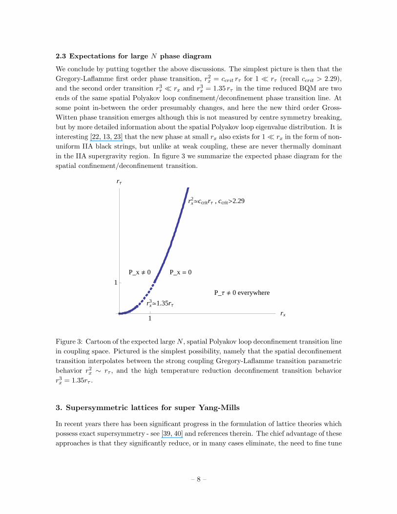
2.3 Expectations for large N phase diagram

We conclude by putting together the above discussions. The simplest picture is then that the

Gregory-Laflamme first order phase transition, r2x = ccrit rτ for 1 ≪ rτ (recall ccrit > 2.29),

and the second order transition r3τ ≪ rx and r3x = 1.35 rτ in the time reduced BQM are two

ends of the same spatial Polyakov loop confinement/deconfinement phase transition line. At

some point in-between the order presumably changes, and here the new third order Gross-

Witten phase transition emerges although this is not measured by centre symmetry breaking,

but by more detailed information about the spatial Polyakov loop eigenvalue distribution. It is

interesting [22, 13, 23] that the new phase at small rx also exists for 1 ≪ rx in the form of non-

uniform IIA black strings, but unlike at weak coupling, these are never thermally dominant

in the IIA supergravity region. In figure 3 we summarize the expected phase diagram for the

spatial confinement/deconfinement transition.

P_x ¹ 0 P_x = 0

P_Τ ¹ 0 everywhere

rx2>ccritrΤ , ccrit>2.29

rx3>1.35rΤ

1rx

1

rΤ

Figure 3: Cartoon of the expected largeN , spatial Polyakov loop deconfinement transition line

in coupling space. Pictured is the simplest possibility, namely that the spatial deconfinement

transition interpolates between the strong coupling Gregory-Laflamme transition parametric

behavior r2x ∼ rτ , and the high temperature reduction deconfinement transition behavior

r3x = 1.35rτ .

3. Supersymmetric lattices for super Yang-Mills

In recent years there has been significant progress in the formulation of lattice theories which

possess exact supersymmetry - see [39, 40] and references therein. The chief advantage of these

approaches is that they significantly reduce, or in many cases eliminate, the need to fine tune

– 8 –

the couplings in the lattice theories to approach the target continuum supersymmetric field

theory as the lattice spacing is sent to zero. The case ofN = 4 super Yang-Mills is particularly

interesting and the corresponding lattice theory was first constructed using orbifold methods

in [41]. Subsequently, it was realized that the same theory could be obtained using a carefully

chosen discretization of a topologically twisted version of the continuum theory [42, 43].

The continuum twist ofN = 4 that is the starting point of the twisted lattice construction

was first written down by Marcus in 1995 [44] although it now plays an important role in the

Geometric-Langlands program and is hence sometimes called the GL-twist [45]. This four

dimensional twisted theory is most compactly expressed as the dimensional reduction of a

five dimensional theory in which the ten (one four component gauge field and six scalars)

bosonic fields are realized as the components of a complexified five dimensional gauge field

Aa, a = 1 . . . 5 while the 16 single component twisted fermionic degrees of freedom are realized

as the 16 components of a Kahler-Dirac field (η, ψa, χab) [43]. The appearance of a scalar

fermion after twisting is crucial – it implies the existence of a nilpotent supersymmetry which

will be preserved in the lattice theory. Its action on the continuum fields3 is given by

Q Aa = ψa

Q ψa = 0

Q Aa = 0

Q χab = −Fab

Q η = d

Q d = 0

The site field d is a non-dynamical field that is included to close the Q-algebra and is subse-

quently integrated out of the final lattice action. Furthermore, the action of this theory can

be written as the sum of two terms; a Q-exact piece of the form

S =1

g2YM

Q∫

Tr

(

χabFab + η[Da,Da]−1

2ηd

)

(3.1)

and an additional Q-closed term

Sclosed = − 1

8g2YM

∫

Tr ǫmnpqrχqrDpχmn (3.2)

The supersymmetric invariance of this term then relies on the Bianchi identity

ǫmnpqrDpF qr = 0 (3.3)

Discretization of this theory proceeds straightforwardly; (Complex) continuum gauge fields

are represented as complexified Wilson gauge links Uµ(x) = eAµ(x) living on links eµ, µ =

3We assume an anti-hermitian basis for all fields which take their values in the adjoint representation of

the SU(N) gauge group.

– 9 –

1 . . . 4 of a hypercubic lattice.4 The field U5 is an exception to this and is placed on the body

diagonal of the hypercube corresponding to a relative position vector e5 = (−1,−1,−1,−1).

Notice that∑5

a=1 ea = 0 which is important to show gauge invariance of the lattice action.

These fields transform in the usual way under U(N) lattice gauge transformations eg:

Ua(x) → G(x)Ua(x)G†(x+ ea) (3.4)

Supersymmetric invariance then implies that ψa(x) live on the corresponding links and trans-

form identically to Ua(x). The scalar fermion η(x) is clearly most naturally associated with

a site and transforms accordingly

η(x) → G(x)η(x)G†(x) (3.5)

The field χab is slightly more difficult. Naturally as a 2-form it should be associated with a

plaquette. In practice we introduce diagonal links running through the center of the plaquette

and corresponding to the vector eab = ea + eb and choose χab(x) to lie with opposite orienta-

tion along those diagonal links. This choice of orientation will again be necessary to ensure

gauge invariance. The scalar lattice supersymmetry transformation is identical to that in the

continuum after the replacement Aa → Ua. Most importantly it remains nilpotent which

means that we can guarantee invariance of the Q-exact part of the lattice action by replacing

the continuum fields by their lattice counterparts. Of course to do so necessarily requires a

prescription for replacing continuum derivative operators by gauge covariant finite difference

operators. The following expressions are used:

D(+)a fb = Ua(x)fb(x+ ea)− fb(x)Ua(x+ eb) (3.6)

D(−)a fa = fa(x)Ua(x)− Ua(x− ea)fa(x− ea) (3.7)

Notice that this definition reduces to the usual adjoint covariant derivative in the naive con-

tinuum limit and furthermore guarantees that the resultant expressions transform covariantly

under lattice gauge transformation. The lattice field strength is then given by the gauged

forward difference Fab = D(+)a Ub and is automatically antisymmetric in its indices. Further-

more it transforms like a lattice 2-form or plaquette and hence yields a gauge invariant loop

on the lattice when contracted with the plaquette fermion χab. Similarly the covariant dis-

crete divergence appearing in D(−)a Ua transforms as a 0-form or site field and hence can be

contracted with the site field η to yield a gauge invariant expression.

This use of forward and backward difference operators guarantees that the solutions of the

theory map one-to-one with the solutions of the continuum theory and hence fermion doubling

problems are evaded [46]. Indeed, by introducing a lattice with half the lattice spacing one

can map this Kahler-Dirac fermion action into the action for staggered fermions [47]. While

4A better choice in four dimensions is the A∗

4 lattice which retains a higher point group symmetry than the

hypercubic lattice. See [39] for details. It is not necessary for two dimensions and indeed would complicate

the calculation of Polyakov lines.

– 10 –

the supersymmetric invariance of the Q-exact term is manifest in the lattice theory it is not

clear how to discretize the continuum Q-closed term. Remarkably, it is possible to discretize

(3.2) in such a way that it is indeed exactly invariant under the twisted supersymmetry

Sclosed = − 1

8g2YM

∑

x

Tr ǫmnpqrχqr(x+ em + en + ep)D(−)p χmn(x+ ep) (3.8)

and can be seen to be supersymmetric since the lattice field strength satisfies an exact Bianchi

identity [48].

ǫmnpqrD(+)p Fqr = 0 (3.9)

Putting all these elements together we arrive at the supersymmetric lattice action [39]

S = Sclosed +1

g2YM

∑

x

Tr

(

F†abFab +

1

2

(

D(−)a Ua

)2− χabD(+)

[a ψ b] − ηD(−)a ψa

)

(3.10)

where we have taken the Q-variation and integrated out the auxiliary field d. To reiterate;

this action is gauge invariant, free of doublers and possesses the one exact supersymmetry

given in (3.1).

Finally to obtain a two dimensional theory we perform a simple dimensional reduction

along two lattice directions using periodic boundary conditions. The resultant lattice action

corresponds in the naive continuum limit to the target Q = 16 YM theory in two dimensions.

In this limit its exact supersymmetry is enhanced to correspond to 4 continuum supercharges

corresponding to the four scalar fermions that now appear in the dimensionally reduced theory

[39].

We will be interested in this theory large N limit with ’t Hooft coupling λ = Ng2YM . The

lattice theory is then governed by the coupling κ = NLT2r2τ

where L and T denote the number

of lattice sites in the spatial and temporal directions.

We have used periodic boundary conditions for the fields on the remaining spatial circle

and anti-periodic boundary conditions for fermions in the temporal direction in order to

access the thermal theory. Simulations were carried out using the RHMC algorithm which

is described in detail in [49]. It has been shown that the existence of a noncompact moduli

space in the theory renders the thermal partition function divergent [8]. In order to regulate

this divergence we have additionally introduced a mass term for the scalar fields appearing

in the lattice action with a dimensionless mass parameter m = mphysβ.

Sm =m2

g2YM

∑

x

[

U†µUµ +

(

U†µUµ

)−1− 2

]

(3.11)

The form of this term is effective at suppressing arbitrarily large fluctuations of the exponen-

tiated scalar fields and reduces to a simple mass term for small fluctuations characterizing

the continuum limit. Notice that this infrared regulator term breaks supersymmetry softly

and lifts the quantum moduli space of the theory. We have performed our simulations for a

range of the parameter m in order to allow for an extrapolation m→ 0.

– 11 –

4. Simulation results

Temporal Polyakov lines

Spatial Polyakov linesSUH3L

Lx = Ly = 1

Lz = 8, LΤ = 2

m = 0.05

m = 0.10

m = 0.20

0.2 0.4 0.6 0.8 1.0rΤ

0.2

0.4

0.6

0.8

1.0

Px and PΤ

Temporal Polyakov lines

Spatial Polyakov linesSUH3L

Lx = Ly = 1

Lz = 12, LΤ = 3

m = 0.05

m = 0.10

m = 0.20

0.2 0.4 0.6 0.8 1.0rΤ

0.2

0.4

0.6

0.8

1.0

Px and PΤ

Figure 4: Spatial and temporal Polyakov lines (Px and Pτ ) against dimensionless time circle

radius rτ for maximally supersymmetric SU(3) Yang-Mills on 2× 8 and 3× 12 lattices using

different values of the infrared regulator m.

In this section we present our numerical results. We have focused on the Polyakov lines

– 12 –

for both the thermal and spatial circle. These are defined in the usual way

Px =1

N

⟨∣

∣

∣Tr ΠL−1

ax=0Uax

∣

∣

∣

⟩

, Pτ =1

N

⟨∣

∣

∣Tr ΠT−1

aτ=0Uaτ

∣

∣

∣

⟩

, (4.1)

where we have extracted the unitary piece of the complexified link Uµ to compute these

expressions. We have evaluated the spatial and temporal Polyakov lines as a function of rτfor two different lattices with the same aspect ratio, a 2 × 8 lattice and a 3 × 12 lattice, for

N = 3 and with values of the infrared regulator m = 0.05, 0.10 and 0.20. The use of two

different lattices with the same aspect ratio allows us to test for and quantify finite lattice

spacing effects. We have performed simulations for values of the dimensionless time circle

radius in the range 0.02 ≤ rτ ≤ 1.0. The results are shown in figure 4.

Notice that the temporal Polyakov remains close to unity over a wide range of rτ . This

indicates the theory is (temporally) deconfined and is consistent with expectations for the

limits discussed in section 2 - the asymmetric torus limits, and the strong coupling regions

where there is a dual supergravity description in terms of black holes. However, the spatial

Polyakov line has a different behavior taking values close to unity for small rτ while falling

rapidly to plateau at much smaller values for large rτ . It is tempting to see the rather rapid

crossover around rτ ∼ 0.2 as a signal for a would be thermal phase transition as the number

of colors is increased. This conjecture is seen to be consistent with the data; in figure 5 we

show the Polyakov lines for N = 2, 3, 4 on 2 × 8 lattices as a function of rτ . The plateau

evident at large rτ falls with increasing N and the crossover sharpens. This is consistent with

the system developing a sharp phase transition in the large N limit.

In the data shown here we see very little dependence of our results on the scalar mass.

Indeed for the length of Monte Carlo we were able to perform it appears that m can be set

to zero for rτ < 2 without fear of encountering the thermal divergence discussed in [8]. This

stability in the scalar sector can be seen in figure 6 which shows the Monte Carlo time series

for the eigenvalues of U †µUµ ∼ e2φ at two different rτ ’s with dimensionless mass parameter

m = 0.05 and gauge group SU(3). There is no evidence of a divergence over thousands of

Monte Carlo sweeps. Furthermore, one sees that the eigenvalues of the scalar fields (rendered

dimensionless using the lattice spacing) cluster with small separation for this range of rτ .5

We have however observed that them = 0 model does exhibit the same thermal instability

observed in the case of supersymmetric quantum mechanics for sufficiently low temperature

rτ >> 1 in agreement with the general arguments given in [8].

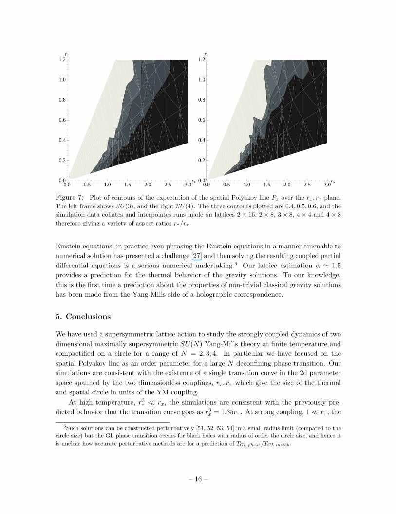
Putting together several lattice aspect ratios for N = 3, 4 we can plot the spatial Polyakov

loop as a function of rs and rτ where data is available. This is done in figure 7. The three

contours Px = 0.4, 0.5, 0.6 are shown. We see that the contours for SU(4) are closer together

than those for SU(3), as we expect for a largeN transition. From this data we can try to assess

where the large N transition in Px may occur. In the detailed studies of the dimensionally

reduced bosonic quantum mechanics [13], it was found that the large N transition occurred

5We thank Masanori Hanada for pointing out the significance of this result which differs from the situation

reported in [15]

– 13 –

Temporal Polyakov lines

Spatial Polyakov linesm = 0.10

LX = LY = 1

LZ = 8, LΤ = 2

SUH2LSUH3LSUH4L

0.2 0.4 0.6 0.8 1.0rΤ

0.2

0.4

0.6

0.8

1.0

Px and PΤ

Figure 5: Plot of the absolute values of the spatial and temporal Polyakov lines (Px and Pτ ) against

the dimensionless time circle radius rτ for maximally supersymmetric SU(N) Yang-Mills on a 2 × 8

lattice for N = 2, 3, 4, using the value of the infrared regulator m = 0.10.

very close to Px ≃ 0.5. Thus from the contours of the SU(3) and SU(4) data we could take the

Px = 0.5 curves to give an estimate for the large N phase transition line. Another estimate is

to plot the function fn ≡ Px(SU(n))−Px(SU(n− 1)) which measures the difference between

the Polyakov lines for SU(n) and SU(n−1). At strong coupling where we expect the large N

transition is first order, the simplest situation is to have fn < 0 in the confined region (where

Px = 0 for N → ∞), and correspondingly fn > 0 in the deconfined region as n → ∞. Then

plotting the boundary of the positive (or negative) region of f4 calculated from our data also

gives an estimate of the critical line. Neither method can give a precise determination, and

they should not be considered as a replacement for calculations at larger N than we have been

able to reach here. However, in the absence of such large N data we plot the Px = 0.5 contours

for SU(4) and SU(3) in figure 7, and in addition the region where f4 is positive. We note that

the SU(3) and SU(4) Px = 0.5 contours are remarkably consistent with each other, which

provides evidence that they are indeed a reasonable approximation to the large N transition

curve. Whilst the f4 data is rather noisy, and hence the positive f4 region has ‘holes’ in it,

the function is positive only to left of the Px = 0.5 curves, and furthermore, extends right

up to these curves. The curve r2x = 3.5rτ is plotted on this graph and matches the contours

Px = 0.5 and the boundary of the positive f4 region very well in the strong coupling region.

We take this to indicate that the gravity prediction for the parametric behavior r2x = ccritrτis consistent with our data, and we have estimated ccrit ≃ 3.5 which indeed obeys the gravity

prediction that ccrit is order one and ccrit > 2.29. Furthermore we see that the contours

Px = 0.5 also appear to be consistent with the high temperature prediction r3x = 1.35rτ as

– 14 –

m = 0.05, rΤ = 0.50, SUH3L

LΤ = 2, LX = LY = 1, LZ = 8

0 2000 4000 6000 8000 10 000 12 000

0.0

0.2

0.4

0.6

0.8

1.0

1.2

1.4

Monte Carlo configuration time

Ave

rageHUÖΜUΜL

m = 0.05, rΤ = 1.0, SUH3L

LΤ = 2, LX = LY = 1, LZ = 8

0 2000 4000 6000 8000

0.0

0.5

1.0

1.5

Monte Carlo configuration time

Ave

rageHUÖΜUΜL

Figure 6: Plots of the average scalar eigenvalues against Monte Carlo configuration time step,

for N = 3 on a 2× 8 lattice with rτ = 0.5 and 1.0. Note that the spread between eigenvalues

reduces as rτ is decreased. We have used the dimensionless mass parameter m = 0.05.

well.

The value of the ratio α ≡ ccrit/2.29 gives the ratio of the GL thermal phase transition

temperature to the GL dynamical instability temperature (the minimum temperature to

which uniform strings can be supercooled), so α = TGL phase/TGL instab. Whilst the GL

instability temperature is known [13] (corresponding to the behavior r2x = 2.29rτ at strong

coupling), the GL phase transition temperature is not known in the gravity theory as the

localized solutions have not been constructed. In fact the near extremal D0-charged black

holes are simply related to vacuum solutions of pure gravity with R1,8 × S1 asymptotics

[13, 23]. Such localized black hole solutions have been constructed for asymptotics R1,3 × S1

and R1,4×S1, using numerical techniques [50, 25, 27]. Extending these methods to the case of

interest here, R1,8 × S1, is obviously an interesting future direction. It is worth emphasizing

that whilst finding localized solutions in the gravity theory only involves solving the classical

– 15 –

0.0 0.5 1.0 1.5 2.0 2.5 3.0rx0.0

0.2

0.4

0.6

0.8

1.0

1.2rΤ

0.0 0.5 1.0 1.5 2.0 2.5 3.0rx0.0

0.2

0.4

0.6

0.8

1.0

1.2rΤ

Figure 7: Plot of contours of the expectation of the spatial Polyakov line Px over the rx, rτ plane.

The left frame shows SU(3), and the right SU(4). The three contours plotted are 0.4, 0.5, 0.6, and the

simulation data collates and interpolates runs made on lattices 2 × 16, 2 × 8, 3 × 8, 4 × 4 and 4 × 8

therefore giving a variety of aspect ratios rτ/rx.

Einstein equations, in practice even phrasing the Einstein equations in a manner amenable to

numerical solution has presented a challenge [27] and then solving the resulting coupled partial

differential equations is a serious numerical undertaking.6 Our lattice estimation α ≃ 1.5

provides a prediction for the thermal behavior of the gravity solutions. To our knowledge,

this is the first time a prediction about the properties of non-trivial classical gravity solutions

has been made from the Yang-Mills side of a holographic correspondence.

5. Conclusions

We have used a supersymmetric lattice action to study the strongly coupled dynamics of two

dimensional maximally supersymmetric SU(N) Yang-Mills theory at finite temperature and

compactified on a circle for a range of N = 2, 3, 4. In particular we have focused on the

spatial Polyakov line as an order parameter for a large N deconfining phase transition. Our

simulations are consistent with the existence of a single transition curve in the 2d parameter

space spanned by the two dimensionless couplings, rx, rτ which give the size of the thermal

and spatial circle in units of the YM coupling.

At high temperature, r3τ ≪ rx, the simulations are consistent with the previously pre-

dicted behavior that the transition curve goes as r3x = 1.35rτ . At strong coupling, 1 ≪ rτ , the

6Such solutions can be constructed perturbatively [51, 52, 53, 54] in a small radius limit (compared to the

circle size) but the GL phase transition occurs for black holes with radius of order the circle size, and hence it

is unclear how accurate perturbative methods are for a prediction of TGL phase/TGL instab.

– 16 –

0.0 0.5 1.0 1.5 2.0 2.5 3.0rx0.0

0.2

0.4

0.6

0.8

1.0

rΤ

Figure 8: Plot showing a superposition of the Px = 0.5 contours for SU(3) and SU(4) as dashed

black lines. Also shown is the region (blue) where the SU(4) loop Px is greater than the SU(3)

loop, which is expected to estimate the large N deconfined region for a first order transition (which

gravity suggests at strong coupling). ‘Holes’ in this blue region are due to statistical errors. We see the

boundary of this region (ignoring ‘holes’) matches well the Px = 0.5 contours, and represents our guess

for where the large N transition resides. This figure should be compared to the previous figure 3 giving

a sketch of the expected phase structure. Plotted on the figure is the high temperature prediction for

the transition (r3x= 1.35rτ , red curve). We note that the estimated large N transition curve fits well

both this high temperature prediction and also the strong coupling dual gravity predicted parametric

behavior r2x= ccritrτ . Our data suggests ccrit ≃ 3.5 (plotted as blue curve), which obeys the constraint

from gravity ccrit > 2.29.

transition is conjectured to be the holographic dual of a first order Gregory-Laflamme phase

transition, with the transition curve going a r2x = ccritrτ , with ccrit an order one constant

obeying the constraint ccrit > 2.29. Our simulations are consistent with this parametric be-

havior, and we have used the N = 3, 4 data to estimate the position of the large N transition,

determining ccrit ≃ 3.5. This gives the ratio of the Gregory-Laflamme phase transition and

dynamical instability temperatures to be TGLphase/TGLinstability ≃ 1.5. Since the dual local-

ized black hole solutions have not been constructed, this constitutes a prediction for these

non-trivial gravity solutions, which hopefully will be tested by their construction in the near

– 17 –

future.

Acknowledgments

SC and AJ are supported in part by the US Department of Energy under grant DE-FG02-

85ER40237. TW is supported by a STFC advanced fellowship and a Halliday award. Simu-

lations were performed using USQCD resources at Fermilab.

References

[1] N. Itzhaki, J. M. Maldacena, J. Sonnenschein, and S. Yankielowicz, Supergravity and the large N

limit of theories with sixteen supercharges, Phys. Rev. D58 (1998) 046004, [hep-th/9802042].

[2] M. Hanada, J. Nishimura, and S. Takeuchi, Non-lattice simulation for supersymmetric gauge

theories in one dimension, Phys. Rev. Lett. 99 (2007) 161602, [0706.1647].

[3] S. Catterall and T. Wiseman, Towards lattice simulation of the gauge theory duals to black holes

and hot strings, JHEP 12 (2007) 104, [0706.3518].

[4] K. N. Anagnostopoulos, M. Hanada, J. Nishimura, and S. Takeuchi, Monte Carlo studies of

supersymmetric matrix quantum mechanics with sixteen supercharges at finite temperature,

Phys. Rev. Lett. 100 (2008) 021601, [0707.4454].

[5] S. Catterall and T. Wiseman, Black hole thermodynamics from simulations of lattice Yang-Mills

theory, Phys. Rev. D78 (2008) 041502, [0803.4273].

[6] M. Hanada, A. Miwa, J. Nishimura, and S. Takeuchi, Schwarzschild radius from Monte Carlo

calculation of the Wilson loop in supersymmetric matrix quantum mechanics, Phys. Rev. Lett.

102 (2009) 181602, [0811.2081].

[7] M. Hanada, Y. Hyakutake, J. Nishimura, and S. Takeuchi, Higher derivative corrections to black

hole thermodynamics from supersymmetric matrix quantum mechanics, Phys. Rev. Lett. 102

(2009) 191602, [0811.3102].

[8] S. Catterall and T. Wiseman, Extracting black hole physics from the lattice, JHEP 04 (2010)

077, [0909.4947].

[9] M. Hanada, J. Nishimura, Y. Sekino, and T. Yoneya, Monte Carlo studies of Matrix theory

correlation functions, Phys. Rev. Lett. 104 (2010) 151601, [0911.1623].

[10] S. Catterall and G. van Anders, First Results from Lattice Simulation of the PWMM,

1003.4952.

[11] G. Ishiki, S.-W. Kim, J. Nishimura, and A. Tsuchiya, Deconfinement phase transition in N=4

super Yang-Mills theory on R× S3 from supersymmetric matrix quantum mechanics, Phys. Rev.

Lett. 102 (2009) 111601, [0810.2884].

[12] G. Ishiki, S.-W. Kim, J. Nishimura, and A. Tsuchiya, Testing a novel large-N reduction for N=4

super Yang-Mills theory on R× S3, JHEP 09 (2009) 029, [0907.1488].

[13] O. Aharony, J. Marsano, S. Minwalla, and T. Wiseman, Black hole-black string phase

transitions in thermal 1+1- dimensional supersymmetric Yang-Mills theory on a circle, Class.

Quant. Grav. 21 (2004) 5169–5192, [hep-th/0406210].

– 18 –

[14] T. Azeyanagi, M. Hanada, T. Hirata, and H. Shimada, On the shape of a D-brane bound state

and its topology change, JHEP 03 (2009) 121, [0901.4073].

[15] M. Hanada and I. Kanamori, Lattice study of two-dimensional N=(2,2) super Yang-Mills at

large-N, Phys. Rev. D80 (2009) 065014, [0907.4966].

[16] M. Hanada, S. Matsuura, and F. Sugino, Two-dimensional lattice for four-dimensional N=4

supersymmetric Yang-Mills, 1004.5513.

[17] M. Hanada, A fine tuning free formulation of 4d N=4 super Yang- Mills, 1009.0901.

[18] O. Aharony et al., The phase structure of low dimensional large N gauge theories on tori, JHEP

01 (2006) 140, [hep-th/0508077].

[19] L. Susskind, Matrix theory black holes and the Gross Witten transition, hep-th/9805115.

[20] M. Li, E. J. Martinec, and V. Sahakian, Black holes and the SYM phase diagram, Phys. Rev.

D59 (1999) 044035, [hep-th/9809061].

[21] E. J. Martinec and V. Sahakian, Black holes and the SYM phase diagram. II, Phys. Rev. D59

(1999) 124005, [hep-th/9810224].

[22] B. Kol, Topology change in general relativity and the black-hole black-string transition, JHEP 10

(2005) 049, [hep-th/0206220].

[23] T. Harmark and N. A. Obers, New phases of near-extremal branes on a circle, JHEP 09 (2004)

022, [hep-th/0407094].

[24] T. Harmark and N. A. Obers, New phases of thermal SYM and LST from Kaluza-Klein black

holes, Fortsch. Phys. 53 (2005) 536–541, [hep-th/0503021].

[25] H. Kudoh and T. Wiseman, Properties of Kaluza-Klein black holes, Prog. Theor. Phys. 111

(2004) 475–507, [hep-th/0310104].

[26] H. Kudoh and T. Wiseman, Connecting black holes and black strings, Phys. Rev. Lett. 94 (2005)

161102, [hep-th/0409111].

[27] M. Headrick, S. Kitchen, and T. Wiseman, A new approach to static numerical relativity, and

its application to Kaluza-Klein black holes, Class. Quant. Grav. 27 (2010) 035002, [0905.1822].

[28] R. Gregory and R. Laflamme, Black strings and p-branes are unstable, Phys. Rev. Lett. 70

(1993) 2837–2840, [hep-th/9301052].

[29] R. Gregory and R. Laflamme, The Instability of charged black strings and p-branes, Nucl. Phys.

B428 (1994) 399–434, [hep-th/9404071].

[30] B. Kol, The Phase Transition between Caged Black Holes and Black Strings - A Review, Phys.

Rept. 422 (2006) 119–165, [hep-th/0411240].

[31] T. Harmark and N. A. Obers, Phases of Kaluza-Klein black holes: A brief review,

hep-th/0503020.

[32] T. Harmark, V. Niarchos, and N. A. Obers, Instabilities of black strings and branes, Class.

Quant. Grav. 24 (2007) R1–R90, [hep-th/0701022].

[33] T. Eguchi and H. Kawai, Reduction of Dynamical Degrees of Freedom in the Large N Gauge

Theory, Phys. Rev. Lett. 48 (1982) 1063.

– 19 –

[34] T. Banks, W. Fischler, S. H. Shenker, and L. Susskind, M theory as a matrix model: A

conjecture, Phys. Rev. D55 (1997) 5112–5128, [hep-th/9610043].

[35] N. Kawahara, J. Nishimura, and S. Takeuchi, Phase structure of matrix quantum mechanics at

finite temperature, JHEP 10 (2007) 097, [0706.3517].

[36] G. Mandal, M. Mahato, and T. Morita, Phases of one dimensional large N gauge theory in a

1/D expansion, JHEP 02 (2010) 034, [0910.4526].

[37] D. J. Gross and E. Witten, Possible Third Order Phase Transition in the Large N Lattice Gauge

Theory, Phys. Rev. D21 (1980) 446–453.

[38] S. Wadia, A STUDY OF U(N) LATTICE GAUGE THEORY IN TWO-DIMENSIONS, .

EFI-79/44-CHICAGO.

[39] S. Catterall, D. B. Kaplan, and M. Unsal, Exact lattice supersymmetry, Phys. Rept. 484 (2009)

71–130, [0903.4881].

[40] S. Catterall, Supersymmetric lattices, 1005.5346.

[41] D. B. Kaplan and M. Unsal, A Euclidean lattice construction of supersymmetric Yang- Mills

theories with sixteen supercharges, JHEP 09 (2005) 042, [hep-lat/0503039].

[42] M. Unsal, Twisted supersymmetric gauge theories and orbifold lattices, JHEP 10 (2006) 089,

[hep-th/0603046].

[43] S. Catterall, From Twisted Supersymmetry to Orbifold Lattices, JHEP 01 (2008) 048,

[0712.2532].

[44] N. Marcus, The Other topological twisting of N=4 Yang-Mills, Nucl. Phys. B452 (1995)

331–345, [hep-th/9506002].

[45] A. Kapustin and E. Witten, Electric-magnetic duality and the geometric Langlands program,

hep-th/0604151.

[46] J. M. Rabin, Homology theory of lattice fermion doubling, Nucl. Phys. B201 (1982) 315.

[47] T. Banks, Y. Dothan, and D. Horn, Geometric fermions, Phys. Lett. B117 (1982) 413.

[48] H. Aratyn, M. Goto, and A. H. Zimerman, A lattice gauge theory for fields in the adjoint

representation, Nuovo Cim. A84 (1984) 255.

[49] S. Catterall, First results from simulations of supersymmetric lattices, JHEP 01 (2009) 040,

[0811.1203].

[50] T. Wiseman, Static axisymmetric vacuum solutions and non-uniform black strings, Class.

Quant. Grav. 20 (2003) 1137–1176, [hep-th/0209051].

[51] T. Harmark, Small black holes on cylinders, Phys. Rev. D69 (2004) 104015, [hep-th/0310259].

[52] D. Gorbonos and B. Kol, A dialogue of multipoles: Matched asymptotic expansion for caged

black holes, JHEP 06 (2004) 053, [hep-th/0406002].

[53] D. Gorbonos and B. Kol, Matched asymptotic expansion for caged black holes: Regularization of

the post-Newtonian order, Class. Quant. Grav. 22 (2005) 3935–3960, [hep-th/0505009].

[54] D. Karasik, C. Sahabandu, P. Suranyi, and L. C. R. Wijewardhana, Analytic approximation to 5

dimensional black holes with one compact dimension, Phys. Rev. D71 (2005) 024024,

[hep-th/0410078].

– 20 –