THERMAL PERFORMANCE OF MECHANICAL PIPE

INSULATION SYSTEMS AT BELOW-AMBIENT

TEMPERATURE

By

SHANSHAN CAI

Bachelor of Science

Huazhong University of Science and Technology

Wuhan, China

2007

Master of Science

Oklahoma State University

Stillwater, OK

2009

Submitted to the Faculty of the

Graduate College of the

Oklahoma State University

in partial fulfillment of

the requirements for

the Degree of

DOCTOR OF PHILOSOPHY

December, 2013

ii

THERMAL PERFORMANCE OF MECHANICAL PIPE

INSULATION SYSTEMS AT BELOW-AMBIENT

TEMPERATURE

Dissertation Approved:

Dr. Lorenzo Cremaschi

Dissertation Adviser

Dr. Afshin Ghajar

Dr. Jeffery Spitler

Dr. James Smay

.

iii Acknowledgements reflect the views of the author and are not endorsed by committee

members or Oklahoma State University.

ACKNOWLEDGEMENTS

I wish to express my sincere appreciation and grateful to my advisor, Dr. Lorenzo Cremaschi, for

his continuous support, patience and guidance. I would also like to extend my appreciation to my

other committee members, Dr. Afshin Ghajar, for his help in the literature review and the first

stage of this project, Dr. Jeffery Spitler, for teaching me VBA, and it becomes an important tool

in my model, and Dr. James Smay, for all the suggestions given during my defense.

I should give my thanks to the person involved in this project: Kasey Worthington, who helped

me design and construct the test apparatus; Jimmy Kim, who helped me in the construction work

during the second stage; Auvi Biswas and Jeremy Smith, who helped me in the Labview

program; Weiwei Zhu, who will continue the tests; I would also like to thank the other team

members: Andrea Bigi, Ardi Yatim, Pratik Deokar, Xiaoxiao Wu for the help in the maintenance

of the Psychrometric chamber. Without your help, I cannot go this far.

Special thanks to my parents for bringing me to the world, supporting me for my each decision

and giving me their endless love.

iv

Name: SHANSHAN CAI

Date of Degree: DECEMBER, 2013

Title of Study: THERMAL PERFORMANCE OF MECHANICAL PIPE INSULATION

SYSTEMS AT BELOW-AMBIENT TEMPERATURE

Major Field: MECHANICAL ENGINEERING

Abstract: Mechanical pipe insulation systems are commonly applied to cold piping

surfaces in most industrial and commercial buildings in order to limit the heat losses and

prevent water vapor condensation on the pipe exterior surfaces. Due to the fact that the

surface temperature of these pipelines is normally below the ambient dew point

temperature, water vapor diffuses inside the pipe insulation systems often condenses

when it reaches the pipe exterior surfaces. The water droplets accumulated in the pipe

insulation system increase its overall thermal conductivity by thermal bridging the cells

or the fibers of the insulation material. The moisture ingress into pipe insulation threatens

the thermal performance and the overall efficiency of the building mechanical system.

The main objective of this research was to investigate the effects of water vapor ingress

on the thermal conductivity of pipe insulation systems. A critical review of the state of

the art literature in this field was included to clarify the similarities and differences on the

apparent thermal conductivity of pipe insulation systems and flat slabs. A new

experimental methodology was developed to isolate and quantify the effect of water

vapor ingress to the pipe insulation systems. Seven fibrous and ten closed-cell pipe

insulation systems were tested on the novel experimental apparatus under dry and wet,

condensing conditions. Under dry condition, the apparent thermal conductivity was

observed linearly varied with insulation mean temperature, and the presence of joint

sealant may increase the apparent thermal conductivity by 15%. During moisture test,

results showed that the moisture diffusion mechanism were different in fibrous and

closed-cell pipe insulation systems. Compared to closed-cell, fibrous pipe insulation

system behaved more sensitive to the moisture content and the thermal conductivity

increased dramatically due to the formation of more thermal bridging and preferential

paths. An analytical model was developed based on the diffusion mechanism to predict

the moisture accumulation and the associated penalization of the apparent thermal

conductivity in different pipe insulation systems operating below ambient room

temperature. The model was validated with the experimental results and the data reported

in the literature on the thermal conductivity ratio with different moisture content. The

differences were within 10% for closed-cell pipe insulation, and within 15% for fibrous

pipe insulation systems.

v

TABLE OF CONTENTS

LIST OF TABLES ............................................................................................................................... VIII

LIST OF FIGURES ............................................................................................................................... IX

1. INTRODUCTION ............................................................................................................................... 1

1.1 BACKGROUND .................................................................................................................................... 1

1.2 CRITICAL ISSUE WITH COLD PIPES ............................................................................................................ 2

1.3 OBJECTIVES ....................................................................................................................................... 4

1.4 ORGANIZATION OF THIS DISSERTATION .................................................................................................... 7

2. LITERATURE REVIEW ........................................................................................................................ 9

2.1 EXPERIMENTAL METHODOLOGIES FOR MEASUREMENT OF PIPE INSULATION THERMAL CONDUCTIVITY UNDER DRY

CONDITIONS .................................................................................................................................................. 10

2.1.1 Brief background on the methodologies for thermal conductivity measurements of flat slabs.

................................................................................................................................................. 11

2.1.2 Review of the thermal conductivity measurements of pipe insulation systems ..................... 14

2.2 REVIEW OF THERMAL CONDUCTIVITY VARIATION IN PIPE INSULATION SYSTEMS .............................................. 18

2.3 METHODOLOGIES FOR MEASUREMENT OF PIPE INSULATION THERMAL CONDUCTIVITY UNDER WET CONDITION AND

WITH MOISTURE INGRESS ................................................................................................................................. 26

2.4 REVIEW OF THE THERMAL CONDUCTIVITY VARIATION WITH MOISTURE CONTENT IN PIPE INSULATION SYSTEMS ..... 32

2.5 CHALLENGES WITH THE CURRENT METHODOLOGIES FOR MEASURING THE PIPE INSULATION APPARENT THERMAL

CONDUCTIVITY WITH MOISTURE INGRESS AND FUTURE RESEARCH NEEDS ................................................................... 40

2.6 CONCLUSIONS .................................................................................................................................. 43

3. EXPERIMENTAL APPARATUS DESIGN AND INSTRUMENTATION ..................................................... 46

3.1 PIPE INSULATION TESTER (PIT) ............................................................................................................ 46

3.2 REFRIGERATION SYSTEMS ................................................................................................................... 57

3.2.1 Refrigeration system in the first stage .................................................................................... 57

3.2.2 Refrigeration system in the second stage ............................................................................... 60

3.3 PSYCHROMETRIC CHAMBER ................................................................................................................ 62

4. MEASUREMENTS AND DATA REDUCTION ...................................................................................... 68

4.1 EXPERIMENTAL TEST CONDITIONS ........................................................................................................ 68

4.2 EXPERIMENTAL PROCEDURES ............................................................................................................... 74

4.2.1 Experimental procedures for calibration test .......................................................................... 75

vi

4.2.2 Experimental procedures for dry non-condensing testes ....................................................... 75

4.2.3 Experimental procedures for wet (condensing) test with moisture ingress ........................... 81

4.3 INSTALLATION OF PIPE INSULATION SYSTEMS .......................................................................................... 85

4.4 DATA REDUCTION ............................................................................................................................. 87

4.4.1 Calibration of the PIT ............................................................................................................... 87

4.4.2 Pipe insulation system thermal conductivity measurements ................................................. 91

4.4.3 Moisture Content Measurements in the Pipe Insulation System ........................................... 92

4.5 EXPERIMENTAL UNCERTAINTY ............................................................................................................. 93

4.5.1 Uncertainty on the thermal conductivity of pipe insulation system ....................................... 93

4.5.2 Uncertainty on the moisture content in the pipe insulation system ...................................... 97

5. EXPERIMENTAL RESULTS ................................................................................................................ 99

5.1 THERMAL CONDUCTIVITY VALIDATION TEST RESULTS FOR TWO TYPES OF PIPE INSULATION SYSTEMS ................... 99

5.1.1 Cellular glass pipe insulation systems V-CG1 and V-CG2 ...................................................... 100

5.1.2 Polyisocyanurate (PIR) pipe insulation system V-PIR1 and V-PIR2 ........................................ 103

5.2 THERMAL CONDUCTIVITY TESTS RESULTS UNDER DRY NON-CONDENSING CONDITIONS (IN THE FIRST STAGE) ...... 105

5.3 SENSITIVITY ANALYSIS OF THE JOINT SEALANT ON THE THERMAL CONDUCTIVITY MEASUREMENTS IN DRY, NON-

CONDENSING CONDITIONS ............................................................................................................................. 112

5.4 THERMAL CONDUCTIVITY TESTS RESULTS UNDER DRY NON-CONDENSING CONDITIONS IN THE SECOND STAGE ..... 115

5.4.1 Fiberglass pipe insulation system .......................................................................................... 116

5.4.2 Cellular glass pipe insulation system ..................................................................................... 118

5.4.3 Elastomeric rubber pipe insulation system ........................................................................... 120

5.4.4 Polyisocyanurate (PIR) pipe insulation system ...................................................................... 121

5.5 THERMAL CONDUCTIVITY OF PIPE INSULATION SYSTEMS UNDER WET CONDENSING CONDITIONS WITH MOISTURE

INGRESS ................................................................................................................................................... 124

5.5.1 Fiberglass Pipe Insulation ...................................................................................................... 124

5.5.2 Closed-cell pipe insulation ..................................................................................................... 149

6. SIMULATION MODEL ................................................................................................................... 177

6.1 INTRODUCTION ............................................................................................................................... 177

6.2 LITERATURE REVIEW OF THE EXISTING MODELS FOR INSULATION THERMAL CONDUCTIVITY ............................. 178

6.3 MODEL FOR CLOSED-CELL PIPE INSULATION SYSTEMS ............................................................................. 180

6.3.1 Sub-model of thermal conductivity for dry pipe insulation systems (closed-cell) ................ 183

6.3.2 Sub-model of water content accumulated in wet pipe insulation systems with moisture

ingress (closed-cell) ............................................................................................................................ 186

6.3.3 Sub-Model of Thermal Conductivity of Wet Pipe Insulation Systems with Moisture Ingress

(Closed-cell) ........................................................................................................................................ 187

6.4 MODEL FOR FIBROUS PIPE INSULATION SYSTEMS ................................................................................... 190

6.4.1 Sub-model of thermal conductivity for dry pipe insulation systems (fibrous) ...................... 191

6.4.2 Sub-model of water content accumulated in pipe insulation systems with moisture ingress

(fibrous) .............................................................................................................................................. 192

6.4.3 Sub-model of thermal conductivity of wet pipe insulation systems with moisture ingress

(fibrous) .............................................................................................................................................. 196

6.5 DETERMINATION OF THE COEFFICIENTS................................................................................................ 199

6.5.1 Condensing coefficient f1 ....................................................................................................... 199

6.5.2 Permeability correction factor f2 ........................................................................................... 200

vii

6.5.3 Parameters a and crad ............................................................................................................ 202

6.6 MODEL IMPLEMENTATION ................................................................................................................ 206

6.6.1 Implement of thermal conductivity model under dry conditions ......................................... 206

6.6.2 Implement of thermal conductivity model under wet conditions with moisture ingress ..... 208

6.7 MODEL VALIDATION FOR DRY CONDITIONS AT BELOW AMBIENT TEMPERATURES .......................................... 218

6.7.1 Closed-cell pipe insulation ..................................................................................................... 218

6.7.2 Fibrous pipe insulation .......................................................................................................... 222

6.8 MODEL VALIDATION UNDER WET CONDITIONS WITH MOISTURE INGRESS .................................................... 224

6.8.1 Closed-cell pipe insulation systems ....................................................................................... 224

6.8.2 Fibrous pipe insulation system systems ................................................................................ 233

6.8.3 Validation with the results reported in the current literature .............................................. 243

6.8.4 Sensitivity analysis on the coefficients .................................................................................. 247

7. CONLCUSIONS AND RECOMMENDATIONS ................................................................................... 251

7.1 CONCLUSIONS ON THE CURRENT WORK ............................................................................................... 251

7.2 RECOMMENDATIONS FOR FUTURE WORK ............................................................................................. 255

REFERENCES ......................................................................................................................................... 257

APPENDICES ......................................................................................................................................... 263

APPENDIX A: THERMAL CONDUCTIVITY OF SEVEN COMMON INSULATION MATERIALS: FIBERGLASS, POLYURETHANE,

POLYSTYRENE, CELLULAR GLASS, POLYISOCYANURATE (PIR), MINERAL WOOL AND ELASTOMERIC RUBBER INSULATION

REPORTED IN THE OPEN DOMAIN LITERATURE ..................................................................................................... 263

APPENDIX B: CAD DRAWINGS OF THE EXPERIMENTAL APPARATUS ......................................................................... 273

APPENDIX C: EXAMPLES OF EXPERIMENTAL DATA SETS ........................................................................................ 276

APPENDIX D: SYSTEM INPUT FILE AND OUTPUT COEFFICIENTS (WET CONDITION)....................................................... 284

APPENDIX E: COMPARISON RESULTS BETWEEN SIMULATION RESULTS AND EXPERIMENTAL DATA .................................. 288

APPENDIX F: VBA CODES SAMPLE ................................................................................................................... 298

viii

LIST OF TABLES

Table 2.1: Summary of interlaboratory/laboratory comparison between steady-state and transient

measurements --- (will add IP unit in final) .................................................................................................. 17 Table 2.2: Common methodologies for insulation thermal conductivity measurements with moisture ingress

....................................................................................................................................................................... 27 Table 2.3: Comparison among experimental methods and test results for fiberglass insulation with moisture

ingress ........................................................................................................................................................... 36 Table 2.4: Comparison among experimental methods and test results for other common insulations with

moisture ingress............................................................................................................................................. 38 Table 4.1: Accuracy and maximum spatial variation of the temperature measurements of the PIT (Phase I)

....................................................................................................................................................................... 95 Table 4.2: Accuracy and maximum spatial variation of the temperature measurements of the PIT (Phase II)

....................................................................................................................................................................... 95 Table 4.3: Accuracy of the moisture gains measurement during the tests in wet conditions ........................ 98 Table 5.1: Pipe insulation systems in the validation test ............................................................................. 100 Table 5.2: Validation experiment results of cellular glass pipe insulation systems..................................... 102 Table 5.3: Comparison cellular glass data of the present work with manufacturer catalog ........................ 103 Table 5.4: Experimental results for PIR pipe insulation systems ................................................................ 105 Table 5.5: Pipe insulation systems tested under dry conditions (in the first stage) ..................................... 106 Table 5.6: Thermal conductivities of pipe insulations under dry condition ................................................ 107 Table 5.7: Pipe insulation systems tested under dry conditions (in the second stage)................................. 116 Table 5.8: Pipe insulation systems tested under dry conditions (Phase 2) .................................................. 123 Table 5.9: Fiberglass pipe insulation systems tested under wet conditions ................................................. 124 Table 5.10: Fiberglass pipe insulation systems tested under wet conditions ............................................... 149 Table 5.11: Comparison between the experimental results and literature values on fiberglass and PIR

insulation ..................................................................................................................................................... 170 Table 5.12: Summary of the test conditions and experimental results on fiberglass pipe insulation systems

under both dry and moisture conditions ...................................................................................................... 171 Table 5.13 Summary of the test conditions and experimental results on closed-cell pipe insulation systems

under both dry and moisture conditions (Part I) .......................................................................................... 173 Table 5.14: Summary of the test conditions and experimental results on closed-cell pipe insulation systems

under both dry and moisture conditions (Part II)......................................................................................... 175 Table 6.1: Parameters of the systems in the tests and literature .................................................................. 219 Table 6.2: Parameters of the systems in the tests and literature .................................................................. 223 Table 6.3: Specifications of systems and ambient conditions in moisture tests .......................................... 224 Table 6.4: Simulation results on coefficient f2 and correlations between moisture content with time ........ 225 Table 6.5: Test samples specifications in moisture tests ............................................................................. 229 Table 6.6: Specifications of test samples and ambient conditions in moisture tests ................................... 233 Table 6.7: Simulation results on the required minimum test length, maximum moisture content and

parameter awet .............................................................................................................................................. 234 Table 6.8: Input parameters to the simulation model in PIR insulation ...................................................... 244 Table 6.9: Input parameters to the simulation model in fiberglass insulation (case 1) ................................ 245 Table 6.10: Input parameters to the simulation model in fiberglass insulation (case 2) .............................. 246

ix

LIST OF FIGURES

Figure 1.1: Example of wet insulation with mold growth on the surface (this photo was taken at Oklahoma

State University Laboratory) ........................................................................................................................... 1 Figure 1.2: Example of wet pipe insulation (this photo was taken at OSU Laboratory) ................................ 2 Figure 1.3: Example of split joins with either one or two seams used to facilitate the installation of pipe

insulation over previously installed pipe (this photo was taken at Oklahoma State University Laboratory) . 3 Figure 1.4: Can the apparent thermal conductivity measured from hot tests be applied to pipe operating at

below ambient conditions? .............................................................................................................................. 3 Figure 1.5: Can the thermal conductivity measured from flat slab tests be applied to pipe operating at

below ambient conditions? .............................................................................................................................. 4 Figure 2.1: Thermal conductivity of fiberglass insulation ............................................................................ 19 Figure 2.2: Thermal conductivity of polyurethane Insulation ....................................................................... 21 Figure 2.3: Thermal conductivity of extruded polystyrene (XPS) and expanded polystyrene (EPS) ............ 22 Figure 2.4: Thermal conductivity of cellular glass, phenolic and PIR insulation ......................................... 23 Figure 2.5: Thermal conductivity of elastomeric rubber and mineral wool ................................................. 25 Figure 2.6: Thermal conductivity of four common insulation materials with moisture effect ...................... 34 Figure 3.1 Photo of the two Pipe Insulation Test apparatus (PIT); first PIT is used to measure the thermal

conductivity of the test insulation specimen while the second PIT is used to measure its moisture content . 47 Figure 3.2: Schematic of the Pipe Insulation Test apparatus (PIT) (technical CAD drawings are reported

in Appendix B) ............................................................................................................................................... 48 Figure 3.3: Photos of the construction stages of Pipe Insulation Test apparatus (PIT) ............................... 50 Figure 3.4: Pipe support for the copper pipe inside the PIT ......................................................................... 51 Figure 3.5: Photos of one incident of frost accumulated in the wet sand inside PITs .................................. 51 Figure 3.6: Photos of the grooves for inserting the thermocouple wires on to the aluminum pipe exterior

surface (CAD drawings are in Appendix B) .................................................................................................. 53 Figure 3.7: Photos of the grooves sealed with aluminum adhesive tape and edge seal with silicone gel ..... 53 Figure 3.8: Photos of the blackened pipe and edge seals ............................................................................. 54 Figure 3.9: Schematic of the test facility consisting of two PITs in line with the refrigeration system (Stage

1) ................................................................................................................................................................... 58 Figure 3.10: Photos of the construction stages of the tube and tube heat exchangers.................................. 60 Figure 3.11: Schematic of the test facility consisting of four PITs in line with the refrigeration system

(Stage 2) ........................................................................................................................................................ 61 Figure 3.12: View of psychrometric chamber with details of the ceiling with reconfigurable air filters, of

the perforated floor with under floor air plenum, and of the chamber conditioning equipment to create dry

and wet conditions of the ambient air surrounding the PIT .......................................................................... 63 Figure 3.13: View of psychrometric chamber and of the chamber conditioning equipment to create dry

conditions of the ambient air surrounding the PIT (second stage) ............................................................... 64 Figure 3.14: View of Pipe Insulation Test apparatus (PIT) with location of ambient dry-bulb temperature

sensors and relative humidity sensors ........................................................................................................... 67 Figure 4.1: Example of surface temperature measurements during a dry test on fiberglass – the first stage

(note that thermocouples are positioned along the axial and angular directions that follow a spiral path

along the pipe surface) .................................................................................................................................. 70 Figure 4.2: Example of surface temperature measurements during a dry test on fiberglass – the second

stage (note that thermocouples are positioned along the axial and angular directions that follow a spiral

path along the pipe surface) .......................................................................................................................... 71

x

Figure 4.3: Example of surface temperature measurements on the first day of fiberglass moisture test (note

that thermocouples are positioned along the axial and angular directions that follow a spiral path along

the pipe surface) ............................................................................................................................................ 73 Figure 4.4: Example of surface temperature measurements on the 10

th day of fiberglass moisture test (note

that thermocouples are positioned along the axial and angular directions that follow a spiral path along

the pipe surface) ............................................................................................................................................ 74 Figure 4.5: Algorithm used in the first stage for measuring the thermal conductivity of pipe insulation, ktest,

using the first PIT as the main apparatus and the second PIT monitors ksand’ (ksand represents the sand

thermal conductivity measured in the first PIT, and ksand’ represents the sand thermal conductivity

measured in the second PIT) ......................................................................................................................... 78 Figure 4.6: Algorithm used in the second stage for measuring the thermal conductivity of pipe insulation,

ktest, using the revised ksand,rev (ksand,rev represents the sand thermal conductivity integrated between two

functions of ksand developed from two calibration tests: one at the beginning of the dry test, and one at the

end of the moisture test) ................................................................................................................................ 79 Figure 4.7: Schematic showing the preparation of the insulation test specimens for the wet test ................ 83 Figure 4.8: Schematic showing the insulation cuts for collecting insulation material without any vapor

sealant and adhesive before baking .............................................................................................................. 84 Figure 4.9: Installation and sealing of the pipe insulation systems .............................................................. 87 Figure 4.10: Cross section of radial flux meter inside the PIT ..................................................................... 88 Figure 4.11: Schematic of the 1-D model of the Pipe Insulation Tester (PIT) and corresponding diameters

....................................................................................................................................................................... 92 Figure 4.12: Uncertainties of the sand thermal conductivity and pipe insulation system thermal

conductivity versus radial heat flux per unit length (data from the calibration phase of the PIT with electric

heater around the aluminum pipe) ................................................................................................................ 97 Figure 4.13: Relative uncertainty on the moisture content measured in the pipe insulation specimen ........ 98 Figure 5.1: Schematic of the installation of the cellular glass test specimen on the PIT ............................ 101 Figure 5.2: Thermal conductivity of cellular glass pipe insulation systems V-CG1 and V-CG2 ................ 102 Figure 5.3: Thermal conductivity of PIR pipe insulation systems V-PIR1 and V-PIR2 .............................. 105 Figure 5.4: Thermal conductivities of fiberglass, elastomeric rubber (flexible elastomeric) and phenolic

pipe insulation systems with 1 to 2-in (25.4 to 50.8 mm) nominal wall thickness ....................................... 108 Figure 5.5: Effect of joint sealant on the thermal conductivity of phenolic pipe insulation system with 1-in

(25.4 mm) nominal wall thickness ............................................................................................................... 109 Figure 5.6: Sketch of combined thermal resistance when considering joint sealant in the pipe insulation 110 Figure 5.7: Simulation results by considering the joint sealant effect on the thermal conductivity of

phenolic pipe insulation system with 1-in (25.4 mm) nominal wall thickness ............................................. 112 Figure 5.8: Sensitivity study of varying the joint sealant layer thickness on thermal conductivity of the pipe

insulation test specimen............................................................................................................................... 114 Figure 5.9: Sensitivity study of varying the joint sealant thermal conductivity on the thermal conductivity of

the pipe insulation test specimen ................................................................................................................. 114 Figure 5.10: The apparent thermal conductivities of five fiberglass pipe insulation systems ..................... 118 Figure 5.11: Thermal conductivities of cellular glass pipe insulation systems ........................................... 120 Figure 5.12: Thermal conductivities of elastomeric rubber pipe insulation systems .................................. 121 Figure 5.13: Thermal conductivities of polyisocyanurate (PIR) pipe insulation systems ........................... 122 Figure 5.14: Photos of the pipe insulations P1-FG for the wet test ............................................................ 126 Figure 5.15: Photos of the pipe insulation system P2-FG5 for the wet test ................................................ 126 Figure 5.16: Photos of the pipe insulation system P2-FG4 for the wet test ................................................ 127 Figure 5.17: Photos of the wet regions of moisture accumulation on the pipe insulation 6-in (152.4) long

sample removed from the second PIT ......................................................................................................... 129 Figure 5.18: Photos of the development of the wet region on the exterior surface of the fiberglass pipe

insulation system P1-FG ............................................................................................................................. 131 Figure 5.19: Moisture absorption in the cross-sections of the fiberglass pipe insulation system P1-FG

between the first and last day of the wet test ............................................................................................... 132 Figure 5.20: Experimental results on pipe insulation system P1-FG: (a) System thermal conductivity in real

time during wet test period; (b) Moisture accumulation during wet test; (c) Effect of moisture content on

the pipe insulation system thermal conductivity ratio ................................................................................. 134

xi

Figure 5.21: Thermal conductivity change with Moisture content in the fiberglass pipe insulation system

P1-FG on the first and second PITs ............................................................................................................ 137 Figure 5.22: Moisture absorption on the bottom shell of pipe insulation system P2-FG5A ....................... 139 Figure 5.23: Experimental results on pipe insulation system P2-FG5A: (a) System thermal conductivity in

real time during wet test period; (b) Moisture accumulation during wet test; (c) Effect of moisture content

on the pipe insulation system thermal conductivity ratio ............................................................................ 140 Figure 5.24: Moisture absorption on the bottom shell of pipe insulation system P2-FG5B ....................... 142 Figure 5.25: Experimental results on pipe insulation system P2-FG5B: (a) System thermal conductivity in

real time during wet test period; (b) Moisture accumulation during wet test; (c) Effect of moisture content

on the pipe insulation system thermal conductivity ratio ............................................................................ 143 Figure 5.26: Comparison of the interior surface of pipe insulation systems P2-FG5A and P2-FG4: (a) P2-

FG5A; (b) P2-FG4 ...................................................................................................................................... 145 Figure 5.27: Experimental results on pipe insulation system P2-FG4: (a) System thermal conductivity in

real time during wet test period; (b) Moisture accumulation during wet test; (c) Effect of moisture content

on the pipe insulation system thermal conductivity ratio ............................................................................ 146 Figure 5.28: Photo of the closed-cell pipe insulation system installation for the wet test .......................... 150 Figure 5.29: Photos of the wet regions at the bottom surface of the phenolic pipe insulation system P1-P2

at the day 24 since the wet test .................................................................................................................... 151 Figure 5.30: Photos of the wet regions at the top and bottom surfaces of the phenolic pipe insulation system

P2-P at the day 45 since the wet test ........................................................................................................... 152 Figure 5.31: Temperature distribution sample in the pipe insulation system with joint sealant ................. 153 Figure 5.32: Photos of the cross section of phenolic pipe insulation during moisture test ......................... 155 Figure 5.33: Experimental results on pipe insulation system P1-P2 and P2-P: (a) System thermal

conductivity in real time during wet test period; (b) Moisture accumulation during wet test; (c) Effect of

moisture content on the pipe insulation system thermal conductivity ratio ................................................. 156 Figure 5.34: Photos of the water marks in PIR pipe insulation system P2-PIR .......................................... 159 Figure 5.35: Experimental results on pipe insulation system P2-PIR: (a) System thermal conductivity in

real time during wet test period; (b) Moisture accumulation during wet test; (c) Effect of moisture content

on the pipe insulation system thermal conductivity ratio ............................................................................ 160 Figure 5.36: Photos of the exterior appearance on cellular glass pipe insulation system P2-CGA and P2-

CGB ............................................................................................................................................................. 162 Figure 5.37: Photos of the wet regions at the top and bottom surfaces of the phenolic pipe insulation system

P2-P at the day 45 since the wet test ........................................................................................................... 162 Figure 5.38: Wet regions in cellular glass pipe insulation system P2-CGA ............................................... 163 Figure 5.39: Experimental results on pipe insulation system P2-CGA and P2-CGB: (a) System thermal

conductivity in real time during wet test period; (b) Moisture accumulation during wet test; (c) Effect of

moisture content on the pipe insulation system thermal conductivity ratio ................................................. 165 Figure 5.40: Photo of the elastomeric rubber pipe insulation system installation for the wet test ............. 166 Figure 5.41: Photo of the interior surface of the elastomeric rubber pipe insulation................................. 166 Figure 5.42: Experimental results on pipe insulation system P2-ER: (a) System thermal conductivity in real

time during wet test period; (b) Moisture accumulation during wet test; (c) Effect of moisture content on

the pipe insulation system thermal conductivity ratio ................................................................................. 167 Figure 6.1: Sketch of combined thermal resistance of cellular pipe insulation under dry condition .......... 180 Figure 6.2: Sketch of combined thermal resistance of cellular pipe insulation .......................................... 188 Figure 6.3: Sketch of combined thermal resistance of fibrous pipe insulation under dry condition ........... 190 Figure 6.4: Flow chart of the procedures for the profile moisture content in the pipe insulation systems . 195 Figure 6.5: Sketch of combined thermal resistance of fibrous pipe insulation under wet condition ........... 197 Figure 6.6: Fiberglass pipe insulation with moisture ingress ..................................................................... 197 Figure 6.7: Sigmoidal function in nonlinear curve-fitting .......................................................................... 204 Figure 6.8: Flow chart of the procedures for computing thermal conductivity of the pipe insulation systems

under dry conditions .................................................................................................................................... 207 Figure 6.9: Sample input and output files of the baseline case under dry condition .................................. 207 Figure 6.10: Sample input file of thermal conductivity model under dry condition .................................... 208 Figure 6.11: Flow chart of the procedures for computing moisture content and thermal conductivity in

closed-cell pipe insulation with moisture content ....................................................................................... 210 Figure 6.12: Sample input file for predicting moisture content under wet conditions (closed-cell) ........... 211

xii

Figure 6.13: Sample output file of moisture content (by volume) in step 1 (closed-cell) ............................ 212 Figure 6.14: Sample input file to the thermal conductivity model in step 2 (closed-cell) ........................... 213 Figure 6.15: Flow chart of the procedures for computing moisture content and thermal conductivity in

fibrous pipe insulation with moisture content ............................................................................................. 214 Figure 6.16: Sample input file for predicting moisture content under wet conditions (fibrous) ................. 215 Figure 6.17: Input and output files for the baseline case (fibrous) ............................................................. 216 Figure 6.18: Sample output files of moisture content and parameter a (fibrous) ....................................... 217 Figure 6.19: Sample input files in step 3 (fibrous) ...................................................................................... 218 Figure 6.20: Comparison between the experimental and simulation results under dry condition .............. 220 Figure 6.21: Comparison between the literature and simulation results under dry condition ................... 222 Figure 6.22: Validation of the simulation results under dry condition (fibrous pipe insulation)................ 223 Figure 6.23: Comparison between experimental and simulation results four types of closed-cell pipe

insulation systems ........................................................................................................................................ 226 Figure 6.24: Comparison between experimental and simulation results on the thermal conductivity ratio

between dry and wet closed-cell pipe insulation systems ............................................................................ 231 Figure 6.25: Comparison between experimental and simulation results on moisture content and the

prediction of parameter awet ........................................................................................................................ 237 Figure 6.26: Comparison between experimental and simulation results on the thermal conductivity ratio

between dry and wet fiberglass pipe insulation ........................................................................................... 241 Figure 6.27: Model validation with the literature values on PIR insulation ............................................... 243 Figure 6.28: Model validation with the literature values on fiberglass insulation: (a) The profile of

parameter a; (b) Comparison on the thermal conductivity ratio with moisture content (McFadden, 1988)

..................................................................................................................................................................... 245 Figure 6.29: Model validation with the literature values on fiberglass insulation: (a) The profile of

parameter a; (b) Comparison on the thermal conductivity ratio with moisture content (Abdou & Budaiwi,

2013) ........................................................................................................................................................... 247 Figure 6.30: Sensitivity study of varying the coefficients f1, f2 and f3 on the simulation of the moisture

content in the pipe insulation systems: (a) the impact of the combined coefficient f (f=f1f2f3); (b) the impact

of each coefficient ........................................................................................................................................ 248 Figure 6.31: Sensitivity study of varying the parameter C1 on the simulation of the parameter a in the pipe

insulation systems ........................................................................................................................................ 249 Figure 6.32: Sensitivity study of varying the parameter C2 on the simulation of the parameter a in the pipe

insulation systems ........................................................................................................................................ 249 Figure 6.33: Sensitivity study of varying the parameter a on the thermal conductivity in the pipe insulation

systems......................................................................................................................................................... 250

xiii

NOMENCLATURE

Latin symbols

a = fraction of series configuration -

b = fraction of moistened pores -

BT = bias uncertainty -

crad = radiation constant Btu/hr-ft-R4 (W/m-K

4)

C1 = coefficient C1 -

C2 = coefficient C2 -

D = diameter in (mm)

Dv = water vapor diffusion coefficient ft2/s (m

2/s)

E = energy activation for permeation Btu/lbmol (kJ/mol)

f1 = condensing coefficient -

f2 = water vapor permeability correction factor -

f3 = water retention coefficient -

G = geometric factor -

g = acceleration due to gravity ft2/hr (m

2/s)

h = latent heat of evaporation Btu/hr-ft2-F (W/m

2-K)

k = thermal conductivity Btu-in/hr-ft2-F (W/m-K)

L = length in (mm)

= mass flow rate lbm/min (kg/s)

m = mass lbm (kg)

n = porosity -

P = pressure psi (Pa)

PIR = Polyisocyanurate

PUR= Polyurethane

Q = heat transfer rate Btu/hr (W)

R = radius in (mm)

R’ = thermal resistance hr-ft2-F/Btu (m

2-C/W)

Rp = vapor resistance (s-m2-Pa/kg)

Rv = gas constant Btu/lbm-R (J/kg-K)

T = temperature ºF (ºC)

V = volume fraction -

Vol = volume ft3 (m

3)

Greek symbols

δ = thickness in (mm)

xiv

ɛ = emissivity -

β = coefficient of expansion K-1

σ = blackbody radiation constant Btu/hr-ft2R

4 (W/m

2K

4)

Ῥ = water vapor permeability ng/s-m-Pa

Dimensionless numbers

Nu = Nusselt number, [

] [

]

,[ ] indicates that if the

quantity in the bracket is negative, it should be equal to zero

Pr = Prandtl number

Ra = Rayleigh number,

1

CHAPTER I

1. INTRODUCTION

1.1 Background

When pipes are used for chilled water, glycol brines, refrigerants, and other chilled fluids, energy

must be expended to compensate for heat gains through the wall of the pipes. Higher fluid

temperature at the point of use decreases the efficiency of the end-use heat exchangers and

increases the parasitic energy consumption, fans power for example. Mechanical pipe insulation

systems are often used to save energy and avoid condensation and mold related problems in

HVAC chiller pipeline systems for industrial

and commercial buildings. These insulation

systems play an important role for the health

of the occupied space. When a chilled pipe

is uninsulated or inadequately insulated,

condensation might occur and water will

drip onto other building surfaces possibly

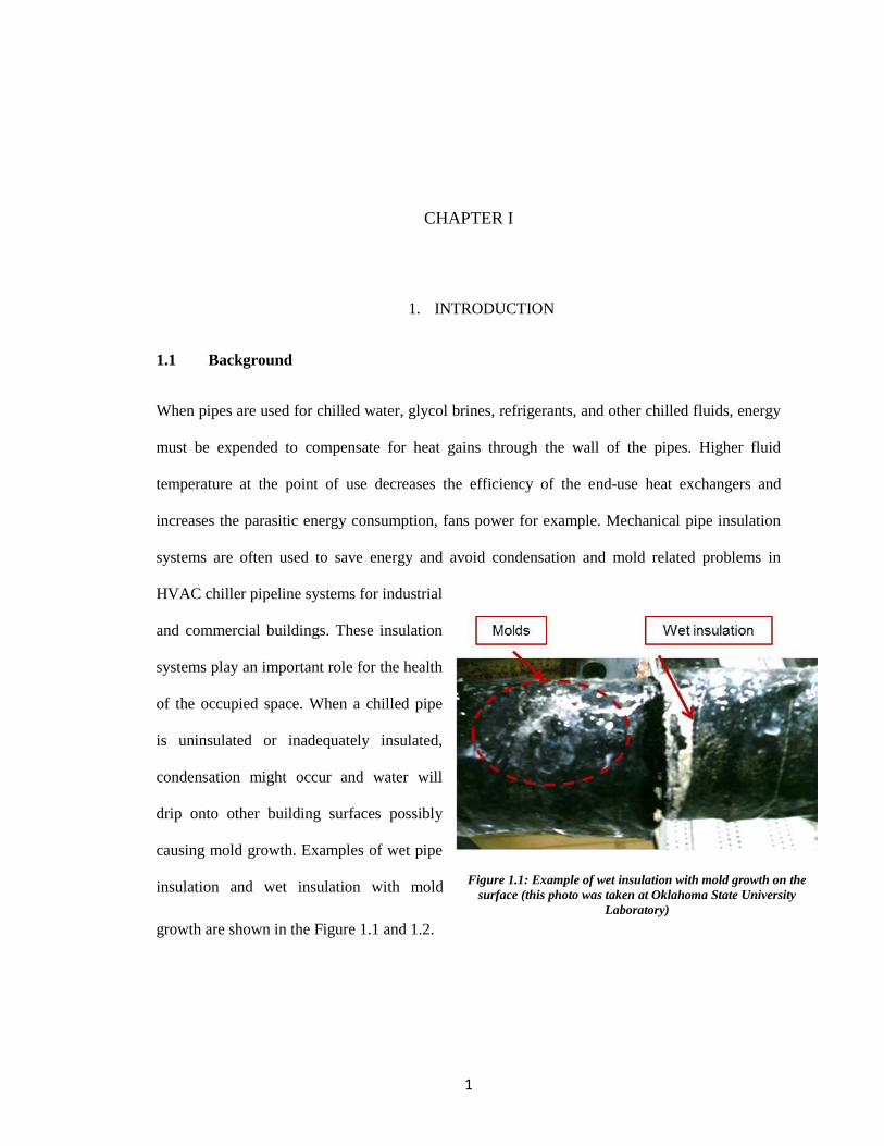
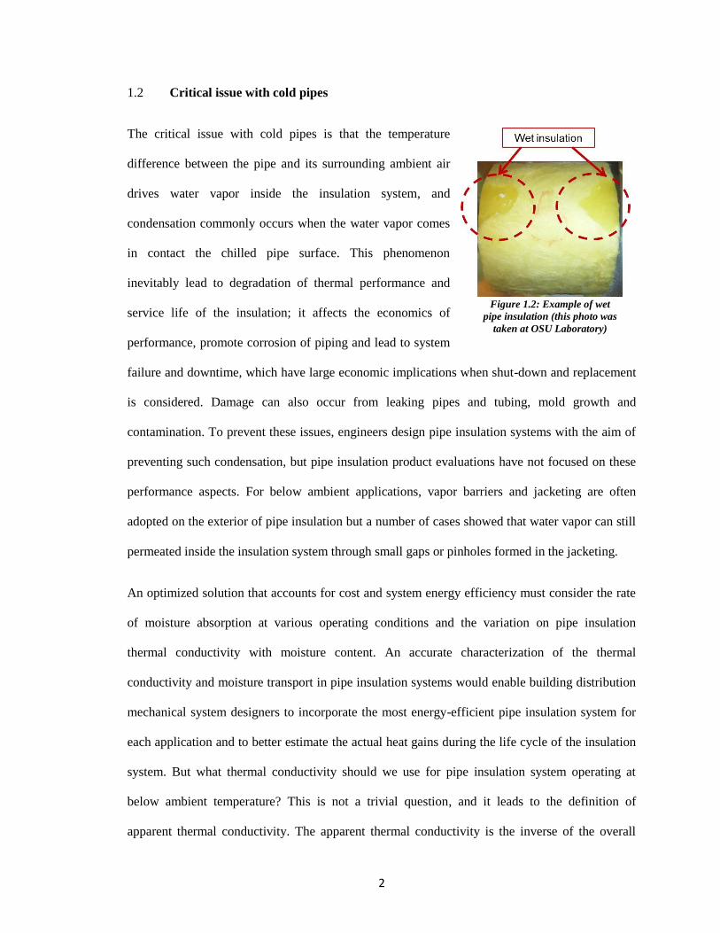
causing mold growth. Examples of wet pipe

insulation and wet insulation with mold

growth are shown in the Figure 1.1 and 1.2.

Figure 1.1: Example of wet insulation with mold growth on the

surface (this photo was taken at Oklahoma State University

Laboratory)

2

1.2 Critical issue with cold pipes

The critical issue with cold pipes is that the temperature

difference between the pipe and its surrounding ambient air

drives water vapor inside the insulation system, and

condensation commonly occurs when the water vapor comes

in contact the chilled pipe surface. This phenomenon

inevitably lead to degradation of thermal performance and

service life of the insulation; it affects the economics of

performance, promote corrosion of piping and lead to system

failure and downtime, which have large economic implications when shut-down and replacement

is considered. Damage can also occur from leaking pipes and tubing, mold growth and

contamination. To prevent these issues, engineers design pipe insulation systems with the aim of

preventing such condensation, but pipe insulation product evaluations have not focused on these

performance aspects. For below ambient applications, vapor barriers and jacketing are often

adopted on the exterior of pipe insulation but a number of cases showed that water vapor can still

permeated inside the insulation system through small gaps or pinholes formed in the jacketing.

An optimized solution that accounts for cost and system energy efficiency must consider the rate

of moisture absorption at various operating conditions and the variation on pipe insulation

thermal conductivity with moisture content. An accurate characterization of the thermal

conductivity and moisture transport in pipe insulation systems would enable building distribution

mechanical system designers to incorporate the most energy-efficient pipe insulation system for

each application and to better estimate the actual heat gains during the life cycle of the insulation

system. But what thermal conductivity should we use for pipe insulation system operating at

below ambient temperature? This is not a trivial question, and it leads to the definition of

apparent thermal conductivity. The apparent thermal conductivity is the inverse of the overall

Figure 1.2: Example of wet

pipe insulation (this photo was

taken at OSU Laboratory)

3

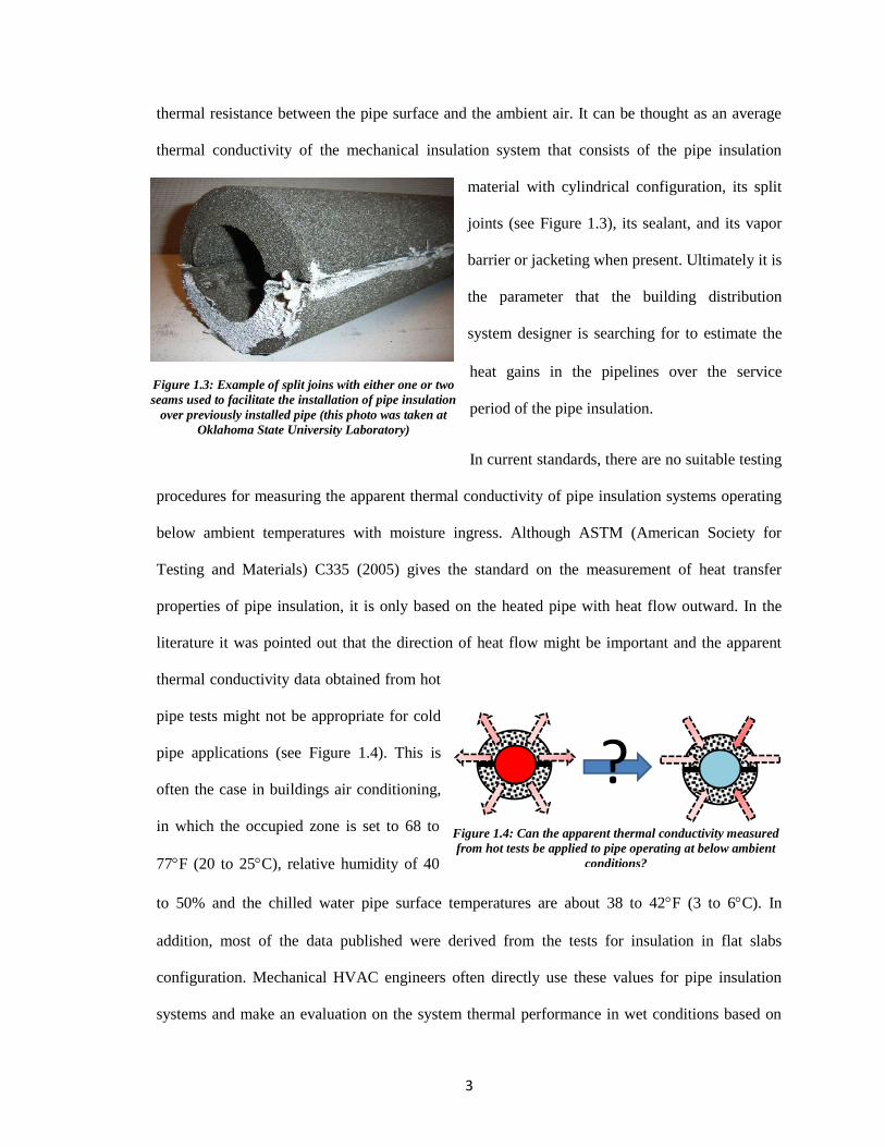
thermal resistance between the pipe surface and the ambient air. It can be thought as an average

thermal conductivity of the mechanical insulation system that consists of the pipe insulation

material with cylindrical configuration, its split

joints (see Figure 1.3), its sealant, and its vapor

barrier or jacketing when present. Ultimately it is

the parameter that the building distribution

system designer is searching for to estimate the

heat gains in the pipelines over the service

period of the pipe insulation.

In current standards, there are no suitable testing

procedures for measuring the apparent thermal conductivity of pipe insulation systems operating

below ambient temperatures with moisture ingress. Although ASTM (American Society for

Testing and Materials) C335 (2005) gives the standard on the measurement of heat transfer

properties of pipe insulation, it is only based on the heated pipe with heat flow outward. In the

literature it was pointed out that the direction of heat flow might be important and the apparent

thermal conductivity data obtained from hot

pipe tests might not be appropriate for cold

pipe applications (see Figure 1.4). This is

often the case in buildings air conditioning,

in which the occupied zone is set to 68 to

77F (20 to 25C), relative humidity of 40

to 50% and the chilled water pipe surface temperatures are about 38 to 42F (3 to 6C). In

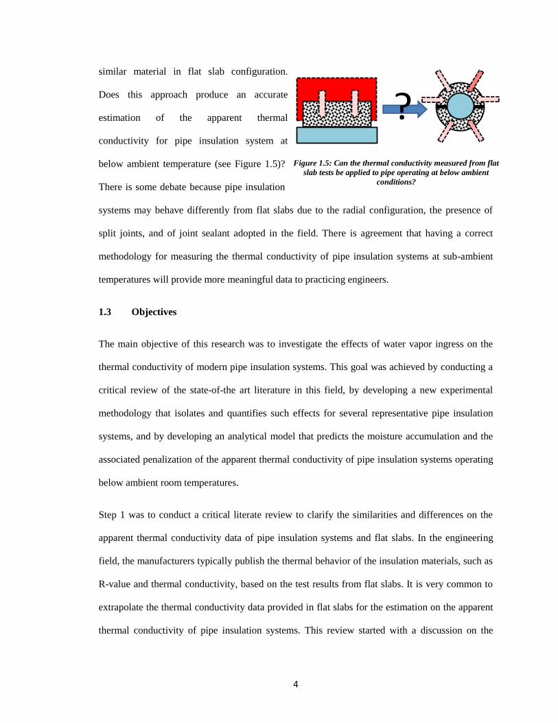
addition, most of the data published were derived from the tests for insulation in flat slabs

configuration. Mechanical HVAC engineers often directly use these values for pipe insulation

systems and make an evaluation on the system thermal performance in wet conditions based on

Figure 1.3: Example of split joins with either one or two

seams used to facilitate the installation of pipe insulation

over previously installed pipe (this photo was taken at

Oklahoma State University Laboratory)

?Figure 1.4: Can the apparent thermal conductivity measured

from hot tests be applied to pipe operating at below ambient

conditions?

4

similar material in flat slab configuration.

Does this approach produce an accurate

estimation of the apparent thermal

conductivity for pipe insulation system at

below ambient temperature (see Figure 1.5)?

There is some debate because pipe insulation

systems may behave differently from flat slabs due to the radial configuration, the presence of

split joints, and of joint sealant adopted in the field. There is agreement that having a correct

methodology for measuring the thermal conductivity of pipe insulation systems at sub-ambient

temperatures will provide more meaningful data to practicing engineers.

1.3 Objectives

The main objective of this research was to investigate the effects of water vapor ingress on the

thermal conductivity of modern pipe insulation systems. This goal was achieved by conducting a

critical review of the state-of-the art literature in this field, by developing a new experimental

methodology that isolates and quantifies such effects for several representative pipe insulation

systems, and by developing an analytical model that predicts the moisture accumulation and the

associated penalization of the apparent thermal conductivity of pipe insulation systems operating

below ambient room temperatures.

Step 1 was to conduct a critical literate review to clarify the similarities and differences on the

apparent thermal conductivity data of pipe insulation systems and flat slabs. In the engineering

field, the manufacturers typically publish the thermal behavior of the insulation materials, such as

R-value and thermal conductivity, based on the test results from flat slabs. It is very common to

extrapolate the thermal conductivity data provided in flat slabs for the estimation on the apparent

thermal conductivity of pipe insulation systems. This review started with a discussion on the

Figure 1.5: Can the thermal conductivity measured from flat

slab tests be applied to pipe operating at below ambient

conditions?

?

5

methodologies that has been reported in the current field for the measurement on the pipe

insulation thermal conductivity. The advantages and shortcomings of each technique were

pointed out to help engineer or researcher choose the methodology that most appropriate for the

test requirement. This literature review also provide a large data set on the thermal behavior of six

insulation systems by summarizing the current values reported both in flat slab and cylindrical

shape, under dry and wet conditions with moisture ingress.

The second step of my research work was the development of an experimental methodology to

measure the apparent pipe insulation thermal conductivity in dry and wet operating conditions

below ambient temperature and with water vapor ingress. This test apparatus improved the

accuracy of the experimental data with respect to modern methodologies used for pipe insulation

thermal conductivity measurements. The construction procedures are document in detail so that

the same test apparatus can be rebuilt in other labs. This test apparatus will be tested on more than

ten typical pipe insulation systems, which are commonly used in the low temperature engineering

field, such as industrial freezer in the cryogenic application, chilled water pipes in HVAC&R, etc.

The results derived from the measurement aimed to i) prove the feasibility and accuracy of the

current test facility; ii) show the differences on the thermal behavior between pipe insulation and

flat slabs, and how the behavior degrades when the insulation system was applied around the cold

surface and gradually become wet; iii) update the handbooks so that engineers can use the

specific values of the apparent thermal conductivity that directly measured from the pipe

insulation systems. The specific objectives in the experiment section are summarized as follows:

a) Design an experimental test apparatus to measure the thermal conductivity of pipe insulation

operating below ambient temperature and under both water vapor non-condensing and

condensing conditions;

b) Construct a prototype apparatus and calibrate its instrumentation;

6

c) Demonstrate that the apparatus operates successfully through the evaluation of at least two

typical insulation products at several pipe insulation mean temperatures;

d) Document the design of the apparatus in a way that others will be able to reproduce it

e) Measure various typical pipe insulation systems in both dry and wet conditions, and

identify seminaries and difference (if any) between their thermal performance

characteristics;

f) Investigate the impact of moisture ingress on the thermal conductivity of different types of

pipe insulation systems.

The third step of my research was to develop a general model that can be applied in the industry

field to help engineers predict the variation on the thermal behavior of different pipe insulation

systems with moisture content and with time. The model aimed to be general so that it can be

applied on various pipe insulation systems, fibrous or closed-cell, with joint sealant or with vapor

jacketing. From this model, the mechanical engineers and designers are able to correlate the

application with the ambient conditions to generate a deficiency profile of the insulation materials

and make estimation on the lifetime of the pipe insulation systems. This will very helpful in

selecting an optimal design between the system efficiency and economy cost. The specific aspects

that aimed to reach in the modeling part are summarized as follows:

a) Verify, expand, and possibly improve the accuracy of the thermodynamic models in the

open domain literature that predict the thermal conductivity of pipe insulation systems

under dry conditions;

b) Develop an analytical model for the prediction of the apparent thermal conductivity of

pipe insulation systems under wet, condensing conditions with moisture ingress;

c) Validate the model with both experimental data of the current thesis and the reported

values from the open domain literature;

7

d) Document the limitations in the current model, and summarize potential improvements in

follow up and future work.

1.4 Organization of this dissertation

This dissertation is organized in seven chapters:

1) Introduction: this section provides a research background on this topic and states project

objectives that need to be achieved by the end of this research work;

2) Literature review: in this section, I reviewed the most up-to-date work available in the

public domain on the measurement of pipe insulation thermal conductivity under both dry

and wet conditions. The advantages and shortcomings of each technique were discussed

at length with the challenges and future research needs in this area discussed at the end;

3) Test apparatus design and instrumentation: this section describes the test approach and

test apparatus that developed for the measurement of pipe insulation system thermal

conductivity. The construction procedures and facility improvements are documented in

detail.

4) Measurements and data reduction: this section discussed the test conditions and

summarized the test procedures applied during the experiment. A 2-D modeling approach

was explained in the data analysis, followed with the equipment accuracy investigation

and the measurement uncertainty analysis;

5) Experimental results: this section included all the findings that observed during each test

and summarized the test results for more than ten pipe insulation systems under both dry

and wet, condensing conditions. The test results were critically compared with possible

explanations provided in detail.

6) Simulation model: in this section, an analytical model was developed for closed-cell and

fibrous pipe insulation system, both under dry, non-condensing and wet conditions with

8

moisture ingress. The model has been validated with experimental data and reported data

from the open domain literature. Limitations are also discussed in this section for further

improvement;

7) Conclusions and recommendations: this section provides a conclusion of all the work I

have done in this research. Recommendations for future work will be provided at the end.

9

CHAPTER II

2. LITERATURE REVIEW

Because there are limited experimental data of thermal conductivity of pipe insulation systems at

below ambient temperature, mechanical HVAC engineers often extrapolate the thermal

conductivity and moisture ingress rates of pipe insulation systems in wet operating conditions

from experimental data originally obtained on the same type of insulation material but in flat slab

configurations. Two studies (Cremaschi et al., 2012a; Wilkes et al., 2002) have reported a

measurable difference on the effective thermal conductivity when considering flat slab and pipe

insulation systems. In addition this approximation might not be suitable for all pipe insulation

systems as it will be explained more in details later in the present report. Considering that the

dissimilar values of thermal conductivity and moisture ingress rates are partially due to the

method of testing, the test methodologies for measuring thermal conductivity of pipe insulation

systems were critically reviewed with the intention to clarify the concept of apparent thermal

conductivity associated with pipe insulation systems. To date there are not any standard methods

of testing pipe insulation systems for below ambient applications. Research was conducted to

extend test methodologies that were originally developed for flat slab configurations to pipe

insulation systems. We will also present standard methods of testing used specifically for pipe

insulation systems for above ambient applications, that is, heated pipes with outward heat flow.

For cold pipes commonly used in building HVAC systems, an inward heat flow occurs through

non-homogenous and anisotropic materials, and selecting the thermal conductivity for this

application based on measurements with outward heat flow is another point of debate among

10

engineers, practitioners, and building owners. The first objective of this review section is to

critically discuss all these aspects by an extensive literature review. The thermal conductivities of

pipe insulation systems measured at various laboratories were compared with the data in the

literature for flat slab configurations, and the second objective of the present review section is to

highlight the differences and similarities between these two sets of data. In addition, the direction

of heat flow is key when considering wet conditions, that is, when the pipe surface temperature is

below the dew point temperature of the surrounding atmosphere. This is often the case in the

building's air conditioning, in which the occupied zone is set to 20 to 25˚C (68 to 77˚F), when the

relative humidity of 40 to 50%, and the chilled water pipe surface temperatures are about 3.3 to

5.6˚C (38 to 42˚F). In these conditions, water vapor enters the insulation systems and condenses

on the pipe surfaces. The impact of moisture ingress on the actual pipe insulation thermal

resistance is still an unresolved question. For wet insulation, four main methods for preparing the

wet samples during laboratory measurements are identified in this review work and the third

objective of this review is to evaluate the impact of each method on the measured apparent

thermal conductivity of the pipe insulation system. The advantages and shortcomings of each

moisturizing strategy are discussed at length, and the thermal conductivities of a few available

pipe insulation systems in wet conditions are compared. The literature review presented in the

next sections should assist system designers in selecting appropriate pipe insulation systems

based on the thermal performance and operating conditions because, as it will be highlighted later

in the present review section, some materials may perform very well under dry conditions, but

condensate can easily accumulate leading to a fast degradation of the thermal performance.

2.1 Experimental methodologies for measurement of pipe insulation thermal conductivity

under dry conditions

In the current open domain literature of experimental data involving thermal conductivity of

cylindrical pipe insulation at below ambient conditions are scarce and mostly restricted to a few

11

insulation systems. Because there is debate on whether the thermal conductivity of pipe insulation

systems can be derived from measurements on flat slabs, it is helpful to highlight some of the

similarities and differences in the thermal conductivity measurements of these two forms. A

comparison between measured thermal conductivity data from the various test methodologies on

pipe insulation systems and flat slab systems may also illuminate this debate.

2.1.1 Brief background on the methodologies for thermal conductivity measurements of flat

slabs

For flat slab insulation systems, steady-state and transient test methodologies are commonly used.

The Guarded Hot Plate (GHP) is one of the most widely used steady-state methodologies for

thermal conductivity measurement on flat slab materials (ASTM_C177, 2010; ISO_8302, 1991).

In the GHP methods, the edge effect is minimized by the end guards. The Heat Flow Meter

methods (HFM), which are mainly represented by ISO 8301 (1991), as well as ASTM C518

(2010) and BS-EN 12667 (2001), are also commonly used due to their simple concept and low

requirements for the application of test specimens. The basic principles of both GHP and HFM

methods are applicable to pipe insulation systems. Compared to the GHP method, which is

normally applied below 200˚C (392˚F), there is no upper temperature limitation for the Thin

Heater Apparatus (THA), which is typically used for refractory bricks and insulation panels. With

considerably less mass than the combined central heater and guard heaters used in the GHP

methods, the THA is able to shorten the time to reach steady-state and may also minimize drift

errors (ASTM_C1114, 2006). However, currently this method is only available for testing flat

slab configurations. Another method commonly used under steady-state is the Hot Box method

(ASTM_C1363, 2011). Considering the severe requirements of the two temperature controlled

boundary conditions on both sides of the test specimen, the same apparatus is not suitable to be

used with material of cylindrical shapes because controlling the inner side might not be feasible

in practice.

12

The Transient Hot Wire (THW) and the Transient Hot Strip (THS) methods are common

techniques applied in transient conditions, and they are able to provide fast measurements of the

thermal conductivity for small size test samples (Gustafsson et al., 1978; Ohmura, 2007). The

Transient Plane Source technique (TPS), also referred to as “hot disk” or as “hot square”, is

developed for evaluation of anisotropic thermal property values by replacing the heating element

with a very thin, double metal spiral heater (Gustafsson et al., 1994; Rides et al., 2009; Sabuga &

Hammerschmidt, 1995). The thermal conductivity probe is a practical method used in the field,

and it provides measurements of the thermal conductivity of regions of the insulation in which it

is installed. It is generally viewed as a trade-off between accuracy and cost (Tye, 1969).

Compared to transient test methods, the thermal conductivity values from steady-state methods

are simpler to be derived from the measured data if the uniform heat flux throughout the test

specimen is a reasonable assumption. But providing a uniform heat flux in the entire test section

is the main challenge for most steady-state methods. Pratt, referred by Tye (1969), mentioned that

the steady-state methods are limited to only homogeneous materials with a thermal conductance

of at least 6000 W/m2-K (1060 Btu/hr-ft2-˚F). In order to prevent end edge effects, the test

samples normally need to be very large, and it takes a considerable amount of time for the test

specimen to reach complete thermal equilibrium. Due to the large surface area, the surface

contact resistances should not be neglected especially when the material thermal resistances are

of the same order. For example, Salmon and Tye (2010) pointed out that the material thermal

conductivity, measured by transient methodologies, are about 3% higher than the values derived

from the GHP due to the effects of surface thermal contact resistance between the test specimens

and the guarded plates. Transient methods are also not affected by the conditions of the

surrounding environments, which may cause the test specimens to become chemically unstable or

contaminated with long testing periods required by steady-state methods (Tye, 1969).

13

For the thermal conductivity measurement of insulating building materials, it seems that the

steady-state heat flow techniques yield more accurate measurements than the transient techniques

(Log, 1993). Using a calibrated insulation sample (McFadden, 1986), the accuracy of steady-state

heat flow techniques can be significantly improved, and anisotropic materials, such as fiber

materials with low bulk densities, can be successfully tested. Wulf et al. (2007) measured the

thermal conductivities of both isotropic and anisotropic materials based on the GHP technique,

the Guarded Heated Pipe technique, which will be discussed in the next section, and the THW

technique. These three techniques showed excellent agreement for isotropic materials, but some

discrepancies were observed in anisotropic materials. It was observed that the position of the

heated wire in the THW technique affected the measured thermal conductivity of anisotropic

materials. When dealing with low thermal conductivity materials, Woodbury and Thomas (1985)

pointed out that probe wires could become highly conductive and created an alternative path for

the heat losses. This would affect the accuracy of the measurements, and Suleiman (2006)

provided recommendations to avoid this. On the other hand, GHPs show large differences when

compare to other techniques at a temperature above 100˚C (212˚F) (Albers, 2002; Salmon & Tye,

2010). This is because the radiation heat transfer cannot be neglected at high temperatures. Tritt

(2004) observed that in using a standard steady-state method for temperatures above 150˚C

(302˚F), radiation loss became a serious problem, and a correction method to account for

radiation was proposed based on Wiedemann-Franz law (Johns & March, 1985). To minimize the

radiative heat transfer component, the surfaces need to be very emissive, especially for the low

density materials (Miller & Kuczmarski, 2009).

Since the GHP and HFM methods measure an overall thermal conductivity on a relatively large

area, they do not allow one to probe the insulation for a measurement of the thermal conductivity

at specific identifiable locations in the sample, which can be considered as a shortcoming of these

techniques in some cases (McFadden, 1988). By inserting the probe into the insulation, it is

14

possible to check the uniformity of the heat flux within the insulation and to determine if the

moisture is absorbed uniformly in the insulation for wet conditions.

2.1.2 Review of the thermal conductivity measurements of pipe insulation systems

For pipe insulation systems, the heat transfer is in radial direction, due to the cylindrical shape,

and heat conduction, which happens in radial symmetric geometries, was studied in the early

literature (Glazebrook, 1922). Because of the cylindrical geometry, the heat transfer area varies

from interior surface to the exterior surface, and this leads to a range of thermal resistances. The

definition of mean insulation temperature is not clear in most reported studies. In some studies, it

is reported as the arithmetic average temperature between the interior and exterior surfaces; in

other studies, it is defined as the temperature of a center layer of insulation obtained by volume-

weighted averages on the insulation samples. During the application of the pipe insulation

systems, joint sealant is usually required between the top and bottom shells. The presence of

longitudinal joints and of joint sealant affects the measured thermal conductivity of pipe

insulation systems if compared to corresponding thermal conductivity data, which is obtained

from flat slab configurations. All the above differences help to explain the reasons why the

apparent thermal conductivity of the pipe insulation systems differs from the measured thermal

conductivity of the insulation material, which is typically measured for flat slab configuration. In

recent years, limited published work in the literature reported the comparison of the thermal

performance and measurement methodologies between the pipe insulation systems and flat slabs

of the same materials. Wilkes et al. (2002) concluded that for polyurethane insulation, the flat

slab configuration had 2 to 5% higher thermal conductivity than the pipe insulation configuration.

Cremaschi et al. (2012a; 2012b) observed that the joint sealant applied on pipe insulation during

the installation might cause a non-negligible effect on the apparent insulation thermal

conductivity. Moore et al. (1985) pointed that measuring the thermal conductivity of pipe

insulation systems would be easier than measuring flat slabs since very long test specimens could

15

be used. Tritt (2004) disagreed because radial flow methods were relatively more difficult to

apply when compared to the linear measurements, especially when the materials were tested

below room temperature. However, Tritt (2004) agreed that the radiative heat loss, which was

severe in the traditional longitudinal heat flow method under high temperatures, could be

minimized when the heating source was placed internally.

From the standards of testing methods and literature reviews, the methodologies for measuring

the thermal conductivity of pipe insulation systems were critically reviewed, and they are

summarized next. The Guarded Heated Pipe method, which was developed from an early radial

flow test apparatus designed by Flynn in 1963 (Tye, 1969), can be considered as a modification

from the GHP method where the test pipe insulation shells are installed around a heated pipe. The

entire test apparatus is required to be placed in a temperature controlled chamber (Kimball, 1974;

Whitaker & Yarbrough, 2002; Wilkes et al., 2002), or a test enclosure (Zehendner, 1983) to

provide constant temperature boundary conditions. The main assumption of heat flux in the radial

direction is reasonable only if the edge effects, at both ends of pipes, are minimized. The standard

ISO 8497 (1994) and several studies in the literature provided guidelines on how to account for

the end edge effects (ASTM_C335-05, 2005; BS-EN253, 2009; ISO_8497, 1994). The Calibrated

Hot Box method, which was first presented by Musgrave (1979), is designed for testing pipe

insulation systems around cold pipes. For this method, it is critical to reduce the humidity inside

the box before the test, either by vacuuming or by dehumidification. In addition, proper sealing

with vapor barrier systems are required, but achieving complete vapor barrier during the test

conditions is critical. The Radial Heat Flow Meter method (concentric cylinder comparative

method) is a modification of the HFM method, and it is applicable for testing pipe insulation with

both inward and outward heat flux. Because of ease of installation, researchers used small pads as

heat flux meters, substituting them for sleeve flux meters (Ramsden, 1985; Rawlins, 2005).

However, the application of the heat flux pads seems to affect the shape of the test specimen --

16

either by compressing the insulation in some locations or by creating gaps of air between the test

insulation and cold surface in other locations. This variation of the contact resistance should be

properly accounted for when measuring the thermal performance of the pipe insulation systems.

While the Guarded Heated Pipe method is only suitable for the thermal conductivity

measurement with the outward heat flow, the Calibrated Hot Box method is used for cold pipe

with inward radial heat flux. For achieving accuracy, it is critical to design appropriate thermal

guards at the ends, and water vapor condensate might be an issue during the thermal conductivity

measurements. Radial heat flow meters are suitable for both heated and cold pipes, but they suffer

similar issues when applied to cold pipes. When using the Radial Heat Flux Meter technique, they

should be either designed as insensitive to the water vapor in the air and potential moisture

accumulation on the meter, or the ambient has to be controlled such that the dew point

temperature is below the surface temperature of the cold pipes. Another challenge with the Radial

Heat Flux Meter is the possibility of forming thermal bridges between the two concentric pipes in

the test apparatus. Cremaschi et al. (2012a; 2012b) pointed out that in order to obtain better

accuracy during the measurement, the materials made for supporting sleeves in between the two

concentric pipes need to be selected with a thermal conductivity of the same magnitude as the one

of test specimen.

There are also some techniques that employed transient methods to measure the thermal

conductivity of pipe insulation systems. Transient methods are suitable for the measurement of

pipe insulation thermal conductivity under non-destructive testing and in the field. The THW

method is applied for the measurement of thermal conductivity in the range from 0.08 to 2.0

W/m-K (0.55 to 13.9 Btu-in/hr-ft2-˚F) (Kulkarni & Vipulanandan, 2006). Adl-Zarrabi (2005)

tested the pipe insulation thermal conductivity by using the TPS method. By comparing to the

results measured from the Guarded Heated Pipe method, all the values derived in the TPS

apparatus were slightly higher. When considering the joint sealant and vapor jacketing of pipe

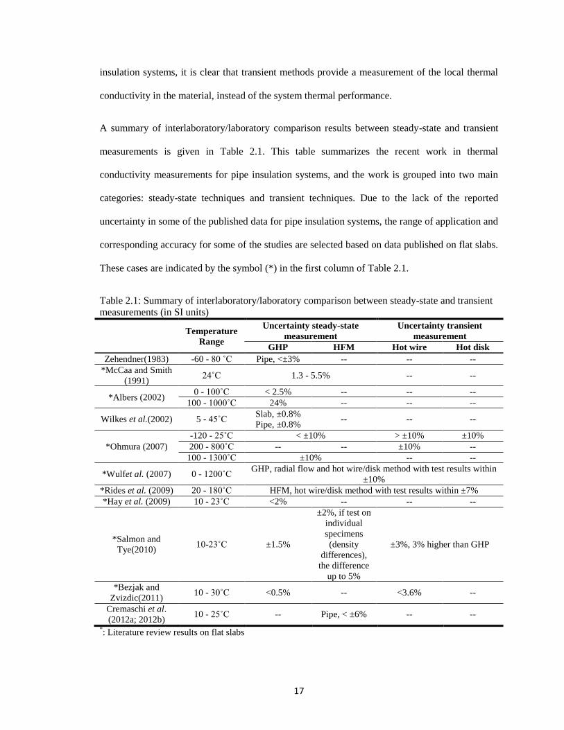
17

insulation systems, it is clear that transient methods provide a measurement of the local thermal

conductivity in the material, instead of the system thermal performance.

A summary of interlaboratory/laboratory comparison results between steady-state and transient

measurements is given in Table 2.1. This table summarizes the recent work in thermal

conductivity measurements for pipe insulation systems, and the work is grouped into two main

categories: steady-state techniques and transient techniques. Due to the lack of the reported

uncertainty in some of the published data for pipe insulation systems, the range of application and

corresponding accuracy for some of the studies are selected based on data published on flat slabs.

These cases are indicated by the symbol (*) in the first column of Table 2.1.

Table 2.1: Summary of interlaboratory/laboratory comparison between steady-state and transient

measurements (in SI units)

Temperature

Range

Uncertainty steady-state

measurement

Uncertainty transient

measurement

GHP HFM Hot wire Hot disk

Zehendner(1983) -60 - 80 ˚C Pipe, <±3% -- -- --

*McCaa and Smith

(1991) 24˚C 1.3 - 5.5% -- --

*Albers (2002) 0 - 100˚C < 2.5% -- -- --

100 - 1000˚C 24% -- -- --

Wilkes et al.(2002) 5 - 45˚C Slab, ±0.8%

Pipe, ±0.8% -- -- --

*Ohmura (2007)

-120 - 25˚C < ±10% > ±10% ±10%

200 - 800˚C -- -- ±10% --

100 - 1300˚C ±10% -- --

*Wulfet al. (2007) 0 - 1200˚C GHP, radial flow and hot wire/disk method with test results within

±10%

*Rides et al. (2009) 20 - 180˚C HFM, hot wire/disk method with test results within ±7%

*Hay et al. (2009) 10 - 23˚C <2% -- -- --

*Salmon and

Tye(2010) 10-23˚C ±1.5%

±2%, if test on

individual

specimens

(density

differences),

the difference

up to 5%

±3%, 3% higher than GHP

*Bezjak and

Zvizdic(2011) 10 - 30˚C <0.5% -- <3.6% --

Cremaschi et al.

(2012a; 2012b) 10 - 25˚C -- Pipe, < ±6% -- --

*: Literature review results on flat slabs

18

2.2 Review of thermal conductivity variation in pipe insulation systems

In this section, a comparison of the thermal conductivity of both flat slab and pipe insulation is

presented with the aim of documenting the methodologies discussed in the previous section. The

differences in material properties, such as density, thickness, porosity, internal structure,

anisotropy, blowing agent, manufacturing time, handling, and installation methods, may affect the

results of the experimental measurements. However, there are no studies that provided detailed

information on the materials being tested for the thermal conductivity of both pipe insulation

systems and flat slabs. In one research study the authors compared these two configurations and

pointed out the differences come from the material density and geometry between the pipe

insulation and flat slabs (Wilkes et al., 2002). In order to provide a general idea of how the

thermal performance of the insulation system varies with the methodologies applied for thermal

conductivity measurement, as well as with different types of materials and material densities, the

reported values in the open literature are summarized in the following sections. The material

properties, such as configurations of the test samples, densities and thicknesses are documented in

the Tables of Appendix A. The thermal conductivity of both pipe insulation systems and flat slabs

are compared between the materials with similar densities. Based on these criteria, nine insulation

materials applied in HVAC field are discussed, and the data have been grouped in Figure 2.1 to 5.

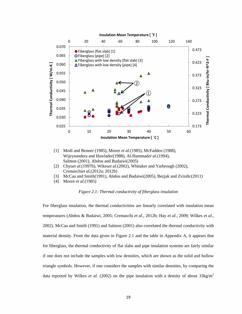
19

[1] Modi and Benner (1985), Moore et al.(1985), McFadden (1988),

Wijeysundera and Hawlader(1988), Al-Hammadet al.(1994),

Salmon (2001), Abdou and Budaiwi(2005)

[2] Chyuet al.(1997b), Wikeset al.(2002), Whitaker and Yarbrough (2002),

Cremaschiet al.(2012a; 2012b)

[3] McCaa and Smith(1991), Abdou and Budaiwi(2005), Bezjak and Zvizdic(2011)

[4] Moore et al.(1985)

Figure 2.1: Thermal conductivity of fiberglass insulation

For fiberglass insulation, the thermal conductivities are linearly correlated with insulation mean

temperatures (Abdou & Budaiwi, 2005; Cremaschi et al., 2012b; Hay et al., 2009; Wilkes et al.,

2002). McCaa and Smith (1991) and Salmon (2001) also correlated the thermal conductivity with

material density. From the data given in Figure 2.1 and the table in Appendix A, it appears that

for fiberglass, the thermal conductivity of flat slabs and pipe insulation systems are fairly similar

if one does not include the samples with low densities, which are shown as the solid and hollow

triangle symbols. However, if one considers the samples with similar densities, by comparing the

data reported by Wilkes et al. (2002) on the pipe insulation with a density of about 33kg/m3

0 20 40 60 80 100 120 140

0.173

0.223

0.273

0.323

0.373

0.423

0.473

0.025

0.030

0.035

0.040

0.045

0.050

0.055

0.060

0.065

0.070

0 10 20 30 40 50 60

Insulation Mean Temperature [ ˚F ]

Th

erm

al C

on

du

ctiv

ity

[ B

tu-i

n/h

r-ft

^2

-F ]

Th

erm

al C

on

du

ctiv

ity

[ W

/m-K

]

Insulation Mean Temperature [ ˚C ]

Fiberglass (flat slab) [1]Fiberglass (pipe) [2]Fiberglass with low density (flat slab) [3]Fiberglass with low density (pipe) [4]

①

②

20

(2.1lbm/ft3), and the data published by Al-Hammad et al. (1994) on the flat slab with a density

between 32 to 37 kg/m3 (2.0 to 2.3 lbm/ft

3), the measured thermal conductivity values on flat slab

was about 10% higher than the pipe insulation, shown as group ① in Figure 2.1. The reported

uncertainty is ±0.8% for the Guarded Heated Pipe method (Wilkes et al., 2002) and ±2% to ±4%

for the GHP (Al-Hammad et al., 1994). When considering material samples with low densities,

ranging from 12 to 27 kg/m3 (0.75 to 1.7 lbm/ft

3) as shown in Appendix A, the thermal

conductivity seems to increase as Langlais et al.(1982) pointed out. In this range, by selecting two

samples with similar densities, 15 kg/m3 (McCaa & Smith, 1991; Moore et al., 1985) and shown

as group ② in the figure, the flat slab seems to be more conductive than the pipe insulation. The

mean error for the measurement of thermal conductivity on the flat slab was reported with an

imprecision around 3% (McCaa & Smith, 1991), and the uncertainty on the pipe insulation tester

was not clarified in the literature.

For polyurethane, the density effect on the thermal conductivity seems not so significant as on

fiberglass (Zehendner, 1983). The data summarized in Figure 2.2 suggests that the polyurethane

insulation has different thermal conductivity when measured from flat slabs and pipe insulation

systems; however, a measurable difference was only reported for one group of data by Ohmura

(2007). Although this group of data was validated by both steady state and transient methods,

within ±10% deviation, the material is affected by “aging” process since the blowing agent

slowly diffuses out, and it is gradually replaced by air that fills in the cells. Kellner and Dirckx

(1999) found that the thermal conductivity was increased by 7% to 30% depending on different

aging methods. Blowing agent is another aspect that also needs to be considered during a critical

comparison. Bhattacharjee et al. (1991) investigated both blowing agent and aging effects by

comparing 20 specimens and concluded that different gas composition would vary the sensitivity

on the thermal conductivity to the insulation mean temperatures. Biedermann et al. (2001)

compared in detail the effect on thermal conductivity of 12 gas compositions, and the differences

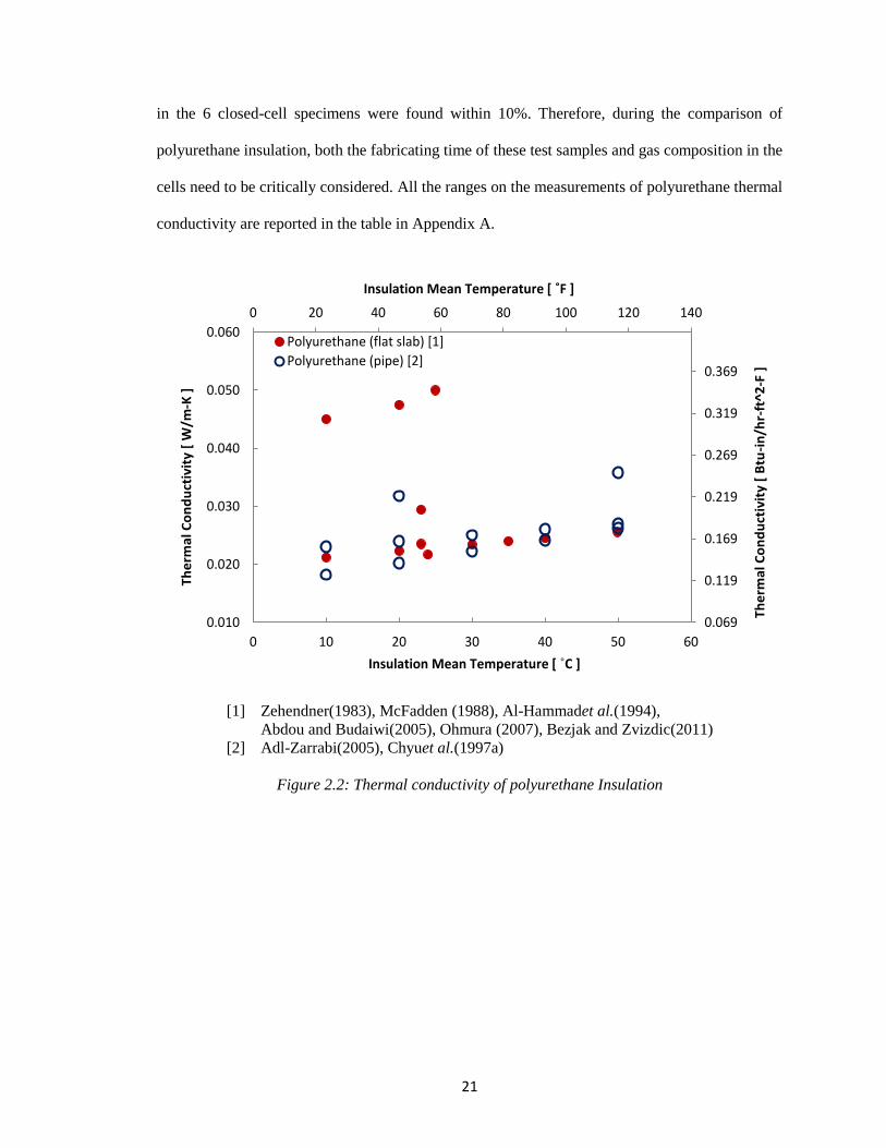
21

in the 6 closed-cell specimens were found within 10%. Therefore, during the comparison of

polyurethane insulation, both the fabricating time of these test samples and gas composition in the

cells need to be critically considered. All the ranges on the measurements of polyurethane thermal

conductivity are reported in the table in Appendix A.

[1] Zehendner(1983), McFadden (1988), Al-Hammadet al.(1994),

Abdou and Budaiwi(2005), Ohmura (2007), Bezjak and Zvizdic(2011)

[2] Adl-Zarrabi(2005), Chyuet al.(1997a)

Figure 2.2: Thermal conductivity of polyurethane Insulation

0 20 40 60 80 100 120 140

0.069

0.119

0.169

0.219

0.269

0.319

0.369

0.010

0.020

0.030

0.040

0.050

0.060

0 10 20 30 40 50 60

Insulation Mean Temperature [ ˚F ]

Th

erm

al C

on

du

ctiv

ity

[ B

tu-i

n/h

r-ft

^2

-F ]

Th

erm

al C

on

du

ctiv

ity

[ W

/m-K

]

Insulation Mean Temperature [ ˚C ]

Polyurethane (flat slab) [1]

Polyurethane (pipe) [2]

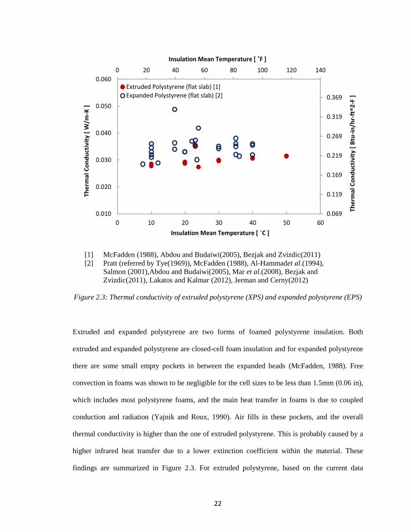
22

[1] McFadden (1988), Abdou and Budaiwi(2005), Bezjak and Zvizdic(2011)

[2] Pratt (referred by Tye(1969)), McFadden (1988), Al-Hammadet al.(1994),

Salmon (2001),Abdou and Budaiwi(2005), Mar et al.(2008), Bezjak and

Zvizdic(2011), Lakatos and Kalmar (2012), Jerman and Cerny(2012)

Figure 2.3: Thermal conductivity of extruded polystyrene (XPS) and expanded polystyrene (EPS)

Extruded and expanded polystyrene are two forms of foamed polystyrene insulation. Both

extruded and expanded polystyrene are closed-cell foam insulation and for expanded polystyrene

there are some small empty pockets in between the expanded beads (McFadden, 1988). Free

convection in foams was shown to be negligible for the cell sizes to be less than 1.5mm (0.06 in),

which includes most polystyrene foams, and the main heat transfer in foams is due to coupled

conduction and radiation (Yajnik and Roux, 1990). Air fills in these pockets, and the overall

thermal conductivity is higher than the one of extruded polystyrene. This is probably caused by a

higher infrared heat transfer due to a lower extinction coefficient within the material. These

findings are summarized in Figure 2.3. For extruded polystyrene, based on the current data

0 20 40 60 80 100 120 140

0.069

0.119

0.169

0.219

0.269

0.319

0.369

0.010

0.020

0.030

0.040

0.050

0.060

0 10 20 30 40 50 60

Insulation Mean Temperature [ ˚F ]

Th

erm

al C

on

du

ctiv

ity

[ B

tu-i

n/h

r-ft

^2

-F ]

Th

erm

al C

on

du

ctiv

ity

[ W

/m-K

]

Insulation Mean Temperature [ ˚C ]

Extruded Polystyrene (flat slab) [1]

Expanded Polystyrene (flat slab) [2]

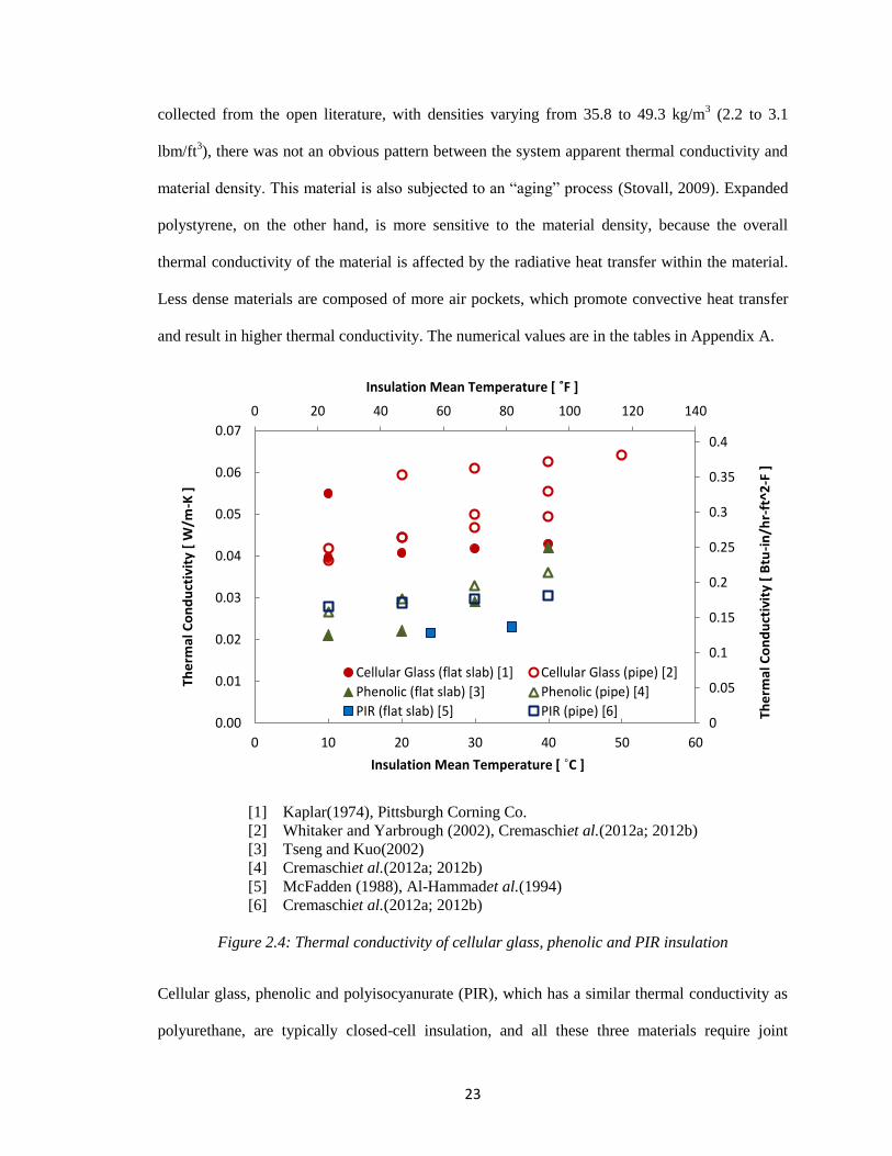
23

collected from the open literature, with densities varying from 35.8 to 49.3 kg/m3 (2.2 to 3.1

lbm/ft3), there was not an obvious pattern between the system apparent thermal conductivity and

material density. This material is also subjected to an “aging” process (Stovall, 2009). Expanded

polystyrene, on the other hand, is more sensitive to the material density, because the overall

thermal conductivity of the material is affected by the radiative heat transfer within the material.

Less dense materials are composed of more air pockets, which promote convective heat transfer

and result in higher thermal conductivity. The numerical values are in the tables in Appendix A.

[1] Kaplar(1974), Pittsburgh Corning Co.

[2] Whitaker and Yarbrough (2002), Cremaschiet al.(2012a; 2012b)

[3] Tseng and Kuo(2002)

[4] Cremaschiet al.(2012a; 2012b)

[5] McFadden (1988), Al-Hammadet al.(1994)

[6] Cremaschiet al.(2012a; 2012b)

Figure 2.4: Thermal conductivity of cellular glass, phenolic and PIR insulation

Cellular glass, phenolic and polyisocyanurate (PIR), which has a similar thermal conductivity as

polyurethane, are typically closed-cell insulation, and all these three materials require joint

0 20 40 60 80 100 120 140

0

0.05

0.1

0.15

0.2

0.25

0.3

0.35

0.4

0.00

0.01

0.02

0.03

0.04

0.05

0.06

0.07

0 10 20 30 40 50 60

Insulation Mean Temperature [ ˚F ]

Th

erm

al C

on

du

ctiv

ity

[ B

tu-i

n/h

r-ft

^2

-F ]

Th

erm

al C

on

du

ctiv

ity

[ W

/m-K

]

Insulation Mean Temperature [ ˚C ]

Cellular Glass (flat slab) [1] Cellular Glass (pipe) [2]

Phenolic (flat slab) [3] Phenolic (pipe) [4]

PIR (flat slab) [5] PIR (pipe) [6]

24

sealant during the installation on pipes. As summarized in Figure 2.4 (and the tables in Appendix

D), the densities of these closed-cell insulation materials are typically in a narrow range, and the

thermal conductivity seems not to be sensitive on the material density. For cellular glass and

phenolic pipe insulation systems, the thermal conductivity is about 20% higher than the thermal

conductivity measured from flat slabs. Cremaschi et al. (2012b) explained that the difference

might be due to the longitudinal joints and the sealant which was applied on these joints. For both

phenolic and PIR insulation, the deterioration of self-performance in the test samples need to be

considered since they are subjected to the aging process (Christian et al., 1998; Stovall, 2009).

Thus the result reported in Figure 2.4 in which pipe insulation systems have 20 to 30% higher

thermal conductivity than flat slabs must be carefully gauged due to different manufacturing time

between the test samples. Similar to polyurethane insulation, different blowing agents are applied

for PIR insulation, and the effect also needs to be accounted for during the comparison on the

effective thermal conductivity (Zarr & Nguyen, 1994). For most closed-cell insulation, one

critical issue that needs to be considered is some blowing agents, such as pentane, propane, which

are defined as natural gas liquid, can be easily turned into liquid with the application of moderate

pressure or freezing and dramatically reduce the thermal conductivity of the insulation.

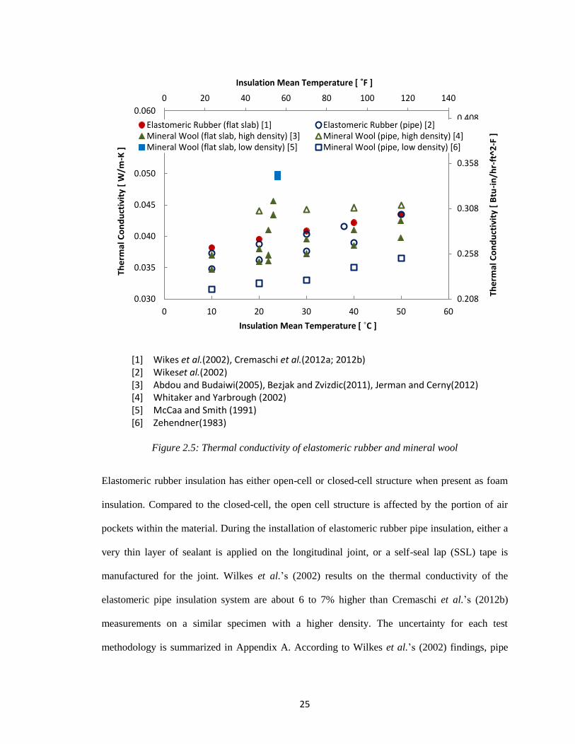
25

Figure 2.5: Thermal conductivity of elastomeric rubber and mineral wool

Elastomeric rubber insulation has either open-cell or closed-cell structure when present as foam

insulation. Compared to the closed-cell, the open cell structure is affected by the portion of air

pockets within the material. During the installation of elastomeric rubber pipe insulation, either a

very thin layer of sealant is applied on the longitudinal joint, or a self-seal lap (SSL) tape is

manufactured for the joint. Wilkes et al.’s (2002) results on the thermal conductivity of the

elastomeric pipe insulation system are about 6 to 7% higher than Cremaschi et al.’s (2012b)

measurements on a similar specimen with a higher density. The uncertainty for each test

methodology is summarized in Appendix A. According to Wilkes et al.’s (2002) findings, pipe

0 20 40 60 80 100 120 140

0.208

0.258

0.308

0.358

0.408

0.030

0.035

0.040

0.045

0.050

0.055

0.060

0 10 20 30 40 50 60

Insulation Mean Temperature [ ˚F ]

Th

erm

al C

on

du

ctiv

ity

[ B

tu-i

n/h

r-ft

^2

-F ]

Th

erm

al C

on

du

ctiv

ity

[ W

/m-K

]

Insulation Mean Temperature [ ˚C ]

Elastomeric Rubber (flat slab) [1] Elastomeric Rubber (pipe) [2]Mineral Wool (flat slab, high density) [3] Mineral Wool (pipe, high density) [4]Mineral Wool (flat slab, low density) [5] Mineral Wool (pipe, low density) [6]

[1] Wikes et al.(2002), Cremaschi et al.(2012a; 2012b) [2] Wikeset al.(2002) [3] Abdou and Budaiwi(2005), Bezjak and Zvizdic(2011), Jerman and Cerny(2012) [4] Whitaker and Yarbrough (2002) [5] McCaa and Smith (1991) [6] Zehendner(1983)

26

insulation systems showed 1.5% to 2.5% lower thermal conductivity when compared to flat slabs

with similar densities and thicknesses, as shown in Figure 2.5, and they considered it as a good

match because the materials were not identical. Mineral wool is another type of fibrous

insulation, and its thermal conductivity is quite sensitive to the material density. From the values

summarized in the table in Appendix E, it seems that with similar densities, the cylindrical shaped

mineral wool insulation has a thermal conductivity 20% higher than the flat slab configuration

(Abdou & Budaiwi, 2005; Whitaker & Yarbrough, 2002). It is noted that one group of pipe

insulation (the hollow rectangles in the figure) showed lower thermal conductivity than the flat

slab which has a similar density. This is because during this group of tests, the test specimen is

mineral fibers bound with synthetic resin (Zehendner, 1983).

2.3 Methodologies for measurement of pipe insulation thermal conductivity under wet

condition and with moisture ingress

To date there are no set criteria for the testing methods of pipe insulation under wet conditions. In

wet conditions, liquid water and water vapor will accumulate in the insulation by filling the air

gaps between the cells, or replacing the gas in the cells if the cell wall is permeable. Water will be

distributed in the insulation due to the gravitational effect and capillary force, and the partial

pressure difference will be the driving force for the water vapor diffusion. From the present

literature review it is found that the method of testing depends on the technique used for

preparing the moist insulation sample. Four methodologies for the measurement of insulation

thermal conductivity with moisture ingress are defined for the first time as shown in Table 2.2.

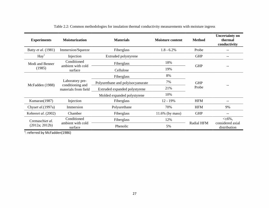
27

Table 2.2: Common methodologies for insulation thermal conductivity measurements with moisture ingress

Experiments Moisturization Materials Moisture content Method

Uncertainty on

thermal

conductivity

Batty et al. (1981) Immersion/Squeeze Fiberglass 1.8 - 6.2% Probe --

Hay1 Injection Extruded polystyrene

GHP --

Modi and Benner

(1985)

Conditioned

ambient with cold

surface

Fiberglass 18% GHP --

Cellulose 19%

McFadden (1988)

Laboratory pre-

conditioning and

materials from field

Fiberglass 8%

GHP

Probe --

Polyurethane and polyisocyanurate 7%

Extruded expanded polystyrene 21%

Molded expanded polystyrene 10%

Kumaran(1987) Injection Fiberglass 12 - 19% HFM --

Chyuet al.(1997a) Immersion Polyurethane 70% HFM 9%

Kehreret al. (2002) Chamber Fiberglass 11.6% (by mass) GHP --

Cremaschiet al.

(2012a; 2012b)

Conditioned

ambient with cold

surface

Fiberglass 12% Radial HFM

<±6%,

considered axial

distribution Phenolic 5%

¹: referred by McFadden(1986)

28

The first group, flooded methods, consists of completely immersing the test specimens in water to

provide a certain amount of moisture and uniform distribution. There exists the assumption that

by immersing the insulation sample in the water would be able to provide the upper limit for the

insulation thermal conductivity. However, a simple immersion without temperature difference

between the two surfaces of the pipe insulation test sample would lead to the water permeation

less than the situation with driving force from the water vapor pressure differences across the

insulation. If immersing the pipe insulation test sample in a water reservoir with the inner surface

maintained at a low temperature and controlling the water temperature in the reservoir, the

thermal conductivity can be measured under isothermal conditions. The water absorption is

determined directly from the water volume variation in the reservoir (Chyu et al., 1997a, 1997b;

Kaplar, 1974). Several more or less cumbersome techniques are proposed to control the desired

amount of water content in the test specimen (Batty et al., 1981; Kumaran, 2006; Langlais &

Klarsfeld, 1984). Full immersion, partial immersion, and immersion under pressure may lead to

different internal moisture distribution (Chalumeau & Felix-Henry, 2006; Kaplar, 1974). In

addition, it is pointed out that the temperature of the water reservoir might affect the moisture

ingress and the apparent thermal conductivity of the test sample. This is due to surface tension

effects (Chyu et al., 1997a) and heat transfer processes which are caused by the natural

convection phenomenon. The convection heat transfer is particularly relevant for fiberglass and

mineral wool insulation. The flooded method is more appropriate on testing insulation systems

applied around pipelines below ground or in deep sea application. However, in the HVAC field,

the insulation systems are applied around pipelines which are normally placed in either indoor or

outdoor environment. Flooded methods create different boundary conditions on the test samples

from the actual field applications, and thus it is difficult to extrapolate the data from these

methods of wet testing.

29

Spraying or injecting water into pipe insulation systems and flat slabs belong to the second group

of methodologies for measuring the thermal conductivity in wet conditions (Langlais et al., 1982;

Wijeysundera et al., 1996). The moisture distribution inside the insulation might be in transient

conditions since water at the hot surface will be vaporized and transported to the cold surface

(Kumaran, 1987). During the transient conditions, the insulation thermal conductivity is a

function of the location of the high moist regions (McFadden, 1986), and the thermal conductivity

of pipe insulation systems depend on whether the high moist regions are closer to the hot side or

to the cold side. This group of methodologies requires a great amount of time to reach steady state

when the moisture content, both in the form of liquid and gas, is completely redistributed to the

cold surface. Once it reaches steady state, the thermal conductivity of insulation systems is

independent of the initial moisture distribution of the test samples. Results show that when the

water content is less than 1% by volume, the heat flux through the material is 3 to 4 times higher

than the dry insulation during transient conditions, but the material will perform as dry insulation

under steady state when the moisture is completely transported to the cold surface (Kumaran,

1987). Considering the sensitivity of the positions of the high moist regions to the thermal

conductivity of pipe insulation systems, spray/injection methods would fail in simulating the

water distribution in the pipe insulation systems applied in the HVAC field.

The third category is defined as laboratory pre-conditioning methods, and it consists of placing

the insulation test specimens in the air with very high humidity before the thermal conductivity

measurements. Several researchers point out that the moisture content accumulated inside the

insulation is lower than the moisture content in the actual operating conditions (Batty et al., 1984;

Kehrer et al., 2002; Kumaran, 1987; Langlais et al., 1982; McFadden, 1988). This is due to a

weak vapor driving potential during the pre-conditioning process of the insulation test specimens.

The other disadvantage of these methods is that water distribution in the insulation systems is

30

different from the real field, and any water redistribution will affect the thermal conductivity

measurements.

The fourth group includes methods that adopt a temperature, humidity and air speed controlled

ambient and simultaneously impose a cold surface/cold pipe on one side of the insulation test

specimen (Cremaschi et al., 2012a; Cremaschi et al., 2012b; Modi & Benner, 1985; Mumaw,

2002; Peuhkuri et al., 2008). Cremaschi et al.(2012a) tested several pipe insulation systems in a

psychrometric chamber. Their approach required a large amount of equipment, and it had a very

high capital cost. The psychrometric chamber is able to better replicate the actual operating

conditions of the pipe insulation systems as those of real service in the chiller applications.

Moisture is driven into the insulation due to a gradient in the water vapor partial pressure across

the insulation specimen, and the water vapor ultimately condenses when it reaches the cold pipe

surface. A great amount of time is required to achieve measurable moisture contents, but

accelerated type of tests can be conducted by increasing the temperature and humidity gradients

to help drive water vapor ingress into the insulation specimen (Cremaschi et al., 2012a; Mumaw,

2002).

If the test samples are prepared according to the two techniques mentioned above (Spray/injection

methods and pre-conditioning methods), steady-state methods are not suitable for the thermal

conductivity measurements with moisture ingress. Kehrer et al. (2002) measured the thermal

conductivity of fiberglass insulation by placing the sample, which had moisture content of about

11.6% by mass, in a GHP test apparatus. The insulation thermal conductivity was approximately

5 to 6% higher when compared to that of the dry sample. The reason is due to the latent heat

convection effects with moisture that evaporates at the hot plate and condenses at the cold

surface. They concluded that “the real thermal conductivity of the insulation material in

equilibrium with 80% RH is not higher than in the dry state”. Langlais et al.(1983) tested a

fiberboard with moisture sprayed on the cold and hot surfaces. The thermal conductivity was

31

measured using the GHP method; it increased rapidly in the first two hours and gradually dropped

in the next five hours. The similar phenomenon was observed by other researchers (Benner &

Modi, 1986; Wijeysundera et al., 1993, 1996). Langlais et al.(1983) explained that the

redistribution of the moisture inside the insulation led to a water vapor enthalpy flow, which was

interpreted as heat conduction by the thermal conductivity test apparatuses. Thus, the steady-state

methods yield to overestimation of the material thermal conductivity under wet conditions.

Sandberg (1995) highly recommended that with redistribution phenomenon, the measurement

should not be taken with a large temperature difference or in a long time, which are the steps

required for both the GHP and HFM methods. These observations suggest that steady-state

methods are not suitable for the thermal conductivity measurements of moisture insulation with

low heat fluxes. Only if the test sample is continuously in contact with a cold surface or a cold

pipe, then steady-state methods can be successfully applied (Cremaschi et al., 2012a). In this

method, the water distribution in the pipe insulation is fairly similar to the real chilled water

application. Water redistribution is minimized because a continuous driving force for the

moisture is established during the tests by the water vapor pressure difference between the cold

surface and the ambient.

For improving the accuracy of the measurement in presence of moisture ingress, the end sections

of the test specimens must be given special considerations in order to avoid longitudinal moisture

ingress that can skew the measurements (Simonson et al., 1996). Batty et al. (1984) concluded

that traditional GHP methods were impractical for the thermal conductivity measurements of

moist insulation due to moisture redistribution, and they proposed using a line-source thermal

conductivity probe. With this transient method, the short measuring time and small temperature

gradient overcome the limitation of vapor redistribution that exists in most steady-state methods.

Woodbury and Thomas (1985) concluded that when measuring with a thermal conductivity

probe, the moisture content was quite sensitive to the thermal conductivity at low concentration,

32

and the thermal conductivity increased dramatically when the insulation becomes slightly wet. Yu

et al. (2009) derived a similar conclusion on the thermal conductivity probe when using the

device to determine the effects of moisture content on the uncertainty during sand thermal

conductivity measurements. If the moisture content is higher than 25% (by volume), the thermal

conductivity is measured accurately by the probe because the evaporation rate and capillary

forces are low. However, if the moisture content is low, such as in pipe insulation systems, the

regions adjacent to the heating tip of the probe may be easily dried out, and this local dry out

phenomenon can bring a large error in the measurement of the actual thermal conductivity of the

wet insulation. Some other challenges include the heat loss from the high conductive probe wire

(Woodbury & Thomas, 1985), the limitation of the sample size based on the probing length

(Suleiman, 2006), and the estimation of the bulk thermal conductivity measured at a finite

number of specific locations.

In order to correlate the thermal conductivity with moisture content in the insulation systems,

scale method is the most common way to measure the water content in the systems (Mumaw,

2002; Vrana & Bjork, 2008). Other techniques for quantifying the moisture content in the test

insulation specimen exist but are costly and require extensive calibration, such as, computing the

water volume from the immersion in a tank (Chyu et al., 1997a), using gamma-ray attenuation

phenomenon (Freitas et al., 1991), and measuring the electric capacitance of the test samples

(Rywotycki, 2003).

2.4 Review of the thermal conductivity variation with moisture content in pipe insulation

systems

Variations of the thermal conductivity with water content are shown in Figure 2.6 for four types

of insulation systems. A summary of the data is provided in Tables 3 and 4.

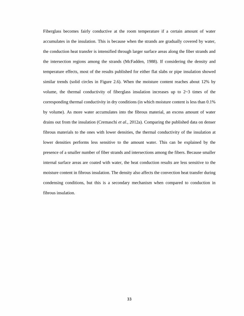
33

Fiberglass becomes fairly conductive at the room temperature if a certain amount of water

accumulates in the insulation. This is because when the strands are gradually covered by water,

the conduction heat transfer is intensified through larger surface areas along the fiber strands and

the intersection regions among the strands (McFadden, 1988). If considering the density and

temperature effects, most of the results published for either flat slabs or pipe insulation showed

similar trends (solid circles in Figure 2.6). When the moisture content reaches about 12% by

volume, the thermal conductivity of fiberglass insulation increases up to 2~3 times of the

corresponding thermal conductivity in dry conditions (in which moisture content is less than 0.1%

by volume). As more water accumulates into the fibrous material, an excess amount of water

drains out from the insulation (Cremaschi et al., 2012a). Comparing the published data on denser

fibrous materials to the ones with lower densities, the thermal conductivity of the insulation at

lower densities performs less sensitive to the amount water. This can be explained by the

presence of a smaller number of fiber strands and intersections among the fibers. Because smaller

internal surface areas are coated with water, the heat conduction results are less sensitive to the

moisture content in fibrous insulation. The density also affects the convection heat transfer during

condensing conditions, but this is a secondary mechanism when compared to conduction in

fibrous insulation.

34

[1] Kaplar(1974), Batty et al.(1981), Langlais et al. (1982), Langlaiset al. (1983)

Langlaisand Klarsfeld(1984), Modi and Benner (1985), McFadden (1988)

Kehreret al.(2002), Cremaschiet al.(2012a; 2012b)

[2] Chyuet al. (1997a), McFadden (1988)

[3] Kaplar(1974), Hay (referred by McFadden (1986)), McFadden (1988)

[4] Cremaschiet al.(2012a; 2012b)

Figure 2.6: Thermal conductivity of four common insulation materials with moisture effect

For the three types of closed-cell insulation reported in Table 2.4, the thermal conductivity of the

test specimens increased with moisture ingress because i) water accumulates on the cell walls,

which increases the wall thickness and offers a better heat flow path; and ii) water fills in the

small air gap and therefore enhances the heat conduction. It should be noted that at one point of

the polyurethane pipe insulation (solid triangle in Figure 2.6), the moisture content reached 70%,

and its thermal conductivity was measured almost 16 times higher than the dry condition.

However, this point was measured by flooded method, and researchers prepared the moist test

specimen by immersing it in the water tank (Chyu et al., 1997a) It was the only data that reported

a very large increase of the thermal conductivity for wet polyurethane insulation. Extruded

polystyrene shows an increase on the system thermal conductivity in moist conditions by about

1.0

10.0

0% 1% 10% 100%

The

rmal

Co

nd

uct

ivit

y R

atio

k_w

et/

k_d

ry [

-]

Moisture Content [ % by volume ]

Fiberglass[1]

Polyurethane[2]

Extruded/Expanded Polystyrene[3]

Phenolic[4]

35

2.2 times with respect to the values in dry conditions (McFadden, 1988). This increase is reported

for a moisture content of 16% by volume. For expanded polystyrene, the water content is around

21% by volume, and the thermal conductivity increases up to 1.9 times of the value in dry

condition. Phenolic is tested as pipe insulation, and it shows that the thermal conductivity

increases by 1.6 times when the moisture content is about 4.9% by volume (Cremaschi et al.,

2012a; Cremaschi et al., 2012b).

Table 2.3 and 2.4 provide a quick one glance summary of the experimental methods and test

results for insulation systems with moisture ingress. Most of the published data are for flat slabs,

and the thermal conductivity of pipe insulation systems with moisture ingress are reported in only

2 studies in the open domain literature. Expanding the database for pipe insulation systems at

below ambient temperatures in wet conditions with moisture ingress is a natural extension of the

current efforts in this field and should be considered for future research. Developing thermal

conductivity correlations with moisture content as the ones published for flat slab configurations

might also be helpful. Since pipe insulation systems have more complex geometries than flat

slabs and consist of multiple C-shell sections and various materials (i.e. Presence of joint sealant

and vapor retarder at the butt joints for example), a generalized correlation that works for all the

systems, even for only the ones with the same insulation material, might not be possible. These

questions should be addressed by future research in this field.

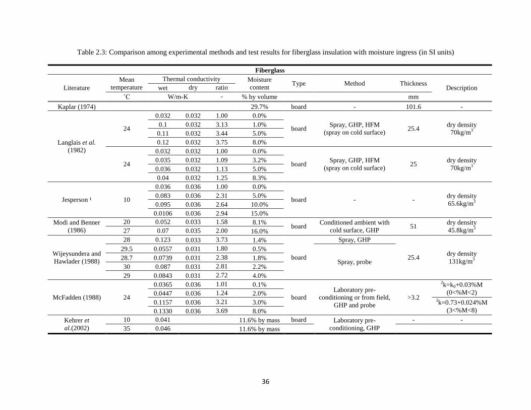
36

Table 2.3: Comparison among experimental methods and test results for fiberglass insulation with moisture ingress (in SI units)

Fiberglass

Literature

Mean

temperature

Thermal conductivity Moisture

content Type Method Thickness

Description wet dry ratio

˚C W/m-K - % by volume mm

Kaplar (1974) 29.7% board - 101.6 -

Langlais et al.

(1982)

24

0.032 0.032 1.00 0.0%

board Spray, GHP, HFM

(spray on cold surface) 25.4

dry density

70kg/m3

0.1 0.032 3.13 1.0%

0.11 0.032 3.44 5.0%

0.12 0.032 3.75 8.0%

24

0.032 0.032 1.00 0.0%

board Spray, GHP, HFM

(spray on cold surface) 25

dry density

70kg/m3

0.035 0.032 1.09 3.2%

0.036 0.032 1.13 5.0%

0.04 0.032 1.25 8.3%

Jesperson ¹ 10

0.036 0.036 1.00 0.0%

board - - dry density

65.6kg/m3

0.083 0.036 2.31 5.0%

0.095 0.036 2.64 10.0%

0.0106 0.036 2.94 15.0%

Modi and Benner

(1986)

20 0.052 0.033 1.58 8.1% board

Conditioned ambient with

cold surface, GHP 51

dry density

45.8kg/m3 27 0.07 0.035 2.00 16.0%

Wijeysundera and

Hawlader (1988)

28 0.123 0.033 3.73 1.4%

board

Spray, GHP

25.4 dry density

131kg/m3

29.5 0.0557 0.031 1.80 0.5%

Spray, probe 28.7 0.0739 0.031 2.38 1.8%

30 0.087 0.031 2.81 2.2%

29 0.0843 0.031 2.72 4.0%

McFadden (1988) 24

0.0365 0.036 1.01 0.1%

board

Laboratory pre-

conditioning or from field,

GHP and probe

>3.2

2k=k0+0.03%M

(0<%M<2) 0.0447 0.036 1.24 2.0%

0.1157 0.036 3.21 3.0% 2k=0.73+0.024%M

(3<%M<8) 0.1330 0.036 3.69 8.0%

Kehrer et

al.(2002)

10 0.041 11.6% by mass board Laboratory pre-

conditioning, GHP

- -

35 0.046 11.6% by mass

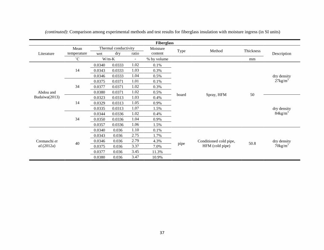
37

(continuted): Comparison among experimental methods and test results for fiberglass insulation with moisture ingress (in SI units)

Fiberglass

Literature

Mean

temperature

Thermal conductivity Moisture

content Type Method Thickness

Description wet dry ratio

˚C W/m-K - % by volume mm

Abdou and

Budaiwa(2013)

14

0.0340 0.0333 1.02 0.1%

board Spray, HFM 50

dry density

27kg/m3

0.0343 0.0333 1.03 0.3%

0.0346 0.0333 1.04 0.5%

34

0.0375 0.0371 1.01 0.1%

0.0377 0.0371 1.02 0.3%

0.0380 0.0371 1.02 0.5%

14

0.0323 0.0313 1.03 0.4%

dry density

84kg/m3

0.0329 0.0313 1.05 0.9%

0.0335 0.0313 1.07 1.5%

34

0.0344 0.0336 1.02 0.4%

0.0350 0.0336 1.04 0.9%

0.0357 0.0336 1.06 1.5%

Cremaschi et

al.(2012a) 40

0.0340 0.036 1.10 0.1%

pipe Conditioned cold pipe,

HFM (cold pipe) 50.8

dry density

70kg/m3

0.0343 0.036 2.75 1.7%

0.0346 0.036 2.79 4.3%

0.0375 0.036 3.37 7.0%

0.0377 0.036 3.45 11.3%

0.0380 0.036 3.47 10.9%

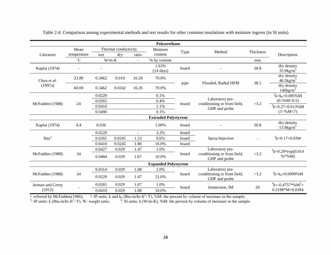
38

Table 2.4: Comparison among experimental methods and test results for other common insulations with moisture ingress (in SI units)

Polyurethane

Literature

Mean

temperature

Thermal conductivity Moisture

content Type Method Thickness

Description wet dry ratio

˚C W/m-K - % by volume

mm

Kaplar (1974) - - 1.63%

(14 days) board - 50.8

dry density

35.9kg/m3

Chyu et al.

(1997a)

23.89 0.3462 0.019 16.26 70.0%

pipe Flooded, Radial HFM 38.1

dry density

46.5kg/m3

60.00 0.3462 0.0242 16.26 70.0% dry density

140kg/m3

McFadden (1988) 24

0.0229 0.1%

board

Laboratory pre-

conditioning or from field,

GHP and probe

>3.2

2k=k0+0.085%M

(0<%M<0.5) 0.0265 0.4%

0.0410 1.1% 2k=0.27+0.013%M

(1<%M<7) 0.0490 0.1%

Extruded Polystyrene

Kaplar (1974) 4.4 0.036 1.00% board - 50.8 dry density

53.8kg/m3

Hay1

0.0229 - 3.2% board

Spray/Injection - 3k=0.17+0.03W 0.0265 0.0245 1.53 9.6% board

0.0410 0.0245 1.88 16.0% board

McFadden (1988) 24 0.0427 0.029 1.47 1.0%

board

Laboratory pre-

conditioning or from field,

GHP and probe

>3.2 2k=0.29*exp(0.014

%*%M) 0.0484 0.029 1.67 10.0%

Expanded Polystyrene

McFadden (1988) 24 0.0314 0.029 1.08 2.0%

board

Laboratory pre-

conditioning or from field,

GHP and probe

>3.2 2k=k0+0.0089%M

0.0229 0.029 1.47 21.0%

Jerman and Cerny

(2012) -

0.0265 0.029 1.67 1.0% board Immersion, IM 20

4k=-0.4757*%M

2+

0.2198*M+0.0394 0.0410 0.029 1.08 10.0%

¹: referred by McFadden(1986); ²: IP units: k and k0 (Btu-in/hr-ft2-˚F), %M: the percent by volume of moisture in the sample;

3: IP units: k (Btu-in/hr-ft

2-˚F), W: weight ratio;

4: SI units: k (W/m-K), %M: the percent by volume of moisture in the sample

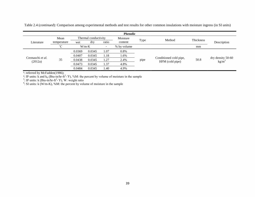
39

Table 2.4 (continued): Comparison among experimental methods and test results for other common insulations with moisture ingress (in SI units)

Phenolic

Literature

Mean

temperature

Thermal conductivity Moisture

content Type Method Thickness

Description wet dry ratio

˚C W/m-K - % by volume mm

Cremaschi et al.

(2012a) 35

0.0369 0.0345 1.07 0.8%

pipe Conditioned cold pipe,

HFM (cold pipe) 50.8

dry density 50-60

kg/m3

0.0407 0.0345 1.18 1.6%

0.0438 0.0345 1.27 2.4%

0.0473 0.0345 1.37 4.8%

0.0484 0.0345 1.40 4.9%

¹: referred by McFadden(1986);

²: IP units: k and k0 (Btu-in/hr-ft2-˚F), %M: the percent by volume of moisture in the sample

3: IP units: k (Btu-in/hr-ft

2-˚F), W: weight ratio

4: SI units: k (W/m-K), %M: the percent by volume of moisture in the sample

40

2.5 Challenges with the current methodologies for measuring the pipe insulation apparent

thermal conductivity with moisture ingress and future research needs

Some challenges are identified for moist tests: 1) How to prepare the test specimen with

controlled and uniform moisture? 2) What are the appropriate techniques that can replicate

similar boundary conditions across the test specimen as the ones observed during pipe insulation

systems field service? Flooded, spray/injection and laboratory conditioning methods are the most

common methodologies adopted for inducing moisture ingress. However, all of these methods

have some trade-off, and ultimately the laboratory conditions deviate from the actual field

conditions. Conditioned ambient with cold surface/pipe method provides a more reliable

measurement on the apparent thermal conductivity of pipe insulation systems. The temperature

and humidity regulated psychrometric chamber, together with a low temperature maintained at

the pipe insulation interior surface, would provide appropriate pressure gradients to help vapor

condensate on the cold surface and lead to water accumulation in the insulation materials. This

will help simulate the moisture distribution in the real application fields. However, the entire test

apparatus, including the psychrometric chamber and the thermal conductivity sensors, may take a

large space and a considerable amount of time for construction, control and calibration. The

equipment maintenance is also a high cost and large capital investment. It is believed that a

compact, easy to install, and inexpensive sensor is still needed in future research.

Any inhomogeneity that exists in the material interior structure would create preferential paths for

moisture transportation and would form wet regions around those preferential paths. The

formation of the wet regions affects the moisture test due to the following two reasons. First, the

preferential paths lead more water to pass through. In this case, when the weight of the water that

accumulates around the surface of the wet spot overcomes the material surface tension, the water

condensate drips out of the insulation material, and some of the water condensate is lost to the

ambient. Once this phenomenon occurs, the experiment has to be terminated since the partial loss

41

of water condensate makes it difficult to correlate the true accumulated moisture content in the

insulation test sample with time. A second reason is that when the test material becomes partially

wet, the thermocouple sensors, which are evenly placed on the insulation surface, read a larger

temperature difference due to a higher thermal conductivity around the wet regions. For example,

for fiberglass pipe insulation, after 10 days of test in the moist ambient, the temperature

difference on the insulation surface increased from 1.7˚C (3˚F) to 6.1˚C (11˚F) (Cremaschi et al.,

2012a). The non-uniformity of the temperature distribution may affect the direction of the heat

flow, and the assumption of one-dimensional flow becomes arguable. For pipe insulation

systems, large temperature variations along the cylindrical surfaces imply that axial heat transfer

has to be considered. This is the same consideration typically made for flat slabs in which large

variations of the insulation surface temperatures produce longitudinal heat transfer in the slab,

and the assumption of unidirectional heat conduction is no longer valid.

For most pipe insulation systems, it is required to use joint sealant or adhesive during the

installation procedure. Joint sealant, which is served as a thermal conductive chemical, may

increase the apparent thermal conductivity of the insulation material. The joint sealant may also

absorb moisture and can create preferential paths for water accumulation (Cremaschi et al.,

2012a). Both effects deteriorate the apparent insulation thermal performance. This can be an

explanation as to why most of the manufacturers’ data, which are tested on flat slabs, under-

predict the thermal performance and water absorption of pipe insulation systems. Mumaw (2002)

measured the moisture content in the pipe insulation by using the Calibrated Hot Box method,

and he pointed out that the measured moisture content was much higher than the value predicted

from the simplified model because the model neglect the effects of the joints and lap seals in the

vapor retarders. By dissecting the specimens, he observed that water absorption, lack of curing,

and shrinkage of insulation materials away from the joints occurred near the sealed joints. Two

technical challenges should be addressed in future studies on joint sealant effects: i) Joint sealant

42

is usually first applied as a thin layer on the cross section of one or both half shells, and the two

half shells of the pipe insulation are compressed towards each other to make a good contact

between the insulation materials. In this case, it is unfeasible to accurately measure the thickness

of joint sealant. One way to determine it is to first measure the perimeter of the pipe insulation

before applying the test specimen around the cold pipe. Once the insulation is installed on the

cold pipe, the perimeter of the test specimen with joint sealant will be measured again. The joint

thickness is computed from the difference between the diameters before and after the installation

procedure. As second challenge is that ii) there are no accurate data for the thermal conductivity

of the joint sealants in the open literature.

On this topic, other areas that can potentially be investigated in future research include the effects

of the split joints, insulation bulk densities, wall thicknesses, insulation jacketings, contact

resistances between pipe and insulation, interior structures and types of fillers and aggregates

(Kulkarni & Vipulanandan, 2006) on the apparent thermal conductivity of pipe insulation systems.

For some closed-cell insulation, aging is a common phenomenon that degrades the thermal

performance of the pipe insulation systems, and very limited work is reported in the literature on

this process (Biedermann et al., 2001; Christian et al., 1998; Kellner & Dirckx, 1999; Stovall,

2009). Insulation thickness affects the volume available for the storage of the gas, and thus it

directly impacts the deterioration of the insulation thermal performance during aging (Eriksson &

Sunden, 1998). The impacts of the exterior water vapor jacketing systems, as well as of the split

joints and seams, are not clear, and the results are sporadic and sometimes contradictory. The

above additional features of the pipe insulation systems and the anisotropic features of the pipe

insulation material on the radial and angular directions, seem to affect the behavior of the pipe

insulation systems during dry and wet operating conditions.

In wet condensing conditions with moisture ingress, the moisture migration inside pipe insulation

systems can result in a temperature re-distribution on the radial and angular directions. What are

43

the predominant forces that drive the moisture from one region to another in different types of

pipe insulation systems, and what are the geometric inner structures that promote or prevent

microscopic water vapor mass transfers inside the pipe insulation are still open questions. Some

works that pioneered in this research topic were studied on a “wick” concept, and they focused on

the methods to limit water moisture accumulation in pipe insulation systems (Guldbrandsen et al.,

2011; Korsgaard, 1993). These studies reported that the microscopic capillary actions inside

fibrous pipe insulation systems were responsible for the removal of moisture from the inside of

the material outward. It is believed that there are opportunities to improve their models for better

prediction of the apparent pipe insulation thermal conductivity in wet conditions and to expand

further their original models to other types of pipe insulation systems beside fibrous type

insulation. A model that describes and predicts water accumulation in pipe insulation systems will

advance the state-of-the-art knowledge of these mechanical insulation systems in cold pipe

applications. It will also cause an enormous potential in the industry for developing sensors that

can detect failure of the insulation systems and local moisture traps in the pipelines, and this

technique can be used for operational and management of the building cooling system.

2.6 Conclusions

This section discussed the experimental methodologies for measuring the apparent thermal

conductivity of pipe insulation systems with the aim of providing some clarification on the

existing thermal conductivity data for pipe insulation systems. Steady-state and transient methods

were discussed, and the measurements from these two methods were critically compared. It is

observed that steady-state methods for pipe insulation systems are commonly adopted for

measuring an average thermal conductivity, which is defined as apparent thermal conductivity of

the pipe insulation systems. Steady-state methods are simpler, more direct, and easier to make

than transients methods in dry operating conditions. However, steady-state methods often need a

considerable amount of time to reach thermal equilibrium, large test sample size to eliminate edge

44

effects, and a limited temperature range to prevent radiation. In addition, when considering

steady-state methods for pipe insulation systems, the flow direction seems to affect the apparent

thermal conductivity. Transient methodologies provide fast measurements, simple installations,

and they can be easily applied to pipe insulation systems. However, these methodologies are

indirect measurements of the thermal conductivity and adopt more or less cumbersome models to

reduce the data from the original measurements. Transient methodologies also provide local

values of thermal conductivity in various regions of the test specimen, and the apparent thermal

conductivity is strongly depended on the number and locations of the probing sensors. The

accuracy and repeatability of transient methods for pipe insulation systems are not as well defined

as steady-state methodologies.

During the measurement of the thermal conductivity of pipe insulation with moisture content,

four moisturizing strategies used to prepare the wet samples were identified as flooded method,

spray/injection method, laboratory pre-conditioning method, and conditioned ambience with cold

surface/pipe method. The advantages and shortcomings of each moisturizing strategy were

discussed at length. It is pointed out in the this review that steady-state methods in wet conditions

with moisture ingress seem to be inadequate because the enthalpy flow occurs due to

redistribution of the water condensate in the insulation systems. Using accelerated types of

techniques, such as high humidity ambient with a cold surface on one side of the test specimen,

seem to provide similar moisture ingress as the ones in the fields but in a shorter time. However,

this technique requires a large investment for the equipment and control of the ambient conditions.

Transient methods applied to wet pipe insulation systems may be sensitive to the moisture content

in the regions adjacent to the probe installed in specific locations of the insulation samples.

The thermal conductivities of several pipe insulation systems were compared under dry

conditions, and some data were discussed for wet conditions with different water content. To date,

challenges still exist in the measurement of apparent thermal conductivity of insulation with

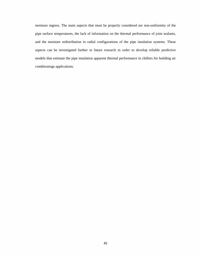
45

moisture ingress. The main aspects that must be properly considered are non-uniformity of the

pipe surface temperatures, the lack of information on the thermal performance of joint sealants,

and the moisture redistribution in radial configurations of the pipe insulation systems. These

aspects can be investigated further in future research in order to develop reliable predictive

models that estimate the pipe insulation apparent thermal performance in chillers for building air

conditionings applications.

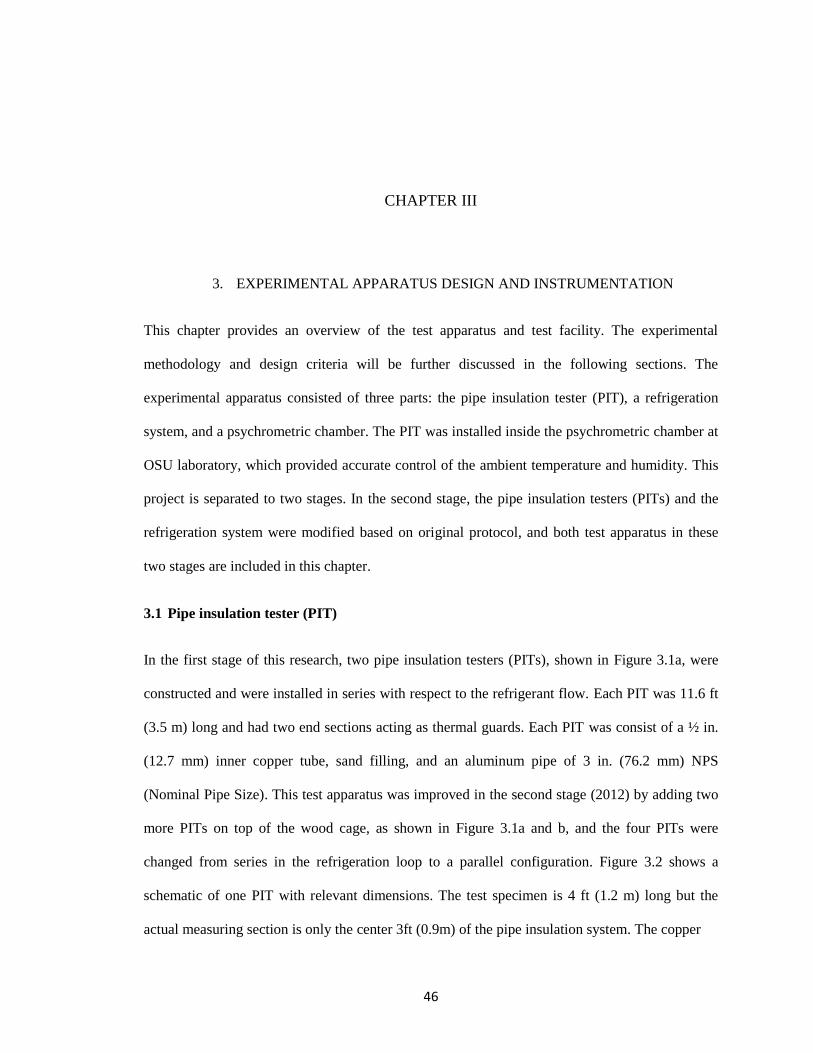
46

CHAPTER III

3. EXPERIMENTAL APPARATUS DESIGN AND INSTRUMENTATION

This chapter provides an overview of the test apparatus and test facility. The experimental

methodology and design criteria will be further discussed in the following sections. The

experimental apparatus consisted of three parts: the pipe insulation tester (PIT), a refrigeration

system, and a psychrometric chamber. The PIT was installed inside the psychrometric chamber at

OSU laboratory, which provided accurate control of the ambient temperature and humidity. This

project is separated to two stages. In the second stage, the pipe insulation testers (PITs) and the

refrigeration system were modified based on original protocol, and both test apparatus in these

two stages are included in this chapter.

3.1 Pipe insulation tester (PIT)

In the first stage of this research, two pipe insulation testers (PITs), shown in Figure 3.1a, were

constructed and were installed in series with respect to the refrigerant flow. Each PIT was 11.6 ft

(3.5 m) long and had two end sections acting as thermal guards. Each PIT was consist of a ½ in.

(12.7 mm) inner copper tube, sand filling, and an aluminum pipe of 3 in. (76.2 mm) NPS

(Nominal Pipe Size). This test apparatus was improved in the second stage (2012) by adding two

more PITs on top of the wood cage, as shown in Figure 3.1a and b, and the four PITs were

changed from series in the refrigeration loop to a parallel configuration. Figure 3.2 shows a

schematic of one PIT with relevant dimensions. The test specimen is 4 ft (1.2 m) long but the

actual measuring section is only the center 3ft (0.9m) of the pipe insulation system. The copper

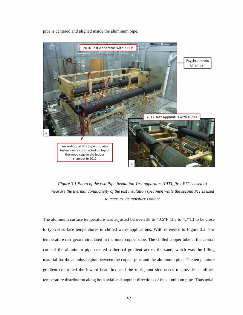
47

pipe is centered and aligned inside the aluminum pipe.

Figure 3.1 Photo of the two Pipe Insulation Test apparatus (PIT); first PIT is used to

measure the thermal conductivity of the test insulation specimen while the second PIT is used

to measure its moisture content

The aluminum surface temperature was adjusted between 38 to 40.5°F (3.3 to 4.7°C) to be close

to typical surface temperatures in chilled water applications. With reference to Figure 3.2, low

temperature refrigerant circulated in the inner copper tube. The chilled copper tube at the central

core of the aluminum pipe created a thermal gradient across the sand, which was the filling

material for the annulus region between the copper pipe and the aluminum pipe. The temperature

gradient controlled the inward heat flux, and the refrigerant side needs to provide a uniform

temperature distribution along both axial and angular directions of the aluminum pipe. Thus axial

2010 Test Apparatus with 2 PITs

Two additional PITs (pipe insulation testers) were constructed on top of

the wood cage in the indoor chamber in 2012

2012 Test Apparatus with 4 PITs

PsychrometricChamber

a

b

48

Figure 3.2: Schematic of the Pipe Insulation Test apparatus (PIT) (technical CAD drawings are

reported in Appendix B)

heat losses were minimized. The refrigeration system was different during the two stages of this

research project. In the first stage, a two-phase refrigerant, R134a, was selected in the

refrigeration system. By controlling the refrigerant as a two-phase vapor and liquid mixture in the

PIT section, the cold pipe surface temperature was close to the saturation temperature, and it

remained constant along the entire length of the copper pipe with small changes in the refrigerant

vapor thermodynamic quality and local pressure. In the second stage, dynalene HC50, which is a

single-phase refrigerant, was selected in the system. The temperature uniformity was controlled

by maintaining the coolant at a high flow rate in the cold pipe through the test section. The

refrigeration systems will be discussed in detail in the following section. Pre-dried play sand was

selected because of easiness of filling, compact structure, and appropriate thermal conductivity

for the radial heat flux measurements. The suitable thermal conductivity of sand provided large

temperature gradients between the inner copper tube and aluminum pipe surface during the

experiments. Sand was inexpensive and available in several local warehouses. It filled the

Refrigerant Inlet Refrigerant Outlet

Refrigerating Cold Copper Pipe

Filling Sand

3'’ (76.2 mm) NPS Al Pipe

Testing Pipe Insulation

3'’ (76.2 mm)

Plastic Pipe

Insulated End

Thermocouples

Inlet thermal Guard

(4.3 ft / 1.3 m)

Insulation Test Specimen

(3 ft / 0.9 m)

Exit Thermal Guard

(4.3 ft / 1.3 m)

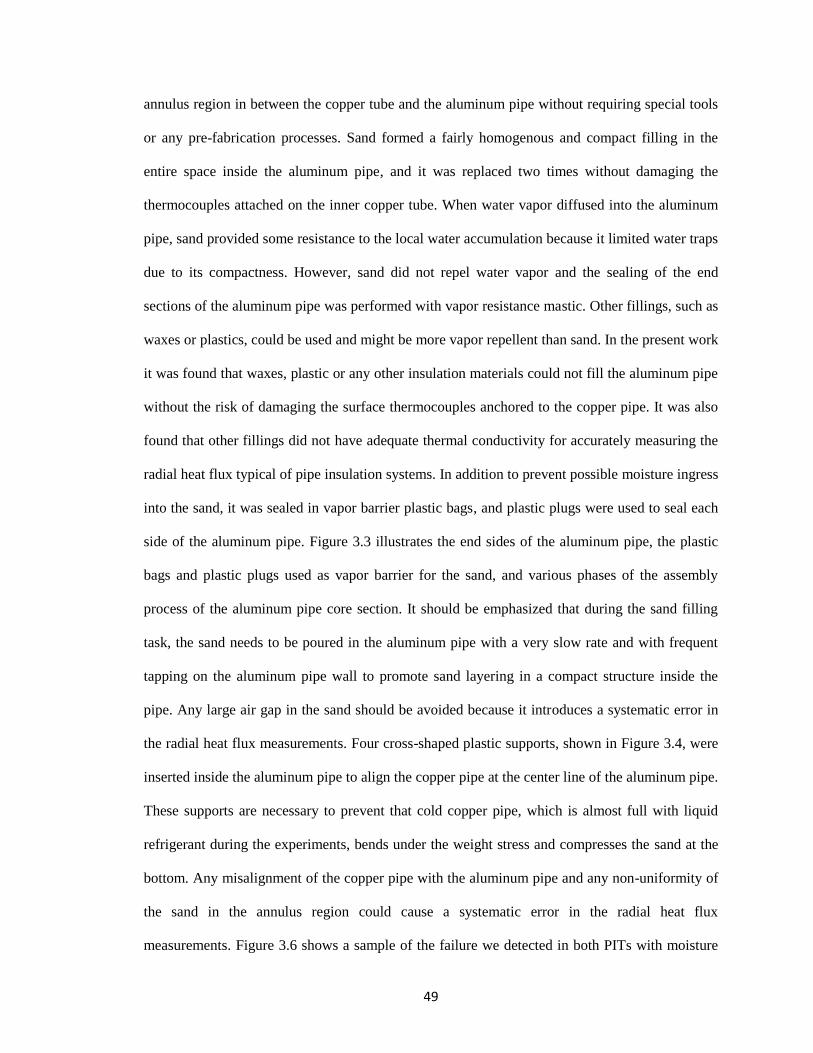
49

annulus region in between the copper tube and the aluminum pipe without requiring special tools

or any pre-fabrication processes. Sand formed a fairly homogenous and compact filling in the

entire space inside the aluminum pipe, and it was replaced two times without damaging the

thermocouples attached on the inner copper tube. When water vapor diffused into the aluminum

pipe, sand provided some resistance to the local water accumulation because it limited water traps

due to its compactness. However, sand did not repel water vapor and the sealing of the end

sections of the aluminum pipe was performed with vapor resistance mastic. Other fillings, such as

waxes or plastics, could be used and might be more vapor repellent than sand. In the present work

it was found that waxes, plastic or any other insulation materials could not fill the aluminum pipe

without the risk of damaging the surface thermocouples anchored to the copper pipe. It was also

found that other fillings did not have adequate thermal conductivity for accurately measuring the

radial heat flux typical of pipe insulation systems. In addition to prevent possible moisture ingress

into the sand, it was sealed in vapor barrier plastic bags, and plastic plugs were used to seal each

side of the aluminum pipe. Figure 3.3 illustrates the end sides of the aluminum pipe, the plastic

bags and plastic plugs used as vapor barrier for the sand, and various phases of the assembly

process of the aluminum pipe core section. It should be emphasized that during the sand filling

task, the sand needs to be poured in the aluminum pipe with a very slow rate and with frequent

tapping on the aluminum pipe wall to promote sand layering in a compact structure inside the

pipe. Any large air gap in the sand should be avoided because it introduces a systematic error in

the radial heat flux measurements. Four cross-shaped plastic supports, shown in Figure 3.4, were

inserted inside the aluminum pipe to align the copper pipe at the center line of the aluminum pipe.

These supports are necessary to prevent that cold copper pipe, which is almost full with liquid

refrigerant during the experiments, bends under the weight stress and compresses the sand at the

bottom. Any misalignment of the copper pipe with the aluminum pipe and any non-uniformity of

the sand in the annulus region could cause a systematic error in the radial heat flux

measurements. Figure 3.6 shows a sample of the failure we detected in both PITs with moisture

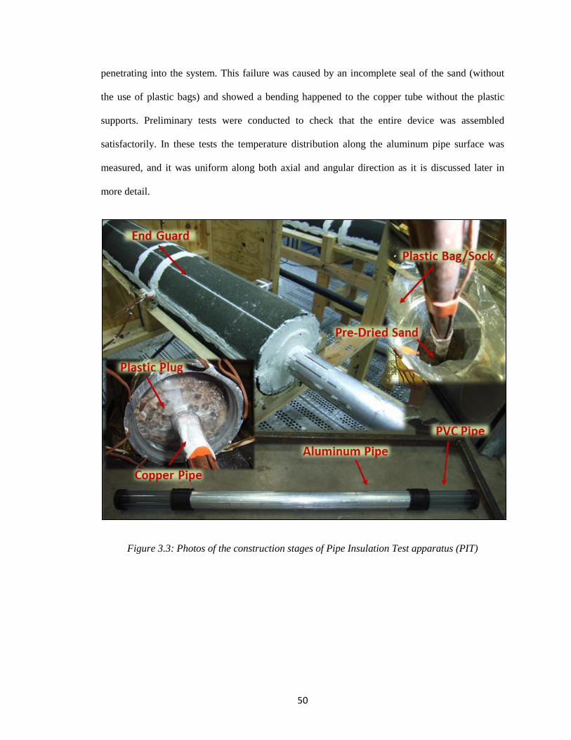
50

penetrating into the system. This failure was caused by an incomplete seal of the sand (without

the use of plastic bags) and showed a bending happened to the copper tube without the plastic

supports. Preliminary tests were conducted to check that the entire device was assembled

satisfactorily. In these tests the temperature distribution along the aluminum pipe surface was

measured, and it was uniform along both axial and angular direction as it is discussed later in

more detail.

Figure 3.3: Photos of the construction stages of Pipe Insulation Test apparatus (PIT)

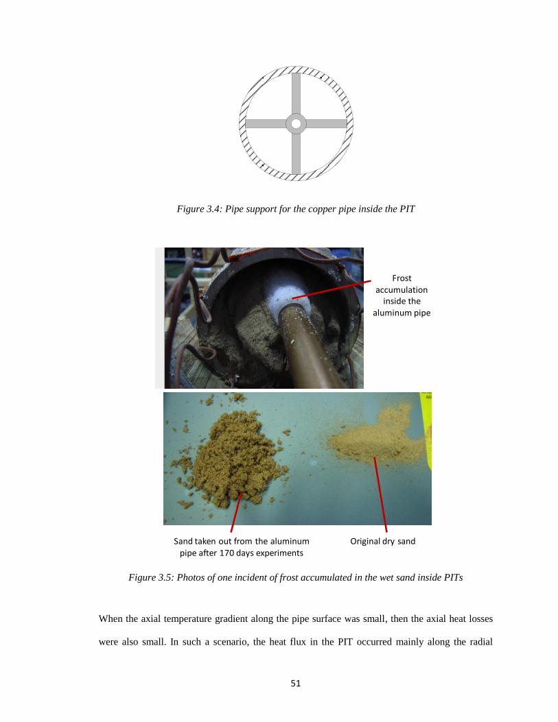
51

Figure 3.4: Pipe support for the copper pipe inside the PIT

Figure 3.5: Photos of one incident of frost accumulated in the wet sand inside PITs

When the axial temperature gradient along the pipe surface was small, then the axial heat losses

were also small. In such a scenario, the heat flux in the PIT occurred mainly along the radial

Sand taken out from the aluminum pipe after 170 days experiments

Original dry sand

Frost accumulation

inside the aluminum pipe

52

direction and from the aluminum pipe toward the inner copper pipe. The radial heat flux was

computed from the surface temperature readings by the thermocouples and from the sand thermal

conductivity. Thermal conductivity of the test insulation specimen was calculated by applying a

1-D heat balance equation to the PIT. For the two PITs constructed in the first stage, the

temperature measurements were taken with 20 in-situ and in-house calibrated thermocouples

distributed evenly on the aluminum pipe surface. The pipe insulation specimen was instrumented

with another 20 in-situ and in-house calibrated thermocouples distributed on its exterior surface.

Six (6) in-situ and in-house calibrated thermocouples were mounted on the inner copper pipe

surface. Fewer in-situ and in-house calibrated thermocouples were applied on the other two PITs

constructed in the second stage: 12 around the aluminum pipe, 12 on the insulation exterior

surface, and 6 for the inner copper pipe. Although the total amount of the temperature sensors at

each surface decreased when compared to the first stage, these thermocouples were calibrated

with a better accuracy, which will be discussed in the next chapter. The thermocouple wires on

the aluminum pipe created small air gaps between the inner surface of the pipe insulation and the

outer surface of the aluminum pipe. To avoid this air gap, 20 longitudinal grooves (12 grooves in

the second stage), with dimensions of 1/8 by 1/8 in. (3.2 by 3.2 mm), were machined on the

aluminum pipe surface. The grooves accommodated the thermocouple wires on the aluminum

pipe, as shown in Figure 3.6.

Considering the fact that these thermocouple grooves may become potential paths for the water

vapor transmission, the surfaces of the aluminum pipes for all PITs were sealed with aluminum

adhesive tape during the second stage, as shown in Figure 3.7. The gaps between the test pipe and

the end guards were sealed with silicone gel. In order to decrease the radiation effect that caused

by the low emissivity of the aluminum surface, the aluminum pipe was further pained as flat

black, and the photos for the blackened pipes are shown in Figure 3.9.

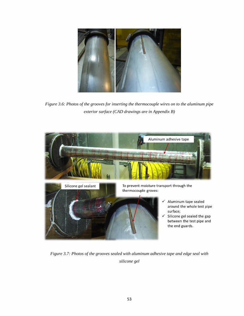
53

Figure 3.6: Photos of the grooves for inserting the thermocouple wires on to the aluminum pipe

exterior surface (CAD drawings are in Appendix B)

Figure 3.7: Photos of the grooves sealed with aluminum adhesive tape and edge seal with

silicone gel

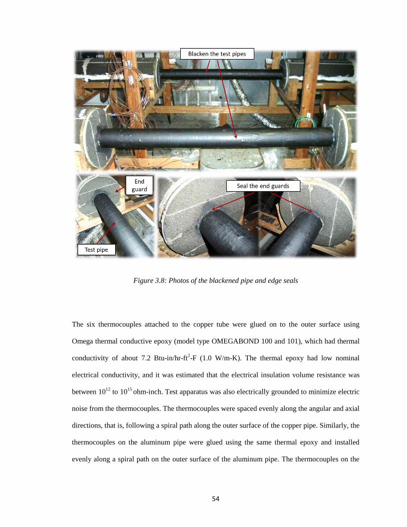
54

Figure 3.8: Photos of the blackened pipe and edge seals

The six thermocouples attached to the copper tube were glued on to the outer surface using

Omega thermal conductive epoxy (model type OMEGABOND 100 and 101), which had thermal

conductivity of about 7.2 Btu-in/hr-ft2-F (1.0 W/m-K). The thermal epoxy had low nominal

electrical conductivity, and it was estimated that the electrical insulation volume resistance was

between 1012

to 1015

ohm-inch. Test apparatus was also electrically grounded to minimize electric

noise from the thermocouples. The thermocouples were spaced evenly along the angular and axial

directions, that is, following a spiral path along the outer surface of the copper pipe. Similarly, the

thermocouples on the aluminum pipe were glued using the same thermal epoxy and installed

evenly along a spiral path on the outer surface of the aluminum pipe. The thermocouples on the

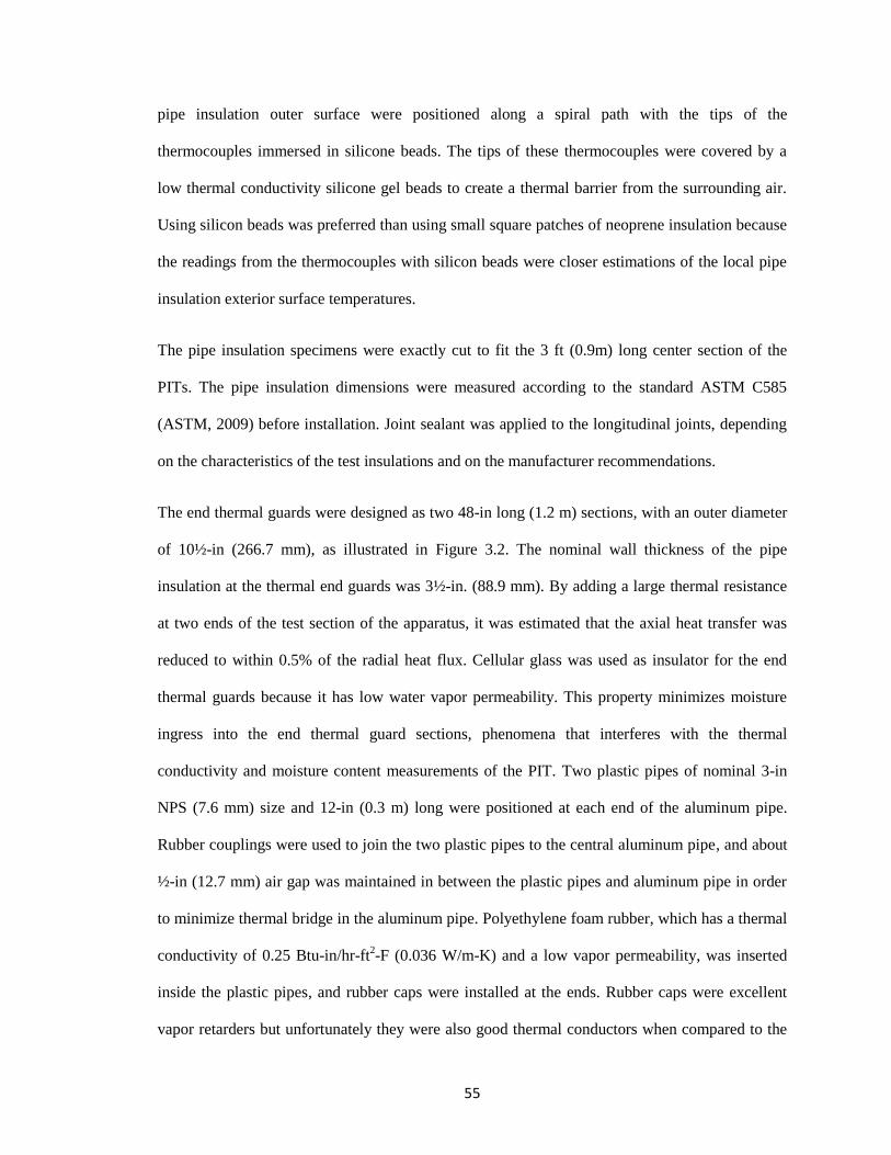
55

pipe insulation outer surface were positioned along a spiral path with the tips of the

thermocouples immersed in silicone beads. The tips of these thermocouples were covered by a

low thermal conductivity silicone gel beads to create a thermal barrier from the surrounding air.

Using silicon beads was preferred than using small square patches of neoprene insulation because

the readings from the thermocouples with silicon beads were closer estimations of the local pipe

insulation exterior surface temperatures.

The pipe insulation specimens were exactly cut to fit the 3 ft (0.9m) long center section of the

PITs. The pipe insulation dimensions were measured according to the standard ASTM C585

(ASTM, 2009) before installation. Joint sealant was applied to the longitudinal joints, depending

on the characteristics of the test insulations and on the manufacturer recommendations.

The end thermal guards were designed as two 48-in long (1.2 m) sections, with an outer diameter

of 10½-in (266.7 mm), as illustrated in Figure 3.2. The nominal wall thickness of the pipe

insulation at the thermal end guards was 3½-in. (88.9 mm). By adding a large thermal resistance

at two ends of the test section of the apparatus, it was estimated that the axial heat transfer was

reduced to within 0.5% of the radial heat flux. Cellular glass was used as insulator for the end

thermal guards because it has low water vapor permeability. This property minimizes moisture

ingress into the end thermal guard sections, phenomena that interferes with the thermal

conductivity and moisture content measurements of the PIT. Two plastic pipes of nominal 3-in

NPS (7.6 mm) size and 12-in (0.3 m) long were positioned at each end of the aluminum pipe.

Rubber couplings were used to join the two plastic pipes to the central aluminum pipe, and about

½-in (12.7 mm) air gap was maintained in between the plastic pipes and aluminum pipe in order

to minimize thermal bridge in the aluminum pipe. Polyethylene foam rubber, which has a thermal

conductivity of 0.25 Btu-in/hr-ft2-F (0.036 W/m-K) and a low vapor permeability, was inserted

inside the plastic pipes, and rubber caps were installed at the ends. Rubber caps were excellent

vapor retarders but unfortunately they were also good thermal conductors when compared to the

56

other components of the PIT. Two cellular glass cylindrical inserts were mounted in between the

rubber caps and the refrigerating cold copper pipe in order to eliminate any direct contact

between rubber caps and the copper pipe surface. The external surface of the plastic pipes was

insulated by using cellular glass insulation with 3½-in (88.9mm) of nominal wall thickness.

In the first stage, two PITs were connected in series with respect to the refrigerant flow, and both

PITs were required for the measurement of the apparent thermal conductivity in one pipe

insulation system. Theses two PITs were identical and were built at the same time. The

temperature sensors on the first PIT aimed to measure the thermal conductivity of the pipe

insulation specimen, while the second PIT served a dual purpose. First, it allowed monitoring the

sand thermal conductivity during the dry tests. If we assume that the PIT is perfectly sealed and

that vapor cannot penetrate into the aluminum pipe, then the second PIT might not be required for

the dry tests. An objective of the second PIT was to validate this hypothesis with the prototypes

constructed in this project. A second objective of the second PIT was to measure the moisture

content in the pipe insulation system at intermediate time intervals during the wet tests. The

measurements of moisture content from the second PIT provided an indication of the moisture

accumulation rate and transitional phase (Mcfadden, 1988) in the pipe insulation system during

the wet test period. Although the second PIT increased the total cost for the test apparatus it was

necessary to demonstrate the feasibility of the test apparatus of this project. The second PIT is

also recommended if water vapor absorption rate must be experimentally estimated during the

period of exposure of the pipe insulation system to the humid ambient with moisture ingress. A

flexible strip electric heater was installed along the surface of the aluminum pipe of the second

PIT during the dry tests. A large amount of insulation was wrapped around the heater to limit

radial heat gain from the surrounding ambient. The power to the heater was controlled to obtain

similar aluminum surface temperature in the second PIT as the one measured in the first PIT

during the dry tests. Since the two PITs were of identical geometry, constructed at the same time,

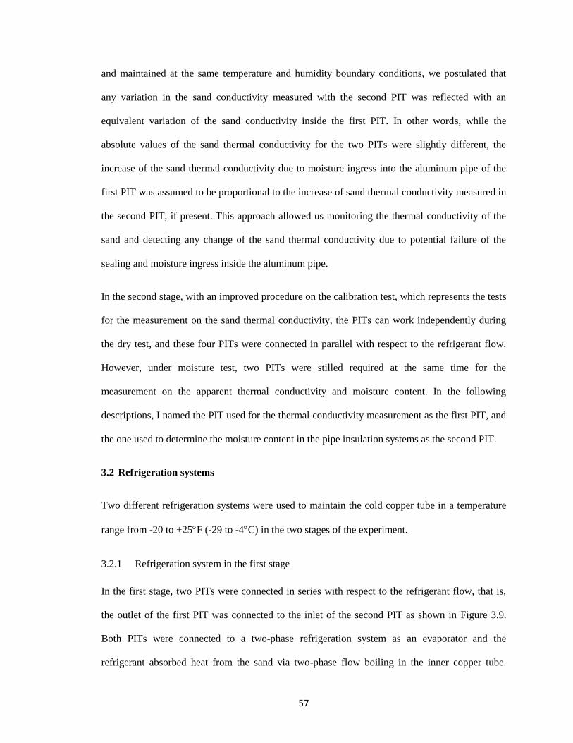
57

and maintained at the same temperature and humidity boundary conditions, we postulated that

any variation in the sand conductivity measured with the second PIT was reflected with an

equivalent variation of the sand conductivity inside the first PIT. In other words, while the

absolute values of the sand thermal conductivity for the two PITs were slightly different, the

increase of the sand thermal conductivity due to moisture ingress into the aluminum pipe of the

first PIT was assumed to be proportional to the increase of sand thermal conductivity measured in

the second PIT, if present. This approach allowed us monitoring the thermal conductivity of the

sand and detecting any change of the sand thermal conductivity due to potential failure of the

sealing and moisture ingress inside the aluminum pipe.

In the second stage, with an improved procedure on the calibration test, which represents the tests

for the measurement on the sand thermal conductivity, the PITs can work independently during

the dry test, and these four PITs were connected in parallel with respect to the refrigerant flow.

However, under moisture test, two PITs were stilled required at the same time for the

measurement on the apparent thermal conductivity and moisture content. In the following

descriptions, I named the PIT used for the thermal conductivity measurement as the first PIT, and

the one used to determine the moisture content in the pipe insulation systems as the second PIT.

3.2 Refrigeration systems

Two different refrigeration systems were used to maintain the cold copper tube in a temperature

range from -20 to +25F (-29 to -4C) in the two stages of the experiment.

3.2.1 Refrigeration system in the first stage

In the first stage, two PITs were connected in series with respect to the refrigerant flow, that is,

the outlet of the first PIT was connected to the inlet of the second PIT as shown in Figure 3.9.

Both PITs were connected to a two-phase refrigeration system as an evaporator and the

refrigerant absorbed heat from the sand via two-phase flow boiling in the inner copper tube.

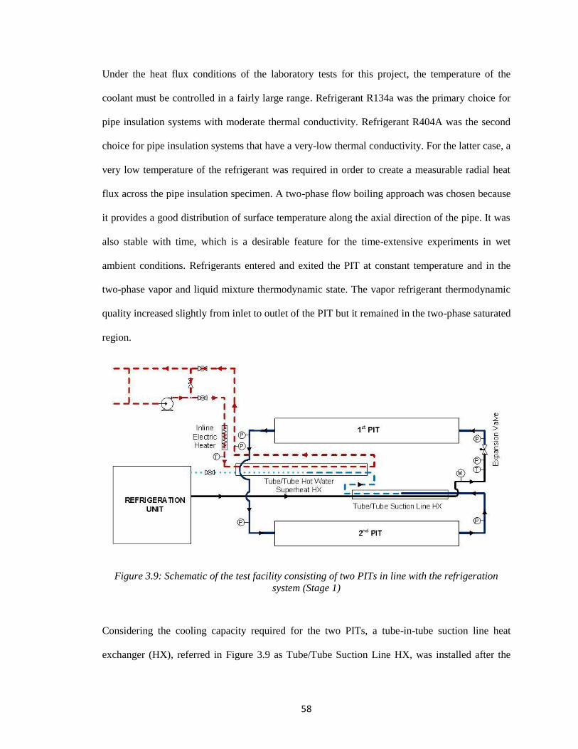
58

Under the heat flux conditions of the laboratory tests for this project, the temperature of the

coolant must be controlled in a fairly large range. Refrigerant R134a was the primary choice for

pipe insulation systems with moderate thermal conductivity. Refrigerant R404A was the second

choice for pipe insulation systems that have a very-low thermal conductivity. For the latter case, a

very low temperature of the refrigerant was required in order to create a measurable radial heat

flux across the pipe insulation specimen. A two-phase flow boiling approach was chosen because

it provides a good distribution of surface temperature along the axial direction of the pipe. It was

also stable with time, which is a desirable feature for the time-extensive experiments in wet

ambient conditions. Refrigerants entered and exited the PIT at constant temperature and in the

two-phase vapor and liquid mixture thermodynamic state. The vapor refrigerant thermodynamic

quality increased slightly from inlet to outlet of the PIT but it remained in the two-phase saturated

region.

Figure 3.9: Schematic of the test facility consisting of two PITs in line with the refrigeration

system (Stage 1)

Considering the cooling capacity required for the two PITs, a tube-in-tube suction line heat

exchanger (HX), referred in Figure 3.9 as Tube/Tube Suction Line HX, was installed after the

59

second PIT to increase the overall cooling capacity of the refrigeration unit. The suction line heat

exchanger was required to increase the cooling capacity of our refrigeration unit and to shift the

vapor refrigerant thermodynamic quality at the inlet of the first PIT toward the saturated liquid

curve. The suction line HX was made in house by welding a 48-in (1.2 m) long, ½-in. (12.7 mm)

OD copper pipe around the system 3/8-in (9.5 mm) copper tube with tee and reducer fittings to

keep the two fluid streams independent. The in-house manufacturing process of the tube-in-tube

suction line HX is shown in Figure 3.10. Before returning to the compressor, proper degree of

superheat at the compressor suction was achieved by an auxiliary water-to-refrigerant tube-in-

tube heat exchanger. The superheat HX was made using a 72-in (1.8m) long, 1-in (25.4 mm)

nominal copper pipe with a tube insert of ½-in (12.7 mm) copper pipe. Warm water was

circulated in an auxiliary loop, which had a pump, a flow valve, and an in-line heater. The power

to the in-line heater was adjusted to guarantee proper refrigerant temperature at the compressor

suction. It should be noted that electric heaters applied directly on the surface of the cold copper

pipelines were intentionally avoided in the test apparatus because they created large axial

temperature gradients in the refrigeration copper pipelines used inside the PITs. These large axial

temperature gradients might be the results of heat conduction across the walls of the pipes and

they greatly affect the uniformity of the surface temperature along the axial direction of PIT. In a

preliminary prototype of the PIT, it was observed that electric tape heaters, which used along the

copper pipe to provide refrigerant superheated vapor to the compressor, altered the temperature

profile of the copper pipes inside the PITs upstream the suction line HX as well as introduced a

systematic error during the measurements of pipe insulation thermal conductivity. Thus, we

purposely avoided to use any electric heater directly in contact with the copper pipes of the test

facility of Figure 3.9 .

60

Figure 3.10: Photos of the construction stages of the tube and tube heat exchangers

3.2.2 Refrigeration system in the second stage

A completely different refrigeration system was designed in the second stage of the project. Due

to the fact that in the previous design, the air-cooled refrigeration unit was constructed in the

indoor chamber next to the PIT test sections, the cooling capacity provided to the condenser was

very limit and highly dependent on the indoor ambient conditions. For example, in the normal

case, the moisture test need to be maintained as a hot and humid environment, and the room was

set at 107˚F (41.7˚C), 83% relative humidity. Under this severe condition, there was not enough

cooling provided to the condenser by passing warm air through the fin-and-tube heat exchanger,

and this results in a difficulty to maintain the refrigerant as two-phase in the test sections. The

room ambient was very unstable due to the heat generated from the compressor and the warm air

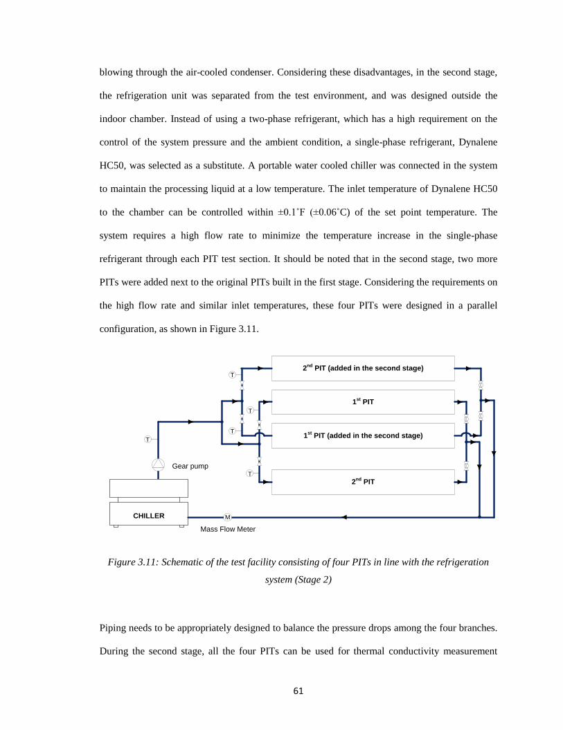
61

blowing through the air-cooled condenser. Considering these disadvantages, in the second stage,

the refrigeration unit was separated from the test environment, and was designed outside the

indoor chamber. Instead of using a two-phase refrigerant, which has a high requirement on the

control of the system pressure and the ambient condition, a single-phase refrigerant, Dynalene

HC50, was selected as a substitute. A portable water cooled chiller was connected in the system

to maintain the processing liquid at a low temperature. The inlet temperature of Dynalene HC50

to the chamber can be controlled within ±0.1˚F (±0.06˚C) of the set point temperature. The

system requires a high flow rate to minimize the temperature increase in the single-phase

refrigerant through each PIT test section. It should be noted that in the second stage, two more

PITs were added next to the original PITs built in the first stage. Considering the requirements on

the high flow rate and similar inlet temperatures, these four PITs were designed in a parallel

configuration, as shown in Figure 3.11.

Figure 3.11: Schematic of the test facility consisting of four PITs in line with the refrigeration

system (Stage 2)

Piping needs to be appropriately designed to balance the pressure drops among the four branches.

During the second stage, all the four PITs can be used for thermal conductivity measurement

CHILLER

2nd

PIT (added in the second stage)

1st

PIT

1st

PIT (added in the second stage)

2nd

PIT

Mass Flow Meter

M

T

T

T

T

T

Gear pump

62

under dry condition, and four pipe insulation systems could be tested simultaneously. The

variation on the sand thermal conductivity would still be monitored by the periodical calibration

tests applied on all the four PITs. The test results derived from each PIT would be corrected based

on a specific correlations developed on the sand thermal conductivity with time between the two

calibration tests. The procedures for the calibration tests will be explained in detail in the section

4.2.2.

3.3 Psychrometric Chamber

Measuring of the actual thermal conductivity of pipe insulation systems under controlled ambient

temperature and humidity could be performed in psychrometric chambers. In this project, a

psychrometric chamber was designed so that a slow motion of the air was maintained during the

tests, with air ascending in the room from a perforated floor. This displacement ventilation

system, shown in Figure 3.12, was consist of a conditioning loop, an under floor air plenum

supply, and a set of adjustable ceiling filters. Air was circulated through the conditioning loop

first, shown on the right side in Figure 3.12, by using a variable speed fan. The air flow rate was

adjusted with the fan motor speed and a set of electro-mechanical dampers. With reference to

Figure 3.12, during the first process, the air stream goes inside the conditioning loop is cooled

down and dehumidified through the water-to-air cooling coils. The coils’ surface temperature and

capacity were controlled by a system with a variable speed pump, electronic mixing valves and

bypass valves. These parameters were adjusted so that the air is cooled and dehumidified at about

43F (6C) of air dew point temperature. This was the minimum air dew point temperature that

the cooling coils of the chamber were able to provide. To achieve proper dry non-condensing

conditions, the ambient air dew point temperature must be below the aluminum pipe surface

temperature of 40F (4.5C) in the first stage and below 38F (3.3C) in the second stage.

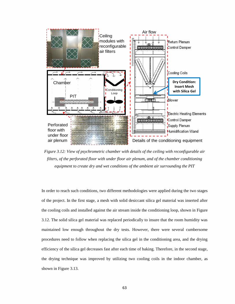
63

Figure 3.12: View of psychrometric chamber with details of the ceiling with reconfigurable air

filters, of the perforated floor with under floor air plenum, and of the chamber conditioning

equipment to create dry and wet conditions of the ambient air surrounding the PIT

In order to reach such conditions, two different methodologies were applied during the two stages

of the project. In the first stage, a mesh with solid desiccant silica gel material was inserted after

the cooling coils and installed against the air stream inside the conditioning loop, shown in Figure

3.12. The solid silica gel material was replaced periodically to insure that the room humidity was

maintained low enough throughout the dry tests. However, there were several cumbersome

procedures need to follow when replacing the silica gel in the conditioning area, and the drying

efficiency of the silica gel decreases fast after each time of baking. Therefore, in the second stage,

the drying technique was improved by utilizing two cooling coils in the indoor chamber, as

shown in Figure 3.13.

Ceiling

modules with

reconfigurable

air filters

Perforated

floor with

under floor

air plenum

R404A Inlet (quality = 0.4 ) R404A Outlet (quality = 0.8 )

3/8 inch Copper Tube

Inner insulation

3 inch NPT Aluminum Pipe

Testing Pipe Insulation

3 inch Plastic Pipe

Insulated End

Inner Heater

Thermocouple

PIT

Chamber

Details of the conditioning equipment

Conditioning

Loop

Air flow

Dry Condition:Insert Mesh

with Silica Gel

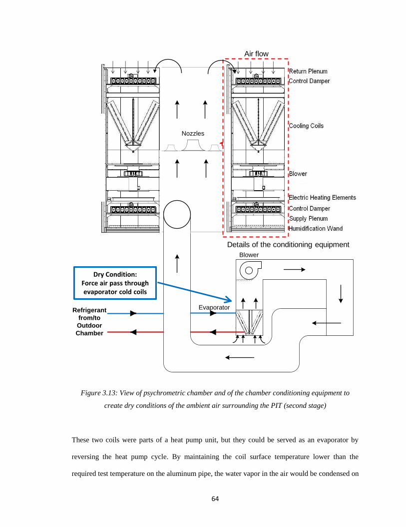
64

Figure 3.13: View of psychrometric chamber and of the chamber conditioning equipment to

create dry conditions of the ambient air surrounding the PIT (second stage)

These two coils were parts of a heat pump unit, but they could be served as an evaporator by

reversing the heat pump cycle. By maintaining the coil surface temperature lower than the

required test temperature on the aluminum pipe, the water vapor in the air would be condensed on

Ceiling

modules with

reconfigurable

air filters

Perforated

floor with

under floor

air plenum

R404A Inlet (quality = 0.4 ) R404A Outlet (quality = 0.8 )

3/8 inch Copper Tube

Inner insulation

3 inch NPT Aluminum Pipe

Testing Pipe Insulation

3 inch Plastic Pipe

Insulated End

Inner Heater

Thermocouple

PIT

Chamber

Details of the conditioning equipment

Conditioning

Loop

Air flowCeiling

modules with

reconfigurable

air filters

Perforated

floor with

under floor

air plenum

R404A Inlet (quality = 0.4 ) R404A Outlet (quality = 0.8 )

3/8 inch Copper Tube

Inner insulation

3 inch NPT Aluminum Pipe

Testing Pipe Insulation

3 inch Plastic Pipe

Insulated End

Inner Heater

Thermocouple

PIT

Chamber

Details of the conditioning equipment

Conditioning

Loop

Air flow

Ceiling

modules with

reconfigurable

air filters

Perforated

floor with

under floor

air plenum

R404A Inlet (quality = 0.4 ) R404A Outlet (quality = 0.8 )

3/8 inch Copper Tube

Inner insulation

3 inch NPT Aluminum Pipe

Testing Pipe Insulation

3 inch Plastic Pipe

Insulated End

Inner Heater

Thermocouple

PIT

Chamber

Details of the conditioning equipment

Conditioning

Loop

Air flow

EvaporatorRefrigerant

from/to

Outdoor

Chamber

Blower

Nozzles

Dry Condition:Force air pass through evaporator cold coils

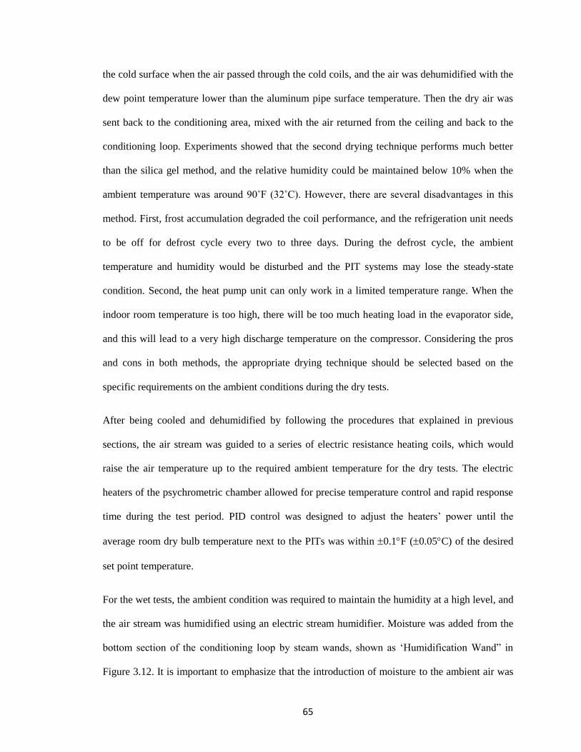
65

the cold surface when the air passed through the cold coils, and the air was dehumidified with the

dew point temperature lower than the aluminum pipe surface temperature. Then the dry air was

sent back to the conditioning area, mixed with the air returned from the ceiling and back to the

conditioning loop. Experiments showed that the second drying technique performs much better

than the silica gel method, and the relative humidity could be maintained below 10% when the

ambient temperature was around 90˚F (32˚C). However, there are several disadvantages in this

method. First, frost accumulation degraded the coil performance, and the refrigeration unit needs

to be off for defrost cycle every two to three days. During the defrost cycle, the ambient

temperature and humidity would be disturbed and the PIT systems may lose the steady-state

condition. Second, the heat pump unit can only work in a limited temperature range. When the

indoor room temperature is too high, there will be too much heating load in the evaporator side,

and this will lead to a very high discharge temperature on the compressor. Considering the pros

and cons in both methods, the appropriate drying technique should be selected based on the

specific requirements on the ambient conditions during the dry tests.

After being cooled and dehumidified by following the procedures that explained in previous

sections, the air stream was guided to a series of electric resistance heating coils, which would

raise the air temperature up to the required ambient temperature for the dry tests. The electric

heaters of the psychrometric chamber allowed for precise temperature control and rapid response

time during the test period. PID control was designed to adjust the heaters’ power until the

average room dry bulb temperature next to the PITs was within 0.1F (0.05C) of the desired

set point temperature.

For the wet tests, the ambient condition was required to maintain the humidity at a high level, and

the air stream was humidified using an electric stream humidifier. Moisture was added from the

bottom section of the conditioning loop by steam wands, shown as ‘Humidification Wand” in

Figure 3.12. It is important to emphasize that the introduction of moisture to the ambient air was

66

far away from the PITs, and this would guarantee enough time for proper mixing in the under-

floor plenum before the moist air stream reaches the PITs. This strategy is critical since uniform

ambient conditions must be achieved around the PITs. In the first stage, two small room

humidifiers were used to provide water vapor and maintain adequate moisture level in the

ambient air during the draining periods of the main humidifier of the chamber. The small room

humidifiers were synchronized so that water vapor was continuously supplied to the room during

the 40 to 50 minute period required for the main humidifier to perform its daily self cleaning and

draining cycles. In the second stage, the draining cycle was expanded to 7 to 10 days because of

the usage of soft water, and soft water would lead to a lower rate of forming scaling in the

humidifier water system.

Two dry bulb and two wet bulb probes were used to measure the dry-bulb and wet-bulb

temperatures of ambient air surrounding the PITs. The probes measured an average value of the

ambient air at various locations along the two sides of the PITs. The sampling tree of the dry-/wet-

bulb probe is made of plastic white PVC and is shown in Figure 3.14 on the left side next to the

PIT. Four additional humidity sensors and six thermocouples were installed around the PIT to

measure the local air humidity and local dry-bulb temperature, respectively. A panel of elastomeric

rubber insulation was positioned directly underneath the pipe insulation test specimen as shown on

the bottom of Figure 3.14. This configuration avoided direct impingement of the air on the bottom

exterior surface of the insulation specimen, which stood at least 33 in. (0.8 m) high from the

perforated floor. Each PIT was supported from the two end side thermal guard sections by a wood

frame. The specifications of the wood cage were attached in Appendix A. The measurements of the

air dry-bulb temperature and humidity in the various locations surrounding the PITs indicated

uniform ambient conditions. The local ambient dry-bulb temperatures were within 0.3F

(0.15C) of the average room dry-bulb temperature and the local relative humidity measurements

were within 4% RH of the average relative humidity in the room.

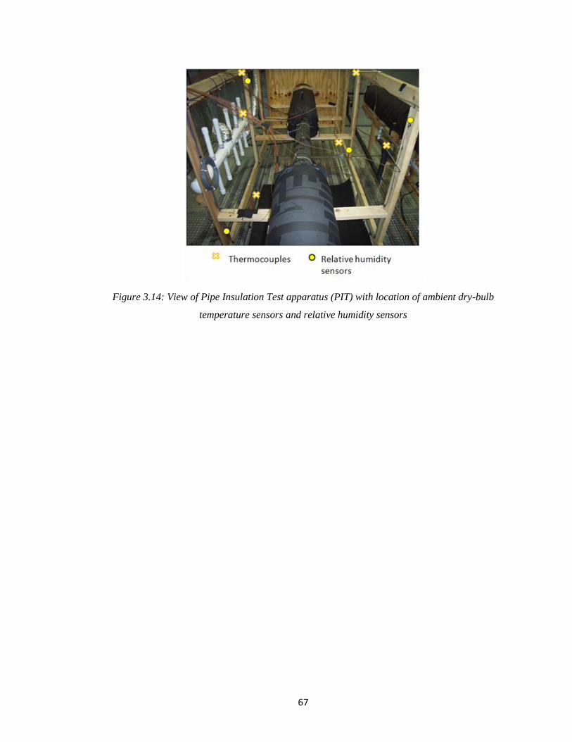
67

Figure 3.14: View of Pipe Insulation Test apparatus (PIT) with location of ambient dry-bulb

temperature sensors and relative humidity sensors

68

CHAPTER IV

4. MEASUREMENTS AND DATA REDUCTION

This chapter discussed the test procedures for the apparent thermal conductivity measurement

under both dry and wet, condensing conditions. A 1-D heat conduction model was used in the

data reduction, and the system uncertainty analysis was provided in detail at the end of this

chapter.

4.1 Experimental Test Conditions

According to the design criteria and controlled strategy described in previous chapter, the developed

test apparatus is expected to guarantee uniform conditions for the ambient air in both dry (non-

condensing) and wet (condensing) tests. Different types of pipe insulation systems with nominal

wall thickness from 1 to 2-in (25.4 to 50.8 mm) were investigated in dry tests. Dry conditions were

achieved by removing all possible water vapor from the room, which took several hours. The

ambient relative humidity was limited to be below 15% to 30% RH depending on the ambient dry

bulb temperature. In dry tests the air dew point temperature was always lower than the aluminum

pipe surface temperature; thus avoiding the risk of condensation on the aluminum pipe surface. The

thermal conductivity of the pipe insulation specimen was measured for insulation mean

temperatures ranging from 55 to 73F (13 to 23C), that is, a cold surface side of 38 to 41F

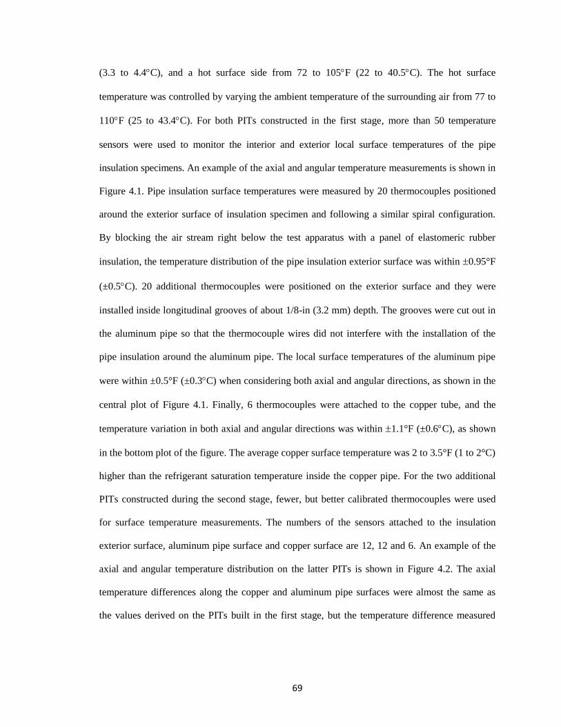
69

(3.3 to 4.4C), and a hot surface side from 72 to 105F (22 to 40.5C). The hot surface

temperature was controlled by varying the ambient temperature of the surrounding air from 77 to

110F (25 to 43.4C). For both PITs constructed in the first stage, more than 50 temperature

sensors were used to monitor the interior and exterior local surface temperatures of the pipe

insulation specimens. An example of the axial and angular temperature measurements is shown in

Figure 4.1. Pipe insulation surface temperatures were measured by 20 thermocouples positioned

around the exterior surface of insulation specimen and following a similar spiral configuration.

By blocking the air stream right below the test apparatus with a panel of elastomeric rubber

insulation, the temperature distribution of the pipe insulation exterior surface was within 0.95°F

(±0.5C). 20 additional thermocouples were positioned on the exterior surface and they were

installed inside longitudinal grooves of about 1/8-in (3.2 mm) depth. The grooves were cut out in

the aluminum pipe so that the thermocouple wires did not interfere with the installation of the

pipe insulation around the aluminum pipe. The local surface temperatures of the aluminum pipe

were within ±0.5°F (±0.3C) when considering both axial and angular directions, as shown in the

central plot of Figure 4.1. Finally, 6 thermocouples were attached to the copper tube, and the

temperature variation in both axial and angular directions was within 1.1°F (±0.6C), as shown

in the bottom plot of the figure. The average copper surface temperature was 2 to 3.5°F (1 to 2°C)

higher than the refrigerant saturation temperature inside the copper pipe. For the two additional

PITs constructed during the second stage, fewer, but better calibrated thermocouples were used

for surface temperature measurements. The numbers of the sensors attached to the insulation

exterior surface, aluminum pipe surface and copper surface are 12, 12 and 6. An example of the

axial and angular temperature distribution on the latter PITs is shown in Figure 4.2. The axial

temperature differences along the copper and aluminum pipe surfaces were almost the same as

the values derived on the PITs built in the first stage, but the temperature difference measured

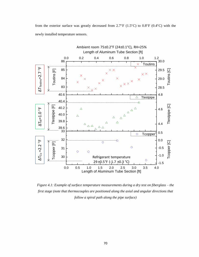
70

from the exterior surface was greatly decreased from 2.7F (1.5C) to 0.8F (0.4C) with the

newly installed temperature sensors.

Figure 4.1: Example of surface temperature measurements during a dry test on fiberglass – the

first stage (note that thermocouples are positioned along the axial and angular directions that

follow a spiral path along the pipe surface)

0.0 0.5 1.0 1.5 2.0 2.5 3.0 3.5 4.0

30

31

32

3339.6

39.8

40.0

40.2

40.4

40.6

83

84

85

86

Length of Aluminum Tube Section [ft]

Tco

pp

er

[C]

Tco

pp

er

[F]

Length of Aluminum Tube Section [ft]

Tcopper

Tte

stp

ipe

[C

]

Tte

stp

ipe

[F

]

Ttestpipe

To

utin

s [C

]

To

utin

s [F

]

Toutins

28.5

29.0

29.5

30.0

-1.5

-1.0

-0.5

0.0

0.5

4.4

4.6

4.8

0.0 0.2 0.4 0.6 0.8 1.0 1.2

∆T C

u=2

.2

F∆

TTe

stin

s=2

.7

F∆

T Al=

1.0

F

Ambient room 75±0.2°F (24±0.1°C), RH=25%

Refrigerant temperature29 ±0.5°F (-1.7 ±0.3 °C)

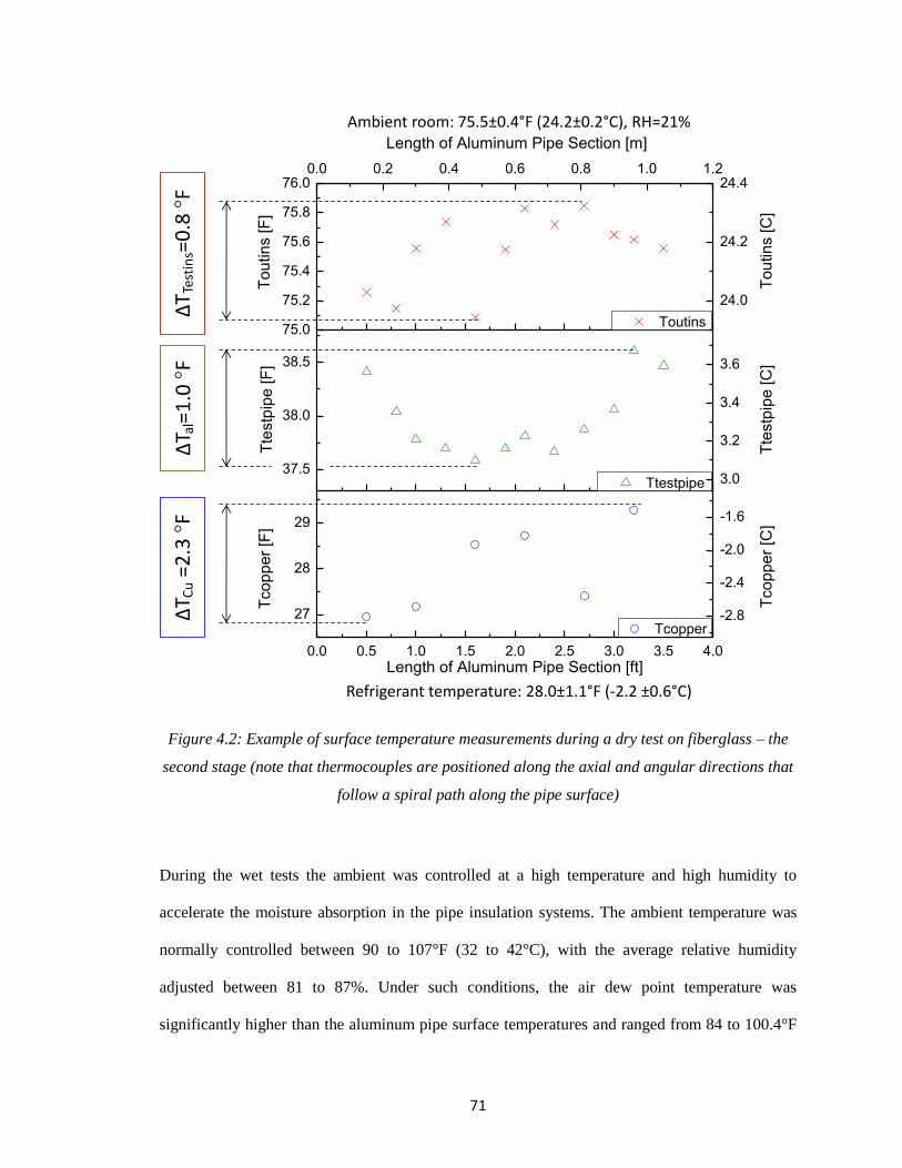
71

Figure 4.2: Example of surface temperature measurements during a dry test on fiberglass – the

second stage (note that thermocouples are positioned along the axial and angular directions that

follow a spiral path along the pipe surface)

During the wet tests the ambient was controlled at a high temperature and high humidity to

accelerate the moisture absorption in the pipe insulation systems. The ambient temperature was

normally controlled between 90 to 107°F (32 to 42°C), with the average relative humidity

adjusted between 81 to 87%. Under such conditions, the air dew point temperature was

significantly higher than the aluminum pipe surface temperatures and ranged from 84 to 100.4°F

0.0 0.5 1.0 1.5 2.0 2.5 3.0 3.5 4.0

27

28

29

37.5

38.0

38.5

75.0

75.2

75.4

75.6

75.8

76.0

Length of Aluminum Pipe Section [m]

Tco

pp

er

[C]

Tco

pp

er

[F]

Length of Aluminum Pipe Section [ft]

Tcopper

Tte

stp

ipe [C

]

Tte

stp

ipe [F

]

Ttestpipe

To

utin

s [C

]

To

utin

s [F

]

Toutins

24.0

24.2

24.4

-2.8

-2.4

-2.0

-1.6

3.0

3.2

3.4

3.6

0.0 0.2 0.4 0.6 0.8 1.0 1.2∆

T Cu

=2.3

F

∆T T

esti

ns=

0.8

F

∆T a

l=1

.0

F

Ambient room: 75.5±0.4°F (24.2±0.2°C), RH=21%

Refrigerant temperature: 28.0±1.1°F (-2.2 ±0.6°C)

72

(29 to 38°C). Figure 4.3 shows the surface temperature measurements on the first day of

fiberglass pipe insulation wet test. While the aluminum pipe surface temperature was controlled

to about 40F 0.6F (4.5C 0.3C) for both the dry-test and for the wet test, the ambient

temperature were 75F in Figure 4.1 (fiberglass in dry non-condensing conditions) and 100F in

Figure 4.3 (first day of fiberglass in wet condensing conditions). The temperature distributions

along the surfaces were quite similar for both cases and the discrepancy of all temperature sensors

reading the pipe insulation exterior surface increased by 0.3°F (0.17°C), that is, from Ttestins of

2.7F in dry non-condensing condition (see Figure 4.1) to Ttestins of 3.0F for the first day of the

wet-test (see Figure 4.3). The temperature distribution on the surfaces after 10 days of exposure

to humid ambient conditions for fiberglass pipe insulation is shown in Figure 4.4. The

temperature profiles on the copper tube, aluminum pipe and insulation specimen exterior surfaces

were not as uniform as the ones measured for dry tests. This was due to local wet regions created

by water condensate that accumulated around the thermocouples on the exterior surface of the

pipe insulation specimen. These wet regions were visually observed and documented during the

wet tests using digital photos. Due to the insulation structure and the gravity effects, preferential

wet regions developed on the insulation specimen and water droplets accumulated at the bottom

shells. The increase of the temperature difference along the vertical direction is evident in Figure

4.4, in which Ttestins gradually increased from 3°F (1.67°C) at day 1 up to 11 °F (6.1 °C) at day

10. It should be noted that a large temperature difference might be due to local values of the

temperature readings in which the water condensate droplets were adjacent to the thermocouple

beads. Thermal bridges might have been occurred due to local regions of wet insulation. The

temperature readings were not uniform because of the insulation material was not homogeneously

wet along the axial and angular directions. Since 20 thermocouples were used on each surface,

the average surface temperatures calculated from all temperature readings were still a good

representation of the exterior temperatures of the aluminum pipe and pipe insulation surfaces.

73

With all 3D effects introduced for wet insulation conditions, the assumption of a 1-D heat transfer

model is an approximate approach that was simple but accurate enough to be useful in practice.

The thermal conductivity value calculated in wet conditions was representative of the average

conductance of heat across the pipe insulation specimen in wet conditions with moisture

accumulated (non-uniformly) on the insulation material.

Figure 4.3: Example of surface temperature measurements on the first day of fiberglass moisture

test (note that thermocouples are positioned along the axial and angular directions that follow a

spiral path along the pipe surface)

0.0 0.5 1.0 1.5 2.0 2.5 3.0 3.5 4.024

25

26

27

38.5

39.0

39.5

40.0

40.597

98

99

100

Length of Aluminum Tube Section [ft]

Tco

pp

er

[C]

Tco

pp

er

[F]

Length of Aluminum Tube Section [ft]

Tcopper

Tte

stp

ipe

[C

]

Tte

stp

ipe

[F

]

Ttestpipe

To

utin

s [C

]

To

utin

s [F

]

Toutins

36.0

36.5

37.0

37.5

38.0

-4.4

-4.0

-3.6

-3.2

-2.8

4.4

4.6

0.0 0.2 0.4 0.6 0.8 1.0 1.2

∆T C

u=

1.9 F

∆T T

esti

ns=

3.0

F

∆T a

l=1

.3

F

Ambient room 100±0.2°F (38.0±0.1°C), RH=19%

Refrigerant temperature24 ±0.5°F (-4.4 ±0.3°C)

74

Figure 4.4: Example of surface temperature measurements on the 10th day of fiberglass moisture

test (note that thermocouples are positioned along the axial and angular directions that follow a

spiral path along the pipe surface)

4.2 Experimental procedures

0.0 0.5 1.0 1.5 2.0 2.5 3.0 3.5 4.0

-6

-4

-2

0

41

42

43

95

100

105

110

Length of Aluminum Tube Section [ft]

Tco

pp

er

[C]

Tco

pp

er

[F]

Length of Aluminum Tube Section [ft]

Tcopper

Tte

stp

ipe

[C

]

Tte

stp

ipe

[F

]

Ttestpipe

To

utin

s [C

]

To

utin

s [F

]

Toutins

36

38

40

42

-21

-20

-19

-18

-17

5.0

5.5

6.0

6.5

0.0 0.2 0.4 0.6 0.8 1.0 1.2∆

T Cu

=6.6

F

∆T

Test

ins=

11.

0 F

∆T a

l=2.

8

F

Ambient room 107±0.2°F (41.5±0.1°C), RH=83%

75

4.2.1 Experimental procedures for calibration test

Calibration tests were required at the beginning of each dry test and at the end of each moisture

test, as a periodically check on the effective thermal conductivity of the sand. Although the sand

was completely sealed in the plastic bag, with two plugs tightly blocked at the ends of the test

pipe, a calibration test was necessary to detect any potential moisture penetration into the

aluminum pipe from the small cracks of the seals between plugs and metal pipe surfaces, if

present. The calibration results served for correcting any potential variation of the sand thermal

conductivity due to moisture accumulation.

During the calibration, two tape electric heaters were installed evenly on the surface of the

aluminum pipe, and they were controlled by a variable transformer. A watt transducer was used

to measure the power to the electric heater. A large volume of rubber foam insulation was applied

around the heaters to limit the heat gains from the ambient. From preliminary tests, it was found

that thermocouple readings were quite sensitive to the power of the tape heaters due to the electric

interferences from the direct contact of the electric tape heater with the aluminum pipe surface.

Therefore, a layer of wax paper was tightly wrapped below the tape heaters to provide an extra

layer of electrical insulation. Another layer of thin film aluminum foil was tightly sandwiched

between the tape heaters and the exterior rubber foam insulation in order to evenly distribute the

heat from the electric heater to the aluminum pipe and avoid local hot spots that could potentially

damage the thermocouple wires. The entire aluminum pipe and corresponding thermocouples

were electrically grounded to reduce electric noise.

4.2.2 Experimental procedures for dry non-condensing testes

76

For the apparent thermal conductivity measurement under dry conditions, two different

procedures were proposed at different stages of this project. These procedures will be explained

in detail in the following paragraphs.

Procedure in the first stage

In the first stage, two PITs were required during one single test. The first PIT was served for the

thermal conductivity measurement, while the second PIT was tested simultaneously to monitor

the sand thermal conductivity. The steps to calculate the apparent thermal conductivity of one

pipe insulation system are shown in the algorithm of Figure 4.5. The first PIT measured the radial

heat flux across the sand, and the thermal conductivity of the pipe insulation system was obtained

from the sand thermal conductivity and temperature measurements across the pipe insulation

system. The sand thermal conductivity was determined during the initial calibration of the

apparatus. The second PIT was operated under similar thermal boundary conditions as the ones of

the first PIT. During the dry test period, the thermal conductivity of the sand in the second PIT

was constantly monitored by measuring the electric power to the heaters and the temperature

gradient across the sand. If the thermal conductivity of the sand showed an obvious deviation

from the initial values then the test on the first PIT was paused. The measured anomaly on the

second PIT was assumed to be an indicator that water vapor diffused inside the aluminum pipe.

The assumption made was that if the second PIT experienced a failure then the first PIT might

have experienced a failure during the same time. With the dry test paused, an intermediate

calibration of the sand thermal conductivity in the first PIT was conducted to assess whether the

sand thermal conductivity in the first PIT also experienced a measurable variation from its initial

value. With updated values of the sand thermal conductivity in the first PIT, the dry test was then

re-started again. At the end of the dry test, a final check of the sand thermal conductivity on the

first PIT was conducted to assess the overall variation of the sand thermal conductivity during the

period of the dry test, if present. This variation was usually small unless water vapor penetrated in

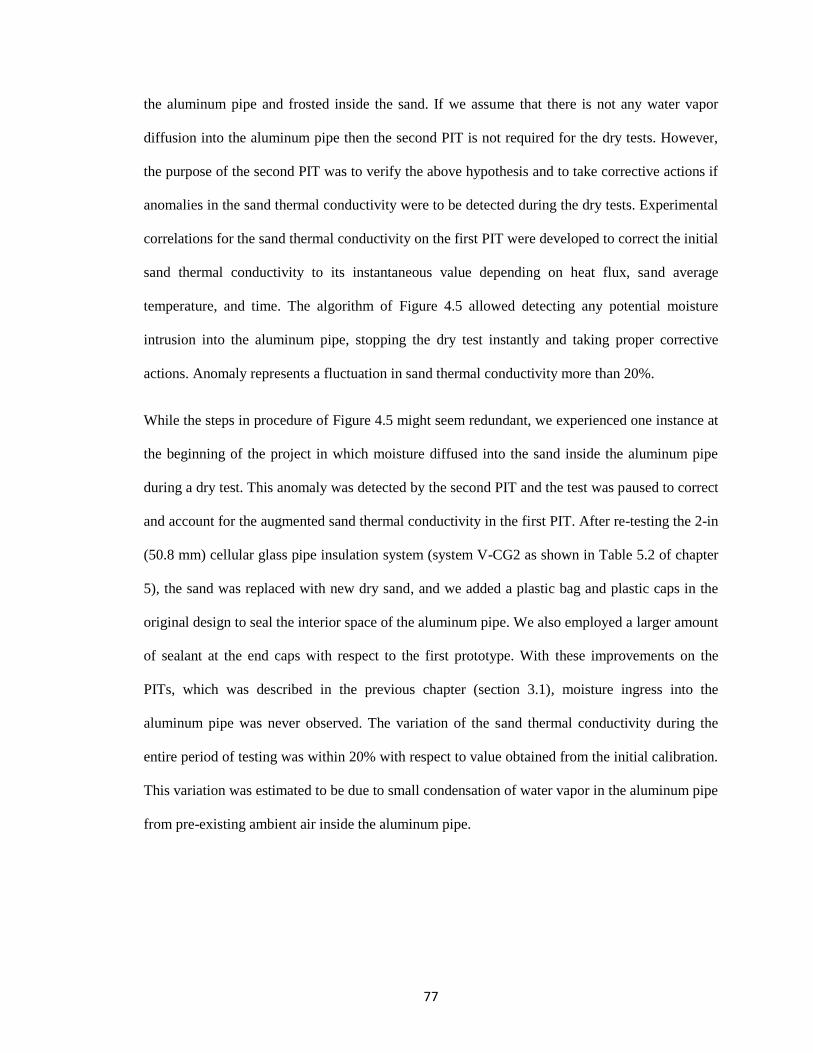
77

the aluminum pipe and frosted inside the sand. If we assume that there is not any water vapor

diffusion into the aluminum pipe then the second PIT is not required for the dry tests. However,

the purpose of the second PIT was to verify the above hypothesis and to take corrective actions if

anomalies in the sand thermal conductivity were to be detected during the dry tests. Experimental

correlations for the sand thermal conductivity on the first PIT were developed to correct the initial

sand thermal conductivity to its instantaneous value depending on heat flux, sand average

temperature, and time. The algorithm of Figure 4.5 allowed detecting any potential moisture

intrusion into the aluminum pipe, stopping the dry test instantly and taking proper corrective

actions. Anomaly represents a fluctuation in sand thermal conductivity more than 20%.

While the steps in procedure of Figure 4.5 might seem redundant, we experienced one instance at

the beginning of the project in which moisture diffused into the sand inside the aluminum pipe

during a dry test. This anomaly was detected by the second PIT and the test was paused to correct

and account for the augmented sand thermal conductivity in the first PIT. After re-testing the 2-in

(50.8 mm) cellular glass pipe insulation system (system V-CG2 as shown in Table 5.2 of chapter

5), the sand was replaced with new dry sand, and we added a plastic bag and plastic caps in the

original design to seal the interior space of the aluminum pipe. We also employed a larger amount

of sealant at the end caps with respect to the first prototype. With these improvements on the

PITs, which was described in the previous chapter (section 3.1), moisture ingress into the

aluminum pipe was never observed. The variation of the sand thermal conductivity during the

entire period of testing was within 20% with respect to value obtained from the initial calibration.

This variation was estimated to be due to small condensation of water vapor in the aluminum pipe

from pre-existing ambient air inside the aluminum pipe.

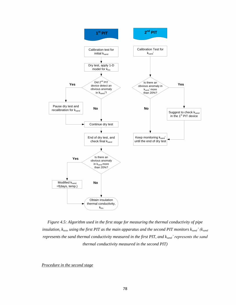
78

Figure 4.5: Algorithm used in the first stage for measuring the thermal conductivity of pipe

insulation, ktest, using the first PIT as the main apparatus and the second PIT monitors ksand’ (ksand

represents the sand thermal conductivity measured in the first PIT, and ksand’ represents the sand

thermal conductivity measured in the second PIT)

Procedure in the second stage

Calibration test for

initial ksand

Dry test, apply 1-D

model for kins

Calibration Test for

ksand'

End of dry test, and

check final ksand

Pause dry test and

recalibration for ksand

Modified ksand

=f(days, temp.)

2nd

PIT

Yes

1st

PIT

Yes

Did 2nd

PIT

device detect an

obvious anomaly

in ksand'?

Is there an

obvious anomaly in

ksand' more

than 20%?

No

Continue dry test

Is there an

obvious anomaly

in ksand more

than 20%?

Obtain insulation

thermal conductivity,

kins

No

Suggest to check ksand

in the 1st PIT device

Keep monitoring ksand'

until the end of dry test

Yes

No

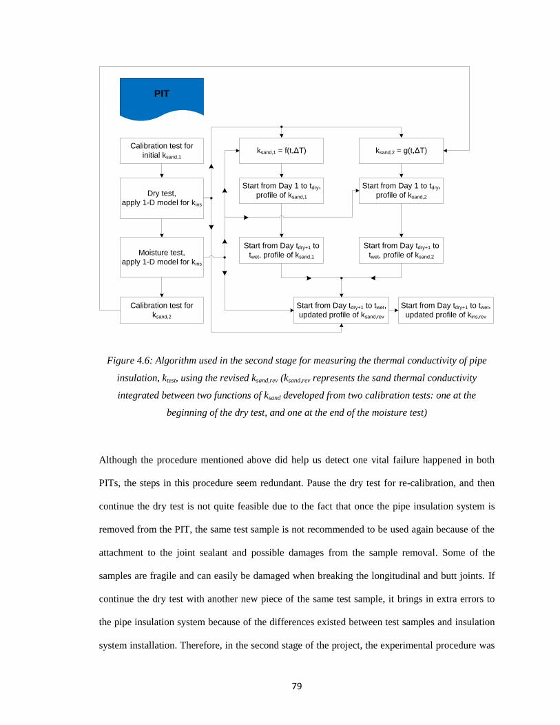
79

Figure 4.6: Algorithm used in the second stage for measuring the thermal conductivity of pipe

insulation, ktest, using the revised ksand,rev (ksand,rev represents the sand thermal conductivity

integrated between two functions of ksand developed from two calibration tests: one at the

beginning of the dry test, and one at the end of the moisture test)

Although the procedure mentioned above did help us detect one vital failure happened in both

PITs, the steps in this procedure seem redundant. Pause the dry test for re-calibration, and then

continue the dry test is not quite feasible due to the fact that once the pipe insulation system is

removed from the PIT, the same test sample is not recommended to be used again because of the

attachment to the joint sealant and possible damages from the sample removal. Some of the

samples are fragile and can easily be damaged when breaking the longitudinal and butt joints. If

continue the dry test with another new piece of the same test sample, it brings in extra errors to

the pipe insulation system because of the differences existed between test samples and insulation

system installation. Therefore, in the second stage of the project, the experimental procedure was

Calibration test for

initial ksand,1

Dry test,

apply 1-D model for kins

PIT

Moisture test,

apply 1-D model for kins

Calibration test for

ksand,2

Start from Day tdry+1 to twet,

updated profile of ksand,rev

ksand,1 = f(t,ΔT) ksand,2 = g(t,ΔT)

Start from Day 1 to tdry,

profile of ksand,1

Start from Day tdry+1 to

twet, profile of ksand,1

Start from Day 1 to tdry,

profile of ksand,2

Start from Day tdry+1 to

twet, profile of ksand,2

Start from Day tdry+1 to twet,

updated profile of kins,rev

80

improved to avoid any interruption during one single test. The steps for the improved procedure

are shown in the flow chart provided in Figure 4.8. By following this new procedure, it is not

required a second PIT to monitor the variation on the sand thermal conductivity, and each PIT

can be served for thermal conductivity measurement independently. This means with the

improved method, four pipe insulation systems can be tested at one time under dry conditions.

Before each dry test, a calibration test is required to determine the initial correlation of sand

thermal conductivity with the sand average temperature and the exterior temperature difference

between the ambient and the cold pipe surface, ksand,1 = f(T,ΔT) for example. After the calibration

test, the dry test starts and will be followed by the moisture test. By the end of the moisture test, a

second calibration test will start immediately for periodical check on the sand thermal

conductivity, and the new correlation from the second calibration is g(T,ΔT), for example (ksand,2 =

g(T,ΔT)). By only considering ksand,1 or ksand,2 in the dry and moisture test, I can derive two sets of

sand thermal conductivity regarding to the same temperature profile. Assume the sand thermal

conductivity varies linearly with time, the revised values on ksand,rev can be interpolated from the

two sets of data. For example, according to the temperature profile recorded on the xth day from

the beginning of the dry test (t=tx), the sand thermal conductivity is computed as ksand,1x by

applying the correlation f(T,ΔT), which is developed from the initial calibration. With the same

temperature profile, but applying the other correlation, g(T,ΔT) from the second calibration test,

the sand thermal conductivity is ksand,2x. Therefore, on day x, the revised sand thermal

conductivity (ksand,revx) is corrected as:

(4.1)

Where tx is the days for testing, tdry is the total days for dry test, and twet is the total days for

moisture test. It should be noted that the first day is considered as t=1.

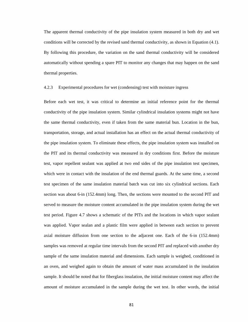
81

The apparent thermal conductivity of the pipe insulation system measured in both dry and wet

conditions will be corrected by the revised sand thermal conductivity, as shown in Equation (4.1).

By following this procedure, the variation on the sand thermal conductivity will be considered

automatically without spending a spare PIT to monitor any changes that may happen on the sand

thermal properties.

4.2.3 Experimental procedures for wet (condensing) test with moisture ingress

Before each wet test, it was critical to determine an initial reference point for the thermal

conductivity of the pipe insulation system. Similar cylindrical insulation systems might not have

the same thermal conductivity, even if taken from the same material bun. Location in the bun,

transportation, storage, and actual installation has an effect on the actual thermal conductivity of

the pipe insulation system. To eliminate these effects, the pipe insulation system was installed on

the PIT and its thermal conductivity was measured in dry conditions first. Before the moisture

test, vapor repellent sealant was applied at two end sides of the pipe insulation test specimen,

which were in contact with the insulation of the end thermal guards. At the same time, a second

test specimen of the same insulation material batch was cut into six cylindrical sections. Each

section was about 6-in (152.4mm) long. Then, the sections were mounted to the second PIT and

served to measure the moisture content accumulated in the pipe insulation system during the wet

test period. Figure 4.7 shows a schematic of the PITs and the locations in which vapor sealant

was applied. Vapor sealan and a plastic film were applied in between each section to prevent

axial moisture diffusion from one section to the adjacent one. Each of the 6-in (152.4mm)

samples was removed at regular time intervals from the second PIT and replaced with another dry

sample of the same insulation material and dimensions. Each sample is weighed, conditioned in

an oven, and weighed again to obtain the amount of water mass accumulated in the insulation

sample. It should be noted that for fiberglass insulation, the initial moisture content may affect the

amount of moisture accumulated in the sample during the wet test. In other words, the initial

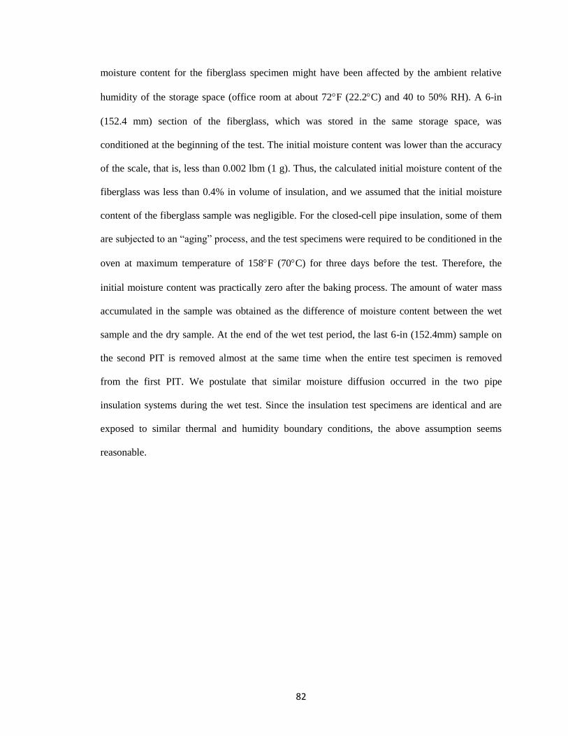
82

moisture content for the fiberglass specimen might have been affected by the ambient relative

humidity of the storage space (office room at about 72F (22.2C) and 40 to 50% RH). A 6-in

(152.4 mm) section of the fiberglass, which was stored in the same storage space, was

conditioned at the beginning of the test. The initial moisture content was lower than the accuracy

of the scale, that is, less than 0.002 lbm (1 g). Thus, the calculated initial moisture content of the

fiberglass was less than 0.4% in volume of insulation, and we assumed that the initial moisture

content of the fiberglass sample was negligible. For the closed-cell pipe insulation, some of them

are subjected to an “aging” process, and the test specimens were required to be conditioned in the

oven at maximum temperature of 158F (70C) for three days before the test. Therefore, the

initial moisture content was practically zero after the baking process. The amount of water mass

accumulated in the sample was obtained as the difference of moisture content between the wet

sample and the dry sample. At the end of the wet test period, the last 6-in (152.4mm) sample on

the second PIT is removed almost at the same time when the entire test specimen is removed

from the first PIT. We postulate that similar moisture diffusion occurred in the two pipe

insulation systems during the wet test. Since the insulation test specimens are identical and are

exposed to similar thermal and humidity boundary conditions, the above assumption seems

reasonable.

83

Figure 4.7: Schematic showing the preparation of the insulation test specimens for the wet test

The moisture content of the insulation test specimen is directly measured only at the beginning

and at the end of the wet test period. The rate of moisture absorption in the pipe insulation test

specimen was obtained by data regression of the moisture content measurements obtained from

the samples removed at regular time intervals from the second PIT. A specific sample was shown

in chapter 5 section 5.5.1. The water mass accumulated on the pipe insulation system was

measured by using the difference in weight of the test specimen in wet conditions with respect to

dry insulation. This weight difference represented the moisture mass accumulated in the

insulation system during the period of exposure to the wet ambient conditions. For some types of

pipe insulation, such as phenolic, cellular glass and PIR, joint sealant was required to apply

between two C-shells along the longitudinal joints. Vapor sealant was applied to fill in the gaps in

between each 6-in (152.4mm) sample. According to the preliminary in-house tests, both

insulation adhesive and vapor sealant absorbed a small amount of moisture. A procedure to

3ft Test Section

Vapor sealant Vapor sealantPlastic film/White mastic to prevent axial moisture

transportation

3ft Test Section

PIT 1st Device

PIT 2nd Device

Vapor sealant Vapor sealant

Installation Method on 1st PIT

Plastic film and vapor sealant to prevent axial moisture transportation

Installation Method on 2nd PIT

84

remove the adhesive and vapor sealant by cutting a piece of pure insulation out of the test

specimen (taken from the second PIT) is shown in Figure 4.8. The pure insulation sample, i.e.

without any adhesive and vapor sealant, is placed in the oven at a baking temperature between

170 to 250 °F (77 to 121 °C) for at least 8 hours. The baking time and baking temperature varied

with moisture content and types of insulation. Usually for the highly permeable materials, such as

fiberglass, the drying process for baking the entire pipe insulation test specimen was up to three

days. Each insulation sample was conditioned in the oven for an enough long period such that its

weight did not change in between two consecutive weight measurements. Each weight

measurement took place in the ambient room temperature every 12 to 24 hours. If two

consecutive weight measurements of the same sample were within 0.0044 lbm (2 grams) after a

baking period, then the insulation sample was considered to have achieved dry conditions. The

final weight measurement after the baking process was assumed to be the weight of the dry

insulation test specimen. The total amount of water mass accumulated in the insulation system

during wet operating conditions was determined from the difference between the wet weight of

the sample and the dry weight of the insulation sample.

Figure 4.8: Schematic showing the insulation cuts for collecting insulation material without any

vapor sealant and adhesive before baking

In order to better compare the system thermal conductivity measured in the moisture test to the

value derived under dry condition, a mapping test was added before the moisture test to provide a

correlation between the pipe insulation system thermal conductivity and the aluminum pipe

3ft Test Section

Vapor sealant Adhesive Pure insulation

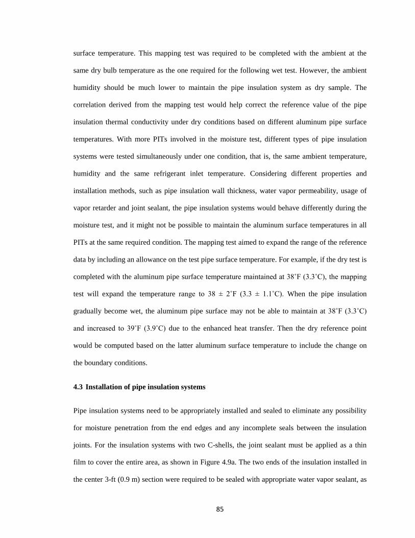
85

surface temperature. This mapping test was required to be completed with the ambient at the

same dry bulb temperature as the one required for the following wet test. However, the ambient

humidity should be much lower to maintain the pipe insulation system as dry sample. The

correlation derived from the mapping test would help correct the reference value of the pipe

insulation thermal conductivity under dry conditions based on different aluminum pipe surface

temperatures. With more PITs involved in the moisture test, different types of pipe insulation

systems were tested simultaneously under one condition, that is, the same ambient temperature,

humidity and the same refrigerant inlet temperature. Considering different properties and

installation methods, such as pipe insulation wall thickness, water vapor permeability, usage of

vapor retarder and joint sealant, the pipe insulation systems would behave differently during the

moisture test, and it might not be possible to maintain the aluminum surface temperatures in all

PITs at the same required condition. The mapping test aimed to expand the range of the reference

data by including an allowance on the test pipe surface temperature. For example, if the dry test is

completed with the aluminum pipe surface temperature maintained at 38˚F (3.3˚C), the mapping

test will expand the temperature range to 38 ± 2˚F (3.3 ± 1.1˚C). When the pipe insulation

gradually become wet, the aluminum pipe surface may not be able to maintain at 38˚F (3.3˚C)

and increased to 39˚F (3.9˚C) due to the enhanced heat transfer. Then the dry reference point

would be computed based on the latter aluminum surface temperature to include the change on

the boundary conditions.

4.3 Installation of pipe insulation systems

Pipe insulation systems need to be appropriately installed and sealed to eliminate any possibility

for moisture penetration from the end edges and any incomplete seals between the insulation

joints. For the insulation systems with two C-shells, the joint sealant must be applied as a thin

film to cover the entire area, as shown in Figure 4.9a. The two ends of the insulation installed in

the center 3-ft (0.9 m) section were required to be sealed with appropriate water vapor sealant, as

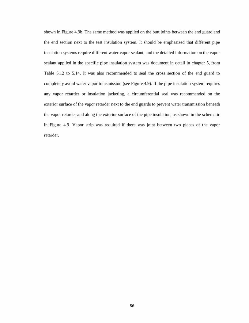
86

shown in Figure 4.9b. The same method was applied on the butt joints between the end guard and

the end section next to the test insulation system. It should be emphasized that different pipe

insulation systems require different water vapor sealant, and the detailed information on the vapor

sealant applied in the specific pipe insulation system was document in detail in chapter 5, from

Table 5.12 to 5.14. It was also recommended to seal the cross section of the end guard to

completely avoid water vapor transmission (see Figure 4.9). If the pipe insulation system requires

any vapor retarder or insulation jacketing, a circumferential seal was recommended on the

exterior surface of the vapor retarder next to the end guards to prevent water transmission beneath

the vapor retarder and along the exterior surface of the pipe insulation, as shown in the schematic

in Figure 4.9. Vapor strip was required if there was joint between two pieces of the vapor

retarder.

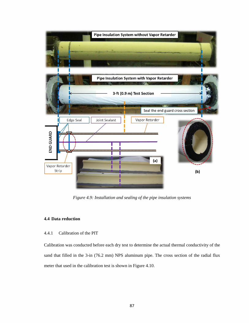
87

Figure 4.9: Installation and sealing of the pipe insulation systems

4.4 Data reduction

4.4.1 Calibration of the PIT

Calibration was conducted before each dry test to determine the actual thermal conductivity of the

sand that filled in the 3-in (76.2 mm) NPS aluminum pipe. The cross section of the radial flux

meter that used in the calibration test is shown in Figure 4.10.

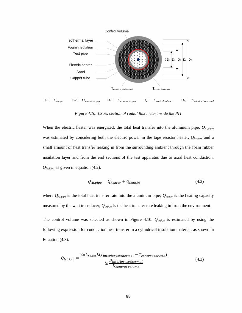
88

D1: Dcopper D2: Dinterior,Al,pipe D3: Dexterior,Al,pipe D4: Dcontrol volume D5: Dinterior,isothermal

Figure 4.10: Cross section of radial flux meter inside the PIT

When the electric heater was energized, the total heat transfer into the aluminum pipe, QAl,pipe,

was estimated by considering both the electric power in the tape resistor heater, Qheater, and a

small amount of heat transfer leaking in from the surrounding ambient through the foam rubber

insulation layer and from the end sections of the test apparatus due to axial heat conduction,

Qleak,in, as given in equation (4.2):

(4.2)

where QAl,pipe is the total heat transfer rate into the aluminum pipe; Qheater is the heating capacity

measured by the watt transducer; Qleak,in is the heat transfer rate leaking in from the environment.

The control volume was selected as shown in Figure 4.10. Qleak,in is estimated by using the

following expression for conduction heat transfer in a cylindrical insulation material, as shown in

Equation (4.3).

D1 D2 D3 D4 D5

Foam insulation

Test pipe

Sand

Copper tube

Isothermal layer

Electric heater

Control volume

Tcontrol volumeTexterior,isothermal

(4.3)

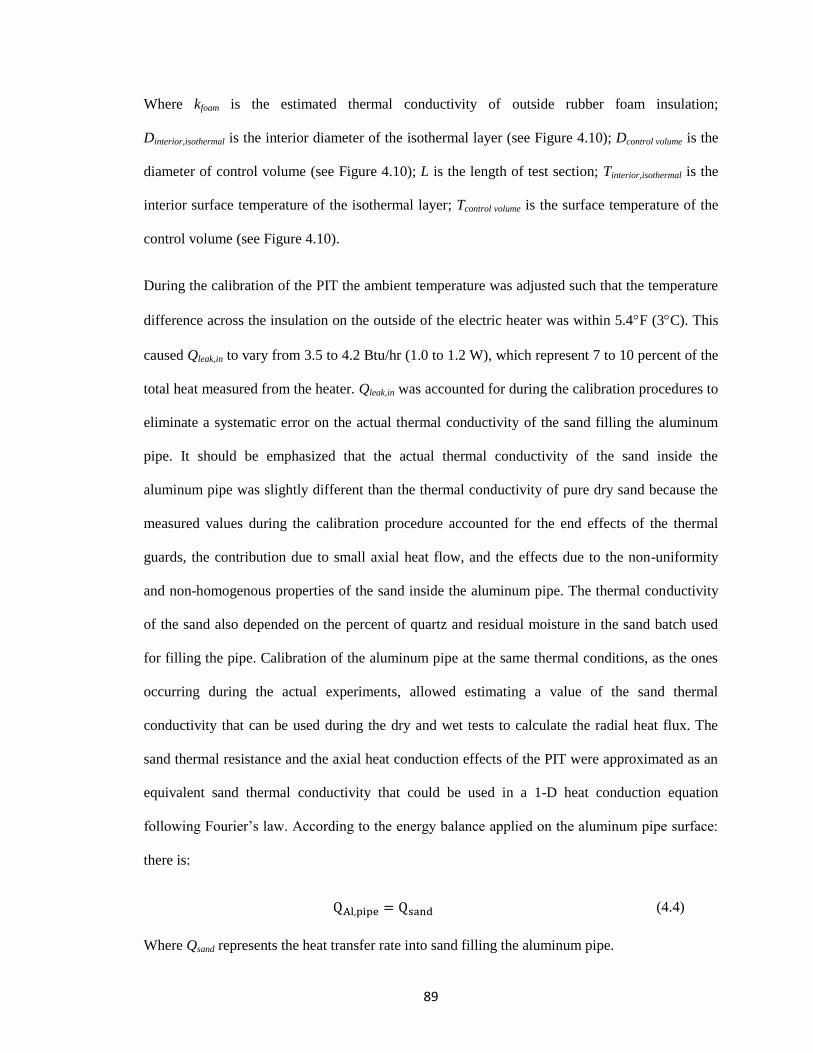
89

Where kfoam is the estimated thermal conductivity of outside rubber foam insulation;

Dinterior,isothermal is the interior diameter of the isothermal layer (see Figure 4.10); Dcontrol volume is the

diameter of control volume (see Figure 4.10); L is the length of test section; Tinterior,isothermal is the

interior surface temperature of the isothermal layer; Tcontrol volume is the surface temperature of the

control volume (see Figure 4.10).

During the calibration of the PIT the ambient temperature was adjusted such that the temperature

difference across the insulation on the outside of the electric heater was within 5.4F (3C). This

caused Qleak,in to vary from 3.5 to 4.2 Btu/hr (1.0 to 1.2 W), which represent 7 to 10 percent of the

total heat measured from the heater. Qleak,in was accounted for during the calibration procedures to

eliminate a systematic error on the actual thermal conductivity of the sand filling the aluminum

pipe. It should be emphasized that the actual thermal conductivity of the sand inside the

aluminum pipe was slightly different than the thermal conductivity of pure dry sand because the

measured values during the calibration procedure accounted for the end effects of the thermal

guards, the contribution due to small axial heat flow, and the effects due to the non-uniformity

and non-homogenous properties of the sand inside the aluminum pipe. The thermal conductivity

of the sand also depended on the percent of quartz and residual moisture in the sand batch used

for filling the pipe. Calibration of the aluminum pipe at the same thermal conditions, as the ones

occurring during the actual experiments, allowed estimating a value of the sand thermal

conductivity that can be used during the dry and wet tests to calculate the radial heat flux. The

sand thermal resistance and the axial heat conduction effects of the PIT were approximated as an

equivalent sand thermal conductivity that could be used in a 1-D heat conduction equation

following Fourier’s law. According to the energy balance applied on the aluminum pipe surface:

there is:

(4.4)

Where Qsand represents the heat transfer rate into sand filling the aluminum pipe.

90

The axial temperature gradient along the aluminum pipe was less than 0.43% of the radial

temperature gradient across the sand. Based on this finding it is reasonable to assume that the

axial heat losses on the aluminum pipe are small and a heat balance across the sand yields

(4.5)

where ksand is the effective thermal conductivity of sand; Dinterior,Al,pipe is the inside diameter of test

pipe, Figure 4.10; Dcold,copper,pipe is the diameter of copper tube, Figure 4.10; Tcold,copper,pipe is the

surface temperature of copper tube.

The average sand temperature is

(4.6)

By measuring the power of the electric heater and the temperatures, the thermal conductivity of

the sand inside the aluminum pipe was obtained using equations (4.1) to (4.5).

It should be noted that according to (4.3), Qleak,in is highly dependent on the ambient conditions.

When the test condition is controlled at a higher temperature, the temperature difference between

the exterior surface of the pipe insulation and the aluminum pipe increases, and Qleak,in weights

more in Qsand, when compared to the low temperature condition. In order to include the impact

from the variation on the boundary conditions, the calibration test was required to be applied at

two different ambient temperatures: 56˚F (13.3˚C) and 90˚F (32.2˚C). Two correlations between

sand thermal conductivity and average sand temperatures were derived from the measurements

under these two ambient conditions in the calibration test. With interpolation between these

curves, the sand thermal conductivity was developed as a second power correlation to both the

average sand temperature and the exterior temperature difference between the ambient and the

91

aluminum pipe, shown in Equation (4.7) This improved correlation included the impact of the

variation on the boundary conditions and further enhance the system accuracy.

(4.7)

Where b1 to b5 are empirical coefficients, ΔTexterior represents the temperature difference between

the ambient and the aluminum pipe.

4.4.2 Pipe insulation system thermal conductivity measurements

Once the thermal conductivity of the sand filling the aluminum pipe, ksand, was obtained from the

calibration procedure, a 1-D heat balance equation along the radial direction was applied to the

PIT, as shown in the schematic of Figure 4.11. As a result, the pipe insulation thermal

conductivity, kins, was determined directly by the following expression (4.8):

(4.8)

Where Gf is a geometry factor that depends on the ratios of pipe insulation exterior diameter, the

aluminum pipe outer diameter, and refrigerating copper tube outer diameters, as shown in Figure

4.11. The diameters of the pipe insulation were measured according to the standard ASTM C585

(ASTM, 2009).

The average temperature of the test insulation specimen was calculated from the measurements of

the surface temperature sensors as follows:

(4.9)

92

Figure 4.11: Schematic of the 1-D model of the Pipe Insulation Tester (PIT) and corresponding

diameters

4.4.3 Moisture Content Measurements in the Pipe Insulation System

The moisture content in the pipe insulation systems during the wet tests was calculated as

percentage of the water volume per unit volume of pipe insulation. Moisture mass was measured

from the weight difference of the samples in wet and dry conditions. Then the water mass was

divided by a reference density of water, which was assumed constant at 62.43 lbm/ft3 (1000

kg/m3) (at 39.2°F/ 4°C). The volume of pipe insulation system was measured from its actual

geometry. The overall expression for moisture content is as follows:

(4.10)

Where Vmoisture is the volume of water present in the insulation system; Vspecimen is the volume of

the insulation system; mwet,specimen is the weight of the wet insulation system; mbake,specimen is the

weight of the dry insulation system after being conditioned in the oven; ρwater is the water density

at 39.2 °F (4 °C).

D1 D2 D3 D4

Cold copper tube

Sand

Al pipe

Test insulation

specimen

Ambient room Qleak,in

Geometric factor, Gf , for the diameter ratios:

)/ln(

)/ln(

12

34

DD

DDGf

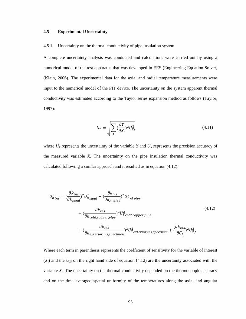
93

4.5 Experimental Uncertainty

4.5.1 Uncertainty on the thermal conductivity of pipe insulation system

A complete uncertainty analysis was conducted and calculations were carried out by using a

numerical model of the test apparatus that was developed in EES (Engineering Equation Solver,

(Klein, 2006). The experimental data for the axial and radial temperature measurements were

input to the numerical model of the PIT device. The uncertainty on the system apparent thermal

conductivity was estimated according to the Taylor series expansion method as follows (Taylor,

1997):

√∑

(4.11)

where UY represents the uncertainty of the variable Y and UX represents the precision accuracy of

the measured variable X. The uncertainty on the pipe insulation thermal conductivity was

calculated following a similar approach and it resulted as in equation (4.12):

(4.12)

Where each term in parenthesis represents the coefficient of sensitivity for the variable of interest

(Xi) and the UXi on the right hand side of equation (4.12) are the uncertainty associated with the

variable Xi. The uncertainty on the thermal conductivity depended on the thermocouple accuracy

and on the time averaged spatial uniformity of the temperatures along the axial and angular

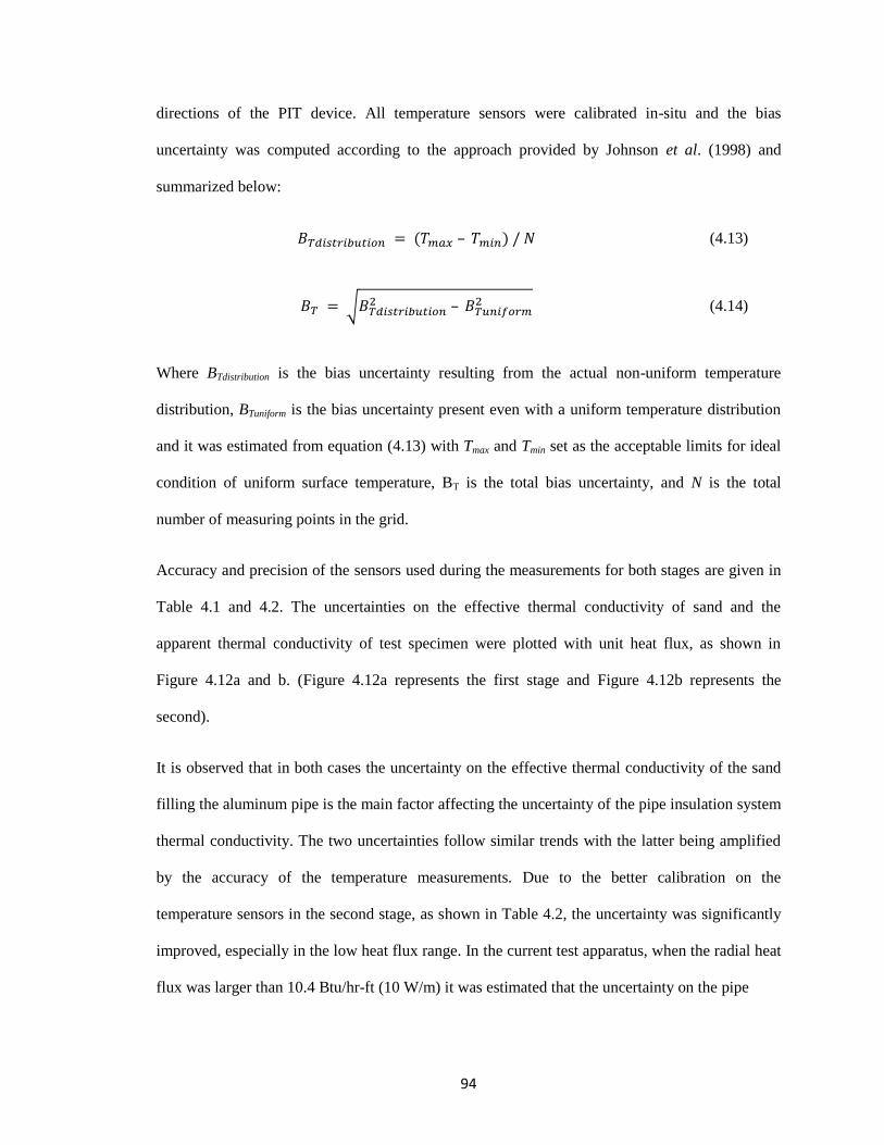
94

directions of the PIT device. All temperature sensors were calibrated in-situ and the bias

uncertainty was computed according to the approach provided by Johnson et al. (1998) and

summarized below:

(4.13)

√

(4.14)

Where BTdistribution is the bias uncertainty resulting from the actual non-uniform temperature

distribution, BTuniform is the bias uncertainty present even with a uniform temperature distribution

and it was estimated from equation (4.13) with Tmax and Tmin set as the acceptable limits for ideal

condition of uniform surface temperature, BT is the total bias uncertainty, and N is the total

number of measuring points in the grid.

Accuracy and precision of the sensors used during the measurements for both stages are given in

Table 4.1 and 4.2. The uncertainties on the effective thermal conductivity of sand and the

apparent thermal conductivity of test specimen were plotted with unit heat flux, as shown in

Figure 4.12a and b. (Figure 4.12a represents the first stage and Figure 4.12b represents the

second).

It is observed that in both cases the uncertainty on the effective thermal conductivity of the sand

filling the aluminum pipe is the main factor affecting the uncertainty of the pipe insulation system

thermal conductivity. The two uncertainties follow similar trends with the latter being amplified

by the accuracy of the temperature measurements. Due to the better calibration on the

temperature sensors in the second stage, as shown in Table 4.2, the uncertainty was significantly

improved, especially in the low heat flux range. In the current test apparatus, when the radial heat

flux was larger than 10.4 Btu/hr-ft (10 W/m) it was estimated that the uncertainty on the pipe

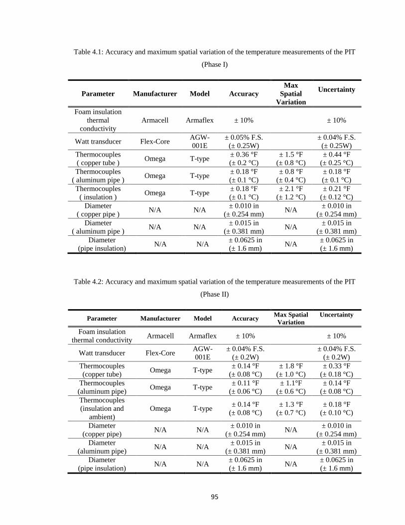
95

Table 4.1: Accuracy and maximum spatial variation of the temperature measurements of the PIT

(Phase I)

Parameter Manufacturer Model Accuracy

Max

Spatial

Variation

Uncertainty

Foam insulation

thermal

conductivity

Armacell Armaflex ± 10% ± 10%

Watt transducer Flex-Core AGW-

001E

± 0.05% F.S.

(± 0.25W)

± 0.04% F.S.

(± 0.25W)

Thermocouples

( copper tube ) Omega T-type

± 0.36 °F

(± 0.2 °C)

± 1.5 °F

(± 0.8 °C)

± 0.44 °F

(± 0.25 °C)

Thermocouples

( aluminum pipe ) Omega T-type

± 0.18 °F

(± 0.1 °C)

± 0.8 °F

(± 0.4 °C)

± 0.18 °F

(± 0.1 °C)

Thermocouples

( insulation ) Omega T-type

± 0.18 °F

(± 0.1 °C)

± 2.1 °F

(± 1.2 °C)

± 0.21 °F

(± 0.12 °C)

Diameter

( copper pipe ) N/A N/A

± 0.010 in

(± 0.254 mm) N/A

± 0.010 in

(± 0.254 mm)

Diameter

( aluminum pipe ) N/A N/A

± 0.015 in

(± 0.381 mm) N/A

± 0.015 in

(± 0.381 mm)

Diameter

(pipe insulation) N/A N/A

± 0.0625 in

(± 1.6 mm) N/A

± 0.0625 in

(± 1.6 mm)

Table 4.2: Accuracy and maximum spatial variation of the temperature measurements of the PIT

(Phase II)

Parameter Manufacturer Model Accuracy Max Spatial

Variation

Uncertainty

Foam insulation

thermal conductivity Armacell Armaflex ± 10% ± 10%

Watt transducer Flex-Core AGW-

001E

± 0.04% F.S.

(± 0.2W)

± 0.04% F.S.

(± 0.2W)

Thermocouples

(copper tube) Omega T-type

± 0.14 °F

(± 0.08 °C)

± 1.8 °F

(± 1.0 °C)

± 0.33 °F

(± 0.18 °C)

Thermocouples

(aluminum pipe) Omega T-type

± 0.11 °F

(± 0.06 °C)

± 1.1°F

(± 0.6 °C)

± 0.14 °F

(± 0.08 °C)

Thermocouples

(insulation and

ambient)

Omega T-type ± 0.14 °F

(± 0.08 °C)

± 1.3 °F

(± 0.7 °C)

± 0.18 °F

(± 0.10 °C)

Diameter

(copper pipe) N/A N/A

± 0.010 in

(± 0.254 mm) N/A

± 0.010 in

(± 0.254 mm)

Diameter

(aluminum pipe) N/A N/A

± 0.015 in

(± 0.381 mm) N/A

± 0.015 in

(± 0.381 mm)

Diameter

(pipe insulation) N/A N/A

± 0.0625 in

(± 1.6 mm) N/A

± 0.0625 in

(± 1.6 mm)

96

insulation system thermal conductivity was about ±5 % and the uncertainty of the sand thermal

conductivity was within ±4%, as shown in Figure 4.12. With the temperature boundary conditions

of the aluminum pipe surface temperature at 38F (3.3C) and room temperature between 56 to

90˚F (13.3 to 32.2˚C), the PITs improved in the second stage could accurately measure the pipe

insulation system thermal conductivity with a heat flux as low as 8.2 Btu/hr-ft (7.9 W/m).

Compared to the uncertainty profile derived from previous apparatus, which showed a dramatic

increase on the uncertainty of sand thermal conductivity when the radial heat flux was below 8.6

Btu/hr-ft (8.3 W/m), the present system was able to maintain the uncertainty in a larger range,

especially in the low heat flux region. This is a significant improvement because under dry

condition, the heat transfer through pipe insulation systems remains at a low level, around or even

below 10.4 Btu/hr (10 W/m) in most cases. With the improved test apparatus, more pipe

insulation systems, such as those with larger wall thicknesses and lower thermal conductivity, can

be tested with acceptable uncertainties. However, it should be noted that the uncertainty might

increase dramatically when the heat flow drops below 8.2 Btu/hr-ft (7.9 W/m). This limitation

was due to the fact that the measured heat transfer from the tape heaters during the calibration

process becomes too small and in particular becomes lower than 1% of the maximum range of the

watt transducer. In these conditions the uncertainty on the power measurements increased

drastically. In the low range of the electric heater, the heat from the ambient into the sand became

a higher fraction of the total heat gain, and the uncertainty on the heat gain from the ambient

became a significant contributor to the overall uncertainty of the sand thermal conductivity.

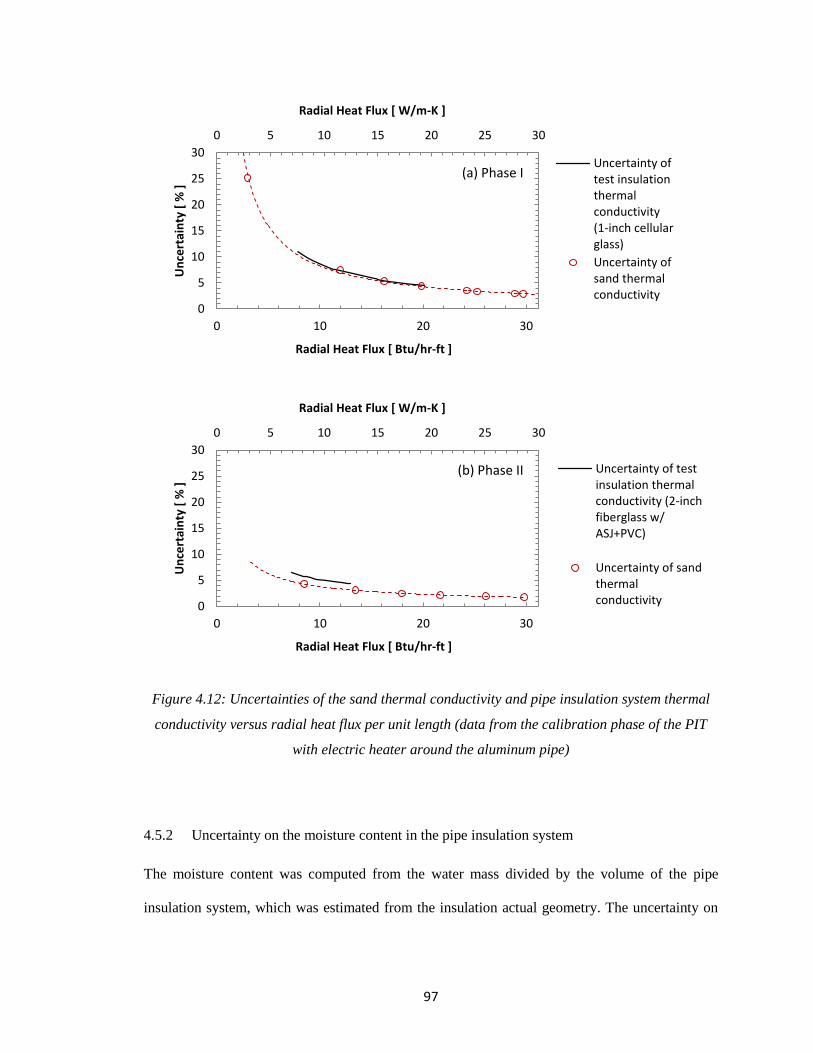
97

Figure 4.12: Uncertainties of the sand thermal conductivity and pipe insulation system thermal

conductivity versus radial heat flux per unit length (data from the calibration phase of the PIT

with electric heater around the aluminum pipe)

4.5.2 Uncertainty on the moisture content in the pipe insulation system

The moisture content was computed from the water mass divided by the volume of the pipe

insulation system, which was estimated from the insulation actual geometry. The uncertainty on

0 5 10 15 20 25 30

0 10 20 30

0

5

10

15

20

25

30

Radial Heat Flux [ W/m-K ]

Radial Heat Flux [ Btu/hr-ft ]

Un

cert

ain

ty [

% ]

Uncertainty oftest insulationthermalconductivity(1-inch cellularglass)

Uncertainty ofsand thermalconductivity

(a) Phase I

0 5 10 15 20 25 30

0 10 20 30

0

5

10

15

20

25

30

Radial Heat Flux [ W/m-K ]

Radial Heat Flux [ Btu/hr-ft ]

Un

cert

ain

ty [

% ]

Uncertainty of testinsulation thermalconductivity (2-inchfiberglass w/ASJ+PVC)

Uncertainty of sandthermalconductivity

(b) Phase II

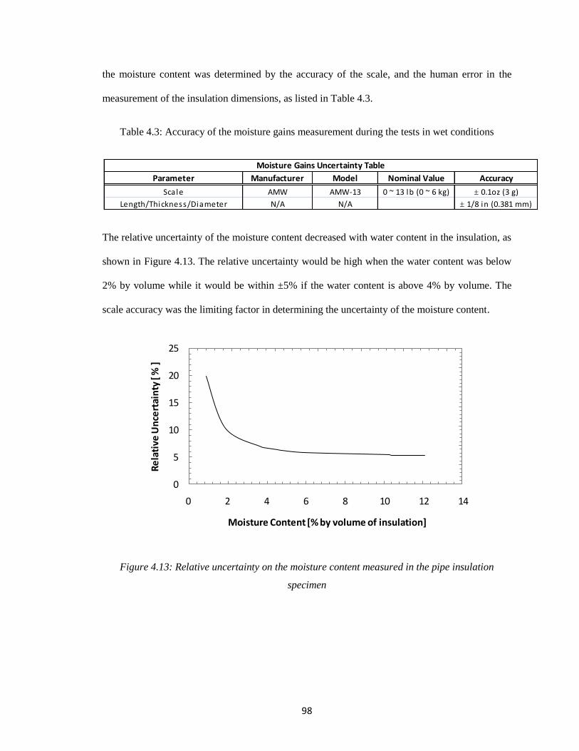
98

the moisture content was determined by the accuracy of the scale, and the human error in the

measurement of the insulation dimensions, as listed in Table 4.3.

Table 4.3: Accuracy of the moisture gains measurement during the tests in wet conditions

The relative uncertainty of the moisture content decreased with water content in the insulation, as

shown in Figure 4.13. The relative uncertainty would be high when the water content was below

2% by volume while it would be within ±5% if the water content is above 4% by volume. The

scale accuracy was the limiting factor in determining the uncertainty of the moisture content.

Figure 4.13: Relative uncertainty on the moisture content measured in the pipe insulation

specimen

Parameter Manufacturer Model Nominal Value Accuracy

Scale AMW AMW-13 0 ~ 13 lb (0 ~ 6 kg) ± 0.1oz (3 g)

Length/Thickness/Diameter N/A N/A ± 1/8 in (0.381 mm)

Moisture Gains Uncertainty Table

0

5

10

15

20

25

0 2 4 6 8 10 12 14

Re

lati

ve U

nce

rtai

nty

[ %

]

Moisture Content [% by volume of insulation]

99

CHAPTER V

5. EXPERIMENTAL RESULTS

The capability of the test apparatus and test methodology described in previous chapters was

demonstrated by the validation tests on four pipe insulation systems, and the test results will be

present in this chapter. Fifteen pipe insulation systems, including both fibrous and closed-cell

pipe insulation with different thicknesses, were tested for system thermal conductivity under dry

conditions. The test results were documented and critically compared. Ten pipe insulation

systems were selected for the moisture test under wet, condensing conditions. The variation on

the system thermal conductivity and moisture content in the pipe insulation systems were

discussed in detail at the end of this chapter.

5.1 Thermal conductivity validation test results for two types of pipe insulation systems

During the validation phase two types of pipe insulation systems, cellular glass and

polyiscoyanurate (PIR) were tested on the experimental apparatus which was constructed in the

first stage. All the pipe insulation systems were tested without insulation jacketing, and more

information on the systems is listed in Table 5.1. The pipe insulation mean temperature was

varied between 50 to 77°F (10 to 25°C). The ambient temperature was varied from 68 to 117°F

(20 to 47°C), with the cold copper pipe surface temperature controlled from 12 up to 39°F (-11 to

4°C) depending on radial thermal gradients required to maintain the aluminum pipe surface

temperature at 40.5°F 0.5°F (4.7°C 0.3°C). The chamber humidity was set as low as possible

100

to reduce any moisture effect, and the dew point temperature of the ambient air was below the

aluminum pipe surface temperature.

Table 5.1: Pipe insulation systems in the validation test

Test Systems

(Ref. No.)

Thickness

in (mm)

Joint Sealant Edge Seal

Cellular Glass (V-CG1) 1 (25.4)

Boss 368 Butyl Rubber

Sealant

Boss 368 Butyl Rubber

Sealant

Cellular Glass (V-CG2) 2 (50.8)

Polyisoyanurate (V-PIR1) 1 (25.4)

Polyisoyanurate (V-PIR2) 2 (50.8)

5.1.1 Cellular glass pipe insulation systems V-CG1 and V-CG2

Cellular glass insulation is a lightweight, rigid insulating material that is used in industrial and

commercial applications. Composed of completely sealed glass cells, which are defined as

insulating spaces, this material is filled with CO2 as the main gas without any significant aging

effect.

Two thicknesses of cellular glass pipe insulation were selected during the validation phase: 1-in

(25.4 mm) and 2-in (50.8 mm). Due to manufacturing constraints, the test samples were provided

with a full length of 2-ft (0.61 m) (ASTM_C552, 2012). As shown in Figure 5.1, the top C-shells

and bottom C-shells of the test insulation were staggered installed on the aluminum pipe. All the

joints were sealed with Boss 368 butyl rubber sealant. The sealant thickness was about 1/8-in

(3.175 mm) and it was applied following an “S” pattern on the edge of the pipe shells. Then the

two C-shells were tightly pressed together around the PIT, and the sealant was flattened in a thin

layer. It should be noted that this insulation system was the first type tested in the PIT. The

application method of the joint sealant was different from the method used on the rest of the

insulation systems. The joint sealant was usually applied as a thin layer through the entire

longitudinal joints of the C-shells for the remaining insulation systems in both dry and wet tests.

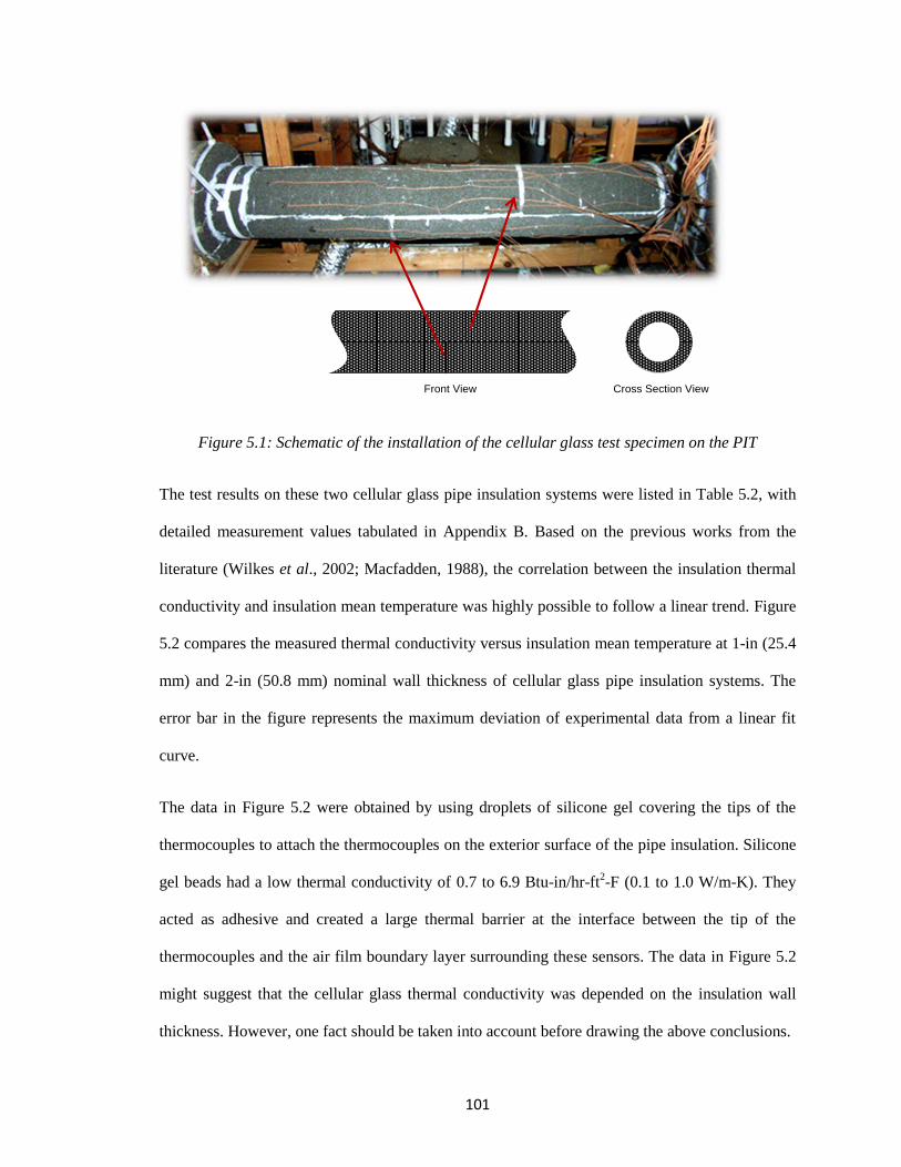
101

Figure 5.1: Schematic of the installation of the cellular glass test specimen on the PIT

The test results on these two cellular glass pipe insulation systems were listed in Table 5.2, with

detailed measurement values tabulated in Appendix B. Based on the previous works from the

literature (Wilkes et al., 2002; Macfadden, 1988), the correlation between the insulation thermal

conductivity and insulation mean temperature was highly possible to follow a linear trend. Figure

5.2 compares the measured thermal conductivity versus insulation mean temperature at 1-in (25.4

mm) and 2-in (50.8 mm) nominal wall thickness of cellular glass pipe insulation systems. The

error bar in the figure represents the maximum deviation of experimental data from a linear fit

curve.

The data in Figure 5.2 were obtained by using droplets of silicone gel covering the tips of the

thermocouples to attach the thermocouples on the exterior surface of the pipe insulation. Silicone

gel beads had a low thermal conductivity of 0.7 to 6.9 Btu-in/hr-ft2-F (0.1 to 1.0 W/m-K). They

acted as adhesive and created a large thermal barrier at the interface between the tip of the

thermocouples and the air film boundary layer surrounding these sensors. The data in Figure 5.2

might suggest that the cellular glass thermal conductivity was depended on the insulation wall

thickness. However, one fact should be taken into account before drawing the above conclusions.

Front View Cross Section View

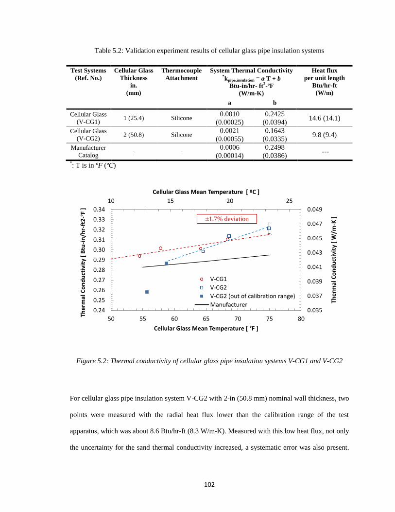
102

Table 5.2: Validation experiment results of cellular glass pipe insulation systems

Test Systems

(Ref. No.)

Cellular Glass

Thickness

in.

(mm)

Thermocouple

Attachment

System Thermal Conductivity *kpipe,insulation = a T + b

Btu-in/hr- ft2-ºF

(W/m-K)

Heat flux

per unit length

Btu/hr-ft

(W/m)

a

b

Cellular Glass

(V-CG1) 1 (25.4) Silicone

0.0010

(0.00025)

0.2425

(0.0394) 14.6 (14.1)

Cellular Glass

(V-CG2) 2 (50.8) Silicone

0.0021

(0.00055)

0.1643

(0.0335) 9.8 (9.4)

Manufacturer

Catalog - -

0.0006

(0.00014)

0.2498

(0.0386) ---

*: T is in ºF (ºC)

Figure 5.2: Thermal conductivity of cellular glass pipe insulation systems V-CG1 and V-CG2

For cellular glass pipe insulation system V-CG2 with 2-in (50.8 mm) nominal wall thickness, two

points were measured with the radial heat flux lower than the calibration range of the test

apparatus, which was about 8.6 Btu/hr-ft (8.3 W/m-K). Measured with this low heat flux, not only

the uncertainty for the sand thermal conductivity increased, a systematic error was also present.

10 15 20 25

0.035

0.037

0.039

0.041

0.043

0.045

0.047

0.049

0.24

0.25

0.26

0.27

0.28

0.29

0.30

0.31

0.32

0.33

0.34

50 55 60 65 70 75 80

Cellular Glass Mean Temperature [ ºC ]

Ther

mal

Co

nd

uct

ivit

y [

W/m

-K ]

Ther

mal

Co

nd

uct

ivit

y [

Btu

-in

/hr-

ft2

-ºF

]

Cellular Glass Mean Temperature [ °F ]

V-CG1

V-CG2

V-CG2 (out of calibration range)

Manufacturer

±1.7% deviation

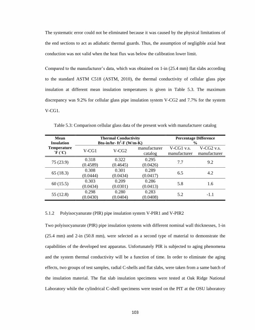
103

The systematic error could not be eliminated because it was caused by the physical limitations of

the end sections to act as adiabatic thermal guards. Thus, the assumption of negligible axial heat

conduction was not valid when the heat flux was below the calibration lower limit.

Compared to the manufacturer’s data, which was obtained on 1-in (25.4 mm) flat slabs according

to the standard ASTM C518 (ASTM, 2010), the thermal conductivity of cellular glass pipe

insulation at different mean insulation temperatures is given in Table 5.3. The maximum

discrepancy was 9.2% for cellular glass pipe insulation system V-CG2 and 7.7% for the system

V-CG1.

Table 5.3: Comparison cellular glass data of the present work with manufacturer catalog

Mean

Insulation

Temperature

˚F (˚C)

Thermal Conductivity

Btu-in/hr- ft2-F (W/m-K)

Percentage Difference

%

V-CG1 V-CG2 manufacturer

catalog

V-CG1 v.s.

manufacturer

V-CG2 v.s.

manufacturer

75 (23.9) 0.318

(0.4589)

0.322

(0.4645)

0.295

(0.0426) 7.7 9.2

65 (18.3) 0.308

(0.0444)

0.301

(0.0434)

0.289

(0.0417) 6.5 4.2

60 (15.5) 0.303

(0.0434)

0.209

(0.0301)

0.286

(0.0413) 5.8 1.6

55 (12.8) 0.298

(0.0430)

0.280

(0.0404)

0.283

(0.0408) 5.2 -1.1

5.1.2 Polyisocyanurate (PIR) pipe insulation system V-PIR1 and V-PIR2

Two polyisocyanurate (PIR) pipe insulation systems with different nominal wall thicknesses, 1-in

(25.4 mm) and 2-in (50.8 mm), were selected as a second type of material to demonstrate the

capabilities of the developed test apparatus. Unfortunately PIR is subjected to aging phenomena

and the system thermal conductivity will be a function of time. In order to eliminate the aging

effects, two groups of test samples, radial C-shells and flat slabs, were taken from a same batch of

the insulation material. The flat slab insulation specimens were tested at Oak Ridge National

Laboratory while the cylindrical C-shell specimens were tested on the PIT at the OSU laboratory

104

at approximately the same time. The results of the experiments are shown in Figure 5.3, and the

correlations for the pipe insulation system thermal conductivity are given in Table 5.4. Similar to

the system V-CG2, the PIR pipe insulation system V-PIR2 with 2-in (50.8 mm) nominal wall

thickness performed more sensitive to the temperature when compared to the system V-PIR1,

which was at 1-in (25.4 mm) nominal wall thickness. One possible reason was that the radial heat

flux in the system V-PIR2 was below the lower calibration limit of the test apparatus. The

effective thermal conductivity of sand was not measured for heat flux below 11.5 Btu/hr-ft (11.1

W/m) at the time the validation tests on systems V-PIR1 and V-PIR2 were conducted. While

extrapolation of the sand thermal conductivity for heat fluxes of about 9.7 Btu/hr-ft (9.3 W/m)

might be still considered acceptable, heat fluxes in the range of 5.14 Btu/hr-ft (4.94 W/m) were

clearly out of the calibration range of the apparatus. By the end of the validation test on the

system V-PIR2, a failure was detected on the second PIT for moisture migration into the

aluminum pipe, and both PITs were disassembled right after the test to replace the wet sand with

new dry sand. The re-constructed PITs could reach a lower limit on the radial heat flux, around

8.6 Btu/hr-ft (8.3 W/m-K), as the one applied for the cellular glass pipe insulation system V-CG2.

In order to improve the uncertainty of the test apparatus, it would be necessary to decrease the

aluminum pipe surface temperature to below 40F (4.5C) and provide a larger radial temperature

gradient. The PIR pipe insulation system V-PIR1 was measured at a higher radial heat flux, and

results showed that differences existed on the measured thermal conductivity between the pipe

insulation system and the flat slab specimens, which were tested by the Building Envelopes

Research Group at OakRidge National Laboratory. The differences were up to 8.8%. These

differences might be due to the edge effects of the longitudinal split joints and the presence of the

joint sealants along the joints between the two C-shells. The anisotropy of the PIR cells is another

potential factor that could explain this discrepancy. The PIR samples were cut out at different

locations of the same batch, and this might result in some differences on the physical properties

of the test samples.

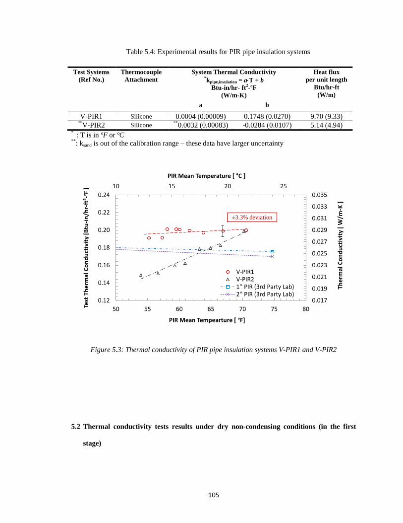
105

Table 5.4: Experimental results for PIR pipe insulation systems

Test Systems

(Ref No.)

Thermocouple

Attachment

System Thermal Conductivity *kpipe,insulation = a T + b

Btu-in/hr- ft2-ºF

(W/m-K)

Heat flux

per unit length

Btu/hr-ft

(W/m)

a

b

V-PIR1 Silicone 0.0004 (0.00009) 0.1748 (0.0270) 9.70 (9.33) **

V-PIR2 Silicone **

0.0032 (0.00083) -0.0284 (0.0107) 5.14 (4.94) * : T is in ºF or ºC

**: ksand is out of the calibration range – these data have larger uncertainty

Figure 5.3: Thermal conductivity of PIR pipe insulation systems V-PIR1 and V-PIR2

5.2 Thermal conductivity tests results under dry non-condensing conditions (in the first

stage)

10 15 20 25

0.017

0.019

0.021

0.023

0.025

0.027

0.029

0.031

0.033

0.035

0.12

0.14

0.16

0.18

0.20

0.22

0.24

50 55 60 65 70 75 80

PIR Mean Temperature [ °C ]

Ther

mal

Co

nd

uct

ivit

y [

W/m

-K ]

Test

Th

erm

al C

on

du

ctiv

ity

[Btu

-in

/hr-

ft2-º

F ]

PIR Mean Tempearture [ ºF]

V-PIR1V-PIR21'' PIR (3rd Party Lab)2'' PIR (3rd Party Lab)

±3.3% deviation

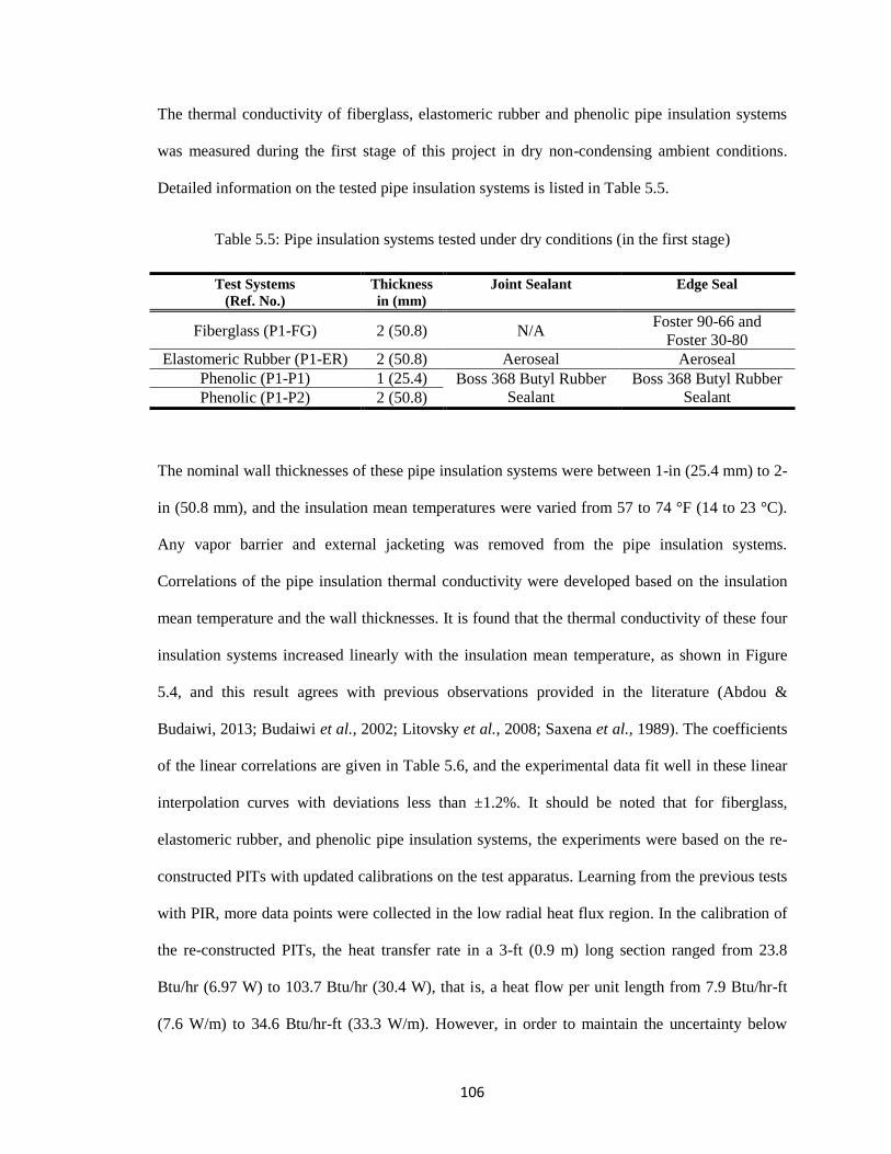
106

The thermal conductivity of fiberglass, elastomeric rubber and phenolic pipe insulation systems

was measured during the first stage of this project in dry non-condensing ambient conditions.

Detailed information on the tested pipe insulation systems is listed in Table 5.5.

Table 5.5: Pipe insulation systems tested under dry conditions (in the first stage)

Test Systems

(Ref. No.)

Thickness

in (mm)

Joint Sealant Edge Seal

Fiberglass (P1-FG) 2 (50.8) N/A Foster 90-66 and

Foster 30-80

Elastomeric Rubber (P1-ER) 2 (50.8) Aeroseal Aeroseal

Phenolic (P1-P1) 1 (25.4) Boss 368 Butyl Rubber

Sealant

Boss 368 Butyl Rubber

Sealant Phenolic (P1-P2) 2 (50.8)

The nominal wall thicknesses of these pipe insulation systems were between 1-in (25.4 mm) to 2-

in (50.8 mm), and the insulation mean temperatures were varied from 57 to 74 °F (14 to 23 °C).

Any vapor barrier and external jacketing was removed from the pipe insulation systems.

Correlations of the pipe insulation thermal conductivity were developed based on the insulation

mean temperature and the wall thicknesses. It is found that the thermal conductivity of these four

insulation systems increased linearly with the insulation mean temperature, as shown in Figure

5.4, and this result agrees with previous observations provided in the literature (Abdou &

Budaiwi, 2013; Budaiwi et al., 2002; Litovsky et al., 2008; Saxena et al., 1989). The coefficients

of the linear correlations are given in Table 5.6, and the experimental data fit well in these linear

interpolation curves with deviations less than ±1.2%. It should be noted that for fiberglass,

elastomeric rubber, and phenolic pipe insulation systems, the experiments were based on the re-

constructed PITs with updated calibrations on the test apparatus. Learning from the previous tests

with PIR, more data points were collected in the low radial heat flux region. In the calibration of

the re-constructed PITs, the heat transfer rate in a 3-ft (0.9 m) long section ranged from 23.8

Btu/hr (6.97 W) to 103.7 Btu/hr (30.4 W), that is, a heat flow per unit length from 7.9 Btu/hr-ft

(7.6 W/m) to 34.6 Btu/hr-ft (33.3 W/m). However, in order to maintain the uncertainty below

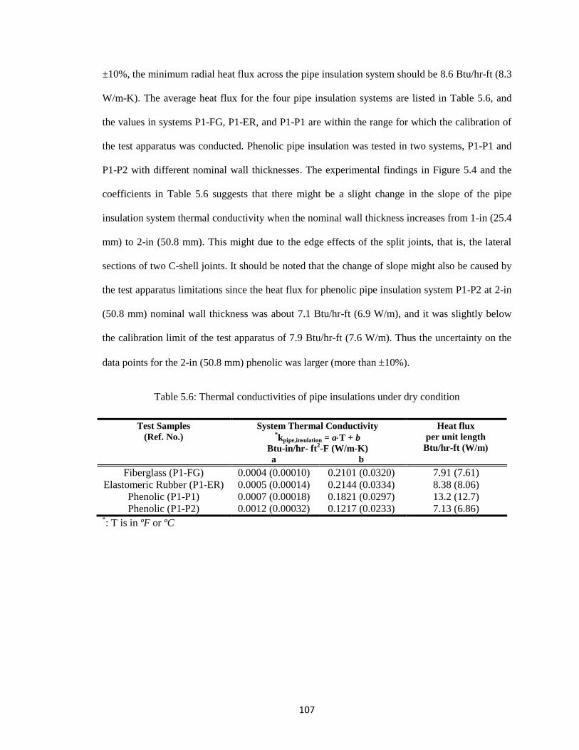
107

±10%, the minimum radial heat flux across the pipe insulation system should be 8.6 Btu/hr-ft (8.3

W/m-K). The average heat flux for the four pipe insulation systems are listed in Table 5.6, and

the values in systems P1-FG, P1-ER, and P1-P1 are within the range for which the calibration of

the test apparatus was conducted. Phenolic pipe insulation was tested in two systems, P1-P1 and

P1-P2 with different nominal wall thicknesses. The experimental findings in Figure 5.4 and the

coefficients in Table 5.6 suggests that there might be a slight change in the slope of the pipe

insulation system thermal conductivity when the nominal wall thickness increases from 1-in (25.4

mm) to 2-in (50.8 mm). This might due to the edge effects of the split joints, that is, the lateral

sections of two C-shell joints. It should be noted that the change of slope might also be caused by

the test apparatus limitations since the heat flux for phenolic pipe insulation system P1-P2 at 2-in

(50.8 mm) nominal wall thickness was about 7.1 Btu/hr-ft (6.9 W/m), and it was slightly below

the calibration limit of the test apparatus of 7.9 Btu/hr-ft (7.6 W/m). Thus the uncertainty on the

data points for the 2-in (50.8 mm) phenolic was larger (more than 10%).

Table 5.6: Thermal conductivities of pipe insulations under dry condition

Test Samples

(Ref. No.)

System Thermal Conductivity *kpipe,insulation = a T + b

Btu-in/hr- ft2-F (W/m-K)

Heat flux

per unit length

Btu/hr-ft (W/m)

a

b

Fiberglass (P1-FG) 0.0004 (0.00010) 0.2101 (0.0320) 7.91 (7.61)

Elastomeric Rubber (P1-ER) 0.0005 (0.00014) 0.2144 (0.0334) 8.38 (8.06)

Phenolic (P1-P1) 0.0007 (0.00018) 0.1821 (0.0297) 13.2 (12.7)

Phenolic (P1-P2) 0.0012 (0.00032) 0.1217 (0.0233) 7.13 (6.86) *: T is in ºF or ºC

108

Figure 5.4: Thermal conductivities of fiberglass, elastomeric rubber (flexible elastomeric)

and phenolic pipe insulation systems with 1 to 2-in (25.4 to 50.8 mm) nominal wall thickness

The effect of joint sealant on the measured thermal conductivity of mechanical pipe insulation

systems was further investigated based on phenolic pipe insulation systems P1-P1 and P1-P2 with

different nominal wall thicknesses. Applying joint sealant is a recommended installation

procedure by the manufacturer, and we investigated edge effects that the compound might have

on the actual thermal conductivity of the pipe insulation system. Figure 5.5 shows the data

derived from the tests on the 1-in (25.4 mm) thick phenolic pipe insulation systems both with and

without joint sealant along the longitudinal joints. The thermal conductivity of the pipe insulation

system with joint sealant was higher than the one without joint sealant. The thermal bridge at the

edges might cause an increase in the system apparent thermal conductivity. The joint sealant was

first applied all the way through the cross sections of the longitudinal joints with a thickness

around ¼-in (6.4mm) when the C-shells were open. Then the C-shells were tightly assembled

around PITs, and the actual thickness of the joint sealant was not directly measurable. It seems

10 15 20 25

0.026

0.028

0.030

0.032

0.034

0.036

0.038

0.18

0.19

0.20

0.21

0.22

0.23

0.24

0.25

0.26

0.27

50 55 60 65 70 75 80

Test Insulation Mean Temperature [ °C ]

Ther

mal

Co

nd

uct

ivit

y [

W/m

-K ]

Ther

mal

Co

nd

uct

ivit

y [

Btu

-in

/hr-

ft2 -

°F]

Test Insulation Mean Temperature [ °F ]

P1-FGP1-ERP1-P1P1-P2

±1.2% deviation

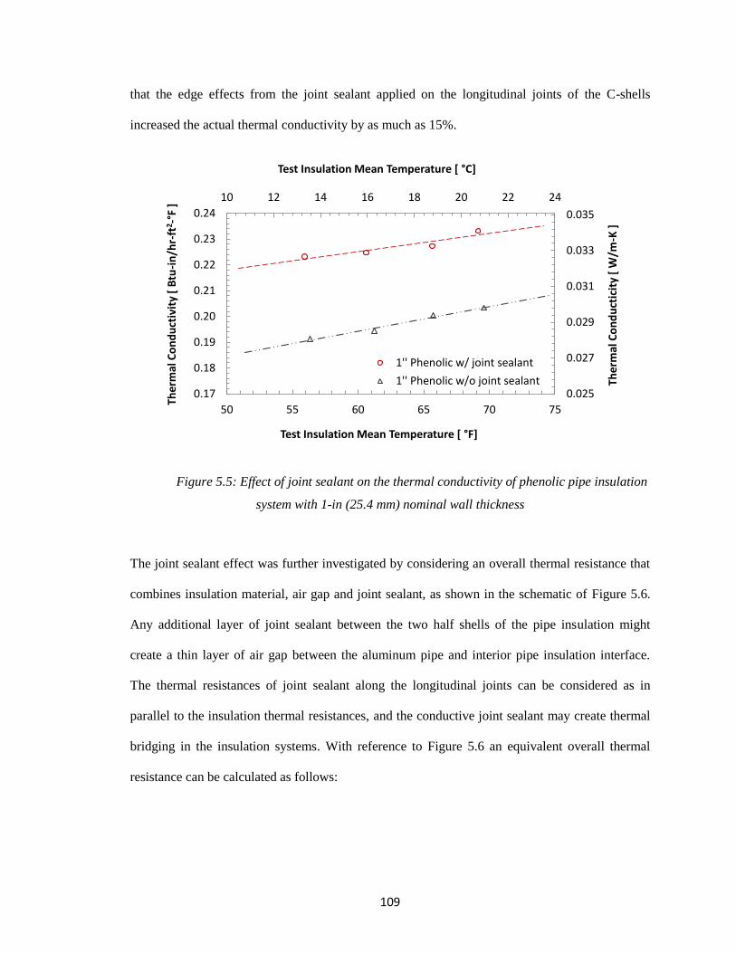
109

that the edge effects from the joint sealant applied on the longitudinal joints of the C-shells

increased the actual thermal conductivity by as much as 15%.

Figure 5.5: Effect of joint sealant on the thermal conductivity of phenolic pipe insulation

system with 1-in (25.4 mm) nominal wall thickness

The joint sealant effect was further investigated by considering an overall thermal resistance that

combines insulation material, air gap and joint sealant, as shown in the schematic of Figure 5.6.

Any additional layer of joint sealant between the two half shells of the pipe insulation might

create a thin layer of air gap between the aluminum pipe and interior pipe insulation interface.

The thermal resistances of joint sealant along the longitudinal joints can be considered as in

parallel to the insulation thermal resistances, and the conductive joint sealant may create thermal

bridging in the insulation systems. With reference to Figure 5.6 an equivalent overall thermal

resistance can be calculated as follows:

10 12 14 16 18 20 22 24

0.025

0.027

0.029

0.031

0.033

0.035

0.17

0.18

0.19

0.20

0.21

0.22

0.23

0.24

50 55 60 65 70 75

Test Insulation Mean Temperature [ °C]

Ther

mal

Co

nd

uct

icit

y [

W/m

-K ]

Ther

mal

Co

nd

uct

ivit

y [

Btu

-in

/hr-

ft2 -

°F ]

Test Insulation Mean Temperature [ °F]

1'' Phenolic w/ joint sealant

1'' Phenolic w/o joint sealant

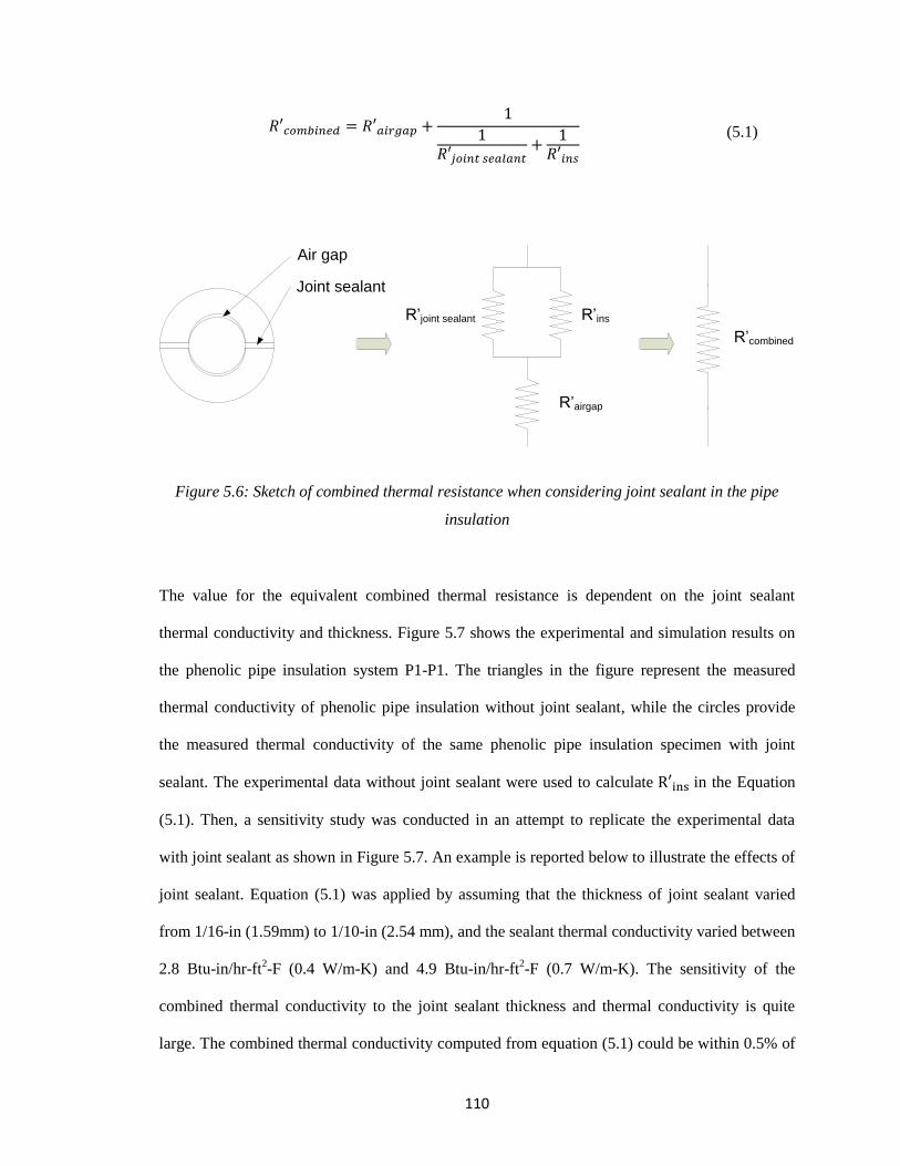
110

(5.1)

Figure 5.6: Sketch of combined thermal resistance when considering joint sealant in the pipe

insulation

The value for the equivalent combined thermal resistance is dependent on the joint sealant

thermal conductivity and thickness. Figure 5.7 shows the experimental and simulation results on

the phenolic pipe insulation system P1-P1. The triangles in the figure represent the measured

thermal conductivity of phenolic pipe insulation without joint sealant, while the circles provide

the measured thermal conductivity of the same phenolic pipe insulation specimen with joint

sealant. The experimental data without joint sealant were used to calculate in the Equation

(5.1). Then, a sensitivity study was conducted in an attempt to replicate the experimental data

with joint sealant as shown in Figure 5.7. An example is reported below to illustrate the effects of

joint sealant. Equation (5.1) was applied by assuming that the thickness of joint sealant varied

from 1/16-in (1.59mm) to 1/10-in (2.54 mm), and the sealant thermal conductivity varied between

2.8 Btu-in/hr-ft2-F (0.4 W/m-K) and 4.9 Btu-in/hr-ft

2-F (0.7 W/m-K). The sensitivity of the

combined thermal conductivity to the joint sealant thickness and thermal conductivity is quite

large. The combined thermal conductivity computed from equation (5.1) could be within 0.5% of

Air gap

Joint sealant

R’insR’joint sealant

R’airgap

R’combined

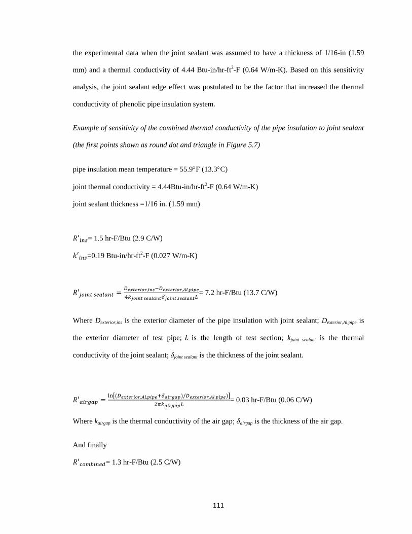
111

the experimental data when the joint sealant was assumed to have a thickness of 1/16-in (1.59

mm) and a thermal conductivity of 4.44 Btu-in/hr-ft2-F (0.64 W/m-K). Based on this sensitivity

analysis, the joint sealant edge effect was postulated to be the factor that increased the thermal

conductivity of phenolic pipe insulation system.

Example of sensitivity of the combined thermal conductivity of the pipe insulation to joint sealant

(the first points shown as round dot and triangle in Figure 5.7)

pipe insulation mean temperature = 55.9F (13.3C)

joint thermal conductivity = 4.44Btu-in/hr-ft2-F (0.64 W/m-K)

joint sealant thickness =1/16 in. (1.59 mm)

= 1.5 hr-F/Btu (2.9 C/W)

=0.19 Btu-in/hr-ft2-F (0.027 W/m-K)

= 7.2 hr-F/Btu (13.7 C/W)

Where Dexterior,ins is the exterior diameter of the pipe insulation with joint sealant; Dexterior,Al,pipe is

the exterior diameter of test pipe; is the length of test section; kjoint sealant is the thermal

conductivity of the joint sealant; δjoint sealant is the thickness of the joint sealant.

[ ]

= 0.03 hr-F/Btu (0.06 C/W)

Where kairgap is the thermal conductivity of the air gap; δairgap is the thickness of the air gap.

And finally

= 1.3 hr-F/Btu (2.5 C/W)

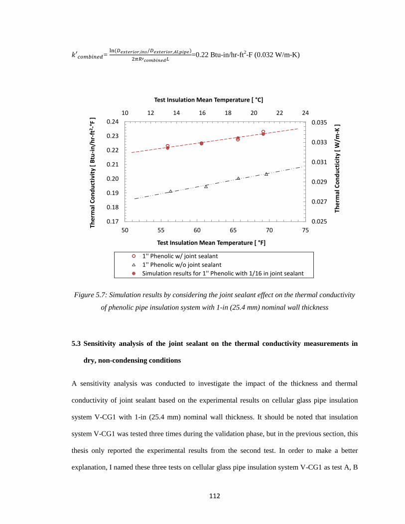
112

=

=0.22 Btu-in/hr-ft

2-F (0.032 W/m-K)

Figure 5.7: Simulation results by considering the joint sealant effect on the thermal conductivity

of phenolic pipe insulation system with 1-in (25.4 mm) nominal wall thickness

5.3 Sensitivity analysis of the joint sealant on the thermal conductivity measurements in

dry, non-condensing conditions

A sensitivity analysis was conducted to investigate the impact of the thickness and thermal

conductivity of joint sealant based on the experimental results on cellular glass pipe insulation

system V-CG1 with 1-in (25.4 mm) nominal wall thickness. It should be noted that insulation

system V-CG1 was tested three times during the validation phase, but in the previous section, this

thesis only reported the experimental results from the second test. In order to make a better

explanation, I named these three tests on cellular glass pipe insulation system V-CG1 as test A, B

10 12 14 16 18 20 22 24

0.025

0.027

0.029

0.031

0.033

0.035

0.17

0.18

0.19

0.20

0.21

0.22

0.23

0.24

50 55 60 65 70 75

Test Insulation Mean Temperature [ °C]

Ther

mal

Co

nd

uct

icit

y [

W/m

-K ]

Ther

mal

Co

nd

uct

ivit

y [

Btu

-in

/hr-

ft2 -

°F ]

Test Insulation Mean Temperature [ °F]

1'' Phenolic w/ joint sealant

1'' Phenolic w/o joint sealant

Simulation results for 1'' Phenolic with 1/16 in joint sealant

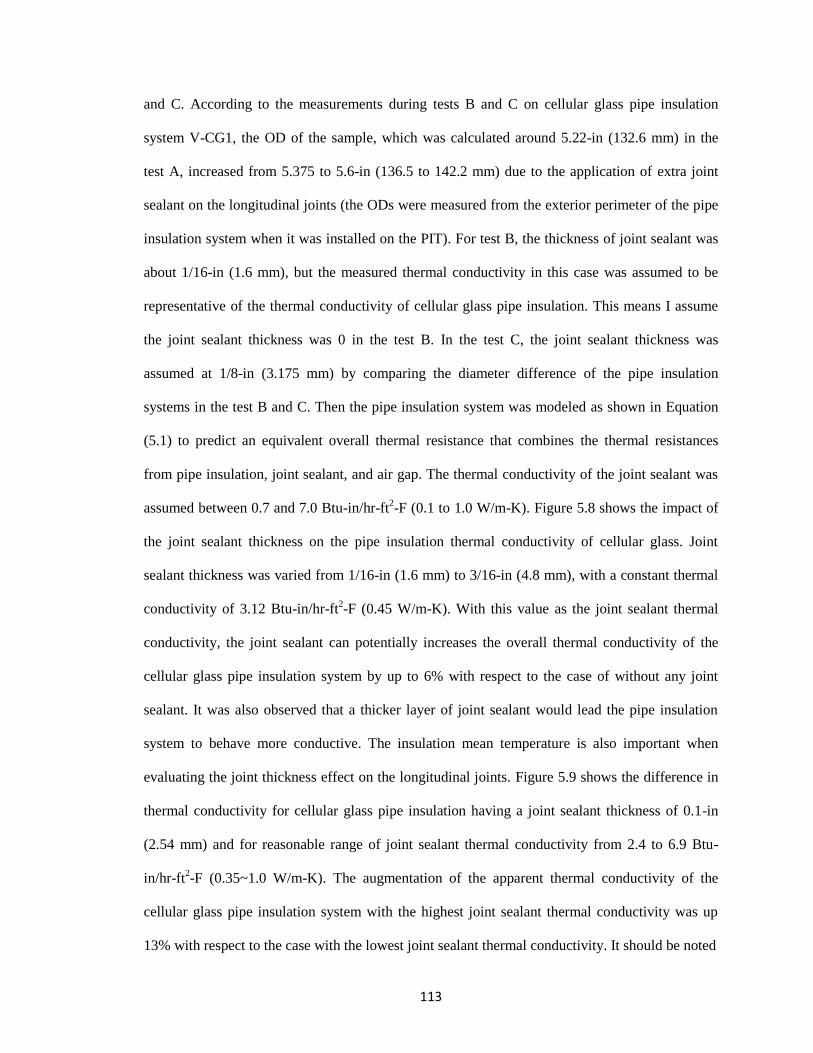
113

and C. According to the measurements during tests B and C on cellular glass pipe insulation

system V-CG1, the OD of the sample, which was calculated around 5.22-in (132.6 mm) in the

test A, increased from 5.375 to 5.6-in (136.5 to 142.2 mm) due to the application of extra joint

sealant on the longitudinal joints (the ODs were measured from the exterior perimeter of the pipe

insulation system when it was installed on the PIT). For test B, the thickness of joint sealant was

about 1/16-in (1.6 mm), but the measured thermal conductivity in this case was assumed to be

representative of the thermal conductivity of cellular glass pipe insulation. This means I assume

the joint sealant thickness was 0 in the test B. In the test C, the joint sealant thickness was

assumed at 1/8-in (3.175 mm) by comparing the diameter difference of the pipe insulation

systems in the test B and C. Then the pipe insulation system was modeled as shown in Equation

(5.1) to predict an equivalent overall thermal resistance that combines the thermal resistances

from pipe insulation, joint sealant, and air gap. The thermal conductivity of the joint sealant was

assumed between 0.7 and 7.0 Btu-in/hr-ft2-F (0.1 to 1.0 W/m-K). Figure 5.8 shows the impact of

the joint sealant thickness on the pipe insulation thermal conductivity of cellular glass. Joint

sealant thickness was varied from 1/16-in (1.6 mm) to 3/16-in (4.8 mm), with a constant thermal

conductivity of 3.12 Btu-in/hr-ft2-F (0.45 W/m-K). With this value as the joint sealant thermal

conductivity, the joint sealant can potentially increases the overall thermal conductivity of the

cellular glass pipe insulation system by up to 6% with respect to the case of without any joint

sealant. It was also observed that a thicker layer of joint sealant would lead the pipe insulation

system to behave more conductive. The insulation mean temperature is also important when

evaluating the joint thickness effect on the longitudinal joints. Figure 5.9 shows the difference in

thermal conductivity for cellular glass pipe insulation having a joint sealant thickness of 0.1-in

(2.54 mm) and for reasonable range of joint sealant thermal conductivity from 2.4 to 6.9 Btu-

in/hr-ft2-F (0.35~1.0 W/m-K). The augmentation of the apparent thermal conductivity of the

cellular glass pipe insulation system with the highest joint sealant thermal conductivity was up

13% with respect to the case with the lowest joint sealant thermal conductivity. It should be noted

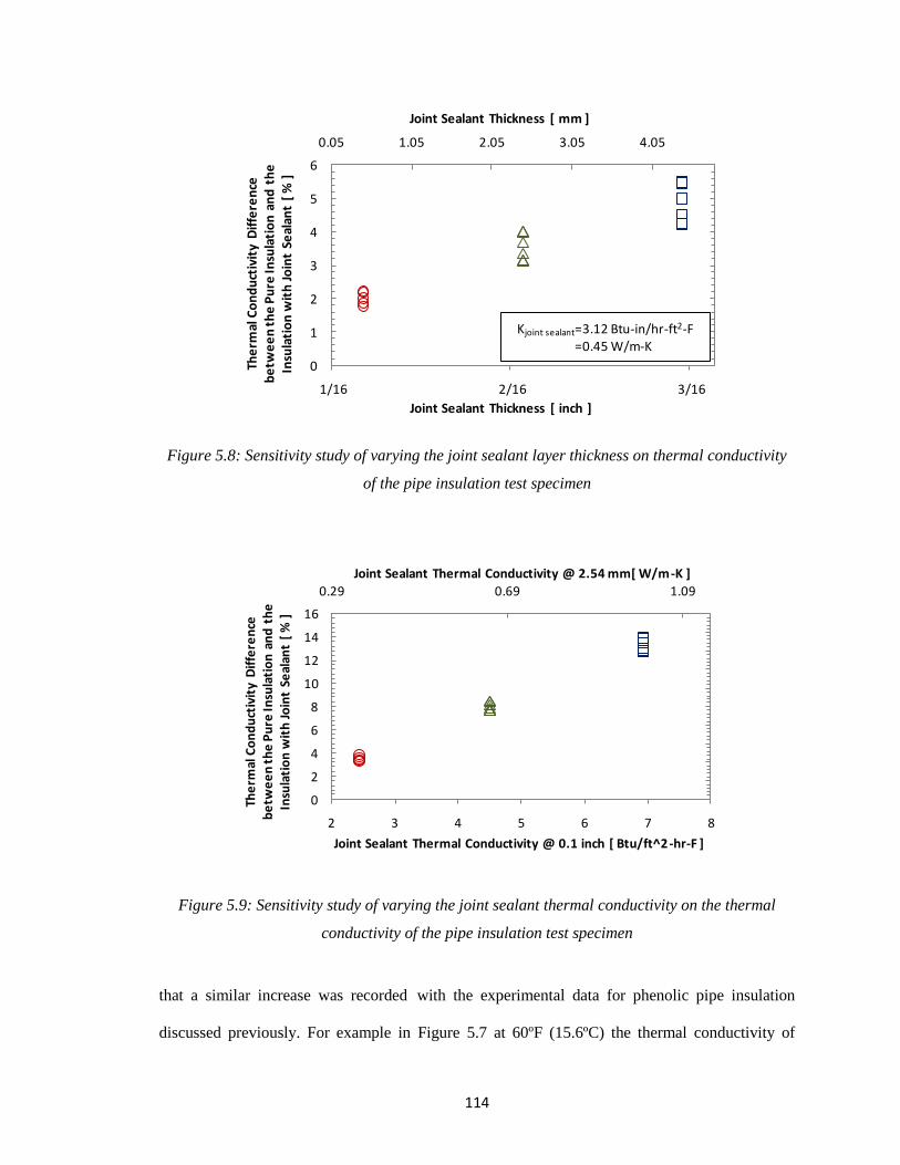
114

Figure 5.8: Sensitivity study of varying the joint sealant layer thickness on thermal conductivity

of the pipe insulation test specimen

Figure 5.9: Sensitivity study of varying the joint sealant thermal conductivity on the thermal

conductivity of the pipe insulation test specimen

that a similar increase was recorded with the experimental data for phenolic pipe insulation

discussed previously. For example in Figure 5.7 at 60ºF (15.6ºC) the thermal conductivity of

0.05 1.05 2.05 3.05 4.05

0

1

2

3

4

5

6

1/16 2/16 3/16

Joint Sealant Thickness [ mm ]

The

rmal

Co

nd

uct

ivit

y D

iffe

ren

ce

be

twe

en

th

e P

ure

Insu

lati

on

an

d t

he

In

sula

tio

n w

ith

Jo

int

Seal

ant

[ %

]

Joint Sealant Thickness [ inch ]

Kjoint sealant=3.12 Btu-in/hr-ft2-F=0.45 W/m-K

0.29 0.69 1.09

0

2

4

6

8

10

12

14

16

2 3 4 5 6 7 8

Joint Sealant Thermal Conductivity @ 2.54 mm[ W/m-K ]

The

rmal

Co

nd

uct

ivit

y D

iffe

ren

ce

be

twe

en

th

e P

ure

Insu

lati

on

an

d t

he

In

sula

tio

n w

ith

Jo

int

Seal

ant

[ %

]

Joint Sealant Thermal Conductivity @ 0.1 inch [ Btu/ft^2-hr-F ]

115

phenolic pipe insulation with joint sealant was 0.224 Btu-in/hr-ft2-F (0.0323 W/m-K) while the

thermal conductivity of phenolic pipe insulation without joint sealant was 0.194 Btu-in/hr-ft2-F

(0.028 W/m-K). The difference was about 15%, and it was attributed to the presence of joint

sealant on the longitudinal joints.

5.4 Thermal conductivity tests results under dry non-condensing conditions in the second

stage

Ten pipe insulation systems, including both closed-cell and fibrous types, were tested in the

second stage of this research project. The detailed information on each system is listed in Table

5.7. It should be noted that for system P2-FG5 and P2-CG, both pipe insulation systems were

tested twice, one on the bare aluminum pipe, and the other one was on the aluminum pipe painted

with flat black, as shown in Figure 3.10. In the following description, the systems tested on the

bare pipe were referred as pipe insulation systems P2-FG5A and P2-CGA, while the systems

tested on the black pipe were referred as pipe insulation systems P2-FG5B and P2-CGB.

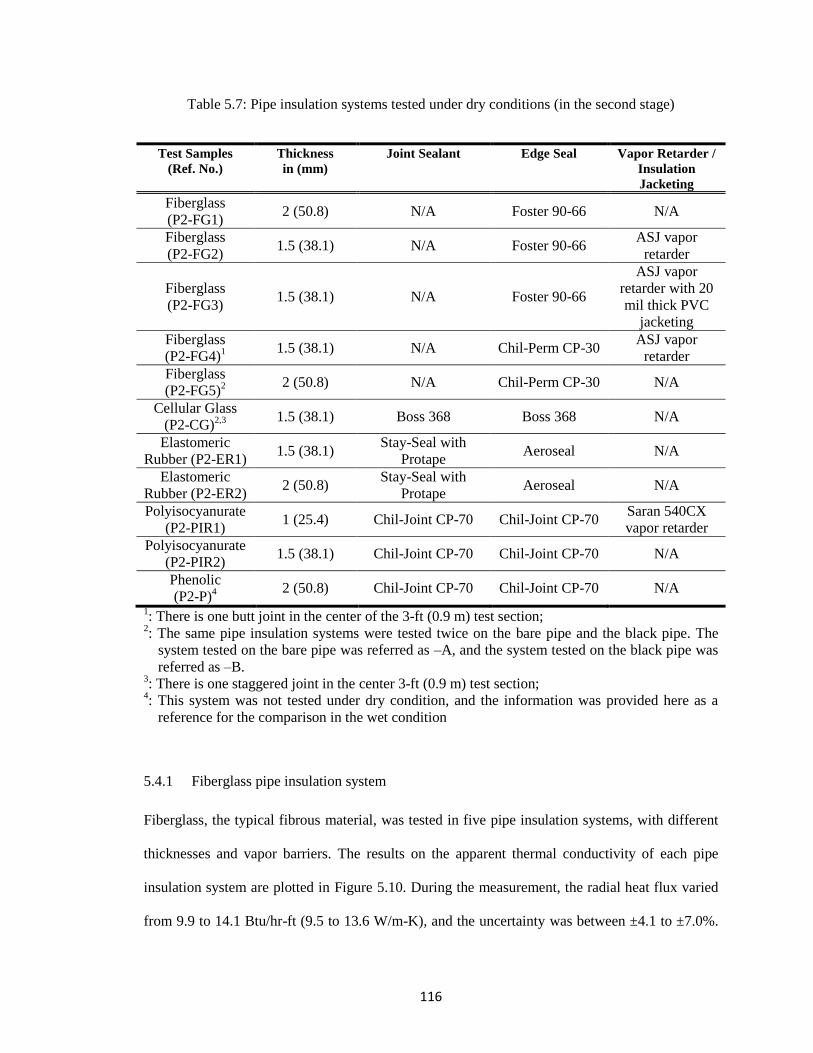
116

Table 5.7: Pipe insulation systems tested under dry conditions (in the second stage)

Test Samples

(Ref. No.)

Thickness

in (mm)

Joint Sealant Edge Seal Vapor Retarder /

Insulation

Jacketing

Fiberglass

(P2-FG1) 2 (50.8) N/A Foster 90-66 N/A

Fiberglass

(P2-FG2) 1.5 (38.1) N/A Foster 90-66

ASJ vapor

retarder

Fiberglass

(P2-FG3) 1.5 (38.1) N/A Foster 90-66

ASJ vapor

retarder with 20

mil thick PVC

jacketing

Fiberglass

(P2-FG4)1

1.5 (38.1) N/A Chil-Perm CP-30 ASJ vapor

retarder

Fiberglass

(P2-FG5)2 2 (50.8) N/A Chil-Perm CP-30 N/A

Cellular Glass

(P2-CG)2,3 1.5 (38.1) Boss 368 Boss 368 N/A

Elastomeric

Rubber (P2-ER1) 1.5 (38.1)

Stay-Seal with

Protape Aeroseal N/A

Elastomeric

Rubber (P2-ER2) 2 (50.8)

Stay-Seal with

Protape Aeroseal N/A

Polyisocyanurate

(P2-PIR1) 1 (25.4) Chil-Joint CP-70 Chil-Joint CP-70

Saran 540CX

vapor retarder

Polyisocyanurate

(P2-PIR2) 1.5 (38.1) Chil-Joint CP-70 Chil-Joint CP-70 N/A

Phenolic

(P2-P)4

2 (50.8) Chil-Joint CP-70 Chil-Joint CP-70 N/A

1: There is one butt joint in the center of the 3-ft (0.9 m) test section;

2: The same pipe insulation systems were tested twice on the bare pipe and the black pipe. The

system tested on the bare pipe was referred as –A, and the system tested on the black pipe was

referred as –B. 3: There is one staggered joint in the center 3-ft (0.9 m) test section;

4: This system was not tested under dry condition, and the information was provided here as a

reference for the comparison in the wet condition

5.4.1 Fiberglass pipe insulation system

Fiberglass, the typical fibrous material, was tested in five pipe insulation systems, with different

thicknesses and vapor barriers. The results on the apparent thermal conductivity of each pipe

insulation system are plotted in Figure 5.10. During the measurement, the radial heat flux varied

from 9.9 to 14.1 Btu/hr-ft (9.5 to 13.6 W/m-K), and the uncertainty was between ±4.1 to ±7.0%.

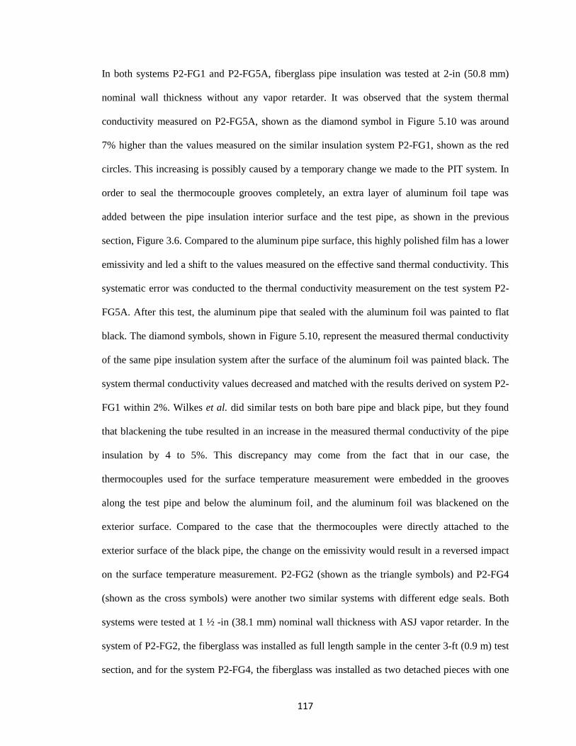
117

In both systems P2-FG1 and P2-FG5A, fiberglass pipe insulation was tested at 2-in (50.8 mm)

nominal wall thickness without any vapor retarder. It was observed that the system thermal

conductivity measured on P2-FG5A, shown as the diamond symbol in Figure 5.10 was around

7% higher than the values measured on the similar insulation system P2-FG1, shown as the red

circles. This increasing is possibly caused by a temporary change we made to the PIT system. In

order to seal the thermocouple grooves completely, an extra layer of aluminum foil tape was

added between the pipe insulation interior surface and the test pipe, as shown in the previous

section, Figure 3.6. Compared to the aluminum pipe surface, this highly polished film has a lower

emissivity and led a shift to the values measured on the effective sand thermal conductivity. This

systematic error was conducted to the thermal conductivity measurement on the test system P2-

FG5A. After this test, the aluminum pipe that sealed with the aluminum foil was painted to flat

black. The diamond symbols, shown in Figure 5.10, represent the measured thermal conductivity

of the same pipe insulation system after the surface of the aluminum foil was painted black. The

system thermal conductivity values decreased and matched with the results derived on system P2-

FG1 within 2%. Wilkes et al. did similar tests on both bare pipe and black pipe, but they found

that blackening the tube resulted in an increase in the measured thermal conductivity of the pipe

insulation by 4 to 5%. This discrepancy may come from the fact that in our case, the

thermocouples used for the surface temperature measurement were embedded in the grooves

along the test pipe and below the aluminum foil, and the aluminum foil was blackened on the

exterior surface. Compared to the case that the thermocouples were directly attached to the

exterior surface of the black pipe, the change on the emissivity would result in a reversed impact

on the surface temperature measurement. P2-FG2 (shown as the triangle symbols) and P2-FG4

(shown as the cross symbols) were another two similar systems with different edge seals. Both

systems were tested at 1 ½ -in (38.1 mm) nominal wall thickness with ASJ vapor retarder. In the

system of P2-FG2, the fiberglass was installed as full length sample in the center 3-ft (0.9 m) test

section, and for the system P2-FG4, the fiberglass was installed as two detached pieces with one

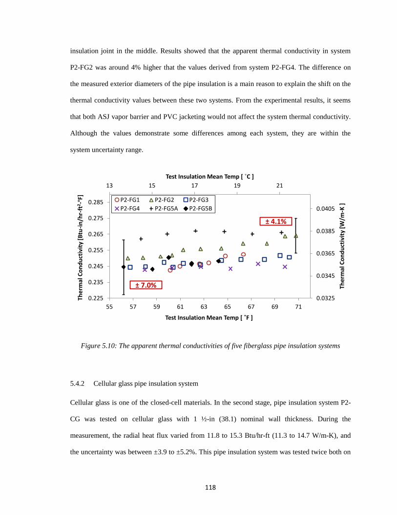
118

insulation joint in the middle. Results showed that the apparent thermal conductivity in system

P2-FG2 was around 4% higher that the values derived from system P2-FG4. The difference on

the measured exterior diameters of the pipe insulation is a main reason to explain the shift on the

thermal conductivity values between these two systems. From the experimental results, it seems

that both ASJ vapor barrier and PVC jacketing would not affect the system thermal conductivity.

Although the values demonstrate some differences among each system, they are within the

system uncertainty range.

Figure 5.10: The apparent thermal conductivities of five fiberglass pipe insulation systems

5.4.2 Cellular glass pipe insulation system

Cellular glass is one of the closed-cell materials. In the second stage, pipe insulation system P2-

CG was tested on cellular glass with 1 ½-in (38.1) nominal wall thickness. During the

measurement, the radial heat flux varied from 11.8 to 15.3 Btu/hr-ft (11.3 to 14.7 W/m-K), and

the uncertainty was between ±3.9 to ±5.2%. This pipe insulation system was tested twice both on

13 15 17 19 21

0.0325

0.0345

0.0365

0.0385

0.0405

0.225

0.235

0.245

0.255

0.265

0.275

0.285

55 57 59 61 63 65 67 69 71

Test Insulation Mean Temp [ ˚C ]

Ther

mal

Co

nd

uct

ivit

y [W

/m-K

]

Ther

mal

Co

nd

uct

ivit

y [B

tu-i

n/h

r-ft

2-º

F]

Test Insulation Mean Temp [ ˚F ]

P2-FG1 P2-FG2 P2-FG3

P2-FG4 P2-FG5A P2-FG5B

± 7.0%

± 4.1%

119

the bare pipe and the black pipe, referred as system P2-CGA and P2-CGB, respectively. The test

results between these two measurements are shown in Figure 5.11. The values derived from the

black pipe were about 6% lower than the thermal conductivity measured at the bare pipe, and the

differences were caused by a variation on the actual exterior diameter of the pipe insulation

systems. The actual diameter for system P2-CGA was measured at 6.8-in (172.7 mm), and the

system P2-CGB was measured with a smaller exterior diameter, at 6.6-in (167.6 mm). The results

on the thermal conductivity of pipe insulation system P2-CGA and P2-CGB were also compared

to the other system V-CG1 that was tested during the validation phase at 1-in (25.4 mm) nominal

wall thickness. Results demonstrate that the thermal conductivity measured in system P2-CG

(shown as the hollow and solid circles) was around 17% higher than the values provided in

system V-CG (shown as the triangle symbols). This is because in the previous stage (validation

phase and the first stage of dry tests), instead of considering actual diameters of the pipe

insulation systems, the nominal diameters were used in the data reduction. With the used of

nominal diameters, the effect of joint sealant was not included, and the measured thermal

conductivity was lower than the actual case. To further investigate the impact of the exterior

diameter, the thermal conductivity of system P2-CG was recomputed with a nominal diameter,

and the results were shown as the rectangle symbols in Figure 5.11. By varying the exterior

diameter from 6.8-in (172.7 mm) to 6.375-in (161.9 mm), the system thermal conductivity

decreased by almost 10%, and matched with the results of system V-CG1 within the uncertainty

range. Another possibility that may also cause this systematic shift is the difference from the

calibration methods that applied under these two scenarios. During the first stage, the sand

thermal conductivity was calibrated at one single ambient condition, while in the second stage,

the sand thermal conductivity was developed as a function of both sand mean temperature and the

exterior temperature difference between the aluminum surface temperature and the ambient, as

described in section 4.4.1. These two methodologies would bring in a difference on the sand

120

thermal conductivity and resulted in a shift on the apparent thermal conductivity of the pipe

insulation systems.

Figure 5.11: Thermal conductivities of cellular glass pipe insulation systems

5.4.3 Elastomeric rubber pipe insulation system

In the second stage, elastomeric rubber was tested in two pipe insulation systems: P2-ER1 with 1-

in (25.4 mm) nominal wall thickness and P2-ER2 with 2-in (50.8 mm) nominal wall thickness.

During the measurement, the radial heat flux through the test sample varied from 7.5 to 12.6

Btu/hr-ft (7.2 to 12.1 W/m-K) for system P2-ER1, and from 6.0 to 10.1 Btu/hr-ft (5.8 to 9.7 W/m-

K) for system P2-ER2. The uncertainties for both systems were between ±4.4 to ±7.2%, as shown

in Figure 5.12. By comparing these two systems with system P1-ER, which was tested in the first

stage on the elastomeric rubber sleeve with 2-in (50.8 mm) wall thickness, all the three systems

showed a similar trend on the thermal conductivity with insulation mean temperature. Although

the values of the thermal conductivity in these three systems matched within the uncertainty

11 13 15 17 19 21

0.0404

0.0444

0.0484

0.0524

0.0564

0.28

0.30

0.32

0.34

0.36

0.38

0.40

52 57 62 67 72

Test Insulation Mean Temp [ ˚C ]

Ther

mal

Co

nd

uct

ivit

y [W

/m-K

]

Ther

mal

Co

nd

uct

ivit

y [B

tu-i

n/h

r-ft

2-º

F]

Test Insulation Mean Temp [ ˚F ]

P2-CGA P2-CGB

V-CG1 P2-CGA (nominal)

± 5.2%

± 3.9%

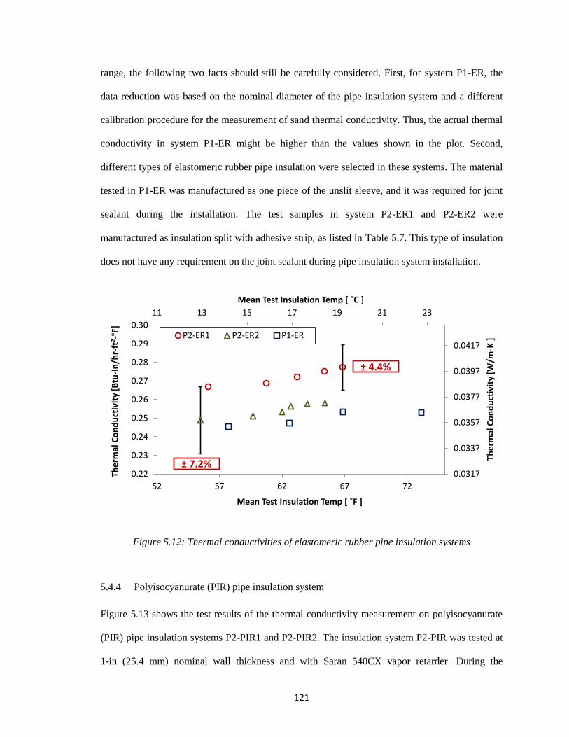
121

range, the following two facts should still be carefully considered. First, for system P1-ER, the

data reduction was based on the nominal diameter of the pipe insulation system and a different

calibration procedure for the measurement of sand thermal conductivity. Thus, the actual thermal

conductivity in system P1-ER might be higher than the values shown in the plot. Second,

different types of elastomeric rubber pipe insulation were selected in these systems. The material

tested in P1-ER was manufactured as one piece of the unslit sleeve, and it was required for joint

sealant during the installation. The test samples in system P2-ER1 and P2-ER2 were

manufactured as insulation split with adhesive strip, as listed in Table 5.7. This type of insulation

does not have any requirement on the joint sealant during pipe insulation system installation.

Figure 5.12: Thermal conductivities of elastomeric rubber pipe insulation systems

5.4.4 Polyisocyanurate (PIR) pipe insulation system

Figure 5.13 shows the test results of the thermal conductivity measurement on polyisocyanurate

(PIR) pipe insulation systems P2-PIR1 and P2-PIR2. The insulation system P2-PIR was tested at

1-in (25.4 mm) nominal wall thickness and with Saran 540CX vapor retarder. During the

11 13 15 17 19 21 23

0.0317

0.0337

0.0357

0.0377

0.0397

0.0417

0.22

0.23

0.24

0.25

0.26

0.27

0.28

0.29

0.30

52 57 62 67 72

Mean Test Insulation Temp [ ˚C ]

Ther

mal

Co

nd

uct

ivit

y [W

/m-K

]

Ther

mal

Co

nd

uct

ivit

y [B

tu-i

n/h

r-ft

2-º

F]

Mean Test Insulation Temp [ ˚F ]

P2-ER1 P2-ER2 P1-ER

± 7.2%

± 4.4%

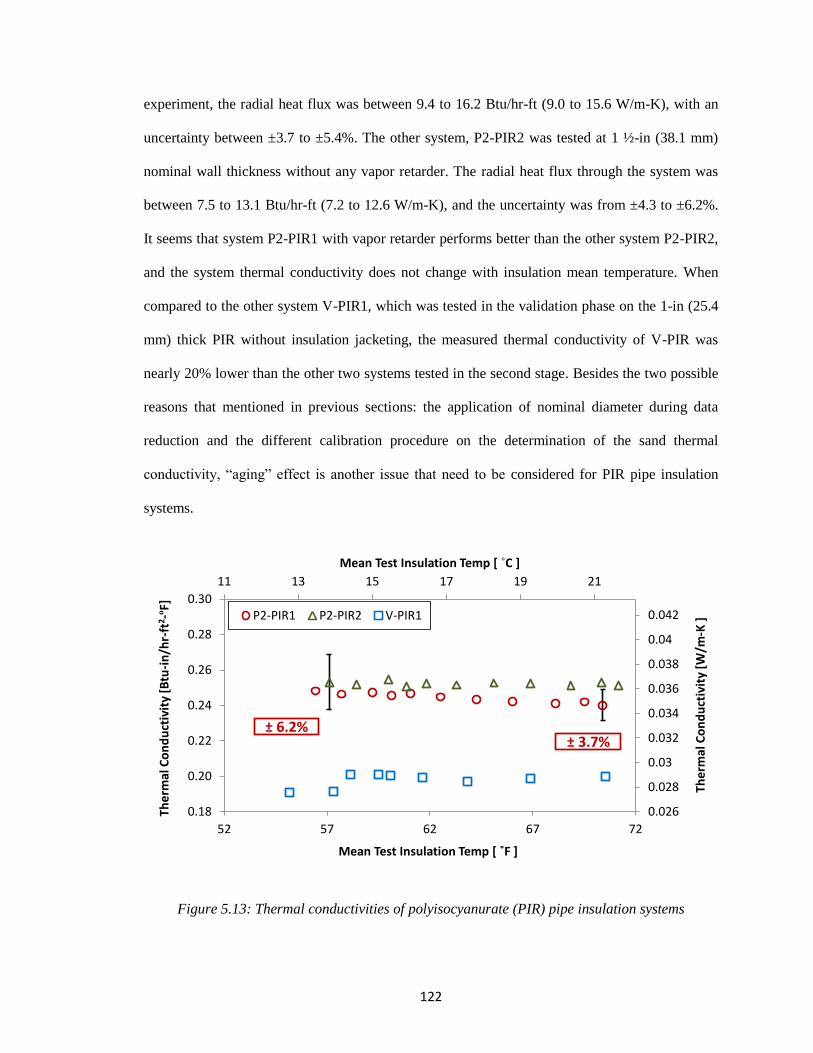
122

experiment, the radial heat flux was between 9.4 to 16.2 Btu/hr-ft (9.0 to 15.6 W/m-K), with an

uncertainty between ±3.7 to ±5.4%. The other system, P2-PIR2 was tested at 1 ½-in (38.1 mm)

nominal wall thickness without any vapor retarder. The radial heat flux through the system was

between 7.5 to 13.1 Btu/hr-ft (7.2 to 12.6 W/m-K), and the uncertainty was from ±4.3 to ±6.2%.

It seems that system P2-PIR1 with vapor retarder performs better than the other system P2-PIR2,

and the system thermal conductivity does not change with insulation mean temperature. When

compared to the other system V-PIR1, which was tested in the validation phase on the 1-in (25.4

mm) thick PIR without insulation jacketing, the measured thermal conductivity of V-PIR was

nearly 20% lower than the other two systems tested in the second stage. Besides the two possible

reasons that mentioned in previous sections: the application of nominal diameter during data

reduction and the different calibration procedure on the determination of the sand thermal

conductivity, “aging” effect is another issue that need to be considered for PIR pipe insulation

systems.

Figure 5.13: Thermal conductivities of polyisocyanurate (PIR) pipe insulation systems

11 13 15 17 19 21

0.026

0.028

0.03

0.032

0.034

0.036

0.038

0.04

0.042

0.18

0.20

0.22

0.24

0.26

0.28

0.30

52 57 62 67 72

Mean Test Insulation Temp [ ˚C ]

The

rmal

Co

nd

uct

ivit

y [W

/m-K

]

The

rmal

Co

nd

uct

ivit

y [B

tu-i

n/h

r-ft

2-º

F]

Mean Test Insulation Temp [ ˚F ]

P2-PIR1 P2-PIR2 V-PIR1

± 6.2%± 3.7%

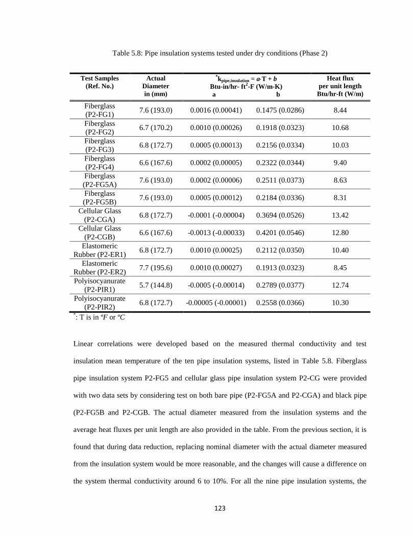
123

Table 5.8: Pipe insulation systems tested under dry conditions (Phase 2)

Test Samples

(Ref. No.)

Actual

Diameter

in (mm)

*kpipe,insulation = a T + b

Btu-in/hr- ft2-F (W/m-K)

Heat flux

per unit length

Btu/hr-ft (W/m) a b

Fiberglass

(P2-FG1) 7.6 (193.0) 0.0016 (0.00041) 0.1475 (0.0286) 8.44

Fiberglass

(P2-FG2) 6.7 (170.2) 0.0010 (0.00026) 0.1918 (0.0323) 10.68

Fiberglass

(P2-FG3) 6.8 (172.7) 0.0005 (0.00013) 0.2156 (0.0334) 10.03

Fiberglass

(P2-FG4) 6.6 (167.6) 0.0002 (0.00005) 0.2322 (0.0344) 9.40

Fiberglass

(P2-FG5A) 7.6 (193.0) 0.0002 (0.00006) 0.2511 (0.0373) 8.63

Fiberglass

(P2-FG5B) 7.6 (193.0) 0.0005 (0.00012) 0.2184 (0.0336) 8.31

Cellular Glass

(P2-CGA) 6.8 (172.7) -0.0001 (-0.00004) 0.3694 (0.0526) 13.42

Cellular Glass

(P2-CGB) 6.6 (167.6) -0.0013 (-0.00033) 0.4201 (0.0546)

12.80

Elastomeric

Rubber (P2-ER1) 6.8 (172.7) 0.0010 (0.00025) 0.2112 (0.0350) 10.40

Elastomeric

Rubber (P2-ER2) 7.7 (195.6) 0.0010 (0.00027) 0.1913 (0.0323) 8.45

Polyisocyanurate

(P2-PIR1) 5.7 (144.8) -0.0005 (-0.00014) 0.2789 (0.0377) 12.74

Polyisocyanurate

(P2-PIR2) 6.8 (172.7) -0.00005 (-0.00001) 0.2558 (0.0366) 10.30

*: T is in ºF or ºC

Linear correlations were developed based on the measured thermal conductivity and test

insulation mean temperature of the ten pipe insulation systems, listed in Table 5.8. Fiberglass

pipe insulation system P2-FG5 and cellular glass pipe insulation system P2-CG were provided

with two data sets by considering test on both bare pipe (P2-FG5A and P2-CGA) and black pipe

(P2-FG5B and P2-CGB. The actual diameter measured from the insulation systems and the

average heat fluxes per unit length are also provided in the table. From the previous section, it is

found that during data reduction, replacing nominal diameter with the actual diameter measured

from the insulation system would be more reasonable, and the changes will cause a difference on

the system thermal conductivity around 6 to 10%. For all the nine pipe insulation systems, the

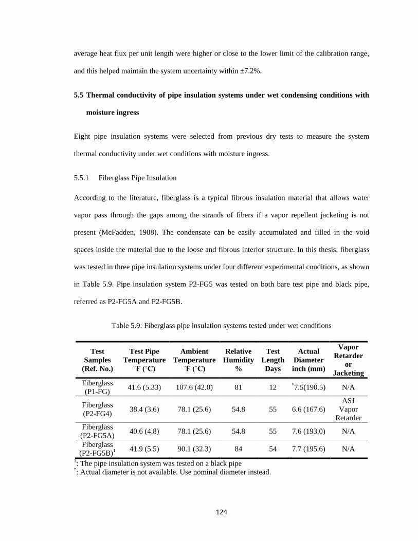
124

average heat flux per unit length were higher or close to the lower limit of the calibration range,

and this helped maintain the system uncertainty within ±7.2%.

5.5 Thermal conductivity of pipe insulation systems under wet condensing conditions with

moisture ingress

Eight pipe insulation systems were selected from previous dry tests to measure the system

thermal conductivity under wet conditions with moisture ingress.

5.5.1 Fiberglass Pipe Insulation

According to the literature, fiberglass is a typical fibrous insulation material that allows water

vapor pass through the gaps among the strands of fibers if a vapor repellent jacketing is not

present (McFadden, 1988). The condensate can be easily accumulated and filled in the void

spaces inside the material due to the loose and fibrous interior structure. In this thesis, fiberglass

was tested in three pipe insulation systems under four different experimental conditions, as shown

in Table 5.9. Pipe insulation system P2-FG5 was tested on both bare test pipe and black pipe,

referred as P2-FG5A and P2-FG5B.

Table 5.9: Fiberglass pipe insulation systems tested under wet conditions

Test

Samples

(Ref. No.)

Test Pipe

Temperature

˚F (˚C)

Ambient

Temperature

˚F (˚C)

Relative

Humidity

%

Test

Length

Days

Actual

Diameter

inch (mm)

Vapor

Retarder

or

Jacketing

Fiberglass

(P1-FG) 41.6 (5.33) 107.6 (42.0) 81 12

*7.5(190.5) N/A

Fiberglass

(P2-FG4) 38.4 (3.6) 78.1 (25.6) 54.8 55 6.6 (167.6)

ASJ

Vapor

Retarder

Fiberglass

(P2-FG5A) 40.6 (4.8) 78.1 (25.6) 54.8 55 7.6 (193.0) N/A

Fiberglass

(P2-FG5B)1

41.9 (5.5) 90.1 (32.3) 84 54 7.7 (195.6) N/A

1: The pipe insulation system was tested on a black pipe

*: Actual diameter is not available. Use nominal diameter instead.

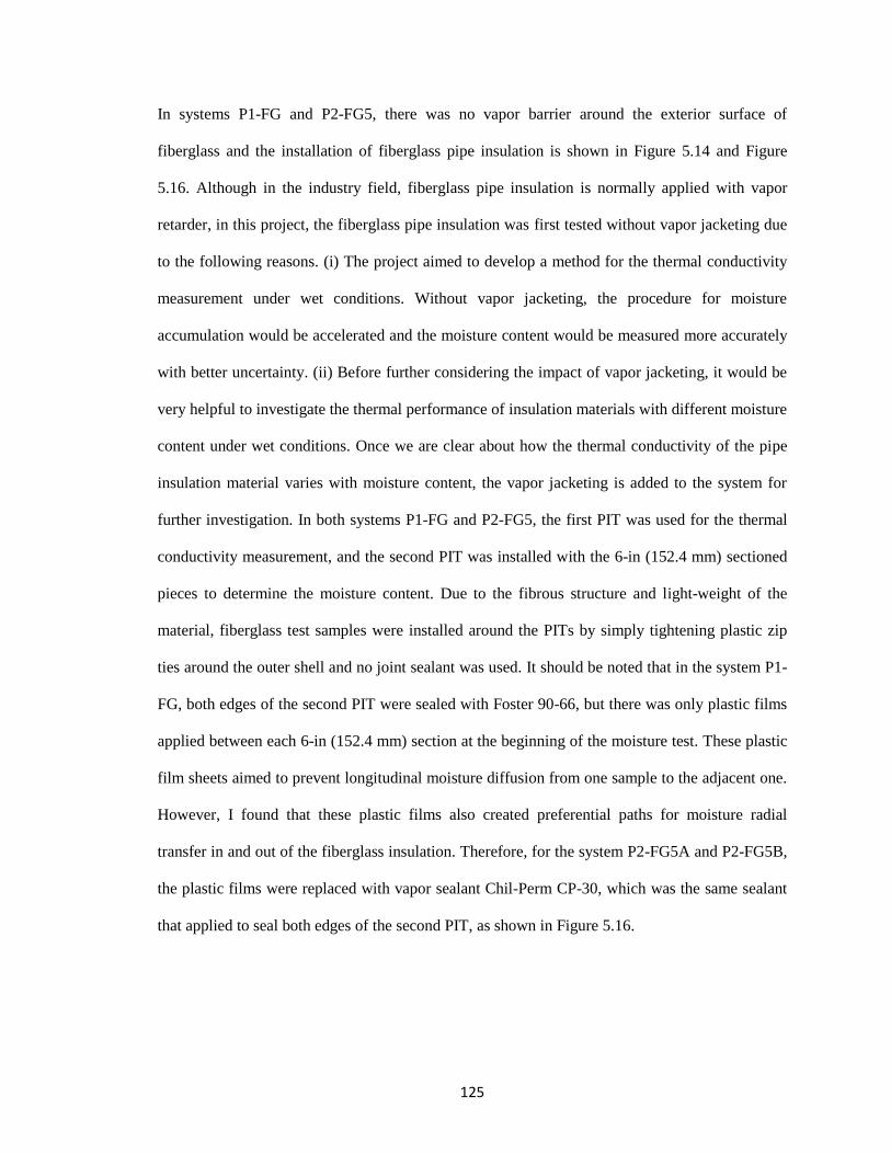
125

In systems P1-FG and P2-FG5, there was no vapor barrier around the exterior surface of

fiberglass and the installation of fiberglass pipe insulation is shown in Figure 5.14 and Figure

5.16. Although in the industry field, fiberglass pipe insulation is normally applied with vapor

retarder, in this project, the fiberglass pipe insulation was first tested without vapor jacketing due

to the following reasons. (i) The project aimed to develop a method for the thermal conductivity

measurement under wet conditions. Without vapor jacketing, the procedure for moisture

accumulation would be accelerated and the moisture content would be measured more accurately

with better uncertainty. (ii) Before further considering the impact of vapor jacketing, it would be

very helpful to investigate the thermal performance of insulation materials with different moisture

content under wet conditions. Once we are clear about how the thermal conductivity of the pipe

insulation material varies with moisture content, the vapor jacketing is added to the system for

further investigation. In both systems P1-FG and P2-FG5, the first PIT was used for the thermal

conductivity measurement, and the second PIT was installed with the 6-in (152.4 mm) sectioned

pieces to determine the moisture content. Due to the fibrous structure and light-weight of the

material, fiberglass test samples were installed around the PITs by simply tightening plastic zip

ties around the outer shell and no joint sealant was used. It should be noted that in the system P1-

FG, both edges of the second PIT were sealed with Foster 90-66, but there was only plastic films

applied between each 6-in (152.4 mm) section at the beginning of the moisture test. These plastic

film sheets aimed to prevent longitudinal moisture diffusion from one sample to the adjacent one.

However, I found that these plastic films also created preferential paths for moisture radial

transfer in and out of the fiberglass insulation. Therefore, for the system P2-FG5A and P2-FG5B,

the plastic films were replaced with vapor sealant Chil-Perm CP-30, which was the same sealant

that applied to seal both edges of the second PIT, as shown in Figure 5.16.

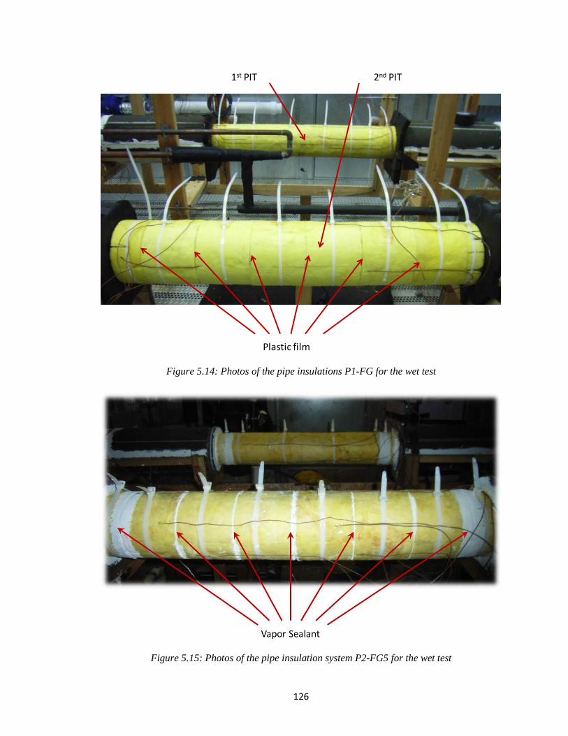
126

Figure 5.14: Photos of the pipe insulations P1-FG for the wet test

Figure 5.15: Photos of the pipe insulation system P2-FG5 for the wet test

1st PIT 2nd PIT

Plastic film

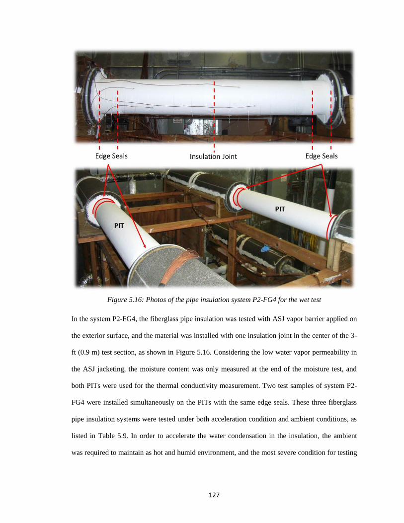
127

Figure 5.16: Photos of the pipe insulation system P2-FG4 for the wet test

In the system P2-FG4, the fiberglass pipe insulation was tested with ASJ vapor barrier applied on

the exterior surface, and the material was installed with one insulation joint in the center of the 3-

ft (0.9 m) test section, as shown in Figure 5.16. Considering the low water vapor permeability in

the ASJ jacketing, the moisture content was only measured at the end of the moisture test, and

both PITs were used for the thermal conductivity measurement. Two test samples of system P2-

FG4 were installed simultaneously on the PITs with the same edge seals. These three fiberglass

pipe insulation systems were tested under both acceleration condition and ambient conditions, as

listed in Table 5.9. In order to accelerate the water condensation in the insulation, the ambient

was required to maintain as hot and humid environment, and the most severe condition for testing

128

fiberglass pipe insulation system was at 107.6 °F (42 °C) and 81% relative humidity, which

resulted in an air dew point of about 100.4 °F (38 °C).

Fiberglass pipe insulation system P1-FG

For a better description on the observations and findings I got from the experiment, the following

discussion will be focused on one specific case, system P1-FG, which was tested under the most

severe condition, 107.6 °F (42 °C) and 81% RH. This test lasted for 12 days. Figure 5.17 shows

the cross-section view of a fiberglass insulation sample which was taken out from the second PIT

after 5 days test. The dark yellow region, circled in the middle of the bottom shell, was

considered as a preferential path which was created due to a less dense area in the fiberglass

material, partially unsealed seams and the gravity effect. The gravity effect would also cause

portion of the water condensate come out from the insulation. Compared to the bottom shell, the

top section remained quite dry at the outer surface. Only small amount of water droplets were

observed on the interior surface of the pipe insulation. Considering the fact that each section on

the second PIT represents one test specimen installed on the first PIT, the phenomenon observed

from the sectional pieces was assumed to be a replicate of what happed in the full length

insulation sample.

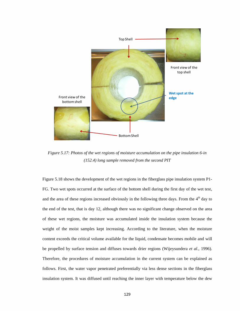
129

Figure 5.17: Photos of the wet regions of moisture accumulation on the pipe insulation 6-in

(152.4) long sample removed from the second PIT

Figure 5.18 shows the development of the wet regions in the fiberglass pipe insulation system P1-

FG. Two wet spots occurred at the surface of the bottom shell during the first day of the wet test,

and the area of these regions increased obviously in the following three days. From the 4th day to

the end of the test, that is day 12, although there was no significant change observed on the area

of these wet regions, the moisture was accumulated inside the insulation system because the

weight of the moist samples kept increasing. According to the literature, when the moisture

content exceeds the critical volume available for the liquid, condensate becomes mobile and will

be propelled by surface tension and diffuses towards drier regions (Wijeysundera et al., 1996).

Therefore, the procedures of moisture accumulation in the current system can be explained as

follows. First, the water vapor penetrated preferentially via less dense sections in the fiberglass

insulation system. It was diffused until reaching the inner layer with temperature below the dew

Top Shell

Bottom Shell

Wet spot at the edgeFront view of the

bottom shell

Front view of the top shell

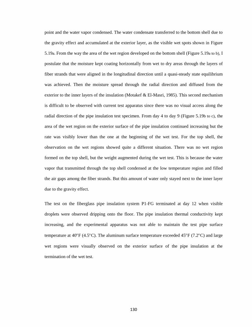
130

point and the water vapor condensed. The water condensate transferred to the bottom shell due to

the gravity effect and accumulated at the exterior layer, as the visible wet spots shown in Figure

5.19a. From the way the area of the wet region developed on the bottom shell (Figure 5.19a to b), I

postulate that the moisture kept coating horizontally from wet to dry areas through the layers of

fiber strands that were aligned in the longitudinal direction until a quasi-steady state equilibrium

was achieved. Then the moisture spread through the radial direction and diffused from the

exterior to the inner layers of the insulation (Motakef & El-Masri, 1985). This second mechanism

is difficult to be observed with current test apparatus since there was no visual access along the

radial direction of the pipe insulation test specimen. From day 4 to day 9 (Figure 5.19b to c), the

area of the wet region on the exterior surface of the pipe insulation continued increasing but the

rate was visibly lower than the one at the beginning of the wet test. For the top shell, the

observation on the wet regions showed quite a different situation. There was no wet region

formed on the top shell, but the weight augmented during the wet test. This is because the water

vapor that transmitted through the top shell condensed at the low temperature region and filled

the air gaps among the fiber strands. But this amount of water only stayed next to the inner layer

due to the gravity effect.

The test on the fiberglass pipe insulation system P1-FG terminated at day 12 when visible

droplets were observed dripping onto the floor. The pipe insulation thermal conductivity kept

increasing, and the experimental apparatus was not able to maintain the test pipe surface

temperature at 40F (4.5C). The aluminum surface temperature exceeded 45F (7.2C) and large

wet regions were visually observed on the exterior surface of the pipe insulation at the

termination of the wet test.

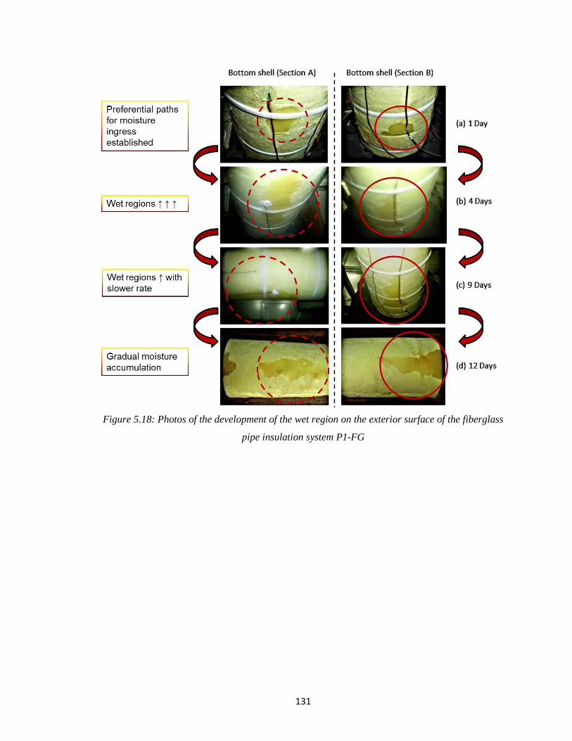
131

Figure 5.18: Photos of the development of the wet region on the exterior surface of the fiberglass

pipe insulation system P1-FG

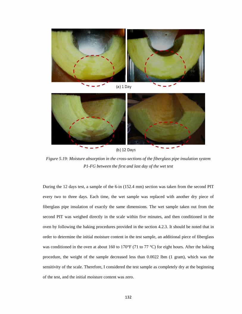
132

Figure 5.19: Moisture absorption in the cross-sections of the fiberglass pipe insulation system

P1-FG between the first and last day of the wet test

During the 12 days test, a sample of the 6-in (152.4 mm) section was taken from the second PIT

every two to three days. Each time, the wet sample was replaced with another dry piece of

fiberglass pipe insulation of exactly the same dimensions. The wet sample taken out from the

second PIT was weighed directly in the scale within five minutes, and then conditioned in the

oven by following the baking procedures provided in the section 4.2.3. It should be noted that in

order to determine the initial moisture content in the test sample, an additional piece of fiberglass

was conditioned in the oven at about 160 to 170°F (71 to 77 °C) for eight hours. After the baking

procedure, the weight of the sample decreased less than 0.0022 lbm (1 gram), which was the

sensitivity of the scale. Therefore, I considered the test sample as completely dry at the beginning

of the test, and the initial moisture content was zero.

133

Figure 5.20 shows the experimental results on the variation of thermal conductivity and moisture

content in the fiberglass pipe insulation systems P1-FG. In these figures, each point of the thermal

conductivity ratio is based on an average value of the system thermal conductivity during a 24

hour long period. The sensors were sampled every one to two seconds for a total of 3600 data

points every 12 hours, and the recording procedure was repeated twice per day. In order to

measure the moisture content, the 6-in (152.4 mm) sectioned samples need to be removed

periodically during the moisture test. This sampling procedure proceeded right after the data

recording so that the measurements on the moisture content and the system thermal conductivity

can be considered as simultaneous measurements. The data recording and sampling procedures

remain the same for the measurements on the other systems. By the end of the moisture tests on

pipe insulation system P1-FG, the system thermal conductivity increased by more than 3 times of

the dry reference value, and the moisture content was about 12% by volume. The moisture

content was computed based on the volume of water that trapped in the system over the total

volume of the insulation, and the upper limit of the moisture content would be equal to the

porosity of the material. It should be noted that for system P1-FG, the reference value for the

thermal conductivity ratio was estimated based on the correlation developed between system

thermal conductivity and insulation mean temperature under dry condition. As shown in the

Figure 5.20a and c, the thermal conductivity ratio followed a two-step variation during the

moisture test. In the first three days, the system thermal conductivity increased dramatically with

the moisture content lower than 2% by volume. From day 3 to day 12, the system thermal

conductivity kept increasing with the moisture content, but the increasing rate was much lower

when compared to the first step. Figure 5.20b provides the data of the moisture content in the top

C-shell (circle data points), bottom C-shell (triangle data points), and the overall cylindrical

section (cross data points). Due to the gravity effect, the moisture content in the bottom shell of

system P1-FG was always higher than the one in the top shell. Water accumulated in the bowl

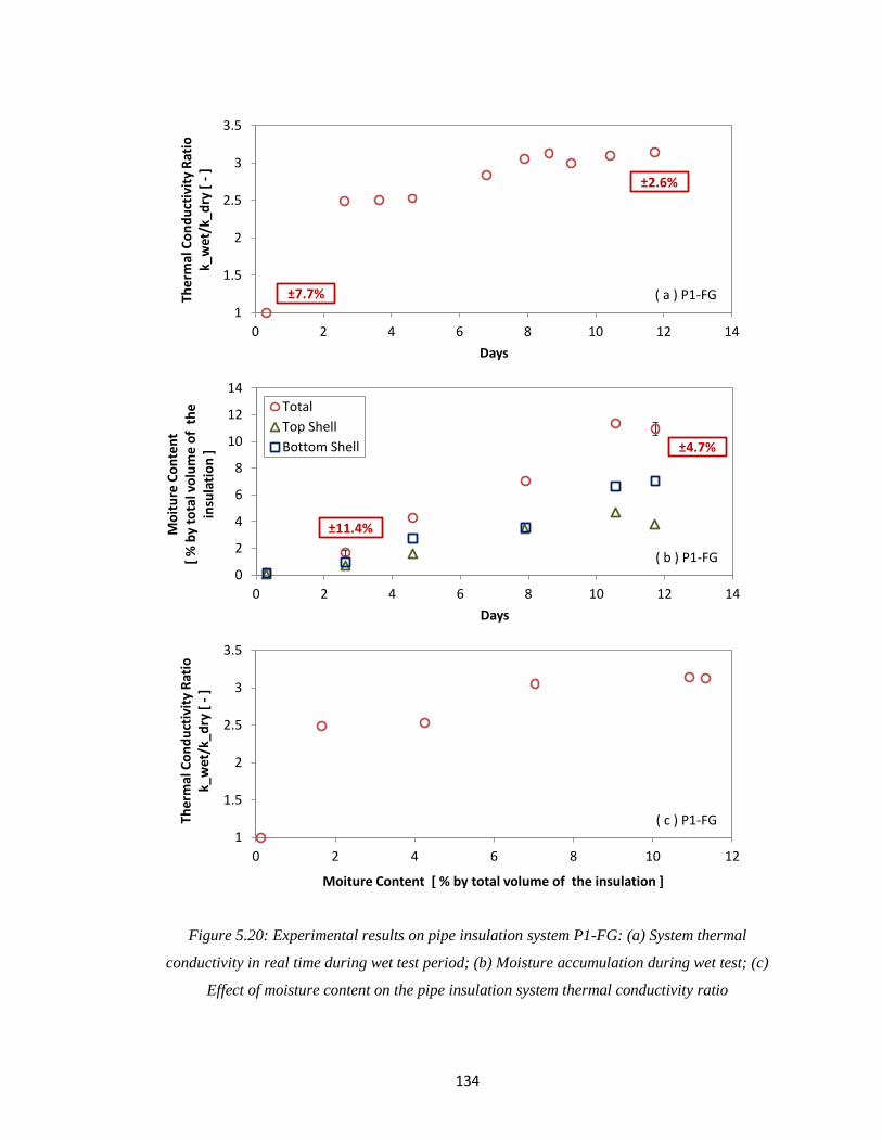
134

Figure 5.20: Experimental results on pipe insulation system P1-FG: (a) System thermal

conductivity in real time during wet test period; (b) Moisture accumulation during wet test; (c)

Effect of moisture content on the pipe insulation system thermal conductivity ratio

1

1.5

2

2.5

3

3.5

0 2 4 6 8 10 12

Ther

mal

Co

nd

uct

ivit

y R

atio

k_

wet

/k_d

ry [

-]

Moiture Content [ % by total volume of the insulation ]

1

1.5

2

2.5

3

3.5

0 2 4 6 8 10 12 14

Ther

mal

Co

nd

uct

ivit

y R

atio

k_

wet

/k_d

ry [

-]

Days

0

2

4

6

8

10

12

14

0 2 4 6 8 10 12 14

Mo

itu

re C

on

ten

t [

% b

y to

tal v

olu

me

of

th

e in

sula

tio

n ]

Days

Total

Top Shell

Bottom Shell

( a ) P1-FG

( c ) P1-FG

( b ) P1-FG

±7.7%

±2.6%

±11.4%

±4.7%

135

shape of the bottom C-shell and large wet regions were visually observed at the bottom surface of

the pipe insulation.

For the moisture measurement, it should be noted that only the initial and final values of the

moisture content were measured for the test specimen from the first PIT (used for thermal

conductivity measurement) while the intermediate values of moisture content in the pipe

insulation were extrapolated from the measurements of the test specimen around the second PIT

(used for moisture measurement with sectional pieces). Due to the presence of more butt joints on

the test samples installed on the second PIT, it was quite possible that the total amount of water

measured from the second PIT would be higher than the first one. However, the second PIT

would only be used for scaling the intermediate moisture content in the first PIT by considering

the same increasing rate of moisture with time. The method used for determining the moisture

profile on the first PIT was explained in detail as follows:

Take pipe insulation system P1-FG as an example. Figure 5.21 shows a comparison of the

moisture content measured in the fiberglass pipe insulation on both first and second PITs. After

12 days in the wet condition, the insulation on the first PIT reached a moisture content of about

11% while the insulation on the second PIT was only about 8.0%. This behavior was consistent

with the observation that some amount of water condensate dripped out from the second PIT, via

the preferential radial cuts in the pipe insulation test specimen, while more water condensate was

trapped in the pipe insulation system on the first PIT. By the end of the moisture test which is day

12, the ratio between the moisture content of the insulation specimen on the first PIT, Vmoisture,1,

and the moisture content of the insulation specimen on the second PIT, Vmoisture,2 was:

(5.2)

136

At the beginning of the moisture test, Vmoisture,1 was the same amount as Vmoisture,2 and the initial

moisture content on both insulation specimens was 0, that is,

(5.3)

Considering a linear increase of the ratio of moisture content in the first and second PITs with

time, the corrections on the moisture content absorbed in the fiberglass test specimen on the first

PIT was determined as follows:

(5.4)

where the interpolating coefficients a and b were derived by using the conditions (5.2) and (5.3).

The variable CFmoisture is referred as the Correction Factor for the moisture content between the

first and second PITs. At the beginning of the wet test, CFmoisture =1, and at the end of the wet test,

CFmoisture =1.4. CFmoisture was assumed to be linearly increasing during the wet test period. The

moisture content Vmoisture,1 during the wet tests was calculated as follows:

(5.5)

Where Vmoisture,1 represents the moisture content in pipe insulation system that installed on the first

PIT, and Vmoisture,2 represents the moisture content measured form the sectional pieces on the

second PIT.

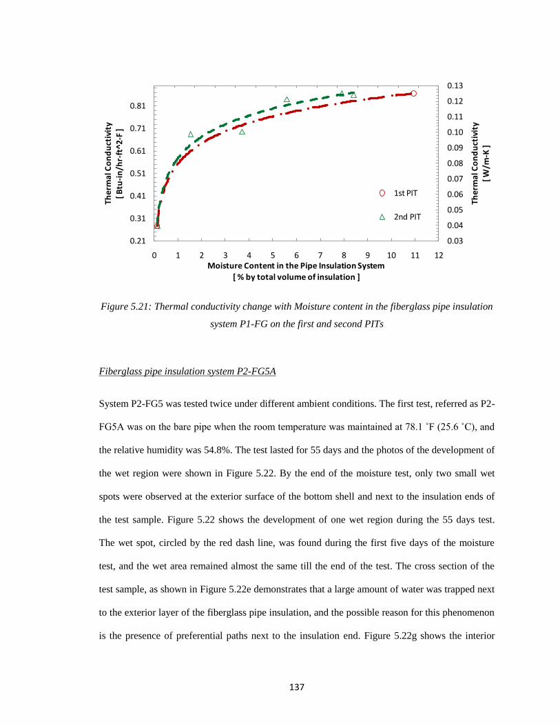
137

Figure 5.21: Thermal conductivity change with Moisture content in the fiberglass pipe insulation

system P1-FG on the first and second PITs

Fiberglass pipe insulation system P2-FG5A

System P2-FG5 was tested twice under different ambient conditions. The first test, referred as P2-

FG5A was on the bare pipe when the room temperature was maintained at 78.1 ˚F (25.6 ˚C), and

the relative humidity was 54.8%. The test lasted for 55 days and the photos of the development of

the wet region were shown in Figure 5.22. By the end of the moisture test, only two small wet

spots were observed at the exterior surface of the bottom shell and next to the insulation ends of

the test sample. Figure 5.22 shows the development of one wet region during the 55 days test.

The wet spot, circled by the red dash line, was found during the first five days of the moisture

test, and the wet area remained almost the same till the end of the test. The cross section of the

test sample, as shown in Figure 5.22e demonstrates that a large amount of water was trapped next

to the exterior layer of the fiberglass pipe insulation, and the possible reason for this phenomenon

is the presence of preferential paths next to the insulation end. Figure 5.22g shows the interior

0.03

0.04

0.05

0.06

0.07

0.08

0.09

0.10

0.11

0.12

0.13

0.21

0.31

0.41

0.51

0.61

0.71

0.81

0 1 2 3 4 5 6 7 8 9 10 11 12

Th

erm

al C

on

du

ctiv

ity

[ W

/m-K

]

Th

erm

al C

on

du

ctiv

ity

[ B

tu-i

n/h

r-ft

^2-

F ]

Moisture Content in the Pipe Insulation System

[ % by total volume of insulation ]

1st PIT

2nd PIT

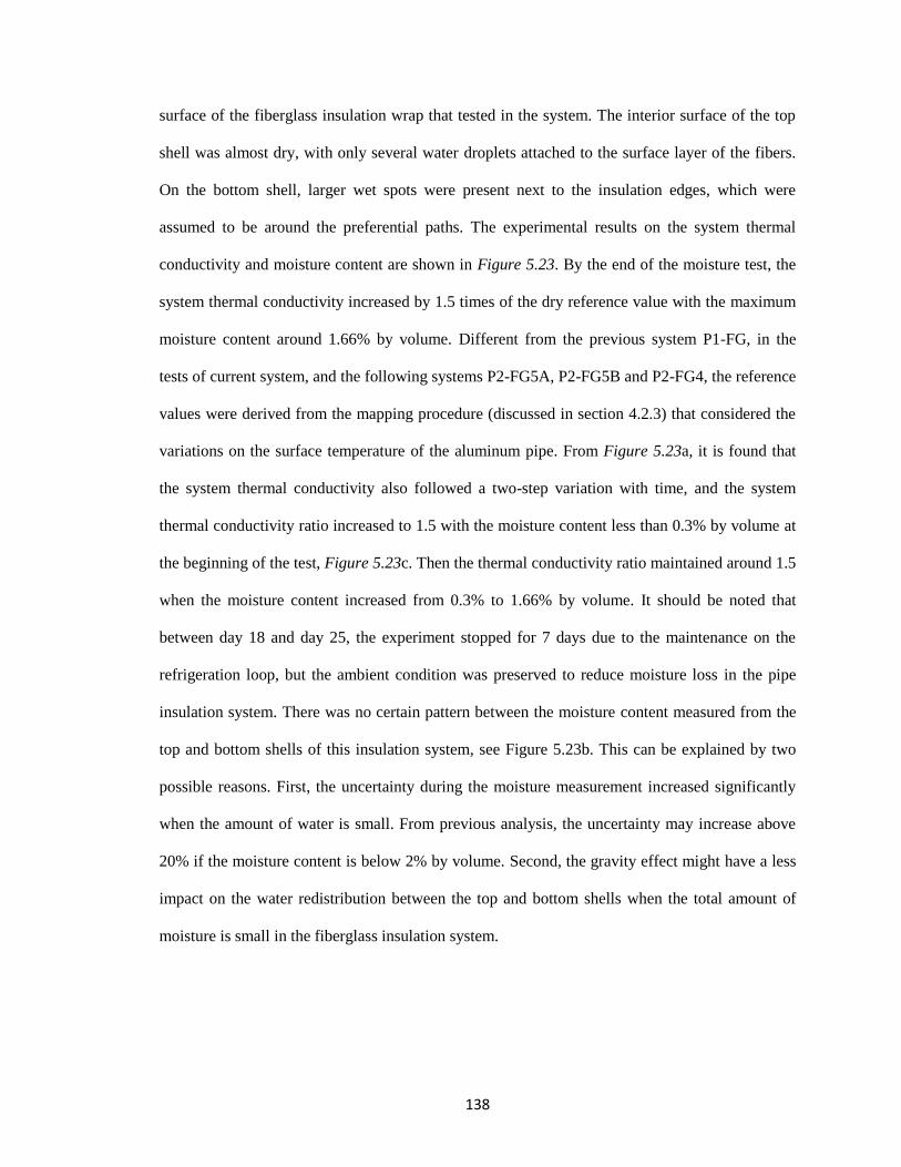
138

surface of the fiberglass insulation wrap that tested in the system. The interior surface of the top

shell was almost dry, with only several water droplets attached to the surface layer of the fibers.

On the bottom shell, larger wet spots were present next to the insulation edges, which were

assumed to be around the preferential paths. The experimental results on the system thermal

conductivity and moisture content are shown in Figure 5.23. By the end of the moisture test, the

system thermal conductivity increased by 1.5 times of the dry reference value with the maximum

moisture content around 1.66% by volume. Different from the previous system P1-FG, in the

tests of current system, and the following systems P2-FG5A, P2-FG5B and P2-FG4, the reference

values were derived from the mapping procedure (discussed in section 4.2.3) that considered the

variations on the surface temperature of the aluminum pipe. From Figure 5.23a, it is found that

the system thermal conductivity also followed a two-step variation with time, and the system

thermal conductivity ratio increased to 1.5 with the moisture content less than 0.3% by volume at

the beginning of the test, Figure 5.23c. Then the thermal conductivity ratio maintained around 1.5

when the moisture content increased from 0.3% to 1.66% by volume. It should be noted that

between day 18 and day 25, the experiment stopped for 7 days due to the maintenance on the

refrigeration loop, but the ambient condition was preserved to reduce moisture loss in the pipe

insulation system. There was no certain pattern between the moisture content measured from the

top and bottom shells of this insulation system, see Figure 5.23b. This can be explained by two

possible reasons. First, the uncertainty during the moisture measurement increased significantly

when the amount of water is small. From previous analysis, the uncertainty may increase above

20% if the moisture content is below 2% by volume. Second, the gravity effect might have a less

impact on the water redistribution between the top and bottom shells when the total amount of

moisture is small in the fiberglass insulation system.

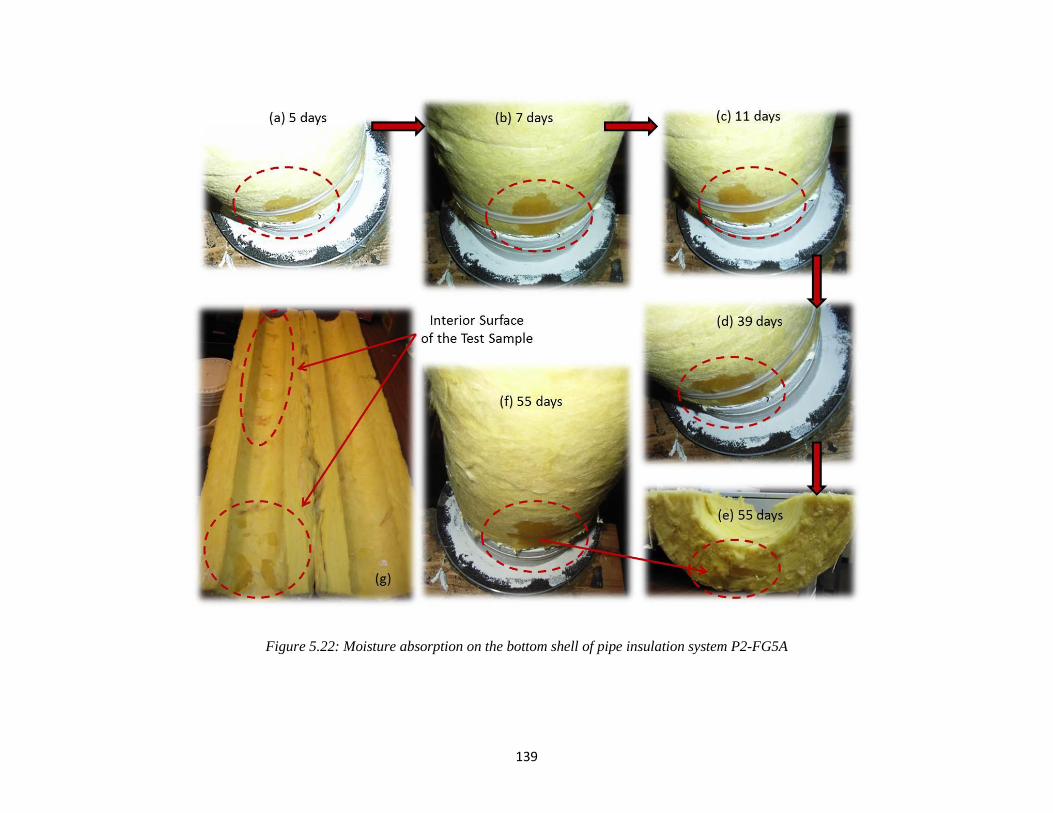
139

Figure 5.22: Moisture absorption on the bottom shell of pipe insulation system P2-FG5A

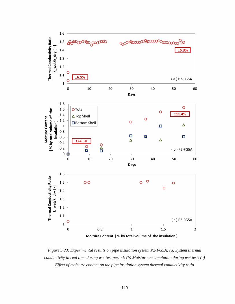
140

Figure 5.23: Experimental results on pipe insulation system P2-FG5A: (a) System thermal

conductivity in real time during wet test period; (b) Moisture accumulation during wet test; (c)

Effect of moisture content on the pipe insulation system thermal conductivity ratio

1

1.1

1.2

1.3

1.4

1.5

1.6

0 0.5 1 1.5 2

Ther

mal

Co

nd

uct

ivit

y R

atio

k_

wet

/k_d

ry [

-]

Moiture Content [ % by total volume of the insulation ]

1

1.1

1.2

1.3

1.4

1.5

1.6

0 10 20 30 40 50 60

Ther

mal

Co

nd

uct

ivit

y R

atio

k_

wet

/k_d

ry [

-]

Days

0

0.2

0.4

0.6

0.8

1

1.2

1.4

1.6

1.8

0 10 20 30 40 50 60

Mo

itu

re C

on

ten

t [

% b

y to

tal v

olu

me

of

th

e in

sula

tio

n ]

Days

Total

Top Shell

Bottom Shell

( a ) P2-FG5A

( c ) P2-FG5A

( b ) P2-FG5A

±6.5%

±5.3%

±24.5%

±11.4%

141

Fiberglass pipe insulation system P2-FG5B

Instead of testing on the bare pipe, the fiberglass pipe insulation system P2-FG5 was also tested

on the black pipe (referred as P2-FG5B) under severe acceleration condition with high

temperature and humidity, 90.1 ˚F (32.3 ˚C), 84%RH. This test lasted for 54 days. Compared to

the large wet area that observed in system P1-FG, only one small wet spot was observed at the

exterior surface of the bottom shell, and this wet region almost maintained the same during the

entire test, as shown in Figure 5.24. One possible explanation for the formation of the much

smaller wet region is the better edge seal in the current system. These better sealed edges affect

the water vapor distribution in the insulation system, and led to a different quasi-steady state

equilibrium in the longitudinal direction. A denser surface might be another possible reason to

explain the smaller wet area that formed on the exterior surface of this system. Figure 5.24e

shows the interior surface of both top and bottom shell of the fiberglass test sample in the system

P2-FG5B. No obvious water marks were observed on the top shell, and the water droplets only

covered the surface layer of the fibers. For the bottom shell, a large area of water mark was found

at the location that circled out in the Figure 5.24a to d. This location might be a less dense region

and led more water pass through the insulation system. The experimental results on the system

thermal conductivity and moisture content were plotted in Figure 5.25. After 54 days test, the

system thermal conductivity ratio increased up to 3.5 with the total moisture content around 15%

by volume. The performance on the system thermal conductivity was similar to the results

derived from the previous systems P1-FG and P2-FG5A, and demonstrates a two-step variation.

The system thermal conductivity changed almost simultaneously with the ambient condition at

the beginning of the moisture test. Figure 5.25b shows the moisture difference between the top

and bottom shells, and similar to system P1-FG, more water was trapped in the bottom shell, and

the moisture content was almost twice of the amount in the top shell.

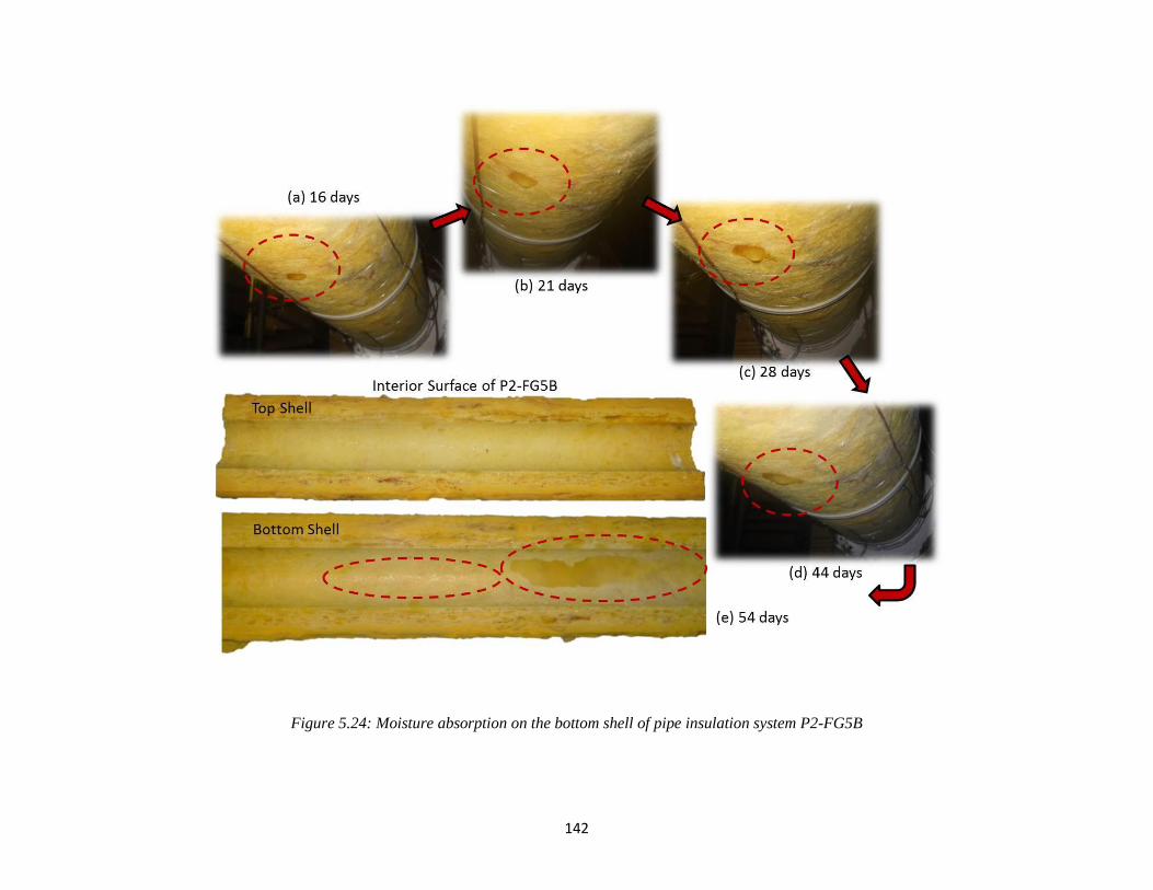
142

Figure 5.24: Moisture absorption on the bottom shell of pipe insulation system P2-FG5B

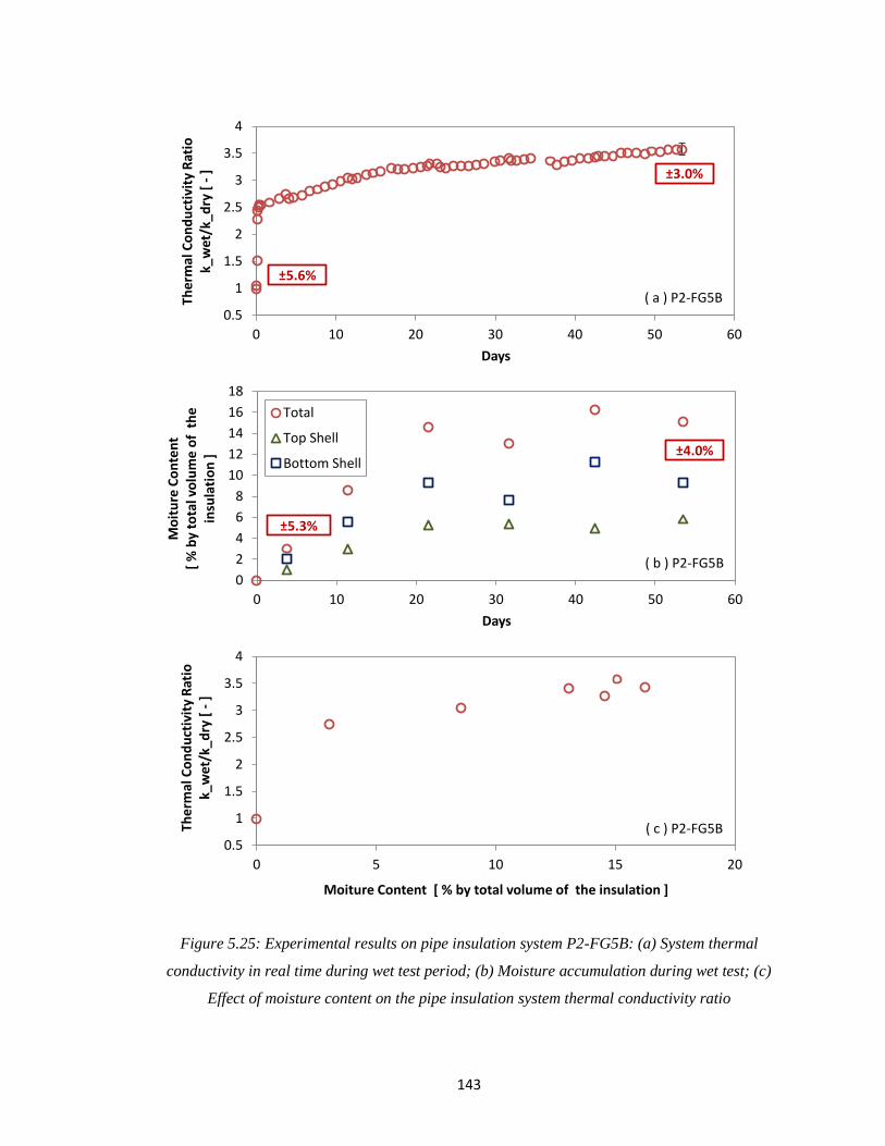
143

Figure 5.25: Experimental results on pipe insulation system P2-FG5B: (a) System thermal

conductivity in real time during wet test period; (b) Moisture accumulation during wet test; (c)

Effect of moisture content on the pipe insulation system thermal conductivity ratio

0.5

1

1.5

2

2.5

3

3.5

4

0 5 10 15 20

The

rmal

Co

nd

uct

ivit

y R

atio

k_

wet

/k_d

ry [

-]

Moiture Content [ % by total volume of the insulation ]

0.5

1

1.5

2

2.5

3

3.5

4

0 10 20 30 40 50 60

Ther

mal

Co

nd

uct

ivit

y R

atio

k_

wet

/k_d

ry [

-]

Days

0

2

4

6

8

10

12

14

16

18

0 10 20 30 40 50 60

Mo

itu

re C

on

ten

t [

% b

y to

tal v

olu

me

of

th

e in

sula

tio

n ]

Days

Total

Top Shell

Bottom Shell

±5.3%

±4.0%

( a ) P2-FG5B

( c ) P2-FG5B

( b ) P2-FG5B

±5.6%

±3.0%

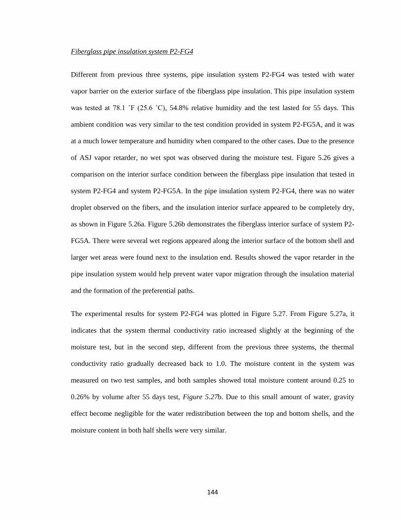
144

Fiberglass pipe insulation system P2-FG4

Different from previous three systems, pipe insulation system P2-FG4 was tested with water

vapor barrier on the exterior surface of the fiberglass pipe insulation. This pipe insulation system

was tested at 78.1 ˚F (25.6 ˚C), 54.8% relative humidity and the test lasted for 55 days. This

ambient condition was very similar to the test condition provided in system P2-FG5A, and it was

at a much lower temperature and humidity when compared to the other cases. Due to the presence

of ASJ vapor retarder, no wet spot was observed during the moisture test. Figure 5.26 gives a

comparison on the interior surface condition between the fiberglass pipe insulation that tested in

system P2-FG4 and system P2-FG5A. In the pipe insulation system P2-FG4, there was no water

droplet observed on the fibers, and the insulation interior surface appeared to be completely dry,

as shown in Figure 5.26a. Figure 5.26b demonstrates the fiberglass interior surface of system P2-

FG5A. There were several wet regions appeared along the interior surface of the bottom shell and

larger wet areas were found next to the insulation end. Results showed the vapor retarder in the

pipe insulation system would help prevent water vapor migration through the insulation material

and the formation of the preferential paths.

The experimental results for system P2-FG4 was plotted in Figure 5.27. From Figure 5.27a, it

indicates that the system thermal conductivity ratio increased slightly at the beginning of the

moisture test, but in the second step, different from the previous three systems, the thermal

conductivity ratio gradually decreased back to 1.0. The moisture content in the system was

measured on two test samples, and both samples showed total moisture content around 0.25 to

0.26% by volume after 55 days test, Figure 5.27b. Due to this small amount of water, gravity

effect become negligible for the water redistribution between the top and bottom shells, and the

moisture content in both half shells were very similar.

145

Figure 5.26: Comparison of the interior surface of pipe insulation systems P2-FG5A and P2-

FG4: (a) P2-FG5A; (b) P2-FG4

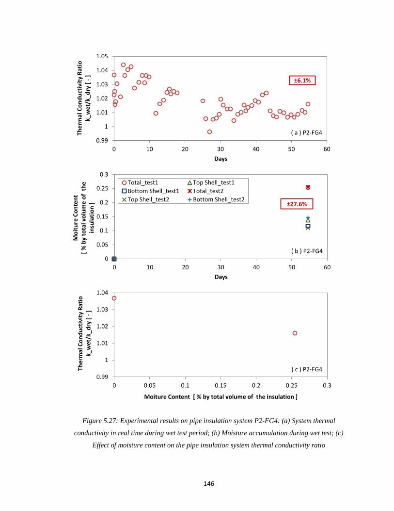
146

Figure 5.27: Experimental results on pipe insulation system P2-FG4: (a) System thermal

conductivity in real time during wet test period; (b) Moisture accumulation during wet test; (c)

Effect of moisture content on the pipe insulation system thermal conductivity ratio

0.99

1

1.01

1.02

1.03

1.04

0 0.05 0.1 0.15 0.2 0.25 0.3

Ther

mal

Co

nd

uct

ivit

y R

atio

k_

wet

/k_d

ry [

-]

Moiture Content [ % by total volume of the insulation ]

0.99

1

1.01

1.02

1.03

1.04

1.05

0 10 20 30 40 50 60

Ther

mal

Co

nd

uct

ivit

y R

atio

k_

wet

/k_d

ry [

-]

Days

0

0.05

0.1

0.15

0.2

0.25

0.3

0 10 20 30 40 50 60

Mo

itu

re C

on

ten

t [

% b

y to

tal v

olu

me

of

th

e in

sula

tio

n ]

Days

Total_test1 Top Shell_test1

Bottom Shell_test1 Total_test2

Top Shell_test2 Bottom Shell_test2

( a ) P2-FG4

( c ) P2-FG4

( b ) P2-FG4

±6.1%

±27.6%

147

In all the three cases on the pipe insulation system without vapor retarder, it is observed that the

thermal conductivity ratio increased by 1.5 to 2.5 times of the dry reference value at the

beginning of the moisture test. One possible reason for these dramatic increases on the system

thermal conductivity is explained as follows. When the water vapor diffuses through the fibrous

insulation and condensed in the regions with temperatures lower than the dew point, the water

condensate would first accumulate at the points of the contact between fibers. The fibers were

aligned perpendicular to the heat flow direction, and these beads of moisture enhanced the radial

heat transfer immediately by providing preferential paths in the radial direction (McFadden,

1988). The presence of these preferential paths led to higher thermal bridging phenomenon that

promoted larger heat losses and increased the thermal conductivity of the pipe insulation systems.

It was also found that after this significant change, the system started to behave more stable.

Although the system thermal conductivity continued rising, the rate was much lower than the

previous step. This continuous increasing on the system thermal conductivity can be explained by

the enlarged areas of the preferential paths and the fact that more regions of air gaps were

replaced with water. Because of the constant water vapor pressure gradient across the pipe

insulation, water vapor kept permeating into the insulation system. This amount of water

condensate started coating along the fiber strands and gradually filled in the voids between the

fibers (Ogniewicz and Tien, 1981). However, the impact of this step was not that severe as the

one happed at the beginning of the test, because the direction of the heat flow would not be varied

with the amount of water. The water amount was postulate to affect the moisture diffusion based

on the diffusion mechanism discussed in the previous paragraph. After the formation of the

preferential paths, the water condensate started accumulating on the exterior surface of the bottom

shell due to surface tension and gravity effects (Modi and Benner, 1985). Water gradually coated

the exterior fiber surfaces and increased the intersect areas among the strands until a quasi-steady

state equilibrium was achieved in the longitudinal direction. Then the water started diffusing

towards the adjacent inner layer of the fibers at a lower rate because of a lower local temperature

148

and water vapor permeability. However, for system P2-FG5B with black pipe, the thermal

conductivity remained constant during the second step, and the moisture content was measured

increasing from 0.3 to 1.66%. This discrepancy might be explained by the small amount of

moisture that accumulated in the system and resulted in a minor change on the system thermal

conductivity.

In the system P2-FG4, which was tested with ASJ vapor retarder, the thermal conductivity ratio

also increased slightly in the first step. Although the vapor barrier around the exterior surface of

the pipe insulation prevented water vapor transmission because of the low permeability, the water

vapor that trapped in the insulation system would still condense in the low temperature region and

formed the moisture beads at the contact points of the fibers. Due to the presence of the vapor

barrier, the water vapor transmitted through system P2-FG4 at a much lower rate when compared

to the water vapor transmission in the systems without vapor barrier. As a result, less preferential

paths were formed during the first step, and the system thermal conductivity increased in a small

range. In the second step, instead of coating the fibers and filling in the voids, the small amount

of moisture might be redistributed in the system, and some of the moisture beads were shifted

from the contact points of the fibers. This moisture redistribution procedure impacts the heat flow

paths and result in a reducing on the system thermal conductivity.

In industry, the surface of the fibers may be manufactured either as hydrophobic or hydrophilic.

According to the literature (Ge et al., 2006), the water layer was found to be in a higher density

near hydrophilic surfaces than in the bulk, while a thin layer of low density of water has been

observed near hydrophobic surfaces. It seems that hydrophilic surfaces would accelerate the

formation of thermal bridging by contacting two layers of fiber strands in the radial direction.

However, with hydrophobic surfaces, more water condensate would drip out of the insulation

system, and the convection heat transfer might be enhanced to decrease the system thermal

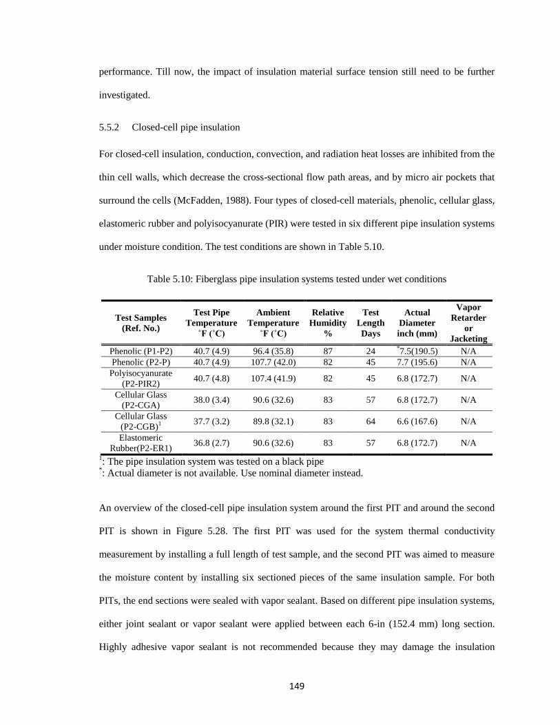
149

performance. Till now, the impact of insulation material surface tension still need to be further

investigated.

5.5.2 Closed-cell pipe insulation

For closed-cell insulation, conduction, convection, and radiation heat losses are inhibited from the

thin cell walls, which decrease the cross-sectional flow path areas, and by micro air pockets that

surround the cells (McFadden, 1988). Four types of closed-cell materials, phenolic, cellular glass,

elastomeric rubber and polyisocyanurate (PIR) were tested in six different pipe insulation systems

under moisture condition. The test conditions are shown in Table 5.10.

Table 5.10: Fiberglass pipe insulation systems tested under wet conditions

Test Samples

(Ref. No.)

Test Pipe

Temperature

˚F (˚C)

Ambient

Temperature

˚F (˚C)

Relative

Humidity

%

Test

Length

Days

Actual

Diameter

inch (mm)

Vapor

Retarder

or

Jacketing

Phenolic (P1-P2) 40.7 (4.9) 96.4 (35.8) 87 24 *7.5(190.5) N/A

Phenolic (P2-P) 40.7 (4.9) 107.7 (42.0) 82 45 7.7 (195.6) N/A

Polyisocyanurate

(P2-PIR2) 40.7 (4.8) 107.4 (41.9) 82 45 6.8 (172.7) N/A

Cellular Glass

(P2-CGA) 38.0 (3.4) 90.6 (32.6) 83 57 6.8 (172.7) N/A

Cellular Glass

(P2-CGB)1

37.7 (3.2) 89.8 (32.1) 83 64 6.6 (167.6) N/A

Elastomeric

Rubber(P2-ER1) 36.8 (2.7) 90.6 (32.6) 83 57 6.8 (172.7) N/A

1: The pipe insulation system was tested on a black pipe

*: Actual diameter is not available. Use nominal diameter instead.

An overview of the closed-cell pipe insulation system around the first PIT and around the second

PIT is shown in Figure 5.28. The first PIT was used for the system thermal conductivity

measurement by installing a full length of test sample, and the second PIT was aimed to measure

the moisture content by installing six sectioned pieces of the same insulation sample. For both

PITs, the end sections were sealed with vapor sealant. Based on different pipe insulation systems,

either joint sealant or vapor sealant were applied between each 6-in (152.4 mm) long section.

Highly adhesive vapor sealant is not recommended because they may damage the insulation

150

samples during the sampling procedure. Water-based sealant also need to be carefully used

because the moisture in the sealant might transport into the insulation and affect the test results.

Figure 5.28: Photo of the closed-cell pipe insulation system installation for the wet test

Phenolic pipe insulation systems P1-P2 and P2-P

Phenolic pipe insulation was tested in two systems, P1-P2 and P2-P under different ambient

conditions, as shown in Table 5.10. For system P1-P2, the ambient temperature was controlled at

96.3 °F (35.7 °C) and the relative humidity was set to 87.1%. In these psychrometric conditions,

the air dew point temperature was about 91.8 °F (33.2 °C). Boss 368 butyl rubber sealant was

applied along the longitudinal joints of the C-shells during the installation of phenolic pipe

insulation. Foster 90-66 was applied at the two end sides of the insulation system as edge seals.

An easy-to-peel off vapor sealant, Foster 30-80, was applied as 1/8-in (3.175 mm) thickness layer

on the entire cross sectional surface of the insulation samples on the second PIT. Pipe insulation

system P2-P was tested at a more severe condition. The ambient temperature was 107.7 °F (42

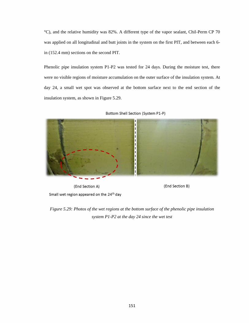
151

°C), and the relative humidity was 82%. A different type of the vapor sealant, Chil-Perm CP 70

was applied on all longitudinal and butt joints in the system on the first PIT, and between each 6-

in (152.4 mm) sections on the second PIT.

Phenolic pipe insulation system P1-P2 was tested for 24 days. During the moisture test, there

were no visible regions of moisture accumulation on the outer surface of the insulation system. At

day 24, a small wet spot was observed at the bottom surface next to the end section of the

insulation system, as shown in Figure 5.29.

Figure 5.29: Photos of the wet regions at the bottom surface of the phenolic pipe insulation

system P1-P2 at the day 24 since the wet test

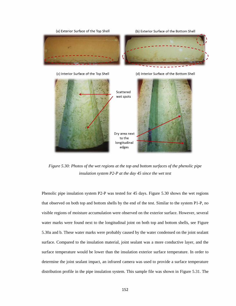
152

Figure 5.30: Photos of the wet regions at the top and bottom surfaces of the phenolic pipe

insulation system P2-P at the day 45 since the wet test

Phenolic pipe insulation system P2-P was tested for 45 days. Figure 5.30 shows the wet regions

that observed on both top and bottom shells by the end of the test. Similar to the system P1-P, no

visible regions of moisture accumulation were observed on the exterior surface. However, several

water marks were found next to the longitudinal joint on both top and bottom shells, see Figure

5.30a and b. These water marks were probably caused by the water condensed on the joint sealant

surface. Compared to the insulation material, joint sealant was a more conductive layer, and the

surface temperature would be lower than the insulation exterior surface temperature. In order to

determine the joint sealant impact, an infrared camera was used to provide a surface temperature

distribution profile in the pipe insulation system. This sample file was shown in Figure 5.31. The

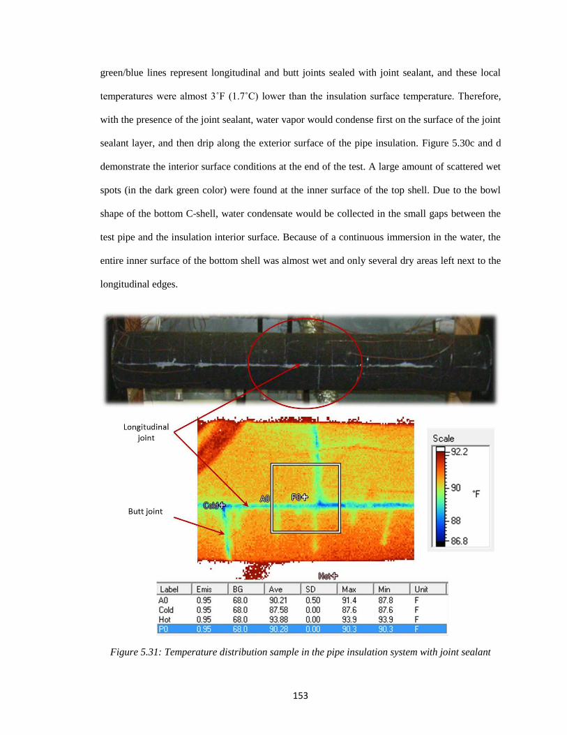
153

green/blue lines represent longitudinal and butt joints sealed with joint sealant, and these local

temperatures were almost 3˚F (1.7˚C) lower than the insulation surface temperature. Therefore,

with the presence of the joint sealant, water vapor would condense first on the surface of the joint

sealant layer, and then drip along the exterior surface of the pipe insulation. Figure 5.30c and d

demonstrate the interior surface conditions at the end of the test. A large amount of scattered wet

spots (in the dark green color) were found at the inner surface of the top shell. Due to the bowl

shape of the bottom C-shell, water condensate would be collected in the small gaps between the

test pipe and the insulation interior surface. Because of a continuous immersion in the water, the

entire inner surface of the bottom shell was almost wet and only several dry areas left next to the

longitudinal edges.

Figure 5.31: Temperature distribution sample in the pipe insulation system with joint sealant

154

The diffusion mechanism was studied in Figure 5.32. Figure 5.32a to d are the photos of the cross

sections of the phenolic test samples that were removed periodically from the second PIT, and

Figure 5.32e to f show the cross section of the full length test sample removed from the first PIT.

An extra piece of insulation, ¼ to ½-in (6.4 to 12.7 mm) thick, was cut off from the sample to

eliminate edge effect, which was caused by the vapor sealant applied between each 6-in (152.4

mm) section and the insulation ends. According to the material characteristics, this type of light

green phenolic will turn into a dark green color if the material becomes wet. On the 10th day of

the moisture test, the cross section of both top and bottom shells almost maintained a light green

color, and only several water droplets were found next to the interior surfaces. After 17 days test,

a very thin layer of dark green area started to form on the bottom shell as shown by the red arrow

in Figure 5.32b. No obvious changes were observed on the top shell. On the 24th day of the wet

test, dark green regions were found next to the interior surface of both top and bottom shells, see

the red arrows in Figure 5.32c. When cutting off the extra piece of insulation, the surfaces of the

cross sections became wet because of the water coming out from the open pores. The piece of

paper that prepared below the insulation sample started to become wet, as the region circled out

by the dash line. After 31 days test, the dark green area increased in both two C-shells and larger

water marks were found on the piece of paper below the insulation samples. By the end of this

moisture test, it seems that the dark green region kept increasing, as shown in Figure 5.32e and f.

Based on these observations, the diffusion mechanism in this closed-cell pipe insulation system

seems to be different from the fiberglass insulation system. Due to the closed-cell structure, much

less preferential paths were formed in the phenolic pipe insulation. Water condensate filled in the

voids among each cell and diffused into closed pores gradually from the interior surface to the

exterior. The only possibility for the formation of the preferential paths is the joints existed in the

pipe insulation system. These joints include longitudinal joints between two half C-shells, butt

joints between two full length pieces of pipe insulation, and the material joints that factory-made

during pipe insulation fabrication. This would explain the fact that only small wet regions were

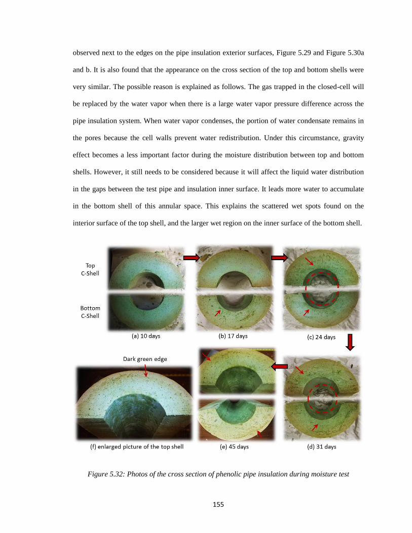
155

observed next to the edges on the pipe insulation exterior surfaces, Figure 5.29 and Figure 5.30a

and b. It is also found that the appearance on the cross section of the top and bottom shells were

very similar. The possible reason is explained as follows. The gas trapped in the closed-cell will

be replaced by the water vapor when there is a large water vapor pressure difference across the

pipe insulation system. When water vapor condenses, the portion of water condensate remains in

the pores because the cell walls prevent water redistribution. Under this circumstance, gravity

effect becomes a less important factor during the moisture distribution between top and bottom

shells. However, it still needs to be considered because it will affect the liquid water distribution

in the gaps between the test pipe and insulation inner surface. It leads more water to accumulate

in the bottom shell of this annular space. This explains the scattered wet spots found on the

interior surface of the top shell, and the larger wet region on the inner surface of the bottom shell.

Figure 5.32: Photos of the cross section of phenolic pipe insulation during moisture test

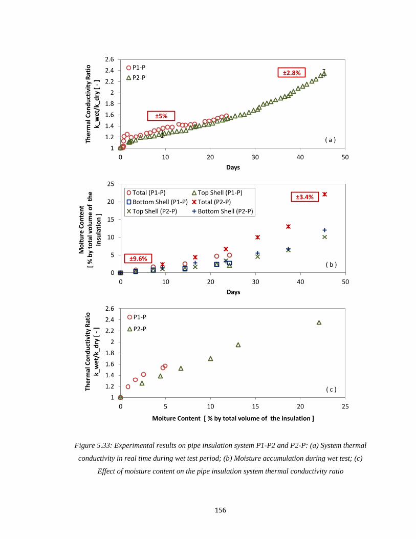
156

Figure 5.33: Experimental results on pipe insulation system P1-P2 and P2-P: (a) System thermal

conductivity in real time during wet test period; (b) Moisture accumulation during wet test; (c)

Effect of moisture content on the pipe insulation system thermal conductivity ratio

1

1.2

1.4

1.6

1.8

2

2.2

2.4

2.6

0 5 10 15 20 25

Ther

mal

Co

nd

uct

ivit

y R

atio

k_

wet

/k_d

ry [

-]

Moiture Content [ % by total volume of the insulation ]

P1-P

P2-P

1

1.2

1.4

1.6

1.8

2

2.2

2.4

2.6

0 10 20 30 40 50

Ther

mal

Co

nd

uct

ivit

y R

atio

k_

wet

/k_d

ry [

-]

Days

P1-P

P2-P

( a )

( c )

0

5

10

15

20

25

0 10 20 30 40 50

Mo

itu

re C

on

ten

t [

% b

y to

tal v

olu

me

of

th

e in

sula

tio

n ]

Days

Total (P1-P) Top Shell (P1-P)

Bottom Shell (P1-P) Total (P2-P)

Top Shell (P2-P) Bottom Shell (P2-P)

( b )

±5%

±2.8%

±9.6%

±3.4%

157

The experimental results on the variation of thermal conductivity and moisture content in

phenolic pipe insulation systems P1-P2 and P2-P are given in Figure 5.33. Figure 5.33a shows the

phenolic pipe insulation thermal conductivity at below ambient temperature in wet condensing

conditions and with moisture ingress. In system P1-P2, the thermal conductivity ratio was derived

from the thermal conductivity in wet conditions, kwet, to the corresponding thermal conductivity in

dry condition, kdry. In system P2-P, the reference value under dry condition was updated based on

the test pipe surface temperature by applying the correlation developed from the mapping test, as

described in section 4.2.3. After 24 days test on system P1-P2, the thermal conductivity ratio

increased to 1.57 with total moisture content around 5% by volume. System P2-P was tested

under a more severe condition for 45 days, and the thermal conductivity ratio increased to 2.35

when the moisture content was around 22%. It seems that there is a slightly increase on the

system thermal conductivity at the beginning of the moisture test, but the increasing range was

much lower than fiberglass pipe insulation systems. Figure 5.33b shows the moisture content in

the phenolic pipe insulation at below ambient temperature and in wet (condensing) conditions. In

system P1-P2, the moisture content reached 5% by volume of the pipe insulation system, and the

moisture content increased to 22% by volume in the system P2-P. For both phenolic pipe

insulation systems, the moisture content was fairly uniform between the top C-shell sections and

the bottom C-shell sections. According to the literature, the maximum moisture absorption for flat

cubic specimen of phenolic insulation is expected to be between 3 to 8% by volume depending on

actual density of the specimen (ASTM_C1126, 2009). However, this value was derived based on

a two hour immersion test under ambient condition with temperature at 73±1˚F (23±2˚C) and

relative humidity around 50±5% (ASTM_C209, 2007). This test might underestimate the

moisture content that can trap in the insulation systems applied in the field because it neglect the

impact of water vapor pressure difference between the cold surface and the ambient conditions.

The water pressure gradient will be the key for the moisture migration in pipe insulation system.

Figure 5.33c plotted the thermal conductivity ratio versus the moisture content, and it shows that

158

for both cases, the system thermal conductivity increased almost linearly with the moisture

content in the pipe insulation system.

Polyisocyanurate (PIR) pipe insulation system P2-PIR

The test sample selected in the system P2-PIR has a nominal thickness of 1 ½ -in (38.1 mm)

without any vapor retarder on the exterior surface, see Table 5.7. Similar to system P2-P, P2-PIR

was also tested under a most severe condition with the ambient temperature at 107.4 °F (41.9 °C),

and the relative humidity around 82%. At this condition, the dew point was around 100.7 °F (38.1

°C). Chil-Perm CP 70 was the vapor sealant applied on all longitudinal and butt joints in the

system on the first PIT, and also between each 6-in (152.4 mm) sections on the second PIT. The

moisture test lasted for 45 days. By the end of the test, no wet regions were observed on the

exterior surface of the pipe insulation system, as shown in Figure 5.34. The water marks circled

out by the red dash line were caused by the movement of the water that condensed on the joint

sealant surface.

The experimental results on the variation of thermal conductivity and moisture content in the pipe

insulation system P2-PIR are shown in Figure 5.35. Figure 5.35a shows the PIR pipe insulation

thermal conductivity at below ambient temperature in wet condensing conditions and with

moisture ingress. By the end of the moisture test, that is, the 45th day, the system thermal

conductivity increased to 1.51 times of the dry reference value, which was determined from the

mapping procedure. At the beginning of the test, the humidifier was on for two hours, and it was

off for 24 hour due to technical problems. When the humidifier was back to work, I immediately

started data recording procedure, and the experimental results from both transient and steady-state

conditions showed that there was a 10% increase on the system thermal conductivity. The total

moisture content accumulated in the insulation system was measured around 16% by volume, and

the difference between the top and bottom C-shells were small and within the uncertainty range,

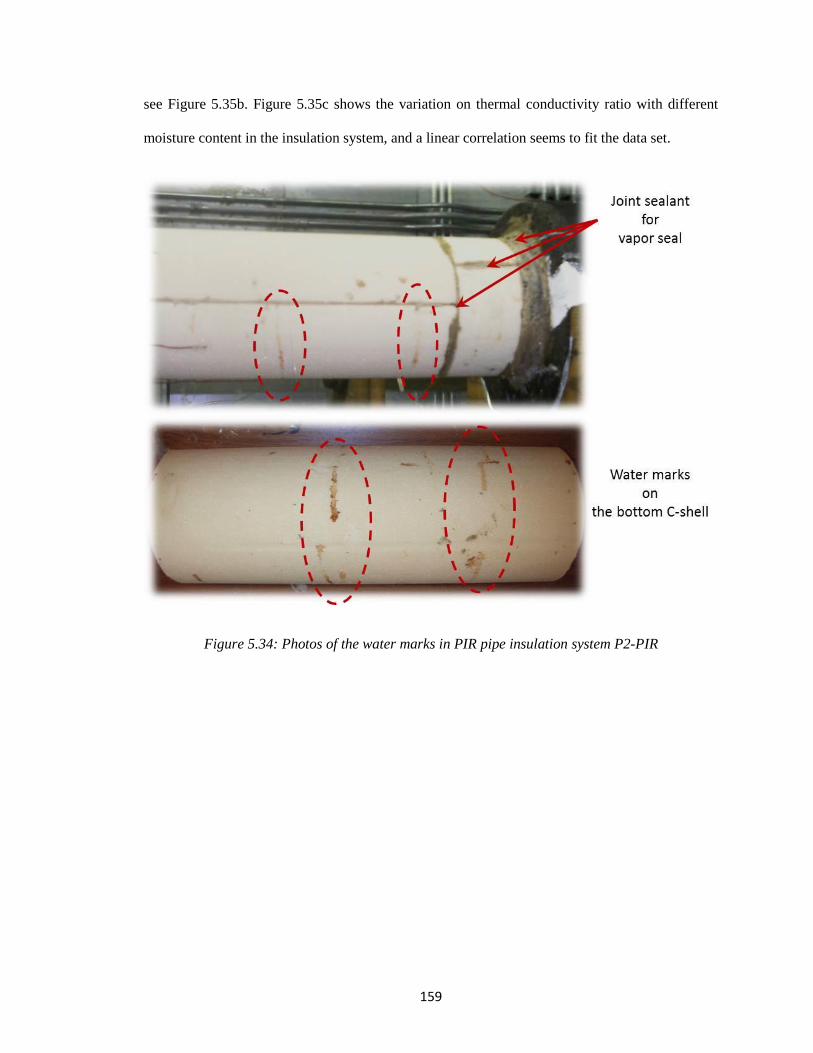
159

see Figure 5.35b. Figure 5.35c shows the variation on thermal conductivity ratio with different

moisture content in the insulation system, and a linear correlation seems to fit the data set.

Figure 5.34: Photos of the water marks in PIR pipe insulation system P2-PIR

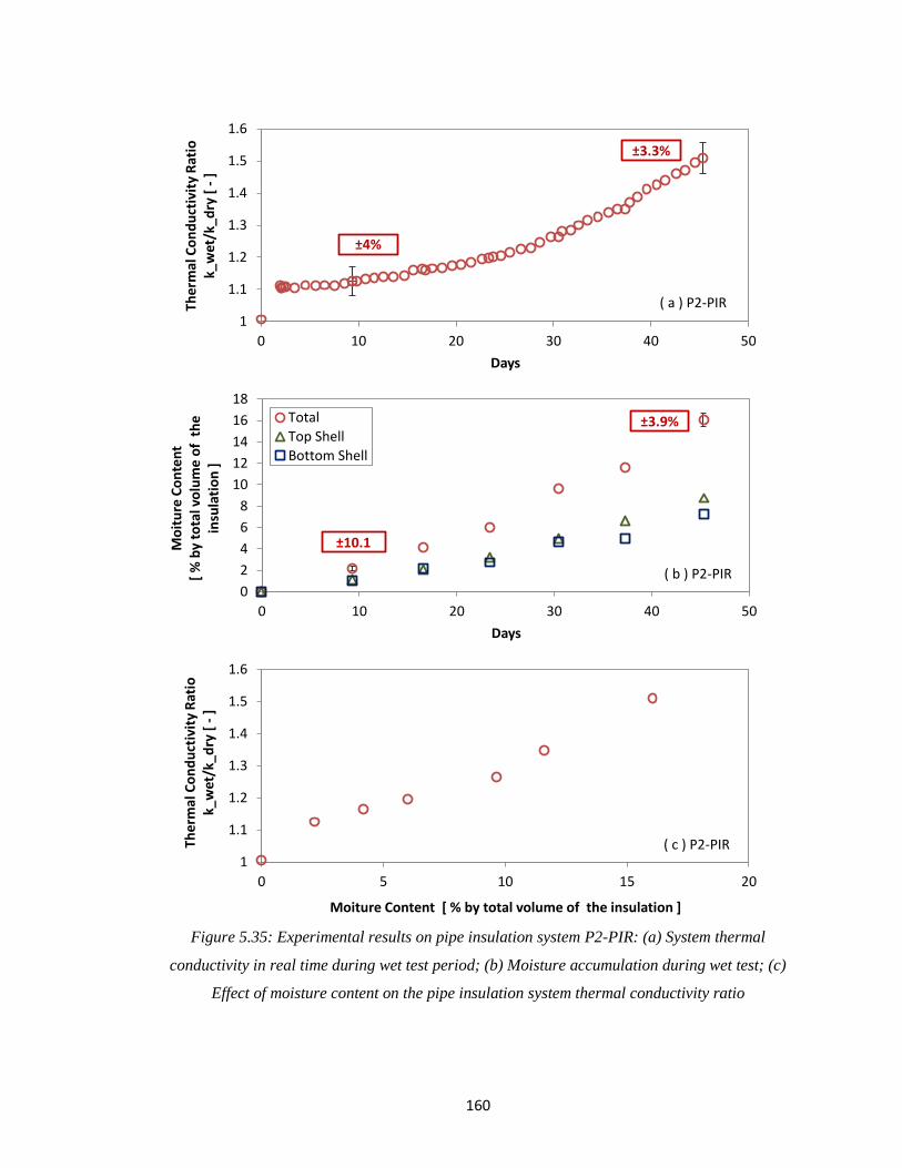
160

Figure 5.35: Experimental results on pipe insulation system P2-PIR: (a) System thermal

conductivity in real time during wet test period; (b) Moisture accumulation during wet test; (c)

Effect of moisture content on the pipe insulation system thermal conductivity ratio

1

1.1

1.2

1.3

1.4

1.5

1.6

0 5 10 15 20

Ther

mal

Co

nd

uct

ivit

y R

atio

k_

wet

/k_d

ry [

-]

Moiture Content [ % by total volume of the insulation ]

1

1.1

1.2

1.3

1.4

1.5

1.6

0 10 20 30 40 50

Ther

mal

Co

nd

uct

ivit

y R

atio

k_

wet

/k_d

ry [

-]

Days

( a ) P2-PIR

( c ) P2-PIR

0

2

4

6

8

10

12

14

16

18

0 10 20 30 40 50

Mo

itu

re C

on

ten

t [

% b

y to

tal v

olu

me

of

th

e in

sula

tio

n ]

Days

Total

Top Shell

Bottom Shell

( b ) P2-PIR

±4%

±3.3%

±10.1

±3.9%

161

Cellular glass pipe insulation systems P2-CGA and P2-CGB

Cellular glass pipe insulation was tested twice in the similar ambient condition. The difference

between system P2-CGA and P2-CGB is the test pipe. In the system P2-CGA, cellular glass pipe

insulation was installed around the bare pipe with thermocouple grooved exposed to the interior

surface of the test sample, and in the system P2-CGB, the test pipe was sealed with aluminum

tape and painted as black to avoid radiation impact. The test samples in both systems has a

nominal wall thickness of 1 ½ -in (38.1 mm). Boss 368 butyl rubber sealant was applied as the

joint sealant, and also used for edge seals on both PITs. System P2-CGA was tested at an ambient

temperature around 90.6 °F (32.6 °C), and the relative humidity at 83%. At this condition, the

dew point was around 84.8 °F (29.3 °C). System P2-CGA was tested with ambient temperature at

89.8 °F (32.1 °C), relative humidity at 83%, and the dew point was around 83.9°F (28.8 °C). The

test length for system P2-CGA and P2-CGB are 57 and 64 days, respectively.

For both cellular glass pipe insulation systems, no wet spots were observed on the insulation

surface, but large amount of water condensate occurred on the joint sealant surface, and dripped

along the exterior surface of the bottom C-shell, as shown in Figure 5.36 and Figure 5.37. By the

end of the moisture test, more water was found to accumulate in the bottom C-shell, and formed

larger wet area at the interior surface. For the top shell, the wet region only formed next to the

insulation ends, as circled out in Figure 5.38a. In pipe insulation system P2-CGA, one piece of

the test sample, which used as the bottom shell, was manufactured with material joint and wet

regions appeared next to the material joints on both interior and exterior surfaces. The material

joints and wet regions are shown in Figure 5.38b.

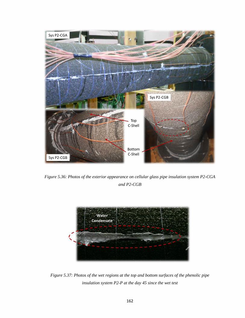
162

Figure 5.36: Photos of the exterior appearance on cellular glass pipe insulation system P2-CGA

and P2-CGB

Figure 5.37: Photos of the wet regions at the top and bottom surfaces of the phenolic pipe

insulation system P2-P at the day 45 since the wet test

163

Figure 5.38: Wet regions in cellular glass pipe insulation system P2-CGA

The experimental results on the variation of thermal conductivity and moisture content in pipe

insulation systems P2-CGA and P2-CGB are shown in Figure 5.39. In both systems, the thermal

conductivity increased slightly at the beginning of the moisture test. In system P2-CGA, the

system thermal conductivity increased by 7% on the 15th day, and maintained almost constant

until the end of the moisture test. The system thermal conductivity in P2-CGB increased slower

than the thermal conductivity in system P2-CGA, and showed a continuous rising till the last day

of the moisture test. For the moisture measurement, due to the small amount of water being

collected in the insulation system, the uncertainties in both pipe insulation systems exceed ±15%.

In system P2-CGA, the total moisture content was 0.32% by volume after 57 days test, and for in

system P2-CGB, the total moisture content reached 0.27% by volume after 64 days test. One

possible reason for the fact that system P2-CGA was found at higher thermal conductivity and

164

moisture content is the presence of the material joint. It should be noted that the difference on the

results between these two systems were within the uncertainty range. Because of the small

amount of water content, there was no certain pattern of correlation suitable between the system

thermal conductivity ratio and moisture content, as shown in Figure 5.39c.

Elastomeric rubber pipe insulation system

Different from previous three pipe insulation systems, elastomeric rubber pipe insulation is

usually manufactured as un-slit sleeves, or as an insulation wrap, and normally joint sealant is not

a requirement during system installation. In this moisture test, elastomeric rubber pipe insulation

system P2-ER was tested as an insulation wrap with adhesive tape along the longitudinal joint.

The test sample has a nominal wall thickness of 1 ½ -in (38.1 mm) and the test sample was

installed as one piece around the whole test pipe on both 1st and 2

nd PITs. The seam with the

adhesive tape must be installed as face-up on the top of the insulation system. During sampling

procedure, one 6-in (152.4 mm) section need to be directly cut out from the entire piece on the 2nd

PIT. Then the void was replaced by another dry sample. Plastic film and joint sealant are required

between the newly installed sample and the adjacent pieces. Aeroseal was the sealant used in the

edge seals and between each 6-in (152.4 mm) sample. Elastomeric rubber pipe insulation system

P2-ER was tested at 90.6 °F (32.6 °C), with relative humidity at 83%, and the dew point was

around 84.8 °F (29.3 °C). The moisture test lasted for 57 days. Similar to the other closed-cell

pipe insulation systems, no visible wet regions were observed on the exterior surface of the pipe

insulation during the moisture test. Two wet regions were found on the interior surface, as shown

in Figure 5.41. It seems that the water condensate only stayed on the interior surface because the

water droplet could still move along the surface.

165

Figure 5.39: Experimental results on pipe insulation system P2-CGA and P2-CGB: (a) System

thermal conductivity in real time during wet test period; (b) Moisture accumulation during wet

test; (c) Effect of moisture content on the pipe insulation system thermal conductivity ratio

0.99

1

1.01

1.02

1.03

1.04

1.05

1.06

1.07

1.08

0 0.2 0.4 0.6 0.8 1

Ther

mal

Co

nd

uct

ivit

y R

atio

k_

wet

/k_d

ry [

-]

Moiture Content [ % by total volume of the insulation ]

P2-CGA P2-CGB

0.96

0.98

1

1.02

1.04

1.06

1.08

1.1

1.12

0 10 20 30 40 50 60 70

Ther

mal

Co

nd

uct

ivit

y R

atio

k_

wet

/k_d

ry [

-]

Days

P2-CGA P2-CGB

( c )

0

0.1

0.2

0.3

0.4

0.5

0.6

0.7

0.8

0.9

0 10 20 30 40 50 60 70

Mo

itu

re C

on

ten

t [

% b

y to

tal v

olu

me

of

th

e in

sula

tio

n ]

Days

Total (P2-CGA) Top Shell (P2-CGA)Bottom Shell (P2-CGA) Total (P2-CGB)

Top Shell (P2-CGB) Bottom Shell (P2-CGB)

( b )

±4%

166

Figure 5.40: Photo of the elastomeric rubber pipe insulation system installation for the wet test

Figure 5.41: Photo of the interior surface of the elastomeric rubber pipe insulation

The experimental results on the variation of thermal conductivity and moisture content in the pipe

insulation system P2-ER are shown in Figure 5.41. In Figure 5.41a, a slightly increase on the

system thermal conductivity was observed at the beginning of the moisture test, then the system

thermal conductivity dropped back, and followed by a gradually increase until the end of the test.

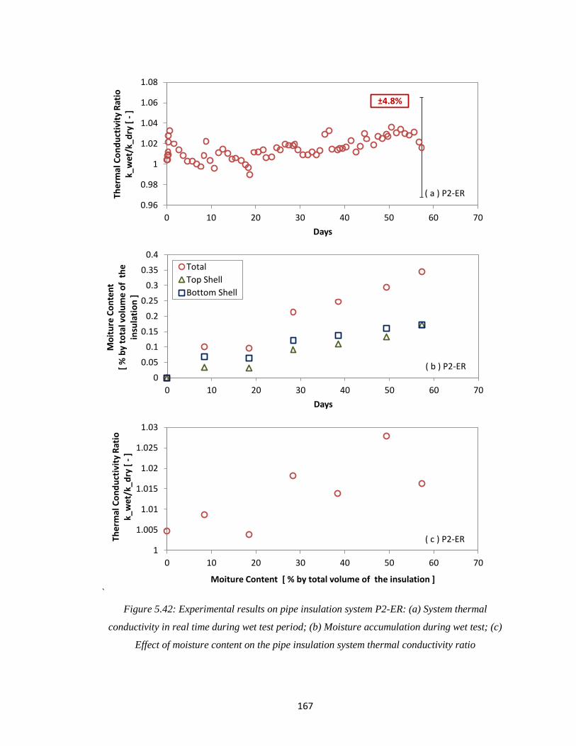
167

`

Figure 5.42: Experimental results on pipe insulation system P2-ER: (a) System thermal

conductivity in real time during wet test period; (b) Moisture accumulation during wet test; (c)

Effect of moisture content on the pipe insulation system thermal conductivity ratio

1

1.005

1.01

1.015

1.02

1.025

1.03

0 10 20 30 40 50 60 70

Ther

mal

Co

nd

uct

ivit

y R

atio

k_

wet

/k_d

ry [

-]

Moiture Content [ % by total volume of the insulation ]

0.96

0.98

1

1.02

1.04

1.06

1.08

0 10 20 30 40 50 60 70

Ther

mal

Co

nd

uct

ivit

y R

atio

k_

wet

/k_d

ry [

-]

Days

( a ) P2-ER

( c ) P2-ER

0

0.05

0.1

0.15

0.2

0.25

0.3

0.35

0.4

0 10 20 30 40 50 60 70

Mo

itu

re C

on

ten

t [

% b

y to

tal v

olu

me

of

th

e in

sula

tio

n ]

Days

Total

Top Shell

Bottom Shell

( b ) P2-ER

±4.8%

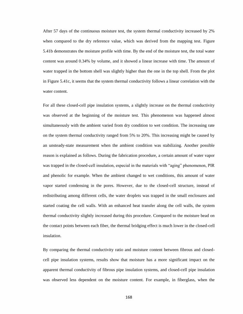
168

After 57 days of the continuous moisture test, the system thermal conductivity increased by 2%

when compared to the dry reference value, which was derived from the mapping test. Figure

5.41b demonstrates the moisture profile with time. By the end of the moisture test, the total water

content was around 0.34% by volume, and it showed a linear increase with time. The amount of

water trapped in the bottom shell was slightly higher than the one in the top shell. From the plot

in Figure 5.41c, it seems that the system thermal conductivity follows a linear correlation with the

water content.

For all these closed-cell pipe insulation systems, a slightly increase on the thermal conductivity

was observed at the beginning of the moisture test. This phenomenon was happened almost

simultaneously with the ambient varied from dry condition to wet condition. The increasing rate

on the system thermal conductivity ranged from 5% to 20%. This increasing might be caused by

an unsteady-state measurement when the ambient condition was stabilizing. Another possible

reason is explained as follows. During the fabrication procedure, a certain amount of water vapor

was trapped in the closed-cell insulation, especial in the materials with “aging” phenomenon, PIR

and phenolic for example. When the ambient changed to wet conditions, this amount of water

vapor started condensing in the pores. However, due to the closed-cell structure, instead of

redistributing among different cells, the water droplets was trapped in the small enclosures and

started coating the cell walls. With an enhanced heat transfer along the cell walls, the system

thermal conductivity slightly increased during this procedure. Compared to the moisture bead on

the contact points between each fiber, the thermal bridging effect is much lower in the closed-cell

insulation.

By comparing the thermal conductivity ratio and moisture content between fibrous and closed-

cell pipe insulation systems, results show that moisture has a more significant impact on the

apparent thermal conductivity of fibrous pipe insulation systems, and closed-cell pipe insulation

was observed less dependent on the moisture content. For example, in fiberglass, when the

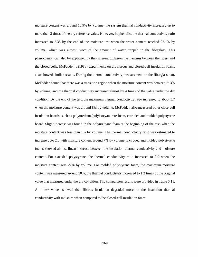
169

moisture content was around 10.9% by volume, the system thermal conductivity increased up to

more than 3 times of the dry reference value. However, in phenolic, the thermal conductivity ratio

increased to 2.35 by the end of the moisture test when the water content reached 22.1% by

volume, which was almost twice of the amount of water trapped in the fiberglass. This

phenomenon can also be explained by the different diffusion mechanisms between the fibers and

the closed cells. McFadden’s (1988) experiments on the fibrous and closed-cell insulation foams

also showed similar results. During the thermal conductivity measurement on the fiberglass batt,

McFadden found that there was a transition region when the moisture content was between 2~3%

by volume, and the thermal conductivity increased almost by 4 times of the value under the dry

condition. By the end of the test, the maximum thermal conductivity ratio increased to about 3.7

when the moisture content was around 8% by volume. McFadden also measured other close-cell

insulation boards, such as polyurethane/polyisocyanurate foam, extruded and molded polystyrene

board. Slight increase was found in the polyurethane foam at the beginning of the test, when the

moisture content was less than 1% by volume. The thermal conductivity ratio was estimated to

increase upto 2.3 with moisture content around 7% by volume. Extruded and molded polystyrene

foams showed almost linear increase between the insulation thermal conductivity and moisture

content. For extruded polystyrene, the thermal conductivity ratio increased to 2.0 when the

moisture content was 22% by volume. For molded polystyrene foam, the maximum moisture

content was measured around 10%, the thermal conductivity increased to 1.2 times of the original

value that measured under the dry condition. The comparison results were provided in Table 5.11.

All these values showed that fibrous insulation degraded more on the insulation thermal

conductivity with moisture when compared to the closed-cell insulation foam.

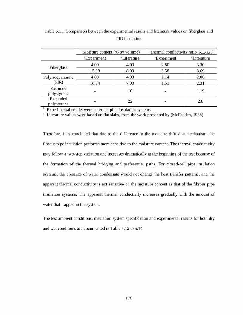
170

Table 5.11: Comparison between the experimental results and literature values on fiberglass and

PIR insulation

Moisture content (% by volume) Thermal conductivity ratio (kwet/kdry) 1Experiment

2Literature

1Experiment

2Literature

Fiberglass 4.00 4.00 2.80 3.30

15.08 8.00 3.58 3.69

Polyisocyanurate

(PIR)

4.00 4.00 1.14 2.06

16.04 7.00 1.51 2.31

Extruded

polystyrene - 10 - 1.19

Expanded

polystyrene - 22 - 2.0

1: Experimental results were based on pipe insulation systems

2: Literature values were based on flat slabs, from the work presented by (McFadden, 1988)

Therefore, it is concluded that due to the difference in the moisture diffusion mechanism, the

fibrous pipe insulation performs more sensitive to the moisture content. The thermal conductivity

may follow a two-step variation and increases dramatically at the beginning of the test because of

the formation of the thermal bridging and preferential paths. For closed-cell pipe insulation

systems, the presence of water condensate would not change the heat transfer patterns, and the

apparent thermal conductivity is not sensitive on the moisture content as that of the fibrous pipe

insulation systems. The apparent thermal conductivity increases gradually with the amount of

water that trapped in the system.

The test ambient conditions, insulation system specification and experimental results for both dry

and wet conditions are documented in Table 5.12 to 5.14.

171

Table 5.12: Summary of the test conditions and experimental results on fiberglass pipe insulation systems under both dry and moisture conditions

Insulation Systems

Fiberglass

Ref No. Units P1-FG P2-FG1 P2-FG2 P2-FG3 P2-FG4 P2-FG5A P2-FG5B

Density kg/m

3

(lbm/ft3)

70 (4.4) 70 (4.4) 56 (3.5) 56 (3.5) 56 (3.5) 70 (4.4) 70 (4.4)

Nominal Wall

Thickness in (mm)

*2 (50.8) 2 (50.8) 1 1/2 (38.1) 1 1/2 (38.1) 1 1/2 (38.1) 2 (50.8) 2 (50.8)

Actual Diameter in (mm) 7.5(190.5)* 7.6 (193.0) 6.7 (170.2) 6.8 (172.7) 6.6 (167.6) 7.6 (193.0) 7.7 (195.6)

Test Pipe

(bare or black) - bare bare bare bare

bare

w/ Al tape bare black

Insulation joint1 - N/A N/A N/A N/A 1 N/A N/A

Joint Sealant - N/A N/A N/A N/A N/A N/A N/A

Edge Seal -

Foster 90-66

and

Foster 30-80

Foster 90-66 Foster 90-66 Foster 90-66 Chil-Perm

CP-30

Chil-Perm

CP-30

Chil-Perm

CP-30

Vapor retarder - N/A N/A ASJ ASJ and PVC

jacketing ASJ N/A N/A

Calibration Method

on keff 2

- 1 2 2 2 2 2 2

Dry test Condition

Ambient Temp ˚F ( ˚C ) 77.2 ~ 110.8

(25.1 ~ 43.8)

75.5 ~ 99.1

(24.2 ~ 37.3)

77.1 ~ 107.2

(25.1 ~ 41.8)

77.0 ~ 106.2

(25 ~ 41.2)

77.0 ~ 101.5

(25 ~ 38.6)

76.9 ~ 101.8

(24.9 ~ 38.8

76.9 ~ 96.3

(24.9 ~ 35.7)

Test Pipe Temp ˚F ( ˚C ) 40.9 (4.9) 36.7 (2.6) 37.7 (3.2) 37.7 (3.2) 40.7 (4.8) 39.5 (4.2) 35.1 (1.7)

Relative Humidity

20.6 ~ 14.2 11.2 ~ 7.0 21.1 ~ 5.8 21.1 ~ 5.8 15.6 ~ 7.3 15.6 ~ 7.3 14.7 ~ 8.0

Dew Point Temp ˚F ( ˚C ) 33.8 ~ 51.2

(1.0 ~ 10.7)

19.4 ~ 25.2

(-7 ~ -3.8)

26.4 ~ 34.3

(-3.1 ~ 1.3)

25.7 ~ 34.1

(-3.5 ~ 1.2)

27.4 ~ 27.7

(-2.6 ~ -2.4)

27.4 ~ 27.9

(-2.6 ~ -2.3)

26.1 ~ 26.3

(-3.3 ~ -3.2)

172

1: Numbers of insulation butt joints in the 3-ft (0.9 m) test section;

2: Calibration under one ambient temperature (1); Calibration under different ambient temperatures (2);

3: Pipe insulation system thermal conductivity kpipe,insulation = a T + b

*: Actual diameter is not available, use nominal diameter instead.

Table 5.12 (Continued): Summary of the test conditions and experimental results on fiberglass pipe insulation systems under both dry and moisture

conditions

Insulation Systems Fiberglass

Ref No. Units P1-FG P2-FG1 P2-FG2 P2-FG3 P2-FG4 P2-FG5A P2-FG5B

Dry Test Results

a3 -

0.0016

(0.00041)

0.0016

(0.00041)

0.0010

(0.00026)

0.0005

(0.00013)

0.0002

(0.00005)

0.0002

(0.00006)

0.0005

(0.00012)

b3 -

0.1475

(0.0286)

0.1475

(0.0286)

0.1918

(0.0323)

0.2156

(0.0334)

0.2322

(0.0344)

0.2511

(0.0373)

0.2184

(0.0336)

Heat Flux Btu/hr-ft

(W/m)

8.44

(8.12)

8.44

(8.12)

10.68

(10.27)

10.03

(9.64)

9.4

(9.04)

8.63

(8.30)

8.31

(7.99)

Uncertainty % 5.8 5.8 4.9 5.1 5.4 5.7 5.8

Wet Test Condition

Ambient Temp ˚F ( ˚C ) 107.6 (42.0) N/A N/A N/A 78.1 (25.6) 78.1 (25.6) 90.1 (32.3)

Test Pipe Temp ˚F ( ˚C ) 41.6 (5.33) N/A N/A N/A 38.4 (3.6) 40.6 (4.8) 41.9 (5.5)

Relative Humidity % 81 N/A N/A N/A 54.8 54.8 84

Dew Point ˚F ( ˚C ) 100.4 (38.0) N/A N/A N/A 60.6 (15.9) 60.6 (15.9) 84.6 (29.2)

Test Length Days 12 N/A N/A N/A 55 55 54

Wet Test Results

Thermal Conductivity

Ratio - 3.15 N/A N/A N/A 1.02 1.49 1.16

Moisture Content % by

volume 10.93 N/A N/A N/A 0.26 1.66 15.08

173

Table 5.13 Summary of the test conditions and experimental results on closed-cell pipe insulation systems under both dry and moisture conditions

(Part I)

Insulation Systems

Phenolic Elastomeric Rubber

Ref No. Units P1-P1 P1-P2 P2-P P1-ER P2-ER1 P2-ER2

Density kg/m

3

(lbm/ft3)

37 37 37 50 40 40

Nominal Wall

Thickness in (mm) 1 (25.4) 2 (50.8) 2 (50.8) 2 (50.8) 1 1/2 (38.1) 2 (50.8)

Actual Diameter in (mm) *5.5 (139.7)

*7.5 (190.5) 7.7 (195.6)

*7.5 (190.5) 6.8 (172.7) 7.7 (195.6)

Test Pipe

(bare or black) - bare bare bare bare bare bare

Insulation joint1 - N/A N/A N/A N/A N/A N/A

Joint Sealant - Boss 368 Boss 368 Chil-Joint CP-70 Aeroseal

Self-adhesive

Tape and

Aeroseal

Self-adhesive

Tape and

Aeroseal

Edge Seal - Boss 368 Foster 90-66 and

Foster 30-80 Chil-Joint CP-70 Aeroseal Aeroseal Aeroseal

Vapor retarder - N/A N/A N/A N/A N/A N/A

Calibration Method

on keff 2

- 1 1 2 1 2 2

Dry test Condition

Ambient Temp ˚F ( ˚C ) 75.6 ~ 101.8

(24.2 ~ 38.8)

80 ~ 110

(26.7 ~ 43.3) N/A

77.3 ~ 110.1

(25.2 ~ 43.4)

75.5 ~ 96.9

(24.2 ~ 36.1)

74.9 ~ 97.2

(23.8 ~ 36.2)

Test Pipe Temp ˚F ( ˚C ) 40.3 (4.6) 40.4 (4.7) N/A 40.7 (4.8) 38.3 (3.5) 36.6 (2.6)

Relative Humidity

19.1 ~ 13.9 17.7 ~ 14.9 N/A 18.3 ~ 14.0 11.2 ~ 7 11.2 ~ 7

Dew Point Temp ˚F ( ˚C ) 36.5 ~ 43.6

(2.5 ~ 6.4)

32.3 ~ 51.8

(0.15 ~ 11.1) N/A

31.1 ~ 50.2

(-0.5 ~ 10.1)

19.4 ~ 23.8

(-7.1 ~ -4.5)

19.0 ~ 24.0

(-7.2 ~ -4.4)

174

Table 5.13 (Continued): Summary of the test conditions and experimental results on closed-cell pipe insulation systems under both dry and

moisture conditions (Part I)

Insulation Systems Phenolic Elastomeric Rubber

Ref No. Units P1-P1 P1-P2 P2-P P1-ER P2-ER1 P2-ER2

Dry Test Results N/A

a3 -

0.0007

(0.00018)

0.0012

(0.00032) N/A

0.0005

(0.00014)

0.0010

(0.00025)

0.0010

(0.00027)

b3 - 0.1821 (0.0297) 0.1217 (0.0233) N/A 0.2144 (0.0334) 0.2112 (0.0350) 0.1913 (0.0323)

Heat Flux Btu/hr-ft 13.20 7.13 N/A 8.38 10.40 8.45

W/m 12.69 6.86 N/A 8.06 10.00 8.13

Uncertainty % 4.3 6.5 N/A 5.8 5.0 5.8

Wet Test Condition

Ambient Temp ˚F ( ˚C ) N/A 96.4 (35.8) 107.7 (42.0) N/A 90.6 (32.6) N/A

Test Pipe Temp ˚F ( ˚C ) N/A 40.7 (4.9) 40.7 (4.9) N/A 36.8 (2.7) N/A

Relative Humidity % N/A 87.1 82 N/A 83 N/A

Dew Point ˚F ( ˚C ) N/A 91.9 (33.3) 100.9 (38.3) N/A 84.7 (29.3) N/A

Test Length Days N/A 24 45 N/A 57 N/A

Wet Test Results

Thermal

Conductivity Ratio - N/A 1.57 2.35 N/A 1.02 N/A

Moisture Content % by

volume N/A 4.87 22.1 N/A 0.34 N/A

1: Numbers of insulation butt joints in the 3-ft (0.9 m) test section;

2: Calibration under one ambient temperature (1); Calibration under different ambient temperatures (2);

3: Pipe insulation system thermal conductivity kpipe,insulation = a T + b

*: Actual diameter is not available, use nominal diameter instead.

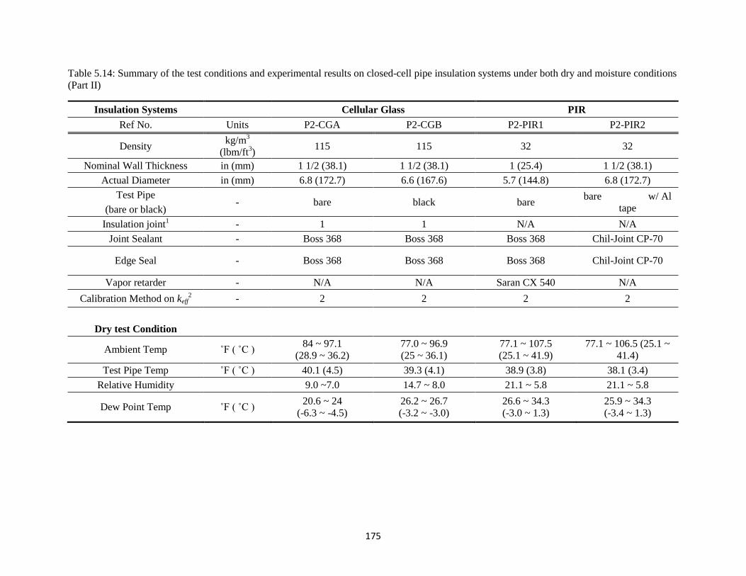
175

Table 5.14: Summary of the test conditions and experimental results on closed-cell pipe insulation systems under both dry and moisture conditions

(Part II)

Insulation Systems Cellular Glass PIR

Ref No. Units P2-CGA P2-CGB P2-PIR1 P2-PIR2

Density kg/m

3

(lbm/ft3)

115 115 32 32

Nominal Wall Thickness in (mm) 1 1/2 (38.1) 1 1/2 (38.1) 1 (25.4) 1 1/2 (38.1)

Actual Diameter in (mm) 6.8 (172.7) 6.6 (167.6) 5.7 (144.8) 6.8 (172.7)

Test Pipe - bare black bare

bare w/ Al

tape (bare or black)

Insulation joint1 - 1 1 N/A N/A

Joint Sealant - Boss 368 Boss 368 Boss 368 Chil-Joint CP-70

Edge Seal - Boss 368 Boss 368 Boss 368 Chil-Joint CP-70

Vapor retarder - N/A N/A Saran CX 540 N/A

Calibration Method on keff2 - 2 2 2 2

Dry test Condition

Ambient Temp ˚F ( ˚C ) 84 ~ 97.1

(28.9 ~ 36.2)

77.0 ~ 96.9

(25 ~ 36.1)

77.1 ~ 107.5

(25.1 ~ 41.9)

77.1 ~ 106.5 (25.1 ~

41.4)

Test Pipe Temp ˚F ( ˚C ) 40.1 (4.5) 39.3 (4.1) 38.9 (3.8) 38.1 (3.4)

Relative Humidity 9.0 ~7.0 14.7 ~ 8.0 21.1 ~ 5.8 21.1 ~ 5.8

Dew Point Temp ˚F ( ˚C ) 20.6 ~ 24

(-6.3 ~ -4.5)

26.2 ~ 26.7

(-3.2 ~ -3.0)

26.6 ~ 34.3

(-3.0 ~ 1.3)

25.9 ~ 34.3

(-3.4 ~ 1.3)

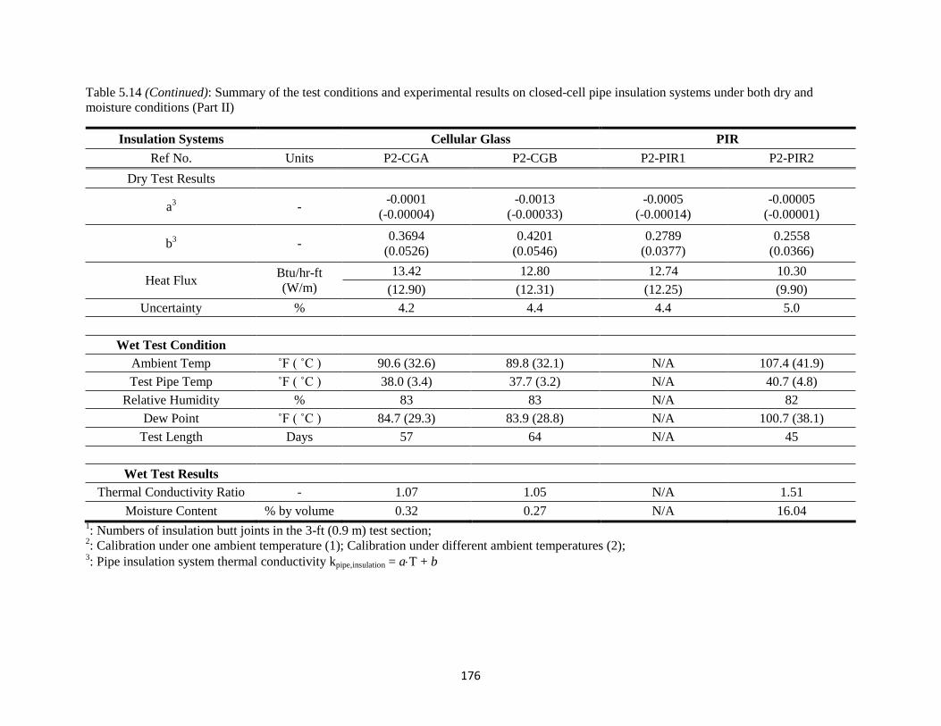
176

Table 5.14 (Continued): Summary of the test conditions and experimental results on closed-cell pipe insulation systems under both dry and

moisture conditions (Part II)

Insulation Systems

Cellular Glass PIR

Ref No. Units P2-CGA P2-CGB P2-PIR1 P2-PIR2

Dry Test Results

a3 -

-0.0001

(-0.00004)

-0.0013

(-0.00033)

-0.0005

(-0.00014)

-0.00005

(-0.00001)

b3 -

0.3694

(0.0526)

0.4201

(0.0546)

0.2789

(0.0377)

0.2558

(0.0366)

Heat Flux Btu/hr-ft

(W/m)

13.42 12.80 12.74 10.30

(12.90) (12.31) (12.25) (9.90)

Uncertainty % 4.2 4.4 4.4 5.0

Wet Test Condition

Ambient Temp ˚F ( ˚C ) 90.6 (32.6) 89.8 (32.1) N/A 107.4 (41.9)

Test Pipe Temp ˚F ( ˚C ) 38.0 (3.4) 37.7 (3.2) N/A 40.7 (4.8)

Relative Humidity % 83 83 N/A 82

Dew Point ˚F ( ˚C ) 84.7 (29.3) 83.9 (28.8) N/A 100.7 (38.1)

Test Length Days 57 64 N/A 45

Wet Test Results

Thermal Conductivity Ratio - 1.07 1.05 N/A 1.51

Moisture Content % by volume 0.32 0.27 N/A 16.04 1: Numbers of insulation butt joints in the 3-ft (0.9 m) test section;

2: Calibration under one ambient temperature (1); Calibration under different ambient temperatures (2);

3: Pipe insulation system thermal conductivity kpipe,insulation = a T + b

177

CHAPTER VI

6. SIMULATION MODEL

6.1 Introduction

In current literature, the common methods for predicting the variation of pipe insulation thermal

conductivity and moisture accumulation are summarized as these three types: (1) curve-fitting

correalations (Abdou & Budaiwi, 2005; Adams, 1974), (2) semi-empirical methods, and (3)

numerical simulation.

Generally, the correlations generated from the experiments are confined to the methodological

conditions. They are case-specific and prone to errors when apply the correlations to a different

ambient conditions, or on the same materials but with different physical properties. Semi-

empirical methods on the other hand are fast and simply to use. Usually these methods start with

analytical model first, and use experimental data set to generate the profile of the coefficients in

the model. These coefficients are normally considered as constant among different cases

according to specific assumptions made in the analytical model. These methods mainly deal with

steady or quasi-steady phase of the heat and mass transfer processes. They are able to give

approximations and can be applied to a wide range of test conditions and different type of test

samples. However, they might be failed to provide detailed information especially through

transient conditions, such as the variation on the local thermal conductivity, and moisture

distribution in the pipe insulation. Numerical simulation is one of the most commonly used

methods for the investigation of transient heat and mass transfer through insulation materials.

178

Computational fluid dynamics (CFD) model will provide a detailed investigation on the thermal

performance of insulation materials during the transfer processes. However, the simulations are

often complex and time consuming. In order to investigate in detail on the moisture diffusion in

different types of pipe insulation systems, a dedicate geometry is required for specific internal

structure of the insulation material. For example, the geometries of fibrous pipe insulation might

need to consist of single fiber, regular arrays of uniform fibers assumed to be parallel with gas

flow. Different diameters and orientation of the fibers may also need to be considered, which will

lead to some difficulties in the determination of appropriate boundary conditions. In order to

provide detailed information on the moisture distribution, a three-dimensional CFD model is very

useful for a complete simulation, but the complex 3-D geometries demand powerful computing

resources and a large amount of time.

In my PhD research work, one of the research objectives is to develop an applicable model that

can be utilized in the field of mechanical engineering for a prediction on the thermal behavior of

pipe insulation systems, and this model should be able to help the mechanical engineers make an

optimization in the design between economy cost and system efficiency. Therefore, the model is

required to be general and applicable to a wide range of insulation systems and materials with

different physical properties. Considering the advantages and disadvantages among these three

approaches, together with the research goals in this study, the semi-empirical methods were

selected, and a lumped model will be discussed in detail in this chapter.

6.2 Literature review of the existing models for insulation thermal conductivity

For porous type of insulation, Luikov (1966) proposed that the apparent thermal conductivity

(kapp) is equal to the summation of the conductive (kcond), convection (kconv) and radiative (krad)

components of thermal conductivity, shown in Equation as follows:

179

( 6.1 )

Bankvall, referred by Batty et al. (1981), proposed four different physical distribution models for

glass fiber insulation: series arrangement, parallel arrangement, bead arrangement, and foam

arrangement. Wijeysundera et al. (1996) agreed that the apparent thermal conductivity of moist

insulation depends on the manner that the liquid distribute in the insulation, and considered the

three patterns be: bead arrangement, series arrangement and parallel arrangement in porous

insulation. However, both researches did not consider a combination of different moisture

distribution patterns. Ochs et al. (2008) developed a model to predict effective thermal

conductivity of moistened porous insulation based on flat slab. The conductive component of the

apparent thermal conductivity was considered as a combination of series and parallel

arrangement, and the radiation effect was considered with pore specifications, while the

convection effect was ignored due to the low Rayleigh number. Based on Equation ( 6.1 ),

Karamanos et al. (2008) developed an analytical model for the impact of temperature and

moisture on the thermal performance of stone wool. By neglecting the small convection term, the

conductive and radiative components of thermal conductivity are still need to be determined from

further specification of the fiber, such as the diameter, density, and orientation factor of the fibers.

Compared to Bankvall’s (Batty et al., 1981) model, Karamanos et al.’s model is not specifying

the shape of fibrous insulation since most of the parameters required for are independent from the

material geometry.

There are also several other analytical methods for computing thermal conductivity under dry and

moist conditions. Mar et al. (2008) considered the heat barrier resistances in the conductive term

of the apparent thermal conductivity. However, the determination for this resistance is so

complicated due to the absence of reliable method for the contact areas between grains, especially

within microcracks, and grain boundaries. Wijeysundera et al. (1993) proposed analytical

solution for the effective thermal conductivity of flat-slab and round-pipe insulations in the

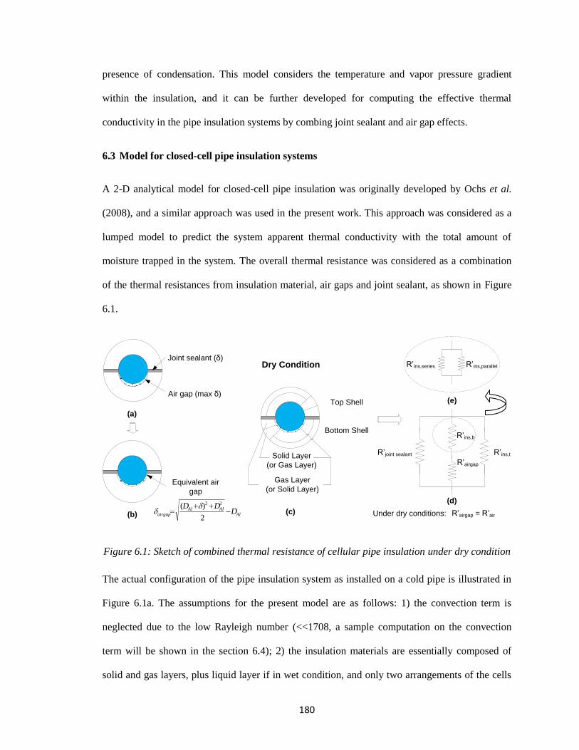
180

presence of condensation. This model considers the temperature and vapor pressure gradient

within the insulation, and it can be further developed for computing the effective thermal

conductivity in the pipe insulation systems by combing joint sealant and air gap effects.

6.3 Model for closed-cell pipe insulation systems

A 2-D analytical model for closed-cell pipe insulation was originally developed by Ochs et al.

(2008), and a similar approach was used in the present work. This approach was considered as a

lumped model to predict the system apparent thermal conductivity with the total amount of

moisture trapped in the system. The overall thermal resistance was considered as a combination

of the thermal resistances from insulation material, air gaps and joint sealant, as shown in Figure

6.1.

Figure 6.1: Sketch of combined thermal resistance of cellular pipe insulation under dry condition

The actual configuration of the pipe insulation system as installed on a cold pipe is illustrated in

Figure 6.1a. The assumptions for the present model are as follows: 1) the convection term is

neglected due to the low Rayleigh number (<<1708, a sample computation on the convection

term will be shown in the section 6.4); 2) the insulation materials are essentially composed of

solid and gas layers, plus liquid layer if in wet condition, and only two arrangements of the cells

R’ins,b

R’joint sealant

R’airgap

R’ins,series R’ins,parallel

R’ins,t

Air gap (max δ)

Joint sealant (δ)

Equivalent air

gap

AlAlAl

airgap DDD

2

)( 22

Solid Layer

(or Gas Layer)

Gas Layer

(or Solid Layer)

Dry Condition

Top Shell

Bottom Shell

Under dry conditions: R’airgap = R’air

(a)

(b) (c)

(d)

(e)

181

are taken into consideration: series and parallel, as shown in Figure 6.1c to e. The arrangement in

Figure 1c, for dry conditions, represents a limiting case for the resistance to the heat flow through

the materials. Under wet conditions, the solid layer remained the same as in dry condition, but the

gas layer is affected by water vapor and condensate and it has to be divided further to include

water layer, moist pores layer and the residual gas layer. Additional underlying assumptions of

the present model are 3) the insulation materials are homogeneous; 4) the fraction of series and

parallel configuration remain constant for the same type of pipe insulation under dry condition;

and 5) the air gap exists only at the interface between the bottom pipe wall surface and the bottom

interior surface of the insulation system and the thickness of the air gap was assumed uniform

within the 180 angle of the bottom shell, as shown in Figure 6.1b. An important parameter a was

introduced in the model, and it represents the volume fraction of the poor conductive layer with

different phases positioned in series configuration, as shown in Figure 6.1c. Therefore, (1-a)

represents the fraction of resistances in parallel. Considering the fact that the value of thermal

resistances in parallel would always be lower that the value of thermal resistance in series,

parameter (1-a) could also be considered as the amount of thermal bridging that existed in the

system. However, the parameter a could not be measured according to the physical procedures.

Based on the above mentioned assumptions, the thermal resistance and thermal conductivity for

the insulation material become as follows:

( 6.2 )

( 6.3 )

where kseries represents the lowest thermal conductivity component of the insulation, while kparallel

represents the maximum. It should be noted that the formulations of kseries and kparallel are different

when the insulation system is considered dry (i.e., no water vapor and condensate) or wet (that is,

water vapor and water condensate present). The sealant on the longitudinal joints behaves as a

182

resistance in parallel to the insulation material and can create a thermal bridge effects based on its

thermal conductivity and sealant thickness. These additional variables due to the presence of joint

sealant and air gaps in cylindrical insulation configuration are considered in the present model for

the first time.

In dry conditions, the combined thermal resistance and the overall thermal conductivity of the

pipe insulation system are expressed by the thermal resistance of the join sealant, R’joint,sealant, the

thermal resistance of the top shell of insulation, R’ins,t, the thermal resistance of the bottom shell

of insulation, R’ins,b, and the thermal resistance from the air gap, R’airgap:

( 6.4 )

Where

( 6.5 )

( 6.6 )

( 6.7 )

( 6.8 )

And in terms of thermal conductivity, Eq. ( 6.4 ) yields to

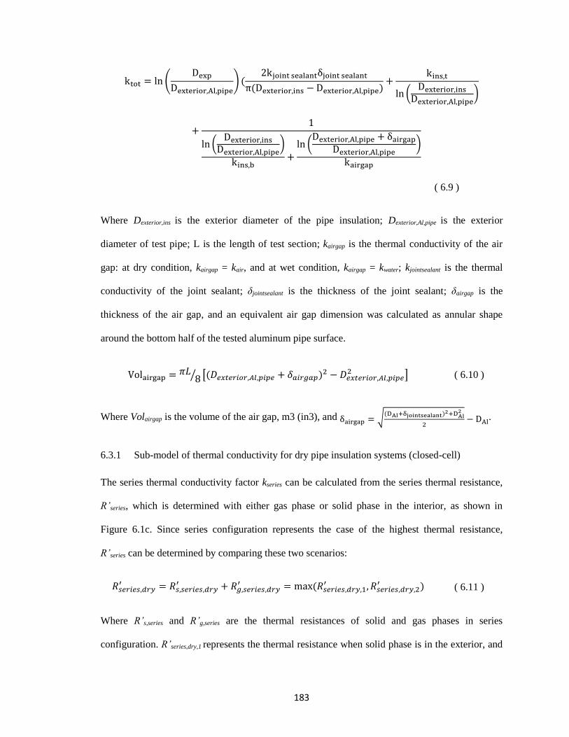
183

(

)

(

)

(

)

(

)

( 6.9 )

Where Dexterior,ins is the exterior diameter of the pipe insulation; Dexterior,Al,pipe is the exterior

diameter of test pipe; L is the length of test section; kairgap is the thermal conductivity of the air

gap: at dry condition, kairgap = kair, and at wet condition, kairgap = kwater; kjointsealant is the thermal

conductivity of the joint sealant; δjointsealant is the thickness of the joint sealant; δairgap is the

thickness of the air gap, and an equivalent air gap dimension was calculated as annular shape

around the bottom half of the tested aluminum pipe surface.

⁄ [

] ( 6.10 )

Where Volairgap is the volume of the air gap, m3 (in3), and √

.

6.3.1 Sub-model of thermal conductivity for dry pipe insulation systems (closed-cell)

The series thermal conductivity factor kseries can be calculated from the series thermal resistance,

R’series, which is determined with either gas phase or solid phase in the interior, as shown in

Figure 6.1c. Since series configuration represents the case of the highest thermal resistance,

R’series can be determined by comparing these two scenarios:

( 6.11 )

Where R’s,series and R’g,series are the thermal resistances of solid and gas phases in series

configuration. R’series,dry,1 represents the thermal resistance when solid phase is in the exterior, and

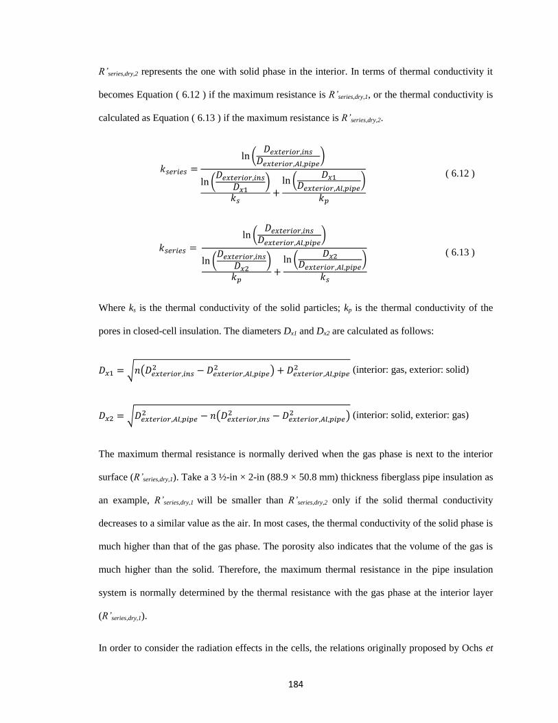
184

R’series,dry,2 represents the one with solid phase in the interior. In terms of thermal conductivity it

becomes Equation ( 6.12 ) if the maximum resistance is R’series,dry,1, or the thermal conductivity is

calculated as Equation ( 6.13 ) if the maximum resistance is R’series,dry,2.

(

)

(

)

(

)

( 6.12 )

(

)

(

)

(

)

( 6.13 )

Where ks is the thermal conductivity of the solid particles; kp is the thermal conductivity of the

pores in closed-cell insulation. The diameters Dx1 and Dx2 are calculated as follows:

√ (

) (interior: gas, exterior: solid)

√ (

) (interior: solid, exterior: gas)

The maximum thermal resistance is normally derived when the gas phase is next to the interior

surface (R’series,dry,1). Take a 3 ½-in × 2-in (88.9 × 50.8 mm) thickness fiberglass pipe insulation as

an example, R’series,dry,1 will be smaller than R’series,dry,2 only if the solid thermal conductivity

decreases to a similar value as the air. In most cases, the thermal conductivity of the solid phase is

much higher than that of the gas phase. The porosity also indicates that the volume of the gas is

much higher than the solid. Therefore, the maximum thermal resistance in the pipe insulation

system is normally determined by the thermal resistance with the gas phase at the interior layer

(R’series,dry,1).

In order to consider the radiation effects in the cells, the relations originally proposed by Ochs et

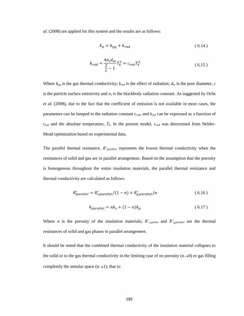
185

al. (2008) are applied for this system and the results are as follows:

( 6.14 )

( 6.15 )

Where kpg is the gas thermal conductivity; krad is the effect of radiation; dm is the pore diameter, ɛ

is the particle surface emissivity and σs is the blackbody radiation constant. As suggested by Ochs

et al. (2008), due to the fact that the coefficient of emission is not available in most cases, the

parameters can be lumped to the radiation constant crad, and krad can be expressed as a function of

crad and the absolute temperature, Tk. In the present model, crad was determined from Nelder-

Mead optimization based on experimental data.

The parallel thermal resistance, R’parallel, represents the lowest thermal conductivity when the

resistances of solid and gas are in parallel arrangement. Based on the assumption that the porosity

is homogenous throughout the entire insulation materials, the parallel thermal resistance and

thermal conductivity are calculated as follows:

( 6.16 )

( 6.17 )

Where n is the porosity of the insulation materials; R’s,parllel and R’g,parallel are the thermal

resistances of solid and gas phases in parallel arrangement.

It should be noted that the combined thermal conductivity of the insulation material collapses to

the solid or to the gas thermal conductivity in the limiting case of no porosity (n0) or gas filling

completely the annular space (n1), that is:

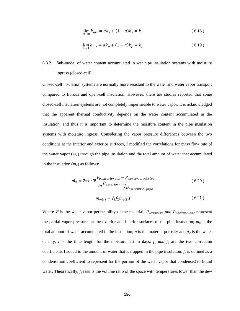
186

( 6.18 )

( 6.19 )

6.3.2 Sub-model of water content accumulated in wet pipe insulation systems with moisture

ingress (closed-cell)

Closed-cell insulation systems are normally more resistant to the water and water vapor transport

compared to fibrous and open-cell insulation. However, there are studies reported that some

closed-cell insulation systems are not completely impermeable to water vapor. It is acknowledged

that the apparent thermal conductivity depends on the water content accumulated in the

insulation, and thus it is important to determine the moisture content in the pipe insulation

systems with moisture ingress. Considering the vapor pressure differences between the two

conditions at the interior and exterior surfaces, I modified the correlations for mass flow rate of

the water vapor ( ) through the pipe insulation and the total amount of water that accumulated

in the insulation (mw) as follows:

⁄

( 6.20 )

( 6.21 )

Where Ῥ is the water vapor permeability of the material; Pv,exterior,ins and Pv,exterior,Al,pipe represent

the partial vapor pressures at the exterior and interior surfaces of the pipe insulation; mw is the

total amount of water accumulated in the insulation; n is the material porosity and ρw is the water

density; t is the time length for the moisture test in days. f1 and f2 are the two correction

coefficients I added to the amount of water that is trapped in the pipe insulation. f1 is defined as a

condensation coefficient to represent for the portion of the water vapor that condensed to liquid

water. Theoretically, f1 results the volume ratio of the space with temperatures lower than the dew

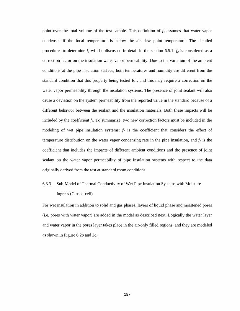
187

point over the total volume of the test sample. This definition of f1 assumes that water vapor

condenses if the local temperature is below the air dew point temperature. The detailed

procedures to determine f1 will be discussed in detail in the section 6.5.1. f2 is considered as a

correction factor on the insulation water vapor permeability. Due to the variation of the ambient

conditions at the pipe insulation surface, both temperatures and humidity are different from the

standard condition that this property being tested for, and this may require a correction on the

water vapor permeability through the insulation systems. The presence of joint sealant will also

cause a deviation on the system permeability from the reported value in the standard because of a

different behavior between the sealant and the insulation materials. Both these impacts will be

included by the coefficient f2. To summarize, two new correction factors must be included in the

modeling of wet pipe insulation systems: f1 is the coefficient that considers the effect of

temperature distribution on the water vapor condensing rate in the pipe insulation, and f2 is the

coefficient that includes the impacts of different ambient conditions and the presence of joint

sealant on the water vapor permeability of pipe insulation systems with respect to the data

originally derived from the test at standard room conditions.

6.3.3 Sub-Model of Thermal Conductivity of Wet Pipe Insulation Systems with Moisture

Ingress (Closed-cell)

For wet insulation in addition to solid and gas phases, layers of liquid phase and moistened pores

(i.e. pores with water vapor) are added in the model as described next. Logically the water layer

and water vapor in the pores layer takes place in the air-only filled regions, and they are modeled

as shown in Figure 6.2b and 2c.

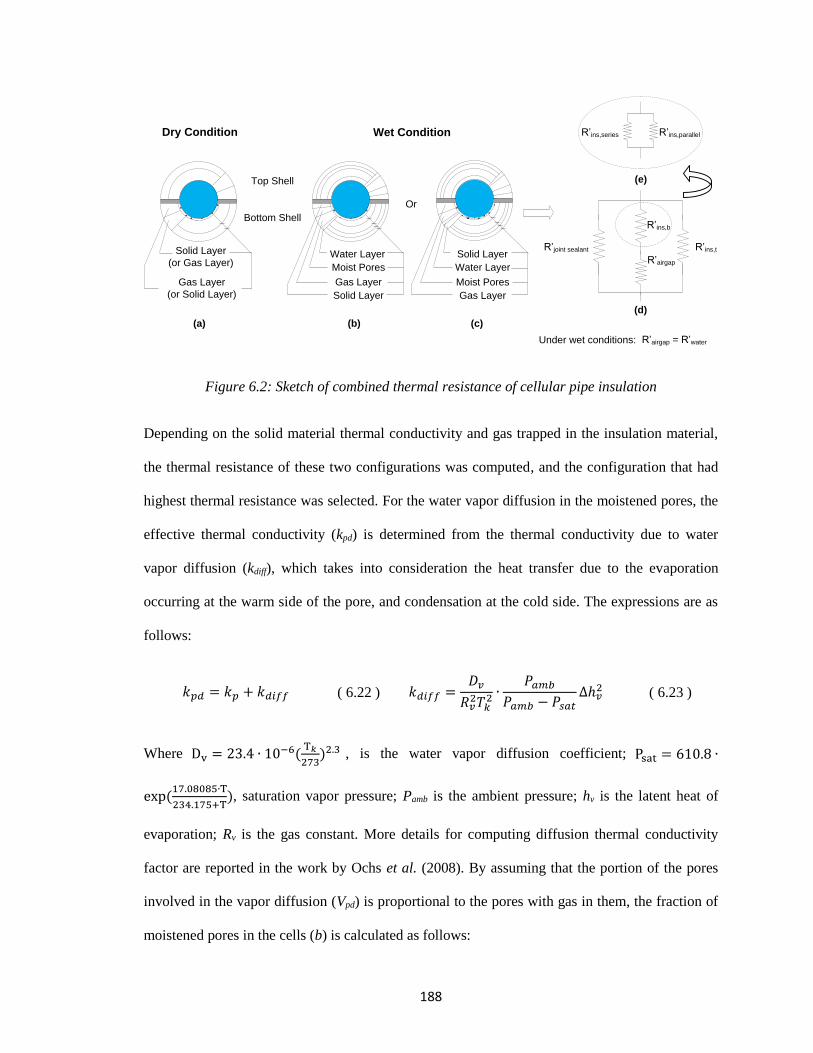
188

Figure 6.2: Sketch of combined thermal resistance of cellular pipe insulation

Depending on the solid material thermal conductivity and gas trapped in the insulation material,

the thermal resistance of these two configurations was computed, and the configuration that had

highest thermal resistance was selected. For the water vapor diffusion in the moistened pores, the

effective thermal conductivity (kpd) is determined from the thermal conductivity due to water

vapor diffusion (kdiff), which takes into consideration the heat transfer due to the evaporation

occurring at the warm side of the pore, and condensation at the cold side. The expressions are as

follows:

( 6.22 )

( 6.23 )

Where

, is the water vapor diffusion coefficient;

, saturation vapor pressure; Pamb is the ambient pressure; hv is the latent heat of

evaporation; Rv is the gas constant. More details for computing diffusion thermal conductivity

factor are reported in the work by Ochs et al. (2008). By assuming that the portion of the pores

involved in the vapor diffusion (Vpd) is proportional to the pores with gas in them, the fraction of

moistened pores in the cells (b) is calculated as follows:

Water Layer

Moist Pores

Gas Layer

Solid Layer

R’ins,b

R’joint sealant

R’airgap

R’ins,series R’ins,parallel

R’ins,tSolid Layer

(or Gas Layer)

Gas Layer

(or Solid Layer)

Dry Condition Wet Condition

Top Shell

Bottom Shell

Under wet conditions: R’airgap = R’water

Solid Layer

Water Layer

Moist Pores

Gas Layer

Or

(a) (b)

(d)

(e)

(c)

189

( 6.24 )

⁄

( 6.25 )

Where Vw is the volume fraction of water per volume of the test sample; Vpd is the volume

fraction of the cells involved with the vapor diffusion per volume of the test sample; and Vfs is the

volume fraction of water condensate in free saturation conditions per volume of the test sample.

The series thermal resistance (R’serial,wet) was calculated from equation ( 6.11 ) to ( 6.13 ) by

adding water and pore diffusion layers.

( 6.26 )

The parallel thermal resistance (R’parallel,wet) was calculated as follow:

( 6.27 )

And, in terms of overall apparent thermal conductivity of the wet pipe insulation systems

(kparallel,wet) results:

( 6.28 )

Based on the experimental observation that moisture content of the bottom shells was typically

higher than the moisture content measured on the top C-shell, the equations ( 6.11 ) to ( 6.28 )

were solved independently for the half shells at the top and bottom, yielding to two values of the

apparent thermal resistance R’series,wet,t and R’series,wet,b, respectively.

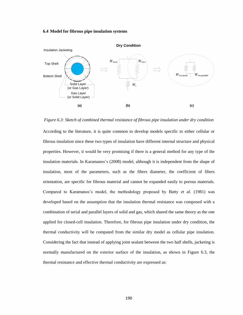
190

6.4 Model for fibrous pipe insulation systems

Figure 6.3: Sketch of combined thermal resistance of fibrous pipe insulation under dry condition

According to the literature, it is quite common to develop models specific to either cellular or

fibrous insulation since these two types of insulation have different internal structure and physical

properties. However, it would be very promising if there is a general method for any type of the

insulation materials. In Karamanos’s (2008) model, although it is independent from the shape of

insulation, most of the parameters, such as the fibers diameter, the coefficient of fibers

orientation, are specific for fibrous material and cannot be expanded easily to porous materials.

Compared to Karamanos’s model, the methodology proposed by Batty et al. (1981) was

developed based on the assumption that the insulation thermal resistance was composed with a

combination of serial and parallel layers of solid and gas, which shared the same theory as the one

applied for closed-cell insulation. Therefore, for fibrous pipe insulation under dry condition, the

thermal conductivity will be computed from the similar dry model as cellular pipe insulation.

Considering the fact that instead of applying joint sealant between the two half shells, jacketing is

normally manufactured on the exterior surface of the insulation, as shown in Figure 6.3, the

thermal resistance and effective thermal conductivity are expressed as:

R’ins,b

R’ins,serial R’ins,parallel

R’ins,t

Solid Layer

(or Gas Layer)

Gas Layer

(or Solid Layer)

Dry Condition

Top Shell

Bottom Shell

R’j

Insulation Jacketing

(a) (b) (c)

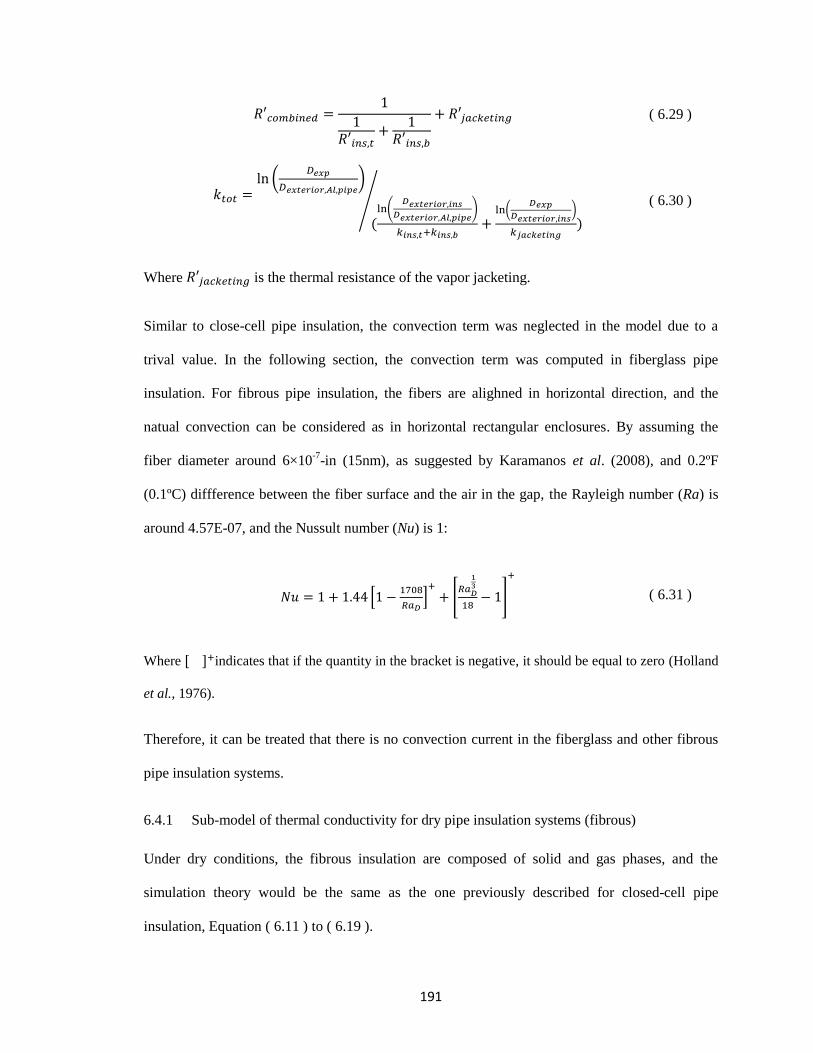
191

( 6.29 )

(

)

(

)

(

)

⁄

( 6.30 )

Where is the thermal resistance of the vapor jacketing.

Similar to close-cell pipe insulation, the convection term was neglected in the model due to a

trival value. In the following section, the convection term was computed in fiberglass pipe

insulation. For fibrous pipe insulation, the fibers are alighned in horizontal direction, and the

natual convection can be considered as in horizontal rectangular enclosures. By assuming the

fiber diameter around 6×10-7

-in (15nm), as suggested by Karamanos et al. (2008), and 0.2ºF

(0.1ºC) diffference between the fiber surface and the air in the gap, the Rayleigh number (Ra) is

around 4.57E-07, and the Nussult number (Nu) is 1:

[

] [

]

( 6.31 )

Where [ ] indicates that if the quantity in the bracket is negative, it should be equal to zero (Holland

et al., 1976).

Therefore, it can be treated that there is no convection current in the fiberglass and other fibrous

pipe insulation systems.

6.4.1 Sub-model of thermal conductivity for dry pipe insulation systems (fibrous)

Under dry conditions, the fibrous insulation are composed of solid and gas phases, and the

simulation theory would be the same as the one previously described for closed-cell pipe

insulation, Equation ( 6.11 ) to ( 6.19 ).

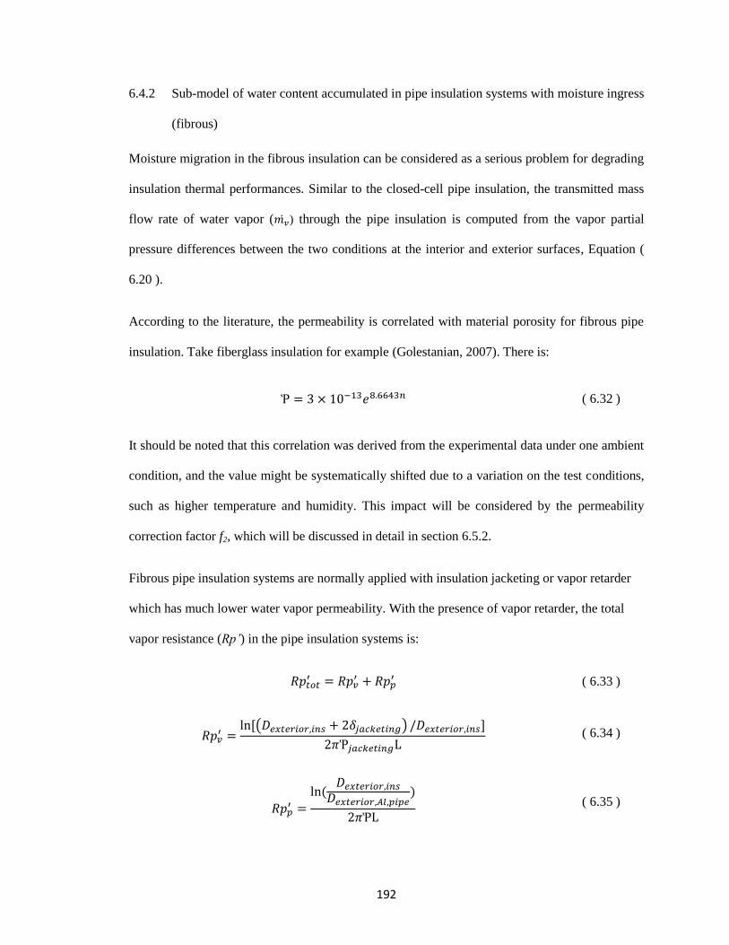
192

6.4.2 Sub-model of water content accumulated in pipe insulation systems with moisture ingress

(fibrous)

Moisture migration in the fibrous insulation can be considered as a serious problem for degrading

insulation thermal performances. Similar to the closed-cell pipe insulation, the transmitted mass

flow rate of water vapor ( ) through the pipe insulation is computed from the vapor partial

pressure differences between the two conditions at the interior and exterior surfaces, Equation (

6.20 ).

According to the literature, the permeability is correlated with material porosity for fibrous pipe

insulation. Take fiberglass insulation for example (Golestanian, 2007). There is:

( 6.32 )

It should be noted that this correlation was derived from the experimental data under one ambient

condition, and the value might be systematically shifted due to a variation on the test conditions,

such as higher temperature and humidity. This impact will be considered by the permeability

correction factor f2, which will be discussed in detail in section 6.5.2.

Fibrous pipe insulation systems are normally applied with insulation jacketing or vapor retarder

which has much lower water vapor permeability. With the presence of vapor retarder, the total

vapor resistance (Rp’) in the pipe insulation systems is:

( 6.33 )

[( ) ]

( 6.34 )

( 6.35 )

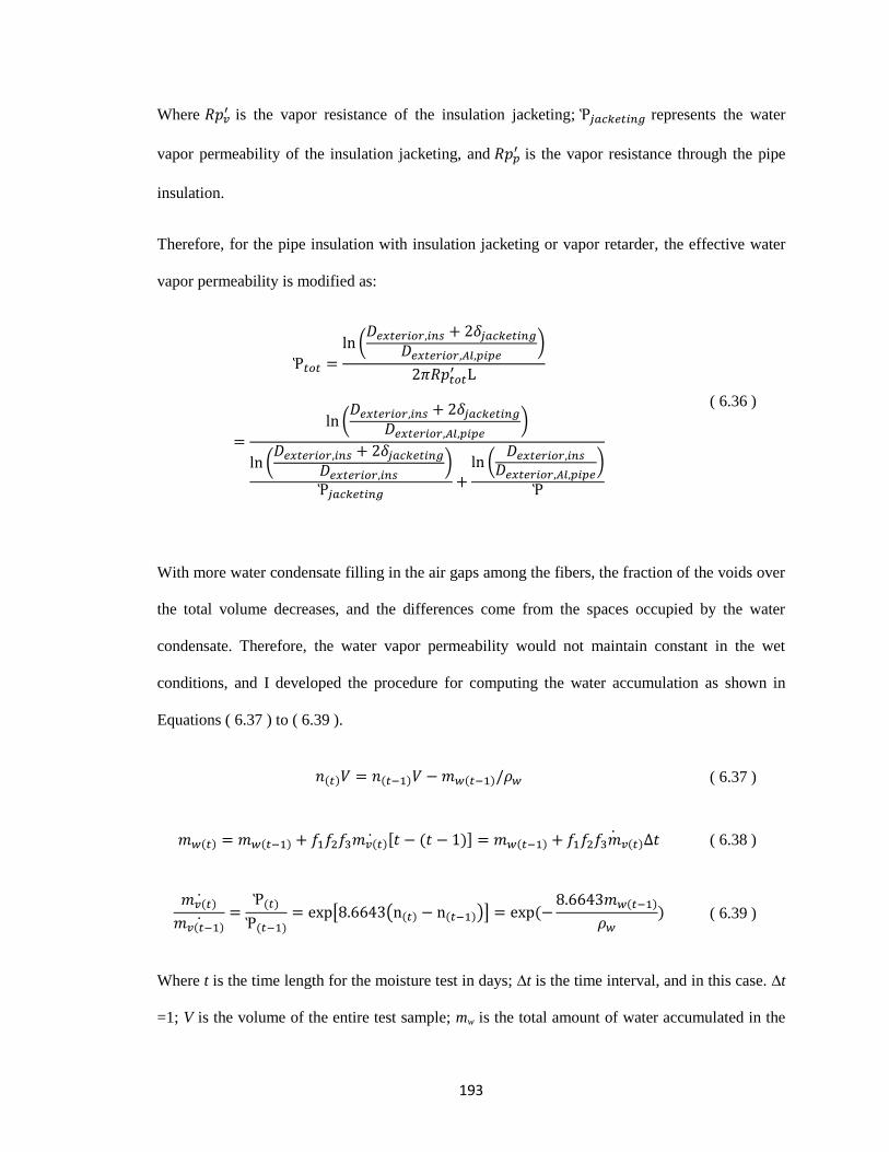
193

Where is the vapor resistance of the insulation jacketing; represents the water

vapor permeability of the insulation jacketing, and is the vapor resistance through the pipe

insulation.

Therefore, for the pipe insulation with insulation jacketing or vapor retarder, the effective water

vapor permeability is modified as:

(

)

(

)

(

)

(

)

( 6.36 )

With more water condensate filling in the air gaps among the fibers, the fraction of the voids over

the total volume decreases, and the differences come from the spaces occupied by the water

condensate. Therefore, the water vapor permeability would not maintain constant in the wet

conditions, and I developed the procedure for computing the water accumulation as shown in

Equations ( 6.37 ) to ( 6.39 ).

( 6.37 )

[ ] ( 6.38 )

[ ( )]

( 6.39 )

Where t is the time length for the moisture test in days; ∆t is the time interval, and in this case. ∆t

=1; V is the volume of the entire test sample; mw is the total amount of water accumulated in the

194

insulation; n is the material porosity and ρw is the water density. Similar to closed-cell pipe

insulation systems, f1 and f2 are the two coefficients that will modify the amount of water trapped

in the pipe insulation. f1 is the condensation coefficient that represents for the portion of the water

vapor condensed to liquid water, and f2 is the correction factor on the water vapor permeability

due to different ambient conditions and installation method. In fibrous pipe insulation, correction

factor f2 is assumed to be 1, which will be explained in the section 6.5.2. Another coefficient, f3, is

defined as water retention factor and represents the portion of water condensate that will remain

trapped in the pipe insulation. Due to the presence of preferential paths, a small amount of water

condensate drips out of the insulation. Although the total amount is small, it is non-negligible

when compared to the closed-cell pipe insulation, and should not be counted in as the moisture

content remained in the insulation. However, till now there is not enough data to provide a

correlation to predict how the ambient conditions affect the water dripping rate out of the pipe

insulation. The coefficient f3 is derived based on the experimental data from one specific case and

assumed to be constant among the same material in fibrous pipe insulation systems. For closed-

cell pipe insulation, very few amount of water drips out from the insulation because of its low

water absorption and the compact gas-filled cellular structure. The portion of water trapped in the

insulation is almost the same as the total amount of water condensed in the insulation materials,

and this coefficient does not need to be considered in the modeling.

Based on the iterations among equations ( 6.37 ) to ( 6.39 ), the mass flow rate of water vapor

transmitted into the insulation can be updated with a varied water vapor permeability, and the

profile of the water amount accumulated in the insulation can be predicted from the days being

tested for. The procedures for computing the water content in fiberglass test samples are

summarized in detail in the flow chart shown in Figure 6.4.

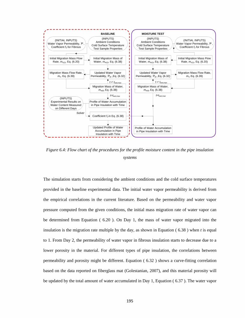
195

Figure 6.4: Flow chart of the procedures for the profile moisture content in the pipe insulation

systems

The simulation starts from considering the ambient conditions and the cold surface temperatures

provided in the baseline experimental data. The initial water vapor permeability is derived from

the empirical correlations in the current literature. Based on the permeability and water vapor

pressure computed from the given conditions, the initial mass migration rate of water vapor can

be determined from Equation ( 6.20 ). On Day 1, the mass of water vapor migrated into the

insulation is the migration rate multiple by the day, as shown in Equation ( 6.38 ) when t is equal

to 1. From Day 2, the permeability of water vapor in fibrous insulation starts to decrease due to a

lower porosity in the material. For different types of pipe insulation, the correlations between

permeability and porosity might be different. Equation ( 6.32 ) shows a curve-fitting correlation

based on the data reported on fiberglass mat (Golestanian, 2007), and this material porosity will

be updated by the total amount of water accumulated in Day 1, Equation ( 6.37 ). The water vapor

(INPUTS)

Ambient Conditions

Cold Surface Temperature

Test Sample Properties

Migration Mass Flow Rate,

mv, Eq. (6.39)

Initial Migration Mass of

Water, mw(1), Eq. (6.38)

(INPUTS)

Experimental Results on

Water Content Measured

on Different Days

Coefficient f3 in Eq. (6.38)

Profile of Water Accumulation

in Pipe Insulation with Time

(INITIAL INPUTS)

Water Vapor Permeability, Ῥ ,

Coefficient f3 for Fibrous

Updated Profile of Water

Accumulation in Pipe

Insulation with Time

BASELINE

Solver

Updated Water Vapor

Permeability, Ῥ(t) ,Eq. (6.32)

Initial Migration Mass Flow

Rate, mv(1), Eq. (6.20)

Migration Mass of Water,

mw(t), Eq. (6.38)

t=twet,max

(INPUTS)

Ambient Conditions

Cold Surface Temperature

Test Sample Properties

Migration Mass Flow Rate,

mv, Eq. (6.39)

Initial Migration Mass of

Water, mw(1), Eq. (6.38)

Profile of Water Accumulation

in Pipe Insulation with Time

(INITIAL INPUTS)

Water Vapor Permeability, Ῥ ,

Coefficient f3 for Fibrous

MOISTURE TEST

Updated Water Vapor

Permeability, Ῥ(t) ,Eq. (6.32)

Initial Migration Mass Flow

Rate, mv(1), Eq. (6.20)

Migration Mass of Water,

mw(t), Eq. (6.38)

t≠ twet,max

t=twet,max

t≠ twet,max

196

permeability and the water vapor migration rate on day 2 will also be varied with the updated

porosity according to Equations ( 6.32 ), ( 6.38 ) and ( 6.39 ). The same procedures are repeated

in the following days to generate a profile of water accumulation in the pipe insulation systems

with time. This moisture profile will be compared to the baseline experimental data to determine

the coefficients f3, which is assumed to be a constant value for the same insulation material.

Therefore, the moisture content accumulated in the pipe insulation systems with the same

insulation material can be predicted from the initial testing conditions.

6.4.3 Sub-model of thermal conductivity of wet pipe insulation systems with moisture ingress

(fibrous)

Similar to closed-cell pipe insulation, under wet condition, the serial arrangement of fibrous pipe

insulation is composed of water layer, gas layer and solid layer. Water layer is part of the gas

layer under dry condition and is closer to the cold surface when compared to the gas layer, as

shown in Figure 6.5(b). Considering the fact that water condensate on the cold surface transfers to

the exterior surface through the preferential paths due to the gravity affect, and accumulate on the

exterior surface because the surface tension effect, the assumption that made for closed-cell pipe

insulation, “the fraction of series and parallel configuration remain constant for the same type of

pipe insulation under both dry and wet conditions”, is not valid any more for fibrous pipe

insulation. Since more water will accumulate at certain region of the pipe insulation, and the

preferential paths are almost filled with water through the interior to the exterior surface, parallel

configuration will weigh more for fibrous pipe insulation under wet condition. Therefore, the

parameter a will be varied from the value derived in dry condition, as the sketch shown in Figure

6.5b and c. The method used for updating the values of parameter a will be discussed in the

section 6.5.3.

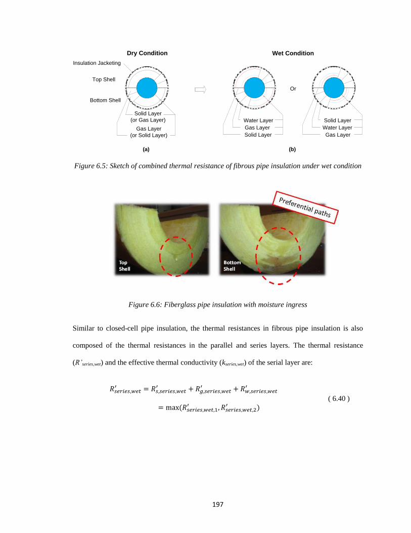
197

Figure 6.5: Sketch of combined thermal resistance of fibrous pipe insulation under wet condition

Figure 6.6: Fiberglass pipe insulation with moisture ingress

Similar to closed-cell pipe insulation, the thermal resistances in fibrous pipe insulation is also

composed of the thermal resistances in the parallel and series layers. The thermal resistance

(R’series,wet) and the effective thermal conductivity (kseries,wet) of the serial layer are:

( 6.40 )

Solid Layer

(or Gas Layer)

Gas Layer

(or Solid Layer)

Top Shell

Bottom Shell

Insulation Jacketing

(a) (b)

Solid Layer

Gas Layer

Water Layer

Wet Condition

Or

Gas Layer

Water Layer

Solid Layer

Dry Condition

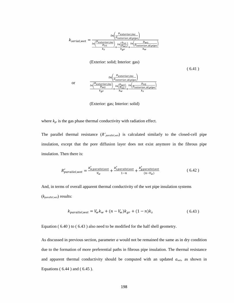
198

(

)

(

)

(

)

(

)

(Exterior: solid; Interior: gas)

or (

)

(

)

(

)

(

)

(Exterior: gas; Interior: solid)

( 6.41 )

where kgr is the gas phase thermal conductivity with radiation effect.

The parallel thermal resistance (R’parallel,wet) is calculated similarly to the closed-cell pipe

insulation, except that the pore diffusion layer does not exist anymore in the fibrous pipe

insulation. Then there is:

( 6.42 )

And, in terms of overall apparent thermal conductivity of the wet pipe insulation systems

(kparallel,wet) results:

( 6.43 )

Equation ( 6.40 ) to ( 6.43 ) also need to be modified for the half shell geometry.

As discussed in previous section, parameter a would not be remained the same as in dry condition

due to the formation of more preferential paths in fibrous pipe insulation. The thermal resistance

and apparent thermal conductivity should be computed with an updated awet, as shown in

Equations ( 6.44 ) and ( 6.45 ).

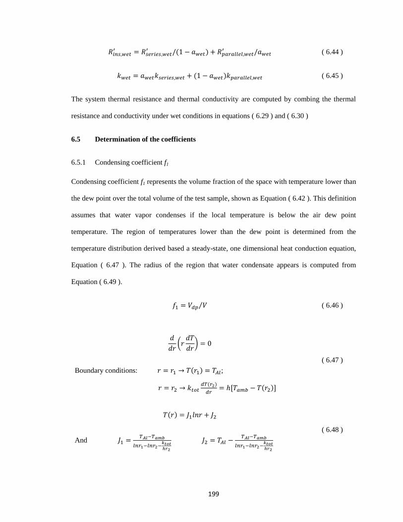
199

( 6.44 )

( 6.45 )

The system thermal resistance and thermal conductivity are computed by combing the thermal

resistance and conductivity under wet conditions in equations ( 6.29 ) and ( 6.30 )

6.5 Determination of the coefficients

6.5.1 Condensing coefficient f1

Condensing coefficient f1 represents the volume fraction of the space with temperature lower than

the dew point over the total volume of the test sample, shown as Equation ( 6.42 ). This definition

assumes that water vapor condenses if the local temperature is below the air dew point

temperature. The region of temperatures lower than the dew point is determined from the

temperature distribution derived based a steady-state, one dimensional heat conduction equation,

Equation ( 6.47 ). The radius of the region that water condensate appears is computed from

Equation ( 6.49 ).

⁄ ( 6.46 )

(

)

Boundary conditions: ;

[ ]

( 6.47 )

And

( 6.48 )

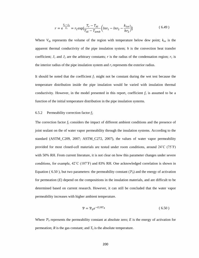
200

[

(

)] ( 6.49 )

Where Vdp represents the volume of the region with temperature below dew point; ktot is the

apparent thermal conductivity of the pipe insulation system; h is the convection heat transfer

coefficient; J1 and J2 are the arbitrary constants; r is the radius of the condensation region; r1 is

the interior radius of the pipe insulation system and r2 represents the exterior radius.

It should be noted that the coefficient f1 might not be constant during the wet test because the

temperature distribution inside the pipe insulation would be varied with insulation thermal

conductivity. However, in the model presented in this report, coefficient f1 is assumed to be a

function of the initial temperature distribution in the pipe insulation systems.

6.5.2 Permeability correction factor f2

The correction factor f2 considers the impact of different ambient conditions and the presence of

joint sealant on the of water vapor permeability through the insulation systems. According to the

standard (ASTM_C209, 2007; ASTM_C272, 2007), the values of water vapor permeability

provided for most closed-cell materials are tested under room conditions, around 24˚C (75˚F)

with 50% RH. From current literature, it is not clear on how this parameter changes under severe

conditions, for example, 42˚C (107˚F) and 83% RH. One acknowledged correlation is shown in

Equation ( 6.50 ), but two parameters: the permeability constant (Ῥ0) and the energy of activation

for permeation (E) depend on the compositions in the insulation materials, and are difficult to be

determined based on current research. However, it can still be concluded that the water vapor

permeability increases with higher ambient temperature.

( 6.50 )

Where Ῥ0 represents the permeability constant at absolute zero; E is the energy of activation for

permeation; R is the gas constant; and Tk is the absolute temperature.

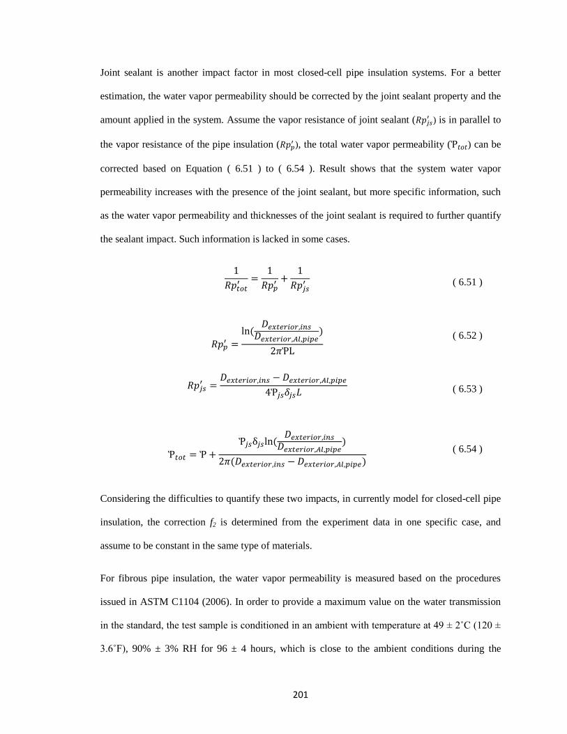
201

Joint sealant is another impact factor in most closed-cell pipe insulation systems. For a better

estimation, the water vapor permeability should be corrected by the joint sealant property and the

amount applied in the system. Assume the vapor resistance of joint sealant ( ) is in parallel to

the vapor resistance of the pipe insulation ( ), the total water vapor permeability ( ) can be

corrected based on Equation ( 6.51 ) to ( 6.54 ). Result shows that the system water vapor

permeability increases with the presence of the joint sealant, but more specific information, such

as the water vapor permeability and thicknesses of the joint sealant is required to further quantify

the sealant impact. Such information is lacked in some cases.

( 6.51 )

( 6.52 )

( 6.53 )

( 6.54 )

Considering the difficulties to quantify these two impacts, in currently model for closed-cell pipe

insulation, the correction f2 is determined from the experiment data in one specific case, and

assume to be constant in the same type of materials.

For fibrous pipe insulation, the water vapor permeability is measured based on the procedures

issued in ASTM C1104 (2006). In order to provide a maximum value on the water transmission

in the standard, the test sample is conditioned in an ambient with temperature at 49 ± 2˚C (120 ±

3.6˚F), 90% ± 3% RH for 96 ± 4 hours, which is close to the ambient conditions during the

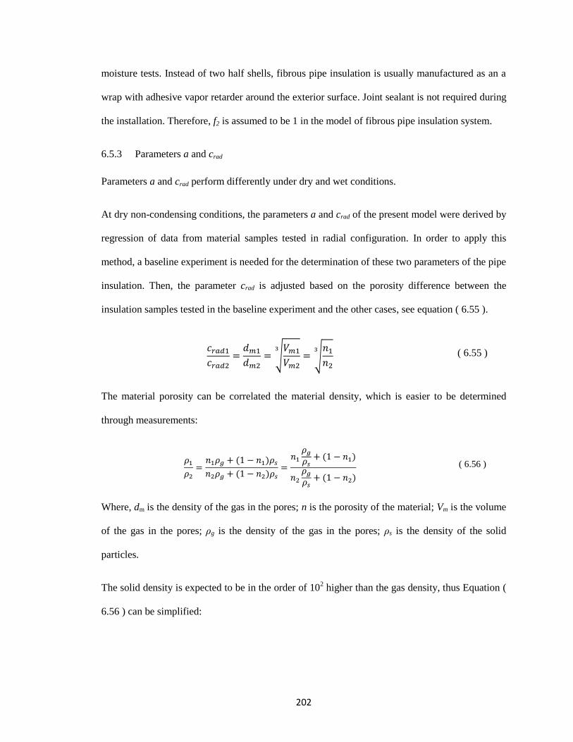
202

moisture tests. Instead of two half shells, fibrous pipe insulation is usually manufactured as an a

wrap with adhesive vapor retarder around the exterior surface. Joint sealant is not required during

the installation. Therefore, f2 is assumed to be 1 in the model of fibrous pipe insulation system.

6.5.3 Parameters a and crad

Parameters a and crad perform differently under dry and wet conditions.

At dry non-condensing conditions, the parameters a and crad of the present model were derived by

regression of data from material samples tested in radial configuration. In order to apply this

method, a baseline experiment is needed for the determination of these two parameters of the pipe

insulation. Then, the parameter crad is adjusted based on the porosity difference between the

insulation samples tested in the baseline experiment and the other cases, see equation ( 6.55 ).

√

√

( 6.55 )

The material porosity can be correlated the material density, which is easier to be determined

through measurements:

( 6.56 )

Where, dm is the density of the gas in the pores; n is the porosity of the material; Vm is the volume

of the gas in the pores; ρg is the density of the gas in the pores; ρs is the density of the solid

particles.

The solid density is expected to be in the order of 102 higher than the gas density, thus Equation (

6.56 ) can be simplified:

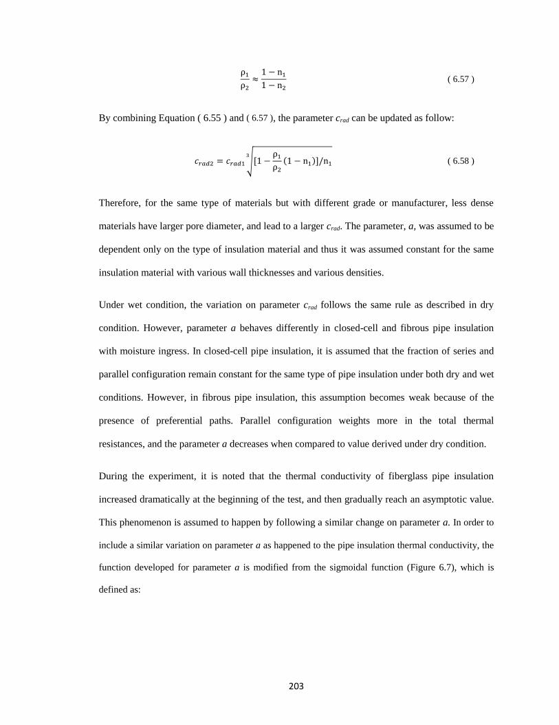
203

( 6.57 )

By combining Equation ( 6.55 ) and ( 6.57 ), the parameter crad can be updated as follow:

√[ ]

( 6.58 )

Therefore, for the same type of materials but with different grade or manufacturer, less dense

materials have larger pore diameter, and lead to a larger crad. The parameter, a, was assumed to be

dependent only on the type of insulation material and thus it was assumed constant for the same

insulation material with various wall thicknesses and various densities.

Under wet condition, the variation on parameter crad follows the same rule as described in dry

condition. However, parameter a behaves differently in closed-cell and fibrous pipe insulation

with moisture ingress. In closed-cell pipe insulation, it is assumed that the fraction of series and

parallel configuration remain constant for the same type of pipe insulation under both dry and wet

conditions. However, in fibrous pipe insulation, this assumption becomes weak because of the

presence of preferential paths. Parallel configuration weights more in the total thermal

resistances, and the parameter a decreases when compared to value derived under dry condition.

During the experiment, it is noted that the thermal conductivity of fiberglass pipe insulation

increased dramatically at the beginning of the test, and then gradually reach an asymptotic value.

This phenomenon is assumed to happen by following a similar change on parameter a. In order to

include a similar variation on parameter a as happened to the pipe insulation thermal conductivity, the

function developed for parameter a is modified from the sigmoidal function (Figure 6.7), which is

defined as:

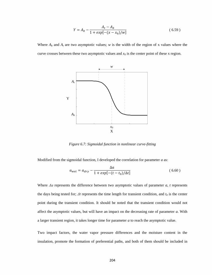
204

[ ] ( 6.59 )

Where Ab and At are two asymptotic values; w is the width of the region of x values where the

curve crosses between these two asymptotic values and x0 is the center point of these x region.

Figure 6.7: Sigmoidal function in nonlinear curve-fitting

Modified from the sigmoidal function, I developed the correlation for parameter a as:

[ ] ( 6.60 )

Where Δa represents the difference between two asymptotic values of parameter a, t represents

the days being tested for; Δt represents the time length for transient condition, and t0 is the center

point during the transient condition. It should be noted that the transient condition would not

affect the asymptotic values, but will have an impact on the decreasing rate of parameter a. With

a larger transient region, it takes longer time for parameter a to reach the asymptotic value.

Two impact factors, the water vapor pressure differences and the moisture content in the

insulation, promote the formation of preferential paths, and both of them should be included in

At

Ab

Y

X

x0

w

205

the function of parameter a. The function of parameter a is further defined as Equation ( 6.61 )

and ( 6.62 ).

( 6.61 )

[ ]

( 6.62 )

Where C1 and C2 are the coefficients represent the sensitivity of water vapor pressure difference

and moisture content on the variation of parameter a. These two coefficients are derived from the

experimental data in one specific case, and it is assumed that the coefficient C1 depends on the

surface water permeability of different pipe insulation systems, while C2 only depends on the type

of pipe insulation materials. If there is a vapor retarder around the exterior surface of the fibrous

pipe insulation, C1 is assumed to be 0 due to the low water vapor permeability on the surface and

a minor reaction to the instant changes from the ambient conditions. This correlation is developed

due to the observation of a dramatic increase on the pipe insulation thermal conductivity at the

beginning of the test and the fact that the area of preferential paths would increase with larger

amount of water accumulated in the pipe insulation. Therefore, the profile of parameter a is

composed of two steps. In the first step, the ambient starts to be humidified, and the vapor partial

pressure difference across the pipe insulation system increases. This promotes the water vapor

transmission and the formation of preferential paths, such as condensate cover the intersection

area between two parallel fibers. The presence of liquid phase significantly changes the internal

structure of the fibrous pipe insulation, and it is considered as a dominant impact on the variation

of parameter a. This procedure is represented by the sigmoidal function, and the decreasing rate

depends on how fast the water condensate finishes covering the intersection areas. The time

length of the transient region (Δt) can be derived from the temperature profile measured at the

exterior surface of the pipe insulation system. In step 2, water condensate starts accumulate in the

insulation and coating the fibers. The areas of preferential paths will continue increasing with the

206

moisture content and further decrease the value of parameter a. However, this is a secondary

impact, and it is assumed that the decreasing rate on parameter a is much slower than the previous

step.

6.6 Model implementation

The model was implemented in Excel spreadsheet with dedicated VBA code.

6.6.1 Implement of thermal conductivity model under dry conditions

Under dry conditions, both closed-cell and fibrous pipe insulation share the same thermal

conductivity model. The procedures for the model under dry conditions are shown in Figure 6.8.

Two steps were needed in the dry model. First, a baseline experimental data set is required to

determine parameters a and crad. In the second step, these two parameters will be updated based

on the dry test sample properties, and apply to the thermal conductivity model. The sample input

and output files in the first step are shown in Figure 6.9. The inputs for the baseline case are as

follows: interior diameter of the pipe insulation (D_i), actual exterior diameter of the pipe

insulation (D_exp), joint sealant thickness (delta_js_ip), test sample length (L), solid thermal

conductivity (k_s), joint sealant thermal conductivity (k_js), porosity (n), number of measuremnts

(N_measrured), type of blowing agent, material density, and experimental results on the

insulation mean temperature (T_ins) and the apparent thermal conductivity (k_exp). The outputs

are: pipe insulation exterior diameter (without joint sealant effect, D_o), parameter a and crad, the

apparent thermal conductivity of the pipe insulation system (k_tot), and the thermal

conductivities in both serial and parallel configurations of the two half shells..

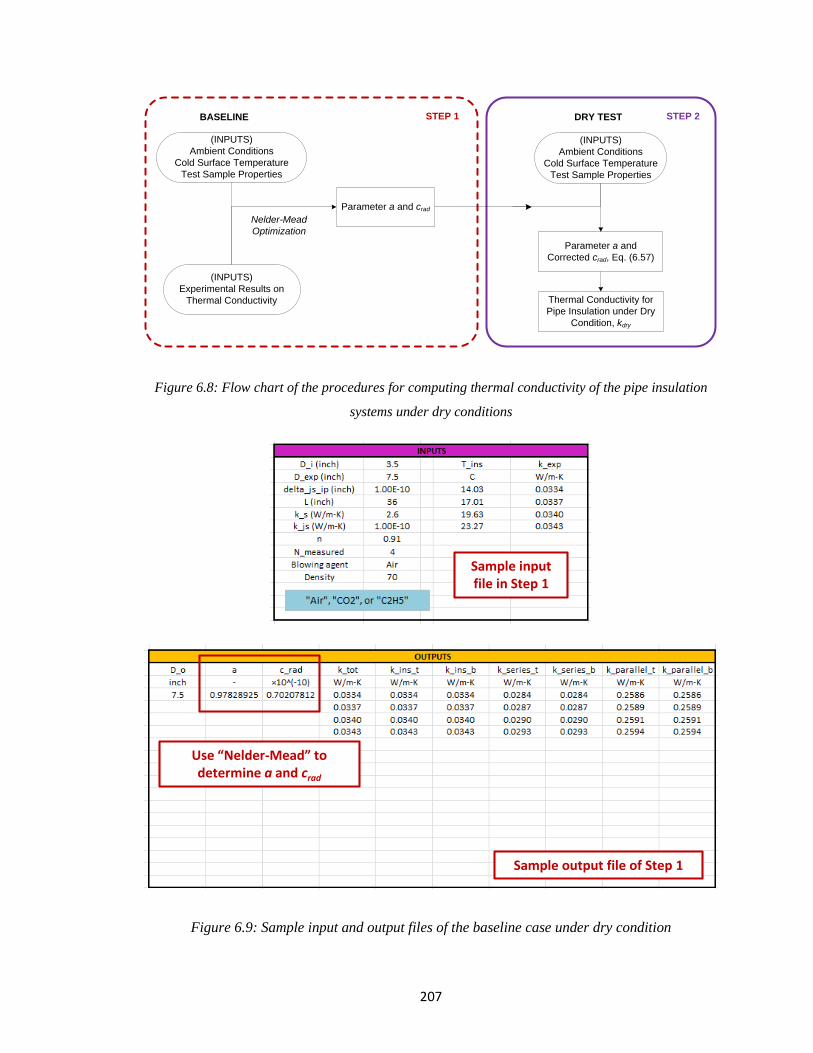
207

Figure 6.8: Flow chart of the procedures for computing thermal conductivity of the pipe insulation

systems under dry conditions

Figure 6.9: Sample input and output files of the baseline case under dry condition

(INPUTS)

Ambient Conditions

Cold Surface Temperature

Test Sample Properties

(INPUTS)

Experimental Results on

Thermal Conductivity

Parameter a and crad

(INPUTS)

Ambient Conditions

Cold Surface Temperature

Test Sample Properties

BASELINE DRY TEST

Thermal Conductivity for

Pipe Insulation under Dry

Condition, kdry

Parameter a and

Corrected crad, Eq. (6.57)

STEP 1 STEP 2

Nelder-Mead

Optimization

Sample input file in Step 1

Sample output file of Step 1

Use “Nelder-Mead” to determine a and crad

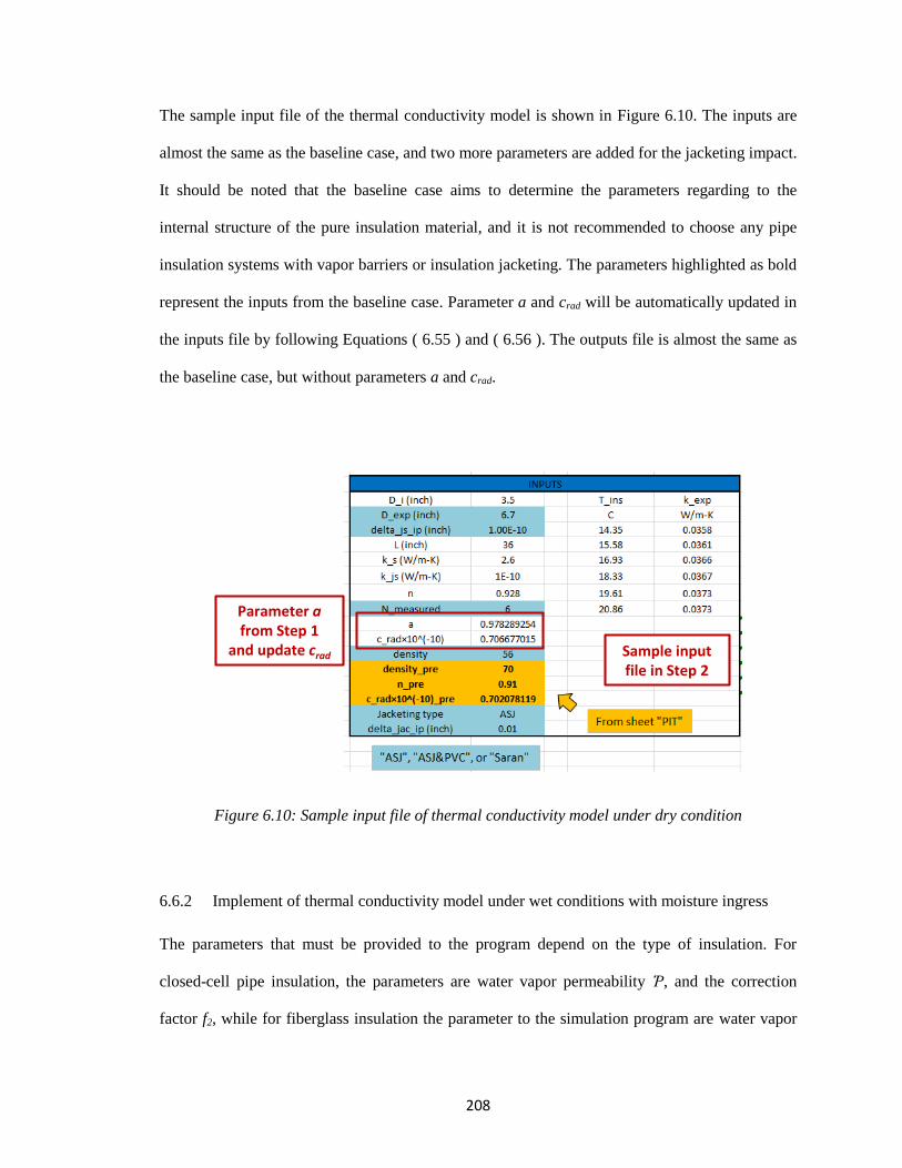
208

The sample input file of the thermal conductivity model is shown in Figure 6.10. The inputs are

almost the same as the baseline case, and two more parameters are added for the jacketing impact.

It should be noted that the baseline case aims to determine the parameters regarding to the

internal structure of the pure insulation material, and it is not recommended to choose any pipe

insulation systems with vapor barriers or insulation jacketing. The parameters highlighted as bold

represent the inputs from the baseline case. Parameter a and crad will be automatically updated in

the inputs file by following Equations ( 6.55 ) and ( 6.56 ). The outputs file is almost the same as

the baseline case, but without parameters a and crad.

Figure 6.10: Sample input file of thermal conductivity model under dry condition

6.6.2 Implement of thermal conductivity model under wet conditions with moisture ingress

The parameters that must be provided to the program depend on the type of insulation. For

closed-cell pipe insulation, the parameters are water vapor permeability Ῥ, and the correction

factor f2, while for fiberglass insulation the parameter to the simulation program are water vapor

Sample input file in Step 2

Parameter afrom Step 1

and update crad

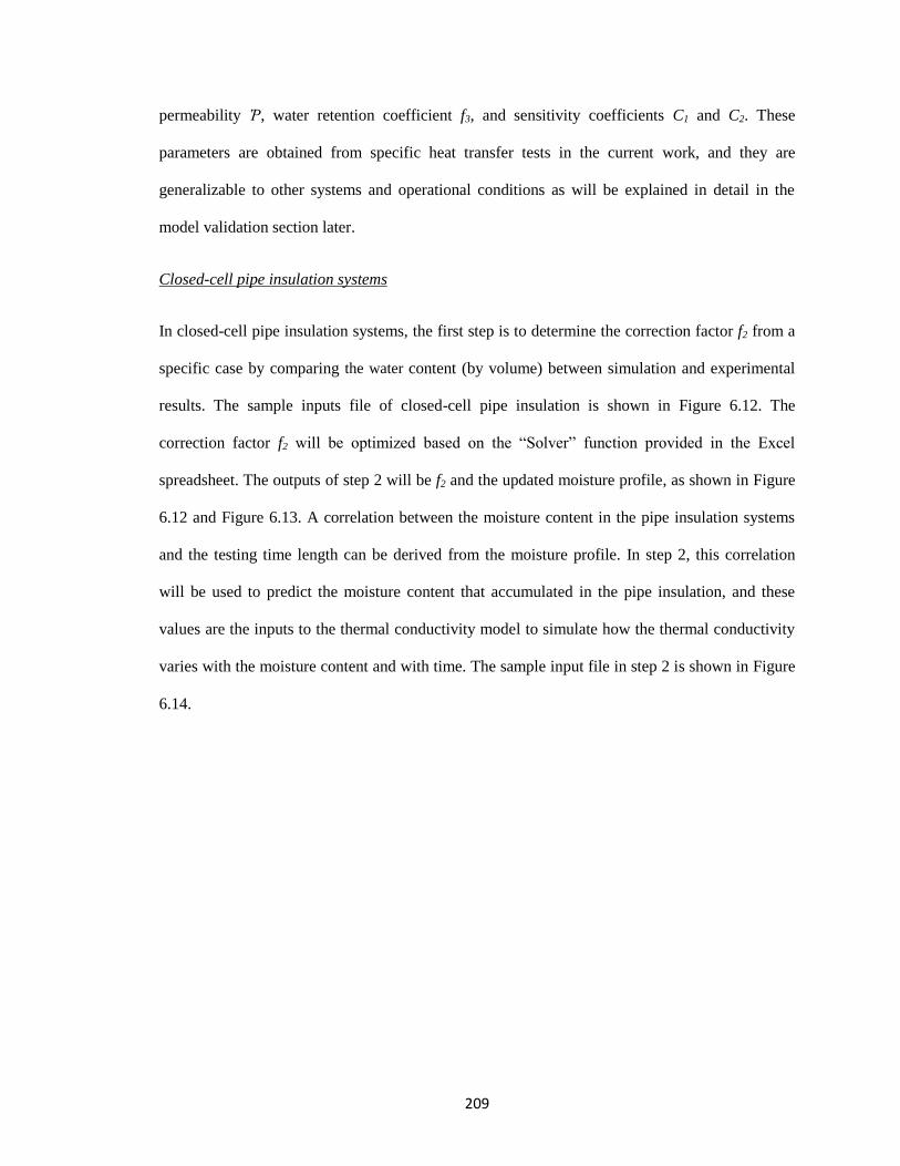
209

permeability Ῥ, water retention coefficient f3, and sensitivity coefficients C1 and C2. These

parameters are obtained from specific heat transfer tests in the current work, and they are

generalizable to other systems and operational conditions as will be explained in detail in the

model validation section later.

Closed-cell pipe insulation systems

In closed-cell pipe insulation systems, the first step is to determine the correction factor f2 from a

specific case by comparing the water content (by volume) between simulation and experimental

results. The sample inputs file of closed-cell pipe insulation is shown in Figure 6.12. The

correction factor f2 will be optimized based on the “Solver” function provided in the Excel

spreadsheet. The outputs of step 2 will be f2 and the updated moisture profile, as shown in Figure

6.12 and Figure 6.13. A correlation between the moisture content in the pipe insulation systems

and the testing time length can be derived from the moisture profile. In step 2, this correlation

will be used to predict the moisture content that accumulated in the pipe insulation, and these

values are the inputs to the thermal conductivity model to simulate how the thermal conductivity

varies with the moisture content and with time. The sample input file in step 2 is shown in Figure

6.14.

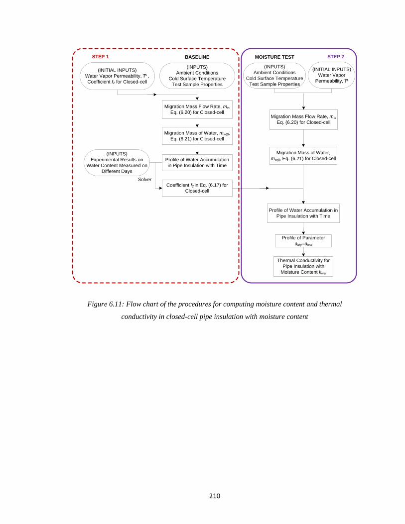
210

Figure 6.11: Flow chart of the procedures for computing moisture content and thermal

conductivity in closed-cell pipe insulation with moisture content

(INPUTS)

Ambient Conditions

Cold Surface Temperature

Test Sample Properties

Migration Mass Flow Rate, mv, Eq. (6.20) for Closed-cell

Migration Mass of Water, mw(t), Eq. (6.21) for Closed-cell

(INPUTS)

Experimental Results on

Water Content Measured on

Different Days

Coefficient f2 in Eq. (6.17) for

Closed-cell

Profile of Water Accumulation

in Pipe Insulation with Time

Profile of Water Accumulation in

Pipe Insulation with Time

Profile of Parameter

adry=awet

Thermal Conductivity for

Pipe Insulation with

Moisture Content kwet

(INITIAL INPUTS)

Water Vapor Permeability, Ῥ ,

Coefficient f2 for Closed-cell

BASELINE MOISTURE TESTSTEP 1 STEP 2

(INPUTS)

Ambient Conditions

Cold Surface Temperature

Test Sample Properties

Migration Mass Flow Rate, mv, Eq. (6.20) for Closed-cell

Migration Mass of Water,

mw(t), Eq. (6.21) for Closed-cell

(INITIAL INPUTS)

Water Vapor

Permeability, Ῥ

Solver

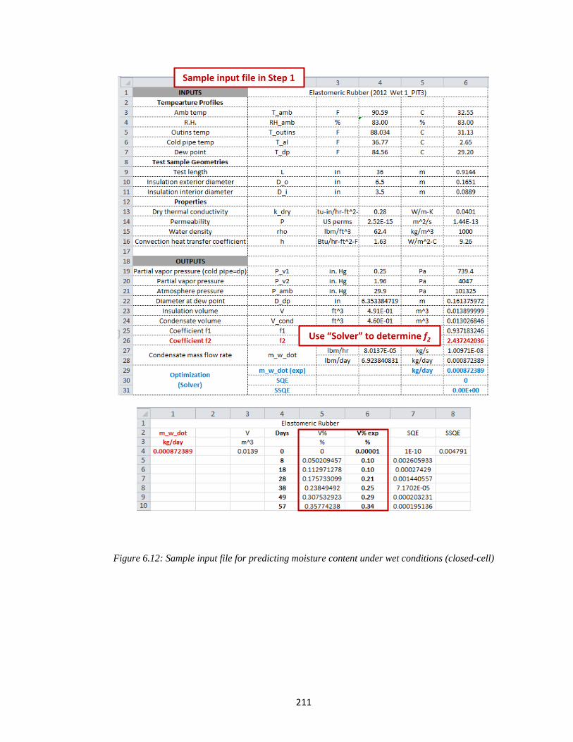
211

Figure 6.12: Sample input file for predicting moisture content under wet conditions (closed-cell)

Sample input file in Step 1

Use “Solver” to determine f2

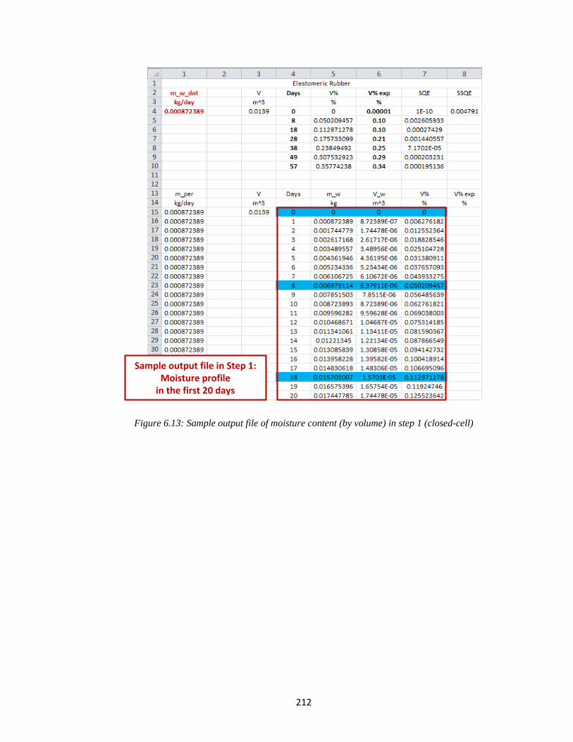
212

Figure 6.13: Sample output file of moisture content (by volume) in step 1 (closed-cell)

Sample output file in Step 1:Moisture profile

in the first 20 days

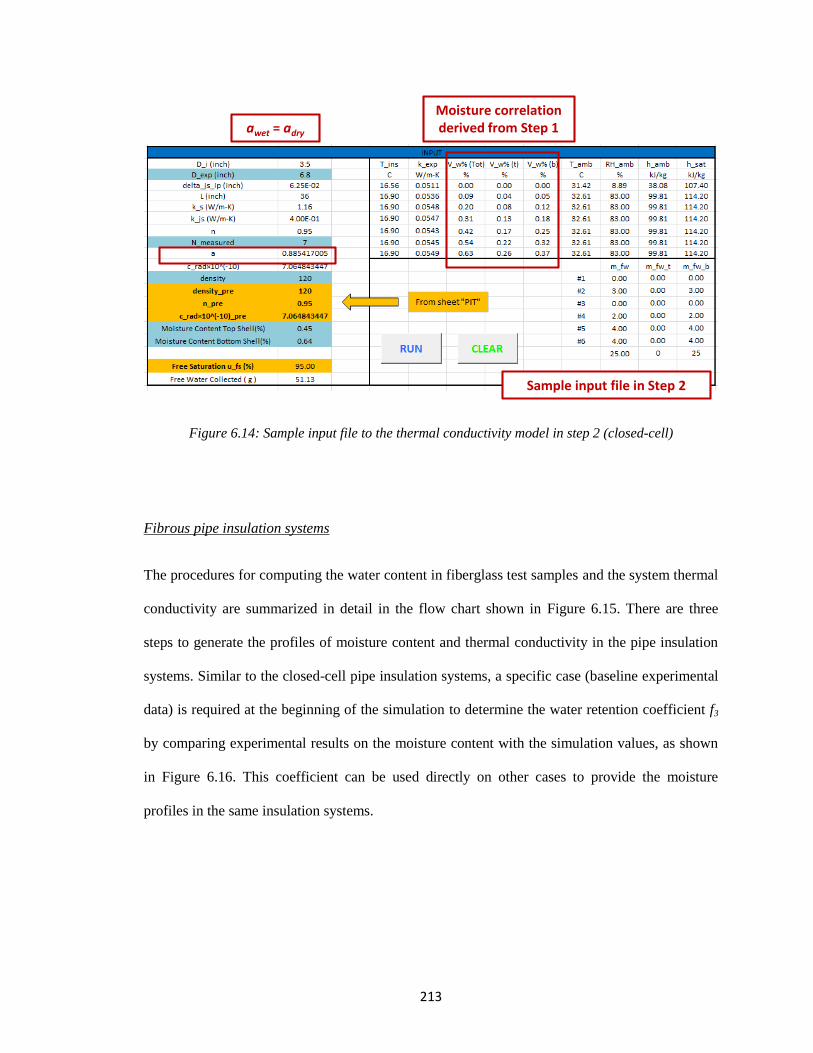
213

Figure 6.14: Sample input file to the thermal conductivity model in step 2 (closed-cell)

Fibrous pipe insulation systems

The procedures for computing the water content in fiberglass test samples and the system thermal

conductivity are summarized in detail in the flow chart shown in Figure 6.15. There are three

steps to generate the profiles of moisture content and thermal conductivity in the pipe insulation

systems. Similar to the closed-cell pipe insulation systems, a specific case (baseline experimental

data) is required at the beginning of the simulation to determine the water retention coefficient f3

by comparing experimental results on the moisture content with the simulation values, as shown

in Figure 6.16. This coefficient can be used directly on other cases to provide the moisture

profiles in the same insulation systems.

Moisture correlation derived from Step 1

Sample input file in Step 2

awet = adry

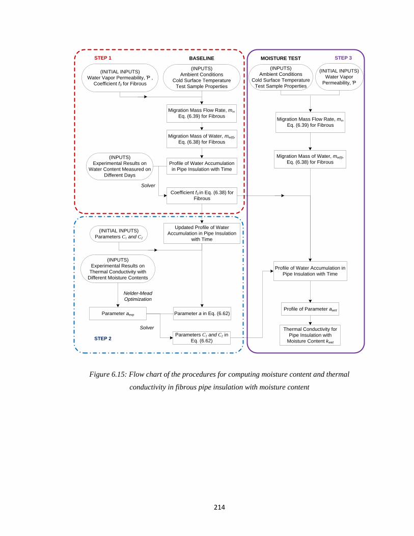
214

Figure 6.15: Flow chart of the procedures for computing moisture content and thermal

conductivity in fibrous pipe insulation with moisture content

(INPUTS)

Ambient Conditions

Cold Surface Temperature

Test Sample Properties

Migration Mass Flow Rate, mv, Eq. (6.39) for Fibrous

Migration Mass of Water, mw(t), Eq. (6.38) for Fibrous

(INPUTS)

Experimental Results on

Water Content Measured on

Different Days

Coefficient f3 in Eq. (6.38) for

Fibrous

(INPUTS)

Experimental Results on

Thermal Conductivity with

Different Moisture Contents

Profile of Water Accumulation

in Pipe Insulation with Time

(INITIAL INPUTS)

Parameters C1 and C2

Parameters C1 and C2 in

Eq. (6.62)

Profile of Water Accumulation in

Pipe Insulation with Time

Profile of Parameter awet

Thermal Conductivity for

Pipe Insulation with

Moisture Content kwet

(INITIAL INPUTS)

Water Vapor Permeability, Ῥ ,

Coefficient f3 for Fibrous

Updated Profile of Water

Accumulation in Pipe Insulation

with Time

BASELINE MOISTURE TESTSTEP 1

STEP 2

STEP 3

(INPUTS)

Ambient Conditions

Cold Surface Temperature

Test Sample Properties

Migration Mass Flow Rate, mv, Eq. (6.39) for Fibrous

Migration Mass of Water, mw(t), Eq. (6.38) for Fibrous

(INITIAL INPUTS)

Water Vapor

Permeability, Ῥ

Parameter a in Eq. (6.62)Parameter aexp

Solver

Nelder-Mead

Optimization

Solver

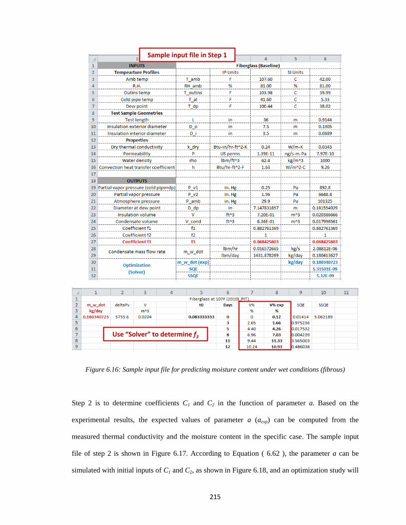
215

Figure 6.16: Sample input file for predicting moisture content under wet conditions (fibrous)

Step 2 is to determine coefficients C1 and C2 in the function of parameter a. Based on the

experimental results, the expected values of parameter a (aexp) can be computed from the

measured thermal conductivity and the moisture content in the specific case. The sample input

file of step 2 is shown in Figure 6.17. According to Equation ( 6.62 ), the parameter a can be

simulated with initial inputs of C1 and C2, as shown in Figure 6.18, and an optimization study will

Sample input file in Step 1

Use “Solver” to determine f3

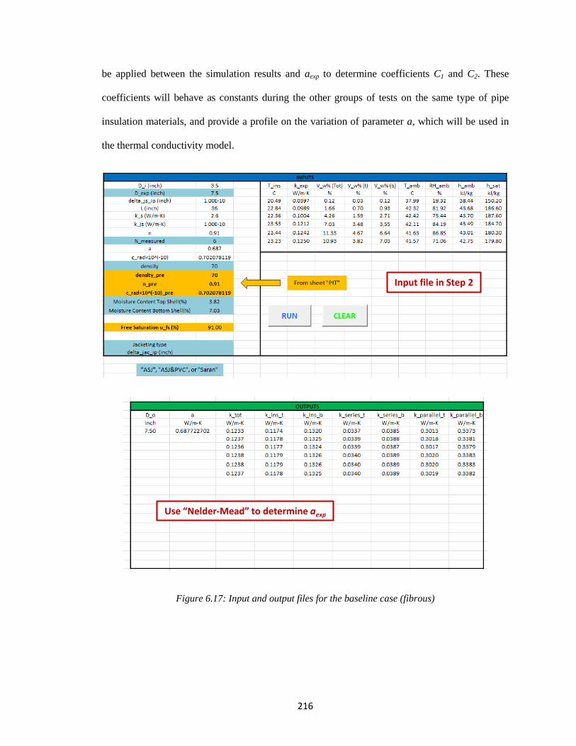
216

be applied between the simulation results and aexp to determine coefficients C1 and C2. These

coefficients will behave as constants during the other groups of tests on the same type of pipe

insulation materials, and provide a profile on the variation of parameter a, which will be used in

the thermal conductivity model.

Figure 6.17: Input and output files for the baseline case (fibrous)

Input file in Step 2

Use “Nelder-Mead” to determine aexp

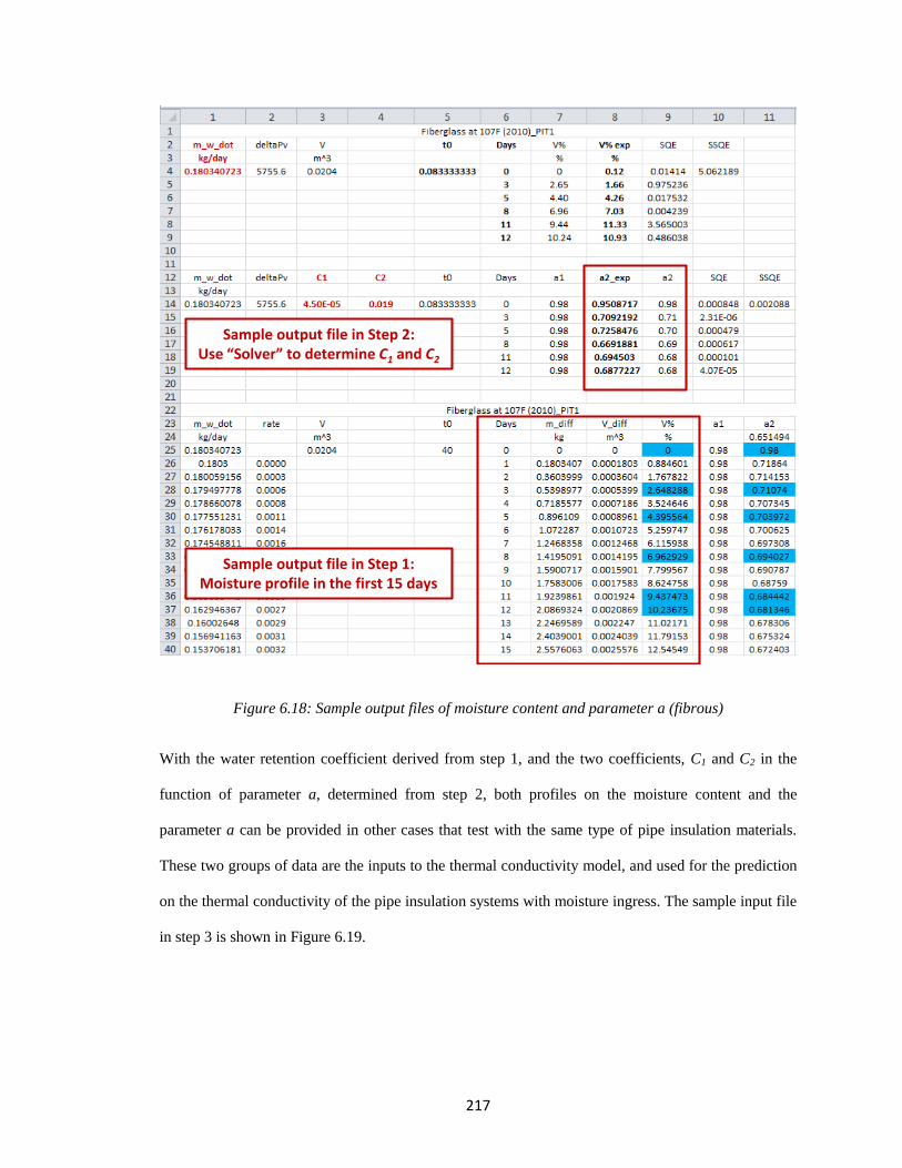
217

Figure 6.18: Sample output files of moisture content and parameter a (fibrous)

With the water retention coefficient derived from step 1, and the two coefficients, C1 and C2 in the

function of parameter a, determined from step 2, both profiles on the moisture content and the

parameter a can be provided in other cases that test with the same type of pipe insulation materials.

These two groups of data are the inputs to the thermal conductivity model, and used for the prediction

on the thermal conductivity of the pipe insulation systems with moisture ingress. The sample input file

in step 3 is shown in Figure 6.19.

Sample output file in Step 2:Use “Solver” to determine C1 and C2

Sample output file in Step 1:Moisture profile in the first 15 days

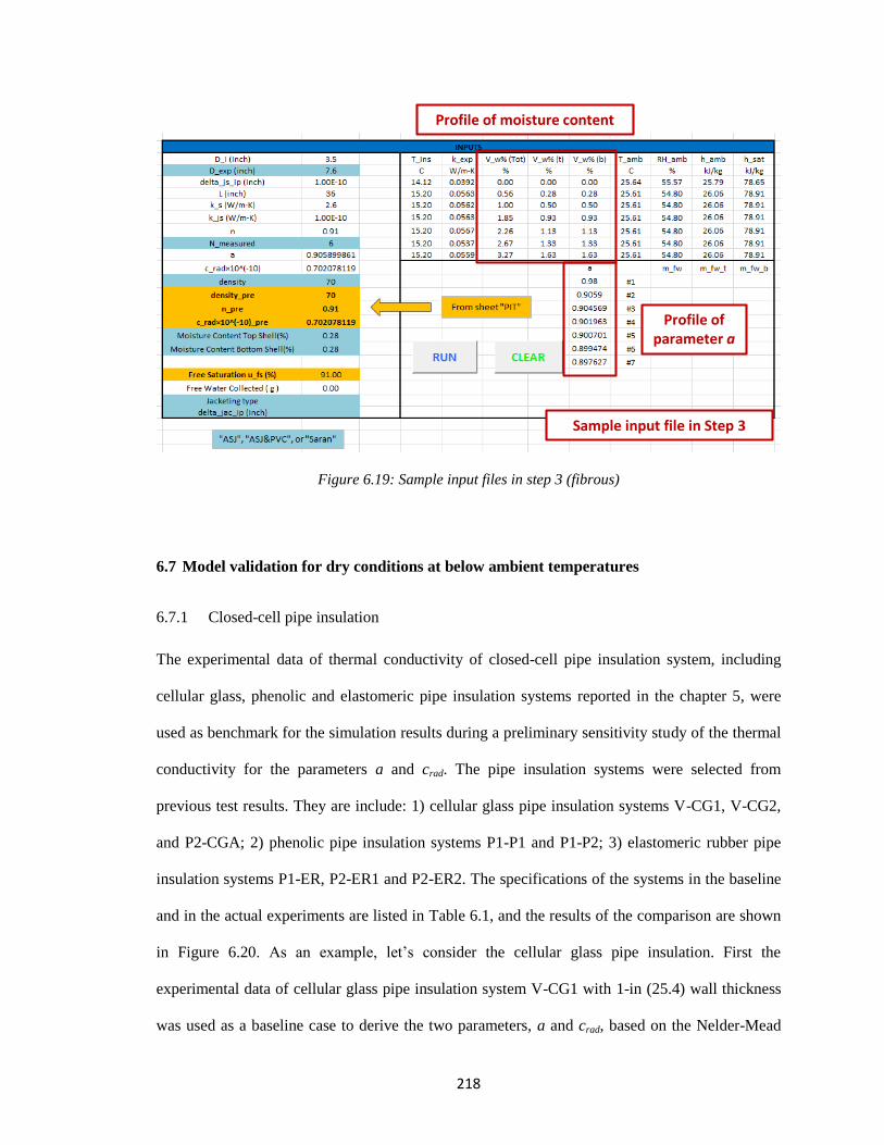
218

Figure 6.19: Sample input files in step 3 (fibrous)

6.7 Model validation for dry conditions at below ambient temperatures

6.7.1 Closed-cell pipe insulation

The experimental data of thermal conductivity of closed-cell pipe insulation system, including

cellular glass, phenolic and elastomeric pipe insulation systems reported in the chapter 5, were

used as benchmark for the simulation results during a preliminary sensitivity study of the thermal

conductivity for the parameters a and crad. The pipe insulation systems were selected from

previous test results. They are include: 1) cellular glass pipe insulation systems V-CG1, V-CG2,

and P2-CGA; 2) phenolic pipe insulation systems P1-P1 and P1-P2; 3) elastomeric rubber pipe

insulation systems P1-ER, P2-ER1 and P2-ER2. The specifications of the systems in the baseline

and in the actual experiments are listed in Table 6.1, and the results of the comparison are shown

in Figure 6.20. As an example, let’s consider the cellular glass pipe insulation. First the

experimental data of cellular glass pipe insulation system V-CG1 with 1-in (25.4) wall thickness

was used as a baseline case to derive the two parameters, a and crad, based on the Nelder-Mead

Sample input file in Step 3

Profile of parameter a

Profile of moisture content

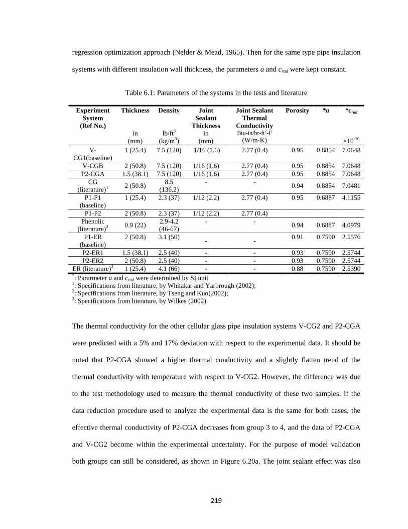
219

regression optimization approach (Nelder & Mead, 1965). Then for the same type pipe insulation

systems with different insulation wall thickness, the parameters a and crad were kept constant.

Table 6.1: Parameters of the systems in the tests and literature

Experiment

System

(Ref No.)

Thickness

in

(mm)

Density

lb/ft3

(kg/m3)

Joint

Sealant

Thickness

in

(mm)

Joint Sealant

Thermal

Conductivity Btu-in/hr-ft2-F

(W/m-K)

Porosity

*a

*crad

×10-10

V-

CG1(baseline)

1 (25.4) 7.5 (120) 1/16 (1.6) 2.77 (0.4) 0.95 0.8854 7.0648

V-CGB 2 (50.8) 7.5 (120) 1/16 (1.6) 2.77 (0.4) 0.95 0.8854 7.0648

P2-CGA 1.5 (38.1) 7.5 (120) 1/16 (1.6) 2.77 (0.4) 0.95 0.8854 7.0648

CG

(literature)1

2 (50.8) 8.5

(136.2)

- - 0.94 0.8854 7.0481

P1-P1

(baseline)

1 (25.4) 2.3 (37) 1/12 (2.2) 2.77 (0.4) 0.95 0.6887 4.1155

P1-P2 2 (50.8) 2.3 (37) 1/12 (2.2) 2.77 (0.4)

Phenolic

(literature)2

0.9 (22) 2.9-4.2

(46-67)

- - 0.94 0.6887 4.0979

P1-ER

(baseline)

2 (50.8) 3.1 (50) - -

0.91 0.7590 2.5576

P2-ER1 1.5 (38.1) 2.5 (40) - - 0.93 0.7590 2.5744

P2-ER2 2 (50.8) 2.5 (40) - - 0.93 0.7590 2.5744

ER (literature)3 1 (25.4) 4.1 (66) - - 0.88 0.7590 2.5390

*: Pararmeter a and crad were determined by SI unit

1: Specifications from literature, by Whitakar and Yarbrough (2002);

2: Specifications from literature, by Tseng and Kuo(2002);

3: Specifications from literature, by Wilkes (2002)

The thermal conductivity for the other cellular glass pipe insulation systems V-CG2 and P2-CGA

were predicted with a 5% and 17% deviation with respect to the experimental data. It should be

noted that P2-CGA showed a higher thermal conductivity and a slightly flatten trend of the

thermal conductivity with temperature with respect to V-CG2. However, the difference was due

to the test methodology used to measure the thermal conductivity of these two samples. If the

data reduction procedure used to analyze the experimental data is the same for both cases, the

effective thermal conductivity of P2-CGA decreases from group 3 to 4, and the data of P2-CGA

and V-CG2 become within the experimental uncertainty. For the purpose of model validation

both groups can still be considered, as shown in Figure 6.20a. The joint sealant effect was also

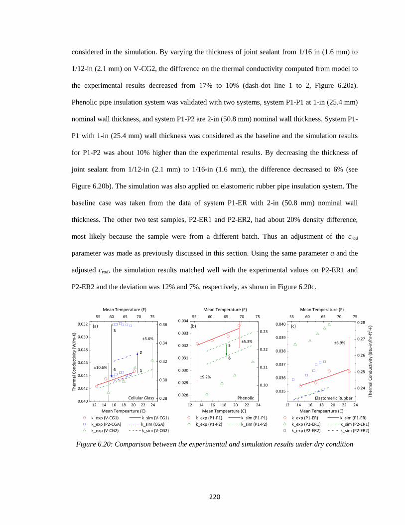
220

considered in the simulation. By varying the thickness of joint sealant from 1/16 in (1.6 mm) to

1/12-in (2.1 mm) on V-CG2, the difference on the thermal conductivity computed from model to

the experimental results decreased from 17% to 10% (dash-dot line 1 to 2, Figure 6.20a).

Phenolic pipe insulation system was validated with two systems, system P1-P1 at 1-in (25.4 mm)

nominal wall thickness, and system P1-P2 are 2-in (50.8 mm) nominal wall thickness. System P1-

P1 with 1-in (25.4 mm) wall thickness was considered as the baseline and the simulation results

for P1-P2 was about 10% higher than the experimental results. By decreasing the thickness of

joint sealant from 1/12-in (2.1 mm) to 1/16-in (1.6 mm), the difference decreased to 6% (see

Figure 6.20b). The simulation was also applied on elastomeric rubber pipe insulation system. The

baseline case was taken from the data of system P1-ER with 2-in (50.8 mm) nominal wall

thickness. The other two test samples, P2-ER1 and P2-ER2, had about 20% density difference,

most likely because the sample were from a different batch. Thus an adjustment of the crad

parameter was made as previously discussed in this section. Using the same parameter a and the

adjusted crad, the simulation results matched well with the experimental values on P2-ER1 and

P2-ER2 and the deviation was 12% and 7%, respectively, as shown in Figure 6.20c.

Figure 6.20: Comparison between the experimental and simulation results under dry condition

12 14 16 18 20 22 240.040

0.042

0.044

0.046

0.048

0.050

0.052

±10.6%

±5.6%

k_exp (V-CG1) k_sim (V-CG1)

k_exp (P2-CGA) k_sim (CGA)

k_exp (V-CG2) k_sim (V-CG2)

Ther

mal

Co

nd

uct

ivit

y (W

/m-K

)

Mean Tempearture (C)

12 14 16 18 20 22 24

0.028

0.029

0.030

0.031

0.032

0.033

0.034

±6.9%±5.3%

±9.2%

4

3(c)(b)(a)

1

Elastomeric RubberPhenolic

k_exp (P1-P1) k_sim (P1-P1)

k_exp (P1-P2) k_sim (P1-P2)

Mean Tempearture (C)

2

5

6

12 14 16 18 20 22 24

0.035

0.036

0.037

0.038

0.039

0.040

Cellular Glass

k_exp (P1-ER) k_sim (P1-ER)

k_exp (P2-ER1) k_sim (P2-ER1)

k_exp (P2-ER2) k_sim (P2-ER2)

Mean Tempearture (C)

0.28

0.30

0.32

0.34

0.36

0.20

0.21

0.22

0.23

0.24

0.25

0.26

0.27

0.28

Ther

mal

Co

nd

uct

ivit

y (B

tu-i

n/h

r-ft

2-F

)

55 60 65 70 75

Mean Temperature (F)

55 60 65 70 75

Mean Temperature (F)

55 60 65 70 75

Mean Temperature (F)

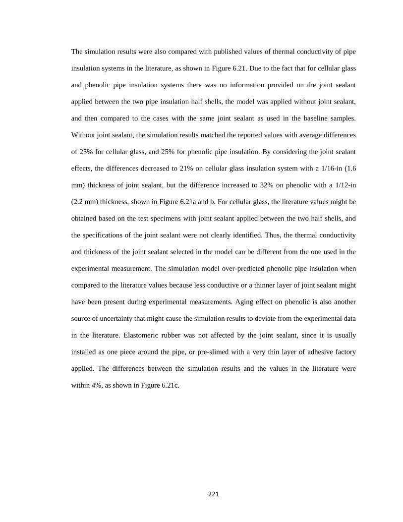
221

The simulation results were also compared with published values of thermal conductivity of pipe

insulation systems in the literature, as shown in Figure 6.21. Due to the fact that for cellular glass

and phenolic pipe insulation systems there was no information provided on the joint sealant

applied between the two pipe insulation half shells, the model was applied without joint sealant,

and then compared to the cases with the same joint sealant as used in the baseline samples.

Without joint sealant, the simulation results matched the reported values with average differences

of 25% for cellular glass, and 25% for phenolic pipe insulation. By considering the joint sealant

effects, the differences decreased to 21% on cellular glass insulation system with a 1/16-in (1.6

mm) thickness of joint sealant, but the difference increased to 32% on phenolic with a 1/12-in

(2.2 mm) thickness, shown in Figure 6.21a and b. For cellular glass, the literature values might be

obtained based on the test specimens with joint sealant applied between the two half shells, and

the specifications of the joint sealant were not clearly identified. Thus, the thermal conductivity

and thickness of the joint sealant selected in the model can be different from the one used in the

experimental measurement. The simulation model over-predicted phenolic pipe insulation when

compared to the literature values because less conductive or a thinner layer of joint sealant might

have been present during experimental measurements. Aging effect on phenolic is also another

source of uncertainty that might cause the simulation results to deviate from the experimental data

in the literature. Elastomeric rubber was not affected by the joint sealant, since it is usually

installed as one piece around the pipe, or pre-slimed with a very thin layer of adhesive factory

applied. The differences between the simulation results and the values in the literature were

within 4%, as shown in Figure 6.21c.

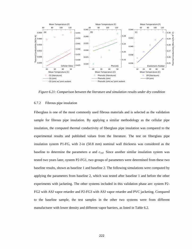
222

Figure 6.21: Comparison between the literature and simulation results under dry condition

6.7.2 Fibrous pipe insulation

Fiberglass is one of the most commonly used fibrous materials and is selected as the validation

sample for fibrous pipe insulation. By applying a similar methodology as the cellular pipe

insulation, the computed thermal conductivity of fiberglass pipe insulation was compared to the

experimental results and published values from the literature. The test on fiberglass pipe

insulation system P1-FG, with 2-in (50.8 mm) nominal wall thickness was considered as the

baseline to determine the parameters a and crad. Since another similar insulation system was

tested two years later, system P2-FG1, two groups of parameters were determined from these two

baseline results, shown as baseline 1 and baseline 2. The following simulations were computed by

applying the parameters from baseline 2, which was tested after baseline 1 and before the other

experiments with jacketing. The other systems included in this validation phase are: system P2-

FG2 with ASJ vapor retarder and P2-FG3 with ASJ vapor retarder and PVC jacketing. Compared

to the baseline sample, the test samples in the other two systems were from different

manufacturer with lower density and different vapor barriers, as listed in Table 6.2.

20 30 40 50

0.044

0.048

0.052

0.056

0.060

0.064 (c)(b)

CG (literature)

CG (sim)

CG (sim) w/ joint sealant

Ther

mal

Co

nd

uct

ivit

y (W

/m-K

)

Mean Temperature (C)

(a)

20 30 40 50

0.020

0.025

0.030

0.035

0.040

0.045

Elastomeric RubberPhenolic

Phenolic (literature)

Phenolic (sim)

Phenolic (sim) w/ joint sealant

Mean Temperature (C)

10 20 30 40 50

0.036

0.038

0.040

0.042

0.044

Cellular Glass

ER (literature)

ER (sim)

Mean Temperature (C)

0.425

0.430

0.435

0.440

0.445

0.450

0.455

0.16

0.20

0.24

0.28

0.25

0.26

0.27

0.28

0.29

0.30

Ther

mal

Co

nd

uct

ivit

y (B

tu-i

n/h

r-ft

2-F

)

60 80 100 120

Mean Temperature (F)

60 80 100 120

Mean Temperature (F)

60 80 100 120

Mean Temperature (F)

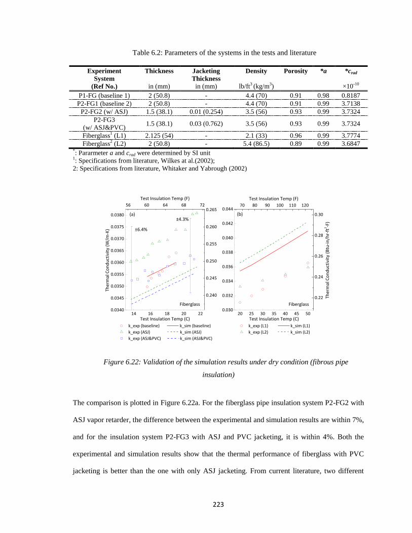
223

Table 6.2: Parameters of the systems in the tests and literature

Experiment

System

(Ref No.)

Thickness

in (mm)

Jacketing

Thickness

in (mm)

Density

lb/ft3 (kg/m

3)

Porosity

*a

*crad

×10-10

P1-FG (baseline 1) 2 (50.8) - 4.4 (70) 0.91 0.98 0.8187

P2-FG1 (baseline 2) 2 (50.8) - 4.4 (70) 0.91 0.99 3.7138

P2-FG2 (w/ ASJ) 1.5 (38.1) 0.01 (0.254) 3.5 (56) 0.93 0.99 3.7324

P2-FG3

(w/ ASJ&PVC) 1.5 (38.1) 0.03 (0.762) 3.5 (56) 0.93 0.99 3.7324

Fiberglass1 (L1) 2.125 (54) - 2.1 (33) 0.96 0.99 3.7774

Fiberglass2 (L2) 2 (50.8) - 5.4 (86.5) 0.89 0.99 3.6847

*: Pararmeter a and crad were determined by SI unit

1: Specifications from literature, Wilkes at al.(2002);

2: Specifications from literature, Whitaker and Yabrough (2002)

Figure 6.22: Validation of the simulation results under dry condition (fibrous pipe

insulation)

The comparison is plotted in Figure 6.22a. For the fiberglass pipe insulation system P2-FG2 with

ASJ vapor retarder, the difference between the experimental and simulation results are within 7%,

and for the insulation system P2-FG3 with ASJ and PVC jacketing, it is within 4%. Both the

experimental and simulation results show that the thermal performance of fiberglass with PVC

jacketing is better than the one with only ASJ jacketing. From current literature, two different

14 16 18 20 220.0340

0.0345

0.0350

0.0355

0.0360

0.0365

0.0370

0.0375

0.0380

±6.4%

±4.3%(b)

Fiberglass

k_exp (L1) k_sim (L1)

k_exp (L2) k_sim (L2)

k_exp (baseline) k_sim (baseline)

k_exp (ASJ) k_sim (ASJ)

k_exp (ASJ&PVC) k_sim (ASJ&PVC)

Ther

mal

Co

nd

uct

ivit

y (W

/m-K

)

Test Insulation Temp (C)

Fiberglass

(a)

20 25 30 35 40 45 500.030

0.032

0.034

0.036

0.038

0.040

0.042

0.044

Test Insulation Temp (C)

56 60 64 68 72

0.240

0.245

0.250

0.255

0.260

0.265

Test Insulation Temp (F)

70 80 90 100 110 120

0.22

0.24

0.26

0.28

0.30

Ther

mal

Co

nd

uct

ivit

y (B

tu-i

n/h

r-ft

2-F

)

Test Insulation Temp (F)

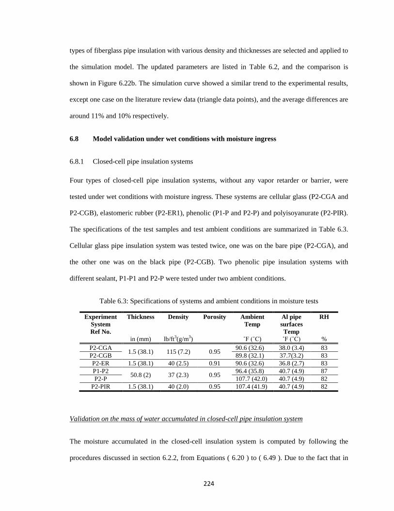
224

types of fiberglass pipe insulation with various density and thicknesses are selected and applied to

the simulation model. The updated parameters are listed in Table 6.2, and the comparison is

shown in Figure 6.22b. The simulation curve showed a similar trend to the experimental results,

except one case on the literature review data (triangle data points), and the average differences are

around 11% and 10% respectively.

6.8 Model validation under wet conditions with moisture ingress

6.8.1 Closed-cell pipe insulation systems

Four types of closed-cell pipe insulation systems, without any vapor retarder or barrier, were

tested under wet conditions with moisture ingress. These systems are cellular glass (P2-CGA and

P2-CGB), elastomeric rubber (P2-ER1), phenolic (P1-P and P2-P) and polyisoyanurate (P2-PIR).

The specifications of the test samples and test ambient conditions are summarized in Table 6.3.

Cellular glass pipe insulation system was tested twice, one was on the bare pipe (P2-CGA), and

the other one was on the black pipe (P2-CGB). Two phenolic pipe insulation systems with

different sealant, P1-P1 and P2-P were tested under two ambient conditions.

Table 6.3: Specifications of systems and ambient conditions in moisture tests

Experiment

System

Ref No.

Thickness

in (mm)

Density

lb/ft3(g/m

3)

Porosity

Ambient

Temp

˚F (˚C)

Al pipe

surfaces

Temp

˚F (˚C)

RH

%

P2-CGA 1.5 (38.1) 115 (7.2) 0.95

90.6 (32.6) 38.0 (3.4) 83

P2-CGB 89.8 (32.1) 37.7(3.2) 83

P2-ER 1.5 (38.1) 40 (2.5) 0.91 90.6 (32.6) 36.8 (2.7) 83

P1-P2 50.8 (2) 37 (2.3) 0.95

96.4 (35.8) 40.7 (4.9) 87

P2-P 107.7 (42.0) 40.7 (4.9) 82

P2-PIR 1.5 (38.1) 40 (2.0) 0.95 107.4 (41.9) 40.7 (4.9) 82

Validation on the mass of water accumulated in closed-cell pipe insulation system

The moisture accumulated in the closed-cell insulation system is computed by following the

procedures discussed in section 6.2.2, from Equations ( 6.20 ) to ( 6.49 ). Due to the fact that in

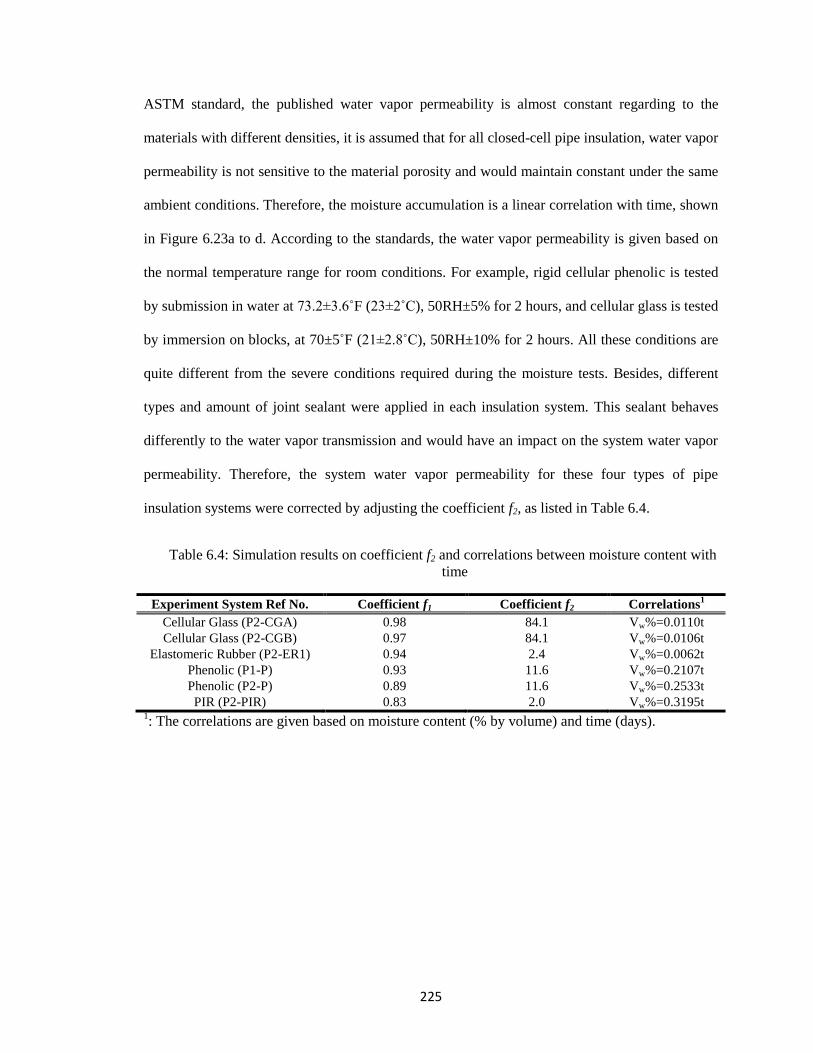
225

ASTM standard, the published water vapor permeability is almost constant regarding to the

materials with different densities, it is assumed that for all closed-cell pipe insulation, water vapor

permeability is not sensitive to the material porosity and would maintain constant under the same

ambient conditions. Therefore, the moisture accumulation is a linear correlation with time, shown

in Figure 6.23a to d. According to the standards, the water vapor permeability is given based on

the normal temperature range for room conditions. For example, rigid cellular phenolic is tested

by submission in water at 73.2±3.6˚F (23±2˚C), 50RH±5% for 2 hours, and cellular glass is tested

by immersion on blocks, at 70±5˚F (21±2.8˚C), 50RH±10% for 2 hours. All these conditions are

quite different from the severe conditions required during the moisture tests. Besides, different

types and amount of joint sealant were applied in each insulation system. This sealant behaves

differently to the water vapor transmission and would have an impact on the system water vapor

permeability. Therefore, the system water vapor permeability for these four types of pipe

insulation systems were corrected by adjusting the coefficient f2, as listed in Table 6.4.

Table 6.4: Simulation results on coefficient f2 and correlations between moisture content with

time

Experiment System Ref No. Coefficient f1 Coefficient f2 Correlations1

Cellular Glass (P2-CGA) 0.98 84.1 Vw%=0.0110t

Cellular Glass (P2-CGB) 0.97 84.1 Vw%=0.0106t

Elastomeric Rubber (P2-ER1) 0.94 2.4 Vw%=0.0062t

Phenolic (P1-P) 0.93 11.6 Vw%=0.2107t

Phenolic (P2-P) 0.89 11.6 Vw%=0.2533t

PIR (P2-PIR) 0.83 2.0 Vw%=0.3195t 1: The correlations are given based on moisture content (% by volume) and time (days).

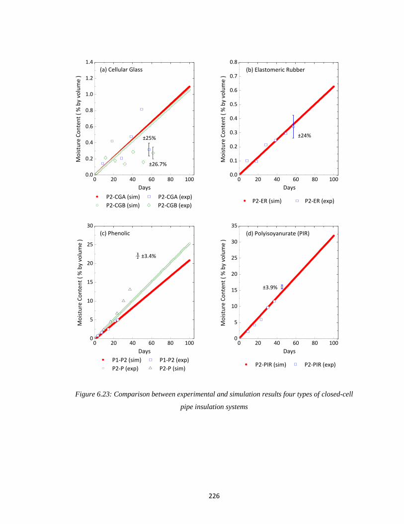
226

Figure 6.23: Comparison between experimental and simulation results four types of closed-cell

pipe insulation systems

0 20 40 60 80 1000.0

0.2

0.4

0.6

0.8

1.0

1.2

1.4

±25%

±26.7%

(b) Elastomeric Rubber

P2-CGA (sim) P2-CGA (exp)

P2-CGB (sim) P2-CGB (exp)

Mo

istu

re C

on

ten

t (

% b

y vo

lum

e )

Days

(a) Cellular Glass

0 20 40 60 80 1000.0

0.1

0.2

0.3

0.4

0.5

0.6

0.7

0.8

±24%

P2-ER (sim) P2-ER (exp)

Days

Mo

istu

re C

on

ten

t (

% b

y vo

lum

e )

0 20 40 60 80 1000

5

10

15

20

25

30

±3.4%

P2-PIR (sim) P2-PIR (exp)

(d) Polyisoyanurate (PIR)

P1-P2 (sim) P1-P2 (exp)

P2-P (exp) P2-P (sim)

Mo

istu

re C

on

ten

t (

% b

y vo

lum

e )

Days

(c) Phenolic

0 20 40 60 80 1000

5

10

15

20

25

30

35

±3.9%

Days

Mo

istu

re C

on

ten

t (

% b

y vo

lum

e )

227

There are several findings from the simulation results on the moisture content in the insulation

system:

Phenolic pipe insulation systems P1-P2 and P2-P were tested under different ambient conditions.

The water vapor permeability correction factor f2 was computed from the experimental results on

the moisture profile provided in system P1-P2. For system P2-P, by maintaining the same

correction factor f2, and updating condensation coefficient f1 according to the ambient conditions,

the simulation results on the moisture content in system P2-P matched with the experimental

results in 30%. The last point was obviously out of the simulation range, and the difference

increased to 48%. By maintaining the same coefficient f2 in the cellular glass pipe insulation

system P2-CGB, although the simulation results over predicted the moisture content by 30~40%,

the total amount of water was very low, and this resulted in a large uncertainty during the

measurement. From these comparisons, it seems that with current assumptions, the simulation

results did not quite follow the experimental results and there are two possible reasons. First, the

water vapor permeability of closed-cell pipe insulation may not be constant and it will be varies

with insulation mean temperature and the volume of water. In this case, the moisture profile

would not follow a linear correlation. The second possible reason is that the water vapor

permeability is sensitive to the ambient temperature and the system joint sealant, the coefficient f2

may not be constant. However, more experimental data is required on the same type of the

insulation systems to further validate the correlations of the moisture profile.

Second, it is found that there are large differences on the values of the coefficient f2 among these

four types of pipe insulation systems. These dissimilarities indicate that each type of the

insulation might behave differently to the changes from the ambient conditions. Some of them are

not sensitive to the water vapor pressure differences, and the water vapor permeability remains

constant under varied temperatures and humidity, such as elastomeric rubber and PIR. However,

some of them perform fairly sensitive when the ambient condition changes, such as cellular glass.

228

The application of joint sealant might be another reason to explain the variation on the coefficient

f2. Compared to other closed-cell materials, cellular glass has a very low water vapor permeance,

0.005 US perm (0.007 metric perm). Boss 368 was used on all the joints as both joint sealant and

vapor sealant. However, this material is not recommended as a good vapor sealant, and the water

vapor permeability might be much larger than cellular glass insulation. With the presence of this

type of joint sealant, the system water permeability increased. In the PIR pipe insulation system

P2-PIR, Chil-Joint CP-70 was applied on all the joints as vapor seal, and this material has very

low water vapor permeability with the maximum permeance is 0.008 perm-inch (0.012 metric

perm). For PIR insulation, the water permeance is reported at 4.0 perm-inch (5.8 metric perm).

This large difference indicates that the water vapor permeability in PIR system may not be

affected by the joint sealant. For the other pipe insulation systems, elastomeric rubber did not

require joint sealant during installation, and f2 was close to 1. Currently, further research is still

needed for better explanations on why this coefficient is large than 1 and why the variations are

large among different types of closed-cell pipe insulation systems.

The third finding is that for closed-cell pipe insulation system, the maximum moisture content

might be reached when all the cells with temperatures below than the dew point are filled with

water. A more specific water distribution profile will help predict how the moisture content in

closed-cell pipe insulation reaches the asymptotic values. It seems that with moisture gradually

filling in the cells from interior outward, the increase on the local thermal conductivity will lead

to lower insulation temperatures and higher values on the coefficient f1, which is assumed to

maintain constant in current model. If the coefficient f1 increases, the water condensate will be

accumulated in the pipe insulation at a higher rate. This might be the reason to explain why the

last points in the following three tests on cellular glass P2-CGA, phenolic P2-P and PIR P2-PIR,

are slightly higher than the simulation results. However, considering the low permeability under

severe test conditions, in current model, the moisture content was assumed to increase linearly

229

with time for the first 100 days of test. The linear correlations for the moisture content in the pipe

insulation are derived based on the optimization between the simulation and experimental results

and documented in Table 6.4. These correlations will be applied next to the thermal conductivity

model.

Validation on the thermal conductivity of closed-cell pipe insulation with moisture ingress

The variation on the thermal conductivity of the pipe insulation with moisture ingress are

predicted with the present model and validated with the experimental data from the present work.

The experimental data were gathered according to the methodology described in details in chapter

3. All the required inputs on the ambient conditions are included in Table 6.3. The parameters a

and crad were computed from one specific case on the same type of insulation tested under dry

conditions, and crad was adjusted based on the material porosity. The values of parameter a and

crad used in the simulation are documented in Table 6.5.

Table 6.5: Test samples specifications in moisture tests

Experiment

System

Ref No.

Joint

Sealant

Thickness

in

(mm)

Joint Sealant

Thermal

Conductivity Btu-in/hr-ft

2-F

(W/m-K)

Water

Vapor

Permeability

perm-in.

(ng/s-m2-Pa)

*a

*crad

×10-10

Cellular Glass (P2-CGA) 1/16 (1.6) 2.77 (0.4) 0.005 (0.007) 0.4159 0.000088

Cellular Glass (P2-CGB)

Elastomeric Rubber

(P2-ER) - - 0.1 (0.0144) 0.9999 5.2052

Phenolic (P1-P1) 1/12 (2.1) 2.77 (0.4) 0.9 (1.3) 0.6887 4.1155

Phenolic (P1-P2)

Polyisocyanurate

(P2-PIR) 1/12 (2.1) 2.77 (0.4) 4.0 (5.8) 0.7503 0.00002

*: Pararmeter a and crad were determined by SI unit

Both cellular glass and elastomeric rubber have very low water vapor permeability, and the

thermal conductivity ratio increased in the similar trends as predicted by the model. In these three

cases (two tests on cellular glass and one test on elastomeric rubber), the thermal conductivity

were better predicted with moisture content than with time. As shown in Figure 6.24a and c, the

230

simulated thermal conductivity ratio with moisture content matched the experimental values

within the uncertainty range. The thermal conductivity ratio was also predicted with time, and the

differences between the simulation and experimental results were within 5%. These differences

were brought into the thermal conductivity model from the deviations in the simulated moisture

profiles. It should be noted that cellular glass pipe insulation system was tested twice under the

same ambient condition (Table 6.3), thus the simulation results on system P2-CGA and P2-CGB

are almost the same. The thermal conductivity of phenolic pipe insulation systems P1-P2 and P2-

P were measured under different ambient conditions, and the test specimens had same nominal

wall thickness and density, as listed in Table 6.5. The simulation results on the thermal

conductivity ratio were compared to the experimental values in Figure 6.24 e and f. It shows that

the simulation results under-predicted the thermal conductivity of the phenolic pipe insulation by

about 8 ~ 9% when considering different moisture content, and the simulation results would

deviate from the experimental curve upto 36% when considering with time. These larger

differences on the thermal conductivity ratio with time were from the inaccurate moisture profile

developed for the closed-cell pipe insulation systems. For PIR pipe insulation system with no

vapor retarder, the model over-predicted the thermal conductivity ratio within 12% when

compared to the experimental results. These differences might be caused by a minor deviation on

the parameter a during the wet condition. Take PIR pipe insulation system as an example, on day

45, the moisture content was 16.04% by volume, when parameter a increased from 0.75 to 0.8,

the thermal conductivity ratio decreased from 1.78 to 1.64, with the difference between

simulation and experimental result (with time) decreased from 12% to 7%. However, more data

sets are required to prove this theory, and in the currently model, parameter a was considered as

constant for all closed-cell pipe insulation systems. It should be noted that based on the

assumption that moisture content is linearly increased with time during the first 100 days of

moisture tests, the variation on the thermal conductivity ratio can only be predicted within these

100 days, and it might increase faster in the long run due a larger condensation region. This larger

231

region will increase the value of coefficient f1, and increase the system water migration rate. The

simulation results are documented in Table E1-5 in the Appendix E.

Figure 6.24: Comparison between experimental and simulation results on the thermal

conductivity ratio between dry and wet closed-cell pipe insulation systems

0.0 0.2 0.4 0.6 0.8 1.0 1.20.90

0.95

1.00

1.05

1.10

1.15

1.20

±4%

±21%

P2-CGA (sim) P2-CGA (exp)

P2-CGB (sim) P2-CGB (exp)

(b) Cellular Glass

P2-CGA (sim) P2-CGA (exp)

P2-CGB (sim) P2-CGB (exp)

Ther

mal

Co

nd

uct

ivit

y R

atio

( k

_wet

/k_d

ry )

Moisture Content ( % by volume )

(a) Cellular Glass

0 20 40 60 80 1000.90

0.95

1.00

1.05

1.10

1.15

1.20

±4%

Days

Ther

mal

Co

nd

uct

ivit

y R

atio

( k

_wet

/k_d

ry )

0.0 0.2 0.4 0.6 0.80.95

1.00

1.05

1.10

±30%

±4.8%

P2-ER (sim) P2-ER (exp)

(d) Elastomeric Rubber

P2-ER (sim) P2-ER (exp)

Ther

mal

Co

nd

uct

ivit

y R

atio

( k

_wet

/k_d

ry )

Moisture Content ( % by volume )

(c) Elastomeric Rubber

0 20 40 60 80 1000.95

1.00

1.05

1.10

±4.8%

Days

Ther

mal

Co

nd

uct

ivit

y R

atio

( k

_wet

/k_d

ry )

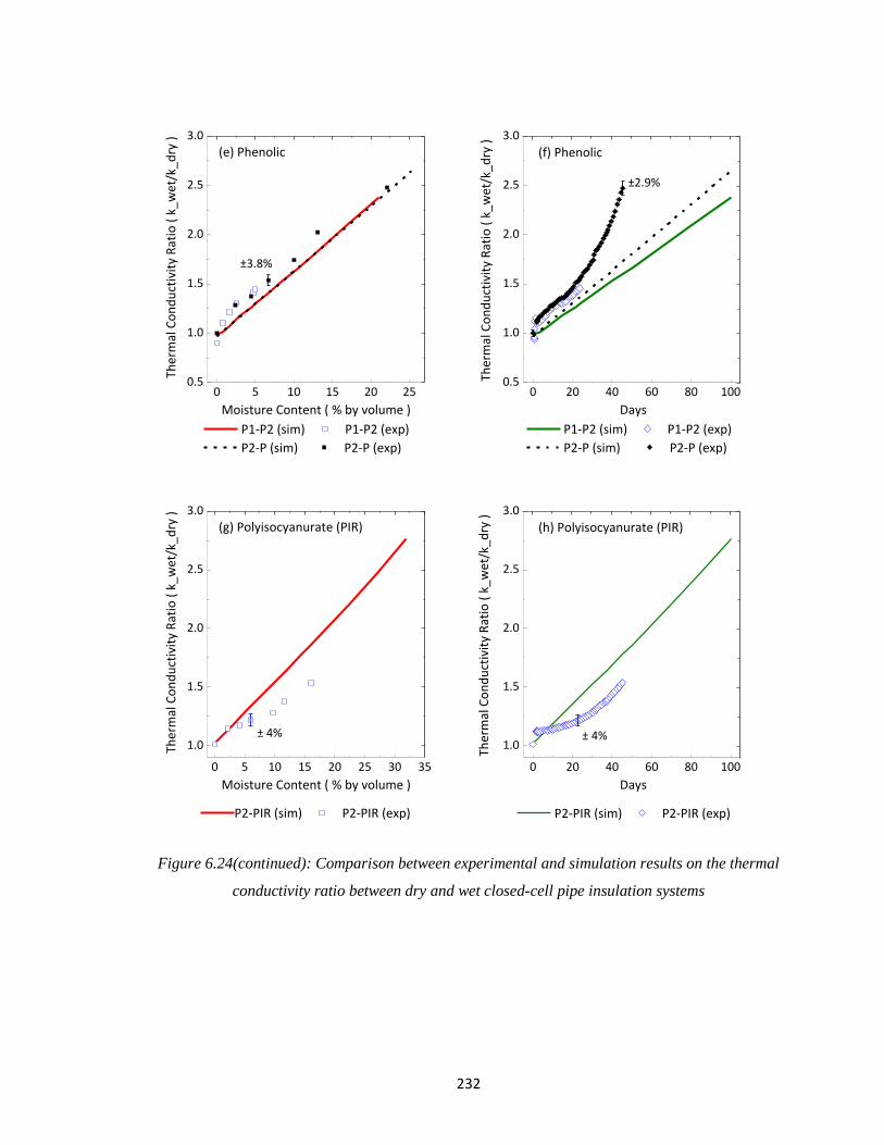
232

Figure 6.24(continued): Comparison between experimental and simulation results on the thermal

conductivity ratio between dry and wet closed-cell pipe insulation systems

0 5 10 15 20 250.5

1.0

1.5

2.0

2.5

3.0

±3.8%

P1-P2 (sim) P1-P2 (exp)

P2-P (sim) P2-P (exp)

(f) Phenolic

P1-P2 (sim) P1-P2 (exp)

P2-P (sim) P2-P (exp)

Ther

mal

Co

nd

uct

ivit

y R

atio

( k

_wet

/k_d

ry )

Moisture Content ( % by volume )

(e) Phenolic

0 20 40 60 80 1000.5

1.0

1.5

2.0

2.5

3.0

±2.9%

Days

Ther

mal

Co

nd

uct

ivit

y R

atio

( k

_wet

/k_d

ry )

0 5 10 15 20 25 30 35

1.0

1.5

2.0

2.5

3.0

± 4%

P2-PIR (sim) P2-PIR (exp)

(h) Polyisocyanurate (PIR)

P2-PIR (sim) P2-PIR (exp)

Ther

mal

Co

nd

uct

ivit

y R

atio

( k

_wet

/k_d

ry )

Moisture Content ( % by volume )

(g) Polyisocyanurate (PIR)

0 20 40 60 80 100

1.0

1.5

2.0

2.5

3.0

± 4%

Days

Ther

mal

Co

nd

uct

ivit

y R

atio

( k

_wet

/k_d

ry )

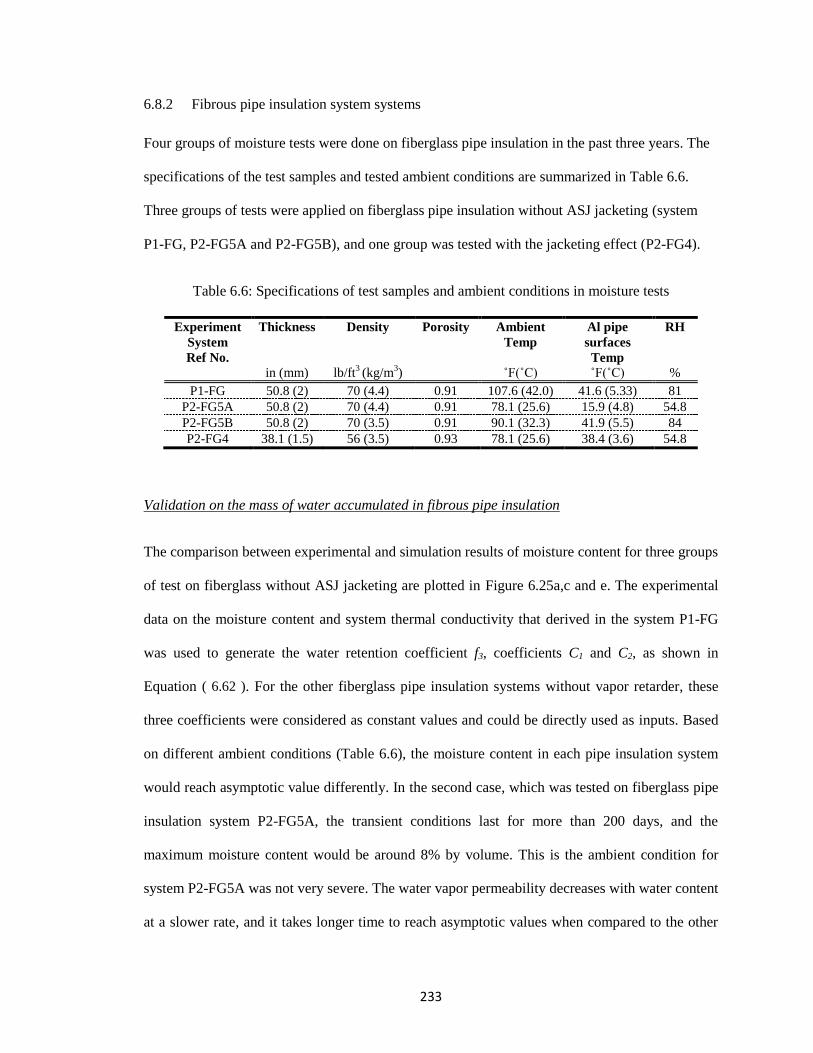
233

6.8.2 Fibrous pipe insulation system systems

Four groups of moisture tests were done on fiberglass pipe insulation in the past three years. The

specifications of the test samples and tested ambient conditions are summarized in Table 6.6.

Three groups of tests were applied on fiberglass pipe insulation without ASJ jacketing (system

P1-FG, P2-FG5A and P2-FG5B), and one group was tested with the jacketing effect (P2-FG4).

Table 6.6: Specifications of test samples and ambient conditions in moisture tests

Experiment

System

Ref No.

Thickness

in (mm)

Density

lb/ft3 (kg/m

3)

Porosity

Ambient

Temp

˚F(˚C)

Al pipe

surfaces

Temp

˚F(˚C)

RH

%

P1-FG 50.8 (2) 70 (4.4) 0.91 107.6 (42.0) 41.6 (5.33) 81

P2-FG5A 50.8 (2) 70 (4.4) 0.91 78.1 (25.6) 15.9 (4.8) 54.8

P2-FG5B 50.8 (2) 70 (3.5) 0.91 90.1 (32.3) 41.9 (5.5) 84

P2-FG4 38.1 (1.5) 56 (3.5) 0.93 78.1 (25.6) 38.4 (3.6) 54.8

Validation on the mass of water accumulated in fibrous pipe insulation

The comparison between experimental and simulation results of moisture content for three groups

of test on fiberglass without ASJ jacketing are plotted in Figure 6.25a,c and e. The experimental

data on the moisture content and system thermal conductivity that derived in the system P1-FG

was used to generate the water retention coefficient f3, coefficients C1 and C2, as shown in

Equation ( 6.62 ). For the other fiberglass pipe insulation systems without vapor retarder, these

three coefficients were considered as constant values and could be directly used as inputs. Based

on different ambient conditions (Table 6.6), the moisture content in each pipe insulation system

would reach asymptotic value differently. In the second case, which was tested on fiberglass pipe

insulation system P2-FG5A, the transient conditions last for more than 200 days, and the

maximum moisture content would be around 8% by volume. This is the ambient condition for

system P2-FG5A was not very severe. The water vapor permeability decreases with water content

at a slower rate, and it takes longer time to reach asymptotic values when compared to the other

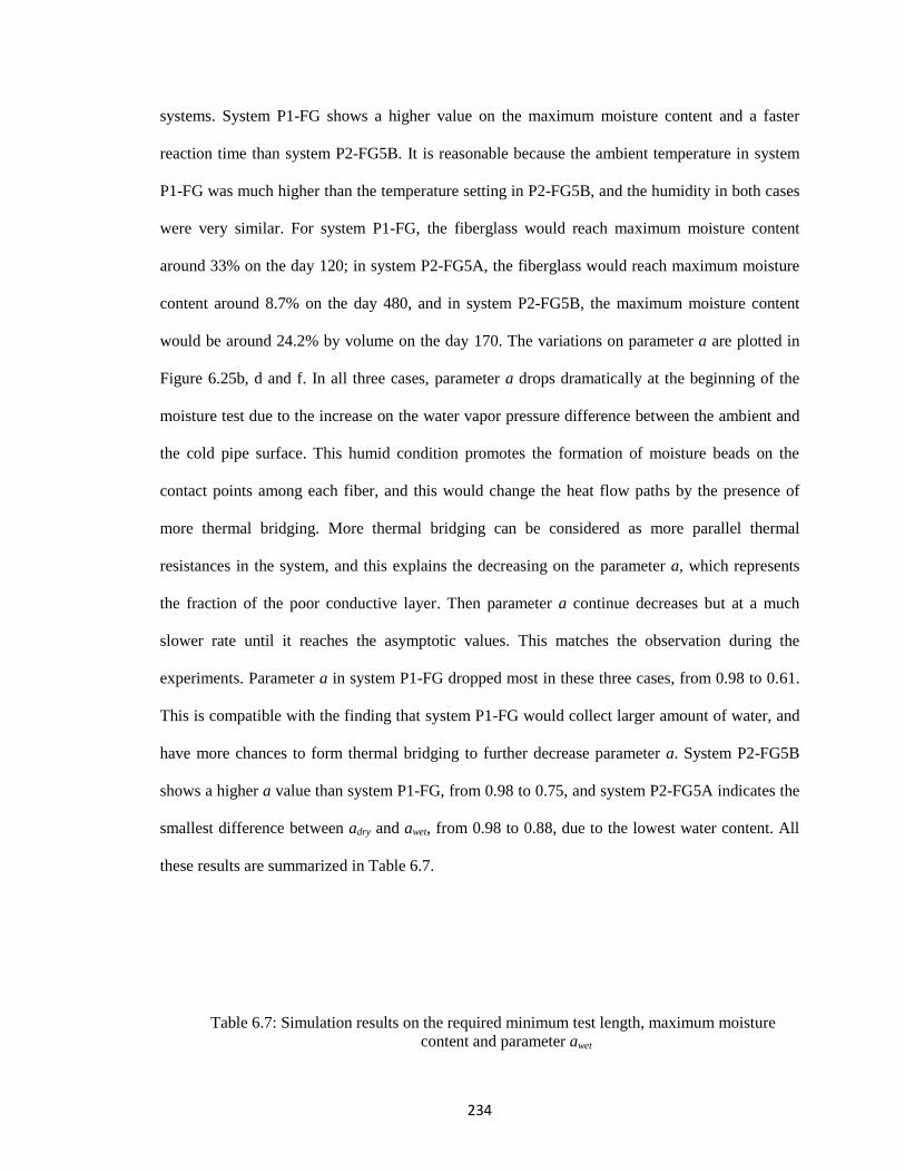
234

systems. System P1-FG shows a higher value on the maximum moisture content and a faster

reaction time than system P2-FG5B. It is reasonable because the ambient temperature in system

P1-FG was much higher than the temperature setting in P2-FG5B, and the humidity in both cases

were very similar. For system P1-FG, the fiberglass would reach maximum moisture content

around 33% on the day 120; in system P2-FG5A, the fiberglass would reach maximum moisture

content around 8.7% on the day 480, and in system P2-FG5B, the maximum moisture content

would be around 24.2% by volume on the day 170. The variations on parameter a are plotted in

Figure 6.25b, d and f. In all three cases, parameter a drops dramatically at the beginning of the

moisture test due to the increase on the water vapor pressure difference between the ambient and

the cold pipe surface. This humid condition promotes the formation of moisture beads on the

contact points among each fiber, and this would change the heat flow paths by the presence of

more thermal bridging. More thermal bridging can be considered as more parallel thermal

resistances in the system, and this explains the decreasing on the parameter a, which represents

the fraction of the poor conductive layer. Then parameter a continue decreases but at a much

slower rate until it reaches the asymptotic values. This matches the observation during the

experiments. Parameter a in system P1-FG dropped most in these three cases, from 0.98 to 0.61.

This is compatible with the finding that system P1-FG would collect larger amount of water, and

have more chances to form thermal bridging to further decrease parameter a. System P2-FG5B

shows a higher a value than system P1-FG, from 0.98 to 0.75, and system P2-FG5A indicates the

smallest difference between adry and awet, from 0.98 to 0.88, due to the lowest water content. All

these results are summarized in Table 6.7.

Table 6.7: Simulation results on the required minimum test length, maximum moisture

content and parameter awet

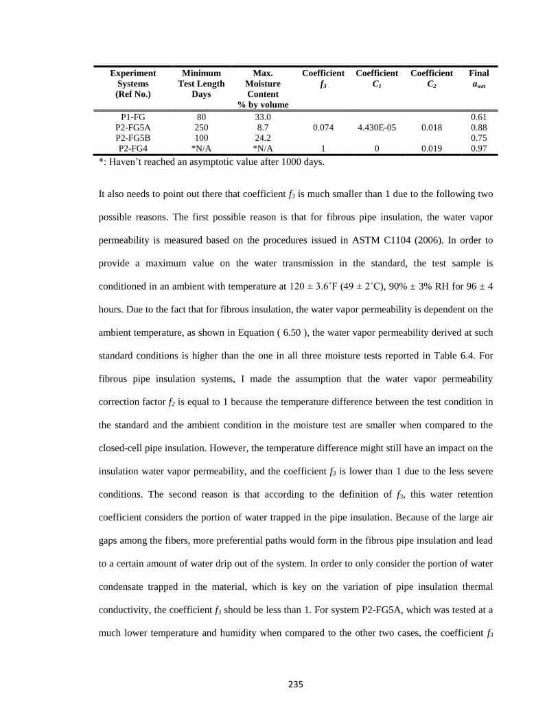
235

Experiment

Systems

(Ref No.)

Minimum

Test Length

Days

Max.

Moisture

Content

% by volume

Coefficient

f3

Coefficient

C1

Coefficient

C2

Final

awet

P1-FG 80 33.0

0.074 4.430E-05 0.018

0.61

P2-FG5A 250 8.7 0.88

P2-FG5B 100 24.2 0.75

P2-FG4 *N/A *N/A 1 0 0.019 0.97

*: Haven’t reached an asymptotic value after 1000 days.

It also needs to point out there that coefficient f3 is much smaller than 1 due to the following two

possible reasons. The first possible reason is that for fibrous pipe insulation, the water vapor

permeability is measured based on the procedures issued in ASTM C1104 (2006). In order to

provide a maximum value on the water transmission in the standard, the test sample is

conditioned in an ambient with temperature at 120 ± 3.6˚F (49 ± 2˚C), 90% ± 3% RH for 96 ± 4

hours. Due to the fact that for fibrous insulation, the water vapor permeability is dependent on the

ambient temperature, as shown in Equation ( 6.50 ), the water vapor permeability derived at such

standard conditions is higher than the one in all three moisture tests reported in Table 6.4. For

fibrous pipe insulation systems, I made the assumption that the water vapor permeability

correction factor f2 is equal to 1 because the temperature difference between the test condition in

the standard and the ambient condition in the moisture test are smaller when compared to the

closed-cell pipe insulation. However, the temperature difference might still have an impact on the

insulation water vapor permeability, and the coefficient f3 is lower than 1 due to the less severe

conditions. The second reason is that according to the definition of f3, this water retention

coefficient considers the portion of water trapped in the pipe insulation. Because of the large air

gaps among the fibers, more preferential paths would form in the fibrous pipe insulation and lead

to a certain amount of water drip out of the system. In order to only consider the portion of water

condensate trapped in the material, which is key on the variation of pipe insulation thermal

conductivity, the coefficient f3 should be less than 1. For system P2-FG5A, which was tested at a

much lower temperature and humidity when compared to the other two cases, the coefficient f3

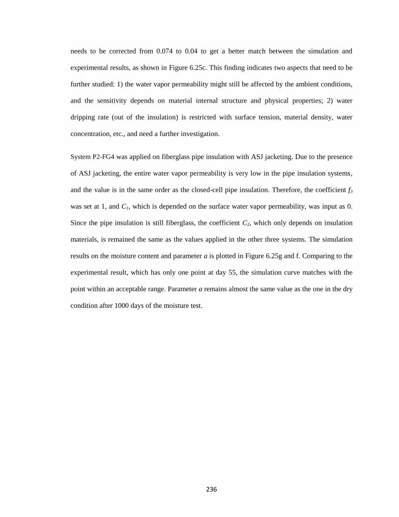
236

needs to be corrected from 0.074 to 0.04 to get a better match between the simulation and

experimental results, as shown in Figure 6.25c. This finding indicates two aspects that need to be

further studied: 1) the water vapor permeability might still be affected by the ambient conditions,

and the sensitivity depends on material internal structure and physical properties; 2) water

dripping rate (out of the insulation) is restricted with surface tension, material density, water

concentration, etc., and need a further investigation.

System P2-FG4 was applied on fiberglass pipe insulation with ASJ jacketing. Due to the presence

of ASJ jacketing, the entire water vapor permeability is very low in the pipe insulation systems,

and the value is in the same order as the closed-cell pipe insulation. Therefore, the coefficient f3

was set at 1, and C1, which is depended on the surface water vapor permeability, was input as 0.

Since the pipe insulation is still fiberglass, the coefficient C2, which only depends on insulation

materials, is remained the same as the values applied in the other three systems. The simulation

results on the moisture content and parameter a is plotted in Figure 6.25g and f. Comparing to the

experimental result, which has only one point at day 55, the simulation curve matches with the

point within an acceptable range. Parameter a remains almost the same value as the one in the dry

condition after 1000 days of the moisture test.

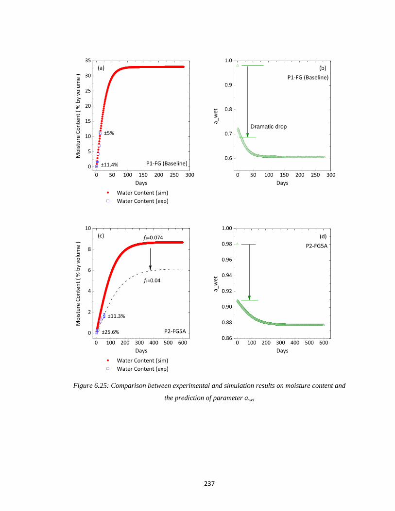
237

Figure 6.25: Comparison between experimental and simulation results on moisture content and

the prediction of parameter awet

0 50 100 150 200 250 300

0

5

10

15

20

25

30

35

±11.4%

±5%

(b)

P1-FG (Baseline)

Water Content (sim)

Water Content (exp)

Mo

istu

re C

on

ten

t (

% b

y vo

lum

e )

Days

P1-FG (Baseline)

(a)

0 50 100 150 200 250 300

0.6

0.7

0.8

0.9

1.0

Days

Dramatic drop

a_w

et

0 100 200 300 400 500 600

0

2

4

6

8

10

±25.6%

±11.3%

f2=0.04

f2=0.074 (d)

P2-FG5A

Water Content (sim)

Water Content (exp)

Mo

istu

re C

on

ten

t (

% b

y vo

lum

e )

Days

P2-FG5A

(c)

0 100 200 300 400 500 6000.86

0.88

0.90

0.92

0.94

0.96

0.98

1.00

Days

a_w

et

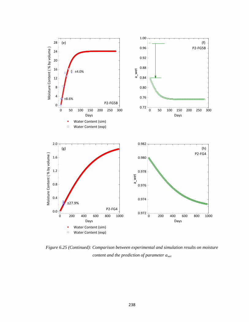
238

Figure 6.25 (Continued): Comparison between experimental and simulation results on moisture

content and the prediction of parameter awet

0 50 100 150 200 250 300

0

4

8

12

16

20

24

28

±4.0%

±8.6%

(f)

P2-FG5B

Water Content (sim)

Water Content (exp)

Mo

istu

re C

on

ten

t (

% b

y vo

lum

e )

Days

P2-FG5B

(e)

0 50 100 150 200 250 3000.72

0.76

0.80

0.84

0.88

0.92

0.96

1.00

Days

a_w

et

0 200 400 600 800 10000.0

0.4

0.8

1.2

1.6

2.0

±27.9%

(h)

P2-FG4

Water Content (sim)

Water Content (exp)

Mo

istu

re C

on

ten

t (

% b

y vo

lum

e )

Days

P2-FG4

(g)

0 200 400 600 800 10000.972

0.974

0.976

0.978

0.980

0.982

Days

a_w

et

239

Validation on the thermal conductivity of fibrous pipe insulation with moisture content

With the profiles of moisture and parameter a derived from previous section, the thermal

conductivity of moist fiberglass pipe insulation could be predicted with water content and with

time. It should be noted that from current model, the moisture profile would only be available on

the total water content in the fiberglass pipe insulation system without considering the moisture

difference between the top and bottom C-shells. In order to take into account for these

differences, the ratio of the mass in the top shell to the total moisture in the test sample was

estimated from each test. By considering the same ratio in the simulation, the moisture profile

was then divided to two groups of inputs, one for the moisture content in the top shell and one for

the bottom. The simulation results on the variation of thermal conductivity with moisture content

and with time for four fiberglass pipe insulation systems are plotted in Figure 6.26a, c, e and g,

with the values.

For systems P1-FG, P2-FG5A, and P2-FG5B, which were fiberglass pipe insulation without

jacketing, the thermal conductivity ratio increased fast due to a dramatic drop on the value of

parameter a, and parameter a was very sensitive to the water vapor pressure differences between

the ambient and the cold pipe surface. Then the thermal conductivity ratio kept increasing but at a

much slower rate. As explained in the previous section, the dramatic increase was due to the

formation of more thermal bridging that changed the direction of the thermal paths; a slower

increasing in the second step was caused by the large amount of high conductive liquid phase that

introduced into the system. Similar to the profiles of moisture content and parameter a, the

thermal conductivity would also reach an asymptotic value, and the pipe insulation system could

be considered as saturated under such test conditions. These simulation results on the thermal

conductivity ratio are also compared to the experimental values. For all three cases, the thermal

conductivity ratio matched with the experimental results within 15%. The thermal conductivity

ratio in system P1-FG would increase most. By the time the insulation system becomes saturated,

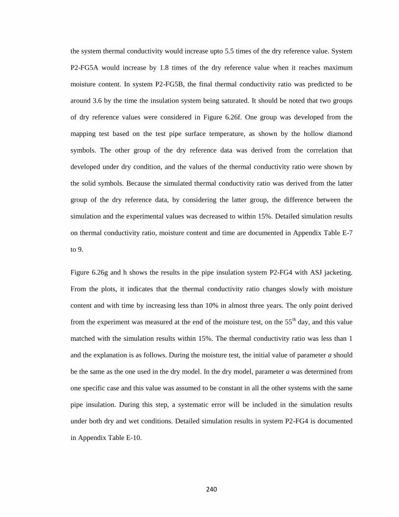
240

the system thermal conductivity would increase upto 5.5 times of the dry reference value. System

P2-FG5A would increase by 1.8 times of the dry reference value when it reaches maximum

moisture content. In system P2-FG5B, the final thermal conductivity ratio was predicted to be

around 3.6 by the time the insulation system being saturated. It should be noted that two groups

of dry reference values were considered in Figure 6.26f. One group was developed from the

mapping test based on the test pipe surface temperature, as shown by the hollow diamond

symbols. The other group of the dry reference data was derived from the correlation that

developed under dry condition, and the values of the thermal conductivity ratio were shown by

the solid symbols. Because the simulated thermal conductivity ratio was derived from the latter

group of the dry reference data, by considering the latter group, the difference between the

simulation and the experimental values was decreased to within 15%. Detailed simulation results

on thermal conductivity ratio, moisture content and time are documented in Appendix Table E-7

to 9.

Figure 6.26g and h shows the results in the pipe insulation system P2-FG4 with ASJ jacketing.

From the plots, it indicates that the thermal conductivity ratio changes slowly with moisture

content and with time by increasing less than 10% in almost three years. The only point derived

from the experiment was measured at the end of the moisture test, on the 55th day, and this value

matched with the simulation results within 15%. The thermal conductivity ratio was less than 1

and the explanation is as follows. During the moisture test, the initial value of parameter a should

be the same as the one used in the dry model. In the dry model, parameter a was determined from

one specific case and this value was assumed to be constant in all the other systems with the same

pipe insulation. During this step, a systematic error will be included in the simulation results

under both dry and wet conditions. Detailed simulation results in system P2-FG4 is documented

in Appendix Table E-10.

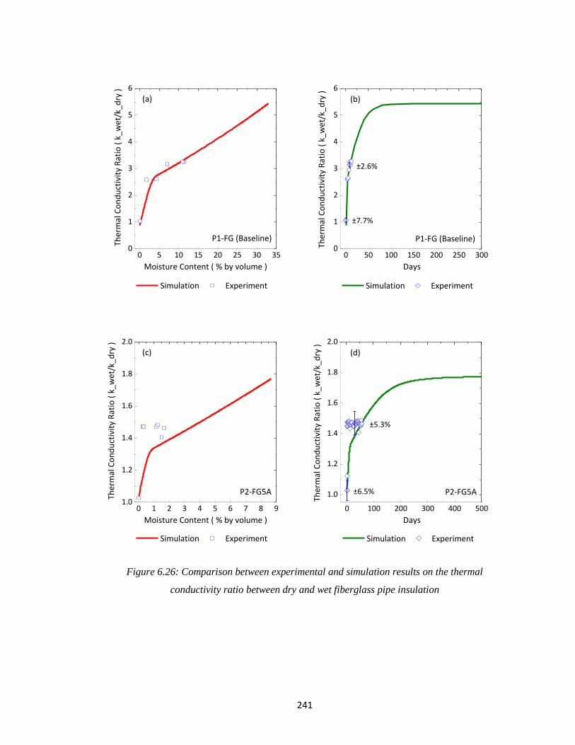
241

Figure 6.26: Comparison between experimental and simulation results on the thermal

conductivity ratio between dry and wet fiberglass pipe insulation

0 5 10 15 20 25 30 350

1

2

3

4

5

6

±7.7%

±2.6%

Simulation Experiment

(b)

P1-FG (Baseline)

Simulation Experiment

Ther

mal

Co

nd

uct

ivit

y R

atio

( k

_wet

/k_d

ry )

Moisture Content ( % by volume )

P1-FG (Baseline)

(a)

0 50 100 150 200 250 3000

1

2

3

4

5

6

Days

Ther

mal

Co

nd

uct

ivit

y R

atio

( k

_wet

/k_d

ry )

0 1 2 3 4 5 6 7 8 91.0

1.2

1.4

1.6

1.8

2.0

±6.5%

±5.3%

Simulation Experiment

P2-FG5A

(d)

Simulation Experiment

Ther

mal

Co

nd

uct

ivit

y R

atio

( k

_wet

/k_d

ry )

Moisture Content ( % by volume )

P2-FG5A

(c)

0 100 200 300 400 500

1.0

1.2

1.4

1.6

1.8

2.0

Days

Ther

mal

Co

nd

uct

ivit

y R

atio

( k

_wet

/k_d

ry )

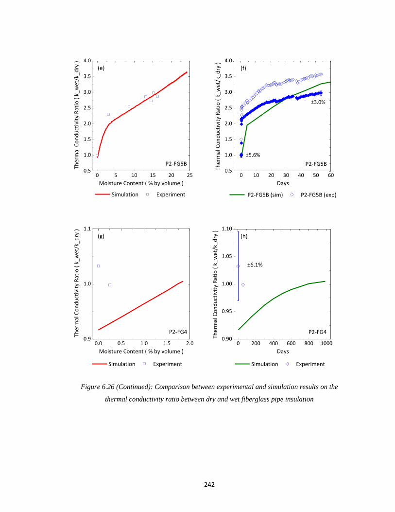
242

Figure 6.26 (Continued): Comparison between experimental and simulation results on the

thermal conductivity ratio between dry and wet fiberglass pipe insulation

0 5 10 15 20 250.5

1.0

1.5

2.0

2.5

3.0

3.5

4.0

P2-FG5B (sim) P2-FG5B (exp)

P2-FG5B

(f)

Simulation Experiment

Ther

mal

Co

nd

uct

ivit

y R

atio

( k

_wet

/k_d

ry )

Moisture Content ( % by volume )

P2-FG5B

(e)

0 10 20 30 40 50 600.5

1.0

1.5

2.0

2.5

3.0

3.5

4.0

±3.0%

±5.6%

Days

Ther

mal

Co

nd

uct

ivit

y R

atio

( k

_wet

/k_d

ry )

0.0 0.5 1.0 1.5 2.00.9

1.0

1.1

Simulation Experiment

P2-FG4

(h)

Simulation Experiment

Ther

mal

Co

nd

uct

ivit

y R

atio

( k

_wet

/k_d

ry )

Moisture Content ( % by volume )

P2-FG4

(g)

0 200 400 600 800 10000.90

0.95

1.00

1.05

1.10

±6.1%

Days

Ther

mal

Co

nd

uct

ivit

y R

atio

( k

_wet

/k_d

ry )

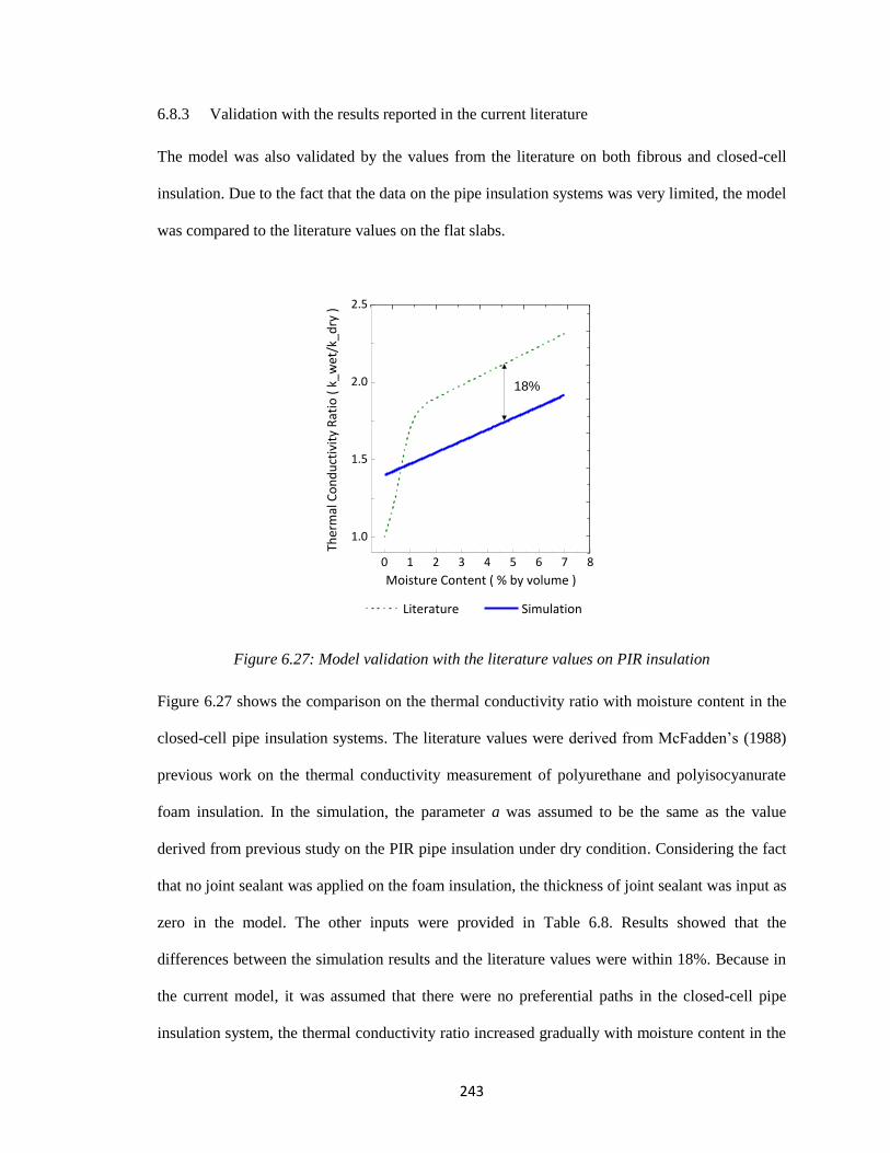
243

6.8.3 Validation with the results reported in the current literature

The model was also validated by the values from the literature on both fibrous and closed-cell

insulation. Due to the fact that the data on the pipe insulation systems was very limited, the model

was compared to the literature values on the flat slabs.

Figure 6.27: Model validation with the literature values on PIR insulation

Figure 6.27 shows the comparison on the thermal conductivity ratio with moisture content in the

closed-cell pipe insulation systems. The literature values were derived from McFadden’s (1988)

previous work on the thermal conductivity measurement of polyurethane and polyisocyanurate

foam insulation. In the simulation, the parameter a was assumed to be the same as the value

derived from previous study on the PIR pipe insulation under dry condition. Considering the fact

that no joint sealant was applied on the foam insulation, the thickness of joint sealant was input as

zero in the model. The other inputs were provided in Table 6.8. Results showed that the

differences between the simulation results and the literature values were within 18%. Because in

the current model, it was assumed that there were no preferential paths in the closed-cell pipe

insulation system, the thermal conductivity ratio increased gradually with moisture content in the

0 1 2 3 4 5 6 7 80.6

0.7

0.8

0.9

1.0

1.1

Literature Simulation

Par

amet

er a

Moisture Content ( % by volume )

(a)

0 1 2 3 4 5 6 7 8

1.0

1.5

2.0

2.5

Moisture Content ( % by volume )

18%

Ther

mal

Co

nd

uct

ivit

y R

atio

( k

_wet

/k_d

ry )

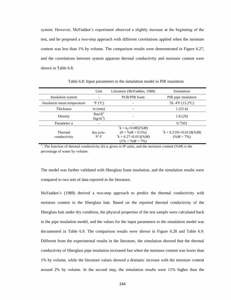
244

system. However, McFadden’s experiment observed a slightly increase at the beginning of the

test, and he proposed a two-step approach with different correlations applied when the moisture

content was less than 1% by volume. The comparison results were demonstrated in Figure 6.27,

and the correlations between system apparent thermal conductivity and moisture content were

shown in Table 6.8.

Table 6.8: Input parameters to the simulation model in PIR insulation

Unit Literature (McFadden, 1988) Simulation

Insulation system - PUR/PIR foam PIR pipe insulation

Insulation mean temperature ºF (ºC) - 59. 4ºF (15.2ºC)

Thickness in (mm) - 1 (25.4)

Density lbm/ft

3

(kg/m3)

- 1.8 (29)

Parameter a - - 0.7503

Thermal

conductivity Btu-in/hr-

ft3-F

1k = k0+0.085(%M)

(0 < %M < 0.5%) 1k = 0.27+0.013(%M)

(1% < %M < 7%)

1k = 0.2191+0.0118(%M)

(%M < 7%)

1: The function of thermal conductivity (k) is given in IP units, and the moisture content (%M) is the

percentage of water by volume.

The model was further validated with fiberglass foam insulation, and the simulation results were

compared to two sets of data reported in the literature.

McFadden’s (1988) derived a two-step approach to predict the thermal conductivity with

moisture content in the fiberglass batt. Based on the reported thermal conductivity of the

fiberglass batt under dry condition, the physical properties of the test sample were calculated back

in the pipe insulation model, and the values for the input parameters to the simulation model was

documented in Table 6.9. The comparison results were shown in Figure 6.28 and Table 6.9.

Different from the experimental results in the literature, the simulation showed that the thermal

conductivity of fiberglass pipe insulation increased fast when the moisture content was lower than

1% by volume, while the literature values showed a dramatic increase with the moisture content

around 2% by volume. In the second step, the simulation results were 11% higher than the

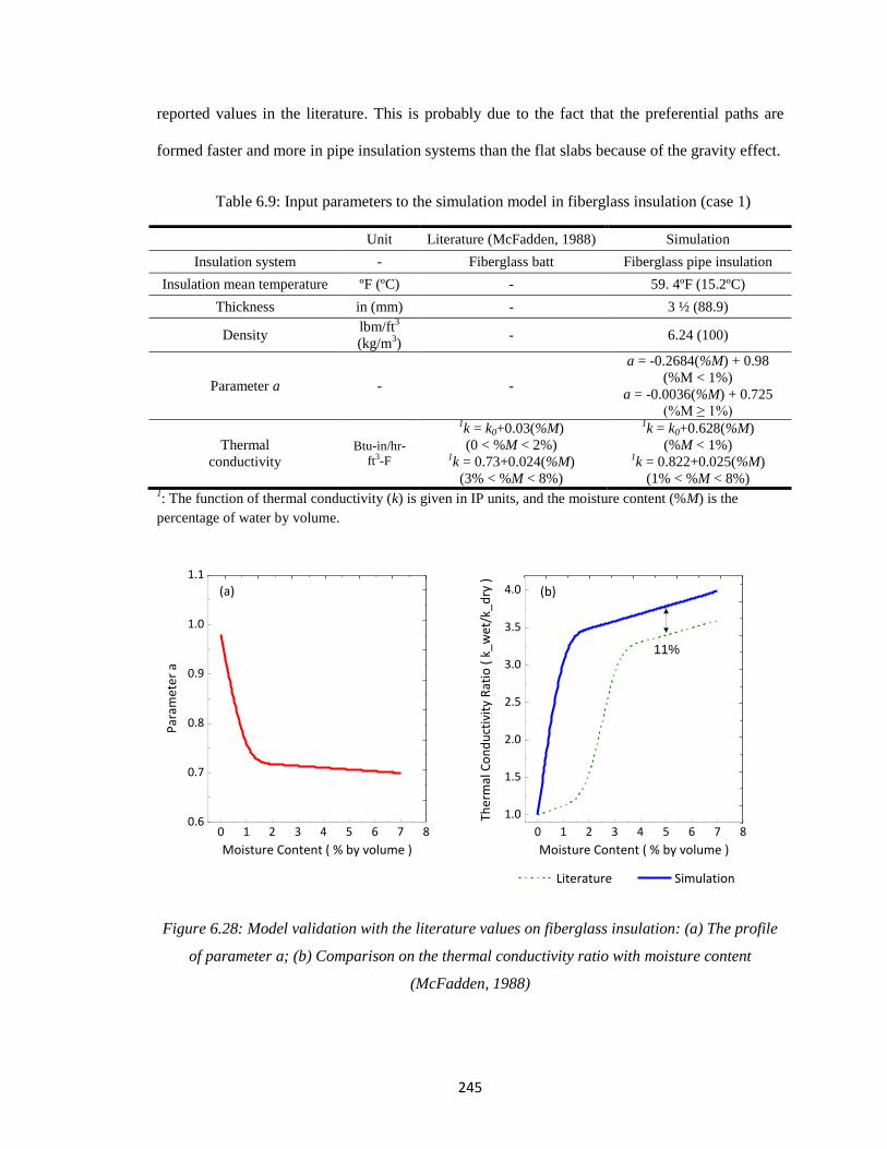
245

reported values in the literature. This is probably due to the fact that the preferential paths are

formed faster and more in pipe insulation systems than the flat slabs because of the gravity effect.

Table 6.9: Input parameters to the simulation model in fiberglass insulation (case 1)

Unit Literature (McFadden, 1988) Simulation

Insulation system - Fiberglass batt Fiberglass pipe insulation

Insulation mean temperature ºF (ºC) - 59. 4ºF (15.2ºC)

Thickness in (mm) - 3 ½ (88.9)

Density lbm/ft

3

(kg/m3)

- 6.24 (100)

Parameter a - -

a = -0.2684(%M) + 0.98

(%M < 1%)

a = -0.0036(%M) + 0.725

(%M ≥ 1%)

Thermal

conductivity Btu-in/hr-

ft3-F

1k = k0+0.03(%M)

(0 < %M < 2%) 1k = 0.73+0.024(%M)

(3% < %M < 8%)

1k = k0+0.628(%M)

(%M < 1%) 1k = 0.822+0.025(%M)

(1% < %M < 8%) 1: The function of thermal conductivity (k) is given in IP units, and the moisture content (%M) is the

percentage of water by volume.

Figure 6.28: Model validation with the literature values on fiberglass insulation: (a) The profile

of parameter a; (b) Comparison on the thermal conductivity ratio with moisture content

(McFadden, 1988)

0 1 2 3 4 5 6 7 80.6

0.7

0.8

0.9

1.0

1.1

Literature Simulation

(b)

Par

amet

er a

Moisture Content ( % by volume )

(a)

0 1 2 3 4 5 6 7 8

1.0

1.5

2.0

2.5

3.0

3.5

4.0

Moisture Content ( % by volume )

11%

Ther

mal

Co

nd

uct

ivit

y R

atio

( k

_wet

/k_d

ry )

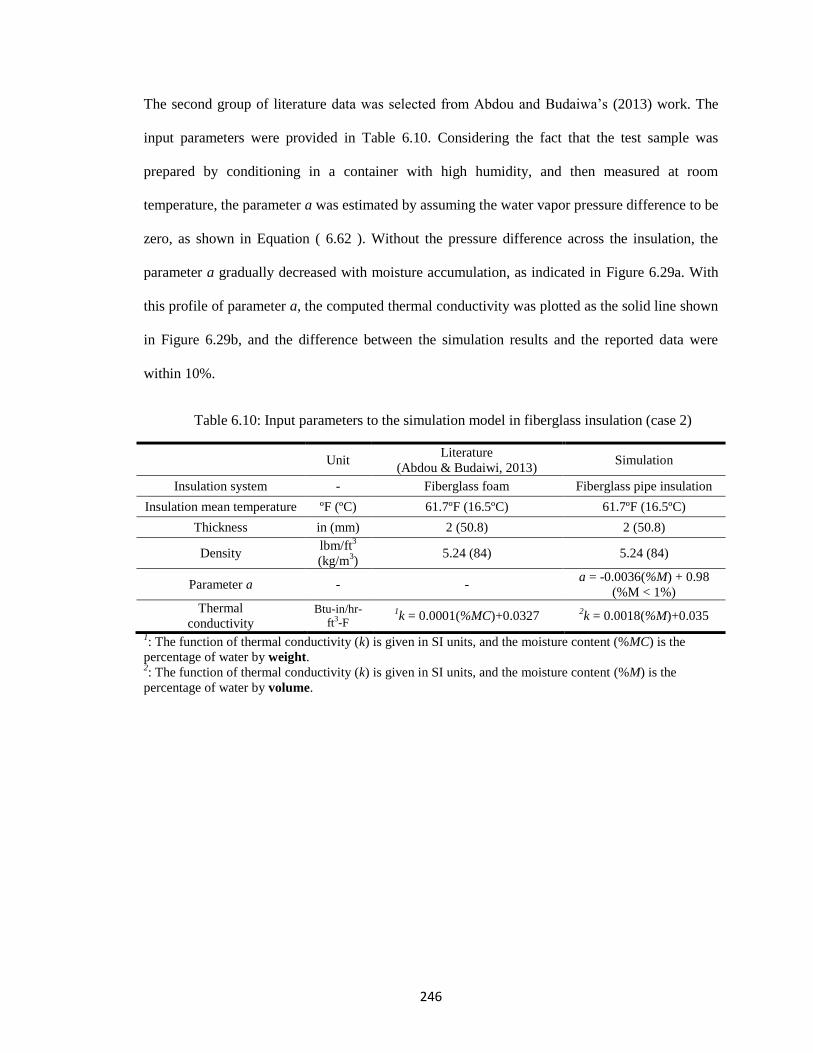
246

The second group of literature data was selected from Abdou and Budaiwa’s (2013) work. The

input parameters were provided in Table 6.10. Considering the fact that the test sample was

prepared by conditioning in a container with high humidity, and then measured at room

temperature, the parameter a was estimated by assuming the water vapor pressure difference to be

zero, as shown in Equation ( 6.62 ). Without the pressure difference across the insulation, the

parameter a gradually decreased with moisture accumulation, as indicated in Figure 6.29a. With

this profile of parameter a, the computed thermal conductivity was plotted as the solid line shown

in Figure 6.29b, and the difference between the simulation results and the reported data were

within 10%.

Table 6.10: Input parameters to the simulation model in fiberglass insulation (case 2)

Unit

Literature

(Abdou & Budaiwi, 2013) Simulation

Insulation system - Fiberglass foam Fiberglass pipe insulation

Insulation mean temperature ºF (ºC) 61.7ºF (16.5ºC) 61.7ºF (16.5ºC)

Thickness in (mm) 2 (50.8) 2 (50.8)

Density lbm/ft

3

(kg/m3)

5.24 (84) 5.24 (84)

Parameter a - - a = -0.0036(%M) + 0.98

(%M < 1%)

Thermal

conductivity Btu-in/hr-

ft3-F 1k = 0.0001(%MC)+0.0327

2k = 0.0018(%M)+0.035

1: The function of thermal conductivity (k) is given in SI units, and the moisture content (%MC) is the

percentage of water by weight. 2: The function of thermal conductivity (k) is given in SI units, and the moisture content (%M) is the

percentage of water by volume.

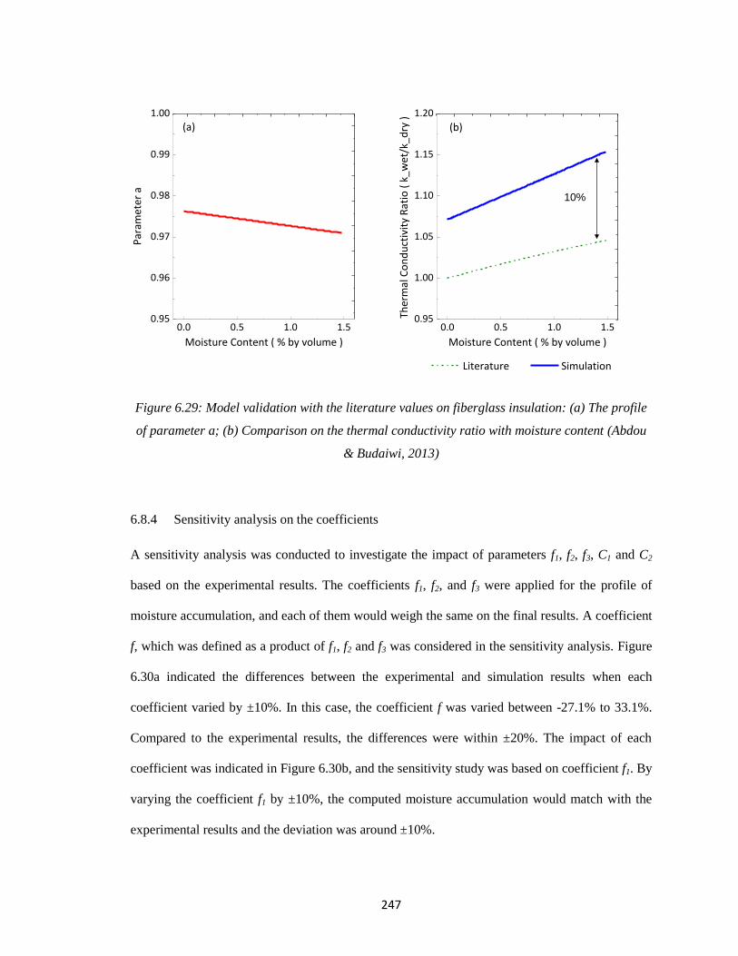
247

Figure 6.29: Model validation with the literature values on fiberglass insulation: (a) The profile

of parameter a; (b) Comparison on the thermal conductivity ratio with moisture content (Abdou

& Budaiwi, 2013)

6.8.4 Sensitivity analysis on the coefficients

A sensitivity analysis was conducted to investigate the impact of parameters f1, f2, f3, C1 and C2

based on the experimental results. The coefficients f1, f2, and f3 were applied for the profile of

moisture accumulation, and each of them would weigh the same on the final results. A coefficient

f, which was defined as a product of f1, f2 and f3 was considered in the sensitivity analysis. Figure

6.30a indicated the differences between the experimental and simulation results when each

coefficient varied by ±10%. In this case, the coefficient f was varied between -27.1% to 33.1%.

Compared to the experimental results, the differences were within ±20%. The impact of each

coefficient was indicated in Figure 6.30b, and the sensitivity study was based on coefficient f1. By

varying the coefficient f1 by ±10%, the computed moisture accumulation would match with the

experimental results and the deviation was around ±10%.

0.0 0.5 1.0 1.50.95

0.96

0.97

0.98

0.99

1.00

Literature Simulation

(b)P

aram

eter

a

Moisture Content ( % by volume )

(a)

0.0 0.5 1.0 1.50.95

1.00

1.05

1.10

1.15

1.20

Moisture Content ( % by volume )

10%

Ther

mal

Co

nd

uct

ivit

y R

atio

( k

_wet

/k_d

ry )

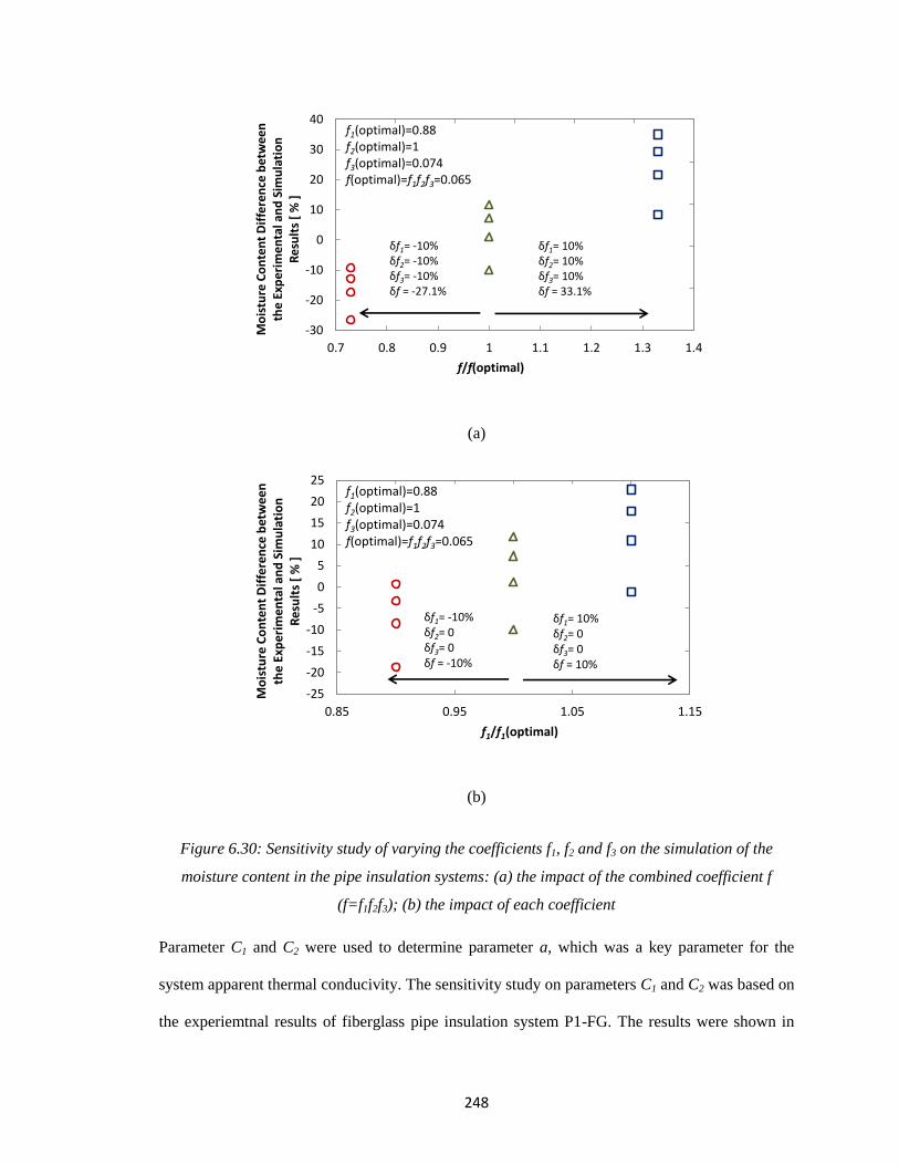
248

(a)

(b)

Figure 6.30: Sensitivity study of varying the coefficients f1, f2 and f3 on the simulation of the

moisture content in the pipe insulation systems: (a) the impact of the combined coefficient f

(f=f1f2f3); (b) the impact of each coefficient

Parameter C1 and C2 were used to determine parameter a, which was a key parameter for the

system apparent thermal conducivity. The sensitivity study on parameters C1 and C2 was based on

the experiemtnal results of fiberglass pipe insulation system P1-FG. The results were shown in

-30

-20

-10

0

10

20

30

40

0.7 0.8 0.9 1 1.1 1.2 1.3 1.4

Mo

istu

re C

on

ten

t D

iffe

ren

ce b

etw

een

th

e Ex

per

imen

tal a

nd

Sim

ula

tio

n

Res

ult

s [

% ]

f/f(optimal)

f1(optimal)=0.88f2(optimal)=1f3(optimal)=0.074f(optimal)=f1f2f3=0.065

δf1= -10%δf2= -10%δf3= -10%δf = -27.1%

δf1= 10%δf2= 10%δf3= 10%δf = 33.1%

-25

-20

-15

-10

-5

0

5

10

15

20

25

0.85 0.95 1.05 1.15

Mo

istu

re C

on

ten

t D

iffe

ren

ce b

etw

een

th

e E

xpe

rim

en

tal a

nd

Sim

ula

tio

n

Re

sult

s [

% ]

f1/f1(optimal)

f1(optimal)=0.88f2(optimal)=1f3(optimal)=0.074f(optimal)=f1f2f3=0.065

δf1= -10%δf2= 0δf3= 0δf = -10%

δf1= 10%δf2= 0δf3= 0δf = 10%

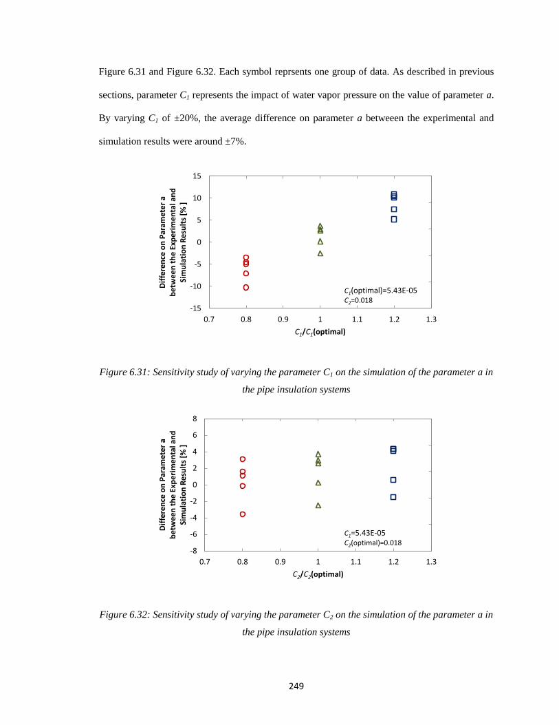
249

Figure 6.31 and Figure 6.32. Each symbol reprsents one group of data. As described in previous

sections, parameter C1 represents the impact of water vapor pressure on the value of parameter a.

By varying C1 of ±20%, the average difference on parameter a betweeen the experimental and

simulation results were around ±7%.

Figure 6.31: Sensitivity study of varying the parameter C1 on the simulation of the parameter a in

the pipe insulation systems

Figure 6.32: Sensitivity study of varying the parameter C2 on the simulation of the parameter a in

the pipe insulation systems

-15

-10

-5

0

5

10

15

0.7 0.8 0.9 1 1.1 1.2 1.3

Dif

fere

nce

on

Par

amet

er a

b

etw

een

th

e Ex

per

imen

tal a

nd

Si

mu

lati

on

Res

ult

s [%

]

C1/C1(optimal)

C1(optimal)=5.43E-05C2=0.018

-8

-6

-4

-2

0

2

4

6

8

0.7 0.8 0.9 1 1.1 1.2 1.3

Dif

fere

nce

on

Par

amet

er a

b

etw

een

th

e Ex

per

imen

tal a

nd

Si

mu

lati

on

Res

ult

s [%

]

C2/C2(optimal)

C1=5.43E-05C2(optimal)=0.018

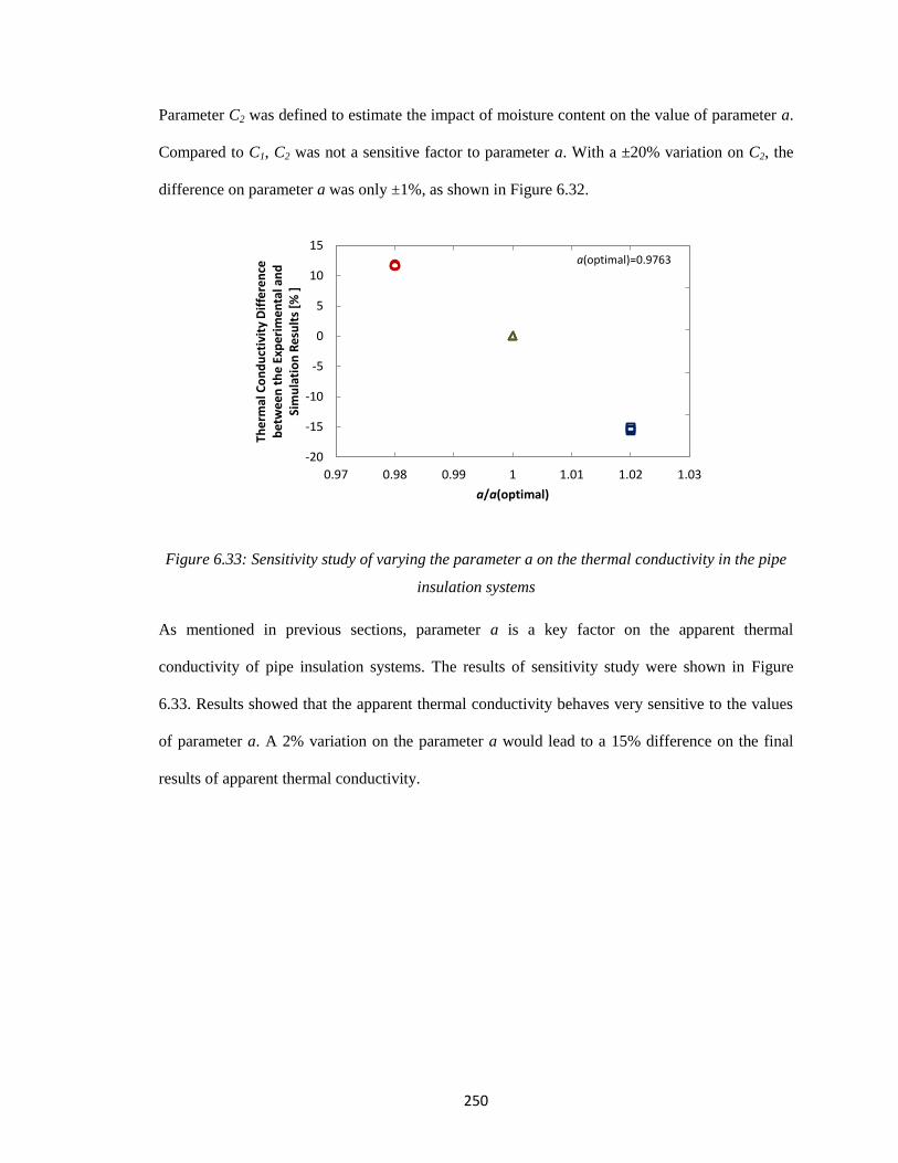
250

Parameter C2 was defined to estimate the impact of moisture content on the value of parameter a.

Compared to C1, C2 was not a sensitive factor to parameter a. With a ±20% variation on C2, the

difference on parameter a was only ±1%, as shown in Figure 6.32.

Figure 6.33: Sensitivity study of varying the parameter a on the thermal conductivity in the pipe

insulation systems

As mentioned in previous sections, parameter a is a key factor on the apparent thermal

conductivity of pipe insulation systems. The results of sensitivity study were shown in Figure

6.33. Results showed that the apparent thermal conductivity behaves very sensitive to the values

of parameter a. A 2% variation on the parameter a would lead to a 15% difference on the final

results of apparent thermal conductivity.

-20

-15

-10

-5

0

5

10

15

0.97 0.98 0.99 1 1.01 1.02 1.03

Ther

mal

Co

nd

uct

ivit

y D

iffe

ren

ce

bet

wee

n t

he

Exp

erim

enta

l an

d

Sim

ula

tio

n R

esu

lts

[% ]

a/a(optimal)

a(optimal)=0.9763

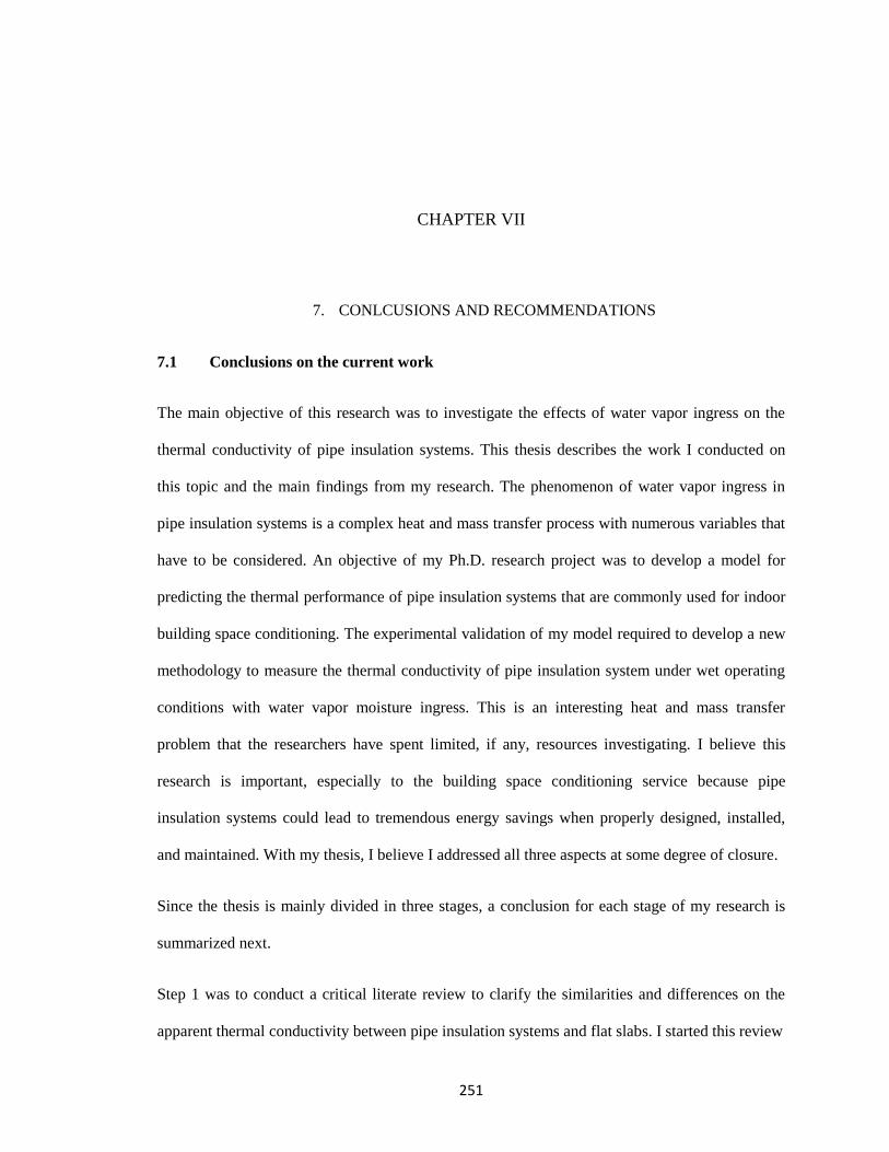
251

CHAPTER VII

7. CONLCUSIONS AND RECOMMENDATIONS

7.1 Conclusions on the current work

The main objective of this research was to investigate the effects of water vapor ingress on the

thermal conductivity of pipe insulation systems. This thesis describes the work I conducted on

this topic and the main findings from my research. The phenomenon of water vapor ingress in

pipe insulation systems is a complex heat and mass transfer process with numerous variables that

have to be considered. An objective of my Ph.D. research project was to develop a model for

predicting the thermal performance of pipe insulation systems that are commonly used for indoor

building space conditioning. The experimental validation of my model required to develop a new

methodology to measure the thermal conductivity of pipe insulation system under wet operating

conditions with water vapor moisture ingress. This is an interesting heat and mass transfer

problem that the researchers have spent limited, if any, resources investigating. I believe this

research is important, especially to the building space conditioning service because pipe

insulation systems could lead to tremendous energy savings when properly designed, installed,

and maintained. With my thesis, I believe I addressed all three aspects at some degree of closure.

Since the thesis is mainly divided in three stages, a conclusion for each stage of my research is

summarized next.

Step 1 was to conduct a critical literate review to clarify the similarities and differences on the

apparent thermal conductivity between pipe insulation systems and flat slabs. I started this review

252

by comparing different experimental methodologies for measuring the apparent thermal

conductivity of pipe insulation and flat slab systems. Both transient and steady-state

methodologies are proposed for the thermal conductivity measurement. Although the steady state

methods have some disadvantages, such as , need a considerable amount of time to reach thermal

equilibrium, large test sample size to eliminate edge effect, and a limited temperature range to

prevent radiation, it is considered as an appropriate method for measuring the system apparent

thermal conductivity. It is simpler and provides a more direct measurement than transient

methods. Transient method can provide a fast measurement on the local thermal conductivity, but

to determine a system behavior, this method is strongly depended on the number and locations of

the probing sensors. The accuracy and repeatability of transient methods for pipe insulation

systems are also not as well defined as steady-state methodologies. Therefore, a steady-state

method was selected for the following experiments in this thesis. Under wet condition, different

techniques are required during thermal conductivity measurement depending on how the test

samples being prepared in the laboratory. Based on the current literature, I summarized four

moisturizing strategies as flooded method, spray/injection method, laboratory pre-conditioning

method, and conditioned ambience with cold surface/pipe method. It is concluded that only the

last moisturizing strategy would provide similar boundary conditions as in the actual field. This

technique can be combined with steady state methodologies to determine the system apparent

thermal conductivity without the water redistribution impact. However, it should be noted that

this technique requires a large investment for the equipment and control of the ambient conditions.

A more compact test apparatus, or a novel technique that would solve current challenges, such as

the non-uniform surface temperatures, and moisture redistribution in radial configuration, is

required for further study. From the literature review, the methodology selected for the following

tests is a radial heat flow meter with temperature and humidity controlled in a psychrometric

chamber.

253

During the second stage of my research, a novel experimental apparatus, referred in this

dissertation as pipe insulation tester, or PIT, was developed for the system thermal conductivity

measurement. Pipe insulation systems were installed around the test pipe of these PITs. The test

pipe surface temperature was maintained by a refrigeration system. The radial heat flux was

calculated by surface temperature measurements on the inner refrigeration tubing and on the test

pipe. The test apparatus kept improving based on what I learned from the experiments, and the

current test apparatus was able to measure a low heat flux of about 8.2 Btu/hr-ft (7.9 W/m) with

an uncertainty at ±5.7%. Up to now, seven fibrous and nine closed-cell pipe insulation systems

were tested on the PITs under dry condition. The ambient temperature was controlled between 75

to 110°F (23.8 to 43.3°C), with the insulation mean temperature varied from 55 to 73°F (12.8

to 22.8°C). For both fibrous and closed-cell pipe insulation systems, the apparent thermal

conductivity varies almost linearly with the insulation mean temperature. I also observed that the

joint sealant seems to be a significant impact for the system thermal performance, and the

presence of the joint sealant may increase the system apparent thermal conductivity by 15%. All

the detailed information, including material properties and installation, are documented in Table

5.13. Four fibrous and six closed-cell pipe insulation systems were tested under wet, condensing

conditions with moisture ingress. The ambient condition was set as a hot and humid environment

to accelerate moisture ingress in the pipe insulation systems. In most cases, the temperature was

controlled from 90 to 110 ºF (32 to 43ºC), with relative humidity between 81 to 84%. According

to the observation during the experiment, I summarized the water diffusion mechanism and

moisture impact on the system performance for both fibrous and closed-cell pipe insulation. In

fibrous pipe insulation systems, moisture diffuses through the preferential paths and the system

behaves fairly sensitive to the ambient at the beginning of the moisture test. This is because under

condensing conditions, moisture bead would start forming at the contact point between each fiber

and change the thermal path by creating more thermal bridging in the insulation systems. The

thermal conductivity would increase dramatically during this process, even with a small amount

254

of water in the system. Closed-cell pipe insulation systems are less affected by the moisture

during the initial stage. This is due to the enclosure structure of the cells in the material would

have less possibility to form thermal bridging and the preferential paths. Moisture will diffuse

gradually from the internal surface outward. These two mechanisms are important and would be

used as the basic theory for model development. All the information regarding to the material

installation, ambient conditions and test results under wet conditions are documented in detail in

Table 5.14.

Based on the conclusions from the experiments, a semi-empirical analytical model was developed

to predict the system thermal conductivity with different ambient conditions and with time.

Considering the similarities between fibrous and closed-cell pipe insulation systems, a general

model was developed for both cases. This model considered the insulation system as a

combination of solid phase, gas phase and liquid phase in different configurations. A parameter,

a, was introduced to represent the portion of each configuration, which would have a significant

impact on the system thermal conductivity. This parameter a was assumed to be constant among

the same type of insulation materials. For closed-cell pipe insulation systems, parameter a would

remain constant between dry and wet conditions due to a steady variation observed on the system

performance. For fibrous pipe insulation systems, parameter a was not a constant value with the

presence of moisture, and this parameter was further correlated with the ambient condition and

the moisture content in the system. Under wet conditions, parameter a would decrease by

following a two-step variation, and gradually approach an asymptotic value. The system thermal

conductivity would also reach a maximum when parameter a become stabilized. This model was

validated with both experimental data and the reported values from the open domain literature.

For closed-cell pipe insulation systems, the moisture profile with time need to be further

investigated. The thermal conductivity ratio could be predicted with moisture content, and the

difference between the simulation and experimental results were within 10%. For fibrous pipe

255

insulation systems, both moisture profile and thermal conductivity ratio with moisture content

and with time matched well with the experimental results. The differences were within 15%.

7.2 Recommendations for future work

The following recommendations are mainly on the modelling part.

In the current model, coefficients f1, f2 and f3 are used to generate moisture profiles. The method

used for the determination of these three factors can be better improved in the future work. The

coefficient f1 is the condensation coefficient that represents the volume ratio of the region with

temperature lower than the dew point to the total volume. In the current model, this coefficient

was derived based on a 2-d steady-state conduction heat transfer equation, with a boundary

condition from the beginning of the test. This value was assumed to be constant during the

moisture test. However, this assumption is weak because the boundary condition keeps changing

and the condensation region varies during the wet period. A detailed temperature distribution

profile may help updating the condensation region, and the coefficient f1. Functioned as a

correction factor on the water vapor permeability, f2 is an important coefficient since the water

vapor permeability is a key parameter to predict the water content that accumulated in the

insulation. According to the literature, it will be varied with ambient temperature and material

porosity. However, currently I haven’t found enough information to correlate the water vapor

permeability with ambient temperature and material porosity for different types of pipe insulation

systems. Either a deeper research in the literature, or another group of test on the same pipe

insulation system, may help determine this correlation. By adding one additional group of test

will help back out the parameter that is required in the current correlation between water vapor

permeability and the ambient temperature. Coefficient f3 is the water retention coefficient that

represents the portion of the water condensate remains trapped in the insulation system. One

additional step in the experiment may do some help in the determination of this coefficient. For

256

example, we can collect all the condensate that drips out from the insulation, and compare to the

amount water trapped in the insulation system. This simple procedure will help us have a better

understand on how this coefficient changes with time and with the total moisture content.

Moisture redistribution is another important factor that need to be further considered in the

model. Especially for fibrous pipe insulation systems, the moisture distributions in the top and

bottom shells are different and it may lead to different internal structures that would be referred to

in the model.

Parameter a is a factor that cannot be physically measured, and it was assumed to vary linearly

with water vapor pressure difference across the insulation and the moisture content trapped in the

insulation system. The only way validate this theory is from more experimental data on the

moisture test under different ambient conditions.

Joint sealant seems to be an important factor to the thermal behavior of pipe insulation systems

under both dry and wet conditions. Under dry condition, the high conductive layer would increase

the system apparent thermal conductivity, and under wet condition, the high water vapor

permeability might impact on the total water content in the insulation system. The high

conductive layer also caused water accumulation on the joint sealant surface, and this may effect

both temperate and moisture distribution in the pipe insulation systems. A parallel study on the

joint sealant would be very helpful on the future research of pipe insulation systems.

At last, it should be noted that all the conclusions derived from both moisture test and simulation

models are only considered the pipe insulation systems applied in the horizontal direction. For

vertically installed pipe insulation systems, the findings that derived from the horizontal tests

might still be applicable if it is under dry condition, but with the presence of moisture in the

system, the results might be quite different due to the effect of gravity.

257

REFERENCES

Abdou, A., & Budaiwi, I. (2013). The variation of thermal conductivity of fibrous insulation

materials under different levels of moisture content. Construction and Building

Materials, 43, 533-544. doi: 10.1016/j.conbuildmat.2013.02.058

Abdou, A. A., & Budaiwi, I. M. (2005). Comparison of thermal conductivity measurements of

building insulation materials under various operating temperatures. Journal of Building

Physics, 29(2), 171-184.

Adams, L. (1974). Thermal conductivity of wet insulations. ASHRAE Journal, 16(10), 61-62.

Adl-Zarrabi, B. (2005). Determination of thermal conductivity: The IPS method for determining

of insulation of pipes. Euroheat and Power (English Edition)(2), 40-42.

Al-Hammad, A.-M., Abdelrahman, M. A., Grondzik, W., & Hawari, A. (1994). Comparison

between actual and published k-values for Saudi insulation materials. Journal of Thermal

Insulation and Building Envelopes, 17, 378-385.

Albers, M. A. (2002). A round robin interlaboratory comparison of thermal conductivity testing

using the guarded hot plate up to 1000C, Charleston, SC, USA.

ASTM C 585 - 09, Standard Practice for Inner and Outer Diameters of Thermal Insulation for

Normal Sizes of Pipe and Tubing. (2009). ASTM International, West Conshohocken, PA.

doi: 10.1520/C0585-10.

ASTM C518 - 10 Standard Test Method for Steady-State Thermal Transmission Properties by

Means of the Heat Flow Meter Apparatus. (2010). ASTM International, West

Conshohocken, PA. doi: 10.1520/C0518-10.

ASTM Standard C177-10. (2010). Standard test method for steady-state heat flux measurements

and thermal transmission properties by means of the guarded-hot-plate apparatus, ASTM

International, Philadelphia. doi: 10.1520/C0177-10.

ASTM Standard C209-07a. (2007). Standard Test Methods for Cellulosic Fiber Insulating Boar,

ASTM International, Philadelphia. doi: 10.1520/C0209-07A.

ASTM Standard C272-01. (2007). Standard Test Method for Water Absorption of Core Materials

for Structural Sandwich Construction, ASTM International, Philadelphia. doi:

10.1520/C0272-01R07.

ASTM Standard C335-05. (2005). Standard test bethod for steady-state heat transfer properties of

pipe insulation, ASTM International, Philadelphia. doi: 10.1520/C0335-05.

ASTM Standard C518-10. (2010). Standard test method for steady-state thermal transmission

properties by means of the heat flow meter apparatus, ASTM International, Philadelphia.

doi: 10.1520/C0518-10.

ASTM Standard C552-12b. (2012). Standard Specification for Cellular Glass Thermal Insulation,

ASTM International, Philadelphia. doi: 10.1520/C0552-12B.

ASTM Standard C1104/C1104M-00. (2006). Standard Test Method for Determining the Water

Vapor Sorption of Unfaced Mineral Fiber Insulation, ASTM International, Philadelphia.

doi: 10.1520/C1104_C1104M-00R06.

258

ASTM Standard C1114. (2006). Standard test method for steady-state thermal transmission

properties by means of the thin-heater apparatus, ASTM International, Philadelphia. doi:

10.1520/C1114-06.

ASTM Standard C1126-04. (2009). Faced or unfaced rigid cellular phenolic thermal insulation,

ASTM Interational, Pheladelphia. doi: 10.1520/C1126.

ASTM Standard C1363-11. (2011). Standard test method for thermal performance of building

materials and envolop assemblies by means of a hot box apparatus, ASTM International,

Philadelphia. doi: 10.1520/C1363-11.

Batty, W. J., O'Callaghan, P. W., & Probert, S. D. (1981). Apparent thermal conductivity of

glass-fiber insulant: effects of compression and moisture content. Applied energy, 9(1),

55-76. doi: 10.1016/0306-2619(81)90042-8.

Batty, W. J., Probert, S. D., Ball, M., & O'Callaghan, P. W. (1984). Use of the thermal - probe

technique for the measurement of the apparent thermal conductivities of moist materials.

Applied energy, 18(4), 301-317.

Benner, S. M., & Modi, D. K. (1986). Moisture gain of spray - applied insulations and its effect

on effective thermal conductivity - Part II. Journal of thermal insulation, 9, 211-223.

Bezjak, M., & Zvizdic, D. (2011). Dynamic measurements of the thermal conductivity of

insulators. International Journal of Thermophysics, 32(7-8), 1467-1478. doi:

10.1007/s10765-011-1025-8.

Bhattacharjee, D., King, J. A., & Whitehead, K. N. (1991). Thermal conductivity of PU/PIR

foams as a function of mean temperature. Journal of Cellular Plastics, 27(3), 240-251.

Biedermann, A., Kudoke, C., Merten, A., Minogue, E., Rotermund, U., Ebert, H. P., Heinemann,

U., Fricke, J., & Seifert, H. (2001). Analysis of heat transfer mechanisms in polyurethane

rigid foam. Journal of Cellular Plastics, 37(6), 467-483. doi: 10.1106/kemu-lh63-v9h2-

kfa3

BS-EN 253. (2009). District heating pipes - Preinsulated bounded pipe systems for directly buried

hot water networks - pipe assembly of steel service pipe, polyurethan thermal insulation

and outer casing of polyethylene, British-Adopted European Standard.

BS-EN 12667. (2001). Thermal Resistance of Building Materials and Products - Determination of

Thermal Resistance by Means of Guarded Hot Plate and Heat Flow Meter Methods -

Products of High and Meduum Resistance, British-Adopted European Standard.

Budaiwi, I., Abdou, A., & Al-Homoud, M. (2002). Variations of thermal conductivity of

insulation materials under different operating temperatures: Impact on envelope-induced

cooling load. Journal of Architectural Engineering, 8(4), 125-132.

Chalumeau, A., & Felix-Henry, A. (2006). Water absorption effect on syntactic foam thermal

insulation of a flexible pipe, Hamburg, Germany.

Christian, J. E., Desjarlais, A., Graves, R., & Smith, T. L. (1998). Five-year field study confirms

accelerated thermal aging method for polyisocyanurate insulation. Journal of Cellular

Plastics, 34(1), 39-64.

Chyu, M.-C., Zeng, X., & Ye, L. (1997a). Effect of moisture content on the performance of

polyurethane insulation used on a district heating and cooling pipe, Philadelphia, PA,

USA.

Chyu, M.-C., Zeng, X., & Ye, L. (1997b). Performance of fibrous glass pipe insulation subjected

to underground water attack, Philadelphia, PA, USA.

Cremaschi, L., Cai, S., Ghajar, A., & Worthington, K. (2012a). ASHRAE RP 1356 final report:

Methodology to measure thermal performance of pipe insulation at below ambient

temperatures: ASHRAE, available by request to ASHRAE.

Cremaschi, L., Cai, S., Worthington, K., & Ghajar, A. (2012b). Measurement of pipe insulation

thermal conductivity at below ambient temperatures Part I: Experimental methodology

and dry tests (ASHRAE RP-1356). Paper presented at the ASHRAE winter conference -

Technical papers, January 21, 2012 - January 25, 2012, Chicago, IL, USA.

259

Eriksson, D., & Sunden, B. (1998). Heat and mass transfer in polyurethane insulated district

cooling and heating pipes. Journal of Thermal Envelope and Building Science, 22, 49-71.

Freitas, V., Crausse, P., & Abrantes, V. (1991). Moisture diffusion in thermal insulating

materials, Gatlinburg, TN, USA.

Ge, Z., Cahill, D. G., & Braun, P. V. (2006). Thermal conductance of hydrophilic and

hydrophobic interfaces. Physical Review Letters, 96(18). doi:

10.1103/PhysRevLett.96.186101

Glazebrook, S. R. (1922). A dictionary of applied physics, Volume 1 (Vol. 1): Macmillan and co.

Golestanian, H. (2007). Physical determination of permeability variation with porosity for

composite performs (Vol. 18, pp. 67-73): IUST International Journal of Engineering

Science (Special Issue).

Guldbrandsen, T., Kaplar, C. W., & Korsgaard, V. (2011). Analytical model of heat transfer in

porous insulation around cold pipes. International Journal of Heat and Mass Transfer,

54(1-3), 288-292.

Gustafsson, M., Karawacki, E., & Gustavson, S. (1994). On the use of transient plane source

sensors for studying materials with direction dependent properties. Review of Scientific

Instruments, 65, 3856.

Gustafsson, S. E., Karawacki, E., & Khan, M. N. (1978). Transient hot - strip method for

simultaneously measuring thermal conductivity and thermal diffusivity of solids and

fluids. Journal of Physics D: Applied Physics, 12(9), 1411-1421.

Hay, B., Cortes, L., Doucey, B., Filtz, J. R., Hammerschmidt, U., Sokolov, N., Stacey, C., Zarr,

R., & Zhang, J. (2009). International comparison on thermal conductivity measurements

of insulating materials by guarded hot plate-preliminary results, Pittsburgh, PA, USA.

ISO 8301. (1991). Thermal insulation - Determination of steady-state thermal resistance and

related properties - Heat flow meter apparatus.

ISO 8302. (1991). Thermal insulation - Determination of steady-state thermal resistance and

related properties - Guarded hot plate apparatus.

ISO 8497. (1994). Thermal Insulation - Determination of steady-state thermal transmission

properties if thermal insulation for circular pipes.

Jerman, M., & Cerny, R. (2012). Effect of moisture content on heat and moisture transport and

storage properties of thermal insulation materials. Energy and Buildings, 53, 39-46. doi:

10.1016/j.enbuild.2012.07.002

Johns, W., & March, N. H. (1985). Theoretical solid state physics: Courier Dover Publications.

Johnson, A. B., Simonson, C. J., and Besant, R. W. (1998). Uncertainty analysis in the testing of

air-to-air heat/energy exchangers installed in buildings. Paper presented at the ASHRAE

Transactions, San Francisco, CA, USA.

Kaplar, C. W. (1974). Moisture and freeze - thaw effects on rigid thermal insulations. United

States Army, Corps of Engineers, Cold Regions Research & Engineering Laboratory,

Hanover, N.H. Technical Report(249).

Karamanos, A., Hadiarakou, S., & Papadopoulos, A. M. (2008). The impact of temperature and

moisture on the thermal performance of stone wool. Energy and Buildings, 40(8), 1402-

1411.

Kehrer, M., Kunzel, H. M., & Sedlbauer, K. (2002). Ecological insulation materials - Does

sorption moisture affect their insulation performance? Journal of Thermal Envelope and

Building Science, 26(3), 207-212. doi: 10.1177/109719603027869.

Kellner, J., & Dirckx, V. (1999). Change of thermal conductivity of polyurethane in pre-insulated

pipes as a function of time. Euroheat and Power/Fernwarme International, 28(6), p 5-p

5.

Kimball, L. R. (1974). Thermal conductance of pipe insulation: a large-scale test apparatus.

American Society of Mechanical Engineers (Paper)(74 -HT-48).

260

Klein, S. A. (2006). Engineering Equation Solver (Version V7.723-3D). Madison, WI, USA: F-

Chart Software.

Korsgaard, V. (1993). Innovative concept to prevent moisture formation and icing of cold pipe

insulation, Chicago, IL, USA.

Kulkarni, S. P., & Vipulanandan, C. (2006). Hot wire method to characterize the thermal

conductivity of particle-filled polymer grouts used in pipe-in-pipe application. Journal of

Testing and Evaluation, 34(3), 224-231.

Kumaran, M. K. (1987). Moisture transport through glass - fibre insulation in the presence of a

thermal gradient. Journal of thermal insulation, 10, 243-255.

Kumaran, M. K. (2006). A thermal and moisture property database for common building and

insulation materials, Quebec City, QC, Canada.

Lakatos, A., & Kalmar, F. (2012). Investigation of thickness and density dependence of thermal

conductivity of expanded polystyrene insulation materials. 1-5. doi: 10.1617/s11527-012-

9956-5

Langlais, C., Hyrien, M., & Klarsfeld, S. (1982). Moisture migration in fibrous insulating

material under the influence of a thermal gradient and its effect on thermal resistance,

Philadelphia, PA, USA.

Langlais, C., Hyrien, M., & Klarsfeld, S. (1983). Influence of moisture on heat transfer through

fibrous-insulating materials, Clearwater Beach, FL, USA.

Langlais, C., & Klarsfeld, S. (1984). Heat and mass transfer in fibrous insulations. Journal of

thermal insulation, 8, 49-80.

Litovsky, E., Issoupov, V., Kleiman, J., Latham, R., Kotrba, A., & Olivier, K. (2008). Thermal

conductivity of mechanically compressed fiber insulation materials in a wide temperature

range: New test method and experimental results, Birmingham, AL, USA.

Log, T. (1993). Transient hot-strip (THS) method for measuring thermal conductivity of

thermally insulating materials. Fire and Materials, 17(3), 131-138.

Luikov, A. V. (1966). Heat and mass transfer in apillary-porous bodies. Oxford, New York:

Pergamon Press.

Mar, J. D., Litovsky, E., & Kleiman, J. (2008). Modeling and database development of

conductive and apparent thermal conductivity of moist insulation materials. Journal of

Building Physics, 32(1), 9-31.

McCaa, D. J., & Smith, D. R. (1991). Interlaboratory comparison of the apparent thermal

conductivity of a fibrous batt and four loose-fill insulations, Gatlinburg, TN, USA.

McFadden, T. (1986). Moisture effects on extruded polystyene insulation, Anchorage, AK, USA.

McFadden, T. (1988). Thermal performance degradation of wet insulations in cold regions.

Journal of Cold Regions Engineering, 2(1), 25-34.

Miller, R. A., & Kuczmarski, M. A. (2009). Method for measuring thermal conductivity of small

samples having very low thermal conductivity. Cleveland, Ohio: Glenn Research Center.

Modi, D. K., & Benner, S. M. (1985). Moisture gain of spray - applied insulations and its effect

on effective thermal conductivity - Part I. Journal of thermal insulation, 8, 259-277.

Moore, J. P., McElroy, D. L., & Jury, S. H. (1985). Technique for measuring the apparent thernal

conductivity of flat insulations. Journal of thermal insulation, 9, 102-110.

Motakef, S., & El-Masri, M. A. (1985). Liquid diffusion in fibrous insulation. Journal of Heat

Transfer, 107(2), 299-306.

Mumaw, J. R. (2002). A test protocol for comparison of the moisture absorption behavior of

below-ambient piping insulation systems operating in hot-humid environments,

Charleston, SC, USA.

Musgrave, D. S. (1979). Thermal performance of urethane foam pipe insulation at cryogenic

temperatures Journal of thermal insulation (Vol. 3, pp. 3-21).

Nelder, J. A., & Mead, R. (1965). A Simplex Method for Function Minimization. The Compiter

Journal, 7(4), 308-313.

261

Ochs, F., Heidemann, W., & Muller-Steinhagen, H. (2008). Effective thermal conductivity of

moistened insulation materials as a function of temperature. International Journal of

Heat and Mass Transfer, 51(3-4), 539-552.

Ohmura, T. (2007). Study on comparison of thermal conductivities of thermal insulations using

different measurement methods in wide range of temperature, Vancouver, BC, Canada.

Peuhkuri, R., Rode, C., & Hansen, K. K. (2008). Non-isothermal moisture transport through

insulation materials. Building and Environment, 43(5), 811-822.

Ramsden, R. (1985). Insulation used on chilled water pipes in South Afican gold mines. Journal

of the Mine Ventilation Society of South Africa, 38(5), 49-54.

Rawlins, A. (2005). Chilled water pipe insulation materials, their properties and application.

Journal of the Mine Ventilation Society of South Africa, 58(2), 45-57.

Rides, M., Morikawa, J., Halldahl, L., Hay, B., Lobo, H., Dawson, A., & Allen, C. (2009).

Intercomparison of thermal conductivity and thermal diffusivity methods for plastics.

Polymer Testing, 28(5), 480-489. doi: 10.1016/j.polymertesting.2009.03.002.

Rywotycki, R. (2003). Electric sensor for prompt measurement of moisture content in solid food

products. Journal of Food Process Engineering, 25(6), 473-483.

Sabuga, W., & Hammerschmidt, U. (1995). New method for the evaluation of thermal

conductivity and thermal diffusivity from transient hot strip measurements. International

Journal of Thermophysics, 16(2), 557-565.

Salmon, D. (2001). Thermal conductivity of insulations using guarded hot plates including recent

developments and sources of reference materials. Measurement Science and Technology,

12(12), R89-R98. doi: 10.1088/0957-0233/12/12/201.

Salmon, D., & Tye, R. P. (2010). An inter-comparison of a steady-state and transient methods for

measuring the thermal conductivity of thin specimens of masonry materials. Journal of

Building Physics, 34(3), 247-261. doi: 10.1177/1744259109360060.

Sandberg, P. I. (1995). Thermal conductivity of moist masonry materials. Journal of Thermal

Insulation and Building Envelopes, 18, 276-288.

Saxena, N. S., Gustafsson, S. E., Chohan, M. A., & Maqsood, A. (1989). Temperature

dependence of thermal conductivities and thermal diffusivities of composites using

transient hot-strip method. International Journal of Energy Research, 13(4), 411-417.

Simonson, C. J., Tao, Y. X., & Besant, R. W. (1996). Simultaneous heat and moisture transfer in

fiberglass insulation with transient boundary conditions. ASHRAE Transactions, 102(1),

315-327.

Stovall, T. (2009). Measuring the impact of experimental parameters upon the estimated thermal

conductivity of closed-cell foam insulation subjected to an accelerated aging protocol:

Two-year results, Vancouver, BC, Canada.

Suleiman, B. M. (2006). Moisture effect on thermal conductivity of some major elements of a

typical Libyan house envelope. Journal of Physics D: Applied Physics, 39(3), 547-551.

Taylor, J. R. (1997). An introduction to error analysis : the study of uncertainties in physical

measurements (pp. xvii, 327 p.). Sausalito, Calif.: University Science Books.

Tritt, T. M. (2004). Thermal conductivity : theory, properties, and applications: New York :

Kluwer Academic/Plenum Publishers.

Tseng, C.-J., & Kuo, K.-T. (2002). Thermal properties of phenolic foam insulation. Journal of the

Chinese Institute of Engineers, Transactions of the Chinese Institute of Engineers,Series

A/Chung-kuo Kung Ch'eng Hsuch K'an, 25(6), 753-758.

Tye, R. P. (1969). Thermal Conductivity. New York: Academic Press Inc.

Vrana, T., & Bjork, F. (2008). A laboratory equipment for the study of moisture processes in

thermal insulation materials when placed in a temperature field. Construction and

Building Materials, 22(12), 2335-2344.

Whitaker, T. E., & Yarbrough, D. W. (2002). Review of thermal properties of a variety of

commercial and industrial pipe insulation materials, Charleston, SC, United states.

262

Wijeysundera, N. E., & Hawlader, M. N. A. (1988). Thermal transmittance property evaluation of

insulation systems. RERIC International Energy Journal, 10(1), 45-65.

Wijeysundera, N. E., Zheng, B. F., Iqbal, M., & Hauptmann, E. G. (1993). Effective thermal

conductivity of flat-slab and round-pipe insulations in the presence of condensation.

Journal of Thermal Insulation and Building Envelopes, 17, 55-76.

Wijeysundera, N. E., Zheng, B. F., Iqbal, M., & Hauptmann, E. G. (1996). Numerical simulation

of the transient moisture transfer through porous insulation. International Journal of Heat

and Mass Transfer, 39(5), 995-1004.

Wilkes, K. E., Desjarlais, A. O., Stovall, T. K., McElroy, D. L., Childs, K. W., & Miller, W. A.

(2002). A pipe insulation test apparatus for use below room temperature, Charleston, SC,

USA.

Woodbury, K. A., & Thomas, W. C. (1985). Measurement of moisture concentration in fibrous

insulation using a microprocessor-based thermistor probe, Washington, DC, USA.

Wulf, R., Barth, G., & Gross, U. (2007). Intercomparison of insulation thermal conductivities

measured by various methods. International Journal of Thermophysics, 28(5), 1679-

1692. doi: 10.1007/s10765-007-0278-8.

Yu, M., Sui, X., Peng, X., & Fang, Z. (2009). Influence of moisture content on measurement

accuracy of porous media thermal conductivity. Heat Transfer - Asian Research, 38(8),

492-500.

Zarr, R. R., & Nguyen, T. (1994). Effects of humidity and elevated temperature on the density

and thermal conductivity of a rigid polyisocyanurate foam co-blown with CCl3F and

CO2. Journal of Thermal Insulation and Building Envelopes, 17, 330-350.

Zehendner, H. (1983). Thermal conductivity of thermal insulation materials on pipes. Journal of

thermal insulation, 7, 52-68.

263

APPENDICES

Appendix A: Thermal conductivity of seven common insulation materials: fiberglass,

polyurethane, polystyrene, cellular glass, polyisocyanurate (PIR), mineral wool and

elastomeric rubber insulation reported in the open domain literature

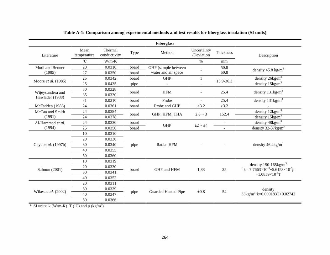
264

Table A-1: Comparison among experimental methods and test results for fiberglass insulation (SI units)

Fiberglass

Literature

Mean

temperature

Thermal

conductivity Type Method

Uncertainty

/Deviation Thickness

Description

˚C W/m-K

% mm

Modi and Benner

(1985)

20 0.0310 board GHP (sample between

water and air space -

50.8

50.8 density 45.8 kg/m

3

27 0.0350 board

Moore et al. (1985) 25 0.0342 board GHP 1

15.9-36.3 density 26kg/m

3

25 0.0435 pipe - - density 15kg/m3

Wijeysundera and

Hawlader (1988)

30 0.0328 board HFM - 25.4 density 131kg/m

3

35 0.0330

31 0.0310 board Probe - 25.4 density 131kg/m3

McFadden (1988) 24 0.0361 board Probe and GHP >3.2 >3.2 -

McCaa and Smith

(1991)

24 0.0384 board GHP, HFM, THA 2.8 ~ 3 152.4

density 12kg/m3

24 0.0378 density 15kg/m3

Al-Hammad et al.

(1994)

24 0.0330 board GHP ±2 ~ ±4

- density 48kg/m3

25 0.0350 board - density 32-37kg/m3

Chyu et al. (1997b)

10 0.0310

pipe Radial HFM - - density 46.4kg/m3

20 0.0330

30 0.0340

40 0.0355

50 0.0360

Salmon (2001)

10 0.0319

board GHP and HFM 1.83 25

density 150-165kg/m3

1k=-7.7663×10

-3+5.6153×10

-5ρ

+1.0859×10-4

T

20 0.0330

30 0.0341

40 0.0352

Wikes et al. (2002)

20 0.0311

pipe Guarded Heated Pipe ±0.8 54 density

33kg/m31

k=0.000183T+0.02742

30 0.0329

40 0.0347

50 0.0366

¹: SI units: k (W/m-K), T (˚C) and ρ (kg/m3)

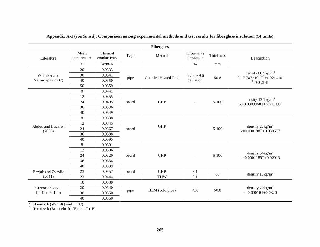
265

Appendix A-1 (continued): Comparison among experimental methods and test results for fiberglass insulation (SI units)

Fiberglass

Literature

Mean

temperature

Thermal

conductivity Type Method

Uncertainty

/Deviation Thickness

Description

˚C W/m-K

% mm

Whitaker and

Yarbrough (2002)

20 0.0333

pipe Guarded Heated Pipe -27.5 ~ 9.6

deviation 50.8

density 86.5kg/m3

2k=7.787×10

-7T

2+1.921×10

-

4T+0.2141

30 0.0341

40 0.0350

50 0.0359

Abdou and Budaiwi

(2005)

8 0.0441

board GHP - 5-100 density 13.1kg/m

3

k=0.0003368T+0.041433

12 0.0455

24 0.0495

36 0.0536

40 0.0549

8 0.0338

board GHP

- 5-100

density 27kg/m3

k=0.000188T+0.030677

12 0.0345

24 0.0367

36 0.0388

40 0.0395

8 0.0301

board GHP - 5-100 density 56kg/m

3

k=0.0001189T+0.02913

12 0.0306

24 0.0320

36 0.0334

40 0.0339

Bezjak and Zvizdic

(2011)

23 0.0457 board GHP 3.1 80 density 13kg/m

3

23 0.0444

THW 8.1

Cremaschi et al.

(2012a; 2012b)

10 0.0330

pipe HFM (cold pipe) <±6 50.8 density 70kg/m

3

k=0.00010T+0.0320

20 0.0340

30 0.0350

40 0.0360

¹: SI units: k (W/m-K) and T (˚C); 2: IP units: k (Btu-in/hr-ft

2-˚F) and T (˚F)

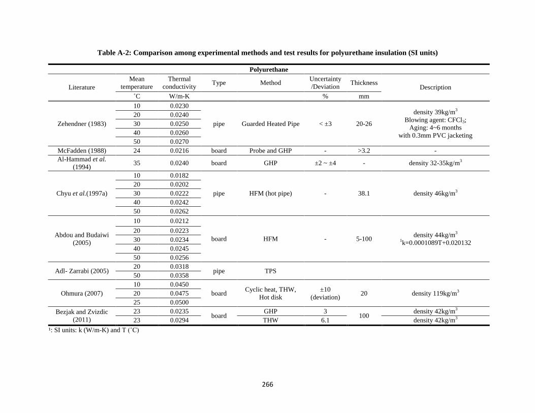
266

Table A-2: Comparison among experimental methods and test results for polyurethane insulation (SI units)

Polyurethane

Literature

Mean

temperature

Thermal

conductivity Type Method

Uncertainty

/Deviation Thickness

Description

˚C W/m-K

% mm

Zehendner (1983)

10 0.0230

pipe Guarded Heated Pipe < ±3 20-26

density 39kg/m3

Blowing agent: CFCl3;

Aging: 4~6 months

with 0.3mm PVC jacketing

20 0.0240

30 0.0250

40 0.0260

50 0.0270

McFadden (1988) 24 0.0216 board Probe and GHP - >3.2 -

Al-Hammad et al.

(1994) 35 0.0240 board GHP ±2 ~ ±4 - density 32-35kg/m

3

Chyu et al.(1997a)

10 0.0182

pipe HFM (hot pipe) - 38.1 density 46kg/m3

20 0.0202

30 0.0222

40 0.0242

50 0.0262

Abdou and Budaiwi

(2005)

10 0.0212

board HFM - 5-100 density 44kg/m

3

1k=0.0001089T+0.020132

20 0.0223

30 0.0234

40 0.0245

50 0.0256

Adl- Zarrabi (2005) 20 0.0318

pipe TPS 50 0.0358

Ohmura (2007)

10 0.0450

board Cyclic heat, THW,

Hot disk

±10

(deviation) 20 density 119kg/m

3 20 0.0475

25 0.0500

Bezjak and Zvizdic

(2011)

23 0.0235 board

GHP 3 100

density 42kg/m3

23 0.0294 THW 6.1 density 42kg/m3

¹: SI units: k (W/m-K) and T (˚C)

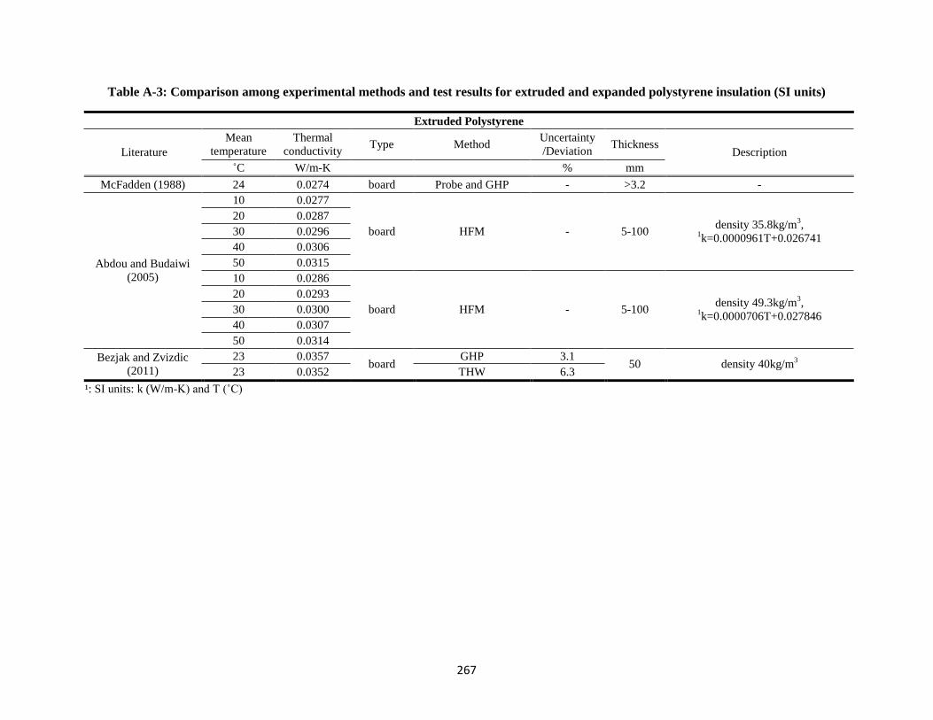
267

Table A-3: Comparison among experimental methods and test results for extruded and expanded polystyrene insulation (SI units)

Extruded Polystyrene

Literature

Mean

temperature

Thermal

conductivity Type Method

Uncertainty

/Deviation Thickness

Description

˚C W/m-K % mm

McFadden (1988) 24 0.0274 board Probe and GHP - >3.2 -

Abdou and Budaiwi

(2005)

10 0.0277

board HFM - 5-100 density 35.8kg/m

3,

1k=0.0000961T+0.026741

20 0.0287

30 0.0296

40 0.0306

50 0.0315

10 0.0286

board HFM - 5-100 density 49.3kg/m

3,

1k=0.0000706T+0.027846

20 0.0293

30 0.0300

40 0.0307

50 0.0314

Bezjak and Zvizdic

(2011)

23 0.0357 board

GHP 3.1 50 density 40kg/m

3

23 0.0352 THW 6.3

¹: SI units: k (W/m-K) and T (˚C)

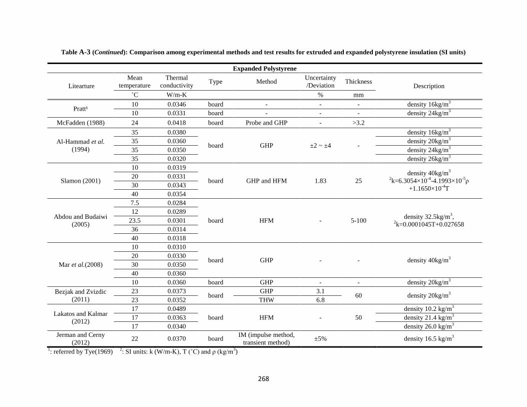
268

Table A-3 (Continued): Comparison among experimental methods and test results for extruded and expanded polystyrene insulation (SI units)

Expanded Polystyrene

Litearture

Mean

temperature

Thermal

conductivity Type Method

Uncertainty

/Deviation Thickness

Description

˚C W/m-K % mm

Pratt¹ 10 0.0346 board - - - density 16kg/m

3

10 0.0331 board - - - density 24kg/m3

McFadden (1988) 24 0.0418 board Probe and GHP - >3.2

Al-Hammad et al.

(1994)

35 0.0380

board GHP ±2 ~ ±4 -

density 16kg/m3

35 0.0360 density 20kg/m3

35 0.0350 density 24kg/m3

35 0.0320 density 26kg/m3

Slamon (2001)

10 0.0319

board GHP and HFM 1.83 25

density 40kg/m3

2k=6.3054×10

-4-4.1993×10

-5ρ

+1.1650×10-4

T

20 0.0331

30 0.0343

40 0.0354

Abdou and Budaiwi

(2005)

7.5 0.0284

board HFM - 5-100 density 32.5kg/m

3,

2k=0.0001045T+0.027658

12 0.0289

23.5 0.0301

36 0.0314

40 0.0318

Mar et al.(2008)

10 0.0310

board GHP - - density 40kg/m3

20 0.0330

30 0.0350

40 0.0360

10 0.0360 board GHP - - density 20kg/m3

Bezjak and Zvizdic

(2011)

23 0.0373 board

GHP 3.1 60 density 20kg/m

3

23 0.0352 THW 6.8

Lakatos and Kalmar

(2012)

17 0.0489

board HFM - 50

density 10.2 kg/m3

17 0.0363 density 21.4 kg/m3

17 0.0340 density 26.0 kg/m3

Jerman and Cerny

(2012) 22 0.0370 board

IM (impulse method,

transient method) ±5% density 16.5 kg/m

3

1: referred by Tye(1969)

2: SI units: k (W/m-K), T (˚C) and ρ (kg/m

3)

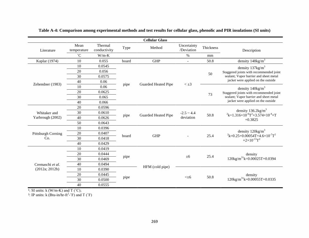
269

Table A-4: Comparison among experimental methods and test results for cellular glass, phenolic and PIR insulations (SI units)

Cellular Glass

Literature

Mean

temperature

Thermal

conductivity Type Method

Uncertainty

/Deviation Thickness

Description

˚C W/m-K % mm

Kaplar (1974) 10 0.055 board GHP - 50.8 density 148kg/m3

Zehendner (1983)

10 0.0545

pipe Guarded Heated Pipe < ±3

50

density 137kg/m3

Staggered joints with recommended joint

sealant; Vapor barrier and sheet metal

jacket were applied on the outside

20 0.056

30 0.0575

40 0.06

10 0.06

73

density 140kg/m3

Staggered joints with recommended joint

sealant; Vapor barrier and sheet metal

jacket were applied on the outside

20 0.0625

30 0.065

40 0.066

Whitaker and

Yarbrough (2002)

20 0.0596

pipe Guarded Heated Pipe -2.5 ~ 4.4

deviation 50.8

density 136.2kg/m3

2k=1.316×10

-6T

2+3.574×10

-4×T

+0.3825

30 0.0610

40 0.0626

50 0.0643

Pittsburgh Corning

Co.

10 0.0396

board GHP - 25.4

density 120kg/m3

2k=0.25+0.00054T+4.6×10

-7T

2

+2×10-11

T2

20 0.0407

30 0.0418

40 0.0429

Cremaschi et al.

(2012a; 2012b)

10 0.0419

pipe

HFM (cold pipe)

±6 25.4 density

120kg/m31

k=0.00025T+0.0394

20 0.0444

30 0.0469

40 0.0494

10 0.0390

pipe <±6 50.8 density

120kg/m31

k=0.00055T+0.0335

20 0.0445

30 0.0500

40 0.0555

¹: SI units: k (W/m-K) and T (˚C);

²: IP units: k (Btu-in/hr-ft2-˚F) and T (˚F)

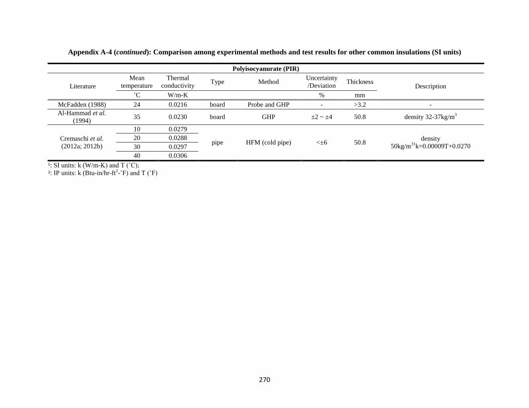
270

Appendix A-4 (continued): Comparison among experimental methods and test results for other common insulations (SI units)

Polyisocyanurate (PIR)

Literature

Mean

temperature

Thermal

conductivity Type Method

Uncertainty

/Deviation Thickness

Description

˚C W/m-K % mm

McFadden (1988) 24 0.0216 board Probe and GHP - >3.2 -

Al-Hammad et al.

(1994) 35 0.0230 board GHP ±2 ~ ±4 50.8 density 32-37kg/m

3

Cremaschi et al.

(2012a; 2012b)

10 0.0279

pipe HFM (cold pipe) <±6 50.8 density

50kg/m31

k=0.00009T+0.0270

20 0.0288

30 0.0297

40 0.0306

¹: SI units: k (W/m-K) and T (˚C);

²: IP units: k (Btu-in/hr-ft2-˚F) and T (˚F)

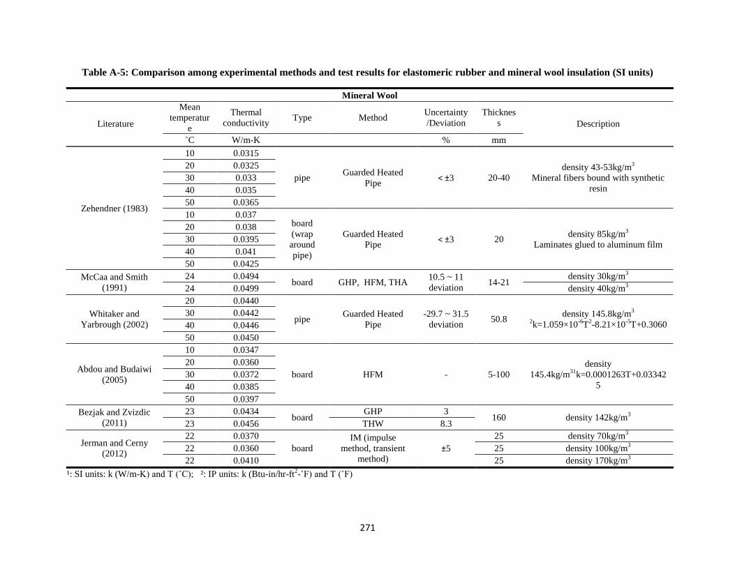
271

Table A-5: Comparison among experimental methods and test results for elastomeric rubber and mineral wool insulation (SI units)

Mineral Wool

Literature

Mean

temperatur

e

Thermal

conductivity Type Method

Uncertainty

/Deviation

Thicknes

s Description

˚C W/m-K % mm

Zehendner (1983)

10 0.0315

pipe Guarded Heated

Pipe < ±3 20-40

density 43-53kg/m3

Mineral fibers bound with synthetic

resin

20 0.0325

30 0.033

40 0.035

50 0.0365

10 0.037 board

(wrap

around

pipe)

Guarded Heated

Pipe < ±3 20

density 85kg/m3

Laminates glued to aluminum film

20 0.038

30 0.0395

40 0.041

50 0.0425

McCaa and Smith

(1991)

24 0.0494 board GHP, HFM, THA

10.5 ~ 11

deviation 14-21

density 30kg/m3

24 0.0499 density 40kg/m3

Whitaker and

Yarbrough (2002)

20 0.0440

pipe Guarded Heated

Pipe

-29.7 ~ 31.5

deviation 50.8

density 145.8kg/m3

2k=1.059×10

-6T

2-8.21×10

-5T+0.3060

30 0.0442

40 0.0446

50 0.0450

Abdou and Budaiwi

(2005)

10 0.0347

board HFM - 5-100

density

145.4kg/m31

k=0.0001263T+0.03342

5

20 0.0360

30 0.0372

40 0.0385

50 0.0397

Bezjak and Zvizdic

(2011)

23 0.0434 board

GHP 3 160 density 142kg/m

3

23 0.0456 THW 8.3

Jerman and Cerny

(2012)

22 0.0370

board

IM (impulse

method, transient

method) ±5

25 density 70kg/m3

22 0.0360 25 density 100kg/m3

22 0.0410 25 density 170kg/m3

¹: SI units: k (W/m-K) and T (˚C); ²: IP units: k (Btu-in/hr-ft2-˚F) and T (˚F)

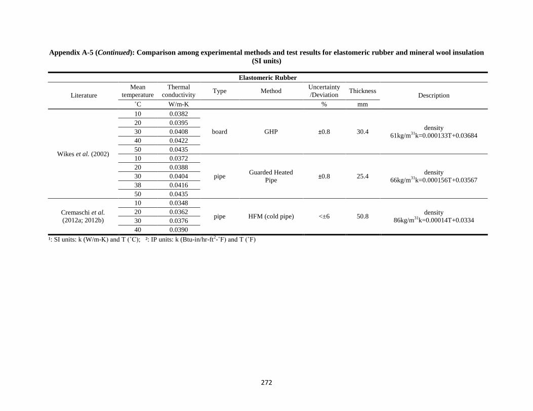
272

Appendix A-5 (Continued): Comparison among experimental methods and test results for elastomeric rubber and mineral wool insulation

(SI units)

Elastomeric Rubber

Literature

Mean

temperature

Thermal

conductivity Type Method

Uncertainty

/Deviation Thickness

Description

˚C W/m-K % mm

Wikes et al. (2002)

10 0.0382

board GHP ±0.8 30.4 density

61kg/m31

k=0.000133T+0.03684

20 0.0395

30 0.0408

40 0.0422

50 0.0435

10 0.0372

pipe Guarded Heated

Pipe ±0.8 25.4

density

66kg/m31

k=0.000156T+0.03567

20 0.0388

30 0.0404

38 0.0416

50 0.0435

Cremaschi et al.

(2012a; 2012b)

10 0.0348

pipe HFM (cold pipe) <±6 50.8 density

86kg/m31

k=0.00014T+0.0334

20 0.0362

30 0.0376

40 0.0390

¹: SI units: k (W/m-K) and T (˚C); ²: IP units: k (Btu-in/hr-ft2-˚F) and T (˚F)

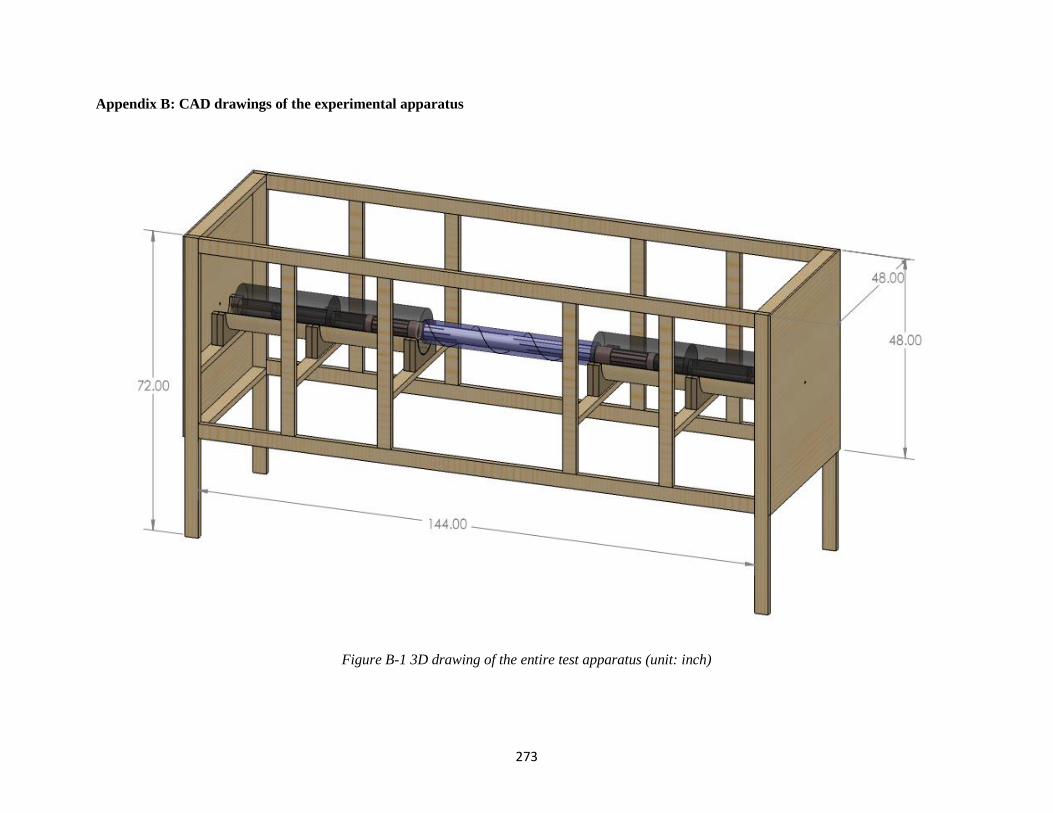
273

Appendix B: CAD drawings of the experimental apparatus

Figure B-1 3D drawing of the entire test apparatus (unit: inch)

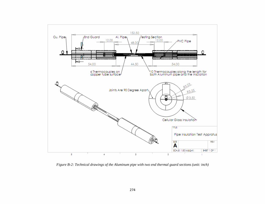
274

Figure B-2: Technical drawings of the Aluminum pipe with two end thermal guard sections (unit: inch)

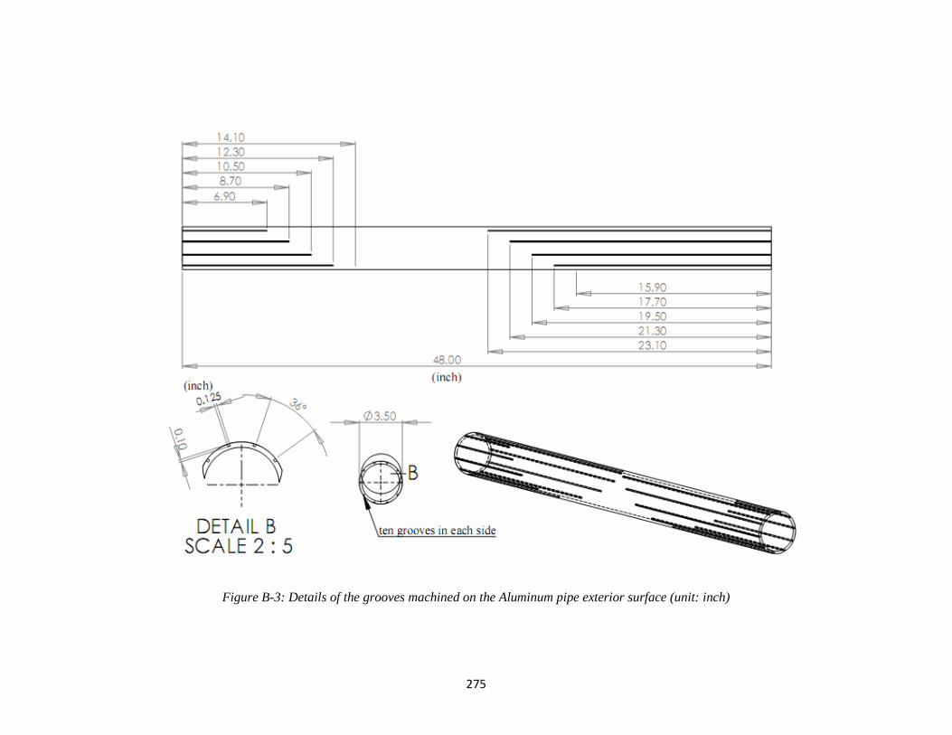
275

Figure B-3: Details of the grooves machined on the Aluminum pipe exterior surface (unit: inch)

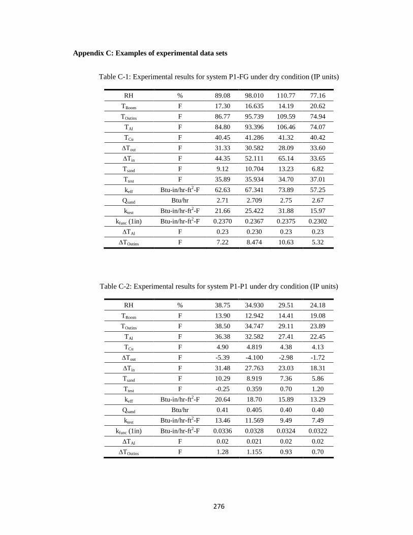
276

Appendix C: Examples of experimental data sets

Table C-1: Experimental results for system P1-FG under dry condition (IP units)

RH % 89.08 98.010 110.77 77.16

TRoom F 17.30 16.635 14.19 20.62

TOutins F 86.77 95.739 109.59 74.94

TAl F 84.80 93.396 106.46 74.07

TCu F 40.45 41.286 41.32 40.42

∆Tout F 31.33 30.582 28.09 33.60

∆Tin F 44.35 52.111 65.14 33.65

Tsand F 9.12 10.704 13.23 6.82

Ttest F 35.89 35.934 34.70 37.01

keff Btu-in/hr-ft2-F 62.63 67.341 73.89 57.25

Qsand Btu/hr 2.71 2.709 2.75 2.67

ktest Btu-in/hr-ft2-F 21.66 25.422 31.88 15.97

kfunc (1in) Btu-in/hr-ft2-F 0.2370 0.2367 0.2375 0.2302

∆TAl F 0.23 0.230 0.23 0.23

∆TOutins F 7.22 8.474 10.63 5.32

Table C-2: Experimental results for system P1-P1 under dry condition (IP units)

RH % 38.75 34.930 29.51 24.18

TRoom F 13.90 12.942 14.41 19.08

TOutins F 38.50 34.747 29.11 23.89

TAl F 36.38 32.582 27.41 22.45

TCu F 4.90 4.819 4.38 4.13

∆Tout F -5.39 -4.100 -2.98 -1.72

∆Tin F 31.48 27.763 23.03 18.31

Tsand F 10.29 8.919 7.36 5.86

Ttest F -0.25 0.359 0.70 1.20

keff Btu-in/hr-ft2-F 20.64 18.70 15.89 13.29

Qsand Btu/hr 0.41 0.405 0.40 0.40

ktest Btu-in/hr-ft2-F 13.46 11.569 9.49 7.49

kfunc (1in) Btu-in/hr-ft2-F 0.0336 0.0328 0.0324 0.0322

∆TAl F 0.02 0.021 0.02 0.02

∆TOutins F 1.28 1.155 0.93 0.70

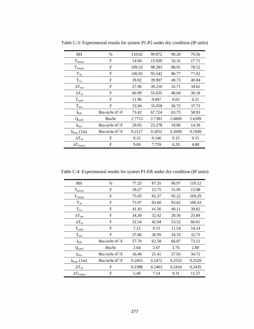
277

Table C-3: Experimental results for system P1-P2 under dry condition (IP units)

RH % 110.02 99.872 90.20 79.56

TRoom F 14.94 15.920 16.31 17.71

TOutins F 109.33 98.393 88.91 78.52

TAl F 106.92 95.542 86.77 77.02

TCu F 39.92 39.907 40.73 40.84

∆Tout F 27.96 30.210 32.71 34.62

∆Tin F 66.99 55.635 46.04 36.18

Tsand F 11.96 9.697 8.02 6.21

Ttest F 33.94 35.058 36.72 37.73

keff Btu-in/hr-ft2-F 73.42 67.724 63.75 58.93

Qsand Btu/hr 2.7713 2.7381 2.6809 2.6399

ktest Btu-in/hr-ft2-F 29.05 23.278 18.86 14.39

kfunc (1in) Btu-in/hr-ft2-F 0.2127 0.2052 0.2009 0.1949

∆TAl F 0.15 0.146 0.15 0.15

∆TOutins F 9.69 7.759 6.29 4.80

Table C-4: Experimental results for system P1-ER under dry condition (IP units)

RH % 77.25 87.35 96.97 110.12

TRoom F 18.27 15.75 15.95 13.98

TOutins F 75.05 85.37 95.22 109.29

TAl F 73.97 83.60 93.62 106.43

TCu F 41.43 41.56 40.11 39.82

∆Tout F 34.30 32.42 28.56 25.69

∆Tin F 32.54 42.04 53.52 66.61

Tsand F 7.12 9.15 11.54 14.14

Ttest F 37.86 36.99 34.33 32.75

keff Btu-in/hr-ft2-F 57.70 62.58 66.87 73.12

Qsand Btu/hr 2.64 2.67 2.76 2.80

ktest Btu-in/hr-ft2-F 16.46 21.41 27.93 34.72

kfunc (1in) Btu-in/hr-ft2-F 0.2455 0.2472 0.2533 0.2529

∆TAl F 0.2388 0.2403 0.2416 0.2435

∆TOutins F 5.49 7.14 9.31 11.57

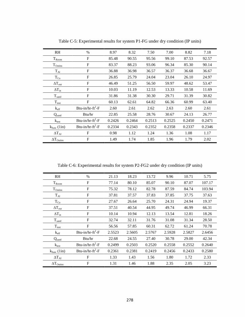
278

Table C-5: Experimental results for system P1-FG under dry condition (IP units)

RH % 8.97 8.32 7.50 7.00 8.82 7.18

TRoom F 85.48 90.55 95.56 99.10 87.53 92.57

TOutins F 83.37 88.23 93.06 96.34 85.30 90.14

TAl F 36.88 36.98 36.57 36.37 36.68 36.67

TCu F 26.85 25.79 24.04 23.04 26.10 24.97

∆Tout F 46.49 51.25 56.50 59.97 48.62 53.47

∆Tin F 10.03 11.19 12.53 13.33 10.58 11.69

Tsand F 31.86 31.38 30.30 29.71 31.39 30.82

Ttest F 60.13 62.61 64.82 66.36 60.99 63.40

keff Btu-in/hr-ft2-F 2.60 2.61 2.62 2.63 2.60 2.61

Qsand Btu/hr 22.85 25.58 28.76 30.67 24.13 26.77

ktest Btu-in/hr-ft2-F 0.2426 0.2464 0.2513 0.2525 0.2450 0.2471

kfunc (1in) Btu-in/hr-ft2-F 0.2334 0.2343 0.2352 0.2358 0.2337 0.2346

∆TAl F 0.98 1.12 1.24 1.36 1.08 1.17

∆TOutins F 1.49 1.74 1.85 1.96 1.79 2.02

Table C-6: Experimental results for system P2-FG2 under dry condition (IP units)

RH % 21.13 18.23 13.72 9.96 10.71 5.75

TRoom F 77.14 80.10 85.07 90.10 87.07 107.17

TOutins F 75.32 78.12 82.78 87.59 84.74 103.94

TAl F 37.81 37.57 37.83 37.85 37.75 37.63

TCu F 27.67 26.64 25.70 24.31 24.94 19.37

∆Tout F 37.51 40.54 44.95 49.74 46.99 66.31

∆Tin F 10.14 10.94 12.13 13.54 12.81 18.26

Tsand F 32.74 32.11 31.76 31.08 31.34 28.50

Ttest F 56.56 57.85 60.31 62.72 61.24 70.78

keff Btu-in/hr-ft2-F 2.5523 2.5605 2.5767 2.5928 2.5827 2.6456

Qsand Btu/hr 22.68 24.55 27.40 30.78 29.00 42.34

ktest Btu-in/hr-ft2-F 0.2499 0.2503 0.2520 0.2558 0.2552 0.2640

kfunc (1in) Btu-in/hr-ft2-F 0.2361 0.2381 0.2419 0.2456 0.2433 0.2580

∆TAl F 1.33 1.43 1.56 1.80 1.72 2.33

∆TOutins F 1.31 1.46 1.88 2.35 2.05 3.23

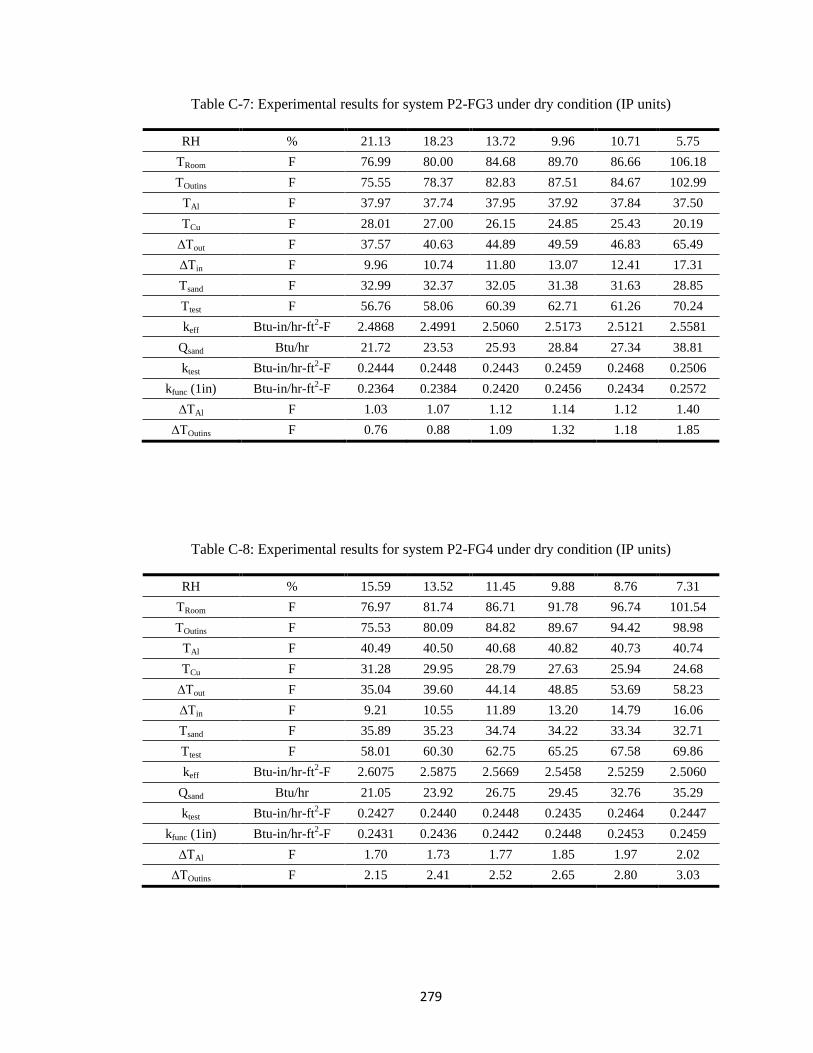
279

Table C-7: Experimental results for system P2-FG3 under dry condition (IP units)

RH % 21.13 18.23 13.72 9.96 10.71 5.75

TRoom F 76.99 80.00 84.68 89.70 86.66 106.18

TOutins F 75.55 78.37 82.83 87.51 84.67 102.99

TAl F 37.97 37.74 37.95 37.92 37.84 37.50

TCu F 28.01 27.00 26.15 24.85 25.43 20.19

∆Tout F 37.57 40.63 44.89 49.59 46.83 65.49

∆Tin F 9.96 10.74 11.80 13.07 12.41 17.31

Tsand F 32.99 32.37 32.05 31.38 31.63 28.85

Ttest F 56.76 58.06 60.39 62.71 61.26 70.24

keff Btu-in/hr-ft2-F 2.4868 2.4991 2.5060 2.5173 2.5121 2.5581

Qsand Btu/hr 21.72 23.53 25.93 28.84 27.34 38.81

ktest Btu-in/hr-ft2-F 0.2444 0.2448 0.2443 0.2459 0.2468 0.2506

kfunc (1in) Btu-in/hr-ft2-F 0.2364 0.2384 0.2420 0.2456 0.2434 0.2572

∆TAl F 1.03 1.07 1.12 1.14 1.12 1.40

∆TOutins F 0.76 0.88 1.09 1.32 1.18 1.85

Table C-8: Experimental results for system P2-FG4 under dry condition (IP units)

RH % 15.59 13.52 11.45 9.88 8.76 7.31

TRoom F 76.97 81.74 86.71 91.78 96.74 101.54

TOutins F 75.53 80.09 84.82 89.67 94.42 98.98

TAl F 40.49 40.50 40.68 40.82 40.73 40.74

TCu F 31.28 29.95 28.79 27.63 25.94 24.68

∆Tout F 35.04 39.60 44.14 48.85 53.69 58.23

∆Tin F 9.21 10.55 11.89 13.20 14.79 16.06

Tsand F 35.89 35.23 34.74 34.22 33.34 32.71

Ttest F 58.01 60.30 62.75 65.25 67.58 69.86

keff Btu-in/hr-ft2-F 2.6075 2.5875 2.5669 2.5458 2.5259 2.5060

Qsand Btu/hr 21.05 23.92 26.75 29.45 32.76 35.29

ktest Btu-in/hr-ft2-F 0.2427 0.2440 0.2448 0.2435 0.2464 0.2447

kfunc (1in) Btu-in/hr-ft2-F 0.2431 0.2436 0.2442 0.2448 0.2453 0.2459

∆TAl F 1.70 1.73 1.77 1.85 1.97 2.02

∆TOutins F 2.15 2.41 2.52 2.65 2.80 3.03

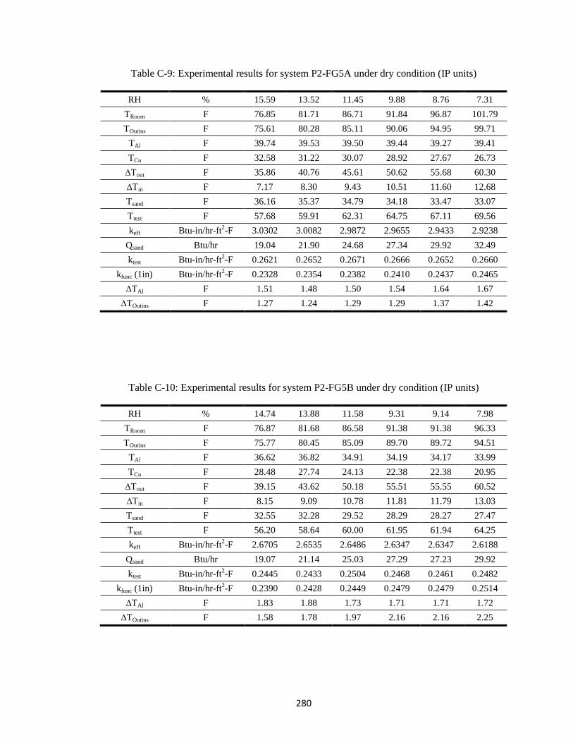
280

Table C-9: Experimental results for system P2-FG5A under dry condition (IP units)

RH % 15.59 13.52 11.45 9.88 8.76 7.31

TRoom F 76.85 81.71 86.71 91.84 96.87 101.79

TOutins F 75.61 80.28 85.11 90.06 94.95 99.71

TAl F 39.74 39.53 39.50 39.44 39.27 39.41

TCu F 32.58 31.22 30.07 28.92 27.67 26.73

∆Tout F 35.86 40.76 45.61 50.62 55.68 60.30

∆Tin F 7.17 8.30 9.43 10.51 11.60 12.68

Tsand F 36.16 35.37 34.79 34.18 33.47 33.07

Ttest F 57.68 59.91 62.31 64.75 67.11 69.56

keff Btu-in/hr-ft2-F 3.0302 3.0082 2.9872 2.9655 2.9433 2.9238

Qsand Btu/hr 19.04 21.90 24.68 27.34 29.92 32.49

ktest Btu-in/hr-ft2-F 0.2621 0.2652 0.2671 0.2666 0.2652 0.2660

kfunc (1in) Btu-in/hr-ft2-F 0.2328 0.2354 0.2382 0.2410 0.2437 0.2465

∆TAl F 1.51 1.48 1.50 1.54 1.64 1.67

∆TOutins F 1.27 1.24 1.29 1.29 1.37 1.42

Table C-10: Experimental results for system P2-FG5B under dry condition (IP units)

RH % 14.74 13.88 11.58 9.31 9.14 7.98

TRoom F 76.87 81.68 86.58 91.38 91.38 96.33

TOutins F 75.77 80.45 85.09 89.70 89.72 94.51

TAl F 36.62 36.82 34.91 34.19 34.17 33.99

TCu F 28.48 27.74 24.13 22.38 22.38 20.95

∆Tout F 39.15 43.62 50.18 55.51 55.55 60.52

∆Tin F 8.15 9.09 10.78 11.81 11.79 13.03

Tsand F 32.55 32.28 29.52 28.29 28.27 27.47

Ttest F 56.20 58.64 60.00 61.95 61.94 64.25

keff Btu-in/hr-ft2-F 2.6705 2.6535 2.6486 2.6347 2.6347 2.6188

Qsand Btu/hr 19.07 21.14 25.03 27.29 27.23 29.92

ktest Btu-in/hr-ft2-F 0.2445 0.2433 0.2504 0.2468 0.2461 0.2482

kfunc (1in) Btu-in/hr-ft2-F 0.2390 0.2428 0.2449 0.2479 0.2479 0.2514

∆TAl F 1.83 1.88 1.73 1.71 1.71 1.72

∆TOutins F 1.58 1.78 1.97 2.16 2.16 2.25

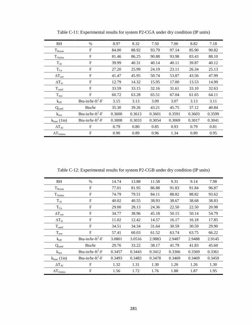
281

Table C-11: Experimental results for system P2-CGA under dry condition (IP units)

RH % 8.97 8.32 7.50 7.00 8.82 7.18

TRoom F 84.00 88.92 93.79 97.14 85.90 90.82

TOutins F 81.46 86.25 90.88 93.98 83.43 88.10

TAl F 39.99 40.31 40.14 40.11 39.87 40.12

TCu F 27.20 25.99 24.19 23.11 26.34 25.13

∆Tout F 41.47 45.95 50.74 53.87 43.56 47.99

∆Tin F 12.79 14.32 15.95 17.00 13.53 14.99

Tsand F 33.59 33.15 32.16 31.61 33.10 32.63

Ttest F 60.72 63.28 65.51 67.04 61.65 64.11

keff Btu-in/hr-ft2-F 3.15 3.13 3.09 3.07 3.13 3.11

Qsand Btu/hr 35.30 39.26 43.21 45.75 37.12 40.84

ktest Btu-in/hr-ft2-F 0.3600 0.3613 0.3601 0.3591 0.3603 0.3599

kfunc (1in) Btu-in/hr-ft2-F 0.3008 0.3033 0.3054 0.3069 0.3017 0.3041

∆TAl F 0.79 0.80 0.85 0.93 0.79 0.81

∆TOutins F 0.90 0.89 0.96 1.34 0.89 0.95

Table C-12: Experimental results for system P2-CGB under dry condition (IP units)

RH % 14.74 13.88 11.58 9.31 9.14 7.98

TRoom F 77.01 81.95 86.88 91.83 91.84 96.87

TOutins F 74.79 79.51 84.11 88.82 88.82 93.62

TAl F 40.02 40.55 38.93 38.67 38.68 38.83

TCu F 29.00 28.13 24.36 22.50 22.50 20.98

∆Tout F 34.77 38.96 45.18 50.15 50.14 54.79

∆Tin F 11.02 12.42 14.57 16.17 16.18 17.85

Tsand F 34.51 34.34 31.64 30.59 30.59 29.90

Ttest F 57.41 60.03 61.52 63.74 63.75 66.22

keff Btu-in/hr-ft2-F 3.0801 3.0516 2.9883 2.9487 2.9488 2.9145

Qsand Btu/hr 29.76 33.22 38.17 41.79 41.83 45.60

ktest Btu-in/hr-ft2-F 0.3457 0.3443 0.3412 0.3366 0.3369 0.3361

kfunc (1in) Btu-in/hr-ft2-F 0.3493 0.3483 0.3478 0.3469 0.3469 0.3459

∆TAl F 1.32 1.31 1.30 1.26 1.26 1.30

∆TOutins F 1.56 1.72 1.76 1.88 1.87 1.95

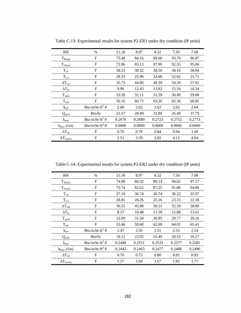
282

Table C-13: Experimental results for system P2-ER1 under dry condition (IP units)

RH % 11.18 8.97 8.32 7.50 7.00

TRoom F 75.48 84.16 89.00 93.79 96.87

TOutins F 73.96 83.13 87.90 92.55 95.66

TAl F 38.23 38.32 38.50 38.16 38.04

TCu F 28.33 25.90 24.68 22.82 21.71

∆Tout F 35.73 44.80 49.39 54.39 57.62

∆Tin F 9.90 12.43 13.82 15.34 16.34

Tsand F 33.28 32.11 31.59 30.49 29.88

Ttest F 56.10 60.73 63.20 65.36 66.85

keff Btu-in/hr-ft2-F 2.60 2.62 2.62 2.63 2.64

Qsand Btu/hr 22.57 28.49 31.80 35.40 37.79

ktest Btu-in/hr-ft2-F 0.2670 0.2689 0.2723 0.2752 0.2773

kfunc (1in) Btu-in/hr-ft2-F 0.0000 0.0000 0.0000 0.0000 0.0000

∆TAl F 0.76 0.78 0.84 0.94 1.00

∆TOutins F 2.53 3.39 3.82 4.11 4.04

Table C-14: Experimental results for system P2-ER2 under dry condition (IP units)

RH % 11.18 8.97 8.32 7.50 7.00

TRoom F 74.88 84.32 89.14 94.02 97.17

TOutins F 73.74 82.62 87.25 91.80 94.86

TAl F 37.19 36.74 36.74 36.22 35.97

TCu F 28.81 26.26 25.16 23.33 22.36

∆Tout F 36.55 45.88 50.51 55.59 58.89

∆Tin F 8.37 10.48 11.59 12.88 13.61

Tsand F 33.00 31.50 30.95 29.77 29.16

Ttest F 55.46 59.68 62.00 64.01 65.41

keff Btu-in/hr-ft2-F 2.47 2.50 2.51 2.53 2.54

Qsand Btu/hr 18.12 22.95 25.49 28.53 30.27

ktest Btu-in/hr-ft2-F 0.2488 0.2511 0.2533 0.2577 0.2581

kfunc (1in) Btu-in/hr-ft2-F 0.2442 0.2465 0.2477 0.2488 0.2496

∆TAl F 0.70 0.75 0.80 0.81 0.93

∆TOutins F 1.57 1.64 1.67 1.82 1.77

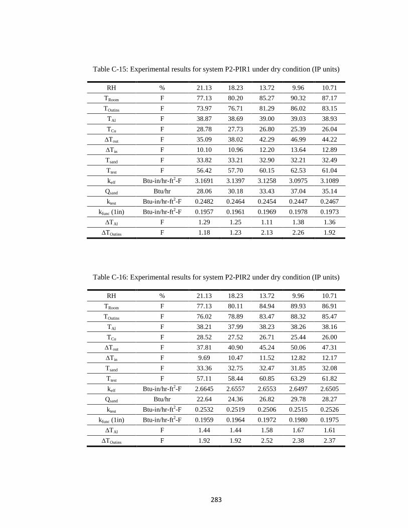
283

Table C-15: Experimental results for system P2-PIR1 under dry condition (IP units)

RH % 21.13 18.23 13.72 9.96 10.71

TRoom F 77.13 80.20 85.27 90.32 87.17

TOutins F 73.97 76.71 81.29 86.02 83.15

TAl F 38.87 38.69 39.00 39.03 38.93

TCu F 28.78 27.73 26.80 25.39 26.04

∆Tout F 35.09 38.02 42.29 46.99 44.22

∆Tin F 10.10 10.96 12.20 13.64 12.89

Tsand F 33.82 33.21 32.90 32.21 32.49

Ttest F 56.42 57.70 60.15 62.53 61.04

keff Btu-in/hr-ft2-F 3.1691 3.1397 3.1258 3.0975 3.1089

Qsand Btu/hr 28.06 30.18 33.43 37.04 35.14

ktest Btu-in/hr-ft2-F 0.2482 0.2464 0.2454 0.2447 0.2467

kfunc (1in) Btu-in/hr-ft2-F 0.1957 0.1961 0.1969 0.1978 0.1973

∆TAl F 1.29 1.25 1.11 1.38 1.36

∆TOutins F 1.18 1.23 2.13 2.26 1.92

Table C-16: Experimental results for system P2-PIR2 under dry condition (IP units)

RH % 21.13 18.23 13.72 9.96 10.71

TRoom F 77.13 80.11 84.94 89.93 86.91

TOutins F 76.02 78.89 83.47 88.32 85.47

TAl F 38.21 37.99 38.23 38.26 38.16

TCu F 28.52 27.52 26.71 25.44 26.00

∆Tout F 37.81 40.90 45.24 50.06 47.31

∆Tin F 9.69 10.47 11.52 12.82 12.17

Tsand F 33.36 32.75 32.47 31.85 32.08

Ttest F 57.11 58.44 60.85 63.29 61.82

keff Btu-in/hr-ft2-F 2.6645 2.6557 2.6553 2.6497 2.6505

Qsand Btu/hr 22.64 24.36 26.82 29.78 28.27

ktest Btu-in/hr-ft2-F 0.2532 0.2519 0.2506 0.2515 0.2526

kfunc (1in) Btu-in/hr-ft2-F 0.1959 0.1964 0.1972 0.1980 0.1975

∆TAl F 1.44 1.44 1.58 1.67 1.61

∆TOutins F 1.92 1.92 2.52 2.38 2.37

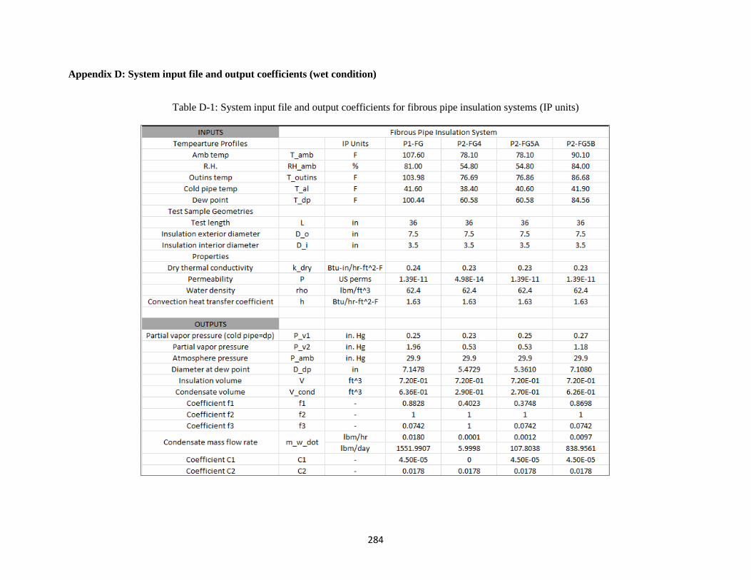
284

Appendix D: System input file and output coefficients (wet condition)

Table D-1: System input file and output coefficients for fibrous pipe insulation systems (IP units)

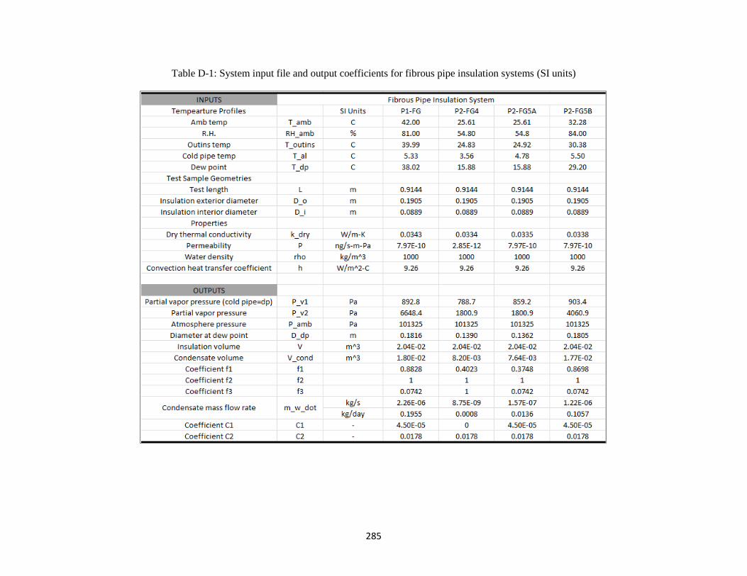
285

Table D-1: System input file and output coefficients for fibrous pipe insulation systems (SI units)

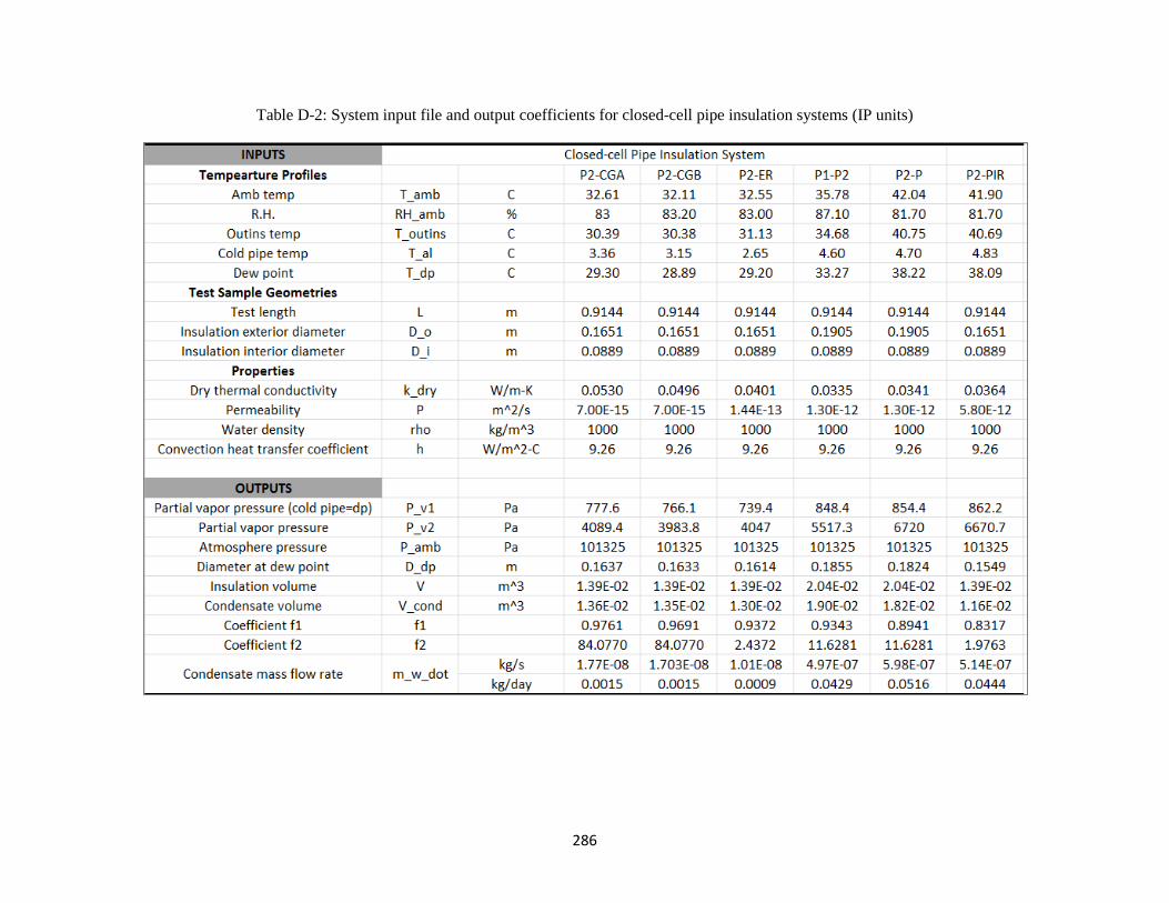
286

Table D-2: System input file and output coefficients for closed-cell pipe insulation systems (IP units)

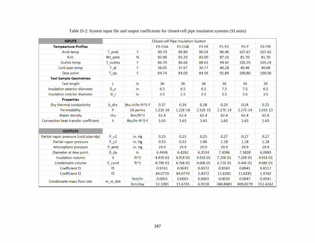
287

Table D-2: System input file and output coefficients for closed-cell pipe insulation systems (SI units)

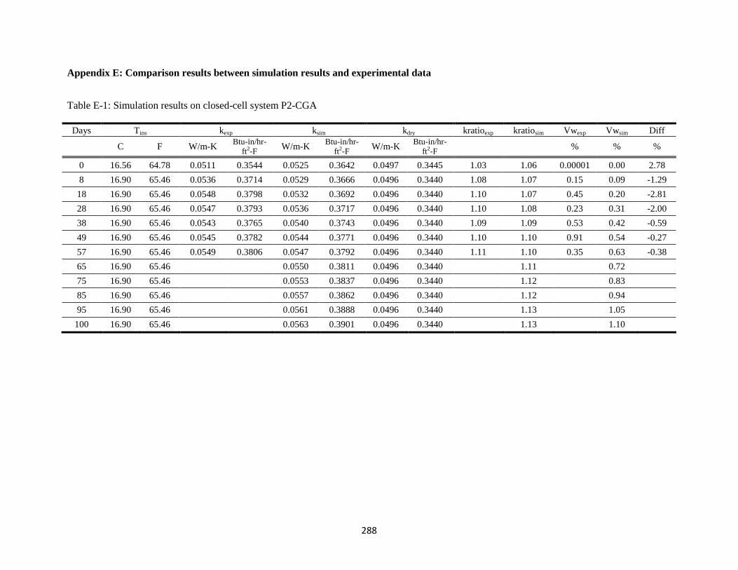
288

Appendix E: Comparison results between simulation results and experimental data

Table E-1: Simulation results on closed-cell system P2-CGA

Days Tins kexp ksim kdry kratioexp kratiosim Vwexp Vwsim Diff

C F W/m-K

Btu-in/hr-

ft2-F W/m-K

Btu-in/hr-

ft2-F W/m-K

Btu-in/hr-

ft2-F % % %

0 16.56 64.78 0.0511 0.3544 0.0525 0.3642 0.0497 0.3445 1.03 1.06 0.00001 0.00 2.78

8 16.90 65.46 0.0536 0.3714 0.0529 0.3666 0.0496 0.3440 1.08 1.07 0.15 0.09 -1.29

18 16.90 65.46 0.0548 0.3798 0.0532 0.3692 0.0496 0.3440 1.10 1.07 0.45 0.20 -2.81

28 16.90 65.46 0.0547 0.3793 0.0536 0.3717 0.0496 0.3440 1.10 1.08 0.23 0.31 -2.00

38 16.90 65.46 0.0543 0.3765 0.0540 0.3743 0.0496 0.3440 1.09 1.09 0.53 0.42 -0.59

49 16.90 65.46 0.0545 0.3782 0.0544 0.3771 0.0496 0.3440 1.10 1.10 0.91 0.54 -0.27

57 16.90 65.46 0.0549 0.3806 0.0547 0.3792 0.0496 0.3440 1.11 1.10 0.35 0.63 -0.38

65 16.90 65.46

0.0550 0.3811 0.0496 0.3440

1.11

0.72

75 16.90 65.46

0.0553 0.3837 0.0496 0.3440

1.12

0.83

85 16.90 65.46

0.0557 0.3862 0.0496 0.3440

1.12

0.94

95 16.90 65.46

0.0561 0.3888 0.0496 0.3440

1.13

1.05

100 16.90 65.46

0.0563 0.3901 0.0496 0.3440

1.13

1.10

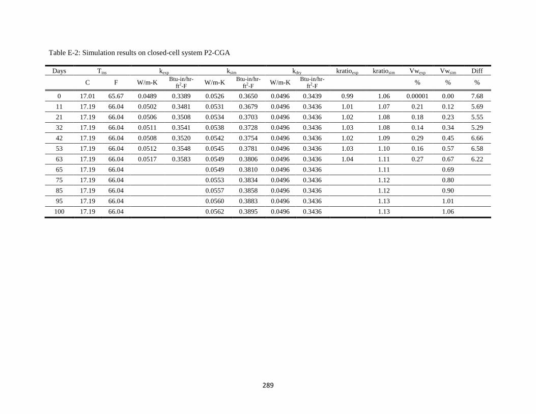
289

Table E-2: Simulation results on closed-cell system P2-CGA

Days Tins kexp ksim kdry kratioexp kratiosim Vwexp Vwsim Diff

C F W/m-K

Btu-in/hr-

ft2-F W/m-K

Btu-in/hr-

ft2-F W/m-K

Btu-in/hr-

ft2-F % % %

0 17.01 65.67 0.0489 0.3389 0.0526 0.3650 0.0496 0.3439 0.99 1.06 0.00001 0.00 7.68

11 17.19 66.04 0.0502 0.3481 0.0531 0.3679 0.0496 0.3436 1.01 1.07 0.21 0.12 5.69

21 17.19 66.04 0.0506 0.3508 0.0534 0.3703 0.0496 0.3436 1.02 1.08 0.18 0.23 5.55

32 17.19 66.04 0.0511 0.3541 0.0538 0.3728 0.0496 0.3436 1.03 1.08 0.14 0.34 5.29

42 17.19 66.04 0.0508 0.3520 0.0542 0.3754 0.0496 0.3436 1.02 1.09 0.29 0.45 6.66

53 17.19 66.04 0.0512 0.3548 0.0545 0.3781 0.0496 0.3436 1.03 1.10 0.16 0.57 6.58

63 17.19 66.04 0.0517 0.3583 0.0549 0.3806 0.0496 0.3436 1.04 1.11 0.27 0.67 6.22

65 17.19 66.04

0.0549 0.3810 0.0496 0.3436

1.11

0.69

75 17.19 66.04

0.0553 0.3834 0.0496 0.3436

1.12

0.80

85 17.19 66.04

0.0557 0.3858 0.0496 0.3436

1.12

0.90

95 17.19 66.04 0.0560 0.3883 0.0496 0.3436 1.13 1.01

100 17.19 66.04 0.0562 0.3895 0.0496 0.3436 1.13 1.06

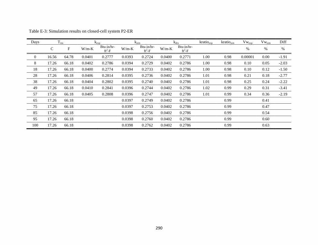
290

Table E-3: Simulation results on closed-cell system P2-ER

Days Tins kexp ksim kdry kratioexp kratiosim Vwexp Vwsim Diff

C F W/m-K

Btu-in/hr-

ft2-F W/m-K

Btu-in/hr-

ft2-F W/m-K

Btu-in/hr-

ft2-F % % %

0 16.56 64.78 0.0401 0.2777 0.0393 0.2724 0.0400 0.2771 1.00 0.98 0.00001 0.00 -1.91

8 17.26 66.18 0.0402 0.2786 0.0394 0.2729 0.0402 0.2786 1.00 0.98 0.10 0.05 -2.03

18 17.26 66.18 0.0400 0.2774 0.0394 0.2733 0.0402 0.2786 1.00 0.98 0.10 0.12 -1.50

28 17.26 66.18 0.0406 0.2814 0.0395 0.2736 0.0402 0.2786 1.01 0.98 0.21 0.18 -2.77

38 17.26 66.18 0.0404 0.2802 0.0395 0.2740 0.0402 0.2786 1.01 0.98 0.25 0.24 -2.22

49 17.26 66.18 0.0410 0.2841 0.0396 0.2744 0.0402 0.2786 1.02 0.99 0.29 0.31 -3.41

57 17.26 66.18 0.0405 0.2808 0.0396 0.2747 0.0402 0.2786 1.01 0.99 0.34 0.36 -2.19

65 17.26 66.18

0.0397 0.2749 0.0402 0.2786

0.99

0.41

75 17.26 66.18

0.0397 0.2753 0.0402 0.2786

0.99

0.47

85 17.26 66.18

0.0398 0.2756 0.0402 0.2786

0.99

0.54

95 17.26 66.18 0.0398 0.2760 0.0402 0.2786 0.99 0.60

100 17.26 66.18 0.0398 0.2762 0.0402 0.2786 0.99 0.63

291

Table E-4: Simulation results on closed-cell system P1-P2

Days Tins kexp ksim kdry kratioexp kratiosim Vwexp Vwsim Diff

C F W/m-K

Btu-in/hr-

ft2-F W/m-K

Btu-in/hr-

ft2-F W/m-K

Btu-in/hr-

ft2-F % % %

0 16.56 64.78 0.0297 0.2056 0.0326 0.2257 0.0329 0.2282 0.90 0.99 0.00 0.00 9.79

3 19.68 70.96 0.0369 0.2561 0.0340 0.2358 0.0335 0.2325 1.10 1.01 0.81 0.70 -7.93

7 19.68 70.96 0.0407 0.2823 0.0358 0.2481 0.0335 0.2325 1.21 1.07 1.63 1.53 -12.09

14 19.68 70.96 0.0438 0.3037 0.0393 0.2724 0.0335 0.2325 1.31 1.17 2.54 3.01 -10.30

21 19.68 70.96 0.0473 0.3278 0.0426 0.2951 0.0335 0.2325 1.41 1.27 4.72 4.50 -9.98

24 19.68 70.96 0.0484 0.3356 0.0439 0.3043 0.0335 0.2325 1.44 1.31 4.96 5.11 -9.33

30 19.68 70.96

0.0465 0.3227 0.0335 0.2325

1.39

6.32

40 19.68 70.96

0.0512 0.3549 0.0335 0.2325

1.53

8.43

50 19.68 70.96

0.0559 0.3874 0.0335 0.2325

1.67

10.54

60 19.68 70.96

0.0606 0.4200 0.0335 0.2325

1.81

12.64

80 19.68 70.96 0.0701 0.4861 0.0335 0.2325 2.09 16.86

100 19.68 70.96 0.0798 0.5535 0.0335 0.2325 2.38 21.07

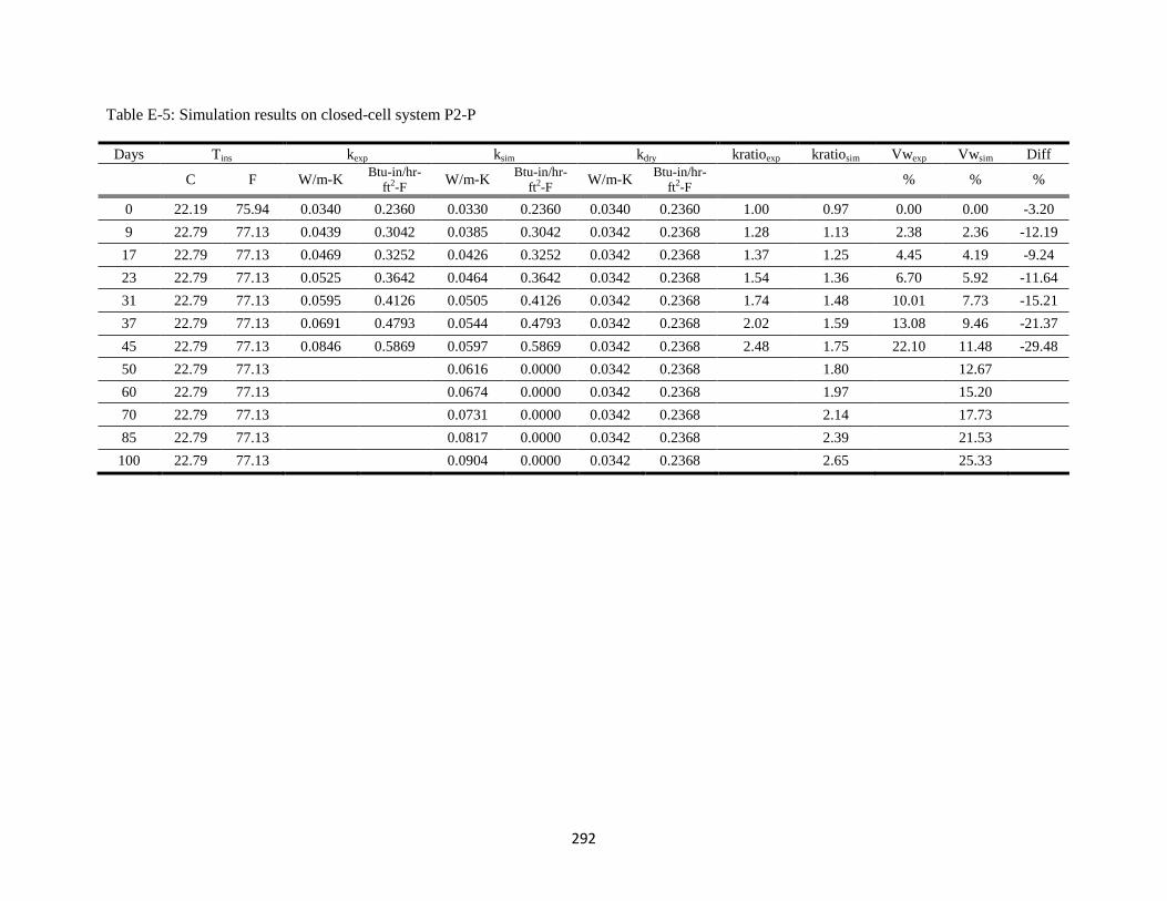
292

Table E-5: Simulation results on closed-cell system P2-P

Days Tins kexp ksim kdry kratioexp kratiosim Vwexp Vwsim Diff

C F W/m-K

Btu-in/hr-

ft2-F W/m-K

Btu-in/hr-

ft2-F W/m-K

Btu-in/hr-

ft2-F % % %

0 22.19 75.94 0.0340 0.2360 0.0330 0.2360 0.0340 0.2360 1.00 0.97 0.00 0.00 -3.20

9 22.79 77.13 0.0439 0.3042 0.0385 0.3042 0.0342 0.2368 1.28 1.13 2.38 2.36 -12.19

17 22.79 77.13 0.0469 0.3252 0.0426 0.3252 0.0342 0.2368 1.37 1.25 4.45 4.19 -9.24

23 22.79 77.13 0.0525 0.3642 0.0464 0.3642 0.0342 0.2368 1.54 1.36 6.70 5.92 -11.64

31 22.79 77.13 0.0595 0.4126 0.0505 0.4126 0.0342 0.2368 1.74 1.48 10.01 7.73 -15.21

37 22.79 77.13 0.0691 0.4793 0.0544 0.4793 0.0342 0.2368 2.02 1.59 13.08 9.46 -21.37

45 22.79 77.13 0.0846 0.5869 0.0597 0.5869 0.0342 0.2368 2.48 1.75 22.10 11.48 -29.48

50 22.79 77.13

0.0616 0.0000 0.0342 0.2368

1.80

12.67

60 22.79 77.13

0.0674 0.0000 0.0342 0.2368

1.97

15.20

70 22.79 77.13

0.0731 0.0000 0.0342 0.2368

2.14

17.73

85 22.79 77.13 0.0817 0.0000 0.0342 0.2368 2.39 21.53

100 22.79 77.13 0.0904 0.0000 0.0342 0.2368 2.65 25.33

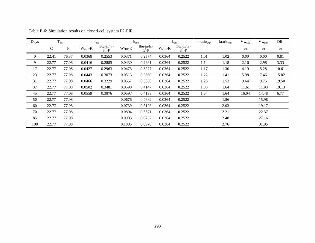
293

Table E-6: Simulation results on closed-cell system P2-PIR

Days Tins kexp ksim kdry kratioexp kratiosim Vwexp Vwsim Diff

C F W/m-K

Btu-in/hr-

ft2-F W/m-K

Btu-in/hr-

ft2-F W/m-K

Btu-in/hr-

ft2-F % % %

0 22.41 76.37 0.0368 0.2553 0.0371 0.2574 0.0364 0.2522 1.01 1.02 0.00 0.00 0.81

9 22.77 77.08 0.0416 0.2885 0.0430 0.2981 0.0364 0.2522 1.14 1.18 2.16 2.98 3.33

17 22.77 77.08 0.0427 0.2963 0.0473 0.3277 0.0364 0.2522 1.17 1.30 4.19 5.28 10.61

23 22.77 77.08 0.0443 0.3073 0.0513 0.3560 0.0364 0.2522 1.22 1.41 5.98 7.46 15.82

31 22.77 77.08 0.0466 0.3229 0.0557 0.3858 0.0364 0.2522 1.28 1.53 9.64 9.75 19.50

37 22.77 77.08 0.0502 0.3481 0.0598 0.4147 0.0364 0.2522 1.38 1.64 11.61 11.93 19.13

45 22.77 77.08 0.0559 0.3876 0.0597 0.4138 0.0364 0.2522 1.54 1.64 16.04 14.48 6.77

50 22.77 77.08

0.0676 0.4689 0.0364 0.2522

1.86

15.98

60 22.77 77.08

0.0739 0.5126 0.0364 0.2522

2.03

19.17

70 22.77 77.08

0.0804 0.5571 0.0364 0.2522

2.21

22.37

85 22.77 77.08 0.0903 0.6257 0.0364 0.2522 2.48 27.16

100 22.77 77.08 0.1005 0.6970 0.0364 0.2522 2.76 31.95

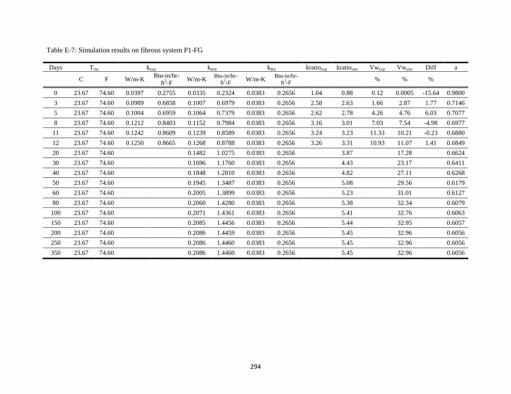
294

Table E-7: Simulation results on fibrous system P1-FG

Days Tins kexp ksim kdry kratioexp kratiosim Vwexp Vwsim Diff a

C F W/m-K

Btu-in/hr-

ft2-F

W/m-K Btu-in/hr-

ft2-F W/m-K

Btu-in/hr-

ft2-F % % %

0 23.67 74.60 0.0397 0.2755 0.0335 0.2324 0.0383 0.2656 1.04 0.88 0.12 0.0005 -15.64 0.9800

3 23.67 74.60 0.0989 0.6858 0.1007 0.6979 0.0383 0.2656 2.58 2.63 1.66 2.87 1.77 0.7146

5 23.67 74.60 0.1004 0.6959 0.1064 0.7379 0.0383 0.2656 2.62 2.78 4.26 4.76 6.03 0.7077

8 23.67 74.60 0.1212 0.8403 0.1152 0.7984 0.0383 0.2656 3.16 3.01 7.03 7.54 -4.98 0.6977

11 23.67 74.60 0.1242 0.8609 0.1239 0.8589 0.0383 0.2656 3.24 3.23 11.33 10.21 -0.23 0.6880

12 23.67 74.60 0.1250 0.8665 0.1268 0.8788 0.0383 0.2656 3.26 3.31 10.93 11.07 1.41 0.6849

20 23.67 74.60 0.1482 1.0275 0.0383 0.2656

3.87

17.28

0.6624

30 23.67 74.60

0.1696 1.1760 0.0383 0.2656

4.43

23.17

0.6411

40 23.67 74.60

0.1848 1.2810 0.0383 0.2656

4.82

27.11

0.6268

50 23.67 74.60

0.1945 1.3487 0.0383 0.2656

5.08

29.56

0.6179

60 23.67 74.60 0.2005 1.3899 0.0383 0.2656 5.23 31.01 0.6127

80 23.67 74.60 0.2060 1.4280 0.0383 0.2656 5.38 32.34 0.6079

100 23.67 74.60 0.2071 1.4361 0.0383 0.2656 5.41 32.76 0.6063

150 23.67 74.60 0.2085 1.4456 0.0383 0.2656 5.44 32.95 0.6057

200 23.67 74.60 0.2086 1.4459 0.0383 0.2656 5.45 32.96 0.6056

250 23.67 74.60 0.2086 1.4460 0.0383 0.2656 5.45 32.96 0.6056

350 23.67 74.60 0.2086 1.4460 0.0383 0.2656 5.45 32.96 0.6056

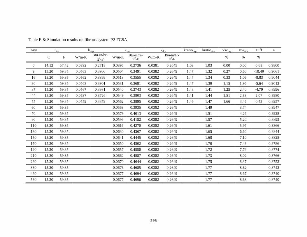
295

Table E-8: Simulation results on fibrous system P2-FG5A

Days Tins kexp ksim kdry kratioexp kratiosim Vwexp Vwsim Diff a

C F W/m-K

Btu-in/hr-

ft2-F

W/m-K Btu-in/hr-

ft2-F W/m-K

Btu-in/hr-

ft2-F % % %

0 14.12 57.42 0.0392 0.2718 0.0395 0.2736 0.0381 0.2645 1.03 1.03 0.00 0.00 0.68 0.9800

9 15.20 59.35 0.0563 0.3900 0.0504 0.3491 0.0382 0.2649 1.47 1.32 0.27 0.60 -10.49 0.9061

16 15.20 59.35 0.0562 0.3899 0.0513 0.3555 0.0382 0.2649 1.47 1.34 0.33 1.06 -8.83 0.9044

30 15.20 59.35 0.0563 0.3901 0.0531 0.3681 0.0382 0.2649 1.47 1.39 1.15 1.96 -5.64 0.9012

37 15.20 59.35 0.0567 0.3931 0.0540 0.3743 0.0382 0.2649 1.48 1.41 1.25 2.40 -4.79 0.8996

44 15.20 59.35 0.0537 0.3726 0.0549 0.3803 0.0382 0.2649 1.41 1.44 1.51 2.83 2.07 0.8980

55 15.20 59.35 0.0559 0.3879 0.0562 0.3895 0.0382 0.2649 1.46 1.47 1.66 3.46 0.43 0.8957

60 15.20 59.35

0.0568 0.3935 0.0382 0.2649

1.49

3.74

0.8947

70 15.20 59.35

0.0579 0.4013 0.0382 0.2649

1.51

4.26

0.8928

90 15.20 59.35

0.0599 0.4152 0.0382 0.2649

1.57

5.20

0.8895

110 15.20 59.35 0.0616 0.4270 0.0382 0.2649 1.61 5.97 0.8866

130 15.20 59.35 0.0630 0.4367 0.0382 0.2649 1.65 6.60 0.8844

150 15.20 59.35 0.0641 0.4445 0.0382 0.2649 1.68 7.10 0.8825

170 15.20 59.35 0.0650 0.4502 0.0382 0.2649 1.70 7.49 0.8786

190 15.20 59.35 0.0657 0.4550 0.0382 0.2649 1.72 7.79 0.8774

210 15.20 59.35 0.0662 0.4587 0.0382 0.2649 1.73 8.02 0.8766

260 15.20 59.35 0.0670 0.4644 0.0382 0.2649 1.75 8.37 0.8752

360 15.20 59.35 0.0676 0.4685 0.0382 0.2649 1.77 8.62 0.8742

460 15.20 59.35 0.0677 0.4694 0.0382 0.2649 1.77 8.67 0.8740

560 15.20 59.35 0.0677 0.4696 0.0382 0.2649 1.77 8.68 0.8740

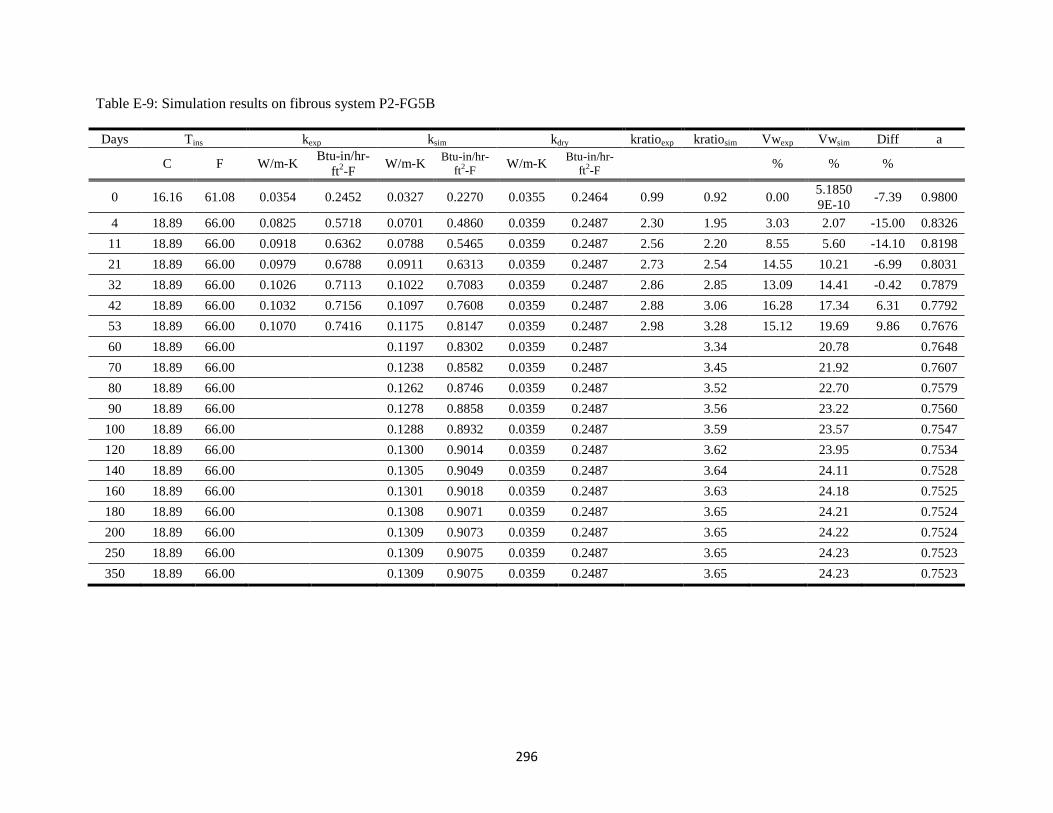
296

Table E-9: Simulation results on fibrous system P2-FG5B

Days Tins kexp ksim kdry kratioexp kratiosim Vwexp Vwsim Diff a

C F W/m-K

Btu-in/hr-

ft2-F

W/m-K Btu-in/hr-

ft2-F W/m-K

Btu-in/hr-

ft2-F % % %

0 16.16 61.08 0.0354 0.2452 0.0327 0.2270 0.0355 0.2464 0.99 0.92 0.00 5.1850

9E-10 -7.39 0.9800

4 18.89 66.00 0.0825 0.5718 0.0701 0.4860 0.0359 0.2487 2.30 1.95 3.03 2.07 -15.00 0.8326

11 18.89 66.00 0.0918 0.6362 0.0788 0.5465 0.0359 0.2487 2.56 2.20 8.55 5.60 -14.10 0.8198

21 18.89 66.00 0.0979 0.6788 0.0911 0.6313 0.0359 0.2487 2.73 2.54 14.55 10.21 -6.99 0.8031

32 18.89 66.00 0.1026 0.7113 0.1022 0.7083 0.0359 0.2487 2.86 2.85 13.09 14.41 -0.42 0.7879

42 18.89 66.00 0.1032 0.7156 0.1097 0.7608 0.0359 0.2487 2.88 3.06 16.28 17.34 6.31 0.7792

53 18.89 66.00 0.1070 0.7416 0.1175 0.8147 0.0359 0.2487 2.98 3.28 15.12 19.69 9.86 0.7676

60 18.89 66.00

0.1197 0.8302 0.0359 0.2487

3.34

20.78

0.7648

70 18.89 66.00

0.1238 0.8582 0.0359 0.2487

3.45

21.92

0.7607

80 18.89 66.00

0.1262 0.8746 0.0359 0.2487

3.52

22.70

0.7579

90 18.89 66.00 0.1278 0.8858 0.0359 0.2487 3.56 23.22 0.7560

100 18.89 66.00 0.1288 0.8932 0.0359 0.2487 3.59 23.57 0.7547

120 18.89 66.00 0.1300 0.9014 0.0359 0.2487 3.62 23.95 0.7534

140 18.89 66.00 0.1305 0.9049 0.0359 0.2487 3.64 24.11 0.7528

160 18.89 66.00 0.1301 0.9018 0.0359 0.2487 3.63 24.18 0.7525

180 18.89 66.00 0.1308 0.9071 0.0359 0.2487 3.65 24.21 0.7524

200 18.89 66.00 0.1309 0.9073 0.0359 0.2487 3.65 24.22 0.7524

250 18.89 66.00 0.1309 0.9075 0.0359 0.2487 3.65 24.23 0.7523

350 18.89 66.00 0.1309 0.9075 0.0359 0.2487 3.65 24.23 0.7523

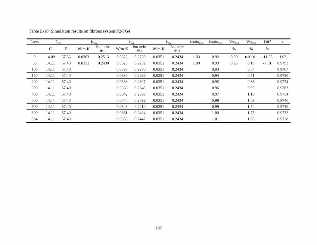
297

Table E-10: Simulation results on fibrous system P2-FG4

Days Tins kexp ksim kdry kratioexp kratiosim Vwexp Vwsim Diff a

C F W/m-K

Btu-in/hr-

ft2-F W/m-K

Btu-in/hr-

ft2-F W/m-K

Btu-in/hr-

ft2-F % % %

0 14.09 57.36 0.0363 0.2513 0.0322 0.2230 0.0351 0.2434 1.03 0.92 0.00 0.00001 -11.26 1.03

55 14.11 57.40 0.0351 0.2430 0.0325 0.2252 0.0351 0.2434 1.00 0.93 0.25 0.19 -7.31 0.9793

100 14.11 57.40 0.0327 0.2270 0.0351 0.2434 0.93 0.34 0.9787

150 14.11 57.40 0.0330 0.2289 0.0351 0.2434 0.94 0.51 0.9780

200 14.11 57.40 0.0333 0.2307 0.0351 0.2434 0.95 0.66 0.9774

300 14.11 57.40 0.0338 0.2340 0.0351 0.2434 0.96 0.95 0.9763

400 14.11 57.40 0.0342 0.2369 0.0351 0.2434 0.97 1.19 0.9754

500 14.11 57.40 0.0345 0.2392 0.0351 0.2434 0.98 1.39 0.9746

600 14.11 57.40 0.0348 0.2410 0.0351 0.2434 0.99 1.54 0.9740

800 14.11 57.40 0.0351 0.2434 0.0351 0.2434 1.00 1.75 0.9732

984 14.11 57.40 0.0353 0.2447 0.0351 0.2434 1.01 1.85 0.9728

298

Appendix F: VBA codes sample

F-1 Sample VBA code of the thermal conductivity model under dry condition (for

fibrous)

Attribute VB_Name = "PIT"

Sub lamdacal(ByRef c_rad As Double, ByRef a As Double, ByRef lamda_tot() As Double, ByRef

lamda_exp() As Double, _

ByRef Niter As Integer)

Dim L As Double

Dim D_o As Double

Dim D_i As Double

Dim D_x1_t As Double

Dim D_x1_b As Double

Dim D_x2_t As Double

Dim D_x2_b As Double

Dim D_exp As Double

Dim delta_js_ip As Double

Dim delta_js As Double

Dim delta_air As Double

Dim lamda_g As Double

Dim lamda_pg As Double

Dim lamda_rad As Double

Dim lamda_s As Double

Dim lamda_ins_t(20) As Double

Dim lamda_ins_b(20) As Double

Dim lamda_series_t(20) As Double

Dim lamda_series_b(20) As Double

Dim lamda_parallel_t(20) As Double

Dim lamda_parallel_b(20) As Double

Dim lamda_js As Double

Dim lamda_air As Double

Dim n As Double

Dim T(20) As Double

Dim R_s_o_t As Double

Dim R_s_o_b As Double

Dim R_g_i_t As Double

Dim R_g_i_b As Double

Dim R_1_t As Double

Dim R_1_b As Double

Dim R_g_o_t As Double

Dim R_g_o_b As Double

Dim R_s_i_t As Double

Dim R_s_i_b As Double

Dim R_2_t As Double

Dim R_2_b As Double

Dim R_series_t As Double

Dim R_series_b As Double

Dim R_g As Double

Dim R_s As Double

Dim R_g_parallel_t As Double

299

Dim R_g_parellel_b As Double

Dim R_s_parallel_t As Double

Dim R_s_parallel_b As Double

Dim R_parallel_t As Double

Dim R_parallel_b As Double

Dim R_ins_t As Double

Dim R_ins_b As Double

Dim R_air As Double

Dim R_js As Double

Dim R_tot(20) As Double

Dim i As Integer

Dim BlowingAgent As String

Const pi = 3.14

Call ReadPIT(D_i, D_exp, delta_js, L, lamda_s, lamda_js, n, Niter, T(), lamda_exp())

'delta_air = delta_js / 4

delta_air = (((D_i + delta_js) ^ 2 + D_i ^ 2) / 2) ^ 0.5 - D_i

D_o = (pi * D_exp - 2 * delta_js) / pi

D_x1_t = (n * (D_o ^ 2 - D_i ^ 2) + D_i ^ 2) ^ 0.5

D_x2_t = (D_o ^ 2 - n * (D_o ^ 2 - D_i ^ 2)) ^ 0.5

D_x1_b = D_x1_t

D_x2_b = D_x2_t

' air thermal conductivity

lamda_air = 0.024

Call ReadBlowingAgent(BlowingAgent)

For i = 1 To Niter

If (BlowingAgent = "CO2") Then

'cellular glass (func curve fitted in the range 10 to 30 C)

lamda_pg = 0.0145570153 + 0.0000807263962 * T(i) - 5.83658784E-09 * T(i) ^ 2

End If

If (BlowingAgent = "C5H12") Then

'PIR(func curve fitted in the range 10 to 30 C)

lamda_pg = 0.0126236067 + 0.000084379968 * T(i) + 0.00000012136 * T(i) ^ 2

End If

If (BlowingAgent = "Air") Then

'(func curve fitted in the range 10 to 30 C)

lamda_pg =0.0236351784 + 0.0000756184913 * T(i) - 2.49407342E-08 * T(i) ^ 2

End If

If (n > 0.999) Then

lamda_rad = 0

Else

lamda_rad = c_rad * 10 ^ (-10) * (T(i) + 273.15) ^ 3

End If

'thermal conductivity in the pores

lamda_g = lamda_pg + lamda_rad

'pure insulation thermal conductivity

'series thermal conductivity

'case 1: solid phase in the exterior layer

300

R_s_o_t = 2 * WorksheetFunction.Ln(D_o / D_x1_t) / (2 * pi * lamda_s * L)

R_g_i_t = 2 * (WorksheetFunction.Ln(D_x1_t / D_i)) / (2 * pi * lamda_g * L)

R_1_t = R_s_o_t + R_g_i_t

R_1_b = R_1_t

'case 2: gas phase in the exterior layer

R_g_o_t = 2 * WorksheetFunction.Ln(D_o / D_x2_t) / (2 * pi * lamda_g * L)

R_s_i_t = 2 * WorksheetFunction.Ln(D_x2_t / D_i) / (2 * pi * lamda_s * L)

R_2_t = R_s_i_t + R_g_o_t

If (R_1_t > R_2_t) Then

R_series_t = R_1_t

Else

R_series_t = R_2_t

End If

R_series_b = R_series_t

lamda_series_t(i) = WorksheetFunction.Ln(D_o / D_i) / (pi * R_series_t * L)

lamda_series_b(i) = WorksheetFunction.Ln(D_o / D_i) / (pi * R_series_b * L)

'parallel thermal codnuctivity

R_g = WorksheetFunction.Ln(D_o / D_i) / (2 * pi * lamda_g * L)

R_s = WorksheetFunction.Ln(D_o / D_i) / (2 * pi * lamda_s * L)

R_g_parallel_t = 2 * R_g / n

R_s_parallel_t = 2 * R_s / (1 - n)

R_parallel_t = 1 / (1 / R_s_parallel_t + 1 / R_g_parallel_t)

R_parallel_b = R_parallel_t

lamda_parallel_t(i) = WorksheetFunction.Ln(D_o / D_i) / (pi * R_parallel_t * L)

lamda_parallel_b(i) = WorksheetFunction.Ln(D_o / D_i) / (pi * R_parallel_b * L)

R_ins_t = 1 / (a / R_series_t + (1 - a) / R_parallel_t)

R_ins_b = 1 / (a / R_series_b + (1 - a) / R_parallel_b)

lamda_ins_t(i) = WorksheetFunction.Ln(D_o / D_i) / (pi * R_ins_t * L)

lamda_ins_b(i) = WorksheetFunction.Ln(D_o / D_i) / (pi * R_ins_b * L)

' combined insulation thermal conductivity with airgaps and joint sealant

R_air = 2 * WorksheetFunction.Ln((D_i + 2 * delta_air) / D_i) / (2 * pi * lamda_air * L)

R_js = (D_o - D_i) / (4 * lamda_js * delta_js * L)

R_tot(i) = 1 / (1 / R_js + 1 / (R_ins_t) + 1 / (R_air + R_ins_b))

lamda_tot(i) = WorksheetFunction.Ln(D_exp / D_i) / (2 * pi * R_tot(i) * L)

Next i

Call WritePIT(D_o, a, c_rad, lamda_tot(), lamda_ins_t(), lamda_ins_b(), lamda_series_t(),

lamda_series_b(), lamda_parallel_t(), lamda_parallel_b(), Niter)

End Sub

301

F-2 Sample VBA code of the thermal conductivity model under dry condition (for

fibrous)

Sub WetPIT(ByRef a As Double, ByRef u_fs As Double, ByRef V_w_t As Double, V_w_b As Double,

ByRef lamda_tot() As Double, ByRef lamda_exp() As Double, ByRef Niter As Integer, _

ByRef Nufs As Integer, ByRef CaseNum As Integer)

Dim L As Double

Dim D_o As Double

Dim D_i As Double

Dim D_xw1_t As Double

Dim D_xw1_b As Double

Dim D_xw2_t As Double

Dim D_xw2_b As Double

Dim D_pd1_t As Double

Dim D_pd1_b As Double

Dim D_pd2_t As Double

Dim D_pd2_b As Double

Dim D_x1_t As Double

Dim D_x1_b As Double

Dim D_x2_t As Double

Dim D_x2_b As Double

Dim D_exp As Double

Dim delta_js_ip As Double

Dim delta_js As Double

Dim delta_jac_ip As Double

Dim delta_jac As Double

Dim delta_air As Double

Dim delta_water As Double

Dim h_amb(20) As Double

Dim h_sat(20) As Double

Dim lamda_g As Double

Dim lamda_pg As Double

Dim lamda_rad As Double

Dim lamda_s As Double

Dim lamda_ins_t(20) As Double

Dim lamda_ins_b(20) As Double

Dim lamda_series_t(20) As Double

Dim lamda_series_b(20) As Double

Dim lamda_parallel_t(20) As Double

Dim lamda_parallel_b(20) As Double

Dim lamda_js As Double

Dim lamda_air As Double

Dim lamda_water As Double

Dim lamda_aw As Double

Dim M_water As Double

Dim n As Double

Dim T(20) As Double

Dim Tk(20) As Double

Dim R_aw_b As Double

Dim R_s1_t As Double

Dim R_s1_b As Double

Dim R_g1_t As Double

Dim R_g1_b As Double

302

Dim R_w1_t As Double

Dim R_w1_b As Double

Dim R_pd1_t As Double

Dim R_pd1_b As Double

Dim R_1_t As Double

Dim R_1_b As Double

Dim R_s2_t As Double

Dim R_s2_b As Double

Dim R_g2_t As Double

Dim R_g2_b As Double

Dim R_w2_t As Double

Dim R_w2_b As Double

Dim R_pd2_t As Double

Dim R_pd2_b As Double

Dim R_2_t As Double

Dim R_2_b As Double

Dim R_series_t As Double

Dim R_series_b As Double

Dim R_g As Double

Dim R_s As Double

Dim R_w As Double

Dim R_pd As Double

Dim R_g_parallel_t As Double

Dim R_g_parellel_b As Double

Dim R_s_parallel_t As Double

Dim R_s_parallel_b As Double

Dim R_w_parallel_t As Double

Dim R_w_parallel_b As Double

Dim R_pd_parallel_t As Double

Dim R_pd_parallel_b As Double

Dim R_parallel_t As Double

Dim R_parallel_b As Double

Dim R_ins_t As Double

Dim R_ins_b As Double

Dim R_air As Double

Dim R_js As Double

Dim R_tot(20) As Double

Dim rho_water As Double

Dim V_a As Double

Dim V_pd_t As Double

Dim V_pd_b As Double

Dim Vol_air As Double

Dim Vol_ins As Double

Dim Vol_water_t As Double

Dim Vol_water_b As Double

Dim Dv As Double

Dim P_amb As Double

Dim P_sat As Double

Dim dh_v As Double

Dim i As Integer

Dim b_t As Double

Dim b_b As Double

Dim c_rad As Double

Dim BlowingAgent As String

Dim Jacketing As String

303

Const pi = 3.1415926

Const Rv = 286.9

If (CaseNum = 2) Then

Call ReadPITAppUfs(D_i, D_exp, delta_js, L, lamda_s, lamda_js, n, Niter, a, c_rad, V_w_t, V_w_b,

Nufs, T(), lamda_exp(), h_amb(), h_sat())

End If

If (CaseNum = 3) Then

Call ReadPITAppWet(D_i, D_exp, delta_js, L, lamda_s, lamda_js, n, Niter, a, c_rad, V_w_t, V_w_b,

u_fs, T(), lamda_exp(), h_amb(), h_sat())

End If

If (CaseNum = 4) Then

Call ReadPITAppa(D_i, D_exp, delta_js, L, lamda_s, lamda_js, n, Niter, c_rad, V_w_t, V_w_b, u_fs,

T(), lamda_exp(), h_amb(), h_sat())

End If

D_o = (pi * D_exp - 2 * delta_js) / pi

Vol_ins = pi * (D_o ^ 2 - D_i ^ 2) / 4 * L

Vol_water_t = V_w_t * Vol_ins

Vol_water_b = V_w_b * Vol_ins

rho_water = 1000

M_water = Vol_air * rho_water

Call ReadBlowingAgent(BlowingAgent)

Call ReadJacketingCase2(Jacketing, delta_jac)

For i = 1 To Niter

Tk(i) = T(i) + 273.15

' air and water thermal conductivity

'(func curve fitted in the range 5 to 80 C)

lamda_water = 0.5466 + 0.002189 * T(i) - 0.00001025 * T(i) ^ 2

If (BlowingAgent = "CO2") Then

'cellular glass (func curve fitted in the range 10 to 30 C)

lamda_pg = 0.0145570153 + 0.0000807263962 * T(i) - 5.83658784E-09 * T(i) ^ 2

End If

If (BlowingAgent = "C5H12") Then

'PIR(func curve fitted in the range 10 to 30 C)

lamda_pg = 0.0126236067 + 0.000084379968 * T(i) + 0.00000012136 * T(i) ^ 2

End If

If (BlowingAgent = "Air") Then

'(func curve fitted in the range 10 to 30 C)

lamda_pg = 0.0236351784 + 0.0000756184913 * T(i) - 2.49407342E-08 * T(i) ^ 2

End If

If (n > 0.999) Then

lamda_rad = 0

Else

lamda_rad = c_rad * 10 ^ (-10) * Tk(i) ^ 3

End If

304

'Thermal conductivity of jacketing

lamda_jac = 0

If (Jacketing = "ASJ") Then

'1 mil (0.001'') Al foil +10 mil (0.01'') paper

lamda_jac = 0.09 * (236.291064 - 0.0254620174 * T(i) + 0.000744945368 * T(i) ^ 2) + 0.91 * 0.18

End If

If (Jacketing = "ASJ&PVC") Then

'1 mil (0.001'') Al foil +9 mil (0.009'') paper+20 mil (0.02'') PVC

lamda_jac = 0.0322 * (236.291064 - 0.0254620174 * T(i) + 0.000744945368 * T(i) ^ 2) + 0.3226 *

0.18 + 0.65 * 0.19

End If

If (Jacketing = "Saran") Then

'4 mil (0.004'') paper

lamda_jac = 0.18

End If

'case 1: solid phase in the exterior layer, gas phase between the water film and solid phase

D_xw1_t = (2 * V_w_t * (D_o ^ 2 - D_i ^ 2) + D_i ^ 2) ^ 0.5

D_xw1_b = (2 * V_w_b * (D_o ^ 2 - D_i ^ 2) + D_i ^ 2) ^ 0.5

D_x1_t = (n * (D_o ^ 2 - D_i ^ 2) + D_i ^ 2) ^ 0.5

D_x1_b = D_x1_t

'case 2: gas phase in the exterior layer, solid phase between the water film and gas phase

D_x2_t = ((1 - n) * (D_o ^ 2 - D_i ^ 2) + D_i ^ 2) ^ 0.5

D_x2_b = D_x2_t

D_xw2_t = (2 * V_w_t * (D_o ^ 2 - D_i ^ 2) + D_x2_t ^ 2) ^ 0.5

D_xw2_b = (2 * V_w_t * (D_o ^ 2 - D_i ^ 2) + D_x2_b ^ 2) ^ 0.5

'series thermal conductivity

'case 1: solid phase in the exterior layer, gas phase between the water film and solid phase

R_w1_t = 2 * WorksheetFunction.Ln(D_xw1_t / D_i) / (2 * pi * lamda_water * L)

'R_pd1_t = 2 * WorksheetFunction.Ln(D_pd1_t / D_xw1_t) / (2 * pi * lamda_pd * L)

R_g1_t = 2 * (WorksheetFunction.Ln(D_x1_t / D_xw1_t)) / (2 * pi * lamda_g * L)

R_s1_t = 2 * WorksheetFunction.Ln(D_o / D_x1_t) / (2 * pi * lamda_s * L)

R_1_t = R_s1_t + R_g1_t + R_w1_t

R_w1_b = 2 * WorksheetFunction.Ln(D_xw1_b / D_i) / (2 * pi * lamda_water * L)

'R_pd1_b = 2 * WorksheetFunction.Ln(D_pd1_b / D_xw1_b) / (2 * pi * lamda_pd * L)

R_g1_b = 2 * (WorksheetFunction.Ln(D_x1_b / D_xw1_b)) / (2 * pi * lamda_g * L)

R_s1_b = 2 * WorksheetFunction.Ln(D_o / D_x1_b) / (2 * pi * lamda_s * L)

R_1_b = R_s1_b + R_g1_b + R_w1_b

'case 2: gas phase in the exterior layer, solid phase between the water film and gas phase

R_s2_t = 2 * WorksheetFunction.Ln(D_x2_t / D_i) / (2 * pi * lamda_s * L)

R_w2_t = 2 * WorksheetFunction.Ln(D_xw2_t / D_x2_t) / (2 * pi * lamda_water * L)

'R_pd2_t = 2 * WorksheetFunction.Ln(D_pd2_t / D_xw2_t) / (2 * pi * lamda_pd * L)

R_g2_t = 2 * (WorksheetFunction.Ln(D_o / D_xw2_t)) / (2 * pi * lamda_g * L)

R_2_t = R_s2_t + R_w2_t + R_g2_t

R_s2_b = 2 * WorksheetFunction.Ln(D_x2_b / D_i) / (2 * pi * lamda_s * L)

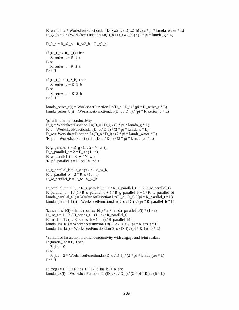
305

R_w2_b = 2 * WorksheetFunction.Ln(D_xw2_b / D_x2_b) / (2 * pi * lamda_water * L)

R_g2_b = 2 * (WorksheetFunction.Ln(D_o / D_xw2_b)) / (2 * pi * lamda_g * L)

R_2_b = R_s2_b + R_w2_b + R_g2_b

If (R_1_t > R_2_t) Then

R_series_t = R_1_t

Else

R_series_t = R_2_t

End If

If (R_1_b > R_2_b) Then

R_series_b = R_1_b

Else

R_series_b = R_2_b

End If

lamda_series_t(i) = WorksheetFunction.Ln(D_o / D_i) / (pi * R_series_t * L)

lamda_series_b(i) = WorksheetFunction.Ln(D_o / D_i) / (pi * R_series_b * L)

'parallel thermal conductivity

R_g = WorksheetFunction.Ln(D_o / D_i) / (2 * pi * lamda_g * L)

R_s = WorksheetFunction.Ln(D_o / D_i) / (2 * pi * lamda_s * L)

R_w = WorksheetFunction.Ln(D_o / D_i) / (2 * pi * lamda_water * L)

'R_pd = WorksheetFunction.Ln(D_o / D_i) / (2 * pi * lamda_pd * L)

R_g_parallel_t = R_g / (n / 2 - V_w_t)

R_s_parallel_t = 2 * R_s / (1 - n)

R_w_parallel_t = R_w / V_w_t

'R_pd_parallel_t = R_pd / V_pd_t

R_g_parallel_b = R_g / (n / 2 - V_w_b)

R_s_parallel_b = 2 * R_s / (1 - n)

R_w_parallel_b = R_w / V_w_b

R_parallel_t = 1 / (1 / R_s_parallel_t + 1 / R_g_parallel_t + 1 / R_w_parallel_t)

R_parallel_b = 1 / (1 / R_s_parallel_b + 1 / R_g_parallel_b + 1 / R_w_parallel_b)

lamda_parallel_t(i) = WorksheetFunction.Ln(D_o / D_i) / (pi * R_parallel_t * L)

lamda_parallel_b(i) = WorksheetFunction.Ln(D_o / D_i) / (pi * R_parallel_b * L)

'lamda_ins_b(i) = lamda_series_b(i) * a + lamda_parallel_b(i) * (1 - a)

R_ins_t = 1 / (a / R_series_t + (1 - a) / R_parallel_t)

R_ins_b = 1 / (a / R_series_b + (1 - a) / R_parallel_b)

lamda_ins_t(i) = WorksheetFunction.Ln(D_o / D_i) / (pi * R_ins_t * L)

lamda_ins_b(i) = WorksheetFunction.Ln(D_o / D_i) / (pi * R_ins_b * L)

' combined insulation thermal conductivity with airgaps and joint sealant

If (lamda_jac = 0) Then

R_jac = 0

Else

R_jac = 2 * WorksheetFunction.Ln(D_o / D_i) / (2 * pi * lamda_jac * L)

End If

R_tot(i) = 1 / (1 / R_ins_t + 1 / R_ins_b) + R_jac

lamda_tot(i) = WorksheetFunction.Ln(D_exp / D_i) / (2 * pi * R_tot(i) * L)

306

Next i

If (CaseNum = 2) Then

Call WritePITUfs(u_fs, lamda_tot(), Niter)

End If

If (CaseNum = 3) Then

Call WritePITAppWet(D_o, M_water, lamda_tot(), lamda_ins_t(), lamda_ins_b(), lamda_series_t(),

lamda_series_b(), lamda_parallel_t(), lamda_parallel_b(), Niter)

End If

If (CaseNum = 4) Then

Call WritePITAppa(a, D_o, M_water, lamda_tot(), lamda_ins_t(), lamda_ins_b(), lamda_series_t(),

lamda_series_b(), lamda_parallel_t(), lamda_parallel_b(), Niter)

End If

End Sub

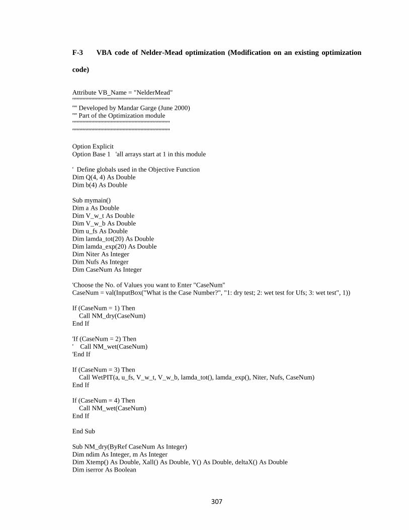
307

F-3 VBA code of Nelder-Mead optimization (Modification on an existing optimization

code)

Attribute VB_Name = "NelderMead"

'''''''''''''''''''''''''''''''''''''''''''''''''''''''''''''''''''''''''''''''''

'''' Developed by Mandar Garge (June 2000)

'''' Part of the Optimization module

'''''''''''''''''''''''''''''''''''''''''''''''''''''''''''''''''''''''''''''''''

'''''''''''''''''''''''''''''''''''''''''''''''''''''''''''''''''''''''''''''''''

Option Explicit

Option Base 1 'all arrays start at 1 in this module

' Define globals used in the Objective Function

Dim Q(4, 4) As Double

Dim b(4) As Double

Sub mymain()

Dim a As Double

Dim V_w_t As Double

Dim V_w_b As Double

Dim u_fs As Double

Dim lamda_tot(20) As Double

Dim lamda_exp(20) As Double

Dim Niter As Integer

Dim Nufs As Integer

Dim CaseNum As Integer

'Choose the No. of Values you want to Enter "CaseNum"

CaseNum = val(InputBox("What is the Case Number?", "1: dry test; 2: wet test for Ufs; 3: wet test", 1))

If (CaseNum = 1) Then

Call NM_dry(CaseNum)

End If

'If (CaseNum = 2) Then

' Call NM_wet(CaseNum)

'End If

If (CaseNum = 3) Then

Call WetPIT(a, u_fs, V_w_t, V_w_b, lamda_tot(), lamda_exp(), Niter, Nufs, CaseNum)

End If

If (CaseNum = 4) Then

Call NM_wet(CaseNum)

End If

End Sub

Sub NM_dry(ByRef CaseNum As Integer)

Dim ndim As Integer, m As Integer

Dim Xtemp() As Double, Xall() As Double, Y() As Double, deltaX() As Double

Dim iserror As Boolean

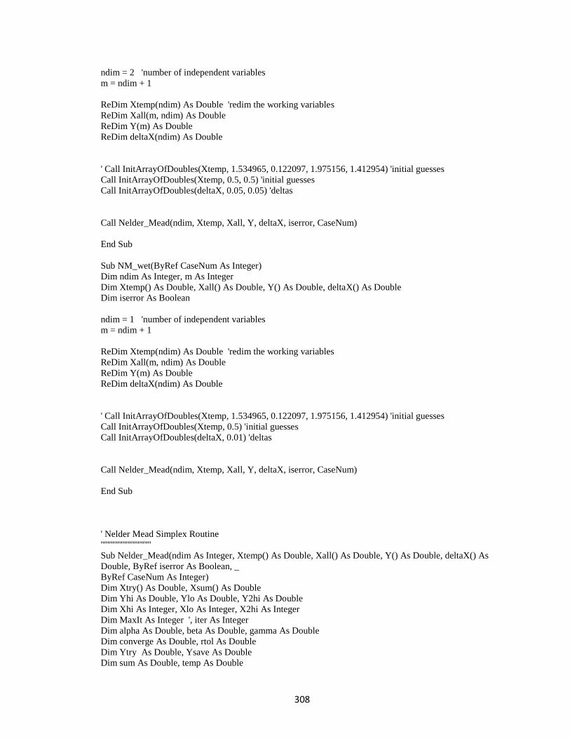
308

ndim = 2 'number of independent variables

m = ndim + 1

ReDim Xtemp(ndim) As Double 'redim the working variables

ReDim Xall(m, ndim) As Double

ReDim Y(m) As Double

ReDim deltaX(ndim) As Double

' Call InitArrayOfDoubles(Xtemp, 1.534965, 0.122097, 1.975156, 1.412954) 'initial guesses

Call InitArrayOfDoubles(Xtemp, 0.5, 0.5) 'initial guesses

Call InitArrayOfDoubles(deltaX, 0.05, 0.05) 'deltas

Call Nelder_Mead(ndim, Xtemp, Xall, Y, deltaX, iserror, CaseNum)

End Sub

Sub NM_wet(ByRef CaseNum As Integer)

Dim ndim As Integer, m As Integer

Dim Xtemp() As Double, Xall() As Double, Y() As Double, deltaX() As Double

Dim iserror As Boolean

ndim = 1 'number of independent variables

m = ndim + 1

ReDim Xtemp(ndim) As Double 'redim the working variables

ReDim Xall(m, ndim) As Double

ReDim Y(m) As Double

ReDim deltaX(ndim) As Double

' Call InitArrayOfDoubles(Xtemp, 1.534965, 0.122097, 1.975156, 1.412954) 'initial guesses

Call InitArrayOfDoubles(Xtemp, 0.5) 'initial guesses

Call InitArrayOfDoubles(deltaX, 0.01) 'deltas

Call Nelder_Mead(ndim, Xtemp, Xall, Y, deltaX, iserror, CaseNum)

End Sub

' Nelder Mead Simplex Routine

''''''''''''''''''''''''''''''

Sub Nelder_Mead(ndim As Integer, Xtemp() As Double, Xall() As Double, Y() As Double, deltaX() As

Double, ByRef iserror As Boolean, _

ByRef CaseNum As Integer)

Dim Xtry() As Double, Xsum() As Double

Dim Yhi As Double, Ylo As Double, Y2hi As Double

Dim Xhi As Integer, Xlo As Integer, X2hi As Integer

Dim MaxIt As Integer ', iter As Integer

Dim alpha As Double, beta As Double, gamma As Double

Dim converge As Double, rtol As Double

Dim Ytry As Double, Ysave As Double

Dim sum As Double, temp As Double

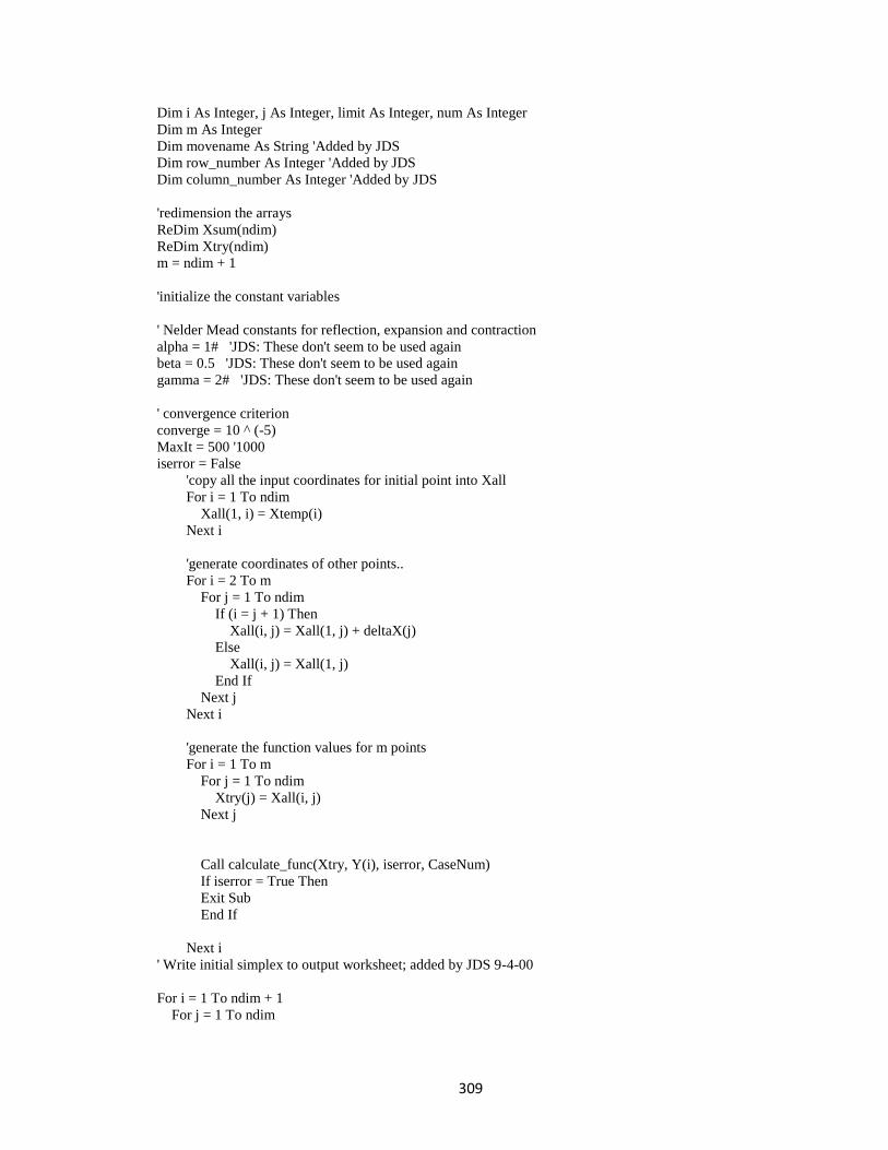
309

Dim i As Integer, j As Integer, limit As Integer, num As Integer

Dim m As Integer

Dim movename As String 'Added by JDS

Dim row_number As Integer 'Added by JDS

Dim column_number As Integer 'Added by JDS

'redimension the arrays

ReDim Xsum(ndim)

ReDim Xtry(ndim)

m = ndim + 1

'initialize the constant variables

' Nelder Mead constants for reflection, expansion and contraction

alpha = 1# 'JDS: These don't seem to be used again

beta = 0.5 'JDS: These don't seem to be used again

gamma = 2# 'JDS: These don't seem to be used again

' convergence criterion

converge = 10 ^ (-5)

MaxIt = 500 '1000

iserror = False

'copy all the input coordinates for initial point into Xall

For i = 1 To ndim

Xall(1, i) = Xtemp(i)

Next i

'generate coordinates of other points..

For i = 2 To m

For j = 1 To ndim

If (i = j + 1) Then

Xall(i, j) = Xall(1, j) + deltaX(j)

Else

Xall(i, j) = Xall(1, j)

End If

Next j

Next i

'generate the function values for m points

For i = 1 To m

For j = 1 To ndim

Xtry(j) = Xall(i, j)

Next j

Call calculate_func(Xtry, Y(i), iserror, CaseNum)

If iserror = True Then

Exit Sub

End If

Next i

' Write initial simplex to output worksheet; added by JDS 9-4-00

For i = 1 To ndim + 1

For j = 1 To ndim

310

row_number = 2

column_number = 1 + (i - 1) * (ndim + 1) + j

Worksheets("Output").Cells(row_number, column_number) = Xall(i, j)

Next j

column_number = 1 + i * (ndim + 1)

Worksheets("Output").Cells(row_number, column_number) = Y(i)

Next i

' start iterations for convergence...

'For limit = 1 To MaxIt 'start iterations

'calculate Xsum()

For j = 1 To ndim

sum = 0#

For i = 1 To m

sum = sum + Xall(i, j)

Next i

Xsum(j) = sum

Next j

' Begin iterations

For num = 1 To MaxIt

iserror = False

'find the function values for the highest and the lowest points

'and the actual high and low points

Call HighLow_point(m, Yhi, Ylo, Y2hi, Xhi, Xlo, X2hi, Y)

rtol = 2# * Abs(Yhi - Ylo) / (Abs(Yhi) + Abs(Ylo) + (0.0000000001))

If rtol < converge Then

temp = Y(1)

Y(1) = Y(Xlo)

Y(Xlo) = temp

For j = 1 To ndim

temp = Xall(1, j)

Xall(1, j) = Xall(Xlo, j)

Xall(Xlo, j) = temp

Next j

' exit the for loop

Exit For

End If

'Begin New Iteration

'First extrapolate by a factor of -1

Call Amotry(ndim, Xhi, -1#, Xsum, Xall, Y, Ytry, iserror, CaseNum)

movename = "Reflection" 'JDS 9-4-00

If iserror = True Then

iserror = False

'Exit Sub

End If

'if the trial point is better than the best point try EXPANSION

If Ytry <= Y(Xlo) Then

Call Amotry(ndim, Xhi, 2#, Xsum, Xall, Y, Ytry, iserror, CaseNum)

311

movename = "Expansion" 'JDS 9-4-00

If iserror = True Then

iserror = False

' Exit Sub

End If

ElseIf Ytry >= Y(X2hi) Then

'the reflected point is worse than the second highest point

'find CONTRACTION point

Ysave = Y(Xhi)

Call Amotry(ndim, Xhi, 0.5, Xsum, Xall, Y, Ytry, iserror, CaseNum)

movename = "Contraction" 'JDS 9-4-00

If iserror = True Then

iserror = False

'Exit Sub

End If

'if cant seem to get rid of that high point

'better contract around the lowest (best) point

If Ytry >= Ysave Then

For i = 1 To m

If i <> Xlo Then

For j = 1 To ndim

Xall(i, j) = Xsum(j) = 0.5 * (Xall(i, j) + Xall(Xlo, j))

Xtry(j) = Xsum(j)

Next j

Call calculate_func(Xtry, Y(i), iserror, CaseNum)

movename = "Multiple Contraction" 'JDS 9-4-00

iserror = False ' JDS: This is strange. 9-4-00

If iserror = True Then

iserror = False

'Exit Sub

End If

End If

Next i

'calculate Xsum()

For j = 1 To ndim

sum = 0#

For i = 1 To m

sum = sum + Xall(i, j)

Next i

Xsum(j) = sum

Next j

End If

End If

' Write simplex to output worksheet; added by JDS 9-4-00

For i = 1 To ndim + 1

312

For j = 1 To ndim

row_number = num + 2

column_number = 1 + (i - 1) * (ndim + 1) + j

Worksheets("Output").Cells(row_number, column_number) = Xall(i, j)

Next j

column_number = 1 + i * (ndim + 1)

Worksheets("Output").Cells(row_number, column_number) = Y(i)

Next i

column_number = column_number + 1

Worksheets("Output").Cells(row_number, column_number) = movename

Next num

End Sub

'Calculate the Function Value

Sub calculate_func(x() As Double, ByRef value As Double, ByRef iserror As Boolean, ByRef CaseNum

As Integer)

iserror = False

Dim lamda_exp(20) As Double ' Holds 20 measured values of the thermal resistance

Dim lamda_tot(20) As Double

Dim a As Double

Dim c_rad As Double

Dim V_w_t As Double

Dim V_w_b As Double

Dim u_fs As Double

Dim i As Integer

Dim Niter As Integer

Dim Nufs As Integer

Dim SSQE As Double

'Sum of the Squares of the Error

'Call InitArrayOfDoubles(R_exp, 3.933, 4.502, 4.955, 5.337, 3.492, 4.179, 4.694, 5.115)

'Call InitArrayOfDoubles(DT, 5, 7.5, 10#, 12.5, 3.5, 6, 8.5, 11)

SSQE = 0

If (CaseNum = 1) Then

a = x(1)

c_rad = x(2)

Call lamdacal(c_rad, a, lamda_tot(), lamda_exp(), Niter)

If a > 1 Or a < 0 Then

SSQE = 10000

End If

If c_rad < 0 Then

313

SSQE = 10000

Else

For i = 1 To Niter

SSQE = SSQE + (lamda_tot(i) - lamda_exp(i)) ^ 2

Next i

End If

End If

If (CaseNum = 2) Then

u_fs = x(1)

If u_fs > 1 Or u_fs < (V_w_t + V_w_b) Then

SSQE = 10000

Else

Call WetPIT(a, u_fs, V_w_t, V_w_b, lamda_tot(), lamda_exp(), Niter, Nufs, CaseNum)

If u_fs < (V_w_t + V_w_b) Then

SSQE = 10000

Else

SSQE = SSQE + (lamda_tot(Nufs) - lamda_exp(Nufs)) ^ 2

End If

End If

End If

If (CaseNum = 4) Then

a = x(1)

'If a > 1 Or a < 0 Then

' SSQE = 0

'Else

Call WetPIT(a, u_fs, V_w_t, V_w_b, lamda_tot(), lamda_exp(), Niter, Nufs, CaseNum)

If a > 1 Or a < 0 Then

SSQE = 10000

Else

314

SSQE = SSQE + (lamda_tot(Niter) - lamda_exp(Niter)) ^ 2

End If

End If

value = SSQE

End Sub

' find the maximum of two

Sub Maxx(a As Double, b As Double, ByRef C As Double)

If (a >= b) Then

C = a

Else

C = b

End If

End Sub

' find the highest and the lowest points

Sub HighLow_point(num As Integer, Yhi As Double, Ylo As Double, Y2hi As Double, Xhi As Integer,

Xlo As Integer, X2hi As Integer, Y() As Double)

Dim count As Integer

Yhi = Y(1)

Ylo = Y(1)

Xhi = 1

Xlo = 1

'Find out the Highest Point

For count = 2 To num

If Y(count) > Yhi Then

Yhi = Y(count)

Xhi = count

End If

Next count

'Find out the Lowest Point

For count = 2 To num

If Y(count) < Ylo Then

Ylo = Y(count)

Xlo = count

End If

Next count

Y2hi = Ylo

X2hi = Xlo

'Find out the Second highest Point

For count = 1 To num

If Y(count) <> Yhi Then

315

If Y(count) > Y2hi Then

Y2hi = Y(count)

X2hi = count

End If

End If

Next count

End Sub

' the actual function evaluation routine

Sub Amotry(ByRef ndim As Integer, hi As Integer, fac As Double, _

Xsum() As Double, Xall() As Double, Y() As Double, _

ByRef Ytrial As Double, ByRef iserror As Boolean, ByRef CaseNum As Integer)

Dim L As Integer

Dim fac1, fac2 As Double

Dim Xtry() As Double

'redimension

ReDim Xtry(ndim)

fac1 = (1# - fac) / ndim

fac2 = fac1 - fac

For L = 1 To ndim

Xtry(L) = Xsum(L) * fac1 - Xall(hi, L) * fac2

Next L

' evaluate function at the trial point

Call calculate_func(Xtry, Ytrial, iserror, CaseNum)

If iserror = True Then

'Exit Sub

End If

'if its better than the highest point replace the highest point

If (Ytrial < Y(hi)) Then

Y(hi) = Ytrial

For L = 1 To ndim

Xsum(L) = Xsum(L) + Xtry(L) - Xall(hi, L)

Xall(hi, L) = Xtry(L)

Next L

End If

End Sub

.

VITA

Shanshan Cai

Candidate for the Degree of

Doctor of Philosophy

Thesis: THERMAL PERFORMANCE OF MECHANICAL PIPE INSULATION

SYSTEMS AT BELOW-AMBIENT TEMPERATURE

Major Field: Mechanical Engineering

Biographical:

Education:

Completed the requirements for the Doctor of Philosophy in Mechanical

Engineering at Oklahoma State University, Stillwater, Oklahoma in December,

2013.

Completed the requirements for the Master of Science in Mechanical

Engineering at Oklahoma State University, Stillwater, Oklahoma in 2009.

Completed the requirements for the Bachelor of Science in Building

Environment and Equipment Engineering at Huazhong Univeristy of Science

and Technology, Wuhan, China in 2007.

Experience: Research/Teaching Assistant in Oklahoma State University

Professional Memberships: ASHRAE Student Member