arX

iv:0

903.

5099

v1 [

cond

-mat

.dis

-nn]

29

Mar

200

9

A theory of amorphous packings of binary mixtures of hard spheres

Indaco Biazzo,1 Francesco Caltagirone,1 Giorgio Parisi,1, 2 and Francesco Zamponi3

1Dipartimento di Fisica, Universita di Roma “La Sapienza”, P.le A. Moro 2, 00185 Roma, Italy2INFM-CNR SMC, INFN, Universita di Roma “La Sapienza”, P.le A. Moro 2, 00185 Roma, Italy

3Laboratoire de Physique Theorique, CNRS UMR 8549,

Ecole Normale Superieure, 24 Rue Lhomond, 75231 Paris Cedex 05, France

We extend our theory of amorphous packings of hard spheres to binary mixtures and more gener-ally to multicomponent systems. The theory is based on the assumption that amorphous packingsproduced by typical experimental or numerical protocols can be identified with the infinite pressurelimit of long lived metastable glassy states. We test this assumption against numerical and experi-mental data and show that the theory correctly reproduces the variation with mixture compositionof structural observables, such as the total packing fraction and the partial coordination numbers.

Amorphous packings of hard spheres are ubiquitousin physics: they have been used as models for liquids,glasses, colloidal systems, granular systems, and pow-ders. They are also related to important problems inmathematics and information theory, such as digitaliza-tion of signals, error correcting codes, and optimizationproblems. Moreover, the structure and density (or poros-ity) of amorphous multicomponent packings is importantin many branches of science and technology, ranging fromoil extraction to storage of grains in silos.

Despite being empirically studied since at least sixtyyears, amorphous packings still lack a precise mathemati-cal definition, due to the intrinsic difficulty of quantifying“randomness” [1]. Indeed, even if a sphere packing is apurely geometrical object, in practice dense amorphouspackings always result from rather complicated dynam-ical protocols: for instance, spheres can be thrown atrandom in a box that is subsequently shaken to achievecompactification [2], or they can be deposited onto a ran-dom seed cluster [3]. In numerical simulations, one startsfrom a random distribution of small spheres and inflatesthem until a jammed state is reached [4, 5]; alternatively,one starts from large overlapping spheres and reducesthe diameter in order to eliminate the overlaps [6–9]. Inprinciple, each of these dynamical prescriptions producesan ensemble of final packings that depends on the de-tails of the procedure used. Still, very remarkably, if thepresence of crystalline regions is avoided, the structuralproperties of amorphous packings turn out to be verysimilar. This observation led to the proposal that “typi-cal” amorphous packings should have common structureand density; the latter has been denoted Random ClosePacking (RCP) density. The definition of RCP has beenintensively debated in the last few years, in connectionwith the progresses of numerical simulations [1, 10].

Nevertheless, the empirical evidence, that amorphouspackings produced according to very different protocolshave common structural properties, is striking and callfor an explanation. This is all the more true for binary ormulticomponent mixtures, where in addition to the usualstructural observables, such as the structure factor, onecan investigate other quantities such as the coordinationbetween spheres of different type, and study their varia-

tion with the composition of the mixture.

In earlier attempts to build statistical models of pack-ings, only the main geometrical factors, such as the rel-ative size and abundance of the different components,were taken into account [11–13]. More precisely, thesemodels focus on a random sphere in the packing andits first neighbors, completely neglecting spatial correla-tions beside the first shell and all the global geometricconstraints. This already accounts for the main qualita-tive structural properties of random packings. However,in order to obtain a quantitative description, some freeparameters have to be introduced and adjusted to matchwith experimental data.

To go beyond these simple models, many authors pro-posed that random packings of hard spheres can bethought as the infinite pressure limit of hard sphereglasses [14–20]. This is very intuitive since a glass isa solid state in which particles vibrate around amor-phous reference positions, and vibrations are reduced onincreasing pressure. A typical algorithm attempting tocreate a random packing starts at low density and com-presses the system at a given rate. During this evolu-tion, when the density is high enough, relaxation becomesmore and more difficult until at some point the systemis stuck into a glass state [19, 20]; at this point furthercompression will only reduce the amplitude of the vibra-tions. In a nutshell, this is why amorphous packings canbe identified with glasses at infinite pressure.

The main advantage of this identification, if it holds, isthat a glass is a metastable state that has a very long life-time; therefore, its properties can be studied using con-cepts of equilibrium statistical mechanics. In this way acomplicated dynamical problem (solving the equations ofmotion for a given protocol) is reduced to a much moresimple equilibrium problem. In [18, 20] it was shown, inthe case of monodisperse packings, that this strategy isvery effective since it allows to compute structural prop-erties of random packings directly from the Hamiltonianof the system, without free parameters and in a controlledstatistical mechanics framework. Note that the existenceof an equilibrium glass transition in hard sphere systems(or in other words the existence of glasses with infinite lifetime) has been questioned [5, 21]. Although very inter-

2

esting, this problem is not relevant for the present discus-sion since we are only interested in long-lived metastableglasses that trap dynamical algorithms. At present itis very well established by numerical simulations [22, 23]that for system sizes of N <∼ 104 particles and on the timescales of typical algorithms, metastable glassy states ex-ist, at least in d ≥ 3. This is enough to compare withmost of the currently available numerical and experimen-tal data. Finally, the relation of this approach to specialpackings such as the MRJ state [1] and the J-point [8]has been discussed in detail in [20].

The aim of this paper is to extend the theory of [18, 20]to binary mixtures. This allows to compare quantita-tively the predictions of the theory and the results ofnumerical simulations. We will focus in particular on thevariation of density and local connectivity as a functionof mixture composition. These results constitute, in ouropinion, a stringent test of the assumption that randompackings reached by standard algorithms can be identi-fied with infinite pressure metastable glasses.

Theory - The equilibrium statistical mechanics com-putation of the properties of the glass is based on stan-dard liquid theory [24] and on the replica method [17, 25]that has been developed in the context of spin glass the-ory [26, 27]. For monodisperse hard spheres, it has beendescribed in great detail in [20]. The extension to multi-component systems is straightforward following [28]; de-tails are given in Appendix.

Here we just recall some features of this approach,based on simple physical considerations. The basic as-sumption of the method are that i) crystallization andphase separation are strongly suppressed by kinetic ef-fects so that the liquid can be safely followed at high den-sity, and ii) that at sufficiently high density, the liquid isa superposition of a collection of amorphous metastablestates. Namely, in the liquid, the system spends sometime inside one of these states, and sometimes under-goes a rearrangement that leads to a different state [29].Each state is characterized by its vibrational entropy perparticle, denoted by s, and the number of such states isassumed to be exponential in N , so defining a configura-tional entropy Σ(ϕ, s) = N−1 logN (ϕ, s), being N (ϕ, s)the number of states having entropy s at density ϕ. Onincreasing the density, the liquid is trapped for longer andlonger times into a metastable state, until at some pointthe transition time becomes so long that for all practicalpurposes the system is stuck into one state: it then be-comes a glass. To compute the properties of the glassystates, the central problem is to compute the functionΣ(ϕ, s). This can be done by means of a simple replicamethod introduced by Monasson [27]. One introduces mcopies of each particle, constrained to be close enough,in such a way that they must be in the same metastablestate. Then, the total entropy of the system of m copiesis given by S(m, ϕ|s) = ms+Σ(ϕ, s); the first term givesthe entropy of the m copies in a state of entropy s, whilethe second term is due to the multiplicity of possiblestates. The total entropy of the system at fixed density

0 0.2 0.4 0.6 0.8 1Volume fraction of small component

0.65

0.7

0.75

0.8

ϕj

r=12r=5.74r=4r=3.41r=2.58r=2r=1.4r=1.2

FIG. 1: (Color online) Packing fraction ϕj as a function ofη = 1/(1 + xr3) at fixed r. Full symbols are numerical datafrom this work. Open symbols are experimental results fromRef. [30]. Lines are predictions from theory, obtained fixingΣj = 1.7. Note that the large r-small η region could not beexplored, since for such very asymmetric mixtures the largespheres form a rigid structure while small spheres are able tomove through the pores and are not jammed [12, 13].

ϕ is obtained by maximizing over s, i.e.

S(m, ϕ) = maxs

[Σ(ϕ, s) + ms] = Σ(ϕ, s∗) + ms∗ , (1)

where s∗(m, ϕ) is determined by the condition∂sΣ(ϕ, s) = m. Then it immediate to show that

s∗(m, ϕ) = ∂mS(m, ϕ) ,

Σ(ϕ, s∗(m, ϕ)) = −m2∂m[S(m, ϕ)/m] .(2)

The knowledge of S(m, ϕ) allows to reconstruct the curveΣ(ϕ, s) for a given density by a parametric plot of Eqs. (2)by varying m. The function Σ(ϕ, s) gives access to theinternal entropy and the number of metastable glassystates; from this one can compute their equation of state,i.e. the pressure as a function of the density; in particu-lar, for each set of glassy states of given configurationalentropy Σj , one can compute the density ϕj (jammingdensity) at which their pressure diverges. Since ϕj turnsout to depend (slightly) on Σj , a prediction of the the-ory is that different glasses will jam at different density:amorphous packings can be found in a finite (but small)interval of density [19, 20].

Results for binary mixtures - The details of the compu-tation of the function S(m, ϕ) for a general multicompo-nent mixture, based on [20], can be found in Appendix.Here we consider a binary mixture of two types of spheresµ = A, B in a volume V , with different diameter Dµ anddensity ρµ = Nµ/V . We define r = DA/DB > 1 thediameter ratio and x = NA/NB the concentration ratio;V3(D) = πD3/6 the volume of a three dimensional sphereof diameter D; ϕ = ρAV3(DA) + ρBV3(DB) the packingfraction; η = ρBV3(DB)/ϕ = 1/(1 + xr3) the volumefraction of the small (B) component.

3

0

2

4

6

8

Con

tact

s

zss

zsl

zls

zll

0 0.2 0.4 0.6 0.8 1Volume Fraction of Small Component

0

2

4

6

8

Con

tact

sr=1.2

r=1.4

0

2

4

6

8

10

12

14

16

Con

tact

s

zss

zsl

zls

zll

0

2

4

6

8

Con

tact

s

0 0.2 0.4 0.6 0.8 1Volume Fraction of Small Component

0

10

20

30

40

50

r=2

r=4

FIG. 2: (Color online) Partial average coordination numbers (small-small, small-large, large-small, large-large) as a function ofvolume fraction of the small particles η = 1/(1 + xr3) for different values of r. Full symbols are numerical data from this work.Open symbols are experimental data from Ref. [31]. Note that in the lower right panel a different scale is used for zls.

Once an equation of state for the liquid has been cho-sen, the jamming packing fraction ϕj is given in termof Σj by the solution of Σj(ϕ) = Σj . The average co-ordination numbers at ϕj are denoted zµν(ϕj), but wechecked that their variations with ϕj are negligible. Weused in d = 3 the equation of state proposed in [32], us-ing the Carnahan-Starling equation for the monodispersesystem [24]. The latter, as well as Σj(ϕ) and zµν(ϕj), aregiven respectively in Eqs. (20), (16), (19), in Appendix.

Numerical simulations - We produced jammed pack-ings of binary mixtures of N = 1000 hard spheres usingthe code developed by Donev et al. [33, 34]. In this al-gorithm spheres are compressed uniformly by increasingtheir diameter at a rate dD/dt = 2γ while event-drivenmolecular dynamics is performed at the same time. In or-der to obtain a perfectly jammed final packing, the laterstages of compression must be performed very slowly.On the other hand, at low density slow compression isa waste of time, since the dynamics of the system is veryfast. Following [35], we find a good compromise by per-forming a four stages compression: starting from randomconfigurations at ϕ = 0.1, i) the first stage is a relativelyfast compression (γ = 10−2) up to a reduced pressurep = βP/ρ = 102; then we compress at ii) γ = 10−3 upto p = 103; iii) γ = 10−4 up to p = 109; iv) γ = 10−5

up to p = 1012. The first stage terminates at a densityϕ ∼ 0.6, and is fast enough to avoid crystallization andphase separation. During the following stages the systemis already dense enough to stay close to the amorphousstructure reached during the first stage. Still, little rear-

rangements (involving many particles) are possible andallow to reach a collectively jammed final state [35]. Inthe final configurations, we observe a huge gap betweencontacting (typical gap ∼ 10−11D) and non-contacting(typical gap >∼ 10−6D) particles. We then say that twoparticles are in contact whenever the gap is smaller than10−8D. Typically, a small fraction (<∼ 5% of the total)of rattlers, i.e. particles having less then 4 contacts, ispresent. Once these are removed, the configuration isisostatic (the total number of contacts is 6N) within 1%accuracy.

Comparison of theory and numerical/experimentaldata - During the four stages of compression, the pressureinitially follows the liquid equation of state up to somedensity close to the glass transition density [20, 36, 37].Above this density, pressure increases faster and divergeson approaching jamming at ϕj . The exact point wherethis happens depends on compression rate. This is a niceconfirmation of a prediction of the theory, that differ-ent glassy states jam at different density; it was alreadyobserved in [5, 35] and recently discussed in great de-tail in [23, 38]. Within the theory ϕj is related to Σj ,the value of configurational entropy at which the systemfalls out of equilibrium; hence there is one free parame-ter, Σj , that depends on the compression protocol. Theequation of state of the glass obtained numerically withour protocol corresponds within our theory to Σj ∼ 1.5.We decided to use the value Σj = 1.7 that gives the bestfit to the numerical data. This is consistent with previ-ous observations, that the configurational entropy is close

4

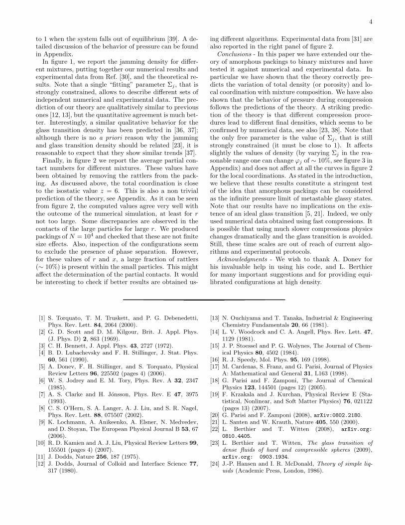
to 1 when the system falls out of equilibrium [39]. A de-tailed discussion of the behavior of pressure can be foundin Appendix.

In figure 1, we report the jamming density for differ-ent mixtures, putting together our numerical results andexperimental data from Ref. [30], and the theoretical re-sults. Note that a single “fitting” parameter Σj , that isstrongly constrained, allows to describe different sets ofindependent numerical and experimental data. The pre-diction of our theory are qualitatively similar to previousones [12, 13], but the quantitative agreement is much bet-ter. Interestingly, a similar qualitative behavior for theglass transition density has been predicted in [36, 37];although there is no a priori reason why the jammingand glass transition density should be related [23], it isreasonable to expect that they show similar trends [37].

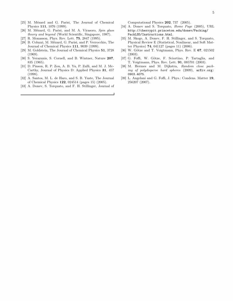
Finally, in figure 2 we report the average partial con-tact numbers for different mixtures. These values havebeen obtained by removing the rattlers from the pack-ing. As discussed above, the total coordination is closeto the isostatic value z = 6. This is also a non trivialprediction of the theory, see Appendix. As it can be seenfrom figure 2, the computed values agree very well withthe outcome of the numerical simulation, at least for rnot too large. Some discrepancies are observed in thecontacts of the large particles for large r. We producedpackings of N = 104 and checked that these are not finitesize effects. Also, inspection of the configurations seemto exclude the presence of phase separation. However,for these values of r and x, a large fraction of rattlers(∼ 10%) is present within the small particles. This mightaffect the determination of the partial contacts. It wouldbe interesting to check if better results are obtained us-

ing different algorithms. Experimental data from [31] arealso reported in the right panel of figure 2.

Conclusions - In this paper we have extended our the-ory of amorphous packings to binary mixtures and havetested it against numerical and experimental data. Inparticular we have shown that the theory correctly pre-dicts the variation of total density (or porosity) and lo-cal coordination with mixture composition. We have alsoshown that the behavior of pressure during compressionfollows the predictions of the theory. A striking predic-tion of the theory is that different compression proce-dures lead to different final densities, which seems to beconfirmed by numerical data, see also [23, 38]. Note thatthe only free parameter is the value of Σj , that is stillstrongly constrained (it must be close to 1). It affectsslightly the values of density (by varying Σj in the rea-sonable range one can change ϕj of ∼ 10%, see figure 3 inAppendix) and does not affect at all the curves in figure 2for the local coordinations. As stated in the introduction,we believe that these results constitute a stringent testof the idea that amorphous packings can be consideredas the infinite pressure limit of metastable glassy states.Note that our results have no implications on the exis-tence of an ideal glass transition [5, 21]. Indeed, we onlyused numerical data obtained using fast compressions. Itis possible that using much slower compressions physicschanges dramatically and the glass transition is avoided.Still, these time scales are out of reach of current algo-rithms and experimental protocols.

Acknowledgments - We wish to thank A. Donev forhis invaluable help in using his code, and L. Berthierfor many important suggestions and for providing equi-librated configurations at high density.

[1] S. Torquato, T. M. Truskett, and P. G. Debenedetti,Phys. Rev. Lett. 84, 2064 (2000).

[2] G. D. Scott and D. M. Kilgour, Brit. J. Appl. Phys.(J. Phys. D) 2, 863 (1969).

[3] C. H. Bennett, J. Appl. Phys. 43, 2727 (1972).[4] B. D. Lubachevsky and F. H. Stillinger, J. Stat. Phys.

60, 561 (1990).[5] A. Donev, F. H. Stillinger, and S. Torquato, Physical

Review Letters 96, 225502 (pages 4) (2006).[6] W. S. Jodrey and E. M. Tory, Phys. Rev. A 32, 2347

(1985).[7] A. S. Clarke and H. Jonsson, Phys. Rev. E 47, 3975

(1993).[8] C. S. O’Hern, S. A. Langer, A. J. Liu, and S. R. Nagel,

Phys. Rev. Lett. 88, 075507 (2002).[9] K. Lochmann, A. Anikeenko, A. Elsner, N. Medvedev,

and D. Stoyan, The European Physical Journal B 53, 67(2006).

[10] R. D. Kamien and A. J. Liu, Physical Review Letters 99,155501 (pages 4) (2007).

[11] J. Dodds, Nature 256, 187 (1975).[12] J. Dodds, Journal of Colloid and Interface Science 77,

317 (1980).

[13] N. Ouchiyama and T. Tanaka, Industrial & EngineeringChemistry Fundamentals 20, 66 (1981).

[14] L. V. Woodcock and C. A. Angell, Phys. Rev. Lett. 47,1129 (1981).

[15] J. P. Stoessel and P. G. Wolynes, The Journal of Chem-ical Physics 80, 4502 (1984).

[16] R. J. Speedy, Mol. Phys. 95, 169 (1998).[17] M. Cardenas, S. Franz, and G. Parisi, Journal of Physics

A: Mathematical and General 31, L163 (1998).[18] G. Parisi and F. Zamponi, The Journal of Chemical

Physics 123, 144501 (pages 12) (2005).[19] F. Krzakala and J. Kurchan, Physical Review E (Sta-

tistical, Nonlinear, and Soft Matter Physics) 76, 021122(pages 13) (2007).

[20] G. Parisi and F. Zamponi (2008), arXiv:0802.2180.[21] L. Santen and W. Krauth, Nature 405, 550 (2000).[22] L. Berthier and T. Witten (2008), arXiv.org:

0810.4405.[23] L. Berthier and T. Witten, The glass transition of

dense fluids of hard and compressible spheres (2009),arXiv.org: 0903.1934.

[24] J.-P. Hansen and I. R. McDonald, Theory of simple liq-

uids (Academic Press, London, 1986).

5

[25] M. Mezard and G. Parisi, The Journal of ChemicalPhysics 111, 1076 (1999).

[26] M. Mezard, G. Parisi, and M. A. Virasoro, Spin glass

theory and beyond (World Scientific, Singapore, 1987).[27] R. Monasson, Phys. Rev. Lett. 75, 2847 (1995).[28] B. Coluzzi, M. Mezard, G. Parisi, and P. Verrocchio, The

Journal of Chemical Physics 111, 9039 (1999).[29] M. Goldstein, The Journal of Chemical Physics 51, 3728

(1969).[30] S. Yerazunis, S. Cornell, and B. Wintner, Nature 207,

835 (1965).[31] D. Pinson, R. P. Zou, A. B. Yu, P. Zulli, and M. J. Mc-

Carthy, Journal of Physics D: Applied Physics 31, 457(1998).

[32] A. Santos, M. L. de Haro, and S. B. Yuste, The Journalof Chemical Physics 122, 024514 (pages 15) (2005).

[33] A. Donev, S. Torquato, and F. H. Stillinger, Journal of

Computational Physics 202, 737 (2005).[34] A. Donev and S. Torquato, Home Page (2005), URL

http://cherrypit.princeton.edu/donev/Packing/

PackLSD/Instructions.html.[35] M. Skoge, A. Donev, F. H. Stillinger, and S. Torquato,

Physical Review E (Statistical, Nonlinear, and Soft Mat-ter Physics) 74, 041127 (pages 11) (2006).

[36] W. Gotze and T. Voigtmann, Phys. Rev. E 67, 021502(2003).

[37] G. Foffi, W. Gotze, F. Sciortino, P. Tartaglia, andT. Voigtmann, Phys. Rev. Lett. 91, 085701 (2003).

[38] M. Hermes and M. Dijkstra, Random close pack-

ing of polydisperse hard spheres (2009), arXiv.org:

0903.4075.[39] L. Angelani and G. Foffi, J. Phys.: Condens. Matter 19,

256207 (2007).

6

Appendix

I. BEHAVIOR OF THE PRESSURE DURING COMPRESSION

0.52 0.56 0.6 0.64 0.68ϕ0

0.02

0.04

0.06

0.08

1/p

Metastable glass Σj = 0.5

Metastable glass Σj = 1.2

Metastable glass Σj = 1.5

Ideal glassLiquidNumerical 2Numerical 1

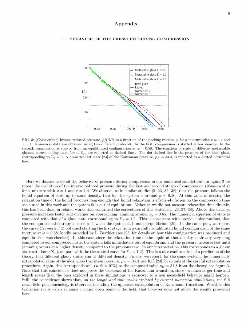
FIG. 3: (Color online) Inverse reduced pressure, ρ/(βP ) as a function of the packing fraction ϕ for a mixture with r = 1.4 andx = 1. Numerical data are obtained using two different protocols. In the first, compression is started at low density. In thesecond, compression is started from an equilibrated configuration at ϕ = 0.58. The equation of state of different metastableglasses, corresponding to different Σj , are reported as dashed lines. The dot-dashed line is the pressure of the ideal glass,corresponding to Σj = 0. A numerical estimate [23] of the Kauzmann pressure, pK = 34.4, is reported as a dotted horizontalline.

Here we discuss in detail the behavior of pressure during compression in our numerical simulations. In figure 3 wereport the evolution of the inverse reduced pressure during the first and second stages of compression (Numerical 1)for a mixture with x = 1 and r = 1.4. We observe, as in similar studies [5, 23, 35, 38], that the pressure follows theliquid equation of state up to some density, that for this system is around ϕ ∼ 0.56. At this value of density, therelaxation time of the liquid becomes long enough that liquid relaxation is effectively frozen on the compression timescale used in this work and the system falls out of equilibrium. Although we did not measure relaxation time directly,this has been done in related works that confirmed the correctness of this statement [23, 37, 38]. Above this density,pressure increases faster and diverges on approaching jamming around ϕj ∼ 0.65. The numerical equation of state iscompared with that of a glass state corresponding to Σj = 1.5. This is consistent with previous observations, thatthe configurational entropy is close to 1 when the system falls out of equilibrium [39]. In the same plot, we reportthe curve (Numerical 2) obtained starting the first stage from a carefully equilibrated liquid configuration of the samemixture at ϕ = 0.58, kindly provided by L. Berthier (see [23] for details on how this configuration was produced andequilibration was checked). In this case, since the relaxation time of the liquid at that density is already very longcompared to our compression rate, the system falls immediately out of equilibrium and the pressure increases fast untiljamming occurs at a higher density compared to the previous case. In our interpretation, this corresponds to a glassystate with lower Σj (compare with the theoretical curve for Σj ∼ 1.2). This is a nice confirmation of a prediction of thetheory, that different glassy states jam at different density. Finally, we report, for the same system, the numericallyextrapolated value of the ideal glass transition pressure, pK = 34.4, see Ref. [23] for details of the careful extrapolationprocedure. Again, this corresponds well (within 10%) to the computed value pK = 31.8 from the theory, see figure 3.Note that this coincidence does not prove the existence of the Kauzmann transition, since on much larger time andlength scales than the ones explored in these simulations, a crossover to a non mean-field behavior might happen.Still, the coincidence shows that, on the length and time scales explored by current numerical simulations, the fullmean field phenomenology is observed, including the apparent extrapolation of Kauzmann transition. Whether thistransition really exists remains a major open point of the field, that however does not affect the results presentedhere.

7

II. REPLICA THEORY FOR MULTICOMPONENT MIXTURES

Here we show in detail how to generalize the computation of [20] to multicomponent mixtures. We will not repeatthe discussion of [20] but we only explain how to modify it for mixtures. Reading Appendix B and C and section VIIof [20] is necessary to follow the discussion.

We consider a multicomponent system in a (large) volume V with partial densities ρµ = Nµ/N . The total densityis ρ =

∑µ ρµ and we define xµ = ρµ/ρ. Spheres of type µ have diameter Dµ and we define Dµν = (Dµ + Dν)/2.

We denote by Ωd = 2πd/2/Γ(d/2) the d-dimensional solid angle, and by Vd(D) = πd/2Dd/Γ(1 + d/2) the volume of ad-dimensional sphere of diameter D. The hard sphere potential φµν(r) is infinite for r < Dµν and zero otherwise: wedenote χµν(r) = exp[−φµν(r)]. gµν(r), as usual, is the µ-ν pair correlation function [24]. We will use the shorthandnotations gµν ≡ gµν(Dµν) for the contact values of gµν(r), and V µν

d = Vd(Dµν) for the volume of a sphere of diameterDµν .

As discussed in [28], we assume that in the replicated liquid molecules are built of particles of the same type. Thisamounts to assume that in a glassy state particles of different type cannot easily exchange. However, as the diffusionconstant is always finite in a glass, this assumption is wrong, since particles can exchange also within a state. Thisis all the more true in the liquid phase before the glass transition. Therefore, in order to correct this error, we willsubtract the mixing entropy from the configurational entropy we will compute in the following, in order to obtain thecorrect physical result.

According to [28], to each molecule of the replicated liquid we can attach a label µ = 1, · · · , n according to thetype of particles that build the molecule. We denote coordinates in a molecule by x = (x1, · · · , xm). We have then tocompute the free energy functional of a liquid made of n species of molecules, with a single molecule density ρµ(x)and an interaction χµν(x, y) =

∏ma=1 χµν(xa − ya).

Effective liquid

We assume that the vibrations of the m copies are described by a Gaussian distribution, corresponding to harmonicvibrations:

ρµ(x) = ρµ

∫dX

m∏

a=1

e−

(xa−X)2

2Aµ

(√

2πAµ)d. (3)

The widths Aµ are variational parameters and we will maximize the entropy with respect to them at the end. Wechoose a replica (say replica 1) as a reference and consider the vibrations of the other m − 1 particles around thereference one. We want to construct an expansion assuming that Aµ is small. For Aµ = 0, the m − 1 copies coincidewith the reference one, and S(m, ϕ) is given by the entropy S(ϕ) of the non-replicated liquid plus the entropy of m−1harmonic oscillators of spring constant Aµ (averaged over the concentration of the different species):

S(0)(m, ϕ) = S(ϕ) +∑

µ

xµSharm(m, Aµ) . (4)

The harmonic part of the entropy is computed straightforwardly from the term∑

µ

∫dxρµ(x)[1 − log ρµ(x)] in the

free energy functional, see section V of [20], where the function Sharm(m, A) is also defined.A first order approximation is obtained by considering the effective two-body interaction induced on the particles of

replica 1 by the coupling to the m−1 copies. This can be justified on the basis of a diagrammatic expansion followingthe derivation in Appendix B of [20], see also [15]. It is possible to show [24] that the diagrammatic expansion ofthe free energy functional for a multicomponent liquid is the same as the one of a simple liquid, provided a label µi

is attached to each vertex i, and in such a labeled diagram ρµi(xi) is placed on each vertex, χµiµj

(xi − xj) on eachlink, and a sum over µi is performed in addition to the integration over xi. The same is true for the molecular liquid.Hence, the treatment of diagrams performed in Appendix B of [20] can be repeated exactly for a mixture, takinginto account the presence of the additional labels. This is straightforward and leads to the introduction of effectivepotentials that now depend on the type of particles involved. In particular, one obtains:

e−φeffµν (x1−y1) =

∫dx2 · · · dxmdy2 · · · dymρµ(x) ρν(y)

m∏

a=1

e−φµν(xa−ya)

≡ e−φµν(x1−y1)[1 + Qµν(x1 − y1)] .

(5)

8

A first order approximation to S(m, ϕ) is then obtained by substituting to the entropy S(ϕ) of the simple hardsphere mixture the free energy of a liquid of particles interacting via the potential φeff

µν (r):

S(1)(m, ϕ) = −F [ϕ, φeffµν (r)] +

∑

µ

xµSharm(m, Aµ) . (6)

It is now evident that we can obtain better approximations of the true function S(m, ϕ) by considering also the threebody interactions induced on particles of the replica 1, and so on. Here, for simplicity, we will limit ourselves toconsider the two-body interactions. To the same approximation, the pair correlation function gµν(r) of the system isgiven by the correlation of the effective liquid of particles interacting via φµν(r). For small Aµ, φeff

µν is close to φµν

and the free energy in Eq. (6) can be computed in perturbation theory around the normal liquid [24], which is takenas an input for the calculation of the properties of the glass.

Small cage expansion

Now we follow the discussion in section VII of [20] to compute the entropy of the effective liquid. We assume thatthe cage radius is small, therefore Qµν can be considered as a perturbation, and one has φeff

µν (r) ∼ φµν(r) − Qµν(r).Using the general relation [24]

δF [ϕ, φµν(r)]

δφµν(r)=

ρµρν

2ρgµν(r) , (7)

we obtain

−F [ϕ, φeffµν (r)] ∼ S(ϕ) +

∑

µ,ν

ρµρν

2ρ

∫drgµν(r)Qµν(r) , (8)

where S(ϕ) = −F [ϕ, φµν(r)] is the entropy of the liquid. The function Qµν(r) is different from zero only for r−Dµν ∼O(√

Aµ + Aν). If√

Aµ + Aν ≪ Dµν we can assume that the function gµν(r) is essentially constant on the scale√Aµ + Aν , then gµν(r) ∼ gµνχµν(r) for r − Dµν ∼ O(

√Aµ + Aν), and

∫drgµν(r)Qµν(r) ∼ gµν

∫drχµν(r)Qµν(r) . (9)

To compute the previous expression, all the considerations of Appendix C of [20] can be repeated. Instead of asingle function Q(r), one has Qµν(r), and in the two Gaussians one has Aµ and Aν instead of A. At the very beginningof the discussion, then, one finds that it is enough to replace 2A → Aµ + Aν and follow the same steps. We obtain

∫drχµν(r)Qµν(r) =

d V µνd

Dµν

√2(Aµ + Aν)Q0(m) . (10)

where Q0(m) is defined in Appendix C of [20].Putting all together, we find the final result

S(m, ϕ; Aµ) =∑

µ

xµSharm(m, Aµ) + S(ϕ) +∑

µ,ν

ρµρν

2ρgµν

d V µνd

Dµν

√2(Aµ + Aν) Q0(m) (11)

This expression generalizes the result of section VII of [20] to multicomponent mixtures; it has to be optimized overall the Aµ to get the replicated entropy S(m, ϕ).

Replicated free energy for binary mixtures

The optimization with respect to Aµ leads to n coupled equations that are not easy to solve in general. Thereforein the following we focus on the case of binary mixtures that is of interest here.

9

For convenience we denote AA = A and AB = B the cage radii of the two species. We then obtain

∂S(m, ϕ; A, B)

∂A=

ρ2AgAAV AA

d d

2ρDAA

Q0(m)√A

+ρAρBgABV AB

d d

ρDAB

Q0(m)√2(A + B)

− xAd(1 − m)

2A= 0

∂S(m, ϕ; A, B)

∂B=

ρ2BgBBV BB

d d

2ρDBB

Q0(m)√B

+ρAρBgABV AB

d d

ρDAB

Q0(m)√2(A + B)

− xBd(1 − m)

2B= 0

(12)

Defining δ = B/A, x = ρA/ρB and r = DA/DB, we obtain the following equation for δ:

x rd−1 gAA −√

δ gBB +

√2(1 − xδ)√(1 + δ)

(1 + r

2

)d−1

gAB = 0 , (13)

and from its solution we obtain the optimal values of A and B = δ A:

√A⋆(δ) =

1 − m

2Q0(m)

⟨Dd⟩(1 + x)

2d ϕΓ

Γ =1

2xgAADd−1

AA + gABDd−1

AB√2(1 + δ)

(14)

where the packing fraction is ϕ = ρAVd(DA)+ ρBVd(DB) and 〈Dp〉 =∑

µ xµDpµ. Substituting these in S(m, ϕ; A, B),

we finally get

S(m, ϕ) = S(ϕ) − d

2(1 − m − log m) − d

2(1 − m) log(2πA⋆) − d

2

1

1 + x(1 − m) log(δ) +

2ddϕ

〈Dd〉Q0(m)

√A⋆∆

(1 + x)2

∆ = x2gAADd−1AA + xgABDd−1

AB

√2(1 + δ) + gBBDd−1

BB

√δ

(15)

From this expression one can compute the complexity using Eq. (2) [20]; here it is not useful to report the completeexpression. However, it is interesting to report the following explicit expressions:

Σj(ϕ) = limm→0

Σ(m, ϕ) = S(ϕ) − d log

(√2⟨Dd⟩(1 + x)

2dϕΓ

)− d

2

1

1 + xlog δ +

d

2,

Σeq(ϕ) = Σ(1, ϕ) = S(ϕ) − d log

[√π

2

⟨Dd⟩(1 + x)

2dKϕΓ

]− d

2

1

1 + xlog δ

(16)

with K = −Q′(1) = 0.638 . . ., see [20] for details. From the latter expressions one can compute the Kauzmanndensity ϕK which is the solution of Σeq(ϕ) = 0, and the Glass Close Packing density ϕGCP which is the solution ofΣj(ϕ) = 0 [20]. More generally, given a set of metastable glasses of complexity Σj , under the so-called isocomplexityassumption [20], one can compute their jamming density as the solution of Σj(ϕ) = Σj . The results of this computationfor binary mixtures are discussed in the main text. One should keep in mind that, as discussed above, Eqs. (16)incorrectly includes the mixing entropy (coming from the S(ϕ) term). This has to be subtracted in order to get thecorrect physical result.

Coordination numbers

Here we show how to compute the partial coordination numbers. The technical part of the computation followclosely the derivation in [20], hence the only nontrivial point is to add indices corresponding to particle types. Asdiscussed in section VII.C.3 of [20], the integral of the glass correlation function, gµν(r), on a shell Dµν ≤ r ≤Dµν + O(

√ϕj − ϕ) gives the number of particles of type ν that are in contact with a given particle of type µ for

ϕ → ϕj . A straightforward generalization of the derivation of section VII.C.2 of [20] shows that, at the leading orderclose to contact, gµν(r) = gµν(r)[1 + Qµν(r)] ∼ gµν [1 + Qµν(r)]. Then one obtains

zµν = ΩdρνDd−1µν gµν

∫ Dµν+O(√

(Aµ+Aν)/2)

Dµν

dr [1 + Qµν(r)] . (17)

10

In the limit ϕ → ϕj , one has Aµ ∝ m → 0 and the integral of Qµν(r) can be easily evaluated [20]. The result is

zµν = ΩdρνDd−1µν gµν

√2(aµ + aν) (18)

where aµ = limm→0 Aµ

(Q0(m)1−m

)2

.

In the explicit case of binary mixtures, note that the equation (13) for δ does not depend on m. Using also Eq. (14),we obtain

zAA = xDd−1AA gAA

dΓ

zBB = Dd−1BB gBB

√δ d

Γ

zAB = Dd−1AB gAB

√1+δ2

dΓ

zBA = xDd−1AB gAB

√1+δ2

dΓ

(19)

Note that it is possible to show, using the definitions of δ and Γ, that the average total coordination z =∑

µν xµzµν = 6,i.e. the packings are predicted to be isostatic irrespective of the mixture composition.

Equation of state for liquid hard sphere mixtures

We used a generalization of the Carnahan-Starling equation of state, which is defined by the following relation forthe contact value of the radial distribution function [32]:

gµν(ϕ) =1

1 − ϕ+

(gpure(ϕ) − 1

1 − ϕ

) ⟨Dd−1

⟩DµµDνν

〈Dd〉Dµν, (20)

where gpure(ϕ) is the contact value of g(r) for the pure system, given by the standard Carnahan-Starling equation [24].The pressure is then given by the exact relation

p(ϕ) =βP

ρ= 1 +

2d−1

〈Dd〉ϕ∑

µν

xµxνDdµνgµν = −ϕ

∂S(ϕ)

∂ϕ(21)

Integrating this expression one obtains the entropy S(ϕ). The additive integration constant is fixed by the conditionthat, for ϕ → 0, the entropy tends to the ideal gas value S(ϕ) = 1 − log ρ −∑µ xµ log xµ. This expression includes

the mixing entropy that must be subtracted before substituting S(ϕ) into Eqs. (16).