arX

iv:c

ond-

mat

/060

3801

v2 [

cond

-mat

.sof

t] 1

4 Ju

l 200

6

Identification of arches in 2D granular packings

Roberto Arevalo and Diego MazaDepartamento de Fısica, Facultad de Ciencias, Universidad de Navarra, E-31080 Pamplona, Spain.

Luis A. PugnaloniInstituto de Fısica de Lıquidos y Sistemas Biologicos (UNLP-CONICET), cc. 565, 1900 La Plata, Argentina.

(Dated: 7 March 2006)

We identify arches in a bed of granular disks generated by a molecular dynamic-type simulation.We use the history of the deposition of the particles to identify the supporting contacts of eachparticle. Then, arches are defined as sets of mutually stable disks. Different packings generatedthrough tapping are analyzed. The possibility of identifying arches from the static structure of adeposited bed, without any information on the history of the deposition, is discussed.

I. INTRODUCTION

Arches are multi-particle structures encountered in non-sequentially deposited granular beds. In some sense, archesare to granular packings what clusters are to colloids: they represent collective structures whose existence and behaviordetermine many properties of the system as a whole. During the settlement of a granular bed, some particles cometo rest simultaneously by contacting and supporting each other. These mutually stabilized sets of particles are calledarches or bridges [1]. Of course, these arches are themselves supported by some of the surrounding particles in thesystem: the arch bases. Typically, 70% of the particles are part of arches in a granular packing of hard spheres [2];and around 60% in packings of hard disks [3]. Arch formation is crucial in the jamming of granular flows driven bygravity [4, 5, 6, 7] and it has also been proposed as a mechanism for size segregation [8, 9].

Arching is the collective process associated to the appearance of voids that lower the packing fraction of the sample.Moreover, arching is directly related to the reduction of particle–particle contacts in the assembly, which determinesthe coordination number [2, 10]. In 2D, for example, the mean support number 〈z〉support—i.e., the coordinationnumber that accounts only for the contacts that serve as support of at least one grain—can be obtained from the archsize distribution n(s) as [3]

〈z〉support = 2

[

1 +1

N

N∑

s=1

n(s)

]

. (1)

Here N is the total number of particles in the packing and n(s) is the number of arches consisting of s grains.The number of particles that do not form part of any arch corresponds to n(s = 1). This mean support numbercoincides with the mean coordination number 〈z〉 when the packing does not have any non-supporting contacts. Innon-sequentially deposited beds—especially for soft particles—there will be contacts that are not essential to thestability of any of the two touching particles.

A systematic study of arching is particularly complex despite the simplicity associated to the concept of arch.The typical structural properties of granular materials are mainly connected with the topological complexity of thecontact network. Concepts like “force chain” and “force propagation” have been profusely studied [11], but many openquestions still remain. The statistical properties of the arching process could give some insight into these complexproblems.

Arches form dynamically during non-sequential particle deposition. Given a settled granular sample, identifyingif two particles belong to the same arch is often impossible without knowing the history of the deposition process.Assuming that we are able to identify (experimentally) the contacts of each particle, it is impossible to know which ofthese contacts are responsible for supporting each particle in place against gravity. For convex hard particles in 2D,only two of the contacts of a given particle provide its stability (in 3D this number is three). The supporting contactsare the first two (three in 3D) contacts made by the given particle that provide stability against the external forcethat drives deposition (e.g. gravity). Any contact made afterwards will not provide the essential stability assumingthat the already formed supporting contacts persist. Of course, if one removes a supporting contact, it is possiblethat a non-supporting contact of the particle becomes a supporting contact, hence some non-supporting contacts mayprovide secondary (alternative) stability to the particle.

Finding the supporting contacts of a particle is simple in a pseudo dynamics simulation approach since thesecontacts are the essence of the simulation algorithm [2, 3, 10, 12]. However, in a realistic granular simulation —as

2

well as in experiments— one needs to track the particle collisions and analyze stability at every instant to catch thesupporting contacts of every particle in the moment they first appear.

In this work, we report a numerical study on the supporting contacts that are created during the non-sequentialdeposition of a granular bed. Then, arches are straightforwardly obtained and analyzed. We use molecular dynamicssimulations and restrict ourselves to a 2D system of inelastic particles in order to reduce the computational cost. Weshow that our identification of supporting contacts is useful in deciding when the packing has settled, which is a majorissue in these type of simulations. We compare our results with those obtained by pseudo dynamics methods. We alsoshow that using simple criteria it is possible to identify arches to some degree without knowing the deposition history.This is of particular interest for experimental studies where tracking particles at high velocities is rather expensive.

II. THE 2D SOFT-PARTICLE MOLECULAR DYNAMICS APPROACH

We simulate the process of filling a box with grains by using a soft-particle two-dimensional molecular dynamics(MD). In this case, the particles (monosized disk) are subjected to the action of gravity. Particle–particle interactionsare controlled by the particle–particle overlap ξ = d − |rij | and the velocities rij , ωi and ωj . Here, rij represents thecenter-to-center vector between particles i and j, d is the particle diameter and ω is the particle angular velocity.These forces are introduced in the Newton’s translational and rotational equations of motion and then numericallyintegrated by standard methods [13].

The contact interactions involve a normal force Fn and a tangential force Ft. In order to simplify the calculus weuse a normal force which involves a linear (Hookean) interaction between particles.

Fn = knξ − γnvni,j (2)

Ft = −min (µ|Fn|, |Fs|) · sign (ζ) (3)

where

Fs = −ksζ − γsvti,j (4)

ζ (t) =

∫ t

t0

vti,j (t′) dt′ (5)

vti,j = rij · s +

1

2d (ωi + ωj) (6)

The first term in Eq. (2) corresponds to a restoring force proportional to the superposition ξ of the interactingdisks and the stiffness constant kn. The second term accounts for the dissipation of energy during the contact andis proportional to the normal component vn

i,j of the relative velocity rij of the disks. The restitution coefficient isan exponentially decaying function of the dissipation coefficient γn [13], i.e., an increase in the dissipation coefficientleads to a nonlinear decline of the restitution coefficient.

Equation (3) provides the magnitude of the force in the tangential direction. It implements the Coulomb’s criterionwith an effective friction following a rule that selects between static or dynamic friction. Dynamic friction is accountedfor by the friction coefficient µ. The static friction force Fs [see Eq. (4)] has an elastic term proportional to the relativeshear displacement ζ and a dissipative term proportional to the tangential component vt

i,j of the relative velocity. InEq. (6), s is a unit vector normal to rij . The elastic and dissipative contributions are characterized by ks and γs

respectively. The shear displacement ζ is calculated through Eq. (5) by integrating vti,j from the beginning of the

contact (i.e., t = t0). The tangential interaction behaves like a damped spring which is formed whenever two grainscome into contact and is removed when the contact finishes [15].

The model presented above includes all features that turned out to be essential in the work here reported. If onlydynamic friction forces are used in the tangential direction, these keep changing slightly but continuously once thedisks have been deposited, making it impossible to decide whether the deposition process has definitively finished.The addition of static friction forces allows the deposit to reach a stable configuration. Furthermore, apart from theenergy dissipation on normal contact, the tangential component is also responsible for energy dissipation throughthe second term in Eq. (4). This leads to a fast decay of the total kinetic energy of the system which final value isnegligible in comparison with simulations without tangential dissipation.

3

III. ARCH IDENTIFICATION

To identify arches one needs first to identify the two supporting particles of each disk in the packing. Then, archescan be identified in the usual way [2, 3, 10]: we first find all mutually stable particles —which we define as directlyconnected— and then we find the arches as chains of connected particles. Two disks i and j are mutually stable if isupports j and j supports i.

Regardless of the way grains are deposited, they meet with and split up from other grains until they come to rest.While this process takes place, each time a new contact happens we can check if any of the two touching particlesmay serve to the stability of the other and save this information. Equally, we can update this data when touchinggrains come apart. Eventually, when all particles have settled, we should find that every particle has two supportingcontacts and that no updates take place any longer. The algorithm that we follow to detect and update supportingcontacts is described below.

We consider that two particles in contact with particle i may provide support to it only if the two particles are oneat each side of i and the center of mass (cm) of particle i is above the segment that joins the two contacts. We callcontact chord to this segment. For a particle and a wall to support particle i we just need to take into account thatthe contact between the wall and i has the same y-coordinate as i. A particle in contact with the base is stable perse.

If at any time a particle i has a single contact, we consider this contact as a potential first stabilizing contact(awaiting for the second stabilizing contact to occur) only if i has a higher y-coordinate than the contacting particle.A contacting wall cannot be considered a first stabilizing contact.

We construct two arrays [nR(i) and nL(i) with i = 0, ...N −1] that store the indices of the right and left supportingparticle of all particles in the system. If a particle has an undefined support the corresponding position in the arrayis set to −2. If one of the supporting contacts is a container’s wall (or base) the corresponding position in the arrayis set to −1. Initially, all elements of nR and nL are set to −2. After an update of all particle positions in thesimulation, we check the status of nR and nL, and update them according to the protocol described below. Theprotocol is repeated until no changes are induced in nR and nL before a new simulation time step is advanced.

There are six different situations that may arise depending on the stability status of a particle previous to theposition update. Within each of these cases there are different actions to take depending on the new positions of theparticles after the position update. A summary of the most relevant situations is shown in Fig. 1. Not all plausiblesituations are considered here because some do not occur in practice or are extremely rare.

Case (a): Here, particle i was resting on the container’s base before the position update. We simply check if theparticle is still in contact with the base; if not, nR(i) and nL(i) are set to −2.

Case (b): In this case, particle i was supported (before the position update took place) by other two particles whichindices are stored in nR(i) and nL(i). We have to check if these particles are still supporting i; if not, the supportingparticles must be redefined according to these possible situations:

(1) nR(i) and nL(i) are still in contact with i, nR(i) is still to the right of i and nL(i) is still to the left of i, andthe cm of i is above the contact chord → leave nR(i) and nL(i) unchanged.

(2) neither nR(i) nor nL(i) are in contact with i → set nR(i) and nL(i) to −2.(3) either nR(i) or nL(i) is no longer in contact with i → set the lost contact to −2 and check that the remaining

contacting particle is still on its side (right or left) and below particle i; if not, set also this contact to −2.(4) nR(i) and nL(i) are still in contact with i, but either nR(i) is not to the right of i or nL(i) is not to the left

of i → say nR(i) is not to the right of i; then (i) set nL(i) to the contacting particle [nR(i) or nL(i)] with lowery-coordinate, (ii) set nR(i) = −2.

(5) nR(i) and nL(i) are still in contact with i, nR(i) is still to the right of i and nL(i) is still to the left of i, butthe cm of i is not above the contact chord → set nR(i) or nL(i) to −2, the one with highest y-coordinate.

Case (c): This case corresponds to a particle with a first potentially stabilizing contact. Let us assume that thiscorresponds to nR(i). We have to check that nR(i) is still in place and if any new contact can complete the stabilitycondition. The following situations may arise:

(1) nR(i) is still in contact with i, nR(i) is still to the right of i → look for any particle j (or wall) contacting i onits left side such that the cm of i is above the contact chord; if any is found, then set nL(i) = j.

(2) nR(i) is still in contact with i, but nR(i) is not to the right of i → set nL(i) = nR(i) and nR(i) = −2.(3) nR(i) is not in contact with i → set nR(i) = −2.Case (d): This case is similar to case (b) but one of the two container’s walls takes the place of one of the

supporting particles. Let us assume that nR(i) = −1, i.e. we are considering the right wall. Again, we have toredefined supporting contacts according to these possible situations:

(1) nR(i) and nL(i) are still in contact with i, nL(i) is still to the left of i, and the cm of i is above the contactchord → leave nR(i) and nL(i) unchanged.

(2) neither nR(i) nor nL(i) are in contact with i → set nR(i) and nL(i) to −2.

4

(3)

(2)

(1)

(2)

(1)

nR(i) = -2nL(i) = -2

nR(i) = -2nL(i) = j

j

j

i

i

nR(i) = -1nL(i) = -1

i

i

j

nR(i) = -2nL(i) = -2

case (e)

nR(i) = -2nL(i) = -2

i

j(5)

i

j

nR(i) = jnL(i) = -2

(4)

nR(i) = -2nL(i) = -2

nR(i) = -2nL(i) = -2

nR(i) = -2nL(i) = j

nR(i) = -2nL(i) = -2

i

i

i

j

j

j

j

i(3)

nR(i) = -2nL(i) = -2j

i(2)

(1)

j

i

j

i

case (d)

nR(i) = -2nL(i) = -2k

i

nR(i) = -2nL(i) = k

i

k

nR(i) = k;if i contactsj or wall andthe cm is below the contact chord then setnL(i) = j or -1accordingly

kj

i

k

i

nR(i) = knL(i) = -2

case (c)

nR(i) = -2nL(i) = jk

ij

(5)

nR(i) = -2nL(i) = kj

k

i(4)

nR(i) = -2nL(i) = -2

nR(i) = -2nL(i) = -2

nR(i) = -2nL(i) = j

j

j

j

i

i

i

k

k

k(3)

(1)

(2)nR(i) = -2nL(i) = -2

kji

nR(i) = knL(i) = j

kj

i

nR(i) = knL(i) = j

kj

i

i

i

i

case (b)

nR(i) = -2nL(i) = -2

(2)

(1)case (a)

nR(i) = -1nL(i) = j

nR(i) = -1nL(i) = j

nR(i) = -1nL(i) = -1nR(i) = -1

nL(i) = -1

FIG. 1: Schematic representation of the possible states of stability that a particle i can have at any given time (left column)and update protocol that is followed according to the particle position after a simulation step (right columns). The arraysnR(i) and nL(i) store the indices of the disks that support disk i (see text). In case (d-4) we draw a small disk j since thissituation is difficult to appreciate by eye for equal-sized disks where small differences in disk-to-wall overlaps are responsiblefor particle j moving to the right of i.

5

(3) either nR(i) or nL(i) is no longer in contact with i → (i) set the lost contact to −2; (ii) if the remaining contactis nR(i) (the wall), then set nR(i) = −2, else check that nL(i) is still to the left of i and with a y-coordinate belowparticle i; if not, set also this contact to −2.

(4) nR(i) and nL(i) are still in contact with i, but nL(i) is not to the left of i → set nR(i) = nL(i) and setnL(i) = −2.

(5) nR(i) and nL(i) are still in contact with i, nL(i) is still to the left of i, but the cm of i is not above the contactchord → set nR(i) and nL(i) to −2.

Case (e): This case corresponds to a particle i that was in the air (without defined supporting contacts) before theposition update. We need to check if any contact has occurred and if it is a potential first stabilizing contact. Beforedoing this, we check that the particle has negative vertical velocity to avoid considering particles that are in their wayup after a bounce. Two situations may arise:

(1) Particle i contacts the container’s base → set nR(i) and nL(i) to −1.(2) Particle i contacts another particle j → if i has higher y-coordinate than j, then set either nR(i) or nL(i)

(depending on which side of i is j) to j .Case (f): This case never arises because a contacting wall cannot be considered a first stabilizing contact.

IV. RESULTS ON TAPPED GRANULAR BEDS

In order to test the algorithm for the identification of supporting contacts and arches in a realistic non-sequentialdeposition we carry out MD simulations of the tapping of 512 disks in a rectangular box 13.91d wide. The valuesused for the parameters of the force model are: µ = 0.5, kn = 105, γn = 300, ks = 2

7kn and γs = 200 with an

integration time step δ = 10−4. The stiffness constants k are measured in units of mg/d, the damping constants γ

in m√

g/d and time in√

d/g. Here, m, d and g stand, respectively, for the mass of the disks, the diameter of thedisks and the acceleration of gravity. The walls and base are represented by disks with infinite mass and diameter.The velocity-Verlet method was used to integrate the equations of motion along with a neighbor list to speed up thesimulation. In order to keep stable the numerical integration, a basic requirement is to use an integration time step δmuch smaller than the contact time between particles, which is essentially controlled by γn. We have chosen δ to be50 times shorter than the typical duration of a contact. A more detailed discussion about the numerical algorithmcan be found in Ref. [14].

The value of γn is chosen deliberately high in order to have a small coefficient of normal restitution (en = 0.058).This way we reduce computer time since fast energy dissipation leads the system to rest in less time. Of course, thisalso reduces the number of bounces and oscillations in the system.

Disks are initially placed at random without overlaps in the simulation box, and the initial velocities are assignedfrom a Gaussian distribution of mean zero. The y-coordinates range from 0 up to 100d. Then, particles are allowedto deposit under the action of gravity. The deposit is said to be stable when the supporting contacts arrays nR(i)and nL(i) (see Sec. III), remain unchanged for 104 time-steps. Then, the stable configuration is saved. It is worthmentioning that this criterion to decide when the system is “at rest” is very reliable. All our simulation runs endup with unchanging supporting contacts arrays. Even though particles may perform small vibrations about theirequilibrium positions and orientations, they remain supported by the same set of particles and this is what definesthe mechanical stability in a macroscopic sense.

The tapping process is simulated by moving the container’s base and walls in the vertical direction half period ofa sine function of amplitude A and frequency w = 2

√

g/d. The tapping amplitude is measured through the peakacceleration Γ = Aw2. After all particles have settled down and the stable configuration has been saved, we increasethe amplitude of the perturbation by ∆Γ = 0.0134g and the process is repeated. The range of the tapping amplitudegoes from 0 to 6.41g. When the maximum amplitude is reached the system is then tapped with decreasing amplitudesdown to Γ = 0. Then, a new increasing Γ cycle is started and so on.

The “annealing” protocol is performed several times starting from different initially deposited beds and then theresults are averaged separating the very first increasing Γ phase from the rest of the tapping ramps. We introducethis averaging method due to the fact that all quantities obtained for the initial increasing ramp do not match thesubsequent decreasing and increasing ramps for amplitudes below some threshold Γ0 [See inset of Fig. 3(b)]. The firstincreasing ramp of the tapping protocol is known as the irreversible branch and the subsequent coinciding rampsare known as the reversible branch. Despite the introduction of static friction (which could induce history dependenteffects) and the fact that we apply a single tap to the system at each Γ, the results show the same trends as manyexperiments [16, 17, 18] where the granular assembly is subjected to some sort of tapped annealing. Unfortunately,the slow decaying time of the compaction process makes virtually impossible to simulate a real experimental situation.

In order to enhance the quality of the averaged arch properties at given states along the tapping ramp we takeintermediate configurations (Γ = 0.71 and 4.99) and tap the system at constant Γ for longer runs (1000 cycles). These

6

FIG. 2: Two snapshots of the configurations obtained for tapping amplitudes Γ = 0.71 (a) and 4.99 (b). Arches identified withthe protocol of Sec. III are indicated by segments that join disks belonging to the same arch. Note that some disks may seemto be in unstable positions since all contacts are above its center. These disks are in fact stable thanks to the static frictionforces. For each arch there are two disks that form the base of the arch, these are not indicated in the figure.

7

FIG. 3: Coordination number, support number and packing fraction as a function of the tapping amplitude Γ within thereversible branch of the annealing protocol. (a) Coordination number 〈z〉 (dashed line) and support number 〈z〉

support(solid

line). (b) Packing fraction φ. The inset in panel (b) shows separately the curves corresponding to several tapping rampsincluding the irreversible branch (lower curve).

values of Γ correspond to a high density and a low density state of the system. The results obtained from these longerruns are essentially the same as those obtained from the corresponding states along the annealing process; only thestatistical dispersion is improved.

We can see two snapshots of configurations obtained at low and high tapping amplitudes in Fig. 2. The archesidentified in the sample can be appreciated by means of the segments that join mutually stabilizing disks (see Sec.III). A single disconnected segment indicates that the two joined disks support each other and therefore form an arch.A chain of connected segments indicates that all joined disks belong to the same arch. For each arch there are twodisks that form the base of the arch, these are not indicated in the figure. The configuration with Γ = 0.71 [Fig. 2(a)]is quite ordered, showing a localized disordered region at middle height in the packing. Large crystal-like domainsof triangular order are observed with clear defect boundaries in agreement with experiments [20]. Here, most archesconsist of only two particles; only a few three-particle arches can be appreciated. Figure 2(b) corresponds to Γ = 4.99.This configuration is clearly more disordered than the former; however, void spaces are rather uniform in size andhomogeneously distributed throughout the packing. This contrasts with the larger degree of disorder displayed bypseudo dynamic simulations [3] where a wider distribution of void sizes is found. Figure 2(b) shows a larger numberof arches than Fig. 2(a), particularly larger arches consisting of up to six disks.

In Fig. 3 we show the results of the mean coordination number 〈z〉 and packing fraction φ obtained for the reversiblebranch of the tapping ramp (i.e., decreasing ramp). We also show the values for 〈z〉support that includes only those

contacts that serve to the stability of at least one of the two touching particles. Unlike hard particles [3], soft particlespresent more contacts than those just needed to make particles stable, therefore 〈z〉support is not related to 〈z〉 in

a trivial way. We have to bear in mind that is 〈z〉support which is directly related to the arch size distribution and

not 〈z〉. Our results show that 〈z〉support and 〈z〉 present qualitatively the same behavior although 〈z〉support presentslower values and varies within a narrower range.

We can see from Fig. 3 that both 〈z〉 and φ have rather high values when the tapping amplitude is small, corre-sponding to an ordered system. As Γ is increased those values undergo a slow decrease as the system gets disordered.Finally, φ and 〈z〉 present a slight increase from their minimum values for high tapping amplitudes. This result qual-itatively agrees with the experimentally observed behavior in 3D [16] where a minimum in the density dependenceon Γ has been observed. However, simulations of disks through pseudo dynamics [3] show a much sharper transitionbetween the ordered (low Γ) and the disordered (high Γ) regime. Moreover, these simulations [3] present a positiveslope in 〈z〉support for low tapping amplitudes within the ordered regime.

Let us look into the relationship between the former quantities and the arches identified by our algorithm. Fig. 4shows the number of arches normalized by the number of particles as a function of Γ along the reversible branch.We see that the large decrease in 〈z〉 and φ (Fig. 3) corresponds to an increase of the total number of arches in thebed. This number reaches a maximum value and then shows a slight decrease in correspondence with the increasein 〈z〉 and φ for high values of Γ. Clearly, there is a correlation between the buildup(breakdown) of arches and thenumber of contacts and the free volume encountered in the sample. At very low tapping amplitudes the particlesdeposit in a very ordered manner without forming many arches; this means that, according to Eq. (1), 〈z〉support is

8

0 1 2 3 4 5 60.12

0.14

0.16

0.18

0.20

0.22

0.24

0.26

Num

ber o

f arc

hes p

er d

isk

FIG. 4: Number of arches per disk as a function of Γ. Only the reversible (decreasing) branch of the tapping ramp is shown.

rather high (≈ 3.5, being 4 the maximum allowed value in 2D); moreover, there are few arch-trapped voids and φ ishigh. At moderate Γ, arches are created with high probability; the coordination number then falls accordingly andthe arch-trapped voids lower the packing fraction. For very high tapping amplitudes arches are again broken downpartially; new particle–particle contacts are created and arch-trapped voids are filled up.

In Fig. 5, the arch size distribution n(s) is shown for two values of the tapping amplitude. We can observe thatfor moderate tapping amplitudes the system has a larger number of large arches whereas for gentle tapping there isa larger amount of disks that do not belong to any arch (s = 1). Interestingly, in both cases the distribution canbe fitted to a second order polynomial, in a semilogarithmic scale. This is in agreement with results from pseudodynamics simulations [3]. In 3D it has been found that n(s) ∝ s−1.0±0.03 [2, 10] which corresponds to a significantlyhigher prevalence of large arches with respect to 2D packings.

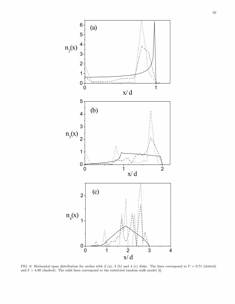
In Fig. 6 we show the distributions of the horizontal span of the arches and compare them with a theoretical model[4] based on a restricted random walk. The horizontal span is the projection onto the horizontal axis of the segmentthat joins the centers of the right-end disk and the left-end disk of an arch. We use the results obtained for archescomposed by two, three and four disks obtained for two different tapping amplitudes. At high packing fractions archextensions appear discretized. Since the system presents an ordered layered structure, the particles of any arch ofs disks form a string that connects layers (or stay in the same layer) so that the end-to-end horizontal projectionof the arch can only be an integer number of on-layer jumps plus an integer number of between-layers jumps; bothjumps have characteristic horizontal projections in the triangular lattice formed by the disks. We saw above thatalthough φ undergoes a decrease in its value for intermediate tapping amplitudes, it remains rather high. For thisreason, although horizontal span distributions are more homogeneous, we still find some characteristic peaks for highΓ. These results do not agree with the prediction of the random walk model where horizontal span distributions aresmooth. However, it must be taken into account that the restricted random walk model was proposed to representarches at the outlet of a hopper where particles cannot order but simply fit in the gap between walls.

V. ARCHES FROM STATIC CONFIGURATIONS

In this section we intend to show to what extent an attempt to identify arches from the static structure of a depositedsystem can yield realistic results. We test two criteria that select two of the contacting particles of each particle asthe supporting pair of the given grain: (a) random stabilizing pair, and (b) lowest stabilizing pair. We identify allpairs of contacting particles that may—according to their relative positions and the contact chord criterion—stabilizea given grain. For criterion (a) we then choose one of these pairs at random as the supporting pair. For criterion (b)

9

0 2 4 6 8 1010-6

10-5

10-4

10-3

10-2

10-1

100

n(s)/N

S

FIG. 5: Distribution of arch sizes for Γ = 4.99 (down triangles) and 0.71 (up triangles). The lines are fits to a second orderpolynomial. The data for s = 1 correspond to the number of disks that are not forming arches.

we choose the pair that has the lower center of mass. In principle, we expect that case (b) should provide a morereliable identification of supporting contacts since those contacting particles in lower positions may correspond to the“real” supports, whereas those in higher positions may correspond to contacts made by further deposition of otherparticles on top of the particle under consideration. We will see that this is not the case.

We have obtained the arch size distribution n(s) by applying the static criteria above to packings correspondingto Γ = 0.71 and 4.99. Fig. 7 shows clearly that, for disordered packings (Γ = 4.99), arches are identified muchbetter by the random criterion. The lowest supporting pair criterion detects less arches than the realistic dynamiccriterion. As we can see from the inset of Fig. 7, for very ordered packings (Γ = 0.71), both criteria fail. Criterion(a) overestimates whereas criterion (b) underestimates the number of arches beyond s = 2. A detailed analysis ofthe supporting contacts detected by the static criteria shows that criterion (a) tends to find many false mutuallystabilizing pair of particles in ordered packings, which leads to the identification of false arches. On the other hand,criterion (b) tends to detect too few of the real mutually stabilizing pairs of particles and for that reason the numberof arches detected are fewer than with the dynamic criterion.

VI. CONCLUSIONS AND FINAL REMARKS

We have presented a protocol to dynamically identify arches during the deposition of granular particles carriedout through realistic granular dynamics. We find that simple static criteria can correctly identify arches to somedegree for not very ordered packings. In particular, the criterion we call random stabilizing pair seems to be themost successful and could be used to identify arches in experimentally generated 2D granular beds [19, 20]. However,in ordered packings is very difficult to identify arches from static configurations. The reason for this is that in anordered packing the coordination number is rather high and then the number of plausible stabilizing pairs for a givenparticle is higher than that in disordered packings. Since choosing the correct pair is the essence of the criterion tosuccessfully identify stabilizing contacts, the more pairs we have to chose from, the more likely we make a mistake.

The packings generated by varying the tapping amplitude “quasistatically” present a low-density disordered regime(at high tapping amplitudes) and a high-density, ordered regime (at low tapping amplitudes). The support numberdecreases with increasing tapping amplitude except for of the very high tapping amplitudes. These observationsare in contrast with pseudo dynamic simulations [3] where 〈z〉support increases with Γ (except at the order–disordertransition). We believe that this is due to the fact that the pseudo dynamics is a good representation for fully inelasticdisks that roll without slip and that “fall down” at constant velocity—a situation that seems to be met by particles

10

FIG. 6: Horizontal span distribution for arches with 2 (a), 3 (b) and 4 (c) disks. The lines correspond to Γ = 0.71 (dotted)and Γ = 4.99 (dashed). The solid lines correspond to the restricted random walk model [4]

11

0 2 4 6 8 1010-610-510-410-310-210-1100

0 2 4 6 8 1010-6

10-5

10-4

10-3

10-2

10-1

100

n(s)

/ N

S

n(s)

/ N

S

FIG. 7: Distribution of arch sizes for Γ = 4.99 comparing the “real” distribution obtained from simulations (circles) with thedistributions obtained from the static structure using criteria (a) (up triangles) and (b) (down triangles). The inset shows thesame results for Γ = 0.71.

carried on a conveyor belt at low velocities [19]. The simulations in the present work are rather far from this regimesince particles can spring away from an impact and so explore a wider range of position in the box before finding alocally stable configuration.

The form of the arch size distributions is in agreement with pseudo dynamic simulations. This suggests that theform of n(s) is rather insensitive to the deposition algorithm. The calculated number of arches grows sharply as thedensity decreases when the tapping amplitude is increased. However, this tendency is not monotonic and above atransition zone the number of arches decreases whereas the density increases. This feature highlights the intuitiveconnection between arches and density fluctuations.

We have to point out here that the criterion we used to decide if two contacts may be the stabilizing contacts for agiven particle i (i.e. that the contact chord is below the cm of i), rules out the possibility that a particle be supportedfrom “above”. This situation does indeed arises occasionally due to static friction. Two contacting particles withy-coordinates slightly above particle i may sustain the particle due to high static friction forces. We have found thatthis situation indeed occurs in our simulations. Indeed, some instances can be appreciated in Fig. 2(b). A detailedanalysis of these types of arches that are also found in experiments (see for example Ref. [4]) will be presentedelsewhere.

Acknowledgments

The authors thanks Gary C. Barker and Angel Garcimartın for useful discussions. This work has been supportedby CONICET of Argentina and also partially by the project FI2005-03881 MEC (Spain), and PIUNA, University ofNavarra. RA thanks Friends of the University of Navarra for a grant.

[1] A. Mehta and G. C. Barker, Rep. Prog. Phys. 57, 383 (1994).[2] L. A. Pugnaloni, G. C. Barker and A. Mehta, Adv. Complex Systems 4, 289 (2001).[3] L. A. Pugnaloni, M. G. Valluzzi, and L. G. Valluzzi, Phys. Rev. E 73, 051302 (2006).[4] K. To, P-Y Lai, and H. K. Pak, Phys. Rev. Lett. 86, 71 (2001).[5] K. To, Phys. Rev. E 71, 060301(R) (2005).[6] I. Zuriguel, L. A. Pugnaloni, A. Garcimartın, and D. Maza, Phys. Rev. E 68, 030301(R) (2003).

12

[7] I. Zuriguel, A. Garcimartın, D. Maza, L. A. Pugnaloni, and J. M. Pastor, Phys. Rev. E 71, 051303 (2005).[8] J. Duran, J. Rajchenbach, and E. Clement, Phys. Rev. Lett. 70, 2431 (1993).[9] J. Duran, T. Mazozi, E. Clement, and J. Rajchenbach, Phys. Rev. E 50, 5138 (1994).

[10] L. A. Pugnaloni and G. C. Barker, Physica A 337, 428 (2004).[11] There is an excellent collection of articles and discussions in Ref. [15] and in Jamming and Rheology, edited by A. J. Liu

and S. Nagel (Taylor & Francis, London, 2001).[12] S. S. Manna and D. V. Khakhar, Phys. Rev. E 58, R6935 (1998).[13] J. Schafer, S. Dippel, and D. E. Wolf, J. Phys. I (France) 6, 5 (1996).[14] Physics of granular media - NATO ASI Series E350, edited by H. J. Hermann, J. P. Hovi, and S. Luding (Kluwer Academic

Publisher, Dordretch, 1998).[15] H. Hinrichsen and D. Wolf, The physics of granular media (Willey-VCH, Weinheim, 2004).[16] E. R. Nowak, J. B. Knight, M. Povinelli, H. M. Jaeger, and S. R. Nagel, Powder Technol. 94, 79 (1997).[17] P. Richard, M. Nicodemi, R. Delannay, P. Ribiere, D. Bideau, Nature Materials 4, 121 (2005).[18] J. Brujic, P. Wang, C. Song, D. L. Johnson, O. Sindt, and H. Makse, Phys. Rev. Lett 95, 128001 (2005).[19] R. Blumenfeld, S. F. Edwards, and R. C. Ball, J. Phys.: Condens. Matter 17, S2481 (2005).[20] I. C. Rankenburg and R. J. Zieve, Phys. Rev. E 63, 061303 (2001).