The massive star initial mass function of the Arches cluster
37
Astronomy & Astrophysics manuscript no. 0015 c ESO 2009 May 7, 2009 The massive star initial mass function of the Arches cluster ?,?? P. Espinoza 1,2 , F. J. Selman 3 , and J. Melnick 3 1 Steward Observatory, The University of Arizona, 933 North Cherry Avenue, Tucson AZ 85719, USA; e-mail: [email protected] 2 Previous Address: Departamento de Astronom´ ıa y Astrof´ ısica, Pontificia Universidad Cat´ olica de Chile, Santiago, Chile 3 European Southern Observatory, Alonso de C´ ordova 3107, Santiago, Chile e-mail: [fselman;jmelnick]@eso.org Received day month / Accepted day month ABSTRACT The massive Arches cluster near the Galactic center should be an ideal laboratory for investigating massive star formation under extreme conditions. But it comes at a high price: the cluster is hidden behind several tens of magnitudes of visual extinction. Severe crowding requires space or AO-assisted instruments to resolve the stellar populations, and even with the best instruments interpreting the data is far from direct. Several investigations using NICMOS and the most advanced AO imagers on the ground revealed an overall top-heavy IMF for the cluster, with a very flat IMF near the center. There are several effects, however, that could potentially bias these results, in particular the strong differential extinction and the problem of transforming the observations into a standard photometric system in the presence of strong reddening. We present new observations obtained with the NAOS-Conica (NACO) AO-imager on the VLT. The problem of photometric transformation is avoided by working in the natural photometric system of NACO, and we use a Bayesian approach to determine masses and reddenings from the broad-band IR colors. A global value of Γ= -1.1 ± 0.2 for the high-mass end ( M > 10M ) of the IMF is obtained, and we conclude that a power law of Salpeter slope cannot be discarded for the Arches cluster. The flattening of the IMF towards the center is confirmed, but is less severe than previously thought. We find Γ= -0.88 ± 0.20, which is incompatible with previous determinations. Within 0.4 pc we derive a total mass of ∼ 2.0(±0.6) × 10 4 M for the cluster and a central mass density ρ = 2(±0.4) × 10 5 M pc -3 that confirms Arches as the densest known young massive cluster in the Milky Way. Key words. Galaxy: open clusters and associations: individual: Arches - stars: luminosity function, mass function - stars: early-type - instrumentation: adaptive optics - ISM: dust, extinction 1. Introduction The young clusters near the Galactic center provide ideal labora- tories for testing theories of the formation and evolution of mas- sive stars and massive clusters (e.g. Figer et al. 1999), but they also pose formidable observational and theoretical challenges. Even at IR wavelengths the large amount of interstellar extinc- tion towards these clusters renders the already difficult interpre- tation of broad-band photometry of massive stars even more dif- ficult. And this difficulty is compounded by how the extinction, even at two micron, can vary by more than one magnitude from star to star. These clusters evolve in the strong tidal field of the Galactic center and, on the theoretical side, they may lose up to several 1000 M /Myr (Portegies Zwart et al. 2004). This implies that the timescale for dynamical evolution is comparable to the lifetimes of the most massive stars. The best studied of these clusters is the massive Arches clus- ter located about 25 pc in projection from the Galactic center. From NICMOS observations, Figer et al. (1999) find that the IMF of the Arches was significantly flatter than the Salpeter law (1955) and concluded that the Galactic center environment fa- Send offprint requests to: P. Espinoza, e-mail: [email protected] ? Based on observations obtained with the ESO/YEPUN telescope at Paranal Observatory. Program 73.D-0815. ?? Tables 2, 3, and 5 are only available in electronic form at the CDS via anonymous ftp to cdsarc.u-strasbg.fr (130.79.128.5) or via http://cdsweb.u-strasbg.fr/cgi-bin/qcat?J/A+A/ vors the formation of massive stars. Stolte et al. (2002; SGB02) using the adaptive optics (AO) camera on Gemini North, found a sharp flattening of the IMF towards the center of the cluster, with a global slope still flatter than the Salpeter value. SGB02 interpreted their observations as evidence of strong mass segre- gation, but did not reach a conclusion about whether this was a sign of dynamical evolution, or if it was inherited from the for- mation of the cluster. The advent of the NACO AO camera on the VLT provided Stolte et al. (2005; SBG05) with the oppor- tunity of probing the Arches cluster to deeper levels with better adaptive optics corrections. While they basically confirmed the strong flattening of the slope in the central regions, they also found evidence of a sharp turnover in the mass function around 6 - 7M that they interpreted as a low-mass truncation in the cluster IMF. A new investigation of Arches by Kim et al. (2006) using the AO camera of the Keck telescope confirmed a flatter slope and revealed the ∼ 6M feature as a local maximum in the cluster mass function. With appropiate parameters as input, this bump was also reproduced later by the coalescence-collapse model of Dib et al. (2007). However, no evidence of the low- mass truncation suggested by SBG05 was found in Kim’s work. All these investigations suffer from the problems of interpret- ing broad-band JHK photometry, the most insidious of which is the large extinction variations from star to star. This effect has been recognized by SGB02 and SBG05, but was taken into ac- count only in an approximate manner, i.e. by modeling the ex- tinction variations as a function of radius. We know from our experience with the 30 Doradus cluster that interpreting broad- arXiv:0903.2222v2 [astro-ph.GA] 7 May 2009
-
Upload
independent -
Category
Documents
-
view
0 -
download
0
Transcript of The massive star initial mass function of the Arches cluster
Astronomy & Astrophysics manuscript no. 0015 c© ESO 2009May 7, 2009
The massive star initial mass function of the Arches cluster?,??P. Espinoza1,2, F. J. Selman3, and J. Melnick3
1 Steward Observatory, The University of Arizona, 933 North Cherry Avenue, Tucson AZ 85719, USA;e-mail: [email protected]
2 Previous Address: Departamento de Astronomıa y Astrofısica, Pontificia Universidad Catolica de Chile, Santiago, Chile3 European Southern Observatory, Alonso de Cordova 3107, Santiago, Chile
e-mail: [fselman;jmelnick]@eso.org
Received day month / Accepted day month
ABSTRACT
The massive Arches cluster near the Galactic center should be an ideal laboratory for investigating massive star formation underextreme conditions. But it comes at a high price: the cluster is hidden behind several tens of magnitudes of visual extinction. Severecrowding requires space or AO-assisted instruments to resolve the stellar populations, and even with the best instruments interpretingthe data is far from direct. Several investigations using NICMOS and the most advanced AO imagers on the ground revealed an overalltop-heavy IMF for the cluster, with a very flat IMF near the center. There are several effects, however, that could potentially bias theseresults, in particular the strong differential extinction and the problem of transforming the observations into a standard photometricsystem in the presence of strong reddening. We present new observations obtained with the NAOS-Conica (NACO) AO-imager onthe VLT. The problem of photometric transformation is avoided by working in the natural photometric system of NACO, and weuse a Bayesian approach to determine masses and reddenings from the broad-band IR colors. A global value of Γ = −1.1 ± 0.2 forthe high-mass end (M > 10M�) of the IMF is obtained, and we conclude that a power law of Salpeter slope cannot be discardedfor the Arches cluster. The flattening of the IMF towards the center is confirmed, but is less severe than previously thought. We findΓ = −0.88 ± 0.20, which is incompatible with previous determinations. Within 0.4 pc we derive a total mass of ∼ 2.0(±0.6) × 104 M�for the cluster and a central mass density ρ = 2(±0.4) × 105 M� pc−3 that confirms Arches as the densest known young massivecluster in the Milky Way.
Key words. Galaxy: open clusters and associations: individual: Arches - stars: luminosity function, mass function - stars: early-type- instrumentation: adaptive optics - ISM: dust, extinction
1. Introduction
The young clusters near the Galactic center provide ideal labora-tories for testing theories of the formation and evolution of mas-sive stars and massive clusters (e.g. Figer et al. 1999), but theyalso pose formidable observational and theoretical challenges.Even at IR wavelengths the large amount of interstellar extinc-tion towards these clusters renders the already difficult interpre-tation of broad-band photometry of massive stars even more dif-ficult. And this difficulty is compounded by how the extinction,even at two micron, can vary by more than one magnitude fromstar to star. These clusters evolve in the strong tidal field of theGalactic center and, on the theoretical side, they may lose up toseveral 1000 M�/Myr (Portegies Zwart et al. 2004). This impliesthat the timescale for dynamical evolution is comparable to thelifetimes of the most massive stars.
The best studied of these clusters is the massive Arches clus-ter located about 25 pc in projection from the Galactic center.From NICMOS observations, Figer et al. (1999) find that theIMF of the Arches was significantly flatter than the Salpeter law(1955) and concluded that the Galactic center environment fa-
Send offprint requests to: P. Espinoza,e-mail: [email protected]? Based on observations obtained with the ESO/YEPUN telescope at
Paranal Observatory. Program 73.D-0815.?? Tables 2, 3, and 5 are only available in electronic form at theCDS via anonymous ftp to cdsarc.u-strasbg.fr (130.79.128.5) or viahttp://cdsweb.u-strasbg.fr/cgi-bin/qcat?J/A+A/
vors the formation of massive stars. Stolte et al. (2002; SGB02)using the adaptive optics (AO) camera on Gemini North, founda sharp flattening of the IMF towards the center of the cluster,with a global slope still flatter than the Salpeter value. SGB02interpreted their observations as evidence of strong mass segre-gation, but did not reach a conclusion about whether this was asign of dynamical evolution, or if it was inherited from the for-mation of the cluster. The advent of the NACO AO camera onthe VLT provided Stolte et al. (2005; SBG05) with the oppor-tunity of probing the Arches cluster to deeper levels with betteradaptive optics corrections. While they basically confirmed thestrong flattening of the slope in the central regions, they alsofound evidence of a sharp turnover in the mass function around6 − 7M� that they interpreted as a low-mass truncation in thecluster IMF. A new investigation of Arches by Kim et al. (2006)using the AO camera of the Keck telescope confirmed a flatterslope and revealed the ∼ 6M� feature as a local maximum inthe cluster mass function. With appropiate parameters as input,this bump was also reproduced later by the coalescence-collapsemodel of Dib et al. (2007). However, no evidence of the low-mass truncation suggested by SBG05 was found in Kim’s work.
All these investigations suffer from the problems of interpret-ing broad-band JHK photometry, the most insidious of which isthe large extinction variations from star to star. This effect hasbeen recognized by SGB02 and SBG05, but was taken into ac-count only in an approximate manner, i.e. by modeling the ex-tinction variations as a function of radius. We know from ourexperience with the 30 Doradus cluster that interpreting broad-
arX
iv:0
903.
2222
v2 [
astr
o-ph
.GA
] 7
May
200
9
2 Espinoza, Selman, and Melnick: The massive star IMF of the Arches cluster
band photometry in the presence of high and variable extinctionis a rather challenging problem (e.g. Selman et al. 1999). To be-gin with, it is not possible to transform the observations to astandard photometric system using the standard calibrators (e.g.Johnson), so one is compelled to work in the natural photomet-ric system of the instrument (Selman, 2004). This means thatthe stellar models and the extinction law must be transformedor calculated for the same photometric system. In the case of 30Doradus, the extinction varies by as much as 3-4 magnitudes inAV due to dust in the parental cloud of the cluster. For Arches,the observed variations of ∼ 2 magnitudes in AKS (nearly 20magnitudes in AV ) are mostly foreground to the cluster alongthe line of sight to the center of the Galaxy. These variations in-duce a magnitude-dependent incompleteness factor which maybe very large for the lowest mass bins in an otherwise completephotometric catalog. Thus, applying an average extinction cor-rection, as done by previous authors, can lead to serious errorsin the final mass determinations. These considerations promptedus to re-observe the Arches, in order to answer the question ofwhether a Salpeter law can be discarded for this cluster.
Taking advantage of the newly commissioned IR wavefrontsensor in the VLT AO camera NACO allowed us to reach a Strehlratio as high as 27% in the KS -band. We find a strong radial de-pendence of the IMF slope, going from Γ ∼ −0.88 for the central0.2 pc of the cluster, to Γ ∼ −1.28 for 0.2 < r < 0.4pc, with aglobal slope of Γ = −1.1±0.2. Thus, while we confirm the trendfound by previous investigations of a significant flattening of theIMF slope in the central region of the cluster, our values are sig-nificantly steeper than previous determinations at all radii. Thediscrepancy is particularly important in the center, where SBG05find a much flatter slope of Γ = −0.26±0.07 over a similar massrange. Our strong conclusions are: (1) even in the extreme envi-ronment of the Galactic center, the global IMF of the Arches isconsistent with that found in other starburst clusters such as 30Doradus in the LMC, and (2), the strong radial gradient in thepresent day mass distribution of the cluster stars provides a clearindication of significant mass segregation in this young cluster(see also discussions in Figer et al. 1999, SGB02).
The paper is organized as follows: Section 2 discusses theobservations, the data reduction procedures, and the photomet-ric calibrations. We also discuss in this Section the incomplete-ness corrections derived from Monte Carlo experiments. Section3 deals with the complicated procedure of deriving stellar physi-cal parameters in the presence of strong and variable reddening.The IMF is computed in Section 4, where we also present ad-ditional evidence of mass segregation in the cluster. Section 5presents a discussion of our results and a comparison with pre-vious investigations and Section 6 summarizes the conclusions.
2. Data Reduction
2.1. Observations
The observations reported here were performed in Service Modeusing the NAOS-CONICA (NACO) AO system on the VLT UT4(Lenzen et al. 2003; Rousset et al. 2003). The data were ob-tained using the imaging mode on September 6th, 2004, underclear weather conditions with subarcsecond seeing. To allowthe quantification of the high and variable IR background, thesame amount of observing time devoted to science frames wasspent on sky, a necessary procedure when the object of interest isseverely affected by crowding. No control fields were observedin order to estimate the effect of background and foreground con-tamination. But our photometry does not reach deep enough to
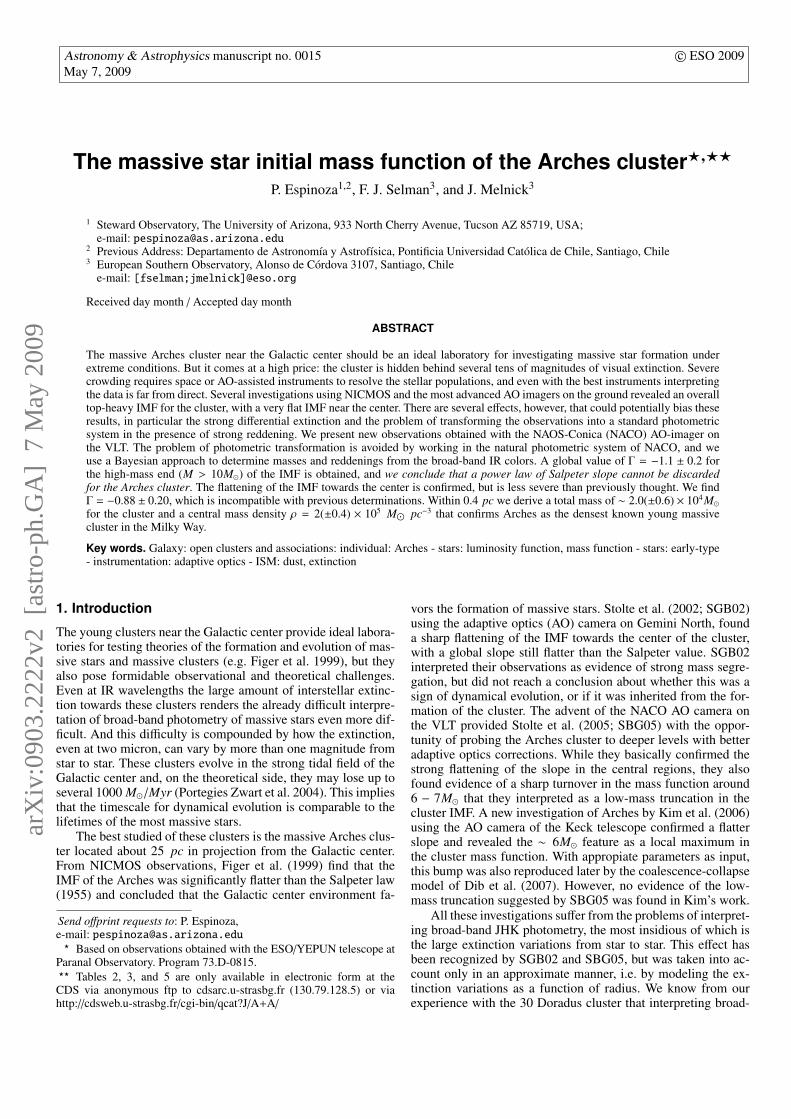
Fig. 1. Three-color composite image of the Arches cluster. Thefield of view is 28′′. North is up, and east is to the left.
sample the faint end of the IMF, and we did apply a color se-lection to the data. Accordingly, non-cluster members are notexpected to contribute significantly to our counts, especially atradii < 10′′.
The chosen reference star, located approximately at 10′′from the cluster center, had KS ∼10 mag. To optimize the AOperformance we used the N90C10 dichroic, i.e. 10% of the lightwas directed to CONICA while 90% went to the IR wavefrontsensor. An excellent AO correction in the KS -band resulted ina uniform PSF across the field with FWHM of 0.09′′. In J andH our frames exhibited larger PSF variations (as the isoplanaticangle is smaller for shorter wavelengths) with mean FWHM of0.17′′ and 0.11′′ respectively. We measured the Strehl ratio ofour observations with the SCISOFT’s STREHL 1 task, exceed-ing 27% in KS and reaching more modest values of 5% in J and11% in H. An observations log summarizing this information ispresented in Table 1, along with exposure times, V-band seeing,and airmasses.
2.2. Reduction
We used ECLIPSE 2 pipeline tools to reduce the data. Individualscience images were flat fielded, dark subtracted, and correctedwith a bad pixel mask. To obtain a reliable estimate of the IRbackground each pixel must see mostly sky signal during obser-vations; this was accomplished with dithered exposures from anearby field (with the AO loop open). All these were combinedinto a median average, i.e. a constant sky was assumed. To val-idate this procedure, we checked that during KS observationsthe variations of different sky planes compared with the medianaverage were within 5%. The combined sky plane was then sub-tracted from all reduced science frames.
The next step was to align the individual images before co-addition. In order to shift by a sub-pixel offset it was necessary toresample frames using an interpolation kernel. In ECLIPSE, thiskernel is defined in the image space and is based on the closest16 pixel values (Devillard, 2001).
1 http://www.eso.org/scisoft2 ESO C Library for an Image Processing Software Environment
(Devillard, 2001)
Espinoza, Selman, and Melnick: The massive star IMF of the Arches cluster 3
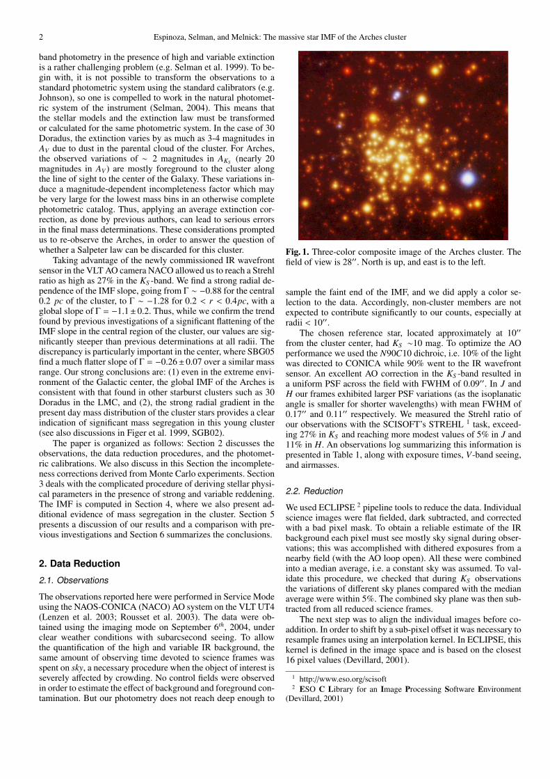
Table 1. Arches (α = 17h45m50s, δ = −28◦49′28′′, J2000) Observing Log
UT Filter N a tb [s] Airmass Seeingc (”) FWHM (”) Strehl ratio01:24:15 - 01:54:20 J 5 200 s 1.13 - 1.22 0.82 0.17 0.0500:52:15 - 01:16:46 H 8 100 s 1.07 - 1.11 1.1 0.11 0.1100:14:40 - 00:47:02 KS 12 60 s 1.02 - 1.06 0.95 0.09 0.27
a Number of exposures.b Integration time of each exposure.c Average value of the DIMM Seeing during observations (taken in the optical V band). It is stressed that in Paranal the DIMM values can be
significantly larger than the image quality measured at the telescope.
Finally, aligned science images were co-added by means ofa simple linear average stack. In this way all the input signalis kept on the final combination, allowing a better faint objectdetection. The process is the same for the J, H and KS -bandframes. The final products combined into a single three colorcomposite image are presented in Fig. 1.
2.3. Photometry
We used the DAOPHOT/IRAF3 package (Stetson, 1987; Davis1994) to do photometry in the severely crowded environ-ment of the Arches cluster. Point sources were identified usingDAOFIND, with a detection threshold set to 3σ above the lo-cal background level. Then aperture photometry was performedon the detected stars computing local sky values for each one.This is important because these values change remarkably fromone star to another; especially at the cluster center, where seeinghaloes dominate background variations (especially in J and H).
The PSF was computed interactively using several bright,isolated stars located away from the frame edges, but other-wise sampling the field as uniformly as possible. We selected9 bright stars in the J, KS frames, and 8 stars in H. The analyt-ical component of the PSF was set to auto to optimize the fit.This gives a Penny1 function for both H and KS and Penny2function for J. Both analytical functions are elliptical arbitrarilyaligned Gaussian cores with Lorentzian wings, with the differ-ence that the wings are also aligned arbitrarily for the Penny2fitting function. For the empirical component, a linearly vari-able model is required for J and H, while, as mentioned above,the KS PSF was found to be constant across the field. Withthese specifications we obtained the lowest residuals in the sub-traction of the PSF stars and their neighbors. Once the PSFwas determined, profile-fitting photometry was performed withALLSTAR. Finally, to obtain total instrumental magnitudes forevery star, we added a constant aperture correction. This correc-tion was obtained from the aperture photometry and later curveof growth analysis of bright isolated stars in the NACO field.
The photometry can now be divided into two catalogs: onefor stars detected in HKS only, and another for stars detectedin the three bands (JHKS ). These catalogs are obtained withDAOMATCH and DAOMASTER (Stetson 1990), which give afinal list of stars matched between frames with a 1-pixel toler-ance. Tables 2 and 3, published electronically, present the pho-tometry of 427 HKS and 126 JHKS stars in the innermost 10′′ ofthe cluster. Table 3 is considerably shorter due to the increasing
3 IRAF is distributed by the National Optical AstronomyObservatories, which is operated by the Association of Universities forResearch in Astronomy, Inc. (AURA) under cooperative agreementwith the NSF
extinction towards bluer wavelengths. Fig. 2 shows the photo-metric errors as a function of magnitude as given by DAOPHOT.
2.3.1. The NACO Natural Photometric System
As noted by Selman (2004), to avoid systematic effectsin transforming broad-band photometry of reddened starsinto a standard photometric system (e.g. Johnson, 2MASS,HST/NICMOS), one must work in the natural system defined bythe instrument. This occurs because extinction distorts the spec-tral energy distributions (SED) in ways that are not matched bystandard stars unless, of course, the standard stars span the samerange in spectral types and extinction as the program stars. Sincethe SEDs of early-type stars and the extinction law are flatter inthe IR, a priory one would expect this problem to be less severefor broad-band JHKS photometry. Unfortunately this is not thecase of the highly reddened stars of the Arches cluster.
If one observes with passbands that differ from that of thestandard system, big color terms can be derived from unred-dened standards. The danger of this procedure is to assume, viaan extrapolation, that these color terms can be applied to stan-dardize reddened program stars. On the basis of synthetic pho-tometry we have reached the conclusion that, at the extinction ofthe Arches cluster, the color terms differ significantly from theones obtained with unreddened standards. Therefore, the extrap-olation leads to a systematic shift of the zero points in J, H, andKS (Fig. 2.7 of Selman 2004 illustrates the effect in the opticalregime).
But to circumvent this problem by working in the naturalphotometric system have a serious drawback: it becomes diffi-cult to compare our observations with previous investigations.Fortunately, Figer et al. (2002) published their photometry cat-alog for bright stars in the Arches, so using these stars as localstandards we can transform our observations to their photometricsystem and thus perform a detailed comparison for 150 stars incommon (as shown in Fig.3). The rms scatter, 0.08 mag. in mag-nitude and 0.09 mag. in color, is consistent with the photometricerrors, but there is a clear trend (specially in color) of the dif-ferences becoming systematically negative for fainter stars (seeFigure 3). This underlies the problem of transforming betweenphotometric systems discussed above, and reaffirms our conclu-sion about the importance of working in the natural photometricsystem of NACO.
2.3.2. Isochrone Conversion
To proceed as described above, it is necessary to transform thestellar models (that will be compared with our observations) intothe NACO system as well. In the work of Lejeune & Schaerer(2001), Geneva isochrones are placed in the observational planeof the Johnson system (Bessell & Brett, 1988). Thus we need
4 Espinoza, Selman, and Melnick: The massive star IMF of the Arches cluster
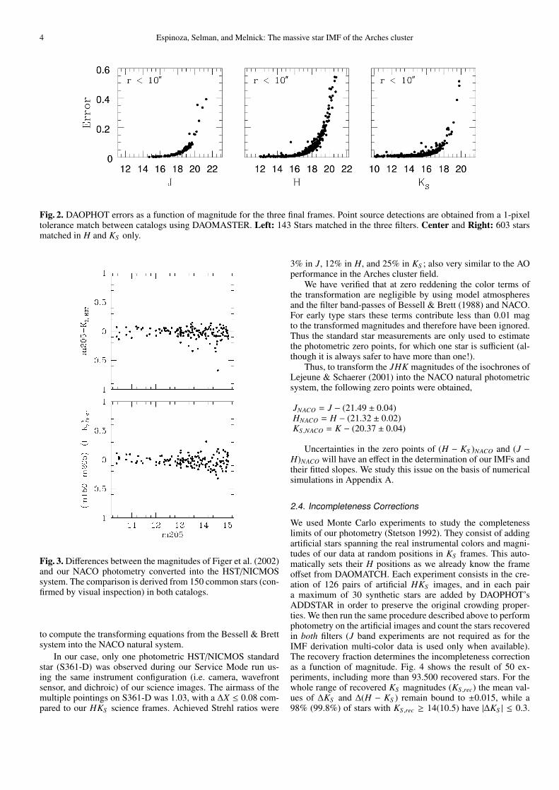
Fig. 2. DAOPHOT errors as a function of magnitude for the three final frames. Point source detections are obtained from a 1-pixeltolerance match between catalogs using DAOMASTER. Left: 143 Stars matched in the three filters. Center and Right: 603 starsmatched in H and KS only.
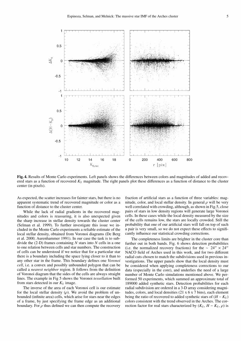
Fig. 3. Differences between the magnitudes of Figer et al. (2002)and our NACO photometry converted into the HST/NICMOSsystem. The comparison is derived from 150 common stars (con-firmed by visual inspection) in both catalogs.
to compute the transforming equations from the Bessell & Brettsystem into the NACO natural system.
In our case, only one photometric HST/NICMOS standardstar (S361-D) was observed during our Service Mode run us-ing the same instrument configuration (i.e. camera, wavefrontsensor, and dichroic) of our science images. The airmass of themultiple pointings on S361-D was 1.03, with a ∆X ≤ 0.08 com-pared to our HKS science frames. Achieved Strehl ratios were
3% in J, 12% in H, and 25% in KS ; also very similar to the AOperformance in the Arches cluster field.
We have verified that at zero reddening the color terms ofthe transformation are negligible by using model atmospheresand the filter band-passes of Bessell & Brett (1988) and NACO.For early type stars these terms contribute less than 0.01 magto the transformed magnitudes and therefore have been ignored.Thus the standard star measurements are only used to estimatethe photometric zero points, for which one star is sufficient (al-though it is always safer to have more than one!).
Thus, to transform the JHK magnitudes of the isochrones ofLejeune & Schaerer (2001) into the NACO natural photometricsystem, the following zero points were obtained,
JNACO = J − (21.49 ± 0.04)HNACO = H − (21.32 ± 0.02)KS ,NACO = K − (20.37 ± 0.04)
Uncertainties in the zero points of (H − KS )NACO and (J −H)NACO will have an effect in the determination of our IMFs andtheir fitted slopes. We study this issue on the basis of numericalsimulations in Appendix A.
2.4. Incompleteness Corrections
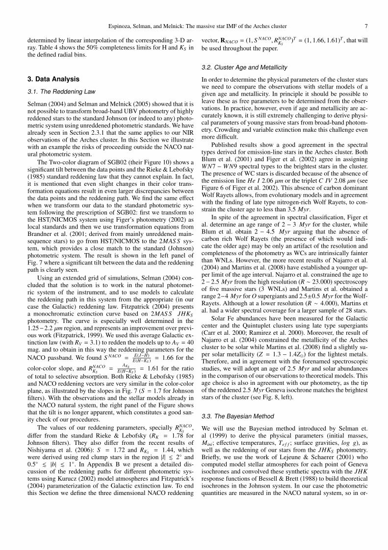
We used Monte Carlo experiments to study the completenesslimits of our photometry (Stetson 1992). They consist of addingartificial stars spanning the real instrumental colors and magni-tudes of our data at random positions in KS frames. This auto-matically sets their H positions as we already know the frameoffset from DAOMATCH. Each experiment consists in the cre-ation of 126 pairs of artificial HKS images, and in each paira maximum of 30 synthetic stars are added by DAOPHOT’sADDSTAR in order to preserve the original crowding proper-ties. We then run the same procedure described above to performphotometry on the artificial images and count the stars recoveredin both filters (J band experiments are not required as for theIMF derivation multi-color data is used only when available).The recovery fraction determines the incompleteness correctionas a function of magnitude. Fig. 4 shows the result of 50 ex-periments, including more than 93.500 recovered stars. For thewhole range of recovered KS magnitudes (KS ,rec) the mean val-ues of ∆KS and ∆(H − KS ) remain bound to ±0.015, while a98% (99.8%) of stars with KS ,rec ≥ 14(10.5) have |∆KS | ≤ 0.3.
Espinoza, Selman, and Melnick: The massive star IMF of the Arches cluster 5
Fig. 4. Results of Monte Carlo experiments. Left panels shows the differences between colors and magnitudes of added and recov-ered stars as a function of recovered KS magnitude. The right panels plot these differences as a function of distance to the clustercenter (in pixels).
As expected, the scatter increases for fainter stars, but there is noapparent systematic trend of recovered magnitude or color as afunction of distance to the cluster center.
While the lack of radial gradients in the recovered mag-nitudes and colors is reassuring, it is also unexpected giventhe sharp increase in stellar density towards the cluster center(Selman et al. 1999). To further investigate this issue we in-cluded in the Monte Carlo experiments a reliable estimate of thelocal stellar density, obtained from Voronoi diagrams (De Berget al. 2000; Aurenhammer 1991). In our case the task is to sub-divide the (2-D) frames containing N stars into N cells in a oneto one relation between cells and star numbers. The constructionof cells can be understood if we notice that for a particular starthere is a boundary including the space lying closer to it than toany other star in the frame. This boundary defines one Voronoicell, i.e. a convex and possibly unbounded polygon that can becalled a nearest neighbor region. It follows from the definitionof Voronoi diagram that the sides of the cells are always straightlines. The example in Fig 5 shows the Voronoi tessellation builtfrom stars detected in our KS image.
The inverse of the area of each Voronoi cell is our estimatefor the local stellar density (ρ). We avoid the problem of un-bounded (infinite area) cells, which arise for stars near the edgesof a frame, by just specifying the frame edge as an additionalboundary. For ρ thus defined we can then compute the recovery
fraction of artificial stars as a function of three variables: mag-nitude, color, and local stellar density. In general ρ will be verywell correlated with crowding, although, as shown in Fig.5, closepairs of stars in low density regions will generate large Voronoicells. In these cases while the local density measured by the sizeof the cells remains low, the stars are locally crowded. Still theprobability that one of our artificial stars will fall on top of sucha pair is very small, so we do not expect these effects to signifi-cantly influence our statistical crowding corrections.
The completeness limits are brighter in the cluster core thanfurther out in both bands. Fig. 6 shows detection probabilities(i.e. the normalized recovery fractions) for the ∼ 24′′ × 24′′NACO field of Arches used in this work, and for two differentradial cuts chosen to match the subdivisions used in previous in-vestigations. The upper panels show that the local density mustbe considered when applying completeness corrections to ourdata (especially in the core), and underlies the need of a largenumber of Monte Carlo simulations mentioned above. We per-formed 50 experiments, which summed an approximate total of189000 added synthetic stars. Detection probabilities for eachradial subdivision are ordered in a 3-D array considering magni-tudes, colors, and local densities (21 x 6 x 7 bins), each elementbeing the ratio of recovered to added synthetic stars of (H − KS )colors consistent with the trend observed in the Arches. The cor-rection factor for real stars characterized by (KS , H − KS , ρ) is

6 Espinoza, Selman, and Melnick: The massive star IMF of the Arches cluster
Fig. 5. Voronoi diagram built from stars brighter than KS = 17 in the NACO field of approximately 24′′ × 24′′. Adopting a distanceto the Galactic center of 8 kpc , circles represents projected distances of 0.2 and 0.4 pc from the cluster center. Note the smallerarea of Voronoi cells at the cluster core, indicating a higher local stellar density (crowding).
Fig. 6. Detection probabilities computed from Monte Carlo experiments in different radial bins. The solid lines represent the recoveryfraction as a function of magnitude only. In the upper panels the dotted lines represent probabilities marginalized by local stellardensity ρ [star/arcsec2]. In the bottom panels dotted lines show probabilities marginalized by (H − KS ) color.
Espinoza, Selman, and Melnick: The massive star IMF of the Arches cluster 7
determined by linear interpolation of the corresponding 3-D ar-ray. Table 4 shows the 50% completeness limits for H and KS inthe defined radial bins.
3. Data Analysis
3.1. The Reddening Law
Selman (2004) and Selman and Melnick (2005) showed that it isnot possible to transform broad-band UBV photometry of highlyreddened stars to the standard Johnson (or indeed to any) photo-metric system using unreddened photometric standards. We havealready seen in Section 2.3.1 that the same applies to our NIRobservations of the Arches cluster. In this Section we illustratewith an example the risks of proceeding outside the NACO nat-ural photometric system.
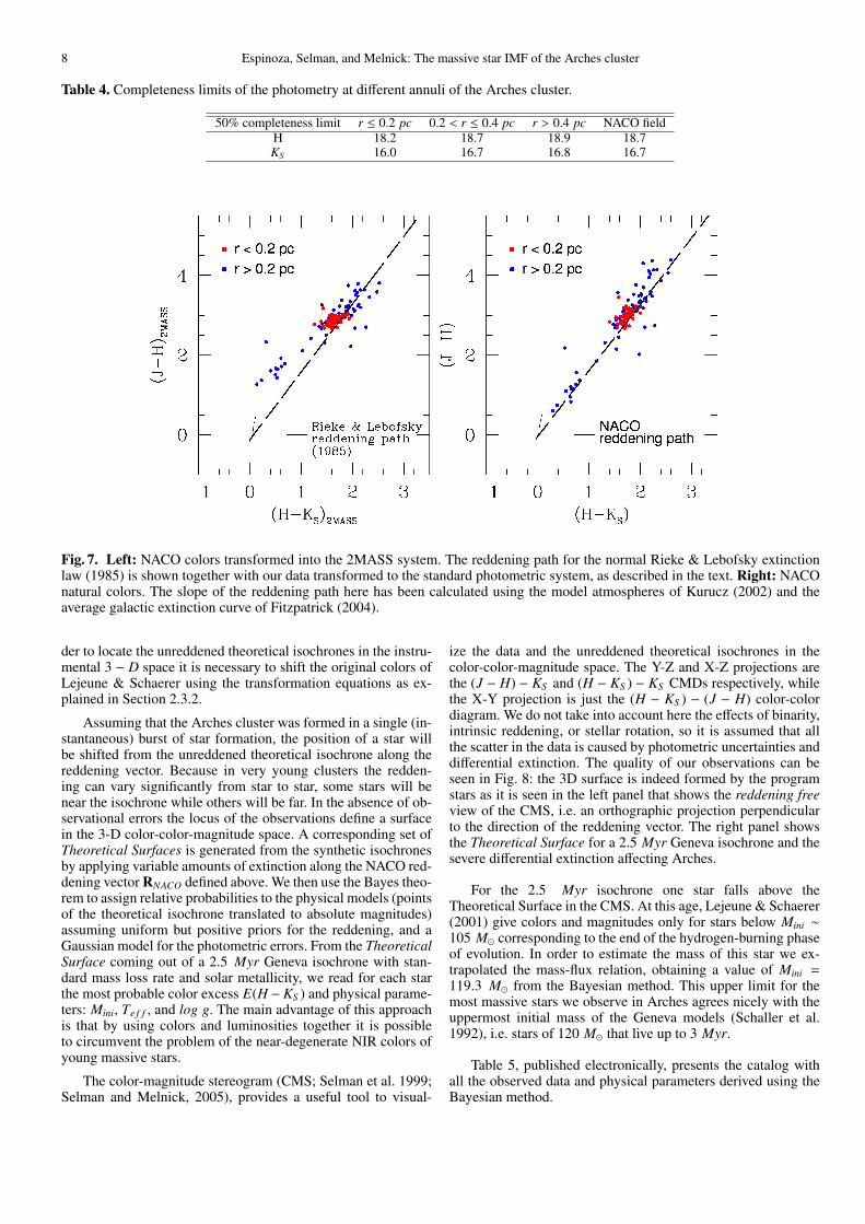
The Two-color diagram of SGB02 (their Figure 10) shows asignificant tilt between the data points and the Rieke & Lebofsky(1985) standard reddening law that they cannot explain. In fact,it is mentioned that even slight changes in their color trans-formation equations result in even larger discrepancies betweenthe data points and the reddening path. We find the same effectwhen we transform our data to the standard photometric sys-tem following the prescription of SGB02: first we transform tothe HST/NICMOS system using Figer’s photometry (2002) aslocal standards and then we use transformation equations fromBrandner et al. (2001; derived from mainly unreddened main-sequence stars) to go from HST/NICMOS to the 2MAS S sys-tem, which provides a close match to the standard (Johnson)photometric system. The result is shown in the left panel ofFig. 7 where a significant tilt between the data and the reddeningpath is clearly seen.
Using an extended grid of simulations, Selman (2004) con-cluded that the solution is to work in the natural photomet-ric system of the instrument, and to use models to calculatethe reddening path in this system from the appropriate (in ourcase the Galactic) reddening law. Fitzpatrick (2004) presentsa monochromatic extinction curve based on 2MAS S JHKSphotometry. The curve is especially well determined in the1.25−2.2 µm region, and represents an improvement over previ-ous work (Fitzpatrick, 1999). We used this average Galactic ex-tinction law (with RV = 3.1) to redden the models up to AV = 40mag. and to obtain in this way the reddening parameters for theNACO passband. We found S NACO =
E(J−H)E(H−KS ) = 1.66 for the
color-color slope, and RNACOKS
=AKS
E(H−KS ) = 1.61 for the ratioof total to selective absorption. Both Rieke & Lebofsky (1985)and NACO reddening vectors are very similar in the color-colorplane, as illustrated by the slopes in Fig. 7 (S = 1.7 for Johnsonfilters). With the observations and the stellar models already inthe NACO natural system, the right panel of the Figure showsthat the tilt is no longer apparent, which constitutes a good san-ity check of our procedures.
The values of our reddening parameters, specially RNACOKS
,differ from the standard Rieke & Lebofsky (RK = 1.78 forJohnson filters). They also differ from the recent results ofNishiyama et al. (2006): S = 1.72 and RKS = 1.44, whichwere derived using red clump stars in the region |l| . 2◦ and0.5◦ . |b| . 1◦. In Appendix B we present a detailed dis-cussion of the reddening paths for different photometric sys-tems using Kurucz (2002) model atmospheres and Fitzpatrick’s(2004) parameterization of the Galactic extinction law. To endthis Section we define the three dimensional NACO reddening
vector, RNACO = (1, S NACO,RNACOKS
)T = (1, 1.66, 1.61)T , that willbe used throughout the paper.
3.2. Cluster Age and Metallicity
In order to determine the physical parameters of the cluster starswe need to compare the observations with stellar models of agiven age and metallicity. In principle it should be possible toleave these as free parameters to be determined from the obser-vations. In practice, however, even if age and metallicity are ac-curately known, it is still extremely challenging to derive physi-cal parameters of young massive stars from broad-band photom-etry. Crowding and variable extinction make this challenge evenmore difficult.
Published results show a good agreement in the spectraltypes derived for emission-line stars in the Arches cluster. BothBlum et al. (2001) and Figer et al. (2002) agree in assigningWN7 − WN9 spectral types to the brightest stars in the cluster.The presence of WC stars is discarded because of the absence ofthe emission line He I 2.06 µm or the triplet C IV 2.08 µm (seeFigure 6 of Figer et al. 2002). This absence of carbon dominantWolf Rayets allows, from evolutionary models and in agreementwith the finding of late type nitrogen-rich Wolf Rayets, to con-strain the cluster age to less than 3.5 Myr.
In spite of the agreement in spectral classification, Figer etal. determine an age range of 2 − 3 Myr for the cluster, whileBlum et al. obtain 2 − 4.5 Myr arguing that the absence ofcarbon rich Wolf Rayets (the presence of which would indi-cate the older age) may be only an artifact of the resolution andcompleteness of the photometry as WCs are intrinsically fainterthan WNLs. However, the more recent results of Najarro et al.(2004) and Martins et al. (2008) have established a younger up-per limit of the age interval. Najarro et al. constrained the age to2− 2.5 Myr from the high resolution (R ∼ 23.000) spectroscopyof five massive stars (3 WNLs) and Martins et al. obtained arange 2−4 Myr for O supergiants and 2.5±0.5 Myr for the Wolf-Rayets. Although at a lower resolution (R ∼ 4.000), Martins etal. had a wider spectral coverage for a larger sample of 28 stars.
Solar Fe abundances have been measured for the Galacticcenter and the Quintuplet clusters using late type supergiants(Carr et al. 2000; Ramirez et al. 2000). Moreover, the result ofNajarro et al. (2004) constrained the metallicity of the Archescluster to be solar while Martins et al. (2008) find a slightly su-per solar metallicity (Z = 1.3 − 1.4Z�) for the lightest metals.Therefore, and in agreement with the forenamed spectroscopicstudies, we will adopt an age of 2.5 Myr and solar abundancesin the comparison of our observations to theoretical models. Thisage choice is also in agreement with our photometry, as the tipof the reddened 2.5 Myr Geneva isochrone matches the brighteststars of the cluster (see Fig. 8, left).
3.3. The Bayesian Method
We will use the Bayesian method introduced by Selman et.al (1999) to derive the physical parameters (initial masses,Mini; effective temperatures, Te f f ; surface gravities, log g), aswell as the reddening of our stars from the JHKS photometry.Briefly, we use the work of Lejeune & Schaerer (2001) whocomputed model stellar atmospheres for each point of Genevaisochrones and convolved these synthetic spectra with the JHKresponse functions of Bessell & Brett (1988) to build theoreticalisochrones in the Johnson system. In our case the photometricquantities are measured in the NACO natural system, so in or-
8 Espinoza, Selman, and Melnick: The massive star IMF of the Arches cluster
Table 4. Completeness limits of the photometry at different annuli of the Arches cluster.
50% completeness limit r ≤ 0.2 pc 0.2 < r ≤ 0.4 pc r > 0.4 pc NACO fieldH 18.2 18.7 18.9 18.7KS 16.0 16.7 16.8 16.7
Fig. 7. Left: NACO colors transformed into the 2MASS system. The reddening path for the normal Rieke & Lebofsky extinctionlaw (1985) is shown together with our data transformed to the standard photometric system, as described in the text. Right: NACOnatural colors. The slope of the reddening path here has been calculated using the model atmospheres of Kurucz (2002) and theaverage galactic extinction curve of Fitzpatrick (2004).
der to locate the unreddened theoretical isochrones in the instru-mental 3 − D space it is necessary to shift the original colors ofLejeune & Schaerer using the transformation equations as ex-plained in Section 2.3.2.
Assuming that the Arches cluster was formed in a single (in-stantaneous) burst of star formation, the position of a star willbe shifted from the unreddened theoretical isochrone along thereddening vector. Because in very young clusters the redden-ing can vary significantly from star to star, some stars will benear the isochrone while others will be far. In the absence of ob-servational errors the locus of the observations define a surfacein the 3-D color-color-magnitude space. A corresponding set ofTheoretical Surfaces is generated from the synthetic isochronesby applying variable amounts of extinction along the NACO red-dening vector RNACO defined above. We then use the Bayes theo-rem to assign relative probabilities to the physical models (pointsof the theoretical isochrone translated to absolute magnitudes)assuming uniform but positive priors for the reddening, and aGaussian model for the photometric errors. From the TheoreticalSurface coming out of a 2.5 Myr Geneva isochrone with stan-dard mass loss rate and solar metallicity, we read for each starthe most probable color excess E(H −KS ) and physical parame-ters: Mini, Te f f , and log g. The main advantage of this approachis that by using colors and luminosities together it is possibleto circumvent the problem of the near-degenerate NIR colors ofyoung massive stars.
The color-magnitude stereogram (CMS; Selman et al. 1999;Selman and Melnick, 2005), provides a useful tool to visual-
ize the data and the unreddened theoretical isochrones in thecolor-color-magnitude space. The Y-Z and X-Z projections arethe (J − H) − KS and (H − KS ) − KS CMDs respectively, whilethe X-Y projection is just the (H − KS ) − (J − H) color-colordiagram. We do not take into account here the effects of binarity,intrinsic reddening, or stellar rotation, so it is assumed that allthe scatter in the data is caused by photometric uncertainties anddifferential extinction. The quality of our observations can beseen in Fig. 8: the 3D surface is indeed formed by the programstars as it is seen in the left panel that shows the reddening freeview of the CMS, i.e. an orthographic projection perpendicularto the direction of the reddening vector. The right panel showsthe Theoretical Surface for a 2.5 Myr Geneva isochrone and thesevere differential extinction affecting Arches.
For the 2.5 Myr isochrone one star falls above theTheoretical Surface in the CMS. At this age, Lejeune & Schaerer(2001) give colors and magnitudes only for stars below Mini ∼
105 M� corresponding to the end of the hydrogen-burning phaseof evolution. In order to estimate the mass of this star we ex-trapolated the mass-flux relation, obtaining a value of Mini =119.3 M� from the Bayesian method. This upper limit for themost massive stars we observe in Arches agrees nicely with theuppermost initial mass of the Geneva models (Schaller et al.1992), i.e. stars of 120 M� that live up to 3 Myr.
Table 5, published electronically, presents the catalog withall the observed data and physical parameters derived using theBayesian method.

Espinoza, Selman, and Melnick: The massive star IMF of the Arches cluster 9
Fig. 8. Left: Color-magnitude Stereogram. This is the projection viewed from the reddening vector direction, i.e. the Reddeningfree view. Right: Theoretical Surface for a 2.5 Myr Geneva isochrone with solar metallicity (in red). The surface does indeed gothrough the cloud of stars: some stars are below, some above the Theoretical Surface.
3.4. Stellar Physical Parameters and Reddening from HKSPhotometry only
Our Bayesian method can only be applied to the brightest starsin the cluster for which we have complete JHKS information.Therefore, to deal with the bulk of the stars (for which we onlyhave HKS data) we have investigated an additional procedure.It consists in “sliding” each star along the reddening vector inthe color-magnitude diagram until the theoretical isochrone isreached. The intersection point determines the intrinsic colorand luminosity for each star. This method to correct for indi-vidual reddening makes use of the ratio of total to selective ab-sorption (RNACO
KS= 1.61) obtained from the average Galactic ex-
tinction curve in Section 3.1. As for the comparison betweenthe two approaches, it is clear that none can discriminate ex-tinction from the effects of e.g., rotation, binarity, or intrinsicNIR excess. However, it is important to note that one drawbackof the CMD Sliding is not dealing with the photometric uncer-tainties: the final dereddened location for the program stars isthe isochrone itself. The Bayesian approach, on the other hand,finds the most likely point in the Theoretical Surface for eachstar and then reads its reddening value. This difference led to, insome cases, underestimate the E(H−KS ) derived from the CMD
Sliding with respect to their Bayesian counterparts. Still, there isan excellent correspondence between the two, as shown in Fig. 9
3.5. Cluster Membership
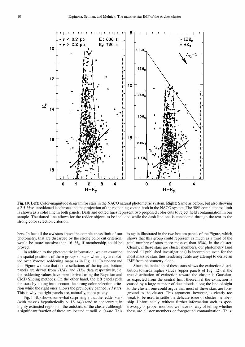
The color-magnitude (CMD) diagram for our data in the natu-ral NACO photometric system is displayed in Fig. 10. Shownin the right hand plot are our photometric completeness limit,the 2.5 Myr isochrone, and the reddening path for the mostluminous stars in the isochrone. Following previous investiga-tions (e.g. SGB02; SBG05), we introduce a strong color cutto improve the rejection of putative non cluster members. Thisis indicated in Fig. 10 by the dashed lines that widen to-wards fainter magnitudes, where the photometric uncertaintiesincrease. Approximately 105 stars would be discarded from ourcatalogs by this criterion.
Fig. 10 exposes a potentially serious problem of complete-ness. Due to the large and variable extinction to the cluster, someof the stars that we consider as field contamination may be verymassive cluster members. While the bluer ones are likely to beforeground stars, the reddest can be foreground or backgroundobjects, but also heavily obscured main sequence cluster mem-
10 Espinoza, Selman, and Melnick: The massive star IMF of the Arches cluster
Fig. 10. Left: Color-magnitude diagram for stars in the NACO natural photometric system. Right: Same as before, but also showinga 2.5 Myr unreddened isochrone and the projection of the reddening vector, both in the NACO system. The 50% completeness limitis shown as a solid line in both panels. Dash and dotted lines represent two proposed color cuts to reject field contamination in oursample. The dotted line allows for the redder objects to be included while the dash line one is considered through the text as thestrong color selection criterion.
bers. In fact all the red stars above the completeness limit of ourphotometry, that are discarded by the strong color cut criterion,would be more massive than 16 M� if membership could beproved.
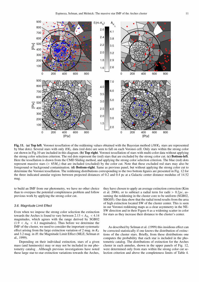
In addition to the photometric information, we can examinethe spatial positions of these groups of stars when they are plot-ted over Voronoi reddening maps as in Fig. 11. To understandthis Figure we note that the tessellations of the top and bottompanels are drawn from JHKS and HKS data respectively, i.e.the reddening values have been derived using the Bayesian andCMD Sliding methods. On the other hand, the left panels pickthe stars by taking into account the strong color selection crite-rion while the right ones allows the previously banned red stars.This is why the right panels are, naturally, more patchy.
Fig. 11 (b) shows somewhat surprisingly that the redder stars(with masses hypothetically > 16 M�) tend to concentrate inhighly extincted regions in the outskirts of the cluster, althougha significant fraction of these are located at radii < 0.4pc. This
is again illustrated in the two bottom panels of the Figure, whichshows that this group could represent as much as a third of thetotal number of stars more massive than 65M� in the cluster.Clearly, if these stars are cluster members, our photometry (andindeed all published investigations) is incomplete even for themost massive stars thus rendering futile any attempt to derive anIMF from photometry alone.
Since the inclusion of these stars skews the extinction distri-bution towards higher values (upper panels of Fig. 12), if thetrue distribution of extinction toward the cluster is Gaussian,as expected from the central limit theorem if the extinction iscaused by a large number of dust clouds along the line of sightto the cluster, one could argue that most of these stars are fore-ground to the cluster. This argument, however, is clearly tooweak to be used to settle the delicate issue of cluster member-ship. Unfortunately, without further information such as spec-troscopy or proper motions, we have no way of telling whetherthese are cluster members or foreground contamination. Thus,
Espinoza, Selman, and Melnick: The massive star IMF of the Arches cluster 11
Fig. 11. (a) Top left. Voronoi tessellation of the reddening values obtained with the Bayesian method (JHKS stars are representedby blue dots). Several stars with only HKS data (red dots) are seen to fall on each Voronoi cell. Only stars within the strong colorcut shown in Fig.10 are included in this diagram. (b) Top right. Voronoi tessellation of stars with multi-color data without applyingthe strong color selection criterion. The red dots represent the (red) stars that are excluded by the strong color cut. (c) Bottom-left.Here the tessellation is drawn from the CMD Sliding method, and applying the strong color selection criterion. The blue (red) dotsrepresent massive stars (> 65M�) that are included (excluded) by the color cut. Note that these excluded red stars may also beforeground or background contamination. (d) Bottom-right. Same as previous panel, but without applying the strong color cut todetermine the Voronoi tessellation. The reddening distributions corresponding to the two bottom figures are presented in Fig. 12 forthe three indicated annular regions between projected distances of 0.2 and 0.4 pc at a Galactic center distance modulus of 14.52mag.
to build an IMF from our photometry, we have no other choicethan to overpass the potential completeness problem and followprevious work by applying the strong color cut.
3.6. Magnitude Limit Effect
Even when we impose the strong color selection the extinctiontowards the Arches is found to vary between 2.13 < AKS < 4.14magnitudes, which agrees with the range derived by SGB02(1.9 < AK < 4.1 magnitudes). Thus before we determine theIMF of the cluster, we need to consider the important systematiceffect arising from the large extinction variation of 2 mag. in KSand 3.2 mag. in H: the Magnitude Limit Effect (MLE; Selman etal., 1999).
Depending on their individual extinction, stars of a givenmass (and luminosity) may or may not be included in our pho-tometry catalog . Although previous investigations have notedthese large star-to-star extinction variations towards the Arches,
they have chosen to apply an average extinction correction (Kimet al. 2006), or to subtract a radial term for radii > 0.2pc, as-suming the reddening in the cluster core to be uniform (SGB02,SBG05). Our data show that the radial trend results from the areaof high extinction located SW of the cluster center. This is seenin our Voronoi reddening maps as a clear asymmetry in the NE-SW direction and in their Figure 6 as a widening scatter in colorfor stars as they increase their distance to the cluster’s center.
As described by Selman et al. (1999) this insidious effect canbe corrected statistically if one knows the distribution of extinc-tions of the cluster stars. Briefly, from these distributions onecomputes the probability that each star is included in the pho-tometric catalog. The distributions of extinction for the Archescluster in each annulus, shown in the upper panels of Fig. 12,were determined only from stars within the strong color cut se-lection criterion and above the completeness limits of Table 4.
12 Espinoza, Selman, and Melnick: The massive star IMF of the Arches cluster
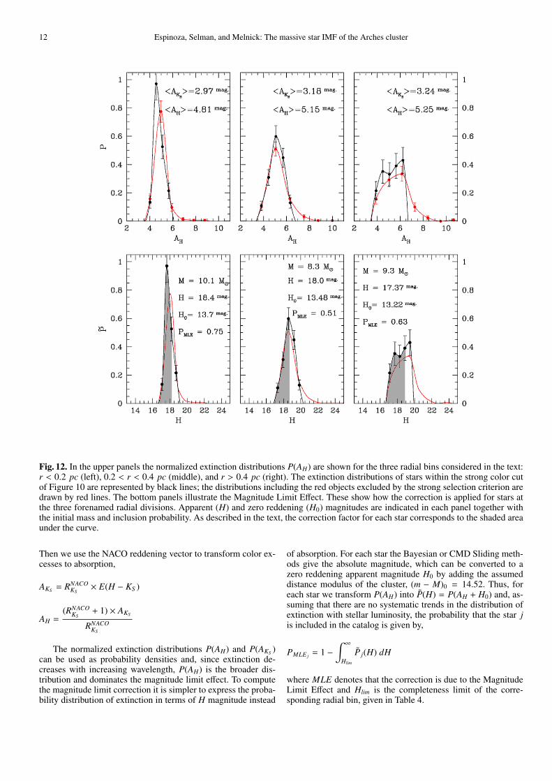
Fig. 12. In the upper panels the normalized extinction distributions P(AH) are shown for the three radial bins considered in the text:r < 0.2 pc (left), 0.2 < r < 0.4 pc (middle), and r > 0.4 pc (right). The extinction distributions of stars within the strong color cutof Figure 10 are represented by black lines; the distributions including the red objects excluded by the strong selection criterion aredrawn by red lines. The bottom panels illustrate the Magnitude Limit Effect. These show how the correction is applied for stars atthe three forenamed radial divisions. Apparent (H) and zero reddening (H0) magnitudes are indicated in each panel together withthe initial mass and inclusion probability. As described in the text, the correction factor for each star corresponds to the shaded areaunder the curve.
Then we use the NACO reddening vector to transform color ex-cesses to absorption,
AKS = RNACOKS
× E(H − KS )
AH =(RNACO
KS+ 1) × AKS
RNACOKS
The normalized extinction distributions P(AH) and P(AKS )can be used as probability densities and, since extinction de-creases with increasing wavelength, P(AH) is the broader dis-tribution and dominates the magnitude limit effect. To computethe magnitude limit correction it is simpler to express the proba-bility distribution of extinction in terms of H magnitude instead
of absorption. For each star the Bayesian or CMD Sliding meth-ods give the absolute magnitude, which can be converted to azero reddening apparent magnitude H0 by adding the assumeddistance modulus of the cluster, (m − M)0 = 14.52. Thus, foreach star we transform P(AH) into P(H) = P(AH + H0) and, as-suming that there are no systematic trends in the distribution ofextinction with stellar luminosity, the probability that the star jis included in the catalog is given by,
PMLE j = 1 −∫ ∞
Hlim
P j(H) dH
where MLE denotes that the correction is due to the MagnitudeLimit Effect and Hlim is the completeness limit of the corre-sponding radial bin, given in Table 4.
Espinoza, Selman, and Melnick: The massive star IMF of the Arches cluster 13
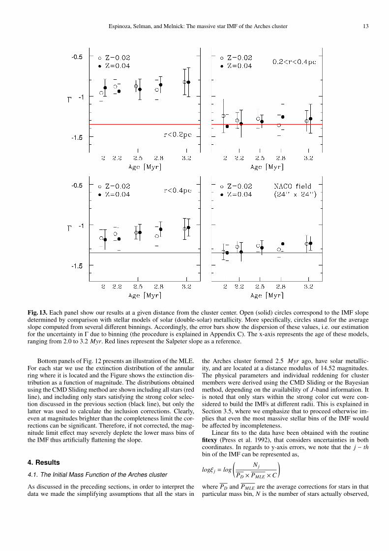
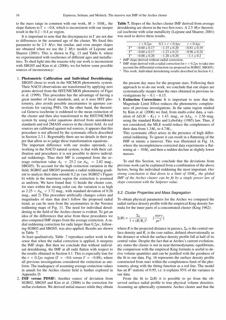
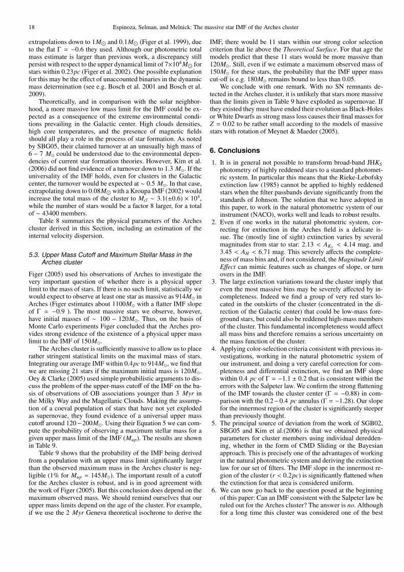
Fig. 13. Each panel show our results at a given distance from the cluster center. Open (solid) circles correspond to the IMF slopedetermined by comparison with stellar models of solar (double-solar) metallicity. More specifically, circles stand for the averageslope computed from several different binnings. Accordingly, the error bars show the dispersion of these values, i.e. our estimationfor the uncertainty in Γ due to binning (the procedure is explained in Appendix C). The x-axis represents the age of these models,ranging from 2.0 to 3.2 Myr. Red lines represent the Salpeter slope as a reference.
Bottom panels of Fig. 12 presents an illustration of the MLE.For each star we use the extinction distribution of the annularring where it is located and the Figure shows the extinction dis-tribution as a function of magnitude. The distributions obtainedusing the CMD Sliding method are shown including all stars (redline), and including only stars satisfying the strong color selec-tion discussed in the previous section (black line), but only thelatter was used to calculate the inclusion corrections. Clearly,even at magnitudes brighter than the completeness limit the cor-rections can be significant. Therefore, if not corrected, the mag-nitude limit effect may severely deplete the lower mass bins ofthe IMF thus artificially flattening the slope.
4. Results
4.1. The Initial Mass Function of the Arches cluster
As discussed in the preceding sections, in order to interpret thedata we made the simplifying assumptions that all the stars in
the Arches cluster formed 2.5 Myr ago, have solar metallic-ity, and are located at a distance modulus of 14.52 magnitudes.The physical parameters and individual reddening for clustermembers were derived using the CMD Sliding or the Bayesianmethod, depending on the availability of J-band information. Itis noted that only stars within the strong color cut were con-sidered to build the IMFs at different radii. This is explained inSection 3.5, where we emphasize that to proceed otherwise im-plies that even the most massive stellar bins of the IMF wouldbe affected by incompleteness.
Linear fits to the data have been obtained with the routinefitexy (Press et al. 1992), that considers uncertainties in bothcoordinates. In regards to y-axis errors, we note that the j − thbin of the IMF can be represented as,
logξ j = log(
N j
PD × PMLE ×C
)where PD and PMLE are the average corrections for stars in thatparticular mass bin, N is the number of stars actually observed,
14 Espinoza, Selman, and Melnick: The massive star IMF of the Arches cluster
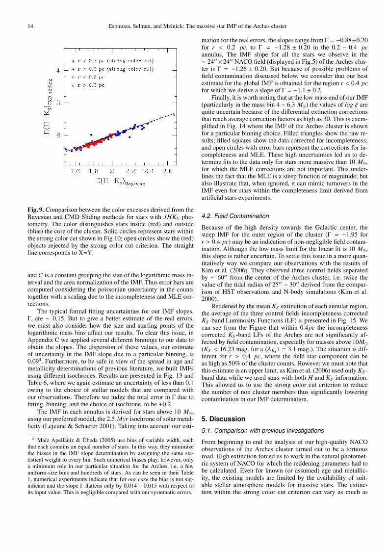
Fig. 9. Comparison between the color excesses derived from theBayesian and CMD Sliding methods for stars with JHKS pho-tometry. The color distinguishes stars inside (red) and outside(blue) the core of the cluster. Solid circles represent stars withinthe strong color cut shown in Fig.10; open circles show the (red)objects rejected by the strong color cut criterion. The straightline corresponds to X=Y.
and C is a constant grouping the size of the logarithmic mass in-terval and the area normalization of the IMF. Thus error bars arecomputed considering the poissonian uncertainty in the countstogether with a scaling due to the incompleteness and MLE cor-rections.
The typical formal fitting uncertainties for our IMF slopes,Γ, are ∼ 0.15. But to give a better estimate of the real errors,we must also consider how the size and starting points of thelogarithmic mass bins affect our results. To clear this issue, inAppendix C we applied several different binnings to our data toobtain the slopes. The dispersion of these values, our estimateof uncertainty in the IMF slope due to a particular binning, is0.094. Furthermore, to be safe in view of the spread in age andmetallicity determinations of previous literature, we built IMFsusing different isochrones. Results are presented in Fig. 13 andTable 6, where we again estimate an uncertainty of less than 0.1owing to the choice of stellar models that are compared withour observations. Therefore we judge the total error in Γ due tofitting, binning, and the choice of isochrone, to be ±0.2.
The IMF in each annulus is derived for stars above 10 M�,using our preferred model, the 2.5 Myr isochrone of solar metal-licity (Lejeune & Schaerer 2001). Taking into account our esti-
4 Maız Apellaniz & Ubeda (2005) use bins of variable width, suchthat each contains an equal number of stars. In this way, they minimizethe biases in the IMF slope determination by assigning the same sta-tistical weight to every bin. Such numerical biases play, however, onlya minimum role in our particular situation for the Arches, i.e. a fewuniform-size bins and hundreds of stars. As can be seen in their Table1, numerical experiments indicate that for our case the bias is not sig-nificant and the slope Γ flattens only by 0.014 − 0.015 with respect toits input value. This is negligible compared with our systematic errors.
mation for the real errors, the slopes range from Γ = −0.88±0.20for r < 0.2 pc, to Γ = −1.28 ± 0.20 in the 0.2 − 0.4 pcannulus. The IMF slope for all the stars we observe in the∼ 24′′×24′′ NACO field (displayed in Fig.5) of the Arches clus-ter is Γ = −1.26 ± 0.20. But because of possible problems offield contamination discussed below, we consider that our bestestimate for the global IMF is obtained for the region r < 0.4 pcfor which we derive a slope of Γ = −1.1 ± 0.2.
Finally, it is worth noting that at the low mass end of our IMF(particularly in the mass bin 4 − 6.3 M�) the values of log ξ arequite uncertain because of the differential extinction correctionsthat reach average correction factors as high as 30. This is exem-plified in Fig. 14 where the IMF of the Arches cluster is shownfor a particular binning choice. Filled triangles show the raw re-sults; filled squares show the data corrected for incompleteness;and open circles with error bars represent the corrections for in-completeness and MLE. These high uncertainties led us to de-termine fits to the data only for stars more massive than 10 M�,for which the MLE corrections are not important. This under-lines the fact that the MLE is a steep function of magnitude; butalso illustrate that, when ignored, it can mimic turnovers in theIMF even for stars within the completeness limit derived fromartificial stars experiments.
4.2. Field Contamination
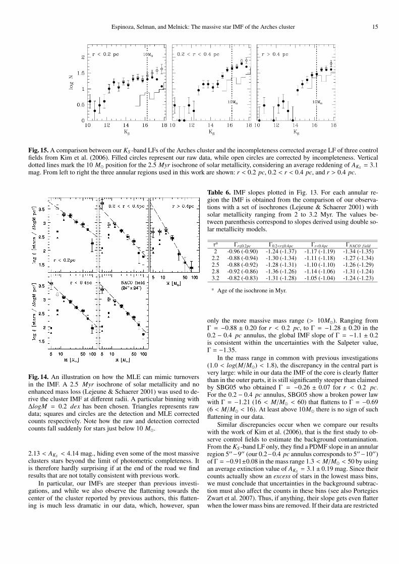
Because of the high density towards the Galactic center, thesteep IMF for the outer region of the cluster (Γ = −1.95 forr > 0.4 pc) may be an indication of non-negligible field contam-ination. Although the low mass limit for the linear fit is 10 M�,this slope is rather uncertain. To settle this issue in a more quan-titatively way we compare our observations with the results ofKim et al. (2006). They observed three control fields separatedby ∼ 60′′ from the center of the Arches cluster, i.e. twice thevalue of the tidal radius of 25′′ − 30′′ derived from the compar-ison of HST observations and N-body simulations (Kim et al.2000).
Reddened by the mean KS extinction of each annular region,the average of the three control fields incompleteness correctedKS -band Luminosity Functions (LF) is presented in Fig. 15. Wecan see from the Figure that within 0.4pc the incompletenesscorrected KS -band LFs of the Arches are not significantly af-fected by field contamination, especially for masses above 10M�(KS < 16.23 mag. for a 〈AKS 〉 = 3.1 mag.). The situation is dif-ferent for r > 0.4 pc, where the field star component can beas high as 50% of the cluster counts. However we must note thatthis estimate is an upper limit, as Kim et al. (2006) used only KS -band data while we used stars with both H and KS information.This allowed us to use the strong color cut criterion to reducethe number of non cluster members thus significantly loweringcontamination in our IMF determination.
5. Discussion
5.1. Comparison with previous investigations
From beginning to end the analysis of our high-quality NACOobservations of the Arches cluster turned out to be a tortuousroad. High extinction forced us to work in the natural photomet-ric system of NACO for which the reddening parameters had tobe calculated. Even for known (or assumed) age and metallic-ity, the existing models are limited by the availability of suit-able stellar atmosphere models for massive stars. The extinc-tion within the strong color cut criterion can vary as much as
Espinoza, Selman, and Melnick: The massive star IMF of the Arches cluster 15
Fig. 15. A comparison between our KS -band LFs of the Arches cluster and the incompleteness corrected average LF of three controlfields from Kim et al. (2006). Filled circles represent our raw data, while open circles are corrected by incompleteness. Verticaldotted lines mark the 10 M� position for the 2.5 Myr isochrone of solar metallicity, considering an average reddening of AKS = 3.1mag. From left to right the three annular regions used in this work are shown: r < 0.2 pc, 0.2 < r < 0.4 pc, and r > 0.4 pc.
Fig. 14. An illustration on how the MLE can mimic turnoversin the IMF. A 2.5 Myr isochrone of solar metallicity and noenhanced mass loss (Lejeune & Schaerer 2001) was used to de-rive the cluster IMF at different radii. A particular binning with∆logM = 0.2 dex has been chosen. Triangles represents rawdata; squares and circles are the detection and MLE correctedcounts respectively. Note how the raw and detection correctedcounts fall suddenly for stars just below 10 M�.
2.13 < AKS < 4.14 mag., hiding even some of the most massiveclusters stars beyond the limit of photometric completeness. Itis therefore hardly surprising if at the end of the road we findresults that are not totally consistent with previous work.
In particular, our IMFs are steeper than previous investi-gations, and while we also observe the flattening towards thecenter of the cluster reported by previous authors, this flatten-ing is much less dramatic in our data, which, however, span
Table 6. IMF slopes plotted in Fig. 13. For each annular re-gion the IMF is obtained from the comparison of our observa-tions with a set of isochrones (Lejeune & Schaerer 2001) withsolar metallicity ranging from 2 to 3.2 Myr. The values be-tween parenthesis correspond to slopes derived using double so-lar metallicity models.
τa Γr≤0.2pc Γ0.2<r≤0.4pc Γr<0.4pc ΓNACO f ield
2 -0.96 (-0.90) -1.24 (-1.37) -1.17 (-1.19) -1.34 (-1.35)2.2 -0.88 (-0.94) -1.30 (-1.34) -1.11 (-1.18) -1.27 (-1.34)2.5 -0.88 (-0.92) -1.28 (-1.31) -1.10 (-1.10) -1.26 (-1.29)2.8 -0.92 (-0.86) -1.36 (-1.26) -1.14 (-1.06) -1.31 (-1.24)3.2 -0.82 (-0.83) -1.31 (-1.28) -1.05 (-1.04) -1.24 (-1.23)
a Age of the isochrone in Myr.
only the more massive mass range (> 10M�). Ranging fromΓ = −0.88 ± 0.20 for r < 0.2 pc, to Γ = −1.28 ± 0.20 in the0.2 − 0.4 pc annulus, the global IMF slope of Γ = −1.1 ± 0.2is consistent within the uncertainties with the Salpeter value,Γ = −1.35.
In the mass range in common with previous investigations(1.0 < log(M/M�) < 1.8), the discrepancy in the central part isvery large: while in our data the IMF of the core is clearly flatterthan in the outer parts, it is still significantly steeper than claimedby SBG05 who obtained Γ = −0.26 ± 0.07 for r < 0.2 pc.For the 0.2 − 0.4 pc annulus, SBG05 show a broken power lawwith Γ = −1.21 (16 < M/M� < 60) that flattens to Γ = −0.69(6 < M/M� < 16). At least above 10M� there is no sign of suchflattening in our data.
Similar discrepancies occur when we compare our resultswith the work of Kim et al. (2006), that is the first study to ob-serve control fields to estimate the background contamination.From the KS -band LF only, they find a PDMF slope in an annularregion 5′′−9′′ (our 0.2−0.4 pc annulus corresponds to 5′′−10′′)of Γ = −0.91±0.08 in the mass range 1.3 < M/M� < 50 by usingan average extinction value of AKS = 3.1± 0.19 mag. Since theircounts actually show an excess of stars in the lowest mass bins,we must conclude that uncertainties in the background subtrac-tion must also affect the counts in these bins (see also PortegiesZwart et al. 2007). Thus, if anything, their slope gets even flatterwhen the lower mass bins are removed. If their data are restricted
16 Espinoza, Selman, and Melnick: The massive star IMF of the Arches cluster
to the mass range in common with our work, M > 10M�, theslope flattens to Γ = −0.8, which is inconsistent with our steeperresult in the 0.2 − 0.4 pc region.
It is important to note that the discrepancies in Γ are not dueto differences in the assumed age of the cluster. We fixed thisparameter to be 2.5 Myr, but similar, and even steeper slopesare obtained when we use the 2 Myr models of Lejeune andShaerer (2001). This is shown in Fig. 13 and Table 6, wherewe experimented with isochrones of different ages and metallic-ities. To shed light into the reasons why our work is inconsistentwith SBG05 and Kim et al. (2006), we list below some possiblesources of inconsistency:
1. Photometric Calibration and Individual Dereddening:SBG05 chose to work in the NICMOS photometric system.Their NACO observations are transformed by applying zeropoints derived from the HST/NICMOS photometry of Figeret al. (1999). This procedure has the advantage of having agreat number of local standards, and, as it uses HST pho-tometry, also avoids possible uncertainties in aperture cor-rections for varying PSFs. On the other hand, the theoreti-cal Geneva isochrone is reddened to the mean extinction ofthe cluster and then also transformed to the HST/NICMOSsystem by using color equations derived from unreddenedstandards and red 2MASS sources in the cluster field. As redsources are calibrated against red sources, it appears that thisprocedure is not affected by the systematic effects describedin Section 2.3.1. Regrettably there are no details in their pa-per that allow us to judge these transformation equations.The important difference with our modus operandi, i.e.working in the NACO natural system, is that with their cal-ibration and procedures it is not possible to derive individ-ual reddenings. Thus their MF is computed from the av-erage extinction value AV = 25.2 (or AKS = 2.82 mag.,SBG05). To account for the high extinction variation in thefield, SGB02 and SBG05 postulate a radial reddening gradi-ent to analyze their data outside 0.2 pc (see SGB02’s Figure6) while in the innermost region the extinction is assumedas uniform. We have found that: 1) Inside the cluster core,for stars within the strong color cut, the variation is as highas 2.25 < AKS < 3.72 mag., with standard deviation of 0.26mag., and 2) This procedure artificially changes colors andmagnitudes of stars that don’t follow the proposed radialtrend, as can be seen from the asymmetries in the Voronoireddening maps of Fig. 11. The need for individual dered-dening in the field of the Arches cluster is evident. To get anidea of the differences that arise from these procedures wealso computed IMF slopes from the average extinction. A ra-dial reddening correction for radii larger than 0.2pc, follow-ing SGB02 and SBG05, was also applied. Results are shownin Table 7.At least qualitatively, Table 7 reproduce earlier work in thesense that when the radial correction is applied, it steepensthe IMF slope. But then we conclude that without individ-ual dereddening, the IMF at all radii flatten with respect tothe results obtained in Section 4.1. This is especially true forthe r < 0.2pc region (Γ = −0.6 versus Γ = −0.88), whereall previous investigations considered the extinction as uni-form. The inadequacy of assuming average extinction valuesin annuli for the Arches cluster field is further explored inAppendix D.
2. IMF versus PDMF: Another source of deviation fromSGB02, SBG05 and Kim et al. (2006) is the correction forstellar evolution. We derived initial masses while they obtain
Table 7. Slopes of the Arches cluster IMF derived from averagedereddening are shown in the two first rows. A 2.5 Myr theoreti-cal isochrone with solar metallicity (Lejeune and Shaerer, 2001)was used to derive these results.
r < 0.2pc 0.2 < r < 0.4pc r < 0.4pcΓa −0.60 ± 0.17 −1.15 ± 0.20 −0.81 ± 0.19Γb −0.60 ± 0.17 −1.23 ± 0.23 −0.96 ± 0.24Γc −0.88 ± 0.20 −1.28 ± 0.20 −1.1 ± 0.2
a IMF slope derived without radial correction.b IMF slope derived with a radial correction for r > 0.2pc to take into
account the differential extinction (as proposed in SGB02, SBG05).c This work. Individual derredening results described in Section 4.1.
the present day mass for the program stars. Following theirapproach to re-do our work, we conclude that our slopes aresystematically steeper than the ones obtained in previous in-vestigations by ∼ 0.1 − 0.15.
3. Extinction Corrections: It is important to note that theMagnitude Limit Effect reduces the photometric complete-ness of previous investigations. In the same region studiedby Kim et al. (2006) we find, from multi-color data, a vari-ation of ∆E(H − KS ) = 1.43. mag., or ∆AKS = 2.56 mag.using the standard Rieke and Lebofsky (1985) law. Thus, ifnot considered, the MLE would reduce the completeness oftheir data from 1.3M� to 4.7M�.This systematic effect arises in the presence of high differ-ential reddening. To ignore it can result in a flattening of theIMF or mimic a turnover. This was illustrated in Fig. 14,where the incompleteness-corrected data experiments a flat-tening at ∼ 10M� and then a sudden decline at slightly lowermasses.
To end this Section, we conclude that the deviations fromprevious work can be explained from a combination of the abovefactors, being the individual reddening the most important. Ourstrong conclusion is that down to a limit of 10M�, the globalIMF of the Arches cluster can be fit by a single power law ofslope consistent with the Salpeter value.
5.2. Cluster Properties and Mass Segregation
To obtain physical parameters for the Arches we compared theradial surface density profile with the empirical King density for-mula for the inner parts of a concentrated cluster (King 1962):
Σ(R) =Σ0
1 + (R/Rc)2 [starspc2 ]
where R is the projected distance in parsecs, Σ0 is the central sur-face density and Rc is the core radius, defined observationally asthe distance at which the surface density profile fall at half of itscentral value. Despite the fact that at Arches’s current evolution-ary status the cluster is not in near-thermodynamic equilibrium,the comparison with the empirical King formula is useful to de-rive volume quantities and can be justified with the goodness ofthe fit to our data. Fig. 16 represents the surface density profileconstructed from stars within the completeness limit of the pho-tometry along with the fitting function as a red line. The modelhas an R2 statistic of 0.95, i.e. it explains 95% of the variance inour data.
From the fit to Σ(R) it is possible to go from the ob-served surface radial profile to true physical volume densities.Assuming an spherically symmetric Arches cluster and that the

Espinoza, Selman, and Melnick: The massive star IMF of the Arches cluster 17
Table 8. Physical parameters of the Arches cluster
Parameter Value CommentsCore radius Rc 0.14 ± 0.05 pc Derived by fitting the empirical King density law
to the observed Σ(R)Tidal radius Rt ∼ 1 pc Derived by Kim et al. (2000)Central concentration c = log Rt
Rc0.84 Comparable to the less concentrated galactic globulars
according to Harris (1996)Central surface density Σ0 2.2(±0.4) × 103 stars pc−2 Derived by fitting the empirical King density law
to the observed Σ(R)Central volume density ρ0 8.0(±1.5) × 103 stars pc−3
Central mass density ρm,0 2.0(±0.4) × 105 M� pc−3 For an average mass of 25.4 M� in the > 10 M� rangeCluster mass Mcl,1 ∼ 2.0(±0.6) × 104 M� For an extrapolation of the photometric mass down to 1 M�
Mcl,2 ∼ 3.1(±0.6) × 104 M� For an extrapolation down to 0.08 M� using a Kroupa IMF (2002)Predictedvelocity dispersiona σ = ( 0.4GMcl
Rhm)1/2 9 km s−1 Using Mcl,1 and a half mass radius of 0.4 pc derived in SGB02
a Equation 4 − 80b of Binney & Tremaine (1987).
Table 9. Using the prescriptions of Oey & Clarke (2005) we compute p(Mmax|Mup), i.e. the probability of observing a maximumstellar mass Mmax for a given Mup.
Γa Mmax N(> 10M�)b p(Mmax|Mup) p(Mmax|Mup) p(Mmax|Mup) p(Mmax|Mup)Mup = 200M� Mup = 150M� Mup = 135M� Mup = 120M�
-1.1 120M� 343 10−5 0.006 0.06 1
a Slope of the IMF within 0.4 pc.b Number of stars within 0.4 pc.
Fig. 16. Radial density profiles for stars at different mass bins,with error bars reflecting the corrections for systematic errorsand Poisson statistics. The red line, with an offset of +0.5 dexfor clarity, represents the fit of the empirical King density law(1962) to the surface density profile built from 10 − 120 M�stars .
volume number density profile ρ(r) remains bound as r → ∞,
we can solve the Abel’s integral equation (see e.g. Arfken &Weber 2005). From this procedure we get a core radius ofRc = 0.14 ± 0.05 pc and a central mass density of ρ0 =
Σ02Rc
=
2.0(±0.4) × 105 M� pc−3. This latter value is similar to thatobtained for the denser globular clusters in the Milky Way ac-cording to the Harris (1996) catalog.
A variation of what we have done so far would be to restrictthe fit of the empirical density law to stars above 30 M�. Inthat case the core radius decreases to Rc = 0.10 ± 0.01, whichimplies that more massive stars are more concentrated in the in-ner parts of the cluster. But besides the observed radial trend inthe IMF slope and the mass-dependent core radius, we can alsocompare the surface density profiles built from stars at two dif-ferent mass bins, 10 < M/M� < 30 and 30 < M/M� < 120,as shown in Fig. 16. A χ2 test rejects the hypothesis that the twosets of counts come from the same parent distribution at a 99.4%confidence level. This adds to the discussion of several authors(e.g. Portegies Zwart et al. 2007 and references therein) aboutthe possibility that the flattening of the IMF towards the centerof Arches may provide the best indication yet for mass segrega-tion in a young starburst cluster
The total mass of the cluster can be obtained by means ofthe integration of the IMF extrapolated towards lower masses.For this purpose and taking into consideration the indications ofmass segregation that we have discussed, we will use the IMFslopes derived for r < 0.2pc and 0.2 < r < 0.4pc, i.e. Γ =−0.88 and Γ = −1.28 respectively. In the range M > 20M� (thetheoretical minimum of O stars) we find a total mass of 5570M�distributed in 135 O stars. Extrapolating the IMF to 1M�, givesa mean mass of 5.5M� and 3.4M� for the core and first annulusrespectively, and a total mass Mcl ∼ 2.0(±0.6)×104M� within aprojected radius of 0.4 pc. This value is significantly larger thanthe earlier photometric estimates of 10800M� and 12000M� for
18 Espinoza, Selman, and Melnick: The massive star IMF of the Arches cluster
extrapolations down to 1M� and 0.1M� (Figer et al. 1999), dueto the flat Γ = −0.6 they used. Although our photometric totalmass estimate is larger than previous work, a discrepancy stillpersist with respect to the upper dynamical limit of 7×10⁴M� forstars within 0.23pc (Figer et al. 2002). One possible explanationfor this may be the effect of unaccounted binaries in the dynamicmass determination (see e.g. Bosch et al. 2001 and Bosch et al.2009).
Theoretically, and in comparison with the solar neighbor-hood, a more massive low mass limit for the IMF could be ex-pected as a consequence of the extreme environmental condi-tions prevailing in the Galactic center. High clouds densities,high core temperatures, and the presence of magnetic fieldsshould all play a role in the process of star formation. As notedby SBG05, their claimed turnover at an unusually high mass of6 − 7 M� could be understood due to the environmental depen-dencies of current star formation theories. However, Kim et al.(2006) did not find evidence of a turnover down to 1.3 M�. If theuniversality of the IMF holds, even for clusters in the Galacticcenter, the turnover would be expected at ∼ 0.5 M�. In that case,extrapolating down to 0.08M� with a Kroupa IMF (2002) wouldincrease the total mass of the cluster to Mcl ∼ 3.1(±0.6) × 104,while the number of stars would be a factor 8 larger, for a totalof ∼ 43400 members.
Table 8 summarizes the physical parameters of the Archescluster derived in this Section, including an estimation of theinternal velocity dispersion.
5.3. Upper Mass Cutoff and Maximum Stellar Mass in theArches cluster
Figer (2005) used his observations of Arches to investigate thevery important question of whether there is a physical upperlimit to the mass of stars. If there is no such limit, statistically wewould expect to observe at least one star as massive as 914M� inArches (Figer estimates about 1100M� with a flatter IMF slopeof Γ = −0.9 ). The most massive stars we observe, however,have initial masses of ∼ 100 − 120M�. Thus, on the basis ofMonte Carlo experiments Figer concluded that the Arches pro-vides strong evidence of the existence of a physical upper masslimit to the IMF of 150M�.
The Arches cluster is sufficiently massive to allow us to placerather stringent statistical limits on the maximal mass of stars.Integrating our average IMF within 0.4pc to 914M�, we find thatwe are missing 21 stars if the maximum initial mass is 120M�.Oey & Clarke (2005) used simple probabilistic arguments to dis-cuss the problem of the upper-mass cutoff of the IMF on the ba-sis of observations of OB associations younger than 3 Myr inthe Milky Way and the Magellanic Clouds. Making the assump-tion of a coeval population of stars that have not yet explodedas supernovae, they found evidence of a universal upper masscutoff around 120−200M�. Using their Equation 5 we can com-pute the probability of observing a maximum stellar mass for agiven upper mass limit of the IMF (Mup). The results are shownin Table 9.
Table 9 shows that the probability of the IMF being derivedfrom a population with an upper mass limit significantly largerthan the observed maximum mass in the Arches cluster is neg-ligible (1% for Mup = 145M�). The important result of a cutofffor the Arches cluster is robust, and is in good agreement withthe work of Figer (2005). But this conclusion does depend on themaximum observed mass. We should remind ourselves that ourupper mass limits depend on the age of the cluster. For example,if we use the 2 Myr Geneva theoretical isochrone to derive the
IMF, there would be 11 stars within our strong color selectioncriterion that lie above the Theoretical Surface. For that age themodels predict that these 11 stars would be more massive than120M�. Still, even if we estimate a maximum observed mass of150M� for these stars, the probability that the IMF upper masscut-off is e.g. 180M� remains bound to less than 0.05.
We conclude with one remark. With no SN remnants de-tected in the Arches cluster, it is unlikely that stars more massivethan the limits given in Table 9 have exploded as supernovae. Ifthey existed they must have ended their evolution as Black-Holesor White Dwarfs as strong mass loss causes their final masses forZ = 0.02 to be rather small according to the models of massivestars with rotation of Meynet & Maeder (2005).
6. Conclusions
1. It is in general not possible to transform broad-band JHKSphotometry of highly reddened stars to a standard photomet-ric system. In particular this means that the Rieke-Lebofskyextinction law (1985) cannot be applied to highly reddenedstars when the filter passbands deviate significantly from thestandards of Johnson. The solution that we have adopted inthis paper, to work in the natural photometric system of ourinstrument (NACO), works well and leads to robust results.
2. Even if one works in the natural photometric system, cor-recting for extinction in the Arches field is a delicate is-sue. The (mostly line of sight) extinction varies by severalmagnitudes from star to star: 2.13 < AKS < 4.14 mag. and3.45 < AH < 6.71 mag. This severely affects the complete-ness of mass bins and, if not considered, the Magnitude LimitEffect can mimic features such as changes of slope, or turnovers in the IMF.
3. The large extinction variations toward the cluster imply thateven the most massive bins may be severely affected by in-completeness. Indeed we find a group of very red stars lo-cated in the outskirts of the cluster (concentrated in the di-rection of the Galactic center) that could be low-mass fore-ground stars, but could also be reddened high-mass membersof the cluster. This fundamental incompleteness would affectall mass bins and therefore remains a serious uncertainty onthe mass function of the cluster.
4. Applying color-selection criteria consistent with previous in-vestigations, working in the natural photometric system ofour instrument, and doing a very careful correction for com-pleteness and differential extinction, we find an IMF slopewithin 0.4 pc of Γ = −1.1 ± 0.2 that is consistent within theerrors with the Salpeter law. We confirm the strong flatteningof the IMF towards the cluster center (Γ = −0.88) in com-parison with the 0.2−0.4 pc annulus (Γ = −1.28). Our slopefor the innermost region of the cluster is significantly steeperthan previously thought.
5. The principal source of deviation from the work of SGB02,SBG05 and Kim et al.(2006) is that we obtained physicalparameters for cluster members using individual deredden-ing, whether in the form of CMD Sliding or the Bayesianapproach. This is precisely one of the advantages of workingin the natural photometric system and deriving the extinctionlaw for our set of filters. The IMF slope in the innermost re-gion of the cluster (r < 0.2pc) is significantly flattened whenthe extinction for that area is considered uniform.
6. We can now go back to the question posed at the beginningof this paper: Can an IMF consistent with the Salpeter law beruled out for the Arches cluster? The answer is no. Althoughfor a long time this cluster was considered one of the best
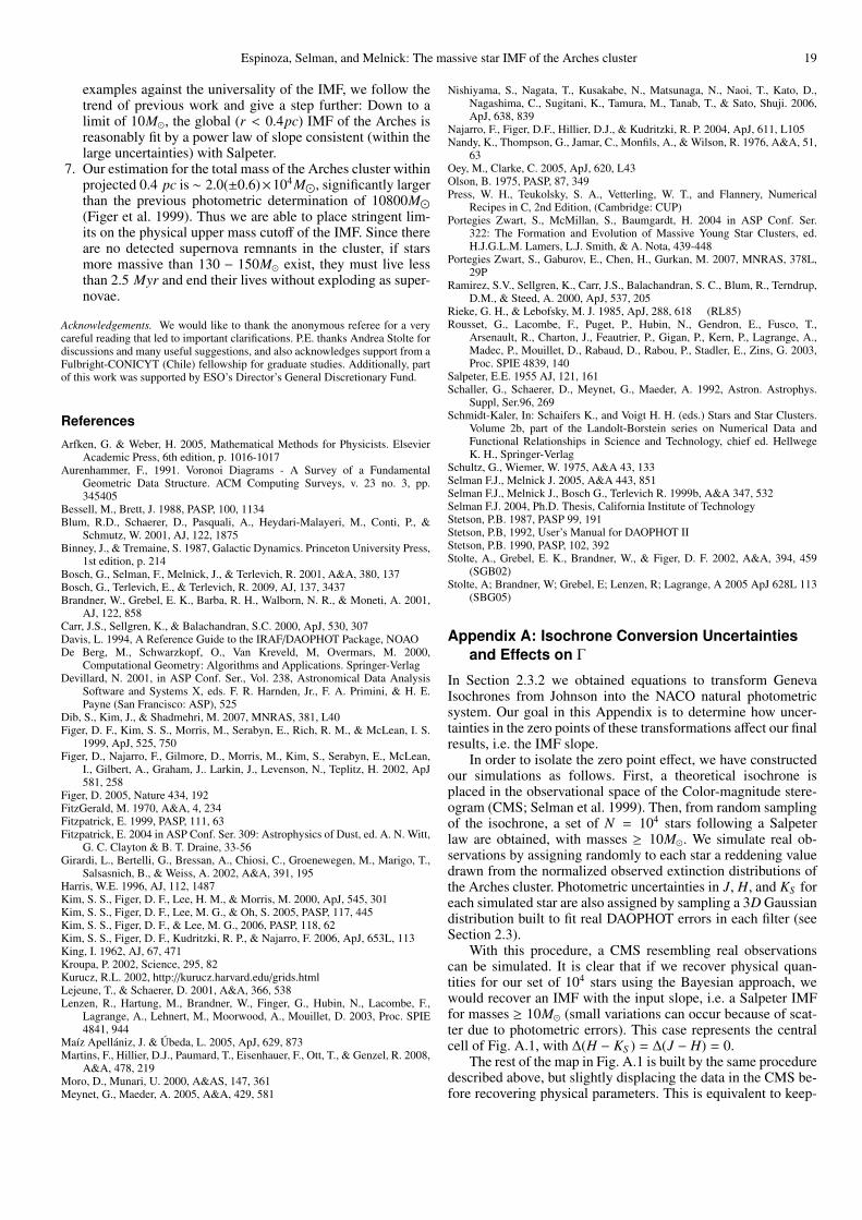
Espinoza, Selman, and Melnick: The massive star IMF of the Arches cluster 19
examples against the universality of the IMF, we follow thetrend of previous work and give a step further: Down to alimit of 10M�, the global (r < 0.4pc) IMF of the Arches isreasonably fit by a power law of slope consistent (within thelarge uncertainties) with Salpeter.
7. Our estimation for the total mass of the Arches cluster withinprojected 0.4 pc is ∼ 2.0(±0.6)×104M�, significantly largerthan the previous photometric determination of 10800M�(Figer et al. 1999). Thus we are able to place stringent lim-its on the physical upper mass cutoff of the IMF. Since thereare no detected supernova remnants in the cluster, if starsmore massive than 130 − 150M� exist, they must live lessthan 2.5 Myr and end their lives without exploding as super-novae.
Acknowledgements. We would like to thank the anonymous referee for a verycareful reading that led to important clarifications. P.E. thanks Andrea Stolte fordiscussions and many useful suggestions, and also acknowledges support from aFulbright-CONICYT (Chile) fellowship for graduate studies. Additionally, partof this work was supported by ESO’s Director’s General Discretionary Fund.
References
Arfken, G. & Weber, H. 2005, Mathematical Methods for Physicists. ElsevierAcademic Press, 6th edition, p. 1016-1017
Aurenhammer, F., 1991. Voronoi Diagrams - A Survey of a FundamentalGeometric Data Structure. ACM Computing Surveys, v. 23 no. 3, pp.345405
Bessell, M., Brett, J. 1988, PASP, 100, 1134Blum, R.D., Schaerer, D., Pasquali, A., Heydari-Malayeri, M., Conti, P., &
Schmutz, W. 2001, AJ, 122, 1875Binney, J., & Tremaine, S. 1987, Galactic Dynamics. Princeton University Press,
1st edition, p. 214Bosch, G., Selman, F., Melnick, J., & Terlevich, R. 2001, A&A, 380, 137Bosch, G., Terlevich, E., & Terlevich, R. 2009, AJ, 137, 3437Brandner, W., Grebel, E. K., Barba, R. H., Walborn, N. R., & Moneti, A. 2001,
AJ, 122, 858Carr, J.S., Sellgren, K., & Balachandran, S.C. 2000, ApJ, 530, 307Davis, L. 1994, A Reference Guide to the IRAF/DAOPHOT Package, NOAODe Berg, M., Schwarzkopf, O., Van Kreveld, M, Overmars, M. 2000,
Computational Geometry: Algorithms and Applications. Springer-VerlagDevillard, N. 2001, in ASP Conf. Ser., Vol. 238, Astronomical Data Analysis
Software and Systems X, eds. F. R. Harnden, Jr., F. A. Primini, & H. E.Payne (San Francisco: ASP), 525
Dib, S., Kim, J., & Shadmehri, M. 2007, MNRAS, 381, L40Figer, D. F., Kim, S. S., Morris, M., Serabyn, E., Rich, R. M., & McLean, I. S.
1999, ApJ, 525, 750Figer, D., Najarro, F., Gilmore, D., Morris, M., Kim, S., Serabyn, E., McLean,
I., Gilbert, A., Graham, J.. Larkin, J., Levenson, N., Teplitz, H. 2002, ApJ581, 258
Figer, D. 2005, Nature 434, 192FitzGerald, M. 1970, A&A, 4, 234Fitzpatrick, E. 1999, PASP, 111, 63Fitzpatrick, E. 2004 in ASP Conf. Ser. 309: Astrophysics of Dust, ed. A. N. Witt,
G. C. Clayton & B. T. Draine, 33-56Girardi, L., Bertelli, G., Bressan, A., Chiosi, C., Groenewegen, M., Marigo, T.,
Salsasnich, B., & Weiss, A. 2002, A&A, 391, 195Harris, W.E. 1996, AJ, 112, 1487Kim, S. S., Figer, D. F., Lee, H. M., & Morris, M. 2000, ApJ, 545, 301Kim, S. S., Figer, D. F., Lee, M. G., & Oh, S. 2005, PASP, 117, 445Kim, S. S., Figer, D. F., & Lee, M. G., 2006, PASP, 118, 62Kim, S. S., Figer, D. F., Kudritzki, R. P., & Najarro, F. 2006, ApJ, 653L, 113King, I. 1962, AJ, 67, 471Kroupa, P. 2002, Science, 295, 82Kurucz, R.L. 2002, http://kurucz.harvard.edu/grids.htmlLejeune, T., & Schaerer, D. 2001, A&A, 366, 538Lenzen, R., Hartung, M., Brandner, W., Finger, G., Hubin, N., Lacombe, F.,
Lagrange, A., Lehnert, M., Moorwood, A., Mouillet, D. 2003, Proc. SPIE4841, 944
Maız Apellaniz, J. & Ubeda, L. 2005, ApJ, 629, 873Martins, F., Hillier, D.J., Paumard, T., Eisenhauer, F., Ott, T., & Genzel, R. 2008,
A&A, 478, 219Moro, D., Munari, U. 2000, A&AS, 147, 361Meynet, G., Maeder, A. 2005, A&A, 429, 581
Nishiyama, S., Nagata, T., Kusakabe, N., Matsunaga, N., Naoi, T., Kato, D.,Nagashima, C., Sugitani, K., Tamura, M., Tanab, T., & Sato, Shuji. 2006,ApJ, 638, 839
Najarro, F., Figer, D.F., Hillier, D.J., & Kudritzki, R. P. 2004, ApJ, 611, L105Nandy, K., Thompson, G., Jamar, C., Monfils, A., & Wilson, R. 1976, A&A, 51,
63Oey, M., Clarke, C. 2005, ApJ, 620, L43Olson, B. 1975, PASP, 87, 349Press, W. H., Teukolsky, S. A., Vetterling, W. T., and Flannery, Numerical
Recipes in C, 2nd Edition, (Cambridge: CUP)Portegies Zwart, S., McMillan, S., Baumgardt, H. 2004 in ASP Conf. Ser.
322: The Formation and Evolution of Massive Young Star Clusters, ed.H.J.G.L.M. Lamers, L.J. Smith, & A. Nota, 439-448
Portegies Zwart, S., Gaburov, E., Chen, H., Gurkan, M. 2007, MNRAS, 378L,29P
Ramirez, S.V., Sellgren, K., Carr, J.S., Balachandran, S. C., Blum, R., Terndrup,D.M., & Steed, A. 2000, ApJ, 537, 205
Rieke, G. H., & Lebofsky, M. J. 1985, ApJ, 288, 618 (RL85)Rousset, G., Lacombe, F., Puget, P., Hubin, N., Gendron, E., Fusco, T.,
Arsenault, R., Charton, J., Feautrier, P., Gigan, P., Kern, P., Lagrange, A.,Madec, P., Mouillet, D., Rabaud, D., Rabou, P., Stadler, E., Zins, G. 2003,Proc. SPIE 4839, 140
Salpeter, E.E. 1955 AJ, 121, 161Schaller, G., Schaerer, D., Meynet, G., Maeder, A. 1992, Astron. Astrophys.
Suppl, Ser.96, 269Schmidt-Kaler, In: Schaifers K., and Voigt H. H. (eds.) Stars and Star Clusters.
Volume 2b, part of the Landolt-Borstein series on Numerical Data andFunctional Relationships in Science and Technology, chief ed. HellwegeK. H., Springer-Verlag
Schultz, G., Wiemer, W. 1975, A&A 43, 133Selman F.J., Melnick J. 2005, A&A 443, 851Selman F.J., Melnick J., Bosch G., Terlevich R. 1999b, A&A 347, 532Selman F.J. 2004, Ph.D. Thesis, California Institute of TechnologyStetson, P.B. 1987, PASP 99, 191Stetson, P.B, 1992, User’s Manual for DAOPHOT IIStetson, P.B. 1990, PASP, 102, 392Stolte, A., Grebel, E. K., Brandner, W., & Figer, D. F. 2002, A&A, 394, 459
(SGB02)Stolte, A; Brandner, W; Grebel, E; Lenzen, R; Lagrange, A 2005 ApJ 628L 113
(SBG05)
Appendix A: Isochrone Conversion Uncertaintiesand Effects on Γ
In Section 2.3.2 we obtained equations to transform GenevaIsochrones from Johnson into the NACO natural photometricsystem. Our goal in this Appendix is to determine how uncer-tainties in the zero points of these transformations affect our finalresults, i.e. the IMF slope.
In order to isolate the zero point effect, we have constructedour simulations as follows. First, a theoretical isochrone isplaced in the observational space of the Color-magnitude stere-ogram (CMS; Selman et al. 1999). Then, from random samplingof the isochrone, a set of N = 104 stars following a Salpeterlaw are obtained, with masses ≥ 10M�. We simulate real ob-servations by assigning randomly to each star a reddening valuedrawn from the normalized observed extinction distributions ofthe Arches cluster. Photometric uncertainties in J, H, and KS foreach simulated star are also assigned by sampling a 3D Gaussiandistribution built to fit real DAOPHOT errors in each filter (seeSection 2.3).
With this procedure, a CMS resembling real observationscan be simulated. It is clear that if we recover physical quan-tities for our set of 104 stars using the Bayesian approach, wewould recover an IMF with the input slope, i.e. a Salpeter IMFfor masses ≥ 10M� (small variations can occur because of scat-ter due to photometric errors). This case represents the centralcell of Fig. A.1, with ∆(H − KS ) = ∆(J − H) = 0.
The rest of the map in Fig. A.1 is built by the same proceduredescribed above, but slightly displacing the data in the CMS be-fore recovering physical parameters. This is equivalent to keep-
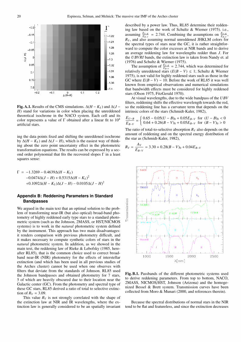
20 Espinoza, Selman, and Melnick: The massive star IMF of the Arches cluster
Fig. A.1. Results of the CMS simulations. ∆(H − KS ) and ∆(J −H) stand for variations in color when placing the unreddenedtheoretical isochrone in the NACO system. Each cell and itscolor represents a value of Γ obtained after a linear fit to 104
artificial stars.
ing the data points fixed and shifting the unreddened isochroneby ∆(H − KS ) and ∆(J − H), which is the easiest way of think-ing about the zero point uncertainty effect in the photometrictransformation equations. The results can be expressed by a sec-ond order polynomial that fits the recovered slopes Γ in a leastsquares sense:
Γ = −1.3269 − 0.4639∆(H − KS )−0.0474∆(J − H) + 0.5315∆(H − KS )2
+0.1092∆(H − KS )∆(J − H) − 0.0105∆(J − H)2
Appendix B: Reddening Parameters in StandardBandpasses
We argued in the main text that an optimal solution to the prob-lem of transforming near-IR (but also optical) broad-band pho-tometry of highly reddened early type stars to a standard photo-metric system (such as the Johnson, 2MASS, or HST/NICMOSsystems) is to work in the natural photometric system definedby the instrument. This approach has two main disadvantages:it renders comparison with previous photometry difficult, andit makes necessary to compute synthetic colors of stars in thenatural photometric system. In addition, as we showed in themain text, the reddening law of Rieke & Lebofsky (1985, here-after RL85), that is the common choice used to correct broad-band near-IR (NIR) photometry for the effects of interstellarextinction (and which has been used in all previous studies ofthe Arches cluster) cannot be used when one observes withfilters that deviate from the standards of Johnson. RL85 usedthe Johnson bandpasses and obtained photometry for 7 stars,5 of which are heavily obscured due to their location near theGalactic center (GC). From the photometry and spectral type ofthese GC stars, RL85 derived a ratio of total to selective extinc-tion of RV = 3.09.
This value RV is not strongly correlated with the shape ofthe extinction law at NIR and IR wavelengths, where the ex-tinction law is generally considered to be an spatially invariant
described by a power law. Thus, RL85 determine their redden-ing law based on the work of Schultz & Wiemer (1975). i.e.,assuming EV−K
EB−V= 2.744. Combining the assumptions on EV−K
EB−V,
RV , and also assuming normal unreddened JHKLM colors forthe spectral types of stars near the GC, it is rather straightfor-ward to compute the color excesses at NIR bands and to derivean average reddening law for wavelengths redder than J. Forthe UBVRI bands, the extinction law is taken from Nandy et. al(1976) and Schultz & Wiemer (1975).
The assumption of EV−KEB−V
= 2.744, which was determined forrelatively unreddened stars (E(B − V) ≤ 1; Schultz & Wiemer1975), is not valid for highly reddened stars such as those in theGC where E(B − V) ∼ 10. Before the work of RL85 it was wellknown from empirical observations and numerical simulationsthat bandwidth effects must be considered for highly reddenedstars (Olson 1975, FitzGerald 1970).
At visual wavelengths, due to the wide bandpass of the UBVfilters, reddening shifts the effective wavelength towards the red,so the reddening line has a curvature term that depends on theintrinsic colors of the stars (Schmidt-Kaler, 1982),
EU−B
EB−V=
{0.65 − 0.05(U − B)0 + 0.05EB−V for (U − B)0 < 00.64 + 0.26(B − V)0 + 0.05EB−V for (B − V)0 > 0
The ratio of total-to-selective absorption RV also depends on theamount of reddening and on the spectral energy distribution ofthe star as (Schmidt-Kaler, 1982),
RV =AV
EB−V= 3.30 + 0.28(B − V)0 + 0.04EB−V
Fig. B.1. Passbands of the different photometric systems usedto derive reddening parameters. From top to bottom, NACO,2MASS, NICMOS/HST, Johnson (Arizona) and the homoge-nized Bessel & Brett system. Transmission curves have beencollected from Moro & Munari (2000, and references therein).
Because the spectral distributions of normal stars in the NIRtend to be flat and featureless, and since the extinction decreases
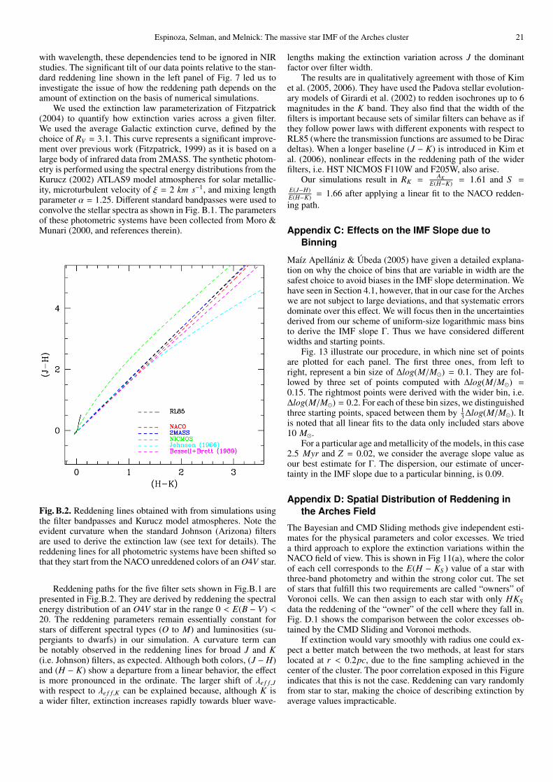
Espinoza, Selman, and Melnick: The massive star IMF of the Arches cluster 21
with wavelength, these dependencies tend to be ignored in NIRstudies. The significant tilt of our data points relative to the stan-dard reddening line shown in the left panel of Fig. 7 led us toinvestigate the issue of how the reddening path depends on theamount of extinction on the basis of numerical simulations.
We used the extinction law parameterization of Fitzpatrick(2004) to quantify how extinction varies across a given filter.We used the average Galactic extinction curve, defined by thechoice of RV = 3.1. This curve represents a significant improve-ment over previous work (Fitzpatrick, 1999) as it is based on alarge body of infrared data from 2MASS. The synthetic photom-etry is performed using the spectral energy distributions from theKurucz (2002) ATLAS9 model atmospheres for solar metallic-ity, microturbulent velocity of ξ = 2 km s−1, and mixing lengthparameter α = 1.25. Different standard bandpasses were used toconvolve the stellar spectra as shown in Fig. B.1. The parametersof these photometric systems have been collected from Moro &Munari (2000, and references therein).
Fig. B.2. Reddening lines obtained with from simulations usingthe filter bandpasses and Kurucz model atmospheres. Note theevident curvature when the standard Johnson (Arizona) filtersare used to derive the extinction law (see text for details). Thereddening lines for all photometric systems have been shifted sothat they start from the NACO unreddened colors of an O4V star.
Reddening paths for the five filter sets shown in Fig.B.1 arepresented in Fig.B.2. They are derived by reddening the spectralenergy distribution of an O4V star in the range 0 < E(B − V) <20. The reddening parameters remain essentially constant forstars of different spectral types (O to M) and luminosities (su-pergiants to dwarfs) in our simulation. A curvature term canbe notably observed in the reddening lines for broad J and K(i.e. Johnson) filters, as expected. Although both colors, (J − H)and (H − K) show a departure from a linear behavior, the effectis more pronounced in the ordinate. The larger shift of λe f f ,Jwith respect to λe f f ,K can be explained because, although K isa wider filter, extinction increases rapidly towards bluer wave-
lengths making the extinction variation across J the dominantfactor over filter width.
The results are in qualitatively agreement with those of Kimet al. (2005, 2006). They have used the Padova stellar evolution-ary models of Girardi et al. (2002) to redden isochrones up to 6magnitudes in the K band. They also find that the width of thefilters is important because sets of similar filters can behave as ifthey follow power laws with different exponents with respect toRL85 (where the transmission functions are assumed to be Diracdeltas). When a longer baseline (J − K) is introduced in Kim etal. (2006), nonlinear effects in the reddening path of the widerfilters, i.e. HST NICMOS F110W and F205W, also arise.
Our simulations result in RK = AKE(H−K) = 1.61 and S =
E(J−H)E(H−K) = 1.66 after applying a linear fit to the NACO redden-ing path.
Appendix C: Effects on the IMF Slope due toBinning
Maız Apellaniz & Ubeda (2005) have given a detailed explana-tion on why the choice of bins that are variable in width are thesafest choice to avoid biases in the IMF slope determination. Wehave seen in Section 4.1, however, that in our case for the Archeswe are not subject to large deviations, and that systematic errorsdominate over this effect. We will focus then in the uncertaintiesderived from our scheme of uniform-size logarithmic mass binsto derive the IMF slope Γ. Thus we have considered differentwidths and starting points.
Fig. 13 illustrate our procedure, in which nine set of pointsare plotted for each panel. The first three ones, from left toright, represent a bin size of ∆log(M/M�) = 0.1. They are fol-lowed by three set of points computed with ∆log(M/M�) =0.15. The rightmost points were derived with the wider bin, i.e.∆log(M/M�) = 0.2. For each of these bin sizes, we distinguishedthree starting points, spaced between them by 1
3 ∆log(M/M�). Itis noted that all linear fits to the data only included stars above10 M�.
For a particular age and metallicity of the models, in this case2.5 Myr and Z = 0.02, we consider the average slope value asour best estimate for Γ. The dispersion, our estimate of uncer-tainty in the IMF slope due to a particular binning, is 0.09.
Appendix D: Spatial Distribution of Reddening inthe Arches Field
The Bayesian and CMD Sliding methods give independent esti-mates for the physical parameters and color excesses. We trieda third approach to explore the extinction variations within theNACO field of view. This is shown in Fig 11(a), where the colorof each cell corresponds to the E(H − KS ) value of a star withthree-band photometry and within the strong color cut. The setof stars that fulfill this two requirements are called “owners” ofVoronoi cells. We can then assign to each star with only HKSdata the reddening of the “owner” of the cell where they fall in.Fig. D.1 shows the comparison between the color excesses ob-tained by the CMD Sliding and Voronoi methods.
If extinction would vary smoothly with radius one could ex-pect a better match between the two methods, at least for starslocated at r < 0.2pc, due to the fine sampling achieved in thecenter of the cluster. The poor correlation exposed in this Figureindicates that this is not the case. Reddening can vary randomlyfrom star to star, making the choice of describing extinction byaverage values impracticable.
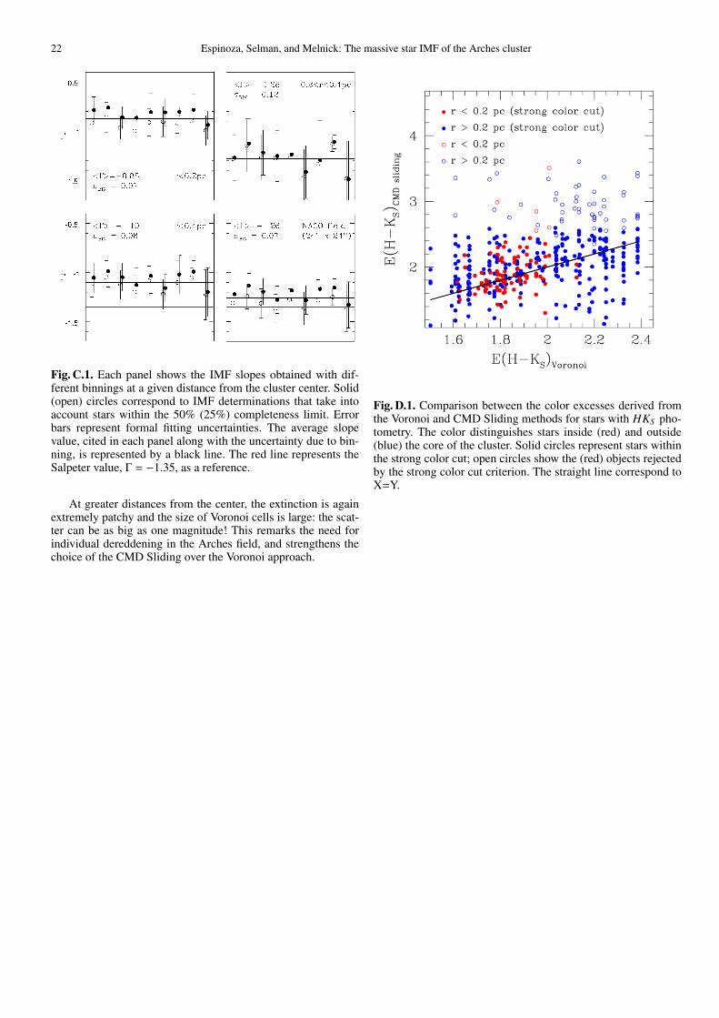
22 Espinoza, Selman, and Melnick: The massive star IMF of the Arches cluster
Fig. C.1. Each panel shows the IMF slopes obtained with dif-ferent binnings at a given distance from the cluster center. Solid(open) circles correspond to IMF determinations that take intoaccount stars within the 50% (25%) completeness limit. Errorbars represent formal fitting uncertainties. The average slopevalue, cited in each panel along with the uncertainty due to bin-ning, is represented by a black line. The red line represents theSalpeter value, Γ = −1.35, as a reference.
At greater distances from the center, the extinction is againextremely patchy and the size of Voronoi cells is large: the scat-ter can be as big as one magnitude! This remarks the need forindividual dereddening in the Arches field, and strengthens thechoice of the CMD Sliding over the Voronoi approach.
Fig. D.1. Comparison between the color excesses derived fromthe Voronoi and CMD Sliding methods for stars with HKS pho-tometry. The color distinguishes stars inside (red) and outside(blue) the core of the cluster. Solid circles represent stars withinthe strong color cut; open circles show the (red) objects rejectedby the strong color cut criterion. The straight line correspond toX=Y.

Espinoza, Selman, and Melnick: The massive star IMF of the Arches cluster, Online Material p 1
Online Material
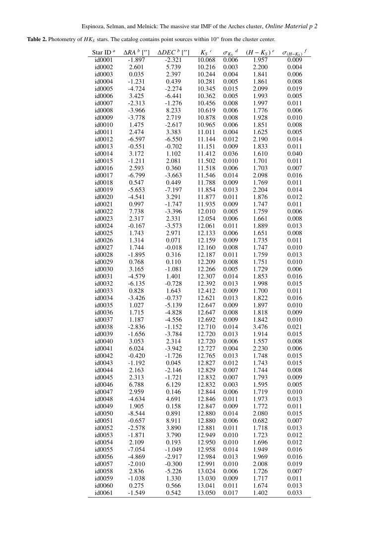
Espinoza, Selman, and Melnick: The massive star IMF of the Arches cluster, Online Material p 2
Table 2. Photometry of HKS stars. The catalog contains point sources within 10′′ from the cluster center.
Star ID a ∆RA b [′′] ∆DEC b [′′] KSc σKS
d (H − KS ) e σ(H−KS )f
id0001 -1.897 -2.321 10.068 0.006 1.957 0.009id0002 2.601 5.739 10.216 0.003 2.200 0.004id0003 0.035 2.397 10.244 0.004 1.841 0.006id0004 -1.231 0.439 10.281 0.005 1.861 0.008id0005 -4.724 -2.274 10.345 0.015 2.099 0.019id0006 3.425 -6.441 10.362 0.005 1.993 0.005id0007 -2.313 -1.276 10.456 0.008 1.997 0.011id0008 -3.966 8.233 10.619 0.006 1.776 0.006id0009 -3.778 2.719 10.878 0.008 1.928 0.010id0010 1.475 -2.617 10.965 0.006 1.851 0.008id0011 2.474 3.383 11.011 0.004 1.625 0.005id0012 -6.597 -6.550 11.144 0.012 2.190 0.014id0013 -0.551 -0.702 11.151 0.009 1.833 0.011id0014 3.172 1.102 11.412 0.036 1.610 0.040id0015 -1.211 2.081 11.502 0.010 1.701 0.011id0016 2.593 0.360 11.518 0.006 1.703 0.007id0017 -6.799 -3.663 11.546 0.014 2.098 0.016id0018 0.547 0.449 11.788 0.009 1.769 0.011id0019 -5.653 -7.197 11.854 0.013 2.204 0.014id0020 -4.541 3.291 11.877 0.011 1.876 0.012id0021 0.997 -1.747 11.935 0.009 1.747 0.011id0022 7.738 -3.396 12.010 0.005 1.759 0.006id0023 2.317 2.331 12.054 0.006 1.661 0.008id0024 -0.167 -3.573 12.061 0.011 1.889 0.013id0025 1.743 2.971 12.133 0.006 1.651 0.008id0026 1.314 0.071 12.159 0.009 1.735 0.011id0027 1.744 -0.018 12.160 0.008 1.747 0.010id0028 -1.895 0.316 12.187 0.011 1.759 0.013id0029 0.768 0.110 12.209 0.008 1.751 0.010id0030 3.165 -1.081 12.266 0.005 1.729 0.006id0031 -4.579 1.401 12.307 0.014 1.853 0.016id0032 -6.135 -0.728 12.392 0.013 1.998 0.015id0033 0.828 1.643 12.412 0.009 1.700 0.011id0034 -3.426 -0.737 12.621 0.013 1.822 0.016id0035 1.027 -5.139 12.647 0.009 1.897 0.010id0036 1.715 -4.828 12.647 0.008 1.818 0.009id0037 1.187 -4.556 12.692 0.009 1.842 0.010id0038 -2.836 -1.152 12.710 0.014 3.476 0.021id0039 -1.656 -3.784 12.720 0.013 1.914 0.015id0040 3.053 2.314 12.720 0.006 1.557 0.008id0041 6.024 -3.942 12.727 0.004 2.230 0.006id0042 -0.420 -1.726 12.765 0.013 1.748 0.015id0043 -1.192 0.045 12.827 0.012 1.743 0.015id0044 2.163 -2.146 12.829 0.007 1.744 0.008id0045 2.313 -1.721 12.832 0.007 1.793 0.009id0046 6.788 6.129 12.832 0.003 1.595 0.005id0047 2.959 0.146 12.844 0.006 1.719 0.010id0048 -4.634 4.691 12.846 0.011 1.973 0.013id0049 1.905 0.158 12.847 0.009 1.772 0.011id0050 -8.544 0.891 12.880 0.014 2.080 0.015id0051 -0.657 8.911 12.880 0.006 0.682 0.007id0052 -2.578 3.890 12.881 0.011 1.718 0.013id0053 -1.871 3.790 12.949 0.010 1.723 0.012id0054 2.109 0.193 12.950 0.010 1.696 0.012id0055 -7.054 -1.049 12.958 0.014 1.949 0.016id0056 -4.869 -2.917 12.984 0.013 1.969 0.016id0057 -2.010 -0.300 12.991 0.010 2.008 0.019id0058 2.836 -5.226 13.024 0.006 1.726 0.007id0059 -1.038 1.330 13.030 0.009 1.717 0.011id0060 0.275 0.566 13.041 0.011 1.674 0.013id0061 -1.549 0.542 13.050 0.017 1.402 0.033
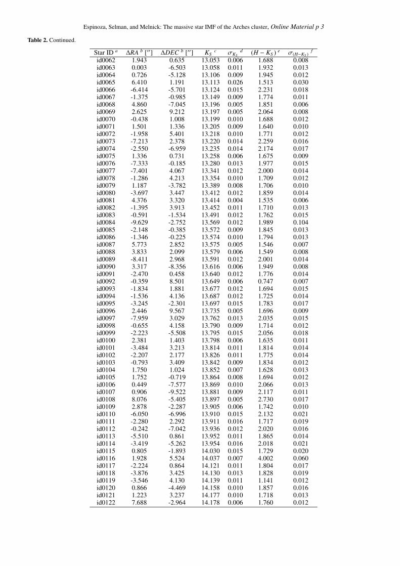
Espinoza, Selman, and Melnick: The massive star IMF of the Arches cluster, Online Material p 3
Table 2. Continued.
Star ID a ∆RA b [′′] ∆DEC b [′′] KSc σKS
d (H − KS ) e σ(H−KS )f
id0062 1.943 0.635 13.053 0.006 1.688 0.008id0063 0.003 -6.503 13.058 0.011 1.932 0.013id0064 0.726 -5.128 13.106 0.009 1.945 0.012id0065 6.410 1.191 13.113 0.026 1.513 0.030id0066 -6.414 -5.701 13.124 0.015 2.231 0.018id0067 -1.375 -0.985 13.149 0.009 1.774 0.011id0068 4.860 -7.045 13.196 0.005 1.851 0.006id0069 2.625 9.212 13.197 0.005 2.064 0.008id0070 -0.438 1.008 13.199 0.010 1.688 0.012id0071 1.501 1.336 13.205 0.009 1.640 0.010id0072 -1.958 5.401 13.218 0.010 1.771 0.012id0073 -7.213 2.378 13.220 0.014 2.259 0.016id0074 -2.550 -6.959 13.235 0.014 2.174 0.017id0075 1.336 0.731 13.258 0.006 1.675 0.009id0076 -7.333 -0.185 13.280 0.013 1.977 0.015id0077 -7.401 4.067 13.341 0.012 2.000 0.014id0078 -1.286 4.213 13.354 0.010 1.709 0.012id0079 1.187 -3.782 13.389 0.008 1.706 0.010id0080 -3.697 3.447 13.412 0.012 1.859 0.014id0081 4.376 3.320 13.414 0.004 1.535 0.006id0082 -1.395 3.913 13.452 0.011 1.710 0.013id0083 -0.591 -1.534 13.491 0.012 1.762 0.015id0084 -9.629 -2.752 13.569 0.012 1.989 0.104id0085 -2.148 -0.385 13.572 0.009 1.845 0.013id0086 -1.346 -0.225 13.574 0.010 1.794 0.013id0087 5.773 2.852 13.575 0.005 1.546 0.007id0088 3.833 2.099 13.579 0.006 1.549 0.008id0089 -8.411 2.968 13.591 0.012 2.001 0.014id0090 3.317 -8.356 13.616 0.006 1.949 0.008id0091 -2.470 0.458 13.640 0.012 1.776 0.014id0092 -0.359 8.501 13.649 0.006 0.747 0.007id0093 -1.834 1.881 13.677 0.012 1.694 0.015id0094 -1.536 4.136 13.687 0.012 1.725 0.014id0095 -3.245 -2.301 13.697 0.015 1.783 0.017id0096 2.446 9.567 13.735 0.005 1.696 0.009id0097 -7.959 3.029 13.762 0.013 2.035 0.015id0098 -0.655 4.158 13.790 0.009 1.714 0.012id0099 -2.223 -5.508 13.795 0.015 2.056 0.018id0100 2.381 1.403 13.798 0.006 1.635 0.011id0101 -3.484 3.213 13.814 0.011 1.814 0.014id0102 -2.207 2.177 13.826 0.011 1.775 0.014id0103 -0.793 3.409 13.842 0.009 1.834 0.012id0104 1.750 1.024 13.852 0.007 1.628 0.013id0105 1.752 -0.719 13.864 0.008 1.694 0.012id0106 0.449 -7.577 13.869 0.010 2.066 0.013id0107 0.906 -9.522 13.881 0.009 2.117 0.011id0108 8.076 -5.405 13.897 0.005 2.730 0.017id0109 2.878 -2.287 13.905 0.006 1.742 0.010id0110 -6.050 -6.996 13.910 0.015 2.132 0.021id0111 -2.280 2.292 13.911 0.016 1.717 0.019id0112 -0.242 -7.042 13.936 0.012 2.020 0.016id0113 -5.510 0.861 13.952 0.011 1.865 0.014id0114 -3.419 -5.262 13.954 0.016 2.018 0.021id0115 0.805 -1.893 14.030 0.015 1.729 0.020id0116 1.928 5.524 14.037 0.007 4.002 0.060id0117 -2.224 0.864 14.121 0.011 1.804 0.017id0118 -3.876 3.425 14.130 0.013 1.828 0.019id0119 -3.546 4.130 14.139 0.011 1.141 0.012id0120 0.866 -4.469 14.158 0.010 1.857 0.016id0121 1.223 3.237 14.177 0.010 1.718 0.013id0122 7.688 -2.964 14.178 0.006 1.760 0.012
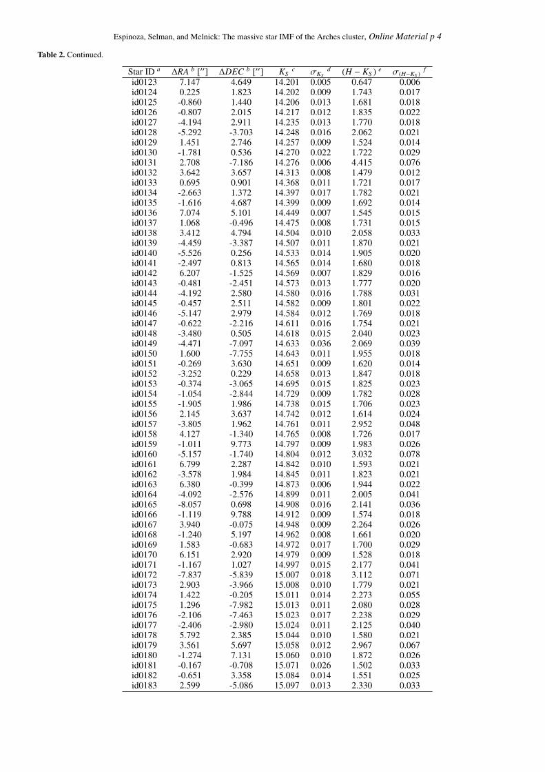
Espinoza, Selman, and Melnick: The massive star IMF of the Arches cluster, Online Material p 4
Table 2. Continued.
Star ID a ∆RA b [′′] ∆DEC b [′′] KSc σKS
d (H − KS ) e σ(H−KS )f
id0123 7.147 4.649 14.201 0.005 0.647 0.006id0124 0.225 1.823 14.202 0.009 1.743 0.017id0125 -0.860 1.440 14.206 0.013 1.681 0.018id0126 -0.807 2.015 14.217 0.012 1.835 0.022id0127 -4.194 2.911 14.235 0.013 1.770 0.018id0128 -5.292 -3.703 14.248 0.016 2.062 0.021id0129 1.451 2.746 14.257 0.009 1.524 0.014id0130 -1.781 0.536 14.270 0.022 1.722 0.029id0131 2.708 -7.186 14.276 0.006 4.415 0.076id0132 3.642 3.657 14.313 0.008 1.479 0.012id0133 0.695 0.901 14.368 0.011 1.721 0.017id0134 -2.663 1.372 14.397 0.017 1.782 0.021id0135 -1.616 4.687 14.399 0.009 1.692 0.014id0136 7.074 5.101 14.449 0.007 1.545 0.015id0137 1.068 -0.496 14.475 0.008 1.731 0.015id0138 3.412 4.794 14.504 0.010 2.058 0.033id0139 -4.459 -3.387 14.507 0.011 1.870 0.021id0140 -5.526 0.256 14.533 0.014 1.905 0.020id0141 -2.497 0.813 14.565 0.014 1.680 0.018id0142 6.207 -1.525 14.569 0.007 1.829 0.016id0143 -0.481 -2.451 14.573 0.013 1.777 0.020id0144 -4.192 2.580 14.580 0.016 1.788 0.031id0145 -0.457 2.511 14.582 0.009 1.801 0.022id0146 -5.147 2.979 14.584 0.012 1.769 0.018id0147 -0.622 -2.216 14.611 0.016 1.754 0.021id0148 -3.480 0.505 14.618 0.015 2.040 0.023id0149 -4.471 -7.097 14.633 0.036 2.069 0.039id0150 1.600 -7.755 14.643 0.011 1.955 0.018id0151 -0.269 3.630 14.651 0.009 1.620 0.014id0152 -3.252 0.229 14.658 0.013 1.847 0.018id0153 -0.374 -3.065 14.695 0.015 1.825 0.023id0154 -1.054 -2.844 14.729 0.009 1.782 0.028id0155 -1.905 1.986 14.738 0.015 1.706 0.023id0156 2.145 3.637 14.742 0.012 1.614 0.024id0157 -3.805 1.962 14.761 0.011 2.952 0.048id0158 4.127 -1.340 14.765 0.008 1.726 0.017id0159 -1.011 9.773 14.797 0.009 1.983 0.026id0160 -5.157 -1.740 14.804 0.012 3.032 0.078id0161 6.799 2.287 14.842 0.010 1.593 0.021id0162 -3.578 1.984 14.845 0.011 1.823 0.021id0163 6.380 -0.399 14.873 0.006 1.944 0.022id0164 -4.092 -2.576 14.899 0.011 2.005 0.041id0165 -8.057 0.698 14.908 0.016 2.141 0.036id0166 -1.119 9.788 14.912 0.009 1.574 0.018id0167 3.940 -0.075 14.948 0.009 2.264 0.026id0168 -1.240 5.197 14.962 0.008 1.661 0.020id0169 1.583 -0.683 14.972 0.017 1.700 0.029id0170 6.151 2.920 14.979 0.009 1.528 0.018id0171 -1.167 1.027 14.997 0.015 2.177 0.041id0172 -7.837 -5.839 15.007 0.018 3.112 0.071id0173 2.903 -3.966 15.008 0.010 1.779 0.021id0174 1.422 -0.205 15.011 0.014 2.273 0.055id0175 1.296 -7.982 15.013 0.011 2.080 0.028id0176 -2.106 -7.463 15.023 0.017 2.238 0.029id0177 -2.406 -2.980 15.024 0.011 2.125 0.040id0178 5.792 2.385 15.044 0.010 1.580 0.021id0179 3.561 5.697 15.058 0.012 2.967 0.067id0180 -1.274 7.131 15.060 0.010 1.872 0.026id0181 -0.167 -0.708 15.071 0.026 1.502 0.033id0182 -0.651 3.358 15.084 0.014 1.551 0.025id0183 2.599 -5.086 15.097 0.013 2.330 0.033
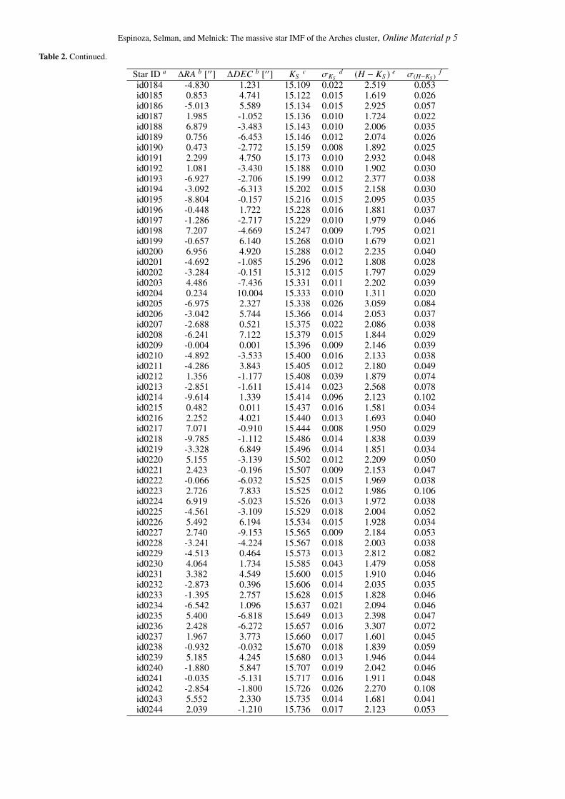
Espinoza, Selman, and Melnick: The massive star IMF of the Arches cluster, Online Material p 5
Table 2. Continued.
Star ID a ∆RA b [′′] ∆DEC b [′′] KSc σKS
d (H − KS ) e σ(H−KS )f
id0184 -4.830 1.231 15.109 0.022 2.519 0.053id0185 0.853 4.741 15.122 0.015 1.619 0.026id0186 -5.013 5.589 15.134 0.015 2.925 0.057id0187 1.985 -1.052 15.136 0.010 1.724 0.022id0188 6.879 -3.483 15.143 0.010 2.006 0.035id0189 0.756 -6.453 15.146 0.012 2.074 0.026id0190 0.473 -2.772 15.159 0.008 1.892 0.025id0191 2.299 4.750 15.173 0.010 2.932 0.048id0192 1.081 -3.430 15.188 0.010 1.902 0.030id0193 -6.927 -2.706 15.199 0.012 2.377 0.038id0194 -3.092 -6.313 15.202 0.015 2.158 0.030id0195 -8.804 -0.157 15.216 0.015 2.095 0.035id0196 -0.448 1.722 15.228 0.016 1.881 0.037id0197 -1.286 -2.717 15.229 0.010 1.979 0.046id0198 7.207 -4.669 15.247 0.009 1.795 0.021id0199 -0.657 6.140 15.268 0.010 1.679 0.021id0200 6.956 4.920 15.288 0.012 2.235 0.040id0201 -4.692 -1.085 15.296 0.012 1.808 0.028id0202 -3.284 -0.151 15.312 0.015 1.797 0.029id0203 4.486 -7.436 15.331 0.011 2.202 0.039id0204 0.234 10.004 15.333 0.010 1.311 0.020id0205 -6.975 2.327 15.338 0.026 3.059 0.084id0206 -3.042 5.744 15.366 0.014 2.053 0.037id0207 -2.688 0.521 15.375 0.022 2.086 0.038id0208 -6.241 7.122 15.379 0.015 1.844 0.029id0209 -0.004 0.001 15.396 0.009 2.146 0.039id0210 -4.892 -3.533 15.400 0.016 2.133 0.038id0211 -4.286 3.843 15.405 0.012 2.180 0.049id0212 1.356 -1.177 15.408 0.039 1.879 0.074id0213 -2.851 -1.611 15.414 0.023 2.568 0.078id0214 -9.614 1.339 15.414 0.096 2.123 0.102id0215 0.482 0.011 15.437 0.016 1.581 0.034id0216 2.252 4.021 15.440 0.013 1.693 0.040id0217 7.071 -0.910 15.444 0.008 1.950 0.029id0218 -9.785 -1.112 15.486 0.014 1.838 0.039id0219 -3.328 6.849 15.496 0.014 1.851 0.034id0220 5.155 -3.139 15.502 0.012 2.209 0.050id0221 2.423 -0.196 15.507 0.009 2.153 0.047id0222 -0.066 -6.032 15.525 0.015 1.969 0.038id0223 2.726 7.833 15.525 0.012 1.986 0.106id0224 6.919 -5.023 15.526 0.013 1.972 0.038id0225 -4.561 -3.109 15.529 0.018 2.004 0.052id0226 5.492 6.194 15.534 0.015 1.928 0.034id0227 2.740 -9.153 15.565 0.009 2.184 0.053id0228 -3.241 -4.224 15.567 0.018 2.003 0.038id0229 -4.513 0.464 15.573 0.013 2.812 0.082id0230 4.064 1.734 15.585 0.043 1.479 0.058id0231 3.382 4.549 15.600 0.015 1.910 0.046id0232 -2.873 0.396 15.606 0.014 2.035 0.035id0233 -1.395 2.757 15.628 0.015 1.828 0.046id0234 -6.542 1.096 15.637 0.021 2.094 0.046id0235 5.400 -6.818 15.649 0.013 2.398 0.047id0236 2.428 -6.272 15.657 0.016 3.307 0.072id0237 1.967 3.773 15.660 0.017 1.601 0.045id0238 -0.932 -0.032 15.670 0.018 1.839 0.059id0239 5.185 4.245 15.680 0.013 1.946 0.044id0240 -1.880 5.847 15.707 0.019 2.042 0.046id0241 -0.035 -5.131 15.717 0.016 1.911 0.048id0242 -2.854 -1.800 15.726 0.026 2.270 0.108id0243 5.552 2.330 15.735 0.014 1.681 0.041id0244 2.039 -1.210 15.736 0.017 2.123 0.053
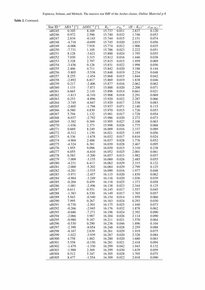
Espinoza, Selman, and Melnick: The massive star IMF of the Arches cluster, Online Material p 6
Table 2. Continued.
Star ID a ∆RA b [′′] ∆DEC b [′′] KSc σKS
d (H − KS ) e σ(H−KS )f
id0245 0.105 8.169 15.737 0.011 2.837 0.120id0246 0.972 2.596 15.740 0.032 1.748 0.053id0247 2.834 -0.143 15.744 0.015 2.151 0.074id0248 -4.716 -0.699 15.745 0.020 2.033 0.056id0249 -6.006 7.918 15.774 0.012 1.906 0.035id0250 -7.731 1.105 15.786 0.023 2.222 0.051id0251 8.128 -3.621 15.800 0.024 1.795 0.055id0252 7.030 3.315 15.812 0.016 1.446 0.038id0253 3.328 2.797 15.815 0.015 1.959 0.069id0254 -3.436 0.126 15.831 0.022 1.998 0.056id0255 2.466 4.711 15.842 0.020 3.188 0.144id0256 -5.805 -5.538 15.848 0.019 2.234 0.048id0257 8.255 -1.454 15.868 0.015 1.844 0.042id0258 -2.892 6.817 15.869 0.019 1.838 0.046id0259 0.217 -2.406 15.877 0.016 2.062 0.062id0260 1.133 -7.871 15.888 0.020 2.208 0.071id0261 6.665 2.110 15.896 0.014 0.661 0.021id0262 -1.813 -6.310 15.908 0.018 2.291 0.069id0263 0.253 -8.896 15.920 0.022 2.287 0.066id0264 -3.745 -6.847 15.929 0.017 2.538 0.083id0265 -2.605 -1.798 15.937 0.071 2.140 0.115id0266 6.580 4.830 15.970 0.015 1.726 0.053id0267 5.794 1.132 15.981 0.017 1.728 0.054id0268 -6.037 -2.792 15.986 0.020 2.272 0.073id0269 -3.382 0.369 15.995 0.027 2.108 0.063id0270 -1.036 2.373 15.998 0.026 1.775 0.068id0271 0.669 8.249 16.009 0.016 2.337 0.089id0272 -0.312 1.159 16.021 0.025 1.185 0.056id0273 6.336 -1.678 16.032 0.017 0.816 0.024id0274 -4.904 2.488 16.037 0.028 1.776 0.052id0275 -4.324 6.381 16.039 0.028 2.467 0.095id0276 1.955 9.096 16.039 0.015 3.310 0.238id0277 6.055 -6.810 16.052 0.025 2.001 0.061id0278 6.583 -5.200 16.057 0.015 1.982 0.057id0279 -7.009 -3.155 16.060 0.026 2.485 0.055id0280 -4.231 6.413 16.062 0.029 2.315 0.122id0281 -2.000 -5.202 16.084 0.029 2.799 0.125id0282 -4.281 -3.535 16.090 0.016 1.977 0.048id0283 -5.971 -2.457 16.115 0.020 1.830 0.062id0284 -4.984 -3.249 16.116 0.020 1.036 0.039id0285 -0.204 0.459 16.118 0.025 1.373 0.058id0286 -1.081 -2.496 16.138 0.023 2.344 0.125id0287 6.611 0.551 16.145 0.017 1.557 0.045id0288 -1.383 6.530 16.149 0.017 1.765 0.057id0289 5.943 -0.540 16.154 0.014 1.959 0.066id0290 7.995 0.267 16.163 0.024 0.293 0.030id0291 -0.730 -2.501 16.175 0.025 1.440 0.073id0292 -0.266 -2.945 16.176 0.032 1.878 0.062id0293 -0.686 -7.271 16.196 0.024 2.392 0.090id0294 -2.066 3.987 16.204 0.026 2.114 0.090id0295 -0.980 9.187 16.211 0.021 1.570 0.064id0296 -0.530 0.290 16.236 0.046 1.896 0.104id0297 -2.390 -8.054 16.248 0.028 2.259 0.088id0298 -8.167 2.639 16.261 0.029 1.919 0.075id0299 -1.022 -3.939 16.267 0.020 2.328 0.084id0300 4.758 1.882 16.280 0.020 1.680 0.063id0301 5.558 -0.150 16.281 0.021 2.418 0.094id0302 -1.479 -1.330 16.299 0.042 1.943 0.132id0303 -1.988 2.369 16.299 0.030 1.639 0.059id0304 0.512 5.347 16.305 0.028 1.705 0.075id0305 8.477 -1.554 16.309 0.022 2.018 0.090
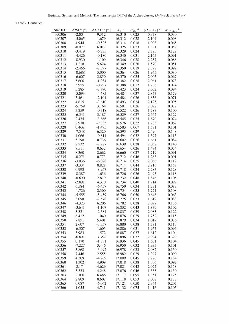
Espinoza, Selman, and Melnick: The massive star IMF of the Arches cluster, Online Material p 7
Table 2. Continued.
Star ID a ∆RA b [′′] ∆DEC b [′′] KSc σKS
d (H − KS ) e σ(H−KS )f
id0306 -2.004 9.312 16.310 0.025 0.378 0.030id0307 -5.065 1.679 16.312 0.028 2.104 0.098id0308 4.944 -0.525 16.314 0.018 1.908 0.065id0309 -0.977 6.017 16.325 0.023 1.881 0.059id0310 -3.419 -6.735 16.329 0.024 2.785 0.128id0311 -4.426 -0.180 16.340 0.031 2.165 0.091id0312 -8.930 1.109 16.346 0.028 2.257 0.088id0313 1.218 5.624 16.349 0.020 1.570 0.051id0314 -2.466 -7.897 16.350 0.019 2.398 0.099id0315 -0.688 5.000 16.364 0.026 1.945 0.080id0316 -6.607 2.850 16.370 0.025 2.005 0.067id0317 5.600 -1.934 16.382 0.028 2.061 0.073id0318 5.955 -0.797 16.388 0.017 1.736 0.074id0319 5.285 -3.970 16.423 0.024 2.052 0.094id0320 -5.093 -4.685 16.484 0.037 2.857 0.179id0321 3.461 -2.101 16.484 0.026 1.856 0.071id0322 4.615 -3.610 16.493 0.024 2.125 0.095id0323 -5.759 3.164 16.501 0.026 2.092 0.077id0324 3.259 -0.318 16.522 0.026 1.787 0.100id0325 -6.541 3.187 16.529 0.027 2.662 0.127id0326 2.435 -3.666 16.545 0.025 1.670 0.074id0327 2.978 -9.335 16.576 0.022 1.783 0.067id0328 0.466 -1.495 16.583 0.067 1.581 0.101id0329 -7.548 6.320 16.593 0.029 2.490 0.148id0330 4.066 -0.814 16.594 0.032 1.597 0.115id0331 5.298 0.736 16.602 0.026 1.661 0.084id0332 2.232 -2.787 16.639 0.028 2.052 0.140id0333 7.511 0.632 16.654 0.026 1.474 0.074id0334 8.360 2.662 16.660 0.027 1.719 0.091id0335 -0.271 0.773 16.712 0.046 1.263 0.091id0336 -3.036 -6.028 16.714 0.025 2.066 0.112id0337 -3.334 8.828 16.714 0.044 2.916 0.157id0338 0.998 -8.957 16.718 0.024 2.283 0.128id0339 -8.387 1.636 16.726 0.026 2.495 0.118id0340 -8.690 2.879 16.732 0.048 1.846 0.105id0341 -2.891 4.370 16.734 0.040 1.714 0.092id0342 6.584 -6.457 16.750 0.034 1.731 0.083id0343 -1.726 2.300 16.754 0.035 1.721 0.108id0344 -5.555 -5.459 16.766 0.050 0.648 0.063id0345 3.098 -2.578 16.775 0.033 1.619 0.088id0346 -4.323 6.206 16.782 0.028 2.097 0.136id0347 -3.641 -1.107 16.832 0.043 1.839 0.102id0348 3.321 -2.584 16.837 0.039 2.083 0.122id0349 8.412 1.040 16.876 0.029 1.752 0.115id0350 7.851 5.401 16.879 0.034 1.017 0.076id0351 2.607 -3.357 16.880 0.038 1.771 0.113id0352 -6.507 1.605 16.886 0.031 1.957 0.096id0353 3.983 1.572 16.887 0.037 1.612 0.104id0354 -6.891 3.352 16.896 0.032 2.994 0.329id0355 0.170 -1.331 16.936 0.045 1.631 0.104id0356 -7.227 3.446 16.950 0.032 1.935 0.101id0357 3.868 -3.492 16.978 0.033 2.082 0.150id0358 7.446 2.555 16.982 0.029 1.397 0.090id0359 4.309 -4.269 17.009 0.045 2.226 0.184id0360 1.302 4.909 17.018 0.038 1.306 0.092id0361 -2.174 4.629 17.021 0.042 2.022 0.158id0362 3.333 4.248 17.076 0.046 1.355 0.130id0363 2.100 6.486 17.117 0.095 1.351 0.125id0364 2.809 8.602 17.118 0.053 2.008 0.178id0365 0.087 -6.062 17.121 0.050 2.344 0.207id0366 1.055 4.741 17.132 0.075 1.416 0.105
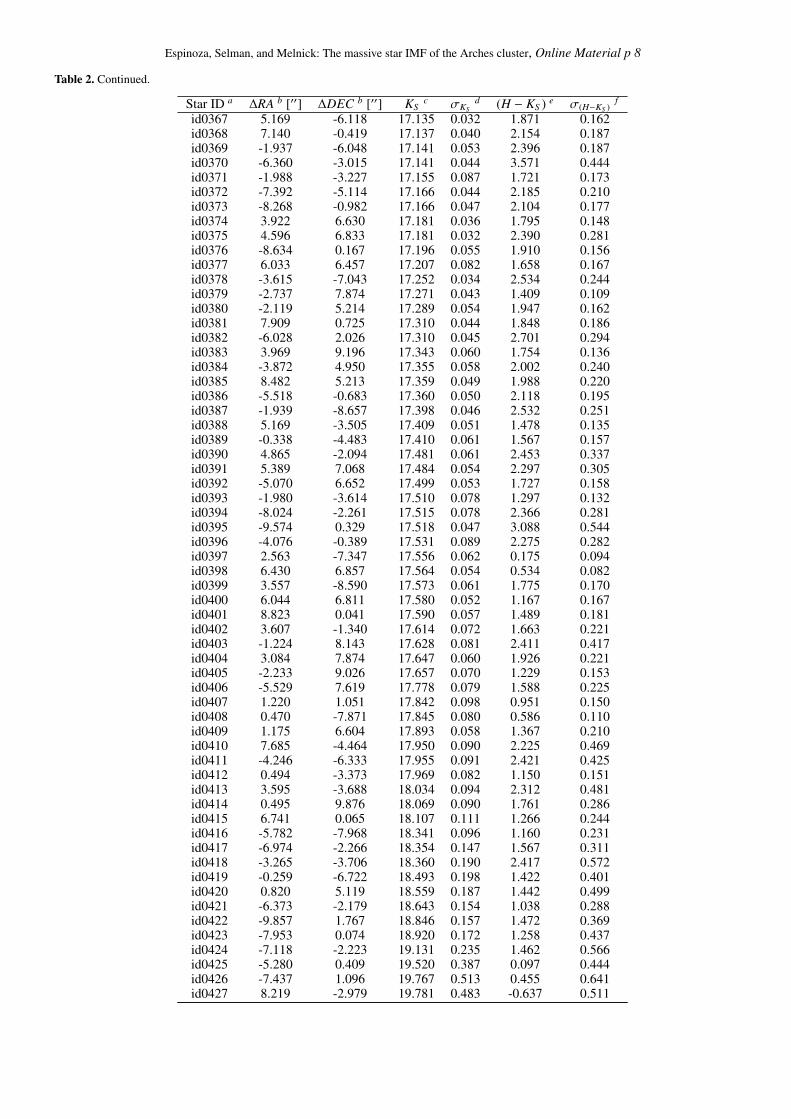
Espinoza, Selman, and Melnick: The massive star IMF of the Arches cluster, Online Material p 8
Table 2. Continued.
Star ID a ∆RA b [′′] ∆DEC b [′′] KSc σKS
d (H − KS ) e σ(H−KS )f
id0367 5.169 -6.118 17.135 0.032 1.871 0.162id0368 7.140 -0.419 17.137 0.040 2.154 0.187id0369 -1.937 -6.048 17.141 0.053 2.396 0.187id0370 -6.360 -3.015 17.141 0.044 3.571 0.444id0371 -1.988 -3.227 17.155 0.087 1.721 0.173id0372 -7.392 -5.114 17.166 0.044 2.185 0.210id0373 -8.268 -0.982 17.166 0.047 2.104 0.177id0374 3.922 6.630 17.181 0.036 1.795 0.148id0375 4.596 6.833 17.181 0.032 2.390 0.281id0376 -8.634 0.167 17.196 0.055 1.910 0.156id0377 6.033 6.457 17.207 0.082 1.658 0.167id0378 -3.615 -7.043 17.252 0.034 2.534 0.244id0379 -2.737 7.874 17.271 0.043 1.409 0.109id0380 -2.119 5.214 17.289 0.054 1.947 0.162id0381 7.909 0.725 17.310 0.044 1.848 0.186id0382 -6.028 2.026 17.310 0.045 2.701 0.294id0383 3.969 9.196 17.343 0.060 1.754 0.136id0384 -3.872 4.950 17.355 0.058 2.002 0.240id0385 8.482 5.213 17.359 0.049 1.988 0.220id0386 -5.518 -0.683 17.360 0.050 2.118 0.195id0387 -1.939 -8.657 17.398 0.046 2.532 0.251id0388 5.169 -3.505 17.409 0.051 1.478 0.135id0389 -0.338 -4.483 17.410 0.061 1.567 0.157id0390 4.865 -2.094 17.481 0.061 2.453 0.337id0391 5.389 7.068 17.484 0.054 2.297 0.305id0392 -5.070 6.652 17.499 0.053 1.727 0.158id0393 -1.980 -3.614 17.510 0.078 1.297 0.132id0394 -8.024 -2.261 17.515 0.078 2.366 0.281id0395 -9.574 0.329 17.518 0.047 3.088 0.544id0396 -4.076 -0.389 17.531 0.089 2.275 0.282id0397 2.563 -7.347 17.556 0.062 0.175 0.094id0398 6.430 6.857 17.564 0.054 0.534 0.082id0399 3.557 -8.590 17.573 0.061 1.775 0.170id0400 6.044 6.811 17.580 0.052 1.167 0.167id0401 8.823 0.041 17.590 0.057 1.489 0.181id0402 3.607 -1.340 17.614 0.072 1.663 0.221id0403 -1.224 8.143 17.628 0.081 2.411 0.417id0404 3.084 7.874 17.647 0.060 1.926 0.221id0405 -2.233 9.026 17.657 0.070 1.229 0.153id0406 -5.529 7.619 17.778 0.079 1.588 0.225id0407 1.220 1.051 17.842 0.098 0.951 0.150id0408 0.470 -7.871 17.845 0.080 0.586 0.110id0409 1.175 6.604 17.893 0.058 1.367 0.210id0410 7.685 -4.464 17.950 0.090 2.225 0.469id0411 -4.246 -6.333 17.955 0.091 2.421 0.425id0412 0.494 -3.373 17.969 0.082 1.150 0.151id0413 3.595 -3.688 18.034 0.094 2.312 0.481id0414 0.495 9.876 18.069 0.090 1.761 0.286id0415 6.741 0.065 18.107 0.111 1.266 0.244id0416 -5.782 -7.968 18.341 0.096 1.160 0.231id0417 -6.974 -2.266 18.354 0.147 1.567 0.311id0418 -3.265 -3.706 18.360 0.190 2.417 0.572id0419 -0.259 -6.722 18.493 0.198 1.422 0.401id0420 0.820 5.119 18.559 0.187 1.442 0.499id0421 -6.373 -2.179 18.643 0.154 1.038 0.288id0422 -9.857 1.767 18.846 0.157 1.472 0.369id0423 -7.953 0.074 18.920 0.172 1.258 0.437id0424 -7.118 -2.223 19.131 0.235 1.462 0.566id0425 -5.280 0.409 19.520 0.387 0.097 0.444id0426 -7.437 1.096 19.767 0.513 0.455 0.641id0427 8.219 -2.979 19.781 0.483 -0.637 0.511

Espinoza, Selman, and Melnick: The massive star IMF of the Arches cluster, Online Material p 9
a In this catalog the star ID is designated by sorting the data in order of increasing KS magnitude.b Positions with respect to α = 17h 45m 50.798s, δ = −28◦ 49
′
25.606′′
(J2000).c NACO KS band magnitude.d The 1σ uncertainty in KS .e NACO (H − KS ) color index.f The 1σ uncertainty in (H − KS ).

Espinoza, Selman, and Melnick: The massive star IMF of the Arches cluster, Online Material p 10
Table 3. Photometry of JHKS stars. The catalog contains point sources within 10′′ from the cluster center.
Star ID a ∆RA b [′′] ∆DEC b [′′] KSc σKS
d (H − KS ) e σ(H−KS )f (J − H) g σ(J−H)
h
id0001 -1.897 -2.321 10.068 0.006 1.957 0.009 3.203 0.009id0002 2.601 5.739 10.216 0.003 2.200 0.004 4.048 0.007id0003 0.035 2.397 10.244 0.004 1.841 0.006 3.021 0.006id0004 -1.231 0.439 10.281 0.005 1.861 0.008 3.064 0.007id0005 -4.724 -2.274 10.345 0.015 2.099 0.019 3.418 0.013id0006 3.425 -6.441 10.362 0.005 1.993 0.005 3.220 0.003id0007 -2.313 -1.276 10.456 0.008 1.997 0.011 3.214 0.009id0008 -3.966 8.233 10.619 0.006 1.776 0.006 3.034 0.003id0009 -3.778 2.719 10.878 0.008 1.928 0.010 3.161 0.008id0010 1.475 -2.617 10.965 0.006 1.851 0.008 3.015 0.007id0011 2.474 3.383 11.011 0.004 1.625 0.005 2.830 0.006id0012 -6.597 -6.550 11.144 0.012 2.190 0.014 3.533 0.011id0013 -0.551 -0.702 11.151 0.009 1.833 0.011 3.018 0.009id0014 3.172 1.102 11.412 0.036 1.610 0.040 2.813 0.019id0015 -1.211 2.081 11.502 0.010 1.701 0.011 2.899 0.007id0016 2.593 0.360 11.518 0.006 1.703 0.007 2.896 0.008id0017 -6.799 -3.663 11.546 0.014 2.098 0.016 3.425 0.012id0018 0.547 0.449 11.788 0.009 1.769 0.011 2.993 0.013id0019 -5.653 -7.197 11.854 0.013 2.204 0.014 3.590 0.016id0020 -4.541 3.291 11.877 0.011 1.876 0.012 3.148 0.010id0021 0.997 -1.747 11.935 0.009 1.747 0.011 2.898 0.009id0022 7.738 -3.396 12.010 0.005 1.759 0.006 3.017 0.010id0023 2.317 2.331 12.054 0.006 1.661 0.008 2.813 0.009id0024 -0.167 -3.573 12.061 0.011 1.889 0.013 3.142 0.012id0025 1.743 2.971 12.133 0.006 1.651 0.008 2.765 0.009id0026 1.314 0.071 12.159 0.009 1.735 0.011 2.911 0.011id0027 1.744 -0.018 12.160 0.008 1.747 0.010 2.933 0.011id0028 -1.895 0.316 12.187 0.011 1.759 0.013 2.976 0.013id0029 0.768 0.110 12.209 0.008 1.751 0.010 2.944 0.014id0030 3.165 -1.081 12.266 0.005 1.729 0.006 3.004 0.012id0032 -6.135 -0.728 12.392 0.013 1.998 0.015 3.361 0.021id0033 0.828 1.643 12.412 0.009 1.700 0.011 2.996 0.013id0034 -3.426 -0.737 12.621 0.013 1.822 0.016 3.107 0.019id0035 1.027 -5.139 12.647 0.009 1.897 0.010 3.099 0.015id0036 1.715 -4.828 12.647 0.008 1.818 0.009 3.001 0.015id0037 1.187 -4.556 12.692 0.009 1.842 0.010 3.040 0.021id0039 -1.656 -3.784 12.720 0.013 1.914 0.015 3.230 0.020id0040 3.053 2.314 12.720 0.006 1.557 0.008 2.704 0.012id0041 6.024 -3.942 12.727 0.004 2.230 0.006 4.367 0.075id0042 -0.420 -1.726 12.765 0.013 1.748 0.015 3.037 0.017id0044 2.163 -2.146 12.829 0.007 1.744 0.008 2.921 0.016id0045 2.313 -1.721 12.832 0.007 1.793 0.009 3.113 0.021id0046 6.788 6.129 12.832 0.003 1.595 0.005 2.917 0.020id0047 2.959 0.146 12.844 0.006 1.719 0.010 2.917 0.021id0048 -4.634 4.691 12.846 0.011 1.973 0.013 3.488 0.032id0049 1.905 0.158 12.847 0.009 1.772 0.011 2.947 0.019id0051 -0.657 8.911 12.880 0.006 0.682 0.007 1.167 0.005id0052 -2.578 3.890 12.881 0.011 1.718 0.013 2.975 0.017id0053 -1.871 3.790 12.949 0.010 1.723 0.012 2.941 0.016id0054 2.109 0.193 12.950 0.010 1.696 0.012 2.896 0.018id0056 -4.869 -2.917 12.984 0.013 1.969 0.016 3.334 0.024id0057 -2.010 -0.300 12.991 0.010 2.008 0.019 3.060 0.029id0058 2.836 -5.226 13.024 0.006 1.726 0.007 2.921 0.017id0059 -1.038 1.330 13.030 0.009 1.717 0.011 2.780 0.016id0060 0.275 0.566 13.041 0.011 1.674 0.013 2.978 0.017id0061 -1.549 0.542 13.050 0.017 1.402 0.033 2.842 0.035id0062 1.943 0.635 13.053 0.006 1.688 0.008 3.057 0.025id0063 0.003 -6.503 13.058 0.011 1.932 0.013 3.113 0.029id0064 0.726 -5.128 13.106 0.009 1.945 0.012 3.161 0.029id0065 6.410 1.191 13.113 0.026 1.513 0.030 2.688 0.021id0066 -6.414 -5.701 13.124 0.015 2.231 0.018 3.482 0.051
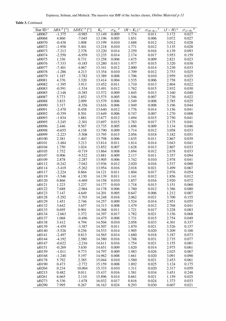
Espinoza, Selman, and Melnick: The massive star IMF of the Arches cluster, Online Material p 11
Table 3. Continued.
Star ID a ∆RA b [′′] ∆DEC b [′′] KSc σKS
d (H − KS ) e σ(H−KS )f (J − H) g σ(J−H)
h
id0067 -1.375 -0.985 13.149 0.009 1.774 0.011 3.172 0.027id0068 4.860 -7.045 13.196 0.005 1.851 0.006 3.072 0.027id0070 -0.438 1.008 13.199 0.010 1.688 0.012 3.012 0.028id0072 -1.958 5.401 13.218 0.010 1.771 0.012 3.135 0.028id0073 -7.213 2.378 13.220 0.014 2.259 0.016 4.139 0.093id0074 -2.550 -6.959 13.235 0.014 2.174 0.017 3.953 0.159id0075 1.336 0.731 13.258 0.006 1.675 0.009 2.821 0.023id0076 -7.333 -0.185 13.280 0.013 1.977 0.015 3.320 0.038id0077 -7.401 4.067 13.341 0.012 2.000 0.014 3.230 0.033id0078 -1.286 4.213 13.354 0.010 1.709 0.012 2.753 0.025id0079 1.187 -3.782 13.389 0.008 1.706 0.010 2.959 0.025id0081 4.376 3.320 13.414 0.004 1.535 0.006 2.758 0.023id0082 -1.395 3.913 13.452 0.011 1.710 0.013 2.804 0.022id0083 -0.591 -1.534 13.491 0.012 1.762 0.015 2.932 0.030id0085 -2.148 -0.385 13.572 0.009 1.845 0.013 3.160 0.040id0087 5.773 2.852 13.575 0.005 1.546 0.007 2.730 0.022id0088 3.833 2.099 13.579 0.006 1.549 0.008 2.785 0.025id0090 3.317 -8.356 13.616 0.006 1.949 0.008 3.196 0.044id0091 -2.470 0.458 13.640 0.012 1.776 0.014 3.156 0.041id0092 -0.359 8.501 13.649 0.006 0.747 0.007 1.270 0.008id0093 -1.834 1.881 13.677 0.012 1.694 0.015 2.750 0.041id0095 -3.245 -2.301 13.697 0.015 1.783 0.017 3.175 0.041id0096 2.446 9.567 13.735 0.005 1.696 0.009 3.134 0.046id0098 -0.655 4.158 13.790 0.009 1.714 0.012 3.058 0.033id0099 -2.223 -5.508 13.795 0.015 2.056 0.018 3.182 0.051id0100 2.381 1.403 13.798 0.006 1.635 0.011 2.867 0.039id0101 -3.484 3.213 13.814 0.011 1.814 0.014 3.043 0.041id0104 1.750 1.024 13.852 0.007 1.628 0.013 2.807 0.033id0105 1.752 -0.719 13.864 0.008 1.694 0.012 2.678 0.033id0107 0.906 -9.522 13.881 0.009 2.117 0.011 3.357 0.094id0109 2.878 -2.287 13.905 0.006 1.742 0.010 2.978 0.041id0112 -0.242 -7.042 13.936 0.012 2.020 0.016 3.537 0.088id0114 -3.419 -5.262 13.954 0.016 2.018 0.021 3.499 0.067id0117 -2.224 0.864 14.121 0.011 1.804 0.017 2.976 0.054id0119 -3.546 4.130 14.139 0.011 1.141 0.012 1.856 0.012id0120 0.866 -4.469 14.158 0.010 1.857 0.016 2.920 0.072id0121 1.223 3.237 14.177 0.010 1.718 0.013 3.151 0.060id0122 7.688 -2.964 14.178 0.006 1.760 0.012 3.386 0.080id0123 7.147 4.649 14.201 0.005 0.647 0.006 1.212 0.007id0128 -5.292 -3.703 14.248 0.016 2.062 0.021 3.700 0.155id0129 1.451 2.746 14.257 0.009 1.524 0.014 2.951 0.055id0132 3.642 3.657 14.313 0.008 1.479 0.012 2.768 0.041id0133 0.695 0.901 14.368 0.011 1.721 0.017 3.228 0.083id0134 -2.663 1.372 14.397 0.017 1.782 0.021 3.156 0.068id0137 1.068 -0.496 14.475 0.008 1.731 0.015 2.754 0.049id0138 3.412 4.794 14.504 0.010 2.058 0.033 4.301 0.337id0139 -4.459 -3.387 14.507 0.011 1.870 0.021 3.526 0.157id0140 -5.526 0.256 14.533 0.014 1.905 0.020 3.209 0.100id0141 -2.497 0.813 14.565 0.014 1.680 0.018 3.187 0.073id0144 -4.192 2.580 14.580 0.016 1.788 0.031 2.735 0.077id0147 -0.622 -2.216 14.611 0.016 1.754 0.021 3.155 0.081id0151 -0.269 3.630 14.651 0.009 1.620 0.014 2.975 0.061id0159 -1.011 9.773 14.797 0.009 1.983 0.026 2.025 0.067id0168 -1.240 5.197 14.962 0.008 1.661 0.020 3.091 0.090id0178 5.792 2.385 15.044 0.010 1.580 0.021 2.453 0.061id0190 0.473 -2.772 15.159 0.008 1.892 0.025 3.124 0.175id0204 0.234 10.004 15.333 0.010 1.311 0.020 2.317 0.059id0215 0.482 0.011 15.437 0.016 1.581 0.034 3.451 0.248id0261 6.665 2.110 15.896 0.014 0.661 0.021 1.159 0.025id0273 6.336 -1.678 16.032 0.017 0.816 0.024 1.373 0.033id0290 7.995 0.267 16.163 0.024 0.293 0.030 0.607 0.021

Espinoza, Selman, and Melnick: The massive star IMF of the Arches cluster, Online Material p 12
Table 3. Continued.
Star ID a ∆RA b [′′] ∆DEC b [′′] KSc σKS
d (H − KS ) e σ(H−KS )f (J − H) g σ(J−H)
h
id0306 -2.004 9.312 16.310 0.025 0.378 0.030 0.748 0.022id0323 -5.759 3.164 16.501 0.026 2.092 0.077 2.702 0.399id0344 -5.555 -5.459 16.766 0.050 0.648 0.063 0.838 0.049id0398 6.430 6.857 17.564 0.054 0.534 0.082 2.185 0.358
a In this catalog the star ID is designated by sorting the data in order of increasing KS magnitude.b Positions with respect to α = 17h 45m 50.798s, δ = −28◦ 49
′
25.606′′
(J2000).c NACO KS band magnitude.d The 1σ uncertainty in KS .e NACO (H − KS ) color index.f The 1σ uncertainty in (H − KS ).g NACO (J − H) color index.h The 1σ uncertainty in (J − H).
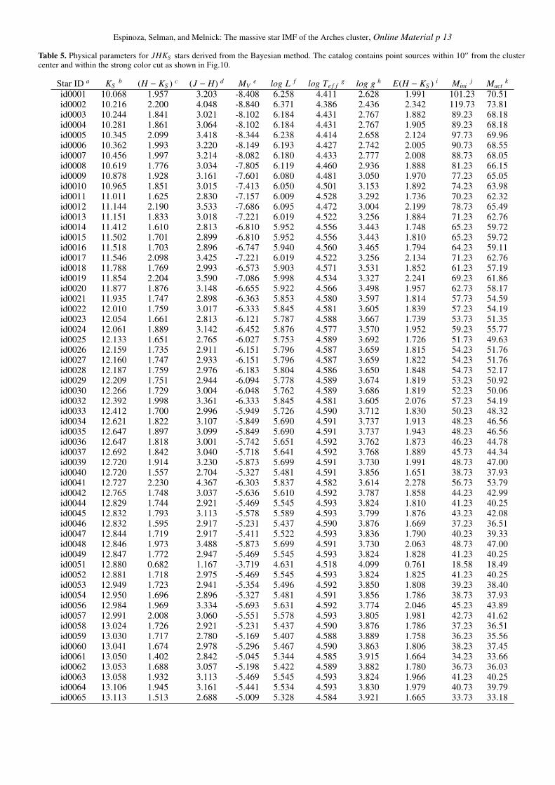
Espinoza, Selman, and Melnick: The massive star IMF of the Arches cluster, Online Material p 13
Table 5. Physical parameters for JHKS stars derived from the Bayesian method. The catalog contains point sources within 10′′ from the clustercenter and within the strong color cut as shown in Fig.10.
Star ID a KSb (H − KS ) c (J − H) d MV
e log L f log Te f fg log g h E(H − KS ) i Mini
j Mactk
id0001 10.068 1.957 3.203 -8.408 6.258 4.411 2.628 1.991 101.23 70.51id0002 10.216 2.200 4.048 -8.840 6.371 4.386 2.436 2.342 119.73 73.81id0003 10.244 1.841 3.021 -8.102 6.184 4.431 2.767 1.882 89.23 68.18id0004 10.281 1.861 3.064 -8.102 6.184 4.431 2.767 1.905 89.23 68.18id0005 10.345 2.099 3.418 -8.344 6.238 4.414 2.658 2.124 97.73 69.96id0006 10.362 1.993 3.220 -8.149 6.193 4.427 2.742 2.005 90.73 68.55id0007 10.456 1.997 3.214 -8.082 6.180 4.433 2.777 2.008 88.73 68.05id0008 10.619 1.776 3.034 -7.805 6.119 4.460 2.936 1.888 81.23 66.15id0009 10.878 1.928 3.161 -7.601 6.080 4.481 3.050 1.970 77.23 65.05id0010 10.965 1.851 3.015 -7.413 6.050 4.501 3.153 1.892 74.23 63.98id0011 11.011 1.625 2.830 -7.157 6.009 4.528 3.292 1.736 70.23 62.32id0012 11.144 2.190 3.533 -7.686 6.095 4.472 3.004 2.199 78.73 65.49id0013 11.151 1.833 3.018 -7.221 6.019 4.522 3.256 1.884 71.23 62.76id0014 11.412 1.610 2.813 -6.810 5.952 4.556 3.443 1.748 65.23 59.72id0015 11.502 1.701 2.899 -6.810 5.952 4.556 3.443 1.810 65.23 59.72id0016 11.518 1.703 2.896 -6.747 5.940 4.560 3.465 1.794 64.23 59.11id0017 11.546 2.098 3.425 -7.221 6.019 4.522 3.256 2.134 71.23 62.76id0018 11.788 1.769 2.993 -6.573 5.903 4.571 3.531 1.852 61.23 57.19id0019 11.854 2.204 3.590 -7.086 5.998 4.534 3.327 2.241 69.23 61.86id0020 11.877 1.876 3.148 -6.655 5.922 4.566 3.498 1.957 62.73 58.17id0021 11.935 1.747 2.898 -6.363 5.853 4.580 3.597 1.814 57.73 54.59id0022 12.010 1.759 3.017 -6.333 5.845 4.581 3.605 1.839 57.23 54.19id0023 12.054 1.661 2.813 -6.121 5.787 4.588 3.667 1.739 53.73 51.35id0024 12.061 1.889 3.142 -6.452 5.876 4.577 3.570 1.952 59.23 55.77id0025 12.133 1.651 2.765 -6.027 5.753 4.589 3.692 1.726 51.73 49.63id0026 12.159 1.735 2.911 -6.151 5.796 4.587 3.659 1.815 54.23 51.76id0027 12.160 1.747 2.933 -6.151 5.796 4.587 3.659 1.822 54.23 51.76id0028 12.187 1.759 2.976 -6.183 5.804 4.586 3.650 1.848 54.73 52.17id0029 12.209 1.751 2.944 -6.094 5.778 4.589 3.674 1.819 53.23 50.92id0030 12.266 1.729 3.004 -6.048 5.762 4.589 3.686 1.819 52.23 50.06id0032 12.392 1.998 3.361 -6.333 5.845 4.581 3.605 2.076 57.23 54.19id0033 12.412 1.700 2.996 -5.949 5.726 4.590 3.712 1.830 50.23 48.32id0034 12.621 1.822 3.107 -5.849 5.690 4.591 3.737 1.913 48.23 46.56id0035 12.647 1.897 3.099 -5.849 5.690 4.591 3.737 1.943 48.23 46.56id0036 12.647 1.818 3.001 -5.742 5.651 4.592 3.762 1.873 46.23 44.78id0037 12.692 1.842 3.040 -5.718 5.641 4.592 3.768 1.889 45.73 44.34id0039 12.720 1.914 3.230 -5.873 5.699 4.591 3.730 1.991 48.73 47.00id0040 12.720 1.557 2.704 -5.327 5.481 4.591 3.856 1.651 38.73 37.93id0041 12.727 2.230 4.367 -6.303 5.837 4.582 3.614 2.278 56.73 53.79id0042 12.765 1.748 3.037 -5.636 5.610 4.592 3.787 1.858 44.23 42.99id0044 12.829 1.744 2.921 -5.469 5.545 4.593 3.824 1.810 41.23 40.25id0045 12.832 1.793 3.113 -5.578 5.589 4.593 3.799 1.876 43.23 42.08id0046 12.832 1.595 2.917 -5.231 5.437 4.590 3.876 1.669 37.23 36.51id0047 12.844 1.719 2.917 -5.411 5.522 4.593 3.836 1.790 40.23 39.33id0048 12.846 1.973 3.488 -5.873 5.699 4.591 3.730 2.063 48.73 47.00id0049 12.847 1.772 2.947 -5.469 5.545 4.593 3.824 1.828 41.23 40.25id0051 12.880 0.682 1.167 -3.719 4.631 4.518 4.099 0.761 18.58 18.49id0052 12.881 1.718 2.975 -5.469 5.545 4.593 3.824 1.825 41.23 40.25id0053 12.949 1.723 2.941 -5.354 5.496 4.592 3.850 1.808 39.23 38.40id0054 12.950 1.696 2.896 -5.327 5.481 4.591 3.856 1.786 38.73 37.93id0056 12.984 1.969 3.334 -5.693 5.631 4.592 3.774 2.046 45.23 43.89id0057 12.991 2.008 3.060 -5.551 5.578 4.593 3.805 1.981 42.73 41.62id0058 13.024 1.726 2.921 -5.231 5.437 4.590 3.876 1.786 37.23 36.51id0059 13.030 1.717 2.780 -5.169 5.407 4.588 3.889 1.758 36.23 35.56id0060 13.041 1.674 2.978 -5.296 5.467 4.590 3.863 1.806 38.23 37.45id0061 13.050 1.402 2.842 -5.045 5.344 4.585 3.915 1.664 34.23 33.66id0062 13.053 1.688 3.057 -5.198 5.422 4.589 3.882 1.780 36.73 36.03id0063 13.058 1.932 3.113 -5.469 5.545 4.593 3.824 1.966 41.23 40.25id0064 13.106 1.945 3.161 -5.441 5.534 4.593 3.830 1.979 40.73 39.79id0065 13.113 1.513 2.688 -5.009 5.328 4.584 3.921 1.665 33.73 33.18
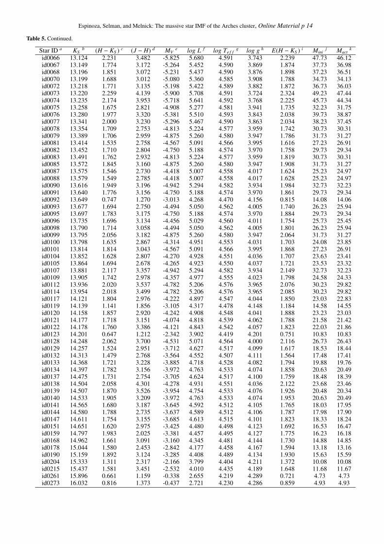
Espinoza, Selman, and Melnick: The massive star IMF of the Arches cluster, Online Material p 14
Table 5. Continued.
Star ID a KSb (H − KS ) c (J − H) d MV
e log L f log Te f fg log g h E(H − KS ) i Mini
j Mactk
id0066 13.124 2.231 3.482 -5.825 5.680 4.591 3.743 2.239 47.73 46.12id0067 13.149 1.774 3.172 -5.264 5.452 4.590 3.869 1.874 37.73 36.98id0068 13.196 1.851 3.072 -5.231 5.437 4.590 3.876 1.898 37.23 36.51id0070 13.199 1.688 3.012 -5.080 5.360 4.585 3.908 1.788 34.73 34.13id0072 13.218 1.771 3.135 -5.198 5.422 4.589 3.882 1.872 36.73 36.03id0073 13.220 2.259 4.139 -5.900 5.708 4.591 3.724 2.324 49.23 47.44id0074 13.235 2.174 3.953 -5.718 5.641 4.592 3.768 2.225 45.73 44.34id0075 13.258 1.675 2.821 -4.908 5.277 4.581 3.941 1.735 32.23 31.75id0076 13.280 1.977 3.320 -5.381 5.510 4.593 3.843 2.038 39.73 38.87id0077 13.341 2.000 3.230 -5.296 5.467 4.590 3.863 2.034 38.23 37.45id0078 13.354 1.709 2.753 -4.813 5.224 4.577 3.959 1.742 30.73 30.31id0079 13.389 1.706 2.959 -4.875 5.260 4.580 3.947 1.786 31.73 31.27id0081 13.414 1.535 2.758 -4.567 5.091 4.566 3.995 1.616 27.23 26.91id0082 13.452 1.710 2.804 -4.750 5.188 4.574 3.970 1.758 29.73 29.34id0083 13.491 1.762 2.932 -4.813 5.224 4.577 3.959 1.819 30.73 30.31id0085 13.572 1.845 3.160 -4.875 5.260 4.580 3.947 1.908 31.73 31.27id0087 13.575 1.546 2.730 -4.418 5.007 4.558 4.017 1.624 25.23 24.97id0088 13.579 1.549 2.785 -4.418 5.007 4.558 4.017 1.628 25.23 24.97id0090 13.616 1.949 3.196 -4.942 5.294 4.582 3.934 1.984 32.73 32.23id0091 13.640 1.776 3.156 -4.750 5.188 4.574 3.970 1.861 29.73 29.34id0092 13.649 0.747 1.270 -3.013 4.268 4.470 4.156 0.815 14.08 14.06id0093 13.677 1.694 2.750 -4.494 5.050 4.562 4.005 1.740 26.23 25.94id0095 13.697 1.783 3.175 -4.750 5.188 4.574 3.970 1.884 29.73 29.34id0096 13.735 1.696 3.134 -4.456 5.029 4.560 4.011 1.754 25.73 25.45id0098 13.790 1.714 3.058 -4.494 5.050 4.562 4.005 1.801 26.23 25.94id0099 13.795 2.056 3.182 -4.875 5.260 4.580 3.947 2.064 31.73 31.27id0100 13.798 1.635 2.867 -4.314 4.951 4.553 4.031 1.703 24.08 23.85id0101 13.814 1.814 3.043 -4.567 5.091 4.566 3.995 1.868 27.23 26.91id0104 13.852 1.628 2.807 -4.270 4.928 4.551 4.036 1.707 23.63 23.41id0105 13.864 1.694 2.678 -4.265 4.923 4.550 4.037 1.721 23.53 23.32id0107 13.881 2.117 3.357 -4.942 5.294 4.582 3.934 2.149 32.73 32.23id0109 13.905 1.742 2.978 -4.357 4.977 4.555 4.023 1.798 24.58 24.33id0112 13.936 2.020 3.537 -4.782 5.206 4.576 3.965 2.076 30.23 29.82id0114 13.954 2.018 3.499 -4.782 5.206 4.576 3.965 2.085 30.23 29.82id0117 14.121 1.804 2.976 -4.222 4.897 4.547 4.044 1.850 23.03 22.83id0119 14.139 1.141 1.856 -3.105 4.317 4.478 4.148 1.184 14.58 14.55id0120 14.158 1.857 2.920 -4.242 4.908 4.548 4.041 1.888 23.23 23.03id0121 14.177 1.718 3.151 -4.074 4.818 4.539 4.062 1.788 21.58 21.42id0122 14.178 1.760 3.386 -4.121 4.843 4.542 4.057 1.823 22.03 21.86id0123 14.201 0.647 1.212 -2.342 3.902 4.419 4.201 0.751 10.83 10.83id0128 14.248 2.062 3.700 -4.531 5.071 4.564 4.000 2.116 26.73 26.43id0129 14.257 1.524 2.951 -3.712 4.627 4.517 4.099 1.617 18.53 18.44id0132 14.313 1.479 2.768 -3.564 4.552 4.507 4.111 1.564 17.48 17.41id0133 14.368 1.721 3.228 -3.885 4.718 4.528 4.082 1.794 19.88 19.76id0134 14.397 1.782 3.156 -3.972 4.763 4.533 4.074 1.858 20.63 20.49id0137 14.475 1.731 2.754 -3.705 4.624 4.517 4.100 1.759 18.48 18.39id0138 14.504 2.058 4.301 -4.278 4.931 4.551 4.036 2.122 23.68 23.46id0139 14.507 1.870 3.526 -3.954 4.754 4.533 4.076 1.926 20.48 20.34id0140 14.533 1.905 3.209 -3.972 4.763 4.533 4.074 1.953 20.63 20.49id0141 14.565 1.680 3.187 -3.645 4.592 4.512 4.105 1.765 18.03 17.95id0144 14.580 1.788 2.735 -3.637 4.589 4.512 4.106 1.787 17.98 17.90id0147 14.611 1.754 3.155 -3.685 4.613 4.515 4.101 1.823 18.33 18.24id0151 14.651 1.620 2.975 -3.425 4.480 4.498 4.123 1.692 16.53 16.47id0159 14.797 1.983 2.025 -3.381 4.457 4.495 4.127 1.775 16.23 16.18id0168 14.962 1.661 3.091 -3.160 4.345 4.481 4.144 1.730 14.88 14.85id0178 15.044 1.580 2.453 -2.842 4.177 4.458 4.167 1.594 13.18 13.16id0190 15.159 1.892 3.124 -3.285 4.408 4.489 4.134 1.930 15.63 15.59id0204 15.333 1.311 2.317 -2.166 3.799 4.404 4.211 1.372 10.08 10.08id0215 15.437 1.581 3.451 -2.532 4.010 4.435 4.189 1.648 11.68 11.67id0261 15.896 0.661 1.159 -0.338 2.655 4.219 4.289 0.721 4.73 4.73id0273 16.032 0.816 1.373 -0.437 2.721 4.230 4.286 0.859 4.93 4.93
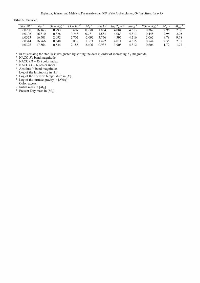
Espinoza, Selman, and Melnick: The massive star IMF of the Arches cluster, Online Material p 15
Table 5. Continued.
Star ID a KSb (H − KS ) c (J − H) d MV
e log L f log Te f fg log g h E(H − KS ) i Mini
j Mactk
id0290 16.163 0.293 0.607 0.778 1.884 4.084 4.313 0.362 2.96 2.96id0306 16.310 0.378 0.748 0.781 1.881 4.083 4.313 0.448 2.95 2.95id0323 16.501 2.092 2.702 -2.092 3.756 4.397 4.216 2.062 9.78 9.78id0344 16.766 0.648 0.838 1.363 1.492 4.011 4.315 0.544 2.35 2.35id0398 17.564 0.534 2.185 2.406 0.937 3.905 4.312 0.606 1.72 1.72
a In this catalog the star ID is designated by sorting the data in order of increasing KS magnitude.b NACO KS band magnitude.c NACO (H − KS ) color index.d NACO (J − H) color index.e Absolute V band magnitude.f Log of the luminosity in [L�].g Log of the effective temperature in [K].h Log of the surface gravity in [N/kg].i Color excess.j Initial mass in [M�].k Present-Day mass in [M�].