Theory and Practical Applications of Treewidth - Tom van der ...
157
Theory and Practical Applications of Treewidth Tom C. van der Zanden
-
Upload
khangminh22 -
Category
Documents
-
view
2 -
download
0
Transcript of Theory and Practical Applications of Treewidth - Tom van der ...
Theory and Practical Applications of Treewidth
Tom C. van der Zanden
Theory a
nd Prac
tical A
pplication
s of Treew
idth Tom
C. va
n der Za
nden
Theory and PracticalApplications of Treewidth
Tom C. van der Zanden
Tom C. van der ZandenTheory and Practical Applications of Treewidth
ISBN: 978-90-393-7147-3
c© Tom C. van der Zanden, Utrecht [email protected]
Cover design and printing: Drukkerij Haveka, Alblasserdam
Theory and PracticalApplications of TreewidthTheorie en Praktische Toepassingen van Treewidth
(met een samenvatting in het Nederlands)
Proefschrift
ter verkrijging van de graad van doctor aan de Universiteit Utrecht opgezag van de rector magnificus, prof.dr. H.R.B.M. Kummeling, ingevolgehet besluit van het college voor promoties in het openbaar te verdedigen
op woensdag 26 juni 2019 des middags te 2.30 uur
door
Tom Cornelis van der Zanden
geboren op 29 december 1992te Nieuwegein

Promotor: Prof. dr. H. L. Bodlaender
i
Acknowledgements
The four years of my PhD have been an amazing adventure. Four years to develop newideas and to explore the mathematical beauty of algorithms, to meet many new friends,and to visit conferences in wonderful and inspiring locations.
First and foremost, I want to thank my advisor, Hans Bodlaender. I was very luckyto have Hans as an advisor: most of the supervision happened during the daily morningand afternoon coffee sessions, where small talk with colleagues was interspersed withoccasional discussions about our research. Formal meetings were rare, but Hans wasalways available to discuss if I had something to ask. Hans provided helpful researchdirections, but also left me plenty of freedom to explore my own interests.
My research would not have been possible without the input of many collaborators.Key among these is Sándor Kisfaludi-Bak, with whom I initiated collaboration duringthe Lorentz Center workshop Fixed-Parameter Computational Geometry in 2016.Sándor was my city guide during our joint two-week research visit to Dániel Marx atthe MTA SZTAKI in Budapest. This visit, together with many days in Eindhovenand Utrecht spent in a small room with a whiteboard, culminated in no less thanthree papers. I cannot commend Sándor enough1: he is a very smart, talented andhard-working mathematician and moreover, a very humble and kind person.
Another very important research visit was that to the Fukuoka Institute of Tech-nology in Japan in 2017. While this was also a very productive visit (resulting inpapers on memory-efficient algorithms, Subgraph Isomorphism, k-Path Vertex Coverand minimal separators), it also resulted in personal growth: being able to spendthree weeks immersed in Japanese culture was transformative, the experience thatI got can simply not be had as a tourist. I want to say arigato gozaimashita to allof my Japanese friends: Tesshu Hanaka, Eiji Miyano, Yota Otachi, Toshiki Saitoh,Hisao Tamaki, Ryuhei Uehara, Yushi Uno, Tsuyoshi Yagita and to the students at theFukuoka Institute of Technology who invited me to their homes.
To people who are not familiar with mathematics and computer science research, itmight appear boring and dry. However, to me, it sometimes feels more like a thinlyveiled excuse for having fun and an extension of my hobby in puzzles. In fact, mywork together with Hans was initiated when I, during his Algorithms and Networkscourse, took a homework assignment on the puzzle game Bloxorz a bit too far. I havemet many people who think alike at various International Puzzle Parties, Gatheringfor Gardner 10 and 13, the 2018 Fun with Algorithms Conference in Sardinia and the2019 Bellairs Workshop on Computational Geometry in Barbados (certainly, the onlything better than having fun with mathematics is having fun with mathematics on abeautiful tropical island). I want to acknowledge all of the people that I met pursuing
1And Sándor tells me I shouldn’t.
ii Acknowledgements
my interest in recreational mathematics, puzzles and their design, and in particularAndrew Cormier, Martin and Erik Demaine, Oskar van Deventer, Bob Hearn, Marcvan Kreveld, Jayson Lynch, Jonathan Schroyer, Joris van Tubergen, Siert Wijnia andmany others. I also want to thank the Gathering for Gardner Foundation and the lateTom Rodgers for their support.
Of course, not everything is fun and games (or at least, not the type of game thatis fun to play). I want to thank Herbert Hamers for our collaboration on terroristnetworks, which was initiated at Lunteren 2017. I am very happy Herbert was willingto take on this interdisciplinary challenge.
I would like to thank the reading committee for critically evaluating this manuscriptand offering valuable comments: Hajo Broersma, Alexander Grigoriev, Marc vanKreveld, Jan Arne Telle and Gerhard Woeginger.
During the NETWORKS training weeks, visiting Eindhoven and at other conferencesI had a lot of fun with my fellow PhD students and other colleagues: Tom Bannink,Julien Baste, Paul Bouman, Jan-Willem Buurlage, Mark de Berg, Huib Donkers, LarsJaffke, Bart Jansen, Aleksandar Markovic, Jesper Nederlof, Tim Ophelders, AstridPieterse, Carolin Rehs, Jan Arne Telle, Abe Wits, Gerhard Woeginger and many, manyothers. Being able to interact with so many people, and especially getting to meetfellow PhDs in similar and different stages of their programme was very valuable to me.I want to say a special thank you to Astrid and Sándor, who have been good friendsfrom the very beginning of our PhD programmes.
Of course, there are also many wonderful and inspiring people at my home base ofUtrecht. My interest in algorithms was first sparked by taking part in programmingcontests, together with my teammates Bas te Kolste, Harry Smit and coaches JeroenBransen and Bas den Heijer. I want to thank Gerard Tel for teaching a wonderfulintroduction to algorithms class and inspiring me in the area of teaching. I have beena student assistant for many of Gerard’s classes, and I appreciate the opportunities hegave me to substitute during classroom lectures and to experiment with developingpractical assignments. I want to thank Erik Jan van Leeuwen for our collaborationwhile teaching the algorithms course, Johan van Rooij for advising me on job searchinginside and out of academia, Tomas Klos for occasionally reminding me to take the traininstead of flying, Han Hoogeveen for our work on data mining and flower power, JaccoBikker for discussions on GPU programming, Linda van der Gaag for making sure Hansstayed on top of his negotiating skills, Marjan van den Akker, Rob Bisseling, JannekeBolt, Anneke Bonsma, Wouter ten Bosch, Cassio de Campos, Gunther Cornelissen,Federico D’Ambrosio, Marcell van Geest, Roland Geraerts, Jurriaan Hage, Ivor van derHoog, Jan van Leeuwen, Till Miltzow, Thijs van Ommen, Silja Renooij, Edith Stap,Dirk Thierens, Sjoerd Timmer, Jérôme Urhausen, Marinus Veldhorst, Peter de Waaland Jordi Vermeulen. I would also like to thank the students who I shared the joy ofmany moments of learning and discovery with. I would like to thank my long-termoffice mates, Roel van den Broek, Nils Donselaar and Marieke van der Wegen, forthe good times we shared inside and out of the office and at conferences in Vienna,Lunteren, Helsinki, Nový Smokovec and Heeze.
Finally, I would like to thank my parents Hans and Loes, and several good friendsand people who meant a lot for me: Elsie, Gerrit, Irene, Marrie, Cor, Daan, Jacco –thank you all very much.
iii
Contents
1. Introduction 11.1. Hard Problems . . . . . . . . . . . . . . . . . . . . . . . . . . . . . . . . 21.2. The Exponential Time Hypothesis . . . . . . . . . . . . . . . . . . . . . 41.3. Graph Separators and Treewidth . . . . . . . . . . . . . . . . . . . . . . 41.4. The Square Root Phenomenon in Planar Graphs . . . . . . . . . . . . . 71.5. Graph Embedding Problems . . . . . . . . . . . . . . . . . . . . . . . . . 81.6. Problems in Geometric Intersection Graphs . . . . . . . . . . . . . . . . 91.7. Treewidth in Practice . . . . . . . . . . . . . . . . . . . . . . . . . . . . 111.8. Published Papers . . . . . . . . . . . . . . . . . . . . . . . . . . . . . . . 12
2. Preliminaries 152.1. Basic Notations and Definitions . . . . . . . . . . . . . . . . . . . . . . . 152.2. Tree Decompositions . . . . . . . . . . . . . . . . . . . . . . . . . . . . . 162.3. Dynamic Programming on Tree Decompositions . . . . . . . . . . . . . . 17
I Graph Embedding Problems 21
3. Algorithms 233.1. Introduction . . . . . . . . . . . . . . . . . . . . . . . . . . . . . . . 233.2. An Algorithm for Subgraph Isomorphism . . . . . . . . . . . . . . 253.3. Reducing the Number of Partial Solutions Using Isomorphism Tests 283.4. Bounding the Number of Non-Isomorphic Partial Solutions . . . . 293.5. Graph Minors and Induced Problem Variants . . . . . . . . . . . . 313.6. Topological Minor . . . . . . . . . . . . . . . . . . . . . . . . . . . 353.7. Conclusions . . . . . . . . . . . . . . . . . . . . . . . . . . . . . . . 38
4. Lower Bounds 414.1. Introduction . . . . . . . . . . . . . . . . . . . . . . . . . . . . . . . 414.2. Additional Notation . . . . . . . . . . . . . . . . . . . . . . . . . . 434.3. String Crafting and Orthogonal Vector Crafting . . . . . . . . . . . 434.4. Lower Bounds for Graph Embedding Problems . . . . . . . . . . . 474.5. Tree and Path Decompositions with Few Bags . . . . . . . . . . . . 494.6. Intervalizing Coloured Graphs . . . . . . . . . . . . . . . . . . . . . 514.7. Conclusions . . . . . . . . . . . . . . . . . . . . . . . . . . . . . . . 59
iv Contents
5. Intermezzo: Polyomino Packing 615.1. Introduction . . . . . . . . . . . . . . . . . . . . . . . . . . . . . . . 615.2. Lower Bounds . . . . . . . . . . . . . . . . . . . . . . . . . . . . . . 625.3. Algorithms . . . . . . . . . . . . . . . . . . . . . . . . . . . . . . . 675.4. Conclusions . . . . . . . . . . . . . . . . . . . . . . . . . . . . . . . 70
II Problems in Geometric Intersection Graphs 73
6. Problems in Geometric Intersection Graphs 756.1. Introduction . . . . . . . . . . . . . . . . . . . . . . . . . . . . . . . 756.2. Separators for Arbitrarily-Sized Fat Objects . . . . . . . . . . . . . 776.3. An Algorithmic Framework for Similarly-Sized Fat Objects . . . . 816.4. Basic Algorithmic Applications . . . . . . . . . . . . . . . . . . . . 846.5. Application of the Rank-Based Approach . . . . . . . . . . . . . . 876.6. Conclusions . . . . . . . . . . . . . . . . . . . . . . . . . . . . . . . 90
III Practical Applications of Treewidth 91
7. Computing Tree Decompositions on the GPU 937.1. Introduction . . . . . . . . . . . . . . . . . . . . . . . . . . . . . . . 937.2. Additional Definitions . . . . . . . . . . . . . . . . . . . . . . . . . 957.3. The Algorithm . . . . . . . . . . . . . . . . . . . . . . . . . . . . . 96
7.3.1. Computing Treewidth . . . . . . . . . . . . . . . . . . . . . 967.3.2. Duplicate Elimination using Bloom Filters . . . . . . . . . . 977.3.3. Minor-Min-Width . . . . . . . . . . . . . . . . . . . . . . . 98
7.4. Experiments . . . . . . . . . . . . . . . . . . . . . . . . . . . . . . . 997.4.1. Instances . . . . . . . . . . . . . . . . . . . . . . . . . . . . 997.4.2. General Benchmark . . . . . . . . . . . . . . . . . . . . . . 997.4.3. Work Size and Global v.s. Shared Memory . . . . . . . . . 1017.4.4. Minor-Min-Width . . . . . . . . . . . . . . . . . . . . . . . 1027.4.5. Loop Unnesting . . . . . . . . . . . . . . . . . . . . . . . . . 104
7.5. Conclusions . . . . . . . . . . . . . . . . . . . . . . . . . . . . . . . 106
8. Computing the Shapley Value of Connectivity Games 1078.1. Introduction . . . . . . . . . . . . . . . . . . . . . . . . . . . . . . . 1078.2. Preliminaries . . . . . . . . . . . . . . . . . . . . . . . . . . . . . . 110
8.2.1. Shapley Value / Power Indices . . . . . . . . . . . . . . . . 1108.2.2. Game-Theoretic Centrality . . . . . . . . . . . . . . . . . . 110
8.3. An Algorithm for Computing Shapley Values . . . . . . . . . . . . 1118.4. Computational Experiments . . . . . . . . . . . . . . . . . . . . . . 1178.5. Conclusions . . . . . . . . . . . . . . . . . . . . . . . . . . . . . . . 119
9. Conclusions 121
Contents v
Appendix 125
A. List of Problems 125A.1. Classical Graph Problems . . . . . . . . . . . . . . . . . . . . . . . . . . . . 125A.2. Graph Embedding Problems . . . . . . . . . . . . . . . . . . . . . . . . . . 127A.3. Miscellaneous Problems . . . . . . . . . . . . . . . . . . . . . . . . . . . . . 128
Bibliography 131
Nederlandse Samenvatting 141
Curriculum Vitae 145

1
Introduction
A combinatorial problem is a problem in which, from a finite set of possibilities, weare asked to pick a solution that is optimal (e.g., lowest cost) or has other desirableproperties. Such problems occur frequently in daily life: finding the fastest route todrive from home to work, determining where to purchase what items to take optimaladvantage of store promotions and creating a seating map for a celebratory dinnerfollowing a PhD defence are all examples of combinatorial problems.
An algorithm is a systematic approach to solve a given problem. Algorithms areoften implemented as computer programs (e.g., as the shortest path computation ina navigation system or as a sorting algorithm to organize files by creation date) butcan also be procedures carried out by hand: for example, when children are taught tomultiply two numbers, what they are being taught is a multiplication algorithm.
When we design algorithms, we aim to make them efficient: we want to do as littlework as possible to arrive at the desired result. A very naïve method to compute theproduct of two numbers A×B is to simply add B to itself A− 1 times. The product5× 6 might be computed by first computing 6 + 6 = 12, 12 + 6 = 18, . . ., 24 + 6 = 30.This is a rather tedious process, and quickly becomes infeasible if we want to computea larger product, such as 153× 12. Long multiplication, as taught in primary school, ismuch more efficient. Instead of adding 153 to itself 12 times, we can instead compute153 × 10 + 153 × 2 = 1530 + 306 = 1836. To multiply two n-digit numbers, longmultiplication requires n2 elementary operations, while the naïve method can require10n − 2 additions.
The complexity of an algorithm determines how much time it uses to solve aparticular problem instance, and also what the maximum size of a problem instanceis that can be solved within reasonable time: the repeated addition method alreadybecomes impractical for numbers with more than, say, two or three digits, while longmultiplication can be performed by hand for numbers tens of digits long.
This thesis deals primarily with problems on graphs: a graph is a set of points
2 Chapter 1: Introduction
(vertices), connected by lines (edges). Graphs can be used to model for instanceroad networks (where edges correspond to roads and vertices to intersections), socialnetworks (where vertices correspond to people and edges to friendships), or any otherstructure with relations between objects.
If a graph has a special underlying structure, this structure can sometimes beexploited to obtain faster algorithms. As a simple example, many problems that aredifficult to solve on graphs in general, often have much lower complexity (or are eventrivial) if the graph considered is a tree (i.e., a graph in which any two vertices areconnected by a unique path). The treewidth of a graph measures, in some sense, how“close” a graph is to being a tree: a graph with low treewidth can be decomposedinto small groups of vertices, the groups connected together in a tree, such that theconnections in the graph are respected by the grouping and the tree. Problems whichcan be solved efficiently on trees can often also be solved efficiently on graphs of lowtreewidth.
As a very high-level overview of this thesis, we study the application of treewidth(and related techniques) to several types of problems, and give both algorithms andlower bounds, showing that these algorithms are (likely) optimal. We also studypractical applications and implementations of treewidth-related algorithms.
In the first part, we study the application of bounded treewidth and geometricstructure (e.g., planarity) to graph embedding problems (e.g., recognizing whethersome small pattern occurs somewhere as a subgraph in a larger host graph). One mightreasonably expect that planarity could be exploited to obtain faster algorithms forthese problems. However, it turns out that this is not the case: while we do obtainslightly faster algorithms, these algorithms are not as efficient as one might expect. Wealso give evidence that the algorithms obtained are probably optimal.
In the second part, we study geometric intersection graphs. A geometric intersectiongraph can be obtained, for instance, by identifying the vertices of graphs with pointsin space, and connecting two points with an edge if they are within a certain distanceof each other. While these graphs do not have small treewidth, we show how a slightlymodified variant of treewidth can still be used to obtain faster algorithms for problemson these graphs. These algorithms also turn out to be (probably) optimal.
In the third and final part, we study practical uses of treewidth. We first studythe computation of treewidth itself: we give a parallel algorithm, implemented on aGPU, for computing treewidth using partial elimination orderings. We then studyhow treewidth can be used to compute the Shapley Value of connectivity games. Thisvalue, a tool from game theory, helps us to estimate the importance of vertices in agraph, i.e., it is a so-called centrality measure. It can be (and has been) used to identifykey players in criminal and terrorist networks. Our method, using treewidth, gives apractical approach to compute this value for graphs on which it could otherwise not becomputed.
1.1. Hard Problems
As observed in the previous section, the long multiplication algorithm is much more effi-cient than the naive one. The time required for long multiplication scales quadraticallywith the number of digits, whereas the naive algorithm scales exponentially with the
1.1. Hard Problems 3
number of digits (n). Doubling the number of digits in long multiplication increasesthe running time fourfold, whereas adding just one more digit in naive multiplicationincreases it tenfold. Long multiplication is an example of a polynomial-time algorithm(running in time O(nc) for some c > 0; in this case, c = 2), whereas the naive algorithmis an example of an exponential-time algorithm (running in time O(cn) for some c > 1).
While on the one hand we strive to find efficient algorithms for problems, on theother hand, we also try to find lower bounds, showing when this can (not) be done.Doing so gives us a greater understanding of the structure of a problem, and alsoenables us to tell when we should stop looking for a faster algorithm (since none islikely to exist).
Perhaps the most widely celebrated technique for showing lower bounds is thetheory of NP-completeness, introduced by Cook [33] and Karp [73] and independentlydiscovered by Levin [81]. NP-completeness is a tool for showing that the existence ofa polynomial algorithm for a given problem is unlikely. By using reductions, that is,showing that one problem A can be rewritten as another problem B, we can show thatif problem B has a polynomial-time algorithm, then A does too. NP-complete problemsare known to be mutually reducible to one another, and, if any one NP-completeproblem has a polynomial-time algorithm, then all NP-complete problems do. It iswidely thought unlikely that NP-complete problems have polynomial-time algorithms,so showing NP-completeness for a problem is good evidence that it does not admit apolynomial-time algorithm.
A central problem in the theory of NP-completeness is Satisfiability. In satisfi-ability, we are given boolean variables x1, . . . , xn, each of which may be set to eithertrue or false and a set of clauses. A clause is the disjunction of one or more literals,where a literal is either a variable xi or its negation ¬xi. For example, the clause(x1 ∨ ¬x2 ∨ ¬x4) can be satisfied by making either x1 true, x2 false, or x4 false.
The Satisfiability problem is to determine whether all given clauses can besatisfied simultaneously by an assignment. For example, the clauses (x1 ∨ x2) ∧ (¬x1 ∨¬x2) can be satisfied by making x1 true and x2 false (so these two clauses together wouldform a yes-instance), but the combination (x1∨x2)∧(¬x1∨¬x2)∧(x1∨¬x2)∧(¬x1∨x2)does not have any satisfying assignments: the first two clauses imply at least onevariable should be true and at least one variable should be false, but the assignmentx1 = false, x2 = true does not satisfy the third clause, and x1 = true, x2 = false doesnot satisfy the fourth (and so this is a no-instance).
The fact that Satisfiability is NP-complete can be used to show other problemsNP-complete1. As a simple example, consider the Independent Set problem: givena graph G, we want to find (at least) k vertices such that no two vertices are adjacent(i.e., are connected by an edge). Given a satisfiability formula with n variables and mclauses, we can create a graph as follows: for every clause with l literals, we create agroup of l vertices, one corresponding to each literal in the clause. We connect thesevertices by edges, so that from each group, we can select at most one vertex. Wethen connect vertices corresponding to conflicting literals by edges, i.e., if v is a vertexcorresponding to literal vi in one clause, and u is a vertex corresponding to ¬vi inanother clause, we add the edge (u, v), ensuring that these vertices cannot be selectedsimultaneously.
1For the purpose of this introduction, we omit the proof that Independent Set is in NP.
4 Chapter 1: Introduction
If we can find an independent set of size m in this graph, we know that it containsexactly one vertex from each group corresponding to a clause (since there are m suchgroups, and the edges in each group ensure we can select at most one vertex from eachgroup), and the literals corresponding to these vertices from a satisfying assignment.Conversely, a satisfying assignment corresponds to an independent set of size m in thisgraph (by picking, from each clause, a literal that satisfies it and selecting the vertexcorresponding to that literal to be in the independent set).
This shows that the existence of a polynomial-time algorithm for IndependentSet implies a polynomial-time algorithm for Satisfiability, because we can solvea Satisfiability instance by applying the above transformation and then solvingIndependent Set. Conversely, if Satisfiability cannot be solved in polynomialtime, then neither can Independent Set.
1.2. The Exponential Time Hypothesis
If one is willing to assume that P 6= NP (i.e., Satisfiability does not have a polynomial-time algorithm), then NP-completeness can be viewed as a tool to show that certainproblems do not have polynomial-time algorithms. However, merely showing that aproblem does not have a polynomial-time algorithm does not preclude the possibilitythere might be a super-polynomial, but still reasonably fast algorithm: for example,an algorithm with running time O(nlog logn) is not polynomial, but would still be fastenough for many practical applications. By making a stronger assumption, we canexclude such running times:
Hypothesis 1.1 (Exponential Time Hypothesis [67]). There exists a constant c > 1such that Satisfiability for n-variable 3-CNF formulas has no O(cn)-time algorithm.
It is possible to use the Sparsification Lemma [68] to show that the hypothesisimplies that there is no O(c′n)-time algorithm for n-clause 3-CNF formulas either (fora different constant c′ > 0).
Now, the previous reduction showed that Satisfiability for a (3-CNF) formulawith n clauses can be reduced to Independent Set on graphs with 3n vertices. Thus,an algorithm for Independent Set on m-vertex graphs running in time O((c′/3)m)would contradict the Exponential Time Hypothesis (ETH). Using the ETH, it is possibleto derive similar lower bounds for many problems [68].
1.3. Graph Separators and Treewidth
Consider the example graph G in Figure 1.1. If we wanted to compute the maximumsize of an independent set in G, we could consider all 29 = 512 possible subsets ofvertices in G, determine which subsets make valid independent set (i.e., contain notwo vertices sharing an edge), and find the largest among these sets. In general, thisgives an O(2nm)-time algorithm (for n-vertex, m-edge graphs). While the base of theexponent can be improved by using more advanced branching techniques (see e.g. [116]for a O∗(1.1996n)-time algorithm), the Exponential Time Hypothesis implies that weshould not expect an algorithm without exponential dependence on n.
1.3. Graph Separators and Treewidth 5
A
C F
E
D
G
H
IB
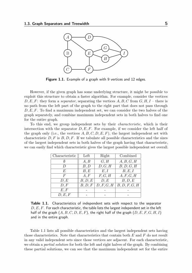
Figure 1.1. Example of a graph with 9 vertices and 12 edges.
However, if the given graph has some underlying structure, it might be possible toexploit this structure to obtain a faster algorithm. For example, consider the verticesD,E, F : they form a separator, separating the vertices A,B,C from G,H, I – there isno path from the left part of the graph to the right part that does not pass throughD,E, F . To find a maximum independent set, we can consider the two halves of thegraph separately, and combine maximum independent sets in both halves to find onefor the entire graph.
To this end, we group independent sets by their characteristic, which is theirintersection with the separator D,E, F . For example, if we consider the left half ofthe graph only (i.e., the vertices A,B,C,D,E, F ), the largest independent set withcharacteristic D,F is B,D,F . If we tabulate all possible characteristics and the sizesof the largest independent sets in both halves of the graph having that characteristic,we can easily find which characteristic gives the largest possible independent set overall.
Characteristic Left Right Combined∅ A,B G,H A,B,G,HD B,D D,G,H B,D,G,HE B,E E, I B,E, IF A, F F,G,H A,F,G,H
D,E B,D,E D,E B,D,ED,F B,D,F D,F,G,H B,D,F,G,HE,F - - -D,E, F - - -
Table 1.1. Characteristics of independent sets with respect to the separatorD,E, F . For each characteristic, the table lists the largest independent set in the lefthalf of the graph (A,B,C,D,E, F ), the right half of the graph (D,E, F,G,H, I)and in the entire graph.
Table 1.1 lists all possible characteristics and the largest independent sets havingthose characteristics. Note that characteristics that contain both E and F do not resultin any valid independent sets since those vertices are adjacent. For each characteristic,we obtain a partial solution for both the left and right halves of the graph. By combiningthese partial solutions, we can see that the maximum independent set for the entire
6 Chapter 1: Introduction
graph is B,D,F,G,H. The number of possibilities we had to consider was greatlyreduced, since we could consider each half of the graph in isolation.
This process of considering a separator and dividing the graph can be repeated.For example, when we are considering the left half of the graph (A,B,C,D,E, F ),we can again split it on the separator B,E and combine solutions for the subgraphsA,B,D,E and B,C,E, F to obtain the needed partial solutions for the left half, andwe can process the right half similarly.
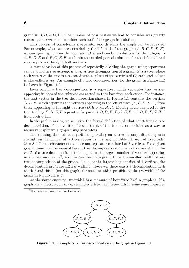
A formalization of this process of repeatedly dividing the graph using separatorscan be found in tree decompositions. A tree decomposition of a graph G is a tree, whereeach vertex of the tree is associated with a subset of the vertices of G; each such subsetis also called a bag. An example of a tree decomposition (for the graph in Figure 1.1)is shown in Figure 1.2.
Each bag in a tree decomposition is a separator, which separates the verticesappearing in bags of the subtrees connected to that bag from each other. For instance,the root vertex in the tree decomposition shown in Figure 1.1 contains the verticesD,E, F , which separates the vertices appearing in the left subtree (A,B,D,E, F ) fromthose appearing in the right subtree (D,E, F,G,H, I). Moving down one level in thetree, the bag B,D,E, F separates the parts A,B,D,E, B,C,E, F and D,E, F,G,H, Ifrom each other.
In the preliminaries, we will give the formal definition of what constitutes a treedecomposition. For now, it suffices to think of the tree decomposition as a way torecursively split up a graph using separators.
The running time of an algorithm operating on a tree decomposition dependsstrongly on the number of vertices appearing in a bag. In Table 1.1, we had to consider23 = 8 different characteristics, since our separator consisted of 3 vertices. For a givengraph, there may be many different tree decompositions. This motivates defining thewidth of a tree decomposition to be equal to the largest number of vertices appearingin any bag minus one2, and the treewidth of a graph to be the smallest width of anytree decomposition of the graph. Thus, as the largest bag consists of 4 vertices, thedecomposition in Figure 1.2 has width 3. However, there exists a decomposition withwidth 2 and this is (for this graph) the smallest width possible, so the treewidth of thegraph in Figure 1.1 is 2.
As the name suggests, treewidth is a measure of how “tree-like” a graph is. If agraph, on a macroscopic scale, resembles a tree, then treewidth in some sense measures
2For historical and technical reasons.
B,D,E, F
B,C,E, FA,B,D,E
D,E, F, I
E,G,H, I
D,E, F
Figure 1.2. Example of a tree decomposition of the graph in Figure 1.1.
1.4. The Square Root Phenomenon in Planar Graphs 7
how much it deviates from being a tree locally (and in fact trees are precisely thegraphs of treewidth 1).
Exploiting the fact that a graph has bounded treewidth is a celebrated and widelyused technique for dealing with NP-complete problems: thanks to the simple structureof trees, many NP-complete problems can be solved in polynomial time on trees. Veryoften, such problems can also be solved in polynomial time on graphs of boundedtreewidth: while the best known algorithms for such problems in general requireexponential time, we can often construct an algorithm that is only exponential inthe treewidth (by doing some exponential computation within each vertex of the tree,which contains a bounded number of vertices of the original graph), and then usingthe properties of the problem that allow it to be solved in polynomial time on trees tocombine the results computed within each node of the decomposition to a solution forthe original problem. For example, on an n-vertex graph of treewidth k, IndependentSet can be solved in time O(2kkO(1)n).
1.4. The Square Root Phenomenon in Planar Graphs
A graph is planar if it can be drawn in the plane without edges crossing each other.The well-known Lipton-Tarjan Separator Theorem [84, 85] states that any n-vertexplanar graph has a separator, consisting of O(
√n) vertices, that divides the graph into
connected components, each having at most 2/3n vertices. As a consequence of this, itfollows that planar graphs have treewidth O(
√n) [14].
This fact can be combined with algorithms operating on tree decompositions, toobtain subexponential-time algorithms for NP-complete problems on planar graphs.For instance, while (under the ETH) Independent Set cannot be solved in time 2o(n)
on general (n-vertex) graphs, if the graph is planar, we can exploit the fact that itstreewidth is at most O(
√n) and solve the problem in 2O(
√n) time [85].
It turns out that this running time is optimal, unless the ETH fails. The standardreduction from Satisfiability to Independent Set shows that Independent Setcannot be solved in 2o(n) time on general graphs. It is possible to take the graphcreated in this reduction, draw it in the plane in some arbitrary way, and then replaceevery crossing with a crossover gadget to make the graph planar. Since (in an n-vertexgraph) there can be O(n2) crossings, this blows up the size of the graph from n verticesto O(n2) vertices. This, in turn, implies that a 2o(
√n)-time algorithm on planar graphs
would give a 2o(n) time algorithm on general graphs (by applying this transformation),and thus, no 2o(
√n)-time algorithm for Independent Set on planar graphs should
exist, unless the ETH fails.Similar arguments show that for many problems, 2Θ(
√n) is the best achievable
running time on planar graphs. Examples include Dominating Set, k-Coloring(for fixed k), Hamiltonian Path and Feedback Vertex Set [86]. Square rootsalso appear in many other settings when dealing with planar graphs, for instance inparameterized complexity: using Bidimensionality Theory [41], it is possible to find (ifit exists) an independent set of size k in an n-vertex planar graph in 2O(
√k)nO(1) time.
The behaviour that square roots often appear in the (optimal) running time foralgorithms on planar graphs is so pervasive, that it has been dubbed the Square RootPhenomenon [88].
8 Chapter 1: Introduction
1.5. Graph Embedding Problems
The first part of this thesis deals with graph embedding problems. A graph embeddingproblem is any problem where we are asked to embed a graph into another graphor some other structure. As prime example of such a problem, consider SubgraphIsomorphism: given two graphs G (guest) and H (host), determine whether G is asubgraph of H. That is, can we delete vertices and edges from H to obtain (a graphthat is isomorphic to) G?
If we let n denote the number of vertices of H and let k denote the number ofvertices of G, then there is a trivial O(nk)-time algorithm, that for each vertex of G,tries all vertices of H to map it to. Surprisingly, this simple algorithm is optimal:assuming the Exponential Time Hypothesis, there is no algorithm solving SubgraphIsomorphism in no(k) time3 [49].
Of course, a natural question then is whether bounded treewidth could help insolving Subgraph Isomorphism. In particular, an open question of Marx [87] iswhether a square root phenomenon occurs for Subgraph Isomorphism on planargraphs.
A straightforward reduction from 3-Partition shows that even if G and H areboth disjoint unions of paths, Subgraph Isomorphism is NP-complete. As suchgraphs have treewidth 1, we cannot expect the problem to be fixed-parameter tractableparameterized by treewidth or even polynomial-time solvable for graphs of treewidthbounded by a constant. However, if we additionally impose the restriction that the graphhas so-called log-bounded fragmentation, Subgraph Isomorphism is polynomial-timesolvable for graphs of bounded (constant) treewidth [60].
Still, there is some hope: it is known that if H is planar, Subgraph Isomorphismcan be solved in 2O(k)n time [43] – faster than the lower bound for general graphs.
In the first chapter of part one, we give an algorithm for Subgraph Isomorphismon planar graphs running in time 2O(n/ logn). This slightly improves the worst-caserunning time of [43] but, in contrast, is not fixed-parameter tractable with respect to k.While the algorithm does take advantage of the fact that planar graphs have boundedtreewidth, the running time is dominated by the necessity of keeping track of subsets ofconnected components (which is exactly what [60] circumvents by assuming boundedfragmentation). We show that through canonization, that is, recognizing isomorphicpartial solutions in the dynamic programming, we can achieve subexponential runningtime of 2O(n/ logn).
In the second chapter, we show that, surprisingly, this result is optimal under theETH. There is no algorithm for Subgraph Isomorphism on planar graphs runningin time 2o(n/ logn). Thus, a “square root phenomenon” does not hold for SubgraphIsomorphism on planar graphs – answering an open question of Marx [87]. Thisresult is obtained by a reduction from Satisfiability, creating graphs with manynon-isomorphic connected components.
Our results are in fact slightly stronger than stated here (the algorithm works fora more general class of graphs, and the lower bounds hold even for more restrictiveclasses of graphs).
3In [49], the authors actually show a stronger result: assuming the ETH, there is no 2o(n logn)-timealgorithm for Subgraph Isomorphism. This also rules out the existence of a no(k)-time algorithm.
1.6. Problems in Geometric Intersection Graphs 9
This result is closely related with that of Fomin et al. [50] who show that, if thegraph (in addition to being planar) is connected and has bounded maximum degree, atype of square root phenomenon does occur. The techniques of [50] also allow us toturn our algorithm into a parameterized one (running in time 2O(k/ log k)nO(1)) if thegraph is connected.
It turns out that 2Θ(n/ logn) is, in fact, the optimal running time for a wide rangeof problems involving graph embedding on planar (or H-minor free graphs): not onlyfor simple simple variations (such as Induced Subgraph, where we are allowed todelete vertices but not edges) and other problems such as Graph Minor, but also forproblems which involve embedding a graph into some other structure (such as a treedecomposition with few bags or an interval graph with few colours).
Thus, for graph embedding problems on planar graphs, it could be said that thereis no square root phenomenon, but that instead there is a “n/ log n-phenomenon”.
In the third and final chapter of part one, we give an interesting and fun applicationof these techniques: we study the relation of the “n/ log n-phenomenon” to solvingpolyomino packing puzzles.
1.6. Problems in Geometric Intersection Graphs
Part two of this thesis is dedicated to problems in geometric intersection graphs. Aplanar graph is an example of a geometric graph, arising from connecting points in theplane with non-crossing lines. A geometric intersection graph arises from a collection ofobjects in Rd, where each object corresponds to a vertex, and two vertices are connectedby an edge if and only if their corresponding objects intersect.
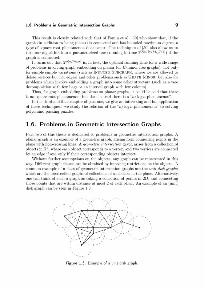
Without further assumptions on the objects, any graph can be represented in thisway. Different graph classes can be obtained by imposing restrictions on the objects. Acommon example of a class of geometric intersection graphs are the unit disk graphs,which are the intersection graphs of collections of unit disks in the plane. Alternatively,one can think of such a graph as taking a collection of points in 2D, and connectingthose points that are within distance at most 2 of each other. An example of an (unit)disk graph can be seen in Figure 1.3.
Figure 1.3. Example of a unit disk graph.
10 Chapter 1: Introduction
Problems in geometric intersection graphs arise naturally. Consider the Independ-ent Set problem in geometric intersection graphs. It corresponds to finding, amonga set of objects (with fixed locations in space), the largest set of objects that can bepacked together without intersecting.
As we have observed with the square root phenomenon, taking advantage of the(geometric) structure of a graph can often result in significant speedups. An interestingquestion is whether it is possible to take advantage of similar phenomena in graphswith a different (geometric) structure, other than planarity.
Intersection graphs can be very dense and can have large cliques (consider a set ofunit disks all mutually intersecting) and therefore, we would not expect treewidth tohelp in this case (as the maximum size of a clique is a lower bound on the treewidth).It turns out that several problems can nevertheless be solved in subexponential time ongeometric intersection graphs. For instance, Fu [53] showed that Independent Setcan be solved in 2O(
√n) time in unit disk graphs (with n disks). More generally, if one
considers the d-dimensional analogue (of finding a maximum independent set in anintersection graph of d-dimensional unit balls), it is possible to solve the problem in2O(n1−1/d) time.
A running time of the form 2O(n1−1/d) or nO(n1−1/d) appears for many differentgeometric problems in various classes of d-dimensional intersection graphs [91, 102], andthis running time is often (close) to optimal under the ETH [91]. Thus, d-dimensionalgeometric intersection graphs exhibit a type of “n1−1/d-phenomenon”.
We present an algorithmic framework for solving problems on d-dimensional geo-metric intersection graphs. The framework unifies various ad-hoc techniques, closesgaps in the running time bounds for several problems, and provides an easy-to-applymethod for solving problems on geometric intersection graphs.
The main observation behind the framework is that while the graphs (being dense)do not admit small separators, we can instead use a kind of weighted separator basedon a partition of the graph into cliques. We then use these separators to build treedecompositions, whose “width” is measured as a function of the number and size ofcliques appearing in a bag. Many problems are easy to solve on cliques (for instance,Independent Set is trivial on a clique as we can select at most one vertex) andthese problems are often also easy to solve for graphs of bounded clique-partitionedtreewidth.
Using the framework, we obtain 2O(n1−1/d)-time algorithms for many problems onintersection graphs of so-called similarly sized fat objects, including Independent Set,Feedback Vertex Set, Dominating Set and Steiner Tree. This improves thebest known running time bounds for these problems, and the running time obtained isin fact optimal (under the ETH).
To complement the algorithmic framework, there also exists a lower-bound frame-work – showing matching lower bounds (under the ETH) of the form 2Ω(n1−1/d) formany problems on (very restricted) classes of geometric intersection graphs. Thisframework is presented in [36] but is not part of this thesis.
1.7. Treewidth in Practice 11
1.7. Treewidth in Practice
While in both the first and second part of this thesis we obtain subexponential-timealgorithms whose running time is optimal under the Exponential Time Hypothesis,there exists a very nice contrast between the two: for graph embedding problems –where one would expect to be able to take significant advantage of planarity – we showthat the benefit of bounded treewidth and/or planarity is severely limited. On theother hand, for problems in geometric graphs, where one would not expect to be ableto benefit (much) from bounded treewidth, we obtain an alternate variation of treedecompositions that allows us to nevertheless obtain faster algorithms.
From a theoretical perspective, having algorithms whose running time matcheslower bounds obtained under the Exponential Time Hypothesis is very satisfying andprovides a lot of insight into the structure of a problem. However, the algorithmsobtained in the first part are not very conducive to practical use: the use of asymptoticnotation in the exponent hides very large constant factors, making the algorithmsunsuitable for many practical purposes (however, some of the ideas contained within,such as identifying isomorphic partial solutions in dynamic programming, may havepractical applications). This is why the third part investigates using treewidth inpractice.
Of course, to be able to take advantage of theory for solving practical problems, onefirst needs a practical method of obtaining a tree decomposition of small width. In recentyears large advances have been made in this area, inspired by the PACE challenges[39, 37]. In particular, the work of Tamaki [104] has been groundbreaking. The firstchapter of of Part 3 investigates exploiting the massive computational power of graphicscards (GPUs) to compute tree decompositions. Compared to traditional processors(CPUs), GPUs offer vast amounts of computation power at a relatively low cost, butpresent unique challenges in designing and implementing algorithms. Investigatingthe applications of GPU computation to parameterized and exact algorithms is a verypromising direction for future research, and we present one of the first steps in thisdirection.
The second chapter of Part 3 deals with using bounded treewidth to solve a practicalproblem: in (social) network analysis, centrality measures play an important role indetermining who the most important participants are. Recently, a very powerful classof centrality measures, game-theoretic centrality measures has received considerableattention in the literature. However, such measures are often hard to compute and arefeasible to evaluate for only very small graphs. By exploiting treewidth, we are ableto compute several such centrality measures (based on the Shapley Value) for graphsof bounded treewidth. We evaluate this algorithm using several graphs representingterrorist networks, and show that it indeed yields a promising method to computegame-theoretic centralities.
12 Chapter 1: Introduction
1.8. Published Papers
The following is a list of peer-reviewed papers that were (co-)authored by the author.This thesis is based in part on the papers [1] (Chapter 3), [3] (Chapter 4), [4] (Chapter 5),[6] (Chapter 6), [13] (Chapter 7); Chapter 8 is based on unpublished joint work withHans L. Bodlaender and Herbert J.M. Hamers.
[1] Hans L. Bodlaender, Jesper Nederlof, and Tom C. van der Zanden. Subexponentialtime algorithms for embedding H-minor free graphs. In Ioannis Chatzigianna-kis, Michael Mitzenmacher, Yuval Rabani, and Davide Sangiorgi, editors, 43rdInternational Colloquium on Automata, Languages, and Programming (ICALP2016), volume 55 of Leibniz International Proceedings in Informatics (LIPIcs),pages 9:1–9:14, Dagstuhl, Germany, 2016. Schloss Dagstuhl–Leibniz-Zentrumfuer Informatik.
[2] Hans L. Bodlaender, Marieke van der Wegen, and Tom C. van der Zanden. Stabledivisorial gonality is in NP. In International Conference on Current Trends inTheory and Practice of Informatics (SOFSEM), pages 111–124. Springer, 2019.
[3] Hans L. Bodlaender and Tom C. van der Zanden. Improved lower bounds forgraph embedding problems. In Dimitris Fotakis, Aris Pagourtzis, and Vangelis Th.Paschos, editors, 10th International Conference on Algorithms and Complexity(CIAC 2017), volume 10236 of LNCS, pages 92–103. Springer, 2017.
[4] Hans L. Bodlaender and Tom C. van der Zanden. On the exact complexity ofpolyomino packing. In Hiro Ito, Stefano Leonardi, Linda Pagli, and GiuseppePrencipe, editors, 9th International Conference on Fun with Algorithms (FUN2018), volume 100 of Leibniz International Proceedings in Informatics (LIPIcs),pages 9:1–9:10, Dagstuhl, Germany, 2018. Schloss Dagstuhl–Leibniz-Zentrumfuer Informatik.
[5] Hans L. Bodlaender and Tom C. van der Zanden. On exploring always-connectedtemporal graphs of small pathwidth. Information Processing Letters, 142:68 – 71,2019.
[6] Mark de Berg, Hans L. Bodlaender, Sándor Kisfaludi-Bak, Dániel Marx, and TomC. van der Zanden. A framework for ETH-tight algorithms and lower bounds ingeometric intersection graphs. In Proceedings of the 50th Annual ACM SIGACTSymposium on Theory of Computing, STOC 2018, pages 574–586, New York, NY,USA, 2018. ACM.
[7] Tesshu Hanaka, Hans L. Bodlaender, Tom C. van der Zanden, and Hirotaka Ono.On the maximum weight minimal separator. In T.V. Gopal, Gerhard Jäger, andSilvia Steila, editors, Theory and Applications of Models of Computation, pages304–318, Cham, 2017. Springer International Publishing.
[8] Han Hoogeveen, Jakub Tomczyk, and Tom C. van der Zanden. Flower power:Finding optimal plant cutting strategies through a combination of optimizationand data mining. Computers & Industrial Engineering, 127:39 – 44, 2019.
1.8. Published Papers 13
[9] Sándor Kisfaludi-Bak and Tom C. van der Zanden. On the exact complexityof Hamiltonian cycle and q-colouring in disk graphs. In Dimitris Fotakis, ArisPagourtzis, and Vangelis Th. Paschos, editors, Algorithms and Complexity, pages369–380, Cham, 2017. Springer International Publishing.
[10] Eiji Miyano, Toshiki Saitoh, Ryuhei Uehara, Tsuyoshi Yagita, and Tom C. van derZanden. Complexity of the maximum k-path vertex cover problem. In M. SohelRahman, Wing-Kin Sung, and Ryuhei Uehara, editors, WALCOM: Algorithmsand Computation, pages 240–251, Cham, 2018. Springer International Publishing.
[11] Tom C. van der Zanden. Parameterized complexity of graph constraint logic. InThore Husfeldt and Iyad Kanj, editors, 10th International Symposium on Param-eterized and Exact Computation (IPEC 2015), volume 43 of Leibniz InternationalProceedings in Informatics (LIPIcs), pages 282–293, Dagstuhl, Germany, 2015.Schloss Dagstuhl–Leibniz-Zentrum fuer Informatik.
[12] Tom C. van der Zanden and Hans L. Bodlaender. PSPACE-completeness ofBloxorz and of games with 2-buttons. In Vangelis Th. Paschos and PeterWidmayer, editors, Algorithms and Complexity, pages 403–415, Cham, 2015.Springer International Publishing.
[13] Tom C. van der Zanden and Hans L. Bodlaender. Computing treewidth on theGPU. In Daniel Lokshtanov and Naomi Nishimura, editors, 12th InternationalSymposium on Parameterized and Exact Computation (IPEC 2017), volume 89of Leibniz International Proceedings in Informatics (LIPIcs), pages 29:1–29:13,Dagstuhl, Germany, 2018. Schloss Dagstuhl–Leibniz-Zentrum fuer Informatik.
The paper [3] received the Best Paper Award at the 10th International Conference on Al-gorithms and Complexity.

15
Preliminaries
2.1. Basic Notations and Definitions
The following notations and definitions are used throughout this thesis.
Graphs Given a graph G, we let V (G) denote its vertex set and E(G) its edge set;alternatively, we may simply write V for the vertex set and E for the edge set. GivenX ⊆ V (G), let G[X] denote the subgraph of G induced by X (i.e., a graph on vertexset X, with an edge present whenever there is an edge between the correspondingvertices in G) and use shorthand notation E(X) = E(G[X]). Let Nb(v) denote theopen neighbourhood of v, that is, the vertices adjacent to v, excluding v itself. For a setof vertices S, let Nb(S) =
⋃v∈S Nb(v) \S. Let CC(G) denote the set of the connected
components of G. Given X ⊆ V (G), we write as shorthand CC(X) = CC(G[X]).
Separators A (vertex) separator is a vertex set S ⊆ V whose removal disconnectsthe graph into two or more connected components (thus, for a disconnected graph, theempty subset is a separator). We say that a subset S ⊆ V is a c-balanced separator ifno connected component of G[V \ S] has more than cn vertices. A separator S is aminimal separator if no proper subset of S separates G. Note that in Chapter 6, weuse a slightly different notion of (balanced) separator, where a set S that “separates”the graph into only one connected component is also considered a separator (i.e., anyset S containing at least (1− c)n vertices is considered a c-balanced separator).
Functions Given a function f : A → B, we let f−1(b) = a ∈ A | f(a) = b.Depending on the context, we may also let f−1(b) denote (if it exists) the unique a ∈ Aso that f(a) = b. We say g : A → B is a restriction of f : A′ → B′ if A ⊆ A′ and
16 Chapter 2: Preliminaries
B ⊆ B′ and for all a ∈ A, g(a) = f(a). We say g is an extension of f if f is a restrictionof g.
Isomorphism We say a graph P is isomorphic to a graph G if there is a bijectionf : V (P )→ V (G) so that (u, v) ∈ E(P ) ⇐⇒ (f(u), f(v)) ∈ E(G). We say a graph Pis a subgraph of G if we can obtain a graph isomorphic to P by deleting edges and orvertices from G, and we say P is an induced subgraph if we can obtain it by deletingonly vertices (and not edges).
Contractions, minors We say a graph G′ is obtained from G by contracting edge(u, v), if G′ is obtained from G by replacing vertices u, v with a new vertex w which ismade adjacent to all vertices in Nb(u) ∪Nb(v). A graph G′ is a minor of G if a graphisomorphic to G′ can be obtained from G by contractions and deleting vertices and/oredges. G′ is an induced minor if we can obtain it by contractions and deleting vertices(but not edges). G′ is a topological minor if we can subdivide the edges of G′ to obtaina subgraph G′′ of G (that is, we may repeatedly take an edge (u, v) and replace it by anew vertex w and edges (u,w) and (w, v)). Finally, G′ is an immersion minor of G ifwe can obtain a graph G′′ from G by a sequence of lifting operations (that is, taking apair of edges (u, v), (v, w) and replacing them by the single edge (u,w)) that containsG′ as a subgraph [46].
For each of (induced) subgraph, induced (minor), topological minor, and immersionminor we define the corresponding decision problem, that is, to decide whether a patterngraph P is an (induced) subgraph/(induced minor)/topological minor/immersion minorof a host graph G. For precise definitions of these problems, we refer to the list ofproblems in Appendix A.
2.2. Tree Decompositions
A tree decomposition of a graph G is a rooted tree T with
• for every vertex i ∈ V (T ) a bag Xi ⊆ V (G), such that⋃i∈V (T )Xi = V (G),
• for all (u, v) ∈ E(G) an i ∈ V (T ) so that u, v ⊆ Xi, and
• for all v ∈ V (G), T [i ∈ V (T ) | v ∈ Xi] is connected.
The width of a tree decomposition is maxi∈V (T ) |Xi| − 1 and the treewidth of agraph G is the minimum width over all tree decompositions of G. For a node t ∈ T ,we let G[t] denote the subgraph of G induced by the vertices contained in the bags ofthe subtree of T rooted at t.
A path decomposition is a tree decomposition where T is a path, and the pathwidthof a graph G is the minimum width of a path decomposition of G.
To simplify our algorithms, we often assume that a tree decomposition is given innice form, where each node is of one of four types:
• Leaf : A leaf node is a leaf i ∈ T , and |Xi| = 1.
2.3. Dynamic Programming on Tree Decompositions 17
• Introduce: An introduce node is a node i ∈ T that has exactly one child j ∈ T ,and Xi differs from Xj only by the inclusion of one additional vertex.
• Forget: A forget node is a node i ∈ T that has exactly one child j ∈ T , and Xi
differs from Xj only by the removal of one vertex.
• Join: A join node is a node i ∈ T with exactly two children j, k ∈ T , so thatXi = Xj = Xk.
A tree decomposition can be converted to a nice tree decomposition of the samewidth and of linear size in linear time [13].
Computing a minimum width tree decomposition is itself an NP-hard problem.The state of the art includes an exact exponential-time algorithm running in timeO∗(2.9512n)1 [20] and a fixed-parameter tractable algorithm running in time 2O(tw3)n[20]. It is thus not known whether a fixed-parameter tractable algorithm with single-exponential running time exists, but where single-exponential running times are desireda 5-approximation algorithm running in time O(1)kn due to Bodlaender et al. [18] canoften be used instead (we say that a value of a minimization problem is c-approximatedif the obtained value is at most c times the optimum).
2.3. Dynamic Programming on Tree Decompositions
As mentioned in the introduction, many problems can be solved efficiently of graphsof bounded treewidth, using dynamic programming. In this section, we describe theframework for dynamic programming that will later be used in Chapters 3, 6 and 8.
We assume that we are given a graph G (on which we have to solve some problemof interest) along with a nice tree decomposition (T, Xt | t ∈ T) of width tw. Foreach node t, we consider the subgraph G[t], which is the subgraph of G induced byvertices appearing in the bags below t (including Xt itself, and note that since a nicetree decomposition is rooted, “below” is well-defined: these are the nodes that can bereached from t without going closer to the root).
To proceed, we need to define a notion of partial solution: we consider how asolution to the problem would look when restricted to a subgraph G[t]. For instance,in the Independent Set problem, a solution is a subset S ⊆ V that is independent.Thus, it might be reasonable to define a partial solution (for Independent Set) asa subset S ⊆ V (G[t]) (however, the way a partial solution is defined depends on theintricacies of the problem under consideration, and as is often the case in definingsubproblems for dynamic programming, it may be necessary to consider more generalversions of the problem to solve the original target problem).
Once a notion of partial solution has been chosen, it is necessary to define thecharacteristic of a partial solution: as in traditional dynamic programming, onesubproblem often has many possible solutions, but it is only necessary to store one ofthese (optimal) solutions due to the optimality principle: any optimal solution can bemodified to include any chosen (optimal) solution to a subproblem, while remainingoptimal. In dynamic programming on tree decompositions, characteristics tell us which
1The O∗-notation suppresses polynomial factors.
18 Chapter 2: Preliminaries
partial solutions can be grouped together as they can replace one another in any optimalsolution.
For Independent Set, a suitable choice of characteristic is the intersection ofthe partial solution with the current bag, i.e.: given a partial solution S ⊆ V (G[t]),its characteristic is S ∩ Xt. We can then create a dynamic programming table: foreach possible characteristic, we store an (optimal) solution having that characteristic(or, more often, we store only the value of the solution, since, as is also the case intraditional dynamic programming, this often provides enough information to do thecomputation, and the solution itself can later be reconstructed).
Thus, in our Independent Set example, for every node t, we would create a tablelisting for every subset S ⊆ Xt the largest size of an independent set S′ of G[t] suchthat S′ ∩ Xt = S. We let Vt(S) denote this quantity (i.e., Vt(S) = max|S′| | S′ ⊆V (G[t]), S′ ∩Xt = S, S is independent).
We process the nodes of T in post-order, i.e., the leaves first and such that wheneverwe process a node t, its children have already been processed (and thus their tablesalready computed). By assuming niceness of a tree decomposition, we can specify theentire algorithm by giving four procedures:
• Leaf : given a leaf node, compute its table from scratch. This procedure is usuallyquite simple, as for leaf node t, G[t] is an isolated vertex.
• Introduce: given an introduce node t and the tables for its child j, compute thenew table that results from introducing a given vertex.
• Forget: given a forget node t and the tables for its child j, compute the newtable that results from forgetting a given vertex.
• Join: given a join node t and its two children j, k, combine partial solutions forG[j] and G[k] to obtain the table for G[t].
Again considering our Independent Set example, the leaf case is quite simple:given a leaf node t and its bag Xt = v, there are two possible partial solutions forG[t] (the empty set, and the singleton set v), thus Vt(∅) = 0 and Vt(v) = 1.
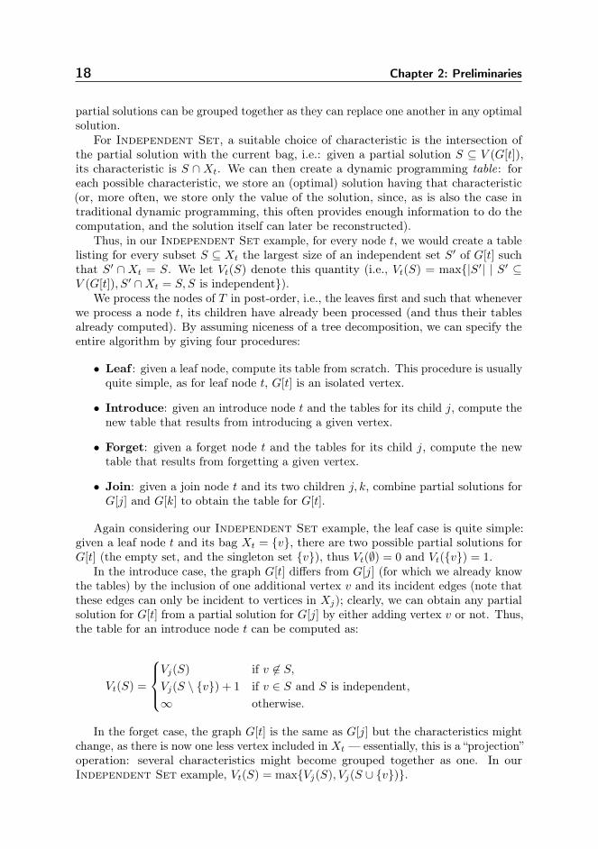
In the introduce case, the graph G[t] differs from G[j] (for which we already knowthe tables) by the inclusion of one additional vertex v and its incident edges (note thatthese edges can only be incident to vertices in Xj); clearly, we can obtain any partialsolution for G[t] from a partial solution for G[j] by either adding vertex v or not. Thus,the table for an introduce node t can be computed as:
Vt(S) =
Vj(S) if v 6∈ S,Vj(S \ v) + 1 if v ∈ S and S is independent,∞ otherwise.
In the forget case, the graph G[t] is the same as G[j] but the characteristics mightchange, as there is now one less vertex included in Xt — essentially, this is a “projection”operation: several characteristics might become grouped together as one. In ourIndependent Set example, Vt(S) = maxVj(S), Vj(S ∪ v).
2.3. Dynamic Programming on Tree Decompositions 19
Finally, in the join case, the graph G[t] is obtained by taking two graphs G[j] andG[k], which are disjoint except for the vertices in Xt, and “gluing” them together onthe vertices in Xt. In our Independent Set example, Vt(S) = Vj(S) + Vk(S)− |S|.
Once all the tables have been computed, the solution for the original problem canbe recovered from the tables in the root node r: for Independent Set, the size of amaximum independent set of G is equal to maxS⊆Xr Vr(S).
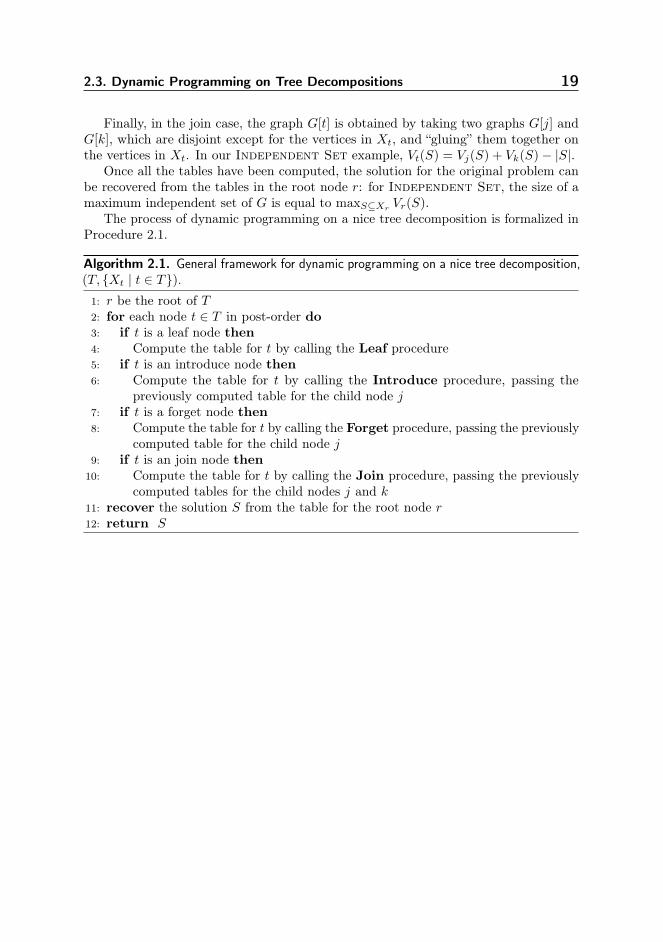
The process of dynamic programming on a nice tree decomposition is formalized inProcedure 2.1.
Algorithm 2.1. General framework for dynamic programming on a nice tree decomposition,(T, Xt | t ∈ T).1: r be the root of T2: for each node t ∈ T in post-order do3: if t is a leaf node then4: Compute the table for t by calling the Leaf procedure5: if t is an introduce node then6: Compute the table for t by calling the Introduce procedure, passing the
previously computed table for the child node j7: if t is a forget node then8: Compute the table for t by calling the Forget procedure, passing the previously
computed table for the child node j9: if t is an join node then
10: Compute the table for t by calling the Join procedure, passing the previouslycomputed tables for the child nodes j and k
11: recover the solution S from the table for the root node r12: return S

IGraph Embedding Problems

23
Algorithms
3.1. Introduction
In this chapter, we will present algorithms for graph embedding problems. We consider(Induced) Subgraph, (Induced) Minor and Topological Minor. We show thateach of these problems can be solved in time 2O(n/ logn) on H-minor free graphs (wheren denotes the number of vertices). In the next chapter, we will give a lower boundunder the Exponential Time Hypothesis, showing that this running time is (likely)optimal.
Our algorithms are based on dynamic programming, enhanced with a canonizationtechnique: we reduce the number of partial solutions by identifying that some of themare isomorphic.
These problems are amongst the first for which both upper and lower bounds of theform 2Θ(n/ logn) are known. We conjecture that there are many more such problems,and that our techniques may be useful to establish similar bounds for them.
In each of these problems, we are asked to embed a pattern graph P into a hostgraph G. We consider the case in which P excludes a specific minor H, ε > 0 isa constant, n = |V (G)| and give algorithms parameterized by the treewidth tw ofG and the number of vertices k of P . Our algorithms are subexponential in k orthe number of vertices of G if tw is sufficiently small. Specifically, we show that forany ε > 0 and graph H, if P is H-minor free and G has treewidth tw, (Induced)Subgraph can be solved 2O(kεtw+k/ log k)nO(1) time and (Induced) Minor can besolved in 2O(kεtw+tw log tw+k/ log k)nO(1) time.
As an important special case of our result, we show that Subgraph Isomorphismcan be solved in time 2O(kε
√n+k/ log k) on H-minor free graphs (which include planar,
bounded-treewidth and bounded-genus graphs). Our result can be combined with arecent result of Fomin et al. [50] to show that Subgraph Isomorphism can be solvedin 2O(k/ log k)nO(1) time if P is connected and G is apex-minor free. In the next chapter,
24 Chapter 3: Algorithms
we will present a lower bound showing that this is optimal (under the ETH).Subgraph Isomorphism has received considerable attention in the literature.
Results include polynomially solvable cases, such as recognizing a fixed (i.e., not partof the input) pattern in planar graphs [43, 47], biconnected outerplanar graphs [83],graphs of log-bounded fragmentation [60], graphs of bounded genus [29] and certainsubclasses of graphs of bounded treewidth [92], exact algorithms [106], lower bounds[35, 58, 103] and results on parameterized complexity [89].
For a pattern graph P of treewidth t, Subgraph Isomorphism can be solved in2O(k)nO(t) time using the colour-coding technique [4]. If the host graph is planar, Sub-graph Isomorphism can be solved in 2O(k)n time [43]. In general graphs, SubgraphIsomorphism can be solved in 2O(n logn) time and, assuming the ETH, this is tight[49].
Graph minor problems are also of interest, especially in the light of Robertsonand Seymour’s seminal work on graph minor theory (see e.g. [105]) and the recentdevelopment of bidimensionality theory [41]. Many graph properties can be tested bychecking for the inclusion of some minor. Testing whether a graph G contains a fixedminor P can be done in O(n3) time [100]; this was recently improved to O(n2) time[74]. However, the dependence on |V (P )| is superexponential. Testing whether a graphP is a minor of a planar graph G can be done in 2O(k)nO(1) time [2], which is onlysingle-exponential. Our lower bound shows that this cannot be improved to 2o(k/ log k)
(assuming the ETH). Our algorithms are subexponential in k, but (in contrast to [2, 74])superpolynomial in n. This is to our knowledge the first subexponential minor testingalgorithm for a non-trivial class of graphs.
Our algorithms are based on dynamic programming on tree decompositions. Inparticular, we use dynamic programming on the host graph and store correspondencesto vertices in the pattern graph. The key algorithmic insight is that this correspondencemay or may not use certain connected components of the pattern graph (that remainafter removing some separator vertices). Instead of storing for each component whetherit is used or not, we identify isomorphic connected components and store only thenumber of times each is used.
In [60], the authors give an algorithm for Subgraph Isomorphism, which runsin polynomial time for a host graph of bounded treewidth and a pattern graph of log-bounded fragmentation (i.e. removing a separator decomposes the graph into at mostlogarithmically many connected components). This is achieved using a similar dynamicprogramming technique, which (in general) uses time exponential in the number ofconnected components that remain after removing a separator. By assuming thenumber of connected components (fragmentation) is logarithmic, the authors obtain apolynomial time algorithm. In contrast, we consider a graph class where fragmentationis unbounded, but the number of non-isomorphic connected components is small. Thisleads to subexponential algorithms.
This chapter builds on techniques due to Bodlaender, Nederlof and van Rooij[25, 28]. They give a 2O(n/ logn)-time algorithm for finding tree decompositions withfew bags and a matching lower bound (based on the Exponential Time Hypothesis),and a 2O(n/ logn)-time algorithm for determining whether a given k-coloured graph is asubgraph of a properly coloured interval graph. These earlier papers, coupled with ourresults, suggest that this technique may have many more applications, and that thereexists a larger class of problems sharing this upper and lower bound.
3.2. An Algorithm for Subgraph Isomorphism 25
We first give the algorithm for Subgraph Isomorphism (which can be triviallyadapted to handle Induced Subgraph), then the algorithm for (Induced) Minor(which extends the algorithm for Subgraph Isomorphism by keeping track of whichvertices are contracted to form a new vertex, and ensuring that these vertices eventuallyinduce a connected subgraph), and finally the algorithm for Topological Minor(which builds upon the one for Subgraph Isomorphism by considering ways to mapvertices of the host graph to edges of the pattern graph).
3.2. An Algorithm for Subgraph Isomorphism
We begin by describing an algorithm for Subgraph Isomorphism, which is based ondynamic programming on a tree decomposition T of the host graph G. This algorithmis similar to that of Hajiaghayi et al. [60] for Subgraph Isomorphism on log-boundedfragmentation graphs, and we use similar notions of (extensible) partial solutions andcharacteristic of a partial solution (Section 3.2). The algorithm does not achieve theclaimed running time bounds. Our main contribution is the canonization technique(Section 3.3) and its analysis (Section 3.4), which can be used to reduce the number ofpartial solutions and gives the subexponential running time.
Definition 3.1 ((Extensible) Partial Solution). For a given node t ∈ T of the treedecomposition of G, a partial solution (relative to t) is a triple (G′, P ′, φ) where G′is a subgraph of G[t], P ′ is an induced subgraph of P and φ : V (G′) → V (P ′) is anisomorphism from G′ to P ′.
A partial solution (G′, P ′, φ) relative to t is extensible if there exists an extension ofφ, ψ : V (G′′)→ V (P ) which is an isomorphism from a subgraph G′′ of G to P whereV (G′′) ∩ V (G[t]) = V (G′).
To facilitate dynamic programming, at node t of the tree decomposition we onlyconsider partial solutions (G′, P ′, φ) which might be extensible (i.e. we attempt to ruleout non-extensible solutions). Note that in a partial solution we have already decidedon how the vertices in G[t] are used, and the extension only makes decisions aboutvertices not in G[t]. Instead of dealing with partial solutions directly, our algorithmworks with characteristics of partial solutions:
Definition 3.2 (Characteristic of a Partial Solution). The characteristic (f, S) of apartial solution (G′, P ′, φ) relative to a node t ∈ T is a function f : Xt → V (P ) ∪ ,together with a subset S ⊆ V (P ) \ f(Xt), so that:
• for all v ∈ V (G′) ∩Xt, f(v) = φ(v) and f(v) = otherwise,
• f is injective, except that it may map multiple elements to ,
• S = V (P ′) \ φ(Xt).
The following easy observation justifies restricting our attention to characteristicsof partial solutions:
Lemma 3.3 (Equivalent to Lemma 10, [60]). If two partial solutions have the samecharacteristic, either both are extensible or neither is extensible.
26 Chapter 3: Algorithms
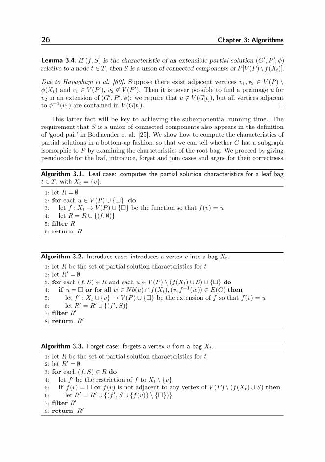
Lemma 3.4. If (f, S) is the characteristic of an extensible partial solution (G′, P ′, φ)relative to a node t ∈ T , then S is a union of connected components of P [V (P )\f(Xt)].
Due to Hajiaghayi et al. [60]. Suppose there exist adjacent vertices v1, v2 ∈ V (P ) \φ(Xt) and v1 ∈ V (P ′), v2 6∈ V (P ′). Then it is never possible to find a preimage u forv2 in an extension of (G′, P ′, φ): we require that u 6∈ V (G[t]), but all vertices adjacentto φ−1(v1) are contained in V (G[t]).
This latter fact will be key to achieving the subexponential running time. Therequirement that S is a union of connected components also appears in the definitionof ‘good pair’ in Bodlaender et al. [25]. We show how to compute the characteristics ofpartial solutions in a bottom-up fashion, so that we can tell whether G has a subgraphisomorphic to P by examining the characteristics of the root bag. We proceed by givingpseudocode for the leaf, introduce, forget and join cases and argue for their correctness.
Algorithm 3.1. Leaf case: computes the partial solution characteristics for a leaf bagt ∈ T , with Xt = v.1: let R = ∅2: for each u ∈ V (P ) ∪ do3: let f : Xt → V (P ) ∪ be the function so that f(v) = u4: let R = R ∪ (f, ∅)5: filter R6: return R
Algorithm 3.2. Introduce case: introduces a vertex v into a bag Xt.1: let R be the set of partial solution characteristics for t2: let R′ = ∅3: for each (f, S) ∈ R and each u ∈ V (P ) \ (f(Xt) ∪ S) ∪ do4: if u = or for all w ∈ Nb(u) ∩ f(Xt), (v, f
−1(w)) ∈ E(G) then5: let f ′ : Xt ∪ v → V (P ) ∪ be the extension of f so that f(v) = u6: let R′ = R′ ∪ (f ′, S)7: filter R′8: return R′
Algorithm 3.3. Forget case: forgets a vertex v from a bag Xt.1: let R be the set of partial solution characteristics for t2: let R′ = ∅3: for each (f, S) ∈ R do4: let f ′ be the restriction of f to Xt \ v5: if f(v) = or f(v) is not adjacent to any vertex of V (P ) \ (f(Xt) ∪ S) then6: let R′ = R′ ∪ (f ′, S ∪ f(v) \ )7: filter R′8: return R′
3.2. An Algorithm for Subgraph Isomorphism 27
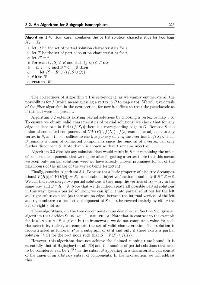
Algorithm 3.4. Join case: combines the partial solution characteristics for two bagsXs = Xt.1: let R be the set of partial solution characteristics for s2: let T be the set of partial solution characteristics for t3: let R′ = ∅4: for each (f, S) ∈ R and each (g,Q) ∈ T do5: if f = g and S ∩Q = ∅ then6: let R′ = R′ ∪ (f, S ∪Q)7: filter R′8: return R′
The correctness of Algorithm 3.1 is self-evident, as we simply enumerate all thepossibilities for f (which means guessing a vertex in P to map v to). We will give detailsof the filter algorithm in the next section, for now it suffices to treat the pseudocode asif this call were not present.
Algorithm 3.2 extends existing partial solutions by choosing a vertex to map v to.To ensure we obtain valid characteristics of partial solutions, we check that for anyedge incident to v in P [S ∪ f(Xt)] there is a corresponding edge in G. Because S is aunion of connected components of G[V (P ) \ f(Xt)], f(v) cannot be adjacent to anyvertex in S, and thus it suffices to check adjacency only against vertices in f(Xt). ThenS remains a union of connected components since the removal of a vertex can onlyfurther disconnect S. Note that u is chosen so that f remains injective.
Algorithm 3.3 discards any solutions that would result in S not remaining the unionof connected components that we require after forgetting a vertex (note that this meanswe keep only partial solutions were we have already chosen preimages for all of theneighbours of the image of the vertex being forgotten).
Finally, consider Algorithm 3.4. Because (as a basic property of nice tree decompos-itions) V (H[i])∩V (H[j]) = Xi, we obtain an injective function if and only if S ∩R = ∅.We can therefore merge two partial solutions if they map the vertices of Xt = Xs in thesame way and S ∩R = ∅. Note that we do indeed create all possible partial solutionsin this way: given a partial solution, we can split it into partial solutions for the leftand right subtrees since (as there are no edges between the internal vertices of the leftand right subtrees) a connected component of S must be covered entirely by either theleft or right subtree.
These algorithms, on the tree decomposition as described in Section 2.3, give analgorithm that decides Subgraph Isomorphism. Note that in contrast to the examplefor Independent Set given in the framework, we do not compute a value for eachcharacteristic, rather, we compute the set of valid characteristics. The solution isreconstructed as follows: P is a subgraph of G if and only if there exists a partialsolution (f, S) for the root node such that S = V (P ) \ f(Xt).
However, this algorithm does not achieve the claimed running time bound: it isessentially that of Hajiaghayi et al. [60] and the number of partial solutions that needto be considered can be 2Ω(k) as the subset S appearing in a characteristic can consistof the union of an arbitrary subset of components. In the next section, we will addressthis.
28 Chapter 3: Algorithms
3.3. Reducing the Number of Partial Solutions UsingIsomorphism Tests
In this section, we show how adapt the algorithm from the previous section to achievethe claimed running time bound. This involves a careful analysis of the numberof characteristics, and using isomorphism tests to reduce this number. Currently,if the connected components of S are small (e.g., O(1) vertices each) then theirnumber is large (e.g., Ω(n) components) and thus in the worst case we have 2Ω(n)
partial solutions. However, if there are many small connected components many willnecessarily be isomorphic to each other (since there are only few isomorphism classesof small connected components) and we can thus reduce the number of characteristicsby identifying isomorphic connected components:
Definition 3.5 (Partial Solution Characteristic Isomorphism). Given a bag t ∈ T , twocharacteristics of partial solutions (f, S), (g,R) for t are isomorphic if:
• f = g,
• there is a bijection h : CC(S)→ CC(R),
• for all connected components c ∈ CC(S), c and h(c) are isomorphic when allvertices v ∈ c vertices are labelled with Nb(v) ∩ f(Xt) (i.e., the set of vertices off(Xt) to which v is adjacent).
Clearly, the algorithm given in the previous section remains correct even if aftereach step we remove duplicate isomorphic characteristics. To this end, we modify thejoin case (Algorithm 3.4): the disjointness check S ∩Q = ∅ should be replaced with acheck that if P [V (P ) \ f(Xt)] contains NP (y) connected components of isomorphismclass y, and P [S] (resp. P [Q]) contains NS(y) (resp. NQ(y)) connected components ofisomorphism class y, then NS(y) + NQ(y) ≤ NP (y). Similarly, the statement S ∪ Qneeds to be changed to, if the union is not disjoint, replace connected components thatoccur more than once with other connected components of the same isomorphism class(so as to make the union disjoint while preserving the total number of components ofthe same type).
Call a connected component small if it has at most c log k vertices, and largeotherwise. We let c > 0 be a constant that depends only on |V (H)| and ε. We do notstate our choice of c explicitly, but in our analysis we will assume it is “small enough”.
For a small connected component s, we label each of its vertices by the subset ofvertices of f(Xt) to which it is adjacent. We then compute a canonical representation ofthis labeled component, for example by considering all permutations of its vertices, andchoosing the permutation that results in the lexicographically smallest representation.Note that since we only canonize the small connected components using such a trivialcanonization algorithm does not affect the running time of our algorithm, as (c log k)!is only slightly superpolynomial.
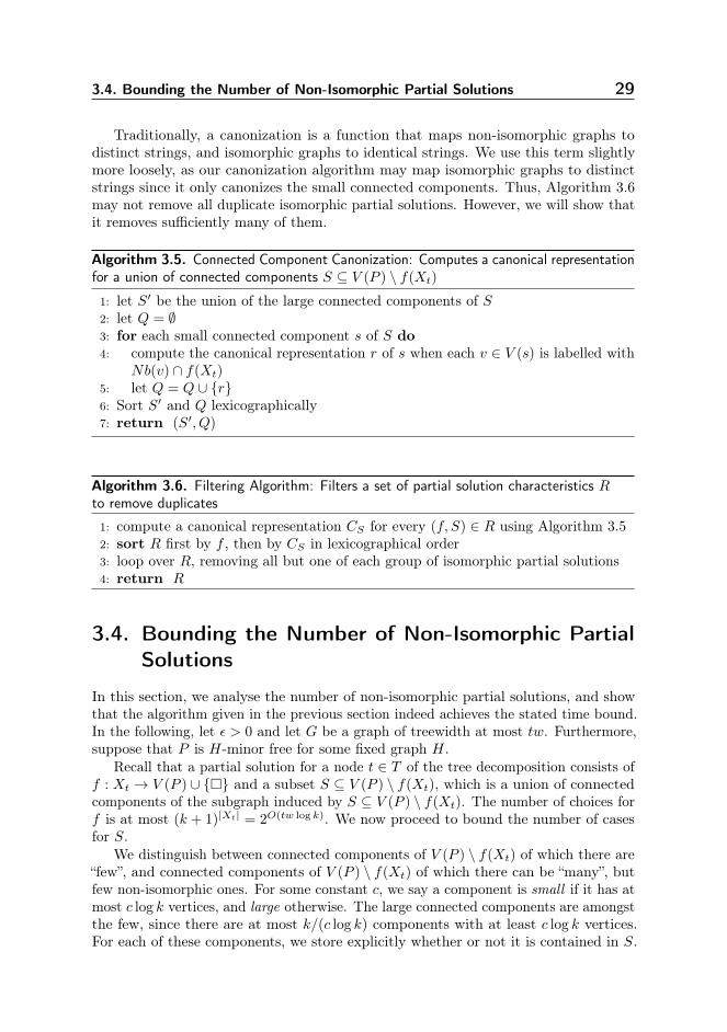
Algorithm 3.5 computes a canonical representation of a partial solution. It requiresthat we have some predefined ordering of the vertices of G. The canonization algorithm(Algorithm 3.5) allows us to define the filter algorithm (Algorithm 3.6).
3.4. Bounding the Number of Non-Isomorphic Partial Solutions 29
Traditionally, a canonization is a function that maps non-isomorphic graphs todistinct strings, and isomorphic graphs to identical strings. We use this term slightlymore loosely, as our canonization algorithm may map isomorphic graphs to distinctstrings since it only canonizes the small connected components. Thus, Algorithm 3.6may not remove all duplicate isomorphic partial solutions. However, we will show thatit removes sufficiently many of them.
Algorithm 3.5. Connected Component Canonization: Computes a canonical representationfor a union of connected components S ⊆ V (P ) \ f(Xt)
1: let S′ be the union of the large connected components of S2: let Q = ∅3: for each small connected component s of S do4: compute the canonical representation r of s when each v ∈ V (s) is labelled with
Nb(v) ∩ f(Xt)5: let Q = Q ∪ r6: Sort S′ and Q lexicographically7: return (S′, Q)
Algorithm 3.6. Filtering Algorithm: Filters a set of partial solution characteristics Rto remove duplicates
1: compute a canonical representation CS for every (f, S) ∈ R using Algorithm 3.52: sort R first by f , then by CS in lexicographical order3: loop over R, removing all but one of each group of isomorphic partial solutions4: return R
3.4. Bounding the Number of Non-Isomorphic PartialSolutions
In this section, we analyse the number of non-isomorphic partial solutions, and showthat the algorithm given in the previous section indeed achieves the stated time bound.In the following, let ε > 0 and let G be a graph of treewidth at most tw. Furthermore,suppose that P is H-minor free for some fixed graph H.
Recall that a partial solution for a node t ∈ T of the tree decomposition consists off : Xt → V (P ) ∪ and a subset S ⊆ V (P ) \ f(Xt), which is a union of connectedcomponents of the subgraph induced by S ⊆ V (P ) \ f(Xt). The number of choices forf is at most (k + 1)|Xt| = 2O(tw log k). We now proceed to bound the number of casesfor S.
We distinguish between connected components of V (P ) \ f(Xt) of which there are“few”, and connected components of V (P ) \ f(Xt) of which there can be “many”, butfew non-isomorphic ones. For some constant c, we say a component is small if it has atmost c log k vertices, and large otherwise. The large connected components are amongstthe few, since there are at most k/(c log k) components with at least c log k vertices.For each of these components, we store explicitly whether or not it is contained in S.
30 Chapter 3: Algorithms
They contribute a factor of 2O(k/ log k) to the number of cases. For the small connectedcomponents, we will show a partition into the “few” (which we treat similarly to thelarge connected components), and into the “many, but few non-isomorphic” (for whichwe store, for each isomorphism class, the number of components from that isomorphismclass contained in S).
Lemma 3.6. For a given node t and function f : Xt → V (P ), there are at mostO(kε/2tw) isomorphism classes of small connected components.
Proof. For a small connected component Q ∈ CC(V (P ) \ f(Xt)), its isomorphism classis determined by the isomorphism class of the graph induced by Q, and the adjacencyof vertices v ∈ Q to vertices in f(Xt). Since |Q| ≤ c log k and P is H-minor free, thereexists a constant CH > 1 so that there are at most 2CH ·c log k cases for the isomorphismclass of the graph induced by Q (see [7]).
What remains is to bound the number of cases for adjacency of Q to Xt. In thisspecific case, Nb(Q) denotes the set of vertices of Xt to which Q is incident, that is,v ∈ Nb(Q) if and only if v ∈ Xt and there exists a vertex u ∈ Q so that (u, v) ∈ E(P ).Using the following lemma, we further divide the small connected components into twocases: the components with a large neighbourhood, and the components with a smallneighbourhood.
Lemma 3.7. Let H be a fixed graph. Then there exists a constant d (depending onH), so that if G = (A,B,E) is H-minor free and bipartite, there are at most
• O(|A|) vertices in B with degree greater than d,
• O(|A|) subsets A′ ⊆ A such that A′ = Nb(u) for some u ∈ B.
Lemma 3.7 follows as a special case of Lemma 3 due to Gajarsky et al. [54]. Wegive a simpler, self-contained proof of this special case:
Proof. Let d = |V (H)| − 1. We prove the first part by repeatedly contracting a high-degree vertex u (degree > d) in B with one of its neighbours in A. Since G is H-minorfree, it certainly does not contain the complete graph K|H| as a minor. Therefore, theneighbourhood of u cannot be complete and the contraction can be performed in sucha way that it creates at least one new edge in the subgraph induced by A. At the endof this process, the number of edges in the subgraph induced by A forms an upperbound on the number of high-degree vertices originally in B. We now use the fact thatH-minor free graphs are sparse: such a subgraph contains at most O(|A|) edges.
For the second part of the lemma, consider only those vertices u ∈ B with degree atmost d – since there are at most O(|A|) vertices with degree > d they trivially contributeat most O(|A|) distinct neighbourhoods. Now, repeatedly contract a low-degree vertexu for which Nb(u) does not induce a complete subgraph of A – again creating atleast one new edge in the subgraph induced by A. At the end of this process, for allremaining low-degree vertices in u ∈ B, Nb(u) induces a clique in A. The result nowfollows from the fact that H-minor free graphs can have at most linearly many cliques(see e.g. [52]).
Taking A = Xt, deleting the edges between vertices in Xt and contracting everyconnected component Q ∈ CC(V (P ) \ f(Xt)) to a single vertex in B, the lemma states
3.5. Graph Minors and Induced Problem Variants 31
that there are at most O(tw) components with |Nb(Q)| > d and that the componentswith |Nb(Q)| ≤ d have at most O(tw) distinct neighbourhoods in Xt.
For the connected components Q ∈ CC(V (P ) \ f(Xt)) with |Nb(Q)| ≤ d, wehave 2CH ·c log k cases for the isomorphism class of Q, O(tw) cases for Nb(x) and forevery vertex of Q, at most 2d cases for incidence to Nb(Q). We thus have at most2Ch·c log k ·O(tw) · (2d)c log k isomorphism classes for Q ∈ CC(S) with Nb(Q) ≤ d. Forsufficiently small c > 0, this is O(kε/2tw).
This finishes the proof of Lemma 3.6.
Since of each component there can be most k occurrences in S, the total numberof cases for storing the multiplicity of each class of components is (k + 1)O(kε/2tw) =
2O(kε/2tw log k) = 2O(kεtw).We now have all the results we need to finish the analysis. Storing the multiplicities
of the small connected components gives 2O(kεtw) cases, while storing the subset of largeconnected components explicitly contributes 2O(k/ log k) cases. A partial solution isfurther characterized by f , for which there are only 2O(tw log k) cases. For a given nodet of the tree decomposition, there are thus at most 2O(kεtw+k/ log k) partial solutions.
Thus, augmenting the dynamic programming algorithm described in the previoussection with the filtering algorithm, we obtain the following result:
Theorem 3.8. For any graph H and ε > 0, Subgraph Isomorphism can be solved intime 2O(kεtw+k/ log k)nO(1) if the host graph has treewidth tw and the pattern graph isH-minor free.
Note that a tree decomposition does not need to be given as part of the input, aswe can compute a 5-approximate tree-decomposition of G in time exponential in tw[18] and this does not increase the asymptotic running time.
3.5. Graph Minors and Induced Problem Variants
In this section, we discuss how our algorithm for Subgraph Isomorphism can beadapted to Induced Subgraph and (Induced) Minor. We begin by describingthe algorithm for Graph Minor, then give a brief description on how to adapt bothalgorithms for the induced cases.
Note that P is a minor of G if and only if we have a function f : V (G)→ V (P )∪,such that
• for all v ∈ V (P ), f−1(v) is non-empty, and induces a connected subgraph of G,
• for all (v, w) ∈ E(P ), there are x ∈ f−1(v) and y ∈ f−1(w) with (x, y) ∈ E(G).
Vertices that are deleted are mapped to , otherwise f(v) gives the vertex that v iscontracted to. Call such a function a solution for the Graph Minor problem.
If we restrict such solutions to a subgraph G[t], we obtain the notion of partialsolution:
Definition 3.9 (Partial Solution (Graph Minor)). Given a node t ∈ T of the treedecomposition of G, a partial solution for the Graph Minor problem relative to t is afunction f : V (G[t])→ V (P ) ∪ , such that
32 Chapter 3: Algorithms
1. For each v ∈ V (P ), at least one of the following three cases holds:
(a) each connected component of G[t][f−1(v)] contains at least one vertex fromXt,
(b) G[t][f−1(v)] has one connected component,
(c) f−1(v) is empty.
2. For all (v, w) ∈ E(P ), at least one of the following cases holds:
(a) Some vertex of f−1(v) is adjacent to some vertex of f−1(w) in G[t],
(b) f−1(v) ∩Xt 6= ∅ and f−1(w) ∩Xt 6= ∅,(c) f−1(v) ∩Xt 6= ∅ and f−1(w) = ∅,(d) f−1(w) ∩Xt 6= ∅ and f−1(v) = ∅,(e) f−1(w) = ∅ and f−1(v) = ∅.
Intuitively, in 1) we require that the preimage of v can still be made connected (a),is already connected (b) or has not been assigned yet (c), and in 2) we require that theedge (v, w) is already covered (a), can still be covered (b,c,d,e).
As before, our dynamic programming algorithm uses characteristics of partialsolutions:
Definition 3.10 (Characteristic of a partial solution (Graph Minor)). Given a nodet ∈ T of the tree decomposition of G and a partial solution for the Graph Minorproblem relative to a node t f : V (G[t]) → V (P ) ∪ , the characteristic of f is atuple (f ′, S,∼, F ) such that:
1. f ′ is the restriction of f to Xt,
2. S ⊆ V (P ) with S = f(V (G[t])) \ (f(Xt) ∪ ),
3. ∼ is an equivalence relation on Xt, with v ∼ w, if and only if f(v) = f(w) andthere exists a path from v to w in G[t] such that for all vertices x on this pathf(x) = f(v).
4. F ⊆ E(P [f(Xt)]) such that for every (v, w) ∈ E(P [f(Xt)]), it holds that (v, w) ∈F if and only if each of the following holds:
(a) f−1(v) ∩Xt 6= ∅,(b) f−1(w) ∩Xt 6= ∅,(c) There are x ∈ f−1(v) and y ∈ f−1(w) with (x, y) ∈ E(G[t]).
As before, it is easy to see the equivalence between the existence of a minor, solution,and partial solution with certain characteristic.
Compared to our approach for Subgraph Isomorphism, we no longer require f tobe injective – f−1(v) corresponds to the vertices that are contracted to form v. Werequire that f−1(v) eventually becomes connected. This can either be achieved insidethe bag, be achieved below the bag (in the tree decomposition), or above the bag. Therelation ∼ tracks which components are already connected by vertices below the bag.
3.5. Graph Minors and Induced Problem Variants 33
Similarly, edges inside P [f(Xt)] might not have corresponding edges inside G[Xt], butmight instead correspond to edges below or above this bag. The set F stores whichedges correspond to edges below the current bag.
The following lemma is the counterpart of Lemma 3.3 and shows that we can applydynamic programming:
Lemma 3.11. If partial solutions for the Graph Minor problem f and g have thesame characteristic and are both relative to t, then f can be extended to a solution ifand only if g can be extended to a solution.
Proof. We will prove that if f can be extended to a solution, then so can g. Bysymmetry, this is sufficient to prove the lemma. Let both f and g have characteristic(f ′, S,∼, F ) and let f∗ be an extension of f to a solution. Let g∗ : V (G)→ V (P )∪be an extension of g, such that g∗(v) = g(v) for all v ∈ V (G[t]) and let g∗(v) = f(v)otherwise. We claim that g∗ is a solution:
• First, we check that for all v ∈ V (P ), g−1∗ (v) is non-empty and induces a connected
subgraph of G:
– If v 6∈ g(G[t]) then the property trivially holds since g−1∗ (v) = f(v)
– If v ∈ g(G[t]) then g−1∗ (v) certainly is non-empty. To see that it is connected,
consider A = f−1∗ (v) \ G[t]. For each of the equivalence classes B of ∼
contained in f−1∗ (v) ∩G[t], some vertex of A must be adjacent to a vertex
of B, since otherwise f−1∗ (v) would not be connected. Therefore g−1
∗ (v) isconnected.
• Secondly, we check that for all (u, v) ∈ E(P ), there exist x ∈ g−1∗ (u) and
y ∈ g−1∗ (v) with (x, y) ∈ E(G). Since f∗ is a solution, there exist x′ ∈ f−1
∗ (v) andy′ ∈ f−1
∗ (w) with (x′, y′) ∈ E(G). We distinguish several cases; since the rolesof x, y′ and y, y′ are symmetrical, without loss of generality we omit cases withreverse roles of x and y.
1. There exists x′ ∈ f−1∗ (u) and y′ ∈ f−1
∗ (v) such that x′ /∈ G[t] and y′ /∈ G[t].Then the property holds, since g′(x′) = f(x′) and g′(x′) = f(x′).
2. There exists x′ ∈ f−1∗ (u) and y′ ∈ f−1
∗ (v) such that x′ ∈ Xt and y′ 6∈ G[t].Then the property holds, since g′(x′) = f(x′) and g′(x′) = f(x′).
3. There exists x′ ∈ f−1∗ (u) and y′ ∈ f−1
∗ (v) such that x′ ∈ Xt and y′ ∈ Xt.Then the property holds, since g′(x′) = f(x′) and g′(x′) = f(x′).
4. It holds that f−1∗ (u) ⊆ V (G[t])−Xt or f−1
∗ (v) ⊆ V (G[t])−Xt. Then, sincef∗ extends f which has the same characteristic g, g−1(u) ⊆ V (G[t])−Xt org−1(v) ⊆ V (G[t])−Xt. Then the property holds by Item 2. of Definition3.9 since g is a partial solution, which is a restriction of g∗.
5. It holds that f−1∗ (u) ∩Xt 6= ∅ and f−1
∗ (v) ∩Xt 6= ∅. If g−1(u) ∩Xt = ∅ org−1(v) ∩Xt = ∅ then we are in the first or second case (since both charac-teristics share S). Therefore (u, v) ∈ F by the Item 4. of Definition 3.10.
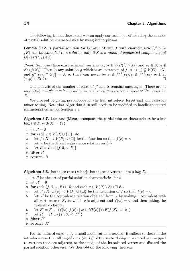
34 Chapter 3: Algorithms
The following lemma shows that we can apply our technique of reducing the numberof partial solution characteristics by using isomorphisms:
Lemma 3.12. A partial solution for Graph Minor f with characteristic (f ′, S,∼, F ) can be extended to a solution only if S is a union of connected components ofG[V (P ) \ f(Xt)].
Proof. Suppose there exist adjacent vertices v1, v2 ∈ V (P ) \ f(Xt) and v1 ∈ S, v2 6∈S ∪ f(Xt). Then in any solution g which is an extension of f , g−1(v1) ⊆ V (G)−Xt
and g−1(v2) ∩ G[t] = ∅, so there can never be x ∈ f−1(v1), y ∈ f−1(v2) so that(x, y) ∈ E(G).
The analysis of the number of cases of f ′ and S remains unchanged. There are atmost (tw)tw = 2O(tw log tw) cases for ∼, and since P is sparse, at most 2O(tw) cases forF .
We proceed by giving pseudocode for the leaf, introduce, forget and join cases forminor testing. Note that Algorithm 3.10 still needs to be modified to handle canonizedcharacteristics, as per Section 3.3.
Algorithm 3.7. Leaf case (Minor): computes the partial solution characteristics for a leafbag t ∈ T , with Xt = v.1: let R = ∅2: for each u ∈ V (P ) ∪ do3: let f : Xt → V (P ) ∪ be the function so that f(v) = u4: let ∼ be the trivial equivalence relation on v5: let R = R ∪ (f, ∅,∼, F )6: filter R7: return R
Algorithm 3.8. Introduce case (Minor): introduces a vertex v into a bag Xt.
1: let R be the set of partial solution characteristics for t2: let R′ = ∅3: for each (f, S,∼, F ) ∈ R and each u ∈ V (P ) \ S ∪ do4: let f ′ : Xt ∪ v → V (P ) ∪ be the extension of f so that f(v) = u5: let ∼′ be the equivalence relation obtained from ∼ by making v equivalent with
all vertices w ∈ Xt to which v is adjacent and f(w) = u and then taking thetransitive closure
6: let F ′ = F ∪ (f(w), f(v)) | w ∈ Nb(v) ∩ E(f(Xt) ∪ u)7: let R′ = R′ ∪ (f ′, S,∼′, F ′)8: filter R′9: return R′
For the induced cases, only a small modification is needed: it suffices to check in theintroduce case that all neighbours (in Xt) of the vertex being introduced are mappedto vertices that are adjacent to the image of the introduced vertex and discard thepartial solution otherwise. We thus obtain the following theorem:
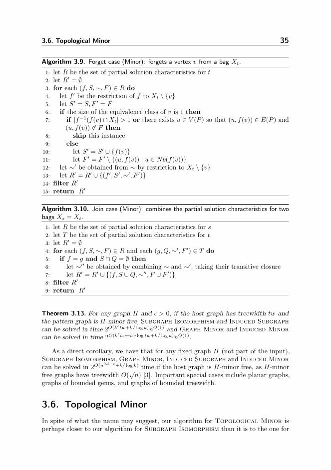
3.6. Topological Minor 35
Algorithm 3.9. Forget case (Minor): forgets a vertex v from a bag Xt.
1: let R be the set of partial solution characteristics for t2: let R′ = ∅3: for each (f, S,∼, F ) ∈ R do4: let f ′ be the restriction of f to Xt \ v5: let S′ = S, F ′ = F6: if the size of the equivalence class of v is 1 then7: if |f−1(f(v) ∩Xt| > 1 or there exists u ∈ V (P ) so that (u, f(v)) ∈ E(P ) and
(u, f(v)) 6∈ F then8: skip this instance9: else
10: let S′ = S′ ∪ f(v)11: let F ′ = F ′ \ (u, f(v)) | u ∈ Nb(f(v))12: let ∼′ be obtained from ∼ by restriction to Xt \ v13: let R′ = R′ ∪ (f ′, S′,∼′, F ′)14: filter R′15: return R′
Algorithm 3.10. Join case (Minor): combines the partial solution characteristics for twobags Xs = Xt.1: let R be the set of partial solution characteristics for s2: let T be the set of partial solution characteristics for t3: let R′ = ∅4: for each (f, S,∼, F ) ∈ R and each (g,Q,∼′, F ′) ∈ T do5: if f = g and S ∩Q = ∅ then6: let ∼′′ be obtained by combining ∼ and ∼′, taking their transitive closure7: let R′ = R′ ∪ (f, S ∪Q,∼′′, F ∪ F ′)8: filter R′9: return R′
Theorem 3.13. For any graph H and ε > 0, if the host graph has treewidth tw andthe pattern graph is H-minor free, Subgraph Isomorphism and Induced Subgraphcan be solved in time 2O(kεtw+k/ log k)nO(1) and Graph Minor and Induced Minorcan be solved in time 2O(kεtw+tw log tw+k/ log k)nO(1).
As a direct corollary, we have that for any fixed graph H (not part of the input),Subgraph Isomorphism, Graph Minor, Induced Subgraph and Induced Minorcan be solved in 2O(n0.5+ε+k/ log k) time if the host graph is H-minor free, as H-minorfree graphs have treewidth O(
√n) [3]. Important special cases include planar graphs,
graphs of bounded genus, and graphs of bounded treewidth.
3.6. Topological Minor
In spite of what the name may suggest, our algorithm for Topological Minor isperhaps closer to our algorithm for Subgraph Isomorphism than it is to the one for
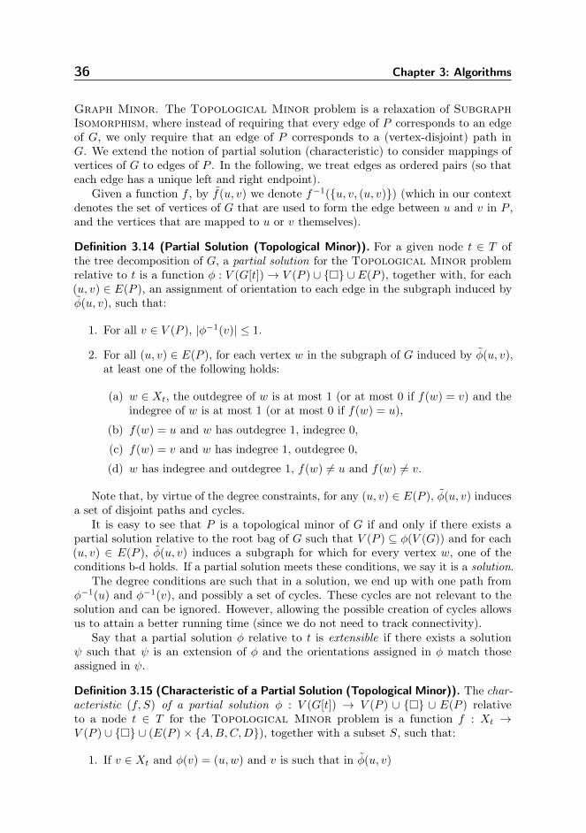
36 Chapter 3: Algorithms
Graph Minor. The Topological Minor problem is a relaxation of SubgraphIsomorphism, where instead of requiring that every edge of P corresponds to an edgeof G, we only require that an edge of P corresponds to a (vertex-disjoint) path inG. We extend the notion of partial solution (characteristic) to consider mappings ofvertices of G to edges of P . In the following, we treat edges as ordered pairs (so thateach edge has a unique left and right endpoint).
Given a function f , by f(u, v) we denote f−1(u, v, (u, v)) (which in our contextdenotes the set of vertices of G that are used to form the edge between u and v in P ,and the vertices that are mapped to u or v themselves).
Definition 3.14 (Partial Solution (Topological Minor)). For a given node t ∈ T ofthe tree decomposition of G, a partial solution for the Topological Minor problemrelative to t is a function φ : V (G[t])→ V (P ) ∪ ∪ E(P ), together with, for each(u, v) ∈ E(P ), an assignment of orientation to each edge in the subgraph induced byφ(u, v), such that:
1. For all v ∈ V (P ), |φ−1(v)| ≤ 1.
2. For all (u, v) ∈ E(P ), for each vertex w in the subgraph of G induced by φ(u, v),at least one of the following holds:
(a) w ∈ Xt, the outdegree of w is at most 1 (or at most 0 if f(w) = v) and theindegree of w is at most 1 (or at most 0 if f(w) = u),
(b) f(w) = u and w has outdegree 1, indegree 0,
(c) f(w) = v and w has indegree 1, outdegree 0,
(d) w has indegree and outdegree 1, f(w) 6= u and f(w) 6= v.
Note that, by virtue of the degree constraints, for any (u, v) ∈ E(P ), φ(u, v) inducesa set of disjoint paths and cycles.
It is easy to see that P is a topological minor of G if and only if there exists apartial solution relative to the root bag of G such that V (P ) ⊆ φ(V (G)) and for each(u, v) ∈ E(P ), φ(u, v) induces a subgraph for which for every vertex w, one of theconditions b-d holds. If a partial solution meets these conditions, we say it is a solution.
The degree conditions are such that in a solution, we end up with one path fromφ−1(u) and φ−1(v), and possibly a set of cycles. These cycles are not relevant to thesolution and can be ignored. However, allowing the possible creation of cycles allowsus to attain a better running time (since we do not need to track connectivity).
Say that a partial solution φ relative to t is extensible if there exists a solutionψ such that ψ is an extension of φ and the orientations assigned in φ match thoseassigned in ψ.
Definition 3.15 (Characteristic of a Partial Solution (Topological Minor)). The char-acteristic (f, S) of a partial solution φ : V (G[t]) → V (P ) ∪ ∪ E(P ) relativeto a node t ∈ T for the Topological Minor problem is a function f : Xt →V (P ) ∪ ∪ (E(P )× A,B,C,D), together with a subset S, such that:
1. If v ∈ Xt and φ(v) = (u,w) and v is such that in φ(u, v)
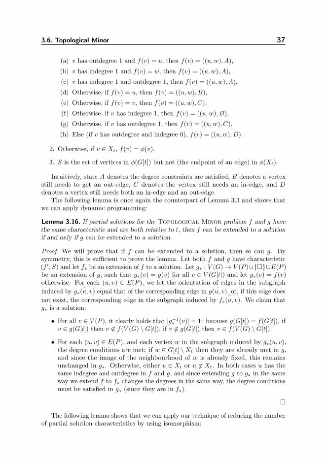
3.6. Topological Minor 37
(a) v has outdegree 1 and f(v) = u, then f(v) = ((u,w), A),
(b) v has indegree 1 and f(v) = w, then f(v) = ((u,w), A),
(c) v has indegree 1 and outdegree 1, then f(v) = ((u,w), A),
(d) Otherwise, if f(v) = u, then f(v) = ((u,w), B),
(e) Otherwise, if f(v) = v, then f(v) = ((u,w), C),
(f) Otherwise, if v has indegree 1, then f(v) = ((u,w), B),
(g) Otherwise, if v has outdegree 1, then f(v) = ((u,w), C),
(h) Else (if v has outdegree and indegree 0), f(v) = ((u,w), D).
2. Otherwise, if v ∈ Xt, f(v) = φ(v).
3. S is the set of vertices in φ(G[t]) but not (the endpoint of an edge) in φ(Xt).
Intuitively, state A denotes the degree constraints are satisfied, B denotes a vertexstill needs to get an out-edge, C denotes the vertex still needs an in-edge, and Ddenotes a vertex still needs both an in-edge and an out-edge.
The following lemma is once again the counterpart of Lemma 3.3 and shows thatwe can apply dynamic programming:
Lemma 3.16. If partial solutions for the Topological Minor problem f and g havethe same characteristic and are both relative to t, then f can be extended to a solutionif and only if g can be extended to a solution.
Proof. We will prove that if f can be extended to a solution, then so can g. Bysymmetry, this is sufficient to prove the lemma. Let both f and g have characteristic(f ′, S) and let f∗ be an extension of f to a solution. Let g∗ : V (G)→ V (P )∪∪E(P )be an extension of g, such that g∗(v) = g(v) for all v ∈ V (G[t]) and let g∗(v) = f(v)otherwise. For each (u, v) ∈ E(P ), we let the orientation of edges in the subgraphinduced by ˜g∗(u, v) equal that of the corresponding edge in ˜g(u, v), or, if this edge doesnot exist, the corresponding edge in the subgraph induced by ˜f∗(u, v). We claim thatg∗ is a solution:
• For all v ∈ V (P ), it clearly holds that |g−1∗ (v)| = 1: because g(G[t]) = f(G[t]), if
v ∈ g(G[t]) then v 6∈ f(V (G) \G[t]), if v 6∈ g(G[t]) then v ∈ f(V (G) \G[t]).
• For each (u, v) ∈ E(P ), and each vertex w in the subgraph induced by g∗(u, v),the degree conditions are met: if w ∈ G[t] \Xt then they are already met in g,and since the image of the neighbourhood of w is already fixed, this remainsunchanged in g∗. Otherwise, either u ∈ Xt or u 6∈ Xt. In both cases u has thesame indegree and outdegree in f and g, and since extending g to g∗ in the sameway we extend f to f∗ changes the degrees in the same way, the degree conditionsmust be satisfied in g∗ (since they are in f∗).
The following lemma shows that we can apply our technique of reducing the numberof partial solution characteristics by using isomorphism:
38 Chapter 3: Algorithms
Lemma 3.17. A partial solution for Topological Minor f with characteristic (f, S)can be extended to a solution only if S is a union of connected components ofG[V (P )\Z],where Z = v ∈ V (P ) | v ∈ f(Xt) or ∃u ∈ Nb(v), t ∈ A,B,C,D : ((u, v), t) ∈f(Xt) or ((v, u), t) ∈ f(Xt).
Proof. Suppose there exist adjacent vertices v1, v2 ∈ V (P ) \ Z and v1 ∈ S, v2 6∈ S ∪ Z.Since v1, v2 are adjacent, there must be a path from f−1(v1) to the vertex that (in anextension of f) is mapped to v2. Since v2 6∈ f(G[t]), this path must contain a vertex ofXt. However, this contradicts the fact that v1, v2 ∈ V (P ) \ Z.
The analysis of the number of cases of f and S remains unchanged: P has O(n)edges, so the fact that both edges and vertices can now appear in the range of f doesnot affect the asymptotic bound, and since there are only four possible vertex states,the size of the range of f is still O(n). Thus, we obtain the following result:
Theorem 3.18. For any graph H and ε > 0, Topological Minor can be solved intime 2O(kεtw+k/ log k)nO(1) if the host graph has treewidth tw and the pattern graph isH-minor free.
3.7. Conclusions
We have presented algorithms for (Induced) Subgraph, (Induced) Minor andTopological Minor that, by taking advantage of isomorphic structures in thepattern graph, run in subexponential time on H-minor free graphs. These algorithmsare essentially optimal since, in the next chapter, we will show that the existence of2o(n/ logn)-time algorithms would contradict the Exponential Time Hypothesis. Thisthus settles the (traditional) complexity of these problems on (general) H-minor freegraphs.
Our result applies to a wide range of graphs: we require P to be H-minor free andG to have truly sublinear treewidth. Some restriction on G is indeed necessary, since ifG is an arbitrary graph then Hamiltonian Path is a special case (in which P is apath) and a 2o(n) algorithm would contradict the ETH [86].
By combining our result with one by Fomin et al. [50], it is possible to obtain afixed-parameter tractable algorithm with running time 2O(k/ log k)nO(1) for the casewhere P is connected and G is apex-minor free. However, this algorithm is randomized.Very recently [96] it has been shown that if G is planar, a deterministic 2O(k/ log k)nO(1)-time algorithm is possible (where P need not necessarily be connected). An interestingopen question is whether this latter result can be generalized to the case of H-minorfree graphs.
We note that our lower bound proof also works for Immersion. However, ouralgorithmic technique does not seem to work for Immersion. Does the Immersionproblem also have a 2O(n/ logn) algorithm, or is a stronger lower bound possible?
Lemma 3.7 holds for a more general class of graphs, and we believe it may be possibleto extend our result to patterns from a graph class with expansion O(1) or perhapsexpansion O(
√r). We note that for different graph classes, a tradeoff between the size
of the small connected components and the factor k/ log k in the exponent is possible:
3.7. Conclusions 39
it might be possible to obtain a 2O(n/ log logn)-time algorithm for less restrictive graphclasses.
Together with the Minimum Size Tree/Path Decomposition problems ([25] – wewill also study these problems in the next chapter), these problems are amongst thefirst for which a 2Θ(n/ logn) upper and lower bound is known. Our work shows thatthe techniques from [25] can be adapted to other problems, and we suspect there maybe many more problems for which identifying isomorphic components can speed updynamic programming algorithms.

41
Lower Bounds
4.1. Introduction
In this chapter, we give tight subexponential lower bounds for a number of graphembedding problems, showing that the algorithms presented in the previous chapterare optimal. We introduce two related combinatorial problems, which we call StringCrafting and Orthogonal Vector Crafting, and show that these cannot besolved in time 2o(|s|/ log |s|), unless the Exponential Time Hypothesis fails.
Previously, Bodlaender et al. [26] showed that several of these graph embeddingproblems could not be solved in 2o(n/ logn) time, even on very restricted classes ofgraphs. We use our results on these string problems to obtain simplified hardnessresults for several graph embedding problems, on more restricted graph classes thanpreviously known: assuming the Exponential Time Hypothesis, there do not existalgorithms that run in 2o(n/ logn) time for
• Subgraph Isomorphism on graphs of pathwidth 1,
• Induced Subgraph Isomorphism on graphs of pathwidth 1,
• Graph Minor on graphs of pathwidth 1,
• Induced Graph Minor on graphs of pathwidth 1,
• Intervalizing 5-Coloured Graphs on trees,
• and finding a tree or path decomposition with width at most c with a minimumnumber of bags, for any fixed c ≥ 16.
2Θ(n/ logn) appears to be the “correct” running time for many packing and em-bedding problems on restricted graph classes, and we think String Crafting and
42 Chapter 4: Lower Bounds
Orthogonal Vector Crafting form a useful framework for establishing lowerbounds of this form.
As noted in the introduction, many NP-complete graph problems admit fasteralgorithms when restricted to planar graphs. In almost all cases, these algorithmshave running times that are exponential in a square root function (e.g. 2O(
√n), nO(
√k)
or 2O(√k)nO(1)) and most of these results are tight, assuming the Exponential Time
Hypothesis. This seemingly universal behaviour has been dubbed the “Square RootPhenomenon” [88].
These results answer an open question [87] of whether the Square Root Phe-nomenon holds for Subgraph Isomorphism in planar graphs negatively1: assumingthe Exponential Time Hypothesis, there is no 2o(n/ logn)-time algorithm for SubgraphIsomorphism, even when restricted to (planar) graphs of pathwidth 2 [26]. The samelower bound holds for Induced Subgraph and (Induced) Minor and is in fact tight:as shown in the previous chapter, the problems admit 2O(n/ logn)-time algorithms onH-minor free graphs.
The original proofs of this type of lower bound [26] followed by reductions froma problem called String 3-Groups. We introduce a new problem, String Craft-ing, and show a 2Ω(|s|/ log |s|)-time lower bound under the ETH for this problem bygiving a direct reduction from 3-Satisfiability. Using this result, we show that the2Ω(|s|/ log |s|)-time lower bounds for (Induced) Subgraph and (Induced) Minor hold evenon graphs of pathwidth 1.
Alongside String Crafting, we introduce the related Orthogonal VectorCrafting problem. Using this problem, we show 2Ω(|n|/ log |n|)-time lower bounds fordeciding whether a 5-coloured tree is the subgraph of an interval graph (for which thesame colouring is proper) and for deciding whether a graph admits a tree (or path)decomposition of width 16 with at most a given number of bags.
For any fixed k, Intervalizing k-Coloured Graphs can be solved in time2O(n/ logn) [28]. Bodlaender and Nederlof [25] conjecture a lower bound (under theExponential Time Hypothesis) of 2Ω(n/ logn) time for k ≥ 6; we settle this conjectureand show that it in fact holds for k ≥ 5, even when restricted to trees. To complementthis result for a fixed number of colours, we also show that there is no algorithm solvingIntervalizing Coloured Graphs (with an arbitrary number of colours) in time2o(n), even when restricted to trees.
Minimum Size Tree Decomposition and Minimum Size Path Decompositioncan also be solved in 2O(n/ logn) time on graphs of bounded treewidth. This is knownto be tight under the Exponential Time Hypothesis for k ≥ 39 [25]. We improve thisto k ≥ 16; our proof is also simpler than that in [25].
Our results show that String Crafting and Orthogonal Vector Craftingare a useful framework for establishing lower bounds of the form 2Ω(n/ logn) underthe Exponential Time Hypothesis. It appears that for many packing and embeddingproblems on restricted graph classes, this bound is tight.
1This was first shown in [26], however, the proofs in this chapter give a somewhat stronger result.
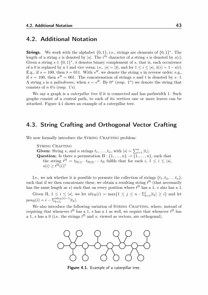
4.2. Additional Notation 43
4.2. Additional Notation
Strings. We work with the alphabet 0, 1; i.e., strings are elements of 0, 1∗. Thelength of a string s is denoted by |s|. The ith character of a string s is denoted by s(i).Given a string s ∈ 0, 1∗, s denotes binary complement of s, that is, each occurrenceof a 0 is replaced by a 1 and vice versa; i.e., |s| = |s|, and for 1 ≤ i ≤ |s|, s(i) = 1− s(i).E.g., if s = 100, then s = 011. With sR, we denote the string s in reverse order; e.g.,if s = 100, then sR = 001. The concatenation of strings s and t is denoted by s · t.A string s is a palindrome, when s = sR. By 0n (resp. 1n) we denote the string thatconsists of n 0’s (resp. 1’s).
We say a graph is a caterpillar tree if it is connected and has pathwidth 1. Suchgraphs consist of a central path, to each of its vertices one or more leaves can beattached. Figure 4.1 shows an example of a caterpillar tree.
4.3. String Crafting and Orthogonal Vector Crafting
We now formally introduce the String Crafting problem:
String CraftingGiven: String s, and n strings t1, . . . , tn, with |s| =
∑ni=1 |ti|.
Question: Is there a permutation Π : 1, . . . , n → 1, . . . , n, such thatthe string tΠ = tΠ(1) · tΠ(2) · · · tΠ fulfils that for each i, 1 ≤ i ≤ |s|,s(i) ≥ tΠ(i)?
I.e., we ask whether it is possible to permute the collection of strings t1, t2, . . . tn,such that if we then concatenate these, we obtain a resulting string tΠ (that necessarilyhas the same length as s) such that on every position where tΠ has a 1, s also has a 1.
Given Π, 1 ≤ i ≤ |s|, we let idxΠ(i) = max1 ≤ j ≤ n : Σjk=1|tk| ≥ i and let
posΠ(i) = i− ΣidxΠ(i)−1k=1 |tk|.
We also introduce the following variation of String Crafting, where, instead ofrequiring that whenever tΠ has a 1, s has a 1 as well, we require that whenever tΠ hasa 1, s has a 0 (i.e. the strings tΠ and s, viewed as vectors, are orthogonal).
Figure 4.1. Example of a caterpillar tree.
44 Chapter 4: Lower Bounds
Orthogonal Vector CraftingGiven: String s, and n strings t1, . . . , tn, with |s| =
∑ni=1 |ti|.
Question: Is there a permutation Π : 1, . . . , n → 1, . . . , n, such thatthe string tΠ = tΠ(1) · tΠ(2) · · · tΠ fulfils that for each i, 1 ≤ i ≤ |s|,s(i) · tΠ(i) = 0, i.e., when viewed as vectors, s is orthogonal to tΠ?
Theorem 4.1. Suppose the Exponential Time Hypothesis holds. Then there is noalgorithm that solves the String Crafting problem in 2o(|s|/ log |s|) time, even whenall strings ti are palindromes and start and end with a 1.
Proof. Suppose we have an instance of 3-Satisfiability with n variables and mclauses. We number the variables x1 to xn and for convenience, we number the clausesCn+1 to Cn+m+1.
We assume by the Sparsification Lemma that m = O(n) [68].Let q = dlog(n+m)e, and let r = 4q+2. We first assign a unique r-bit number to each
variable and clause; more precisely, we give an injective mapping id : 1, . . . , n+m →0, 1r. Let nb(i) be the q-bit binary representation of i, such that 0 ≤ nb(i) ≤ 2r − 1.We set, for 1 ≤ i ≤ n+m:
id(i) = 1 · nb(i) · nb(i) · nb(i)R· nb(i)R · 1
Note that each id(i) is an r-bit string that is a palindrome, ending and starting with a1.
We first build the string s. We let s be the concatenation of 2n strings, eachrepresenting one of the literals.
Suppose the literal xi appears ci times in a clause, and the literal ¬xi appears ditimes in a clause. Set fi = ci + di. Assign the following strings to the pair of literals xiand ¬xi:
• axi is the concatenation of the id’s of all clauses in which xi appears, followed bydi copies of the string 1 · 0r−2 · 1.
• a¬xi is the concatenation of the id’s of all clauses in which ¬xi appears, followedby ci copies of the string 1 · 0r−2 · 1.
• bi = id(i) · axi · id(i) · a¬xi · id(i).
Now, we set s = b1 · b2 · · · bn−1 · bn.We now build the collection of strings ti. We have three different types of strings:
• Variable selection: For each variable xi we have one string of length (fi + 2)r ofthe form id(i) · 0r·fi · id(i).
• Clause verification: For each clause Ci, we have a string of the form id(i).
• Filler strings: A filler string is of the form 1 · 0r−2 · 1. We have n + 2m fillerstrings.
4.3. String Crafting and Orthogonal Vector Crafting 45
Thus, the collection of strings ti consists of n variable selection strings, m clauseverification strings, and n + 2m filler strings. Notice that each of these strings is apalindrome and ends and starts with a 1.
The idea behind the reduction is that s consists of a list of variable identifiersfollowed by which clauses a true/false assignment to that variable would satisfy. Thevariable selection gadget can be placed in s in two ways: either covering all the clausessatisfied by assigning true to the variable, or covering all the clauses satisfied byassigning false. The clause verification strings then fit into s only if we have not coveredall of the places where the clause can fit with variable selection strings (correspondingto that we have made some assignment that satisfies the clause).
Furthermore, note that since Σni=1fi = 3m, the length of s is (3n + 6m)r, the
combined length of the variable selection strings is (2n+ 3m)r, the combined lengthof the clause verification strings is mr, and the filler strings have combined length(n+ 2m)r.2
In the following, we say a string ti is mapped to a substring s′ of s if s′ is thesubstring of s corresponding to the position (and length) of ti in tΠ.
Lemma 4.2. The instance of 3-Satisfiability is satisfiable, if and only if the con-structed instance of String Crafting has a solution.
Proof. First, we show the forward implication. Suppose we have a satisfying assignmentto the 3-Satisfiability instance. Consider the substring of s formed by bi, which is ofthe form id(i) ·axi · id(i) ·a¬xi · id(i). If in the satisfying assignment xi is true, we choosethe permutation Π so that variable selection string id(i) · 0r·fi · id(i) correspondingto xi is mapped to the substring id(i) · a¬xi · id(i); if xi is false, we map the variableselection string onto the substring id(i) · axi · id(i). A filler string is mapped to theother instance of id(i) in the substring.
Now, we show how the clause verification strings can be mapped. Suppose clauseCj is satisfied by the literal xi (resp. ¬xi). Since xi is true (resp. false), the substringaxi (resp. a¬xi) of s is not yet used by a variable selection gadget and contains id(j)as a substring, to which we can map the clause verification string corresponding to Cj .
Note that in s now remain a number of strings of the form 1 · 0r−2 · 1 and a numberof strings corresponding to id’s of clauses, together 2m such strings, which is exactlythe number of filler strings we have left. These can thus be mapped to these strings,and we obtain a solution to the String Crafting instance. It is easy to see thatwith this construction, s has a 1 whenever the string constructed from the permutationdoes.
Next, for the reverse implication, consider a solution Π to the String Craftinginstance. We require the following lemma:
Lemma 4.3. Suppose that ti = id(j). Then the substring w of s corresponding to theposition of ti in tΠ is id(j).
2Note that a single given variable may appear as literal in many clauses, but since the total numberof clauses is linear (by the Sparsification Lemma), we still obtain the claimed lower bound bound. Inthe next chapter, we will see a variation on this proof that reduces from Satisfiability with fewoccurrences per variable, further simplifying the proof (in this proof, the variable selection gadgets allhave the same length).
46 Chapter 4: Lower Bounds
Proof. Because the length of each string is a multiple of r, w is either id(k) for some k,or the string 1 · 0r−2 · 1. Clearly, w cannot be 1 · 0r−2 · 1 because the construction ofid(i) ensures that it has more than 2 non-zero characters, so at some position w wouldhave a 1 where w′ does not. Recall that id(i) = 1 · nb(i) · nb(i) · nb(i)
R· nb(i)R · 1. If
j 6= k, then either at some position nb(k) has a 0 where nb(j) has a 1 (contradictingthat Π is a solution) or at some position nb(k) has a 0 where nb(j) has a 1 (againcontradicting that Π is a solution). Therefore j = k.
Clearly, for any i, there are only two possible places in tΠ where the variableselection string id(i) ·0r·fi · id(i) can be mapped to: either in the place of id(i) ·axi · id(i)in s or in the place of id(i) · a¬xi · id(i), since these are the only (integer multiple of r)positions where id(i) occurs in s. If the former place is used we set xi to false, otherwisewe set xi to true.
Now, consider a clause Cj , and the place where the corresponding clause verificationgadget id(j)is mapped to. Suppose it is mapped to some substring of id(i) · axi · id(i) ·a¬xi · id(i). If id(j) is mapped to a substring of axi then (by construction of axi) xiappears as a positive literal in Cj and our chosen assignment satisfies Cj (since wehave set xi to true). Otherwise, if id(j) is mapped to a substring of a¬xi xi appearsnegated in Cj and our chosen assignment satisfies Cj (since we have set xi to false).
We thus obtain a satisfying assignment for the 3-Satisfiability instance.
Since in the constructed instance, |s| = (3n + 6m)r and r = O(log n),m = O(n),we have that |s| = O(n log n). A 2o(|s|/ log |s|)-time algorithm for String Craftingwould give a 2o(n logn/ log (n logn)) = 2o(n)-time algorithm for deciding 3-Satisfiability,violating the ETH.
Note that we can also restrict all strings ti to start and end with a 0 by a slightmodification of the proof.
Theorem 4.4. Assuming the Exponential Time Hypothesis, Orthogonal VectorCrafting cannot be solved in 2o(|s|/ log |s|) time, even when all strings ti are palindromesand start and end with a 1.
Proof. This follows from the result for String Crafting, by taking the complementof the string s.
Again, we can also restrict all strings ti to start and end with a 0.As illustrated by the following theorem, these lower bounds are tight. The algorithm
is a simpler example of the techniques used in [25, 28] and those in Chapter 3. There,the authors use isomorphism tests on graphs; here, we use equality of strings.
Theorem 4.5. There exists algorithms, solving String Crafting and OrthogonalVector Crafting in 2O(|s|/ log |s|) time.
Proof. The brute-force algorithm of trying all n! permutations of the strings t1, . . . , tnwould take O(|s|!s) time in the worst case. This can be improved to O(2|s|s2) by simpleHeld-Karp [66] dynamic programming: for each (multi-)subset K ⊆ t1, . . . , tn andl = Σt∈K |t| we memoize whether the substring s(1) · · · s(l) of s together with K formsa positive instance of String Crafting (resp. Orthogonal Vector Crafting).
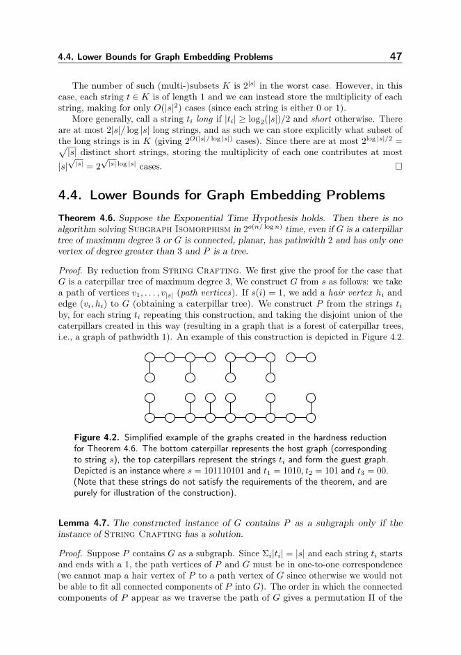
4.4. Lower Bounds for Graph Embedding Problems 47
The number of such (multi-)subsets K is 2|s| in the worst case. However, in thiscase, each string t ∈ K is of length 1 and we can instead store the multiplicity of eachstring, making for only O(|s|2) cases (since each string is either 0 or 1).
More generally, call a string ti long if |ti| ≥ log2(|s|)/2 and short otherwise. Thereare at most 2|s|/ log |s| long strings, and as such we can store explicitly what subset ofthe long strings is in K (giving 2O(|s|/ log |s|) cases). Since there are at most 2log |s|/2 =√|s| distinct short strings, storing the multiplicity of each one contributes at most|s|√|s| = 2
√|s| log |s| cases.
4.4. Lower Bounds for Graph Embedding Problems
Theorem 4.6. Suppose the Exponential Time Hypothesis holds. Then there is noalgorithm solving Subgraph Isomorphism in 2o(n/ logn) time, even if G is a caterpillartree of maximum degree 3 or G is connected, planar, has pathwidth 2 and has only onevertex of degree greater than 3 and P is a tree.
Proof. By reduction from String Crafting. We first give the proof for the case thatG is a caterpillar tree of maximum degree 3, We construct G from s as follows: we takea path of vertices v1, . . . , v|s| (path vertices). If s(i) = 1, we add a hair vertex hi andedge (vi, hi) to G (obtaining a caterpillar tree). We construct P from the strings tiby, for each string ti repeating this construction, and taking the disjoint union of thecaterpillars created in this way (resulting in a graph that is a forest of caterpillar trees,i.e., a graph of pathwidth 1). An example of this construction is depicted in Figure 4.2.
Figure 4.2. Simplified example of the graphs created in the hardness reductionfor Theorem 4.6. The bottom caterpillar represents the host graph (correspondingto string s), the top caterpillars represent the strings ti and form the guest graph.Depicted is an instance where s = 101110101 and t1 = 1010, t2 = 101 and t3 = 00.(Note that these strings do not satisfy the requirements of the theorem, and arepurely for illustration of the construction).
Lemma 4.7. The constructed instance of G contains P as a subgraph only if theinstance of String Crafting has a solution.
Proof. Suppose P contains G as a subgraph. Since Σi|ti| = |s| and each string ti startsand ends with a 1, the path vertices of P and G must be in one-to-one correspondence(we cannot map a hair vertex of P to a path vertex of G since otherwise we would notbe able to fit all connected components of P into G). The order in which the connectedcomponents of P appear as we traverse the path of G gives a permutation Π of the
48 Chapter 4: Lower Bounds
strings ti. We claim that this permutation is a solution to the String Craftinginstance, since G must have a hair vertex whenever P has one (or else we would nothave found P as a subgraph) we have that s has a 1 whenever tΠ has a 1. Note that itdoes not matter that we can flip a component of P (embed the vertices of the path inthe reverse order) since the strings ti are palindromes.
Lemma 4.8. The constructed instance of G contains P as a subgraph if the instanceof String Crafting has a solution.
Proof. Let Π be a solution for the String Crafting instance. We can map the pathvertices of the connected components of P to the path vertices of G in the order thecorresponding strings appear in the permutation Π (e.g. the first path vertex of theconnected component corresponding to Π(1) gets mapped to the first path vertex v1,the first path vertex of the component corresponding to Π(2) gets mapped to the|tΠ(1)|+ 1th path vertex,...). Whenever a path vertex in P is connected to a hair vertex,tΠ has a 1 in the corresponding position, and therefore s has a 1 in the correspondingposition as well and thus G also has a hair vertex in the corresponding position. Wecan thus appropriately map the hair vertices of P to the hair vertices of G, and seethat P is indeed a subgraph of G.
Since the constructed instance has O(|s|) vertices, this establishes the first part ofthe lemma. For the case that G is connected, we add to the graph G constructed inthe first part of the proof a vertex u and, for each path vertex vi, an edge (vi, u). To Pwe add a vertex u′ that has an edge to some path vertex of each component. By virtueof their high degrees, u must be mapped to u′ and the remainder of the reductionproceeds in the same way as in the first part of the proof.
We now show how to adapt this hardness proof to the case of Induced Subgraph:
Theorem 4.9. Suppose the Exponential Time Hypothesis holds. Then there is noalgorithm solving Induced Subgraph in 2o(n/ logn) time, even if G is a caterpillartree of maximum degree 3 or G is connected, planar, has pathwidth 2 and has only onevertex of degree greater than 3 and P is a tree.
Proof. Matoušek and Thomas [92] observe that by subdividing each edge once, asubgraph problem becomes an induced subgraph problem. Due to the nature of ourconstruction, we do not need to subdivide the hair edges. We can adapt the proofof Theorem 4.6 by subdividing every path edge (but not the hair edges) and for theconnected case, also subdividing the edges that connect to the central vertices u andu′.
We now show how to adapt this proof to (Induced) Minor, Shallow Minorand Topological Minor:
Theorem 4.10. Suppose the Exponential Time Hypothesis holds. Then there is noalgorithm solving (Induced) Minor, Shallow Minor or Topological Minor in2o(n/ logn) time, even if G is a caterpillar tree of maximum degree 3 or G is connected,planar, has pathwidth 2 and has only one vertex of degree greater than 3 and P is atree.
4.5. Tree and Path Decompositions with Few Bags 49
Proof. We can use the same reduction as for (induced) subgraph. Clearly, if P isan (induced) subgraph of G then it is also an (induced/shallow/topological) minor.Conversely, if P is not a subgraph of G then allowing contractions in G or subdivisionsin P do not help: contracting a hair edge simply removes that edge and vertex fromthe graph, while contracting a path edge immediately makes the path too short to fitall the components.
4.5. Tree and Path Decompositions with Few Bags
In this section, we study the minimum size tree and path decomposition problems:
Minimum Size Tree Decomposition of width k (k-MSTD)Given: A graph G, integers k, n.Question: Does G have a tree decomposition of width at most k, that has
at most n bags?
The Minimum Size Path Decomposition (k-MSPD) problem is defined analogously.The following theorem is an improvement over Theorem 3 of [25], where the same wasshown for k ≥ 39; our proof is also simpler.
Theorem 4.11. Let k ≥ 16. Suppose the Exponential Time Hypothesis holds, thenthere is no algorithm for k-MSPD or k-MSTD using 2o(n/ logn) time.
Proof. By reduction from Orthogonal Vector Crafting. We begin by showingthe case for MSPD, but note the same reduction is used for MSTD.
For the string s, we create a connected component in the graph G as follows: for1 ≤ i ≤ |s|+ 1 we create a clique Ci of size 6, and (for 1 ≤ i ≤ |s|) make all vertices ofCi adjacent to all vertices of Ci+1. For 1 ≤ i ≤ |s|, if s(i) = 1, we create a vertex siand make it adjacent to the vertices of Ci and Ci+1.
For each string ti, we create a component in the same way as for s, but rather thanusing cliques of size 6, we use cliques of size 2: for each 1 ≤ i ≤ n and 1 ≤ j ≤ |ti|+ 1create a clique Ti,j of size 2 and (for 1 ≤ j ≤ |ti|) make all vertices of Ti,j adjacentto all vertices of Ti,j+1. For 1 ≤ j ≤ |ti|, if ti(j) = 1, create a vertex ti,j and make itadjacent to the vertices of Ti,j and Ti,j+1.
An example of the construction (for s = 10110 and t1 = 01001) is shown in Figure4.3. We now ask whether a path decomposition of width 16 exists with at most |s|bags.
Lemma 4.12. If there exists a solution Π to the Orthogonal Vector Craftinginstance, then G has a path decomposition of width 16 with at most |s| bags.
Proof. Given a solution Π, we show how to construct such a decomposition withbags Xi, 1 ≤ i ≤ |s|. In bag Xi we take the vertices Ci, Ci+1 and (if it exists) thevertex si. We also take the cliques TidxΠ(i),posΠ(i), TidxΠ(i+1),posΠ(i+1) and the vertextidxΠ(i),posΠ(i) (if it exists).
Each bag contains two cliques of size 6 and two cliques of size 2, adding up to16 vertices in each bag. Each bag may additionally contain a vertex si or a vertextidxΠ(i),posΠ(i), but, by nature of a solution to Orthogonal Vector Crafting, not
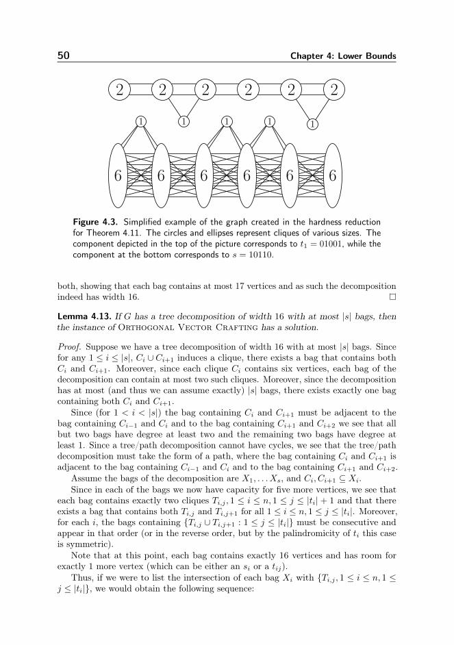
50 Chapter 4: Lower Bounds
6 6 6 6 6 6
2 2 2 2 2 2
1 11 1 1
Figure 4.3. Simplified example of the graph created in the hardness reductionfor Theorem 4.11. The circles and ellipses represent cliques of various sizes. Thecomponent depicted in the top of the picture corresponds to t1 = 01001, while thecomponent at the bottom corresponds to s = 10110.
both, showing that each bag contains at most 17 vertices and as such the decompositionindeed has width 16.
Lemma 4.13. If G has a tree decomposition of width 16 with at most |s| bags, thenthe instance of Orthogonal Vector Crafting has a solution.
Proof. Suppose we have a tree decomposition of width 16 with at most |s| bags. Sincefor any 1 ≤ i ≤ |s|, Ci ∪ Ci+1 induces a clique, there exists a bag that contains bothCi and Ci+1. Moreover, since each clique Ci contains six vertices, each bag of thedecomposition can contain at most two such cliques. Moreover, since the decompositionhas at most (and thus we can assume exactly) |s| bags, there exists exactly one bagcontaining both Ci and Ci+1.
Since (for 1 < i < |s|) the bag containing Ci and Ci+1 must be adjacent to thebag containing Ci−1 and Ci and to the bag containing Ci+1 and Ci+2 we see that allbut two bags have degree at least two and the remaining two bags have degree atleast 1. Since a tree/path decomposition cannot have cycles, we see that the tree/pathdecomposition must take the form of a path, where the bag containing Ci and Ci+1 isadjacent to the bag containing Ci−1 and Ci and to the bag containing Ci+1 and Ci+2.
Assume the bags of the decomposition are X1, . . . Xs, and Ci, Ci+1 ⊆ Xi.Since in each of the bags we now have capacity for five more vertices, we see that
each bag contains exactly two cliques Ti,j , 1 ≤ i ≤ n, 1 ≤ j ≤ |ti|+ 1 and that thereexists a bag that contains both Ti,j and Ti,j+1 for all 1 ≤ i ≤ n, 1 ≤ j ≤ |ti|. Moreover,for each i, the bags containing Ti,j ∪ Ti,j+1 : 1 ≤ j ≤ |ti| must be consecutive andappear in that order (or in the reverse order, but by the palindromicity of ti this caseis symmetric).
Note that at this point, each bag contains exactly 16 vertices and has room forexactly 1 more vertex (which can be either an si or a tij).
Thus, if we were to list the intersection of each bag Xi with Ti,j , 1 ≤ i ≤ n, 1 ≤j ≤ |ti|, we would obtain the following sequence:
4.6. Intervalizing Coloured Graphs 51
TΠ(1),1, TΠ(1),2, . . . , TΠ(1),|tΠ(1)|, TΠ(1),|tΠ(1)|+1
TΠ(2),1, TΠ(2),2, . . . , TΠ(2),|tΠ(2)|, TΠ(2),|tΠ(2)|+1
. . .
TΠ(n),1, TΠ(n),2, . . . , TΠ(n),|tΠ(n)|, TΠ(n),|tΠ(n)|+1
Which gives us the permutation Π and string tΠ we are after. Note that s(i) andtΠ(i) cannot both be 1, because otherwise the vertex si (being adjacent to the verticesof Ci and Ci+1) must go in bag Xi, but so must the vertex tidxΠ(i),posΠ(i) which wouldexceed the capacity of the bag.
The size of the graph created in the reduction is O(|s|), so we obtain a 2Ω(n/ logn)
lower bound for 16-MSPD under the Exponential Time Hypothesis. We can extendthe reduction to k > 16 by adding universal vertices to the graph.
For the tree decomposition case, note that a path decomposition is also a treedecomposition. For the reverse implication, we claim that a tree decomposition of Gof width 16 with at most |s| bags must necessarily be a path decomposition. This isbecause for each 1 ≤ i ≤ |s|, there exists a unique bag containing Ci and Ci+1 whichis adjacent to the bag containing Ci − 1 and Ci (if i > 1) and to the bag containingCi+1 and Ci+2 (if i < |s|). All but two bags are thus adjacent to at least two otherones, and a simple counting argument shows that there therefore is no bag with degreegreater than two (or we would not have enough edges).
4.6. Intervalizing Coloured Graphs
In this section, we consider the problem of intervalizing coloured graphs:
Intervalizing Coloured GraphsGiven: A graph G = (V,E) together with a proper colouring c : V →1, 2, . . . , k.
Question: Is there an interval graph G′ on the vertex set V , for which cis a proper colouring, and which is a supergraph of G?
Intervalizing Coloured Graphs is known to be NP-complete, even for 4-coloured caterpillars (with hairs of unbounded length) [5]. In contrast with this resultwe require five colours instead of four, and the result only holds for trees instead ofcaterpillars. However, we obtain a 2Ω(n/ logn) lower bound under the Exponential TimeHypothesis, whereas the reduction in [5] is from Multiprocessor Scheduling andto our knowledge, the best lower bound obtained from it is 2Ω( 5
√n) (the reduction is
weakly polynomial in the length of the jobs, which following from the reduction from3-Partition in [70] is Θ(n4)). In contrast to these hardness results, for the case with3 colours there is an O(n2) time algorithm [16, 17].
Theorem 4.14. Intervalizing Coloured Graphs does not admit a 2o(n/ logn)-timealgorithm, even for 5-coloured trees, unless the Exponential Time Hypothesis fails.
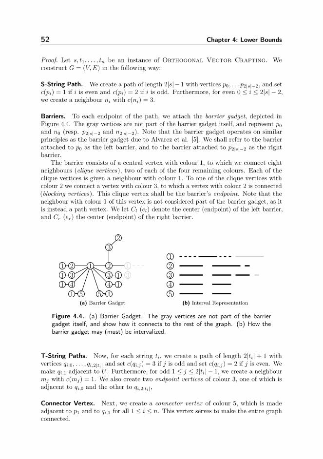
52 Chapter 4: Lower Bounds
Proof. Let s, t1, . . . , tn be an instance of Orthogonal Vector Crafting. Weconstruct G = (V,E) in the following way:
S-String Path. We create a path of length 2|s|−1 with vertices p0, . . . p2|s|−2, and setc(pi) = 1 if i is even and c(pi) = 2 if i is odd. Furthermore, for even 0 ≤ i ≤ 2|s| − 2,we create a neighbour ni with c(ni) = 3.
Barriers. To each endpoint of the path, we attach the barrier gadget, depicted inFigure 4.4. The gray vertices are not part of the barrier gadget itself, and represent p0
and n0 (resp. p2|s|−2 and n2|s|−2). Note that the barrier gadget operates on similarprinciples as the barrier gadget due to Alvarez et al. [5]. We shall refer to the barrierattached to p0 as the left barrier, and to the barrier attached to p2|s|−2 as the rightbarrier.
The barrier consists of a central vertex with colour 1, to which we connect eightneighbours (clique vertices), two of each of the four remaining colours. Each of theclique vertices is given a neighbour with colour 1. To one of the clique vertices withcolour 2 we connect a vertex with colour 3, to which a vertex with colour 2 is connected(blocking vertices). This clique vertex shall be the barrier’s endpoint. Note that theneighbour with colour 1 of this vertex is not considered part of the barrier gadget, as itis instead a path vertex. We let Cl (el) denote the center (endpoint) of the left barrier,and Cr (er) the center (endpoint) of the right barrier.
1
4
5 5
41
1 1
1
3 131
1 2 2 1
3
3
2
(a) Barrier Gadget
4
3
2
5
1
(b) Interval Representation
Figure 4.4. (a) Barrier Gadget. The gray vertices are not part of the barriergadget itself, and show how it connects to the rest of the graph. (b) How thebarrier gadget may (must) be intervalized.
T-String Paths. Now, for each string ti, we create a path of length 2|ti| + 1 withvertices qi,0, . . . , qi,2|ti| and set c(qi,j) = 3 if j is odd and set c(qi,j) = 2 if j is even. Wemake qi,1 adjacent to U . Furthermore, for odd 1 ≤ j ≤ 2|ti| − 1, we create a neighbourmj with c(mj) = 1. We also create two endpoint vertices of colour 3, one of which isadjacent to qi,0 and the other to qi,2|ti|,
Connector Vertex. Next, we create a connector vertex of colour 5, which is madeadjacent to p1 and to qi,1 for all 1 ≤ i ≤ n. This vertex serves to make the entire graphconnected.
4.6. Intervalizing Coloured Graphs 53
Marking Vertices. Finally, for each 1 ≤ i ≤ |s| (resp. for each 1 ≤ i ≤ n and1 ≤ j ≤ |ti|), if s(i) = 1 (resp. ti(j) = 1), we give p2i−1 (resp. qi,2j−1) two neighbours(called the marking vertices) with colour 4. For each of the marking vertices, we createa neighbour with colour 3.
This construction is depicted in Figure 4.5. In this example s = 10100, t1 = 01 andt2 = 001. Note that this instance of Orthogonal Vector Crafting is illustrative,and does not satisfy the restrictions required in the proof.
Informally, the construction works as follows: the barriers at the end of the pathof p-vertices cannot be passed by the remaining vertices, meaning we have to "weave"the shorter q-paths into the long p-path. The colours enforce that the paths are in"lockstep", that is, we have to traverse them at the same speed. We have to map everyq-vertex with colour 3 to a p-vertex with colour 2, but the marking vertices prevent usfrom doing so if both bitstrings have a 1 at that particular position.
Lemma 4.15. G can be intervalized if the Orthogonal Vector Crafting instancehas a solution.
Proof. As an example, Figure 4.6 shows how the graph from Figure 4.5 may beintervalized. Let Π be a solution to the instance of Orthogonal Vector Crafting.We can intervalize the barriers as depicted in Figure 4.4b, noting that the right barriershould be intervalized in a mirrored fashion. The connector vertex (which is theonly remaining vertex of colour 5) can be assigned an interval that covers the entireinterval between the two barrier gadgets. If no marker vertices are present, then wecan weave the q-paths into the p-path as depicted in Figure 4.6, whereby each intervalcorresponding to a q-vertex of colour 3 completely contains the interval of a p-vertex ofcolour 2 (note that the endpoint vertices of the q-paths are treated differently fromthe q-path vertices with colour 3). If we intervalize the q-paths in the same order thecorresponding strings appear in Π, then we can also intervalize the marking vertices:Figure 4.6 shows that the marker vertices can also be intervalized, so long as a p-vertexand its corresponding q-vertex are not both adjacent to marker vertices, but this isguaranteed by the orthogonality of s and tΠ.
Lemma 4.16. G can be intervalized only if the Orthogonal Vector Craftinginstance has a solution.
Proof. Suppose we are given a properly coloured interval supergraph of G that assignsto each vertex v ∈ V its left endpoint l(v) and right endpoint r(v). For vertices u, v ∈ V ,we write v ⊂ u if l(u) < l(v) < r(v) < r(u), and we write v < u if r(v) < l(u). Wewrite v l u if l(v) < l(u) < r(v) < r(u) - that is, the interval of v starts to the left ofthe interval of u and the two intervals overlap.
We may without loss of generality assume that Cl < Cr and that no two endpointsof intervals coincide.
Claim. For any non-barrier vertex v, we have that r(Cl) < l(v) < r(v) < l(Cr).
Proof. Examining the situation for the left barrier, we see that a clique vertex cannotbe contained completely inside the interval of the center vertex Cl since it is adjacentto another vertex with colour 1 (whose interval may not intersect that of the center).
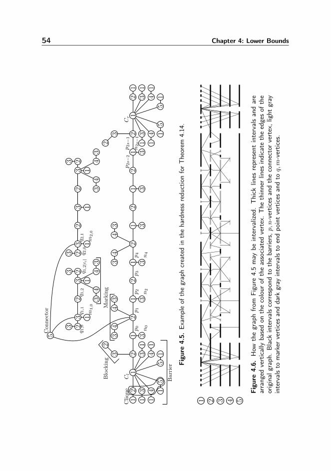
54 Chapter 4: Lower Bounds
21
21
2
33
44
33
44
33
12
3
12
3
2
44
33
33
11
1
4
55
41
11
1
31
311
21
4
55
41
11
1
31
31
21
21
12
33
22
22
44
33
33
3
11
1
22
3
2
3
2
33
33
5
Cl
Cr
Clique
Barrier
Blocking
p0
n0
p1
p2
n2
p3
p4
n4
p2s−2
p2s−1
n2s−1
Marking
q 1,0
q 1,1
m1,0
q 1,2
q 2,1
m2,0
q 2,0
Connector
q 1,2|t i|
Figu
re4.5.
Exam
pleof
thegraphcreatedin
thehardness
redu
ctionforTheorem
4.14.
432 51
Figu
re4.6.
How
thegraphfrom
Figu
re4.5may
beintervalized.Thick
lines
representintervalsandare
arrang
edvertically
basedon
thecolour
oftheassociated
vertex.The
thinnerlines
indicate
theedgesof
the
original
graph.
Black
intervalscorrespo
ndto
thebarriers,p,n
-vertic
esandtheconn
ectorvertex,light
gray
intervalsto
markervertices
anddark
gray
intervalsto
endpo
intvertices
andtoq,m-vertic
es.
4.6. Intervalizing Coloured Graphs 55
Since there are two clique vertices of each colour, for each colour, the interval of oneclique vertex of that colour must extend to the left of the central vertex’ interval andthe other must extend to the right. Therefore, these intervals that contain r(cl) inducea clique of size 5. Since we are looking for a 5-coloured supergraph, no other intervalscan contain r(cl).
Note that the clique vertices are interchangeable, except the ones coloured 2: theclique vertex that is adjacent to p0 must go to the right of the center vertex, sinceotherwise the path from it to Cr could not pass the clique at r(cl).
Suppose that for some non-barrier vertex v, it holds that l(v) ≤ r(cr). This is notpossible, since the path from v to cr cannot pass the clique induced at r(cl). Therefore,r(cl) < l(v).
The case for the right barrier is symmetric.
Claim. For all 0 ≤ i < 2|s| − 1, we have that pi l pi+1. Furthermore, Cl l el l p0 andp2|s|−1 l er l Cr.
Proof. The fact that Cl l el l p0 (resp. p2|s|−1 l er l Cr) follows from the analysisof the barrier gadget in the previous claim. We now proceed by induction, for thepurposes of which we shall write el = p−1 and er = p2|s|: suppose the claim holds fori− 1, i.e. pi−1 l pi. It cannot hold that pi+1 ⊂ pi, since it is adjacent to pi+2, nor canit hold that pi+1 l pi (since then it would intersect the interval of pi−1.
For any 1 ≤ i ≤ n, a similar fact holds for the path qi,0, . . . , qi,2|ti|:
Claim. We may without loss of generality assume that qi,0 l . . .l qi,2|ti|.
Proof. By a similar induction argument as above, it must hold that either qi,0 l . . .lqi,2|ti| or qi,0 m . . . m qi,2|ti|. However, since ti is palindromic, these two cases areequivalent.
Claim. Let 1 ≤ i ≤ n, 1 ≤ j ≤ |ti|. Then there exists 1 ≤ k ≤ |s| such thatp2k−1 ⊂ qi,2j−1.
Proof. The interval of qi,2j−1 cannot be completely contained in the interval of a vertexwith colour 1, since qi,2j−1 is adjacent to mi,2j−1 which has colour 1 as well. Therefore(since r(Cl) < l(qi,2j−1) < r(qi,2j−1) < l(Cr)), the interval of qi,2j−1 must intersectthe interval of either a barrier endpoint or a path vertex p2k−1 for some 1 ≤ k ≤ |s|.It is not possible that qi,2j−1 intersects the interval of a barrier endpoint, since (dueto the blocking and clique vertices with colour 3, see Figure 4.4) it would have to becompletely contained inside this interval, which is impossible since qi,2j−1 is adjacentto vertices with colour 2. Therefore there exists a 1 ≤ k ≤ |s| such that the interval ofqi,2j−1 intersects that of p2k−1.
Since qi,2j−2 l qi,2j−1 l qi,2j and c(qi,2j−2) = c(qi,2j) = c(p2k−1) = 2 we must havethat qi,2j−2 < q2k−1 < qi,2j . It now follows that p2k−1 ⊂ qi,2j−1.
This allows us to define the position 1 ≤ P (i, j) ≤ |s| for each 1 ≤ i ≤ n, 1 ≤ j ≤ |ti|,which is equal to the k from the previous claim. Note that P is a bijection, since eachinterval p2k−1 is the subset of (the interval of) exactly one q-vertex (each p-vertexinterval cannot be the subset of more than one q-vertex interval, and the number
56 Chapter 4: Lower Bounds
of p-vertices is such that no q-vertex can completely contain more than one q-vertexinterval).
Claim. Let 1 ≤ i ≤ n, 1 ≤ j ≤ |ti| − 1. Then P (i, j + 1) = P (i, j) + 1.
Proof. This follows from the fact that a q-vertex with colour 3 cannot completelycontain a p-vertex with colour 1 (since it has an n-vertex as neighbour that has colour1 as well) and the fact that a q-vertex with colour 2 cannot overlap a p-vertex withcolour 2.
Formally, let P (i, j) = k, then p2k−1 ⊂ qi,2j−1. Since qi,2j−1 l qi,2j l qi,2j+1, if theclaim does not hold, we must have p2k+1+2m ⊂ qi,2j+1 for some m > 0. We must haveqi,2j ⊂ p2k+2r for some r ≥ 0. If r = 0, then qi,2j < qi,2j+1 which is a contradiction.On the other hand, if r > 0 then qi,2j−1 < qi,2j which is also a contradiction.
Claim. Let Π be the permutation of 1, . . . , n such that P (idxΠ(i), posΠ(i)) = i. ThenΠ exists and is a solution to the Orthogonal Vector Crafting instance.
Proof. The existence of Π follows from the previous claim. Suppose that Π is not asolution. Then there exists an i, such that S(i) = TidxΠ(i)(posΠ(i)) = 1. However, thismeans that p2i−1 ⊂ qidxΠ(i),2posΠ(i)−1. Since both p2i−1 and qidxΠ(i),2posΠ(i)−1 havemarking vertices, this is impossible as the marking vertices with colour 4 would haveoverlapping intervals.
This completes the proof of Lemma 4.16.
The number of vertices of G is linear in |s| and we thus obtain a 2Ω(n/ logn) lowerbound under the Exponential Time Hypothesis.
Note that the graph created in this reduction only has one vertex of super-constantdegree. This is tight, since the problem is polynomial-time solvable for bounded degreegraphs (for any fixed number of colours) [72].
To complement this result for a bounded number of colours, we also show a 2Ω(n)-time lower bound for graphs with an unbounded number of colours, assuming the ETH.Note that this result implies that the algorithm from [28] is optimal. A complication inthe proof is that to obtain the stated bound, one can only use (on average) a constantnumber of vertices of each colour (when using O(n) colours). A variation on theprevious proof whereby instead of using bitstrings, colours are used to identify clausesand variables is thus unlikely to work since one would need to repeat each colour manytimes (in each place where a particular bitstring does not fit).
Theorem 4.17. Assuming the Exponential Time Hypothesis, there is no algorithmsolving Intervalizing Coloured Graphs in time 2o(n), even when restricted totrees.
Proof. By reduction from Exact Cover by 3-Sets (X3C). X3C is the followingproblem: given a set X with |X| = n and a collection M of subsets X1, . . . , Xm of size3, decide whether there exists a subset M ′ of size n/3 such that
⋃M ′ = X. Assuming
the Exponential Time Hypothesis, there does not exist an algorithm solving X3C in
4.6. Intervalizing Coloured Graphs 57
time 2o(m) (See e.g. [25, 9, 55]. Note that 3-Dimensional Matching is a special caseof X3C.).
The intuition behind the reduction is that, to leverage the large number of colours,one needs to force the creation of a very large clique in the intervalized graph. Foreach element of Xi ∈ M , we create a component of which the vertices have coloursthat correspond to the elements of Xi. The graph created in the reduction will be sothat all but n/3 of the components corresponding to elements of M can be placed indistinct intervals, but the remaining n/3 components will have to overlap. This, inturn, is only possible if no two components in this latter collection contain duplicatedcolours, that is, each element is represented at most (and thus exactly) once in theselected n/3 components.
We assume the elements of X are labelled 1, . . . , n. We may assume that n is amultiple of 3 (or we may return a trivial no-instance) and that m > n/3 (or we cancheck immediately whether M covers X).
The graph created in the reduction has n+ 4 colours: two colours ei and fi for each1 ≤ i ≤ n and four additional colours a, b, c, d.
We construct the graph G as follows: we start with a path of 2(m−n/3)+1 verticesp0, . . . , p2(m−n/3), where pi has colour a if i is even and p1 has colour b if i is odd. Top2(m−n/3) we make adjacent a vertex with colour d, which we shall refer to as the rightbarrier vertex.
Next, for each 1 ≤ i ≤ n, we create a vertex vi with colour ei, that is made adjacentto p0. For each i, we create an additional vertex with colour d that is made adjacentto vi. These vertices (with colour d) are called the left barrier vertices.
Next, for each 3-set Xi ∈ M , we create a set component, consisting of a centralvertex with colour a, to which are made adjacent: two vertices with colour c, each ofwhich is adjacent to a vertex with colour b and, for each of the three elements of Xi,two vertices with the corresponding (to that element) colour fi, each of which is madeadjacent to a vertex with colour ei.
Finally, we connect all the components together with a connector vertex of colourd, which is made adjacent to each set gadget and to a vertex of the path (for instanceto p0). Figure 4.7 provides an example of the construction.
As with the case for five colours, a solution somehow has to “pack” the set componentsinto the part of the graph between the barriers: m− n/3 of the set components canbe packed into the path (each interval corresponding to a b-vertex can hold at mostone component); the remaining n/3 components have to be packed between the leftbarrier vertices and p0 and this is possible only if the corresponding sets are disjoint(otherwise intervals of the corresponding colours would have to overlap).
Lemma 4.18. If G can be intervalized, then the X3C instance has a solution.
Proof. In any interval supergraph of G, the interval of the connector vertex shouldlie between the intervals of the left barrier vertices and the right barrier vertex. LetXi ∈ M . The interval of the central vertex of the set component corresponding toXi must either be contained in the interval corresponding to some vertex pi for someodd 1 ≤ i < 2(m− n/3) or it should be contained in the intersection of the intervalscorresponding to the vertices vj | 1 ≤ j ≤ n (since its interval cannot intersect anyinterval of a vertex with colour a, nor can its interval be contained in the interval of a
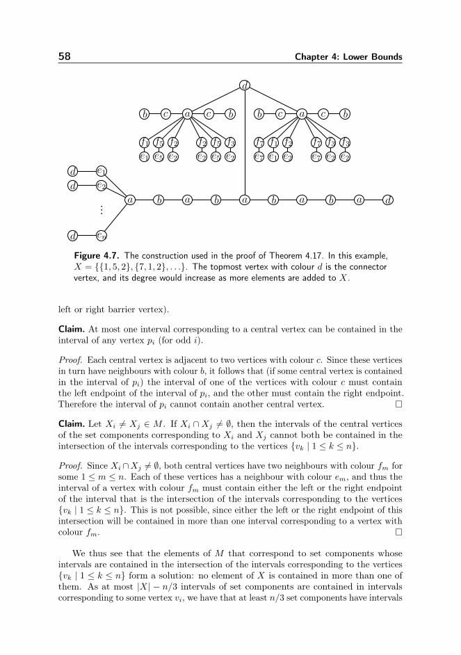
58 Chapter 4: Lower Bounds
en
e2
e1
a...b a b a b ab a
a
f1 f5 f2 f2 f5 f3e1 e5 e2 e2 e5 e2
bb c c a
f7 f1 f2 f3 f3e7 e1 e2 e2 e2
bb c c
d
f7e7
d
d
d
d
Figure 4.7. The construction used in the proof of Theorem 4.17. In this example,X = 1, 5, 2, 7, 1, 2, . . .. The topmost vertex with colour d is the connectorvertex, and its degree would increase as more elements are added to X.
left or right barrier vertex).
Claim. At most one interval corresponding to a central vertex can be contained in theinterval of any vertex pi (for odd i).
Proof. Each central vertex is adjacent to two vertices with colour c. Since these verticesin turn have neighbours with colour b, it follows that (if some central vertex is containedin the interval of pi) the interval of one of the vertices with colour c must containthe left endpoint of the interval of pi, and the other must contain the right endpoint.Therefore the interval of pi cannot contain another central vertex.
Claim. Let Xi 6= Xj ∈ M . If Xi ∩Xj 6= ∅, then the intervals of the central verticesof the set components corresponding to Xi and Xj cannot both be contained in theintersection of the intervals corresponding to the vertices vk | 1 ≤ k ≤ n.
Proof. Since Xi ∩Xj 6= ∅, both central vertices have two neighbours with colour fm forsome 1 ≤ m ≤ n. Each of these vertices has a neighbour with colour em, and thus theinterval of a vertex with colour fm must contain either the left or the right endpointof the interval that is the intersection of the intervals corresponding to the verticesvk | 1 ≤ k ≤ n. This is not possible, since either the left or the right endpoint of thisintersection will be contained in more than one interval corresponding to a vertex withcolour fm.
We thus see that the elements of M that correspond to set components whoseintervals are contained in the intersection of the intervals corresponding to the verticesvk | 1 ≤ k ≤ n form a solution: no element of X is contained in more than one ofthem. As at most |X| − n/3 intervals of set components are contained in intervalscorresponding to some vertex vi, we have that at least n/3 set components have intervals
4.7. Conclusions 59
that are contained in the aforementioned intersection. These must thus form a solutionto the X3C instance.
Lemma 4.19. If the X3C instance has a solution, then G can be intervalized.
Proof. The v-vertices are assigned to identical intervals. Their d-coloured neighbourscan be assigned arbitrarily small intervals that are placed in the left half of the v-vertexinterval. The p-vertices can then be placed from left to right, so that p0 overlaps a smallportion of the right end of the v-vertex intervals, and each p vertex interval overlaps theinterval of the preceding p-vertex slightly. Finally the right barrier vertex (with colourd) should be placed in the right half of the interval corresponding to p22(m− n/3).
Next, the connector vertex (with colour d) can be assigned a long interval betweenthe left and right barrier vertices, that overlaps the v-vertex intervals and all of thep-vertex intervals. This placement of the connector vertex allows us to place theintervals of set components anywhere between the left and right barriers.
Let M ′ ⊆M be a solution to the X3C instance. Since |M ′| = n/3, and there arem− n/3 p-vertices with colour b, we can assign each element of M that is not in thesolution a unique p-vertex with colour a. We assign the central vertex (which hascolour a) of the set component of each such element an interval inside the interval ofits p-vertex, such that it does not intersect neighbouring p-vertices (which have coloura). The vertices with f - or e-colours of the set component can be assigned similarintervals (not intersecting neighbouring p-vertices). One of the vertices with colour c isassigned an interval that extends past the left endpoint of the p-vertex interval (andthus intersects the preceding p-vertex interval), which allows us to assign its neighbourwith colour b an interval that is contained in the preceding p-vertex interval (and doesnot intersect any other p-vertex interval). The other vertices with colours b and c canbe placed similarly on the right.
Finally, for the set components corresponding to elements of M ′, we can assign thevertices with colours a, b, c arbitrarily small intervals in the right half of the v-vertexintervals; the f -coloured vertices can be placed so that their intervals stick out beyondthe right and left endpoints of the v-vertex intervals, so that the e-coloured verticescan be placed not overlapping the v-vertex intervals. The fact that M ′ is a solutionguarantees this can be done without any e, f -colours overlapping each other, since eachsuch colour occurs exactly twice (one such pair of vertices can be placed on the left,the other on the right).
This completes the reduction. Since the number of vertices of G is linear in |M |and |X|, we see that Intervalizing Coloured Graphs does not admit a 2o(n)-timealgorithm, unless the Exponential Time Hypothesis fails.
4.7. Conclusions
In this chapter, we have shown for several problems that, under the Exponential TimeHypothesis, 2Θ(n/ logn) is the best achievable running time – even when the instancesare very restricted (for example in terms of pathwidth or planarity). For each of theseproblems, algorithms that match this lower bound are known and thus 2Θ(n/ logn) is(likely) the asymptotically optimal running time.
60 Chapter 4: Lower Bounds
For problems where planarity or bounded treewidth of the instances (or, throughbidimensionality, of the solutions) can be exploited, the optimal running time is often2Θ(√n) (or features the square root in some other way). On the other hand, each
of problems studied in this chapter exhibits some kind of “packing” or “embedding”behaviour. For such problems, 2Θ(n/ logn) is often the optimal running time. We haveintroduced two artificial problems, String Crafting and Orthogonal VectorCrafting, that form a useful framework for proving such lower bounds.
It would be interesting to study which other problems exhibit such behaviour, or tofind yet other types of running times that are “natural” under the Exponential TimeHypothesis. The loss of the log n-factor in the exponent is due to the fact that log nbits or vertices are needed to “encode” n distinct elements; it would be interestingto see if there are any problems or graph classes where a more compact encoding ispossible (for instance only log1−ε n vertices required, leading to a tighter lower bound)or where an encoding is less compact (for instance log2 n vertices required, leading to aweaker lower bound) and whether this can be exploited algorithmically.
61
Intermezzo: Polyomino Packing
5.1. Introduction
In this chapter, we show that the problem of deciding whether a collection of poly-ominoes, each fitting in a 2 × O(log n) rectangle, can be packed into a 3 × n boxdoes not admit a 2o(n/ logn)-time algorithm, unless the Exponential Time Hypothesisfails. We also give an algorithm that attains this lower bound, solving any instance ofpolyomino packing with total area n in 2O(n/ logn). This establishes a tight bound onthe complexity of Polyomino Packing, even in a very restricted case. In contrast, for a2× n box, we show that the problem can be solved in strongly subexponential time.
The complexity of games and puzzles is a widely studied topic, and the complexity ofmost games and puzzles in terms of completeness for a particular complexity class (NP,PSPACE, EXPTIME, . . .) is generally well-understood (see e.g. [64] for an overview).Results in this area are not only mathematically interesting and fun, but are also agreat educational tool for teaching hardness reductions. However, knowing that a gameor puzzle is NP-complete does not provide a very detailed picture: it only tells us thatthere is unlikely to be a polynomial-time algorithm, but leaves open the possibility thatthere might be a very fast superpolynomial but subexponential-time algorithm. Thisissue was precisely the motivation for introducing the Exponential Time Hypothesis[67].
We study the Polyomino Packing problem from the viewpoint of exact complexity.We give a reduction from 3-SAT, showing that Polyomino Packing cannot be solvedin 2o(n/ logn) time, even if the target shape is a 3× n rectangle and each piece fits ina 2 × O(log n) rectangle. As the reduction is self-contained, direct from 3-SAT andrather elegant, it could be an excellent example to use for teaching. We also show thatthis is tight: Polyomino Packing can be solved in 2O(n/ logn) time for any set ofpolyominoes of total area n that have to be packed into any shape.
Polyomino Packing appears to behave similarly to Subgraph Isomorphism
62 Chapter 5: Intermezzo: Polyomino Packing
on planar graphs, which, as shown in the previous chapters, has exact complexity2Θ(n/ logn) (i.e., there exists an algorithm solving the problem in 2O(n/ logn) time onn-vertex graphs, and unless the ETH fails there is no 2o(n/ logn)-time algorithm).
Demaine and Demaine [40] showed that packing n polyominoes of size Θ(log n)×Θ(log n) into a square box is NP-complete. This result left open a gap, namely ofwhether the problem remained NP-complete for polyominoes of area O(log n). Thisgap was recently closed by Brand [30], who showed that Polyomino Packing isNP-complete even for polyominoes of size 3×O(log n) that have to be packed into asquare. However, Brand’s construction effectively builds up larger (more-or-less square)polyominoes by forcing smaller (rectangular) polyominoes to be packed together in aparticular way, by using jagged edges that correspond to binary encodings of integersto enforce that certain pieces are placed together.
Our reduction also uses binary encoding of integers to force that various pieces areplaced together. However, in contrast, it gives hardness for a much more restrictedcase (packing polyomino pieces of size 2 × O(log n) into a rectangle of height 3)and also reduces directly from 3-SAT, avoiding the polynomial blowup incurred byBrand’s reduction from 3-Partition, thus giving a tight (under the ExponentialTime Hypothesis) lower bound. As 3-Partition is a frequently used tool for showinghardness of various types of packing puzzles and games, we believe that these techniquescould be used to give (tight, or at least strong) lower bounds on the complexity ofother games and puzzles.
This result is tight in another sense: we show that Polyomino Packing wherethe target shape is a 2× n rectangle admits a 2O(n3/4 logn)-time algorithm, so 3× n isthe smallest rectangle in which a 2Ω(n/ logn)-time lower bound can be attained.
Note that our results are agnostic to the type (free, fixed or one-sided) of polyominoused. That is, it does not matter whether we are able to rotate (one-sided), rotateand flip (free) or not (fixed) our polyominoes. Our reduction creates instances whosesolvability is preserved when changing the type of polyomino, while the algorithms caneasily be adapted to work with any type of polyomino. In the following, we considerthe Polyomino Packing problem, which asks whether a given set of polyominoes canbe packed to fit inside a given target shape. If we include the additional restrictionthat the area of the target shape is equal to the total area of the pieces, we obtain theExact Polyomino Packing problem.
5.2. Lower Bounds
Theorem 5.1. Unless the Exponential Time Hypothesis fails, there exists no 2o(n/ logn)-time algorithm for Polyomino Packing, even if the target shape is a 3× n box, andthe bounding box of each polyomino is of size 2×Θ(log n).
Proof. A weaker version of the statement follows by a simple reduction from theOrthogonal Vector Crafting problem from the previous chapter. However,because obtaining the bound on the piece size requires a deeper understanding of theproof, and to illustrate the technique, we give a different proof that is neverthelesssomewhat similar to the reduction from the previous chapter.
We proceed by reduction from n-variable 3-SAT, which, unless the Exponential
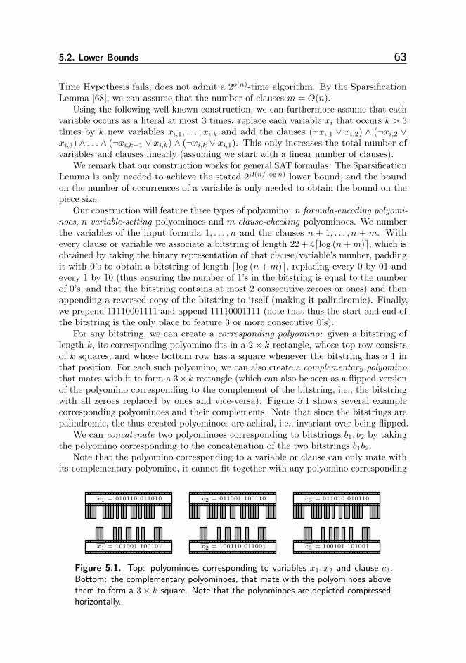
5.2. Lower Bounds 63
Time Hypothesis fails, does not admit a 2o(n)-time algorithm. By the SparsificationLemma [68], we can assume that the number of clauses m = O(n).
Using the following well-known construction, we can furthermore assume that eachvariable occurs as a literal at most 3 times: replace each variable xi that occurs k > 3times by k new variables xi,1, . . . , xi,k and add the clauses (¬xi,1 ∨ xi,2) ∧ (¬xi,2 ∨xi,3) ∧ . . . ∧ (¬xi,k−1 ∨ xi,k) ∧ (¬xi,k ∨ xi,1). This only increases the total number ofvariables and clauses linearly (assuming we start with a linear number of clauses).
We remark that our construction works for general SAT formulas. The SparsificationLemma is only needed to achieve the stated 2Ω(n/ logn) lower bound, and the boundon the number of occurrences of a variable is only needed to obtain the bound on thepiece size.
Our construction will feature three types of polyomino: n formula-encoding polyomi-noes, n variable-setting polyominoes and m clause-checking polyominoes. We numberthe variables of the input formula 1, . . . , n and the clauses n + 1, . . . , n + m. Withevery clause or variable we associate a bitstring of length 22 + 4dlog (n+m)e, which isobtained by taking the binary representation of that clause/variable’s number, paddingit with 0’s to obtain a bitstring of length dlog (n+m)e, replacing every 0 by 01 andevery 1 by 10 (thus ensuring the number of 1’s in the bitstring is equal to the numberof 0’s, and that the bitstring contains at most 2 consecutive zeroes or ones) and thenappending a reversed copy of the bitstring to itself (making it palindromic). Finally,we prepend 11110001111 and append 11110001111 (note that thus the start and end ofthe bitstring is the only place to feature 3 or more consecutive 0’s).
For any bitstring, we can create a corresponding polyomino: given a bitstring oflength k, its corresponding polyomino fits in a 2× k rectangle, whose top row consistsof k squares, and whose bottom row has a square whenever the bitstring has a 1 inthat position. For each such polyomino, we can also create a complementary polyominothat mates with it to form a 3×k rectangle (which can also be seen as a flipped versionof the polyomino corresponding to the complement of the bitstring, i.e., the bitstringwith all zeroes replaced by ones and vice-versa). Figure 5.1 shows several examplecorresponding polyominoes and their complements. Note that since the bitstrings arepalindromic, the thus created polyominoes are achiral, i.e., invariant over being flipped.
We can concatenate two polyominoes corresponding to bitstrings b1, b2 by takingthe polyomino corresponding to the concatenation of the two bitstrings b1b2.
Note that the polyomino corresponding to a variable or clause can only mate withits complementary polyomino, it cannot fit together with any polyomino corresponding
x1 = 010110 011010
x1 = 101001 100101
x2 = 011001 100110
x2 = 100110 011001
c3 = 011010 010110
c3 = 100101 101001
Figure 5.1. Top: polyominoes corresponding to variables x1, x2 and clause c3.Bottom: the complementary polyominoes, that mate with the polyominoes abovethem to form a 3× k square. Note that the polyominoes are depicted compressedhorizontally.
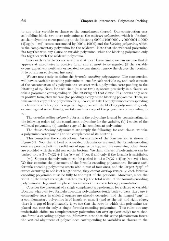
64 Chapter 5: Intermezzo: Polyomino Packing
to any other variable or clause or the complement thereof. Our construction usesas building blocks two more polyominoes: the wildcard polyomino, which is obtainedas the polyomino corresponding to the bitstring 00001110000000 . . . 00000001110000(4dlog (n+m)e zeroes surrounded by 00001110000) and the blocking polyomino, whichis the complementary polyomino for the wildcard. Note that the wildcard polyominofits together with any clause or variable polyomino, while the blocking polyomino onlyfits together with the wildcard polyomino.
Since each variable occurs as a literal at most three times, we can assume that itappears at most twice in positive form, and at most twice negated (if the variableoccurs exclusively positively or negated we can simply remove the clauses that containit to obtain an equivalent instance).
We are now ready to define the formula-encoding polyominoes. The constructionwill have n variable-encoding polyominoes, one for each variable xi, and each consistsof the concatenation of 7 polyominoes: we start with a polyomino corresponding to thebitstring of xi. Next, for each time (at most two) xi occurs positively in a clause, wetake a polyomino corresponding to (the bitstring of) that clause. If xi occurs only oncein positive form, then we take (for padding) a copy of the blocking polyomino. Then, wetake another copy of the polyomino for xi. Next, we take the polyominoes correspondingto clauses in which xi occurs negated. Again, we add the blocking polyomino if xi onlyoccurs negated once. Finally, we take another copy of the polyomino corresponding toxi.
The variable-setting polyomino for xi is the polyomino formed by concatenating, inthe following order: (a) the complement polyomino for the variable, (b) 2 copies of thewildcard polyomino, (c) another copy of the complement polyomino.
The clause-checking polyominoes are simply the following: for each clause, we takea polyomino corresponding to the complement of its bitstring.
This completes the construction. An example of the construction is shown inFigure 5.2. Note that if fixed or one-sided polyominoes are used, the formula-encodingones are provided with the solid row of squares on top, and the remaining polyominoesare provided with the solid row on the bottom. We claim this set of polyominoes can bepacked into a 3× 7n(22 + 4dlog (n+m)e) box if and only if the formula is satisfiable.
(⇒). Suppose the polyominoes can be packed in a 3× 7n(22 + 4dlog (n+m)e) box.We first examine the placement of the formula-encoding polyominoes. Because eachformula-encoding polyomino starts with a row of four ones, and the largest “gap” ofzeroes occurring in one is of length three, they cannot overlap vertically; each formula-encoding polyomino must be fully to the right of the previous. Moreover, since thewidth of the target rectangle matches exactly the total width of the formula-encodingpolyominoes, they must be placed back-to-back in some arbitrary permutation.
Consider the placement of a single complementary polyomino for a clause or variable.Because wherever two formula-encoding polyominoes touch back-to-back there are 8consecutive rows in which 2 squares are already occupied, and the longest “gap” ina complementary polyomino is of length at most 5 (and at the left and right edges,there is a gap of length exactly 4, we see that the rows in which this polyomino areplaced can contain only a single formula-encoding polyomino. This rules out anyundesirable shifts: no complementary polyomino can overlap (vertically) more thanone formula-encoding polyomino. Moreover, note that this same phenomenon forcesthe vertical alignment of polyominoes corresponding to variables or clauses in the
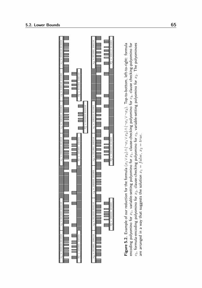
5.2. Lower Bounds 65
x1
=010110
011010
x1
=010110
011010
c3
=011010
010110
c4
=100101
101001
x1
=010110
011010
x1
=101001
100101
x1
=101001
100101
c5
=100110
011001
c3
=011010
010110
x2
=011001
100110
x2
=011001
100110
x2
=011001
100110
x2
=100110
011001
x2
=100110
011001
c4
=100101
101001
c5
=100110
011001
c3
=100101
101001
c5
=011001
100110
c4
=011010
010110
Figu
re5.2.
Exam
pleof
ourreductio
nforthe
form
ula
(x1∨x
2)∧
(¬x
1∨x
2)∧
(¬x
1∨¬x
2).
Top-to-bottom,left-to-right:form
ula
encoding
polyom
inoforx
1,v
ariable-settingpo
lyom
inoforx
1,c
lause-checking
polyom
inoforc 4,c
lausechecking
-polyominofor
c 5,form
ula-encoding
polyom
inoforx
2,clause-checkingpo
lyom
inoforc 3,varia
ble-settingpo
lyom
inoforx
2.The
polyom
inoes
arearrang
edin
away
that
suggests
thesolutio
nx
1=false,x
2=true.
66 Chapter 5: Intermezzo: Polyomino Packing
formula-encoding polyominoes with the complementary polyominoes in variable-settingand clause-checking polyominoes.
Now, consider the placement of a variable-setting polyomino (for variable xi). Sinceit starts with a complementary polyomino for xi, and also ends with one xi, it toomuch be placed such that it only overlaps at most (and exactly) one formula-encodingpolyomino, namely the one for xi. It thus suffices to consider each formula-encodingpolyomino in isolation. Note that then, there are only two possible placements forthe variable-setting polyomino for variable xi: either overlapping the first half of theformula-encoding polyomino, with the wildcard polyominoes used as building blocksin the variable-setting polyomino overlapping (and thus blocking) the polyominoescorresponding to clauses that are satisfied by setting xi to true, or, overlapping thesecond half of the formula-encoding polyomino, overlapping (and thus blocking) thepolyominoes corresponding to clauses that are satisfied by setting xi to false.
Thus, the placement of the variable-setting polyominoes (unsurprisingly) correspondsto an assignment for the variables of the formula. It is easy to see that the clause-checking polyominoes can then be packed into the space left only if the assignment issatisfying: if the assignment does not satisfy some clause, then all the places wherethe respective clause-checking polyomino could fit are blocked by variable-settingpolyominoes.
(⇐). We can consider each formula-encoding polyomino in isolation. An assignmentfor the formula immediately tells us how to pack the variable-setting polyomino forxi into the formula-encoding polyomino for xi (namely: if xi is true we place thevariable-setting polyomino in the second half, otherwise, we place it in the first half ofthe formula-encoding polyomino). It is easy to see that if the assignment is satisfying,then for each clause-checking polyomino there is at least one possible placement insidea formula-encoding polyomino. For an example of how the pieces fit together for asatisfying assignment, see Figure 5.2.
Remark that our reduction leaves gaps inside the packing. If we consider the variantof the problem where total area of the pieces is equal to the area of the target shape, andthus the entire rectangle must be filled (Exact Polyomino Packing), the instancecan be padded with several 1 × 1 polyominoes to make the total area of the piecesequal to the area of the target rectangle.
Corollary 5.2. Unless the Exponential Time Hypothesis fails, there exists no 2o(n/ logn)-time algorithm for Exact Polyomino Packing, even if the target shape is a 3× nbox, and the bounding box of each polyomino is of size 2×O(log n).
This raises an interesting open problem: does Exact Polyomino Packing stilladmit a 2Ω(n/ logn)-time lower bound when the pieces are similarly sized, that is, eachpiece must have area Θ(log n) (or even just Ω(n)). This seems to greatly limit thenumber of possible interactions between two polyomino pieces, since they cannot becombined in a way that creates small gaps.
Note that in the previous reduction we can fix the position of the formula-encodingpolyominoes in advance. The problem then reduces to packing variable-setting andclause-checking polyominoes into the shape left when subtracting the formula-encodingpolyominoes from the 3× n rectangle, which fits inside a 2× n rectangle. Doing so weobtain the following corollary:
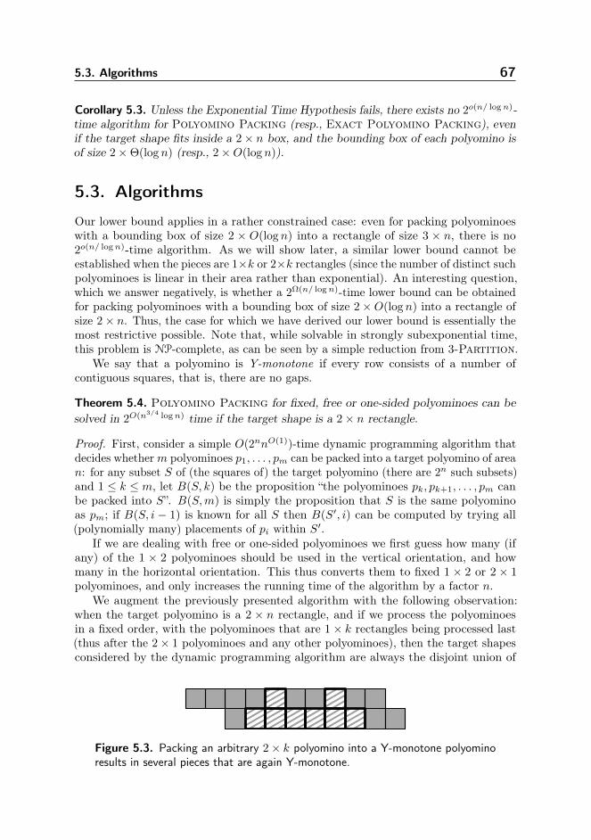
5.3. Algorithms 67
Corollary 5.3. Unless the Exponential Time Hypothesis fails, there exists no 2o(n/ logn)-time algorithm for Polyomino Packing (resp., Exact Polyomino Packing), evenif the target shape fits inside a 2× n box, and the bounding box of each polyomino isof size 2×Θ(log n) (resp., 2×O(log n)).
5.3. Algorithms
Our lower bound applies in a rather constrained case: even for packing polyominoeswith a bounding box of size 2 × O(log n) into a rectangle of size 3 × n, there is no2o(n/ logn)-time algorithm. As we will show later, a similar lower bound cannot beestablished when the pieces are 1×k or 2×k rectangles (since the number of distinct suchpolyominoes is linear in their area rather than exponential). An interesting question,which we answer negatively, is whether a 2Ω(n/ logn)-time lower bound can be obtainedfor packing polyominoes with a bounding box of size 2×O(log n) into a rectangle ofsize 2× n. Thus, the case for which we have derived our lower bound is essentially themost restrictive possible. Note that, while solvable in strongly subexponential time,this problem is NP-complete, as can be seen by a simple reduction from 3-Partition.
We say that a polyomino is Y-monotone if every row consists of a number ofcontiguous squares, that is, there are no gaps.
Theorem 5.4. Polyomino Packing for fixed, free or one-sided polyominoes can besolved in 2O(n3/4 logn) time if the target shape is a 2× n rectangle.
Proof. First, consider a simple O(2nnO(1))-time dynamic programming algorithm thatdecides whetherm polyominoes p1, . . . , pm can be packed into a target polyomino of arean: for any subset S of (the squares of) the target polyomino (there are 2n such subsets)and 1 ≤ k ≤ m, let B(S, k) be the proposition “the polyominoes pk, pk+1, . . . , pm canbe packed into S”. B(S,m) is simply the proposition that S is the same polyominoas pm; if B(S, i − 1) is known for all S then B(S′, i) can be computed by trying all(polynomially many) placements of pi within S′.
If we are dealing with free or one-sided polyominoes we first guess how many (ifany) of the 1 × 2 polyominoes should be used in the vertical orientation, and howmany in the horizontal orientation. This thus converts them to fixed 1 × 2 or 2 × 1polyominoes, and only increases the running time of the algorithm by a factor n.
We augment the previously presented algorithm with the following observation:when the target polyomino is a 2 × n rectangle, and if we process the polyominoesin a fixed order, with the polyominoes that are 1× k rectangles being processed last(thus after the 2× 1 polyominoes and any other polyominoes), then the target shapesconsidered by the dynamic programming algorithm are always the disjoint union of
Figure 5.3. Packing an arbitrary 2× k polyomino into a Y-monotone polyominoresults in several pieces that are again Y-monotone.
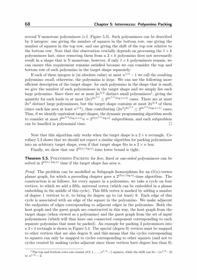
68 Chapter 5: Intermezzo: Polyomino Packing
several Y-monotone polyominoes (c.f. Figure 5.3). Such polyominoes can be describedby 3 integers: one giving the number of squares in the bottom row, one giving thenumber of squares in the top row, and one giving the shift of the top row relative tothe bottom row. Note that this observation crucially depends on processing the 1× kpolyominoes last, since removing them from a 2× k polyomino does not necessarilyresult in a shape that is Y-monotone, however, if only 1× k polyominoes remain, wecan ensure this requirement remains satisfied because we can consider the top andbottom row of each polyomino in the target shape separately.
If each of these integers is (in absolute value) at most n1/4 − 1 we call the resultingpolyomino small, otherwise, the polyomino is large. We can use the following moreefficient description of the target shape: for each polyomino in the shape that is small,we give the number of such polyominoes in the target shape and we simply list eachlarge polyomino. Since there are at most 2n3/4 distinct small polyominoes1, giving thequantity for each leads to at most (2n)2n3/4 ≤ 22n3/4(logn+1) cases. There are at most2n3 distinct large polyominoes, but the target shape contains at most 2n3/4 of them(since each has area at least n1/4), thus contributing (2n3)2n3/4 ≤ 26n3/4(logn+1) cases.Thus, if we identify equivalent target shapes, the dynamic programming algorithm needsto consider at most 28n3/4(logn+1)n = 2O(n3/4 logn) subproblems, and each subproblemcan be handled in polynomial time.
Note that this algorithm only works when the target shape is a 2× n rectangle. Co-rollary 5.3 shows that we should not expect a similar algorithm for packing polyominoesinto an arbitrary target shape, even if that target shape fits in a 2× n box.
Finally, we show that our 2Ω(n/ logn)-time lower bound is tight:
Theorem 5.5. Polyomino Packing for free, fixed or one-sided polyominoes can besolved in 2O(n/ logn) time if the target shape has area n.
Proof. The problem can be modelled as Subgraph Isomorphism for an O(n)-vertexplanar graph, for which a preceding chapter gave a 2O(n/ logn)-time algorithm. Theconstruction is as follows: for every square in a polyomino, we take a cycle on fourvertices, to which we add a fifth, universal vertex (which can be embedded in a planarembedding in the middle of this cycle). This fifth vertex is marked by adding a numberof degree 1 vertices to it, to bring its degree up to (at least) 9. Each edge of thiscycle is associated with an edge of the square in the polyomino. We make adjacentthe endpoints of edges corresponding to adjacent edges in the polyomino. Both thehost graph and the guest graph are constructed in this way, the host graph from thetarget shape (when viewed as a polyomino) and the guest graph from the set of inputpolyominoes (which will thus have one connected component corresponding to eachseparate polyomino that must be packed). An example for packing 3 polyominoes intoa 3×4 rectangle is shown in Figure 5.4. The special (degree 9) vertices must be mappedto other vertices that are also degree 9, and this means that the cycles correspondingto squares can only be mapped to cycles corresponding to other squares (and not tocycles created by making cycles adjacent since those vertices have degree less than 9).
1The top and bottom rows can consist of 0, 1, . . . , n1/4−1 squares, while the shift can be −(n1/4−2)to n1/4 − 2.
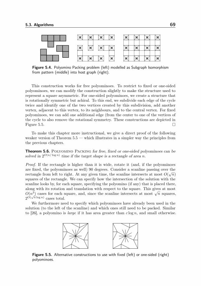
5.3. Algorithms 69
Figure 5.4. Polyomino Packing problem (left) modelled as Subgraph Isomorphismfrom pattern (middle) into host graph (right).
This construction works for free polyominoes. To restrict to fixed or one-sidedpolyominoes, we can modify the construction slightly to make the structure used torepresent a square asymmetric. For one-sided polyominoes, we create a structure thatis rotationally symmetric but achiral. To this end, we subdivide each edge of the cycletwice and identify one of the two vertices created by this subdivision, add anothervertex, adjacent to this vertex, to its neighbours, and to the central vertex. For fixedpolyominoes, we can add one additional edge (from the center to one of the vertices ofthe cycle to also remove the rotational symmetry. These constructions are depicted inFigure 5.5.
To make this chapter more instructional, we give a direct proof of the followingweaker version of Theorem 5.5 — which illustrates in a simpler way the principles fromthe previous chapters.
Theorem 5.6. Polyomino Packing for free, fixed or one-sided polyominoes can besolved in 2O(n/ logn) time if the target shape is a rectangle of area n.
Proof. If the rectangle is higher than it is wide, rotate it (and, if the polyominoesare fixed, the polyominoes as well) 90 degrees. Consider a scanline passing over therectangle from left to right. At any given time, the scanline intersects at most O(
√n)
squares of the rectangle. We can specify how the intersection of the solution with thescanline looks by, for each square, specifying the polyomino (if any) that is placed there,along with its rotation and translation with respect to the square. This gives at mostO(n3) cases for each square, and, since the scanline intersects at most
√n squares,
2O(√n logn) cases total.
We furthermore need to specify which polyominoes have already been used in thesolution (to the left of the scanline) and which ones still need to be packed. Similarto [26], a polyomino is large if it has area greater than c log n, and small otherwise.
Figure 5.5. Alternative constructions to use with fixed (left) or one-sided (right)polyominoes.
70 Chapter 5: Intermezzo: Polyomino Packing
Since the number of polyominoes with area k is bounded by 4.65k [77], the number ofdistinct small polyominoes it at most 4.65c logn. For c ≤ 0.22, this is at most
√n. We
can specify the quantity of each small polyomino left with a single number from 0 to n,giving (n+ 1)
√n = 2O(
√n logn) cases. Meanwhile, the number of large polyominoes is
at most n/(c log n), and thus there are 2O(n/ logn) possible subsets of them.The problem can now be solved by dynamic programming. For each position of
the scanline, we have 2O(n/ logn) subproblems: can a given subset of pieces (2O(n/ logn)
cases) be packed entirely to the left of the scanline (with only the pieces intersectingthe scanline possibly sticking out to the right of it), such that the intersection with thescanline looks as specified (2O(
√n logn) cases) (and, in the case of Exact Polyomino
Packing, leaving no gaps)? For each such subproblem, we can find its answer bydeleting the pieces whose leftmost square(s) intersect the scanline, and checking whetherthe instance thus obtained is compatible with some subproblem with the scanline movedone position to the left.
There is an interesting contrast between these algorithms. Whereas the stronglysubexponential algorithm for the case of the 2× n rectangle works by considering theinput polyominoes in a fixed order (so that we always know which subset we haveused) and uses a bound on the number of subsets of the target shape that have tobe considered, the algorithm for the general case works the opposite way around: itconsiders subsets of the target shape in a (more-or-less) fixed order (by the scanlineapproach) and bounds the number of possible subsets of the input polyominoes.
Note that our 2Ω(n/ logn)-time lower bound exploits the fact that we can constructexponentially many polyominoes that fit inside a 2×O(log n) rectangle. If we considerpolyominoes with simpler shapes, that is, polyominoes that are a× b rectangles, thenthe problem can be solved in strongly subexponential time:
Corollary 5.7. Polyomino Packing can be solved in 2O(√n logn) time if the polyomi-
noes are rectangular and the target shape is a rectangle with area n.
Proof. Consider the algorithm presented in the proof of Theorem 5.6. The runningtime is dominated by the number of cases for tracking a subset of the polyominoes. Ifthe polyominoes are rectangles, then note that the number of distinct rectangles ofarea at most n is also at most n. Call a polyomino large if it has area ≥
√n and small
otherwise: there are at most√n large polyominoes in the input, and thus at most 2
√n
subsets of them. The number of distinct small polyominoes is at most√n, and thus
specifying the quantity for each leads to at most n√n = 2
√n logn cases.
5.4. Conclusions
We have given a precise characterization of the complexity of (Exact) PolyominoPacking. For a set of polyominoes of total area n, the problem can be solved in2O(n/ logn) time. Even when restricted to the case where the pieces are of size 2×O(log n)and they have to be packed into a 3×n rectangle or into a given shape which fits insidea 2× n rectangle, there is no faster (up to the base of the exponentiation) algorithmunless the Exponential Time Hypothesis fails. In contrast, in the case where the targetshape is a 2× n rectangle, a strongly subexponential algorithm exists.
5.4. Conclusions 71
We conclude by listing several interesting open problems:
• Exact polyomino packing with excess pieces: we are given some target shape, anda set of polyominoes with total area possibly exceeding the target shape. Is itpossible to use a subset of the polyominoes to build the target shape? Clearly thisproblem is at least as hard as (exact) polyomino packing; however, consideringthe set of pieces may be much larger than the target shape, it would be interestingto study this problem from a parameterized perspective (where the parameterk is the area of the target shape). The problem can be solved in 2knO(1)-time(using the simple dynamic programming algorithm of Section 5.3); is there a2o(k)nO(1)-time (or even 2o(k)2o(n/ logn)-time) algorithm?
• What is the complexity of Exact Polyomino Packing when every piece hasarea Ω(log n) or Θ(log n)?
• We do not believe that our algorithm for packing polyominoes into a 2 × nrectangle is tight. What is the exact complexity of this problem? This is closelyrelated to the exact complexity of 3-Partition with the input given in unary,which (to our knowledge) is also an open problem.

IIProblems in Geometric
Intersection Graphs

75
Problems in GeometricIntersection Graphs
6.1. Introduction
As noted in the introduction, many hard graph problems that seem to require 2Ω(n) timeon general graphs (where n is the number of vertices) can be solved in subexponentialtime on planar graphs. In particular, many of these problems can be solved in 2O(
√n)
time on planar graphs — with a notable exception being the graph embedding problemswe saw in the previous part.
In this chapter, we explore a different direction: rather than investigate whetherother problems exhibit a “square root phenomenon” in planar graphs, we study whetherclassical problems (ones that are known to have square root behaviour in planar graphs,such as Independent Set, Vertex Cover and Hamiltonian Cycle) also exhibitsquare root behaviour in other graph classes.
One promising class of graphs where square root (or at least: strongly subexponentialtime) behaviour has also been observed, are geometric intersection graphs, with runningtimes of the form nO(n1−1/d) (or in one case 2O(n1−1/d)) in the d-dimensional case havingbeen obtained [91, 102].
The planar separator theorem [84, 85] and treewidth-based algorithms [34] couldbe considered a “framework” for obtaining subexponential algorithms on planar graphsor, more generally, on H-minor free graphs. In this chapter we aim to give a similarframework to obtain algorithms for problems in a wide class of geometric intersectiongraphs, while guaranteeing the running time 2O(n1−1/d).
The intersection graph G[F ] of a set F of objects in Rd is the graph whose vertexset is F and in which two vertices are adjacent when the corresponding objects intersect.(Unit-)disk graphs, where F consists of (unit) disks in the plane are a widely studied
76 Chapter 6: Problems in Geometric Intersection Graphs
class of intersection graphs. Disk graphs form a natural generalization of planar graphs,since any planar graph can be realized as the intersection graph of a set of disks in theplane. In this chapter we consider intersection graphs of a set F of fat objects, wherean object o ⊆ Rd is α-fat, for some 0 < α ≤ 1 if there are balls Bin and Bout in Rd suchthat Bin ⊆ o ⊆ Bout and radius(Bin)/ radius(Bout) ≥ α. For example, disks are 1-fatand squares are (1/
√2)-fat. From now on we assume that α is an absolute constant,
and often simply speak of fat objects. Note that we do not require the objects in Fto be convex, or even connected. Thus our definition is very general. In most of ourresults we furthermore assume that the objects in F are similarly sized, meaning thatthe ratio of their diameters is bounded by a fixed constant.
As mentioned, many subexponential results for planar graphs rely on planar separ-ators. Our first contribution is a generalization of this result to intersection graphsof (arbitrarily-sized) fat objects in Rd. Since these graphs can have large cliques wecannot bound the number of vertices in the separator. Instead, we build a separatorconsisting of cliques. We then define a weight function γ on these cliques — in ourapplications it suffices to define the weight of a clique C as γ(|C|) := log(|C|+ 1). Wedefine the weight of a separator as the sum of the weights of its constituent cliques Ci,which is useful since for many problems a separator can intersect the solution vertexset in 2O(
∑i γ(|Ci|)) many ways. Formally, the theorem can be stated this way:
Theorem 6.1. Let F be a set of n α-fat objects in Rd and let γ be a weight functionsuch that γ(t) = O(t1−1/d−ε), for constants d ≥ 2, α > 0, and ε > 0. Then theintersection graph G[F ] has a (6d/(6d + 1))-balanced separator and a clique partitionC(Fsep) of Fsep with weight O(n1−1/d). Such a separator and a clique partition C(Fsep)can be computed in O(nd+2) time if the objects have constant complexity.
A direct application of our separator theorem is a 2O(n1−1/d) algorithm for Inde-pendent Set. For general fat objects, only the 2-dimensional case was known to havesuch an algorithm [90].
Our separator theorem can be seen as a generalization of the work of Fu [53] whoconsiders a weighting scheme similar to ours. However, Fu’s result is significantly lessgeneral as it only applies to unit balls and his proof is arguably more complicated.Our result can also be seen as a generalization of the separator theorem of Har-Peledand Quanrud [62] which gives a small separator for constant ply—indeed, our proofborrows some ideas from theirs.
Finally, the technique employed by Fomin et al. [51] in two dimensions has alsosimilar qualities; in particular, the idea of using cliques as a basis for a separator canalso be found there, and leads to subexponential parameterized algorithms, even forsome problems that we do not tackle here.
After proving the weighted separator theorem for arbitrarily-sized fat objects, weswitch to similarly-sized objects. Here the idea is as follows: We find a suitableclique-decomposition P of the intersection graph G[F ], contract each clique to a singlevertex, and then work with the contracted graph GP where the node corresponding toa clique C gets weight γ(|C|). We then prove that the graph GP has constant degreeand, using our separator theorem, we prove that GP has weighted treewidth O(n1−1/d).Moreover, we can compute a tree decomposition of this weight in 2O(n1−1/d) time.
These weighted tree decompositions can often be used (with a small adaptation)
6.2. Separators for Arbitrarily-Sized Fat Objects 77
in “traditional” dynamic programming algorithms on tree decompositions. Thus weobtain a framework that gives 2O(n1−1/d)-time algorithms for intersection graphs ofsimilarly-sized fat objects for many problems for which treewidth-based algorithms areknown. Our framework recovers and often slightly improves the best known results forseveral problems1, including Independent Set, Hamiltonian Cycle and FeedbackVertex Set. Our framework also gives the first subexponential algorithms in geometricintersection graphs for, among other problems, r-Dominating Set for constant r,Steiner Tree and Connected Dominating Set.
Furthermore, we show that our approach can be combined with the rank-basedapproach [15], a technique to speed up algorithms for connectivity problems.
A desirable property of algorithms for geometric graphs is that they are robust,meaning that they can work directly on the graph without knowledge of the underlyinggeometry. Most of the known algorithms are in fact non-robust, which could be aproblem in applications, since finding a geometric representation of a given geometricintersection graph is NP-hard [31] (and many recognition problems for geometric graphsare ER-complete [71]). One of the advantages of our framework is that it yields robustalgorithms for many problems. To this end we need to generalize our scheme slightly:We no longer work with a clique partition to define the contracted graph GP, butwith a partition whose classes are the union of constantly many cliques. We showthat such a partition can be found efficiently without knowing the set F defining thegiven intersection graph. Thus we obtain robust algorithms for many of the problemsmentioned above, in contrast to known results which almost all need the underlyingset F as input.
6.2. Separators for Arbitrarily-Sized Fat Objects
Let F be a set of n α-fat objects in Rd for some constant α > 0, and let G[F ] = (F,E)be the intersection graph induced by F . For a given decomposition C(Fsep) of Fsep
into cliques and a given weight function γ we define the weight of Fsep, denoted byweight(Fsep), as weight(Fsep) :=
∑C∈C(Fsep) γ(|C|). Next we prove that G[F ] admits a
balanced separator of weight O(n1−1/d) for any cost function γ(t) = O(t1−1/d−ε) withε > 0. Our approach borrows ideas from Har-Peled and Quanrud [62], who show theexistence of small separators for low-density sets of objects, although our argumentsare significantly more involved.
Step 1: Finding candidate separators. Let H0 be a minimum-size hypercube con-taining at least n/(6d + 1) objects from F , and assume without loss of generality thatH0 is the unit hypercube centered at the origin. Let H1, . . . ,Hm be a collection ofm := n1/d hypercubes, all centered at the origin, where Hi has edge length 1 + 2i
m .Note that the largest hypercube, Hm, has edge length 3, and that the distance betweenconsecutive hypercubes Hi and Hi+1 is 1/n1/d.
Each hypercube Hi induces a partition of F into three subsets: a subset Fin(Hi)containing all objects that lie completely in the interior ofHi, a subset F∂(Hi) containing
1Note that most of the earlier results are in the parameterized setting, but we do not considerparameterized algorithms here.
78 Chapter 6: Problems in Geometric Intersection Graphs
all objects that intersect the boundary ∂Hi of Hi, and a subset Fout(Hi) containingall objects that lie completely in the exterior of Hi. Obviously an object from Fin(Hi)cannot intersect an object from Fout(Hi), and so F∂(Hi) defines a separator in a naturalway. It will be convenient to add some more objects to these separators, as follows.We call an object large when its diameter is at least 1/4, and small otherwise. Wewill add all large objects that intersect Hm to our separators. Thus our candidateseparators are the sets Fsep(Hi) := F∂(Hi) ∪ Flarge, where Flarge is the set of all largeobjects intersecting Hm. We show that our candidate separators are balanced:
Lemma 6.2. For any 0 ≤ i ≤ m we have
max(|Fin(Hi) \ Flarge|, |Fout(Hi) \ Flarge|
)<
6d
6d + 1n.
Proof. Consider a hypercube Hi. Because H0 contains at least n/(6d + 1) objects fromF , we immediately obtain
∣∣F∩(Fout(Hi)\Flarge)∣∣ ≤ |F∩Fout(H0)| ≤ |F \Fin(H0)| <
(1− 1
6d + 1
)n =
6d
6d + 1n.
To bound∣∣Fin(Hi) \ Flarge
∣∣, consider a subdivision of Hi into 6d sub-hypercubes ofedge length 1
6 (1 + 2im ) ≤ 1/2. We claim that any sub-hypercube Hsub intersects fewer
than n/(6d + 1) small objects from F . To see this, recall that small objects havediameter less than 1/4. Hence, all small objects intersecting Hsub are fully containedin a hypercube of edge length less than 1. Since H0 is a smallest hypercube containingat least n/(6d + 1) objects from F , Hsub must thus contain fewer than n/(6d + 1)objects from F , as claimed. Each object in Fin(Hi) intersects at least one of the 6d
sub-hypercubes, so we can conclude that∣∣Fin(Hi) \ Flarge
∣∣ < (6d/(6d + 1))n.
Step 2: Defining the cliques and finding a low-weight separator. Define F ∗ :=F \ (Fin(H0) ∪ Fout(Hm) ∪ Flarge). Note that F∂(Hi) ⊆ F ∗ for all i. We partition F ∗into size classes F ∗s , based on the diameter of the objects. More precisely, for integerss with 1 ≤ s ≤ smax, where smax := d(1− 1/d) log ne − 2, we define
F ∗s :=
o ∈ F ∗ :
2s−1
n1/d≤ diam(o) <
2s
n1/d
.
We furthermore define F ∗0 to be the subset of objects o ∈ F ∗ with diam(o) < 1/n1/d.Note that 2smax/n1/d ≥ 1/4, which means that every object in F ∗ is in exactly one sizeclass.
Each size class can be decomposed into cliques, as follows. Fix a size class F ∗s , with1 ≤ s ≤ smax. Since the objects in F are α-fat for a fixed constant α > 0, each o ∈ F ∗scontains a ball of radius α · (diam(o)/2) = Ω( 2s
n1/d ). Moreover, each object o ∈ F ∗s liesfully or partially inside the outer hypercube Hm, which has edge length 3. This implieswe can stab all objects in F ∗s using a set Ps of O((n
1/d
2s )d) points. Thus there existsa decomposition C(F ∗s ) of F ∗s consisting of O( n
2sd) cliques. In a similar way we can
argue that there exists a decomposition C(Flarge) of Flarge into O(1) cliques. For F ∗0the argument does not work since objects in F ∗0 can be arbitrarily small. Hence, we
6.2. Separators for Arbitrarily-Sized Fat Objects 79
create a singleton clique for each object in F ∗0 . Together with the decompositions of thesize classes F ∗s and of Flarge we thus obtain a decomposition C(F ∗) of F ∗ into cliques.
A decomposition of Fsep(Hi) into cliques is induced by C(F ∗), which we denoteby C(Fsep(Hi)). Thus, for a given weight function γ, the weight of Fsep(Hi) is equalto∑C∈C(Fsep(Hi))
γ(|C|). Our goal is now to show that at least one of the separatorsFsep(Hi) has weight O(n1−1/d), when γ(t) = O(t1−1/d−ε) for some ε > 0. To this endwe will bound the total weight of all separators Fsep(Hi) by O(n). Using that thenumber of separators is n1/d we then obtain the desired result.
Lemma 6.3. If γ(t) = O(t1−1/d−ε) for some ε > 0 then∑mi=1 weight(Fsep(Hi)) = O(n).
Proof. First consider the cliques in C(F ∗0 ), which are singletons. Since objects in F ∗0have diameter less than 1/n1/d, which is the distance between consecutive hypercube Hi
and Hi+1, each such object is in at most one set F∂(Hi). Hence, its contribution tothe total weight
∑mi=1 weight(Fsep(Hi)) is γ(1) = O(1). Together, the cliques in C(F ∗0 )
thus contribute O(n) to the total weight.Next, consider C(Flarge). It consists of O(1) cliques. In the worst case each clique
appears in all sets F∂(Hi). Hence, their total contribution to∑mi=1 weight(Fsep(Hi)) is
bounded by O(1) · γ(n) · n1/d = O(n).Now consider a set C(F ∗s ) with 1 ≤ s ≤ smax. A clique C ∈ C(F ∗s ) consists of
objects of diameter at most 2s/n1/d that are stabbed by a common point. Since thedistance between consecutive hypercubes Hi and Hi+1 is 1/n1/d, this implies that Ccontributes to the weight of O(2s) separators Fsep(Hi). The contribution to the weightof a single separator is at most γ(|C|). (It can be less than γ(|C|) because not allobjects in C need to intersect ∂Hi.) Hence, the total weight contributed by all cliques,which equals the total weight of all separators, is
smax∑s=1
∑C∈C(F∗s )
(weight contributed by C) ≤smax∑s=1
∑C∈C(F∗s )
2sγ(|C|) =
smax∑s=1
2s∑
C∈C(F∗s )
γ(|C|)
.
Next we wish to bound∑C∈C(F∗s ) γ(|C|). Define ns := |F ∗s | and observe that∑smax
s=1 ns ≤ n. Recall that C(F ∗s ) consists of O(n/2sd) cliques, that is, of at mostcn/2sd cliques for some constant c. To make the formulas below more readable weassume c = 1 (so we can omit c), but it is easily checked that this does not influencethe final result asymptotically. Similarly, we will be using γ(t) = t1−1/d−ε instead ofγ(t) = O(t1−1/d−ε). Because γ is positive and concave, the sum
∑C∈C(F∗s ) γ(|C|) is
maximized when the number of cliques is maximal, namely min(ns, n/2sd), and when
the objects are distributed as evenly as possible over the cliques. Hence,∑C∈C(F∗s )
γ(|C|) ≤
ns if ns ≤ n/2sd,(n/2sd) · γ
(ns
n/2sd
)otherwise.
We now split the set 1, . . . , smax into two index sets S1 and S2, where Si contains allindices s such that ns ≤ n/2sd, and S2 contains all remaining indices. Thus
smax∑s=1
2s∑
C∈C(F∗s )
γ(|C|)
=∑s∈S1
2s∑
C∈C(F∗s )
γ(|C|)
+∑s∈S2
2s∑
C∈C(F∗s )
γ(|C|)
80 Chapter 6: Problems in Geometric Intersection Graphs
The first term in the previous equation can be bounded by
∑s∈S1
2s∑
C∈C(F∗s )
γ(|C|)
≤ ∑s∈S1
2sns ≤∑s∈S1
2s(n/2sd) = n∑s∈S1
1/2s(d−1) = O(n),
where the last step uses that d ≥ 2. For the second term we get
∑s∈S2
2s∑
C∈C(F∗s )
γ(|C|)
≤ ∑s∈S2
(2s(n/2sd) · γ
(ns
n/2sd
))
≤∑s∈S2
(n
2s(d−1)·(ns2
sd
n
)1−1/d−ε)
≤ n∑s∈S2
(nsn
)1−1/d−ε 1
2sdε
≤ n∑s∈S2
(1
2dε
)s= O(n).
We are now ready to prove Theorem 6.1.
Proof of Theorem 6.1. Each candidate separator Fsep(Hi) is (6d/(6d + 1))-balancedby Lemma 6.2. Their total weight is O(n) by Lemma 6.3, and since we have n1/d
candidates one of them must have weight O(n1−1/d). This separator can be found inO(nd+2) time by brute force. Indeed, to find the hypercube H0 = [x1, x
′1]×· · ·× [xd, x
′d]
in O(nd+2) time we first guess the object defining xi, for all 1 ≤ i ≤ d, then guessthe object defining x′1 (and, hence, the size of the hypercube), and finally determinethe number of objects inside the hypercube. Once we have H0, we can generate thehypercubes H1, · · · , Hn1/d , generate the cliques as described above, and then computethe weights of the separators Fsep(Hi) by brute force within the same time bound.
Corollary 6.4. Let F be a set of n fat objects in Rd, where d ≥ 2 is a constant. ThenIndependent Set on the intersection graph G[F ] can be solved in 2O(n1−1/d) time.
Proof. Let γ(t) := log(t+1), and compute a separator Fsep for G[F ] using Theorem 6.1.For each subset Ssep ⊆ Fsep of independent (that is, pairwise non-adjacent) vertices wefind the largest independent set S of G such that S ⊇ Ssep, by removing the closedneighbourhood of Ssep from G and recursing on the remaining connected components.Finally, we report the largest of all these independent sets. Because a clique C ∈ C(Fsep)can contribute at most one vertex to Ssep, we have that the number of candidate setsSsep is at most∏
C∈C(Fsep)
(|C|+ 1) = 2∑C∈C(Fsep) log(|C|+1)
= 2O(n1−1/d).
Since all components on which we recurse have at most (6d/(6d + 1))n vertices, therunning time T (n) satisfies
T (n) = 2O(n1−1/d)T ((6d/(6d + 1))n) + poly(n),
6.3. An Algorithmic Framework for Similarly-Sized Fat Objects 81
which solves to T (n) = 2O(n1−1/d).
6.3. An Algorithmic Framework for Similarly-Sized FatObjects
We restrict our attention to similarly-sized fat objects. More precisely, we considerintersection graphs of sets F of objects such that, for each o ∈ F , there are balls Bin
and Bout in Rd such that Bin ⊆ F ⊆ Bout, and radius(Bin) = α and radius(Bout) = 1for some fatness constant α > 0. The restriction to similarly-sized objects makes itpossible to construct a clique cover of F with the following property: if we consider theintersection graph G[F ] where the cliques are contracted to single vertices, then thecontracted graph has constant degree. Moreover, the contracted graph admits a treedecomposition whose weighted treewidth is O(n1−1/d). This tool allows us to solvemany problems on intersection graphs of similarly-sized fat objects.
Our tree-decomposition construction uses the separator theorem from the previoussubsection. That theorem also states that we can compute the separator for G[F ] inpolynomial time, provided we are given F . However, finding the separator if we areonly given the graph and not the underlying set F is not easy. Note that decidingwhether a graph is a unit-disk graph is already ER-complete [71]. Nevertheless, weshow that for similarly-sized fat objects we can find certain tree decompositions withthe desired properties, purely based on the graph G[F ].
κ-partitions, P-contractions, and separators. Let G = (V,E) be the intersectiongraph of an (unknown) set F of similarly-sized fat objects, as defined above. Theseparators in the previous section use cliques as basic components. We need to generalizethis slightly, by allowing connected unions of a constant number of cliques as basiccomponents. Thus we define a κ-partition of G as a partition P = (V1, . . . , Vk) of Vsuch that every partition class Vi induces a connected subgraph that is the union of atmost κ cliques. Note that a 1-partition corresponds to a clique cover of G.
Given a κ-partition P of G we define the P-contraction of G, denoted by GP, to bethe graph obtained by contracting all partition classes Vi to single vertices and removingloops and parallel edges. In many applications it is essential that the P-contractionwe work with has maximum degree bounded by a constant. From now on, when wespeak of the degree of a κ-partition P we refer to the degree of the correspondingP-contraction.
The following theorem and its proof are very similar to Theorem 6.1, but it appliesonly for similarly-sized objects because of the degree bound on GP. The other maindifference is that the separator is defined on the P-contraction of a given κ-partition,instead of on the intersection graph G itself.
Theorem 6.5. Let G = (V,E) be the intersection graph of a set of n similarly-sizedfat objects in Rd, and let γ be a weight function such that γ(t) = O(t1−1/d−ε), forconstants d ≥ 2 and ε > 0. Suppose we are given a κ-partition P of G such that GP
has maximum degree at most ∆, where κ and ∆ are constants. Then there exists a(6d/(6d + 1))-balanced separator for GP of weight O(n1−1/d).
82 Chapter 6: Problems in Geometric Intersection Graphs
The following lemma shows that a partition P as needed in Theorem 6.5 can becomputed even in the absence of geometric information.
Lemma 6.6. Let G = (V,E) be the intersection graph of an (unknown) set of nsimilarly-sized fat objects in Rd for some constant d ≥ 2. There there exist constants κand ∆ such that a κ-partition P for which GP has maximum degree ∆ can be computedin polynomial time.
Proof. Let S ⊆ V be a maximal independent set in G (e.g., it is inclusion-wisemaximal). We assign each vertex v ∈ V \ S to an arbitrary vertex s ∈ S that is aneighbour of v; such a vertex s always exists since S is maximal. For each vertexs ∈ S define Vs := s ∪ v ∈ V \ S : v is assigned to s. We prove that the partitionP := Vs : s ∈ S, which can be computed in polynomial time, has the desiredproperties.
Let ov denote the (unknown) object corresponding to a vertex v ∈ V , and fora partition class Vs define U(Vs) :=
⋃v∈Vs ov. We call U(Vs) a union-object. Let
US := U(Vs) : s ∈ S. Because the objects defining G are similarly-sized andfat, there are balls Bin(ov) of radius α = Ω(1) and Bout(ov) of radius 1 such thatBin(ov) ⊆ ov ⊆ Bout(ov).
Now observe that each union-object U(Vs) is contained in a ball of radius 3. Hence,we can stab all balls Bin(ov), v ∈ Vs using O(1) points, which implies that P is aκ-partition for some κ = O(1).
To prove that the maximum degree of GP is O(1), we note that any two balls Bin(s),Bin(s′) with s, s′ ∈ S are disjoint (because S is an independent set in G). Since allunion-objects U(s′) that intersect U(s) are contained in a ball of radius 9, an easypacking argument now shows that U(s) intersects O(1) union-objects U(s). Hence, thenode in GP corresponding to Vs has degree O(1).
Weighted tree decompositions for P-contractions. We now introduce the notion ofweighted treewidth [108]. Recall that the width of a tree decomposition is the size ofits largest bag minus 1, and the treewidth of a graph G equals the minimum width ofa tree decomposition of G. In weighted treewidth, each vertex has a weight, and theweighted width of a tree decomposition is the maximum over the bags of the sum of theweights of the vertices in the bag (note: without the −1). The weighted treewidth of agraph is the minimum weighted width over its tree decompositions.
Now let P = (V1, . . . , Vk) be a κ-partition of a given graph G which is the intersectiongraph of similarly-sized fat objects, and let γ be a given weight function on partitionclasses. We apply the concept of weighted treewidth to GP, where we assign eachvertex Vi of GP a weight γ(|Vi|). Because we have a separator for GP of low weight byTheorem 6.5, we can prove a bound on the weighted treewidth of GP using standardtechniques.
Lemma 6.7. Let P be a κ-partition of a family of similarly-sized fat objects such thatGP has maximum degree at most ∆, where κ and ∆ are constants. Then the weightedtreewidth of GP is O(n1−1/d) for any weight function γ with γ(t) = O(t1−1/d−ε).
Proof. The lemma follows from Theorem 6.5 by a minor variation on standard techniques— see for example [14, Theorem 20]. Take a separator S of GP as indicated by
6.3. An Algorithmic Framework for Similarly-Sized Fat Objects 83
Theorem 6.5. Recursively, make tree decompositions of the connected components ofGP \ S. Take the disjoint union of these tree decompositions, add an edge between thetwo trees and then add S to all bags. We now have a tree decomposition of GP. Asbase case, when we have a subgraph of GP with O(n1−1/d) vertices, then we take onebag with all vertices in this subgraph.
The weight of bags for subgraphs of GP with r vertices fulfils w(r) = O(r1−1/d) +w(6d/(6d + 1)r), which gives that the weighted width of this tree decomposition isw(n) = O(n1−1/d).
By combining Lemmas 6.6 and 6.7 we can obtain a κ-partition such that GP hasconstant degree, and such that the weighted treewidth of GP is as desired. In whatfollows, we work towards finding a suitable weighted tree decomposition.
A blowup of a vertex v by an integer t results in a graph where we replace the vertexv with a clique of size t (called the clique of v), in which we connect every vertex tothe neighbourhood of v. The vertices in these cliques all have weight 1.
Lemma 6.8 ([24]). Let W ⊆ V form a clique in G = (V,E). Every tree decomposition(TG, XG
t | t ∈ TG) of G has a bag XGt ∈ XG
t | t ∈ TG with W ⊆ XGt .
Lemma 6.9. The weighted treewidth of a graph G with weight function w : V (G)→ Nis equal to 1 plus the treewidth of H that is gained from G by blowing up each vertexv by γ(v). Let (TH , XH
t | t ∈ TH) be a tree decomposition of H. Then we cancreate a tree decomposition (TG, XG
t | t ∈ TG) of G where TG is isomorphic to THthe following way: a vertex v ∈ G is added to a bag if and only if the correspondingbag in TH contains all vertices from the clique of v. Furthermore, the treewidth of(TH , XH
t | t ∈ TH) is at most the weighted width of (TG, XGt | t inTG) minus 1.
Proof. The proof we give below is a simple modification of folklore insights on treewidth;For related results see [27, 19]. First, we notice that (TG, XG
t | t ∈ TG) is a treedecomposition of G. From Lemma 6.8, we have that for each vertex v and edge v, wthere is a bag in (TG, XG
t | t ∈ TG) that contains v, respectively v, w. For thethird condition of tree decompositions, suppose j2 is in TG on the path from j1 toj3. If v belongs to the bags of j1 and j3, then all vertices in the clique resulting ofblowing up v belong in (TH , XH
t | t ∈ TH) to the bags of j1 and j3, hence by theproperties of tree decompositions to the bag of j2, and hence v ∈ XG
( j2). It followsthat the preimage of each vertex in VG is a subtree of TG. The total weight of verticesin a bag in (TG, XG
t | t ∈ TG) is never larger than the size of the corresponding bagin (TH , XH
t | t ∈ TH). Thus, by taking for (TG, XGt | t ∈ TG) a tree decomposition
with minimum weighted treewidth, we see that the weighted treewidth of G is at mostthe treewidth of H plus 1; the additive term of 1 comes from the −1 in the definitionof treewidth.
In the other direction, if we take a tree decomposition (TG, XGt | t ∈ TG) of G, we
can obtain one of H by replacing in each bag each vertex v by the clique that resultsfrom blowing up G. The size of a bag in the tree decomposition of H now equals thetotal weight of the vertices in G; hence the width of (TG, XG
t | t ∈ TG) equals theweighted width of the obtained tree decomposition of H; it follows that the weightedtreewidth of G is at least the treewidth of H minus 1.
84 Chapter 6: Problems in Geometric Intersection Graphs
We are now ready to prove our main theorem for algorithms.
Theorem 6.10. Let G = (V,E) be the intersection graph of an (unknown) set of nsimilarly-sized α-fat objects in Rd, and let γ be a weight function such that 1 ≤ γ(t) =O(t1−1/d−ε), for constants d ≥ 2, α > 0, and ε > 0. Then there exist constants κand ∆ such that there is a κ-partition P with the following properties: (i) GP hasmaximum degree at most ∆, and (ii) GP has weighted treewidth O(n1−1/d). Moreover,such a partition P and a corresponding tree decomposition of weight O(n1−1/d) can becomputed in 2O(n1−1/d) time.
Proof. Lemma 6.6 provides a partition P built around a maximal independent set. ByLemma 6.7, the weighted treewidth of GP is O(n1−1/d).
To get a tree decomposition, consider the above partition again, with a weightfunction γ(t) = O(t1−1/d−ε). We work on the contracted graph GP; we intend tosimulate the weight function by modifying GP. Let H be the graph we get from GP
by blowing up each vertex vC by an integer that is approximately the weight of thecorresponding class, more precisely, we blow up vC by dγ(|C|)e. By Lemma 6.9, itstreewidth (plus one) is a 2-approximation of the weighted treewidth of G (since γ(t) ≥ 1).Therefore, we can run a treewidth approximation algorithm that is single exponential inthe treewidth ofH. We can use the algorithm from either [100] or [18] for this, both haverunning time 2O(tw(H))|V (H)|O(1) = 2O(n1−1/d)(nγ(n))O(1) = 2O(n1−1/d), and providea tree decomposition whose width is a c-approximation of the treewidth of H, fromwhich we gain a tree decomposition whose weighted treewidth is a 2c-approximation ofthe weighted treewidth of GP.
6.4. Basic Algorithmic Applications
In this section, we give examples of how κ-partitions and weighted tree decompositionscan be used to obtain subexponential-time algorithms for classical problems on geometricintersection graphs.
Given a κ-partition P and a weighted tree decomposition of GP of width τ , we notethat there exists a nice tree decomposition of G (i.e., a “traditional”, non-partitionedtree decomposition) with the property that each bag is a subset of the union of anumber of partition classes, such that the total weight of those classes is at most τ .This can be seen by creating a nice version of the weighted tree decomposition of GP,and then replacing every introduce/forget bag (that introduces/forgets a class of thepartition) by a series of introduce/forget bags (that introduce/forget the individualvertices). We call such a decomposition a traditional tree decomposition. Using such adecomposition, it becomes easy to give algorithms for problems for which we alreadyhave dynamic-programming algorithms operating on nice tree decompositions. We canre-use the algorithms for the leaf, introduce, join and forget cases, and either show thatthe number of partial solutions remains bounded (by exploiting the properties of theunderlying κ-partition) or show that we can discard some irrelevant partial solutions.
We present several applications for our framework, resulting in 2O(n1−1/d)-timealgorithms for various problems. In addition to the (non-robust) Independent Setalgorithm for fat objects based on our separator, we also give a robust algorithm
6.4. Basic Algorithmic Applications 85
for similarly sized fat objects. This adds robustness compared to the state of theart [91]. In the rest of the applications, our algorithms work on intersection graphsof d-dimensional similarly sized fat objects; this is usually a larger graph class thanwhat has been studied. We have non-robust algorithms for Hamiltonian Path andHamiltonian Cycle; this is a simple generalization of the previously known [51, 76]algorithm for unit disks. For Feedback Vertex Set, we give a robust algorithmwith the same running time improvement, over a non-robust algorithm that worksin 2-dimensional unit disk graphs [51]. For r-Dominating Set, we give a robustalgorithm for d ≥ 2, which is the first subexponential algorithm in dimension d ≥ 3,and the first robust subexponential algorithm for d = 2 [90]. (The algorithm in [90]is for Dominating Set in unit disk graphs.) Finally, we give robust algorithms forSteiner Tree, r-Dominating Set, Connected Vertex Cover, ConnectedFeedback Vertex Set and Connected Dominating Set, which are – to ourknowledge – also the first subexponential algorithms in geometric intersection graphsfor these problems.
In the following, we fix our weight function to be γ(k) = log(k + 1).
Theorem 6.11. If a κ-partition and a weighted tree decomposition of width at most τis given, Independent Set and Vertex Cover can be solved in time 2κτnO(1).
Proof. A well-known algorithm (see, e.g., [34]) for solving Independent Set on graphsof bounded treewidth, computes, for each bag t and subset S ⊆ Xt, the maximum sizec[t, S] of an independent subset S ⊂ G[t] such that S ∩Xt = S.
An independent set never contains more than one vertex of a clique. Therefore,if we have a traditional tree decomposition (T, Xt | t ∈ T), obtained from a κ-partitioned weighted tree decomposition, Xt is a subset of the union of partitionclasses Vi | i ∈ Xt (where Xt denotes the corresponding bag of the weighted treedecomposition). Since from each partition class we can select at most κ vertices (onevertex from each clique), the number of subsets S that need to be considered is at most∏i∈Xt(|Vi|+ 1)κ = exp
(∑i∈Xt κ log (|Vi|+ 1)
)= 2κτ .
Applying the standard algorithm for Independent Set on a traditional treedecomposition, using the fact that only solutions that select at most one vertex fromeach clique get a non-zero value, we obtain the claimed algorithm. Minimum VertexCover can be solved by finding a solution I to Maximum Independent Set andreturning the complement V \ I, which is a minimum vertex cover.
Corollary 6.12. For any constant d ≥ 2, Independent Set and Vertex Cover canbe solved in 2O(n1−1/d) time on intersection graphs of similarly-sized d-dimensional fatobjects, even if the geometric representation is not given.
In the remainder of this section, because we need additional assumptions that arederived from the properties of intersection graphs, we state our results in terms ofalgorithms operating directly on intersection graphs. However, note that underlyingeach of these results is an algorithm operating on a weighted tree decomposition of thecontracted graph.
To obtain the algorithm for Independent Set, we exploited the fact that we canselect at most one vertex from each clique, and that thus, we can select at most κvertices from each partition class. For Dominating Set, our bound for the treewidth
86 Chapter 6: Problems in Geometric Intersection Graphs
is however not enough. Instead, we need the following, stronger result, which statesthat the weight of a bag in the decomposition can still be bounded by O(n1−1/d), evenif we take the weight to be the total weight of the classes in the bag and that of theirdistance-r neighbours:
Theorem 6.13. Let G be an intersection graph of n similarly-sized d-dimensionalfat objects, and let r ≥ 1 be a constant. For any weight function γ, there existsa constant κ = O(1) such that G has a κ-partition P and a corresponding GP ofmaximum degree at most ∆, where GP has a weighted tree decomposition withthe additional property that for any bag b, the total weight of the partition classesVi ∈ P | (some vertex in) Vi is within distance r of some Vj ∈ σ(b) is O(n1−1/d).
Proof. As per Theorem 6.10, there exist constants κ,∆ = O(1) such that G has aκ-partition in which each class of the partition is adjacent to at most ∆ other classes.
We now create a new geometric intersection graph G′, which is made by copyingeach vertex (and its corresponding object) at most κr times. We create the followingκr-partition Pr: for each class Vi of the original partition, create a class that contains acopy of the vertices from Vi and copies of the vertices from the classes within distanceat most r from Vi. This graph Gr has at most κrn = O(n) vertices, and it is anintersection graph of similarly-sized objects; furthermore, the set Pr has low union ply.Therefore, we can find a weighted tree decomposition of GrPr of width O(n1−1/d) byLemma 6.7.
This decomposition can also be used as a decomposition for the original κ-partition,by replacing each partition class with the corresponding original partition class.
Theorem 6.14. Let r ∈ Z+, d ≥ 2 be constants. Then r-Dominating Set can besolved in 2O(n1−1/d) time on intersection graphs of similarly-sized d-dimensional fatobjects.
Proof. We first present the argument for Dominating Set. It is easy to see that fromeach partition class, we need to select at most κ2(∆ + 1) vertices: each partition classcan be partitioned into at most κ cliques, and each of these cliques is adjacent to atmost κ(∆ + 1) other cliques. If we select at least κ(∆ + 1) + 1 vertices from a clique,we can instead select only one vertex from the clique, and select at least one vertexfrom each neighbouring clique.
We once again proceed by dynamic programming on a traditional tree decomposition(see e.g. [34] for an algorithm solving Dominating Set using tree decompositions).However, rather than needing just two states per vertex (in the solution or not), weneed three: a vertex can be either in the solution, not in the solution and not dominated,or not in the solution and dominated. After processing each bag, we discard partialsolutions that select more than κ2(∆ + 1) vertices from any class of the partition. Notethat all vertices of each partition class are introduced before any are forgotten, sowe can guarantee we do indeed never select more than κ2(∆ + 1) vertices from eachpartition class.
The way vertices outside the solution are dominated or not is completely determinedby the vertices that are in the solution and are neighbours of the vertices in thebag. While the partial solution does not track this explicitly for vertices that areforgotten, by using the fact that we need to select at most κ∆ vertices from each
6.5. Application of the Rank-Based Approach 87
class of the partition, and the fact that Theorem 6.13 bounds the total weight ofthe neighbourhood of the partition classes in a bag, we see that there are at mostΠi(|Vi|+ 1)κ
2(∆+1) = exp(κ2(∆ + 1)∑i log (|Vi|+ 1)) = 2O(n1−1/d), where the product
(resp., sum) is taken over all partition classes Vi that appear in the current bag or area neighbours of such a class.
For the generalization where r > 1, the argument that we need to select at mostκ(∆ + 1) vertices from each clique still holds: moving a vertex from a clique with morethan κ(∆ + 1) vertices selected to an adjacent clique only decreases the distance toany vertices it helps cover. The dynamic programming algorithm needs, in a partialsolution, to track at what distance from a vertex in the solution each vertex is. This,once again, is completely determined by the solution in partition classes at distance atmost r; the number of such cases we can bound using Theorem 6.13.
6.5. Application of the Rank-Based Approach
To illustrate how our algorithmic framework can be combined with the rank-basedapproach, we now give an algorithm for Steiner Tree.
We only consider the unweighted variant of Steiner Tree, as, assuming theETH, the Weighted Steiner Tree problem does not admit a subexponential-timealgorithm, even on a clique (as Weighted Steiner Tree on a clique can encodeSteiner Tree on an arbitrary graph by setting the weights of non-edges to a sufficientlylarge number). Therefore, we should not expect Theorem 6.15 to hold for the weightedcase.
Theorem 6.15. Let d ≥ 2 be a constant. Then Steiner Tree can be solved in2O(n1−1/d) time on intersection graphs of d-dimensional similarly-sized fat objects.
Proof. The algorithm works by dynamic programming on a traditional tree decom-position. The leaf, introduce, join and forget cases can be handled as they are inthe conventional algorithm for Steiner Tree on tree decompositions, see e.g. [15].However, after processing each bag, we can reduce the number of partial solutions thatneed to be considered by exploiting the properties of the underlying κ-partition.
To this end, we first need a bound on the number of vertices that can be selectedfrom each class of the κ-partition P.
Lemma 6.16. Let C be a clique in a κ-sized clique cover of a partition class Vi ∈ P.Then any optimal solution X contains at most κ(∆ + 1) vertices from C that are notalso in K. Furthermore, any optimal solution thus contains at most κ2(∆ + 1) vertices(that are not also in K) from each partition class.
Proof. To every vertex v ∈ (C∩X)\K we greedily assign a private neighbour u ∈ X \Csuch that u is adjacent to v and u is not adjacent to any other previously assignedprivate neighbour. If this process terminates before all vertices in (C ∩X) \K havebeen assigned a private neighbour, then the remaining vertices are redundant and canbe removed from the solution.
We now note that since the neighbourhood of C can be covered by at most κ(∆ + 1)cliques, this gives us an upper bound on the number of private neighbours that can
88 Chapter 6: Problems in Geometric Intersection Graphs
be assigned and thus bounds the number of vertices that can be selected from anypartition class.
The algorithm for Steiner Tree presented in [15] is for the weighted case, but wecan ignore the weights by setting them to 1. A partial solution is then represented bya subset S ⊆ Xt (representing the intersection of the partial solution with the verticesin the bag), together with an equivalence relation on S (which indicates which verticesare in the same connected component of the partial solution).
Since we select at most κ2(∆ + 1) vertices from each partition class, we can discardpartial solutions that select more than this number of vertices from any partition class.Then the number of subsets S considered is at most
∏i∈Xt)
(|Vi|+ 1)κ2(∆+1) = exp
κ2(∆ + 1) ·∑i∈Xt
log(|Vi|+ 1)
≤ exp(κ2(∆ + 1)τ
).
For any such subset S, the number of possible equivalence relations is 2Θ(|S| log |S|).However, the rank-based approach [15] provides an algorithm called “reduce” that, givena set of equivalence relations2 on S, outputs a representative set of equivalence relationsof size at most 2|S|. Thus, by running the reduce algorithm after processing each bag,we can keep the number of equivalence relations considered single exponential.
Since |S| is also O(κ2(∆ + 1)τ) (we select at most κ2(∆ + 1) vertices from eachpartition class and each bag contains at most τ partition classes), for any subset S,the rank-based approach guarantees that we need to consider at most 2O(κ2(∆+1)τ)
representative equivalence classes of S (for each set S).
Theorem 6.17. For any constant d ≥ 2, Maximum Induced Forest (and FeedbackVertex Set) can be solved in 2O(n1−1/d) time on intersection graphs of d-dimensionalsimilarly-sized fat objects.
Proof. We once again proceed by dynamic programming on a traditional tree decom-position corresponding to the weighted tree decomposition of GP of width τ , where P isa κ-partition, and the maximum degree of GP is at most ∆. We describe the algorithmfrom the viewpoint of Maximum Induced Forest, but Feedback Vertex Set issimply its complement.
Using the rank-based approach with Maximum Induced Forest requires somemodifications to the problem, since the rank-based approach is designed to get max-imum connectivity, whereas in Maximum Induced Forest, we aim to “minimize”connectivity (i.e., avoid creating cycles). To overcome this issue, the authors of [15] adda special universal vertex v0 to the graph (increasing the width of the decompositionby 1) and ask (to decide if a Maximum Induced Forest of size k exists in the graph)whether we can delete some of the edges incident to v0 such that there exists an induced,connected subgraph, including v0, of size k + 1 in the modified graph that has exactlyk edges. Essentially, the universal vertex allows us to arbitrarily glue together the treesof an induced forest into a single (connected) tree. This thus reformulates the problemsuch that we now aim to find a connected solution.
2What we refer to as “equivalence relation”, [15] refers to as “partition”.
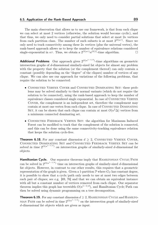
6.5. Application of the Rank-Based Approach 89
The main observation that allows us to use our framework, is that from each cliquewe can select at most 2 vertices (otherwise, the solution would become cyclic), andthat thus, we only need to consider partial solutions that select at most 2κ verticesfrom each partition class. The number of such subsets is at most 2O(κτ). Since weonly need to track connectivity among these 2κ vertices (plus the universal vertex), therank-based approach allows us to keep the number of equivalence relations consideredsingle-exponential in κτ . Thus, we obtain a 2O(κτ)nO(1)-time algorithm.
Additional Problems Our approach gives 2O(n1−1/d)-time algorithms on geometricintersection graphs of d-dimensional similarly-sized fat objects for almost any problemwith the property that the solution (or the complement thereof) can only contain aconstant (possibly depending on the “degree” of the cliques) number of vertices of anyclique. We can also use our approach for variations of the following problems, thatrequire the solution to be connected:
• Connected Vertex Cover and Connected Dominating Set: these prob-lems may be solved similarly to their normal variants (which do not require thesolution to be connected), using the rank-based approach to keep the number ofequivalence classes considered single exponential. In case of Connected VertexCover, the complement is an independent set, therefore the complement maycontain at most one vertex from each clique. In case of Connected DominatingSet, it can be shown that each clique can contain at most O(κ2∆) vertices froma minimum connected dominating set.
• Connected Feedback Vertex Set: the algorithm for Maximum InducedForest can be modified to track that the complement of the solution is connected,and this can be done using the same connectivity-tracking equivalence relationthat keeps the solution cycle-free.
Theorem 6.18. For any constant dimension d ≥ 2, Connected Vertex Cover,Connected Dominating Set and Connected Feedback Vertex Set can besolved in time 2O(n1−1/d) on intersection graphs of similarly-sized d-dimensional fatobjects.
Hamiltonian Cycle. Our separator theorems imply that Hamiltonian Cycle/Pathcan be solved in 2O(n1−1/d) time on intersection graphs of similarly-sized d-dimensionalfat objects. However, in contrast to our other results, this requires that a geometricrepresentation of the graph is given. Given a 1-partition P whereGP has constant degree,it is possible to show that a cycle/path only needs to use at most two edges betweeneach pair of cliques; see e.g. [69, 76] and that we can obtain an equivalent instancewith all but a constant number of vertices removed from each clique. Our separatortheorem implies this graph has treewidth O(n1−1/d), and Hamiltonian Cycle/Path canthen be solved using dynamic programming on a tree decomposition.
Theorem 6.19. For any constant dimension d ≥ 2, Hamiltonian Cycle and Hamilto-nian Path can be solved in time 2O(n1−1/d) on the intersection graph of similarly-sizedd-dimensional fat objects which are given as input.
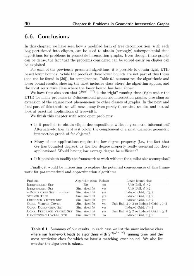
90 Chapter 6: Problems in Geometric Intersection Graphs
6.6. Conclusions
In this chapter, we have seen how a modified form of tree decomposition, with eachbag partitioned into cliques, can be used to obtain (strongly) subexponential timealgorithms for problems in geometric intersection graphs. Even though these graphscan be dense, the fact that the problems considered can be solved easily on cliques canbe exploited.
For each of the previously presented algorithms, it is possible to obtain tight, ETH-based lower bounds. While the proofs of these lower bounds are not part of this thesis(and can be found in [36]), for completeness, Table 6.1 summarizes the algorithmic andlower bound results, showing the most inclusive class where the algorithm applies, andthe most restrictive class where the lower bound has been shown.
We have thus also seen that 2Θ(n1−1/d) is the “right” running time (tight under theETH) for many problems in d-dimensional geometric intersection graphs, providing anextension of the square root phenomenon to other classes of graphs. In the next andfinal part of this thesis, we will move away from purely theoretical results, and insteadlook at practical applications of treewidth.
We finish this chapter with some open problems:
• Is it possible to obtain clique decompositions without geometric information?Alternatively, how hard is it colour the complement of a small diameter geometricintersection graph of fat objects?
• Many of our applications require the low degree property (i.e., the fact thatGP has bounded degree). Is the low degree property really essential for theseapplications? Would having low average degree be sufficient?
• Is it possible to modify the framework to work without the similar size assumption?
Finally, it would be interesting to explore the potential consequences of this frame-work for parameterized and approximation algorithms.
Problem Algorithm class Robust Lower bound classIndependent Set Fat no Unit Ball, d ≥ 2Independent Set Sim. sized fat yes Unit Ball, d ≥ 2r-Dominating Set, r = const Sim. sized fat yes Induced Grid, d ≥ 2Steiner Tree Sim. sized fat yes Induced Grid, d ≥ 2Feedback Vertex Set Sim. sized fat yes Induced Grid, d ≥ 2Conn. Vertex Cover Sim. sized fat yes Unit Ball, d ≥ 2 or Induced Grid, d ≥ 3Conn. Dominating Set Sim. sized fat yes Induced Grid, d ≥ 2Conn. Feedback Vertex Set Sim. sized fat yes Unit Ball, d ≥ 2 or Induced Grid, d ≥ 3Hamiltonian Cycle/Path Sim. sized fat no Induced Grid, d ≥ 2
Table 6.1. Summary of our results. In each case we list the most inclusive classwhere our framework leads to algorithms with 2O(n1−1/d) running time, and themost restrictive class for which we have a matching lower bound. We also listwhether the algorithm is robust.
IIIPractical Applications of
Treewidth

93
Computing Tree Decompositions onthe GPU
7.1. Introduction
As seen in the previous parts, treewidth and (structures similar to) tree decompositionscan be very useful theoretical tools. The fact that many otherwise hard graph problemsare linear time solvable on graphs of bounded treewidth [22] can also be exploited inpractical applications — we will see an example of this in the next chapter. For suchapplications, it is important to have efficient algorithms, that given a graph, determinethe treewidth and find tree decompositions with optimal (or near-optimal) width.
The interest in practical algorithms to compute treewidth and tree decompositionsis also illustrated by the fact that both the PACE 2016 and PACE 2017 challenges[37] included treewidth as one of the two challenge topics. Remarkably, while mosttracks in the PACE 2016 challenge attracted several submissions [38], there were nosubmissions for the call for GPU-based programs for computing treewidth. Currentsequential exact algorithms for treewidth are only practical when the treewidth is small(up to 4, see [65]), or when the graph is small (see [57, 20, 118, 44, 117]). As computingtreewidth is NP-hard, an exponential growth of the running time is to be expected;unfortunately, the exact FPT algorithms that are known for treewidth are assumedto be impractical; e.g., the algorithm of [12] has a running time of 2O(tw3)n for ann-vertex graph of treewidth tw. This creates the need for good parallel algorithms, asparallelism can help to significantly speed up the algorithms, and thus deal with largergraph sizes.
We present a parallel algorithm for computing the treewidth of a graph on a GPU.We implement this algorithm in OpenCL, and experimentally evaluate its performance.Our algorithm is based on an O∗(2n)-time algorithm that explores the elimination
94 Chapter 7: Computing Tree Decompositions on the GPU
orderings of the graph using a Held-Karp like dynamic programming approach. Weuse Bloom filters to detect duplicate solutions.
GPU programming presents unique challenges and constraints, such as constraintson the use of memory and the need to limit branch divergence. We experiment withvarious optimizations to see if it is possible to work around these issues. We achieve avery large speed up (up to 77×) compared to running the same algorithm on the CPU.
The starting point of our algorithm is a sequential algorithm by Bodlaender etal. [20]. This algorithm exploits a characterization of treewidth in terms of the width ofan elimination ordering, and gives a dynamic programming algorithm with a structurethat is similar to the textbook Held-Karp algorithm for TSP [66].
Prior work on parallel algorithms for treewidth is limited to one paper, by Yuan[117], who implements a branch and bound algorithm for treewidth on a CPU with a(relatively) small number of cores. With the advent of relatively inexpensive consumerGPUs that offer more than an order of magnitude more computational power than theirCPU counterparts do, it is very interesting to explore how exact and fixed-parameteralgorithms can take advantage of the unique capabilities of GPUs. We take a first stepin this direction, by exploring how treewidth can be computed on the GPU.
Our algorithm is based on the elimination ordering characterization of treewidth.Given a graph G = (V,E), we may eliminate a vertex v ∈ V from G by removing vand turning its neighbourhood into a clique, thus obtaining a new graph. One way tocompute treewidth is to find an order in which to eliminate all the vertices of G, suchthat the maximum degree of each vertex (at the time it is eliminated) is minimized.This formulation is used by e.g. [57] to obtain a (worst-case) O∗(n!)-time algorithm.However, it is easy to obtain an O∗(2n)-time algorithm by applying Held-Karp styledynamic programming as first observed by Bodlaender et al. [20]: given a set S ⊆ V ,eliminating the vertices in S from G will always result in the same intermediate graph,regardless of the order in which the vertices are eliminated (and thus, the order inwhich we eliminate S only affects the degrees encountered during its elimination). Thisoptimization is used in the algorithms of for instance [45] and [117].
We explore the elimination ordering space in a breadth-first manner. This enablesefficient parallelization of the algorithm: during each iteration, a wavefront of states(consisting of the sets of vertices S of size k for which there is a feasible eliminationorder) is expanded to the wavefront of the next level, with each thread of the GPUtaking a set S and considering which candidate vertices of the graph can be added toS. Since multiple threads may end up generating the same state, we then use a bloomfilter to detect and remove these duplicates.
To reduce the number of states explored, we experiment with using the minor-min-width heuristic [57], for which we also provide a GPU implementation. Whereasnormally this heuristic would be computed by operating on a copy of the graph, weinstead compute it using only the original graph and a smaller auxiliary data structure,which may be more suitable for the GPU. We also experiment with several techniquesunique to GPU programming, such as using shared/local memory (which can best belikened to the cache of a CPU) and rewriting nested loops into a single loop to attemptto improve parallelism.
We provide an experimental evaluation of our techniques, on a platform equippedwith an Intel Core i7-6700 CPU (3.40GHz) with 32GB of RAM (4x8GB DDR4), and anNVIDIA GeForce GTX 1060 with 6GB GDDR5 memory (manufactured by Gigabyte,
7.2. Additional Definitions 95
Part Number GV-N1060WF2OC-6GD). Our algorithm is implemented in OpenCL (andthus highly portable). We achieve a very large speedup compared to running the samealgorithm on the CPU.
7.2. Additional Definitions
Treewidth. Throughout this thesis, we have been using the characterization of tree-width of a graph G in terms of the smallest width of a tree decomposition of G. In thischapter, we use an alternative characterization, in terms of elimination orderings. Ouralgorithm is based on the O(2nnm)-time algorithm of Bodlaender et al. [20], whichalso uses this characterization.
Let G = (V,E) be a graph with vertices v1, . . . vn. An elimination ordering is apermutation π : V → 1, . . . , n of the vertices of G. The treewidth of G is equalto minπ maxv |Q(u ∈ V | π(u) < π(v), v)|, where Q(S, v) is the set of verticesu ∈ V \ S | there is a path v, p1, . . . , pm, u such that p1, . . . , pm ∈ S, i.e., Q(S, v) isthe subset of vertices of V \ S reachable from v by paths whose internal vertices are inS [20].
An alternative view of this definition is that given a graph G, we can eliminate avertex v by removing it from the graph, and turning its neighbourhood into a clique.The treewidth of a graph is at most k, if there exists an elimination order such that allvertices have degree at most k at the time they are eliminated.
GPU Terminology. Parallelism on a GPU is achieved by executing many threads inparallel. These threads are grouped into warps of 32 threads. The 32 threads thatmake up a warp do not execute independently: they share the same program counter,and thus must always execute the same “line” of code (thus, if different threads need toexecute different branches in the code, this execution is serialized - this phenomenon,called branch divergence, should be avoided). The unit that executes a single thread iscalled a CUDA core.
We used a GTX1060 GPU, which is based on the Pascal architecture [97]. TheGTX1060 has 1280 CUDA cores, which are distributed over 10 Streaming Multipro-cessors (SMs). Each SM thus has 128 CUDA cores, which can execute up to 4 warpsof 32 threads simultaneously. However, a larger number of warps may be assigned toan SM, enabling the SM to switch between executing different warps, for instance tohide memory latency.
Each SM has 256KiB1 of register memory (which is the fastest, but which registersare addressed must be known at compile time, and thus for example dynamicallyindexing an array stored in register memory is not possible), 96KiB of shared memory(which can be accessed by all threads executing within the thread block) and 48KiB ofL1 cache.
Furthermore, we have approximately 6GB of global memory available which canbe written to and read from by all threads, but is very slow (though this is partiallyalleviated by caching and latency hiding). Shared memory can, in the right circum-stances, be read and written much faster, but is still significantly slower than registermemory. Finally, there is also texture memory (which we do not use) and constant
1A kibibyte is 210 bytes.
96 Chapter 7: Computing Tree Decompositions on the GPU
memory (which is a cached section of the global memory) that can be used to storeconstants that do not change over the kernel’s execution (we use constant memory tostore the adjacency lists of the graph).
Shared memory resides physically closer to the SM than global memory, and itwould thus make sense to call it “local” memory (in contrast to the more remoteglobal memory). Indeed, OpenCL uses this terminology. However, NVIDIA/CUDAconfusingly use “local memory” to indicate a portion of the global memory dedicatedto a single thread.
7.3. The Algorithm
7.3.1. Computing Treewidth
Our algorithm works with an iterative deepening approach: for increasing values of k,it repeatedly runs an algorithm that tests whether the graph has treewidth at most k.This means that our algorithm is in practice much more efficient than the worst-caseO∗(2n) behaviour shown by [20], since only a small portion of the 2n possible subsetsmay be feasible for the target treewidth k. A similar approach (of solving the decisionversion of the problem for increasing values of k) was also used by Tamaki [104], whorefers to it as positive-instance driven dynamic programming.
This algorithm lends itself very well to parallelization, since the subsets can beevaluated (mostly) independently in parallel. This comes at the cost of slightly reducedefficiency (in terms of the number of states expanded) compared to a branch and boundapproach (e.g. [44, 117, 118]) since the states with treewidth < k − 1 are expandedmore than once. However, even a branch and bound algorithm needs to expand allof the states with treewidth k − 1 before it can conclude that treewidth k is optimal,so the main advantage of branch and bound is that it can settle on a solution withtreewidth k without expanding all such solutions (of width k).
To test whether the graph has treewidth at most k, we consider subsets S ⊆ V ofincreasing size, such that the vertices of S can be eliminated in some order withouteliminating a vertex of degree > k. For each k, the algorithm starts with an input list(that initially contains just the empty set) and then forms an output list by for each setS in the input list, attempting to add every vertex v 6∈ S to S, which is feasible only ifthe degree of v in the graph that remains after eliminating the vertices in S is not toolarge. This is tested using a depth first search. Then, the input and output lists areswapped and the process is repeated. If after n iterations the output list is not empty,we can conclude that the graph has treewidth at most k. Otherwise, we proceed totest for treewidth k + 1. Pseudocode for this algorithm is given in Algorithm 7.1.
We include three optimizations: first, if C ⊆ V induces a clique, there is anelimination order that ends with the vertices in C [20]. We can thus precompute amaximum clique C, and on line 7 of Listing 7.1, skip any vertices in C. Next, if Ghas treewidth at most k and there are at least k + 1 vertex-disjoint paths betweenvertices u and v, we may add the edge uv to G without increasing its treewidth [32].Thus, we precompute for each pair of vertices u, v the number of vertex-disjoint pathsbetween them, and when testing whether the graph has treewidth at most k we addedges between all vertices which have at least k + 1 disjoint paths (note that this has
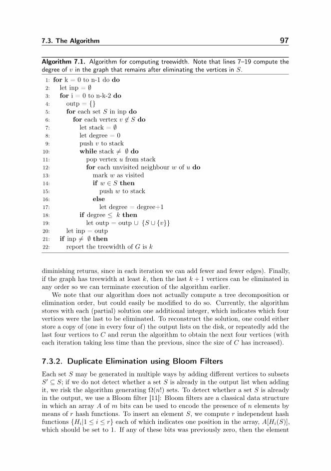
7.3. The Algorithm 97
Algorithm 7.1. Algorithm for computing treewidth. Note that lines 7–19 compute thedegree of v in the graph that remains after eliminating the vertices in S.1: for k = 0 to n-1 do do2: let inp = ∅3: for i = 0 to n-k-2 do4: outp = 5: for each set S in inp do6: for each vertex v 6∈ S do7: let stack = ∅8: let degree = 09: push v to stack
10: while stack 6= ∅ do11: pop vertex u from stack12: for each unvisited neighbour w of u do13: mark w as visited14: if w ∈ S then15: push w to stack16: else17: let degree = degree+118: if degree ≤ k then19: let outp = outp ∪ S ∪ v20: let inp = outp21: if inp 6= ∅ then22: report the treewidth of G is k
diminishing returns, since in each iteration we can add fewer and fewer edges). Finally,if the graph has treewidth at least k, then the last k + 1 vertices can be eliminated inany order so we can terminate execution of the algorithm earlier.
We note that our algorithm does not actually compute a tree decomposition orelimination order, but could easily be modified to do so. Currently, the algorithmstores with each (partial) solution one additional integer, which indicates which fourvertices were the last to be eliminated. To reconstruct the solution, one could eitherstore a copy of (one in every four of) the output lists on the disk, or repeatedly add thelast four vertices to C and rerun the algorithm to obtain the next four vertices (witheach iteration taking less time than the previous, since the size of C has increased).
7.3.2. Duplicate Elimination using Bloom Filters
Each set S may be generated in multiple ways by adding different vertices to subsetsS′ ⊆ S; if we do not detect whether a set S is already in the output list when addingit, we risk the algorithm generating Ω(n!) sets. To detect whether a set S is alreadyin the output, we use a Bloom filter [11]: Bloom filters are a classical data structurein which an array A of m bits can be used to encode the presence of n elements bymeans of r hash functions. To insert an element S, we compute r independent hashfunctions Hi|1 ≤ i ≤ r each of which indicates one position in the array, A[Hi(S)],which should be set to 1. If any of these bits was previously zero, then the element
98 Chapter 7: Computing Tree Decompositions on the GPU
was not yet present in the filter, and otherwise, the probability of a false positive isapproximately (1− e−kn/m)r.
In our implementation, we compute two 32-bit hashes h1(S), h2(S) using Murmur3[8], which we then combine linearly to obtain hashes Hi(S) = h1(S) + i · h2(S) (whichis nearly as good as using r independent hash functions [75]).
In our experiments, we have used mn ≥ 24 and r = 17 to obtain a low (theoretical)
false positive probability of around 1 in 100.000. We note that the possibility of falsepositives results in a Monte Carlo algorithm (the algorithm may inadvertently decidethat the treewidth is higher than it really is). Indeed, given that many millions ofstates are generated during the search we are guaranteed that the Bloom filter willreturn some false positives, however, this does not immediately lead to incorrect results:it is still quite unlikely that all of the states leading to an optimal solution are pruned,since there are often multiple feasible elimination orders.
The Bloom filter is very suitable for implementation on a GPU, since our targetarchitecture (and indeed, most GPUs) offers a very fast atomic OR operation [98]. Wenote that addressing a Bloom filter concurrently may also introduce false negatives ifmultiple threads attempt to insert the same element simultaneously. To avoid this, weuse the initial hash value to pick one of 65.536 mutexes to synchronize access (thisallows most operations to happen wait-free and only a collision on the initial hash valuecauses one thread to wait for another).
7.3.3. Minor-Min-Width
Search algorithms for treewidth are often enhanced with various heuristics and pruningrules to speed up the computation. One very popular choice (used by e.g. [57, 117, 118])is minor-min-width (MMW) [57] (also known as MMD+(min-d)) [23]). MMW is basedon the observation that the minimum degree of a vertex is a lower bound on thetreewidth, and that contracting edges (i.e. taking minors) does not increase thetreewidth. MMW repeatedly selects a minimum degree vertex, and then contractsit with a neighbour of minimum degree, in an attempt to obtain a minor with largeminimum degree (if we encounter a minimum degree that exceeds our target treewidth,we know that we can discard the current state). As a slight improvement to thisheuristic, the second smallest vertex degree is also a lower bound on the treewidth [23].
Given a subset S ⊆ G, we would like to compute the treewidth of the graphs thatremains after eliminating S from G. The most straightforward method is to explicitlycreate a copy of G, eliminate the vertices of S, and then repeatedly perform thecontraction as described above. However, storing e.g. an adjacency list representationof these intermediate graphs would exceed the available shared memory and size ofthe caches. As we would like to avoid transferring large amounts of data to and fromglobal memory, we implemented a method to compute MMW without explicitly storingthe intermediate graphs.
Our algorithm tracks the current degrees of the vertices (which, conveniently, wealready have computed to determine which vertices can be eliminated). It is thus easyto select a minimum degree vertex v. Since we do not know what vertices it is adjacentto (in the intermediate graph), we must select a minimum degree neighbour by using adepth-first search, similarly to how we compute the vertex degrees in Algorithm 7.1.Once we have found a minimum degree neighbour u, we run a second dept-first search
7.4. Experiments 99
to compute the number of neighbours u has in common with v, allowing us to updatethe degree of v. To keep track of which vertices have been contracted, we use a disjointset data structure.
The disjoint set structure and list of vertex degrees together use only two bytesper vertex (for a graph of up to 256 vertices), thus, they fit our memory constraintswhereas an adjacency matrix or adjacency list (for dense graphs, noting that the graphsin question can quickly become dense as vertices are eliminated) would readily exceedit.
7.4. Experiments
7.4.1. InstancesWe selected a number of instances from the PACE 2016 dataset [37] and libtw [113].All instances were preprocessed using the preprocessing rules of our PACE submission[111], which split the graph using safe separators: we first split the graph into itsconnected components, then split on articulation points, then on articulation pairs(making the remaining components 3-connected) and finally – if we can establish thatthis is safe – on articulation triplets (resulting in the 4-connected components of thegraph). We then furthermore try to detect and split on (almost) clique separators inthe graph. For a more detailed treatment of these preprocessing rules, we refer to [21].
7.4.2. General BenchmarkWe first present an experimental evaluation of our algorithm (without using MMW)on a set of benchmark graphs. Table 7.1 shows the number of vertices, computedtreewidth, time taken (in seconds) on the GPU and the number of sets S explored.Note that the time does not include the time taken for preprocessing, and that thevertex count is that of the preprocessed graph (and thus, the original graph may havebeen larger).
The size of the input and output lists were limited by the memory available onour GPU. With the current configuration (limited to graphs of at most 64 vertices -though the code is written to be flexible and can easily be changed to support up to 256vertices), these lists could hold at most 180 million states (i.e., subsets S ⊆ V that havea feasible partial elimination order) each. If at any iteration this number was exceeded,the excess states were discarded. The algorithm was allowed to continue execution forthe current treewidth k, but was terminated when trying the next higher treewidth(since we might have discarded a state that would have led to a solution with treewidthk, the answer would no longer be exact). The states where the capacity of the listswas exceed are marked with *, if the algorithm was terminated then the treewidthis stricken through (and represents the candidate value for treewidth at which thealgorithm was terminated, and not the treewidth of the graph, which is likely higher).
For instance, for graph 1ubq the capacity of the lists was first exceeded at treewidth10, and the algorithm was terminated at treewidth 11 (and thus the actual treewidthis at least 10, but likely higher). For graph myciel5, the capacity of the lists wasfirst exceeded at treewidth 19, but still (despite discarding some states) a solution oftreewidth 19 was nevertheless found (which we thus know is the exact treewidth).
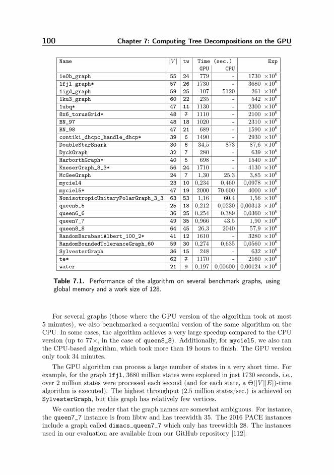
100 Chapter 7: Computing Tree Decompositions on the GPU
Name |V | tw Time (sec.) ExpGPU CPU
1e0b_graph 55 24 779 - 1730 ×1061fjl_graph* 57 26 1730 - 3680 ×1061igd_graph 59 25 107 5120 261 ×1061ku3_graph 60 22 235 - 542 ×1061ubq* 47 11 1130 - 2300 ×1068x6_torusGrid* 48 7 1110 - 2100 ×106BN_97 48 18 1020 - 2310 ×106BN_98 47 21 689 - 1590 ×106contiki_dhcpc_handle_dhcp* 39 6 1490 - 2930 ×106DoubleStarSnark 30 6 34,5 873 87,6 ×10⁶DyckGraph 32 7 280 - 639 ×106HarborthGraph* 40 5 698 - 1540 ×106KneserGraph_8_3* 56 24 1710 - 4130 ×106McGeeGraph 24 7 1,30 25,3 3,85 ×10⁶myciel4 23 10 0,234 0,460 0,0978 ×10⁶myciel5* 47 19 2000 70.600 4000 ×106NonisotropicUnitaryPolarGraph_3_3 63 53 1,16 60,4 1,56 ×10⁶queen5_5 25 18 0,212 0,0230 0,00313 ×10⁶queen6_6 36 25 0,254 0,389 0,0360 ×10⁶queen7_7 49 35 0,966 43,5 1,90 ×10⁶queen8_8 64 45 26,3 2040 57,9 ×10⁶RandomBarabasiAlbert_100_2* 41 12 1610 - 3280 ×106RandomBoundedToleranceGraph_60 59 30 0,274 0,635 0,0560 ×10⁶SylvesterGraph 36 15 248 - 632 ×106te* 62 7 1170 - 2160 ×106water 21 9 0,197 0,00600 0,00124 ×10⁶
Table 7.1. Performance of the algorithm on several benchmark graphs, usingglobal memory and a work size of 128.
For several graphs (those where the GPU version of the algorithm took at most5 minutes), we also benchmarked a sequential version of the same algorithm on theCPU. In some cases, the algorithm achieves a very large speedup compared to the CPUversion (up to 77×, in the case of queen8_8). Additionally, for myciel5, we also ranthe CPU-based algorithm, which took more than 19 hours to finish. The GPU versiononly took 34 minutes.
The GPU algorithm can process a large number of states in a very short time. Forexample, for the graph 1fjl, 3680 million states were explored in just 1730 seconds, i.e.,over 2 million states were processed each second (and for each state, a Θ(|V ||E|)-timealgorithm is executed). The highest throughput (2.5 million states/sec.) is achieved onSylvesterGraph, but this graph has relatively few vertices.
We caution the reader that the graph names are somewhat ambiguous. For instance,the queen7_7 instance is from libtw and has treewidth 35. The 2016 PACE instancesinclude a graph called dimacs_queen7_7 which only has treewidth 28. The instancesused in our evaluation are available from our GitHub repository [112].
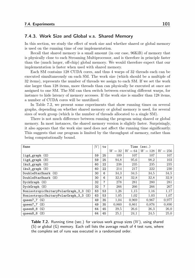
7.4. Experiments 101
7.4.3. Work Size and Global v.s. Shared MemoryIn this section, we study the effect of work size and whether shared or global memoryis used on the running time of our implementation.
Recall that shared memory is a small amount (in our case, 96KiB) of memory thatis physically close to each Streaming Multiprocessor, and is therefore in principle fasterthan the (much larger, off-chip) global memory. We would therefore expect that ourimplementation is faster when used with shared memory.
Each SM contains 128 CUDA cores, and thus 4 warps of 32 threads each can beexecuted simultaneously on each SM. The work size (which should be a multiple of32 items), represents the number of threads we assign to each SM. If we set the worksize larger than 128 items, more threads than can physically be executed at once areassigned to one SM. The SM can then switch between executing different warps, forinstance to hide latency of memory accesses. If the work size is smaller than 128 items,a number of CUDA cores will be unutilized.
In Table 7.2, we present some experiments that show running times on severalgraphs, depending on whether shared memory or global memory is used, for severalsizes of work group (which is the number of threads allocated to a single SM).
There is not much difference between running the program using shared or globalmemory. In most instances, the shared memory version is slightly faster. Surprisingly,it also appears that the work size used does not affect the running time significantly.This suggests that our program is limited by the throughput of memory, rather thanbeing computationally bound.
Name |V | tw Time (sec.)W = 32 W = 64 W = 128 W = 256
1igd_graph (G) 59 25 109 107 107 107
1igd_graph (S) 59 25 94,8 95,6 98,2 103
1ku3_graph (G) 60 22 238 235 235 235
1ku3_graph (S) 60 22 214 217 222 230
DoubleStarSnark (G) 30 6 34,3 34,5 34,5 34,5
DoubleStarSnark (S) 30 6 32,8 32,8 32,8 32,9
DyckGraph (G) 32 7 278 281 280 281
DyckGraph (S) 32 7 266 266 266 267
NonisotropicUnitaryPolarGraph_3_3 (G) 63 53 1,26 1,15 1,16 1,17
NonisotropicUnitaryPolarGraph_3_3 (S) 63 53 1,05 1,02 1,03 1,07
queen7_7 (G) 49 35 1,04 0,969 0,967 0,977
queen7_7 (S) 49 35 0,860 0,861 0,876 0,890
queen8_8 (G) 64 45 29,5 26,6 26,3 26,0
queen8_8 (S) 64 45 25,1 24,1 24,5 25,0
Table 7.2. Running time (sec.) for various work group sizes (W ), using shared(S) or global (G) memory. Each cell lists the average result of 4 test runs, wherethe complete set of runs was executed in a randomized order.
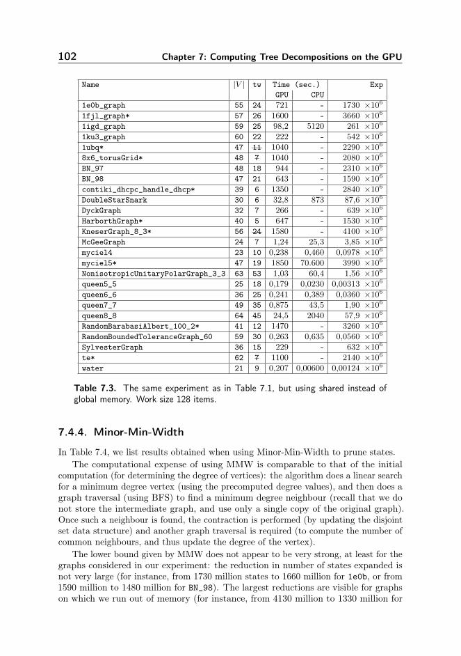
102 Chapter 7: Computing Tree Decompositions on the GPU
Name |V | tw Time (sec.) ExpGPU CPU
1e0b_graph 55 24 721 - 1730 ×1061fjl_graph* 57 26 1600 - 3660 ×1061igd_graph 59 25 98,2 5120 261 ×1061ku3_graph 60 22 222 - 542 ×1061ubq* 47 11 1040 - 2290 ×1068x6_torusGrid* 48 7 1040 - 2080 ×106BN_97 48 18 944 - 2310 ×106BN_98 47 21 643 - 1590 ×106contiki_dhcpc_handle_dhcp* 39 6 1350 - 2840 ×106DoubleStarSnark 30 6 32,8 873 87,6 ×10⁶DyckGraph 32 7 266 - 639 ×106HarborthGraph* 40 5 647 - 1530 ×106KneserGraph_8_3* 56 24 1580 - 4100 ×106McGeeGraph 24 7 1,24 25,3 3,85 ×10⁶myciel4 23 10 0,238 0,460 0,0978 ×10⁶myciel5* 47 19 1850 70.600 3990 ×106NonisotropicUnitaryPolarGraph_3_3 63 53 1,03 60,4 1,56 ×10⁶queen5_5 25 18 0,179 0,0230 0,00313 ×10⁶queen6_6 36 25 0,241 0,389 0,0360 ×10⁶queen7_7 49 35 0,875 43,5 1,90 ×10⁶queen8_8 64 45 24,5 2040 57,9 ×10⁶RandomBarabasiAlbert_100_2* 41 12 1470 - 3260 ×106RandomBoundedToleranceGraph_60 59 30 0,263 0,635 0,0560 ×10⁶SylvesterGraph 36 15 229 - 632 ×106te* 62 7 1100 - 2140 ×106water 21 9 0,207 0,00600 0,00124 ×10⁶
Table 7.3. The same experiment as in Table 7.1, but using shared instead ofglobal memory. Work size 128 items.
7.4.4. Minor-Min-Width
In Table 7.4, we list results obtained when using Minor-Min-Width to prune states.The computational expense of using MMW is comparable to that of the initial
computation (for determining the degree of vertices): the algorithm does a linear searchfor a minimum degree vertex (using the precomputed degree values), and then does agraph traversal (using BFS) to find a minimum degree neighbour (recall that we donot store the intermediate graph, and use only a single copy of the original graph).Once such a neighbour is found, the contraction is performed (by updating the disjointset data structure) and another graph traversal is required (to compute the number ofcommon neighbours, and thus update the degree of the vertex).
The lower bound given by MMW does not appear to be very strong, at least for thegraphs considered in our experiment: the reduction in number of states expanded isnot very large (for instance, from 1730 million states to 1660 million for 1e0b, or from1590 million to 1480 million for BN_98). The largest reductions are visible for graphson which we run out of memory (for instance, from 4130 million to 1330 million for
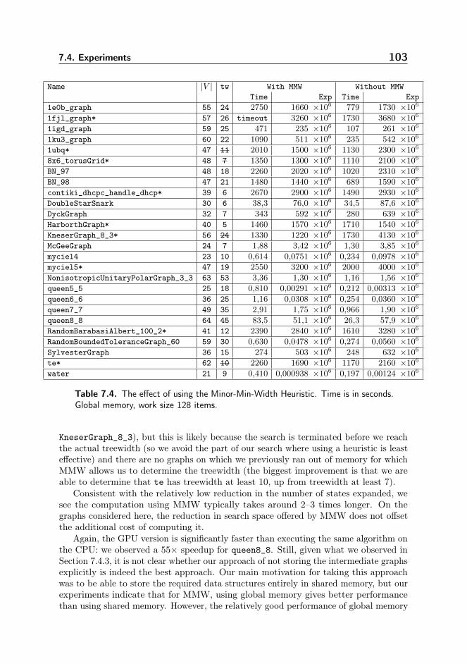
7.4. Experiments 103
Name |V | tw With MMW Without MMWTime Exp Time Exp
1e0b_graph 55 24 2750 1660 ×106 779 1730 ×1061fjl_graph* 57 26 timeout 3260 ×106 1730 3680 ×1061igd_graph 59 25 471 235 ×106 107 261 ×1061ku3_graph 60 22 1090 511 ×106 235 542 ×1061ubq* 47 11 2010 1500 ×106 1130 2300 ×1068x6_torusGrid* 48 7 1350 1300 ×106 1110 2100 ×106BN_97 48 18 2260 2020 ×106 1020 2310 ×106BN_98 47 21 1480 1440 ×106 689 1590 ×106contiki_dhcpc_handle_dhcp* 39 6 2670 2900 ×106 1490 2930 ×106DoubleStarSnark 30 6 38,3 76,0 ×10⁶ 34,5 87,6 ×10⁶DyckGraph 32 7 343 592 ×106 280 639 ×106HarborthGraph* 40 5 1460 1570 ×106 1710 1540 ×106KneserGraph_8_3* 56 24 1330 1220 ×106 1730 4130 ×106McGeeGraph 24 7 1,88 3,42 ×10⁶ 1,30 3,85 ×10⁶myciel4 23 10 0,614 0,0751 ×10⁶ 0,234 0,0978 ×10⁶myciel5* 47 19 2550 3200 ×106 2000 4000 ×106NonisotropicUnitaryPolarGraph_3_3 63 53 3,36 1,30 ×10⁶ 1,16 1,56 ×10⁶queen5_5 25 18 0,810 0,00291 ×10⁶ 0,212 0,00313 ×10⁶queen6_6 36 25 1,16 0,0308 ×10⁶ 0,254 0,0360 ×10⁶queen7_7 49 35 2,91 1,75 ×10⁶ 0,966 1,90 ×10⁶queen8_8 64 45 83,5 51,1 ×10⁶ 26,3 57,9 ×10⁶RandomBarabasiAlbert_100_2* 41 12 2390 2840 ×106 1610 3280 ×106RandomBoundedToleranceGraph_60 59 30 0,630 0,0478 ×10⁶ 0,274 0,0560 ×10⁶SylvesterGraph 36 15 274 503 ×106 248 632 ×106te* 62 10 2260 1690 ×106 1170 2160 ×106water 21 9 0,410 0,000938 ×10⁶ 0,197 0,00124 ×10⁶
Table 7.4. The effect of using the Minor-Min-Width Heuristic. Time is in seconds.Global memory, work size 128 items.
KneserGraph_8_3), but this is likely because the search is terminated before we reachthe actual treewidth (so we avoid the part of our search where using a heuristic is leasteffective) and there are no graphs on which we previously ran out of memory for whichMMW allows us to determine the treewidth (the biggest improvement is that we areable to determine that te has treewidth at least 10, up from treewidth at least 7).
Consistent with the relatively low reduction in the number of states expanded, wesee the computation using MMW typically takes around 2–3 times longer. On thegraphs considered here, the reduction in search space offered by MMW does not offsetthe additional cost of computing it.
Again, the GPU version is significantly faster than executing the same algorithm onthe CPU: we observed a 55× speedup for queen8_8. Still, given what we observed inSection 7.4.3, it is not clear whether our approach of not storing the intermediate graphsexplicitly is indeed the best approach. Our main motivation for taking this approachwas to be able to store the required data structures entirely in shared memory, but ourexperiments indicate that for MMW, using global memory gives better performancethan using shared memory. However, the relatively good performance of global memory
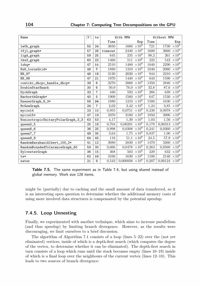
104 Chapter 7: Computing Tree Decompositions on the GPU
Name |V | tw With MMW Without MMWTime Exp Time Exp
1e0b_graph 55 24 3650 1660 ×106 721 1730 ×1061fjl_graph* 57 26 timeout 2440 ×106 1600 3660 ×1061igd_graph 59 25 645 235 ×106 98,2 261 ×1061ku3_graph 60 22 1460 511 ×106 222 542 ×1061ubq* 47 11 2510 1480 ×106 1040 2290 ×1068x6_torusGrid* 48 7 1890 1310 ×106 1040 2080 ×106BN_97 48 18 3130 2020 ×106 944 2310 ×106BN_98 47 21 1970 1440 ×106 643 1590 ×106contiki_dhcpc_handle_dhcp* 39 6 3270 2860 ×106 1350 2840 ×106DoubleStarSnark 30 6 50,9 76,0 ×10⁶ 32,8 87,6 ×10⁶DyckGraph 32 7 440 592 ×106 266 639 ×106HarborthGraph* 40 5 1900 1560 ×106 647 1530 ×106KneserGraph_8_3* 56 24 1880 1210 ×106 1580 4100 ×106McGeeGraph 24 7 2,02 3,42 ×10⁶ 1,24 3,85 ×10⁶myciel4 23 10 0,955 0,0751 ×10⁶ 0,238 0,0978 ×10⁶myciel5* 47 19 3370 3180 ×106 1850 3990 ×106NonisotropicUnitaryPolarGraph_3_3 63 53 4,17 1,30 ×10⁶ 1,03 1,56 ×10⁶queen5_5 25 18 0,704 0,00291 ×10⁶ 0,179 0,00313 ×10⁶queen6_6 36 25 0,998 0,0308 ×10⁶ 0,241 0,0360 ×10⁶queen7_7 49 35 3,64 1,75 ×10⁶ 0,837 1,90 ×10⁶queen8_8 64 45 116 51,1 ×10⁶ 24,5 57,9 ×10⁶RandomBarabasiAlbert_100_2* 41 12 3080 2830 ×106 1470 3260 ×106RandomBoundedToleranceGraph_60 59 30 0,666 0,0478 ×10⁶ 0,263 0,0560 ×10⁶SylvesterGraph 36 15 368 503 ×106 229 632 ×106te* 62 10 3100 1630 ×106 1100 2140 ×106water 21 9 0,543 0,000938 ×10⁶ 0,207 0,00124 ×10⁶
Table 7.5. The same experiment as in Table 7.4, but using shared instead ofglobal memory. Work size 128 items.
might be (partially) due to caching and the small amount of data transferred, so itis an interesting open question to determine whether the additional memory costs ofusing more involved data structures is compensated by the potential speedup.
7.4.5. Loop Unnesting
Finally, we experimented with another technique, which aims to increase parallelism(and thus speedup) by limiting branch divergence. However, as the results werediscouraging, we limit ourselves to a brief discussion.
The algorithm of Algorithm 7.1 consists of a loop (lines 5–22) over the (not yeteliminated) vertices, inside of which is a depth-first search (which computes the degreeof the vertex, to determine whether it can be eliminated). The depth-first search inturn consists of a loop which runs until the stack becomes empty (lines 10–19) insideof which is a final loop over the neighbours of the current vertex (lines 12–18). Thisleads to two sources of branch divergence:
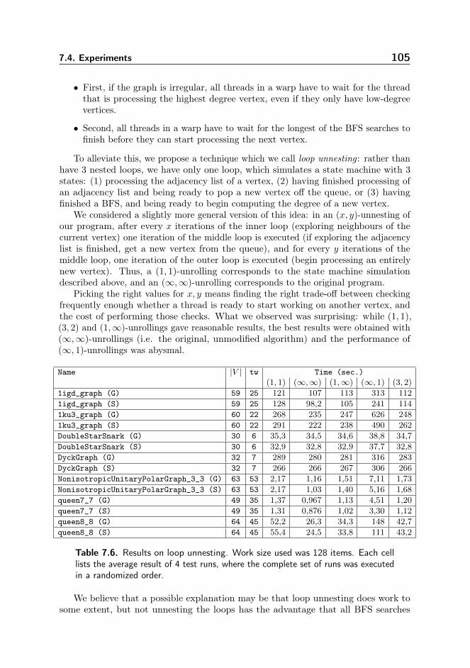
7.4. Experiments 105
• First, if the graph is irregular, all threads in a warp have to wait for the threadthat is processing the highest degree vertex, even if they only have low-degreevertices.
• Second, all threads in a warp have to wait for the longest of the BFS searches tofinish before they can start processing the next vertex.
To alleviate this, we propose a technique which we call loop unnesting : rather thanhave 3 nested loops, we have only one loop, which simulates a state machine with 3states: (1) processing the adjacency list of a vertex, (2) having finished processing ofan adjacency list and being ready to pop a new vertex off the queue, or (3) havingfinished a BFS, and being ready to begin computing the degree of a new vertex.
We considered a slightly more general version of this idea: in an (x, y)-unnesting ofour program, after every x iterations of the inner loop (exploring neighbours of thecurrent vertex) one iteration of the middle loop is executed (if exploring the adjacencylist is finished, get a new vertex from the queue), and for every y iterations of themiddle loop, one iteration of the outer loop is executed (begin processing an entirelynew vertex). Thus, a (1, 1)-unrolling corresponds to the state machine simulationdescribed above, and an (∞,∞)-unrolling corresponds to the original program.
Picking the right values for x, y means finding the right trade-off between checkingfrequently enough whether a thread is ready to start working on another vertex, andthe cost of performing those checks. What we observed was surprising: while (1, 1),(3, 2) and (1,∞)-unrollings gave reasonable results, the best results were obtained with(∞,∞)-unrollings (i.e. the original, unmodified algorithm) and the performance of(∞, 1)-unrollings was abysmal.
Name |V | tw Time (sec.)(1, 1) (∞,∞) (1,∞) (∞, 1) (3, 2)
1igd_graph (G) 59 25 121 107 113 313 112
1igd_graph (S) 59 25 128 98,2 105 241 114
1ku3_graph (G) 60 22 268 235 247 626 248
1ku3_graph (S) 60 22 291 222 238 490 262
DoubleStarSnark (G) 30 6 35,3 34,5 34,6 38,8 34,7
DoubleStarSnark (S) 30 6 32,9 32,8 32,9 37,7 32,8
DyckGraph (G) 32 7 289 280 281 316 283
DyckGraph (S) 32 7 266 266 267 306 266
NonisotropicUnitaryPolarGraph_3_3 (G) 63 53 2,17 1,16 1,51 7,11 1,73
NonisotropicUnitaryPolarGraph_3_3 (S) 63 53 2,17 1,03 1,40 5,16 1,68
queen7_7 (G) 49 35 1,37 0,967 1,13 4,51 1,20
queen7_7 (S) 49 35 1,31 0,876 1,02 3,30 1,12
queen8_8 (G) 64 45 52,2 26,3 34,3 148 42,7
queen8_8 (S) 64 45 55,4 24,5 33,8 111 43,2
Table 7.6. Results on loop unnesting. Work size used was 128 items. Each celllists the average result of 4 test runs, where the complete set of runs was executedin a randomized order.
We believe that a possible explanation may be that loop unnesting does work tosome extent, but not unnesting the loops has the advantage that all BFS searches
106 Chapter 7: Computing Tree Decompositions on the GPU
running simultaneously start from the same initial vertex, and (up to differences causedby different sets S being used) will access largely the same values from the adjacencylists at the same time, which may increase the efficiency of read operations. On theother hand, (∞, 1)-unnesting can not take advantage of either phenomenon: differentinitial vertices may be processed at any given time (so there is little consistency inmemory accesses) and the inner loop is not unnested at all so there is no potential togain speedup there either. Perhaps for larger graphs, where the difference in length ofadjacency lists may be more pronounced, or the amount of time a BFS takes variesmore strongly with the initial vertex and S, loop unnesting does provide speed up, butfor the graphs considered here it does not appear to be a beneficial choice.
7.5. Conclusions
We have presented an algorithm that computes treewidth on the GPU, achieving avery large speedup over running the same algorithm on the CPU. Our algorithm isbased on the classical O∗(2n)-time dynamic programming algorithm [20] and our resultsrepresent (promising) first steps in speeding up dynamic programming for treewidth onthe GPU. The current best known practical algorithm for computing treewidth is thealgorithm due to Tamaki [104]. This algorithm is much more complicated, and portingit to the GPU would be a formidable challenge but could possibly offer an extremelyefficient implementation for computing treewidth.
Given the large speedup achieved, we are no longer mainly limited by computationtime. Instead, our ability to solve larger instances is hampered by the memory requiredto store the very large lists of partial solutions. Using minor-min-width did not proveeffective in reducing the number of states considerably, so it would be interesting tosee how other heuristics and pruning rules (such as simplicial vertex detection) couldbe implemented on the GPU.
GPUs are traditionally used to solve easy (e.g. linear time) problems on very largeinputs (such as the millions of pixels rendered on a screen, or exploring a graph withmillions of nodes), but clearly, the speedup offered by inexpensive GPUs would also bevery welcome in solving hard (NP-complete) problems on small instances. Exploringhow techniques from FPT and exact algorithms can be used on the GPU raises manyinteresting problems - not only practical ones, but also theoretical: how should wemodel complex devices such as GPUs, with their many types of memory and branchdivergence issues?
Source Code and Instances. We have made our source code, as well as thegraphs used for the experiments, available on GitHub [112].
107
Computing the Shapley Value ofConnectivity Games
8.1. Introduction
Motivated by the need to identify important vertices in networks, many measuresfor ranking vertices have been suggested. Among these are the classical centralitymeasures, such as betweenness, closeness [61] and – perhaps the simplest – degree.However, what makes a “good” centrality measure is subjective and strongly dependenton the application. In light of this, game-theoretic centrality measures have receivedconsiderable interest. By viewing subgraphs of the input network as coalitions in acoalitional game, we can apply game-theoretic measures (such as the Shapley value[101] or Banzhaf power index [10]) to determine the importance of vertices (and/oredges) in a network.
The game-theoretic approach is very flexible, since we can adapt the underlyinggame to obtain different measures. It can also take information other than the networkstructure into account [82]. However, as both the Shapley value and Banzhaf index aredefined as an expression in terms of all possible coalitions, save for a few special cases(see e.g. [93]), they cannot be computed efficiently.
In this chapter, we consider two game-theoretic centrality measures: one based onthe Shapley value associated with a 0, 1-valued game due to Amer and Gimenez [6],the second a vertex-weighted variant of the same due to Lindelauf et al. [82]. Lindelaufet al. studied these centrality measures in the context of identifying the most importantvertices in terrorist networks [82, 107]. They considered two networks: one (due toKoschade [78]) consisting of 17 terrorists involved in a 2002 bombing in Bali, the second(due to Krebs [79]) consisting of 69 terrorists involved in planning and executing the9/11 attacks. Whereas for the first network they were able to compute the exactShapley value, for the second network this was infeasible and they considered only the
108 Chapter 8: Computing the Shapley Value of Connectivity Games
part of the network made up by the 19 hijackers that actually carried out the attack.Michalak et al. [94] showed that computing the Shapley value for the unweighted
game is unfortunately #P-hard. As such, it is unlikely that there exists an efficientalgorithm for computing these values. On the other hand, Michalak et al. proposed analgorithm that is slightly more efficient than the brute-force approach used by Lindelaufet al., called FasterSVCG. Using this algorithm, the authors computed the Shapleyvalue for a larger version of the 9/11 network, with 36 vertices (corresponding to thehijackers and some accomplices). Their approach, rather than considering all 2|V |
coalitions, considers only the connected coalitions, of which there may be considerablyfewer than 2|V |. However, in the worst case, the number of connected coalitions maystill be exponential. As such, for the full 69-vertex network, running this algorithm isstill infeasible.
Michalak et al. [94] also considered an approximation method based on randomsampling and studied its performance on the 36-vertex 9/11 network. Lindelauf etal. [107] proposed a different sampling method, structured random sampling, that aimsto be more efficient than random sampling. Using this method, they computed anapproximation of the Shapley value for the 69-vertex 9/11 network. Unfortunately,neither method comes with any formal guarantees on the quality of the approximation.
While, in general, one should not expect to find an efficient algorithm for computingthe exact Shapley value of these games (due to the #P-hardness), we can attemptto exploit the structure that the networks may have in order to obtain more efficientalgorithms.
We show that the Shapley value (for both the weighted and the unweighted game)can be computed efficiently on graphs of bounded treewidth. Our result is not merelytheoretical: we also provide an implementation and show that it can be used to computeShapley values for graphs of practical interest.
Using our approach, we are able to compute the exact Shapley value for thefull 69-vertex network of the 9/11 attacks. Given the exact values, we evaluate theapproximation computed by Lindelauf et al. [107]. We are also able to compute theexact Shapley value for some much larger networks, having up to a thousand vertices.
Of course, our method crucially depends on the network having bounded treewidth.Fortuitously, the network of the 9/11 attacks has a rather low treewidth of only 8. Ingeneral one cannot expect social networks to have small treewidth: social networksoften have large cliques, and the size of the largest clique forms a lower bound on thetreewidth of a graph (see e.g. [1] for a study of tree decompositions of social networks).However, terrorist and criminal organizations are often well-served by keeping theirnetworks sparsely connected, as this helps to avoid detection and as such one wouldnot expect large cliques. As another example of networks that may have low treewidth,the interaction networks in a hierarchical organization would naturally be tree-like.
Our goal is to develop an algorithm that, given a graph G with n = |V | and treedecomposition of G of width tw, computes the Shapley value in time f(tw)nO(1), wheref is some exponential function and nO(1) a (low-degree) polynomial. As such, we hopeto “hide” the exponential behaviour of computing φ in a function that depends only onthe treewidth of the graph, and obtain an algorithm whose running time is (for graphsof bounded treewidth) polynomial in n.
Specifically, we show that for a graph G of treewidth tw and a vertex v ∈ V ,φv(v
wconn2) can be computed in time 2O(tw log tw)n4 log n. Note that our algorithm
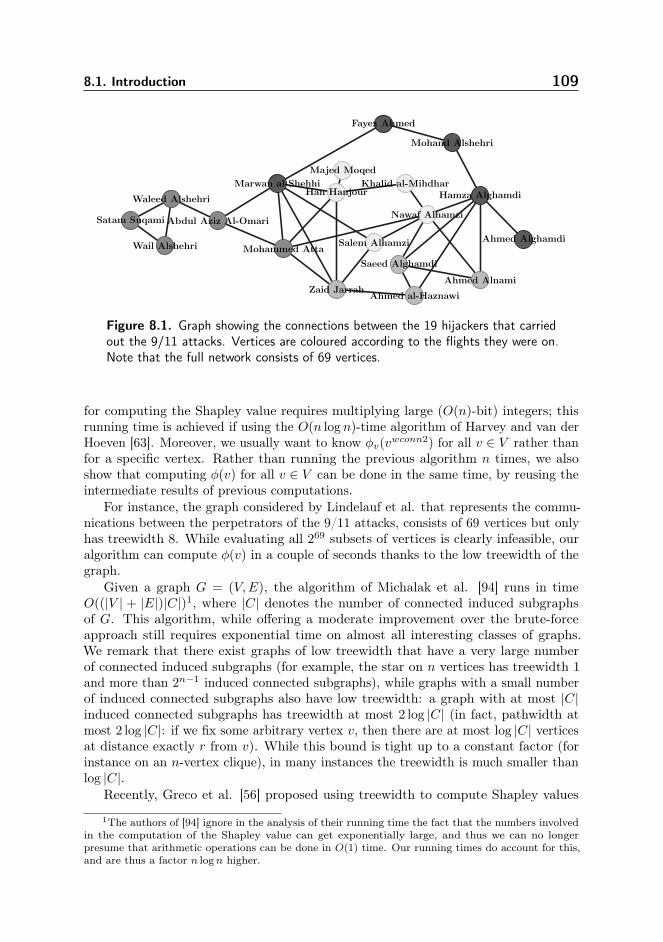
8.1. Introduction 109
Majed Moqed
Khalid al-Mihdhar
Nawaf Alhamzi
Han Hanjour
Salem Alhamzi
Zaid Jarrah
Saeed Alghamdi
Ahmed al-Haznawi
Ahmed Alnami
Mohammed Atta
Abdul Aziz Al-Omari
Waleed Alshehri
Wail Alshehri
Satam Suqami
Fayez Ahmed
Mohand Alshehri
Hamza Alghamdi
Ahmed Alghamdi
Marwan al-Shehhi
Figure 8.1. Graph showing the connections between the 19 hijackers that carriedout the 9/11 attacks. Vertices are coloured according to the flights they were on.Note that the full network consists of 69 vertices.
for computing the Shapley value requires multiplying large (O(n)-bit) integers; thisrunning time is achieved if using the O(n log n)-time algorithm of Harvey and van derHoeven [63]. Moreover, we usually want to know φv(vwconn2) for all v ∈ V rather thanfor a specific vertex. Rather than running the previous algorithm n times, we alsoshow that computing φ(v) for all v ∈ V can be done in the same time, by reusing theintermediate results of previous computations.
For instance, the graph considered by Lindelauf et al. that represents the commu-nications between the perpetrators of the 9/11 attacks, consists of 69 vertices but onlyhas treewidth 8. While evaluating all 269 subsets of vertices is clearly infeasible, ouralgorithm can compute φ(v) in a couple of seconds thanks to the low treewidth of thegraph.
Given a graph G = (V,E), the algorithm of Michalak et al. [94] runs in timeO((|V | + |E|)|C|)1, where |C| denotes the number of connected induced subgraphsof G. This algorithm, while offering a moderate improvement over the brute-forceapproach still requires exponential time on almost all interesting classes of graphs.We remark that there exist graphs of low treewidth that have a very large numberof connected induced subgraphs (for example, the star on n vertices has treewidth 1and more than 2n−1 induced connected subgraphs), while graphs with a small numberof induced connected subgraphs also have low treewidth: a graph with at most |C|induced connected subgraphs has treewidth at most 2 log |C| (in fact, pathwidth atmost 2 log |C|: if we fix some arbitrary vertex v, then there are at most log |C| verticesat distance exactly r from v). While this bound is tight up to a constant factor (forinstance on an n-vertex clique), in many instances the treewidth is much smaller thanlog |C|.
Recently, Greco et al. [56] proposed using treewidth to compute Shapley values
1The authors of [94] ignore in the analysis of their running time the fact that the numbers involvedin the computation of the Shapley value can get exponentially large, and thus we can no longerpresume that arithmetic operations can be done in O(1) time. Our running times do account for this,and are thus a factor n logn higher.
110 Chapter 8: Computing the Shapley Value of Connectivity Games
for matching games in graphs. In the matching game, the value of a coalition is thesize of the maximum matching in the graph induced by that coalition. However, theiralgorithm is based on a formulation in Monadic Second Order Logic and the applicationof theoretical frameworks that allow counting of satisfying assignments of MSO formulas.For graphs of bounded treewidth, this yield a polynomial-time algorithm, where thedegree of the polynomial may depend on the treewidth. In contrast, the degree ofthe polynomial in our algorithm is fixed, and only the constant factor in the runningtime is affected by the treewidth (i.e., we obtain a fixed-parameter tractable algorithm).Moreover, due to the application of these algorithmic metatheorems, their algorithmis not very efficient in practice: Greco et al. [56] report that, even for a graph oftreewidth only 3 with 30 vertices, their implementation (using the MSO solver Sequoia[80]) took nearly 9 minutes to determine the Shapley value. We are able to processmuch more complex (i.e., higher treewidth) graphs with significantly more vertices in amuch shorter time.
8.2. Preliminaries
8.2.1. Shapley Value / Power IndicesA coalitional game consists of a set of players N (the grand coalition) together witha characteristic function v : 2N → R such that v(∅) = 0. In this chapter, weconsider coalitional games where the players correspond to vertices in a graph. Givena characteristic function, the Shapley value Φi(v) of a player i is defined as [101]:
Φi(v) =∑
S⊆N\i
|S|!(|N | − |S| − 1)!
|N |!(v(S ∪ i)− v(S)) (8.1)
While this chapter focuses primarily on the Shapley value, we remark that ourtechniques can also be used to compute the Banzhaf Value, which is defined as [10]:
ΦBi (v) =1
2|N |−1
∑S⊆N\i
(v(S ∪ i)− v(S)) (8.2)
Essentially the same techniques may be used to compute the Banzhaf value as weuse for computing the Shapley value, merely a change in weighting factors is required.
8.2.2. Game-Theoretic CentralityThe connectivity game vconn, introduced by Amer and Giminez [6], is given by theweight function:
vconn(S) =
1 if G[S] is connected and |S| > 1,0 otherwise.
Note that a coalition consisting of a single player, while connected, has value 0.
8.3. An Algorithm for Computing Shapley Values 111
Lindelauf et al. [82] consider several weighted variants of this connectivity game.They assume each vertex i has a weight wi and each edge (between vertices i, j) aweight fij . They consider three games: one that uses vertex weights, one that uses edgeweights, and one that combines both. The games are given by the following weightfunctions:
vwconn1(S) =
maxi,j∈S,i 6=j fij if G[S] is connected,0 otherwise.
vwconn2(S) =
∑i∈S wi if G[S] is connected,
0 otherwise.
vwconn3(S) =
(∑i∈S wi) ·maxi,j∈S,i 6=j fij if G[S] is connected,
0 otherwise.
We give an algorithm for computing vwconn2, that, as a byproduct, also computesvconn. Similar techniques can be used to compute vwconn1 and vwconn3, though thiswould increase the running time by a factor of n.
Henceforth, we shall use the letter v to refer to vertices of G, rather than to a game(but we still use the notation vconn and vwconn2 to denote games). In the following, welet n = |V (G)|.
8.3. An Algorithm for Computing Shapley Values
In this section, we present our algorithm for computing the Shapley value of vconn andvwconn2.
Theorem 8.1. Given a graph G = (V,E) and a tree decomposition T of width tw,the Shapley value φv(vconn), v ∈ V and φv(vwconn2), v ∈ V can be computed in time2O(tw log tw)n4 log n.
We give the algorithm for computing φv(vwconn2); the results obtained from thisalgorithm can also be used to compute φv(vconn). We first show that for a given v ∈ V ,the (single) value φv(vwconn2) can be computed in time 2O(tw log tw)n4 log n. Next, notethat computing a table of the values φv(vwconn2) for all v ∈ V would require runningthis algorithm n times, and thus have a time complexity of 2O(tw log tw)n5 log n. Toavoid this, we then show that by reusing intermediate results of the computation, wecan preserve the 2O(tw log tw)n4 log n running time.
We begin by rewriting Equation 8.1 to obtain the following more suitable expressionfor computing φv(vwconn2), by splitting the summation into different terms, dependingon the cardinality k of S:
112 Chapter 8: Computing the Shapley Value of Connectivity Games
φv(vwconn2) =
|V |−1∑k=0
(|S|!(|V | − |S| − 1)!
|V |!∑
S⊆V \v,|S|=k(vwconn2(S ∪ v)− vwconn2(S))
)
=
|V |−1∑k=0
(|S|!(|V | − |S| − 1)!
|V |!
( ∑S⊆V \v,|S|=k
vwconn2(S ∪ v)−∑
S⊆V \v,|S|=kvwconn2(S)
))
Since vwconn2(S) = 0 whenever S induces a subgraph with more than one connectedcomponent, the problem of computing φv(vwconn2) reduces to computing, for eachk, the total value over all connected subsets S ⊆ V (G) with |S| = k and v ∈ S,respectively v 6∈ S.
In the following, we assume that we are given a graph G = (V,E) and a nice treedecomposition of G with width tw. Furthermore, we assume that the bag Xr associatedwith the root node r of T contains only a single vertex v (which is the vertex of whichwe will compute the Shapley value).
As is standard for algorithms using dynamic programming on tree decompositions,for each node t of the tree decomposition we consider the subgraph G[t]. For each suchsubgraph, we consider the subsets (coalitions) S ⊆ G[t] (i.e., all subsets of verticesappearing in the bag Xt or a bag below it in the decomposition; see Chapter 2).
Call a subset S ⊆ G[t] good if G[S] is connected or every connected component ofG[S] has a non-empty intersection with Xt.
Our algorithm considers, for each t ∈ T , all good subsets S ⊆ V (G[t]). The followinglemma shows that subsets that are not good do not count towards the Shapley value ofthe game.
Lemma 8.2. Let S ⊆ V (G) induce a connected subgraph of G and let t ∈ T . Theneither each connected component of the subgraph induced by S ∩ V (G[t]) has a non-empty intersection with Xt or S ∩ V (G[t]) is connected.
Proof. By contradiction. Suppose S ∩V (G[t]) is not connected. Then some componentof S ∩ V (G[t]) has an empty intersection with Xt. Then S cannot be connected, sinceXt separates G[t] from the rest of the graph.
Of course, there can still be exponentially many good subsets. The key to ouralgorithm is that for each such subset S, we do not need to know exactly how the subsetis made up: if we know how the subset S behaves within Xt, we know how it interactswith the rest of the graph (outside of G[t]), since Xt is a separator. Subsets whichbehave similarly within Xt can be grouped together, thus speeding up the computation.Specifically, each subset S ⊆ G[t] has a characteristic (w.r.t. G[t]) that consists of
• the intersection R = S ∩Xt,
• an equivalence relation ∼ on S ∩Xt such that a ∼ b if and only if a and b are inthe same connected component of the subgraph induced by S,
• the cardinality of S, k = |S|.
The number of distinct characteristics is 2O(tw log tw)n. For every node t ∈ T andeach characteristic (R,∼, k), we will compute
8.3. An Algorithm for Computing Shapley Values 113
• nt(R,∼, k): the number of good subsets S ⊆ G[t] with characteristic (R,∼, k),
• wt(R,∼, k): the total weight of all good subsets S ⊆ G[t] with characteristic(R,∼, k).
We define the weight of a subset S ⊆ G[t] as the sum of the vertex weights, i.e.∑v∈S w(v).Suppose that r is the root of T , and Xr = v. Then wr(v, (v, v), k) is exactly
the total weight of connected subsets S ⊆ V (G) with |S| = k and v ∈ S, whereaswr(∅, ∅, k) is the total weight of connected subsets of size k not including v. This givesus exactly the information we need to compute φ(v).
For every node t ∈ T we compute nt(R,∼, k) and wt(R,∼, k) for each characteristic(R,∼, k) in a bottom-up fashion. We may start at the leaf vertices, and then work ourway up to the root of the tree. We handle each of the cases as follows:
Leaf. If t ∈ T is a leaf node, then Xt = v for some v ∈ V . Therefore t has exactlytwo characteristics c1 = (∅, ∅, 0) and c2 = (v, (v, v), 1). It is easy to see thatnt(c1) = 1, wt(c1) = 0 and nt(c2) = 1, wt(c1) = w(v).
Introduce. If t ∈ T is an introduce node, then it has a child u ∈ T such that Xt =Xu∪v for some v ∈ V (G). Every characteristic (R,∼, k) (w.r.t. G[u]) correspondsto nu(R,∼, k) distinct subsets of G[u], and we may extend these subsets to subsets ofG[t] by either adding the introduced vertex v or not. Thus, the nu(R,∼, k) subsets ofG[u] give rise to
• nu(R,∼, k) good subsets of G[t] with characteristic (R,∼ ∪(v, v), k) and totalweight wt(R,∼, k), and, if k = 0 or R 6= ∅ to
• nu(R,∼, k) good subsets of G[t] with characteristic (R ∪ v,∼′, k + 1) and totalweight wu(R,∼, k) + nu(R,∼, k) · w(v),
where ∼′ is the relation obtained as the transitive closure of ∼ ∪(v, v) ∪ (v, x) |x ∈ R, (v, x) ∈ E(G).
Note that two distinct characteristics (R,∼, k) and (R′,∼′, k′) with R = R′, k = k′
and ∼6=∼′ may give rise (upon addition of the vertex v) to nu(R,∼, k) + nu(R′,∼′, k′)subsets with the same characteristic (R ∪ v,∼′′, k + 1) with total weight wu(R,∼, k)+wu(R′,∼′, k′)+(nu(R,∼, k)+nu(R′,∼′, k′)) ·w(v). Indeed, subsets correspondingto many distinct characteristics may end up having the same characteristic when v isadded to them, and so the subsets of G[t] with characteristic (R ∪ v,∼′, k + 1) maycorrespond to subsets of G[u] with characteristics (R,∼, k) for many different ∼ (andthus, to compute nt and wt, we should take the sum over all such ∼).
The following lemma (cf. Lemma 8.2) ensures the correctness of the introduce step:
Lemma 8.3. Let t ∈ T and suppose that t is an introduce node with child u ∈ T .Suppose S ⊆ G[t] is a good subset. Then S ∩G[u] is a good subset of G[u].
Proof. Suppose that S ∩G[u] is not connected, and some connected component C ofS ∩G[u] has an empty intersection with Xu. Suppose the introduced vertex is v. Thenv must be adjacent to some vertex of C, but this is impossible since C ∩Xu = ∅ and vis not incident to G[u] \Xu.
114 Chapter 8: Computing the Shapley Value of Connectivity Games
This ensures that we count each good subset S ⊆ G[t] at least once. That we counteach good subset S ⊆ G[t] at most once follows from the fact that S ∩G[u] correspondsto a unique characteristic w.r.t G[t].
Forget. If t ∈ T is a forget node, it has a child u ∈ T such that Xu∪v = Xt forsome v ∈ V (G). If for characteristic (R,∼, k) (w.r.t. G[u]), v 6∈ R, then (R,∼, k) isalso a characteristic w.r.t. G[t]. If v ∈ R, then there are three cases:
1. R = v. Then we obtain nu(R,∼, k) good subsets of G[t] with characteristic∅, ∅, k and total weight wt(R,∼, k),
2. R 6= v and (r, r) ∈∼. Then none of the nu(R,∼, k) good subsets of G[u] aregood for G[t], since the connected component containing v does not intersect Xt,and there is some other connected component that does intersect Xt.
3. Otherwise, we obtain nu(R,∼, k) good subsets of G[t] with characteristic (R ∩Xt,∼′, k),
where ∼′ is the relation obtained by projecting the relation ∼ on R to R ∩Xt (i.e.,∼′=∼ ∩(u, v) | u, v ∈ Xt).
Similarly to the introduce case, multiple distinct characteristics for umay correspondto the same characteristic for t; we should again take the sum over these characteristics.The correctness follows from the following Lemma:
Lemma 8.4. Let t ∈ T and suppose that t is a forget vertex with child u ∈ T . SupposeS ⊆ G[t] is a good subset. Then S is a good subset of G[u].
Proof. If S is not connected, then S has a non-empty intersection with Xt. SinceXt ⊂ Xu, S also has a non-empty intersection with Xu.
Join. If t ∈ T is a join node, then it has two children l, r such that Xl = Xr = Xt.Suppose that (Rl,∼l, kl) is a characteristic of l and (Rr,∼r, kr) is a characteristic ofr and suppose that Rl = Rr. Then there are nl(Rl,∼l, kl) · nr(Rr,∼r, kr) subsetswith characteristic (Rl,∼′, kl + kr − |Rl|) and total weight nl(Rl,∼l, kl) · wr(Rr,∼r, kr)+nr(Rr,∼r, kr) ·wl(Rl,∼l, kl)−nl(Rl,∼l, kl) ·nr(Rr,∼r, kr) · (Σv∈Rlw(v)), where∼ is the transitive closure of ∼l ∪ ∼r.
Similarly to the introduce and forget cases, multiple distinct characteristics for l, rmay, when combined, correspond to the same characteristic for t; we should again takethe sum over these characteristics. The correctness follows from the following Lemma:
Lemma 8.5. Let t ∈ T and suppose that t is a join vertex children l, r ∈ T . SupposeS ⊆ G[t] is a good subset. Then S ∩ V (G[l]) (resp. S ∩ V (G[r])) is a good subset ofG[l] (resp. G[r]).
Proof. By contradiction. We show the case for the left child, the case for the rightchild is symmetric.
If S ⊆ V (G[l]) then the lemma follows automatically. Therefore, assume thereexists v ∈ S such that v /∈ V (G[l]). In particular, this means that v ∈ G[r] \Xr.
8.3. An Algorithm for Computing Shapley Values 115
Suppose S∩V (G[l]) is not connected and has a connected component C with emptyintersection with Xl. Since none of the vertices of S ∩ V (G[r]) are incident to C, Cis still a maximal connected component of S, but S has at least one other connectedcomponent (since S ∩ V (G[l]) is not connected) and so is not connected, and C hasempty intersection with Xl = Xt.
By processing the vertices of the tree decomposition in a bottom-up fashion, wecan compute the values nr(R,∼, k) and wr(R,∼, k) for all characteristics (R,∼, k) ofthe root node r. As we have seen before, knowing these values is sufficient to computethe Shapley value of vertex v. We thus obtain the following result:
Theorem 8.6. Given a graph G of treewidth at most tw, the Shapley value of a vertexv ∈ V (G) can be computed in time 2O(tw log tw)n4 log n and space 2O(tw log tw)n2 log n.
Proof. We assume that we are given a nice tree decomposition of G (which we mayassume has O(n) nodes). For each node, there are 2O(tw log tw)n characteristics. Tocompute the values for one characteristic requires considering (in the worst case, whichis the join node) 2O(tw log tw)n2 pairs of characteristics for the child nodes. For eachsuch pair, we perform a constant number of multiplications of O(n)-bit integers, takingO(n log n) time. The dynamic programming table for one node of the tree decompositiontakes up 2Θ(tw log tw)n2 space, but at any given time we only need to keep O(log n) ofthem in memory.
Of course, this only allows us to evaluate the Shapley value for a single vertex v,under the assumption that for the root bag r, Xr = v (i.e., v is the only vertex inthe root bag). To compute the Shapley value for all vertices, we perform the followingoperations, starting from a nice tree decomposition:
• For every join node t, we create a new node t′ with Xt′ = Xt. t′ is made theparent of t, and the original parent of t becomes the parent of t′. In case t wasthe root, t′ becomes the root. Note that t′ is neither a join, introduce, forget, orleaf node, however, the dynamic programming tables for t′ are simply equal tothose for t (we shall from now on, refer to nodes such as t′ as nochange nodes).
• For every vertex v ∈ V (G), we pick a node of the tree decomposition t such thatv ∈ Vt. We create a copy t′ of t, which is made the parent of t, and the originalparent of t becomes the parent of t′. In case t was the root, t′ becomes the root.Next, we create another copy t′′ of t′. t′ is made the parent of t′′ (making t′into a join node). We then create a series of introduce nodes, starting from t′′,such that eventually we end up with a leaf node u, whose bag contains only v.If we now reroot our tree decomposition so that the root becomes u, thanks tothe previous transformation, every join node remains a join node – the roles ofintroduce, forget and nochange nodes can become interchanged.
Figure 8.2 shows an example of this process. Starting from a nice tree decomposition(Figure 8.2a) a nochange node is added before the join bag A,B (Figure 8.2b). Tocreate a leaf bag for vertex B, we pick a bag t containing it (in this example theright child of the join bag), insert a node t′ which becomes the parent of t, create
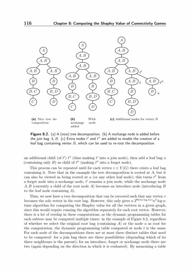
116 Chapter 8: Computing the Shapley Value of Connectivity Games
DC
A,B
A,B A,B
B B
B,C B,D
A
(a) Nice tree de-composition
A,B
A,B A,B
B B
B,C B,D
A
A,B
DC
(b) Withnochange nodeadded
A,B
A,B
B
B,C
A
A,B
A,B
B
B,D
A,B
A,B
B
t t′′
t′
C
D
u
(c) Additional nodes for vertex B
Figure 8.2. (a) A (nice) tree decomposition. (b) A nochange node is added beforethe join bag A,B. (c) Extra nodes t′ and t′′ are added to enable the creation of aleaf bag containing vertex B, which can be used to re-root the decomposition.
an additional child (of t′) t′′ (thus making t′ into a join node), then add a leaf bag u(containing only B) as child of t′′ (making t′′ into a forget node).
This process can be repeated until for each vertex v ∈ V (G) there exists a leaf bagcontaining it. Note that in the example the tree decomposition is rooted at A, but itcan also be viewed as being rooted at u (or any other leaf node); this turns t′′ froma forget node into a nochange node, t′ remains a join node, while the nochange nodeA,B (currently a child of the root node A) becomes an introduce node (introducing Bto the leaf node containing A).
Thus, we now have a tree decomposition that can be rerooted such that any vertex vbecomes the sole vertex in the root bag. However, this only gives a 2Θ(tw log tw)n5 log n-time algorithm for computing the Shapley value for all the vertices in a given graph,since this would require running the algorithm separately for each root vertex. However,there is a lot of overlap in these computations, as the dynamic programming tables foreach subtree may be computed multiple times: in the example of Figure 8.2, regardlessof whether we select the original root bag (containing A) or the node u as root forthe computation, the dynamic programming table computed at node t is the same.For each node of the decompositions there are at most three distinct tables that needto be computed: for a join bag there are three possibilities (depending which of itsthree neighbours is the parent); for an introduce, forget or nochange node there aretwo (again depending on the direction in which it is evaluated). By memoizing a table
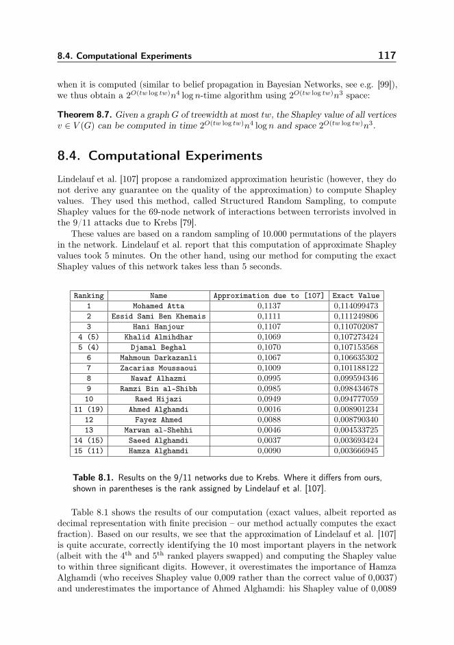
8.4. Computational Experiments 117
when it is computed (similar to belief propagation in Bayesian Networks, see e.g. [99]),we thus obtain a 2O(tw log tw)n4 log n-time algorithm using 2O(tw log tw)n3 space:
Theorem 8.7. Given a graph G of treewidth at most tw, the Shapley value of all verticesv ∈ V (G) can be computed in time 2O(tw log tw)n4 log n and space 2O(tw log tw)n3.
8.4. Computational Experiments
Lindelauf et al. [107] propose a randomized approximation heuristic (however, they donot derive any guarantee on the quality of the approximation) to compute Shapleyvalues. They used this method, called Structured Random Sampling, to computeShapley values for the 69-node network of interactions between terrorists involved inthe 9/11 attacks due to Krebs [79].
These values are based on a random sampling of 10.000 permutations of the playersin the network. Lindelauf et al. report that this computation of approximate Shapleyvalues took 5 minutes. On the other hand, using our method for computing the exactShapley values of this network takes less than 5 seconds.
Ranking Name Approximation due to [107] Exact Value1 Mohamed Atta 0,1137 0,114099473
2 Essid Sami Ben Khemais 0,1111 0,111249806
3 Hani Hanjour 0,1107 0,110702087
4 (5) Khalid Almihdhar 0,1069 0,107273424
5 (4) Djamal Beghal 0,1070 0,107153568
6 Mahmoun Darkazanli 0,1067 0,106635302
7 Zacarias Moussaoui 0,1009 0,101188122
8 Nawaf Alhazmi 0,0995 0,099594346
9 Ramzi Bin al-Shibh 0,0985 0,098434678
10 Raed Hijazi 0,0949 0,094777059
11 (19) Ahmed Alghamdi 0,0016 0,008901234
12 Fayez Ahmed 0,0088 0,008790340
13 Marwan al-Shehhi 0,0046 0,004533725
14 (15) Saeed Alghamdi 0,0037 0,003693424
15 (11) Hamza Alghamdi 0,0090 0,003666945
Table 8.1. Results on the 9/11 networks due to Krebs. Where it differs from ours,shown in parentheses is the rank assigned by Lindelauf et al. [107].
Table 8.1 shows the results of our computation (exact values, albeit reported asdecimal representation with finite precision – our method actually computes the exactfraction). Based on our results, we see that the approximation of Lindelauf et al. [107]is quite accurate, correctly identifying the 10 most important players in the network(albeit with the 4th and 5th ranked players swapped) and computing the Shapley valueto within three significant digits. However, it overestimates the importance of HamzaAlghamdi (who receives Shapley value 0,009 rather than the correct value of 0,0037)and underestimates the importance of Ahmed Alghamdi: his Shapley value of 0,0089
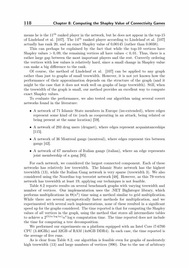
118 Chapter 8: Computing the Shapley Value of Connectivity Games
means he is the 11th ranked player in the network, but he does not appear in the top-15of Lindelauf et al. [107]. The 14th ranked player according to Lindelauf et al. [107]actually has rank 20, and an exact Shapley value of 0,00145 (rather than 0.0038).
This can perhaps be explained by the fact that while the top-10 vertices haveShapley values > 0, 09, the remaining vertices all have values < 0, 01. Thus, there is arather large gap between the most important players and the rest. Correctly orderingthe vertices with low values is relatively hard, since a small change in Shapley valuecan make a big difference to the rank.
Of course, the method of Lindelauf et al. [107] can be applied to any graphrather than just to graphs of small treewidth. However, it is not yet known how theperformance of their approximation depends on the structure of the graph (and itmight be the case that it does not work well on graphs of large treewidth). Still, whenthe treewidth of the graph is small, our method provides an excellent way to computeexact Shapley values.
To evaluate the performance, we also tested our algorithm using several covertnetworks found in the literature:
• A network of 71 Islamic State members in Europe (ise-extended), where edgesrepresent some kind of tie (such as cooperating in an attack, being related orbeing present at the same location) [59].
• A network of 293 drug users (drugnet), where edges represent acquaintanceships[115].
• A network of 36 Montreal gangs (montreal), where edges represent ties betweengangs [42].
• A network of 67 members of Italian gangs (italian), where an edge representsjoint membership of a gang [95].
For each network, we considered the largest connected component. Each of thesenetworks has relatively low treewidth. The Islamic State network has the highesttreewidth (13), while the Italian Gang network is very sparse (treewidth 3). We alsoconsidered using the Noordins top terrorist network [48]. However, as this 79-vertexnetwork has treewidth at least 19, applying our techniques is not feasible.
Table 8.2 reports results on several benchmark graphs with varying treewidth andnumber of vertices. Our implementation uses the .NET BigInteger library, whichperforms multiplications in Θ(n2) time using a method similar to grid multiplication.While there are several asymptotically faster methods for multiplication, and weexperimented with several such implementations, none of these resulted in a significantspeed up for the graphs considered. The time reported is that for computing the Shapleyvalues of all vertices in the graph, using the method that stores all intermediate tablesto achieve a 2O(tw log tw)n4 log n computation time. The time reported does not includethe time for computing a tree decomposition.
We performed our experiments on a platform equipped with an Intel Core i7-6700CPU (3.40GHz) and 32GB of RAM (4x8GB DDR4). In each case, the time reported isthe average of five runs.
As is clear from Table 8.2, our algorithm is feasible even for graphs of moderatelyhigh treewidth (13) and large numbers of vertices (990). Due to the use of arbitrary
8.5. Conclusions 119
Graph Treewidth Vertices Edges Time (seconds)italian 3 65 113 0,40
montreal 6 29 75 0,23
9/11 8 69 163 4,6
drugnet 8 193 273 1.026,5
ise-extended 13 77 274 38,7
pace_005 5 201 253 29,9
pace_012 5 572 662 1.777
pace_022 6 732 1084 20.833
pace_023 6 990 1258 26.429
pace_028 7 139 202 2.003
pace_070 10 106 399 43,6
Table 8.2. Performance of the algorithm on several real-world social networks andseveral benchmark graphs from the PACE 2018 challenge. For disconnected graphs,we considered only the largest connected component in the graph (for which thenumber of vertices and edges is given).
precision integers, the polynomial factor in the running time is quite significant andoften, the feasibility of our algorithm is determined not by treewidth, but by the numberof vertices. Note that several of the covert networks considered in the literature, doindeed have rather small treewidth compared to their size.
8.5. Conclusions
Game-theoretic centrality measures are a powerful tool for identifying important verticesin networks. We have shown that, using treewidth, two game-theoretic centralitymeasures can be practically computed on graphs much larger than previously feasible,allowing us to analyze larger networks than before.
Our algorithm runs in time 2O(tw log tw)nO(1). The log-factor in the exponent is dueto the need to keep track of a connectivity partition. A very interesting open questionis whether the algorithm can be improved to have running time single-exponential in n,that is, is it possible to attain a 2O(tw)nO(1)-time algorithm? For several (counting)problems involving connectivity, this is indeed possible: For instance, it is possibleto count Hamiltonian Cycles or Steiner Trees in single-exponential time [15] by usingapproaches involving matrix determinants. Either a positive answer to this question ora conditional lower bound ruling out such an algorithm would be interesting.
A well-known technique to speed up dynamic programming on tree decompositionsis to use subset convolution in the join procedure [114]. In a join node, to computethe values for a specific characteristic (R,∼, k), we need to consider all Θ(k2) ways tosplit up k = a + b. It is likely that this could be improved using convolution-basedtechniques.
We remark that the log-factor in the exponent represents only the worst case.However, since we are dealing with induced subgraphs, if two vertices share an edge,they can never be in two distinct connected components. Therefore, the actual number
120 Chapter 8: Computing the Shapley Value of Connectivity Games
of connectivity partitions considered may be lower than suggested by the worst casebound. It would be interesting to see if it is possible to take this phenomenon intoaccount when generating a tree decomposition: perhaps it would be possible to optimizea tree decomposition to limit the number of feasible partitions (for instance, by givingpreference to bags that are cliques). Such an approach has previously been consideredfor Steiner Tree [109].
Another interesting question is which other connectivity measures can be computedusing treewidth. For instance, vconn assigns a value of 0 to any disconnected coalition,even if there exists a large connected component. It might be more reasonable to makethe value of a coalition equal to the size of the largest connected component insidethis coalition. It is easy to adapt our techniques to obtain an algorithm running intime nO(tw) for this case; it would be interesting to see if a fixed-parameter tractablealgorithm exists.
Source Code and Instances. We have made our source code, as well as thegraphs used for the experiments, available on GitHub [110].
121
Conclusions
Treewidth and tree decompositions provide us with very versatile techniques that canbe used to solve many problems efficiently in graphs of bounded treewidth. Even incases where we are not operating on a graph of bounded treewidth directly, treewidthis often an important technical ingredient.
In this thesis, we have studied treewidth from both a theoretical and practicalperspective. On the theoretical side, we have seen two classes of problems: one beingthe graph embedding problems where, although treewidth can be exploited, the factthat we have to track subsets of connected components makes it (under the ETH)impossible to improve upon our running time of 2Θ(n/ logn). In the case of problemson geometric intersection graphs, we have given a framework that allows us to usetreewidth-based techniques to tackle problems, even though geometric intersectiongraphs can be dense and do not have bounded treewidth. In this case, we have obtainedrunning times of the form 2O(n1−1/d), which, just like our results for graph embeddingproblems, can not be improved upon unless the ETH fails.
Many problems in planar graphs can be solved in time 2O(√n) (and this is tight
under the ETH). Since this is seemingly universal behaviour, this fact has been dubbedthe “square root phenomenon”. Our results could be viewed as two new “phenomena”:a n/ log n-phenomenon for solving graph embedding problems in planar or H-minorfree graphs, and a n1−1/d-phenomenon for solving problems in intersection graphs ofd-dimensional objects.
While on the theoretical side we have thus obtained tight bounds and algorithms,we have also explored how treewidth can be used in practice. Our results on usingthe GPU to compute treewidth shows that it is promising to exploit the massiveprocessing power of GPUs to solve NP-hard graph problems. Our results on computingShapley values show that treewidth can be used to solve problems on real-world graphsfrom other fields (in this case social network analysis and game theory) of practicalimportance.
122 Chapter 9: Conclusions
We conclude by giving several open problems related to the chapters of this thesis.
FPT algorithms for Graph Embedding Problems. Whereas we have shown thatSubgraph Isomorphism (and several related problems) can be solved in 2O(n/ logn)
time on planar graphs, it would be very interesting to see if it is possible to obtainan FPT algorithm with running time 2O(k/ log k)nO(1) (where k denotes the numberof vertices of the pattern graph). Our results can be combined with those of Fominet al. [50] to obtain a randomized algorithm achieving this running time for the casewhere the pattern is connected. Very recently [96] it has been shown that for the caseof a planar host graph (and a pattern that need not be connected), this running timecan be achieved without randomization. It would be interesting to see whether thiscan be generalized to H-minor free graphs.
3-Partition. What is the best possible running time (under the ETH) for solving3-Partition, in terms of the size of the input (given in unary)? It is fairly easy toobtain a 2O(
√n logn)-time algorithm. Is this tight under the ETH, or is an improvement
possible?
Practical uses of Canonization. We have used canonization extensively in our al-gorithms for graph embedding problems. The theoretical results we obtain have largeconstants hidden in the exponent, so the theoretical bounds likely do not lead topractical improvements. However, it is still possible that using isomorphism tests toidentify isomorphic partial solutions could be used to speed up dynamic programming,even for problems other than graph embedding. Which problems benefit from this andhow can such isomorphism tests be implemented practically?
Finding better tree decompositions. For practical use in dynamic programming, itis important to have good tree decompositions. While Tamaki’s algorithm [104] hasbeen an impressive recent advance in this area, it only computes a tree decompositionwith minimum width. It would be very helpful to have good heuristics or algorithmsthat compute tree decompositions that are optimized for use with a particular dynamicprogramming algorithm, for instance by minimizing the number of join bags (whilekeeping the width reasonable) or trying to create bags of maximum density. Here,the question is not only to find a good measure of the “cost” of a tree decomposition,but to find such a measure for which a decomposition minimizing it is feasible tocompute. This will require balancing the accuracy of the measure with the complexityof computing it.
Centrality Measures. Our results on Shapley values show that two game-theoreticcentrality measures can be practically computed on graphs of bounded treewidth. Forwhich other centrality measures can we obtain feasible treewidth-based algorithms?There are many interesting theoretical and practical problems related to centralitymeasures, for instance computing how the graph could be modified to affect thecentrality of a given vertex (allowing a certain player to strategically break/formbonds).
Appendix

125
List of Problems
This appendix provides a list of (NP-hard) problems that were studied in this thesis.
A.1. Classical Graph Problems
Vertex CoverGiven: A graph G = (V,E) and an integer s.Question: Does there exist a vertex set X ⊆ V of size at most s, such
that for any edge (u, v) ∈ E, u ∈ X or v ∈ X (i.e., X is a vertex cover)?
Independent SetGiven: A graph G = (V,E) and an integer s.Question: Does there exist a vertex set X ⊆ V of size at least s, such that
for all u 6= v ∈ V , (u, v) 6∈ E (i.e., X is an independent set)?
Dominating SetGiven: A graph G = (V,E) and an integer s.Question: Does there exist a vertex set X ⊆ V of size at most s, such
that for all v ∈ V , if v 6∈ X then there exists an edge (u, v) ∈ E suchthat u ∈ X (i.e., X is a dominating set)?
126 Appendix A: List of Problems
r-Dominating SetGiven: A graph G = (V,E) and an integer s.Question: Does there exist a vertex set X ⊆ V of size at most s, such
that for all v ∈ V , if v 6∈ X then there exists a vertex u ∈ X such thatv is within distance at most r of u?
Feedback Vertex SetGiven: A graph G = (V,E), a set of terminals K ⊆ V and an integer s.Question: Does there exist a vertex set X ⊆ V of size at most s, such
that V \X induces a forest (i.e., X is a feedback vertex set)?
Hamiltonian PathGiven: A graph G = (V,E).Question: Does G contain a (simple) path that visits all vertices of G?
Steiner TreeGiven: A graph G = (V,E), a set of terminals K ⊆ V and an integer s.Question: Does there exist a vertex set X ⊆ V of size at most s, such
that K ⊆ X, and X induces a connected subgraph of G?
Hamiltonian CycleGiven: A graph G = (V,E).Question: Does G contain a (simple) cycle that visits all vertices of G?
Connected Vertex CoverGiven: A graph G = (V,E) and an integer s.Question: Does there exist a vertex set X ⊆ V of size at most s, such that
for any edge (u, v) ∈ E, u ∈ X or v ∈ X and X induces a connectedsubgraph of G?
Connected Dominating SetGiven: A graph G = (V,E) and an integer s.Question: Does there exist a vertex set X ⊆ V of size at most s, such
that for all v ∈ V , if v 6∈ X then there exists an edge (u, v) ∈ E suchthat u ∈ X and X induces a connected subgraph of G?
Connected Feedback Vertex SetGiven: A graph G = (V,E), a set of terminals K ⊆ V and an integer s.Question: Does there exist a vertex set X ⊆ V of size at most s, such
that V \X induces a forest and X induces a connected subgraph of G?
A.2. Graph Embedding Problems 127
Travelling Salesman (TSP)Given: A graph G = (V,E), a weight function w : E → R≥0 and a number
s ∈ R.Question: Does there exist a (simple) cycle in G, the total weight of whose
edges is at most s and that visits all vertices?
Graph ColouringGiven: A graph G = (V,E) and an integer k.Question: Does there exist a function f : V → 1, . . . , k (a k-colouring)
such that for all (u, v) ∈ E, f(u) 6= f(v)?
A.2. Graph Embedding Problems
Subgraph IsomorphismGiven: A graph G = (V,E) (host) and a graph P = (V,E) (pattern).Question: Does P occur as a subgraph of G, that is, do there exist subsets
V ′ ⊆ V (G), E′ ⊆ E(G), such that P is isomorphic to (V ′, E′)?
Induced SubgraphGiven: A graph G = (V,E) (host) and a graph P = (V,E) (pattern).Question: Does P occur as an induced subgraph of G, that is, does there
exist a subset V ′ ⊆ V (G), such that P is isomorphic to G[V ′]?
Graph MinorGiven: A graph G = (V,E) (host) and a graph P = (V,E) (pattern).Question: Is P a minor of G?
Induced MinorGiven: A graph G = (V,E) (host) and a graph P = (V,E) (pattern).Question: Is P an induced minor of G?
Topological MinorGiven: A graph G = (V,E) (host) and a graph P = (V,E) (pattern).Question: Is P a topological minor of G?
ImmersionGiven: A graph G = (V,E) (host) and a graph P = (V,E) (pattern).Question: Is P an immersion minor of G?
128 Appendix A: List of Problems
A.3. Miscellaneous Problems
SatisfiabilityGiven: A set of m clauses C over n variables x1, . . . , xn.Question: Does C have a satisfying assignment?
3-SATGiven: A set of m clauses C over n variables x1, . . . , xn, where each clause
is the disjunction of exactly three variables.Question: Does C have a satisfying assignment?
Exact Cover by 3-Sets (X3C)Given: A set (universe) X with X = 3q and a set C of three-element
subsets of X.Question: Does C have a q-element subset whose union is X?
3-Dimensional MatchingGiven: Sets X,Y, Z, a set of triples T ⊆ X × Y × Z and an integer s.Question: Does there exist a subset M ⊆ T of size s such that for any
(x1, y1, z1) 6= (x2, y2, z2) ∈M , it holds that x1 6= x2, y1 6= y2, z1 6= z2?
3-PartitionGiven: A collection C of 3n integers x1, . . . , x3n.Question: Does there exist a partition of C into n triples, such that the
sum of each triple is equal to 1nΣ3n
i=1xi?
String CraftingGiven: String s, and n strings t1, . . . , tn, with |s| =
∑ni=1 |ti|.
Question: Is there a permutation Π : 1, . . . , n → 1, . . . , n, such thatthe string tΠ = tΠ(1) · tΠ(2) · · · tΠ fulfils that for each i, 1 ≤ i ≤ |s|,s(i) ≥ tΠ(i)?
Orthogonal Vector CraftingGiven: String s, and n strings t1, . . . , tn, with |s| =
∑ni=1 |ti|.
Question: Is there a permutation Π : 1, . . . , n → 1, . . . , n, such thatthe string tΠ = tΠ(1) · tΠ(2) · · · tΠ fulfils that for each i, 1 ≤ i ≤ |s|,s(i) · tΠ(i) = 0, i.e., when viewed as vectors, s is orthogonal to tΠ?
Minimum Size Tree Decomposition (k-MSTD)Given: A graph G, integers k, s.Question: Does G admit a tree decomposition (T, Xt | t ∈ T) of width
at most k, such that |V (T )| ≤ s?
A.3. Miscellaneous Problems 129
Minimum Size Path Decomposition (k-MSPD)Given: A graph G, integers k, s.Question: Does G admit a path decomposition (P, Xp | p ∈ P) of width
at most k, such that |V (P )| ≤ s?
Intervalizing Coloured GraphsGiven: A graph G = (V,E) together with a proper colouring c : V →1, 2, . . . , k.
Question: Is there an interval graph G′ on the vertex set V , for which cis a proper colouring, and which is a supergraph of G?
Polyomino PackingGiven: A collection of polyominoes C and a target shape T .Question: Is it possible to pack the polyominoes in C into the target shape
of T?
Exact Polyomino PackingGiven: A collection of polyominoes C and a target shape T , such that the
total area of polyominoes in C is equal to the area of T .Question: Is it possible to pack the polyominoes in C into the target shape
of T?

131
Bibliography
[1] Aaron B. Adcock, Blair D. Sullivan, and Michael W. Mahoney. Tree decomposi-tions and social graphs. Internet Mathematics, 12(5):315–361, 2016.
[2] Isolde Adler, Frederic Dorn, Fedor V. Fomin, Ignasi Sau, and Dimitrios M.Thilikos. Fast minor testing in planar graphs. Algorithmica, 64(1):69–84, 2012.
[3] Noga Alon, Paul Seymour, and Robin Thomas. A separator theorem for nonplanargraphs. Journal of the American Mathematical Society, 3(4):801–808, 1990.
[4] Noga Alon, Raphy Yuster, and Uri Zwick. Color-coding: A new method for findingsimple paths, cycles and other small subgraphs within large graphs. In Proceedingsof the Twenty-sixth Annual ACM Symposium on Theory of Computing, STOC’94, pages 326–335, New York, NY, USA, 1994. ACM.
[5] Carme Àlvarez, Josep Diáz, and Maria Serna. The hardness of intervalizing fourcolored caterpillars. Discrete Mathematics, 235(1):19 – 27, 2001.
[6] Rafael Amer and José Miguel Giménez. A connectivity game for graphs. Mathe-matical Methods of Operations Research, 60(3):453–470, 2004.
[7] Omid Amini, Fedor V. Fomin, and Saket Saurabh. Counting subgraphs viahomomorphisms. SIAM Journal on Discrete Mathematics, 26(2):695–717, 2012.
[8] Austin Appleby. SMHasher. Accessed 12-04-2017. URL: https://github.com/aappleby/smhasher.
[9] Nikhil Bansal, Tjark Vredeveld, and Ruben van der Zwaan. Approximating vectorscheduling: Almost matching upper and lower bounds. In Alberto Pardo and Al-fredo Viola, editors, LATIN 2014: Theoretical Informatics: 11th Latin AmericanSymposium, Montevideo, Uruguay, March 31–April 4, 2014. Proceedings, pages47–59. Springer, 2014.
[10] John F. Banzhaf III. Weighted voting doesn’t work: A mathematical analysis.Rutgers L. Rev., 19:317, 1964.
[11] Burton H. Bloom. Space/time trade-offs in hash coding with allowable errors.Communications of the ACM, 13(7):422–426, 1970.
[12] Hans L. Bodlaender. A linear time algorithm for finding tree-decompositions ofsmall treewidth. SIAM Journal on Computing, 25:1305–1317, 1996.
132 Bibliography
[13] Hans L. Bodlaender. Treewidth: Algorithmic techniques and results. In IgorPrívara and Peter Ruzicka, editors, Mathematical Foundations of ComputerScience 1997, volume 1295 of Lecture Notes in Computer Science, pages 19–36.Springer Berlin Heidelberg, 1997.
[14] Hans L. Bodlaender. A partial k-arboretum of graphs with bounded treewidth.Theoretical Computer Science, 209(1-2):1–45, 1998.
[15] Hans L. Bodlaender, Marek Cygan, Stefan Kratsch, and Jesper Nederlof. Determ-inistic single exponential time algorithms for connectivity problems parameterizedby treewidth. Information and Computation, 243:86–111, 2015.
[16] Hans L. Bodlaender and Babette de Fluiter. Intervalizing k-colored graphs.Technical Report UU-CS-1995-15, Department of Information and ComputingSciences, Utrecht University, 1995.
[17] Hans L. Bodlaender and Babette de Fluiter. On intervalizing k-colored graphsfor DNA physical mapping. Discrete Applied Mathematics, 71(1):55 – 77, 1996.
[18] Hans L. Bodlaender, Pål Grønås Drange, Markus S. Dregi, Fedor V. Fomin,Daniel Lokshtanov, and Michał Pilipczuk. A ckn 5-approximation algorithm fortreewidth. SIAM Journal on Computing, 45(2):317–378, 2016.
[19] Hans L. Bodlaender and Fedor V. Fomin. Tree decompositions with small cost.Discrete Applied Mathematics, 145(2):143–154, 2005.
[20] Hans L. Bodlaender, Fedor V. Fomin, Arie M.C.A. Koster, Dieter Kratsch, andDimitrios M. Thilikos. On exact algorithms for treewidth. ACM Transactions onAlgorithms, 9(1):12:1–12:23, December 2012.
[21] Hans L. Bodlaender and Arie M.C.A. Koster. Safe separators for treewidth.Discrete Mathematics, 306(3):337–350, 2006.
[22] Hans L. Bodlaender and Arie M.C.A. Koster. Combinatorial optimization ongraphs of bounded treewidth. The Computer Journal, 51(3):255–269, 2008.
[23] Hans L. Bodlaender and Arie M.C.A. Koster. Treewidth computations II. Lowerbounds. Information and Computation, 209(7):1103 – 1119, 2011.
[24] Hans L. Bodlaender and Rolf H. Möhring. The pathwidth and treewidth ofcographs. SIAM Journal on Discrete Mathematics, 6(2):181–188, 1993.
[25] Hans L. Bodlaender and Jesper Nederlof. Subexponential time algorithms forfinding small tree and path decompositions. In 23rd Annual European Symposiumon Algorithms (ESA 2015), pages 179–190. Springer, 2015.
[26] Hans L. Bodlaender, Jesper Nederlof, and Tom C. van der Zanden. Subexponentialtime algorithms for embedding H-minor free graphs. In Ioannis Chatzigianna-kis, Michael Mitzenmacher, Yuval Rabani, and Davide Sangiorgi, editors, 43rdInternational Colloquium on Automata, Languages, and Programming (ICALP2016), volume 55 of Leibniz International Proceedings in Informatics (LIPIcs),pages 9:1–9:14, Dagstuhl, Germany, 2016. Schloss Dagstuhl–Leibniz-Zentrum fuerInformatik.

Bibliography 133
[27] Hans L. Bodlaender and Udi Rotics. Computing the treewidth and the minimumfill-in with the modular decomposition. Algorithmica, 36(4):375–408, 2003.
[28] Hans L. Bodlaender and Johan M. M. van Rooij. Exact algorithms for intervalizingcoloured graphs. Theory of Computing Systems, 58(2):273–286, 2016.
[29] Paul Bonsma. Surface split decompositions and subgraph isomorphism in graphson surfaces. arXiv preprint arXiv:1109.4554, 2011.
[30] Michael Brand. Small polyomino packing. Information Processing Letters, 126:30–34, 2017.
[31] Heinz Breu and David G. Kirkpatrick. Unit disk graph recognition is NP-hard.Computational Geometry, 9(1):3 – 24, 1998.
[32] François Clautiaux, Jacques Carlier, Aziz Moukrim, and Stéphane Nègre. Newlower and upper bounds for graph treewidth. In Klaus Jansen, Marian Margraf,Monaldo Mastrolilli, and José D. P. Rolim, editors, Experimental and EfficientAlgorithms: Second International Workshop, WEA 2003, Ascona, Switzerland,May 26–28, 2003 Proceedings, pages 70–80, Berlin, Heidelberg, 2003. SpringerBerlin Heidelberg.
[33] Stephen A. Cook. The complexity of theorem-proving procedures. In Proceedingsof the third annual ACM Symposium on Theory of Computing, pages 151–158.ACM, 1971.
[34] Marek Cygan, Fedor V. Fomin, Łukasz Kowalik, Daniel Lokshtanov, DánielMarx, Marcin Pilipczuk, Michał Pilipczuk, and Saket Saurabh. ParameterizedAlgorithms. Springer, 1st edition, 2015.
[35] Marek Cygan, Jakub Pachocki, and Arkadiusz Socała. The hardness of subgraphisomorphism. arXiv preprint arXiv:1504.02876, 2015.
[36] Mark de Berg, Hans L. Bodlaender, Sándor Kisfaludi-Bak, Dániel Marx, and TomC. van der Zanden. A framework for ETH-tight algorithms and lower bounds ingeometric intersection graphs. In Proceedings of the 50th Annual ACM SIGACTSymposium on Theory of Computing, STOC 2018, pages 574–586, New York, NY,USA, 2018. ACM.
[37] Holger Dell, Thore Husfeldt, Bart M.P. Jansen, Petteri Kaski, ChristianKomusiewicz, and Frances A. Rosamond. The parameterized algorithms andcomputational experiments challenge (PACE). Accessed 05-04-2017. URL:https://pacechallenge.wordpress.com/pace-2016/track-a-treewidth/.
[38] Holger Dell, Thore Husfeldt, Bart M.P. Jansen, Petteri Kaski, ChristianKomusiewicz, and Frances A. Rosamond. The first parameterized algorithms andcomputational experiments challenge. In Jiong Guo and Danny Hermelin, editors,11th International Symposium on Parameterized and Exact Computation (IPEC2016), volume 63 of Leibniz International Proceedings in Informatics (LIPIcs),pages 30:1–30:9, Dagstuhl, Germany, 2017. Schloss Dagstuhl–Leibniz-Zentrumfuer Informatik.
134 Bibliography
[39] Holger Dell, Christian Komusiewicz, Nimrod Talmon, and Mathias Weller. Thepace 2017 parameterized algorithms and computational experiments challenge:The second iteration. In Daniel Lokshtanov and Naomi Nishimura, editors, 12thInternational Symposium on Parameterized and Exact Computation (IPEC 2017),Leibniz International Proceedings in Informatics (LIPIcs), pages 30:1–30:12,Dagstuhl, Germany, 2018. Schloss Dagstuhl–Leibniz-Zentrum fuer Informatik.
[40] Erik D. Demaine and Martin L. Demaine. Jigsaw puzzles, edge matching, andpolyomino packing: Connections and complexity. Graphs and Combinatorics,23(1):195–208, 2007.
[41] Erik D. Demaine and Mohammad Taghi Hajiaghayi. Bidimensionality: Newconnections between FPT algorithms and PTASs. In Proceedings of the sixteenthannual ACM-SIAM Symposium on Discrete Algorithms, pages 590–601. Societyfor Industrial and Applied Mathematics, 2005.
[42] Karine Descormiers and Carlo Morselli. Alliances, conflicts, and contradictionsin Montreal’s street gang landscape. International Criminal Justice Review,21(3):297–314, 2011.
[43] Frederic Dorn. Planar subgraph isomorphism revisited. arXiv preprintarXiv:0909.4692, 2009.
[44] P. Alex Dow. Search Algorithms for Exact Treewidth. PhD thesis, University ofCalifornia, Los Angeles, CA, USA, 2010. AAI3405666.
[45] P. Alex Dow and Richard E. Korf. Best-first search for treewidth. In Proceedingsof the 22nd National Conference on Artificial Intelligence - Volume 2, AAAI’07,pages 1146–1151. AAAI Press, 2007.
[46] Rodney G. Downey and Michael R. Fellows. Parameterized Complexity. Mono-graphs in Computer Science. Springer-Verlag New York, 1999.
[47] David Eppstein. Subgraph isomorphism in planar graphs and related problems. InProceedings of the Sixth Annual ACM-SIAM Symposium on Discrete Algorithms,SODA ’95, pages 632–640, Philadelphia, PA, USA, 1995. Society for Industrialand Applied Mathematics.
[48] Sean F. Everton. Disrupting Dark Networks, volume 34. Cambridge UniversityPress, 2012.
[49] Fedor V. Fomin, Alexander Golovnev, Alexander S. Kulikov, and Ivan Mihajlin.Tight bounds for subgraph isomorphism and graph homomorphism. arXiv preprintarXiv:1507.03738, 2015.
[50] Fedor V. Fomin, Daniel Lokshtanov, Dániel Marx, Marcin Pilipczuk, MichałPilipczuk, and Saket Saurabh. Subexponential parameterized algorithms forplanar and apex-minor-free graphs via low treewidth pattern covering. In Found-ations of Computer Science (FOCS), 2016 IEEE 57th Annual Symposium on,pages 515–524. IEEE, 2016.
Bibliography 135
[51] Fedor V. Fomin, Daniel Lokshtanov, Fahad Panolan, Saket Saurabh, and MeiravZehavi. Finding, hitting and packing cycles in subexponential time on unitdisk graphs. In Proceedings of the 44th International Colloquium on Automata,Languages, and Programming, ICALP 2017, volume 80 of LIPICS, pages 65:1–65:15. Schloss Dagstuhl–Leibniz-Zentrum für Informatik, 2017.
[52] Fedor V. Fomin, Sang-il Oum, and Dimitrios M. Thilikos. Rank-width and tree-width of H-minor-free graphs. European Journal of Combinatorics, 31(7):1617 –1628, 2010.
[53] Bin Fu. Theory and application of width bounded geometric separators. Journalof Computer and System Sciences, 77(2):379 – 392, 2011.
[54] Jakub Gajarsky, Petr Hliněny, Jan Obdržálek, Sebastian Ordyniak, Felix Reidl,Peter Rossmanith, Fernando Sanchez Villaamil, and Somnath Sikdar. Kerneliza-tion using structural parameters on sparse graph classes. In 21st Annual EuropeanSymposium on Algorithms (ESA 2013), pages 529–540. Springer, 2013.
[55] Michael R. Garey and David S. Johnson. Computers and Intractability: A Guideto the Theory of NP-completeness. W. H. Freeman & Co., New York, NY, USA,1979.
[56] Francesco Scarcello Gianluigi Greco, Francesco Lupia. The tractability of theShapley value over bounded treewidth matching games. In Proceedings of theTwenty-Sixth International Joint Conference on Artificial Intelligence, IJCAI-17,pages 1046–1052, 2017.
[57] Vibhav Gogate and Rina Dechter. A complete anytime algorithm for treewidth.In Proceedings of the 20th Conference on Uncertainty in Artificial Intelligence,UAI ’04, pages 201–208, Arlington, Virginia, United States, 2004. AUAI Press.
[58] Arvind Gupta and Naomi Nishimura. The complexity of subgraph isomorphismfor classes of partial k-trees. Theoretical Computer Science, 164(1):287–298, 1996.
[59] Alexander Gutfraind and Michael Genkin. A graph database framework for covertnetwork analysis: An application to the Islamic State network in Europe. SocialNetworks, 51:178–188, 2017.
[60] MohammadTaghi Hajiaghayi and Naomi Nishimura. Subgraph isomorphism,log-bounded fragmentation, and graphs of (locally) bounded treewidth. Journalof Computer and System Sciences, 73(5):755–768, 2007.
[61] Robert A. Hanneman and Mark Riddle. Introduction to Social Network Meth-ods. 2005. Accessed 19-12-2018. URL: http://faculty.ucr.edu/~hanneman/nettext/.
[62] Sariel Har-Peled and Kent Quanrud. Approximation algorithms for polynomial-expansion and low-density graphs. In 23rd Annual European Symposium onAlgorithms (ESA 2015), volume 9294 of Lecture Notes in Computer Science,pages 717–728. Springer, 2015.
136 Bibliography
[63] David Harvey and Joris van der Hoeven. Integer multiplication in time O(n logn). hal-02070778, 2019.
[64] Robert A. Hearn and Erik D. Demaine. Games, Puzzles, and Computation. CRCPress, 2009.
[65] Alexander Hein and Arie M.C.A. Koster. An experimental evaluation of treewidthat most four reductions. In Panos M. Pardalos and Steffen Rebennack, editors,Proceedings of the 10th International Symposium on Experimental and EfficientAlgorithms, SEA 2011, volume 6630 of Lecture Notes in Computer Science, pages218–229. Springer Verlag, 2011.
[66] Michael Held and Richard M. Karp. A dynamic programming approach to sequen-cing problems. Journal of the Society for Industrial and Applied Mathematics,10(1):196–210, 1962.
[67] Russell Impagliazzo and Ramamohan Paturi. On the complexity of k-SAT.Journal of Computer and System Sciences, 62(2):367–375, 2001.
[68] Russell Impagliazzo, Ramamohan Paturi, and Francis Zane. Which problemshave strongly exponential complexity? Journal of Computer and System Sciences,63(4):512 – 530, 2001.
[69] Hiro Ito and Masakazu Kadoshita. Tractability and intractability of problemson unit disk graphs parameterized by domain area. In Proceedings of the 9thInternational Symposium on Operations Research and Its Applications, ISORA2010, pages 120–127, 2010.
[70] Klaus Jansen, Felix Land, and Kati Land. Bounding the running time of al-gorithms for scheduling and packing problems. In Frank Dehne, Roberto Solis-Oba,and Jörg-Rüdiger Sack, editors, Algorithms and Data Structures: 13th Inter-national Symposium, WADS 2013, London, ON, Canada, August 12-14, 2013.Proceedings, pages 439–450. Springer, 2013.
[71] Ross J. Kang and Tobias Müller. Sphere and dot product representations ofgraphs. Discrete & Computational Geometry, 47(3):548–568, 2012.
[72] Haim Kaplan and Ron Shamir. Bounded degree interval sandwich problems.Algorithmica, 24(2):96–104, 1999.
[73] Richard M. Karp. Reducibility among combinatorial problems. In Raymond E.Miller, James W. Thatcher, and Jean D. Bohlinger, editors, Complexity ofComputer Computations: Proceedings of a symposium on the Complexity ofComputer Computations, pages 85–103. Springer, 1972.
[74] Ken-ichi Kawarabayashi, Yusuke Kobayashi, and Bruce Reed. The disjoint pathsproblem in quadratic time. Journal of Combinatorial Theory, Series B, 102(2):424– 435, 2012.
[75] Adam Kirsch and Michael Mitzenmacher. Less hashing, same performance:Building a better Bloom filter. In Yossi Azar and Thomas Erlebach, editors, 14th
Bibliography 137
Annual European Symposium on Algorithms (ESA 2006), pages 456–467, Berlin,Heidelberg, 2006. Springer Berlin Heidelberg.
[76] Sándor Kisfaludi-Bak and Tom C. van der Zanden. On the exact complexityof Hamiltonian cycle and q-colouring in disk graphs. In Dimitris Fotakis, ArisPagourtzis, and Vangelis Th. Paschos, editors, Algorithms and Complexity, pages369–380, Cham, 2017. Springer International Publishing.
[77] David A. Klarner and Ronald L. Rivest. A procedure for improving the upperbound for the number of n-ominoes. Canadian Journal of Mathematics, 25(3):585–602, 1973.
[78] Stuart Koschade. A social network analysis of Jemaah Islamiyah: The applicationsto counterterrorism and intelligence. Studies in Conflict & Terrorism, 29(6):559–575, 2006.
[79] Valdis E. Krebs. Mapping networks of terrorist cells. Connections, 24(3):43–52,2002.
[80] Alexander Langer. Fast Algorithms for Decomposable Graphs. PhD thesis, RWTHAachen, 2013.
[81] Leonid A. Levin. Universal sequential search problems. Problemy PeredachiInformatsii, 9(3):115–116, 1973.
[82] Roy H. A. Lindelauf, Herbert J. M. Hamers, and Bart G. M. Husslage. Cooperativegame theoretic centrality analysis of terrorist networks: The cases of JemaahIslamiyah and Al Qaeda. European Journal of Operational Research, 229(1):230–238, 2013.
[83] Andrzej Lingas. Subgraph isomorphism for biconnected outerplanar graphs incubic time. Theoretical Computer Science, 63(3):295 – 302, 1989.
[84] Richard J. Lipton and Robert E. Tarjan. A separator theorem for planar graphs.SIAM Journal on Applied Mathematics, 36(2):177–189, 1979.
[85] Richard J. Lipton and Robert Endre Tarjan. Applications of a planar separatortheorem. SIAM Journal on Computing, 9(3):615–627, 1980.
[86] Daniel Lokshtanov, Dániel Marx, and Saket Saurabh. Lower bounds based onthe exponential time hypothesis. Bulletin of the EATCS, (105):41–72, 2011.
[87] Dániel Marx. What’s next? Future directions in parameterized complexity. InHans L. Bodlaender, Rod Downey, Fedor V. Fomin, and Dániel Marx, editors, TheMultivariate Algorithmic Revolution and Beyond: Essays Dedicated to MichaelR. Fellows on the Occasion of His 60th Birthday, pages 469–496. Springer, 2012.
[88] Dániel Marx. The square root phenomenon in planar graphs. In Michael Fellows,Xuehou Tan, and Binhai Zhu, editors, Frontiers in Algorithmics and AlgorithmicAspects in Information and Management: Third Joint International Conference,FAW-AAIM 2013, Dalian, China, June 26-28, 2013. Proceedings., pages 1–1.Springer, 2013.
138 Bibliography
[89] Dániel Marx and Michał Pilipczuk. Everything you always wanted to know aboutthe parameterized complexity of subgraph isomorphism (but were afraid to ask).arXiv preprint arXiv:1307.2187, 2013.
[90] Dániel Marx and Michal Pilipczuk. Optimal parameterized algorithms for planarfacility location problems using Voronoi diagrams. In 23rd Annual EuropeanSymposium on Algorithms (ESA 2015), volume 9294 of Lecture Notes in ComputerScience, pages 865–877. Springer, 2015.
[91] Dániel Marx and Anastasios Sidiropoulos. The limited blessing of low dimension-ality: When 1− 1/d is the best possible exponent for d-dimensional geometricproblems. In Proceedings of the 30th Annual Symposium on ComputationalGeometry, SOCG 2014, pages 67–76. ACM, 2014.
[92] Jiří Matoušek and Robin Thomas. On the complexity of finding iso-and othermorphisms for partial k-trees. Discrete Mathematics, 108(1):343–364, 1992.
[93] Tomasz P. Michalak, Karthik V. Aadithya, Piotr L. Szczepanski, BalaramanRavindran, and Nicholas R. Jennings. Efficient computation of the Shapley valuefor game-theoretic network centrality. Journal of Artificial Intelligence Research,46:607–650, 2013.
[94] Tomasz P. Michalak, Talal Rahwan, Nicholas R. Jennings, Piotr L. Szczepański,Oskar Skibski, Ramasuri Narayanam, and Michael J. Wooldridge. Computationalanalysis of connectivity games with applications to the investigation of terroristnetworks. In Proceedings of the Twenty-Third international joint conference onArtificial Intelligence, pages 293–301. AAAI Press, 2013.
[95] Mitchell Centre for Social Network Analysis. Italian gangs network. UCINETwebsite. Accessed 26-07-2018. URL: https://sites.google.com/site/ucinetsoftware/datasets/covert-networks/italiangangs.
[96] Jesper Nederlof. Detecting and counting small patterns in planar graphs insubexponential parameterized time. arXiv preprint arXiv:1904.11285, 2019.
[97] NVIDIA. NVIDIA GeForce GTX 1080 whitepaper. Accessed 10-04-2017. URL: http://international.download.nvidia.com/geforce-com/international/pdfs/GeForce_GTX_1080_Whitepaper_FINAL.pdf.
[98] NVIDIA. NVIDIA’s next generation CUDA compute architecture: FERMI. Ac-cessed 12-04-2017. URL: http://www.nvidia.com/content/pdf/fermi_white_papers/nvidia_fermi_compute_architecture_whitepaper.pdf.
[99] Judea Pearl. Probabilistic Reasoning in Intelligent Systems: Networks of PlausibleInference. Morgan Kaufmann Publishers Inc., San Francisco, CA, USA, 1988.
[100] Neil Robertson and Paul D. Seymour. Graph minors. XIII. The disjoint pathsproblem. Journal of Combinatorial Theory, Series B, 63(1):65 – 110, 1995.
[101] Lloyd S. Shapley. A value for n-person games. Contributions to the Theory ofGames, 2(28):307–317, 1953.
Bibliography 139
[102] Warren D. Smith and Nicholas C. Wormald. Geometric separator theorems &applications. In Proceedings of the 39th Annual Symposium on Foundations ofComputer Science, FOCS 1998, pages 232–243. IEEE Computer Society, 1998.
[103] Maciej M. Sysło. The subgraph isomorphism problem for outerplanar graphs.Theoretical Computer Science, 17(1):91 – 97, 1982.
[104] Hisao Tamaki. Positive-instance driven dynamic programming for treewidth. InKirk Pruhs and Christian Sohler, editors, 25th Annual European Symposium onAlgorithms (ESA 2017), volume 87 of Leibniz International Proceedings in In-formatics (LIPIcs), pages 68:1–68:13, Dagstuhl, Germany, 2017. Schloss Dagstuhl–Leibniz-Zentrum fuer Informatik.
[105] Dimitrios M. Thilikos. Graph minors and parameterized algorithm design. InHans L. Bodlaender, Rod Downey, Fedor V. Fomin, and Dániel Marx, editors, TheMultivariate Algorithmic Revolution and Beyond, pages 228–256. Springer-Verlag,Berlin, Heidelberg, 2012.
[106] Julian R. Ullmann. An algorithm for subgraph isomorphism. Journal of theACM (JACM), 23(1):31–42, 1976.
[107] Tjeerd van Campen, Herbert J. M. Hamers, Bart G. M. Husslage, and Roy H. A.Lindelauf. A new approximation method for the Shapley value applied to theWTC 9/11 terrorist attack. Social Network Analysis and Mining, 8(1):3, Dec2017.
[108] Frank van den Eijkhof, Hans L. Bodlaender, and Arie M.C.A. Koster. Safereduction rules for weighted treewidth. Algorithmica, 47(2):139–158, 2007.
[109] Luuk W. van der Graaff. Dynamic programming on nice tree decompositions.Master’s thesis, Utrecht University, 2015.
[110] Tom C. van der Zanden. ShapleyTreewidth. Accessed 14-01-2019. URL: https://github.com/TomvdZanden/ShapleyTreewidth.
[111] Tom C. van der Zanden and Hans L. Bodlaender. BZTreewidth. Accessed11-04-2017. URL: https://github.com/TomvdZanden/BZTreewidth.
[112] Tom C. van der Zanden and Hans L. Bodlaender. GPGPU treewidth. Accessed21-04-2017. URL: https://github.com/TomvdZanden/GPGPU-Treewidth.
[113] Thomas C. van Dijk, Jan-Pieter van den Heuvel, and Wouter Slob. Com-puting treewidth with LibTW, 2006. Accessed 16-06-2017. URL: http://www.treewidth.com/treewidth.
[114] Johan M.M. van Rooij, Hans L. Bodlaender, and Peter Rossmanith. Dynamicprogramming on tree decompositions using generalised fast subset convolution.In 17th Annual European Symposium on Algorithms (ESA 2009), pages 566–577.Springer, 2009.

140 Bibliography
[115] Margaret R. Weeks, Scott Clair, Stephen P. Borgatti, Kim Radda, and Jean J.Schensul. Social networks of drug users in high-risk sites: Finding the connections.AIDS and Behavior, 6(2):193–206, 2002.
[116] Mingyu Xiao and Hiroshi Nagamochi. Exact algorithms for maximum independentset. Information and Computation, 255:126 – 146, 2017.
[117] Yang Yuan. A fast parallel branch and bound algorithm for treewidth. In 2011IEEE 23rd International Conference on Tools with Artificial Intelligence, pages472–479, Nov 2011.
[118] Rong Zhou and Eric A. Hansen. Combining breadth-first and depth-first strategiesin searching for treewidth. In Proceedings of the 21st International Joint Confer-ence on Artifical Intelligence, IJCAI’09, pages 640–645, San Francisco, CA, USA,2009. Morgan Kaufmann Publishers Inc.
141
Nederlandse Samenvatting
Voor het oplossen van alledaagse – en minder alledaagse – problemen zijn algoritmenvan groot belang. Een algoritme is een precies omschreven, stapsgewijze manier om eenbepaalde taak uit te voeren. Zo kan men denken aan een algoritme dat gebruikt wordtdoor een routeplanner om de beste route uit te rekenen, of aan het sorteeralgoritme datgegevens in een spreadsheet ordent. Een algoritme is vaak een computerprogramma,maar hoeft dat niet per se te zijn: een algoritme kan ook met de hand worden uitgevoerd– zoals een vermenigvuldigingsalgoritme dat kinderen op de basisschool leren.
Het aantal stappen dat nodig is om een algoritme uit te voeren (c.q. de tijd die hetkost) is de complexiteit. De complexiteit geeft aan hoe de looptijd van een algoritmeafhangt van de grootte van de invoer: zo zal het uitrekenen van een (kortste) route vanUtrecht naar Madrid meer tijd kosten dan het uitrekenen van een route van Utrechtnaar Eindhoven aangezien er meer informatie moet worden verwerkt (de kaart van heelEuropa in plaats van de kaart van alleen Nederland).
De complexiteit van een algoritme bepaalt hoe goed het schaalt naar grotere invoeren:het uitrekenen van een product door herhaald optellen is redelijk te doen voor kleinegetallen zoals 5× 6 = 6 + 6 + 6 + 6 + 6 = 30, maar voor het uitrekenen van een groterproduct zoals 153× 12 is het beter om een andere methode (= algoritme) te gebruiken,zoals rekenen met tientallen: 153× 12 = 153× 10 + 153× 2 = 1530 + 306 = 1836.
In dit proefschrift kijken we naar problemen op grafen: een graaf is een verzamelingpunten (de knopen) die verbonden zijn middels lijnstukken (de kanten). Een graafkan bijvoorbeeld een wegennetwerk modelleren (waarbij knopen steden zijn en kantenwegen) of een sociaal netwerk (waarin knopen mensen zijn en kanten vriendschappen).
Veel ogenschijnlijk simpele problemen op grafen zijn moeilijk op te lossen. Eenvoorbeeld daarvan is Independent Set: de vraag is om in een graaf k knopen vinden,waarvan geen enkel paar door een kant verbonden is. Dit probleem is NP-volledig, enhet best bekende algoritme heeft een looptijd die exponentieel is in het aantal knopenn van de graaf.
Als een graaf een bepaalde onderliggende structuur heeft, is het soms mogelijkom die te gebruiken om een probleem sneller op te lossen. Zo zijn veel problemen(waaronder Independent Set) in lineaire tijd op te lossen als de graaf de structuurvan een boom heeft (d.w.z.: een graaf waar iedere knoop te bereiken is vanuit iedereandere knoop door een uniek (kortste) pad). Vaak zijn zulke problemen ook op te lossenals een graaf op een boom lijkt, iets wat te formaliseren is in het begrip boombreedte(treewidth). Boombreedte hangt nauw samen met het begrip boomdecompositie. Eenboomdecompositie is een recursieve opdeling van de graaf voor middel van separato-ren: kleine verzamelingen knopen die de graaf opdelen in qua grootte gebalanceerdeverbonden componenten.
Een planaire graaf is een graaf die in het platte vlak getekend kan worden zonder dat
142 Nederlandse Samenvatting
kanten elkaar kruisen. Het is welbekend dat planaire grafen gebalanceerde separatorenvan grootte O(
√n) hebben (waarbij n het aantal knopen van de graaf is). Hieruit volgt
dat de boombreedte van een planaire graaf, ook O(√n) is. Door gebruik te maken
van standaardtechnieken voor dynamisch programmeren op boomdecomposities, is hetmogelijk om veel problemen in 2O(
√n) tijd op te lossen in planaire grafen — hieronder
ook Independent Set. Als men aanneemt dat Independent Set in algemene grafenniet op te lossen is in 2o(n) tijd (iets wat volgt uit aanname van de Exponential TimeHypothesis (ETH)), dan volgt daaruit verrassenderwijs dat Independent Set inplanaire grafen ook niet is op te lossen in tijd 2o(
√n).
Dit fenomeen blijkt bij veel (moeilijke) problemen voor te komen: als het bestbekende algoritme in algemene grafen looptijd 2O(n) heeft, is het probleem in planairegrafen vaak op te lossen in tijd 2O(
√n) en is het (tenzij de ETH niet waar blijkt te zijn)
niet mogelijk dat er een sneller algoritme bestaat. Dit staat bekend als het square rootphenomenon.
In het eerste deel van dit proefschrift kijken we naar graafinbeddingsproblemen. Hetmeest bekende voorbeeld daarvan is Subgraph Isomorphism: gegeven een graafG (de host) moeten we bepalen of een (kleinere) graaf P (het pattern) ergens in Gvoorkomt als subgraaf (dus, is het mogelijk om door kanten en knopen van G weg tegooien, de graaf P te krijgen?). We geven antwoord op de vraag of dit probleem inplanaire grafen (en meer algemeen: in H-minor-vrije grafen) sneller op te lossen is danin het algemeen.
Enerzijds laten we zien dat het probleem voor een planaire host G (met n knopen)op te lossen is in tijd 2O(n/ logn). Dit is sneller dan het beste (onder de ETH) algoritmevoor algemene grafen (met looptijd 2O(n logn)), maar langzamer dan de 2O(
√n) die
men misschien zou verwachten op basis van het square root phenomenon. Anderzijdslaten we zien dat dit optimaal is: als de ETH geldt, dan is er geen algoritme voorSubgraph Isomorphism in planaire grafen met looptijd 2o(n/ logn) — het square rootphenomenon gaat dus niét op voor Subgraph Isomorphism.
De techniek voor het algoritme is gebaseerd op traditioneel dynamisch programmerenop boomdecomposities, gecombineerd met canonizatie. Door te herkennen dat bepaaldepartiële oplossingen isomorf (d.w.z.: dat twee (deel-)grafen met een mogelijk eenverschillende set knopen, toch qua structuur dezelfde graaf voorstellen) aan elkaar zijn,is het mogelijk om, ook indien de graaf uiteen valt in een zeer groot aantal kleinecomponenten, het aantal opties dat bekeken moet worden terug te brengen van 2Θ(n)
naar 2Θ(n/ logn).Voor het bewijzen van de ondergrens maken we gebruik van binaire encodering, om
kleine bouwsteentjes te maken die corresponderen met een specifieke clause of variabeleuit een satisfiability-formule. We introduceren twee hulp-problemen, String Craftingen Orthogonal Vector Crafting, die als handig startpunt voor reducties omondergrenzen van de vorm 2Ω(n/ logn) te laten zien kunnen dienen.
Gebruikmakend van deze technieken, laten we zien dat de looptijd en ondergrens2Θ(n/ logn) geldt voor een groot aantal graafinbeddingsproblemen in planaire grafen,zoals Subgraph Isomorphism, Graph Minor en Topological Minor. Terafsluiting van het eerste deel geven we een klein intermezzo, waarin we onze techniekenvoor graafinbedding toepassen op het oplossen van polyomino-puzzels.
In het tweede deel kijken we naar problemen in geometrische doorsnijdingsgrafen.Een geometrische doorsnijdingsgraaf ontstaat door te kijken naar een verzameling
Nederlandse Samenvatting 143
objecten in de ruimte, deze objecten te identificeren met knopen van een graaf, en eenkant tussen twee knopen toe te voegen als de corresponderende objecten elkaar in deruimte doorsnijden.
In tegenstelling tot een planaire graaf, kan een geometrische doorsnijdingsgraafdicht zijn (d.w.z.: veel kanten hebben) en hoge treewidth hebben. Daarom is hetverrassend dat er zich in dit soort grafen toch een soort square root phenomenonvoordoet. Het is bijvoorbeeld bekend dat Independent Set in 2O(
√n) tijd kan worden
opgelost in doorsnijdingsgrafen van cirkels met straal 1 in het platte vlak, en er zijngeneralisaties van dit soort resultaten bekend naar hogere dimensies, waarbij problemenin tijd nO(n1−1/d) of 2O(n1−1/d) kunnen worden opgelost voor doorsnijdingsgrafen vanbepaalde klassen d-dimensionale objecten.
Wij geven een framework, waarmee het mogelijk is bestaande algoritmen voordynamisch programmeren op boomdecomposities aan te passen voor gebruik in dit soortgrafen. Hiermee kunnen veel problemen, waaronder Independent Set, DominatingSet, Steiner Tree en Hamiltonian Cycle, worden opgelost in 2O(n1−1/d) tijd indoorsnijdingsgrafen van een zeer algemene klasse van d-dimensionale objecten. Hetframework is gebaseerd op een boomdecompositie van een samengetrokken graaf, waarbijelke knoop van de boomdecompositie correspondeert met een separator bestaande uiteen aantal cliques, die onder een bepaalde wegingsfunctie een laag gewicht hebben.
Het blijkt dat deze looptijd van 2O(n1−1/d) optimaal is: het is mogelijk (alhoeweldit geen onderdeel is van dit proefschrift) om te laten zien dat, uitgaande van de ETH,er geen algoritme voor deze problemen bestaat met looptijd 2o(n
1−1/d), zelfs in een zeerbeperkte klasse van doorsnijdingsgrafen.
Er is een interessant contrast tussen de resultaten over graafimbeddingsproblemenen de resultaten over doorsnijdingsgrafen. Men zou namelijk misschien verwachten datgraafimbeddingsproblemen in planaire grafen in 2O(
√n) tijd kunnen worden opgelost,
maar dit blijkt niet zo te zijn. Daarentegen zou men voor problemen in doorsnijdings-grafen juist géén snellere algoritmen verwachten (aangezien de boombreedte van dezegrafen onbegrensd is), en blijken deze juist wel te bestaan.
In het derde en laatste deel van dit proefschrift kijken we naar praktische toe-passingen van boombreedte en algoritmen op boomdecomposities. Eerst kijken wenaar parallelle algoritmen voor het berekenen van een boomdecompositie, en hoe zo’nalgoritme op de GPU geïmplementeerd kan worden. Het berekenen van een (optimale)boomdecompositie kost in het algemeen exponentiële tijd, dus daarom is het aantrek-kelijk om parallellisme te gebruiken om grotere instanties toch binnen redelijke tijdop te kunnen lossen. Het gebruik van een Graphical Processing Unit (GPU) is zeerinteressant, omdat GPU’s een hele grote hoeveelheid rekenkracht bieden tegen eenrelatief lage prijs. GPU’s zijn eigenlijk bedoeld voor het uitvoeren van videotakenop een computer, maar kunnen middels General Purpose computing on GraphicalProcessing Units (GPGPU) toch worden ingezet voor andere taken. Dit brengt welbijzondere uitdagingen met zich mee.
We laten zien hoe een klassiek DP-algoritme voor het berekenen van boombreedtekan worden aangepast voor gebruik op de GPU, en dat het mogelijk is om hiermeeeen grote versnelling in de rekentijd te halen. Ook experimenteren we met enkeleoptimalisaties en de implementatie van de heuristiek “minor-min width” op de GPU.
De tweede praktische toepassing die we bekijken is het uitrekenen van Shapleywaar-
144 Nederlandse Samenvatting
den van connectiviteitsspellen. De motivatie hiervoor is dat, als we een sociaal netwerkbekijken (een graaf waarin de knopen personen zijn en de kanten relaties tussen perso-nen), we dan – op basis van de structuur van het netwerk – een rangschikking kunnenmaken van hoe belangrijk iedere persoon is. Een dergelijke rangschikking kan gemaaktworden met behulp van een centraliteitsmaat. Er bestaan veel verschillende centraliteits-maten, en een interessante groep daarvan zijn de speltheoretische centraliteitsmaten.We bekijken enkele voorbeelden van speltheoretische centraliteitsmaten, gebaseerd opde Shapleywaarden van enkele connectiviteitsspellen. Door gebruik te maken van eenboomdecompositie van de graaf, kunnen we deze maten efficiënt uitrekenen. We passendit onder andere toe op een “sociaal” netwerk van Al-Qaedaterroristen, die betrokkenwaren bij de aanslagen van 11 september. Voor dit netwerk was het eerder nog nietmogelijk om de Shapleywaarde (exact) uit te rekenen, maar met onze methode is ditgoed mogelijk.
145
Curriculum Vitae
Tom C. van der Zanden was born on December 29, 1992 in Nieuwegein, The Netherlands.In 2010, he obtained his preparatory scientific education (VWO) degree from theUtrechts Stedelijk Gymnasium. In 2013, he obtained bachelor degrees (Cum Laude) inboth Mathematics and Computer Science from Utrecht University. In 2015, he obtainedhis master’s degree (in Computing Science, also Cum Laude) from the same university,with his master’s thesis entitled “Parameterized Complexity of Graph Constraint Logic”.After finishing his master’s, Tom started his PhD with Hans L. Bodlaender, in theDepartment of Information and Computing Sciences at Utrecht University.