Theoretical calculations of phase diagrams and self-assembly in patchy colloids

Achille Giacometti, Flavio Romano and Francesco Sciortino∗

Dipartimento di Dipartimento di Scienze Molecolari e Nanosistemi,

Universita Ca’ Foscari Venezia, Calle Larga S. Marta DD2137, I-30123 Venezia, Italy

Flavio Romano†

Physical and Theoretical Chemistry Laboratory, Oxford University (UK)

Francesco Sciortino‡

Dipartimento di Fisica and CNR-ISC, Sapienza Universita di Roma, Piazzale A. Moro 5, 00185 Roma, Italy

(Dated: December 11, 2012)

PACS numbers:

Keywords:

2

I Introduction

Self-assembly processes in patchy colloids represent one of the most striking examples where experimental methodologies and

theoretical tools have progressed in parallel within a relatively short time scale1–3. While the former have been addressed

elsewhere in this volume and in recent reviews4,5, in this contribution we will address the latter and, more specifically, the main

methodologies that have been envisaged over the years to tackle the computation of the phase diagrams and phase transitions

from one phase to another in dispersions of new-generation colloids, i.e., particles interacting via non-spherical potentials.

Indeed, chemists and material scientists are starting to gain control on the shapes6 and local properties of colloids. Hard cubes,

tetrahedra, cones, rods as well as composed shapes of nano or microscopic size have made their appearance in the laboratories,

and are becoming available in bulk quantities. Patterning of the surface properties of these particles7–9 provides additional

degrees of freedom to be exploited by scientists to engineer materials with peculiar properties. Patches on the particle surface

can be functionalized with specific molecules10,11 (including DNA single strands12,13) to create hydrophobic or hydrophilic areas,

providing specificity to the particle-particle interaction5,14.

Statistical physics provides a very rich and flexible toolbox to study thermo-physical and structural properties of complex

fluids15,16, especially when coupled with the most recent and powerful computing techniques devised to deal with systems

with a large number of degrees of freedom17,18. While simple liquids and conventional colloidal systems have a long and venera-

ble tradition19, theoretical studies on patchy colloids are relatively new, as in the past it was always tacitly assumed that even the

unavoidable inhomogeneities in their surface composition could be neglected at a sufficiently coarse-grained scale. This is not

the case, however, for patchy colloids that have surface patterns, chemical compositions and functionalities that are explicitly

meant to be inhomogeneous4,5,14. Hence, the corresponding pair potentials describing inter-particle interactions depend on their

relative orientations besides distances, and the analysis clearly becomes more complex. This is, however, by no means an insur-

mountable difficulty, as several analytical and computational techniques have been devised in statistical physics to cope with the

orientational dependence of the potentials15,16.

In this Chapter, we shall discuss some of them in the framework of a particular pair potential that can be reckoned as a reasonable

compromise between the complexity of the real interactions, and the necessary simplicity required to keep the analysis amenable.

The basic idea of the model is built on the hard-sphere model, by providing a fraction of the surface sphere with a square-well

character. This attractive region can be either condensed into a single large patch, or distributed over two (or more) patches

symmetrically placed over the surface. Different spheres then interact via a square-well or hard-sphere potentials depending on

their relative orientations and distances.

This model was proposed in 2003 by Kern and Frenkel20 and has ever since attracted considerable attention. There are two

main reasons for this. On the one hand, the model is very flexible, as both the size and the number of the patches can be

independently tuned, and this allows to mimic several different physical situations ranging from nanocolloids with more isolated

attractive spots21 to globular proteins with large regions of solvophobic exposed surfaces22,23. On the other hand, the phase

diagram obtained from the model can be directly compared with those obtained from experiments, as recently shown in several

cases24–27. In addition, the model displays some unusual features that can be paradigmatic for more complex systems28–31.

The aim of this Chapter is to introduce the main theoretical techniques to the evaluation of the phase diagram. This includes

various Monte Carlo techniques (Section IV), integral equations (Section V), and perturbation theory (Section VI). The level is

3

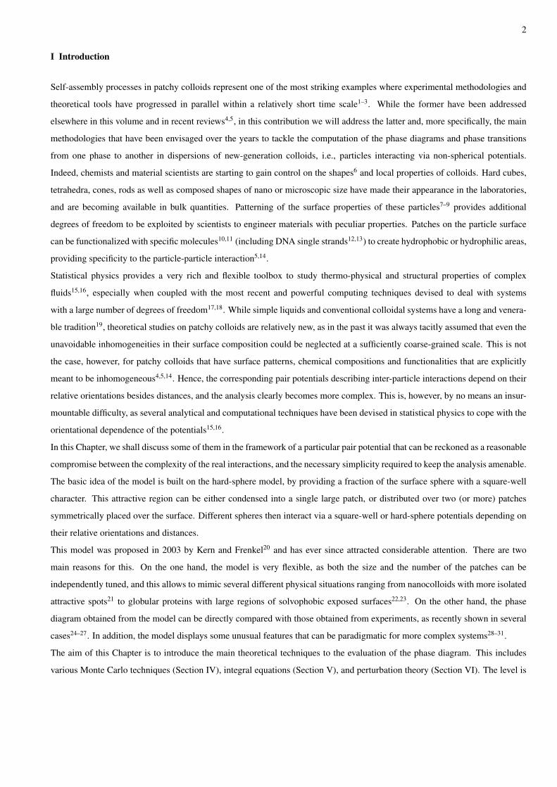
FIG. 1: Sketch of one-patch parchy particles as modelled by the Kern-Frenkel potential. The surface of each sphere is partitioned into an

attractive part (color code: blue) and a repulsive part (color code: white). The unit vectors n1 and n2 define the orientations of the pathces,

whereas the vector r12 joins the centers of the two spheres, from sphere 1 to sphere 2. The particular case shown corresponds to a 50% fraction

of attractive surface (coverage χ = 0.5).

intended to be pedagogic, with the main ideas behind each method outlined for non-experts in the field. Emphasis will be given

on the calculations of thermodynamic quantities necessary for the phase diagram analysis, and hence a number of additional

important results related to structural properties and other thermodynamical probes will be omitted.

II The Kern-Frenkel model

Consider a set of N identical hard-spheres of diameter σ in a volume V at temperature T suspended in a microscopic fluid. When

the surface of the spheres are uniform with no other interactions as their steric hindrance, the model has been often employed as

a paradigm of sterically stabilized colloidal suspensions in the limit of high temperature or good solvent.

As discussed elsewhere in this volume, colloids that are envisaged as elementary building blocks for the self-assembly process,

are patchy colloids with different philicities in different part of the surface4,5. This means, for instance, that one fraction of the

surface may be solvophilic and the other solvophobic. In solution, the solvophobic part will tend to avoid contact with the solvent

and hence will act as an effective attractive force in the presence of another solvophobic patch laying on a different sphere.

One can then consider the following model that was introduced in 2003 by Kern and Frenkel in the present form20, but it is worth

remarking that the idea of considering hard spheres and decorating them with patches of various forms and patterns dates back

to much earlier, and several earlier versions in different fields can be considered as its ancestors32–35.

A circular patch is attached to the surface of each sphere, as depicted in Figure 1, with the central position of the patch identified

by the unit vector n, and its amplitude measured by the angle θ0. Unlike the case of uniform sphere the interactions among

spheres is anisotropic as it depends on the relative orientation of the unit vectors on each spheres with the direction connecting

their centers. Then the idea is that two spheres attract each other if they are within the range of the attractive potential, with the

corresponding attractive patches on each sphere properly aligned.

If n1 and n2 are the unit vectors associated with each patch on spheres 1 and 2, and r12 is the direction connecting the centers of

4

the two spheres, then the interparticle potential reads

Φ (12) = φ0 (r12) + ΦI (12) , (1)

where the first term is the hard-sphere contribution

φ0 (r) =

∞, 0 < r < σ

0, σ < r, (2)

and the second term

ΦI (n1, n2, r12) = φSW (r12) Ψ (n1, n2, r12) (3)

is the orientation-dependent attractive part which can be factorized into an isotropic square-well tail

φSW (r) =

−ε, σ < r < λσ

0, λσ < r, (4)

multiplied by an angular dependent factor

Ψ(n1, n2, r12) =

1, if n1 · r12 ≥ cos θ0 and −n2 · r12 ≥ cos θ0

0, otherwise. (5)

Here σ is the sphere diameter, (λ − 1)σ is the width of the square-well interaction and ε its depth. 2θ0 defines the angular

amplitude of the patch. The unit vectors ni(ωi), (i = 1, 2), are defined by the spherical angles ωi = (θi, ϕi) in an arbitrarily

oriented coordinate frame and r12(Ω) is identified by the spherical angle Ω in the same frame. Reduced units, for temperature

T ∗ = kBT/ε, pressure P ∗ = βP/ρ and density ρ∗ = ρσ3, will be used throughout, with kB being the Boltzmann constant. For

future reference, we also introduce the packing fraction η = πρ∗/6.

The coverage χ is the fraction of attractive surface on the particle. χ can be related to the patch half-width θ0 as

χ =⟨Ψ

(n1, n2, Ω

)⟩1/2

ω1ω2

=1− cos θ0

2(6)

where we have introduced the angular average

〈. . .〉ω =14π

∫dω . . . . (7)

III The tools of statistical physics

Statistical physics has developed a number of different theoretical approaches to compute the thermophysical properties of a

fluid15–17. In order to compare with experiments, we are most interested in the computation of the fluid-fluid and fluid-solid

phase diagram on the one hand, and on the specific mechanism driving aggregation, and hence self-assembly, on the other

hand. Among this arsenal of different available techniques, here we will review three different methodologies that were recently

exploited in the framework of the Kern-Frenkel model. These are Monte Carlo simulations17,18, integral equation theories15 and

thermodynamical perturbation theories16.

5

Monte Carlo simulations are undoubtably one the most efficient ways to accurately compute the properties of a model fluid.

As discussed in more details below, the main limitations of simulations are that they can be very demanding from a computa-

tional point of view, especially for sufficiently realistic potentials, and that they are unable to distinguish metastable from stable

equilibrium states. On the other hand, they provide virtually exact estimates of all static quantities of interest. Several improve-

ments have been proposed over the years, some of them triggered by the problems discussed in this contribution, so that the

methodology is very well established and by now extensively reviewed and described in detail in several books (see Refs. 17,18

and references therein). The case of patchy colloids, however, is relatively recent, although it builds upon previous established

procedures on other complex fluids.

Integral equation and thermodynamics perturbation theories are two of the main methodologies from the toolbox of Statistical

Physics that are at the basis of our current understaing of simple and molecular fluids15,16. In spite of their known drawbacks and

shortcomings, they are known to provide reliable predictions for both structural and thermodynamical properties each in their

own domain of applications. Their applications to patchy colloids is a rather natural, albeit not trivial, extension of formalisms

already developed in the last two decades for molecular fluids16. As it will become clear, they both become particularly attractive

in view of the large computational effort involved in Monte Carlo simulations. In addition, they are able to access to some details

and nuances that are not easily accessible by other methods.

IV Monte Carlo simulations

The aim of Monte Carlo simulations is the computation of thermodynamic quantities by performing an average over a suitable

ensemble of microstates. The choice of the ensemble is dictated both by the quantities to be computed and by the specific system

under investigation, for which one ensemble can be more convenient than the others. Below we review the most interesting

techniques that have been used to calculate phase diagram of patchy colloid models.

A Canonical NV T and NPT methods

Simulations in the NV T (isothermal-isochoric) and NPT (isothermal-isobaric) ensembles are probably the most common

example. In these ensembles, the number of particles N , the temperature T and the volume V (NV T ) or the pressure P (NPT )

are held constant. The Markov chain in configuration space is constructed via a sequence of translational and rotational moves,

accepted with an appropriate probability that depends upon the change in potential energy and T . In the NPT case, the volume

is also varied. With a proper choice of the acceptance probability, the system first evolves toward equilibrium and then starts to

sample equilibrium configurations with the Boltzmann statistical weight. The equilibration process can be rather long, especially

in cases where kinetic traps are present (as in the vicinity of gel or glass transitions) or when an activation barrier needs to be

overcome. This last case arises when the system is metastable with respect to a lower energy phase or when it organizes into

mesoscopic structures and specific self-assembly processes involving large numbers of particles are requested. The approach to

equilibrium can be monitored by focusing on the time evolution of collective properties (e.g. the potential energy, the density,

the pressure). Since equilibration can be rather slow, it is highly recommended to make use of a logarithmic time scale when

6

searching for a drift in the time dependence of the investigated property.

When a sufficiently large number of statistically independent equilibrium configurations have been generated and stored, all

possible structural (static) information can be calculated. Typical quantities that are computed are the total energy U , the radial

distribution function g(r) and the structure factor. In the case of anisotropic systems, such as patchy particles, the orientational

dependence of the structural properties needs to be evaluated as well. The center-center g(r) is indeed not sufficient to evaluate

the average potential energy or the pressure, at variance of the isotropic case where calculation of U or P from the g(r) usually

simply requires a one-dimensional integration.

In the case of hard bodies or in the presence of step-wise potentials (e.g. the square-well potential), direct evaluation of P in

NV T simulations is in principle possible36,37 but not straightforward. To evaluate the equation of state, i.e., the relation between

density and P at constant T , the NPT ensemble is often preferred in this case.

Various additional improvements can be (and are) used to improve the convergence of the scheme in a way that will be described

in each specific example.

B Gibbs ensemble method

A convenient scheme was devised by Panagiotopulos38 to specifically address the problem of a direct evaluation of the gas-

liquid phase coexistence by Monte Carlo simulations. This is known as the Gibbs Ensemble Monte Carlo (GEMC) method. N

particles are partitioned into two distinct simulation boxes. In addition to intra-box translational and rotational moves, particle

and volume swap moves (keeping both the total number of particles and the total volume fixed) are proposed and accepted with

the appropriate probability17. In this way the two coexisting phases are simulated without the intervention of a interface between

them. When convergence is reached, the densities in the two boxes provide the value of the coexisting densities of the liquid and

gas phase. It should be pointed out that the GEMC method becomes inefficient when the density of the liquid phase becomes

large, since the probability of inserting a particle with in a favourable state — i.e., not overlapping with any other — becomes

extremely small.

For the specific case of KF particles discussed later in this Chapter, GEMC simulations have been performed for a system of

1200 particles in a total volume of (16σ)3. On average, the code attempts one volume change every five particle-swap moves

and 500 displacement moves. Each displacement move is composed of a simultaneous random translation of the particle center

(uniformly distributed between ±0.05σ) and a rotation (with an angle uniformly distributed between ±0.1 radians) around a

random axis.

C Grand-canonical ensemble µV T

In the neighborhood of the gas-liquid critical point the free-energy barrier separating the two phases becomes comparable to

the amplitude of the thermal fluctuations of of the relatively small systems that can be accessed in simulation. In this case, the

GEMC method cannot be used to investigate the system since it becomes size effects and spontaneous swapping of the average

densities between the two boxes.

7

A precise evaluation of the critical parameters (density and temperature) can be obtained performing simulations in the grand-

canonical µV T ensemble17, where density fluctuations are accounted for at fixed volumes and temperature, coupled with the

finite-size scaling analysis envisaged by Wilding39. MC simulations in the gran canonical ensemble are implemented by per-

forming trial insertions and deletions of particles, besides trial displacements and rotations. The critical parameters of the system

can be extracted by matching the calculated distribution of density fluctuations to the expected distribution at the critical point,

a feature which is largely system independent39.

In the implementation of the grand-canonical simulations to the KF model reported later on, one insertion/deletion attempt was

performed, on average, every 500 trial translational/rotational displacements.

D Fluid-Solid coexistence: thermodynamic integration

To compute numerically the free energies of the fluid and the crystals and their coexistence lines it is possible to resort to

thermodynamic integration methods. Details of this procedure were recently given in a detailed review by Vega et al40.

The starting point of the procedure requires the identification of a state point in the pressure-temperature plane where two phases,

I and II, share the same chemical potential, i.e., µI(P, T ) = µII(P, T ) . The chemical potential of the fluid can be computed

by thermodynamic integration using the ideal gas as a reference state, and by integrating the equation of state, P (ρ), at fixed

temperature

βF (T, ρ)N

= log(ρσ3

)− 1 +

∫ ρ

0

βP/ρ′ − 1ρ′

dρ′ (8)

where F/N is the Helmholtz energy per particle. The first term on the right-hand-side of Eq.(8) is the ideal gas part and depends

upon the system dimensionality. The chemical potential can then be recovered as

βµ (P (ρ) , T ) =βF (P (ρ) , T )

N+ βP (ρ) /ρ . (9)

To compute the chemical potential of a crystal one can perform thermodynamic integration at fixed density and T using an

ideal Einstein crystal as the reference system. This method, known as Frenkel-Ladd procedure17,40, is very efficient and by now

standard. Integration of the crystal equation of state provides a way to evaluate the chemical potential at different T and P . The

pressure at which the chemical potential of the fluid and of the crystal are identical along an isotherm provides the coexisting

pressure at the selected T .

Starting from a coexistence point, coexistence lines can finally be inferred by using Gibbs-Duhem integration, as described by

Kofke41, numerically integrating over the Clausius-Clapeyron equation.

V Integral equation theories

A General scheme

At first, let us consider simple fluids first where the particles can be regarded as spherically symmetric. All thermodynamic

properties of such fluids can be straightforwardly computed from the radial distribution function g(r). In integral equation

8

theory15, the strategy to infer the thermophysical properties of a fluid hinges on the calculation of the total correlation function

h(r) ≡ g(r)− 1 that, in turn, is related to the direct correlation function c(r) by the Ornstein-Zernike (OZ) equation

h (r) = c (r) + ρ

∫dr′ c (r′) h (|r− r′|) (10)

Once that h(r) is known, all statistical and thermodynamical properties can in principle be computed. However, as h(r) de-

pends upon the unknown quantity c(r), an additional equation involving both quantities is required for the solution. Unlike

equation (10), which is exact, the second equation always involves some approximation. This gives rise to some well known

thermodynamic inconsistencies, that are the main shortcomings of this method, and that may severely limit its applicability.

The second relation between h(r) and c(r) also involves the two-body potential φ(r), and can be cast in the general form

c (r) = exp [−βφ (r) + γ (r) + B (r)]− 1− γ (r) (11)

where γ (r) = h (r) − c (r) is an auxiliary function. Although this equation is again exact in principle, it involves the bridge

function B(r) that in general depends upon higher body correlation functions, so in practice an approximation (closure) is

always necessary. The quality of the results obtained will depend crucially on the reliability of the involved approximations;

several closures have been proposed over the years with their pros and cons well classified and under control. Among them, the

reference hyper-netted chain (RHNC) stands out as an optimal trade-off between simplicity and precision of its predictions, and

this is the one that will be the object of the present Chapter.

Having closed the systems of two equations in two unknowns (h(r), and c(r)), the system may then be solved iteratively with

the convolution appearing in the OZ equation (10) simplified in Fourier space, as

h (k) =c (k)

1− ρc (k)(12)

h(k) and c(k) being the Fourier transform of h(r) and c(r) respectively.

The RHNC closure was introduced by Lado42 for spherical potentials and later extended to molecular fluids43,44. In the RHNC

closure, one replaces the exact B(r) appearing in (11) by its hard-sphere counterpart B0(r), that is the only system for which

a reliable expression (the Verlet-Weiss expression45) is available. Rosenfeld and Ashcroft46 demonstrated that the effectiveness

of the reference system could be magnified by treating its parameters as variables to be optimized in some fashion. It is in fact

possible to determine them via a variational free energy principle47 that enhances internal thermodynamic consistency. With the

effective hard sphere diameter σ0 suitably chosen in this way, the RHNC has been shown to provide rather precise estimates

of the chemical potential and pressure, that is the two crucial thermodynamical quantities needed for the calculation of phase

diagrams.

The case of anisotropic potentials is significantly more complex from the algorithmic point of view, but the philosophy behind

the methodology is identical. The procedure hinges on a remarkable piece of work carried out by Fred Lado in a series of

papers43,44,47 in the framework of molecular fluids and more recently adapted to the case of patchy colloids. Here we just sketch

the idea, referring to Refs. 48–50 for details.

The angular dependent counterparts of Eqs.(10) and (11) are given in terms of γ(12) = h(12)− c(12), and are

γ (12) =ρ

4π

∫dr3dω3 [γ (13) + c (13)] c (32) , (13)

9

c (r)Fourier transform−−−−−−−−→ c (k)xClosure

yOZ equation

γ (r)Inverse Fourier transform←−−−−−−−−−−−− γ (k)

TABLE I: Schematic flow-chart for the solution of the OZ equation for isotropic potentials.

for the OZ equation, and

c (12) = exp [−βΦ (12) + γ (12) + B (12)]− 1− γ (12) . (14)

for the closure equation. Again, the RHNC approximation amounts to assume B(12) = B0(r12), but clearly this is a much

more drastic approximation in the present case, as the real B(12) depends on the relative orientations of the particles whereas

the reference B0(r12) does not. As a result, one might expect the results to be less precise in this case as compared with the

isotropic fluid counterpart.

B Iterative procedure

As discussed before, the iterative procedure in the case of the spherical isotropic potential is very simple and outlined in Table

I. It requires a series of transformation to and from Fourier space, where the solution of the OZ equation is more conveniently

carried out in view of Eq.(12) The iterative solution of the angular dependent Ornstein-Zernike (OZ) equation (13) along with the

approximate closure equation (14) again requires a series of direct and inverse Fourier transforms between real and momentum

space involving the bridge function B(12), the direct correlation function c(12), the pair distribution function g(12), the total

correlation functions h(12) and the auxiliary function γ(12) = h(12)− c(12).

In addition to this, however, the orientational degrees of freedom introduce additional direct and inverse Clebsch-Gordan (CG)

transformation between the coefficients of the angular expansions in different frames16. Two important examples are the so-

called “axial” or “molecular” frames, with z = rij in real space, and the k representation with z = k in momentum space,

because in those representations some of the calculations become particularly simple. This set of transformations also allows

the definition of the correlation functions (in particular the g(12)) in an arbitrarily-oriented axes. We further note that, in the

presence of an anisotropic potential, the Fourier transform is implemented through a Hankel transform, and that the cylindrical

symmetry of the angular dependence included in the Kern-Frenkel potential of Section II (when the number of patches present

on each sphere is one or two) allows us to use the simpler version of the procedure for linear molecules.

All necessary equations can be found in Ref. 16, that is the standard reference for this topic, and only the most important ones

will be reported in the following.

The resulting scheme is illustrated in Table II and is the extension of the isotropic case given in Table I49. Consider the expansion

in spherical harmonics of the auxiliary function γ(12) in the axial frame

γ(12) = γ (r, ω1, ω2) = 4π∑

l1,l2,m

γl1l2m (r) Yl1m (ω1) Yl2m (ω2) , (15)

10

c (r; l1l2l)Hankel transform−−−−−−−−→ c (k; l1l2l)

Inverse CG transform−−−−−−−−−−→ cl1l2m (k)xCG transform

yOZ equation

cl1l2m (r) γl1l2m (k)xExpansion inverse

yCG transform

c (r, ω1, ω2) γ (k; l1l2l)xClosure

yInverse Hankel transform

γ (r, ω1, ω2) γ (r; l1l2l)xExpansion

yInverse CG transform

[γl1l2m (r)]old ←−−− Iterate ←−−− [γl1l2m (r)]new

TABLE II: Schematic flow-chart for the solution of the OZ equation for the Kern-Frenkel angle-dependent potential.See Section V for a

description of the scheme

where m ≡ −m, and its inverse reads

γl1l2m (r) =14π

∫dω1dω2γ (r, ω1, ω2) Y ∗

l1m (ω1) Y ∗l2m (ω2) . (16)

Eq.(16) provides the initial set [γl1l2m(r)]old described as the initial point in Table II, whereas Eq.(15) yields the next term in the

iteration map γ(r12, ω1, ω2).

Using the aforementioned RHNC closure approximation B(12) = B0(r12), the bridge function is constructed and then inserted

in Eq.(14) to get c(r, ω1, ω2). Eq.(16) with the replacement γ → c is then exploited to infer the corresponding axial coefficients

cl1l2m(r12)

The next step is to implement a Clebsh-Gordan transform in direct space, in order to transform from axial coefficients cl1l2m(r)

where z = r to space coefficients c (r; l1l2l) in an arbitrarly oriented frame. The necessary expressions are the equation pairs

c (r; l1l2l) =(

4π

2l + 1

)1/2 ∑m

C (l1l2l;mm0) cl1l2m (r) , (17)

where the C (l1l2l;mm0) are Clebsch-Gordan coefficients, with the inverse transform given by

cl1l2m (r) =∑

l

C (l1l2l;mm0)(

2l + 14π

)1/2

c (r; l1l2l) . (18)

and the coefficients c(r; l1l2l) are then given by Eq.(18).

The last required tool is the Fourier transform of the radial parts, that is a Henkel transform as given by the pairs

c (k; l1l2l) = 4πil∫ ∞

0

dr r2c (r; l1l2l) jl (kr) , (19)

with the inverse transform reading

c (r; l1l2l) =1

2π2il

∫ ∞

0

dk k2c (k; l1l2l) jl (kr) , (20)

11

where jl(x) is the spherical Bessell function of order l. By using “raising” and “lowering” operations on the integrands these

are finally evaluated with j0(kr) = sin kr/kr kernels, for l even, and j−1(kr) = cos kr/kr kernels, for l odd. Fast Fourier

Transforms are programmed for both instances. (Note that Hankel transforms X (k; l1l2l) are imaginary for l odd while for l

even they are real.)

Having obtained c(k; l1l2l) from Eq.(19), we have then reached the turning point in Table II, from which the returning part

can then be started with a parallel sequence of operation in Fourier space. These include, a backward Clebsch-Gordan trans-

formation to return to an axial frame in k space and get cl1l2m(k); a OZ equation in k-space to get γl1l2m(k), followed by a

forward Clebsch-Gordan transformation, and an inverse Hankel transform, to find γ(r; l1l2l). A final backward Clebsch-Gordan

transformation, brings a new estimate of the original coefficients [γl1l2m(r)]new. This cycle is repeated until self-consistency

between input and output γl1l2m(r) is achieved as before.

Note that the OZ equation required in k representation,as expressed in terms of the axial expansion coefficients of the trans-

formed pair functions, is given by the following matrix form

γl1l2m (k) = (−1)mρ

∞∑l3=m

[γl1l3m (k) + cl1l3m (k)] cl3l2m (k) , (21)

C Thermodynamics

Once that the correlation function h(12) (and hence the distribution function g(12) = h(12) + 1) is known, the excess free

energy can be computed as44,49

βFex

N=

βF1

N+

βF2

N+

βF3

N, (22)

where

βF1

N= −1

2ρ

∫dr12

⟨12h2 (12) + h (12)− g (12) ln

[g (12) eβΦ(12)

]⟩ω1ω2

, (23)

βF2

N= − 1

2ρ

∫dk

(2π)3∑m

lnDet

[I + (−1)m

ρhm (k)]− (−1)m

ρTr[hm (k)

], (24)

βF3

N=

βF 03

N− 1

2ρ

∫dr12 〈[g (12)− g0 (12)]B0 (12)〉ω1ω2

. (25)

In Eq. (24), hm(k) is a Hermitian matrix with elements hl1l2m(k), l1, l2 ≥ m, and I is the unit matrix. The last equation, for

F3, directly expresses the RHNC approximation. Here F 03 is the reference system contribution, computed from the known free

energy F 0ex of the reference system as F 0

3 = F 0ex − F 0

1 − F 02 , with F 0

1 and F 02 calculated as above but with reference system

quantities.

The bridge function B0(12) appearing in (25) is the key approximation in the RHNC scheme, since it replaces the unknown

bridge function B(12) in the general closure equation (14). This is taken from the Verlet-Weiss expression of the hard-sphere

model45, as anticipated, in view of its simplicity and of the fact that it works reasonably well for the case of the square-well as

we will see, but with a renormalized diameter σ0 for the hard-sphere that is selected by enforcing the variational condition47

ρ

∫dr [g000 (r)− gHS (r;σ0)]

∂BHS (r;σ0)∂σ0

= 0. (26)

12

From the free energy F , one of course compute all thermodynamics following standard procedures. For the computation of the

phase diagram, the pressure and chemical potential are required at any fixed temperature.

The virial pressure P is obtained as16

P = ρkBT − 13V

⟨N∑

i=1

N∑j>i

rij∂

∂rijΦ (ij)

⟩= ρkBT − 1

6ρ2

∫dr12

⟨g (12) r12

∂

∂r12Φ (12)

⟩ω1ω2

. (27)

that in turns can be cast in the form involving the cavity function y(12) = g(12)eβΦ(12) with the result49

βP

ρ= 1 +

23πρσ3

⟨y (σ, ω1, ω2) eβεΨ(ω1,ω2)

⟩ω1ω2

− λ3⟨y (λσ, ω1, ω2)

[eβεΨ(ω1,ω2) − 1

]⟩ω1ω2

, (28)

As already remarked, one of the main advantages of the RHNC closure stems from the fact that the calculation of the chemical

potential does not introduce any approximation in addition to that already included in the closure. It can be obtained from the

thermodynamic relation

βµ =βF

N+

βP

ρ, (29)

that was already used in Eq.(9).

Finally, we note that the ideal quantities for the free energy, the virial pressure and the chemical potential are

βFid

N= ln(ρΛ3)− 1

βPid

ρ= 1 βµid = ln(ρΛ3) (30)

VI Barker-Henderson perturbation theory

Another powerful method to access thermophysical properties of a fluid is thermodynamical perturbation theory, that directly

extracts the free energy of the system from the knowledge of the free energy F0 of a reference fluid (the hard-sphere fluid in

the present case). This is a well-known techniques in several fields of physics, including simple15 and complex16 fluids, and

hinges on the fact that often the system under investigation is not very different from the reference one, so that an expansion in

this perturbation term is a reasonable approximation. Under these conditions, the results are expected to be rather reliable, even

when stopping the expansion at the lowest orders.

In the square-well fluid case the analysis has been carried out in details in the late 70s51,52, starting from the pionieering work by

Zwanzig53, and recently extended to the patchy case23,54.

Working in the grand-canonical ensemble as this is the most convenient one52, we assume the total potential U to have the

following form

Uγ (1, . . . , N) = U0 (1, . . . , N) + γUI (1, . . . , N) (31)

=∑i<j

Φγ (ij) =∑i<j

Φ0 (ij) + γ∑i<j

ΦI (ij) ,

where U0(1, . . . , N) =∑

i,j Φ0(ij) is the unperturbed part and UI(1, . . . , N) =∑

i,j ΦI(ij) is the perturbation part. Here

0 ≤ γ ≤ 1 is used as perturbative parameter. Note that when each coordinate i includes both the coordinate ri and patch

orientation ni, so that i ≡ (ri, ni), then the expression is valid also for the Kern-Frenkel model23,54. For simple fluids, then

13

i ≡ ri only. Introducing the following short-hand notation∫1,...,N

(· · · ) ≡∫ [

N∏i=1

dri 〈(· · · )〉ωi

](32)

for the integration over all particle coordinates, the grand-canonical partition function

Qγ =+∞∑N=0

eβµN

N !Λ3NT

∫1,...,N

e−βUγ = e−βΩγ (33)

(here ΛT is the de Broglie thermal wavelength, and Ωγ is the grand-potential) can then be used to obtain an expansion of the

Helmholtz free energy52.

Fγ = F0 + γ

(∂Fγ

∂γ

)γ=0

+12!

γ2

(∂2Fγ

∂γ2

)γ=0

+ · · · (34)

that is valid for arbitrary γ.

Taking the derivative of lnQγ at fixed chemical potential µ, one has, using Eq.(31)[∂

∂γlnQγ

]µ

=12

∫1,2

∂

∂γ[−βΦγ (12)] ργ (12) , (35)

where

ργ (1 . . . h) =1Qγ

+∞∑N=h

eβµN

(N − h)!Λ3NT

∫1,...,N

e−βUγ . (36)

When γ = 1, this yields the free energy correct to first order in the expansion Eq.(34).

The second order correction is far more laborious. Indeed, the extension of this analysis involves higher orders correlation

functions and this forces additional approximations to come into play51,52, thus humpering its practical utility. In 1967, Barker-

Henderson gave a much simpler recipe55 that was found to be rather effective in predicting the phase diagram of the square-well

fluid52 and was recently extended to the Kern-Frenkel case54.

The final result for arbitrary angular dependent potential, correct to second-order, reads54

βF

N=

βF0

N+

βF1

N+

βF2

N+ . . . , (37)

where

βF1 =12ρN

∫drg0 (r) 〈βΦI (r, Ω, ω1, ω2)〉ω1,ω2

(38)

and

βF2 = −14kBTρN

(∂ρ

∂P

)0

∫drg0 (r)

⟨[βΦI (r, Ω, ω1, ω2)]

2⟩

ω1,ω2

, (39)

In the particular case if the Kern-Frenkel potential, one obtains23,54

βF1

N=

12η

σ3

∫drg0 (r) 〈βΨ(12)〉ω1,ω2

. (40)

14

and

βF2

N= −6η

σ3

(∂η

∂P ∗0

)T

∫drg0 (r) φ2

SW (r)⟨[βΨ(12)]2

⟩ω1,ω2

, (41)

Here P ∗0 = βP0/ρ is the reduced pressure of the HS reference system and g0(r) the corresponding radial distribution function.

As before, the pressure and chemical potential can be derived from the reduced free energy per particle βF/N , using the exact

thermodynamic identities

βP

ρ= η

∂

∂η

(βF

N

)(42)

βµ =∂

∂η

(ηβF

N

). (43)

The phase diagram in the temperature-density plane can then be computed using a numerical procedure that will discussed in

connections with Eqs.(44) and (45) below, as it is identical to the one used for integral equations.

VII Calculation of the fluid-fluid coexistence curves for integral equation and pertubation theory

The common feature of integral equations and thermodynamic perturbation theory is that one is able to obtain approximate

expressions for both the pressure P and the chemical potential µ as a function of the temperature T and the density ρ. In the

presence of a fluid-fluid (gas-liquid) transition, both P and µ will have well defined dependence on T and ρ in the gas and liquid

branches, but not in the coexistence regions. Hence, in order to obtain the coexistence curves, and hence the phase diagram in

the temperature-density plane two procedures are possible. First a graphical procedure where one plots the chemical potential

versus the pressure at a given fixed temperature, and seeks the intersections between the gas and the liquid branches. An example

of this procedure in the case of the square-well potential was given in Ref. 48. This procedure, however, is neither very practical

nor very precise, as it involves qualitative deduction of the crossing points. Yet it can be used as a first preliminary estimate of a

more precise numerical calculations as follows.

For a fixed temperature T , one can then compute the pressure of the gas (colloidal poor) phase Pg and of the liquid (colloidal

rich) Pl phases, and the corresponding chemical potentials µg and µl. The fluid-fluid (gas-liquid) coexistence line then follows

from a numerical solution of a system of non-linear equations

Pg (T, ρg) = Pl (T, ρl) (44)

µg (T, ρg) = µl (T, ρl) (45)

whose solutions are the gas ρg and liquid ρl densities associated with the coexistence lines. By plotting the resulting ρg and ρl as a

function of T the coexistence curve can be constructed in the region where the transition occurs. This procedure will be followed

in the analysis of the Kern-Frenkel fluid-fluid phase diagram for both integral equations (see Section VIII A) and thermodynamic

perturbation theory (see Section VIII D), but can also be exploited for the computation of the fluid-solid transition, as explained

in Section VIII E.

15

0 0.1 0.2 0.3 0.4 0.5 0.6ρσ

3

0.95

1.00

1.05

1.10

1.15

1.20

1.25

kBT

/εGEMC (Vega et. al.)RHNCGEMC (del Rio et. al.)

FIG. 2: Fluid-fluid coexistence curves kBT/ε versus ρσ3 for the SW fluid of range λ = 1.5. Data from RHNC integral equation (squares) are

contrasted with Monte Carlo simulations by Vega et al.58 (circles), and del Rıo et al.59 (crosses). Adapted from Ref.48.

VIII Results

A Fluid-Fluid coexistence curves from RHNC integral equation

We start by reviewing the quality of the RHNC integral equation theory for the simple case of the isotropic square-well case, a

model which has often be used as an effective potential (in the implicit solvent representation) to model colloidal particles inter-

acting via depletion interactions56,57. Fig.2 shows the RHNC predictions for the gas-liquid coexistence from Ref.48 contrasted

with Monte Carlo simulations on the same system carried out by different groups58,59.

Although the integral equation results appear to reproduce reasonably well those from numerical simulations, two features are

worth noticing.

First, thermodynamic inconsistencies associated with the approximate nature of the closure are at the origin of the incorrect

evaluation of the pressure and chemical potentials and hence of the exact location of the coexistence lines. This is an unavoidable

feature of all integral equations, and its origin and effects are well known. For most of the cases, in fact, the whole critical region

is inaccessible to integral equation theories.

A second additional point is related to the non-linear nature of the self-consistence procedure, and gives rise to numerical

instabilities that may or may not be controlled depending on the considered state point. As a general rule, lower temperatures

and higher densities are harder to converge, and hence for some points the solution of the system of Eqs. (44) and (45) might

not even exist.

These considerations are even more compelling in the more complex case of the Kern-Frenkel fluid where condensation takes

place at lower T associated with the involved lower coverages. Hence one might expect an agreement with respect to numerical

simulations not better than what has been reported for the isotropic square-well case. This is indeed the case, as shown in Fig.3

for the representative example of single-patch particles with coverage χ = 0.8, for which 80% of the surface has a SW character,

condensed into a unique patch. The width of the square-well has been selected to be λ = 1.5 as before, so that the limit of full

16

0 0.1 0.2 0.3 0.4 0.5 0.6 0.7 0.8

ρσ3

0.4

0.5

0.6

0.7

0.8

0.9

kBT/ε

GCMC

RHNC

FIG. 3: Fluid-fluid coexistence curves kBT/ε versus ρσ3 for the Kern-Frenkel fluid with coverage χ = 0.8 and range λ = 1.5. Data from

RHNC integral equation (circles) are compared against MC simulations (squares). Adapted from Ref.49.

coverage gives back the result of Fig.2, and the value χ = 0.8 has been selected to be half-way between the fully occupied fluid

and half-coverage that has peculiar behavior, as will be discussed shortly.

In Fig.3 we also report the coexistence lines and critical points using Gibbs ensemble and Gran Canonical Monte Carlo simu-

lations, as outlined in Sections IV B and IV C. The former were used to evaluate coexistence in the region where the gas-liquid

free-energy barrier is sufficiently high to avoid crossing between the two phases, whereas the latter was used to locate exactly

the critical point. The details of the analysis can be found in Refs. 48 (and in Ref. 50 for the corresponding two-patch case).

The comparison between RHNC integral equation and MC simulations for the Kern-Frenkel model with intermediate coverage

χ = 0.8 displayed in Fig.3 shows that indeed the agreement is comparable with the square-well case as anticipated.

The Kern-Frenkel model offers the possibility to continuously change the coverage interpolating from the isotropic square-well

to the symmetric Janus-like potential, when the coverage moves from χ = 1 to χ = 0.5 (see Fig. 4-(a)). To investigate how

the phase diagram of Janus particles arises, we calculate how the gas-liquid coexistence is modified on progressively reducing

χ. Fig. 4-(b) shows MC simulations (Gibbs ensemble for the coexistence lines and gran-canonical µV T for the critical point)

results for the gas-liquid phase coexistence for several χ values, extending the original data by Kern and Frenkel20. A progressive

shrinking of the coexistence region to lower temperatures and densities accompanies the decrease of the coverage. Consistently,

as the coverage decreases, both the critical temperature and critical density decrease (see Fig.7). This is not surprising, in

view of the fact that the coverage is a measure of the attractive interactions intensity (by controlling the maximum number of

nearest neighbors contacts21,60) that dictates the value of Tc and (perhaps more indirectly) ρc. It can be explicitly shown that this

shrinking of the coexistence region is a non-trivial one, and that it cannot be inferred by a simple scaling of either the temperature

or the density. Up to χ = 0.6 coverage, however, the morphology of the curve appears to be the standard one, with the gas and

liquid coexistence lines widening on cooling down.

The half-coverage χ = 0.5 is known as the Janus limit and will be discussed in the next Section, as it displays an interesting

unconventional behavior28.

17

FIG. 4: (a) Cartoon of a one-patch particle with the coverage (fraction of attractive surface, depicted in blue) changes from one (square well) to

one half (Janus). (b) Fluid-fluid coexistence curves kBT/ε versus ρσ3 for the Kern-Frenkel fluid with descreasing coverages from χ = 1.0 (the

SW case) to the Janus limit χ = 0.5. The range is always set to λ = 1.5. Data are from Gibbs ensemble MC simulations for the coexistence

lines and from grand-canonical MC simulations for the critical points. This is the one-patch result: for the two-patches counterpart, see Fig.6.

Adapted from Ref.31.

B The Janus limit

The value of χ = 0.5 plays a special role in the Kern-Frenkel model with a single patch. This can be seen by following the

change in the coexistence line locations as the coverage is reduced from the fully isotropic square-well fluid (χ = 1.0) to the

Janus case (χ = 0.5), as discussed in the previous section.

In Fig. 5 (a) the Janus case χ = 0.5, already reported in Figure 4, is shown by magnifying the very narrow region where the

transition occurs.

The difference with the standard phase diagram appears rather clearly. As the fluid is cooled down to lower and lower tem-

peratures, the coexistence region shrinks, contrary to the standard case, and the two coexistence lines appear to approach one

another at sufficiently low temperatures. The origin of this anomaly has far reaching consequences that have been discussed

in details28,31. The crucial point is that at low temperature and density, monomers tend to aggregate in micelles and vesicles

(see Fig 5-(b)) bearing a well defined number of particles (10, 41, . . .) so that all favorable contacts are saturated inside the

aggregate28,31. This means that, in all cases, the clusters always expose the hard-sphere parts to the external fluid, and the

condensation process is thus inhibited and eventually destroyed altogether. The specificity of these magic numbers can be also

18

FIG. 5: (a) The anomalous phase diagram of the Janus limit (χ = 0.5), adapted from Ref.28. (b) Cartoon of the aggregates which form in the

gas phase on cooling, micelles and vesicles. The blue surface is attractive, modeled via a square-well potential.

explained by means of a simple cluster theory61, and an even simpler approach62 can be developed to mimic the onset of the

re-entrant gas branch. Below the Janus limit, no evidence of fluid-fluid transition was found, in full agreement with the above

interpretation28,31.

The unconventional shape of the phase diagram arises from the particular energetic and entropic balance associated to the

transition from the micelles gas to the liquid phase. It has been found that, differently from the usual gas-liquid behavior, the

potential energy per particle is higher in the liquid phase than in the micellar gas phase, a consequence of the greater energetic

stability of the micelles and vesicles as compared to the disordered liquid phase. Hence, despite the fact that the gas phase is

stabilized by the translational entropy of the micelles, the coexisting liquid phase is more disordered than the gas one. Such

unconventional entropic stabilization of the liquid phase arises from the orientational entropy, since particles are orientationally

disordered in the liquid phase while they are properly oriented in the micelles gas phase.

19

FIG. 6: (a) Cartoon of two-patch particles, when the coverage (blue) varies from one (square well limit) to zero (hard sphere limit). (b)

Fluid-fluid coexistence curves kBT/ε versus ρσ3 for the Kern-Frenkel fluid with two-patches and descreasing coverages from χ = 1.0 (the

SW case) to the value χ = 0.3. The range is always set to λ = 1.5. Data are from Gibbs ensemble MC simulations for the coexistence lines

and from grand-canonical MC simulations for the critical points. This is the two-patches counterpart of Fig.4. Adapted from Ref.50.

C One versus two-patches

It is interesting to investigate the effects of having the same attractive square-well coverage split in two parts, at the opposite poles

of the sphere so that they are symmetrically distributed. This is the two-patche case, and again this case smoothly interpolates

between the fully occupied isotropic SW case χ = 1 and the empty hard-sphere χ = 0 case. The corresponding fluid-fluid

(gas-liquid) phase diagram is depicted in Fig.6, that should be contrasted with the single patch counterpart reported in Fig.4.

Two main differences are noteworthy. First, the case χ = 0.5 does not appear to play any particular role, at variance with the

single patch counterpart. Its coverage value corresponds to the so-called tri-block Janus case, and will be further discussed later

on25–27. This can be attributed to the fact that at higher valences it is not possible to saturate all favorable contacts, and hence the

condensation process always takes places in complete agreement with the previous interpretation of the Janus case. The second

main difference is related with the fact that in the two-patch case coverages below χ = 0.5 do exhibit fluid-fluid transition, as

displayed in Fig.6, where coverages as low as χ = 0.3 are depicted. Below this value, the transition becomes metastable with

respect to crystallization as explained in details in Ref. 50.

The χ dependence of the critical point can be inferred by plotting the reduced critical densities and temperatures, as a function

of the different coverages, as shown in Fig.750. Clearly, the two-patch densities and temperatures lie always above the one-patch

counterparts, thus supporting the interpretation that it is easier to form a fluid with higher valence at a given coverage, a feature

20

0.3 0.4 0.5 0.6 0.7 0.8 0.9 1χ

0

0.2

0.4

0.6

0.8

1

1.2

1.4

kBT/ε

0

0.1

0.2

0.3

ρcσ

3

2P

2P

1P

1P

FIG. 7: Comparison between the one and the two-patches coverage dependence of the reduced critical density (right axis) and of the reduced

critical temperature (left axis). Adapted from Ref. 50.

0 0.1 0.2 0.3 0.4 0.5 0.6 0.7 0.8

ρσ 3

0

0.2

0.4

0.6

0.8

1

1.2

1.4

1.6

kBT/ε

χ = 1.0

χ = 0.9

χ = 0.8

χ = 0.7

χ = 0.6

χ = 0.5χ = 0.4

χ = 0.3χ = 0.2χ = 0.1

FIG. 8: The fluid-fluid phase diagram from BH thermodynamic perturbation theory (continuous lines) contrasted against numerical simulations

(open symbols). Closed symbols refer to the BH critical points. Adapted from Ref.54.

that is related to the existence of the fluid-fluid transition even for low coverages.

D Evaluation of the fluid-fluid coexistence curves from thermodynamic perturbation theory

As in the case of integral equation theory, the fluid-fluid phase diagram for in the temperature-density plane can be computed

even from Barker-Henderson (BH) thermodynamic perturbation theory54, as indicated in Section VII.

This is shown in Fig. 8 for the one-patch case, and compared with the same MC simulations used for comparison with integral

equation theory.

Given the simplicity of the theory, the accuracy of the BH theoretical prediction is rather remarkable. On the one hand, this

21

0.5 0.6 0.7 0.8 0.9 1 1.1 1.2 1.3

ρσ 3

0

0.4

0.8

1.2

1.6

2

kBT/ε

χ = 1.0χ = 0.9χ = 0.8χ = 0.7χ = 0.6χ = 0.5χ = 0.4χ = 0.3χ = 0.2χ = 0.1

FIG. 9: The fluid-solid phase diagram from BH thermodynamic perturbation theory (continuos lines) contrasted against numerical simulations

(open symbols). Closed symbols refer to the BH critical points. The case χ = 1.0 (open squares) corresponds to the Young and Adler

molecular dynamics results63 and includes the FCC-FCC transition not considered in the patchy cases. Adapted from Ref.54.

allows to provide a prediction on the possible location of the true coexisting lines, even for coverages where MC results are not

yet available or in regions where crystallization prevents the evaluation of the location of the metastable gas-liquid critical point.

Note that there are no restrictions in the applicability of the BH theory, neither in thermodynamical parameters, nor in coverages,

the only limitations being the convergence of the numerical non-linear solvers for Eqs.(44) and (45). On the other hand, the BH

perturbation theory can be applied in its current form only to the one-patch case, as it lacks the possibility of discriminating the

location of the patches. Notwithstanding these limitations, this approach is very promising as it even allows the computation of

the fluid-solid branch, as we will see in the next section.

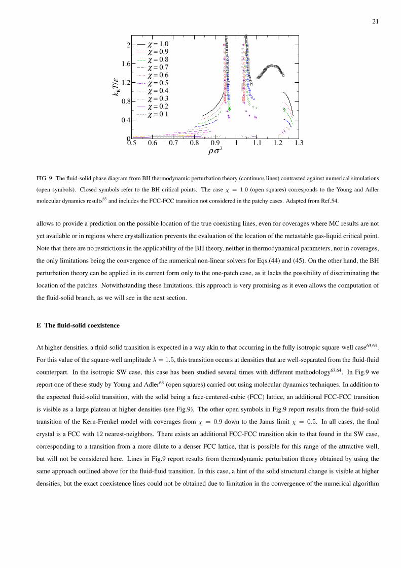
E The fluid-solid coexistence

At higher densities, a fluid-solid transition is expected in a way akin to that occurring in the fully isotropic square-well case63,64.

For this value of the square-well amplitude λ = 1.5, this transition occurs at densities that are well-separated from the fluid-fluid

counterpart. In the isotropic SW case, this case has been studied several times with different methodology63,64. In Fig.9 we

report one of these study by Young and Adler63 (open squares) carried out using molecular dynamics techniques. In addition to

the expected fluid-solid transition, with the solid being a face-centered-cubic (FCC) lattice, an additional FCC-FCC transition

is visible as a large plateau at higher densities (see Fig.9). The other open symbols in Fig.9 report results from the fluid-solid

transition of the Kern-Frenkel model with coverages from χ = 0.9 down to the Janus limit χ = 0.5. In all cases, the final

crystal is a FCC with 12 nearest-neighbors. There exists an additional FCC-FCC transition akin to that found in the SW case,

corresponding to a transition from a more dilute to a denser FCC lattice, that is possible for this range of the attractive well,

but will not be considered here. Lines in Fig.9 report results from thermodynamic perturbation theory obtained by using the

same approach outlined above for the fluid-fluid transition. In this case, a hint of the solid structural change is visible at higher

densities, but the exact coexistence lines could not be obtained due to limitation in the convergence of the numerical algorithm

22

associated with the non-linear solver in Eqs.(44) and (45). In spite of this drawback, thermodynamic theory is able to capture

the main features of the transition even for lower coverages (as low as χ = 0.1). It should be stressed, however, that transitions

to different crystal structures may be envisaged at low coverages, and this feature has not be accounted in the analysis reported

in Fig. 9.

F Self-assembly in a predefined Kagome lattice

The subtle interplay between the fluid-fluid and the fluid-solid transition is one of the most delicate issue in the framework of

self-assembly patchy colloids, especially in the presence of additional effects such as inhibiting clustering transitions. This was

already hinted before, but a very illuminating example of this is provided by the phase diagram of the triblock Janus fluid, that

has also been considered elsewhere in this volume from the experimental point of view.

Triblock Janus colloids are spherical colloidal particles decorated with two hydrophobic poles of tunable area, separated by

an electrically charged middle band (triblock Janus)25. The electric charge of the particles allows for a controlled switch of

the interaction via addition of salt, which effectively screens the overall repulsion, offering the possibility to the hydrophobic

attraction between patches to express itself. Once deposited on a flat surface, after the addition of the salt, particles organize

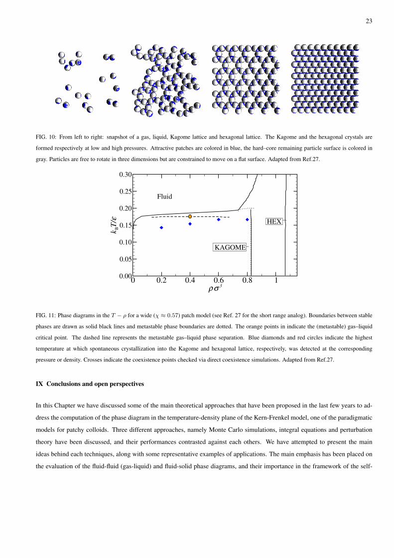
themselves into a Kagome lattice. The crystallization kinetics has been followed in real space in full details25. The patch width

in the experimental system, of the order of 65 degrees corresponding to χ ≈ 0.57, allows for simultaneous bonding of two

particles per patch, stabilizing the locally four–coordinated structure of the Kagome lattice (see Fig. 10).

A triblock Janus particle can be modeled via the two-patches Kern-Frenkel model in which the attractive region is split in two

parts at the opposite poles of the sphere, whereas the repulsive part is concentrated in the middle strip at the equator. The

square-well mimics the short-range hydrophobic attraction, while the hard-sphere region represents the repulsive charge-charge

interaction. Depending on the considered state point and on the patch amplitude several possible phases are possible, as shown

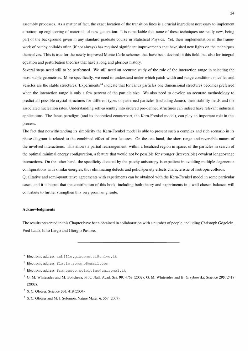
in Ref. 27 and summarized in Fig.11. In full agreement with the experiments, we observe at comparable interaction strength the

spontaneous nucleation of a Kagome lattice. We also find at larger pressure spontaneous crystal formation in a dense hexagonal

structure. Such easiness to crystallize suggests that in this system crystallization barriers are comparable to the thermal energy

at all densities. Interestingly enough, we find that for this model a (metastable) gas–liquid phase separation can be observed for

large patch width.

The ability of accurately describing Janus triblock particles with the KF potential is particularly rewarding and provides a strong

support for the use of such model for predicting the self–assembly properties of this class of patchy colloids. The possibility

of numerically exploring the sensitivity of the phase diagram to the parameters (patch width and interaction range) entering in

the interaction potential provides an important instrument and a guide to the design of these new particles to obtain specific

structures by self–assembly.

23

FIG. 10: From left to right: snapshot of a gas, liquid, Kagome lattice and hexagonal lattice. The Kagome and the hexagonal crystals are

formed respectively at low and high pressures. Attractive patches are colored in blue, the hard–core remaining particle surface is colored in

gray. Particles are free to rotate in three dimensions but are constrained to move on a flat surface. Adapted from Ref.27.

0 0.2 0.4 0.6 0.8 1

ρσ3

0.00

0.05

0.10

0.15

0.20

0.25

0.30

kBT/ε

Fluid

HEX

KAGOME

FIG. 11: Phase diagrams in the T − ρ for a wide (χ ≈ 0.57) patch model (see Ref. 27 for the short range analog). Boundaries between stable

phases are drawn as solid black lines and metastable phase boundaries are dotted. The orange points in indicate the (metastable) gas–liquid

critical point. The dashed line represents the metastable gas–liquid phase separation. Blue diamonds and red circles indicate the highest

temperature at which spontaneous crystallization into the Kagome and hexagonal lattice, respectively, was detected at the corresponding

pressure or density. Crosses indicate the coexistence points checked via direct coexistence simulations. Adapted from Ref.27.

IX Conclusions and open perspectives

In this Chapter we have discussed some of the main theoretical approaches that have been proposed in the last few years to ad-

dress the computation of the phase diagram in the temperature-density plane of the Kern-Frenkel model, one of the paradigmatic

models for patchy colloids. Three different approaches, namely Monte Carlo simulations, integral equations and perturbation

theory have been discussed, and their performances contrasted against each others. We have attempted to present the main

ideas behind each techniques, along with some representative examples of applications. The main emphasis has been placed on

the evaluation of the fluid-fluid (gas-liquid) and fluid-solid phase diagrams, and their importance in the framework of the self-

24

assembly processes. As a matter of fact, the exact location of the transition lines is a crucial ingredient necessary to implement

a bottom-up engineering of materials of new generation. It is remarkable that none of these techniques are really new, being

part of the background given in any standard graduate course in Statistical Physics. Yet, their implementation in the frame-

work of patchy colloids often (if not always) has required significant improvements that have shed new lights on the techniques

themselves. This is true for the newly improved Monte Carlo schemes that have been devised in this field, but also for integral

equation and perturbation theories that have a long and glorious history.

Several steps need still to be performed. We still need an accurate study of the role of the interaction range in selecting the

most stable geometries. More specifically, we need to understand under which patch width and range conditions micelles and

vesicles are the stable structures. Experiments24 indicate that for Janus particles one dimensional structures becomes preferred

when the interaction range is only a few percent of the particle size. We also need to develop an accurate methodology to

predict all possible crystal structures for different types of patterned particles (including Janus), their stability fields and the

associated nucleation rates. Understanding self-assembly into ordered pre-defined structures can indeed have relevant industrial

applications. The Janus paradigm (and its theoretical counterpart, the Kern-Frenkel model), can play an important role in this

process.

The fact that notwithstanding its simplicity the Kern-Frenkel model is able to present such a complex and rich scenario in its

phase diagram is related to the combined effect of two features. On the one hand, the short-range and reversible nature of

the involved interactions. This allows a partial rearrangement, within a localized region in space, of the particles in search of

the optimal minimal energy configuration, a feature that would not be possible for stronger (irreversible) covalent longer-range

interactions. On the other hand, the specificity dictated by the patchy anisotropy is expedient in avoiding multiple degenerate

configurations with similar energies, thus eliminating defects and polidispersity effects characteristic of isotropic colloids.

Qualitative and semi-quantitative agreements with experiments can be obtained with the Kern-Frenkel model in some particular

cases, and it is hoped that the contribution of this book, including both theory and experiments in a well chosen balance, will

contribute to further strengthen this very promising route.

Acknowledgments

The results presented in this Chapter have been obtained in collaboration with a number of people, including Christoph Gogelein,

Fred Lado, Julio Largo and Giorgio Pastore.

∗ Electronic address: achille.giacometti@unive.it† Electronic address: flavio.romano@gmail.com‡ Electronic address: francesco.sciortino@uniroma1.it1 G. M. Whitesides and M. Boncheva, Proc. Natl. Acad. Sci. 99, 4769 (2002); G. M. Whitesides and B. Grzybowski, Science 295, 2418

(2002).2 S. C. Glotzer, Science 306, 419 (2004).3 S. C. Glotzer and M. J. Solomon, Nature Mater. 6, 557 (2007).

25

4 A. Walther and A. H. E. Muller, Soft Matter 4, 663 (2008).5 A. B. Pawar and I. Kretzchmar, Macromol. Rapid Commun 31, 150 (2010).6 A. Yethiraj, A. van Blaaderen, Nature 421, 513–517 (2003).7 V. N. Manoharan, M. T. Elsesser, D. J. Pine, Science 301, 483–487 (2003).8 Y.-S. Cho, G.-R. Yi, J.-M. Lim, S.-H. Kim, V. N. Manoharan, D. J. Pine, S.-M. Yang, J. Am. Chem. Soc. 127, 15968–15975 (2005).9 D. J. Kraft, J. Groenewold, W. K. Kegel, Soft Matter 5, 3823–3826 (2009).

10 A. L. Hiddessen, S. D. Rotgers, D. A. Weitz, D. A. Hammer, Langmuir 16, 9744–9753 (2000).11 G. Zhang, D. Wang, H. Mohwald, Angew. Chem. Int. Ed. 44, 1–5 (2005).12 C. Mirkin, R. Letsinger, R. Mucic, J. Storhoff., Nature 382 , 607–609 (1996).13 V. T. Milam, A. Hiddessen, S. Rodgers, J. C. Crocker, Langmuir 19, 10317–10323 (2003).14 E. Bianchi, R. Blaak and C. N. Likos, Phys. Chem. Chem. Phys. 13, 6397 (2011)15 J. P. Hansen and I. R. McDonald, Theory of Simple Liquids (Academic, New York, 1986).16 C. G. Gray and K. E. Gubbins, Theory of Molecular Fluids, Vol. 1: Fundamentals (Clarendon, Oxford, 1984).17 B. Smith and D. Frenkel, Understanding Molecular Simulation: From Algorithms to Applications (Academic, San Diego, 2002)18 M.P. Allen and D. J. Tildesley, Computer Simulations of Liquids (Clarendon, Oxford 1987)19 J. Lyklema, Fundamentals of Interface and Colloid Science, Vol. I: Fundamentals (Academic, London, 1991).20 N. Kern and D. Frenkel, J. Chem. Phys. 118, 9882 (2003).21 E. Bianchi, J. Largo, P. Tartaglia, E. Zaccarelli, and F. Sciortino, Phys. Rev. Lett. 97, 168301 (2006)22 H. Liu, S. K. Kumar, and F. Sciortino, J. Chem. Phys. 127, 084902 (2007).23 C. Gogelein, G. Nagele, R. Tuinier, T. Gibaud, A. Stradner, and P. Schurtenberger, J. Chem. Phys. 129, 085102 (2008)24 L. Hong, A. Cacciuto, E. Luijten , and S. Granick, Langmuir 24, 621 (2008).25 Q. Chen, S. C. Bae and S. Granick, Nature 469, 382 (2011)26 F. Romano and F. Sciortino, Nature Materials 10, 171 (2011)27 F. Romano, and F. Sciortino, Soft Matter 7, 5799 (2011)28 F. Sciortino, A. Giacometti, and G. Pastore, Phys. Rev. Lett. 103 , 237801 (2009).29 J. Russo, J. M. Tavares, P. I. C. Teixeira, M. M. Telo da Gama, F. Sciortino, Phys. Rev. Lett. 106 085703 (2011).30 J. Russo, J. Tavares, P. Teixeira, M. da Gama, F. Sciortino, J. Chem. Phys. 135 034501 (2011).31 F. Sciortino, A. Giacometti, and G. Pastore, Phys. Chem. Chem. Phys. 12, 11869 (2010)32 Bol W., Mol. Phys. 1982, 45, 60533 D. M. Tsangaris and J. J. de Pablo, J. Chem. Phys. 101, 1477 (1994);34 J. Kolafa and I. Nezbeda, Mol. Phys. 61,161 (1987)35 A. Lomakin, N. Asherie, and G. B. Benedek, Proc. Natl. Acad. Sci. USA 96, 9465 (1999).36 R. Eppenga and D. Frenkel, Mol. Phys. 52, 1303 (1984)37 V. I. Harismiadis, J. Vorholz, and A. Z. Panagiotopoulos, J. Chem. Phys. 105, 8469 (1996)38 A.Z. Panagiotopulos, Mol. Phys. 61, 813 (1987); A.Z. Panagiotopulos, N. Quirkem M,39 N.B. Wilding, Phys. Rev. E 52, 602 (1995); for a review see also N.B. Wilding, J. Phys.: Cond. Matt. 9, 585 (1997).40 C. Vega and E. Sanz and J. L. F. Abascal and E. G. Noya, J. Phys.: Condens. Matter, 20, 153101 (2008).41 D. A. Kofke, J. Chem. Phys. 98, 4149 (1993)42 F. Lado, Phys. Rev. A 8, 2548 (1973).43 F. Lado, Mol. Phys. 47, 283 (1982).

26

44 F. Lado, Mol. Phys. 47, 299 (1982).45 L. Verlet and J.J. Weis, Phys. Rev. A 5, 939 (1972).46 Y. Rosenfeld and N.W. Ashcroft, Phys. Rev. A 20, 1208 (1979).47 F. Lado, Phys. Lett. 89A, 196 (1982).48 A. Giacometti, G. Pastore, and F. Lado, Mol. Phys. 107, 555 (2009).49 A. Giacometti, F. Lado, J. Largo, G. Pastore, and F. Sciortino, J. Chem. Phys. 131, 174114 (2009).50 A. Giacometti,F. Lado, J. Largo, G. Pastore, and F. Sciortino, J. Chem. Phys. 132, 174110 (2010).51 J.A. Barker and D. Henderson, Rev. Mod. Phys. 48, 587 (1976).52 D. Henderson and J.A. Parker, in Physical Chemistry, an advanced treatise Vol VIIIA page 377 (1971).53 R. Zwanzig, J. Chem. Phys. 22, 1420 (1954).54 C. Gogelein, F. Romano, F. Sciortino, and A. Giacometti J. Chem. Phys. 136, 094512 (2012)55 J.A. Barker and D. Henderson, J. Chem. Phys. 47, 2856 (1967).56 E. Zaccarelli, G. Foffi, K. A. Dawson, S. V. Buldyrev, F. Sciortino, P. Tartaglia Phys. Rev. E 66, 041402, (2002).57 G. Foffi, E. Zaccarelli, S. V. Buldyrev, F. Sciortino, P. Tartaglia J. Chem. Phys. 120, 8824-8830, (2004).58 L. Vega, E. de Miguel, L.F. Rull, G. Jackson, and I.A. McLure, J. Chem. Phys. 96, 2296 (1992).59 F. del Rıo, E. Avalos, R. Espındola, L.F. Rull, G. Jackson, and S. Lago, Mol. Phys. 100, 2531 (2002).60 E. Bianchi, P. Tartaglia, E. La Nave, F. Sciortino, J. Phys. Chem. B 111 11765–11769 (2007).61 R. Fantoni, A. Giacometti, F. Sciortino, and G. Pastore, Soft Matter 7, 2419 (2011).62 A. Reinhardt, A. J. Williamson, J. P. K. Doyle, J. Carrete, L. M. Varele, and A. A. Louis, J. Chem. Phys. 134, 104905 (2011).63 D. A. Young and B. J. Adler, J. Chem. Phys. 73, 2430 (1980).64 H. Liu, S. Garde, S. Kumar, J. Chem. Phys. 123, 174505 (2005).