THE WEALTH OF OLDER AMERICANS AND THE SUB-PRIME DEBACLE

Barry Bosworth and Rosanna Smart*

CRR WP 2009-21

Released: November 2009 Draft Submitted: November 2009

Center for Retirement Research at Boston College Hovey House

140 Commonwealth Avenue Chestnut Hill, MA 02467

Tel: 617-552-1762 Fax: 617-552-0191 * Barry Bosworth is a Senior Fellow at The Brookings Institution. Rosanna Smart is a senior research assistant at The Brookings Institution. The research reported herein was pursuant to a grant from the U.S. Social Security Administration (SSA) funded as part of the Retirement Research Consortium (RRC). The opinions and conclusions expressed are solely those of the authors and do not represent the views of SSA, any agency of the federal government, The Brookings Institution, the RRC, or Boston College.

© 2009, by Barry Bosworth and Rosanna Smart. All rights reserved. Short sections of text, not to exceed two paragraphs, may be quoted without explicit permission provided that full credit, including © notice, is given to the source.

About the Center for Retirement Research

The Center for Retirement Research at Boston College, part of a consortium that includes parallel centers at the University of Michigan and the National Bureau of Economic Research, was established in 1998 through a grant from the Social Security Administration. The Center’s mission is to produce first-class research and forge a strong link between the academic community and decision makers in the public and private sectors around an issue of critical importance to the nation’s future. To achieve this mission, the Center sponsors a wide variety of research projects, transmits new findings to a broad audience, trains new scholars, and broadens access to valuable data sources.

Center for Retirement Research at Boston College Hovey House

140 Commonwealth Avenue Chestnut Hill, MA 02467

phone: 617-552-1762 fax: 617-552-0191 e-mail: crr@bc.edu

www.bc.edu/crr

Affiliated Institutions: The Brookings Institution

Massachusetts Institute of Technology Syracuse University

Urban Institute

Abstract

This study explores the consequences of the housing price bubble and its collapse

for the wealth of older households. We utilize micro survey data to follow the rise in

home values to 2007, observing which households enjoyed home price appreciation and

how they responded in terms of equity withdrawal. We then use the SCF survey data on

wealth holdings from 2007 in combination with national price indexes to simulate the

magnitude and distribution of wealth loss from the 2008-2009 financial crisis. The

collapse of the housing market triggered a broad decline of asset prices that greatly

reduced the wealth of all households. While older households mitigated their real estate

and equity losses with relatively stable fixed-value assets and pension programs, no

demographic group was left unscathed.

Prior to the financial crisis, our study and others had concluded that the current

baby-boom cohort of near retirees were surprisingly well-prepared for retirement

compared with similarly aged households over the past quarter century. Unless there is a

strong recovery of asset values in the next few years, that favorable assessment is no

longer true.

Introduction

In recent years a substantial number of studies have addressed the adequacy of the baby-

boom generation’s preparation for retirement. In particular, are they better off in terms of

retirement wealth than prior cohorts of retirees? The general conclusion has been that the

wealth accumulation of the boomers is equal to or greater than that of earlier cohorts.2

That finding is surprising in light of the repeated observation that American households

are saving far less than in the past. However, a quick glance at the national wealth

statistics of the Flow of Funds Accounts (FoFs) provides an immediate reconciliation

because it highlights the extraordinary capital gains that were generated over the period

covered by the studies. As illustrated in Figure 1, the past two decades stand out for the

magnitude of capital gains in real estate and equity holdings that have been more than

enough to offset the decline in household saving rates and pushed the aggregate wealth-

income ratio to record high levels in 2006. The baby-boom generation was the primary

beneficiary of that surge in asset prices.

However, all of this changed in 2008 when the bursting of the housing price

bubble and the catastrophic implosion of the sub-prime mortgage market triggered a

widespread financial crisis that destroyed large portions of household wealth. The FoFs

report a $13 trillion (15 percent) loss of household wealth between the peak of mid-2007

2 Studies undertaken prior to 2003 are summarized in CBO (2003). More recent reports that focus on a comparison with prior age cohorts are those of Sinai and Souleles (2007) and Wolff (2007). A different perspective is evident in Munnell and Soto (2005) and Love and others (2008), where the focus is on a comparison of pre- and post-retirement income, or the “replacement rate.” Finally, a few other studies, such as Scholz and Seshadri (2008), have sought to determine if the accumulation of retirement wealth is consistent with optimal saving patterns obtained from a life-cycle model.

2

and March 2009; and, as shown in Figure 1, the wealth-income ratio has basically fallen

back to the levels of the early 1990s.

The primary purpose of this study is to explore the consequences of the housing

price bubble and its collapse for the wealth of older households. Which households

experienced a large rise in home values and how did they respond? Using longitudinal

data from the Panel Study of Income Dynamics (PSID), we can follow the rise in home

values to 2006 as well as the mortgage financing decisions of aged and near-aged

households.3 The Survey of Consumer Finances (SCF) does not have a panel dimension,

but it has included a set of questions about households’ housing finance decisions in each

wave of the survey since 1995, and its information is as recent as mid-2007. Thus, we

have information on which households enjoyed large home price appreciation and how

they responded to this appreciation. While we do not have direct observation of the extent

of wealth loss in the 2008 crisis, we can use the distribution of wealth and its components

in the above surveys together with national measures of average asset price changes to

simulate the likely magnitude of loss and its distribution among major socioeconomic

groups.

We focus first on the aggregate measures of the rise in home values and changes

in housing finance and the extent to which those changes are captured in the micro survey

data. In the second section, we explore the determinants of mortgage refinancings and

the extraction of home equity. The analysis is largely based on the answers to a series of

questions in the various waves of the SCF and PSID. In the third section, we focus more

broadly on the overall wealth position of older households and the effects of the collapse

of housing and asset prices more generally.

Macro to Micro

The residential housing market has undergone a remarkable transformation over

the past two decades. The real price of homes – adjusted for general inflation – was

3 We initially planned to make use of the Health and Retirement Survey, but until 2008, it only collected information on the value of mortgages with no questions about refinancing or equity withdrawal. The 2008 wave has an expanded set of questions revolving around the impacts of the mortgage crisis.

3

largely unchanged throughout the 1980s and the first half the 1990s, but then shot up by

60 percent between 1995 and the peak of 2006. With the bursting of the asset price

bubble in 2007 and the resulting financial crisis, home prices have fallen back by an

average of 10-15 percent at the national level. The mortgage market also changed in

important ways. Adjustable rate mortgages, aimed at shifting the balance of interest-

rate risk between lender and borrower, were introduced in 1982. The steady decline in

inflation and nominal interest rates from their historical peaks in the early 1980s

resulted in political pressures to eliminate mortgage prepayment penalties. The option

to renegotiate the mortgage contract has become standard practice for the conforming

mortgages held by federally sponsored agencies.4 Declining interest rates, rising home

values, innovations that reduced the costs of mortgage transactions, and the reduced

frequency of prepayment penalties all contributed to the growth in mortgage

refinancings. By 2000, about half of all mortgage borrowers had refinanced at least

once after their initial purchase.5 However, interest savings were not the sole motivation

for refinancing; during the period of rapid increases in home values, many households

could not resist the temptation to increase the size of the mortgage and use it as a

vehicle to remove some of the accumulated home equity. Home equity lines of credit

(HELOCs) also became popular beginning in the mid-1980s as a response to the

termination of tax deductions for consumer interest and as an alternative means of

extracting equity.

National trends in home prices are available from two major statistical sources.

The home price index of the Federal Housing Finance Agency (FHFA) uses data on

repeat sales and refinancings of single-family homes obtained from the records of the

federally-sponsored enterprises for conforming mortgages transactions. The S&P Case-

Shiller index is based on repeat sales of homes as recorded in local deed records of all

residential properties. The two indexes differ in methodology, geographical coverage,

4 The absence of prepayment penalties is standard for conforming mortgages securitized through the federally sponsored agencies, but prepayment penalties often applied to sub-prime and alt-A mortgages that had reduced rates in the early years of the contract. 5 Canner and others (2002).

4

and type of properties that are included.6 However, they both show similar long-run

trends in home prices with the S&P Case-Shiller index showing a somewhat larger

increase in prices during the boom and a larger decline in the post-2007 collapse. In

Figure 2, we compare these measures of home price change with two indexes constructed

from the longitudinal data of the HRS and the PSID. In both cases, we computed the

change in the self-reported home price for households who did not move between two

consecutive waves of the survey, and chained them together to form a price index. The

data for the PSID begins in 1985 and is available on an annual basis through 1997 and

biennial until 2005. The data for the HRS is biennial between 1992 and 2006 for the

1931-1941 birth cohort. The PSID index, in particular, closely follows the FHFA index,

whereas the increases in the HRS survey are about 90 percent of those reported in the

FHFA index and three-quarters of the S&P measure. For the SCF, we can only report the

change in the mean home price between successive waves, but it also seems to capture

the pattern of price change.

Two papers by Greenspan and Kennedy (2005, 2008) document the growth in

mortgage refinancing and the extraction of home equity from an aggregate or

macroeconomic perspective. Their estimate of the volume of mortgage refinancing is

shown in the top panel of Figure 3. Refinancings ranged between $0.2 trillion and $1

trillion in the 1990s when interest rates fluctuated in the 7-8 percent range, down from the

10 percent levels of the late 1980s. But activity exploded in 2002-2004 when mortgage

interest rates dropped below 6 percent, reaching a peak of $3 trillion in 2003. The lower

panel reports on the extraction of home equity both through home equity loans and

increases in the size of the mortgage at the time of refinancing.7 Slightly more than half

of the funds have been withdrawn in the form of home equity loans and the rest is

associated with the refinancing of the mortgage. Equity withdrawal has grown in line

with refinancings, but it shows a more consistent pattern of growth right up to the

bursting of the housing bubble in 2007, rising from less than 1 percent of household

6 The methodological issues are discussed in Rappaport (2007). 7 We exclude equity extractions that take place at the time of a home sale. At the micro survey level, we have no means of matching the mortgages of the buyer and the seller.

5

disposable income in the early 1990s to more than 5 percent in 2004-2006. Both forms

of withdrawal have nearly stopped during the financial crisis.

If the survey data show a similar pattern in home equity withdrawal, we can

obtain additional information on the factors driving this behavior. The SCF has asked a

series of questions about mortgage refinancing and equity withdrawal beginning in 1995.

Information is obtained on the date of the last loan origination or refinancing and the

outstanding balance. Respondents are also asked about equity withdrawals, but until

2004, the survey did not specifically inquire about the magnitude of increase in the loan

balances. A direct question about the amount was added in 2004, but only for the first

mortgage. The frequency of refinancing and equity withdrawal is shown in Table 1 for

the three-year period before each survey, distinguishing between households with a head

under and over age 50. The survey conforms to the national data in indicating a sharp

rise of refinancing activity after 2001. At the peak of the refinancing in 2001-2004, 20

percent of homeowners refinanced their mortgage. Similarly, equity withdrawal became

an increasingly common phenomenon and did not recede after 2004. Refinancing and

equity withdrawal are more common among younger households, but conditional on

having debt, older households are more likely to make use of the opportunity to withdraw

equity. This seems to be particularly true if the purpose was to finance consumption.

Estimates of the dollar magnitude of equity withdrawal and its uses are reported

in Table 2. The public use version of the SCF aggregates some of the detailed uses; but

the division of funds among consumption and consumer debt repayment, home

improvements, and other investments is comparable with a Federal Reserve sponsored

survey for 2001-2002 (Canner and others, 2002). Equity withdrawal (three-year total)

has averaged about 4 percent of home value in the recent surveys. The largest single use

is the financing of home improvements, and we cannot fully distinguish between

consumption and debt consolidation. Interestingly, households with a head over age 50

are slightly less likely to withdraw equity when it is measured as a percent of their

housing wealth, but there is no consistent difference in the purposes for which the funds

6

are withdrawn.8 The withdrawal of home equity for purposes of consumption and debt

consolidation averages between 1.0 and 1.5 percent of housing wealth over the three-year

sub-periods – or less that 0.5 percent on an annual basis – with no consistent difference

across age groups.

The PSID provides an alternative source of some information on home

refinancing. Since 1996, it has asked respondents about the outstanding value of the first

two mortgages, the current interest rate, and whether they refinanced. In addition, the

panel dimension of the survey makes it possible to determine the change in the interest

rate of refinanced loans from 1996 forward and the amount of the change in the mortgage

balance. Thus, we can use the change in the loan value to infer whether the household

withdrew equity. We define a change in the reported mortgage value of more than

$10,000 (in a two-year period) as indicating equity withdrawal. As shown in Table 3, the

PSID yields estimates of the number of households that refinanced their mortgage or

extracted equity that are very similar to those of the SCF. However, a substantial number

of households report a major change in their mortgage value despite saying that they did

not refinance since the prior wave of the survey.9 Thus, the change in the mortgage

between successive waves may be an unreliable measure of the extracted equity. The

PSID, however, does show a substantial rise in the probability of refinancing and equity

withdrawal after 2001, and conditional on having a mortgage, older and younger

households seem equally likely to withdraw equity.

Modeling Equity Withdrawal

Hurst and Stafford (2004) is one of the first studies that used micro survey data to

model the decision to refinance the mortgage and/or extract equity. Their analysis was

8 The estimates of equity withdrawal probably have an upward bias because the original focus was on the amount of the mortgage and the date that it was originated or refinanced. In 2004, a question was added to the SCF to inquire about the magnitude of additional debt associated with refinanced first mortgages. The estimated increase was 20 percent of the new balance. We scaled down the estimates of the equity withdrawal for first mortgages in earlier waves of the survey. Yet, we still use the balance on new second mortgages and equity loans as the estimate of additional equity for those transactions. 9 Our inspection of the individual responses does indicate a high degree of time inconsistency in that the reported mortgage amount is highly variable across serial waves of the survey.

7

based on the 1989-1996 waves of the PSID, and thus preceded much of the more recent

refinancing boom. The conceptual model incorporated both the financial motivation for

refinancing at a lower interest rate to save on future mortgage payments and a

consumption-smoothing motivation in which liquidity-constrained households use equity

extraction as part of the adjustment to unexpected shocks.10 They used the present value

of the future interest saving to measure the financial motivation for refinancing and

unemployment as the income shock and interacted the shock with the household’s

holdings of liquid assets. Households with high levels of liquidity would not need to

withdraw housing equity to smooth consumption. They found statistical support in their

data set for both the financial motivation and the hypothesis that liquidity-constrained

households would be more likely to utilize equity withdraw in responding to spells of

unemployment.

Canner and others (2002) used data from a special version of the Surveys of

Consumers in early 2002 that obtained detailed information on mortgage refinancing and

the extent of equity withdrawal.11 They found that over 90 percent of households that

refinanced did so to lower the interest rate, and that the reduction averaged about two

percentage points. About half of the refinancers withdrew equity, and used the funds in

roughly equal proportions for debt consolidation, home improvements, consumption, and

other investments. Munnell and Soto (2008) use the 2004 SCF to explore characteristics

of households that withdrew equity from their home and the factors that influenced their

decisions to consume the funds.12 They conclude that households extracted about 19

percent and consumed 6 percent of the rise in home values between 2001 and 2004.

However, those values represent a much smaller percentage of housing wealth, and given

that the increase in consumption was only one-third of the withdrawn equity, the effect

on consumption operating through equity withdrawal is quite small. Their estimate is

10 Many authors have explored the financial motivation for and optimal timing of refinancing. A recent paper with an extensive bibliography is Agarwal and others (2008). 11 The Surveys of Consumers are based on monthly telephone interviews conducted by the Survey Research Center of the University of Michigan. 12 The SCF has no information on the prior mortgage, and therefore cannot provide direct information on the financial benefits of refinancing.

8

consistent with the findings of Canner and others, but far below the effect of an increase

in housing wealth on consumption as reported in some macroeconomic studies.13

We have extended the above empirical studies in two respects. First, the

questions about mortgage refinancing have been continued in the PSID after the 1996

wave, which was the source of the data for Hurst and Stafford. Thus, we have four

additional waves extending through 2005. Second, the questions on mortgage refinancing

have been a regular part of the SCF since 1995 and we can expand the analysis of

Munnell and Soto to five waves covering the years of 1995 to 2007.

The regression estimates of our version of the Hurst and Stafford model are

shown in Table 4. The number of observations is expanded from the original 1,400 to

8,900.14 The present value of the wealth gain from a refinancing is computed using the

outstanding mortgage balance and the interest rate reported in the prior wave of the

survey together with the lowest market rate in the intervening period. We also included

the same set of demographic and income controls, but do not report them to conserve

space. The first column shows the results of estimating a dprobit regression on the

probability of refinancing the mortgage. The decision is dominated by the potential

wealth gain (interest saving), which is highly significant. In addition, the probability of

refinancing is positively related to the loan-to-value ratio unless it is very high. Finally,

we included shift terms for each sub-period, and they indicate that the probability of

refinancing was high in the early 1990s, when there was a major decline in interest rates,

and in the years since 2001.

The wealth gain from refinancing and the loan-to-value ratio are also strongly

correlated with the probability that the homeowners will extract some of their home

equity. The PSID does not directly ask about equity extraction, but we computed it as a

change in excess of $10,000 and more than 10% of the mortgage balance between two

13 A recent example of the macroeconomic literature with additional references is Carroll and others (2006). However, as discussed below, those findings have been challenged by several more recent studies. 14 The number of observations was reduced by our efforts to filter the data and exclude implausible extreme values. For further details, see Bosworth and Smart (2009).

9

survey waves. The marginal effect of the interest rate gain on the probability of equity

withdraw is about half as large as that for refinancing and the effect of high loan-to-value

ratios is uniformly negative. Also, consistent with Hurst and Stafford, households with

high levels of liquid assets are less likely to withdraw equity. However, we do not find a

significant role for unemployment as a measure of the negative income shocks that the

household might seek to offset with equity withdraw. The lack of a significant role for

the unemployment rate remains true even if we interact it with liquid assets, as in the

Hurst and Stafford study. The final column shows the effect of making the decision to

withdraw equity conditional on the decision to refinance. Knowledge of refinancing

greatly increases the predictability of the withdrawal decision, but it has only small

effects on the other variables. Lower interest rates, in particular, appear to encourage

households to withdraw equity, in addition to the benefits to refinancing. Finally, we

include age and a special categorical indicator of households with a head over age 50, but

neither is statistically significant.

The SCF does not collect information on the prior interest rate and therefore we

cannot use that survey to examine the financial motive for refinancing; however, the

survey does ask about current house value and the original purchase price. It also

provides extensive information on other assets and liabilities. Furthermore, the SCF

includes some interesting questions about attitudes toward risk and credit constraints that

were also used by Munnell and Soto (2008). People who said they were unwilling to take

any risk are characterized as risk-averse. If they had been turned down for credit in the

prior five years, they are classified as credit-constrained. Long-term planners are those

who indicate a planning horizon over five years.

The basic dprobit results for refinancing and equity withdrawal using the SCF

data are reported in Table 5. Our results for a pooled data set based on the five waves of

the survey beginning with 1995 are similar to those of Munnell and Soto, with some

differences in specification. Rapid home price appreciation increases the probability of

equity withdrawal, but it has a small effect on the refinancing decision. The probabilities

of refinance and equity withdrawal are both positively correlated with the loan-to-value

ratio until it reaches levels of 0.9 or above, but the dominant effect is on the refinance

decision. We find a strong negative correlation between large holdings of liquid assets

10

and equity withdrawal – a result that is consistent with the hypothesis of Hurst and

Stafford. Furthermore, liquid asset holdings have no apparent effect on the decision to

refinance. Risk-averse households are less likely to refinance and less likely to withdraw

equity. Those who are credit-constrained are less likely to refinance but more likely to

withdraw equity, and interestingly, those heads of household with a long planning

horizon or a college education are more likely to refinance but less likely to withdraw

equity. However, unlike the results with the PSID, older households (age 50-plus) are

less likely to refinance and less likely to withdraw equity. We find no statistically

significant role for unemployment as a measure of negative income shocks, but there is a

positive correlation between equity withdrawal and large anticipated future medical or

education expenses.15 In addition, the coefficients on the period fixed effects indicate a

steadily growing propensity to withdraw home equity throughout the period of 1992 to

2007.

In summary, the regression analysis indicates that home price appreciation and

interest rate decisions have played key roles in the decisions to refinance existing

mortgages and to withdraw home equity. Thus, much of the refinancing activity has been

a rational response to opportunities to reduce mortgage interest costs. While we do not

have a direct estimate of consumption expenditures in the SCF or the PSID, the responses

from the SCF suggest that it accounts for less than a third of home equity extraction. On

that basis, home equity extraction has had a relatively minor influence on consumption.

Retirement Wealth

While housing accounts for a large portion of the increase in the net wealth of

households in recent decades, it is only part of total household wealth, and the collapse of

the secondary market for sub-prime mortgages triggered a financial crisis that extended

far beyond housing. Thus, an analysis of the full effects to the run-up of asset prices and

their collapse needs to incorporate a broader measure of wealth than just housing.

15 The SCF does ask about large current education and medical expenses, but only for those who had a loan increase.

11

Using data from eight waves of the SCF extending over a 25-year span preceding

the financial crisis, we find that American families had experienced large gains in their

real wealth positions, and the gains of older Americans exceeded those of younger

families by a significant amount. A summary of wealth holdings by major components

for families with a head over and under age 50 is shown in Figure 4.16 While older

households have always been considerably wealthier than younger households, the

differences have steadily widened since the early 1980s. Older households own more

valuable homes and they have greater progress in paying off their mortgages. However,

the higher wealth holdings and relative gains over the past quarter century are largely

attributable to their greater holding of financial assets – particularly those subject to

capital gains – not housing.17 The home values of older households and younger

households have grown at very similar rates. Older households also have less mortgage

and other debt, but the differences across age groups have narrowed considerably.

The percentage gains in wealth also have consistently exceeded the gains in

income for all age groups, leading to a substantial rise in wealth-income ratios. The

wealth-income ratio for various age groups is shown in Figure 5 for the 1989-2007

period. While the ratios for recent surveys are consistently higher than those of 1989, the

differences are much larger for older households. Households with a head aged 50-61

experienced an increase to 6.7 times income in 2007 compared with 4.9 in 1989. In

contrast, households with a head aged 30-39 had a rise in the ratio from 2.0 to 2.4. based

on more detailed calculations that are not reported herein; the greater gains among older

households can be traced to the larger role of assets subject to capital gains in their wealth

portfolios.

The wealth estimates of the SCF are very consistent with the aggregate measures

of wealth reported in the FoFs – see Appendix Table A1 – and the survey suggests that

16 The data were initially computed by 10-year brackets for those under age 50 and for ages 50-61 and 62 and over. The conclusions are not materially different from those reported above. 17 The category of financial assets subject to capital gains includes equities, mutual funds, real estate, equity in own business, defined-contribution retirement accounts, and IRAs. Fixed value assets include savings, checking and money market accounts, and bonds, all net of credit card and other consumer debt.

12

the wealth gains were widespread across household of various socioeconomic

characteristics. However, if we control for levels of educational attainment, much of the

relative wealth gains of older households disappears. Between 1983 and 2007, the

proportion of household heads over age 50 who had a college degree more than doubled,

while the increase for household heads below the age of 50 was a more modest 30

percent. The levels of wealth by age and educational attainment are shown in the first

four columns of the top panel of Table 6 for the 1983-2007 period. Because college

graduates have much higher levels of income and wealth, the increase in their

representation among older households can account for nearly all of the relative wealth

gains. Younger workers with less than a high school education and high school graduates

over age 50 stand out with low rates of net wealth gain, largely because of major

increases in consumer debt balances.18

We obtain similar effects if we divide each wave of the survey into income

terciles, as shown in the bottom panel of Table 6. Again, the evidence of large relative

wealth gains for older households is greatly reduced. Because of the strong association

between education and income, the two controls yield similar results, but low-income

households below age 50 stand out for a particularly low rate of wealth accumulation.

Although we do not report the calculations in detail, we also computed average incomes

by age, controlling for education and relative position in the income distribution. Those

results closely mirror those for wealth, suggesting that the effects of education on wealth

accumulation have largely operated through increases in household incomes.

Our findings for the wealth position of older households are very similar to earlier

studies, such as CBO (2003), Wolff (2007), and Sinai and Souleles (2007), differing only

in our use of more recent waves of the SCF. They too report substantial gains in the

wealth position of older age cohorts. However, much has changed since the last SCF in

2007. The collapse of housing prices and equity prices have destroyed a large portion of

household wealth holdings. Unfortunately, a comprehensive survey of post-crisis wealth

18 The SCF is a small and very heterogeneous survey and there is some concern about the sample size for subgroups of the population, but these patterns are evident in the last three waves of the survey.

13

holdings will not be available until 2011. However, we know from previous work

(Bosworth and Smart, 2008) that the wealth components of the SCF line up very closely

at the aggregate level with the wealth estimates of the FoFs. Therefore, we use the

estimates of price changes for detailed categories of wealth from the reconciliation tables

of the FoFs for the period between the middle of 2007 (the last SCF) and the second

quarter of 2009 to adjust the individual SCF estimates of net worth. We have no means

of adjusting for compositional changes in portfolio holdings after mid-2007, and we can

only use national averages for changes in the prices of housing and other assets

categories.19 However, this should not be a serious problem as long as we restrict the

comparisons to national averages of socioeconomic groups.

The projections to early 2009 are shown in the fifth and sixth columns of Table 6.

On average, U.S. households have lost a fourth of their wealth between 2007 and 2009.

It is also notable that the percentage losses are larger for younger than for older

households. The larger loss among younger families is concentrated in housing wealth,

which reflects their lower ratio of home equity to value. Thus, a 20 percent loss in home

value became a 45 percent loss in home equity. Older households have a larger equity

position and that translates into a smaller 30 percent loss of housing wealth. There are no

significant differences in the percentage loss in capital-gain and fixed-value assets, but

older household benefited from having a higher share of their net worth in fixed-value

assets.

The separations by education and income in the lower portion of the table

reinforce the finding that the losses have been larger for younger households and that

less-educated and lower-income households below age 50 have suffered particularly large

declines in wealth. Younger middle-income households show the largest losses, 40

percent, because their wealth holdings are dominated by housing with a low equity share,

and reliance on defined-contribution retirement accounts, which also were hard hit by the

fall in equity prices.

19 A recent paper by Rosnick and Baker (2009) uses a similar methodology, but they rely on the 2004 SCF and develop scenarios based on alternative projections of asset price changes. Their projections are much more pessimistic than the results reported here.

14

These calculations overstate the degree of wealth loss because they exclude the

wealth equivalent of employer-provided defined benefit plans and Social Security

pensions. Both defined-benefit pensions and expected Social Security wealth were not

directly affected by the asset-price meltdown. Social Security is a particularly essential

component of retirement wealth for low- and moderate-income households. We have

constructed wealth-equivalent estimates for both pension programs. In the case of

defined-benefit plans, the SCF does ask respondents about when they expect the pension

to start and the expected amount. We used an algorithm of Karen Pence (Gale and Pence,

2006) to estimate the present discounted value of those pensions over the individual’s

lifetime. However, the SCF provides very little information that we could use to

construct lifetime wages, which is the basic input to the computation of Social Security

benefits. Fortunately, a recent paper by Mermin, Zedlewski, and Toohey (2008) provides

estimates of the present value of Social Security pensions for the 2004 SCF. They first

matched lifetime earnings from the Urban Institute’s DYNAMSIM3 model to adults in

the SCF using a set of demographic and economic characteristics, and those earnings

were used to estimate future benefits and their present value.20 We used the same

characteristics to statistically match their estimates for 2004 to the 2007 SCF on the basis

that there were no significant changes in Social Security provisions in the interim. We

have extended the wealth valuation of defined-benefit pensions back to 1989, but

currently have estimates of Social Security wealth only for 2004 and 2007.

The last column of Table 6 restates the estimated percentage wealth losses with

defined benefit pensions and Social Security included in the denominator. It greatly

reduces the percentage losses for all groups, but it also narrows the differences by age

and changes the conclusions about the magnitude of loss by education and income. Both

retirement programs represent a major share of total wealth – 15 percent for defined-

benefit pensions and 18 percent for Social Security. Furthermore, the importance of

Social Security varies inversely with income, representing 40 percent of total wealth for

20 The DYNASIM3 model is based on a survey sample that includes historical earnings records. The matching characteristics include age, gender, race, education, annual earnings, years worked since age 18, financial assets, homeownership, and pension coverage.

15

households in the bottom third of the distribution and only 12 percent for those at the top.

Defined-benefit pensions are most significant for households in the middle of the

distribution because low-income households are unlikely to be enrolled in a pension plan,

and higher income households have shifted to defined-contribution plans. Both forms of

pension yield slightly higher values for younger households, but that conclusion is

sensitive to the discount rate that is used in the calculations. The wealth losses are

reduced from an average of 26 percent of net worth to 19 percent of total wealth. Also,

the percentage losses are largest for households in the top third of the income distribution

and those with a college-educated head because Social Security represents a relatively

small share of their total wealth. However, the most striking aspect is the uniformity of

the losses across household types. The breadth of the asset price meltdown implies that

few households have been immune from its effects.

Finally, the inclusion of housing price changes may overstate the actual loss to

households. Several economists have argued that home ownership should be viewed as a

hedge against future rent increases, rather than a simple element of household wealth.21 If

homeownership is equivalent to an annuity that adjusts to the cost of future rent

payments, fluctuations in its price may not imply equivalent wealth changes. Instead,

households that are invested more in housing than they plan to consume over their

lifetime will lose from a price decline whereas those that are short – have not yet

purchased a home – will gain. Some older households may have a larger investment in

their home because they view the home as a protected vehicle for future bequests, as

collateral for future loans, or they plan to use the proceeds of a future sale to enroll in

assisted living or a nursing home. For such households, the decline in value represents a

partial loss of wealth, but in the aggregate, changes in home prices have offsetting effects

on the expected future cost of housing services, leaving nothing to spend on non-housing

consumption.

We can illustrate the importance of the hedging aspect by re-computing the

wealth change in Table 6 after excluding home values. Those results are reported in

21 Examples are provided by Ortalo-Magne and Rady (2002), Sinai and Souleles (2005), and Buiter (2008).

16

Table 8. Housing represents about 25 percent of net worth, and while it is larger in

absolute amount for those over age 50, the shares are roughly similar. However, because

younger households hold a smaller portion of their net worth in equities, their percentage

loss between 2007 and 2009 is smaller than shown in Table 6 – 24 versus 30 percent –

whereas the percentage loss for older households is very similar in both cases. The

bigger difference is in the evaluation of the total wealth loss. As noted previously, lower-

income households’ wealth largely consists of their house and expected Social Security

payments. Thus, the decline in other asset prices is of little consequence, and their total

wealth loss is limited to about 10 percent compared with the 14 percent loss reported in

Table 6. The loss on non-housing assets is still substantial for upper income groups.

Thus, the exclusion of housing reduces the magnitude of apparent loss to low-income

families.

However, the exclusion ignores the fact that some households will lose their

homes as a result of foreclosure. Clearly, for those households the loss is real. In our

projection of the SCF home values, 15 percent of homeowners are estimated to be in a

negative equity position in March of 2009 compared with 1 percent in the 2007 survey.

This result also seems consistent with contemporaneous survey estimates; a Pew survey

in February found that 20 percent of households believed that they were in a negative

equity position. The likelihood of a negative equity position is much higher for

households under age 50 and those in the middle income category – an incidence of 30

percent. A realistic picture of the losses would seem to be best represented by an average

of the results in Tables 6 and 7.

Conclusion

We have used information from a series of household surveys to construct a broader

picture of the impact on U.S. households of the rise and fall in home prices and the

financial crisis. Encouraged by home price appreciation and advantageous interest rates,

households increased their refinancing activity and home equity withdrawal until 2004.

While, as a percentage of homeowners, more young households refinanced their

mortgage, older households were equally likely to utilize their housing wealth to finance

consumption, repay debt, and make home improvements.

17

However, with the collapse of the housing market, the primary factors driving this

equity withdrawal disappeared, and households across the age distribution experienced

major wealth losses. Since younger families have a larger share of their net wealth in

housing and hold larger mortgages as share of home value, they typically suffered a

larger percentage loss in net worth. In contrast, older households were hit harder by the

decline in equity prices. Overall, while older households buffered their real estate and

equity losses with relatively stable fixed-value assets, no age, education, or income group

was left unscathed by the economic meltdown. Older households lost much of their

presumed gains relative to earlier cohorts, and they will have less time to recover.

18

References

Agarwal, Sumit, John Driscoll and David Laibson. 2002. “When Should Borrowers Refinance Their Mortgages?” Mimeo.

Agarwal, Sumit, John Driscoll and David Laibson. 2008. “Optimal Mortgage Refinancing: A Closed Form Solution,” NBER Working Paper 13487.

Bosworth, Barry, and Rosanna Smart. 2009. “Evaluating Micro-Survey Estimates of Saving and Wealth,” Working Paper 2009-4, Center for Retirement Research at Boston College.

Buiter, Willem. 2008. “Housing Wealth is Not Wealth,” NBER Working Paper 14204 (June).

Calomiris, Charles, Stanley Longhofer, and William Miles. 2009. “The (Mythical?) Housing Wealth Effect,” NBER Working Paper 15075 (June).

Canner, Glenn B., Karen Dynan, and Wayne Passmore. 2002. “Mortgage Refinancing in 2001 and Early 2002,” Federal Reserve Bulletin (December): 469–81.

Carroll, Christopher, Misuzu Otsaka, and Jirka Slacalek. 2006. “How Large Is The Housing Wealth Effect? A New Approach,” NBER Working Paper 12746 (December).

Congressional Budget Office. 2003. Baby Boomers’ Retirement Prospects: An Overview. United States Congress.

Gale, William, and Karen Pence. 2006. “Are Successive Generations Getting Wealthier, and If So, Why? Evidence from the 1990s,” Brookings Papers on Economic Activity, No 1: 155-230.

Greenspan, Alan, and James Kennedy. 2005. “Estimates of Home Mortgage Originations, Repayments and Debt on One-to-Four-Family Residences,” September. Finance and Economics Discussion Series No. 2005-41, Board of Governors of the Federal Reserve.

______. 2008. “Sources and uses of equity extracted from homes,” Oxford Economic Journal, 24(1):120-144

Hurst, E., and F. Stafford. 2004. “Home is Where the Equity is: Liquidity Constraints, Refinancing and Consumption,” Journal of Money, Credit and Banking, December, 36(6): 985-1014.

Love, David, Paul Smithy, and Lucy McNairz. 2008. “A New Look at the Wealth Adequacy of Older U.S. Households,” Finance and Economics Discussion Series No 2008-20, Divisions of Research & Statistics and Monetary Affairs, Federal Reserve Board, Washington, D.C.

Mermin, Gordon, Sheila Zedlewski, and Desmond Toohey. 2008. “Diversity in Retirement Wealth Accumulation,” Brief No. 24 (December).

19

Munnell, Alicia H. and Mauricio Soto. 2005. What Replacement Rates Do Households Actually Experience in Retirement?” Center for Retirement Research at Boston College, Working Paper 2005-10.

Munnell, Alicia H. and Mauricio Soto. 2008. “The Housing Bubble and Retirement Security.” Center for Retirement Research at Boston College, Working Paper 2008-13.

Ortalo-Magne´, Francois, and Sven Rady. 2002. “Tenure Choice and the Riskiness of Non-housing Consumption,” Journal of Housing Economics, XI: 266–279.

Rappaport, Jordan. 2007. “A Guide to Aggregate House Price Measures,” Economic Review, Kansas City Federal Reserve, Second Quarter.

Rosnick, David, and Dean Baker. 2009. “The Wealth of the Baby Boom Cohorts After the Collapse of the Housing Bubble,” Center for Economic and Policy Research (February). Available at: http://www.cepr.net/index.php/publications/reports/

John Karl Scholz and Ananth Seshadri. 2008. “Are All Americans Saving ‘Optimally’ for Retirement?” Working Paper 2008-189, University of Michigan Retirement Research Center.

Sinai, Todd and Nicholas Souleles. 2005. “Owner-Occupied Housing as a Hedge Against Rent Risk,” Quarterly Journal of Economics (May): 763-789.

_____. 2007. “Net Worth and Housing Equity in Retirement,” FRB of Philadelphia Working Paper 07-33.

Wolff, Edward. 2007. “The Retirement Wealth of the Baby-boom Generation,” Journal of Monetary Economics, 54:1-40.

Figure 1. Household Wealth as a Ratio to Income, 1970-2008

Source: Computed from tables B100 and R100 of the Flow of Funds Accounts.Net investment flows are converted to real values, cumulated, and converted back to nominal values.

0.0

1.0

2.0

3.0

4.0

5.0

6.0

7.0

1970 1975 1980 1985 1990 1995 2000 2005

year

Rat

io to

Inco

me

Net Investment/Saving

Capital Gains

Figure 2. Indexes of Home Price Change, 1985-2007Index, 1992 = 1.00

Sources: Federal Housing Finance Agency, Standard and Poors, Housing and Retirement Survey, and the Panel Study of Income Dynamics. Both the HRS and PSID estimates are estimated as the percent change in the mean home price of households who owned their home and did not move between two adjacent survey waves. The HRS is limited to the 1931-41 birth cohort. Households in the PSID and HRS are weighted by the initial period weight. The SCF estimate is the change between survey waves in the mean home value for all homeowners.

0.50

1.00

1.50

2.00

2.50

3.00

1985 1990 1995 2000 2005

year

Inde

x

FHFACase-SchillerPSIDSCFHRS

Figure 3. Mortgage Market Activity, 1991-2008

Sources: Data from Kennedy and Greenspan (2008). Data exclude equity extracted through home sales.

Refinance Originations

0

1,000

2,000

3,000

4,000

1990 1995 2000 2005

Year

Bill

ons

of 2

000

dolla

rs

Home Equity Extraction

0

100

200

300

400

500

1990 1992 1994 1996 1998 2000 2002 2004 2006 2008

Bill

ions

(200

0$)

Home Equity Loans

MortgageRefinancing Cashout

Figure 4. Average Net Worth of Households by Major Component and Age of Head, 1983-2007

Source: computed by the authors from selected waves of the Survey of Consumer Finances

-100

0

100

200

300

400

500

600

700

800

1983 1989 1995 2001 2007

Thou

sand

s 20

00$

Housing Assets Capital Gain Assets Fixed Value Assets Housing Debt Non-Housing debt

50+

<50

Figure 5. Wealth Income Ratios by Age, Surveys of Consumer Finances 1983-2007

Source: Computed by the authors from various waves of the Survey of Consumer Finances.Note: Wealth is net worth excluding the present value of future Social Security and defined-benefit pensions. Income is total household income. The ratios are the computed as the sum of all wealth in the age group divided by the sum of income.

0.00

2.00

4.00

6.00

8.00

10.00

12.00

<30 30-39 40-49 50-61 62+

Age

1989 1995 2001 2007 2009

Table 1. Number of Households with Mortgage Activity, by Age Group, Survey of Consumer Finances, 1995-20071995-1998 1998-2001 2001-2004 2004-2007

<50 50+ <50 50+ <50 50+ <50 50+

Homeowners (thousands) 32,952 34,993 34,928 37,126 35,049 42,365 34,818 44,888

Percent homeowners with mortgages 85 46 87 47 91 52 89 57

17 7 17 9 37 20 20 12

30 18 32 19 47 34 37 30

15 10 15 11 27 22 27 24

7 5 6 5 13 11 13 10

Sources: Authors' estimations from the Surveys of Consumer Finances, 1995-2007. Homeowners with recent refinancing or borrowing either refinanced or rolled over a first, second, or third mortgage since the prior wave. Homeowners who extracted money borrowed additional money on their mortgages or a line of credit secured by home equity. Homeowners who financed consumption used the money for purposes other than home improvements or repairs, home purchases, or business/asset/real estate investment. See table 2 for details.

Percent homeowners with recent refinancing or borrowing

Percent homeowners with recent refinancing of 1st mortgage

Percent homeowners who extracted money from their home equity

Percent homeowners who financed consumption with their home equity

Table 2. Home Equity Extractions and Their Use, by Age Group, Surveys of Consumer Finances, 1992-2007billions 2000$

1992-1995 1995-1998 1998-2001 2001-2004 2004-2007<50 50+ <50 50+ <50 50+ <50 50+ <50 50+

Final Period Value of Homes 4,074 4,027 4,566 5,511 5,763 7,097 7,380 10,260 8,262 12,019

Amount Extracted from Home Equity 127 67 173 122 254 141 341 382 363 479

Percent Used for Consumption or Debt Consolidation 26 37 41 46 36 45 33 40 38 36

Percent Used for Home Improvements 45 32 43 40 41 38 39 32 39 45

Percent Used for Other Investments 38 39 24 23 32 25 37 37 32 27

Sources: authors' estimations using the 1992-2007 Surveys of Consumer FinancesNotes: Age is defined as age in the final year of the period. Investment includes home purchases in addition to investment in real estate, financial assets, business, or "other" investments. In general, the data for equity extractions refers to new borrowing or refinancing when respondents indicated the funds were used to withdraw equity or both equity withdraw and refinancing in the prior three years. In 2004, the Survey of Consumer Finances added a question specifically focusing on the "additional amount borrowed" from the first mortgage. The ratio of additional fund borrowed to funds raised in 2001-04 was used to adjust the estimates of equity withdrawal from first mortgages for the prior surveys. Also there is no origination date for home equity loan transactions and they are assumed to be recent.

Table 3. Number of Households with Mortgage Activity, by Age Group, PSID 1994-20051994-1996 1997-1999 1999-2001 2001-2003 2003-2005

<50 50+ <50 50+ <50 50+ <50 50+ <50 50+

Homeowners (thousands) 28,541 29,260 28,555 33,163 29,533 34,787 29,807 36,654 30,658 39,235

86 43 86 47 88 49 89 52 89 54

12 5 19 9 13 5 34 17 34 17

12 9 14 11 12 9 18 13 17 12

3 2 7 4 4 2 11 7 11 6

Sources: Authors' estimates from the Panel Study of Income Dynamics, 1994-2005. The percent who recently refinanced is based on the response to a direct PSID question. Those who withdrew equity reported an increase in their mortgage debt between two waves of the survey by more than $10,000 and more than 10 percent of the original amount.

Percent of homeowners with mortgages

Percent of homeowners with recent refinancing

Percent of homeowners who recently withdrew equity

Percent of homeowners who recently withdrew equity and refinanced

Table 4. Probability of Refinancing or Extracting Home Equity, Marginal Effects, PSIDRefinancing Equity Extraction

(1) (2) (3) (4) (5)

Present Value of Wealth Gain 0.015 ** 0.006 ** 0.005 ** 0.009 ** 0.006 **(0.00) (0.00) (0.00) (0.00) (0.00)

Loan-to-Value Ratio 0.196 ** -0.175 ** -0.243 **(0.02) (0.02) (0.02)

.8 < LTV < .9 -0.066 ** -0.083 ** -0.066 **(0.02) (0.01) (0.01)

LTV > .9 -0.152 ** -0.101 ** -0.065 **(0.02) (0.01) (0.01)

Liquid Assets -0.0003 -0.023 ** -0.023 **(0.00) (0.00) (0.00)

Unemployed -0.029 * 0.000 0.009(0.01) (0.01) (0.01)

Period Dummy: 1991-1996 0.198 -0.042 ** -0.078 ** -0.100 **(0.02) (0.01) (0.01) (0.01)

Period Dummy: 1997-1999 0.117 ** 0.067 ** 0.053 ** 0.024(0.02) (0.01) (0.01) (0.01)

Period Dummy: 2001-2003 0.284 ** 0.111 ** 0.106 ** 0.035 **(0.02) (0.01) (0.01) (0.01)

Period Dummy: 2003-2005 0.339 ** 0.057 ** 0.056 ** -0.016(0.02) (0.01) (0.01) (0.01)

Dummy: Refinanced 0.266 **(0.01)

Observations 8,899 9,270 9,270 8,899 8,899Log Likelihood -4,849 -4,122 -4,024 -3,715 -3,328Pseudo R-squared 0.108 0.0073 0.0309 0.0795 0.176Sources: Authors' estimates and Panel Study of Income Dynamics 1991-2005. Notes: these are dprobit regressions reporting household equity withdrawal or refinancing over the given period. Standard errors are in parentheses; and "*" indicates p>0.05, "**" indicates p>0.01. Demographic categorical variables are included in all regressions excepting (2). Equity extraction is defined as an increase in the household's real mortgage value by more than 10 percent over the 2-year period (or more than 27 percent over the 5-year period)

Table 5. Probability of Refinancing and Extracting Home Equity, Homeowners Under Age 62Refinancing of First Mortgage Equity ExtractionMarginal

EffectStandard

ErrorSignifi-cance

Marginal Effect

Standard Error

Signifi-cance

(House Price Appreciation/Income) 0.000 0.0002 0.002 0.0003 **Loan-to-Value Ratio 0.468 0.0072 ** 0.073 0.0051 **LTV > 0.9 -0.169 0.0031 ** -0.051 0.0051 **Liquid Assets/income Greater than 0.5 -0.003 0.0039 -0.070 0.0035 **Have Children under 18 0.064 0.0040 ** 0.030 0.0038 **Risk Averse -0.058 0.0042 ** -0.061 0.0039 **Credit Constrained -0.034 0.0043 ** 0.025 0.0046 **Long Planning Horizon 0.022 0.0036 ** -0.013 0.0035 **Age 0.006 0.0003 ** 0.004 0.0003 **Age 50 or Older -0.046 0.0059 ** -0.036 0.0056 **College Educated 0.040 0.0037 ** -0.004 0.0035Non-white -0.026 0.0048 ** -0.050 0.0043 **Anticipated Education or Medical Expenses 0.009 0.0036 ** 0.019 0.0035 **Believe Interest Rates will Increase -0.012 0.0074 -0.003 0.0072Adjustable First Mortgage 0.023 0.0051 ** 0.024 0.0051 **Period Dummy: 1992-1995 0.088 0.0064 ** -0.036 0.0052 **Period Dummy: 1995-1998 0.006 0.0059 -0.001 0.0054Period Dummy: 2001-2004 0.218 0.0067 ** 0.121 0.0060 **Period Dummy: 2004-2007 0.044 0.0060 ** 0.125 0.0061 **

Psuedo R-squared 0.1236 0.0546Log likelihood 26,640 -26,193Observations 56,709 56,709 Sources: Authors' estimates and Surveys of Consumer Finances, 1992-2007. Dprobit regression reporting household equity withdrawal or refinancing over the past 3 years. *p>0.05, **p>0.01.

Table 6. Net Household Wealth by Age: 1983, 1995, 2007, and 2009thousands of 2000 dollars

Category 1983 1995 2007Ratio

2007/1983Projected

2009Percent Loss

2009/2007

All households 194 220 454 2.35 335 26 19Under age 50 114 121 222 1.94 154 30 20Age 50 and over 303 358 708 2.33 533 25 18

Less than High School 79 82 106 1.34 79 26 15Under age 50 32 23 36 1.15 21 41 18Age 50 and over 104 112 168 1.62 129 23 14

High School 157 159 233 1.49 170 27 16Under age 50 81 75 119 1.46 78 35 19Age 50 and over 320 302 364 1.14 276 24 15

College and above 440 453 1,024 2.33 760 26 20Under age 50 253 248 493 1.95 353 28 20Age 50 and over 812 861 1,609 1.98 1,209 25 20

Lower Tercile 47 58 88 1.88 67 24 14Under age 50 24 26 27 1.09 17 36 16Age 50 and over 67 88 144 2.15 111 22 13

Middle Tercile 94 107 178 1.89 127 29 15Under age 50 50 57 76 1.53 45 41 17Age 50 and over 174 190 308 1.77 231 25 14

Upper Tercile 443 503 1,119 2.53 830 26 20Under age 50 249 256 557 2.24 398 29 20Age 50 and over 770 957 1,769 2.30 1,330 25 19

Source: computed by the authors from various waves of the Survey of Consumer Finances.Note: Total wealth is net worth plus the present value of future Social Security and defined-benefit pensions.

By Educational Attainment

By Income Tercile

Total Wealth Loss

2009/2007

Net wealth - SCF

Table 7. Net Household Wealth Excluding Housing Wealth by Age: 1983, 1995, 2007, and 2009thousands of 2000 dollars

Category 1983 1995 2007Ratio

2007/1983Projected

2009Percent Loss

2009/2007

All households 139 168 339 2.44 259 24 16Under age 50 77 90 155 2.02 118 24 13Age 50 and over 225 277 541 2.40 414 23 16

Less than High School 41 46 50 1.21 38 23 9Under age 50 12 13 9 0.75 5 47 8Age 50 and over 56 64 86 1.53 69 20 9

High School 106 114 153 1.44 118 23 11Under age 50 48 50 74 1.55 55 25 11Age 50 and over 234 224 244 1.04 190 22 12

College and above 352 372 817 2.32 623 24 17Under age 50 194 198 369 1.90 283 23 15Age 50 and over 666 719 1,311 1.97 997 24 18

Lower Tercile 22 30 41 1.86 33 21 8Under age 50 13 17 14 1.10 9 32 10Age 50 and over 31 43 66 2.14 54 19 8

Middle Tercile 52 65 105 2.01 80 24 9Under age 50 26 35 37 1.43 26 30 8Age 50 and over 101 114 192 1.91 149 23 10

Upper Tercile 344 415 890 2.58 679 24 17Under age 50 178 199 411 2.31 315 23 15Age 50 and over 625 813 1,444 2.31 1,101 24 18

Source: computed by the authors from various waves of the Survey of Consumer Finances.Note: Total wealth is net worth plus the present value of future Social Security and defined-benefit pensions minus housing wealth.

By Educational Attainment

By Income Tercile

Total Wealth Loss

2009/2007

Net wealth excluding housing wealth - SCF

Table A1. Comparison of SCF Asset and Liability Categories With Flow of Funds Estimates, 1989-2007Billions of dollars

Components SCF FFA Difference SCF FFA Difference SCF FFA Difference SCF FFA Difference

Assets -matching components 15,538 15,922 -384 19,603 21,749 -2,146 38,357 34,810 3,547 63,876 55,011 8,8650.976 0.901 1.102 1.161

Deposits 2,031 3,145 -1,114 2,065 3,168 -1,104 3,740 4,443 -702 4,935 6,852 -1,917

Credit market instruments 850 1,071 -221 797 1,863 -1,066 1,158 1,961 -803 1,293 3,199 -1,906

Mutual funds 491 511 -20 1,679 1,280 399 4,334 2,762 1,572 6,650 4,881 1,769

Corporate equity 2,386 1,726 660 3,456 3,373 83 8,314 6,659 1,655 10,458 8,046 2,412Publicly Traded 944 1,235 -291 1,420 2,286 -867 4,360 4,950 -591 4,590 5,951 -1,361Closely Held 1,442 491 951 2,036 1,086 950 3,954 1,709 2,246 5,868 2,094 3,773

Noncorporate business equity 2,951 2,880 70 3,097 3,347 -250 5,433 4,639 794 12,233 8,154 4,078

Pension assets 686 652 34 1,348 1,296 52 2,612 2,363 248 4,762 3,606 1,156 (Defined contribution only)Owner occupied real estate 6,144 5,936 207 7,160 7,421 -260 12,766 11,982 783 23,547 20,274 3,273

Liabilities - matching components 3,573 2,958 615 4,040 4,384 -344 6,111 6,929 -818 11,670 12,654 -984

Home mortgages 2,436 2,166 271 3,068 3,257 -190 4,750 5,074 -324 9,544 10,169 -625

Consumer credit 1,081 792 289 869 1,127 -258 1,225 1,855 -630 2,005 2,485 -480

Other 56 0 56 103 0 103 136 0 136 122 0 122

Net worth - matching components 11,965 12,965 -999 15,562 17,365 -1,802 32,246 27,881 4,365 52,206 42,357 9,8490.923 0.896 1.157 1.233

Overall totals Total assets 19,272 19,116 156 23,567 26,907 -3,340 46,053 43,204 2,849 72,710 67,000 5,710

Matching component shares 0.806 0.833 0.832 0.808 0.833 0.806 0.878 0.821

Total liabilities 2,429 3,089 -660 3,598 4,578 -979 5,806 7,272 -1,466 11,272 13,110 -1,838 Matching component shares 1.471 0.957 1.123 0.958 1.053 0.953 1.035 0.965

Total net worth 16,842 16,027 815 19,969 22,329 -2,360 40,247 35,932 4,315 61,438 53,890 7,548 Matching component shares 0.710 0.809 0.779 0.778 0.801 0.776 0.850 0.786

Source: 1983-2004 Surveys of Consumer Finances, Flow of Funds Accounts, Antoniewicz (2000), and author's estimates.

2001

Notes: All FFA estimates are two-year averages of end-of-year data and exclude consumer durables and the assets and liabilities of nonprofit institutions. Total assets and liabilities of the SCF are consistent with the definitions used on the the SCF web site with the exception of the exclusion of motor vehicles. Note that SCF liabilities in the matching components exceed total liabilities because the SCF definition nets nonresidential real estate debt against non-residential assets.

20071989 1995

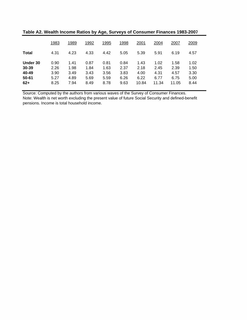
Table A2. Wealth Income Ratios by Age, Surveys of Consumer Finances 1983-2007

1983 1989 1992 1995 1998 2001 2004 2007 2009

Total 4.31 4.23 4.33 4.42 5.05 5.39 5.91 6.19 4.57

Under 30 0.90 1.41 0.87 0.81 0.84 1.43 1.02 1.58 1.0230-39 2.26 1.98 1.84 1.63 2.37 2.18 2.45 2.39 1.5040-49 3.90 3.49 3.43 3.56 3.83 4.00 4.31 4.57 3.3050-61 5.27 4.89 5.69 5.59 6.26 6.22 6.77 6.75 5.0062+ 8.25 7.94 8.49 8.78 9.63 10.84 11.34 11.05 8.44

Source: Computed by the authors from various waves of the Survey of Consumer Finances.Note: Wealth is net worth excluding the present value of future Social Security and defined-benefit pensions. Income is total household income.

RECENT WORKING PAPERS FROM THE CENTER FOR RETIREMENT RESEARCH AT BOSTON COLLEGE

The Asset and Income Profile of Residents in Seniors Care Communities Norma B. Coe and Melissa Boyle, September 2009 Pension Buyouts: What Can We Learn From the UK Experience? Ashby H.B. Monk, September 2009 What Drives Health Care Spending? Can We Know Whether Population Aging is a ‘Red Herring’? Henry J. Aaron, September 2009 Unusual Social Security Claiming Strategies: Costs and Distributional Effects Alicia H. Munnell, Steven A. Sass, Alex Golub-Sass, and Nadia Karamcheva, August 2009 Determinants and Consequences of Moving Decisions for Older Homeowners Esteban Calvo, Kelly Haverstick, and Natalia A. Zhivan, August 2009 The Implications of Declining Retiree Health Insurance Courtney Monk and Alicia H. Munnell, August 2009 Capital Income Taxes With Heterogeneous Discount Rates Peter Diamond and Johannes Spinnewijn, June 2009 Are Age-62/63 Retired Worker Beneficiaries At Risk? Eric R. Kingson and Maria T. Brown, June 2009 Taxes and Pensions Peter Diamond, May 2009 How Much Do Households Really Lose By Claiming Social Security at Age 62? Wei Sun and Anthony Webb, April 2009 Health Care, Health Insurance, and the Relative Income of the Elderly and Nonelderly Gary Burtless and Pavel Svaton, March 2009 Do Health Problems Reduce Consumption at Older Ages? Barbara A. Butrica, Richard W. Johnson, and Gordon B.T. Mermin, March 2009

All working papers are available on the Center for Retirement Research website (http://www.bc.edu/crr) and can be requested by e-mail (crr@bc.edu) or phone (617-552-1762).