arX

iv:1

004.

3382

v1 [

astr

o-ph

.CO

] 20

Apr

201

0

Mon. Not. R. Astron. Soc.000, 1–17 (0000) Printed 21 April 2010 (MN LATEX style file v2.2)

TheUV –Optical Color Dependence of Galaxy Clustering in theLocal Universe.

Yeong-Shang Loh1⋆, R. Michael Rich1, Sebastien Heinis,9 Ryan Scranton13,Ryan P. Mallery1, Samir Salim14, D. Christopher Martin,2 Ted Wyder2, Stephane Arnouts9,Tom A. Barlow2, Karl Forster2, Peter G. Friedman2, Patrick Morrissey2, Susan G. Neff5,David Schiminovich6, Mark Seibert2, Luciana Bianchi7, Jose Donas8,Timothy M. Heckman9, Young-Wook Lee10, Barry F. Madore11, Bruno Milliard8,Alex S. Szalay9, Barry Y. Welsh12 and Suk Young Yi101Department of Physics and Astronomy, University of California, Los Angeles, CA 90095-15622California Institute of Technology,MC 405-47, 1200 East California Boulevard, Pasadena, CA 911253Max-Planck Institut fur Astrophysik, D-85748 Garching, Germany4Institut d’Astrophysique de Paris, CNRS, 98 bis boulevard Arago, F-75014 Paris, France5Laboratory for Astronomy and Solar Physics, NASA Goddard Space Flight Center, Greenbelt, MD 207716Department of Astronomy, Columbia University, New York, NY100277Center for Astrophysical Sciences, The Johns Hopkins University, 3400 N. Charles St., Baltimore, MD 212188Laboratoire d’Astrophysique de Marseille, BP 8, Traverse du Siphon, 13376 Marseille Cedex 12, France9Department of Physics and Astronomy, The Johns Hopkins University, Homewood Campus, Baltimore, MD 2121810Center for Space Astrophysics, Yonsei University, Seoul 120-749, Korea11Space Sciences Laboratory, University of California at Berkeley, 601 Campbell Hall, Berkeley, CA 9472011Observatories of the Carnegie Institution of Washington, 813 Santa Barbara St., Pasadena, CA 9110112Space Sciences Laboratory, University of California at Berkeley, 601 Campbell Hall, Berkeley, CA 9472013Department of Physics and Astronomy, University of Pittsburgh, 3941 OHara St., Pittsburgh, PA 1526014National Optical Astronomy Observatory, 950 North Cherry Avenue, Tucson, AZ 85719

21 April 2010

ABSTRACTWe measure the UV-optical color dependence of galaxy clustering in the local universe. Usingthe clean separation of the red and blue sequences made possible by theNUV − r color-magnitude diagram, we segregate the galaxies into red, blueand intermediate “green” classes.We explore the clustering as a function of this segregation by removing the dependence onluminosity and by excluding edge-on galaxies as a means of a non-model dependent veto ofhighly extincted galaxies. We find thatξ(rp, π) for both red and green galaxies shows strongredshift space distortion on small scales – the “finger-of-God” effect, with green galaxieshaving a lower amplitude than is seen for the red sequence, and the blue sequence showingalmost no distortion. On large scales,ξ(rp, π) for all three samples show the effect of large-scale streaming from coherent infall. On scales1h−1Mpc < rp < 10h−1Mpc, the projectedauto-correlation functionwp(rp) for red and green galaxies fits a power-law with slopeγ ∼

1.93 and amplituder0 ∼ 7.5 and5.3, compared withγ ∼ 1.75 andr0 ∼ 3.9h−1Mpc forblue sequence galaxies. Compared to the clustering of a fiducial L∗ galaxy, the red, green,and blue have a relative bias of1.5, 1.1, and0.9 respectively. Thewp(rp) for blue galaxiesdisplay an increase in convexity at∼ 1h−1 Mpc, with an excess of large scale clustering. Ourresults suggest that the majority of blue galaxies are likely central galaxies in less massivehalos, while red and green galaxies have larger satellite fractions, and preferentially reside invirialized structures. If blue sequence galaxies migrate to the red sequence via processes likemergers or quenching that take them through the green valley, such a transformation may beaccompanied by a change in environment in addition to any change in luminosity and color.

Key words: methods: statistical – galaxies: elliptical and lenticular – galaxies: evolution –galaxies: clusters: general

2 Y.-S. Loh et al.

1 INTRODUCTION

With the advent of the Sloan Digital Sky Survey (SDSS;York etal.2000) and its value added galaxy catalogs, it has been possible tostudy the subject of galaxy bimodality and its relationshipto fun-damental properties, such as stellar mass and star-formation history(e.g., Kauffmann et al. 2004; Schiminovich et al. 2007; Salim et al.2007). The broad division of galaxies into star forming disks andquiescent early type galaxies is the fundamental principleof Hub-ble’s tuning fork system of classification and is well established.In a plot of opticalg − r color vsMr, red galaxies define a clearsequence, while the locus of blue galaxies is broadened intothe so-called ”blue cloud”. The red sequence has been shown to maintainits integrity with look-back time (Bower et al. 1992) and hasgrownin mass since redshift∼ 1. Studies by Bell et al. (2004), Blanton(2006), Faber et al. (2007), and Brown et al. (2008) argue that thestellar mass contained within the red population has increased byroughly a factor of two in half the Hubble time.

A significant breakthrough in expressing this blue/red di-chotomy occurred when photometry from theGalaxy Evolu-tion Explorer (GALEX ), notably the near-ultra violet (NUV )band, was matched with SDSS photometry (Martin et al. 2007;Wyder et al. 2007; Schiminovich et al. 2007; Salim et al. 2007).When the diagram is plotted usingNUV − r as the color, twoclear sequences emerge: the familiar red sequence and a new bluesequence in place of the ”blue cloud” of optical studies. Betweenthe blue and red sequences there are galaxies present in a so-called “green valley”. Many of these are spectroscopicallyclassi-fied Type II active galactic nuclei (Rich et al. 2005; Martin et al.2007; Salim et al. 2007).

Faber et al. (2007), Martin et al. (2007), andSchiminovich et al. (2007) propose several paths by whichgalaxies might transition from the blue to the red sequence.Thepresence of AGN in the green valley suggests that AGN activityis associated with a quenching of star formation (Silk & Rees1998; Hopkins et al. 2006, 2007). Other paths from the blue tothered sequence might, hypothetically, involve gas-rich mergers ofblue galaxies (Toomre & Toomre 1972), or virial shock heatingof cold gas streams (Dekel & Birnboim 2006). The red sequencemight consolidate in luminosity via dissipationless mergers of redgalaxies, or low luminosity blue galaxies might acquire bulgesthrough mergers with starbursts, retaining sufficient massto landthe evolved galaxy on the red sequence. However, the green valleymight also be populated by casual visitors — red galaxies thatacquire gas and form stars or feed a central AGN. Following thisbrief burst of star formation, these galaxies might ultimately returnto the red sequence from which they started.

In Salim et al. (2007), a plot of mass against specific star for-mation rate reveals a clear division between lower mass, star form-ing, blue sequence galaxies, and more massive AGN, which arenotdetected in large numbers until stellar massM ∼ 3 × 1010M⊙.The process responsible for populating the green valley andfor po-tentially contributing to evolution from blue to red must bear somerelationship to environment and to the dark matter halos in whichthe galaxies reside. In this study, we investigate the clustering en-vironment of the blue and red sequences, and for the green valley.

The current paradigm of structure formation assumes thatgalaxies are assembled in dark-matter halos. The dependence ofthe clustering on galaxy properties may provide clues to thebary-onic processes that are important to galaxy formation and evo-lution. The dependence of galaxy clustering on galaxy type hasbeen known since the earliest studies of extragalactic astronomy

(Hubble 1936; Zwicky et al. 1968). In the modern era of large-scale galaxy surveys, Davis & Geller (1976) showed that the an-gular auto-correlation of ellipticals has a steeper power-law slopethat those of spirals. Recent redshift surveys using the Two-Degree Field Galaxy Survey (2dF) and SDSS confirms these ear-lier results and the apparent bimodal nature of galaxy clustering(Madgwick et al. 2003; Budavari et al. 2003; Zehavi et al. 2005;Li et al. 2006a; Wang et al. 2007).

Studies using SDSS have further revealed that galaxy coloris the property most predictive of local environment. Blanton et al.(2005b) found that at fixed luminosity and color, density does notcorrelate with surface brightness nor the Sersic index, andarguethat morphological properties of galaxies are less closelyrelatedto environment than their star-formation history, and are traced bybroadband optical colors. (See Park et al. (2007) for an alternativeanalysis and point of view.) Li et al. (2006a) found that the de-pendence of clustering on opticalg − r color andD4000 is muchstronger than structural parameters like concentration and surfacebrightness, and extend to5h−1 Mpc, beyond what is expected fromthe localized halo paradigm of structure formation. They concludedthat at fixed stellar mass, the clustering properties of the surround-ing dark matter haloes are correlated with the color of the selectedgalaxies. They further argued that different physical processes maybe required to explain environmental trends in star formation, dis-tinct from those established by galaxy structure.

In this paper, we will consider the color dependence of thetwo-point physical correlation function of galaxies usingsamplesconstructed fromGALEX , augmented with redshift and opticaldata from SDSS. In particular, we use the natural separationfromthe NUV − r color to assign galaxies into three subsamples ofred, green and blue galaxies. Our study complements recent workby Heinis et al. (2009) who investigate the physical clustering ofgalaxies as a function of star-formation history in the local universe,as well as earlier studies by Milliard et al. (2007), Heinis et al.(2007) and Basu-Zych et al. (2008) who investigate the angular-correlation function of rest frameUV -selected galaxies and theirevolution. We measure the auto-correlation function each of thedifferent subsamples of galaxies, as well as the cross-correlationfunction between the subsamples. In section 2, we describe in detailthe data used in this analysis. In section 3 we describe the methodfor estimating correlation functions. We present our results in sec-tion 4, and discuss their implications for the nature of green valleygalaxies and the formation of red sequence galaxies. We summarizeour findings in section 6.

2 DATA

2.1 GALEX and SDSS Data

The ultraviolet imaging portion of the data-set is from theGalaxy Evolution Explorer Satellite (GALEX ) that was launchedin 2003 April (Martin et al. 2005; Morrissey et al. 2005, 2007).GALEX obtains wide field imaging in both the far-UV (FUV ;centered at1540A) and the near-UV (NUV , 2300A) over a1.2◦

diameter field of view, with5′′ images. Here we use data fromthe Medium Imaging Survey (MIS); these images are≈ 1500sec in duration reachingNUV ≈ 23 mag, covering an orbitalshadow crossing. The MIS pointing that defines our sample tar-gets the North Galactic Cap, which overlaps the SDSS spectro-scopic footprint; this part of the program was designed fromstud-ies cross-matching SDSS andGALEX data. The data-set used for

UV – Optical Clustering 3

our current analysis is from the Galaxy Release 3 (GR3) whichisavailable from the Multi-mission Archive at STScI (MAST). TheGALEX pipeline uses SExtrator (Bertin & Arnouts 1996) to de-tect sources and measure fluxes. We use the “MAGAUTO” outputfrom SExtrator as our default flux measurement; it is essentially aKron (1980) magnitude with an elliptical aperture.

Because our analysis requires each galaxy to have a spectro-scopic redshift, we start our cross-matching with a galaxy from theSDSS Main spectroscopic survey. For each SDSS galaxy, we searchfor the closestGALEX detection within4′′ radius from the loca-tion of the SDSS spectroscopic fiber. OnlyGALEX sources within0.55◦ of the tile center field-of-view (FOV) are retained, since as-trometry degrades toward the periphery of the FOV (a problemwhich will be resolved in later releases) and the incidence of ar-tifacts increases as well. After the matching ofGALEX and SDSSsources, we further trim the sample to create a statistically completedata-set following the procedure of Wyder et al. (2007). We will re-fer the reader to their table 1 for the full details. Here, we list a fewessential parameters and the minor modifications we employed:14.0 < r < 17.6, 0.03 < z < 0.25, σr < 0.2, zconf > 0.67,GALEX exposure timet > 750s and16.0 < NUV < 23.0.1

All magnitudes are AB magnitudes and corrected for Galacticfore-ground extinction.

2.2 SDSS Large-Scale Structure Sample

Considerable effort has been invested by the SDSS team to preparethe redshift data for large-scale structure studies. This secondarydata-set known as the New York University Value Added Catalog(NYU-VAGC) is documented in Blanton et al. (2005a) and avail-able from the NYU website. Proprietary versions of this cataloguehave been used by many groups within the SDSS collaborationfor various investigations of clustering and luminosity function ofgalaxies. We match theGALEX -SDSS catalog constructed abovewith the SDSS large-scale structure (LSS) DR5 sample. The ver-sion used for our analysis includes all of the detailed radial andangular selection functions for the various statistical subsamplesused in previous analyses (e.g. Zehavi et al. 2005). This sample isideal because we can compare our result with that of Zehavi etal.(2005) which was based solely on selection from optical criteria.

2.3 GALEX –SDSS Overlapping Footprint

In order to statistically define our combinedGALEX –SDSS sur-vey, we need to have the understanding of the angular samplingfunction of the two surveys, which varies across different regions ofthe sky.GALEX ’s Medium Imaging Survey (MIS) survey consistsof overlapping circular tiles (radius0.55◦), while the SDSS spec-troscopic survey is a combination of circular spectroscopic plates,but with fiber placement based on a rectangular imaging survey thatruns along great circles. To combine the footprints of both surveys,we use the GESTALT footprint server. GESTALT2 uses a hier-archical pixelization system, enabling one to encode observationsof arbitrary geometry while tagging information about complete-ness and the masking of artifacts. We first encode theGALEX MISsurvey using GESTALT. We then obtain the detailed observational

1 Our faint-end limit of23.0 is about0.5 mag fainter than those employedby Wyder et al. (2007).2 http://nvogre.phyast.pitt.edu:8080/gestalttutorial/

footprint of the SDSS Large-scale structure sample from theNYU-VAGC website. The SDSS footprint is expressed as a set of dis-joint polygons using the software MANGLE (Hamilton & Tegmark2002) which takes into account the complex angular mask and ge-ometry of the SDSS survey. We convert these polygons into thepixelization scheme of GESTALT and consider the intersectionof the two surveys. There are approximately 490 square deg intheGALEX –SDSS overlapping footprints after masking for holes,bright stars and satellite trails, and excluding defects.

In order to measure the correlation function, a random sampleneeds to be constructed to normalize the galaxy pair counts.Angu-lar sampling completeness as a function of position in the sky en-coded in the footprint server is used to generate random samples ofdensity roughly 50 times the galaxy density. We adopt the methodproposed by Li et al. (2006a) where we assign each galaxy in oursample to a random position on the sky but keep all other attributesthe same (e.g. redshift, color, magnitude). This random sample byconstruction has the same redshift distribution as the original sam-ple, and thus does not smooth out the redshift structure likethosegenerated via the luminosity function. As noted in Li et al. (2006a),this approach works well in surveys with a wide-angular sky cov-erage (e.g. much larger than the typical large-scale structure), andwith small variation in survey depth. We note here that our randomsample would inherit the redshift correlation function of the color-magnitude distribution of the parent galaxy sample, only spatialdistribution has been randomized, hence any excess in clusteringmust be due to positional differences.

In the SDSS spectroscopic survey, no two galaxies with sep-arationθ less than55′′ can both be assigned spectroscopic fibersfor observation on any given observing plate. Hence, a largefrac-tion of galaxy pairs withθ < 55′′ are missing. We correct for this“fiber-collision” problem by using the observed angular correlationfunction, a method first suggested Li et al. (2006a), and describedin detail in the companion paper by Heinis et al. (2009). In brief,the observed projected two-point angular correlation function forboth the photometric samplewph(θ) and the spectroscopic samplewsp(θ) are measured and used to construct the pair weighting ratio:

F (θ) =wph(θ) + 1

wsp(θ) + 1(1)

as a function of separation. Empirically, Heinis et al. (2009) findsF (θ) ∼ 3 for θ < 55′′ and zero otherwise for the allGALEX –SDSS cross-matched galaxies. We apply this correction to each ofthe red, green and blue subsamples equally.

3 METHODOLOGY

3.1 The Two-point Correlation Function

In brief, the two-point auto-correlation functionξ(r) measures theexcess probability of finding a galaxy pair with separationr from arandom galaxy distribution,

dP = n[1 + ξ(r)]dV (2)

wheren is the mean number density of galaxy sample. For thelast forty years, the correlation function has served as thepri-mary method for cosmologists to quantify the clustering proper-ties of galaxies from large scale surveys (Totsuji & Kihara 1969;Peebles 1980). If the underlying density distribution is Gaussian,then the correlation function fully describes all statistical propertiesof a given distribution. Since early cosmological models are oftenbased on primordial Gaussian dark matter density fields, theuse

4 Y.-S. Loh et al.

of the correlation function leads to a straightforward comparisonbetween empirical studies on the statistical distributionof galax-ies with such models. Recently, with the widespread adoption ofa standardΛ-dominated cosmology (Ostriker & Steinhardt 1995;Riess et al. 1998; Perlmutter et al. 1999; Spergel et al. 2007), thecorrelation function is used instead to probe the growth of structurein the universe and the range of formation scenarios for varyingkinds of galaxies.3 The correlation length – the amplitude from apower-law correlation function – provides information on the massof dark-matter halos in which the various galaxies reside, link-ing observation with theoretical description of structureformation(Bower et al. 2006; Croton et al. 2006)

For a galaxy survey with a well-defined angular selectionfunction, ξ can be estimated using an optimal estimator like theLandy & Szalay (1993) estimator:

ξLS =DD − 2DR +RR

RR(3)

whereDD, DR andRR are normalized counts of galaxy pairsin the data-data, data-random and random-random catalogs.4 TheLandy & Szalay (1993) estimator is preferred because it is rela-tively insensitive to the size of the random catalog and to edge cor-rections (Kerscher et al. 2000).

Because we observe galaxies in redshift and projected spaceand not in physical space, in practice, the correlation function isfirst measured on a two-dimensional grid of separations:π alongthe line of sight (redshift space) andrp for angular separation onthe sky. In addition to providing information about the underly-ing mass distribution through the amplitude of the clustering sig-nals, the two-dimensional correlation functionξ(π, rp), containsadditional information about the dynamics of the galaxies (Peebles1980). At small projected separationsrp, random motions withinvirialized over-density (e.g. clusters of galaxies) causes an elonga-tion along the line-of-sight (π direction) known as the “finger-of-God” effect. On large scales, coherent streaming of galaxies intopotential wells causes an apparent compression of structure alongthe line-of-sight (Sargent & Turner 1977; Kaiser 1987; Hamilton1992). Various studies have usedξ(π, rp) to extract cosmologicaland dynamical information (e.g., Tinker 2007).

3.1.1 Real-Space Correlation

Because redshift space distortion only affects the line-of-sight com-ponent ofξ(π, rp), we can recover the true space correlation func-tion ξ(r) by following the standard procedure of computing theprojected correlation function:

wp(rp) = 2

∫ ∞

0

dπξ(rp, π). (4)

In practice, we integrate along the line-of-sight direction out toπ = 30h−1 Mpc. This is large enough to include almost all cor-related pairs but also stable enough to suppress noise from distantuncorrelated pairs. The projected correlation function can in turnbe related to the real space correlation functionξ(r),

wp(rp) = 2

∫ ∞

0

rdrξ(r)(r2 − rp)−1/2. (5)

3 The use of correlation function to probe the growth of structure predatethe advent ofΛ-CDM, especially in the study of faint blue galaxies (e.g.Efstathiou et al. 1991).4 Normalized counts of galaxy pairs are weighted by the selection functionof the galaxies involved.

If the real-space correlation function follows a power-lawξ(r) =(r/r0)

γ , we can infer its parameters: the correlation lengthr0 andthe power-law slopeγ from the best-fit power-law towp(rp) usingthe following deprojection:

wp(rp) = rp

(rpr0

)−γ

Γ

(1

2

)Γ

(γ − 1

2

)/Γ(γ2

). (6)

3.1.2 Cross-correlation

Related to the auto-correlation function is the cross-correlationfunction between two classes of galaxies. The cross-correlationfunction ξ1,2(r), measures the clustering of one type of galaxyaround another.ξ1,2(r) is essentially the probability of finding agalaxies of type 1 around a galaxy of type 2 as a function of sep-arationr. For our analysis, we use the cross-correlation version ofthe classical Davis & Peebles (1983) estimator:

ξ1,2 =D1D2

D1R2− 1 (7)

whereD1D2 are the normalized counts of cross-pairs; whileD1R2

are cross-pairs of type 1 with random galaxies having the sameredshift distributions as galaxies of type 2.

Recently, the cross-correlation function has been used exten-sively in clustering studies of galaxy properties (Zehavi et al. 2005;Wang et al. 2007; Coil et al. 2008; Padmanabhan et al. 2008; Chen2009) since the auto-correlation function alone tells us little abouthow galaxies of various types relate to one another. Two popula-tions of galaxies may both have comparable correlation strength,and yet be physically unrelated if they are spatially segregated.Specifically, the cross-correlation function may be used inconjunc-tion with the auto-correlation functions of the galaxies togleaninformation as to how they mix statistically. For example, if thetwo populations are well mixed, i.e. they are consistent with beingdrawn stochastically from their respective auto-correlation functionequally, their projected cross-correlation functionw1,2

p (rp) wouldfollow that of the geometric mean of their auto-correlationfunc-tions

w1,2p (rp) =

√w1,1

p (rp)w2,2p (rp). (8)

On the other hand, if the populations were segregation between thepopulations and do not distribute evenly in all space, e.g. they siton different halos, the amplitude ofw1,2

p (rp) would be lower than

that ofw1,2p (rp) known in the literature as stochastic anti-bias (e.g.

Blanton 2000; Swanson et al. 2008)

3.1.3 Bootstrap Errors

We estimate the errors for the correlation measurements using amodified bootstrap (Efron 1981) method for spatial statistics knownas marked-point bootstrap (Loh 2008). We first estimate the contri-bution of each galaxy to the correlation function – the marks:

ξi(r) =

n∑

j=1,j 6=i

φ{|xi − xj | ∈ (r − dr, r + dr)} (9)

such that

ξ(r) =n∑

i=1

ξi (10)

wheren is the number of galaxies andφ is the chosen correlationestimator (e.g.ξLS). Hence, the markξi associated with galaxyxi

UV – Optical Clustering 5

is the number of excess pairs at a distantr from xi. Theseξi are(roughly) independent, and identically distributed, and can be usedto replicateB bootstrap samples by the sampling with replacement.An estimate of the correlation functionξ∗j can be computed fromeach of thej-th bootstrap samples. We useB = 999 bootstrapsamples for our analysis. The distribution ofξ∗(ri) can be use toestimate the error bars of the correlation function at each separationri. For an equivalent of one sigma errors, we rankedξ∗(ri) and takethe159nd and840th for the lower and upper error bounds. Becausethe ξ errors for theri are correlated, when we estimate parametersfor the two parameter power-law model (equation 6), we refittedeach bootstrap sample to obtain a two dimension distribution of theparameters.

We chose this method over the conventional jackknife meth-ods because of the fragmented nature of theGALEX –SDSS foot-print. Our bootstrap errors are consistent with the jackknife er-rors estimated by excluding oneGALEX tile at a time. We notehere that jackknife errors are known to overestimate the vari-ance on small-scale, and often bias the overall correlationesti-mates (Norberg et al. 2009). Since bootstrap is a form of internallyestimated errors, and internally estimated errors are known notto reproduce externally estimated errors accurately (Norberg et al.2009), our clustering results should be treated with caution.

4 DEPENDENCE OF CLUSTERING ON UV –OPTICALCOLOR

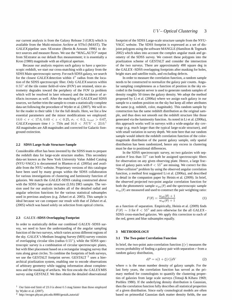
Figure 1 shows theNUV − r color-magnitude diagram (CMD) inthe local universe. All absolute magnitudes arek-corrected usingthe K CORRECT program by Blanton & Roweis (2007) and arequoted in units with Hubble constantH0 = 100h km s−1 Mpc−1

, i.e.Mr ≡ Mr − 5 log(h = 1). Compared with the optical color-magnitude diagram (e.g.g − r vs Mr), theNUV − r color axishas a higher dispersive power. The scatter plot shows two clearsequences: red and blue, and an intermediate “valley” of “green”population. Conventional optical diagrams only display a singlered sequence with an extended blue cloud. Hence, diagnosticdi-agrams like Figure 1 separate galaxies into three natural groupings:(1) a red sequence of bulge-dominated galaxies with old stellarsystems, (2) a blue sequence of star-forming systems consistingof mainly late-type galaxies, and (3) galaxies in a “green valley”that in principle might exhibit transitional properties (Martin et al.2007; Schiminovich et al. 2007). Detailed luminosity functions andphysical properties analysis of these galaxies derived from thisUV –optical CMD has been reported elsewhere (Wyder et al. 2007;Martin et al. 2007; Salim et al. 2007; Schiminovich et al. 2007).Here, we investigate the clustering properties of these three sub-populations of galaxies, separated by the two tilted horizontal lines,using the two-point auto-correlation function, as well as their rela-tion to each other using the cross-correlation function. Our resultsare not sensitive to0.25 mag shift in the oblique equation used toclassify the galaxies.

4.1 Dust

Dust content within each galaxy can modify their broadband col-ors, hence the resultant color-magnitude diagram, as galaxies movefrom one group to another (Martin et al. 2007; Schiminovich et al.2007). This is a concern, as it might affect our estimate of the cor-relation function by either increasing the scatter betweengroups,or bias the result in a systematic but unknown manner. Indeed, a

fraction of the green valley galaxies are dusty star forminggalax-ies whose intrinsic color would have placed them on the blue se-quence in the absence of dust (Wyder et al. 2007). However, theavailable procedures for dust correction are highly uncertain. Theygive inconsistent results depending on whether one uses a primar-ily photometric approach (Salim et al. 2007; Johnson et al. 2006),or one based on spectroscopic indices (Kauffmann et al. 2004).The former, for example, has the side effect of reducing the redsequence number counts substantially (Schiminovich et al.2007;Heinis et al. 2009), while the latter approach requires spectroscopyof modest S/N, which is not available for part of our sample. Acomprehensive analysis of the clustering as a function of star-formation history with a dust-corrected color-magnitude diagramusing the method of Johnson et al. (2006) is done in Heinis et al.(2009).

Here, we adopt a geometric approach. Because dust lanesin galaxies usually appear when viewed edge-on, we can reducethe effect of dust on galaxy color by restricting our analysis togalaxies that are primarily face-on. The middle panel of Figure 1shows the “dust-corrected” color-magnitude diagram obtained byincluding only galaxies with isophotal (minor-over-major) axis ra-tio b/a > 0.6. To the extent that each of the subpopulations havethe same intrinsic distribution ofb/a, removing edge-on galax-ies will give a correct mixture of galaxies that mimic the intrinsiccolor-magnitude distribution. Comparing the dust-corrected CMDwith the CMD on the left panel (hereafter the full distribution),the density of green galaxies aroundMr ∼ −21 is reduced sub-stantially, with the contours showing a more pronounced “valley”separating the sequence of galaxies.

The righthand panel of Figure 1 shows the median ratio ofedge-on (b/a < 0.4) to face-on (b/a > 0.8) as a function of colorand magnitude, with the same density contours from the middlepanel. The region with the highest edge-on/face-on ratio falls inthe green valley and towards the faint end of the luminosity dis-tribution (Choi et al. 2007; Martin et al. 2007; Schiminovich et al.2007). For the galaxies with the magnitude range with−23.5 <Mr < −19.0 used to construct our flux-limited sample, the me-dian b/a for red and blue sequence galaxies are0.73 and 0.72respectively, while for green valley galaxies it is0.66. Choi et al.(2007) find that edge-on galaxies are also statistically fainter dueto the internal extinction, and it affects morphologicallylate-typegalaxies (classified by eye) more than early-type galaxies.Henceby limiting our analysis to face-on galaxies, we would reduce bi-ases associated with differential dimming in addition to the biasesfrom color shifts. Following Choi et al. (2007), we restrictour anal-ysis to galaxies withb/a > 0.6 as a proxy for a galaxy distributionderived from a dust-corrected CMD.

4.2 Luminosity bias

The clustering of galaxies is luminosity dependent. Norberg et al.(2002), Zehavi et al. (2005) and Li et al. (2006a) show that the am-plitude of the projected correlation functionwp increases mono-tonically as a function of luminosity (or stellar mass) on scalesranging from0.2h−1 Mpc to 10h−1 Mpc. In order to study thecolor dependence on clustering, or to compare the clustering in-trinsic to the membership of discrete subpopulations, it isvital toremove this known luminosity dependence. The top two panelsofFigure 2 shows the luminosity distribution of the red, greenandblue population of galaxies withMr < −19 from our flux-limitedsample. The series of dashed histograms (in red, green and blue)show the original luminosity distributions. Blue galaxiesare more

6 Y.-S. Loh et al.

Figure 1.NUV − r vsMr color-magnitude diagram (CMD) of galaxies in the local Universe. The left panel shows the full distribution. The middlepanelshows the distribution drawn from face-on galaxies withb/a > 0.6, used to correct for the effect of dust on the CMD. The right panel shows the distributionof edge-on/face-on ratio overlay onto the CMD contours. Thegreen valley is dominated by region of the CMD with high relative fraction of edge-on galaxies.By limiting ourselve to galaxies withMr < −20.3 (dashed vertical lines) for the volume-limited sample, we also eliminate region of the CMD with thehighest fraction of edge-on galaxies.

numerous and less luminous, on average, compare to red and greengalaxies, reflecting a steeper blue luminosity function at the faint-end (Wyder et al. 2007). To remove this luminosity dependence, weresample the luminosity histograms to match the number countsof the smallest of the three distributions at each magnitudebin.The result of this resampling is shown by the solid histograms.The left panel shows histograms from the full distribution,whilethe right shows those from a dust-corrected distribution. There are4177 (full) and 3148 (dust-corrected) galaxies in each of the resam-pled luminosity distribution of red, green and blue galaxies, with acommon median luminosity ofMr ∼ −21.0, about half a magni-tude brighter thanM∗, the typical luminosity (Blanton et al. 2003).Note that if the fundamental attribute that drive clustering is stellarmass, removing the luminosity dependence like what we have donehere would still leave residual clustering due to the difference inmass-to-light ratio of the respective color selected sample.

4.3 Volume-limited sample

While the resampled red, green and blue galaxies are matchedinluminosity, they are not matched in volume and have differentredshift distributions. This makes the interpretation of the phys-ical correlation function problematic. To this end, we select thelargest possible volume within our catalog, using a redshift cut of0.03 < z < 0.12 and an additional luminosity cut atMr < −20.3to construct a volume-limited sample.5 The luminosity distribu-tions of this sample are shown on the bottom row of Figure 2. Asbefore, the left panel is for the full CMD, while the right panel arefor the dust-corrected (restricted) CMD. Similar to the flux-limitedcase, the (original) blue dashed histograms are substantially differ-ent the red and the green, and are weighted more heavily towardsthe faint-end. We resample the histograms to match in luminosity.Note that in the case, the procedure outlined in section 4.2 essen-tially amounts to looking for an optimal functionW (L) such thatW (L)Φ(L) gives the minimum luminosity function of the three

5 This is not strictly volume-limited sinceNUV is not complete at theseredshifts. An additional weighting is applied using the luminosity functionof Wyder et al. (2007).

subsamples. The new red, green and blue volume-limited subsam-ples each consists of 1971 (full) and 1226 (dust-corrected)galaxieswith a common median luminosity ofMr ∼ 20.9, almost identicalto the flux-limited case.

4.4 Red, Green, Blue Auto-correlation

Figure 3 and 4 shows the two-dimensional auto-correlation func-tion ξ(π, rp) as a function of line-of-sight (π) and projected (rp)separation for the flux-limited and volume-limited samples. Thepanels on the first row in each figure are from the full distribu-tion, while the second row are from the dust-corrected distribution.The panels are for red sequence (left), green valley (middle) andblue sequence (right) galaxies. We have binnedπ andrp linearlyat 1h−1 Mpc. For all panels, the grey scale has the same range,and the contours are boxcar smoothed at2h−1 Mpc. Theξ(π, rp)contours indicate the constant probability of finding pairsat a givenπ andrp. The heavy solid line marksξ(π, rp) = 1, and contoursare spaced with increment (inner) and decrement (outer) by afac-tor of 2. The effect of redshift-space distortion is clearlyseen inall panels, manifested by their departure from isotropy (concentriccircles). At smallrp, the contours are elongated along the line-of-sight (π) due to virial motions of galaxies in clusters. At largerp,the contours are compressed in theπ direction due to the coher-ent large-scale streaming as galaxy infall into potential well. Werecover the results of Zehavi et al. (2005): red sequence galaxiesshow the strongest finger-of-God effect and the larger correlationamplitude; and all three subpopulations (of all samples anddistri-bution) show clear signs of large-scale compression.

We see a clear finger-of-God effect for green valley galaxies,but not for blue sequence galaxies. In Figure 3, if one compares thefirst contour inwards fromξ = 1 (heavy line) for red galaxies tothe ξ = 1 contour of green galaxies, green and red galaxies haveidentical kinematics, differing only by a scaling in the amplitude.The blue sequence appears to have a dynamical structure domi-nated by large-scale streaming distinct from both red and greengalaxies, similar to the optical blue cloud sample of Zehaviet al.(2005). We will consider the implications of this in the discussionbelow. The same conclusion can be drawn from the volume-limited

UV – Optical Clustering 7

Figure 2. The luminosity distribution of our flux-limited (top row) and volume-limited (bottom row) samples. The two panels on theleft are for the fulldistribution, the right is for dust-corrected CMD, using only galaxies withb/a > 0.6. The dashed histograms show the original luminosity distribution foreach of the subsamples of red, green and blue galaxies. We resampled the luminosity to match the number counts of the minimal of the three distribution ateach magnitude bin, shown as solid histograms. Even for the volume-limited samples, the variations in the original luminosity distribution among the threesubsamples are substantial. Blue galaxies are heavily weighted towards the less luminous end compared to red or green galaxies.

sample shown on in Figure 4. The dust-corrected samples (bottomrow) is substantially noisier. We also note that the contours of theblue sequence of the volume-limited full sample (top right panel)are roughly circular for∼ 4 < π, rp < 10h−1 Mpc where thefinger-of-God elongation is balanced by compression due in infall.

Figure 5 and 6 shows the projected correlation functionwp(rp) for the flux-limited and volume-limited samples. The col-ored (red, green, blue) points are the respective measured corre-lation function. The panel on the left (right) is for the full(dust-corrected) distribution. As expected, in all four panels, the red sam-ple has the largest amplitude, the blue the lowest, and greenin be-tween. On large scales (rp & 1h−1 Mpc), the ratio of projectedauto-correlation function of the respective samples are constant asa function of scales, as expected from linear theory. All correlation

functions appear to have a form that is well fit by a broken power-law with the dust-corrected distribution having a more pronounceconvexity. It is noteworthy that the flux-limited analysis (Figure5) is more noisy than the volume-limited analysis (Figure 6), de-spite having a factor of two greater numbers. We believe thatthisis due to the inclusion of uncorrelated (in redshift space) galaxies,which dilute the clustering signal, especially for blue galaxies onsmall scales. From here onwards, we will restrict our analysis tothe volume-limited sample.

When we fit the projected correlation function of the full dis-tribution with the standard two parameter power-law for scalesfrom 1 < rp < 10h−1 Mpc, red and green galaxies appears tohave similar slope withγ ∼ 1.93, while blue galaxies have asubstantially shallower slope, withγ ∼ 1.75. The best fit corre-

8 Y.-S. Loh et al.

Figure 3.Contours and normalized counts of the two-dimensional correlation functionξ(π, rp) for red (left), green (middle) and blue (left) populations for theflux-limited sample. The panels on the top row are for the fulldistribution, bottom row are restricted to face-on galaxies (b/a > 0.6). The contours obtainedafter 2 x 2h−1 Mpc boxcar smoothing. The levels are 0.0 (dotted lines), 0.25, 0.5, 1.0 (heavy lines), 2.0, 4.0, 8.0 and 16.0. Red galaxies have the strongestfinger of God effect (extension in theπ direction). The finger-of-God effect is seen in the green sample as well, while it is not present in the blue. Galaxies inthe green valley appear to have clustering characteristicsof the red sequence.

lation lengthsr0 are7.5h−1 Mpc (red),5.3h−1 Mpc (green), and3.9h−1 Mpc (blue). The result of the covariance analysis using 999bootstrap samples is shown as confidence interval contours –68%(inner) and 95% (outer) in Figure 7 (left panel). These results arein excellent agreement with Heinis et al. (2009). The correlationfunction from the dust-corrected distribution is substantially nois-ier, in part due to the smaller number of galaxies. Applying thesame power-law fit, we obtain a larger uncertainty inγ, but compa-rable uncertainty inr0. This is shown on the right panel of Figure7 and tabulated in Table 1.

On the left panel, the projected correlation function of greengalaxies is evidently intermediate between the red and the blue ona range of scales (0.2 < rp < 6h−1 Mpc), and runs faithfullyparallel with the red correlation function, but with a lowerampli-tude. The picture for the dust-corrected distribution is slightly dif-ferent. While the green still runs in between the red and blueforrp < 1h−1 Mpc and mostly parallel to the red with a lower ampli-tude for broad range of scales, for larger scales (rp & 2h−1 Mpc),it coincides with the blue. This is a consequence of the more promi-nent two-halo excess on large scales seen in the blue correlationfunction.

One way to compare the clustering between subpopulationsof galaxies is through their relative bias (e.g. Norberg et al. 2002),

defined as

bib∗

(r) =

√ξi(r)

ξ∗(r)≃

rγi/20,i

rγ/20

r(γ−γi)/2 (11)

where ξi is the correlation function of interest,ξ∗ is the fidu-cial correlation function that all correlation function iscomparewith. The approximate equality holds when the correlation func-tion takes a power-law form. Zehavi et al. (2005) found that atyp-ical L∗ galaxies in the local universe with−20 < Mr < −21from the SDSS main spectroscopic sample have a fiducial power-law correlation function withξ∗(r) = (r/5h−1 Mpc)−1.8 on scale1 < rp < 10h−1 Mpc. By fitting the correlation function us-ing a constantγ = 1.8 on scales1 < rp < 10h−1 Mpc, weobtained the bias relative atrp = 5h−1 Mpc to a fiducialL∗

galaxies for each of our subpopulations:bred/b∗ = 1.53 ± 0.08,bgreen/b∗ = 1.08 ± 0.06 andbblue/b∗ = 0.81 ± 0.06 for the full-sample, andbred/b∗ = 1.47 ± 0.10, bgreen/b∗ = 1.13 ± 0.09 andbblue/b∗ = 0.92±0.09 for the dust-corrected samples (Table 1). InFigure 8, we plotbi/b∗(r = 5h−1 Mpc) = (r0/5h

−1 Mpc)γ asa function of the co-moving number density and compare our val-ues with those obtained by Zehavi et al. (2005). Co-moving numberdensity of our sample is estimated using the1/Vmax method andfurther corrected to match those obtained by Wyder et al. (2007).While all the samples by construction have almost identicalco-

UV – Optical Clustering 9

Figure 4. Contours and normalized counts of the two-dimensional correlation functionξ(π, rp) for red (left), green (middle) and blue (left) populations forthe volume-limited sample. The panels on the top row are for the full distribution, bottom panels are restricted to face-on galaxies (b/a > 0.6). The contoursobtained after 2 x 2h−1 Mpc boxcar smoothing. The levels are 0.0 (dotted lines), 0.25, 0.5, 1.0 (heavy lines), 2.0, 4.0, 8.0 and 16.0. Red galaxies have thestrongest finger of God effect (extension in theπ direction). Similar to Figure 3, but with lower signal-to-noise, the finger-of-God effect is seen in the greensample as well, while it is not present in the blue.

Figure 5. The projected correlation function,wp(rp), of red sequence, green valley, and blue sequence galaxies for the flux-limited sample. The left (right)panel is from the full (dust-corrected) distribution. Fromred to blue, there is an increase in convexity, with the progressive shallowing of the slope on largescales, indicating an excess of two-halo signals at scale (rp & 1h−1 Mpc).

10 Y.-S. Loh et al.

Figure 6. The projected correlation function,wp(rp), of red sequence, green valley, and blue sequence galaxies for the volume-limited sample. Similarto Figure 5, from red to blue, there is an increase in convexity, with the progressive shallowing if the slope on large scale, indicating an excess of two-halo signals. at scale (rp & 1h−1 Mpc). For the full distribution (left panel), the greenwp(rp) is parallel to the red with a lower amplitude for scales0.2 < rp < 10h−1 Mpc. For the dust-corrected distribution (right panel), the bluewp(rp) approaches the green on large scales.

Figure 7. Confidence contours of the power-law fits towp(rp) on scales1h−1 Mpc < rp < 10h−1 Mpc for the full (left panel) and dust-corrected (right)distributions from the volume-limited sample. The three colors are for red, green and blue subsamples, with the inner (outer) contours encircling the 68 (95)% confidence region in ther0–γ space.

moving density, there is a range of relative bias, with the red hav-ing the highest bias, and blue the lowest. The spread among the biasare much smaller among the dust-corrected samples. Red galaxieshave clustering strength above the nominal strength (inferred froma typical SDSS galaxy) for a given number density. One plausiblescenario suggest that red galaxies have a larger than average satel-lite fraction. On the other hand, blue and green galaxies have lowerobserved number density compare to their clustering. If we assumeall blue and green galaxies are central galaxies in the halo they re-

side in, the lower observed number densities (∼ 0.001h3 Mpc−3)suggest that only a small fraction of these halos, as described bytheir lower bias, host a blue or green galaxy, as their expected num-ber density (inferred from SDSS to be∼ 0.01h3 Mpc−3) is muchhigher. These fractions are increased if the average phasesof greenand blue is shorter then the lifetime of the halos (Haiman & Hui2001; Martini & Weinberg 2001). In the case of the green galaxies,the transitional nature of these galaxies may be closely related tothe AGN they host, or to minor mergers and starbursts, with trig-

UV – Optical Clustering 11

Table 1.Power-law fit to the projected auto-correlation function ofvolume-limited samples (1h−1 Mpc < rp < 10h−1 Mpc)

FULL -SAMPLE N z MEDIAN Mr r0 γ RELATIVE BIAS χ2/dof

Red.......... 1971 (0.03, 0.12) −20.9 7.5± 0.27 1.94 ± 0.07 1.53± 0.08 1.36Green........ 1971 (0.03, 0.12) −20.9 5.3± 0.19 1.93 ± 0.08 1.08± 0.06 0.40Blue......... 1971 (0.03, 0.12) −20.9 3.9± 0.25 1.73 ± 0.10 0.81± 0.06 1.54

FACE-ON

Red.......... 1226 (0.03, 0.12) −20.9 7.6± 0.38 1.81 ± 0.11 1.47± 0.10 2.47Green........ 1226 (0.03, 0.12) −20.9 5.5± 0.24 1.92 ± 0.15 1.13± 0.09 0.48Blue......... 1226 (0.03, 0.12) −20.9 4.6± 0.31 1.74 ± 0.17 0.92± 0.09 1.17

Figure 8. Bias relative to the typicalL∗ galaxy with a ξfid(r) =(r/r0)−1.8 at rp = 5h−1 Mpc versus co-moving number density. Wealso plotted points from SDSS (Zehavi et al.2005). The solidcircles arefrom their luminosity range analysis, i.e. galaxy with absolute magnitudebetweenM1 and M2, while the open circles are from their luminositythreshold analysis, i.e.Mr < Mlim. While far from unique, the higherred bias suggests that on average red galaxies are more likely to be satellitegalaxies then a typical galaxy with those number densities.If we assumethe lower blue and green galaxies are all central galaxies inthe halo theyreside in, the lower observed number densities suggest thatonly a fractionof these halos, as described by their bias, host a blue or green galaxy, astheir expected number density is much higher.

gering cycles corresponding to the duty cycles for these respectivephenomena. We defer a more detail analysis of halo occupation andthe life cycle of transition galaxies using star-formationrate tracersof different lags to a future paper (Heinis et al. in prep.). Usinga theoretical bias function of dark matter halos (Seljak & Warren2004) and normalizing toM∗ = 1012h−1 M⊙

6, red galaxies clus-ter similar to halos with mass∼ 1012.7h−1 M⊙, green galaxies1012.2h−1 M⊙, and blue galaxies1011.6h−1 M⊙.

6 The halo mass that a typicalL∗ galaxy resides in.

4.5 Cross-Correlation Functions

Figure 9 shows the two-dimensionalξ(rp, π) cross-correlationfunction (CCF) for the three cross-pairs of galaxies in our volume-limited sample, with the panels on the top for the full distribu-tion, and the bottom panels for the dust-corrected distribution. Thelarge scale infall effect is seen in all three panels suggesting thatthe galaxies, on average, trace a similar matter distribution as ex-pected from linear theory. On small scales, the finger-of-God ef-fect is strongest for the red-green CCF, intermediate for red-blueand green-blue. In Figure 10 we plot the relative amplitude of ξat the projected distancerp = 1h−1 Mpc as a function of line-of-sight distanceπ. The circles are for green-red cross correlation,squares for red-blue, and triangles for green-blue. Green-red havelargest amplitude for a wide range ofπ, while red-blue and green-blue have smaller amplitudes. The stronger finger-of-god compo-nent suggest that the dynamics of red and green are more stronglycoupled compared with red-blue or green-blue pairs. Note that red-blue CCF have a very differentξ(π, rp) compared with the greenauto-correlation function (ACF), the former has a weaker finger-of-God and stronger infall compression.

As discussed in section 3.1.2, one way to understand the re-lationship between two populations is to compare the projectedcross-correlation function between the two with their geometricmean. If the two populations are mixed evenly, the cross-correlationfunctions should trace the geometric mean. If they are spatial seg-regated (partially) beyond what was expected from their respec-tive auto-correlation function, the cross-correlation function shouldbe systematically below the geometric mean. The projected cross-correlation functions for the red and blue galaxieswr,b

p (rp) areplotted as open circles in Figure 11. Also plotted for comparisonare the red and blue auto-correlation functions (solid lines), andthe red-blue geometric meanwr,b

p (rp) (dashed lines). On scaleslarger than∼ 3h−1 Mpc, thewr,g

p (rp) approaches the geometricmean. For scales0.2 < rp < 2h−1 Mpc, wr,g

p (rp) is systemati-cally below the geometric mean for the full distribution (left panel).For the dust-corrected distribution (right panel),wr,b

p (rp) starts toinch below the geometric mean only fromrp . 0.7h−1 Mpc on-wards. Our results are consistent with the partial morphology seg-regation within galaxy clusters (Dressler 1980). At the one-haloregime (rp . 1 − 3h−1 Mpc), the relevant scales for galaxy clus-ters, red galaxies tend to occupy the cores of the clusters, whileblue galaxies tend to lie towards the periphery. The lower level ofspatial mixing on these scales suppresses amplitude of the cross-correlation function. Note that the green auto-correlation function(green solid line) does trace the red-blue geometric mean onlargescales, suggesting that blue and red galaxies do mix evenly on thesescales.

12 Y.-S. Loh et al.

Figure 9. Contours and normalized counts of the two-dimensional cross-correlation functionξ(π, rp) for red-blue (left), green-red (middle) and green-blue(left) for the volume-limited sample. The panels on the top row are for the full distribution, bottom panels are restricted to face-on galaxies (b/a > 0.6). Thecontours obtained after 2 x 2h−1 Mpc boxcar smoothing. The levels are 0.0 (dotted lines), 0.25, 0.5, 1.0 (heavy lines), 2.0, 4.0, 8.0 and 16.0. The large scaleinfall effect is seen in all three panels. On small scales, the finger-of-God effect is strongest for the red-green, intermediate for red-blue and weakest for green-blue, as expected. Note that red-blue CCFξ(π, rp) has a weaker finger-of-God and stronger infall compression compare to the green valley auto-correlationfunction (Figure 4 middle panels).

Figure 12 shows the projected cross-correlation function be-tween the green and redwg,r

p (rp), and green and bluewg,bp (rp).

The solid green line is the auto-correlation function of thegreensample (wgg

p (rp)), while the dashed lines are the geometric means:

wg,rp (rp) and wg,b

p (rp). For the full distribution (left panel),wg,r

p (rp) is systematically belowwg,rp for a range of scales within

errors.wg,bp (rp) are consistent, or slightly abovewg,b

p (rp) for rp &

1h−1 Mpc, and systematically below for0.3 . rp . 1h−1 Mpc.These inferences are shown more clearly in Figure 13 (left for full,right for dust-corrected), where we plot the normalized cross clus-tering strength – the ratiowg,x

p /wggp , wherex is either red, or blue

– relative to the auto-correlation of the green galaxies. The addi-tional solid lines are the normalized ACF of the red and blue.Thissuggest that red and green are consistent with being drawn from thesame statistical sample on average for a large range of scales witha slight anti-bias on small scales. For the green and blue, there isa stronger anti-bias forr . 1h−1 Mpc as they avoid each otheron these scales. Our results suggest that on scales typical of darkmatter halos, galaxies drawn from the green and blue populationsare less associated than would be predicted by their respective auto-correlation function.

5 DISCUSSION

5.1 Comparison with DEEP2z ∼ 1

The GALEX NUV selected sample used in our analysis is di-rectly comparable to the high redshift (z ≈ 1) galaxy sample ofthe DEEP2 survey (Coil et al. 2008) since their optical selectionmimics the rest-frameNUV . In that paper, clustering analysis wasdone on green valley galaxies for the first time. In their analysis,the green valleyξ(rp, π) appears to display kinematic structureintermediate between red and blue galaxies, with an intermediatefinger-of-God effect and an intermediate overall clustering ampli-tude. When redshift space distortion is removed, the projected cor-relation functionwp(rp) shows a scale dependence convergence.At rp > 1h−1 Mpc the functions converge to those of red popula-tions, while forrp < 1h−1 Mpc it tends toward the clustering ofthe blue population.

In contrast, we find that our green valleyξ(rp, π) has a strongfinger-of-God effect consistent with that measured for red sequencegalaxies, differing only in their amplitude. This can be seen mostclearly in thewp(rp) analysis for the volume-limited sample (Fig-ure 6), where the green function has form similar to that of the redfunction for scales0.2 < rp < 15h−1 Mpc, but is displaced tolower amplitude. It is noteworthy that the slope of the blue cor-

UV – Optical Clustering 13

Figure 11. The projected cross-correlation function between red and blue sequence galaxieswr,bp (rp) are shown as open circles. The solid lines are the

auto-correlation function of the red and blue galaxies. Thedashed line is the red-blue geometric meanwr,bp (rp). On scales larger than∼ 3h−1 Mpc, the

cross-correlation approaches the geometric mean. For scales0.2h−1 Mpc < rp < 2h−1 Mpc, the cross-correlation function is systematically below thegeometric mean. This result suggests that on small scales, blue and red galaxies are spatially segregated beyond what was expected from their auto-correlationfunction. This is consistent with the morphology density relation (Dressler 1980).

Figure 12.The projected cross-correlation function of green sample with bluewg,bp (rp) (blue open circles) and redwg,r

p )(rP ) (red open circles) subsamples.The solid line shows the auto-correlation function of the green sample. The dashed lines are the geometric mean of the green-red (in red) and green-blue (inblue) auto-correlation. On the left (right) we show the analysis from the full (dust-corrected) distribution from the volume-limited sample. (See Figure 13 formore details.)

relation function begins shallowing atr ∼ 1h−1 Mpc, display-ing the kind of one-halo and two-halo segregation expected froma correlation function dominated by central galaxies. In contrast toCoil et al. (2008), the green auto-correlation function converges tothat of the blue atrp > 1h−1 Mpc. We emphasize that the greengalaxy sample of Coil et al. (2008) is defined differently from ours.We divide the CMD into three disjoint parts to separate our galax-

ies into the subpopulations while in Coil et al., the green overlapsboth the red and the blue.

5.2 Green Valley

Many recent studies reveal that blue sequence mass has remainedroughly constant sincez ∼ 1 (Blanton 2006; Faber et al. 2007)

14 Y.-S. Loh et al.

Figure 13. The ratio of projected correlation function (wp(rp)) with the auto-correlation function (wggp (rp)) of the green subsample. The two ratios from

the cross-correlation functions,wg,rp (rp) andwg,b

p (rp), are indicated by colored open circles. Dashed lines are forgeometric means, as in figure 12. The

additional solid lines are ratios from the auto-correlation function of red and blue respectively. The fact that bothwg,rp (rp) andwg,b

p (rp) are below theirrespective geometric mean on small scales suggest that bothred and blue galaxies are found in different environments compared to the green on these scales,albeit with large uncertainties.

Figure 10. This figure shows the relative amplitude ofξ at projected dis-tancerp = 1h−1 Mpc as a function of the line-of-sight distanceπ. Thecircles are for green-red cross correlation, squares for red-blue, and trian-gles for green-blue. Green-red have largest amplitude for awide range ofπ,while red-blue and green-blue have smaller amplitudes. These results sug-gest that the finger-of-god component of green-red cross correlation func-tion is stronger then those from red-blue or green-blue.

because the average ongoing star formation over0 < z . 1 isbalanced by mass flux off the blue sequence, presumably towardsthe build-up of the red sequence sincez ≈ 1 (Bell et al. 2004;Martin et al. 2007). Hence, green valley galaxies occupy a position

where one expect to find many transitional galaxies. Martin et al.also note that the AGN fraction peaks at the green valley. Forourgreen valley definition using the oblique color cuts from Figure 1,the AGN fraction is∼ 50%7.

In their study of AGN using SDSS, Constantin & Vogeley(2006) found that the redshift space two-point correlationfunctionof Seyferts is less clustered than that of LINERS (low-ionizationnuclear emission-line regions). However, Miller et al. (2003) andLi et al. (2006b) found that AGN as a whole cluster similarly astypical L∗ galaxies, if one takes into account luminosity bias.Wang & Kauffmann (2008) argues that almost all galaxies in the lo-cal universe with stellar mass& 10h−1 M⊙ have active nuclei, of-ten LINERS with lines too weak to be detected spectroscopically inSDSS. Our green galaxies, with luminosities peaked atMr ∼ −21,have stellar masses well above10h−1 M⊙, and could be domi-nated by LINERS (either detected or undetected). This wouldinpart explain the clustering effect we see in Figures 3 and 4 (middlepanels) where those bulge-dominated LINERS display kinematicssimilar to red sequence (primarily non-active) galaxies. The rea-son that AGN fromr-band selected survey (e.g. Miller et al. 2003)cluster on average much like typicalL∗ galaxies may merely becoincidental.

The lack of such behavior in thez ∼ 1 green valley (Coil et al.2008) may be attributable to evolution in the AGN population.There may be fewer LINERS, or the red sequence galaxies mayhave been experiencing more gas infall, feeding their AGN. Wenote that with a relative bias∼ 1.1, green galaxies cluster similarlyto a typical galaxy withL∗ − 0.5 ≈ −21, the median luminosityof our sample.

As was discussed in section 4.1, a substantial fraction of the

7 This is a lower limit since the fraction of low luminosity AGNand com-posite objects is unknown.

UV – Optical Clustering 15

galaxies in the green valley are dusty star forming galaxies. Be-cause dust content can modify the color-magnitude diagram weuse to separate the galaxies into red, green and blue populations,this might potentially change the behavior of the correlation func-tion. We argue here that to the extent that dust modifies the numbercounts of green galaxies, it is to promote the migration fromtheblue sequence to the green valley (Choi et al. 2007). Our resultsfrom Figure 4 (for the volume-limited sample) suggest that theirinfluence in modest at best, and merely acts as additional poissonnoise to the two-dimensionalξ(π, rp) without altering the kinemat-ics in the sample. The projected correlation functions of Figure 6show similar characteristics.

5.3 Blue (UV ) vs. Blue (Optical)

In their studies usingg−r color, Zehavi et al. (2005) found that thecorrelation function of blue galaxies exhibits a lower amplitude andshallower correlation functions. By fitting thewp(rp) with halo oc-cupation distribution (HOD) models, they found that the majority(∼ 70 − 90%) of blue galaxies are central galaxies in dark mat-ter halos, usually halos with mass. 1013M⊙, in contrast to onlythe most luminous red galaxies being central objects of massivehalos, while the majority of (less luminous) red galaxies are satel-lites. This fits well with the notion that blue galaxies are field galax-ies – the central objects of low mass halos; red galaxies, with theexception of the central galaxy in clusters and groups, are mostlysatellites of massive halos.

One can infer a similar conclusion from the auto-correlationwp(rp) plot for the blue galaxies (Figure 6). If we decompose thecorrelation function into two parts, one due to the one halo term andthe other due to the two halo term, blue galaxies show strong two-halo excess on scales& 1h−1 Mpc, implying that on those suchscales, the majority of galaxy pairs are from different halos. Thiswas seen in the optical analysis of Zehavi et al. (2005) but promi-nently in our blue sequence sample. For the dust-corrected volume-limited sample (right panel of Figure 6), the amplitude of the auto-correlation function of the blue sample beyond∼ 3h−1 Mpc actu-ally rises to match the clustering strength of the green sample.

Li et al. (2006a) found that the dependence ofwp(rp) on op-tical g − r color extends beyond5h−1 Mpc, suggesting that theconventional wisdom that clustering should converge at large scalesmay not occur until at a scales larger than5h−1 Mpc. Here, we ar-gue that this is an effect due to the mixture of population betweenblue galaxies, and green and red; that the opticalg − r color doesnot have sufficient power to separate the green from the blue.Bluegalaxies, by themselves, have a very pronounced two halo excessand are dominated entirely by central galaxies, flattening the cor-relation function substantially at large scales, comparedto the redand green population. To the extent that one can eliminate orcor-rect for the internal reddening due to dust,NUV − r color is veryefficient in isolating a sequence of purely star-forming galaxies.

6 SUMMARY AND CONCLUSIONS

We have constructed aGALEX and SDSS matched catalog, wherewe have used the GR3 catalog fromGALEX and the SDSS DR5main spectroscopic galaxy sample. We construct the galaxy distri-bution ofNUV − r vs Mr color-magnitude diagram, and dividethe distribution into populations of red sequence, green valley andblue sequence. Since our main goal is to study the color dependenceof clustering, we took substantial care in matching the luminosity

distribution of each population. For each population, we measurethe two-dimensional correlation functionξ(π, rp), and the one-dimensional projected correlation functionwp. We also performcross-correlation analyses between each of the sub-populations.

Our principle finding is that the red sequence and green val-ley appear to show similar clustering properties, as expressed in thefinger-of-God effect in the auto-correlation function. Theprojectedcorrelation function is consistent with red and green galaxies re-siding as satellites of massive halos, while the blue sequence showswhat appears to be a clear two-halo signature, hence primarily serv-ing as central galaxies of less massive halos. The cross-correlationfunction also shows that green and blue galaxies, on small scales,are not a mere statistical mix, but are spatially segregatedfrom eachother.

The findings would appear to place the green valley populationwith the red sequence. The green valley would largely consist ofmassive galaxies that reside in massive halos, and which cluster likethe red sequence. We note that Martin et al. (2007), Wyder et al.(2007), and Salim et al. (2007) show that a large fraction of typeII AGN are found in the green valley. Salim et al. show that in theplot of specific star formation rate vs stellar mass, the AGN tend tobe found in massive (> 3 × 1010M⊙) galaxies. The AGN occupya region in these plots that strongly resembles that of the reddestclass of galaxies, the “no-Hα” red sequence galaxies. Significantly,the AGN are clearly offset from the locus of the blue sequence, inthe plot of specific star-formation rate (SFR) versus mass. The sig-nificance is that while a minority of AGN are found with propertiesthat coincide with those of the more massive blue sequence galax-ies, green valley galaxies – the subsample with the largest AGNfraction — exhibit properties similar to those of the red sequence,but showing mildly elevated star formation.

In this study, we have shown that the green valley populationclusters in ways that are characteristic of, but also less stronglythan, the red sequence. One may suggest that these studies painta picture in which both the properties of the green valley andthe“demographics” are different from those of the blue sequence, atthe present epoch. These findings do not necessarily contradict thestudies that find an increase in the total mass of red sequencegalax-ies sincez ∼ 1. They do suggest, however, that if blue sequencegalaxies evolve by some process to the green valley, and ultimatelyto the red sequence, such evolution must also accompanied byatransition from the field environment to a group/cluster environ-ment. Such a change could conceivably occur if the blue popula-tion resides along filaments that infall into clusters, overtime. Ourcross-correlation results show that green galaxies avoid both redand blue galaxies on small scales is consistent with the changein environment hypothesis. We note that models like ram pres-sure stripping (Gunn & Gott 1972), starvation of (cold) gas,andthe virial shock heating model of (Dekel & Birnboim 2006) nat-urally incorporate environmental factors in their mechanism forcolor transformation in galaxies.

It is also possible that the downsizing (Cowie et al. 1996) ef-fect is so strong that most star forming galaxies are evolving rapidlywith redshift (e.g. Tinsley 1968). One must recall that starformingactivity at z ∼ 1 resides in considerably more massive galaxies,and that a color-based population separation, as we have done, willrefer to much higher masses; the rest-frame colors may be similar,but the fundamental nature of the galaxies, not.

One may speculate that the the green valley is occupied bynominally red galaxies that experience the infall of a gas rich sys-tem that either induces star formation and/or fuels the AGN,ren-dering it visible via its emission lines. However, the feedback of an

16 Y.-S. Loh et al.

AGN might inhibit star formation and move a blue sequence galaxyto the green valley. Any number of environmental effects (e.g. ha-rassment, starvation) might speed the consumption of gas ina disk,again moving a galaxy to the green valley. A small sample of opti-cally quiescent members of the green valley that nominally have aUV excess show clear star formation signatures (spirals) when im-aged in the UV using HST (Salim & Rich 2009). There is still theissue of the origin of the low mass red sequence, and the evolutionof blue sequence, into the green valley and ultimately the red se-quence, might have an important role in the growth of the lowermass portion of the red sequence. This was partially addressedby semi-analytical work of Benson et al. (2003) and Bower et al.(2006).

In contrast to the construction of color-magnitude diagramsfor stellar populations, the environment, for galaxies, isa criticalphysical variable in their evolution. This is true both the in thesense of their dark matter environment as well as the presence ofdetectable companion stellar systems. In considering the major pro-cesses driving galaxy evolution, it would appear that evolution ofboth of these observables must be considered, as a function of look-back time.

ACKNOWLEDGMENTS

Y.S.L. would like to thank C. Hirata, S. Salim, C. Park, J. Kor-mendy and Z. Zheng for helpful discussions. This work has madeextensive use of IDLUTILS8 and Goddard IDL libraries. RMR ac-knowledges support from grant GO-11182 from the Space Tele-scope Science Institute.

GALEX (Galaxy Evolution Explorer) is a NASA Small Ex-plorer, launched in April 2003. We gratefully acknowledge NASA’ssupport for construction, operation, and science analysisfor theGALEX mission, developed in cooperation with the Centre Na-tional dEtudes Spatiales of France and the Korean Ministry of Sci-ence and Technology.

Facilities: GALEX , SDSS

REFERENCES

Basu-Zych, A.R., et al., 2008, submitted to ApJBell, E.F., et al., 2004, ApJ, 608, 752Benson, A.J., et al., 2003, ApJ, 599, 38Bertin, E., & Arnouts, S., 1996, A&AS, 117, 393Blanton, M.R., 2000, ApJ, 544, 63Blanton, M.R., et al., 2003, ApJ, 592, 819Blanton, M.R., et al., 2005, AJ, 129, 2562Blanton, M.R., et al., 2005, ApJ, 629, 143Blanton, M.R., 2006, ApJ, 648, 268Blanton, M.R., & Roweis, S., 2007, AJ, 133, 734Bower, R.G., et al., 1992, MNRAS, 254, 601Bower, R.G., et al., 2006, MNRAS, 370, 645Brown, M.J.I., et al., 2008, ApJ, 682, 937Budavari, T., et al., 2003, ApJ, 595, 59Chen, J., 2009, A&A, 494, 867Choi, Y.-Y., et al., 2007, 658, 884Coil, A.L., et al., 2008, ApJ, 672, 153Constantin, A., & Vogeley, M.S., 2006, ApJ, 650, 727Cowie, L.L, et al., 1996, AJ, 112, 839

8 http://spectro.princeton.edu/idlutils

Croton, D.J., et al., 2006, MNRAS, 365, 11Davis, M., & Geller, M.J., 1976, ApJ, 208, 13Davis, M., & Peebles, P.J.E., 1983, ApJ, 267, 465Davison, A.C., & Hinkley, D.V., 1997, Bootstrap Methods andTheir Applications (Cambridge: Cambridge Univ. Press)

Dekel, A., & Birnboim, Y., 2006, MNRAS, 368, 2Dressler, A., 1980, ApJ, 236, 351Efron, B., 1981, Biometrika, 68, 589Efstathiou, G., et al., 1991, ApJ, 380L, 47Faber, S.M., et al., 2007, ApJ, 665, 265Gunn, J.E., & Gott, J.R., 1972, ApJ, 176, 1Heinis, S., et al., 2007, ApJS, 173, 503Heinis, S., et al., 2009, submitted to ApJHaiman, Z., & Hui, L., 2001, ApJ, 547, 27Hamilton, A.J.S., 1992, ApJ, 385, L5Hamilton, A.J.S., & Tegmark, M., 2002, MNRAS, 330, 506Hopkins, P.F., et al., 2007, ApJS, 163, 1Hopkins, P.F., et al., 2007, ApJ, 659, 976Hubble E.P, et al., 1936, The Realm of the Nebulae (Oxford: Ox-ford Univ. Press), 79

Johnson, B.D., et al., 2006, ApJ, 619, L109Kauffmann, G. et al., 2004, MNRAS, 341, 33Kaiser, N., 1987, MNRAS, 227, 1Kerscher, M., et al., 2000, ApJ, 535, L5Kron, R. G. 1980, ApJS, 43, 305Landy, S.D., & Szalay, A., 1993, ApJ, 412, 64Li, C., et al., 2006a, MNRAS, 368, 21Li, C., et al., 2006b, MNRAS, 373, 457Loh, J.M., 2008, ApJ, 681, 726Madgwick, D.S., et al., 2003, MNRAS, 344, 847Martin, D.C., et al., 2005, ApJ, 619, L1Martin, D.C., et al., 2007, ApJS, 173, 342Martini, P, & Weinberg, D.H., 2001, ApJ, 547, 12Miller, C.J., et al., 2003, ApJ, 597, 142Milliard, B., et al., 2007, ApJS, 173,Morrissey, P., et al., 2005, 619, L7Morrissey, P., et al., 2007, ApJS, 173, 682Norberg, P., et al., 2002, MNRAS, 332, 837Norberg, P., et al., 2009, arXiv:0810.1885v1Ostriker, J.P., & Steinhardt, P.J., 1995, Nature, 377, 600Padmanabhan, N., et al., 2008, arXiv:0802.2105Park, C., et al., 2007, ApJ, 658, 898Peebles, P.J.E., 1980, The Large-scale Structure of the Universe,Princeton Univ. Press

Perlmutter, S., et al., 1999, ApJ, 517, 565Rich, R.M., et al., 2005, ApJ, 619L, 107Salim, S., & Rich, R.M., 2009, BAAS 213, 435.03Riess, A.G., et al., 1998, AJ, 116, 1009Salim, S., et al., 2007, ApJS, 173, 267Sargent, W.L.W., & Turner, E.L., 1977, ApJ, 212, L3Seljak, U., & Warren, M.S., 2004, MNRAS, 355, 129Schinomovich, D., et al., 2007, ApJS, 173, 315Silk, J., & Rees, M.J., 1998, A&A, 331L, 1Swanson, M.E.C., et al., (2008), MNRAS, 387, 1391Spergel, D.N., et al., 2007, ApJS, 170, 377Tinker, J., 2007, MNRAS, 374, 477Tinsley, B.M., 1968, ApJ, 151, 547Toomre, A., & Toomre, J., 1972, ApJ, 178, 623Totsuji, H., & Kihara, T., 1969, PASJ, 21, 221Wang, L., & Kauffmann, G., 2008, MNRAS, 391 785Wang, Y., et al., 2007, ApJ, 664, 609Wyder, T. K., et al.2007, ApJS, 173, 293

UV – Optical Clustering 17

York D. et al., 2000, AJ, 120, 1579Zehavi, I., et al., 2005, ApJ, 630, 1Zwicky, F., et al., 1968, Catalog of Galaxies and of ClustersofGalaxies, Vols. 1 – 6 (Pasadena, Caltech)