FORESTRY IDEAS, 2010, vol. 16, No 2 (40)

THE USEFULNESS OF TIME SERIES ANGLE-COUNT FOREST INVENTORY DATA IN ASSESSING FOREST

GROWTH MODEL ACCURACY

Chris Stuart Eastaugh and Hubert Hasenauer

Universität für Bodenkultur (BOKU) Institute of Silviculture. Peter Jordan Strasse 82, A-1190 Vienna, Austria. E-mail: cseastaugh@yahoo.com.au

UDC 630.6 Received: 13 May 2010Accepted: 26 May 2011

AbstractForest policy and forest carbon accounting systems must be underpinned by appropriate-

ly accurate information, yet such information is often difficult and expensive to collect. This has led to the promotion of more cost-efficient forest sampling methodologies, and to the rise of modeling as a means to predict or interpolate changes to forest conditions in response to various stimuli. The accuracy of such modeling is usually determined through comparison with field data, often collected at a relatively limited number of sites.

Large bodies of relevant forest data are collected in National Forest Inventories, but there are inherent methodological problems in using this NFI data for model validation, particularly if such data is collected using angle-count sampling. Angle-count sampling has the advan-tage of being a relatively fast and cheap method of collecting forest data, but it is generally considered that at least four samples should be taken at a site for the results to be usefully precise. Some NFIs however take only a single angle-count sample at each fixed sampling point. Although at a broad scale these results may give useful figures, their usefulness at the plot scale is severely limited, especially if the intent is to judge plot timber volume increments or prepare forest carbon budgets. The availability of a time series does however allow for some statistical correction to single angle-count estimations. This study demonstrates the statistical uncertainties in using angle-count time series, and develops a method of reducing such 0 to a level that angle-count NFI data may be usefully used for comparisons with forest models.

Key words: carbon accounting, carbon budgets, sampling, statistics.

Introduction

Rising interest in forest carbon ac-counting has led to a renewed interest in forest inventories and forest process modelling as a means to accurately as-sess carbon stocks, both as presently existing and under a range of future

scenarios. Although process model-ling shows great promise in being able to track changes to ecosystem car-bon stocks and fluxes in response to various stimuli, there is always a need for modelling to be properly validated against field data to give confidence in results. Model validation often relies on

C.S. Eastaugh and H. Hasenauer172

a relatively small number of experimen-tal plots.

Large bodies of forest growth data are available in many countries, through the various National Forest Inventories (Tomppo et al. 2010). Inventories how-ever are designed to aggregate samples taken at many points to give accurate in-formation at large scales, whereas proc-ess modelling aims to accurately simu-late single stands based on point-specific input information. Although at the large scale aggregated results found with either method should be similar, this is not ad-equate for validating model performance as model errors in some areas may be masked by opposing errors elsewhere in the aggregated dataset. This problem is compounded in the case of inventories that use more sophisticated sampling techniques such as angle-count sampling.

Angle count sampling for efficiently estimating forest stocks was developed in Austria by Bitterlich (1947, 1984), and popularised in North America by Grosen-baugh (1952). The method is now well known to practicing foresters across most of the world, and if properly per-formed has been proven to give unbiased estimates of stand basal areas in timber cruising operations (Palley and Horwitz 1961). Recently however angle-count sampling has also become an integral part of some National Forest Inventories (i.e. Austria (Gabler and Schadauer 2006) and Germany (Kändler 2006)). Since the late 1950s three methods have been de-veloped for calculating increments from successive angle count samples: the Dif-ference method, the Starting Value meth-od and the End Value method (Shieler 1997). These were attributed by Hradetz-ky (1995) to Van Deusen et al. (1986), Grosenbaugh (1958) and Roesch et al.

(1989). In the case of Austria, a single angle-count sample is taken at each cor-ner of a 200 m square, with these squares located on a systematic grid of 3.889 km resolution over all forested land.

The volume (V) of a single tree is a function of basal area (g). Common al-lometrics such as those of Pollanschütz (1974) multiply g by height (h) and a shape-dependant form factor (f).

fhgV TREE **= Equation 1

In order to determine volume per hectare, the number of trees per hectare must be estimated. Angle-count meth-odology relies on the fact that each tree counted in the sample may be taken to represent a fixed number of trees per hectare (nrep). The nrep for each tree sampled is estimated as the basal area factor (K) used in the sampling divided by the basal area of the tree.

i

i gKnrep = Equation 2

The volume per hectare is then:

∑=

=sampledtreesalli

iiPLOT nrepVV

__

* Equation 3

Difference method

Using the Difference method to calculate increment, the growth between time 1 (t1) and time 2 (t2) is simply the difference between the volumes at the two periods plus any removals due to harvesting or mortality.

removalsVVGrowth PLOTt

PLOTt +−= 12 Equation 4

The shortcoming of the Difference method is apparent from an examination of equations 2 and 3. As trees grow g increases, but this increase in growth (which should contribute to an increase in VPLOT) is offset by an equivalent fall

The Usefulness of Time Series... 173

in nrep. Observed growth with the dif-ference method can only come from in-creases in h, or increases in i (that is, when new trees are added to the sample between t1 and t2). If no new trees are added to the sample then the calculated increment will be an underestimation, whereas if many new trees are added (due to the random physical location of the trees in the plot), then the method may considerably overestimate growth.

Starting value method

The Starting Value method avoids the problem of new trees introducing high variance into increment calculations by keeping nrepi constant between time peri-ods, and ignoring any increases in i. Thus:

1,1,2,

tititi g

BAFnrepnrep ==

Equation 5New trees in the second sample pe-

riod may be either ingrowth (I) or non-growth, depending on whether they were under or over a particular dbh threshold in the first period. Ingrowth are trees that are newly present in the sample at t2 that were effectively not present in the stand at t1. If the dbh threshold is greater than zero then in-growth must be further differentiated into ingrowth or ongrowth (cf Martin 1982), but this complication is not rel-evant to our discussion here.

( ) ∑∑ ++−==

IremovalsnrepVVGrowthsamplesbothinpresenttreesi

iTREEti

TREEti

____

1,2, *

( ) ∑∑ ++−==

IremovalsnrepVVGrowthsamplesbothinpresenttreesi

iTREEti

TREEti

____

1,2, * Equation 6

With this method, Vt2PLOT ≠ Vt1

PLOT + +Growth + removals. Because nrepi is constant between measurements, any random variation in g is greatly ampli-

fied when upscaling to the per hectare values.

End value method

The End Value method also keeps nrepi constant between time periods, but uses the nrepi values from the second time period:

2,1,2,

tititi g

BAFnrepnrep == Equation 7

( ) ∑∑ ++−==

IremovalsnrepVVGrowthsampleondtheinpresenttreesi

iTREEti

TREEti

_sec___

1,2, *

( ) ∑∑ ++−==

IremovalsnrepVVGrowthsampleondtheinpresenttreesi

iTREEti

TREEti

_sec___

1,2, * Equation 8

This method also results in an incre-ment estimate that is not necessarily equal to the change in estimated vol-ume. There are some theoretical im-provements in variance because of the larger number of trees used to estimate nrep, but to some extent this is offset by the need to estimate the t1 basal area of trees that only entered the sam-ple in t2.

Either of the latter two of these methods are currently preferred, due to a lower variance in increment results (Hradetzky 1995). Recent work how-ever (Eastaugh and Hasenauer 2011) points to possible bias in results from the Starting Value and End Value meth-ods, hence our efforts will focus on the Difference method.

We use a case study example to in-vestigate the range of error in timber growth increments estimated by apply-ing the Difference method to time-series of single angle-count samples, and de-velop a correction method that signifi-cantly reduces the variance on single points. Our purpose is to demonstrate that the errors in Difference method in-

C.S. Eastaugh and H. Hasenauer174

crement calculations applied to single points are not completely random, but are correlated with the number of new trees that enter the sample at the sub-sequent inventory. By estimating this systemic error we are able to apply a simple correction to increment results, achieving substantially reduced vari-ance than the original. As an example of the benefits of the improvement, we show how the corrected results may be

used to better test the accuracy of a forest growth model.

Data and Methods

23 fixed-area research plots were estab-lished in a spruce/pine forest at Litschau (northern Austria) in 1977, and have been remeasured each 5th year since that time. This study uses plot number 10, which

Fig. 1. Permanent research plot No 10 at Litschau, in 1977. Green circles are an exaggerated representation of tree diameter (1.3 to 32.1 cm), red diamonds show the

centre-points of the 5 simulated angle-count samples.

The Usefulness of Time Series... 175

is predominantly spruce and formed part of the validation dataset for the biogeo-chemical process model BIOME BGC (Pietsch et al. 2005). The plot is 486 m2, and in 1977 consisted of a range of tree sizes up to 32.1cm (Fig. 1).

In each measurement period, all trees on the plot are measured for height and diameter at breast height (dbh), and their location coordinates recorded. This al-lows us to reconstruct the stand as it ap-peared in each measurement period, and determine what an angle count sample from any point would have measured, if such a sample had been made. As shown in figure 1, we simulate an angle-count sample at the geometric centre of the plot, and five metres in each cardinal di-rection from that centre. Given the range of tree sizes on the plot, none of these samples (in any time period) overlaps the fixed-area plot boundary. Tree volumes are calculated based on dbh, height and a form factor according to parameters determined by Pollanschütz (1974).

Process modelling with BIOME BGC (Thornton 1998) is performed using in-

put criteria from internal plot documen-tation, species parameters from Pietsch et al. (2005) and interpolated DAYMET daily climate data (Petritsch 2002). The model gives results in terms of kilo-grams of stem carbon per square me-tre, which are then converted to timber volume according to biomass expansion factors from Pietsch et al. (2005).

Standing volume estimates for 1977 taken from the fixed-area plot data, sim-ulated angle-count sampling and model-ling are shown in figure 2.

An indicative range of the estimate variability from the Difference method (derived from the Litschau plot 10 data) is shown in figure 3. More formal dis-cussions of Difference method variance may be found in Palley and Horwitz (1961), Van Deusen (1986) and Hra-detzky (1995).

Correction method

The Correction method developed here relies on the fact that the error in the Difference method is due mainly to the

Fig. 2. Individual angle counts are poor estimates of stand volume. Aggregation of angle-counts is necessary to produce a reasonable estimate of stand volume.

C.S. Eastaugh and H. Hasenauer176

(largely random) chance of new trees entering the sample in t2. This informa-tion is extractable from standard angle-count records, and so the component of the error that is due to this chance is to some extent correctable.

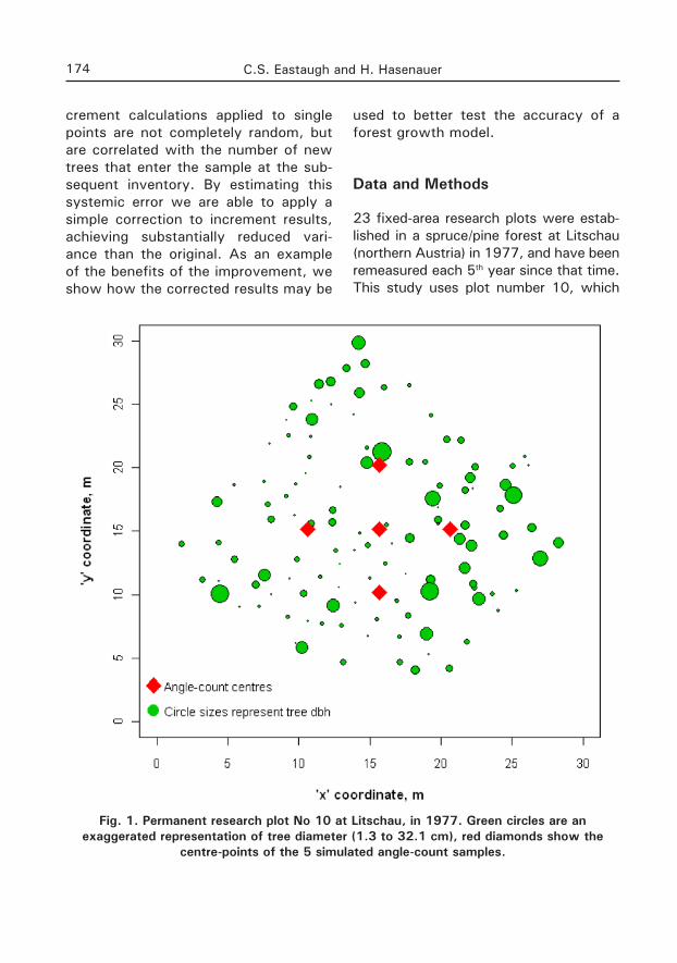
The error in Difference method es-timates is strongly correlated to the number of new trees entering the sam-ple in the subsequent measurement pe-riod (Fig. 5). Although the function of the regression in figure 4 is drawn from empirical data, it is possible to estimate this function through determining the ‘x’ intercept and the slope directly from measured data at any individual angle-count point.

The ‘x’ intercept of the error func-tion in figure 5 represents the point where the Difference method will accu-rately estimate the stand growth (error = 0). This represents the point where the number of trees entering a sample between measurement periods is equal to the true growth increment of the stand. As angle-counts are an unbiased estimate of stand volume, this point

may be approximated by the mean number of new trees entering a stand, averaged over either time or space (assuming that we average within a reasonably homogenous space). The slope of the error function matches the mean volume per hectare represented by a new tree added to the sample. Correcting the Difference method val-ues involves adding or subtracting the estimated error derived from the error function, according to the number of new trees added.

Results

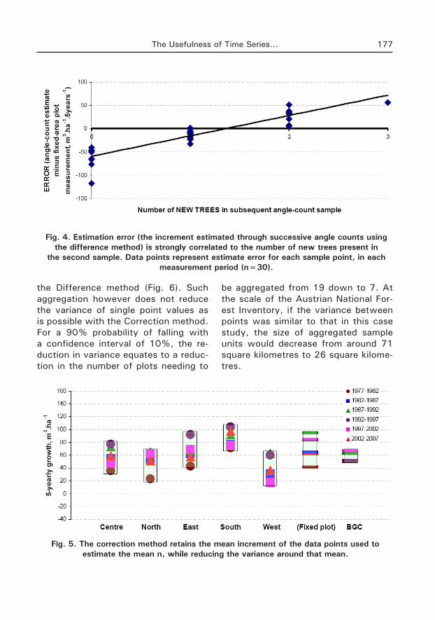
Applying the Correction method based only on information available from one point retains the mean for that point, but allows the variation around the mean for that point to be considerably reduced (Fig 5, compare with Fig. 3).

If, as in this example, all points may validly be aggregated in space, then less (but still some) improvement is gained over aggregating results from

Fig. 3. Range of variation in increments calculated according to the Difference method.

The Usefulness of Time Series... 177

the Difference method (Fig. 6). Such aggregation however does not reduce the variance of single point values as is possible with the Correction method. For a 90% probability of falling with a confidence interval of 10%, the re-duction in variance equates to a reduc-tion in the number of plots needing to

be aggregated from 19 down to 7. At the scale of the Austrian National For-est Inventory, if the variance between points was similar to that in this case study, the size of aggregated sample units would decrease from around 71 square kilometres to 26 square kilome-tres.

Fig. 4. Estimation error (the increment estimated through successive angle counts using the difference method) is strongly correlated to the number of new trees present in

the second sample. Data points represent estimate error for each sample point, in each measurement period (n=30).

Fig. 5. The correction method retains the mean increment of the data points used to estimate the mean n, while reducing the variance around that mean.

C.S. Eastaugh and H. Hasenauer178

Discussion

Although the example here used only a small number of points, the relation-ship between the estimate error of in-crements derived from the Difference method with the number of new trees entering a sample is clear, and may be seen in larger datasets (in development).

The error behaviour of the Difference method is a well-known problem, and most forest agencies avoid it by using either the Starting Value method or the End Value method. Van Deusen et al. (1986) demonstrated that each of these three methods are theoretically unbiased estimators of volume increment but did not account for the errors that are inevi-tably part of any forest inventory. Re-cent work on large datasets (Eastaugh and Hasenauer 2011) has shown that the Starting Value and End Value meth-ods introduce a positive bias into incre-ment estimates due to the propagation of measurement errors. The Difference method is more resistant to these biases.

The Correction method outlined here relies on the spatial and temporal auto-correlation that will be present among groups of sample points. In the simple example presented here spatial and temporal autocorrelations are weighted equally (through deriving the slope and intercept of the error function using all available samples), but greater improve-ment could perhaps be obtained through applying different weighs to the spatial and temporal components, depending on the variance present in their respec-tive dimensions.

Determining the population from which to derive the mean number of new trees added is a question of ho-mogeneity. In the example above the 5 sample points are clearly drawn from the same stand (being all within a 5 me-tre radius), but some caution must be taken if the parameters of the correction function were to be drawn from a more diverse sample set. As the ‘x’ intercept represents the mean basal area incre-ment of the stand divided by the basal

Fig. 6. Forest growth averaged across five sample sites within a 5 metre radius, in each measurement period. Error bars show one standard deviation above and below the mean

for each period.

The Usefulness of Time Series... 179

area factor, the mean number of trees should be drawn from sample popula-tions that could be expected to show similar growth characteristics. These are however the same issues that must be faced when determining the appro-priate level of stratification and aggre-gation of uncorrected samples.

Conclusions

Errors arising from the difference meth-od are largely systemic rather than fully random, and are thus partly correctable. The correction method developed here retains the same mean as groups of es-timates made with the difference meth-od, but removes the systemic error com-ponent. Random error will of course still be apparent in results, but the reduction in variance allows for smaller scale ag-gregations of angle count data to meet particular precision requirements.

Although this paper is not intended to be a formal proof of the general ap-plicability of our proposed increment correction procedure, we believe that the corrected difference method will provide more precise estimates of incre-ment from time-series of angle-count data than the uncorrected Difference method, without the biasing effects of currently used alternatives. An unbiased method with reduced variance will be a better basis for comparisons with proc-ess model results.

References

Bitterlich W. 1947. Die Winkelzahlmes sung (Measurement of basal area per hec-tare by means of angle measurement).

Allgemeine Forst- und Holzwirtschaftliche Zeitung 58: 94–96.

Bitterlich W. 1984. The Relascope Idea: Relative Measurements in Forestry. Commonwealth Agricultural Bureau: Slough, England.

Eastaugh C.S., Hasenauer H. 2011. Bias in volume increment estimates derived from successive angle-count sampling. (submitted).

Gabler K., Schadauer K. 2006. Methoden der Österreichischen Waldinventur 2000/02. Grundlagen, Entwicklung, Design, Daten, Modelle, Auswertung und Fehlerrechnung. BFW-Berichte 135: 1–6.

Grosenbaugh L.R. 1952. Plotless Timber Estimates-New, Fast, Easy. Journal of Forestry 50: 32–37.

Grosenbaugh L.R. 1958. Point-sampling and line-sampling: probability theory, geo-metric implications, synthesis. USDA Forest Service South Forest Experimental Station Occasional Paper 160, 34 p.

Hradetzky J. 1995. Concerning the pre-cision of growth estimation using permanent horizontal point samples. Forest Ecology and Management 71: 203–210.

Kändler G. 2006. The Design of the Second German National Forest Inventory. In: McRoberts, Ronald E.; Reams, Gregory A.; Van Deusen, Paul C.; McWilliams, William H., eds. 2009. Proceedings of the eighth annual forest inventory and analysis sym-posium, 2006. October 16–19; Monterey, CA. Gen. Tech. Report WO-79. Washington, DC: U.S. Department of Agriculture, Forest Service, 408 p.

Martin G.L. 1982. A method for estimat-ing ingrowth on permanent horizontal sample points. Forest Science, 28: 110–114.

Palley M.N., Horwitz L.G. 1961. Properties of some random and systematic point sampling estimators. Forest Science 5 (1): 53–65.

Petritsch R. 2002. Anwendung und Validierung des Klimainterpolationsmodells DAYMET in Öesterreich. Diploma thesis, University of Natural Resources and Applied Life Sciences Vienna.

C.S. Eastaugh and H. Hasenauer180

Pietsch S.A., Hasenauer H., Thornton P.E. 2005. BGC-model parameters for tree species growing in central European forests. Forest Ecology and Management 211: 264–295.

Pollanschütz J. 1974. Formzahlfunktionen der Hauptbaumarten Österreichs. Allgemeine Forstzeitung 85: 341–343.

Roesch F.A., Green E.J., Scott C.T. 1989. New compatible basal area and number of tree estimators from remeasured horizontal point samples. Forest Science 35: 281–293.

Schieler K. 1997. Methode der Zuwachsberechnung der Österreichischen Waldinventur. Dissertation, University of

Natural Resources and Applied Life Sciences Vienna.

Thornton P.E. 1998. Description of a nu-merical simulation model for predicting the dynamics of energy, water carbon and nitro-gen in a terrestrial ecosystem. PhD thesis, University of Montana, Missoula.

Tomppo E., Gschwantner T., Lawrence M., McRoberts R.E. 2010. (eds) National Forest Inventories: Pathways for common reporting. Springer, Berlin.

Van Deusen P., Dell T.R., Thomas C.E. 1986. Volume growth estimation from per-manent horizontal plots. Forest Science 32 (2): 415–432.