Working Paper SeriesHealth Economics Series No. 2016-05

The Upside-down Economics of Regulated andOtherwise Rigid Prices

Casey B. Mulligan and Kevin K. Tsui

August 5, 2016

Keywords: health economics, health sector, price regulations, quality-quantitytradeoffs

JEL Codes: I1, I11, I18

Becker Friedman Institute for Research in Economics

Contact:773.702.5599

bf @ uchicago . edubf . uchicago . edu

NBER WORKING PAPER SERIES

THE UPSIDE-DOWN ECONOMICS OF REGULATED AND OTHERWISE RIGIDPRICES

Casey B. MulliganKevin K. Tsui

Working Paper 22305http://www.nber.org/papers/w22305

NATIONAL BUREAU OF ECONOMIC RESEARCH1050 Massachusetts Avenue

Cambridge, MA 02138June 2016

We appreciate discussions with Bill Dougan, Al Harberger, Robert Jackman, Alex MacKay, Kevin M. Murphy, Glen Weyl, seminar participants at Chicago, Clemson, and the financial support of the University of Chicago’s Stigler Center and the Thomas W. Smith Foundation. The views expressed herein are those of the authors and do not necessarily reflect the views of the National Bureau of Economic Research.

NBER working papers are circulated for discussion and comment purposes. They have not been peer-reviewed or been subject to the review by the NBER Board of Directors that accompanies official NBER publications.

© 2016 by Casey B. Mulligan and Kevin K. Tsui. All rights reserved. Short sections of text, not to exceed two paragraphs, may be quoted without explicit permission provided that full credit, including © notice, is given to the source.

The Upside-down Economics of Regulated and Otherwise Rigid PricesCasey B. Mulligan and Kevin K. TsuiNBER Working Paper No. 22305June 2016JEL No. K2,L15,L51

ABSTRACT

A version of the Becker-Lancaster characteristics model featuring quality-quantity tradeoffs reveals a number of surprising market behaviors that can result from price regulations that are imposed on competitive markets for products that have adjustable non-price attributes. Quality need not clear a competitive market in the same way that prices do, because quality can reduce the willingness to pay for quantity. Producers can benefit from price ceilings, at the expense of consumers. Price ceilings can result in quality-degradation “death spirals” that would not occur under quality regulation or excise taxation. The features of tastes and technology that lead to such outcomes are summarized with pairwise comparisons of (not necessarily constant) elasticities.

Casey B. MulliganUniversity of ChicagoDepartment of Economics1126 East 59th StreetChicago, IL 60637and NBERc-mulligan@uchicago.edu

Kevin K. TsuiSirrine HallClemson, SC 29634ktsui@clemson.edu

1

Although not always highly visible outside of Communist countries, price

regulations apply to a large fraction of economic transactions, even in the United States.

There are, of course, controls on apartment rents and taxi fares in major cities, and

minimum wages for low-skill workers. A number of states regulate interest rates on

loans with usury laws and the federal government regulates interest and insurance rates

with redlining prohibitions and antidiscrimination rules. Basic telephone and cable TV

rates are regulated. Outside the state of Nevada, the price of sex is legislated to be zero.

Price controls are the norm in the health sector, which by itself is already a sixth of the

U.S. economy. Much modern research on business cycles features “sticky” prices, and

the technology sector includes several markets with natural constraints on monetary

prices (Lanier 2014): these are not exactly regulated prices but potentially share many of

their economic characteristics.1

The textbook model of price ceilings says that binding ceilings reduce

expenditure and the quantity traded in competitive markets, primarily by queuing or a

random allocation mechanism. Price ceilings are supposed to benefit buyers, especially if

the ceiling is not too far from the unregulated price.2 These results are special, and

misleading as to the economic mechanisms that might deliver them.

Following Cheung (1974), Murphy (1980), Leffler (1982), Raymon (1983),

Barzel (1997), and Ippolito (2003), we assume that, although a price regulation prohibits

competition on price, other forms of competition among buyers are not necessarily

prohibited.3 Practically all goods and services have non-price dimensions (hereafter,

“quality”) that can be and are distorted by a binding price ceiling. The quality

dimensions include the time, place, or pleasantness of delivery. It could be the durability

or reliability of the product, or the number of advertisements attached to it. Or the

amount of customers’ time that is required to acquire, finish, maintain, or consume the

1 The degree of price stickiness can also be affected by regulation. For instance, item-pricing laws

increase menu costs of changing prices, and result in less frequent price adjustments (Levy, et al.

1997). Unregulated industries with sticky prices may also have different cost structures than industries with regulated prices (Telser 2009). 2 See, for example, Lee and Saez (2012) and Bulow and Klemperer (2012) for recent citations of

this result, and possible qualifications of it. 3 See also Telser (1960) who explains self-imposed pricing restrictions on the basis of non-price

competition.

2

good. Or the size of the package. Quality responses to price ceilings help suppliers be

compliant with the regulation.

There is considerable scope for adjustment of non-price attributes that would

permit a regulated market to comply with a price ceiling without necessarily supplying

less quantity because sellers spend considerable amounts as they attempt to make their

product more attractive to buyers. Take apartments, for which it is sometimes said that

the purchase price of land and structure equals the expected present value of the rental

income to be received from tenants. In fact, about half of the revenues obtained from

tenants is spent on short-run variable inputs rather than financing the structure’s purchase

or initial construction. Figure 1 shows the claims on national tenant-occupied housing

output for 2006, as reported by Mayerhauser and Reinsdorf (2007). Almost half of

housing output went to intermediate goods and services (e.g., realtor and advertising

activities) and depreciation (a proxy for normal repairs and maintenance). Another five

percent went to labor (largely management), and about three percent went to compensate

landlords for holding vacant units. Landlords could adjust any of these items in order to

reduce the ratio of costs to revenue.4

When non-price product attributes are adjustable, the impacts of a ceiling on

quantity, quality, and the surplus of buyers and sellers have little to do with the supply

and demand for the controlled good by comparison to not having/producing the good at

all. On the demand side, it is not the same when price falls by regulation as when it

changes due to a reduction in the marginal costs of producing the services delivered by

the controlled good. On the supply side, it is not the same when price falls by regulation

as when it falls due to a reduction in the buyers’ marginal willingness to pay for the

services delivered by the controlled good. Even when the curves are properly adjusted to

reflect changes in non-price attributes, the usual supply and demand diagram is not

4 Also note that costs can, in effect, be negative. This was typically the case in the market for

broadcast radio programming, where listeners paid no money but tolerated advertisements, which

allowed broadcasters to cover their costs. The zero price for broadcast radio programming was

set by technology rather than regulator or statute, but the example illustrates how an industry can

function and competition occur without sellers’ covering their costs exclusively from customer revenues.

3

suitable for welfare analysis. These are our primary disagreements with textbook

treatments of price controls, and begin to indicate why our results are so different.5

A price ceiling in a competitive market might increase the quantity sold because

there is a quality-quantity tradeoff.6 Holding expenditure constant, a ceiling prohibits

low quantities. Take, for example, retail fruit and vegetable sales. Absent regulations,

suppliers spend resources to preserve, cull, and promptly deliver their produce

inventories so that the consumer receives fresh items. With a price ceiling set on, say, a

per-ounce basis, suppliers cut down on their quality-enhancing expenditures and thereby

reduce the fraction of the produce obtained by the consumer that is edible. Consumers

with a price-inelastic demand for edible produce purchase more total produce because the

survival rate of purchased produce is reduced by the price ceiling. A variety of goods

from apartments to light bulbs to doctor appointments have this feature that the

unregulated market serves customers with less, but more expensive, quantity because that

quantity is efficiently managed to provide the maximum value for the customer’s dollar.

Our model does not assume that controlled goods necessarily have such ease of

substitution between quality and quantity, but these examples begin to show why the

textbook predictions may not be reliable.

To the extent that supply slopes up, producers tend to benefit, relative to the

unregulated allocation, from the increase in quantity and lose from the reduction in

quality. Indeed, we find a simple supply-elasticity condition that indicates whether a

price ceiling net redistributes from consumers to producers, or vice versa. For some of

the same reasons, the possibility for producer gains is still present even when the

equilibrium quantity impact of a price ceiling is not positive.

Many studies before ours have noted that regulated or rigid prices can result in

less quality as buyers compete by accepting less of the non-price attributes. Economist

and experienced price regulator John Kenneth Galbraith (1980) explained why regulators

5 On the geometry of, and conclusions regarding, market surplus, we also disagree with Spence

(1975), Frech and Samprone (1980), Ippolito (2003), and others. See Section IV below. 6 Murphy (1980) concludes that a price ceiling might increase quantity sold, but, without

featuring the quantity-quality tradeoff, does not examine other consequences of it. Leffler’s

(1982) discussion of price ceilings does emphasize the tradeoff, and notes that quality can reduce

the demand for quantity. Neither paper provides clear conditions for determining the sign of a price regulation’s impact on quantity or on the position of the demand curve.

4

have difficulty preventing it.7 Assar Lindbeck (1971, p. 39) noted the “deterioration of

the housing stock” that results from rent control, adding that “next to bombing, rent

control seems in many cases to be the most efficient technique so far known for

destroying cities.”8 In discussing price controls during the Nixon administration, Barzel

(1997, p. 20) noted that “[f]or many commodities the price controls caused

inconveniences: fewer sales were made on credit, a smaller variety of goods was

available, and free delivery was less frequent.” Caps on physicians’ fees are said to result

in shorter appointments and longer wait times (Frech 2001). Numerous scholars,

including Welch (1974), Hall (1982), Holzer, Katz and Krueger (1991), and Ippolito

(2003) have noted that minimum wage laws may affect the non-pecuniary attributes of

jobs. Frech and Samprone (1980) find that price regulation in the insurance industry

affects the supply of non-price attributes. Boudreaux and Ekelund (1992) and Hazlett

and Spitzer (1997) document that deregulating cable rates led to price increases driven by

quality upgrades in the package (measured by the number of channels, program costs,

etc.), whereas reregulation was accompanied by a dramatic drop in viewer ratings, which

suggests a loss of quality. Gresham’s Law says that currency-price regulations degrade

the quality of money. It is also noted that queues can result from price ceilings, and take

away from the customer experience (Taylor, Tsui and Zhu 2003, McCloskey 1985). But

few of these, even those attempting to document the welfare costs of non-price rationing

(e.g., Besley, Hall, and Preston (1999), Deacon and Sonstelie (1985), Hassin and Haviv

(2003)), note that the supply of quantity shifts down, or that the willingness to pay for

quantity may increase as buyers compete to accept less quality.9 The supply effects have

7 He cites the famous example of candy-bar price controls during World War II, to which

manufacturers responded by putting less candy in each bar. Regulators hoped that they could

prevent this reaction by setting the price ceiling based on the weight shown on the package, but failed to anticipate that, prior to controls, each candy package actually contained more weight

than indicated, so that weight per package could be reduced while complying with the regulation. 8 See Block and Olsen (1981) and Moon and Stotsky (1993) for evidence on this point.

9 Regarding retail gasoline price controls, Barzel’s (1997, p. 21) did conclude that supply shifts

down, noting that “[d]uring the period of price controls, market participants were able to alter the

levels of gasoline transaction attributes not controlled by the government,” such as lowering octane levels, excluding additives, shortening station operating hours, and requiring cash payment

in order to reduce costs. However, Barzel assumes that adjustments of non-price attributes

necessarily reduce the consumer’s quantity demanded at any given price, which is contrary to our

produce/lightbulbs/doctor appointments examples, and dramatically affects the results. See also Hall (1982) and our discussion of the Jevons (1866) paradox.

5

been noted in articles on “pure quality competition” (Abbott 1953, Gal-Or 1983) and in

studies of specific industries in which competition occurs primarily in terms of quality

(Steiner 1952, Koelln and Rush 1993), but our purpose is to provide a general model that

can represent a variety of non-price attributes and connect the impact of price regulations

to properties of tastes and technology.

Using a comparatively compact notation, previous results can be succinctly

organized and clarified, and surprising new ones obtained. The effects of price

regulations on quantity, expenditure, and the allocation of surplus between (identical)

buyers and (identical) sellers are shown to depend on simple pairwise comparisons of

(not necessarily constant) elasticities describing the economic environment. Price

regulations create interdependencies among market participants, even though we assume

that neither tastes nor technology are interdependent. The results differ remarkably from

the previous literature, and presumably could differ even more in a model that had

heterogeneous buyers, heterogeneous sellers, or imperfect competition, in addition to the

endogenous product attributes featured here.

For conciseness, the scope of price regulations considered here is limited in three

ways. First, the rest of this paper refers to ceilings, but not floors.10

Our framework

applies to price floors too, but ignoring them removes numerous provisos, inversions,

etc., from the discussion. Also, the contrast between our results and previous ones are

less subtle with ceilings than floors. Second, we do not consider price ceiling regulations

that also specify the amount supplied. For example, supply could be conscripted, in

which case yet additional factors are necessary to make predictions about the equilibrium

quantity (Mulligan and Shleifer 2005, Mulligan 2015). Or the price regulation could also

specify a rationing mechanism that itself restricts quantities, such as limiting how many

items each household can buy (Taylor, Tsui and Zhu 2003). These are different than the

competitive environment described here, but they are rarely described by the textbook

analysis, either. Third, this paper features regulation-induced changes in non-price

attributes that, holding price and expenditure constant, primarily affect the services

consumers receive from the controlled good, rather than affecting the resources that the

consumer has available for consuming other goods. The featured case encompasses the

10

We also abstract from the case in which price ceilings become floors through regulatory capture.

6

examples cited above: the price regulation is misspecified in the sense that it normalizes

expenditure with a quantity (say, ounces of produce received from a retailer) that is

different from what consumers ultimately value from the controlled good (edible ounces

of produce). In the latter model, not treated in this paper, the price regulation is

misspecified in that some of the expenditure on the controlled good occurs downstream

of the price regulation, so that compliance is achieved by moving production

downstream.

Section I of the paper introduces our model of the taste, technology, and market

structure in a single industry, which is the standard competitive model except that

quantity and quality are combined in a production function to produce the services

desired by the industry’s customers. Section II considers a quality regulation both for its

intrinsic interest and that it highlights some of the price-regulation results. Sections III

and IV have conclusions about the positive and redistribution effects of price ceilings,

respectively. Section V concludes.

I. Quantity and quality as intermediate inputs

We follow the literature and specify a continuously differentiable production

function Y(n,q) as a function of quantity n and quality q.11

A contribution of this paper is

to show how the properties of Y() relate to the consequences of price ceilings.

Define the (quality-) conditional cost function as

𝑐(𝑌, 𝑞) = min𝑛

𝑔(𝑛, 𝑞) 𝑠. 𝑡. 𝑌(𝑛, 𝑞) = 𝑌 (1)

where the continuously differentiable function g > 0 reflects the resource costs of

producing goods of the specified quality and quantity.12

q and n are scalars.

11

This quality-quantity specification is, of course, an application of Becker (1965) and Lancaster

(1966). See also the discussion in Dreze and Hagen (1978) and Dixit (1979). Raymon (1983)

applies the characteristics model to price ceilings, but does not report any comparative statics for quantities and assumes that (a) Y = nq and (b) the industry has perfectly elastic factor supplies.

7

The price regulation puts a ceiling on per-unit-quantity expenditures (more on this

below). Regarding the relationship between quality and regulatory compliance, this

paper assumes (subscripts denote partial derivatives):

Assumption A gq, gnq and Yq are positive in the relevant range.

Yq > 0 is just a normalization so that “quality” refers to more services rather than less.

Assumption A rules out zero first derivatives with respect to quality in order to examine

situations in which compliance with the price ceiling can be achieved by adjusting non-

price product attributes in a direction that makes each unit quantity fundamentally less

valuable. As noted long ago by Becker and Lewis (1973), a distinctive feature of quality-

quantity tradeoffs relative to other economic tradeoffs is that the price of quantity

increases with quality, and vice versa. Assumption A captures this with its positive cross

derivative gnq.

The impacts of the price ceiling are closely related to the comparative statics with

respect to q, beginning from the unregulated quality level, in the direction of less quality.

We make assumptions about various consequences of adjusting quality and quantity:

Assumption B gn and n are positive in the relevant range. gqq and gnn are

nonnegative. The partial elasticity of g with respect to n is at least one. gnq is no less

than gq/n. Yn and Ynq are positive.

gn must be positive because quantity is not free. The elasticity restriction in Assumption

B allows for upward-sloping supply. It is sometimes convenient to summarize the

production function Y and cost function g with,

𝜎(𝑛, 𝑞) ≡𝑌𝑛(𝑛, 𝑞)𝑌𝑞(𝑛, 𝑞)

𝑌𝑛𝑞(𝑛, 𝑞)𝑌(𝑛, 𝑞) ,

𝜃(𝑛, 𝑞)

𝜃(𝑛, 𝑞) + 1≡

𝑔𝑞(𝑛, 𝑞)/𝑛

𝑔𝑛𝑞(𝑛, 𝑞)≤ 1 (2)

12

For q small enough relative to Y, there may not be any quantity that satisfies Y = Y(n,q).

However, Assumption C below guarantees that an unregulated equilibrium (Y,q) pair would have a quantity satisfying the constraint.

8

(n,q) is a combination of the elasticity of substitution between inputs at

allocation (n,q) and the returns to scale of Y in the two inputs at that point. If Y exhibits

constant returns, or is a Cobb-Douglas function with any returns to scale, then (n,q) is

just the elasticity of substitution at allocation (n,q). In the fruit/vegetable example from

our introduction, one might take n to be the number of ounces of produce that the

customer obtains at retail, q as the fraction of those ounces that are edible, and Y = nq as

the number of edible ounces. In this case, is the same constant for all (n,q) and equal to

one. This paper shows how the intuition from the produce example can be applicable to

production functions with a lot less substitution between quality and quantity.

We refer to (n,q) as the “price elasticity of the supply of quality” because the

numerator of its definition is an average cost – the per unit cost of adding quality to all

units sold – and the denominator is the marginal effect of expanding quantity on the

marginal cost of quality.13

We show how is an indicator of whether a price ceiling

stifles competition among buyers, or among sellers, and thereby indicates the incidence

of the regulation.

Let n(Y,q) denote the quantity achieving the minimum (1) for a given quality

amount q. The impact of quality on quantity is therefore the sum of a scale and a

substitution effect:

𝑑𝑛

𝑑𝑞= 𝑛𝑌

𝑑𝑌

𝑑𝑞+ 𝑛𝑞 (3)

The substitution effect nq is negative by Assumption A. In other words, the substitution

effect by itself – moving along an isoquant for Y in the [n,q] plane – says that regulation

might increase quantity by reducing quality, even if quality and quantity are not

particularly good substitutes in the production function in the sense of having an

elasticity of substitution between zero and one. The scale effect is a movement from one

isoquant to another. As shown below, the scale effect on quantity has the opposite sign

13

For example, if were a constant, then the cost function g would have to have the form

𝑔(𝑛, 𝑞) = 𝐶𝑛(𝑛) + [𝑛𝑓(𝑞)](1+𝜃)/𝜃 . The Cn term can be interpreted as the cost of supplying raw

quantity (without “any” quality) and the square-bracket term the cost of adding quality to all of the n units produced. See also the appendix.

9

of the cross derivative cqY, which can be positive, negative, or zero without violating

Assumption A or B.

To assess the direction and magnitude of the scale effect, it helps to concisely

describe the efficient amount of services of the controlled good corresponding to any

quality level q:

max𝑌

𝑢(𝑌, 𝐼 − 𝑐(𝑌, 𝑞)) (4)

where I is the consumer’s income that is used to finance Y and other goods.14

We restrict

the preference function u so that:

Assumption C The preferences u for Y and other goods are (a) sufficiently smooth

that the demand for Y is continuous, (b) such that the marginal willingness to pay for any

Y > 0 is finite, (c) such that a nonnegative amount of Y is efficient, and (d) such that Y is

not a Giffen good. u is increasing in both arguments. u is concave enough in both

arguments that the quality-constant demand for quantity slopes down in the price-

quantity space.

With Assumption C, the average and marginal value of consuming Y are different,

although we do not rule out the possibility that the two values are close, as they would be

as the u function becomes approximately linear in Y. In this sense, our preference setup

is more general than some of previous studies of quality that assume that any one

consumer obtains the same marginal and average value from a purchase of a given

quality because he is limited to purchase only one unit.15

As we show below, cases with

14

This formulation includes the income effects of changes in total surplus, but does not include any income effect from the redistribution of surplus between consumers and producers of the

controlled good. This assumption can be justified (a) for brevity, (b) as representing an economy

where the owners of the factors of production are also consumers of the controlled good, or, especially, (c) the demand for the controlled good has negligible income effects (our approach in

Assumption D below). See also Spence (1975), Dixit (1979), and many others writing on product

quality without income effects. 15

Bulow and Klemperer’s (2012) paper examines the one-unit case, which they suggest to be

applicable to “rental housing, health care, and minimum wages.” Although we agree that it is

uncommon for one family to have multiple rental houses or one worker to have more than one

job, sometimes it is of interest to model the duration of time that a rented house is occupied or a job is held, and to do so without assuming that marginal and average values are the same.

10

significant differences between marginal and average value have some of the opposite

results.16

The unconstrained efficient allocation is described by maximizing (4) with respect

to both q and Y. Although they are not featured in this paper, increases in the preference

for Y, or multiplicative reductions in the cost function g, would increase the efficient

quality or quantity or both, according to the shape of the expansion path shown in [n,q]

plane.

II. Competitive equilibrium with regulated quality

This paper is about price regulations rather than quality regulations, but the latter

are both of intrinsic interest and highlight some of the economic effects of the former.

We therefore begin with the case in which quality is limited to �̅� by regulation rather than

market forces. For brevity, our discussion of quality regulation refers only to the case in

which the quality ceiling �̅� is binding, so that market participants effectively take quality

as given. Given �̅� and consumers’ outside income I, we therefore define a quality-

regulated equilibrium as an output level Y, a quantity n, a price p, and profit amount a

such that (i) Y and n maximize 𝑢(𝑌, 𝐼 + 𝑎 − 𝑝𝑛) subject to 𝑌 = 𝑌(𝑛, �̅�) and taking p, �̅�,

and a as given, and (ii) n maximizes 𝑎 = 𝑝𝑛 − 𝑔(𝑛, �̅�) taking p and �̅� as given.

Note that, for a given quality level �̅�, the price p refers to the revenue per unit

quantity, and not revenue per unit output. Our quality-regulated equilibrium is

competitive in the sense that consumers and producers each take the price p as given. At

the equilibrium price, the same quantity n is both utility maximizing and profit

maximizing.

16

To be clear, we disagree with Spence’s (1975, p. 417) assertion that it is “inessential” to

assume that “each consumer buys only one unit of the good,” even if values are heterogeneous

across consumers. His assumption that average and marginal are the same at the consumer level is the source of the differences between his competitive results and ours.

11

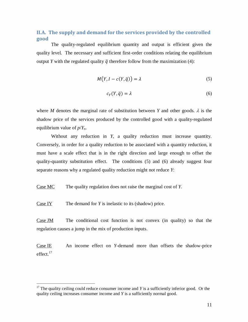
II.A. The supply and demand for the services provided by the controlled good

The quality-regulated equilibrium quantity and output is efficient given the

quality level. The necessary and sufficient first-order conditions relating the equilibrium

output Y with the regulated quality �̅� therefore follow from the maximization (4):

𝑀(𝑌, 𝐼 − 𝑐(𝑌, �̅�)) = 𝜆 (5)

𝑐𝑌(𝑌, �̅�) = 𝜆 (6)

where M denotes the marginal rate of substitution between Y and other goods. is the

shadow price of the services produced by the controlled good with a quality-regulated

equilibrium value of p/Yn.

Without any reduction in Y, a quality reduction must increase quantity.

Conversely, in order for a quality reduction to be associated with a quantity reduction, it

must have a scale effect that is in the right direction and large enough to offset the

quality-quantity substitution effect. The conditions (5) and (6) already suggest four

separate reasons why a regulated quality reduction might not reduce Y:

Case MC The quality regulation does not raise the marginal cost of Y.

Case IY The demand for Y is inelastic to its (shadow) price.

Case JM The conditional cost function is not convex (in quality) so that the

regulation causes a jump in the mix of production inputs.

Case IE An income effect on Y-demand more than offsets the shadow-price

effect.17

17

The quality ceiling could reduce consumer income and Y is a sufficiently inferior good. Or the quality ceiling increases consumer income and Y is a sufficiently normal good.

12

Although the unregulated quality minimizes conditional cost c(Y,q) with respect

to quality, it does not necessarily minimize marginal cost. For the same reason, a quality

limit that is binding for consumers cannot reduce conditional cost c, but it may reduce the

shadow price . Without further assumptions about the functions g and Y, we cannot

assume that a regulated quality reduction reduces scale even if the demand for Y is

sensitive to its shadow price.18

Suppose, as just an example, that the conditional cost function were

multiplicatively separable in Y and q. This is equivalent to saying that there is a single

efficient quality level that is independent of scale Y. The unregulated quality minimizes

both c and cY, and the first-order effect of a quality ceiling on Y and is zero (Case MC)

even though the ceiling’s quality-quantity substitution effect is not. If, instead, quality

were an inferior input in the production of Y, then a regulated quality that is below, but

near enough to, the unregulated equality would increase Y – necessarily with more

quantity – and thereby add to the quality-quantity substitution effect. Even if quality

were a normal input, the quality regulation would not affect Y if the demand for Y were

inelastic with respect to its shadow price (Case IY).

Case JM is frequently ruled out for analytical convenience, but the failure of the

second-order conditions is more likely with quality-quantity tradeoffs than with many

other economic tradeoffs because quantity and quality multiply each other in costs

(Hirshleifer 1955, Theil 1952, Becker and Lewis 1973). Case JM says that the quantity

jumps up, and quality jumps down, in response to a quality regulation, whereas

Assumption C says that the demand for Y does not jump. In the neighborhood of the

jump, the substitution effect dominates the scale effect because the former is a discrete

change whereas the latter is continuous.

Case IE features income effects on the demand for Y, which can go in either

direction. Because of the ambiguous sign, likely second-order magnitude, and that the

previous literature’s positive analysis does not emphasize income effects, the rest of this

paper abstracts from income effects too. Assumption D formalizes this and, to prevent

our presentation from getting too long, also rules out Case JM.

18

Recall that the conditional cost function, and therefore its Y derivative, depends only on the “technology” g() and Y(), and not on “preferences” u.

13

Assumption D Y-demand is income inelastic: the marginal rate of substitution function M

depends only on Y, and not on the consumption of other goods. The conditional cost

function is convex in quality.

Note that Assumption D does not rule out equilibrium effects of ceilings on Y, just those

that occur through an income effect. With this assumption, the (not necessarily constant)

magnitude of the price elasticity of demand for Y is:

𝜂(𝑌) ≡ −𝑀(𝑌)

𝑀′(𝑌)𝑌 (7)

In order to refer to elasticities, we normalize Y so that it is positive in the relevant range.

It follows from (2) and (7) that and are both positive.

II.B. The supply and demand for quantity

The quality-regulated equilibrium can equivalently be described in terms of the

supply and demand for quantity:

𝑔𝑛(𝑛, �̅�) = 𝑝 = 𝑀(𝑌(𝑛, �̅�))𝑌𝑛(𝑛, �̅�) (8)

where p is the price that consumers pay for each unit quantity that they consume.

Although, for the moment, p is not an object of regulation (quality is), the equivalent

representation (8) helps to link the consequences of quality and price regulations.

Each of the functions from (8) can be drawn in the [n,p] plane, as in Figures 2 and

3. In this context, we refer to them as the marginal cost and willingness-to-pay curves,

respectively. Assumption B requires that the marginal cost curve slopes up (or be

horizontal). Assumption A requires that a lower curve marginal cost curve corresponds

to a lesser quality level. Assumption C requires that the willingness-to-pay curve slopes

down.

None of the assumptions requires that quality increase the willingness to pay at all

points, or any points, on the curve. As an example consistent with light bulbs and

14

grocery-store produce, consider Y = nq, with a Y-demand function M that has a finite

negative slope everywhere. At the demand choke point n = Y = 0, the willingness to pay

is 𝑀(0)�̅�, which necessarily increases with the quality ceiling �̅� because the consumer

gets more output from a high-quality good than a low-quality one. But the high-quality

good also moves the consumer further down his Y-demand curve, which reduces his

marginal willingness to pay for Y. As a result, in the neighborhood of the choke point,

the high-quality demand curve is above and steeper than the low-quality one. If any point

on the Y-demand curve has < (the latter is one in this example), then the high-quality

willingness-to-pay curve could cross the low-quality one from above. A consumer of

higher-quality goods gets more output per unit quantity but, at the crossing point, =

and his low valuation of output results in a willingness to pay for quantity that is the same

as it would be if he had been consuming low-quality goods.

More generally, the direction of the effect of quality on the willingness to pay at

any point on the quantity-demand curve is the sign of ( ) at the same point.

Wherever the difference is negative, consumers are more willing at the margin to

substitute quantity, rather than other goods, for quality: a tighter quality ceiling increases

their willingness to pay at that point. When the difference is positive, a quality ceiling

reduces the willingness to pay.19

If Y demand also has a satiation point, which we

assumed for the purposes of drawing Figure 2, then willingness-to-pay curves

corresponding to different qualities must cross – that is have points with > as well as

points with < – because it takes more quantity to reach satiation with low quality than

with high. It is possible that the curves cross more than once. Conversely, the only way

to have the high-quality curve always above (below) the low-quality curve is for Y-

demand to have no satiation (choke) point, respectively.20

A constant-elasticity demand

19

The positive-difference case conforms with the Jevons (1866) paradox: increasing quality (say,

the productivity of coal) increases the willingness to pay for each pound of coal because it sufficiently expands the use of coal-sourced energy. 20

To be clear, we say that there is a choke point if (a) the willingness to pay for Y is finite at Y = 0

and (b) Y(0,q) = 0 for any quality in the relevant range. We say that there is a satiation point if (a) the willingness to pay for Y is zero for a finite amount of Y and (b) the satiation service level can

be achieved with finite amounts of quantity and quality. Here we use satiation and choke points

to help describe the global properties of the demand system, but note that a satiation point is of

practical interest in those markets where the price ceiling is zero (i.e., buyers are prohibited from paying the sellers).

15

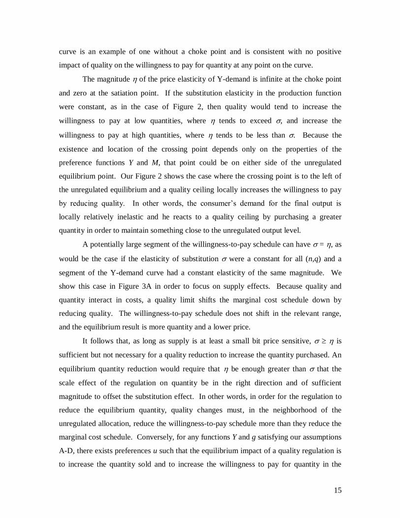
curve is an example of one without a choke point and is consistent with no positive

impact of quality on the willingness to pay for quantity at any point on the curve.

The magnitude of the price elasticity of Y-demand is infinite at the choke point

and zero at the satiation point. If the substitution elasticity in the production function

were constant, as in the case of Figure 2, then quality would tend to increase the

willingness to pay at low quantities, where tends to exceed , and increase the

willingness to pay at high quantities, where tends to be less than . Because the

existence and location of the crossing point depends only on the properties of the

preference functions Y and M, that point could be on either side of the unregulated

equilibrium point. Our Figure 2 shows the case where the crossing point is to the left of

the unregulated equilibrium and a quality ceiling locally increases the willingness to pay

by reducing quality. In other words, the consumer’s demand for the final output is

locally relatively inelastic and he reacts to a quality ceiling by purchasing a greater

quantity in order to maintain something close to the unregulated output level.

A potentially large segment of the willingness-to-pay schedule can have = , as

would be the case if the elasticity of substitution were a constant for all (n,q) and a

segment of the Y-demand curve had a constant elasticity of the same magnitude. We

show this case in Figure 3A in order to focus on supply effects. Because quality and

quantity interact in costs, a quality limit shifts the marginal cost schedule down by

reducing quality. The willingness-to-pay schedule does not shift in the relevant range,

and the equilibrium result is more quantity and a lower price.

It follows that, as long as supply is at least a small bit price sensitive, is

sufficient but not necessary for a quality reduction to increase the quantity purchased. An

equilibrium quantity reduction would require that be enough greater than that the

scale effect of the regulation on quantity be in the right direction and of sufficient

magnitude to offset the substitution effect. In other words, in order for the regulation to

reduce the equilibrium quantity, quality changes must, in the neighborhood of the

unregulated allocation, reduce the willingness-to-pay schedule more than they reduce the

marginal cost schedule. Conversely, for any functions Y and g satisfying our assumptions

A-D, there exists preferences u such that the equilibrium impact of a quality regulation is

to increase the quantity sold and to increase the willingness to pay for quantity in the

16

relevant range.21

These surprising results are not solely a matter of the degree of

substitution between quantity and quality.

It is helpful to consider the demand and supply for n alongside the demand and

supply for Y, as in Figures 3A and 3B. The prices shown in the two charts are different: p

in 3A and the shadow price (= p/Yn) in 3B. The willingness-to-pay-function in Figure

3A would shift with quality whereever is different from , but the Figure 3B’s demand

curve is independent of quality because it is just a graph of the consumer’s marginal rate

of substitution M(Y) versus the services amount Y. As noted above, a quality reduction

shifts Figure 3A’s supply curve gn(n,q) down because gnq > 0. Both figures, especially

Figure 3B, are drawn for the cYq = 0 case in which quality is neither a normal nor an

inferior input.22

As a result, a quality change in either direction shifts up Figure 3B’s

supply curve and the shift is only second order.

If quality is either normal or inferior, then cYq is negative or positive at the

efficient allocation, respectively. However, because the impact of quality on the total

cost of producing the efficient services amount is still second order, there still must be a

point on Figure 3B’s supply curve, with services less than the efficient amount, where cYq

is zero. A quality ceiling therefore rotates Figure 3B’s supply curve around that point.

The rotation is counterclockwise (clockwise) if quality is a normal (inferior) input,

respectively.

In the inferior case, a quality ceiling therefore reduces the marginal cost of

producing the efficient services amount even though it does not reduce the total cost. The

equilibrium result of a quality ceiling is therefore more services Y and more quantity n.

This is a case in which the scale and substitution effects on quantity go in the same

direction. The surprising effect of regulation on quantity is not necessarily a mere

“relabeling” of how the services Y are produced with q and n, but may also reflect a

regulation-induced reduction in the marginal (but not average) cost of producing those

services.

21

Specifically, as approaches zero, the locus of equilibrium combinations of q and n is just an isoquant of Y, which must slope down in the [n,q] plane. 22

Figure 3B’s supply curve is a graph of the marginal conditional cost cY(Y,q), holding q fixed.

To be clear, because the marginal cost of quality depends on quantity, we do not define “normal

input” with respect to an expansion path with Y’s MRS constant, but rather with respect to an expansion path that equates the MRS in Y to the MRT in g.

17

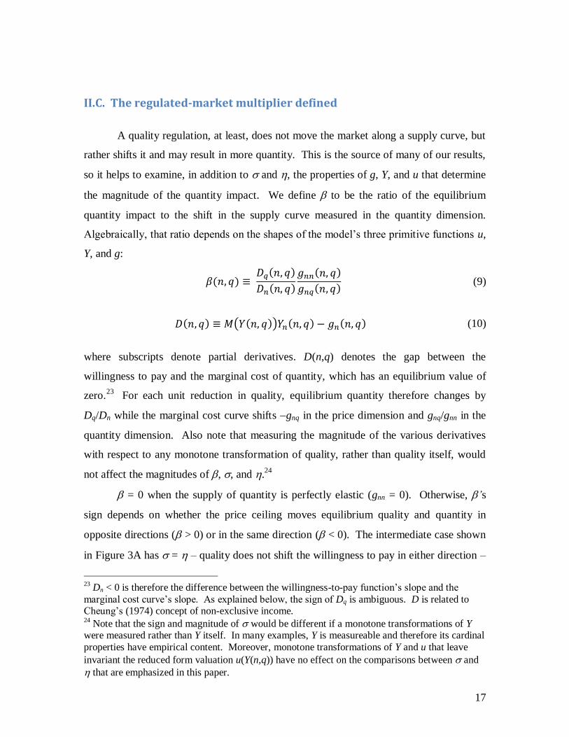
II.C. The regulated-market multiplier defined

A quality regulation, at least, does not move the market along a supply curve, but

rather shifts it and may result in more quantity. This is the source of many of our results,

so it helps to examine, in addition to and , the properties of g, Y, and u that determine

the magnitude of the quantity impact. We define to be the ratio of the equilibrium

quantity impact to the shift in the supply curve measured in the quantity dimension.

Algebraically, that ratio depends on the shapes of the model’s three primitive functions u,

Y, and g:

𝛽(𝑛, 𝑞) ≡ 𝐷𝑞(𝑛, 𝑞)

𝐷𝑛(𝑛, 𝑞)

𝑔𝑛𝑛(𝑛, 𝑞)

𝑔𝑛𝑞(𝑛, 𝑞) (9)

𝐷(𝑛, 𝑞) ≡ 𝑀(𝑌(𝑛, 𝑞))𝑌𝑛(𝑛, 𝑞) − 𝑔𝑛(𝑛, 𝑞) (10)

where subscripts denote partial derivatives. D(n,q) denotes the gap between the

willingness to pay and the marginal cost of quantity, which has an equilibrium value of

zero.23

For each unit reduction in quality, equilibrium quantity therefore changes by

Dq/Dn while the marginal cost curve shifts gnq in the price dimension and gnq/gnn in the

quantity dimension. Also note that measuring the magnitude of the various derivatives

with respect to any monotone transformation of quality, rather than quality itself, would

not affect the magnitudes of , , and .24

= 0 when the supply of quantity is perfectly elastic (gnn = 0). Otherwise, ’s

sign depends on whether the price ceiling moves equilibrium quality and quantity in

opposite directions ( > 0) or in the same direction ( < 0). The intermediate case shown

in Figure 3A has = – quality does not shift the willingness to pay in either direction –

23

Dn < 0 is therefore the difference between the willingness-to-pay function’s slope and the

marginal cost curve’s slope. As explained below, the sign of Dq is ambiguous. D is related to Cheung’s (1974) concept of non-exclusive income. 24

Note that the sign and magnitude of would be different if a monotone transformations of Y were measured rather than Y itself. In many examples, Y is measureable and therefore its cardinal

properties have empirical content. Moreover, monotone transformations of Y and u that leave

invariant the reduced form valuation u(Y(n,q)) have no effect on the comparisons between and

that are emphasized in this paper.

18

so that is just a function of the relative slopes of the marginal cost and willingness-to-

pay curves:

𝛽(𝑛, 𝑞) → [1 −

𝑑𝑑𝑛 𝑀(𝑌(𝑛, 𝑞))𝑌𝑛(𝑛, 𝑞)

𝑔𝑛𝑛(𝑛, 𝑞)]

−1

∈ [0,1] (11)

where the fraction’s numerator is the slope of the willingness-to-pay curve and the

denominator is the marginal cost curve’s slope. At one extreme, the supply of quantity is

fixed, and the market multiplier is one. At the other extreme, the marginal cost curve is

horizontal and the market multiplier is zero. Both of these results for Figure 3A, and

results for marginal cost curves that are neither horizontal nor vertical, are akin to results

from tax incidence because quality changes are shifting marginal cost without shifting

demand.

Although not shown in Figure 3A, can exceed by enough that a regulated

quality reduction increases the price per unit because it sufficiently shifts the willingness-

to-pay function. exceeds one in such cases, and quality ceilings have different effects

than price ceilings do, because the former raises price and the latter reduces it. Our

analysis of price ceilings therefore begins with further examination of , distinguishes

comparative statics at allocations with < 1 from those with 1, and explains why

can be interpreted as a “market multiplier.”

III. Competitive equilibrium with regulated prices

We ultimately want to examine the consequences of regulations that constrain

prices but do not effectively constrain all of the non-price attributes of the controlled

good. Following Murphy (1980), Leffler (1982), Raymon (1983), Barzel (1997), and

Ippolito (2003), our model has an equilibrium quality, rather than an equilibrium price,

that coordinates the consumers and producers. We define a price-regulated equilibrium

that is competitive in the sense that consumers and producers each take the quality q as

given. Each consumer would prefer to be able to make greater-than-equilibrium-quality

19

purchases at the regulated price, but no producer has an incentive to supply that extra

quality. Each producer would prefer to be able to sell less-than-equilibrium quality at the

regulated price, but no consumer has an incentive to accept less quality.

III.A. Equilibrium defined

Formally, given a price ceiling �̅� and consumers’ outside income I, a price-

regulated equilibrium is an output level Y, a quantity n, a quality level q, and profit

amount a such that (i) Y and n maximize 𝑢(𝑌, 𝐼 + 𝑎 − �̅�𝑛) subject to 𝑌 = 𝑌(𝑛, 𝑞) and

taking �̅�, q, and a as given, and (ii) n maximizes 𝑎 = �̅�𝑛 − 𝑔(𝑛, 𝑞) taking �̅� and q as

given. We assume that the price ceiling is binding and build that assumption into the

definition above.25

Both our quality-regulated equilibrium and price-regulated equilibrium have

consumers and producers each “choosing” a quantity, taking price and quality as given.

D(n,q) = 0, as defined in equation (10), is zero in either case. The difference – nontrivial

as we show below – is whether price or quality is set by regulation, with the other

coordinating the two sides of the market.

A level curve of D(n,q) = 0 can be displayed in the [n,q] plane together with level

curves for Y and g, and the former’s slope shows a lot about the comparative static

𝑑𝑛/𝑑�̅�. Moreover, (the inverse of) that slope is readily decomposed into scale and

substitution effects:

𝐷𝑞

−𝐷𝑛= −

𝑌𝑞(𝑛, 𝑞)

𝑌𝑛(𝑛, 𝑞)+

𝑐𝑌𝑞(𝑌(𝑛, 𝑞), 𝑞)

𝐷𝑛/𝑌𝑛(𝑛, 𝑞) (12)

The first term on the RHS of (12) is the slope of the isoquant, and thereby

represents the substitution effect shown in equation (3). The second term represents the

remaining quantity and quantity changes that involve changing isoquants. The second

25

The appendix offers a more detailed description of revenues and costs and what each buyer and

seller understands to be his consequence of accepting a quality level that is different from the

equilibrium value. Because we primarily consider price ceilings below the price that prevails

absent regulation, we refer to comparative statics with 𝑑�̅� < 0 as “tightening the ceiling” and

comparative statics with 𝑑�̅� > 0 as “relaxing” it.

20

term has the opposite sign of the cross derivative cYq, and therefore can be positive,

negative or, as in Case MS, zero. Case IY also features a special case of the second term,

namely that the term goes to zero as the term’s denominator becomes large.

III.B. Comparative statics with the market multiplier

A quality reduction among a subset of suppliers would cause their customers to

change the quantity that they buy. If the supply of quantity is not perfectly elastic, this

change affects the market’s marginal cost of quantity according to the marginal rate of

substitution in the marginal cost function gn(n,q), which is gnn/gnq. The direction and

magnitude of this price impact is therefore measured by the market multiplier function

that we defined above (equation (9)). Moreover, using (12), we can decompose the

market multiplier into substitution and scale effects:

𝛽(𝑛, 𝑞) = (𝑌𝑞

𝑌𝑛+

𝑐𝑌𝑞

−𝐷𝑛/𝑌𝑛)

𝑔𝑛𝑛

𝑔𝑛𝑞 (13)

Note that the market multiplier depends on all three primitive functions u, Y, and g, but

the preference function u enters only through the Dn term and with an ambiguous sign

because cYq can have either sign.

Assuming for the moment that the equilibrium quantity and quality are

differentiable with respect to the price ceiling, the comparative statics for the system

D(n,q) = 0 and �̅� = 𝑔𝑛(𝑛, 𝑞) with respect to �̅� are:

𝑑𝑛

𝑑�̅�=

𝐷𝑞/(−𝐷𝑛)

𝑔𝑛𝑞

1

1 − 𝛽 (14)

𝑑𝑞

𝑑�̅�=

1

𝑔𝑛𝑞

1

1 − 𝛽 (15)

In an unregulated market, a quantity-for-quality substitution among a subset of the

sellers would, through the price mechanism, cause the rest of the market to substitute

quality for quantity. It can have the opposite effect in the regulated market because the

21

higher marginal cost of quantity makes it more difficult for market participants to comply

with the price ceiling. In other words, when > 0, a price ceiling in a competitive market

creates an element of strategic complementarity in quality choices. Quality-quantity

substitution by a subset of consumers induces the rest of the market to adjust in the same

direction, even though we assume no interdependency in preferences. The competitive

analysis of price ceilings therefore resembles Becker’s (1991) and Becker and Murphy’s

(2003) competitive analysis of “social interactions” in which each buyer’s willingness to

pay for the social good is increasing with the number of other buyers who are purchasing

that good. The complementarity among market participants is especially strong when >

1, when the multiplier changes the signs of the derivatives (14) and (15). Hereafter we

refer to as the “regulated-market multiplier”, or “market multiplier” for short.26

Figure 4A graphs the locus of price-regulated equilibrium quality-price

combinations, holding constant the taste and technology functions u, Y, g.27

The locus

slopes up if and only if < 1. We draw one downward-sloping portion on the quality

interval q [q2,q1], where > 1, although for some taste and technology functions there

not be any downward-sloping portion (there also could be multiple parts with > 1). The

companion Figure 4B shows the locus of equilibrium quantity, assuming that supply is

neither perfectly elastic nor perfectly inelastic. It is, qualitatively, the horizontally

mirrored image of Figure 4A wherever > 0 and thereby in those cases closely resembles

the demand curve drawn by Becker (1991, Figure 2). The point (𝑛1, �̅�1) in Figure 4B

represents the same equilibrium as the point (𝑞1, �̅�1) in Figure 4A. The same relation

holds for (𝑛2, �̅�2) and (𝑞2, �̅�2) . Because the market multiplier does not have to be

26

Becker and Murphy’s (2003) study of demand interactions for social goods refers to as a “social multiplier.” The goods in our model are, by assumption, not “social,” but inter-consumer

complementarities are created by the combination of price regulation and competition. Also, we do not consider imperfect competition in this paper, but the reader may guess that the presence of

a market multiplier is one reason why a price ceiling can be more harmful in a competitive

market than an imperfectly competitive one. 27

It is a graph of p = M(Y(n,q))Yn(n,q), but only for combinations (n,q) that are a regulated equilibrium for some p.

22

positive, especially for low ceilings, we show two upward-sloping parts in Figure 4B.

One of them slopes up because > 1 and the other because < 0.28

At < 1 allocations, the comparative statics are qualitatively the same as they are

for a quality-regulated equilibrium because tightening the price ceiling involves a

reduction in the quality limit experienced by consumers. It follows that may be more

or less than , but in the former case it follows from section II’s results that 𝑑𝑛/𝑑�̅� is

negative or, if supply is completely inelastic, zero.

The > 1 allocations are the most different from the quality-regulated results

shown in Section II. They occur only where > .29

A substitution of quantity for

quality, which suppliers implement as they attempt to comply with the ceiling, increases

the equilibrium marginal cost of quantity by affecting factor prices (see also the

Appendix) and thereby frustrates suppliers’ adjustments. Any regulated equilibrium on

this portion is unstable in the sense that a small reduction in the price ceiling that induces

suppliers to cut their product quality must, in order to result in a market price that is

compliant with the new price ceiling, involve a quality reduction great enough to be on an

upward-sloping part of the curve. Assuming that an actual controlled market is better

represented by a stable equilibrium than an unstable one, then the differentiable

comparative statics (14) and (15) do not apply and our price-regulation analysis has some

resemblance with (special cases of) insurance premium “death spiral” models in which a

relatively efficient allocation can be supported as a competitive equilibrium, but that

28

When gnn > 0, dn/dp can also be written as –𝛽

1−𝛽

1

𝑔𝑛𝑛, which is negative only in the interval

(0,1). In drawing Figures 4A and 4B, we assume that the consumer’s first-order condition D(n,q)

= 0 is sufficient for describing utility maximization and that the marginal rate of substitution between quantity and quality in production Y diminishes more rapidly than does the

corresponding marginal rate of substitution in cost g. As in Becker’s (1991) model, the

nonmonotonic relationship between price and quantity shown in Figure 4B is therefore not the result of failures of the second-order conditions of competitive market participants. Those

failures are possible too, and discussed below. 29

Also note from equation (9) that either sign of (1) is consistent with scale effects in either direction (i.e., cYq of either sign). For example, cases MC and IY are both cases with zero scale

effect but are consistent with either [0,1) or 1, according to the elasticity of the supply of quantity. Although our Assumption D rules out Case JM, we note here that JM is consistent with

either a positive, negative, or zero social multiplier (JM’s jump can be represented as a gap in Figures 4A and 4B’s schedules for those quantities and qualities that are skipped by the jump).

23

equilibrium is unstable because equilibrium pricing is inefficient (Feldman and Dowd

1991).30

Nothing is shown or assumed in Figures 4A and 4B about the price, quality, or

quantity that would prevail without regulation. In theory, the multiplier formula (9)

could be evaluated at the unregulated quantity and quality. The result says little about

unregulated comparative statics, but it would be informative about some of the

consequences of imposing a price regulation on that market. Figure 4C illustrates with a

zoomed-in version of Figure 4A for the case in which the market multiplier exceeds one

at the unregulated allocation shown as U. A price ceiling introduced below, but close to,

the unregulated price, the regulation would (a) induce a discrete quality reduction (from

qu to qr << qu), (b) harm consumers, (c) benefit producers, (d) cause a discrete loss in

social surplus,31

and, if the supply of quantity were at all responsive to prices, (e)

increases expenditure and the quantity sold. To prove the second and third points, note

that, absent regulation, a consumer chooses quality qu and pays pu per unit quantity, even

though he could obtain qr more cheaply (namely, at a discount of (qu qr)gq/n per unit).

In effect, a price ceiling close to pu forces each consumer to accept quality qr without

receiving the discount that is available absent regulation.32

Meanwhile, producers benefit

from the price ceiling because they deliver less quality and get essentially the same price

per unit, thereby getting more surplus from the first nu units they produce and getting a

nonnegative surplus on the remaining (nr nu) units.33

To prove the remaining points, note that small quality reductions are not enough

to comply with a price ceiling, regardless of how close it is to the unregulated price pu,

because quality reductions by each supplier frustrate the compliance attempts by the

30

Although it is not the case for the situation shown in Figures 4A-4C, it is theoretically possible

that no stable price-regulated equilibrium exists (any unregulated equilibrium is stable, and unique). However, in any application with a Y-demand curve that has a choke point with a finite

negative slope, approaches infinity as one moves along that demand curve toward the choke

point, which means that < 1 in that neighborhood. In other words, willingness-to-pay schedules consistent with Figures 4A-4C may be look like those drawn in Figure 2. 31

Note that the regulation induces a discrete movement along the conditional cost function in the

quality dimension, away from the conditional-cost-minimizing quality. 32

The algebraic proof uses the consumer’s value function v(q) ≡ maxn u(Y(n, q)) − p̅n, which,

given �̅�, is strictly increasing in the quality level q. 33

Because < 1 at the allocation R, further reductions in the ceiling may reduce producer surplus below what it is at R, and perhaps even below what it is at U.

24

others. Quality must fall at least to qr. R is a regulated equilibrium for a price ceiling that

is near the unregulated price, and therefore has essentially the same marginal cost of

quantity as the unregulated equilibrium does. Because (i) the marginal cost schedule

gn(n,q) is increasing in both arguments and (ii) qr < qu, expenditure and quantity at

allocation R must exceed what they are at allocation U unless the supply of quantity is

completely inelastic to price, in which case nr = nu. These results for quantity,

expenditure, and the allocation of surplus are our first of several that are essentially

opposite of the textbook analysis, where a price ceiling benefits consumers (and, if

supply is competitive, reduces quantity) as long as the ceiling is close enough to the

unregulated price.

Consider Figure 4C again. A price ceiling of �̅� ∈ (𝑝𝑢 , �̅�2) introduced to the

unregulated and efficient market U might have no effect, because the unregulated

equilibrium price and marginal cost gn are less than such a ceiling. However, for a

regulated market with a ceiling at (or nearby and below) pu, relaxing its ceiling to a level

in the interval (𝑝𝑢 , �̅�2) may not result in the efficient allocation. An individual seller

does not, given the factor prices prevailing at R, have an incentive to supply as much

quality as qu because he would need to charge more than �̅�2, which would be in violation

of the regulation. The problem is that quantity-quality substitution that resulted in the

quality level qr makes the marginal unit of quantity more expensive to produce than it is

in the unregulated economy. In order to willingly supply the efficient quality, an

individual seller must not only see the price regulation relaxed above pu, but also

anticipate that the other sellers will supply the efficient quality, rather than the quality

level between q2 and qu that corresponds to the relaxed ceiling and is part of a stable

regulated equilibrium. We leave a rigorous dynamic analysis for future research, and

here just note that Figure 4C might have some of the foundations for a conclusion that the

effects of price regulation depend not only on tastes and technologies, but also the

market’s prior regulatory history.

At first glance, it might seem that quality is isomorphic with price in that either by

itself could coordinate the demand and supply of quantity, albeit less efficiently than

price and quality would together. This is true if were everywhere less than one,

because then the “supply” of quantity (gn(n,q) = p) would cross the “demand”

(M(Y(n,q))Yn(n,q) = p) only once in the [n,q] plane. Moreover, a price regulation would

25

amount to a quality regulation, just in different units. But, if there are regions where >

1, then there exist price ceilings p such that the supply and demand cross multiple times,

even though the second-order conditions for utility and profit maximization are satisfied.

This is a fundamental difference between prices and quality as allocators of quantity and

a difference between quality regulations and price regulations.34

III.C. Welfare costs that are worse than first order

The social welfare losses from a quality regulation are second-order because

consumer willingness to pay is smooth and the unregulated equilibrium has a quality

level that minimizes total conditional costs c(Y,q). This resembles the textbook model

where price regulations create second-order losses. However, if the unregulated

allocation has > 1, then it is unstable as a price-regulated equilibrium. A price ceiling

below the unregulated price level, no matter how close, produces a discrete reduction in

quality and therefore in social welfare. As shown above, consumers are discretely worse

off and producers may be better off.

These welfare results are not only directionally different from the textbook

analysis, they are of an entirely different character. Indeed, they are different from most

tax analyses, where imposing a small tax on an otherwise efficient market creates only

second-order welfare losses.35

The reaso is that, say, an excise tax creates a gross-of-tax

price that is automatically indexed to marginal cost. In contrast, a price regulation is

typically not indexed to marginal cost and thereby cannot prevent discrepancies between

price and marginal cost that are arbitrarily large.36

34

For other differences, see Telser (1987) and Weitzman (1974). 35

Although rarely analyzed, tax rates that are indexed to market conditions could result in multiple equilibria and “multiplier” comparative statics. One such tax is the “Rising-Tide Tax

System” (Burman, et al. 2006) that proposes to index the rate of taxation of high earnings to

market outcomes for the high earners. The paper containing the proposal and analysis thereof fails to note that high tax rates might make skills more scarce, and thereby result in a feedback

loop in which rising tax rates and falling skills quantities mutually reinforce each other (we owe

this point to Kevin M. Murphy). 36

This result resembles Hayek’s (1945) exposition of the socially important role of market prices in coordinating human activity. See also the appendix.

26

Figure 5 illustrates the distinction, under the assumption that gnn > 0, which means

that the supply of quantity is less than perfectly elastic. The horizontal axis measures the

amount by which the price ceiling �̅� is set below the unregulated price pu. Allocations to

the left indicate ceilings that are close to the unregulated price while those to the right

indicate more severe price ceilings. The vertical axis measures the impact of the ceiling

on various outcomes. The green and red curves describe the impact when the market

multiplier is at least as large as one at the unregulated allocation. Regulated quantity n

and expenditure �̅�𝑛 (green curve) are each discretely higher than its unregulated

counterpart, although they tend to decline as the ceiling gets more severe.37

Total surplus

u, consumer surplus (𝑢 + 𝑔 − �̅�𝑛) , and quality q are each discretely less than its

unregulated counterpart (see the red curve). They continue to decline with further

increases in the ceiling. Compare the green and the red curves, which relate to

multipliers of at least one, with the black and blue curves, respectively, which relate to

multipliers less than one. In the latter case, each of the outcomes is close to its

unregulated counterpart (i.e., the origin) as long as the price ceiling is close enough.

Moreover, with < 1, the marginal effect of the ceiling on total surplus is zero in the

neighborhood of the unregulated allocation (see the gray curve).

A full analysis of efficient and robust redistribution is beyond the scope of this

paper, but Figure 5 already suggests that such an analysis must account for the different

character of the redistribution that occurs for < 1 and > 1. If the sign of ( 1) were

unknown, consumers’ expected loss from a price ceiling could well be negative even

though a gain were far more likely than a loss, because the amount lost conditional on

losing is of a different order of magnitude than the amount gained conditional on gaining.

Note that Barzel (1997), Glaeser and Luttmer (2003) and others have argued that

price ceilings create first-order social losses due to the rationing mechanism used to

resolve the “shortage.” These allocative losses have been ruled out in our approach,

which treats all consumers as identical and has no shortage (unless the shortage is

interpreted as a non-price product attribute – see below). In other words, a large market

37

Although not shown in Figure 5, there may be a range where quantity increases at the margin with ceiling severity because the ceiling has not yet sufficiently increased the marginal cost of Y.

27

multiplier is an additional reason why the losses from price regulation need not be second

order.

III.D. Example: Quantity is in fixed supply

The sign of ( 1) depends on the direction in which level curves of the marginal

cost function gn(n,q) cross the level curves of the willingness to pay (for quantity)

function M(Y(n,q))Yn(n,q) in the [n,q] plane. The former slope down or, in the limit of

price-inelastic supply of quantity, vertical. therefore exceeds one if and only if the

latter level curves are both sloping down and flatter than the level curves of former.

The special case with inelastically-supplied quantity is potentially applicable to

rent control and other price regulations where supply is fixed in the short run, but it also

highlights some of reasons why could exceed one. Given n and p, a price-regulated

fixed-quantity equilibrium is a quality limit x that satisifies M(Y(n,q))Yn(n,q) = p. At the

unregulated allocation, the market multiplier is:38

𝛽(𝑛, 𝑞) → 1 + (𝜎(𝑛, 𝑞)

𝜂(𝑛, 𝑞)− 1)

𝑛

𝑔𝑞(𝑛, 𝑞) + 𝑥𝑔𝑞𝑞(𝑛, 𝑞)𝑀(𝑌(𝑛, 𝑞))𝑌𝑛𝑞(𝑛, 𝑞) (16)

It follows that, with inelastic supply, the multiplier at (n,q) exceeds one if and only if the

elasticity of substitution in production exceeds the magnitude of the price elasticity

of Y-demand at that point.39

Because, as shown in Section II, any continuous demand

curve with a satiation point has points on it with < , there must also be points with >

1.

The reason that the character of the multiplier hinges on a comparison of and

is that, holding quantity fixed, quality increases the willingness to pay if and only if >

; so that the scale effect on willingness to pay exceeds the quality-quantity substitution

38

We derive a multiplier for the inelastic supply case by (a) taking the definition (9), (b)

assuming g(n,q) = n1+

/(1+)+G(nq), and (c) taking the limit as goes to infinity, holding constant the marginal cost at the unregulated allocation. 39

In the more general case that the supply of quantity is at least somewhat sensitive to the price,

< is necessary but not sufficient for > 1. Or to put it another way, > 1 means that

exceeds by enough to offset the degree to which the willingness to pay for n decreases with n.

28

effect. When < , quality reductions – implemented by suppliers as they attempt to

comply with the price ceiling – increase consumers’ willingness to compete on the basis

of accepting low quality, which further reduces quality. There is not a stable equilibrium

until a part of the parameter space is reached in which > , such as the allocation U

shown in Figure 4C and the < allocations shown in Figure 2.

When the supply of quantity is fixed at n, Figures 4A and 4C are graphs of

M(Y(n,q))Yn(n,q) versus q. If < at the unregulated equilibrium, then the unregulated

price is in the interval (�̅�1, �̅�2), and the unregulated quality in the interval (q2,q1). A price

ceiling close to the unregulated price discretely reduces quality to a level less than q2

(specifically, a point on the curve that coincides with the price ceiling measured on the

vertical axis) and has no effect on quantity. As noted above, consumers are

unambiguously worse off because they are paying essentially the same but getting less

quality. Producers are unambiguously better off because their revenue is essentially the

same, but they have reduced their average costs by providing less quality. This is yet

another result the opposite of the textbook analysis, where it is reported that producer

surplus is lost, and consumer surplus is gained, in industries with price ceilings and

inelastic supply, at least if the regulated price is close enough to the unregulated. This

result does not even require that quality be a particular good substitute for quantity, as

long as other goods are an even worse substitute.

IV. Who benefits from price and quality ceilings?

Beginning from an allocation with > 1, introducing a price ceiling close to the

unregulated price, or marginally tightening one, results in discretely less consumer and

social surplus and discretely more producer surplus. The purpose of this section is to also

address the cases in which < 1 and the price or quality ceiling is not necessarily near the

unregulated equilibrium value. The two are related because a ceiling that is discretely

below the unregulated value can be achieved by introducing a ceiling close to the

unregulated value, followed by a sequence of marginal reductions in that ceiling.

The marginal cost curve gn(n,q) drawn in the [n,p] plane (see Figure 3A) is shifted

down by a quality ceiling, or by a price ceiling that results in less equilibrium quality. As

29

shown in Figure 6, the equilibrium price change is a combination of the vertical distance

gnq(n,q)dq of the marginal cost shift and the movement along that curve, which can be in

either direction. Supposing for the moment that regulation has no quantity impact (i.e.,

= 0), as at the allocation R0 shown in Figure 6, then producers are losing revenue

𝑛𝑑�̅� = 𝑛𝑔𝑛𝑞(𝑛, 𝑞)𝑑𝑞 but saving the total costs gq(n,q)dq that are shaded in the figure.40

By our Assumption B, the net cannot be positive. Because movements down the

marginal cost curve (i.e., < 0) further reduce revenue more than total costs, it follows

that producers cannot benefit from ceiling regulations without > 0 at enough of the

allocations between the regulated and unregulated allocations that the net impact on

quantity is positive.

Now consider a quality ceiling that increases quantity enough that there is no

price impact, as at the allocation R0 in the figure. Here there is no change in revenue, but

a reduction in costs. It follows that producers cannot lose, and consumers cannot gain,

from quality ceilings unless < 1 at enough of the allocations between the regulated and

unregulated allocations that the net impact on price is negative. As shown in Section III,

the same reasoning applies to the marginal tightening of a price ceiling: producers benefit

and consumers lose unless < 1.

For discrete changes in a price ceiling or, when (0,1), marginal changes in

either type of ceiling regulation, the producer’s benefit cannot be signed without more

information about regulation’s relative impacts on revenue and costs. The cost savings

on the unregulated quantity is gnq(n,q)dq, while the corresponding revenue loss is nudp.41

If we define for discrete regulation changes the same way that we do for marginal

changes – as the ratio of equilibrium price change to the amount of the shift of the

marginal cost curve measured in the price dimension – the revenue loss on the

unregulated quantity is (1)nugnq(n,q)dq. The cost savings exceed the revenue loss if

and only if:

40

Although Figure 3B, which graphs supply and demand in the [Y,] plane, is effective for measuring social surplus, it is less effective for measuring the allocation of surplus because the

equilibrium shadow price is not necessarily what consumers pay sellers per unit Y. The latter does occur, however, when production function takes the form Y(n,q) = ny(q), so that the shadow

price = p/Yn. 41

Costs and revenue on the increment (nrnu) to quantity are essentially zero because price equals marginal cost.

30

𝛽 >1

1 + 𝜃 (17)

The inequality (17) is a necessary and sufficient condition for producers to benefit from

ceiling regulations, and a sufficient condition for consumers to lose.42

Whenever

producers gain from a tighter ceiling, consumers lose because the ceiling reduces total

surplus.

Notice that the inequality (17) includes , which we have called the “elasticity of

supply of quality.” The appendix to this paper has a special case of the model that

illustrates the connection in more detail, but the tradeoff featured in (17) comes from the

fact that our model has two potential sources of surplus for producers: quality and

quantity. The unregulated equilibrium maximizes social surplus, but not producer

surplus (producers compete!), which opens the possibility that regulation could change

the mix of quantity and quality in a way that benefits producers. When quality is

elastically supplied ( large), producers are not harmed much by the quality reduction,

and can make up for it if their production of quantity sufficiently expands ( large).

The two directional possibilities are shown with black and blue curves in Figure

5. Both curves exhibit a first-order impact on producer surplus, by which we mean that,

at the unregulated equilibrium, the marginal effect of reducing the ceiling is not zero.

But producers gain from a tighter ceiling when the inequality (17) holds, which is the

case represented by the black curve.

Because > 0, Section III.D and the inequality (17) show that a positive – in

other words, either supply is completely inelastic or the quality reduction that results

from a ceiling is associated with a quantity increase – is necessary but not sufficient for

producers to benefit. This is essentially the opposite of the textbook analysis (see also

Bulow and Klemperer (2012)), where quantity reductions are taken as evidence that

supply is price elastic and therefore that consumers may be losing from a price ceiling.

42

Murphy (1980) has a characteristics model of the supply side in which producers can benefit

from price ceilings. In the rent control context, Autor, Palmer and Pathak’s (2014) empirical

results suggests that price ceilings in Cambridge, Massachusetts harmed producers. But note that

Cambridge rent control enforcement included conscription – such as the taking of properties by the power eminent domain (Mulligan 2015) – which is not part of our model of price ceilings.

31

V. Conclusions

This paper abstracts from the question of which buyers receive the goods in a

regulated market, and previous studies have noted the first-order efficiency losses from

the misallocations caused by ceilings. Nevertheless, we find that the welfare costs of

price regulation can be worse than first order, and of a different character than the costs

of excise taxes or quality regulations, because flexible prices may be needed to prevent

beggar-thy-neighbor reactions among the sellers. In effect, decisions about non-price

product attributes become complementary in the absence of a price mechanism, even

though tastes and technology are not fundamentally complementary. The price-regulated

equilibrium behavior need not be close to efficient even when the regulated price is.

If Bulow and Klemperer (2012) are correct that price ceilings on average harm

both consumers and producers, then the existence of ceilings would suggest that support

for the regulation among market participants, if any, would either be misguided or come

from subsets of consumers or producers that are different enough from the average. Our

model suggests an alternative: that producers may benefit on average from a price or

quality ceiling because it softens the non-price (a.k.a., quality) competition that would

otherwise dissipate some of their surplus. Moreover, markets with relatively inelastic

supply are especially likely to feature this type of benefit for producers.

Real-world products have many non-price attributes, and our model is not detailed

enough to predict the types and composition of quality adjustments that would occur.

But those adjustments could include something like customer “waiting” if it reduces

sellers’ costs. Take, for example, the inventories that sellers have on hand. Low average

inventories mean lower costs but more stock outs and thereby less average value for

consumers. A customer encountering a stock out is waiting in the sense that he must

defer his purchase until the seller replenishes the inventory (Yurukoglu, Liebman and

Ridley 2016). Our model can capture this by treating seller average inventory levels as a

non-price attribute q that goes in the customer’s production function Y. This approach

contrasts with previous models in which, akin to an excise tax, waiting is an additional

cost borne in part by buyers but (purportedly) yielding no benefit to sellers (McCloskey

32

1985, pp. 325-6, Frech and Lee 1987, Friedman 1990, Figure 17-4, Bulow and Klemperer

2012).

In contrast to the standard analysis of price controls, our model has no random or

purely wasteful mechanism for resolving the “shortages” associated with price ceilings.

Market participants in our model have no incentive to engage in such schemes, because

sellers prefer to adjust non-price attributes in a way that reduces costs and buyers prefer

to get a low-quality product than no product at all. A practical implication of our

approach is that regulated-equilibrium quantity and quality reflect both supply and

demand conditions, whereas the standard approach says that changes in demand only

affect the amount of the shortage without affecting what sellers do.

We show that quality degradation can either increase or decrease buyers’

willingness to pay at a given quantity, and provide an elasticity condition that describes

which case applies in any particular situation. Even though strong assumptions are

needed to guarantee the latter case, the former is largely absent from the literature, and is

the source of some of the “upside-down” results. With lower supply costs and little or no

reduction in the willingness to pay, a price ceiling could increase the quantity traded,

especially when there is an inelastic demand for the services provided by the controlled

good. It is even possible that the ceiling increases the services themselves.

More empirical work on these predictions is needed, especially with a framework

that is consistent with the discontinuities suggested by the theory, but for now we point to

a couple of examples that seem to confirm. One is the case of doctor appointments,

where it has been suggested that ceilings on the price per visit results in patients’ visiting

the doctor more frequently for the same health condition. As Frech (2001, p. 338) puts it,

Japanese patients “are often told to come back for return visits. And, even injections of

drugs were often split in half to make two visits necessary.” Indeed, we wonder whether

price ceilings in health care increase spending in that market, rather than decrease it.

Another is the case of rent control of pre-war premises in Hong Kong, which appears to

have increased the number of leases and perhaps even the number of square feet under

lease as tenants engaged in partial subletting and landlords rented to “rooftop squatters.”

Cheung (2016) interprets these practices as choices to reduce rent dissipation, but they

are also consistent with the predictions of our model.

33

With sufficiently inelastic supply, pure non-price competition may have multiple

equilibria, and that the transition from one to another might be heuristically described as

a quality-degradation spiral with some resemblance to insurance premium “death spiral”

models. In these cases, the incidence of price regulations is especially far from the

standard analysis. A few studies such as Block and Olsen (1981), and experiences with

communism itself, have shown that price ceilings can result in extraordinary quality

degradation. Recent advocates of rent control, pointing to the case of modern Germany,

also assert that ceilings do not always harm quality (Bourne 2014). Nevertheless, there

do not appear to be many statistical analyses of actual price ceilings that formally attempt

to confirm the existence of multiple competitive equilibria. Perhaps this absence is due

to a paucity of real examples, or merely because this implication of competitive behavior

had not yet been developed. But even if it were the former, perhaps understanding this

potential of competitive behavior would help regulators to avoid creating any new ones.43

The direction of the quantity impact of price controls is sometimes used as a

litmus test for whether the controlled market is competitive or not. A ceiling that

increases quantity is supposed to reveal noncompetitive behavior and social gains from

the ceiling. More work is needed to understand non-price adjustments in imperfect

competition settings, but we can already say that, without additional information about

tastes and technology, either direction of quantity impact is simultaneously consistent

with perfect competition, with social harm, and with consumer harm from price

regulations. A price ceiling that increases the quantity traded may only reveal that the

market is substituting quantity for quality, and not that sellers were ever holding back

supply.

43

With respect to Gresham’s Law, Rolnick and Weber (1986) confirm both possibilities:

currency-market regulators often recognize that fixing prices can create multiple equilibria, but that sometimes the low-quality equilibrium is observed for small-denomination currencies.

34

VI. Appendix: A Detailed Description of the Economic Environment

VI.A. Equilibrium defined, with specification for off-equilibrium qualities This appendix offers a more detailed interpretation of an economic environment

described by (1) and (4), as well as showing what would be the consequences of an

individual consumer or producer of dealing in a product quality that is different from the

equilibrium. Two factors of production are required to produce the products in the

controlled market, Zn and Zq, with factor prices wn and wq, respectively. Zn is used to

produce the raw items, before any quality enhancements. Each raw item requires one

unit of Zn. Zq is used to make the quality enhancements. If q is the quality level and n is

the number of items, then G(q)n units of Zq are needed. G is not necessarily monotonic

in q, but for q large enough it is increasing and unbounded. The surplus a of the factor

suppliers to the controlled market are:

𝑎 = [𝑤𝑛 + 𝑤𝑞𝐺(𝑞)]𝑛 − 𝑔(𝑛, 𝑞) (18)

The inverse factor supplies are wn = Sn(Zn) and wq = Sq(Zq). It follows that the cost

function g is the total factor resource cost of quantity and quality:

𝑔(𝑛, 𝑞) ≡ ∫ 𝑆𝑛(𝑍𝑛)𝑑𝑍𝑛

𝑛

0

+ ∫ 𝑆𝑞(𝑍𝑞)𝑑𝑍𝑞

𝑛𝐺(𝑞)

0

(19)

There is free entry in the business of hiring the factors of production to make the

controlled good, so intermediate-supplier profits are zero and their revenues are equal to

the revenue term in the surplus equation (18). Their revenue per unit quantity must be

compliant with the price ceiling. It follows from the price ceiling constraint that there is

a quality level x such that only qualities q x are available in the market. The

intermediate suppliers are willing to sell goods of any quality strictly less than x as long

as they receive at least [wn+wqG(q)] per unit.

Given a price ceiling �̅� and consumers’ outside income I, the more detailed

equilibrium described in this appendix is an available-quality ceiling x, a pair of factor

35

input prices wn and wq, profits a, factor quantities Zn and Zq, a quality level q, and a

quantity n, such that:

(i) The available-quality ceiling x is consistent with the price ceiling �̅�.

𝑤𝑛 + 𝑤𝑞𝐺(𝑥) = �̅� (20)

(ii) Given the factor prices wn and wq, the available quality ceiling x, and factor

income a, the quantity n and quality q maximize utility:

{𝑛, 𝑞} = argmax𝑛≥0,𝑞≤𝑥

𝑢(𝑌(𝑛, 𝑞), 𝐼 + 𝑎 − [𝑤𝑛 + 𝑤𝑞𝐺(𝑞)]𝑛) (21)

(iii) Profits a satisfy (18) and (19)

(iv) and, given the factor prices, factor supplies equal factor demands,

𝑤𝑛 = 𝑆𝑛(𝑛) = 𝑆𝑛(𝑍𝑛), 𝑤𝑞 = 𝑆𝑞(𝑛𝐺(𝑞)) = 𝑆𝑞(𝑍𝑞) (22)

Algebraically, this more detailed equilibrium description is eight unknown scalars

described by eight equations. In the main text, our equilibrium has just four of these

equations, which is why the main text has no explicit predictions for factor prices or

factor quantities.

The unregulated equilibrium is the equilibrium corresponded to a ceiling of

�̅� = ∞. Any ceiling less than infinity binds in the sense that it restricts quality choices (x

< ), although those quality choices may be irrelevant because they are beyond the

unregulated quality. An equilibrium does not exist if the price ceiling is so low than it

does not cover the factor costs of even the lowest quality levels.

In this appendix’s example, the marginal cost of quantity is:

𝑔𝑛(𝑛, 𝑞) = 𝑆𝑛(𝑛) + 𝑆𝑞(𝑛𝐺(𝑞))𝐺(𝑞) (23)

The conditional cost function is:

𝑐(𝑌, 𝑞) = 𝑔(𝑛(𝑌, 𝑞), 𝑞) (24)

36

where n(Y,q) is the quantity needed of quality q needed to deliver services Y. A price or

quality ceiling that increases quantity therefore changes the composition of producer

surplus by moving the market up one of the factor-supply curves and down the other, as

shown in Figure 7. Total producer surplus can be greater to the extent that quantity is

increasing enough or that the surplus from selling the unregulated quality is small

enough. These tradeoffs are summarized by the inequality (17) in the main text.

In order to look at the market multiplier in more detail, consider a price-regulated

equilibrium, and normalize its price and quality to one. Now consider lowering the

ceiling to �̅� < 1. This affects the equilibrium quality and quantity, and therefore the

factor prices wn and wq. If, hypothetically, there were a seller still supplying the good

with quality one, he would find that the new ceiling both reduces the price received and

changes the marginal cost of supplying the same good, which is wn + wqG(1). The

former comes directly from the regulation, but the latter comes from the compliance

responses of the other suppliers. In order for the market multiplier to exceed one, the

lower ceiling must (a) increase quantity (thereby increasing wn) and (b) have a small

enough effect on wq (e.g., Sq = 0) that the net effect is to increase wn + wqG(1). In this

case, the quality reductions implemented by any group of sellers raise the marginal costs

of all sellers and thereby further encourage quality reductions.

More generally, a price ceiling drives a wedge between the private and social

benefits of supplying quality because factor prices respond to that behavior. Consider a

“price-regulated planner” that was choosing quality x and quantity n subject to the

constraint that the marginal cost of quantity cannot exceed �̅�. That planner’s Lagrangian

is:

ℒ ≡ 𝑢(𝑌(𝑛, 𝑥)) − 𝑔(𝑛, 𝑥) + [�̅� − 𝑔𝑛(𝑛, 𝑥)]𝜆 (25)

The optimal quantity for the price-regulated planner satisfies:

𝑀(𝑌(𝑛, 𝑥))𝑌𝑛(𝑛, 𝑥) = �̅� + 𝜆𝑔𝑛𝑛(𝑛, 𝑥) (26)

By comparison, our model’s price-regulated equilibrium satisfies:

37

𝑀(𝑌(𝑛, 𝑥))𝑌𝑛(𝑛, 𝑥) = �̅� (27)

The price-regulated planner and the market coincide only if (a) both factors are perfectly

elastically supplied (gnn = 0) or (b) the price regulation is not binding ( = 0). The price-

regulated planner’s decision considers the fact that quantity choices affect the cost of

compliance, whereas the decision of an individual seller (subject to regulation) does

not.44

The price-regulated planner’s condition (26) shows that, with special exceptions

(a) and (b) noted above, the marginal cost of quantity exceeds �̅� = 𝑔𝑛(𝑛, 𝑞). In other

words, regulated prices fail to reflect all of the relevant marginal costs, and this failure is

the source of some of the most damaging market reactions to the regulation. Quality

regulation does not fail in this way. If the planner were subject to quality regulation

instead, she would be maximizing u(Y(n,x))g(n,x) with respect to quantity (only), just as

the quality-regulated market does.

VI.B. A special case that demonstrates the upside-down results

The cost function, production function, and utility function do not have to be

exotic in order to obtain our model’s unusual results. Here we assume that the factor

supply functions each have a constant elasticity, 𝑆𝑛(𝑍𝑛) = 𝑍𝑛1/𝛾

/𝐴 and 𝑆𝑞(𝑍𝑞) =

𝑍𝑞1/𝜃

𝐵/𝐴, with A, B, , all positive, and the function G(q) to be increasing and convex

with an elasticity greater than one. In this case, the cost function is

𝑔(𝑛, 𝑞) =𝛾

1 + 𝛾

𝑛(1+𝛾)/𝛾

𝐴+ 𝐵

𝜃

1 + 𝜃

[𝑛𝐺(𝑞)](1+𝜃)/𝜃

𝐴 (28)

We also take the marginal rate of substitution function M(Y) = 1 – Y to be linear on the

range Y [0,1] and the production function to be Y(n,q) = nq. In this case, the

44

Conversely, by making the equilibrium condition (8) or (27) rather (26), we assume that the

industry’s marginal costs are either constant or rising because of factors that are not perfectly elasticity supplied to the industry.

38

willingness to pay for quantity is (1nq)q. The magnitude of the price elasticity of Y-

demand is less than one, and therefore less than the elasticity of substitution = 1, at any

allocation with Y > ½. It follows that, beginning at any such allocation, reducing quality

will increase the willingness to pay for quantity.

The expansion path in the [n,q] plane is described by:

[𝑞𝐺′(𝑞) − 𝐺(𝑞)][𝐺(𝑞)]1/𝜃𝐵 = 𝑛1/𝛾−1/𝜃 (29)

The expansion path therefore can have a slope of either sign, which is the same as the

sign of (). If < , then a quality ceiling sufficiently close to the unregulated quality

results in more equilibrium output Y.

The market multiplier can exceed one at the unregulated allocation. Take the

special case of the cost function (28) that has a perfectly elastic supply of the quality

factor Zq and an elasticity of supply of the quantity factor Zn that is 1/2:

𝑔(𝑛, 𝑞) =1

5(

16

27𝑛3 +

𝑛𝑞5

4) (30)

The efficient allocation is n = ¾ and q = 1. At this allocation, the marginal cost gn is ¼,

the elasticity of Y-demand is 1/3, and the market multiplier is 24/23. There are three

price-regulated equilibria with gn = ¼: the unstable efficient allocation and the stable

allocations with (n,q) approximately equal to (0.84,0.36) and (0.74,1.02).

Figure 1. Claims on gross tenant-occupied housing output, 2006

Intermediate goods and services

consumed, 23%

Compensation of Employees, 5%

Taxes on production (property

taxes), net of subsidies,

14%

Net Operating Surplus (mortgage interest & business

income), 37%

Consumption of fixed capital, 22%

Note: the smaller NOS piece is the part allocated to vacant units.Note: the smaller NOS piece is the part allocated to vacant units.

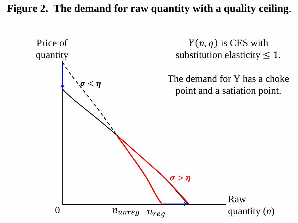
𝑛𝑟𝑒𝑔

Figure 2. The demand for raw quantity with a quality ceiling.

Raw

quantity (n)

Price of

quantity

𝑛𝑢𝑛𝑟𝑒𝑔

𝝈 > 𝜼

𝝈 < 𝜼

𝑌 𝑛, 𝑞 is CES with

substitution elasticity ≤ 1.

The demand for Y has a choke

point and a satiation point.

0

Figure 3B. The services provided by the controlled good, with separable conditional cost: Y-supply shift is second order.

Figure 3A. The raw quantity of the controlled good, with quality regulation and 𝜎 = 𝜂 on the relevant parts of demand.

Supply with

efficient quality

Services

demand

𝑌𝑢𝑛𝑟𝑒𝑔

Services

amount

Services

shadow price

Supply with

inefficient

quality

𝑌𝑟𝑒𝑔

Supply with

efficient quality

Willingness

to pay

𝑛𝑟𝑒𝑔

Raw

quantity

p

Supply with

regulated

quality

𝑛𝑢𝑛𝑟𝑒𝑔

𝛽 > 1

Quality

Price

ceiling

𝛽 = 0

𝛽 = 1

𝛽 = 1

𝛽 ∈ (0,1)

𝛽 ∈ (0,1)

𝑝 1

𝑝 2

Figure 4A. Equilibrium quality vs. the price ceiling The role of the market multiplier

𝑞1 𝑞2

𝑝 0

𝛽 > 1

Raw

quantity

Price

ceiling

𝛽 = 0

𝛽 = 1

𝛽 = 1

𝛽 ∈ (0,1)

𝛽 ∈ (0,1)

𝛽 < 0

𝑝 1

𝑝 2

Figure 4B. Equilibrium quantity vs. the price ceiling The role of the market multiplier, assuming gnn > 0

𝑛1 𝑛2

𝑝 0

U

Quality

Price

ceiling

𝑝 1

𝑝 2

Figure 4C. Equilibrium quality vs. the price ceiling Example: the multiplier exceeds one at the unregulated allocation

𝑞1 𝑞2 𝑞𝑢 𝑞𝑟

𝑝𝑢 R

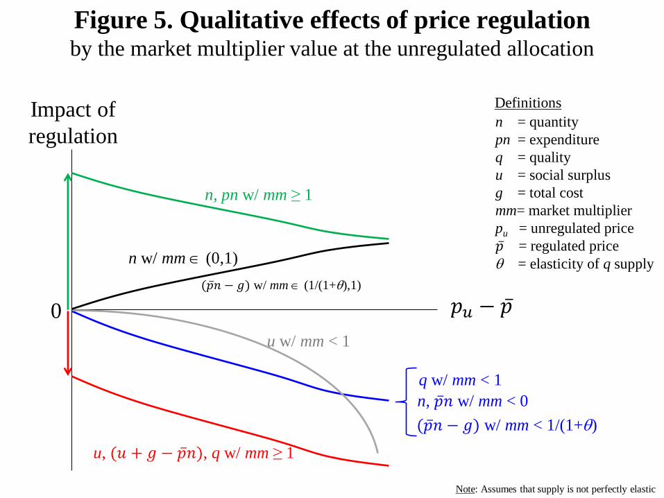
𝑝𝑢 − 𝑝

Impact of

regulation

Figure 5. Qualitative effects of price regulation by the market multiplier value at the unregulated allocation

0

q w/ mm < 1

n, 𝑝 𝑛 w/ mm < 0

u w/ mm < 1

u, (𝑢 + 𝑔 − 𝑝 𝑛), q w/ mm ≥ 1

n, pn w/ mm ≥ 1

n w/ mm (0,1)

Definitions

n = quantity

pn = expenditure

q = quality

u = social surplus

g = total cost

mm= market multiplier

pu = unregulated price

𝑝 = regulated price

= elasticity of q supply

Note: Assumes that supply is not perfectly elastic

(𝑝 𝑛 − 𝑔) w/ mm (1/(1+),1)

(𝑝 𝑛 − 𝑔) w/ mm < 1/(1+)

Figure 6. Producer surplus

with a quality or price ceiling.

Raw

quantity (n)

Price of

quantity

𝒈𝒏 𝒏,𝒒

𝑛𝑟𝑒𝑔 𝑛𝑢𝑛𝑟𝑒𝑔

𝛽 = 1

𝛽 = 0

𝒈𝒏𝒒 𝒏,𝒒 𝒅𝒒

Factors for adding quality Factors for producing raw quantity

𝑍𝑛,𝑟𝑒𝑔

Factor

quantity

Factor supply

Factor

price

𝑍𝑛,𝑢𝑛𝑟𝑒𝑔 𝑍𝑞,𝑟𝑒𝑔

Factor

quantity

Factor supply

Factor

price

𝑍𝑞,𝑢𝑛𝑟𝑒𝑔

𝑔 𝑛, 𝑞 = 𝑆𝑛 𝑍𝑛 𝑑𝑍𝑛

𝑛

0

+ 𝑆𝑞 𝑍𝑞 𝑑𝑍𝑞

𝑛𝐺(𝑞)

0

Figure 7. Quality regulation changes the composition

of producer surplus.

39

Bibliography Abbott, Lawrence. "Vertical Equilibrium under Pure Quality Competition." American

Economic Review 43, no. 5 (December 1953): 826-45.

Autor, David, Christopher J. Palmer, and Parag A. Pathak. "Housing Market Spillovers:

Evidence from the End of Rent Control in Cambridge, Massachusetts." Journal of

Political Economy 122, no. 3 (June 2014): 661-.

Barzel, Yoram. Economic Analysis of Property Rights. Cambridge: Cambridge

University Press, 1997.

Becker, Gary S. "A Note on Restaurant Pricing and Other Examples of Social Influences

on Price." Journal of Political Economy 99, no. 5 (October 1991): 1109-16.

Becker, Gary S. "A Theory of the Allocation of Time." Economic Journal 75, no. 299

(September 1965): 493-517.

Becker, Gary S., and H. Gregg Lewis. "On the Interaction between the Quantity and

Quality of Children." Journal of Political Economy 81, no. 2, Part 2 (March

1973): S279-S288.

Becker, Gary S., and Kevin M. Murphy. Social Economics. Cambridge, MA: Harvard

University Press, 2003.

Besley, Timothy, John Hall, and Ian Preston. "The demand for private health insurance:

do waiting lists matter?" Journal of Public Economics 72, no. 2 (May 1999): 155-

81.

Block, Walter, and Edgar, eds. Olsen. Rent Control: Myths & Realities. Vancouver:

Fraser Institute, 1981.

Boudreaux, Donald J., and Jr. Robert B. Ekelund. "The Cable Television Consumer

Protection and Competition Act of 1992: The Triumph of Private over Public

Interest." Alabama Law Review 44 (1992): 355-391.

Bourne, Ryan. "The Flaws in Rent Ceilings." IEA Discussion Paper, no. 55 (September

2014).

Bulow, Jeremy, and Paul Klemperer. "Regulated Prices, Rent-Seeking, and Consumer

Surplus." Journal of Political Economy 120, no. 1 (February 2012): 160-86.

Burman, Leonard E., Robert J. Shiller, Gregory Leiserson, and Jeffrey Rohaly. "The

Rising Tide Tax System: Indexing the Tax System for Changes in Inequality."

December 2006.

https://www.aeaweb.org/annual_mtg_papers/2007/0107_0800_0403.pdf

(accessed January 14, 2016).

Cheung, Steven N.S. "A Theory of Price Control." Journal of Law and Economics 17, no.

1 (April 1974): 53-71.

Cheung, Steven N.S. "Steven N.S. Cheung's Reminiscence of Himself -- A Reply to Ning

Wang." Man and the Economy, April 2016: forthcoming.

Deacon, Robert T., and Jon Sonstelie. "Rationing by Waiting and the Value of Time:

Results from a Natural Experiment." Journal of Political Economy 93, no. 4

(August 1985): 627-47.

Dixit, Avinash. "Quality and Quantity Competition." Review of Economic Studies 46, no.

4 (October 1979): 587-99.

40

Dreze, Jacques, and Kare P. Hagen. "Choice of Product Quality: Equilibrium and

Efficiency." Econometrica 46, no. 3 (May 1978): 493-513.

Feldman, Roger, and Bryan Dowd. "Must Adverse Selection Cause Premium Spirals?"

Journal of Health Economics 10, no. 3 (October 1991): 349-57.

Frech, H.E. III. Physician Fees and Price Controls. Vol. 102, in American Health Care,

Government, Market Processes, and the Public Interest, by Roger D., ed.

Feldman, 333-50. Washington, DC: American Enterprise Institute, 2001.

Frech, H.E. III, and James C., Jr. Samprone. "The Welfare Loss of Excess Nonprice

Competition: The Case of Property-Liability Insurance Regulation." Journal of

Law and Economics 23, no. 2 (October 1980): 429-40.

Frech, H.E. III, and William C. Lee. "The Welfare Cost of Rationing-by-Queueing across

Markets: Theory and Estimates from the U.S. Gasoline Crisis." Quarterly Journal

of Economics 102, no. 1 (February 1987).

Friedman, David D. Price Theory: An Intermediate Text. South-Western Publishing Co.,

1990.

Galbraith, John Kenneth. A Theory of Price Control. Cambridge, MA: Harvard

University Press, 1980.

Gal-Or, Esther. "Quality and Quantity Competition." Bell Journal of Economics 14, no. 2

(Autumn 1983): 590-600.

Glaeser, Edward L., and Erzo F.P. Luttmer. "The Misallocation of Housing under Rent

Control." American Economic Review 93, no. 4 (September 2003): 1027-46.

Hall, Robert E. "The Minimum Wage and Job Turnover in Markets for Young Workers."

In The Youth Labor Market Problem: Its Nature, Causes, and Consequences, by

Richard B. Freeman and David A. Wise. Chicago: University of Chicago Press,

1982.

Hassin, Refael, and Moshe Haviv. To Queue or not to Queue: Equilibrium Behavior in

Queueing Systems. Boston: Kluwer Academic Publishers, 2003.

Hayek, Friedrich A. "The Use of Knowledge in Society." American Economic Review 35,

no. 4 (September 1945): 519-30.

Hazlett, Thomas W, and Matthew L. Spitzer. Public Policy toward Cable Television: The

Economics of Rate Controls. AEI Press, 1997.

Hirshleifer, Jack. "The Exchange between Quality and Quantity." Quarterly Journal of

Economics 69, no. 4 (1955): 596-606.

Holzer, Harry J., Lawrence F. Katz, and Alan B. Krueger. "Job Queues and Wages."

Quarterly Journal of Economics 106, no. 3 (August 1991): 739-68.

Ippolito, Richard A. "The Impact of the Minimum Wage if Workers Can Adjust Effort."

Journal of Law and Economics 46, no. 1 (April 2003): 207-27.

Jevons, William Stanley. The Coal Question. London: Macmillan and Co., 1866.

Koelln, Kenneth, and Mark Rush. "Rigid Prices and Flexible Products." Journal of

Economics 19, no. 1 (Spring 1993): 57-64.

Lancaster, Kelvin J. "A New Approach to Consumer Theory." Journal of Political

Economy 74 (April 1966): 132-56.

Lanier, Jaron. Who Owns the Future? New York: Simon & Schuster, 2014.

Lee, David, and Emmanuel Saez. "Optimal Minimum Wage Policy in Competitive Labor

Markets." Journal of Public Economics 96 (October 2012): 739-49.

Leffler, Keith B. "Ambiguous Changes in Product Quality." American Economic Review

72, no. 5 (December 1982): 956-67.

41

Levy, Daniel, Mark Bergen, Shantanu Dutta, and Robert Venable. "The Magnitude of

Menu Costs: Direct Evidence from Large U.S. Supermarket Chains." Quarterly

Journal of Economics 112, no. 3 (August 1997): 791-825.

Lindbeck, Assar. The Political Economy of the New Left: An Outsider's View. New York:

Harpercollins, 1971.

Mayerhauser, Nicole, and Marshall Reinsdorf. "Housing Services in the National

Economic Accounts." Manuscript, Bureau of Economic Analysis, September

2007.

McCloskey, Donald N. The Applied Theory of Price. London: Macmillian, 1985.

Moon, Choon-Geol, and Janet G. Stotsky. "The Effect of Rent Control on Housing

Quality Change: A Longitudinal Analysis." Journal of Political Economy 101, no.

6 (December 1993): 1114-48.

Mulligan, Casey B. "In-Kind Taxes, Behavior, and Comparative Advantage." NBER

working paper, no. 21586 (September 2015).

Mulligan, Casey B., and Andrei Shleifer. "Conscription as Regulation." American

Journal of Law and Economics 7, no. 1 (Spring 2005): 85-111.

Murphy, Michael M. "Price Controls and the Behavior of the Firm." International

Economic Review 21, no. 2 (June 1980): 285-91.

Raymon, Neil. "Price Ceilings in Competitive Markets with Variable Quality." Journal of

Public Economics 22 (1983): 257-64.

Rolnick, Arthur J., and Warren E. Weber. "Gresham's Law or Gresham's Fallacy."

Journal of Political Economy 94, no. 1 (February 1986): 185-99.

Spence, A. Michael. "Monopoly, Quality, and Regulation." Bell Journal of Economics 6,

no. 2 (Autumn 1975): 417-29.

Steiner, Peter O. "Program Patterns and Preferences, and the Workability of Competition

in Radio Broadcasting." Quarterly Journal of Economics 66, no. 2 (May 1952):

194-233.

Stigler, George J. "Price and Non-price Competition." Journal of Political Economy 76,

no. 1 (January 1968): 149-54.

Taylor, Grant A., Kevin K.K. Tsui, and Lijing Zhu. "Lottery or Waiting-line Auction?"

Journal of Public Economics 87, no. 5-6 (May 2003): 1313-34.

Telser, Lester G. A Theory of Efficient Cooperation and Competition. Cambridge:

Cambridge University Press, 1987.

—. The Core Theory in Economics: Problems and Solutions. New York: Routledge,

2009.

Telser, Lester G. "Why Should Manufacturers Want Fair Trade?" Journal of Law and

Economics 3 (October 1960): 86-105.

Theil, Henry. "Qualities, Prices, and Budget Enquiries." Review of Economic Studies 19,

no. 3 (1952): 129-47.

Weitzman, Martin L. "Prices vs. Quantities." Review of Economic Studies 41, no. 4

(October 1974): 477-91.

Welch, Finis. "Minimum Wage Legislation in the United States." Economic Inquiry 12,

no. 3 (September 1974): 285-318.

Yurukoglu, Ali, Ali Liebman, and David B. Ridley. "The Role of Government

Reimbursement in Drug Shortages." manuscript, Stanford University, January

2016.