The Transmission of Monetary Policy in a Multi-Sector Economy

2005-16

BOUAKEZ, HafedCARDIA EmanuelaRUGE-MURCIA Francisco

The Transmission of Monetary Policy in a Multi-Sector Economy

Département de sciences économiques

Université de Montréal

Faculté des arts et des sciences

C.P. 6128, succursale Centre-Ville

Montréal (Québec) H3C 3J7

Canada

http://www.sceco.umontreal.ca

[email protected]

Téléphone : (514) 343-6539

Télécopieur : (514) 343-7221

Ce cahier a également été publié par le Centre interuniversitaire de recherche en

économie quantitative (CIREQ) sous le numéro 20-2005.

This working paper was also published by the Center for Interuniversity Research in

Quantitative Economics (CIREQ), under number 20-2005.

ISSN 0709-9231

The Transmission of Monetary Policy

in a Multi-Sector Economy

H. Bouakez†, E. Cardia‡, and F. J. Ruge-Murcia§

July 2005

Abstract

This paper constructs and estimates a sticky-price, Dynamic Stochastic GeneralEquilibrium model with heterogenous production sectors. Sectors di er in price stick-iness, capital-adjustment costs and production technology, and use output from eachother as material and investment inputs following an Input-Output Matrix and CapitalFlow Table that represent the U.S. economy. By relaxing the standard assumptionof symmetry, this model allows di erent sectoral dynamics in response to monetarypolicy shocks. The model is estimated by Simulated Method of Moments using sec-toral and aggregate U.S. time series. Results indicate 1) substantial heterogeneity inprice stickiness across sectors, with quantitatively larger di erences between servicesand goods than previously found in micro studies that focus on final goods alone, 2)a strong sensitivity to monetary policy shocks on the part of construction and durablemanufacturing, and 3) similar quantitative predictions at the aggregate level by themulti-sector model and a standard model that assumes symmetry across sectors.

JEL Classification: E3, E4, E5Key Words: Multi-sector models, sticky-price DGSE models, monetary policy

We have received helpful comments from Rui Castro, Juan Dolado, and participants in the Meetings ofthe Canadian Economics Association (Toronto, May 2004), the conference on Dynamic Models and MonetaryPolicymaking at the Federal Reserve Bank of Cleveland (Cleveland, September 2004), and seminars at theFederal Reserve Bank of Richmond and UQAM. Financial support from the Social Sciences and HumanitiesResearch Council is gratefully acknowledged. Correspondence: Francisco J. Ruge-Murcia, Departement desciences economiques, Universite de Montreal, C.P. 6128, succursale Centre-ville, Montreal (Quebec) H3C3J7, Canada. E-mail: [email protected]. The latest version of this paper is available atwww.cireq.umontreal.ca/personnel/ruge.html

†Institut d’economie appliquee, HEC Montreal, and CIREQ‡Departement de sciences economiques and CIREQ, Universite de Montreal§Departement de sciences economiques and CIREQ, Universite de Montreal

1 Introduction

Economies involve the production and exchange of di erent goods produced in di erent

sectors using distinct technologies and inputs. However, this heterogeneity is only partly

acknowledged in standard sticky-price Dynamic Stochastic General Equilibrium (DSGE)

models which have become the main tool of monetary policy analysis.1 These models

assume that goods are di erent enough to confer the producer a degree of monopoly power,

but in the symmetric equilibrium all relative prices are equal to one and allocations are

identical across sectors. This approach simplifies aggregation, but it also means that the

standard model cannot address some important questions in monetary economics.

In addition to obvious realism, there are at least two reasons why sectoral heterogeneity

matters. First, understanding sectoral responses to monetary policy shocks can be help-

ful in explaining the mechanism(s) through which money has real e ects. For example, if

nominal rigidity is concentrated in one or two sectors, then monetary policy can still have

nontrivial e ects on flexible-price sectors through input-output interactions. Second, sec-

toral heterogeneity has implications for the design of monetary policy. In contrast to the

standard model where optimal monetary policy involves stabilizing the aggregate price level,

research by Aoki (2001), Erceg and Levin (2002), Benigno (2004) and Huang and Liu (2004)

shows that this strategy is sub-optimal in an economy where sectors are characterized by

di erent degrees of nominal rigidity. Instead, these authors find potential welfare gains from

targeting sectoral inflation rates.

This paper constructs and estimates a sticky-price DSGE model with heterogenous pro-

duction sectors. Sectors are heterogenous in price stickiness, capital-adjustment costs,

production functions, and the combination of goods used as material and investment inputs.

In particular, sectors in this model use output from each other following an Input-Output

Matrix and Capital Flow Table that represent the U.S. economy. The model is estimated

by Simulated Method of Moments (SMM) using sectoral and aggregate U.S. time series.

The main empirical results are the following. First, there is heterogeneity in price stickiness

across sectors. This heterogeneity is large and statistically significant. The null hypothe-

sis that prices are flexible can be rejected for services and durable manufacturing, but not

for the other sectors. These results are in qualitative agreement with micro evidence for

the U.S. (Bils and Klenow, 2004) and other countries. However, they also imply a quan-

titatively larger di erence between the price rigidity of services and goods than previously

1See, among many others, Blanchard and Kiyotaki (1987), Yun (1996), Rotemberg and Woodford (1997),Chari, Kehoe and McGrattan (2000), Kim (2000), Ireland (2001, 2003), and Christiano, Eichenbaum andEvans (2005).

[1]

reported. One reason is that estimates in this paper are based on both final and intermedi-

ate goods. Micro studies on intermediate goods (see Carlton, 1986) find long-term relations

between buyer-seller pairs and larger price rigidity than for final goods. This is important

because data from the Input-Output accounts indicate that services is the largest producer

of intermediate goods in the U.S. economy.

Second, there is substantial heterogeneity in the response of sectoral variables to monetary

policy shocks. In particular, output in construction, durable manufacturing, and services

increase proportionally more than in the other sectors, but the mechanisms by which these

responses take place are di erent. The response of services reflects the partial accommo-

dation of a demand increase by the monopolistically competitive producer of a sticky-price

good. The response of construction is due to the input-output structure of the economy

and, in particular, to the increase in demand for investment goods by other sectors. The

response of durable manufacturing is due to a combination of these two mechanisms. Al-

though prices in agriculture, mining and nondurable manufacturing are flexible and these

sectors do not produce capital goods, their output increases because they produce material

inputs employed by the other sectors. In summary, the output e ects of a monetary policy

shock arise from price stickiness in some sectors of the economy and are transmitted to the

other sectors via the input-output structure. The observation that output responses to

monetary policy shocks are positively correlated across sectors and are larger on the part of

durable-good producers is also documented by the Vector Autoregressions (VAR) in Barth

and Ramey (2001), Dedola and Lippi (2003), and Peersman and Smets (2005). In general,

however, VAR analysis does not reveal the economic mechanism by which the heterogenous

sectoral responses arise.

Finally, in the presence of moderate frictions in the transfer of capital and labor across

sectors, the aggregate predictions of the multi-sector and standard symmetric models are

similar. Hence, modeling sectoral heterogeneity and interactions explicitly does not modify

in a substantive manner the aggregate implications of DSGE models. This result is impor-

tant because it suggests that previous literature that imposes symmetry across sectors may

still provide a reasonable characterization of the dynamics of aggregate variables.

The paper is organized as follows. Section 2 constructs the monetary model with hetero-

geneous production sectors. Section 3 describes the data and econometric methodology, and

reports the parameter estimates. Section 4 studies the properties of the estimated model.

Finally, Section 4 discusses the limitations of this analysis and outlines future research.

[2]

2 A Monetary Economy with Heterogenous Produc-

tion Sectors

2.1 Households

The economy is populated by identical, infinitely-lived households. The population size is

constant and normalized to one. The representative household maximizes

EXt=

t U (Ct,mt, 1 Nt) , (1)

where (0, 1) is the subjective discount factor; U (·) is an instantaneous utility function

that satisfies the Inada conditions and is assumed to be strictly increasing in all arguments,

strictly concave, and twice continuously di erentiable; Ct is consumption; mt = Mt/Pt is

real money balances; Mt is the nominal money stock; Pt is an aggregate price index; and

Nt is hours worked. Since the total time endowment is normalized to one, 1 Nt represents

leisure time.

Consumption is a constant-elasticity-of-substitution (CES) aggregate over the J available

goods:

Ct =JXj=1

j(cjt)( 1)/

/( 1)

, (2)

where j [0, 1] are aggregation weights that satisfyJPj=1

j = 1, cjt is the household’s con-

sumption of good j, and > 1 is the elasticity of substitution between di erent goods.

Notice that since j can be equal to zero for a given good j, not all goods are necessarily

final in the sense that they are ultimately consumed by households. Instead some goods

might be intermediate, meaning that they are used only in the production of other goods.

The price index Pt is defined as

Pt =JXj=1

( j) (pjt)1

1/(1 )

, (3)

where pjt is the price of good j. Because Pt is the price index associated with the bundle of

goods consumed by households, it can be interpreted as the Consumer Price Index (CPI) in

our model economy.

Households have a preference for diversity in their labor supply. That is,

Nt =JXj=1

(njt)( +1)/

/( +1)

, (4)

[3]

where > 0 and njt is the number of hours worked in sector j at time t. This implies that

households are willing to work a positive number of hours in every sector even if wages are

not equal in all sectors. This assumption permits heterogeneity in wages and hours worked

across sectors while preserving the representative-agent setup.2

In what follows, we specialize the instantaneous utility function to

U (Ct,mt, 1 Nt) = log(Ct) + t log(mt) + % log(1 Nt), (5)

where % > 0 is the utility weight of leisure and t is a strictly positive preference shock. The

functional form of the instantaneous utility is motivated by theoretical results in Ngai and

Pissarides (2004) who show that necessary and su cient conditions for the existence of an

aggregate balanced growth path in a multi-sector economy are logarithmic preferences and

a non-unit price elasticity of demand.

There are J + 2 financial assets in this economy: money, a one-period interest-bearing

nominal bond, and shares in each of the J productive sectors. The household enters period

t with Mt 1 units of currency, Bt 1 nominal private bonds, and sjt 1 shares in sectors j =

1, . . . , J , and then receives interests and dividends, wages from its work in each sector, and a

lump-sum transfer from the government. These resources are used to finance consumption

and the acquisition of financial assets to be carried over to next period. Expressed in real

terms, the household’s budget constraint in every period is

bt +JXj=1

pjtcjt

Pt+

JXj=1

ajtsjt

Pt+mt =

Rt 1bt 1

t+

JXj=1

wjtnjt

Pt+

JXj=1

(djt + ajt)s

jt 1

Pt+mt 1

t+

t

Pt, (6)

where bt = Bt/Pt is the real value of nominal bond holdings, ajt is the unit price of a share

in sector j, djt is the dividend paid by a share in sector j, Rt is the gross nominal interest

rate on bonds that mature at time t+ 1, t is the gross inflation rate between periods t 1

and t, wjt is the nominal wage in sector j, and t is the government lump-sum transfer.

The household’s utility maximization is carried out by choosing optimal sequences {cjt , njt ,

Mt, Bt, sjt}t= subject to the sequence of budget constraints (6), a no-Ponzi-game condition,

and initial asset holdings sj 1, M 1, and B 1. The 3J + 2 first-order conditions for this

problem determine the consumption demand for each good, labor supplied to each sector and

money demand, and price the nominal bond and the shares in each sector. In particular,

2The aggregator (4) implies that, strictly speaking, Nt is an index of hours worked. Only in the specialcase where and the aggregator is linear does Nt correspond to total hours worked. However, inthis case, hours worked in each sector are perfect substitutes and, consequently, the model would predictcounterfactually that wages are the same in all sectors.

[4]

the consumption demand for each good is

cjt = (j)

ÃpjtPt

!Ct, (7)

where the price elasticity of demand is . Using this demand function and the definition

of the price index, it is easy to show thatJPj=1pjtc

jt = PtCt.

2.2 Firms

The J di erentiated goods are produced in monopolistically competitive sectors. The num-

ber of firms in each sector is normalized to one. As in Dixit and Stiglitz (1977), it is

assumed that J is large enough that firms take aggregate variables as given and do not

engage in strategic behavior. The representative firm in sector j uses the technology,

yjt = (kjt )

j

(ztnjt)

j

(Hjt )

j

, (8)

where yjt is output, kjt is capital, zt is an aggregate labor-augmenting productivity shock,

Hjt is material inputs, and the parameters

j, j, j (0, 1) and satisfy the linear restrictionj + j + j = 1. The e ect of a productivity shock will be di erent across sectors because

sectors di er in factor intensities.3

Material inputs are goods produced by other sectors that are used as inputs in the

production of good j. These inputs are combined according to

Hjt =

ÃJXi=1

ij(hji,t)

( 1)/

! /( 1)

, (9)

where hji,t is the quantity of input i purchased by sector j and ij [0, 1] is the weight

that input i receives in sector j. The weights ij satisfy the conditionJPi=1

ij = 1. The

weights ij and quantities hji,t are indexed by j because every sector uses a di erent input

combination in its production process. For the empirical analysis of the model, estimates

of ij are constructed using the Use Table of the U.S. Input-Output accounts. The price of

the composite good Hjt is

QHj

t =

ÃJXi=1

( ij) (pit)1

!1/(1 )

. (10)

3In an earlier version of this paper, productivity shocks were modeled as sector specific. However, theirprocess parameters were poorly identified unless arbitrary restrictions were imposed during the estimationof the model. In addition, it is well known that the e ect of uncorrelated sector-specific shocks tends todissipate through aggregation due to the law of large numbers (see Dupor, 1999).

[5]

Firms own directly their capital stock. The stock of capital follows the law of motion

kjt+1 = (1j)kjt +X

jt , (11)

where j is the sector-specific rate of depreciation and Xjt is an investment technology that

aggregates di erent goods into additional units of capital. Specifically,

Xjt =

ÃJXi=1

ij(xji,t)

( 1)/

! /( 1)

, (12)

where xji,t is the quantity of good i purchased by sector j for investment purposes and

ij [0, 1] is the weight that good i receives in the production of capital in sector j. The

weights ij satisfy the conditionJPi=1

ij = 1. Empirical estimates of ij are constructed below

using data from the U.S. Capital Flow Table. The price of the composite investment good

Xjt is

QXj

t =

ÃJXi=1

( ij) (pit)1

!1/(1 )

. (13)

Adjusting the capital stock is assumed to involve a quadratic cost that is proportional to the

current capital stock,

jt = (Xj

t , kjt ) =

j

2

ÃXjt

kjt

j

!2kjt , (14)

where j is a nonnegative parameter.

Equation (12) allows each sector to use di erent goods in di erent quantities to accumu-

late a stock of capital that is sector specific. Note, however, that the specificity of capital in

this model is di erent from the one in Woodford (2005) and Altig, Christiano, Eichenbaum

and Linde (2005). In those models, firms accumulate a form of capital that is not transfer-

able to other firms. This real rigidity helps reconcile the quantitatively small estimate of the

coe cient of the marginal cost in the New Keynesian Phillips curve with the high frequency

of price adjustments found in micro data. In this model, capital is sector specific only in

the sense that the nonlinear combination of investment inputs is di erent across sectors.

However, the composite Xjt can be unbundled and its parts sold to other sectors in a market

with frictions of the form described by equation (14).

The assumption that the elasticity of substitution between goods is the same in equations

(2), (9) and (12) implies that the price elasticity of demand of good i does not depend on

the use given to the good by the buyer. Hence, the monopolistically competitive producer

of good i will charge the same price to firms in all sectors and to households regardless of

[6]

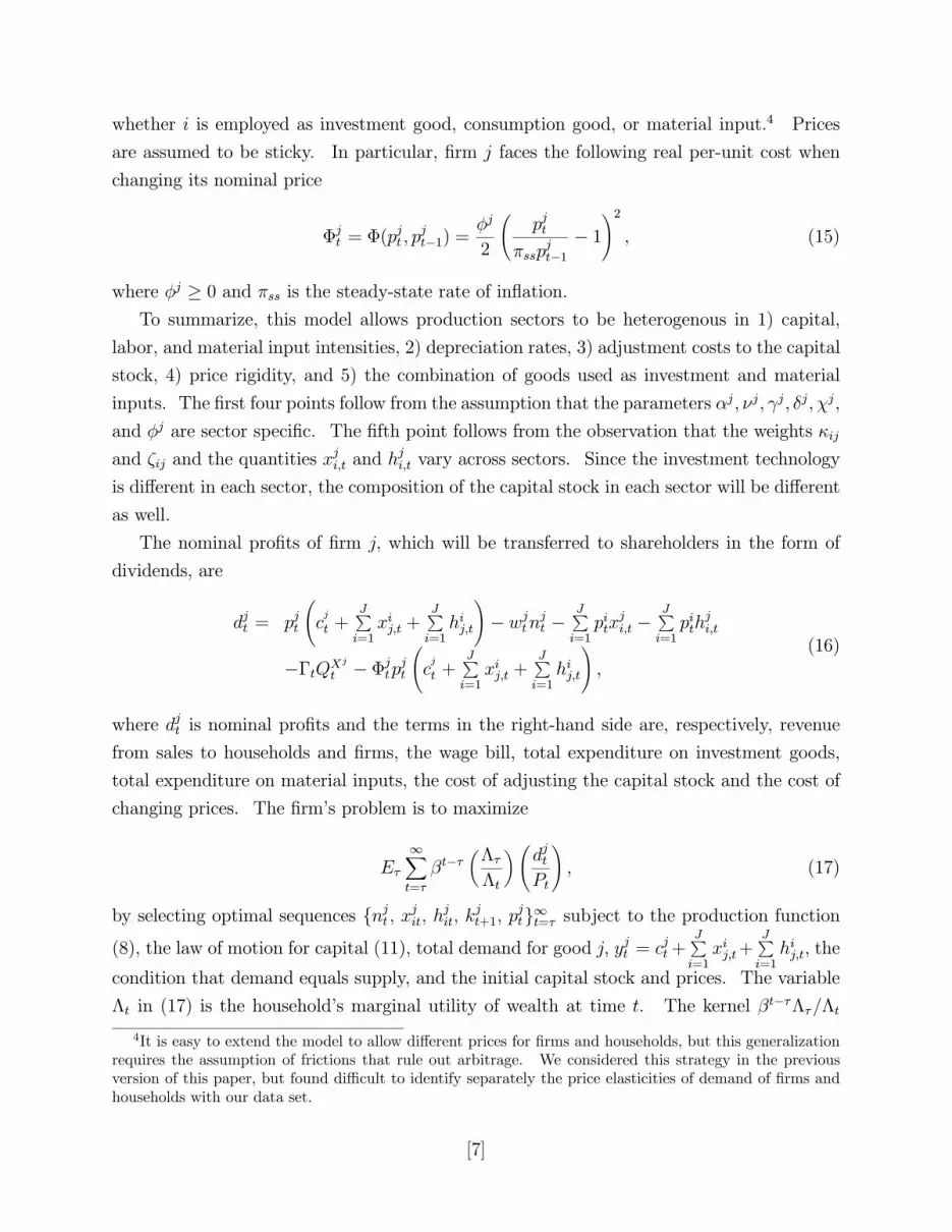
whether i is employed as investment good, consumption good, or material input.4 Prices

are assumed to be sticky. In particular, firm j faces the following real per-unit cost when

changing its nominal price

jt = (pjt , p

jt 1) =

j

2

Ãpjt

sspjt 1

1

!2, (15)

where j 0 and ss is the steady-state rate of inflation.

To summarize, this model allows production sectors to be heterogenous in 1) capital,

labor, and material input intensities, 2) depreciation rates, 3) adjustment costs to the capital

stock, 4) price rigidity, and 5) the combination of goods used as investment and material

inputs. The first four points follow from the assumption that the parameters j, j, j, j, j,

and j are sector specific. The fifth point follows from the observation that the weights ij

and ij and the quantities xji,t and h

ji,t vary across sectors. Since the investment technology

is di erent in each sector, the composition of the capital stock in each sector will be di erent

as well.

The nominal profits of firm j, which will be transferred to shareholders in the form of

dividends, are

djt = pjt

Ãcj

t +JPi=1xij,t +

JPi=1hij,t

!wjtn

jt

JPi=1pitx

ji,t

JPi=1pith

ji,t

tQXj

tjtpjt

Ãcj

t +JPi=1xij,t +

JPi=1hij,t

!,

(16)

where djt is nominal profits and the terms in the right-hand side are, respectively, revenue

from sales to households and firms, the wage bill, total expenditure on investment goods,

total expenditure on material inputs, the cost of adjusting the capital stock and the cost of

changing prices. The firm’s problem is to maximize

EXt=

tµ

t

¶ÃdjtPt

!, (17)

by selecting optimal sequences {njt , xjit, h

jit, k

jt+1, p

jt}t= subject to the production function

(8), the law of motion for capital (11), total demand for good j, yjt = cjt+

JPi=1xij,t+

JPi=1hij,t, the

condition that demand equals supply, and the initial capital stock and prices. The variable

t in (17) is the household’s marginal utility of wealth at time t. The kernel t / t

4It is easy to extend the model to allow di erent prices for firms and households, but this generalizationrequires the assumption of frictions that rule out arbitrage. We considered this strategy in the previousversion of this paper, but found di cult to identify separately the price elasticities of demand of firms andhouseholds with our data set.

[7]

is used to value profits because the firm is owned directly by households through the stock

market.

In order to solve this problem, we first conjectured the form of the demands xij,t and hij,t.

Given the functional forms employed here, natural candidates are xij,t = ( ji)³pjt/Q

Xi

t

´X it

and hij,t = ( ji)³pjt/Q

Hi

t

´Hit . Then we showed that in equilibrium these are indeed the

optimal demands of good j on the part of firms in the other sectors. For these demand

functions, the relationsJPi=1pitx

ji,t = Q

Xj

t Xjt and

JPi=1pith

ji,t = Q

Hj

t Hjt hold.

2.3 Monetary and Fiscal Policy

The government comprises both fiscal and monetary authorities. Fiscal policy consists of

lump-sum transfers to households each period that are financed by printing additional money

in each period. Thus, the government budget constraint is

t/Pt = mt mt 1/ t, (18)

where the term in the right-hand side is seigniorage revenue at time t. Money is supplied

by the government according toMt = µtMt 1, where µt is the stochastic gross rate of money

growth.5 In real terms, this process implies mt t = µtmt 1.

2.4 Shocks

The exogenous shocks to the model, namely the preference shock t, the technology shock

zt, and the monetary policy shock µt, follow the processes

ln( t) = (1 ) ln( ss) + ln( t 1) + ² ,t,

ln(zt) = (1 z) ln(zss) + z ln(zt 1) + ²z,t,

ln(µt) = (1 µ) ln(µss) + µ ln(µt 1) + ²µ,t,

where , z, and µ are strictly bounded between 1 and 1; ln( ss), ln(zss) and ln(µss) are

the unconditional means of their respective shocks; and the innovations ² ,t, ²z,t and ²µ,t are

mutually independent, serially uncorrelated and normally distributed with mean zero and

variances 2z ,

2µ and

2b , respectively.

5In preliminary work, we considered the case where monetary policy takes the form of a Taylor rule forthe nominal interest rate. Calibration results were very similar to the ones reported below and are availablefrom the corresponding author upon request. However, a potential problem with the econometric estimationof that version of the model is that the coe cients of the Taylor rule for the U.S. do not appear to be stableover the sample (see, Clarida, Gali and Gertler, 2000).

[8]

2.5 Aggregation and Equilibrium

In equilibrium, 1) private bond holdings equal zero because households are identical, and 2)

the total share holdings in sector j add up to one. Thus, the aggregate counterpart of the

representative household’s budget constraint is

JXj=1

pjtcjt

Pt+mt =

JXj=1

wjtnjt

Pt+

JXj=1

djtPt+mt 1

t+

t

Pt. (19)

Substituting the government budget constraint (18) into this equation and multiplying

through by the price level yield

JXj=1

pjtcjt =

JXj=1

wjtnjt +

JXj=1

djt . (20)

Let V jt pjt

Ãcj

t +JPi=1xij,t +

JPi=1hij,t

!denote the value of gross output produced by sector j.

Then, aggregate nominal dividends are equal to

JXj=1

djt =JXj=1

V jt

JXj=1

wjtnjt

JXj=1

QXj

t Xjt

JXj=1

QHj

t Hjt

JXj=1

Ajt , (21)

where we have usedJPi=1pitx

ji,t = Q

Xj

t Xjt and

JPi=1pith

ji,t = Q

Hj

t Hjt , and defined A

jt =

jtQ

Xj

t +

jtpjt

Ãcj

t +JPi=1xij,t +

JPi=1hij,t

!to be the sum of all adjustment costs in sector j. The nominal

value added in sector j is denoted by Y jt , and it is defined as the value of gross output

produced by that sector minus the cost of material inputs. That is,

Y jt = Vjt QH

j

t Hjt . (22)

Substituting (21) and (22) into (20), usingJPj=1pjtc

jt = PtCt, and rearranging yield

JXj=1

Y jt = PtCt +JXj=1

QXj

t Xjt +

JXj=1

Ajt . (23)

Thus, total output equals household consumption plus investment by all sectors plus the

sum of all adjustment costs in all sectors.

The equilibrium of the model is not symmetric due to the heterogeneity in production.

That is, relative prices are not all equal to one as is the case in the standard sticky-price

model, and real wages and allocations are di erent across sectors. This observation has two

implications for the solution of the model and the computation of its steady state. First,

[9]

the state variables of the system include J capital stocks and J real prices. Second, finding

the steady-state allocations requires the solution of a set of 2J2 + J nonlinear equations

that determine labor, material and investment inputs in each sector. Then, the remaining

allocations and all relative prices in steady state can be recovered from the model equations.

In contrast, in the standard sticky-price model, the state vector includes only one capital

stock and one real price, and all steady-state allocations are pinned down by the proportion

of hours worked.

The model is solved numerically by log-linearizing the first-order and equilibrium condi-

tions around the deterministic steady state to obtain a system of linear di erence equations

with expectations. The rational-expectation solution of this system is found using the

approach in Blanchard and Kahn (1980).

3 Econometric Estimation

3.1 Data

The empirical analysis of the model is based on sectoral and aggregate U.S. time series at

the quarterly frequency for the period 1959:1 to 2002:4. After the first half of 2003, the Bu-

reau of Labor Statistics (BLS) stopped reporting sectoral data under the Standard Industry

Classification (SIC) codes and switched to the new North American Industry Classification

System (NAICS). This means that pre- and post-2003 sectoral data might not be fully

comparable.

Although the theoretical model allows any level of disaggregation, this paper focuses on

six broad sectors of the U.S. economy at the division level of the SIC, namely agriculture,

mining, construction, durable manufacturing, nondurable manufacturing and services. The

list of six sectors is exhaustive in the sense that their output aggregate to privately-produced

U.S. Gross Domestic Product (GDP). Agriculture (Division A) includes the production of

crops and livestock, agriculture-related services, and forestry. Mining (Division B) in-

cludes oil and gas extraction, metallic and nonmetallic mining, and mining-related services.

Construction (Division C) includes building construction (for example, housing), heavy con-

struction (for example, bridges) and special trade contractors (plumbing, electrical work,

etc.). Although mining and construction respectively represent only 2.5 and 5.2 per cent of

privately-produced GDP, their contribution to aggregate fluctuations may be large because

they produce most of the energy goods6 and fixed capital that enter the production function

6Oil and gas production accounts for 73 per cent of the output value in the mining sector. These figureand the ones in the text are the averages of annual observations for the period 1959 to 2001.

[10]

of all sectors. The division of manufacturing between durables (Division D, Groups 24,

25, and 32 to 39) and nondurables (Division D, Groups 20 to 23 and 26 to 31) is based on

the BLS definition of good durability. Finally, services (Divisions E to I) include, among

others, wholesale and retail trade, transportation, communications, finance and health. As

in the National Income and Product Accounts, rental housing is treated as a service for the

purpose of computing the households’ expenditure shares.

The number and size of the sectors is to some extent determined by data availability

and computational considerations. SIC sectoral data are available at discrete aggregation

levels, say division level (roughly six sectors), two-digit level (roughly thirty sectors), etc.

In addition, BLS data tend to be much more exhaustive for manufacturing than for services.

In particular, manufacturing categories are more finely divided than service ones. This

means that the sector sizes are uneven and that service variables receive a large weight in the

aggregates. On the other hand, focusing on the six sectors above has four advantages. First,

these sectors are natural partitions of the U.S. economy. Second, they are associated with

concrete goods, as opposed to the generic distinction between “sticky-price” and “flexible-

price” goods in some two-sector models (see, for example, Ohanian et al., 1995). Third, they

are computationally manageable. The computation of the steady state requires the solution

of 2J2+J nonlinear equations, that is 78 equations for the six-sector model at division level

but 1830 equations for the thirty-sector model at the two-digit level of the SIC. Finally,

there are su cient sectoral data to identify econometrically their sector-specific parameters.7

The sectoral data consist of quarterly series on Producer Price Indices at the division

level of the SIC, observations on yearly expenditures on labor, capital and material inputs

by each sector, and data from the U.S. Input-Output accounts. The commodity-based Pro-

ducer Price Indices collected by the BLS for farm products, durable manufactured goods,

and nondurable manufactured goods were used to construct sectoral inflation series for agri-

culture, durable manufacturing, and nondurable manufacturing, respectively.8 Since the

raw data are seasonally unadjusted, we control for seasonal e ects by regressing each series

on seasonal dummies and purging the seasonal components.

The data on input expenditures by each sector are used to construct estimates of the

production function parameters (see Section 3.2 below). This data set was originally con-

7A drawback of this level of disaggregation is that the assumption in the theoretical model that J is largeenough such that firms take aggregate quantities as given is less plausible in this case. This means that,for example, the service sector may recognize its nonnegligible e ect on the aggregate price level and behavestrategically. These e ects may be theoretically interesting, but we abstract from them in the empiricalanalysis that follows.

8The BLS only started constructing PPIs at the industry level in the mid-1980s. The three commodity-based indices mentioned above match well with their respective industries, but we were unable to find orconstruct similar matches for mining, construction, and services for the complete sample period.

[11]

structed by Dale Jorgenson and is described in detail in Jorgenson and Stiroh (2000). The

observations are available at the annual frequency for the years 1958 to 1996 for more than

30 sectors, but aggregation up to the division level of the SIC is straightforward.

Data from the U.S. Input-Output (I-O) accounts are used to construct estimates of

the weights ij and ij. Input—Output accounts show how industries use output from and

provide input to each other to produce gross domestic product. The Bureau of Economic

Analysis (BEA) prepares both benchmark and annual I-O accounts. Benchmark accounts

are produced every five years using detailed data from the economic censuses conducted

by the Bureau of the Census. Annual accounts are prepared for selected years between

the benchmarks using less comprehensive data than those from the censuses. We use

the 1992 benchmark accounts because both the Use Table and the Capital Flow Table are

electronically available for that year.9

The Use Table is used to construct the weights ij. Use Tables contain the value in

producer prices of each input used by each U.S. industry. As in Horvath (2000), the weight

ij is computed as the share of total input expenditures by sector j that goes into inputs from

sector i.10 The Capital Flow Table (CFT) is used to construct the weights ij. The CFT

shows the purchases of new structures, equipment and software, allocated by using industry

in producer prices. The weight ij is computed as the share of total investment expenditures

by sector j that goes into inputs from sector i. Most of the investment commodities are

produced by the construction and durable manufacturing sectors. The service sector has

nonnegligible weights because it produces goods that are ancillary to investment, for example,

engineering and landscaping services. Mining produces most of its own capital stock because

exploration, shafts and wells in the oil industry are coded as goods produced in the mining

sector in the I-O accounts. By construction, ij, ij [0, 1] andJPi=1

ij =JPi=1

ij = 1 for all j.

The aggregate data consist of quarterly series on the rates of inflation, nominal money

growth and nominal interest, and per capita real money balances, investment and consump-

9The only other year for which this is true is 1982, but documentation is more extensive and user friendlyfor 1992 than for 1982.10We equate commodities with sectors as in the theoretical model where good j is produced exclusively by

sector j. This means that we are implicitly treating the Make Table of the I-O accounts as diagonal and it isthe reason we can construct the weights ij using the Use Table alone. The Make Table contains the value ofeach commodity produced by each domestic industry and, in reality, it is not perfectly diagonal because thereis a small proportion of commodities that are produced by industries in a di erent SIC division. For example,the I-O accounts treat printed advertisement as a business service (Division I) even though it is producedby the printing and publishing sector (Division D). In order to examine the quantitative importance ofthe o -diagonal terms, we computed the share of each commodity that is produced in each sector. Sincethe diagonal elements vary between 0.988 and 1, the original assumption of the model that associates eachcommodity with only one sector seems to the a reasonable approximation for the U.S. economy at this levelof disaggregation.

[12]

tion. With the exceptions noted below, the raw data were taken from the database of the

Federal Reserve Bank of St-Louis. The inflation rate is the percentage change in the CPI.

The rate of nominal money growth is the percentage change in M2. The nominal interest

rate is the three-month Treasury Bill rate. Real money balances are computed as the ratio

of M2 per capita to the CPI. Real investment and consumption are measured, respectively,

by Gross Private Domestic Investment and Personal Consumption Expenditures per capita

divided by the CPI. The raw investment and consumption series were taken from the Na-

tional Income and Product Accounts produced by the BEA. Real balances, investment and

consumption are computed in per capita terms in order to make these data compatible with

the model, where there is no population growth. The population series corresponds to the

quarterly average of the mid-month U.S. population estimated by the BEA. Except for the

nominal interest rate, all data are seasonally adjusted at the source.

Since the variables in the model are expressed in percentage deviations from the steady

state, all series were logged and quadratically detrended, except the rates of inflation (sectoral

and aggregate), money growth, and nominal interest, which were logged and demeaned.

3.2 Methodology and Parameter Estimates

The model is estimated by Simulated Method of Moments (SMM). SMM has been proposed

by McFadden (1989) and Pakes and Pollard (1989) to estimate discrete-choice problems, and

by Lee and Ingram (1991) and Du e and Singleton (1993) to estimate time-series models.

SMM is attractive for the estimation of DSGE models for two reasons. First, the stochastic

singularity of DGSE models imposes weaker restrictions on moments-based procedures than

on Maximum Likelihood (ML). In particular, estimation requires the use of linearly indepen-

dent moments for SMM, but linearly independent variables for ML. The former is a weaker

restriction because it is possible to find independent moments that incorporate information

about more variables than those that are linearly independent. Second, moments-based pro-

cedures are more robust to misspecification than ML. See Ruge-Murcia (2003) for further

discussion.

In order to develop the reader’s intuition, consider the following comparison between

SMM and calibration. In calibration, the macroeconomist computes the unconditional

moments of artificial series generated by the DSGE model given the parameter values, and

then compares these artificial moments with the ones estimated using actual data. This

comparison may be casual or based on measures of fit like the ones proposed, for example,

by Gregory and Smith (1991) and Watson (1993). The Simulated Method of Moments also

compares simulated and empirical unconditional moments, but then updates the estimates of

[13]

the parameter values in a manner that minimizes a well-defined measure of distance between

the moments.

Formally, define gt to be the vector of empirical observations on variables whose moments

are of interest. Define g ( ) to be the synthetic counterpart of gt whose elements are

computed on the basis of artificial data generated by the model using parameter values .

The sample size is denoted by T and the number of observations in the artificial time series

is T. The (optimal) SMM estimator, b, is the value of that solves

min{ }

G( )0WG( ), (24)

where

G( ) = (1/T )TXt=1

gt (1/ T )TX=1

g ( ),

andW is the optimal weighting matrix

W = limT

V ar

Ã(1/ T )

TXt=1

gt

! 1

. (25)

Under the regularity conditions in Du e and Singleton (1993),

T ( b ) N(0,(1 + 1/ )(D0W 1D) 1), (26)

where D = E( g ( )/ ) is a matrix assumed to be finite and of full rank.

The optimal weighting matrix,W, is computed using the Newey-West estimator with a

Barlett kernel, and the derivatives g ( )/ are computed numerically with the expec-

tation approximated by the sample average of the simulated T data points. The results

reported below are based on = 5, meaning that the simulated series are 5 times larger

than the sample size. The term (1 + 1/ ) in (26) is a measure of the increase in sample

uncertainty due to the use of simulation to compute the population moments. Using a larger

value of permits a more accurate estimation of the simulated moments and increases the

statistical e ciency of SMM, but it also increases the time required for each iteration of the

minimization routine. Sensitivity analysis indicates that results are robust to the value of

used.

In order to limit the e ect of the starting values used to generate the artificial series,

100 extra observations were generated in every iteration of the minimization routine and the

initial 100 observations were discarded. The seed in the random numbers generator is fixed

throughout the estimation. The use of common random draws is essential here to calculate

the numerical derivatives of the minimization algorithm. Otherwise, the objective function

would be discontinuous and the optimization algorithm would be unable to distinguish a

[14]

change in the objective function due to a change in the parameters from a change in the

random draw used to simulate the series.

A number of parameters were estimated or calibrated prior to SMM estimation. The

reason is that the estimation of this model requires the computation of the steady state and

the Blanchard-Khan solution of the model in every iteration of the optimization algorithm.

The former is extremely costly computationally because it involves the solution of a large

system of nonlinear equations. Thus, for estimation purposes, it is useful to distinguish

between 1) parameters that a ect the dynamics of the system but not the steady state, and

2) parameters that determine the steady state and may or may not a ect the dynamics.

The latter parameters include the subjective discount rate ( ), the preference parameter

, the parameters of the sectoral production functions ( j, j, and j), the parameter

that measures the elasticity of substitution in production and consumption, the sectoral

depreciation rates ( j), and the consumption weights ( j). An advantage of estimating

these parameters beforehand is that solving (24) then requires only the computation of the

model solution, but not of the steady state, in every iteration of the minimization routine.

The consumption weights, sectoral depreciation rates, and were taken from Horvath

(2000). Horvath measures the consumption weights as the average expenditure shares in

the National Income and Product Accounts from 1959 to 1995. The shares for agriculture,

mining, construction, durable manufacturing, nondurable manufacturing and services are

0.02, 0.04, 0.01, 0.16, 0.29 and 0.48, respectively. The sectoral depreciation rates are 0.01,

0.02, 0.04, 0.02, 0.02 and 0.02, respectively. Finally, Horvath constructs an estimate of

from a regression of the change in the relative labor supply on the change in the relative

labor share in each sector. Since his results indicate that b = 0.9996 (0.0027), where theterm in parenthesis is the standard error, we set = 1 in our empirical analysis.11

An estimate of the subjective discount rate was constructed using the sample average

of the inverse of the gross ex-post real interest rate to obtain b = 0.997 (0.0005). By the

Central Limit Theorem, this estimator is normally distributed with mean and variance2/T where T = 175 is the sample size and 2 is the variance of the t+1/Rt. Previous

multi-sector models calibrate to values between 1 (Hornstein and Praschnik, 1997) and 3

(Bergin and Feenstra, 2000). We use = 2, but results appear robust to using values similar

to those employed in earlier multi-sector literature.12 The mean of the technology shock is

11In addition, we tested this parametric restriction using a Lagrange Multiplier (LM) test. Since thep-value is 0.70, the restriction is not rejected by our data at standard significance levels.12The restriction = 2 was tested using a LM test. The p-value was 0.35 meaning that this restriction

would not be rejected by the data at standard levels. In preliminary calibrations, we considered largervalues of , which would be consistent with earlier markup estimates in Basu and Fernald (1994). However,in this case, the model predicts counterfactually that mostly the good with the lowest relative price will be

[15]

calibrated to minimize the distance between the actual and predicted share of each sector in

aggregate output. Due to the normalization that the total time endowment is equal to 1,

the mean of this shock is just a scaling factor.

Estimates of the parameters of the production functions are constructed using data on

annual labor, capital, and material inputs expenditures for each sector collected by Dale

Jorgenson for the period 1958 to 1996. The real expenditures predicted by the model may

be obtained from the first-order conditions of the firm’s problem,13

j³

jtyjt

´=

wjtnjt

Pt, (27)

j³

jtyjt

´=

JPi=1pith

ji,t

Pt, (28)

j³

jtyjt

´=

ÃÃt 1

t

!jt 1 (1 j) j

t

!kjt +

QXj

t kjt

Pt

Ãt

kjt

!, (29)

where jt is the real marginal cost. The right-hand sides of (27) and (28) are, respectively, the

wage bill and total expenditure on material inputs in sector j. The right-hand side of (29)

is the total opportunity cost (net of capital gains) of the capital stock in sector j plus a term

that represents the net cost of increasing the current capital stock. Jorgeson’s expenditure

data may be interpreted as the empirical counterpart of the right-hand side of these equations

(see Jorgenson and Stiroh, 2000). Although the data set does not contain observations onjtyjt , it is possible to construct estimates of

j, j, and j as follows. For a given year, use

two of the following three ratios: (27)/(28), (27)/(29) and (28)/(29),14 and the conditionj + j + j = 1, to obtain a system of three equations with three unknowns. The unique

solution of this system delivers an observation of the production function parameters for that

year. The estimates of j, j, and j are the sample averages of the yearly observations and

their standard deviations areq

2/T where T = 39 is the sample size and 2 is the variance

of the yearly observations. These estimates are reported in Table 1 and indicate substantial

heterogeneity in capital, labor and material intensities across sectors. For example, mining

is very intensive in capital; construction, agriculture and manufacturing are intensive in

materials but not in capital; and services are equally intensive in labor and materials. This

heterogeneity is quantitatively important and statistically significant. That is, the di erence

in parameter estimates across sectors is numerically large and the null hypothesis that ,

used for consumption and production in steady state.13In deriving equation (29) from first-order condition for kjt+1, we exploit the assumption of rational

expectations. Thus, strictly speaking, this equation holds up to a serially uncorrelated forecast error withzero mean.14Note that only two of these three ratios are linearly independent.

[16]

and are the same in all sectors would be rejected by the data.

The SMM estimates of the model parameters are reported in Table 3. These results are

based on a restricted version of the model where 1) the price-adjustment-cost parameters

in agriculture, mining and construction are assumed to be the same, and 2) the capital-

adjustment-cost parameters in all sectors are also assumed to be the same. These two

restrictions were tested using LM tests. Since the p-values were 0.096 and 0.106, respectively,

the restrictions would not be rejected by the data at the 5 per cent significance level.15 The

moments included in the loss function (24) are the variances and autocovariances of the

variables, and the covariance between the nominal interest rate and the other variables one

quarter ahead. The first set of moments allows us to exploit the information contained

in the volatility and persistence of the data series. The second set of moments is included

because this project is concerned specifically with the interaction between monetary and real

variables. Sensitivity analysis indicates that results are robust to using other moments.

The SMM estimates indicate heterogenous price rigidity at the sectoral level. The hy-

pothesis that price rigidity is the same in all sectors is strongly rejected by a Wald test

(p-value < 0.01). The hypothesis that = 0 can be rejected for services and durable man-

ufacturing, but it cannot be rejected for the other sectors. Since = 0 corresponds to the

case of flexible prices, this result indicates that price flexibility may be a reasonable approx-

imation in all sectors of the U.S. economy, except for services and durable manufacturing.

These results are in qualitative agreement with micro evidence for the U.S. (Bils and

Klenow, 2004) and various European countries. See, for example, Alvarez and Hernando

(2004) for Spain, Baudry et al. (2004) for France, Ho mann and Kurz-Kim (2004) for

Germany, Veronese et al. (2004) for Italy, and Vilmunen and Laakkonen (2004) for Finland.

Using final goods and services that enter the Consumer Price Index in their respective

countries, these researchers typically find heterogeneous price stickiness, more frequent price

adjustments for goods than for services, and for nondurable goods (including energy and

agricultural products) than for durable goods.16 This paper confirms their results using an

empirical approach that exploits the structure of a fully-specified general equilibrium model

and the cross-sectional variation in sectoral inflation rates.

Quantitatively, the estimates here indicate a larger di erence between the price rigidity

of services and goods than that reported in some of the earlier micro studies. There are two

possible explanations for this result. First, although this paper does not model explicitly

15Note, however, that the first restriction would be marginally rejected at the 10 per cent level.16There is also substantial heterogeneity within these broad categories. For example within services, price

adjustments are much more frequent for transportation (which includes air travel) than for health servicesand rents. Cecchetti (1986) and Kashyap (1995) report heterogeneity even within narrowly defined goodcategories like magazines and shoes sold by catalog.

[17]

the housing decision, rental housing is included in the service sector for the purpose of

computing the households’ expenditure shares. Ho mann and Kurz-Kim (2004, p. 22)

report that including housing rents in their sample increases the overall duration of price

spells from 16 to 21 months in Germany. Second, the estimates in this paper are based on

both final and intermediate goods. Carlton (1986) studies U.S. micro data on firm-to-firm

transactions of intermediate goods and finds long-term relations between buyer-seller pairs

and larger price rigidity than that found, for example, by Bils and Klenow (2004) using final

goods alone. This is important because data from the Input-Output accounts show that

services is the largest producer of intermediate goods in the U.S. economy. In particular,

services account (on average) for 36 per cent of the material-input expenditures by other

sectors, and for 74 per cent of the expenditures by services itself.

The capital adjustment cost parameter is estimated to be 10.93 (1.94). In order to give

meaning to this estimate and to allow its comparison with estimates based on other functional

forms, it is useful to compute the elasticity of investment with respect to the price of installed

capital. The elasticity implied by this estimate is 4.40 (0.78).17 This value is much larger

than the estimates of 0.34 and 0.28 reported by Kim (2000) and Christiano, Eichenbaum,

and Evans (2005), respectively, but is smaller than the value of 15 used, for example, by

Baxter and Crucini (1993) to calibrate a Real Business Cycle model. Simulations reported

below in Table 4 show that this estimate implies an investment volatility of 9.5, which is

very similar to that of 10.6 found in U.S. data.

The estimates of the autoregressive coe cients of the shock processes indicate that all

shocks are persistent. The estimate of is very close to one, perhaps reflecting trends in

financial innovation that are not completely removed from the data by quadratic detrending.

The estimate of µ is similar to values found when money growth is estimated using an

univariate process (for example, Chari, Kehoe and McGrattan, 2000).

The overidentification restrictions of the model are tested using a J test. Since the p-

value is less than 0.001, the restrictions are rejected at standard significance levels. However,

this result must be interpreted with caution because, as is well known, the actual size of this

test in small samples far exceeds the nominal size and, consequently, the test rejects too

often (see Burnside and Eichenbaum, 1996, and Christiano and den Haan, 1996).

17The elasticity is computed as 1/( ) using a depreciation rate of 0.0208. This depreciation rate corre-sponds to an economy-wide rate computed as the weighted average of sectoral depreciation rates.

[18]

4 Properties of the Estimated Model

In order to understand better the properties the estimated multi-sector model, this section

examines the responses of sectoral and aggregate variables to a monetary policy shock,

computes the variance decomposition, volatility and persistence of these variables, compares

the multi-sector model with a standard DSGE model that imposes symmetry across sectors,

studies the sectoral reallocation of labor following a monetary policy shock, and computes a

measure of price rigidity at the aggregate and sectoral levels.

4.1 Responses to a Monetary Policy Shock

Consider an experiment where, starting at the deterministic steady state, the economy is

subjected to an unexpected, temporary increase in the growth rate of the money supply of

1 per cent. Then, the growth rate returns to its steady state at the rate µ. Figure 1 plots

the dynamic responses of various aggregate and sectoral variables following this monetary

policy shock.

The shock generates a rise in aggregate demand that causes aggregate output to increase

(see Panel A). However, this increase is not evenly spread across sectors. In particular,

output in construction, durable manufacturing and services increase proportionally more

than in the other sectors (see Panel B). The initial increases in these three sectors are

4, 3 and 2.1 per cent, respectively, while in the other sectors they are all approximately

1 per cent. The output increase in services reflects the usual mechanism whereby the

monopolistically competitive producer of a sticky-price good partially accommodates an

increase in demand by raising its output. The output increase in construction takes place

despite the fact that its price is flexible and is due to the input-output structure of the

economy. Firms in services and other sectors (see below) increase their current output

but also their demand for investment goods in order to build up their capital stock and

meet future demand. Since the production of investment goods is heavily concentrated in

construction and durable manufacturing, the output increase in these two sectors is large.

In the durable-manufacturing sector this increase is due to both monopoly power in the

presence of nominal frictions, and input-output e ects.

Although prices in agriculture, mining and nondurable manufacturing are flexible and

these sectors do not produce capital goods, their output rises persistently as a result of the

current and future output increases in construction, services and durable manufacturing (12,

12 and 15 per cent, respectively, of their material-input expenditures go to these sectors).18

18Authors’ calculations based on the 1992 U.S. Input-Output accounts.

[19]

In summary, the output e ects of a monetary policy shock arise from price stickiness in

services and durable manufacturing, and are transmitted to the other sectors via the input-

output structure of the economy. The input-output structure is crucial in generating a large

response in the investment-good producers and positive output comovement across sectors

following a monetary policy shock.

Ohanian, Stockman and Kilian (1995) construct a two-sector model without input-output

interactions. One sector has a flexible price and the other fixes its price one period in

advance. Following a monetary policy shock, the relative price of the flexible-price good

raises and, conversely, that of the sticky-price good decreases. This change in relative

prices induces a substitution e ect in consumption that leads to an output decrease in the

flexible-price sector and an increase in the sticky-price sector. Thus, sectoral outputs are

negatively correlated. Barth and Ramey (2001), Dedola and Lippi (2003), and Peersman

and Smets (2005) use VAR analysis to study the output e ects of monetary policy shocks

on di erent manufacturing industries. As in this paper, they also find positively-correlated

output responses across industries, and quantitatively larger responses on the part of durable

good producers, which they interpret as evidence for the conventional cost-of-capital channel

of monetary policy transmission.19

Panels C and D plot the responses of hours worked at the aggregate and sectoral levels,

respectively. These responses primarily reflect the increase in labor demand on the part of

firms, and they follow the same pattern as the output responses reported above. Thus, the

sectoral responses of hours worked in constructions, durable manufacturing and services are

larger than in the other three sectors. The relative magnitudes of their initial responses

are similar to those of output, except for services which is the most labor-intensive sector

in the economy. The responses of aggregate and sectoral real wages are plotted in Panels

E and F, respectively.20 The e ect of a monetary policy shock on the aggregate wage is

relatively persistent, and there is substantial heterogeneity in the response of sectoral wages,

with wages in construction, durable manufacturing and services being the most sensitive to

this shock.

The dispersion of sectoral hours and wages is less than the dispersion of sectoral outputs

at all horizons. For example, the ratio of the standard deviation of sectoral wages to that of

19These authors also find that industries where small firms are more prevalent tend to react more stronglyto monetary policy shocks. This finding suggest that financial frictions may also play an important role.

20The aggregate real wage is measured by the index wt/Pt =

ÃJPj=1

³wjt/Pt

´1+ !1/(1+ )

. This index has

the property thatJPj=1

wjtnjt = wtNt.

[20]

sectoral outputs is only 0.61 in the quarter at which the shock takes place. This result is due

in part to the assumption of a preference for diversity in the household’s labor supply, which

acts as a friction to the reallocation of hours across sectors. As an example, consider the

counterfactual assumption that = 2, meaning that hours worked across sectors are better

substitutes than implied by the empirical work in Horvath (2000), where 1. In this case,

the ratio reported above decreases to 0.39. In the limit, as , hours worked in each

sector become perfect substitutes, wages in all sector are equalized, and this ratio would

be zero. In terms of hours, the increase in substitutability of labor supply across sectors

associated with a larger value of means that the sectoral dispersion of hours is increasing in

. These results reflect some degree of labor mobility across sectors and are consistent with

earlier findings by Davis and Haltiwanger (2001) who report reallocative e ects of monetary

policy shocks in U.S. manufacturing.

A monetary policy shock leads to an increase in aggregate consumption and substantial

changes in the composition of household consumption (see Panels G and H). The over-

all e ect of the monetary policy shock is largest for manufactured goods (both durable

and nondurables) and services. Except for construction, the initial e ects are all posi-

tive. The consumption of construction decreases on impact and reaches its steady state

non-monotonically from below. The dynamics of sectoral consumption reflects the role of

relative prices in the economy’s adjustment following a shock. To see this, note the path of

relative prices in Panel J. The relative price of services declines because its nominal price is

sticky. In contrast, the relative price of the other goods rises because their nominal prices

are more flexible. The largest increases in relative prices are in construction and mining.

From Panels H and J, it is clear that the increase in household consumption is smaller for

goods whose relative prices rise the most following a monetary policy shock. Thus, the tem-

porary change in the composition of the consumption bundle simply reflects intratemporal

substitution by households.

These impulse-responses are roughly in line with VAR evidence reported in Erceg and

Levin (2002). Following a decrease in the U.S. Federal Funds Rate, the consumption of

durable goods, residential structures, business equipment and business structures all increase.

In the case of the latter two, the response is sluggish and becomes statistically di erent

from zero only after three and seven quarters, respectively. In our multi-sector model, the

firms’ demand for durables and structures, and the households’ demand for durables increase

immediately following the monetary policy shock. However, the households’ demand for

structures decreases, while it increases in Erceg and Levin’s VAR. As pointed out above, the

reason is that the consumption demand for an individual good is primarily a function of its

relative price. Since, construction prices are relatively flexible and there is strong demand

[21]

on the part of firms, its relative price rises steeply and households’ demand falls.

Panels K and L plot the response of CPI and sectoral inflation rates to the monetary

policy shock. In all cases, the rates increase following the shock and then return mono-

tonically to their steady-state values. Inflation in services increases the least following a

monetary policy shock but is also the most persistent. In contrast, inflation in construction

and durable manufacturing increase the most but return fairly rapidly to their steady state.

This observation is also true for productivity and money demand shocks (not reported).

Since the share of services in the CPI is approximately one-half, this means that the dynam-

ics of aggregate inflation at horizons of a year or less are jointly determined by service and

non-service sectors. However, since inflation in non-service sectors return much faster to

the steady state, the aggregate dynamics at horizons beyond a year are mostly determined

by service inflation.

Finally, the response of the real interest rate is plotted in Panel I. The drop in the real

rate is substantial and persistent. However, it is clear from panels I and K, that the response

of the nominal interest rate (not shown) would be positive and relatively muted. Hence,

as in standard sticky-price models, the multi-sector model also fails to produce a liquidity

e ect. The reason is that the estimated money growth process is highly autocorrelated.

Thus, following a monetary policy shock, expected inflation increases by a magnitude that

is slightly larger than the decrease in the real interest rate. It follows that the net e ect of

the monetary shock on the nominal interest rate is quantitatively small and positive.

4.2 Variance Decomposition

One way to evaluate the relative importance of monetary policy shocks in explaining the

volatility of aggregate and sectoral variables is to compute their variance decomposition.

This entails the calculation of the proportion of the conditional variance of the forecast error

at di erent horizons that is attributable to the monetary policy shock. As the horizon

increases, the conditional variance of the forecast error of a given variable tends to the

unconditional variance of that variable. Results are reported in Figure 2 for forecast horizons

of one to twenty quarters ahead, and in Table 3 for the infinite horizon.

Regarding aggregate variables, monetary policy shocks account for most of the conditional

variance of output and consumption at horizons of less than a year, but only for 36 and 40 per

cent, respectively, in the long run. The same pattern is observed for investment, where the

contribution of this shock decreases (non-monotonically) from about 30 per cent at the one-

quarter horizon to 21 per cent in the long run. In contrast, monetary policy shocks explain

a larger part of the conditional variances of hours, wages and inflation in the long than in the

[22]

short run. For example, the proportion of the conditional variance of CPI inflation that is

explained by this shock increases monotonically from 9 per cent at the one-quarter horizon

to 19 per cent in the long run.

Regarding sectoral variables, monetary policy shocks explain a substantial part of the

conditional variance of output and consumption of durable manufacturing and services, and

of hours worked in construction, both in the short and long runs. There is large hetero-

geneity in the proportion of sectoral wages and investment that is attributable to monetary

policy shocks at horizons of less than a year, but these proportions start to converge after

about four quarters. Although monetary policy shocks tend to be more important in the

short run, their contribution in the long run is quantitatively large in some sectors. For

example, they explain 41, 30 and 20 per cent of the unconditional variance of wages in

durable manufacturing, nondurable manufacturing and services, respectively, and between

11 (durable manufacturing) and 26 per cent (construction) of the unconditional variance of

sectoral investment.

Finally, monetary policy shocks account for less than 15 per cent of the conditional

variance of sectoral inflations in the very short run, but (except for services) their contribution

increases with the forecast horizon. In the long run, they explain 18 and 32 per cent of the

unconditional variance of inflation in construction and durable manufacturing, respectively.

4.3 Sectoral Volatility and Persistence

This section computes the unconditional standard deviations and first-order autocorrelations

of aggregate and sectoral variables predicted by the multi-sector model, and compares them

with those estimated using aggregate U.S. data and those predicted by a standard DSGE

model. By standard DSGE model we mean a model that allows material inputs in the

production function but di ers from our multi-sector model in that it imposes symmetry

across sectors in production and assumes identical consumption weights for all goods. The

standard deviations predicted by the two DSGE models are based on simulated series of 175

observations and averaged over 500 replications. The length of the simulated series is equal

to the number of observations in the sample of U.S. data.

The parameters used to simulate the multi-sector model are the SMM estimates reported

in Tables 1 and 2. The parameters used to simulate the standard DSGE model are the

following. The consumption, investment and material input weights (that is, j, ij and

ij, respectively) are all set to 1/6. Thus, the Input-Output and Capital Flow Tables of

the standard economy are symmetric. The parameters of the production functions are the

same for all sectors and are estimated using the same strategy described in Section 3.2 but

[23]

using the sum of expenditures on labor, capital, and material inputs by all sectors. The

price-rigidity coe cients and depreciation rates are also the same for all sectors and are

computed as the weighted averages of the sectoral estimates reported in Table 2 and the

sectoral depreciation rates in Section 3.2, respectively. The values of , , and the mean of

the technology shock are the same as in the multi-sector model. The other model parameters

are those reported in Table 2.

The aggregate and sectoral standard deviations are reported in Table 4. The standard

deviations of aggregate variables in the multi-sector and standard models are fairly simi-

lar. Notice that for all variables, the standard DSGE model predicts sectoral standard

deviations that are identical to the aggregate ones because this model assumes symmetry in

production.21 In contrast, the multi-sector predicts substantial heterogeneity in the volatil-

ity of sectoral variables. Comparing the predicted volatilities with those of the sectoral

variables for which data are available shows that they are quantitatively similar. Two

exceptions are durable consumption and hours worked (notably, in services).

The model counterfactually predicts that the households’ consumption of nondurable

manufactured goods is more volatile than that of durable goods. In U.S. data, the stan-

dard deviations are 3.66 and 8.98, respectively, but in the model they are 4.55 and 2.95,

respectively. This discrepancy is due to the fact that the theoretical model abstracts from

consumption durability and, consequently, sectoral household demand depends primarily on

relative prices. Thus, the larger volatility of inflation in nondurable than durable manufac-

turing translates into more volatile consumption of the former compared with the latter.

The multi-sector model predicts substantial volatility in sectoral hours and wages. The

volatility of hours worked is larger in the model than in the data for construction, nondurable

manufacturing and, specially, services.22 This suggests that it may be fruitful to incorporate

labor market frictions, such as labor-adjustment costs and sector-specific skills, in multi-

sector models. The output of construction and agriculture are the most volatile, while that

of services is the least volatile. The volatility of construction output is 3 times larger than

that of services and aggregate output. On the other hand, investment by the construction

sector is the least volatile, perhaps because this sector is the least capital-intensive in the

U.S. economy.

21The only exception is output because sectoral output is measured by gross output while aggregate outputis measured by value added. The same caveat applies to estimates of the first-order autocorrelation. Thevolatility and autocorrelation of sectoral output are 3.68 and 0.77, respectively, for all sectors.22These results should be interpreted with caution because the notion of hours and wages in the model

and the data are not exactly the same. In the model, hours worked are a share while in the data they areaverage weekly hours of production workers. It is not possible to construct a better data equivalent becausedata on hours worked in agriculture are missing from the BLS database. The measure of wages in the datais average weekly earnings of production workers and may include compensation other than wages.

[24]

Comparing the predicted sectoral inflation volatilities and their empirical counterparts

indicates that their magnitudes are quantitatively similar, with inflation in agricultural goods

being more volatile than that of manufactured goods. The model also predicts large volatility

in the inflation rate of mining goods. Industry-level data for mining are not available for the

complete sample, but this prediction of the model accords well with the observed volatility

in the price inflation of various mineral commodities.

The aggregate and sectoral autocorrelations are reported in Table 5. The multi-sector

model generates predictions for the persistence of aggregate and sectoral variables that are

roughly in line with the data, except for hours worked. In particular, notice the large

heterogeneity in the predicted persistence of sectoral inflation rates, and their similarity to

the values found in the data.

4.4 Comparison with the Standard Symmetric Model

Results regarding the predicted standard deviations and autocorrelations reported in Tables

4 and 5 indicate that the multi-sector and standard DSGE models di er only modestly in

their aggregate predictions. This result is explored further in this Section by comparing

the impulse responses of aggregate variables to a monetary policy shock under both models.

Figure 2 reproduces the responses of aggregate output, consumption, hours worked, real

wages, CPI inflation, and the real interest rate following a monetary policy shock that were

previously reported in Figure 1 for the multi-sector model, and plots the corresponding

responses for the standard model.

The responses from both models are very similar for output, consumption, and real

wages. There are quantitatively small di erences in the initial response of inflation and the

real interest rate, but after four quarters the predictions of both models coincide exactly. The

only appreciable di erence between the two models is in the dynamic response of aggregate

hours. While the initial response is almost the same in the multi-sector and standard models,

the converge to the steady state is somewhat faster in the former than in the latter.

Overall, these results and those in Tables 4 and 5 indicate that modeling the heterogeneity

of the di erent production sectors in the economy does not modify in a substantive manner

the aggregate implications of DSGE models that impose symmetry. This result is important

because it suggests that literature that imposes symmetry across goods may still provide a

reasonable description of the behavior of aggregate variables.23

The reason for this result is that the multi-sector model permits the reallocation (al-

23A similar result is reported by Balke and Nath (2003) in a calibrated multi-sector with no capital andperfect labor mobility across sectors.

[25]

beit imperfect) of labor and capital across sectors. The reallocation of labor depends on

the degree of substitutability of hours worked in the utility function of the representative

household. Also, although capital is sector-specific in the multi-sector model in that each

sector uses a di erent nonlinear combination of investment inputs, the composite Xjt can be

unbundled and its parts sold to other sectors in a frictional market. Thus, in the presence

of moderate frictions in the movement of capital and labor across sectors, the aggregates of

a multi-sector economy behave in similar manner to those generated by a standard model

that ignores heterogeneity in production.24

4.5 Sectoral Versus Aggregate Price Rigidity

The multi-sector DSGE model also allows us to compare price rigidity at the sectoral and

aggregate levels. A distinction is made between ex-ante price rigidity, which is measured by

the price-adjustment-cost parameters reported in Table 2, and ex-post price rigidity, which

depends on both these parameters and the optimal pricing behavior of firms in each sector.

This Section computes ex-post price rigidity at the sectoral and aggregate levels as the ratio

of price-adjustment costs to output. By construction, price-adjustment costs are zero in

steady state, but estimates of their average magnitude outside steady state can be computed

by means of simulation. The results below are based on simulated series of 175 observations

averaged over 500 replications.

For the sectoral estimates, it is easy to see from the definition of dividends in Equation

(16) that the ratio of adjustment costs to output is simply jt . For the aggregate estimate,

the ratio isJPj=1

jtpjt

Ãcj

t +JPi=1xij,t +

JPi=1hij,t

!JPj=1Y jt

, (30)

whereJPj=1Y jt is aggregate nominal output and is defined in (23).

Estimates reported in Table 6 indicate that sectoral price-adjustment costs vary between

0.011 and 0.058 per cent of output in mining and services, respectively. On the other hand,

the aggregate price-adjustment costs are 0.061 per cent of GDP. This aggregate estimate

is larger than each of the sectoral estimates and than their weighted average, which is 0.04.

This means that ex-post price rigidity is larger at the aggregate than at the sectoral level.

24In related work, Carlstrom, Fuerst, Ghironi and Hernandez (2005) construct and calibrate a two-sectormodel with heterogenous price rigidity and labor immobility across sectors, and report additional persistence(vis-a-vis the one-sector model) stemming from relative price dynamics.

[26]

In order to understand this result, note that firms pay price-adjustment costs on all trans-

actions regardless of whether the good is used for final or intermediate consumption. How-

ever, aggregate output in the model, as in the U.S. National Income and Product Accounts,

is measured by value added, which avoids double counting by excluding the transactions of

intermediate goods. Since the numerator in (30) is the sum of all sectoral price-adjustment

costs, but the denominator is only the sum of all sectoral values added, the aggregate ratio

is larger than the weighted average of the sectoral estimates.

5 Discussion

This paper studies the e ects of monetary policy through the lens of a multi-sector model.

In contrast to earlier sticky-price models that impose symmetry across sectors, this analysis

models explicitly the heterogeneity in production and frictions that are a prominent feature

of the data. The paper shows that although sectoral heterogeneity makes quantitatively

little di erence for the dynamics of aggregate variables, modeling the input-output structure

of the economy is crucial in understanding the sensitivity of di erent sectors to monetary

policy shocks, as well as the sectoral reallocation of productive resources. Econometric

results indicate subtantial heterogeneity in price rigidity across sectors, and that services

and, to a lesser extent, durable manufacturing account for most of the rigidity observed at

the aggregate level. Due to the input-output structure, monetary policy shocks have large

e ects even on flexible-price sectors.

The parameter values are estimated so as to minimize the distance between the moments

of artificial series generated by the multi-sector model and those computed from a mix of

aggregate and sectoral U.S. data. Yet, there are a few dimensions along which the multi-

sector model fails to match the data, namely the volatility and persistence of aggregate

wages and hours worked, and the volatility of durable consumption. Hence, in future work,

we intend to incorporate explicit frictions in the labor market, such as wage stickiness and

labor-adjustment costs.

[27]

Table 1. Estimates of Production Function Parameters

Sector

Agriculture 0.142 0.261 0.597(0.005) (0.006) (0.006)

Mining 0.380 0.243 0.377(0.009) (0.004) (0.011)

Construction 0.052 0.394 0.554(0.001) (0.004) (0.005)

Durables 0.100 0.321 0.579(0.001) (0.003) (0.002)

Nondurables 0.113 0.225 0.662(0.004) (0.002) (0.006)

Services 0.222 0.399 0.379(0.004) (0.003) (0.007)

Notes: , and are, respectively, the exponents of capital, labor and material inputs in

the sectoral production functions. The numbers in parenthesis are standard errors. The

superscript denotes the rejection of the hypothesis that the true parameter is zero at the

5 per cent significance level.

[28]

Table 2. SMM Estimates

Parameter Estimate

durables 13.51(5.25)

nondurables 2.47(1.55)

services 98.55(34.89)

others 0.65(0.77)10.93(1.94)

z 0.67(0.09)

µ 0.45(0.12)0.99(0.01)

z 0.10(0.04)

µ 0.005(0.001)0.004(0.004)

Notes: others is the price-adjustment-cost parameter for agriculture, mining and construction

estimated under the restriction that it is the same in the three sectors. See the notes to

Table 1.

[29]

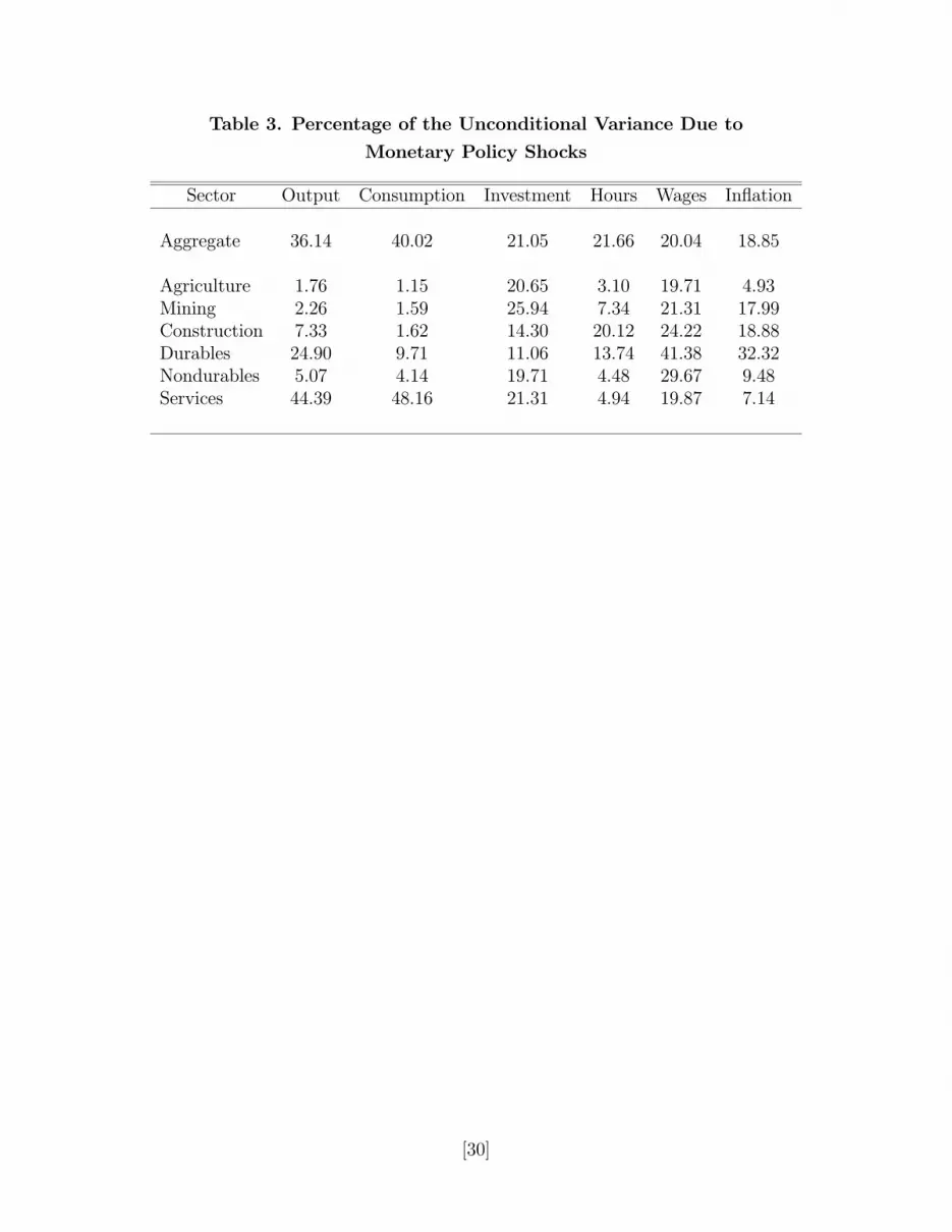
Table 3. Percentage of the Unconditional Variance Due to

Monetary Policy Shocks

Sector Output Consumption Investment Hours Wages Inflation

Aggregate 36.14 40.02 21.05 21.66 20.04 18.85

Agriculture 1.76 1.15 20.65 3.10 19.71 4.93Mining 2.26 1.59 25.94 7.34 21.31 17.99Construction 7.33 1.62 14.30 20.12 24.22 18.88Durables 24.90 9.71 11.06 13.74 41.38 32.32Nondurables 5.07 4.14 19.71 4.48 29.67 9.48Services 44.39 48.16 21.31 4.94 19.87 7.14

[30]

Table 4. Sectoral Volatility


A. U.S. Data

Aggregate 3.74 3.40 10.59 0.55 4.15 0.80

Agriculture n.a. n.a. n.a. n.a. n.a. 2.72Mining n.a. n.a. n.a. 1.87 2.91 n.a.Construction n.a. n.a. n.a. 1.31 7.14 n.a.Durables n.a. 8.98 n.a. 1.69 3.44 0.99Nondurables n.a. 3.66 n.a. 1.11 3.18 1.68Services n.a. 3.07 n.a. 0.38 4.07 n.a.

B. Multi-Sector Model

Aggregate 3.06 2.44 9.48 2.30 6.11 0.49


C. Standard Model

Aggregate 2.78 2.29 8.02 6.58 3.85 0.30

Notes: n.a. stands for not available. The sample used to compute the statistics for U.S.

data is 1959:2 to 2002:4. The exceptions are aggregate hours and wages, and the sectoral

hours and wages for services that were computed using data from 1964:1 to 2002:4. The

standard model predicts sectoral standard deviations that are identical to the aggregate ones

reported in the last row of this Table.

[31]

Table 5. Sectoral Persistence


A. U.S. Data

Aggregate 0.96 0.97 0.90 0.75 0.95 0.72

Agriculture n.a. n.a. n.a. n.a. n.a. 0.06Mining n.a. n.a. n.a. 0.80 0.80 n.a.Construction n.a. n.a. n.a. 0.44 0.96 n.a.Durables n.a. 0.93 n.a. 0.88 0.92 0.75Nondurables n.a. 0.96 n.a. 0.81 0.95 0.43Services n.a. 0.95 n.a. 0.59 0.95 n.a.

B. Multi-Sector Model

Aggregate 0.89 0.91 0.85 0.40 0.69 0.48


C. Standard Model

Aggregate 0.89 0.91 0.86 0.63 0.74 0.69

Notes: See the notes to Table 4.

[32]

Table 6. Ratio of Price Adjustment Costs to Output

Sector Ratio (in percent)

Aggregate 0.0608

Agriculture 0.0206Mining 0.0110Construction 0.0179Durables 0.0348Nondurables 0.0205Services 0.0576

[33]

References

[1] Altig, D., Christiano, L. J., Eichenbaum, M., and Linde, J., (2005), “Firm-Specific

Capital, Nominal Rigidities and the Business Cycle,” NBER Working Paper No. 11034.

[2] Alvarez, L. J. and Hernando, I., (2004), “Price Setting Behaviour in Spain: Stylized

Facts Using Consumer Price Micro Data,” Bank of Spain Working Paper No. 0422.

[3] Aoki, K., (2001), “Optimal Monetary Policy Responses to Relative Price Changes,”

Journal of Monetary Economics 48, 55-80.

[4] Balke, N. S., and Nath, H. K., “Nominal Price Rigidities in a Multisector Model,”

Southern Methodist University, Mimeo.

[5] Barth, M. J., and Ramey, V. A., (2001), “The Cost Channel of Monetary Transmission,”

NBER Macroeconomics Annual 16, 199-239.

[6] Basu, S. and Fernald, J., (1994), “Constant Returns and Small Markups in U.S. Man-

ufacturing,” International Finance Discussion Paper 483.

[7] Baudry, L., Le Bihan, H., Sevestre, P., and Tarrieu, S., (2004), “Price Rigidity: Evidence

from the French CPI Micro-Data,” European Central Bank Working Paper No. 384.

[8] Baxter, M. and Crucini, M. J. (1993), “Explaining Saving-Investment Correlations,”

American Economic Review 83, 416-436.

[9] Benigno, P., (2004), “Optimal Monetary Policy in a Currency Area,” Journal of Inter-

national Economics 63, 293-320.

[10] Bergin, P. and Feenstra, R. (2000), “Staggered Price Setting, Translog Preferences, and

Endogenous Persistence,” Journal of Monetary Economics 45, 657-680.

[11] Bils, M. and Klenow, P. J., (2004), “Some Evidence on the Importance of Sticky Prices,”

Journal of Political Economy 112, 947-985.

[12] Blanchard, O. J. and Khan, C. M., (1980), “The Solution of Linear Di erence Models

Under Rational Expectations,” Econometrica 48, 1305-1311.

[13] Blanchard, O. J. and Kiyotaki, N., (1987), “Monopolistic Competition and the E ects

of Aggregate Demand,” American Economic Review 77, 647-666.

[34]

[14] Burnside, C. and Eichenbaum, M., (1996), “Small-Sample Properties of GMM-Based

Wald Tests,” Journal of Business and Economic Statistics 14, 294-308.

[15] Carlton, D. W., (1986), “The Rigidity of Prices,” American Economic Review 76, 637-

658.

[16] Carlstrom, C. T., Fuerst, T. S., Ghironi, F., and Hernandez, K., (2005), “Relative Price

Dynamics and the Aggregate Economy,” Boston College, Mimeo.

[17] Cecchetti, S. G. (1986), “The Frequency of Price Adjustment: A Study of the Newsstand

Prices of Magazines,” Journal of Econometrics 31, 255-274.

[18] Clarida, R., Gali, J., and Gertler, M., (2000), “Monetary Policy Rules and Macroe-

conomic Stability: Evidence and Some Theory,” Quarterly Journal of Economics 115,

147-180.

[19] Chari, V., Kehoe, P., and McGrattan, E. (2000), “Sticky Price Models of the Business

Cycle: Can the Contract Multiplier Solve the Persistence Problem,” Econometrica, 68,

1151-1179.

[20] Christiano, L. J. and den Haan, W. J., (1996), “Small-Sample Properties of GMM for

Business Cycle Analysis,” Journal of Business and Economic Statistics 14, 309-327.

[21] Christiano, L. J., Eichenbaum, M., and Evans, C. L., (2005), “Nominal Rigidities and

the Dynamic E ects of a Shock to Monetary Policy,” Journal of Political Economy 113,

1-45.

[22] Davis, S. J. and Haltiwanger, J., (2001), “Sectoral Job Creation and Destruction Re-

sponses to Oil Price Changes,” Journal of Monetary Economics 48, 465-512.

[23] Dedola, L. and Lippi, F. (2003), “The Monetary Transmission Mechanism: Evidence

from the Industries of Five OECD Countries,” Bank of Italy, Mimeo.

[24] Dixit, A. and Stiglitz, J., (1977), “Monopolistic Competition and Optimum Product

Diversity,” American Economic Review 67, 297-308.

[25] Du e, D. and Singleton, K. J., (1993), “Simulated Moments Estimation of Markov

Models of Asset Prices,” Econometrica 61, 929-952.

[26] Dupor, B., (1999), “Aggregation and Irrelevance in Multi-Sector Models,” Journal of

Monetary Economics 43, 391-410.

[35]

[27] Erceg, C. J. and Levin, A., (2002), “Optimal Monetary Policy with Durable and Non-

Durable Goods,” European Central Bank Working Paper No. 179.

[28] Gregory, A. and Smith, G., (1991), “Calibration as Testing: Inference in Simulated

Macroeconomic Models,” Journal of Business and Economic Statistics 9, 297-304.

[29] Ho mann, J. and Kurz-Kim J.-R., (2004), “Consumer Price Adjustment Under the

Microscope: Germany in a Period of Low Inflation,” Deutsche Bundesbank, Mimeo.

[30] Hornstein, A. and Praschnik, J., (1997), “Intermediate Inputs and Sectoral Comove-

ments in the Business Cycle,” Journal of Monetary Economics 40, 573-598.

[31] Horvath, M., (2000), “Sectoral Shocks and Aggregate Fluctuations,” Journal of Mone-

tary Economics 45, 69-106.

[32] Huang, K. and Liu Z., (2004), “Inflation Targeting: What Inflation Rate to Target,”

Journal of Monetary Economics, forthcoming.

[33] Ireland, P., (2001), “Sticky-Price Models of the Business Cycle: Specification and Sta-

bility,” Journal of Monetary Economics 47, 3-18.

[34] Ireland, P., (2003), “Endogenous Money or Sticky Prices?,” Journal of Monetary Eco-

nomics 50, 1623-1648.

[35] Jorgenson, D. W., and Stiroh, K. J., (2000), “Rising the Speed Limit: U.S. Economic

Growth in the Information Age,” Brookings Papers on Economic Activity, 125-235.

[36] Kashyap, A. K. (1995), “Sticky Prices: New Evidence from Retail Catalogs,” Quarterly

Journal of Economics 110, 245-274.

[37] Kim, J., (2000), “Constructing and Estimating a Realistic Optimizing Model of Mone-

tary Policy,” Journal of Monetary Economics 45, 329-359.

[38] Lee, B.-S., and Ingram, B. F., (1991), “Simulation Estimation of Time-Series Models,”

Journal of Econometrics 47, 195-205.

[39] McFadden, D., (1986), “A Method of Simulated Moments for Estimation of Discrete

Response Models without Numerical Integration,” Econometrica 57, 995-1026.

[40] Ngai, L. R., and Pissarides, C. A., (2004), “Structural Change in a Multisector Model

of Growth,” London School of Economics, Mimeo.

[36]

[41] Ohanian, L. E., Stockman, A. C., and Kilian, L., (1995), “The E ects of Real and

Monetary Shocks in a Business Cycle Model with Some Sticky Prices,” Journal of

Money, Credit and Banking 27, 1210-1234.

[42] Pakes, A. and Pollard, D., (1989), “The Asymptotic Distribution of Simulation Exper-

iments,” Econometrica, 57, 1027-1057.

[43] Peersman, G. and Smets, F., (2005), “The Industry E ects of Monetary Policy in the

Euro Area,” Economic Journal, forthcoming.

[44] Rotemberg, J. and Woodford, M., (1997), “An Optimization-Based Econometric Frame-

work for the Evaluation of Monetary Policy,” NBER Macroeconomics Annual 12, 297-

345.

[45] Ruge-Murcia, Francisco, J., (2003), “Methods to Estimate Dynamic Stochastic General

Equilibrium Models,” University of Montreal, CIREQ Working Paper No. 17-2003.

[46] Veronese, G., Fabiani, S., Gattulli, A., and Sabbatini, R., (2004), “Consumer Price

Behaviour in Italy: Evidence from Micro CPI Data,” Bank of Italy Working Paper No.

[47] Vilmunen, J. and Laakkonen, H., (2004), “How Often do Prices Change in Finland?

Micro-Level Evidence from the CPI,” Bank of Finland, Mimeo.

[48] Watson, M., (1993), “Measures of Fit for Calibrated Models,” Journal of Political Econ-

omy 101, 1011-1041.

[49] Woodford, M., (2005), “Firm-Specific Capital and the New Keynesian Phillips Curve,”

NBER Working Paper No. 11149.

[50] Yun, T., (1996), “Nominal Price Rigidity, Money Supply Endogeneity, and Business

Cycles,” Journal of Monetary Economics 37, 345-370.

[37]

Figure 1. Impulse Responses to a Monetary Policy Shock

Figure 1. Impulse Responses to a Monetary Policy Shock (cont.)

Figure 2. Percentage of the Conditional Variance Due toMonetary Policy Shocks

Figure 2. Percentage of the Conditional Variance Due toMonetary Policy Shocks (cont.)

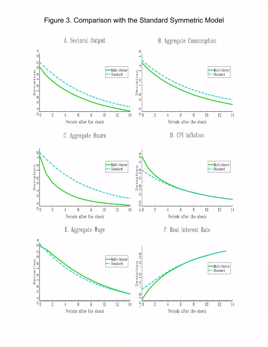
Figure 3. Comparison with the Standard Symmetric Model

The Transmission of Monetary Policy in a Multi-Sector Economy

Documents

Transcript of The Transmission of Monetary Policy in a Multi-Sector Economy