The Tolerance Optimization Problem using a Near to Global Optimum

Proceedings of DETC'20002000 ASME Design Engineering Technical Conferences

September 10-13, 2000, Baltimore, Maryland

DETC 2000/DAC-14294

THE TOLERANCE OPTIMIZATION PROBLEM using A NEAR t o -GLOBAL OPTIMUM

Mohamed H. GadallahAssistant Professor,

Operations Research GroupCairo University, Institute of Statistical Studies and Research (ISSR), Giza, Cairo, Egypt

Email: [email protected]

ABSTRACTIn this paper, an algorithm is developed to deal with thediscrete optimization problem. The algorithmapproximates any design continuous domain with finitenumber of discrete points and employs single andmulti-level search to reach near-to-global optimum. Insingle level search, one orthogonal array is used tomodel any given search domain. In multi-level search,two or more orthogonal arrays are coupled in series andused to model the search domain. The number ofdesign levels are increased with the number of arraysvia different coefficients. The tolerance synthesisproblem with optimum process combination isrevisited to compare our method with well-establishedalgorithms such as Simulated Annealing (SA) andSequential Quadratic Programming (SQP). The effectof algorithm parameters: different structurecombinations, reducing move factors, weighing factorsand column assignments on optimum for single andmulti-level search are investigated. Results indicatethe capability of the approach to reach near-to-globaloptimum in about 5.20 % - 19.5% of time taken byother methods. A survey of available algorithms isgiven and the method is validated with few test cases.

KEYWORDS: Discrete Optimization, MathematicalProgramming, Tolerance Synthesis, DesignOptimization.

BACKGROUNDSeveral researchers were interested in optimizationtechniques and algorithms. Methods ranged fromglobal techniques such as Branch and Bound methods,combination of Sequential Linearization techniqueswith Branch and Bound methods, Genetic algorithmsand random search techniques. Gupta and Ravindran(1983) presented a study on the feasibility of theBranch and Bound method in solving general nonlinearmixed integer programming and discrete methods.Ringertz (1988) considered the use of 3-algorithms for

1

discrete structural optimization. The original problemis replaced by a sequence of approximate discrete sub-problems. For each sub-problem, the Branch andBound is used to find the global minimum and thegeneralized Lagrangian function is minimized over thediscrete set using a neighbourhood search technique.

Rajesekera and Fang (1995) developed an algorithmfor tolerance allocation assuming an exponential cost-tolerance model. The algorithm used a continuous andmonotonic non-increasing function based on the binarysearch method. Dong et al. (1994) presented new cost-tolerance models for design tolerance synthesis.Characteristic processes are used such as turning,milling, grinding and casting. Lee et al. (1993) wereinterested in the problem of dimensional toleranceallocation of mechanical systems. The study employs aprobabilistic model. The model allocates tolerances onlink length and radial clearances. The synthesisproblem aims to optimize the system performance withtolerances (uncertainties). The performance ispresented in terms of system mean and standarddeviations with constraints imposed on the variance ofthe output variables. A similar approach was taken byZhang et al. (1995).

Multi-objective design problems were also of interest(Hajela and Shih, 1989). This involves a mix ofcontinuous discrete and integer design variables. Thismethod is used in conjunction with a Branch andBound algorithm. Lately, Sequential LinearizationTechniques were also used to deal with mixed discretestructural problems (Loh and Papalambros, 1991).Random search techniques modified with the flexibletolerance method were used (Fenton et al., 1989).Large number of randomly selected feasible solutionsare distributed in every part of the feasible region. Thisprevents the search from being trapped at a localoptimum. A similar approach using genetic globaloptimization was used (Lin et al., 1992). This is based

Copyright (C) 2000 by ASME

on transforming the original mixed discrete model intoa penalty optimization program with continuousvariables. The multi-level single linkage techniquegenerates several starting points to search for mostlocal optima within the feasible region. The globaloptimum is then found at a pre-specified sufficientlyhigh confidence level. The Simulated Annealing wasalso used to solve nonlinear problems (Zhang andWang, 1993). The results of this study were used tocompare the validity of our approach. Gadallah andEl-Maraghy (1995) presented a new algorithm forcombinatorial optimization. The algorithm usesorthogonal arrays to model search in any given domain.The algorithm was applied to several discrete andcontinuous problems and results indicate the potentialof the algorithm to return an optimum in a fraction ofthe time taken by other search methods. We will callthe search used by this algorithm as single level searchas only one orthogonal array is used.

The existing techniques can be distinguished as eitherlocal deterministic or global stochastic methods.Continuous problems are discretized to simplify andreduce the computational burden. In this article, wepropose a modification to our algorithm (Gadallah andElMaraghy, 1995). The algorithm can model one ormore design search domains using orthogonal arrays.These arrays are capable of discretizing any continuousdomains, since we are interested in the problem of leastcost tolerance allocation and optimum processselection, we employ the developed algorithm to modelthe first domain (tolerance allocation) and the seconddomain (optimum process selection) using inner-outerarrays. We modify the algorithm by increasing thenumber of design levels by coupling more than oneorthogonal array in series. This is called multi-levelsearch. The algorithm depends on the followingparameters: i) structure of orthogonal array (2-levels,3-levels, 2-3 levels etc.), ii) number of levels used tomodel each search domain, iii) reducing move factorand iv) column assignment within the orthogonal array.

This paper serves the purpose of proposing a newalgorithm for discrete optimization and studying theeffect of these parameters on the optimum. We'll usethe tolerance synthesis problem with optimum processselection as an example to validate the algorithm. Themodification, which we introduce by using multi-levelsearch, will allow reaching near-to-global optimum.Some definitions are given next.

DEFINITION 1: Single Level vs. Multi-Level Search

When the algorithm uses one orthogonal array (i.e.L9OA, L27OA, L81OA, Taguchi, G., 1987) toapproximate the search in any given domain, theresulting search is called single search. When two ormore orthogonal arrays are connected in series toapproximate the search in any given domain, the searchis called multi-level search. For instance, when two-L27OA are connected in series, 54 experiments willresult and the number of tolerance levels will be 6instead of 3 in case of 1-L27OA.

2

DEFINITION 2: Tolerance Levels

L8OA, L16OA and L12OA have two tolerance levels{-1.0,+1.0}. L9OA, L27OA and L81OA have threetolerance levels {-1.0, 0.0, +1.0}. When 2-L16OA arecoupled in series, we obtain 4 tolerance levels.Accordingly, the number of tolerance intervals increaseby the number of orthogonal arrays arranged in series(i.e. can be 2, 3, 4 or 4, 6, 8 or 6, 9, 12). When a singlelevel search is used {-1.0, 0.0, +1.0}, the search foroptimum occurs between -1.0 & 0.0 and 0.0 & +1.0.The more the number of discrete levels between {-1.0,0.0, +1.0}, the more we expect the algorithm to find itsway to reach near-to-global optimum.

DEFINITION 3: Reducing Move Factor

Reducing move factor refers to the ratio of the step sizeto the difference between {-1.0, 0.0} or {0.0,1.0}coded design levels (assuming a 3-design levelorthogonal array). From computational experience, thecloser the reducing moves factor to 1.0, the slower thealgorithm in scanning the design domain.A compromise between a slow search and optimalsolution has to be reached by the designer.

DEFINITION 4: Inner/ Outer Orthogonal Array

Inner array refers to an orthogonal array used to hostthe first search domain (tolerance allocation). The term'outer' refers to the orthogonal array used to host thesecond search domain (optimum process selection). Ateach iteration, the tolerance values are selected, thecorresponding cost of production for differentdimensions are determined and the optimum processcombinations are selected as the base for the nextiteration. The tolerance values corresponding to theprocess combinations are used to construct the newtolerance levels. This process continues until the exitcriterion is reached.

DEFINITION 5: Algorithm Parameters

Weighing factors: when two orthogonal arrays arecoupled in series, weighing factors are assigned to eachlevel within the range {-1.0, +1.0}. For instance, wecan consider having five weighing factors {-1.0, -0.5,0.0, 0.5, 1.0}. This is equivalent to 5-locations wherethe objective function has known values.

Column Assignments: Each design variable has tooccupy a search branch within the array. This appliesequally to inner/outer orthogonal arrays. For instance,if an L27OA is used, X,X,X 321 can be assigned to

columns 1, 2 and 5; 1,2 and 9; 1,2 and 8 and finally 1,2and 11 respectively. A column in the arraycorresponds to a branch in the search tree and clearlydifferent branches correspond to different searchdirections. If an objective function, f is evaluatedover 9 different combinations of design variablesX 1 and X 2 ( X,X,X 131211 refer to first, second and


third levels of design variables 1 andX,X,X 232221 refer to first, second and third levels of

design variable 2).

Different structures: any structure refers to a certainarray to model the search in any given domain. Forinstance, a problem can be modeled using an L9OA,L27OA and L81OA respectively. Accordingly, thedesign domain can be approximated by 9, 27 and 81combinations of design parameter settings.

ALGORITHM1. The algorithm is made up of one, two and multi-search domains. For instance, in the problem of leastcost tolerance allocation with optimum processselection, we have 2 domains: the first is toleranceallocation and the second is optimum process selection.The overall objective is to find the combinations ofmanufacturing processes and the correspondingtolerance values (physical tolerance) such that the costof production is minimum.

2. Seed: The initial seed corresponds to the initialstarting points in the usual local optimizationalgorithms. Suppose an L27OA is used for search, 27seed points are needed. Accordingly, 16, 36, 64 and 81seed points are used for L16OA, L36OA, L64OA andL81OA respectively. This is a major differencebetween the modified orthogonal-based algorithm(MOBA) and any other local algorithm where thenumber of starting points is equivalent to the number ofdesign variables.

3. Inner/Outer Orthogonal Array: The term'inner/ to the sequence of loop usedfor searching the tolerance domain and cost-processcombinations. Here, the cost combinations arecalculated with every tolerance value selection. Forinstance, if the cost domain is approximated by L27OAand the tolerance search is approximated by L81OA,the array of cost-tolerance values is (81,27); in otherwords, 2187 function evaluations.

Tolerance Model: The cost tolerance model used foroptimization is

)1( TTT Tb/+a=)T(C uii

liiij ≤≤

Where:ba, ( 0>b are process constants, define the tolerance

range for a given process);=)TC( ij Cost of producing tolerance on dimension i

by process j;=T,T l

ijuij Upper and lower tolerance limits.

The tolerance synthesis problem is a discrete problembecause the domain is not continuous. The costtolerance relations are not continuous and can splitfrom one range to the other (corresponding to differentprocesses). Besides, the tolerance design domain isapproximated by a finite number of experiments (equalto the size of orthogonal array used to host the search).The optimization problem can be given as:

3

( )[ ]∑∑= =

=n

i

P

jijijTXijijTX

i

ijijijijTCXTXf

1 1,, )2( ,min),( min

Subject to:analysis case worst TT.X KijijC j i, k

≤∑ ε

analysis case tistical StaTT.X 2K

2ijijC j i, k

≤∑ ε

,TuijT ijT l

ij δδ ≤≤

)3( 1,......m)=(k 1,......n)=(i 1,=X ijPi

1=j∑

Where:f = Total machining cost of design dimensions in

assembly;T k = Tolerance of resultant design element k;

C k = Dimension chain for resultant design element k;

T ij = Manufacturing tolerance on the i-component

using process j;X ij = 1 if process j is chosen to produce component

dimension i, 0 otherwise;)T(C ij = Cost of producing tolerance on dimension i

by process j;

T,T uij

lij δδ = Lower and upper tolerance limits;

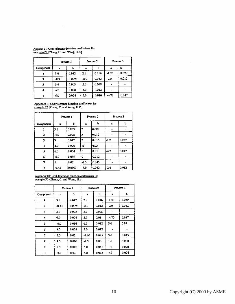
EXPERIMENTSThree example problems are tested using the suggestedmodified orthogonal based algorithm (MOBA), theSimulated Annealing (SA) and the SequentialQuadratic Programming (SQP) (Zhang and Wang,1993). These problems are referred to as P1, P2 and P3respectively. The cost tolerance describing the modelgiven by equation 1 are given in appendices I-III. Inappendix I, the assembly problem is made of 5components and there are 3 processes available tomanufacture these components to the requiredtolerance. For instance, there are 3 cost tolerancefunctions for design dimension 1:

T0.012/+3.0=f 11 , T0.016/+2.0=f 12 and

T0.029/+-1.2=f 13 . This applies to design

dimension 2 and 5 respectively. Design dimensions 3and 4 have two processes available. This means thatthere are 13 cost tolerance functions to evaluate at eachtolerance level. In problem P2 (appendix II), thenumber of design dimensions is 8 and there are 19available processes. In problem P3 (appendix III), thenumber of design dimensions is 10 and there are 28available processes. This represents a range ofpractical problems and signifies the computationalsaving in using our algorithm to discretize anycontinuous domain. The results of these optimizationproblems are in the form of optimum cost(corresponding to minimum objective function),optimum tolerances (design variables, optimumprocess combinations). Asstol1 and Asstol2 denote theconstraint function 1 and 2 respectively and representthe bound on the objective function.These limits are often dictated by design functionalrequirements. For problem P1, seven coupled inner


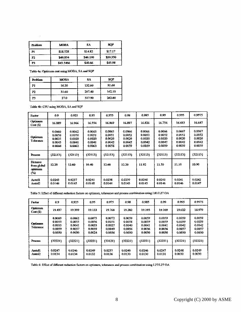
and outer orthogonal arrays are used to model thetolerance process curves. These are: L27/L16OA,L27/L36OA, L64/L36OA, L81/L36OA, L81/L16OA,L81/L27OA and L81/L81OA respectively. Thiscorresponds to 432, 972, 2304, 2916, 1296, 2187 and6561 function evaluations. The correspondingoptimum costs returned are: $22.63, $20.504, $19.379,$19.959, $20.064 and $18.528 respectively. Thecorresponding optimum processes are {33212},{33121}, {33121}, {33113}, {33213} and {33113}respectively. {33212} means process 3 for dimension1, process 3 for dimension 2, process 2 for dimension3, process 1 for dimension 4 and process 2 fordimension 5 and collectively refers to the optimumprocess combinations that results in minimumproduction cost. Table 1 details the optimum solutionsusing different structures. In all the structures, onlyone orthogonal array is used to model either the inneror outer domains. When L27/L16OA is used, theoptimum tolerances are {0.0055, 0.0032, 0.0061,0.0052 and 0.0031} for design dimensions 1, 2, 3, 4and 5 respectively. The optimum cost ranges from$18.528 - $22.633 and we conclude that theoptimization problem is very sensitive to the choice ofstructure. The larger the number of experiments(number of experiments in inner array x number ofexperiments in outer array), the lower the returnedoptimum. For instance, when L81/L81OA is used,the CPU taken by our algorithm is 12.2 % of theSimulated Annealing and 17.7 % of the SequentialQuadratic Programming respectively (Zhang andWang, 1993). This is obviously an advantage andclearly will benefit even more when the number ofdesign variables and processes increase. A comparisonbetween L81/L81OA and L64/L36OA indicates thatalthough the number of experiments is high for the firstthan the second, the CPU taken by L64/L36OA ishigher than L81/L81 OA. We also believe that 3-design level arrays are better in performance than 2 and4 design levels over the range of problems tested.Table 2 and 3 give results for problems P2 and P3respectively. Table 4a gives the optimum cost usingMOBA, SA and SQP respectively. Table 4b givesCPU taken for problems P1, P2 and P3 respectivelyusing the 3-methods. From the results, it is clear thatthe MOBA is capable of reaching near-to-globaloptimum in about 12.2% of SA and 17.7% of SQP (forproblem P1), 10.6% of SA and 19.5% of SQP (forproblem P2) and 5.2% of SA and 10.3% of SQP (forproblem P3) respectively. We believe that differentalgorithm parameters will have effect on the resultingoptimum; therefore, we study their effects individually.

Effect of Different Reducing Move FactorsThe effect of different reducing move factors isdetermined by modelling problem P1 usingL81/L27OA and L27/L27OA respectively. Fromcomputational experience, we determined that therange 0.9-0.9975 is the most suitable to obtain thelowest production cost. The minimum production costis $16.554 ($18.979) using L81/L27 OA (L27/L27OA)and occurs at a reduction factor of 0.95 (0.9975).Table 5 gives the effect of different reduction factors

4

on optimum, tolerances and process combinationsusing L81/L27OA. The optimum tolerances obtainedindicate that the optimization scheme is stable. Theoptimum process combination is {33113} for differentreduction factors. Since the global optimum is known,we calculated the distance from the global optimum.The minimum distance occurs at a reduction factor of0.95 and optimum cost of $16.554. The optimumtolerances are {0.0063, 0.0051, 0.0020, 0.0041,0.0063}. Table 6 details a similar solution usingL27/L27OA. The minimum cost is $18.979 at areduction factor of 0.9975. The optimum processcombinations are {32221} vs. {32113} using anL81/L27OA. The optimum tolerances are {0.0059,0.0059, 0.0042, 0.0057, 0.0030}. The optimum costclearly signifies that the optimum is further away fromthe global optimum using L27/L27OA thanL81/L27OA. Accordingly, the move factor has a strongeffect on the resulting optimum. For instance, a movefrom 0.98 to 0.985 changes the optimum by 0.45%. Inthe range 0.9-0.9975, the optimum returned varies froma minimum of 10.40% - 12.6% from the globaloptimum.

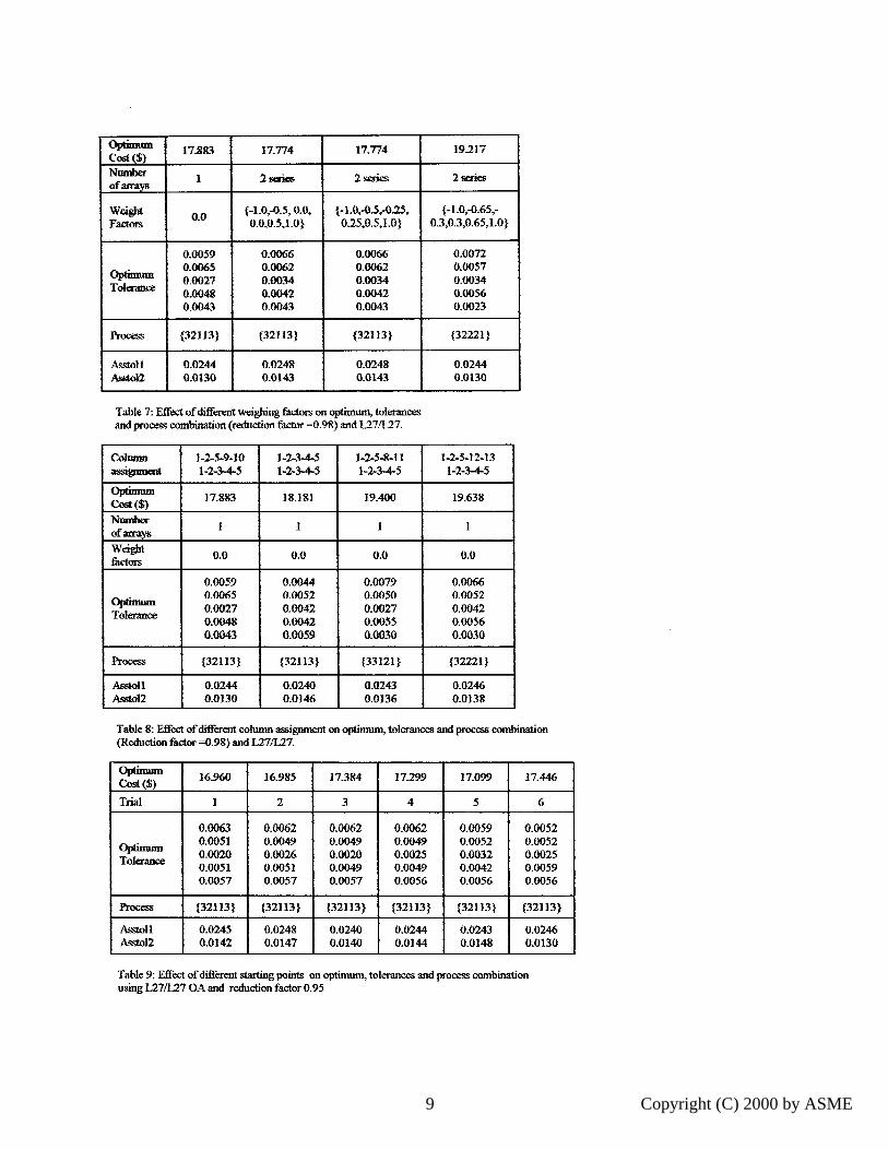
Effect of Different Weighing FactorsProblem P1 is used to study the effect of differentweighing factors on the optimum. For L27OA, thereare 3 design levels {-1.0, 0.0, 1.0} and the search islimited by these levels. The more the number ofdiscrete points, the easier to reach the global optimum.We tended to increase these points by inserting threeother weighing factors. Table 7 gives the effect ofdifferent weighing factors on optimum tolerances andprocess combinations for a reduction factor of 0.98using an L27/L27OA. Multi-level search is equivalentto increasing the number of discrete design levels.When the weighing factor is 0.0, only one orthogonalarray is used to model either the inner or outer array.The optimum cost returned is $17.883, the optimumtolerances are {0.0059, 0.0065, 0.0027, 0.0048,0.0043} and the optimum process combinations is{32113}. When 2-L27OA are combined in series, thesearch is idealized by 54 experiments and 6 designlevels {-1.0,-0.5,0.0,0.0,0.5,1.0} and {-1.0,-0.5,-0.25,0.25,0.5,1.0} vs. {-1.0,0.0,1.0} for single levelsearch. The optimum tolerances are identical {0.0066,0.0062, 0.0034, 0.0042, 0.0043} and the optimumprocess combination is {32113}. When the designlevels changed to {-1.0, -0.65, -0.3,0.3,0.65,1.0}, theoptimum cost increased from $17.774 to $19.217 andthe optimum process combination changed from{32113} to {32221}. This shows that multiple searchlevels allow increasing the number of design levels;which in turn, increases the capability of the algorithmto reach near to global optimum (from $17.883 usingsingle search level to $17.774 using multi-searchlevel).Effect of Different Column AssignmentsIn this study, we can assign design variables 1, 2, 3, 4and 5 to columns 1, 2, 5, 9 and 10; 1, 2, 3, 4 and 5; 1, 2,5, 8 and 11; 1, 2, 5, 12 and 13 respectively using anL27/L27OA and a reduction factor of 0.98. Table 8gives the corresponding optimum tolerances and


optimum process combinations for different columnassignments. The minimum cost varied from $17.883(for assignment 1-2-5-9-10) to $19.638 (forassignment 1-2-5-12-13). The optimum processcombination changed from {32113} to {32221}. Thismeans that there are certain column assignments thatallow reaching closer to the global optimum thanothers. This might imply that different assignments foreach problem must be performed to determine the mostsuitable column assignments.

Effect of Different Structures and Initial StartingPointsProblem P1 is used to investigate further the effect,different structures have on the optimum. Seven inner-outer orthogonal arrays are used to model the 2-searchdomains. These are: L27/L16OA, L27/L36OA,L64/L36OA, L81/L16OA, L81/L27OA and L81/L81OA respectively. The corresponding optimum cost is$22.63, $20.504, $19.379, $19.959, $20.064 and$18.528 respectively. The optimum combination ofprocesses are {33212}, {33121}, {33113}, {33113}.{33213} and {33113} respectively. We can concludethat the larger the number of experiments, the higherthe capability of the algorithm to reach near to globaloptimum. This is an important conclusion especiallywhen we realize that the number of experiments can becontrolled by the user by proper choice of orthogonalarrays combined in series and weighing factors.Regarding the effect of starting points, problem P1 isinvestigated further and six different starting points,herein called trial 1, 2, 3, 4, 5 and 6 for simplicity areused as input for the algorithm. These points areintroduced to the program in a data file. The reductionfactor is 0.95. Table 9 gives the effect of differentstarting points on optimum tolerance and processcombinations using an L27/L27OA for inner/outerdomains. The optimum tolerances remained almost thesame although the minimum cost varied from $16.96 to$17.446. The optimum process combination is thesame, {32113}, for the 6 trials. Again, this shows thatthe optimization method proposed is stable althoughthe initial starting points may vary.

CONCLUSIONA modification to the orthogonal based algorithm OBA(Gadallah and El-Maraghy, 1995) is presented, throughwhich a near-to-global optimum can be reached. Theproblem of tolerance synthesis with optimum processselection is revisited and results are compared with theSimulated Annealing (SA) and Sequential QuadraticProgramming (SQP). The merits of the algorithm maybe summarized as:

i) It can be easily adapted to different problems suchas discrete problems, which can have 2, 3 or moredesign levels. The only difference between one searchand another would be in the choice of coded design(orthogonal array) which idealizes the search. Thisstudy investigated five different effects: a) effect ofdifferent structures on optimum, b) effect of differentreducing move factors on optimum, c) effect of

5

different weighing factors, d) effect of different columnassignments and e) effect of different starting points.

ii) The algorithm is very efficient as compared withother conventional algorithms, especially the globaloptimization techniques. In the three exampleproblems, the required CPU range from 5.20% - 19.5%of that required by the SA and SQP algorithms.Instead of trying every combination similar to theexhaustive search, the new algorithm employs theorthogonal arrays to approximate the number of trialcombinations needed.

iii) The idea of single vs. multi-level search isexploited to obtain near-to-global optimum. In singlelevel search, only one orthogonal array is used. Inmulti-level search, two or more arrays are coupled inseries and different weighing factors are assigned. Thisis equivalent to increasing the number of discretepoints in any continuous domain. The only restrictionabout this idea, is regarding the computational costassociated with multi-level search. When two arraysare coupled in series, different weighing factors areused, as shown. It is clear that the idea of multi-levelsearch has the effect of reaching a better optimum thansingle level search. For instance, in experiment 3, theoptimum cost returned is $18.181 (for single levelsearch) vs. $ 17.774 (for multi-level search andweighing factors {-1.0, -0.5, 0.0, 0.0, 0.5, 1.0}.Finding the optimum weighing factors is anotheroptimization problem. However, the advantages ofhaving an algorithm that offers a near-to-globaloptimum in fraction of the time taken by otheralgorithms are tremendous. Besides, the number ofexperiments needed to reach the optimum is alwaysknown and finite.

iv) The orthogonal based algorithm, OBA (1995) andits modifications herein presented are believed to havemore valuable solutions other than the ToleranceOptimization Problem. One idea is to couple theMOBA with a global optimizer to serve as a hybridtechnique for future research.

REFERENCES Bremicker, M., Papalambros, P.Y. and Loh, T.H."Solution of Mixed-Discrete Structural OptimizationProblems With A New Sequential LinearizationAlgorithms", Computers & Structures, Vol. 37, # 4,1990, pp. 451-461.

Chi, H.-W. and Bloebaum, C.L. "A Mixed VariableOptimization using Taguchi's Orthogonal Arrays",DE-Vol. 82, 1995, Vol. 1, pp. 501-508.

Corana A., Marchesi, M., Martini,C., and RidellaS."Minimizing Multi-modal Functions of ContinuousVariables with The Simulated Annealing Algorithm",ACM Transactions on Mathematical Software, Vol. 13,no. 3, 1987, pp. 262-280.


Dong, Z., Hu, W. and Xue, D. "New Production Cost-Tolerance Models for Tolerance Synthesis", Journal ofEngineering for Industry, Vol. 116, 1994, pp. 199-206.

Fenton, R.G., Cleghorn W.L. and Fu, J.F. "AModified Flexible Tolerance Method for NonlinearProgramming", Engineering Optimization, Vol. 15,1989, pp. 141-152.

Fu, J.F, Fenton, R.G., Cleghorn W.L. "A MixedDiscrete-Continuous Programming Method and itsApplications to Engineering Design Optimization",Engineering Optimization, Vol. 17, 1991, pp. 263-280.

Gadallah, M.H. and ElMaraghy, H.A. "A NewAlgorithm for Combinatorial Optimization", ASMEAdvances in Design Automation Conference DE-Vol82(1), 1995, pp. 447-454.

Gadallah, M.H. "Robust Design and ExperimentalOptimization Approaches for Concurrent Design",Doctoral Dissertation, Department of MechanicalEngineering, McMaster University, Hamilton, Ontario,Canada.

Gupta, O.K. "Nonlinear Integer Programming andDiscrete Optimization", ASME Journal of MechanicalDesign, Vol. 105,pp.160-164.

Han-L. L. and Chou C. T. " A Global Approach forNonlinear Mixed Discrete Programming In DesignOptimization", Engineering Optimization, Vol. 22,1994, pp. 109-122.

Hajela, P. and Shih, C.J. "Multi-Objective OptimumDesign in Mixed Integer and Discrete Design VariableProblems", AIAA Journal, Vol. 28, no. 4, 1990, pp.670-675.

Kopardekar, P. and Anand, S. "Tolerance Allocationusing Neural Networks", Advanced Journal ofManufacturing Technology, 1995, Vol. 10, pp. 269 -276.

Loh, H.T. and Papalambros P.Y. "A SequentialLinearization Approach for Solving Mixed DiscreteNonlinear Design Optimization", Journal ofMechanical Design, Vol. 113, 1991, pp. 325-334.

Loh, H.T. and Papalambros P.Y. "ComputationalImplementation and Tests of a Sequential LinearizationAlgorithm for Mixed Discrete Nonlinear DesignOptimization", Journal of Mechanical Design, Vol.113, 1991, pp. 335-345.

Lee S.S. and Wang H.P. "Modified SimulatedAnnealing for Multiple Objective Engineering DesignOptimization", Journal of Intelligent Manufacturing,Vol. 3, 1992, pp. 101-108.

6

Lee, J.S., Gilmore, B.J. and Ogot, M.M."Dimensional Tolerance Allocation of StochasticDynamic Mechanical Systems Through Performanceand Sensitivity Analysis", Transactions of ASME, Vol.115, 1993, pp. 392-402.

Rajasekera, J.R. and Fang, S.C. "A New Approach toTolerance Allocation in Design Cost Analysis",Engineering Optimization, 1995, Vol. 24, pp. 283-291.

Taguchi, G., " System of Experimental Design -Engineering Methods to Optimize Quality andMinimize Costs", Volume I and II, American SupplierInstitute, Dearborn, Michigan, 1987.

Zhang, C. and Wang H.P. "Mixed Discrete NonlinearOptimization With Simulated Annealing", EngineeringOptimization, Vol. 21, 1993, pp.297-291.

Zhang, C. and Wang, H.P. "The Discrete ToleranceOptimization Problem ", Manufacturing Review, Vol.6, 1993, pp. 60-71.

Zhang, F., Gilmore, B.J. and Sinha, A. "AProbabilistic Tolerance Allocation Method forDynamic Mechanical Systems with Periodic Responseand Discontinuous Forcing Functions", ASME DE-Vol. 82, 1995, pp. 369-376.

Zhang, C. and Wang, H.P. "Integrated ToleranceOptimization with Simulated Annealing", AdvancedInternational Journal of Manufacturing Technology,1993, Vol. 8, pp. 167 - 174.

Wei, C.C., Lee, Y. - C. "Determining the ProcessTolerances Based on Manufacturing ProcessCapabilities", Advanced International Journal ofManufacturing Technology, 1995, Vol. 10, pp. 416 - 42

Copyright @ 2000 by ASME


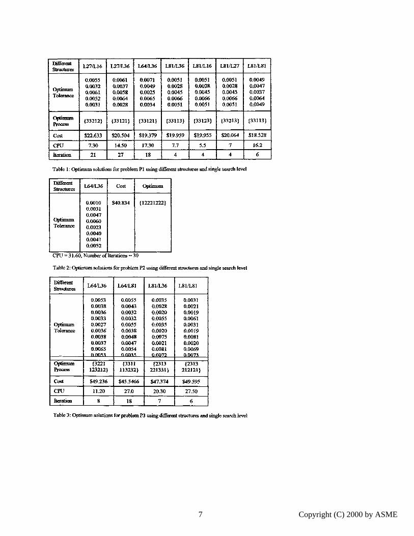
Differ:at t

L27/LI6 I L27/L36 L64/L36 LgI/L36 Lgl/LI6 Lgl/L27 Structures i

Lgl/Lgl

10.0055 0.0061 0.0071 0.005t 0 . 0 0 5 1 0 . 0 0 5 1 0.0049 0.0O32 0.0037 0.0049 0.0028 0.0028 0.0028 0.0047

Optimum 0.0061 0.0058 0 .002 .5 0.0045 0.0045 0.0045 0.0037 Tolerame

0.0O52 0.0064 0.0O65 0.0066 0.0066 0.0066 0.0064 0.0031 0.0028 0.0034 0.0051 0.005I 0.0051 0.0049

O p t i m a {33212} {33121} {33121} {33113} {33123} {33213} {33113} Process

Cost $22.633 $20.504 $19.379 $19.959 $19.955 $20.064 $18.528

CPU 7.30 14.50 17.30 7.7 5.5 7 16.2

Itexati~a 21 27 lg 4 4 4 6

Table 1: Optimum solutions for problem P 1 using different structures and single search level

Different L64/L36 Cost Optimum ~ e s

0.0010 $40.834 {12221222} 0.0031 0.0047

Optim,m 0.0O60 Tolerance 0.0023

0,0040 0.0041 0.0052

CPU = 31.6(), Nttmber ofIteratious = 30

Table 2: Optimum solutiot~s for problem P2 using different structures and single search level

L64/L36 L64 /L81 LSI/L36 Lgl/L81 Smlctures

0.0053 0.0038 0.0036 0.0033 0.0027 0.0036 0.0038 0.0037 0.0065

0.0055 0.0043 0.0032 0.0032 0.0055 0.0038 0.0048 0.0047 0.0054 t3 00~5

0.0035 0.0028 0,0020 0.0055 0.0035 0.0020 0,0075 0.0021 0.(3081 0,0072

0.0031 0.002 I 0.0019 0.0061 0,0031 0.0019 0.0081 0.0020 0.0069 0,0073

optm~ Tolerance

Optimum {3221 {3311 {2313 {2313 Process 123212} 113232} 221331} 212121}

Cost $49.236 $45.5466 $47.374 $49.595

CPU 11.20 27.0 20.30 27.50

lteratien 8 lg 7 6

Table 3: Optimum solutiotts for problem P3 using different structures and single search level


7 Copyright (C) 2000 by ASME

MtmA [ SA Problem sQP

PI $18.528 $14.82 $17.17

P2 $40.834 $40,190 $39,350

1'3 $,O.5466 $40.66 $43_9~

Table 4a: Optimum cost using MOBA, SA and SQP

Problem MOBA SA SQP

PI 16.20 132.60 9L60

P2 31.60 297.410 162.10

P3 27.0 517.90 262.60

Table 4b: CPU using MOBA, SA and SQP

Factor 0.9 0,925 0.95 0,975 0.98 0,985 0.99 0.995 0.9975

16,889 16.966 16_554 16.969 16.897 16,826 16.754 16,683 16,647 c0a(S)

Opamm Tolerance

Prooess

Distance #obal

op~mm (%)

Asstoll £~to12

0.0060 0.0050 0.0025 0.0045 0.0060

~32113}

12.20

0.0243 0.0146

0.0062 0.0050 0.0020 0.0041 0.0062

~32113}

12.60

0.0237 0.0145

0.0063 0.0051 0.0020 0.0041 0.0063

(32113}

10.40

0.0241 0.0148

0.0065 0.0051 0.0020 0.0042 0.0058

~32113}

12.60

0.0238 0.0144

0.0066 0.0052 0.0020 0.0042 0.0059

~32113}

12.20

0.0239 0.0145

0.0066 0.0052 0.0020 0.0042 0.0059

~321t3}

11.92

0.0240 0 .01~

0.0066 0.0052 0.0020 0.0042 0.0059

~32113}

11.50

0 .0~1 0.0146

0.0067 0.0052 0.0020 0.0042 0.0059

~32113}

11.10

0.0241 0.0146

0.0067 0.0052 0.0020 0.0042 0.0059

~32113)

10.90

0.0242 0.0147

Table 5: Effect of different reduction factors on optimum, tolerances and process eombinatton using LS1/L27 OA

Factor 0.9 0.925 0.95 ~ 0.975 0.98 0.985 0.99 0.995 0.9975

op~mm Cost ($)

ol~tmnn Tolerance

Proce~

Asstoil Asstol2

19.437

0.0069 0.0053 0.0035 0.0059 0.0030

{32221}

0,0247 0.0134

19.399

0.0062 0.0055 0.0041 0.0057 0.0030

{32221}

0.024.6 0.0134

19.133

0.0075 0.0056 0.0033 0.0059 0.0024

{32221}

0.0249 0.0132

19.768

0.0072 0.0051 0,0027 0.0049 0.0036

{33121}

0.0237 0.0136

19.282

0.0059 0.0058 0.0040 0.0056 0.0030

{32221}

0.0240 0.0130

19.195

0.0059 0.0059 0.0041 0.0056 0.0030

{32221}

0.0246 0.0130

19.109

0.0059 0.0059 0.0041 0.0056 0.0030

{32221)

0.0247 0.0131

19.022

0.0059 0.0059 0.0042 0.0057 0,0030

{32221)

0.0248 0.0030

18.979

0.0059 0.0059 0.0042 0.0057 0.0030

{32221}

0.0249 0.0030

Table 6: Effect of different reduction factors on optimum, tolerances and process combination using L27/L27 OA

Copyright @ 2000 by A S M E


O l j I ~ll ~mrl 17.gg3 17.7"74 17.774 19.217

Cost(S) Number 1 2 ~qwies 2 series 2 series ofarmys

Wd~ht 0.0 {-1.0--0.5, 0.0, {-I.0,-0.5,-0.25, {-1.0,-0.65,- Factors 0.0.,0.5,1.0} 0.25,0.5,1.0} 0.3,0.3,0.65,I.0}

0,0059 0.0066 0.0066 0.0072 0.0065 0.0062 0.0062 0.0057

Optimum 0.0027 0.0034 0.0034 0.0034 Tolerance 0.004g 0.0042 0.0042 0.0056

0.0043 0.0043 0.0043 0.0023

Process {32113} {32113} {32113} {32221}

Asstoll 0.02244 0.0248 0.0248 0.0244 Asstol2 0.0130 0.0143 0.0143 0.0130

Table 7: Effect of different weighing factors on optimum, tolerances and process etnnbination (reduction faR-tot =0.98) and L27/L27.

Column 1-2-5-9-10 1-2-3-4-5 1-2-5-8-11 1-2-5-12-13 assiL2nnu~at 1-2-3-4.-5 1-2-3 . . .4 - -5 1-2-3-.4..5 1-2-3-.4-5

Optimum 17.883 l g . l g l 19.400 19.638 Cost(S) Number

I I ofaa:rays

Weight 0.0 0.0 0.0 0.0 factors

0.0059 0.0044 0.0079 0.0066 0.0065 0.0052 0.0050 0.0052

Oplirmim 0.0027 0.0042 0.0027 0.00.42 Tolerance

0.0048 0.0042 0.0055 0.0056 0.0043 0.0059 0.0030 0.0030

Process {32113} {32113} {33121} {32221}

A.,~oll 0.0244 0.0240 0.0243 0.0246 Asstol2 0.0130 0.0146 0.0136 0.0138

Table 8: Effect of different column assignment on optimum, tolerances and pr~ess combination (Reduction factor =0.98) and L27/L2Z

Optimum 16.960 16.985 17.394 17.299 17.099 17.446 C o a ($)

Trial 1 2 3 4 5 6

o~a~nn Tolerance

0.0063 0.0051 0.0020 0.0051 0.0057

0.0062 0.0049 0.0026 0.0051 0.0057

0.0062 0.0049 0.0020 0.0049 0.0057

0.0062 0.0049 0.0025 0.0049 0.0056

0.0059 0.0052 0.0032 0.0042 0.0056

0.0052 0.0052 0.0025 0.0059 0.0056

Process {32113} {32113} {32113} {32113} {32113} {32113}

Asstoll 0.0245 0.0248 0.0240 0.0244 0.0243 0.0246 Asstol2 0.0142 0.0147 0.0140 0.0144 0.0148 0.0130

Table 9: Effect of different starting points on op t~um, tolerances and process combination using L27/L27 OA and reduction factor 0.95



Appondix I: Cost-tol~ance fimction coefficients for example P1 [Zhan B. C. and Wang, H.P.]

Process 1 Process 2

Compon~t a b a [ b

1 3.0 0.012 2.0 0.016

2 -0.33 0.0093 -8.0 0.042

3 3.0 0.003 2.0 0.008

4 4 . 0 0.00g 3.0 ! 0.012 !

5 6,0 0.004 5.0 i 0.010

Appendix II: Cost-tolerance function co¢fficienL~ for example P2 [Zhang, C. and Wang, H.P.]

Proc~s 3

a b

-1.20 0.029

-2.0 0.012

-4.70 0.O47

1

2

3

4

5

6

7

Process 1

a b

3.0 0.003

-4.0 0.00g I

3 0.012

4.0 0.006

6.0 0.004

..6.0 0.036

5 0.02 i

i-0.33 0.0093

Process 2

a i b

2 i O.OOg

3 0.012

2 0.016

-2 0.03

5 0.01

0 0.012

-1.6 i 0.045

-g.o 0.042

Appendix III: Cost4olcrance function coefficients for example P3 [Zhang, C. and Wang, H.P]

Process 3

a ~ b

-1.2 0.029

-4.7 0.047

i i-2-0 !0.012

Component

1

2

3

4

5

6

7

g

9

10

Process 1

a b

3.0 0.012

-.0.33 0.0093

3.0 0.003

6.0 0.004

-6.0 0.036

4.0 0.008

5.0 0.02

4.0 0.006

6.0 0.005

-2.0 0.03

Process 2

a b

2.0 0.016

-g.O 0.042

2.0 0.008

5.0 0.01

0.0 0.012

3.0 0.012

-1.60 0.045

-2.0 0.03

5.0 0.01l

4.0 0.015

Process 3

a b

-1.20 0.029

-2.0 0.012

-.4.70 0.047

3.0 0.01

3.0 0.025

1.0 0.008

1.0 0.020

7.0 0.004

Copyright @ 2000 by A S M E


The Tolerance Optimization Problem using a Near to Global Optimum

Documents

Transcript of The Tolerance Optimization Problem using a Near to Global Optimum